Unsteady Aerodynamics of Vertical Axis Wind Turbines
187
Unsteady Aerodynamics of Vertical Axis Wind Turbines Nidiana Rosado Hau A thesis submitted in partial fulfilment of the requirements for the degree of Doctor of Philosophy The University of Sheffield Faculty of Engineering Department of Mechanical Engineering January, 2021
-
Upload
khangminh22 -
Category
Documents
-
view
3 -
download
0
Transcript of Unsteady Aerodynamics of Vertical Axis Wind Turbines

Unsteady Aerodynamics of Vertical Axis Wind Turbines
Nidiana Rosado Hau
A thesis submitted in partial fulfilment of the requirements for the degree of
Doctor of Philosophy
The University of Sheffield
Faculty of Engineering
Department of Mechanical Engineering
January, 2021

I, the author, confirm that the Thesis title “Unsteady aerodynamics of vertical axis windturbines” is my own work. I am aware of the University’s Guidance on the Use of UnfairMeans (www.she f f ield.ac.uk /ssid/un f air−means). This work has not been previouslypresented for an award at this, or any other, university. This thesis is accompanied forsome published research articles and some of them in preparation as follows:
• (Published) Rosado Hau N., Ma L., Ingham D. & Pourkashanian M., A critical analysis of
the stall onset in vertical axis wind turbines, Journal of Wind Engineering and Industrial
Aerodynamics, Vol 204, September 2020.
• (Published) Rosado Hau N., Ma L., Ingham D. & Pourkashanian M. , A Procedure to Predict
the Power Coefficient of Vertical Axis Wind Turbines at Low Tip Speed Ratios, Confer-
ence proceedings, AIAA Scitech 2019 Forum, San Diego California, htt ps : //doi.org/10.2514
/6.2019−1066.
• (In preparation) Rosado Hau N., Ma L., Ingham D. & Pourkashanian M , Effect of the
upstream and downstream torque contributions on the performance of vertical axis wind
turbines
Signature
Date

ACKNOWLEDGMENTS
I would like to express my deep gratitude to Professor Lin Ma, Derek Ingham and Mo-
hamed Pourkashanian, my research supervisors, for their guidance during these four years
and their patience in the reading and improvement of this thesis.
I wish to thank to the National Council of Science and Technology (CONACYT) and
the Secretary of Energy of Mexico (SENER) for the PhD funding and for give me the op-
portunity to learn in an international environment.
I also want to extent my special gratitude to my friends, especially to Mohamed El
Sakka and Oscar Farias for their valuable support during my CFD learning process.
ii

This thesis is dedicated with all my love to my parents, Filomeno Rosado Gonzalez and
Benigna Hau, who taught me to never stop learning from others.
To my dear David F. Morales Aldana and his family for all their support and affection
during all these years.
When you think you have no reason to go on, use that pain to create your own art.
Someone, somewhere and somehow, will be inspired by your resilience.
Nidiana
iii
ABSTRACT
This thesis aims to substantially contribute to the understanding of the unsteady aero-
dynamics that remains unclear in the VAWTs. The analysis has been carried out by using
computational fluid dynamics techniques very carefully verified with experimental data and
using a modified Leishman-Beddoes dynamic stall algorithm. The results of this investiga-
tion are based on the analysis of oscillating aerofoils at constant and time-varying Reynolds
and VAWTs with one, two and three blades evaluated at the tip speed ratio range of 1.5-5
using four symmetrical aerofoils and two-cambered aerofoils. The results have shown that:
(i) the stall-onset angle in the VAWTs is defined by the combined effect of the tip speed ratio,
pitch angle, angular frequency and relative velocity in the final value of the non-dimensional
pitch rate when the angle of attack approaches the static stall angle; (ii) Under the fully
attached regime, the symmetrical aerofoils performed better than the cambered aerofoils
especially at the downstream zone of the rotor. This zone has shown to play the most
significant role in the reduction of the overall torque coefficient and this reduction increases
with the tip speed ratio, thus, a poor lift force coefficient at negative angles of attack can
mitigate the advantages of a high lift/drag aerofoil observed at positive angles of attack.
(iii) The curvature effect becomes more relevant with the increase of the tip speed ratio but
also appears to be affected by the number of blades, therefore, a fast tool to design VAWTs
needs to take into account this phenomenon in order to give reliable results. In the methods
proposed in this thesis, despite being limited to the cases investigated, they demonstrate
to be a potential tool to predict the unsteady loads in the VAWTs. The present investi-
gation gives sufficient aerodynamic information to design strategies that improve VAWT
performance.
iv

v

CONTENTS
List of Figures xiii
List of Tables xxi
List of Acronyms xxii
Chapter 1: Introduction 1
1.1 Background . . . . . . . . . . . . . . . . . . . . . . . . . . . . . . . . . . . 1
1.2 Aims and objectives of this thesis . . . . . . . . . . . . . . . . . . . . . . . 3
1.3 Limitations . . . . . . . . . . . . . . . . . . . . . . . . . . . . . . . . . . . . 4
1.4 Outline of the thesis . . . . . . . . . . . . . . . . . . . . . . . . . . . . . . 5
Chapter 2: Unsteady aerodynamics 7
2.1 Background . . . . . . . . . . . . . . . . . . . . . . . . . . . . . . . . . . . 7
2.2 Aerodynamics on VAWTs . . . . . . . . . . . . . . . . . . . . . . . . . . . . 11
2.2.1 Instantaneous loads on VAWTs . . . . . . . . . . . . . . . . . . . . 15
2.2.2 Dynamic stall on VAWTs . . . . . . . . . . . . . . . . . . . . . . . . 18
2.3 Summary . . . . . . . . . . . . . . . . . . . . . . . . . . . . . . . . . . . . . 23
Chapter 3: Methodology 25
3.1 Overview . . . . . . . . . . . . . . . . . . . . . . . . . . . . . . . . . . . . . 25
3.2 Computational fluid dynamic simulations . . . . . . . . . . . . . . . . . . 27
3.2.1 Governing equations . . . . . . . . . . . . . . . . . . . . . . . . . . 28
3.2.2 Simulations for oscillating simulations . . . . . . . . . . . . . . . . 29
3.2.3 CFD technique for VAWT simulations . . . . . . . . . . . . . . . . 36
3.3 Dynamic stall method . . . . . . . . . . . . . . . . . . . . . . . . . . . . . . 45
3.4 Double multiple streamtube theory . . . . . . . . . . . . . . . . . . . . . . 47
3.5 Summary . . . . . . . . . . . . . . . . . . . . . . . . . . . . . . . . . . . . . 50
vi

Chapter 4: The stall onset angle 52
4.1 Overview . . . . . . . . . . . . . . . . . . . . . . . . . . . . . . . . . . . . . 52
4.2 Methodology . . . . . . . . . . . . . . . . . . . . . . . . . . . . . . . . . . . 52
4.2.1 Stall-onset estimation . . . . . . . . . . . . . . . . . . . . . . . . . 55
4.3 Influence of κ, λ and β at constant Reynolds number . . . . . . . . . . . 56
4.3.1 Stall onset as a function of κ, λ and β . . . . . . . . . . . . . . . . 61
4.4 Non-dimensional pitch rate and Reynolds number effect . . . . . . . . . 63
4.5 Effect of the relative velocity on the stall-onset angle . . . . . . . . . . . 66
4.6 Discussion . . . . . . . . . . . . . . . . . . . . . . . . . . . . . . . . . . . . 70
4.7 Summary . . . . . . . . . . . . . . . . . . . . . . . . . . . . . . . . . . . . . 73
Chapter 5: Unsteady aerodynamics both upstream and downstream of
VAWTs 74
5.1 Overview . . . . . . . . . . . . . . . . . . . . . . . . . . . . . . . . . . . . . 74
5.2 Methodology . . . . . . . . . . . . . . . . . . . . . . . . . . . . . . . . . . . 74
5.2.1 Numerical settings . . . . . . . . . . . . . . . . . . . . . . . . . . . 75
5.3 Operating regimes on VAWTs . . . . . . . . . . . . . . . . . . . . . . . . . 75
5.4 Influence of the aerofoil on the upstream and downstream torque contri-
butions . . . . . . . . . . . . . . . . . . . . . . . . . . . . . . . . . . . . . . 80
5.4.1 Dynamic stall regime . . . . . . . . . . . . . . . . . . . . . . . . . . 85
5.4.2 Fully unsteady attached regime . . . . . . . . . . . . . . . . . . . . 90
5.5 Discussion . . . . . . . . . . . . . . . . . . . . . . . . . . . . . . . . . . . . 93
5.6 Summary . . . . . . . . . . . . . . . . . . . . . . . . . . . . . . . . . . . . . 95
Chapter 6: Predicting unsteady loads using a dynamic stall algorithm 97
6.1 Overview . . . . . . . . . . . . . . . . . . . . . . . . . . . . . . . . . . . . . 97
6.2 The Leishman-Beddoes dynamic stall: modifications . . . . . . . . . . . . 97
6.2.1 Time delay constant database . . . . . . . . . . . . . . . . . . . . . 98
6.2.2 Kirchhoff flow equation: Static parameters . . . . . . . . . . . . . 100
6.3 Analysis of the LB-dynamic stall model under an oscillating motion . . . 108
6.4 Prediction of the torque coefficient of VAWTs using the dynamic stall model110
6.5 Discussion . . . . . . . . . . . . . . . . . . . . . . . . . . . . . . . . . . . . 115
vii

6.6 Summary . . . . . . . . . . . . . . . . . . . . . . . . . . . . . . . . . . . . . 118
Chapter 7: Curvature effect on the prediction of the torque coefficient
of VAWTs 120
7.1 Overview . . . . . . . . . . . . . . . . . . . . . . . . . . . . . . . . . . . . . 120
7.2 Interference factor . . . . . . . . . . . . . . . . . . . . . . . . . . . . . . . . 120
7.3 Curvature effects . . . . . . . . . . . . . . . . . . . . . . . . . . . . . . . . 125
7.3.1 Virtual camber estimation . . . . . . . . . . . . . . . . . . . . . . . 129
7.4 Prediction of the torque coefficient: New proposed method . . . . . . . . 134
7.5 Influence of the pitch angle of the performance of VAWTs . . . . . . . . . 135
7.6 Summary . . . . . . . . . . . . . . . . . . . . . . . . . . . . . . . . . . . . . 138
Chapter 8: Conclusions and Future work 139
8.1 Conclusions . . . . . . . . . . . . . . . . . . . . . . . . . . . . . . . . . . . 139
8.2 Future work . . . . . . . . . . . . . . . . . . . . . . . . . . . . . . . . . . . 142
References 144
Appendix A: Original algorithm of the Leishman-Beddoes dynamic stall
model 159
A.1 Unsteady Attached flow . . . . . . . . . . . . . . . . . . . . . . . . . . . . 159
A.2 Stall onset . . . . . . . . . . . . . . . . . . . . . . . . . . . . . . . . . . . . 161
A.3 Separated flow . . . . . . . . . . . . . . . . . . . . . . . . . . . . . . . . . . 161
A.3.1 Trailing edge separated module . . . . . . . . . . . . . . . . . . . . 162
A.3.2 Vortex shedding . . . . . . . . . . . . . . . . . . . . . . . . . . . . . 162
Appendix B: Interference factor 164
viii
NOMENCLATURE
A Area
C Constant variable
CC, CD, CL Chordwise, drag and lift force coefficients
CD0 Drag coefficient at zero angle of attack
CLα Slope of the static attached flow coefficients
CN1 Normal force at the separation point
CINα
Impulsive component due step change in the angle of attack
CINq Impulsive component due to the pitch rate
CN Normal force coefficient
CCN Circulatory component of the normal force
C fN Boundary layer component of the normal force
CvN Vortex component of the normal force
CP Power coefficient
CQ,T Total torque coefficient
CQ Torque coefficient
CR, CT Radial and tangential force coefficient on a VAWT.
C f x Skin friction, σx/0.5ρU2re f
ix

D Rotor diameter, m
DI,Dq,D f ,Dp,Dα Deficiency functions
E0 Parameter to adjust the static chordwise force coefficient
L, M Lift stall and moment stall points
Nb Number of blades
Nth Number of streamtubes elements
Pcoe f f Pressure coefficient
R Rotor radius, m
S1,S2 Parameters to adjust the Kirchoff flow equation.
T Period of oscillation
Tp Time delay constant base in the pressure criteria
Tr Time delay constant base in the chordwise force criteria
U Incoming wind flow for the oscillating aerofoil, m/s
Ure f Actual wind speed on the aerofoil, m/s
V∞ Free stream wind velocity in the VAWTs, m/s
Vdw Induced velocity on the downwind rotor
Ve Equilibrium velocity between the upwind and the downwind rotor
Vinst Wind sped at a specific time, m/s
Vmean Average of the relative velocity in one revolution, m/s
Vrel Relative velocity, m/s
x

Vup Induced velocity on the upwind rotor
Vx X-component of the wind velocity, m/s
X ,Y Deficiency functions
Xr Local tip speed ratio, ωR/V
a1, a2 Maximum interference factors at upstream and downstream respectively
c Chord, m
di, dw, do Geometrical dimensions of the mesh domain.
dw Downstream
f Non dimensional static separation point, f = x/c
fcrt Critical point of the TE separation point
n Number of time step
q Non-dimensional pitch rate
r Normalized pitch rate q = αc/V
t Time, s
u, u′ Interference factors, upstream and downstream
up Upstream
x/c Non-dimensional chord distance
∆s Non-dimensional time step, 2Ure f ∆t/c
∆tsep Time elapsed from the static to the dynamic stall angle
α Angle of attack, (◦)
xi

α0 Virtual increase in the effective angle due to the camber effects, (◦)
αE Effective angle
α f Effective angle of the dynamic separation point
αmax Maximum angle of attack in the upstroke
αos Dynamic stall-onset angle, (◦)
αss Static stall angle, (◦)
β Pitch angle, (◦)
δ Angle between the blades and the z-axis
α Pitch rate, (rad/s)
γ Compressibility factor√
1−M2
κ Reduced frequency, (ωc/2Ure f )
λ Tip speed ratio, ωR/V∞
ω Rotational speed, rad/s
φ Path angle, (◦)
ρ Density
σ Solidity, (Nbc/2R)
τ Non-dimensional time constant, (t/T)
θ Azimuthal angle, (◦)
θin Azimuthal angle with the stall inception, (◦)
θmax Azimuthal angle with a maximum CQ, (◦)
xii

LIST OF FIGURES
2.1 The normal force coefficient as a function of the angle of attack for a
steady NACA0015 aerofoil at Reynold number of 1.5×10⁶ compared with
the normal force coefficient of oscillatory NACA0015 with a maximum
angle of attack (a) within the static stall angle and, (b) larger than the
static stall angle [1]. . . . . . . . . . . . . . . . . . . . . . . . . . . . . . . 9
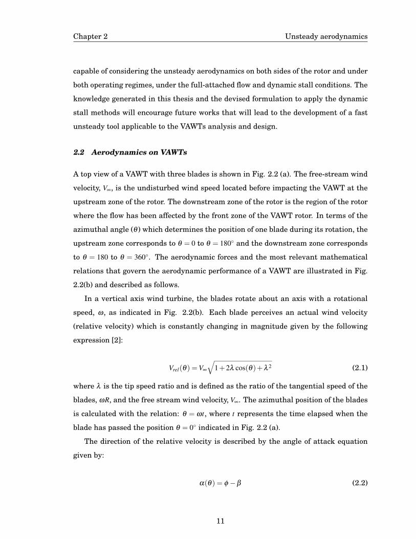
2.2 (a) A schematic representation of a three-bladed VAWT and its repre-
sentative zones and, (b) a schematic representation of the aerodynamic
forces generated during the rotation of the VAWT blade. . . . . . . . . . 12
2.3 A typical power coefficient of a VAWT as a function of the tip speed ra-
tio (the range of tip speed ratio might change accordingly to the VAWT
design) [2]. . . . . . . . . . . . . . . . . . . . . . . . . . . . . . . . . . . . . 14
2.4 (a) Contours of spanwise-averaged skin friction coefficient (C f ) and (b)
pressure coefficient on the suction side of the NACA0015 aerofoil through
the constant pitch-rate motion at Re 2×10⁵ and, using LES. [3] . . . . . 20
2.5 (a) Distributions of the pressure coefficient and, (b) the skin friction along
the NACA0015 chord at five angle of attack during the pith up manoeu-
vre and at Re 2×10⁵ using LES. [3] . . . . . . . . . . . . . . . . . . . . . . 21
3.1 Schematic representation of the global methodology adopted in the thesis
(philosophical methodology). . . . . . . . . . . . . . . . . . . . . . . . . . . 26
3.2 Mesh topology for the CFD technique applied to the oscillating aerofoil.
(a) The rotating region with an aerofoil with 1000 nodes along its surface,
(b) the stationary domain and, (c) the interface between the rotating and
the stationary domain zones. . . . . . . . . . . . . . . . . . . . . . . . . . 33
3.3 (a) Mesh independence study, and (b) time step independence study for
the CFD simulation of an oscillating NACA 0012 aerofoil. . . . . . . . . 34
xiii
3.4 (a) The lift coefficient as a function of the angle of attack of the oscillating
aerofoil NACA0012 at Re 1.35×10⁵ predicted with the present CFD tech-
nique and the comparison with the experimental data [4]. (b) Chordwise
force coefficient of the oscillating NACA0015 as a function of the angle
of attack predicted with the present CFD technique and compared with
experimental data with the same characteristics at Re 2×10⁵ [5]. . . . . 35
3.5 Mesh topology of the stationary and the rotating grid zones used in the
VAWT simulations. . . . . . . . . . . . . . . . . . . . . . . . . . . . . . . . 39
3.6 Schematic representation of the CFD domain used for the VAWTs simu-
lations (not scale) and the boundary conditions. . . . . . . . . . . . . . . 39
3.7 Influence of the upper and lower domain boundaries in the torque coeffi-
cient predicted at the 20th cycle for a λ = 2.19. . . . . . . . . . . . . . . . 40
3.8 Torque coefficient as a function of the azimuthal angle predicted with
the different grids presented in Table 3.3 in the 20th revolution and a tip
speed ratio of λ = 2.19. An azimuthal increment of 0.25◦ was employed. 41
3.9 Prediction of the instantaneous torque coefficient in [6] for the last revo-
lution versus azimuth angle for different grids in last revolution for a tip
speed ratio of λ = 4.5. . . . . . . . . . . . . . . . . . . . . . . . . . . . . . 42
3.10 Torque coefficient as a function of the azimuthal angle predicted with
different time steps at the 20th cycle. The tip speed ratio is λ = 2.19 and
the Mesh2 with 1000 element around the blades was employed. . . . . . 43
3.11 Prediction of the instantaneous torque coefficient at the 20th revolution
for (a) TSR 2.58, (b) TSR 2.19 and, (c) TSR 1.38 for a two-bladed VAWT. 44
3.12 Vorticity contours for a two-bladed VAWTs at (a) λ= 2.58, (b) λ= 2.19
and, (c) λ = 1.38 . . . . . . . . . . . . . . . . . . . . . . . . . . . . . . . . . 45
3.13 Schematic representation of the Leishman-Beddoes algorithm. . . . . . 46
4.1 Sketch of an oscillating aerofoil with the VAWT angle of attack α(t) and
an incoming flow (U). U can take a constant magnitude or a time-varying
magnitude given by the relative velocity equation. . . . . . . . . . . . . . 53
xiv

4.2 (a) Pressure coefficient, and (b) skin friction along the chord of an os-
cillating aerofoil at the angle of attack 13◦. Laminar boundary layer
separation, I Reattachment of LSB, � Start of reversal flow in the tur-
bulence boundary layer at TE. . . . . . . . . . . . . . . . . . . . . . . . . 57
4.3 (a) Skin friction, and (b) chordwise force coefficient, as a function of the
angle of attack for λ= 3, 2.37 and 2 with values of κ = 0.06, β = 0 and
Re = 2×10⁵. Arrows indicate the direction in the angle of attack with the
motion of the aerofoil. . . . . . . . . . . . . . . . . . . . . . . . . . . . . . . 58
4.4 The x-component velocity contour for the oscillating NACA0015 with (a)
λ = 2 at α = 26.8◦, and (b) λ = 3 at α = 20◦ at Re = 2×10⁵. . . . . . . . . . 59
4.5 (a) Skin friction along the non-dimensional chord length, and (b) chord-
wise force coefficient for several values of β at Re = 2×10⁵. . . . . . . . . 60
4.6 The predicted stall-onset angle for the simulations performed for all the
cases in Table 4.1 and described as a function of the (a) reduced fre-
quency, (b) tip speed ratio and, (c) pitch angle. . . . . . . . . . . . . . . . 62
4.7 Results from Buchner et al. [7] of the trailing edge vortex formation at
the leading edge of the aerofoil (TEV) as a function of the tip speed ratio
investigated using a VAWT rotor with β = 0◦ and wind tunnel test. A
black dot correspond to the parameter Kc = c/2R with a value of 0.10 and
blue for 0.15. . . . . . . . . . . . . . . . . . . . . . . . . . . . . . . . . . . . 63
4.8 (a) Stall-onset angle as a function of the non-dimensional pitch rate and
Reynolds number for the NACA0015 aerofoil. The red dot corresponds to
the αos predicted with LES for a q= 0.25 in [3] and, (b) Skin friction along
the non-dimensional chord length for two Reynolds numbers at α = 13◦. 64
4.9 (a) Pressure coefficient and, (b) skin friction for two simulations with
closed non-dimensional pitch rate value at α = 13◦. . . . . . . . . . . . . 66
4.10 Chordwise force coefficient for λ = 2 using an incoming flow with: a con-
stant velocity and with time-varying velocity given by the relative veloc-
ity Eq. (2.1). Arrows indicate the direction in the angle of attack with
the motion. . . . . . . . . . . . . . . . . . . . . . . . . . . . . . . . . . . . . 69
xv

5.1 Schematic representation of the VAWT CFD simulations investigated in
this Chapter. For each blade configuration, 6 aerofoils were employed.
The range of tip speed ratio this 18 configurations is included accordingly
the number of blades. . . . . . . . . . . . . . . . . . . . . . . . . . . . . . . 75
5.2 The total torque coefficient of as a function of the tip speed ratio for a
VAWTs using the NACA0012 and a constant free-stream wind speed of
8 m/s. . . . . . . . . . . . . . . . . . . . . . . . . . . . . . . . . . . . . . . . 77
5.3 (a) Azimuthal torque coefficient in one revolution at several tip speed
ratios of the one- bladed NACA0012 aerofoil, (b) drag force coefficient,
and (c) lift force coefficient as a function of the angle of attack for several
tip speed ratios for the one-bladed NACA0012 aerofoil. . . . . . . . . . . 78
5.4 Azimuthal torque coefficient at several tip speed ratios for a VAWTs us-
ing the NACA0012 aerofoil and with the number of blades (a) two, and
(b) three. . . . . . . . . . . . . . . . . . . . . . . . . . . . . . . . . . . . . . 79
5.5 Upstream torque coefficient, CQ,up, of six aerofoils for a VAWT with (a)
one blade, (b) two blades and, (c) three blades. . . . . . . . . . . . . . . . 80
5.6 Downstream torque coefficient, CQ,dw, of six aerofoils for a VAWT with (a)
one blade, (b) two blades and, (c) three blades. . . . . . . . . . . . . . . . 81
5.7 Total torque coefficient, CQ,T , , as a function of the tip speed ratio for the
six aerofoils for a VAWT with (a) one blade, (b) two blades and, (c) three
blades. . . . . . . . . . . . . . . . . . . . . . . . . . . . . . . . . . . . . . . 82
5.8 Power coefficient as a function of the tip speed ratio for the six aerofoils
for the six aerofoils for a VAWT with (a) one blade, (b) two blades and, (c)
three blades. . . . . . . . . . . . . . . . . . . . . . . . . . . . . . . . . . . . 84
5.9 Instantaneous torque coefficient for a three blades turbine and a tip
speed ratio 1.5 . . . . . . . . . . . . . . . . . . . . . . . . . . . . . . . . . . 86
5.10 Static force coefficient as a function of the angle of attack for the six
aerofoils calculated by using Xfoil at Reynolds number of 5×10⁵ (a) Lift
force coefficient (CL), (b) drag force coefficient (CD), and (c) chordwise force
coefficient (CC) . . . . . . . . . . . . . . . . . . . . . . . . . . . . . . . . . . 87
xvi

5.11 Vorticity contours of the flow field around the blade of a three-bladed tur-
bine at λ = 1.5 in the downstream region of the rotor of the three-bladed
turbine: (a) NACA0012, (b) NACA0015, (c) NACA0018, (d) NACA0021,
(e) S1210 and (f) NACA2418. . . . . . . . . . . . . . . . . . . . . . . . . . 88
5.12 Azimuthal torque coefficient for the six aerofoils with (a) two blades and
a tip speed ratio 4, and (b) three-blades and tip speed ratio 3.5 . . . . . . 90
5.13 (a) Diagram representation along the vertical line where the velocity was
collected for a three-bladed VAWT; Non-dimensional velocity V/V∞ for the
six aerofoils at (b) λ = 1.5, (c) λ = 3.5, and (d) Non-dimensional velocity
for the NACA0021 aerofoil at four tip speed ratios. . . . . . . . . . . . . . 92
6.1 Stall-onset angle as a function of the non-dimensional pitch rate for (a)
NACA0015, (b) NACA0018 and, (c) NACA0021. . . . . . . . . . . . . . . . 100
6.2 Effect on lift force coefficient due to the trailing edge separation ( f ) [8] . 102
6.3 Trailing edge separation point as a function of the angle of attack cal-
culated with the skin friction being obtained using CFD simulations for
the NACA0015 under static conditions at (a) Re 3.3×10⁵ and (b) 2.0×10⁵ 104
6.4 TE separation point calculated in step 2 using the Kirchhoff flow Eq.(6.3)
and in red, adjusting the S1 and S2 parameters in the Eq. (6.4). This
example corresponds to the NACA0015 at Re 3.3×10⁵. . . . . . . . . . . 106
6.5 (a) Lift force coefficient as a function of the angle of attack calculated
with fluent and using the Kirchhoff flow model, and (b) Chordwise force
coefficient calculated by the CFD and predicted with the separation equa-
tion. . . . . . . . . . . . . . . . . . . . . . . . . . . . . . . . . . . . . . . . . 107
6.6 The chordwise force coefficient predicted with the original (LB-OR) and
the modified dynamic stall model (LB-OR) at Re 3.3×10⁵, λ = 3 and, (a)
κ = 0.025 and (b) κ = 0.05. Arrows for both cases of CFD, indicate the
direction in the angle of attack. . . . . . . . . . . . . . . . . . . . . . . . . 109
xvii
6.7 The chordwise force coefficient of an oscillating NACA0015 predicted
with numerical techniques at the Re 3.3× 10⁵ (λ = 4 and κ = 0.1) and
compared with the experimental data [1] at Re 1.5× 10⁶. The arrows
indicate the direction in the angle of attack during the oscillating motion. 110
6.8 Azimuthal torque coefficient predicted for a one-bladed VAWT and λ =
2 when employing CFD, non-stall algorithm (DMST plain), the DMST
method coupled with the original LB (DMST+LB-OR), and the DMST
method coupled with the modified LB (DMST+LB-mod). . . . . . . . . . 111
6.9 Azimuthal torque coefficient predicted for a two-bladed VAWT and λ =
1.5 when using CFD, non-stall algorithm (DMST plain), the DMST method
coupled with the original LB (DMST+LB-OR), and the DMST method
coupled with the modified LB (DMST+LB-mod). . . . . . . . . . . . . . . 112
6.10 Azimuthal torque coefficient predicted numerically for a NACA 0015 two-
bladed VAWT with λ = 2.5 and β = 0◦ using CFD, non-stall algorithm
(DMST plain), the DMST method coupled with the original LB (DMST+LB-
OR), and the DMST method coupled with the modified LB (DMST+LB-
mod) and, compared with experimental data of a two-bladed VAWT for
the NACA0015 at λ = 2.29 and β = 6◦ [9]. . . . . . . . . . . . . . . . . . . 113
6.11 Azimuthal torque coefficient predicted for a one-bladed VAWT and λ = 3
using the CFD, non-stall algorithm (DMST plain), the DMST method
coupled with the original LB (DMST+LB-OR), and the DMST method
coupled with the modified LB (DMST+LB-mod). . . . . . . . . . . . . . . 115
6.12 Azimuthal torque coefficient predicted for a three-bladed VAWT and λ =
2.5 when using CFD, non-stall algorithm (DMST plain), the DMST method
coupled with the original LB (DMST+LB-OR), and the DMST method
coupled with the modified LB (DMST+LB-mod). . . . . . . . . . . . . . . 116
7.1 A typical representation of the streamlines when a flow past a VAWT [2] 121
7.2 Interference factor at nine positions along the x-direction for:(a) One
bladed-turbine and a tip speed ratio of 2, and (b) a three-bladed turbine
and a tip speed ratio of 2. Both VAWTs with the NACA0015 aerofoil. . . 123
xviii

7.3 Interference factor as a function of the azimuthal angle for (a) a two-
bladed VAWT at λ = 3.5 and, (b) a three-bladed VAWT at λ = 2. Both
VAWTs using the NACA0015 aerofoil. . . . . . . . . . . . . . . . . . . . . 125
7.4 Representation of the curvature effect on the blades of VAWTs [10]. Above,
the streamlines of the flow when the blades is rotating around the axis;
at the bottom, the transformed aerofoil with equivalent aerodynamics
characteristics of the curved flow. . . . . . . . . . . . . . . . . . . . . . . 126
7.5 Camber effect on (a) the lift force coefficient and, (b) the drag force coeffi-
cient as a function of the angle of attack at Re=3.3×10⁵. Data calculated
using Xfoil. . . . . . . . . . . . . . . . . . . . . . . . . . . . . . . . . . . . . 127
7.6 Lift force coefficient calculated with xfoil and predicted with the Kirch-
hoff flow model by introducing a camber angle of: α0 = 0 for the NACA0015
(red); α0 =−2: for the NACA2415 (blue) and, α0 =−4 for the NACA2415
(black). . . . . . . . . . . . . . . . . . . . . . . . . . . . . . . . . . . . . . . 128
7.7 Streamlines for (a) one-bladed VAWT with λ = 2, (b) one-bladed VAWT
with λ = 5, (c) ) two-bladed VAWT with λ = 2 and, (d) three-bladed VAWT
with λ = 2. . . . . . . . . . . . . . . . . . . . . . . . . . . . . . . . . . . . . 130
7.8 Prediction of the torque coefficient with different approaches as a func-
tion of the azimuthal angle using a one-bladed VAWT at (a) λ = 2 and,
(b) λ = 5. . . . . . . . . . . . . . . . . . . . . . . . . . . . . . . . . . . . . . 131
7.9 Torque coefficient as a function of the azimuthal angle predicted with the
new proposed method at the tip speed ratio of 3 and a (a) one-bladed, (b)
two-bladed and, (c) a three-bladed VAWT. . . . . . . . . . . . . . . . . . . 132
7.10 The torque coefficient as a function of the azimuthal angle predicted with
the new methodology for one, two and three-bladed VAWTs at (a) λ = 2
and, (b) λ = 3.5 . . . . . . . . . . . . . . . . . . . . . . . . . . . . . . . . . 136
7.11 Effect of the pitch angle on a three-bladed VAWT with the NACA0015
aerofoil, (a) the power coefficient as a function of the tip speed ratio,
(b) azimuthal torque coefficient at λ = 2 and, (c) the azimuthal torque
coefficient at λ = 4. . . . . . . . . . . . . . . . . . . . . . . . . . . . . . . . 137
xix

B.1 Linear adjustment of the maximum values of the interference factors at
three positions along the x-axis, -1D, 0D and 1D for VAWTs with one, two
and three blades and several tip speed ratios. . . . . . . . . . . . . . . . 164
xx

LIST OF TABLES
3.1 Characteristics of the evaluated meshes for CFD technique employed for
the oscillating aerofoils. . . . . . . . . . . . . . . . . . . . . . . . . . . . . 32
3.2 Geometrical characteristics of the VAWT used as a reference case for the
CFD verifications. . . . . . . . . . . . . . . . . . . . . . . . . . . . . . . . . 37
3.3 Characteristics of the evaluated meshes for the CFD technique employed
for the VAWT simulations. . . . . . . . . . . . . . . . . . . . . . . . . . . 41
4.1 The values of κ, λ , β used in the CFD simulations of the oscillating aero-
foils at the Re 2× 10⁵. The predicted stall-onset angle, αos explained in
Section 4.2.1 is also included. . . . . . . . . . . . . . . . . . . . . . . . . . 54
4.2 The instantaneous non-dimensional pitch rate calculated at αss for simu-
lations with a constant kappa = 0.06 and different pitch angles and, their
predicted stall-onset angle . . . . . . . . . . . . . . . . . . . . . . . . . . . 66
4.3 Main characteristics of the stall onset for the two cases studied and eval-
uated upstream (up) and downstream (dw) of the rotor. . . . . . . . . . . 68
5.1 Summary of the numerical setting to perform the CFD simulations of the
VAWTs. . . . . . . . . . . . . . . . . . . . . . . . . . . . . . . . . . . . . . . 76
5.2 Azimuthal angle with a minimum in the pressure coefficient and az-
imuthal angle with a maximum in the torque coefficient for the six aero-
foils of a 3 bladed-turbine and λ = 1.5 . . . . . . . . . . . . . . . . . . . . 85
6.1 Predicted time delay constant at different Reynolds number. . . . . . . . 101
6.2 The static parameter to replicate the lift force coefficient and the chord-
wise force coefficient. . . . . . . . . . . . . . . . . . . . . . . . . . . . . . . 106
xxi

LIST OF ACRONYMS
AOA Angle of attack
CFD Computational Fluid Dynamics
CFL Courant-Friedrichs-Lewy
DMST Double Multiple Stream Theory
HAWT Horizontal Axis Wind Turbine
LB Leishman-Beddoes
LE Leading Edge
LES Large Eddy Simulation
LSB Laminar Separated Bubble
TSR Tip Speed Ratio
TE Trailing Edge
PIV Particle Image Velocimetry
RANS Reynolds-averaged Navier-Stokes equations
VAWT Vertical Axis Wind Turbine
xxii

Chapter 1
Introduction
1.1 Background
The use of renewable energies to produce electricity has rapidly expanded all around
the world in the last few years. This expansion has been due to the growing interest in
reducing the C02 emissions produced by the electricity sector when using fossil fuels.
Therefore, some international agreements have been achieved in order to reduce the
CO2 emissions by many of the countries throughout the world [11].
Among the renewable energy technologies, the wind energy has continued to gain
more attention since it is considered to be the most competitive economically regard-
ing the traditional fossil fuels technologies and has been demonstrated to be the least
expensive renewable energy at the end of 2018 [12]. Wind energy technologies con-
sist mainly of horizontal axis wind turbines (HAWTs) and vertical axis wind turbines
(VAWTs).
HAWTs are typically spread out as large wind farms. Still, despite the maturity
of the HAWT technology [13, 14, 15, 16, 17], some issues regarding the grid intercon-
nections remain to be solved due to the centralization of the power systems [16]. Also,
large farms require to be located in locations with very good wind resource, i.e. high
average wind speed, over 10 m/s and far away from the ground obstacles in order to
reduce the wind turbulence and thus the increasing of the tower-height [18, 14, 16].
VAWTs, despite being a technology under development, have been demonstrated to
have a huge potential to be installed in urban regions and thus closer to the consumer
locations [19]. For example, (i) VAWTs present omnidirectional capabilities without
a need of an alignment system to the wind direction, and operate independently of
the variable wind direction; (ii) have less sensitivity to the turbulence created by the
1
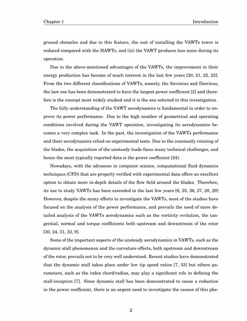
Chapter 1 Introduction
ground obstacles and due to this feature, the cost of installing the VAWTs tower is
reduced compared with the HAWTs, and (iii) the VAWT produces less noise during its
operation.
Due to the above-mentioned advantages of the VAWTs, the improvement in their
energy production has become of much interest in the last few years [20, 21, 22, 23].
From the two different classifications of VAWTs, namely, the Savonius and Darrieus,
the last one has been demonstrated to have the largest power coefficient [2] and there-
fore is the concept most widely studied and it is the one selected in this investigation.
The fully understanding of the VAWT aerodynamics is fundamental in order to im-
prove its power performance. Due to the high number of geometrical and operating
conditions involved during the VAWT operation, investigating its aerodynamics be-
comes a very complex task. In the past, the investigation of the VAWTs performance
and their aerodynamics relied on experimental tests. Due to the constantly rotating of
the blades, the acquisition of the unsteady loads faces many technical challenges, and
hence the most typically reported data is the power coefficient [24].
Nowadays, with the advances in computer science, computational fluid dynamics
techniques (CFD) that are properly verified with experimental data offers an excellent
option to obtain more in-depth details of the flow field around the blades. Therefore,
its use to study VAWTs has been extended in the last few years [6, 25, 26, 27, 28, 29]
However, despite the many efforts to investigate the VAWTs, most of the studies have
focused on the analysis of the power performance, and prevails the need of more de-
tailed analysis of the VAWTs aerodynamics such as the vorticity evolution, the tan-
gential, normal and torque coefficients both upstream and downstream of the rotor
[30, 24, 31, 32, 9].
Some of the important aspects of the unsteady aerodynamics in VAWTs, such as the
dynamic stall phenomenon and the curvature effects, both upstream and downstream
of the rotor, prevails not to be very well understood. Recent studies have demonstrated
that the dynamic stall takes place under low tip speed ratios [7, 33] but others pa-
rameters, such as the index chord/radius, may play a significant role in defining the
stall-inception [7]. Since dynamic stall has been demonstrated to cause a reduction
in the power coefficient, there is an urgent need to investigate the causes of this phe-
2
Chapter 1 Introduction
nomenon in the VAWTs.
During the operation of the VAWTs at high tip speed ratio, where dynamic stall does
not take place, it has been observed that there is a decrease in the power coefficient and
this has been associated to secondary effects such as the shaft, arms, etc. In addition,
a few investigations on the curvature effect have shown that this parameter becomes
significant at high tip speed ratios but its influence on the VAWT performance at both
upstream and downstream of the rotor remains also unrevealed.
Overall, the lack of understanding in the above-described aspects of the VAWTs
aerodynamics has limited the development of a fast engineering tool that is capable
of accurately and quickly predicting the power coefficient of any VAWT. That means
that although many efforts have been made in the past in order to develop a fast tool
capable of predicting the power coefficient of any VAWT, none of the existing methods
are reliable since many aspects of the VAWT aerodynamics remains unclear and as a
result, on using current methods, requires a strict verification with experimental data,
and this has not been available until the last few years.
1.2 Aims and objectives of this thesis
The aim of this thesis is to contribute to a much better understanding of the unsteady
aerodynamics of the vertical axis wind turbines at both sides, upstream and down-
stream, of the VAWT rotor and then, to contribute to the development of an engineer-
ing tool that is capable of predicting accurately the unsteady loads on VAWTs.
This thesis bridges some of the most important and essential gaps in the unsteady
aerodynamics of VAWTs that contribute to the progress in the maturity of the VAWT
technology as described in the following major objectives:
• To elucidate the significance of the chord, rotational speed, tip speed ratio, pitch
angle, Reynolds number and relative velocity in the stall-inception of the VAWTs.
• To analyse the unsteady aerodynamics at both zones of the rotor with the increase
of the tip speed ratio by using symmetrical and cambered aerofoils.
3

Chapter 1 Introduction
• To assess and modify the Leishman-Beddoes algorithm in order to be able to
accurately predict the unsteady loads of oscillating aerofoils and VAWTs in the
range of Reynolds number of 0.8−3.3×10⁵.
• To investigate the influence of the tip speed ratio and the number of blades on
the induced-virtual camber due to the curvature effects.
• To developed a new method that is able to predict accurately the unsteady loads
present under dynamic stall and non-stall conditions.
This investigation uses computational fluid dynamic simulations that have been
rigorously assessed for oscillating aerofoils and vertical axis wind turbine unsteady
loads, i.e. the azimuthal torque coefficient in both the upstream and downstream re-
gions of the rotor at several tip speed ratios. Further, the Leishman-Beddoes model
has been employed to compute and validate the modelling results with the experimen-
tal data for oscillating aerofoils and to assess it as a tool to predict the unsteady loads
on the VAWTs. The more pertinent modification to the dynamic stall model was made
in order to consider the influence of the number of blades and this model was very
useful to understand the influence of the curvature effect on the VAWT performance.
Moreover, the double multiple streamtube theory has been assessed in the prediction
of the unsteady loads at both zones of the rotor.
1.3 Limitations
This investigation is limited to the range of solidity 0.1325-0.3975 and this range is
considered to be in the range of interest in VAWTs design for urban locations. Ad-
ditionally, this investigation has considered two-dimensional analyses, and thus 3D
effects are not considered but this is an important issue that needs to be fully investi-
gated in the future in order to include the best corrections to the 2D model.
In order to obtain a full engineering tool that is capable of predicting the VAWT per-
formance under any operating conditions, more effort is required in the understanding
of the unsteady aerodynamics that characterizes these devices, constantly changing
4

Chapter 1 Introduction
in both the angle of attack and relative velocity and to develop a mathematical model
that best reflects the physics of the flow. Despite this, the thesis has addressed the
issues that are most urgent to be investigated and has laid out the solid groundwork
for future improvements.
1.4 Outline of the thesis
This thesis includes in Chapter 2 a valuable background of unsteady aerodynamics
with a focus on the dynamic stall phenomenon and the current theory stage. In ad-
dition, it presents a literature review of the unsteady aerodynamic theory of VAWTs
that describes the aspects that until now remain unrevealed.
Chapter 3 describes the research methodology followed in this thesis and gives more
insights into the methods adopted to investigate the unsteady aerodynamics, namely,
the CFD simulations, the Leishman-Beddoes dynamics stall and some discussion of
the double multiple streamtube method as a fast tool to predict the performance of
VAWTs. As a novel outcome of this chapter, the verification with experimental data
of the CFD numerical technique to predict the torque coefficient at the downstream of
the rotor at several tip speed ratios is included.
Chapter 4 includes for the first time an extensive analysis of the operating con-
ditions of VAWTs that influence the stall-inception. The tip speed ratio, reduced fre-
quency, pitch angle, relative velocity, Reynolds number and aerofoil profile are inves-
tigated using an oscillating aerofoil that describes the angle of attack and relative
velocity present in VAWTs. The results are fundamental in the understanding of the
dynamic stall in any VAWT since it has correlated the influence of the operating con-
ditions with the stall inception.
Chapter 5 evaluates the upstream and downstream contribution of the torque coef-
ficient for several aerofoils in order to better understand the range of tip speed ratios
where dynamic stall takes place and to correlate the behaviour of the azimuthal torque
coefficient with the optimum tip speed ratio of operation on the VAWTs. These results
present much useful information that enables one to identify the important behaviour,
not only of the dynamic stall phenomenon but also on the poor unsteady forces down-
5

Chapter 1 Introduction
stream of the rotor, with the increase in the tip speed ratio.
Chapter 6 discusses the key parameters of the Leishman-Beddoes dynamic stall to
predict the unsteady loads at low Reynolds number in the range of 0.8−3.3×10⁵. In ad-
dition, it computes the time delay constant of the aerofoils NACA0015, NACA0018 and
NACA0021 within the mentioned range of Reynolds number not previously reported
in the literature. The modifications to the LB algorithm are described and assessed in
the prediction of the unsteady loads for oscillating aerofoils under dynamic stall condi-
tions. Additionally, the assessment of the double multiple streamtube method coupled
with the modified LB algorithm to predict the VAWTs performance is carried out.
Chapter 7, the last research chapter, analyses the curvature effect due to the tip
speed ratio and the number of blades using CFD simulations and the modified LB dy-
namic stall model. In addition, the interference factor, both upstream and downstream
of the rotor, was investigated and a mathematical relationship was proposed. For the
virtual incidence due to the curvature effects, it is found that there is a mathematical
relationship with the tip speed ratio and the number of blades. The virtual incidence
increases with the tip speed ratio but at the same tip speed ratio reduced its value with
the increase in the number of blades. The present findings have allowed the proposing
of a new method that is promising in predicting the unsteady loads of VAWT and that
takes into account the dynamic stall and non-stall conditions.
Finally, in Chapter 8 the general conclusions of these investigations are presented
as well a discussion of the limitations and future work that will further improve the
prediction of VAWTs.
6
Chapter 2
Unsteady aerodynamics
2.1 Background
Aerodynamics is defined as the science of the fluid dynamics dealing with the interac-
tion between the air and a solid body when a relative movement exists between them
[34]. When the properties of the fluid are considered to be independent of the time, the
aerodynamics is called steady; when the nature of the flow field is characterized by a
time-dependent variation of their parameters at a given position, then the aerodynam-
ics is called unsteady [34]. The unsteady aerodynamics may result from a different
number of unsteady sources. For example, from a non-uniform velocity such as from a
sudden gust or a time-varying incident flow and, from the movement pattern described
by the solid body merged into a flow field such as rotation, pitching, plunging, flutter,
etc. [35].
The great interest in unsteady aerodynamics has emerged when the use of a steady
aerodynamic analysis was not able to explain and predict the loads present in devices
such as wings and helicopters [36]. After that, over the years, the interest has been
ever increasing since unsteady aerodynamics can explain the reason why some insects
are able to fly [37] and more recently to improve the design of unmanned aerial vehicles
performance [38] and wind turbines [39].
In the earliest development of unsteady theories, Theodorsen [40] proposed an an-
alytical solution based on the non-stationary potential flow to predict the loads on a
wing section oscillating within a very small amplitude of oscillation. At that time, the
large amplitudes of oscillation were neglected since the interest was focused on pre-
dicting the loads due to the flutter motion of the wings. After that, with the growing
aircraft industry and the interest to improve the performance and design of those vehi-
7

Chapter 2 Unsteady aerodynamics
cles, the number of experimental tests increased as well as the theories which proposed
some analytical solutions to predict the loads due to different unsteady mechanisms
[39, 41, 42].
An interesting phenomenon, called dynamic stall and related to the unsteady aero-
dynamics was discovered for the first time in helicopters as stated in [39]. Since then,
enormous efforts have been made experimentally in order to understand its physics
and its influence on the aerodynamic loads. Many experiments using aerofoils oscil-
lating and describing the movement pattern of the blades, that usually takes place on
helicopters, have been performed under several conditions. For example, the influence
of variables such as the Mach number, Reynolds number, oscillatory frequency, mean
and amplitudes in the angles of oscillation, aerofoils shape, etc. have been carried out
[43, 44, 4, 45, 46]. All these investigations have led to a much better understanding
of the unsteady aerodynamics and to the development of semi-empirical mathematical
methods, that use the Theodorsen theory as a basis [41] and that are able to predict
the unsteady aerodynamic loads due to the influence of the dynamic stall phenomenon.
The two main characteristics that have been observed under unsteady conditions
are the time-lag in the aerodynamic response of the aerofoil regarding the steady con-
ditions, and the presence of the dynamic stall phenomenon characterised by a vortex
formation near the leading edge of the aerofoil. The transient mechanism may cause
an effective angle of attack (the angle between the incident wind velocity and the chord
of the aerofoil) being larger than the static stall angle (the moment when a sudden loss
in the static forces is observed as shown in Fig. 2.1(a). This figure 2.1(a) includes the
normal force coefficient (the resultant aerodynamic force perpendicular to the aerofoil-
chord when a flow past the aerofoil surface) as a function of the angle of attack for a
steady aerofoil NACA0015 and, an oscillatory NACA0015 where the angle of attack is
within the static stall angle. The Fig. 2.1(b) includes the normal force coefficient for a
steady aerofoil NACA0015 and, an oscillatory NACA0015 describing an angle of attack
that goes further the static stall angle.
Either the transient mechanism produces an angle of attack within the static stall
angle or larger than the static stall angle, then the time lag takes place. Under this
regime, called the unsteady attached regime, the observed force coefficient presents a
8

Chapter 2 Unsteady aerodynamics
lower magnitude than the steady values during the upstroke motion (with an increase
in the angle of attack) and presents larger values than the steady values during the
downstroke motion (with the decrease in the angle of attack), see Fig. 2.1(a). A more
detailed discussion is included in [35, 47].
(a) (b)
Figure 2.1: The normal force coefficient as a function of the angle of attack for a steady NACA0015 aerofoil
at Reynold number of 1.5×10⁶ compared with the normal force coefficient of oscillatory NACA0015 with
a maximum angle of attack (a) within the static stall angle and, (b) larger than the static stall angle [1].
The second characteristic of the unsteady aerodynamics is the development of the
dynamic stall phenomenon that may take place when the effective angle of attack
increases further than the static stall angle. In Fig. 2.1(b), the normal force coefficient
on an oscillating aerofoil describing an angle of attack that goes beyond the static stall
angle is presented [1]. It is observed that under this unsteady condition, the force
coefficient stalls at a larger angle of attack and a large hysteresis is described in the
force coefficient during the downstroke motion of the aerofoil. More details of this
phenomenon are included later in this section.
In vertical axis wind turbines, two main sources of unsteadiness are found, namely,
the oscillating values in both the angle of attack and the incident velocity on the blades
through one cycle of the VAWT rotor [2]. The aerodynamic investigations have pro-
posed that the dynamic stall phenomenon is likely to take place at low tip speed ratios,
9

Chapter 2 Unsteady aerodynamics
that is the ratio between the tangential speed of the blades and the free-stream ve-
locity, and usually, where large amplitudes of the angle of attack are experienced [33].
In contrast, at high tip speed ratios, the absence of this phenomenon occurs, but the
unsteady effect may take place, as explained above, for smaller amplitudes of the angle
of attack under attached flows [30].
Despite that, the use of the available dynamic stall methods to predict the unsteady
loads in VAWTs appears to be a good idea [48, 49], its efficiency or deficiency and the
assumptions considered in the methods, remains without any solid supporting analysis
due to the following three main issues.
(i) VAWTs suffer from a combined transient effect of the angle of attack and the
incident velocity on the blades during one cycle of the rotation. The impact of these
simultaneous mechanisms in the dynamic stall has been rarely investigated and this
is attributed mainly to the complexity in replicating experimentally the time-varying
incoming flows [50].
(ii) The dynamic stall has been demonstrated to depend on several variables, such
as the frequency of oscillation, and the mean and amplitudes of the angles of oscil-
lations, Reynolds number, Mach number, aerofoil profile and the movement pattern,
i.e. the function described by the angle of attack. Also, many of the investigations on
dynamic stall have used a sine function as the variation in time of the angle of attack.
In addition, the typical angle of the attack described in a VAWT has been little inves-
tigated and these investigations have concentrated mainly on Reynolds number larger
than 1 million. Therefore, the influence of the Reynolds number lower than one million
on the dynamic stall remains unclear [1, 51].
(iii) There is a shortage of experimental data, including the unsteady loads on
the VAWTs at both sides of the rotor and, under the dynamic stall and full attached
regimes of operation. Thus, a more in-depth understanding of the unsteady aerody-
namics on the VAWTs needs to be investigated in order to present a fair assessment of
the application of dynamic stall methods to predict the VAWTs performance.
This thesis aims, in the first instance, to study and to analyse the dynamic stall
phenomenon in vertical axis wind turbines and, later, with the knowledge gained, for-
mulate a strategy to implement and improve the current dynamic stall methods to be
10
Chapter 2 Unsteady aerodynamics
capable of considering the unsteady aerodynamics on both sides of the rotor and under
both operating regimes, under the full-attached flow and dynamic stall conditions. The
knowledge generated in this thesis and the devised formulation to apply the dynamic
stall methods will encourage future works that will lead to the development of a fast
unsteady tool applicable to the VAWTs analysis and design.
2.2 Aerodynamics on VAWTs
A top view of a VAWT with three blades is shown in Fig. 2.2 (a). The free-stream wind
velocity, V∞, is the undisturbed wind speed located before impacting the VAWT at the
upstream zone of the rotor. The downstream zone of the rotor is the region of the rotor
where the flow has been affected by the front zone of the VAWT rotor. In terms of the
azimuthal angle (θ ) which determines the position of one blade during its rotation, the
upstream zone corresponds to θ = 0 to θ = 180◦ and the downstream zone corresponds
to θ = 180 to θ = 360◦. The aerodynamic forces and the most relevant mathematical
relations that govern the aerodynamic performance of a VAWT are illustrated in Fig.
2.2(b) and described as follows.
In a vertical axis wind turbine, the blades rotate about an axis with a rotational
speed, ω, as indicated in Fig. 2.2(b). Each blade perceives an actual wind velocity
(relative velocity) which is constantly changing in magnitude given by the following
expression [2]:
Vrel(θ) =V∞
√1+2λ cos(θ)+λ 2 (2.1)
where λ is the tip speed ratio and is defined as the ratio of the tangential speed of the
blades, ωR, and the free stream wind velocity, V∞. The azimuthal position of the blades
is calculated with the relation: θ = ωt, where t represents the time elapsed when the
blade has passed the position θ = 0◦ indicated in Fig. 2.2 (a).
The direction of the relative velocity is described by the angle of attack equation
given by:
α(θ) = φ −β (2.2)
11

Chapter 2 Unsteady aerodynamics
Figure 2.2: (a) A schematic representation of a three-bladed VAWT and its representative zones and, (b)
a schematic representation of the aerodynamic forces generated during the rotation of the VAWT blade.
12

Chapter 2 Unsteady aerodynamics
where β represents the pitch angle, and it is positive outwards from the circle described
by the outer edge of the rotation of the blade, see Fig. 2.2. The path angle φ , is the
angle between the tangential speed vector of the blade and the relative velocity and, is
given by the following expression.
φ(θ) = arctan(sin(θ)
λ + cos(θ)) (2.3)
As was mentioned previously, the angle of attack is the angle between the relative
velocity direction and the chord of the aerofoil. When the flow past the blades and the
relative velocity impacts the aerofoil surface, thus the aerodynamic forces are gener-
ated and a tangential force (FT ) results, which finally produce the torque coefficient,
CQ, in the VAWT. Among the most relevant aerodynamic forces are the lift force co-
efficient, CL, and the drag force coefficient, CD. The lift force, L, is aerodynamic force
that is perpendicular to the relative velocity and, in VAWTs the lift force coefficient is
calculated with the next expression.
CL =L
1/2ρAbV 2rel
(2.4)
where, Ab represents the blade area and typically is the product of the chord length,
c with the span-length of the blade, H. The drag force, D, is the aerodynamic force
parallels to the relative velocity of the blades and the the drag force coefficient in the
VAWT blade is calculated with the next expression:
CD =D
1/2ρAbV 2rel
(2.5)
Both equations of CL and CD are used with steady simulations but instead of the Vrel
the constant incoming flow velocity is used. The tangential force, FT and the radial
force FR result of the lift and drag aerodynamic forces generated when the flow past
the blades. The FT is tangential to the circle describe by the rotation of the blades and
the radial force, FR, is the resultant aerodynamic force along the radius.
Both equations (2.1) and (2.2) are theoretical expressions and may be modified by
the curvature index, that represents the ratio between the chord (c) and the radius
13

Chapter 2 Unsteady aerodynamics
of the turbine (R); the number of blades and the streamlines expansion due to the
presence of the rotor [2, 52, 10, 53, 54].
The typical performance of a VAWT rotor is represented by its power coefficient, CP,
as a function of the tip speed ratio, λ , as illustrated in Fig. 2.3. The power coefficient
is the coefficient between the power generated by the wind turbine and the available
wind power and is given by the following expression:
CP =P
0.5ρV 3∞A
(2.6)
where A represents the transversal area of the rotor that is being impacted on by the
incoming flow and ρ represents the air density.
Figure 2.3: A typical power coefficient of a VAWT as a function of the tip speed ratio (the range of tip
speed ratio might change accordingly to the VAWT design) [2].
As observed in Fig. 2.3, the power coefficient at low tip speed ratios is low and this
is associated to the dynamic stall phenomenon [33, 55]. After an optimum value of CP is
reached , the power coefficient starts to decrease again and this is attributed to the low
magnitude of the aerodynamic forces due to the decrease in the angle of attack and the
secondary effects, such as the shaft, struts, etc. [2]. This typical curve of VAWTs is the
result of the extensive experimental tests carried out by the Sandia Laboratories since
1968 using mainly the NACA0012 and a rotor with very low solidities [56, 57]. Most of
14
Chapter 2 Unsteady aerodynamics
the theory resulting from these experimental tests has been included in Paraschivoiu
in [2].
In the book by Paraschivoiu [2] several parameters that influence the VAWT perfor-
mance have been investigated, namely, the rotational speed, Reynolds number, aero-
foil, number of blades, the chord length, struts, shaft, etc. As a result, a method called
the double multiple stream-tube theory (DMST) was developed that analyses the rotor
in two main regions, the upstream and downstream regions. This method uses the
momentum theory and blade element theory and considers the flow to be inviscid and
steady.
In the mentioned work [2], some efforts were made to include dynamic stall meth-
ods to improve the power predictions but, despite that, the details of the efficiency/de-
ficiency of the dynamic stall methods were not clearly discussed. This is attributed to
the fact that dynamic stall remains to be not well understood under the VAWTs con-
ditions and due to the several parameters that affect the VAWTs unsteady loads are
not suficient to fully understand the dynamic stall in VAWTs and PIV visualization,
for example, are also crucial [33, 58].
2.2.1 Instantaneous loads on VAWTs
In order to gain a more in-depth understanding of the VAWTs aerodynamics, the non-
integrated forces such as the tangential force, the pressure coefficient, the skin friction
and the torque coefficient are required to be investigated at each azimuthal position. In
the last few years, due to the progress on the measurements techniques and materials
science, more detailed experimental data on VAWTs are becoming available.
Recently, Li et al. [54, 32, 31] has performed the most extensive experimental test
on VAWTs using the NACA0021 aerofoil. The angle of attack, relative velocity, the
tangential and radial forces, torque coefficient at each azimuthal angle for two, three,
four and five blades can be found. Although these detailed data is provided for a few tip
speed ratios, the data includes important representative conditions under the dynamic
stall and high tip speed ratios. Also, the pressure coefficient is provided for some
azimuthal angles. In addition, the power coefficient as a function of the tip speed ratio
can be found for a range of tip speed ratios, a different number of blades and several
15
Chapter 2 Unsteady aerodynamics
pitch angles. In the above mentioned experimental test, pressure taps in the mid-span
of the blades were employed (approximating the measurements to be two-dimensional)
and, additionally, a six-component balance was used to take into account the 3D effect
of the rotor.
Nguyen et al. [24] measured the radial force coefficient as a function of the az-
imuthal angles for VAWTs with a NACA0021 aerofoil and four tip speed ratios in the
range [1.84-4.57]. It is mentioned that only the radial force coefficients were measured
due to the stiffness of the blades that were sufficient to not disturb the measurements.
CFD simulations were also validated with these experimental data and it was found
that there was a good agreement between the numerical and experimental data; how-
ever, some differences at the downstream zone of the rotor were found.
Vittecoq and Laneville in [59] measured the radial force coefficients and tangential
force coefficients for a two-bladed VAWTs with the NACA0018. The radial force coef-
ficient was presented for a range of tip speed ratios [1.5-5] while the tangential force
coefficient was presented for tip speed ratios of 2, 2.5 and 3. It is mentioned that, for
the tangential force coefficient downstream, the signal presented some complexity that
required further analysis.
Rossander et al. [60] measured the radial and tangential force coefficients using
load cells at the hub of a three-bladed VAWTs using a NACA0021 aerofoil. The method
to measure the tangential force coefficients was concluded to be unsuitable due to the
large fluctuations observed in the forces attributed to the dynamic oscillations on the
blades. However, the radial force coefficients were consistent with the numerical esti-
mations.
Peng et al. [61] have also performed experimental tests to measure the tangential
and radial force coefficients as a function of the azimuthal angle of a three-bladed
turbine. It is mentioned that because of the larger magnitude on the radial forces
coefficient compared with the tangential force, larger errors where expected in the
tangential forces and thus corrections were applied. A two-component force sensor
was connected directly at the top and the bottom of the axis of each blade that used
the NACA0018 aerofoil.
In the revision of the above experimental investigations [24, 59, 60] difficulties in
16

Chapter 2 Unsteady aerodynamics
the measuring of the tangential forces as a function of the azimuthal angle have been
discussed. The magnitude of the tangential forces are smaller than the radial forces
and hence, the fluctuations and the errors found in the tangential forces coefficients
are larger than in the radial force coefficients. In the case of Li. et al. [54, 32, 31], they
used the pressure measurements in the mid-span and the actual flow field around the
blade is used. This avoids the problem found in the previous investigations that used
cell-loads.
As has been explained previously, the experimental tests represent many chal-
lenges when measuring the forces produced by the blades on a VAWT. The tangential
force coefficient is considered to be the most relevant to investigate the performance
of the VAWTs since the torque produced by the blade is the product of the tangen-
tial force and the radius [24] but it is the most difficult to be obtained accurately in
experimental investigations. Therefore, validated computational fluid dynamic tech-
niques still represent a crucial tool in order to assist in the prediction of the tangential
and radial forces coefficients on the blades, as well to better understand the flow field
development upstream and downstream of the rotor.
Due to the small amount of data available for the forces as a function of the angles
of attack, very few CFD investigations on VAWTs have been verified accurately both
upstream and downstream of the rotor [62, 24]. As a result, no single investigation has
included an analysis of the unsteady aerodynamic forces as a function of the azimuthal
angle with the increase in the tip speed ratio. Rather than this, the integrated value
of the power coefficient as a function of the tip speed ratio has been widely considered
to investigate the influence of several parameters.
Rezaeiha et al. in [29] have proposed a CFD numerical strategy that claims to be
highly accurate since the power coefficient (CP) as a function of the tip speed ratio (λ )
showed a good agreement with the experimental data. Nevertheless, the power coeffi-
cient, CP, showed a good agreement for the tip speed ratios before the optimum CP and
disagreement after this point. Since no comparison with the azimuthal torque coeffi-
cient or other non-integrated forces were made, a deeper analysis as to where those
differences are coming from, i.e. coming from the upstream, downstream regions or
both cannot be discussed. Further investigations by Rezaeiha et al. [63, 64] evaluated
17

Chapter 2 Unsteady aerodynamics
the influence of the Reynolds number, number of blades, solidity and pitch angle in the
power performance of VAWTs.
This thesis aims to analyse the unsteady aerodynamics at both sides, upstream and
downstream of a VAWT and take into account the tip speed ratios where the dynamic
stall occurs as well as where non-stall conditions are present. This information is
substantial and very important in order to much better assess the capabilities of the
method to be used to predict the power coefficient of VAWTs.
2.2.2 Dynamic stall on VAWTs
The dynamic stall phenomena have been widely studied experimentally for several
unsteady motions, namely: pitching, flapping, fluttering, wind velocity variation in
[58, 35, 43, 44, 4, 45, 46, 65]. In addition, using Large Eddy Simulation techniques
the dynamic stall phenomenon has been investigated using oscillating aerofoils in [66,
67, 68, 69] and ramp-up test in [70, 3, 71]. A similar topology of this mechanism
has been found among all the motion patterns, including the VAWTs according to the
experimental observations using PIV (particle image velocimetry) technique in [30, 72,
33, 73]. For the purpose of this thesis, the main parameters involved to describe this
phenomenon are explained in the following paragraphs.
In an unsteady motion with a rapid increase in the angle of attack, α(t) that goes
further than the static stall angle then the dynamic stall phenomenon follows the next
stages:
• At the static stall angle, αss, the dynamic boundary layer experiences a delay
in the reversal flow (backflow) compared with the static case. Additionally, the
lift force coefficient increases its value following the same trend as if it remains
attached. The state of the boundary layer at this point plays a vital role in deter-
mining the dynamic stall delay [74].
• If α(t) increases further than αss then the flow reversal from the aerofoil trail-
ing edge (TE) moves towards the leading edge (LE) and the laminar bubble that
is concentrated at the aerofoil LE experiences a maximum in the pressure co-
efficient (negative), and then a vortex is initiated and detaches from the LE.
18
Chapter 2 Unsteady aerodynamics
This point is called the stall-onset angle αos and determines the inception of the
stalling process. Additionally, at this point, the lift coefficient deviates from its
linear attached trend and increases in value (over-lift) due to the movement of
the vortex downstream along the chord of the aerofoil. (It should be noted that
the stall-onset mechanism depends on the aerofoil thickness [75, 70]).
• If the increase in α(t) is sufficient to allow the vortex to reach the trailing edge,
then the lift force reaches its maximum value, this is characterized by a signifi-
cant peak, and then a sudden loss in the lift is observed, this point is known as lift
stall (L). Consequently, the pitching moment coefficient diverges to high negative
values; this point is called the moment stall (M). Multiple vortex sheddings are
possible if the aerofoil motion does not change direction and the angle of attack
continues increasing.
• With the decrease of α(t), and a change in the motion direction of the aerofoil,
a boundary layer reattachment can take place, and a large hysteresis in the un-
steady loads is observed [46].
The stall-onset angle is a critical parameter in describing the dynamic stall process
since it marks the inception of the leading edge vortex; thus the success of a dynamic
stall method depends on the accurate prediction of the stall-onset angle [46]. Despite
that, the available experimental and numerical investigations have focused on describ-
ing the topology of the dynamic stall phenomenon [43, 46, 44, 41, 76, 4] rather than
understanding the factors that dictate the stall inception. Additionally, the Reynolds
numbers under investigation have been larger than 1 million. Therefore, there is still
a need on understanding which physical parameters affect the stall onset at lower val-
ues of Reynolds number in order to fully describe this phenomenon in the VAWTs when
these devices operate at low wind speeds.
The ramp-up tests that have a constant pitch rate α = C, have demonstrated this
parameter as being the most crucial parameter to define the stall-onset in the exper-
imental test carried out in[77, 74, 78, 79, 80, 81, 82]. High-fidelity techniques such
as the Large eddy simulations (LES) are able to provide more insights into the flow
19

Chapter 2 Unsteady aerodynamics
physics of the dynamic stall phenomenon such as the investigations in [70, 3, 71]. For
instance, Sharma et al. [3] presented the evolution of the pressure coefficient and the
skin friction along the aerofoil surface for the NACA0015 at a Reynolds number of
2×10⁵ for a constant pitch rate motion. As observed in Fig. 2.4(a), with the increase in
the angle of attack the transition point of the boundary layer, identified by the bound-
ary between the negative and positive skin friction, moves towards the leading edge.
Around the angle of attack of 19.3◦ the laminar separation bubble (LSB) bursts and
full stall occurs. Similarly, the negative pressure coefficient of the suction side of the
aerofoil surface is analysed in Fig. 2.4(b). For this parameter, a more negative pres-
sure coefficient occurs around the leading edge of the aerofoil with the increase of the
angle of attack, and when the LSB bursts then, the pressure coefficient reaches its
most negative magnitude.
(a) (b)
Figure 2.4: (a) Contours of spanwise-averaged skin friction coefficient (C f ) and (b) pressure coefficient on
the suction side of the NACA0015 aerofoil through the constant pitch-rate motion at Re 2×10⁵ and, using
LES. [3]
To understand better the skin friction and pressure coefficient behaviour when the
stall-onset is about to occur then five angles of attack are selected and included in Fig.
2.5 by Sharma et al. [3]. Fig. 2.5(a) shows that the pressure coefficient increases
20
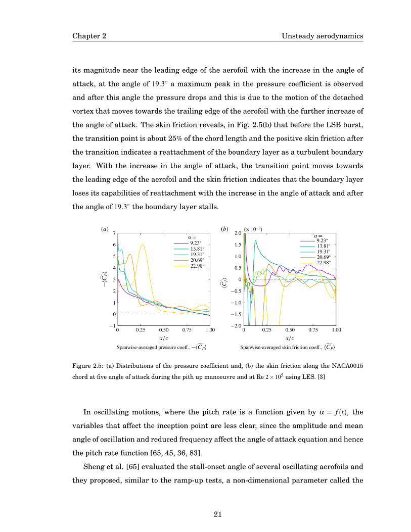
Chapter 2 Unsteady aerodynamics
its magnitude near the leading edge of the aerofoil with the increase in the angle of
attack, at the angle of 19.3◦ a maximum peak in the pressure coefficient is observed
and after this angle the pressure drops and this is due to the motion of the detached
vortex that moves towards the trailing edge of the aerofoil with the further increase of
the angle of attack. The skin friction reveals, in Fig. 2.5(b) that before the LSB burst,
the transition point is about 25% of the chord length and the positive skin friction after
the transition indicates a reattachment of the boundary layer as a turbulent boundary
layer. With the increase in the angle of attack, the transition point moves towards
the leading edge of the aerofoil and the skin friction indicates that the boundary layer
loses its capabilities of reattachment with the increase in the angle of attack and after
the angle of 19.3◦ the boundary layer stalls.
Figure 2.5: (a) Distributions of the pressure coefficient and, (b) the skin friction along the NACA0015
chord at five angle of attack during the pith up manoeuvre and at Re 2×10⁵ using LES. [3]
In oscillating motions, where the pitch rate is a function given by α = f (t), the
variables that affect the inception point are less clear, since the amplitude and mean
angle of oscillation and reduced frequency affect the angle of attack equation and hence
the pitch rate function [65, 45, 36, 83].
Sheng et al. [65] evaluated the stall-onset angle of several oscillating aerofoils and
they proposed, similar to the ramp-up tests, a non-dimensional parameter called the
21

Chapter 2 Unsteady aerodynamics
equivalent reduced pitch rate that is the product of the amplitude and the reduced
frequency. This equivalent reduced pitch rate was shown to be the most crucial pa-
rameter that defines the stall-onset in the oscillating motion. The same equivalent
reduced pitch rate was used in [84] and a similar linear trend between the equivalent
reduced pitch rate and the stall-onset angle was found.
More recently, Mulleners et al. [58] experimentally found for oscillating aerofoils
that the non-dimensional pitch rate at the static-stall angle was the parameter that
is the most critical factor in determining the stall-onset and the previous proposed
equivalent reduced pitch rate in [65] did not show a clear relation with the stall-onset.
In the VAWT, when dynamic stall takes place, then this degrades its power coeffi-
cient and induces high structural loads on the rotor [2]. The vortex formation and its
release to the wake characterize the dynamic stall on VAWTs. If the dynamic stall is
severe, multiple vortices are released, and an additional decrease in the power coef-
ficient is observed [85]. The generation of the vortices has been observed to be more
prominent in the upstream section of the rotor but may appear downstream of the
rotor [86, 55].
Thus, in order to improve the VAWTs performance and to regulate the dynamic stall
that induces the undesired unsteady loads, determining the operational and physical
parameters that control the stall-onset in the upstream region of the VAWTs rotor
represents an essential task. Despite this importance, most of the investigations have
been focused on describing the development of the dynamic stall phenomenon under
some of the variables and, a very few investigations have paid attention to the stall-
onset angle, the angle at which the vortex is released in the VAWTs.
Observations of the dynamic stall phenomenon using PIV techniques have been
most studied by changing the tip speed ratio (TSR), but the dynamic stall has been
observed at different TSRs values, and its influence remains unclear. For example,
Fujisawa and Shubuya [33] observed the vortex formation for TSRs 1, 2 and 3; Brochier
et al. [55] tested TSRs of 2.14 and 3.85, observing the dynamic stall for the lowest TSR.
Simeira et al. [30] tested TSRs 2, 3 and 4 and the vortex formation was observed for
TSRs 2 and 3; Laneville and Vittecoq [87] observed dynamic stall for TSRs less than 4.
Moreover, Li et al. [73] observed dynamic stall for TSRs less than 1.8 and Edwards et
22

Chapter 2 Unsteady aerodynamics
al. [88] observed the shedding vortex for TSRs from 2 to 4.
Recently, Bucher et al. [7] investigated the stall-onset angle using TSRs from 1 to
5, three Reynolds numbers (average) and three-chord lengths. It was concluded that
the tip speed ratio alone is not sufficient to describe the stall-onset and the dynamic
stall phenomenon. It is also recommended that more parameters, such as c/D, that
relates the chord length and diameter needs more investigations.
In the VAWTs, the number of operating conditions that may affect the stall-onset
angle is larger compared with the ramp-up and sine-pitching motions. For example, in
the VAWTs the stall-onset can be affected by the tip speed ratio, pitch angle, rotational
speed, Reynolds number and the constantly changing relative velocity. Thus, despite
the efforts made by several authors, defining how these operating parameters affect
the stall-onset angle results in a very complicated task when using a full wind turbine
[7].
Now, the important research question is to know which variables and operating
conditions affect the stall-onset in the VAWTs. Without answering this question, the
possibilities to improve or assess a dynamic stall model are going to be minimal. There-
fore, it is the main interest of this thesis to investigate how all the operating conditions
present in the VAWTs affect its stall-onset angle, namely, tip speed ratio, pitch angle,
rotational speed, Reynolds number and relative velocity. Since the experimental data
to be used to assess the VAWTs in [31] is within the range of Reynolds number of
2− 4× 10⁵, thus the stall-onset angle needs to be investigated within this range of
Reynolds number. Therefore, this thesis investigates a range of Reynolds number that
has not been previously investigated before (to the best of the knowledge of the au-
thor after an exhaustive literature review) and hence this thesis contributes with data
that can be used for dynamic stall methods to accurately predict the unsteady forces
at these Reynolds numbers.
2.3 Summary
In this chapter, it has been discussed the main characteristics of the unsteady aero-
dynamics, namely, the delay in the pressure response and the vortex formation at the
23

Chapter 2 Unsteady aerodynamics
leading edge of the aerofoil causing the dynamic stall phenomenon.
Under the dynamic stall regime, it has been identified the existing gaps in the
literature that remains unclear: how all the operating conditions of a VAWT affect
the stall-onset angle. In addition, it has been identified as the need for understanding
the stall-onset angle at Reynolds number lower than 1 million. At those low Reynolds
numbers, the understanding of this phenomenon results crucial in order to improve
the performance of VAWTs operating at low wind speeds and also, to improve the
predicting methods of unsteady loads such as the dynamic stall models. This gaps in
the literature are covered in Chapter 4.
This chapter also identified the existence of a severe shortage of experimental tests
on the azimuthal force coefficient of VAWTs and thus encouraging the use of validated
computational fluid dynamics in the prediction of the unsteady forces on VAWTs and
to gain a much deeper insight into the aerodynamics. The assessment of the CFD sim-
ulations with experimental data consisting of azimuthal torque coefficient is presented
in Chapter 3.
Moreover, it has been demonstrated the existence of a shortage in the details of the
unsteady blades loads at upstream and downstream of the VAWTs. Then, investigat-
ing the aerodynamics characteristics of the aerofoils that are fundamental upstream
and downstream of the rotor would reveal valuable information to improve the aero-
dynamic design of the aerofoils and the main aerodynamic characteristics that become
more important with the increase of the tip speed ratio. This gaps in the literature are
covered in Chapters 5 and 6.
24

Chapter 3
Methodology
3.1 Overview
As was mentioned in the previous chapter, there is a need for a full understanding
of the unsteady aerodynamic of VAWTs in order to improve their performance and, to
develop a fast engineering tool that is capable of predicting with accuracy the unsteady
loads of the vertical axis wind turbines (VAWTs) under any operating regime, i.e.,
under the dynamic stall and full attached regimes. In order to bridge this gap in
the literature then, a large analysis of the unsteady aerodynamics is carried out in
this thesis. Starting with oscillating aerofoils to understand how the combined effect
of the operating parameters in the VAWTs influence the stall-onset, followed by the
CFD simulations of the full rotor under a wide range of tip speed ratios of operations
and several aerofoils profiles and, last, using a dynamic stall-algorithm to obtain a
more in-depth analysis of the aerodynamics of VAWTs under the dynamic stall and
the unsteady attached regimes.
The steps that have been undertaken in this thesis and their corresponding method
are presented schematically in Fig. 3.1 and described as following.
(i) The influence of the operating parameters on the stall-onset angle, namely, tip
speed ratio, pitch angle and rotational speed is investigated by using an oscillating
aerofoil describing the angle of attack on VAWTs with an incoming flow with a wind
speed at a constant magnitude.
(ii) The influence of the relative velocity on the stall-onset angle is investigated
using an oscillating aerofoil with an incoming flow with the fluctuating relative velocity
found in VAWTs. These steps, (i) and (ii), used CFD simulations that were validated
with experimental data of oscillatory aerofoils. More details of the employed CFD
25

Chapter 3 Methodology
Figure 3.1: Schematic representation of the global methodology adopted in the thesis (philosophical
methodology).
techniques are given in Section 3.2.2 and results are presented in Chapter 4.
(iii) Two-dimensional CFD simulations using one-bladed turbine were performed
under a range of tip speed ratios of 2-5 and six aerofoils profiles were investigated. Af-
ter that, the two-bladed turbine was investigated under a TSRs range 1.5-4, and also
the six aerofoil profiles were analysed. Last, a three-bladed VAWTs was analysed at
the range of TSRs 1.5-3.5 and again the six aerofoils were investigated. These simu-
lations were enough to study the unsteady aerodynamics of VAWTs at both upstream
26

Chapter 3 Methodology
and downstream of the rotor and also, under both regimes of operation, the dynamic
stall and unsteady full attached regime. The VAWTs CFD simulations were carefully
verified with the available experimental data, i.e, the azimuthal torque coefficient as
described in Section 3.2.3. Results of these simulations are included in Chapter 5.
With the gained understanding of the unsteady aerodynamics, thus the evaluation
and improvement of the existing fast methods that are able to predict the torque co-
efficient of VAWTs under both regimes of operation are carried out following the next
steps.
(iv) The dynamic stall Leishman-Beddoes is selected and evaluated by using the
CFD simulations carried out in the step (i). This method is explained in Section 3.3
and more details of its performance and improvement are included in Chapter 6.
(v) The double multiple streamtube method is assessed in its accuracy to predict the
torque coefficient at upstream and downstream of the rotor and also under the dynamic
stall and the unsteady attached regimes. The results were included in Chapter 6.
(vi) A more in-depth analysis of the VAWTs aerodynamics has been performed by
investigating the virtual incidence angle due to the curvature effects. This step uses
the CFD simulations and it is assisted by a modifying the effective angle of attack into
the Leishman-Beddoes model.
In the following section, the description of the methods used in this thesis are fully
explained: The computational fluid dynamic techniques for the simulation using os-
cillating aerofoils and the CFD techniques for the VAWTs simulations; the Leishman-
Beddoes model and, the Double multiple streamtube. A further discussion of the selec-
tion of these mentioned methods and their previous use in the reviewed literature to
predict the VAWTs is also included.
3.2 Computational fluid dynamic simulations
This section describes the numerical techniques: (i) that have been used to investigated
the stall-onset angle consisting of two-dimensional CFD simulations with an oscillat-
ing aerofoil describing the VAWT angle of attack and, (ii) the CFD numerical technique
to investigate the VAWTs aerodynamics and its verification with experimental data.
27

Chapter 3 Methodology
3.2.1 Governing equations
Computational fluid dynamics (CFD) are based in the continuity, momentum and en-
ergy equations (the Navier-Stokes equations) to fully described the flow field around
a body or system. For practical solution when the flow becomes turbulent, the in-
stantaneous quantities are decomposed into a mean and fluctuating elements. These
representations of the Navier-Stokes equations are called the Averaged Navier-Stokes
equations (RANS) and for transient and incompressible flows (the cases investigated
in this thesis) are represented by following expressions:
ρ(∂Ui
∂ t+U j
∂Ui
∂x j) =− ∂P
∂xi+
∂
∂x j(µ
∂Ui
∂x j−ρu′iu
′j)+ρFi (3.1)
∂Ui
∂xi= 0 (3.2)
Eq.(3.1) represents the momentum equation and Eq.(3.2) represents the continuity
equation. The decomposition of the instantaneous velocity adds new unknown vari-
ables into the momentum equation. The term, (ρu′iu′j) is known as the Reynolds stress
(also called apparent stress) and its modelling is the purpose of the turbulence models.
The turbulence model solves a different number of transport equations to obtain
the Reynolds stress tensor. Most of the available turbulence model in Fluent are base
in the eddy viscosity concept and solves one, two, three or Four transport equations.
The number of transport equations to solve increases the computational time of the
simulations.
The Shear Stress Transport model, SST , uses the two-equation model κ −ω (tur-
bulent kinetic energy-specific dissipation rate) to solve the flow within the boundary
layer and the model κ − ε (turbulent kinetic energy-turbulent dissipation rate) in the
free-stream flow. This model is one of the most used in aerodynamic flows and takes
into account within the turbulent viscosity the turbulent shear stress.
In order to predict the transition of the laminar to turbulent flow, the model Tran-
sitional SST has been proposed (also known as the γ − Reθ transition model). This
model is a further development of the SST model and solves two additional transport
equations: for the intermittency, γ, and the momentum-thickness, Reθ . A variation
28

Chapter 3 Methodology
of the Transitional SST is the intermittency model, γ transition, and it solves one
transport equation for the turbulence intermittency γ, but ignores the solution of the
momentum-thickness, Reθ . This turbulent model, the intermittency transition model,
reduces the computational effort by solving one transport equation instead of two and,
can be applied for surfaces moving regarding a coordinate system.
The transport equation of the intermittency is given by following expression:
∂ (ργ)
∂ t+
∂ (ρU jγ)
∂x j) = Pγ −Eγ +
∂
∂x j[(µ +
µt
σγ
)∂γ
∂x j] (3.3)
the transition source terms, Pγ and Eγ are similar in formulation for the Transitional
model. This model uses the same transport equation for ω than the SST model and
the intermittency is only included in the production term of the κ transport equation
as follows [89]:
∂ (ρκ)
∂ t+
∂ (ρU jκ)
∂x j) = γe f f Pκ −D∗κ +
∂
∂x j[(µ +
µt
σκ
)∂κ
∂x j] (3.4)
where, D∗κ = min[max(γe f f ,0.1),0.1]Dκ . Dκ is the destruction term and Pκ is the pro-
duction term of the original SST model and γe f f is the effective intermittency. The
intermittency function, for a laminar flow, takes a value of 0 and a value of 1 for a
fully turbulent flow. Observing the Eq.(3.4), while γ increases from zero to 1 within
the boundary layer, the production term, Pκ , turns on and the eddy viscosity starts to
increase [90]. Much more details of this model may be found in [89] and the Ansys
Fluent guide user.
This Section 3.2.1 employs the symbols most widely used to represent the math-
ematical expression of the governing equations and more in-depth details are maybe
found in [91]. Only for this Section 3.2.1, the variable P means pressure and F repre-
sents the external forces.
3.2.2 Simulations for oscillating simulations
This section presents the numerical settings and the verification carried out for the os-
cillating aerofoils simulations. The present two-dimensional CFD technique was care-
fully validated against experimental data. The available experimental data consists
29

Chapter 3 Methodology
of the normal force coefficient of an oscillating NACA0012 aerofoil with the Reynolds
number 1.35× 10⁵ (chord-based), a chord (c) of 15 cm and a reduced frequency of 0.1
[4]. The intensity of the turbulence was 0.08%, similar to the experimental conditions
of the wind tunnel test case. This experimental data is selected since VAWTs for ur-
ban environments can experience a Reynolds number as low as 1× 10⁵ [92, 93] and
this is the main interest of this investigation. Also, several numerical investigations of
this case have been performed in order to determine a numerical strategy that consid-
ers the mesh, time and domain independence for oscillating aerofoils at low Reynolds
numbers [94, 68, 83, 69]
Numerical settings
In the present simulations, the turbulent transitional model κω−SST − γ was selected
due to the Reynolds number being studied, namely 0.8−3.3×10⁵, where the boundary
layer flow transition is likely to occur and a transitional model is recommended at such
Reynolds numbers [95, 96, 97]. A discussion of the influence of the turbulence models
of this experimental case has been made in [97] and the use of a transitional model is
recommended.
Among the pressure-based velocity coupling schemes available in Fluent: SIMPLE,
SIMPLEC, PISO and Coupled, the first three used the segregated algorithm and Cou-
pled uses the pressure-based coupled solver. The Coupled scheme uses an implicit time
integration that is unconditionally stable regarding the time step. Despite that, since
each time step requires a convergence criterion and hence several iterations to ob-
tain this convergence, the non-linearities associated to the discretized equations may
produce a large change in the quantities calculate at each iteration and produce slow
convergence or divergence. To solve this, the coupled algorithm, introduces the under-
relaxation factor, a, for the momentum and pressure variables to reduce the changes
in these quantities during each iteration. The CFL number in the coupled algorithm,
is a solution parameter and, in terms of under-relaxation factor is written as:
1−aa
=1
CFL(3.5)
30

Chapter 3 Methodology
As consequence, large CFL numbers are possible to be employed for this implicit
scheme and this can lead to faster convergence. This algorithm uses an algebraic
multigrid method (AMG) that has the capabilities to detect divergence within an it-
eration, automatically reduces the CFL number. This coupled algorithm has demon-
strated to be efficient with coarse time steps and coarse meshes. More in-depth detail
may be found in the Fluent users guide and in [98]. Explicit time integration is only
available for the density-based solver and the time step is restricted to the stability
condition given by the Courant-Friedrichs-Lewy conditions with a suggested Courant
number of 1.
The default CFL in the coupled algorithm is 200 but a reduction to 10-50 is rec-
ommended if there are difficulties with convergence, thus a CFL=10 was selected. A
full convergence criterion with a relative residual less than 1× 10⁻⁵ was used with
100 iterations per time step. At least four oscillating cycles were performed for each
simulation before collecting the results, and in most cases, a convergence in the lift
force coefficient was achieved after the second cycle. This agrees with the statistical
convergence observed by Geng. et al. [97]. A second-order discretization (spatial and
temporal) and a hybrid initialization was set up in all the simulations.
Mesh domain and boundary conditions
In the experimental data, a closed wind tunnel was used with the walls allocated to
be three times the chord-length of the aerofoil from the centre of the pitching motion.
Thus, to be consistent with the experimental test conditions, non-slip conditions were
applied for the upper and lower bounds of the domain with an original distance of 3
times the chord-length. Moreover, due to the interest in studying aerofoils in an open
environment, then the distance of the upper and lower boundaries from the pitching
position of the aerofoils (1/4 c) was increased to 3, 10, 15 and 20 times the characteristic
length, c, in order to find a domain with no influence on the forces on the aerofoil. The
influence of this distance is observed in the resulting lift coefficient and very similar
results were obtained using distances of 10, 15 and 20 c. Therefore, 15c was selected as
the distance from the pitching point to the boundaries (lower and upper), and this was
enough to avoid the influence of the upper and lower boundaries. The pressure outlet
31

Chapter 3 Methodology
was set to be 45c from the pitching point of the oscillating aerofoil, and the velocity
inlet was set to be 15c from the oscillating point. Both distances are considered to be
large enough to allow the development of the wake and within the recommendations
of several investigations [94, 69].
The aerofoil profile was set as non-slip conditions and due to the importance of
solving the viscous layer, then 60 layers were collocated around the aerofoil and the y+
in the boundary layer was less than 1.2.
In the mesh topology, two domains were used: a rotating domain with an unstruc-
tured mesh as illustrated in Fig 3.2(a), and a stationary domain consisting of a struc-
tured mesh, Fig. 3.2(b). The interface between the rotating zone (denoted with tri-
angles) and the stationary domain (quadrilaterals) is shown in Fig.3.2 (c). In order to
reduce the interpolation error during the motion, both domains contain in the interface
the same number of nodes, thus the element size in the contact region was of the same
length. For the rotating zone, a hard face sizing method was used and at the contact
interface for both domains, the stationary and the rotating domains, a hard edge sizing
method was used. This guarantees the very similar size elements in the interface zone,
that reduces the interpolation error, and also agrees with the user guide in Fluent and
other reported strategies of meshing at the interface zone [51].
A mesh independence analysis with four grids with the parameters as given in
Table 3.1 was performed. The number of nodes around the aerofoil investigated was
500, 1000, 2000 and 4000; however, no large impact was found in the force coefficients
observed in Fig. 3.3(a) within this range of nodes, and therefore 1000 nodes were
selected for the final settings.
Table 3.1: Characteristics of the evaluated meshes for CFD technique employed for the oscillating aero-
foils.
Parameter G1 G2 G3 G4
Nodes on aerofoil 500 1000 2000 4000
Total mesh elements 140000 200000 300000 500000
32
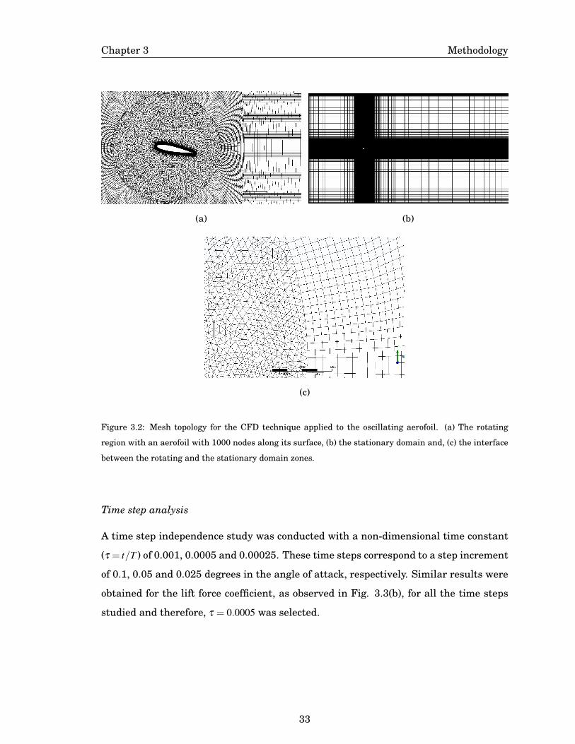
Chapter 3 Methodology
(a) (b)
(c)
Figure 3.2: Mesh topology for the CFD technique applied to the oscillating aerofoil. (a) The rotating
region with an aerofoil with 1000 nodes along its surface, (b) the stationary domain and, (c) the interface
between the rotating and the stationary domain zones.
Time step analysis
A time step independence study was conducted with a non-dimensional time constant
(τ = t/T ) of 0.001, 0.0005 and 0.00025. These time steps correspond to a step increment
of 0.1, 0.05 and 0.025 degrees in the angle of attack, respectively. Similar results were
obtained for the lift force coefficient, as observed in Fig. 3.3(b), for all the time steps
studied and therefore, τ = 0.0005 was selected.
33

Chapter 3 Methodology
(a) (b)
Figure 3.3: (a) Mesh independence study, and (b) time step independence study for the CFD simulation
of an oscillating NACA 0012 aerofoil.
Numerical verification
The present URANS simulations were validated against the URANS simulation per-
formed by Geng et al. [69], and two Large Eddy Simulations (LES) carried out by
Geng et al. [69] and Kim et al. [68], and a comparison among these four simulations is
shown in Fig. 3.4(a). Very good agreement in the prediction of the lift force coefficient,
CL, was observed among both 2D CFD simulations and the LES simulations. For all
the numerical simulations, 2D CFD and LES, the linear region of variation of the lift
force coefficient with angle of attack is in very good agreement with the experimental
data. Further, the deviation in CL appears once the vortex has been released and it can
be concluded that the stall-onset angle may be predicted with the same accuracy for
all the numerical techniques compared in Fig. 3.4 (a). Unfortunately, a significant CL
peak was observed in the experimental data and this is not captured by any of the nu-
merical simulations. Since this peak indicates that a vortex is located at the mid-chord
of the aerofoil, thus, the accuracy in predicting the stall-onset angle is not affected.
Further, to demonstrate the accuracy of the present numerical methodology to cap-
ture the stall-onset angle, a second validation is performed by using the experimental
data in [5] consisting of a NACA0015 aerofoil that describes the same motion as the
34
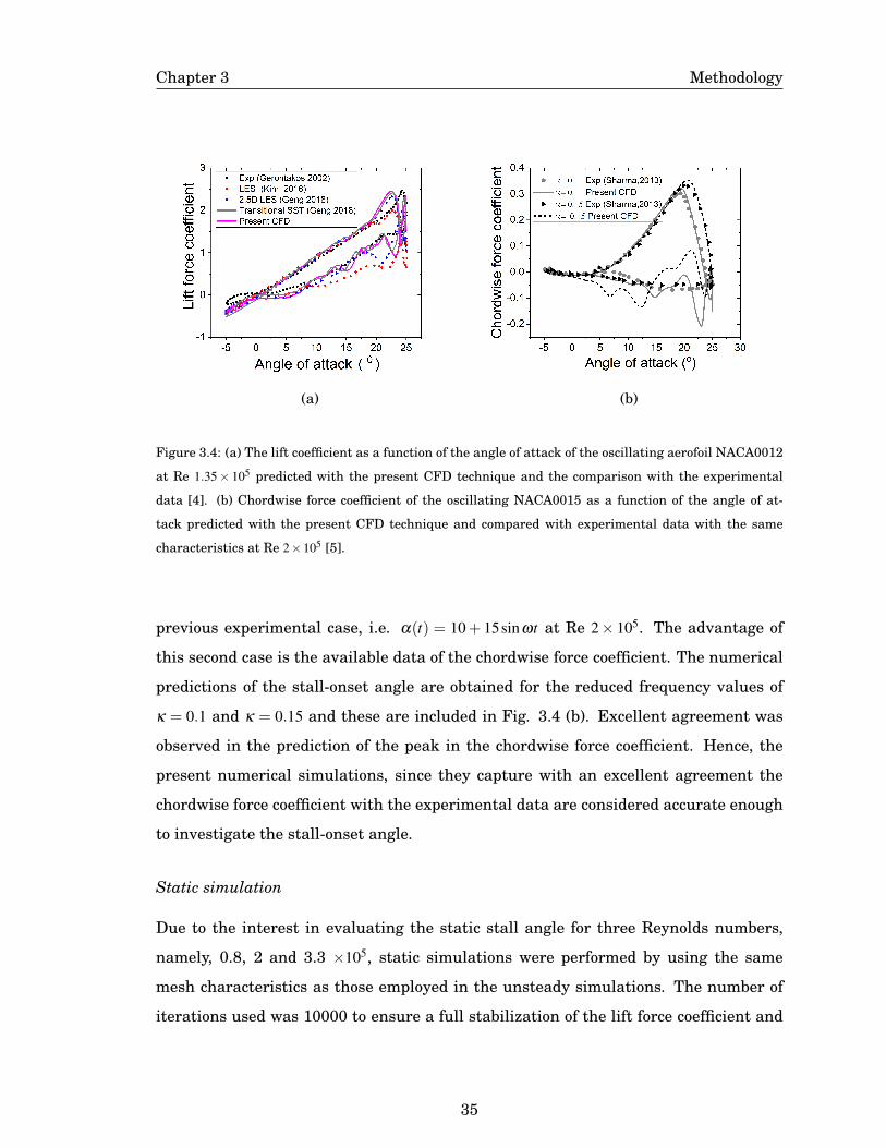
Chapter 3 Methodology
(a) (b)
Figure 3.4: (a) The lift coefficient as a function of the angle of attack of the oscillating aerofoil NACA0012
at Re 1.35× 10⁵ predicted with the present CFD technique and the comparison with the experimental
data [4]. (b) Chordwise force coefficient of the oscillating NACA0015 as a function of the angle of at-
tack predicted with the present CFD technique and compared with experimental data with the same
characteristics at Re 2×10⁵ [5].
previous experimental case, i.e. α(t) = 10+ 15sinωt at Re 2× 10⁵. The advantage of
this second case is the available data of the chordwise force coefficient. The numerical
predictions of the stall-onset angle are obtained for the reduced frequency values of
κ = 0.1 and κ = 0.15 and these are included in Fig. 3.4 (b). Excellent agreement was
observed in the prediction of the peak in the chordwise force coefficient. Hence, the
present numerical simulations, since they capture with an excellent agreement the
chordwise force coefficient with the experimental data are considered accurate enough
to investigate the stall-onset angle.
Static simulation
Due to the interest in evaluating the static stall angle for three Reynolds numbers,
namely, 0.8, 2 and 3.3 ×10⁵, static simulations were performed by using the same
mesh characteristics as those employed in the unsteady simulations. The number of
iterations used was 10000 to ensure a full stabilization of the lift force coefficient and
35
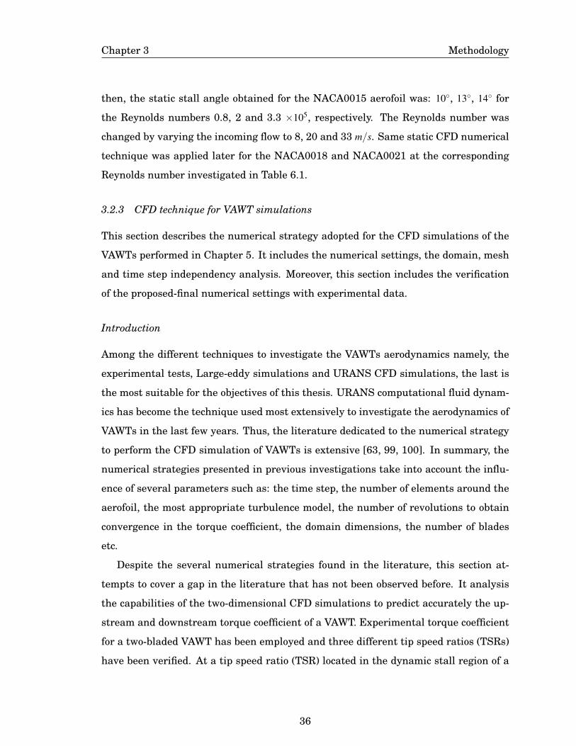
Chapter 3 Methodology
then, the static stall angle obtained for the NACA0015 aerofoil was: 10◦, 13◦, 14◦ for
the Reynolds numbers 0.8, 2 and 3.3 ×10⁵, respectively. The Reynolds number was
changed by varying the incoming flow to 8, 20 and 33 m/s. Same static CFD numerical
technique was applied later for the NACA0018 and NACA0021 at the corresponding
Reynolds number investigated in Table 6.1.
3.2.3 CFD technique for VAWT simulations
This section describes the numerical strategy adopted for the CFD simulations of the
VAWTs performed in Chapter 5. It includes the numerical settings, the domain, mesh
and time step independency analysis. Moreover, this section includes the verification
of the proposed-final numerical settings with experimental data.
Introduction
Among the different techniques to investigate the VAWTs aerodynamics namely, the
experimental tests, Large-eddy simulations and URANS CFD simulations, the last is
the most suitable for the objectives of this thesis. URANS computational fluid dynam-
ics has become the technique used most extensively to investigate the aerodynamics of
VAWTs in the last few years. Thus, the literature dedicated to the numerical strategy
to perform the CFD simulation of VAWTs is extensive [63, 99, 100]. In summary, the
numerical strategies presented in previous investigations take into account the influ-
ence of several parameters such as: the time step, the number of elements around the
aerofoil, the most appropriate turbulence model, the number of revolutions to obtain
convergence in the torque coefficient, the domain dimensions, the number of blades
etc.
Despite the several numerical strategies found in the literature, this section at-
tempts to cover a gap in the literature that has not been observed before. It analysis
the capabilities of the two-dimensional CFD simulations to predict accurately the up-
stream and downstream torque coefficient of a VAWT. Experimental torque coefficient
for a two-bladed VAWT has been employed and three different tip speed ratios (TSRs)
have been verified. At a tip speed ratio (TSR) located in the dynamic stall region of a
36

Chapter 3 Methodology
VAWT curve performance, a TSR located at the optimum torque coefficient and, a TSR
under a fully attached flow regime.
Description of the experimental VAWT data
The available experimental data in [31] contain the azimuthal torque coefficient as a
function of the azimuthal angle, CQ(θ) for the VAWT with the characteristics included
in Table 3.2. This data was obtained by using the pressure coefficient measured by
32 pressure taps located at the mid-span of the straight blade with the NACA0021
aerofoil. A total of 10 000 samples were collected at three different tip speed ratios with
a sampling frequency of 1250 Hz, thus the pressure coefficient data were averaged and
used to calculate the torque coefficient at each 5◦ azimuthal angle during one cycle, i.e.
one wind turbine revolution.
Table 3.2: Geometrical characteristics of the VAWT used as a reference case for the CFD verifications.
Nb 2 Aerofoil NACA0021
R 1 m H 1.2 m
Ds 0.216 m c 0.265m
β 6◦ U∞ 8 m/s
The explained experimental data in [31] allows a comparison with the two dimen-
sional CFD simulations since the pressure coefficient at the mid-span has only a mi-
nor influence of the 3D effects regarding the torque-meter data that include all the tip
losses. As mentioned in the introduction, most of the CFD simulations of VAWTs have
relied on the average power coefficient and here, the azimuthal torque coefficient at
different TSRs are used since they allow much more insight into the performance of
the CFD simulations. The three tested TSRs were, one low TSR, 1.38, where the tur-
bine exhibits low performance and dynamic stall. Secondly, at the optimum TSR 2.19
and one at a high TSR of 2.58 where the power coefficient decreases again and usually
the blades are far away from the dynamic stall condition.
37
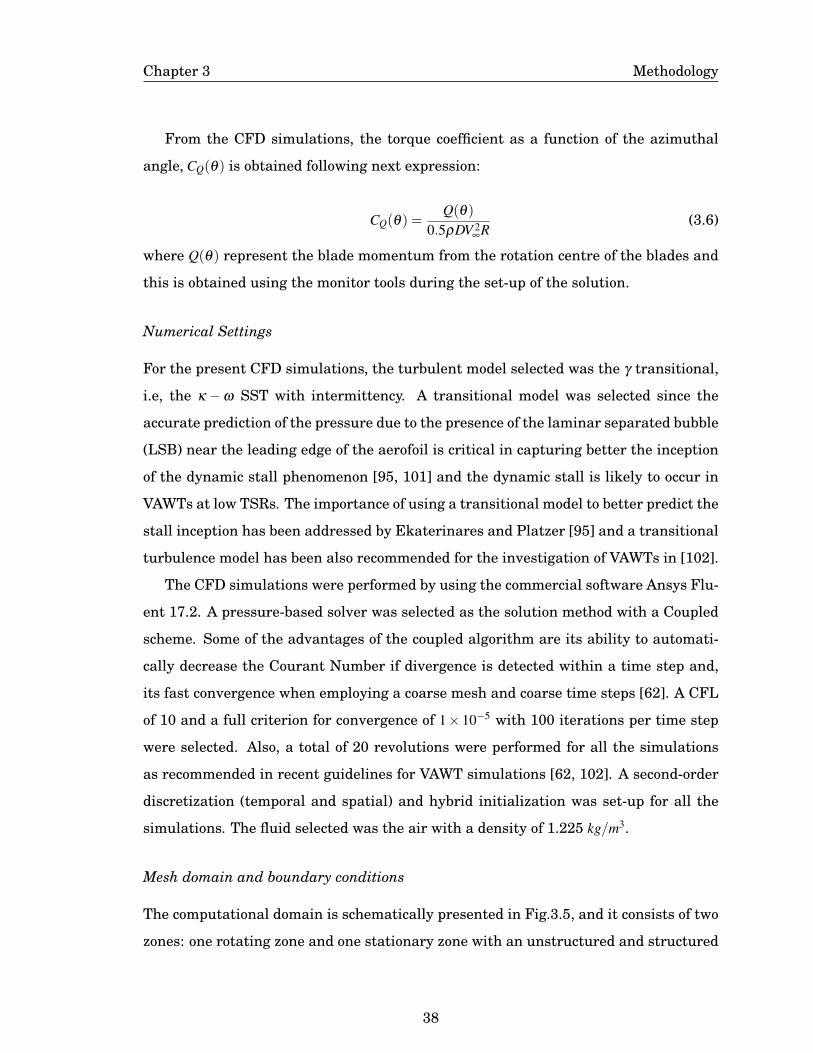
Chapter 3 Methodology
From the CFD simulations, the torque coefficient as a function of the azimuthal
angle, CQ(θ) is obtained following next expression:
CQ(θ) =Q(θ)
0.5ρDV 2∞R
(3.6)
where Q(θ) represent the blade momentum from the rotation centre of the blades and
this is obtained using the monitor tools during the set-up of the solution.
Numerical Settings
For the present CFD simulations, the turbulent model selected was the γ transitional,
i.e, the κ −ω SST with intermittency. A transitional model was selected since the
accurate prediction of the pressure due to the presence of the laminar separated bubble
(LSB) near the leading edge of the aerofoil is critical in capturing better the inception
of the dynamic stall phenomenon [95, 101] and the dynamic stall is likely to occur in
VAWTs at low TSRs. The importance of using a transitional model to better predict the
stall inception has been addressed by Ekaterinares and Platzer [95] and a transitional
turbulence model has been also recommended for the investigation of VAWTs in [102].
The CFD simulations were performed by using the commercial software Ansys Flu-
ent 17.2. A pressure-based solver was selected as the solution method with a Coupled
scheme. Some of the advantages of the coupled algorithm are its ability to automati-
cally decrease the Courant Number if divergence is detected within a time step and,
its fast convergence when employing a coarse mesh and coarse time steps [62]. A CFL
of 10 and a full criterion for convergence of 1× 10⁻⁵ with 100 iterations per time step
were selected. Also, a total of 20 revolutions were performed for all the simulations
as recommended in recent guidelines for VAWT simulations [62, 102]. A second-order
discretization (temporal and spatial) and hybrid initialization was set-up for all the
simulations. The fluid selected was the air with a density of 1.225 kg/m3.
Mesh domain and boundary conditions
The computational domain is schematically presented in Fig.3.5, and it consists of two
zones: one rotating zone and one stationary zone with an unstructured and structured
38

Chapter 3 Methodology
mesh, respectively. The rotating zone was moved using the mesh motion condition and
by varying the rotational velocity accordingly to next expression:
ω =λV∞
R(3.7)
Figure 3.5: Mesh topology of the stationary and the rotating grid zones used in the VAWT simulations.
The boundary conditions were defined as a velocity inlet, pressure outlet and sym-
metry for the upper and lower boundaries as indicated in Fig.3.6. The aerofoils, which
represent the blades, were considered as non-slip boundary conditions.
Figure 3.6: Schematic representation of the CFD domain used for the VAWTs simulations (not scale) and
the boundary conditions.
In order to define the distance from the inlet to the turbine centre, di, the extent
39
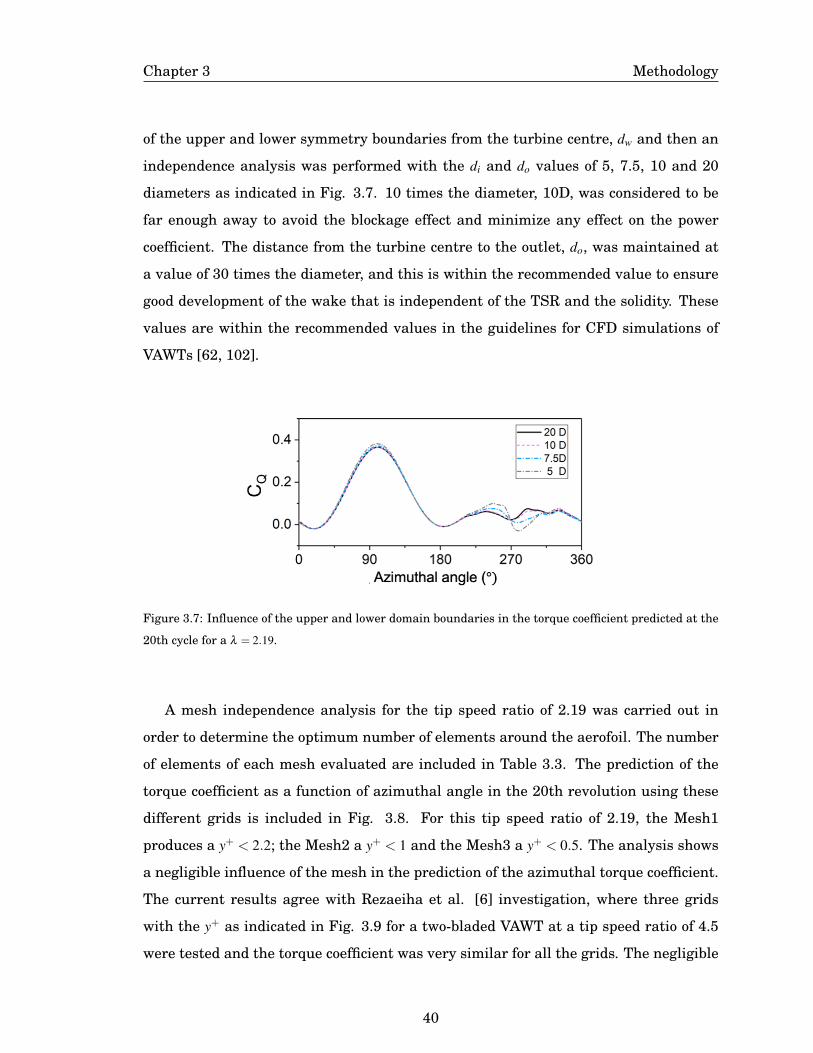
Chapter 3 Methodology
of the upper and lower symmetry boundaries from the turbine centre, dw and then an
independence analysis was performed with the di and do values of 5, 7.5, 10 and 20
diameters as indicated in Fig. 3.7. 10 times the diameter, 10D, was considered to be
far enough away to avoid the blockage effect and minimize any effect on the power
coefficient. The distance from the turbine centre to the outlet, do, was maintained at
a value of 30 times the diameter, and this is within the recommended value to ensure
good development of the wake that is independent of the TSR and the solidity. These
values are within the recommended values in the guidelines for CFD simulations of
VAWTs [62, 102].
Figure 3.7: Influence of the upper and lower domain boundaries in the torque coefficient predicted at the
20th cycle for a λ = 2.19.
A mesh independence analysis for the tip speed ratio of 2.19 was carried out in
order to determine the optimum number of elements around the aerofoil. The number
of elements of each mesh evaluated are included in Table 3.3. The prediction of the
torque coefficient as a function of azimuthal angle in the 20th revolution using these
different grids is included in Fig. 3.8. For this tip speed ratio of 2.19, the Mesh1
produces a y+ < 2.2; the Mesh2 a y+ < 1 and the Mesh3 a y+ < 0.5. The analysis shows
a negligible influence of the mesh in the prediction of the azimuthal torque coefficient.
The current results agree with Rezaeiha et al. [6] investigation, where three grids
with the y+ as indicated in Fig. 3.9 for a two-bladed VAWT at a tip speed ratio of 4.5
were tested and the torque coefficient was very similar for all the grids. The negligible
40

Chapter 3 Methodology
influence of the mesh in the present CFD simulations is attributed to the fact that the
γ transition model predicts similar results as long as the y+ is lower than 5 accordingly
the Fluent user guide.
Table 3.3: Characteristics of the evaluated meshes for the CFD technique employed for the VAWT simu-
lations.
Parameter Mesh1 Mesh2 Mesh3
Nodes on aerofoil 500 1000 2000
Total mesh elements 140000 230000 550000
Figure 3.8: Torque coefficient as a function of the azimuthal angle predicted with the different grids
presented in Table 3.3 in the 20th revolution and a tip speed ratio of λ = 2.19. An azimuthal increment of
0.25◦ was employed.
To carried out the further CFD simulations for the VAWTs, the Mesh2 with 1000
elements around the aerofoils was selected. The most important factor for the selection
of the mesh was the computational time: Mesh 1 requires 22:15:10 CPU hours; Mesh2
requires 25:44:55 CPU hours and, Mesh 3 54:00:26 hours. Therefore, the Mesh2 re-
sults in the most convenient mesh to be used for further simulations to be performed
in Chapter 5. The number of elements around the aerofoils is within the range recom-
mended in [62].
41

Chapter 3 Methodology
Figure 3.9: Prediction of the instantaneous torque coefficient in [6] for the last revolution versus azimuth
angle for different grids in last revolution for a tip speed ratio of λ = 4.5.
Time independence analysis
In this section, a time independence analysis was performed in terms of the azimuthal
angle step, ∆θ . The time step, ∆t, is related with the azimuthal angle by the next
expression:
ω =∆θ
∆t(3.8)
Since the rotational speed, ω, depends on the tip speed ratio according to Eq. 3.7,
then, it affects the time step value and thus, the azimuthal increment is more repre-
sentative parameter to perform the time step analysis.
Figure 3.10 presents the prediction of the torque coefficient using four azimuthal
angles increment: 0.05, 0.1, 0.25 and 0.5◦. The case analyzed correspond to a two-
bladed VAWT at a tip speed ratio of 2.19. It is observed that the difference in the
torque coefficient is almost negligible among the four azimuthal increments. Therefore,
a time step corresponding to an azimuthal increment of 0.25◦ was selected for all the
simulations and this value is within the recommendations in several investigations
[62, 103] where the impact of the tip speed ratio and the number is blades in the
selection of the azimuthal increment was analyzed.
42

Chapter 3 Methodology
Figure 3.10: Torque coefficient as a function of the azimuthal angle predicted with different time steps at
the 20th cycle. The tip speed ratio is λ = 2.19 and the Mesh2 with 1000 element around the blades was
employed.
Effectiveness of the numerical simulations
The numerical settings, the mesh and the azimuthal increment selected in previous
sections have been verified with the experimental VAWT described in Table 3.2 for
three tip speed ratios. The tip speed ratios investigated were 2.58, 2.19 and 1.38.
The results have revealed that for high TSR of 2.58, the present CFD simulations
can capture, with a very good agreement, both the contribution of the torque coefficient
in the upstream and downstream regions of the rotor, see Fig. Fig. 3.11(a). The
average torque coefficient predicted by the CFD simulations was 0.16 and this value
is in very good agreement with the experimental value of 0.17. Similar results were
found with the prediction at the optimum TSR 2.19, see Fig. 3.11(b), and the average
torque coefficient of 0.18 was obtained with the CFD simulation and this is in very
good agreement to the value of 0.19 for the experimental data.
For the very low TSR of 1.38, vortex shedding was observed upstream of the rotor
and these vortexes were released downstream of the rotor. The multiple vortex shed-
ding is observed in Fig. 3.12(c) and additionally to the vortex formed on the blade,
the shaft also produced vortex formation released at downstream of the rotor. The up-
stream contribution of the torque coefficient at this low tip speed ratio was predicted
with good agreement, nevertheless, the downstream instantaneous torque coefficient
43

Chapter 3 Methodology
(a) (b)
(c)
Figure 3.11: Prediction of the instantaneous torque coefficient at the 20th revolution for (a) TSR 2.58, (b)
TSR 2.19 and, (c) TSR 1.38 for a two-bladed VAWT.
oscillates in value during all the revolutions, see for example the revolution numbers
19 and 20 in Fig. 3.11(c). This oscillation was attributed to two main effects; namely,
the blade interaction with its detached separated vortex at the leading edge of the aero-
foil and the vortices formed by the shaft (with D = 216 mm) that were fluctuating in the
direction related to the Von Karman effect. Thus, when the wind turbine blade passes
θ = 270◦, behind the shaft, in some revolutions the blade interacts with the vortex that
is generated by the shaft and then the torque coefficient is reduced as indicated in Fig.
3.11(c) in the 20th cycle. The experimental average torque coefficient at TSR=1.38 was
predicted to be 0.12 and with the CFD predicts oscillations in the range 0.076-0.107.
For the tip speed ratios of 2.58 and 2.19, Fig. 3.12(a-b), the influence of the vortex
shedding due to the shaft in the torque coefficient at downstream was minimal. Addi-
tionally, in practical situations, the diameter of the shaft is smaller, thus the shaft is
not considered in the subsequence simulations. Twenty revolutions were employed in
44

Chapter 3 Methodology
(a) (b)
(c)
Figure 3.12: Vorticity contours for a two-bladed VAWTs at (a) λ= 2.58, (b) λ= 2.19 and, (c) λ = 1.38
order to secure the convergence of the torque coefficient, and this is the recommended
value given in [103].
3.3 Dynamic stall method
The dynamic stall behaviour depends on several parameters. The most studied are as
follows: the reduced frequency, the amplitude of the oscillation, mean angle of oscilla-
tion, Reynolds number, Mach number, pattern of the angle of attack, and the aerofoil
shape. Due to all these parameters, reproducing the unsteady forces accurately repre-
sents a significant challenge for the dynamic stall models. Among the several existing
dynamic stall models, one of the most used dynamic stall algorithms is the Leishman-
Beddoes (LB) model. This model considers most of the physical aspect of the dynamic
45

Chapter 3 Methodology
stall phenomenon described in Section 2.2.2
The objective of the LB dynamic stall model is to compute the normal (CN) and
the chordwise force coefficient (CC) over an aerofoil undergoing unsteady conditions.
To compute such forces the original LB modules represented in Fig. 3.13. The full
algorithm of this original LB dynamic stall is included in Section A and a summary is
described as following:
Figure 3.13: Schematic representation of the Leishman-Beddoes algorithm.
• A fully unsteady attached flow regime. Within this module of the LB algorithm,
the time lag in the force responses are computed using the Equation included
in Section A.1. To compute the unsteady forces under a full attached regime the
most substantial parameter is the the slope of the lift force coefficient under static
conditions, CLα and obtained as described in Section 6.2.2.
• The stall-onset module is able to predict the instance when the leading edge (LE)
pressure collapse and the vortex is shedded downstream from the LE towards the
trailing edge of the aerofoil. To compute this lag in the pressure response a series
of deficiency functions are applied to the normal force coefficient as described in
Section A.2 and also analysed in Section 6.2.2
46

Chapter 3 Methodology
• The unsteady separated flow. This module is able to compute the non-linear un-
steady forces due to the vortex movement downstream along the aerofoil surface
as well as the loads due to the trailing edge separation. See more details in Sec-
tion A.3
The Leishman-Beddoes dynamic stall model has been widely tested to predict the
unsteady forces for oscillating aerofoils at Reynolds number larger than one million.
It requires the history of the angle of attack, α(t) and the Reynolds number as the
main first initial input. Immediately, the algorithm calls for the parameters S1, S2, CLα ,
α1, CN1 which are empirical parameters obtained by applying the Kirchhoff flow equa-
tion to the static force coefficients data from a specific aerofoil and Reynolds number.
These parameters are crucial to predict accurately the unsteady forces under the dy-
namic stall and fully attached regimes. Since most of the existing investigations have
focused on Reynolds larger as one million, then, there is an urgent need of assessing
the pertinence of the Kirchhoff flow model at lower Reynolds number. Therefore, this
Kirchhoff flow model is analysed in detail in Chapter 6.
Among the three modules of the LB-algorithm, the most critical one is the stall-
onset module. This module requires to predict the delay in the stall angle and, in order
to accurately predict this point, requires of a time delay constant Tp, that represent
the lag in the pressure coefficient regarding the static conditions. Two major issues
are found within this point: (i) stall-onset angle remains unclear for the VAWTs and
this is addressed in Chapter 4 and, (ii) the time delay constant requires for the LB-
algorithm remains unclear and very little studied at the Reynolds numbers of interest
lower than one million. Therefore, the time delays constants and the assessment of
the LB dynamic stall at low Reynolds number is carried out in Chapter 6.
3.4 Double multiple streamtube theory
Due to the role that wind turbine technology plays now in the production of electricity
and the need to improve the designs in order to increase the power generation, several
attempts have been made to develop an aerodynamic model that is capable of pre-
dicting the power coefficient of a VAWT [104, 105]. One of the most used models is the
47

Chapter 3 Methodology
Double Multiple Streamtube Theory (DMST) proposed by Parashivoiu [2]. This method
takes into account the geometry of the wind turbine and others secondary effects, such
as the streamtube expansion, when computing the power coefficient. This author vali-
dated his method with few wind turbines that used two or three blades and TSRs with
a value larger than two. The dynamic stall models, such as Gormont, MIT and indicial
methods, were included in the analysis and a good agreement with the cases evaluated
was found. Other authors have used the DMST combined with dynamic stall models
in order to take into account the unsteady aerodynamics [53, 106, 107] and among the
tested models the Leishman-Beddoes (LB) has demonstrated a better response when
computing the normal and tangential forces. Due to the early limitations in the avail-
able experimental data, the validations were restricted to only a few cases, and the
influence of the dynamic stall over the power coefficient for conditions of low TSRs is
still not well understood.
The original DMST method proposed by Parashivoiu analyses the unsteady loads of
the rotor by dividing the rotor in Nth number of elements and proposed the interference
factors for both section of the rotor: at upstream and downstream of the rotor.
The expression to estimated the interference factor at upstream of the rotor, u takes
into account the geometry of the rotor and some secondary effects and is calculated by
follows:
u(θ) = KK0η/[KK0η +∫
θ+ ∆θ
2
θ− ∆θ
2
f (θ)dθ ] (3.9)
where K is the geometrical parameter of the rotor, K0 = sin(θ +∆θ/2)− sin(θ −∆θ/2)
and the function f (θ) is given by next equation:
f (θ) =Vrel
V∞
[CR cos(θ)+CT sin(θ)] (3.10)
The interference factor for the upstream section, u, is calculated iteratively at each i
element and when convergence is reached, this value is used as an input to estimated
the interference factor at downstream zone of the rotor, u′. The radial force coefficient,
CR(θ) and the tangential force coefficient CT (θ) are obtained using the static values of
the lift and drag forces.
The theoretical equations of the relative velocity, Eq.(2.1) and the angle of attack,
48

Chapter 3 Methodology
Eq.(2.2) introduces the interference factor by using the following expressions:
Vrel(θ) =V (1+2Xr cos(θ)+X2r )
1/2 (3.11)
where, the local tip speed ratio Xr = ωR/V and V is called the induced velocity and is
given by:
V = u/V∞ (3.12)
The path angle including the interference factor reads:
φ(θ) = arctan(sin(θ)
Xr + cos(θ)) (3.13)
and the angle of attack is estimated by using Eq.(2.2). Equations (3.11-3.13 ) ap-
plies similarly to the downstream section. More details maybe found in [108].
Finally, the torque coefficient at each azimuthal angle is predicted as follows:
CQ(θ) = (CL sin(φ)−CD sin(φ))2cR
(Vrel
V∞
)2
(3.14)
The upstream (CQ,up) and dowsntream (CQ,dw) torque contributions were calculating
following the expressions:
CQ,up =Nb
2π
∫π
0CQ(θ)dθ (3.15)
CQ,dw =Nb
2π
∫ 2π
π
CQ(θ)dθ (3.16)
where, Nb represents the number of blades.
The total torque coefficient results in the expression:
CQ,T =CQ,up +CQ,dw (3.17)
The torque coefficient produced by the blades, is the tangential force, FT times the
radius, by using the definition of moment, where a moment is represented by M = rxF .
In the vertical axis wind turbines, the tangential force is calculated by:
FT = FLsin(φ)−FDcos(φ) (3.18)
49
Chapter 3 Methodology
where FL and FD represent the lift and drag forces on the blades. In the investigated
cases where, β = 0◦ and the path angle results in φ = α. Therefore, dividing FT by the
actual Vrel kinetic energy, a tangential force coefficient is given by:
CT =CL sin(α)−CD cos(α) (3.19)
3.5 Summary
This Chapter has described the methodology followed in the thesis to understand the
aerodynamics in the VAWTs in order to bridge the gaps found in the literature as
described in Chapter 2. The methods that have been employed along the Chapters are
described and consisting of: two-dimensional CFD simulations for oscillating aerofoils;
two-dimensional CFD simulations for VAWTs; the dynamic stall Leishman-Beddoes
algorithm and, the double multiple streamtube model.
Some of the important outcomes in the present Chapter are described as follows:
(i) A verified CFD technique that is accurate enough to compute the stall-onset
angle is described. The CFD numerical techniques agree with the available data for
two oscillatory aerofoils, the NACA0012 and the NACA0015 at low Reynolds number,
1.35×10⁵ and 2.0×10⁵ respectively. These good results provide the confidence to inves-
tigate in detail the stall-onset angle in Chapter 4.
(ii) The CFD numerical technique for the VAWTs is described as well as the avail-
able data to verify this numerical technique. The description of the six aerofoils under
investigation, namely, the NACA0021, NACA0018, NACA0015, NACA0012 and the
cambered S1210 and NACA2418 is included.
(iii) The effectiveness analysis of the CFD simulations has demonstrated that the
current CFD simulations are able to predict accurately both the upstream and down-
stream aerodynamics of the VAWTs.
(iv) The Leishman-Beddoes model has been identified as the most pertinent dy-
namic stall model to predict the unsteady loads for the VAWTs. Its algorithm has been
explained and the critical sections of this algorithm that requires a more in-depth dis-
cussion to be applied in the prediction of the unsteady loads of VAWTs are defined: the
50

Chapter 3 Methodology
time-delay constant to predict the stall-onset at Reynolds number lower than one mil-
lion and the assessment of Kirchhoff flow model to predict the obtained the empirical
parameters from a specific aerofoil. These two critical points are further discussed in
Chapter 6.
(v) The double multiple stream-tube has been identified as the most used fast tool
to predict the VAWTs performance but still need an assessment of its capabilities to
predict the upstream and downstream torque contribution under the full-unsteady
attached regime. A further discussion is included in Chapter 7.
51

Chapter 4
The stall onset angle
4.1 Overview
The stall-onset is the most critical parameter to describe the development of the dy-
namic stall; it marks the inception of the vortex at leading of the aerofoil. In the
VAWTs, this parameter has been very little evaluated as explained in Section 2.2.2
and, the effect of the relative velocity, pitch angle, the tip speed ratio, rotational speed
and Reynolds number remains unclear. This chapter presents the analysis of the sev-
eral operating parameters that dictate the final value of the stall-onset angle. Ad-
ditionally, the range of Reynolds number investigated, 0.8− 3.3× 10⁵, has not been
previously studied and this range of Re are very important for the understanding of
the dynamic stall phenomenon of VAWTs operating at low wind speeds.
4.2 Methodology
The two-dimensional CFD numerical technique for an oscillating aerofoil explained
in Section 3.2.2 was used in this Chapter. The present simulations agree very well
with the experimental data employed. In order to evaluate the effect of the operating
conditions on the stall-onset angle, then two approaches were used.
First, an incoming wind flow U with a constant magnitude (depending on the chord-
based Reynolds number under evaluation) past an oscillating aerofoil, as illustrated in
Fig. 4.1. The oscillating aerofoil describes a motion with the angle of attack α(t) for
a VAWTs given by Eq.(2.2) [2]. For this oscillating aerofoil β positive is indicated in
Fig. 4.1. The angle of attack represents the angle between the aerofoil-chord and the
incoming wind flow U aligned all the time to the x-axis.
The value of ωt from 0 to π represents the upstream zone of the rotor, and from π
52

Chapter 4 The stall onset angle
Figure 4.1: Sketch of an oscillating aerofoil with the VAWT angle of attack α(t) and an incoming flow (U).
U can take a constant magnitude or a time-varying magnitude given by the relative velocity equation.
to 2π the downstream zone. Positive angles of attack are associated with the upstream
zone of the rotor and negative angles with the downstream zone.
In order to replicate the angle of attack motion given by Eq. (2.2) in the CFD
simulations, a user defined function (UDF) was employed to control the pitching rate
of the rotating mesh domain (mesh domain explained in Section 3.2.2) according to the
equation:
α(t) = ω(1+λ cos(ωt))
(1+2λ cos(ωt)+λ 2)(4.1)
(i) Using this first approach, at a constant Reynolds number, the influence of the
tip speed ratio (λ ), pitch angle (β ) and the angular velocity (ω) on the stall-onset angle
were investigated. The rotational speed for these oscillating aerofoils was expressed
in terms of the non-dimensional parameter called the reduced frequency (κ), as ω =
2κUre f /c. Ure f represents the actual wind speed that impacts the aerofoil. This analysis
was performed for a Reynolds number base on the chord of 2× 10⁵. The chord length
was 0.15 cm and the constant incoming wind flow had a magnitude Ure f = 20 m/s.
The CFD simulations performed for the oscillating aerofoils and the variables used
in each case investigated at a constant Reynolds number are included in Table 4.1.
Table 4.1 indicates, for example for cases 1 and 2, the same tip speed ratio and pitch
angle were used in the simulation and it only changes the reduced frequency, allowing
53
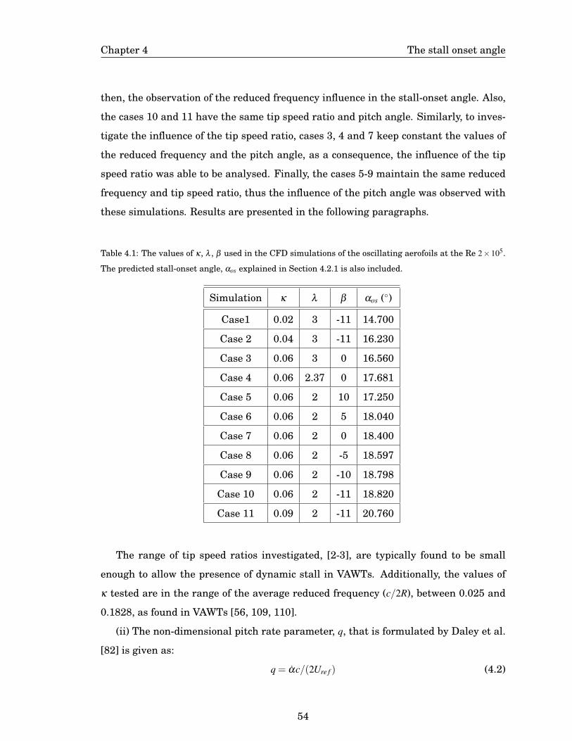
Chapter 4 The stall onset angle
then, the observation of the reduced frequency influence in the stall-onset angle. Also,
the cases 10 and 11 have the same tip speed ratio and pitch angle. Similarly, to inves-
tigate the influence of the tip speed ratio, cases 3, 4 and 7 keep constant the values of
the reduced frequency and the pitch angle, as a consequence, the influence of the tip
speed ratio was able to be analysed. Finally, the cases 5-9 maintain the same reduced
frequency and tip speed ratio, thus the influence of the pitch angle was observed with
these simulations. Results are presented in the following paragraphs.
Table 4.1: The values of κ, λ , β used in the CFD simulations of the oscillating aerofoils at the Re 2×10⁵.
The predicted stall-onset angle, αos explained in Section 4.2.1 is also included.
Simulation κ λ β αos (◦)
Case1 0.02 3 -11 14.700
Case 2 0.04 3 -11 16.230
Case 3 0.06 3 0 16.560
Case 4 0.06 2.37 0 17.681
Case 5 0.06 2 10 17.250
Case 6 0.06 2 5 18.040
Case 7 0.06 2 0 18.400
Case 8 0.06 2 -5 18.597
Case 9 0.06 2 -10 18.798
Case 10 0.06 2 -11 18.820
Case 11 0.09 2 -11 20.760
The range of tip speed ratios investigated, [2-3], are typically found to be small
enough to allow the presence of dynamic stall in VAWTs. Additionally, the values of
κ tested are in the range of the average reduced frequency (c/2R), between 0.025 and
0.1828, as found in VAWTs [56, 109, 110].
(ii) The non-dimensional pitch rate parameter, q, that is formulated by Daley et al.
[82] is given as:
q = αc/(2Ure f ) (4.2)
54

Chapter 4 The stall onset angle
It is necessary to emphasize that the pitch rate α and the velocity changes con-
stantly in VAWTs, thus, the non-dimensional pitch rate q uses the values of the pitch
rate and the relative velocity at a specific time, t, as input values corresponding to
α and Ure f respectively. The expression in Eq.(4.2) is also used to calculate the non-
dimensional pitch rate in the ramp-up motion, but because the pitch rate α has a
constant value then q is easily calculated.
In the second approach, the incoming wind flow U , as represented in Fig. 4.1, was
a time-depend function given by the relative velocity Eq. (2.1) of VAWTs. For this
approach, a user defined function was implemented to vary the incoming flow (inlet
velocity) according to Eq. (2.1) and at the same time the pithing rate according to
Eq. (2.2). In order to have a single value of the non-dimensional pitch rate using Eq.
(4.2) then, the pitch rate, α and Ure f uses the value of the Eq. (2.2) and Eq. (2.1),
respectively, at the instant of time t when the angle of attack approaches the static
stall angle.
(iii) The constantly changing relative velocity described by the Eq. (2.1), has been
investigated in order to assess its influence on the stall-onset and to compared the
existing difference on the stall-onset angle when using a constant-average relative
velocity. The average relative velocity, ωR or λV∞, that is an approximated average
of the Eq. (2.1) in one revolution, is typically used in VAWTs in order to simplify the
analysis [30, 48]. Thus, it is interesting to investigate if a difference exists when using
the actual relative velocity rather than its average value.
4.2.1 Stall-onset estimation
As mentioned previously, there are several techniques to identify the stall-onset angle.
In this Chapter, the stall-onset angle, αos, is calculated as the angle where a maximum
value in the chordwise force coefficient is observed. This criterion is also recommended
in [45, 44, 111].
The chordwise force coefficient, Cc, for an oscillating aerofoil is represented in Fig.
4.1 and is described as follows:
Cc =CL sin(α)−CD cos(α) (4.3)
55

Chapter 4 The stall onset angle
Due to the prominent influence of the dynamic stall in the upstream zone of the
VAWT, [86, 55], i.e. from ωt = 0−π, in this chapter we focus on evaluating the stall-
onset angle in this range of angle of attack.
4.3 Influence of κ, λ and β at constant Reynolds number
The analysis of the influence of the reduced frequency (κ), tip speed ratio (λ ) and pitch
angle (β ) on the stall-onset angle by using the first approach for a constant Reynolds
number has shown the following results:
(i) With the increase in the reduced frequency (κ), the calculated stall-onset angle
(αos) increases. For example, in the simulation with a reduced frequency of κ = 0.09,
the stall-onset angle was αos = 20.60◦. Decreasing the reduced frequency to κ = 0.06
produced the stall-onset angle αos = 18.79◦. For both values of κ the tip speed ratio was
λ = 2 and the pitch angle was β =−11◦.
The delay in the stall conditions with the increase in the reduced frequency is also
observed in the comparison of the pressure coefficient (Cp) and skin friction (C f x) curves
including in Fig. 4.2(a-b). The skin friction at the Reynolds number 2×10⁵ for two dy-
namic cases with reduced frequencies κ = 0.09 and κ = 0.06, and one static simulation
were computed at the angle of attack of 13◦. At the static condition, the aerofoil stalls
at 13◦ and thus a high negative pressure coefficient is observed close to the aerofoil
leading edge. This is a critical point where a laminar separation bubble (LSB) con-
centrated at the LE collapsed [44]. For the unsteady simulations, this high minimum
pressure is not reached, suggesting a delay in the pressure collapsed for the reduced
frequency κ = 0.06 and a further delay for the reduced frequency κ = 0.09.
Another interesting characteristic that confirms the delay in the stall is recognized
by observing the skin friction (C f x), as plotted in Fig. 4.2(b). The closer the laminar
separation bubble (LSB) to the aerofoil leading-edge indicates an earlier collapse of
the pressure coefficient and, an earlier separation of the boundary layer occurs. The
region occupied by the LSB is exemplified for the static case in Fig. 4.2(b) by circular
and triangular symbols; at these two points the skin friction experiences a zero value.
The LSB region for the unsteady cases with a reduced frequency κ = 0.06 is closer
56

Chapter 4 The stall onset angle
to the leading edge of the aerofoil compared for the case with the reduced frequency
κ = 0.09.
Figure 4.2: (a) Pressure coefficient, and (b) skin friction along the chord of an oscillating aerofoil at the
angle of attack 13◦. Laminar boundary layer separation, I Reattachment of LSB, � Start of reversal
flow in the turbulence boundary layer at TE.
Moreover, the point where the turbulent boundary layer (formed after the reattach-
ment of the LSB) experience C f x = 0 is an additional parameter of reference to evaluate
the magnitude of the delay in the stall-onset angle; closer is this point to the LE, then
the sooner stall occurs. For the static case, the turbulent boundary layer experiencies
C f x = 0 at 50 % of the chord, this point is indicated with a square in Fig 4.2 (b). For the
unsteady cases with κ = 0.06 and κ = 0.09 the turbulent boundary layer with C f x = 0 is
located at 95% and 97 % from the LE. More details on the pressure coefficient and skin
friction behaviours under unsteady conditions are described by Ekaterinaris & Platzer
[95].
The increase of the stall-onset angle with the reduced frequency is confirmed by
comparing the calculated stall-onset angle, αos, for another two dynamic simulations
with κ = 0.02 and κ = 0.04 using both a tip speed ratio of λ = 3 and a pitch angle of
57

Chapter 4 The stall onset angle
β = −11◦ at Re 2× 10⁵. The stall-onset angle, αos, results in 14.70◦ and 16.22◦ for the
reduced frequencies κ = 0.02 and 0.04, respectively.
(ii) The influence analysis of the tip speed ratio (λ ) has shown that with a decrease
in λ the stall-onset angle (αos) grows. For the tip speed ratios investigated with values
2, 2.37 and 3, the computed αos were 18.82◦, 17.68◦ and 16.56◦, respectively. The skin
friction for these dynamic cases is illustrated in Fig. 4.3 (a) and it was revealed that
the lower is λ then more is the delay in the stall-onset angle. For example, the position
of the laminar bubble (first two locations with C f x = 0), is closer to the leading edge
aerofoil for λ = 3, followed by λ = 2.37 and finally λ = 2. Moreover, the point where the
turbulent boundary layer experiences C f x = 0, which indicates the start of reverse flow,
is located at 84 % from the aerofoil LE for λ = 3, at 86 % for λ = 2.37 and 88% for λ = 2.
Therefore, this indicates that the tip speed ratio λ = 2 presents the largest delay in the
stall conditions. Compared with the location of the LSB in the skin friction between
the two values of the reduced frequency in Fig. 4.2(b), the effect on the skin friction
due to the tip speed ratio in Fig.4.3(a) is minimal.
(a) (b)
Figure 4.3: (a) Skin friction, and (b) chordwise force coefficient, as a function of the angle of attack for λ=
3, 2.37 and 2 with values of κ = 0.06, β = 0 and Re = 2×10⁵. Arrows indicate the direction in the angle of
attack with the motion of the aerofoil.
The tip speed ratio plays a key role that is extremely important for the VAWT
58
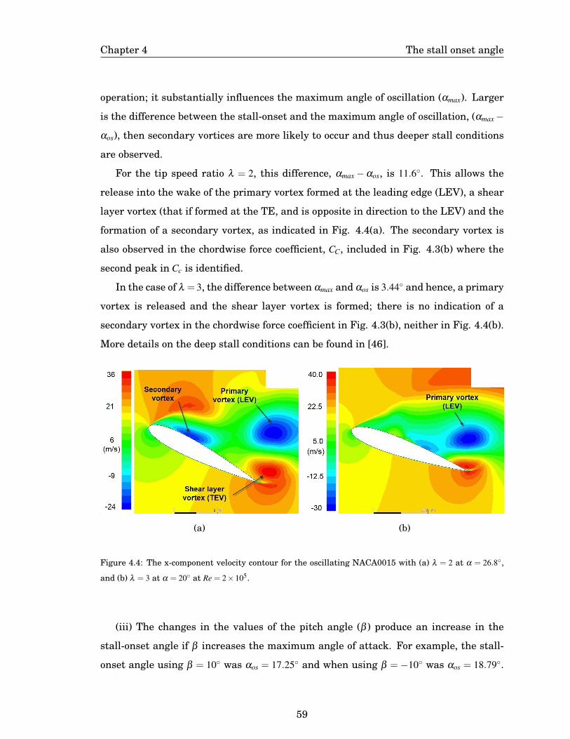
Chapter 4 The stall onset angle
operation; it substantially influences the maximum angle of oscillation (αmax). Larger
is the difference between the stall-onset and the maximum angle of oscillation, (αmax−
αos), then secondary vortices are more likely to occur and thus deeper stall conditions
are observed.
For the tip speed ratio λ = 2, this difference, αmax−αos, is 11.6◦. This allows the
release into the wake of the primary vortex formed at the leading edge (LEV), a shear
layer vortex (that if formed at the TE, and is opposite in direction to the LEV) and the
formation of a secondary vortex, as indicated in Fig. 4.4(a). The secondary vortex is
also observed in the chordwise force coefficient, CC, included in Fig. 4.3(b) where the
second peak in Cc is identified.
In the case of λ = 3, the difference between αmax and αos is 3.44◦ and hence, a primary
vortex is released and the shear layer vortex is formed; there is no indication of a
secondary vortex in the chordwise force coefficient in Fig. 4.3(b), neither in Fig. 4.4(b).
More details on the deep stall conditions can be found in [46].
(a) (b)
Figure 4.4: The x-component velocity contour for the oscillating NACA0015 with (a) λ = 2 at α = 26.8◦,
and (b) λ = 3 at α = 20◦ at Re = 2×10⁵.
(iii) The changes in the values of the pitch angle (β ) produce an increase in the
stall-onset angle if β increases the maximum angle of attack. For example, the stall-
onset angle using β = 10◦ was αos = 17.25◦ and when using β = −10◦ was αos = 18.79◦.
59

Chapter 4 The stall onset angle
The corresponding maximum angle of attack (αmax) for both pitch angles was 20◦ for
β = 10◦ and αmax=40◦ for β =−10◦. The maximum angle of attack, αmax, is calculated by
performing a mathematical analysis of Eq.(2.2) that results in the expression αmax =
arctan([λ 2− 1]−1/2)−β . Thus, the maximum angle of attack could be calculated using
the corresponding pitch angle, a reduced frequency κ = 0.06 and, a tip speed ratio of
λ = 2.
In Fig. 4.5(a), the skin friction for five values of β are plotted. It is observed that
more positive is β thus closer is the laminar bubble to the leading edge and thus the
stall occurs at a lower angle of attack. Additionally, the turbulent boundary layer point
with C f x = 0 has progressed closest to the LE for the most positive β value of 10◦ (Fig.
4.5(a)). Nevertheless, in general, the difference among the skin frictions curves for
the range of pitch angles tested [-10◦ to 10◦] are minimal and the overall variation in
αos due to the influence of the pitch angle (β ) is less than 1.54◦. The impact of the
pitch angle on the stall-onset angle, compared with the tip speed ratio and the reduced
frequency is the lowest.
(a) (b)
Figure 4.5: (a) Skin friction along the non-dimensional chord length, and (b) chordwise force coefficient
for several values of β at Re = 2×10⁵.
Similar to the tip speed ratio, the pitch angle also influences the maximum angle of
attack. Thus, the severity in the stall conditions may be affected by changing the pitch
60
Chapter 4 The stall onset angle
angle. In Fig. 4.5(b) the chordwise force coefficient for the five values of β are plotted.
With a more positive β value as explained in the previous paragraph, a slight decrease
in αos is observed but also a decrease in the maximum angle of oscillation. Thus, as
observed in Fig. 4.5(b) for the most positive β value there is no indication of secondary
vortices. On the contrary, with the most negative β value, despite experiences the
larger stall-onset angle, it also produces a very large maximum angle of attack that
causes two secondary peaks in the chordwise force as observed in Fig. 4.5(b). Those
peaks in CC indicate the formation of multiple secondary vortices and therefore, the
largest severity in the stall conditions.
4.3.1 Stall onset as a function of κ, λ and β
The simulation cases in Table 4.1 have assisted in investigating the influence of each
variable on the stall-onset angle: the increase of the reduced frequency increases the
stall-onset angle; the increase of the tip speed ratio decreases the stall-onset angle
and, the increase of the pitch angle then a small decrease in the stall-onset is observed,
see the previous Section 4.3. In order to observe the behaviour of the stall-onset for
all the simulations as a function of a single variable, then, the predicted αos for the
simulations given in Table 4.1 are plotted as a function of the reduced frequency (κ),
the tip speed ratio (λ ) and the pitch angle (β ) in Fig. 4.6 (a-c).
The analysis of the stall-onset, αos, as a function of the reduced frequency, κ, in
Fig.4.6(a) shows that with the increase of κ the stall-onset angle trends to a linear in-
crement. Nevertheless, at the value of κ = 0.06, the cases from 3 to 10 despite having
the same reduced frequency do not report the same αos and, on the contrary, the stall-
onset angles vary between 16◦ and 19◦ due to influences of the other two quantities.
Fig. 4.6(b), which reports the αos as a function of the tip speed ratio, λ , shows that for
the simulations with the same λ = 2 the stall-onset angle varies between 18 and 21◦
and for λ = 3, αos is between 14 and 17◦. The Fig. 4.6(c) shows a large variation in the
stall-onset angle for a given pitch angle. Although on the increase of the pitch angle a
small decrease in the stall-onset is observed, the influence of the other two quantities
shows a significantly larger influence on the stall-onset. These results confirm the sug-
gested conclusions by Bucher at al. [7], which stated that the single parameter of the
61

Chapter 4 The stall onset angle
(a) (b)
(c)
Figure 4.6: The predicted stall-onset angle for the simulations performed for all the cases in Table 4.1
and described as a function of the (a) reduced frequency, (b) tip speed ratio and, (c) pitch angle.
tip speed ratio is not enough to define both, the stall-inception and the dynamic stall
range of operation in a VAWT. The Bucher et al. experimental tests were performed at
Re=70,000 and are included in Fig. 4.7. This shows an agreement with the presented
CFD results in Fig. 4.6(b) that takes into account, in addition to the tip speed ratio
and reduced frequency investigated by Bucher at al.[7], the pitch angle.
62

Chapter 4 The stall onset angle
Figure 4.7: Results from Buchner et al. [7] of the trailing edge vortex formation at the leading edge of the
aerofoil (TEV) as a function of the tip speed ratio investigated using a VAWT rotor with β = 0◦ and wind
tunnel test. A black dot correspond to the parameter Kc = c/2R with a value of 0.10 and blue for 0.15.
4.4 Non-dimensional pitch rate and Reynolds number effect
In this section, the stall-onset angle is evaluated as a function of the non-dimensional
pitch rate, q, given by Eq. (4.2). This parameter involves the pitch rate, α, given
by Eq. (4.1). Because α is a time-dependent function, its value is evaluated at the
instance when the angle of attack approaches the static stall angle. Three Reynolds
number (based on the chord length) were evaluated by changing the magnitude of the
incoming flow Ure f to 8, 20 and 33 m/s and obtaining the Reynolds number of 0.8, 2.0
and 3.3×10⁵, respectively.
The analysis has revealed that the stall-onset angle, αos increases linearly with the
increase of the non-dimensional pitch rate, q, for all the Reynolds numbers tested, see
Fig.4.8(a). Further, at the same q with the increase of the Reynolds number an increase
in the stall-onset angle is observed.
The increase in the dynamic stall-onset angle, αos, due to the increase of the Reynolds
number is consistent with the increase in the static stall angle that has been studied
experimentally in several investigations [75]. Also, Fig. 4.8(a) includes the stall-onset
angle predicted by Sharma et al. [3] for a constant non-dimensional pitch rate, q= 0.25,
63
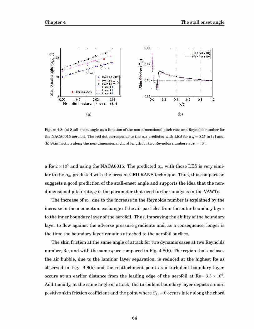
Chapter 4 The stall onset angle
(a) (b)
Figure 4.8: (a) Stall-onset angle as a function of the non-dimensional pitch rate and Reynolds number for
the NACA0015 aerofoil. The red dot corresponds to the αos predicted with LES for a q = 0.25 in [3] and,
(b) Skin friction along the non-dimensional chord length for two Reynolds numbers at α = 13◦.
a Re 2×10⁵ and using the NACA0015. The predicted αos with those LES is very simi-
lar to the αos predicted with the present CFD RANS technique. Thus, this comparison
suggests a good prediction of the stall-onset angle and supports the idea that the non-
dimensional pitch rate, q is the parameter that need further analysis in the VAWTs.
The increase of αos due to the increase in the Reynolds number is explained by the
increase in the momentum exchange of the air particles from the outer boundary layer
to the inner boundary layer of the aerofoil. Thus, improving the ability of the boundary
layer to flow against the adverse pressure gradients and, as a consequence, longer is
the time the boundary layer remains attached to the aerofoil surface.
The skin friction at the same angle of attack for two dynamic cases at two Reynolds
number, Re, and with the same q are compared in Fig. 4.8(b). The region that encloses
the air bubble, due to the laminar layer separation, is reduced at the highest Re as
observed in Fig. 4.8(b) and the reattachment point as a turbulent boundary layer,
occurs at an earlier distance from the leading edge of the aerofoil at Re= 3.3× 10⁵.
Additionally, at the same angle of attack, the turbulent boundary layer depicts a more
positive skin friction coefficient and the point where C f x = 0 occurs later along the chord
64

Chapter 4 The stall onset angle
for Re= 3.3× 10⁵. Thus, this indicated the boundary layer persists being attached at
a larger angle of attack before separation occurs with an increase in the Reynolds
number [112, 113].
Surprisingly, at the same Reynolds number, two dynamic simulations with different
values of the tip speed ratio, reduced frequency and pitch angle that present similar
values of non-dimensional pitch rate predict the stall-onset angles, αos, with very sim-
ilar values. For example, a simulation with tip speed ratio λ = 2, reduced frequency
κ = 0.09 and pitch angle β =−11◦ produces a stall-onset αos = 18.37◦; for a second sim-
ulation with λ = 1.5, κ = 0.075 and β =−13◦ the predicted αos is 18.32◦.
For the mentioned-above two cases with a similar non-dimensional pitch rate, the
pressure coefficient peaks due to the laminar separation bubbles are very similar, as
shown in Fig. 4.9(a). Further, for these same dynamic cases, their skin friction values
with C f x = 0 are encountered at similar locations along the chord, thus indicating lami-
nar separation bubbles with the same size for both dynamic cases, see Fig. 4.9(b). Also,
the turbulent boundary layer achieves C f x = 0 at the same chord locations. Therefore,
present results suggest the non-dimensional pitch rate value when approaches to the
static stall angle is the most important parameter that defines the stall-onset angle in
the VAWT motion. Therefore, the effect of the tip speed ratio, reduced frequency and
pitch angle on the non-dimensional pitch rate (q) requires more attention when the
stall-onset angle is being predicted in the VAWTs.
The positive effect of non-dimensional pitch rate, q, on the stall-onset angle has
been supporting by analysing the simulations presented in Section 4.3. It has been
observed that the reduced frequency (κ) in the dynamic simulations increases the non-
dimensional pitch rate (q) from 0.018 to 0.029 for the reduced frequencies of κ = 0.06
and κ = 0.09 respectively. Thus, the stall-onset angle increases. In the case of the
tip speed ratio (λ ), the decrease in λ increases the q values: for λ = 2, 2.37 and 3,
the values of q were 0.018, 0.016 and 0.0121 respectively, and the stall-onset angle
decreases in value. Similarly, the pitch angle β that increases the q values increases
the stall-onset angle, see Table 4.2. The increase in the stall-onset angle due to the
increase of q due to the changes in the pitch angles are marked with arrows in Fig. 4.8
(a). Therefore, it is confirmed that anytime the operating parameters, individually or
65

Chapter 4 The stall onset angle
Figure 4.9: (a) Pressure coefficient and, (b) skin friction for two simulations with closed non-dimensional
pitch rate value at α = 13◦.
combined, increase the non-dimensional pitch rate, then, an increase in the stall-onset
angle is also observed.
Table 4.2: The instantaneous non-dimensional pitch rate calculated at αss for simulations with a constant
kappa = 0.06 and different pitch angles and, their predicted stall-onset angle
β (◦) -10 -5 0 5 10
q 0.0199 0.0196 0.0188 0.0176 0.0152
αos (◦) 18.79 18.59 18.40 18.04 17.25
αmax (◦) 40 35 30 25 20
4.5 Effect of the relative velocity on the stall-onset angle
In the previous sections, it was found that the stall-onset angle depends on the non-
dimensional pitch rate and Reynolds number. In a VAWT with a constantly changing
66

Chapter 4 The stall onset angle
relative velocity, a fluctuation in both the non-dimensional pitch rate and Reynolds
number occurs and this fluctuation increases in amplitude by decreasing the tip speed
ratio. Therefore, the effect of the fluctuating relative velocity is investigated by using a
time-varying incoming flow as given by Eq.(2.1) and described in the second approach
in Section 4.2(iii).
The fluctuation in the Reynolds number gives rise to the interest in investigating
whether or not a difference on the stall-onset angle exists if using an average of the
fluctuating relative velocity, Vmean ≈ λV∞, instead of the actual fluctuating relative ve-
locity. Two cases are being analysed using the fluctuating relative velocity described
in Eq. (2.1). First, using a tip speed ratio λ = 2 and V∞ = 10 m/s and, second, using a tip
speed ratio λ = 3 and V∞ = 20/3 m/s. For both cases, κ = 0.06 and β = 0◦ were employed.
The analysis shows that the tip speed ratio λ = 2 produces a Reynolds number
that fluctuates in the range 1− 3× 10⁵ and λ = 3 produces Reynolds number in the
range 1.4− 2.6× 10⁵. These two cases with a fluctuating velocity maintain a similar
average relative velocity, λV∞ = 20 m/s, thus resulting in the same average Reynolds
number 2×10⁵. In Table 4.3, the predicted stall-onset angle, αos, for λ = 2 and 3, with a
fluctuating velocity Vrel and a constant wind velocity Vmean, is presented. The stall-onset
angle, αos is included for the positive angles of attack (upstream zone of the rotor) and
the negative angles of attack (downstream zone). In addition, the non-dimensional
pitch rate (q) and the instantaneous velocity (Vins) when the angle of attack approaches
13◦ are included for all the cases investigated in the upstream and downstream zones.
For the case (i) with λ = 2, the stall-onset angle predicted using a fluctuating wind
velocity results in αos = 18.37◦ for the upstream zone of the rotor, and this is very
similar to αos = 18.32◦ when using the average wind velocity, Vmean. For all the cases,
the non-dimensional pitch rate (q) and Reynolds number are evaluated at the instant
the angle of attack is α = 13◦ 1.
For the incoming flow using the Vrel equation, the wind velocity calculated at α = 13◦
is Vinst = 28.41 m/s and q = 0.013; on the other hand, for the constant incoming wind
velocity of 20 m/s case, the non-dimensional pitch rate is q = 0.018. Since q is larger for
1Despite the Reynolds number fluctuation can change αss, this fluctuation is very small, and the vari-ation in q is negligible
67

Chapter 4 The stall onset angle
Table 4.3: Main characteristics of the stall onset for the two cases studied and evaluated upstream (up)
and downstream (dw) of the rotor.
Case (i) (λ=2) Case (ii) (λ=3)
Parameter Vrel(t) Vmean Vrel(t) Vmean
αos (◦) [upstream] 18.37 18.32 16.31 16.56
q [upstream] 0.013 0.0189 0.01 0.012
Vins(m/s) [upstream] 28.41 20.00 24.30 20.00
αos (◦) [downstream] 23.97 21.80 18.14 17.63
q [downstream] 0.096 0.050 0.027 0.020
Vins(m/s) [downstream] 10.55 20 14.57 20
the constant wind velocity case, then it is expected to have a larger αos, as explained in
the previous section and illustrated in Fig. 4.8(a), but this is not observed because of
the change in the Reynolds number. The Reynolds number has resulted in Re= 2.8×10⁵
for the incoming flow with the Vrel equation, and in contrast to the effect on q, the
incoming flow with the constant wind velocity produces a Re = 2× 10⁵ that is lower
than the fluctuating velocity case.
For the case (ii) with λ = 3, similar results were obtained. The stall-onset angle
αos produced by both incoming flow conditions were very close in value; the calculated
αos with the fluctuating wind velocity was 16.31◦ and using a constant wind velocity,
αos = 16.56◦. The relative velocity again increases the actual wind velocity during the
upstroke motion of the aerofoil, being Vins = 24.30 m/s and q reduces its value to 0.01.
Then, the increase in the Reynolds number, Re = 2.4×10⁵ increases αos, see Table 4.3.
On the other hand, the constant wind velocity produces q = 0.012 that is larger than
in the Vrel of the incoming flow, but the Reynolds number is 2×10⁵, slightly lower than
the Vrel case; thus, both incoming flow conditions, the constant-average and the time-
varying velocities predict similar stall-onset angles.
Present results suggest that for the upstream zone of the rotor, despite the fluctu-
ations in both, the Reynolds number and the non-dimensional pitch rate (due to the
68

Chapter 4 The stall onset angle
relative velocity fluctuation), the use of average relative velocity, λV∞ gives a good ap-
proach to the stall-onset angle.
Moreover, for the negative angles of attack (downstream zone of the VAWT rotor),
and at a tip speed ratio of λ = 2, it is observed in Fig. 4.10 that the stall-onset angle,
αos, increases to 23.97◦ when using the Vrel as the incoming flow. This increase is due
to the large increase in non-dimensional pitch rate, q, as a result of the very low wind
speed Vins of 10.55 m/s, see Table 4.3. Using the average relative velocity Vmean, the
stall-onset angle was 21.80◦ and q = 0.50, and this non-dimensional pitch rate has half
the value compared to that of the non-dimensional pitch rate when using Vrel.
Figure 4.10: Chordwise force coefficient for λ = 2 using an incoming flow with: a constant velocity and
with time-varying velocity given by the relative velocity Eq. (2.1). Arrows indicate the direction in the
angle of attack with the motion.
This difference on the non-dimensional pitch rate and in the Reynolds number be-
tween the use of the Vrel incoming flow and the average value V∞λ in the downstream
region of the rotor is larger than in the upstream region of the rotor. Therefore, these
findings suggest the use of an average relative velocity downstream is less convenient
when evaluating the stall-onset angle in VAWTs.
Additionally, the computed chordwise force coefficients for the negative angles of
attack, in Fig. 4.10, do not show a secondary peak after the stall-onset angle when
compared with the constant velocity case of 20 m/s. The absence of a secondary CC peak
suggests that the dynamic stall phenomenon is less severe downstream than upstream
69

Chapter 4 The stall onset angle
due the higher values of the non-dimensional pitch rate q = 0.093. Thus, this explained
why the vortex shedding in the experimental tests (in previous investigations) has been
observed to be more frequent upstream of the VAWT rotor (positive angles of attack)
than in the downstream of the rotor.
4.6 Discussion
The analysis of the operating parameters that affect the stall-onset angle in VAWTs
carried out in the present investigation has revealed important findings for the appli-
cations in VAWTs and for the applications in dynamic stall algorithms.
The increase in the reduced frequency, κ, increases the stall-onset angle and de-
lay the separation of the boundary layer to larger angles of attack. This delay in the
separation of the boundary layer is in agreement with previous investigations on the
reduced frequency that have used the ramp-up and sine-pitching motion and have fo-
cused mainly on the lift stall (L) rather than the stall-onset angle [45, 74, 78]). The
present findings explain why other authors that have studied the full rotor have found
that an increment in the average reduced frequency (c/2R) may reduce the deep dy-
namic stall conditions to light stall or even non-stall at the same tip speed ratio [29].
The tip speed ratio and the pitch angle influence the magnitude of stall-onset angle.
Nevertheless, their main role consists of defining the maximum angle of attack. When
the maximum angle of attack is further increased to be larger than the stall-onset an-
gle, deeper stall conditions are likely to occur. Hence, this means the several vortices
formed upstream of the VAWT rotor can be released downstream and hence, reduce
the power contribution of the VAWT in this latter zone. Thus, using the pitch angle as
a strategy to control the maximum angle of attack can reduce the stalling degree con-
ditions upstream of the rotor. Nevertheless, the tip speed ratio needs to be considered
in order to select the most appropriate pitch angle, since both of them influence the
maximum angle of attack and the stall-onset angle.
The pitch angle (β ) evaluated here can be seen as being equivalent to the mean
angle of oscillation from the sine-pitching motion. In previous investigations using
the sine-pitching motions, instead of the VAWT angle of attack given by Eq. (2.2),
70

Chapter 4 The stall onset angle
a parameter called the equivalent reduced pitch rate has been proposed to evaluate
the stall-onset angle [65, 84]. Nevertheless, in those studies, an independence of the
mean angle of oscillation with the stall-onset angle was suggested while in this thesis,
the pitch angle influences the stall-onset angle. Thus, the changes in the stall-onset
with different β values explains why changing the pitch angle in the VAWTs blades
changes the azimuthal angle where stall occurs and affects the severity of the stalling
conditions [6].
The most interesting finding of this work is the influence of the typical parameters
of VAWTs, namely, the tip speed ratio (λ ), reduced frequency (κ) and pitch angle (β ) on
the investigated non-dimensional pitch rate (q) when the angle of attack approaches
the static stall value. The larger is the non-dimensional pitch rate, then the larger is
the stall-onset angle.
The positive effect of the non-dimensional pitch rate to delay the stall and calcu-
lated here using the VAWTs equations agrees with the effect of the non-dimensional
pitch rate calculated with the ramp-up motion in some previous investigations. For
example, using a ramp-up motion, the increase in the constant non-dimensional pitch
rate produces an increase in the stall point (stall-onset or lift stall) [77, 74, 78, 82]. In
addition, the non-dimensional pitch rate, as calculated for the sine-pitching motion in
[58], has been shown to have a positive effect, namely increasing the stall-onset angle.
The confirmation of the equivalence among the non-dimensional pitch rates corre-
sponding to the angle of attack of VAWTs, the sine-pitching and ramp-up motions are
very important investigations that require much more exploration.
The increase in the stall-onset angle due to the increase in the Reynolds number
observed in this Chapter using the VAWT angle of attack agrees with the results of
the ramp-up tests performed by Choudhry et al. [74] where the lift-stall angle (L)
as a function of the non-dimensional pitch rate was investigated at three Reynolds
numbers.
The stall-onset angle as a function of the non-dimensional pitch rate, q, has not
been well investigated at low Reynolds numbers, such as the requirement of VAWTs
to operate at low wind speeds. Therefore, the obtained results for the stall-onset angle
calculated in this chapter, as a function of the non-dimensional pitch-rate at differ-
71
Chapter 4 The stall onset angle
ent Reynolds number, results in an essential tool in predicting the stall-onset angle
for VAWTs. Also, this is very useful data that should be incorporated into the semi-
empirical dynamic stall methods [41, 46, 65].
Semi-empirical dynamic stall methods use a time-delay constant that defines the
linear relation of the stall-onset as a function of the non-dimensional pitch rate. This
time delay constant depends on the Reynolds number and has been evaluated before
mostly for Reynolds number as large as 1 million [114, 48, 115]. Therefore, the present
results can be integrated into some of the dynamic stall models, such as the Leishman-
Beddoes, to predict the unsteady loads in applications with a range of operation of the
Reynolds number 0.8−3.3×10⁵.
Overall, the present analysis has revealed that the combined effect of the tip speed
ratio, reduced frequency and pitch angle on the non-dimensional pitch rate is an es-
sential factor that dictates the level of delay in the stall conditions. Thus, this effect
explains why it has been not possible in the previous studies to define a range of tip
speed ratios where the dynamic stall occurs in VAWTs: the resulting non-dimensional
pitch rate can increase or decrease according to the combined effect of the tip speed
ratio, reduced frequency, pitch angle and relative velocity.
In VAWT analyses, it is very common to use the average of the fluctuating relative
velocity to investigate its aerodynamics instead of using the actual fluctuating relative
velocity. The findings of this Chapter have shown that in the upstream region of the
rotor, the stall-onset angle is not significantly affected when an average the relative
velocity, rather than the actual relative velocity is employed. In contrast, in the down-
stream region of the rotor, where the low magnitudes of the relative velocity produce
high values of the non-dimensional pitch rate and low Reynolds numbers, the predic-
tion of the stall-onset angle using an average of the relative velocity instead of the
actual relative velocity may have a significant impact.
In this Chapter, a single blade using the angle of attack and relative velocity equa-
tions of a VAWT has been used to investigate the stall-onset angle. Although these
equations can be modified by using the full rotor due to the number of blades or the
curvature effects, the effect of the non-dimensional pitch rate and Reynolds number on
the stall-onset angle are likely to still valid.
72

Chapter 4 The stall onset angle
4.7 Summary
The critical analysis of the variables that may affect the stall-onset performed in this
Chapter have revealed some interesting results:
(i) The non-dimensional pitch rate and the Reynolds number are the primary pa-
rameters that affect the stall-onset angle in the VAWTs. The non-dimensional pitch
rate is the result of the combined effect of all the operating parameters such as the
tip speed ratio, pitch angle, angular velocity, incoming wind flow and relative velocity.
Additionally, the stall-onset angle presents similar values when using an average ve-
locity of the rotor and the actual relative velocity at the upstream zone of the rotor.
On the contrary, at downstream of the rotor the stall-onset angle differs when using
the actual relative velocity instead using the average velocity of the rotor. The present
findings guide the verification procedure of the dynamic stall model (in Chapter 6) in
order to consider the actual dynamic stall mechanism of the flow in the VAWTs.
(ii) The linear increase of the stall-onset angle with the non-dimensional pitch
rate has been observed for the range of Reynolds number investigated here, namely,
0.8− 3.3× 10⁵. These relations are fundamental to predict the time-delay constant at
several Reynolds number as described in Chapter 6 and these time-delay constants are
essential for an accurate prediction of the stall-onset for any dynamic stall method.
73
Chapter 5
Unsteady aerodynamics both upstream and
downstream of VAWTs
5.1 Overview
In this Chapter, the VAWTs simulations have performed using six aerofoils, NACA0012,
NACA0015, NACA0018, NACA0021, S1210 and NACA2418 with a different number
of blades and several tip speed ratios. These simulations are carried out in order to
gain a better understanding of the aerodynamics in the VAWTs and its influence in
the torque contribution at upstream and downstream of the rotor. The information
generated, namely, the torque coefficient at each azimuthal angle is used in Chapter
6 to assess the dynamic stall method and the double multiple streamtube theory. The
main novelty of this chapter is the identification of the downstream zone of the rotor
has being the zone which causes a decrease in the total torque coefficient that becomes
more relevant with the increase of the tip speed ratio. The aerodynamics characteris-
tics of the aerofoil profile that dictates the amount of torque produced at upstream and
downstream of the rotor are deeply analysed. The present analysis, based on 132 CFD
simulations, gives enough details that lead to the definition of strategies to improve
the performance on VAWTs.
5.2 Methodology
To investigate both contributions to the total torque coefficient, from the upstream and
downstream zones of the rotor, thus, a total of 132 VAWTs simulations were performed
and are represented schematically in Fig. 5.1. The geometrical configurations of the
VAWTs consist of 18 different rotors: at each configuration of VAWT with one, two and
74

Chapter 5 Unsteady aerodynamics both upstream and downstream of VAWTs
three blades, as represented in Fig. 5.1, six aerofoils shapes where tested. Thus, each
of these 18 rotor designs where simulating at several tip speed ratios.
Figure 5.1: Schematic representation of the VAWT CFD simulations investigated in this Chapter. For
each blade configuration, 6 aerofoils were employed. The range of tip speed ratio this 18 configurations is
included accordingly the number of blades.
5.2.1 Numerical settings
The CFD simulations perform in this Chapter 5 for the vertical axis wind turbines
use the numerical settings explained in detailed in Section 3.2.3. Consult that section
for more details of the boundary conditions, domain, mesh and time step analysis. A
summary of the final numerical setting for the simulation performing in this Chapter
is addresed in Table 5.1
5.3 Operating regimes on VAWTs
A typical performance curve of a VAWTs describes almost a normal distribution in
the power coefficient as a function of the tip speed ratio; this is similar to the power
curve observed in Fig. 2.3. The region corresponding to the tip speed ratios before the
optimum operating conditions are frequently related to the presence of the dynamic
75
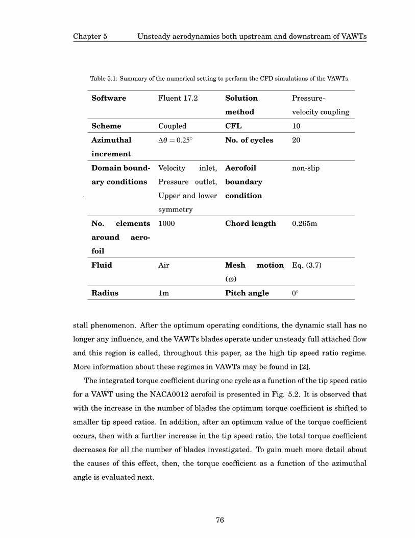
Chapter 5 Unsteady aerodynamics both upstream and downstream of VAWTs
Table 5.1: Summary of the numerical setting to perform the CFD simulations of the VAWTs.
.
Software Fluent 17.2 Solution
method
Pressure-
velocity coupling
Scheme Coupled CFL 10
Azimuthal
increment
∆θ = 0.25◦ No. of cycles 20
Domain bound-
ary conditions
Velocity inlet,
Pressure outlet,
Upper and lower
symmetry
Aerofoil
boundary
condition
non-slip
No. elements
around aero-
foil
1000 Chord length 0.265m
Fluid Air Mesh motion
(ω)
Eq. (3.7)
Radius 1m Pitch angle 0◦
stall phenomenon. After the optimum operating conditions, the dynamic stall has no
longer any influence, and the VAWTs blades operate under unsteady full attached flow
and this region is called, throughout this paper, as the high tip speed ratio regime.
More information about these regimes in VAWTs may be found in [2].
The integrated torque coefficient during one cycle as a function of the tip speed ratio
for a VAWT using the NACA0012 aerofoil is presented in Fig. 5.2. It is observed that
with the increase in the number of blades the optimum torque coefficient is shifted to
smaller tip speed ratios. In addition, after an optimum value of the torque coefficient
occurs, then with a further increase in the tip speed ratio, the total torque coefficient
decreases for all the number of blades investigated. To gain much more detail about
the causes of this effect, then, the torque coefficient as a function of the azimuthal
angle is evaluated next.
76

Chapter 5 Unsteady aerodynamics both upstream and downstream of VAWTs
Figure 5.2: The total torque coefficient of as a function of the tip speed ratio for a VAWTs using the
NACA0012 and a constant free-stream wind speed of 8 m/s.
The azimuthal torque coefficient, CQ(θ), for the one-bladed VAWT with the NACA0012
and the lift and drag force coefficients are presented in Fig. 5.3 (a-c). For the tip speed
ratios λ ≤ 3.5, a loss in CQ has been identified upstream of the rotor. The loss in CQ
is marked with a square in Fig. 5.3(a) and this suggests that the dynamic stall phe-
nomenon has taken place. Interestingly, these tip speed ratios occur before the opti-
mum torque coefficient (total) observed at λ = 4 in Fig. 5.2 for the one-blade VAWT.
The analysis of the lift and drag force coefficients for λ ≤ 3.5 in Fig. 5.3 (b-c) shows
clearly the presence of the dynamic stall phenomenon. For the upstream section of
the rotor, from 0 to 180◦, deep stall conditions are observed, i.e. a large hysteresis is
experienced in the lift and drag force coefficients as shown for the tip speed ratios of 2
and 2.5. Despite the hysteresis being small for the tip speed ratios of 3 and 3.5, this
indicates that the dynamic stall phenomenon still influences the unsteady loads, and
usually this is called light dynamic stall.
At the downstream section of the rotor, from 180 to 360◦, the sudden loss in the
torque coefficient is no longer observed at any tip speed ratio as well as the loss in
the force coefficients. Nevertheless, the presence of a slight hysteresis in both the lift
and the drag force coefficients indicate the influence of the dynamic stall as a light
stall condition for the tip speed ratios of 2 and 2.5. Thus, it may be concluded that
the dynamic stall phenomenon is less severe downstream of the rotor and upstream of
77
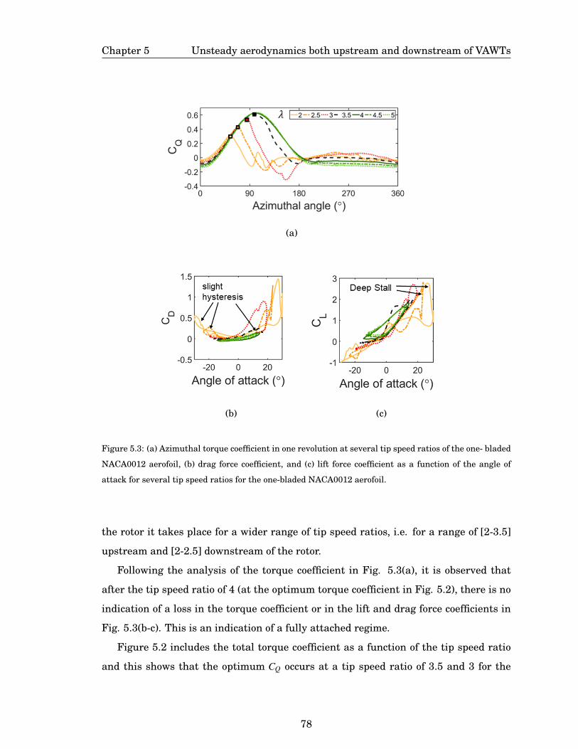
Chapter 5 Unsteady aerodynamics both upstream and downstream of VAWTs
(a)
(b) (c)
Figure 5.3: (a) Azimuthal torque coefficient in one revolution at several tip speed ratios of the one- bladed
NACA0012 aerofoil, (b) drag force coefficient, and (c) lift force coefficient as a function of the angle of
attack for several tip speed ratios for the one-bladed NACA0012 aerofoil.
the rotor it takes place for a wider range of tip speed ratios, i.e. for a range of [2-3.5]
upstream and [2-2.5] downstream of the rotor.
Following the analysis of the torque coefficient in Fig. 5.3(a), it is observed that
after the tip speed ratio of 4 (at the optimum torque coefficient in Fig. 5.2), there is no
indication of a loss in the torque coefficient or in the lift and drag force coefficients in
Fig. 5.3(b-c). This is an indication of a fully attached regime.
Figure 5.2 includes the total torque coefficient as a function of the tip speed ratio
and this shows that the optimum CQ occurs at a tip speed ratio of 3.5 and 3 for the
78

Chapter 5 Unsteady aerodynamics both upstream and downstream of VAWTs
two-bladed and three-bladed turbines, respectively. Similar to the analysis of the one-
bladed turbine, the azimuthal torque coefficient is presented for two and three-bladed
VAWTs in Fig. 5.4 and is compared with the total torque coefficient in Fig. 5.2. The
azimuthal torque coefficient upstream shows the loss at λ < 3.5 for the two-bladed
turbine, and for the three-bladed turbine, this loss in the torque coefficient is observed
at λ < 3.
(a)
(b)
Figure 5.4: Azimuthal torque coefficient at several tip speed ratios for a VAWTs using the NACA0012
aerofoil and with the number of blades (a) two, and (b) three.
In general, it can be concluded that a dynamic stall regime takes place at the tip
speed ratios before an optimum value on the total torque coefficient and after this
value, a fully attached flow regime is experienced, where a decrease in the total torque
79

Chapter 5 Unsteady aerodynamics both upstream and downstream of VAWTs
coefficient is observed for all the number of blades investigated.
5.4 Influence of the aerofoil on the upstream and downstream torque con-
tributions
The analysis of the upstream torque contributions for the six aerofoils presented in
Fig.5.5 (a-c) shows that the S1210 is the aerofoil with the largest torque coefficient
for the different number of blades investigated on the upstream side of the turbine.
Further, the differences of the CQ for the S1210 with the CQ of the symmetrical aero-
foils increases with the increase in the tip speed ratio. The next best torque coefficient
upstream is produced by the cambered NACA2418. Subsequently, the torque contri-
butions upstream were observed, in decreasing order, for the symmetrical aerofoils
NACA0021 and NACA0018, then NACA0015 and last the NACA0012. The torque
coefficient using the S1210 aerofoil increases by up to 70% compared with the sym-
metrical aerofoils torque coefficient for the one bladed-turbine and at a tip speed ratio
λ = 5; also, the S1210 increase in CQ for the two and three-bladed turbines was 62% (
at λ = 4) and 56% ( at λ = 4), respectively.
(a) (b) (c)
Figure 5.5: Upstream torque coefficient, CQ,up, of six aerofoils for a VAWT with (a) one blade, (b) two
blades and, (c) three blades.
Following the upstream analysis, all the aerofoils show an increase in the torque
coefficient, CQ, with the increase in the tip speed ratio, λ , approaching to a maximum
CQ value, that barely decreases in magnitude with a further increase in the tip speed
80

Chapter 5 Unsteady aerodynamics both upstream and downstream of VAWTs
ratio. For instance, the NACA0012 for the two-bladed turbine (Fig. 5.5b) starts with
a very poor torque coefficient at the lowest tip speed ratio λ = 1.5; while increasing λ
the torque coefficient increases and reaches a maximum torque coefficient CQ = 0.17
at λ = 3 and, after this tip speed ratio the magnitude of torque coefficient decreases
by only 3%. A similar behaviour in the torque coefficient upstream is observed for
the other cases investigated. Upstream, the NACA012 aerofoil is the aerofoil with the
poorest torque coefficient at small tip speed ratios, λ . Nevertheless, when this aerofoil
reaches its optimum torque coefficient at λ = 4, 3.5 and 3, for one, two and three-
bladed VAWT, respectively, then it produces a better torque coefficient than the other
aerofoils.
In the analysis of the downstream torque coefficients, see Fig. 5.6(a-c), it has been
observed that the cambered S1210 aerofoil produces the more negative torque coeffi-
cient, followed by another cambered aerofoil, the NACA2418. In none of the number
of blades investigated does the S1210 aerofoil produce a positive torque in the down-
stream region. While the NACA2418 produces a small positive torque coefficient at
low tip speed ratios, such as λ = 2.5 for the one-bladed turbine and, at λ = 1.5 for the
three-bladed turbine. The torque coefficient for the symmetrical and cambered aero-
foils becomes more negative with the increase in the tip speed ratio.
(a) (b) (c)
Figure 5.6: Downstream torque coefficient, CQ,dw, of six aerofoils for a VAWT with (a) one blade, (b) two
blades and, (c) three blades.
Further, at the downstream analysis of the rotor, all the symmetrical aerofoils ex-
cept the NACA0021, present a smaller and negative torque coefficient for all the tip
81
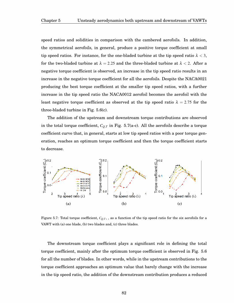
Chapter 5 Unsteady aerodynamics both upstream and downstream of VAWTs
speed ratios and solidities in comparison with the cambered aerofoils. In addition,
the symmetrical aerofoils, in general, produce a positive torque coefficient at small
tip speed ratios. For instance, for the one-bladed turbine at the tip speed ratio λ < 3,
for the two-bladed turbine at λ = 2.25 and the three-bladed turbine at λ < 2. After a
negative torque coefficient is observed, an increase in the tip speed ratio results in an
increase in the negative torque coefficient for all the aerofoils. Despite the NACA0021
producing the best torque coefficient at the smaller tip speed ratios, with a further
increase in the tip speed ratio the NACA0012 aerofoil becomes the aerofoil with the
least negative torque coefficient as observed at the tip speed ratio λ = 2.75 for the
three-bladed turbine in Fig. 5.6(c).
The addition of the upstream and downstream torque contributions are observed
in the total torque coefficient, CQ,T in Fig. 5.7(a-c). All the aerofoils describe a torque
coefficient curve that, in general, starts at low tip speed ratios with a poor torque gen-
eration, reaches an optimum torque coefficient and then the torque coefficient starts
to decrease.
(a) (b) (c)
Figure 5.7: Total torque coefficient, CQ,T , , as a function of the tip speed ratio for the six aerofoils for a
VAWT with (a) one blade, (b) two blades and, (c) three blades.
The downstream torque coefficient plays a significant role in defining the total
torque coefficient, mainly after the optimum torque coefficient is observed in Fig. 5.6
for all the number of blades. In other words, while in the upstream contributions to the
torque coefficient approaches an optimum value that barely change with the increase
in the tip speed ratio, the addition of the downstream contribution produces a reduced
82

Chapter 5 Unsteady aerodynamics both upstream and downstream of VAWTs
total torque with the increase in the tip speed ratio. The aerofoils with the most effect
on the total torque coefficient have been the cambered aerofoils, and this is due to the
large negative torque coefficient downstream of the rotor.
Despite the very good performance upstream of the S1210 aerofoil, its high nega-
tive CQ,dw contribution has dramatically affected its total torque coefficient for all the
number of blades investigated. As a result, the S1210 torque coefficient is observed
to be lower than the total torque coefficient produced by the aerofoils NACA0021,
NACA0018, NACA0015 and NACA2418. The cambered NACA2418 aerofoil, similarly,
presented a good upstream torque coefficient, nevertheless downstream its negative
impact was smaller than that of the S1210, and thus produced a similar total torque
coefficient as the symmetrical NACA0018 for all the solidities evaluated.
Moreover, the analysis of the total torque coefficients shows each aerofoil has its
own optimum tip speed ratio and torque coefficient magnitude. This influence of the
aerofoil becomes more evident with the increase in the number of blades. For instance,
for the one-bladed turbine, see Fig.5.7(a), the NACA0015, NACA0018 and NACA0021
aerofoils have an optimum tip speed ratio λ = 3; for the three-bladed turbine, the
NACA0021 and NACA0018 produced a maximum torque coefficient at λ = 2.25 and
the NACA0015 at λ = 2.5.
The NACA0021 was the aerofoil with the best total torque coefficients of all the
aerofoils and the number of blades evaluated. The difference with the other aerofoils
before its optimum torque coefficient (low tips speed ratios) is attributed to the fact that
the NACA0021 presents some positive torque coefficients upstream at low tip speed
ratios; thus, despite having very similar upstream torque contributions with other
aerofoils, the downstream contribution results are beneficial for the overall torque co-
efficients.
At high tip speed ratios, after the optimum torque coefficient, the NACA0012 aero-
foil shows the largest torque coefficient (despite being a small increase), followed by
the NACA0015, NACA0018, NACA2418, NACA0021 and last is the S1210 aerofoil for
all the number of blades investigated. This better performance of the NACA0012 at
large tip speed ratio is attributed to its better downstream contributions than the other
aerofoils as explained previously in this section.
83

Chapter 5 Unsteady aerodynamics both upstream and downstream of VAWTs
In order to understand the influence of the aerofoil profile on the power coefficient,
CP, this parameter is included in Fig. 5.8(a-c). The analysis of CP has revealed that
at the optimum operating conditions, the magnitude of the power coefficient is very
similar among the symmetrical aerofoils. For the one-bladed turbine, the optimum
power coefficient was CP = 0.47, and this was obtained for a tip speed ratio λ = 3.5 for
the NACA0021 and NACA0018; the NACA0015 aerofoil shows an optimum CP = 0.48 at
λ = 4 and the NACA0012 aerofoil produced an optimum CP = 0.49 at λ = 4. For the two-
bladed turbine, the NACA0012 shows an optimum power coefficient CP = 0.42 at the tip
speed ratio λ = 3.5; the NACA0015 aerofoil produces CP = 0.44 at λ = 3 and NACA0018,
NACA0021 produces CP = 0.44 at λ = 2.75 . Moreover, for the three-bladed turbine, an
optimum power coefficient CP = 0.38 at the tip speed ratio λ = 2.5 was obtained for the
NACA0021 and NACA0018; the NACA0015 produced CP = 0.38 at the tip speed ratio
λ = 2.75 and the NACA0012 shows CP = 0.35 at the tip speed ratio λ = 3.
(a) (b) (c)
Figure 5.8: Power coefficient as a function of the tip speed ratio for the six aerofoils for the six aerofoils
for a VAWT with (a) one blade, (b) two blades and, (c) three blades.
Despite a similar optimum power coefficient among the aerofoils, at low tip speed
ratios, the influence of the aerofoil shape on the power coefficient magnitude becomes
substantial. In contrast, at high tip speed ratios, the influence of the aerofoil profile is
minor and the thinner aerofoil NACA0012 produces the best power coefficient; this is
followed by the NACA0015, NACA0018, NACA2418, NACA0021 and last S1210.
84

Chapter 5 Unsteady aerodynamics both upstream and downstream of VAWTs
5.4.1 Dynamic stall regime
The dynamic stall phenomenon has been shown to play the most important role in the
poor torque coefficient that is observed at low tip speed ratios before an optimum total
torque coefficient is observed as explained above. The most quantifiable parameter
in the dynamic stall phenomenon is the stall-inception, and thus this parameter is
analysed here. This stall-inception point represents the moment when the bubble that
occurs near the leading edge of the aerofoil collapses and a vortex near the leading edge
starts to move downstream along the aerofoil chord. This moment can be recognized by
the moment when a minimum pressure coefficient is reached [95, 46]. In addition, the
stall-inception instance is the most critical parameter that describes the dynamic stall
process as discussed in Chapter 4. The pressure coefficient is calculated as follows:
Pcoe f f =Ps−P∞
1/2 ρV 2rel
(5.1)
To understand the importance of the stall-inception (θin), the three-bladed VAWT
at the tip speed ratio 1.5 was selected for a rigorous analysis. This case has been
selected since the three-bladed turbine represents the most practical design. For the
six aerofoils, upstream of the rotor, the calculated azimuthal angle where a minimum
in the pressure coefficient is observed is included in Table 5.2 . Also, the azimuthal
torque coefficient for the same case is included in 5.9 for the six aerofoils as a piece of
complementary information in order to better understand the dynamic stall regime.
Table 5.2: Azimuthal angle with a minimum in the pressure coefficient and azimuthal angle with a
maximum in the torque coefficient for the six aerofoils of a 3 bladed-turbine and λ = 1.5
.NACA0021 NACA0018 NACA0015 NACA0012 NACA2418 S1210
θmax (◦) 76.88 76.77 66.50 58.75 75.76 75.76
θin (◦) 78.87 77.91 65.51 56.53 75.64 74.68
The azimuthal angle corresponding to the stall-inception point (θin), see Table 5.9,
shows the largest delay in the inception angle being produce by the NACA0021 and
the second was the NACA0018 aerofoil with θin = 78.87◦ and θin = 77.91◦, respectively.
85

Chapter 5 Unsteady aerodynamics both upstream and downstream of VAWTs
(a)
Figure 5.9: Instantaneous torque coefficient for a three blades turbine and a tip speed ratio 1.5
The aerofoils, NACA2418 and S1210, produce a stall-inception at the azimuthal angle
θin = 75.64◦ and θin = 74.68◦, respectively. The smaller stall-inceptions are shown by the
NACA0015 with θin = 65.51◦ and the last by the NACA0012 aerofoil with θin = 56.53◦.
An interesting observation was that the stall-inception angles were located at very
similar azimuthal angles where the torque coefficient presents a maximum value, θmax
before there is a sudden loss in CQ(θ) occurs.
Upstream, the four aerofoils, NACA0021, NACA0018, NACA2418 and S1210 with
similar stall-inception angles show a loss in the torque coefficient in Fig. 5.9 at similar
azimuthal angles but the magnitude of the azimuthal torque coefficient is different.
As observed previously in the torque coefficient analysis upstream of the rotor in Fig.
5.5, the largest torque coefficient was observed for the S1210 and NACA2418. This
torque coefficient produced by the S1210 and 2418 aerofoils upstream is explained due
to the high lift force, CL at positive angles of attack for these aerofoils that influence
the tangential force coefficient produced by the blades according to Eq. (3.19).
In Fig. 5.10 (a-c), the coefficients of the static lift, drag and tangential force gener-
ated for the investigated aerofoils are compared in the range of angle of attack (AOA)
experienced by the turbine. The S1210 aerofoil presents the largest lift force coeffi-
cient, CL. The NACA2418 shows a minor increase in CL in regards to the symmetrical
aerofoil NACA0018 at positive angles of attack. The chordwise force coefficient, CC that
86

Chapter 5 Unsteady aerodynamics both upstream and downstream of VAWTs
relates the lift and drag force coefficients according to Eq.(4.3), allows a better under-
standing of the aerofoil influence. The S1210 aerofoil presents the largest chordwise
force coefficient at positive angles of attack, followed by the NACA2418 and the last
are the symmetrical NACA aerofoils.
(a) (b) (c)
Figure 5.10: Static force coefficient as a function of the angle of attack for the six aerofoils calculated by
using Xfoil at Reynolds number of 5×10⁵ (a) Lift force coefficient (CL), (b) drag force coefficient (CD), and
(c) chordwise force coefficient (CC)
Despite the symmetrical aerofoils show similar static tangential force coefficient
in Fig. 5.10(c), the dynamic stall-inception point occurs earlier for the NACA0012,
followed by the NACA0015 and later by the NACA0018 and NACA0021. Consequently,
this explained the sooner loss in CQ for the NACA0012 at the upstream according to
Fig. 5.9 and also explained why the NACA0012 exhibits the poorest torque coefficient
in Fig. 5.5(c).
The present results suggest that under dynamic stall conditions, the primary pa-
rameter that controls the torque coefficient is the stall-inception; larger is this angle,
then larger is the torque contribution upstream. In addition, if the aerofoil exhibits a
high tangential force, i.e. high lift/drag ratio, then there is observed to be an improve-
ment in the torque coefficient upstream, such as in the S1210 that presents a similar
stall-inception as the NACA0018 and NACA0021 but with a larger upstream torque
coefficient.
The dynamic stall upstream of the rotor produces a vortex released by the blades
87

Chapter 5 Unsteady aerodynamics both upstream and downstream of VAWTs
at downstream of the rotor and this induces high disturbances to the flow field down-
stream of the blade. The flow field at downstream of the rotor is also affected by the
blockage effect due to the number of blades and the tip speed ratio. To visualize the
vortex formation on the blades, then the vorticity contours become much more useful
in the understanding of the dynamic stall phenomenon and this is presented in Fig.
5.11.
Figure 5.11: Vorticity contours of the flow field around the blade of a three-bladed turbine at λ = 1.5
in the downstream region of the rotor of the three-bladed turbine: (a) NACA0012, (b) NACA0015, (c)
NACA0018, (d) NACA0021, (e) S1210 and (f) NACA2418.
88
Chapter 5 Unsteady aerodynamics both upstream and downstream of VAWTs
Figure 5.11 illustrated the instants when the blades are located downstream of the
rotor at three azimuthal angles, θ = 225◦, θ = 270◦ and θ = 315◦ At the azimuthal an-
gle θ = 225◦ the S1210 aerofoil presents the largest separation. A separated boundary
layer is indicative of a loss in lift force coefficient and an increase in the drag force
coefficient [44], and this agrees with the force coefficient observation in Fig. 5.10 at
the negative angles of attack for the S1210, where low CL and large CD are observed.
In addition, at the azimuthal angles θ = 270◦ and θ = 315◦ the S1210 aerofoil presents
the largest separation. Then, this suggests that the cambered S1210 does not have
the same beneficial characteristics observed at positive (upstream) AOA when it is at
negative angles of attack (downstream), and this is the reason why its total torque coef-
ficient for all the range of tip speed ratios and solidities investigated did not performed
better than the NACA0021 and NACA0018 aerofoils.
The vorticity contours illustrated in Fig. 5.11, indicate that at the azimuthal an-
gle θ = 225◦ the NACA0021, NACA0018 and NACA2418 show the presence of two
small vortices (opposite in the rotational direction) attached to the surface of the lead-
ing edge of the aerofoil. Moreover, at θ = 270◦ and θ = 315◦, the aerofoils NACA0021
and NACA0018 show the most extended attached flows on the surface of the aero-
foil. Therefore, as in the upstream region, the symmetrical aerofoils NACA0021 and
NACA0018 have the largest delay in the dynamic stall, and downstream it has still
the capabilities to maintain their boundary layers to be attached. The cambered
NACA2418 shows that it has as good stalling capabilities downstream as upstream,
and overall its torque coefficient remains similar to the NACA0018.
The NACA0012 aerofoil under dynamic conditions is the worst of the aerofoils in-
vestigated because the stall occurs too early upstream, and hence the secondary vortex
(the peak in the torque coefficient at θ = 100◦ in Fig. 5.11) is released downstream of
the VAWT, and as a results the torque contribution downstream is minimal. There-
fore, aerofoils in which the stall-inception occurs earlier are not recommended at low
tip speed ratios since the dynamic stall upstream and downstream are stronger.
89

Chapter 5 Unsteady aerodynamics both upstream and downstream of VAWTs
5.4.2 Fully unsteady attached regime
The regime called fully unsteady attached regime has been observed to be located after
a maximum in the total torque coefficient is experienced. The optimum torque coeffi-
cient takes place at different tip speed ratios and depends on the aerofoil profile and
the number of blades, hence, the range of tip speed ratios under a fully attached regime
(high tip speed ratio) also depends on the number of blades and the aerofoil profile. In
this section, two cases with all the aerofoils behaving under the fully attached regime
are exemplified. Fig. 5.12(a) includes the azimuthal torque coefficient for a two-bladed
turbine at a tip speed ratio λ = 4 and 5.12(b) includes the azimuthal torque coefficient
for a three-bladed turbine at λ = 3.5.
(a)
(b)
Figure 5.12: Azimuthal torque coefficient for the six aerofoils with (a) two blades and a tip speed ratio 4,
and (b) three-blades and tip speed ratio 3.5
It is observed in Fig. 5.12(a-b) that the S1210 (cambered 6%) aerofoil produces a
large torque coefficient upstream but also the largest negative torque coefficient down-
90

Chapter 5 Unsteady aerodynamics both upstream and downstream of VAWTs
stream for both number of blades. The NACA2418 (cambered 2%) improved the torque
coefficient upstream compared with the symmetrical NACA0018 but also produced a
more negative torque coefficient downtream than the NACA0018 aerofoil. Therefore
its total torque coefficient is very similar to the symmetrical aerofoil.
Under this high tip speed ratio regime, the total torque coefficient depends on the
lift and drag force coefficients generated for each aerofoil under the attached flow. De-
spite the upstream contributions producing a positive torque coefficient for all the aero-
foils, under this regime, the negative torque coefficient produced by all the aerofoils
downstream is the factor that is more detrimental to the total torque coefficient and
this becomes worst with the further increase in the tip speed ratio. The downstream
torque coefficients previously presented in Fig. 5.6, shows that the aerofoil NACA0012
has the least negative torque contribution with the increase in the tip speed ratio.
In order to gain more details to understand the poor torque coefficient at down-
stream of the rotor, the deficit in the velocity is analysed in Fig. 5.13. Fig. 5.13 (b-d)
shows the velocity distribution downstream of the rotor at a distance of one diameter
from the rotation centre. It can be seen that the wind speed decreases dramatically
when increasing the tip speed ratio. For a three-bladed turbine at a tip speed ratio
λ = 1.5, it is known that the dynamic stall phenomenon is severe, despite that the
deficit in the downstream velocity (V/V∞), see Fig. 5.13(b), is less severe than the
deficit for the tip speed ratio λ = 3.5 where the non-stall conditions are present, see
Fig. 5.13(b) and (c). This deficit is explained by the appearance of the blades as a solid
disk when rotating fast, thus the interference factor increases and this leads to a dra-
matic reduction in the magnitude of the velocities. Fig. 5.13(d) compares the velocity
deficit, (V/V∞) for a three-bladed turbine with the NACA0021 at a tip speed ratio with
a dynamic stall (λ = 1.5), at the optimum torque coefficient (λ = 2.25) and two tip speed
ratios far away from that of the dynamic stall (λ = 2.5 and λ = 3.5). At the optimum
torque coefficient, it is observed that the velocity downstream decays by more than
75% and similar decays are observed at higher values of λ .
Therefore, under the high tip speed ratios, in addition to the decrease in the angle
of attack due to the increase in the blade speed, the interference factor may cause a
further decrease in the angle of attack, in the relative velocity and then in the Reynolds
91

Chapter 5 Unsteady aerodynamics both upstream and downstream of VAWTs
(a) (b) (c) (d)
Figure 5.13: (a) Diagram representation along the vertical line where the velocity was collected for a
three-bladed VAWT; Non-dimensional velocity V/V∞ for the six aerofoils at (b) λ = 1.5, (c) λ = 3.5, and (d)
Non-dimensional velocity for the NACA0021 aerofoil at four tip speed ratios.
numbers. The reduction of the angle of attack in the downstream of the rotor due to
the increase of the number of blades has been observed in [93]. The deficit in the down-
stream velocities are further explained in Chapter 7 in order to understand the effect
of the number of blades and tip speed ratio in the reduction of the torque coefficient at
downstream of the rotor.
At high TSRs, the blade AOA tends to be small in the downstream region as ex-
plained previously. At small AOA, sin−α ≈−α and, cos(−α)≈ 1, hence the tangential
force coefficient approximates to CT ≈ αCL−CDO. Therefore, the smaller the angle of
attack, the drag coefficient of the aerofoils at around zero angles of attack becomes
more important, and this means the thinner the aerofoil then the smaller the drag
coefficient at zero angle of attack. This explains why the NACA0012 aerofoil is the
aerofoil with the least negative torque coefficient with the increase in the tip speed
ratio downstream of the rotor.
The case of the cambered aerofoil S1210 that presents some small positive lift force
coefficients at negative angles of attack and an increase in the drag coefficient at these
negative angles of attack (see Fig. 5.10), the first term αCL becomes negative and this
92

Chapter 5 Unsteady aerodynamics both upstream and downstream of VAWTs
may increase the negative magnitude in the torque coefficient downstream. This is
also confirmed in Fig. 5.10 (c) where the chordwise force coefficient for the six aerofoils
is compared at negative angles of attack, the worst tangential force is observed with
the S1210 and the best for the NACA0012.
5.5 Discussion
The present analysis in the VAWTs including a combination of different number of
blades, 4 symmetrical aerofoils and two cambered aerofoils, and a wide range of tip
speed ratios has highlighted the most beneficial aerodynamic characteristics of the
aerofoil profiles at different tip speed ratios. In addition, the analysis gives a basis to
re-think the design of aerofoils that are applicable for VAWTs.
From the results of this chapter the most interesting finding is the role of the down-
stream torque contribution in the total torque coefficient. All the aerofoils, and all the
number of blades investigated here found with the increase of the tip speed ratio a
more negative torque that overall, causes a reduction on the VAWT performance and,
overcomes the positive torque coefficient produced at upstream of the rotor for all the
aerofoils. Therefore, despite some aerofoils produced very good lift/drag relation at
positive angles of attack, at negative angles of attack the poor relation lift/drag impact
negatively in the performance of the VAWT. As a result, more attention is required at
negative angles of attack in order to obtain an aerofoil profile that produced good lift
force coefficient and low drag force coefficient. Under this subject, at negative angles of
attack, the symmetrical aerofoils since are expected to present the same aerodynamic
characteristics than at positive angles of attack, then may found a huge amount of
available information [116]. Different, other geometrical aerofoils, cambered, slotted,
with flap, with trailing edge modification, etc, have been very rare investigated at neg-
ative angles of attack and then, more future investigation is required [117, 118, 112].
These results have shown that the cambered aerofoil may improve the power coef-
ficient under some tip speed ratios. For example, the S1210 possess 6% of camber and
12% thickness and compared with the NACA0012 with 0% camber and 12% thickness,
produces a larger torque coefficient than the NACA0012 since it has a larger stall-onset
93

Chapter 5 Unsteady aerodynamics both upstream and downstream of VAWTs
angle upstream and a high lift force coefficient. Only at tip speed ratios corresponding
to the optimum operating conditions of the NACA0012, this last aerofoil performed bet-
ter than the cambered S1210. This observation is in agreement with results presented
in [27] where the NACA0012 and cambered NACA5512 and NACA7512 were com-
pared in the power coefficient; both cambered aerofoils present a better performance
at low tip speed ratios, where the NACA0012 showed poor performance. In contrast,
the NACA2418 with a 2% camber and 18% thickness offer no advantages compared
with the symmetrical NACA0018 with 0% camber and 18% thickness. The pointless
use of a small percentage-camber of a thick aerofoil was also observed in [119]. In this
mentioned investigation, the NACA634221 aerofoil with 1.1 camber and 21% thickness
was compared with the NACA0021; the power coefficient as a function of the tip speed
ratio was very similar but in the optimum tip speed ratio, the symmetrical aerofoils
performed slightly better than the cambered aerofoil. This agrees with our results by
using the NACA2418 and the NACA0018 aerofoil. In [120] a similar conclusion was
obtained by using the symmetrical NACA0022 and the camber NACA5522, both with
21% thickness.
Therefore, if the camber percentage improves the delay in the stall angle compared
with its symmetrical aerofoil, then some improvement maybe notice at tip speed ratios
where dynamic stall occurs. Nevertheless, if the cambered aerofoil has a poor lift force
coefficient and large drag force coefficient at negative angles of attack then this can
have a detrimental effect on the performance, mainly at high tip speed ratios. While
an increase in the magnitudes of the wind velocity downstream at high tip speed ratios
is almost impossible, the control in the angle of attack needs to be investigated as a
possible strategy to reduce the negative torque production downstream of the rotor.
Present results solves the controversy existing in the last few years in the use of cam-
bered over the symmetrical. For instance, some authors claim that cambered aerofoils
are promising for VAWTs; others have predicted that it is detrimental for their perfor-
mance [120, 121, 27, 122, 123]. The results in this Chapter suggest that more than
focusing the investigation on the use of cambered or symmetrical aerofoils attention
need to be paid in the final aerodynamic characteristics, i.e, the stall-onset and the lift
and drag force coefficient at positive and negative angles of attack.
94

Chapter 5 Unsteady aerodynamics both upstream and downstream of VAWTs
In addition, the results presented have shown that independent of the number of
blades the dynamic stall region always take place, thus, in order to increases the torque
under the dynamic stall conditions, the dynamic stall-inception of the aerofoil needs
to be considered when selecting the aerofoil. The stall-inception point is also known
as the stall-onset angle and under dynamic conditions, the most evaluated aerofoils
have been symmetrical [65] but some cambered aerofoils have been tested under dy-
namic conditions and at positive angles of attack [124]. In the present results, the
larger dynamic stall inception was shown by the NACA00021, then followed by the
NACA0018 and this agrees with the experimental investigation on stall-onset angle
under dynamic conditions in [65].
Despite the optimum tip speed ratios differing among the aerofoils and the num-
ber of blades, under the optimum operating conditions the symmetrical NACA aero-
foils present very similar optimum power coefficients. In addition, after the dynamic
stall region, where the flow over the blades is fully attached, huge attention needs
to be paid to the performance of the aerofoil under negative angles of attack and low
Reynolds number, since the downstream torque contribution plays a significant role in
the reduction of the total torque coefficient.
5.6 Summary
The key new information identified in this chapter would allow an analysis of the dy-
namic stall method to predict the unsteady forces under dynamic stall conditions and
fully attached regimen and to assess the DSMT model and its capabilities to take into
account the effect of the number of blades under both regimes. Simulations performed
in this Chapter has bridged the existing gap in the literature regarding the influence
of the upstream and downstream torque contributions on the overall performance of
VAWTs. Some of the most important findings are described as following.
(i) When the dynamic stall occurs at upstream of the rotor as well as the down-
stream of the rotor the lowest is the total torque coefficient. After the optimum torque
coefficient, a fully attached flow regime occurs and it has been demonstrated that the
decrease in the total torque coefficient is attributed mainly to the downstream region
95

Chapter 5 Unsteady aerodynamics both upstream and downstream of VAWTs
of the rotor.
(ii) The symmetrical aerofoils NACA0015, NACA0018 and NACA0021 have been
demonstrated to be the most effective both upstream and downstream of the rotor.
Thus, these aerofoils are further investigated in this thesis. The cambered aerofoil,
despite showing some advantages, requires to be optimized in order to work well at
negative angles of attack, otherwise, this will cause a significant negative torque down-
stream that limit the overall power coefficient of the VAWT.
(iii) Under dynamic stall conditions, the most important parameter is the stall-
onset angle that is highly dependent on the aerofoil. Under the fully attached regime,
the downstream torque contribution becomes critical and hence the more negative its
value the larger is the depletion in the VAWT performance. Therefore, the lift/drag
relation at negative angles of attack need to be carefully investigated during the selec-
tion of the aerofoils profile if large tip speed ratio becomes the range of interest for the
VAWT under operation.
(iv) The generated knowledge would assist in the assessment of the LB dynamic
stall and the DMST to predict the torque coefficient on VAWTs and that is carried out
in Chapter 6.
96

Chapter 6
Predicting unsteady loads using a dynamic stall
algorithm
6.1 Overview
The Leishman-Beddoes dynamic stall algorithm has been used the most to predict the
unsteady loads of oscillating aerofoils. Additionally, the existing investigations have
been focused on Reynolds number larger than 1 million and therefore, most of the
empirical parameters that this dynamic stall model requires are restricted to a few
aerofoils and high Reynolds number. As was discussed in previous Chapter, the dy-
namic stall phenomenon takes place before the optimum tip speed ratio of any turbine
and its modelling results crucial for an accurate prediction of the torque coefficient in
the VAWTs. Under this subject, still remain a need of a detailed analysis of the use of
this LB dynamic stall algorithm to predict the performance of VAWTs, specifically, the
implementation of the Kirchhoff flow model and the estimation of the stall-onset at low
Reynolds number that is likely to be found in VAWTs operating at low tip speed ratios
and low wind speeds. This chapter bridges these gaps in the literature and addition-
ally evaluates the effectiveness of the double multiple streamtube to predict the torque
coefficient of VAWTs under the dynamic stall and a fully attached regime of operation.
6.2 The Leishman-Beddoes dynamic stall: modifications
The Leishman-Beddoes dynamic stall (LB) algorithm is based on the physics of the
dynamic stall phenomenon described in Section 2.2.2. It predicts the unsteady loads
under the fully attached regime; next, it computes the stall-onset angle and finally,
calculates the unsteady loads under the separated flow regime, see Section 3.3. Some
97

Chapter 6 Predicting unsteady loads using a dynamic stall algorithm
of the aspect of the LB model that requires a depth analysis before its application are
described in the consecutive sections.
6.2.1 Time delay constant database
The stall-onset module of the Leishman-Beddoes method has the objective to predict
the stall-inception. At this point, a minimum value in the leading edge pressure occurs,
this is the critical instant when the circulation that is accumulated at the leading edge
of the aerofoil (LE) is released downstream and this rolls up to form a vortex which
increases in size with its movement along the chord. This vortex is called the detached
separated vortex (DSV) and the stall-inception is the most critical parameter for an
accurate representation of the dynamic stall phenomenon.
In order to predict accurately the dynamic stall inception, the Leishman-Beddoes
method is based on the time delay method. This method is able to predict the stall
inception from the static aerofoil data [114, 44] and uses a non-dimensional time (refers
as a time delay constant) which may be expressed as follows:
Tr =2Ure f ∆tsep
c(6.1)
where ∆tsep represents the time elapsed from the static stall angle, αss, to the dynamic
stall-onset angle αos, then ∆tsep = (αos−αss)/α .
Previous investigations have calculated the time delay constant, Tr, using experi-
mental test consisting on oscillating aerofoils and ramp-up tests [46, 65]. Despite that,
the available Tr values are restricted to high Reynolds numbers and then, the need to
understand this parameter at low Reynolds number has been investigated as follows.
In the analysis carried out in Chapter 4, corresponding to the stall-onset angle in
VAWTs and the operating parameters that affects its value, surprisingly the stall-onset
was found to have a linear relationship with the non-dimensional pitch rate, q = αc2Ure f
calculated when the angle of attack approaches to the static stall angle, αss. This linear
relation was obtained at each tested Reynolds number as observed in Fig. 6.1 (a) for
the NACA0015 and following same procedure described in Chapter 4 then, the stall-
onset as a function of q was obtained for the NACA0018 and NACA0021 as illustrated
98

Chapter 6 Predicting unsteady loads using a dynamic stall algorithm
in Fig. 6.1(b) and (c) respectively. The slope of the linear adjustment of the graphs
presented in Fig. 6.1 at each Reynolds number give the expression:
m = (y−b)/x (6.2)
where, m, y, b and x are the variables representing a typical linear equation. The slope
m given by Eq.(6.2) produces m = (αos−αss)/q and substituting the definition of the
non-dimensional pitch rate q given by Eq. (4.2) then m results to be the time delay
constant, Tr.
The values of Tr are calculated for NACA0015, NACA0018 and NACA0021 aerofoils
at the corresponding Reynolds numbers included in Table 6.1. The results presented
in Table 6.1 showed that the time delay constants for each aerofoil changes with the
Reynolds numbers within the range of Re investigated. It was found that Tr increases
with the increasing Reynolds number; for the NACA0015 aerofoil Tr varies within a
range of 4.28-5.70, and for the NACA0018 aerofoil then Tr changes between 3.45 and
6.35.
The influence of Re on the time delay constant for the NACA0021 is less pronounced
compared with the other two aerofoils, being in the range of 5.58-6.78. In addition, the
NACA0021 showed the largest value of Tr for all the Re values investigated, but, at
Re = 3.3×10⁵ both the NACA0018 and NACA0021 showed a very similar value of Tr.
The present results then suggest that the NACA0021 may persist attached under
larger angle of attacks than the other two aerofoils. Moreover, the similar values of
the time delay observed in the range of Re tested for the NACA0021 suggests that this
aerofoil is less affected by the decrease in the Reynolds numbers, i.e. it is appropriated
to operate at low wind speeds.
The time delay constants calculated by Sheng et al. using experimental data for
large Reynolds number of 1 million were as follows: for the NACA0015 , Tr = 5.78, for
the NACA0018 Tr = 6.22 and for the NACA0021 Tr = 6.30. These values are similar
to the time delay values found with present simulations at Re = 3.3× 10⁵ (the largest
tested considered) for each aerofoil according to Table 6.1. This suggests that, after
Re = 3.3× 10⁵, the Reynolds number has a minor effect on the time delay constant.
99

Chapter 6 Predicting unsteady loads using a dynamic stall algorithm
(a) (b)
(c)
Figure 6.1: Stall-onset angle as a function of the non-dimensional pitch rate for (a) NACA0015, (b)
NACA0018 and, (c) NACA0021.
However this observation needs further verification with experimental data.
6.2.2 Kirchhoff flow equation: Static parameters
In order to replicate the unsteady forces, the LB dynamic stall method requires some
empirical parameters that are obtained usually using the static lift force coefficient
and are specific for each aerofoil and Reynolds number. The LB method is assisted by
the Kirchhoff flow model to obtained these empirical parameters and one of the issues
100
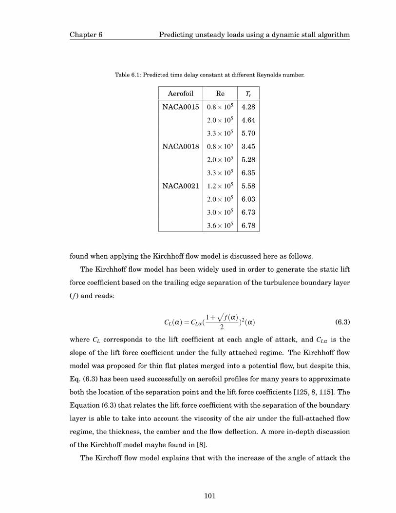
Chapter 6 Predicting unsteady loads using a dynamic stall algorithm
Table 6.1: Predicted time delay constant at different Reynolds number.
Aerofoil Re Tr
NACA0015 0.8×10⁵ 4.28
2.0×10⁵ 4.64
3.3×10⁵ 5.70
NACA0018 0.8×10⁵ 3.45
2.0×10⁵ 5.28
3.3×10⁵ 6.35
NACA0021 1.2×10⁵ 5.58
2.0×10⁵ 6.03
3.0×10⁵ 6.73
3.6×10⁵ 6.78
found when applying the Kirchhoff flow model is discussed here as follows.
The Kirchhoff flow model has been widely used in order to generate the static lift
force coefficient based on the trailing edge separation of the turbulence boundary layer
( f ) and reads:
CL(α) =CLα(1+√
f (α)
2)2(α) (6.3)
where CL corresponds to the lift coefficient at each angle of attack, and CLα is the
slope of the lift force coefficient under the fully attached regime. The Kirchhoff flow
model was proposed for thin flat plates merged into a potential flow, but despite this,
Eq. (6.3) has been used successfully on aerofoil profiles for many years to approximate
both the location of the separation point and the lift force coefficients [125, 8, 115]. The
Equation (6.3) that relates the lift force coefficient with the separation of the boundary
layer is able to take into account the viscosity of the air under the full-attached flow
regime, the thickness, the camber and the flow deflection. A more in-depth discussion
of the Kirchhoff model maybe found in [8].
The Kirchoff flow model explains that with the increase of the angle of attack the
101
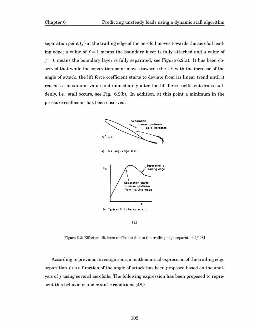
Chapter 6 Predicting unsteady loads using a dynamic stall algorithm
separation point ( f ) at the trailing edge of the aerofoil moves towards the aerofoil lead-
ing edge; a value of f = 1 means the boundary layer is fully attached and a value of
f = 0 means the boundary layer is fully separated, see Figure 6.2(a). It has been ob-
served that while the separation point moves towards the LE with the increase of the
angle of attack, the lift force coefficient starts to deviate from its linear trend until it
reaches a maximum value and immediately after the lift force coefficient drops sud-
denly, i.e. stall occurs, see Fig. 6.2(b). In addition, at this point a minimum in the
pressure coefficient has been observed.
(a)
Figure 6.2: Effect on lift force coefficient due to the trailing edge separation ( f ) [8]
According to previous investigations, a mathematical expression of the trailing edge
separation f as a function of the angle of attack has been proposed based on the anal-
ysis of f using several aerofoils. The following expression has been proposed to repre-
sent this behaviour under static conditions [48]:
102

Chapter 6 Predicting unsteady loads using a dynamic stall algorithm
f (α) =
(1− fcrt)exp( |α|−αss
S1), |α|< ass
fLE +( fcrt − fLE)exp(αss−|α|S2
), |α| ≥ ass.
(6.4)
where fLE represents the point around the leading edge where the boundary layer
separates at larger angles of attack; fcrt represents the critical separation point where
the lift coefficient reaches its maximum value, i.e. at the angle of attack where the
static stall occurs, αss. A value of fcrt = 0.6 or 0.7 has been usually associated with αss
and after this value, the flow is considered as a separated flow. The critical separation
point fcrt = 0.6,0.7 has been proposed for high Reynolds numbers, and in order to apply
this value with confidence a more in-depth assessment of the separation point f is
mandatory. Therefore this parameter is further discussed later in this section. The
parameters S1 and S2 are the adjusted parameters in Eq. (6.4) with the experimental
data of f as a function of the angle of attack and this depends on the Reynolds number.
It is important to mention that Eq. (6.4) has been formulated based on several ex-
perimental tests and through the years several different formulations have been pro-
posed. Formulations that are more complex and requires a larger number of empirical
parameters are found in [126].
The critical separation point
Due to the shortage of literature about the static separation point f as a function of
the angle of attack at Reynolds number lower than one million and being the interest
of this thesis, therefore the analysis of the actual f at two Reynolds number as been
carried out using the NACA0015 aerofoil. The numerical technique used for these
simulations is included in Section 3.2.2.
The trailing edge separation point, f , has been calculated by using the skin friction
(C f x) along the aerofoil chord and selecting a value of C f x = 0 as the criteria to define
the separation point. In addition, the lift force coefficient has been calculated for each
angle of attack and the comparison of both these parameters is included in Fig.6.3 at
two Reynolds numbers.
Figure 6.3(a) presents the results for a Re of 3.3×10⁵. At this Re, the maximum lift
103

Chapter 6 Predicting unsteady loads using a dynamic stall algorithm
(a) (b)
Figure 6.3: Trailing edge separation point as a function of the angle of attack calculated with the skin
friction being obtained using CFD simulations for the NACA0015 under static conditions at (a) Re 3.3×10⁵
and (b) 2.0×10⁵
force coefficient (CL,max) occurs when fcrt = 0.53 and αss = 14◦. A fully attached boundary
layer with f = 1 is observed up to α = 9◦. In the case of Re 2.0× 10⁵, Fig. 6.3(b),
the maximum lift force coefficient occurs when fcrt = 0.50 at αss = 13◦. Additionally,
at this Re a value of f = 1 is observed up to α = 7◦. According to these results a
critical separation point of fcrt = 0.5 is recommended to be used in Eq.(6.4) at these low
Reynolds number. The assessment of the using this value is presented in following
paragraphs. The value of the separation point, fLE under a larger angle of attack was
found to be around 0.02 for both Reynolds number.
The separation of the boundary layer, f , also permit the prediction of the chordwise
force coefficient by using next relations [65, 48]:
CC =
CLαα2√ f −CD0 f (α)> fcrit
CLαα2( f −E0)−CD0 f (α)< fcrit
(6.5)
where, CD0 represents the drag coefficient at the angle of attack zero and, E0 is the
adjusted parameter that allows to obtained negative values on the chordwise force
coefficient under the separated regime.
104
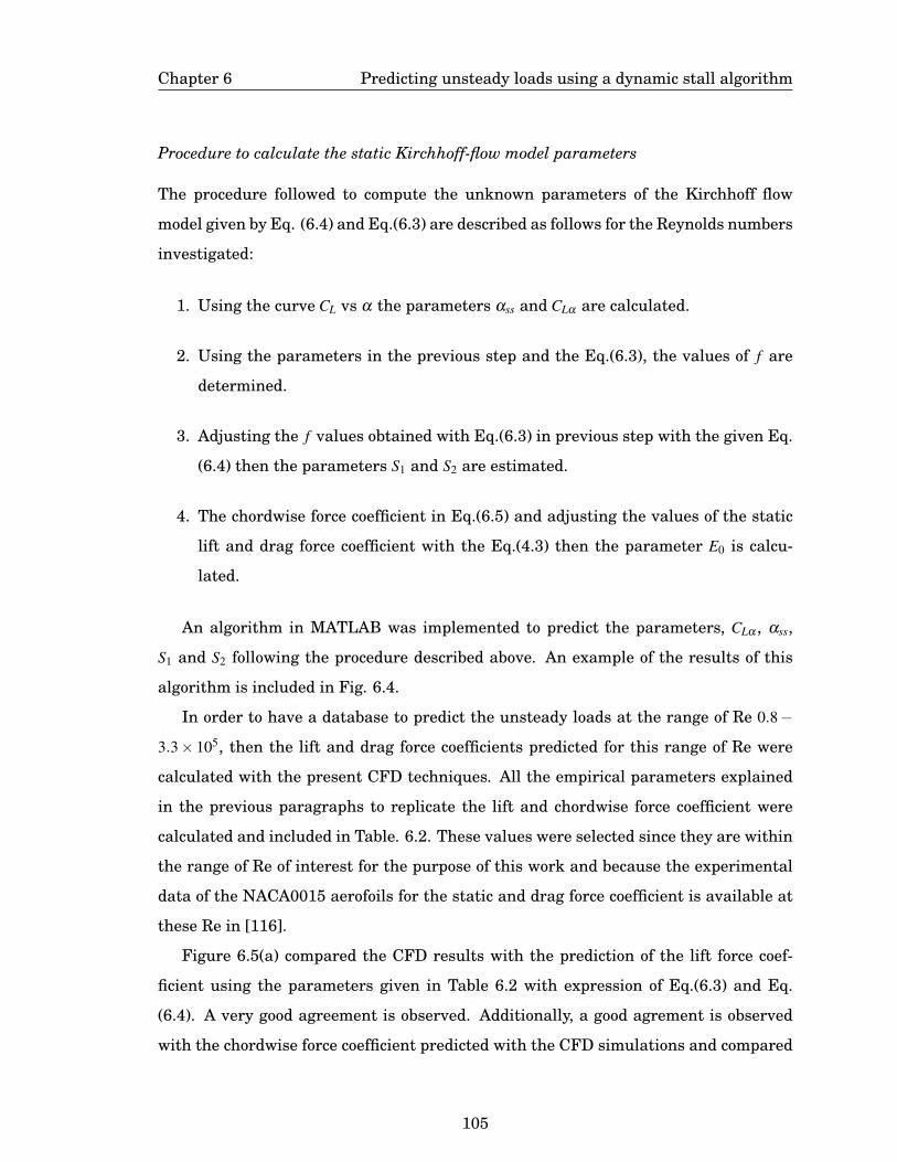
Chapter 6 Predicting unsteady loads using a dynamic stall algorithm
Procedure to calculate the static Kirchhoff-flow model parameters
The procedure followed to compute the unknown parameters of the Kirchhoff flow
model given by Eq. (6.4) and Eq.(6.3) are described as follows for the Reynolds numbers
investigated:
1. Using the curve CL vs α the parameters αss and CLα are calculated.
2. Using the parameters in the previous step and the Eq.(6.3), the values of f are
determined.
3. Adjusting the f values obtained with Eq.(6.3) in previous step with the given Eq.
(6.4) then the parameters S1 and S2 are estimated.
4. The chordwise force coefficient in Eq.(6.5) and adjusting the values of the static
lift and drag force coefficient with the Eq.(4.3) then the parameter E0 is calcu-
lated.
An algorithm in MATLAB was implemented to predict the parameters, CLα , αss,
S1 and S2 following the procedure described above. An example of the results of this
algorithm is included in Fig. 6.4.
In order to have a database to predict the unsteady loads at the range of Re 0.8−
3.3× 10⁵, then the lift and drag force coefficients predicted for this range of Re were
calculated with the present CFD techniques. All the empirical parameters explained
in the previous paragraphs to replicate the lift and chordwise force coefficient were
calculated and included in Table. 6.2. These values were selected since they are within
the range of Re of interest for the purpose of this work and because the experimental
data of the NACA0015 aerofoils for the static and drag force coefficient is available at
these Re in [116].
Figure 6.5(a) compared the CFD results with the prediction of the lift force coef-
ficient using the parameters given in Table 6.2 with expression of Eq.(6.3) and Eq.
(6.4). A very good agreement is observed. Additionally, a good agrement is observed
with the chordwise force coefficient predicted with the CFD simulations and compared
105

Chapter 6 Predicting unsteady loads using a dynamic stall algorithm
Figure 6.4: TE separation point calculated in step 2 using the Kirchhoff flow Eq.(6.3) and in red, adjusting
the S1 and S2 parameters in the Eq. (6.4). This example corresponds to the NACA0015 at Re 3.3×10⁵.
Table 6.2: The static parameter to replicate the lift force coefficient and the chordwise force coefficient.
Aerofoil Re αss (◦) CLα S1 S2 Cd0 E0 fcrt
NACA0015 0.8×10⁵ 10.41 0.10 1.25 2.64 0.020 0.05 0.5
2.0×10⁵ 13.31 0.10 3.08 1.02 0.012 0.05 0.5
3.3×10⁵ 14.95 0.10 2.25 1.83 0.009 0.05 0.5
with the parameters given in Table 6.2 used in Eq. (6.5). These results suggest that
the use of the investigated critical value fcrt = 0.5 predicts accurately the static force
coefficients for the NACA0015 at these low Reynolds number investigated. Despite
that, much more efforts need to be made in order to evaluate a wide range of Reynolds
number and, additionally take into account different aerofoils profiles to elucidate a
general formulation for the TE separation point that improves the current Kirchhoff
flow model.
106
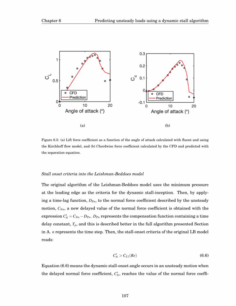
Chapter 6 Predicting unsteady loads using a dynamic stall algorithm
(a) (b)
Figure 6.5: (a) Lift force coefficient as a function of the angle of attack calculated with fluent and using
the Kirchhoff flow model, and (b) Chordwise force coefficient calculated by the CFD and predicted with
the separation equation.
Stall onset criteria into the Leishman-Beddoes model
The original algorithm of the Leishman-Beddoes model uses the minimum pressure
at the leading edge as the criteria for the dynamic stall-inception. Then, by apply-
ing a time-lag function, DPn, to the normal force coefficient described by the unsteady
motion, CNn, a new delayed value of the normal force coefficient is obtained with the
expression C′N =CNn−DPn. DPn represents the compensation function containing a time
delay constant, Tp, and this is described better in the full algorithm presented Section
in A. n represents the time step. Then, the stall-onset criteria of the original LB model
reads:
C′N >CL1(Re) (6.6)
Equation (6.6) means the dynamic stall-onset angle occurs in an unsteady motion when
the delayed normal force coefficient, C′N , reaches the value of the normal force coeffi-
107

Chapter 6 Predicting unsteady loads using a dynamic stall algorithm
cient at the static stall conditions that approaches to the value of maximum lift force
coefficient, CL1.
Sheng et al. [65] have proposed another stall-onset criteria and this approach con-
sists of applying a delay, Dαn, directly to the angle of attack, αn. Hence, the stall-onset
occurs as follows:
αn′ > αss(Re) (6.7)
where, αn′ = αn−Dαn and,
Dαn = Dαn−1exp(−∆s/Tr)+(αn−αn−1)exp(−∆s/2T r) (6.8)
where ∆s represent a non-dimensional time step ∆t accordingly the expression ∆s =
2Ure f ∆t/c This criteria has been used in the modified-Leishman Beddoes algorithm.
Additionally, the static parameters investigated in this thesis and included in Table
6.2 as well as the time-delays constants computed in Table 6.1 are also included in this
called the LB-modified.
6.3 Analysis of the LB-dynamic stall model under an oscillating motion
At this point, the time delay constants and the Kirchhoff flow parameters have been
already computed and hence, the assessment of complete LB algorithm to predict the
unsteady loads at Reynolds number lower than one million it can be made. This section
analyses the performance of the LB model using the database consisting of the static
parameters given in Table 6.2 and the time delay constants included in Table 6.1.
The unsteady chordwise force coefficient (given by Eq. (A.23) has been predicted:
(i) using the original LB dynamic stall (LB-OR) model that used the stall-onset criteria
given by Eq. (6.6), and, (ii) changing the stall-onset criteria of the original LB dynamic
stall model with Eq. (6.7) (LB-mod). The results of the predicted chordwise force coef-
ficient, CC, with the original and modified LB dynamic stall model has been presented
in Fig.6.6.
The Fig. 6.6 (a) includes the case of an oscillating motion at a constant Reynolds
number using the VAWT angle of attack equation and a reduced frequency of κ =
108
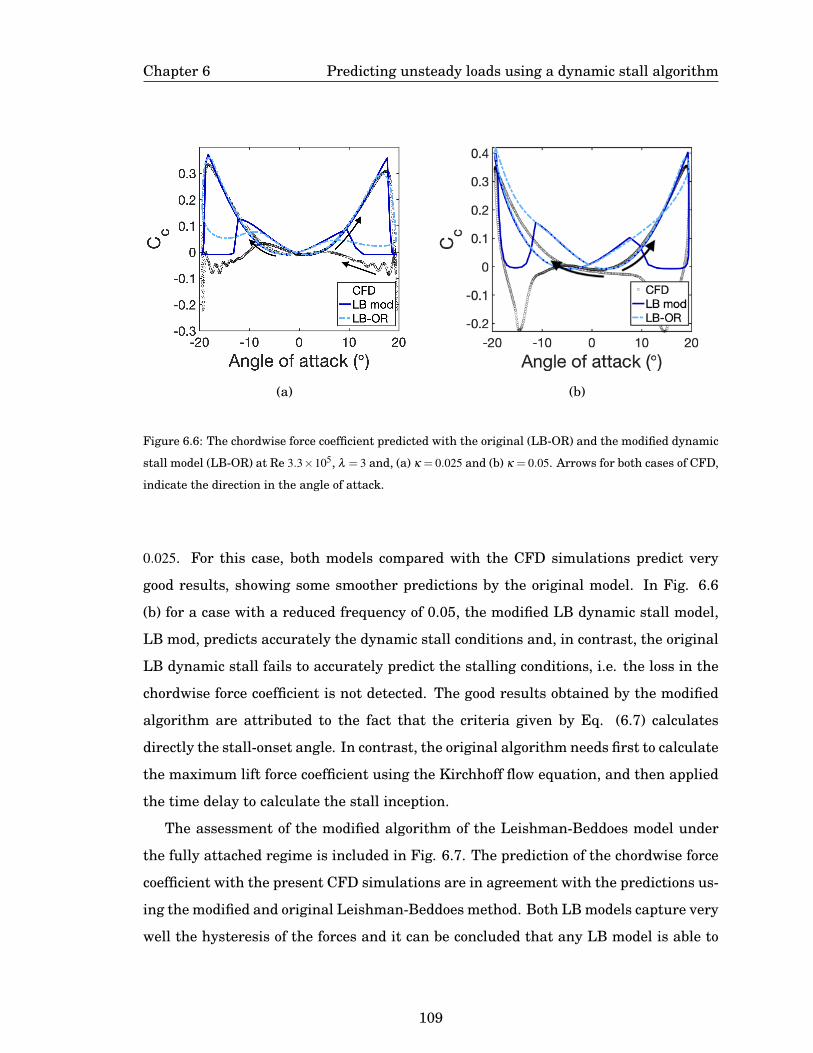
Chapter 6 Predicting unsteady loads using a dynamic stall algorithm
(a) (b)
Figure 6.6: The chordwise force coefficient predicted with the original (LB-OR) and the modified dynamic
stall model (LB-OR) at Re 3.3×10⁵, λ = 3 and, (a) κ = 0.025 and (b) κ = 0.05. Arrows for both cases of CFD,
indicate the direction in the angle of attack.
0.025. For this case, both models compared with the CFD simulations predict very
good results, showing some smoother predictions by the original model. In Fig. 6.6
(b) for a case with a reduced frequency of 0.05, the modified LB dynamic stall model,
LB mod, predicts accurately the dynamic stall conditions and, in contrast, the original
LB dynamic stall fails to accurately predict the stalling conditions, i.e. the loss in the
chordwise force coefficient is not detected. The good results obtained by the modified
algorithm are attributed to the fact that the criteria given by Eq. (6.7) calculates
directly the stall-onset angle. In contrast, the original algorithm needs first to calculate
the maximum lift force coefficient using the Kirchhoff flow equation, and then applied
the time delay to calculate the stall inception.
The assessment of the modified algorithm of the Leishman-Beddoes model under
the fully attached regime is included in Fig. 6.7. The prediction of the chordwise force
coefficient with the present CFD simulations are in agreement with the predictions us-
ing the modified and original Leishman-Beddoes method. Both LB models capture very
well the hysteresis of the forces and it can be concluded that any LB model is able to
109

Chapter 6 Predicting unsteady loads using a dynamic stall algorithm
predict accurately the unsteady forces of the oscillatory motion under a fully attached
regime. In order to have a second point of comparison, the experimental data consist-
ing of an oscillating NACA0015 reproducing the theoretical equation of the VAWT at
Re 1.5×10⁶, λ = 4.2 and a frequency of oscillation of 1.463 is included in Fig 6.7. This
experimental data shows a maximum angle of attack of 14.47◦ that is very similar to
our present CFD simulations at the tip speed ratio of 4 and a fully attached regime is
observed. The hysteresis of the chordwise force coefficient with the experimental data
is in agreement with the current CFD simulations and the numerical prediction of the
LB models.
(a)
Figure 6.7: The chordwise force coefficient of an oscillating NACA0015 predicted with numerical tech-
niques at the Re 3.3×10⁵ (λ = 4 and κ = 0.1) and compared with the experimental data [1] at Re 1.5×10⁶.
The arrows indicate the direction in the angle of attack during the oscillating motion.
6.4 Prediction of the torque coefficient of VAWTs using the dynamic stall
model
The Leishman-Beddoes algorithm including the database tested in the previous Sec-
tion has been incorporated into the double multiple stream method (DMST) to analyse
110
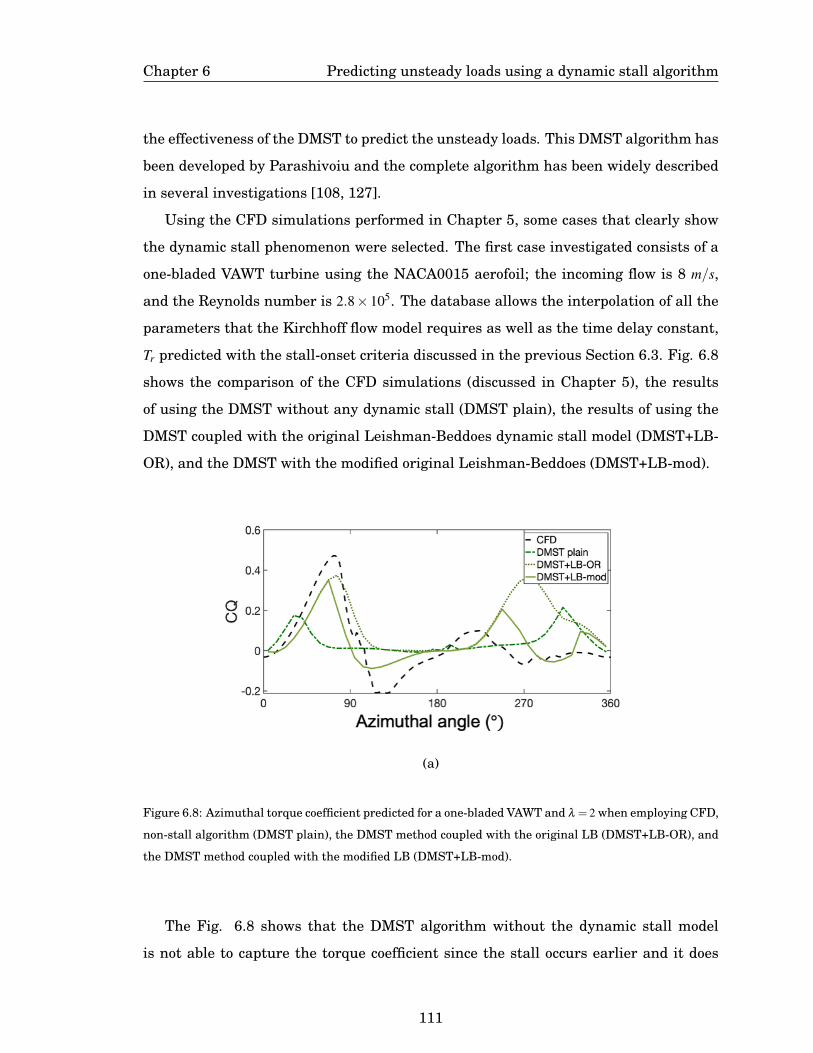
Chapter 6 Predicting unsteady loads using a dynamic stall algorithm
the effectiveness of the DMST to predict the unsteady loads. This DMST algorithm has
been developed by Parashivoiu and the complete algorithm has been widely described
in several investigations [108, 127].
Using the CFD simulations performed in Chapter 5, some cases that clearly show
the dynamic stall phenomenon were selected. The first case investigated consists of a
one-bladed VAWT turbine using the NACA0015 aerofoil; the incoming flow is 8 m/s,
and the Reynolds number is 2.8×10⁵. The database allows the interpolation of all the
parameters that the Kirchhoff flow model requires as well as the time delay constant,
Tr predicted with the stall-onset criteria discussed in the previous Section 6.3. Fig. 6.8
shows the comparison of the CFD simulations (discussed in Chapter 5), the results
of using the DMST without any dynamic stall (DMST plain), the results of using the
DMST coupled with the original Leishman-Beddoes dynamic stall model (DMST+LB-
OR), and the DMST with the modified original Leishman-Beddoes (DMST+LB-mod).
(a)
Figure 6.8: Azimuthal torque coefficient predicted for a one-bladed VAWT and λ = 2 when employing CFD,
non-stall algorithm (DMST plain), the DMST method coupled with the original LB (DMST+LB-OR), and
the DMST method coupled with the modified LB (DMST+LB-mod).
The Fig. 6.8 shows that the DMST algorithm without the dynamic stall model
is not able to capture the torque coefficient since the stall occurs earlier and it does
111

Chapter 6 Predicting unsteady loads using a dynamic stall algorithm
not take into account the delay in the stall conditions due to the pitch rate. Using
a dynamic stall model, the torque coefficient upstream presents a better agreement
with the CFD simulations with both the original and the modified Leishman-Beddoes
models. However, downstream, the modified LB dynamic stall model predicts better
the torque coefficient and this is attributed to the use of the stall-onset criteria base on
the angle of attack.
A second case consisting of two-bladed VAWTs using the NACA0015 and a tip speed
ratio λ = 1.5 has been analysed. It observed in Fig. 6.9 that the DMST alone is not able
to capture the stall-onset upstream of the rotor. However, including the dynamic stall
model allows a good prediction of the stall-onset upstream of the rotor but downstream
the original model over-predicts the torque coefficient. In contrast, the modified LB
algorithm is able to calculate not only the stall-onset but also the negative contribution
of the torque coefficient.
(a)
Figure 6.9: Azimuthal torque coefficient predicted for a two-bladed VAWT and λ = 1.5 when using CFD,
non-stall algorithm (DMST plain), the DMST method coupled with the original LB (DMST+LB-OR), and
the DMST method coupled with the modified LB (DMST+LB-mod).
A third case, which shows a light dynamic stall condition at the upstream zone
of the rotor in the CFD simulation has been analysed. This case consists of a two-
112
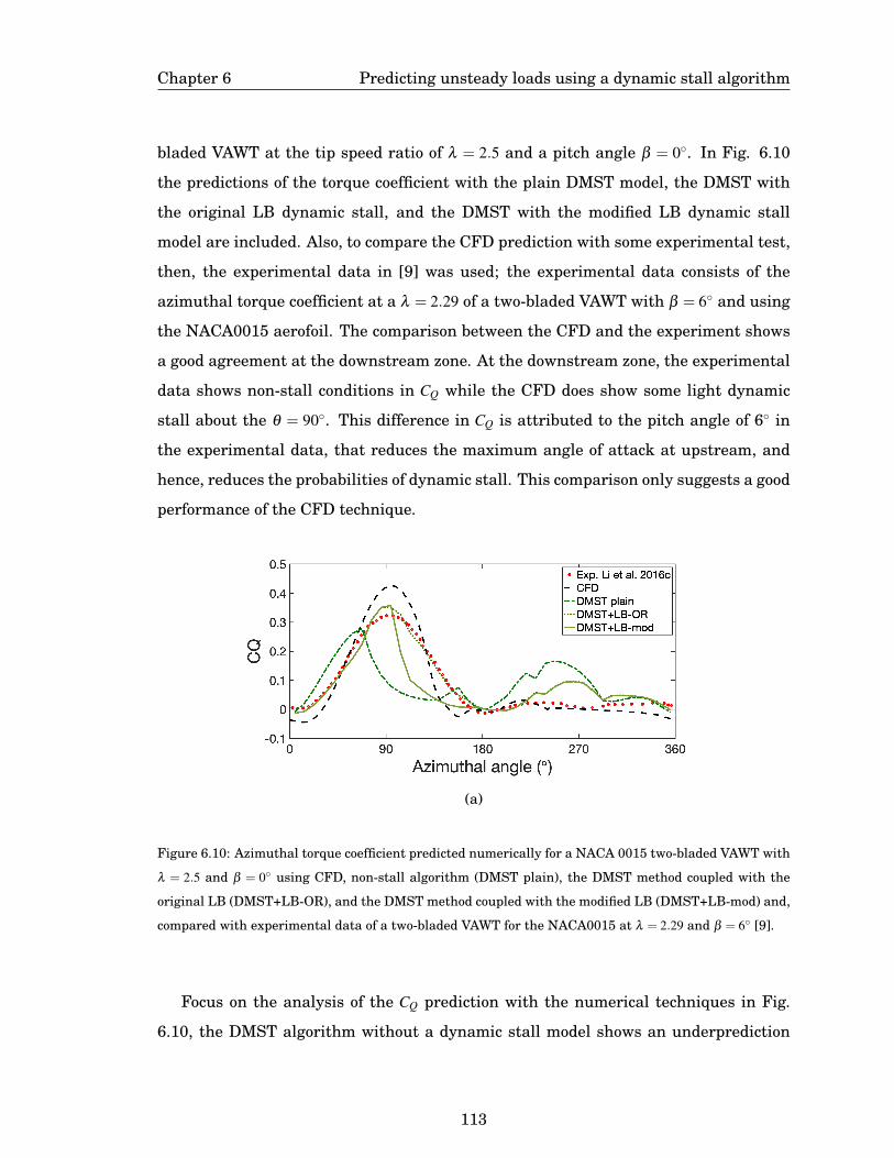
Chapter 6 Predicting unsteady loads using a dynamic stall algorithm
bladed VAWT at the tip speed ratio of λ = 2.5 and a pitch angle β = 0◦. In Fig. 6.10
the predictions of the torque coefficient with the plain DMST model, the DMST with
the original LB dynamic stall, and the DMST with the modified LB dynamic stall
model are included. Also, to compare the CFD prediction with some experimental test,
then, the experimental data in [9] was used; the experimental data consists of the
azimuthal torque coefficient at a λ = 2.29 of a two-bladed VAWT with β = 6◦ and using
the NACA0015 aerofoil. The comparison between the CFD and the experiment shows
a good agreement at the downstream zone. At the downstream zone, the experimental
data shows non-stall conditions in CQ while the CFD does show some light dynamic
stall about the θ = 90◦. This difference in CQ is attributed to the pitch angle of 6◦ in
the experimental data, that reduces the maximum angle of attack at upstream, and
hence, reduces the probabilities of dynamic stall. This comparison only suggests a good
performance of the CFD technique.
(a)
Figure 6.10: Azimuthal torque coefficient predicted numerically for a NACA 0015 two-bladed VAWT with
λ = 2.5 and β = 0◦ using CFD, non-stall algorithm (DMST plain), the DMST method coupled with the
original LB (DMST+LB-OR), and the DMST method coupled with the modified LB (DMST+LB-mod) and,
compared with experimental data of a two-bladed VAWT for the NACA0015 at λ = 2.29 and β = 6◦ [9].
Focus on the analysis of the CQ prediction with the numerical techniques in Fig.
6.10, the DMST algorithm without a dynamic stall model shows an underprediction
113

Chapter 6 Predicting unsteady loads using a dynamic stall algorithm
of CQ at upstream of the rotor and, overpredicts CQ at the downstream of the rotor
compared with the CFD prediction. The DMST coupled with the original-LB dynamic
stall fails in predicting the loss in the torque coefficient at θ = 90◦ upstream of the rotor
and shows some overprediction of CQ at the downstream zone. In another hand, the
DMST coupled with the modified LB model predicts the azimuthal angle where the
maximum in the torque coefficient occurs but, after that, the loss in CQ is not estimate
properly accordingly to the CFD results. The underprediction of the torque coefficient
at upstream, using both LB algorithms, is associated with curvature effects that need
to be included in the numerical predictions with the LB dynamic stall model. This is
further discussed in Chapter 7.
In order to assess the capabilities of the DMST+LB to predict the unsteady loads
when dynamic stall is not longer observed. Then, two cases without the evidence of
dynamic stall were selected. The four case evaluated consists of a one-blade turbine
at a tip speed ratio λ = 3. Figure 6.11 shows that when using the OR LB dynamic
stall and the modified, LB mod, the prediction of torque coefficient is equivalent at
both the upstream and downstream of the rotor. This agrees also with the predictions
for an oscillating aerofoil in Fig. 6.7 under non-stall conditions carried out with both
LB models. Despite that, a large underprediction of the torque coefficient is observed
upstream of the rotor and an overprediction downstream of the rotor when compared
with the CFD simulations. The DMST alone produces the largest difference between
the torque coefficients when using the CFD simulations.
The difference observed in Fig. 6.11 between the CFD and the models evaluated
maybe attributed to the lack of corrections due to the influence of the curvature effect
that is not captured by any of the methods. For example, at the azimuthal angle 0◦,
all the methods predict a torque coefficient of zero, while the CFD simulations predict
a negative torque coefficient. Another reason is explained due to the miscalculation of
the interference factor by the DMST model. This is due to the fact that the DMST was
formulated based on the VAWTs with very low solidity.
The last case, consisting of a three-bladed VAWTs at a tip speed ratio λ = 2.5 has
been analysed in Fig. 6.12. This case represents a non-stall condition and the results
have shown that with and without dynamic stall the torque coefficient is not predicted
114
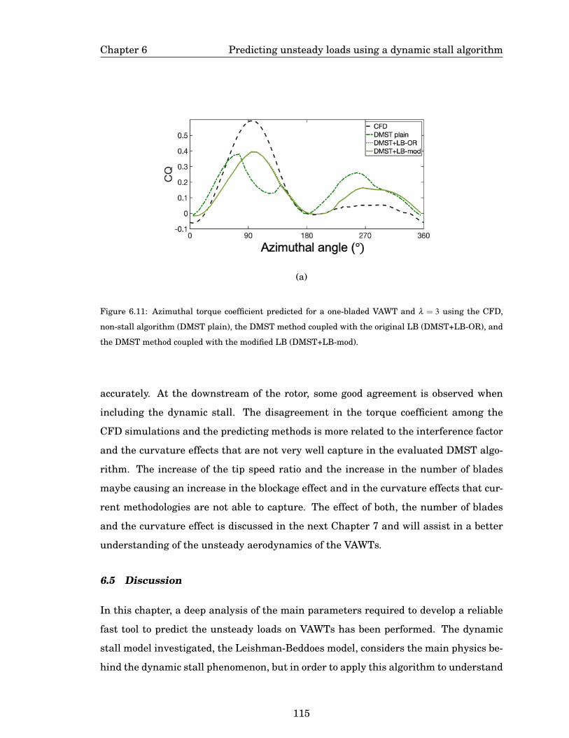
Chapter 6 Predicting unsteady loads using a dynamic stall algorithm
(a)
Figure 6.11: Azimuthal torque coefficient predicted for a one-bladed VAWT and λ = 3 using the CFD,
non-stall algorithm (DMST plain), the DMST method coupled with the original LB (DMST+LB-OR), and
the DMST method coupled with the modified LB (DMST+LB-mod).
accurately. At the downstream of the rotor, some good agreement is observed when
including the dynamic stall. The disagreement in the torque coefficient among the
CFD simulations and the predicting methods is more related to the interference factor
and the curvature effects that are not very well capture in the evaluated DMST algo-
rithm. The increase of the tip speed ratio and the increase in the number of blades
maybe causing an increase in the blockage effect and in the curvature effects that cur-
rent methodologies are not able to capture. The effect of both, the number of blades
and the curvature effect is discussed in the next Chapter 7 and will assist in a better
understanding of the unsteady aerodynamics of the VAWTs.
6.5 Discussion
In this chapter, a deep analysis of the main parameters required to develop a reliable
fast tool to predict the unsteady loads on VAWTs has been performed. The dynamic
stall model investigated, the Leishman-Beddoes model, considers the main physics be-
hind the dynamic stall phenomenon, but in order to apply this algorithm to understand
115

Chapter 6 Predicting unsteady loads using a dynamic stall algorithm
(a)
Figure 6.12: Azimuthal torque coefficient predicted for a three-bladed VAWT and λ = 2.5 when using CFD,
non-stall algorithm (DMST plain), the DMST method coupled with the original LB (DMST+LB-OR), and
the DMST method coupled with the modified LB (DMST+LB-mod).
the VAWTs some its sections needs a detailed assessment not previously presented in
the reviewed literature.
The analysis of the static separation point of the boundary layer at low Reynolds
numbers and its corresponding value of lift force coefficient has revealed that the loss
in the lift force coefficient does not occur suddenly as the observations experimentally
at high Re as found in several investigations [116], i.e., it occurs smoothly. This as-
pect has makes the obtention of the representative parameters to predict the lift and
the chordwise force coefficient being more challenging as well as very important for an
accurate prediction of the static and unsteady forces. Despite that, the database gen-
erated has been tested to be good enough to predict the static and unsteady loads for
the NACA0015 at the range of Reynolds number investigated. This database can be
used complementary to the database presented for the NACA0015 at larger Reynolds
number in [48].
The analysis of the trailing edge separation point using the location along the chord
where a zero skin friction is experienced have revealed that, at the low Reynolds num-
116
Chapter 6 Predicting unsteady loads using a dynamic stall algorithm
bers investigated here, the maximum lift coefficient occurs at the critical separation
point about 0.5. This value is different from the values 0.6-0.7 usually found in the
literature for Reynolds number larger than 1 million. Despite this investigation using
CFD simulations, such simulations where very carefully verified with the experimen-
tal data of the static lift force coefficient. As a result, the use of a critical separation
point of 0.5 into the Leishman-Beddoes model predicts accurately the unsteady forces
under dynamic stall conditions. Nevertheless, experimental tests that confirms these
results are worthy to be made; i.e. since the VAWTs can operate at low Reynolds
number, the more in-depth analysis of how the trailing edge separation point of the
boundary layer behaves with the Reynolds number decreasing are crucial for a much
better understanding of the unsteady aerodynamics and to improve the Kirchhoff flow
model to take into account the effect of these low Reynolds numbers.
The time delay constants investigated for the three aerofoils NACA0015, NACA0018
and NACA0021 at low Reynolds number represents a huge effort to understand the
stall inception of VAWTs. The more than 80 CFD unsteady simulations performed
to compute the curves of the stall-onset as a function of the non-dimensional pitch
rate have to assist to meet the urgent objective of having a broader idea of the time
delay constants at different Reynolds numbers. Present results suggest that each aero-
foil dictates the behaviour of the time delay constant, Tr but in general Tr reduced its
value with the decrease in Re. Additionally, the present analysis revealed that after
a Reynolds number of 3.6×10⁵ the time delay constant suffers of minor changes in its
value. The NACA0021 aerofoil has demonstrated to be the aerofoil with the less impact
in the time delay values Tr with the change of the Reynolds. Present results despite
they need to be confirmed using experimental data are based in a large number of CFD
verifications using static, oscillating and VAWTs cases and then are considered to be
accurate enough for the final objective of this thesis, to contribute to the development
of fast and reliable engineering tool to predict the performance of VAWTs.
The LB dynamic stall algorithm including the present modifications to the stall-
onset criteria and the critical separation point in the Kirchhoff flow model, has demon-
strated to be a potential algorithm to predict the unsteady loads under both regimes,
under the dynamic stall and non-stall conditions. Also, the results of using the double
117

Chapter 6 Predicting unsteady loads using a dynamic stall algorithm
multiple streamtube algorithm by incorporating the dynamic stall model have pre-
sented some good predictions of the torque coefficient at low tip speed ratios when
comparing with the CFD simulations. Nevertheless, with the increase of the tip speed
ratio and the number of blades the prediction becomes less reliable since both up-
stream and downstream torque coefficient predictions present some deficiencies. These
deficiencies are attributed to the lack of corrections regarding the curvature effects of
the blades. Despite this phenomenon have been discussed and incorporated into the
DMST algorithm in [53], still, this mechanism suffers from a shortage of investigations
and hence required further investigations to be properly addressed and assessed as de-
scribed in Chapter 7. This chapter has presented a detailed assessment of the critical
aspects that need to be considered during the modelling of the torque coefficient of a
VAWT.
6.6 Summary
This chapter has discussed the details that are required for the dynamic stall algorithm
to be able to predict the unsteady loads at low Reynolds number that are very useful
for the VAWTs torque prediction. Some of the important contributions of this chapter
are as follows:
• A database of the time delay constant of three aerofoils at Reynolds number lower
than 3.6×10⁵. The studied range of Reynolds number has not been studied previ-
ously, as far as the knowledge and literature review carried out on this thesis, and
thus, this investigation represents a very useful contribution in order to predict
unsteady loads in the range of Reynolds number studied here.
• The parameters representing the Kirchhoff flow model to predict the lift force
coefficient and chordwise force coefficient at static conditions are very useful data
to predict the unsteady loads using the Leishman-Beddoes algorithm.
• The trailing separation point has been analysed by using the skin friction along
the chord at each angle of attack. It has been observed that the critical separation
118

Chapter 6 Predicting unsteady loads using a dynamic stall algorithm
point occurs at the static stall conditions and it has a value of 0.5 at the low
Reynolds numbers evaluated in this Chapter. Using this critical value of 0.5 has
led to a very good predictions of the lift and chordwise force coefficients.
• The analysis has revealed that the modified Leishman-Beddoes model using the
database of the time-delay constant and Kirchhoff flow parameters predict accu-
rately the unsteady loads under both dynamic stall and non-stall conditions for
oscillating aerofoils.
• An assessment of the DMST algorithm coupled with the dynamic stall algorithm
to predict the torque coefficient of VAWTs has been carried out. The results have
demonstrated that under dynamic stall conditions some good agreement with the
CFD results are observed. On the contrary, under the fully attached regime the
results have shown disagreements with the CFD results where it is observed that
there is an under-prediction at the upstream of the rotor and an over-prediction
at the downstream of the rotor.
119
Chapter 7
Curvature effect on the prediction of the torque
coefficient of VAWTs
7.1 Overview
Despite previous investigations having studied the influence of the curvature index
on the VAWT performance, the assessment of this phenomenon has missed some im-
portant details due to the lack of experimental data, such as the azimuthal forces,
but instead have relied on the average torque coefficient per revolution. Thus, a full
understanding of this phenomenon remains unclear. This chapter analyses the cur-
vature index effect on the torque coefficient of the VAWTs by using CFD simulations
and the modified Leishman-Beddoes model introduced in Chapter 6. A new concept to
investigate the VAWTs aerodynamics has been proposed. This new concept has been
demonstrated to have a huge potential towards the development of a fast tool to predict
the power coefficient of VAWTs and that takes into account the unsteady aerodynamics
of VAWTs over a wide range of TSRs.
7.2 Interference factor
The increase in the number of blades, as well as the increase in the tip speed ratio,
promotes an increase in the blockage effect of the rotor, i.e. the rotor behaves as a
solid disk that reduces the magnitude of the actual wind velocity acting on the VAWTs
blades. The percentage of the reduction in the incoming wind speed, V∞, due to the solid
aspect of the rotor is called the interference factor and its value may depend on solidity
(σ = Nc/D), the tip speed ratio and the azimuthal position of the blades . Once the flow
past the blades with a reduced velocity, Vup, at the upstream zone of the rotor, the
120

Chapter 7 Curvature effect on the prediction of the torque coefficient of VAWTs
actual wind speed that impacts on the blades downstream, Vdw, is further reduced, see
Fig. 7.1. Thus, the interference factor upstream, u, is much less than the interference
factor downstream of the rotor, u′. Bearing in mind that the theoretical expressions
of the relative velocity, Eq. (2.1) and the angle of attack, Eq.(2.2) cannot replicate the
effect of the number of blades, the use of the interference factor plays a significant role
to compute the actual velocity on the blades and the actual angle of attack.
(a)
Figure 7.1: A typical representation of the streamlines when a flow past a VAWT [2]
In previous investigations, the mathematical expressions for the interference fac-
tors both upstream and downstream of the rotor has been proposed accordingly Eq.
(3.9) in [2]. Despite that, those interference factor relations were obtained for a spe-
cific geometry of the rotor (troposkein design) and and are based in a blade element
momentum analysis. Using those expressions to predict the torque coefficient of the
121

Chapter 7 Curvature effect on the prediction of the torque coefficient of VAWTs
VAWTs investigated in this thesis raised some difficulties in obtaining convergence
when using the large solidity VAWTs (results from Chapter 6). In addition, despite
some investigations have attempt to investigate the interference factor [128], the data
with details of this parameter at each azimuthal position are very limited. Nowadays,
with the current CFD techniques, is possible to obtained much more details of the flow
filed around the blades and then improve or elucidate new interference factor expres-
sions. Therefore, this section investigates by using the CFD simulations carried out in
Chapter 5, the interference factors on the VAWTs using the NACA0015 aerofoil with
one, two and three bladed and, at a range of tip speeds ratio [1.5-5].
In order to observe the behaviour of the interference factor across the rotor, the x-
component of the velocity, Vx, is computed using the CFD simulations along the y-axis,
from the centre line of the rotor to two times the rotor diameter, i.e, from y = −2D to
y = 2D. Moreover, nine positions along the incoming wind flow direction (x-axis) were
analysed: at the positions of -10D, -5D, -2D, -1D, 0 at upstream zone of the rotor and,
downstream at the positions of 1D, 2D, 5D, 10D. Therefore, any changes in the inter-
ference factor perpendicular to the incoming flow directions due to the presence of the
rotor were observed. Fig. 7.2(a) includes the interference factor evolution along the x-
direction for a one-bladed VAWT and a tip speed ratio of 4 and, Fig. 7.2(b) corresponds
to a three-bladed VAWT at a tip speed ratio of 2.
Since the interest is the interference factor on the blades, three positions are the
main focus for this analysis, namely (i) the position−1D corresponding to the upstream
zone of the rotor when the flow is about to impact the blades, (ii) the position 0D that
represent the interference factor of the flow before impacting on the blades of the rotor
at downstream, and (iii) the position 1D that represent the flow interference factor
immediately when the flow past the blades that are downstream of the rotor.
It is observed for the one-bladed VAWT in Fig. 7.2(a) that upwind (at x =−1D) the
interference factor is almost zero and hence the flow disturbances on the flow due to
one blade at λ = 2 is almost negligible. Downstream of the rotor, the interference factor
reaches a maximum value of 0.28 at the middle of the rotor at the position x = 0D. For
the three-bladed VAWT in Fig. 7.2(b) a maximum of 0.17 is reached at the position
x = −1D; at the position of x = 0D the interference factor reaches a value of 0.80 and
122

Chapter 7 Curvature effect on the prediction of the torque coefficient of VAWTs
(a)
(b)
Figure 7.2: Interference factor at nine positions along the x-direction for:(a) One bladed-turbine and a
tip speed ratio of 2, and (b) a three-bladed turbine and a tip speed ratio of 2. Both VAWTs with the
NACA0015 aerofoil.
further downstream at the position of x = 1D the interference factor reaches a value of
0.92.
The analysis of the maximum interference factor at the position x = −1D, x = 0D
123
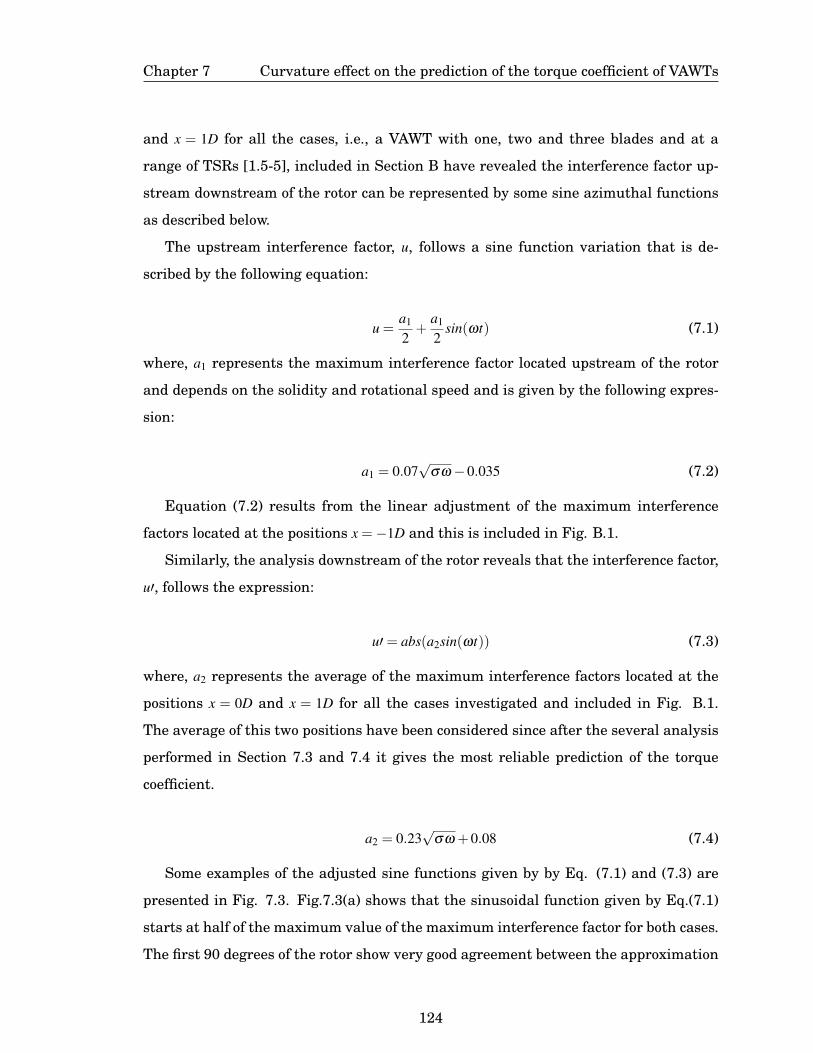
Chapter 7 Curvature effect on the prediction of the torque coefficient of VAWTs
and x = 1D for all the cases, i.e., a VAWT with one, two and three blades and at a
range of TSRs [1.5-5], included in Section B have revealed the interference factor up-
stream downstream of the rotor can be represented by some sine azimuthal functions
as described below.
The upstream interference factor, u, follows a sine function variation that is de-
scribed by the following equation:
u =a1
2+
a1
2sin(ωt) (7.1)
where, a1 represents the maximum interference factor located upstream of the rotor
and depends on the solidity and rotational speed and is given by the following expres-
sion:
a1 = 0.07√
σω−0.035 (7.2)
Equation (7.2) results from the linear adjustment of the maximum interference
factors located at the positions x =−1D and this is included in Fig. B.1.
Similarly, the analysis downstream of the rotor reveals that the interference factor,
u′, follows the expression:
u′= abs(a2sin(ωt)) (7.3)
where, a2 represents the average of the maximum interference factors located at the
positions x = 0D and x = 1D for all the cases investigated and included in Fig. B.1.
The average of this two positions have been considered since after the several analysis
performed in Section 7.3 and 7.4 it gives the most reliable prediction of the torque
coefficient.
a2 = 0.23√
σω +0.08 (7.4)
Some examples of the adjusted sine functions given by by Eq. (7.1) and (7.3) are
presented in Fig. 7.3. Fig.7.3(a) shows that the sinusoidal function given by Eq.(7.1)
starts at half of the maximum value of the maximum interference factor for both cases.
The first 90 degrees of the rotor show very good agreement between the approximation
124

Chapter 7 Curvature effect on the prediction of the torque coefficient of VAWTs
and the CFD results, but from 90 to 180 degrees there is a small difference that overall
does not impact the results since the parameters that define the stall-onset angle are
more likely to occur before this azimuthal angle. Downstream of the rotor, the sinu-
soidal Eq. (7.3) results in the most useful and practical approximation since it captures
the reduction in the wind speed. Fig. 7.3(b) illustrates that the sine functions starts
almost from zero, reaches a maximum and then decays, therefore expression (7.3) it
better represents the behaviour of the interference factors at downstream of the rotor.
(a)
(b)
Figure 7.3: Interference factor as a function of the azimuthal angle for (a) a two-bladed VAWT at λ = 3.5
and, (b) a three-bladed VAWT at λ = 2. Both VAWTs using the NACA0015 aerofoil.
7.3 Curvature effects
The curvature effects of the VAWTs originated due to the rotation of the blades around
the axis, causes the aerofoil to move along a curved streamlines instead of along a
straight line flow. This phenomenon is illustrated in Fig. 7.4. Due to this curved flow,
125
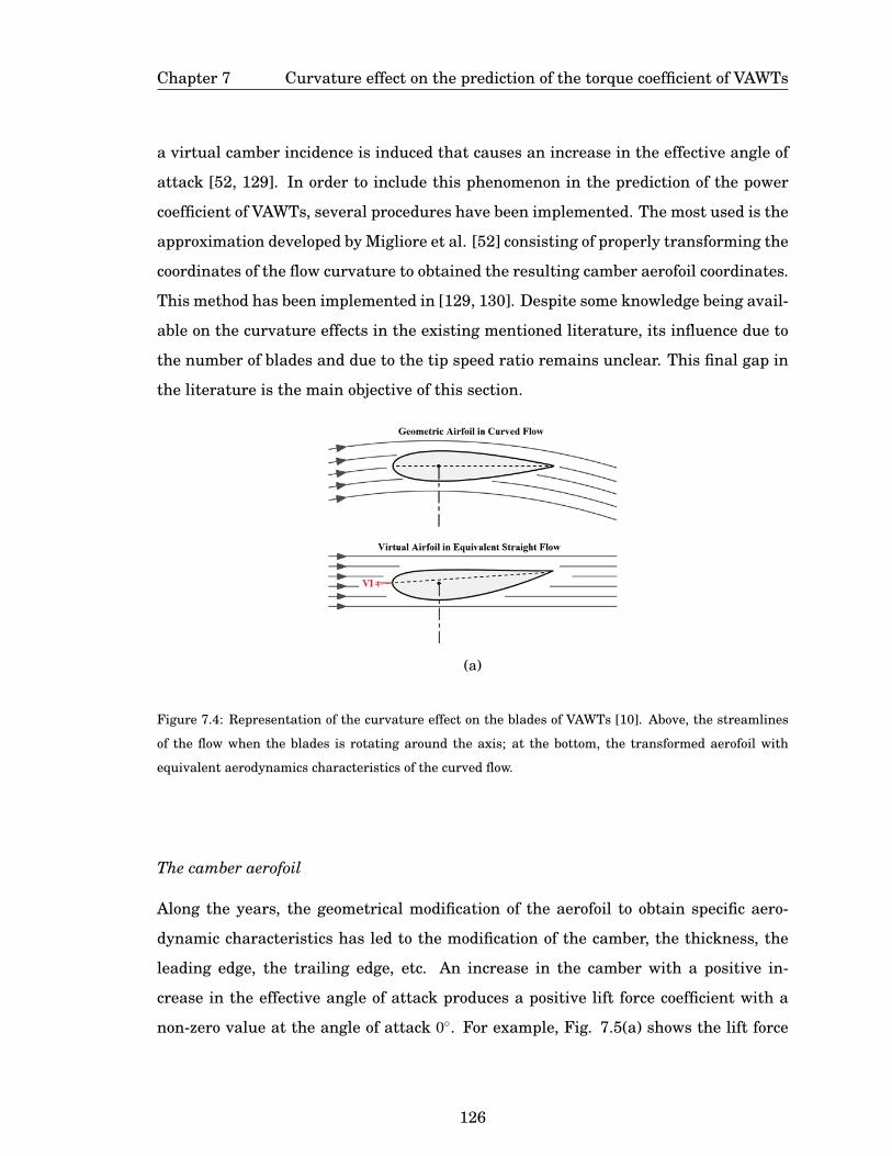
Chapter 7 Curvature effect on the prediction of the torque coefficient of VAWTs
a virtual camber incidence is induced that causes an increase in the effective angle of
attack [52, 129]. In order to include this phenomenon in the prediction of the power
coefficient of VAWTs, several procedures have been implemented. The most used is the
approximation developed by Migliore et al. [52] consisting of properly transforming the
coordinates of the flow curvature to obtained the resulting camber aerofoil coordinates.
This method has been implemented in [129, 130]. Despite some knowledge being avail-
able on the curvature effects in the existing mentioned literature, its influence due to
the number of blades and due to the tip speed ratio remains unclear. This final gap in
the literature is the main objective of this section.
(a)
Figure 7.4: Representation of the curvature effect on the blades of VAWTs [10]. Above, the streamlines
of the flow when the blades is rotating around the axis; at the bottom, the transformed aerofoil with
equivalent aerodynamics characteristics of the curved flow.
The camber aerofoil
Along the years, the geometrical modification of the aerofoil to obtain specific aero-
dynamic characteristics has led to the modification of the camber, the thickness, the
leading edge, the trailing edge, etc. An increase in the camber with a positive in-
crease in the effective angle of attack produces a positive lift force coefficient with a
non-zero value at the angle of attack 0◦. For example, Fig. 7.5(a) shows the lift force
126

Chapter 7 Curvature effect on the prediction of the torque coefficient of VAWTs
coefficient for two cambered aerofoils, NACA2415 and NACA4415, and the symmetri-
cal NACA0015. It is observed that the cambered aerofoils produce a larger lift force
coefficient at positive angles of attack. On the contrary, at a negative angle of attack
the lift force coefficient reduces its magnitude with the increase in the camber. The
drag coefficient remains very similar in value for the three aerofoils as observed in Fig.
7.5(b).
(a) (b)
Figure 7.5: Camber effect on (a) the lift force coefficient and, (b) the drag force coefficient as a function of
the angle of attack at Re=3.3×10⁵. Data calculated using Xfoil.
The main objective of introducing a camber with a non-zero value consists of modi-
fying the effective angle of attack of the aerofoil profile. Then, this camber effect can be
modelled into the LB model by using the angle of attack where the lift force coefficient
becomes zero, α0 and introduces this angle into the effective angle of attack, al phaE .
Therefore, in the Leishman-Beddoes algorithm, the effective angle of attack, αE given
by Eq.(A.3) is replaced by: .
αEn = αn + rn/2−Xn−Yn−α0 (7.5)
Under static conditions and using the Kirchhoff flow model, the lift force coefficient
of the cambered NACA2415 and NACA4415 are predicted and included in Fig. 7.6. The
127

Chapter 7 Curvature effect on the prediction of the torque coefficient of VAWTs
percentage of cambered corresponds to 2% and 4% for the NACA2414 and NACA4415,
respectively. For the NACA2415, the lift force coefficient with CL = 0 is found at
α0 = −2◦; for the NACA4415, CL = 0 at α0 = −4◦. Replacing the geometrical angle of
attack, α(t) by α(t)−α0 into the Kirchhoff flow model and using the static-parameter
characteristic of the symmetrical aerofoil, the NACA0015 produces the actual lift force
coefficient of the cambered aerofoil as illustrated in Fig. 7.6. Both cambered aerofoils,
NACA2415 and NACA4415, produce a the similar CL for the NACA0015 but with an
initial zero value located at a negative angle of attack, α0. Therefore, by predicting the
virtual angle of incidence, α0, the curvature effect can be easily investigated.
(a)
Figure 7.6: Lift force coefficient calculated with xfoil and predicted with the Kirchhoff flow model by
introducing a camber angle of: α0 = 0 for the NACA0015 (red); α0 = −2: for the NACA2415 (blue) and,
α0 =−4 for the NACA2415 (black).
The qualitatively analysis of the streamlines in Fig. 7.7(a) of a one-bladed VAWT
has revealed that: at the lowest tip speed ratio, λ = 2, the streamlines describe a vir-
tual curvature index, c/R′, where R′ represents the radius described by the streamlines.
This virtual curvature index is reduced compared with the geometrical curvature in-
dex, c/R. At a higher tip speed ratio of λ = 5, Fig. 7.7(b), shows that the virtual curva-
ture index described by the streamlines are in accordance to the geometrical curvature
128

Chapter 7 Curvature effect on the prediction of the torque coefficient of VAWTs
index. In addition, the streamlines at the same tip speed ratio λ = 2 show that for the
two-bladed VAWT shown in Fig. 7.7(c) that the virtual curvature index is larger than
the geometrical curvature index, and also a similar virtual curvature index with the
one-bladed VAWTs is observed. In the case of the three-bladed VAWT shown in Fig.
7.7(d), the streamlines describe a virtual curvature index that is not clearly defined
but are influenced by the blades interaction.
7.3.1 Virtual camber estimation
In this thesis, the estimation of the virtual camber, α0 has followed a systematically
methodology and using previous investigations [52] as a basis to define a relation of
the virtual camber with the curvature index, the tip speed ratio and the number of
blades.
The results shows that with the increase in the tip speed ratio, the virtual curvature
index trends towards the value of the geometrical curvature index, and this is observed
in Fig. 7.7(b). Therefore, the virtual camber α0 was investigated for a range of tip
speed ratio of [2-5] using a one-bladed VAWT with a geometric curvature index of
c/R = 0.1325.
To investigate the influence of the virtual camber in the torque coefficient, then,
the torque coefficient as a function of the azimuthal angle has been predicted using
the modified Leishman-Beddoes model with: (i) the theoretical angle of attack and
theoretical relative velocity given by Eq.(2.2) and Eq.(2.1) respectively; (ii) the new
method consisting of the use of the interference factor correlations described in the
previous section plus the virtual camber modification to the effective angle of attack by
including the virtual incidence, α0 and; (iii) the CFD simulations performed in Chapter
5.
The torque coefficient predicted with the new proposed method has shown very
good agreement with the CFD simulations. At the tip speed ratio of 2, the use of the
virtual camber is essential to predict accurately the torque coefficient. As an illustra-
tion of this influence, Fig. 7.8(a) shows that the lack of use of the virtual camber, the
theoretical case, shows an underprediction of the torque coefficient upstream of the
rotor and an over prediction downstream. For a high tip speed ratio of 5, again Fig.
129
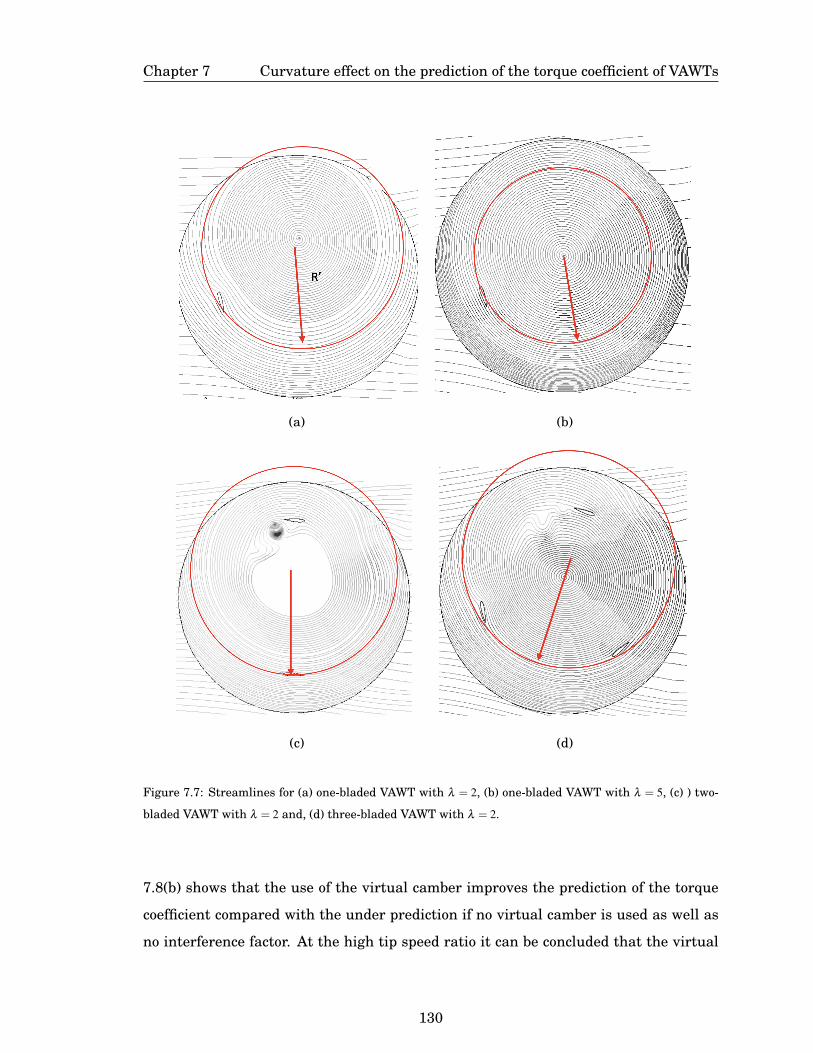
Chapter 7 Curvature effect on the prediction of the torque coefficient of VAWTs
(a) (b)
(c) (d)
Figure 7.7: Streamlines for (a) one-bladed VAWT with λ = 2, (b) one-bladed VAWT with λ = 5, (c) ) two-
bladed VAWT with λ = 2 and, (d) three-bladed VAWT with λ = 2.
7.8(b) shows that the use of the virtual camber improves the prediction of the torque
coefficient compared with the under prediction if no virtual camber is used as well as
no interference factor. At the high tip speed ratio it can be concluded that the virtual
130

Chapter 7 Curvature effect on the prediction of the torque coefficient of VAWTs
camber is essential to capture the torque coefficient. Using the new method, it has
been found that for the range of tip speed ratio [2-5] and using a one-bladed VAWT, the
virtual camber, α0 presents a value from −2◦ to −3◦.
(a)
(b)
Figure 7.8: Prediction of the torque coefficient with different approaches as a function of the azimuthal
angle using a one-bladed VAWT at (a) λ = 2 and, (b) λ = 5.
Using the new proposed method for two-bladed and a three bladed VAWTs, the vir-
tual camber effect has been analysed in detail. It has been observed that for the same
tip speed ratio that the increase in the number of blades reduces the virtual camber
effect. For example, at the tip speed ratio of 3 the value of α0 has resulted in −2.7◦,
−1.76◦ and −0.77◦ for one, two and three-bladed VAWT, respectively. In addition, using
these values, the predicted torque coefficient has resulted in a very good agreement
with the CFD simulations, see Fig. 7.9(a-c).
The present observations have led to the formulation of a mathematical expression
131

Chapter 7 Curvature effect on the prediction of the torque coefficient of VAWTs
(a)
(b)
(c)
Figure 7.9: Torque coefficient as a function of the azimuthal angle predicted with the new proposed
method at the tip speed ratio of 3 and a (a) one-bladed, (b) two-bladed and, (c) a three-bladed VAWT.
that relate the camber effect, α0, with the tip speed ratio and the number of blades and
this is described as follows.
The values of α0 estimated with the new proposed method by adjusting this angle
132

Chapter 7 Curvature effect on the prediction of the torque coefficient of VAWTs
with all the CFD simulations for the NACA0015 VAWT performed in Chapter 5 relates
with the following expression:
α0 = (− ωc
4Vrel(t))(1−2σ)(180◦/π) (7.6)
where the expression for the Vrel(t) is given by the average of following equation.
Vrel(t) =V (1+2Xr cos(ωt)+X2r )
1/2 (7.7)
where, the induced velocity, V , represents the reduced velocity due to the interference
factor given by Eq.(7.1) and Eq. (7.3).
V =
V∞(1−u), i f ωt < π(upstream)
V∞(1−u′), i f ωt > π(downstream)
(7.8)
In addition, the local tip speed ratio is given by Xr = ωR/V .
The term, (− ωc4Vrel(t)
) in Eq.(7.6) takes into account the effect of the tip speed ratio.
Since the average of the relative velocity, Vrel(t) increases with the increase in the tip
speed ratio, and approximates to Vrel ≈ ωR. Then, at larger tip speed ratios, − ωc4Vrel(t)
=
− c4R . For the VAWT investigated here with c/R = 0.265, − c
4R = −3.79◦. This result
agrees with the predicted virtual incidence of 3.7◦ corresponding to a curvature index
c/R = 0.260 calculated by Migliore et. al [52] with a method consisting of an inverse
virtual transformation of the aerofoil.
It is worth to mentioning that surprisingly, a similar expression (− ωc4Vrel
) was also
used in [53] to take into account the curvature effect in the angle of attack. However,
in this work, the virtual camber changes with the azimuthal angle. Despite this rep-
resentation of the virtual incidence it is similar, the concept remains different since
in this work the aerofoil seems to behave as a cambered aerofoil with a define α0 ac-
cordingly to the T SR and the number of blades instead of changing constantly at each
azimuthal position the virtual incidence. Nevertheless it is worthy to investigate at
each azimuthal position of the blades the curvature of the streamlines to elucidate the
actual influence of the curvature effect. The proposed investigation represents a huge
effort and due to the amount of CFD data required are out of the scope of this thesis.
133

Chapter 7 Curvature effect on the prediction of the torque coefficient of VAWTs
Moreover, in the Eq.(7.6), in order to consider the influence of the solidity then the
expression (1−2σ) has been included. This expression is limited for the VAWTs evalu-
ated here, despite that, with some further CFD simulations a more general expression
may be found.
7.4 Prediction of the torque coefficient: New proposed method
In this section the main governing equations of a new method to predict the torque
coefficient of VAWTs has been explained. In summary, the methodology consists of the
following steps:
1. Define the geometrical characteristics of the rotor: chord (c), number of blades
(N), radius (R), pitch angle (β ) and wind speed, V∞.
2. Predict the interference factor, u and u′ using the Eqns. (7.1-7.4).
3. Calculates the relative velocity equation, Eq. (7.7).
4. Estimate the angle of incidence due to the virtual camber, α0, Eq.(7.6).
5. Estimate the angle of attack using following expression:
α(t) = atan(sin(ωt)
Xr + cos(ωt))−β (7.9)
6. Use the expressions of α(t), Vrel(t) and α0 given in previous steps to calculate the
dynamic lift CL(t) and drag CD(t) force coefficients using the Leishman-Beddoes
dynamic stall model with the modifications, namely, the stall-onset criteria, the
new predicted static parameters and by modifying the effective angle of attack.
7. Compute the torque coefficient using the expression:
CQ(θ) =c
2R(Vrel
V∞
)2(CLsin(φ)−CDcos(φ)) (7.10)
where φ = α +β .
134

Chapter 7 Curvature effect on the prediction of the torque coefficient of VAWTs
8. Calculate the power coefficient :
Cp =Nλ
2π
2π
∑0
CQ(θ)dθ (7.11)
where, dθ = π/Nth and Nth represents the number of divisions required to analyse
the rotor.
The described methodology has been used to predict the azimuthal torque coeffi-
cient at two tip speed ratios. At λ = 2 in Fig. 7.10(a) and at λ = 3.5 in Fig. 7.10
(b). This method accurately predicts the torque coefficient for the one and two bladed
VAWTs. A small over prediction is observed for a three bladed VAWT at λ = 2 at the
upstream zone of the rotor. Despite that, due to the complexity of the flow and the
time consumed by a CFD simulation, this fast tool gives a very good approximation
of the torque coefficient. The proposed new method predict with very good agreement
azimuthal angle of inception of the CFD simulations of the VAWTs. This suggests that
the modifications to the Leishman-Beddoes model and the time delay constant as a
function of the Reynolds number performs well under dynamic stall conditions.
The virtual incidence due to the camber effect with the increase in the tip speed
ratio has been very well predicted for all the number of blades investigated as observed
in Fig. 7.10(b). The results suggest that the equation to predict the camber effect is
crucial in the prediction of the torque coefficient at large tip speed ratios
7.5 Influence of the pitch angle of the performance of VAWTs
The pitch angle has been investigated in several studies before, despite that some
aspects in the detail both upstream and downstream of the rotor has been missed due
to the time consumption of a CFD simulation. Therefore, using the current method,
the effect of the pitch angle has been investigated for a wide range of tip speed ratios.
The power coefficient, Cp, as a function of the tip speed ratio, λ , has been predicted
for a three bladed VAWT with the pitch angles of β = −1,0,1,2,3 and 4◦. It has been
observed in Fig. 7.11(a) that with a more positive β the power coefficient increases at
low tip speed ratio. Nevertheless, after β = 2◦ this increment is minimal and for λ = 1.5
the power coefficient reduces for these pitch angles. Also, the maximum Cp occurs
135
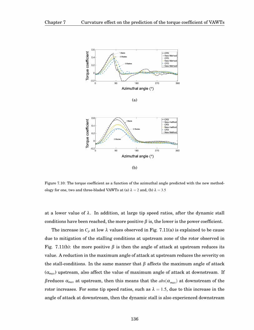
Chapter 7 Curvature effect on the prediction of the torque coefficient of VAWTs
(a)
(b)
Figure 7.10: The torque coefficient as a function of the azimuthal angle predicted with the new method-
ology for one, two and three-bladed VAWTs at (a) λ = 2 and, (b) λ = 3.5
at a lower value of λ . In addition, at large tip speed ratios, after the dynamic stall
conditions have been reached, the more positive β is, the lower is the power coefficient.
The increase in Cp at low λ values observed in Fig. 7.11(a) is explained to be cause
due to mitigation of the stalling conditions at upstream zone of the rotor observed in
Fig. 7.11(b): the more positive β is then the angle of attack at upstream reduces its
value. A reduction in the maximum angle of attack at upstream reduces the severity on
the stall-conditions. In the same manner that β affects the maximum angle of attack
(αmax) upstream, also affect the value of maximum angle of attack at downstream. If
βreduces αmax at upstream, then this means that the abs(αmax) at downstream of the
rotor increases. For some tip speed ratios, such as λ = 1.5, due to this increase in the
angle of attack at downstream, then the dynamic stall is also experienced downstream
136
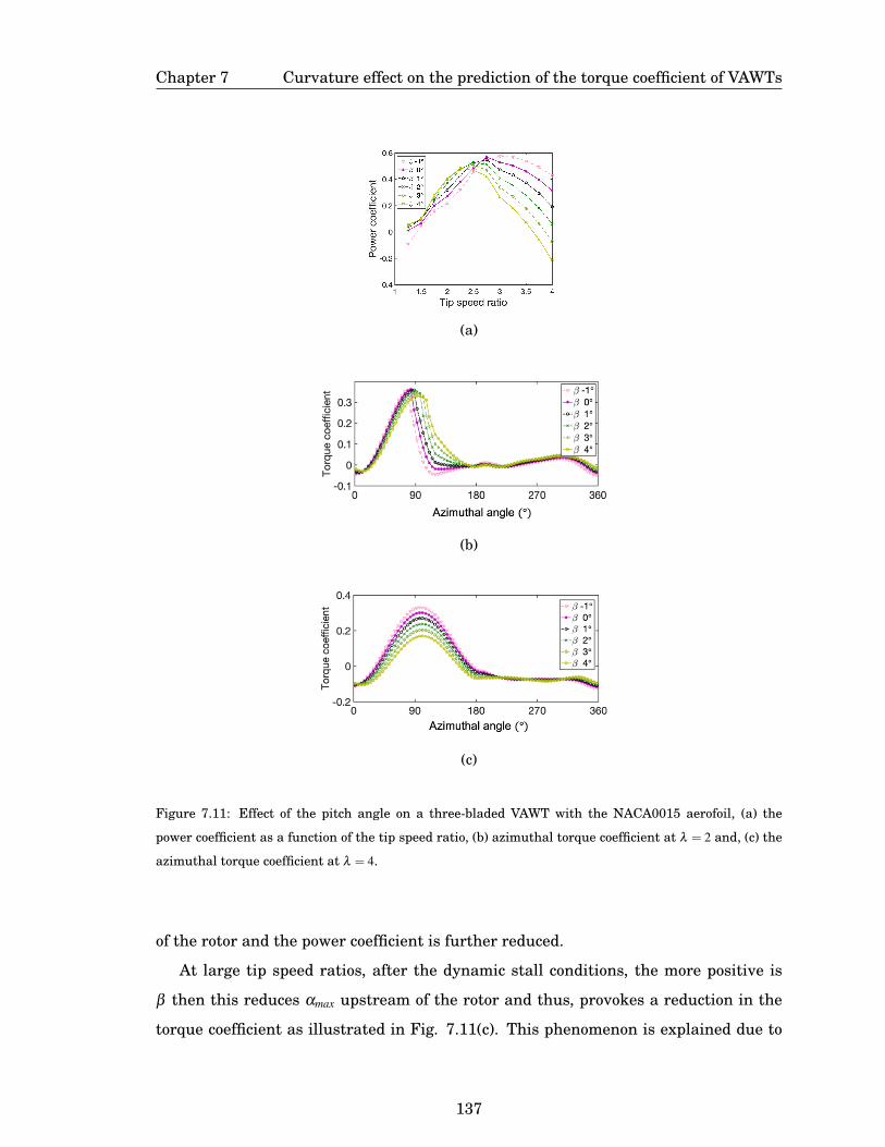
Chapter 7 Curvature effect on the prediction of the torque coefficient of VAWTs
(a)
(b)
(c)
Figure 7.11: Effect of the pitch angle on a three-bladed VAWT with the NACA0015 aerofoil, (a) the
power coefficient as a function of the tip speed ratio, (b) azimuthal torque coefficient at λ = 2 and, (c) the
azimuthal torque coefficient at λ = 4.
of the rotor and the power coefficient is further reduced.
At large tip speed ratios, after the dynamic stall conditions, the more positive is
β then this reduces αmax upstream of the rotor and thus, provokes a reduction in the
torque coefficient as illustrated in Fig. 7.11(c). This phenomenon is explained due to
137

Chapter 7 Curvature effect on the prediction of the torque coefficient of VAWTs
the reduction in the maximum angle of attack that reduced the aerodynamic forces
upstream and hence the overall torque coefficient. Therefore, accordingly to the final
application of the VAWTs and the tip speed ratio of operation, the β value needs to be
optimize in order to increase the power coefficient.
7.6 Summary
This chapter has presented an analysis of the curvature effects on the aerodynamic of
VAWTs. Some important outcomes have been elucidated, such as the influence of the
number of blades on the virtual camber effect. Therefore, the methods to predict the
camber effect needs to consider not only the influence of the tip speed ratio but also
the influence of the number of blades.
In addition, the interference factor both upstream and downstream of the rotor was
analysed and for both sides of the rotor, the interference factor behaves in a sinusoidal
function. The equations for the interference factor both upstream and downstream of
the rotor as a function of the rotational speed and the solidity has been proposed and
verified with the cases investigated in this thesis.
The mathematical expression to estimate the virtual incidence due to the camber
effect takes into account the tip speed ratio and the number of blades. This expression,
with further verification, is a potential function that may be confidently employed to
improve the prediction capabilities of a 1D model for VAWTs.
The methodology presented in this chapter to predict the torque coefficient of VAWTs
suggests that these devices need to be analysed as a dynamic system, i.e, interference
factor and virtual incidence needs to be investigated with more in-depth detail using
unsteady simulations instead using static momentum methods. Further, the momen-
tum methods without a proper assessment such as the large number of conditions
tested in this thesis may lead to a fake-good prediction.
138

Chapter 8
Conclusions and Future work
8.1 Conclusions
In this thesis, an exhaustive analysis of the unsteady aerodynamics of VAWTs has
been carried out by using CFD simulations and the new predictions have been rigor-
ously verified with the best available experimental data. As a result, these new CFD
predictions have greatly assisted in the proposing of a new methodology to predict
the unsteady loads of VAWTs that is based on the Leishman-Beddoes algorithm. The
present conclusions are based on the detailed analysis of a wide range of cases: oscillat-
ing aerofoils, VAWTs with one, two and three blades; six aerofoils: 4 symmetrical and
two cambered and, also covers a wide range of tip speed ratios, namely 1.5-5, where all
the aerofoils operate under the dynamic stall and non-stall conditions.
The generated knowledge has allowed the identification of the aerodynamics char-
acteristics that are relevant the most in dictating the performance of the VAWTs. The
principal findings of this intensive investigation are summarized as follows:
The dynamic stall-onset angle has been demonstrated to be the most critical pa-
rameter in defining the VAWTs performance, i.e. defining the range of tip speed ratio
operation. Larger is the stall-onset angle then the lower is the tip speed ratio where
the VAWT can produce a positive torque and the optimum power coefficient is observed
at a lower value of the tip speed ratio. The stall-onset angle increases its value with
the increase of the non-dimensional pitch rate calculated when the angle of attack ap-
proaches the static angle. This final value of the non-dimensional pitch rate is dictated
by the combined effect of the governing parameter in the VAWTs, namely, the rota-
tional speed, the wind incoming flow, the chord, the pitch angle, the Reynolds number
and the aerofoil shape.
139

Chapter 8 Conclusions and Future work
The analysis of the torque coefficient, at both upstream and downstream zones of
the rotor and using the six different aerofoils, has revealed that: (i) among the two
zones, the torque contribution at the downstream zone of the rotor impacts negatively
for the total torque coefficient, i.e., its negative magnitude increases with the tip speed
ratio for all the aerofoils tested. Therefore, is the main factor that causes the reduction
in the total torque coefficient mainly at the tip speed ratios where a fully attached
regime is observed. At low tip speed ratios where the dynamic stall is observed at the
downstream zone of the rotor, the symmetrical aerofoils NACA0021 and NACA0018
show a torque coefficient with a positive and small torque coefficient.
Under the fully attached regime at upstream the cambered aerofoil S1210 was the
aerofoils with the largest torque generation, followed by the cambered NACA2418; the
symmetrical aerofoils performed very similarly. Under this fully attached regime and
at the downstream zone of the rotor, the cambered S1210 aerofoil was the aerofoil with
the most negative torque coefficient generation.
Based in the analysis of the aerofoil profile influence, it is concluded that under the
fully attached regime, the lift and drag characteristics of the aerofoils at a negative
angle of attack is the most crucial parameter to consider if an improvement in the
torque coefficient is pursued. Therefore, as a strategy to increase the performance
of VAWTs then morphing blades capable of adjusting their lift and drag coefficient
in the downstream region may substantially improve the overall torque coefficient of
VAWTs.
The analysis Reynolds number influence on the time delay constant reveals the
following outcomes. For the same Reynolds number the three aerofoils studied, the
NACA0021, NACA0018 and NACA0015 present a different value in the time-delay
constant. Also, the increase of the Reynolds number increases the time delay constant
value for the three aerofoils, but this increase becomes less notorious with the increase
of the Reynolds number. In addition, the results show that the NACA0021 is the aero-
foils with the largest values of time-delay constants and presents a very small increase
in the time delays constant values due to the increase in the Reynolds number. Thus,
the NACA0021 which the largest stall-onset angles is considered the most potential
aerofoil, among the investigated in this thesis, to be used in the design of VAWTs,
140

Chapter 8 Conclusions and Future work
especially for devices operating at low wind speed and thus, at low Reynolds numbers.
The modified Leishman-Beddoes algorithm using the time-delay constant as a func-
tion of the Reynolds number has been assessed for oscillating aerofoils. The results
show this dynamic stall model is able to predict accurately the unsteady loads of oscil-
lating aerofoils under both dynamic stall and fully attached regimes. The assessment
of the double multiple streamtube coupled with the Leishman-Beddoes algorithm has
demonstrated to fail in the accurate prediction of the torque coefficient at upstream
and downstream zones of the rotor. This discrepancy in the predictions was observed
mainly under the fully attached regimes.
The virtual incidence angle added by the curvature effects of the rotating blades
was investigated by modifying the effective angle of attack in the Leishman-Beddoes
algorithm. It has been observed, in agreement with the previous investigations of
other authors that the virtual incidence angle increases with the tip speed ratio. The
largest estimated virtual incidence angle was 3◦ and this was observed for the one-
bladed VAWT at the tip speed ratio 5. Using this approach to evaluate the curvature
effects, it was observed that the increase in the number of blades decreases the value
of the virtual incidence angle. Nevertheless, the effect of the number of blades on the
curvature requires much more CFD analysis. Since the curvature effects increase the
effective angle of attack of the aerofoil, it is a more in depth-investigation that may
lead to the development of improved techniques for predicting the power coefficient.
The analysis of the velocity deficit along the streamwise direction of the rotor has
been made by using a different number of blades and tip speed ratios. The results
have shown that the interference factor at the upstream of the rotor can be accurately
represented by a continuous sine function as well as in the downstream zone of the
rotor.
The new-proposed method in this thesis was used to investigate the effect of the
pitch angle in the performance of the VAWTs. It has been observed that the variation
of the pitch angle at high tip speed ratios (under the fully attached regime) produces
a huge benefit by increasing the power coefficient. A low tip speed ratios where the
dynamic stall phenomenon takes place, if the pitch angle increases the angle of attack,
then the overall power coefficient deteriorates. Therefore, the selection of the pitch
141

Chapter 8 Conclusions and Future work
angle, if this angle is fixed, depends strongly on the tip speed ratio, but, if a pitch
blade control is available, then the power coefficient of the VAWTs can be substantially
improved by controlling the pitch angle accordingly to the tip speed ratio of operation.
As the last conclusion, it can be stated that this thesis has substantially contributed
to the development of a very deep understanding of the aerodynamics features that are
crucial to define the torque coefficient according to the regime of operation of a VAWT
and how the performance of VAWTs can be improved by modifying those aerodynamic
characteristics. Additionally, the generated knowledge has laid the solid foundations
to develop a fast tool that is capable of predicting the power coefficient of VAWTs that
is very reliable according to the actual aerodynamics on the blades.
8.2 Future work
The unsteady aerodynamics has been demonstrated to be a very complex subject and in
VAWTs this unsteady aerodynamics becomes even more complicated due to the several
aspects affecting its performance. Despite this thesis making a huge contribution in
the understanding of the unsteady aerodynamics of the VAWTs there are still many
aspects that require a much more in depth investigation to guide the theory behind
the VAWT performance to a well-known subject, i.e. a well-developed theory.
A possible first interesting investigation consists of the understanding the influ-
ence of the Reynolds number ( less than 1 million) on the time that the vortex shed
from the leading edge travels along the chord up to the trailing edge. Since this means
that a fully separated flow needs to be modelled, then experimental tests are highly
recommended. This new information would benefit not only the better understanding
of the VAWTs aerodynamics but also improve the dynamic stall methods as well as
the verification of the large-eddy simulations and other computational fluid dynamics
techniques. In addition, a complete design tool for VAWTs needs to consider the struc-
tural analysis, i.e. the unsteady momentum coefficient that may affect the bending
and other displacements of the blades when the VAWTs are rotating.
Secondly, despite this thesis presenting a new-proposed method that includes the
interference factor due to the number of blades, a new method that includes the vir-
142

Chapter 8 Conclusions and Future work
tual incidence as a function of the number of blades and tip speed ratio, these results
are still limited. Much more investigations using CFD simulations, dealing with the
solidity by changing the chord length can lead to a more complete understanding of
the interference factor as well as obtaining a more complete mathematical expression
that relates the virtual incidence with the tip speed ratio and the solidity. The results
from the mentioned future work can lead to a simplified mathematical expression able
to compute the power coefficient of the VAWTs and thus considerably reduce the time-
consumption of the CFD simulations and give better confidence about the performance
of the VAWTs.
Thirdly, the 2D unsteady aerodynamic of the VAWTs, while being the fundamental
theory in order to obtain the best power coefficient, it does not take into account the
3D effects of the rotating blade, specifically the dynamic 3D effect of the tip losses. In-
vestigating how the unsteady aerodynamics behaves along the blade from the central
vertical position of the blade to the tips are substantially important in order to propose
new strategies that mitigate these losses, such as the tip loss devices, but also would
contribute substantially to the better understanding of the unsteady aerodynamics of
the VAWTs.
143

REFERENCES
[1] R. K. Angell, P. J. Musgrove, R. A. Galbraith, and R. B. Green, “Summary of the
collected data for tests on the NACA 0015, NACA 0018, NACA 0021, NACA 0025
and NACA 0030 aerofoils,” tech. rep., University of Glasgow, 1990.
[2] I. Paraschivoiu, Wind Turbine Design with empasis on Darrieus Concept. 2002.
[3] A. Sharma and M. Visbal, “Numerical Investigation of the Effect of Airfoil Thick-
ness on Onset of Dynamic Stall,” J. Fluids Mech., vol. 870, pp. 870–900, 2019.
[4] T. Lee and P. Gerontakos, “Investigation of flow over an oscillating airfoil,” Jour-
nal of Fluid Mechanics, vol. 512, no. 2004, pp. 313–341, 2004.
[5] D. M. Sharma and K. Poddar, “Investigation of dynamic stall characteristics for
flow past an oscillating airfoil at various reduced frequencies by simultaneous
PIV and surface pressure measurements,” 10th Internationnal symposium on
particle image velocimetry -PIV13, 2013.
[6] A. Rezaeiha, I. Kalkman, and B. Blocken, “CFD simulation of a vertical axis
wind turbine operating at a moderate tip speed ratio: guidelines for minimum
domain size and azimuthal increment,” Renewable Energy, 2017.
[7] A.-J. Buchner, J. Soria, D. Honnery, and A. J. Smits, “Dynamic stall in vertical
axis wind turbines: scaling and topological considerations,” Journal of Fluid
Mechanics, vol. 841, pp. 746–766, 2018.
[8] D. G. Mabey, “Review of the normal force fluctuations on aerofoils with separated
flow,” Progress in Aerospace Sciences, vol. 29, no. 1, pp. 43–80, 1992.
144
[9] Q. Li, T. Maeda, Y. Kamada, J. Murata, T. Kawabata, K. Shimizu, T. Ogasawara,
A. Nakai, and T. Kasuya, “Wind tunnel and numerical study of a straight-bladed
vertical axis wind turbine in three-dimensional analysis (Part I: For predicting
aerodynamic loads and performance),” Energy, vol. 106, pp. 443–452, 2016.
[10] A. Bianchini, F. Balduzzi, G. Ferrara, and L. Ferrari, “Virtual incidence effect
on rotating airfoils in Darrieus wind turbines,” Energy Conversion and Manage-
ment, vol. 111, pp. 329–338, 2016.
[11] International Energy Agency (IEA), “World Energy Outlook 2016,” tech. rep.,
2016.
[12] R. Secretariat, Renewables 2019 Global Status Report. Paris: REN21, 2020.
[13] E. Hau, Wind turbines: Fundamentals, technologies, application, economics.
2013.
[14] M. R. Islam, S. Mekhilef, and R. Saidur, “Progress and recent trends of wind en-
ergy technology,” Renewable and Sustainable Energy Reviews, vol. 21, pp. 456–
468, 2013.
[15] J. F. Manwell, J. G. McGowan, and A. L. Rogers, Wind Energy Explained. Wiley,
2nd ed., 2002.
[16] Y. Kumar, J. Ringenberg, S. S. Depuru, V. K. Devabhaktuni, J. W. Lee, E. Niko-
laidis, B. Andersen, and A. Afjeh, “Wind energy: Trends and enabling technolo-
gies,” Renewable and Sustainable Energy Reviews, vol. 53, pp. 209–224, 2016.
[17] Z. Simic, J. G. Havelka, and M. Bozicevic Vrhovcak, “Small wind turbines - A
unique segment of the wind power market,” Renewable Energy, vol. 50, pp. 1027–
1036, 2013.
[18] T. Burton, N. Jenkins, D. Sharpe, and E. Bossanyi, Wind Energy Handbook.
Wiley, 2nd ed., 2011.
145
[19] X. Jin, G. Zhao, K. Gao, and W. Ju, “Darrieus vertical axis wind turbine: Basic
research methods,” Renewable and Sustainable Energy Reviews, vol. 42, pp. 212–
225, 2015.
[20] K. Y. Lee, S. H. Tsao, C. W. Tzeng, and H. J. Lin, “Influence of the vertical wind
and wind direction on the power output of a small vertical-axis wind turbine
installed on the rooftop of a building,” Applied Energy, 2018.
[21] W. T. Chong, A. Fazlizan, S. C. Poh, K. C. Pan, W. P. Hew, and F. B. Hsiao, “The
design, simulation and testing of an urban vertical axis wind turbine with the
omni-direction-guide-vane,” Applied Energy, vol. 112, pp. 601–609, 2013.
[22] C. Li, Y. Xiao, Y. lin Xu, Y. xin Peng, G. Hu, and S. Zhu, “Optimization of blade
pitch in H-rotor vertical axis wind turbines through computational fluid dynam-
ics simulations,” Applied Energy, vol. 212, no. December 2017, pp. 1107–1125,
2018.
[23] Z. Wang and M. Zhuang, “Leading-edge serrations for performance improvement
on a vertical-axis wind turbine at low tip-speed-ratios,” Applied Energy, vol. 208,
no. September, pp. 1184–1197, 2017.
[24] M. T. Nguyen, F. Balduzzi, A. Bianchini, G. Ferrara, and A. Goude, “Evaluation
of the unsteady aerodynamic forces acting on a vertical-axis turbine by means of
numerical simulations and open site experiments,” Journal of Wind Engineering
and Industrial Aerodynamics, 2020.
[25] A. Sagharichi, M. Zamani, and A. Ghasemi, “Effect of solidity on the performance
of variable-pitch vertical axis wind turbine,” Energy, vol. 161, pp. 753–775, 2018.
[26] Y. L. Xu, Y. X. Peng, and S. Zhan, “Optimal blade pitch function and control
device for high-solidity straight-bladed vertical axis wind turbines,” Applied En-
ergy, vol. 242, no. March, pp. 1613–1625, 2019.
146

[27] S. B. Qamar and I. Janajreh, “Investigation of Effect of Cambered Blades on
Darrieus VAWTs,” Energy Procedia, vol. 105, pp. 537–543, 2017.
[28] M. H. Mohamed, A. M. Ali, and A. A. Hafiz, “CFD analysis for H-rotor Darrieus
turbine as a low speed wind energy converter,” Engineering Science and Tech-
nology, an International Journal, vol. 18, no. 1, pp. 1–13, 2015.
[29] A. Rezaeiha, H. Montazeri, and B. Blocken, “Characterization of aerodynamic
performance of vertical axis wind turbines: Impact of operational parameters,”
Energy Conversion and Management, vol. 169, no. February, pp. 45–77, 2018.
[30] C. Simao Ferreira, G. Van Kuik, G. Van Bussel, and F. Scarano, “Visualization
by PIV of dynamic stall on a vertical axis wind turbine,” Experiments in Fluids,
vol. 46, no. 1, pp. 97–108, 2009.
[31] Q. Li, T. Maeda, Y. Kamada, J. Murata, K. Furukawa, and M. Yamamoto, “The
influence of flow field and aerodynamic forces on a straight-bladed vertical axis
wind turbine,” Energy, vol. 111, pp. 260–271, 2016.
[32] Q. Li, T. Maeda, Y. Kamada, J. Murata, K. Furukawa, and M. Yamamoto, “Mea-
surement of the flow field around straight-bladed vertical axis wind turbine,”
Journal of Wind Engineering and Industrial Aerodynamics, vol. 151, pp. 70–78,
2016.
[33] N. Fujisawa and S. Shibuya, “Observations of dynamic stall on turbine blades,”
Journal of Wind Engineering and Industrial Aerodynamics, 2001.
[34] N. F. Krasnov, Aerodynamics 1: Fundamentals of theory. Reading, Mas-
sachusetts: Mir Publishers Moscow, 1985.
[35] J. G. Leishman, “Challenges in modelling the unsteady aerodynamics of wind
turbines,” Wind Energy, vol. 5, no. 2-3, pp. 85–132, 2002.
147

[36] W. J. Mccroskey, “Unsteady Airfoils!,” Ann. Rev. Fluid Mech, vol. 14, pp. 285–311,
1982.
[37] R. Dudley, “Unsteady aerodynamics,” 1999.
[38] W. Shyy, Y. Lian, J. Tang, D. Viieru, and H. Liu, Aerodynamics of low reynolds
number flyers. 2007.
[39] L. W. CARR, “Progress in analysis and prediction of dynamic stall,” Journal of
Aircraft, vol. 25, no. 1, pp. 6–17, 1988.
[40] T. Theodorsen, “General theory of aerodynamic inestability and the mechanism
of flutter,” tech. rep., National Adivisory Commitee for Aeronautics, 1949.
[41] F. J. Tarzanin, “Prediction of control loads due to blade stall,” 27th Annual Na-
tional Forum of the American Helicopter Society, 1971.
[42] B. G. van der Wall and J. G. Leishman, “The Influence of Variable Flow Velocity
on Unsteady Airfoil Behavior,” Eightteenth European Rotorcraft Forum, no. 81,
1992.
[43] W. J. Mccroskey, L. W. Carr, and K. W. Mcalister, “Dynamic Stall Experiments on
Oscillating Airfoils,” AIAA Journal, vol. 14, no. 1, pp. 57–63, 1976.
[44] W. J. McCroskey, “The Phenomenon of Dynamic Stall,” tech. rep., 1981.
[45] K. W. McAlister, L. W. Carr, and M. W. J., “Dynamic Stall Experiements on the
NACA 0012 Airfoil,” p. 161, 1978.
[46] J. G. Leishman and T. S. Beddoes, “A generalised model for airofoil unsteady
aerodynamic behaviour and dynamic stall using the indicial method,” in 42nd
Annual Forum of the American He copter Society, pp. 243–265, 1986.
148
[47] M. R. Amiralaei, H. Alighanbari, and S. M. Hashemi, “An investigation into the
effects of unsteady parameters on the aerodynamics of a low Reynolds number
pitching airfoil,” Journal of Fluids and Structures, vol. 26, no. 6, pp. 979–993,
2010.
[48] E. Dyachuk, A. Goude, and H. Bernhoff, “Dynamic Stall Modeling for the Con-
ditions of Vertical Axis Wind Turbines,” AIAA Journal, vol. 52, no. 1, pp. 72–81,
2014.
[49] Gupta S. and J. Leishman, “Stall Modeling of a Parked Wind Turbine Blade
and Comparison with Experiment,” Proc. of the 43rd AIAA Aerospace Sciences
Meeting and Exhibit, no. January, pp. 1–20, 2005.
[50] K. Gharali and D. A. Johnson, “Dynamic stall simulation of a pitching airfoil
under unsteady freestream velocity,” Journal of Fluids and Structures, vol. 42,
pp. 228–244, 2013.
[51] B. Hand, A. Cashman, and G. Kelly, “Numerical simulation of a vertical axis
wind turbine airfoil experiencing dynamic stall at high Reynolds numbers (Un-
der Review),” Computers & Fluids, vol. 149, pp. 12–30, 2016.
[52] P. Migliore and W. Wolfe, “The Effects of Flow Curvature on the Aerodynamics of
Darrieus Wind Turbines,” United States Department of Energy, Division of Solar
Energy, 1980.
[53] E. Dyachuk and A. Goude, “Simulating dynamic stall effects for vertical axis
wind turbines applying a double multiple streamtube model,” Energies, vol. 8,
no. 2, pp. 1353–1372, 2015.
[54] Q. Li, T. Maeda, Y. Kamada, J. Murata, K. Furukawa, and M. Yamamoto, “Effect
of number of blades on aerodynamic forces on a straight-bladed Vertical Axis
Wind Turbine,” Energy, vol. 90, pp. 784–795, 2015.
149
[55] G. Brochier, P. Fraunie, C. Beguier, and I. Paraschivoiu, “Water Channel Exper-
iments of Dynamic Stall on Darrieus Wind Turbine Blades,” Journal of Propul-
sion and Power, vol. Vol. 2, no. No. 5, pp. pp. 445 – 449, 1986.
[56] B. F. Blackwell, R. E. Sheldahl, and L. V. Feltz, “Wind Tunnel Performance Data
for the Darrieus Wind Turbine with NACA 0012 Blades,” Tech. Rep. May, Sandia
Laboratories, 1976.
[57] M. H. Worstell, “Aerodynamic Performance of the 17 Meter Diameter Darrieus
Wind Turbine,” no. September, 1978.
[58] K. Mulleners and M. Raffel, “The onset of dynamic stall revisited,” Experiments
in Fluids, vol. 52, no. 3, pp. 779–793, 2012.
[59] P. Vittecoq and A. Laneville, “The aerodynamic forces for a Darrieus rotor with
straight blades: Wind tunnel measurements,” Journal of Wind Engineering and
Industrial Aerodynamics, vol. 15, no. 1-3, pp. 381–388, 1983.
[60] M. Rossander, E. Dyachuk, S. Apelfrojd, K. Trolin, A. Goude, H. Bernhoff, and
S. Eriksson, “Evaluation of a Blade Force Measurement System for a Vertical
Axis Wind Turbine Using Load Cells,” Energies, vol. 8, no. 6, pp. 5973–5996,
2015.
[61] Y. X. Peng, Y. L. Xu, S. Zhan, and K. M. Shum, “High-solidity straight-bladed
vertical axis wind turbine: Aerodynamic force measurements,” Journal of Wind
Engineering and Industrial Aerodynamics, 2019.
[62] F. Balduzzi, A. Bianchini, R. Maleci, G. Ferrara, and L. Ferrari, “Critical issues
in the CFD simulation of Darrieus wind turbines,” Renewable Energy, vol. 85,
pp. 419–435, 2016.
[63] A. Rezaeiha, H. Montazeri, and B. Blocken, “Towards optimal aerodynamic de-
sign of vertical axis wind turbines: Impact of solidity and number of blades,”
Energy, vol. 165, pp. 1129–1148, 2018.
150

[64] A. Rezaeiha, H. Montazeri, and B. Blocken, “Characterization of aerodynamic
performance of vertical axis wind turbines: Impact of operational parameters,”
Energy Conversion and Management, vol. 169, no. February, pp. 45–77, 2018.
[65] W. Sheng, R. A. Galbraith, and F. N. Coton, “Prediction of Dynamic Stall On-
set for Oscillatory Low-Speed Airfoils,” Journal of Fluids Engineering, vol. 130,
no. 10, p. 101204, 2008.
[66] N. Guillaud, G. Balarac, and E. Goncalves, “Large Eddy Simulations on a pitch-
ing airfoil: Analysis of the reduced frequency influence,” Computers and Fluids,
2018.
[67] D. H. Kim and J. W. Chang, “Low-Reynolds-number effect on the aerodynamic
characteristics of a pitching NACA0012 airfoil,” Aerospace Science and Technol-
ogy, vol. 32, no. 1, pp. 162–168, 2014.
[68] Y. Kim and Z.-T. Xie, “Modelling the effect of freestream turbulence on dynamic
stall of wind turbine blades,” Computers & Fluids, vol. 129, pp. 53–66, 2016.
[69] F. Geng, I. Kalkman, A. S. Suiker, and B. Blocken, “Sensitivity analysis of airfoil
aerodynamics during pitching motion at a Reynolds number of 1.35×10⁵,” Jour-
nal of Wind Engineering and Industrial Aerodynamics, vol. 183, no. November,
pp. 315–332, 2018.
[70] A. Sharma and M. R. Visbal, “Airfoil Thickness Effects on Dynamic Stall Onset,”
23rd AIAA Computational Fluid Dynamics Conference, no. June, 2017.
[71] M. R. Visbal and D. J. Garmann, “Analysis of Dynamic Stall on a Pitching Airfoil
Using High-Fidelity Large-Eddy Simulations,” AIAA Journal, 2017.
[72] A. J. Buchner, M. W. Lohry, L. Martinelli, J. Soria, and A. J. Smits, “Dynamic
stall in vertical axis wind turbines: Comparing experiments and computations,”
Journal of Wind Engineering and Industrial Aerodynamics, vol. 146, pp. 163–
171, 2015.
151
[73] Q. Li, T. Maeda, Y. Kamada, Y. Hiromori, A. Nakai, and T. Kasuya, “Study on
stall behavior of a straight-bladed vertical axis wind turbine with numerical
and experimental investigations,” Journal of Wind Engineering and Industrial
Aerodynamics, vol. 164, no. January, pp. 1–12, 2017.
[74] A. Choudhry, R. Leknys, M. Arjomandi, and R. Kelso, “An insight into the
dynamic stall lift characteristics,” Experimental Thermal and Fluid Science,
vol. 58, pp. 188–208, 2014.
[75] G. B. Mccullough and D. E. Gault, “Examples of Three Representative Types
of Airfoil-section Stall at Low Speed. Technical Note 2502,” tech. rep., National
Advisory Committee for Aeronautics, 1951.
[76] J. W. Larsen, S. R. Nielsen, and S. Krenk, “Dynamic stall model for wind turbine
airfoils,” Journal of Fluids and Structures, vol. 23, no. 7, pp. 959–982, 2007.
[77] J. H. Strickland and G. Graham, “Dynamic stall inception correlation for airfoils
undergoing constant pitch rate motions,” AIAA Journal, vol. 24, no. 4, pp. 678–
680, 1985.
[78] J. Walker, H. Helin, and D. Chou, “Unsteady Surface Pressure Measurements on
a Pitching Airfoil,” in AIAA Shear Flow Control Conference, Colorado, 1985.
[79] J. Strickland and G. Graham, “Force coefficients for a NACA0015 airfoil under-
going constant pitch rate motions,” AIAA Journal, vol. 25, pp. 622–624, 1987.
[80] S. J. Schreck, W. E. Faller, and M. C. Robinson, “Unsteady separation processes
and leading edge vortex precursors: Pitch rate and reynolds number influences,”
Journal of Aircraft, vol. 39, no. 5, pp. 868–875, 2002.
[81] J. Walker, H. Helin, and J. Strickland, “An experimental investigation of an air-
foil undergoing large-amplitude pitching motion,” AIAA Journal, vol. 23, no. 8,
pp. 1142–1985, 1985.
152

[82] D. Daley and E. Jumper, “Experimental investigation of dynamic stall for a pitch-
ing airfoil,” AIAA Journal, vol. 21, no. 10, pp. 831–832, 1984.
[83] K. Lu, Y. H. Xie, D. Zhang, and J. B. Lan, “Numerical investigations into the
asymmetric effects on the aerodynamic response of a pitching airfoil,” Journal of
Fluids and Structures, vol. 39, pp. 76–86, 2013.
[84] B. Rocchio, C. Chicchiero, M. V. Salvetti, and S. Zanforlin, “A simple model
for deep dynamic stall conditions,” Wind Energy, no. November 2019, pp. 1–24,
2020.
[85] F. Scheurich and R. E. Brown, “Effect of Dynamic Stall on the Aerodynamics
of Vertical-Axis Wind Turbines,” AIAA Journal, vol. 49, no. 11, pp. 2511–2521,
2011.
[86] P. A. Kozak, D. Vallverdu, and D. Rempfer, “Modeling vertical-axis wind-turbine
performance: Blade-Element method versus finite volume approach,” Journal of
Propulsion and Power, vol. 32, no. 3, pp. 592–601, 2016.
[87] A. Laneville and P. Vittecoq, “Dynamic Stall: The Case of the Vertical Axis Wind
Turbine,” Transactions of the ASME, vol. 108, no. May 1986, pp. 140–145, 1986.
[88] J. Edwards, L. A. Danao, and R. J. Howell, “PIV measurements and CFD simula-
tion of the performance and flow physics and of a small-scale vertical axis wind
turbine,” Wind Energy, vol. 18, pp. 201–217, 2015.
[89] F. R. Menter, R. B. Langtry, S. R. Likki, Y. B. Suzen, P. G. Huang, and S. Volker,
“A Correlation-Based Transition Model Using Local Variables - Part I: Model
Formulation,” Journal of Turbomachinery, vol. 128, no. 3, p. 413, 2006.
[90] P. Durbin, “An intermittency model for bypass transition,” International Journal
of Heat and Fluid Flow, vol. 36, pp. 1–6, 2012.
153
[91] B. Andersson, R. Andersson, L. Hakansson, M. Mortensen, R. Sudiyo, and B. Van
Wachem, Computational fluid dynamics for engineers. 2011.
[92] R. Bravo, S. Tullis, and S. Ziada, “Performance testing of a small vertical-
axis wind turbine,” 21st Canadian Congress of Applied Mechanics CANCAM,
no. September, pp. 2–3, 2007.
[93] Q. Li, T. Maeda, Y. Kamada, J. Murata, K. Shimizu, T. Ogasawara, A. Nakai,
and T. Kasuya, “Effect of solidity on aerodynamic forces around straight-bladed
vertical axis wind turbine by wind tunnel experiments (depending on number of
blades),” Renewable Energy, vol. 96, pp. 928–939, 2016.
[94] P. Ouro, T. Stoesser, and L. Ramirez, “Effect of blade cambering on dynamic
stall in view of designing vertical axis turbines,” Journal of Fluids Engineering,
vol. 140, no. June, pp. 1–12, 2018.
[95] J. A. Ekaterinaris and M. F. Platzer, “Computational prediction of airfoil dy-
namic stall,” Progress in Aerospace Sciences, vol. 33, no. 11-12, pp. 759–846,
1998.
[96] A. S. Rezaei and H. Taha, “Transition regime and its effects on the unsteady
aerodynamic characteristics of a pitching airfoil,” in AIAA Scitech 2019 Forum,
no. January, pp. 1–13, 2019.
[97] M. Ge, H. Zhang, Y. Wu, and Y. Li, “Effects of leading edge defects on aerody-
namic performance of the S809 airfoil,” Energy Conversion and Management,
vol. 195, no. April, pp. 466–479, 2019.
[98] F. J. Kelecy, “Coupling Momentum and Continuity Increases CFD Robustness,”
ANSYS Advantage, vol. II, no. 2, pp. 49–51, 2008.
[99] F. Trivellato and M. Raciti Castelli, “On the Courant-Friedrichs-Lewy criterion
of rotating grids in 2D vertical-axis wind turbine analysis,” Renewable Energy,
vol. 62, pp. 53–62, 2014.
154
[100] K. M. Almohammadi, D. B. Ingham, L. Ma, and M. Pourkashan, “Computational
fluid dynamics (CFD) mesh independency techniques for a straight blade vertical
axis wind turbine,” Energy, vol. 58, pp. 483–493, 2013.
[101] S. I. Benton and M. R. Visbal, “The onset of dynamic stall at a high, transitional
Reynolds number,” Journal of Fluid Mechanics, vol. 861, pp. 860–885, 2019.
[102] A. Rezaeiha, H. Montazeri, and B. Blocken, “On the accuracy of turbulence mod-
els for CFD simulations of vertical axis wind turbines,” Energy, 2019.
[103] A. Rezaeiha, H. Montazeri, and B. Blocken, “Towards accurate CFD simulations
of vertical axis wind turbines at different tip speed ratios and solidities: Guide-
lines for azimuthal increment, domain size and convergence,” Energy Conversion
and Management, vol. 156, no. November 2017, pp. 301–316, 2018.
[104] C. S. Ferreira, H. A. Madsen, M. Barone, B. Roscher, P. Deglaire, I. Arduin, and
I. Arduin, “Comparison of aerodynamic models for Vertical Axis Wind Turbines,”
Journal of Physics: Conference Series, vol. 524, p. 012125, 2014.
[105] Z. Cheng, H. A. Madsen, Z. Gao, and T. Moan, “Aerodynamic Modeling of Float-
ing Vertical Axis Wind Turbines Using the Actuator Cylinder Flow Method,”
Energy Procedia, vol. 94, no. 1876, pp. 531–543, 2016.
[106] D. Vallverdu, Study on vertical axis wind turbine using streamtube and dynamic
stall models. PhD thesis, Univerisitat Politecnica de Catalunya, 2014.
[107] P. Jain and A. Abhishek, “Performance prediction and fundamental understand-
ing of small scale vertical axis wind turbine with variable amplitude blade pitch-
ing,” Renewable Energy, vol. 97, pp. 97–113, 2016.
[108] I. Paraschivoiu, “Double-Multiple Streamtube Model for Studying VAWT’s,”
Journal of Propulsion and Power, vol. 4, no. 4, pp. 370–378, 1988.
155

[109] O. Eboibi, L. A. M. Danao, and R. J. Howell, “Experimental investigation of the
influence of solidity on the performance and flow field aerodynamics of verti-
cal axis wind turbines at low Reynolds numbers,” Renewable Energy, vol. 92,
pp. 474–483, 2016.
[110] J. McNaughton, F. Billard, and A. Revell, “Turbulence modelling of low Reynolds
number flow effects around a vertical axis turbine at a range of tip-speed ratios,”
Journal of Fluids and Structures, vol. 47, pp. 124–138, 2014.
[111] W. Sheng, R. Galbraith, and F. Coton, A new stall onset criterion for low speed
dynamic stall. PhD thesis, 2006.
[112] I. H. Abbott and A. E. Von Doenhoff, Theory of Wing Sections: Including a Sum-
mary of Airfoil data. first ed., 1959.
[113] R. Gerakopulos, M. S. H. Boutilier, and S. Yarusevych, “Aerodynamic Character-
ization of a NACA 0018 Airfoil at Low Reynolds Numbers,” 40th Fluid Dynamics
Conference and Exhibit, no. July, pp. 1–13, 2010.
[114] R. Carlson, R. Blackwell, G. Commerford, and P. Mirick, “Dynamic stall
modelling and correlation with experimental data on airfoils and rotors,” in
AHS/NACA-Ames Specialists Meeting on Rotorcraft Dynamics, 1974.
[115] M. Elgammi and T. Sant, “A Modified Beddoes-Leishman Model for Unsteady
Aerodynamic Blade Load Computations on Wind Turbine Blades,” Journal of
Solar Energy Engineering, vol. 138, no. October 2016, pp. 1–18, 2016.
[116] E. N. Jacobs and A. Sherman, “Airfoil section characteristics as affected by vari-
ations of the Reynold number. Report No. 586,” tech. rep., National Advisory
Committee for Aeronautics, 1939.
[117] M. Selig, J. J. Guglielmo, A. P. Broeren, and P. Giguere, Summary of Low-Speed
Airfoil Data Summary of Low-Speed Airfoil Data, vol. 1. 1995.
156

[118] G. J. Bingham and K. W. Noonan, “Low-speed aerodynamic characteristics 35
percentage-chord single-slotted flaps,” Tech. Rep. TM X-2623, NASA, 1974.
[119] M. Elkhoury, T. Kiwata, and E. Aoun, “Experimental and numerical investiga-
tion of a three-dimensional vertical-axis wind turbine with variable-pitch,” Jour-
nal of Wind Engineering and Industrial Aerodynamics, vol. 139, pp. 111–123,
2015.
[120] L. A. Danao, N. Qin, and R. Howell, “A numerical study of blade thickness and
camber effects on vertical axis wind turbines,” Journal of Power and Energy,
vol. 226, no. 7, pp. 867–881, 2012.
[121] M. D. Bausas and L. A. M. Danao, “The aerodynamics of a camber-bladed vertical
axis wind turbine in unsteady wind,” Energy, 2015.
[122] M. Jafari, A. Razavi, and M. Mirhosseini, “Effect of airfoil profile on aerodynamic
performance and economic assessment of H-rotor vertical axis wind turbines,”
Energy, 2018.
[123] J. Healy, “The Influence of Blade Camber on the Output of Vertical-Axis Wind
Turbines,” Wind Engineering, vol. 2, no. 3, pp. 146–155, 1978.
[124] W. J. McCroskey, K. McAlister, L. Carr, and S. Pucci, “An experimental study on
Dynamic Stall on Advanced Airfoil Sections Volume 1 Summary of the experi-
ments,” tech. rep., National Aeronautics and Space Administration, 1982.
[125] M. H. Hansen, M. Gaunaa, and H. Aasaard Madsen, “A Beddoes-Leishman type
dynamic stall model in state-space and indicial formulations,” tech. rep., Techni-
cal University of Denmarck, 2004.
[126] S. Gupta and J. G. Leishman, “Dynamic stall modelling of the S809 aerofoil and
comparison with experiments,” Wind Energy, vol. 9, no. 6, pp. 521–547, 2006.
157

[127] Z. Zhao, C. Yan, T. Wang, B. Xu, and Y. Zheng, “Study on approach of performance
improvement of VAWT employing double multiple stream tubes model,” Journal
of Renewable and Sustainable Energy, vol. 9, no. 2, p. 023305, 2017.
[128] E. Saber, R. Afify, and H. Elgamal, “Performance of SB-VAWT using a modified
double multiple streamtube model,” Alexandria Engineering Journal, vol. 57,
no. 4, pp. 3099–3110, 2018.
[129] A. Bianchini, D. Marten, A. Tonini, F. Balduzzi, C. N. Nayeri, G. Ferrara, and
C. O. Paschereit, “Implementation of the ”virtual Camber” Transformation into
the Open Source Software QBlade: Validation and Assessment,” Energy Proce-
dia, vol. 148, no. Ati, pp. 210–217, 2018.
[130] D. Keisar, T. De Troyer, and D. Greenblatt, “Concept and operation of a wind
turbine driven by dynamic stall,” AIAA Journal, vol. 58, no. 6, pp. 2370–2376,
2020.
[131] J. G. Leishman and T. S. Beddoes, “A Semi-Empirical Model for Dynamic Stall,”
in 42nd Annual Forum of the American Helicopter Society, vol. 34, pp. 3–17,
1986.
[132] J. Leishman and G. L. Crouse, “State-space model for unsteady airfoil behav-
ior and dynamic stall,” in 90th Structures, structural dynamics and materials
Conferences. Mobile, Alabama, april 3-5, 1989, pp. 1372–1382, 1989.
[133] J. G. Leishman and K. Q. Nguyen, “State-space representation of unsteady airfoil
behavior,” AIAA Journal, vol. 28, no. 5, pp. 836–844, 1990.
[134] J. G. Leishman, “Validation of approximate indicial aerodynamic functions for
two-dimensional subsonic flow,” Journal of Aircraft, vol. 25, no. 10, pp. 914–922,
1988.
158
Appendix A
Original algorithm of the Leishman-Beddoes
dynamic stall model
After several investigations, Leishman and Beddoes (LB) studied how the vortex
provokes the overshoot in the lift coefficient [46, 131, 132, 133]. They proposed the
methodology to be explained in this section, to compute the dynamic forces produced
by an aerofoil under unsteady conditions. The three stages that the model considers
are: (i) during the attached flow regime, (ii) during the onset stall and, (iii) during the
separated flow.
A.1 Unsteady Attached flow
During the dynamic movement, the flow around the aerofoil experiences a state of at-
tached flow regime. The LB model calculates the attached response using the Kirchhoff
flow parameters as explained in Section 6.2.2.
To compute the normal force in this state, CPN , indicial functions have been used.
An indicial function is defined as “the response to a disturbance which is applied in-
stantaneously at time zero and held constant after that” [46]. In the case of a pitching
motion, the disturbances are due to the step change in the angle of attack and to the
pitch rate, in other words due to the variation with the time in the angle of attack and
in the pitch rate. The indicial functions are full describe in Leishman [134].
The total aerodynamic force under the attached regime and considering a step
change in the angle of attack and in the pitch rate is computed as follows:
CPNn
=CCNn+CI
Nαn+CI
Nqn(A.1)
Where the first component, CCN , represents the circulatory response ( this term in-
159

Appendix A Original algorithm of the Leishman-Beddoes dynamic stall model
clude the step change in the attack angle and the pitch rate). The second term, CINα
,
represents the impulsive response considering only a step change in the angle of at-
tack, and the third term, CINq, describes the impulsive response due to the pitch rate
step change. To compute the circulatory component for the normal force CCNn
, the slope
of the static lift coefficients CNα is used :
CCNn
=CNααEn (A.2)
αEn = αn + rn/2−Xn−Yn (A.3)
Xn = Xn−1e(−b1γ2∆s)+A1∆αne(−b1γ2∆s/2) (A.4)
Yn = Yn−1e(−b2γ2∆s)+A2∆αne(−b2γ2∆s/2) (A.5)
where M is the Mach number. The normalize pitch rate is defined as r = αc/V and
the attack angle by α. The constant A1, A2, b1, b2 are defined by the indicial function
and their values are fixed to 0.3, 0.7, 0.14, and 0.23, respectively, and those values are
independent of the aerofoil.
The factor of compressibility is γ =√
(1−M2). The time constant ∆s = 2V ∆tn/c,
where ∆t = tn− tn−1 represents the difference between the current time and the pre-
vious time. Due to the continuity in the pitching motion, t(0) = t(n).
For the impulsive response due to the step change in the attack angle, the Equation
(A.6) is used.
CINα = (4KαTI/M)(Dαn−DIn) (A.6)
DIn = DI(n−1)e(−∆t/KaTI)+(Dαn−Dαn−1)e(−∆t/2KaTI) (A.7)
where Dαn = ∆αn/∆t, Kα = 1(1−M)+πγM2(A1b1+A2b2)
, and TI = c/a
Due to the pitch rate at 3/4 about the axis, the impulsive component is computed
using the Equation is (A.8).
CINq = (−KqTI/M)(Dqn−Dqn) (A.8)
Dqn = Dq(n−1)e(−∆t/KqTI)+(Dqn−Dqn−1)e(−∆t/2KqTI) (A.9)
where Dqn = ∆rn/∆t, and Kq =1
(1−M)+2πγM2(A1b1+A2b2).
160

Appendix A Original algorithm of the Leishman-Beddoes dynamic stall model
For the corresponding chordwise force coefficient in this attached state, the follow-
ing equation is employed.
CPC =CNαα
2E (A.10)
A.2 Stall onset
For unsteady conditions, there is a lag in the pressure response and then the attack
angle at which the stall starts is delayed, i.e. the angle of attack at which the stall
onset occurs is greater than the static angle. This compensation to the normal force CPN
is as follows:
C′N =CP
Nn−DPn (A.11)
DPn = DPn−1e(−∆s/Tp)+(CPNn−CP
Nn−1)e(−∆s/2Tp) (A.12)
Thus, if C′N > CN1 then there is a stall condition, where CN1 is the static stall lift
force and Tp is an empirical constant related to the delay pressure response and its
value is 1.7. In unsteady conditions, due to this lag in the pressure, a new effective
flow separation point is calculated as follows:
α f =C′N/CNα (A.13)
A.3 Separated flow
With the increase of the angle of attack, the flow at the trailing edge of the aerofoils
starts its separation. The dimensionless position along the aerofoil surface where the
boundary layer detaches is called the trailing edge separation point, f = x/c. As de-
scribed in Section 6.2.2 the Kirchhoff flow model related the separation point, f with
the static lift force coefficient. Therefore, the empirical parameters required to model
the separation point with the angle of attack can be found following the procedure
described in Section 6.2.2.
In addition to the lag in the pressure, during the dynamic conditions, the separa-
tion of the boundary layer, f is time dependent, and the vortex formation induced an
overshoot in the lift coefficient that is computed as described in the following sections.
161

Appendix A Original algorithm of the Leishman-Beddoes dynamic stall model
A.3.1 Trailing edge separated module
The dynamic separated boundary layer is calculated using a first lag in the separation
point ( f ′). This lag due to the delay in the pressure response is computed with the
following equations:
f ′ =
1−0.3exp(α f −α1)/S1 if α f ≤ α1
0.04+0.66exp(α1−α f )/S2 si α f > α1
(A.14)
A second lag, due to the unsteady boundary layer response, is included as follows:
f ′′ = f ′−D f (A.15)
D f = D f (n−1) exp(−∆s
Tf
)+( f ′n− f ′n−1)exp
(−∆s2Tf
)(A.16)
where Tf , is the time constant which controls the velocity of the boundary layer flow.
This time constant has a value of three, and the vortex has an influence in its be-
haviour.
The normal force, C fN , incorporating the effects of the unsteady behaviour of the
boundary layer is given by [131, 46],
C fN =CC
N
(1+√
f ′′
2
)2+CI
N (A.17)
The chordwise force coefficient due to the dynamic boundary layer, is given by fol-
lowing expression.
C fC = ηCNαα
2E
√f ′′ (A.18)
where η = 0.95.
A.3.2 Vortex shedding
The objective of this part of the model is to calculate the overshoot in the normal co-
efficient due to the formation of the vortex. The vortex is shed when C′N ≥CN1 (τ = 0),
then the over lift due to the vortex is computed using the following equation:
Cv =CCN
(1−(1+
√f ′′
2
)2)(A.19)
162

Appendix A Original algorithm of the Leishman-Beddoes dynamic stall model
This vortex lift force exits during the development of the vortex over the chord, i.e.
after the aerofoil reaches the trailing edge Cv = 0. At this point (τ = Tvl), where Tvl is a
non-dimensional parameter that has been studied experimentally and represents the
travel of the centre of pressure of the aerofoil.
The normal force due to the vortex, CvN , decays at each time and is accumulated
with a new increment in the vortex lift as follows:
CvN =Cv
N(n−1) exp(−∆S
Tv
)+(Cv(n)−Cv(n−1))exp
(−∆S2Tv
)(A.20)
where Tv is the non-dimensional time constant that controls the velocity of the move-
ment of the vortex during its development. After the vortex reaches the trailing edge,
the vortex lift is zero, Cv = 0, thus, the normal force due to the vortex is represented as
follows.
CvN =Cv
N(n−1) exp(−∆S
Tv
)(A.21)
The normal force due to the vortex when the vortex passes the trailing edge is
dissipated faster, i.e., Tv is halved after the trailing edge.
Finally, the normal force is calculated using the following equation:
CN =C fN +Cv
N (A.22)
and the chordwise force coefficient is represented by next equation:
CC =
CLαα2√ f ′′−CD0 f (α)> 0.7
CLαα2( f ′′−E0)−CD0 f (α)< 0.7(A.23)
163

Appendix B
Interference factor
This section includes the maximum values of the interferences factor for 22 CFD
simulations performed in Chapter 5. The CFD simulations consist of VAWTs using
one, two and three blades. These VAWTs were tested at the range of Reynolds number
of 1.5-5. The maximum interference factors were calculated at the x positions of −1D,
0D and 1D. Therefore in Fig. B.1 the linear regression that adjusted the most the
interferences factor are presented.
Figure B.1: Linear adjustment of the maximum values of the interference factors at three positions along
the x-axis, -1D, 0D and 1D for VAWTs with one, two and three blades and several tip speed ratios.
164