Transp Porous MedDOI 10.1007/s11242-010-9676-7

Unsteady Flux-Vector-Based Green Element Method

P. Lorinczi · S. D. Harris · L. Elliott

Received: 16 July 2009 / Accepted: 14 October 2010© Springer Science+Business Media B.V. 2010

Abstract This article extends the mathematical formulation and solution procedure of themodified ‘q-based’ GEM to unsteady situations, namely to the modified unsteady ‘q-based’GEM. Solutions that provide information on the evolution of the pressure and the flux overlong time intervals are available by incorporating the additional dimension of time into steadyproblems. This approach is first tested by solving an example for which an analytical solu-tion is available. The numerical results for this example is found to be in excellent agreementwith the analytical solution. Several problems involving geological features, such as wellsand faults, are then investigated, with different properties applying to the faults. A stronginfluence of the low permeability faults is in evidence in these problems.

Keywords Green element method · Flux-vector-based GEM · Fluid flow · Unsteady-state ·Nodal flux condition · Permeability

1 Introduction

Unsteady fluid flow in porous media is a topic of a high interest, and therefore, widely inves-tigated. A numerical tool for solving unsteady fluid flow problems is the Green elementmethod (GEM), which was introduced by Taigbenu (1990). This retains the singular integraltheory of the boundary element method (BEM), implementing it in a finite-element method(FEM) element-by-element fashion.

P. Lorinczi (B)School of Earth and Environment, University of Leeds, Leeds, LS2 9JT, UKe-mail: p.lorinczi@see.leeds.ac.uk

S. D. HarrisRock Deformation Research Ltd, School of Earth and Environment, University of Leeds, Leeds, LS2 9JT,UK

L. ElliottDepartment of Applied Mathematics, University of Leeds, Leeds, LS2 9JT, UK

123

P. Lorinczi et al.

Taigbenu and Onyejekwe (1997) considered in detail the transient one-dimensional trans-port equation, with different time-stepping schemes being examined. The numerical examplesinvestigated show that incorporating the second-order-correct Crank–Nicolson scheme andthe modified fully implicit scheme with a time weighting value of two produces the mostsuperior results.

Archer and Horne (2000) investigated the advantages of the GEM for the modelling ofsingle-phase well tests in heterogeneous porous media. The GEM is used in combination withsingularity programming in their study to simulate the well test examples and the results werecompared to analytical solutions and finite-difference simulations.

Regional flow problems in multi-aquifer systems were solved by Taigbenu and Onyejekwe(2000) using the GEM by coupling the one- and the two-dimensional transient Green ele-ment models of Taigbenu and Onyejekwe (1998, 1999). This study highlights the numericalfeatures of the GEM related to well problems, demonstrating that the GEM is particularlysuited for such situations, correctly capturing the singularity from wells with its fundamentalsolution, which in itself is singular, and thereby permitting the use of a coarser grid in thevicinity of the wells. The problem of flow in multiple layered aquifers was solved by Taigbenu(2003b) using a new formulation of the GEM based on the transient Green’s function of thediffusion differential operator. The numerical implementation of the GEM when it incorpo-rates this time-dependent Green’s function was presented earlier by Taigbenu (2003a) andwas used to solve heat transfer and contaminant problems in two dimensions.

Onyejekwe (2005) demonstrated the effectiveness of the GEM in the study of unsteadyflow in a rigid pipe driven by an oscillatory pressure gradient. A finite-element domain-basedapproach was adopted to solve the resulting integral equations.

Nonlinear problems can be solved with different GEM formulations, see Taigbenu andOnyejekwe (1995), Taigbenu (1999) or Taigbenu (2003c, 2004). One- and two-dimensionalgroundwater flow problems in unsaturated media with special soil constitutive relations areinvestigated by Taigbenu and Onyejekwe (1995). Taigbenu (2003c, 2004) use the transientGreen’s function for calculations of nonlinear transient two-dimensional flows of stream-unconfined aquifer interaction and nonlinear heat conduction.

The high accuracy of the GEM is, however, altered by some approximations (see Taigbenu1999). Another concept has been introduced by Pecher et al. (2001), the flux-vector-based(q-based) GEM, which maintains its high accuracy by retaining the normal fluxes as un-knowns. Lorinczi et al. (2006) introduced the modified ‘q-based’ GEM, which enables fluidflow steady-state problems with high heterogeneity contrasts to be solved. The ‘q-based’GEM was further extended to anisotropic media, by Lorinczi et al. (2009). This approachis derived by applying the theory from the BEM for anisotropic media over finite-elementmeshes. It represents a numerical tool for solving steady-state problems in heterogeneous andanisotropic media with layers of different permeability, or in the presence of faults/fracturesand wells.

The FEM is widely used in combination with other methods, leading to different mixedfinite-element methods, see for example Durlofsky (1994), Karimi-Fard et al. (2004), Klausenand Eigestad (2004) or Aarnes and Lie (2004). Just like the ‘q-based’ GEM, these mixedfinite-element methods treat simultaneously both the pressure and the velocity, leading to anincrease in the level of accuracy.

This article is concerned with extending the ‘q based’ GEM to unsteady fluid flow prob-lems. The approach is tested first on an example for which an analytical solution is available,then problems involving geological features, such as wells and faults, are investigated. Dif-ferent properties are applied to the faults (i.e. variable permeabilities).

123

Unsteady Flux-Vector-Based Green Element Method

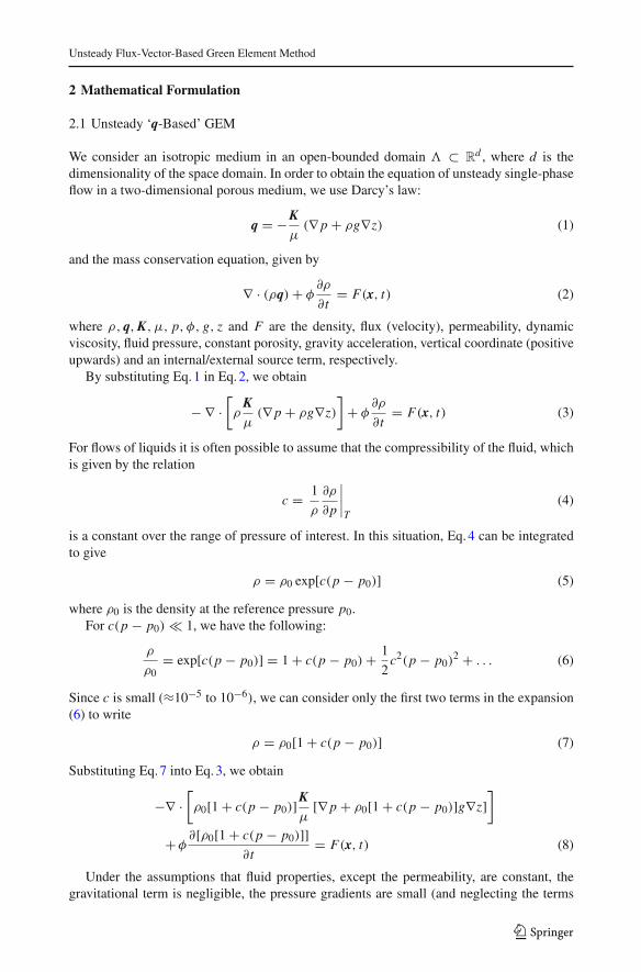
2 Mathematical Formulation

2.1 Unsteady ‘q-Based’ GEM

We consider an isotropic medium in an open-bounded domain � ⊂ Rd , where d is the

dimensionality of the space domain. In order to obtain the equation of unsteady single-phaseflow in a two-dimensional porous medium, we use Darcy’s law:

q = −Kμ

(∇ p + ρg∇z) (1)

and the mass conservation equation, given by

∇ · (ρq) + φ∂ρ

∂t= F(x, t) (2)

where ρ, q, K, μ, p, φ, g, z and F are the density, flux (velocity), permeability, dynamicviscosity, fluid pressure, constant porosity, gravity acceleration, vertical coordinate (positiveupwards) and an internal/external source term, respectively.

By substituting Eq. 1 in Eq. 2, we obtain

− ∇ ·[ρ

Kμ

(∇ p + ρg∇z)

]+ φ

∂ρ

∂t= F(x, t) (3)

For flows of liquids it is often possible to assume that the compressibility of the fluid, whichis given by the relation

c = 1

ρ

∂ρ

∂p

∣∣∣∣T

(4)

is a constant over the range of pressure of interest. In this situation, Eq. 4 can be integratedto give

ρ = ρ0 exp[c(p − p0)] (5)

where ρ0 is the density at the reference pressure p0.For c(p − p0) � 1, we have the following:

ρ

ρ0= exp[c(p − p0)] = 1 + c(p − p0) + 1

2c2(p − p0)

2 + . . . (6)

Since c is small (≈10−5 to 10−6), we can consider only the first two terms in the expansion(6) to write

ρ = ρ0[1 + c(p − p0)] (7)

Substituting Eq. 7 into Eq. 3, we obtain

−∇ ·[ρ0[1 + c(p − p0)]K

μ[∇ p + ρ0[1 + c(p − p0)]g∇z]

]

+φ∂[ρ0[1 + c(p − p0)]]

∂t= F(x, t) (8)

Under the assumptions that fluid properties, except the permeability, are constant, thegravitational term is negligible, the pressure gradients are small (and neglecting the terms

123

P. Lorinczi et al.

involving the square of the pressure gradient multiplied by c in comparison with other termsin the equation), and we can reduce Eq. 8 to (see Sato 1992):

ρ0

μ∇ · (K∇ p) = φρ0c

∂p

∂t− F(x, t) (9)

or

∇ · (K∇ p) = φμc∂p

∂t− μ

ρ0F(x, t) (10)

We can rearrange Eq. 10 so that the time is rescaled, and μρ0

F(x, t) is redefined as F(x, t),and then this equation can be simplified to

∇ · (K∇ p) = ∂p

∂t− F(x, t) (11)

Equation 11 is hence the governing equation of the problems considered in this article.To obtain unique solutions to the differential equation (11), boundary and initial condi-

tions must be specified. The boundary conditions, uniquely prescribed along the boundary�, can be classified as follows:

(i) the Dirichlet condition

p = p0(x, t) on �, t > t0 (12)

(ii) the Neumann condition

qn = ϕ0(x, t) on �, t > t0 (13)

(iii) the Robin condition

α1 p + β1qn = ϕ1(x, t) on �1, t > t0 (14)

α2 p + β2qn = ϕ2(x, t) on �2, t > t0 (15)

where �1 ∪ �2 = � and �1 ∩ �2 = ∅, α1, α2, β1, β2 are known constants, andp0, ϕ0, ϕ1 and ϕ2 are prescribed functions of x and t .

In the above expressions qn represents the flux in the direction of the unit outward vector nnormal to the boundary.

An additional condition has to be imposed for a unique solution to be achieved. Thatcondition, referred to as the initial condition, describes an earlier attained equilibrium stateof the system at the initial time t0. The initial condition specifies the pressure p everywhereon the domain:

p(x, t = t0) = pinitial0 (x) on � (16)

When the medium is isotropic, with the tensor permeability given by

K =(

K 00 K

)(17)

where K is heterogeneous, the governing differential equation is given by

∇ · [K (x, p, t)∇ p ] = ∂p

∂t− F(x, t) on �, t > t0 (18)

which can be rearranged to give (see, for example, Taigbenu 1999)

∇2 p = −∇ · ∇ p + �∂p

∂t− �F on �, t > t0 (19)

123

Unsteady Flux-Vector-Based Green Element Method

where = ln K and � = 1K .

We use the complementary differential equation

∇2G = δ(x − xi ) (20)

where x = (x, y) is considered the coordinate of the field node and xi = (xi , yi ) is thecoordinate of the source node. The solution to Eq. 20 is

G = ln(x − xi ) (21)

By using Eqs. 19 and 20 in Green’s second identity, we obtain the integral representationof the differential equation:

−2πλp(xi , t) +∫�

[p∇G · n + G

1

Kqn

]d�

+∫�

G

[−∇ · ∇ p + �

∂p

∂t− �F

]d� = 0 (22)

where λ is the corner coefficient at the node xi .We further make the assumption that K is uniform in each element, with K ≈ K , but it can

vary from element to element. This approximation essentially treats the entire domain as apiecewise homogeneous medium. With this assumption, the differential equation is modifiedfrom Eq. 11 to

K∇2 p = ∂p

∂t− F(x, t) on �, t > t0 (23)

The integral representation of this equation is given by

− 2πλp(xi , t) +∫�

[p∇G · n + G

1

Kqn

]d� +

∫�

G�

[∂p

∂t− F

]d� = 0 (24)

The domain is now discretised by suitable polygonal elements (in our case by rectangularelements) over which each functional quantity is interpolated by the basis functions of theLagrange family. The expressions for these interpolating functions for a rectangular elementare

�1 = (1 − ξ)(1 − η), �2 = ξ(1 − η), �3 = ξη and �4 = (1 − ξ)η (25)

in which ξ and η are local coordinates, given by ξ = x−x0�x (e) and η = y−y0

�y(e) , where x and y are

space coordinates, �x (e) and �y(e) are the dimensions of the sides of the element (e) and(x0, y0) denotes the coordinates of the bottom left corner of the element (e).

The same concept is used as in the ‘q-based’ GEM, therefore, the flux will be approximatedby the basis functions as

qx (x) ≈N ′

e∑j=1

� j (x)qx, j , qy(x) ≈N ′

e∑j=1

� j (x)qy, j , qz(x) ≈N ′

e∑j=1

� j (x)qz, j (26)

where we denote by qx, j the value of qx at node j , for j = 1, N ′e (and similarly for qy, j

and qz, j ), with N ′e denoting the number of corners of a typical element, and the � j are the

Lagrange interpolation functions.

123

P. Lorinczi et al.

Δt

t t1 2+ωΔtt1 Timet0

Fig. 1 Discretisation of time domain

The discrete form of Eq. 24 for a typical element (e) after interpolation is

R(e)i j p j − L(e)

i j1

Kqn, j + T (e)

i j �(e)

[d p(e)

j

dt− F (e)

j

]= 0 i, j = 1, N ′

e (27)

where the element matrices Ri j , Li j and Ti j are defined by

R(e)i j = ∫

�(e)

∂G(x,xi )∂n � j d�(e) − 2πδi jλ

(e) (28)

L(e)i j = − ∫

�(e)

G(x, xi )� j d�(e) (29)

T (e)i j = ∫

�(e)

G(x, xi )� j d�(e) (30)

in which the superscript (e) denotes a typical element, p(e)i stands for the value of p at the

source point xi in the element (e), Ne is the total number of polygonal elements that are usedto discretise the domain, and �(e) and �(e) are, respectively, the boundary and domain of thetypical element.

A difference approximation for the temporal derivative is used in Eq. 27. For this, the timehistory is divided into elements of length �t , with a typical element having two nodes or timelevels: t1 being the previous time level at which solution information is completely specified,and t2 being the current time level at which solution information is sought (see Fig. 1). Thedifference approximation is given by

d p(e)j

dt

∣∣∣∣∣t=t1+ω�t

≈ p(e)j (t2) − p(e)

j (t1)

�t, 0 ≤ ω ≤ 1 (31)

where ω is a fixed difference weighting factor whose value lies between 0 and 1.Equation 31 indicates that the temporal derivative is evaluated at a time t1 + ω�t . The

value of ω positions the time level at which the temporal derivative is evaluated. A schemewith ω = 0 is said to be a fully explicit scheme, that with ω = 0.5 is the Crank–Nicolsonscheme, that with ω = 0.67 is the Galerkin scheme, whilst that with ω = 1 is usually referredto as the fully implicit scheme. Since the temporal derivative has been evaluated at t1 +ω�t , itis reasonable to evaluate the other terms of Eq. 27 at that time level using a weighted averageof the form

123

Unsteady Flux-Vector-Based Green Element Method

ω

[R(e)

i j p(e)j − L(e)

i j1

K(e)

q(e)n, j − T (e)

i j �(e)

F (e)j

]t=t2

+ (1 − ω)

[R(e)

i j p(e)j − L(e)

i j1

K(e)

q(e)n, j − T (e)

i j �(e)

F (e)j

]t=t1

+ T (e)i j �

(e) d p(e)j

dt

∣∣∣∣∣t=t1+ω�t

= 0, i, j = 1, N ′e, 0 ≤ ω ≤ 1 (32)

Until now the superscript (e) on variables and parameters has been used to indicate thatthe equations are derived specifically for a typical element. However, this superscript willfurther be omitted for convenience.

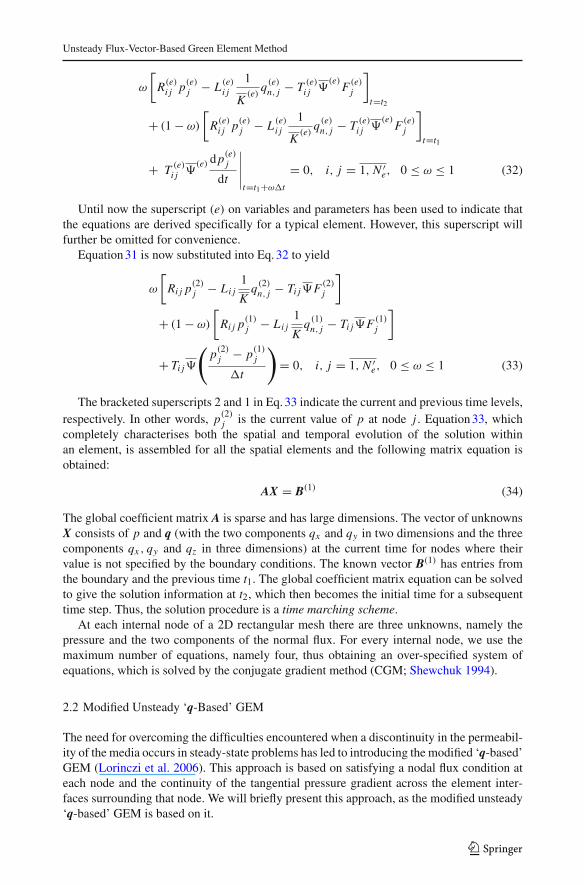
Equation 31 is now substituted into Eq. 32 to yield

ω

[Ri j p(2)

j − Li j1

Kq(2)

n, j − Ti j�F (2)j

]

+ (1 − ω)

[Ri j p(1)

j − Li j1

Kq(1)

n, j − Ti j�F (1)j

]

+ Ti j�

(p(2)

j − p(1)j

�t

)= 0, i, j = 1, N ′

e, 0 ≤ ω ≤ 1 (33)

The bracketed superscripts 2 and 1 in Eq. 33 indicate the current and previous time levels,respectively. In other words, p(2)

j is the current value of p at node j . Equation 33, whichcompletely characterises both the spatial and temporal evolution of the solution withinan element, is assembled for all the spatial elements and the following matrix equation isobtained:

AX = B(1) (34)

The global coefficient matrix A is sparse and has large dimensions. The vector of unknownsX consists of p and q (with the two components qx and qy in two dimensions and the threecomponents qx , qy and qz in three dimensions) at the current time for nodes where theirvalue is not specified by the boundary conditions. The known vector B(1) has entries fromthe boundary and the previous time t1. The global coefficient matrix equation can be solvedto give the solution information at t2, which then becomes the initial time for a subsequenttime step. Thus, the solution procedure is a time marching scheme.

At each internal node of a 2D rectangular mesh there are three unknowns, namely thepressure and the two components of the normal flux. For every internal node, we use themaximum number of equations, namely four, thus obtaining an over-specified system ofequations, which is solved by the conjugate gradient method (CGM; Shewchuk 1994).

2.2 Modified Unsteady ‘q-Based’ GEM

The need for overcoming the difficulties encountered when a discontinuity in the permeabil-ity of the media occurs in steady-state problems has led to introducing the modified ‘q-based’GEM (Lorinczi et al. 2006). This approach is based on satisfying a nodal flux condition ateach node and the continuity of the tangential pressure gradient across the element inter-faces surrounding that node. We will briefly present this approach, as the modified unsteady‘q-based’ GEM is based on it.

123

P. Lorinczi et al.

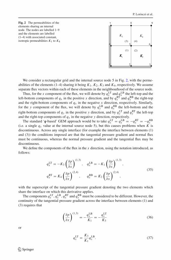
Fig. 2 The permeabilities of theelements sharing an internalnode. The nodes are labelled 1–9and the elements are labelled(1–4) with associated constant,isotropic permeabilities K1 to K4

2 3

5 6

7 8 9

K K

KK

2KK

3

1KK

4

(1) (2)

(4)(3)

1

4

We consider a rectangular grid and the internal source node 5 in Fig. 2, with the perme-abilities of the elements (1–4) sharing it being K1, K2, K3 and K4, respectively. We assumeseparate flux vectors within each of these elements in the neighbourhood of the source node.

Thus, for the x component of the flux, we will denote by qLTx and qLB

x the left-top and theleft-bottom components of qx in the positive x direction, and by qRT

x and qRBx the right-top

and the right-bottom components of qx in the negative x direction, respectively. Similarly,for the y component of the flux, we will denote by qLB

y and qRBx the left-bottom and the

right-bottom components of qy in the positive y direction, and by qLTy and qRT

y the left-topand the right-top components of qy in the negative y direction, respectively.

The standard ‘q-based’ GEM approach would be to take qLTx = qLB

x = −qRTx = −qRB

x(i.e. a single qx value at the internal source node 5), but this causes problems when K isdiscontinuous. Across any single interface (for example the interface between elements (1)and (3)) the conditions imposed are that the tangential pressure gradient and normal fluxmust be continuous, whereas the normal pressure gradient and the tangential flux may bediscontinuous.

We define the components of the flux in the x direction, using the notation introduced, asfollows:

qLTx = −K3

(∂p

∂x

)(1,3)

, qLBx = −K1

(∂p

∂x

)(1,3)

,

qRTx = K4

(∂p

∂x

)(2,4)

, qRBx = K2

(∂p

∂x

)(2,4)

,

(35)

with the superscript of the tangential pressure gradient denoting the two elements whichshare the interface on which this derivative applies.

The components qLTx , qLB

x , qRTx and qRB

x must be considered to be different. However, thecontinuity of the tangential pressure gradient across the interface between elements (1) and(3) requires that

(∂p

∂x

)(1,3)

= −qLBx

K1= −qLT

x

K3(36)

or

qLTx = K3

K1qLB

x . (37)

123

Unsteady Flux-Vector-Based Green Element Method

Similarly, for the interface between elements (2) and (4), the continuity of the tangentialpressure gradient requires that

qRBx = K2

K4qRT

x . (38)

To illustrate the nodal flux condition at the source node 5, we consider a small square ofside 2ε centred on node 5 and with the interfaces between the elements sharing node 5 beingperpendicular to the sides of the square. Thus, the interfaces will intersect the square at themiddle of its sides and the nodal flux condition in the x direction can be written as follows:

εqLBx + εqLT

x + εqRTx + εqRB

x = 0, (39)

and hence we can take the limit as ε → 0. Introducing expressions (37) and (38) into Eq. 39allows us to reformulate the nodal flux condition in terms of just two of the components ofqx as follows:

(1 + K3

K1

)qLB

x +(

1 + K2

K4

)qRT

x = 0. (40)

Thus, Eqs. 37, 38 and 40 allow us to rewrite the remaining three x direction flux values interms of a single known qx component.

Using the definitions of qLBx and qRT

x , Eq. 40 can also be written as follows:

− (K1 + K3)

(∂p

∂x

)(1,3)

+ (K2 + K4)

(∂p

∂x

)(2,4)

= 0. (41)

We further introduce the following notation for the two terms in Eq. 41:

− K1 + K3

2

(∂p

∂x

)(1,3)

= q Lx , (42a)

K2 + K4

2

(∂p

∂x

)(2,4)

= q Rx , (42b)

with qLx and qR

x oriented in the positive and in the negative x direction, respectively, and thisleads to qL

x = −qRx . The continuity of these expressions for the ‘left-hand’ and ‘right-hand’

x direction fluxes, necessary to satisfy the nodal flux condition, avoids an incorrect definitionfor qx at a discontinuity of K in the y direction. Along the interface between elements (1)and (3) the tangential pressure derivative has the form

(∂p

∂x

)(1,3)

= − 2

K1 + K3qL

x , (43)

and similarly for elements (2) and (4) we have

(∂p

∂x

)(2,4)

= 2

K2 + K4qR

x . (44)

The number of unknown flux components in the x direction can thus be reduced to one.

123

P. Lorinczi et al.

A very similar treatment is applied for the components of the flux in the y direction (seeLorinczi et al. 2006).

To express the qx component of the flux at node 5, when writing the integral equationsfor elements (1) and (3), we write their corresponding fluxes as follows:

q(1)x = qLB

x = −K1

(∂p

∂x

)(1,3)

= 2K1

K1 + K3qL

x , (45a)

q(3)x = qLT

x = −K3

(∂p

∂x

)(1,3)

= 2K3

K1 + K3qL

x . (45b)

Likewise, the remaining flux components at node 5 are taken to have the following form:

q(2)x = qRB

x = K2

(∂p

∂x

)(2,4)

= 2K2

K2 + K4qR

x , (46a)

q(4)x = qRT

x = K4

(∂p

∂x

)(2,4)

= 2K4

K2 + K4qR

x , (46b)

q(1)y = qLB

y = −K1

(∂p

∂y

)(1,2)

= 2K1

K1 + K2qB

y , (47a)

q(2)y = qRB

y = −K2

(∂p

∂y

)(1,2)

= 2K2

K1 + K2qB

y , (47b)

q(3)y = qLT

y = K3

(∂p

∂y

)(3,4)

= 2K3

K3 + K4qT

y , (47c)

q(4)y = qRT

y = K4

(∂p

∂y

)(3,4)

= 2K4

K3 + K4qT

y . (47d)

A similar approach is presented in Lorinczi et al. (2006) for side and corner source nodes.This procedure for the flux components is implemented at each node, within the unsteady

‘q-based’ GEM described in Sect. 2.1. In this way we get the modified unsteady ‘q-based’GEM. All the examples presented in this article are solved using this approach.

2.3 Well Test Simulation

In testing the modified unsteady ‘q-based’ GEM, some examples will be considered for thesimulation of wells (sources and sinks) in a domain.

If the wells are located at (x j , y j ), j = 1, Nw, where Nw represents the number of wells,then the expression of the internal/external source term from Eq. 11 will now be given by

F(x, t) = −Nw∑j=1

q jδ(x − x j )δ(y − y j ) on �, t > t0 (48)

where q j is the given strength of the j th well and δ is the Dirac delta function.

123

Unsteady Flux-Vector-Based Green Element Method

The domain integrations for the examples in this article involving wells have been avoidedby specifying the two components of the flux at each of the four corners of the elements con-taining the wells. The two components of the flux at each of these corners are specifiedby

|qx, j | = |qy, j | = |q j |4(�x) j

, j = 1, Nw (49)

where qx, j and qy, j are the two components of the flux from a corner of the element con-taining the well and (�x) j is the dimension of a side of the element. Appropriate signs wereused for specifying the flux values at each corner, according to the sign of q j .

3 Numerical Results and Discussion

3.1 Numerical Results When Known Analytical Solutions are Available

The example in this section has been solved using both the Crank–Nicolson (ω = 0.5) andthe fully implicit scheme (ω = 1). The absolute errors between the numerical results forthe pressure and flux obtained using the two schemes are less than 2 × 10−6. Hence, thenumerical results illustrated in this section are those obtained using the Crank–Nicolsonscheme.

Example 1To test the modified unsteady ‘q-based’ GEM, we first consider a problem in which K = 1

in the absence of any source term, which is thus governed by the following equation:

∇2 p = ∂p

∂ton � = {(x, y) : 0 ≤ x, y ≤ 1}, t > 0 (50)

with the boundary and initial conditions given by

p(x, 0, t) = x + e−4t , p(x, 1, t) = x + 1 + e−4t cos 2, 0 ≤ x ≤ 1, t > 0

qx (0, y, t) = −1, qx (1, y, t) = −1, 0 ≤ y ≤ 1, t > 0

p(x, y, 0) = x + y + cos 2y, 0 ≤ x, y ≤ 1

(51)

The exact solution to this example is given by

p = x + y + e−4t cos 2y (52)

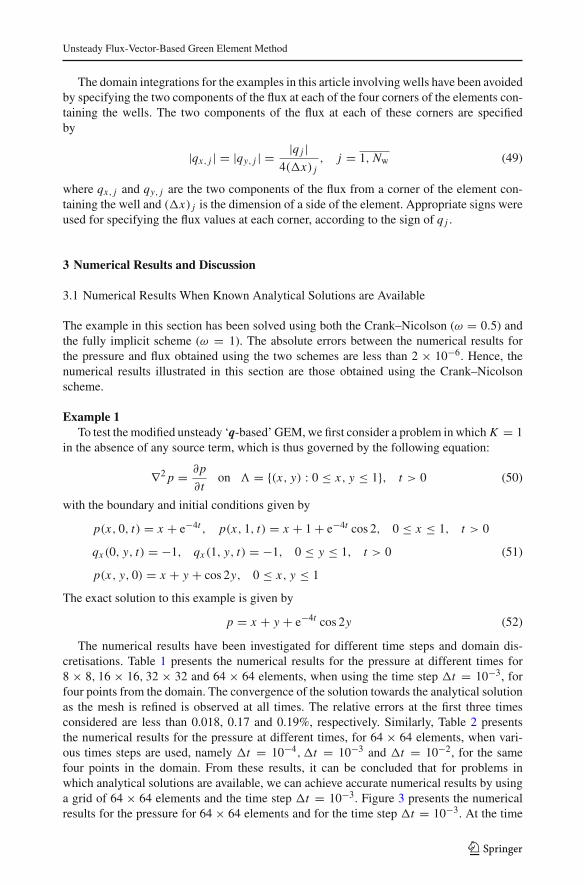
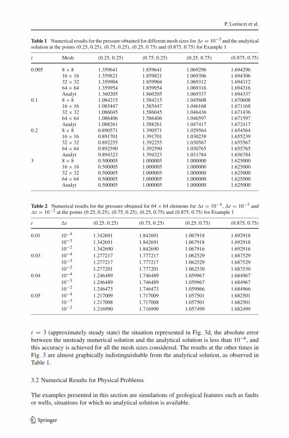
The numerical results have been investigated for different time steps and domain dis-cretisations. Table 1 presents the numerical results for the pressure at different times for8 × 8, 16 × 16, 32 × 32 and 64 × 64 elements, when using the time step �t = 10−3, forfour points from the domain. The convergence of the solution towards the analytical solutionas the mesh is refined is observed at all times. The relative errors at the first three timesconsidered are less than 0.018, 0.17 and 0.19%, respectively. Similarly, Table 2 presentsthe numerical results for the pressure at different times, for 64 × 64 elements, when vari-ous times steps are used, namely �t = 10−4,�t = 10−3 and �t = 10−2, for the samefour points in the domain. From these results, it can be concluded that for problems inwhich analytical solutions are available, we can achieve accurate numerical results by usinga grid of 64 × 64 elements and the time step �t = 10−3. Figure 3 presents the numericalresults for the pressure for 64 × 64 elements and for the time step �t = 10−3. At the time

123

P. Lorinczi et al.

Table 1 Numerical results for the pressure obtained for different mesh sizes for �t = 10−3 and the analyticalsolution at the points (0.25, 0.25), (0.75, 0.25), (0.25, 0.75) and (0.875, 0.75) for Example 1

t Mesh (0.25, 0.25) (0.75, 0.25) (0.25, 0.75) (0.875, 0.75)

0.005 8 × 8 1.359641 1.859641 1.069296 1.69429616 × 16 1.359821 1.859821 1.069306 1.69430632 × 32 1.359904 1.859904 1.069312 1.69431264 × 64 1.359954 1.859954 1.069316 1.694316Analyt 1.360205 1.860205 1.069337 1.694337

0.1 8 × 8 1.084215 1.584215 1.045608 1.67060816 × 16 1.085447 1.585447 1.046168 1.67116832 × 32 1.086045 1.586045 1.046436 1.67143664 × 64 1.086406 1.586406 1.046597 1.671597Analyt 1.088261 1.588261 1.047417 1.672417

0.2 8 × 8 0.890571 1.390571 1.029564 1.65456416 × 16 0.891701 1.391701 1.030239 1.65523932 × 32 0.892255 1.392255 1.030567 1.65556764 × 64 0.892590 1.392590 1.030765 1.655765Analyt 0.894323 1.394323 1.031784 1.656784

3 8 × 8 0.500005 1.000005 1.000000 1.62500016 × 16 0.500005 1.000005 1.000000 1.62500032 × 32 0.500005 1.000005 1.000000 1.62500064 × 64 0.500005 1.000005 1.000000 1.625000Analyt 0.500005 1.000005 1.000000 1.625000

Table 2 Numerical results for the pressure obtained for 64 × 64 elements for �t = 10−4,�t = 10−3 and�t = 10−2 at the points (0.25, 0.25), (0.75, 0.25), (0.25, 0.75) and (0.875, 0.75) for Example 1

t �t (0.25, 0.25) (0.75, 0.25) (0.25, 0.75) (0.875, 0.75)

0.01 10−4 1.342691 1.842691 1.067918 1.69291810−3 1.342691 1.842691 1.067918 1.69291810−2 1.342690 1.842690 1.067916 1.692916

0.03 10−4 1.277217 1.777217 1.062529 1.68752910−3 1.277217 1.777217 1.062529 1.68752910−2 1.277201 1.777201 1.062530 1.687530

0.04 10−4 1.246489 1.746489 1.059967 1.68496710−3 1.246489 1.746489 1.059967 1.68496710−2 1.246473 1.746473 1.059966 1.684966

0.05 10−4 1.217009 1.717009 1.057501 1.68250110−3 1.217008 1.717008 1.057501 1.68250110−2 1.216990 1.716990 1.057499 1.682499

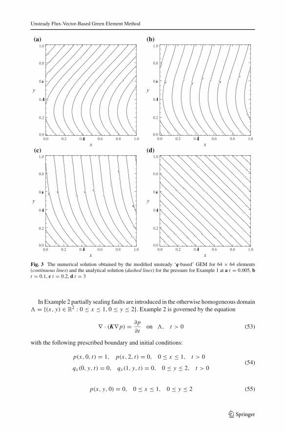
t = 3 (approximately steady state) the situation represented in Fig. 3d, the absolute errorbetween the unsteady numerical solution and the analytical solution is less than 10−6, andthis accuracy is achieved for all the mesh sizes considered. The results at the other times inFig. 3 are almost graphically indistinguishable from the analytical solution, as observed inTable 1.

3.2 Numerical Results for Physical Problems

The examples presented in this section are simulations of geological features such as faultsor wells, situations for which no analytical solution is available.

123

Unsteady Flux-Vector-Based Green Element Method

(a)

(c)

(b)

(d)

Fig. 3 The numerical solution obtained by the modified unsteady ‘q-based’ GEM for 64 × 64 elements(continuous lines) and the analytical solution (dashed lines) for the pressure for Example 1 at a t = 0.005, bt = 0.1, c t = 0.2, d t = 3

In Example 2 partially sealing faults are introduced in the otherwise homogeneous domain� = {(x, y) ∈ R

2 : 0 ≤ x ≤ 1, 0 ≤ y ≤ 2}. Example 2 is governed by the equation

∇ · (K∇ p) = ∂p

∂ton �, t > 0 (53)

with the following prescribed boundary and initial conditions:

p(x, 0, t) = 1, p(x, 2, t) = 0, 0 ≤ x ≤ 1, t > 0

qx (0, y, t) = 0, qx (1, y, t) = 0, 0 ≤ y ≤ 2, t > 0(54)

p(x, y, 0) = 0, 0 ≤ x ≤ 1, 0 ≤ y ≤ 2 (55)

123

P. Lorinczi et al.

The governing equation (53) on the domain � and the conditions (54) and (55) are obtainedby considering initially an equation of a similar form to Eq. 11 on the domain [0, l] × [0, 2l]with the following boundary and initial conditions:

p(x, 0, t) = p0, p(x, 2l, t) = p0 − �p0, 0 ≤ x ≤ l, t > 0

qx (0, y, t) = 0, qx (l, y, t) = 0, 0 ≤ y ≤ 2l, t > 0

p(x, y, 0) = p0 − �p0, 0 ≤ x ≤ l, 0 ≤ y ≤ 2l

(56)

by applying a non-dimensionalisation according to

x = x

l, y = y

l, t = t

t∞, p = p − (p0 − �p0)

�p0(57)

and rescaling each of the components of K by the representative value K ∗. Here �p0 > 0is the pressure difference suddenly applied vertically across the domain at t = 0 and keptconstant thereafter, t∞ = l2/K ∗ is the ‘time’ taken to reach the steady-state flow regime andno-flow conditions are applied on the vertical boundaries of the domain.

In the remaining problems from this section such a non-dimensionalisation is used first toobtain the equation and the conditions imposed.

The faults in Example 2 are represented by two thin layers of thickness 2tf = 10−2 andof length 0.75. One is situated in the bottom-right part of the domain over [0.25, 1] × [0.5 −tf , 0.5 + tf ] and the other one is located over [0, 0.75] × [1.5 − tf , 1.5 + tf ]. The two faultshave the same permeability. The permeability K = 1 applies on the remainder of the do-main. A fully implicit scheme has been used, and a time step of �t = 10−3 has been used,in accordance with the results from Example 1. Similarly, the spatial discretisation used inthis example was chosen to be close to the value determined in Example 1.

Example 2The permeability of the faults in this example is Kf = 10−1. The pressure and the flux

vectors have been plotted in Figs. 4 and 5, respectively, at different times using a discret-isation of 64 × 130 elements and a time step of �t = 10−3. At t = 0.02 many of thepressure contours are very close to the bottom boundary of the domain where the pressureis unity. However, the distance between the pressure contours gradually increases in time,with the contours representing small pressure values gradually moving away from the bottomboundary towards the top boundary.

The flux vectors at the same times are illustrated in Fig. 5. At t = 0.02 the arrows rep-resenting the flux are very large in the lower part of the domain in comparison with the restof the domain, and near to y = 0 the flux vectors are virtually parallel to the Oy-axis. In theupper part of the domain at t = 0.02 the impulsive pressure change at y = 0 has not beenfelt and the fluid remains almost undisturbed. The magnitude of the arrows in the lower partof the domain decreases in time, and when the flow reaches the first fault they show how thefluid starts to avoid the fault and is slightly focused towards the gap at the left-hand side. Thisis very noticeable at the left tip of the lower fault where the arrows representing the fluid fromthis region are the most affected. The fluxes at the other nodes are not so affected as the faultsare quite permeable. Hence in this situation the faults have allowed a considerable amount offluid to pass through them. This is mostly evident in Fig. 5d, where the steady-state solutionhas almost been reached.

123

Unsteady Flux-Vector-Based Green Element Method

(a)

(c)

(b)

(d)

Fig. 4 The pressure contours obtained by the modified unsteady ‘q-based’ GEM for 64 × 130 elements forExample 2 at a t = 0.02, b t = 0.05, c t = 0.2, d t = 2.0

Example 3Example 3 is a simulation of two wells inside the sealed rectangular domain {(x, y) ∈ � :

0 ≤ x ≤ 1, 0 ≤ y ≤ 2}, with a permeability of K = 1 everywhere in the domain, so that thegoverning equation is given by

123

P. Lorinczi et al.

(a)

(c)

(b)

(d)

Fig. 5 The flux vectors obtained by the modified unsteady ‘q-based’ GEM for 64×130 elements for Example2 at a t = 0.02, b t = 0.05, c t = 0.2, d t = 2.0

∇2 p = ∂p

∂t+

2∑j=1

q jδ(x − x j )δ(y − y j ) on �, t > 0 (58)

123

Unsteady Flux-Vector-Based Green Element Method

The boundary and initial conditions imposed are

qy(x, 0, t) = 0, qy(x, 2, t) = 0, 0 ≤ x ≤ 1, t > 0

qx (0, y, t) = 0, qx (1, y, t) = 0, 0 ≤ y ≤ 2, t > 0(59)

p(x, y, 0) = 0, 0 ≤ x ≤ 1, 0 ≤ y ≤ 2, (60)

One well is located at (0.25, 1.75) and is considered as a source (injection) with strengthq1 = 1; the other well, considered as a sink (production), has strength q2 = −1 and is locatedat (0.75, 0.25). The domain discretisations allow the representation of the wells within squarecells.

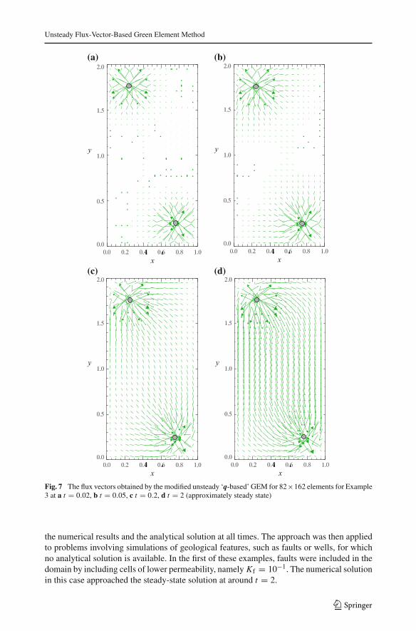
The evolutions of the pressure contours and the flow field in time are illustrated in Figs. 6and 7, respectively, for this example at the same times, using 82 × 162 elements and the timestep �t = 10−3.

At the earlier times the flux close to the wells is much larger than in the rest of the domain.At t = 0.02, the flow in the centre of the domain is hardly observable, a situation whichis represented in Fig. 7a. The producer and injector are only having a significant influenceon the fluid flow in their immediate vicinity. The flow across the centre of the domain startsincreasing in time, as is evident in Fig. 7b–d, and the flow from the injector to the producerbecomes apparent. This evolution of the flow is also reflected in the pressure contours, seeFig. 6.

Example 4Example 4 is again a simulation of wells when sealing boundary conditions are imposed

on the rectangular domain � = {(x, y) : 0 ≤ x ≤ 1, 0 ≤ y ≤ 2}, but now including faults.The governing equation for Example 4 is

∇ · (K∇ p) = ∂p

∂t+

2∑j=1

q jδ(x − x j )δ(y − y j ) on �, t > 0 (61)

with the same boundary and initial conditions as given in equations (59) and (60). The twowells have the same locations as in Example 3 namely (0.75, 0.25) and (0.25, 1.75). Thewells are located in square cells. Two faults of thickness 2tf = 10−2, located in the domainover [0.2, 1]× [0.5 − tf , 0.5 + tf ] and over [0, 0.8]× [1.5 − tf , 1.5 + tf ], have been included.The permeability of the faults is Kf = 10−3 whilst the permeability of the remainder of thedomain is in each example K = 1.

The numerical results have been investigated for the same discretisation of 82 × 148 ele-ments, using the time step �t = 0.0025. Figures 8 and 9 illustrate the pressure and the fluxvectors for times t ≤ 0.3.

In this case, as expected, the faults have an important influence on the pressure field andon the flow pattern. Even at relatively early times, such as t = 0.1 and t = 0.3, it is noticeablehow the fluid is forced to avoid the faults, resulting in a pressure build up across the faults.At small times when the flow is localised around the wells, the flow is mainly horizontal, i.e.parallel to the faults. At t = 0.3 the fluid reaches the fault tips and begins to flow around them.

More examples using the unsteady ‘q-based’ GEM can be found in Lorinczi (2006).

123

P. Lorinczi et al.

(a)

(c)

(b)

(d)

Fig. 6 The pressure contours obtained by the modified unsteady ‘q-based’ GEM for 82 × 162 elements forExample 3 at a t = 0.02, b t = 0.05, c t = 0.2, d t = 2.0 (approximately steady state)

4 Conclusions

In this article, we have illustrated the modified unsteady ‘q-based’ GEM, which is an exten-sion of the modified ‘q-based’ GEM when applied to unsteady situations.

The modified unsteady ‘q-based’ GEM was first tested on a numerical example withknown analytical solution, situation for which there was a very good agreement between

123

Unsteady Flux-Vector-Based Green Element Method

(a)

(c)

(b)

(d)

Fig. 7 The flux vectors obtained by the modified unsteady ‘q-based’ GEM for 82×162 elements for Example3 at a t = 0.02, b t = 0.05, c t = 0.2, d t = 2 (approximately steady state)

the numerical results and the analytical solution at all times. The approach was then appliedto problems involving simulations of geological features, such as faults or wells, for whichno analytical solution is available. In the first of these examples, faults were included in thedomain by including cells of lower permeability, namely Kf = 10−1. The numerical solutionin this case approached the steady-state solution at around t = 2.

123

P. Lorinczi et al.

(a)

(c)

(b)

(d)

Fig. 8 The pressure contours obtained by the modified unsteady ‘q-based’ GEM for 82 × 148 elements forExample 4 at a t = 0.02, b t = 0.05, c t = 0.1, d t = 0.3

An example with wells in the absence of any faults was then presented. The wells had aconstant strength. The final example involved both faults and wells, with a low permeabilityof the faults: Kf = 10−3. A strong influence of the faults was in evidence in both the pressurefield and flow pattern.

123

Unsteady Flux-Vector-Based Green Element Method

(a)

(c)

(b)

(d)

Fig. 9 The flux vectors obtained by the modified unsteady ‘q-based’ GEM for 82×148 elements for Example4 at a t = 0.02, b t = 0.05, c t = 0.1, d t = 0.3

In all the situations including geological features the evolutions of the pressure contoursand of the flux vector field in time were illustrated. Overall, from the numerical resultspresented it can be concluded that the modified unsteady ‘q-based’ GEM is a suitable andaccurate method for solving unsteady problems involving flow across partially sealing faultswhen generated by the presence of (injection/production) wells, as it enables the evolutionof such geological processes to be represented in time.

123

P. Lorinczi et al.

References

Aarnes, J.E., Lie, K.-A.: Toward reservoir simulation on geological grid models. In: 9th European Conferenceon the Mathematics of Oil Recovery, Cannes, (2004)

Archer, R.A., Horne, R.N.: The Green element method for numerical well test analysis. Soc. Pet. Eng. J. 62916(2000)

Durlofsky, L.J.: Accuracy of mixed and control volume finite element approximations to Darcy velocity andrelated quantities. Water Resour. Res. 30(4), 965–974 (1994)

Karimi-Fard, M., Durlofsky, L.J., Aziz, K.: An efficient discrete-fracture model applicable for general-purposereservoir simulators. Soc. Pet. Eng. J. 9, 227–236 (2004)

Klausen, R.A., Eigestad, G.T.: Multi point flux approximations and finite element methods; practical aspects ofdiscontinuous media. In: 9th European Conference on the Mathematics of Oil Recovery, Cannes (2004)

Lorinczi, P.: Applications of the Green element method to flow in heterogeneous porous media. Ph.D. Thesis,University of Leeds (2006)

Lorinczi, P., Harris, S.D., Elliott, L.: Modelling of highly-heterogeneous media using a flux-vector basedGreen element method. Eng. Anal. Bound Elem. 30, 818–833 (2006)

Lorinczi, P., Harris, S.D., Elliott, L.: Modified flux-vector based GEM for problems in steady-state anisotropicmedia. Eng. Anal. Bound Elem. 33, 368–387 (2009). doi:10.1016/j.enganabound.2008.06.004

Pecher, R., Harris, S.D., Knipe, R.J., Elliott, L., Ingham, D.B.: New formulation of the Green element methodto maintain its second-order accuracy in 2D/3D. Eng. Anal. Bound Elem. 25, 211–219 (2001)

Sato, K.: Accelerated perturbation boundary element model for flow problems in heterogeneous reservoirs.Ph.D. Thesis, Stanford University (1992)

Shewchuk, J.R.: An Introduction to the Conjugate Gradient Method Without the Agonizing Pain. Tech. Rep.CMU-CS-94-125, School of Computer Science, Carnegie Mellon University, Pittsburgh, PA 15213(1994)

Taigbenu, A.E.: A more efficient implementation of the boundary element theory. In: Proceedings of theFifth International Conference on Boundary Element Technology (BETECH 90), pp. 355–366. Newark,Delaware (1990)

Taigbenu, A.E. : The Green element method. Vol. 38, Kluwer Academic Publishers, Boston (1999)Taigbenu, A.E.: Features of a time-dependent fundamental solution in the Green element method. Appl. Math.

Model. 27, 125–143 (2003a)Taigbenu, A.E.: Green element simulations of multiaquifer flows with a time-dependent Green’s function.

J. Hydrol. 284, 131–150 (2003b)Taigbenu, A.E.: A time-dependent Green’s function-based model for stream-unconfined aquifer flows. Water

SA 29, 257–265 (2003c)Taigbenu, A.E.: Green element calculations of nonlinear heat conduction with a time-dependent fundamental

solution. Eng. Anal. Bound Elem. 28, 53–60 (2004)Taigbenu, A.E., Onyejekwe, O.O.: Green element simulations of the transient nonlinear unsaturated flow

equation. Appl. Math. Model. 19, 675–684 (1995)Taigbenu, A.E., Onyejekwe, O.O.: Transient 1D transport equation simulated by a mixed Green element

formulation. Int. J. Numer. Methods Fluids 25, 437–454 (1997)Taigbenu, A.E., Onyejekwe, O.O.: Green’s function-based integral approaches to linear transient boundary-

value problems and their stability characteristics (I). Appl. Math. Model. 22, 687–702 (1998)Taigbenu, A.E., Onyejekwe, O.O.: Green’s function-based integral approaches to nonlinear transient bound-

ary-value problems (II). Appl. Math. Model. 23, 241–253 (1999)Taigbenu, A.E., Onyejekwe, O.O.: A flux-correct Green element model of quasi three-dimensional multiaqu-

ifer flow. Water Resour. Res. 36, 3631–3640 (2000)

123