Journal of Computational and Applied Mathematics 234 (2010) 2336–2341

Contents lists available at ScienceDirect

Journal of Computational and AppliedMathematics

journal homepage: www.elsevier.com/locate/cam

Numerical modeling of unsteady flow in steam turbine stageJ. Halama a,b,∗, J. Dobeš a, J. Fořt a, J. Fürst a, K. Kozel ba Department of Technical Mathematics, Czech Technical University FME Prague, Karlovo nám. 13, CZ-12135 Praha 2, Czech Republicb IT AS CR, Dolejškova 1402/5, CZ-18200 Praha 8, Czech Republic

a r t i c l e i n f o

Article history:Received 5 September 2008Received in revised form 9 January 2009

Keywords:Stator-rotor interactionUnsteady flowTwo-phase flow

a b s t r a c t

This work deals with numerical solution of unsteady flow in turbine stage. We use modelsof compressible single-phase flow of air and two-phase flow of wet steam. Presentednumerical methods are based on different stator-rotor matching algorithms, as well asdifferent numerical schemes. Numerical results achieved by bothmethods and flowmodelsare discussed.

© 2009 Elsevier B.V. All rights reserved.

1. Introduction

It is generally difficult to specify flow field parameters (boundary conditions) at the inlet and the outlet of a single turbinecascade due to upstream and downstream located structures, see e.g. [1]. Therefore, it is interesting to couple severalcascades together, and the flow field at the interfaces is then the result of numerical simulation. Of course, this couplingcan provide much more information about, e.g. blade forces, clocking etc. Different coupling techniques from mixing planeto fully unsteady interaction, are being used. This paper is aimed at fully unsteady interaction between stator and rotor.We have developed two finite volume methods. The first method has a relatively simple stator-rotor matching algorithmimplemented into already existing in-house 2D finite volume code based on the Roe approximate Riemann solver for generalunstructured grids, which has been previously verified and used to compute one-phase transonic flow in various singleturbine cascades, see e.g. [2]. The second method has been created from the in-house Lax-Wendroff finite volume code fortwo-phase flow of condensing steam by addition of Giles’smatching algorithm [3], which has been already successfully usedfor one-phase stator-rotor interaction in high pressure turbine stage, see [1].

2. Governing equations and problem formulation

Both flow models are given by the set of PDE’s of the form

∂tW = −∂xF− ∂yG+ Q, (1)

where the 2D flow of perfect gas described by the Euler’s equations, further referred as one-phase flow model, is given byvectors

W = [ρ, ρu, ρv, e]T , F =[ρu, ρu2 + p, ρuv, (e+ p)u

]T,

Q = [0, 0, 0, 0]T , G =[ρu, ρvu, ρv2 + p, (e+ p)v

]T,

(2)

∗ Corresponding author at: Department of Technical Mathematics, Czech Technical University FME Prague, Karlovo nám. 13, CZ-12135 Praha 2, CzechRepublic.E-mail addresses: halama@marian.fsik.cvut.cz (J. Halama), dobes@marian.fsik.cvut.cz (J. Dobeš), fort@marian.fsik.cvut.cz (J. Fořt),

furst@marian.fsik.cvut.cz (J. Fürst), kozelk@fsik.cvut.cz (K. Kozel).

0377-0427/$ – see front matter© 2009 Elsevier B.V. All rights reserved.doi:10.1016/j.cam.2009.08.090

J. Halama et al. / Journal of Computational and Applied Mathematics 234 (2010) 2336–2341 2337

and the closure is p = (γ − 1)[e − ρ(u2 + v2)/2]. The symbol ρ denotes density, u and v velocity vector components,p pressure, e total energy per unit volume and γ specific heat ratio. The next model describes flow of mixture containingvapor and condensed droplets, and it is referred as two-phase flow model. We consider a convection of droplets by vapor.The governing equations consists of Euler’s equation for the mixture and transport equations for parameters of dropletspectra (Hill’s moments, Q0, Q1 a Q2, see [4]), so the vectors are

W = [ρ, ρu, ρv, e, ρχ, ρQ2, ρQ1, ρQ0]T ,

F =[ρu, ρu2 + p, ρuv, (e+ p)u, ρχu, ρQ2u, ρQ1u, ρQ0u

]T,

G =[ρu, ρvu, ρv2 + p, (e+ p)v, ρχv, ρQ2v, ρQ1v, ρQ0v

]T,

Q =[0, 0, 0, 0,

43πr3c ρlJ + 4πρQ2 rρl, r

2c J + 2ρQ1 r, rc J + Q0ρ r, J

]T,

(3)

where ρ now denotes the mixture density, u and v velocity components common for both vapor and liquid, p the commonpressure, e the total energy per unit volume, χ wetness (i.e. the mass fraction of liquid). The system of equations is closedby the equation for pressure according to Šejna [5]

p = (γ − 1)(1− χ)

1+ χ(γ − 1)

[e−

12ρ(u2 + v2)+ ρχL

], (4)

with L denoting the latent heat of condensation and the specific heat ratio γ is here taken as a function of temperature. TheHill’s moments are

Q0 = N, Q1 =N∑i=1

ri, Q2 =N∑i=1

r2i , r =⟨0, χ ≤ 10−6√Q2/Q0, χ > 10−6,

(5)

with N denoting the total number of droplets per unit mass of mixture, ri the radius of i-th droplet and r is the averageradius. The limit value 10−6 is chosen to stabilize numerical algorithm. The number J of new condensed droplets per unitvolume and per second is based on Becker’s work [6]

J =

√2σπm3v

·ρ2v

ρl· exp

(−β ·

4πr2c σ3kBTv

), rc =

2σρlRvTv ln(p/ps)

. (6)

The new droplet has radius equal to rc . The vapor density is ρv = (1 − χ)ρ. The vapor temperature is calculated using aperfect gas law Tv =

pρvRv. The value of surface tension σ is corrected by the coefficient β , for further details see [7]. The

droplet growth is given by

r =λv(Ts − Tv)

Lρl(1+ 3.18 · Kn)·r − rcr2

, Kn =νv ·√2πRvTv4rp

. (7)

The remaining symbols are: water molecule mass mv , Boltzman constant kB, saturation pressure ps, vapor gas constantRv , vapor thermal conductivity λv , saturation temperature Ts, water density ρl and vapor kin. viscosity νv . Let’s considercomputational domain unbounded in vertical direction, see the Fig. 1 on the left. The stator subdomain Ωs has inletboundary Γi and interface boundary Γc and the rotor subdomain Ωr has interface boundary Γc and outlet boundary Γo.The equations are solved in the coordinate system attached to the respective blade cascade. Fixed values of total pressure,total temperature and the flowdirection are specified atΓi (inlet axial velocity for all presented cases is subsonic). A constantvalue of pressure is given at Γo (outlet axial velocity is again in all presented cases subsonic), because steady non-reflectingboundary conditions already implemented in both codes fail for unsteady stator-rotor interaction. The continuity of solution(in common frame of reference) is considered along the curveΓc . To respect the different pitch of both cascades and to avoidcomplicated algorithms like, for example, time inclination plane of Giles [3] we apply a commonly used multiple bladechannel domain withmPS = nPR, where PS and PR are stator and rotor pitch andm and n are small integers, see the examplein the Fig. 1 on the right, then the periodicity conditions are simplyW(A) = W(B) andW(C) = W(D).

3. Numerical method I

The method I is a cell-centered finite volumemethod for unstructured triangular mesh with non equal number of pointsalong both sides of interface Γc , see the Fig. 2 left. The line integral from finite volume formulation is approximated on eachcell face in one Gauss point. A numerical flux is computed by the modified Roe approximate Riemann solver [8].∫

c[F(W)nx + G(W)ny]ds ≈ l F(WL,WR, nx, ny), (8)

2338 J. Halama et al. / Journal of Computational and Applied Mathematics 234 (2010) 2336–2341

Fig. 1. Computational domain for stage (left) and periodicity treatment (right).

Fig. 2. Method I: Interface between stator and rotor subdomains (stator is on the left).

Fig. 3. Matching algorithm for method II, grid reconnection (left) and point correspondence (right).

where F is thenumerical flux in the face center and l is the length of cell face andWL,WR are approximations of the solution onthe left and right side of face. Higher spatial accuracy is achieved using linear reconstruction with Barth limiter [9]. Gradientof solution in each element is computed by the least square method. Temporal discretization is based upon explicit TVDRunge–Kutta method [10]. Details about the method I can be found e.g. in [2]. Rotor subdomain moves with the constantvelocity (0, vrotor) with respect to stator subdomain. The matching algorithm is based on a simple linear interpolation of‘missing right states’. The right stateWR in the center of face of i-th stator cell coinciding with the interface Γc is denotedin the Fig. 2 as WR

ij and is computed using the value Wj and the gradient of W in the j-th cell. Of course, the values haveto be properly recomputed from relative frame into the absolute frame of reference. The right stateWR

ji for the summationof numerical fluxes in the j-th rotor cell is computed analogously. Although this technique is slightly non-conservative,practical tests have not shown any problems.

4. Numerical method II

The method II uses structured quadrilateral H-type grid. It is based on the Ni’s cell-vertex scheme [11] stabilized by aconservative artificial viscosity terms of Stringer [12]. The computational grid has equally distributed points along bothsides of Γc and, therefore, the stator and rotor grids are connected directly. The relative movement of stator and rotor is

J. Halama et al. / Journal of Computational and Applied Mathematics 234 (2010) 2336–2341 2339

Fig. 4. NASA HP turbine stage, pressure isolines at three successive moments during rotor shift of one rotor pitch, upper row method I and lower rowmethod II.

provided by a deformation of one cell column. The grids are periodically reconnected in a proper time to prevent excessivecell deformation, see the Fig. 3(left). This technique was originally proposed by Giles [3]. Thanks to direct grid connectivity,the finite volumes along the interface Γc do not differ from those inside the domain. The stator and the rotor grids areoverlapped over three cells due to method stencil, see the Fig. 3(right). The point Bs is ‘the last’ point in the stator for whichwe construct a finite volume (denoted by grey color) and similarly ‘the first’ one for the rotor’ is the point Cr . The solutionfrom points Cr and Dr is transferred after each time step into ‘ghost’ points Cs and Ds and similarly the information fromAs and Bs is transferred into ‘ghost points’ Ar and Br . The only modification of scheme is due to the cell movement, i.e. theintegral of time derivative ofW in the finite volume formulation has the form∫∫

V∂tWdV = ∂t

∫∫VWdV −

∮∂V

WEu∂V En∂Vds, (9)

where Eu∂V is the velocity of finite volume boundary.

5. One-phase stator-rotor interaction in HP gas turbine stage

The first presented case is 2D one-phase flow at the midspan (cylindrical cut at diameter d = 0.4699 m) of NASA HPgas turbine stage [13]. We consider a computational domain with 3 stator and 5 rotor blade channels, i.e. the originalnumber of 36 stator and 64 rotor blades has been slightly modified. The computed case is given by the inlet total pressurep0 = 101 300 Pa, the inlet total temperature T0 = 288.2 K and the axial flow direction at the inlet. The outlet pressure isp/p0 = 0.225. The rotor runs at 8081 RPM. The gas constant for air is R = 287 J kg−1 K−1 and the specific heat ratio γ = 1.4.Numerical results, in the form of pressure isolines, are plotted in the Fig. 4. The flow field upstream the stator throat is steadysince the stator cascade is choked. Both numerical algorithms provide a continuous solution across the stator-rotor interface.

2340 J. Halama et al. / Journal of Computational and Applied Mathematics 234 (2010) 2336–2341

(a) 1-phase, p/p0, t = t1 . (b) 2-phase, p/p0, t = t1 . (c) 2-phase, χ, t = t1 .

(d) 1-phase, p/p0, t = t2 . (e) 2-phase, p/p0, t = t2 . (f) 2-phase, χ, t = t2 .

Fig. 5. Steam turbine stage, isolines of denoted variables at denoted time, method II.

The results of both methods are in overall good agreement. Besides expected interaction of trailing edge shocks with rotorblades, we also observe an upstream traveling reflection of right running trailing edge shock. Shock waves obtained by themethod II are not so sharp as the ones captured by the method I, since method II is more dissipative.

6. One- and two-phase flow in HP steam turbine stage

The computational domain of HP steam turbine stage consists of 4 stator and 7 rotor blade passages, it corresponds tothe stage with 32 stator and 56 rotor blades, which is an approximation of real existing stage with 32 stator and 54 rotorblades. Each blade passage was discretized by a H-type grid with 131× 113 points per one stator and 138× 65 points perone rotor blade passage, i.e with the total number approx. 1.2× 105 points in the whole domain. For the first computationswere chosen following boundary conditions: inlet total pressure p01 = 78 390 Pa, inlet total temperature T01 = 338.0 K andaxial flow direction at the inlet. The outlet pressure is p2 = 78 390 Pa. The rotor runs at 3000 RPM.We consider the constantspecific heat ratio γ = 1.32. The inlet total pressure to outlet pressure ratio corresponds to real stage conditions. Values forboundary conditions were chosen with respect to previously computed cases of two phase flow in nozzles, and in order tokeep the start of condensation inside the computational domain. We recognize two cases: the first, where the condensationis ‘artificially switched off’, i.e. only vapor flow with no influence through the latent heat extraction or addition. This caseis referred as one-phase flow. The second case, referred as two-phase flow, takes into account the condensation terms andmodels the effect of extraction or addition of latent heat to the flow. Numerical results of one-phase and two phase flowcases are plotted in form of pressure andwetness isolines for two timemoments, where at time t2 is rotor shifted about PR/2with respect to t1, see the Fig. 5. The flow in turbine stage is subsonic, therefore the rotor cascade influences even the flowat the stator inlet. This means a slower convergence to periodical solution compared to typical transonic cases with chokedstator. The two consequent pressure distributions along stator and rotor blade are plotted in the Fig. 6. It is well visible thatpressure fluctuations travel upstream up to the stator inlet and that pressure fluctuations are stronger in the rotor cascade,as one would expect. The heat released by condensation in the two-phase flow case results in slightly different pressure

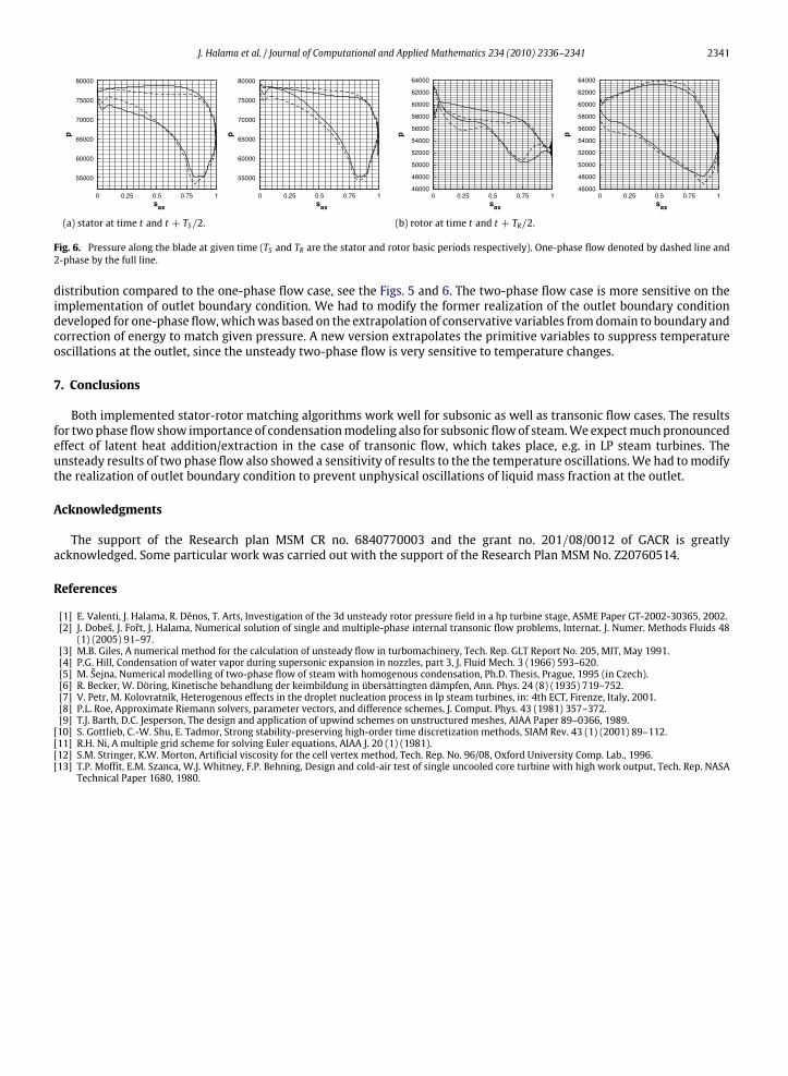
J. Halama et al. / Journal of Computational and Applied Mathematics 234 (2010) 2336–2341 2341

55000

60000

65000

70000

75000

80000

55000

60000

65000

70000

75000

80000

0 0.25 0.5 0.75 1sax

0 0.25 0.5 0.75 1sax

pp

48000

50000

52000

54000

56000

58000

60000

62000

0 0.25 0.5 0.75 1sax

p

46000

64000

48000

50000

52000

54000

56000

58000

60000

62000

0 0.25 0.5 0.75 1sax

p

46000

64000

(a) stator at time t and t + TS/2. (b) rotor at time t and t + TR/2.

Fig. 6. Pressure along the blade at given time (TS and TR are the stator and rotor basic periods respectively). One-phase flow denoted by dashed line and2-phase by the full line.

distribution compared to the one-phase flow case, see the Figs. 5 and 6. The two-phase flow case is more sensitive on theimplementation of outlet boundary condition. We had to modify the former realization of the outlet boundary conditiondeveloped for one-phase flow,whichwas based on the extrapolation of conservative variables fromdomain to boundary andcorrection of energy to match given pressure. A new version extrapolates the primitive variables to suppress temperatureoscillations at the outlet, since the unsteady two-phase flow is very sensitive to temperature changes.

7. Conclusions

Both implemented stator-rotor matching algorithms work well for subsonic as well as transonic flow cases. The resultsfor twophase flow show importance of condensationmodeling also for subsonic flowof steam.We expectmuch pronouncedeffect of latent heat addition/extraction in the case of transonic flow, which takes place, e.g. in LP steam turbines. Theunsteady results of two phase flow also showed a sensitivity of results to the the temperature oscillations.We had tomodifythe realization of outlet boundary condition to prevent unphysical oscillations of liquid mass fraction at the outlet.

Acknowledgments

The support of the Research plan MSM CR no. 6840770003 and the grant no. 201/08/0012 of GACR is greatlyacknowledged. Some particular work was carried out with the support of the Research Plan MSM No. Z20760514.

References

[1] E. Valenti, J. Halama, R. Dénos, T. Arts, Investigation of the 3d unsteady rotor pressure field in a hp turbine stage, ASME Paper GT-2002-30365, 2002.[2] J. Dobeš, J. Fořt, J. Halama, Numerical solution of single and multiple-phase internal transonic flow problems, Internat. J. Numer. Methods Fluids 48(1) (2005) 91–97.

[3] M.B. Giles, A numerical method for the calculation of unsteady flow in turbomachinery, Tech. Rep. GLT Report No. 205, MIT, May 1991.[4] P.G. Hill, Condensation of water vapor during supersonic expansion in nozzles, part 3, J. Fluid Mech. 3 (1966) 593–620.[5] M. Šejna, Numerical modelling of two-phase flow of steam with homogenous condensation, Ph.D. Thesis, Prague, 1995 (in Czech).[6] R. Becker, W. Döring, Kinetische behandlung der keimbildung in übersättingten dämpfen, Ann. Phys. 24 (8) (1935) 719–752.[7] V. Petr, M. Kolovratník, Heterogenous effects in the droplet nucleation process in lp steam turbines, in: 4th ECT, Firenze, Italy, 2001.[8] P.L. Roe, Approximate Riemann solvers, parameter vectors, and difference schemes, J. Comput. Phys. 43 (1981) 357–372.[9] T.J. Barth, D.C. Jesperson, The design and application of upwind schemes on unstructured meshes, AIAA Paper 89–0366, 1989.[10] S. Gottlieb, C.-W. Shu, E. Tadmor, Strong stability-preserving high-order time discretization methods, SIAM Rev. 43 (1) (2001) 89–112.[11] R.H. Ni, A multiple grid scheme for solving Euler equations, AIAA J. 20 (1) (1981).[12] S.M. Stringer, K.W. Morton, Artificial viscosity for the cell vertex method, Tech. Rep. No. 96/08, Oxford University Comp. Lab., 1996.[13] T.P. Moffit, E.M. Szanca, W.J. Whitney, F.P. Behning, Design and cold-air test of single uncooled core turbine with high work output, Tech. Rep. NASA

Technical Paper 1680, 1980.