Validating and Modeling of Steam TurbineTemperature Distribution for Different

Operational Cases

Sebastian Sporre

Thesis for the Degree of Master of Science

Thesis Advisor: Magnus Genrup and Oskar Mazur

Thesis Examiner: Marcus Thern

2

"I’ve believed in the Toronto Maple Leafs my entire life. The least you could do is believe inyourself"

Steve Dangle Glynn

This thesis for the degree of Master of Science in Engineering has been conducted at theDivision of Thermal Power Engineering, Department of Energy Sciences, Lunds TekniskaHögskola (LTH) – Lund University (LU) and at Siemens Industrial Turbomachinery AB (SITAB).

Supervisor at SIT AB: Oskar Mazur;Supervisor at LU-LTH: Professor Magnus Genrup;Examiner at LU-LTH: Associate Professor Marcus Thern.

Abstract

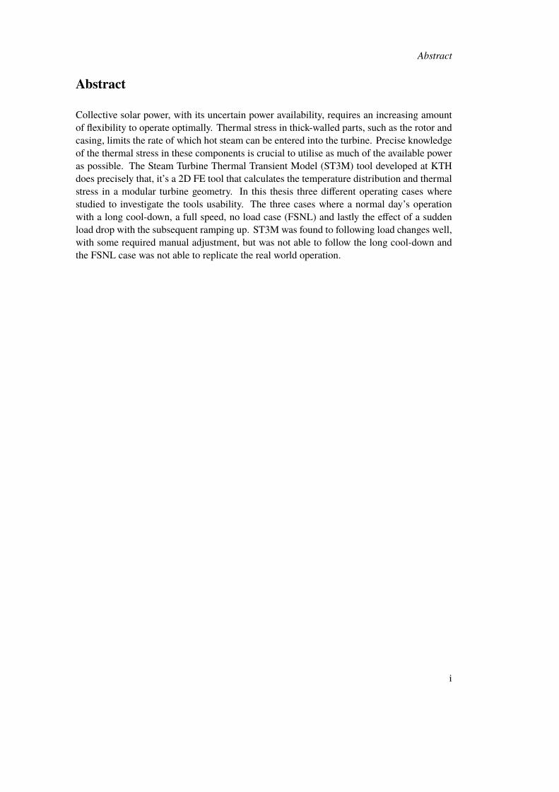
Abstract

Collective solar power, with its uncertain power availability, requires an increasing amountof flexibility to operate optimally. Thermal stress in thick-walled parts, such as the rotor andcasing, limits the rate of which hot steam can be entered into the turbine. Precise knowledgeof the thermal stress in these components is crucial to utilise as much of the available poweras possible. The Steam Turbine Thermal Transient Model (ST3M) tool developed at KTHdoes precisely that, it’s a 2D FE tool that calculates the temperature distribution and thermalstress in a modular turbine geometry. In this thesis three different operating cases wherestudied to investigate the tools usability. The three cases where a normal day’s operationwith a long cool-down, a full speed, no load case (FSNL) and lastly the effect of a suddenload drop with the subsequent ramping up. ST3M was found to following load changes well,with some required manual adjustment, but was not able to follow the long cool-down andthe FSNL case was not able to replicate the real world operation.

i

Nomenclature

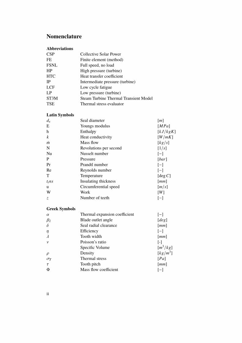
AbbreviationsCSP Collective Solar PowerFE Finite element (method)FSNL Full speed, no loadHP High pressure (turbine)HTC Heat transfer coefficientIP Intermediate pressure (turbine)LCF Low cycle fatigueLP Low pressure (turbine)ST3M Steam Turbine Thermal Transient ModelTSE Thermal stress evaluator

Latin Symbolsds Seal diameter [m]E Youngs modulus [MPa]h Enthalpy [k J/kgK]k Heat conductivity [W/mK]Ûm Mass flow [kg/s]N Revolutions per second [1/s]Nu Nusselt number [−]P Pressure [bar]Pr Prandtl number [−]Re Reynolds number [−]T Temperature [deg C]tins Insulating thickness [mm]u Circumferential speed [m/s]W Work [W]z Number of teeth [−]

Greek Symbolsα Thermal expansion coefficient [−]β2 Blade outlet angle [deg]δ Seal radial clearance [mm]η Efficiency [−]λ Tooth width [mm]ν Poisson’s ratio [-]

Specific Volume [m3/kg]ρ Density [kg/m3]σT Thermal stress [Pa]τ Tooth pitch [mm]Φ Mass flow coefficient [−]

ii

Contents

Abstract . . . . . . . . . . . . . . . . . . . . . . . . . . . . . . . . . . . . . . . iNomenclature . . . . . . . . . . . . . . . . . . . . . . . . . . . . . . . . . . . . ii

1 Introduction 11.1 Objectives . . . . . . . . . . . . . . . . . . . . . . . . . . . . . . . . . . . 2

2 Theory 32.1 Steam turbine fundamentals . . . . . . . . . . . . . . . . . . . . . . . . . 32.2 Thermal stress . . . . . . . . . . . . . . . . . . . . . . . . . . . . . . . . . 52.3 Start-up curves . . . . . . . . . . . . . . . . . . . . . . . . . . . . . . . . 72.4 Thermal Expansion . . . . . . . . . . . . . . . . . . . . . . . . . . . . . . 82.5 Concentrated solar power plants . . . . . . . . . . . . . . . . . . . . . . . 92.6 Flexibility . . . . . . . . . . . . . . . . . . . . . . . . . . . . . . . . . . . 12

3 Steam Turbine Thermal Transient Model 153.1 Steam expansion model . . . . . . . . . . . . . . . . . . . . . . . . . . . . 173.2 Gland steam sealing model . . . . . . . . . . . . . . . . . . . . . . . . . . 193.3 Heat transfer calculations . . . . . . . . . . . . . . . . . . . . . . . . . . . 21

3.3.1 Modular geometry and material properties . . . . . . . . . . . . . . 213.3.2 Boundary conditions . . . . . . . . . . . . . . . . . . . . . . . . . 22

3.4 Finite element thermo-mechanical model . . . . . . . . . . . . . . . . . . 27

4 Results 294.1 Daily Operation Case . . . . . . . . . . . . . . . . . . . . . . . . . . . . . 294.2 Full Speed, No Load Case . . . . . . . . . . . . . . . . . . . . . . . . . . 324.3 Load Drop . . . . . . . . . . . . . . . . . . . . . . . . . . . . . . . . . . . 34

5 Discussion and conclusion 41

iii

Chapter 1

Introduction

Todays energy market requires more and more flexible generation, both heat and electricity.This is especially true for collective solar power, where at least one startup of the turbine isrequired each day but it is also true for previously baseload plants that now has been forcedinto more and more cyclical use due to the penetration of intermittent renewable energysources. Thermal stress in thick-walled components is the most limiting factor to allow forfaster start-ups, this demands greater and greater knowledge from the turbine manufacturerto be confident in pushing the limits of the turbines. Accurate knowledge of the exact thermalstress in the turbine is critical to maximize the usage of the turbine during its lifetime andthe tools to analyze this is of much importance. The Concentrating Solar Power and Techno-Economic Analysis Group as a part of the Department of Energy at KTH has developed atool for just that, called ST3M. This is a MATLAB based code that utilizes the multi-physicsprogram COMSOL to create a 2D axissymmetric model of a turbine in order to calculate thethermo-mechanic properties of the modeled turbine.

This was used to run three different cases of operation:

1. Operation during one day based on measured inlet data with a cool-down equal to oneweekend

2. A unique case where the mass flow unintentionally was restricted and heat was gener-ated due to friction and ventilation

3. The effect of sudden load drops associated with clouds in solar power plants

All the cases studied were based on the same high pressure turbine and therefore the geometri-cal modeling aspect of the code was not studied, the geometry of the turbine was provided bypreviously completed studies. In all three cases the heat transfer coefficients were calculatedwith the built-in theoretical equations found in literature, however the tool is equipped tohandle pre-determined heat transfer coefficients from manufacturers. The boundary condi-tions was fairly similar for the first and third case, with the most common thermal boundarycondition being that of convection. However for the second case where no live steam wasintroduced, no convection can occur and radiation instead took its place.

1

Chapter 1 Introduction

1.1 Objectives

The objectives for this master thesis is to:

• Validate ST3M against operational data and Full Speed, No load case

• Calculate temperature differences in major components during sudden load drop andsubsequent ramping

• Evaluate industrial usefulness of the ST3M code

The first to cases was run as validating cases, while the second one presented results to theindustry for evaluation. However due to the time-line of this thesis, there was not enoughtime in this thesis or by Siemens to fully evaluate the results. The industrial usefulnesses wasevaluated throughout the thesis gathered from the experience with using the tool.

2

Chapter 2

Theory

2.1 Steam turbine fundamentals

We classify turbo machines as a device that transfers energy either to or from a continuouslyflowing fluid. This is a rather large field of machines that stretches to everything from yourordinary desk fan, to pumps, to wind power plants and to steam turbines which will be thefocus of this thesis. [1]

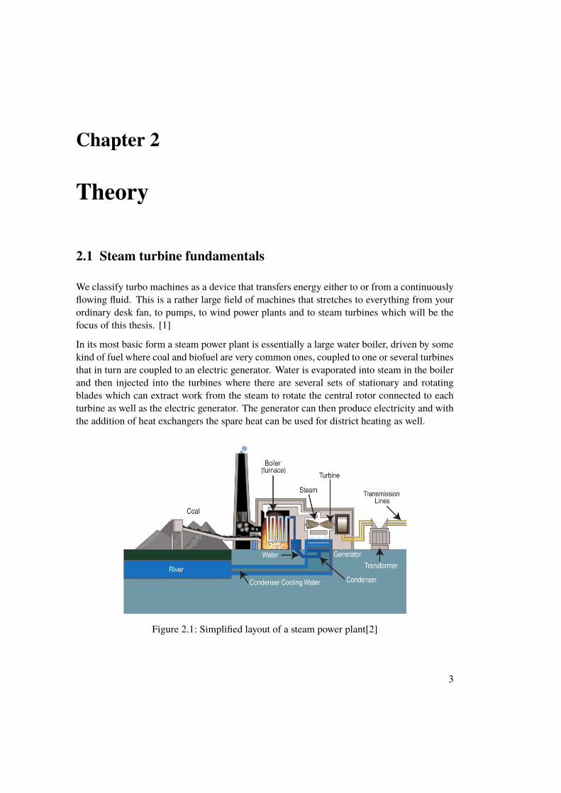
In its most basic form a steam power plant is essentially a large water boiler, driven by somekind of fuel where coal and biofuel are very common ones, coupled to one or several turbinesthat in turn are coupled to an electric generator. Water is evaporated into steam in the boilerand then injected into the turbines where there are several sets of stationary and rotatingblades which can extract work from the steam to rotate the central rotor connected to eachturbine as well as the electric generator. The generator can then produce electricity and withthe addition of heat exchangers the spare heat can be used for district heating as well.

Figure 2.1: Simplified layout of a steam power plant[2]

3

Chapter 2 Theory

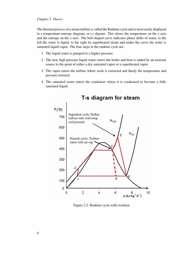
The thermal process of a steam turbine is called the Rankine cycle and is most easily displayedin a temperature-entropy diagram, or t-s digram. This shows the temperature on the y axisand the entropy on the x axis. The bell-shaped curve indicates phase shifts of water, to theleft the water is liquid, to the right its superheated steam and under the curve the water issaturated liquid-vapor. The four steps in the rankine cycle are:

1. The liquid water is pumped to a higher pressure

2. The now high pressure liquid water enters the boiler and heat is added by an externalsource to the point of either a dry saturated vapor or a superheated vapor

3. The vapor enters the turbine where work is extracted and thusly the temperature andpressure lowered

4. The saturated water enters the condenser where it is condensed to become a fullysaturated liquid.

Figure 2.2: Rankine cycle with overheat

4

2.2 Thermal stress

2.2 Thermal stress

There is an ever-growing demand on steam turbines’ flexibility, their ability to start quickerand handle faster load change rates. What has traditionally limited a faster start-up is theincreased thermal stress that would occur due to inducing a high temperature difference.Start-ups in turbines are usually categorized in three temperature regions:

• Cold starts with an outage of more than 72 hours or a metal temperature not exceeding160°C

• Warm starts with an outage of between 10-72 hours or metal temperature between160-400°C

• Hot starts with an outage of less than 10 hours or a metal temperature exceeding 400°C

There is also something called ambient starts which is exceedingly rare and occurs after amajor outage or when the metal temperature is below 50°C. Hot starts are often associatedwith the turbine being turned off during the night for non-baseload plants, while warm startsis associated with being turned off over the weekend. To stay within the allowed rangeof thermal stresses the cold starts takes the longest time with about 75-150 minutes for a450 MW combined cycle plant, 75-110 minutes for warm starts and 40-50 minutes for hotstarts.[3]

The importance of the difference in metal temperature in the turbine is because of the sourceof thermal stresses, which can be found to be proportional to the temperature difference overthe thick-walled parts of the turbine. During operation the rotor of the turbine will heat up toa temperature roughly equal to the inlet steam temperature at the inlet side of the rotor, whenthe turbine trips or is unloaded the rotor will cool down. When steam then is reintroducedduring start-up the difference between the hot inlet steam and the now cooled off rotor willcause high thermal stresses in the metal of the rotor. The same happens in the thick walls ofthe turbine casing which is often seen as the main limiting components in regards to turbinestart-ups. [4]

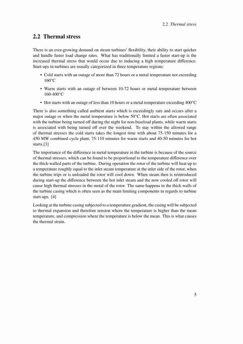
Looking at the turbine casing subjected to a temperature gradient, the casing will be subjectedto thermal expansion and therefore tension where the temperature is higher than the meantemperature, and compression where the temperature is below the mean. This is what causesthe thermal strain.

5

Chapter 2 Theory

Figure 2.3: Thermal strain[5]

If the casing is seen as thin-walled, the induced temperature difference can be translated tothermal stresses with equation 2.1. However this is a simplification compared to reality andfor more accurate calculations finite element calculations are applied.[5]

σT =α ∗ E1 − ν ∆T (2.1)

Where σT is the induced thermal stresses and ∆T is the temperature difference. α is thethermal expansion coefficient, ν is the Poisson’s ratio and E is the elasticity module and areall material properties. This means that a higher starting temperature of the thick-walledcomponents will, for the acceptable thermal stress, allow for a higher temperature of the inletsteam. The closer the temperature of the inlet steam is to the nominal value the shorter thestartup time will become.

The thermal stresses generated will unavoidably consume the lifetime of the turbine and willin the end always lead to cracks and eventually failure. Due to the lifetime of the turbine andthe expected number of starts this is usually categorized as low cycle fatigue (LCF), whichis defined as a component failing due to repetitive stresses in less than 100 000 cycles.[4]Depending on the intended usage, the startup can be designed to be more aggressive and inturn consume more lifetime per start. However the lifetime is designed, the thermal stressesintroduced in the turbine will cause performance deterioration before reaching the end of thelifetime. The efficiency of the turbine will slowly deteriorate caused by several factors, oneexample being an increased leakage in the steam path caused by rubbing of the seals.

When converting thermal stresses to consumption in life time one of the simplest and

6

2.3 Start-up curves

most straight-forward models is the Palmgren-Miner’s rule, which is a cumulative damagemodel:

k∑i=1

niNi= 1 (2.2)

It states that there are k number of different stress levels, Ni is the average number of cyclesuntil failure at a specific stress level and ni is the number of cycles accumulated at this stresslevel, when the total sum of all fractions reaches 1 failure will occur. For example, if it isknown that a component will fail after 500 cycles at 10 MPa, we know that after 250 cyclesat 10 MPa half of the lifetime has been consumed. If the stress is instead reduced to 5 MPafrom 10 MPa, according to Palmgren-Miner failure will occur at 1000 cycles instead. If halfthe lifetime has been consumed by running 250 cycles at 10 MPa, only 500 cycles at 5 MPais needed to reach failure.[6]

2.3 Start-up curves

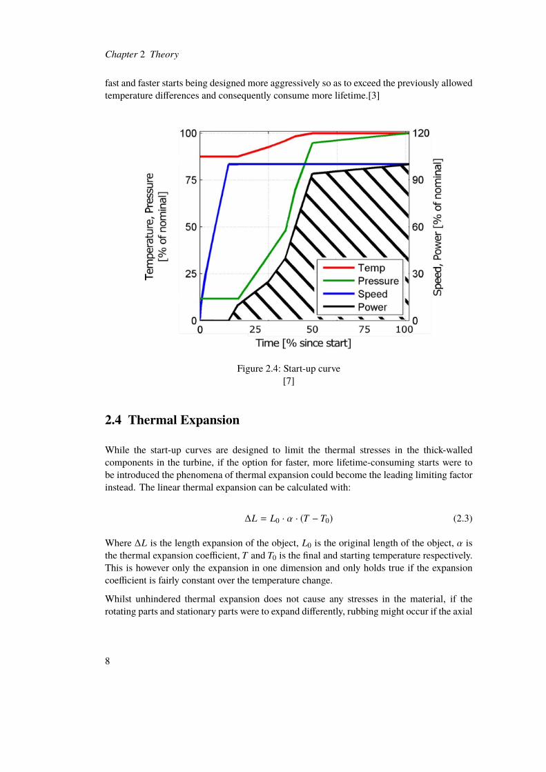
Depending on the designed number of starts certain thermal stresses and in turn temperaturedifferences are allowed. The measure with which the manufacturers of turbines control theallowed range is start-up curves, which typically defines the rotational speed of the rotor, theinlet pressure, temperature and the subsequent power produced. A typical start-up curve isshown in figure 2.4. To be noted is that this would be just one of many start-up curves for onespecific turbine, there would be several start-up curves for each starting state (cold, warm,hot) for each specific steam turbine. Since there is however a finite amount of startup curves,they are a compromise of sorts. There is not one startup curve for every single temperature,but instead one specific curve covers a span of temperatures. If the actual temperature is inthe lower end of of this span, the curve is in reality over-conservative and isn’t utilizing thefull potential of the acceptable thermal stress. This means the turbine is starting slower thanit has too and takes longer to reach nominal power, which means the operator stands to losepotential profit.

One technology to help do away with the old system of start-up curves are thermal stressevaluators (TSE) which measures the temperature of the casing and a non-rotating point inclose proximity to the rotor directly. The temperature in the rotor is calculated from thesecond measurement and heat conduction equations. The TSE can then directly control theturbine to stay close to, but under the allowed temperature range. This technology wouldrender the start-up curves obsolete for all types of starts, except as last resort backups. As aresult of introducing TSE not only would it always utilize the full potential during every start,it would also open up opportunities to give the operator more control over the time neededfor the start-up with the choice of several start-up speeds but at the cost of more lifetimeconsumption per start. This would present the option of a normal, fast, faster start with the

7

Chapter 2 Theory

fast and faster starts being designed more aggressively so as to exceed the previously allowedtemperature differences and consequently consume more lifetime.[3]

Figure 2.4: Start-up curve[7]

2.4 Thermal Expansion

While the start-up curves are designed to limit the thermal stresses in the thick-walledcomponents in the turbine, if the option for faster, more lifetime-consuming starts were tobe introduced the phenomena of thermal expansion could become the leading limiting factorinstead. The linear thermal expansion can be calculated with:

∆L = L0 · α · (T − T0) (2.3)

Where ∆L is the length expansion of the object, L0 is the original length of the object, α isthe thermal expansion coefficient, T and T0 is the final and starting temperature respectively.This is however only the expansion in one dimension and only holds true if the expansioncoefficient is fairly constant over the temperature change.

Whilst unhindered thermal expansion does not cause any stresses in the material, if therotating parts and stationary parts were to expand differently, rubbing might occur if the axial

8

2.5 Concentrated solar power plants

and radial clearances are not large enough. This would reduce the lifetime of the componentsexperiencing the rubbing and could quickly lead to machine failure. While today turbinemanufacturers set clearances large enough to handle the thermal expansion caused by thethermal gradients during start-up operation, an introduction of more aggressive start-upsmight cause rubbing in the pre-existing turbines with already set clearances. This would notbe a problem for newly produced turbines designed for this new technology though, since theclearances can be set to handle the faster start-ups. Whether or not this relative expansionwill create problems is not a well researched topic although some studies have shown it mightcause problems. [8]

2.5 Concentrated solar power plants

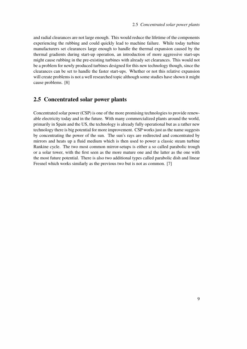
Concentrated solar power (CSP) is one of the more promising technologies to provide renew-able electricity today and in the future. With many commercialized plants around the world,primarily in Spain and the US, the technology is already fully operational but as a rather newtechnology there is big potential for more improvement. CSP works just as the name suggestsby concentrating the power of the sun. The sun’s rays are redirected and concentrated bymirrors and heats up a fluid medium which is then used to power a classic steam turbineRankine cycle. The two most common mirror-setups is either a so called parabolic troughor a solar tower, with the first seen as the more mature one and the latter as the one withthe most future potential. There is also two additional types called parabolic dish and linearFresnel which works similarly as the previous two but is not as common. [7]

9

Chapter 2 Theory

Figure 2.5(a) Parabolic Trough (b)Power Tower (c) Parabolic Dish (d) Linear Fresnel[7]

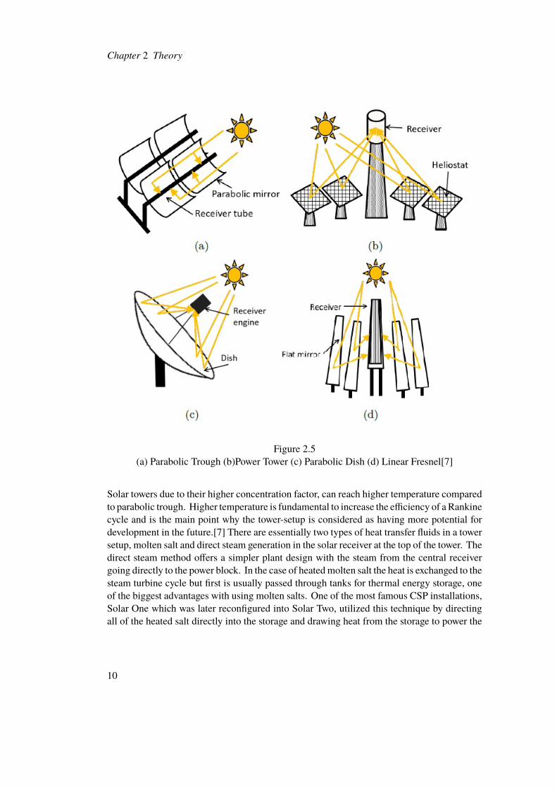
Solar towers due to their higher concentration factor, can reach higher temperature comparedto parabolic trough. Higher temperature is fundamental to increase the efficiency of a Rankinecycle and is the main point why the tower-setup is considered as having more potential fordevelopment in the future.[7] There are essentially two types of heat transfer fluids in a towersetup, molten salt and direct steam generation in the solar receiver at the top of the tower. Thedirect steam method offers a simpler plant design with the steam from the central receivergoing directly to the power block. In the case of heatedmolten salt the heat is exchanged to thesteam turbine cycle but first is usually passed through tanks for thermal energy storage, oneof the biggest advantages with using molten salts. One of the most famous CSP installations,Solar One which was later reconfigured into Solar Two, utilized this technique by directingall of the heated salt directly into the storage and drawing heat from the storage to power the

10

2.5 Concentrated solar power plants

turbine. This decouples the heat generation from the electricity generation which provideshigher availability of electricity. [9] Today typical storage sizes are about 8-12 hours to coverthe production during nighttime.[7]

Figure 2.6Solar Two setup with two tank molten-salt storage.[9]

The largest CSP plant in operation today is the Ivanpah Solar Facility, it has a gross capacity of392 MW. It has a direct steam configuration with no storage powered by a Siemens SST-900steam turbine and consists of 173 500 heliostats with two mirrors on each heliostats. It islocated outside the townof Primm inCalifornia, close to the state border toNevada.[10]

11

Chapter 2 Theory

Figure 2.7Ivanpah Solar Power Plant.[11]

CSP operation is a heavy cyclical one, with startup and shutdown at least once every day,compared to a few times a year for large base-load plants. In the base-load combined cycleplants the loading rates and main steam parameters are all controllable and can be kept underthe allowed maximum limit, this is not possible in the same way for a weather dependentsolar tower plant. Modern steam turbines can handle cycling operation relatively well but it’sstill one of the most intricate parts of turbine operation and will need further developmentand adaption to CSP-specific usage.[12]

2.6 Flexibility

With the introduction of an increasing penetration of intermittent renewable energy sourcesthe future need for steam turbines ability to adapt for more flexible operation will increaseas well. While steam turbines has historically been used for base load operation, the non-dispatchability of solar andwind energy production forces steam turbine to entermore cyclicaloperation. This is due both to the usage of steam turbines in concentrated solar plants whichis highly cyclical in nature but mainly due to current steam turbine power plants being usedto meet the demand when renewable productions drops. These steam turbines would have toadapt the cyclical nature of the renewable energy sources.

Flexibility, though, is not a simple one-type attribute. It can instead be seen as a spectrumof different attributes categorized by its response time, from practically instantaneous to

12

2.6 Flexibility

long-term, yearly response times. Flexibility can then be categorized in five major types,namely:

1. Spinning reserve and load following

2. Short-term reserve

3. Ramping

4. Daily balancing

5. Seasonal balancing

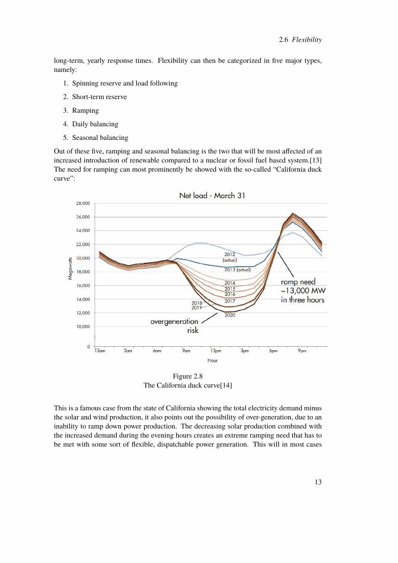
Out of these five, ramping and seasonal balancing is the two that will be most affected of anincreased introduction of renewable compared to a nuclear or fossil fuel based system.[13]The need for ramping can most prominently be showed with the so-called “California duckcurve”:

Figure 2.8The California duck curve[14]

This is a famous case from the state of California showing the total electricity demand minusthe solar and wind production, it also points out the possibility of over-generation, due to aninability to ramp down power production. The decreasing solar production combined withthe increased demand during the evening hours creates an extreme ramping need that has tobe met with some sort of flexible, dispatchable power generation. This will in most cases

13

Chapter 2 Theory

fall upon the steam turbine facilities already in use. While this is an extreme case wherethe demand increases and production decreases almost simultaneously, it could very wellbe close to reality in most developed countries with a high penetration of renewable energyproduction in the near future. [14] The new generation of steam turbines designed to tacklethis problemwould not only have to have very high efficiency during all types of operation butwould also have to be much more flexible in their operation compared to previous iterations.This seems to be the most difficult obstacle facing the industry today.

14

Chapter 3

Steam Turbine Thermal TransientModel

Turbine stresses and in turn the degradation of life time in the turbine derives from the thermaltransients in the material. During a transient start-up operation an uneven temperature distri-bution would be created. Without a sufficiently accurate model, predicting the temperaturedistribution would be very difficult and therefore a model was developed at KTH, namedSteam Turbine Thermal Transient Model (ST3M).

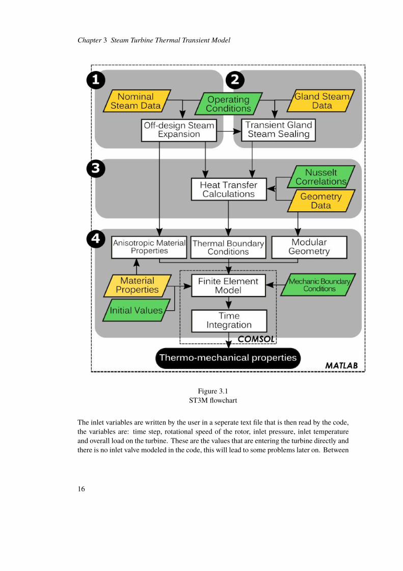
The model uses the program COMSOL and its coupling with MATLAB, with the codebeing written in MATLAB and calling COMSOL to execute the finite element calculations.ST3M creates a 2D axisymmetric modular geometry modeled after the turbines studied andcalculates the metal temperature distribution in the turbine and other thermo-mechanicalproperties like thermal stresses and thermal induced expansion. ST3M consists of four mainsub-models:

1. Steam expansion model - Calculates the temperature and mass flow of the live steam

2. Gland steam sealing model - Calculates the gland coefficients and steam flow throughthe glands

3. Heat transfer calculations - Either calculates HTCs from theoretical correlations oradjusts HTCs provided by the manufacturer

4. Finite element thermo-mechanical model - Calls COMSOL to handle the finite elementcalculations and determines the temperature distribution and other thermo-mechanicalattributes

The flow chart of the model can be shown in Figure 3.1, where the white boxes indicatescalculating steps with no user input. The skewed rectangles indicates user inputs where theyellow ones are determined by design factors usually provided by the turbine manufacturerand the green ones relates to operational decisions.

15

Chapter 3 Steam Turbine Thermal Transient Model

Figure 3.1ST3M flowchart

The inlet variables are written by the user in a seperate text file that is then read by the code,the variables are: time step, rotational speed of the rotor, inlet pressure, inlet temperatureand overall load on the turbine. These are the values that are entering the turbine directly andthere is no inlet valve modeled in the code, this will lead to some problems later on. Between

16

3.1 Steam expansion model

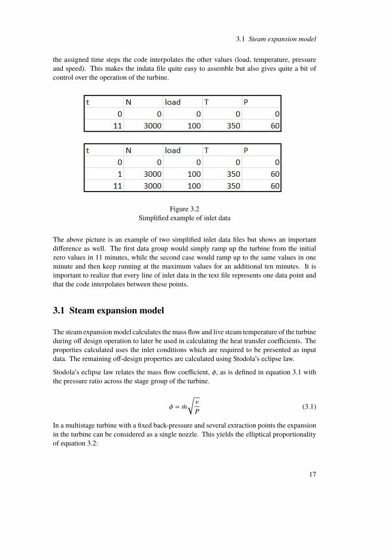
the assigned time steps the code interpolates the other values (load, temperature, pressureand speed). This makes the indata file quite easy to assemble but also gives quite a bit ofcontrol over the operation of the turbine.

Figure 3.2Simplified example of inlet data

The above picture is an example of two simplified inlet data files but shows an importantdifference as well. The first data group would simply ramp up the turbine from the initialzero values in 11 minutes, while the second case would ramp up to the same values in oneminute and then keep running at the maximum values for an additional ten minutes. It isimportant to realize that every line of inlet data in the text file represents one data point andthat the code interpolates between these points.

3.1 Steam expansion model

The steam expansionmodel calculates themass flow and live steam temperature of the turbineduring off design operation to later be used in calculating the heat transfer coefficients. Theproperties calculated uses the inlet conditions which are required to be presented as inputdata. The remaining off-design properties are calculated using Stodola’s eclipse law.

Stodola’s eclipse law relates the mass flow coefficient, φ, as is defined in equation 3.1 withthe pressure ratio across the stage group of the turbine.

φ = Ûm√ν

P(3.1)

In a multistage turbine with a fixed back-pressure and several extraction points the expansionin the turbine can be considered as a single nozzle. This yields the elliptical proportionalityof equation 3.2:

17

Chapter 3 Steam Turbine Thermal Transient Model

φ ∝

√1 −

(Pin

Pout

)2(3.2)

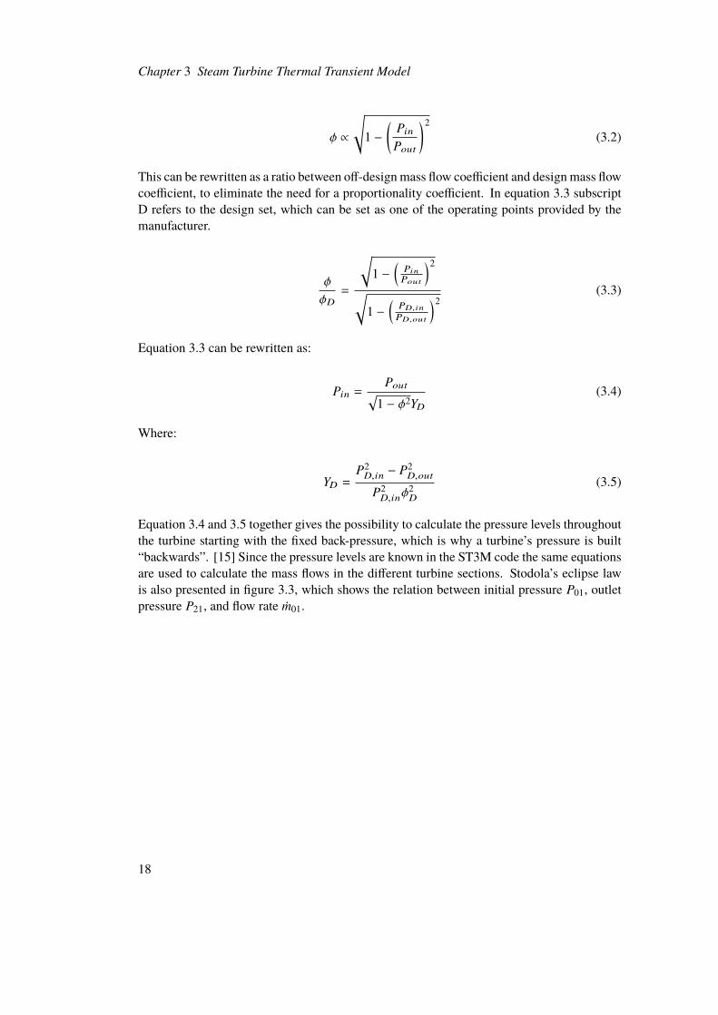
This can be rewritten as a ratio between off-design mass flow coefficient and design mass flowcoefficient, to eliminate the need for a proportionality coefficient. In equation 3.3 subscriptD refers to the design set, which can be set as one of the operating points provided by themanufacturer.

φ

φD=

√1 −

(Pin

Pout

)2√1 −

(PD, in

PD,out

)2(3.3)

Equation 3.3 can be rewritten as:

Pin =Pout√

1 − φ2YD(3.4)

Where:

YD =P2D,in − P2

D,out

P2D,inφ

2D

(3.5)

Equation 3.4 and 3.5 together gives the possibility to calculate the pressure levels throughoutthe turbine starting with the fixed back-pressure, which is why a turbine’s pressure is built“backwards”. [15] Since the pressure levels are known in the ST3M code the same equationsare used to calculate the mass flows in the different turbine sections. Stodola’s eclipse lawis also presented in figure 3.3, which shows the relation between initial pressure P01, outletpressure P21, and flow rate Ûm01.

18

3.2 Gland steam sealing model

Figure 3.3Stodola’s elliptical cone

The Stodola law only applies for expansion under adiabatic conditions however. This isnot the case and therefore the isentropic efficiency needs to be calculated. The isentropicefficiency of the steam expansion is calculatedwith equation 3.6. ηs,0 is the nominal isentropicefficiency, N is the off-design rotational speed and ∆h is the off-design enthalpy difference.The subscript “0” denotes the nominal operational values of the same properties.

ηs = ηs,0 − 2 ©­« NN0

√∆hs,0

∆hs− 1ª®¬

2

(3.6)

All of these steam properties together with the efficiency are later used as input into the glandsteam sub-model as well as in the heat transfer calculations. The conductivity will be usedin the definition of the anisotropic material properties of the inner parts of the turbine. Themass flow will be used together with the steam temperatures to help define the boundaryconditions in the blade passage of the turbine.

3.2 Gland steam sealing model

In the studied turbine and all turbines previously studied utilizing the ST3M code, labyrinthgland seals has been used to stop external air from leaking into the system and also stopinternal steam leaking out. One labyrinth seal is located at each end of the rotor shaft andworks in the way that it creates a long and, for the steam, hard to maneuver channel made upof many teeth. The steam expansion in the seals is a case of throttling with alternating wide

19

Chapter 3 Steam Turbine Thermal Transient Model

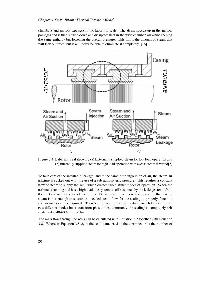
chambers and narrow passages in the labyrinth seals. The steam speeds up in the narrowpassages and is then slowed down and dissipates heat in the wide chamber, all while keepingthe same enthalpy but lowering the overall pressure. This limits the amount of steam thatwill leak out from, but it will never be able to eliminate it completely. [16]

(a) (b)

Figure 3.4: Labyrinth seal showing (a) Externally supplied steam for low load operation and(b) Internally supplied steam for high load operationwith excess steam diverted[7]

To take care of the inevitable leakage, and at the same time ingression of air, the steam-airmixture is sucked out with the use of a sub-atmospheric pressure. This requires a constantflow of steam to supply the seal, which creates two distinct modes of operation. When theturbine is running and has a high load, the system is self sustained by the leakage steam fromthe inlet and outlet section of the turbine. During start up and low load operation the leakingsteam is not enough to sustain the needed steam flow for the sealing to properly function,so external steam is required. There’s of course not an immediate switch between thesetwo different modes but a transition phase, most commonly the sealing is completely selfsustained at 40-60% turbine load.

The mass flow through the seals can be calculated with Equation 3.7 together with Equation3.8. Where in Equation 3.8 ds is the seal diameter, δ is the clearance, z is the number of

20

3.3 Heat transfer calculations

teeth, τ is the tooth pitch and λ is the tooth width.

Ûmleak = Cseal

√Pin

vin

√1 −

(Pin

Pout

)2(3.7)

Cseal =π · ds · δ · Ks(δ, τ, z) · µ(δ, λ)√

z(3.8)

3.3 Heat transfer calculations

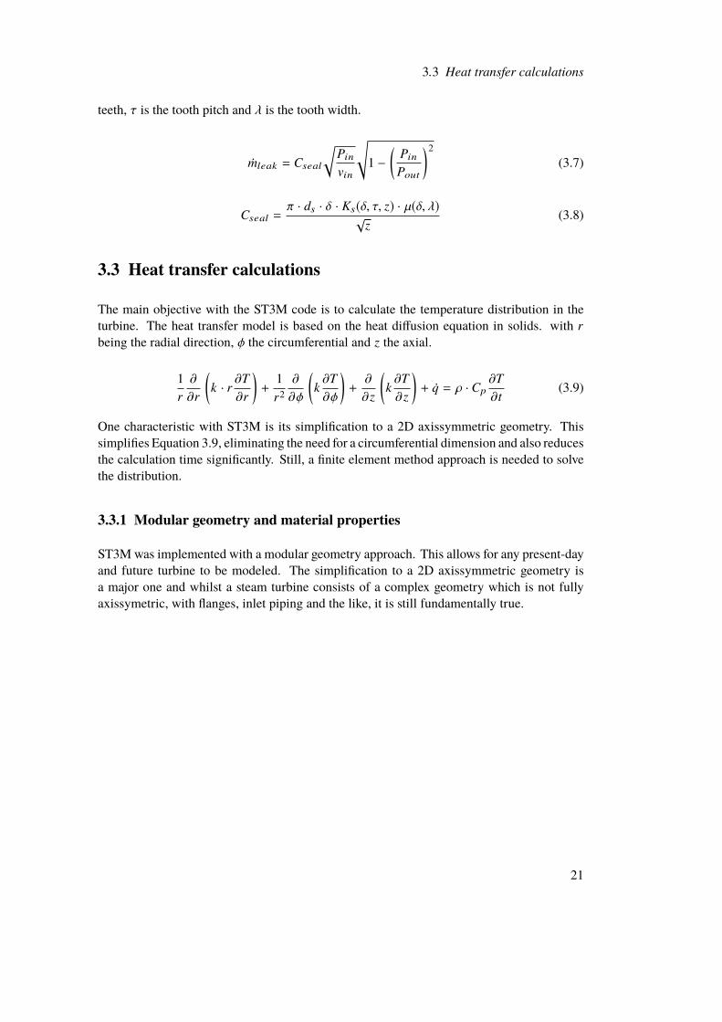
The main objective with the ST3M code is to calculate the temperature distribution in theturbine. The heat transfer model is based on the heat diffusion equation in solids. with rbeing the radial direction, φ the circumferential and z the axial.

1r∂

∂r

(k · r ∂T

∂r

)+

1r2

∂

∂φ

(k∂T∂φ

)+∂

∂z

(k∂T∂z

)+ Ûq = ρ · Cp

∂T∂t

(3.9)

One characteristic with ST3M is its simplification to a 2D axissymmetric geometry. Thissimplifies Equation 3.9, eliminating the need for a circumferential dimension and also reducesthe calculation time significantly. Still, a finite element method approach is needed to solvethe distribution.

3.3.1 Modular geometry and material properties

ST3Mwas implemented with a modular geometry approach. This allows for any present-dayand future turbine to be modeled. The simplification to a 2D axissymmetric geometry isa major one and whilst a steam turbine consists of a complex geometry which is not fullyaxissymetric, with flanges, inlet piping and the like, it is still fundamentally true.

21

Chapter 3 Steam Turbine Thermal Transient Model

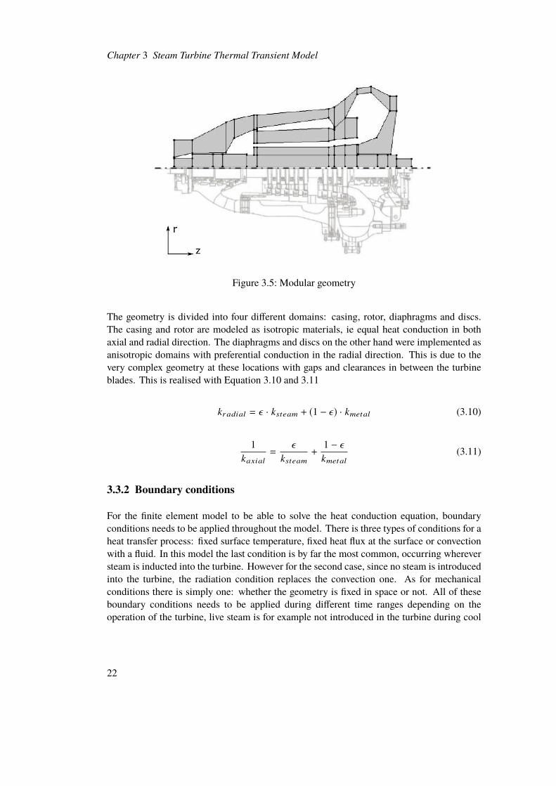
Figure 3.5: Modular geometry

The geometry is divided into four different domains: casing, rotor, diaphragms and discs.The casing and rotor are modeled as isotropic materials, ie equal heat conduction in bothaxial and radial direction. The diaphragms and discs on the other hand were implemented asanisotropic domains with preferential conduction in the radial direction. This is due to thevery complex geometry at these locations with gaps and clearances in between the turbineblades. This is realised with Equation 3.10 and 3.11

kradial = ε · ksteam + (1 − ε) · kmetal (3.10)

1kaxial

=ε

ksteam+

1 − εkmetal

(3.11)

3.3.2 Boundary conditions

For the finite element model to be able to solve the heat conduction equation, boundaryconditions needs to be applied throughout the model. There is three types of conditions for aheat transfer process: fixed surface temperature, fixed heat flux at the surface or convectionwith a fluid. In this model the last condition is by far the most common, occurring whereversteam is inducted into the turbine. However for the second case, since no steam is introducedinto the turbine, the radiation condition replaces the convection one. As for mechanicalconditions there is simply one: whether the geometry is fixed in space or not. All of theseboundary conditions needs to be applied during different time ranges depending on theoperation of the turbine, live steam is for example not introduced in the turbine during cool

22

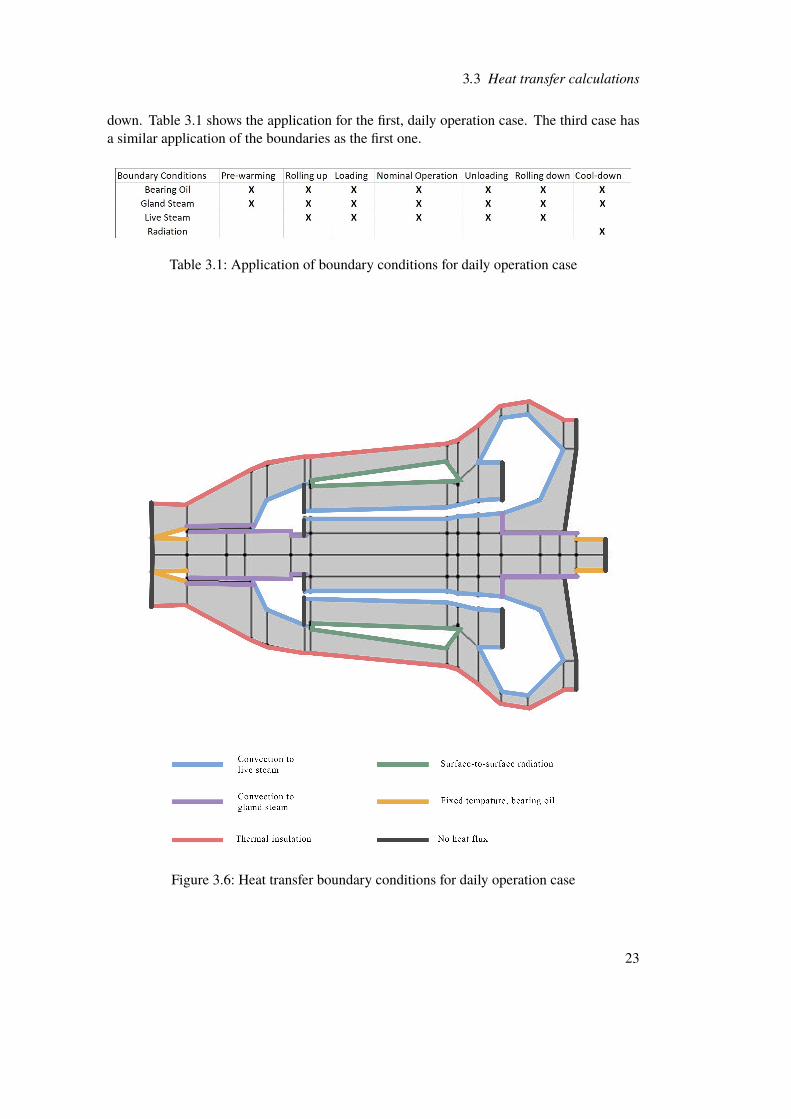
3.3 Heat transfer calculations

down. Table 3.1 shows the application for the first, daily operation case. The third case hasa similar application of the boundaries as the first one.

Table 3.1: Application of boundary conditions for daily operation case

Figure 3.6: Heat transfer boundary conditions for daily operation case

23

Chapter 3 Steam Turbine Thermal Transient Model

Convection to gland steam The mode of the glands (self sustained or externally supplied)is handled by the code automatically during the operation of the turbine. However whenrunning a long cool down the vacuum of the turbine can be broken and air be allowed toleak in through the gland seals, this was not done in any of the cases studied here though.During the operation of the first two modes the convection boundary condition is active and,if a cool down is studied, is turned off at a specific time step (usually about 5-10 hours afterunloading the turbine). Due to the difference in leaked mass flow in the different parts of thelabyrinth seals, different HTCs were needed. This was handled by splitting the gland sealsin different sections and assigning them different HTCs. The HTC for the gland seals werecalculated using equation 3.12 where H is the height of expanding steam and δ is the radialclearance.

Nu = 0.476 ·(

Hδ

)−0.56· Re0.7 · Pr0.43 (3.12)

Bearing oil The boundaries related to the bearings are determined with a fixed temperatureboundary condition. This is active during all of the operation of the turbine. Relatively coldoil is introduced to the bearings but as the transient commences the temperature is assumedto increase dependent on the square of the rotational speed, due to the increase in friction.Still, the oil cannot get too hot and common industrial practise is to cool the oil when thetemperature reaches a set value as to avoid kindling temperature. This leads to a lower andupper temperature limit on the oil being introduced.

Toil = TOFFoil +

(TONoil − TOFF

oil

)· N2 (3.13)

Thermal insulation The casing of all turbines are insulated with some sort of insulatingmaterial. This is a cheap, permanent way to keep the turbine innards warmer for longer.However the insulation is not directly represented in the geometry but is instead implementedin the ways of combining the convection to ambient air and heat conduction through theinsulating layer. Equation 3.14 shows the way this is achieved, where tins is the thickness ofthe insulating layer, kins is the heat conduction of the insulating layer and HTCNC is the heattransfer calculation related to non-insulated natural convection, this has been set to 8 W

m2 ·K .[7]

HTCins =

[tinskins+

1HTCNC

]−1(3.14)

Convection to live steam The convection in the area affected by the live steam is activeduring the rolling up and down, loading and unloading as well as the full load operationphase. The ST3M code can handle HTCs both provided by the manufacturer and if they

24

3.3 Heat transfer calculations

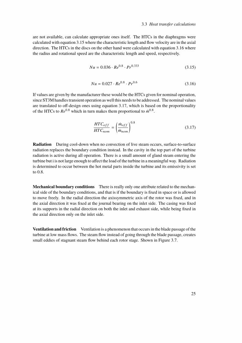
are not available, can calculate appropriate ones itself. The HTCs in the diaphragms werecalculated with equation 3.15 where the characteristic length and flow velocity are in the axialdirection. The HTCs in the discs on the other hand were calculated with equation 3.16 wherethe radius and rotational speed are the characteristic length and speed, respectively.

Nu = 0.036 · Re0.8 · Pr0.333 (3.15)

Nu = 0.027 · Re0.8 · Pr0.6 (3.16)

If values are given by the manufacturer these would be the HTCs given for nominal operation,since ST3Mhandles transient operation aswell this needs to be addressed. The nominal valuesare translated to off-design ones using equation 3.17, which is based on the proportionalityof the HTCs to Re0.8 which in turn makes them proportional to Ûm0.8.

HTCof f

HTCnom=

( Ûmof f

Ûmnom

)0.8(3.17)

Radiation During cool-down when no convection of live steam occurs, surface-to-surfaceradiation replaces the boundary condition instead. In the cavity in the top part of the turbineradiation is active during all operation. There is a small amount of gland steam entering theturbine but i is not large enough to affect the load of the turbine in ameaningful way. Radiationis determined to occur between the hot metal parts inside the turbine and its emissivity is setto 0.8.

Mechanical boundary conditions There is really only one attribute related to the mechan-ical side of the boundary conditions, and that is if the boundary is fixed in space or is allowedto move freely. In the radial direction the axissymmetric axis of the rotor was fixed, and inthe axial direction it was fixed at the journal bearing on the inlet side. The casing was fixedat its supports in the radial direction on both the inlet and exhaust side, while being fixed inthe axial direction only on the inlet side.

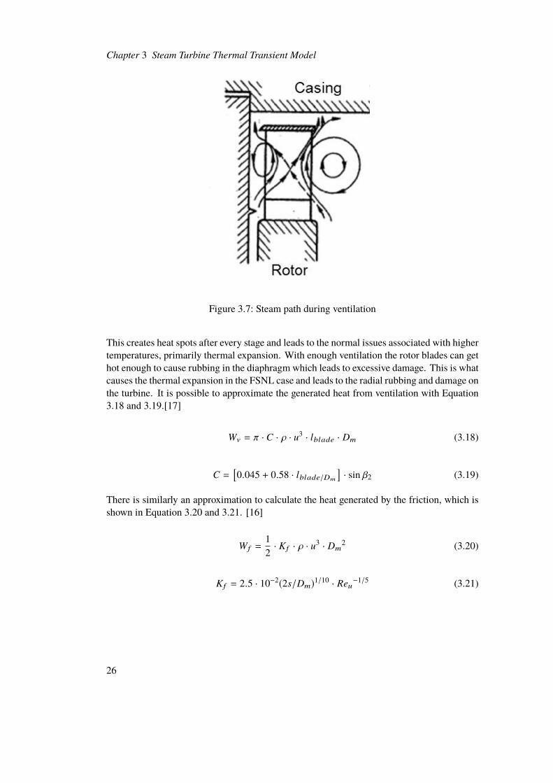
Ventilation and friction Ventilation is a phenomenon that occurs in the blade passage of theturbine at lowmass flows. The steam flow instead of going through the blade passage, createssmall eddies of stagnant steam flow behind each rotor stage. Shown in Figure 3.7.

25

Chapter 3 Steam Turbine Thermal Transient Model

Figure 3.7: Steam path during ventilation

This creates heat spots after every stage and leads to the normal issues associated with highertemperatures, primarily thermal expansion. With enough ventilation the rotor blades can gethot enough to cause rubbing in the diaphragm which leads to excessive damage. This is whatcauses the thermal expansion in the FSNL case and leads to the radial rubbing and damage onthe turbine. It is possible to approximate the generated heat from ventilation with Equation3.18 and 3.19.[17]

Wv = π · C · ρ · u3 · lblade · Dm (3.18)

C =[0.045 + 0.58 · lblade/Dm

]· sin β2 (3.19)

There is similarly an approximation to calculate the heat generated by the friction, which isshown in Equation 3.20 and 3.21. [16]

W f =12· K f · ρ · u3 · Dm

2 (3.20)

K f = 2.5 · 10−2(2s/Dm)1/10 · Reu−1/5 (3.21)

26

3.4 Finite element thermo-mechanical model

3.4 Finite element thermo-mechanical model

All of the Finite element calculations are handled by COMSOL. The boundary conditions areapplied on its previously determined locations. The different materials are implemented inthe correct sections. The initial temperature distribution was set as uniform at 365°C. Withall the inputs the temperature distribution can be calculated.

27

Chapter 4

Results

Different versions of the ST3M code was provided, a newer version for another IP turbine andan older, geometrically similar HP turbine. The newer IP version of the code was modifiedto be able to use with an HP turbine instead. Whilst fundamentally similar in structure, manydetails needed to be adapted not only to be able to operate the code for an HP turbine butalso for the different cases to be studied. For example, an IP turbine always operates againstthe condensing pressure whilst an HP turbine has a dynamic back-pressure. A large part ofwork of the thesis consisted of understanding and implementing the new version of the ST3Mcode.

4.1 Daily Operation Case

As an introductory and validating case real-world data from a CSP plant with a power towersetup was gathered. The cool down time on this data set was limited so it was complementedwith industrial cool down curves. The data set was real-world, measured data and wastherefore "true to life" while the cool down curve was approximated based on both theoryand real-world data. The ST3Mmodel was used to run a case with same inlet data as the dataset and then left to cool down for an extended period and was then compared to both the dataset and cool down curve. The ambient temperature of the day was gathered and averagedduring the whole operating time.[18]

29

Chapter 4 Results

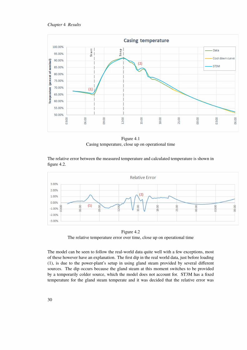
Figure 4.1Casing temperature, close up on operational time

The relative error between the measured temperature and calculated temperature is shown infigure 4.2.

Figure 4.2The relative temperature error over time, close up on operational time

The model can be seen to follow the real-world data quite well with a few exceptions, mostof these however have an explanation. The first dip in the real world data, just before loading(1), is due to the power-plant’s setup in using gland steam provided by several differentsources. The dip occurs because the gland steam at this moment switches to be providedby a temporarily colder source, which the model does not account for. ST3M has a fixedtemperature for the gland steam temperate and it was decided that the relative error was

30

4.1 Daily Operation Case

insignificant and that the focus should lie elsewhere due to the nature of the thesis focusedon evaluating rather then developing of the code.

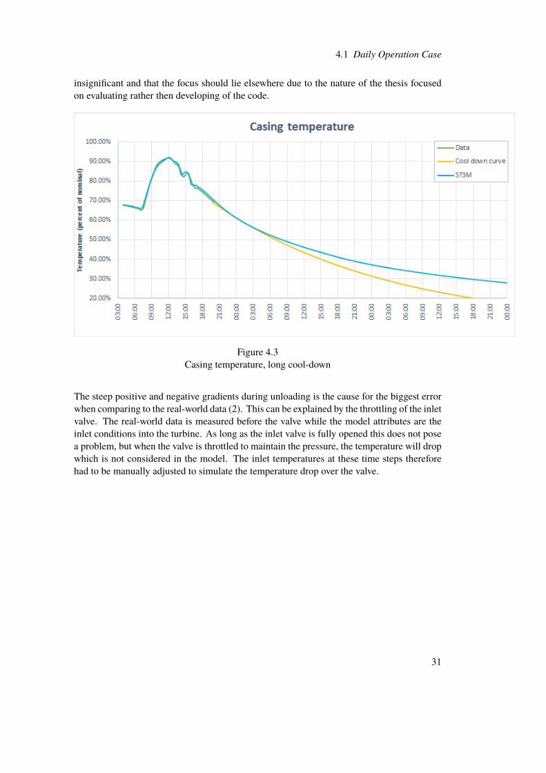
Figure 4.3Casing temperature, long cool-down

The steep positive and negative gradients during unloading is the cause for the biggest errorwhen comparing to the real-world data (2). This can be explained by the throttling of the inletvalve. The real-world data is measured before the valve while the model attributes are theinlet conditions into the turbine. As long as the inlet valve is fully opened this does not posea problem, but when the valve is throttled to maintain the pressure, the temperature will dropwhich is not considered in the model. The inlet temperatures at these time steps thereforehad to be manually adjusted to simulate the temperature drop over the valve.

31

Chapter 4 Results

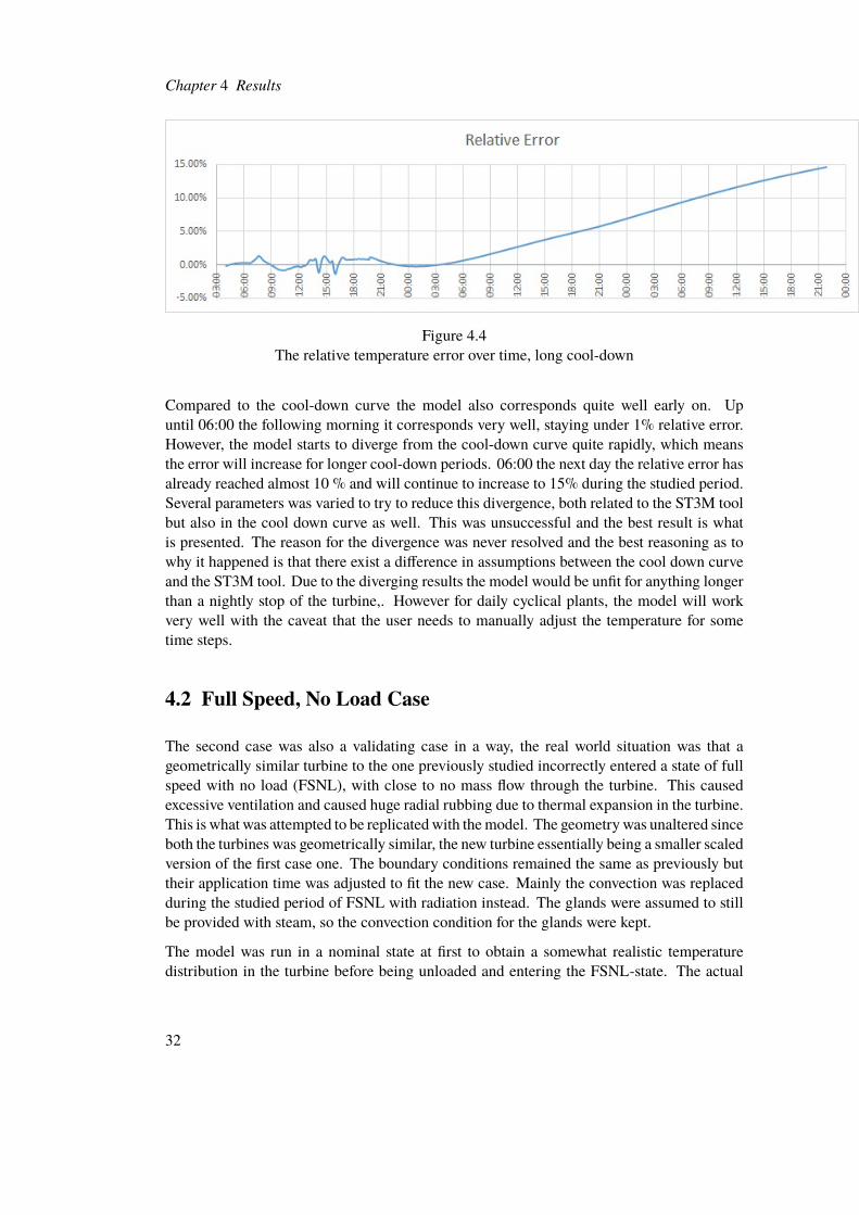
Figure 4.4The relative temperature error over time, long cool-down

Compared to the cool-down curve the model also corresponds quite well early on. Upuntil 06:00 the following morning it corresponds very well, staying under 1% relative error.However, the model starts to diverge from the cool-down curve quite rapidly, which meansthe error will increase for longer cool-down periods. 06:00 the next day the relative error hasalready reached almost 10 % and will continue to increase to 15% during the studied period.Several parameters was varied to try to reduce this divergence, both related to the ST3M toolbut also in the cool down curve as well. This was unsuccessful and the best result is whatis presented. The reason for the divergence was never resolved and the best reasoning as towhy it happened is that there exist a difference in assumptions between the cool down curveand the ST3M tool. Due to the diverging results the model would be unfit for anything longerthan a nightly stop of the turbine,. However for daily cyclical plants, the model will workvery well with the caveat that the user needs to manually adjust the temperature for sometime steps.

4.2 Full Speed, No Load Case

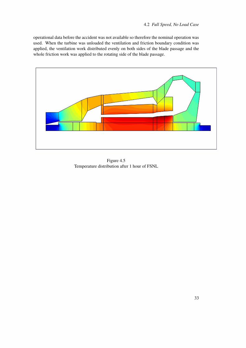
The second case was also a validating case in a way, the real world situation was that ageometrically similar turbine to the one previously studied incorrectly entered a state of fullspeed with no load (FSNL), with close to no mass flow through the turbine. This causedexcessive ventilation and caused huge radial rubbing due to thermal expansion in the turbine.This is what was attempted to be replicatedwith themodel. The geometry was unaltered sinceboth the turbines was geometrically similar, the new turbine essentially being a smaller scaledversion of the first case one. The boundary conditions remained the same as previously buttheir application time was adjusted to fit the new case. Mainly the convection was replacedduring the studied period of FSNL with radiation instead. The glands were assumed to stillbe provided with steam, so the convection condition for the glands were kept.

The model was run in a nominal state at first to obtain a somewhat realistic temperaturedistribution in the turbine before being unloaded and entering the FSNL-state. The actual

32

4.2 Full Speed, No Load Case

operational data before the accident was not available so therefore the nominal operation wasused. When the turbine was unloaded the ventilation and friction boundary condition wasapplied, the ventilation work distributed evenly on both sides of the blade passage and thewhole friction work was applied to the rotating side of the blade passage.

Figure 4.5Temperature distribution after 1 hour of FSNL

33

Chapter 4 Results

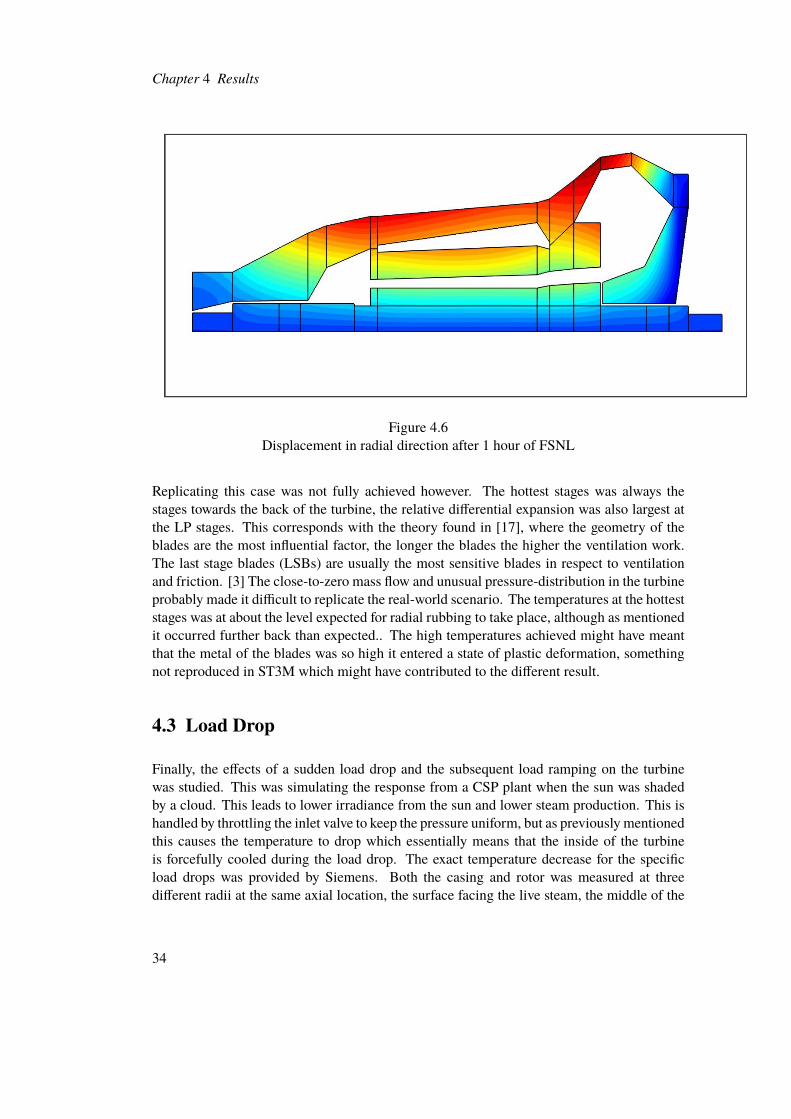
Figure 4.6Displacement in radial direction after 1 hour of FSNL

Replicating this case was not fully achieved however. The hottest stages was always thestages towards the back of the turbine, the relative differential expansion was also largest atthe LP stages. This corresponds with the theory found in [17], where the geometry of theblades are the most influential factor, the longer the blades the higher the ventilation work.The last stage blades (LSBs) are usually the most sensitive blades in respect to ventilationand friction. [3] The close-to-zero mass flow and unusual pressure-distribution in the turbineprobably made it difficult to replicate the real-world scenario. The temperatures at the hotteststages was at about the level expected for radial rubbing to take place, although as mentionedit occurred further back than expected.. The high temperatures achieved might have meantthat the metal of the blades was so high it entered a state of plastic deformation, somethingnot reproduced in ST3M which might have contributed to the different result.

4.3 Load Drop

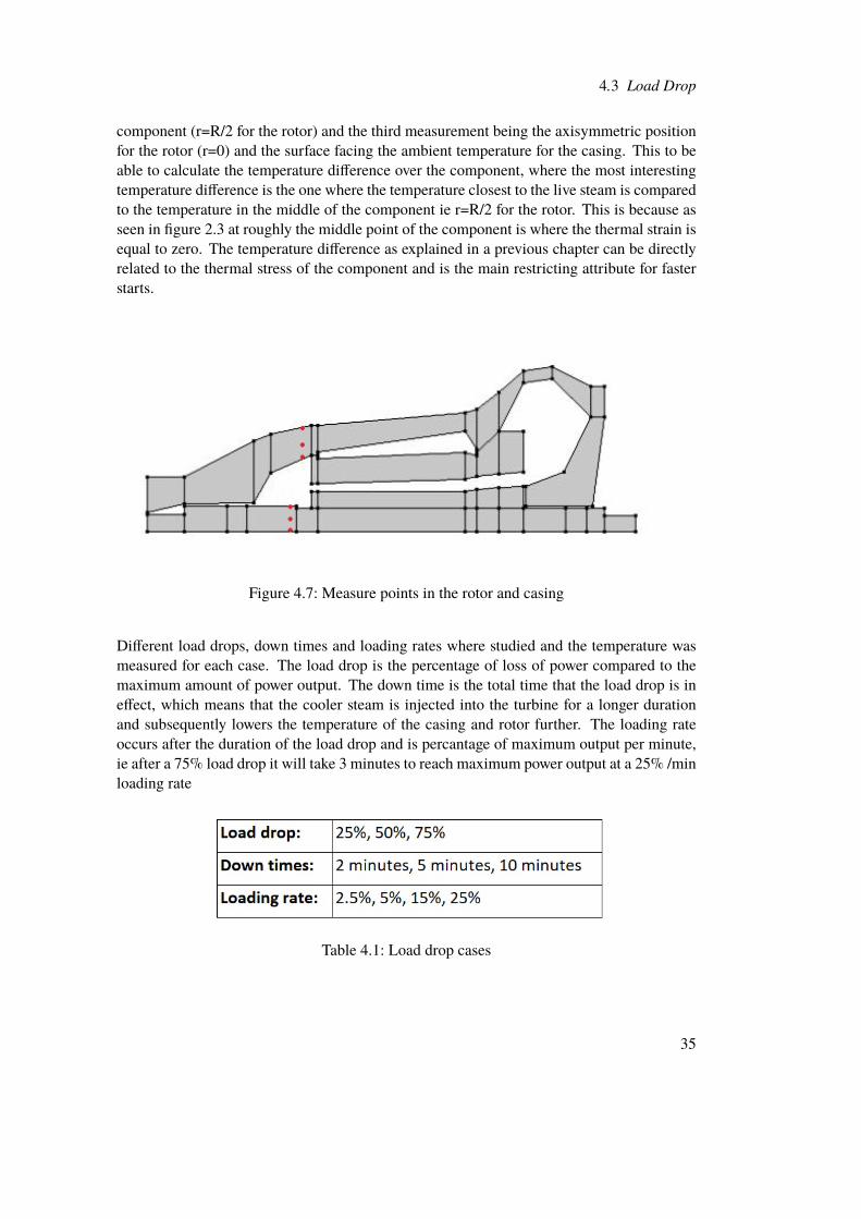
Finally, the effects of a sudden load drop and the subsequent load ramping on the turbinewas studied. This was simulating the response from a CSP plant when the sun was shadedby a cloud. This leads to lower irradiance from the sun and lower steam production. This ishandled by throttling the inlet valve to keep the pressure uniform, but as previously mentionedthis causes the temperature to drop which essentially means that the inside of the turbineis forcefully cooled during the load drop. The exact temperature decrease for the specificload drops was provided by Siemens. Both the casing and rotor was measured at threedifferent radii at the same axial location, the surface facing the live steam, the middle of the

34

4.3 Load Drop

component (r=R/2 for the rotor) and the third measurement being the axisymmetric positionfor the rotor (r=0) and the surface facing the ambient temperature for the casing. This to beable to calculate the temperature difference over the component, where the most interestingtemperature difference is the one where the temperature closest to the live steam is comparedto the temperature in the middle of the component ie r=R/2 for the rotor. This is because asseen in figure 2.3 at roughly the middle point of the component is where the thermal strain isequal to zero. The temperature difference as explained in a previous chapter can be directlyrelated to the thermal stress of the component and is the main restricting attribute for fasterstarts.

Figure 4.7: Measure points in the rotor and casing

Different load drops, down times and loading rates where studied and the temperature wasmeasured for each case. The load drop is the percentage of loss of power compared to themaximum amount of power output. The down time is the total time that the load drop is ineffect, which means that the cooler steam is injected into the turbine for a longer durationand subsequently lowers the temperature of the casing and rotor further. The loading rateoccurs after the duration of the load drop and is percantage of maximum output per minute,ie after a 75% load drop it will take 3 minutes to reach maximum power output at a 25% /minloading rate

Table 4.1: Load drop cases

35

Chapter 4 Results

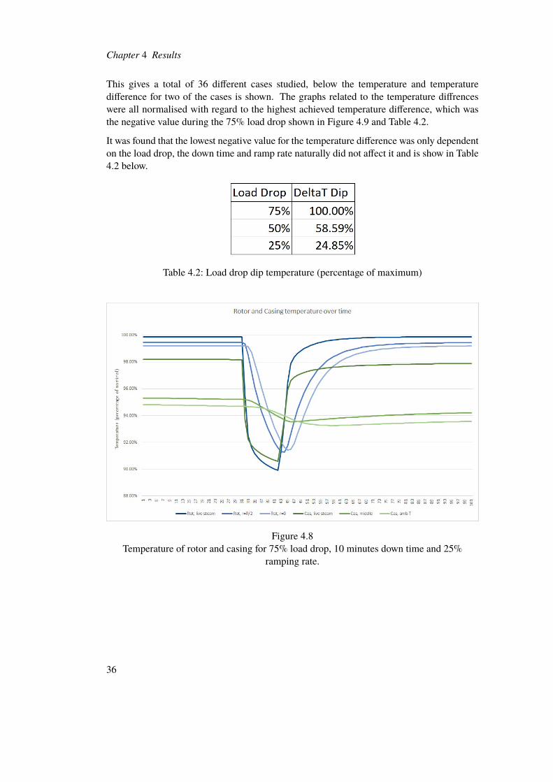
This gives a total of 36 different cases studied, below the temperature and temperaturedifference for two of the cases is shown. The graphs related to the temperature diffrenceswere all normalised with regard to the highest achieved temperature difference, which wasthe negative value during the 75% load drop shown in Figure 4.9 and Table 4.2.

It was found that the lowest negative value for the temperature difference was only dependenton the load drop, the down time and ramp rate naturally did not affect it and is show in Table4.2 below.

Table 4.2: Load drop dip temperature (percentage of maximum)

Figure 4.8Temperature of rotor and casing for 75% load drop, 10 minutes down time and 25%

ramping rate.

36

4.3 Load Drop

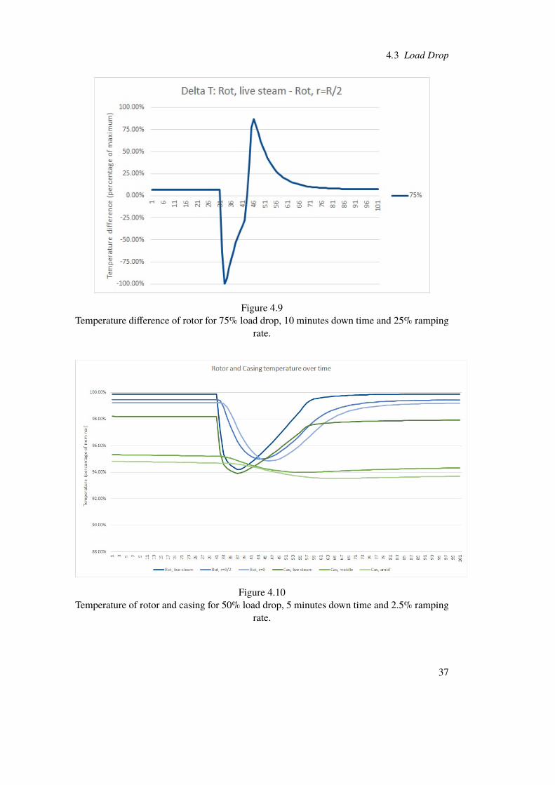
Figure 4.9Temperature difference of rotor for 75% load drop, 10 minutes down time and 25% ramping

rate.

Figure 4.10Temperature of rotor and casing for 50% load drop, 5 minutes down time and 2.5% ramping

rate.

37

Chapter 4 Results

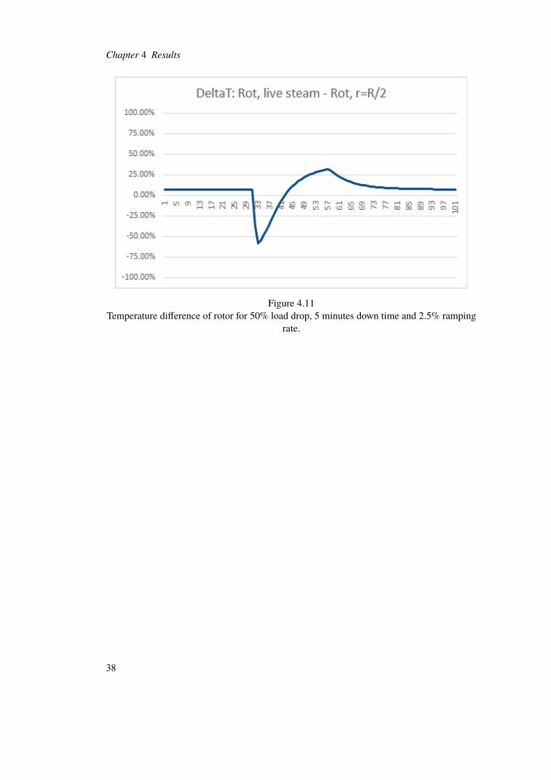
Figure 4.11Temperature difference of rotor for 50% load drop, 5 minutes down time and 2.5% ramping

rate.

38

4.3 Load Drop

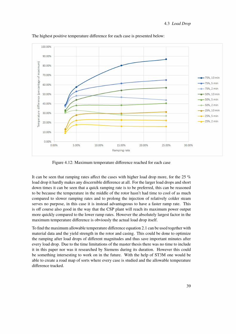
The highest positive temperature difference for each case is presented below:

Figure 4.12: Maximum temperature difference reached for each case

It can be seen that ramping rates affect the cases with higher load drop more, for the 25 %load drop it hardly makes any discernible difference at all. For the larger load drops and shortdown times it can be seen that a quick ramping rate is to be preferred, this can be reasonedto be because the temperature in the middle of the rotor hasn’t had time to cool of as muchcompared to slower ramping rates and to prolong the injection of relatively colder steamserves no purpose, in this case it is instead advantageous to have a faster ramp rate. Thisis off course also good in the way that the CSP plant will reach its maximum power outputmore quickly compared to the lower ramp rates. However the absolutely largest factor in themaximum temperature difference is obviously the actual load drop itself.

To find themaximum allowable temperature difference equation 2.1 can be used together withmaterial data and the yield strength in the rotor and casing. This could be done to optimizethe ramping after load drops of different magnitudes and thus save important minutes afterevery load drop. Due to the time limitations of the master thesis there was no time to includeit in this paper nor was it researched by Siemens during its duration. However this couldbe something intersesting to work on in the future. With the help of ST3M one would beable to create a road map of sorts where every case is studied and the allowable temperaturedifference tracked.

39

Chapter 5

Discussion and conclusion

In this thesis a 2D FE model based on MATLAB code coupled with COMSOL was studied.A modular axissymmetric geometry of an HP turbine provided by previously studies wasused as the base for three different cases of operation.

1. Daily operation with long cool down

2. Full Speed, No Load case with ventilation and friction heat generation

3. Sudden load drop with subsequent ramping to nominal

The two first cases served as validating cases, the first one to see if the model could closelyfollow the daily operation of a CSP plant with a shutdown for a duration similar to a nightlyand weekend shutdown. The relative error was well within an acceptable range during thedaily operation but diverged during the cool down which led to large errors for a cool downduration similar to a weekend shutdown. Since both the cool down curve and the ST3Mresults are theoretical in essence, the difference between themmight be different assumptionsabout the properties of the turbine (the insulation, gland steam temperature etc). Since theproblem starts to appear when the measured data ends and the cool-down curve is introduced,this would lead one to believe that there is some disparity between them not considered. Alsoworth mentioning is that the relative error increases linearly, which furthers supports the ideathat there is some parameter that has not been fully considered. During testing this has notbeen resolved however.

The second case evaluated if the heat generation and differential thermal expansion causedby ventilation work would occur at the same stage as in the real world case. This was notcompletely achieved however and the reason why has not yet been fully understood. Theresults in ST3M corresponds to what can be expected from the theory, the most ventilationis developed at the last stages in the turbine. This does not fit with what happened in theactual case, the best reasoning as to why is that there are some characteristics of the operationthat was not considered in the model. The precise state of the turbine during this operationmay have contributed to the different result. The unusual pressure distribution in the turbineand the low mass flow may have added to the difficulty in modeling the operation and mayhave caused unknown phenomenas in the real turbine not at all considered. The temperatures

41

Chapter 5 Discussion and conclusion

reached was in the region associated with radial rubbing as well as plastic deformation even ifthe stages did not correspond to what happened in the real turbine, this gives some hope to theutility of the tool and would make it somewhat usable to evaluate the maximum temperatureachieved in FSNL operation.

The third case related to sudden load drops and their effect on the life time of the turbinerelated to maximum achieved temperature difference in the rotor. The main factor impactingthe temperature difference was the load drop itself, higher load drops resulted in overallhigher temperature differences. Other than that, longer down times always resulted in higherdifferences. Although this affected the higher load drops more so than the lower load drops.The difference between 10 minutes and 2 minutes down time was 40 percentage points forthe 75% load drop compared to only 15 percentage points for the 25% load drop. The ramprates affected the bigger load drops more in general. For the 10 and 5 minute down time,increasing the ramp rate increased the temperature difference. While for the 2 minute downtime the temperature difference actually dropped with higher ramp rates, excluding the 2.5%ramp rate which always was lower than the 5% ramp rate. The temperature difference seemsto converge when the ramp rate is set to 2.5%, if the ramp rate would be infinitively slow aminimal value should be achieved no matter the load drop nor down time. These temperaturedifferences that were calculated could be used to optimize the ramping rate after a load dropbased on the allowed thermal stress in the turbine. This could not only lead to saving crucialminutes after every load drop, it would also give the operator a greater insight in the life timeconsumed. Considering the amount of load drops during a plants operational life this couldlead to a great amount of extra production for the operator and also contribute to a greaterlife time which also would save money in the long run.

ST3M has been found throughout the thesis to follow load changes very well and can alsobe utilized for shorter duration cool downs. It is not however a universal tool capable ofhandling every sort of case. When a low mass flow was introduced, both in the longer cooldown and in the FSNL, the model deviated from the real world data. This might be becausesomething not considered either in the model or some circumstance in the real world. Thetool always needs quite a bit of user-input and thought behind it before using it and is nota plug-and-play type of tool. This should not however pose a problem with suitable casesand as experience with the tool increases so should the usability of it. In this study only onetype of HP turbine was studied, to be truly usable the whole turbine fleet would need to bemodeled and implemented. This would surely take some time but can be done with a needsbased approach and once completed will be usable forever.

42

Bibliography

[1] S.L Dixon. Fluid Mechanics, Thermodynamics of Turbomachinery. Butterworth-Heinemann, 1998.

[2] 21st Centyry Tech. https://www.21stcentech.com/technology-steam-turbine-power-plants-increases-efficiency-reducing-co2-emissions/, Last accessed 22 August 2018.

[3] Alexander S. Leyzerovich. Steam Turbines for Modern Fossil-Fuel Power Plants. CRCPress, 2007.

[4] Y. Enomoto. Steam turbine retrofitting for the life extension of power plants. In TadashiTanuma, editor, Advances in Steam Turbines for Modern Power Plants, pages 397–436.Woodhead Publishing, 2017.

[5] Magnus Genrup and Marcus Thern. Ångturbinteknik - årsrapport 2016. Technicalreport, Energiforsk, Oktober 2017.

[6] Weibull. Miner’s rule and cumulative damage models, 2017.http://www.weibull.com/hotwire/issue116/hottopics116.htm, Last accessed 29May 2018.

[7] Monika Topel. Improving Concentrating Solar Power Plant Performance though SteamTurbine Flexibility. PhD thesis, KTH Royal Institute of Technology, 2017.

[8] Monika Topel, Åsa Nilsson, Markus Jöcker, and Björn Laumert. Investigation into thethermal limitations of steam turbines during start-up operation. Journal of Engineeringfor Gas Turbines and Power, 140, 2018.

[9] L. L. Vant-Hull. Central tower concentrating solar power (csp) systems. In KeitghLovegrove and Wes Stein, editors, Concentrating solar power technology, pages 24+0–281. Woodhead Publishing, 2012.

[10] NREL. https://www.nrel.gov/csp/solarpaces/project_detail.cfm/projectID=62, Last ac-cessed 9 August 2018.

[11] TechXplore. https://techxplore.com/news/2016-09-china-investing-heavily-solar-power.html, Last accessed 9 August 2018.

[12] Jurgen Birnbaum, Jan Fabian Feldhoff, Markus Fichtner, Tobias Hirsch, Markus Jöcker,Robert Pitz-Paal, and Gerhard Zimmerman. Steam temperature stability in a directsteam generation solar power plant. Solar Energy, 85(4), 2011.

43

Bibliography

[13] Brendan Pierpoint, David Nelson, Andrew Goggins, and David Posner. Flexibility,the path to low-carbon, low-cost electricity grids. Technical report, Climate PolicyInitiative, April 2017.

[14] Paul Denholm, Matthew O’Connell, Gregory Brinkman, and Jennie Jorgenson. Over-generation from solar energy in california: A field guide to the duck chart. Technicalreport, NREL, November 2015.

[15] David H. Cooke. Energy incorperated. In Modeling of off-design multistage turbinepressures by Stodola’s ellipse, pages 205–234, 1983.

[16] Alexander S. Leyzerovich. Large Power Steam Turbines: Design and Operation,volume 1. PennWell Books, 1997.

[17] Walter Traupel. Thermische Turbomaschinen. Springer-Verlag, 3 edition, 1982.

[18] Western Regional Climate Center RAWS USA Climate Archive.https://raws.dri.edu/cgi-bin/rawMAIN.pl?caCMID, Last accessed 7 June 2018.

44