Validating Predictions from Climate Envelope Models

Validating Predictions from Climate Envelope ModelsJames I. Watling1*, David N. Bucklin1, Carolina Speroterra1, Laura A. Brandt2, Frank J. Mazzotti1,

Stephanie S. Romanach3

1 Ft Lauderdale Research and Education Center, University of Florida, Ft Lauderdale, Florida, United States of America, 2 U.S. Fish and Wildlife Service, Ft Lauderdale,

Florida, United States of America, 3 Southeast Ecological Science Center, U.S. Geological Survey, Ft Lauderdale, Florida, United States of America

Abstract

Climate envelope models are a potentially important conservation tool, but their ability to accurately forecast species’distributional shifts using independent survey data has not been fully evaluated. We created climate envelope models for 12species of North American breeding birds previously shown to have experienced poleward range shifts. For each species,we evaluated three different approaches to climate envelope modeling that differed in the way they treated climate-induced range expansion and contraction, using random forests and maximum entropy modeling algorithms. All modelswere calibrated using occurrence data from 1967–1971 (t1) and evaluated using occurrence data from 1998–2002 (t2). Modelsensitivity (the ability to correctly classify species presences) was greater using the maximum entropy algorithm than therandom forest algorithm. Although sensitivity did not differ significantly among approaches, for many species, sensitivitywas maximized using a hybrid approach that assumed range expansion, but not contraction, in t2. Species for which thehybrid approach resulted in the greatest improvement in sensitivity have been reported from more land cover types thanspecies for which there was little difference in sensitivity between hybrid and dynamic approaches, suggesting that habitatgeneralists may be buffered somewhat against climate-induced range contractions. Specificity (the ability to correctlyclassify species absences) was maximized using the random forest algorithm and was lowest using the hybrid approach.Overall, our results suggest cautious optimism for the use of climate envelope models to forecast range shifts, but alsounderscore the importance of considering non-climate drivers of species range limits. The use of alternative climateenvelope models that make different assumptions about range expansion and contraction is a new and potentially usefulway to help inform our understanding of climate change effects on species.

Citation: Watling JI, Bucklin DN, Speroterra C, Brandt LA, Mazzotti FJ, et al. (2013) Validating Predictions from Climate Envelope Models. PLoS ONE 8(5): e63600.doi:10.1371/journal.pone.0063600

Editor: Raphael Arlettaz, University of Bern, Switzerland

Received August 1, 2012; Accepted April 8, 2013; Published May 23, 2013

This is an open-access article, free of all copyright, and may be freely reproduced, distributed, transmitted, modified, built upon, or otherwise used by anyone forany lawful purpose. The work is made available under the Creative Commons CC0 public domain dedication.

Funding: Funding for this work was provided by the U.S. Fish and Wildlife Service (http://www.fws.gov/), Everglades and Dry Tortugas National Park through theSouth Florida and Caribbean Cooperative Ecosystem Studies Unit (http://www.nps.gov/ever/index.htm), and USGS Greater Everglades Priority Ecosystem Science(http://access.usgs.gov/). The views in this paper do not necessarily represent the views of the U.S. Fish and Wildlife Service. Use of trade, product, or firm namesdoes not imply endorsement by the U.S. Government. The funders had no role in study design, data collection and analysis, decision to publish, or preparation ofthe manuscript.

Competing Interests: The authors have declared that no competing interests exist.

* E-mail: [email protected]

Introduction

Climate change is one of the major conservation issues of the

twenty-first century. Because the effects of increasing greenhouse

gas are expected to exacerbate climate change over the course of

the twenty-first century and beyond [1], models are an important

tool for anticipating potential future effects of climate change and

identifying proactive mitigation and adaptation strategies. Climate

envelope models (CEMs) establish species-climate relationships

that can be extrapolated in space and time [2]. Because climate is

one of the major filters determining broad patterns of species

distribution [3], [4] and because models can be constructed using

relatively simple statistical models and data inputs [2], CEMs have

become a widely-used tool for forecasting climate change effects

on species distributions [5], [6]. However, CEMs have been

criticized as lacking a sound theoretical foundation, making

unrealistic assumptions about species-climate relationships (e.g.,

assuming niche conservatism [7]), and too-easily leading to

unjustified conclusions [3], [4], [7]. In some cases, empirical data

refute the importance of climate change in underlying contempo-

rary range shifts, even for species presumed to be vulnerable to

climate change [8]. Here, we use independent data on changes in

the distribution of selected breeding birds in North America from

1967–71 to 1998–2002 to evaluate the ability of three alternative

models, including one with no climate change, to correctly classify

species and absence.

If CEMs are to be used as a robust natural resource

management tool, their ability to accurately forecast species’

distributional shifts [9] or population trends [10] needs to be

evaluated with field data. Relatively few studies that have

evaluated CEMs by calibrating models with historical data (i.e.,

an initial time period, t1) and evaluating them with data from a

future time period for which there are empirical data on climate

and species occurrence (t2). Those studies that have been

conducted have differed in their assessments of CEM perfor-

mance, with one study suggesting that CEMs are capable of

making predictions that are of fair to good performance [9], one

indicating relatively poor predictive performance [11], and

another showing mixed results [8]. To some degree, the

determination of a model’s ability to accurately forecast a species’

future distribution depends on the metric used to evaluate model

performance [12], which depends in part on the relative

PLOS ONE | www.plosone.org 1 May 2013 | Volume 8 | Issue 5 | e63600

importance of omission and commission errors [13]. Although

some have suggested that when projecting future climate change

effects, omission errors (i.e., failing to predict a known occurrence)

are more serious than commission errors (predicting species

presence in areas where it is not known to occur; [13], [14]), the

decision of how to balance omission versus commission errors is

highly case-specific.

To determine the ability of CEMs to forecast geographic range

shifts presumed to have occurred in response to recent climate

change, we evaluated performance of CEMs using metrics

describing both omission and commission error. We compared

three alternative approaches to model construction and evaluation

(Figure 1) that differed in the way they described areas of

expansion and contraction of the climate envelope. The first

approach incorporated climate change between t1 and t2 by

calibrating a model with the t1 occurrences and t1 climate data,

extrapolating the model into t2 climate conditions, and evaluating

model classification with the t2 occurrence data. We refer to this as

the ‘dynamic’ approach to climate envelope modeling. Under a

dynamic model, the climate envelope was allowed to both contract

and expand in response to changing climate. The second

approach calibrated a model with the t1 occurrence and t1 climate

data and evaluated the ability of that model to correctly classify t2occurrences. In other words, the second ‘static’ approach tested

the ability of a model that described no change in climate

suitability (e.g., neither expansion nor contraction of the climate

envelope) to classify the t2 occurrences. A third ‘hybrid’ approach

calibrated a model with the t1 occurrences and t1 climate data and

projected the model into t2 climate conditions. We then identified

those portions of the map that changed from being outside of the

climate envelope in t1 to within the climate envelope in t2 (i.e., the

areas in which the climate envelope expanded between the two

time steps, Figure 2), appended those areas of expansion to the t1climate envelope, and evaluated the ability of the model to

correctly classify the t2 occurrences. This approach explicitly

assumes that areas of climate suitability at t1 will remain suitable at

t2, while also considering newly suitable areas when classifying t2occurrences. We did not eliminate areas where the climate

envelope contracted between 1967–71 and 1998–2002 because

recent work suggests the potential for long-term persistence of sink

populations experiencing negative growth rates [15].

Materials and Methods

Species occurrences for model calibration and evaluation were

drawn from the Breeding Bird Survey (BBS) dataset [16]. Breeding

Bird Survey data are collected annually by thousands of volunteers

who record species observations along fixed survey routes, and are

a key source of long-term population data for North American

breeding birds. To define the pool of species for which models

would be constructed, we searched the primary literature for

studies of latitudinal range shifts in birds; three studies presented

data for multiple species and were used to create our species pool

([17], [18], [19]). We created models for species known on the

basis of previously published data to have experienced a poleward

distributional shift (either north or south). Hitch & Leberg [17]

tested for significant distributional shifts among species included in

their study so we included species for which their tests were

significant at a # 0.05. In the remaining two studies, the

significance of range shifts was not tested for individual species,

and different metrics were used to describe range shifts. In lieu of a

significance test, we developed operational criteria for including

species in our study. For species reported on in La Sorte &

Thompson [18] we included species for which the slope of the

relationship describing movement of the northern range boundary

through time was 5, slope,25 (e.g., the species that had

experienced the most dramatic range shifts in their study). For

species reported on in Zuckerberg et al. [19], we included species

for which the northern or southern range boundary shifted

.50 km. In all cases, migratory species were excluded from

consideration because fine temporal resolution climate data for

evaluating models are not available for much of the Neotropics.

Modeled species therefore had to be resident in and restricted to

the contiguous United States (two species, the Wild turkey Meleagris

gallopavo and Gambel’s quail, Callipepla gambelii also occur in parts

of Mexico, but because most of their range is within the contiguous

United States, they were included in our analysis) and have

experienced a significant poleward distributional shift according to

criteria described above. Across the three studies, our selection

criteria identified 12 species for modeling (Table 1).

Following Hitch & Leberg [17], we used two five-year time

periods for model development, the first for calibration and the

second for evaluation. Models were calibrated using t1 observa-

tions made on BBS routes (e.g., between the years 1967–1971).

Repeat observations of a species from a survey route were

removed such that if a species was observed at any point during

the five year t1 period, it was counted as a single presence. Latitude

and longitude coordinate data for routes were obtained from the

BBS database ([16]; coordinates are expressed as a single latitude

and longitude observation for each 24.5 mile route). Using the

coordinate data for each survey route, we extracted the values of

seven climate variables at routes known to be occupied by each

species. We also selected 1000 random routes from which focal

species were unobserved and assumed to be absent, and extracted

the values of the same seven variables. Climate variables included

were: annual precipitation, precipitation of the driest month,

precipitation of the wettest month, mean annual temperature,

temperature annual range, maximum mean monthly temperature

and minimum mean monthly temperature. Models were evaluated

with occurrence data from t2 (1998–2002), which were compiled

from BBS survey routes as described for the t1 data. Climate data

were obtained from the PRISM dataset (PRISM Climate Group,

Oregon State University, August 2011, and average values for all

variables were calculated for each of the two five year periods used

in our study. Because the PRISM data were downloaded at a

resolution of 464 km, we resampled the climate grids to

40 km640 km to approximate the resolution of the BBS survey

routes (24.5 miles = ,39.4 km).

Models were constructed using two different algorithms: the

random forest algorithm, which classifies observations (e.g., species

presence/absence) based on an iterative, recursive partitioning of

observations into the most homogeneous subsets possible [20], and

maximum entropy, which calculates a species’ probability of

occurrence based on knowledge of environmental conditions at

sites known to be occupied by the species and background

environmental conditions [21], [22]. Here, we used the 1000

random absences for each species to calculate the environmental

background for maximum entropy modeling. Random forest

models and all other statistical analyses were conducted in R [23]

and maximum entropy modeling was done using the MaxEnt

software package [21], [22] using default settings.

We evaluated performance of all CEMs by constructing models

with calibration data (t1) and testing them with t2 occurrences.

Four criteria were used to assess model performance: the area

under the receiver-operator curve (AUC), the true skill statistic,

sensitivity and specificity [12]. The AUC metric ranges from 0–1

and measures the tendency for a random presence point to have a

higher predicted probability of climate suitability than a random

Climate Envelope Model Validation


background point. In addition to using AUC to evaluate the

extrapolated model (based on t2 climate and occurrences), we also

calculated AUC using a static model in which the t2 occurrences

were evaluated against t1 climate conditions. We expected that

species whose ranges were shifting in response to climate change

would have greater AUC values using the t2 climate data

compared with the static AUC calculation. Like AUC, the true

skill statistic also ranges from 0–1, but is independent of species

prevalence [24]. Sensitivity measures the proportion of correctly

classified presences in the test dataset, whereas specificity measures

the proportion of correctly classified absences; both metrics range

from 0–1. Sensitivity is a measure of omission error (high

sensitivity = low omission), and specificity is a measure of

commission error (high specificity = low commission). A number

of authors have suggested that the ‘best’ models should achieve low

rates of omission (i.e., they should accurately classify presences)

even if commission error is relatively high, because at least some

commission error is not truly error but rather reflects our

incomplete knowledge of species distributions or the identification

of environmentally suitable area that is inaccessible to species

because of dispersal barriers, species interactions or other factors

[13], [14]).

Because two of our performance metrics describe the ability of a

model to correctly classify presences and absences, they require the

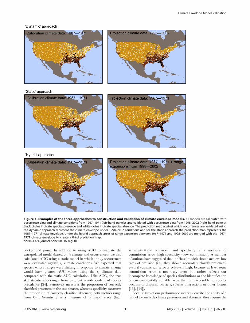
Figure 1. Examples of the three approaches to construction and validation of climate envelope models. All models are calibrated withoccurrence data and climate conditions from 1967–1971 (left-hand panels), and validated with occurrence data from 1998–2002 (right hand panels).Black circles indicate species presence and white dotes indicate species absence. The prediction map against which occurrences are validated usingthe dynamic approach represent the climate envelope under 1998–2002 conditions and for the static approach the prediction map represents the1967–1971 climate envelope. Under the hybrid approach, areas of range expansion between 1967–1971 and 1998–2002 are merged with the 1967–1971 climate envelope to create a third prediction map.doi:10.1371/journal.pone.0063600.g001



user define the threshold probabilities at which presence is

differentiated from absence. We used two alternative criteria to

determine that threshold. One criterion converted continuous

probabilities into a categorical prediction by identifying the

threshold that maximized Cohen’s kappa, a model performance

metric that measures overall classification ability [25]. To identify

this threshold, we ran five replicate model runs using random

subsets of the species occurrence data in the calibration dataset

(1967–1971) for each 0.01 unit change in threshold between.01

and 0.99 and calculated kappa for each randomization (using a

75–25% training-testing partition of the occurrence data). We

calculated the average kappa for each incremental change in the

threshold to identify the threshold at which kappa was maximized.

A second criterion used a prevalence-based approach to defining

the threshold used to calculate kappa [25]. We calculated the

prevalence of each species as number of occurrences/(number of

occurrences +1000) because all CEMs used 1000 absence points,

and used the estimate of prevalence as the threshold for converting

probability into categorical predictions. We calculated each

threshold (maximum kappa and prevalence) once for each species,

and report the threshold that resulted in the greatest model

sensitivity (e.g., best classified species presences at t2). We

calculated all performance metrics using a 75–25% training-

testing split on 100 random partitions of the occurrence data, and

tested for significant effects of algorithm and approach on AUC,

the true skill statistic, sensitivity and specificity using generalized

linear mixed-effects models [26] with a binomial distribution and a

logit link. Algorithm and approach were tested as fixed effects, and

species were treated as a random effect. The significance of fixed

effects and their interaction was tested as the likelihood ratio

between the full model and a model with the effect being tested

removed.

The dynamic, static and hybrid approaches to model evaluation

differ in the extent to which they treat range expansion and

contraction (see above). To understand how model performance

varied as a function of classification specifically in areas of range

change, we calculated the proportion of t2 presences and absences

of each species that occurred in areas of range expansion or

contraction between 1967–71 and 1998–2002 using the dynamic

approach to model evaluation. We expected that the hybrid

approach would result in increased sensitivity compared with the

dynamic approach because the hybrid approach assumes no range

contraction and therefore maximizes the area of predicted

suitability. We further expected that the hybrid approach would

improve sensitivity the most for those species for which the

dynamic approach resulted in the greatest number of misclassified

presences. In other words, models assuming no range contraction

should yield the biggest gains in sensitivity for species that continue

to persist in areas where range contraction is predicted under the

dynamic approach. Therefore, we used linear regression to

determine whether species-by-species differences in sensitivity

between the dynamic and hybrid approaches were associated with

proportions of misclassified presences (i.e., those occurring in areas

of range contraction) using the dynamic approach. We also

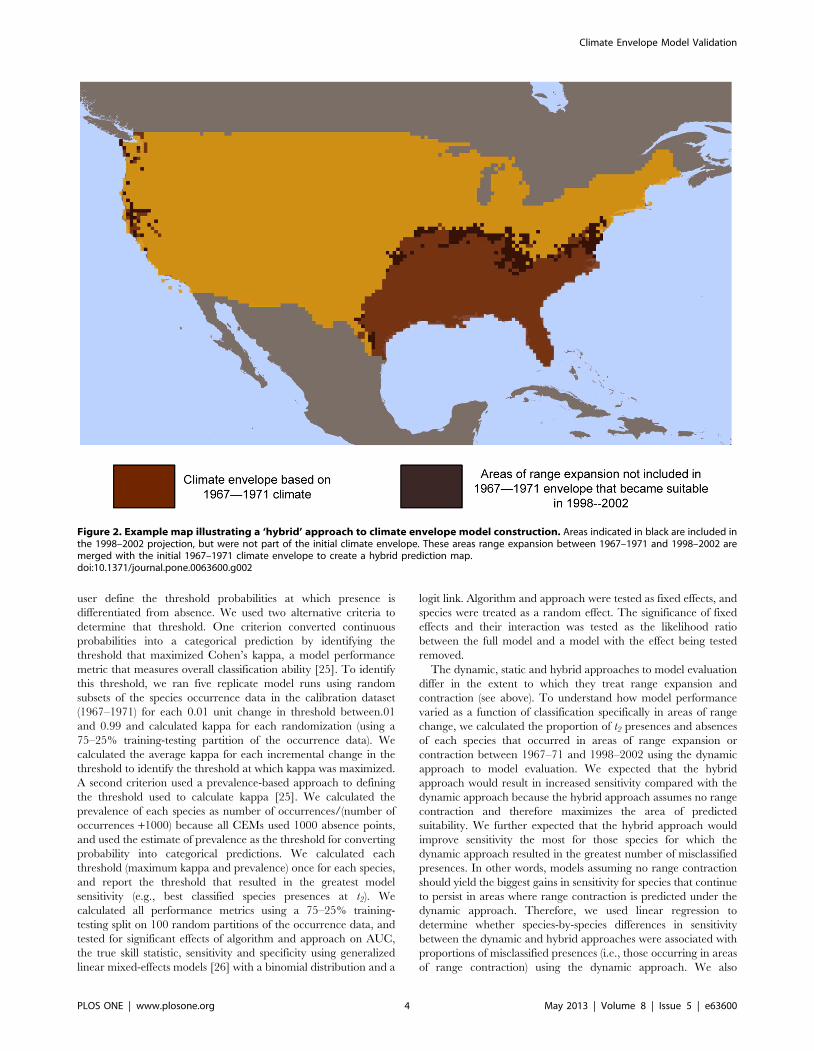
Figure 2. Example map illustrating a ‘hybrid’ approach to climate envelope model construction. Areas indicated in black are included inthe 1998–2002 projection, but were not part of the initial climate envelope. These areas range expansion between 1967–1971 and 1998–2002 aremerged with the initial 1967–1971 climate envelope to create a hybrid prediction map.doi:10.1371/journal.pone.0063600.g002



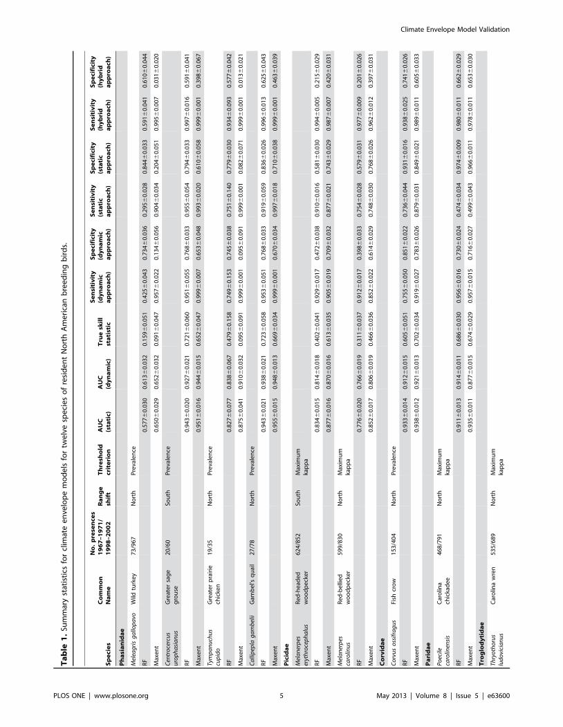
Ta

ble

1.

Sum

mar

yst

atis

tics

for

clim

ate

en

velo

pe

mo

de

lsfo

rtw

elv

esp

eci

es

of

resi

de

nt

No

rth

Am

eri

can

bre

ed

ing

bir

ds.

Sp

eci

es

Co

mm

on

Na

me

No

.p

rese

nce

s1

96

7–

19

71

/1

99

8–

20

02

Ra

ng

esh

ift

Th

resh

old

crit

eri

on

AU

C(s

tati

c)A

UC

(dy

na

mic

)T

rue

skil

lst

ati

stic

Se

nsi

tiv

ity

(dy

na

mic

ap

pro

ach

)

Sp

eci

fici

ty(d

yn

am

ica

pp

roa

ch)

Se

nsi

tiv

ity

(sta

tic

ap

pro

ach

)

Sp

eci

fici

ty(s

tati

ca

pp

roa

ch)

Se

nsi

tiv

ity

(hy

bri

da

pp

roa

ch)

Sp

eci

fici

ty(h

yb

rid

ap

pro

ach

)

Ph

asi

an

ida

e

Mel

eag

ris

ga

llop

avo

Wild

turk

ey

73

/96

7N

ort

hP

reva

len

ce

RF

0.5

776

0.0

30

0.6

136

0.0

32

0.1

596

0.0

51

0.4

256

0.0

43

0.7

346

0.0

36

0.2

956

0.0

28

0.8

446

0.0

33

0.5

916

0.0

41

0.6

106

0.0

44

Max

en

t0

.65

06

0.0

29

0.6

526

0.0

32

0.0

916

0.0

47

0.9

576

0.0

22

0.1

346

0.0

56

0.9

046

0.0

34

0.2

046

0.0

51

0.9

956

0.0

07

0.0

316

0.0

20

Cen

tro

cerc

us

uro

ph

asi

an

us

Gre

ate

rsa

ge

gro

use

20

/60

Sou

thP

reva

len

ce

RF

0.9

436

0.0

20

0.9

276

0.0

21

0.7

216

0.0

60

0.9

516

0.0

55

0.7

686

0.0

33

0.9

556

0.0

54

0.7

946

0.0

33

0.9

976

0.0

16

0.5

916

0.0

41

Max

en

t0

.95

16

0.0

16

0.9

446

0.0

15

0.6

526

0.0

47

0.9

996

0.0

07

0.6

536

0.0

48

0.9

936

0.0

20

0.6

106

0.0

58

0.9

996

0.0

01

0.3

986

0.0

67

Tym

pa

nu

chu

scu

pid

oG

reat

er

pra

irie

chic

ken

19

/35

No

rth

Pre

vale

nce

RF

0.8

276

0.0

77

0.8

386

0.0

67

0.4

796

0.1

58

0.7

496

0.1

53

0.7

456

0.0

38

0.7

516

0.1

40

0.7

796

0.0

30

0.9

346

0.0

93

0.5

776

0.0

42

Max

en

t0

.87

56

0.0

41

0.9

106

0.0

32

0.0

956

0.0

91

0.9

996

0.0

01

0.0

956

0.0

91

0.9

996

0.0

01

0.0

826

0.0

71

0.9

996

0.0

01

0.0

136

0.0

21

Ca

llip

epla

ga

mb

elii

Gam

be

l’sq

uai

l2

7/7

8N

ort

hP

reva

len

ce

RF

0.9

436

0.0

21

0.9

386

0.0

21

0.7

236

0.0

58

0.9

536

0.0

51

0.7

686

0.0

33

0.9

196

0.0

59

0.8

366

0.0

26

0.9

966

0.0

13

0.6

256

0.0

43

Max

en

t0

.95

56

0.0

15

0.9

486

0.0

13

0.6

696

0.0

34

0.9

996

0.0

01

0.6

706

0.0

34

0.9

976

0.0

18

0.7

106

0.0

38

0.9

996

0.0

01

0.4

636

0.0

39

Pic

ida

e

Mel

an

erp

eser

yth

roce

ph

alu

sR

ed

-he

ade

dw

oo

dp

eck

er

62

4/8

52

Sou

thM

axim

um

kap

pa

RF

0.8

346

0.0

15

0.8

146

0.0

18

0.4

026

0.0

41

0.9

296

0.0

17

0.4

726

0.0

38

0.9

106

0.0

16

0.5

816

0.0

30

0.9

946

0.0

05

0.2

156

0.0

29

Max

en

t0

.87

76

0.0

16

0.8

706

0.0

16

0.6

136

0.0

35

0.9

056

0.0

19

0.7

096

0.0

32

0.8

776

0.0

21

0.7

436

0.0

29

0.9

876

0.0

07

0.4

206

0.0

31

Mel

an

erp

esca

rolin

us

Re

d-b

elli

ed

wo

od

pe

cke

r5

99

/83

0N

ort

hM

axim

um

kap

pa

RF

0.7

766

0.0

20

0.7

666

0.0

19

0.3

116

0.0

37

0.9

126

0.0

17

0.3

986

0.0

33

0.7

546

0.0

28

0.5

796

0.0

31

0.9

776

0.0

09

0.2

016

0.0

26

Max

en

t0

.85

26

0.0

17

0.8

066

0.0

19

0.4

666

0.0

36

0.8

526

0.0

22

0.6

146

0.0

29

0.7

486

0.0

30

0.7

686

0.0

26

0.9

626

0.0

12

0.3

976

0.0

31

Co

rvid

ae

Co

rvu

so

ssif

rag

us

Fish

cro

w1

53

/40

4N

ort

hP

reva

len

ce

RF

0.9

336

0.0

14

0.9

126

0.0

15

0.6

056

0.0

51

0.7

556

0.0

50

0.8

516

0.0

22

0.7

366

0.0

44

0.9

316

0.0

16

0.9

386

0.0

25

0.7

416

0.0

26

Max

en

t0

.93

86

0.0

12

0.9

216

0.0

13

0.7

026

0.0

34

0.9

196

0.0

27

0.7

836

0.0

26

0.8

796

0.0

31

0.8

496

0.0

21

0.9

896

0.0

11

0.6

056

0.0

33

Pa

rid

ae

Po

ecile

caro

linen

sis

Car

olin

ach

icka

de

e4

68

/79

1N

ort

hM

axim

um

kap

pa

RF

0.9

116

0.0

13

0.9

146

0.0

11

0.6

866

0.0

30

0.9

566

0.0

16

0.7

306

0.0

24

0.4

746

0.0

34

0.9

746

0.0

09

0.9

806

0.0

11

0.6

626

0.0

29

Max

en

t0

.93

56

0.0

11

0.8

776

0.0

15

0.6

746

0.0

29

0.9

576

0.0

15

0.7

166

0.0

27

0.4

996

0.0

43

0.9

666

0.0

11

0.9

786

0.0

11

0.6

536

0.0

30

Tro

glo

dy

tid

ae

Thry

oth

oru

slu

do

vici

an

us

Car

olin

aw

ren

53

5/6

89

No

rth

Max

imu

mka

pp

a



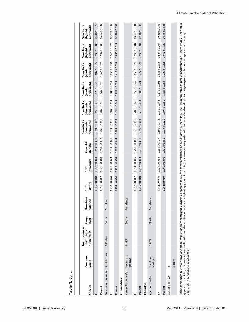
Ta

ble

1.

Co

nt.

Sp

eci

es

Co

mm

on

Na

me

No

.p

rese

nce

s1

96

7–

19

71

/1

99

8–

20

02

Ra

ng

esh

ift

Th

resh

old

crit

eri

on

AU

C(s

tati

c)A

UC

(dy

na

mic

)T

rue

skil

lst

ati

stic

Se

nsi

tiv

ity

(dy

na

mic

ap

pro

ach

)

Sp

eci

fici

ty(d

yn

am

ica

pp

roa

ch)

Se

nsi

tiv

ity

(sta

tic

ap

pro

ach

)

Sp

eci

fici

ty(s

tati

ca

pp

roa

ch)

Se

nsi

tiv

ity

(hy

bri

da

pp

roa

ch)

Sp

eci

fici

ty(h

yb

rid

ap

pro

ach

)

RF

0.8

156

0.0

18

0.8

686

0.0

14

0.4

516

0.0

30

0.9

916

0.0

07

0.4

596

0.0

30

0.8

286

0.0

23

0.6

026

0.0

25

0.9

996

0.0

02

0.2

486

0.0

22

Max

en

t0

.86

16

0.0

17

0.8

756

0.0

18

0.6

626

0.0

32

0.9

606

0.0

17

0.7

026

0.0

28

0.8

476

0.0

23

0.7

666

0.0

27

0.9

946

0.0

06

0.4

546

0.0

32

Thry

om

an

esb

ewic

kii

Be

wic

k’s

wre

n2

46

/44

0So

uth

Pre

vale

nce

RF

0.7

806

0.0

24

0.7

256

0.0

23

0.3

326

0.0

41

0.8

246

0.0

30

0.5

076

0.0

31

0.7

836

0.0

34

0.6

586

0.0

32

0.9

616

0.0

20

0.3

076

0.0

32

Max

en

t0

.77

46

0.0

24

0.7

176

0.0

24

0.3

356

0.0

44

0.8

816

0.0

28

0.4

546

0.0

41

0.8

296

0.0

37

0.6

116

0.0

33

0.9

826

0.0

12

0.2

496

0.0

33

Em

be

riz

ida

e

Aim

op

hila

aes

tiva

lisB

ach

man

’ssp

arro

w8

1/9

5So

uth

Pre

vale

nce

RF

0.9

626

0.0

12

0.9

546

0.0

15

0.7

626

0.0

41

0.9

766

0.0

35

0.7

856

0.0

26

0.9

556

0.0

42

0.8

596

0.0

21

0.9

996

0.0

04

0.6

576

0.0

31

Max

en

t0

.96

56

0.0

10

0.9

576

0.0

13

0.7

166

0.0

31

0.9

996

0.0

04

0.7

166

0.0

31

0.9

866

0.0

21

0.7

726

0.0

28

0.9

996

0.0

01

0.5

366

0.0

37

Icte

rid

ae

Ag

ela

ius

tric

olo

rT

rico

lore

db

lack

bir

d1

5/2

9N

ort

hP

reva

len

ce

RF

0.9

426

0.0

44

0.9

016

0.0

54

0.6

546

0.1

27

0.8

666

0.1

13

0.7

866

0.0

43

0.9

196

0.0

98

0.8

336

0.0

35

0.9

846

0.0

49

0.6

596

0.0

52

Max

en

t0

.95

46

0.0

19

0.9

406

0.0

30

0.6

706

0.0

65

0.9

766

0.0

79

0.6

946

0.0

69

0.9

836

0.0

65

0.7

276

0.0

64

0.9

976

0.0

20

0.5

156

0.1

21

Ave

rag

e6

1SD

RF

Max

en

t

Th

ree

app

roac

he

sto

clim

ate

en

velo

pe

mo

de

leva

luat

ion

we

reco

mp

are

d,a

dyn

amic

app

roac

hin

wh

ich

am

od

elc

alib

rate

do

nco

nd

itio

ns

att 1

(he

re1

96

7–

19

71

)w

asp

roje

cte

dto

pre

dic

to

ccu

rre

nce

sat

t 2(h

ere

19

98

–2

00

2),

ast

atic

app

roac

hin

wh

ich

t 2o

ccu

rre

nce

sar

ep

red

icte

du

sin

gth

et 1

clim

ate

dat

a,an

da

hyb

rid

app

roac

hin

wh

ich

t 2o

ccu

rre

nce

sar

ep

red

icte

du

sin

ga

mo

de

lth

atal

low

sfo

rra

ng

ee

xpan

sio

n,

bu

tn

ot

ran

ge

con

trac

tio

nat

t 2.

do

i:10

.13

71

/jo

urn

al.p

on

e.0

06

36

00

.t0

01



wanted to determine whether species-specific gains in model

sensitivity under a hybrid approach were related to species traits.

We reasoned that if the gain in sensitivity achieved using the

hybrid approach is indeed greatest for species that maintain

populations in areas deemed unsuitable by a dynamic CEM, there

may be a positive effect of niche breadth on such resistance, much

as has been described for the relatively generalist species that

persist in fragmented landscapes [27]. We counted the number of

habitat categories to which species were assigned in the Zip Code

Zoo database (www.zipcodezoo.com) as an index of habitat niche

breadth. To test whether habitat generalists showed the greatest

improvement in sensitivity using the hybrid approach, we used

linear regression to determine whether differences in sensitivity

between the dynamic and hybrid approaches were positively

associated with habitat niche breadth. In contrast, we expected the

static approach to result in increased specificity relative to the

dynamic approach (because the range expansion predicted using

the dynamic approach may increase the number of misclassified

absences). Therefore, we used linear regression to determine

whether differences in specificity between the dynamic and static

approaches were associated with proportions of absences in areas

of range expansion. We reasoned that species for which the

dynamic approach most overestimated range expansion may be

dispersal limited, and unable to track changing climate [28].

Although we searched for information on known dispersal

distances for species using online databases and literature searches,

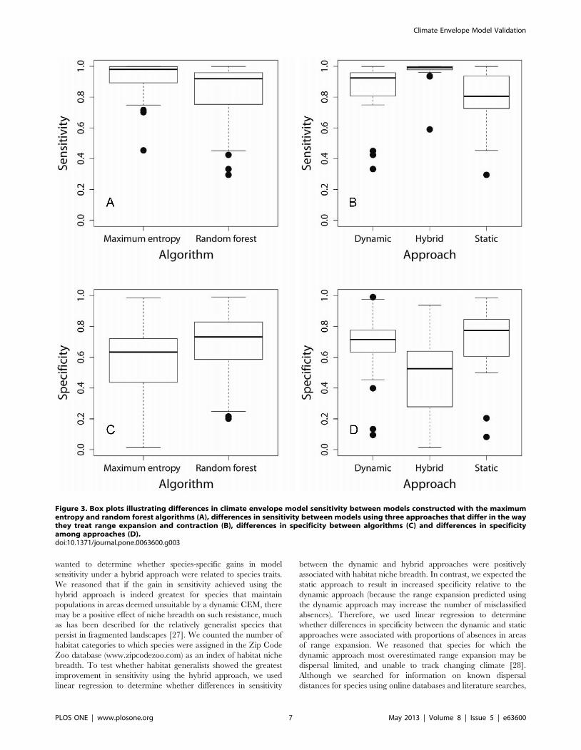
Figure 3. Box plots illustrating differences in climate envelope model sensitivity between models constructed with the maximumentropy and random forest algorithms (A), differences in sensitivity between models using three approaches that differ in the waythey treat range expansion and contraction (B), differences in specificity between algorithms (C) and differences in specificityamong approaches (D).doi:10.1371/journal.pone.0063600.g003



we were only able to obtain dispersal data for seven of our twelve

study species. Because body size is positively correlated with

dispersal distance for active dispersers [29], we used body size as a

proxy for dispersal ability. We obtained data on maximum body

mass from online databases (Animal Diversity Web, and Zip Code

Zoo), which we log-transformed prior to analysis. We used linear

regression to determine whether differences in specificity between

the static and dynamic approaches were greatest for the species

with the smallest body mass (i.e., the species expected to be most

dispersal limited).

Results

The PRISM data describe a warmer and slightly wetter climate

across the contiguous United States in 1998–2002 compared with

the 1967–1971 period. Annual precipitation in 1998–2002

averaged 768.5 mm compared with 763.3 mm in 1967–1971.

Precipitation of the driest month was slightly greater in 1998–2002

(25.9 mm) than in 1967–1971 (25.4 mm), although precipitation

of the wettest month was slightly lower (118.7 mm in 1998–2002

compared with 125.2 mm in 1967–1971). Temperature annual

mean, maximum mean monthly temperature and minimum mean

monthly temperature were all warmer in 1998–2002 compared

with 1967–1971 (11.6uC vs 10.7uC, 30.8uC vs 30.3uC, 25.7uC vs

27.8uC, respectively), and the temperature annual range was

lower in 1998–2002 (23.4uC) than in 1967–1971 (24.6uC).

Of the 12 species included in the study, previously published

data suggest that eight experienced a northward range shift and

four experienced a southward range shift (Table 1). In general,

model sensitivity was greatest when presences were differentiated

from absences using a prevalence criterion for the rarest species in

the analysis (those represented by 262 or fewer occurrences in the

calibration dataset, Table 1), whereas for more common species,

model sensitivity was greatest when presence and absence was

differentiated using the threshold that maximized kappa in the

calibration dataset (Table 1). Although all 12 species have been

suggested to have shifted their range in response to changing

climate, static AUC values were higher than projected AUC values

for at least one algorithm in nine out of 12 species (Table 1),

suggesting that not all range shifts are consistent with a climate

change model.

Average (dynamic) AUC values for the 12 random forest CEMs

were 0.84860.103 and for the maximum entropy CEMs average

AUC was 0.86860.097 (Table 1). The difference in AUC between

algorithms was significant (x2 = 5.021, df = 1, P = 0.025). Values of

the true skill statistic averaged 0.52460.196 for random forest

CEMs and 0.55160.258 for maximum entropy CEMs, but this

difference was not statistically significant (x2 = 0.324, df = 1,

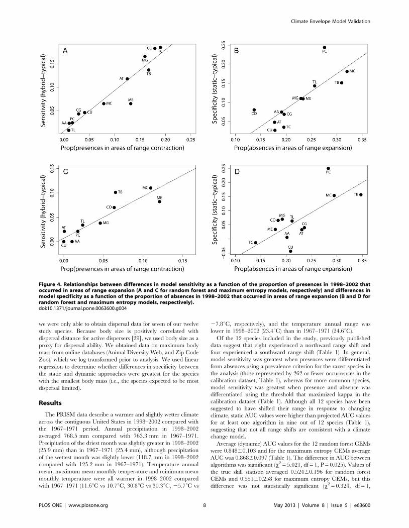
Figure 4. Relationships between differences in model sensitivity as a function of the proportion of presences in 1998–2002 thatoccurred in areas of range expansion (A and C for random forest and maximum entropy models, respectively) and differences inmodel specificity as a function of the proportion of absences in 1998–2002 that occurred in areas of range expansion (B and D forrandom forest and maximum entropy models, respectively).doi:10.1371/journal.pone.0063600.g004



P = 0.569). Generalized linear mixed effects models describing

effects of algorithm and approach on CEM sensitivity did not

differ with or without interaction terms (x2 = 0.865, df = 2,

P = 0.649), so the significance of fixed effects was tested against

the full model without interaction terms. Although maximum

entropy models had greater sensitivity (0.9260.122) than random

forest models (0.8260.202; Table 1, Figure 3A), the effect of

algorithm on sensitivity was not significant (x2 = 1.624, df = 1,

P = 0.203). Mean sensitivity of the hybrid approach (0.9760.082)

was greater than either the dynamic (0.8560.189) or static

approach (0.8060.183), but this difference was not statistically

significant (x2 = 3.902, df = 2, P = 0.142; Figure 3B).

Like the test for sensitivity, tests of all fixed effects on CEM

specificity did not differ with or without interaction terms

(x2 = 1.132, df = 2, P = 0.568), so the significance of fixed effects

was again tested against the full model without interaction terms.

The effect of algorithm on specificity was significant (x2 = 7.806,

df = 1, P = 0.005), with random forest models having greater

specificity (0.6860.207) than maximum entropy models

(0.5660.263; Table 1, Figure 3C). The different approaches also

varied in specificity (x2 = 21.059, df = 2, P,0.001), with the hybrid

approach having lower specificity (0.4760.228) than either

dynamic (0.6760.219) or static approaches (0.7160.218;

Table 1, Figure 3D). Prediction maps for all species using the

two algorithms and three approaches to model construction are

included as supplementary figures (Figures S1–S6).

Both random forest and maximum entropy models indicated

that difference in sensitivity between dynamic and hybrid

approaches increased with the proportion of presences occurring

in areas of range contraction between t1 and t2 (F1,10 = 89.80,

P,0.001 and F1,10 = 49.36, P,0.001; Figure 4A and 4C for

random forest and maximum entropy models, respectively). The

difference in specificity between dynamic and static approaches

increased with the proportion of absences in areas of range

expansion for both random forest and maximum entropy models

(F1,10 = 18.24, P = 0.002 and F1,10 = 12.41, P = 0.006 for random

forest and maximum entropy models, respectively; Figure 4B &

4D). For tests investigating the effect of niche breadth on changes

in sensitivity between hybrid and dynamic approaches, we focused

on results from maximum entropy models because sensitivity was

greater, on average, than for random forest models (Table 1,

Table 2). As hypothesized, species for which the hybrid approach

yielded the greatest increase in sensitivity have been reported from

more habitat types than species for which the hybrid approach had

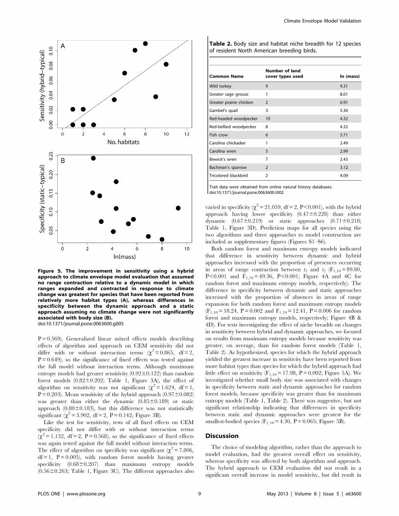
little effect on sensitivity (F1,10 = 17.98, P = 0.002; Figure 5A). We

investigated whether small body size was associated with changes

in specificity between static and dynamic approaches for random

forest models, because specificity was greater than for maximum

entropy models (Table 1, Table 2). There was suggestive, but not

significant relationship indicating that differences in specificity

between static and dynamic approaches were greatest for the

smallest-bodied species (F1,10 = 4.30, P = 0.065; Figure 5B).

Discussion

The choice of modeling algorithm, rather than the approach to

model evaluation, had the greatest overall effect on sensitivity,

whereas specificity was affected by both algorithm and approach.

The hybrid approach to CEM evaluation did not result in a

significant overall increase in model sensitivity, but did result in

Figure 5. The improvement in sensitivity using a hybridapproach to climate envelope model evaluation that assumedno range contraction relative to a dynamic model in whichranges expanded and contracted in response to climatechange was greatest for species that have been reported fromrelatively more habitat types (A), whereas differences inspecificity between the dynamic approach and a staticapproach assuming no climate change were not significantlyassociated with body size (B).doi:10.1371/journal.pone.0063600.g005

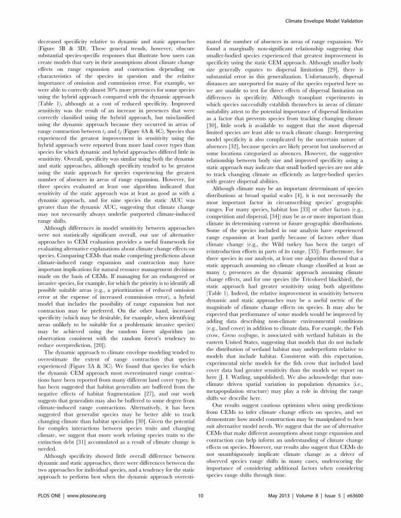
Table 2. Body size and habitat niche breadth for 12 speciesof resident North American breeding birds.

Common NameNumber of landcover types used ln (mass)

Wild turkey 9 9.31

Greater sage grouse 1 8.01

Greater prairie chicken 2 6.91

Gambel’s quail 3 5.30

Red-headed woodpecker 10 4.32

Red-bellied woodpecker 8 4.32

Fish crow 6 5.71

Carolina chickadee 1 2.49

Carolina wren 5 2.99

Bewick’s wren 7 2.43

Bachman’s sparrow 2 3.12

Tricolored blackbird 2 4.09

Trait data were obtained from online natural history databases.doi:10.1371/journal.pone.0063600.t002



decreased specificity relative to dynamic and static approaches

(Figure 3B & 3D). These general trends, however, obscure

substantial species-specific responses that illustrate how users can

create models that vary in their assumptions about climate change

effects on range expansion and contraction depending on

characteristics of the species in question and the relative

importance of omission and commission error. For example, we

were able to correctly almost 30% more presences for some species

using the hybrid approach compared with the dynamic approach

(Table 1), although at a cost of reduced specificity. Improved

sensitivity was the result of an increase in presences that were

correctly classified using the hybrid approach, but misclassified

using the dynamic approach because they occurred in areas of

range contraction between t1 and t2 (Figure 4A & 4C). Species that

experienced the greatest improvement in sensitivity using the

hybrid approach were reported from more land cover types than

species for which dynamic and hybrid approaches differed little in

sensitivity. Overall, specificity was similar using both the dynamic

and static approaches, although specificity tended to be greatest

using the static approach for species experiencing the greatest

number of absences in areas of range expansion. However, for

three species evaluated at least one algorithm indicated that

sensitivity of the static approach was at least as good as with a

dynamic approach, and for nine species the static AUC was

greater than the dynamic AUC, suggesting that climate change

may not necessarily always underlie purported climate-induced

range shifts.

Although differences in model sensitivity between approaches

were not statistically significant overall, our use of alternative

approaches to CEM evaluation provides a useful framework for

evaluating alternative explanations about climate change effects on

species. Comparing CEMs that make competing predictions about

climate-induced range expansion and contraction may have

important implications for natural resource management decisions

made on the basis of CEMs. If managing for an endangered or

invasive species, for example, for which the priority is to identify all

possible suitable areas (e.g., a prioritization of reduced omission

error at the expense of increased commission error), a hybrid

model that includes the possibility of range expansion but not

contraction may be preferred. On the other hand, increased

specificity (which may be desirable, for example, when identifying

areas unlikely to be suitable for a problematic invasive species)

may be achieved using the random forest algorithm (an

observation consistent with the random forest’s tendency to

reduce overprediction, [20]).

The dynamic approach to climate envelope modeling tended to

overestimate the extent of range contraction that species

experienced (Figure 3A & 3C). We found that species for which

the dynamic CEM approach most overestimated range contrac-

tions have been reported from many different land cover types. It

has been suggested that habitat generalists are buffered from the

negative effects of habitat fragmentation [27], and our work

suggests that generalists may also be buffered to some degree from

climate-induced range contractions. Alternatively, it has been

suggested that generalist species may be better able to track

changing climate than habitat specialists [30]. Given the potential

for complex interactions between species traits and changing

climate, we suggest that more work relating species traits to the

extinction debt [31] accumulated as a result of climate change is

needed.

Although specificity showed little overall difference between

dynamic and static approaches, there were differences between the

two approaches for individual species, and a tendency for the static

approach to perform best when the dynamic approach overesti-

mated the number of absences in areas of range expansion. We

found a marginally non-significant relationship suggesting that

smaller-bodied species experienced that greatest improvement in

specificity using the static CEM approach. Although smaller body

size generally equates to dispersal limitation [29], there is

substantial error in this generalization. Unfortunately, dispersal

distances are unreported for many of the species reported here so

we are unable to test for direct effects of dispersal limitation on

differences in specificity. Although transplant experiments in

which species successfully establish themselves in areas of climate

suitability attest to the potential importance of dispersal limitation

as a factor that prevents species from tracking changing climate

[30], little work is available to suggest that the most dispersal

limited species are least able to track climate change. Interpreting

model specificity is also complicated by the uncertain nature of

absences [32], because species are likely present but unobserved at

some locations categorized as absences. However, the suggestive

relationship between body size and improved specificity using a

static approach may indicate that small bodied species are not able

to track changing climate as efficiently as larger-bodied species

with greater dispersal abilities.

Although climate may be an important determinant of species

distributions at broad spatial scales [4], it is not necessarily the

most important factor in circumscribing species’ geographic

ranges. For many species, habitat loss [33] or other factors (e.g.,

competition and dispersal, [34]) may be as or more important than

climate in determining current or future geographic distributions.

Some of the species included in our analysis have experienced

range expansion at least partly because of factors other than

climate change (e.g., the Wild turkey has been the target of

reintroduction efforts in parts of its range, [35]). Furthermore, for

three species in our analysis, at least one algorithm showed that a

static approach assuming no climate change classified at least as

many t2 presences as the dynamic approach assuming climate

change effects, and for one species (the Tricolored blackbird), the

static approach had greater sensitivity using both algorithms

(Table 1). Indeed, the relative improvement in sensitivity between

dynamic and static approaches may be a useful metric of the

magnitude of climate change effects on species. It may also be

expected that performance of some models would be improved by

adding data describing non-climate environmental conditions

(e.g., land cover) in addition to climate data. For example, the Fish

crow, Corvus ossifragus, is associated with wetland habitats in the

eastern United States, suggesting that models that do not include

the distribution of wetland habitat may underperform relative to

models that include habitat. Consistent with this expectation,

experimental niche models for the fish crow that included land

cover data had greater sensitivity than the models we report on

here (J. I. Watling, unpublished). We also acknowledge that non-

climate driven spatial variation in population dynamics (i.e.,

metapopulation structure) may play a role in driving the range

shifts we describe here.

Our results suggest cautious optimism when using predictions

from CEMs to infer climate change effects on species, and we

demonstrate how model construction may be manipulated to best

suit alternative model needs. We suggest that the use of alternative

CEMs that make different assumptions about range expansion and

contraction can help inform an understanding of climate change

effects on species. However, our results also suggest that CEMs do

not unambiguously implicate climate change as a driver of

observed species range shifts in many cases, underscoring the

importance of considering additional factors when considering

species range shifts through time.



Supporting Information

Figure S1 Figure panels with binary prediction mapsindicating areas of suitable (brick red) and unsuitable(dark yellow) climate for 12 species of resident NorthAmerican breeding birds. Models were calibrated on climate

conditions for the 1967–1971 period and projected using climate

conditions for 1998–2002. Presences (dark circles) and absences

(white circles) from 1998–2002 surveys are indicated. Illustrated

are predictions from a random forest model using the dynamic

approach described in the text.

(TIF)





are predictions from a maximum entropy model using the

dynamic approach described in the text.

(TIF)





are predictions from a random forest model using the static


(TIF)





are predictions from a maximum entropy model using the static


(TIF)





are predictions from a random forest model using the hybrid


(TIF)





are predictions from a maximum entropy model using the hybrid


(TIF)

Acknowledgments

The views in this paper do not necessarily represent the views of the U.S.

Fish and Wildlife Service. Use of trade, product, or firm names does not

imply endorsement by the US Government.

Author Contributions

Conceived and designed the experiments: JIW DNB CS LAB SSR FJM.

Performed the experiments: JIW DNB CS. Analyzed the data: JIW DNB

CS. Contributed reagents/materials/analysis tools: JIW DNB CS. Wrote

the paper: JIW DNB CS LAB SSR FJM.

References

1. Solomon S, Qin D, Manning M, Chen Z, Marquis M, et al. (2007) Climate

Change 2007: The physical Science Basis. Contribution of Working Group I to

the Fourth Assessment Report of the Intergovernmental Panel on Climate

Change. Cambridge, UK and New York, USA : Cambridge University Press.

996 p.

2. Franklin J (2009) Mapping species distributions: spatial inference and prediction.

New York: Cambridge University Press. 320 p.

3. Toledo M, Pena-Claros M, Bongers F, Alarcon A, et al. (2012) Distribution

patterns of tropical woody species in response to climatic and edaphic gradients.

J Ecol 100: 253–263.

4. Pearson RG, Dawson TP (2003) Predicting the impacts of climate change on the

distribution of species: are bioclimate envelope models useful? Glob Ecol

Biogeogr 12: 361–371.

5. Thomas CD, Cameron A, Green RE, Bakkenes M, Beaumont LJ, et al. (2004)

Extinction risk from climate change. Nature 427: 145–148.

6. Lawler JJ, Shafer SL, White D, Kareiva P, Maurer EP, et al. (2009) Projected

climate-induced faunal change in the Western Hemisphere. Ecology 90: 588–

597.

7. Wiens JA, Stralberg D, Jongsomjit D, Howell CA, Snyder MA (2009) Niches,

models, and climate change: assessing the assumptions and uncertainties. Proc

Nat Acad Sci USA 106: 19729–19736.

8. Rubidge EM, Monahan WB, Parra JL, Cameron SE, Brashares JS (2011) The

role of climate, habitat, and species co-occurrence as drivers of change in small

mammal distributions over the past century. Glob Change Biol 17: 696–708.

9. Araujo MB, Pearson RG, Thuiller W, Erhard M (2005) Validation of species-

climate impact models under climate change. Glob Change Biol 11: 1504–1513.

10. Green RE, Collingham YC, Willis SG, Gregory RD, Smith KW, et al. (2008)

Performance of climate envelope models in retrodicting recent changes in bird

population size from observed climate change. Biol Lett 4: 599–602.

11. Mitikka V, Heikkinen RK, Luoto M, Araujo MB, Saarinen K, et al. (2008)

Predicting range expansion of the map butterfly in Northern Europe using

bioclimate models. Biodiver Conserv 17: 623–641.

12. Fielding AH, Bell JF (1997) A review of methods for the assessment of prediction

errors in conservation presence/absence models. Environ Conserv 24: 38–49.

13. Anderson RP, Lew D, Townsend Peterson A (2003) Evaluating predictive

models of species’ distributions: criteria for selecting optimal models. Ecol Model

162: 211–232.

14. Peterson AT, Papes M, Soberon J (2008) Rethinking receiver operator

characteristic analysis applications in ecological niche modeling. 2008. Ecol

Model 213: 63–72.

15. Matthews DP, Gonzalez A (2007) The inflationary effects of environmental

fluctuations ensure the persistence of sink metapopulations. Ecology 88: 2848–

2856.

16. Sauer JR, Hines JE, Fallon JE, Pardieck KL, Ziolkowski D Jr, et al. (2011) The

North American Breeding Bird Survey, Results and Analysis 1966–2009.

Version 3.23.2011. USGS Patuxent Wildlife Research Center, Laurel, MD.

17. Hitch AT, Leberg PL (2007) Breeding distributions of North American bird

species moving north as a result of climate change. Conserv Biol 21: 534–539.

18. La Sorte FE, Thompson III FR (2007) Poleward shifts in winter ranges of North

American birds. Ecology 88: 1803–1812.

19. Zuckerberg B, Woods AM, Porter WF (2009) Poleward shifts in breeding bird

distributions in New York state. Glob Change Biol 35: 1866–1883.

20. Cutler DR, Edwards Jr, TC, Beard KH, Cutler A, Hess KT, et al. (2007)

Random forests for classification in ecology. Ecology 88: 2783–2792.

21. Phillips SJ, Anderson RP, Schapire RE (2006) Maximum entropy modeling of

species geographic distributions. Ecol Model 190: 231–259.

22. Elith J, Phillips SJ, Hastie T, Dudık M, Chee YE, et al. (2011) A statistical

explanation of MaxEnt for ecologists. Div Distrib 17: 43–57.

23. R project website. Available: www.R-project.org. Accessed 2013 1 April.



24. Allouche O, Tsoar A, Kadmon R (2006) Assessing the accuracy of species

distribution models: prevalence, kappa and the true skill statistic (TSS). J Appl

Ecol 43: 1223–1232.

25. Freeman EA, Moisen GG (2008) A comparison of the performance of threshold

criteria for binary classification in terms of predicted prevalence and kappa. Ecol

Model 217: 48–58.

26. Bolker BM, Brook ME, Clark CJ, Geange SW, Poulson JR, et al. (2008)

Generalized linear mixed models: a practical guide for ecology and evolution.

Trends Ecol Evol 24: 127–135.

27. Swihart RK, Gehring TM, Kolozsvary MB, Nupp TE (2003) Responses of

‘resistant’ vertebrates to habitat loss and fragmentation: the importance of niche

breadth and range boundaries. Div Distrib 9: 1–18.

28. Schloss CA, Nunez TA, Lawler JJ (2012) Dispersal will limit ability of mammals

to track climate change in the Western Hemisphere. Proc Nat Acad Sci USA

109: 8606–8611.

29. Jenkins DG, Brescarin CR, Duxbury CV, Elliott JA, Evans JA et al. (2007) Does

size matter for dispersal distance? Glob Ecol Biogeogr 16: 415–425.30. Menendez R, Gonzalez Megıas A, Hill JK, Braschler B, Willis SC, et al. (2006)

Species richness changes lag behind climate change. Proc Royal Soc B: Biol. Sci.

273: 1465–1470.31. Tilman D, May RM, Lehman CL, Nowak MA (1994) Habitat destruction and

the extinction debt. Nature 371: 65–66.32. Lobo JM, Jimenez-Valverde A, Hortal J (2010) The uncertain nature of absences

and their importance in species distribution modeling. Ecography 33: 103–114.

33. Fahrig L (2003) Effects of habitat fragmentation on biodiversity. Ann Rev EcolEvol Syst 34: 487–515.

34. Urban MC, Tewksbury JJ, Sheldon KS (2012) On a collision course:competition and dispersal differences create no-analogue communities and

cause extinctions during climate change. Proc Royal Soc B Biol Sci: 1–9.35. Mitchell MD, Kimmel RO, Snyders J (2011) Reintroduction and range

expansion of eastern wild turkeys in Minnesota. Geogr Rev 101: 269–284.



Validating Predictions from Climate Envelope Models

Documents

Transcript of Validating Predictions from Climate Envelope Models