Cross-validating precipitation datasets in the Indus River basin
24
Hydrol. Earth Syst. Sci., 24, 427–450, 2020 https://doi.org/10.5194/hess-24-427-2020 © Author(s) 2020. This work is distributed under the Creative Commons Attribution 4.0 License. Cross-validating precipitation datasets in the Indus River basin Jean-Philippe Baudouin 1 , Michael Herzog 1 , and Cameron A. Petrie 2 1 Department of Geography, University of Cambridge, Cambridge, UK 2 Department of Archaeology, University of Cambridge, Cambridge, UK Correspondence: Jean-Philippe Baudouin ([email protected], [email protected]) Received: 20 June 2019 – Discussion started: 8 July 2019 Revised: 2 October 2019 – Accepted: 6 November 2019 – Published: 28 January 2020 Abstract. Large uncertainty remains about the amount of precipitation falling in the Indus River basin, particularly in the more mountainous northern part. While rain gauge measurements are often considered as a reference, they pro- vide information for specific, often sparse, locations (point observations) and are subject to underestimation, particu- larly in mountain areas. Satellite observations and reanalysis data can improve our knowledge but validating their results is often difficult. In this study, we offer a cross-validation of 20 gridded datasets based on rain gauge, satellite, and reanalysis data, including the most recent and less studied APHRODITE-2, MERRA2, and ERA5. This original ap- proach to cross-validation alternatively uses each dataset as a reference and interprets the result according to their de- pendency on the reference. Most interestingly, we found that reanalyses represent the daily variability of precipitation as well as any observational datasets, particularly in winter. Therefore, we suggest that reanalyses offer better estimates than non-corrected rain-gauge-based datasets where under- estimation is problematic. Specifically, ERA5 is the reanal- ysis that offers estimates of precipitation closest to observa- tions, in terms of amounts, seasonality, and variability, from daily to multi-annual scale. By contrast, satellite observa- tions bring limited improvement at the basin scale. For the rain-gauge-based datasets, APHRODITE has the finest tem- poral representation of the precipitation variability, yet it im- portantly underestimates the actual amount. GPCC products are the only datasets that include a correction factor of the rain gauge measurements, but this factor likely remains too small. These findings highlight the need for a systematic characterisation of the underestimation of rain gauge mea- surements. 1 Introduction Throughout the Holocene, the Indus River and its tributaries have provided much of the water needed by the people liv- ing in its basin for various purposes (e.g. food, energy, in- dustry). The diversity of use and the risks associated with scarcity or excess of water under variable and changing cli- matic and socio-economic conditions highlight the impor- tance of water management in both Pakistan and north-west India (Archer et al., 2010; Laghari et al., 2012). Moreover, the Indus headwaters are an important locus of water storage, with numerous glaciers whose current and future change re- mains uncertain (Hewitt, 2005; Gardelle et al., 2012). There- fore, a comprehensive evaluation of the basin-wide water cy- cle is needed. Studies that have addressed this issue have stressed the uncertainties inherent in the observed precipi- tation (Singh et al., 2011; Gardelle et al., 2012; Immerzeel et al., 2015; Wang et al., 2017; Dahri et al., 2018). Gridded products allow for a homogeneous spatial repre- sentation of precipitation at a river basin-scale for statistical purposes (Palazzi et al., 2013). They can be derived from rain gauges, satellite imagery or atmospheric models (e.g. reanal- ysis) but need validation to assess their quality. Most stud- ies that validate precipitation products in Pakistan, India, or in the adjacent mountainous areas (Hindu Kush, Karakoram, Himalayas) make use of rain gauge data as a reference, ei- ther directly from weather stations (Ali et al., 2012; Khan et al., 2014; Ghulami et al., 2017; Hussain et al., 2017; Iqbal and Athar, 2018), or after gridding (Palazzi et al., 2013; Ra- jbhandari et al., 2015; Rana et al., 2015, 2017). However, some authors have pointed out that these reference datasets also suffer from limitations that could dramatically reduce correlation and increase biases, incorrectly lowering the con- Published by Copernicus Publications on behalf of the European Geosciences Union.
-
Upload
khangminh22 -
Category
Documents
-
view
1 -
download
0
Transcript of Cross-validating precipitation datasets in the Indus River basin
Hydrol. Earth Syst. Sci., 24, 427–450, 2020https://doi.org/10.5194/hess-24-427-2020© Author(s) 2020. This work is distributed underthe Creative Commons Attribution 4.0 License.
Cross-validating precipitation datasets in the Indus River basinJean-Philippe Baudouin1, Michael Herzog1, and Cameron A. Petrie2
1Department of Geography, University of Cambridge, Cambridge, UK2Department of Archaeology, University of Cambridge, Cambridge, UK
Correspondence: Jean-Philippe Baudouin ([email protected], [email protected])
Received: 20 June 2019 – Discussion started: 8 July 2019Revised: 2 October 2019 – Accepted: 6 November 2019 – Published: 28 January 2020
Abstract. Large uncertainty remains about the amount ofprecipitation falling in the Indus River basin, particularlyin the more mountainous northern part. While rain gaugemeasurements are often considered as a reference, they pro-vide information for specific, often sparse, locations (pointobservations) and are subject to underestimation, particu-larly in mountain areas. Satellite observations and reanalysisdata can improve our knowledge but validating their resultsis often difficult. In this study, we offer a cross-validationof 20 gridded datasets based on rain gauge, satellite, andreanalysis data, including the most recent and less studiedAPHRODITE-2, MERRA2, and ERA5. This original ap-proach to cross-validation alternatively uses each dataset asa reference and interprets the result according to their de-pendency on the reference. Most interestingly, we found thatreanalyses represent the daily variability of precipitation aswell as any observational datasets, particularly in winter.Therefore, we suggest that reanalyses offer better estimatesthan non-corrected rain-gauge-based datasets where under-estimation is problematic. Specifically, ERA5 is the reanal-ysis that offers estimates of precipitation closest to observa-tions, in terms of amounts, seasonality, and variability, fromdaily to multi-annual scale. By contrast, satellite observa-tions bring limited improvement at the basin scale. For therain-gauge-based datasets, APHRODITE has the finest tem-poral representation of the precipitation variability, yet it im-portantly underestimates the actual amount. GPCC productsare the only datasets that include a correction factor of therain gauge measurements, but this factor likely remains toosmall. These findings highlight the need for a systematiccharacterisation of the underestimation of rain gauge mea-surements.
1 Introduction
Throughout the Holocene, the Indus River and its tributarieshave provided much of the water needed by the people liv-ing in its basin for various purposes (e.g. food, energy, in-dustry). The diversity of use and the risks associated withscarcity or excess of water under variable and changing cli-matic and socio-economic conditions highlight the impor-tance of water management in both Pakistan and north-westIndia (Archer et al., 2010; Laghari et al., 2012). Moreover,the Indus headwaters are an important locus of water storage,with numerous glaciers whose current and future change re-mains uncertain (Hewitt, 2005; Gardelle et al., 2012). There-fore, a comprehensive evaluation of the basin-wide water cy-cle is needed. Studies that have addressed this issue havestressed the uncertainties inherent in the observed precipi-tation (Singh et al., 2011; Gardelle et al., 2012; Immerzeelet al., 2015; Wang et al., 2017; Dahri et al., 2018).
Gridded products allow for a homogeneous spatial repre-sentation of precipitation at a river basin-scale for statisticalpurposes (Palazzi et al., 2013). They can be derived from raingauges, satellite imagery or atmospheric models (e.g. reanal-ysis) but need validation to assess their quality. Most stud-ies that validate precipitation products in Pakistan, India, orin the adjacent mountainous areas (Hindu Kush, Karakoram,Himalayas) make use of rain gauge data as a reference, ei-ther directly from weather stations (Ali et al., 2012; Khanet al., 2014; Ghulami et al., 2017; Hussain et al., 2017; Iqbaland Athar, 2018), or after gridding (Palazzi et al., 2013; Ra-jbhandari et al., 2015; Rana et al., 2015, 2017). However,some authors have pointed out that these reference datasetsalso suffer from limitations that could dramatically reducecorrelation and increase biases, incorrectly lowering the con-
Published by Copernicus Publications on behalf of the European Geosciences Union.
428 J.-P. Baudouin et al.: Precipitation in the Indus River basin
fidence in the dataset validated (Tozer et al., 2012; Ménégozet al., 2013; Rana et al., 2015, 2017).
The first issue of validating gridded precipitation productswith rain gauge measurements is simply the uncertainty ofthe measurements. Beside the risk of corruption or missingvalues in the reporting process, it has been demonstrated thatrain gauges can underestimate precipitation (Sevruk, 1984;Goodison et al., 1989). The main source of underestima-tion is the wind-driven under-catchment that can reach upto 50 % during snowfall (Goodison et al., 1989; Adam andLettenmaier, 2003; Wolff et al., 2015; Dahri et al., 2018),but also includes the wetting of the instrument, evaporationbefore measuring, and splashing out (WMO, 2008). Dahriet al. (2018) used the guidelines from the World Meteoro-logical Organization (WMO) to re-evaluate the precipitationmeasured from hundreds of rain gauges in the upper Indusand found the underestimation to be between 1 % and 65 %for each station, and 21 % across the basin. The second issueis the one of spatial representativeness. A rain gauge recordsa measurement at a specific location whereas in a griddeddataset, each value represents the mean over all the grid box.Thus, the two types of data have a different spatial represen-tativeness. This discrepancy in representativeness increaseswhen considering shorter timesteps and areas with strongheterogeneity such as mountainous terrains, which is espe-cially impactful when studying extreme events. Some meth-ods exist to quantify and tackle this issue (e.g. Tustison et al.,2001; Habib et al., 2004; Wang and Wolff, 2010).
Gridding methods are used to spatially homogenise pointmeasurements and they also have limitations. Firstly, thespecificity of the interpolation method can impact the result(Ensor and Robeson, 2008; Newlands et al., 2011). Secondly,the sparsity of the weather stations increases the uncertain-ties, which can range from 15 % to 100 % in areas with a lownumber of rain gauges (Rudolf and Rubel, 2005). This lastpoint is especially problematic in the Indus River basin. Forclimatological purposes, the WMO has published guidelinesfor the density of rain gauges: from one station per 900 km2
in flat coastal areas, to one every 250 km2 in mountains(WMO, 2008). However, the Meteorological Department ofPakistan have recently published a 50-year climatology ofprecipitation for the country based on 56 stations, which isaround one station per 15 000 km2 (Faisal and Gaffar, 2012).Gridded rain-gauge-based datasets rely on a similar densityof observations in the Indus River basin (see Fig. 2, Table 2).The situation in India is better as the Indian Meteorologi-cal Department produces a country-wide dataset of precipi-tation that is used for monsoon monitoring and includes upto 6300 stations. This distribution makes around one stationper 500 km2, which is well within the WMO guideline. How-ever, areas of lower density remain, especially in the westernHimalayas and the Thar Desert, which are both in the In-dus River basin (Kishore et al., 2016). Rain gauges are notonly scarce in mountainous areas, but their location is alsobiased. In order to be accessible all year long, they are gener-
ally situated at the bottom of valleys, and these locations ap-pear to be significantly drier than locations at altitude (Archerand Fowler, 2004; Ménégoz et al., 2013; Immerzeel et al.,2015; Dahri et al., 2018), which means that the interpola-tion method underestimates precipitation in the surroundingmountains.
There are a number of ways of overcoming the limitationsof gridded rain gauge data, including the use of data derivedfrom satellites and reanalyses. Satellite imagery can help toreduce both the lack and the heterogeneity of surface mea-surements. Satellite-based products generally make use ofglobal infrared observations of cloud cover and microwavemeasurements along a swath (the narrow band where the ob-servations are made as the satellite passes). However, theirabilities over a heterogeneous terrain are more limited thanover a flat and homogeneous one (Khan et al., 2014; Hussainet al., 2017; Iqbal and Athar, 2018). Moreover, these prod-ucts still need rain gauges for calibration and are thereforedependent on the quality of station data.
Reanalyses of the atmosphere offer another way to esti-mate precipitation. Many valuable variables in a reanalysisare the result of the assimilation of observations with modeloutputs, but estimates of precipitation are, in most cases, apure model product. That is, the precipitation is a forecastgenerated by the model used for the reanalysis and is notconstrained by direct observations in the way that other as-similated quantities are. Models are known to predict pre-cipitation with difficulty and most studies highlight that pre-cipitation from reanalyses is less reliable than that based onobservations (Rana et al., 2015; Kishore et al., 2016). Thereasons often invoked include discrepancies in spatial pat-terns and important model biases. However, recent progressin assimilation techniques has made it possible to integrateprecipitation observations in the most recent reanalysis prod-uct (ERA5, Hersbach et al., 2018), and significant improve-ments are possible (e.g. Beck et al., 2019).
This study aims to better understand the quality and limita-tions of 20 precipitation datasets that are available for a studyarea encompassing the Indus River basin. Previous studieshave investigated the strengths and limitations of precipita-tion datasets in this area (e.g. Ali et al., 2012; Palazzi et al.,2013; Khan et al., 2014; Hussain et al., 2017), but none haslooked at such a large number of datasets nor at the most re-cent ones. Moreover, our method differs slightly, as we offera cross-validation, thereby avoiding the problems that comefrom the selection of a unique reference. We cross-compareeach of the datasets, identify their similarities and discrepan-cies, and using the diversity of data source and methods weassess their strengths and weaknesses. After presenting thedatasets selected for the study, we give a general descriptionof the methods. The subsequent result section is split intofour parts, which review the following, for the precipitation:(i) the annual mean, (ii) the seasonality, (iii) the daily vari-ability, and (iv) the monthly and longer-term variability. The
Hydrol. Earth Syst. Sci., 24, 427–450, 2020 www.hydrol-earth-syst-sci.net/24/427/2020/
J.-P. Baudouin et al.: Precipitation in the Indus River basin 429
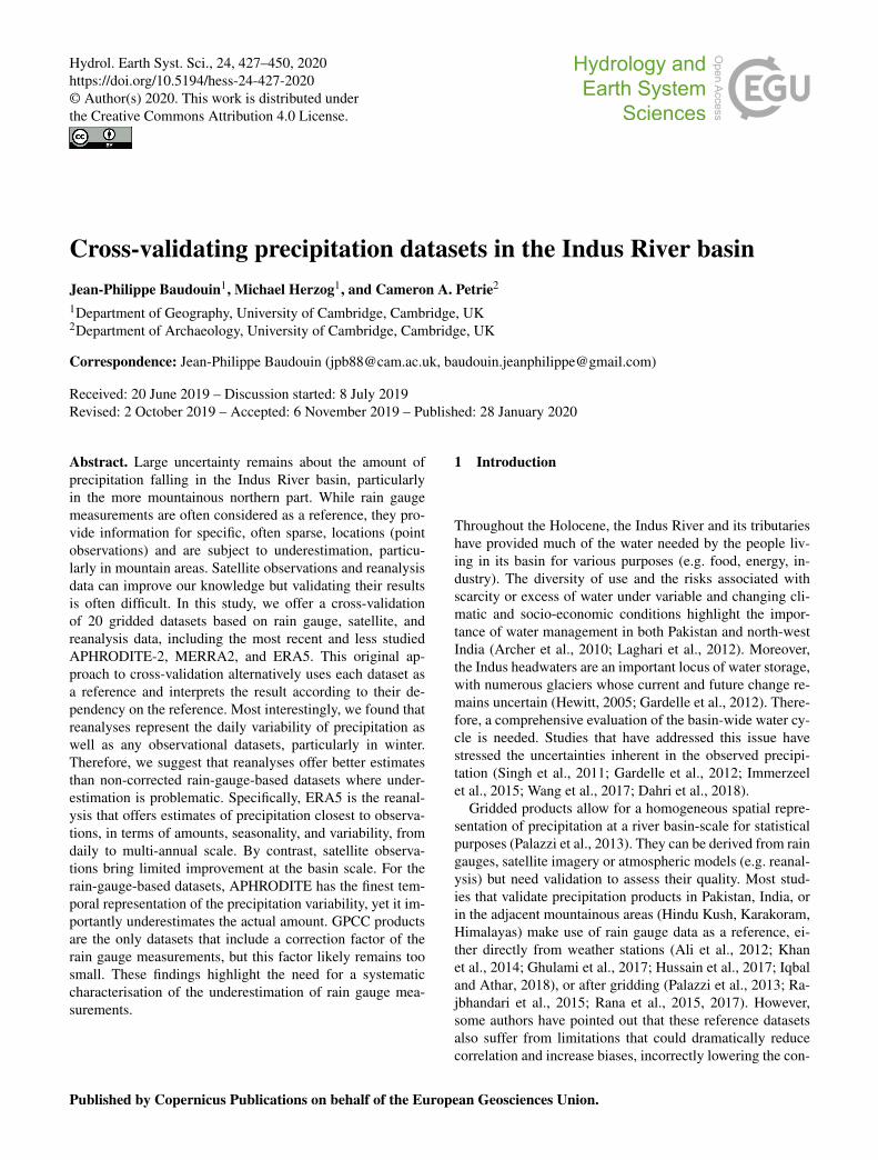
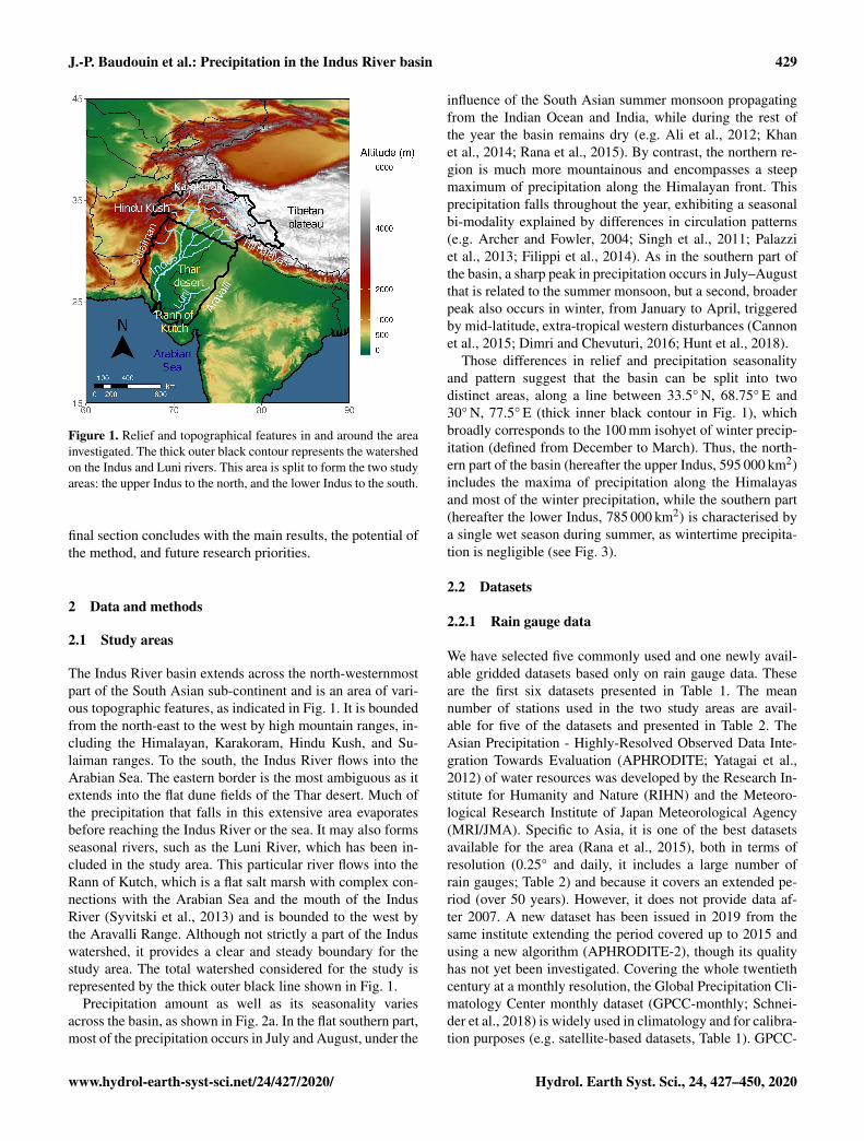
Figure 1. Relief and topographical features in and around the areainvestigated. The thick outer black contour represents the watershedon the Indus and Luni rivers. This area is split to form the two studyareas: the upper Indus to the north, and the lower Indus to the south.
final section concludes with the main results, the potential ofthe method, and future research priorities.
2 Data and methods
2.1 Study areas
The Indus River basin extends across the north-westernmostpart of the South Asian sub-continent and is an area of vari-ous topographic features, as indicated in Fig. 1. It is boundedfrom the north-east to the west by high mountain ranges, in-cluding the Himalayan, Karakoram, Hindu Kush, and Su-laiman ranges. To the south, the Indus River flows into theArabian Sea. The eastern border is the most ambiguous as itextends into the flat dune fields of the Thar desert. Much ofthe precipitation that falls in this extensive area evaporatesbefore reaching the Indus River or the sea. It may also formsseasonal rivers, such as the Luni River, which has been in-cluded in the study area. This particular river flows into theRann of Kutch, which is a flat salt marsh with complex con-nections with the Arabian Sea and the mouth of the IndusRiver (Syvitski et al., 2013) and is bounded to the west bythe Aravalli Range. Although not strictly a part of the Induswatershed, it provides a clear and steady boundary for thestudy area. The total watershed considered for the study isrepresented by the thick outer black line shown in Fig. 1.
Precipitation amount as well as its seasonality variesacross the basin, as shown in Fig. 2a. In the flat southern part,most of the precipitation occurs in July and August, under the
influence of the South Asian summer monsoon propagatingfrom the Indian Ocean and India, while during the rest ofthe year the basin remains dry (e.g. Ali et al., 2012; Khanet al., 2014; Rana et al., 2015). By contrast, the northern re-gion is much more mountainous and encompasses a steepmaximum of precipitation along the Himalayan front. Thisprecipitation falls throughout the year, exhibiting a seasonalbi-modality explained by differences in circulation patterns(e.g. Archer and Fowler, 2004; Singh et al., 2011; Palazziet al., 2013; Filippi et al., 2014). As in the southern part ofthe basin, a sharp peak in precipitation occurs in July–Augustthat is related to the summer monsoon, but a second, broaderpeak also occurs in winter, from January to April, triggeredby mid-latitude, extra-tropical western disturbances (Cannonet al., 2015; Dimri and Chevuturi, 2016; Hunt et al., 2018).
Those differences in relief and precipitation seasonalityand pattern suggest that the basin can be split into twodistinct areas, along a line between 33.5° N, 68.75° E and30° N, 77.5° E (thick inner black contour in Fig. 1), whichbroadly corresponds to the 100 mm isohyet of winter precip-itation (defined from December to March). Thus, the north-ern part of the basin (hereafter the upper Indus, 595 000 km2)includes the maxima of precipitation along the Himalayasand most of the winter precipitation, while the southern part(hereafter the lower Indus, 785 000 km2) is characterised bya single wet season during summer, as wintertime precipita-tion is negligible (see Fig. 3).
2.2 Datasets
2.2.1 Rain gauge data
We have selected five commonly used and one newly avail-able gridded datasets based only on rain gauge data. Theseare the first six datasets presented in Table 1. The meannumber of stations used in the two study areas are avail-able for five of the datasets and presented in Table 2. TheAsian Precipitation - Highly-Resolved Observed Data Inte-gration Towards Evaluation (APHRODITE; Yatagai et al.,2012) of water resources was developed by the Research In-stitute for Humanity and Nature (RIHN) and the Meteoro-logical Research Institute of Japan Meteorological Agency(MRI/JMA). Specific to Asia, it is one of the best datasetsavailable for the area (Rana et al., 2015), both in terms ofresolution (0.25° and daily, it includes a large number ofrain gauges; Table 2) and because it covers an extended pe-riod (over 50 years). However, it does not provide data af-ter 2007. A new dataset has been issued in 2019 from thesame institute extending the period covered up to 2015 andusing a new algorithm (APHRODITE-2), though its qualityhas not yet been investigated. Covering the whole twentiethcentury at a monthly resolution, the Global Precipitation Cli-matology Center monthly dataset (GPCC-monthly; Schnei-der et al., 2018) is widely used in climatology and for calibra-tion purposes (e.g. satellite-based datasets, Table 1). GPCC-
www.hydrol-earth-syst-sci.net/24/427/2020/ Hydrol. Earth Syst. Sci., 24, 427–450, 2020

430 J.-P. Baudouin et al.: Precipitation in the Indus River basin
Table 1. Observational datasets of precipitation selected for this study, derived from rain gauges or satellites.
Name Version Time coverage Time Spatial Based on Referenceresolution resolution
APHRODITE V1101 1951–2007 Daily 0.25° Rain gauge only Yatagai et al. (2012)
APHRODITE-2 V1901 1998–2015 Daily 0.25° Rain gauge only
CPC V1.0 1979 (monthly)/ Daily 0.5° Rain gauge only Xie et al. (2010)1998 (daily) to 2018
GPCC-daily V2 1982–2016 Daily 1° Rain gauge and Ziese et al. (2018)GPCC-monthly
GPCC-monthly V8 1891–2016 Monthly 0.25° Rain gauge only Schneider et al. (2018)
CRU TS4.02 1901–2017 Monthly 0.5° Rain gauge only Harris and Jones (2017)
TMPA 3B42 V7 1998–2016 3-hourly 0.25° GPCC, satellites Huffman et al. (2007)
GPCP-1DD V1.2 1996–2015 Daily 1° GPCC, satellites Huffman and Bolvin (2013)
GPCP-SG V2.3 1979–2018 Monthly 2.5° GPCC, satellites Adler et al. (2016)
CMAP V1810 1979–2018 Monthly 2.5° CPC, satellites Xie and Arkin (1997)
Table 2. Number of stations used on average for the rain-gauge-based datasets (except CRU for which this information was not di-rectly available), per time step, for the two study areas, and over theperiod 1998–2007.
Datasets Upper LowerIndus Indus
APHRODITE 55 48APHRODITE-2 88 65CPC 15 21GPCC-daily 11 16GPCC-monthly 35 33
daily (Ziese et al., 2018) offers a better temporal resolution(daily), but at a lower spatial resolution, and has a much-reduced time coverage compared to GPCC-monthly. It uses asmaller number of rain gauges (Table 2) but is constrained byGPCC-monthly. The precipitation dataset from the ClimateResearch Unit (CRU; Harris and Jones, 2017) has a simi-lar resolution and time coverage to GPCC-monthly. We alsoselected another daily dataset from NOAA’s Climate Predic-tion Center (CPC; Xie et al., 2010). Although CPC uses alower number of rain gauges compared to APHRODITE (Ta-ble 2), its availability extends to the present with near-real-time updates, which means that it can be used for calibrat-ing other near-real-time products (e.g. CMAP in Table 1 andMERRA2 in Table 3).
2.2.2 Satellite data
Various satellite-based gridded precipitation products areavailable, but we have only selected datasets providing data
from 1998, to ensure a long enough common period withthe rain-gauge-based datasets (the common period reaches10 years due to APHRODITE ending in 2007). Four wereeventually selected (last four datasets in Table 1). The Tropi-cal Rainfall Measuring Mission (TRMM) Multi-satellite Pre-cipitation Analysis (TMPA; Huffman et al., 2007) is the mostwidely used satellite-based datasets. It has the highest tem-poral and spatial resolution of the selection (sub-daily, and0.25° like APHRODITE and GPCC-monthly) and includesa large diversity of satellite observations. We also selectedthe daily product from the Global Precipitation ClimatologyProject (GPCP-1DD; Huffman and Bolvin, 2013) as well asthe monthly product issued by the same group (GPGP-SGAdler et al., 2016). All three of these datasets (TMPA, GPCP-1DD, and GPGP-SG) use GPCC for calibration, which couldintroduce some similarities. By contrast, the last dataset in-cluded, CPC Merged Analysis of Precipitation (CMAP; Xieand Arkin, 1997), uses CPC for calibration. It has the sametime coverage and resolution as GPCP-SG. This version doesnot include reanalysis data, to simplify the analysis.
2.2.3 Reanalysis data
Unlike the observation datasets, reanalysis data can be quitedifferent from one another. They generally use their ownatmospheric model and assimilation scheme, and the typeand number of observations assimilated can vary. Table 3shows the ensemble of the 10 reanalysis datasets that havebeen used in this study. The four reanalyses of the lat-est generation are as follows, from most recent to oldest:ERA5 (Hersbach et al., 2018) from the European Centre forMedium-Range Weather Forecasts (ECMWF), the ModernEra Retrospective-analysis for Research and Applications
Hydrol. Earth Syst. Sci., 24, 427–450, 2020 www.hydrol-earth-syst-sci.net/24/427/2020/
J.-P. Baudouin et al.: Precipitation in the Indus River basin 431
Table 3. Datasets of precipitation selected for this study, derived from reanalysis.
Name Time coverage Spatial resolution Remarks Reference
ERA5 1979–2018 0.25° 4DVAR, precipitation assimilated Hersbach et al. (2018)
ERA-Interim 1979–2018 0.75° 4DVAR assimilation scheme Dee et al. (2011)
JRA 1958–2018 0.5° Kobayashi et al. (2015)
MERRA2 1980–2018 0.5°/0.625° Correction of the precipitation with CPC for Gelaro et al. (2017)land interaction. Assimilate aerosol observations
MERRA1 1979–2010 0.5°/0.66° Rienecker et al. (2011)
CFSR 1979–2018 0.5° Coupled reanalysis (atmosphere, ocean, land, Saha et al. (2010, 2014)cryosphere). Same analyses as MERRA1.Version 2 starting in April 2011
NCEP2 1979–2018 1.875° Fixed errors and updated model since NCEP1 Kanamitsu et al. (2002)No satellite radiance assimilated
NCEP1 1948–2018 1.875° No satellite radiance assimilated Kalnay et al. (1996)
20CR 1871–2012 1.875° Assimilate surface pressure only Compo et al. (2011)
ERA-20C 1900–2010 1° Assimilate surface pressure and marine wind only Poli et al. (2016)
version 2 (MERRA2; Gelaro et al., 2017) from NASA, theJapanese 55-year Reanalysis (JRA; Kobayashi et al., 2015)from the JMA, and the Climate Forecast System Reanalysis(CFSR; Saha et al., 2010, 2014) from the National Centerfor Environmental Prediction (NCEP). These are still reg-ularly updated, and they all include the latest observationsfrom satellites and cover the full satellite era from at least1980. JRA goes back to 1958, when the global radiosondeobserving system was established. ERA5 currently starts in1979 but future releases are expected to extend this back to1950.
In terms of technical differences, ERA5 uses a more com-plex assimilation scheme than the other reanalysis (4DVAR),which allows for better integration of the observations. Itis also the only one that assimilates precipitation measure-ments. MERRA2 also uses observations, but takes them froma gridded dataset (CPC) and only uses them to correct theprecipitation field before analysing the atmospheric impacton the land surface; this changes land surface feedbackson the atmosphere. CFSR is an ocean–atmosphere coupledreanalysis – that is, the sea surface is modelled and pro-vides feedback to the atmospheric model, instead of be-ing prescribed by an analysis from observations. ERA5 andMERRA2 are the most recent of the reanalysis datasets tobe published, and not many studies have looked at the im-provement from their predecessors, ERA-Interim (Dee et al.,2011) and MERRA1 (Rienecker et al., 2011), respectively.Both have stopped being updated or will be very shortly, butthey are included in this study for comparison purposes.
Reanalyses for the whole twentieth century have also beenproduced, but to retain the homogeneity of the type of obser-
vations assimilated they only include surface observations.The twentieth century reanalysis from NCEP (20CR; Compoet al., 2011) only assimilates surface pressure, but more re-cently, the ECMWF produced ERA-20C (Poli et al., 2016),which has surface wind assimilated along with surface pres-sure.
We have also made use of older-generation reanaly-sis datasets that are still being updated, including theNCEP/NCAR reanalysis (NCEP1; Kalnay et al., 1996) andthe NCEP/NDOE reanalysis (NCEP2; Kanamitsu et al.,2002). Both are useful to quantify the progress in reanalysissystems as well as to compare them with more observation-limited century-long reanalyses.
2.3 Methods
For each dataset, the time series of precipitation are aver-aged over the two study areas (upper and lower Indus) andcalculated at a monthly resolution, and daily if possible.The datasets have different spatial resolution, which causesa problem when calculating the precipitation averages overthe study areas. Simply selecting the cells whose centre iswithin these areas leads to small biases in the extent of theregion considered. These biases are reduced by bi-linearly in-terpolating all data to a 0.25° grid, common to APHRODITE,APHRODITE-2, and GPCC-monthly. This choice is furtherdiscussed in Sect. 3.1.1.
The analysis is performed over the 10-year period from1998–2007, which is common to all datasets, except whenanalysing the trends and inter-annual to decadal variability,for which we use all data available. We focus on the two wetseasons of the upper Indus. Summer is defined from June to
www.hydrol-earth-syst-sci.net/24/427/2020/ Hydrol. Earth Syst. Sci., 24, 427–450, 2020
432 J.-P. Baudouin et al.: Precipitation in the Indus River basin
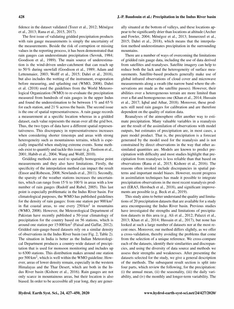
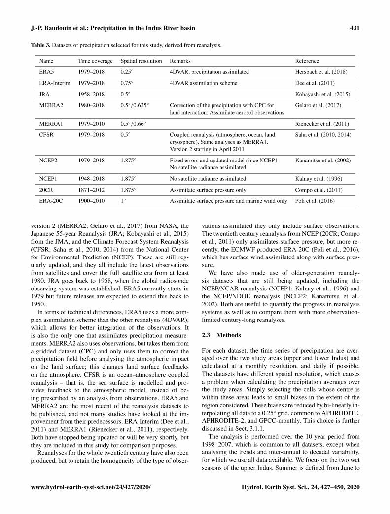
Figure 2. Map of annual mean precipitation for different datasets. The annual mean is computed over the period 1998–2007. GPCCmonthly (a) is used as a reference to compute the anomaly for the other datasets (b–h). The grey lines are the isohyets whose level cor-responds to the labels in the legend. The boundaries of the two study areas are displayed in dark blue on each map. The stars mark the gridcells that include at least one gauge observation. The size of the stars represents the number of time steps with at least one observation overthat cell, relative to the total number of time steps needed to compute the annual mean (120 for a, 3652 for c, d, and e). This information wasnot available for CRU (b) nor ERA5 (h) and does not apply to the satellite-based TMPA (f) and MERRA2 (g).
Hydrol. Earth Syst. Sci., 24, 427–450, 2020 www.hydrol-earth-syst-sci.net/24/427/2020/
J.-P. Baudouin et al.: Precipitation in the Indus River basin 433
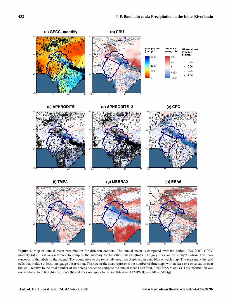
Figure 3. Monthly mean of precipitation, over the period 1998–2007, representing the seasonal cycle. Results are split between upperIndus (a, b) and lower Indus (c, d) as well as observation datasets (a, c) and reanalyses (b, d).
September, which matches the monsoon precipitation peak.Winter is defined from December to March. This fits thesnowfall peak rather than the precipitation peak but makesit possible to focus on issues of snowfall estimation (Palazziet al., 2013). In the lower Indus, we use the same definitionfor summer, but winter is not analysed, as it is a dry season.
We first compare the mean and seasonal cycle of eachdataset in Sects. 3.1 and 3.2. For quantitative statements, weuse GPCC-monthly as a reference. However, in Sect. 3.1.3,we use the precipitation dataset from Dahri et al. (2018) asreference instead. This dataset cannot be used in other partsof the study, as it is limited to one part of the upper Indus andonly provides annual means.
Then, in Sect. 3.3 we compare the daily variability of theprecipitation using the Pearson correlation. The correlationsignificance is discussed at the 95 % probability level. To re-duce the impact of abnormally large rainfall events when in-vestigating trends in daily variability (see Sect. 3.3.4), weuse the Spearman correlation. Lastly, in Sect. 3.4, othertimescales of variability of the precipitation are investigated:monthly, seasonal, inter-annual, and decadal, still using thePearson correlation at the 95 % confidence interval.
3 Results
3.1 Annual mean
3.1.1 Differences between rain-gauge-based datasets
Annual mean precipitation in both study areas and for eachdataset are given in Table 4 (last two columns). We first focuson the rain-gauge-based datasets (upper part of the table).Spatial pattern differences are shown in Fig. 2a to e.
First, we should mention that the bi-linear method we useto interpolate each dataset to the same grid (cf. Sect. 2.3)leads to some differences between datasets. The two GPCCproducts can be used to evaluate the impact of our interpo-lation method, as they have a different spatial resolution butuse the same monthly climatology. Hence, the small underes-timation of GPCC-daily compared to GPCC-monthly (about1 % in the upper Indus and 5 % in the lower Indus) is relatedto the interpolation method. However, these differences aresmall enough to justify the use of our method.
More generally, annual mean differences can be explainedby methods and data that each dataset uses. Particularly,the interpolation of station measurements to a grid differsfrom one dataset to the other. APHRODITE’s interpolationmethod, for instance, considers the orientation of the slopeto quantify the influence of nearby stations. This greatly re-duces the amount of precipitation falling in the inner moun-tains compared to GPCC-monthly. An example of this pat-tern is evident to the north of the Himalayas where only
www.hydrol-earth-syst-sci.net/24/427/2020/ Hydrol. Earth Syst. Sci., 24, 427–450, 2020
434 J.-P. Baudouin et al.: Precipitation in the Indus River basin
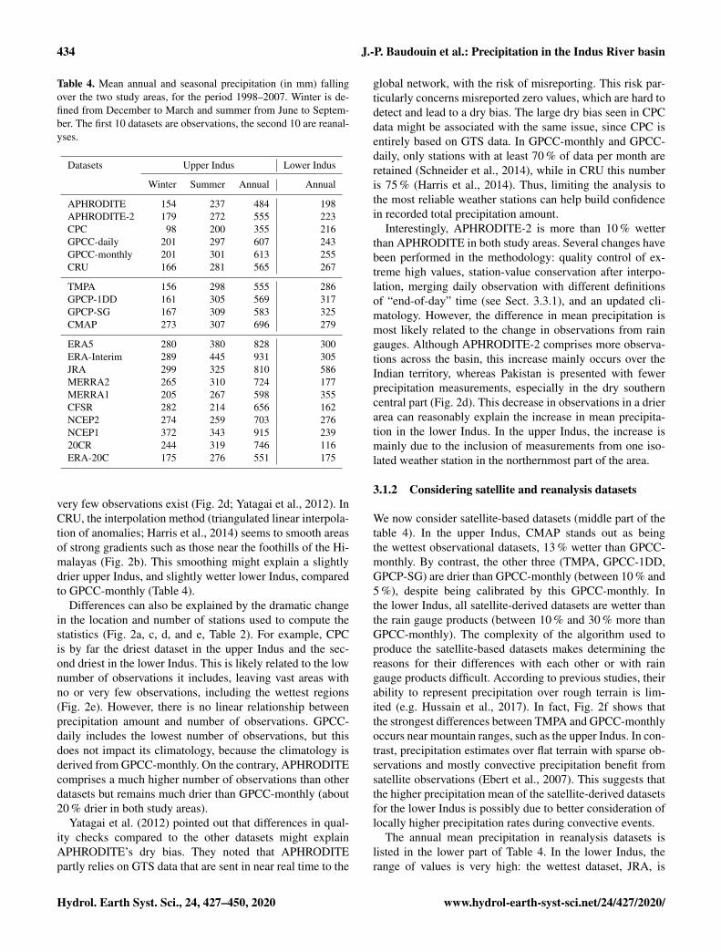
Table 4. Mean annual and seasonal precipitation (in mm) fallingover the two study areas, for the period 1998–2007. Winter is de-fined from December to March and summer from June to Septem-ber. The first 10 datasets are observations, the second 10 are reanal-yses.
Datasets Upper Indus Lower Indus
Winter Summer Annual Annual
APHRODITE 154 237 484 198APHRODITE-2 179 272 555 223CPC 98 200 355 216GPCC-daily 201 297 607 243GPCC-monthly 201 301 613 255CRU 166 281 565 267
TMPA 156 298 555 286GPCP-1DD 161 305 569 317GPCP-SG 167 309 583 325CMAP 273 307 696 279
ERA5 280 380 828 300ERA-Interim 289 445 931 305JRA 299 325 810 586MERRA2 265 310 724 177MERRA1 205 267 598 355CFSR 282 214 656 162NCEP2 274 259 703 276NCEP1 372 343 915 23920CR 244 319 746 116ERA-20C 175 276 551 175
very few observations exist (Fig. 2d; Yatagai et al., 2012). InCRU, the interpolation method (triangulated linear interpola-tion of anomalies; Harris et al., 2014) seems to smooth areasof strong gradients such as those near the foothills of the Hi-malayas (Fig. 2b). This smoothing might explain a slightlydrier upper Indus, and slightly wetter lower Indus, comparedto GPCC-monthly (Table 4).
Differences can also be explained by the dramatic changein the location and number of stations used to compute thestatistics (Fig. 2a, c, d, and e, Table 2). For example, CPCis by far the driest dataset in the upper Indus and the sec-ond driest in the lower Indus. This is likely related to the lownumber of observations it includes, leaving vast areas withno or very few observations, including the wettest regions(Fig. 2e). However, there is no linear relationship betweenprecipitation amount and number of observations. GPCC-daily includes the lowest number of observations, but thisdoes not impact its climatology, because the climatology isderived from GPCC-monthly. On the contrary, APHRODITEcomprises a much higher number of observations than otherdatasets but remains much drier than GPCC-monthly (about20 % drier in both study areas).
Yatagai et al. (2012) pointed out that differences in qual-ity checks compared to the other datasets might explainAPHRODITE’s dry bias. They noted that APHRODITEpartly relies on GTS data that are sent in near real time to the
global network, with the risk of misreporting. This risk par-ticularly concerns misreported zero values, which are hard todetect and lead to a dry bias. The large dry bias seen in CPCdata might be associated with the same issue, since CPC isentirely based on GTS data. In GPCC-monthly and GPCC-daily, only stations with at least 70 % of data per month areretained (Schneider et al., 2014), while in CRU this numberis 75 % (Harris et al., 2014). Thus, limiting the analysis tothe most reliable weather stations can help build confidencein recorded total precipitation amount.
Interestingly, APHRODITE-2 is more than 10 % wetterthan APHRODITE in both study areas. Several changes havebeen performed in the methodology: quality control of ex-treme high values, station-value conservation after interpo-lation, merging daily observation with different definitionsof “end-of-day” time (see Sect. 3.3.1), and an updated cli-matology. However, the difference in mean precipitation ismost likely related to the change in observations from raingauges. Although APHRODITE-2 comprises more observa-tions across the basin, this increase mainly occurs over theIndian territory, whereas Pakistan is presented with fewerprecipitation measurements, especially in the dry southerncentral part (Fig. 2d). This decrease in observations in a drierarea can reasonably explain the increase in mean precipita-tion in the lower Indus. In the upper Indus, the increase ismainly due to the inclusion of measurements from one iso-lated weather station in the northernmost part of the area.
3.1.2 Considering satellite and reanalysis datasets
We now consider satellite-based datasets (middle part of thetable 4). In the upper Indus, CMAP stands out as beingthe wettest observational datasets, 13 % wetter than GPCC-monthly. By contrast, the other three (TMPA, GPCC-1DD,GPCP-SG) are drier than GPCC-monthly (between 10 % and5 %), despite being calibrated by this GPCC-monthly. Inthe lower Indus, all satellite-derived datasets are wetter thanthe rain gauge products (between 10 % and 30 % more thanGPCC-monthly). The complexity of the algorithm used toproduce the satellite-based datasets makes determining thereasons for their differences with each other or with raingauge products difficult. According to previous studies, theirability to represent precipitation over rough terrain is lim-ited (e.g. Hussain et al., 2017). In fact, Fig. 2f shows thatthe strongest differences between TMPA and GPCC-monthlyoccurs near mountain ranges, such as the upper Indus. In con-trast, precipitation estimates over flat terrain with sparse ob-servations and mostly convective precipitation benefit fromsatellite observations (Ebert et al., 2007). This suggests thatthe higher precipitation mean of the satellite-derived datasetsfor the lower Indus is possibly due to better consideration oflocally higher precipitation rates during convective events.
The annual mean precipitation in reanalysis datasets islisted in the lower part of Table 4. In the lower Indus, therange of values is very high: the wettest dataset, JRA, is
Hydrol. Earth Syst. Sci., 24, 427–450, 2020 www.hydrol-earth-syst-sci.net/24/427/2020/
J.-P. Baudouin et al.: Precipitation in the Indus River basin 435
5 times wetter than the driest dataset, 20CR. This rangeshows the significant difficulties for reanalyses to representprecipitation in an area where convection dominates. Amongthe most recent reanalyses, ERA5 has the closest estimatesof precipitation to the observational datasets, yet they remainabove the estimates from rain gauges. Figure 2h suggests thatthese wetter conditions mainly come from the north-westernedge of the Suleiman range, an area with sparse precipita-tion observations (cf. Fig. 2a), therefore increasing confi-dence in ERA5 estimation. The two twentieth century reanal-ysis (20CR and ERA-20C) are amongst the driest reanalysisdatasets, suggesting that their models have difficulties prop-agating the monsoon precipitation into the lower Indus re-gion, when only surface observations are assimilated. Lastly,MERRA2 exhibits a severe drop in precipitation compared tothe previous version, MERRA1. Summer monsoon precipi-tation is known to be strongly affected by surface moisturecontent, especially in flat areas like the lower Indus (Dou-ville et al., 2001). MERRA2 uses CPC data to constrain theprecipitation flux at the surface. Due to the dry bias of CPC,soil moisture is reduced for most of India (Fig. 3 in Reichleet al., 2017), explaining the drop in precipitation.
For the upper Indus, the most striking feature is thatall reanalysis datasets except MERRA1 and ERA-20C pre-dict higher precipitation amounts than GPCC-monthly, about20 % higher on average. In the following we investigatewhether this difference can be explained by an underestima-tion of rain gauge measurements.
3.1.3 Impact of rain gauge biases in mountainousterrains
Rain gauge measurements are known to potentially underes-timate precipitation and particularly snowfall (Sevruk, 1984;Goodison et al., 1989). This is an important issue for moun-tainous regions such as the upper Indus. However, among thesix rain-gauge-based datasets, only GPCC’s products con-sider a correction of the data. Based on a study by Legatesand Willmott (1990), a correction factor, which depends onthe month, is applied at each grid cell. Most of these factorsvary between 5 % and 10 % (Fig. 4 in Schneider et al., 2014)and explain why GPCC’s products are wetter than most of theother rain-gauge-based datasets. Recently, Dahri et al. (2018,hereafter Dahri2018) compiled the measurements from over270 rain gauges in the upper Indus and adjusted their valuesto the under-catchment, following WMO guidelines. Theyfound a basin-wide adjustment of 21 %, but this varies from65 % for high altitude stations to around 1 % for the stationsin the plains.
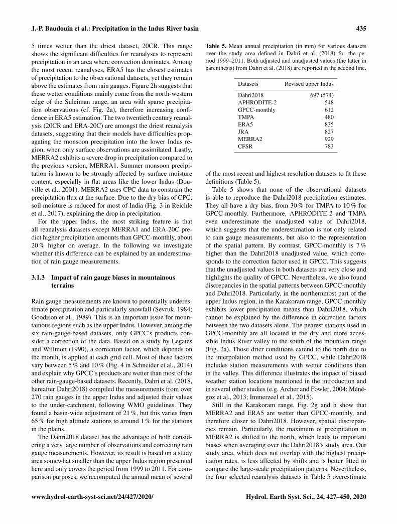
The Dahri2018 dataset has the advantage of both consid-ering a very large number of observations and correcting raingauge measurements. However, its result is based on a studyarea somewhat smaller than the upper Indus region presentedhere and only covers the period from 1999 to 2011. For com-parison purposes, we recomputed the annual mean of several
Table 5. Mean annual precipitation (in mm) for various datasetsover the study area defined in Dahri et al. (2018) for the pe-riod 1999–2011. Both adjusted and unadjusted values (the latter inparenthesis) from Dahri et al. (2018) are reported in the second line.
Datasets Revised upper Indus
Dahri2018 697 (574)APHRODITE-2 548GPCC-monthly 612TMPA 480ERA5 835JRA 827MERRA2 929CFSR 783
of the most recent and highest resolution datasets to fit thesedefinitions (Table 5).
Table 5 shows that none of the observational datasetsis able to reproduce the Dahri2018 precipitation estimates.They all have a dry bias, from 30 % for TMPA to 10 % forGPCC-monthly. Furthermore, APHRODITE-2 and TMPAeven underestimate the unadjusted value of Dahri2018,which suggests that the underestimation is not only relatedto rain gauge measurements, but also to the representationof the spatial pattern. By contrast, GPCC-monthly is 7 %higher than the Dahri2018 unadjusted value, which corre-sponds to the correction factor used in GPCC. This suggeststhat the unadjusted values in both datasets are very close andhighlights the quality of GPCC. Nevertheless, we also founddiscrepancies in the spatial patterns between GPCC-monthlyand Dahri2018. Particularly, in the northernmost part of theupper Indus region, in the Karakoram range, GPCC-monthlyexhibits lower precipitation means than Dahri2018, whichcannot be explained by the difference in correction factorsbetween the two datasets alone. The nearest stations used inGPCC-monthly are all located in the dry and more acces-sible Indus River valley to the south of the mountain range(Fig. 2a). Those drier conditions extend to the north due tothe interpolation method used by GPCC, while Dahri2018includes station measurements with wetter conditions thanin the valley. This difference illustrates the impact of biasedweather station locations mentioned in the introduction andin several other studies (e.g. Archer and Fowler, 2004; Méné-goz et al., 2013; Immerzeel et al., 2015).
Still in the Karakoram range, Fig. 2g and h show thatMERRA2 and ERA5 are wetter than GPCC-monthly, andtherefore closer to Dahri2018. However, spatial discrepan-cies remain. Particularly, the maximum of precipitation inMERRA2 is shifted to the north, which leads to importantbiases when averaging over the Dahri2018’s study area. Ourstudy area, which does not overlap with the highest precip-itation rates, is less affected by shifts and is better fitted tocompare the large-scale precipitation patterns. Nevertheless,the four selected reanalysis datasets in Table 5 overestimate
www.hydrol-earth-syst-sci.net/24/427/2020/ Hydrol. Earth Syst. Sci., 24, 427–450, 2020

436 J.-P. Baudouin et al.: Precipitation in the Indus River basin
the Dahri2018 adjusted values, by 20 % on average. This sug-gests that part but not all of the differences between reanal-yses and observational data can be explained by biases fromthe latter. This overestimation of modelled precipitation inreanalyses for the upper Indus is corroborated by previousstudies (e.g. Palazzi et al., 2015).
To conclude, all rain-gauge-based datasets suffer from anunderestimation of annual mean precipitation for the upperIndus when compared to Darhi2018. This results from biasesin rain gauge locations and measurements. Quality controland interpolation methods also impact precipitation amountin both parts of the basin. Satellite observations probably im-prove precipitation estimates in flat areas with sparse obser-vations. However, they cannot correct observational biasessince they use them for calibration, and biases remain un-changed or even become amplified for the upper Indus. Re-analyses do not include rain gauge measurement, except forERA5 and MERRA2, and are therefore not affected by ob-servational biases. However, model biases can also be signif-icant, as suggested by the spread of the annual mean precipi-tation values. Reanalyses tend to be wetter than observationaldatasets in the upper Indus, which is partly explained bythe underestimation of the observations. Lastly, all datasetssuffer from spatial discrepancies, which are detrimental tosmall-scale comparisons, especially near mountains, but jus-tify our choice to use a larger study area.
3.2 Seasonal cycle
The seasonal cycle of precipitation for each dataset is pre-sented in Fig. 3. Analysing the seasonality is particularly in-teresting in the upper Indus, as it is characterised by two wetseasons. The mean precipitation of each season is presentedin Table 4 (second and third column). The rain-gauge-baseddatasets exhibit a very similar seasonality for both study ar-eas. In the upper Indus, the maxima of precipitation occur inFebruary and July, the minima in May and November. Thedifferences between the datasets vary little from one monthto another, which suggests that the causes of the differencesidentified in the previous section (e.g. misreporting, stationlocation and number, interpolation method) are independentof the seasonality. The satellite-based datasets represent thesummer precipitation almost exactly the same as GPCC-monthly. The annual mean differences are explained by bi-ases during the winter season, which suggests that winterprecipitation is more difficult to estimate for those datasets.
The reanalyses represent the dry and wet seasons of theupper Indus, but with a larger spread than in the observa-tions and some differences in seasonal cycle (Fig. 3b). Onaverage, winter precipitation is 30 % higher than in GPCC-monthly, with the notable exception of ERA-20C (Table 4).Those wetter conditions also extend to the surrounding driermonths: April–May and October–November. However, themean summer precipitation in reanalyses is not significantlydifferent from GPCC-monthly (Table 4). Only ERA-Interim
stands out with a wet summer precipitation bias, mainly inthe north-west corner of the upper Indus, a bias partly cor-rected in ERA5 (Fig. 2h). The winter wet bias is not surpris-ing after the comparison with the Dahri2018 dataset in theSect. 3.1.3. Indeed, Dahri2018 found that the most impor-tant rain gauge underestimations happen in winter when pre-cipitation mostly falls as snow. More interestingly, we foundthat the latest reanalyses (ERA5, JRA, MERRA2, and CFSR)represent winter precipitation in similar ways. We have notbeen able to investigate the seasonality of the Dahri2018dataset, but we suggest that the latest reanalyses better repre-sent winter precipitation than the observational datasets.
We noted another discrepancy in seasonality between amajority of the reanalyses and the observations for the upperIndus: a delay of the summer precipitation starting from thepre-monsoon season (Fig. 3b). The observations show thatMay is the driest month of that season, followed by a sharpincrease in precipitation in June. Only ERA5, ERA-Interim,and MERRA1 reproduce this behaviour. In contrast, NCEP2and CFSR are much drier in June than in May. For other re-analyses, precipitation during May and June are comparable.This delay continues into the summer monsoon period: whilethe observations clearly show a wetter July than August, thisis only the case for ERA5, ERA-Interim, and both MERRAreanalyses. A similar delay can be found over the Gangesplain and along the Himalayas, which suggests wider un-certainties in the monsoon propagation in the reanalyses. Bycontrast, no such delay is found in the lower Indus, despitethe large uncertainty in the amount of precipitation (Fig. 3d).
3.3 Daily variability
3.3.1 Lag analysis
Investigating the daily precipitation variability helps to bet-ter quantify the quality of each dataset. Before computingthe daily correlation, we checked for possible lags betweenthe datasets. Lags can have different origins. The first is theaccumulation period considered for the rain gauge measure-ments. CPC documentation (Xie et al., 2010) points out thatthe official period is different from one country to another (inour case, Afghanistan, Pakistan, and India all use differentperiods, or end-of-day time: 00:00, 06:00, and 03:00 UTC,respectively), which could impact precipitation estimates.Neither GPCC-daily nor APHRODITE documentation men-tion this issue, while a specific effort has been made to ho-mogenise all observations in APHRODITE-2. Secondly, theTMPA algorithm uses the 00:00 h imagery for the followingday of accumulation and therefore could be more represen-tative of an accumulation starting at 22:30 UTC (Huffmanet al., 2007). Thirdly, biases in the daily cycle are possible inthe reanalyses.
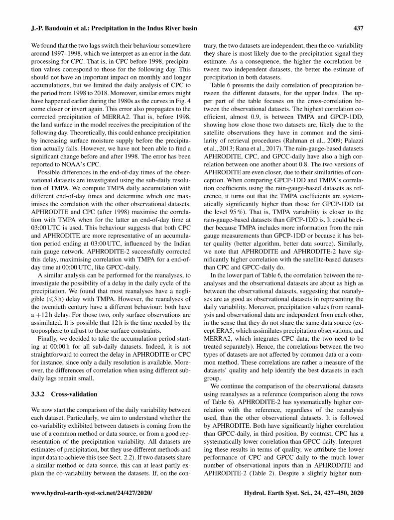
Our main finding relates to CPC. Figure 4 shows the dailycorrelation year per year of CPC against APHRODITE andMERRA2, for two lags: 0 and−24 h (previous day for CPC).
Hydrol. Earth Syst. Sci., 24, 427–450, 2020 www.hydrol-earth-syst-sci.net/24/427/2020/
J.-P. Baudouin et al.: Precipitation in the Indus River basin 437
We found that the two lags switch their behaviour somewherearound 1997–1998, which we interpret as an error in the dataprocessing for CPC. That is, in CPC before 1998, precipita-tion values correspond to those for the following day. Thisshould not have an important impact on monthly and longeraccumulations, but we limited the daily analysis of CPC tothe period from 1998 to 2018. Moreover, similar errors mighthave happened earlier during the 1980s as the curves in Fig. 4come closer or invert again. This error also propagates to thecorrected precipitation of MERRA2. That is, before 1998,the land surface in the model receives the precipitation of thefollowing day. Theoretically, this could enhance precipitationby increasing surface moisture supply before the precipita-tion actually falls. However, we have not been able to find asignificant change before and after 1998. The error has beenreported to NOAA’s CPC.
Possible differences in the end-of-day times of the obser-vational datasets are investigated using the sub-daily resolu-tion of TMPA. We compute TMPA daily accumulation withdifferent end-of-day times and determine which one max-imises the correlation with the other observational datasets.APHRODITE and CPC (after 1998) maximise the correla-tion with TMPA when for the latter an end-of-day time at03:00 UTC is used. This behaviour suggests that both CPCand APHRODITE are more representative of an accumula-tion period ending at 03:00 UTC, influenced by the Indianrain gauge network. APHRODITE-2 successfully correctedthis delay, maximising correlation with TMPA for a end-of-day time at 00:00 UTC, like GPCC-daily.
A similar analysis can be performed for the reanalyses, toinvestigate the possibility of a delay in the daily cycle of theprecipitation. We found that most reanalyses have a negli-gible (63 h) delay with TMPA. However, the reanalyses ofthe twentieth century have a different behaviour: both havea +12 h delay. For those two, only surface observations areassimilated. It is possible that 12 h is the time needed by thetroposphere to adjust to those surface constraints.
Finally, we decided to take the accumulation period start-ing at 00:00 h for all sub-daily datasets. Indeed, it is notstraightforward to correct the delay in APHRODITE or CPCfor instance, since only a daily resolution is available. More-over, the differences of correlation when using different sub-daily lags remain small.
3.3.2 Cross-validation
We now start the comparison of the daily variability betweeneach dataset. Particularly, we aim to understand whether theco-variability exhibited between datasets is coming from theuse of a common method or data source, or from a good rep-resentation of the precipitation variability. All datasets areestimates of precipitation, but they use different methods andinput data to achieve this (see Sect. 2.2). If two datasets sharea similar method or data source, this can at least partly ex-plain the co-variability between the datasets. If, on the con-
trary, the two datasets are independent, then the co-variabilitythey share is most likely due to the precipitation signal theyestimate. As a consequence, the higher the correlation be-tween two independent datasets, the better the estimate ofprecipitation in both datasets.
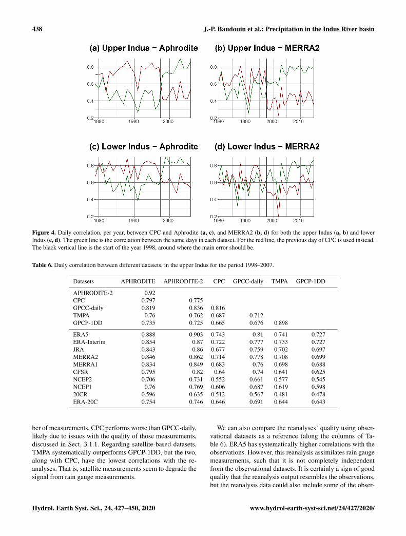
Table 6 presents the daily correlation of precipitation be-tween the different datasets, for the upper Indus. The up-per part of the table focuses on the cross-correlation be-tween the observational datasets. The highest correlation co-efficient, almost 0.9, is between TMPA and GPCP-1DD,showing how close those two datasets are, likely due to thesatellite observations they have in common and the simi-larity of retrieval procedures (Rahman et al., 2009; Palazziet al., 2013; Rana et al., 2017). The rain-gauge-based datasetsAPHRODITE, CPC, and GPCC-daily have also a high cor-relation between one another about 0.8. The two versions ofAPHRODITE are even closer, due to their similarities of con-ception. When comparing GPCP-1DD and TMPA’s correla-tion coefficients using the rain-gauge-based datasets as ref-erence, it turns out that the TMPA coefficients are system-atically significantly higher than those for GPCP-1DD (atthe level 95 %). That is, TMPA variability is closer to therain-gauge-based datasets than GPCP-1DD is. It could be ei-ther because TMPA includes more information from the raingauge measurements than GPCP-1DD or because it has bet-ter quality (better algorithm, better data source). Similarly,we note that APHRODITE and APHRODITE-2 have sig-nificantly higher correlation with the satellite-based datasetsthan CPC and GPCC-daily do.
In the lower part of Table 6, the correlation between the re-analyses and the observational datasets are about as high asbetween the observational datasets, suggesting that reanaly-ses are as good as observational datasets in representing thedaily variability. Moreover, precipitation values from reanal-ysis and observational data are independent from each other,in the sense that they do not share the same data source (ex-cept ERA5, which assimilates precipitation observations, andMERRA2, which integrates CPC data; the two need to betreated separately). Hence, the correlations between the twotypes of datasets are not affected by common data or a com-mon method. These correlations are rather a measure of thedatasets’ quality and help identify the best datasets in eachgroup.
We continue the comparison of the observational datasetsusing reanalyses as a reference (comparison along the rowsof Table 6). APHRODITE-2 has systematically higher cor-relation with the reference, regardless of the reanalysisused, than the other observational datasets. It is followedby APHRODITE. Both have significantly higher correlationthan GPCC-daily, in third position. By contrast, CPC has asystematically lower correlation than GPCC-daily. Interpret-ing these results in terms of quality, we attribute the lowerperformance of CPC and GPCC-daily to the much lowernumber of observational inputs than in APHRODITE andAPHRODITE-2 (Table 2). Despite a slightly higher num-
www.hydrol-earth-syst-sci.net/24/427/2020/ Hydrol. Earth Syst. Sci., 24, 427–450, 2020
438 J.-P. Baudouin et al.: Precipitation in the Indus River basin
Figure 4. Daily correlation, per year, between CPC and Aphrodite (a, c), and MERRA2 (b, d) for both the upper Indus (a, b) and lowerIndus (c, d). The green line is the correlation between the same days in each dataset. For the red line, the previous day of CPC is used instead.The black vertical line is the start of the year 1998, around where the main error should be.
Table 6. Daily correlation between different datasets, in the upper Indus for the period 1998–2007.
Datasets APHRODITE APHRODITE-2 CPC GPCC-daily TMPA GPCP-1DD
APHRODITE-2 0.92CPC 0.797 0.775GPCC-daily 0.819 0.836 0.816TMPA 0.76 0.762 0.687 0.712GPCP-1DD 0.735 0.725 0.665 0.676 0.898
ERA5 0.888 0.903 0.743 0.81 0.741 0.727ERA-Interim 0.854 0.87 0.722 0.777 0.733 0.727JRA 0.843 0.86 0.677 0.759 0.702 0.697MERRA2 0.846 0.862 0.714 0.778 0.708 0.699MERRA1 0.834 0.849 0.683 0.76 0.698 0.688CFSR 0.795 0.82 0.64 0.74 0.641 0.625NCEP2 0.706 0.731 0.552 0.661 0.577 0.545NCEP1 0.76 0.769 0.606 0.687 0.619 0.59820CR 0.596 0.635 0.512 0.567 0.481 0.478ERA-20C 0.754 0.746 0.646 0.691 0.644 0.643
ber of measurements, CPC performs worse than GPCC-daily,likely due to issues with the quality of those measurements,discussed in Sect. 3.1.1. Regarding satellite-based datasets,TMPA systematically outperforms GPCP-1DD, but the two,along with CPC, have the lowest correlations with the re-analyses. That is, satellite measurements seem to degrade thesignal from rain gauge measurements.
We can also compare the reanalyses’ quality using obser-vational datasets as a reference (along the columns of Ta-ble 6). ERA5 has systematically higher correlations with theobservations. However, this reanalysis assimilates rain gaugemeasurements, such that it is not completely independentfrom the observational datasets. It is certainly a sign of goodquality that the reanalysis output resembles the observations,but the reanalysis data could also include some of the obser-
Hydrol. Earth Syst. Sci., 24, 427–450, 2020 www.hydrol-earth-syst-sci.net/24/427/2020/
J.-P. Baudouin et al.: Precipitation in the Indus River basin 439
vation errors. ERA-Interim has the second highest correla-tions and is the best-performing reanalysis among those thatdo not assimilate precipitation observations. It is closely fol-lowed by MERRA2, while CFSR has poorer results amongthe latest generation of reanalyses. Interestingly for NCEP’sreanalyses, the first version outperforms the second version.The two twentieth century reanalyses also show interestingbehaviour: while 20CR has the lowest correlations with theobservations, ERA-20C performance is between CFSR andNCEP1, despite only assimilating surface observations. Thisbehaviour clearly shows the progress made in reanalysis pro-cessing (e.g. in atmospheric modelling and data assimilation)over the last decades.
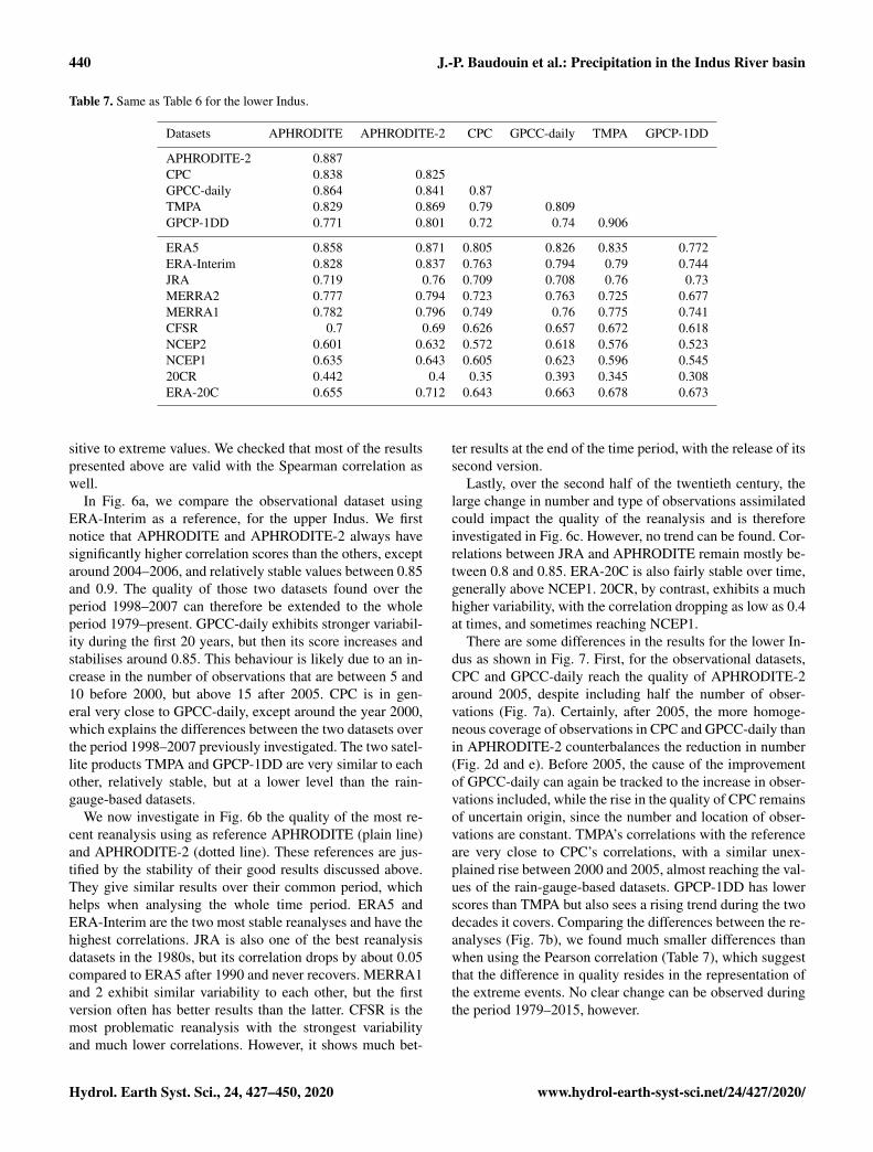
The same correlation analysis is performed for the lowerIndus (Table 7). The results are quite similar, but we alsonote some interesting differences. The correlations betweenthe observations are all higher for this study area. In thisflat area, precipitation is less heterogeneous, and observa-tions are more representative of their surrounding (i.e. largerspatial representativeness). In contrast, the reanalyses havelower correlations with observations than for the upper In-dus. The lower Indus only receives precipitation during thesummer monsoon, which is less well represented in mod-els than the winter precipitation in the upper Indus (see fol-lowing section on seasonality). In particular, APHRODITE-2and APHRODITE still perform best among the observationaldatasets, but the four other datasets rank in a different order:satellite products are possibly better in that flatter area. Forthe reanalyses, we noticed that MERRA2 does not outper-form MERRA1. It echoes the large change in precipitationamount between the two discussed above (Table 4) and, simi-larly, could be related to the integration of CPC in MERRA2.Indeed, Table 7 suggests that CPC does not perform as wellas the other observational datasets in terms of variability,and, indeed, surface moisture content variability was not im-proved from MERRA1 to MERRA2 in the study area (Fig. 1in Reichle et al., 2017). As for ERA5 and ERA-Interim, theyremain the two reanalysis datasets with the highest correla-tion with the observations.
3.3.3 Influence of the seasonality
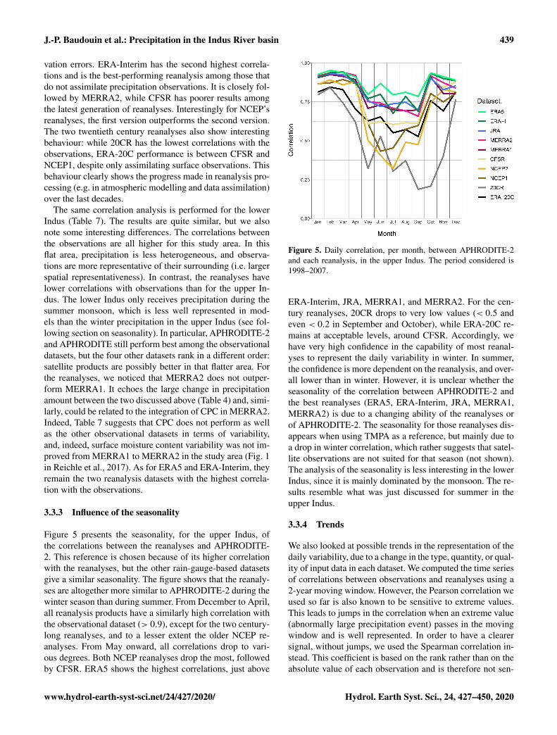
Figure 5 presents the seasonality, for the upper Indus, ofthe correlations between the reanalyses and APHRODITE-2. This reference is chosen because of its higher correlationwith the reanalyses, but the other rain-gauge-based datasetsgive a similar seasonality. The figure shows that the reanaly-ses are altogether more similar to APHRODITE-2 during thewinter season than during summer. From December to April,all reanalysis products have a similarly high correlation withthe observational dataset (> 0.9), except for the two century-long reanalyses, and to a lesser extent the older NCEP re-analyses. From May onward, all correlations drop to vari-ous degrees. Both NCEP reanalyses drop the most, followedby CFSR. ERA5 shows the highest correlations, just above
Figure 5. Daily correlation, per month, between APHRODITE-2and each reanalysis, in the upper Indus. The period considered is1998–2007.
ERA-Interim, JRA, MERRA1, and MERRA2. For the cen-tury reanalyses, 20CR drops to very low values (< 0.5 andeven < 0.2 in September and October), while ERA-20C re-mains at acceptable levels, around CFSR. Accordingly, wehave very high confidence in the capability of most reanal-yses to represent the daily variability in winter. In summer,the confidence is more dependent on the reanalysis, and over-all lower than in winter. However, it is unclear whether theseasonality of the correlation between APHRODITE-2 andthe best reanalyses (ERA5, ERA-Interim, JRA, MERRA1,MERRA2) is due to a changing ability of the reanalyses orof APHRODITE-2. The seasonality for those reanalyses dis-appears when using TMPA as a reference, but mainly due toa drop in winter correlation, which rather suggests that satel-lite observations are not suited for that season (not shown).The analysis of the seasonality is less interesting in the lowerIndus, since it is mainly dominated by the monsoon. The re-sults resemble what was just discussed for summer in theupper Indus.
3.3.4 Trends
We also looked at possible trends in the representation of thedaily variability, due to a change in the type, quantity, or qual-ity of input data in each dataset. We computed the time seriesof correlations between observations and reanalyses using a2-year moving window. However, the Pearson correlation weused so far is also known to be sensitive to extreme values.This leads to jumps in the correlation when an extreme value(abnormally large precipitation event) passes in the movingwindow and is well represented. In order to have a clearersignal, without jumps, we used the Spearman correlation in-stead. This coefficient is based on the rank rather than on theabsolute value of each observation and is therefore not sen-
www.hydrol-earth-syst-sci.net/24/427/2020/ Hydrol. Earth Syst. Sci., 24, 427–450, 2020
440 J.-P. Baudouin et al.: Precipitation in the Indus River basin
Table 7. Same as Table 6 for the lower Indus.
Datasets APHRODITE APHRODITE-2 CPC GPCC-daily TMPA GPCP-1DD
APHRODITE-2 0.887CPC 0.838 0.825GPCC-daily 0.864 0.841 0.87TMPA 0.829 0.869 0.79 0.809GPCP-1DD 0.771 0.801 0.72 0.74 0.906
ERA5 0.858 0.871 0.805 0.826 0.835 0.772ERA-Interim 0.828 0.837 0.763 0.794 0.79 0.744JRA 0.719 0.76 0.709 0.708 0.76 0.73MERRA2 0.777 0.794 0.723 0.763 0.725 0.677MERRA1 0.782 0.796 0.749 0.76 0.775 0.741CFSR 0.7 0.69 0.626 0.657 0.672 0.618NCEP2 0.601 0.632 0.572 0.618 0.576 0.523NCEP1 0.635 0.643 0.605 0.623 0.596 0.54520CR 0.442 0.4 0.35 0.393 0.345 0.308ERA-20C 0.655 0.712 0.643 0.663 0.678 0.673
sitive to extreme values. We checked that most of the resultspresented above are valid with the Spearman correlation aswell.
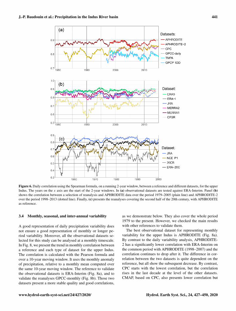
In Fig. 6a, we compare the observational dataset usingERA-Interim as a reference, for the upper Indus. We firstnotice that APHRODITE and APHRODITE-2 always havesignificantly higher correlation scores than the others, exceptaround 2004–2006, and relatively stable values between 0.85and 0.9. The quality of those two datasets found over theperiod 1998–2007 can therefore be extended to the wholeperiod 1979–present. GPCC-daily exhibits stronger variabil-ity during the first 20 years, but then its score increases andstabilises around 0.85. This behaviour is likely due to an in-crease in the number of observations that are between 5 and10 before 2000, but above 15 after 2005. CPC is in gen-eral very close to GPCC-daily, except around the year 2000,which explains the differences between the two datasets overthe period 1998–2007 previously investigated. The two satel-lite products TMPA and GPCP-1DD are very similar to eachother, relatively stable, but at a lower level than the rain-gauge-based datasets.
We now investigate in Fig. 6b the quality of the most re-cent reanalysis using as reference APHRODITE (plain line)and APHRODITE-2 (dotted line). These references are jus-tified by the stability of their good results discussed above.They give similar results over their common period, whichhelps when analysing the whole time period. ERA5 andERA-Interim are the two most stable reanalyses and have thehighest correlations. JRA is also one of the best reanalysisdatasets in the 1980s, but its correlation drops by about 0.05compared to ERA5 after 1990 and never recovers. MERRA1and 2 exhibit similar variability to each other, but the firstversion often has better results than the latter. CFSR is themost problematic reanalysis with the strongest variabilityand much lower correlations. However, it shows much bet-
ter results at the end of the time period, with the release of itssecond version.
Lastly, over the second half of the twentieth century, thelarge change in number and type of observations assimilatedcould impact the quality of the reanalysis and is thereforeinvestigated in Fig. 6c. However, no trend can be found. Cor-relations between JRA and APHRODITE remain mostly be-tween 0.8 and 0.85. ERA-20C is also fairly stable over time,generally above NCEP1. 20CR, by contrast, exhibits a muchhigher variability, with the correlation dropping as low as 0.4at times, and sometimes reaching NCEP1.
There are some differences in the results for the lower In-dus as shown in Fig. 7. First, for the observational datasets,CPC and GPCC-daily reach the quality of APHRODITE-2around 2005, despite including half the number of obser-vations (Fig. 7a). Certainly, after 2005, the more homoge-neous coverage of observations in CPC and GPCC-daily thanin APHRODITE-2 counterbalances the reduction in number(Fig. 2d and e). Before 2005, the cause of the improvementof GPCC-daily can again be tracked to the increase in obser-vations included, while the rise in the quality of CPC remainsof uncertain origin, since the number and location of obser-vations are constant. TMPA’s correlations with the referenceare very close to CPC’s correlations, with a similar unex-plained rise between 2000 and 2005, almost reaching the val-ues of the rain-gauge-based datasets. GPCP-1DD has lowerscores than TMPA but also sees a rising trend during the twodecades it covers. Comparing the differences between the re-analyses (Fig. 7b), we found much smaller differences thanwhen using the Pearson correlation (Table 7), which suggestthat the difference in quality resides in the representation ofthe extreme events. No clear change can be observed duringthe period 1979–2015, however.
Hydrol. Earth Syst. Sci., 24, 427–450, 2020 www.hydrol-earth-syst-sci.net/24/427/2020/
J.-P. Baudouin et al.: Precipitation in the Indus River basin 441
Figure 6. Daily correlation using the Spearman formula, on a running 2-year window, between a reference and different datasets, for the upperIndus. The years on the x axis are the start of the 2-year windows. In (a) observational datasets are tested against ERA-Interim. Panel (b)shows the correlation between a selection of reanalysis and APHRODITE data over the period 1979–2005 (plain line) and APHRODITE-2over the period 1998–2013 (dotted line). Finally, (c) presents the reanalyses covering the second half of the 20th century, with APHRODITEas reference.
3.4 Monthly, seasonal, and inter-annual variability
A good representation of daily precipitation variability doesnot ensure a good representation of monthly or longer pe-riod variability. Moreover, all the observational datasets se-lected for this study can be analysed at a monthly timescale.In Fig. 8, we present the trend in monthly correlation betweena reference and each type of dataset for the upper Indus.The correlation is calculated with the Pearson formula andover a 10-year moving window. It uses the monthly anomalyof precipitation, relative to a monthly mean computed overthe same 10-year moving window. The reference to validatethe observational datasets is ERA-Interim (Fig. 8a), and tovalidate the reanalyses GPCC-monthly (Fig. 8b). Those twodatasets present a more stable quality and good correlations,
as we demonstrate below. They also cover the whole period1979 to the present. However, we checked the main resultswith other references to validate them.
The best observational dataset for representing monthlyvariability for the upper Indus is APHRODITE (Fig. 8a).By contrast to the daily variability analysis, APHRODITE-2 has a significantly lower correlation with ERA-Interim onthe common period with APHRODITE (1998–2007) and thecorrelation continues to drop after it. The difference in cor-relation between the two datasets is quite dependent on thereference, but all show the subsequent decrease. By contrast,CPC starts with the lowest correlation, but the correlationrises in the last decade at the level of the other datasets.CMAP, based on CPC, also presents lower correlation but
www.hydrol-earth-syst-sci.net/24/427/2020/ Hydrol. Earth Syst. Sci., 24, 427–450, 2020

442 J.-P. Baudouin et al.: Precipitation in the Indus River basin
Figure 7. Same as Fig. 6 but for the lower Indus.
is more variable, and it depicts a similar rise around the year2000. All the other datasets are very close to each other.
Still for monthly variability, the closest reanalysis to theobservations is ERA5 (Fig. 8b), except when using CPC andCMAP as reference: then, MERRA2 has higher correlationat times, likely due to the use of CPC data in both CMAPand MERRA2. Several datasets show a decrease in corre-lation during the 1990s: JRA has a drop more pronouncedthan what is observed for the daily variability, and a dropappears for NCEP1, NCEP2, and ERA-20C. 20CR has thelowest correlation, while MERRA2, MERRA1, and ERA-Interim are quite similar, with correlation just below ERA5.CFSR also has relatively high values but exhibits a decreas-ing trend, especially in the last 10 years, which is evenmore pronounced when testing with the other observationaldatasets. It is possible that version 2 of CFSR gives better re-sults, but it has not been running long enough to evaluate themonthly variability over a 10-year period. Instead, the corre-
lations in Fig. 8b include both versions toward the end of thetime period, which could add discrepancies when computingthe monthly mean anomaly.
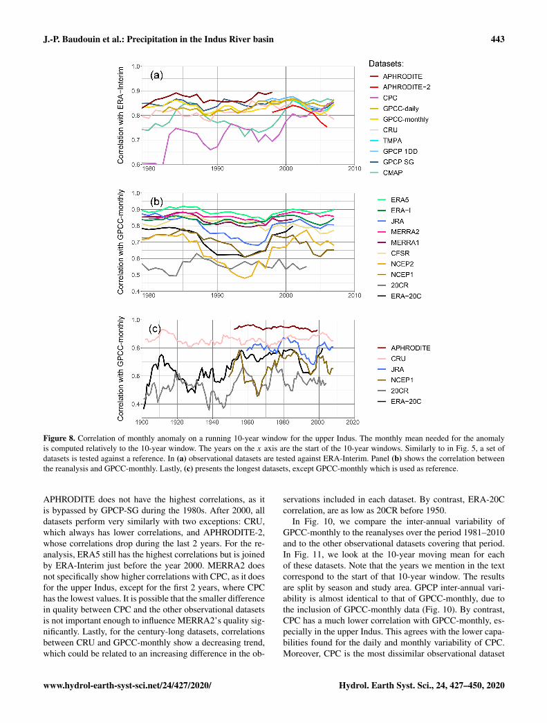
We also tested the datasets with the longest time coverageagainst GPCC-monthly (Fig. 8c). We found relatively stablecorrelations with APHRODITE and CRU during the twenti-eth century: the time series do not diverge, despite the low-ering number of observations. However, since the datasetsare not independent, we cannot say that the quality of thosedatasets remains constant. The reanalyses present fluctuatingcorrelations with the reference. ERA-20C has lower correla-tions in the first half of the century, which could be due toa lowering confidence in either the reference or the reanaly-sis. However, ERA-20C correlations get closer to 20-CR dur-ing that period, which suggests the variation in the reanalysisquality is the most important factor.
The lower Indus shows somewhat different results interms of monthly variability (Fig. 9). For the observations,
Hydrol. Earth Syst. Sci., 24, 427–450, 2020 www.hydrol-earth-syst-sci.net/24/427/2020/
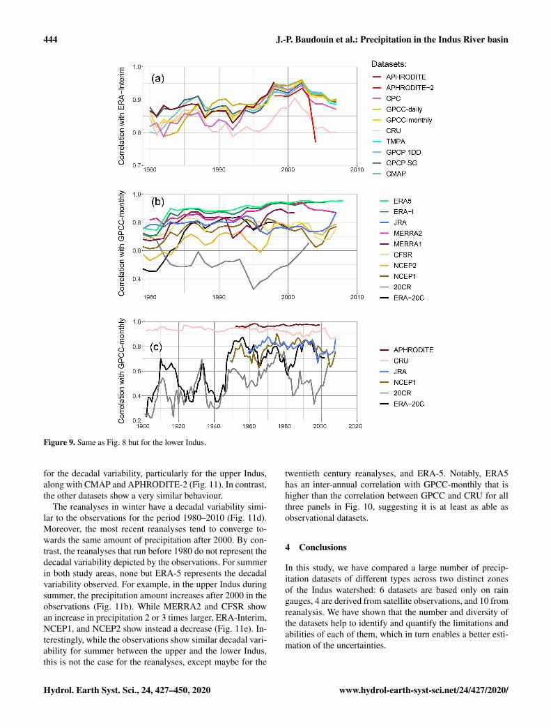
J.-P. Baudouin et al.: Precipitation in the Indus River basin 443
Figure 8. Correlation of monthly anomaly on a running 10-year window for the upper Indus. The monthly mean needed for the anomalyis computed relatively to the 10-year window. The years on the x axis are the start of the 10-year windows. Similarly to in Fig. 5, a set ofdatasets is tested against a reference. In (a) observational datasets are tested against ERA-Interim. Panel (b) shows the correlation betweenthe reanalysis and GPCC-monthly. Lastly, (c) presents the longest datasets, except GPCC-monthly which is used as reference.
APHRODITE does not have the highest correlations, as itis bypassed by GPCP-SG during the 1980s. After 2000, alldatasets perform very similarly with two exceptions: CRU,which always has lower correlations, and APHRODITE-2,whose correlations drop during the last 2 years. For the re-analysis, ERA5 still has the highest correlations but is joinedby ERA-Interim just before the year 2000. MERRA2 doesnot specifically show higher correlations with CPC, as it doesfor the upper Indus, except for the first 2 years, where CPChas the lowest values. It is possible that the smaller differencein quality between CPC and the other observational datasetsis not important enough to influence MERRA2’s quality sig-nificantly. Lastly, for the century-long datasets, correlationsbetween CRU and GPCC-monthly show a decreasing trend,which could be related to an increasing difference in the ob-
servations included in each dataset. By contrast, ERA-20Ccorrelation, are as low as 20CR before 1950.
In Fig. 10, we compare the inter-annual variability ofGPCC-monthly to the reanalyses over the period 1981–2010and to the other observational datasets covering that period.In Fig. 11, we look at the 10-year moving mean for eachof these datasets. Note that the years we mention in the textcorrespond to the start of that 10-year window. The resultsare split by season and study area. GPCP inter-annual vari-ability is almost identical to that of GPCC-monthly, due tothe inclusion of GPCC-monthly data (Fig. 10). By contrast,CPC has a much lower correlation with GPCC-monthly, es-pecially in the upper Indus. This agrees with the lower capa-bilities found for the daily and monthly variability of CPC.Moreover, CPC is the most dissimilar observational dataset
www.hydrol-earth-syst-sci.net/24/427/2020/ Hydrol. Earth Syst. Sci., 24, 427–450, 2020
444 J.-P. Baudouin et al.: Precipitation in the Indus River basin
Figure 9. Same as Fig. 8 but for the lower Indus.
for the decadal variability, particularly for the upper Indus,along with CMAP and APHRODITE-2 (Fig. 11). In contrast,the other datasets show a very similar behaviour.
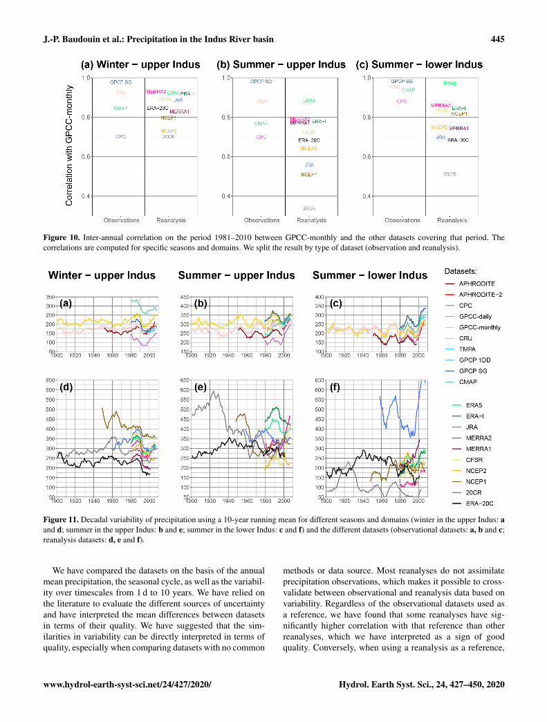
The reanalyses in winter have a decadal variability simi-lar to the observations for the period 1980–2010 (Fig. 11d).Moreover, the most recent reanalyses tend to converge to-wards the same amount of precipitation after 2000. By con-trast, the reanalyses that run before 1980 do not represent thedecadal variability depicted by the observations. For summerin both study areas, none but ERA-5 represents the decadalvariability observed. For example, in the upper Indus duringsummer, the precipitation amount increases after 2000 in theobservations (Fig. 11b). While MERRA2 and CFSR showan increase in precipitation 2 or 3 times larger, ERA-Interim,NCEP1, and NCEP2 show instead a decrease (Fig. 11e). In-terestingly, while the observations show similar decadal vari-ability for summer between the upper and the lower Indus,this is not the case for the reanalyses, except maybe for the
twentieth century reanalyses, and ERA-5. Notably, ERA5has an inter-annual correlation with GPCC-monthly that ishigher than the correlation between GPCC and CRU for allthree panels in Fig. 10, suggesting it is at least as able asobservational datasets.
4 Conclusions
In this study, we have compared a large number of precip-itation datasets of different types across two distinct zonesof the Indus watershed: 6 datasets are based only on raingauges, 4 are derived from satellite observations, and 10 fromreanalysis. We have shown that the number and diversity ofthe datasets help to identify and quantify the limitations andabilities of each of them, which in turn enables a better esti-mation of the uncertainties.
Hydrol. Earth Syst. Sci., 24, 427–450, 2020 www.hydrol-earth-syst-sci.net/24/427/2020/
J.-P. Baudouin et al.: Precipitation in the Indus River basin 445
Figure 10. Inter-annual correlation on the period 1981–2010 between GPCC-monthly and the other datasets covering that period. Thecorrelations are computed for specific seasons and domains. We split the result by type of dataset (observation and reanalysis).
Figure 11. Decadal variability of precipitation using a 10-year running mean for different seasons and domains (winter in the upper Indus: aand d; summer in the upper Indus: b and e; summer in the lower Indus: c and f) and the different datasets (observational datasets: a, b and c;reanalysis datasets: d, e and f).
We have compared the datasets on the basis of the annualmean precipitation, the seasonal cycle, as well as the variabil-ity over timescales from 1 d to 10 years. We have relied onthe literature to evaluate the different sources of uncertaintyand have interpreted the mean differences between datasetsin terms of their quality. We have suggested that the sim-ilarities in variability can be directly interpreted in terms ofquality, especially when comparing datasets with no common
methods or data source. Most reanalyses do not assimilateprecipitation observations, which makes it possible to cross-validate between observational and reanalysis data based onvariability. Regardless of the observational datasets used asa reference, we have found that some reanalyses have sig-nificantly higher correlation with that reference than otherreanalyses, which we have interpreted as a sign of goodquality. Conversely, when using a reanalysis as a reference,
www.hydrol-earth-syst-sci.net/24/427/2020/ Hydrol. Earth Syst. Sci., 24, 427–450, 2020
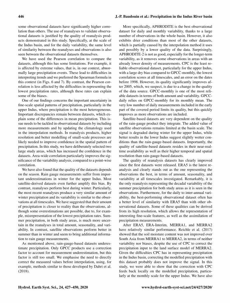
446 J.-P. Baudouin et al.: Precipitation in the Indus River basin
some observational datasets have significantly higher corre-lation than others. The use of reanalyses to validate observa-tional datasets is justified by the quality of reanalysis prod-ucts demonstrated in this study. Specifically, at the scale ofthe Indus basin, and for the daily variability, the same levelof similarity between the reanalyses and observations is alsoseen between the observational datasets themselves.
We have used the Pearson correlation to compare thedatasets, although this has some limitations. For example, itis affected by extreme values, that is, in our context, abnor-mally large precipitation events. These lead to difficulties ininterpreting trends and we preferred the Spearman formula inthis context (in Figs. 6 and 7). By contrast, the Pearson cor-relation is less affected by the difficulties in representing thelowest precipitation rates, although these rates can explainsome of the biases.
One of our findings concerns the important uncertainty infine-scale spatial patterns of precipitation, particularly in theupper Indus, where precipitation is the most heterogeneous.Important discrepancies remain between datasets, which ex-plain some of the differences in mean precipitation. This is-sue needs to be tackled in observational datasets by includingmore measurements and by updating the climatology usedin the interpolation methods. In reanalysis products, higherresolution and better modelling of small-scale processes arelikely needed to improve confidence in the spatial pattern ofprecipitation. In this study, we have deliberately selected twolarge study areas, which has increased the confidence in thedatasets. Area-wide correlation particularly improves the sig-nificance of the variability analysis, compared to a point-wisecorrelation.
We have also found that the quality of the datasets dependson the season. Rain gauge measurements suffer from impor-tant underestimations in winter for the upper Indus. Mostsatellite-derived datasets even further amplify this bias. Bycontrast, reanalyses perform best during winter. Particularly,the most recent reanalyses produce a very similar amount ofwinter precipitation and its variability is similar to the obser-vations at all timescales. We have suggested that their amountof precipitation is closer to reality than the observations, al-though some overestimations are possible, due to, for exam-ple, misrepresentation of the lowest precipitation rates. Sum-mer precipitation, in both study areas, is much more uncer-tain in the reanalyses in total amount, seasonality, and vari-ability. In contrast, satellite observations perform better insummer than in winter and seem to bring additional informa-tion to rain gauge measurements.
As mentioned above, rain-gauge-based datasets underes-timate precipitation. Only GPCC products use a correctionfactor to account for measurement underestimation, but thisfactor is still too small. We emphasise the need to directlycorrect the measured values before interpolation, using, forexample, methods similar to those developed by Dahri et al.(2018).
More specifically, APHRODITE is the best observationaldataset for daily and monthly variability, thanks to a largenumber of observations in the whole basin. However, it alsoexhibits drier conditions than most of the other datasets,which is partially caused by the interpolation method it usesand possibly by a lower quality of the data. Surprisingly,APHRODITE-2 is not as good, especially for the longer-termvariability, as it removes some observations in areas with analready lower density of measurements. CPC is the least re-liable observational dataset, particularly for the upper Indus,with a large dry bias compared to GPCC-monthly, the lowestcorrelation scores at all timescales, and an error on the datesbefore 1998. However, its quality significantly improves af-ter 2005, which, we suspect, is due to a change in the qualityof the data source. GPCC-monthly is one of the most reli-able datasets in terms of both amount and variability. GPCC-daily relies on GPCC-monthly for its monthly mean. Thevery low number of daily measurements included in the earlypart of the covered period limits its quality, but this quicklyimproves as more observations are included.
Satellite-based datasets are very dependent on the qualityof the rain-gauge product they integrate. The added value ofsatellite observations remains limited at the basin scale. Thesignal is degraded during winter for the upper Indus, whilebetter results in the lower Indus suggest slightly wetter con-ditions than the rain-gauge-based datasets. Importantly, thequality of satellite-based datasets resides in their near-real-time availability as well as their higher temporal and spatialresolution than rain-gauge-based datasets.
The quality of reanalysis datasets has clearly improvedsince the first datasets were released. ERA5 is the latest re-analysis and clearly stands out as the one representing theobservations the best, in terms of amount, seasonality, andvariability at all timescales investigated. Remarkably, it isthe only reanalysis representing the decadal variability of thesummer precipitation for both study areas as it is seen in theobservations. Furthermore, for the daily to inter-annual vari-ability, the best-performing observational dataset often hasa better level of similarity with ERA5 than with other ob-servational datasets. Some of these qualities can be derivedfrom its high resolution, which allows the representation ofinteresting fine-scale features, as well as the assimilation ofprecipitation measurements.
After ERA5, ERA-Interim, MERRA1, and MERRA2have relatively similar performance. Reichle et al. (2017)showed that the soil moisture content was not improved overSouth Asia from MERRA1 to MERRA2, in terms of neithervariability nor biases, despite the use of CPC to correct theprecipitation input to the land surface model of MERRA2.Given the difficulties CPC has in representing precipitationin the Indus basin, correcting the modelled precipitation withthis dataset probably does not improve the signal. In thisstudy, we were able to show that the correction with CPCfeeds back locally on the modelled precipitation, particu-larly at the monthly scale for the upper Indus. We have also
Hydrol. Earth Syst. Sci., 24, 427–450, 2020 www.hydrol-earth-syst-sci.net/24/427/2020/
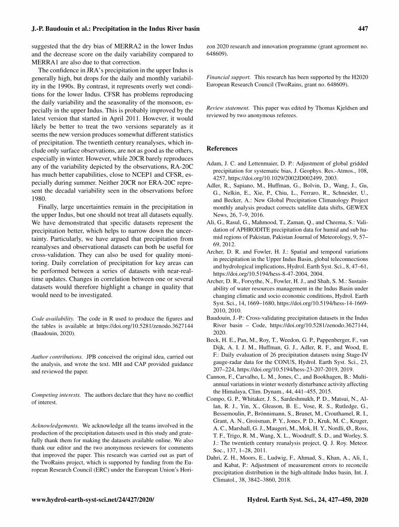
J.-P. Baudouin et al.: Precipitation in the Indus River basin 447
suggested that the dry bias of MERRA2 in the lower Indusand the decrease score on the daily variability compared toMERRA1 are also due to that correction.
The confidence in JRA’s precipitation in the upper Indus isgenerally high, but drops for the daily and monthly variabil-ity in the 1990s. By contrast, it represents overly wet condi-tions for the lower Indus. CFSR has problems reproducingthe daily variability and the seasonality of the monsoon, es-pecially in the upper Indus. This is probably improved by thelatest version that started in April 2011. However, it wouldlikely be better to treat the two versions separately as itseems the new version produces somewhat different statisticsof precipitation. The twentieth century reanalyses, which in-clude only surface observations, are not as good as the others,especially in winter. However, while 20CR barely reproducesany of the variability depicted by the observations, RA-20Chas much better capabilities, close to NCEP1 and CFSR, es-pecially during summer. Neither 20CR nor ERA-20C repre-sent the decadal variability seen in the observations before1980.
Finally, large uncertainties remain in the precipitation inthe upper Indus, but one should not treat all datasets equally.We have demonstrated that specific datasets represent theprecipitation better, which helps to narrow down the uncer-tainty. Particularly, we have argued that precipitation fromreanalyses and observational datasets can both be useful forcross-validation. They can also be used for quality moni-toring. Daily correlation of precipitation for key areas canbe performed between a series of datasets with near-real-time updates. Changes in correlation between one or severaldatasets would therefore highlight a change in quality thatwould need to be investigated.
Code availability. The code in R used to produce the figures andthe tables is available at https://doi.org/10.5281/zenodo.3627144(Baudouin, 2020).
Author contributions. JPB conceived the original idea, carried outthe analysis, and wrote the text. MH and CAP provided guidanceand reviewed the paper.
Competing interests. The authors declare that they have no conflictof interest.
Acknowledgements. We acknowledge all the teams involved in theproduction of the precipitation datasets used in this study and grate-fully thank them for making the datasets available online. We alsothank our editor and the two anonymous reviewers for commentsthat improved the paper. This research was carried out as part ofthe TwoRains project, which is supported by funding from the Eu-ropean Research Council (ERC) under the European Union’s Hori-
zon 2020 research and innovation programme (grant agreement no.648609).
Financial support. This research has been supported by the H2020European Research Council (TwoRains, grant no. 648609).
Review statement. This paper was edited by Thomas Kjeldsen andreviewed by two anonymous referees.
References
Adam, J. C. and Lettenmaier, D. P.: Adjustment of global griddedprecipitation for systematic bias, J. Geophys. Res.-Atmos., 108,4257, https://doi.org/10.1029/2002JD002499, 2003.
Adler, R., Sapiano, M., Huffman, G., Bolvin, D., Wang, J., Gu,G., Nelkin, E., Xie, P., Chiu, L., Ferraro, R., Schneider, U.,and Becker, A.: New Global Precipitation Climatology Projectmonthly analysis product corrects satellite data shifts, GEWEXNews, 26, 7–9, 2016.
Ali, G., Rasul, G., Mahmood, T., Zaman, Q., and Cheema, S.: Vali-dation of APHRODITE precipitation data for humid and sub hu-mid regions of Pakistan, Pakistan Journal of Meteorology, 9, 57–69, 2012.
Archer, D. R. and Fowler, H. J.: Spatial and temporal variationsin precipitation in the Upper Indus Basin, global teleconnectionsand hydrological implications, Hydrol. Earth Syst. Sci., 8, 47–61,https://doi.org/10.5194/hess-8-47-2004, 2004.
Archer, D. R., Forsythe, N., Fowler, H. J., and Shah, S. M.: Sustain-ability of water resources management in the Indus Basin underchanging climatic and socio economic conditions, Hydrol. EarthSyst. Sci., 14, 1669–1680, https://doi.org/10.5194/hess-14-1669-2010, 2010.
Baudouin, J.-P.: Cross-validating precipitation datasets in the IndusRiver basin – Code, https://doi.org/10.5281/zenodo.3627144,2020.
Beck, H. E., Pan, M., Roy, T., Weedon, G. P., Pappenberger, F., vanDijk, A. I. J. M., Huffman, G. J., Adler, R. F., and Wood, E.F.: Daily evaluation of 26 precipitation datasets using Stage-IVgauge-radar data for the CONUS, Hydrol. Earth Syst. Sci., 23,207–224, https://doi.org/10.5194/hess-23-207-2019, 2019.
Cannon, F., Carvalho, L. M., Jones, C., and Bookhagen, B.: Multi-annual variations in winter westerly disturbance activity affectingthe Himalaya, Clim. Dynam., 44, 441–455, 2015.
Compo, G. P., Whitaker, J. S., Sardeshmukh, P. D., Matsui, N., Al-lan, R. J., Yin, X., Gleason, B. E., Vose, R. S., Rutledge, G.,Bessemoulin, P., Brönnimann, S., Brunet, M., Crouthamel, R. I.,Grant, A. N., Groisman, P. Y., Jones, P. D., Kruk, M. C., Kruger,A. C., Marshall, G. J., Maugeri, M., Mok, H. Y., Nordli, Ø., Ross,T. F., Trigo, R. M., Wang, X. L., Woodruff, S. D., and Worley, S.J.: The twentieth century reanalysis project, Q. J. Roy. Meteor.Soc., 137, 1–28, 2011.
Dahri, Z. H., Moors, E., Ludwig, F., Ahmad, S., Khan, A., Ali, I.,and Kabat, P.: Adjustment of measurement errors to reconcileprecipitation distribution in the high-altitude Indus basin, Int. J.Climatol., 38, 3842–3860, 2018.
www.hydrol-earth-syst-sci.net/24/427/2020/ Hydrol. Earth Syst. Sci., 24, 427–450, 2020
448 J.-P. Baudouin et al.: Precipitation in the Indus River basin
Dee, D. P., Uppala, S. M., Simmons, A. J., Berrisford, P., Poli,P., Kobayashi, S., Andrae, U., Balmaseda, M. A., Balsamo, G.,Bauer, P., Bechtold, P., Beljaars, A. C. M., van de Berg, L., Bid-lot, J., Bormann, N., Delsol, C., Dragani, R., Fuentes, M., Geer,A. J., Haimberger, L., Healy, S. B., Hersbach, H., Hólm, E. V.,Isaksen, L., Kållberg, P., Köhler, M., Matricardi, M., McNally,A. P., Monge-Sanz, B. M., Morcrette, J.-J., Park, B.-K., Peubey,C., de Rosnay, P., Tavolato, C., Thépaut, J.-N., and Vitart, F.: TheERA-Interim reanalysis: Configuration and performance of thedata assimilation system, Q. J. Roy. Meteor. Soc., 137, 553–597,2011.
Dimri, A. and Chevuturi, A.: Western disturbances-an Indian mete-orological perspective, Springer, 2016.
Douville, H., Chauvin, F., and Broqua, H.: Influence of soil mois-ture on the Asian and African monsoons. Part I: Mean monsoonand daily precipitation, J. Climate, 14, 2381–2403, 2001.
Ebert, E. E., Janowiak, J. E., and Kidd, C.: Comparison of near-real-time precipitation estimates from satellite observations andnumerical models, B. Am. Meteorol. Soc., 88, 47–64, 2007.
Ensor, L. A. and Robeson, S. M.: Statistical characteristics of dailyprecipitation: comparisons of gridded and point datasets, J. Appl.Meteorol. Clim., 47, 2468–2476, 2008.
Faisal, N. and Gaffar, A.: Development of Pakistan’s new areaweighted rainfall using Thiessen polygon method, Pakistan Jour-nal of Meteorology, 9, 107–116, 2012.
Filippi, L., Palazzi, E., von Hardenberg, J., and Provenzale, A.:Multidecadal variations in the relationship between the NAO andwinter precipitation in the Hindu Kush–Karakoram, J. Climate,27, 7890–7902, 2014.
Gardelle, J., Berthier, E., and Arnaud, Y.: Slight mass gainof Karakoram glaciers in the early twenty-first century, Nat.Geosci., 5, 322–325, 2012.
Gelaro, R., McCarty, W., Suárez, M. J., Todling, R., Molod, A.,Takacs, L., Randles, C. A., Darmenov, A., Bosilovich, M. G., Re-ichle, R., Wargan, K., Coy, L,. Cullather, R., Draper, C., Akella,S., Buchard, V., Conaty, A., da Silva, A. M., Gu, W., Kim, G.-K., Koster, R., Lucchesi, R., Merkova, D., Nielsen, J. E., Par-tyka, G., Pawson, S., Putman, W., Rienecker, M., Schubert, S.D., Sienkiewicz, M., and Zhao, B.: The modern-era retrospectiveanalysis for research and applications, version 2 (MERRA-2), J.Climate, 30, 5419–5454, 2017.
Ghulami, M., Babel, M. S., and Singh Shrestha, M.: Evaluation ofgridded precipitation datasets for the Kabul Basin, Afghanistan,Int. J. Remote Sens., 38, 3317–3332, 2017.
Goodison, B., Sevruk, B., and Klemm, S.: WMO solid precipitationmeasurement intercomparison: Objectives, methodology, analy-sis, Atmos. Depos, 179, 57–64, 1989.
Habib, E., Ciach, G. J., and Krajewski, W. F.: A method for filter-ing out raingauge representativeness errors from the verificationdistributions of radar and raingauge rainfall, Adv. Water Resour.,27, 967–980, 2004.
Harris, I. and Jones, P.: CRU TS4. 00: Climatic Research Unit(CRU) Time-Series (TS) version 4.00 of high resolution griddeddata of month-by-month variation in climate (Jan. 1901–Dec.2015), Centre for Environmental Data Analysis, 25, 2017.
Harris, I., Jones, P. D., Osborn, T. J., and Lister, D. H.: Updatedhigh-resolution grids of monthly climatic observations–the CRUTS3. 10 Dataset, Int. J. Climatol., 34, 623–642, 2014.
Hersbach, H., de Rosnay, P., Bell, B., Schepers, D., Simmons,A., Soci, C., Abdalla, S., Alonso-Balmaseda, M., Balsamo, G.,Bechtold, P., Berrisford, P., Bidlot, J.-R., de Boisséson, E.,Bonavita, M., Browne, P., Buizza, R., Dahlgren, P., Dee, D.,Dragani, R., Diamantakis, M., Flemming, J., Forbes, R., Geer,A., Haiden, T., Hólm, E., Haimberger, L., Hogan, R., Horányi,A., Janiskova, M., Laloyaux, P., Lopez, P., Munoz-Sabater, J.,Peubey, C., Radu, R., Richardson, D., Thépaut, J.-N., Vitart, F.,Yang, X., Zsótér, E., and Zuo, H.: Operational global reanalysis:progress, future directions and synergies with NWP, ERA-report,Serie 27, https://doi.org/10.21957/tkic6g3wm, 2018.
Hewitt, K.: The Karakoram anomaly? Glacier expansion and the“elevation effect”, Karakoram Himalaya, Mt. Res. Dev., 25, 332–341, 2005.
Huffman, G. J. and Bolvin, D. T.: Version 1.2 GPCP one-degreedaily precipitation data set documentation, NASA, GoddardSpace Flight Center, Greenbelt, MD, USA, 2013.
Huffman, G. J., Bolvin, D. T., Nelkin, E. J., Wolff, D. B., Adler,R. F., Gu, G., Hong, Y., Bowman, K. P., and Stocker, E. F.:The TRMM multisatellite precipitation analysis (TMPA): Quasi-global, multiyear, combined-sensor precipitation estimates atfine scales, J. Hydrometeorol., 8, 38–55, 2007.
Hunt, K. M., Turner, A. G., and Shaffrey, L. C.: The evolution, sea-sonality and impacts of western disturbances, Q. J. Roy. Meteor.Soc., 144, 278–290, 2018.
Hussain, S., Song, X., Ren, G., Hussain, I., Han, D., and Zaman,M.: Evaluation of gridded precipitation data in the Hindu Kush–Karakoram–Himalaya mountainous area, Hydrolog. Sci. J., 62,2393–2405, 2017.
Immerzeel, W. W., Wanders, N., Lutz, A. F., Shea, J. M., andBierkens, M. F. P.: Reconciling high-altitude precipitation in theupper Indus basin with glacier mass balances and runoff, Hydrol.Earth Syst. Sci., 19, 4673–4687, https://doi.org/10.5194/hess-19-4673-2015, 2015.
Iqbal, M. F. and Athar, H.: Validation of satellite based precipitationover diverse topography of Pakistan, Atmos. Res., 201, 247–260,2018.
Kalnay, E., Kanamitsu, M., Kistler, R., Collins, W., Deaven, D.,Gandin, L., Iredell, M., Saha, S., White, G., Woollen, J., Zhu, Y.,Chelliah, M., Ebisuzaki, W., Higgins, W., Janowiak, J., Mo, K.C., Ropelewski, C., Wang, J., Leetmaa, A., Reynolds, R., Jenne,R., and Joseph, D.: The NCEP/NCAR 40-year reanalysis project,B. Am. Meteorol. Soc., 77, 437–472, 1996.
Kanamitsu, M., Ebisuzaki, W., Woollen, J., Yang, S.-K., Hnilo, J.,Fiorino, M., and Potter, G.: Ncep–doe amip-ii reanalysis (r-2), B.Am. Meteorol. Soc., 83, 1631–1644, 2002.
Khan, S. I., Hong, Y., Gourley, J. J., Khattak, M. U. K., Yong, B.,and Vergara, H. J.: Evaluation of three high-resolution satelliteprecipitation estimates: Potential for monsoon monitoring overPakistan, Adv. Space Res., 54, 670–684, 2014.
Kishore, P., Jyothi, S., Basha, G., Rao, S., Rajeevan, M., Velicogna,I., and Sutterley, T. C.: Precipitation climatology over India:validation with observations and reanalysis datasets and spatialtrends, Clim. Dynam., 46, 541–556, 2016.
Kobayashi, S., Ota, Y., Harada, Y., Ebita, A., Moriya, M., Onoda,H., Onogi, K., Kamahori, H., Kobayashi, C., Endo, H., Miyaoka,K., and Takahashi, K.: The JRA-55 reanalysis: General specifi-cations and basic characteristics, J. Meteorol. Soc. Jpn. Ser. II,93, 5–48, 2015.
Hydrol. Earth Syst. Sci., 24, 427–450, 2020 www.hydrol-earth-syst-sci.net/24/427/2020/
J.-P. Baudouin et al.: Precipitation in the Indus River basin 449
Laghari, A. N., Vanham, D., and Rauch, W.: The Indusbasin in the framework of current and future water re-sources management, Hydrol. Earth Syst. Sci., 16, 1063–1083,https://doi.org/10.5194/hess-16-1063-2012, 2012.
Legates, D. R. and Willmott, C. J.: Mean seasonal and spatial vari-ability in gauge-corrected, global precipitation, Int. J. Climatol.,10, 111–127, 1990.
Ménégoz, M., Gallée, H., and Jacobi, H. W.: Precipitation andsnow cover in the Himalaya: from reanalysis to regional cli-mate simulations, Hydrol. Earth Syst. Sci., 17, 3921–3936,https://doi.org/10.5194/hess-17-3921-2013, 2013.
Newlands, N. K., Davidson, A., Howard, A., and Hill, H.: Valida-tion and inter-comparison of three methodologies for interpolat-ing daily precipitation and temperature across Canada, Environ-metrics, 22, 205–223, 2011.
Palazzi, E., Von Hardenberg, J., and Provenzale, A.: Precipitation inthe Hindu-Kush Karakoram Himalaya: observations and futurescenarios, J. Geophys. Res.-Atmos., 118, 85–100, 2013.
Palazzi, E., von Hardenberg, J., Terzago, S., and Provenzale, A.:Precipitation in the Karakoram-Himalaya: a CMIP5 view, Clim.Dynam., 45, 21–45, https://doi.org/10.1007/s00382-014-2341-z,2015.
Poli, P., Hersbach, H., Dee, D. P., Berrisford, P., Simmons, A. J.,Vitart, F., Laloyaux, P., Tan, D. G., Peubey, C., Thépaut, J.-N.,Trémolet, Y., Hólm, E. V., Bonavita, M., Isaksen, L., and Fisher,M.: ERA-20C: An atmospheric reanalysis of the twentieth cen-tury, J. Climate, 29, 4083–4097, 2016.
Rahman, S., Sengupta, D., and Ravichandran, M.: Variabil-ity of Indian summer monsoon rainfall in daily data fromgauge and satellite, J. Geophys. Res.-Atmos., 114, D17113,https://doi.org/10.1029/2008JD011694, 2009.
Rajbhandari, R., Shrestha, A., Kulkarni, A., Patwardhan, S., andBajracharya, S.: Projected changes in climate over the Indus riverbasin using a high resolution regional climate model (PRECIS),Clim. Dynam., 44, 339–357, 2015.
Rana, S., McGregor, J., and Renwick, J.: Precipitation seasonalityover the Indian subcontinent: An evaluation of gauge, reanalyses,and satellite retrievals, J. Hydrometeorol., 16, 631–651, 2015.
Rana, S., McGregor, J., and Renwick, J.: Wintertime precipitationclimatology and ENSO sensitivity over central southwest Asia,Int. J. Climatol., 37, 1494–1509, 2017.
Reichle, R. H., Draper, C. S., Liu, Q., Girotto, M., Mahanama, S. P.,Koster, R. D., and De Lannoy, G. J.: Assessment of MERRA-2 land surface hydrology estimates, J. Climate, 30, 2937–2960,2017.
Rienecker, M. M., Suarez, M. J., Gelaro, R., Todling, R., Bacmeis-ter, J., Liu, E., Bosilovich, M. G., Schubert, S. D., Takacs, L.,Kim, G.-K., Bloom, S., Chen, J., Collins, D., Conaty, A., daSilva, A., Gu, W., Joiner, J., Koster, R. D., Lucchesi, R., Molod,A., Owens, T., Pawson, S., Pegion, P., Redder, C. R., Reichle, R.,Robertson, F. R., Ruddick, A. G., Sienkiewicz, M., and Woollen,J.: MERRA: NASA’s modern-era retrospective analysis for re-search and applications, J. Climate, 24, 3624–3648, 2011.
Rudolf, B. and Rubel, F.: Global precipitation, in: Observed globalclimate, chap. 11, Springer, 1–24, 2005.
Saha, S., Moorthi, S., Pan, H.-L., Wu, X., Wang, J., Nadiga, S.,Tripp, P., Kistler, R., Woollen, J., Behringer, D., Liu, H., Stokes,D., Grumbine, R., Gayno, G., Wang, J., Hou, Y.-T., Chuang, H.-Y., Juang, H.-M. H., Sela, J., Iredell, M., Treadon, R., Kleist,
D., Van Delst, P., Keyser, D., Derber, J., Ek, M., Meng, J., Wei,H., Yang, R., Lord, S., van den Dool, H., Kumar, A., Wang,W., Long, C., Chelliah, M., Xue, Y., Huang, B., Schemm, J.-K.,Ebisuzaki, W., Lin, R., Xie, P., Chen, M., Zhou, S., Higgins, W.,Zou, C.-Z., Liu, Q., Chen, Y., Han, Y., Cucurull, L., Reynolds, R.W., Rutledge, G., and Goldberg, M.: The NCEP climate forecastsystem reanalysis, B. Am. Meteorol. Soc., 91, 1015–1058, 2010.
Saha, S., Moorthi, S., Wu, X., Wang, J., Nadiga, S., Tripp, P.,Behringer, D., Hou, Y.-T., Chuang, H.-Y., Iredell, M., Ek, M.,Meng, J., Yang, R., Mendez, M. P., van den Dool, H., Zhang, Q.,Wang, W., Chen, M., and Becker, E.: The NCEP climate forecastsystem version 2, J. Climate, 27, 2185–2208, 2014.
Schneider, U., Becker, A., Finger, P., Meyer-Christoffer, A., Ziese,M., and Rudolf, B.: GPCC’s new land surface precipitation cli-matology based on quality-controlled in situ data and its role inquantifying the global water cycle, Theor. Appl. Climatol., 115,15–40, 2014.
Schneider, U., Becker, A., Finger, P., Meyer-Christoffer, A., andZiese, M.: GPCC Full Data Monthly Product Version 2018at 0.5°: Monthly Land-Surface Precipitation from Rain-GaugesBuilt on GTS-Based and Historical Data, Deutscher Wetterdi-enst: Offenbach am Main, Germany, 2018.
Sevruk, B.: International comparison of national precipitationgauges with a reference pit gauge, WMO Instrument and Ob-serving Methods Report, No. 17, 111, 1984.
Singh, S. P., Bassignana-Khadka, I., Singh Karky, B., and Sharma,E.: Climate change in the Hindu Kush-Himalayas: the state ofcurrent knowledge, Tech. rep., International Centre for IntegratedMountain Development (ICIMOD), 2011.
Syvitski, J. P., Kettner, A. J., Overeem, I., Giosan, L., Brakenridge,G. R., Hannon, M., and Bilham, R.: Anthropocene metamorpho-sis of the Indus Delta and lower floodplain, Anthropocene, 3,24–35, 2013.
Tozer, C. R., Kiem, A. S., and Verdon-Kidd, D. C.: On theuncertainties associated with using gridded rainfall data as aproxy for observed, Hydrol. Earth Syst. Sci., 16, 1481–1499,https://doi.org/10.5194/hess-16-1481-2012, 2012.
Tustison, B., Harris, D., and Foufoula-Georgiou, E.: Scale issues inverification of precipitation forecasts, J. Geophys. Res.-Atmos.,106, 11775–11784, 2001.
Wang, J. and Wolff, D. B.: Evaluation of TRMM ground-validationradar-rain errors using rain gauge measurements, J. Appl. Mete-orol. Clim., 49, 310–324, 2010.
Wang, Q., Yi, S., and Sun, W.: Precipitation-driven glacier changesin the Pamir and Hindu Kush mountains, Geophys. Res. Lett.,44, 2817–2824, 2017.
WMO: Guide to Hydrological Practices, Volume I, Hydrology –From Measurement to Hydrological Information, 2008.
Wolff, M. A., Isaksen, K., Petersen-Øverleir, A., Ødemark, K., Rei-tan, T., and Brækkan, R.: Derivation of a new continuous adjust-ment function for correcting wind-induced loss of solid precipita-tion: results of a Norwegian field study, Hydrol. Earth Syst. Sci.,19, 951–967, https://doi.org/10.5194/hess-19-951-2015, 2015.
Xie, P. and Arkin, P. A.: Global precipitation: A 17-year monthlyanalysis based on gauge observations, satellite estimates, and nu-merical model outputs, B. Am. Meteorol. Soc., 78, 2539–2558,1997.
www.hydrol-earth-syst-sci.net/24/427/2020/ Hydrol. Earth Syst. Sci., 24, 427–450, 2020
450 J.-P. Baudouin et al.: Precipitation in the Indus River basin
Xie, P., Chen, M., and Shi, W.: CPC unified gauge-based analysisof global daily precipitation, in: Preprints, 24th Conf. on Hydrol-ogy, Atlanta, GA, Amer. Meteor. Soc, vol. 2, 2010.
Yatagai, A., Kamiguchi, K., Arakawa, O., Hamada, A., Yasutomi,N., and Kitoh, A.: APHRODITE: Constructing a long-term dailygridded precipitation dataset for Asia based on a dense networkof rain gauges, B. Am. Meteorol. Soc., 93, 1401–1415, 2012.
Ziese, M., Rauthe-Schöch, A., Becker, A., Finger, P., Meyer-Christoffer, A., and Schneider, U.: GPCC full data daily version2018 at 1.0°: Daily land-surface precipitation from rain-gaugesbuilt on GTS-based and historic data, 2018.
Hydrol. Earth Syst. Sci., 24, 427–450, 2020 www.hydrol-earth-syst-sci.net/24/427/2020/