
Validating Screening Questionnaires for Internalizing ... - INEE
Upload
independentCategory
view
0download
0
International Journal of Marine Energy xxx (2013) xxx–xxx
Contents lists available at ScienceDirect
International Journal of Marine Energy
journa l homepage: www.e lsev ier .com/ locate / i jome
On validating numerical hydrodynamic modelsof complex tidal flow
2214-1669/$ - see front matter � 2013 Elsevier Ltd. All rights reserved.http://dx.doi.org/10.1016/j.ijome.2013.11.013
⇑ Corresponding author.E-mail addresses: [email protected] (K. Gunn), [email protected] (C. Stock-Williams).
Please cite this article in press as: K. Gunn, C. Stock-Williams, On validating numerical hydrodymodels of complex tidal flow, International Journal of Marine Energy (2013), http://dx.d10.1016/j.ijome.2013.11.013
Kester Gunn ⇑, Clym Stock-WilliamsE.ON New Build & Technology, Technology Centre, Ratcliffe-on-Soar, Nottingham NG11 0EE, UK
a r t i c l e i n f o
Article history:Available online xxxx
Keywords:Tidal currentTidal flowHydrodynamic model3D modelValidationShear profile
a b s t r a c t
The construction of numerical hydrodynamic models is animportant task for offshore renewable energy development, in par-ticular for tidal current farms. An accurate understanding of thespatial variation in resource is necessary for optimally locatingfixed measurement devices and turbines, as well as planning siteoperations.
This work presents a comprehensive methodology for the valida-tion of numerical models in two and three dimensions. First, alter-native methods practised in the literature for both time-domainand frequency-domain comparison are assessed and compared.Next, certain novel extended methods are presented for the valida-tion of 3D data, which is not often attempted in the literature. Inparticular, the shear profiles encountered in real high-velocity sitesdo not often follow the traditional logarithmic laws, so a newparameterisation is presented and tested.
Finally, acoustic Doppler profiler (ADP) data are analysed andused in a case study validation exercise of a 3D hydrodynamicmodel of the Fall of Warness in the Orkney Islands, UK. Conclusionsare drawn about the validity of the model, as well as the method-ology applied.
� 2013 Elsevier Ltd. All rights reserved.
Introduction
The planned deployment of tidal current turbines has stimulated an increased number of hydrody-namic models of sites with energetic tidal flows [1,3,4]. Such sites often contain highly complex spatialand temporal flow fields. Reproducing these in sufficient accuracy requires a selection of model
namicoi.org/
2 K. Gunn, C. Stock-Williams / International Journal of Marine Energy xxx (2013) xxx–xxx
sophistication dependant upon the objectives for the model and the amount of computing poweravailable to the modeller. For tidal current energy, model objectives will normally include designingsite layout or performing early-stage energy yield assessment. These models are equally invaluable indesigning the measurement campaign used to collect data for later-stage energy yield assessments.
For all these uses it is both necessary and received wisdom to assess the validity of a tidal model.However, despite the existing examples [11] and guidance [2] available in this well-developed area ofresearch, validation exercises of hydrodynamic models in this sector often consist of little more thancomparisons of time series between the model and measured data. This approach gives neither anumerical demonstration of the accuracy of the model, nor a detailed insight into the – potentiallyvariable – ability of the model to reproduce specific features of a site. Furthermore, quantitative val-idation should provide an estimate of error, which can be fed into a calculation of uncertainty on thefinal energy yield.
Guiding principles for assessing model validity
The validation objective
Many well-considered descriptions of the purpose of validation have been published [2,17]. For ahydrodynamic flow model, ‘‘validation’’ is a quantitative assessment of the accuracy of the model’spredictions of flow velocity and tidal height in a particular region of interest. The final assessment,of whether a model is sufficiently accurate for the purpose to which its predictions will be put, canonly be a matter of judgement for the user of the model’s outputs. A well-chosen set of validation sta-tistics will, however, greatly aid the user in determining acceptance or rejection.
Target values of such parameters can be set for a given use [10], however, these values should becarefully examined against the requirements on the model outputs. For instance, a model to be used topredict energy yield of a tidal current turbine may need to be more accurate, over more of the watercolumn, than an operational forecast model. Alternatively, if the model is to be used for initial arraylayout design or planning of further measurement campaigns, then small systematic errors are accept-able so long as the spatial distribution of resource is correctly captured.
The burden of proof is, as for all science [13], asymmetrical: while one can categorically say, from apredetermined set of validation statistics and target values, that a model is invalid, it is never possibleto state that a model is unconditionally ‘‘validated’’.
Calibration and validation
Calibration and validation are clearly separate tasks and should be carried out with separate data.Less obviously, they also require different sets of statistics.
Calibration is the process of tuning a model to best fit calibration data through, for example, mod-ification of boundary conditions, mesh density or bottom friction. Validation is the process of assessingthe accuracy of a single model. For hydrodynamic flow models, the data sets used for validationshould, if possible, be both spatially and temporally distinct from calibration data sets and coverthe same range of physical parameters: both tidal height and current velocity. This increases thechance of discovering whether a model is ‘‘tuned’’ only to a particular location, or overly affectedby non-tidal signal in the calibration data set.
Calibration is a well-documented procedure [9]. Statistics such as Skill Score (d) [17] or Pearsonproduct-moment correlation coefficient (r) are excellent for comparing one model’s performancerelative to another. Conversely, validation requires an understanding of the physical meaning of thestatistics in order to set numerical criteria before the exercise is conducted. Acceptable values for ror d might become intuitive to an experienced modeller, however, they are too abstract to convey sig-nificance to others without support from large amounts of robust literature (e.g. [16]).
In order to set criteria for model validity before conducting the validation exercise, the chosen sta-tistics need to be less abstract than many of those used in calibration. A good selection of candidatestatistics have been proposed by NOAA [10]. These are supplemented here with a method based on
Please cite this article in press as: K. Gunn, C. Stock-Williams, On validating numerical hydrodynamicmodels of complex tidal flow, International Journal of Marine Energy (2013), http://dx.doi.org/10.1016/j.ijome.2013.11.013
K. Gunn, C. Stock-Williams / International Journal of Marine Energy xxx (2013) xxx–xxx 3
confidence and prediction intervals. This approach allows the modeller to state that ‘‘the model is/isnot valid to X% confidence’’, where the modeller may select the confidence required a priori on eachvariable.
The example hydrodynamic flow model
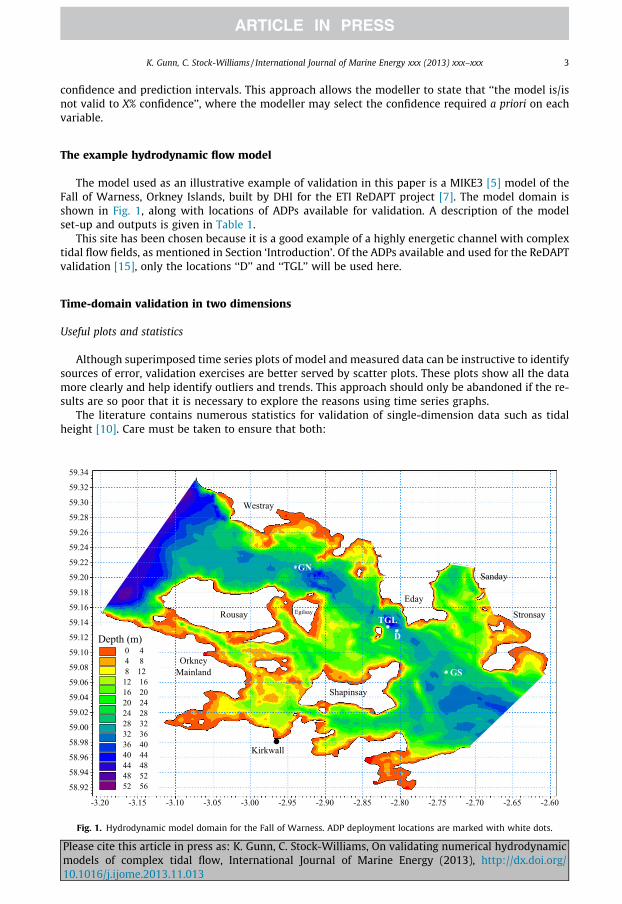
The model used as an illustrative example of validation in this paper is a MIKE3 [5] model of theFall of Warness, Orkney Islands, built by DHI for the ETI ReDAPT project [7]. The model domain isshown in Fig. 1, along with locations of ADPs available for validation. A description of the modelset-up and outputs is given in Table 1.
This site has been chosen because it is a good example of a highly energetic channel with complextidal flow fields, as mentioned in Section ‘Introduction’. Of the ADPs available and used for the ReDAPTvalidation [15], only the locations ‘‘D’’ and ‘‘TGL’’ will be used here.
Time-domain validation in two dimensions
Useful plots and statistics
Although superimposed time series plots of model and measured data can be instructive to identifysources of error, validation exercises are better served by scatter plots. These plots show all the datamore clearly and help identify outliers and trends. This approach should only be abandoned if the re-sults are so poor that it is necessary to explore the reasons using time series graphs.
The literature contains numerous statistics for validation of single-dimension data such as tidalheight [10]. Care must be taken to ensure that both:
Fig. 1. Hydrodynamic model domain for the Fall of Warness. ADP deployment locations are marked with white dots.
Please cite this article in press as: K. Gunn, C. Stock-Williams, On validating numerical hydrodynamicmodels of complex tidal flow, International Journal of Marine Energy (2013), http://dx.doi.org/10.1016/j.ijome.2013.11.013

Table 1MIKE simulation settings.
Simulation time 24/7/2011 00:00 to 27/8/2011 00:00
Output Timestep 30 minMesh size 11,802 nodes, 22,203 elementsVertical layers 10 equidistant sigma layersBoundary
conditionsFlather (velocities and heights) at all seven mesh boundaries – from larger 2D model. Constantdomain roughness height (0.017 m)
Initial conditions Soft-start (3600 s sinus) on boundaries
4 K. Gunn, C. Stock-Williams / International Journal of Marine Energy xxx (2013) xxx–xxx
1. the statistics chosen have physical meaning for the parameter being validated; and2. the statistics are the smallest unique set possible to examine the potential errors.
For example, since tidal height is a displacement from mean sea level, bias (the difference betweenthe means of the series) will be always close to zero. Any differences are more likely to be due touncertainty in the location of the measurement equipment than any error in the model. This measureis, however, useful for current speed.
Secondly, while absolute scatter and root mean squared (RMS) error will provide different values,they are measures of almost the same properties of the fit, with different nuances.
As discussed in Section ‘The validation objective’, the chosen validation statistic or statistics mustbe applicable to the purpose for which the model outputs are to be used. The two most common usesfor such models are:
1. investigating trends in the flow field – such as exploring spatial variation in order to design anarray layout or design a measurement campaign; and
2. producing velocity values which can be used to perform early-stage yield assessment.
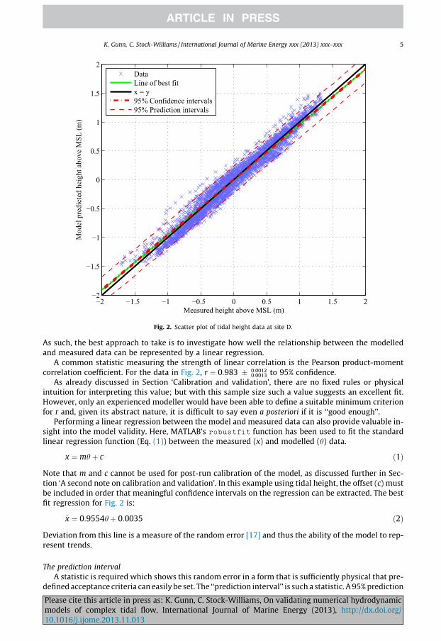
For both of these potential uses the scatter plot is an invaluable tool, as demonstrated in Fig. 2 fortidal height data at site D. From a quick glance at this figure, it is possible to tell:
� there is little, or no, phase error between the model and the measured data (which would likelyshow up as a much larger spread in the data);� the relationship is linear (which will be checked using the correlation coefficient);� there is little scatter – i.e. the model is a good fit to the measured data.
While such qualitative comments do not meet the needs of a true validation exercise, they do allowthe reader to visualise and confirm the quantitative assessment to follow.
Model output and post-run calibration
Although it is best practice to calibrate a model by modifying inputs (as discussed in Section‘Calibration and validation’) often a post-run calibration is performed on outputs from models. Mostcommonly, this takes the form of a linear correction to the raw outputs from the model. The discus-sions here assume that model outputs have had an appropriate post-run calibration as part of themodelling process to be validated. It should be noted, however, that in the illustrative example nopost-run calibration was applied.
Validating trends
Linear regressionFollowing the common assumption that systematic errors will present as a linear offset and gain
[17]: if the model outputs are to be used to assess trends then systematic errors are of no concern.Trends will be preserved no matter what the linear relationship between the model and the data.
Please cite this article in press as: K. Gunn, C. Stock-Williams, On validating numerical hydrodynamicmodels of complex tidal flow, International Journal of Marine Energy (2013), http://dx.doi.org/10.1016/j.ijome.2013.11.013
−2 −1.5 −1 −0.5 0 0.5 1 1.5 2−2
−1.5
−1
−0.5
0
0.5
1
1.5
2
Measured height above MSL (m)
Mod
el p
redi
cted
hei
ght a
bove
MSL
(m)
DataLine of best fitx = y95% Confidence intervals95% Prediction intervals
Fig. 2. Scatter plot of tidal height data at site D.
K. Gunn, C. Stock-Williams / International Journal of Marine Energy xxx (2013) xxx–xxx 5
As such, the best approach to take is to investigate how well the relationship between the modelledand measured data can be represented by a linear regression.
A common statistic measuring the strength of linear correlation is the Pearson product-momentcorrelation coefficient. For the data in Fig. 2, r ¼ 0:983 � 0:0012
0:0013 to 95% confidence.As already discussed in Section ‘Calibration and validation’, there are no fixed rules or physical
intuition for interpreting this value; but with this sample size such a value suggests an excellent fit.However, only an experienced modeller would have been able to define a suitable minimum criterionfor r and, given its abstract nature, it is difficult to say even a posteriori if it is ‘‘good enough’’.
Performing a linear regression between the model and measured data can also provide valuable in-sight into the model validity. Here, MATLAB’s robustfit function has been used to fit the standardlinear regression function (Eq. (1)) between the measured (x) and modelled (h) data.
Pleasmode10.10
x ¼ mhþ c ð1Þ
Note that m and c cannot be used for post-run calibration of the model, as discussed further in Sec-tion ‘A second note on calibration and validation’. In this example using tidal height, the offset (c) mustbe included in order that meaningful confidence intervals on the regression can be extracted. The bestfit regression for Fig. 2 is:
x̂ ¼ 0:9554hþ 0:0035 ð2Þ
Deviation from this line is a measure of the random error [17] and thus the ability of the model to rep-resent trends.
The prediction intervalA statistic is required which shows this random error in a form that is sufficiently physical that pre-
defined acceptance criteria can easily be set. The ‘‘prediction interval’’ is such a statistic. A 95% prediction
e cite this article in press as: K. Gunn, C. Stock-Williams, On validating numerical hydrodynamicls of complex tidal flow, International Journal of Marine Energy (2013), http://dx.doi.org/16/j.ijome.2013.11.013
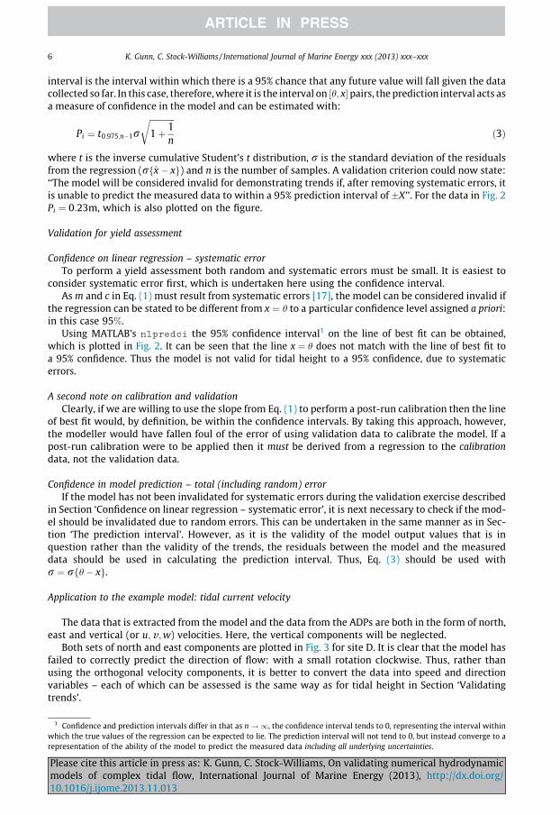
6 K. Gunn, C. Stock-Williams / International Journal of Marine Energy xxx (2013) xxx–xxx
interval is the interval within which there is a 95% chance that any future value will fall given the datacollected so far. In this case, therefore, where it is the interval on ½h; x�pairs, the prediction interval acts asa measure of confidence in the model and can be estimated with:
1 Conwhich treprese
Pleasemode10.10
Pi ¼ t0:975;n�1rffiffiffiffiffiffiffiffiffiffiffiffi1þ 1
n
rð3Þ
where t is the inverse cumulative Student’s t distribution, r is the standard deviation of the residualsfrom the regression (rfx̂� xg) and n is the number of samples. A validation criterion could now state:‘‘The model will be considered invalid for demonstrating trends if, after removing systematic errors, itis unable to predict the measured data to within a 95% prediction interval of �X’’. For the data in Fig. 2Pi ¼ 0:23m, which is also plotted on the figure.
Validation for yield assessment
Confidence on linear regression – systematic errorTo perform a yield assessment both random and systematic errors must be small. It is easiest to
consider systematic error first, which is undertaken here using the confidence interval.As m and c in Eq. (1) must result from systematic errors [17], the model can be considered invalid if
the regression can be stated to be different from x ¼ h to a particular confidence level assigned a priori:in this case 95%.
Using MATLAB’s nlpredci the 95% confidence interval1 on the line of best fit can be obtained,which is plotted in Fig. 2. It can be seen that the line x ¼ h does not match with the line of best fit toa 95% confidence. Thus the model is not valid for tidal height to a 95% confidence, due to systematicerrors.
A second note on calibration and validationClearly, if we are willing to use the slope from Eq. (1) to perform a post-run calibration then the line
of best fit would, by definition, be within the confidence intervals. By taking this approach, however,the modeller would have fallen foul of the error of using validation data to calibrate the model. If apost-run calibration were to be applied then it must be derived from a regression to the calibrationdata, not the validation data.
Confidence in model prediction – total (including random) errorIf the model has not been invalidated for systematic errors during the validation exercise described
in Section ‘Confidence on linear regression – systematic error’, it is next necessary to check if the mod-el should be invalidated due to random errors. This can be undertaken in the same manner as in Sec-tion ‘The prediction interval’. However, as it is the validity of the model output values that is inquestion rather than the validity of the trends, the residuals between the model and the measureddata should be used in calculating the prediction interval. Thus, Eq. (3) should be used withr ¼ rfh� xg.
Application to the example model: tidal current velocity
The data that is extracted from the model and the data from the ADPs are both in the form of north,east and vertical (or u;v ;w) velocities. Here, the vertical components will be neglected.
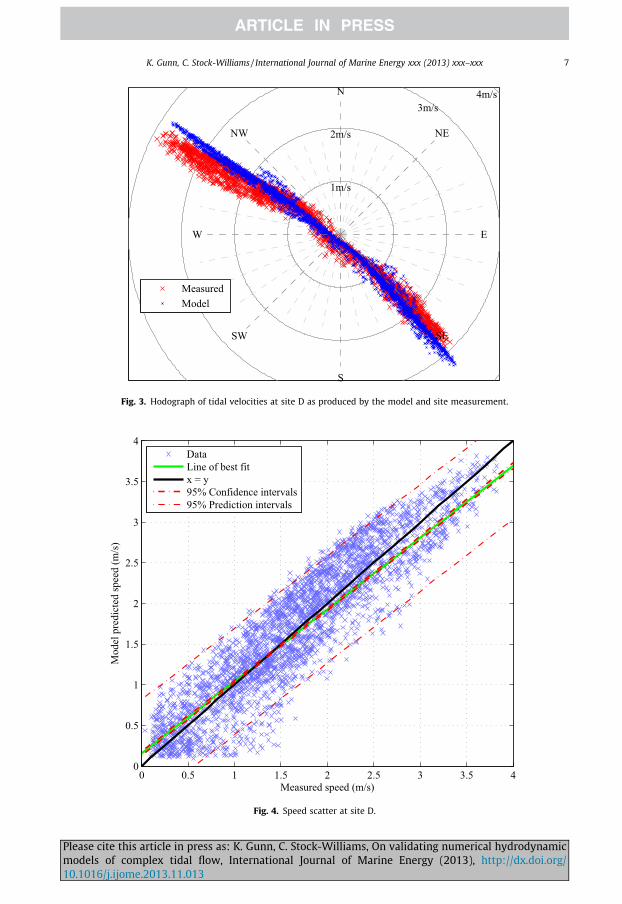
Both sets of north and east components are plotted in Fig. 3 for site D. It is clear that the model hasfailed to correctly predict the direction of flow: with a small rotation clockwise. Thus, rather thanusing the orthogonal velocity components, it is better to convert the data into speed and directionvariables – each of which can be assessed is the same way as for tidal height in Section ‘Validatingtrends’.
fidence and prediction intervals differ in that as n!1, the confidence interval tends to 0, representing the interval withinhe true values of the regression can be expected to lie. The prediction interval will not tend to 0, but instead converge to antation of the ability of the model to predict the measured data including all underlying uncertainties.
cite this article in press as: K. Gunn, C. Stock-Williams, On validating numerical hydrodynamicls of complex tidal flow, International Journal of Marine Energy (2013), http://dx.doi.org/16/j.ijome.2013.11.013
N
NE
E
SE
S
SW
W
NW
1m/s
2m/s
3m/s4m/s
MeasuredModel
Fig. 3. Hodograph of tidal velocities at site D as produced by the model and site measurement.
0 0.5 1 1.5 2 2.5 3 3.5 40
0.5
1
1.5
2
2.5
3
3.5
4
Measured speed (m/s)
Mod
el p
redi
cted
spee
d (m
/s)
DataLine of best fitx = y95% Confidence intervals95% Prediction intervals
Fig. 4. Speed scatter at site D.
K. Gunn, C. Stock-Williams / International Journal of Marine Energy xxx (2013) xxx–xxx 7
Please cite this article in press as: K. Gunn, C. Stock-Williams, On validating numerical hydrodynamicmodels of complex tidal flow, International Journal of Marine Energy (2013), http://dx.doi.org/10.1016/j.ijome.2013.11.013
8 K. Gunn, C. Stock-Williams / International Journal of Marine Energy xxx (2013) xxx–xxx
Fig. 4 shows the scatter plot for speed. As before, it is clear that the model does not fit the measureddata to a 95% confidence.
The direction data needs to be treated more carefully due to its circular nature. However, furtherdiscussion is omitted here for brevity.
Frequency-domain validation in two dimensions
Useful plots and statistics
The primary aim of producing a tidal current model is often, but not exclusively, the prediction oftime-domain information. Therefore, validating solely in the time domain would seem sufficient.However, it is valuable also to use the power of harmonic analysis to detect and evaluate errorsand their sources.
For example, resonant phenomena – such as standing waves – may exist in the model but not inthe measured data (or vice versa). Such resonant phenomena will exist only at certain frequencies,so can be most easily detected by isolating these components from the others.
Furthermore, frequency domain analysis allows data collected at times for which the model has notbeen run to be used in the validation. This can be extremely valuable if several intermittent datasetsare available for validation. If harmonic analysis is to be used to create time series data for a differentperiod it is far preferable to keep the measured data untouched and calculate new model values ratherthan the reverse. This both simplifies the error analysis and reduces likely errors.
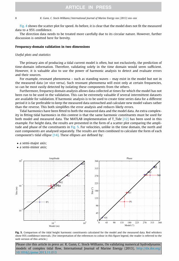
Tidal harmonics have been fitted to both the measured data and the model data. An extra complex-ity in fitting tidal harmonics in this context is that the same harmonic constituents must be used forboth model and measured data. The MATLAB implementation of T_Tide [12] has been used in thisexample. For height data, the results are presented in the form of a scatter plot comparing the ampli-tude and phase of the constituents in Fig. 5. For velocities, unlike in the time domain, the north andeast components are analysed separately. The results are then combined to calculate the form of eachcomponent’s tidal ellipse [14]. These ellipses are defined by:
� a semi-major axis;� a semi-minor axis;
10−1 100
10−2
10−1
100
O1
P1
K1N2
M2
S2
K2M4
Amplitude
Model (m)
Site
(m)
0 45 90 135 180 225 270 315 3600
45
90
135
180
225
270
315
360Phase
Model (°)
Site
(°)
O1
P1
K1
N2M2
S2K2
M4
Fig. 5. Comparison of the tidal height harmonic constituents calculated for the model and the measured data. Red whiskersshow 95% confidence intervals. (For interpretation of the references to colour in this figure legend, the reader is referred to theweb version of this article.)
Please cite this article in press as: K. Gunn, C. Stock-Williams, On validating numerical hydrodynamicmodels of complex tidal flow, International Journal of Marine Energy (2013), http://dx.doi.org/10.1016/j.ijome.2013.11.013
K. Gunn, C. Stock-Williams / International Journal of Marine Energy xxx (2013) xxx–xxx 9
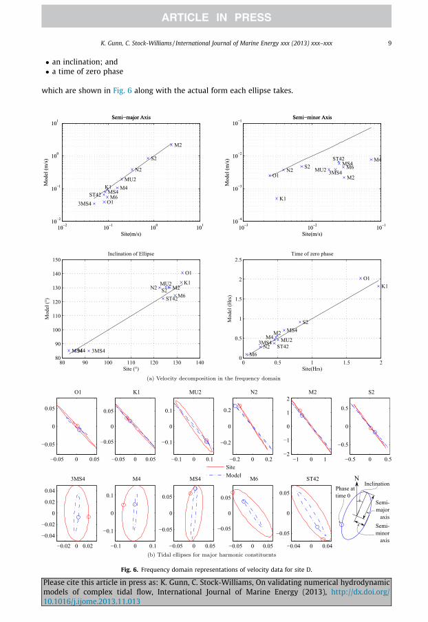
� an inclination; and� a time of zero phase
which are shown in Fig. 6 along with the actual form each ellipse takes.
10−2 10−1 100 10110−2
10−1
100
101
Site(m/s)
Mod
el (m
/s)
O1
K1 MU2
N2
M2
S2
3MS4
M4 MS4 M6 ST42
Semi−major Axis
10−3 10−2 10−110−4
10−3
10−2
10−1
Site(m/s)M
odel
(m/s
)
Semi−minor Axis
O1
K1
MU2 N2 M2
S23MS4
M4 MS4 M6
ST42
80 90 100 110 120 130 14080
90
100
110
120
130
140
150Inclination of Ellipse
Site (°)
Mod
el (°
)
O1
K1 MU2 N2 M2 S2
3MS4 M4 MS4
M6 ST42
0 0.5 1 1.5 20
0.5
1
1.5
2
2.5Time of zero phase
Site(Hrs)
Mod
el (H
rs)
O1 K1
MU2 N2
M2
S2
3MS4 M4
MS4
M6 ST42
10−2 10−1 100 10110−2
10−1
100
101
Site(m/s)
Mod
el (m
/s)
Semi−major Axis
10−3 10−2 10−110−4
10−3
10−2
10−1
Site(m/s)M
odel
(m/s
)
Semi−minor Axis
−0.05 0 0.05
−0.05
0
0.05
O1
−0.05 0 0.05
−0.05
0
0.05
K1
−0.1 0 0.1
−0.1
0
0.1
MU2
−0.2 0 0.2
−0.2
0
0.2
N2
−1 0 1−2
−1
0
1
2M2
−0.5 0 0.5
−0.5
0
0.5
S2
−0.02 0 0.02
−0.04
−0.02
0
0.02
0.04
3MS4
−0.1 0 0.1
−0.1
0
0.1
M4
−0.05 0 0.05
−0.05
0
0.05
MS4
−0.05 0 0.05
−0.05
0
0.05
M6
−0.04 0 0.04
−0.05
0
0.05
ST42
SiteModel N
Inclination
Semi-major
axisSemi-minor
axis
Phase at time 0
Fig. 6. Frequency domain representations of velocity data for site D.
Please cite this article in press as: K. Gunn, C. Stock-Williams, On validating numerical hydrodynamicmodels of complex tidal flow, International Journal of Marine Energy (2013), http://dx.doi.org/10.1016/j.ijome.2013.11.013
10 K. Gunn, C. Stock-Williams / International Journal of Marine Energy xxx (2013) xxx–xxx
Although omitted here for brevity, in a full validation [15], tables of the amplitudes, phases, andother variables for the major harmonic constituents would be presented.
Application to the example model: tidal height
From the amplitude graph in Fig. 5 it can be seen that the majority of the constituents are well rep-resented by the model. The mismatch in most constituents is less than the confidence intervals, thusthe model can be said to agree, to 95% confidence, for those constituents. However, N2 does not match– with the model over-predicting by a small margin. From the phase plot it can be seen that the con-stituents for the model and measured data match to 95% confidence (with the exception of N2).
This small mismatch in N2 suggests that a harmonic effect has been incorrectly accounted for bythe model at site D.
Application to the example model: tidal current velocity
Both the ellipses and the decomposed velocity variables are presented, for Site D, in Fig. 6. Theaccurate calculation of confidence intervals on these data is a task for a further study and would ide-ally be present.
These figures show that the model has produced an excellent representation of the semi-majoraxes, but has a tendency to under-estimate the semi-minor axes. This provides a quantification ofthe effect visible in Fig. 3: that the model predicts a considerably smaller spread in velocity directions.
Validation or cross comparison of three dimensional flow
An accurate understanding of the velocity depth profile is essential for correctly predicting yield fora tidal current farm and planning installation or maintenance. This section is concerned with two re-lated aspects of modelling a site’s spatially-varying velocity profile using a 3D hydrodynamic model.First, with presenting methods for quantitatively validating the model’s prediction of velocity profiles(primarily shear and veer). Second, with discussing the ability of such models to provide informationabout velocity depth profiles.
Parameterising the velocity depth profile
As previously explained in this paper, the first step in validation is to select appropriate variablesand statistics to use.
It might, at first glance, seem reasonable to simply perform the 2D velocity validation exercisesdescribed above at several depths in the water column. Unfortunately, this approach is not viable,for two reasons. Firstly, the noise on the ADCP data is such that making a direct comparison betweenindividual measurements is unreasonable (a depth-averaged velocity does not suffer from these issuesto the same extent). Secondly, such an approach obscures the details of the actual depth profiles, mak-ing interpretation of the results much harder. Instead, therefore, it is necessary to parameterise theshear profile, allowing direct comparison between the shear parameters or values derived from them.
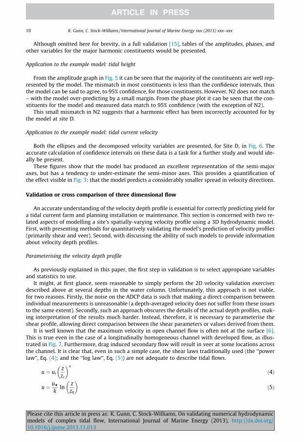
It is well known that the maximum velocity in open channel flow is often not at the surface [6].This is true even in the case of a longitudinally homogeneous channel with developed flow, as illus-trated in Fig. 7. Furthermore, drag induced secondary flow will result in veer at some locations acrossthe channel. It is clear that, even in such a simple case, the shear laws traditionally used (the ‘‘powerlaw’’, Eq. (4); and the ‘‘log law’’, Eq. (5)) are not adequate to describe tidal flows.
Pleasemode10.10
u ¼ urzzr
� �a
ð4Þ
u ¼ uH
kln
zz0
� �ð5Þ
cite this article in press as: K. Gunn, C. Stock-Williams, On validating numerical hydrodynamicls of complex tidal flow, International Journal of Marine Energy (2013), http://dx.doi.org/16/j.ijome.2013.11.013
Isotachs Secondarycurrents
,
Fig. 7. Flow in a longitudinally homogeneous open channel and the potential resulting shear (variation in speed, u) and veer(variation in heading, /).
K. Gunn, C. Stock-Williams / International Journal of Marine Energy xxx (2013) xxx–xxx 11
where for the power law: ur is the velocity at reference height zr ;a is the ‘‘shear exponent’’; and for thelog law: z0 is the roughness length which provides an indication of the size of the roughness elements(z0 is in the range of 1=30th to 1=10th the size of the roughness elements [8]), uH is the friction velocityand k the von Kármán constant.
Although it is possible to derive an analytical expression for the shear profile in the simple channelexample, the more complex nature in real channels has not yet succumbed to such treatment. Inhighly energetic tidal sites, the 3D flow depth profile is altered by the drag-induced flows describedabove (although resulting from a more complex topography), local topographical effects such as tur-bulent shedding from variations in the sea bed, wind-driven currents and waves. The Authors and oth-ers have observed that often the shear profile fits neither the equations above nor the form predictedfor an open channel. In fact, the shear is sometimes seen to increase, rather than reverse, towards thesurface.
Therefore a hybrid mechanistic–empirical shear profile is proposed here which has been found tofit flow profiles with mean flow speeds relevant to tidal turbines (above 0.5 m/s). This is given in Eq.(6), where a, z0, b and c are the free parameters that define the shear profile.
Pleasmode10.10
uðzÞ ¼ a logzz0
� �þ bznþ1 þ czn
� �a > 0; z0 > 0; n 2 N ð6Þ
Although several alternatives were tried, this function satisfies a range of physical and mathemat-ically aesthetic considerations, as follows:
1. Accounting for the lower section of the shear profile, where the dominant effect will be from sea-bed friction, a slight modification from the ‘‘log law’’ is used.
2. Accounting for the remainder of the flow shear profile, given no analytical profile is available, thesimplest form available is a polynomial. It has been determined empirically, for the flow speedunder study, that only two terms of the polynomial are required.
3. As few free parameters as possible should be available.4. The equation should be continuous in zeroth, first and second derivatives (to be compatible with
the Navier–Stokes equation).5. The speed at the sea bed (or close to it) should be zero.6. The modification from the conventional log law should still allow physical interpretations of the
fitted parameters.
The scaling parameter, a, can be calculated from the mean of the flow speed but here is also fitted inthe same manner as z0; b and c. Finally, the exponent (n) is used to specify the form of the polynomial.Values of n ¼ 1 or n ¼ 2 have been found to produce valuable results. For n ¼ 1 the fitting algorithmwas able to produce lower RMS errors; however, n ¼ 2 removes the linear term, which would interferewith the log law near the seabed. Thus, n ¼ 2 tended to give more stable, meaningful results for z0.
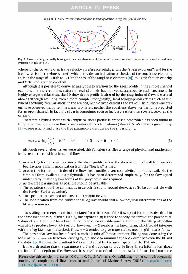
The new shear law has been fitted to each 10-min ADP measurement. Fitting was done using theMATLAB fminsearch function, varying z0; a; b and c to minimise the RMS error between the fit andthe data. Fig. 8 shows the resultant RMS error divided by the mean speed for the TGL site.
It is worth noting that the parameters a; b and c appear to provide little direct information aboutthe form of the depth profile. However, it is possible to calculate more useful information from some
e cite this article in press as: K. Gunn, C. Stock-Williams, On validating numerical hydrodynamicls of complex tidal flow, International Journal of Marine Energy (2013), http://dx.doi.org/16/j.ijome.2013.11.013
0 0.05 0.1 0.15 0.2 0.25 0.3 0.35 0.4 0.45 0.50
50
100
150
200
250
300
350
Normalised RMS error
Freq
uenc
y
Fig. 8. Histogram of normalised RMS error for the new shear equation, with n ¼ 1, to the ADP data at the TGL site.
12 K. Gunn, C. Stock-Williams / International Journal of Marine Energy xxx (2013) xxx–xxx
manipulation of the equation. For example, the derivative with respect to z can be calculated at a pointclose to the surface and used to identify reverse shear:
2 Theby rotataccelerabearing
Pleasemode10.10
dudz¼ a
1zþ bðnþ 1Þzn þ cnzn�1
� �ð7Þ
Furthermore, if n ¼ 1 is used, then the depth of maximum velocity can be calculated (for timeswhen the flow has reverse shear) by taking du=dz ¼ 0, giving:
zðumaxÞ ¼�c þ
ffiffiffiffiffiffiffiffiffiffiffiffiffiffiffiffic2 � 8bp
4bð8Þ
It could be possible to use the parameters of Eq. (6) as validation statistics, or indeed the gradient ofthe profile near the surface, using Eq. (7). However, with the example data set, the correlation coeffi-cients for du=dz near the surface are on the order of 0.5 between model and ADP. Thus, at this point,the hydrodynamic model could be declared invalid, if faithful representation of the measured velocitydepth profiles were essential.
However, valuable qualitative information can still be derived about the model (and the true nat-ure of the site) using this parameterisation of the shear profile, which will now be discussed.
Parametric comparison of shear profiles
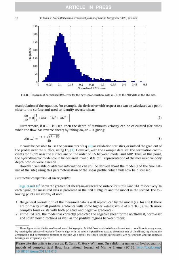
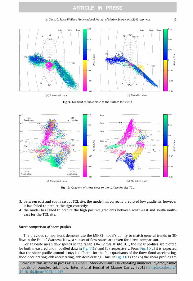
Figs. 9 and 102 show the gradient of shear (du=dz) near the surface for sites D and TGL respectively. Ineach figure, the measured data is presented in the first subfigure and the model in the second. The fol-lowing points are worthy of note:
1. the general overall form of the measured data is well reproduced by the model (i.e. for site D thereare primarily small positive gradients with some higher values; while at site TGL, a much morecomplex form exists with both positive and negative gradients);
2. at the TGL site, the model has correctly predicted the negative shear for the north-west, north-eastand south flow directions as well as the positive regions between them;
se figures take the form of transformed hodographs. As tidal flow tends to follow a form close to an ellipse in many cases,ing the primary direction of flow to align with the axes it is possible to expand the minor axis of the ellipse, separating theting and decelerating portions of the tide. As a result, the speed isolines (or isotachs) are not circular, and the compass
s are irregularly spaced.
cite this article in press as: K. Gunn, C. Stock-Williams, On validating numerical hydrodynamicls of complex tidal flow, International Journal of Marine Energy (2013), http://dx.doi.org/16/j.ijome.2013.11.013
N NEE
SE
SSWW
NW
1m/s
2m/s 3m/s 4m/s
dU/d
Z at
20m
−0.06
−0.04
−0.02
0
0.02
0.04
0.06
N NEE
SE
SSWW
NW
1m/s
2m/s 3m/s 4m/s
dU/d
Z at
20m
−0.06
−0.04
−0.02
0
0.02
0.04
0.06
Fig. 9. Gradient of shear close to the surface for site D.
N
NE
E
SE
S
SW
W
NW
1m/s
2m/s
3m/s
4m/s
FloodAccelerating
FloodDecelerating
EbbDecelerating
EbbAccelerating
dU/d
Z at
30m
−0.06
−0.04
−0.02
0
0.02
0.04
0.06
N
NE
E
SE
S
SW
W
NW
1m/s
2m/s
3m/s
4m/s
dU/d
Z at
30m
−0.06
−0.04
−0.02
0
0.02
0.04
0.06
Fig. 10. Gradient of shear close to the surface for site TGL.
K. Gunn, C. Stock-Williams / International Journal of Marine Energy xxx (2013) xxx–xxx 13
3. between east and south east at TGL site, the model has correctly predicted low gradients, howeverit has failed to predict the sign correctly;
4. the model has failed to predict the high positive gradients between south-east and south-south-east for the TGL site.
Direct comparison of shear profiles
The previous comparisons demonstrate the MIKE3 model’s ability to match general trends in 3Dflow in the Fall of Warness. Now, a subset of flow states are taken for direct comparison.
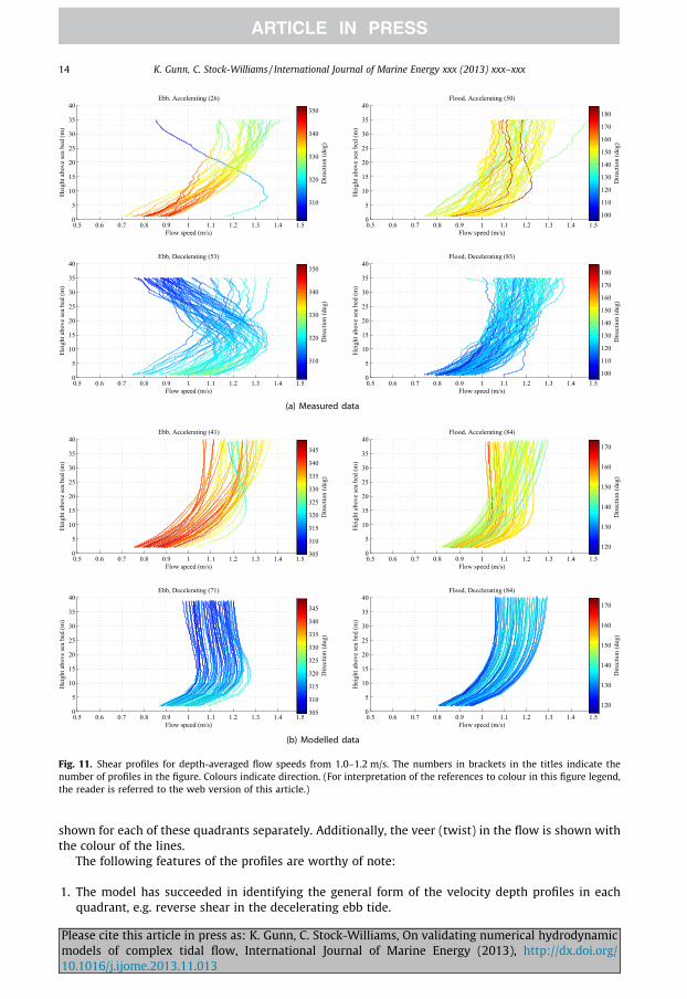
For absolute mean flow speeds in the range 1.0–1.2 m/s at site TGL, the shear profiles are plottedfor both measured and modelled data in Fig. 11(a) and (b) respectively. From Fig. 10(a) it is expectedthat the shear profile around 1 m/s is different for the four quadrants of the flow: flood accelerating,flood decelerating, ebb accelerating, ebb decelerating. Thus, in Fig. 11(a) and (b) the shear profiles are
Please cite this article in press as: K. Gunn, C. Stock-Williams, On validating numerical hydrodynamicmodels of complex tidal flow, International Journal of Marine Energy (2013), http://dx.doi.org/10.1016/j.ijome.2013.11.013
0.5 0.6 0.7 0.8 0.9 1 1.1 1.2 1.3 1.4 1.50
5
10
15
20
25
30
35
40
Flow speed (m/s)
Hei
ght a
bove
sea
bed
(m)
Ebb, Accelerating (26)
Dire
ctio
n (d
eg)
310
320
330
340
350
0.5 0.6 0.7 0.8 0.9 1 1.1 1.2 1.3 1.4 1.50
5
10
15
20
25
30
35
40
Flow speed (m/s)
Hei
ght a
bove
sea
bed
(m)
Flood, Accelerating (50)
Dire
ctio
n (d
eg)
100
110
120
130
140
150
160
170
180
0.5 0.6 0.7 0.8 0.9 1 1.1 1.2 1.3 1.4 1.50
5
10
15
20
25
30
35
40
Flow speed (m/s)
Hei
ght a
bove
sea
bed
(m)
Ebb, Decelerating (53)
Dire
ctio
n (d
eg)
310
320
330
340
350
0.5 0.6 0.7 0.8 0.9 1 1.1 1.2 1.3 1.4 1.50
5
10
15
20
25
30
35
40
Flow speed (m/s)
Hei
ght a
bove
sea
bed
(m)
Flood, Decelerating (83)
Dire
ctio
n (d
eg)
100
110
120
130
140
150
160
170
180
(a) Measured data
0.5 0.6 0.7 0.8 0.9 1 1.1 1.2 1.3 1.4 1.50
5
10
15
20
25
30
35
40
Flow speed (m/s)
Hei
ght a
bove
sea
bed
(m)
Ebb, Accelerating (41)
Dire
ctio
n (d
eg)
305
310
315
320
325
330
335
340
345
0.5 0.6 0.7 0.8 0.9 1 1.1 1.2 1.3 1.4 1.50
5
10
15
20
25
30
35
40
Flow speed (m/s)
Hei
ght a
bove
sea
bed
(m)
Flood, Accelerating (84)
Dire
ctio
n (d
eg)
120
130
140
150
160
170
0.5 0.6 0.7 0.8 0.9 1 1.1 1.2 1.3 1.4 1.50
5
10
15
20
25
30
35
40
Flow speed (m/s)
Hei
ght a
bove
sea
bed
(m)
Ebb, Decelerating (71)
Dire
ctio
n (d
eg)
305
310
315
320
325
330
335
340
345
0.5 0.6 0.7 0.8 0.9 1 1.1 1.2 1.3 1.4 1.50
5
10
15
20
25
30
35
40
Flow speed (m/s)
Hei
ght a
bove
sea
bed
(m)
Flood, Decelerating (84)
Dire
ctio
n (d
eg)
120
130
140
150
160
170
(b) Modelled data
Fig. 11. Shear profiles for depth-averaged flow speeds from 1.0–1.2 m/s. The numbers in brackets in the titles indicate thenumber of profiles in the figure. Colours indicate direction. (For interpretation of the references to colour in this figure legend,the reader is referred to the web version of this article.)
14 K. Gunn, C. Stock-Williams / International Journal of Marine Energy xxx (2013) xxx–xxx
shown for each of these quadrants separately. Additionally, the veer (twist) in the flow is shown withthe colour of the lines.
The following features of the profiles are worthy of note:
1. The model has succeeded in identifying the general form of the velocity depth profiles in eachquadrant, e.g. reverse shear in the decelerating ebb tide.
Please cite this article in press as: K. Gunn, C. Stock-Williams, On validating numerical hydrodynamicmodels of complex tidal flow, International Journal of Marine Energy (2013), http://dx.doi.org/10.1016/j.ijome.2013.11.013
K. Gunn, C. Stock-Williams / International Journal of Marine Energy xxx (2013) xxx–xxx 15
2. The model has further correctly produced multiple flow profiles in some quadrants, e.g. the yellowand green profiles in the accelerating flood tide.
3. The model has identified the existence of veer, most notably in the accelerating ebb tide.4. The model has produced an excellent representation of the shear and veer profiles for the simple
case of the decelerating flood tide.
However, the model has failed on the following points:
1. It has considerably under-predicted the magnitude of the reverse shear in the decelerating ebbtide.
2. It has under-predicted the magnitude of veer in the accelerating ebb tide.3. It has predicted reverse shear where it does not exist in the accelerating flood tide. In reality the
differential tends towards 0 at the surface.
Conclusions
This paper restates a philosophy to guide validation exercises:
1. that meaningful statistics should be chosen for each variable to be assessed; and2. that required values for those statistics be chosen before the exercise begins, based on the use to
which the model is to be put.
In particular (and while valuable for calibration) the use of Skill Score, correlation coefficient andsimilarly abstract statistics is discouraged for validation.
For the specific case of validation of a 3D hydrodynamic model of an energetic tidal site, methodsfor validating key variables (using suitable statistics and plots) are presented and tested on a MIKE3model of the Fall of Warness, Orkney Islands, UK.
For variables such as tidal height, prediction and confidence intervals on a linear regression havebeen shown to be useful tools for validation:
� Using the linear regression to first remove systematic errors, the prediction interval provides anexcellent measure of the random error: validating the ability of the model to represent trends.� Confidence intervals on the regression show whether the model is significantly different from the
measured data: validating for systematic errors.� Having shown that the systematic errors are insignificant, the prediction interval between the
model and the measured data can be used to determine uncertainty for use in further calculations.
The first of these points is relevant if the model is to be used for tasks such as array layout or plan-ning measurement campaigns. The second and third are useful if the model is to be used in yieldassessment work.
The value of examining the flow in the frequency domain has also been considered by conductingharmonic analysis. Assessing the match in tidal harmonic constituents is a powerful method fordetecting if the model has correctly accounted for, or has erroneously introduced, resonantphenomena.
Last, validation of the 3D flow profiles has been found to be more problematic. After discussing thefailures of traditional equations to represent velocity depth profiles in highly-energetic tidal sites, anew parameterisation for the depth profile has been proposed and was found to fit the tidal data con-sidered. It has been found that the hydrodynamic model used here – which is representative of thebest current-generation 3D tidal hydrodynamic models – is not able to provide faithful representa-tions of the 3D flow. Direct comparisons of the model shear and the measured shear could not passany quantitative tests of model validity. However, valuable qualitative information about the flowis still available from the model. For example, the model has been able to predict that one site inthe channel has simple depth profiles, while another location 1.3km distant is considerably more
Please cite this article in press as: K. Gunn, C. Stock-Williams, On validating numerical hydrodynamicmodels of complex tidal flow, International Journal of Marine Energy (2013), http://dx.doi.org/10.1016/j.ijome.2013.11.013
16 K. Gunn, C. Stock-Williams / International Journal of Marine Energy xxx (2013) xxx–xxx
complex. Furthermore, in most situations it has correctly predicted the nature of the complexity, forexample reverse sheared flow at certain times of the tide.
It is, therefore, proposed that such model outputs provide an invaluable resource for planning mea-surement campaigns. For example, having chosen potential tidal turbine locations, the model wouldindicate which of these locations are most likely to have complex phenomena which may warrant fur-ther investigation with an ADP installation.
Acknowledgment
This work was partly conducted for the ReDAPT project, commissioned and funded by the EnergyTechnologies Institute.
References
[1] T. Adcock, S. Draper, G. Houlsby, A. Borthwick. On the tidal resource of the Pentland Firth, in: Proceedings of the 4thInternational Conference on Ocean Energy, Dublin, 2012.
[2] ASME. Standard for verification and validation in computational fluid dynamics and heat transfer, 2009.[3] S. Baston, R.E. Harris. Modelling the hydrodynamic characteristics of tidal flow in the Pentland Firth, in: Proceedings of the
9th European Wave and Tidal Energy Conference, Southampton, 2011.[4] I. Bryden, S. Couch, A. Owen, G. Melville, Tidal current resource assessment, Proc. IMechE Part A: J. Power and Energy 221
(2007) 125–135.[5] MIKE by DHI. MIKE 21 & MIKE 3 flow model FM, hydrodynamic and transport module, scientific documentation. Technical
report, MIKE by DHI, 2011.[6] F.M. Henderson, Open Channel Flow, Collier Mackmillan, 1989.[7] K. Kaergaard, O. Svenstrup Petersen. Development of 3D HD model, Fall of Warness, UK. Technical report, ETI, 2011.[8] J.C. Kaimal, J.J. Finnigan, Atmospheric Boundary Layer Flows, Oxford University Press, 1994.[9] A.H. Murphy, Climatology, persistence, and their linear combination as standards of reference in skill scores, Weather and
Forecasting 7 (1992) 692–698.[10] NOAA. NOS standards for evaluating operational nowcast and forecast hydrodynamic model systems, 2003.[11] P.R. Oke, J.S. Allen, R.N. Miller, G.D. Egbert, J.A. Austin, J.A. Barth, T.J. Boyd, P.M. Kosro, M.D. Levine, A modeling study of the
three-dimensional continental shelf circulation off Oregon. Part I: model-data comparisons, Journal of PhysicalOceanography 32 (2002) 1360–1382.
[12] R. Pawlowicz, B. Beardsley, S. Lentz, Classical tidal harmonic analysis including error estimates in MATLAB using T_TIDE,Computers and Geosciences 28 (2002) 929–937.
[13] Karl Popper, The Logic of Scientific Discovery, Routledge, 1959.[14] David T. Pugh, Tides, Surges and Mean Sea-Level, John Wiley & Sons, 1987.[15] C. Stock-Williams and K. Gunn, Fall of Warness 3D model validation report. Technical report, ETI, 2012.[16] John C. Warner, W. Rockwell Geyer, James A. Lerczak, Numerical modeling of an estuary: a comprehensive skill
assessment, Journal of Geophysical Research: Oceans 110 (2005).[17] C.J. Wilmott, On the validation of models, Physical Geography 2 (1981) 184–194.
Please cite this article in press as: K. Gunn, C. Stock-Williams, On validating numerical hydrodynamicmodels of complex tidal flow, International Journal of Marine Energy (2013), http://dx.doi.org/10.1016/j.ijome.2013.11.013
Copyright © 2022 FDOKUMEN