Hydrodynamic and sediment suspension modelling in ...

Ž .Journal of Marine Systems 22 1999 105–116

Hydrodynamic and sediment suspension modelling inestuarine systems

Part I: Description of the numerical models

Leonor Cancino, Ramiro Neves )

Instituto Superior Tecnico, Department of Mechanical Engineering, AÕ. RoÕisco Pais, P-1096 Lisbon, Portugal´

Received 15 October 1996; accepted 1 November 1998

Abstract

A fully-3D finite difference baroclinic model system for hydrodynamics and fine suspended sediment transport isdescribed. The hydrodynamic model is based on the hydrostatic and Boussinesq approximations, and uses a vertical doublesigma co-ordinate with a staggered grid and a semi-implicit two-time level scheme. In addition to the momentum andcontinuity equations, the model solves two transport equations for salt and temperature and an equation of state to includethe baroclinic effects. The simulation of cohesive sediment transport processes is performed solving the 3D-conservativeadvection–diffusion equation, in the same grid used by the hydrodynamic model. Flocculation, erosion and deposition ofsediments on the bottom are represented by means of empirical formulations parameterized by field data. The models were

Žtested and calibrated by simulating tidal flows and suspended sediment transport in several estuaries two applications are.described in Part II . The results show good agreement between the numerical predictions and the corresponding field

measurements. q 1999 Elsevier Science B.V. All rights reserved.

Keywords: hydrodynamic suspension; estuarine systems; numerical models

1. Introduction

The filtering role of estuaries makes them crucialtransitional areas trapping significant quantities ofparticulate and dissolved matter through a wide vari-ety of physical and biogeochemical processes. Cohe-sive sediments play an important role in these pro-cesses. Unlike sand, well characterised by its grainsize distribution, cohesive sediments are complexmixtures of different clay minerals—mainly illite,

) Corresponding author. E-mail: [email protected]

montmorillonite and kaolinite—organic matter and asmall percentage of sand and silt.

Hydrodynamic action is the most important mech-anism involved in sediment transport. It advects thesuspended sediments, provides the force need toerode the bed and, through turbulence, plays a majorrole in the flocculation of cohesive sediments. Rela-tively large velocities generally occur in tidal estuar-ies. Because the hydrodynamic processes involved insediment transport are mainly non-linear, the sedi-ments are very mobile in these estuaries. They areeroded and transported upwards during flood, de-posited during slack water, eroded again and trans-

0924-7963r99r$ - see front matter q 1999 Elsevier Science B.V. All rights reserved.Ž .PII: S0924-7963 99 00035-4

( )L. Cancino, R. NeÕesrJournal of Marine Systems 22 1999 105–116106

ported downwards during ebb and redeposited duringnext slack water, to restart their movement in theforthcoming tidal cycle.

In tidal estuaries the amount of sediments inmovement can be very large but, due to its oscillat-ing nature, the net sediment transport can be verysmall. So, time scales of bottom evolution should beexpected to be much larger than a tidal period. Forthese reasons, the field study of sediment transport isvery difficult. If the tidal period is chosen as the timescale, the mechanisms and the detailed motion of thesediments can be studied. On the other hand, forlonger time scales, the study can yield the monitor-ing of net erosionrdeposition of sediments. Short-term processes are frequently a concern of CoastalEngineering, whereas the long-term evolution ismainly a matter of geological studies. Mathematicalmodelling can be a bridge between them.

The first attempt to correlate sediment transportŽ .and fluid dynamics is due to Bagnold 1936, 1937 .

He was a soldier during the First World War, placedin duty in the Egyptian Sahara desert. The frequentsandstorms drove his interest on the subject. The

Ž .works carried out later by Einstein 1950 and hiscollaborators, and the development of the computingcapacity, turned the mathematical modelling of sedi-ment transport into a major subject in coastal sci-ences.

Cohesive and non-cohesive sediments are differ-ent from each other in two major aspects: floccula-tion and consolidation of deposited material withcompaction of the sediments. Flocs are formed bygluing individual particles and can strongly modifythe settling velocity of particulate matter. After bot-tom deposition, the water content is still a significantpart of the bed material. The expulsion of this wateris part of the sediment consolidation process. Thesmall pore dimensions imply long times for sedimentdeposition, which creates conditions for fluid–mudformation in environments with very high availabil-ity of sediments.

The long time scale associated with consolidationand the strong dynamics of sediment in tidal estuar-ies make this process of secondary importance inshort-term studies. In an estuary, three types of areasmay be considered according to the deposition bud-get: erosion areas, deposition areas and equilibriumareas. In deposition areas, there are available sedi-

ments but the flow cannot erode them. In equilibriumareas, the amount of deposited sediments balancesthe erosion and there is no place to consolidation. Inerosion areas, the important information is theknowledge of the vertical structure of the bed inorder to know how the critical shear stress increasesas erosion proceeds. In these conditions, consolida-tion becomes important only in fluid–mud formation

Ž .or in very long-term simulations decades whensediment deposition is able to modify the hydrody-namic regime.

In these conditions, cohesive sediment transportmodels can be classified into two main groups ac-cording to their ability to model the formation andtransport of fluid mud. The model presented in thispaper does not consider the formation of fluid–mudand can be used only in estuaries with moderatesediment concentrations. Models of this type con-sider tidal advection, flocculation and the exchanges

Ž .with the bottom erosion and deposition . The basicdifferences among them arise mainly from the num-ber of dimensions considered, the numerical tech-nique adopted, the complexity of the description ofthe bed and from the effects considered in the hydro-

Ždynamic forcing e.g., tides, density flows, and wind.waves . For reasons of computing costs, until re-

cently most applications have been restricted toŽ .transport processes in one-dimension 1D or two-di-

Ž .mension 2D .One of the earliest studies concerning fluid–mud

Ž .conditions Einstein and Chien, 1955 was under-taken dividing the water column into a bed heavyfluid zone with high sediment concentration, and alight fluid zone with lower sediment concentrationoccupying the remainder of the water column. Avelocity distribution was derived for each zone. Inthis work, both flocculation and bed consolidationwere studied. It was verified that a minimum salinityof 1‰ was required for the onset of flocculation.The consolidation was quantified by noting the varia-tion of the bed thickness with time in two differentphases and by order of aggregation. More recently,

Ž .Odd and Owen 1972 developed, along the samelines, a 1D model considering a deeper thin lowerlayer with constant depth and an upper layer ofvarying thickness. Erosion and deposition rates were

Ž .based on the formulations proposed by Krone 1962Ž .and Partheniades 1965 . 1D models have been fre-

( )L. Cancino, R. NeÕesrJournal of Marine Systems 22 1999 105–116 107

quently used to simulate sediment transport andŽlarge-scale morphological changes in rivers De Vries

. Žet al., 1989 , in tidal channels Dyer and Evans,.1989 and for the simulation of lutocline formation

Žin estuaries Ross and Mehta, 1989; Smith and Kirby,.1989 .

An early 2D vertical integrated model was pre-Ž .sented by O’Connor 1971 . Other 2D vertical inte-

grated models have followed this one. Ariathurai andŽ .Krone 1976 presented a finite element model

adopting triangular elements with a quadratic ap-proximation for the concentration and a Galerkianweighted residual method. The model utilises theclassical relations for erosion and deposition men-tioned above. Flocculation is accounted for by speci-fying different settling velocities in each element asa function of time. In this work, the authors defendthat each clay mineral becomes cohesive at a differ-

Ž .ent salinity value. Mulder and Udink 1991 pre-sented a 2D model for the Western Scheldt estuaryŽ .The Netherlands in which the tide and wind wavemodels were combined to produce stationary wavefields. The model solves a spectral action balance

Žequation with interpolation between the calculatedwave heights and wave periods at different tidal

.stages to determine the orbital velocity and bottomshear stress component due to waves. Classical em-pirical expressions for sedimentation and erosionwere used. Uniform values for critical shear stress oferosion and deposition and constant settling velocitywere imposed. Consolidation was neglected.

Ž .Li et al. 1994 developed a coupled 2-DV width-integrated hydrodynamic and sediment transport

Ž .model for the Gironde estuary France . Aturbulent-closure model is described to compute tur-bulent viscosity and diffusion coefficients. Bottomexchange was calculated based on the classical for-mulations.

Ž .Sediment transport is a three-dimensional 3Dphenomenon. Even if there is no strong densitygradient, the settling velocity and the water–bottominteraction generate vertical gradients of suspendedsediment. For these reasons, 3D approaches are themost adequate for sediment transport modelling pur-poses. Nowadays, even with inexpensive computers,these models are feasible and are capable of simulat-ing the tide, wind and density forcing. Important 3Deffects are present in regions with strong curvature,

generating secondary flows responsible for the accu-mulation of sediments along the concave side of theestuary domain.

In 3D formulations, the bottom boundary layerŽ .can be simulated explicitly. Sheng 1986 discussed

the erosion and deposition processes together withthe bottom boundary layer model. O’Connor and

Ž .Nicholson 1988 provided a fully 3D model, includ-ing a fluid–mud transport model, flocculation and

Ž .consolidation. Katopodi and Ribberink 1992 devel-oped a quasi-3D model for suspended sedimenttransport based on an asymptotic solution of theadvection–diffusion equation for currents and waves.A sensitivity analysis of the relative importance ofcurrent and wave parameters on the suspended ad-justment phenomenon shows that the presence of thelatter considerably increases the suspended load andits adjustment time and length scales. The modelresults are compared with 2D width-integrated andfully 3D numerical solutions. Baroclinic models forhydrodynamic and sediment transport has been de-

Ž .veloped for coastal zones De Kok et al., 1995 andŽ .for estuaries Cancino and Neves, 1994a,b; 1995 .

Applications of the latter to the Western Scheldt andGironde estuaries are described in Part II of thispaper.

2. Hydrodynamic model

2.1. Model equations

The hydrodynamic model used is a fully 3D-baroclinic model. It considers the hydrostatic andBoussinesq approximations, uses a vertical doublesigma co-ordinate with a staggered grid and a semi-

Žimplicit two-time level scheme Santos and Neves,.1991; Santos, 1995 .

The horizontal transport and the Coriolis term aresolved explicitly, while the model uses an implicitalgorithm for the pressure terms and for the verticaltransport. The horizontal viscosity calculation isbased on Kolmogorov’s law. The computation of thevertical viscosity is based on a mixing length ap-proach.

Tidal forcing is prescribed at the marine bound-ary, whereas the flow rate is imposed at the riverboundary. At the natural air–sea boundary, the con-


ditions are prescribed by using known-atmosphericvalues. In addition to the momentum and continuityequations, the model can optionally solve two trans-port equations for salt and temperature and an equa-tion of state to include the baroclinic effects.

The momentum and continuity equations in Carte-sian co-ordinates are:

Eu Eu Eu Euqu qÕ qw y fÕ

Et Ex E y Ez

1 Ep E Eu E Eusy q A q AH Hž / ž /r Ex Ex Ex E y E yr

E Euq A , 1Ž .Vž /Ez Ez

EÕ EÕ EÕ EÕqu qÕ qw q fu

Et Ex E y Ez

1 Ep E EÕ E EÕsy q A q AH Hž / ž /r E y Ex Ex E y E yr

E EÕq A , 2Ž .Vž /Ez Ez

Epqr gs0, 3Ž .

Ez

Eu EÕ Ewq q s0, 4Ž .

Ex E y Ez

where t is time, u, Õ, w are the velocity componentsin the x, y, z directions, f is the Coriolis parameter,p is pressure, r is water density, g is the accelera-tion of gravity, and A and A are the horizontalH V

and vertical turbulent viscosities.At the bottom, the friction shear stress is imposed

assuming a logarithmic velocity profile:

< <tsc u u , 5Ž .d q q

y2zq2c sk ln , 6Ž .d ž /z0

where: t is the bed shear stress, u is the horizontalqvelocity vector at the distance z above the bottom,qc is bottom drag coefficient, k is the von Karmand

constant, and z is the physical roughness height.0

At the free surface, the flux of momentum is alsoimposed in the form of a shear stress. The modelsolves two transport equations for salt and tempera-

ture and an equation of state to include the barocliniceffects. The governing transport equations can bewritten as:

E S E uS E ÕS E wSŽ . Ž . Ž . Ž .q q q

Et Ex E y Ez

E ES E ESs K q KH Hž / ž /Ex Ex E y E y

E ESq K , 7aŽ .Vž /Ez Ez

E T E uT E ÕT E wTŽ . Ž . Ž . Ž .q q q

Et Ex E y Ez

E ET E ETs K q KH Hž / ž /Ex Ex E y E y

E ETq K , 7bŽ .Vž /Ez Ez

rs 5890q38Ty0.375T 2 q3SŽ .r 1779.5q11.25Ty0.0745T 2Žy 3.8q0.01T Sq0.698 5890q38TŽ . Žq0.375T 2 q3S , 7c. Ž ..

where S and T are salinity and temperature, t istime, x, y are the horizontal co-ordinates, z is thevertical co-ordinate, K , K are the horizontal andH V

the vertical salinity and heat diffusion coefficients,and u, Õ, w are the flow velocity components in thex, y, z directions.

In these equations, the bottom boundary conditionis zero flux, while at the surface fluxes of heat andwater are imposed. At the open boundaries, thediffusive fluxes are neglected. During ebb, no otherboundary condition is needed. During flood, a relax-ation is imposed for known marine values. Therelaxation time is estimated by using field data.

2.2. The simple Õertical sigma co-ordinate

The quality of the results of a 3D model thatŽ . Ž . Ž .solves Eq. 1 – 4 , Eq. 7a–c , depends on its ability

to describe the vertical processes. The sigma co-ordinate introduced in meteorology by PhillipsŽ .1957 , and used in marine systems by a number of

Žauthors Blumberg and Mellor, 1983; Beckers, 1991;


.Santos, 1995 , allows the same number of layers tobe used independently of the local depth.

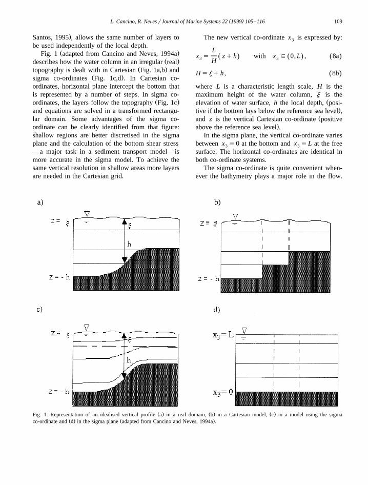
Ž .Fig. 1 adapted from Cancino and Neves, 1994aŽ .describes how the water column in an irregular real

Ž .topography is dealt with in Cartesian Fig. 1a,b andŽ .sigma co-ordinates Fig. 1c,d . In Cartesian co-

ordinates, horizontal plane intercept the bottom thatis represented by a number of steps. In sigma co-

Ž .ordinates, the layers follow the topography Fig. 1cand equations are solved in a transformed rectangu-lar domain. Some advantages of the sigma co-ordinate can be clearly identified from that figure:shallow regions are better discretised in the sigmaplane and the calculation of the bottom shear stress—a major task in a sediment transport model—ismore accurate in the sigma model. To achieve thesame vertical resolution in shallow areas more layersare needed in the Cartesian grid.

The new vertical co-ordinate x is expressed by:3

Lx s zqh with x g 0, L , 8aŽ . Ž . Ž .3 3H

Hsjqh , 8bŽ .

where L is a characteristic length scale, H is themaximum height of the water column, j is the

Želevation of water surface, h the local depth, posi-.tive if the bottom lays below the reference sea level ,

Žand z is the vertical Cartesian co-ordinate positive.above the reference sea level .

In the sigma plane, the vertical co-ordinate variesbetween x s0 at the bottom and x sL at the free3 3

surface. The horizontal co-ordinates are identical inboth co-ordinate systems.

The sigma co-ordinate is quite convenient when-ever the bathymetry plays a major role in the flow.

Ž . Ž . Ž .Fig. 1. Representation of an idealised vertical profile a in a real domain, b in a Cartesian model, c in a model using the sigmaŽ . Ž .co-ordinate and d in the sigma plane adapted from Cancino and Neves, 1994a .


This is very often the case in shallow coastal areas,but very seldom in the ocean where density is amajor forcing or, through vertical turbulence inhibi-tion, determines the vertical fluxes of momentumand heat across the water column. Even in the shal-low areas, intertidal regions are harder to deal within a simple sigma co-ordinate. A double sigma co-ordinate can minimise both problems.

2.3. The double Õertical sigma co-ordinate

The consideration of the same number of layersregardless of the local depth is generally pointed outas a major advantage of this type of co-ordinates. Inintertidal areas, during the drying process, as thewater height approaches zero the local thickness ofthe layers becomes very small. In a numerical model,this has direct implications on stability and accuracy,since the time step depends on the courant anddiffusion numbers. For that reason, a numericalmodel must consider a minimum thickness for eachlayer. In intertidal areas, this implies that the number

Ž .of layers must be small 1 to 3 . This does not arisein practical problems because in intertidal areas thevertical stratification is very weak and there is noneed for a vertical discretisation.

A double sigma co-ordinate uses a horizontalplane to split the water column into two verticaldomains and considers a sigma transformation ineach of them. In regions where the bottom laysbelow the splitting plane, the two domains exist,while in the shallow areas, only the upper one does.The number of layers is constant in each of thedomains. If the splitting plane is close to the mini-mum water level—e.g., coincident with the hydro-graphic zero—the number of layers in the intertidalareas is equal to the number of layers of the upperdomain. In the limiting case of one layer in the upperdomain, intertidal areas are dealt with by a 3D modelas in a 2D vertical integrated model and the timestep is limited only by the reflected waves associatedwith the discrete process of moving thedryingrflooding boundary. If more than one layer isused in the upper domain, a smaller time step mustbe used, which, however, is larger than in the case ofa simple sigma co-ordinate.

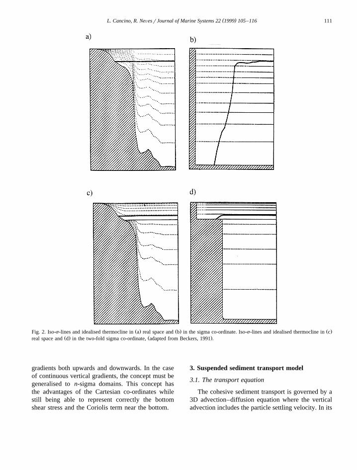
This type of co-ordinate also minimises the lackof ability of the sigma co-ordinate to deal withstratified flows. In these flows, pycnoclines in gen-eral are quasi-horizontal and do not follow the bot-

Žtom topography. Fig. 2a adapted from Beckers,.1991 shows the sigma grid and a horizontal line

representing a pycnocline. Fig. 2b represents thetransformed domain and the transformed horizontalline crossing the sigma grid.

In a stratified flow, the velocity over a horizontalpycnocline is horizontal. In the transformed domainthe horizontal velocity remains invariant. In the caseof Fig. 2b, a horizontal velocity displaces the lineleftwards. This corresponds in the real domain to aleftward plus an upward movement, and to a down-ward movement in the case of a rightward transport.If the property being considered is an active tracerŽ .e.g., temperature or salinity this artificial move-ment will modify the vertical distribution of thedensity and consequently the flow. This error in-creases with the vertical depth gradient and thehorizontal grid step. In case of stratified flows with aclear thermocline, a double sigma co-ordinate can beused with the splitting plane located immediately

Žabove the region of larger density gradients De-.lleersnijder and Beckers, 1992; Santos, 1995 . Fig.

2b and c compare the grids in both co-ordinatesystems and show how a horizontal pycnocline isrepresented in both systems of co-ordinates.

Fig. 2b also puts into evidence that the baroclinicpressure gradient cannot be calculated in the sigmagrid. In case of an irregular bathymetry, this wouldcorrespond to an integration from the surface untillevels corresponding to different real coordinates.Considering a situation where all density gradientsare horizontal, it is clear that this procedure wouldcreate an artificial horizontal baroclinic gradient anda corresponding flow. The errors again increase withthe vertical depth gradient and the horizontal step ofthe grid. This can only be solved using a Cartesianco-ordinate system to calculate the baroclinic pres-sure gradient.

The use of a double sigma co-ordinate cannotsolve all the limitations of the sigma grids. However,it can minimise the problems associated with thedrying processes in intertidal areas and the errorsassociated with the density gradients in flows wherethere is a narrow thermocline with small vertical


Ž . Ž . Ž .Fig. 2. Iso-s-lines and idealised thermocline in a real space and b in the sigma co-ordinate. Iso-s-lines and idealised thermocline in cŽ . Ž .real space and d in the two-fold sigma co-ordinate, adapted from Beckers, 1991 .

gradients both upwards and downwards. In the caseof continuous vertical gradients, the concept must begeneralised to n-sigma domains. This concept hasthe advantages of the Cartesian co-ordinates whilestill being able to represent correctly the bottomshear stress and the Coriolis term near the bottom.

3. Suspended sediment transport model

3.1. The transport equation

The cohesive sediment transport is governed by a3D advection–diffusion equation where the verticaladvection includes the particle settling velocity. In its


conservative form, the equation can be written asŽ .Cancino and Neves, 1994a,b; 1995 :

E C E uC E ÕC E wqW CŽ . Ž . Ž . Ž .Ž .sq q q

Et Ex E y Ez

E EC E EC E ECs ´ q ´ q ´ ,x y zž / ž /ž /Ex Ex E y E y Ez Ez

9Ž .

where C is the suspended sediment concentration, tis time, x, y are the horizontal co-ordinates, z is thevertical co-ordinate, ´ , ´ , ´ are the sedimentx y z

mass diffusion coefficients, W is the sediment fallS

velocity, and u, Õ, w are the flow velocity compo-nents in x, y, z directions.

Ž .Conservative properties are assumed in Eq. 9 .The total mass of suspended sediments can changeonly due to fluxes across the estuarine boundariesŽ .open boundaries, free surface and bottom . Thefluxes across the open boundaries and across the freesurface are to be imposed using field data. Thefluxes across the bottom interface are a function ofthe concentrations calculated by the model, of thehydrodynamics and of the bottom sediment proper-ties. Numerically, horizontal transport is solved ex-

Ž .plicitly, while the vertical one including settling issolved implicitly, for numerical stability reasons.

In tidal flows, the horizontal transport is mainlyadvective. In a sigma co-ordinate, the vertical trans-port is mainly forced by settling velocity and verticaldiffusion. The fluxes across the water–bottom inter-face make the vertical transport especially important.During high velocity periods, there are conditions forerosion and the material removed from the bottom istransported upwards by diffusion. During periods ofslack water, turbulence intensity is reduced and verti-cal settling imposes a net downward movement withpossible bottom deposition.

3.2. The turbulent closure

In estuarine tidal systems, the maximum velocitygradients are located near the bottom and so is thegeneration of turbulence. As a consequence, therandom component of the velocity increases from thebottom to the surface. This type of evolution hasbeen found in coastal waters during the sixties by

Ž .Bowden and Howe 1963 and confirmed later inŽ .laboratory experiments e.g., Nezu and Rodi, 1986

Žand also in the field West and Shiono, 1988; French.et al., 1993 .

In stratified systems, there is an increase of thepotential energy when the water from lower layers

Žmoves upwards and consequently, water from upper.layers moves downwards . This energy is taken out

from the turbulent kinetic energy, reducing the turbu-lent intensity. Stratification can be measured by the

Ž .Richardson number R :i

2R sy g ErrEz r r EUrEz . 10Ž . Ž . Ž .Ž . Ž .i

This number compares the rate of change of thepotential energy of water moving upwards and theproduction rate of turbulent kinetic energy. Smallervalues of R correspond to higher diffusion capacity,i

whereas at values close to unity, vertical diffusionnearly vanishes.

In general it is considered that the propertiescontributing to the water density are temperature andsalinity; R is calculated accordingly. Darbyshire andi

Ž .West 1993 argue that cohesive sediments can givea non-negligible contribution and that the differencesoften found in turbulent intensities during ebb and

Ž Ž .flood tides e.g. West and Oduyemi, 1989 andŽ ..French et al. 1993 can be explained by the contri-

bution of suspended matter to fluid density. Thismust be expected to be a major contribution to fluidmud formation.

All the experimental data obtained in estuarinesystems have been explained without recurring tohorizontal transport of turbulent properties. Thismeans that local equilibrium can be assumed inestuaries. This should be expected based on thedifference between vertical and horizontal lengthscales. In this situation a mixing length approachmay be used to calculate eddy viscosity.

The hydrodynamic model used in estuarine appli-cations considers a Prandtl mixing length hypothesisŽ .Robert and Ouellet, 1987 corrected, in stratifiedflows, by the local Richardson number. The horizon-tal viscosity is calculated using Kolmogorov’s theoryŽ .Nihoul, 1984 . The length scale is the grid size ofthe model as a measure of the non-resolved eddies.Vertical diffusivity is assumed to be proportional tothe vertical eddy viscosity.


3.3. The settling Õelocity

The vertical transport is due to vertical advection,particle settling or turbulent diffusion. The hydrody-namic model computes the vertical velocity and theturbulent diffusivity. The settling velocity dependson the gravitational forces, and on the vertical sheardue to settling movement. The gravitational forcesdepend on the density of each individual particleŽ .terrigenous or biological forming flocs and on thefloc porosity occupied by water.

The frictional forces depend on the form of thefloc and on the Reynolds number of the surroundingflow during settling. For very small bodies, the flowis laminar and the ratio between the gravitational andthe frictional force is proportional to the reciprocalof the diameter of the floc. So, the settling velocity isexpected to increase with floc size. Unfortunately,larger flocs can have smaller density and there is nounique relation between floc size and settling veloc-ity.

The probability of particles to aggregate into flocsdepends on the probability of the particles to collide.This probability is proportional to the concentration,and also increases with the amplitude and frequencyof the turbulent random movement. Aggregation is areversible process. Flocs are fragile and, if submittedto shear, they can disaggregate. Because shear in-creases also with turbulence intensity the latter playsa double role in the aggregation process.

Concentration also plays a double role. It in-creases the probability of flocculation and so thesettling velocity. Nevertheless, when the number offlocs moving downward is very large, there is aninteraction between the flows around adjacent ones.In these conditions, the upward friction tends toincrease and the particle velocity decreases. Theconcentration at which the settling velocity starts todecrease is known as the ‘hindering settling concen-tration’.

The concentration and the turbulence intensitydetermine the probability of two particles to meet.To form a floc, the particles must collide but, inaddition, they must adhere to each other. Gluing

Žforces depend on the type of particles some biologi-.cal particles have adhesive surfaces , and also on the

ionisation of the environment. The latter is a functionof the salinity, however, there is no correlation relat-

Žing salinity and flocculation. From field work Wol-.last, 1986 , there is clear evidence that an intensive

flocculation occurs as soon as salinity reaches about1‰ and is complete for values higher than 2.5‰.

Models representing cohesive sediment by a bulkconcentration use a bulk settling velocity. If noinformation is available on the type of particles inthe system and no evolution equation is solved foreach class of flocs, then it is not possible to explic-itly represent the flocculation processes in this typeof correlation. The general correlation for the settling

Ž .velocity in the flocculation range 11a and in theŽ .hindered settling range 11b is:

W sK C m for C-C , 11aŽ .S 1 HS

m1mW sK C 1.0yK CyCŽ .S 1 HS 2 HS

for C)C , 11bŽ .HS

Ž y1 . Žwhere W ms is the settling velocity, C kgSy3 .m is the concentration, and the subscript HS

Žrefers to the onset of the hindered settling of about 2y3 . Ž 4 y1 y1.to 5 kg m . The coefficients K m kg s1

Ž 3 y1.and K m kg depend on the mineralogy of the2

mud and the exponents m and m depend on particle1

size and shape.Ž .Krone 1962 , based on the kinetics of floccula-

tion, proposed a theoretical value for m equal toŽ .4r3. Mehta 1986 found, experimentally, values

Ž .varying between 1 and 2. In expression 11b , theexponent m is usually taken as 4.65 for small1

Ž .particles and 2.32 for large particles Dyer, 1986 .Ž . Ž .To ensure that Eqs. 11a and 11b are dimension-

ally correct, both m and m should be 1.1

This type of correlation is adequate for modelsthat calculate a bulk concentration. In 3D hydrody-namic models, the intensity of turbulence is calcu-lated and a more complex correlation could be used.That type of correlation is not yet available. How-ever, the situation is expected to improve, due toadvances in measuring techniques and modelling.

3.4. Bottom interface module

Although there is evidence that matter is continu-Žously deposited and removed from the bottom e.g.,

.Stanford and Halka, 1993 , most models follow Ein-Ž .stein 1950 and consider that the two processes

cannot occur simultaneously. In such models, it is


assumed that, when bottom friction is smaller than acritical value for deposition, there is addition ofmatter to the bottom, and, when the bottom shear ishigher than a minimum value, erosion occurs. Be-tween those values, erosion and deposition balanceeach other. In fact, only very recently has it beenpossible to measure the downward and upwardmovement of particles at the bottom interface. Informer times, the best that could be achieved was tomeasure the net erosion or deposition as a functionof the bottom shear. Both formulations can easily beincluded in the same model. In this work, the tradi-tional approach was adopted because it is mucheasier to find data in the literature to specify theparameters.

3.4.1. The erosion modelErodibility of a cohesive bed is driven by shear,

but also depends on bottom cohesive nature, whichin turn depends, in a poorly understood way, on claymineralogy and on the geochemistry and microbio-logical processes occurring in the bottom. Someauthors argue that it should also depend on the

Ž .salinity Hayter and Mehta, 1986 . However, nodependency laws have yet been advanced.

Again, a useful correlation must depend only onthe variables calculated by the model and on parame-ters. The erosion algorithm used in this work isbased on the classical approach of Partheniades,Ž .1965 . Erosion occurs when the ambient shear stressexceeds the threshold of erosion. The flux of erodedmatter is given by:

EM tEsE y1 for t)t , 12aŽ .Ež /Et tE

EMEs0 for t-t , 12bŽ .E

Et

where t is the bed shear stress, t is a critical shearEŽstress for erosion and E is the erosion constant kg

y2 y1.m s .Ž .The parameter E Eq. 12a depends on the

physico-chemical characteristics of bottom sediment.Ž .In the Western Scheldt, Mulder and Udink, 1991

used 5=10y5 kg my2 sy1. As a general rule,bottom-sediments are a mixture of cohesive andnon-cohesive sediments; this parameter must also

account for that and so a gradient must be expectedin the estuary.

Critical shear stress for erosion is a function ofthe degree of compaction of bottom sediments mea-sured by the dry density of the bottom sediments:

Žratio between the mass of sediment after extraction.of the interstitial water at 1058C and its initial

volume.Ž .Stephens et al. 1992 , based on the formulationsŽ .proposed by Delo 1988 , used:

E1t sA r , 13Ž . Ž .E 1 d

Ž y3 .where r kg m is dry density of bed sediments,dŽ 2 y2 .and A m s and E are coefficients depending1 1

on mud type.This equation is dimensionally correct only for

Ž .E s1. Nevertheless, Stephens et al. 1992 cali-1

brated their model with A s0.0012 m2 sy2 and1

E s1.2. This is a critical point when a compaction1

model is used, otherwise, this correlation becomes anindirect means of imposing a critical shear stress forerosion knowing the bed sediment dry density, mucheasier to measure. The deviation of the coefficientE from unity can be seen as a measure of the error1

of the input data.

3.4.2. The deposition modelThe deposition algorithm, like the erosion algo-

rithm, is based on the assumption that deposition anderosion never occur simultaneously. An algorithm

Ž .was first proposed by Krone 1962 and later onŽ .modified by Odd and Owen, 1972 . The algorithm

is based on the assumption that a particle reachingthe bottom has a probability of remaining there thatvaries between 0 and 1 as the bottom shear stressvaries between its upper limit for deposition andzero, respectively. Deposition is calculated as theproduct of the settling flux and the probability of aparticle to remain on the bed:

EM tDsC W 1y for t)t ,Ž .B S Dž /Et t D

14aŽ .EMD

s0 for t-t , 14bŽ .DEt

where t is the critical stress for deposition andD

subscript B means ‘at the sediment–water interface’.


The critical shear stress for deposition, t , de-D

pends mainly on the size of the flocs. Bigger flocshave higher probability of remaining on the bed thansmaller flocs. Nevertheless, previous work suggestthat a constant value is a reasonable approximation.Based on laboratory experiments with natural mud

Ž .from the Western Scheldt, Winterwerp et al. 1991found t s0.2 N my2 . For the Gironde, Li et al.DŽ . y21994 used values in the range 0.3–0.5 N m .

4. Concluding remarks

In this paper, a 3D baroclinic model is presentedfor hydrodynamics and cohesive sediment transportin tidal estuaries. The model employs a double sigmaco-ordinate for vertical discretisation and a classicalapproach for sediment transport. The use of a doublesigma coordinate has improved the stability proper-ties of the model in intertidal areas and can begeneralized to a larger number of sigma domainsvery easily. The inconsistencies in terms of dimen-sions in the correlations describing settling velocityand exchanges with the bottom suggest that somemore experimental work is still needed on this sub-ject.

The present situation can be understood by takinginto account that, when solving an equation withseveral terms, the global error has a contributionfrom each term. So, the optimal strategy to minimizethe global error is the simultaneous minimization ofevery error. Until recently, models were of 1D or 2Dtype and were unable to describe the vertical pro-cesses without resorting to highly simplified hy-potheses. The present stage of development of 3Dmodels will stimulate the improvement of the corre-lations used in a sediment transport model, as well asthe collection of the data needed to characterise thebottom sediments. The development of non-disturb-ing and remote sensing measuring techniques willalso simplify field work.

Mathematical models can give a very useful con-tribution to that development, by providing a detaileddescription of the hydrodynamic field—includingthe wave induced circulation—and a continuous testof hypotheses.

Acknowledgements

Most of this work was undertaken as a part of theproject ‘Biogeochemistry of the MAximum TURbid-

Ž .ity Zone in Estuaries’ MATURE , funded by theCommission of the European Communities, Environ-ment Programme under contract no. 910357. Thefirst author gratefully acknowledges the financialsupport of the Programa CienciarJNICT and is in-ˆdebted to Professor Antonio Falcao for encourage-´ ˜ment and kind help.

References

Ariathurai, R., Krone, R.B., 1976. Finite element model forŽ .cohesive sediment transport. J. Hydr. Div., ASCE 102 HY3 ,

323–338.Bagnold, R.A., 1936. The movement of desert sand. Proc. R. Soc.

London A 157, 594–620.Bagnold, R.A., 1937. The size-grading of sand by wind. Proc. R.

Soc. London A 163, 250–264.Beckers, J.M., 1991. Application of the GHER 3D general circula-

tion model to the Western Mediterranean. In: J. Mar. Syst. 1Elsevier, Amsterdam, pp. 315–332.

Blumberg, A.F., Mellor, G.L., 1983. Diagnostic and prognosticnumerical circulation studies of the South Atlantic Bight. J.Geophys. Res. 88, 4579–4592.

Bowden, K.F., Howe, M.R., 1963. Observations of turbulence in atidal current. Journal of Fluid Mechanics 17, 271–284.

Cancino, L., Neves, R., 1994a. Numerical modelling of three-di-mensional cohesive sediment transport in an estuarine environ-

Ž .ment. In: Belorgey, M., Rajaona, R.D., Sleath, J.F.A. Eds. ,´Sediment Transport Mechanisms in Coastal Environments andRivers. World Scientific, pp. 107–121.

Cancino, L., Neves, R., 1994b. 3D-numerical modelling of cohe-Žsive suspended sediment in the Western Scheldt estuary The

. ŽNetherlands . Netherlands Journal of Aquatic Ecology 28 3–.4 , 337–345.

Cancino, L., Neves, R., 1995. Three-dimensional model systemfor baroclinic estuarine dynamics and suspended sedimenttransport in a mesotidal estuary. In: Computer Modelling ofSeas and Coastal Regions. Computational Mechanics Publica-tions, pp. 353–360.

Darbyshire, E.J., West, J.R., 1993. Turbulence and cohesive sedi-ment transport in the Parrett estuary. In: Clifford, N.J., French,

Ž .J.R., Hardisty, J. Eds. , Turbulence: Perspectives and Sedi-ment Transport. Wiley.

De Kok, J.M., Salden, R., Rozendaal, I.D.M., Blokland, P.,Lander, J., 1995. Transport path of suspended matter along theDutch coast. In: Modelling of Seas and Coastal Regions.Computational Mechanics Publications, pp. 75–86.

De Vries, M., Klaassen, G.J., Striksma, N., 1989. On the use of


movable bed models for rivers problems: state of the art,Symp. River Sedimentation, Beijing, China.

Delleersnijder, E., Beckers, J.-M., 1992. On the use of the sigma-coordinate system in regions of large bathymetric variations. J.Mar. Syst. 3, 381–390.

Delo, E.A., 1988. Estuarine Muds Manual. Report No. SR 164.Hydraulics Research, Wallingford, UK, 64 pp.

Dyer, K.R., 1986. Coastal and Estuarine Sediment Dynamics.Wiley-Interscience, 342 pp.

Dyer, K.R., Evans, E.M., 1989. Dynamics of turbidity maximumin a homogeneous tidal channel. J. Coastal Research, 23–30,Special Issue No.5, Fort Lauderdale, FL.

Einstein, H.A., 1950. The bedload function for sediment trans-portation in open channel flows. Soil Cons. Serv. US Dept.Agric. Tech. Bull. 1026, 78 pp.

Einstein, H.A., Chien, N., 1955. Effects of heavy sediment con-centration near bed on velocity and sediment distribution,MRD Series Rep.8. Inst. Eng. Research, Univ. of Calif.,Berkeley.

French, J.R., Clifford, N.J., Spence, T., 1993. High frequencyflow and suspended sediment measurements in a tidal wetland

Ž .channel. In: Clifford, N.J., French, J.R., Hardisty, J. Eds. ,Turbulence: Perspectives and Sediment Transport. Wiley.

Hayter, E.J., Mehta, A.J., 1986. Modelling cohesive sedimenttransport in estuarine waters. Appl. Math. Modelling 10, 294–303.

Katopodi, I., Ribberink, J.S., 1992. Quasi-3D modelling of sus-pended sediment transport by currents and waves. CoastalEngineering 18, 83–110.

Krone, R.B., 1962. Flume Studies of the Transport in EstuarineShoaling Processes. Hydr. Eng. Lab., Univ. of Berkeley, CA,USA, 110 pp.

Li, Z.H., Nguyen, K.D., Brun-Cottan, J.C., Martin, J.M., 1994.Numerical simulation of the turbidity maximum transport in

Ž .the Gironde estuary France . Oceanologica Acta.Mehta, A.J., 1986. Characterisation of cohesive sediment proper-

Ž .ties and transport processes in estuaries. In: Mehta, A.J. Ed. ,Estuarine Cohesive Sediment Dynamics 14 Springer-Verlag,Berlin, pp. 290–325.

Mulder, H.P.J., Udink, C., 1991. Modelling of cohesive sedimenttransport. A case study: the western Scheldt estuary. In: Edge,

Ž .B.L. Ed. , Proceedings of the 22nd International Conferenceon Coastal Engineering. American Society of Civil Engineers,New York, pp. 3012–3023.

Nezu, Rodi, 1986. Open channel flow measurements with a laserDoppler anemometer. Journal of Hydraulic Engineering,American Society of Civil Engineers 112, 335–355.

Nihoul, J.C.J., 1984. A three-dimensional general marine circula-tion model in a remote sensing perspective. Annales Geophys-icae 2–4, 433–442.

O’Connor, B.A., 1971. Mathematical Model for Sediment Distri-bution. Proc. 14th IAHR Conf., Paper D23, Paris, France.

O’Connor, B.A., Nicholson, J.A., 1988. Mud transport modelling.Ž .In: Dronkers, J., van Leussen, W. Eds. , Physical Processes in

Estuaries. Springer-Verlag, pp. 532–544.Odd, N.V.M., Owen, M.W., 1972. A two-layer model of mud

transport in the Thames estuary. In: Proceedings. Institution ofCivil Engineers, London, pp. 195–202.

Partheniades, E., 1965. Erosion and deposition of cohesive soils.Ž .J. Hydr. Div., ASCE 91 HY1 , 105–139.

Phillips, N.A., 1957. A coordinate system having some spacialadvantages for numerical forecasting. J. Meteorol. 14, 184–186.

Robert, J.L., Ouellet, Y., 1987. A three-dimensional finite elementmodel for the study of steady and non-steady natural flows. In:

Ž .Nihoul, J.C.J., Jamart, B.M. Eds. , Elsevier OceanographySeries 45, pp. 359–372.

Ross, M.A., Mehta, A.J., 1989. On the mechanics of lutoclinesand fluid mud. J. Coastal Res. 5, 51–62.

Santos, A.J., 1995. 3D Hydrodynamic Model for Estuarine andŽ .Oceanic Circulation, in Portuguese . PhD Thesis, I.S.T., Por-

tugal.Santos, A.J, Neves, R., 1991. Radiative artificial boundaries in

Ž .ocean barotropic models. In: Arcilla, A.S. Ed. , Proceedingsof the 2nd Int. Conf. on Computer Modelling in OceanEngineering, Barcelona, pp. 373–383.

Sheng, Y.P., 1986. Modelling bottom boundary layer and cohe-sive sediment dynamics in estuarine and coastal waters. In:

Ž .Mehta, A.J. Ed. , Estuarine Cohesive Sediment Dynamics 14Springer-Verlag, Berlin, pp. 360–400.

Smith, T.J., Kirby, R., 1989. Generation, stabilisation and dissipa-tion of layered fine sediment suspensions. J. Coastal Res. 5,63–73.

Stanford, L.P., Halka, J.P., 1993. Assessing the paradigm ofmutually exclusive erosion and deposition of mud with exam-ples from upper Chesapeake Bay. Mar. Geol. 114, 37–57.

Stephens, J.A., Uncles, R.J., Barton, M.L., Fitzpatrick, F., 1992.Bulk properties of intertidal sediments in a muddy macrotidalestuary. Mar. Geol. 103, 15 pp.

West, J.R., Oduyemi, K.O.K., 1989. Turbulence measurements ofsuspended solids concentration in estuaries. Journal of Hy-draulic Engineering, American Society of Civil Engineers 115,457–474.

West, J.R., Shiono, K., 1988. Vertical turbulent mixing processeson ebb tides in partially mixed estuaries. Estuarine, Coastaland Shelf Science 20, 51–66.

Winterwerp, J.C., Cornelisse, J.M., Kuijper, C., 1991. The be-haviour of mud from the Western Scheldt under tidal condi-tions. Delft Hydraulics, The Netherlands, Rep. z161–37rHWrpaper1.wm, 14 pp.

Wollast, R., 1986. The Scheldt estuary. In: Salomon, W., Bayne,Ž .B.L., Duursma, E.K., Forstner, U. Eds. , Pollution of the

North Sea. An Assessment. Springer-Verlag, pp. 183–193.

Hydrodynamic and sediment suspension modelling in ...

Documents

Transcript of Hydrodynamic and sediment suspension modelling in ...