Hydrodynamic Design of Ship Bulbous Bows Considering ...
191
Hydrodynamic Design of Ship Bulbous Bows Considering Seaway and Operational Conditions vorgelegt von Gonzalo Tampier Brockhaus aus Chile von der Fakult¨ at V - Verkehrs- und Maschinensysteme der Technischen Universit¨at Berlin zur Erlangung des Akademischen Grades Doktor der Ingenieurwissenschaften - Dr.-Ing - genehmigte Dissertation Promotionsausschuss: Vorsitzender: Prof. Dr. rer. nat. Heinz Lehr Berichter: Prof. Dr.-Ing. Andr´ es Cura Hochbaum Berichter: Prof. Dr.-Ing. Apostolos Papanikolaou Tag der wissenschaftlichen Aussprache: 30. September 2010 Berlin 2011 D 83
-
Upload
khangminh22 -
Category
Documents
-
view
1 -
download
0
Transcript of Hydrodynamic Design of Ship Bulbous Bows Considering ...

Hydrodynamic Design of Ship
Bulbous Bows Considering Seaway
and Operational Conditions
vorgelegt von
Gonzalo Tampier Brockhaus
aus Chile
von der Fakultat V - Verkehrs- und Maschinensystemeder Technischen Universitat Berlin
zur Erlangung des Akademischen Grades
Doktor der Ingenieurwissenschaften- Dr.-Ing -
genehmigte Dissertation
Promotionsausschuss:
Vorsitzender: Prof. Dr. rer. nat. Heinz LehrBerichter: Prof. Dr.-Ing. Andres Cura HochbaumBerichter: Prof. Dr.-Ing. Apostolos Papanikolaou
Tag der wissenschaftlichen Aussprache: 30. September 2010
Berlin 2011D 83


iii
Danksagung
Ich mochte diese Danksagung auf Deutsch schreiben, obwohl ich diese Arbeit auf Eng-lisch verfasst habe, denn es handelt sich großtenteils um Personen, die ich mit meinemAufenthalt in Deutschland verbinde, denen ich diese Danksagung widme.
An erster Stelle mochte ich mich bei meinem Betreuer und Hauptberichter dieser Dis-sertation, Prof. Dr.-Ing. Andres Cura Hochbaum, fur seine permanente Unterstutzung,aktive Betreuung und wertvolle Kritik bedanken. Gerne hatte ich mir gewunscht, dassProf. Cura seinen Dienst fruher angetreten hatte und ich so seine Betreuung uber einelangere Zeit hatte genießen konnen. Auch bei meinem Betreuer und zweiten Berichterdieser Dissertation, Prof. Dr.-Ing. Apostolos Papanikolaou, mochte ich mich fur seine Un-terstutzung und wertvolle Kritik bedanken. Fur seine Bereitschaft, jede meiner Fragenmit Geduld und praktischen Hinweisen zu beantworten bin ich ihm besonders dankbar.
An gleich wichtiger Stelle mochte ich meine Dankbarkeit an meinen langjahrigen Men-tor und geistigen Vater dieser Arbeit, Dr.-Ing. Alfred Kracht, zum Ausdruck bringen.Sein Glauben an meine Person, die stetige Unterstutzung und die Gute, mir das Gefuhlvermittelt zu haben, mit ihm fur jedes Problem oder Fragestellung rechnen zu konnen,sind fur mich uber diese gesamte Zeit von großter Bedeutung gewesen.
Fur die langjahrige Zusammenarbeit und Unterstutzung mochte ich mich auch bei Dr.-Ing. Stefan Harries und Dr.-Ing. Karsten Hochkirch bedanken. Fur ihr stetes Interessean den Fortschritten meiner Arbeit, ihre Unterstutzung mit Hinweisen und Diskussionen,aber auch fur die zur Verfugung gestellte Software, bin ich ihnen besonders dankbar.
Auch meinen ehemaligen Kollegen Dr.-Ing. Jorn Hinnenthal und Felix Fliege mochte ichauf diesem Weg danken. Ihr Vertrauen und ihr Einsatz ermoglichte uberhaupt erst meineAnkunft an der Technischen Universitat Berlin. Unsere Zusammenarbeit und wertvollenDiskussionen wahrend der darauffolgenden Jahre werden fur mich als eine der pragendstenErinnerungen an meine Zeit an dieser Universitat bleiben. Auch meinen aktuellen Kollegenund Mitarbeitern des gesamten Bereiches der Schiffs- und Meerestechnik gilt ein großesDankeschon, insbesondere meinem Kollegen Christian Eckl fur seine Unterstutzung undgroßartige Zusammenarbeit in der letzten Zeit.
Auch bei meinen Freunden und bei meiner Familie, sowohl hier in Deutschland alsauch in Chile, mochte ich mich herzlichst fur jede einzelne kleine und große Hilfestellungbedanken.
Zuletzt schulde ich die großte Dankbarkeit meiner geliebten Ehefrau Andrea Sacher.Diese Arbeit ist zu einem großen Teil auch ihre Arbeit, denn die gleiche Energie, dieich fur diese Arbeit eingesetzt habe, und die damit verbundenen Stunden der physischenund geistigen Abwesenheit, hat sie mit viel Verstandnis, Geduld und Starke fur unsereFamilie und mit Begeisterung, Optimismus und Freude fur unsere gemeinsamen Projekte

iv
eingesetzt.Meinen Sohnen, Anton und Bruno, widme ich in diesem Sinne nicht die Inhalte die-
ser Arbeit, sondern vielmehr alle positiven Auswirkungen, die diese Arbeit und dieserAbschluss fur unser gemeinsames Familienleben haben mogen.
Berlin, August 2010 – Gonzalo Tampier B.
Contents v
Contents
Abstract . . . . . . . . . . . . . . . . . . . . . . . . . . . . . . . . . . . . . . . . 1
1. Introduction 51.1. Background . . . . . . . . . . . . . . . . . . . . . . . . . . . . . . . . . . . 51.2. State of the Art . . . . . . . . . . . . . . . . . . . . . . . . . . . . . . . . . 61.3. Objectives and Outline . . . . . . . . . . . . . . . . . . . . . . . . . . . . . 10
2. Basic Principles 132.1. Overview . . . . . . . . . . . . . . . . . . . . . . . . . . . . . . . . . . . . . 132.2. Simulational Approach . . . . . . . . . . . . . . . . . . . . . . . . . . . . . 132.3. Operational Simulations: a Short Introduction . . . . . . . . . . . . . . . . 15
2.3.1. Operational Simulations for Ships . . . . . . . . . . . . . . . . . . . 152.4. Coordinate Systems . . . . . . . . . . . . . . . . . . . . . . . . . . . . . . . 172.5. Resistance . . . . . . . . . . . . . . . . . . . . . . . . . . . . . . . . . . . . 20
2.5.1. Resistance Prediction in Ship Design: an Overview . . . . . . . . . 202.5.2. Resistance Model Tests . . . . . . . . . . . . . . . . . . . . . . . . . 202.5.3. Resistance Calculation with Potential CFD Methods . . . . . . . . 222.5.4. Resistance Calculation with RANS CFD Methods . . . . . . . . . . 24
2.6. Seakeeping . . . . . . . . . . . . . . . . . . . . . . . . . . . . . . . . . . . . 272.6.1. Prediction of Seakeeping Performance: an Overview . . . . . . . . . 272.6.2. Potential Theory Methods for Seakeeping . . . . . . . . . . . . . . . 272.6.3. Application of RANS CFD Methods for Seakeeping . . . . . . . . . 32
2.7. Validation of CFD Solver . . . . . . . . . . . . . . . . . . . . . . . . . . . . 352.7.1. Background . . . . . . . . . . . . . . . . . . . . . . . . . . . . . . . 352.7.2. 2D Wave Tank . . . . . . . . . . . . . . . . . . . . . . . . . . . . . 372.7.3. DTMB5415 Surface Combatant . . . . . . . . . . . . . . . . . . . . 38
2.8. Partially Parametric Approach for Geometry Variation . . . . . . . . . . . 502.8.1. General Aspects . . . . . . . . . . . . . . . . . . . . . . . . . . . . . 502.8.2. Bulbous Bow Transformation Parameters . . . . . . . . . . . . . . . 50
3. Modeling of Ship Operation 553.1. General Aspects . . . . . . . . . . . . . . . . . . . . . . . . . . . . . . . . . 553.2. Environment Model . . . . . . . . . . . . . . . . . . . . . . . . . . . . . . . 55
3.2.1. Operational Model . . . . . . . . . . . . . . . . . . . . . . . . . . . 553.2.2. Weather Model . . . . . . . . . . . . . . . . . . . . . . . . . . . . . 56
3.3. Ship Model . . . . . . . . . . . . . . . . . . . . . . . . . . . . . . . . . . . 593.3.1. Geometry and Hydrostatics . . . . . . . . . . . . . . . . . . . . . . 59
vi Contents
3.3.2. Calm Water Resistance . . . . . . . . . . . . . . . . . . . . . . . . . 60
3.3.3. Ship Motions and Added Resistance in Waves . . . . . . . . . . . . 61
3.3.4. Total Resistance, Propulsion and Machinery . . . . . . . . . . . . . 66
3.4. Measure of Merit . . . . . . . . . . . . . . . . . . . . . . . . . . . . . . . . 69
3.5. Implementation of the Simulation Platform . . . . . . . . . . . . . . . . . . 71
3.5.1. Integration and Automatization for Design Purposes . . . . . . . . 73
4. Special Application Case 75
4.1. Introduction . . . . . . . . . . . . . . . . . . . . . . . . . . . . . . . . . . . 75
4.2. Simulation Routes . . . . . . . . . . . . . . . . . . . . . . . . . . . . . . . 76
4.3. Parent Geometry . . . . . . . . . . . . . . . . . . . . . . . . . . . . . . . . 76
4.4. Hydrodynamic Characteristics of Variants . . . . . . . . . . . . . . . . . . 80
4.4.1. Calm Water Resistance of Variants . . . . . . . . . . . . . . . . . . 80
4.4.2. Seakeeping and Added Resistance in Waves of Variants . . . . . . . 84
4.5. Preliminary Operational Simulations with Fixed Speed and Fixed FloatingCondition . . . . . . . . . . . . . . . . . . . . . . . . . . . . . . . . . . . . 88
4.5.1. Simulation Setup . . . . . . . . . . . . . . . . . . . . . . . . . . . . 88
4.5.2. Results . . . . . . . . . . . . . . . . . . . . . . . . . . . . . . . . . . 88
4.6. Operational Simulations with Variable Speed and Fixed Floating Condition 91
4.6.1. Simulation Setup . . . . . . . . . . . . . . . . . . . . . . . . . . . . 91
4.6.2. Results . . . . . . . . . . . . . . . . . . . . . . . . . . . . . . . . . . 95
4.6.3. Variation of Fuel Costs Coefficient kf . . . . . . . . . . . . . . . . . 96
4.6.4. Variation of Service Speed: Slow Steaming Simulations . . . . . . . 96
4.7. Operational Simulations with Variable Speed and Variable Floating Con-dition . . . . . . . . . . . . . . . . . . . . . . . . . . . . . . . . . . . . . . 100
4.7.1. Simulation Setup . . . . . . . . . . . . . . . . . . . . . . . . . . . . 100
4.7.2. Results . . . . . . . . . . . . . . . . . . . . . . . . . . . . . . . . . . 102
4.8. Conclusions about Simulation Modes . . . . . . . . . . . . . . . . . . . . . 102
5. General Application Case 107
5.1. Introduction . . . . . . . . . . . . . . . . . . . . . . . . . . . . . . . . . . . 107
5.2. Generation of Subvariants . . . . . . . . . . . . . . . . . . . . . . . . . . . 108
5.2.1. Parent Geometry and Overview of Calculations . . . . . . . . . . . 108
5.2.2. Design Space Exploration for Wave Resistance with Potential CFDMethod . . . . . . . . . . . . . . . . . . . . . . . . . . . . . . . . . 108
5.3. Viscous CFD Calculations . . . . . . . . . . . . . . . . . . . . . . . . . . . 111
5.3.1. Overview . . . . . . . . . . . . . . . . . . . . . . . . . . . . . . . . 111
5.3.2. Solver, Boundary Conditions and Numerical Setup . . . . . . . . . 112
5.3.3. Grid Generation . . . . . . . . . . . . . . . . . . . . . . . . . . . . . 112
5.3.4. Calculations . . . . . . . . . . . . . . . . . . . . . . . . . . . . . . . 113
5.3.5. CFD Results of Variants and Comparison with Experimental Data . 117
5.3.6. CFD Results of Subvariants . . . . . . . . . . . . . . . . . . . . . . 120

Contents vii
5.4. Operational Simulations with Variable Speed and Fixed Floating Condition 1215.4.1. Simulation Setup . . . . . . . . . . . . . . . . . . . . . . . . . . . . 1215.4.2. Comparison with Results Recalling Experimental Data . . . . . . . 1225.4.3. Results of Subvariants . . . . . . . . . . . . . . . . . . . . . . . . . 122
5.5. Operational Simulations with Variable Speed and Variable Floating Con-dition . . . . . . . . . . . . . . . . . . . . . . . . . . . . . . . . . . . . . . 1265.5.1. Simulation Setup . . . . . . . . . . . . . . . . . . . . . . . . . . . . 1265.5.2. Results . . . . . . . . . . . . . . . . . . . . . . . . . . . . . . . . . . 126
5.6. Conclusions about Application Case . . . . . . . . . . . . . . . . . . . . . . 128
6. Summary and Outlook 1316.1. Summary . . . . . . . . . . . . . . . . . . . . . . . . . . . . . . . . . . . . 1316.2. Outlook . . . . . . . . . . . . . . . . . . . . . . . . . . . . . . . . . . . . . 132
Bibliography 141
Alphabetic Index 142
Appendix 143A. Mesh Generation with snappyHexMesh . . . . . . . . . . . . . . . . . . . . 144
A.1. General Aspects . . . . . . . . . . . . . . . . . . . . . . . . . . . . . 144A.2. Mesh Generation for Application Case . . . . . . . . . . . . . . . . 147
B. Wave Resistance for Different Floating Conditions and Speeds: Definitionof Response Surfaces . . . . . . . . . . . . . . . . . . . . . . . . . . . . . . 152
C. Systematic Variation of Bulbous Bow for Potential CFD Calculations: Ad-ditional Tables and Figures . . . . . . . . . . . . . . . . . . . . . . . . . . 156
D. Additional Tables and Diagrams for Chapter 4 . . . . . . . . . . . . . . . . 163E. Additional Tables and Diagrams for Chapter 5 . . . . . . . . . . . . . . . . 170


List of Figures ix
List of Figures
2.1. Defined Euler angles and relationship between ICS and SCS when no trans-lations are present (Based partly on a figure from Juan Sempere, Creative Commons License) . 18
2.2. World- and inertial coordinate systems . . . . . . . . . . . . . . . . . . . . 192.3. Flowchart of TUBsixDOFFoam . . . . . . . . . . . . . . . . . . . . . . . . 362.4. Wave elevation for two different grids (fine, with 29120 cells and coarse
with 7280 cells) . . . . . . . . . . . . . . . . . . . . . . . . . . . . . . . . . 402.5. Wave elevation at three different time steps (after 9.5, 10.5 and 11.5 wave
phases) . . . . . . . . . . . . . . . . . . . . . . . . . . . . . . . . . . . . . . 412.6. DTMB 5415 (5512) model (Source: Hino [44]) . . . . . . . . . . . . . . . . 412.7. Grids generated with snappyHexMesh . . . . . . . . . . . . . . . . . . . . . 422.8. Wave elevation at y/L=0.172 from experiments and CFD calculations . . . 462.9. Wave elevations from CFD calculations (upper half of each plot) and ex-
periments (EFD, lower half of each plot) . . . . . . . . . . . . . . . . . . . 472.10. Wave elevations of ship in waves, without motions, calculated with 200k
(left) and 500k (right) grid compared to experiments (EFD, lower half ofeach plot) . . . . . . . . . . . . . . . . . . . . . . . . . . . . . . . . . . . . 48
2.11. Heave and pitch motion time histories from CFD calculations (200k grid)and experiments [51] . . . . . . . . . . . . . . . . . . . . . . . . . . . . . . 49
2.12. Heave and pitch motion time histories from CFD calculations (200k grid)and experiments [51] . . . . . . . . . . . . . . . . . . . . . . . . . . . . . . 49
2.13. x-tip shifting (left) and x-inner shifting (right) . . . . . . . . . . . . . . . . 522.14. z-tip shifting (left) and radial scaling (right) . . . . . . . . . . . . . . . . . 53
3.1. Example of a route creation starting with an unfeasible route. Note thatthe optimum (shortest) route quality depends of the number of control points 56
3.2. Example of a ERA-40 dataset: significant wave height in the north Pacific 583.3. Example of a response surface for wave resistance . . . . . . . . . . . . . . 613.4. Added resistance in waves for different heading angles . . . . . . . . . . . . 643.5. Open water diagram and propeller working point . . . . . . . . . . . . . . 683.6. Example of main engine layout diagram . . . . . . . . . . . . . . . . . . . . 683.7. SimOShip 0.12 Program Structure . . . . . . . . . . . . . . . . . . . . . . . 74
4.1. Simulated routes in the Pacific, Atlantic and Indic Oceans (source: GoogleMaps) . . . . . . . . . . . . . . . . . . . . . . . . . . . . . . . . . . . . . . 77
4.2. Aft hull lines of ship 2388.0, 2388.1. 2388.2 and 2388.3 [68] . . . . . . . . . 804.3. Fwd hull lines of ship 2388.0 and 2388.1 [68] . . . . . . . . . . . . . . . . . 81
x List of Figures
4.4. Fwd hull lines of ship 2388.2 and 2388.3 [68] . . . . . . . . . . . . . . . . . 81
4.5. Relative fuel consumption in calm waters . . . . . . . . . . . . . . . . . . . 82
4.6. Comparison of residual/wave resistance coefficients from experiments, po-tential CFD and Holtrop & Mennen for full loaded condition (left) andpartially loaded condition (right) . . . . . . . . . . . . . . . . . . . . . . . 85
4.7. Residual/wave resistance coefficients of considered floating conditions frompotential CFD calculations . . . . . . . . . . . . . . . . . . . . . . . . . . . 86
4.8. Compared wave elevations between parent geometry (2388.2) and variants2388.0 and 2388.3 . . . . . . . . . . . . . . . . . . . . . . . . . . . . . . . . 87
4.9. Dimensionless added resistance in waves from experiments for differentFroude numbers [68] . . . . . . . . . . . . . . . . . . . . . . . . . . . . . . 89
4.10. Added resistance in waves (dimensionless) for models 2388.0, 2388.2 and2388.3 from experiments and strip theory calculations . . . . . . . . . . . . 90
4.11. Log summary from operational simulation of ship 2388.2 with λ = 17 inroute San Francisco - Yokohama. Added resistance in waves is representedas percentage of calm water resistance. . . . . . . . . . . . . . . . . . . . . 91
4.12. Mean RAW (as percentage of RTS) for Mod. 2388 with different bulbousbows for all considered routes and mean relative mean RAW of all routesas function of the scaling factor λ from operational simulations with fixedspeed and fixed floating condition . . . . . . . . . . . . . . . . . . . . . . . 92
4.13. Relative FOC variants 2388.0, .2 and .3 with fixed speed and fixed floatingcondition for all considered routes and mean relative FOC of all routesas function of the scaling factor λ from operational simulations with fixedspeed and fixed floating condition . . . . . . . . . . . . . . . . . . . . . . . 93
4.14. Open water diagram with propeller working point and main engine layoutdiagram, with engine working point . . . . . . . . . . . . . . . . . . . . . . 94
4.15. FEC (in US$ cent/nmi t) of variants 2388.0, .2 and .3 with fixed floating con-dition for all considered routes and mean FEC as function of the scalingfactor λ . . . . . . . . . . . . . . . . . . . . . . . . . . . . . . . . . . . . . 97
4.16. Relative FEC of variants 2388.0, .2 and .3 with fixed floating conditionfor all considered routes and mean relative FEC as function of the scalingfactor λ . . . . . . . . . . . . . . . . . . . . . . . . . . . . . . . . . . . . . 98
4.17. Variation of the fuel costs coefficient kf . Relative FEC of variants 2388.0,.2 and .3 with fixed floating condition for all considered routes as functionof the scaling factor λ . . . . . . . . . . . . . . . . . . . . . . . . . . . . . . 99
4.18. Relative FOC of slow steaming simulations for variants 2388.0, .2 and .3with fixed floating condition for all considered routes and mean relativeFOC as function of the scaling factor λ . . . . . . . . . . . . . . . . . . . . 101
4.19. Relative FEC of variants 2388.0, .2 and .3 with variable floating conditionfor all considered routes and mean relative FEC as function of the scalingfactor λ . . . . . . . . . . . . . . . . . . . . . . . . . . . . . . . . . . . . . 103
4.20. Probability distributions of wave direction, significant wave height, meanwave period and mean wave length . . . . . . . . . . . . . . . . . . . . . . 105

List of Figures xi
5.1. Wave resistance (as percentage of parent hull wave resistance) of subvari-ants for Fn = 0.200 . . . . . . . . . . . . . . . . . . . . . . . . . . . . . . . 109
5.2. Wave resistance (as percentage of parent hull wave resistance) of subvari-ants for Fn = 0.225 . . . . . . . . . . . . . . . . . . . . . . . . . . . . . . . 110
5.3. Wave resistance (as percentage of parent hull wave resistance) of subvari-ants for Fn = 0.250 . . . . . . . . . . . . . . . . . . . . . . . . . . . . . . . 110
5.4. Wave resistance (as percentage of parent hull wave resistance) over bulbvolume parameter C∇PR for Fn = 0.200 . . . . . . . . . . . . . . . . . . . . 112
5.5. Wave resistance (as percentage of parent hull wave resistance) over bulbvolume parameter C∇PR for Fn = 0.225 . . . . . . . . . . . . . . . . . . . . 113
5.6. Wave resistance (as percentage of parent hull wave resistance) over bulbvolume parameter C∇PR for Fn = 0.250 . . . . . . . . . . . . . . . . . . . . 114
5.7. Foreship sections of selected subvariants compared to parent hull 2388.2-1111115
5.8. Meshes with different refinement levels . . . . . . . . . . . . . . . . . . . . 116
5.9. Diagrams of continuity and residuals . . . . . . . . . . . . . . . . . . . . . 117
5.10. Results of total longitudinal force in waves for different mesh refinementlevels (λW/L = 1.00, ζA = 0.05) . . . . . . . . . . . . . . . . . . . . . . . . 118
5.11. Time histories of pitch, sinkage and total resistance in calm water . . . . . 119
5.12. Wave elevation in calm waters for variant 2388.2 . . . . . . . . . . . . . . . 120
5.13. Heave and pitch time histories for parent hull, λW/L = 1.750 (black) andleast square fitted harmonic function (blue) . . . . . . . . . . . . . . . . . 120
5.14. Longitudinal force time history for parent hull, λW/L = 1.750 (black) andleast square fitted harmonic function (blue) . . . . . . . . . . . . . . . . . 121
5.15. Added resistance in waves for variants 2388.2 and 2388.3 from experimentsand RANSE CFD calculations . . . . . . . . . . . . . . . . . . . . . . . . . 122
5.16. Responses in head waves for variants 2388.2 and 2388.3 from experimentsand RANSE CFD calculations . . . . . . . . . . . . . . . . . . . . . . . . . 123
5.17. Added resistance in waves for variants 2388.2 and 2388.3 and subvariantsfrom RANSE CFD calculations . . . . . . . . . . . . . . . . . . . . . . . . 124
5.18. Comparison of relative FEC of Mod. 2388 from operational simulationsrecalling experimental (2 Exp and 3 Exp) and numerical data (2 1111 and3 1111) for all considered routes and mean values for all routes as functionof the scaling factor λ. Note that values for (sub)variants 2388.2 Exp and2388.2 1111 are used as reference and are constants (100%) . . . . . . . . . 125
5.19. Relative FEC of Mod. 2388 with different bulbous bows for all consideredroutes and mean relative FEC as function of the scaling factor λ fromsimulations with fixed floating condition . . . . . . . . . . . . . . . . . . . 127
5.20. Relative FEC of Mod. 2388 with different bulbous bows for all consideredroutes and mean relative FEC as function of the scaling factor λ fromsimulations with variable floating condition . . . . . . . . . . . . . . . . . . 129
A.1. snappyHexMesh steps of mesh generation . . . . . . . . . . . . . . . . . . . 144

xii List of Figures
A.2. Mesh generation for a cube. Note the unsharp edges after mapping despiteof good pre-mapping edge . . . . . . . . . . . . . . . . . . . . . . . . . . . 145
A.3. Mesh generation for a cube not orthogonal to the background mesh. Theedge quality gets even worse . . . . . . . . . . . . . . . . . . . . . . . . . . 145
A.4. Mesh example with and without scaling during the execution of snappyHexMesh147
A.5. Meshing of the ship box . . . . . . . . . . . . . . . . . . . . . . . . . . . . 149
A.6. Meshing of the outer box and stitching both meshes . . . . . . . . . . . . . 150
A.7. Meshes with different refinement levels . . . . . . . . . . . . . . . . . . . . 151
B.1. Polynomial response surfaces and coefficients for the wave resistance coef-ficient cW for variants 2388.0, 2388.2 and 2388.3 for Fn = 0.200 . . . . . . . 153
B.2. Polynomial response surfaces and coefficients for the wave resistance coef-ficient cW for variants 2388.0, 2388.2 and 2388.3 for Fn = 0.225 . . . . . . . 154
B.3. Polynomial response surfaces and coefficients for the wave resistance coef-ficient cW for variants 2388.0, 2388.2 and 2388.3 for Fn = 0.250 . . . . . . . 155
C.1. Wave resistance (as percentage of baseline) over bulb volume parameterC∇PR at Fn = 0.200 for main- and subvariants . . . . . . . . . . . . . . . . 156
C.2. Wave resistance (as percentage of baseline) over bulb volume parameterC∇PR at Fn = 0.225 for main- and subvariants . . . . . . . . . . . . . . . . 160
C.3. Wave resistance (as percentage of baseline) over bulb volume parameterC∇PR at Fn = 0.250 for main- and subvariants . . . . . . . . . . . . . . . . 161
C.4. foreship surface of selected subvariants compared to optimization baseline2388.2. From left, upper side: variant 2388.2-1111 (baseline), subvariants2388.2-2111, 2388.2-3121, 2388.2-3211, 2388.2-3223 and variant 2388.3 . . . 162
D.1. Relative mean RAW of variants 2388.0, .2 and .3 for all considered routesand mean relative mean RAW of all routes as function of the scaling factorλ from simulations with fixed floating condition . . . . . . . . . . . . . . . 165
D.2. Relative FOC of variants 2388.0, .2 and .3 with fixed speed and fixed float-ing condition for all considered routes and mean relative FOC of all routesas function of the scaling factor λ from simulations with fixed floating con-dition . . . . . . . . . . . . . . . . . . . . . . . . . . . . . . . . . . . . . . 166
D.3. Mean velocity of variants 2388.0, .2 and .3 for all considered routes andmean value of all routes as function of the scaling factor λ from simulationswith fixed floating condition . . . . . . . . . . . . . . . . . . . . . . . . . . 167
D.4. Relative mean RAW of variants 2388.0, .2 and .3 for all considered routesand mean relative mean RAW of all routes as function of the scaling factorλ from simulations with variable floating condition . . . . . . . . . . . . . 168
D.5. Mean velocity of variants 2388.0, .2 and .3 for all considered routes andmean value of all routes as function of the scaling factor λ from simulationswith variable floating condition . . . . . . . . . . . . . . . . . . . . . . . . 169
E.1. Relative mean RAW for Mod. 2388 with different bulbous bows for allconsidered routes and mean relative mean RAW of all routes as function ofthe scaling factor λ from simulations with fixed floating condition . . . . . 172

List of Figures xiii
E.2. Mean velocity for Mod. 2388 with different bulbous bows for all consideredroutes and mean value for all routes as function of the scaling factor λ fromsimulations with fixed floating condition . . . . . . . . . . . . . . . . . . . 173

List of Tables xv
List of Tables
2.1. Definition of translational and rotational ship motions . . . . . . . . . . . . 182.2. Numerical schemes for CFD calculations . . . . . . . . . . . . . . . . . . . 392.3. Solution algorithms for CFD calculations . . . . . . . . . . . . . . . . . . . 442.4. Main dimensions of DTMB5512 model . . . . . . . . . . . . . . . . . . . . 442.5. Mesh refinement levels . . . . . . . . . . . . . . . . . . . . . . . . . . . . . 442.6. Boundary fields. The groovyBC condition has been decribed in section 2.7.2 452.7. Results of CFD calculations in calm water for DTMB model 5512 compared
to experiments. Since experimental data was only available for DTMB 5415model, Reynolds-dependent CFD results for DTMB 5512 model were scaledaccordingly . . . . . . . . . . . . . . . . . . . . . . . . . . . . . . . . . . . 45
4.1. Main dimensions of investigated ships in model scale . . . . . . . . . . . . 784.2. Dimensionless bulbous bow parameters as defined by Kracht [67] . . . . . . 794.3. Main dimensions of investigated ships. Displacements are given for each
bulbous bow variant. Note that categories are intended only as an orientation 804.4. Designation of draft indexes for resistance calculations . . . . . . . . . . . 834.5. Trim angles θ for each combination of floating condition indexes a and b . . 834.6. Selection of floating conditions for potential CFD wave resistance calcula-
tions (fields marked with * for Fn = 0.250 only) . . . . . . . . . . . . . . . 844.7. Loading conditions. Example for ships with λ = 25 . . . . . . . . . . . . . 102
5.1. Parameter variation for subvariants . . . . . . . . . . . . . . . . . . . . . . 1085.2. Drafts considered into calculations . . . . . . . . . . . . . . . . . . . . . . . 1095.3. Mesh refinement levels . . . . . . . . . . . . . . . . . . . . . . . . . . . . . 113
B.1. Wave resistance coefficients calculated with FS-Flow for variants 2388.0,2388.2 and 2388.3 . . . . . . . . . . . . . . . . . . . . . . . . . . . . . . . . 152
C.1. Bulb parameters and wave resistance (as percentage of baseline) of sub-variants for Fn = 0.200 . . . . . . . . . . . . . . . . . . . . . . . . . . . . . 157
C.2. Bulb parameters and wave resistance (as percentage of baseline) of sub-variants for Fn = 0.225 . . . . . . . . . . . . . . . . . . . . . . . . . . . . . 158
C.3. Bulb parameters and wave resistance (as percentage of baseline) of sub-variants for Fn = 0.250 . . . . . . . . . . . . . . . . . . . . . . . . . . . . . 159
D.1. Engine characteristics for base engines and fictive engines for all ships . . . 164E.1. Engine characteristics for base engines and fictive engines for all subvariants171
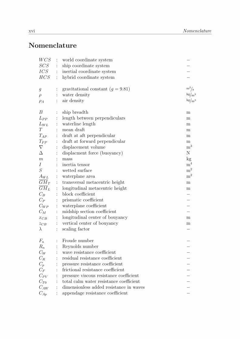
xvi Nomenclature
Nomenclature
WCS : world coordinate system −SCS : ship coordinate system −ICS : inertial coordinate system −HCS : hybrid coordinate system −
g : gravitational constant (g = 9.81) m2/s
ρ : water density kg/m3
ρA : air density kg/m3
B : ship breadth mLPP : length between perpendiculars mLWL : waterline length mT : mean draft mTAP : draft at aft perpendicular mTFP : draft at forward perpendicular m∇ : displacement volume m3
∆ : displacment force (buoyancy) Nm : mass kgI : inertia tensor m4
S : wetted surface m2
AWL : waterplane area m2
GMT : transversal metacentric height mGML : longitudinal metacentric height mCB : block coefficient −CP : prismatic coefficient −CWP : waterplane coefficient −CM : midship section coefficient −xCB : longitudinal center of bouyancy mzCB : vertical center of bouyancy mλ : scaling factor −
Fn : Froude number −Rn : Reynolds number −CW : wave resistance coefficient −CR : residual resistance coefficient −Cp : pressure resistance coefficient −CF : frictional resistance coefficient −CPV : pressure viscous resistance coefficient −CT0 : total calm water resistance coefficient −CAW : dimensionless added resistance in waves −CAp : appendage resistance coefficient −
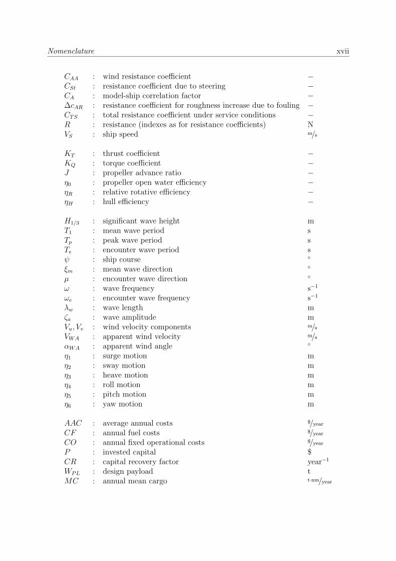
Nomenclature xvii
CAA : wind resistance coefficient −CSt : resistance coefficient due to steering −CA : model-ship correlation factor −∆cAR : resistance coefficient for roughness increase due to fouling −CTS : total resistance coefficient under service conditions −R : resistance (indexes as for resistance coefficients) NVS : ship speed m/s
KT : thrust coefficient −KQ : torque coefficient −J : propeller advance ratio −η0 : propeller open water efficiency −ηR : relative rotative efficiency −ηH : hull efficiency −
H1/3 : significant wave height mT1 : mean wave period sTp : peak wave period sTe : encounter wave period sψ : ship course ◦
ξm : mean wave direction ◦
µ : encounter wave direction ◦
ω : wave frequency s−1
ωe : encounter wave frequency s−1
λw : wave length mζa : wave amplitude mVu, Vv : wind velocity components m/s
VWA : apparent wind velocity m/s
αWA : apparent wind angle ◦
η1 : surge motion mη2 : sway motion mη3 : heave motion mη4 : roll motion mη5 : pitch motion mη6 : yaw motion m
AAC : average annual costs $/year
CF : annual fuel costs $/year
CO : annual fixed operational costs $/year
P : invested capital $CR : capital recovery factor year−1
WPL : design payload tMC : annual mean cargo t·nm/year

xviii Nomenclature
RFR : required freight rate $/tnm
FEC : fuel equivalent costs $/tnm
kf : fuel costs coefficient $/tnm
n : rate of revolutions s−1
rpm : rate of revolutions per minute min−1
MCR : maximum continuous rating kWmep : mean effective pressure Pasfoc : specific fuel oil consumption g/W·h

Abstract 1
Abstract
In the present work, long-term operational simulations within a hydrodynamic ship de-sign procedure were conducted, in which specifically the hydrodynamic design of bulbousbows is explored. In this approach, the operation of the ship considering aspects suchas weather, routing and cargo, is simulated over a time period considered statisticallyrepresentative for the lifetime of the ship. Simulations are finally evaluated on the basisof economic criteria.
In particular, different bulbous bow variants, for different ship sizes and different routes,are systematically studied by the presented approach, and obtained results are assessedwithin the formulated design procedure. For the simulations, a central aspect is the eval-uation of the responses and, in particular, of the added resistance of the ship in waves.For this purpose, an Open Source CFD code is adapted to the needs of the present workand obtained results are compared with available experimental data. Thereafter, furtherdesigns are generated by means of parametric variation and are evaluated numericallyby the above mentioned CFD code. Obtained results are assessed, showing the depen-dence in ship size, simulated route and simulational approach, leading to the ranking ofthe economic indexes of the investigated bulbous bow configurations. The advantage ofconsidering the operational life of the ship within ship design is highlighted and discussed.


Abstract 3
Kurzdarstellung
Diese Arbeit zeigt die Anwendung von Langzeitsimulationen fur den hydrodynamischenSchiffsentwurf, insbesondere fur die Auslegung von Bugwulsten. Die vorgestellte Methodikvereint mehrere beteiligte Aspekte in einer zentralen Entwurfsplattform mit Simulationen,die u.a. Routen, Wetter-, und Beladungszustande mit berucksichtigen, uber einen fur dasBetriebsleben des Schiffes als statistisch reprasentativ ansehbaren Zeitraum. Simulations-ergebnisse werden nachfolgend uber okonomische Kriterien bewertet.
Unterschiedliche Bugwulstkonfigurationen, fur unterschiedliche Schiffsgroßen und Hoch-seerouten, werden mit diese Entwurfsmethode untersucht und bewertet. Ein zentralerPunkt fur eine gute Vergleichbarkeit zwischen den unterschiedlichen untersuchten Fallenist eine zuverlassige Methode fur die Ermittlung des Verhaltens der Schiffe im Seegang,insbesondere des Zusatzwiderstandes im Seegang. Fur diesen Zweck wird ein Open SourceCFD-Verfahren an die Erfordernisse dieser Arbeit angepasst und mit verfugbare experi-mentelle Daten verglichen und validiert. Nachfolgend werden mit einer parametrischenMethode neue Varianten generiert und mit numerischen Verfahren errechnet. Anschlie-ßend werden auch fur diese Varianten Betriebssimulationen durchgefuhrt und die erzieltenErgebnisse miteinander verglichen. Die Abhangigkeiten zwischen Schiffsgroße, gefahrenerRoute und Simulationsmethodik werden aufgezeigt, um die Rangfolge der Wirtschaft-lichkeit der untersuchten Varianten zu diskutieren. Schließlich werden die Vorteile derBerucksichtigung des Schiffsbetriebes uber die gesamte Lebenszeit im Entwurf herausge-stellt und diskutiert.


CHAPTER 1. INTRODUCTION 5
1. Introduction
1.1. Background
In the present day, keen business competition in a characteristically global maritime mar-ket and the growing awareness about the need of reducing global emissions encourages theship designer to seek for innovative techniques to improve the design of ships and offshorestructures. While seeking larger economic profit, greater safety and reduced emissions,the handling of complex tasks in early design stages becomes mandatory attempting,in this way, to find improvements and solutions to a wide range of possible problemswhich may appear in future design stages or during operation. Normally, these tasks (e.g.hull form optimization, seakeeping performance calculations or general arrangement) havebeen handled separately and have often been considered as almost independent from eachother. The integration of many of these tasks is a promising approach to achieve thedesired profit surplus.
Within all aspects of ship design, the development of different numerical and exper-imental techniques in the field of hydrodynamics in the last decades has made a morein-depth study of many detail aspects possible. For example, the application of CFD(computational fluid dynamics) techniques has become a standard tool in industry, andnew computational methods are expected to do so in a near future.
The answers provided by these highly specialized techniques alone do not always lead tobetter designs; integrating these answers into a more global context can, in some cases, bevery advantageous. Holistic design, simulation-based design, life cycle design or predictiveengineering are some of the many terms used to name this principle, applied in each caseslightly differently, but in general terms with many similarities.
In the present work, simulation-based design will be applied to improve the transportefficiency of ships, attempting to integrate aspects which are usually considered separatelyat an early design stage. Rising fuel costs over the last years increase considerably theimportance of these within the total costs. Particularly, the influence of fuel in operationalcosts when considering off-design conditions will be studied here. Off-design conditions aredefined within this document as loading conditions, service speeds and weather conditionswhich are different to the design loading condition, design or contract speed and calmweather.
Nowadays, hydrodynamic design of ships is, in many cases, still undertaken for a singledesign condition with a specified speed, trim and draft and for calm weather, i.e. with-out considering either wind or waves. These conditions are also normally applied for theoptimization of the ship geometry, leading to optimum designs which might potentiallyhave a suboptimal performance outside their design specifications, leading subsequently

6 1.2. STATE OF THE ART
to an economic loss. Since most ships operate for considerable amounts of time outsidethese specified conditions, it can be expected that considering them can be advantageous.This paper presents a procedure which includes relevant operational factors at an earlydesign stage and can thus provide the designer with important informations to achievean optimum ship design. A simulation environment is implemented and employed forthe hydrodynamic design of the bulbous bow of a merchant vessel, modeling environ-mental, operational and technical characteristics of its operational life and quantifying itsperformance by an economic index.
1.2. State of the Art
Simulation techniques, especially those where many different tasks are integrated intoone system and the performance evaluation process occurs often within an optimizationstrategy, have experienced a ceaseless development since electronic computers becameavailable for engineering purposes and have found many applications in ship design. For adiscussion of the state of the art in this field, one can distinguish between the simulationmethods for modeling the operational life of the ship itself and the underlying (partialsimulation) methods involved, such as those for structural analysis, ship resistance or shippropulsion. Additionally, the integration of these methods into an optimization strategyplays a role in many cases also, a short discussion about this task being appropriate.From this three elements (partial simulations, operational performance assessment andoptimization), a design methodology can be defined. The present state of the art willrefer to hydrodynamic design methodologies, specifically those considering the effect ofoff-design conditions (and to a great extent the influence of weather factors). For a moregeneral state of the art in marine design methodology, the reader is referred to the recentpublication of Nowacki [86].
A detailed hydrodynamic model for performing an operational simulation needs to con-sider resistance, propulsion and seakeeping aspects. From these aspects, special attentionshall be paid to the added resistance in waves. This has two main reasons: firstly, it is (atleast for conventional ships) the largest resistance component not considered accuratelyin the design conditions (for which, else, very accurate estimations and measurements areundertaken) and, secondly, the commonly applied methodologies are in many cases notaccurate enough for the qualitative or even quantitative comparison of design variants1,or, if then, more accurate but of very recent date, being not enough experience with themto be applied in ship design. For the evaluation of the added resistance in irregular wavesover longer time periods, reliable weather information has to be available. This kind ofinformation was first available in the late sixties and, together with the availability ofthe necessary hydrodynamic and statistical theory, an increased amount of investigationsabout added resistance in waves could be observed in the following decade. Probablythe most important contributions to this theoretical background were strip theory, pre-sented by Grim in 1953 [37], and the probabilistic model of ship motions in irregular seas,
1This matter will be discussed in more detail further in section 2.6

CHAPTER 1. INTRODUCTION 7
presented by St. Denis and Pierson in the same year [107]. Several authors have pre-sented approximation methods for the calculation of added resistance in regular waves,remarking the contributions of Maruo [80] in 1957, Joosen [61] in 1966, Boese [18] in1970, Gerritsma and Beukelmann [33] in 1972, Salvesen [99] in 1978 and Faltinsen [29] in1980. All these methods are based on potential theory and contain, to a greater or lesserextent, some of the assumptions made in strip theory2. In Pedersen [96], an exhaustivecomparison of some of the mentioned methods is performed and critically discussed. In1986, in a theoretical work, Sakamoto and Baba [98] performed a hull form optimizationfor minimal added resistance in short waves. Although the approximations undertakenwere questionable for practical purposes [42], it was shown that optimal hull forms canbe designed for minimal added resistance in short waves. In 1998, Matsumoto et al. [81]presented a so-called “beak bow” for full ships such as bulk carriers, obtaining a reductionof the added resistance in waves between 20% to 30% in an experimental investigation.This study also proposed a theoretical formulation for the calculation of the added resis-tance to take indirect account of the above-water shape of the ship, consisting of simplemodifications to linear theory. The method agrees well with experiments for the exampleshown, but its applicability to a wider range of ship types is questionable.
The development of 3D potential panel codes for seakeeping in the 1970’s and 1980’s(e.g. Papanikolaou [95], Sclavounos et al. [103], Kring et al. [71], Bertram et al. [12])brought new perspectives for the prediction of added resistance in waves. For seakeepingcalculations solved by nonlinear, time-domain panel codes as presented by Sclavounos etal. [103], results of added resistance fall out directly from seakeeping calculations withan - at least from a theoretical point of view - inherently higher accuracy than linearmethods. Nevertheless, two-dimensional methods still remained as a standard tool inindustry and have been developed continuously until now. As an example, Kihara et al.[63] [64] presented in 2000 a two-dimensional nonlinear method, calculating in his workthe influence of the above-water bow form on the added resistance in waves.
In the late nineties, first investigations on seakeeping with RANS CFD methods werepresented, which were followed by many more during the next decade. In 1998, Wilsonet al. [111] presented RANS calculations for a Wigley hull and a surface combatantin regular waves, without motions. In 1999, Gentaz et al. [32] showed results for forcedoscillation motions in waves from RANS calculations for a Series 60 ship and different wavefrequencies and in the same year, Sato et al. [100] calculated ship motions in regular headwaves with forward speed. In 2002, Cura Hochbaum et al. [26] calculated the seakeepingcharacteristics of two ships, showing results of motions and forces (also added resistancein waves), with a RANS-Method. Results were in good agreement with experiments, evenfor the coarsest grids presented. In 2003, Orihara and Miyata [92] evaluated the addedresistance in head waves for a ship with an overlapping grid system. Of special interestis that the authors modified the above-water bow shape to reduce the added resistancein waves of a medium-speed tanker. The calculations were compared with experiments,showing good agreement and demonstrating the ability of complex CFD calculations tobe used as a design tool in this field. In 2005, Weymouth et al. [110] calculated the
2A short description of strip theory is given in section 2.6.2
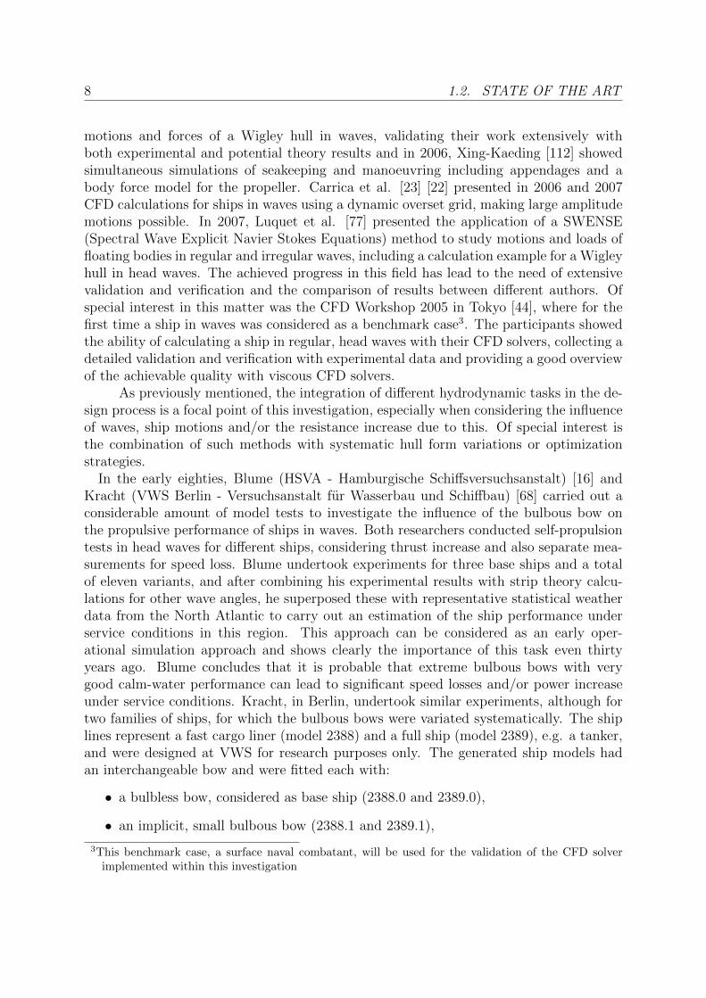
8 1.2. STATE OF THE ART
motions and forces of a Wigley hull in waves, validating their work extensively withboth experimental and potential theory results and in 2006, Xing-Kaeding [112] showedsimultaneous simulations of seakeeping and manoeuvring including appendages and abody force model for the propeller. Carrica et al. [23] [22] presented in 2006 and 2007CFD calculations for ships in waves using a dynamic overset grid, making large amplitudemotions possible. In 2007, Luquet et al. [77] presented the application of a SWENSE(Spectral Wave Explicit Navier Stokes Equations) method to study motions and loads offloating bodies in regular and irregular waves, including a calculation example for a Wigleyhull in head waves. The achieved progress in this field has lead to the need of extensivevalidation and verification and the comparison of results between different authors. Ofspecial interest in this matter was the CFD Workshop 2005 in Tokyo [44], where for thefirst time a ship in waves was considered as a benchmark case3. The participants showedthe ability of calculating a ship in regular, head waves with their CFD solvers, collecting adetailed validation and verification with experimental data and providing a good overviewof the achievable quality with viscous CFD solvers.
As previously mentioned, the integration of different hydrodynamic tasks in the de-sign process is a focal point of this investigation, especially when considering the influenceof waves, ship motions and/or the resistance increase due to this. Of special interest isthe combination of such methods with systematic hull form variations or optimizationstrategies.
In the early eighties, Blume (HSVA - Hamburgische Schiffsversuchsanstalt) [16] andKracht (VWS Berlin - Versuchsanstalt fur Wasserbau und Schiffbau) [68] carried out aconsiderable amount of model tests to investigate the influence of the bulbous bow onthe propulsive performance of ships in waves. Both researchers conducted self-propulsiontests in head waves for different ships, considering thrust increase and also separate mea-surements for speed loss. Blume undertook experiments for three base ships and a totalof eleven variants, and after combining his experimental results with strip theory calcu-lations for other wave angles, he superposed these with representative statistical weatherdata from the North Atlantic to carry out an estimation of the ship performance underservice conditions in this region. This approach can be considered as an early oper-ational simulation approach and shows clearly the importance of this task even thirtyyears ago. Blume concludes that it is probable that extreme bulbous bows with verygood calm-water performance can lead to significant speed losses and/or power increaseunder service conditions. Kracht, in Berlin, undertook similar experiments, although fortwo families of ships, for which the bulbous bows were variated systematically. The shiplines represent a fast cargo liner (model 2388) and a full ship (model 2389), e.g. a tanker,and were designed at VWS for research purposes only. The generated ship models hadan interchangeable bow and were fitted each with:
• a bulbless bow, considered as base ship (2388.0 and 2389.0),
• an implicit, small bulbous bow (2388.1 and 2389.1),
3This benchmark case, a surface naval combatant, will be used for the validation of the CFD solverimplemented within this investigation

CHAPTER 1. INTRODUCTION 9
• an additive, small bulbous bow (2388.2 and 2389.2),
• an additive, larger bulbous bow (2388.3 and 2389.3).
The combination of systematic hull form variation and the investigation of the perfor-mance of bulbous bows in waves is unique and was apparently not repeated in any otherresearch project since then. Both authors together published their results in [17].
In the following years, different authors studied the hydrodynamic performance of shipsconsidering seakeeping aspects. Of special interest are those including a shape variationapproach and will be therefore mentioned here. In 1990, Nowacki et al. [87] presented asystematic computational design study for an innovative hull form (SWATH), includingboth ship resistance and seakeeping aspects for design assessment by means of poten-tial theory. In 2003, Zaraphonitis et al. [113] presented an optimization study for ahigh speed vessel considering powering and wash by a potential flow method. The twoobjective functions, namely total resistance and wave wash, were optimized with a multi-objective genetic algorithm and a Pareto-front was obtained. In 2006, Boulougouris et al.[19] presented an investigation on hull form optimization, specifically a bulbous bow op-timization considering calm water resistance and motions in head waves. The calm waterresistance calculations were performed with a nonlinear potential CFD code and seakeep-ing calculations with the potential, linear 3D seakeeping code NEWDRIFT. The bulbousbow geometry was defined by a total of nine form parameters, from which geometry vari-ants were generated. First results dealt in some cases with numerical instabilities, anda thorough investigation was made to overcome this problem and finally find an optimaldesign.
In 2006, Campana et al. [21] presented an hydrodynamic hull optimization making useof RANS CFD methods for the calculation of the total resistance in calm water. Theauthors considered, as a design constraint, the motion amplitudes of the ship in regularhead waves. These were calculated by a means of strip theory. A detailed validation andverification of the RANS CFD calculations was undertaken. Unfortunately, this was notthe case for the linear seakeeping calculations.
The development of fuel prices and the subsequent interest of many ship owners to havea deeper insight into the economic performance of ship designs under real-life conditionshave impulsed the development of new performance assessment methods, some of themby means of operational simulations. In 2004, Dallinga et al. [27] presented operationalsimulations considering the in-service performance of ships under different scenarios con-sidering the influence of weather and prudent seamanship. For this purpose, the authorsdeveloped a simulation platform in a very similar manner to the one to be presented inthis thesis. The hydrodynamic performance is evaluated by means of a “ship behaviordatabase” which can be fed with existing data from numerical calculations or model tests.The authors showed different examples of operational simulations including speed loss,accelerations and added resistance in waves calculated by linear, frequency domain meth-ods. Additionally, an example showing the effect of bow flare on trip duration based onexperimental data was presented. Unfortunately, neither advanced hydrodynamic meth-ods (e.g. nonlinear-potential or RANS methods) nor systematic form variations were
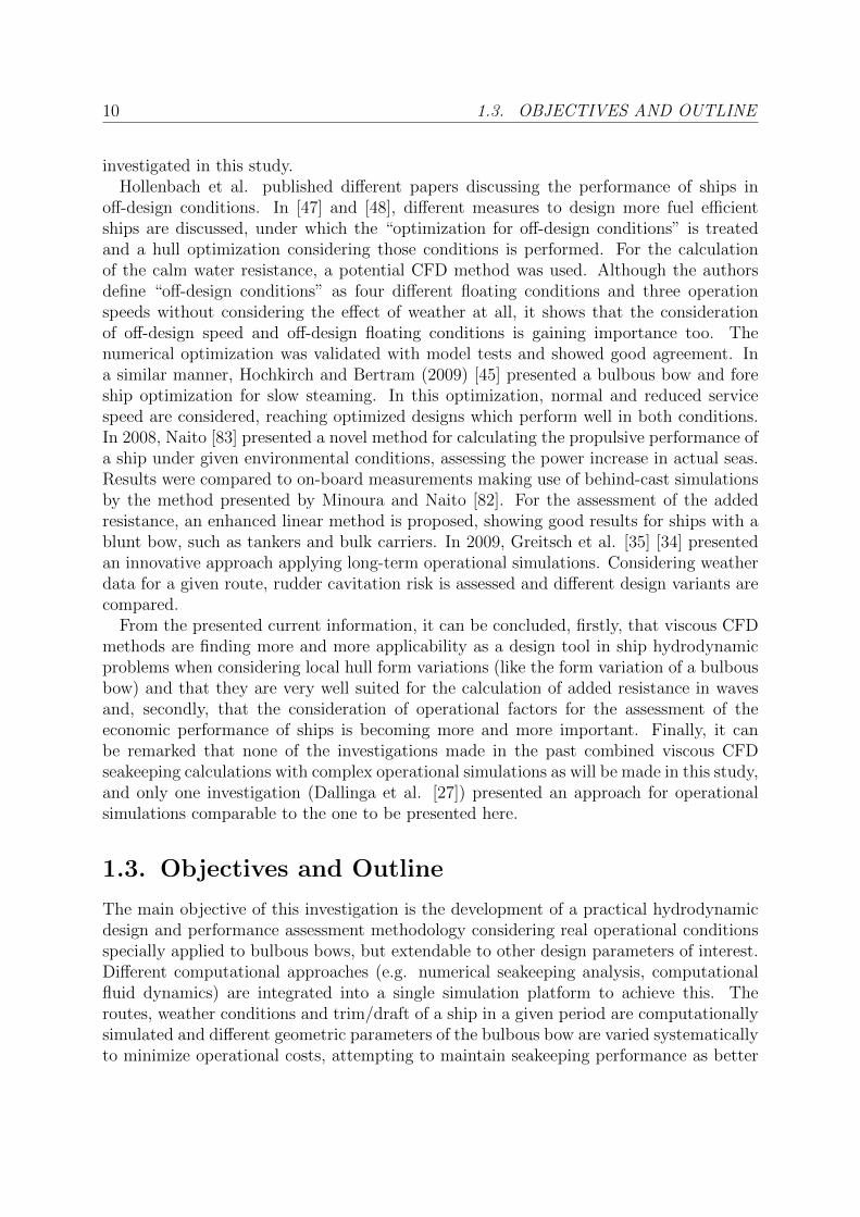
10 1.3. OBJECTIVES AND OUTLINE
investigated in this study.Hollenbach et al. published different papers discussing the performance of ships in
off-design conditions. In [47] and [48], different measures to design more fuel efficientships are discussed, under which the “optimization for off-design conditions” is treatedand a hull optimization considering those conditions is performed. For the calculationof the calm water resistance, a potential CFD method was used. Although the authorsdefine “off-design conditions” as four different floating conditions and three operationspeeds without considering the effect of weather at all, it shows that the considerationof off-design speed and off-design floating conditions is gaining importance too. Thenumerical optimization was validated with model tests and showed good agreement. Ina similar manner, Hochkirch and Bertram (2009) [45] presented a bulbous bow and foreship optimization for slow steaming. In this optimization, normal and reduced servicespeed are considered, reaching optimized designs which perform well in both conditions.In 2008, Naito [83] presented a novel method for calculating the propulsive performance ofa ship under given environmental conditions, assessing the power increase in actual seas.Results were compared to on-board measurements making use of behind-cast simulationsby the method presented by Minoura and Naito [82]. For the assessment of the addedresistance, an enhanced linear method is proposed, showing good results for ships with ablunt bow, such as tankers and bulk carriers. In 2009, Greitsch et al. [35] [34] presentedan innovative approach applying long-term operational simulations. Considering weatherdata for a given route, rudder cavitation risk is assessed and different design variants arecompared.
From the presented current information, it can be concluded, firstly, that viscous CFDmethods are finding more and more applicability as a design tool in ship hydrodynamicproblems when considering local hull form variations (like the form variation of a bulbousbow) and that they are very well suited for the calculation of added resistance in wavesand, secondly, that the consideration of operational factors for the assessment of theeconomic performance of ships is becoming more and more important. Finally, it canbe remarked that none of the investigations made in the past combined viscous CFDseakeeping calculations with complex operational simulations as will be made in this study,and only one investigation (Dallinga et al. [27]) presented an approach for operationalsimulations comparable to the one to be presented here.
1.3. Objectives and Outline
The main objective of this investigation is the development of a practical hydrodynamicdesign and performance assessment methodology considering real operational conditionsspecially applied to bulbous bows, but extendable to other design parameters of interest.Different computational approaches (e.g. numerical seakeeping analysis, computationalfluid dynamics) are integrated into a single simulation platform to achieve this. Theroutes, weather conditions and trim/draft of a ship in a given period are computationallysimulated and different geometric parameters of the bulbous bow are varied systematicallyto minimize operational costs, attempting to maintain seakeeping performance as better
CHAPTER 1. INTRODUCTION 11
or equal.For the correct assessment of operational costs, an accurate prediction of the added
resistance in waves is mandatory. In this work, the comparison of different bulbous bowvariants leads to even higher accuracy requirements in this matter, since the influence ofrelatively small, local shape variations must be taken into account. For this purpose, theapplication of a viscous CFD method proved to be a suitable approach. Thus, developmentand application of the required CFD solver for seakeeping problems is another of the mainobjectives of this thesis.
The author’s hypothesis is, in this context, that assessing the system’s performancewith the presented methodology can lead, within an optimization approach, to a differentoptimal design compared to the one obtained when only a single condition (calm weather,design trim & draft and design speed) is considered. Thus, the presented work attemptsto demonstrate the feasibility of applying such a design methodology and the economicadvantages of designs which were conceived specifically for their operational profile.
In general terms, the integration of different design aspects playing a role in hydrody-namic design are presented and demonstrated for the hydrodynamic design of the bulbousbow of a vessel. In chapter 2, the main principles and methodologies applied in this studyare described, discussing their applicability for design purposes at an early design stage.In chapter 3, the integration of these methods into an operational simulation platformis outlined, describing the most relevant characteristics of the resultant implementationSimOship. In the following chapter (chapt. 4), a special application case is presented;namely the operational simulation of a ship is undertaken for which - opposite to the usualcase in early design stages - experimental data is available for validation of numerical re-sults. The main purpose of this chapter is to present the functionality of the presentedoperational simulations, giving a discussion about the different simulational approachesthemselves rather than about the achieved results. In chapter 5, a general application caseis presented, describing the operational simulation of a ship where no experimental datais available. This application case is of central relevance since it represents the reality inan early ship design stage. A systematic shape variation is included and some recommen-dations for the design of bulbous bows are given. Final remarks about the results and anoutlook are presented in chapter 6.
In summary, the present thesis deals with a design methodology which differs from thecommon practice in hydrodynamic ship design. Instead of considering a single designcondition for the performance assessment of a design, an increased number of operationalfactors which influence the performance assessment are considered, integrating all thesefactors by means of an operational simulation representing the whole operational life ofthe ship. For the successful application of this approach to the design of bulbous bows,the applied methodologies, specially the assessment of the added resistance in waves withviscous CFD methods and the influence of the most relevant operational factors, sea stateand operational conditions, are of great importance. These aspects will be elaborated anddiscussed in detail during the entire course of the presented thesis.

CHAPTER 2. BASIC PRINCIPLES 13
2. Basic Principles
2.1. Overview
In this chapter, basic principles of the most relevant methodologies applied within thiswork will be depicted. Due to the high number of different tasks integrated in thisinvestigation, the principles described in this section might not appear to be related toeach other at a first glance. For this reason, an introductory explanation appears to benecessary.
In this study, simulations for the performance assessment of the operational life ofa ship are performed. In section 2.2, simulations are defined from a general point ofview and in section 2.3, operational simulations are defined in more detail. Within theseoperational simulations, several hydrodynamic and ship design techniques are integrated.The common coordinate system for all these techniques is described in section 2.4.
The main hydrodynamic tasks which are studied within this work are ship resistanceand seakeeping. A detailed description of the methods applied within this work in thesetwo fields is found in sections 2.5 and 2.6. As previously mentioned, the use of a viscousCFD method for the evaluation of the seakeeping performance of ships plays a centralrole, especially when considering that a solver was implemented for this purpose. Dueto the fact that the mentioned solver is presented for a first time here, a more detaileddescription and a thorough validation for two different benchmark cases is presented insection 2.7.
The ship design technique described thereafter is a partial parametrical approach forthe geometric variation of the bulbous bow, which will take place to elaborate operationalsimulations for different ship subvariants. A detailed description of this form variationapproach is described in section 2.8 .
2.2. Simulational Approach
Simulation (def.):
Scientific method in industry, science, and education, a research or teachingtechnique that reproduces actual events and processes under test conditions.(Encyclopædia Britannica)
Within this investigation, a simulation will be meant specifically as a computer simulationfor engineering and/or design purposes. Since this specific definition of simulation coversalso a very ample field in engineering and design applications, it will be proper to explainand categorize simulations more accurately.

14 2.2. SIMULATIONAL APPROACH
Simulation techniques are becoming very popular for the investigation or the improve-ment of the performance of processes or systems along their design process. They areinherently inexpensive (compared to model or full scale tests) and allow the evaluation ofcomplex tasks with many different variants. In many engineering problems, the simulationof the system’s performance consists of the addition of different, fully isolated method-ologies into a representative value which can be compared to other design variants. Asan example, one could consider the total resistance of a ship in the following fictive case:The wave resistance of the naked hull is calculated by a potential CFD method, thefrictional resistance and the resistance of the appendages by empirical formulae and theadded resistance in waves by means of strip theory, neglecting all other possible resistancecomponents. In this example, and also in a very general context, each mentioned methodcould even be considered as a restricted simulation method itself1. Under these simulationmethods, the numerical solution of fluid flow problems is of special interest, consideringin this context the mentioned potential CFD methods (including strip theory) but alsoviscous CFD methods. For the described case, for example, only a single viscous CFDsimulation would be necessary (including free surface, incoming waves and appendages),from which the system’s performance (e.g. total resistance) can be evaluated. With thisexample, the multiple character of simulations, which can be in some cases a very partialreproduction of the actual process or system to be modeled, is shown.
Considering that the system’s performance has been evaluated for a single operationalcondition (or for instance for a set of n selected conditions), the question if this or theseconditions are representative for the operational life of the system arises. Obtaining therelationship between these conditions and the actual performance of the system over itscomplete lifetime becomes a logical, further step to undertake. This step will be definedhere as an operational simulation. In a simplest approach, the application of a securityfactor (e.g. service factor) would roughly fulfill this purpose. This common practice formany engineering applications is mostly done when information about the operational lifeof the system is to a large extent not available or is too difficult to obtain.
A more robust approach is the application of statistical methods, which permit a muchdeeper insight into the stochastic character of the operational life of the system. In thecase of the operational life of a ship, an essential component is long term weather data forthe region where the ship operates. This data, superposed with ship response functions,can be used to obtain representative statistical information, from mean values up toprobability distribution functions over the ship’s lifetime. The reliability of this approachdepends on a correct statistical model (e.g. representative sea spectra) and the qualityand applicability of the input data (e.g. parameters used to define a sea state).
For more detailed results, deterministic, time domain simulations of the operation of thesystem under realistic conditions become necessary. For this purpose, time histories for theunknown environmental (i.e. weather) or boundary conditions are needed. These can beobtained from representative data from past experience (e.g. behind-cast weather data) or
1It can be matter of discussion if the calculation of e.g. a force by means of a semi-empirical formulacan be interpreted as a simulation or not, i.e. for which level of complexity an algebraic formula canbe defined as a simulation model. A deeper discussion on this matter is out of scope in this study.

CHAPTER 2. BASIC PRINCIPLES 15
generated from statistical data. Different categories of detail level (e.g. different time stepsizes) can be identified for this kind of simulation. The time domain simulation of everyphenomenon involved in the operation of the system would represent the highest level ofdetail. In this case, the detail level (e.g. time step) of the simulation is limited by thephenomenon with the highest detail requirement (e.g. smallest time step requirement).In many cases, this leads to an extremely high simulation effort which is not alwayscompensated by the improvement in the results when compared to simpler methods. Inorder to reduce the computational effort, simulational approaches in the time domainincluding a statistical approach for those phenomenon which would be problematic tosolve (when considering the necessary computational effort) have shown to be a goodcompromise for many engineering applications. For numerical flow simulations (CFD), thepopularity of RANS methods with statistically based turbulence models are an exampleof this. In the case of the simulation of the operational life of a ship, this approachshows itself to be advantageous too. While certain aspects of the operation (e.g. route,ship position, cargo or bunkering) are simulated in the time domain, other aspects aresimulated by a statistical approach (e.g. ship responses by means of short-term statistics).A complete description of the operational simulation approach presented in this study willbe given in detail in the following section.
2.3. Operational Simulations: a Short Introduction
Within this study, reference will be made to operational simulations as a computationalsimulation attempting to model the operation of a system. For industrial applications,this model must be as realistic as possible, within a limited, given amount of resources.This can be only achieved with:
• realistic input data (the interaction of the system with its exterior),
• proven, robust and qualitatively accepted methods and
• validated output data.
Operational simulations are intended to aid the designer and/or engineer within the designprocess, bringing answers about complex, interrelated processes which act together in asystem. Additionally, a deep insight into the operation mechanisms of the system ismade possible, revealing problems which might not yet have been recognized as suchby the designer. Normally, operational simulations are undertaken at an early designstage where these answers cannot be obtained by any other means without excessive costsand/or risks.
2.3.1. Operational Simulations for Ships
The operational simulation of a ship implies synthesizing the operational life of a ship asa system. This system acts according to certain rules and a given input. For a merchant

16 2.3. OPERATIONAL SIMULATIONS: A SHORT INTRODUCTION
ship, this is done simulating not only the ship as such. The system to be evaluated is itsoperational life. This synthesized operational life has two main components: a ship andan environment. In this way, an important part of the classical input is treated now aspart of the simulation.
Simulation of the Environment
The environment of a typical merchant ship during its operation has two main compo-nents: the first component groups all aspects which can be considered as known. Itcomprises a known amount of time to carry a known amount of cargo between a knownamount of known places. The second component groups all unknown aspects, viz., allother factors which can influence the operation of the ship during its lifetime. Leavingaside extreme situations such as damage by any means, system failures or force majeure(piracy, war, etc.), the most characteristic and permanent unknown environment factor isweather. Within all weather factors (meteorologists distinguish about 55 different weatherparameters), waves, wind, currents, sight (e.g. fog) and tides are key-role players withinthe operation of ships.
At an early design stage, realistic weather information can be only retrieved from thepast, selecting a convenient amount of time so that it can be considered representative forthe ship’s lifetime. For this purpose, weather data from the European Centre for Medium-Range Weather Forecasts (ECMWF) were used. The ERA-40 database from ECMWFprovides weather data for a period from 1957 to 2002 in six-hour steps. Providing datapoints every 1.5◦ latitude and longitude, this data is only suitable for long voyages andlong distances. Details about the ECMWF weather data will be discussed in section 3.2.2on page 56.
Simulation of the Ship
An exhaustive simulation of all ship’s systems, their interaction among each other andwith the environment must be seen, for the presented design methodology, as impossible.For the purposes of this investigation, the simulation of the propulsion and the motionsof the ship for any given condition is sufficient. To model this, appropriate informationabout floating condition, total resistance, seakeeping and machinery characteristics arenecessary.
Considering the six-hour periods of the available weather data, the propulsion is con-sidered as stationary for each time period and its simulation will be made according tothe ITTC’78 Performance Prediction Method. The seakeeping simulation will be madefor each 6 hrs. period by means of short time statistics, considering a sea- and a responsespectrum from which representative data can be derived.
Here, the selection of the methods for obtaining the required information for these sim-ulations plays a crucial role: considering an early design stage, most of this informationwill not be available or can be estimated with limited reliability. On the other hand,information which is believed to play a significant role within the simulation or for theevaluation of different design variants must be obtained by methods which are able to
CHAPTER 2. BASIC PRINCIPLES 17
indicate the differences between the evaluated variants with enough accuracy. In the caseof the present investigation, it will be shown that the ship’s calm water resistance andits seakeeping characteristics, especially the added resistance in waves, play an impor-tant role. Different state-of-the-art techniques which were used during the course of thisinvestigation for these two tasks will be discussed in sections 2.5 and 2.6.
2.4. Coordinate Systems
Three main coordinate systems are defined: a world coordinate system (WCS), a shipcoordinate system (SCS) and an inertial coordinate system (ICS).
The WCS is defined in degrees of latitude and longitude, with its origin in the equator,and the Greenwich meridian. West longitudes and north latitudes are positive and eastlongitudes and south latitudes negative. The heading angle of the ship, ψ, is defined asusual with 0◦for north heading, with positive angles in clockwise direction. This coor-dinate system is mainly used for the global weather data and for the definition of theroutes.
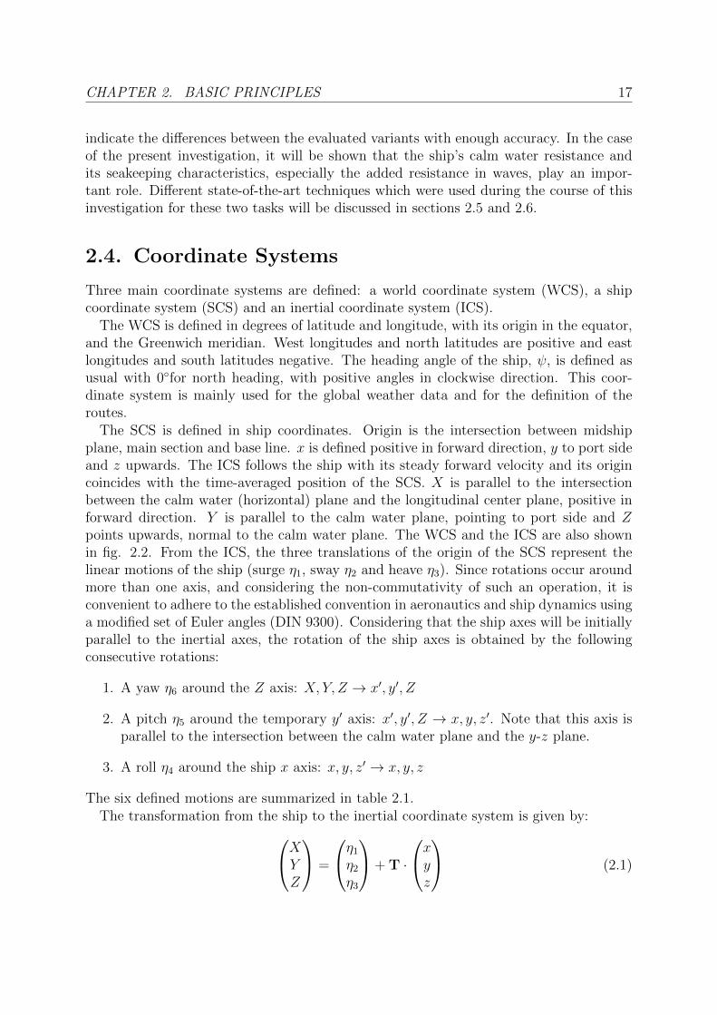
The SCS is defined in ship coordinates. Origin is the intersection between midshipplane, main section and base line. x is defined positive in forward direction, y to port sideand z upwards. The ICS follows the ship with its steady forward velocity and its origincoincides with the time-averaged position of the SCS. X is parallel to the intersectionbetween the calm water (horizontal) plane and the longitudinal center plane, positive inforward direction. Y is parallel to the calm water plane, pointing to port side and Zpoints upwards, normal to the calm water plane. The WCS and the ICS are also shownin fig. 2.2. From the ICS, the three translations of the origin of the SCS represent thelinear motions of the ship (surge η1, sway η2 and heave η3). Since rotations occur aroundmore than one axis, and considering the non-commutativity of such an operation, it isconvenient to adhere to the established convention in aeronautics and ship dynamics usinga modified set of Euler angles (DIN 9300). Considering that the ship axes will be initiallyparallel to the inertial axes, the rotation of the ship axes is obtained by the followingconsecutive rotations:
1. A yaw η6 around the Z axis: X, Y, Z → x′, y′, Z
2. A pitch η5 around the temporary y′ axis: x′, y′, Z → x, y, z′. Note that this axis isparallel to the intersection between the calm water plane and the y-z plane.
3. A roll η4 around the ship x axis: x, y, z′ → x, y, z
The six defined motions are summarized in table 2.1.The transformation from the ship to the inertial coordinate system is given by:XY
Z
=
η1
η2
η3
+ T ·
xyz
(2.1)
18 2.4. COORDINATE SYSTEMS
Translations Rotationssurge: η1 roll: η4
sway: η2 pitch: η5
heave: η3 yaw: η6
Table 2.1.: Definition of translational and rotational ship motions
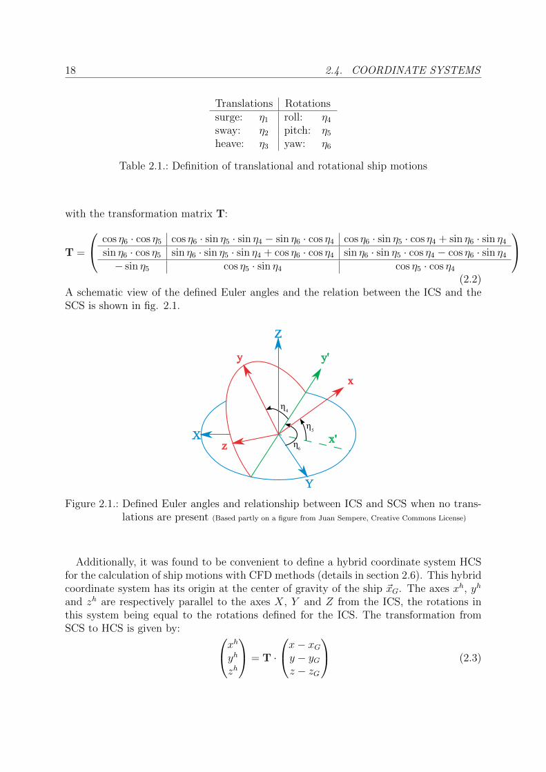
with the transformation matrix T:
T =
cos η6 · cos η5 cos η6 · sin η5 · sin η4 − sin η6 · cos η4 cos η6 · sin η5 · cos η4 + sin η6 · sin η4
sin η6 · cos η5 sin η6 · sin η5 · sin η4 + cos η6 · cos η4 sin η6 · sin η5 · cos η4 − cos η6 · sin η4
− sin η5 cos η5 · sin η4 cos η5 · cos η4
(2.2)
A schematic view of the defined Euler angles and the relation between the ICS and theSCS is shown in fig. 2.1.
X
Y
Z
y'
x'
x
y
z
η
η
η
4
5
6
Figure 2.1.: Defined Euler angles and relationship between ICS and SCS when no trans-lations are present (Based partly on a figure from Juan Sempere, Creative Commons License)
Additionally, it was found to be convenient to define a hybrid coordinate system HCSfor the calculation of ship motions with CFD methods (details in section 2.6). This hybridcoordinate system has its origin at the center of gravity of the ship ~xG. The axes xh, yh
and zh are respectively parallel to the axes X, Y and Z from the ICS, the rotations inthis system being equal to the rotations defined for the ICS. The transformation fromSCS to HCS is given by: xhyh
zh
= T ·
x− xGy − yGz − zG
(2.3)

CHAPTER 2. BASIC PRINCIPLES 19
or alternatively in terms of the ICS:xhyhzh
=
XYZ
−η1
η2
η3
−T ·
xGyGzG
(2.4)
For the rates of change of the Euler angles η4, η5 and η6, a relationship to the angular
velocity ~ωh around the hybrid coordinate system can be established by relating unitvectors along the Euler rotation axes, resulting in the relationship:
~ωh =
1 0 00 1 0
− sin η5 0 1
·η4
η5
η6
(2.5)
Finally, it has been considered convenient to define the direction of the wave propagation(which will be recalled here as wave direction) in the different coordinate systems. In theWCS, the wave direction is defined by the angle χ, with 0◦for wave propagation in northdirection, with positive angles in clockwise direction. From the ICS (or alternativelyfrom the HCS), the direction of the wave propagation (to be recalled further on as waveencounter angle) is defined by the angle µ, with 0◦for wave propagation in X-direction,also positive in counter-clockwise direction (i.e. µ=180◦for head seas). The relationbetween both angles is given by:
µ = 180− ψ + χ (2.6)
For all rotations and moments in all defined coordinate systems, the right-hand rule isconsidered.
Figure 2.2.: World- and inertial coordinate systems

20 2.5. RESISTANCE
2.5. Resistance
2.5.1. Resistance Prediction in Ship Design: an Overview
The resistance of a ship advancing in water with constant speed has an important meaningduring the complete ship design process. Different methodologies are applied withindifferent design stages to estimate it and it is a permanent challenge for the designer toachieve an optimal (minimum resistance) value.
During a preliminary design phase (normally in a conceptual, very early stage), the useof simple estimation methods based on statistical data, similar ships or systematic seriesmay appear to be suitable. Typical representants of methods based on statistical data,especially suitable for merchant vessels, are the methods of Holtrop and Mennen [50], [49]and Hollenbach [46]. The limitations of these approaches have been amply discussed inliterature and textbooks (e.g. [70]) and will not be discussed here.
At a later design stage (normally at the beginning of the preliminary design stage),potential CFD methods can be applied to calculate the wave resistance of a wide rangeof design variants, often within an automatized optimization process. Potential CFDmethods can be seen as a good compromise between computational resources and accuracyfor such a task, especially when the performance assessment is done comparatively. Theabsolute values of resistance provided by potential CFD must always be interpreted withcare, and model tests are usually performed to confirm final results. These model testsrepresent the maximal level of accuracy in the prediction of the resistance of the shipduring its design. Their almost contractual character2, the use of world-wide conventions(which is owed to a great extent to the ITTC conferences over the last half century)and the long experience of ship model basins are also additional reasons for the specialimportance of resistance model tests.
Additionally, RANSE CFD solvers can be used for the prediction of ship resistance orfor the improvement of wake characteristics and/or the analysis of appendages. Due to thehigh requirement of computational resources for an acceptable accuracy, a high meshingeffort and a still not completely satisfactory turbulence modeling, RANSE CFD meth-ods are rarely applied for this task for practical (industrial) applications. Nevertheless,RANSE methods are expected to gain more and more acceptance as the development ofinnovative numerical methods, new physical (e.g. turbulence) models and more powerfulhardware become available.
2.5.2. Resistance Model Tests
Since for practically every ship a resistance model test is carried out, it is convenient todescribe it briefly and apply similar conventions to post-process results from numericalcalculations. In this study, the latest recommendations of the ITTC [55] will be used. For
2since they are used for the ship speed prediction at sea trials, which have contractual character betweenshipyard and shipowner

CHAPTER 2. BASIC PRINCIPLES 21
convenience, all resistance formulas will be shown in dimensionless form by:
cX =RX
12ρV 2S
(2.7)
cX being an arbitrary resistance coefficient, RX an arbitrary resistance component and Vand S a reference speed and a reference area, respectively.
In a model test, the total model resistance is measured for different model speeds. Onthe basis of Froude’s hypothesis, the total model resistance is broken down into:
cTM = cFM(1 + k) + cR (2.8)
with:
cFM =0.075
(log(Rn)− 2)2(2.9)
Rn =v · Lν
(2.10)
where cFM is the frictional resistance coefficient of the model according to the ITTC1957 friction line with the Reynolds number Rn, k represents Prohaska’s form factor asrecommended by the ITTC in 1978 and cR the residual resistance coefficient, being itsmain component the wave resistance coefficient cW . For equal Froude numbers (Froude’ssimilitude law), the residual resistance coefficient of the model is assumed to be equal tothe residual resistance coefficient of the ship. Detailed descriptions of the similarity lawsapplied and the theoretical background can be found e.g. in Lewis [75], Kracht [70] andmany others.
For a ship in calm waters, without appendages and neglecting air resistance, the totalship resistance coefficient cTS0 is represented by the sum:
cTS0 = cFS(1 + k) + cR + cA (2.11)
where cFS is the frictional resistance coefficient of the ship according to ITTC 1957 frictionline and cA the model-ship correlation allowance. According to the ITTC 1978 procedure,cA can be estimated as:
cA =
[105
(kSLWL
)1/3
− 0.64
]· 10−3 (2.12)
The hull roughness kS for a new ship, if no better information is available, can be assumedto be kS = 150 · 10−6m.
In service conditions, many additional components are added to calm water resistance,so that the total ship resistance coefficient in service conditions cTSS is the sum (accordingto Kracht [70]):
cTSS = cTS0 + cAW + cAP + cAA + cST + cPAR + ∆cAR (2.13)

22 2.5. RESISTANCE
where cAW represents the added resistance in waves coefficient, cAP the appendage re-sistance coefficient, cAA the wind resistance coefficient, cST the resistance coefficient dueto steering and ∆cAR the roughness increase in service conditions, mainly due to fouling.For convenience, the parasitic resistance coefficient cPAR, e.g. due to openings in the hull,will be hereinafter included in the appendage resistance coefficient.
2.5.3. Resistance Calculation with Potential CFD Methods
For many decades, potential theory has been used to calculate the wave resistance ofships. Today, nonlinear potential panel codes are widely used in industry and providefast calculations for ship wave resistance (e.g. as presented in [97], [60], [59] and [72]).Most of these codes make use of the same principles and assumptions, superposing a setof singularities over the discretized boundary field of a domain of interest (the wetted partof the hull and a free surface region) in form of a Boundary Value Problem (BVP).
Since in potential theory the fluid is assumed to be inviscid, incompressible and irro-tational, the velocity vector ~u can be determined from the gradient of a scalar quantity,the potential φ as follows:
~u = ∇φ (2.14)
The fundamental equation to be solved is the Laplace equation, a linear partial differentialequation. Beginning from mass conservation:
∂ρ
∂t+∇ · (ρ~u) = 0 (2.15)
when ρ = const:∇ · ~u = 0 (2.16)
Combined with eq. 2.14, it leads to the Laplace equation:
∇2φ = 0 (2.17)
On the other hand, for momentum conservation in an inviscid flow, the Euler equation istaken:
ρ
(∂~u
∂t+ (~u · ∇)~u
)= f −∇p (2.18)
with f representing body forces (e.g. gravitation, Coriolis force, etc.). From this equation,the generalized Bernoulli equation for irrotational flow can be obtained:
∂φ
∂t+
(∇φ)2
2+p
ρ+ gz = const. (2.19)
These fundamental equations are used to obtain the solution of the potential flow problem.For this purpose, the potential field φ must be found.
Due to the linear character of the Laplace equation, the potential can be assumed asthe superposition of different components, i.e. the undisturbed flow potential φ∞, wavespotential and/or the potential of a perturbation caused by a body:
φ = φ∞ + φ1 + φ2 + ... (2.20)

CHAPTER 2. BASIC PRINCIPLES 23
To solve this equation, boundary conditions on the body, free surface, bottom and atinfinity must be considered.
The body condition defines a tangential flow on the wetted part of the hull. This canbe written: (
∇~u− ~Vb
)· ~n = 0 (2.21)
where ~n is the unitary normal vector at a given position of the body and ~Vb the velocityof the body at this position. This condition implies that no particles will flow throughthe body.
The steady kinematic free surface boundary condition on the water surface (z = ζ) canbe written:
∇φ · ∇ζ − ∂φ
∂z= 0 (2.22)
This condition implies that the movement of particles at the water surface must be parallelto the perturbed free surface, i.e. no water particle leaves the free surface.
The steady dynamic free surface boundary condition implies atmospheric pressure atthe free surface. For z = ζ, this can be written in the form:
gz +1
2(∇φ)2 − 1
2U2 = 0 (2.23)
Different discretization methods and numerical techniques are available today for solv-ing flow problems with potential theory. Most panel codes make use of Rankine panelsand an iterative approach for the relocation of the discretized free surface. The geometryand the free surface domain are discretized by quadrilateral elements and, at each of these,a Rankine-source is placed. These sources can be of first or higher order and are normallylocated slightly behind the defined panel. A collocation point is defined, normally at thecenter of the panel, where the boundary conditions are to be fulfilled. A similar, but incertain aspects different method has been proposed by Soding [105] and is known as patchmethod, making use of shifted point-sources and the fulfillment of the boundary condi-tions as an averaged value over the whole patch instead of at the collocation point only.Both methods solve therefore the potential flow problem by finding the source strengthdistribution for which the respective residuals become zero.
The iterative approach, correcting both the wave elevations and the dynamic floatingcondition of the ship at each step, is finalized when changes between iterations becomesmall, obtaining finally the nonlinear wave field and the pressure distribution over thehull. From the integration of this pressure distribution, the wave resistance RW of theship is obtained, being usually added to the viscous resistance (obtained e.g. from thefrictional resistance according to the ITTC’57 and an estimated form factor k) to estimatethe total resistance of the ship.
Potential flow methods, when disregarding their evident drawbacks, provide valuableresults in early stages of ship design, representing a good trade-off between requiredcomputational resources and accuracy of results.

24 2.5. RESISTANCE
2.5.4. Resistance Calculation with RANS CFD Methods
The application of Computational Fluid Dynamics (CFD) by means of solving the Reynolds-Averaged Navier Stokes Equations by numerical means has become an important compo-nent of the available tools for solving ship hydromechanics problems. Specifically, theirapplication to the prediction of ship resistance will be discussed here, including relevantbasic principles which apply to other application fields too.
The reports from the resistance committee of the ITTC conferences show the advancesof CFD in resistance prediction over the last decades (e.g. in [53], [54], [56] and [57]),being the increased presence of RANSE CFD since the beginning of the nineties evident.Another important mirror of the developments of each period have been the CFD work-shops, e.g. Tokyo 1994 (Kodama [65]), Gothenburg 2000 (Larsson [73], [74]) and Tokyo2005 (Hino [44]). Beginning from simple applications solving single-phase fluid problemswithout turbulence, the application of turbulence models in the beginnings of the ninetieswere an important step for further, more realistic applications in ship hydrodynamics. Atthat time, an important trend could be observed: the prevalence of finite volume methodscompared to finite differences and finite element methods. Later on, the development offree surface techniques could be observed, the techniques of Volume of Fluid, Level Set andSurface Tracking becoming the most widespread for this purpose. Later developments forunsteady simulations, grid motion and further advances in numerics and physical model-ing, hand in hand with the ceaseless development of hardware and massive parallelizationmake the future of RANSE CFD even more promising.
Governing Equations
The number of governing equations depends of the problem to be solved, and consideringthat a continuum mechanics problem is handled here, mass and momentum conservationare always present. Thermal and/or chemical energy balance and additional scalar trans-port equations such as turbulent kinetic energy or phase fraction (e.g. in the Volume ofFluid Method) are typical exponents of additional transport equations which are usuallysolved together with the basic conservation equations. For mass conservation:
∂ρ
∂t+∇ · (ρ~u) = 0 (2.24)
and for momentum conservation:
ρ
(∂(~u)
∂t+ (~u · ∇) ~u
)= f −∇p+∇T (2.25)
where f are body forces (e.g. gravitation, Coriolis force, etc.) and T is the stress tensordefined by:
T = µ
(∇~u+ (∇~u)T − 2
3(∇ · ~u)I
)(2.26)
CHAPTER 2. BASIC PRINCIPLES 25
where I represents a 3x3 identity matrix. For an incompressible flow, the stress tensorcan be simplified, leading to:
ρ
(∂(~u)
∂t+ (~u · ∇) ~u
)= f −∇p+ µ∇2~u (2.27)
For engineering problems, the application of the Reynolds Averaged Navier-StokesEquations for turbulent flows represents a good trade-off between computational effortand quality of the results. In this approach, the small scales of the unsteadiness of theflow are averaged (by means of time averaging for statistically steady flows or ensembleaveraging for unsteady flows), permitting the solution of the problem with a much largerspatial and temporal discretization as when turbulence is calculated totally (e.g. directnumerical simulations, DNS) or partially (e.g. large eddy simulations, LES) with nu-merical methods. Due to the non-linearity of the Navier-Stokes equation, time-averagingcauses the appearance of an additional term, the Reynolds stress tensor R, writing forthe RANS equations:
ρ
(∂(~u)
∂t+(~u · ∇
)~u
)= −∇p+ µ∇2~u+ f −∇R (2.28)
with R (in index notation):Ri,j = ρu′iu
′j (2.29)
and considering ~u as the average velocity and ~u′ the fluctuation of it. Since the equation isnot closed anymore, the Reynolds stress tensor must be modeled by means of a turbulencemodel. For ship hydrodynamics problems, two-equation turbulence models are the mostwidespread ones and, among these, to mention but some of them, the k-ε, the k-ω and thethe k-ω-SST models are quite popular ones. A common characteristic of the mentionedmodels is that the Reynolds stresses are collected into the shear stress term µ∇2~u by meansof replacing µ by the effective viscosity µeff = µ + µt. Each of the mentioned modelsapplies a different approach for the estimation of the turbulent viscosity µt. These detailswill not be discussed here; a reading of Ferziger and Peric [30] is recommended.
An additional matter of interest for ship hydrodynamic problems is the treatment ofthe free surface. A widespread method, which has also been applied in this investigationwork, is the Volume of Fluid method (VoF). This methodology, an interface capturingmethod, determines the shape of the free surface in a fixed mesh allocating for each cell ascalar quantity, the phase fraction γ, and solving the correspondent transport equation:
∂γ
∂t+∇ · (γ~u) = 0 (2.30)
The phase fraction has a value of γ = 0 for total absence of a definite phase in a celland γ = 1 for a completely filled cell. For two-phase problems (in ship hydrodynamicsapplications normally water and air), the second phase has a phase fraction equal to 1−γ(see also [30]).

26 2.5. RESISTANCE
Discretization and Solution Techniques
For engineering purposes, and for ship hydrodynamics applications almost without excep-tion, the discretization of the equations to be solved is done by the finite volume method(FVM). This method makes use of the governing equations in integral form for a set ofcontrol volumes (CVs) which constitute the computational mesh where the flow simulationis to be undertaken. The discretization by the finite volume method includes the approx-imation of volume integral quantities, the use of numerical interpolation and differencingschemes between control volumes and the proper selection of boundary conditions.
For the treatment of the boundaries of the domain (viz. for the treatment of CVs invicinity of these boundaries), the definition of physically correct boundary conditions playsa central role. These conditions must either be known (Dirichlet boundary conditions)or must be expressed in dependency of interior values, e.g. by means of a given gradient(Neumann boundary condition) or by the combination of a gradient and a known quantity.For all these alternatives, this means that boundary conditions do not introduce newunknowns into the problem, and further means that each boundary condition requires adifferent treatment for the discretization of governing equations of CVs affected to theseconditions.
The governing equations, when discretized, are represented by the summation of eachof the approximations and assumptions made and the corresponding source terms leading,for an arbitrary control volume, to an algebraic equation. This algebraic equation relatesthe unknown in the CV (e.g. phase fraction γ) to the unknowns from its neighbors.For the complete computational domain, this leads into a sparse system of n algebraicequations, being n the number of control volumes of the computational domain. Writtenin matricial form, the equation system can be defined as:
Aφ = Q (2.31)
with A representing an n × n coefficient matrix, φ an n-dimensional vector representingthe quantity to be solved (e.g. the phase fraction γ) and Q an n-dimensional vectorcontaining source terms. This system of equations, as previously mentioned, is inherentlysparse and can be solved by different computational methods. The most widespreadsolution methods for engineering purposes, and specially those suited for the governingequations of interest, have been extensively discussed in Ferziger and Peric [30].
For the calculation of the resistance of a ship, an appropriate computational domainrepresenting the region of interest must be defined, i.e. providing adequate resolution ofthe ship geometry and adequate overall dimensions in order to avoid undesired effectssuch as blockage or wave reflection. This step is followed by the careful definition ofall necessary boundary conditions, numerical schemes, solution strategies and an appro-priate turbulence model. For ship hydrodynamics problems, valuable recommendationson these matters are given from the EU-Thematic Network “MARNET-CFD” [8]. Oncecalculations have been performed successfully, the ship total resistance is obtained by theintegration of the resultant normal and shear stresses over the wetted surface of the ship,resulting for the first the total pressure forces and, for the second, the total frictional
CHAPTER 2. BASIC PRINCIPLES 27
forces over the ship. In section 2.7.3, an example of the described steps is given for anapplication case.
2.6. Seakeeping
2.6.1. Prediction of Seakeeping Performance: an Overview
The seakeeping performance of a ship plays a decisive role for its operation, this aspectbeing often underestimated during early stages of the design process. This section willdescribe general aspects of three different methods for the estimation of ship responses:strip theory, panel methods and viscous CFD methods. The two methods applied duringthis investigation, strip theory and viscous CFD, will be discussed in more detail.
The calculation of the motions of a rigid body in waves is a complex phenomenon,including many different forces and the interaction of them. The rigid body, in our casea ship, is assumed to move in six degrees of freedom in the time domain (with motions asdefined in sect. 2.4). This results in a nonlinear system of six equations which must bedefined and solved. At a first instance, the calculation of these motions in regular wavesappears to be a convenient approach, reducing the computational effort considerably. Bysuperposing the evaluated responses in regular waves with a sea spectrum, the responsesof the ship in irregular waves can be obtained (Details on the superposition principle forseakeeping will be given in section 3.2.2).
Different methods, most of them developed in the second half of the 20th century, ap-ply several assumptions to linearize the problem of the ship in regular waves and thus beable to solve it easily. Frequency domain methods consider both waves and the resultingmotions as harmonic functions, eliminating in this manner the time-dependency of theproblem. Additionally, motions are often linearized, being considered as small enough forthis purpose in calm to moderate seas, and equations are partially uncoupled, consideringthe usual symmetry of the ship. Many strip theory methods and linear potential methodsapply these linearizations to a greater or lesser extent (see sect. 2.6.2). Time-domainmethods, on the other hand, are able to consider those nonlinearities being, however, con-fronted with a much higher computational effort. The equations of motion can thus besolved directly from the resulting flow, making this a clear advantage since also responsesin irregular waves can be directly considered. For a deeper insight into the different es-tablished methods Soding et al. [106] is also recommended. The time-domain calculationof ship responses in combination with viscous CFD methods, as it was done in this study,represents the highest level of complexity for practical applications today. This approachwill be explained further in sect. 2.6.3.
2.6.2. Potential Theory Methods for Seakeeping
In the same manner as defined in 2.5.3 for the wave resistance, inviscid, incompressibleand irrotational flow is assumed and a potential of the velocity vector field is defined. Inpractice, potential flow methods are widely used for the calculation of ship responses in
28 2.6. SEAKEEPING
waves due to their low requirement of computational resources, making the calculationof a large amount of calculations possible (e.g. for different wave angles and wave en-counter frequencies).In this section, potential flow methods for the calculation of linearship responses in the frequency domain will be discussed first, paying special attention tostrip theory. Due to the widely known drawbacks of strip theory, especially for certainwave conditions or for atypical geometries, 3D-potential methods have become a practicaltool for this purpose over the past few decades. Under these methods, frequency domainand time domain methods can be distinguished and for each of those, linear and (quasi-)nonlinear approaches for the wave elevations are possible. These approaches will be alsodescribed briefly here.
For all methods described in this section, the linearized equation of motion in six degreesof freedom in the inertial coordinate system ICS has the form:
~F = M · ~η (2.32)
with:
~F = (F1, F2, F3, F4, F5, F6)T (2.33)
M =
m 0 0 0 mzG −myG0 m 0 −mzG 0 mxG0 0 m myG −mxG 00 −mzG myG I44 −I45 −I46
mzG 0 −mxG −I45 I55 −I56
−myG mxG 0 −I46 −I56 I66
(2.34)
~η = (η1, η2, η3, η4, η5, η6)T (2.35)
where ~F is the six-component vector of total forces and moments, M being the generalizedinertia matrix and ~η the six-component vector of motions. For the generalized inertiamatrix, m represents the mass of the ship, Iij the inertial moment of the ship around thej-th axis when rotated around the i-th axis and (xG, yG, zG) the three coordinates of thecentre of gravity of the body in ship coordinates. The lower-right quarter of the matrixrepresents the moment of inertia tensor I in ship coordinates. Note that, for small motionamplitudes, (xG, yG, zG) ≈ (XG, YG, ZG) and (η4, η5, η6) ≈ (~ωi) ≈ ( ~ωs) are considered,where ωi and ωs represent the angular velocities in the ICS and SCS, respectively.
Strip Theory Method
Since ~η, as defined in eq. 2.35, is a function of time and sinusoidal waves of length λWare considered, the motion vector can be written as a harmonic function:
~η = <(ηeiωet) (2.36)
where η is the six-component complex amplitude vector and ωe the encounter wave fre-quency:
ωe = ω − k · VS cos(µ) (2.37)
CHAPTER 2. BASIC PRINCIPLES 29
with wave frequency ω, wave number k = 2π/λW and wave encounter angle µ, definedas the angle between the X-axis and the direction of wave propagation (i.e. µ = 180represents head seas).
From the defined complex motion amplitudes, velocities and accelerations are found:
ˆη = iωeη (2.38)ˆη = −ω2
e η (2.39)
It is assumed that the total force can be split in an excitation and a hydrodynamicradiation force component, that is:
~F = ~FE + ~FR (2.40)
The hydrodynamic radiation force ~FR, when linearized, can be obtained from forcedmotions in calm waters and can be expressed as the sum of parts directly proportional tothe displacements, the velocities and the accelerations, respectively, and can be writtenas:
~FR = −[A · ~η + B · ~η + C · ~η
](2.41)
or alternatively in complex amplitudes as:
FR =[−ω2
e ·A + iωe ·B + C]· η (2.42)
where A is the matrix of the hydrodynamic added mass coefficients, B the matrix ofdamping coefficients and C the matrix of hydrostatic restoring force coefficients, whichcan be written for a symmetric ship as:
C =
0 0 0 0 0 00 0 0 0 0 00 0 ρgAWL 0 −ρgAWLxCF 00 0 0 mgGMT 0 00 0 −ρgAWLxCF 0 mgGML 00 0 0 0 0 0
(2.43)
where AWL is the waterplane area, xCF the center of flotation and GMT and GML thetransversal and longitudinal metacentric height, respectively. An empirical value for thesteering force of the rudder when keeping course can be assumed as a restoring forcecoefficient C66, as described by Soding [104]. From eq. 2.32, 2.40 and 2.41, the equationof motion can be rewritten as:
~FE = (M + A) · ~η + B · ~η + C · ~η (2.44)
or with complex amplitudes, taking eq. 2.42:
FE =[−ω2
e(M + A) + iωeB + C]η (2.45)
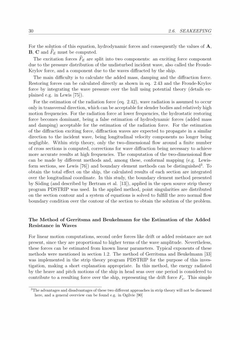
30 2.6. SEAKEEPING
For the solution of this equation, hydrodynamic forces and consequently the values of A,B, C and FE must be computed.
The excitation forces FE are split into two components: an exciting force componentdue to the pressure distribution of the undisturbed incident wave, also called the Froude-Krylov force, and a component due to the waves diffracted by the ship.
The main difficulty is to calculate the added mass, damping and the diffraction force.Restoring forces can be calculated directly as shown in eq. 2.43 and the Froude-Krylovforce by integrating the wave pressure over the hull using potential theory (details ex-plained e.g. in Lewis [75]).
For the estimation of the radiation force (eq. 2.42), wave radiation is assumed to occuronly in transversal direction, which can be acceptable for slender bodies and relatively highmotion frequencies. For the radiation force at lower frequencies, the hydrostatic restoringforce becomes dominant, being a false estimation of hydrodynamic forces (added massand damping) acceptable for the estimation of the radiation force. For the estimationof the diffraction exciting force, diffraction waves are expected to propagate in a similardirection to the incident wave, being longitudinal velocity components no longer beingnegligible. Within strip theory, only the two-dimensional flow around a finite numberof cross sections is computed, corrections for wave diffraction being necessary to achievemore accurate results at high frequencies. The computation of the two-dimensional flowcan be made by different methods and, among these, conformal mapping (e.g. Lewis-form sections, see Lewis [76]) and boundary element methods can be distinguished3. Toobtain the total effect on the ship, the calculated results of each section are integratedover the longitudinal coordinate. In this study, the boundary element method presentedby Soding (and described by Bertram et al. [13]), applied in the open source strip theoryprogram PDSTRIP was used. In the applied method, point singularities are distributedon the section contour and a system of equations is solved to fulfill the zero normal flowboundary condition over the contour of the section to obtain the solution of the problem.
The Method of Gerritsma and Beukelmann for the Estimation of the AddedResistance in Waves
For linear motion computations, second order forces like drift or added resistance are notpresent, since they are proportional to higher terms of the wave amplitude. Nevertheless,these forces can be estimated from known linear parameters. Typical exponents of thesemethods were mentioned in section 1.2. The method of Gerritsma and Beukelmann [33]was implemented in the strip theory program PDSTRIP for the purpose of this inves-tigation, making a short explanation appropriate. In this method, the energy radiatedby the heave and pitch motions of the ship in head seas over one period is considered tocontribute to a resulting force over the ship, representing the drift force Fx. This simple
3The advantages and disadvantages of these two different approaches in strip theory will not be discussedhere, and a general overview can be found e.g. in Ogilvie [90]

CHAPTER 2. BASIC PRINCIPLES 31
relationship leads to the formula:
Fx =πωeLW
L∫0
b(x)∣∣∣ ˆξ3,R
∣∣∣2 (x)dx (2.46)
with
b(x) = b33 − VSd (a33(x))
dx(2.47)
where the terms b33 and a33 represent the damping and added mass in pure vertical
motion for a 2D section, respectively. The term ˆξ3,R represents the complex amplitudeof the vertical relative velocity between the ship and the water surface at a given crosssection. Neglecting wave diffraction and radiation (considering the wave as undisturbed),linearizing eq. 2.2 for small rotations and assuming that z = 0, the complex amplitude ofthe relative vertical motion is expressed:
ξ3,R = η3 − xη5 + yη4 − ζae−ik(x cosµ+y sinµ) (2.48)
The value of the velocity amplitude is thereafter obtained according to eq. 2.38.For application purposes, the longitudinal drift force at zero speed is considered to be
equal to the added resistance in waves RAW = Fx and will be hereinafter recalled as suchwhen provenient from strip theory computations. Considering the inherent deficienciesof this approach (which have been amply discussed in the past, see e.g. [96], [99]), itappears obvious that the accuracy of the results will be limited. Nevertheless, the wideapplication of this method over decades and for many test cases has shown robustnessand acceptable quality of results for rough estimations. In chapter 3, the applicationof the method of Gerritsma and Beukelmann within this investigation will be described,remarking its valuability when combined with results from viscous CFD computations.
Panel Methods
Panel methods represent a good trade-off for the calculations of ship responses in waves,being positioned between strip theory and RANSE CFD methods both in their accu-racy and resource requirements. The most widespread methodology, namely the RankineSingularity Method (RSM), makes use of the same principles described in section 2.5.3.Within this method, frequency and time domain methods can be distinguished. An indepth review on existing implementations and methods was given by Bertam et al. [14]in 1996.
Frequency domain panel methods are able to consider important aspects which are(in most cases) completely neglected in strip theory. The advance speed of the ship, itssteady wave profile or its dynamic trim and sinkage are some of these aspects which,depending on the implementation, can be included or not. In the same manner as forstrip theory, the linearization of incoming waves and motions leads to the consequencethat second order forces such as added resistance in waves may be estimated from knownfirst-order quantities. A description of such an approach is given in Bertram [15]. In his

32 2.6. SEAKEEPING
paper, the author emphasizes the advantage of the consideration of the fully nonlinearsteady wave field for seakeeping calculations, showing, for the estimation of motions, goodagreement with experimental results. For the the added resistance in waves, the need ofestimative methods is certainly a considerable drawback (especially for the purpose ofthis investigation), although a deeper validation of these estimative methods would bedesirable to demonstrate or refute this statement [11]. Further research in this field isbeing undertaken by Papanikolaou [94].
Time domain panel methods might probably offer, at least from a theoretical pointof view, the best trade-off between accuracy of results and computational effort. Thesemethods can account for the nonlinearities of both the steady and the unsteady wavefield and are also able to perform calculations in irregular waves. Regrettably, only a fewimplementations presented so far have reached enough maturity for industrial applica-tions. The group around Sclavounos (Massachusets Inst. of Technology - MIT) and theircommercial RSM solver SWAN (ShipWaveANalysis) [71],[84],[103] can be considered asthe most advanced one in this field (as surveyed by Bertram et al. [14]).
A time domain nonlinear potential RSM code, such as the previously mentioned codeSWAN, would have certainly been of great advantage, especially in order to perform alarge amount of calculations for different variants. However, no such code was availableand all attempts to obtain a time-domain code fulfilling the requirements for the intendedanalysis did not succeed. Considering the free availability of a general purpose, opensource field solver for CFD applications (OpenFOAM) and the author’s experience withsimilar codes, the decision of applying a viscous CFD method was enforced, despite thehigher computational resources required by such a method. The result of following thisapproach lead to the adaption and partial reimplementation of a CFD solver for seakeepingproblems, TUBsixDOFFoam.
2.6.3. Application of RANS CFD Methods for Seakeeping
As previously mentioned in section 1.2, the simulation of motions and forces of a ship inwaves solving the Navier-Stokes equations in the time domain is a promising approach.Here, all described discretization and solution approaches as described in section 2.5.4 forthe calculation of the calm water resistance with viscous CFD methods apply. Addition-ally, the solution of the equations of motion for rigid bodies becomes necessary, makingalso a mesh motion approach necessary (to be described later on in this section). Specialcare has also to be taken in the time discretization approach in order to achieve goodresults.
Analogous to the calculation of the calm water resistance with RANSE CFD methods,the total resistance in waves is obtained by the integration of the resultant normal andshear stresses over the wetted surface of the ship. The subtraction of the calm waterresistance leads to the added resistance in waves for a given time step. In regular waves,the mean value of the added resistance in waves is of special interest, assuming thatthe periodic character of added resistance over a defined number of wave periods canbe assured. The calculation of the added resistance for different wave lengths, wave

CHAPTER 2. BASIC PRINCIPLES 33
encounter angles and/or wave heights leads to a large number of calculations, especiallywhen different geometry variants are to be studied. Practical examples of the applicationof a viscous CFD method for a ship in regular waves will be given in section 2.7 (forvalidation purposes) and in chapter 5 (main application case).
In the following, the main principles of the implemented solver TUBsixDOFFoam will bedescribed.
TUBsixDOFFoam
In the present investigation, the OpenFOAM (Open Source Field Operation and Manip-ulation) toolbox [6] has been used to implement the CFD solver TUBsixDOFFoam. TheOpenFOAM toolbox is a collection of open source C++ libraries released under the gen-eral public license (GPL) which can be used to build numerical solvers specially (but notuniquely) for continuum mechanics problems. Additionally, this toolbox includes severalpre-configured solvers and utilities intended to solve specific engineering problems, espe-cially in the field of CFD. For a detailed description of general characteristics of theseOpenFOAM solvers, Jasak [58] is recommended. The constitution of the presented solveris very similar to any standard OpenFOAM-solver for multiphase flows, differing in theability of considering rigid body motions and some resultant minor issues. All of thesewill be described in the following.
The presented solver has been based on the existing solver shipFoam [24], and multipleadditions, corrections and improvements have been done. The outcome of this is a finitevolume solver for multiphase laminar flows permitting solid body motions in six degreesof freedom (6-DoF) by grid deformation. Its multiphase ability is realized by the Volumeof Fluid (VoF) method and the solid body motions by means of the explicit solutionof the equations of motion. The base solver shipFoam is based itself on other existingsolvers, and is intended for laminar flows (i.e. no turbulence models are available for thissolver). This means that results from TUBsixDOFFoam will consider laminar flows only, i.e.shear stresses are not being correctly represented for turbulent flows. Since the main forcecomponents for the correct prediction of motions and forces in waves are pressure forces,this aspect does not represent a significant problem for the presented application cases.Nevertheless, newer versions of OpenFOAM present approaches for including turbulencemodels in combination with moving meshes, making the possibility of including turbulencemodels in a future reimplementation of TUBsixDOFFoam possible.
The equation of motion to be solved is defined in the hybrid coordinate system (HCS)and is presented here separately for translational (eq. 2.49) and rotational (eq. 2.50)

34 2.6. SEAKEEPING
motions: F1
F2
F3
= m ·
η1
η2
η3
(2.49)
F4
F5
F6
=d
dt
(Ih · ~ωh
)(2.50)
Ih = T · I ·TT =
I44h −I45
h −I46h
−I45h I55
h −I56h
−I46h −I56
h I66h
(2.51)
The force vector ~F = (F1, F2, F3, F4, F5, F6)T represents the total force and is obtaineddirectly from the solution of the RANS equations by integration over the body surface,adding the weight force of the body in vertical direction. Due to the usage of an hybridcoordinate system, the moment of inertia tensor I in ship-fixed coordinates must betransformed to the moment of inertia tensor Ih in the HCS as shown in eq. 2.51, withT from eq. 2.2. The main drawback of this approach is the time dependency of Ih,being the solution for rotational motions only in its generalized form possible (eq. 2.50).Considering motions without yaw and a symmetric geometry where I45 = 0 and I56 = 0,the inertial moments for the remaining matrix elements are:
Ih44 = I44 cos2 η5 − 2I46 cos η4 cos η5 sin η5 + I55 sin2 η4 sin2 η5 +
+I66 cos2 η4 sin2 η5 (2.52)
Ih55 = I55 cos2 η4 + I66 sin2 η4 (2.53)
Ih46 = I46 cos η4
(2 sin2 η5 − 1
)− I44 cos η5 sin η5 +
(I55 sin2 η4+
)(+I66 cos2 η4
)cos η5 sin η5 (2.54)
The field and matrix operation abilities of the OpenFOAM toolkit permit the implemen-tation of the coordinate transformation in matricial form, reducing the necessary pro-gramming effort considerably. Note that, since the calculations performed in this studywill include only pitch and heave motions, the presented equations can be simplified evenmore, and the equations of heave and pitch can be then rewritten:
η3 =F3
m(2.55)
ωhy = η5 =F5
I55
(2.56)
The equations of motion can be subsequently solved by an explicit Euler method oralternatively by a Runge-Kutta method to obtain the velocity and displacement vectors ~ηand ~η, respectively. From these, the mesh is updated by an automatic mesh motion solver,firstly for the translations and then, for the rotations. This solver makes use of a simplifiedmesh motion equation in the form of a Laplace equation with variable diffusivity:
∇ · (k∇q) = 0 (2.57)
CHAPTER 2. BASIC PRINCIPLES 35
where q represents the mesh deformation velocity and k the variable diffusivity. Thisdiffusivity can be chosen to be related to the distance l from the moving boundary or,alternatively, based on the quality of the resulting mesh. For the first, the diffusivitycoefficient is proportional to 1/la, representing a = 1 an inverse proportional relation. Inthe original implementation, only a = 1 and a = 2 are available. This has been extendedfor any value of a, providing an increased flexibility and better chances to avoid largermesh deformations in regions placed near to the ship.
Due to the explicit handling of the motion equations, an additional outer iteration foreach time step has been implemented in the solver, in a similar manner as presented bySchmode et al. [101]. In this approach, resulting forces from the actual outer iterationare compared with the forces from the last outer iteration, repeating the iteration until adesired convergence is achieved (see also fig. 2.3). For each time step t, resultant forcesare first guessed by means of a damped extrapolation:
Ft,guess = (1− r)Ft−1 + rFt−2 + (1− r)Ft−1 − Ft−2
dtt−1
dtt (2.58)
with r representing a force damping factor and the subindexes t, t−1 and t−2 representinglast three time steps of the simulation. The damping factor r can be controlled by theuser and is reduced automatically if the force guessing of previous iterations was notsuccessful. With the guessed force, motions are calculated, the mesh is updated and theflow calculations, including the pressure-velocity correction, are performed. After this,the new resultant forces at the ship are calculated and are compared to the initial guessas previously mentioned. The process is repeated until a given convergence is achieved,being in most cases, specially for slow motions, only a single outer iteration necessary. Infigure 2.3, a flowchart including all the mentioned solver steps is shown.
The mentioned outer iteration is intended to undergo force peaks, caused by numericalinstabilities, especially when high force gradients are encountered. Compared to the initialsolver implementation without the mentioned outer iteration, this approach has shownto provide a higher stability during calculations and a higher accuracy when high forcegradients arise (e.g. slamming events), without increasing the required computationalresources significantly.
2.7. Validation of CFD Solver
2.7.1. Background
The quality of results from CFD calculations plays an important role for the successfulapplication of this technique for the assessment of added resistance in waves within thisinvestigation. For this purpose, and considering that the presented solver TUBsixDOFFoamhas a very short history, several benchmark calculations were undertaken. To guaranteeappropriate conditions for these calculations, a two-dimensional wave tank was studiedin order to test different numerical and solution schemes, validating attained results withthe underlying analytical description of the inlet wave. After this preliminary step, an
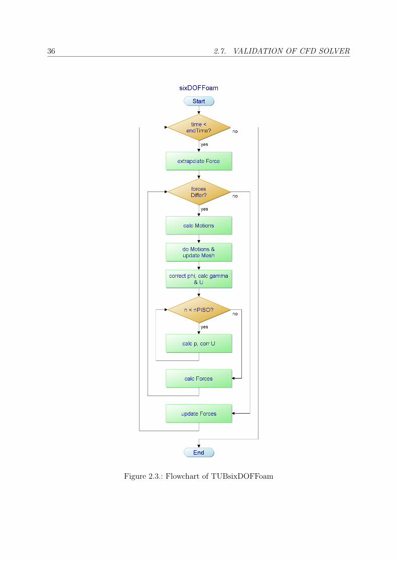
36 2.7. VALIDATION OF CFD SOLVER
Figure 2.3.: Flowchart of TUBsixDOFFoam

CHAPTER 2. BASIC PRINCIPLES 37
exhaustive validation of OpenFOAM is undertaken with a ship geometry where accurateexperimental data and results from other authors using similar solvers are available. Thislead to the choice of the surface combatant model 5415 from the David Taylor Model Basin(DTMB5415), including the validation of the calm water resistance and its performancein waves.
Measurements from IIHR [4] (Iowa Institute of Hydraulic Research) for DTMB model5512 (a 3.05m geosim model of the 5.72m 5415 model) were taken for the intended val-idation, making use of the same benchmark cases from the CFD Workshop Tokyo 2005[44]. The usage of the DTMB combatant model within the CFD workshop in Gothen-burg (2000) [73] and the mentioned workshop in Tokyo (2005) [44] permits a comparisonof the presented OpenFOAM solver with other, well established CFD codes from theparticipants these CFD workshops.
2.7.2. 2D Wave Tank
The inlet condition of every CFD setup for seakeeping applications, providing a regularwave in a moving frame (equal to advance speed), showed to be a sensitive task withinthe setup of the solver. This applies not only for the implemented solver, but also forall other multiphase solvers provided by OpenFOAM. To attain the desired wave shapequality, a 2D wave tank case was studied and different numerical setups were tested andcompared to the analytical solution. A complete description of each tested setup is outof scope, but the final setup will be discussed here.
Grid Generation, Boundary Conditions and Numerical Setup
To avoid wave reflection from the outlet boundary, appropriate boundary conditions mustbe chosen (non-reflective boundary conditions, sponge layers and similar solutions havebeen discussed by many authors). Since the OpenFOAM toolkit does not provide such aboundary condition for multiphase problems, a simple solution was applied. By extremelycoarsening the grid at the outlet region, especially in longitudinal direction, the reflectiondisappears completely and zero-gradient outlet boundary conditions can be used withoutdifficulties. It must be recalled that this solution is valid for the head waves condition,and is in many cases not possible to apply e.g. for manoeuvring simulations. For thewave tank case, a Cartesian 2D grid with the mentioned coarseness at the outlet region isrequired. A finer grid with 29120 cells and a coarser grid with 7280 (half number of cellsin longitudinal and vertical direction) were generated.
A special treatment is required for the inlet boundary: since a regular wave must bedefined, a time-variable inlet is needed. In most of commercial CFD applications, this isdone by user coding, which must be compiled additionally and linked to the executablefile. In the present case, a directly interpreted boundary condition named groovyBC isused. This condition permits the input of formulas, datasets and many other variables intothe boundary condition. In the present case, the inlet boundary defines a second-order,

38 2.7. VALIDATION OF CFD SOLVER
regular Stokes wave. The wave deflection for a wave of amplitude ζA is defined:
ζ(t) = ζA · cos (k x− ωe t) + 0.5ζ2A · cos (2 (k x− ωe t)) (2.59)
and is taken to check whether a cell is located below or above the water surface, and thusthe boundary conditions for the longitudinal and vertical components u and w of watervelocity and for the phase fraction γ can be defined:
γ(z, t) =
{10
∀ z ≤ ζ(t)∀ z > ζ(t)
(2.60)
u(z, t) =
{VA + ζA · ω · ek z · cos(k x− ωe t)VA
∀ z ≤ ζ(t)∀ z > ζ(t)
(2.61)
w(z, t) =
{ζA · ω · ek z · sin(k x− ωe t)0
∀ z ≤ ζ(t)∀ z > ζ(t)
(2.62)
(2.63)
The outlet boundary is defined by a zero-gradient condition, the bottom boundary by aslip-wall condition and the top-wall by an atmospheric condition. A detailed descriptionof the boundary conditions for calculations considering ships, including the boundariesmentioned here, is given in the next section (2.7.3).
The selection of appropriate numerical schemes to solve the governing equations is atask where intensive testing was necessary. Since the OpenFOAM toolkit neither pro-vides a detailed documentation nor general guidelines on this, testing of practically everyphysically and numerically reasonable scheme was necessary. A detailed description ofthese is considered outside the scope of this work. The final numerical setup applied forall calculations is given in tables 2.2 and 2.3.
Results
As a known fact, the diffusion or loss of wave height along the computational domainan issue of matter, especially for coarser grids, when making use of the VoF method forcapturing the free surface. This fact arose in this validation case too, showing a waveheight diffusivity along the computational domain. Figure 2.4 shows this phenomenoncomparing both test cases. Additionally, the steadiness of the harmonic cycles was testedby comparing the wave elevation after different numbers of wave periods. This is shownin figure 2.5, being compared to an analytical, second order Stokes wave as given in theinlet boundary condition.
Although results obtained show a certain loss in wave height along the domain, slope,phase and shape match the analytical definition adequately.
2.7.3. DTMB5415 Surface Combatant
The DTMB surface combatant model 5415 is a widely known benchmark model for bothexperimental and numerical investigation on ship flows and has been explicitly recom-mended by the ITTC [54] for this purpose. This model was conceived as a preliminary

CHAPTER 2. BASIC PRINCIPLES 39
Item Symbol Keyword Description
1First and secondtime derivatives
∂∂t
EulerFirst order, bounded, im-plicit
2 Gradient ∇faceLimited
leastSquares
0.5
Limited, second order leastsquares
3Divergence (veloc-ity terms)
∇ · ~u Gauss
vanLeerV
Second order Gaussian inte-gration, van Leer interpola-tion for face centres
4Divergence (phasefraction terms)
∇ · γ Gauss
vanLeer01
As 3, strictly bounded be-tween 0 and 1
5 Laplacian ∇2
Gauss
linear
corrected
Second order, Gaussian in-tegration, linear interpola-tion for face centres, conser-vative
6Point-to-pointinterpolation
linearLinear interpolation for gen-eral fields
7Gradient compo-nent normal toface
∇SN correctedExplicit non-orthogonalcorrection
Table 2.2.: Numerical schemes for CFD calculations
design of a surface combatant for the US navy in the early eighties. The main dimensionsand the geometry of the hull can be found in table 2.4 and figure 2.6, respectively. Theavailable experimental data provided by IIHR covers model tests both in calm water andin waves, with and without motions. The model tests for the validation consider a singlespeed (Fn = 0.280, Rn = 4.860 · 106) and measurements in waves a single wave length(λW/LPP = 1.50). Detailed measurements of the nominal wake field, wave elevationsand global quantities such as motions, forces and moments are also available from thisinstitution.
Grid Generation
The grid generation is undertaken by the OpenFOAM-utility snappyHexMesh, a script-driven, unstructured grid generator. snappyHexMesh generates meshes containing hexae-dra and split-hexaedra, opposite to most of commercially or freely available automaticgrid generators which generate mainly tetrahedral meshes. Since only poor documenta-tion is available, a short discussion, specially for its application in meshing ship hulls, isgiven in appendix A.
Four refinement levels (80k, 200k, 500k and 2M cells approx.) and two additional gridsfor calculations without free surface (using the topologies from the 200k and 2M meshes)were generated. These are summarized in table 2.5. The four meshes for free surface
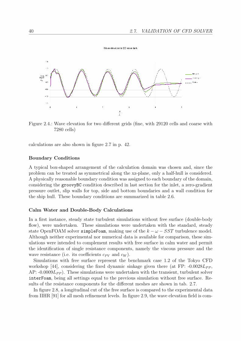
40 2.7. VALIDATION OF CFD SOLVER
Figure 2.4.: Wave elevation for two different grids (fine, with 29120 cells and coarse with7280 cells)
calculations are also shown in figure 2.7 in p. 42.
Boundary Conditions
A typical box-shaped arrangement of the calculation domain was chosen and, since theproblem can be treated as symmetrical along the xz-plane, only a half-hull is considered.A physically reasonable boundary condition was assigned to each boundary of the domain,considering the groovyBC condition described in last section for the inlet, a zero-gradientpressure outlet, slip walls for top, side and bottom boundaries and a wall condition forthe ship hull. These boundary conditions are summarized in table 2.6.
Calm Water and Double-Body Calculations
In a first instance, steady state turbulent simulations without free surface (double-bodyflow), were undertaken. These simulations were undertaken with the standard, steadystate OpenFOAM solver simpleFoam, making use of the k− ω− SST turbulence model.Although neither experimental nor numerical data is available for comparison, these sim-ulations were intended to complement results with free surface in calm water and permitthe identification of single resistance components, namely the viscous pressure and thewave resistance (i.e. its coefficients cPV and cW ).
Simulations with free surface represent the benchmark case 1.2 of the Tokyo CFDworkshop [44], considering the fixed dynamic sinkage given there (at FP: -0.0028LPP ,AP: -0.0009LPP ). These simulations were undertaken with the transient, turbulent solverinterFoam, being all settings equal to the previous simulation without free surface. Re-sults of the resistance components for the different meshes are shown in tab. 2.7.
In figure 2.8, a longitudinal cut of the free surface is compared to the experimental datafrom IIHR [91] for all mesh refinement levels. In figure 2.9, the wave elevation field is com-
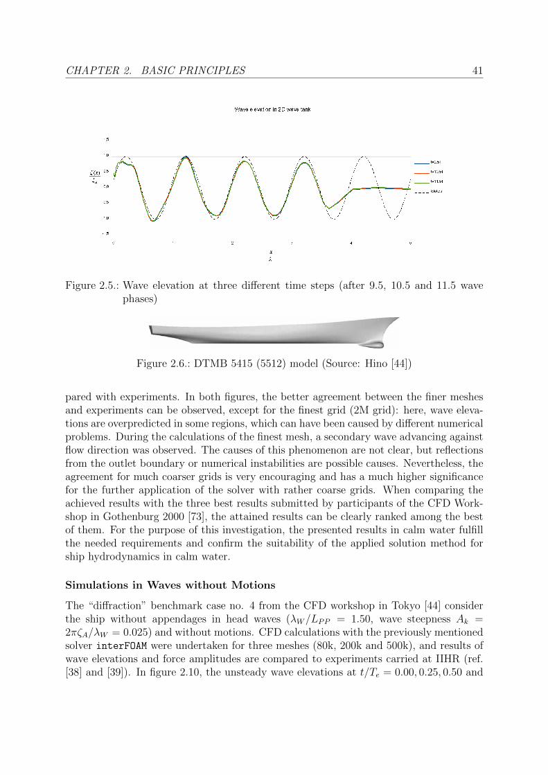
CHAPTER 2. BASIC PRINCIPLES 41
Figure 2.5.: Wave elevation at three different time steps (after 9.5, 10.5 and 11.5 wavephases)
Figure 2.6.: DTMB 5415 (5512) model (Source: Hino [44])
pared with experiments. In both figures, the better agreement between the finer meshesand experiments can be observed, except for the finest grid (2M grid): here, wave eleva-tions are overpredicted in some regions, which can have been caused by different numericalproblems. During the calculations of the finest mesh, a secondary wave advancing againstflow direction was observed. The causes of this phenomenon are not clear, but reflectionsfrom the outlet boundary or numerical instabilities are possible causes. Nevertheless, theagreement for much coarser grids is very encouraging and has a much higher significancefor the further application of the solver with rather coarse grids. When comparing theachieved results with the three best results submitted by participants of the CFD Work-shop in Gothenburg 2000 [73], the attained results can be clearly ranked among the bestof them. For the purpose of this investigation, the presented results in calm water fulfillthe needed requirements and confirm the suitability of the applied solution method forship hydrodynamics in calm water.
Simulations in Waves without Motions
The “diffraction” benchmark case no. 4 from the CFD workshop in Tokyo [44] considerthe ship without appendages in head waves (λW/LPP = 1.50, wave steepness Ak =2πζA/λW = 0.025) and without motions. CFD calculations with the previously mentionedsolver interFOAM were undertaken for three meshes (80k, 200k and 500k), and results ofwave elevations and force amplitudes are compared to experiments carried at IIHR (ref.[38] and [39]). In figure 2.10, the unsteady wave elevations at t/Te = 0.00, 0.25, 0.50 and

42 2.7. VALIDATION OF CFD SOLVER
(a) 80k cells (b) 200k cells
(c) 500k cells cells (d) 2M cells
Figure 2.7.: Grids generated with snappyHexMesh
0.75 are presented for the 200k and 500k grids (upper half of each plot) and are comparedto experimental results (lower half of each plot). The wave elevations show, especially forthe 500k grid, good agreement with experiments. In figure 2.11, the time history of thelongitudinal force in waves is compared to experiments. The force amplitude, in the samemanner as the calm water resistance for coarser meshes, is overestimated for all meshesconsidered. The influence of grid fineness is not comparable to the calm water case, beingthe observed overprediction practically independent of the fineness of the grid. Since therole of hydrostatic forces is significant in comparison to calculations in calm water, thegood agreement of results from very coarse meshes can be expected. The attained resultsalso agree well with results submitted by participants of the CFD Workshop Tokyo 2005(see e.g. Cura Hochbaum et al. [25]), showing the suitability of the presented solutionmethod for ship hydrodynamic problems in waves.
Simulations in Waves with Motions
The main objective of the application of CFD in this study is the simulation of shipmotions in head waves, and calculations were made for three grids (80k, 200k and 500kgrids) with the implemented solver TUBsixDOFFoam. Considering the architecture of any
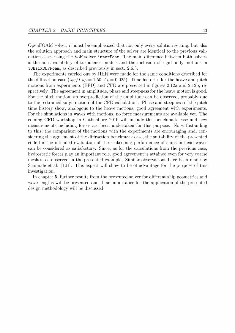
CHAPTER 2. BASIC PRINCIPLES 43
OpenFOAM solver, it must be emphasized that not only every solution setting, but alsothe solution approach and main structure of the solver are identical to the previous vali-dation cases using the VoF solver interFoam. The main difference between both solversis the non-availability of turbulence models and the inclusion of rigid-body motions inTUBsixDOFFoam, as described previously in sect. 2.6.3.
The experiments carried out by IIHR were made for the same conditions described forthe diffraction case (λW/LPP = 1.50, Ak = 0.025). Time histories for the heave and pitchmotions from experiments (EFD) and CFD are presented in figures 2.12a and 2.12b, re-spectively. The agreement in amplitude, phase and steepness for the heave motion is good.For the pitch motion, an overprediction of the amplitude can be observed, probably dueto the restrained surge motion of the CFD calculations. Phase and steepness of the pitchtime history show, analogous to the heave motions, good agreement with experiments.For the simulations in waves with motions, no force measurements are available yet. Thecoming CFD workshop in Gothenburg 2010 will include this benchmark case and newmeasurements including forces are been undertaken for this purpose. Notwithstandingto this, the comparison of the motions with the experiments are encouraging and, con-sidering the agreement of the diffraction benchmark case, the suitability of the presentedcode for the intended evaluation of the seakeeping performance of ships in head wavescan be considered as satisfactory. Since, as for the calculations from the previous case,hydrostatic forces play an important role, good agreement is attained even for very coarsemeshes, as observed in the presented example. Similar observations have been made bySchmode et al. [101]. This aspect will show to be of advantage for the purpose of thisinvestigation.
In chapter 5, further results from the presented solver for different ship geometries andwave lengths will be presented and their importance for the application of the presenteddesign methodology will be discussed.
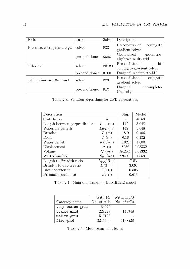
44 2.7. VALIDATION OF CFD SOLVER
Field Task Solver Description
Pressure, corr. pressure pd solver PCGPreconditioned conjugategradient solver
preconditioner GAMGGeneralised geometric-algebraic multi-grid
Velocity U solver PBiCGPreconditioned bi-conjugate gradient solver
preconditioner DILU Diagonal incomplete-LU
cell motion cellMotionU solver PCGPreconditioned conjugategradient solver
preconditioner DICDiagonal incomplete-Cholesky
Table 2.3.: Solution algorithms for CFD calculations
Description Ship ModelScale factor λ - 46.59Length between perpendiculars LPP (m) 142 3.048Waterline Length LWL (m) 142 3.048Breadth B (m) 18.9 0.406Draft T (m) 6.16 0.132Water density ρ (t/m3) 1.025 1.000Displacement ∆ (t) 8636 0.08332Volume ∇ (m3) 8425.4 0.08332Wetted surface SW (m2) 2949.5 1.359Length to Breadth ratio LPP/B (-) 7.53Breadth to depth ratio B/T (-) 3.091Block coefficient CB (-) 0.506Prismatic coefficient CP (-) 0.613
Table 2.4.: Main dimensions of DTMB5512 model
With FS Without FSCategory name No. of cells No. of cellsvery coarse grid 84520 -coarse grid 228228 145948medium grid 517128 -fine grid 2245406 1138528
Table 2.5.: Mesh refinement levels

CHAPTER 2. BASIC PRINCIPLES 45
Field NameVelocity Phase fraction PressureU gamma pd
Inlet minX groovyBC groovyBC zero gradientOutlet maxX zero gradient zero gradient zero gradientSymmetry plane minY symmetry symmetry symmetrySide wall maxY slip wall zero gradient zero gradientBottom wall minZ slip wall zero gradient zero gradientTop wall maxZ zero gradient zero gradient fixed value (0)Ship ship moving wall zero gradient zero gradient
Table 2.6.: Boundary fields. The groovyBC condition has been decribed in section 2.7.2
80k 200k 500k 2M EFDCF 2.53E-03 2.61E-03 2.86E-03 3.11E-03 2.89E-03e(%) -12.38% -9.77% -0.88% 7.70%
CP 3.12E-03 2.65E-03 1.88E-03 1.35E-03 1.35E-03e(%) 130.65% 95.83% 39.13% -0.11%
CT 5.65E-03 5.25E-03 4.74E-03 4.46E-03 4.24E-03e(%) 33.27% 23.93% 11.89% 5.21%
Table 2.7.: Results of CFD calculations in calm water for DTMB model 5512 comparedto experiments. Since experimental data was only available for DTMB 5415model, Reynolds-dependent CFD results for DTMB 5512 model were scaledaccordingly
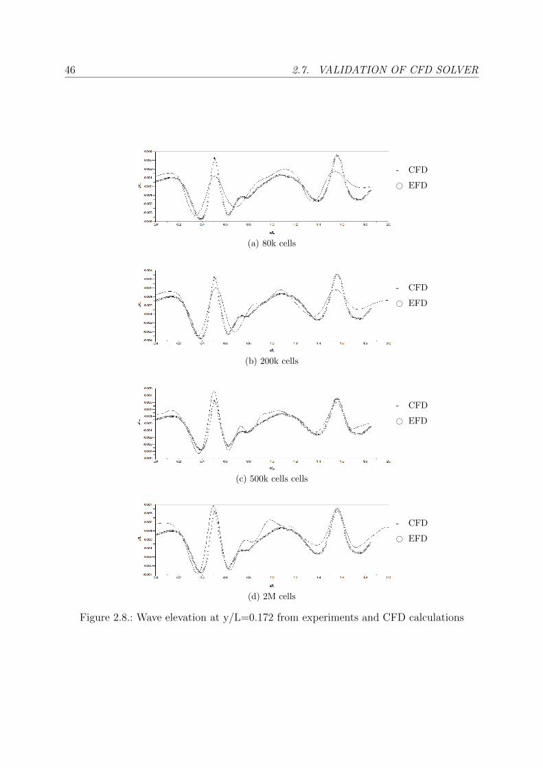
46 2.7. VALIDATION OF CFD SOLVER
- CFD
# EFD
(a) 80k cells
- CFD
# EFD
(b) 200k cells
- CFD
# EFD
(c) 500k cells cells
- CFD
# EFD
(d) 2M cells
Figure 2.8.: Wave elevation at y/L=0.172 from experiments and CFD calculations

CHAPTER 2. BASIC PRINCIPLES 47
(a) 80k cells
(b) 200k cells
(c) 500k cells cells
(d) 2M cells
Figure 2.9.: Wave elevations from CFD calculations (upper half of each plot) and experi-ments (EFD, lower half of each plot)

48 2.7. VALIDATION OF CFD SOLVER
(a) t/T=0.00
(b) t/T=0.25
(c) t/T=0.50
(d) t/T=0.75
Figure 2.10.: Wave elevations of ship in waves, without motions, calculated with 200k(left) and 500k (right) grid compared to experiments (EFD, lower half ofeach plot)

CHAPTER 2. BASIC PRINCIPLES 49
-10
-8
-6
-4
-2
0
2
4
6
8
10
0,0 1,0
103
CA
W=
103
(CIW
-C
CW
)
t/Te
Added resistance in Waves
2,0 3,0
Added resistance in Waves
EFD
CFD-80k
CFD-200k
CFD-500k
Figure 2.11.: Heave and pitch motion time histories from CFD calculations (200k grid)and experiments [51]
0,015
0,020
Heave time history
-0,005
0,000
0,005
0,010
He
av
e (
m)
-0,020
-0,015
-0,010
0 2 4 6 8 10
time (s)
Heave time history
EFD
CFD
10 12 14 16 18
time (s)
(a)
1,000
1,500
2,000
Pitch time history
-1,000
-0,500
0,000
0,500
1,000
Pit
ch (
°)
-2,000
-1,500
-1,000
0 2 4
time (s)
Pitch time history
EFD
CFD
time (s)
(b)
Figure 2.12.: Heave and pitch motion time histories from CFD calculations (200k grid)and experiments [51]
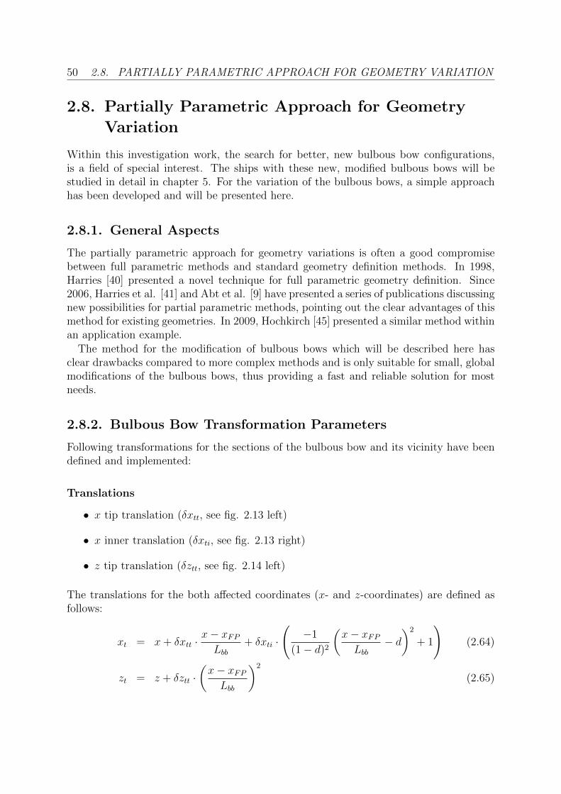
50 2.8. PARTIALLY PARAMETRIC APPROACH FOR GEOMETRY VARIATION
2.8. Partially Parametric Approach for Geometry
Variation
Within this investigation work, the search for better, new bulbous bow configurations,is a field of special interest. The ships with these new, modified bulbous bows will bestudied in detail in chapter 5. For the variation of the bulbous bows, a simple approachhas been developed and will be presented here.
2.8.1. General Aspects
The partially parametric approach for geometry variations is often a good compromisebetween full parametric methods and standard geometry definition methods. In 1998,Harries [40] presented a novel technique for full parametric geometry definition. Since2006, Harries et al. [41] and Abt et al. [9] have presented a series of publications discussingnew possibilities for partial parametric methods, pointing out the clear advantages of thismethod for existing geometries. In 2009, Hochkirch [45] presented a similar method withinan application example.
The method for the modification of bulbous bows which will be described here hasclear drawbacks compared to more complex methods and is only suitable for small, globalmodifications of the bulbous bows, thus providing a fast and reliable solution for mostneeds.
2.8.2. Bulbous Bow Transformation Parameters
Following transformations for the sections of the bulbous bow and its vicinity have beendefined and implemented:
Translations
• x tip translation (δxtt, see fig. 2.13 left)
• x inner translation (δxti, see fig. 2.13 right)
• z tip translation (δztt, see fig. 2.14 left)
The translations for the both affected coordinates (x- and z-coordinates) are defined asfollows:
xt = x+ δxtt ·x− xFPLbb
+ δxti ·
(−1
(1− d)2
(x− xFPLbb
− d)2
+ 1
)(2.64)
zt = z + δztt ·(x− xFPLbb
)2
(2.65)
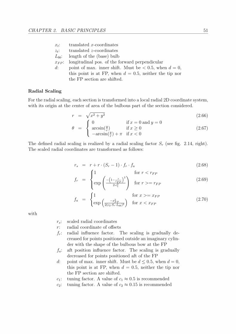
CHAPTER 2. BASIC PRINCIPLES 51
xt: translated x-coordinateszt: translated z-coordinatesLbb: length of the (base) bulbxFP : longitudinal pos. of the forward perpendiculard: point of max. inner shift. Must be < 0.5, when d = 0,
this point is at FP, when d = 0.5, neither the tip northe FP section are shifted.
Radial Scaling
For the radial scaling, each section is transformed into a local radial 2D coordinate system,with its origin at the center of area of the bulbous part of the section considered.
r =√x2 + y2 (2.66)
θ =
0 if x = 0 and y = 0arcsin(y
r) if x ≥ 0
−arcsin(yr) + π if x < 0
(2.67)
The defined radial scaling is realized by a radial scaling factor Sr (see fig. 2.14, right).The scaled radial coordinates are transformed as follows:
rs = r + r · (Sr − 1) · fr · fa (2.68)
fr =
1 for r < rFP
exp
(−(
1− rrFP
)2
2·c21
)for r >= rFP
(2.69)
fa =
{1 for x >= xFP
exp(
−x2FP
2(c2·Sr·Lbb)2
)for x < xFP
(2.70)
with
rs: scaled radial coordinatesr: radial coordinate of offsetsfr: radial influence factor. The scaling is gradually de-
creased for points positioned outside an imaginary cylin-der with the shape of the bulbous bow at the FP
fa: aft position influence factor. The scaling is graduallydecreased for points positioned aft of the FP
d: point of max. inner shift. Must be d ≤ 0.5, when d = 0,this point is at FP, when d = 0.5, neither the tip northe FP section are shifted.
c1: tuning factor. A value of c1 ≈ 0.5 is recommendedc2: tuning factor. A value of c2 ≈ 0.15 is recommended

52 2.8. PARTIALLY PARAMETRIC APPROACH FOR GEOMETRY VARIATION
Figure 2.13.: x-tip shifting (left) and x-inner shifting (right)

CHAPTER 2. BASIC PRINCIPLES 53
Figure 2.14.: z-tip shifting (left) and radial scaling (right)

CHAPTER 3. MODELING OF SHIP OPERATION 55
3. Modeling of Ship Operation
3.1. General Aspects
In this chapter, the model applied for the operational simulations will be described. Aspreviously introduced in section 2.3.1 (p. 15), two main components, an environmentmodel and a ship model can be distinguished. In the following, these two main componentswill be described in detail. Finally, a brief description of the implemented simulationplatform SimOship will be given (sect. 3.5). It must be mentioned that all descriptionsapply for the simulation of the operation of a cargo vessel.
3.2. Environment Model
As mentioned in section 2.3.1, the environment model contains all aspects which are notinherently part of the ship, being two main components distinguished, the operation ofthe ship and the influence of weather. These will be described here in the form as theywere modeled within this study.
3.2.1. Operational Model
The operational model will be defined as all aspects belonging to the environment of theship which can be considered as known for the purpose of the simulation, mainly those oflogistic/strategic nature. These aspects will be considered as constants within this designstudy and will remain constant for each design variant.
Routes
Routes are defined as the path to be sailed by a ship between a given number of geographicpoints. In oceanic navigation, the shortest line between two points over a sphere is anorthodromic curve (details see e.g. Dunlap [28]), and routes are subsequently defined assuch. Special treatment is needed for routes, whose orthodromic curves lead over land. Inthis case, the orthodromic route must be considered as unfeasible, but as a basis route for afurther modification. This basis route can be approximated by a spline, which is definedby control points. Except of the starting and the ending point, the remaining controlpoints can be shifted–perpendicular to the course of the route–by a perturbance vector.This perturbance vector can be varied until the route is feasible. A more straightforwardalternative is to apply an optimization strategy to solve this problem, finding the shortestfeasible route in a very short time. This has been applied within this work with a simple,

56 3.2. ENVIRONMENT MODEL
deterministic quasi-Newton algorithm. An example of this approach is shown in figure3.1.
Figure 3.1.: Example of a route creation starting with an unfeasible route. Note that theoptimum (shortest) route quality depends of the number of control points
Cargo
Cargo modeling is a task where no certainty of the assumptions made is given. Theo-retically, different scenarios can be considered to show the sensitivity of the results dueto this task. Nevertheless, and in the same way as for many other aspects within thesesimulations, simplified approaches will be necessary. Within this study, cargo will beconsidered as known for each trip made, modeled simply as a mass and a correspondingcentre of gravity. In a similar way, ballast and fuel can be treated here as special cargo,considering bunkering after certain mileages or when arriving at a certain port. In thisstudy, fuel and ballast water will be simply added to the total cargo mass.
3.2.2. Weather Model
The modeling of weather is an extremely complex task, which cannot be modeled withoutsimplifications making use of statistical information, especially in the case of a practicalapplication such as an operational simulation representative for the complete lifetime ofthe ship. In this case, depending on the available resources, weather can be modeled indifferent complexity levels, such as:
CHAPTER 3. MODELING OF SHIP OPERATION 57
• Arbitrarily defined “worst case conditions”, “mean” conditions and comparable ap-proaches
• Global statistical information, such as long-term statistics, e.g. for a region ofinterest
• Local statistical information (short term statistics), for a defined route and a definedperiod of time
• Local statistical information, (short term statistics), for different locations in adefined region and a defined period of time
The latter modality will be applied here, since it provides maximum flexibility and permitsthe consideration of additional features such as route optimization, circumnavigation ofrough weather regions, etc. Although these features will not be applied here, furtherinvestigations are applying (Balloch [10]) or will apply these using the simulation platformpresented here.
The presented operational simulations are performed with existing weather data overa past period of time, so-called behind-casts. The ERA-40 database from the EuropeanCentre of Medium Range Weather Forecasts (ECMWF) was employed for this purpose[2]. This database contains reanalyzed weather data for a period from 1956 to 2002 in six-hour steps for each 1.5◦latitude and longitude. An example of this data for the significantwave height is shown in fig. 3.2. For each six-hour period, a statistical representation ofthe weather needs to be undertaken. Following information is recalled from the ERA-40database:
• Significant wave height H1/3 [m]
• Mean wave period T1 [s]
• Mean wave direction χm [◦]
• Wind velocity components Vu (west-east) and Vv (south-north) [m/s]
With this information, an 1D-spectrum for the sea can be calculated. Such a wave spec-trum can be modeled using different formulations; typical wave spectrum formulationsare Pierson-Moskovitz, JONSWAP and Bretschneider. In this study, the mean JON-SWAP spectrum was used according to the formulation of the ITTC’78 for fetch limitedsituations [52]:
Sζ(ω) =172.8 ·H2
1/3
T 41
· ω−5 · exp{−691.2
T 41
· ω−4
}· A · γB (3.1)
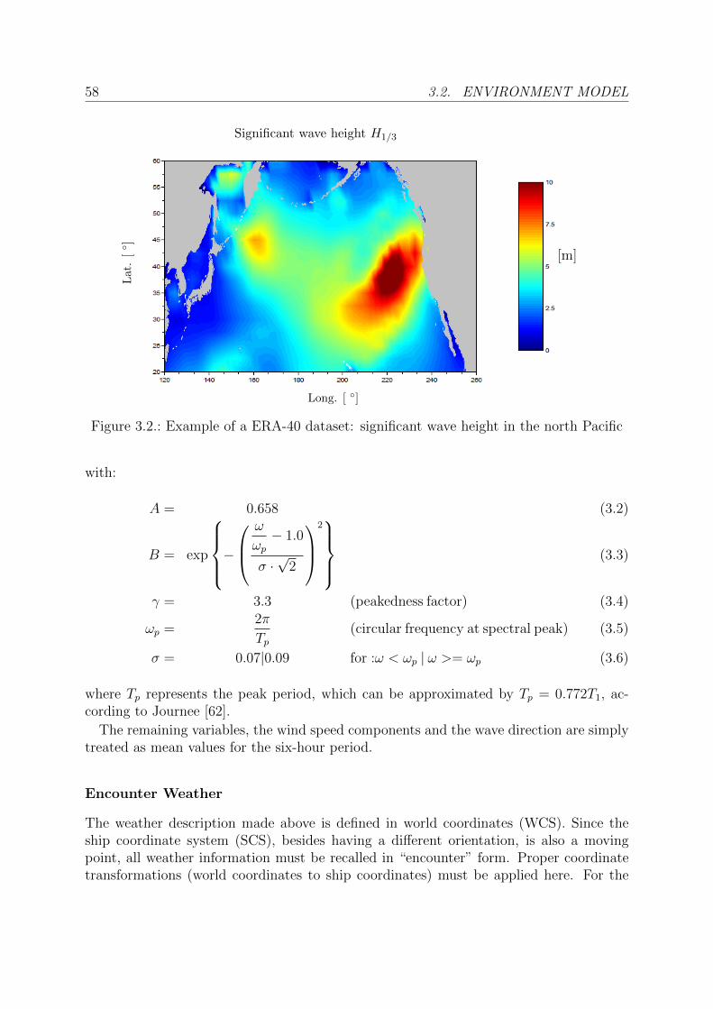
58 3.2. ENVIRONMENT MODEL
Significant wave height H1/3
[m]
Long. [ ◦]
Lat.
[◦ ]
Figure 3.2.: Example of a ERA-40 dataset: significant wave height in the north Pacific
with:
A = 0.658 (3.2)
B = exp
−ω
ωp− 1.0
σ ·√
2
2 (3.3)
γ = 3.3 (peakedness factor) (3.4)
ωp =2π
Tp(circular frequency at spectral peak) (3.5)
σ = 0.07|0.09 for :ω < ωp | ω >= ωp (3.6)
where Tp represents the peak period, which can be approximated by Tp = 0.772T1, ac-cording to Journee [62].
The remaining variables, the wind speed components and the wave direction are simplytreated as mean values for the six-hour period.
Encounter Weather
The weather description made above is defined in world coordinates (WCS). Since theship coordinate system (SCS), besides having a different orientation, is also a movingpoint, all weather information must be recalled in “encounter” form. Proper coordinatetransformations (world coordinates to ship coordinates) must be applied here. For the
CHAPTER 3. MODELING OF SHIP OPERATION 59
wave spectrum, an encounter wave spectrum is defined:
Sζ,e(ω, VS, µ) =Sζ(ω)
1− (2ωVS/g) · cos µ(3.7)
For the wind, the wind speed and the wind angle must be transformed firstly into theSCS (into true wind speed VWT and true wind angle αWT ), and then be made relativeto the ship considering its advance velocity, leading to the apparent wind speed VWA andthe apparent wind angle αWA as follows:
VWT =√V 2u + V 2
v (3.8)
αWT = arccos
(Vv√
V 2u + V 2
v
)· Vu|Vu|− ψ (3.9)
VWA =
√(VWT · sin(αWT ))2 + (VWT · cos(αWT )− VS)2 (3.10)
αWA = arccos
(VWT · cos(αWT )− VS
VWA
)(3.11)
From this data, ship responses in irregular waves and ship resistance due to wind areobtained. This will be discussed in sections 3.3.3 and 3.3.4.
3.3. Ship Model
Modeling the ship accurately is an important factor for the success of an operationalsimulation, and it shall represent a good compromise between accuracy and simplicitywhile considering available computational resources and existing information about theship. Due to the focus on hydrodynamics in the present investigation, all aspects relatedto this task were modeled as accurately as possible, considered from the point of view ofan early design stage. These aspects will be described in the present section.
3.3.1. Geometry and Hydrostatics
The geometry of the hull is discretized in form of offsets from which the necessary hydro-static characteristics are calculated. These offsets are comprised by a variable number ofcross sections and a longitudinal contour. From these, hydrostatic data for a matrix ofaft and forward drafts TAP and TFP is calculated. Following parameters are calculated:
• Displacement volume ∇
• Longitudinal center of buoyancy xCB
• Vertical center of buoyancy zCB
• Wetted surface S

60 3.3. SHIP MODEL
• Waterline length LWL
• Waterline breadth BWL
• Waterplane area AWL
• Main section area AMS
• Transom area ATr
• Bulbous bow area Abb
These can be recalled within the simulations to find the floating condition for any givencargo. This is done given the ship’s total weight W = g∆ and the longitudinal centreof gravity xCG by solving a two equation system, with TAP and TFP as unknowns andconsidering static equilibrium (∆ = ρ∇ and xCG = xCB). This can be formulated:
∇(TAP , TFP ) = ∆/ρ (3.12)
xCB(TAP , TFP ) = xCG (3.13)
The solution is solved numerically and the actual floating condition is obtained. This willbe addressed by all simulation modules where this is relevant, especially for ship resistanceand seakeeping.
3.3.2. Calm Water Resistance
Different options have been considered for the modeling of calm water resistance. Flexi-bility must be provided here, since, as a tool intended to be used during an early designstage, different methods must be available. As usual, if no model test data is available,the determination of the wave resistance coefficient cW and the form factor k are themain points of interest. The remaining coefficients are estimated according to the ITTCas described in section 2.5.
Holtrop & Mennen’s Method
The estimation of the ship’s resistance by statistically based methods is always a goodstarting point in the iterative process of ship design. The method of Holtrop and Mennen(1982, [50] and 1984, [49]) has been made available in the simulation platform SimOship.All necessary hydrostatic information is addressed from the hydrostatics calculations andtotal calm water resistance is calculated for all floating conditions defined. This add-ononly has value for very preliminary computations or to compare CFD or experimentalresults with it.
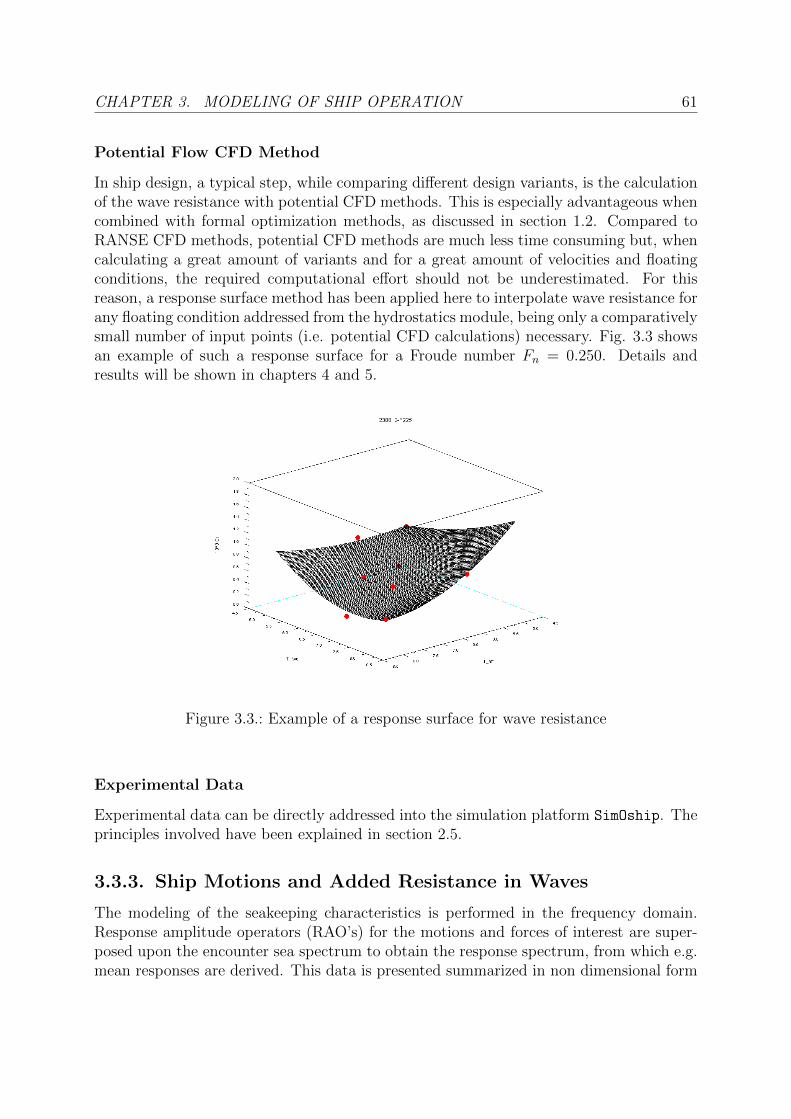
CHAPTER 3. MODELING OF SHIP OPERATION 61
Potential Flow CFD Method
In ship design, a typical step, while comparing different design variants, is the calculationof the wave resistance with potential CFD methods. This is especially advantageous whencombined with formal optimization methods, as discussed in section 1.2. Compared toRANSE CFD methods, potential CFD methods are much less time consuming but, whencalculating a great amount of variants and for a great amount of velocities and floatingconditions, the required computational effort should not be underestimated. For thisreason, a response surface method has been applied here to interpolate wave resistance forany floating condition addressed from the hydrostatics module, being only a comparativelysmall number of input points (i.e. potential CFD calculations) necessary. Fig. 3.3 showsan example of such a response surface for a Froude number Fn = 0.250. Details andresults will be shown in chapters 4 and 5.
Figure 3.3.: Example of a response surface for wave resistance
Experimental Data
Experimental data can be directly addressed into the simulation platform SimOship. Theprinciples involved have been explained in section 2.5.
3.3.3. Ship Motions and Added Resistance in Waves
The modeling of the seakeeping characteristics is performed in the frequency domain.Response amplitude operators (RAO’s) for the motions and forces of interest are super-posed upon the encounter sea spectrum to obtain the response spectrum, from which e.g.mean responses are derived. This data is presented summarized in non dimensional form
62 3.3. SHIP MODEL
considering unitary wave amplitude ζa = 1, re-writing the motions notation as follows:
|η| =|η|ζa
(3.14)
Analogous to this, local motion amplitudes∣∣∣ξ∣∣∣ and local, relative motion amplitudes
∣∣∣ξR∣∣∣will be rewritten in the same form. For the added wave resistance, its dimensionless formis defined:
CAW =RAW
ρ · g · B2
L· ζ2
a
(3.15)
Both the experiments carried out by Kracht in the VWS and the viscous CFD computa-tions have been made only for head seas and regular waves, for different wave lengths andship speeds. This appears to be a suitable solution for saving resources, and an approachto make use of this data is presented here, as applied also by Blume [16]. A discussion onthis approach will be given after its description.
For encounter angles between µ =90◦and µ =180◦, the dimensionless added resistancein waves is assumed as follows [16]:
CAW (ω, µ) = CAW (ω, 180) · cos(180− µ) (3.16)
For encounter angles between 0◦and 90◦, the added wave resistance is taken from striptheory calculations. The heave and pitch motion amplitudes available for head seas fromexperiments or RANS-CFD calculations (|ηhead|) are complemented with data computedusing strip theory (|ηstrip|) for encounter angles between 90◦and 180◦with a squared cosinefunction:
|η3(ω, µ)| = |η3,strip(ω, µ)|+{|η3,head(ω)| − |η3,strip(ω, µ)|
}· cos2(µ) (3.17)
|η5(ω, µ)| = |η5,strip(ω, µ)|+{|η5,head(ω)| − |η5,strip(ω, µ)|
}· cos2(µ) (3.18)
In this form, head seas (µ =180◦) motions correspond to experimental measurements orviscous CFD calculations, with a decreasing influence up to beam seas (µ =90◦), usingfrom this angle until µ =0◦(following seas) the results from strip theory calculationsdirectly.
As it will be explained in chapters 4 and 5, the operational simulations to be undertakenare intended to compare the performance of different bulbous bow variants with verysimilar shapes. Preliminary results of added resistance in waves and motions from striptheory calculations showed practically no sensitivity to the small shape variations betweenbulbous bow variants, which is opposite to the tendency shown by results from moreaccurate methods such as viscous CFD computations or from experiments (a discussionof these results will be given in sect. 4.4.2). For the presented approach, this means thatthe main differences between the seakeeping performance of different bulbous bow variants
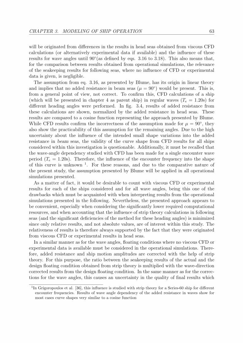
CHAPTER 3. MODELING OF SHIP OPERATION 63
will be originated from differences in the results in head seas obtained from viscous CFDcalculations (or alternatively experimental data if available) and the influence of theseresults for wave angles until 90◦(as defined by eqs. 3.16 to 3.18). This also means that,for the comparison between results obtained from operational simulations, the relevanceof the seakeeping results for following seas, where no influence of CFD or experimentaldata is given, is negligible.
The assumption from eq. 3.16, as presented by Blume, has its origin in linear theoryand implies that no added resistance in beam seas (µ = 90◦) would be present. This is,from a general point of view, not correct. To confirm this, CFD calculations of a ship(which will be presented in chapter 4 as parent ship) in regular waves (Te = 1.20s) fordifferent heading angles were performed. In fig. 3.4, results of added resistance fromthese calculations are shown, normalized by the added resistance in head seas. Theseresults are compared to a cosine function representing the approach presented by Blume.While CFD results confirm the incorrectness of the assumption made for µ = 90◦, theyalso show the practicability of this assumption for the remaining angles. Due to the highuncertainty about the influence of the intended small shape variations into the addedresistance in beam seas, the validity of the curve shape from CFD results for all shipsconsidered within this investigation is questionable. Additionally, it must be recalled thatthe wave-angle dependency studied with CFD has been made for a single encounter waveperiod (Te = 1.20s). Therefore, the influence of the encounter frequency into the shapeof this curve is unknown 1. For these reasons, and due to the comparative nature ofthe present study, the assumption presented by Blume will be applied in all operationalsimulations presented.
As a matter of fact, it would be desirable to count with viscous CFD or experimentalresults for each of the ships considered and for all wave angles, being this one of thedrawbacks which must be acquainted with when interpreting results from the operationalsimulations presented in the following. Nevertheless, the presented approach appears tobe convenient, especially when considering the significantly lower required computationalresources, and when accounting that the influence of strip theory calculations in followingseas (and the significant deficiencies of the method for these heading angles) is minimizedsince only relative results, and not absolute values, are of interest within this study. Therelativeness of results is therefore always supported by the fact that they were originatedfrom viscous CFD or experimental results in head seas.
In a similar manner as for the wave angles, floating conditions where no viscous CFD orexperimental data is available must be considered in the operational simulations. There-fore, added resistance and ship motion amplitudes are corrected with the help of striptheory. For this purpose, the ratio between the seakeeping results of the actual and thedesign floating condition obtained from strip theory is multiplied with the wave-directioncorrected results from the design floating condition. In the same manner as for the correc-tions for the wave angles, this causes an uncertainty in the quality of final results which
1In Grigoropoulos et al. [36], this influence is studied with strip theory for a Series-60 ship for differentencounter frequencies. Results of wave angle dependency of the added resistance in waves show formost cases curve shapes very similar to a cosine function
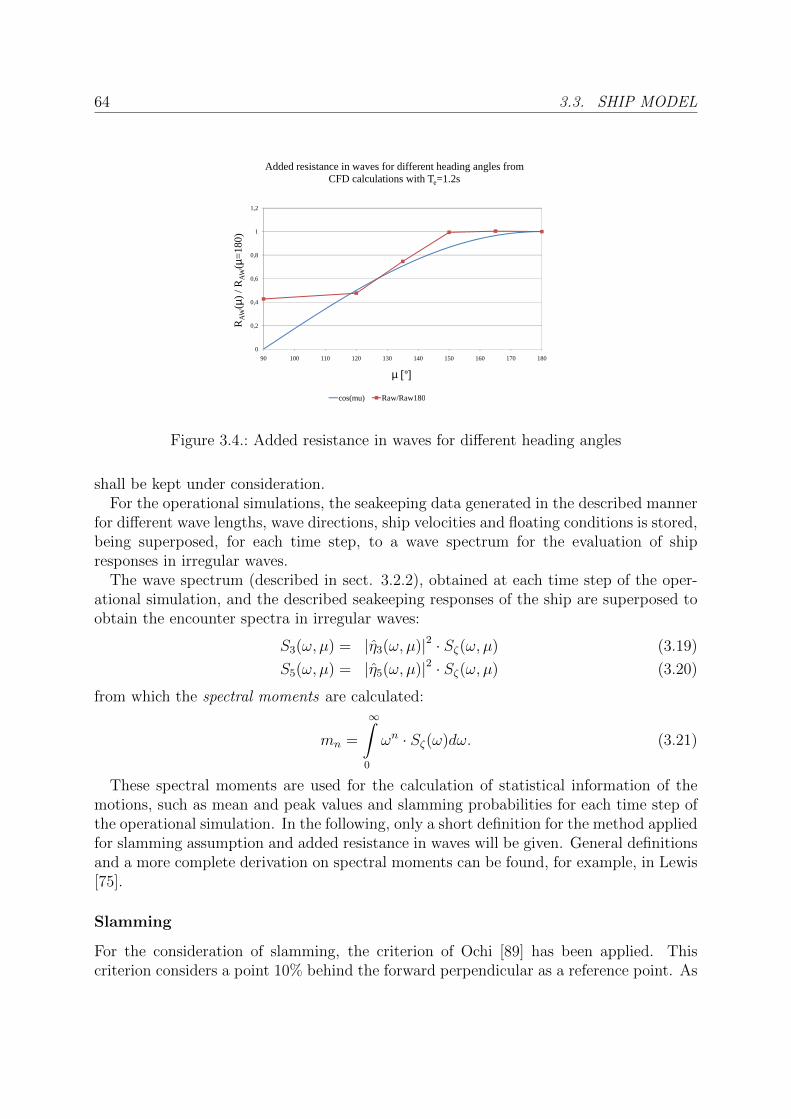
64 3.3. SHIP MODEL
0,6
0,8
1
1,2
AW
(µ=
180)
Added resistance in waves for different heading angles from CFD calculations with Te=1.2s
0
0,2
0,4
0,6
90 100 110 120 130 140 150 160 170 180
RA
W(µ
) / R
AW
µ [°]
cos(mu) Raw/Raw180
Figure 3.4.: Added resistance in waves for different heading angles
shall be kept under consideration.For the operational simulations, the seakeeping data generated in the described manner
for different wave lengths, wave directions, ship velocities and floating conditions is stored,being superposed, for each time step, to a wave spectrum for the evaluation of shipresponses in irregular waves.
The wave spectrum (described in sect. 3.2.2), obtained at each time step of the oper-ational simulation, and the described seakeeping responses of the ship are superposed toobtain the encounter spectra in irregular waves:
S3(ω, µ) = |η3(ω, µ)|2 · Sζ(ω, µ) (3.19)
S5(ω, µ) = |η5(ω, µ)|2 · Sζ(ω, µ) (3.20)
from which the spectral moments are calculated:
mn =
∞∫0
ωn · Sζ(ω)dω. (3.21)
These spectral moments are used for the calculation of statistical information of themotions, such as mean and peak values and slamming probabilities for each time step ofthe operational simulation. In the following, only a short definition for the method appliedfor slamming assumption and added resistance in waves will be given. General definitionsand a more complete derivation on spectral moments can be found, for example, in Lewis[75].
Slamming
For the consideration of slamming, the criterion of Ochi [89] has been applied. Thiscriterion considers a point 10% behind the forward perpendicular as a reference point. As
CHAPTER 3. MODELING OF SHIP OPERATION 65
a first condition for slamming occurrence, emergence of this point must happen. This isthe case when the vertical motion amplitude at this point is greater than the local draftdbow (the use of d for draft instead of T has been selected in this section to avoid confusionwith periods, also defined by T ). The probability of occurrence of such an emergence is:
Pξ,em = exp
{−dbow2
2 ·m0,rb
}(3.22)
where m0,rb represents the 0th spectral moment (n = 0 in eq. 3.21) of the relative verticalmotion at the reference point 10% behind the forward perpendicular of the ship.
The second condition for slamming occurrence is the exceedance of a critical localvelocity at the reference point. Ochi presented in his work a threshold relative velocityof 12 feet per second for a 520 feet ship. In non-dimensional form, this critical relativevelocity writes:
ξbow,cr = 0.0928 ·√g · LPP (3.23)
The probability of occurrence of local relative velocities higher than the critical valueis:
Pξ,cr = exp
{−ξbow,cr
2
2 ·m2,rb
}(3.24)
where m2,rb represents the 2nd spectral moment of the relative motions at the referencepoint at the bow of the ship, which is equal to the 0th spectral moment of the relativevelocity at this point m0,rv.
From these two probabilities, the total slamming probability is defined:
PSlamming = Pξ,crit · Pξ,em (3.25)
= exp
{−dbow2
2 ·m0,rb
+−ξbow,cr
2
2 ·m2,rb
}(3.26)
Additionally, the slamming events per hour
NSlamming =3600
T0,rb
· PSlamming (3.27)
can be obtained with a zero-upcrossing period:
T0,rb = 2π
√m0,rb
m2,rb
(3.28)
Added Resistance in Irregular Waves
The mean added resistance in irregular waves RAW for a given wave spectrum Sζ iscalculated from:
RAW = 2
∞∫0
Sζ(ω) ·RAW (ω)dω (3.29)
with RAW in regular waves obtained from CFD computations or experimental data com-bined with strip theory results, as previously explained.
66 3.3. SHIP MODEL
3.3.4. Total Resistance, Propulsion and Machinery
The total ship resistance in service conditions RTS is modeled as:
RTS = RTS0 +RAW +RAA + ∆RAR (3.30)
with total ship resistance in calm waters RTS0, added resistance in waves RAW , windresistance RAA, and increased roughness resistance ∆RAR (considering fouling). Shipresistance in calm waters and added resistance in waves are available from experiments ornumerical flow simulations (CFD) as described in sections 3.3.2 and 3.3.3, wind resistanceis calculated using the Wilson drag coefficients (in [75]) and fouling resistance is estimatedusing a fouling diagram for a five year period provided by International Marine Co. [5]for a self polishing copolymer coating2. Other resistance components, as mentioned insection 2.5, have not been considered for the simulations, since they are constants andnot of interest for comparative purposes.
The propulsion of the ship is modeled according to the ITTC 1978 recommended proce-dures [55] using an open water diagram for the full-scale propeller and considering thrustidentity. For this purpose, model data for resistance (resistance model test), propellercharacteristics (open water mode test) and propulsion (self-propulsion test) should beavailable. If this is not the case, appropriate estimations can be made.
For the open water diagram, propeller thrust T and torque Q are represented in dimen-sionless form:
KT =T
ρn2D4(3.31)
KQ =Q
ρn2D5(3.32)
and are plotted over the propeller advance velocity J :
J =VAnD
(3.33)
where ρ is the water density, n the propeller rate of revolutions, D the propeller diameterand VA the advance speed of the propeller. An example of such an open water diagram isshown in fig. 3.5. The correlation between model- and full-scale is made as recommendedby the mentioned procedure (ITTC 1978). The working point of the propeller is founddefining:
KT
J2=
RTS
(1− t) · (1− weS)2 · V 2SD
2ρ(3.34)
with RTS from eq. 3.30, the thrust deduction factor t from a thrust variation test (oralternatively as recommended by ITTC 1978 [55]) and the effective wake fraction of the
2The choice of this coating is arbitrary and represents a typical modern, TBT-free antifouling coating.The data presented by International Marine Co. originates from the monitoring of over 70.000 shipsand over 30 years

CHAPTER 3. MODELING OF SHIP OPERATION 67
ship weS from the full-scale corrections of the effective wake fraction of the model (weM) asrecommended by the ITTC 1978 procedure. A detailed description of the involved modeltest procedures and detailed definitions about the mentioned propulsive factors (thrustdeduction and wake factors) have been amply discussed in several textbooks (e.g. Kracht[70]) and will not be discussed here.
When multiplying the resultant term of eq. 3.34 with the range of J2, a curve for therequired thrust is obtained. The intersection of this curve with the thrust coefficient curveKT shows the propeller working point. An example is outlined in fig. 3.5. For this workingpoint, the required propeller torque coefficient KQS, the open water efficiency η0S andadvance ratio JS are obtained. From these, and considering the relative rotative efficiencyηR as known (assuming thrust identity and available open water and self-propulsion tests),the propeller rate of revolutions,
n =VS(1− weS)
JSDS
(3.35)
the delivered power,
PD = 2πρn3D5KQSB
ηR(3.36)
and the engine brake power by considering a given mechanical efficiency ηM
PB =PDηM
(3.37)
are obtained and can be taken as input for the engine operation diagram.The main engine characteristic is defined by an engine layout diagram. In this diagram,
the engine manufacturer defines the power and speed combination points L1, L2, L3 andL4. Additionally, the specific fuel oil consumption sfoc is given for each layout point. Fromthese points, several lines are defined, which themselves define the permitted operationarea of the main engine and conform the engine layout diagram. An exemplar enginelayout diagram is shown in figure 3.6. According to the marine engine manufacturerMAN B&W [78], the main engine can be thus defined by following lines:
• an engine overload line, caused by the limited achievable charge pressure of theturbo compressor at lower rates of revolutions. This line is also known as “turbobound” and is approximately proportional to the square of the rate of revolutionsn.
• a line between layout points L1 and L3 defining the maximum mean effective pressure(mep) allowable for continuous operation.
• a line between layout points L2 and L4 defining a constant mean effective pres-sure (values vary depending of the engine). This line is used as an orientation forthe choice of the engine [78], being engine operation below and above this line al-lowed. This line also represents approximately the region with lowest specific fueloil consumption of the engine.
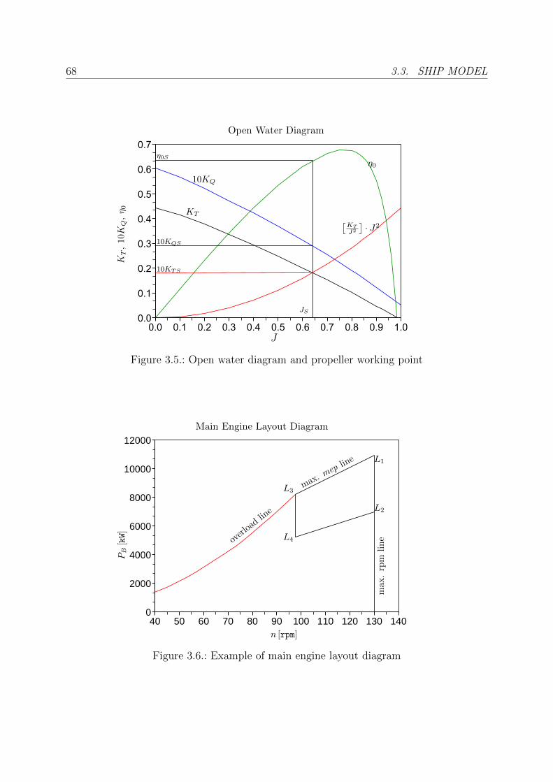
68 3.3. SHIP MODEL
! !" !# !$ !% !& !' !( !) !* "!
!
!"
!#
!$
!%
!&
!'
!(
Open Water Diagram
J
JS
KT,
10K
Q,η 0
η0
[KT
J2
]· J2
10KQ
10KQS
10KTS
η0S
KT
Figure 3.5.: Open water diagram and propeller working point
40 50 60 70 80 90 100 110 120 130 1400
2000
4000
6000
8000
10000
12000
Main Engine Layout Diagram
n [rpm]
PB
[kW]
L1
L2
L3
L4over
load
line
max
.rp
mli
ne
max. mep
line
Figure 3.6.: Example of main engine layout diagram

CHAPTER 3. MODELING OF SHIP OPERATION 69
• a maximum rate of revolutions line (100% to 105% of max. rpm)
Entering the brake power from eq. 3.37 with the corresponding rate of revolutions in theengine layout diagram, the feasibility of the attempted working point can be controlled.Subsequently, the specific fuel oil consumption can be obtained from the manufacturer(normally as function of the mean effective pressure mep) and at last, the fuel oil con-sumption for a time period ∆t can be obtained:
FOC = PB ·∆t · sfoc (3.38)
This fuel oil consumption is, within the simulations, added over the total simulation timeto obtain the fuel oil consumption during the total time period.
3.4. Measure of Merit
To compare different design variants within a design study, and especially for optimizationpurposes, a measure of merit must be defined. This measure of merit must identify clearlythe aspect to be compared between all variants simulated. In most of the cases, the directcomparison of economic profit is a very suitable measure of merit when enough reliableand detailed information of all aspects involved is available. If this is not the case, atypical established economic measure of merit can be used. Most of these measures ofmerit define the average annual costs AAC (normally in US$) as follows:
AAC = CF + CO + CR · P (3.39)
where CF are the annual fuel costs, CO are the annual fixed operating costs and CR · Pthe annual capital costs, defined themselves by the capital recovery factor CR and theinvested capital P in US$. A widespread exponent of an economic measure of merit isthe required freight rate RFR:
RFR =AAC
MC=CF + CO + CR · P
kc ·WPL ·D(3.40)
where MC is the annual transport volume (in tons-nmi per year), kc is a service factorfor the cargo (i.e. ratio of mean transported cargo to design payload), WPL the designpayload (in t) and D the covered distance per year (in nmi). For further information seee.g Nowacki (1985, [85]).
For this study, a comparative measure would be of special interest, to identify differencesbetween the bulbous bow variants for each region and scaling factor investigated, as it willbe described in chapters 4 and 5. For this purpose, ships will be compared within groups.A group is a set of ships of similar characteristics (e.g. different bulbous bow variants butequal main dimensions) and normally covering the same route. This reflects the typicalevaluation made by shipping companies when deciding between different variants, vendorsor concepts for a transport task.
70 3.4. MEASURE OF MERIT
For this purpose, a fuel equivalent cost FEC will be defined, i.e. a measure of economicmerit relatively comparable to annual fuel costs. In this approach, only fuel oil costs areconsidered as variable, while all other operating and capital costs remain equal (for shipsof the same group, e.g. same size). This is expressed in terms of an assumed relationshipbetween the mean fuel costs within a group and the average annual costs valid for eachship of this group. This relationship is expressed by a fuel costs coefficient kf as follows:
CFmean = kf · AAC (3.41)
Applying this fuel costs coefficient into eq. 3.40, it can be written:
RFR =CFS +
1−kfkf· CFmean
MCS(3.42)
where CFS are the annual fuel oil costs of the ship (in US$), CFmean the average fuel oilcosts of all ships of the group considered (in US$) and MCS the annual transport volumeof the ship (in t-nmi/year). The value of kf , viz., the relationship between fuel costs andaverage annual costs is of special interest and depends on many parameters, especially offuel prices and global economy and must be set according to realistic shipping costs. Adetailed discussion about shipping costs can be found in Buxton [20]. Additionally, differ-ent scenarios with different values for kf can be studied and thus establish a profitabilityrange (a discussion on this aspect will be given for an application case in sect. 4.6.3 ,p.96). In this study, the input of realistic values for kf is attempted by means of simpleestimations and actual fuel prices.
The different annual transport volume MCS of each ship within a group also plays animportant role. A ship being able to achieve a higher mean speed can, at least theoret-ically, complete more voyages per year increasing its transport capacity. Alternatively,this ship can decrease its mean speed and thus save considerable fuel costs3. Taking eq.3.40 and decomposing the fixed costs component (CO+CR·P
MCS) into a component which is
common to all ships and a difference value, the required freight rate can be rewritten:
RFR =
{CF
MC
}S
+ {CO + CR · P}[
1
MCmean+ δ
1
MCS
](3.43)
The fuel equivalent costs attempt to consider all costs which are not common for eachship within a group and are defined as:
FEC =
{AAC
MC
}S
−{CO + CR · P
MC
}mean
=
{CF
MC
}S
+
{δCO + CR · P
MC
}S
(3.44)
In this form, fuel equivalent costs show the fuel costs of the ship and the costs differencedue to the different transport efficiency of the ship and the mean transport efficiency valuefor the group. All values represent the costs of the transportation of one tonne cargo over
3A short discussion on this task for an application case is given in section 4.6.4 “Slow Steaming Simu-lations”

CHAPTER 3. MODELING OF SHIP OPERATION 71
a nautical mile. If WPL and kc as defined in eq. 3.40 are equal for all ships, FEC can berewritten as:
FEC =
[CFSDS
+1− kfkf
· CFmean{
1
DS
− 1
Dmean
}]· 1
kc ·WPL
(3.45)
The second summand can be thus interpreted as “penalty costs” due to less navigatedmiles or alternatively “cost savings” due to more navigated miles. The most importantadvantage of this definition, compared to RFR, is that the magnitude of the value remainssimilar to pure fuel costs (per mile and cargo tonne), being able to be easily compared tothese. Additionally, no information about capital or further operational costs is needed.Since fuel prices are always known and fuel consumption (e.g. per year) is often cal-culated during ship design, the described fuel equivalent costs per mile and tonne canbe advantageous for comparison purposes, despite the slightly higher complexity of itsdefinition.
3.5. Implementation of the Simulation Platform
The presented components modeling the ship operaion have been implemented into theprogram SimOship by means of the SciLab interpreted language. SciLab [7] is an opensource project and the language attempts an easy handling of complex matricial oper-ations, including several pre-implemented functions for this purpose. The implementa-tion of SimOship was started for the simulation of the operation of wind assisted ships(Tampier [109]), and has been applied successfully for different purposes within several de-gree theses (Geittner [31], Oschmann [93], Balloch [10]) under the guidance of the author.The main characteristics of the implemented simulation environment are:
• Easy usability (both for the programmer and the end-user). This is centered in twofeatures: a graphical user interface (GUI) and the ability to be run fully automatizedby scripts.
• Modular. Functions are generalized and usable for and from any other modules orprograms
• Strict separation between code and simulation data. This means, the program canbe used for any ship, in any region of the world and any simulation time. It is notconstrained to the performed examples nor code modifications have to be undertakento simulate new cases.
• Flexible. Several data import functionalities have been implemented, speciallyfor the geometry (offsets as generated by DelftShip or NAPA), for hydrodynamicdata (e.g. PDSTRIP-Import) and for weather data from the ECMWF (grib- andnc-data).
72 3.5. IMPLEMENTATION OF THE SIMULATION PLATFORM
• Optimized. When possible, code has been optimized in order to reduce computa-tional time (iterations, interpolations, file operations have been conveniently imple-mented for this purpose).
• Open. Chosen modules have been contributed to other projects (e.g. Scilab,PDSTRIP) as Open Source Code.
Briefly described, the program simulates the operation of merchant ships from the infor-mation collected in a case (case file), which declares further files which describe all aspectsof the two main components of the simulation: a ship and an environment. These filescontain information about ship geometry, hydrostatics, resistance, propeller, seakeeping,machinery but also environment information about the route, cargo and weather, amongothers. A complete description can be found in the program manual (SimOship - Gen-eral Description and Usage) [108]. The full program structure is depicted in fig. 3.7.From the structure of the program, four important tasks will be described in more detail:Preprocessing, Simulation modes, Trip evaluation and Time step evaluations.
Preprocessing
The preprocessing for each simulation case (marked in yellow in fig. 3.7) consists ofthe collection of all necessary information for the execution of an operational simulation.This includes the previously mentioned descriptions of ship and environment, includingthe possibility of feasibility checks (e.g. cargo check for realistic floating conditions). Allsteps within preprocessing are done with a graphical user interface (GUI).
Simulation Modes
The simulations can be realized in four different modes (marked in pale red in fig. 3.7),as it will be shown for the application cases in chapters 4 and 5:
• Full simulation mode: for simulations with variable speed and variable floatingcondition
• Fixed trim simulation mode: for simulations with variable speed but fixed floatingcondition
• Target speed simulation mode: full or fixed simulations where speed is adjusteddynamically to achieve a target mean speed over the simulation time
• Simple simulation mode: for simulations with fixed service speed and fixed floatingcondition.
Operational Simulation
For the given time period, the ship undertakes the programmed trips repeatedly (thistrips can be also combinations of different routes or round-trips) including, if needed,
CHAPTER 3. MODELING OF SHIP OPERATION 73
port and/or dock time periods. For each trip, following steps are realized (marked in palepurple in fig. 3.7):
• Processing of route, departure time and estimated time of arrival
• Loading of given cargo, re-filling of tanks if required and calculation of resultingfloating condition
• Determination of the hydrodynamic characteristics of the ship in the departurefloating condition (by means of response surfaces, interpolation or look-up tables)
• Operational simulation of the trip
Time Step Evaluations
For each time step of the operational simulation, following tasks are considered (markedin pale grey in fig. 3.7):
• Local weather conditions according to sect. 3.2.2
• Calculation of ship responses, total resistance and propulsion characteristics accord-ing to sect. 3.3.4
• Feasibility check leading to voluntary or involuntary speed loss and the repetitionof the previous tasks until a feasible condition is reached
Post-processing
Results can be processed for a single ship (e.g. total fuel consumption, mean servicespeed, encounter weather) or compared with other ships (e.g. FEC for several designvariants). Results for the application cases will be shown in detail in chapters 4 and 5.
3.5.1. Integration and Automatization for Design Purposes
A central feature of the presented implementation and the underlying design methodologyis a high automatization grade, intending to make design studies with a large number ofdesign variants possible and, if required, the application of formal optimization techniques.Especially the integration of the presented simulation environment into an optimizationprocess including automatic geometry generation, automatically executed numerical flowcalculations (CFD) and automatic full data analysis are mayor issues which were notpossible to realize. Notwithstanding to this, all steps were conceived in order to do so inthe future, in case of further studies applying the proposed methodology. The lack of fullautomatization is justified by following aspects:
• Since many methodologies had to be coordinated to work together for a first time,the error probability in single steps is very high. A rigorous control of all datafluxes, intermediate results and programming issues (mainly code optimization anddebugging) was imperative.

74 3.5. IMPLEMENTATION OF THE SIMULATION PLATFORM
Fleet postprocessing
Ship data postprocessingand statistical analysis
SimOship
0.12
RunFull
RunTrimFixed
RunTargetVs
RunSimple
Route
Time/Datum processing
Cargo database
Seakeeping database
Route Evaluation
GUI
SCRIPT
igs2geo
Open geometry
Geometry transformation
Hydrostatics
Propeller
Create resistance data
Create seakeeping data
PDSTRIP input
Wind
Waves
Seakeeping
Ship machine
Create route
World map call
Route penalty
Route change
Main engine check
Open seakeeping file
Write logs
Ship resistance
Route feasibility
Response surface
Holtrop
For each time step
For each trip
Preprocessing
Cargo check
Simulation modes
Figure 3.7.: SimOShip 0.12 Program Structure
• The parametric model used for the creation of subvariants has been kept very simpleand does not include any surface quality control mechanism. For this reason, themanual control of each subvariant generated was necessary.
• One of the goals of this investigation was to use a minimum of proprietary soft-ware. This was successfully achieved, with the drawback of a higher implementa-tion effort for different format or data converters and (small) software limitations.Some of these tools would have required further refinement to be able to work ina fully automatic mode. A major issue in this context was the implementation ofTUBsixDOFFoam.
CHAPTER 4. SPECIAL APPLICATION CASE 75
4. Special Application CaseExploiting Experimental Data
4.1. Introduction
In this chapter, the application of operational simulations is shown by means of a practicalexample. This example - the simulation of the operational life of a ship - makes useof available experimental data to model seakeeping performance (motions and addedresistance) and calm water resistance of the ship in question.
From a general point of view, the ship operation model presented in the previous chap-ter, intended to simulate the operational life of a merchant vessel, can be applied recallingdata from any available source. Keeping in mind that, in a preliminary design stage, ex-perimental data is rarely available, the example presented in this chapter represents therather unusual case of some experimental data being available.
Since the application of operational simulations in the manner as it is presented in thisstudy is not a widespread technique yet, it has been considered convenient to discusssome detail aspects about these operational simulations with the help of an example casewhere relevant hydrodynamic data relies on experiments. Since the uncertainty of thosecentral hydrodynamic aspects is minimal (at least when compared to numerical data),they can be excluded from the discussion about the presented simulational approachesthemselves (i.e. the simulation modes presented in sect. 3.5). This special applicationcase is therefore intended to discuss about aspects of the operational simulations morethan about the results of each of the studied design variants and the consequences of theapplication of this methodology for the design of bulbous bows. These aspects, of centralmeaning for the outcome of this investigation, are discussed in chapter 5, where a generalapplication case, recalling numerical data only and thus representing the usual situationof no experimental data being available, is presented. Since some of the operationalsimulations presented in this chapter have been performed with experimental data bothfor seakeeping and ship resistance, results will serve also as a validation for further resultsfrom operational simulations where numerical results are addressed partially or totally.
The presented application case will make use of the experimental data provided bythe investigation of Kracht [68]. This dataset, which can be recalled as model data, isextrapolated with different scaling factors λ and simulations are executed for differentroutes over a given time period. For all simulations undertaken within this study, asimulation period of five years was chosen, considering it as statistically representativefor the operational life of the ship. This decision was made after comparing the resultsfrom simulations over one, two, five and ten years of duration, showing that simulations
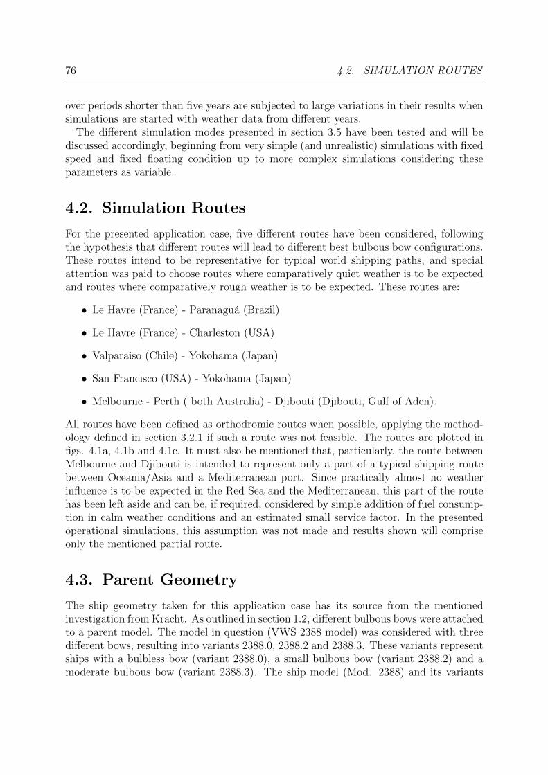
76 4.2. SIMULATION ROUTES
over periods shorter than five years are subjected to large variations in their results whensimulations are started with weather data from different years.
The different simulation modes presented in section 3.5 have been tested and will bediscussed accordingly, beginning from very simple (and unrealistic) simulations with fixedspeed and fixed floating condition up to more complex simulations considering theseparameters as variable.
4.2. Simulation Routes
For the presented application case, five different routes have been considered, followingthe hypothesis that different routes will lead to different best bulbous bow configurations.These routes intend to be representative for typical world shipping paths, and specialattention was paid to choose routes where comparatively quiet weather is to be expectedand routes where comparatively rough weather is to be expected. These routes are:
• Le Havre (France) - Paranagua (Brazil)
• Le Havre (France) - Charleston (USA)
• Valparaiso (Chile) - Yokohama (Japan)
• San Francisco (USA) - Yokohama (Japan)
• Melbourne - Perth ( both Australia) - Djibouti (Djibouti, Gulf of Aden).
All routes have been defined as orthodromic routes when possible, applying the method-ology defined in section 3.2.1 if such a route was not feasible. The routes are plotted infigs. 4.1a, 4.1b and 4.1c. It must also be mentioned that, particularly, the route betweenMelbourne and Djibouti is intended to represent only a part of a typical shipping routebetween Oceania/Asia and a Mediterranean port. Since practically almost no weatherinfluence is to be expected in the Red Sea and the Mediterranean, this part of the routehas been left aside and can be, if required, considered by simple addition of fuel consump-tion in calm weather conditions and an estimated small service factor. In the presentedoperational simulations, this assumption was not made and results shown will compriseonly the mentioned partial route.
4.3. Parent Geometry
The ship geometry taken for this application case has its source from the mentionedinvestigation from Kracht. As outlined in section 1.2, different bulbous bows were attachedto a parent model. The model in question (VWS 2388 model) was considered with threedifferent bows, resulting into variants 2388.0, 2388.2 and 2388.3. These variants representships with a bulbless bow (variant 2388.0), a small bulbous bow (variant 2388.2) and amoderate bulbous bow (variant 2388.3). The ship model (Mod. 2388) and its variants
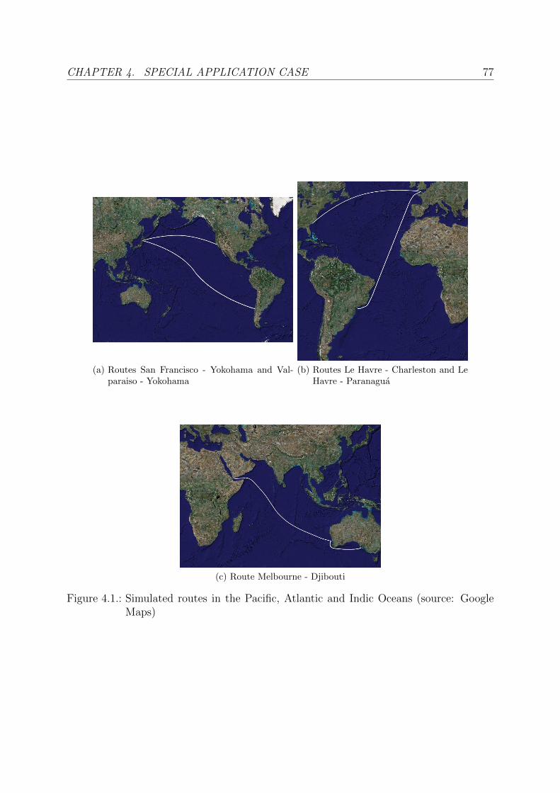
CHAPTER 4. SPECIAL APPLICATION CASE 77
(a) Routes San Francisco - Yokohama and Val-paraiso - Yokohama
(b) Routes Le Havre - Charleston and LeHavre - Paranagua
(c) Route Melbourne - Djibouti
Figure 4.1.: Simulated routes in the Pacific, Atlantic and Indic Oceans (source: GoogleMaps)

78 4.3. PARENT GEOMETRY
Model: 2388Variant: 0 2 3LPP (m) 5.8500B (m) 0.9750T (m) 0.3250LWL (m) 5.7506 5.7769 5.7792LOS (m) 5.7506 5.9256 6.0076STotal (m2) 6.6391 6.7825 6.8548∇ (m3) 1.1690 1.1786 1.1866cB (-) 0.6306 0.6358 0.6401cP (-) 0.6454 0.6507 0.6551cWP (-) 0.7218 0.7224 0.7236
bulbous bow parameters:cABT (-) - 0.0768 0.1251cABL (-) - 0.0947 0.1610c∇PR (-) - 0.1945 0.4908cLPR (-) - 0.0260 0.0401cBB (-) - 0.1327 0.1754cZB (-) - 0.6129 0.5720
Table 4.1.: Main dimensions of investigated ships in model scale
were designed for investigation purposes only, and should represent a fast cargo linerof the 1970’s decade. The bulbless variant 2388.0, considered as parent model withinKracht’s investigation, will be considered here only for comparison purposes and it willbe shown, already in early results, that such a variant is economically not viable forany operational profile. For this reason, model 2388.2 (moderate bulb) will be used hereas parent geometry for all comparisons and results throughout this work. Additionally,further subvariants will be generated from variant 2388.2 later, as it will be outlined inthe next chapter (chap. 5). In table 4.1, the main particulars and the bulbous bowparameters of the variants are shown. The meaning of the bulbous bow parameters issketched in table 4.2. Figures 4.2, 4.3 and 4.4 show the ship’s lines of the consideredvariants.
Within the investigations of Kracht, a (fictive) scaling factor of λ = 25 was chosen torepresent a full scale ship. For the operational simulations presented here, different shipswere “designed” from model scale and variants with different (fictive) scaling factors werecreated. In this way, the model, initially with a scaling factor of λ = 25, was scaled alsofor three further factors λ = 17, 33, 50, as to obtain an idea of the influence of ship sizeinto the results obtained from operational simulations. The considered scaling factorswere chosen to address similar main dimensions of typical categories of actual containerships. Nevertheless, these ships are not intended to represent exactly modern ships, butthey can be useful for orientation purposes. The classification of the differently scaledships into typical container ship classes together with a selection of main parameters is

CHAPTER 4. SPECIAL APPLICATION CASE 79
Breadth parameter cBB = BB
BMS
Length parameter cLPR = LPR
LPP
Depth parameter cZB = zBTFP
Cross area parameter cABT = ABT
AMS
Length area parameter cABL = ABL
AMS
Volumetric parameter c∇PR = ∇PR
∇WL
Table 4.2.: Dimensionless bulbous bow parameters as defined by Kracht [67]
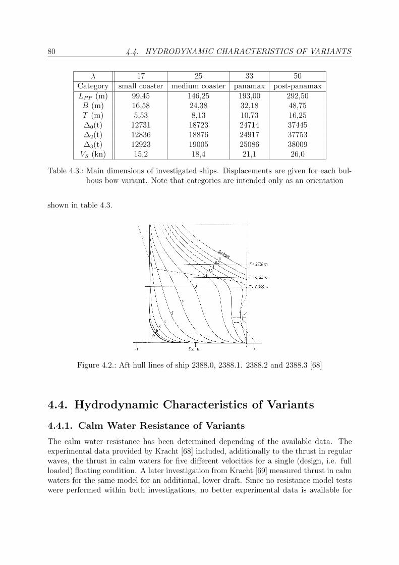
80 4.4. HYDRODYNAMIC CHARACTERISTICS OF VARIANTS
λ 17 25 33 50Category small coaster medium coaster panamax post-panamaxLPP (m) 99,45 146,25 193,00 292,50B (m) 16,58 24,38 32,18 48,75T (m) 5,53 8,13 10,73 16,25∆0(t) 12731 18723 24714 37445∆2(t) 12836 18876 24917 37753∆3(t) 12923 19005 25086 38009VS (kn) 15,2 18,4 21,1 26,0
Table 4.3.: Main dimensions of investigated ships. Displacements are given for each bul-bous bow variant. Note that categories are intended only as an orientation
shown in table 4.3.
Figure 4.2.: Aft hull lines of ship 2388.0, 2388.1. 2388.2 and 2388.3 [68]
4.4. Hydrodynamic Characteristics of Variants
4.4.1. Calm Water Resistance of Variants
The calm water resistance has been determined depending of the available data. Theexperimental data provided by Kracht [68] included, additionally to the thrust in regularwaves, the thrust in calm waters for five different velocities for a single (design, i.e. fullloaded) floating condition. A later investigation from Kracht [69] measured thrust in calmwaters for the same model for an additional, lower draft. Since no resistance model testswere performed within both investigations, no better experimental data is available for
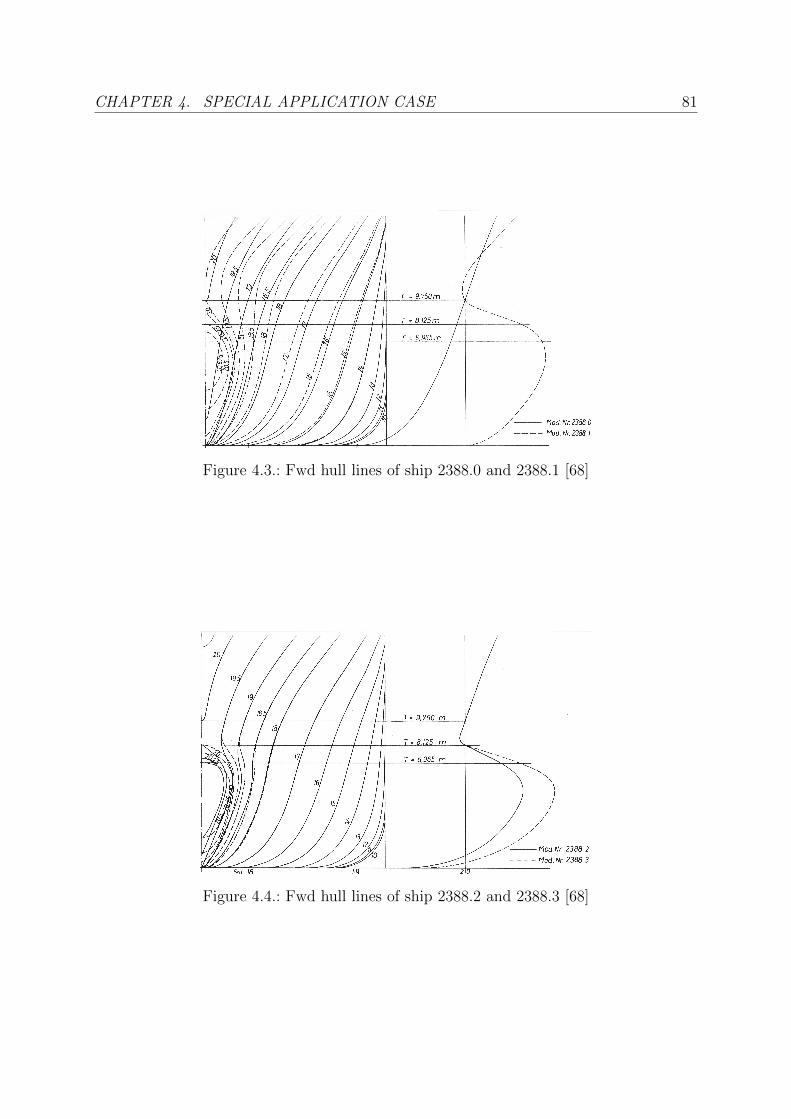
CHAPTER 4. SPECIAL APPLICATION CASE 81
Figure 4.3.: Fwd hull lines of ship 2388.0 and 2388.1 [68]
Figure 4.4.: Fwd hull lines of ship 2388.2 and 2388.3 [68]

82 4.4. HYDRODYNAMIC CHARACTERISTICS OF VARIANTS
this purpose. A thrust deduction factor t must be thus estimated to obtain a total modelresistance in the form:
RTM = (1− t) TM (4.1)
According to the estimation formula of Holtrop [50] a thrust deduction factor t = 0.19was estimated for all models. Regardless of the statements of Kracht [66] and Schneekluth[102], remarking that a bulbous bow can induce changes in the propulsive factors (effectivewake we and thrust deduction t), this influence was left consequently aside to reduce thenumber of variables affecting directly the final results. This experimental data will be usedfor all simulations where only one floating condition was considered. For all consideredscaling factors (λ = 17, 25, 33, 50), the resistance is extrapolated according to section 2.5.2and recalled within the simulations.
As introduced in section 4.3, variant 2388.2 will be used as parent geometry throughoutthis work. Consequently, all diagrams with simulation results will be normalized bydividing actual values by the parent values. Figure 4.5 shows such normalized results forthe total fuel oil consumption in calm water at Fn = 0.250 for all three variants and allfour scaling factors. This figure will serve as comparison with further simulation results.It shall be noticed that the increase in the differences between the variants for largerscaling factors is simply originated by the lower viscous resistance fraction due to thehigher Reynolds numbers.
15 20 25 30 35 40 45 50 5594
96
98
100
102
104
106
108
Fuel Oil Consumption in Calm Waters
λ
+ 2388.2
5 2388.3
u 2388.0
FOC
FOC
2388.2·1
00
Figure 4.5.: Relative fuel consumption in calm waters
For certain operational simulations, the calm water resistance for additional floatingconditions was required. Each floating condition is labeled in the form Tab, with a in-dexing the aft perpendicular draft and b the forward perpendicular draft. These indexesare summarized, for the different scaling factors, in table 4.4. Table 4.5 summarizes theresulting trim angles for each combination of floating condition indexes a and b. The
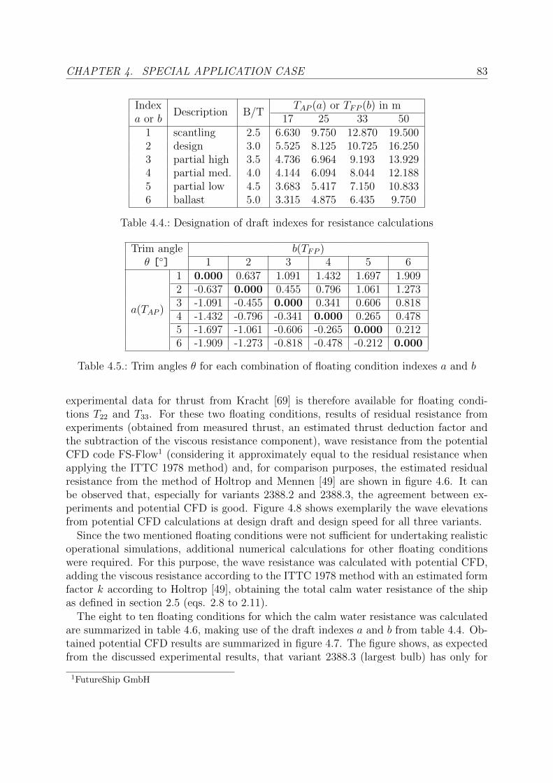
CHAPTER 4. SPECIAL APPLICATION CASE 83
IndexDescription B/T
TAP (a) or TFP (b) in ma or b 17 25 33 50
1 scantling 2.5 6.630 9.750 12.870 19.5002 design 3.0 5.525 8.125 10.725 16.2503 partial high 3.5 4.736 6.964 9.193 13.9294 partial med. 4.0 4.144 6.094 8.044 12.1885 partial low 4.5 3.683 5.417 7.150 10.8336 ballast 5.0 3.315 4.875 6.435 9.750
Table 4.4.: Designation of draft indexes for resistance calculations
Trim angle b(TFP )θ [◦] 1 2 3 4 5 6
a(TAP )
1 0.000 0.637 1.091 1.432 1.697 1.9092 -0.637 0.000 0.455 0.796 1.061 1.2733 -1.091 -0.455 0.000 0.341 0.606 0.8184 -1.432 -0.796 -0.341 0.000 0.265 0.4785 -1.697 -1.061 -0.606 -0.265 0.000 0.2126 -1.909 -1.273 -0.818 -0.478 -0.212 0.000
Table 4.5.: Trim angles θ for each combination of floating condition indexes a and b
experimental data for thrust from Kracht [69] is therefore available for floating condi-tions T22 and T33. For these two floating conditions, results of residual resistance fromexperiments (obtained from measured thrust, an estimated thrust deduction factor andthe subtraction of the viscous resistance component), wave resistance from the potentialCFD code FS-Flow1 (considering it approximately equal to the residual resistance whenapplying the ITTC 1978 method) and, for comparison purposes, the estimated residualresistance from the method of Holtrop and Mennen [49] are shown in figure 4.6. It canbe observed that, especially for variants 2388.2 and 2388.3, the agreement between ex-periments and potential CFD is good. Figure 4.8 shows exemplarily the wave elevationsfrom potential CFD calculations at design draft and design speed for all three variants.
Since the two mentioned floating conditions were not sufficient for undertaking realisticoperational simulations, additional numerical calculations for other floating conditionswere required. For this purpose, the wave resistance was calculated with potential CFD,adding the viscous resistance according to the ITTC 1978 method with an estimated formfactor k according to Holtrop [49], obtaining the total calm water resistance of the shipas defined in section 2.5 (eqs. 2.8 to 2.11).
The eight to ten floating conditions for which the calm water resistance was calculatedare summarized in table 4.6, making use of the draft indexes a and b from table 4.4. Ob-tained potential CFD results are summarized in figure 4.7. The figure shows, as expectedfrom the discussed experimental results, that variant 2388.3 (largest bulb) has only for
1FutureShip GmbH

84 4.4. HYDRODYNAMIC CHARACTERISTICS OF VARIANTS
b(TFP )1 2 3 4 5 6
a(TAP )
12 x x *3 x x *4 x x x56 x
Table 4.6.: Selection of floating conditions for potential CFD wave resistance calculations(fields marked with * for Fn = 0.250 only)
the design draft T22 and the higher velocities (eq. to Fn = 0.225 and 0.250) a lower waveresistance. For lower drafts (e.g. T34, T46 or T66), significant differences between bothbulbous bows can be observed.
Instead of limiting the simulations to the calculated floating conditions, a more gen-eralized and flexible handling is obtained by determining response surfaces by regression(least square fit) methods. For each calculated velocity, a response surface is defined asa function of aft and forward drafts TAP and TFP , providing the wave resistance coeffi-cient for any floating condition as a polynomial surface. Consequently, the error of thisapproach outside the bounds of the calculated floating conditions must be acquaintedand handled with care. A description of the exact coefficients and response surfaces willbe given in appendix B, figs. B.1, B.2 and B.3 and table B.1. In table B.1, the waveresistance coefficients CW shown in figure 4.7 are presented in tabular form.
4.4.2. Seakeeping and Added Resistance in Waves of Variants
The simulations discussed in this chapter will recall the ship responses and the addedresistance in waves as described in section 3.3.3 using the head seas data from the exper-iments undertaken by Kracht. As previously mentioned, the results of the experimentsare available for a single floating condition and different velocities. The added resistancesin regular waves for the three variants studied are shown in figure 4.9 for different Froudenumbers.
In order to complement results in head seas from experiments, strip theory calculationswere made for the remaining heading angles, velocities and floating conditions2. Fig-ure 4.10 compares added resistance from strip theory (calculated with the implementedmethod of Gerritsma and Beukelmann in PDSTRIP) with experimental data in headseas. The figure states evidently the previously discussed non-suitability of strip theoryto compare such similar variants (see sect. 3.3.3). This lies to a great extent in theinherent limitations of the linearity assumption of strip theory and in the limitations ofthe implemented method of Gerritsma and Beukelmann (both discussed in section 2.6.2)
2this approach will be applied in the same manner in the next chapter, complementing results in headseas from viscous CFD computations
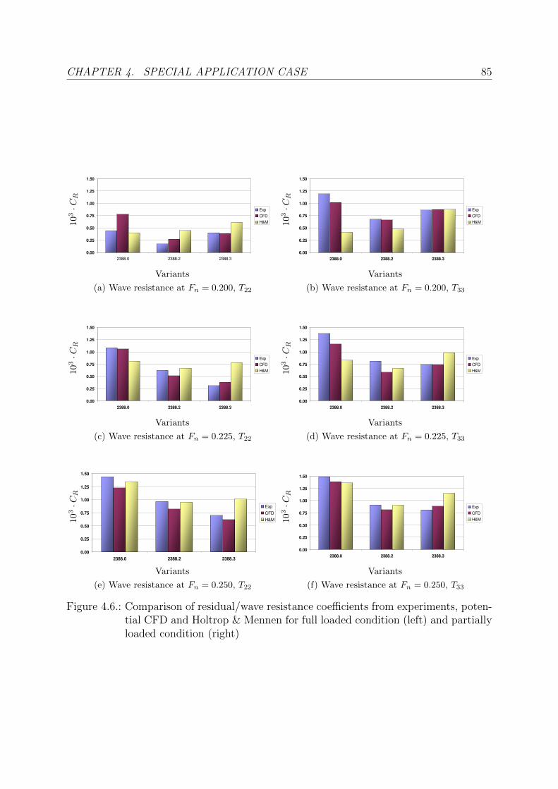
CHAPTER 4. SPECIAL APPLICATION CASE 85
0.00
0.25
0.50
0.75
1.00
1.25
1.50
2388.0 2388.2 2388.3
Exp
CFD
H&M
Variants
103·C
R
(a) Wave resistance at Fn = 0.200, T22
0.00
0.25
0.50
0.75
1.00
1.25
1.50
2388.0 2388.2 2388.3
Exp
CFD
H&M
Variants103·C
R(b) Wave resistance at Fn = 0.200, T33
0.00
0.25
0.50
0.75
1.00
1.25
1.50
2388.0 2388.2 2388.3
Exp
CFD
H&M
Variants
103·C
R
(c) Wave resistance at Fn = 0.225, T22
0.00
0.25
0.50
0.75
1.00
1.25
1.50
2388.0 2388.2 2388.3
Exp
CFD
H&M
Variants
103·C
R
(d) Wave resistance at Fn = 0.225, T33
0.00
0.25
0.50
0.75
1.00
1.25
1.50
2388.0 2388.2 2388.3
Exp
CFD
H&M
Variants
103·C
R
(e) Wave resistance at Fn = 0.250, T22
0.00
0.25
0.50
0.75
1.00
1.25
1.50
2388.0 2388.2 2388.3
Exp
CFD
H&M
Variants
103·C
R
(f) Wave resistance at Fn = 0.250, T33
Figure 4.6.: Comparison of residual/wave resistance coefficients from experiments, poten-tial CFD and Holtrop & Mennen for full loaded condition (left) and partiallyloaded condition (right)
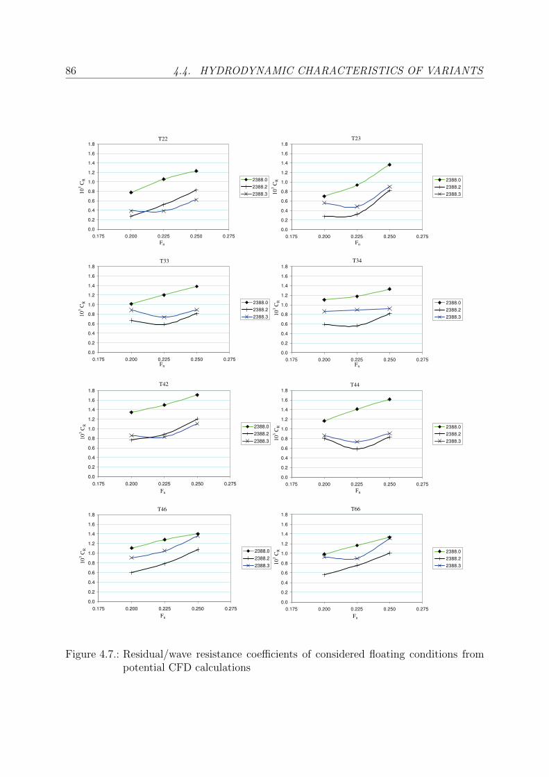
86 4.4. HYDRODYNAMIC CHARACTERISTICS OF VARIANTS
0.0
0.2
0.4
0.6
0.8
1.0
1.2
1.4
1.6
1.8
0.175 0.200 0.225 0.250 0.275
2388.0
2388.2
2388.3
0.0
0.2
0.4
0.6
0.8
1.0
1.2
1.4
1.6
1.8
0.175 0.200 0.225 0.250 0.275
2388.0
2388.2
2388.3
0.0
0.2
0.4
0.6
0.8
1.0
1.2
1.4
1.6
1.8
0.175 0.200 0.225 0.250 0.275
2388.0
2388.2
2388.3
0.0
0.2
0.4
0.6
0.8
1.0
1.2
1.4
1.6
1.8
0.175 0.200 0.225 0.250 0.275
2388.0
2388.2
2388.3
0.0
0.2
0.4
0.6
0.8
1.0
1.2
1.4
1.6
1.8
0.175 0.200 0.225 0.250 0.275
2388.0
2388.2
2388.3
0.0
0.2
0.4
0.6
0.8
1.0
1.2
1.4
1.6
1.8
0.175 0.200 0.225 0.250 0.275
2388.0
2388.2
2388.3
0.0
0.2
0.4
0.6
0.8
1.0
1.2
1.4
1.6
1.8
0.175 0.200 0.225 0.250 0.275
2388.0
2388.2
2388.3
0.0
0.2
0.4
0.6
0.8
1.0
1.2
1.4
1.6
1.8
0.175 0.200 0.225 0.250 0.275
2388.0
2388.2
2388.3
T22
T33
T23
T34
T44T42
T66T46
10
3 C
R
10
3 C
R
10
3 C
R
10
3 C
R
10
3 C
R
10
3 C
R1
03 C
R
10
3 C
R
Fn Fn
FnFn
FnFn
FnFn
Figure 4.7.: Residual/wave resistance coefficients of considered floating conditions frompotential CFD calculations

CHAPTER 4. SPECIAL APPLICATION CASE 87
2388.2 2388.0
(a) 2388.2 (left) and 2388.0 (right)
2388.2 2388.3
(b) 2388.2 (left) and 2388.3 (right)
Figure 4.8.: Compared wave elevations between parent geometry (2388.2) and variants2388.0 and 2388.3
884.5. PRELIMINARY OPERATIONAL SIMULATIONS WITH FIXED SPEED AND
FIXED FLOATING CONDITION
which, among other aspects, takes account only of the undisturbed wave field instead ofthe diffraction wave field. As previously discussed in section 3.3.3, strip theory will betherefore only applied, with proper corrections from experimental or viscous CFD results,to fill missing data needed to perform the operational simulations.
4.5. Preliminary Operational Simulations with Fixed
Speed and Fixed Floating Condition
4.5.1. Simulation Setup
In a first attempt to identify the main dependencies between the different routes, bulbousbow configurations and scaling factors, extremely simple operational simulations wereundertaken. These simulations include fixed values for:
• Ship speed VS (design service speed, with Fn = 0.250)
• Floating condition (design draft T22)
• Propulsive efficiency (ηD = 0.70)
• Specific fuel consumption (sfoc = 0.180[kg
kWh
])
The simulations were undertaken for a five-year period recalling weather data from ECMWFfrom the years 1997 to 2001 and considering the ships as in continuous operation, with12 hours at each port visited and without any additional stops.
The main purpose of these simulations was to have a first insight on main dependencies.Results from them can be thus addressed as a comparison when discussing results frommore complex simulation modes. An important aspect is to discuss if this approach makessense for comparison purposes or to be embedded into an optimization strategy.
4.5.2. Results
For each simulation, all relevant information (e.g. added resistance, brake power, fuelconsumption, sea state parameters and many others) are logged for the five-year periodand mean values are obtained. An example of this data is shown for the route SanFrancisco - Yokohama in figure 4.11. Significant seasonal, as well as yearly differencescan be observed in this figure. Especially for the significant wave height, the seasonalvariation is remarkably high in this route. The fuel oil consumption diagram shows thistendency as well, and differences between the different years can also be observed.
In figures 4.12a to 4.12e (pp.92), the mean values of the added resistance in waves RAW
of the different variants are shown as a function of ship size, represented by the scalingfactor λ, for the different routes. Figure 4.12f shows the average of all five routes simulated.The expected influence of ship size, with decreasing added resistances for increasing shipsize, can be observed for all routes. The ranking between the three bulbous bow variants

CHAPTER 4. SPECIAL APPLICATION CASE 89
0
1
2
3
4
5
6
7
8
9
10
0.50 0.75 1.00 1.25 1.50 1.75 2.00
Exp-2388.0
Exp-2388.2
Exp-2388.3
CAW at Fn = 0.150
λW /L
CAW
0
1
2
3
4
5
6
7
8
9
10
0.50 0.75 1.00 1.25 1.50 1.75 2.00
Exp-2388.0
Exp-2388.2
Exp-2388.3
CAW at Fn = 0.175
λW /LC
AW
0
1
2
3
4
5
6
7
8
9
10
0.50 0.75 1.00 1.25 1.50 1.75 2.00
Exp-2388.0
Exp-2388.2
Exp-2388.3
CAW at Fn = 0.200
λW /L
CAW
0
1
2
3
4
5
6
7
8
9
10
0.50 0.75 1.00 1.25 1.50 1.75 2.00
Exp-2388.0
Exp-2388.2
Exp-2388.3
CAW at Fn = 0.225
λW /L
CAW
0
1
2
3
4
5
6
7
8
9
10
0.50 0.75 1.00 1.25 1.50 1.75 2.00
Exp-2388.0
Exp-2388.2
Exp-2388.3
CAW at Fn = 0.250
λW /L
CAW
Figure 4.9.: Dimensionless added resistance in waves from experiments for different Froudenumbers [68]

904.5. PRELIMINARY OPERATIONAL SIMULATIONS WITH FIXED SPEED AND
FIXED FLOATING CONDITION
0
1
2
3
4
5
6
7
8
9
10
11
12
0.50 0.75 1.00 1.25 1.50 1.75 2.00
Exp-2388.0
Exp-2388.2
Exp-2388.3
Strip-2388.0
Strip-2388.2
Strip-2388.3
CAW at Fn = 0.250
λW /L
CAW
Strip theory
Experiments
Figure 4.10.: Added resistance in waves (dimensionless) for models 2388.0, 2388.2 and2388.3 from experiments and strip theory calculations
are in accordance with the trend observed from the added resistance in regular waves fromexperiments and can be distinguished for all routes, with the lowest values for the bulblessvariant 2388.0 and highest for variant 2388.3. Additionally, differences between the routescan be observed, reflecting the typical sea state character of the regions where the routesare placed. These can be categorized into two groups: routes, where predominantly calmweather is found (routes Le Havre - Paranagua and Valparaiso - Yokohama) and routeswhere predominantly rough weather is found (routes Le Havre - Charleston, San Francisco- Yokohama and Melbourne - Djibouti).
Since velocity is considered constant, the measure of merit, FEC, is equal to the fuel oilconsumption FOC. For the different routes, the FOC of the different variants is shown asa function of ship size in fig. 4.13 (pp. 93). The figure shows the relative fuel consumptionfor each of the simulated routes compared to the fuel consumption of the parent geometry(model 2388.2) for the different scaling factors considered (λ = 17, 25, 33, 50). Smalldifferences between the simulated routes can be observed, but the general trend is thatthe larger bulbous bow (2388.3) performs better in almost every route and scaling factor,similar to the fuel oil consumption in calm water, as seen in fig. 4.5 (p. 82). Resultsfrom more complex simulation modes presented in sections 4.6 and 4.7 will show theimportance of not performing such simple simulations for design purposes. Especially,the approach of neglecting speed loss has shown to be not suitable for a proper predictionof the economical performance of a design. This aspect will be illustrated when comparingthe present results with results obtained from simulations with variable ship speed.

CHAPTER 4. SPECIAL APPLICATION CASE 91
0 10 20 30 40 50 60 70 80 90 1000
10
20
30
40
50
60
70Added Resistance in Waves
Time [%]
Raw
[%]
0 10 20 30 40 50 60 70 80 90 1000
2
4
6
8
10
12Significant Wave Height
Time [%]
SW
H [m
]
0 50 100120
130
140
150
160
170
180
190
200
Fuel Consumption
Time [%]
FO
C [t
]
0 10 20 30 40 50 60 70 80 90 1001000
2000
3000
4000
5000
6000
7000
8000Ship brake power
Time [%]
Pb
[kW
]
Figure 4.11.: Log summary from operational simulation of ship 2388.2 with λ = 17 inroute San Francisco - Yokohama. Added resistance in waves is representedas percentage of calm water resistance.
4.6. Operational Simulations with Variable Speed
and Fixed Floating Condition
4.6.1. Simulation Setup
For a more realistic simulation, voluntary and involuntary speed loss must be considered.For the voluntary speed loss, the relative motions at bow and the subsequent slammingprobability according to Ochi [88] and maximum accelerations at the bridge have beenconsidered as described in section 3.3.3. The speed is reduced until the slamming prob-ability has a value lower than 3% and vertical significant accelerations lower than 0.15g.This threshold has been taken from the investigation within the European Union researchproject SEAROUTES, as recalled by Hinnenthal [43]. For the involuntary speed losses,the propeller and machine working points are considered as described in section 3.3.4.For this purpose, an additional module is called within the simulations using the openwater characteristics of the test propeller (with ITTC’78 extrapolation to full scale) andthe layout diagram of each main engine. In this case, the speed is reduced until the powerrequirement is feasible within the engine layout diagram described in section 3.3.4.
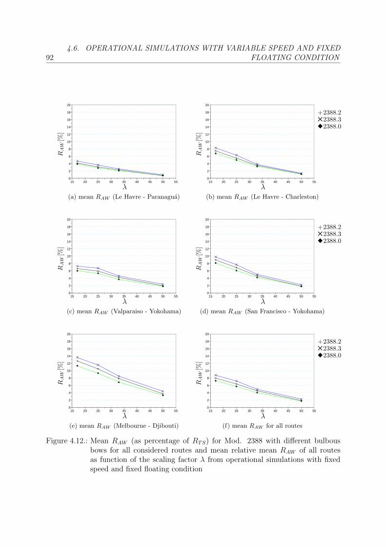
924.6. OPERATIONAL SIMULATIONS WITH VARIABLE SPEED AND FIXED
FLOATING CONDITION
15 20 25 30 35 40 45 50 550
2
4
6
8
10
12
14
16
18
20
λ
RAW
[%]
(a) mean RAW (Le Havre - Paranagua)
15 20 25 30 35 40 45 50 550
2
4
6
8
10
12
14
16
18
20
λ
+2388.252388.3u2388.0
RAW
[%]
(b) mean RAW (Le Havre - Charleston)
15 20 25 30 35 40 45 50 550
2
4
6
8
10
12
14
16
18
20
λ
RAW
[%]
(c) mean RAW (Valparaiso - Yokohama)
15 20 25 30 35 40 45 50 550
2
4
6
8
10
12
14
16
18
20
λ
+2388.252388.3u2388.0
RAW
[%]
(d) mean RAW (San Francisco - Yokohama)
15 20 25 30 35 40 45 50 550
2
4
6
8
10
12
14
16
18
20
λ
RAW
[%]
(e) mean RAW (Melbourne - Djibouti)
15 20 25 30 35 40 45 50 550
2
4
6
8
10
12
14
16
18
20
λ
+2388.252388.3u2388.0
RAW
[%]
(f) mean RAW for all routes
Figure 4.12.: Mean RAW (as percentage of RTS) for Mod. 2388 with different bulbousbows for all considered routes and mean relative mean RAW of all routesas function of the scaling factor λ from operational simulations with fixedspeed and fixed floating condition

CHAPTER 4. SPECIAL APPLICATION CASE 93
15 20 25 30 35 40 45 50 5594
96
98
100
102
104
106
108
λ
FOC
FOC
2388.2·1
00
(a) FOC for route Le Havre - Paranagua
15 20 25 30 35 40 45 50 5594
96
98
100
102
104
106
108
λ
+2388.252388.3u2388.0
FOC
FOC
2388.2·1
00(b) FOC for route Le Havre - Charleston
15 20 25 30 35 40 45 50 5594
96
98
100
102
104
106
108
λ
FOC
FOC
2388.2·1
00
(c) FOC for route Valparaiso - Yokohama
15 20 25 30 35 40 45 50 5594
96
98
100
102
104
106
108
λ
+2388.252388.3u2388.0
FOC
FOC
2388.2·1
00
(d) FOC for route San Francisco - Yokohama
15 20 25 30 35 40 45 50 5594
96
98
100
102
104
106
108
λ
FOC
FOC
2388.2·1
00
(e) FOC for route Melbourne - Djibouti
15 20 25 30 35 40 45 50 5594
96
98
100
102
104
106
108
λ
+2388.252388.3u2388.0
FOC
FOC
2388.2·1
00
(f) mean FOC of all routes
Figure 4.13.: Relative FOC variants 2388.0, .2 and .3 with fixed speed and fixed floatingcondition for all considered routes and mean relative FOC of all routes asfunction of the scaling factor λ from operational simulations with fixed speedand fixed floating condition

944.6. OPERATIONAL SIMULATIONS WITH VARIABLE SPEED AND FIXED
FLOATING CONDITION
Engine Characteristic
First computations were performed recalling engine characteristics from the product rangeof the engine manufacturer MAN B&W [79]. Since it was not always possible to obtainan adequate engine for each ship studied, engine margins differed significantly in somecases, making the comparability of the results very difficult. To avoid this problem inthis design study, “fictive engines” were declared. Each of these engines operates at itsMCR with an added resistance of 25% (equivalent to a sea margin of the same value),obtaining also the same specific fuel oil consumption sfoc for each ship of the same size.These sfoc’s were taken from reference engines of similar characteristics. The remaininglayout points (2, 3 and 4) were made proportional to the MCR, using the ratios fromreference engines of similar size from the manufacturer’s product range. An example ofthis is shown in fig. 4.14. Table D.1 in appendix D summarizes the power characteristicsof the fictive and reference engines used in this chapter.
0.0 0.1 0.2 0.3 0.4 0.5 0.6 0.7 0.8 0.9 1.00.0
0.1
0.2
0.3
0.4
0.5
0.6
0.7Open Water Diagram
J
KT,
10K
Q,η 0
η0
[KT
J2
]· J2
10KQ
KT
(a) Open water diagram
40 50 60 70 80 90 100 110 120 130 1400
2000
4000
6000
8000
10000
12000
Main Engine Layout Diagram
n [rpm]
PB
[kW]
L1
L2
L3
L4over
load
max
.rp
m
max. mep
req.
power
engine working point
(b) Main engine layout diagram
Figure 4.14.: Open water diagram with propeller working point and main engine layoutdiagram, with engine working point
Measure of Merit
When considering variable speed in the simulations, the fuel consumption alone cannotbe taken as a comparison measure as made in section 4.5, due to the evident fact thatships cover different distances over the five-year period. The measure of merit describedin section 3.4, the Fuel Equivalent Costs FEC will be applied here.
As discussed previously, an important task for addressing realistic fuel equivalent costsFEC is the choice of the fuel costs coefficient kf . The choice of this value will certainlydepend on the operational profile of the ship, its service speed, size, the actual and theestimated future fuel costs and, at last, the development of global economy during theperiod of interest. For the application case presented here, very little information aboutall these tasks is available, and for the purely comparative nature of this work, a unitary
CHAPTER 4. SPECIAL APPLICATION CASE 95
and rather conservative value of kf = 0.25 for all ship groups (as defined in sect. 3.4) willbe applied. Based in the discussion presented by Buxton [20], fuel costs can make up from10% to 50% of the operational costs of a ship. Indeed, the high dependency of the bunkerprices is evident, being the higher values of kf reached when bunker prices explode. Ashort example of the influence of kf into the results will be discussed in section 4.6.3.
4.6.2. Results
The Fuel Equivalent Costs FEC obtained from the operational simulations with variablespeed and fixed floating condition for each of the considered routes are shown in figures4.15a to 4.15f (p.97). The shown Fuel Equivalent Costs FEC in US$ consider a fuel priceof US$500 per tonne 3. The clear influence of ship size into the final costs is evident anddepicts clearly the advantages of large ships. This aspect is not of interest here, since onlyrelative differences between the variants are important for a proper ranking and a subse-quent design decision. For this reason, results presented in the following are normalized bythe results from the parent model 2388.2. In figures 4.16a to 4.16f (p.98), the normalizedFEC is shown for the presented simulations. A certain similarity to the results of FuelOil Consumption FOC shown in the previous section can be observed. Notwithstandingto this similarity, the present results show cases where the smaller bulbous bow (2388.2)has a better performance than the larger one (2388.3), contrary to the prediction in calmwater and the largest part of the results shown in the previous section. For the smallership sizes (λ = 17, 25), this applies for almost every route.
The differences between results from the routes Le Havre - Paranagua (moderateweather route) and Melbourne - Djibouti (rough weather route) are notorious. For thefirst route (Le Havre - Paranagua), a small influence of weather factors can be observed,being results very similar to the ranking of FOC in calm waters. The second route (Mel-bourne - Djibouti) shows an evidently larger influence of weather factors, being in thiscase the Fuel Equivalent Costs of the larger bulbous bow (2388.3) up to 4% higher than forthe parent ship (2388.2). This confirms the hypothesis made in chapter 1, showing thatthe best bulbous bow configuration, when considering weather factors, can be different tothe one in calm waters.
It shall be recalled that differences in the FEC from all three variants are caused notonly by different fuel consumptions, but also by the achieved mean service speed, viz.the total covered distance over the five-year period. Diagrams for this data (fuel oilconsumption and mean service speed) and for the added resistance in waves are shown inappendix D, in figures D.1, D.2 and D.3. These results show an important dependencynot only in the parameters of interest (region and bulbous bow), but also on ship size.The direct relation between ship size and RAW is predominant, but other factors, such ascharacteristic wave length or periods in the different regions certainly play a role.
Since the operational simulations presented in this section are the only ones includingexperimental data both for seakeeping and calm water resistance, results obtained here
3IFO 180, representative for the years 2008 and 2009
964.6. OPERATIONAL SIMULATIONS WITH VARIABLE SPEED AND FIXED
FLOATING CONDITION
are of special relevance for the validation of operational simulations including numericaldata only. This aspect will be discussed in detail in chapter 5 (sect. 5.4, pp. 121).
4.6.3. Variation of Fuel Costs Coefficient kf
As previously mentioned, the impact of the value of the fuel costs coefficient kf will betreated here by means of two examples, namely the routes Le Havre - Paranagua andMelbourne - Djibouti. Additionally to the shown diagrams of FEC with kf = 0.25,diagrams with values of kf = 0.1, 0.5, 1.0 are shown in figures 4.17a to 4.17f (p.99)for the mentioned routes. These values of kf represent scenarios of very low fuel prices(kf = 0.10) and very high fuel prices (kf = 0.50), showing with kf = 1.00 pure fuel costs(or disabled “punishment” costs according to the definition of FEC) as a reference.
For the calm weather route between Le Havre and Paranagua, only small changes canbe observed in the FEC for the different values of kf . Nevertheless, these small changeslead for kf = 0.10 to a different best configuration at λ = 17 (variant 2388.2). In thecase of the second route (Melbourne - Djibouti), the influence of kf is significantly higher.Specifically for smaller ship sizes (λ = 17, 25), the relatively higher influence of weatherfactors, especially when leading to speed loss, causes large differences in the results. Forkf = 0.10, these large differences are caused to a great extent due to the higher influenceof the achieved mean speed (i.e. speed loss). The similarity between the results withk = 0.50 and k = 1.00 show that, for higher fuel prices, a low fuel oil consumption is moreadvantageous than a high mean achieved speed. Interestingly, the better performanceof variant 2388.2 is, for smaller ship sizes, almost independent of the chosen value ofkf . The application of the presented Fuel Equivalent Costs permit, in this manner, theevaluation and comparison of different fuel price scenarios, making a subsequent decisionfor a representative value of kf much easier. It shall be remarked that this decision isrelevant for design purposes and should be confirmed at a later design stage by a moredetailed economical study.
4.6.4. Variation of Service Speed: Slow Steaming Simulations
To illustrate the impact of the different bulbous bows in a simple manner, a slightlydifferent approach can also be chosen and will be shortly described here: by decreasingthe service speed of the ships in order to obtain the same mean velocity for all ships withina group, which is equal to the mean speed of the slowest ship (over the five year period)in the group, the fuel costs can be compared directly, i.e., costs surplus of the voluntaryspeed loss for the faster ships can be acquainted. These simulations will be recalled hereas slow steaming simulations.
For the present application case, variant 2388.3 achieved the lowest mean speed, withoutexception, for all routes and for all ship sizes studied. For this reason, the design servicespeed of variants 2388.0 and 2388.2 was adjusted in order to obtain the same mean speedthan variant 2388.3 over the five-year period. This was achieved by an additional routinewhich changes therefore service speed dynamically until this equality condition is reached.
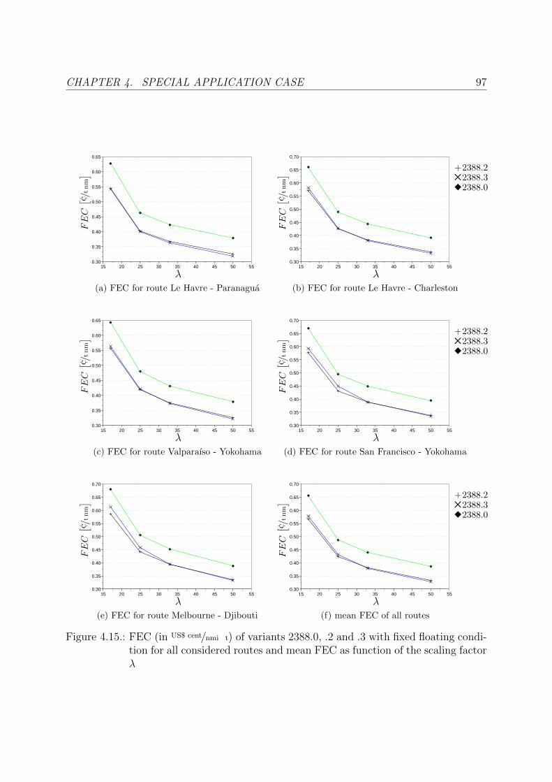
CHAPTER 4. SPECIAL APPLICATION CASE 97
15 20 25 30 35 40 45 50 550.30
0.35
0.40
0.45
0.50
0.55
0.60
0.65
λ
FEC[ ¢ /tn
m]
(a) FEC for route Le Havre - Paranagua
15 20 25 30 35 40 45 50 550.30
0.35
0.40
0.45
0.50
0.55
0.60
0.65
0.70
λ
+2388.252388.3u2388.0
FEC[ ¢ /tn
m]
(b) FEC for route Le Havre - Charleston
15 20 25 30 35 40 45 50 550.30
0.35
0.40
0.45
0.50
0.55
0.60
0.65
λ
FEC[ ¢ /tn
m]
(c) FEC for route Valparaıso - Yokohama
15 20 25 30 35 40 45 50 550.30
0.35
0.40
0.45
0.50
0.55
0.60
0.65
0.70
λ
+2388.252388.3u2388.0
FEC[ ¢ /tn
m]
(d) FEC for route San Francisco - Yokohama
15 20 25 30 35 40 45 50 550.30
0.35
0.40
0.45
0.50
0.55
0.60
0.65
0.70
λ
FEC[ ¢ /tn
m]
(e) FEC for route Melbourne - Djibouti
15 20 25 30 35 40 45 50 550.30
0.35
0.40
0.45
0.50
0.55
0.60
0.65
0.70
λ
+2388.252388.3u2388.0
FEC[ ¢ /tn
m]
(f) mean FEC of all routes
Figure 4.15.: FEC (in US$ cent/nmi t) of variants 2388.0, .2 and .3 with fixed floating condi-tion for all considered routes and mean FEC as function of the scaling factorλ
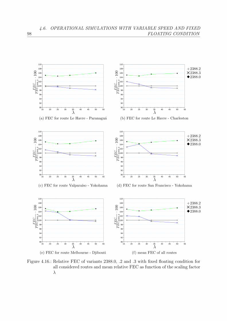
984.6. OPERATIONAL SIMULATIONS WITH VARIABLE SPEED AND FIXED
FLOATING CONDITION
15 20 25 30 35 40 45 50 5590
92
94
96
98
100
102
104
106
108
110
λ
FEC
FEC
2388.2·1
00
(a) FEC for route Le Havre - Paranagua
15 20 25 30 35 40 45 50 5590
92
94
96
98
100
102
104
106
108
110
λ
+2388.252388.3u2388.0
FEC
FEC
2388.2·1
00(b) FEC for route Le Havre - Charleston
15 20 25 30 35 40 45 50 5590
92
94
96
98
100
102
104
106
108
110
λ
FEC
FEC
2388.2·1
00
(c) FEC for route Valparaıso - Yokohama
15 20 25 30 35 40 45 50 5590
92
94
96
98
100
102
104
106
108
110
λ
+2388.252388.3u2388.0
FEC
FEC
2388.2·1
00
(d) FEC for route San Francisco - Yokohama
15 20 25 30 35 40 45 50 5590
92
94
96
98
100
102
104
106
108
110
λ
FEC
FEC
2388.2·1
00
(e) FEC for route Melbourne - Djibouti
15 20 25 30 35 40 45 50 5590
92
94
96
98
100
102
104
106
108
110
λ
+2388.252388.3u2388.0
FEC
FEC
2388.2·1
00
(f) mean FEC of all routes
Figure 4.16.: Relative FEC of variants 2388.0, .2 and .3 with fixed floating condition forall considered routes and mean relative FEC as function of the scaling factorλ

CHAPTER 4. SPECIAL APPLICATION CASE 99
15 20 25 30 35 40 45 50 5590
92
94
96
98
100
102
104
106
108
110
λ
FEC
FEC
2388.2·1
00
(a) FEC with kf = 0.10 (Le Havre - Paranagua)
15 20 25 30 35 40 45 50 5590
92
94
96
98
100
102
104
106
108
110
λ
+2388.252388.3u2388.0
FEC
FEC
2388.2·1
00(b) FEC with kf = 0.10 (Melbourne - Djibouti)
15 20 25 30 35 40 45 50 5590
92
94
96
98
100
102
104
106
108
110
λ
FEC
FEC
2388.2·1
00
(c) FEC with kf = 0.50 (Le Havre - Paranagua)
15 20 25 30 35 40 45 50 5590
92
94
96
98
100
102
104
106
108
110
λ
+2388.252388.3u2388.0
FEC
FEC
2388.2·1
00
(d) FEC with kf = 0.50 (Melbourne - Djibouti)
15 20 25 30 35 40 45 50 5590
92
94
96
98
100
102
104
106
108
110
λ
FEC
FEC
2388.2·1
00
(e) FEC with kf = 1.00 (Le Havre - Paranagua)
15 20 25 30 35 40 45 50 5590
92
94
96
98
100
102
104
106
108
110
λ
+2388.252388.3u2388.0
FEC
FEC
2388.2·1
00
(f) FEC with kf = 1.00 (Melbourne - Djibouti)
Figure 4.17.: Variation of the fuel costs coefficient kf . Relative FEC of variants 2388.0,.2 and .3 with fixed floating condition for all considered routes as functionof the scaling factor λ
1004.7. OPERATIONAL SIMULATIONS WITH VARIABLE SPEED AND VARIABLE
FLOATING CONDITION
In figures 4.18a to 4.18f (p.101), results for the fuel oil consumption FOC for thedifferent routes are shown. In contrast to the previous simulations, the advantage ofvariant 2388.2 is considerably higher, even for the largest scaling factors λ = 50. Variant2388.3, with the best resistance in calm waters, remains even in calm weather routeswith results of the same order of magnitude than the bulbless variant 2388.0. This trenddecreases for larger scaling factors, but in no single case the fuel oil consumption of variant2388.3 becomes lower than the one of variant 2388.2.
This simulations with lowered service speed can be considered as a valuable alternativefor the designer to compare different variants. On the other side, it depends of thephilosophy of the ship operator and of many other factors if the decision of operating atslightly lower speeds is advantageous or not. Further possibilities for this approach wouldbe the declaration of a “target mean service speed”, for which the engine power and thepropulsion unit is adjusted for each ship until this mean speed is reached. This approachwill not be followed in this study, and further comparisons will be made with the proposedmeasure of merit FEC.
4.7. Operational Simulations with Variable Speed
and Variable Floating Condition
4.7.1. Simulation Setup
As a further and last step of complexity, attempting to model ship operation as realistic aspossible, simulations with variable floating condition were undertaken. It can be consid-ered as a fact that practically every cargo ship operates, over significant amounts of time,in partially loaded or in fully unloaded (ballast) conditions, so-called off-design floatingconditions. As previously discussed, the consequence of the operation under these condi-tions, for which the ship was neither designed nor optimized for, can lead to a subsequenteconomic loss, making the consideration of these of particular interest in this study.
Floating Conditions
The floating condition of the ship is found, for every single trip, given an amount ofcargo, fuel and ballast with their respective centers of gravity. This is done as describedin section 3.3.1.
For the purpose of this investigation, three different floating conditions were alternatedfor each trip, in order to obtain the same conditions for all ships studied. The selection ofa total of three conditions ensures, for the period of five simulation years, that each trip, ineach direction, will be undertaken with almost equal amounts of each floating condition.These conditions, namely full loaded, partially loaded and ballast, are summarized intable 4.7. The generalized approach of the implementation permits no limitations on thisand further loading conditions, recalling statistical data from shipping companies, can beincluded without restrictions.

CHAPTER 4. SPECIAL APPLICATION CASE 101
15 20 25 30 35 40 45 50 5596
98
100
102
104
106
108
110
112
114
116
λ
FOC
FOC
2388.2·1
00
(a) FOC for route Le Havre - Paranagua
15 20 25 30 35 40 45 50 5596
98
100
102
104
106
108
110
112
114
116
λ
+2388.252388.3u2388.0
FOC
FOC
2388.2·1
00
(b) FOC for route Le Havre - Charleston
15 20 25 30 35 40 45 50 5596
98
100
102
104
106
108
110
112
114
116
λ
FOC
FOC
2388.2·1
00
(c) FOC for route Valparaıso - Yokohama
15 20 25 30 35 40 45 50 5596
98
100
102
104
106
108
110
112
114
116
λ
+2388.252388.3u2388.0
FOC
FOC
2388.2·1
00
(d) FOC for route San Francisco - Yokohama
15 20 25 30 35 40 45 50 5596
98
100
102
104
106
108
110
112
114
116
λ
FOC
FOC
2388.2·1
00
(e) FOC for route Melbourne - Djibouti
15 20 25 30 35 40 45 50 5596
98
100
102
104
106
108
110
112
114
116
λ
+2388.252388.3u2388.0
FOC
FOC
2388.2·1
00
(f) mean FOC of all routes
Figure 4.18.: Relative FOC of slow steaming simulations for variants 2388.0, .2 and .3 withfixed floating condition for all considered routes and mean relative FOC asfunction of the scaling factor λ

102 4.8. CONCLUSIONS ABOUT SIMULATION MODES
Description Cargo [t] xcargo [m] TAP [m] TFP [m]
full loaded 8700 2.5 8.1132 8.0884partially loaded 4000 0 6.8254 5.7306
ballast 0 0 5.1088 4.224
Table 4.7.: Loading conditions. Example for ships with λ = 25
4.7.2. Results
In the same manner as in the previous sections, results for the measure of merit (FEC)are summarized in figures 4.19a to 4.19f. Additional results for RAW and achieved speedVS can be found in appendix D, figs. D.4 and D.5 respectively.
As expected from the resistance in calm waters for off-design floating conditions, variant2388.2 performs better in almost every route and scaling factor of the comparison. Theresults show also the influence of weather on the relative ranking between the variants:especially for λ = 25 a change in the relative values can be observed for almost everyroute. A statistical analysis presented in the next section (sect. 4.8) for the encounteredsea states in the considered routes attempts to give an answer to this finding.
The differences in the fuel equivalent costs between calm and rough weather routes arehere partially damped by the equally relevant influence of the partial and ballast floatingconditions. Nevertheless, differences of up to 5% between the parent ship and variant2388.3 can be observed for the route Melbourne-Djibouti (fig. 4.19e) for λ = 25, beingthese a few percent smaller (2%) for the route between Le Havre and Paranagua (fig.4.19a).
This insight shows again the importance of considering all components of the opera-tional profile of the ship for the selection of the most adequate variant including, addi-tionally to weather factors, realistic assumptions about the (expected) floating conditionsduring the operational life of the ship.
4.8. Conclusions about Simulation Modes
For the presented operational simulations exploiting existing experimental data, differentsimulation modes were tested. The first and simplest setup, with fixed speed and fixedfloating condition, was in a first instance expected to correlate with variable speed sim-ulations. This would have shown that, in an early design stage, such simulations can beuseful for the comparison between variants and thus help the designer to choose the eco-nomically most profitable one. Since this was not the case, this simulation setup cannotbe recommended for design purposes.
The simulations with variable speed and fixed floating condition demonstrated their ap-plicability. They showed the importance of the consideration of machinery and propulsionunit, causing the subsequent involuntary speed loss, variable specific fuel oil consumptionsand propeller efficiencies. Also the further consideration of slamming events and acceler-ations at the bridge causing voluntary speed loss played an important role, especially for

CHAPTER 4. SPECIAL APPLICATION CASE 103
15 20 25 30 35 40 45 50 5596
98
100
102
104
106
108
110
112
114
116
λ
FEC
FEC
2388.2·1
00
(a) FEC for route Le Havre - Paranagua
15 20 25 30 35 40 45 50 5596
98
100
102
104
106
108
110
112
114
116
λ
+2388.252388.3u2388.0
FEC
FEC
2388.2·1
00(b) FEC for route Le Havre - Charleston
15 20 25 30 35 40 45 50 5596
98
100
102
104
106
108
110
112
114
116
λ
FEC
FEC
2388.2·1
00
(c) FEC for route Valparaıso - Yokohama
15 20 25 30 35 40 45 50 5596
98
100
102
104
106
108
110
112
114
116
λ
+2388.252388.3u2388.0
FEC
FEC
2388.2·1
00
(d) FEC for route San Francisco - Yokohama
15 20 25 30 35 40 45 50 5596
98
100
102
104
106
108
110
112
114
116
λ
FEC
FEC
2388.2·1
00
(e) FEC for route Melbourne - Djibouti
15 20 25 30 35 40 45 50 5596
98
100
102
104
106
108
110
112
114
116
λ
+2388.252388.3u2388.0
FEC
FEC
2388.2·1
00
(f) mean FEC of all routes
Figure 4.19.: Relative FEC of variants 2388.0, .2 and .3 with variable floating conditionfor all considered routes and mean relative FEC as function of the scalingfactor λ

104 4.8. CONCLUSIONS ABOUT SIMULATION MODES
ships of smaller size. The measure of merit presented, the Fuel Equivalent Costs FEC,showed its robustness for different fuel costs factors kf .
The simulations with variable speed and variable floating condition show, despite thesimple cargo profile applied, the significance of off-design floating conditions into theperformance assessment of a design. Especially for ships operating significant amounts oftime in ballast conditions, the application of such simulations is mandatory for the correctidentification of the most convenient design variant. As previously mentioned, the higheruncertainty regarding the seakeeping characteristics considered in these simulations mustbe considered when interpreting these results.
As mentioned in the previous section, a change in the relative values of FOC forλ = 25 can be observed for almost every route in both simulation modes. To understandthe causes of this phenomenon, the encountered weather factors from all simulations per-formed were collected, classified and analyzed, generating occurrence probability functionsof sea state parameters for each of the routes considered. In figure 4.20, occurrence prob-abilities of mean encounter wave direction, significant wave height, mean wave periodand mean wave length are presented. This information is gained from the encounteredweather of all ships simulated over the five-year period and is therefore representative,over this time period, for each of the considered routes. Of special interest is figure4.20d for the mean wave length: the peak values of these curves are found for mean wavelengths between 100m and 170m approx., decreasing drastically for larger wave lengths.This leads, to a certain extent, to the change in the trend of the curves of relative FEC(considering that for λ = 25, LPP = 146.25m). The final outcome of the values of FECalso depend of the encountered wave angles and significant wave heights, but also of theadded resistance in regular waves and ship motions, leading to a complex interdependencybetween them. For the wave encounter angles (fig 4.20a), clear differences can be observedbetween the different routes. It shall be remarked that the weather data was collected inboth directions (outward and return), which takes account for the symmetry of the oc-currences. While beam seas are slightly predominant for the routes Le Havre-Paranaguaand Valparaıso-Yokohama, head and following seas are slightly predominant for the re-maining routes. From the occurrence probability of significant wave heights, the previousclassification of calm weather and rough weather routes can be confirmed. Particularly,the considerably higher occurrence probability of large wave heights can be observed forrough weather routes (this tendency is observed especially for significant wave heights ofapprox. 3 m and greater). Considering the quadratic relation between wave height andwave energy, the relevance of these significant wave heights is considerable.
From the presented special application case exploiting existing experimental data, it canbe concluded that the presented operational simulations should be performed consideringvoluntary and involuntary speed loss, that different routes and ship sizes lead to differ-ent ship performances and that certain sea state characteristics have special influence forcertain ship lengths (in the present case for λ = 25). Considering these aspects, the pre-sented method will be applied in the next chapter for a design study including new designsand recalling the hydrodynamic characteristics of these designs from numerical methods,representing the general form of application of the presented design methodology.

CHAPTER 4. SPECIAL APPLICATION CASE 105
0
0,001
0,002
0,003
0,004
0,005
0,006
0,007
0,008
0,009
0 30 60 90 120 150 180
Pro
ba
bil
ity
of
occ
urr
en
ce
Wave encounter angle µ µ µ µ [°]
Probability distribution of wave encounter angle
(a) Mean encounter wave direction
0
0,2
0,4
0,6
0,8
1
1,2
0 1 2 3 4 5 6 7 8
Pro
ba
bil
ity
of
occ
urr
en
ce
Significant wave height SWH [m]
Probability distribution of significant wave height
Le Havre-Paranaguá
Le Havre-Charleston
Melbourne-Djibouti
San Francisco-Yokohama
Valparaíso-Yokohama
(b) Significant wave height
0
0,05
0,1
0,15
0,2
0,25
0,3
0,35
0 5 10 15 20
Pro
ba
bil
ity
of
occ
urr
en
ce
Mean wave period MWP [s]
Probability distribution of mean wave period
(c) Mean wave period
0
0,05
0,1
0,15
0,2
0,25
0,3
0,35
0,00 100,00 200,00 300,00 400,00 500,00
Pro
ba
bil
ity
of
occ
urr
en
ce
Mean wave length λλλλm [m]
Probability distribution of mean wave length
Le Havre-Paranaguá
Le Havre-Charleston
Melbourne-Djibouti
San Francisco-Yokohama
Valparaíso-Yokohama
(d) Mean wave length
Figure 4.20.: Probability distributions of wave direction, significant wave height, meanwave period and mean wave length


CHAPTER 5. GENERAL APPLICATION CASE 107
5. General Application Case
5.1. Introduction
In this chapter, the application of operational simulations for design purposes is presentedby means of a second practical example. Opposite to the application case discussed in theprevious chapter, the hydrodynamic characteristics of the ships in question are obtainedfrom numerical calculations only, including potential and viscous CFD methods. Newgeometries, generated by a partially parametric approach with model 2388.2 as parentform, are also included in the presented practical example. In this manner, an attemptto reproduce normal conditions in an early design stage, being experimental data notavailable and studying a large number of variants, is made. All of these aspects make theexample presented in this chapter of central relevance for this investigation, demonstratingthe applicability of the presented methodology for design purposes in early design.
In a first stage, 36 different subvariants (differing only in their bulbous bow and in somecases slightly in their foreships) have been generated from the parent geometry (model no.2388.2). For these geometries, wave resistance calculations with a potential CFD solverwere undertaken for different floating conditions and advance speeds.
From these subvariants, after studying potential CFD results, four of them have been se-lected to undertake further viscous CFD calculations in regular waves with the OpenFOAM-solver TUBsixDOFFoam. Additionally, the same viscous CFD calculations were undertakenfor the ships studied in chapter 4 (with exception of the bulbless variant 2388.0), validatingresults from these calculations with the available experimental results.
In a similar manner as in chapter 4, operational simulations were carried out for theconsidered routes, making use of the same environment conditions (weather, routes andcargo) from the previous chapter. For convenience, simple simulations with fixed speedand fixed floating condition (as presented in section 4.5) were omitted, considering there-fore only variable speed simulations.
The attained results from the operational simulations are discussed, and the variantsproviding best economic profit are identified for each route and ship size, showing thatthe magnitude of the achieved economic surplus is, in most cases, worth to be considered.Finally, a short discussion considering certain design aspects of bulbous bows is given.
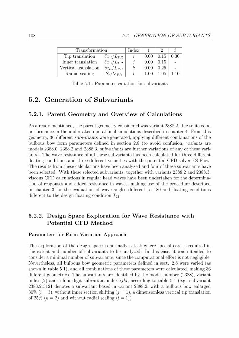
108 5.2. GENERATION OF SUBVARIANTS
Transformation Index 1 2 3Tip translation δxtt/LPR i 0.00 0.15 0.30
Inner translation δxti/LPR j 0.00 0.15 -Vertical translation δztt/LPR k 0.00 0.25 -
Radial scaling Sr/∇PR l 1.00 1.05 1.10
Table 5.1.: Parameter variation for subvariants
5.2. Generation of Subvariants
5.2.1. Parent Geometry and Overview of Calculations
As already mentioned, the parent geometry considered was variant 2388.2, due to its goodperformance in the undertaken operational simulations described in chapter 4. From thisgeometry, 36 different subvariants were generated, applying different combinations of thebulbous bow form parameters defined in section 2.8 (to avoid confusion, variants aremodels 2388.0, 2388.2 and 2388.3, subvariants are further variations of any of these vari-ants). The wave resistance of all these subvariants has been calculated for three differentfloating conditions and three different velocities with the potential CFD solver FS-Flow.The results from these calculations have been analyzed and four of these subvariants havebeen selected. With these selected subvariants, together with variants 2388.2 and 2388.3,viscous CFD calculations in regular head waves have been undertaken for the determina-tion of responses and added resistance in waves, making use of the procedure describedin chapter 3 for the evaluation of wave angles different to 180◦and floating conditionsdifferent to the design floating condition T22.
5.2.2. Design Space Exploration for Wave Resistance withPotential CFD Method
Parameters for Form Variation Approach
The exploration of the design space is normally a task where special care is required inthe extent and number of subvariants to be analyzed. In this case, it was intended toconsider a minimal number of subvariants, since the computational effort is not negligible.Nevertheless, all bulbous bow geometric parameters defined in sect. 2.8 were varied (asshown in table 5.1), and all combinations of these parameters were calculated, making 36different geometries. The subvariants are identified by the model number (2388), variantindex (2) and a four-digit subvariant index ijkl, according to table 5.1 (e.g. subvariant2388.2 3121 denotes a subvariant based in variant 2388.2, with a bulbous bow enlarged30% (i = 3), without inner section shifting (j = 1), a dimensionless vertical tip translationof 25% (k = 2) and without radial scaling (l = 1)).

CHAPTER 5. GENERAL APPLICATION CASE 109
Description Index TAP (m) TFP (m)Design draft T22 8.125 8.125
Partially loaded T34 6.964 6.094Ballast T46 6.094 4.875
Table 5.2.: Drafts considered into calculations
Potential CFD Calculations with FS-Flow
For each geometry, three different floating conditions (T22, , T34 and T46), as defined in table5.2, and three different speeds (equivalent to Fn = 0.200, 0.225, 0.250) were calculated,making a total of 324 potential flow calculations. All calculations were made within anautomatized batch routine and results were extracted automatically.
Results and Choice of Subvariants for further RANSE-CFD SeakeepingCalculations
The wave resistance of each of the subvariants is shown, normalized by the wave resistanceof the parent hull, in figures 5.1 (Fn = 0.200), 5.2 (Fn = 0.225) and 5.3 (Fn = 0.250)for the three considered floating conditions (T22, T34, T46). Additional data (bulbous bowparameters and results in tabular form), can be found in appendix C, tables C.1, C.2 andC.3 (pp. 156-159).
Figure 5.1.: Wave resistance (as percentage of parent hull wave resistance) of subvariantsfor Fn = 0.200
Clear differences can be observed in figs. 5.1 to 5.3 between the three different floatingconditions calculated:
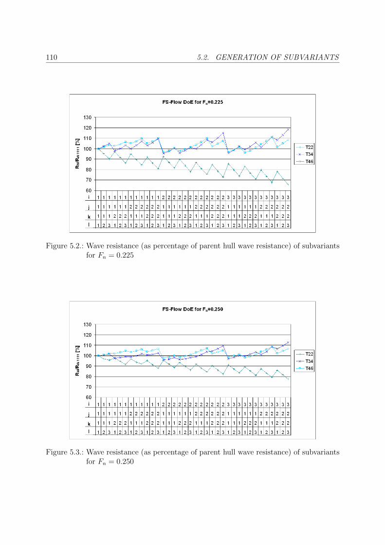
110 5.2. GENERATION OF SUBVARIANTS
Figure 5.2.: Wave resistance (as percentage of parent hull wave resistance) of subvariantsfor Fn = 0.225
Figure 5.3.: Wave resistance (as percentage of parent hull wave resistance) of subvariantsfor Fn = 0.250
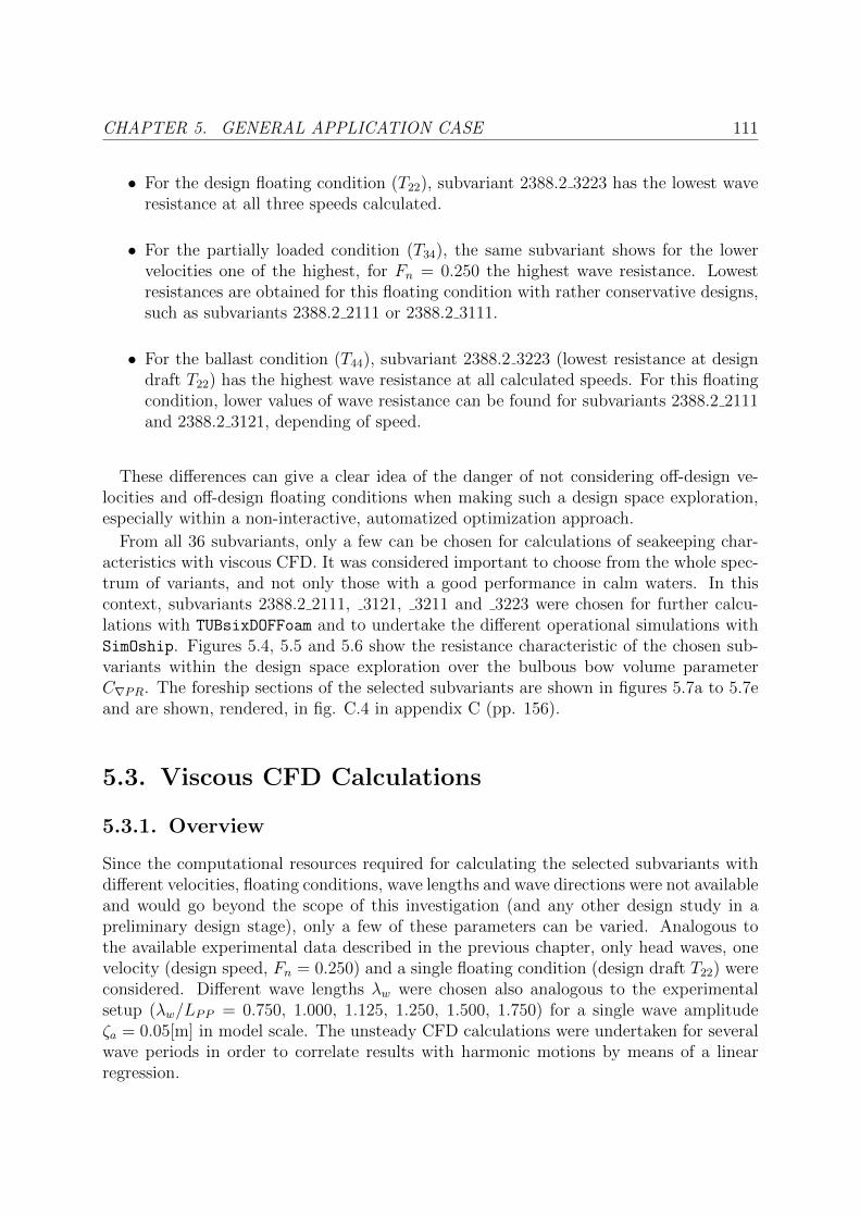
CHAPTER 5. GENERAL APPLICATION CASE 111
• For the design floating condition (T22), subvariant 2388.2 3223 has the lowest waveresistance at all three speeds calculated.
• For the partially loaded condition (T34), the same subvariant shows for the lowervelocities one of the highest, for Fn = 0.250 the highest wave resistance. Lowestresistances are obtained for this floating condition with rather conservative designs,such as subvariants 2388.2 2111 or 2388.2 3111.
• For the ballast condition (T44), subvariant 2388.2 3223 (lowest resistance at designdraft T22) has the highest wave resistance at all calculated speeds. For this floatingcondition, lower values of wave resistance can be found for subvariants 2388.2 2111and 2388.2 3121, depending of speed.
These differences can give a clear idea of the danger of not considering off-design ve-locities and off-design floating conditions when making such a design space exploration,especially within a non-interactive, automatized optimization approach.
From all 36 subvariants, only a few can be chosen for calculations of seakeeping char-acteristics with viscous CFD. It was considered important to choose from the whole spec-trum of variants, and not only those with a good performance in calm waters. In thiscontext, subvariants 2388.2 2111, 3121, 3211 and 3223 were chosen for further calcu-lations with TUBsixDOFFoam and to undertake the different operational simulations withSimOship. Figures 5.4, 5.5 and 5.6 show the resistance characteristic of the chosen sub-variants within the design space exploration over the bulbous bow volume parameterC∇PR. The foreship sections of the selected subvariants are shown in figures 5.7a to 5.7eand are shown, rendered, in fig. C.4 in appendix C (pp. 156).
5.3. Viscous CFD Calculations
5.3.1. Overview
Since the computational resources required for calculating the selected subvariants withdifferent velocities, floating conditions, wave lengths and wave directions were not availableand would go beyond the scope of this investigation (and any other design study in apreliminary design stage), only a few of these parameters can be varied. Analogous tothe available experimental data described in the previous chapter, only head waves, onevelocity (design speed, Fn = 0.250) and a single floating condition (design draft T22) wereconsidered. Different wave lengths λw were chosen also analogous to the experimentalsetup (λw/LPP = 0.750, 1.000, 1.125, 1.250, 1.500, 1.750) for a single wave amplitudeζa = 0.05[m] in model scale. The unsteady CFD calculations were undertaken for severalwave periods in order to correlate results with harmonic motions by means of a linearregression.
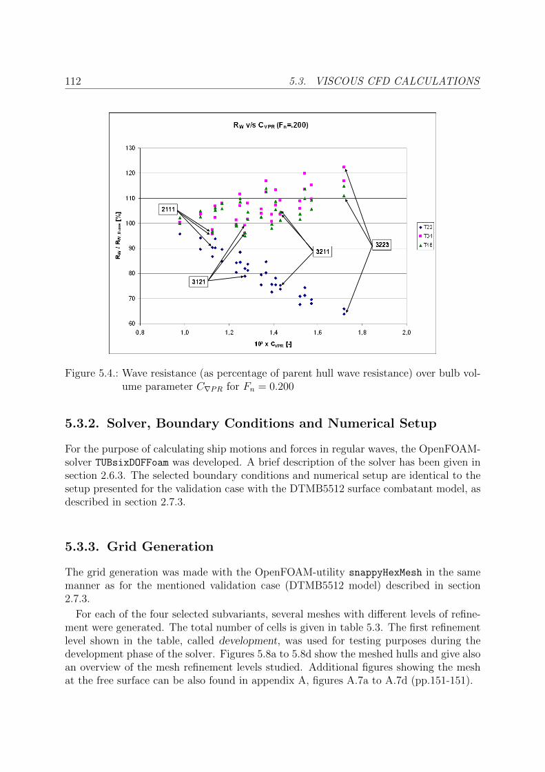
112 5.3. VISCOUS CFD CALCULATIONS
Figure 5.4.: Wave resistance (as percentage of parent hull wave resistance) over bulb vol-ume parameter C∇PR for Fn = 0.200
5.3.2. Solver, Boundary Conditions and Numerical Setup
For the purpose of calculating ship motions and forces in regular waves, the OpenFOAM-solver TUBsixDOFFoam was developed. A brief description of the solver has been given insection 2.6.3. The selected boundary conditions and numerical setup are identical to thesetup presented for the validation case with the DTMB5512 surface combatant model, asdescribed in section 2.7.3.
5.3.3. Grid Generation
The grid generation was made with the OpenFOAM-utility snappyHexMesh in the samemanner as for the mentioned validation case (DTMB5512 model) described in section2.7.3.
For each of the four selected subvariants, several meshes with different levels of refine-ment were generated. The total number of cells is given in table 5.3. The first refinementlevel shown in the table, called development, was used for testing purposes during thedevelopment phase of the solver. Figures 5.8a to 5.8d show the meshed hulls and give alsoan overview of the mesh refinement levels studied. Additional figures showing the meshat the free surface can be also found in appendix A, figures A.7a to A.7d (pp.151-151).

CHAPTER 5. GENERAL APPLICATION CASE 113
Figure 5.5.: Wave resistance (as percentage of parent hull wave resistance) over bulb vol-ume parameter C∇PR for Fn = 0.225
5.3.4. Calculations
Hardware
A large number of calculations was undertaken during the different phases of the develop-ment and final use of TUBsixDOFFOAM, starting from initial tests up to final calculationswith fine grids. This was done making use of different hardware setups available duringthis study and, due to their special characteristics, they will be shortly described here:
• Initial calculations during the development of TUBsixDOFFoam, both for coarse andmedium grids, were made, when possible, in available machines from the depart-ments dynamics of maritime systems and design and operation of maritime systems.When this was not sufficient, additional resources were booked from Amazon Web
Category name No. of cellsdevelopment 16628evencoarser 82183coarser 187666standard 365216finer 791319
Table 5.3.: Mesh refinement levels

114 5.3. VISCOUS CFD CALCULATIONS
Figure 5.6.: Wave resistance (as percentage of parent hull wave resistance) over bulb vol-ume parameter C∇PR for Fn = 0.250
ServicesTM[1]. AWS is a cloud-based platform of remote computing resources, offer-ing the possibility of practically unlimited on-demand resources. In the case of thisinvestigation work, high performance hardware was purchased, at hourly rates andonly when more resources were needed than locally available. One of the decisiveadvantages of this principle is the possibility of storing complete machine config-urations, being those ready-to-use when needed. For general use in ship design,on-demand computing services can be of significant advantage for computationallyintensive or time-sensitive projects, when the acquisition of additional hardware isnot a cost-effective solution.
• Final calculations, for the complete range of meshes, were made at the large clus-ter of the North-German Supercomputing Alliance (Norddeutscher Verbund zurForderung des Hoch- und Hochstleistungsrechnens - HLRN [3]). This alliance of-fers, free of charge for academic investigation projects, full access to the completerange of computational resources for a given amount of credits, billed for each hourand processor used. Since the number of credits is limited, only small to mediumprojects can be undertaken in this modality, which can be attractive e.g. for mastertheses. Additional resources for large investigation projects can also be booked fora fee.
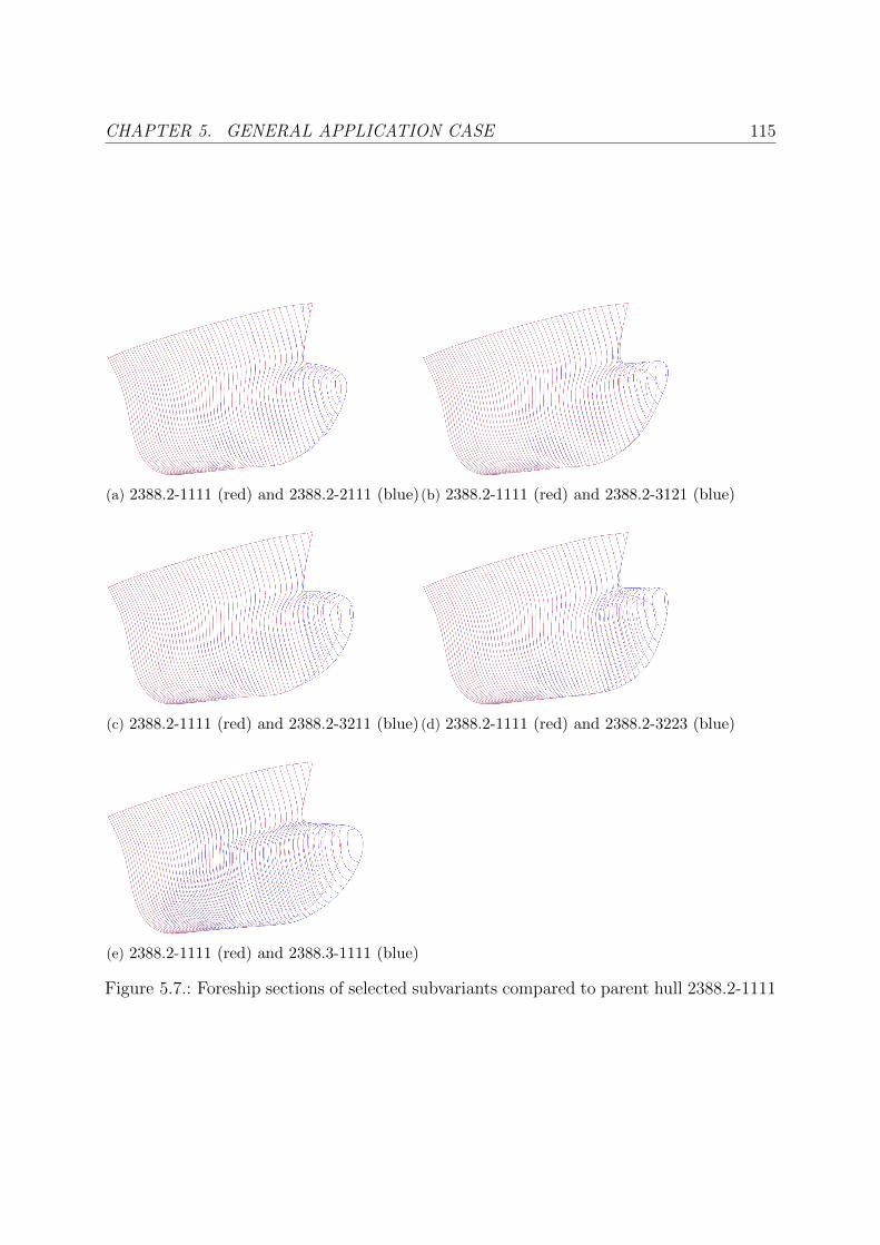
CHAPTER 5. GENERAL APPLICATION CASE 115
(a) 2388.2-1111 (red) and 2388.2-2111 (blue)(b) 2388.2-1111 (red) and 2388.2-3121 (blue)
(c) 2388.2-1111 (red) and 2388.2-3211 (blue) (d) 2388.2-1111 (red) and 2388.2-3223 (blue)
(e) 2388.2-1111 (red) and 2388.3-1111 (blue)
Figure 5.7.: Foreship sections of selected subvariants compared to parent hull 2388.2-1111

116 5.3. VISCOUS CFD CALCULATIONS
(a) 80k cells (b) 190k cells
(c) 370k cells (d) 800k cells
Figure 5.8.: Meshes with different refinement levels
Parallelization
The OpenFOAM toolkit offers parallelization features for practically every solver. Unfor-tunately, due to a known bug in the used version of OpenFOAM (v. 1.5.x) for dynamicmeshes, calculations decomposed into more than four domains were unstable and crashedalmost without exception. It is to expect that this problem has been solved in the mean-time, but the present version of TUBsixDOFFOAM still makes use of the old dynamic meshlibraries. Due to the large amount of calculations, and additionally due to the smallmemory requirement of coarser meshes, it was in many cases more convenient to runmany single-processor calculations at the same time instead of single, highly parallelizedcalculations sequentially.
Execution and Convergence
The calculations were run for a simulation time of a total of 20 to 30 seconds, a time inwhich for each wave length an harmonic steady state could be identified. In figure 5.9,the convergence and continuity progression is shown exemplarily for a calculation with20s simulation time.
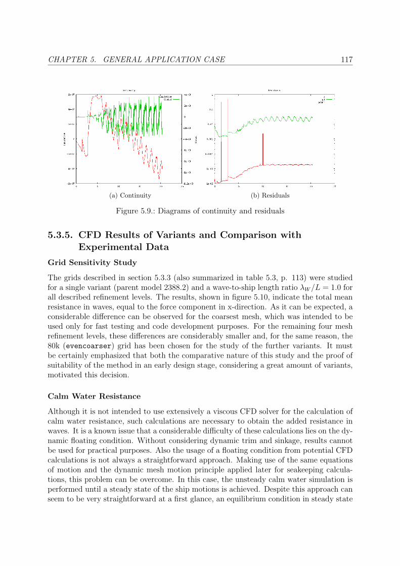
CHAPTER 5. GENERAL APPLICATION CASE 117
(a) Continuity (b) Residuals
Figure 5.9.: Diagrams of continuity and residuals
5.3.5. CFD Results of Variants and Comparison withExperimental Data
Grid Sensitivity Study
The grids described in section 5.3.3 (also summarized in table 5.3, p. 113) were studiedfor a single variant (parent model 2388.2) and a wave-to-ship length ratio λW/L = 1.0 forall described refinement levels. The results, shown in figure 5.10, indicate the total meanresistance in waves, equal to the force component in x-direction. As it can be expected, aconsiderable difference can be observed for the coarsest mesh, which was intended to beused only for fast testing and code development purposes. For the remaining four meshrefinement levels, these differences are considerably smaller and, for the same reason, the80k (evencoarser) grid has been chosen for the study of the further variants. It mustbe certainly emphasized that both the comparative nature of this study and the proof ofsuitability of the method in an early design stage, considering a great amount of variants,motivated this decision.
Calm Water Resistance
Although it is not intended to use extensively a viscous CFD solver for the calculation ofcalm water resistance, such calculations are necessary to obtain the added resistance inwaves. It is a known issue that a considerable difficulty of these calculations lies on the dy-namic floating condition. Without considering dynamic trim and sinkage, results cannotbe used for practical purposes. Also the usage of a floating condition from potential CFDcalculations is not always a straightforward approach. Making use of the same equationsof motion and the dynamic mesh motion principle applied later for seakeeping calcula-tions, this problem can be overcome. In this case, the unsteady calm water simulation isperformed until a steady state of the ship motions is achieved. Despite this approach canseem to be very straightforward at a first glance, an equilibrium condition in steady state

118 5.3. VISCOUS CFD CALCULATIONS
Figure 5.10.: Results of total longitudinal force in waves for different mesh refinementlevels (λW/L = 1.00, ζA = 0.05)
appears to be very difficult to find. One can expect that such small motions dissipateenergy through very short waves. These waves, if present, would not be resolved by thecalculations due to the insufficient transversal and longitudinal discretization of the freesurface, being therefore the energy dissipation of these waves not present. Additionally,small numerical disturbances (such as reflections of long, narrow waves from the domainboundaries) make considerably longer CFD simulation times necessary in order to achievethe pursued steady state. By means of an artificial damping constant for the heave andpitch motions of the ship, the first of these difficulties is partially overcome, although theadjustment of this constant requires previous testing and simulation times are not reducedconsiderably. In figure 5.11, the time histories of total resistance, trim and sinkage areshown for an example case. A long total simulation times and the large oscillations showthe mentioned difficulties which were dealt with.
Added Resistance and Motions in Waves
The main purpose of the application of the presented CFD tool is the prediction ofmotions and added resistance in waves in regular head waves, as outlined in section5.3.1. For this purpose, unsteady simulations of 20s to 30s (of simulation time) havebeen performed. The achieved results were considered adequate when a minimum of fivefull periods are simulated successfully. From these results, mean values for the forces(e.g. total resistance in waves) were obtained. Additionally, a least square regressionwas made to identify the amplitude and phase of motions and forces. An example ofthe time histories of motions and forces, including fitted harmonic functions, are shownin figures 5.13 and 5.14. The mean value of the force was therefore obtained from themaximal number of full periods available from the CFD calculations. These results areprocessed for every variant and subvariant for the mentioned wave lengths (λw/LPP =0.750, 1.000, 1.125, 1.250, 1.500, 1.750).
The mean added resistance in waves obtained for variants 2388.2 and 2388.3 is comparedto the experimental results from Kracht. Figure 5.15 shows both the experimental and nu-merical results in dimensionless form for the mentioned variants. The accordance between
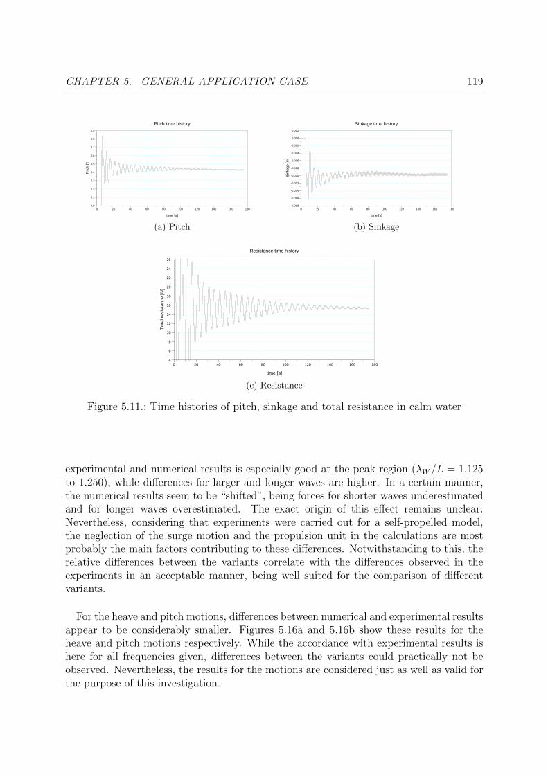
CHAPTER 5. GENERAL APPLICATION CASE 119
0 20 40 60 80 100 120 140 160 1800.0
0.1
0.2
0.3
0.4
0.5
0.6
0.7
0.8
0.9
Pitch time history
time [s]
Pitc
h [°]
(a) Pitch
0 20 40 60 80 100 120 140 160 180-0.018
-0.016
-0.014
-0.012
-0.010
-0.008
-0.006
-0.004
-0.002
0.000
0.002
Sinkage time history
time [s]
Sin
kage
[m]
(b) Sinkage
0 20 40 60 80 100 120 140 160 1804
6
8
10
12
14
16
18
20
22
24
26
Resistance time history
time [s]
Tot
al r
esis
tanc
e [N
]
(c) Resistance
Figure 5.11.: Time histories of pitch, sinkage and total resistance in calm water
experimental and numerical results is especially good at the peak region (λW/L = 1.125to 1.250), while differences for larger and longer waves are higher. In a certain manner,the numerical results seem to be “shifted”, being forces for shorter waves underestimatedand for longer waves overestimated. The exact origin of this effect remains unclear.Nevertheless, considering that experiments were carried out for a self-propelled model,the neglection of the surge motion and the propulsion unit in the calculations are mostprobably the main factors contributing to these differences. Notwithstanding to this, therelative differences between the variants correlate with the differences observed in theexperiments in an acceptable manner, being well suited for the comparison of differentvariants.
For the heave and pitch motions, differences between numerical and experimental resultsappear to be considerably smaller. Figures 5.16a and 5.16b show these results for theheave and pitch motions respectively. While the accordance with experimental results ishere for all frequencies given, differences between the variants could practically not beobserved. Nevertheless, the results for the motions are considered just as well as valid forthe purpose of this investigation.

120 5.3. VISCOUS CFD CALCULATIONS
Figure 5.12.: Wave elevation in calm waters for variant 2388.2
6 8 10 12 14 16 18 20 22 24 26−0.12
−0.10
−0.08
−0.06
−0.04
−0.02
0.00
0.02
0.04
0.06
Heave
time [s]
heav
e [m
]
(a) Heave time history
6 8 10 12 14 16 18 20 22 24 26−3
−2
−1
0
1
2
3
Pitch
time [s]
pitc
h [°
]
(b) Pitch time history
Figure 5.13.: Heave and pitch time histories for parent hull, λW/L = 1.750 (black) andleast square fitted harmonic function (blue)
5.3.6. CFD Results of Subvariants
Added Resistance and Motions in Waves
After the comparison of numerical and experimental results from the main variants 2388.2and 2388.3, calculations in regular head waves for the remaining subvariants were under-taken. For this purpose, the same setup and meshing approach presented previously wasapplied, to ensure absolute comparability of final results. Calculations for the same sevenwave lengths, a single velocity and a single floating condition were performed.
Results of added resistance in waves for all variants are shown in fig. 5.17. The resultsshow clear differences between subvariants, demonstrating the ability of the presentedCFD calculations to reflect such slight geometrical differences in the results.
As it could be expected, results for variant 2388.3, having the most pronounced bulbousbow, show the highest added resistance in the same way as experimental results do.
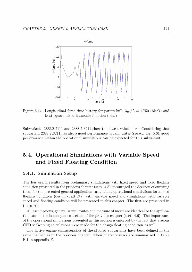
CHAPTER 5. GENERAL APPLICATION CASE 121
0 5 10 15 20 25−100
−50
0
50
100
150
x−force
time [s]
x−fo
rce
[N]
Figure 5.14.: Longitudinal force time history for parent hull, λW/L = 1.750 (black) andleast square fitted harmonic function (blue)
Subvariants 2388.2 2111 and 2388.2 3211 show the lowest values here. Considering thatsubvariant 2388.2 3211 has also a good performance in calm water (see e.g. fig. 5.6), goodperformance within the operational simulations can be expected for this subvariant.
5.4. Operational Simulations with Variable Speed
and Fixed Floating Condition
5.4.1. Simulation Setup
The less useful results from preliminary simulations with fixed speed and fixed floatingcondition presented in the previous chapter (sect. 4.5) encouraged the decision of omittingthese for the presented general application case. Thus, operational simulations for a fixedfloating condition (design draft T22) with variable speed and simulations with variablespeed and floating condition will be presented in this chapter. The first are presented inthis section.
All assumptions, general setup, routes and measure of merit are identical to the applica-tion case in the homonymous section of the previous chapter (sect. 4.6). The importanceof the operational simulations presented in this section is enforced by the fact that viscousCFD seakeeping calculations were made for the design floating condition as well.
The fictive engine characteristics of the studied subvariants have been defined in thesame manner as in the previous chapter. Their characteristics are summarized in tableE.1 in appendix E.

1225.4. OPERATIONAL SIMULATIONS WITH VARIABLE SPEED AND FIXED
FLOATING CONDITION
0
1
2
3
4
5
6
7
8
9
10
0.50 0.75 1.00 1.25 1.50 1.75 2.00
Exp-2388.2
Exp-2388.3
2388-2_1111
2388-3_1111
CAW at Fn = 0.250
λW /L
CAW
Figure 5.15.: Added resistance in waves for variants 2388.2 and 2388.3 from experimentsand RANSE CFD calculations
5.4.2. Comparison with Results Recalling Experimental Data
The results from the operational simulations obtained for subvariants 2388.2 1111 and2388.3 1111 are compared with results for the same ships from the operational simu-lations recalling experimental data (from section 4.6). Figures 5.18a to 5.18f show thenormalized Fuel Equivalent Costs FEC as obtained from operational simulations withexperimental and numerical data. In these diagrams, “experimental” and “numerical”results are normalized separately by their respective parent ship results. Differences areevidently present and can be expected when comparing numerical and experimental re-sults for calm water resistance and added resistance in waves. Notwithstanding to this,the comparative ranking between variants shows consistency in all diagrams, particularlyin the location of crossings between the curves.
Considering all aspects mentioned here, the applicability of operational simulationsrecalling only numerical data is demonstrated for design purposes, making their usage forthe evaluation of new designs (in our case the presented subvariants) a further, logicalstep to undertake.
5.4.3. Results of Subvariants
The operational simulations with variable speed and fixed floating condition play a centralrole in this investigation. The design exploration by means of a performance assessmentfor selected subvariants, including the usage of advanced numerical methods and the

CHAPTER 5. GENERAL APPLICATION CASE 123
0,75
1
1,25
1,5
2388.2exp
2388.3exp
2388-
0
0,25
0,5
0,50 0,75 1,00 1,25 1,50 1,75 2,00
2388-2_1111
2388-3_1111
η3 at Fn = 0.250
λW /L
η 3/ζ
a
(a) Heave responses from CFD and experi-ments
0,75
1
1,25
1,5
2388.2exp
2388.3exp
2388-
0
0,25
0,5
0,50 0,75 1,00 1,25 1,50 1,75 2,00
2388-2_1111
2388-3_1111
η5 at Fn = 0.250
λW /Lη 5/(kζ a
)
(b) Heave responses from CFD and experi-ments
Figure 5.16.: Responses in head waves for variants 2388.2 and 2388.3 from experimentsand RANSE CFD calculations
simulation of the operational life of these designs has been one of its main purposes. Asfor the results presented in the previous chapter for simulations with variable speed andfixed floating condition, results presented here have the advantage of addressing addedresistance and motions in waves from the CFD calculations without additional correctionsfor floating condition from strip theory calculations.
The obtained results for fuel equivalent costs FEC are shown in figure 5.19 (p.127) foreach subvariant as function of the scaling factor λ for all considered routes. Additionalresults for RAW and achieved speed VS can be found in appendix E, figs. E.1 and E.2respectively.
In general terms, similar tendencies as discussed in chapter 4 (sect. 4.6) can be observed:
• Routes can be categorized here into calm weather routes (Le Havre-Paranaguaand Valparaıso-Yokohama) and rough weather routes (Le Havre-Charleston, SanFrancisco-Yokohama and Melbourne-Djibouti) as in the previous chapter
• In calm weather routes, subvariant 2388.2 3223 (purple line) shows the best perfor-mance for larger ship sizes (λ = 33, 50)
• In rough weather routes, subvariant 2388.2 3211 (red line) shows the best perfor-mance, except for the greatest length class with λ = 50
• Specifically in the route Melbourne - Djibouti (fig. 5.19e), this subvariant (2388.2 3211)shows the best performance for all length classes
• Again, a peak in the influence of added resistance in rough weather routes for λ = 25can be observed.

1245.4. OPERATIONAL SIMULATIONS WITH VARIABLE SPEED AND FIXED
FLOATING CONDITION
0
1
2
3
4
5
6
7
8
9
10
0.50 0.75 1.00 1.25 1.50 1.75 2.00
2388-2_1111
2388-3_1111
2388-2_2111
2388-2_3121
2388-2_3211
2388-2_3223
CAW at Fn = 0.250
λW /L
CAW
Figure 5.17.: Added resistance in waves for variants 2388.2 and 2388.3 and subvariantsfrom RANSE CFD calculations
A short discussion will be made for the results with λ = 25, since this scaling factorrepresents the ship as it was originally designed.
First, results of (sub-)variants 2388.2 (2388.2 1111) and 2388.3 (2388.3 1111) will bediscussed. Recalling only the fuel oil consumption in calm water (see. fig. 4.5. p.82),an advantage of less than 2% is obtained for the larger bulbous bow (here 2388.3 1111)when compared to the parent ship (here 2388.2 1111). This would have probably leada designer to choose the larger bulbous bow for his design if no further informationwould have been available for his decision. After the accomplishment of the operationalsimulations presented here, this advantage becomes for some routes the opposite: for theroute Melbourne-Djibouti, for example, the larger bulbous bow is now more than 5%worse in its performance than the parent ship (fig. 5.19e). For the mean of all routes(fig. 5.19f), this difference is lower (approx. 2%), but still opposite to the results incalm water. Even if both performance assessments had different measures of merit andwithout considering the possibility of insufficient precision or false assumptions in any oftwo methods (calm water resistance and operational simulations), this comparison showsclearly that operational aspects are worth to consider in ship design.
When including the newly designed subvariants in this comparison for λ = 25, the differ-ences become slightly larger. From the evaluation in calm water, subvariant 2388.2 3223appears to be the best configuration (see e.g. fig. C.3 in app. C). For the operational sim-ulation between Melbourne and Djibouti, the best performance is attained by subvariant2388.2 3211 which has, according to the operational simulation, a performance about 6%
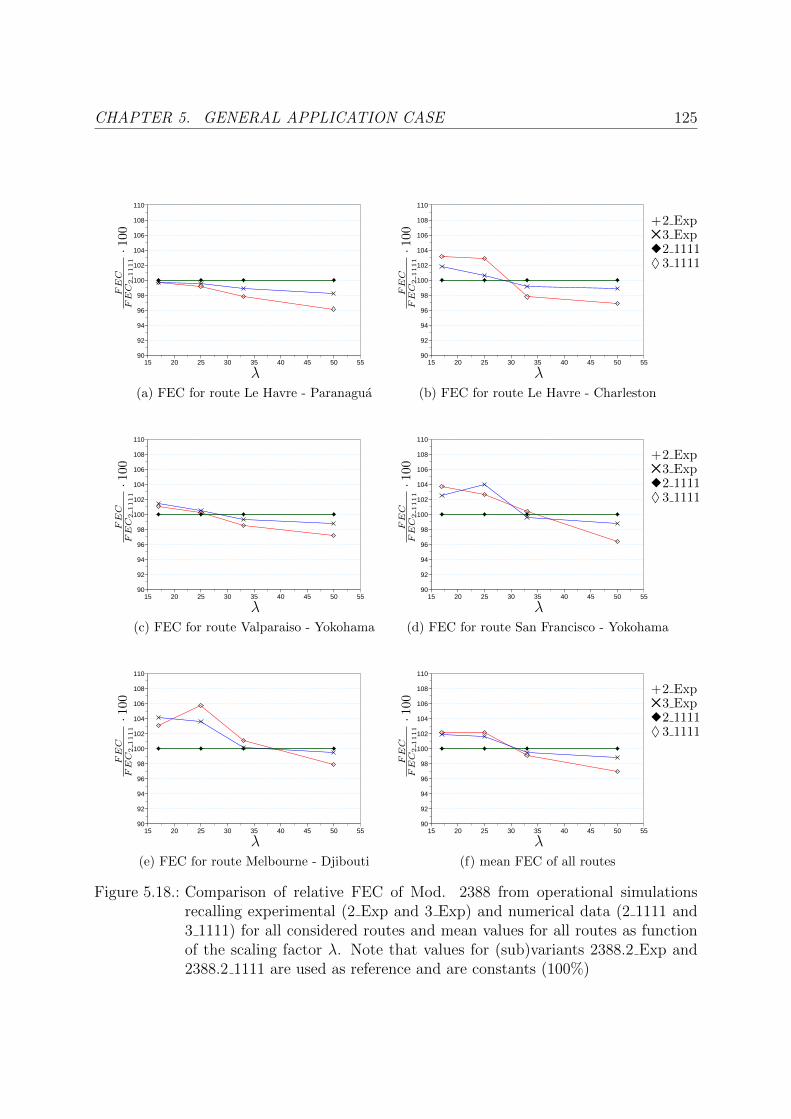
CHAPTER 5. GENERAL APPLICATION CASE 125
15 20 25 30 35 40 45 50 5590
92
94
96
98
100
102
104
106
108
110
λ
FEC
FEC
21111·1
00
(a) FEC for route Le Havre - Paranagua
15 20 25 30 35 40 45 50 5590
92
94
96
98
100
102
104
106
108
110
λ
+2 Exp53 Expu2 1111♦ 3 1111
FEC
FEC
21111·1
00(b) FEC for route Le Havre - Charleston
15 20 25 30 35 40 45 50 5590
92
94
96
98
100
102
104
106
108
110
λ
FEC
FEC
21111·1
00
(c) FEC for route Valparaiso - Yokohama
15 20 25 30 35 40 45 50 5590
92
94
96
98
100
102
104
106
108
110
λ
+2 Exp53 Expu2 1111♦ 3 1111
FEC
FEC
21111·1
00
(d) FEC for route San Francisco - Yokohama
15 20 25 30 35 40 45 50 5590
92
94
96
98
100
102
104
106
108
110
λ
FEC
FEC
21111·1
00
(e) FEC for route Melbourne - Djibouti
15 20 25 30 35 40 45 50 5590
92
94
96
98
100
102
104
106
108
110
λ
+2 Exp53 Expu2 1111♦ 3 1111
FEC
FEC
21111·1
00
(f) mean FEC of all routes
Figure 5.18.: Comparison of relative FEC of Mod. 2388 from operational simulationsrecalling experimental (2 Exp and 3 Exp) and numerical data (2 1111 and3 1111) for all considered routes and mean values for all routes as functionof the scaling factor λ. Note that values for (sub)variants 2388.2 Exp and2388.2 1111 are used as reference and are constants (100%)
1265.5. OPERATIONAL SIMULATIONS WITH VARIABLE SPEED AND VARIABLE
FLOATING CONDITION
better than subvariant 2388.2 3223. For the mean of all routes, this difference is reducedto approx. 2%, due to the good performance of subvariant 2388.2 3223 in calm weatherroutes. When comparing results of the best subvariant (2388.2 3211) with variant 2388.3,differences become approx. 10% for the route Melbourne-Djibouti and 5% for the meanof all routes.
Considering that only a small design exploration has been performed here, it can beexpected that greater improvements can be achieved by the application of an optimizationstrategy with a large number of designs.
5.5. Operational Simulations with Variable Speed
and Variable Floating Condition
5.5.1. Simulation Setup
The simulations with variable speed and floating condition were made analogous to thedescription made in section 4.7. The main difference is the number of floating conditionscalculated with potential CFD. For the present case, only three floating conditions foreach velocity and subvariant were calculated. Results have been extensively describedin section 5.2.2 and, as in the previous chapter, response surfaces (in this case responseplanes) were defined. Due to the small differences between the calculated and simulatedfloating conditions (defined in table 4.7), approximation errors due to the definition ofthe response planes are kept minimal.
5.5.2. Results
As in the previous chapter, since seakeeping data for off-design floating conditions wasnot included in the viscous CFD calculations, results for these floating conditions areobtained by means of corrections with help of strip theory calculations and offer thereforea higher uncertainty than results from simulations with fixed floating condition. Figures5.20a to 5.20f show the relative fuel equivalent costs FEC for each route and subvariantas a function of ship size. The following tendencies can be observed:
• In contrast to the results from operational simulations with fixed floating condition,subvariant 2388.2 3223 has the worst performance, without exception, for all routesand all ship sizes. This is addressed by the high added resistance in waves and thepoor calm water performance of this model.
• The opposite statement can be made for subvariant 2388.2 3211, showing for everyroute and ship size the best performance, without exception.
• In general terms, it can be observed, when compared to fixed floating conditionresults, that the influence of ship size in the performance ranking is significantlysmaller. This can be also observed for the results in the previous chapter.

CHAPTER 5. GENERAL APPLICATION CASE 127
15 20 25 30 35 40 45 50 5590
92
94
96
98
100
102
104
106
108
110
λ
FEC
FEC
21111·1
00
(a) FEC for route Le Havre - Paranagua
15 20 25 30 35 40 45 50 5590
92
94
96
98
100
102
104
106
108
110
λ
+2 111152 2111u2 3121♦ 2 3211∇2 3223#3 1111F
EC
FEC
21111·1
00
(b) FEC for route Le Havre - Charleston
15 20 25 30 35 40 45 50 5590
92
94
96
98
100
102
104
106
108
110
λ
FEC
FEC
21111·1
00
(c) FEC for route Valparaıso - Yokohama
15 20 25 30 35 40 45 50 5590
92
94
96
98
100
102
104
106
108
110
λ
+2 111152 2111u2 3121♦ 2 3211∇2 3223#3 1111F
EC
FEC
21111·1
00
(d) FEC for route San Francisco - Yokohama
15 20 25 30 35 40 45 50 5590
92
94
96
98
100
102
104
106
108
110
λ
FEC
FEC
21111·1
00
(e) FEC for route Melbourne - Djibouti
15 20 25 30 35 40 45 50 5590
92
94
96
98
100
102
104
106
108
110
λ
+2 111152 2111u2 3121♦ 2 3211∇2 3223#3 1111F
EC
FEC
21111·1
00
(f) mean FEC of all routes
Figure 5.19.: Relative FEC of Mod. 2388 with different bulbous bows for all consideredroutes and mean relative FEC as function of the scaling factor λ from sim-ulations with fixed floating condition
128 5.6. CONCLUSIONS ABOUT APPLICATION CASE
• The maximal FEC gain, when compared to the parent ship 2388.2, is found for theroute between Melbourne and Djibouti for λ = 25 and is only of approx. 2.5%. Forthe same route and ship size, subvariant 2388.2 3223 shows approx. 7.5% higherfuel equivalent costs than the parent ship. When considering that this subvariant(2388.2 3223) presents the lowest calm water resistance at design conditions (designdraft and design speed), a difference in performance of 10% is obtained betweenthose subvariants. This would represent an economic loss of 10% of the Fuel Equiv-alent Costs when choosing the best configuration considering only the calm waterperformance at design conditions instead considering operational and weather as-pects by means of an operational simulation. Even if this difference applies fora single example and a route with significant weather influence, it depicts clearlythe evident disadvantage (or economic risk) of designing hull forms only for designconditions.
The presented operational simulations with variable speed and variable floating condi-tion show the importance of considering off-design floating conditions, despite the draw-back of unavailability of numerical seakeeping data for floating conditions other thandesign draft.
An evident change can be observed when comparing attained results to fixed floatingcondition simulations: the influence of the calm water resistance becomes higher, beingthe change in the rankings along ship size considerably less. This is shown by the evidentlysmaller number of “crossings” between the lines of FEC along the scaling factor λ. Where,for fixed floating condition simulations, a ship with a less pronounced bulbous bow wassuitable for rather smaller ship sizes and a more pronounced one for larger sizes, variablefloating condition simulations show a predominance of rather less pronounced bulbousbows as best configurations (lowest FEC) along all ship sizes studied. This recalls boththe advantage of such a bulb in off-design floating conditions and its better seakeepingperformance (i.e. lower added resistance in waves), at least in the form as it has beenmodeled here.
5.6. Conclusions about Application Case
The presented example case represents the general form of application of the proposeddesign methodology, integrating different numerical methods, a parametric geometry vari-ation approach and operational simulations to improve the performance of a ship in anearly design stage.
Different methods have been applied to model the operation of the ship. Unavoidably,some of these methods make assumptions of limited applicability. If these assumptionshave also consequences in the relative rankings between different designs remains an openquestion. In this context, two aspects should be exposed:
• The consideration of a wide range of both floating conditions and velocities in theviscous CFD calculations in regular waves would have been of great advantage. Sincethis was not the case, and although this would increase the required computational
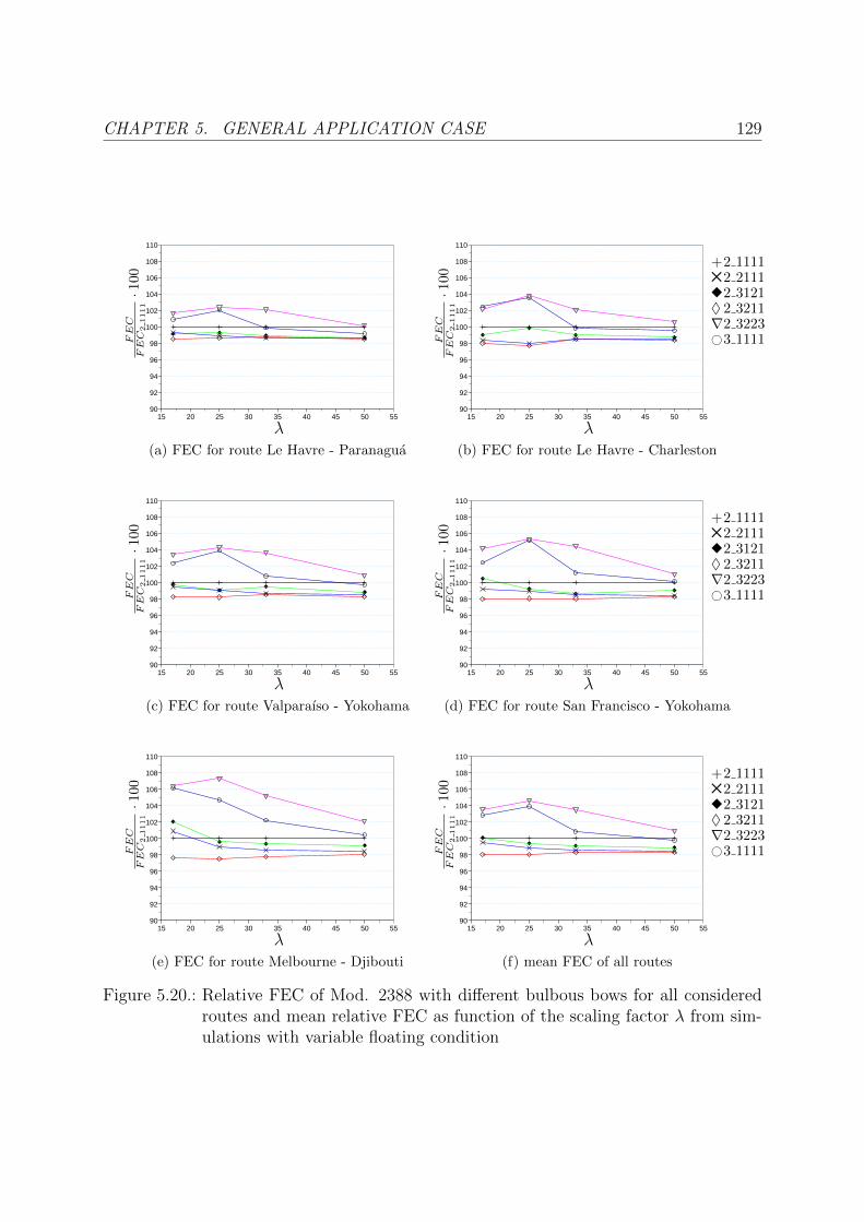
CHAPTER 5. GENERAL APPLICATION CASE 129
15 20 25 30 35 40 45 50 5590
92
94
96
98
100
102
104
106
108
110
λ
FEC
FEC
21111·1
00
(a) FEC for route Le Havre - Paranagua
15 20 25 30 35 40 45 50 5590
92
94
96
98
100
102
104
106
108
110
λ
+2 111152 2111u2 3121♦ 2 3211∇2 3223#3 1111F
EC
FEC
21111·1
00
(b) FEC for route Le Havre - Charleston
15 20 25 30 35 40 45 50 5590
92
94
96
98
100
102
104
106
108
110
λ
FEC
FEC
21111·1
00
(c) FEC for route Valparaıso - Yokohama
15 20 25 30 35 40 45 50 5590
92
94
96
98
100
102
104
106
108
110
λ
+2 111152 2111u2 3121♦ 2 3211∇2 3223#3 1111F
EC
FEC
21111·1
00
(d) FEC for route San Francisco - Yokohama
15 20 25 30 35 40 45 50 5590
92
94
96
98
100
102
104
106
108
110
λ
FEC
FEC
21111·1
00
(e) FEC for route Melbourne - Djibouti
15 20 25 30 35 40 45 50 5590
92
94
96
98
100
102
104
106
108
110
λ
+2 111152 2111u2 3121♦ 2 3211∇2 3223#3 1111F
EC
FEC
21111·1
00
(f) mean FEC of all routes
Figure 5.20.: Relative FEC of Mod. 2388 with different bulbous bows for all consideredroutes and mean relative FEC as function of the scaling factor λ from sim-ulations with variable floating condition
130 5.6. CONCLUSIONS ABOUT APPLICATION CASE
resources considerably, this aspect and the influence of the assumption made shallbe investigated in the future.
• The criterion for the slamming occurrence has been taken from the proposal byOchi [89]. This methodology was defined for bulbless ships, and its applicability forships with bulbous bows is clearly restricted. A deeper study of this aspect, e.g.by means of viscous CFD calculations without the need of any empirical criterion,would certainly bring more accurate predictions for this aspect.
Notwithstanding to this, the applicability of the presented design methodology has beendemonstrated. Beginning with an extensive design exploration, the calm water resistancewas evaluated by means of a potential CFD solver, leading to the choice of four designs forthe evaluation of their seakeeping performances with a viscous CFD method. By means oftwo different operational simulation modes (fixed and variable floating condition), designvariants with best performance were identified for each route and ship size considered.
For both simulation modes considered, subvariants 2388.2 3223 and 2388.2 3211 showedthe best performance. Subvariant 2388.2 3223 achieved best performance in simulationswith fixed floating condition, especially for calm weather routes and large ship sizes. Thisoutcome can be expected, taking account of the advantageous calm water resistance of thissubvariant. For rough weather routes and smaller ship sizes, and also for all simulationswith variable floating condition, subvariant 2388.2 3211 showed the best performance.The bulbous bow of this subvariant is 30% larger than the baseline bow and part of itsvolume has been moved in forward direction (15% inner translation), remaining the verti-cal translation and the radial scaling unchanged. Within the bulbous bows considered inthis design study, subvariant 2388.2 3211 can be placed, in both geometrical and hydro-dynamic aspects, in the middle-field. The fact that this bulbous bow could be identifiedas the best configuration, shows the importance of including off-design conditions in earlystages of ship design. In the same manner, this outcome points out the danger of de-signing and optimizing ships for a single condition (e.g. design speed, design draft andcalm weather) leading, potentially, to designs of poor performance in waves and underoff-design conditions.
If, for any reason, the consideration of weather aspects is not possible for the design of abulbous bow, the choice of rather conservative bulbous bow sizes, with good performancein off-design speeds and off-design floating conditions, is recommended. Additionally,the consideration of the absolute size of the ship for the design of the bulbous bow isrecommended, contrary to the common practice of considering scale-independent aspectsonly (such as Froude number and form coefficients).
CHAPTER 6. SUMMARY AND OUTLOOK 131
6. Summary and Outlook
6.1. Summary
The presented study presents a design methodology considering the simulation of theoperational life of the ship, including weather factors and off-design floating conditions.Different methods are integrated within a simulation environment to achieve this purpose,remarking the application of potential and viscous CFD methods for the evaluation ofresistance and motions in waves.
Two different application cases were included in this investigation. In a first stage,operational simulations recalling existing experimental data were undertaken, discussingthe applicability of the presented operational approach for design purposes. In a secondstage, a general application case presents similar operational simulations, being all hy-drodynamic characteristics recalled from numerical calculations. Of special interest arethe ship responses and added resistance in waves, which are recalled from viscous CFDcomputations. For this application case, further designs were generated by a partiallyparametric approach and were included in the design study. Finally, the performanceof each design for a given route and ship size was assessed and best configurations wereidentified.
The applied methods, especially those regarding hydrodynamic aspects, are well estab-lished and widely spread both in research and industry applications. Nevertheless, someof them have been applied in this investigation either in a novel form or in combinationwith other methods. In the case of viscous CFD methods, their application within adesign study, intended to be applied in an early design stage, is new. The use of rathercoarse meshes and simple setups emphasize the preliminary character of these computa-tions in the design process. The combination of results from intensive CFD calculationswith results from simple, computationally inexpensive methods such as strip theory, hasbeen demonstrated. Although this has been already undertaken by other authors in thepast, their use within operational simulations is new. Further studies in this issue shallbe undertaken in the future.
The presented study demonstrates the practicability of an integrated approach for hy-drodynamic ship (or specifically bulbous bow) design including resistance, responses inwaves and off-design conditions in a single platform, considering realistic operational con-ditions and showing the possibility of identifying designs performing better under thoseconditions.

132 6.2. OUTLOOK
6.2. Outlook
The present study can be regarded as a further step towards the integration of all relevantmethodologies involved in ship design, taking account of weather (especially seaway) andoperational aspects for design evaluation.
Many aspects, which came to light during this investigation, brought also new questionswith them. Due to the modular character of the simulation platform, further studies canbe realized with a significantly reduced effort. An important prerequisite for this would bea more comprehensive validation of the simulation platform by studying a large numberof existing ships under operation, where measured data can be compared with.
Detailed information about motions and forces in waves were available for head seasonly. As a matter of fact, these are considered especially relevant for the added resistancein waves, but not necessarily critical for the security of the ship. Security-relevant situa-tions (e.g. parametric rolling, wave-riding or reduction of stability), especially in followingand quartering seas, with the subsequent voluntary speed loss, were not considered. Al-though it can be expected that the performance loss when including these aspects willnot induce relevant relative differences between the studied variants and subvariants, thisaspect shall be studied in the future.
Additional aspects, such as the inclusion of route optimization into the simulationsis also a task showing the possibility of combining different approaches towards highertransport efficiency. Investigations related to this task are been undertaken at the momentby Balloch [10]. The consideration of security- or pollution-related tasks, combined witha more complex measure of merit able to include these aspects, can lead to a furtherstep into the integration of all relevant aspects in ship design, being a potentially valuablecontribution into concepts such as “holistic ship design” or “simulation-based ship design”.
The presented general application case, in all its simulation modes, has shown thepracticability of the proposed method when recalling essential data alone from numericalmethods. The inclusion of parametrically generated subvariants showed the ability of themethodology of helping the designer to identify economically convenient solutions alongthe design process. A higher automatization grade within all steps performed, togetherwith a massive parallelization, can make this method a viable approach for practicalapplications in industry in the future.

Bibliography 133
Bibliography
[1] Amazon Web Services (AWS) website. http://aws.amazon.com. – last visited:may 2009
[2] ECMWF ERA-40 data portal. http://data-portal.ecmwf.int/data/d/era40_
daily. – last visited: feb. 2010
[3] HLRN Supercomputing Service. https://www.hlrn.de/home/view/Service. – lastvisited: nov. 2009
[4] IIHR - Hydroscience and Engineering website - experimental validation data. http://www.iihr.uiowa.edu/~shiphydro/efd.htm. – last visited : 06.07.2010
[5] International Marine Coatings - Hull Roughness Penalty Calculator. http://www.
international-marine.com/newbuilding/brochures/HRPCFolder&Paper.pdf.– last visited: feb 2007
[6] OpenFOAM user manual. http://www.openfoam.com. – last visited: jan. 2010
[7] SciLab (Digiteo). http://www.scilab.org. – last visited: 07.2008
[8] W.S. Atkins Consultants: MARNET-CFD - Best Practice Guidelines for Ma-rine Applications of Computational Fluid Dynamics. 2003. – Tech. report
[9] Abt, C. ; Harries, S.: A New Approach to Integration of CAD and CFD forNaval Architects. In: 6th International Conference on Computer Applications andInformation Technology in the Maritime Industries (COMPIT2007), 2007
[10] Balloch, M.: Integration of Hydrodynamic Ship Design and Route Optimizationusing Long-Term Simulations: an Application Example for Different Bulbous BowVariants, Universita di Genoa, MSc thesis, 2010
[11] Bertram, V.: Numerical Investigation of Steady Flow Effects in Three-Dimensional Seakeeping Computations. In: 22nd Symposium on Naval Hydrody-namics, 2000
[12] Bertram, V. ; Thiart, G.: Fully 3-d ship seakeeping computations with a surge-corrected Rankine panel method. In: Jour. of Marine Science and Technology 3(1998), no. 2, pp. 94–101

134 Bibliography
[13] Bertram, V. ; Veelo, B. ; Soding, H. ; Graf, K.: Development of a Freely Avail-able Strip Method for Seakeeping. In: COMPIT’06 (5th International Conferenceon Computer Applications and Information Technology in the Maritime Industries),2006
[14] Bertram, V. ; Yasukawa, H.: Rankine source methods for seakeeping problems.In: STG Jahrbuch 90 (1996), pp. 411–425
[15] Bertram, V. ; Yasukawa, H.: Investigation of Global and Local Flow Detailsby a Fully Three-Dimensional Seakeeping Method. In: 23th Symposium on NavalHydrodynamics, 2001, pp. 355–367
[16] Blume, P.: Uber die Effektivitat von Bugwulsten unter Seebedingungen / HSVA.1981 (1513). – Tech. report
[17] Blume, P. ; Kracht, A.: Prediction of the Behavior and Propulsive Performanceof Ships with Bulbous Bow in Waves. In: SNAME Transactions 93 (1985), pp.79–94
[18] Boese, P.: Eine einfache Methode zur Berechnung der Widerstanderhohung einesSchiffes im Seegang. In: Schiffstechnik 17 (1970), no. 86, pp. 29–32
[19] Boulougouris, E. ; Papanikolaou, A.: Hullform Optimization of a HighSpeed Wave Piercing Monohull. In: Ninth International Marine Design Confer-ence (IMDC’06), 2006
[20] Buxton, I.: Fuel costs and their relationship with capital and operating costs. In:Maritime Policy & Management 12 (1985), Jan., no. 1, pp. 47–54
[21] Campana, E. ; Peri, D. ; Tahara, Y. ; Stern, F.: Shape optimization inship hydrodynamics using computational fluid dynamics. In: Computer methods inapplied mechanics and engineering 196 (2006), pp. 634–651
[22] Carrica, P. ; Wilson, R. ; Noack, R. ; Stern, F.: Ship motions unsing single-phase level set with dynamic overset grids. In: Elsevier (ed.): Computers & Fluidsvol. 36, 2007, 1415-1433
[23] Carrica, P. ; Wilson, R. ; Stern, F.: Unsteady RANS simulation of the shipforward speed diffraction problem. In: Computers & Fluids 35 (2006), July, pp.545–570
[24] Couwenberg, M.: shipFoam contribution. CFD-Online fo-rum. http://www.cfd-online.com/Forums/openfoam-solving/
57774-hydrostatic-pressure-gravity-2.html. – last visited: aug. 2008
[25] Cura Hochbaum, A. ; Pierzynski, M.: Flow Simulation for a Combatant inHead Waves. In: Proceedings of the CFD Workshop Tokyo 2005, 2005
Bibliography 135
[26] Cura Hochbaum, A. ; Vogt, M.: Numerische Simulation der Schiffsbewegungenin Wellen von vorme mit einem RANSE-Verfahren / HSVA-Report. 2002 (1648). –Tech. report
[27] Dallinga, R. P. ; Daalen, E.V. ; Grin, R. ; Willemstein, T.: ScenarioSimulations in Design for Service. In: Proceedings PRADS 2004. Travemunde,Germany, 2004
[28] Dunlap, G. D. ; Shufeldt, H. H.: Dutton’s Navigation and Piloting. NavalInstitute Press, 1975
[29] Faltinsen, O. ; Minsaas, K. ; Liapis, N. ; Skjordal, S.: Prediction of Resis-tance and Propulsion of a Ship in a Seaway. In: Proc. 13th. Symposium on NavalHydrodynamics. Tokyo, Japan, 1980, pp. 505–529
[30] Ferziger, J. H. ; Peric, M.: Computational Methods for Fluid Dynamics.Springer, 2002
[31] Geittner, M.: Betriebssimulation von Frachtschiffen mit Windzusatzantrieb,Technical University of Berlin, Design and Operation of maritime Systems, MScthesis, 2007
[32] Gentaz, L. ; Guillerm, B. ; Alessandrini, B. ; Delhommeau, G.: Three-dimensional free surface viscous flow around a ship in forced motion. In: Proceedingsof the 7th International Conference on Numerical Ship Hydrodynamics. Nantes, 1999
[33] Gerritsma, J. ; Beukelmann, W.: Analysis of the Resistance Increase in Wavesof a Fast Cargo Ship. In: International Shipbuilding Progress 19 (1972), pp. 285–293
[34] Greitsch, L. ; Eljardt, G.: Simulation of Lifetime Operating Conditions asInput Parameters for CFD Calculations and Design Evaluation. In: NumericalTowing Tank Symposium. Cortona, 2009
[35] Greitsch, L. ; Eljardt, G. ; Krueger, S.: Operating Conditions Aligned ShipDesign and Evaluation. In: First International Symposium on Marine Propulsors.Trondheim, Norway, 2009
[36] Grigoropoulos, G.J. ; Loukakis, T.A. ; Perakis, A.N.: Seakeeping StandardSeries for Oblique Seas (a Synopsis). In: Ocean Engineering 27 (2000), pp. 111–126
[37] Grim, O.: Berechnung der durch Schwingungen eines Schiffskorpers erzeugtenhydrodynamischen Krafte. In: STG Jahrbuch 47 (1953), pp. 277–299
[38] Gui., L. ; Longo, L. ; Metcal, B. ; Shao, J. ; Stern, F.: Forces, Moment, andWave Pattern for Surface Combatant in Regular Head Waves -Part 1: MeasurementSystems and Uncertainty Analysis. In: Experiments in Fluids 31 (2001), no. 6, pp.674–680

136 Bibliography
[39] Gui., L. ; Longo, L. ; Metcalf, B. ; Shao, J. ; Stern, F.: Forces, Moment, andWave Pattern for Surface Combatant in Regular Head Waves-Part 2: MeasurementResults and Discussions. In: Experiments in Fluids 32 (2002), no. 1, pp. 27–36
[40] Harries, S.: Parametric design and hydrodynamic optimization of ship hull forms,Technische Universitat Berlin, PhD thesis, 1998. – ISBN: 3-933346-24-X
[41] Harries, S. ; Abt, C. ; Heimann, J. ; Hochkirch, K.: Advanced hydrody-namic design of container carriers for improved transport efficiency. In: Design andOperation of Container Ships, RINA, 2006
[42] Hermans, A. J.: Slowly moving hull forms in short waves. In: Journal of Engi-neering Mathematics 25 (1991), February, no. 1, pp. 63–75
[43] Hinnenthal, J.: Robust Pareto - Optimum Routing of Ships utilizing Deterministicand Ensemble Weather Forecasts, Technical University of Berlin, PhD thesis, 2007
[44] Hino, T. (ed.) ; NMRI Report 2005 (Veranst.): Proceedings of the CFD WorkshopTokyo 2005. 2005
[45] Hochkirch, K. ; Bertram, V.: Slow Steaming Bulbous Bow Optimization for aLarge Containership. In: COMPIT 2009, 2009
[46] Hollenbach, U.: Estimating Resistance and Propulsion for Single-Screw andTwin-Screw Ships. In: Schiffstechnik 45 (1998), pp. 72–76
[47] Hollenbach, U. ; Friesch, J.: Efficient hull forms. What can be gained? In:International Conference on Ship Efficiency, 2007
[48] Hollenbach, U. ; Klug, H.: Optimising Hull Forms for Design- and ”Off-Design”-Conditions. In: STG-Sprechtag ”Verbesserung der Propulsions- und Manovri-ereigenschaften von Schiffen”. Emden, September 2008
[49] Holtrop, J.: A Statistical Re-Analysis of Resistance and Propulsion Data. In:International Shipbuilding Progress 353 (1984), pp. 272–276
[50] Holtrop, J. ; Mennen, G.: An Approximate Power Prediction Method. In:International Shipbuilding Progress 329 (1982), pp. 166–170
[51] Irvine, M. ; Longo, J. ; Stern, F.: Pitch and Heave Tests and UncertaintyAssessment for a Surface Combatant in Regular Head Waves. In: Journal of ShipResearch 52 (2008), pp. 146–163
[52] ITTC: Report of the Seakeeping Commitee. 1978. – Tech. report
[53] ITTC: Report of the Resistance and Flow Commitee (20h ITTC). San Francisco,California, 1993. – Tech. report
Bibliography 137
[54] ITTC: Report of the Resistance and Flow Commitee (21h ITTC). Trondheim,Norway, 1996. – Tech. report
[55] ITTC: ITTC Recommended Procedures and Guidelines - ITTC 1978 PerformancePrediction Method. 1999 (7.5-02-03-01.4). – Tech. report
[56] ITTC: Report of the Resistance Commitee (22h ITTC). Seoul and Shanghai, 1999.– Tech. report
[57] ITTC: Report of the Resistance Commitee (23h ITTC). Venice, Italy, 2002. –Tech. report
[58] Jasak, H.: OpenFOAM: Open source CFD in research and industry. In: Inter-national Journal of Naval Architecture and Ocean Engineering 1 (2009), no. 2, pp.89–94
[59] Jensen, G.: Berechnung der stationaren Potentialstromung um ein Schiff unterBerucksichtigung der nichtlinearen Randbedingung an der freien Wasseroberflache,Technical University of Harburg-Hamburg, PhD thesis, 1988
[60] Jensen, G. ; Mi, Z.-X. ; SA¶ding, H.: Rankine Methods for the Solution of theSteady Wave Resistance Problem. In: Sixteenth Symposium on Naval Hydrodynam-ics, 1986
[61] Joosen, W.P.A.: Added Resistance of Ships in Waves. In: 6th Symp. on NavalHydrodynamics. Washington D.C., 1966, pp. 12
[62] Journee, J.M.J. ; Adegeest, L.J.M.: Theoretical Manual of StripTheory Pro-gram ”SEAWAY for Windows” / TU Delft, Amarcon. 2003 (Rep. 1370). – Theo-retical manual
[63] Kihara, H. ; Naito, S. ; Sueyoshi, M.: On the Practical Prediction of AddedResistance Using Nonlinear Slender Body Theory. In: 4th Osaka Colloquium onSeakeeping Performance of Ships, 2000, pp. 115–129
[64] Kihara, H. ; Naito, S. ; Sueyoshi, M.: Numerical Analysis of the Influence ofAbove-Water Bow Form on Added Resistance using Nonlinear Slender Body Theory.In: Journal of Ship Research 49 (2005), pp. 191–206
[65] Kodama, Y. (ed.): Proceedings of the CFD Workshop Tokyo 1994. Japan, 1994
[66] Kracht, A.: Der Bugwulst als Entwurfselement im Schiffbau. In: STG Jahrbuch70 (1976), pp. 139–159
[67] Kracht, A.: Weitere Untersuchungen uber die Anwendung von Bugwulsten /VWS. 1979 ((811/78)). – Tech. report

138 Bibliography
[68] Kracht, A.: Einfluss des Bugwulstes auf den Leistungsbedarf eines Schiffes imSeegang / VWS. 1984 (988/84). – Tech. report
[69] Kracht, A.: Untersuchung des Einflusses teilgetauchter Bugwulste auf die er-forderliche Antriebsleistung / VWS. 1984 (989/84). – Tech. report
[70] Kracht, A.: Vorlesungsskript Schiffshydrodynamik I und II. 2005. – Lessonsmaterial for ship hydrodynamics, held at TU Berlin
[71] Kring, D. ; Huang, Y.-F. ; Sclavounos, P. ; Vada, T. ; Braathen, A.: Nonlin-ear Ship Motions and Wave-Induced Loads by a Rankine Method. In: Twenty-FirstSymposium on Naval Hydrodynamics, 1997
[72] Larsson, L. ; Broberg, L. ; Kim, K.J. ; Zhang, D.H.: New Viscous and Invis-cid CFD Techniques for Ship Flows. In: Proc. 5th Int. Conf. on Numerical ShipHydrodynamics, 1990
[73] Larsson, L. (ed.) ; Stern, F. (ed.) ; Betram, V. (ed.): Gothenburg 2000 - AWorkshop on Numerical Ship Hydrodynamics. Sweden, 2000
[74] Larsson, L. ; Stern, F. ; Betram, V.: Benchmarking of Computational FluidDynamics for Ship Flows: The Gothenburg 2000 Workshop. In: Journal of ShipResearch 47 (2003), pp. 63–81
[75] Lewis, E. (ed.): Principles of Naval Architecture. vol. 3. SNAME, 1989
[76] Lewis, F.M.: The inertia of the water surrounding a vibrating ship. In: SNAMETransactions 37 (1929), pp. 1–20
[77] Luquet, R. ; Ducrozet, G. ; Gentaz, L. ; Ferrant, P. ; Alessandrini, B.:Applications of the SWENSE Method to seakeeping simulations in irregular waves.In: 9th International Conference in Numerical ShipHydrodynamics, 2007
[78] MAN B&W (ed.): Ship Propulsion - Basic Principles of Ship Propulsion (MANB&W). MAN B&W, 2006. http://www.manbw.com
[79] MAN B&W (ed.): MAN B&W Marine Engine Programme 2007. MAN B&W,2007. http://www.manbw.com
[80] Maruo, H.: The Excess Resistance of a Ship in Rough Seas. In: InternationalShipbuilding Progress 4 (1957), no. 35, pp. 337–345
[81] Matsumoto, K. ; Naito, S. ; Takagi, K. ; Hirota, K. ; Takagishi, K.: Beak-Bow to Reduce the Wave Added Resistance at Sea. In: PRADS’98, Practical Designof Ships and Mobile Units, 1998
[82] Minoura, M. ; Naito, S.: Stochastic Sea Climate Simulation Based on HindcastData. In: Proc. ISOPE vol. III. San Francisco, California, 2006, pp. 94–101

Bibliography 139
[83] Naito, S.: Propulsive Performence of Ships in Actual Seas. In: 7th Osaka Collo-quium on Seakeeping and Stability, 2008
[84] Nakos, D. ; Kring, DF. ; Sclavounos, P.: Rankine panel methods for time-domain free surface ows. In: Proceedings of the Sixth International Conference onNumerical Ship Hydrodynamics, 1994
[85] Nowacki, H.: Economic and technical issues in hull form development. 1985. –Lessons material for ship theory, held at TU Berlin
[86] Nowacki, H.: Developments in Marine Design Methodology: Roots, Results andFuture Trends. In: Erikstad, S. O. (ed.): 10th International Marine DesignConference (IMDC 2009) vol. 1. Trondheim, Norway : Tapir Academic Press,2009, pp. 47–80
[87] Nowacki, H. ; Holbach, G. ; Papanikolaou, A. ; Zaraphonitis, G.: Conceptand Hydrodynamic Design of a High-Speed SWATH Passenger/Car Ferry for theMediterranean Sea. In: Jahrbuch der Schiffbautechnischen Gesellschaft 84 (1990),pp. 171–181
[88] Ochi, M.: Wave Statistics for the Design of Ships and Ocean Structures. In:SNAME Transactions 86 (1978), pp. 47–76
[89] Ochi, M. K.: Prediction of Occurrence and Severity of Ship Slamming at Sea. In:Proceedings of 5th Symposium on Naval Hydrodynamics. Bergen, Norway, 1964, pp.545–596
[90] Ogilvie, T.: Recent Progress Towards the Understanding and Prediction of ShipMotions. In: Proc. of the 6th Symposium on Naval Hydrodynamics, 1964
[91] Olivieri, A. ; Pistani, F. ; Avanzini, A. ; Stern, F. ; Penna, R.: Towing TankExperiments of Resistance, Sinkage and Trim, Boundary Layer, Wake, and FreeSurface Flow Around a Naval Combatant INSEAN 2340 Model / Iowa Institute ofHydraulic Research, The University of Iowa. 2001 (421). – Tech. report
[92] Orihara, H. ; Miyata, H.: Evaluation of added resistance in regular incidentwaves by computational fluid dynamics motion simulation using an overlappinggrid system. In: Journal of Marine Science and Technology 8 (2003), pp. 47–60
[93] Oschmann, P.: Betriebssimulation innovativer und konventioneller Hauptmaschi-nenkonzepte: ein Vergleich fur unterschiedliche Szenarien und Schiffstypen, Tech-nical University of Berlin, Design and Operation of maritime Systems, MSc thesis,2009
[94] Papanikolaou, A.: Added Resistance in Waves. – Presentation held at TU Berlin,May 2010 (unpublished)

140 Bibliography
[95] Papanikolaou, A.: On integral-equation-methods for the evaluation of motionsand loads of arbitrary bodies in waves. In: Journ. Ingenieur-Archiv 55 (1985), pp.17–29
[96] Pedersen, B. P.: A Comparative Study of Methods for Predicting Added Resistancein Waves, Technical University of Denmark, MSc thesis, 2006
[97] Raven, H.C.: A Solution Method for the Nonlinear Ship Wave Resistance Problem,Delft Univ. Techn., PhD thesis, 1996
[98] Sakamoto, T. ; Baba, E.: Minimization of Resistance of Slowly Moving FullHull Forms in Short Waves. In: Proceedings of the 16th Symposium on NavalHydrodynamics. Berkeley, USA, 1986, pp. 598–612
[99] Salvesen, N.: Added Resistance of Ships in Waves. In: Journal of Hydronautics12 (1978), no. 1, pp. 24–34
[100] Sato, Y. ; Miyata, H. ; Sato, T.: CFD simulation of 3-dimensional motion of aship in waves: application to an advancing ship in regular heading waves. In: Jour.of Marine Science and Technology 4 (1999), pp. 108–116
[101] Schmode, D. ; Bertram, V. ; Tenzer, M.: Simulating Ship Motions and Loadsusing OpenFOAM. In: STG Conference “CFD in Ship-Design”. Hamburg, 25. sept.2009. – unpublished
[102] Schneekluth, H.: Kriterien zur Bugwulstverwendung. In: STG Jahrbuch 69(1975), pp. 1–1
[103] Sclavounos, P.D. ; Nakos, Y. D.E.and H. D.E.and Huang: Seakeeping and WaveInduced Loads on Ships with Flare by a Rankine Panel Method. In: Proceedings ofthe Sixth International Conference on Numerical Ship Hydrodynamics, 1994
[104] Soding, H.: Bewegungen und Belastungen der Schiffe im Seegang / TechnicalUniversity of Hamburg-Harburg. 1982. – course material
[105] Soding, H.: A Method for Accurate Force Calculations in Potential Flow. In: ShipTechnical Research 40 (1993), no. 4, pp. 176–186
[106] Soding, H. ; Bertram, V.: Schiffe im Seegang. In: Handbuch der Werften XXIV(1998), pp. 151–189
[107] St. Denis, M. ; Pierson, W.J.: On the Motion of Ships in Confused Seas. In:SNAME Transactions 61 (1953), pp. 280–357
[108] Tampier, G.: SimOship - General Description and Usage. TU Berlin, 2008. – UserManual

Bibliography 141
[109] Tampier, G. ; Clauss, G. ; Siekmann, H.: Betriebssimulation von Frachtschiffenmit Windzusatzantrieb. In: Jahrbuch der Schiffbautechnischen Gesellschaft 101(2008), pp. 320–335. – ISBN: 978-3-8167-7798-4
[110] Weymouth, G. ; Wilson, R. ; Stern, F.: RANS Computational Fluid DynamicsPredictions of Pitch and Heave Ship Motions in Head Seas. In: Journal of ShipResearch 49 (2005), no. 2, pp. 80–97
[111] Wilson, R. ; Paterson, E. ; Stern, F.: Unsteady RANS CFD Method forNaval Combatants in Waves. In: 22nd Symposium on Naval Hydrodynamics, 1998,532-549
[112] Xing-Kaeding, Y.: Unified Approach to Ship Seakeeping and Maneuvering by aRANSE Method, Technische Universitat Hamburg-Harburg, PhD thesis, 2006
[113] Zaraphonitis, G. ; Papanikolaou, A. ; Mourkoyannis, D.: Hull-Form Op-timization of High Speed Vessels with Respect to Wash and Powering. In: EighthInternational Marine Design Conference (IMDC’03). Athens, 2003

142 Index
Index
added resistance, 30, 61, 65
bulbous bow parameters, 78
cargo, 56coordinate systems, 17
environment model, 55
fuel costs coefficient, 70, 96fuel equivalent costs, 69, 94
Gerritsma and Beukelmann method, 30
Holtrop & Mennen method, 60
JONSWAP spectrum, 57
Laplace equation, 22
machine characteristic, 67, 94measure of merit, 69, 94
operational model, 55operational simulation, 15
parametric form variation, 50parent ship, 76
potential CFD, 22potential CFD for seakeeping, 31propulsion, 66
RANS CFD, 23RANS equations, 24resistance, 20, 80routes, 55, 76
seakeeping, 27, 84ship hydrostatics, 59ship model, 59ship motions, definitions, 18ship operation, 55SimOship, 71simulation, 13slamming, 64slow steaming, 96snappyHexMesh, 39, 112, 144strip theory, 28subvariants, 108
TUBsixDOFFoam, 33, 35
weather model, 56

Appendix 143
Appendix

144 A. MESH GENERATION WITH SNAPPYHEXMESH
A. Mesh Generation with snappyHexMesh
A.1. General Aspects
The OpenFOAM meshing utility snappyHexMesh generates grids starting from an initial,so-called background mesh (e.g. a block structured, Cartesian mesh) and a definition ofthe geometry in .stl-format. In a first step, the utility maps the surface and conformsthe mesh to it by an iterative process of refining the mesh and adjusting point positionsto match the surface contained in the stl-file. In a further step, a boundary layer of cellscan be inserted by moving the generated mesh back. A sample of these steps for a simplegeometry is shown in fig. A.1. At a first look, clear advantages due to its non-interactive
(a) Background grid (b) Refinement, removal (c) Mapping (d) Added Layers
Figure A.1.: snappyHexMesh steps of mesh generation
approach, compared to manual mesh generation, are evident, and it suggests an almostideal suitability for its use within automatized generation of large amounts of variants,even if topological changes are necessary. Notwithstanding these advantages, it must berecalled that this tool is by far not fully developed and different problems appear. Whilesome of these problems can be solved very easily, there are certain ones which cannot besolved at all yet. Some of these aspects will be briefly discussed and solutions for some ofthe problems will be shown.
The mesh generation for viscous CFD calculations of a ship in regular waves must bedone very carefully and several aspects must be considered when doing this with thesnappyHexMesh utility. First, it must be considered that snappyHexMesh starts from abackground mesh. This mesh is normally created with the blockMesh utility and, for atypical ship hydrodynamics case, it is a rectangular box. In this case, the orientation,grading, fineness and aspect ratio of the cells of the background mesh play an importantrole in final mesh quality.
From the example in figures A.2 and A.3, different mesh quality improvement methodswill be described. In these figures, the typical steps within the creation of such a mesh isshown for a cube. Figures A.2a and A.3a show the background mesh. The only differencebetween both figures is that in the latter, the background mesh was rotated in 30◦.

Appendix 145
(a) Background grid (b) Refinement, removal (c) Mapping (d) Added Layers
Figure A.2.: Mesh generation for a cube. Note the unsharp edges after mapping despiteof good pre-mapping edge
(a) Background grid (b) Refinement, removal (c) Mapping (d) Added Layers
Figure A.3.: Mesh generation for a cube not orthogonal to the background mesh. Theedge quality gets even worse

146 A. MESH GENERATION WITH SNAPPYHEXMESH
Edges
The detection of edges is not implemented in the utility and it shall be its most importantdeficiency. This leads to massive quality losses in edges and makes the tool not suitablefor many industrial applications. Fortunately, sharp edges in a typical ship are onlypresent at the deck line and at the transom. For the deck line the problem is evidentlynot relevant, while for the transom only refinement can help to improve, at least partially,the transom edge. Even for the example case in figure A.2, where the cube to be meshedmatches the cells exactly and, theoretically, no mapping would be necessary, the edgesare mapped erroneously (compare figs. A.2b and A.2c). In detail, and compared to themapped mesh in fig. A.3c, a small difference can be observed in the edge quality. Thus,orthogonality between the background mesh and the object to be meshed is recommended,when possible.
First Cell Layer After Mapping
Observing fig. A.3c in detail, a first layer containing half-hexaedral elements (wedges) canbe observed. When possible, orthogonality between the geometry and the backgroundgeometry shall be attempted to avoid the presence of such cells. For complex geometries,this is not a trivial process and improvements can be only achieved with more complex,geometry-adapted background meshes. Further investigations shall be undertaken in thistask.
Refinement and Boundary Layer Cells
Within snappyHexMesh, refinement regions can be declared. These can be linked to asurface (from the .stl file) or to a box-shaped region. A refinement level declares therefinement of a single cell in all directions, resulting into eight new cells. This addressesa new problem, since in many cases refinement in only one or two directions is needed,resulting into large amounts of cells and a subsequent reduction of the time step. Thisproblem can be eliminated by the creation of an already refined background mesh or adirectional refinement after the execution of snappyHexMesh.
For a selected surface, a cell layer of hexaedral elements parallel to the surface canbe created. This is usually very convenient for boundary layer flows, diminishing thenumerical quality loss of the results. An important problem can be observed here andno solution is yet present: when the layer is added, sharp edges and surface bounds arenot extruded, resulting a zero thickness at these edges. This can be clearly observed infigures A.2d and A.3d.
Another problem in the boundary cell layer arises from the declaration of refinementlevels and can be observed in both figs. A.2d and A.3d. Since a minimal and a maxi-mal value for the refinement is given, the utility applies the most convenient refinementlevel (within max. and min.) depending of the achieved mesh quality. In the examplecase, a higher refinement near the edges can be observed. This leads to non-uniformboundary layer cells, which is usually not desired. Although theoretically convenient, the

Appendix 147
feature must be switched off by entering the same value for the minimal and the maximalrefinement level.
Mapping High Aspect Ratio Cells
For a typical ship mesh, high aspect ratio cells are for some regions convenient. This isusually the case for coarse meshes, where, in an attempt of saving both cells and timestep size, a low number of cells in longitudinal direction is desired while keeping a goodresolution in vertical direction to obtain a good definition of the free surface. This resultsin high aspect ratios and long, flat cells. This circumstance showed to be problematic forthe snappyexMesh utility, and it seems to deliver optimum results only for aspect ratiosnear to one (cubes). This problem is solved easily by scaling the mesh down in the desireddirection and rescaling it back after the execution of snappyHexMesh. An example of thisis shown in figure A.4
without scaling
with scaling
Figure A.4.: Mesh example with and without scaling during the execution ofsnappyHexMesh
A.2. Mesh Generation for Application Case
Applying all principles described in the previous section, the mesh generation took placein several steps. For convenience, two regions, one near the ship geometry (called shipbox) and another for the rest of the domain (called outer box) were generated separatelyand stitched afterwards together. This has several advantages:
• savings in computational resources and increase maximum number of cells meshedfor a given RAM memory

148 A. MESH GENERATION WITH SNAPPYHEXMESH
• time savings for large amounts of meshes for different subvariants, since the outerbox remains unchanged
• independent refinement of regions. An example is the transom region near thefree surface: since this region had to be refined additionally by snappyHexMesh,additional directional refinement would be highly inconvenient.
The complete meshing process comprises thus following steps:
• Shipbox and scaling of .stl-file
• snappyHexMesh in scaled box
• rescaling
• Generation of outer box
• stitch both boxes (trick - stackable boxes!)
• refinement in vertical and longitudinal dir for wave orbits
• additional vertical refinement at the free surface
These steps are shown for the presented application case in figures A.5, A.6 and A.7.

Appendix 149
(a) Down-scaled background grid
(b) Refinement and removal of cells
(c) Rescaled mesh after mapping
Figure A.5.: Meshing of the ship box
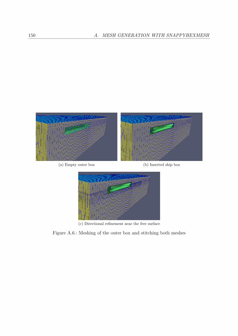
150 A. MESH GENERATION WITH SNAPPYHEXMESH
(a) Empty outer box (b) Inserted ship box
(c) Directional refinement near the free surface
Figure A.6.: Meshing of the outer box and stitching both meshes

Appendix 151
(a) 100k cells (b) 200k cells
(c) 400k cells (d) 800k cells
Figure A.7.: Meshes with different refinement levels
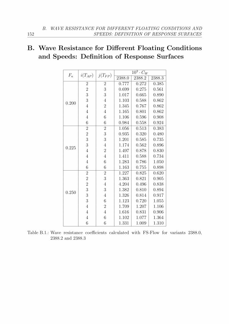
152B. WAVE RESISTANCE FOR DIFFERENT FLOATING CONDITIONS AND
SPEEDS: DEFINITION OF RESPONSE SURFACES
B. Wave Resistance for Different Floating Conditions
and Speeds: Definition of Response Surfaces
Fn i(TAP ) j(TFP )103 · CW
2388.0 2388.2 2388.3
0.200
2 2 0.777 0.272 0.3852 3 0.699 0.275 0.5613 3 1.017 0.665 0.8903 4 1.103 0.588 0.8624 2 1.345 0.767 0.8624 4 1.165 0.801 0.8624 6 1.106 0.596 0.9086 6 0.984 0.558 0.924
0.225
2 2 1.056 0.513 0.3832 3 0.935 0.320 0.4803 3 1.201 0.585 0.7353 4 1.174 0.562 0.8964 2 1.497 0.878 0.8304 4 1.411 0.588 0.7344 6 1.283 0.786 1.0506 6 1.163 0.755 0.898
0.250
2 2 1.227 0.825 0.6202 3 1.363 0.821 0.9052 4 4.204 0.496 0.8383 3 1.382 0.810 0.8943 4 1.326 0.814 0.9173 6 1.123 0.720 1.0554 2 1.709 1.207 1.1064 4 1.616 0.831 0.9064 6 1.102 1.077 1.3646 6 1.331 1.009 1.310
Table B.1.: Wave resistance coefficients calculated with FS-Flow for variants 2388.0,2388.2 and 2388.3
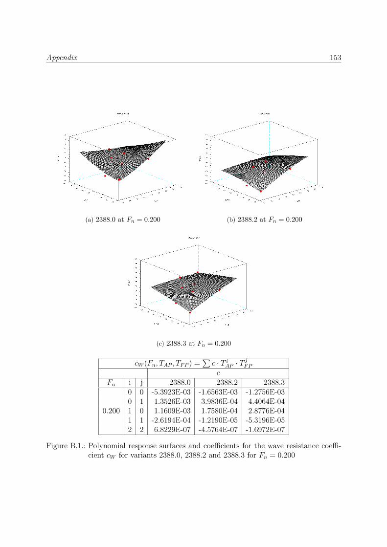
Appendix 153
(a) 2388.0 at Fn = 0.200 (b) 2388.2 at Fn = 0.200
(c) 2388.3 at Fn = 0.200
cW (Fn, TAP , TFP ) =∑c · T iAP · T
jFP
cFn i j 2388.0 2388.2 2388.3
0.200
0 0 -5.3923E-03 -1.6563E-03 -1.2756E-030 1 1.3526E-03 3.9836E-04 4.4064E-041 0 1.1609E-03 1.7580E-04 2.8776E-041 1 -2.6194E-04 -1.2190E-05 -5.3196E-052 2 6.8229E-07 -4.5764E-07 -1.6972E-07
Figure B.1.: Polynomial response surfaces and coefficients for the wave resistance coeffi-cient cW for variants 2388.0, 2388.2 and 2388.3 for Fn = 0.200
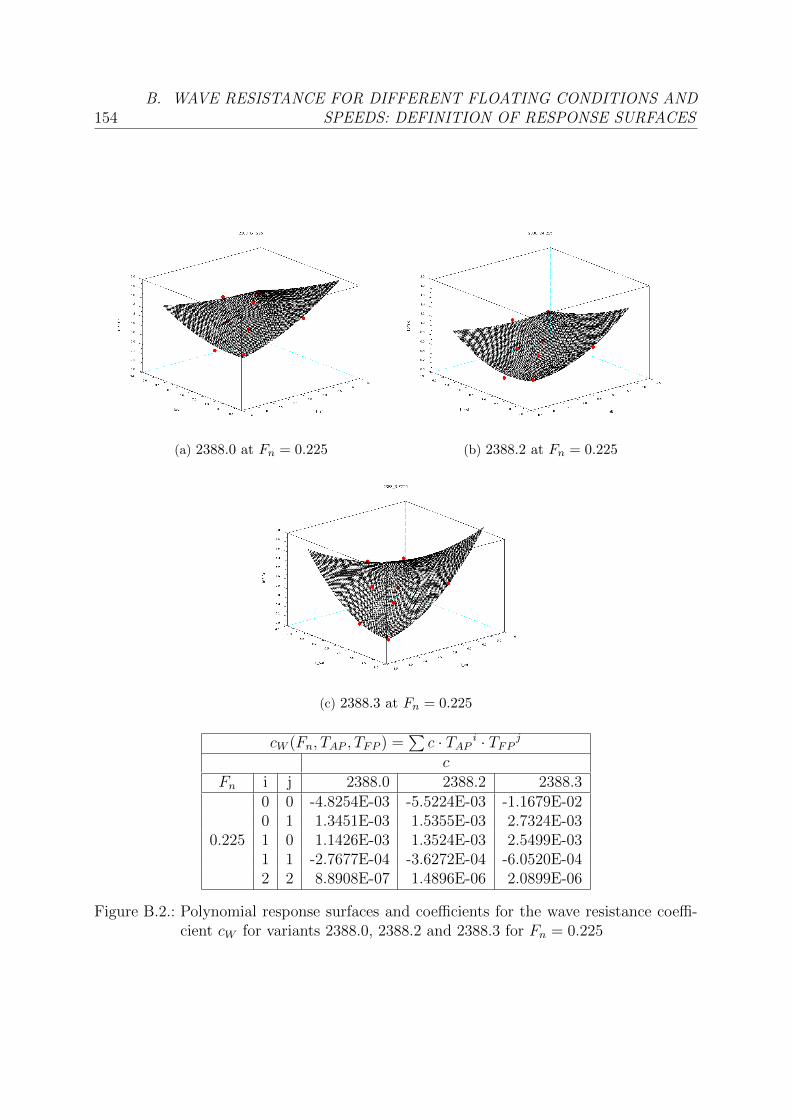
154B. WAVE RESISTANCE FOR DIFFERENT FLOATING CONDITIONS AND
SPEEDS: DEFINITION OF RESPONSE SURFACES
(a) 2388.0 at Fn = 0.225 (b) 2388.2 at Fn = 0.225
(c) 2388.3 at Fn = 0.225
cW (Fn, TAP , TFP ) =∑c · TAP i · TFP jc
Fn i j 2388.0 2388.2 2388.3
0.225
0 0 -4.8254E-03 -5.5224E-03 -1.1679E-020 1 1.3451E-03 1.5355E-03 2.7324E-031 0 1.1426E-03 1.3524E-03 2.5499E-031 1 -2.7677E-04 -3.6272E-04 -6.0520E-042 2 8.8908E-07 1.4896E-06 2.0899E-06
Figure B.2.: Polynomial response surfaces and coefficients for the wave resistance coeffi-cient cW for variants 2388.0, 2388.2 and 2388.3 for Fn = 0.225

Appendix 155
(a) 2388.0 at Fn = 0.250 (b) 2388.2 at Fn = 0.250
(c) 2388.3 at Fn = 0.250
cW (Fn, TAP , TFP ) =∑c · T iAP · T
jFP
cFn i j 2388.0 2388.2 2388.3
0.250
0 0 2.5771E-03 -1.2578E-03 -5.9903E-040 1 -1.4904E-04 7.5844E-04 5.7989E-041 0 -4.0316E-04 4.5406E-04 4.8872E-041 1 8.2847E-05 -1.6888E-04 -1.5402E-042 2 -5.3199E-07 7.8641E-07 6.4139E-07
Figure B.3.: Polynomial response surfaces and coefficients for the wave resistance coeffi-cient cW for variants 2388.0, 2388.2 and 2388.3 for Fn = 0.250

156C. SYSTEMATIC VARIATION OF BULBOUS BOW FOR POTENTIAL CFD
CALCULATIONS: ADDITIONAL TABLES AND FIGURES
C. Systematic Variation of Bulbous Bow for
Potential CFD Calculations: Additional Tables
and Figures
Figure C.1.: Wave resistance (as percentage of baseline) over bulb volume parameter C∇PRat Fn = 0.200 for main- and subvariants

Appendix 157
Fn = 0.200 C∇PR CLPR CABT L3PR/ RW/RW−1111 · 100
i(δxtt) j(δxti) k(δztt) l(Sr) ·103 ·102 ·102 ∇PR T22 T34 T46
1 1 1 1 1.96 2.68 7.78 1.692 100.0 100.0 100.01 1 1 2 2.14 2.68 8.57 1.545 94.2 103.5 102.71 1 1 3 2.34 2.68 9.41 1.416 89.7 107.8 105.91 1 2 1 1.96 2.68 7.78 1.692 95.7 100.3 102.21 1 2 2 2.14 2.68 8.57 1.545 89.7 103.8 104.91 1 2 3 2.34 2.68 9.41 1.416 84.9 107.9 108.01 2 1 1 2.28 2.68 7.78 1.454 93.9 102.2 106.31 2 1 2 2.50 2.68 8.57 1.324 88.4 107.0 109.91 2 1 3 2.73 2.68 9.41 1.212 84.7 112.7 114.01 2 2 1 2.28 2.68 7.78 1.454 90.2 106.9 105.41 2 2 2 2.50 2.68 8.57 1.324 84.5 111.6 108.71 2 2 3 2.73 2.68 9.41 1.212 80.4 117.0 112.52 1 1 1 2.25 3.09 7.78 2.238 90.5 95.8 96.22 1 1 2 2.46 3.09 8.57 2.043 84.3 99.6 99.02 1 1 3 2.69 3.09 9.41 1.872 79.6 104.0 102.42 1 2 1 2.25 3.09 7.78 2.238 86.7 97.5 97.02 1 2 2 2.46 3.09 8.57 2.043 80.4 101.2 99.52 1 2 3 2.69 3.09 9.41 1.872 75.5 105.7 102.72 2 1 1 2.57 3.09 7.78 1.959 83.8 101.7 104.62 2 1 2 2.82 3.09 8.57 1.785 78.1 107.2 108.82 2 1 3 3.08 3.09 9.41 1.633 74.3 113.6 113.72 2 2 1 2.57 3.09 7.78 1.959 81.3 107.9 101.82 2 2 2 2.82 3.09 8.57 1.785 75.4 113.4 105.52 2 2 3 3.08 3.09 9.41 1.633 71.3 119.8 110.03 1 1 1 2.54 3.49 7.78 2.860 82.0 96.2 96.43 1 1 2 2.79 3.49 8.57 2.610 75.6 100.7 99.73 1 1 3 3.04 3.49 9.41 2.392 71.0 106.0 103.83 1 2 1 2.54 3.49 7.78 2.860 79.0 99.2 95.03 1 2 2 2.79 3.49 8.57 2.610 72.6 103.6 98.03 1 2 3 3.04 3.49 9.41 2.392 67.7 109.0 101.83 2 1 1 2.86 3.49 7.78 2.540 75.3 103.6 104.63 2 1 2 3.14 3.49 8.57 2.315 69.6 109.8 109.43 2 1 3 3.43 3.49 9.41 2.118 65.9 117.0 114.93 2 2 1 2.86 3.49 7.78 2.540 73.8 109.2 101.43 2 2 2 3.14 3.49 8.57 2.315 67.9 115.3 105.83 2 2 3 3.43 3.49 9.41 2.118 63.9 122.4 111.0
Table C.1.: Bulb parameters and wave resistance (as percentage of baseline) of subvariantsfor Fn = 0.200

158C. SYSTEMATIC VARIATION OF BULBOUS BOW FOR POTENTIAL CFD
CALCULATIONS: ADDITIONAL TABLES AND FIGURES
Fn = 0.225 C∇PR CLPR CABT L3PR/ RW/RW−1111 · 100
i(δxtt) j(δxti) k(δztt) l(Sr) ·103 ·102 ·102 ∇PR T22 T34 T46
1 1 1 1 1.96 2.68 7.78 1.692 100.0 100.0 100.01 1 1 2 2.14 2.68 8.57 1.545 95.0 102.2 101.61 1 1 3 2.34 2.68 9.41 1.416 90.1 105.1 103.61 1 2 1 1.96 2.68 7.78 1.692 96.9 98.0 102.71 1 2 2 2.14 2.68 8.57 1.545 91.5 100.0 104.41 1 2 3 2.34 2.68 9.41 1.416 86.2 103.2 106.51 2 1 1 2.28 2.68 7.78 1.454 94.8 100.0 105.01 2 1 2 2.50 2.68 8.57 1.324 89.5 103.2 107.21 2 1 3 2.73 2.68 9.41 1.212 84.5 107.1 109.81 2 2 1 2.28 2.68 7.78 1.454 92.0 103.0 105.11 2 2 2 2.50 2.68 8.57 1.324 86.3 105.9 107.21 2 2 3 2.73 2.68 9.41 1.212 81.0 109.4 109.72 1 1 1 2.25 3.09 7.78 2.238 92.6 95.4 96.72 1 1 2 2.46 3.09 8.57 2.043 86.9 97.7 98.32 1 1 3 2.69 3.09 9.41 1.872 81.4 100.5 100.22 1 2 1 2.25 3.09 7.78 2.238 89.7 96.1 97.92 1 2 2 2.46 3.09 8.57 2.043 83.7 98.3 99.42 1 2 3 2.69 3.09 9.41 1.872 78.0 101.0 101.42 2 1 1 2.57 3.09 7.78 1.959 86.8 99.9 103.72 2 1 2 2.82 3.09 8.57 1.785 80.9 103.7 106.52 2 1 3 3.08 3.09 9.41 1.633 75.5 108.3 109.82 2 2 1 2.57 3.09 7.78 1.959 84.6 106.3 102.02 2 2 2 2.82 3.09 8.57 1.785 78.4 110.3 104.62 2 2 3 3.08 3.09 9.41 1.633 72.8 115.0 107.53 1 1 1 2.54 3.49 7.78 2.860 85.8 95.8 97.03 1 1 2 2.79 3.49 8.57 2.610 79.6 98.7 99.23 1 1 3 3.04 3.49 9.41 2.392 73.7 102.3 101.83 1 2 1 2.54 3.49 7.78 2.860 83.2 98.9 96.33 1 2 2 2.79 3.49 8.57 2.610 76.7 102.0 98.33 1 2 3 3.04 3.49 9.41 2.392 70.7 105.8 100.73 2 1 1 2.86 3.49 7.78 2.540 79.7 101.5 104.03 2 1 2 3.14 3.49 8.57 2.315 73.4 105.9 107.33 2 1 3 3.43 3.49 9.41 2.118 67.7 111.1 111.23 2 2 1 2.86 3.49 7.78 2.540 78.1 108.2 101.83 2 2 2 3.14 3.49 8.57 2.315 71.5 112.9 104.93 2 2 3 3.43 3.49 9.41 2.118 65.7 118.4 108.6
Table C.2.: Bulb parameters and wave resistance (as percentage of baseline) of subvariantsfor Fn = 0.225
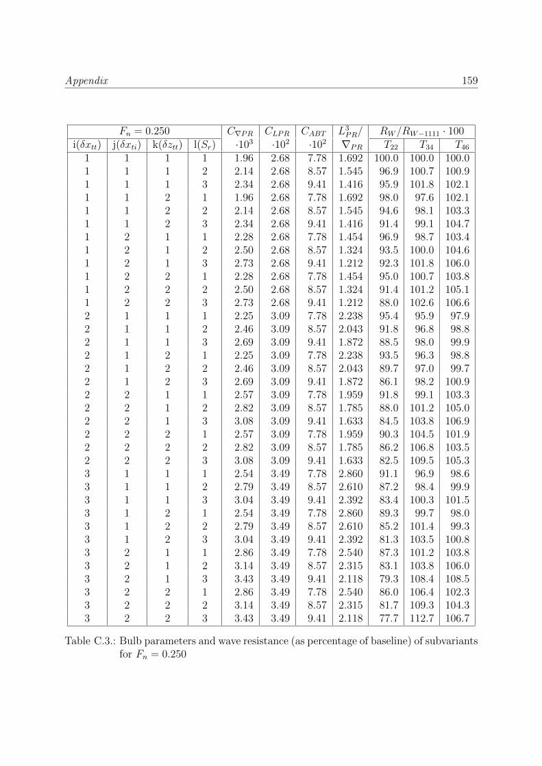
Appendix 159
Fn = 0.250 C∇PR CLPR CABT L3PR/ RW/RW−1111 · 100
i(δxtt) j(δxti) k(δztt) l(Sr) ·103 ·102 ·102 ∇PR T22 T34 T46
1 1 1 1 1.96 2.68 7.78 1.692 100.0 100.0 100.01 1 1 2 2.14 2.68 8.57 1.545 96.9 100.7 100.91 1 1 3 2.34 2.68 9.41 1.416 95.9 101.8 102.11 1 2 1 1.96 2.68 7.78 1.692 98.0 97.6 102.11 1 2 2 2.14 2.68 8.57 1.545 94.6 98.1 103.31 1 2 3 2.34 2.68 9.41 1.416 91.4 99.1 104.71 2 1 1 2.28 2.68 7.78 1.454 96.9 98.7 103.41 2 1 2 2.50 2.68 8.57 1.324 93.5 100.0 104.61 2 1 3 2.73 2.68 9.41 1.212 92.3 101.8 106.01 2 2 1 2.28 2.68 7.78 1.454 95.0 100.7 103.81 2 2 2 2.50 2.68 8.57 1.324 91.4 101.2 105.11 2 2 3 2.73 2.68 9.41 1.212 88.0 102.6 106.62 1 1 1 2.25 3.09 7.78 2.238 95.4 95.9 97.92 1 1 2 2.46 3.09 8.57 2.043 91.8 96.8 98.82 1 1 3 2.69 3.09 9.41 1.872 88.5 98.0 99.92 1 2 1 2.25 3.09 7.78 2.238 93.5 96.3 98.82 1 2 2 2.46 3.09 8.57 2.043 89.7 97.0 99.72 1 2 3 2.69 3.09 9.41 1.872 86.1 98.2 100.92 2 1 1 2.57 3.09 7.78 1.959 91.8 99.1 103.32 2 1 2 2.82 3.09 8.57 1.785 88.0 101.2 105.02 2 1 3 3.08 3.09 9.41 1.633 84.5 103.8 106.92 2 2 1 2.57 3.09 7.78 1.959 90.3 104.5 101.92 2 2 2 2.82 3.09 8.57 1.785 86.2 106.8 103.52 2 2 3 3.08 3.09 9.41 1.633 82.5 109.5 105.33 1 1 1 2.54 3.49 7.78 2.860 91.1 96.9 98.63 1 1 2 2.79 3.49 8.57 2.610 87.2 98.4 99.93 1 1 3 3.04 3.49 9.41 2.392 83.4 100.3 101.53 1 2 1 2.54 3.49 7.78 2.860 89.3 99.7 98.03 1 2 2 2.79 3.49 8.57 2.610 85.2 101.4 99.33 1 2 3 3.04 3.49 9.41 2.392 81.3 103.5 100.83 2 1 1 2.86 3.49 7.78 2.540 87.3 101.2 103.83 2 1 2 3.14 3.49 8.57 2.315 83.1 103.8 106.03 2 1 3 3.43 3.49 9.41 2.118 79.3 108.4 108.53 2 2 1 2.86 3.49 7.78 2.540 86.0 106.4 102.33 2 2 2 3.14 3.49 8.57 2.315 81.7 109.3 104.33 2 2 3 3.43 3.49 9.41 2.118 77.7 112.7 106.7
Table C.3.: Bulb parameters and wave resistance (as percentage of baseline) of subvariantsfor Fn = 0.250
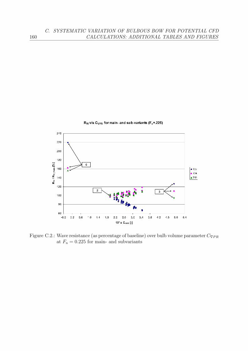
160C. SYSTEMATIC VARIATION OF BULBOUS BOW FOR POTENTIAL CFD
CALCULATIONS: ADDITIONAL TABLES AND FIGURES
Figure C.2.: Wave resistance (as percentage of baseline) over bulb volume parameter C∇PRat Fn = 0.225 for main- and subvariants

Appendix 161
Figure C.3.: Wave resistance (as percentage of baseline) over bulb volume parameter C∇PRat Fn = 0.250 for main- and subvariants
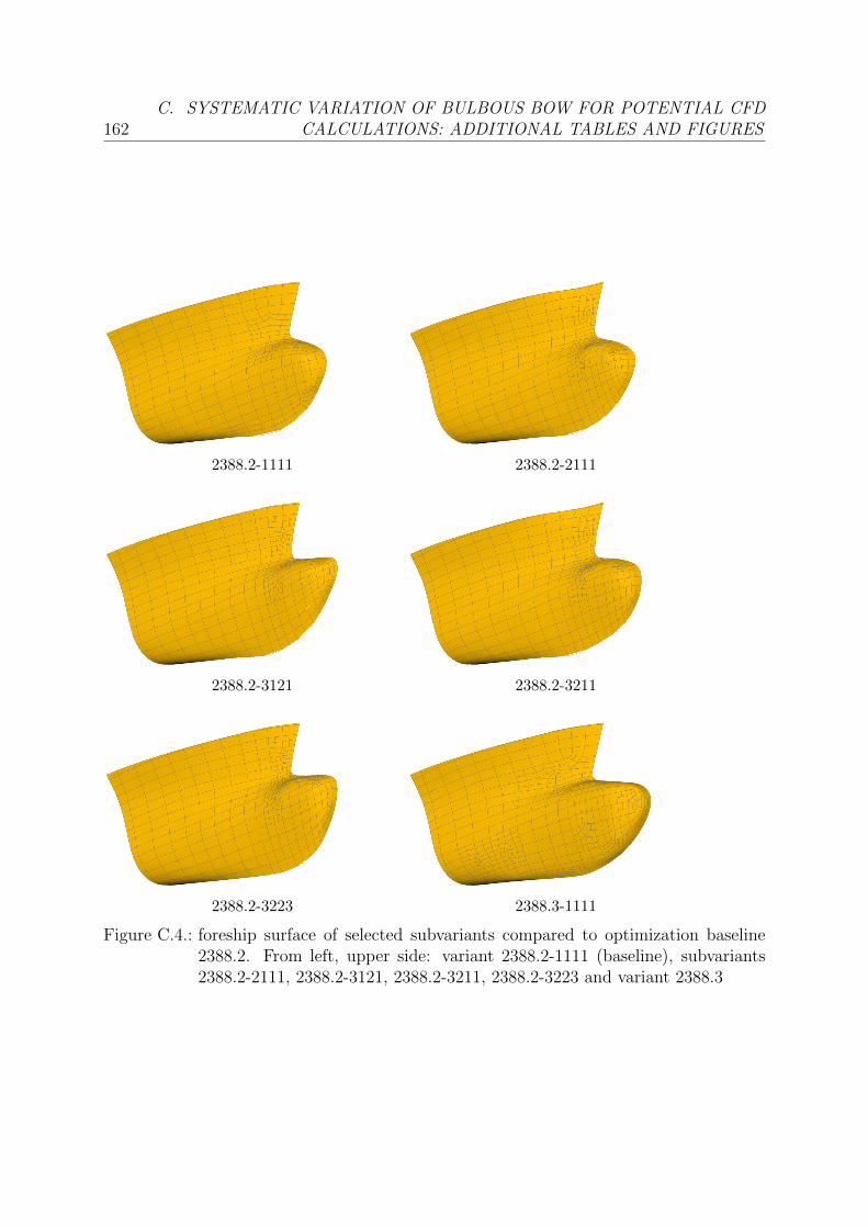
162C. SYSTEMATIC VARIATION OF BULBOUS BOW FOR POTENTIAL CFD
CALCULATIONS: ADDITIONAL TABLES AND FIGURES
2388.2-1111 2388.2-2111
2388.2-3121 2388.2-3211
2388.2-3223 2388.3-1111
Figure C.4.: foreship surface of selected subvariants compared to optimization baseline2388.2. From left, upper side: variant 2388.2-1111 (baseline), subvariants2388.2-2111, 2388.2-3121, 2388.2-3211, 2388.2-3223 and variant 2388.3

Appendix 163
D. Additional Tables and Diagrams for Chapter 4

164 D. ADDITIONAL TABLES AND DIAGRAMS FOR CHAPTER 4
PB [kW] n [RPM ]Engine L1 L2 L3 L4 L1, L2 L3, L4
Ships with λ = 17:MAN 9 S26 MC6 3600 2880 3060 2430 250 212as percentage of L1 100% 80% 85% 68% 100% 85%FE 2388-17.0 3713 2970 3156 2506 169 143FE 2388-17.2 3512 2810 2985 2371 166 141FE 2388-17.3 3463 2770 2944 2338 166 141Ships with λ = 25:MAN 6 S60 MC6 12240 7800 9240 5880 105 79as percentage of L1 100% 64% 75% 48% 100% 75%FE 2388-25.0 12219 7787 9224 5870 134 101FE 2388-25.2 11564 7369 8730 5555 132 99FE 2388-25.3 11406 7269 8610 5479 132 99Ships with λ = 33:MAN 8 S80 MC6 29120 18640 21760 13920 79 59as percentage of L1 100% 64% 75% 48% 100% 75%FE 2388-33.0 28457 18216 21265 13603 114 85FE 2388-33.2 26947 17249 20136 12881 112 84FE 2388-33.3 26583 17016 19864 12707 111 83Ships with λ = 50:MAN 14 K108 ME-C6 97800 77980 93100 74760 94 90as percentage of L1 100% 80% 95% 76% 100% 96%FE 2388-50.0 111119 88600 105779 84941 90 86FE 2388-50.2 104539 83353 99515 79911 89 85FE 2388-50.3 95110 75835 90539 72704 87 83
Table D.1.: Engine characteristics for base engines and fictive engines for all ships

Appendix 165
15 20 25 30 35 40 45 50 550
2
4
6
8
10
12
14
16
18
20
λ
RAW
[%]
(a) mean RAW (Le Havre - Paranagua)
15 20 25 30 35 40 45 50 550
2
4
6
8
10
12
14
16
18
20
λ
+2388.252388.3u2388.0
RAW
[%]
(b) mean RAW (Le Havre - Charleston)
15 20 25 30 35 40 45 50 550
2
4
6
8
10
12
14
16
18
20
λ
RAW
[%]
(c) mean RAW (Valparaiso - Yokohama)
15 20 25 30 35 40 45 50 550
2
4
6
8
10
12
14
16
18
20
λ
+2388.252388.3u2388.0
RAW
[%]
(d) mean RAW (San Francisco - Yokohama)
15 20 25 30 35 40 45 50 550
2
4
6
8
10
12
14
16
18
20
λ
RAW
[%]
(e) mean RAW (Melbourne - Djibouti)
15 20 25 30 35 40 45 50 550
2
4
6
8
10
12
14
16
18
20
λ
+2388.252388.3u2388.0
RAW
[%]
(f) mean RAW for all routes
Figure D.1.: Relative mean RAW of variants 2388.0, .2 and .3 for all considered routesand mean relative mean RAW of all routes as function of the scaling factorλ from simulations with fixed floating condition
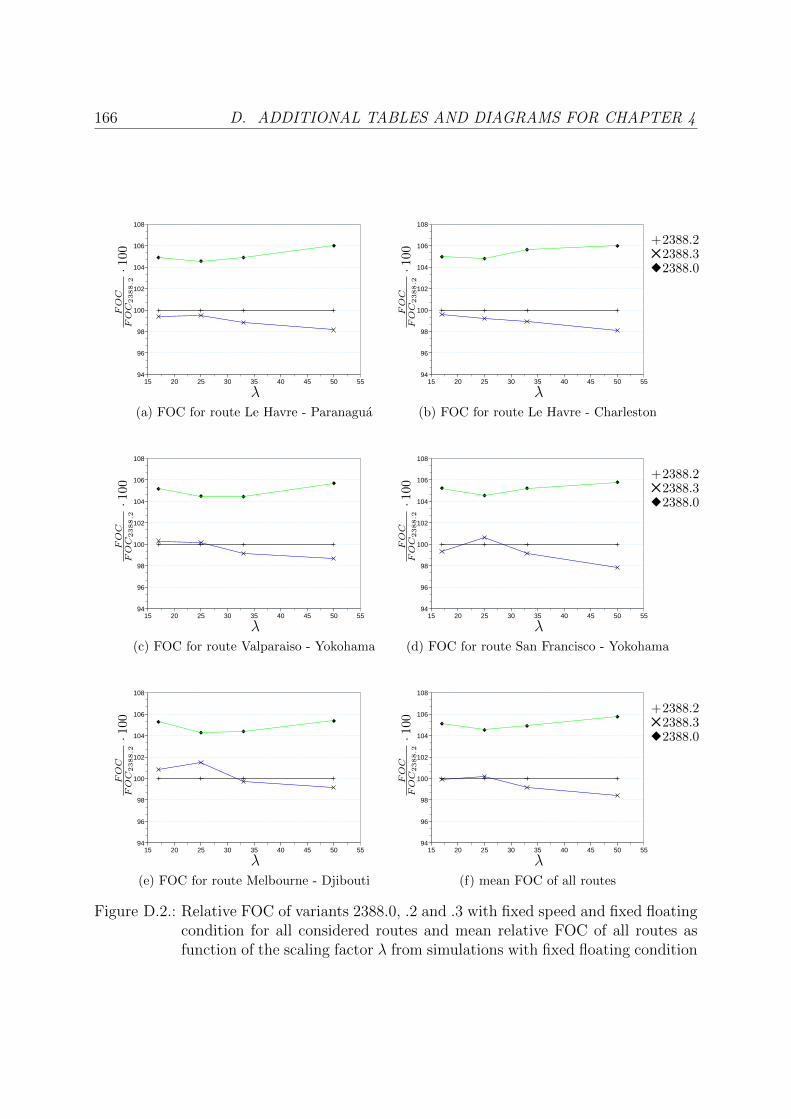
166 D. ADDITIONAL TABLES AND DIAGRAMS FOR CHAPTER 4
15 20 25 30 35 40 45 50 5594
96
98
100
102
104
106
108
λ
FOC
FOC
2388.2·1
00
(a) FOC for route Le Havre - Paranagua
15 20 25 30 35 40 45 50 5594
96
98
100
102
104
106
108
λ
+2388.252388.3u2388.0
FOC
FOC
2388.2·1
00
(b) FOC for route Le Havre - Charleston
15 20 25 30 35 40 45 50 5594
96
98
100
102
104
106
108
λ
FOC
FOC
2388.2·1
00
(c) FOC for route Valparaiso - Yokohama
15 20 25 30 35 40 45 50 5594
96
98
100
102
104
106
108
λ
+2388.252388.3u2388.0
FOC
FOC
2388.2·1
00
(d) FOC for route San Francisco - Yokohama
15 20 25 30 35 40 45 50 5594
96
98
100
102
104
106
108
λ
FOC
FOC
2388.2·1
00
(e) FOC for route Melbourne - Djibouti
15 20 25 30 35 40 45 50 5594
96
98
100
102
104
106
108
λ
+2388.252388.3u2388.0
FOC
FOC
2388.2·1
00
(f) mean FOC of all routes
Figure D.2.: Relative FOC of variants 2388.0, .2 and .3 with fixed speed and fixed floatingcondition for all considered routes and mean relative FOC of all routes asfunction of the scaling factor λ from simulations with fixed floating condition

Appendix 167
15 20 25 30 35 40 45 50 5592
93
94
95
96
97
98
99
100
101
λ
VS
VD
es[%
]
(a) mean VS (Le Havre - Paranaguai)
15 20 25 30 35 40 45 50 5592
93
94
95
96
97
98
99
100
101
λ
+2388.252388.3u2388.0
VS
VD
es[%
](b) mean VS (Le Havre - Charleston)
15 20 25 30 35 40 45 50 5592
93
94
95
96
97
98
99
100
101
λ
VS
VD
es[%
]
(c) mean VS (Valparaiso - Yokohama)
15 20 25 30 35 40 45 50 5592
93
94
95
96
97
98
99
100
101
λ
+2388.252388.3u2388.0
VS
VD
es[%
]
(d) mean VS (San Francisco - Yokohama)
15 20 25 30 35 40 45 50 5592
93
94
95
96
97
98
99
100
101
λ
VS
VD
es[%
]
(e) mean VS (Melbourne - Djibouti)
15 20 25 30 35 40 45 50 5592
93
94
95
96
97
98
99
100
101
λ
+2388.252388.3u2388.0
VS
VD
es[%
]
(f) mean VS for all routes
Figure D.3.: Mean velocity of variants 2388.0, .2 and .3 for all considered routes and meanvalue of all routes as function of the scaling factor λ from simulations withfixed floating condition

168 D. ADDITIONAL TABLES AND DIAGRAMS FOR CHAPTER 4
15 20 25 30 35 40 45 50 550
2
4
6
8
10
12
14
16
18
20
λ
RAW
[%]
(a) mean RAW (Le Havre - Paranagua)
15 20 25 30 35 40 45 50 550
2
4
6
8
10
12
14
16
18
20
λ
+2388.252388.3u2388.0
RAW
[%]
(b) mean RAW (Le Havre - Charleston)
15 20 25 30 35 40 45 50 550
2
4
6
8
10
12
14
16
18
20
λ
RAW
[%]
(c) mean RAW (Valparaiso - Yokohama)
15 20 25 30 35 40 45 50 550
2
4
6
8
10
12
14
16
18
20
λ
+2388.252388.3u2388.0
RAW
[%]
(d) mean RAW (San Francisco - Yokohama)
15 20 25 30 35 40 45 50 550
2
4
6
8
10
12
14
16
18
20
λ
RAW
[%]
(e) mean RAW (Melbourne - Djibouti)
15 20 25 30 35 40 45 50 550
2
4
6
8
10
12
14
16
18
20
λ
+2388.252388.3u2388.0
RAW
[%]
(f) mean RAW for all routes
Figure D.4.: Relative mean RAW of variants 2388.0, .2 and .3 for all considered routesand mean relative mean RAW of all routes as function of the scaling factorλ from simulations with variable floating condition
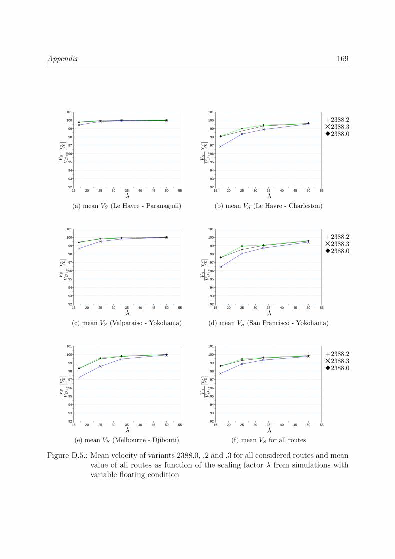
Appendix 169
15 20 25 30 35 40 45 50 5592
93
94
95
96
97
98
99
100
101
λ
VS
VD
es[%
]
(a) mean VS (Le Havre - Paranaguai)
15 20 25 30 35 40 45 50 5592
93
94
95
96
97
98
99
100
101
λ
+2388.252388.3u2388.0
VS
VD
es[%
](b) mean VS (Le Havre - Charleston)
15 20 25 30 35 40 45 50 5592
93
94
95
96
97
98
99
100
101
λ
VS
VD
es[%
]
(c) mean VS (Valparaiso - Yokohama)
15 20 25 30 35 40 45 50 5592
93
94
95
96
97
98
99
100
101
λ
+2388.252388.3u2388.0
VS
VD
es[%
]
(d) mean VS (San Francisco - Yokohama)
15 20 25 30 35 40 45 50 5592
93
94
95
96
97
98
99
100
101
λ
VS
VD
es[%
]
(e) mean VS (Melbourne - Djibouti)
15 20 25 30 35 40 45 50 5592
93
94
95
96
97
98
99
100
101
λ
+2388.252388.3u2388.0
VS
VD
es[%
]
(f) mean VS for all routes
Figure D.5.: Mean velocity of variants 2388.0, .2 and .3 for all considered routes and meanvalue of all routes as function of the scaling factor λ from simulations withvariable floating condition

170 E. ADDITIONAL TABLES AND DIAGRAMS FOR CHAPTER 5
E. Additional Tables and Diagrams for Chapter 5

Appendix 171
PB [kW] n [RPM ]Engine L1 L2 L3 L4 L1, L2 L3, L4
Ships with λ = 17:MAN 9 S26 MC6 3600 2880 3060 2430 250 212parametrized 100% 80% 85% 68% 100% 85%FE 2388-17.2-1111 3250 2600 2763 2194 163 138FE 2388-17.2-2111 3230 2584 2746 2180 163 138FE 2388-17.2-3121 3160 2528 2686 2133 162 137FE 2388-17.2-3211 3140 2512 2669 2120 162 137FE 2388-17.2-3223 3080 2464 2618 2079 161 137FE 2388-17.3-1111 3135 2508 2665 2116 162 137Ships with λ = 25:MAN 6 S60 MC6 12240 7800 9240 5880 105 79parametrized 100% 64% 75% 48% 100% 75%FE 2388-25.2-1111 11230 7156 8478 5395 131 99FE 2388-25.2-2111 11080 7061 8364 5323 131 99FE 2388-25.2-3121 10930 6965 8251 5251 130 98FE 2388-25.2-3211 10850 6914 8191 5212 130 98FE 2388-25.2-3223 10560 6729 7972 5073 130 98FE 2388-25.3-1111 10780 6870 8138 5179 130 98Ships with λ = 33:MAN 8 S80 MC6 29120 18640 21760 13920 79 59parametrized 100% 64% 75% 48% 100% 75%FE 2388-33.2-1111 27600 17667 20624 13193 112 84FE 2388-33.2-2111 27300 17475 20400 13050 111 83FE 2388-33.2-3121 26700 17091 19952 12763 111 83FE 2388-33.2-3211 26500 16963 19802 12668 110 82FE 2388-33.2-3223 25650 16419 19167 12261 110 82FE 2388-33.3-1111 26300 16835 19653 12572 111 83Ships with λ = 50:MAN 14 K108 ME-C6 97800 77980 93100 74760 94 90parametrized 100% 80% 95% 76% 100% 96%FE 2388-50.2-1111 105500 84120 100430 80646 89 85FE 2388-50.2-2111 104000 82924 99002 79499 89 85FE 2388-50.2-3121 101900 81249 97003 77894 88 84FE 2388-50.2-3211 101200 80691 96337 77359 88 84FE 2388-50.2-3223 98000 78139 93290 74913 87 83FE 2388-50.3-1111 100500 80133 95670 76824 88 84
Table E.1.: Engine characteristics for base engines and fictive engines for all subvariants
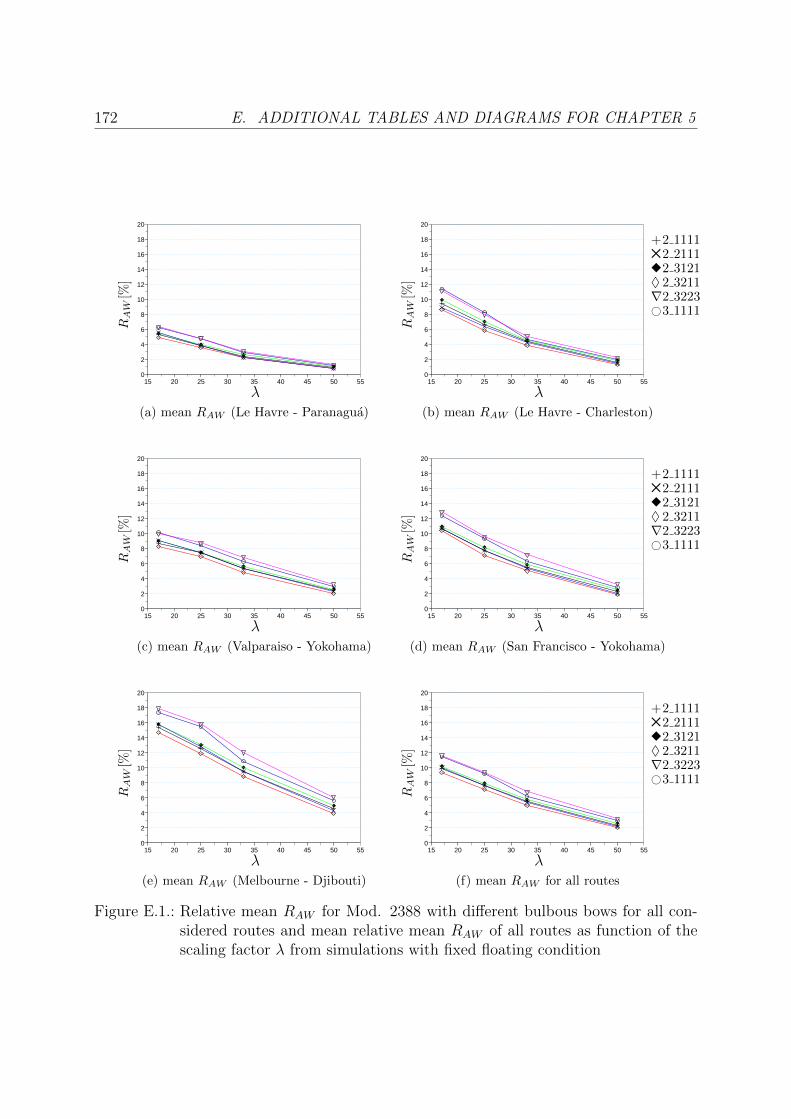
172 E. ADDITIONAL TABLES AND DIAGRAMS FOR CHAPTER 5
15 20 25 30 35 40 45 50 550
2
4
6
8
10
12
14
16
18
20
λ
RAW
[%]
(a) mean RAW (Le Havre - Paranagua)
15 20 25 30 35 40 45 50 550
2
4
6
8
10
12
14
16
18
20
λ
+2 111152 2111u2 3121♦ 2 3211∇2 3223#3 1111
RAW
[%]
(b) mean RAW (Le Havre - Charleston)
15 20 25 30 35 40 45 50 550
2
4
6
8
10
12
14
16
18
20
λ
RAW
[%]
(c) mean RAW (Valparaiso - Yokohama)
15 20 25 30 35 40 45 50 550
2
4
6
8
10
12
14
16
18
20
λ
+2 111152 2111u2 3121♦ 2 3211∇2 3223#3 1111
RAW
[%]
(d) mean RAW (San Francisco - Yokohama)
15 20 25 30 35 40 45 50 550
2
4
6
8
10
12
14
16
18
20
λ
RAW
[%]
(e) mean RAW (Melbourne - Djibouti)
15 20 25 30 35 40 45 50 550
2
4
6
8
10
12
14
16
18
20
λ
+2 111152 2111u2 3121♦ 2 3211∇2 3223#3 1111
RAW
[%]
(f) mean RAW for all routes
Figure E.1.: Relative mean RAW for Mod. 2388 with different bulbous bows for all con-sidered routes and mean relative mean RAW of all routes as function of thescaling factor λ from simulations with fixed floating condition

Appendix 173
15 20 25 30 35 40 45 50 5592
93
94
95
96
97
98
99
100
101
λ
VS
VD
es[%
]
(a) mean VS (Le Havre - Paranagua)
15 20 25 30 35 40 45 50 5592
93
94
95
96
97
98
99
100
101
λ
+2 111152 2111u2 3121♦ 2 3211∇2 3223#3 1111
VS
VD
es[%
](b) mean VS (Le Havre - Charleston)
15 20 25 30 35 40 45 50 5592
93
94
95
96
97
98
99
100
101
λ
VS
VD
es[%
]
(c) mean VS (Valparaiso - Yokohama)
15 20 25 30 35 40 45 50 5592
93
94
95
96
97
98
99
100
101
λ
+2 111152 2111u2 3121♦ 2 3211∇2 3223#3 1111
VS
VD
es[%
]
(d) mean VS (San Francisco - Yokohama)
15 20 25 30 35 40 45 50 5592
93
94
95
96
97
98
99
100
101
λ
VS
VD
es[%
]
(e) mean VS (Melbourne - Djibouti)
15 20 25 30 35 40 45 50 5592
93
94
95
96
97
98
99
100
101
λ
+2 111152 2111u2 3121♦ 2 3211∇2 3223#3 1111
VS
VD
es[%
]
(f) mean VS for all routes
Figure E.2.: Mean velocity for Mod. 2388 with different bulbous bows for all consideredroutes and mean value for all routes as function of the scaling factor λ fromsimulations with fixed floating condition