HYDROLOGICAL PROCESSESHydrol. Process. 29, 692–711 (2015)Published online 17 March 2014 in Wiley Online Library(wileyonlinelibrary.com) DOI: 10.1002/hyp.10173

Modelling soil water dynamics considering measurementuncertainty

Isaya Kisekka,1,2* K. W. Migliaccio,2 R. Muñoz-Carpena,3 B. Schaffer2 and Y. Khare31 Kansas State University, Southwest Research-Extension Center, 4500 E. Mary St., Garden City, KS, 67846

2 University of Florida, IFAS Tropical Research and Education Center, 18905 SW 280th St, Homestead, FL, 330313 University of Florida, Agricultural and Biological Engineering Department, P. O. Box 110570, Gainesville, FL, 32611

*CoResE-m

Cop

Abstract:

In shallow water table-controlled environments, surface water management impacts groundwater table levels and soil waterdynamics. The study goal was to simulate soil water dynamics in response to canal stage raises considering uncertainty inmeasured soil water content. Water and Agrochemicals in the soil, crop and Vadose Environment (WAVE) was applied tosimulate unsaturated flow above a shallow aquifer. Global sensitivity analysis was performed to identify model input factors withthe greatest influence on predicted soil water content. Nash–Sutcliffe increased and Root Mean Square Error reduced whenuncertainties in measured data were considered in goodness-of-fit calculations using measurement probability distributions andprobable asymmetric error boundaries, implying that appropriate model performance evaluation should be carried out usinguncertainty ranges instead of single values. Although uncertainty in the experimental measured data limited evaluation of theabsolute predictions by the model, WAVE was found a useful exploratory tool for estimating temporal variation in soil watercontent. Visual analysis of soil water content time series under proposed changes in canal stage management indicated that siteswith land surface elevation of less than 2.0-m NGVD29 were predicted to periodically experience saturated conditions in the rootzone and shortening of the growing season if canal stage is raised more than 9 cm and maintained at this level. The modelsdeveloped could be combined with high-resolution digital elevation models in future studies to identify areas with the greatestrisk of experiencing saturated root zone. The study also highlighted the need to incorporate measurement uncertainty whenevaluating performance of unsaturated flow models. Copyright © 2014 John Wiley & Sons, Ltd.

KEY WORDS soil water; measurement uncertainty; vadose zone; WAVE; root zone saturation

Received 19 September 2013; Accepted 10 February 2014

INTRODUCTION

In shallow water table-controlled environments, regionalsurface water management operations impact groundwatertable levels, which in turn affect soil water dynamics. Anexample is the operational adjustments in surface watermanagement that are occurring in south Florida as part ofan effort to restore the hydrology of Everglades NationalPark (ENP) (USACE and SFWMD, 2011). Rises in watertable due to proposed rises in canal stage could affect soilwater content in agricultural fields adjacent to ENP throughtransient root zone saturation. Negative impacts of asaturated root zone on plants including reduced yield andphysiological function are well documented in literature(Lizaso and Ritchie, 1997; Schaffer, 1998).In addition, rises in shallow water table could increase

risk of temporary groundwater flooding because of rapidwater table responses to storm events. Earlier studies have

rrespondence to: Isaya Kisekka, Kansas State University, Southwestearch-Extension Center, 4500 E. Mary St., Garden City, KS 67846.ail: ikisekka@ksu.edu

yright © 2014 John Wiley & Sons, Ltd.

observed disproportionate rises in water table elevationsafter intense rainfall (Kayane and Kaihotsu, 1988; Waswaet al., 2013). Germann and Levy (1986) attributed therapid rise in water table elevation in response toprecipitation to capillary fringe groundwater ridging inwhich a small addition of water to the capillary fringeresulted in a rapid and large rise in water table elevationthat drops immediately after the storm.One way of assessing potential impacts of surface water

management decisions on soil water dynamics is throughmonitoring and modelling. A normally preferred approachis the use of process models. The main advantage ofprocess-based vadose zone models over statistical orempirical models such as that used by Kisekka et al.(2013c) is that they are transferable. Several vadose zonemodels are available, such as Water and Agrochemicals inthe soil, crop and Vadose Environment (WAVE),HYDRUS and Soil-Water-Atmosphere-Plant. Thesemodels typically predict water, heat and solute movementin the unsaturated zone.To adequately characterize vadose models and enhance

their proper use, model uncertainty as well as uncertainty in

Figure 1. Showing soil water monitoring sites, agricultural lands adjacentto Everglades National Park and canal network within the C-111 basin of

south Miami-Dade County, Florida

693SOIL WATER MODELLING CONSIDERING UNCERTAINTY

measured soil water data used in model parameterizationand evaluation needs to be considered. There are manysources of uncertainty, which make soil water contentmeasured by indirect soil water monitoring methods (e.g.time domain reflectometer [TDR] and capacitance sensors)uncertain. Sources of uncertainty include (1) errors relatedto equipment installation and calibration, (2) errorsassociated with the measurement technique and algorithmsthat are used to convert surrogate measurements to soilwater content and (3) errors associated with spatialvariability of soil properties (IAEA, 2008). For example,uncertainty in TDRmeasurements can mostly be attributedto effects of soil electrical conductivity and dielectricrelaxation on the calibration equation (Lin, 2003). Errors insoil water measurements by capacitance sensors can beattributed to small-scale variations in soil water content dueto the small volume of soil sensed, temperature and soilbulk electrical conductivity (Evett et al., 2012). Errors maybe random or systematic. Random errors maybeminimizedthrough proper sampling and calibration, but other types oferrors are beyond the control of the user of the soil watermonitoring equipment, and these become a source ofsystematic uncertainty in measured soil water data (e.g.non-uniform distribution of the electromagnetic field ofcapacitance probes around the access tube, which results inoverestimation of soil water).In many soil water prediction model performance

evaluations (Whiting et al., 2004; Merdun et al., 2006;Chen et al., 2012; Ritter and Muñoz-Carpena, 2013),goodness-of-fit indicators such as Nash–Sutcliffe (NSE),Willmot index (d), Root Mean Square Error (RMSE) andMean Absolute Error are used. These goodness-of-fitindicators are usually based on calculating the pair-wiseerror between observed and predicted soil water contentwithout accounting for the uncertainty in measured data.Accurate evaluation of model performance needs to considerthis source of uncertainty whenever possible in order toprovide a more realistic assessment of model performanceand to provide guidance for model output interpretation(Harmel et al., 2010). Bilskie (2001) describes a simplestatistical procedure to quantify uncertainty due to spatialvariability in soil water content but does not cover uncertaintydue to instrumentation. Harmel and Smith (2007) provide aframework for quantifying uncertainty in measured data,whereas Harmel et al. (2010) outlines a procedure forquantifying model uncertainty for models in which thepredicted state variable can be assumed independent. Thelater approach may need modification for soil watersimulations because soil water content cannot be assumedindependent because of autocorrelation. Another approachthat has been used to address measurement uncertainty inhydrologic model inputs include the use of the Bayesian totalerror analysis methodology (Kavetski et al., 2006), but thisapproach tends to be computationally intensive.

Copyright © 2014 John Wiley & Sons, Ltd.

The study goal was to simulate soil water dynamics inresponse to surface water management in the C-111 basinof Florida considering measurement uncertainty. Theobjectives were to (1) apply the vadose zone modelWAVE for simulating soil and limestone bedrock watercontent dynamics at four sites monitored (2) evaluatemodel performance considering uncertainty in measuredsoil and limestone bedrock water content and (3) applythe models to investigate the effect of 6, 9 and 12-cmincremental rises in canal stage on soil and limestonebedrock water dynamics at 10, 20, 30 and 40-cmmonitoring depths.

MATERIAL AND METHODS

Study area and experimental set up

The study was conducted in Miami-Dade County closeto Homestead, Florida, within an agricultural areaapproximately 17 km2 (Figure 1) immediately to the eastof canal C-111. Topography is essentially flat, implyingthat the assumption of 1D vertical flow for the unsaturatedzone is valid. Soil depth is shallow ranging between 10

Hydrol. Process. 29, 692–711 (2015)

694 I. KISEKKA ET AL.

and 25 cm. The limestone bedrock layer is highly porousand reached on average at 20-cm depth.Two multi-sensor capacitance probes (EnviroScan

probes, Sentek Technologies, Ltd., Stepney, Australia)for soil water monitoring were installed at four locations(Figure 1) at distances of 500, 1000 and 2000m from thecanal. Each probe had four sensors positioned at 10, 20,30 and 40 cm from the ground surface (Figure 2). Soilwater content was recorded every 15min and averageddaily. A detailed description of EnviroScan operation canbe found in the work of Kisekka et al. (2013c). The top20 cm typically represented the scarified soil layer, whichis used for crop production, and the lower 20 cmrepresented the underlying limestone bedrock in whichplant roots cannot penetrate.Calibration of capacitance sensors in the field using the

standard gravimetric sampling approach (Sentek Pty Ltd,2001) was attempted but later abandoned because of severalfactors including (1) difficulty obtaining soil samplesadjacent to the sensor access tube without interfering withthe operation of the sensors, (2) difficulty in obtaining awide range of soil water content under field conditions toproperly calibrate the sensors and (3) presence of a shallowlimestone bedrock in which it was difficult to sample. Evettet al. (2012) noted that field calibration may not resolve theissue of accuracy associatedwith capacitance type soil watersensors. This was attributed to the high sensitivity of thesensors to soil bulk electrical conductivity and temperature,non-uniformdistribution of the electromagnetic field aroundthe plastic access tubes and changes in soil structure overtime and space. However, Gabriel et al. (2010) compareddefault and calibrated volumetric soil water content fromEnviroScan sensors in a field study and concluded thatalthough the sensors tend to overestimate water content, thesensors were accurate in reproducing soil water dynamics.Thus, the value of capacitance probes in the present study

Layer 1(Root zone)

Layer 2(Limestone Bedrock)

Multi Sensor Capacitance Probe Crop

1

23

4

5

6

7

8

5 cmCompartmentNo 1

Water Table

Center of compartment

Figure 2. Depiction of the discretizing of the soil profile and location ofthe capacitance sensors

Copyright © 2014 John Wiley & Sons, Ltd.

was their ability to respond well to dynamics of soil watercontent (Evett, 2000).

Numerical modelling of unsaturated flow with WAVE

A vadose zone computer code called WAVE developedby Vanclooster et al. (1995) that solves the one dimensional(1D) Richards’ equation using finite difference techniqueswas applied. WAVE simulates the transport of water,energy, non-reactive solutes, nitrogen and pesticides in thesoil-crop continuum.Simulated system depth varied between 200 and 220 cm

to account for the variations in depth to the water table atthe different locations. The soil profile was discretized into5-cm compartments, and a numerical solutionwas obtainedat the centre of each of the compartment (Figure 2).The minimum and maximum time steps were set to

0.01 and 1 day, respectively. The initial condition wasobtained by assuming drain to equilibrium conditionswithin the soil profile.In WAVE, unsaturated flow is simulated using h-based

formulation of Richards’ equation:

C hð Þ ∂h∂t

¼ ∂∂z

K hð Þ ∂h∂z

þ 1

� �� �� S z; hð Þ (1)

where C(h) is the differential moisture capacity (L�1),equal to the slope of the soil water retention curve; h is thesoil water pressure head (L); t is the time (T); z is thevertical space coordinate; and K(h) is unsaturatedhydraulic conductivity. The van Genuchten–Mualemmodels were used to calculate K(h) in this study(Equations (2) and (3); Mualem, 1976 and vanGenuchten, 1980):

θ hð Þ ¼ θr þ θs � θr1þ αhj jn½ � 1�1=nð Þ h < 0

θs h > 0

8<: (2)

K hð Þ ¼ Ksat * Sλe 1� 1� S1= 1�1=nð Þe

� � 1�1=nð Þ� �2(3)

where θr and θs are residual and saturated soil watercontent respectively, α is inverse of the air entry value,n is pore size distribution index, Ksat is saturatedhydraulic conductivity, Se is effective saturation(normalized volumetric water content θ) and λ is poreconnectivity. The parameters of the van Genuchtenequation for layer 1 were estimated in the laboratoryusing measurements of suction and volumetric watercontents collected using Tempe cells and Richards’spressure plate and then fitted the retention curve usingRETC tool (van Genuchten et al., 1991). Soil waterretention characteristics for layer 2 were not directly

Hydrol. Process. 29, 692–711 (2015)

695SOIL WATER MODELLING CONSIDERING UNCERTAINTY

measured because of difficulty in obtaining undisturbedsamples from the limestone bedrock and the extremelyporous nature of the material. Saturated water content forthe limestone bedrock was estimated when the sensors at30 and 40 cm were below the water table. Initial literaturevalues for the other retention curve parameters for layer 2,i.e. θr and parameters n and α, were obtained fromliterature (Muñoz-Carpena et al., 2008). Initial poreconnectivity parameter (λ) values were obtained fromliterature (Mualem, 1976) but were assumed to varybetween 0.5 and 1.5.The sink term S(z, h) was expressed as a function of the

maximum root water uptake (Smax) as proposed byFeddes et al. (1978), which is a function of z. In thisstudy, a linear relationship was assumed for Smax, and theparameters A and B in Equation (4) were obtained byspecifying Smax at different compartments to rangebetween 0.001 and 0.012 (Vanclooster et al., 1996). Adimensionless reduction function α(h) ranged between0 and 1 as described by Vanclooster et al., 1996.

S z; hð Þ ¼ α hð Þ Smax ¼ α hð Þ A� Bz½ � (4)

We simulated root water uptake by describing a LeafAreas Index (LAI), root growth depth and crop coefficient(Kc) time series for sweet corn as it represented adominant crop grown at the study site. Crop evapotrans-piration (ETcrop) was partitioned into potential soilevaporation (Ep) and potential transpiration (Tp) follow-ing Ritchie (1972):

Ep ¼ e�c*LAI*ETcrop (5)

Tp ¼ ETcrop � Ep � CanStor

1 day(6)

where c is the radiation extinction coefficient that was setto 0.6 (Vanclooster et al., 1995), CanStor represents theamount of water intercepted and released from the canopy(mm), which was assumed negligible and considered tobe zero for computational purposes, ETcrop is calculatedas a product of reference evapotranspiration and a cropcoefficient, and other terms in Equations (5) and (6) aredescribed as before. Meteorological data for calculatingreference evapotranspiration were obtained from theFlorida Automated Weather Network station located10 km north of the study site. LAI for sweet corn wasmeasured using a LI-3100C Area Meter (LI-COR, Inc,Lincoln, Nebraska, USA). Kc values for sweet corngrown in south Florida were obtained from Muñoz-Carpena et al. (2008).A groundwater table boundary condition was used as

the bottom boundary, as study motivation was in part toinvestigate the impact of the raised water table on soil

Copyright © 2014 John Wiley & Sons, Ltd.

water dynamics. The time series of water table depth weresimulated using MODFLOW as described by Kisekkaet al. (2013b). The boundary condition at the top was aflux calculated as

K hð Þ ∂h∂z

þ 1

� �¼ �Qs

¼ � Epot � Rainþ Irr þ Pond � Intc

Δt

� �� �

z ¼ 0

(7)

where Qs is the potential flux through the soil surface(cm day�1) defined positive upwards, Epot is the potentialsoil evaporation, Rain is the precipitation (cm day�1), Irris the irrigation (cm day�1), Pond is the ponding depth atsurface (cm) and Intc is storage capacity of the canopy(m). Irr, Pond and Intc were not measured and forcomputational purposes were assigned values of zero. Weacknowledge that having information on irrigationapplications especially in the growing season (Novemberto May) would have improved our model representationof the real physical system, but the study was conductedon commercial production farms where irrigation appli-cation was not metered.

Calibration, sensitivity analysis and model validationof WAVE

To avoid overfitting the model to uncertain data, we didnot use parameter estimation techniques that seek tominimize the difference between measured and predictedvalue. Instead, calibration was completed by adjustingparameter values within ranges established throughmeasurement or literature until the fit between simulatedand measured soil water content was acceptable (withinthe uncertainty range of measured data). The length ofsoil water content time series at each site varied becauseof the differences in the dates of installation of thecapacitance probes and also malfunction and replacementof sensors at different sites during the study (Table I). Foreach site, half of the data were used for model calibrationand the remaining half for model validation.Global sensitivity analysis was implemented in two

stages (Saltelli et al., 2004; Muñoz-Carpena et al., 2007).First, the improved Morris method by Campolongo et al.(2007) was applied to obtain qualitative ranking ofparameters, and then using a subset of critical parametersfrom step 1, Sobol analysis was performed to determinequantitative first-order and total effects sensitivity indices.Parameters included in sensitivity analysis for layers 1and 2 at different sites are given in Table II. For all theparameters with the exception of LAI and Kc, a uniformdistribution was assumed, and parameter ranges were

Hydrol. Process. 29, 692–711 (2015)

Table I. Water and Agrochemicals in the soil, crop and Vadose Environment calibration and validation periods at the differentmonitoring sites for soil water content

Sites Calibration Validation

1 21 April 2011 to 31 December 2011 1 January 2012 to 28 February 20132 21 January 2011 to 31 December 2011 1 January 2012 to 28 February 20133 1 October 2010 to 30 September 2011 1 October 2011 to 28 February 20134 26 January 2011 to 31 December 2011 1 January 2012 to 28 February 2013

Table II. Parameters used in Water and Agrochemicals in the soil, crop and Vadose Environment for simulating soil water content atfour sites within the C-111 basin assuming a uniform distribution for all parameters

Description Parameter Value Source

Layer 1Saturated soil water content (m3m�3) θs1 0.20–0.46 Measuredd

Residual soil water content (m3m�3) θr1 0.0–0.092 MeasuredInverse of the air entry value (cm�3) α1 0.003–0.093 MeasuredCurve shape parameter n1 1.0–1.2 MeasuredPore connectivity parametera λ1 0.10–1.10 LiteratureUnsaturated hydraulic conductivity (cm day�1) b K1 500–1551 LiteratureMaximum water uptake rate (day�1)c Smax1 0.01–0.014 Literature

Layer 2Saturated soil water content (m3m�3)d θs2 0.20–0.46 LiteratureResidual soil water content (m3m�3)b θr2 0.0–0.01 LiteratureInverse of the air entry value (cm�3)b α2 0.009–0.15 LiteratureCurve shape parameterb n2 0.9–1.2 LiteraturePore connectivity parametera λ2 0.10–4.5 LiteratureUnsaturated hydraulic conductivity (cm day�1)b K2 5000–14000 Literature

a Obtained from Mualem (1976).b Obtained from Muñoz-Carpena et al. (2008).c Obtained from Vanclooster et al. (1995).d Estimated from measured data.

Table III. Crop coefficient (Kc) and leaf area index (LAI) valuesused in a discrete uniform distribution in the sensitivity analysis of

simulated soil water content

Developmentstage Kca value Kc symbol LAIb

LAIsymbol

Initial 0.6 Kc1 0.5 LAI1Mid-season 1.1 Kc2 2.9 LAI2Late-season 0.85 Kc3 1.45 LAI3

a Crop coefficient, value obtained from Muñoz-Carpena et al. (2008).b Leaf area index, value measured.

696 I. KISEKKA ET AL.

obtained from measurements or literature. To test thesensitivity of simulated volumetric soil water content tovariations in LAI, a discrete uniform distribution wasassumed using three values representing LAI duringinitial plant development stage, mid-season stage andlate-season stage. LAI values are based on measurementscollected in a sweet corn field during the study (Table III).A similar approach was used for testing sensitivity ofsimulated volumetric water content to variations in Kc.Campolongo et al. (2007) sensitivity analysis was

implemented using Matlab algorithms (R2012a,Mathworks Inc., Natick, Massachusetts) developed bySaltelli et al. (2008) (http://sensitivityanalysis.jrc.it/soft-ware/index.htm). Matlab was used to automaticallyexecute WAVE for each parameter set in the generatedsample input file. For sample generation usingCampolongo et al. (2007) method, the following settingswere used: number of levels (p) was 4, size of

Copyright © 2014 John Wiley & Sons, Ltd.

oversampling (N) was 1000, number of trajectories (r)was 20 and number of parameters (k) was 19. Thisresulted in a total of 400 parameter sample sets (i.e.r (k+ 1) = 400). The number of WAVE executions forSobol analysis was estimated as 2n(k + 1), where thesample size, n was 512 and k is the number of critical

Hydrol. Process. 29, 692–711 (2015)

697SOIL WATER MODELLING CONSIDERING UNCERTAINTY

parameters identified from the analysis of Campolongoet al. (2007). The NSE and RMSE were calculated as themodel output for each simulation as described in Kisekkaet al. (2013a).

Estimating uncertainty in measured soil and bed rockwater content

To account for error sources, we quantified uncertaintyfor each measured soil and bedrock water content value.Uncertainty in measured soil and bedrock water contentdata was accounted for using a correction factor based onan assumed probability distribution for each measurement(Harmel and Smith, 2007; Harmel et al., 2010). Thecorrection factor modifies the error term (i.e. the pair-wisedifference between measured and predicted values) ingoodness-of-fit indicators by incorporating the distribu-tion of the measurement uncertainty as shown:

e measuredð Þi ¼CF measuredð Þi

0:5Oi � Pið Þ (8)

where e (measured)i is the modified deviation betweenmeasured and predicted soil water content for point iconsidering only measurement uncertainty, CF(measured)i isthe non-dimensional correction factor (ranges between 0 and 1)for each measured soil and bedrock water content (Oi) andpredicted soil and bedrock water content (Pi) consideringmeasurement uncertainty and0.5 refers to one sidedprobabilityfor (Oi) at mean value assuming a symmetric distribution.The WAVE model was calibrated by manually

adjusting parameter values within the ranges in Table II.These ranges were selected on the basis of laboratorymeasurements or literature and represented the range invalues for each parameter. Thus, these ranges were thebest estimate of parameter distribution. Parameter valueswere adjusted until the simulated soil water content waswithin the maximum and minimum uncertainty bounds ofthe measured data and calculated as

α ¼ x�ffiffiffi3

pxCv (9)

β ¼ xþffiffiffi3

pxCv (10)

where the uncertainty bounds α and β are the lower andupper bounds of the uniform distribution, x is the mean ofthe distribution for measurement i set at the measured valueand Cv is coefficient of variation (Harmel et al., 2010). Weassumed a uniform distribution for all measurements andminor (Cv = 0.02) to moderate (Cv = 0.08) uncertaintydepending on how variable the data collected from twoadjacent capacitance probes was. However, this methodassumes a symmetric distribution, which may deviate fromthe true distribution for each measurement.Because probability distribution of measured soil water

can be asymmetric, to account for asymmetry corresponding

Copyright © 2014 John Wiley & Sons, Ltd.

to each measurement, we used the probable error range(PER) approach for modifying the error between observedand predicted values described by Harmel and Smith(2007). This approach does not require knowing theprobability distribution of the measurements; it involvesthe use of PER in measurement based on professionaljudgment or literature. We set a probable uncertaintylower boundary length of 5% of the measured value andan upper boundary length of 2.5% of the measured valuebased on average deviations of measured values fromlong-term average soil water content during the studyperiod. In this approach, the deviation between thepredicted and measured values for each correspondingpair for calculating Goodness-of-fit is modified on thebasis of whether the predicted value falls within theuncertainty range of the corresponding measured value oroutside the uncertainty range as shown in Equations (11)and (12) (Harmel and Smith, 2007):

UOi uð Þ ¼ Oi þ PERiu*Oi

100;

UOi lð Þ ¼ Oi � PERil*Oi

100

(11)

Modified Oi � Pið Þ ¼0; UOi lð Þ≤ Pi ≤UOi uð ÞUOi lð Þ � Pi; Pi < UOi lð ÞUOi uð Þ � Pi; Pi > UOi uð Þ

8><>:

(12)

whereUOi(u) is the upper uncertainty boundary,UOi(l) isthe lower uncertainty boundary, PERiu is the upper PERfor each measured data point, PERil is the lower PER foreach measured data point, and Oi and Pi are described aspreviously.After calibration, model performance (validation) was

assessed using the procedure described by Ritter andMuñoz-Carpena (2013), which determines the statisticalsignificance of Goodness-of-fit indicators. The method-ology is implemented by the computer programFITEVAL. Ritter and Muñoz-Carpena (2013) use thebootstrapping technique described by Politis and Romano(1994) to derive approximate probability distributions forthe NSE and RMSE goodness-of-fit indicators. Thederived probability distribution is then used in ahypothesis testing of the goodness-of-fit exceeding athreshold value (NSEthreshold = 0.65 is used in this study).The null hypothesis (H0) denotes that the medianNSE<NSEthreshold (model performance is not accept-able), whereas the alternative hypothesis (H1) denotesthat the median NSE≥NSEthreshold (model is acceptable).The null hypothesis is rejected, and alternative wasaccepted when the p-value is below the significance levelα, which can be 0.01, 0.05 or 0.1. The p-value represents

Hydrol. Process. 29, 692–711 (2015)

698 I. KISEKKA ET AL.

the probability of wrongly accepting the model fit when itshould have been rejected (i.e. H0 is true). Theprobability distribution is also used for computing theprobability of the NSE being within a given range. UsingFITEVAL, validation was performed in two stages: (1)without considering uncertainty in measured values and(2) accounting for uncertainty in measured values

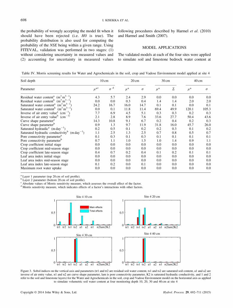
Table IV. Morris screening results for Water and Agrochemicals in

Soil depth 10 cm

Parameter μ*c σ d

Residual water contenta (m3m3�1) 4.3 5.7Residual water contentb (m3m3�1) 0.0 0.0Saturated water contenta (m3m3�1) 24.2 16.7Saturated water contentb (m3m3�1) 0.0 0.1Inverse of air entry valuea (cm�1) 7.7 6.9Inverse of air entry valueb (cm�1) 2.1 2.8Curve shape parametera 14.3 10.8Curve shape parameterb 0.9 1.3Saturated hydraulica (m day�1) 0.2 0.5Saturated hydraulic conductivityb (m day�1) 1.1 2.5Pore connectivity parametera 0.1 0.3Pore connectivity parameterb 0.7 1.1Crop coefficient initial stage 0.0 0.0Crop coefficient mid-season stage 0.0 0.0Crop coefficient late-season stage 0.4 0.7Leaf area index initial stage 0.0 0.0Leaf area index mid-season stage 0.0 0.0Leaf area index late-season stage 0.1 0.2Maximum root water uptake 0.0 0.0

a Layer 1 parameter (top 20 cm of soil profile).b Layer 2 parameter (bottom 20 cm of soil profile).c Absolute values of Morris sensitivity measure, which assesses the overall ed Morris sensitivity measure, which indicates effects of a factor’s interaction

tr1 tr2 ts1 ts2 a1 a2 n10

0.5

1Site 4 10 cm

tr1 tr2 ts1 ts2 a1 a2 n10

0.5

1Site 4 30 cm

n2lam2K2

n2lam2K2

Main effects

Total effects

Figure 3. Sobol indices on the vertical axis and parameters (tr1 and tr2 are resinverse of air entry value, n1 and n2 are curve shape parameter, lam is pore crefer to the soil and limestone layers) for the Water and Agrochemicals in the

to simulate volumetric soil water content at four m

Copyright © 2014 John Wiley & Sons, Ltd.

following procedures described by Harmel et al. (2010)and Harmel and Smith (2007).

MODEL APPLICATIONS

The validated models at each of the four sites were appliedto simulate soil and limestone bedrock water content at

the soil, crop and Vadose Environment model applied at site 4

20 cm 30 cm 40 cm

μ* σ μ* Σ μ* σ

2.4 2.9 0.0 0.0 0.0 0.00.3 0.4 1.4 1.4 2.0 2.016.0 14.7 0.1 0.1 0.0 0.111.8 11.4 69.4 49.9 120.1 105.34.5 5.1 0.3 0.3 0.2 0.38.9 7.6 33.6 27.7 50.4 43.69.1 6.7 0.2 0.4 0.2 0.39.7 11.9 31.8 16.0 45.7 26.00.1 0.2 0.2 0.3 0.1 0.21.3 2.5 0.7 0.8 0.5 0.70.1 0.3 0.1 0.1 0.1 0.11.0 1.5 1.0 1.4 0.9 1.10.0 0.0 0.0 0.0 0.0 0.00.0 0.0 0.0 0.0 0.0 0.00.2 0.4 0.1 0.2 0.1 0.10.0 0.0 0.0 0.0 0.0 0.00.0 0.0 0.0 0.0 0.0 0.00.0 0.1 0.0 0.0 0.0 0.00.0 0.0 0.0 0.0 0.0 0.0

ffect of the factor.s with other factors.

tr1 tr2 ts1 ts2 a1 a2 n10

0.5

1Site 4 20 cm

tr1 tr2 ts1 ts2 a1 a2 n1 n2lam2K2

n2lam2K2

0

0.5

1

Site 4 40 cm

idual soil water content, ts1 and ts2 are saturated soil content, a1 and a2 areonnectivity parameter, K2 is saturated hydraulic conductivity, and 1 and 2soil, crop and Vadose Environment model on the horizontal axis as appliedonitoring depth 10, 20, 30 and 40 cm at site 4

Hydrol. Process. 29, 692–711 (2015)

699SOIL WATER MODELLING CONSIDERING UNCERTAINTY

different depths under 6, 9 and 12-cm incremental raises incanal stage. Effect of surface water management on watertable elevation was simulated using MODFLOW asdescribed by Kisekka et al. (2013c). The simulated water

Table V. Water and Agrochemicals in the soil, crop and Vadose En(1 October 2010 to 3

Parameter Site 1 S

Layer 1 (top 20 cm)Residual water content (θr) 0.09Saturated water content (θs) 0.30Curve shape parameter (n) 1.09Inverse of air entry value (α) 0.04Pore connectivity parameter (λ) 0.50

Layer 2 (bottom 40 cm)Residual water content (θr) 0.09Saturated water content (θs) 0.31Curve shape parameter (n) 1.12Inverse of air entry value (α) 0.08Pore connectivity parameter (λ) 0.50Sat. hydraulic conductivity (K) 8000 9

ET

o (m

m/d

ay)

0.0

2.0

4.0

6.0

8.0

Wat

er ta

ble

NG

VD

29 (

m)

0.0

0.2

0.4

0.6

0.8

1.0

1.2

1.4

1.6

Site 4Site 3Site 2Site 1

8/1/10

9/1/10

10/1/

10

11/1/

10

12/1/

10

1/1/11

2/1/11

3/1/11

4/1/11

5/1/11

6/1/11

7/1/1

Can

al s

tage

NG

VD

29 (

m)

0.0

0.2

0.4

0.6

0.8

1.0

1.2

1.4

S177HS177T

Figure 4. Showing model input variables evapotranspiration, rainfall and watetable ele

Copyright © 2014 John Wiley & Sons, Ltd.

table elevation was then used as a lower boundary conditionof the WAVE soil profile, which allowed us to simulate theeffect of the proposed changes in surfacewater managementon soil water dynamics in the agricultural fields.

vironment parameters obtained from calibration at different sites1 December 2011)

ite 2 Site 3 Site 4 Avg.

0.08 0.10 0.10 0.090.32 0.34 0.30 0.311.22 1.17 1.15 1.140.06 0.09 0.09 0.080.62 0.54 0.62 0.58

0.06 0.09 0.09 0.080.31 0.35 0.30 0.321.11 1.11 1.10 1.110.10 0.10 0.09 0.100.62 0.54 0.62 0.58307 8511 8419 8514

Rai

nfal

l (m

m)

0

20

40

60

80

100

120

140

160

ASCE ETo Rainfall (mm)

1

8/1/11

9/1/11

10/1/

11

11/1/

11

12/1/

11

1/1/12

2/1/12

3/1/12

4/1/12

5/1/12

r table elevation as well as the canal stage, which drives variations in watervation

Hydrol. Process. 29, 692–711 (2015)

700 I. KISEKKA ET AL.

RESULTS AND DISCUSSION

Sensitivity analysis and calibration

Because of brevity, only Morris results for site 4 (theclosest site to the canal; Figure 1) are presented(Table IV). Values for the other sites were within theranges of site 4; it is also worth noting that parameterranking at all sites was similar. The magnitudes of theMorris sensitivity measures μ* (which assesses theoverall effect of the factor on model output) and σ(which indicates effects of a factor’s interactions withother factors) were greater for parameters of the vanGenuchten equation, i.e. θr and θs, α and n (Table IV).This indicates that the predicted soil and limestonebedrock water contents were more sensitive to soil

Soil

wat

er v

olum

etri

c (%

)

10

15

20

25

30

35

40

Soil

wat

er v

olum

etri

c (%

)

10

15

20

25

30

35

40

Soil

wat

er v

olum

etri

c (%

)

10

15

20

25

30

35

40

5/1/11

6/1/11

7/1/11

8/1/11

9/1/11

10/1/

11

11/1/

11

12/1/

11

1/1/12

2/1/12

3/1/12

Soil

wat

er v

olum

etri

c (%

)

10

15

20

25

30

35

40

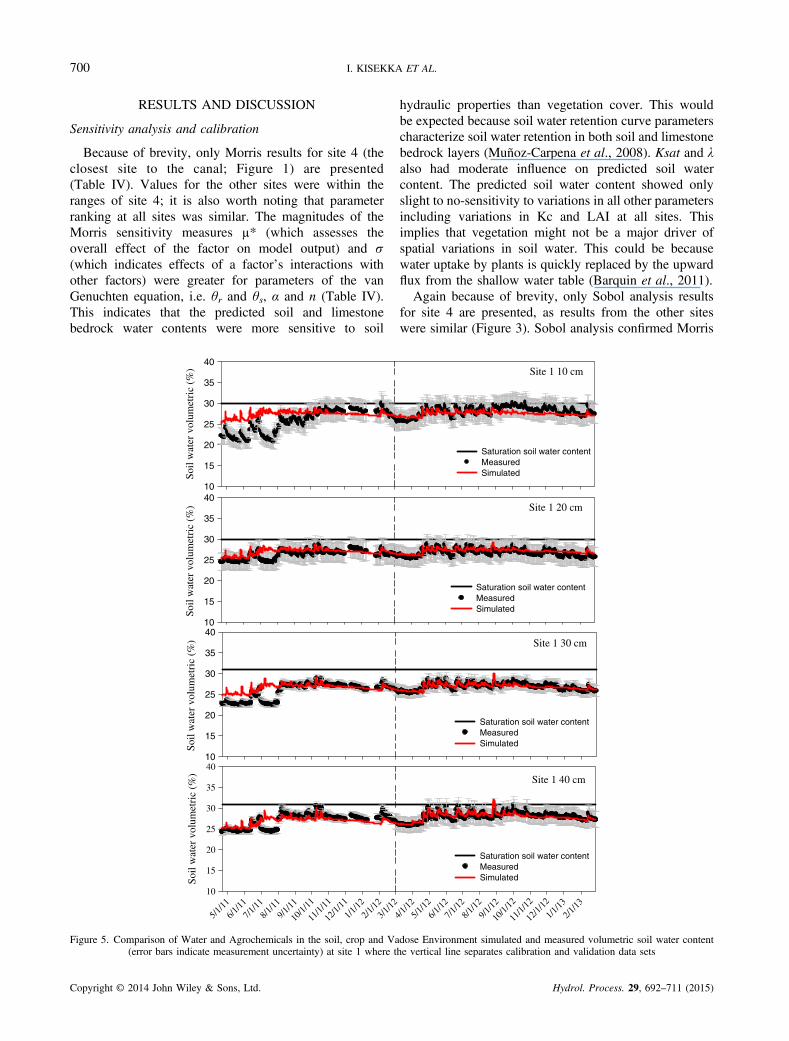
Figure 5. Comparison of Water and Agrochemicals in the soil, crop and Va(error bars indicate measurement uncertainty) at site 1 where t

Copyright © 2014 John Wiley & Sons, Ltd.

hydraulic properties than vegetation cover. This wouldbe expected because soil water retention curve parameterscharacterize soil water retention in both soil and limestonebedrock layers (Muñoz-Carpena et al., 2008). Ksat and λalso had moderate influence on predicted soil watercontent. The predicted soil water content showed onlyslight to no-sensitivity to variations in all other parametersincluding variations in Kc and LAI at all sites. Thisimplies that vegetation might not be a major driver ofspatial variations in soil water. This could be becausewater uptake by plants is quickly replaced by the upwardflux from the shallow water table (Barquin et al., 2011).Again because of brevity, only Sobol analysis results

for site 4 are presented, as results from the other siteswere similar (Figure 3). Sobol analysis confirmed Morris

Site 1 10 cm

Saturation soil water contentMeasuredSimulated

Site 1 20 cm

Saturation soil water contentMeasuredSimulated

Site 1 30 cm

Saturation soil water contentMeasuredSimulated

Site 1 40 cm

4/1/12

5/1/12

6/1/12

7/1/12

8/1/12

9/1/12

10/1/

12

11/1/

12

12/1/

12

1/1/13

2/1/13

Saturation soil water contentMeasuredSimulated

dose Environment simulated and measured volumetric soil water contenthe vertical line separates calibration and validation data sets

Hydrol. Process. 29, 692–711 (2015)

701SOIL WATER MODELLING CONSIDERING UNCERTAINTY

screening results indicating that saturated soil watercontent was the most important parameter explainingvariations in predicted soil water content as measured byNSE and RMSE (as goodness-of-fit statistics were used asa summary measure of model output) at all sites. Thefraction of the total variation in predicted soil andlimestone bedrock water content explained by variationin each of the ten important parameters is representedusing first-order and total-order Sobol sensitivity indicesalong the vertical axis (Figure 3). The first bar representsfirst-order effects, whereas the second represents total-order effects (quantifies the overall effect of a factor onmodel output), and the difference between the two barsrepresents parameter interactions.

Soil

wat

er v

olum

etri

c (%

)

10

15

20

25

30

35

40

Soil

wat

er v

olum

etri

c (%

)

10

15

20

25

30

35

40

Soil

wat

er v

olum

etri

c (%

)

10

15

20

25

30

35

40

2/1/11

6/1/11

10/1/

11

2/

Soil

wat

er v

olum

etri

c (%

)

10

15

20

25

30

35

40

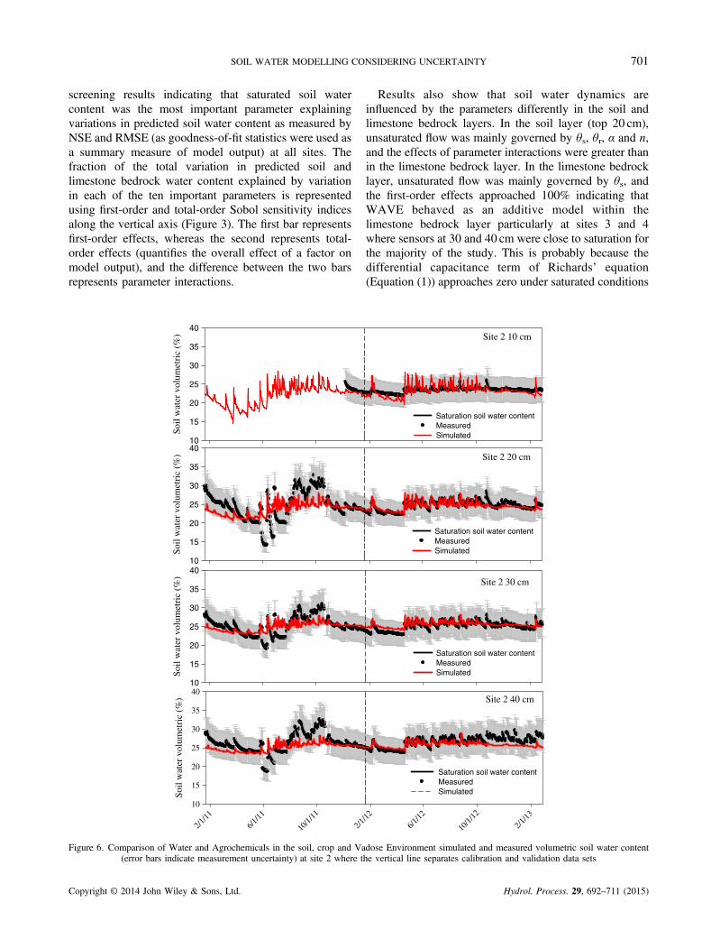
Figure 6. Comparison of Water and Agrochemicals in the soil, crop and Va(error bars indicate measurement uncertainty) at site 2 where t

Copyright © 2014 John Wiley & Sons, Ltd.

Results also show that soil water dynamics areinfluenced by the parameters differently in the soil andlimestone bedrock layers. In the soil layer (top 20 cm),unsaturated flow was mainly governed by θs, θr, α and n,and the effects of parameter interactions were greater thanin the limestone bedrock layer. In the limestone bedrocklayer, unsaturated flow was mainly governed by θs, andthe first-order effects approached 100% indicating thatWAVE behaved as an additive model within thelimestone bedrock layer particularly at sites 3 and 4where sensors at 30 and 40 cm were close to saturation forthe majority of the study. This is probably because thedifferential capacitance term of Richards’ equation(Equation (1)) approaches zero under saturated conditions

Site 2 10 cm

Saturation soil water contentMeasuredSimulated

Site 2 20 cm

Saturation soil water contentMeasuredSimulated

Site 2 30 cm

Saturation soil water contentMeasuredSimulated

Site 2 40 cm

1/12

6/1/12

10/1/

12

2/1/13

Saturation soil water contentMeasuredSimulated

dose Environment simulated and measured volumetric soil water contenthe vertical line separates calibration and validation data sets

Hydrol. Process. 29, 692–711 (2015)

702 I. KISEKKA ET AL.

(Vanclooster et al., 1995). WAVE behaving as anadditive model at 30 and 40-cm depth indicated that itcould be calibrated using accurately measured soil andlimestone bedrock water content data with less uncer-tainty in estimated parameter values. The results fromsensitivity analysis indicate that future investigations ofsoil water dynamics within the C-111 basin should focusresources on proper characterization of soil hydraulicproperties in order to develop models that can be used toexplore soil water response to regional water managementand possibly climate variability with less uncertainty.Estimated parameters after calibration show that the

average values of hydraulic parameters were not substan-tially different among calibrated values at each site

Soil

wat

er v

olum

etri

c (%

)

10

15

20

25

30

35

40

Soil

wat

er v

olum

etri

c (%

)

10

15

20

25

30

35

40

Soil

wat

er v

olum

etri

c (%

)

10

15

20

25

30

35

40

10/1/

10

2/1/11

6/1/11

10/1/

11

Soil

wat

er v

olum

etri

c (%

)

10

15

20

25

30

35

40

Figure 7. Comparison of Water and Agrochemicals in the soil, crop and Va(error bars indicate measurement uncertainty) at site 3 where t

Copyright © 2014 John Wiley & Sons, Ltd.

(Table V) implying that if the goal is not to simulate exactvalues of soil water but rather general trends in soil watercontent responses to different driving factors, averagevalues of estimated parameters can be used anywherewithin the study area. Estimated θs were compared withsaturated soil and limestone bedrock water content whenthe sensors were below the water table and the valueswere in close agreement. For example, at site 3, θs (whenthe sensor were below water table) was identified as35 (m3m3�1), and the manually estimated values forlayers 1 and 2 were 35 and 34, respectively. It has beenshown by Evett et al. (2012) that under wet conditions,there tends to be less spatial variability in soil water contentand that EnviroScan data are more accurate under these

Site 3 10 cm

Saturation soil water contentMeasuredSimulated

Site 3 20 cm

Saturation soil water contentMeasuredSimulated

Site 3 30 cm

Saturated soil water contentMeasuredSimulated

Site 3 40 cm

2/1/12

6/1/12

10/1/

12

2/1/13

Saturation soil water contentMeasuredSimulated

dose Environment simulated and measured volumetric soil water contenthe vertical line separates calibration and validation data sets

Hydrol. Process. 29, 692–711 (2015)

703SOIL WATER MODELLING CONSIDERING UNCERTAINTY

conditions.We attributed difficulty of achieving a perfect fitbetween measured and predicted soil water content atvarious depth at the same site and across the different foursites to the following factors: (1) uncertainty in measureddata, (2) intrinsic spatial variability in soil and limestonehydraulic parameters and (3) exclusion of irrigation waterapplied from the conceptual model.

Soil water content predictionComparison between simulated and measured volu-

metric water content from capacitance probes at 10, 20,30 and 40-cm depths under current canal stage operationcriteria along C-111 was plotted (Figures 5–8). Visualinspection indicates that WAVE was able to reproduce

Soil

wat

er v

olum

etri

c (%

)

10

15

20

25

30

35

40

Soil

wat

er v

olum

etri

c (%

)

10

15

20

25

30

35

40

Soil

wat

er v

olum

etri

c (%

)

10

15

20

25

30

35

40

2/1/11

6/1/11

10/1/

11

2/

Soil

wat

er v

olum

etri

c (%

)

10

15

20

25

30

35

40

Figure 8. Comparison of Water and Agrochemicals in the soil, crop and Va(error bars indicate measurement uncertainty) at site 4 where t

Copyright © 2014 John Wiley & Sons, Ltd.

temporal variations in soil water content as influenced byseasonal variations in rainfall, evapotranspiration andcanal stage (Figure 4). Some substantial deviationsbetween predicted and measured volumetric water contentat some sites and monitoring depths were observedparticularly during the summer of 2011 months (May toOctober), which also corresponded to the lowest recordedsoil water content.Although the model was able to show the wetting and

drying cycles during the summer of 2011 (Figures 5–8),these cycles substantially deviated from the measuredtrends probably because the hydraulic parameters of thesoil water retention curve that were estimated in thelaboratory and whose ranges were used in the calibration

Site 4 10 cm

Saturation soil water contentMeasuredSimulated

Site 4 20 cm

Saturation soil water contentMeasuredSimulated

Site 4 30 cm

Saturation soil water contentMeasuredSimulated

Site 4 40 cm

1/12

6/1/12

10/1/

12

2/1/13

Saturation soil water contentMeasuredSimulated

dose Environment simulated and measured volumetric soil water contenthe vertical line separates calibration and validation data sets

Hydrol. Process. 29, 692–711 (2015)

704 I. KISEKKA ET AL.

may not have been representative of the spatially variablesoil properties in field. This highlights the need for in situdetermination of soil water retention curves. The apparentcontradiction in soil water content trends during themonths June and July of 2011 in which the modelindicated continued wetting conditions whereas themeasured soil water indicated drying conditions couldbe attributed to the unexplained drop in potentialevapotranspiration during this period as shown in(Figure 4). We speculate that meteorological data forthe months of June and July 2011obtained from theFlorida Automated Weather Network Station locatedapproximately 10 km away from the study site, which wasused in this study, might not have been accurate.Alternatively, the long distance between the ET stationand the study site could also have been a factor or errorsin gauge-adjusted NEXRAD rainfall data. Small-scale

Table VI. Goodness-of-fit statistics without consideration of meascrop and Vadose Environment water content simulations by soil d

to 28 February 2013 at site 1 and 1 January

Depth 10 cm 20 cm

Site 1NSEa 0.26 (�0.32 to 0.66) 0.35 (0.03–0.59)RMSEb 0.95 (0.72–1.19) 0.62 (0.52–0.73)Ac (%) 0.0 0.0Bd (%) 0.0 0.0Ce (%) 3.1 0.5Df (%) 93.9 99.5

Site 2NSE �2.79 (�6.21 to 1.3) 0.57 (0.28–0.76)RMSE 1.16 (0.94–1.37) 0.81 (0.71–0.96)A (%) 0.0 0.0B (%) 0.0 0.6C (%) 0.0 67.1D (%) 100.0 32.3

Site 3NSE 0.25 (�0.24 to 0.50) 0.30 (�0.66 to 0.6RMSE 1.42 (1.16–1.66) 0.63 (0.52–0.81)A (%) 0.0 0.0B (%) 0.0 0.0C (%) 0.0 2.6D (%) 100.0 97.4

Site 4NSE �0.35 (�1.80 to 0.45) 0.31 (�0.99 to 0.6RMSE 0.95 (0.63–1.29) 0.52 (0.41–0.66)A (%) 0.0 0.0B (%) 0.0 0.1C (%) 0.2 5.2D (%) 99.8 94.7

NSE, Nash–Sutcliffe; RMSE, Root Mean Square Error.a Nash–Sutcliffe coefficient (95% confidence interval).b Root mean square error (95% confidence interval).c Probability of fit being very good 0.9<NSE< 1.0.d Probability of fit being good 0.8<NSE< 0.9.e Probability of fit being acceptable 0.65<NSE< 0.8.f p-value less than α is model acceptable, whereas p-value less than α is mo

Copyright © 2014 John Wiley & Sons, Ltd.

heterogeneity in soil properties amplified under dryconditions causes the geometric constant of the sensorto change with each measurement depth and access tube,which results in a different resonant frequency andvariable water content estimates even if mean watercontent around the access tube is the same (Evett et al.,2012). The increase in small-scale variability in soil watercontent under dry conditions is compounded by the smallvolumes sensed by capacitance sensors. For example,EnviroScans measures an effective distance of only3–5 cm from the access tube and may be affected bynon-isothermal conditions and soil bulk electrical con-ductivity (Evett et al., 2009).Missing data at 10-cm depth and large deviation

between predicted and measured soil water content atsite 2 (Figure 5) during the first months of the study weredue to poor sensor installation, which was subsequently

urement uncertainty for Water and Agrochemicals in the soil,epth during the validation period ranging from 1 January 20122012 to 28 February 2013 at other sites

30 cm 40 cm

0.80 (0.66–0.88) 0.77 (0.74–0.88)0.35 (0.31–0.41) 0.48 (0.41–0.54)0.5 0.551.4 29.146.4 54.31.7** 16.1

0.44 (0.27–0.57) 0.10 (�0.90 to 066)0.84 (0.65–1.06) 1.35 (0.94–1.72)0.0 0.00.0 0.00.1 0.099.1 100.0

0) �1.95 (�5.5 to 0.17) �3.80 (�6.2 to 0.87)0.99 (0.73–1.22) 0.89 (0.55–1.28)0.0 3.20.0 5.30.0 10.4

100.0 81.1

6) �0.63 (�2.11 to 0.01) �12.2 (�29.6 to 4.18)0.63 (0.43–0.80) 0.97 (0.79–1.11)0.0 0.00.0 0.00.0 0.5

100.0 99.5

del rejected; α could be ***1%, **5% or *10%.

Hydrol. Process. 29, 692–711 (2015)

705SOIL WATER MODELLING CONSIDERING UNCERTAINTY

re-installed thus improving data at 20, 30 and 40 cm, butre-installation did not improve data at 10 cm at this site.It is worth noting that transformation of measured datausing the capacitance sensor calibration equationdeveloped in the laboratory by Al-Yahyai et al. (2006)for gravely loam soils of south Florida was tried but gaveinconsistent results at various depths and sites and wasabandoned.Goodness-of-fit statistics for model validation for the

different sites and monitoring depth without and withconsideration of measurement uncertainty were calculated(Tables VI and VII). Fit between measured water contentand simulated water content was unsatisfactory for allsites, and the model was rejected (Ritter and Muñoz-Carpena, 2013) at all sites and depths with the exceptionof 30 and 40-cm depths at site 1 when uncertainty inmeasured soil water content was not taken into account

Table VII. Goodness-of-fit statistics considering measurement uncerEnvironment water content simulations by soil depth during the vali

site 1 and 1 January 2012 to 28

Depth 10 cm 20 cm

Site 1NSEa 0.78 (0.50–0.92) 0.87 (0.75–0.9RMSEb 0.53 (0.33–0.74) 0.28 (0.20–0.3Ac (%) 7.2 23.4Bd (%) 31.3 70.2Ce (%) 42.6 5.9Df (%) 18.9 0.0***

Site 2NSE �1.66 (�5.39 to 0.3) 0.89 (0.78–0.9RMSE 0.70 (0.70–1.30) 0.41 (0.31–0.5A (%) 0.0 41.2B (%) 0.0 56.2C (%) 0.0 2.6D (%) 100.0 0.0***

Site 3NSE 0.81 (0.59–0.89) 0.76 (0.02–0.9RMSE 0.71 (0.53 to 0.93) 0.37 (0.20–0.6A (%) 3.3 20.5B (%) 54.7 23.6C (%) 37.7 28.6D (%) 4.3** 27.3

Site 4NSE 0.78 (0.49–0.93) 0.87 (0.39–0.9RMSE 0.39 (0.22–0.54) 0.22 (0.13–0.3A (%) 8.5 40.9B (%) 34.6 35.0C (%) 43.8 17.1D (%) 13.1 0.7***

NSE, Nash–Sutcliffe; RMSE, Root Mean Square Error.a Nash–Sutcliffe coefficient (95% confidence interval).b Root mean square error (95% confidence interval).c Probability of fit being very good 0.9<NSE< 1.0.d Probability of fit being good 0.8<NSE< 0.9.e Probability of fit being Acceptable 0.65<NSE< 0.8.f p-value less than α is model acceptable, whereas p-value less than α is mo

Copyright © 2014 John Wiley & Sons, Ltd.

(Table VI). This outcome is expected when performanceis evaluated using measured data with high uncertaintywithout consideration of uncertainty boundaries inestimating the deviation between measured and predictedvalues. However, when uncertainty in measured soilwater content data was considered by assuming a uniformprobability distribution and using the procedure proposedby Harmel et al. (2010), there was an improvement in thegoodness-of-fit measures (Table VII) sometime substan-tially. Goodness-of-fit calculated using this approachwould be more appropriate for evaluating modelperformance compared with simply using measuredvalues, which are inherently uncertain, despite itsweakness of assuming symmetry. Future research couldexplore developing statistical methodologies for modify-ing the deviation between measured and predicted valuebased on asymmetric probability distributions.

tainty for Water and Agrochemicals in the soil, crop and Vadosedation period ranging from 1 January 2012 to 28 February 2013 atFebruary 2013 at other sites

30 cm 40 cm

3) 0.89 (0.75–0.94) 0.85 (0.68–0.93)9) 0.26 (0.20–0.40) 0.38 (0.31–0.51)

47.3 15.051.0 58.41.7 26.10.0*** 0.5***

4) 0.88 (0.79–0.93) 0.65 (0.24–0.91)5) 0.38 (0.25–0.54) 0.81 (0.43–1.13)

37.2 4.661.1 13.61.7 33.40.0*** 48.4

4) 0.70 (0.25–0.91) 0.30 (�0.31 to 0.88)0) 0.32 (0.21–0.42) 0.34 (0.13–0.55)

3.4 3.219.1 5.337.9 10.439.6 81.1

7) 0.75 (0.52–0.87) �0.20 (�1.95–0.54)7) 0.24 (0.14–0.33) 0.30 (0.23–0.35)

1.9 0.025.6 0.059.7 0.512.8 99.5

del rejected; α could be ***1%, **5% or *10%.

Hydrol. Process. 29, 692–711 (2015)

706 I. KISEKKA ET AL.

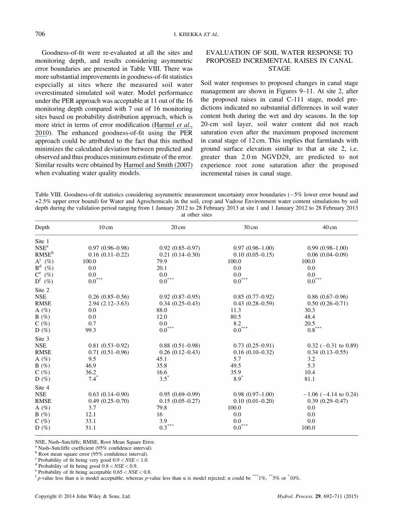
Goodness-of-fit were re-evaluated at all the sites andmonitoring depth, and results considering asymmetricerror boundaries are presented in Table VIII. There wasmore substantial improvements in goodness-of-fit statisticsespecially at sites where the measured soil wateroverestimated simulated soil water. Model performanceunder the PER approach was acceptable at 11 out of the 16monitoring depth compared with 7 out of 16 monitoringsites based on probability distribution approach, which ismore strict in terms of error modification (Harmel et al.,2010). The enhanced goodness-of-fit using the PERapproach could be attributed to the fact that this methodminimizes the calculated deviation between predicted andobserved and thus produces minimum estimate of the error.Similar results were obtained by Harmel and Smith (2007)when evaluating water quality models.

Table VIII. Goodness-of-fit statistics considering asymmetric measu+2.5% upper error bound) for Water and Agrochemicals in the soil,depth during the validation period ranging from 1 January 2012 to 28

at other

Depth 10 cm 20 cm

Site 1NSEa 0.97 (0.96–0.98) 0.92 (0.85–0.97)RMSEb 0.16 (0.11–0.22) 0.21 (0.14–0.30)Ac (%) 100.0 79.9Bd (%) 0.0 20.1Ce (%) 0.0 0.0Df (%) 0.0*** 0.0***

Site 2NSE 0.26 (0.85–0.56) 0.92 (0.87–0.95)RMSE 2.94 (2.12–3.63) 0.34 (0.25–0.43)A (%) 0.0 88.0B (%) 0.0 12.0C (%) 0.7 0.0D (%) 99.3 0.0***

Site 3NSE 0.81 (0.53–0.92) 0.88 (0.51–0.98)RMSE 0.71 (0.51–0.96) 0.26 (0.12–0.43)A (%) 9.5 45.1B (%) 46.9 35.8C (%) 36.2 16.6D (%) 7.4* 3.5*

Site 4NSE 0.63 (0.14–0.90) 0.95 (0.69–0.99)RMSE 0.49 (0.25–0.70) 0.15 (0.05–0.27)A (%) 3.7 79.8B (%) 12.1 16C (%) 33.1 3.9D (%) 51.1 0.3***

NSE, Nash–Sutcliffe; RMSE, Root Mean Square Error.a Nash–Sutcliffe coefficient (95% confidence interval).b Root mean square error (95% confidence interval).c Probability of fit being very good 0.9<NSE< 1.0.d Probability of fit being good 0.8<NSE< 0.9.e Probability of fit being acceptable 0.65<NSE< 0.8.f p-value less than α is model acceptable, whereas p-value less than α is mo

Copyright © 2014 John Wiley & Sons, Ltd.

EVALUATION OF SOIL WATER RESPONSE TOPROPOSED INCREMENTAL RAISES IN CANAL

STAGE

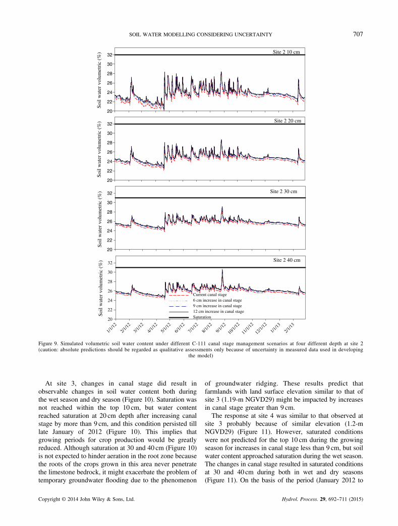
Soil water responses to proposed changes in canal stagemanagement are shown in Figures 9–11. At site 2, afterthe proposed raises in canal C-111 stage, model pre-dictions indicated no substantial differences in soil watercontent both during the wet and dry seasons. In the top20-cm soil layer, soil water content did not reachsaturation even after the maximum proposed incrementin canal stage of 12 cm. This implies that farmlands withground surface elevation similar to that at site 2, i.e.greater than 2.0m NGVD29, are predicted to notexperience root zone saturation after the proposedincremental raises in canal stage.

rement uncertainty error boundaries (�5% lower error bound andcrop and Vadose Environment water content simulations by soilFebruary 2013 at site 1 and 1 January 2012 to 28 February 2013sites

30 cm 40 cm

0.97 (0.96–1.00) 0.99 (0.98–1.00)0.10 (0.05–0.15) 0.06 (0.04–0.09)

100.0 100.00.0 0.00.0 0.00.0*** 0.0***

0.85 (0.77–0.92) 0.86 (0.67–0.96)0.43 (0.28–0.59) 0.50 (0.26–0.71)

11.3 30.380.5 48.48.2 20.50.0*** 0.8***

0.73 (0.25–0.91) 0.32 (�0.31 to 0.89)0.16 (0.10–0.32) 0.34 (0.13–0.55)5.7 3.2

49.5 5.335.9 10.48.9* 81.1

0.98 (0.97–1.00) �1.06 (�4.14 to 0.24)0.10 (0.01–0.20) 0.39 (0.29–0.47)

100.0 0.00.0 0.00.0 0.00.0*** 100.0

del rejected; α could be ***1%, **5% or *10%.

Hydrol. Process. 29, 692–711 (2015)

Site 2 10 cm

Soil

wat

er v

olum

etri

c (%

)

20

22

24

26

28

30

32

Site 2 20 cm

Soil

wat

er v

olum

etri

c (%

)

20

22

24

26

28

30

32

Site 2 30 cm

Soil

wat

er v

olum

etri

c (%

)

20

22

24

26

28

30

32

Site 2 40 cm

1/1/12

2/1/12

3/1/12

4/1/12

5/1/12

6/1/12

7/1/12

8/1/12

9/1/12

10/1/

12

11/1/

12

12/1/

12

1/1/13

2/1/13

Soil

wat

er v

olum

etri

c (%

)

20

22

24

26

28

30

32

Current canal stage6 cm increase in canal stage9 cm increase in canal stage12 cm increase in canal stageSaturation

Figure 9. Simulated volumetric soil water content under different C-111 canal stage management scenarios at four different depth at site 2(caution: absolute predictions should be regarded as qualitative assessments only because of uncertainty in measured data used in developing

the model)

707SOIL WATER MODELLING CONSIDERING UNCERTAINTY

At site 3, changes in canal stage did result inobservable changes in soil water content both duringthe wet season and dry season (Figure 10). Saturation wasnot reached within the top 10 cm, but water contentreached saturation at 20 cm depth after increasing canalstage by more than 9 cm, and this condition persisted tilllate January of 2012 (Figure 10). This implies thatgrowing periods for crop production would be greatlyreduced. Although saturation at 30 and 40 cm (Figure 10)is not expected to hinder aeration in the root zone becausethe roots of the crops grown in this area never penetratethe limestone bedrock, it might exacerbate the problem oftemporary groundwater flooding due to the phenomenon

Copyright © 2014 John Wiley & Sons, Ltd.

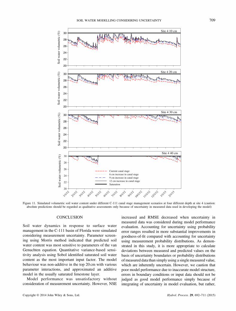
of groundwater ridging. These results predict thatfarmlands with land surface elevation similar to that ofsite 3 (1.19-m NGVD29) might be impacted by increasesin canal stage greater than 9 cm.The response at site 4 was similar to that observed at

site 3 probably because of similar elevation (1.2-mNGVD29) (Figure 11). However, saturated conditionswere not predicted for the top 10 cm during the growingseason for increases in canal stage less than 9 cm, but soilwater content approached saturation during the wet season.The changes in canal stage resulted in saturated conditionsat 30 and 40 cm during both in wet and dry seasons(Figure 11). On the basis of the period (January 2012 to

Hydrol. Process. 29, 692–711 (2015)

Site 3 10 cm

Soil

wat

er v

olum

etri

c (%

)

20

22

24

26

28

30

32

34

36

Site 3 20 cm

Soil

wat

er v

olum

etri

c (%

)

20

22

24

26

28

30

32

34

36

Site 3 30 cm

Soil

wat

er v

olum

etri

c (%

)

20

22

24

26

28

30

32

34

36

Site 3 40 cm

1/1/12

2/1/12

3/1/12

4/1/12

5/1/12

6/1/12

7/1/12

8/1/12

9/1/12

10/1/

12

11/1/

12

12/1/

12

1/1/13

2/1/13

Soil

wat

er v

olum

etri

c (%

)

20

22

24

26

28

30

32

34

36

Current canal stage6 cm increase in canal stage9 cm increase in canal stage12 cm increase in canal stageSaturation

Figure 10. Simulated volumetric soil water content under different C-111 canal stage management scenarios at four different depth at site 3(caution: absolute predictions should be regarded as qualitative assessments only because of uncertainty in measured data used in developing

the model)

708 I. KISEKKA ET AL.

February 2013) investigated for potential impacts ofraising canal stage on root zone soil water content, thesites with land surface elevation greater than 2.0-mNGVD29 did not experience saturated conditions in thetop 20-cm soil layer. Raising canal stage by more than9 cm is predicted (within uncertainty ranges in Tables VIIand VIII) to result in saturated root zone and shortening ofthe growing season at sites with land surface elevation lessthan 2.0 cm NGVD29, which is critical for continued useof the land for agricultural production.Application of this model is limited to exploratory

assessments because of the uncertainty in measureddata. This uncertainty could be reduced by improving

Copyright © 2014 John Wiley & Sons, Ltd.

the method for obtaining soil water content data that areused in model calibration. This is a very challengingproposition for this particular study site because of thecomplex texture of the soil, being composed oflimestone bedrock that has been rock-plowed. Soilwater equipment that senses a larger soil volume and isnot impacted by soil texture effects, temperature andsalinity should be explored for measuring soil watercontent at this site. Future investigations with thesemodels would also benefit from high-resolution digitalelevation maps that could be linked to the vadose zonemodel to identify areas with potential to experiencetransient root zone saturation.

Hydrol. Process. 29, 692–711 (2015)

Site 4 10 cm

Soil

wat

er v

olum

etri

c (%

)

20

22

24

26

28

30

Site 4 20 cm

Soil

wat

er v

olum

etri

c (%

)

20

22

24

26

28

30

Site 4 30 cm

Soil

wat

er v

olum

etri

c (%

)

20

22

24

26

28

30

Site 4 40 cm

1/1/12

2/1/12

3/1/12

4/1/12

5/1/12

6/1/12

7/1/12

8/1/12

9/1/12

10/1/

12

11/1/

12

12/1/

12

1/1/13

2/1/13

Soil

wat

er v

olum

etri

c (%

)

20

22

24

26

28

30

Current canal stage6 cm increase in canal stage9 cm increase in canal stage12 cm increase in canal stageSaturation

Figure 11. Simulated volumetric soil water content under different C-111 canal stage management scenarios at four different depth at site 4 (caution:absolute predictions should be regarded as qualitative assessments only because of uncertainty in measured data used in developing the model)

709SOIL WATER MODELLING CONSIDERING UNCERTAINTY

CONCLUSION

Soil water dynamics in response to surface watermanagement in the C-111 basin of Florida were simulatedconsidering measurement uncertainty. Parameter screen-ing using Morris method indicated that predicted soilwater content was most sensitive to parameters of the vanGenuchten equation. Quantitative variance-based sensi-tivity analysis using Sobol identified saturated soil watercontent as the most important input factor. The modelbehaviour was non-additive in the top 20 cm with variousparameter interactions, and approximated an additivemodel in the usually saturated limestone layer.Model performance was unsatisfactory without

consideration of measurement uncertainty. However, NSE

Copyright © 2014 John Wiley & Sons, Ltd.

increased and RMSE decreased when uncertainty inmeasured data was considered during model performanceevaluation. Accounting for uncertainty using probabilityerror ranges resulted in more substantial improvements ingoodness-of-fit compared with accounting for uncertaintyusing measurement probability distributions. As demon-strated in this study, it is more appropriate to calculatedeviations between measured and predicted values on thebasis of uncertainty boundaries or probability distributionsofmeasured data than simply using a singlemeasured value,which are inherently uncertain. However, we caution thatpoor model performance due to inaccurate model structure,errors in boundary conditions or input data should not bejudged as good model performance simply because ofintegrating of uncertainty in model evaluation, but rather,

Hydrol. Process. 29, 692–711 (2015)

710 I. KISEKKA ET AL.

models should be judged on their ability to represent thephysical processes. This suggests that parameterizing themodel using the measured soil water content withoutconsideration of measurement uncertainty would likelyresult in a model calibrated to the collected data rather thanto the system or over calibration.Model application to predict soil water dynamics under

raised canal stage indicated that sites with land surfaceelevation of less than 2.0m NGVD29 might experiencetransient root zone saturation and shortening of thegrowing season if canal stage is raised more than 9 cm. Atdepths greater than 20 cm, raises in canal stage werepredicted to result in prolonged saturated conditions. Thesaturated conditions at the 30 and 40-cm depth at lowelevation sites could exacerbate the problem of temporarygroundwater flooding due to groundwater ridging,suggesting that water management practices would needto be modified.The models developed in this study could be could be

combined with high-resolution digital elevation models infuture studies to identify areas that should not be plantedto minimize potential losses. The study also highlightedthe need to develop methodologies for modifications ofthe error term between predicted and observed based onasymmetric measurement probability distributions.

ACKNOWLEDGEMENTS

We would like to thank the anonymous reviewers for theuseful suggestions that helped improve the quality of themanuscript. The authors would also like to thank the SouthFlorida Water Management District for providing thefunding for this study,Mr Vito Strano andMr SamAccursiofor allowing us to use their lands and Ms. Tina Dispenza forher contribution towards data collection and processing.

REFERENCES

Al-Yahyai R, Schaffer B, Davies FS, Muñoz-Carpena R. 2006.Characterization of soil-water retention of a very gravelly-loam soilvaried with determination method. Soil Science 171(2): 85–93. DOI:10.1097/01.ss.0000187372.53896.9d.

Barquin LP, Migliaccio KW, Muñoz-Carpena R, Schaffer B, Crane JH,Li YC. 2011. Shallow water table contribution to soil-water retentionin capillary fringe of a very gravelly loam soil of south Florida.Vadose Zone Journal 10:1–8.

Bilskie J. 2001. Soil water measurements: considering variability anduncertainty. App. Note: 2S J. Campbell Scientific, Logan Utah.

Campolongo F, Cariboni J, Saltelli A. 2007. An effective screening designfor sensitivity analysis of large models. Environmental Modeling andSoftware 22: 1509–1518.

Chen M, Willgoose GR, Saco PM. 2012. Spatial prediction of temporalsoil moisture dynamics using HYDRUS-1D. Hydrological Processes.DOI: 10.1002/hyp.9518

Evett SR. 2000. Some aspects of time domain reflectometry (TDR),neutron scattering, and capacitance methods of soil water contentmeasurement. Pp. 5–49 In Comparison of soil water measurement using

Copyright © 2014 John Wiley & Sons, Ltd.

the neutron scattering, time domain reflectometry and capacitancemethods. International Atomic Energy Agency, Vienna, Austria, IAEA-TECDOC-1137.

Evett SR, Schwartz RC, Tolk JA, Howell TA. 2009. Soil profile watercontent determination: spatio-temporal variability of electromagnetic andneutron probe sensors in access tubes. Vadose Zone Journal 8(4): 1–16.

Evett SR, Schwartz RC, Casanova JJ, Heng LK. 2012. Soil water sensing forwater balance, ET andWUE. J. AgriculturalWaterManagement. 104:1–9.

Feddes RA, Kowalik PJ, Zaradny H. 1978. Simulation of Field Water Useand Crop Yield. Simulation Monographs. PUDOC: Wageningen, TheNetherlands.

Gabriel JL, Lizaso JI, Miguel Q. 2010. Laboratory versus fieldcalibration of capacitance probes. Soil Science Society of AmericaJournal 74:593–601.

van Genuchten MT. 1980. A closed-form equation for predicting thehydraulic conductivity of soil. Soil Science Society of America Journal44: 892–898.

van Genuchten MTh, Leij FJ, Yates SR. 1991. The RETC code forquantifying the hydraulic functions of unsaturated soils, Version 1.0.EPA Report 600/2-91/065, U.S Salinity Laboratory, USDA-ARS,Riverside, California.

Germann P, LevyB. 1986.Groundwater response to precipitation.EOS 67: 91.Harmel RD, Smith PK. 2007. Consideration of measurement uncertaintyin the evaluation of goodness-of-fit in hydrologic and water qualitymodeling. J. Hydrology. 337: 326–336.

Harmel RD, Smith PK, Migliaccio K. 2010. Modifying goodness-of-fitindicators to incorporate both measurement and model uncertainty inmodel calibration and validation. Transactions of the ASABE 53(1): 55–63.

IAEA. 2008. Field Estimation of Soil Water Content: A Practical Guide toMethods, Instrumentation and Sensor Technology, Training CourseSeries No. 30. International Atomic Energy Agency: Vienna, Austria.

Kavetski D, Kuczera G, Franks SW. 2006. Bayesian analysis of inputuncertainty in hydrological modeling. Water Resources Research42: W03408. doi:10.1029/2005WR004376.

Kayane I, Kaihotsu I. 1988. Some experimental results concerningrapid water table response to surface phenomena. J. Hydrology 102:215–234.

Kisekka I, Migliaccio KW, Muñoz-Carpena R, Khare Y, Boyer TH.2013a. Sensitivity analysis and parameter estimation for an approximateanalytical model of canal-aquifer interaction applied in the C-111 Basin.Trans. ASABE 56(3): 977–992.

Kisekka I, Migliaccio KW, Muñoz-Carpena R, Li YC, Boyer TH. 2013b.simulating water table response to proposed changes in surface watermanagement in agricultural lands adjacent to Everglades National Park.Under peer review Journal of Agricultural Water Management.

Kisekka I, Migliaccio KW, Muñoz-Carpena R, Schaffer B. 2013c.Dynamic factor analysis of surface water management impacts on soiland bedrock water contents in Southern Florida Lowlands. Journal ofHydrology. http://dx.doi.org/10.1016/j.jhydrol.2013.02.035

Lin C. 2003. Frequency domain versus travel time analyses of TDRwaveforms for soil moisture measurements. Soil Science Society ofAmerica Journal 67(3): 720–729.

Lizaso JI, Ritchie JT. 1997. Maize shoot and root response to rootzone saturation during vegetative growth. Agronomy Journal89: 125–134.

Merdun H, Cnar O, Meral R, Apan M. 2006. Comparison of artificialneural network and regression pedotransfer functions for prediction ofsoil water retention and saturated hydraulic conductivity. Soil andTillage Research 90: 108–116.

Mualem Y. 1976. A new model for predicting the hydraulicconductivity of unsaturated porous media. Water ResourcesResearch 12: 513–522.

Muñoz-Carpena R, Zajac Z, Kuo Y. 2007. Global Sensitivity anduncertainty analyses of the water quality model VFSMOD-W. Trans-actions of the ASABE 50(5): 1719–1732.

Muñoz-Carpena R, Ritter A, Bosch DD, Schaffer B, Potter TL. 2008.Summer cover crop impacts on soil percolation and nitrogenleaching from a winter corn field. Agricultural Water Management95: 633–644.

Politis DN, Romano JP. 1994. The stationary bootstrap. Journal of theAmerican Statistical Association 89: 1303–1313

Hydrol. Process. 29, 692–711 (2015)

711SOIL WATER MODELLING CONSIDERING UNCERTAINTY

Ritchie JT. 1972. Model for predicting evaporation from a row crop withincomplete cover. Water Resources Research 8(5): 1204–1213.DOI:10.1029/WR008i005p01204

Ritter A, Muñoz-Carpena R. 2013. Predictive ability of hydrological models:objective assessment of goodness-of-fit with statistical significance.J. Hydrology 480(1): 33–45. doi:10.1016/j.jhydrol.2012.12.004

Saltelli A, Tarantola S, Campolongo F, Ratto M. 2004. Sensitivity Analysisin Practice: A Guide to Assessing Scientific Models. John Wiley andSons: Chichester, U.K.

Saltelli A, Ratto M, Andres T, Campolongo F, Cariboni J, Gatelli D,Saisana M, Tarantola S. 2008. Global Sensitivity Analysis. The Primer.John Wiley and Sons.

Schaffer B. 1998. Flooding responses and water-use efficiency ofsubtropical and tropical fruit trees in an environmentally-sensitivewetland. Annals of Botany 81: 475–481.

Sentek Pty Ltd. 2001. Calibration of the Sentek Pty Ltd Soil MoistureSensors. Stepney, South Australia. Soil Survey Division Staff. 1993.Soil survey manual.

Copyright © 2014 John Wiley & Sons, Ltd.

USACE and SFWMD. 2011. Comprehensive Everglades RestorationPlan: C-111 Spreader Canal Western Project: Final Integrated ProjectImplementation Report and Environmental Impact Statement. U.S.Army Corps of Engineers Jacksonville, District.

Vanclooster M, Viaene P, Diels J, Feyen J. 1995. A deterministicevaluation analysis applied to an integrated soil-crop model. EcologicalModelling 81: 183–195.

Vanclooster M, Viaene P, Diels J, Christiaens K. 1996. WAVE: AMathematical Model for Simulating Water and Agrochemicals in theSoil and Vadose Environment. Reference and user’s manual(release2.0). Institute for Land and Water Management, KatholiekeUniversiteit Leuven: Leuven, Belgium.

WaswaGW,ClulowC, FreeseC, LeRouxPAL, Lorentz SA. 2013. Transientpressure waves in the vadose zone and the rapid water table response. SoilScience Society of America Journal. doi:10.2136/vzj2012.0054.

Whiting ML, Li L, Ustin SL. 2004. Predicting water content usingGaussian model on soil spectra Remote Sensing of Environment. 89:535–552.

Hydrol. Process. 29, 692–711 (2015)