Ordering Quantity Decisions Considering Uncertainty in

Supply-Chain Logistics Operations

Hyoungtae Kim, Jye-Chyi Lu, Paul H. Kvam

School of Industrial and Systems Engineering

Georgia Institute of Technology, Atlanta, GA 30332

Abstract

This research seeks to determine the optimal order amount for the retailer given uncertainty

in a supply-chain’s logistics network due to unforseeable disruption or various types of defects

(e.g., shipping damage, missing parts and misplacing products). Mixture distribution models

characterize problems from solitary failures and contingent events causing network to function

ineffectively. The uncertainty in the number of good products successfully reaching the distri-

bution center (DC) and retailer poses a challenge in deciding product-order amounts. Because

the commonly used ordering plan developed for maximizing expected profits does not allow

retailers to address concerns about contingencies, this research proposes two improved proce-

dures with risk-averse characteristics towards low probability and high impact events. Several

examples illustrate the impact of DC’s operation policies and model assumptions on retailer’s

product-ordering plan and resulting sales profit.

Key Words: contingency, logistics network, mixture distribution, stochastic optimization,

supply chain.

1 Introduction

In this era of global sourcing, to reduce purchase costs and attract a larger base of customers,

retailers such as Wal-Mart, Home Depot and Dollar General are constantly seeking suppliers with

lower prices and finding them at greater and greater distances from their distribution centers (DCs)

and stores. Consequently, a significant proportion of shipped products from overseas suppliers is

susceptible to defects. Reasons for defects include missing parts, misplaced products (at DCs,

stores) or mistakes in orders and shipments. Sometimes, products are damaged from mishandling

in transportation or are affected by the low probability and high impact contingency such as extreme

1

weather, labor dispute and terrorist attack. When there are logistics delays due to security inspec-

tions at U.S. borders and seaports, or simply traffic problems, orders, packagings and shipments do

not arrive at the DCs or stores on time. Regardless of the problems contributed from the supply

sources or logistics operations, this article considers all of them as supply and logistics defects. Two

case studies with a major retailing chain indicate that the proportion of the “defects” could reach

20%. This creates significant challenge in product-ordering and shelf-space management.

If the defect rate is not accounted for in the purchase order, the resulting product shortages serve

as precursors to several consequences, including inconveniencing their customers, compromising the

retailer’s reputation for service quality, and then having to trace, sell, repair or return the defective

products. Based on our interaction experience with retailers, the stock-out problem can cause more

than billion dollars in a large retail chain. On the other hand, use of excessive inventory to handle

the uncertain supply and logistics defects is also costly. This article models the defect process in

a three-level supply chain network with many suppliers, one DC and one store, and link it to DCs

operation policy for developing an optimal product-ordering scheme.

The literature on supply-chain contract decisions feature methods that utilize a high-level gen-

eral model to describe supply uncertainties without getting into any degree of logistics details. See

examples in Sculli and Wu [8], Ramasech [7], Lau and Lau [2], Parlar and Perry [6], Parlar [5], Weng

[11], and Mohebbi [3] for diverse implications of random production lead-time on inventory policies.

Gulyani [1] studied the effects of poor transportation on the supply chain (i.e., highly ineffective

freight transportation systems) and showed how it increases the probability of incurring damage in

transit and total inventories, while also increasing overhead costs. Silver [10] used the Economic

Order Quantity (EOQ) formulation to model the situation that the order quantity received from

the supplier does not necessarily match the quantity requisitioned. He showed that the optimal

order quantity depends only on the mean and standard deviation of the amount received. Shih [9]

studied the optimal ordering schemes in the case where the proportion of defective products (PDP)

in the accepted lots has a known probability distribution. Noori and Keller [4] extended Silver’s

model to obtain an optimal production quantity when the amount of products received at stores

assumes probability distributions such as uniform, normal and gamma.

Papers concerned with logistics or probabilistic networks are more common in the area of

transportation, especially in the hazardous material routing problem. In the transportation of

hazardous material, the event of an accident with a truck fully loaded with hazardous material

can be treated as contingency, but in most past models, the main objective has been to find the

optimal route to minimize the expected total system cost, without concern for supply chain contract

decisions such as the optimal ordering quantity.

In general, these models do not link the supply chain and logistics decision processes together.

Without understanding the details of the logistics networks (e.g., how defects occurred in the supply

network, how different operation policies in the DC affect the defect process), the supply-chain

2

contract decisions are prone to inaccuracies, especially in dealing with stochastic optimizations due

to supply uncertainties. For example, suppose the typical defect rate is θn and a contingent event

occurs with probability p (e.g., 0.00001), and upon occurrence, θc × 100 percentage of the total

shipment is damaged. Then, the overall defect rate is (1−I)×θn +I ×θc = θ+I × (θc−θn), where

I = 1 under the contingency and I = 0 otherwise. Even though θc (e.g., 90%) product damage under

the contingent situation can cause enormous stockout costs to the retailer, the average defect rate

θn +p× (θc−θn) is nearly the same as θn without the contingency due to the very small probability

p. Consequently, orders based on the average defect rate (as seen in most of supply-chain contracts)

do not prepare the retailer for potentially severe losses that accompany contingencies. Thus, it is

important to know how defects will impact the uncertainty in the amount of good products arriving

at stores and to develop optimization strategies to encounter these situations.

In this paper, we describe two procedures with which retailers can generate reasonable solutions

that exhibit risk-averse characteristics toward extreme events. In Section 2 we first model processes

for product defect rates between any two points in the network, which are directly linked to logistics

operations. Next, we construct a random variable representing the total proportion of defective

products (TPDP) by integrating models of defects at various stages of the supply-chain network.

TPDP is based on a series of mixture distributions and characterizes the overall service levels

(defect rates) of logistics operations in contingent and non-contingent circumstances. Moreover,

we investigate the impact of two different policies of DCs operations on the resulting distributions

of TPDP. Section 3 shows the ineffectiveness of using the expected profit in locating the optimal

ordering quantity. In Section 4, a probability constrained optimization procedure is developed to

handle the low probability and high impact events that lead to logistics uncertainties. Numerical

examples are provided in Section 5. Section 6 summarizes the results of the article and outlines

future research opportunities.

2 A Product-defect Model for Logistics Networks

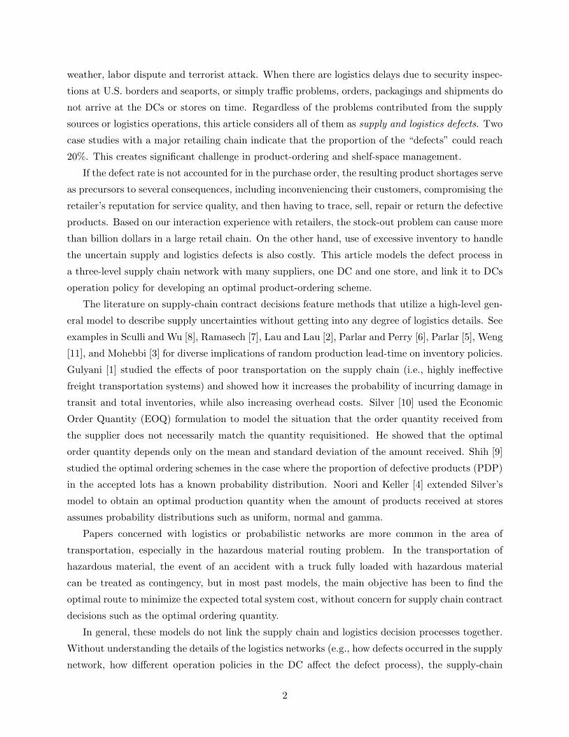
We consider the problem of a retailer who is buying products from k identical suppliers. Each

supplier provides the retailer with identical products at the same price. Products from the k

suppliers are transported and stored in a single DC before being sent out to the retail outlet (see

Figure 1).

A contingent event to products shipped from supplier j to the DC is assumed to have high

impact, low probability and affects logistics operations (e.g., product defects or delivery delays)

between suppliers and the DC. We assume that given a contingency, the damage proportion, de-

noted by XjC , is independent of the size of actual shipment, with distribution function GC . More

generally, we define

3

S 2

S k

S 1

DC R

Figure 1: Supply chain network with k suppliers and one DC

XjC = Proportion of defective products (PDP) due to contingency between supplier j and DC

XjC ∼ GC where E(XjC) = µC , V ar(XjC) = σ2C ,

XjN = PDP due to non-contingency between supplier j and DC

XjN ∼ GN where E(XjN ) = µN , V ar(XjN ) = σ2N ,

Ij = 1 if a contingent event occurs between supplier and DC, = 0 otherwise

and {I1, . . . , Ik} are independent with P (Ij = 1) = pj , and

PjW = (1 − Ij)XjN + IjXjC , PDP from supplier j to DC.

Note that PjW is a simple mixture distribution, where Ij serves as the Bernoulli mixing distribution.

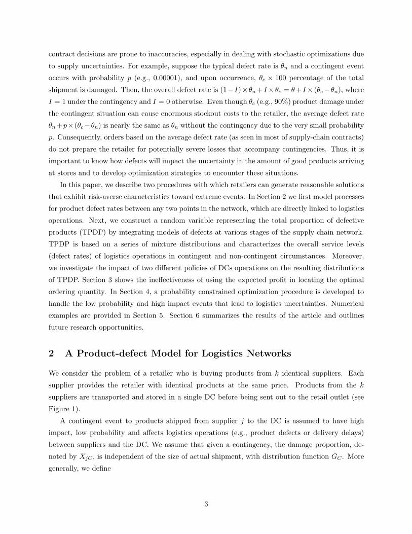
We consider two scenarios to model how products from the supplier reach the retailer (see Figure

2).

2.1 Separate Supply Lines Between Suppliers and Retailer

In the first scenario, illustrated in Figure 2A (with k = 2), different trucks (or other methods of

transport) are used for each supplier, so products from different suppliers are not mixed together

in transport. We define

X∗jC = PDP of supplier j due to contingency between DC and retailer

X∗jC ∼ GC ,

X∗jN = PDP of supplier j due to non-contingency between DC and retailer

X∗jN ∼ GN ,

I∗j = 1 if a contingent event occurs to supplier j between DC and retailer, = 0 otherwise

and {I∗1, . . . , I∗k} are independent with P (I∗j = 1) = p∗j , and

PjR = PDP of supplier j from DC to retailer = (1 − I∗j)X∗jN + I∗jX

∗jC j = 1, 2, · · · , k.

To derive the distribution of the total proportion of defective products at the retail level, we

first need to derive distributions of the PDP from each supplier that precedes it. For notational

convenience, we use random variable Y to represent the TPDP. For the non-mixed case we denote

this by YNM . If we let Pj be the proportion of defective products among all shipments from supplier

j, then we have

4

R

S2

DC

S1

S2

DC R

A) Two different trucks from DC to R

B) Same truck from DC to R

S1 P

1W =(1-I

1 )X

1N + I

1 X

1C

P 1R

=(1-I 1

* )X 1N

* + I 1R

X 1C

*

P 2 W

=(1-I 2 )X

2N + I

2 X

2C

P 1W

=(1-I 1 )X

1N + I

1 X

1C

P 2R

=(1-I 2

* )X 2N

* + I 2R

X 2C

*

P 2 W

=(1-I 2 )X

2N + I

2 X

2C

P R =(1-I

0 )X

N * + I

0 X

C *

Figure 2: Different truck-load vs. same truck-load

Pj = PjW + PjR(1 − PjW ), and

YNM =1

k

k∑

j=1

Pj , j = 1, 2, · · · , k.

2.2 Mixed Supply Lines Between Suppliers and Retailer

In the “mixed supply lines” scenario, products from different suppliers are delivered from the DC

to the retail store using the same transport units (e.g., trucks), and only one indicator variable is

required to model the logistics defects under contingency along the route; products loaded in the

same truck are exposed to the same risk. Similar to the definitions in Section 2.1, let PR be the

PDP of the remaining good products that are shipped from the DC to the retail store, and define

X∗C = Total PDP due to contingency between DC and retailer

X∗C ∼ GC ,

X∗N = Total PDP due to non-contingency between DC and retailer

X∗N ∼ GN ,

I0 = 1 if a contingent event occurs between DC and retailer, = 0 otherwise

with P (I0 = 1) = p0,

PR = PDP from DC to retailer = (1 − I0)X∗N + I0X

∗C , and

P ′j = Total PDP from supplier j.

5

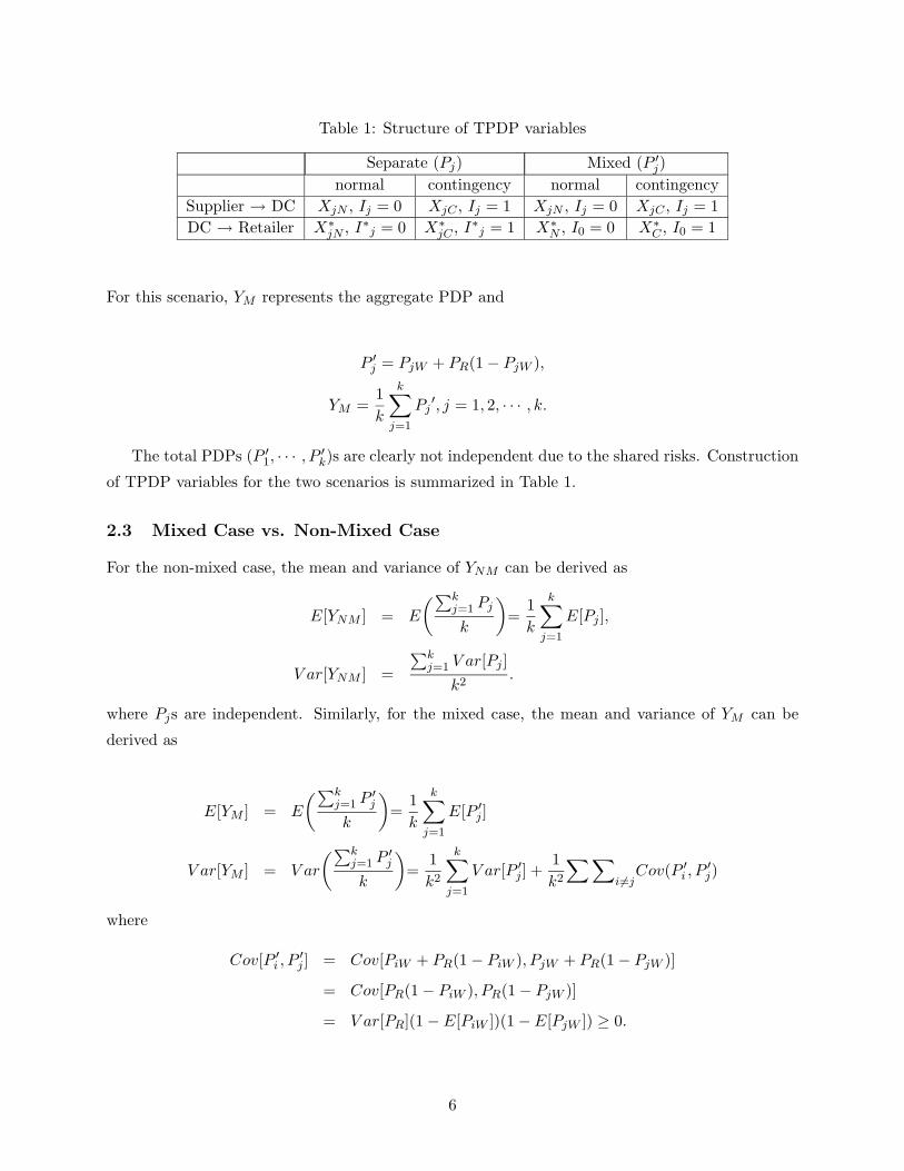
Table 1: Structure of TPDP variables

Separate (Pj) Mixed (P ′j)

normal contingency normal contingency

Supplier → DC XjN , Ij = 0 XjC , Ij = 1 XjN , Ij = 0 XjC , Ij = 1

DC → Retailer X∗jN , I∗j = 0 X∗

jC , I∗j = 1 X∗N , I0 = 0 X∗

C , I0 = 1

For this scenario, YM represents the aggregate PDP and

P ′j = PjW + PR(1 − PjW ),

YM =1

k

k∑

j=1

Pj′, j = 1, 2, · · · , k.

The total PDPs (P ′1, · · · , P ′

k)s are clearly not independent due to the shared risks. Construction

of TPDP variables for the two scenarios is summarized in Table 1.

2.3 Mixed Case vs. Non-Mixed Case

For the non-mixed case, the mean and variance of YNM can be derived as

E[YNM ] = E

(

∑kj=1 Pj

k

)

=1

k

k∑

j=1

E[Pj ],

V ar[YNM ] =

∑kj=1 V ar[Pj ]

k2.

where Pjs are independent. Similarly, for the mixed case, the mean and variance of YM can be

derived as

E[YM ] = E

(

∑kj=1 P ′

j

k

)

=1

k

k∑

j=1

E[P ′j ]

V ar[YM ] = V ar

(

∑kj=1 P ′

j

k

)

=1

k2

k∑

j=1

V ar[P ′j ] +

1

k2

∑ ∑

i6=jCov(P ′

i , P′j)

where

Cov[P ′i , P

′j ] = Cov[PiW + PR(1 − PiW ), PjW + PR(1 − PjW )]

= Cov[PR(1 − PiW ), PR(1 − PjW )]

= V ar[PR](1 − E[PiW ])(1 − E[PjW ]) ≥ 0.

6

If we assume Ij ’s, I∗j ’s, and I0 to be independent and identically distributed with P [I0 = 1] = p

then we can further simplify the means and variances for both cases. For the non-mixed case,

E[YNM ] =1

k

k∑

j=1

E[Pj ] =1

k

k∑

j=1

E[PjW + PjR(1 − PjW )]

= [(1 − p)µN + pµC ]

(

2 − [(1 − p)µN + pµC ]

)

, (2.1)

V ar[YNM ] =

∑kj=1 V ar[Pj ]

k2=

∑kj=1 V ar[PjW + PjR(1 − PjW )]

k2

=1

k2

k∑

j=1

[(1 − p)σ2N + pσ2

C ]

(

2

[

1 − ((1 − p)µN + pµC)

]

+(1 − p)σ2N + pσ2

C

)

=1

k[(1 − p)σ2

N + pσ2C ]

(

2

[

1 − ((1 − p)µN + pµC)

]

+(1 − p)σ2N + pσ2

C

)

. (2.2)

Under the mixed case we have

E[YM ] =1

k

k∑

j=1

E[P ′j ] =

1

k

k∑

j=1

E[PjW + PR(1 − PjW )]

= [(1 − p)µN + pµC ]

(

2 − [(1 − p)µN + pµC ]

)

(2.3)

= E[YNM ],

V ar[YM ] = V ar

(

∑kj=1 P ′

j

k

)

=1

k2

k∑

j=1

V ar[P ′j ] +

1

k2

∑ ∑

i6=jCov(P ′

i , P′j)

=1

k

{

[(1 − p)σ2N + pσ2

C ]

(

2[1 − ((1 − p)µN + pµC)] + (1 − p)σ2N + pσ2

C

)}

+1

k2

(

k

2

)(

(1 − p)σ2N + pσ2

C

)(

1 − [(1 − p)µN + pµC ]

)2

. (2.4)

These results are used in later sections to investigate the effect of contingency on the optimal order

quantity and the retailer’s profit function.

2.4 Risk-Pooling Effects of Mixed Supply Lines

In this section, we consider a two-supplier example to illustrate the risk pooling effects when the

decision maker adopts the mixed supply line strategy. We focus on the implications of mixed versus

non-mixed (or separated) supply lines and disregard all logistics operations between suppliers and

DC.

The following notation aids in formulating of the example:

7

Q = total order quantity requested by retailer,

c1 = unit wholesale price from supplier 1,

c2 = unit wholesale price from supplier 2, assume c1 < c2,

r = unit retail price,

m1 = profit margin of unit product purchased from supplier 1, m1 = r − c1,

m2 = profit margin of unit product purchased from supplier 2, m2 = r − c2,

(note that m1 > m2),

h = unit holding cost per period for unsold products,

π = unit shortage cost,

ξ = fixed total demand per period,

P1 = r.v. representing total proportion of defects among products from supplier 1,

P2 = r.v. representing total proportion of defects among products from supplier 2,

Y = r.v. representing total proportion of defects among Q in transit, Y = 12(P1 + P2).

Following assumptions are made on risk pooling:

A1) Contingency dictates the magnitude of PDP from each truck

A2) Under mixed, the damage amount is evenly distributed

among products from different suppliers

A3) Under non-mixed, we exclude the situation when

both trucks experience a contingency simultaneously

In addition to these assumptions, we use the following discrete distributions for P1 and P2 and

Y :

P1 =

{

1, w/p p;

0, w/p 1 − p,P2 =

{

1, w/p p;

0, w/p 1 − p,Y =

{

0.5, w/p p;

0, w/p 1 − p.

We use distributions P1 and P2 for the non-mixed case and Y for the mixed case. According to the

assumption A2), Y = 0.5 represents (P1, P2) = (0.5, 0.5).

Given Q, the retailer’s profit is a function of P1 and P2:

Π(P1, P2) ≡ rMin[ξ, (1 − Y )Q] − c1(1 − P1)Q/2 − c2(1 − P2)Q/2

−h[(1 − Y )Q − ξ]+ − π[ξ − (1 − Y )Q]+

= (r − c1)(1 − P1)Q/2 + (r − c2)(1 − P2)Q/2

−(h + r)[(1 − Y )Q − ξ]+ − π[ξ − (1 − Y )Q]+

= m1(1 − P1)Q/2 + m2(1 − P2)Q/2 − (h + r)[(1 − Y )Q − ξ]+ − π[ξ − (1 − Y )Q]+.

Under the mixed case, the possible profits are:

Π(0, 0) = (m1 + m2)Q/2 − (h + r)(Q − ξ)+ − π(ξ − Q)+

Π(0.5, 0.5) = (m1 + m2)Q/4 − (h + r)(0.5Q − ξ)+ − π(ξ − 0.5Q)+.

8

Under the non-mixed case, retailer’s profit can take one of following forms:

Π(0, 0) = (m1 + m2)Q/2 − (h + r)(Q − ξ)+ − π(ξ − Q)+

Π(1, 0) = m2Q/2 − (h + r)(0.5Q − ξ)+ − π(ξ − 0.5Q)+

Π(0, 1) = m1Q/2 − (h + r)(0.5Q − ξ)+ − π(ξ − 0.5Q)+

Π(1, 1) = −πξ.

The expected profit based on the mixing case is:

E[Π(P1, P2)] = p × Π(0.5, 0.5) + (1 − p) × Π(0, 0),

and the expected profit based on the non-mixing case is:

E[Π(P1, P2)] = p2 × Π(1, 1) + p(1 − p) × Π(1, 0)

+(1 − p)p × Π(0, 1) + (1 − p)2 × Π(0, 0)

' p × Π(1, 0) + p × Π(0, 1) + (1 − 2p) × Π(0, 0).

Here, E[Π(P1, P2)] is simplified by assuming p2 ≈ 0. When there is no contingency (i.e., P1 =

0, P2 = 0), the two different strategies do not differ. Upon contingency, the mixed case generates

equal amount of product damages among mixed products from two suppliers while the non-mixed

case can result in the entire loss of products from each supplier. Because the profit margins of

products from two suppliers are different (m1 > m2), with m2 < (m1 + m2)/2 < m1, profit using

the non-mixed case can be larger and smaller compared to the profit using the mixed case depending

on the source of the damaged products under contingency. But if the decision maker is a risk averse

person who wants to avoid the worst case situation under which a contingency happens to the high

margin products only, the mixed case strategy is the better choice than the non-mixed strategy

because the half of damaged products among total fixed number of damages are from the low

margin products when the mixed case is used.

2.5 Formulation of K-Supplier Product-Ordering Problems

The following notation aids the formulation of the uncertain supply problem in the logistics network

and is slightly different from notation used in the previous section. We assume same wholesale prices

for all the available suppliers and relax the fixed demand assumption:

Q = total order quantity requested by retailer

c = unit wholesale price

r = unit retail price

h = unit holding cost per period for unsold products

π = unit shortage cost

ξ = r.v. representing demand per period

F (ξ) = distribution fuction of ξ (with p.d.f. f(x))

Y = r.v. representing total proportion of defects among Q in transit

9

In the k-supplier model, we assume that the total order quantity Q is split equally between k

suppliers. The retail price is fixed and strictly greater than wholesale cost (r > c) regardless of the

terms of trade. The holding cost per period at the retail store level is h for each unsold product. In

the event of a stock out, unmet demand is lost, resulting in the margin being lost (to the retailer).

The related stock-out penalty cost is π. All cost parameters are assumed to be known.

The retailer’s profit consists of three components: Sales revenue (SR) , procurement costs (PC)

from suppliers, and the total system inventory cost (TSIC). After the completion of the logistics

operations, the total amount of products received may or may not be enough to meet the demand

amount, ξ. TSIC has two components: overstock inventory cost and total stock-out penalty cost.

The shortage amount is primarily due to the unknown actual demand, but partly due to the

potential logistics defects.

We can construct the retailer’s profit function using the results from the previous section. For

a given Q and TPDP (either case), the retailer’s profit is

Π(Q, Y ) ≡ rMin[ξ, (1 − Y )Q] − c(1 − Y )Q

−h[(1 − Y )Q − ξ]+ − π[ξ − (1 − Y )Q]+, (2.5)

where (x − y)+ represents max[(x − y), 0].

White [12] considers the problem of deciding the optimum batch production quantity when the

probability of producing a good-for-sale item is p, so the total number of good items is distributed

Binomial(Q, p). He shows the expected profit function is strictly concave and derives the optimum

batch production quantity. In the next section, we address the concavity of the retailer’s expected

profit function and derive the optimal order quantity that maximizes the expected profit. We also

explore the behavior of the optimal solution when parameters of the distribution for logistics defects

changed.

3 Solution Strategies

3.1 Risk Neutral Solutions

This section shows how the standard expected value approach fails in the case of a low-probability-

high-consequence contingency event. Below, we derive the optimal order quantity as a function of

the logistics defect model parameters. From equation (2.5), the retailer’s expected profit can be

expressed as

E[Π(Q, Y )] = rE[Min(ξ, (1 − Y )Q)] − c(1 − E[Y ])Q

−hE[((1 − Y )Q − ξ)+] − πE[(ξ − (1 − Y )Q)+]

≡ ESR − ETIC,

10

where ESR (Expected Sales Revenue) and ETIC (Expected Total Inventory Cost) are

ESR = rE[Min(ξ, (1 − Y )Q)] − c(1 − E[Y ])Q

= rE[ξ] − c(1 − E[Y ])Q − r

∫ 1

0

∫ ∞

(1−y)Q[ξ − (1 − y)Q]f(ξ)g(y)dξdy,

ETIC = h

∫ 1

0

∫ (1−y)Q

0[(1 − y)Q − ξ]f(ξ)g(y)dξdy

+ π

∫ 1

0

∫ ∞

(1−y)Q[ξ − (1 − y)Q]f(ξ)g(y)dξdy.

Shih [9] proved the convexity of ETIC; to prove the concavity of E[Π(Q, Y )] it suffices to show

the concavity of ESR, which is guranteed because its second derivative is

∂2ESR

∂Q2= −r

∫ 1

0(1 − y)2f((1 − y)Q)g(y)dy < 0, for all Q. (3.6)

The proof of equation 3.6 is listed in Appendix.

For illustration, we consider the simple case in which demand is uniformly distributed with

parameters a and b:

f(ξ) =

(b − a)−1, if a ≤ ξ ≤ b,

0, otherwise.

Under uniformly distributed demand, we have:

∫ (1−y)Q

0f(ξ)dξ =

(1 − y)Q − a

b − aand

∫ (1−y)Q

0ξf(ξ)dξ =

(1 − y)2Q2

2(b − a)

so that expected profit simplifies to:

E[Π(Q, Y )] = ra + b

2− c(1 − µ)Q −

1

2(b − a)

[

(h + r + π)(σ2 + (1 − µ)2)Q2

−2(1 − µ)(ah + b(r + π))Q + a2h + b2(r + π)

]

= −(h + r + π)(σ2 + (1 − µ)2)

2(b − a)

(

Q −(1 − µ)

(1 − µ)2 + σ2

[

b(r + π − c) + a(h + c)

r + π + h

])2

+(a + b)

2+ a2h + b2(r + π) +

(1 − µ)2

(1 − µ)2 + σ2

(b(r + π − c) + a(h + c))2

2(b − a)(h + r + π)), (3.7)

where µ = E[Y ], and σ2 = V ar[Y ]. The optimal order quantity Q∗ represents the boundary value

between where an increased order provides cost or benefit.

Proposition 3.1 Let Q0 = {b(r+π−c)+a(h+c)}/{r+π+h}, which is the optimal order quantity

in the conventional “news vendor” problem assuming no product defects in the order process (i.e.,

11

µ = σ = 0). In terms of Q0, the order quantity which maximizes E[Π(Q)] is

Q∗ =(1 − µ)

(1 − µ)2 + σ2

(

b(r + π − c) + a(h + c)

r + π + h

)

=(1 − µ)

(1 − µ)2 + σ2× Q0.

Proposition 3.1 shows that the optimal order quantity which maximizes the retailer’s expected

profits depends only on the mean and the standard deviation of Y . Then, the amount received has

the form of Z = (1 − Y )Q, with E[Z] = (1 − µ)Q and V ar[Z] = σ2Q2. This result coincides with

results of Noori and Keller [4] where Q∗ is proportional to µ and is reduced by an increase in the

variability of Y .

Proposition 3.2 The order quantities which maximize ESR and ETIC are, respectively,

Q∗A =

(1 − µ)

(1 − µ)2 + σ2

(

b − (b − a)c

r

)

,

Q∗B =

(1 − µ)

(1 − µ)2 + σ2

(

a + (b − a)π

π + h

)

.

Furthermore, Q∗ is a convex combination of Q∗A and Q∗

B:

Q∗ = λQ∗A + (1 − λ)Q∗

B, where λ =r

r + π + h.

Proposition 3.2 shows that the optimal order quantity is a weighted average of the separate

order quantities that maximize ESR (Q∗A) and ETIC (Q∗

B); if r > π + h, more weight is assigned

to the quantity which maximizes ESR. Because the optimal order quantity depends only on the

mean and the variance of Y , we focus on those parameters. If contingency probability is small (e.g.,

p ≤ 0.001), the equations 2.1 through 2.4 show that

E[YNM ] = E[YM ] ∼= µN (2 − µN ),

V ar[YNM ] ∼=1

kσ2

N [2(1 − µN ) + σ2N ] and (3.8)

V ar[YM ] ∼= V ar[YNM ] +k − 1

2kσ2

N (1 − µN )2.

The equations in 3.8 suggest that expected profit does not significantly change under contingency

if p is small enough. A coherent solution for the decision making process must provide a means of

protection against the severe effects of contingency; the expected value approach fails to do this. The

following section introduces two procedures that allow the retailer to generate reasonable solutions

reflecting natural risk-averse characteristics toward extreme events that have low probability.

12

3.2 Risk Averse Solutions

This section discusses two alternative solutions to the expected value approach for optimal ordering.

The first method limits the solution space to the set of order quantities which guarantees an expected

profit level under contingency. The second method features a constraint based on the quantile

function of the profit distribution. While both methods restrict the solution space to control the

consequence of the contingency, they differ in important ways; the first method considers only the

measured contingency and not its probability while the second method is based directly on the

contingency distribution. The following result (see Appendix for proof) is useful to understand the

behavior of the retailer’s profit function.

Proposition 3.3 Whenever (c + h) > (r + π − c), the variability of retailer’s profit is increasing

in order quantity Q.

Proposition 3.3 states that whenever the profit margin loss from the unit surplus is greater than

that from the unit short, the variance of retailer’s profit is an increasing function of Q.

3.2.1 Constrained Optimization I - Profit constraint

Given a contingent event, we consider only solutions that lead to (conditionally) expected profit of

at least Π0. Let I denote the indicator function for a contingency. The problem becomes

maxQ≥0

EG[Π(Q, Y )] (3.9)

s.t. EGC[Π(Q, Y )] ≡ EG[Π(Q, Y )|I = 1] ≥ Π0.

The retailer’s strong risk-aversion can be reflected by increasing the value of Π0. The restricted

solution space is based on the following sets of order quantities:

SΠ0= Set of possible order quantities which lead to unconditional expected profit ≥ Π0,

= {Q | EG[Π(Q, Y )] ≥ Π0}

SΠ0,C = Set of possible order quantities which lead to contingency expected profit ≥ Π0,

= {Q | EGC[Π(Q, Y )] ≥ Π0}

S1Π0

= SΠ0∩ SΠ0,C .

With uniformly distributed demand, the expected profit function in (3.7) simplifies:

E[Π(Q, Y )] = −A(µ, σ2)[

Q − B(µ, σ2)]2

+C(µ, σ2), (3.10)

where

A(µ, σ2) = (h+r+π)(σ2+(1−µ)2)2(b−a) determines the spread of the profit function,

B(µ, σ2) = (1−µ)(1−µ)2+σ2

[

b(r+π−c)+a(h+c)r+π+h

]

determines the optimal order quantity , and

C(µ, σ2) = (a+b)2 + a2h + b2(r + π) + (1−µ)2

(1−µ)2+σ2

[

(b(r+π−c)+a(h+c))2

2(b−a)(h+r+π))

]

determines the maximum expected profit.

13

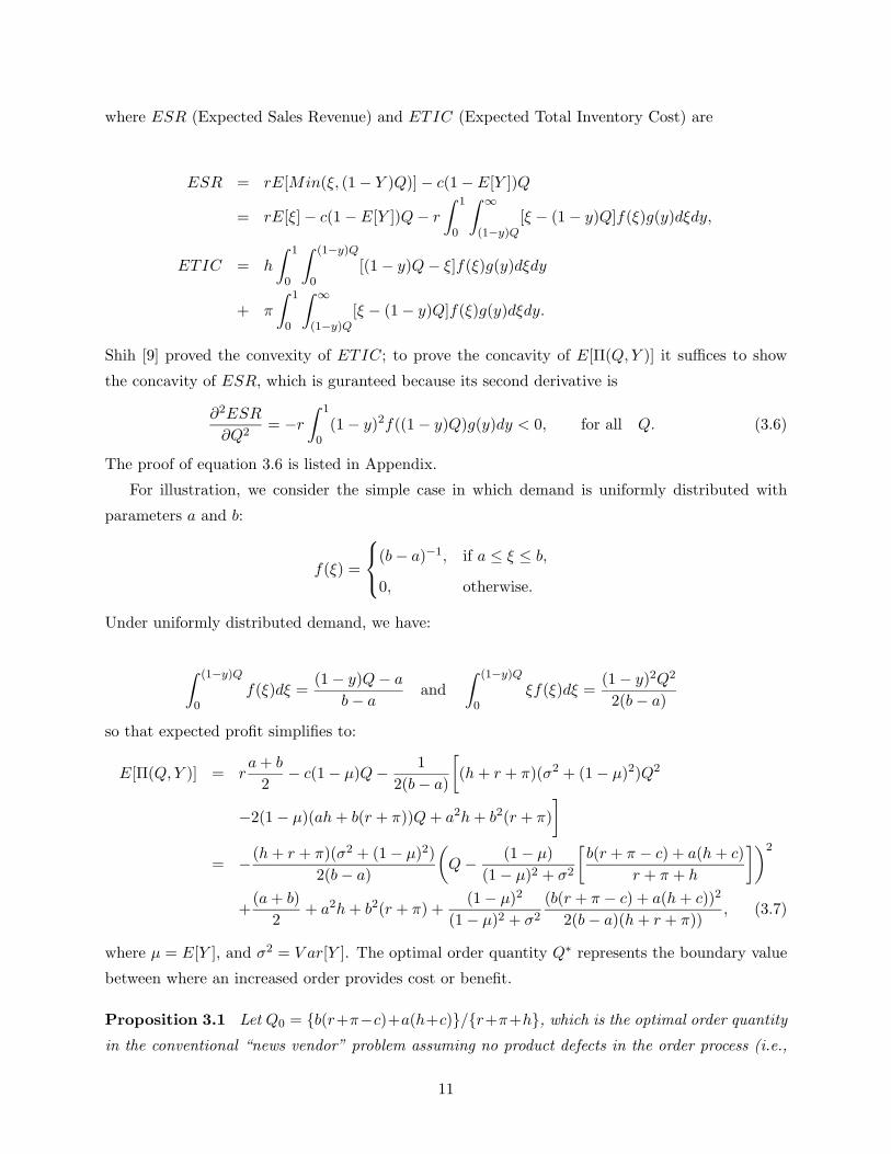
Figure 3: Expected profits based on increased mean in defect distribution after contingency

From the expression in (3.10), it is clearly seen that the expected profit only depends on the

the mean and the variance of Y . By partitioning E[Π(Q, Y )] into three parts, its behavior is more

clearly manifest when the mean and the variance of the defect distribution vary. Specifically, A and

C are decreasing functions of µ while B is an increasing function of µ. A is increasing in σ2, while B

and C decrease in σ2. When the mean increases, the expected profit curve broadens (∂A/∂µ < 0),

shifts to the right (e.g. the optimal order quantity increases) (∂B/∂µ > 0), and the corresponding

maximum expected profit decreases (∂C/∂µ < 0). When the variance increases, the curve shrinks

(∂A/∂σ2 > 0), shifts to the left (e.g. the optimal order quantity decreases) (∂B/∂σ2 < 0), and the

maximum expected profit decreases (∂C/∂σ2 < 0).

Based on these properties, we consider two ways contingency affects the expected profit through

the distribution of the total defect proportion: (1) contingency increases the mean of Y , and (2)

contingency increases the variance of Y . Let Q̂ = the optimal ordering quantity of the unconditional

problem, Q̂C = the optimal ordering quantity under contingency, and Q∗ = the optimal solution to

the constrained optimization problem in (3.9). As Π0 increases, the solution Q∗ increases toward

Q̂C ; as Π0 decreases, the constraint eventually disappears. Figure 3 illustrates the approach with

the conditional and unconditional profit functions. This problem formulation provides flexibility to

the decision maker, with Π0 serving as a utility function that shrinks the unconstrained solution

towards Q̂C in the case of contingency.

14

Figure 4: Increased mean causes infeasible solution

We first examine the case where the contingency causes a location shift (to the right) in defect

distribution, so GC is increased from G by a constant. The location shift (to the right) in G causes

both the location shift (to the right) and increased variability in the expected profit (see Figure

3). In the case S1Π0

= SΠ0∩ SΠ0,C 6= ∅, if Q̂ ∈ S1

Π0then Q∗ = Q̂, otherwise Q∗ = minQ∈S1

Π0

{Q}.

If S1Π0

= ∅, it is not possible to keep conditional expected profit above Π0 (in case of contingency)

without allowing overall expected profit to go below Π0 (see Figure 4). To rectify this problem, Π0

must be reduced until there is an overlap between SΠ0and SΠ0,C . In general, the order quantity

increasing in the level of risk-aversion (e.g. when Π0 increases, Q∗ increases) under the location

shift case.

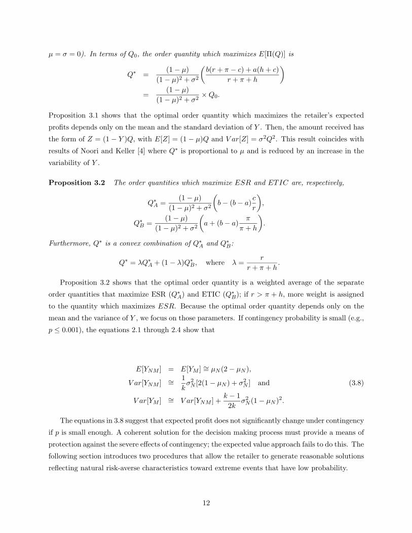
From Proposition 3.1, the optimal order quantity which maximizes expected profit decreases as

the variance increases. Accordingly, increased variability in Y shifts the expected profit to the left

as illustrated in Figure 5. Furthermore, the increase in variance results in a decrease in expected

profit. The vertical distance between the two local maxima in the expected profit curves represents

the decrease in maximum possible profits due to the increase in variance. When the variance under

contingency is σ2 + δ, this distance is

∆ = C(µ, σ2) − C(µ, σ2 + δ)

=

[

(1 − µ)2

(1 − µ)2 + σ2−

(1 − µ)2

(1 − µ)2 + σ2 + δ

][

(b(r + π − c) + a(h + c))2

2(b − a)(h + r + π))

]

.

15

Figure 5: Increased variance shifts expected profits to the left

If S1Π0

= SΠ0∩ SΠ0,C 6= ∅, then a unique solutions exists; if Q̂ ∈ S1

Π0then Q∗ = Q̂, otherwise

Q∗ = maxQ∈S1

Π0

{Q}. Again, if no overlap between SΠ0and SΠ0,C exists, the constraint Π0 must

be reduced. Not like the location shift case, strong risk-aversion (bigger value of Π0) reduces the

order quantity due to the increased variance. The section that follows illustrates these solution

procedures with a numerical example.

3.2.2 Constrained Optimization II - Probability constraint

As an alternative to controlling the profit function by conditioning on the occurrence of a con-

tingency, here we restrict the solutions space by restricting the probability space of the profit

distribution. That is, we bound from below (with γ) the probability that the profit is less than an

amount Π1. If we assume, for simplicity, that the demand level ξ is fixed, the problem becomes

maxQ≥0

Eg[Π(Q, Y )]

s.t. Pg(Π(Q, Y ) ≤ Π1) ≤ γ, (3.11)

where

Π(Q, Y ) =

{

rξ − c(1 − Y )Q − h((1 − Y )Q − ξ), (1 − Y )Q ≥ ξ,

rξ − c(1 − Y )Q − (r + π)(ξ − (1 − Y )Q), (1 − Y )Q ≤ ξ.

In this case, the retailer’s strong risk-aversion can be reflected by either increasing the value of

Π1 or decreasing the value of γ. Denote by Q̂ the optimal order quantity for the unconstrained

16

maximization problem that satisfies the following expression (see Shih [9]):

∫ 1−ξ/Q̂

0(1 − y)g(y)dy =

(1 − µ)(r − c + π)

r + h + π. (3.12)

If we tacitly assume Q ≥ ξ, the probability constraint becomes

P [Π(Q, Y ) ≤ Π1] = P

(

Y ≥ 1 −πξ + Π1

(r + π − c)Q

∣

∣

∣

∣

Y ≥ 1 −ξ

Q

)

P

(

Y ≥ 1 −ξ

Q

)

+ P

(

Y ≤ 1 −rξ + hξ − Π1

(h + c)Q

∣

∣

∣

∣

Y ≤ 1 −ξ

Q

)

P

(

Y ≤ 1 −ξ

Q

)

.

The following propositions characterize the solution to the stochastic constraint placed on the profit

distribution.

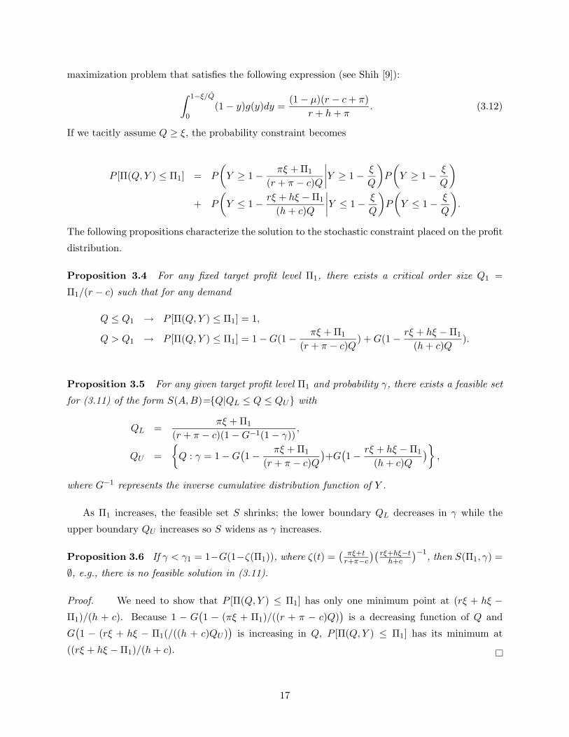
Proposition 3.4 For any fixed target profit level Π1, there exists a critical order size Q1 =

Π1/(r − c) such that for any demand

Q ≤ Q1 → P [Π(Q, Y ) ≤ Π1] = 1,

Q > Q1 → P [Π(Q, Y ) ≤ Π1] = 1 − G(1 −πξ + Π1

(r + π − c)Q) + G(1 −

rξ + hξ − Π1

(h + c)Q).

Proposition 3.5 For any given target profit level Π1 and probability γ, there exists a feasible set

for (3.11) of the form S(A, B)={Q|QL ≤ Q ≤ QU} with

QL =πξ + Π1

(r + π − c)(1 − G−1(1 − γ)),

QU =

{

Q : γ = 1 − G(

1 −πξ + Π1

(r + π − c)Q

)

+G(

1 −rξ + hξ − Π1

(h + c)Q

)

}

,

where G−1 represents the inverse cumulative distribution function of Y .

As Π1 increases, the feasible set S shrinks; the lower boundary QL decreases in γ while the

upper boundary QU increases so S widens as γ increases.

Proposition 3.6 If γ < γ1 = 1−G(1−ζ(Π1)), where ζ(t) =( πξ+t

r+π−c

)( rξ+hξ−th+c

)−1, then S(Π1, γ) =

∅, e.g., there is no feasible solution in (3.11).

Proof. We need to show that P [Π(Q, Y ) ≤ Π1] has only one minimum point at (rξ + hξ −

Π1)/(h + c). Because 1 − G(

1 − (πξ + Π1)/((r + π − c)Q))

is a decreasing function of Q and

G(

1 − (rξ + hξ − Π1(/((h + c)QU ))

is increasing in Q, P [Π(Q, Y ) ≤ Π1] has its minimum at

((rξ + hξ − Π1)/(h + c).

17

Proposition 3.7 If Q ≥ Q1, then γ1 is increasing in Π1 and γ1 = 1 when Π1 is set at the

maximum profit level, e.g. Π1 = (r − c)ξ, which can be achieved only when there are no product

shortages nor unsold products.

Proof. It is easy to see that ζ(t) is an increasing function of t. If Q ≥ Q1, it can be shown that

ζ(Π1) ≤ 1. When Π1 = (r − c)ξ, then ζ(Π1) = 1, hence γ1 = 1.

Proposition 3.8 For any given profit level Π1 and probability γ, γ ≥ γ1, the optimal order

quantity for the constrained optimization problem (3.11) is

Q∗ =

Q̂, if Q̂ ∈ S(Π1, γ),

QL, if Q̂ ≤ QL,

QU , if Q̂ ≥ QU

where Q̂ is determined by (3.12).

Whenever the order quantity Q̂ satisfies the probability constraint (e.g. Q̂ ∈ S(Π1, γ)), then the

retailer orders Q̂. Otherwise, the retailer should order either QL or QU according to whether

Q̂ ≤ QL or not. Figure 6 shows the result in Proposition 3.8.

In the previous section, only the mean and the variance of Y are needed to derive the optimal

solution, but in this case, the distribution of Y must be known to apply probability constraints and

derive an optimal solution. If the distribution is known along with appropriate values of Π1 and γ,

profit loss can be avoided in the case of contingency. However, because of the small probability of

contingency, the value of γ must be selected carefully.

Remarks: It is interesting to note that traditional Mean-Variance and Max-Min procedures are

not appropriate to generate risk-averse solutions under possible contingency. First, we consider the

Mean-Variance procedure. The objective function can be written as:

maxQ≥0

EG[Π(Q, Y )] − αV arG[Π(Q, Y )]

or

maxQ≥0

(EGN[Π(Q, Y )] − αV arGN

[Π(Q, Y )])P [I = 0]

+(EGC[Π(Q, Y )] − αV arGC

[Π(Q, Y )])P [I = 1].

Assuming p = P [I = 1] is vary small, the solution to the above maximization problem will maximize

the objective function under the non-contingency case. Due to its small probability, the contingency

does not effect the derivation of risk-averse solutions.

18

r 1

r

Q 1 =

Q 2 =

Figure 6: Shape of the probability constraint

19

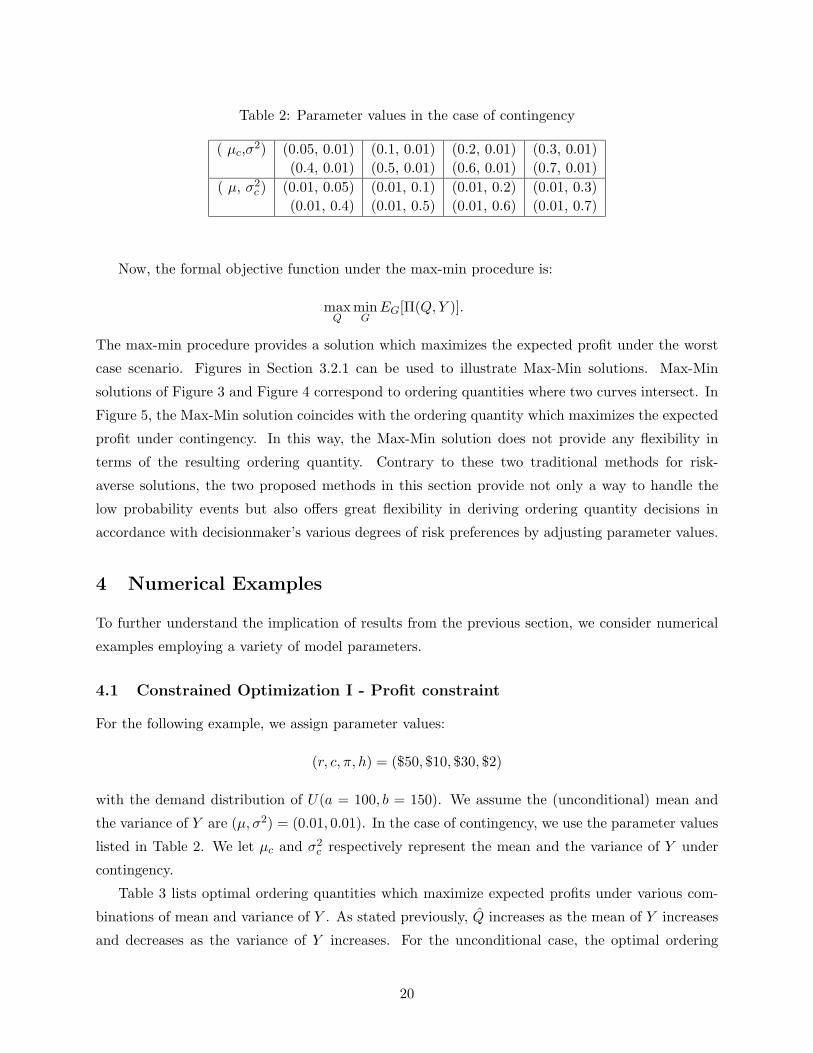
Table 2: Parameter values in the case of contingency

( µc,σ2) (0.05, 0.01) (0.1, 0.01) (0.2, 0.01) (0.3, 0.01)

(0.4, 0.01) (0.5, 0.01) (0.6, 0.01) (0.7, 0.01)

( µ, σ2c ) (0.01, 0.05) (0.01, 0.1) (0.01, 0.2) (0.01, 0.3)

(0.01, 0.4) (0.01, 0.5) (0.01, 0.6) (0.01, 0.7)

Now, the formal objective function under the max-min procedure is:

maxQ

minG

EG[Π(Q, Y )].

The max-min procedure provides a solution which maximizes the expected profit under the worst

case scenario. Figures in Section 3.2.1 can be used to illustrate Max-Min solutions. Max-Min

solutions of Figure 3 and Figure 4 correspond to ordering quantities where two curves intersect. In

Figure 5, the Max-Min solution coincides with the ordering quantity which maximizes the expected

profit under contingency. In this way, the Max-Min solution does not provide any flexibility in

terms of the resulting ordering quantity. Contrary to these two traditional methods for risk-

averse solutions, the two proposed methods in this section provide not only a way to handle the

low probability events but also offers great flexibility in deriving ordering quantity decisions in

accordance with decisionmaker’s various degrees of risk preferences by adjusting parameter values.

4 Numerical Examples

To further understand the implication of results from the previous section, we consider numerical

examples employing a variety of model parameters.

4.1 Constrained Optimization I - Profit constraint

For the following example, we assign parameter values:

(r, c, π, h) = ($50, $10, $30, $2)

with the demand distribution of U(a = 100, b = 150). We assume the (unconditional) mean and

the variance of Y are (µ, σ2) = (0.01, 0.01). In the case of contingency, we use the parameter values

listed in Table 2. We let µc and σ2c respectively represent the mean and the variance of Y under

contingency.

Table 3 lists optimal ordering quantities which maximize expected profits under various com-

binations of mean and variance of Y . As stated previously, Q̂ increases as the mean of Y increases

and decreases as the variance of Y increases. For the unconditional case, the optimal ordering

20

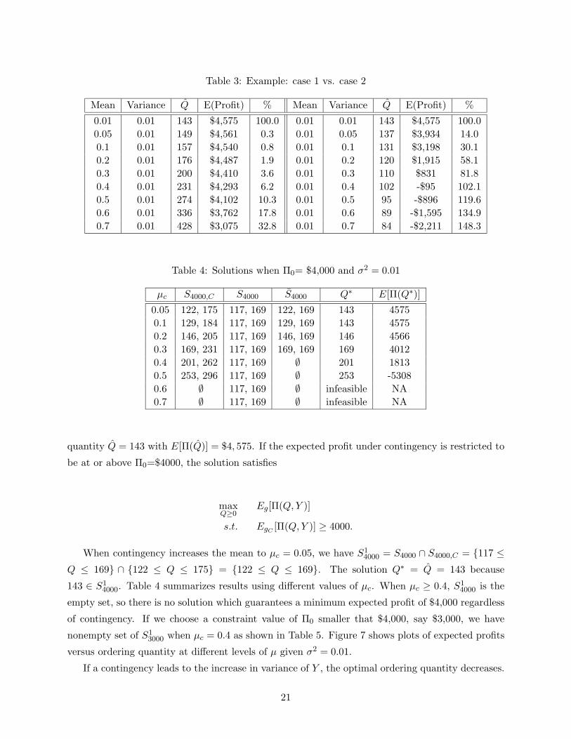
Table 3: Example: case 1 vs. case 2

Mean Variance Q̂ E(Profit) % Mean Variance Q̂ E(Profit) %

0.01 0.01 143 $4,575 100.0 0.01 0.01 143 $4,575 100.0

0.05 0.01 149 $4,561 0.3 0.01 0.05 137 $3,934 14.0

0.1 0.01 157 $4,540 0.8 0.01 0.1 131 $3,198 30.1

0.2 0.01 176 $4,487 1.9 0.01 0.2 120 $1,915 58.1

0.3 0.01 200 $4,410 3.6 0.01 0.3 110 $831 81.8

0.4 0.01 231 $4,293 6.2 0.01 0.4 102 -$95 102.1

0.5 0.01 274 $4,102 10.3 0.01 0.5 95 -$896 119.6

0.6 0.01 336 $3,762 17.8 0.01 0.6 89 -$1,595 134.9

0.7 0.01 428 $3,075 32.8 0.01 0.7 84 -$2,211 148.3

Table 4: Solutions when Π0= $4,000 and σ2 = 0.01

µc S4000,C S4000 S̄4000 Q∗ E[Π(Q∗)]

0.05 122, 175 117, 169 122, 169 143 4575

0.1 129, 184 117, 169 129, 169 143 4575

0.2 146, 205 117, 169 146, 169 146 4566

0.3 169, 231 117, 169 169, 169 169 4012

0.4 201, 262 117, 169 ∅ 201 1813

0.5 253, 296 117, 169 ∅ 253 -5308

0.6 ∅ 117, 169 ∅ infeasible NA

0.7 ∅ 117, 169 ∅ infeasible NA

quantity Q̂ = 143 with E[Π(Q̂)] = $4, 575. If the expected profit under contingency is restricted to

be at or above Π0=$4000, the solution satisfies

maxQ≥0

Eg[Π(Q, Y )]

s.t. EgC[Π(Q, Y )] ≥ 4000.

When contingency increases the mean to µc = 0.05, we have S14000 = S4000 ∩ S4000,C = {117 ≤

Q ≤ 169} ∩ {122 ≤ Q ≤ 175} = {122 ≤ Q ≤ 169}. The solution Q∗ = Q̂ = 143 because

143 ∈ S14000. Table 4 summarizes results using different values of µc. When µc ≥ 0.4, S1

4000 is the

empty set, so there is no solution which guarantees a minimum expected profit of $4,000 regardless

of contingency. If we choose a constraint value of Π0 smaller that $4,000, say $3,000, we have

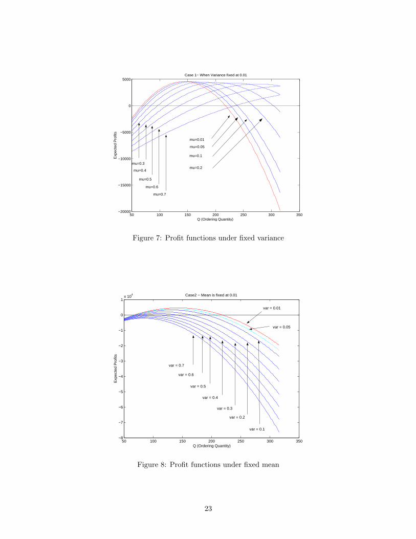
nonempty set of S13000 when µc = 0.4 as shown in Table 5. Figure 7 shows plots of expected profits

versus ordering quantity at different levels of µ given σ2 = 0.01.

If a contingency leads to the increase in variance of Y , the optimal ordering quantity decreases.

21

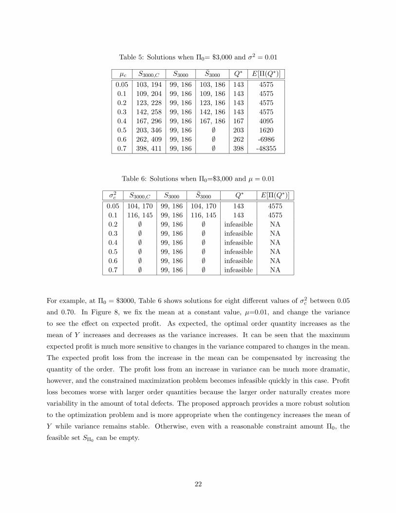
Table 5: Solutions when Π0= $3,000 and σ2 = 0.01

µc S3000,C S3000 S̄3000 Q∗ E[Π(Q∗)]

0.05 103, 194 99, 186 103, 186 143 4575

0.1 109, 204 99, 186 109, 186 143 4575

0.2 123, 228 99, 186 123, 186 143 4575

0.3 142, 258 99, 186 142, 186 143 4575

0.4 167, 296 99, 186 167, 186 167 4095

0.5 203, 346 99, 186 ∅ 203 1620

0.6 262, 409 99, 186 ∅ 262 -6986

0.7 398, 411 99, 186 ∅ 398 -48355

Table 6: Solutions when Π0=$3,000 and µ = 0.01

σ2c S3000,C S3000 S̄3000 Q∗ E[Π(Q∗)]

0.05 104, 170 99, 186 104, 170 143 4575

0.1 116, 145 99, 186 116, 145 143 4575

0.2 ∅ 99, 186 ∅ infeasible NA

0.3 ∅ 99, 186 ∅ infeasible NA

0.4 ∅ 99, 186 ∅ infeasible NA

0.5 ∅ 99, 186 ∅ infeasible NA

0.6 ∅ 99, 186 ∅ infeasible NA

0.7 ∅ 99, 186 ∅ infeasible NA

For example, at Π0 = $3000, Table 6 shows solutions for eight different values of σ2c between 0.05

and 0.70. In Figure 8, we fix the mean at a constant value, µ=0.01, and change the variance

to see the effect on expected profit. As expected, the optimal order quantity increases as the

mean of Y increases and decreases as the variance increases. It can be seen that the maximum

expected profit is much more sensitive to changes in the variance compared to changes in the mean.

The expected profit loss from the increase in the mean can be compensated by increasing the

quantity of the order. The profit loss from an increase in variance can be much more dramatic,

however, and the constrained maximization problem becomes infeasible quickly in this case. Profit

loss becomes worse with larger order quantities because the larger order naturally creates more

variability in the amount of total defects. The proposed approach provides a more robust solution

to the optimization problem and is more appropriate when the contingency increases the mean of

Y while variance remains stable. Otherwise, even with a reasonable constraint amount Π0, the

feasible set SΠ0can be empty.

22

50 100 150 200 250 300 350−20000

−15000

−10000

−5000

0

5000Case 1− When Variance fixed at 0.01

Q (Ordering Quantity)

Exp

ecte

d P

rofit

s

mu=0.01

mu=0.05

mu=0.1

mu=0.2mu=0.4

mu=0.5

mu=0.7

mu=0.6

mu=0.3

Figure 7: Profit functions under fixed variance

50 100 150 200 250 300 350−8

−7

−6

−5

−4

−3

−2

−1

0

1x 10

4 Case2 − Mean is fixed at 0.01

Q (Ordering Quantity)

Exp

ecte

d P

rofit

s

var = 0.01

var = 0.05

var = 0.1

var = 0.2

var = 0.3

var = 0.4

var = 0.5

var = 0.6

var = 0.7

Figure 8: Profit functions under fixed mean

23

0 0.1 0.2 0.3 0.4 0.5 0.6 0.70

50

100

150

200

250

300

350

400

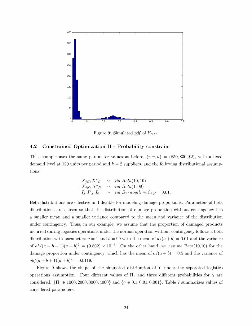
Figure 9: Simulated pdf of YNM

4.2 Constrained Optimization II - Probability constraint

This example uses the same parameter values as before, (r, π, h) = ($50, $30, $2), with a fixed

demand level at 120 units per period and k = 2 suppliers, and the following distributional assump-

tions:

XjC , X∗C ∼ iid Beta(10, 10)

XjN , X∗N ∼ iid Beta(1, 99)

Ij , I∗j , I0 ∼ iid Bernoulli with p = 0.01.

Beta distributions are effective and flexible for modeling damage proportions. Parameters of beta

distributions are chosen so that the distribution of damage proportion without contingency has

a smaller mean and a smaller variance compared to the mean and variance of the distribution

under contingency. Thus, in our example, we assume that the proportion of damaged products

incurred during logistics operations under the normal operation without contingency follows a beta

distribution with parameters a = 1 and b = 99 with the mean of a/(a + b) = 0.01 and the variance

of ab/(a + b + 1)(a + b)2 = (9.802) × 10−5. On the other hand, we assume Beta(10,10) for the

damage proportion under contingency, which has the mean of a/(a + b) = 0.5 and the variance of

ab/(a + b + 1)(a + b)2 = 0.0119.

Figure 9 shows the shape of the simulated distribution of Y under the separated logistics

operations assumption. Four different values of Π1 and three different probabilities for γ are

considered: {Π1 ∈ 1000, 2000, 3000, 4000} and {γ ∈ 0.1, 0.01, 0.001}. Table 7 summarizes values of

considered parameters.

24

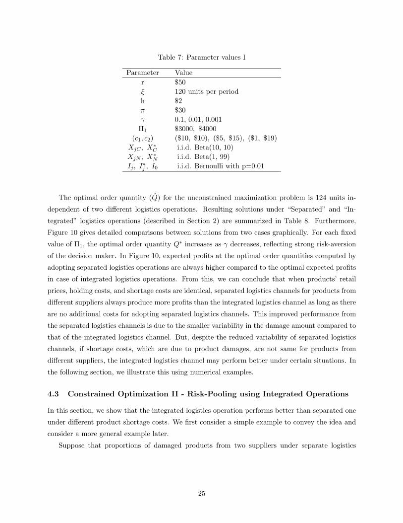
Table 7: Parameter values I

Parameter Value

r $50

ξ 120 units per period

h $2

π $30

γ 0.1, 0.01, 0.001

Π1 $3000, $4000

(c1, c2) ($10, $10), ($5, $15), ($1, $19)

XjC , X∗C i.i.d. Beta(10, 10)

XjN , X∗N i.i.d. Beta(1, 99)

Ij , I∗j , I0 i.i.d. Bernoulli with p=0.01

The optimal order quantity (Q̂) for the unconstrained maximization problem is 124 units in-

dependent of two different logistics operations. Resulting solutions under “Separated” and “In-

tegrated” logistics operations (described in Section 2) are summarized in Table 8. Furthermore,

Figure 10 gives detailed comparisons between solutions from two cases graphically. For each fixed

value of Π1, the optimal order quantity Q∗ increases as γ decreases, reflecting strong risk-aversion

of the decision maker. In Figure 10, expected profits at the optimal order quantities computed by

adopting separated logistics operations are always higher compared to the optimal expected profits

in case of integrated logistics operations. From this, we can conclude that when products’ retail

prices, holding costs, and shortage costs are identical, separated logistics channels for products from

different suppliers always produce more profits than the integrated logistics channel as long as there

are no additional costs for adopting separated logistics channels. This improved performance from

the separated logistics channels is due to the smaller variability in the damage amount compared to

that of the integrated logistics channel. But, despite the reduced variability of separated logistics

channels, if shortage costs, which are due to product damages, are not same for products from

different suppliers, the integrated logistics channel may perform better under certain situations. In

the following section, we illustrate this using numerical examples.

4.3 Constrained Optimization II - Risk-Pooling using Integrated Operations

In this section, we show that the integrated logistics operation performs better than separated one

under different product shortage costs. We first consider a simple example to convey the idea and

consider a more general example later.

Suppose that proportions of damaged products from two suppliers under separate logistics

25

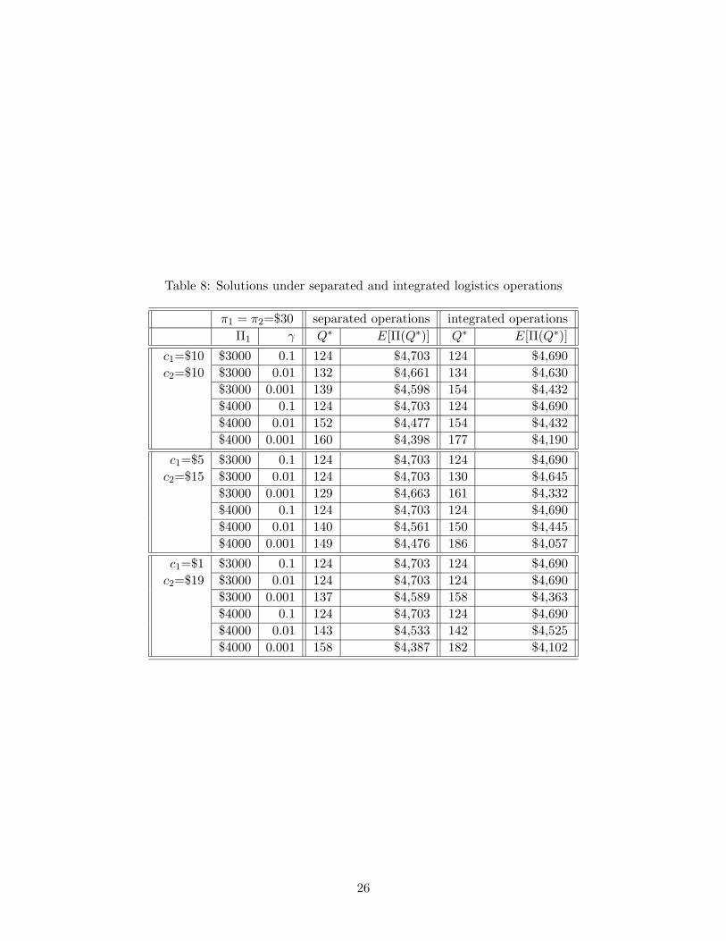
Table 8: Solutions under separated and integrated logistics operations

π1 = π2=$30 separated operations integrated operations

Π1 γ Q∗ E[Π(Q∗)] Q∗ E[Π(Q∗)]

c1=$10 $3000 0.1 124 $4,703 124 $4,690

c2=$10 $3000 0.01 132 $4,661 134 $4,630

$3000 0.001 139 $4,598 154 $4,432

$4000 0.1 124 $4,703 124 $4,690

$4000 0.01 152 $4,477 154 $4,432

$4000 0.001 160 $4,398 177 $4,190

c1=$5 $3000 0.1 124 $4,703 124 $4,690

c2=$15 $3000 0.01 124 $4,703 130 $4,645

$3000 0.001 129 $4,663 161 $4,332

$4000 0.1 124 $4,703 124 $4,690

$4000 0.01 140 $4,561 150 $4,445

$4000 0.001 149 $4,476 186 $4,057

c1=$1 $3000 0.1 124 $4,703 124 $4,690

c2=$19 $3000 0.01 124 $4,703 124 $4,690

$3000 0.001 137 $4,589 158 $4,363

$4000 0.1 124 $4,703 124 $4,690

$4000 0.01 143 $4,533 142 $4,525

$4000 0.001 158 $4,387 182 $4,102

26

c1=c2=10, r=0.1

$4,680

$4,685

$4,690

$4,695

$4,700

$4,705

1000 2000 3000 4000

Desired profit level

Separated

Operaions

Integrated

Operation

c1=c2=10, r=0.01

$4,250

$4,300

$4,350

$4,400

$4,450

$4,500

$4,550

$4,600

$4,650

$4,700

$4,750

1000 2000 3000 4000

Desired profit level

Separage

Operations

Integrated

Operation

c1=c2=10, r=0.001

$3,900

$4,000

$4,100

$4,200

$4,300

$4,400

$4,500

$4,600

$4,700

$4,800

1000 2000 3000 4000

Desired profit level

Separate

Operations

Integrated

Operation

c1=5, c2=15, r=0.1

$4,680

$4,685

$4,690

$4,695

$4,700

$4,705

1000 2000 3000 4000

Desired profit level

Separated

Operaions

Integrated

Operation

c1=5, c2=15, r=0.01

$4,300

$4,350

$4,400

$4,450

$4,500

$4,550

$4,600

$4,650

$4,700

$4,750

1000 2000 3000 4000

Desired profit level

Separated

Operations

Integrated

Operation

c1=5, c2=15, r=0.001

$3,600

$3,800

$4,000

$4,200

$4,400

$4,600

$4,800

1000 2000 3000 4000

Desired profit level

Separated

Operations

Integrated

Operation

c1=1, c2=19, r=0.1

$4,680

$4,685

$4,690

$4,695

$4,700

$4,705

1000 2000 3000 4000

Desired profit level

Separated

Operations

Integrated

Operaion

c1=1, c2=19, r=0.01

$4,400

$4,450

$4,500

$4,550

$4,600

$4,650

$4,700

$4,750

1000 2000 3000 4000

Desired profit level

Separated

Operations

integrated

Operation

c1=1, c2=19, r=0.001

$3,800

$4,000

$4,200

$4,400

$4,600

$4,800

1000 2000 3000 4000

Desired profit level

Separated

Operations

Integrated

Operation

Figure 10: Comparison between separated logistics operation and integrated logistics operation

27

operations and integrated logistics operation are distributed as follows:

P1(and P2) =

{

0, w/p 0.5;

0.2, w/p 0.5.P ′

1(and P ′2) =

{

0, w/p 0.5;

0.2, w/p 0.5.

Separated logistics operations (e.g. two trucks to separately ship products from two suppliers) result

in independence of P1 and P2 while integrated logistics operation renders P ′1 and P ′

2 dependent. We

adopt a shock model to explain the dependency between proportions of product damages from two

suppliers in case of integrated operation. When only one truck is used to transport products from

two suppliers from DC to the retailer, only two contingency cases are possible. If a contingency

occurs, products from both suppliers will jointly experience an increased rate of product damages.

If a contingency does not occur, proportions of damaged products will be smaller. Based on this,

we construct following distributions for total proportion of damaged products:

YNM =

0, w/p 0.25;

0.1, w/p 0.5;

0.2, w/p 0.25.

YM =

{

0, w/p 0.5;

0.2, w/p 0.5.

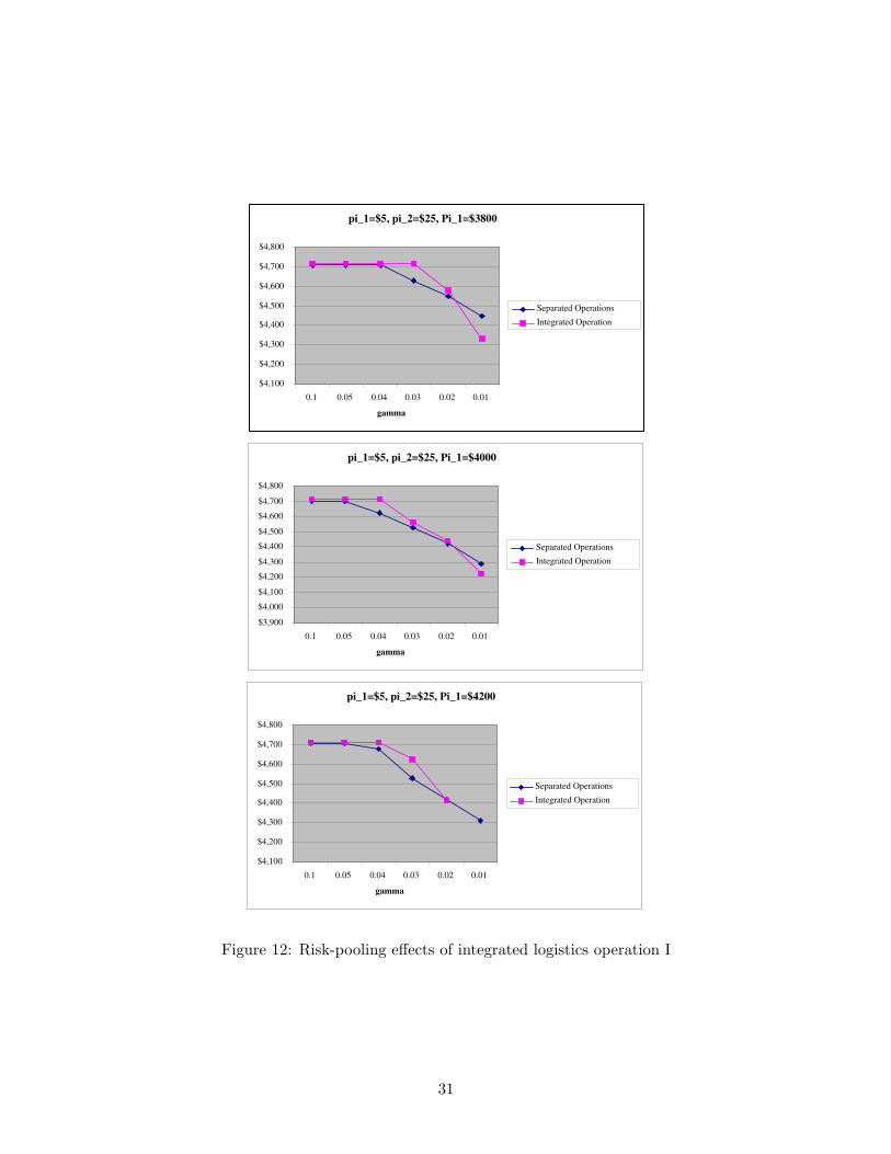
In our first example, we use different shortage costs for different suppliers (π1 = $1, π2 = $29), γ

is fixed at 0.5 and Π1 = ($4200, $4250, $4300). All other parameter values are kept same as in 4.2.

Figure 11 shows how the integrated logistics operations perform better than the separated opera-

tions. This second example illustrates the risk-pooling effects of the integrated operation with more

general distributional assumptions. Instead of using simple two-point mass discrete distributions as

in the first example, we use set of beta distributions shown in Table 13. In this example, we assume

shortage costs of π1 = $5, π2 = $25. As explained in Section 6.1, beta distribution parameters

are chosen so that the distribution of damage proportion without contingency has a smaller mean

and variance compared to mean and variance under contingency. The results are summarized in

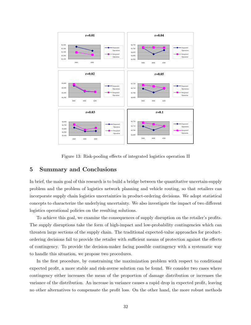
Table 10, Figure 12 and Figure 13. Again, the integrated logistics operations perform better in

the cases where parameters are Π1 = ($3800, $4000, $4200) and γ = (0.02, 0.03, 0.04, 0.05, 0.1). In

both examples, by adopting integrated logistics operation, the retailer will produce more profits

whenever the logistics operations are exposed to possible contingencies and inventory costs such

as unit shortage cost are different for products from different suppliers (e.g. π1 = $5, π2 = $25).

Contingency to the logistics operation for products with higher unit shortage cost may significantly

affect the retailer profit. But if the retailer employs an integrated operation then the total resulting

damages from contingency may be evenly spread among pooled products from different suppliers.

In this way, product-pooling, using the integrated logistics operation, dampens the possible risk of

having a large portion of damaged products, which have higher shortage costs by introducing the

risk of having evenly distributed damaged products among all products.

28

pi_1=$1, pi_2=$29, r=0.5

$3,900

$4,000

$4,100

$4,200

$4,300

$4,400

$4,500

$4,600

$4,700

4200 4250 4300

Separated

Integrated

Figure 11: Risk-pool effects of integrated logistics operation

Table 9: Parameter values II

Parameter Value

r $50

ξ 120 units per period

h $2

π π1=$5, π1=$25

γ 0.1, 0.05, 0.04, 0.03, 0.02, 0.01

Π1 $3800, $4000, $4200

c = c1 = c2 $10

XjC , X∗C i.i.d. Beta(10, 10)

XjN , X∗N i.i.d. Beta(1, 99)

Ij , I∗j , I0 i.i.d. Bernoulli with p=0.01

29

Table 10: Solutions under separated and integrated logistics operations with different shortage

costs

π1=5, π2=25 separated operations integrated operations

Π1 γ Q∗ E[Π(Q∗)] Q∗ E[Π(Q∗)]

$3800 0.1 124 $4,709 124 $4,717

$3800 0.05 124 $4,709 124 $4,717

$3800 0.04 124 $4,709 124 $4,717

$3800 0.03 133 $4,627 124 $4,717

$3800 0.02 141 $4,548 138 $4,577

$3800 0.01 151 $4,447 161 $4,331

$4000 0.1 124 $4,701 124 $4,714

$4000 0.05 124 $4,701 124 $4,714

$4000 0.04 133 $4,621 124 $4,714

$4000 0.03 143 $4,524 139 $4,565

$4000 0.02 153 $4,425 151 $4,438

$4000 0.01 166 $4,290 171 $4,221

$4200 0.1 124 $4,709 124 $4,710

$4200 0.05 124 $4,709 124 $4,710

$4200 0.04 128 $4,677 124 $4,710

$4200 0.03 143 $4,529 133 $4,625

$4200 0.02 154 $4,417 153 $4,415

$4200 0.01 164 $4,311 n/a n/a

30

pi_1=$5, pi_2=$25, Pi_1=$3800

$4,100

$4,200

$4,300

$4,400

$4,500

$4,600

$4,700

$4,800

0.1 0.05 0.04 0.03 0.02 0.01

gamma

Separated Operations

Integrated Operation

pi_1=$5, pi_2=$25, Pi_1=$4200

$4,100

$4,200

$4,300

$4,400

$4,500

$4,600

$4,700

$4,800

0.1 0.05 0.04 0.03 0.02 0.01

gamma

Separated Operations

Integrated Operation

pi_1=$5, pi_2=$25, Pi_1=$4000

$3,900

$4,000

$4,100

$4,200

$4,300

$4,400

$4,500

$4,600

$4,700

$4,800

0.1 0.05 0.04 0.03 0.02 0.01

gamma

Separated Operations

Integrated Operation

Figure 12: Risk-pooling effects of integrated logistics operation I

31

r=0.1

$4,690

$4,700

$4,710

$4,720

3800 4000 4200

Separated

Operations

Integrated

Operation

r=0.05

$4,690

$4,700

$4,710

$4,720

3800 4000 4200

Separated

Operations

Integrated

Operation

r=0.04

$4,550

$4,600

$4,650

$4,700

$4,750

3800 4000 4200

Separated

Operations

Integrated

Operation

r=0.03

$4,400

$4,500

$4,600

$4,700

$4,800

3800 4000 4200

Separated

Operation

Integrated

Operation

r=0.02

$4,300

$4,400

$4,500

$4,600

3800 4000 4200

Separated

Operations

Integrated

Operation

r=0.01

$4,100

$4,200

$4,300

$4,400

$4,500

3800 4000

Separated

Operations

Integrated

Operation

Figure 13: Risk-pooling effects of integrated logistics operation II

5 Summary and Conclusions

In brief, the main goal of this research is to build a bridge between the quantitative uncertain-supply

problem and the problem of logistics network planning and vehicle routing, so that retailers can

incorporate supply chain logistics uncertainties in product-ordering decisions. We adopt statistical

concepts to characterize the underlying uncertainty. We also investigate the impact of two different

logistics operational policies on the resulting solutions.

To achieve this goal, we examine the consequences of supply disruption on the retailer’s profits.

The supply disruptions take the form of high-impact and low-probability contingencies which can

threaten large sections of the supply chain. The traditional expected-value approaches for product-

ordering decisions fail to provide the retailer with sufficient means of protection against the effects

of contingency. To provide the decision-maker facing possible contingency with a systematic way

to handle this situation, we propose two procedures.

In the first procedure, by constraining the maximization problem with respect to conditional

expected profit, a more stable and risk-averse solution can be found. We consider two cases where

contingency either increases the mean of the proportion of damage distribution or increases the

variance of the distribution. An increase in variance causes a rapid drop in expected profit, leaving

no other alternatives to compensate the profit loss. On the other hand, the more robust methods

32

introduced here compensate for a mean shift of the profit curve, resulting in an increased quantity of

the order. In practice, it is recommended that the retailer investigate the characteristic of potential

contingency to see how and if it affects the mean or variance of Y . If the model implies that the

contingency changes only the mean, then the retailer can benefit from the constrained optimization

solution in Section 5. However, if the contingency adversely affects the variance, the decision maker

should find a way to reduce the variance, perhaps using multiple sourcing or purchasing options by

which the damage distribution can be truncated.

In the other procedure, we utilize the probability constraint to restrict possible solutions. With

this procedure, the decision-maker has more options to include risk preferences in the solution; one

can change either the target profit level or the target probability level to derive risk-averse solutions.

This procedure illustrates the risk-pooling effects of the integrated logistics operations under certain

conditions. Whenever the inventory holding cost, the shortage cost, and retail prices of products

from different suppliers are identical, separated logistics operations between the distribution center

and the retailer generate solutions with higher expected profits compared to those of the integrated

logistics operation case. But in our examples, we show that the resulting expected profits may be

higher under the integrated logistics operation strategy than the expected profits under separated

logistics operations when shortage costs are significantly different.

The investigation of the effects of non i.i.d. defect distributions associated with different routes

can be considered for future research. To make our model more practical, we also need to introduce

the logistics cost element in the retailer’s profit function. In that case, it will be an interesting

problem to study the systematic trade-off methods between the cost saving effects due to the

reduced variance from separated logistics operations and the additional logistics costs required

for separated logistics operations. Extending our problem to a multi-period setting is another

challenging task.

APPENDIX

Proof of Proposition 5.2:

Proof. If Q ≤ Q1, using the previous assumption, Q ≥ ξ, we can show that

πξ + Π1

(r + π − c)≥

πξ + (r − c)Q

(r + π − c)≥

πξ + (r − c)ξ

(r + π − c)= ξ,

thus, {Y ≥ 1 − πξ+Π1

(r+π−c)Q} ∩ {Y ≥ 1 − ξQ} = {Y ≥ 1 − ξ

Q} and similarly

rξ + hξ − Π1

(h + c)≤

rξ + hξ − (r − c)Q

(h + c)≤

rξ + hξ − (r − c)ξ

(h + c)= ξ,

and {Y ≤ 1 − rξ+hξ−Π1

(h+c)Q } ∩ {Y ≤ 1 − ξQ} = {Y ≤ 1 − ξ

Q}. From these results, the conditional

probabilities from the first and the second term in P [Π(Q, Y ) ≤ Π1] become equal to 1 so that

33

P [Π(Q, Y ) ≤ Π1] = P (Y ≥ 1− ξQ)+P (Y ≤ 1− ξ

Q) = 1. If Q > Q1, then {Y ≥ 1− πξ+Π1

(r+π−c)Q}∩{Y ≥

1 − ξQ} = {Y ≥ 1 − πξ+Π1

(r+π−c)Q} and {Y ≤ 1 − rξ+hξ−Π1

(h+c)Q } ∩ {Y ≤ 1 − ξQ} = {Y ≤ 1 − rξ+hξ−Π1

(h+c)Q } to

yield

P [Π(Q, Y ) ≤ Π1] = 1 − G(

1 −πξ + Π1

(r + π − c)Q

)

+G(

1 −rξ + hξ − Π1

(h + c)Q

)

.

Proof of Equation 3.6:

The first derivative is:

∂ESR

∂Q= −c(1 − µ) − r

∂

∂Q

(∫ 1

0

∫ ∞

(1−y)Q[ξ − (1 − y)Q]f(ξ)g(y)dξdy

)

= −c(1 − µ) − r∂

∂Q

(∫ 1

0

∫ ∞

(1−y)Qξf(ξ)dξg(y)dy −

∫ 1

0(1 − y)Q

∫ ∞

(1−y)Qf(ξ)dξg(y)dy

)

where

∂

∂Q

(∫ 1

0

∫ ∞

(1−y)Qξf(ξ)dξg(y)dy

)

= −

∫ 1

0(1 − y)2Qf((1 − y)Q)g(y)dy,

∂

∂Q

(∫ 1

0(1 − y)Q

∫ ∞

(1−y)Qf(ξ)dξg(y)dy

)

=

∫ 1

0(1 − y)F̄ ((1 − y)Q)g(y)dy

−

∫ 1

0(1 − y)2Qf((1 − y)Q)g(y)dy.

If we simplify the above expression we have:

∂ESR

∂Q= −c(1 − µ) + r

∫ 1

0(1 − y)F̄ ((1 − y)Q)g(y)dy.

And now it is easy to see the following result:

∂2ESR

∂Q2= −r

∫ 1

0(1 − y)2f((1 − y)Q)g(y)dy

which is negative for all possible values of Q.

34

Proof of Proposition 3.3:

The variance of the profit is

V ar[Π(Q, Y )] = V ar

(

Π(Q, Y )|Y ≤ 1 −ξ

Q

)

P

(

Y ≤ 1 −ξ

Q

)

+V ar

(

Π(Q, Y )|Y > 1 −ξ

Q

)

P

(

Y > 1 −ξ

Q

)

= V ar

(

c(1 − Y )Q + h((1 − Y )Q − ξ)

)

P

(

Y ≤ 1 −ξ

Q

)

+V ar

(

c(1 − Y )Q + (r + π)(ξ − (1 − Y )Q)

)

P

(

Y > 1 −ξ

Q

)

= (c + h)2V ar[(1 − Y )Q]G

(

1 −ξ

Q

)

+(r + π − c)2V ar[(1 − Y )Q]

(

1 − G

(

1 −ξ

Q

))

= (c + h)2Q2σ2G

(

1 −ξ

Q

)

+(r + π − c)2Q2σ2

(

1 − G

(

1 −ξ

Q

))

=

{

(c + h)2G

(

1 −ξ

Q

)

+(r + π − c)2(

1 − G

(

1 −ξ

Q

))}

Q2σ2.

The first derivative of this variance with respect to the order quantity Q is

∂V ar[Π(Q, Y )]

∂Q= 2σ2Q

{

(c + h)2G

(

1 −ξ

Q

)

+(r + π − c)2[

1 − G

(

1 −ξ

Q

)]}

+ σ2ξ

(

(c + h)2 − (r + π − c)2)

g

(

1 −ξ

Q

)

.

The first term is always positive and the second term is positive whenever (c + h) > (r + π − c).

References

[1] S. Gulyani. Effects of poor transportation on lean production and industrial clustering: Evi-

dence from the indian auto industry. World Development, 29:1157–1177, 2001.

[2] H. Lau and A. Lau. Coordinating two suppliers with offsetting lead time and price performance.

Journal of Operations Management, 11:327–337, 1994.

[3] E. Mohebbi. Supply interruptions in a lost-sales inventory system with random lead time.

Computers & Operations Reserch, 30:411–426, 2003.

[4] A. Noori and G. Keller. One-period order quantity strategy with uncertain match between the

amount received and quantity requisitioned. INFOR, 24:1–11, 1984.

35

[5] M. Parlar. Continuous-review inventory problem with random supply interruptions. EJOR,

99:366–385, 1997.

[6] M. Parlar and D. Perry. Analysis of a (q,r,t) inventory policy with dterministic and random

yields when future supply is uncertain. European Journal of Operational Research, 84:431–443,

1995.

[7] R. Ramasech, J. Ord, J. Hayya, and A. Pan. Sole versus dual sourcing in stochastic lead- time

(s, q) inventory models. Management Science, 37:428–443, 1991.

[8] D. Sculli and S. Wu. Stock control wit two suppliers and normal lead times. Journal of

Operations Research Society, 32:1003–1009, 1981.

[9] W. Shih. Optimal inventory policies when stockouts result from defective products. Int. J.

Production Research, 18:677–686, 1980.

[10] E. Silver. Establishing the order quantity when the amount received is uncertain. INFOR,

14:32–39, 1976.

[11] Z. Weng and T. McClurg. Coordinated ordering decisions for short life cycle products with

uncertainty in delivery time and demand. European Journal of Operational Research, 151:12–

24, 2003.

[12] J. White. On absorbing markov chains and optimum batch production quantities. AIIE

Transactions, 2:82–88, 1970.

36