Ordering conjunctive queries

ARTIFICIAL INTELLIGENCE 171

Ordering Conjunctive Queries

David E. Smith and Michael R. Genesereth C o m p u t e r Sc ience D e p a r t m e n t , S tan ford Universi ty , S tanford,

C A 94305, U . S . A .

Recommended by Drew McDermott

ABSTRACT Conjunctive problems are pervasive in artificial intelligence and database applications. In general, such problems cannot be solved without carefully ordering the set of conjuncts for the problem-solving system. In this paper, the problem of determining the best ordering for a set of conjuncts is addressed. We first show how simple information about set sizes can be used to estimate the cost of solving a conjunctive problem. Assuming the availability of this information, methods for ordering conjuncts are developed, based on several theorems and corollaries about ordering. We also consider two well- known heuristic ordering rules and discuss their advantages and disadvantages. Finally, the overall efficiency of including conjunct ordering in a problem solver is considered. To help reduce the overhead we present an approach of monitoring problem -solving cost at run-time. In this way conjunct ordering is limited to difficult problems where the cost of ordering is less significant. We also consider several issues involved in extending conjunct ordering to problems involving inference and planning problems.

I. Introduction

A conjunctive problem is a set of propositions which share variables and must be satisfied simultaneously. Such problems occur in every sort of intelligent system as well as in many other kinds of programs. For example, any non- trivial PROLOG program contains conjunctive clauses, and most interesting database queries are conjunctions. In problem solvers and planners that deal with a wide range of tasks, conjunctive problems are often given to the top level. They also occur as the result of conjunctive rule premises in the knowledge base. In expert systems, this is the primary source of conjunctive problems. For example, in the MVCIN system [2], nearly all of the over 400 rule premises are conjunctions of two or more clauses.

Occasionally, with inference, a system can reduce a conjunctive problem to a single conjunct, and can readily enumerate the answers to that conjunct. But more often, no such reduction is possible, either because the system does not

Artificial Intelligence 26 (1985) 171-215 0004-3702/85/$3.30 O 1985, Elsevier Science Publishers B.V. (North-Holland)

172 D.E. SMITH AND M.R. GENESERETH

have sufficient knowledge to perform such inference, or because there is no single conjunct which is equivalent to the problem statement. In this event there is little alternative but to generate solutions to one of the conjuncts, substitute those solutions into the remaining conjuncts, and try to solve those remaining conjuncts.

1.1. Motivation

The difficulty with a naive generate-and-test procedure is that random choice of the conjunct to 'generate ' next may result in gross inefficiency, or may even make the problem impossible to solve. Conjunct order can make a difference of orders of magnitude in the size of the search space. Some conjuncts may have far too many solutions to enumerate within practical time limitations. For other conjuncts, it may not be possible for a system to enumerate the solutions until other conjuncts have been solved. Thus, in some cases the choice of conjunct order is merely a matter of efficiency, but for others it determines whether or not a problem solver or planner will be capable of solving the problem at all.

One application where the ordering problem is manifest is the Intelligent Agents Project at Stanford [4]. The task of an intelligent agent is to serve as an expert interface for dealing with an operating system. An agent must accept requests from a user, make appropriate plans for realizing those requests, and perform and monitor the operating system commands for carrying out those plans. Nearly every interesting request to an intelligent agent is a conjunction. For example, commands to find, format, and print documentation, or commands to move groups of files are all conjunctive. One simple but important class consists of requests for information. In these cases it is possible to ignore the added complexity of inference and planning and treat the request purely as a conjunctive query. As a specific example, suppose that the user of the system wishes to know all of the Scribe files which are larger than 100 pages and belong to a member of his directory group. Formally this is a request to find f such that

Fi le(f) ^ Format(f , Scribe) ^ Size(f, s) A s > 100

^ DirectoryOf(f , d) ^ DirectoryGroup(d, g)

^ DirectoryGroup(u, g) A CurrentDirec tory(u) ,

(1)

where Fi le(f) means that f is a file, Format(f , s) means that the file is in format s, DirectoryOf(f , d) means that the file f is in directory d, DirectoryGroup(d, g) means that the directory d is in group g and CurrentDirectory(u) means that u is the directory that the user is currently connected to.

Given this request, a typical generate-and-test problem solver would

O R D E R I N G CONJUNCTIVE Q U E R I E S 173

enumera te all of the ~104 files in the system, checking each one to see if it satisfied the format, size, and (lastly) directory-group requirements. This is clearly undesirable, if not absolutely unacceptable. In contrast, if the conjuncts are enumerated in the reverse order only the relevant directories are searched. While the ordering of the above conjuncts may appear malicious, it could have been worse. Consider what would happen if the conjunct s > 100 was first. Equally bad would be to have the directory conjuncts in such an order that the problem solver would find all possible file/directory pairs ( ~ 1 0 6) before pruning those that do not belong to a member of the same user group. Arbitrary conjunct ordering might be practical for a blocks-world problem solver, but it is clearly not feasible, or even possible, in the solution of problems such as this.

It should be equally clear that parallel hardware would not help with this problem. For example, suppose we were to at tempt to produce the solutions to each conjunct independently (in parallel) and intersect the resulting sets in an appropriate order. For the intelligent agent 's problem this would involve enumerat ing the solutions to an infinite set as well as to several sets having -~-10 4

members . In contrast, if the conjuncts are optimally ordered, the total size of the search space is ~ 1 0 3. Likewise, it is not practical to try all possible conjunct orderings in parallel. For the above problem this would require 8! processors.

It is important to recognize that the need for conjunct ordering is not merely a byproduct of our formalism, or of our choice of vocabulary for talking about directories and files. It is true that any given conjunctive problem can be made to disappear by appropriate choice of vocabulary. But, no matter how one chooses a set of predicates for stating facts about the world, it will always be necessary to search for objects having characteristics which can only be expressed as a conjunction of the existing predicates.

If conjunctive problems are so pervasive and conjunct ordering is so important, why have most previous AI systems survived without it? In fact they have not. The system builders do the ordering a priori, so that the system itself does not have to. Anyone who has built a backward-reasoning system or a non-trivial PROLO~ program is painfully aware that clauses in rule premises must be carefully ordered. It is not just expedient to do so, in many cases it is absolutely crucial 1.

Fortunately, it has been possible to do this ordering ahead of time for most expert systems because each one solves only a very limited class of problems. The classic diagnosis system, for example, is always faced with the same problem of finding the diagnosis (and perhaps therapy) for a patient. In circuit analysis, the problem is to determine some functional characteristic(s) for a circuit given its structure. In systems like these, the problem can be stated (and

i For example, consider the rule Mother(x, y) A Sister(y, z)=> Aunt(x, z), when the goal is to find someone 's aunts (e.g. find all of the x such that Aunt(Tillie, x)). Attacking the premise clauses in the wrong order requires enumerating all person/sister pairs in the universe.

174 D.E. SMITH AND M.R. G E N E S E R E T H

built in) a priori, and the generated subproblems can be optimally ordered by judicious ordering of the premise clauses in the rules. Unfortunately it is not always possible to find a single ordering that will be effective for systems that must accept a wide variety of goals.

1.2. Conventions

In this paper we have chosen to represent knowledge about the world and about the problem-solving process in an explicit declarative manner. We have chosen this approach because it lays bare the essential relationships and concepts involved. It also facilitates implementation by simplifying entry and modification of these relationships.

Of course, a declarative representation is not a requirement. The methods developed in this paper could be compiled into procedures in any chosen programming language. It is therefore the techniques and concepts which should be considered paramount. The declarative approach and the particular language we have chosen should be regarded as incidental.

The language of predicate calculus will be used throughout this paper for writing both base-level propositions (about the world), and meta-level propositions (about problems and the problem-solving process). The techniques described here do not depend on this choice. Any other language with sufficient expressive power would do as well.

Several syntactic conventions are used to simplify examples. All constant, function and relation symbols begin with capital letters while lower case letters are used for variables. All free variables are universally quantified. Braces are used to denote sets (e.g. {1,3,5}) and angle brackets are used to denote ordered tuples of objects, (e.g. (1, 3, 5)). The notation sit will be used to denote the concatenation of two sequences (i.e. "append") . Expressions like {f: DirectoryOf(f, d)} will sometimes be used to refer to the set of things which satisfy a given predicate or proposition. This is understood to be a shorthand for writing an axiom like

f E FilesOf(d) ¢¢, DirectoryOf(f, d)

and using a functional expression like FilesOf(d) in place of the above abbreviation.

When it is necessary to refer to a base-level expression, it will be enclosed in quotation marks, e.g. Provable("Father(A, B)"). Lower case Greek letters occurring within quotation marks can be assumed to be meta-variables, i.e. they range over expressions in the base-level language. From Provable("Father(x, qJ)"), it is legal to infer Provable("Father(A, B)").

Finally, the notation sly will be used to refer to the proposition s' in which the variables v in s are bound (i.e. are replaced by unique constants).

ORDERING CONJUNCTIVE QUERIES 175

Alternatively, when v is a specific set of variable bindings this expression refers to the proposition s' in which the bindings v have been substituted into the expression s. This usage is analogous to the model theory notation for assign- ment.

1.3. Approach and assumptions

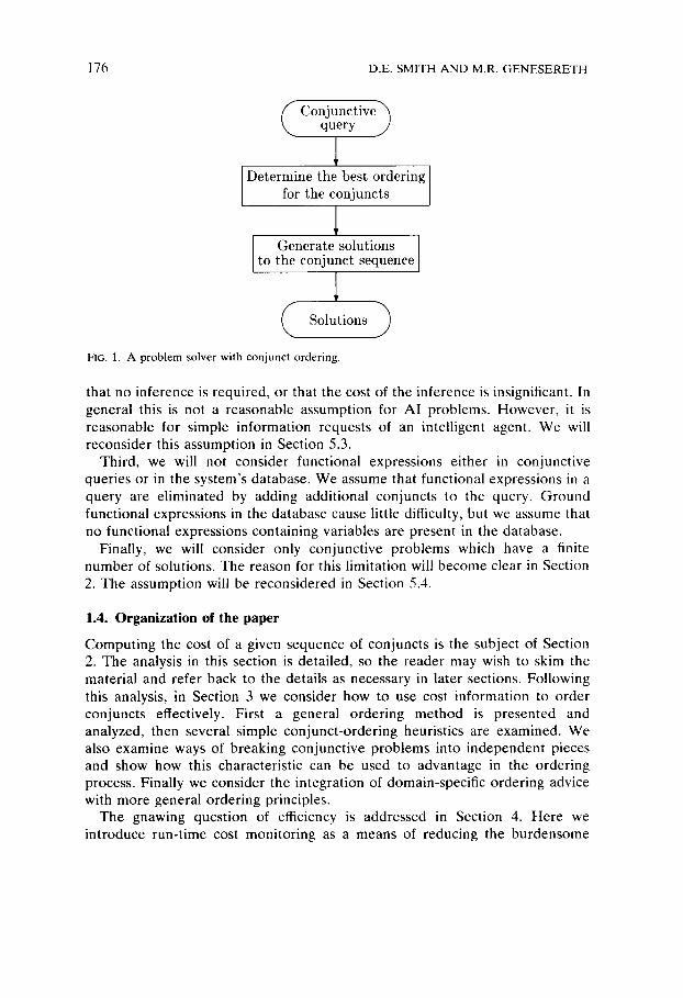
We will make the basic assumption that adequate improvement in system performance can be obtained by ordering each specific set of conjuncts right before giving it to the generate-and-test engine. We call this the static ordering assumption. Under this assumption the problem solver can be represented as consisting of a conjunct-ordering step followed by the generate-and-test step, as in Fig. 1. If s is the set of conjuncts given, then the conjunct-ordering step can be characterized as

find t such that BestOrdering(s, t ) ,

where BestOrdering is a relation between a set of conjuncts and any optimal ordering for that set. The best ordering for a set of conjuncts is one which will cost the problem solver the least to enumerate

BestOrdering(s, t) ¢:>

Ordering(s, t) A Vx(Ordering(s, x) f f Cost(t) ~< Cost(x)). (2)

Clearly the best ordering for the empty set is just the empty sequence and the best ordering for the singleton set is just the singleton sequence

BestOrdering(~, ( ) ) ,

BestOrdering({x}, (x)) .

In general, the cost of solving a conjunction depends upon many factors, such as the nature of the problem-solving engine, the characteristics of the database available to the problem solver and the characteristics of the problem itself. For the analysis and examples in the body of this paper (Sections 2 and 3) we have made some limiting assumptions.

First of all, we assume a simple sequential generate-and-test procedure, which enumerates the answers to the next conjunct in the sequence, plugs those answers into the remaining conjuncts and repeats. We assume that it has no special capabilities such as selective backtracking [11] or the ability to treat independent conjuncts separately. We will reconsider these assumptions in Section 5.1.

Second, we will assume that, for a solvable conjunct, all of the answers are directly available in the problem solver's database. In other words, we assume


[ Determine the best ordering

for the eonjunets

1 Generate solutions

to the eonjunet sequence

( S o l u t i o n s )

FIG. 1. A problem solver with conjunct ordering.

that no inference is required, or that the cost of the inference is insignificant. In general this is not a reasonable assumption for AI problems. However, it is reasonable for simple information requests of an intelligent agent. We will reconsider this assumption in Section 5.3.

Third, we will not consider functional expressions either in conjunctive queries or in the system's database. We assume that functional expressions in a query are eliminated by adding additional conjuncts to the query. Ground functional expressions in the database cause little difficulty, but we assume that no functional expressions containing variables are present in the database.

Finally, we will consider only conjunctive problems which have a finite number of solutions. The reason for this limitation will become clear in Section 2. The assumption will be reconsidered in Section 5.4.

1.4. Organization of the paper

Computing the cost of a given sequence of conjuncts is the subject of Section 2. The analysis in this section is detailed, so the reader may wish to skim the material and refer back to the details as necessary in later sections. Following this analysis, in Section 3 we consider how to use cost information to order conjuncts effectively. First a general ordering method is presented and analyzed, then several simple conjunct-ordering heuristics are examined. We also examine ways of breaking conjunctive problems into independent pieces and show how this characteristic can be used to advantage in the ordering process. Finally we consider the integration of domain-specific ordering advice with more general ordering principles.

The gnawing question of efficiency is addressed in Section 4. Here we introduce run-time cost monitoring as a means of reducing the burdensome

O R D E R I N G C O N J U N C T I V E Q U E R I E S 177

overhead of the strategies introduced in the previous section. In Section 5 we consider what is required to relax the limiting assumptions

introduced in Section 1.3 above, and mention some of the open research questions involved in doing so. In particular we consider the effects and prospects of alternative generation strategies, dynamic ordering and mixing inference with generation.

Finally, in Section 6, related work is discussed. Within the database community considerable work has been done on the problem of optimizing conjunctive database queries. We discuss differences between the ordering techniques developed in Section 3 and those used in database systems. Differences in general methodology are also discussed. Finally, we indicate the current state of our research and implementation.

2. Cost

2.1. The cost of solving a conjunctive problem

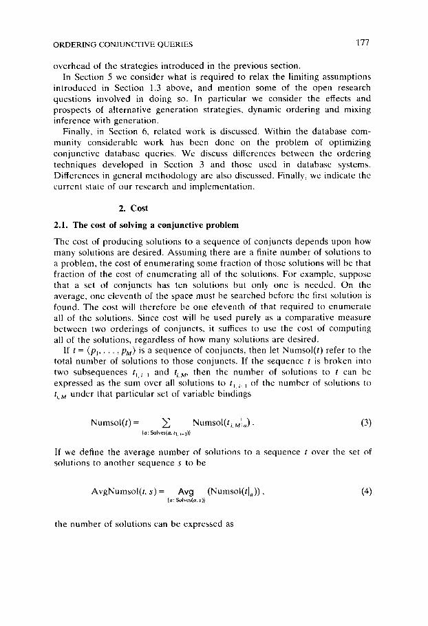
The cost of producing solutions to a sequence of conjuncts depends upon how many solutions are desired. Assuming there are a finite number of solutions to a problem, the cost of enumerating some fraction of those solutions will be that fraction of the cost of enumerating all of the solutions. For example, suppose that a set of conjuncts has ten solutions but only one is needed. On the average, one eleventh of the space must be searched before the first solution is found. The cost will therefore be one eleventh of that required to enumerate all of the solutions. Since cost will be used purely as a comparative measure between two orderings of conjuncts, it suffices to use the cost of computing all of the solutions, regardless of how many solutions are desired.

If t = (p~ . . . . . PM) is a sequence of conjuncts, then let Numsol(t) refer to the total number of solutions to those conjuncts. If the sequence t is broken into two subsequences t~,~ 1 and t~.M, then the number of solutions to t can be expressed as the sum over all solutions to tLi_ ~ of the number of solutions to ti.M under that particular set of variable bindings

Numsol(t) = ~ Numsol(t,, MI a)' (3) {a: Solves(a, tl, i - 1)}

If we define the average number of solutions to a sequence t over the set of solutions to another sequence s to be

AvgNumsol(t, s) = Avg (Numsol(tl.)), (4) {a: Solves(a, s)}

the number of solutions can be expressed as


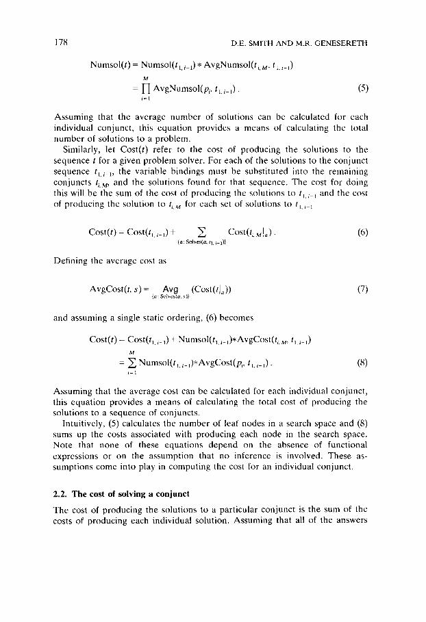
Numsol ( t ) = Numsol ( t 1./-1) * A v g N u m s o l ( t / . M, t 1. i-1)

M

= 1~ AvgNumsol(p i , t l , i 1)" i=1

(5)

Assuming that the average n u m b e r of solutions can be calculated for each individual conjunct , this equat ion provides a means of calculating the total n u m b e r of solutions to a p rob lem.

Similarly, let Cost( t ) refer to the cost of producing the solutions to the sequence t for a given p rob lem solver. For each of the solutions to the conjunct sequence tl, i_ l, the var iable bindings must be subst i tuted into the remaining conjuncts t~, M, and the solut ions found for that sequence. The cost for doing this will be the sum of the cost of producing the solut ions to tl,/_ 1 and the cost of producing the solution to t/, M for each set of solutions to tl. / 1

C o s t ( t ) : Cost(tl, i_0 + ~'~ C o s t ( t ~ , M l a ) • {a: Solves(a, tl. i-I)}

(6)

Defining the average cost as

AvgCost( t , s) = Av9 (Cost(tlo)) {a : Solves(a, s)}

(7)

and assuming a single static order ing, (6) becomes

Cost( t ) = Cost(t1, i-l) + Numsol(t l , i - 0 * A v g C ° s t (ti, M, tl, i-l) M

= ~ Numsol ( t 1, i-1)*AvgC°st(pi, t l, i-1)- i=1

(8)

Assuming that the average cost can be calculated for each individual conjunct , this equat ion provides a means of calculating the total cost of producing the solut ions to a sequence of conjuncts .

Intuit ively, (5) calculates the n u m b e r of leaf nodes in a search space and (8) sums up the costs associated with producing each node in the search space. No te that none of these equat ions depend on the absence of functional express ions or on the assumpt ion that no inference is involved. These assumpt ions come into play in comput ing the cost for an individual conjunct .

2.2. The cost of so lv ing a conjunct

The cost of producing the solutions to a par t icular conjunct is the sum of the costs of producing each individual solution. Assuming that all of the answers


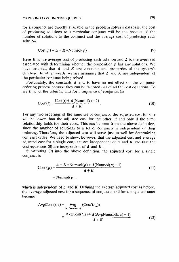
for a conjunct are directly available in the problem solver's database, the cost of producing solutions to a particular conjunct will be the product of the number of solutions to the conjunct and the average cost of producing each solution.

Cost(p) = A + K* Numsol(p) . (9)

Here K is the average cost of producing each solution and zl is the overhead associated with determining whether the proposition p has any solutions. We have assumed that A and K are constants and properties of the system's database. In other words, we are assuming that A and K are independent of the particular conjunct being solved.

Fortunately, the constants A and K have no net effect on the conjunct- ordering process because they can be factored out of all the cost equations. To see this, let the adjusted cost for a sequence of conjuncts be

Cost(t) + A (Numsol(t) - 1) Cost'(t) = (10)

A + K

For any two orderings of the same set of conjuncts, the adjusted cost for one will be lower than the adjusted cost for the other, if and only if the same relationship holds for their costs. This can be seen from the above definition, since the number of solutions to a set of conjuncts is independent of their ordering. Therefore, the adjusted cost will serve just as well for determining conjunct order. We need to show, however, that the adjusted cost and average adjusted cost for a single conjunct are independent of zl and K and that the cost equations (8) are independent of A and K.

Substituting (9) into the above definition, the adjusted cost for a single conjunct is

,3 + K* Numsol(p) + A (Numsol(p) - 1) Cost '(p) =

= Numsol(p) ,

A + K (11)

which is independent of A and K. Defining the average adjusted cost as before, the average adjusted cost for a sequence of conjuncts and for a single conjunct become

AvgCost'(t, s) = Avg (Cost'(tla)) {a: Solves(a, s)}

= AvgCost(t, s) + A (AvgNumsol(t, s) - 1)

A + K (12)

180 D.E. S M I T H A N D M.R. G E N E S E R E T H

and

AvgCost'(p, s) = Avg (Cost'(Pla)) = AvgNumsol(p, s) . {a: Solves(a, s)}

Again, the latter is independent of A and K. To show that the cost equations remain independent of A and K, we solve

equations (10) and (12) for Cost and AvgCost and substitute into t h e cost equation (8). This gives

Cost(t) = Cost(tl, i-1) + Numsol(tl.i 1) * AvgCost(ti, M, tl, i-x),

(A + K)Cost '(t) + A (Numsol(t) - 1) =

= (A + K)Cos t ' ( t l . i l)+ A(Numsol(tl, i_l)- 1)

+ Numsol ( t t . i_ l ) ( (A + K)AvgCos t ' ( t i , M, tl.i_l)

+ A ( A v g N u m s o l ( t i , M, tl, i 1 ) - 1)),

(A + K ) C o s t ' ( t ) =

= (A + K)Cos t ' ( t l , i_l)+ (A + K ) N u m s o l ( t l , i_l)AVgCost '( t i .M, tl, i_i),

Cost'(t) = Cost'(tl, i-1) + Nums°l(tl, i-1) * AvgCost'(ti, M, tl, i-1)-

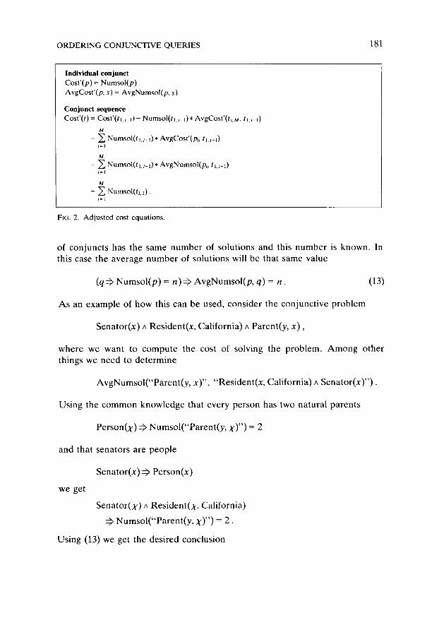
The cost equations (8) therefore remain unchanged for adjusted cost. Because of this, we will use adjusted cost for the remainder of this paper. The equations for adjusted cost are summarized in Fig. 2 for easy reference. With these simplifications, the characteristics of the cost equation can be easily seen. If the search space for the problem continues to expand dramatically with each conjunct then the net cost will be proportional to the total number of solutions. If, however, the space first expands and then undergoes dramatic reduction (as in most conjunctive problems), one of the intermediate terms will dominate. This corresponds to the widest portion of the search tree.

2.3. The average number of solutions to a conjunct

Using information about the number of solutions to individual conjuncts and the definition of average number of solutions, we could theoretically compute the average number of solutions for any desired set of conjuncts. However, this would be expensive and pointless, since we would have to find all of the solutions to the various subsequences of conjuncts in order to compute the averages required. If these solutions were known there would be no reason to reorder the conjuncts.

It is sometimes possible to estimate or infer these averages based on available information. The easiest case is when every member of the desired set


Individual conjunct Cos t ' ( p ) = N u m s o l ( p ) AvgCos t ' ( p , s) = A v g N u m s o l ( p , s )

Conjunct sequence Cost ' ( t ) = Cost ' ( t l , i_l) + Numsol( t l , i -1) * AvgCost'(ti, M, t l , i - l )

M

= ~', N u m s o l ( t I. i 1) * AvgCost ' (p i , t t, i-1) i=1

M

= ~'~ N u m s o l ( t t. i-l) * AvgNumso l (p i , t l, i-1) i=1

M

= ~ ' Numsol( t t , i ) . i=1

FIG. 2. A d j u s t e d cost equa t ions .

of conjuncts has the same number of solutions and this number is known. In this case the average number of solutions will be that same value

(q ~ Numsol(p) = n ) ~ AvgNumsol(p, q) = n. (13)

As an example of how this can be used, consider the conjunctive problem

Senator(x) A Resident(x, California) A Parent(y, x ) ,

where we want to compute the cost of solving the problem. Among other things we need to determine

AvgNumsol("Parent(y, x)", "Resident(x, California) ^ Senator(x)") .

Using the common knowledge that every person has two natural parents

Person(x) ~ Numsol("Parent(y, X)") = 2

and that senators are people

Senator(x) ~ Person(x)

we get

Senator(x) ^ Resident(x, California)

Numsol("Parent(y, X)") = 2.

Using (13) we get the desired conclusion


AvgNumsol("Parent(y, x)",

"Senator(x) A Resident(x, California)") = 2.

Thus, using information about the implications of previous conjuncts can permit direct computation of the average number of solutions to a conjunct.

A second case where the average number of solutions to a set of conjuncts can be computed is when the set can be broken up into two smaller sets and the average number of solutions can be computed for these smaller sets. In general we know that

A v g ( f ) = ,, u,z Card(s I tO s2)

Avg ( f ) Card(s1) + Avg ( f ) Card(s2) - Avg( f ) Card(s 1 N s2) S l S 2 S 1 A S 2

where Card(s) refers to the cardinality of the set s. Applying this to the average number of solutions gives

AvgNumsol(p, ql v q2) =

= (AvgNumsol(p, q0Numsol(ql) + AvgNumsol(p, q2)Numsol(q2)

- AvgNumsol(p, ql A q2)Numsol(ql A qE)) /Numsol (q I v q2)- (14)

Thus AvgNumsol(p, q) can be computed in cases where q can be broken into two disjoint pieces ql and q2, and the average number of solutions to p is known for these two sets.

A useful special case of this is when p f f q. In this case, if ql is taken to be p and q2 is taken to be disjoint with ql

AvgNumsol(p, ql) = AvgNumsol(p, p) = 1,

A v g N u m s o l ( p , q2) = AvgNumsol(p, ~ p ) = 0,

which gives

(p:ff q):ff AvgNumsol(p, q) - Numsol(p)

Numsol(q) " (15)

As an example, if we know that

CurrentDirectory(u) ~ Direc tory(u) ,

Numsol("CurrentDirec tory(u)") = 1,

Numsol("Direc tory(u)") = 100,


then (15) applies giving

AvgNumsol ("Curren tDirec tory(u)" , "Direc tory(u)" ) =

Numsol("Current Directory(u)") 1

Numsol ("Direc tory(u)") 100

If none of the above special cases apply (the number of solutions is not the same for every member of p and q cannot be broken into two useful subsets), an assumption must be made in order to compute the average number of solutions. In such cases the most reasonable assumption is that AvgNumsol(p, q) is the same as the average number for some larger set q' containing q. This assumption can be stated formally as

(qzff q') A AvgNumsol(p, q') = n

d :ff AvgNumsol(p, q ) = n, (16)

d

where the notation pzff q means that if p is true, and q is consistent, then q can be assumed. 2

Extending the example above, suppose our object were to compute the average number of solutions to the last conjunct in the intelligent agent 's problem

A vgNumso l ( "Curren t Directory( u )",

" . . . A DirectoryGroup(u, g ) " ) . (17)

In this case CurrentDirectory(u) does not necessarily imply the other conjuncts. There is also no useful way to divide the solutions to the other conjuncts into two sets, and no exact information is available. However, using the facts that

and • .. A DirectoryGroup(u, g) ~ Directory(u)

AvgNumsol ("Curren tDirec tory(u)" , "Direc tory(u)") =

Numsol("CurrentDirec tory(u)") = 1

Numsol("Direc tory(u)") 100

the above default allows the desired conclusion

2 T h e s e a re s o m e t i m e s r e f e r r e d to as normal defau l t s . A d i scuss ion of such d e f a u l t s c a n be f o u n d in

[131.


AvgNumsol("CurrentDirectory(u)",

1 " . . . ^ DirectoryGroup(u, g)") = 100 ' (18)

With the knowledge that the average number of solutions can at least be estimated from more primitive number of solutions information, we now turn to the issue of computing that primitive information for individual conjuncts.

2.4. Computing the number of solutions to a conjunct

The number of solutions for an individual conjunct can frequently be determined from available information about the sizes of sets. If a is the set corresponding to the solutions to a proposition ~(5), the number of solutions to the proposition will be the cardinality of the set o-

True("5 ~ or ¢ , &(g)") ::) Numsol(&(5)) = Card(o-). (19)

2.4.1. Exact information

It is not uncommon to have exact information about the number of solutions to a problem, even when the bindings for some of the variables are not yet known. Take, for example, the problem of finding the parents of a particular individual. Every individual has exactly two parents and the problem therefore has two solutions. It is not at all unreasonable to expect an intelligent system to have some information of this sort. In the case of the intelligent agent there are several pieces of relevant exact information. For example, CurrentDirectory, DirectoryOf and Size are all function symbols. Ground functional expressions (i.e., expressions which do not contain variables) only have a single solution. We can formally express this information to the intelligent agent as

and

Function(Size),

Function(DirectoryOf),

Function(CurrentDirectory)

Function(r) ^ Variable(v) ^ Ground(Y)

Card({v: r(£, v)}) = 1 .

(20)

(21)

An additional piece of information that is useful to the intelligent agent is knowledge that there are an infinite number of solutions to the conjunct s > 100. This fact of arithmetic can be stated generally as

VnCard({x: x > n}) = 2 . (22)


2.4.2. Average information

There are equally many situations where exact information is not available, but average values are available. Take, for example, the problem of determining the children of a given person. The upper bound on the number of children a person could theoretically produce is quite large, especially for males. However the average number is between two and three. Certainly, for purposes of estimating the cost of solving a problem, and ordering conjuncts, the average number is much more valuable than an upper bound would be. For the example above, we could express such average information as

Av 9 ( C a r d ( C h i l d r e n ( y ) ) ) = 2 . 3 , {y: Adult(y)}

Av 9 ( C a r d ( C h i l d r e n ( y ) ) ) = 3 . 5 . {y: Adult(y) ^ Catholic(y)}

Average information can sometimes be computed using information about a relation and its domain. For example, suppose that there are one hundred tuples which satisfy the relation R, and hence the proposition R(x, y), and that the domain of the first argument, x, contains twenty elements. Then on the average, given x, the number of y ' s that will satisfy the proposition is five. For binary relations, this relationship can be stated as

Card({(x, y): r(x, y)}) = n A Card(Domain( l , r)) = d

Avg (Card({y : r(x, y)}) ) = n/d. x~Domain(1, r)

More generally, for relations of arbitrary arity

Card({v: r(Y)}) = n A X i E V ^ Card(Domain(i , r)) = d

=), Avg (Card({v - {xi}: r(Y)})) = n/d. xiEDomain(i, r)

(23)

As an example, consider the conjunct Format(f , Scribe) from the intelligent agent 's problem. Suppose we knew that there w e r e 10 4 files on the machine, and 500 of them are Scribe files. The chance that a given file will be a Scribe file is therefore 500/104 or 1/20.

2.4.3. Approximations and bounds

When exact information or averages are not available, approximate information or bounds are sometimes valuable. For approximate values, a bound on


the error of the approximation is necessary in order for the information to be useful. A very useful special case of approximations is the order of magnitude approximation. When we say that a quantity has order of magnitude n we mean that it is within a factor of ten of the number n. We use the function symbol O for the order of magnitude of a quantity

O(v) = n <::> 0.1n < v ~< 10n. (24)

Much of the remaining interesting information for the intelligent agent 's problem is order of magnitude information.

O(Card(Files)) = 1(I 4 ,

O(Card(Directories)) : 1 0 2 ,

O(Card({g: DirectoryGroup(d, g)})) = 1 ,

O(Card({d: DirectoryGroup(d, g)})) = 10,

O(Card({f: DirectoryOf(f~ d)}))= 50.

(25)

Upper and lower bounds are stated in the normal way

102 < Card(Directories) < 103 ,

104 < Card(Files).

A fact about bounds which is generally useful is that ground clauses have at most one solution. If a ground clause is true, then there is exactly one solution, otherwise there is no solution.

Ground(c) ~ Card({( ): c}) ~< 1 . (26)

In the previous section domain information could sometimes be used to derive average values. In the opposite manner, domain information can be used to give upper bounds for an otherwise unknown conjunct. In general, the number of solutions to a conjunct must always be less than the product of the sizes of domains of the unbound variables. Thus

Card({v: r(£)}) <~ [ l Card(Domain(i , r)). {i: Variable(xi)}

(27)

As an example, consider the conjunct Di rec to ryGroup(d ,g ) from the intelligent agent 's problem. If there are one hundred directories in the machine.


and only five groups, then the maximum number of solutions to this conjunct would be five hundred.

Using an upper bound on the number of solutions gives an upper bound for the cost of solving a particular conjunct which leads to an upper bound on the cost of solving an entire problem. This is still useful information if it indicates that one particular ordering of conjuncts is cheaper than any other. Similarly, lower-bound information is valuable if it indicates that some conjunct ordering is more expensive than some other. Approximate and order-of-magnitude values can be used more liberally as estimates, recognizing, of course, that the final estimate of the cost of solving the problem may be in error by a similar factor.

In order of descending preference, we will use exact information, average values for larger sets, order-of-magnitude approximations, and lastly, upper and lower bounds for computing the number of solutions and cost information. Using the default notation introduced earlier, these can be stated formally as

d

( q ~ q') ^ AvgNumsol(p, q') = n ~ AvgNumsol(p, q) = n ,

d

O(Numsol(q)) = n ~ Numso l (q )= n ,

d

Numsol(q)~< n ~ Numsol(q) = n .

2.5. An example

Using information about set sizes and the cost equations given in Fig. 2 it is possible to compute the cost of solving a problem for any given ordering of the conjuncts.

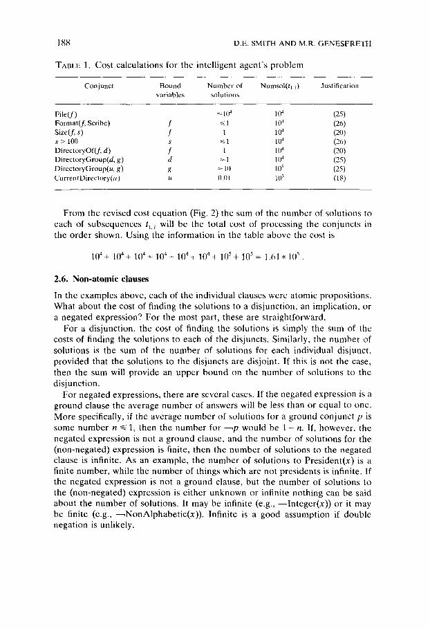
As an illustration, Table 1 shows the calculations for the conjuncts (in the order given) in the intelligent agent problem (equation (1)). Each row of this table gives data for the next conjunct in the sequence, assuming that the conjuncts listed above it have been processed. The columns contain the list of variables bound by previous conjuncts, the number of solutions to the conjunct as calculated using one of the axioms of the previous sections, and finally the total number of solutions of the conjunct sequence so far (the product of the number of solutions of all conjuncts processed). For example, the conjunct s > 100 is the fourth conjunct in the sequence. When it is encountered, the variable s will have been bound by solution of the previous conjunct. The number of solutions will be one (as given by equation (26)), since it is a ground clause. The total number of solutions to the first four conjuncts will be the product of the number of solutions to each of the first four conjuncts, which is 10 4"


TABLE 1. Cost calculations for the intelligent agent 's problem

Conjunct Bound Number of Numsol(h, i) Justification variables solutions

File(f) ~ 104 1(I 4 (25) Format(f, Scribe) f ~ 1 l04 (26) Size(f, s) f 1 1(14 (20) s > 100 s ~< l 10 a (26) DirectoryOf(f, d) f 1 104 (20) DirectoryGroup(d, g) d ~ 1 104 (25) DirectoryGroup(u, g) g ~ 10 105 (25) CurrentDirectory(u) u 0.01 1() ~ (18)

From the revised cost equation (Fig. 2) the sum of the number of solutions to each of subsequences tl. i will be the total cost of processing the conjuncts in the order shown. Using the information in the table above the cost is

104+ 104+ 104+ 104+ 104+ 104+ 105+ I 0 3 = 1.61 * 105 .

2.6. Non-atomic clauses

In the examples above, each of the individual clauses were atomic propositions. What about the cost of finding the solutions to a disjunction, an implication, or a negated expression? For the most part, these are straightforward.

For a disjunction, the cost of finding the solutions is simply the sum of the costs of finding the solutions to each of the disjuncts. Similarly, the number of solutions is the sum of the number of solutions for each individual disjunct, provided that the solutions to the disjuncts are disjoint. If this is not the case, then the sum will provide an upper bound on the number of solutions to the disjunction.

For negated expressions, there are several cases. If the negated expression is a ground clause the average number of answers will be less than or equal to one. More specifically, if the average number of solutions for a ground conjunct p is some number n ~< 1, then the number for ~ p would be 1 - n. If, however, the negated expression is not a ground clause, and the number of solutions for the (non-negated) expression is finite, then the number of solutions to the negated clause is infinite. As an example, the number of solutions to President(x) is a finite number, while the number of things which are not presidents is infinite. If the negated expression is not a ground clause, but the number of solutions to the (non-negated) expression is either unknown or infinite nothing can be said about the number of solutions. It may be infinite (e.g., ~ I n t e g e r ( x ) ) or it may be finite (e.g., ~NonAlphabe t i c (x ) ) . Infinite is a good assumption if double negation is unlikely.


Finally, the number of solutions to complex expressions such as implications, if-and-only-if statements, and negations of complex expressions can be computed by reducing the expression to conjunctive normal form and using the rules developed for conjunction, disjunction and negation.

2.7. The closed-world assumption

Thus far we have been assuming that the closed-world assumption holds for our problem-solving system

True(p) =:> InDataBase(p) .

In other words, we have been assuming that the problem solver is capable of completely enumerating the solutions to any of the conjuncts in a problem. Of course this is not always a valid assumption for AI systems. For example, the intelligent agent might be unable to enumerate the solutions to a conjunct such as DirectoryGroup(d, g) unless the directory variable d is bound. Such limitations must be considered in the choice of conjunct order or the answers that result will be incomplete or erroneous. For example, given that there are only about a dozen directories in any given directory group, an agent operating under the closed-world assumption might decide to first expand conjuncts binding the directory group g and then expand the conjunct DirectoryGroup(d, g). This would lead to the incorrect answer that no directories and hence no files satisfied the query. This would merely be frustrating if the user were looking for a particular file. It could be disastrous if the intelligent agent's response were used as the basis of a backup or deletion operation.

For purposes of conjunct ordering, the closed-world assumption can be handled by adding the condition to the cost equation (Fig. 2) that the conjunct be enumerable

Enumerable(p) ~ Cost '(p) = Numsol(p) ,

where Enumerable(p) means that the proposition p obeys the closed-world assumption. If a conjunct is not enumerable its cost is taken to be infinite

~ E n u m e r a b l e ( p ) ~ Cost '(p) = ~ .

In this way, conjuncts which are not enumerable will not be chosen for expansion over others which are enumerable and finite.

Finally we include the default that the closed-world assumption is valid except in those cases where explicit information to the contrary has been provided

d =), Enumerab le (p) .


In the case of the intelligent agent we will assume that it cannot enumerate the set of Scribe files, the set of file-size pairs, or the set of file-directory pairs without first enumerating the set of files. Thus

~Enumerab le ( "Forma t ( f , o ' )") ,

~ E n u m e r a b l e ("Size(f, s ) " ) ,

~Enumerab le ("Di rec to ryOf( f , d ) " ) ,

~Enumerab le ("Di rec to ryGroup(d , g )") .

(2s)

This information will prevent an intelligent agent from making potentially disastrous mistakes.

3. Ordering

Given the cost axioms (Fig. 2) we could (theoretically) enumerate all possible orderings of the conjuncts in a problem, compute the cost for each, and choose the minimal one. For a problem with m conjuncts, this requires enumerating and computing the cost for m! orderings. This is not unreasonable for a problem with only four conjuncts (twenty-four orderings to examine, possibly resulting in a savings of several orders of magnitude in the size of the search tree), but for larger problems the cost is prohibitive. For the intelligent agent's problem (equation (1)) this exhaustive approach would require examining over 40 000 possible conjunct orderings.

How then, can we prune this search space without sacrificing optimality? In the sections that follow, several ordering techniques are examined with this consideration in mind.

3.1. Optimal ordering

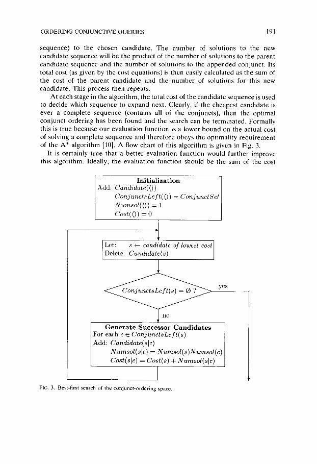
The conjunct-ordering problem has been shown to be NP-complete [20]. Thus in the worst case, it is necessary to examine a large number of possible conjunct orderings for a set of conjuncts. Fortunately, we can usually do very much better than this without sacrificing optimality. Using best-first search [1] it is possible to search the space in a way which rapidly leads to the optimal solution for most practical sets of conjuncts, and degrades gracefully to m ! for a worst-case set of conjuncts. The evaluation functions used in this search (to decide which branch of the space to explore next) is the total cost of the partial sequence of conjuncts for that branch (as given by the cost equation, Fig. 2). To illustrate, we begin with a set of 'candidate' conjunct sequences, which initially contains only the null sequence. We then choose the candidate of lowest cost and expand it. Expanding a candidate means constructing all possible candidates formed by appending one of the remaining conjuncts (not yet in the


sequence) to the chosen candidate. The number of solutions to the new candidate sequence will be the product of the number of solutions to the parent candidate sequence and the number of solutions to the appended conjunct. Its total cost (as given by the cost equations) is then easily calculated as the sum of the cost of the parent candidate and the number of solutions for this new candidate. This process then repeats.

At each stage in the algorithm, the total cost of the candidate sequence is used to decide which sequence to expand next. Clearly, if the cheapest candidate is ever a complete sequence (contains all of the conjuncts), then the optimal conjunct ordering has been found and the search can be terminated. Formally this is true because our evaluation function is a lower bound on the actual cost of solving a complete sequence and therefore obeys the optimality requirement of the A* algorithm [10]. A flow chart of this algorithm is given in Fig. 3.

It is certainly true that a bet ter evaluation function would further improve this algorithm. Ideally, the evaluation function should be the sum of the cost

I n i t i a l i z a t i o n Add: Candidate(O )

C o n j u n c t s L e f t ( O ) = C o n j u n c t S e t N u m s o l ( () ) = 1 Co. t( <) ) = o

Let: s *- candidate of lowest cost Delete: Candida te (s )

Generate Successor Candidates For each c E C o n j u n c t s L e f t ( s ) Add: Candidate(s ic )

N u m s o l ( s l c ) = N u m s o l ( s ) N u r n s o l ( c ) Cost(sic) = Colt(s) + iumsol(slc)

!

FIG. 3. Best-first search of the conjunct-ordering space.

yes


for the candidate and some good estimate of the minimum cost of solving the remaining conjuncts. Unfortunately, no such estimate exists. About the best that we could do is to multiply the number of outstanding conjuncts by some weighting factor (say some fraction of the number of solutions to the problem so far) and add this to the computed cost. This might improve the performance in some cases, but sacrifices the guarantee of optimality. A minor enhance- ment, that still retains optimality, would be to add the number of outstanding conjuncts to the cost for a candidate. This estimate satisfies the lower-bound requirement since the added cost for each of the remaining conjuncts will be at least one.

Several other optimizations can be performed on the algorithm. The first three of these optimizations are syntactic, while the final three depend upon particular properties of the conjunct ordering problem.

(1) The candidate set can be kept as an ordered list. (2) When expanding a candidate, only its cheapest successor need be added

to the candidate set immediately. If that successor is ever expanded, then the next-cheapest successor must be added to the candidate set. This is a form of 'partial expansion' of a candidate (see [10, p. 67]) equivalent to leaving the expanded candidate on the candidate list but updating its 'cost' to reflect the next conjunct.

(3) If a candidate is generated which is simply a permutation of an existing candidate (i.e., the same remaining set of conjuncts), then only the cheapest of the two candidates need be preserved. This optimization is a general one for searching graphs rather than trees and is discussed at length in [10, p. 64ff]. Note that no 'cost readjustment' will be necessary in discarding candidates. Either the existing candidate will be cheaper, or the existing candidate won't be expanded yet. This is because the evaluation function is 'monotonic' (see [10, p. 81ttl).

(4) If a conjunct is not practically enumerable, or has an infinite set size it need not be considered in generating candidates. In other words, candidates whose cost is too large can be thrown away.

(5) The most expensive conjunct at each stage need not be considered (Theorem 3.2 in the next section).

(6) When expanding a candidate, if the cheapest conjunct actually reduces the search space (its average number of solutions is less than one) only that successor candidate need be added to the list (Theorem 3.1 in the next section).

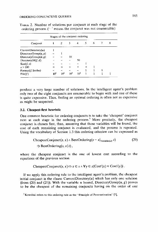
The final three optimizations can significantly reduce the size of the search space for practical conjunct-ordering problems. By looking at the data for the intelligent agent's problem (Table 2) it is clear that the space searched by this algorithm is not nearly as large as what might be expected. For this problem, only 18 out of the total of 8! possible orderings are ever explored by this algorithm. This sort of behavior is quite common because practical problems often contain many conjuncts which are not immediately enumerable, or which

O R D E R I N G C O N J U N C ' r l V E Q U E R I E S

TABLE 2. Number of solutions per conjunct at each stage of the ordering process ( ' - ' means the conjunct was not enumerable)

193

Stages of t he c o n j u n c t o r d e r i n g

C o n j u n c t 1 2 3 4 5 6 7 8

C u r r e n t D i r e c t o r y ( u ) 1

D i r e c t o r y G r o u p ( u , g ) - 1

D i r e c t o r y G r o u p ( d , g ) - - 10

D i r e c t o r y O f ( f , d ) - - - 50

Size(f, s) . . . . s > 100 ~ ~ oo ~c

F o r m a t ( f , Sc r ibe ) . . . . F i l e ( f ) 104 104 10 4 10 4

1

1

1 1 1 1 1 1

produce a very large number of solutions. In the intelligent agent's problem only two of the eight conjuncts are enumerable to begin with and one of these is quite expensive. Thus, finding an optimal ordering is often not as expensive as might be suspected.

3.2. Cheapest-first heuristic

One common heuristic for ordering conjuncts is to take the 'cheapest' conjunct next at each stage in the ordering process. 3 More precisely, the cheapest conjunct is chosen first, then, assuming that those variables will be found, the cost of each remaining conjunct is evaluated, and the process is repeated. Using the vocabulary of Section 1.3 this ordering criterion can be expressed as

CheapestConjunct(s, x) ^ BestOrdering(s - Xlvariables(x ), t )

BestOrdering(s, x l t ) ,

(29)

where the cheapest conjunct is the one of lowest cost according to the equations of the previous section

CheapestConjunct(s, x)¢¢, x E s ^ Vy E s(Cost'(x)~< Cost'(y)).

If we apply this ordering rule to the intelligent agent's problem, the cheapest initial conjunct is the clause CurrentDirectory(u) which has only one solution (from (20) and (21)). With the variable u bound, DirectoryGroup(u, g) proves to be the cheapest of the remaining conjuncts having on the order of one

3 K o w a l s k i r e f e r s to th is o r d e r i n g ru le as the " P r i n c i p l e of P r o c r a s t i n a t i o n " [7].


solution (proposition (25)). With the variable g bound, the next cheapest is DirectoryGroup(d, g) having on the order of ten solutions (proposition (25)). Table 2 summarizes the results of this process. The conjuncts are listed in the order that they would be chosen using the 'cheapest-first' heuristic and the columns show the cost of each remaining conjunct at each step in the ordering process. From the table, it is clear that the cheapest-first heuristic leads to an optimal ordering of the conjuncts.

While this heuristic works very well for this particular problem, there are many simple examples where it fails miserably. The difficulty is that this heuristic will not necessarily focus the problem-solving effort. Instead, it may direct the problem solver to jump helter-skelter about the problem, picking off the easy tidbits. All the while, the size of the search space increases and the inevitable tough part of the problem is simply delayed. Sometimes this sort of opportunism will help solve the tough part of a problem, but often it does not. In fact, solving the tough part of the problem first may very well make everything else trivial to solve. This is where the cheapest-first heuristic can lead to totally unacceptable orderings.

As an example, consider the problem of finding all of the files on a particular directory that occupy less than ten pages

DirectoryOf(f, Genesereth) ^ Size(f, s) ^ s < 10.

According to the cheapest-first heuristic the conjunct s < 10 is cheapest, and is selected first. Following this, the conjunct DirectoryOf(f, Genesereth) would be selected leaving the conjunct Size(f, s). According to the cost equation, the cost of solving the conjuncts in this order is ~ 1 0 3. Solving them in the order given, however, results in a cost ~10 2. In this case, the cheapest-first heuristic increases the cost by a factor of ten. The penalty could easily be much higher.

The reason for this failing is clear. Solving the final conjunct does not help in the solution of either the first or second conjuncts, which constitute the 'crux' of the problem. Once the first two conjuncts are solved, the final conjunct becomes a ground clause and costs little to solve. As a result there is no advantage to solving the final conjunct first, even though it is the cheapest.

While general use of the cheapest-first heuristic may cause serious difficul- ties, there are two special cases where it is valuable.

Theorem 3.1. When the cheapest conjunct will reduce the search space rather than expand it (i.e. the average number of solutions is less than one), this conjunct should be chosen first. The resulting ordering will always have a cost less than twice that of the optimal ordering and will be the optimal ordering if the problem is non-trivial.


Proof. Consider a set of conjuncts whose cheapest conjunct c has an expected number of solutions less than one (Numsol(c) < 1). Suppose that some ordering t = tl, i_llClt~+l, M of the conjuncts is optimal. Using the cost equations (Fig. 2) the cost of solving t is

Cost '(t) = Cost'(tl, i-0 + Numsol(tl, i-1)AvgCost'( c, tx, i-1)

+ Nums°l(tl , i-1 ] c ) Av gC os t ' ( t i + l , M, tl, i -1]c) • (30)

Alternatively, if the conjunct c were placed first in the sequence giving t ' = cl t l , / - l[ t~+a,M the cost would be

Cost '( t ' ) = Cos t ' ( c )+ N u m s o l ( c ) A v g C o s t ' ( t l , / l, c)

+ Numsol(c ] t 1. i-1)Avgfost'(ti+l, M, c l t 1, i - l ) . (31)

The final terms in these two equations are identical, since the number of solutions to c[ t l , i_l is the same as for t l,~_llC. The other two terms in (31) are both smaller than the initial term in (30) since

Cost ' (c) < Cost '(t L/-l),

AvgCost ' ( t l, i- 1, c ) <~ Cost '(t 1, i-1) '

Numsol(c) < 1 .

If Cost'(tl,/_ 0 is small (i.e. less than one) then the sequence tL~_l lc is easy to solve and order makes little difference. In this case the cost of doing c first is no worse than twice the cost for doing t l , i_ 1 first since the first two terms of (31) are both smaller than the first term of (30). If the second or third terms of (30) are significant, the latter ordering will be as good or better. Alternatively, if Cost'(tL/_ 0 is not small, the first term of (31) becomes insignificant since

Cost ' (c) ~ Cost'(tl ,/_l).

In addition the second term of (31) will be smaller than the first term of (30)

Nums°l(c)AvgC°st ' ( t l . i -1, c) < Cost '(t 1, i-l)"

The cost of solving t' will therefore be strictly less than the cost of solving the original ordering t. As a result, the optimal ordering must begin with the conjunct c in this case. []

Formally, the ordering principle of Theorem 3.1 can be expressed as


CheapestConjunct(s , x) ^ Cost '(x) ~ 1

^ BestOrdering(s - X lva r i ab l e s (x ) , t)

BestOrdering(s, x l t ) .

(32)

This principle is useful for reducing the best-first search described in the previous section.

Another useful special case of the cheapest-first heuristic is the Adjacency Restriction.

Theorem 3.2. (Adjacency Restriction). Suppose that the conjunct sequence t - t i, i-11 c ldlt~+2, M is an optimal ordering of the conjuncts involved. For any adjacent pair of conjuncts c and d the number of solutions to the second conjunct d (under the bindings to the preceding conjuncts tl, i_l) m u s t be greater than the number of solutions to the conjunct c (under the bindings to the preceding sequence tl,i_ O. Formally, AvgNumsol(c, tl .i_l) ~ AvgNumsol(d, tl, i i).

Proof. According to the cost equations (Fig. 2)

Cost '(t) = Cost'(tl, i_l)+ Numsol(tl. i 0AvgNumsol(c, tl, i l)

+ Numsol(tl, i l lc)AvgNumsol(d, tl,i 11c)

+ Numsol(t~,i_11cld)AvgCost'(ti+z.M, tl, i llCtd)

= Cost'(tl, i-l) + Nums°l(tl , i -0AvgNums°l ( c, tl.i-1)

+ Nums°l(tl , i-llcld)

+ Numsol(tl, i_l]cld)AvgCost'(ti+z,M, tl, i llcld).

Similarly, if t ' = tl, i_lldlclti+z,M (c and d reversed) the cost is

Cost'(t ') = Cost '(t ~, i-~) + Numsol(t 1, i 1)Avg Nums°l(d, tl. i-1)

+ Numsol(t 1, i_llcld)

+ Numsol(tl, i_llcld)AvgCost'(ti+z,M, tl, i llCld).

The first, third and fourth terms in each of these equations are identical. Therefore

Cost '(t) ~< Cost'(t')¢:> AvgNumsol(c, tl, i_l) <~ AvgNumsol(d, t1,~_1).

By our assumption that t is an optimal ordering, the left-hand side must be true. Therefore

AvgNumsol(c, tl, ~ 0 ~ AvgNumsol(d, t l , i l)- []


Note that the adjacency restriction is much weaker than the cheapest-first heuristic. It does not imply that a conjunct should be less expensive than all subsequent conjuncts, only that it should be less expensive than its immediate successor. In other words, the adjacency restriction does not necessarily imply that the conjunct c will be cheaper than other conjuncts in t~+2, M. Although this restriction may appear weak, it has several useful corollaries

Corollary 3.3. The most expensive conjunct is never the optimal one to do next.

If the most expensive one was selected, then any conjunct chosen to follow it would be less expensive, violating the adjacency restriction.

Corollary 3.4. The search for conjuncts to immediately follow a conjunct c can be limited to those which were more expensive than c at the time c was selected.

These corollaries significantly reduce the size of the space that must be searched in order to find the optimal ordering. In fact, some simple analysis shows that the number of possible orderings that must be considered by a procedure employing the adjacency restriction will be bounded by F(n) where n is the number of remaining conjuncts and

F(n) = G(n, 0),

1, G(n, d) =

n - d - 1

Z i=0

i f n = d ;

i f n = l , d = 0 ;

G ( n - 1, i ) , otherwise.

Here d can be thought of as the number of remaining conjuncts that cannot appear as the next conjunct because of the adjacency restriction. Note that if the second argument to g is ignored, this formula reduces to n! as expected. The case of i = 0 corresponds to the case where the cheapest remaining conjunct is chosen. In this case any other remaining conjunct will be allowed in the next position. Similarly, the case of i = n - 1 corresponds to choosing the most expensive conjunct. In this case none of the remaining conjuncts will be allowed in the next position (by Corollary 3.4).

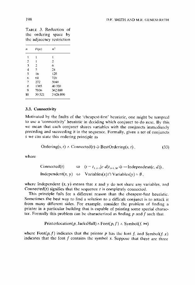
In Table 3 the values of F(n) and n! are shown for different values of n. For four conjuncts the adjacency restriction reduces the search to only five possible orderings. For eight conjuncts, the space is reduced from over forty-thousand possible orderings to only 1385 possible orderings. From these figures it is clear that the adjacency restriction significantly reduces the possible worst-case search for a best-first search of the space of conjunct orderings.

We will make further use of the adjacency restriction in Section 3.4.


TABLE 3. Reduction of the ordering space by the adjacency restriction

n F(n) n!

1 1 1 2 1 2

3 2 6 4 5 24 5 16 120 6 61 720 7 272 5040

8 1385 40320 9 7936 362 88O

10 50 521 3 628 800

3.3. Connectivity

Motivated by the faults of the 'cheapest-first' heuristic, one might be tempted to use a 'connectivity' heuristic in deciding which conjunct to do next. By this we mean that each conjunct shares variables with the conjuncts immediately preceding and succeeding it in the sequence. Formally, given a set of conjuncts s we can state this ordering principle as

Ordering(s, t) ^ Connec ted( t ) f f BestOrdering(s, t ) , (33)

where

Connected(t) ¢¢, (t = tl.i_ltcldlti+l. M ~ ~Independen t (c , d)) ,

Independent(x, y) ~ Variables(x) 71 Variables(y) = fl,

where Independent (x, y) means that x and y do not share any variables, and Connected(t) signifies that the sequence t is completely connected.

This principle fails for a different reason than the cheapest-first heuristic. Sometimes the best way to find a solution to a difficult conjunct is to attack it from many different sides. For example, consider the problem of finding a printer in a particular building that is capable of printing some special charac- ter. Formally this problem can be characterized as finding p and f such that

Printerlocation(p, JacksHall) ^ Font(p, f ) ^ Symbol(f, ~ )

where Font(p, f ) indicates that the printer p has the font f, and Symbol(f, x) indicates that the font f contains the symbol x. Suppose that there are three


printers in Jacks' Hall and that each printer has more than fifty fonts, but that only four fonts contain a bowtie symbol. According to the connectivity heuristic the ordering given would be acceptable since each conjunct shares variables with its neighbors. According to the cost equations (Fig. 2) the cost for enumerating this ordering would be greater than

3+ 3(50)+ 1 = 154.

Alternatively, if the conjuncts were processed in the optimal order

Printerlocation(p, JacksHalt) ^ Symbol(f, ~ ) ^ Font(p, f )

the cost is bounded by

3 + 3(4) + 3(4) = 26.

Because the conjunct Font(p, f ) has many solutions it is cheaper to attack it from two different angles. In general, then, the connectivity heuristic can also lead to arbitrarily poor orderings.

Since the cheapest-first and connectivity heuristics behave somewhat differently, it is tempting to ask whether these two heuristics taken together can guarantee optimal ordering. Unfortunately, the answer is no. First of all, the connectivity heuristic provides no guidance on which conjunct to start with. As we illustrated in the previous section, the cheapest-first heuristic can suggest a suboptimal starting conjunct. Even assuming that the ordering were started correctly both the connectivity heuristic and the cheapest-first heuristic can suggest and agree upon a conjunct that is irrelevant to solving the crux of the problem. In the previous example suppose that the user were also interested in knowing the queue lengths for the printers involved. The problem then becomes find p, f and l such that

Printerlocation(p, JacksHall) ^ Font(p, f )

^ Symbol(f, t~ ) ^ QueueLength(p, 1).

In this case, after the printer location conjunct was enumerated, both the connectivity heuristic and the cheapest-first heuristic would agree on the queue-length conjunct (since it is a functional expression). This is clearly suboptimal.

3.4. Problem independence

In the solution of a conjunctive problem, it is not uncommon to find two or more pieces of the problem which are independent. We say that two pieces of a


problem are independent if, and only if, the two pieces do not share any variables. As an example of independence, consider the intelligent agent's problem (equation (1)), where the conjuncts are given in the optimal order (as calculated in Section 3.2 and shown in Table 2)

CurrentDirectory(u) ^ DirectoryGroup(u, g)

^ DirectoryGroup(d, g) ^ DirectoryOf(f, d)

^ Size(f, s) ^ s > 100 ^ Format(f, Scribe) ^ F i le ( f ) .

As in most realistic problems, independence does not arise at the top level of the problem, but only becomes manifest after several of the conjuncts have been solved. In this case, when the fourth conjunct is solved, the variable f is bound and the remaining four conjuncts divide into three independent subproblems

Size(f, s) ^ s > 100,

Format(f, Scribe),

F i le ( f ) .

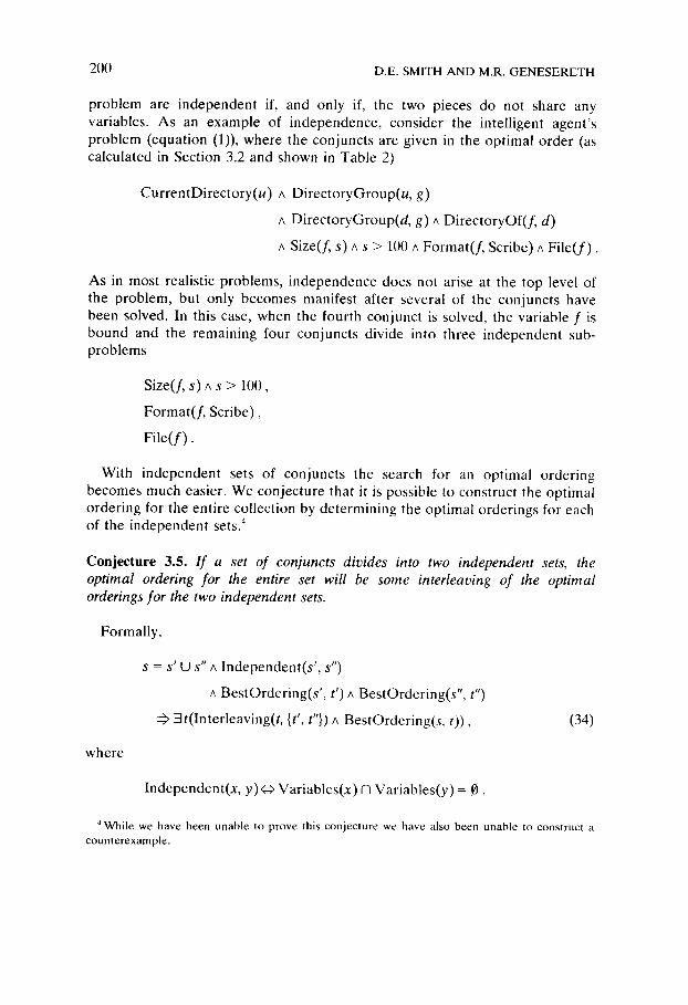
With independent sets of conjuncts the search for an optimal ordering becomes much easier. We conjecture that it is possible to construct the optimal ordering for the entire collection by determining the optimal orderings for each of the independent sets. 4

Conjecture 3.5. If a set of conjuncts divides into two independent sets, the optimal ordering for the entire set will be some interleaving of the optimal orderings for the two independent sets.

Formally,

s = s' U s" ^ Independent(s ' , s")

A BestOrdering(s', t') A BestOrdering(s", t")

:ff ::It(Interleaving(t, {t', t"}) ^ BestOrdering(s, t)), (34)

where

Independent(x, y)¢~ Variables(x) 0 Variables(y) = O.

4 While we have been unable to prove this conjecture we have also been unable to construct a counterexample.


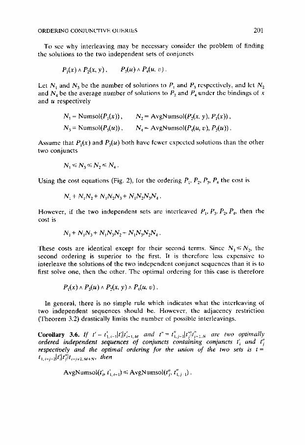
To see why interleaving may be necessary consider the problem of finding the solutions to the two independent sets of conjuncts

Pl(x) ^ P2(x, y) , P3(u) ^ P4(u, v) .

Let N~ and N s be the number of solutions to P~ and/:'3 respectively, and let N 2 and N 4 be the average number of solutions to "°2 and P4 under the bindings of x and u respectively

N l = Numsol(Pl(X)) ,

N 3 = Numsol(P3(u)) ,

N 2 = AvgNumsol(Pz(x , y), PI(x)),

N 4 = A v g N u m s o l ( P 4 ( u , v), /93(/,/)) .

Assume that PI(X) and P3(u) both have fewer expected solutions than the other two conjuncts

N I ~ N 3 ~ N 2 < ~ N 4 .

Using the cost equations (Fig. 2), for the ordering P~, P2, P3, P4 the cost is

N~ + N~N 2 + N~N2N 3 + N~N2N3N 4 .

However, if the two independent sets are interleaved P~, P3, P2, P4, then the cost is

N 1 + N 1 N 3 + N I N 3 N 2 + N I N 3 N 2 N 4 .

These costs are identical except for their second terms. Since N3~< N2, the second ordering is superior to the first. It is therefore less expensive to interleave the solutions of the two independent conjunct sequences than it is to first solve one, then the other. The optimal ordering for this case is therefore

Pl(x) A P3(u) A P2(x, y) A P4(u, v ) .

In general, there is no simple rule which indicates what the interleaving of two independent sequences should be. However, the adjacency restriction (Theorem 3.2) drastically limits the number of possible interleavings.

t p ! t i t tp t ! l / Corollary 3.6. I f t '= tl, i_llti]ti+l, M and = tl.]_lltjltj+Ls are two optimally ordered independent sequences of conjuncts containing conjuncts t'~ and t'~ respectively and the optimal ordering for the union of the two sets is t = t l. i+ j -21 t;[ t;I ti+j+2, M+N, then

AvgNumsol(t'i, ' -< " 1 , j - 1 1 • tLi_l) ~ AvgNumsol(tj, t"


This follows directly from the adjacency restriction but is stronger because the conjuncts in the two sequences are independent. A consequence of this result is that if the beginning conjunct of one sequence has fewer solutions than all conjuncts in the other sequence (i.e., VjNumsol(t'l) ~< AvgNumsol(tT, t';,j 0), it must be the first conjunct in the interleaving. Likewise, if the final conjunct in one sequence has more solutions than all conjuncts in the other sequence (i.e., VjNumsol(t£~)/> AvgNumsol(t~, t'[,j_l)), then it must be last in the interleaving. It is also relatively simple to show that any sequence of conjuncts having a monotonically decreasing sequence of average number of solutions (i.e., AvgNumsol(t'i,t'l. i 0~>AvgNumsol(t'i<,t 'l.~))will not be split by interleaving.

In the example above, these consequences of the adjacency restriction limit the field to only one possible interleaving. P~ must come first because NI is smaller than both N 3 and N 4. Similarly, P4 must come last because N 4 is larger than both N~ and N 2. Finally, P3 must come before P2 because the two conjuncts are adjacent and N 3 ~< N 2.

Although interleaving is necessary in theory, we have been unable to find any practical examples where it is necessary or even advantageous. There is a good reason for this. Independent problems, each of which produce multiple answers, are almost always posed as separate queries. As a result, the optimal ordering for independent sets of conjuncts is almost always a simple concatenation of the optimal orderings for each of the independent pieces. This heuristic can be stated formally as

s = s' U s" A Independent(s ' , s")

^ BestOrdering(s', t') ^ BestOrdering(s", t")

BestOrdering(s, t' I t") v BestOrdering(s, t"] t ' ) .

The advantage of using this criterion should be clear. Given a set of independent conjuncts that divides into n independent pieces, each consisting of k, conjuncts, then the ordering cost is at worst

n

n! + ~ ki! i 1

as opposed to

n

if all possible orderings are considered. For a problem containing ten conjuncts


that divide into two independent sets of five conjuncts each, this amounts to a potential savings of over four orders of magnitude in the cost of finding the optimal ordering.

3.5. Domain-specific ordering advice

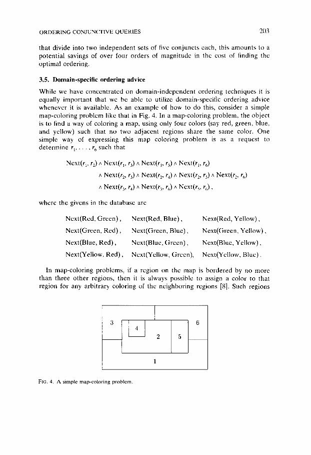
While we have concentrated on domain-independent ordering techniques it is equally important that we be able to utilize domain-specific ordering advice whenever it is available. As an example of how to do this, consider a simple map-coloring problem like that in Fig. 4. In a map-coloring problem, the object is to find a way of coloring a map, using only four colors (say red, green, blue, and yellow) such that no two adjacent regions share the same color. One simple way of expressing this map coloring problem is as a request to determine r l , . . . , r 6 such that

Next(r1, r2) A Next(rl, r3) A Next(r1, rs) ^ Next(rl, r6)

^ Next(r 2, r 3) ^ Next(r 2, r4) ^ Next(r 2, rs) ^ Next(r 2, r 6)

^ Next(r3, r4) A Next(r3, r6) A Next(rs, r6),

where the givens in the database are

Next(Red, Green),

Next(Green, Red) ,

Next(Blue, Red) ,

Next(Yellow, Red) ,

Next(Red, Blue),

Next(Green, Blue),

Next(Blue, Green),

Next(Yellow, Green),

Next(Red, Yellow),

Next(Green, Yellow),

Next(Blue, Yellow),

Next(Yellow, Blue).

In map-coloring problems, if a region on the map is bordered by no more than three other regions, then it is always possible to assign a color to that region for any arbitrary coloring of the neighboring regions [8]. Such regions

FIG. 4. A simple map-coloring problem.


can therefore be postponed, or effectively removed from the map, until the other regions on the map have been determined. For the map above, regions 4 and 5 have this property initially and can therefore be postponed. After these regions are postponed, all of the remaining regions on the map have fewer than four neighbors and can also be postponed, resulting in the null map.

To implement this postponement rule, it must be restated in terms of the set of conjuncts being postponed. If the set of conjuncts containing a given variable has fewer than four members, then the best ordering will amount to postponing that set of conjuncts until after the remaining conjuncts have been solved. Using the vocabulary of Section 1.3 we can state this domain-specific ordering rule formally as

Variable(v) A Contains(s, v) A X = {C: C C S A Contains(c, v)}

A Card(x) < 4 A BestOrdering(s - x, t')

:::> :It"Ordering(x, t") A BestOrdering(s, t'[t"),

(3s)

where Contains indicates that a given conjunct or set of conjuncts contains a particular symbol.

A second domain-specific ordering rule is also useful in map-coloring problems. Regions with exactly four neighbors can also be postponed. In this case, given a coloring for the four neighboring regions, there is a deterministic procedure (known as a Kempe transformation) for adjusting the coloring of the regions already assigned, so that this new region with four neighbors can be colored. (For a complete explanation of the revision algorithm and the rationale behind this ordering rule, see [8].)

The formal statement of this ordering principle is nearly identical to the ordering criterion for regions having fewer than four neighbors (equation (35)). There is, however, a second component . The problem solver must be advised of the revision algorithm. This requires a domain-specific addition to the problem solver and would force us to give some of the details of the problem solver. Since this topic is somewhat tangential we will not pursue it here. The interested reader is referred to [6] for an indication of how this might be done.

4. The Efficiency Issue

As we have seen, conjunct ordering is unavoidable for many difficult problems. Yet for the vast majority of simple problems conjunct ordering does not pay. For these cases the expected savings from performing conjunct ordering is more than offset by the overhead of the ordering strategy.

The solution to this di lemma is a strategy of setting cost thresholds and performing run-time cost monitoring of the problem-solving process. When solving a conjunction the problem solver keeps track of the effort expended in


generating solutions to that conjunct. If that effort ever exceeds the designated threshold, some form of conjunct ordering is invoked and the conjuncts are ordered before proceeding with the problem-solving process. The effect of this technique is that simple problems slip through without incurring significant overhead, while more difficult problems still receive scrutiny.

Of course such a strategy is not limited to single thresholds. For conjunct ordering the most promising approach is to invoke the cheapest-first heuristic when problem cost exceeds a lower threshold. During this calculation, if problem cost is found to exceed a second threshold, a best-first search of the space of possible conjunct orderings is warranted. With such a strategy the heuristic power of a method like cheapest-first can be exploited without fear that its fallibility will lead the system to disaster. The optimal ordering strategy is always invoked if the problem proves sufficiently hard.

In general, cost monitoring and multiple strategy thresholds are valuable for controlling meta-level reasoning, because they have the property that the harder the problem, the more effort the system will put into reasoning about how best to solve the problem. This matches our intuitions that, for easy problems, our systems should not expend much effort analyzing the problem, but should instead just jump in and crank. This seems to be a key to making control reasoning practical. 5

5. Extensions

Throughout this paper we have made several limiting assumptions about the nature of the generate-and-test engine, the characteristics of the database, and the characteristics of conjunctions given to the problem solver. In this section we consider what is necessary to relax these assumptions and discuss some of the open research questions involved in these extensions.

5.1. Augmenting the problem solver

Throughout this paper, we have been assuming a very simple generate-and-test mechanism. Several more sophisticated mechanisms have been proposed and used in various AI systems, often with great success. Though it is not our objective to present or analyze such problem-solving methods, the use of any of these methods will have a subtle effect upon the enterprise of conjunct ordering. The cost equations developed in Section 2 are only valid for the simple generate-and-test mechanism. Different generate-and-test mechanisms have different cost equations and different cost equations give rise to different optimal orderings.

Most augmented generate-and-test procedures take advantage of sub-

A more detailed analysis of the costs and benefits of control strategies can be found in [14, 18]. Further analysis and discussion of run-time cost monitoring can also be found in [18].


problem independence to eliminate unnecessary backtracking. As an example of such a method, consider a generate-and-tes t engine embell ished so that whenever a sequence of conjuncts divides into two independent subsequences, the problem solver finds the solutions to each piece independent ly (as if on separate processors) and then produces the cross-product of the two solution sets (i.e. every solution to one subproblem is paired with every solution to the o ther subproblem).

As an example, consider the problem of finding all of the students who may have had access to a set of files. The conjunct sequence is

Direc toryOf(f , Genesere th)

^ NameField(f , CS223exam)

^ Student(s, CS223) A HasAccoun tOn(s , S U M E X )

^ Username(s , u) ^ Access(u, f ) .

The first two conjuncts of this problem are independent of the next three conjuncts, so our augmented problem solver would independent ly find the indicated exam files and the students in the class that have accounts on the requisite machine. It would then take the cross-product of the two solution sets and try these solutions in the final conjunct to determine which student had access to which files.

The cost of this opera t ion is the sum of the costs of finding the solutions to each independent subsequence plus the cost of construct ing the cross-product of the solution sets. The cost equat ion for this problem solver would therefore be

t = t l , , - l l t , ,m ^ Independent( t l , i 1, ti, M)

Cost '( t) = Cost'(tl, i 1) + C°st'(ti, M) + Numsol(t l , i l)Numsol(ti, M)

as opposed to

Cost ' ( t) = Cost ' ( t i, i-t) + Numsol( t l, i-0Cost'(ti. M)

for s t raightforward generate-and-test . The issue here is not one of determining which method is superior 6 but

rather of finding a cost equat ion that accurately characterizes the behavior of

6In this case the more sophisticated generate-and-test mechanism only pays off when Cost'(t,.M)~>Numsol(ti.M) and Numsol(tl, i-i) ~> 1. When Numsol(tl,i 1) is less than or equal to one, there is no advantage to breaking the problem into independent pieces since solving tl.i i first will actually eliminate solutions that would otherwise have to be tried in ti.M.

O R D E R I N G CONJUNCTIVE Q U E R IE S 207

the problem solver being used. While this was simple enough for the example method given above, it is not necessarily easy in general. One well-known generate-and-test procedure that takes advantage of total independence is selective backtracking [11]. 7 This method functions like a simple generate-and- test procedure as long as the search continues successfully. Under these conditions the cost would be described by the cost equations of Section 2.1. But when failure occurs, and backtracking takes place, previous conjuncts that are independent of the failing conjunct are bypassed by the intelligent backtracking. Thus, the cost equation for failing cases looks more like that in the example above. The actual cost equation for this method is a weighted average of the two different cost equations, where the weighting is a function of the probability of failure for the particular problem at hand.

It would be a mistake to think that ordering and selective backtracking (or any other more sophisticated generate-and-test mechanism) are alternative techniques. They are not. In fact, they are largely orthogonal. The intelligent agent's problem (equation (1)) serves to illustrate that selective backtracking is no substitute for conjunct ordering. For this sequence of conjuncts, smart backtracking provides virtually no improvement over an ordinary generate- and-test engine. Yet, as we argued in Section 1.1 conjunct ordering can provide an improvement of two orders of magnitude.

Likewise, conjunct ordering does not eliminate the advantage of selective backtracking. It is true that an optimally ordered set of conjuncts will naturally involve less backtracking than an arbitrarily ordered set since an optimally ordered set of conjuncts describes a smaller search space and therefore contains fewer branches that fail. However, backtracking does occur any time failure occurs, and intelligent backtracking will be of value in those cases where the optimal ordering consists of whittling away at some portion of the problem by attacking it from several different angles. As an example, consider the problem of finding a president having a brother and a sister who live in Massachusetts. The optimally ordered set of conjuncts is

President(x) ^ Brother(x, b) ^ Resident(b, Mass)

^ Sister(x, s) A Resident(s, Mass).

Suppose that we have found a president with a brother that lives in Mas- sachusetts. If this president has no sisters it is pointless to look for additional

7 There is a strong connection between selective backtracking and dependency-directed backtracking [19]. It is fairly easy to show that selective backtracking is a special case of dependency- directed backtracking or reason maintenance [3] applied to explicit meta-level statements about the satisfiability of the current goals of a problem solver. New goals for a problem solver 'depend upon' previous variable bindings. Hence, when the assumption that a goal is satisfiable proves false one of the premises that led to that assumption must be false, namely one of its variable bindings must be

incorrect.


resident brothers. Selective backtracking is valuable here, since it bypasses the independent brother clause and immediately backtracks to the first clause.

5.2. Dynamic ordering

So far we have been assuming that a single static ordering for a set of conjuncts is optimal for producing all of the solutions. In fact this is not always the case. For example, consider the conjunct

DirectoryOf(f , d),

where the variable d will be bound at the time the conjunct is to be solved. The average number of solutions to this conjunct is

O(Card({f: DirectoryOf(f , d)})) = 20.

Yet some directories have very few files while others have hundreds of files. As a result, the optimal ordering of the remaining conjuncts might be different for different bindings of the directory variable. In general, the optimal ordering for a set of conjuncts is an ordering tree, where each branch of the tree represents a different ordering of the remaining conjuncts corresponding to a different set of solutions to the preceding conjuncts in the tree. The branching factor at each level of the tree corresponds to the sensitivity of the solution-set size for a particular conjunct to the actual variable bindings resulting from previous conjuncts.

Unfortunately, the techniques developed in Section 3 are of little use in determining the optimal-ordering tree. They assume a single static ordering, and base that ordering on averages over the set of all solutions to previous conjuncts. If different orderings are used for different solutions to preceding conjuncts, then the cost equations of Section 2 are not accurate and may not correctly determine even the optimal first conjunct. In general, finding the optimal-ordering tree for a set of conjuncts requires searching through the space of all possible ordering trees. Of course this is an enormous space. Furthermore, generating each tree requires knowledge of the actual solutions to each conjunct. Determining the optimal tree therefore requires solving the problem many times over.

The best that can be done is to choose the first conjunct based on the cost equations of Section 2, generate the solutions to that conjunct, and then for each solution to that conjunct choose the best next conjunct, and so forth. In other words, at each step in the generate-and-test process the remaining conjuncts are ordered for each solution to the preceding conjuncts. We refer to this as dynamic ordering.

Assuming that the set sizes used in ordering calculations are accurate,


dynamic ordering is guaranteed to result in a problem search space which is at least as small as that produced by the initial (static) ordering. In cases where set size is sensitive to the actual variable bindings, the improvement resulting from dynamic ordering can be dramatic.

Unfortunately, dynamic ordering is very costly because it multiplies the complexity of the search space by the complexity of the ordering problem. A solution to this difficulty is to limit dynamic reordering to those cases where it is likely to have a pronounced effect. This requires preserving the number of solutions information (calculated during the initial ordering of the conjuncts) and at each step in the generate-and-test process, verifying that the actual number of solutions to each of the remaining conjuncts does not vary significantly from the average calculated initially. If the actual number of solutions for some conjunct grossly exceeds the estimated value, dynamic reordering is warranted. Similarly, if some remaining conjunct has far fewer solutions than anticipated, there might be considerable advantage to reordering the remaining conjuncts.

Of course, run-time cost monitoring should also be used in conjunction with any dynamic ordering strategy. For easy or even modera te problems, the expense of reordering is not warranted. But for very hard problems dynamic reordering can make the difference between solution and failure.

5.3. Including inference

In Section 2.2 we restricted our analysis to the case where the cost of finding a solution to a conjunct is constant. In doing so we limited our analysis to cases in which all answers to a conjunct are available in the system's database. This assumption is not reasonable for many AI systems. For these systems the cost of inference must also be included in the total cost of finding the answers to a conjunction.

It is relatively simple to extend the cost equation (9) to include the cost of inference. Instead of the total number of solutions to the problem we are now interested in the number that can be found in the database, together with the cost of finding answers by all available inference paths. A simple way to express this cost is with three factors: the cost of producing answers available in the database, the cost of one level of backward inference, and the cost of producing answers to all of the subgoals. 8 Formally,

8 If sensory actions are used to find answers to queries, then their cost must also be included. This can be handled by including an additional factor CostSensing(q) in the cost equation. For the

case of an intell igent agent most data are gathered using sensory actions of querying the operating system. However, in this case the query cost is insignificant in comparison to the cost of the generate-and-test . We can therefore omit this additional complication in this case.


Cost(q) = A + K* Numlndb(q)

+ L * N u m l n d b ( " p ~ q" ) + ~'~ Cost (p ) , /p: p~ q~

where K is the cost of retrieving a single answer in the database and L is the cost of performing a single backward inference. This formula is recursive and cannot be simplified in any obvious way. This is because subgoals may themselves be conjunctive and as a result may cost far more to solve than the number of answers that they produce. In addition, redundant answers may appear in different branches of the search space, and this cost must be included. To compute cost using this formula, a system must therefore have information about the relative costs of database references and backward inferences, the number of solutions available in the database, and the number of rules relevant to backward inference for a conjunct. In general, the latter factor is difficult to estimate since the amount of inference may depend upon the particular variable bindings for a conjunct. An upper bound on the number of inferences is possible by considering all rules that could be applicable. A more accurate estimate is possible by computing the 'expected ' number of inferences given arbitrary instances of the set of bound variables. This can be done by dividing the upper-bound figure by the domain sizes for the bound variables.

Given all this information the cost of finding the solutions to a specific sequence of conjuncts can be found by recursively computing the cost for each branch of the inference tree. For a large inference tree this computation is quite expensive. It must therefore be done only when the difficulty of the conjunctive problem warrants it.

Unfortunately, ordering conjuncts that involve inference raises a much more serious difficulty. Some of the answers to a conjunct may be readily available in the system's database while others may require extensive inference. As a result there may be a large discrepancy between the cost of finding one group of answers to a problem, and the cost of finding the remaining answers. One ordering may be preferable for finding the first group of answers, while another is preferable for the remaining answers. This violates the assumption that a single static ordering will be sufficient. In addition, as Moore points out [9, p. 82ff] the optimal ordering may require interleaving conjuncts from a conjunctive subgoal with the remaining top-level conjuncts. All of this points to the necessity of run-time cost monitoring and dynamic ordering in cases where inference is involved. This subject demands considerably more study.

5.4. Infinite sets

Finally, suppose that every conjunct has an infinite number of solutions, but only a finite number of answers are needed. Such cases are particularly


prevalent in planning problems. For example, a conjunct such as On(B, x) effectively has an infinite number of solutions because the robot arm can move the block B to an infinite number of different locations. Clearly in such cases the cost analysis of Section 2 does not apply. The assumption that "the cost of finding a single solution will be that fraction of the cost of finding all solutions" is not valid since all of the quantities involved are infinite. In computing cost for this case what must be considered is not the total number of solutions for each of the conjuncts, but rather the likelihood that a solution to one conjunct will satisfy the succeeding conjuncts. In other words, the cost for finding one solution to the conjunction is computed directly by estimating the number of solutions that must be generated to the first conjunct in order to find one that will satisfy succeeding conjuncts. This can be made precise by dividing each term in the cost equations (Fig. 2) by the total number of solutions to the conjunction. Simplification then gives a usable cost equation for determining conjunct order in those cases. Further analysis and discussion of this topic can be found in [18].

6. Discussion

6.1. Related work

Many papers have been published on the subject of optimizing relational database queries. (A good summary of this work can be found in [20].) While the basic problem is the same in both cases (finding the optimal way of generating the answers satisfying a conjunctive expression) the methodology and assumptions are usually quite different.

In the database community, the language of Relational Algebra [20] has been widely adopted as a means of expressing queries. The algebra is a language for expressing sequences of referencing and combining operations on databases indexed by relation. In general, any query can be implemented in terms of these operations.

A large percentage of query-optimization research has been concerned with syntactic transformations of these relational-algebra expressions. These optimizations can, and usually do improve the efficiency of such expressions. However these inefficiencies are, to a large extent, introduced by the language of relational algebra. A simple generate-and-test engine, operating on predicate calculus expressions, automatically includes these optimizations as a side effect of substituting variable bindings into the remaining conjuncts (at each step in the generation process). We take these optimizations entirely for granted. As a result, work on relational algebra has little relevance to the work presented in this paper.

Leaving the work on relational algebra aside, database work often differs from the work here in the criterion used for calculating the cost of solving a conjunct. For example, in the database world, some of the assumptions are:


- D a t a b a s e s are extremely large and must be stored on disk rather than kept in memory. As a consequence, the number of disk accesses is the important optimization criterion, not the size of the search space.

- O f t e n databases employ incomplete indexing mechanisms (e.g. indexing only on the relations of facts). For example, the cost of finding the father of a given person can therefore be just as high as the cost of producing all father-progeny pairs in the database. In contrast, we have assumed that the database is completely indexed which implies that the cost of finding the father of a given person is the constant factor K.

- T h e database can be regarded as a 'closed world' [12]. The ability to enumerate the solutions to a particular conjunct is never in question.

-Concur ren t accesses and updates to the database must be considered. As a result, the amount of time that a given portion of the database is ' locked' is an important (sometimes the most important) cost criterion. If we factor out differences in the calculation of cost, there are several

database systems which employ some simple conjunct-ordering heuristics similar to those presented in Section 3.

In the INGRES system [20, 22] a graph-decomposition algorithm is used for ordering conjuncts. This algorithm implicitly encodes several ordering heuristics: - Prefer conjuncts which contain one or more constant arguments -P r e f e r 'simply connected' conjuncts (a simple connected conjunct is one

whose variables do not appear in any inequality or disjunction). - P r e f e r conjuncts have a 'small' number of solutions. -P r e f e r conjuncts which break the problem into two or more totally in-

dependent pieces. A second system, called SYSTEM R [15,20], uses a similar set of ordering heuristics: - P r e f e r conjuncts containing one or more constant arguments. - P r e f e r conjuncts containing one or more arguments that participate in an

inequality with a constant. - P r e f e r the conjunct having the fewest solutions. For both of these systems, the combination of heuristics has an effect similar to that of the cheapest-first and connectivity heuristics examined in Section 3.

The cheapest-first heuristic was introduced to artificial intelligence by Kowalski [7, p. 93] and later by Moore [9, p. 78ff]. Warren describes its use in a eROLOG-based natural-language system called CHAT-80 [21]. This work is particularly notable because it uses more sophisticated cost computations than in the systems mentioned above. In particular, the use of domain information in CHAT-a0 provided the inspiration for the analysis in Sections 2.3 and 2.4.2.

There are several important differences between the work described above and the work described in this paper. As we pointed out in Section 3 there are many cases where simple ordering heuristics fail badly. As a result, we have


stressed the importance of searching the space of possible conjunct orderings to determine an optimal ordering. We have also argued that this need not be outrageously expensive if best-first search is employed. In addition we have stressed run-time cost monitoring and thresholds as a way of avoiding the overhead of conjunct ordering for the majority of cases in which conjunct ordering is not cost-effective.

A second difference between our approach and that employed in the above work is that we have used an explicit declarative language for expressing conjunct-ordering strategies, rather than encoding this information procedurally. However, as we mentioned in Section 1.2 this distinction is superficial. It is the techniques and results which are important and not the language of description. Any of the techniques developed in this paper could be encoded procedurally for use in an intelligent system.

However there is one interesting manifestation of our choice of language; predicate calculus has allowed us to express information about set sizes that could not be expressed in the systems described above. Specifically, information about the cost of solving whole groups of problems can be stated in this language. For example, to determine the number of solutions to the problem Parent(x, y) where the variable x is given, a database system would determine how many parent-progeny tuples were in the database, then determine how many different x's there were in these tuples, and divide the two numbers to produce an average value. In contrast, using the approach presented here, we could directly state the general fact that a person has only two parents:

Person(x) ~ Numsol("Parent(y, X)") = 2.

A final distinction between our work and that of the work described above is our (preliminary) consideration of issues such as embellished generate-and-test engines, dynamic ordering, and treatment of inference and infinite sets. These are issues which are relatively unimportant to the database community.

6.2. Current status

The methods described in Section 3 have been implemented in experimental versions of the MRS system [5] and have been tested on sample problems from the Intelligent Agents project at Stanford [4]. We are currently attempting to further test these methods by integrating them into the planning and problem- solving system being developed for the Intelligent Agents project.

Run-time cost monitoring with thresholding is currently undergoing implementation in the MRS system. This implementation relies on the basic reflective architecture of MRS [6].

Finally we are involved in further research on several of the questions


m e n t i o n e d in Sect ion 5. In par t icu lar , we are ex tend ing the me thods of this p a p e r to hand le p lanning p r o b l e m s and p r o b l e m s that involve inference .

6.3. Conclusions

In this p a p e r we have a rgued that conjnnc t o rde r ing is unavo idab l e for many inte l l igent systems. F o r the in te l l igent agent many real is t ic reques t s cannot be solved wi thout recourse to con junc t order ing .

Whi le s imple o rde r ing heuris t ics may work well for the ma jo r i t y of cases, there are still many examples where such heuris t ics lead to in to le rab le o rder - ings. F o r these cases it is necessary to resor t to a search of the space of poss ib le con junc t order ings . Best-f irst search can significantly reduce the cost of this exp lo ra t ion , of ten to the ex ten t that it is not significantly more expens ive than the use of fal l ible heur is t ics such as ' cheapes t - f i r s t ' .

Desp i t e this advan tage , ind i sc r imina te use of any c o n j u n c t - o r d e r i n g procedure can add subs tant ia l o v e r h e a d to a p rob lem-so lv ing system. As a result , run- t ime cost mon i to r ing and select ive con junc t o rde r ing may be necessary for many appl ica t ions . If a given sequence costs lit t le to solve, the expense of o rde r ing is not just if ied. Howeve r , if a sequence is m o d e r a t e l y expens ive to solve, a s imple con junc t -o rde r i ng s t ra tegy (such as the cheapest - f i rs t heuris t ic) should be invoked . If the o rde r ing found by this s t ra tegy is still sufficiently expens ive , a best-f irst search of the conjunc t o rde r ing space is war ran ted .

The cost or 'difficulty ' of solving a p r o b l e m is a centra l t heme of this research . In add i t ion to its uti l i ty for o rde r ing conjuncts , such in fo rmat ion has o the r app l i ca t ions in cont ro l l ing inference [17, 18]. W e also be l ieve that this not ion is a crucial c o m p o n e n t of bui ld ing truly robus t in te l l igent systems. The abi l i ty to eva lua te the difficulty of a p r o b l e m pe rmi t s a system to eva lua te its own abi l i ty or inabi l i ty to solve a p r o b l e m before or dur ing the p rob lem-so lv ing process . This capaci ty is necessary if a system is to avoid p r o b l e m s that lie ou ts ide of its doma in of exper t i se , or are too difficult for it to solve.

ACKNOWLEDGMENT

We wish to thank John McCarthy for bringing an interesting example o1 domain-specific ordering to our attention. Thanks also to Gordon Novak, Jeff Ullman, and Gio Wiederhold for pointers to relevant database literature on this subject. Jim Bennett, Jan Clayton, Tom Dienerich, Russ Greiner, Pat Hayes, Jock Mackinlay, John McCarthy, Drew McDermott and Richard Treitel provided useful comments on drafts of this paper.

This work was supported by ONR contract N00014-81-K-0004.

REFERENCES

1. Barr, A. and Feigenbaum, E., The Handbook of Artificial Intelligence I (HeurisTech Press, Stanford, CA, 1981).

2. Buchanan, B.G. and Shortliffe, E.H., Rule-Based Expert Systems: The M Y ( I N Experiments of the Stanford Heuristic Programming Project (Addison-Wesley, Reading, MA, 1984).


3. Doyle, J., A truth maintenance system, Artificial Intelligence 12 (1979) 231-272. 4. Feigenbaum, E.A., Genesereth, M., Kaplan, S.J. and Mostow, D.J., Intelligent Agents,

Proposal to the Defence Advanced Research Projects Agency, 1980. 5. Genesereth, M.R., An overview of MRS, Heuristic Programming Project Memo, Stanford

University, Stanford, CA, 1983. 6. Genesereth, M.R., An overview of meta-level architecture, in: Proceedings Third National

Conference on Artificial Intelligence, Washington, DC, 1983. 7. Kowalski, R., Logic for Problem Solving (North-Holland, Amsterdam, 1979). 8. McCarthy, J., Coloring maps and the Kowalski doctrine, Tech. Rept. STAN-CS-82-903,

Stanford University, Stanford, CA, 1982. 9. Moore, R.C., Reasoning from incomplete knowledge in a procedural deduction system,

Artificial Intelligence Laboratory Memo AI-TR-347, Massachusets Institute of Technology, Cambridge, MA, 1975.

10. Nilsson, N.J., Principles of Artificial Intelligence (Tioga, Palo Alto, CA, 1980). 11. Pereira, L.M. and Porto, A., Selective backtracking, in: K. Clark and S. Tarnlund (Eds.), Logic

Programming (Academic Press, New York, 1982) 107-114. 12. Reiter, R., On closed world databases, in: H. Gaillaire and J. Minker (Eds.), Logic and Data

Bases (Plenum Press, New York, 1978) 55-76. 13. Reiter, R., A logic for default reasoning, Artificial Intelligence 13 (1980) 81-132. 14. Rosenschein, J. and Singh, V., The utility of meta-level effort, Heuristic Programming Project

Memo HPP-83-20, Stanford University, Stanford, CA, 1983. 15. Selinger, P., Astrahan, M., Chamberlin, D.. Lorie, R. and Price, T., Access path selection in a

relational database management system, in: Proceedings ACM/SIGMOD International Con- ference on Management of Data (1979) 23-34.

16. Simon, H. and Kadane, J., Optimal problem-solving search: All-or-none solutions, Artificial Intelligence 6 (1975) 235-247.

17. Smith, D.E., Finding all of the solutions to a problem, in: Proceedings Third National Conference on Artificial Intelligence, Washington, DC, 1983.

18. Smith, D.E., Controlling inference, Ph.D. Dissertation, Stanford University, Stanford, CA, 1985.

19. Stallman, R.M. and Sussman, G.J., Forward reasoning and dependency-directed backtracking in a system for computer-aided circuit analysis, Artificial Intelligence 9 (2) (1977) 135-196.

20. Ullman, J.D., Principles of DataBase Systems (Computer Science Press, Rockville, MD, 1982). 21. Warren, D., Efficient processing of interactive relational database queries expressed in logic, in:

Proceedings Seventh VLDB Conference (1981) 272-281. 22. Wong, E. and Youssefi, K., Decomposi t ion-a strategy for query processing, ACM Trans.

Database Systems 1 (3) (1976) 223-241.

Rece ived December 1983; revised version received October 1984

Ordering conjunctive queries

Documents

Transcript of Ordering conjunctive queries