arX

iv:p

hysi

cs/0

4030

31v1

[ph

ysic

s.da

ta-a

n] 3

Mar

200

4

Deriving Laws from Ordering Relations

Kevin H. Knuth

Computational Sci. Div., NASA Ames Research Ctr., M/S 269-3, Moffett Field CA 94035

Abstract. The effect of Richard T. Cox’s contribution to probability theory was to generalizeBoolean implication among logical statements to degrees ofimplication, which are manipulatedusing rules derived from consistency with Boolean algebra.These rules are known as the sumrule, the product rule and Bayes’ Theorem, and the measure resulting from this generalization isprobability. In this paper, I will describe how Cox’s technique can be further generalized to includeother algebras and hence other problems in science and mathematics. The result is a methodologythat can be used to generalize an algebra to a calculus by relying on consistency with order theoryto derive the laws of the calculus. My goals are to clear up themysteries as to why the same basicstructure found in probability theory appears in other contexts, to better understand the foundationsof probability theory, and to extend these ideas to other areas by developing new mathematicsand new physics. The relevance of this methodology will be demonstrated using examples fromprobability theory, number theory, geometry, informationtheory, and quantum mechanics.

INTRODUCTION

The algebra of logical statements is well-known and is called Boolean algebra[1, 2].There are three operations in this algebra: conjunction∧, disjunction∨, and comple-mentation∼. In terms of the English language, the logical operation of conjunction isimplemented by the grammatical conjunction ‘and’, the logical operation of disjunc-tion is implemented by the grammatical conjunction ‘or’, and the logical complementis denoted by the adverb ‘not’. Implication among assertions is defined so that a logicalstatementa implies a logical statementb, writtena→ b, whena∨b = b or equivalentlywhena∧b = a. These are the basic ideas behind Boolean logic.

The effect of Richard T. Cox’s contribution to probability theory [3, 4] was to general-ize Boolean implication among logical statements to degrees of implication representedby real numbers. These real numbers, which represent the degree to which we believeone logical statement implies another logical statement, are now recognized to be equiv-alent to probabilities. Cox’s methodology centered on deriving the rules to manipulatethese numbers. The key idea is that these rules must maintainconsistency with the un-derlying Boolean algebra. Cox showed that the product rule derives from associativityof the conjunction, and that the sum rule derives from the properties of the complement.Commutativity of the logical conjunction leads to the celebrated Bayes’ Theorem. Thisset of rules for manipulating these real numbers is not one ofset of many possible rules;it is the unique generalization consistent with the properties of the Boolean algebraicstructure.

Boole recognized that the algebra of logical statements wasthe same algebra thatdescribed sets [1]. The basic idea is that we can exchange ‘set’ for ‘logical statement’,

‘set intersection’ for ‘logical conjunction’, ‘set union’for ‘logical disjunction’, ‘setcomplementation’ for ‘logical complementation’, and ‘is asubset of’ for ‘implies’ andyou have the same algebra. We exchanged quite a few things above and its useful tobreak them down further. We exchanged theobjectswe are studying: ‘sets’ for ‘logicalstatements’. Then we exchanged theoperationswe can use to combine them, such as‘set intersection’ for ‘logical conjunction’. Finally, weexchanged the means by whichwe order these objects: ‘is a subset of’ for ‘implies’. The obvious implication of this isthat Cox’s results hold equally well for defining measures onsets. That is we can assignreal numbers to describe the degree to which one set is a subset of another set. Thealgebra allows us to have a sum rule, a product rule, and a Bayes’ Theorem analog—justlike in probability theory!

It has been recognized for some time that there exist relationships between othertheories and probability theory, but the underlying reasons for these relationships havenot been well understood. The most obvious example is quantum mechanics, which hasmuch in common with probability theory. However, it is clearly not probability theorysince quantum amplitudes are complex numbers rather than real numbers. Anotherexample is the analogy recognized by Carlos Rodríguez between the cross-ratio inprojective geometry and Bayes’ Theorem [5]. In this paper, Iwill describe how Cox’stechnique can be further generalized to include other algebras and hence other problemsin science and mathematics. I hope to clear up some mysteriesas to why the samebasic structure found in probability theory appears in other contexts. I expect thatthese ideas can be taken much further, and my hope is that theywill eventually leadto new mathematics and new physics. Last, scattered throughout this paper are manyobservations and connections that I hope will help lead us todifferent ways of thinkingabout these topics.

LATTICES AND ALGEBRAS

Basic Ideas

The first step is to generalize the basic idea behind the elements described in ourBoolean algebra example: objects, operations, and ordering relations. We start with a setof objects, and we select a way to compare two objects by deciding whether one object is‘greater than’ another object. This means of comparison allows us to order the objects. Aset of elements together with abinary ordering relationis called apartially ordered set,or aposet. It is called apartial order to allow for the possibility that some elements in theset cannot be directly compared. In our example with logicalimplication, the orderingrelation was ‘implies’, so that if ‘a impliesb’, written a → b, thenb is in some sense‘greater than’a, or equivalently,a is in some sense ‘included in’b. An ordering relationis generally written asa≤ b, and read as ‘b includesa’ or ‘ a is contained inb’. Whena≤ b, buta 6= b then we writea < b, and read it as ‘a is properly contained inb’. Last,if a < b, but there does not exist any elementx in the setP such thata < x < b, then wesay that ‘b coversa’, and writea≺ b. In this case,b is an immediate successor toa inthe hierarchy imposed by the ordering relation. It should bestressed that this notation is

FIGURE 1. Four different posets. (a) The positive integers ordered by‘is less than or equal to’. (b)The positive integers ordered by ‘divides’. (c) The powerset of a,b,c ordered by ‘is a subset of’. (d)Three mutually exclusive logical statementsa, k, n ordered by ‘implies’. Note that the same set can lead todifferent posets under different ordering relations (a andb), and that different sets under different orderingrelations can lead to isomorphic posets (c and d).

general for all posets, but that the relation≤ means different things in different examples.We can draw diagrams of posets using the ordering relation and the concept of

covering. If for two elementsa andb, a ≤ b then we drawb abovea in the diagram.If a ≺ b then we connect the elements with a line. Figure 1 shows examples of foursimple posets. Figure 1a is the set of positive integers ordered according the the usualrelation ‘is less than or equal to’. From the diagram one can see that 2≤ 3, 2≺ 3, butthat 2⊀ 4. Figure 1b shows the set of positive integers ordered according to the relation‘divides’. In this poset 2≤ 8 means that 2 divides 8. Also, 4≺ 12 since 4 divides 12,but there does not exist any positive integerx, wherex 6= 4 andx 6= 12, such that 4dividesx andx divides 12. This poset is clearly important in number theory. Figure 1cshows the set of all subsets (thepowerset) of a,b,c ordered by the usual relation ‘isa subset of’, so that in this case≤ represents⊆. From the diagram one can see thata ⊆ a,b,c, and thatb is covered by botha,b andb,c. There are elementssuch asa andb wherea * b andb * a. In other words, the two elementsare incomparable with respect to the ordering relation. Last, Figure 1d shows the setof three mutually exclusive assertionsa,k, andn ordered by logical implication. Theseassertions, discussed in greater detail in [6], represent the possible suspects implicatedin the theft of the tarts made by the Queen of Hearts in Chapters XI and XII of Lewis

Carroll’sAlice’s Adventures in Wonderland

a = ‘Alice stole the tarts!’

k = ‘The Knave of Hearts stole the tarts!’

n = ‘No one stole the tarts!’

Logical disjunctions of these mutually exclusive assertions appear higher in the poset.The element⊥ represents the absurdity, and⊤ represents the disjunction of all threeassertions,⊤ = a∨k∨n, which is the truism.

There are two obvious ways to combine elements to arrive at new elements. Thejoinof two elementsa andb, written a∨ b, is their least upper bound, which is found byfinding botha andb in the poset and following the lines upward until they intersect ata common element. Dually, themeetof a andb, written a∧b, is their greatest lowerbound. In Figure 1c,a∨ b = a,b, anda,b∧ b,c = b. In that poset, thejoin ∨ is found by the set union∪ and the meet∧ by set intersection∩. For the posetof logical statements in Figure 1d the notation is a bit more transparent as the joinis the logical disjunction (OR). For the meet we have,(a∨ k)∧ (k∨ n) = k, which isthe logical conjunction (AND). In Figure 1b,∧ represents the greatest common divisorgcd(); whereas∨ represents the least common multiplelcm(). In Figure 1a, 2∨3 = 3,and 2∧3 = 2. In this case∨ acts as themax() function selecting the greatest element;whereas∧ acts as themin() function selecting the least element. Again, it is importantto keep in mind that the symbols∨ and∧ mean different things in different posets.

Some posets possess a top element, which is calledtopand is generally written as⊤.The bottom element, calledbottom, is generally written as⊥ or equivalently∅. There isan important set of elements in the poset called thejoin-irreducible elements. These areelements that cannot be written as the join of two other elements in the poset. The bottomis never included in the join-irreducible set. In Figure 1c,there are three join-irreducibleelementsa,b,c.

The join-irreducible elements that cover the bottom element are called theatoms.In Figure 1b, the bottom element is 1, the atoms are the prime numbers, and thejoin-irreducible elements are powers of primes. Furthermore, two primesp andq arerelatively prime if their meet is the bottom elementp∧q = ⊥, that is if gcd(p,q) = 1.1 In Figure 1d, the atoms are the the exhaustive set of mutuallyexclusive assertionsa, kandn. The join-irreducible elements are extremely important asall the elements in theposet can be formed from joins of the join-irreducible elements.

These examples show that the same set under two different ordering relations canresult in two different posets (Figures 1a and b), and that two different sets underdifferent ordering relations can result in isomorphic posets (Figures 1c and d). I havediscussed these ideas before [6, 8], and one can search out more details in the accessiblebook by Davey & Priestly [9], and the classic by Birkhoff [10].

1 This is reminiscent of the notation advocated by Graham, Knuth, & and Patashnik [7, p.115] wherep⊥qdenotes thatp andq are relatively prime.

Lattices

Posets have the following properties. For a posetP, and elementsa,b,c∈ P,

P1. For all a, a≤ a (Reflexive)P2. I f a ≤ b and b≤ a, then a= b (Antisymmetry)P3. I f a ≤ b and b≤ c, then a≤ c (Transitivity)

If a unique meetx∧ y and joinx∨ y exists for allx,y ∈ P, then the poset is called alattice. Each latticeL is actually analgebradefined by the operations∨ and∧ alongwith any other relations induced by the structure of the lattice. Dually, the operationsof the algebra uniquely determine the ordering relation, and hence the lattice structure.Viewed as operations, the join and meet obey the following properties for allx,y,z∈ L

L1. x∨x = x, x∧x = x (Idempotency)L2. x∨y = y∨x, x∧y = y∧x (Commutativity)L3. x∨ (y∨z) = (x∨y)∨z, x∧ (y∧z) = (x∧y)∧z (Associativity)L4. x∨ (x∧y) = x∧ (x∨y) = x (Absorption)

There is a special class of lattices calleddistributive latticesthat follow

D1. x∧ (y∨z) = (x∧y)∨ (x∧z) (Distributivity of∧ over∨)

and its dual

D2. x∨ (y∧z) = (x∨y)∧ (x∨z) (Distributivity of∨ over∧)

All distributive lattices can be expressed in terms of elements consisting of sets where thejoin∨ and the meet∧ are identified as the set union∪ and set intersection∩, respectively.

Some distributive lattices possess the property calledcomplementationwhere forevery elementx in the lattice, there exists a unique element∼ x such that

C1. x∨ ∼ x = ⊤C2. x∧ ∼ x = ⊥

Boolean lattices arecomplemented distributive lattices. Since all distributive lattices canbe described in terms of a lattice of sets, the condition of a distributive lattice beingcomplemented is equivalent to the condition that the lattice contains all possible subsetsof the lattice elements, which is called thepowerset. Thus lattices of powersets areBoolean lattices. The situation gets interesting when one starts removing elements fromthe powerset. For example, if one element is removed from a Boolean lattice, then therewill be another element that no longer has a unique complement. This is equivalent toadding constraints, and these constraints take the Booleanlattice to a distributive lattice,which no longer has complementation as a general property.

These are basic mathematical concepts and are not restricted to the area of logicalinference. Viewed as a collection of partially ordered objects, we have a lattice. Viewedas a collection of objects and a set of operations, such as∨ and∧, we have an algebra.What I will show in the remainder of this paper is that a given lattice (or equivalentlyits algebra) can be extended to a calculus using the methodology introduced by Cox,and that there already exist a diverse array of examples outside the realm of probabilitytheory.

DEGREES OF INCLUSION

For distinctx andy in a poset wherey includesx, writtenx≤ y, it is clear thatx does notincludey, y x. However, we would like to generalize this notion of inclusion so thateven thoughx does not includey, we can describe thedegreeto whichx includesy. Thisidea is perhaps made more clear by thinking about a concrete problem in probabilitytheory. Say that we know that a logical statementa∨b∨c is true. Clearly,a→ a∨b∨csincea≤ a∨b∨c. However, it is useful to quantify thedegreeto whicha∨b∨c impliesa, or equivalently the degree to whicha includesa∨b∨c. It is in this sense that we aimto generalize inclusion on a poset to degrees of inclusion.

The goal of this paper is to emphasize that inclusion on a poset can be generalized todegrees of inclusion, which results in a set of rules or laws by which these degrees maybe manipulated. These rules are derived by requiring consistency with the structure ofthe poset. At this stage, it is not clear for exactly what types of posets or lattices this canbe done, precisely what rules one obtains and under what conditions, and exactly whattypes of mathematical structures can be used to describe these degrees of inclusion.These remain open questions and will not be explicitly considered in this paper.

What is clear is that Cox’s basic methodology of deriving thesum and product rulesof probability from consistency requirements with Booleanalgebra [3, 4] has a muchgreater range of applicability than he imagined. His specific results are restricted tocomplemented lattices as he used the property of complementation to derive the sumrule. In the following sections, I will consider the larger class of distributive lattices,which include Boolean lattices as a special case. To derive the laws governing themanipulation of degrees of inclusion, I will rely on the proofs introduced by ArielCaticha [11], which utilize consistency with associativity and distributivity. As I willshow below, the sum rule is consistent with associativity ofthe join, and therefore mostlikely enjoys a much greater range of applicability—perhaps extending to all lattices.The derivations that follow will focus on finite lattices, although extension to an infinitelattice is reasonable.

Joins and the Sum Rule

Throughout this subsection, I will follow and expand on Caticha’s derivation andmaintain consistency with his basic notation, all the whileconsidering this endeavor asa generalization of inclusion on a poset. We begin by defininga functionφ that assignsto a pair of elementsx andy of the latticeL a real number2 d ∈ R, so thatφ : L×L → R

d = φ(x,y), (1)

2 For simplicity I will work with degrees of inclusion measured by real numbers. However, it should bekept in mind that Caticha’s derivations were developed for complex numbers [11], Aczél’s solutions forthe associativity equation were for real numbers, groups and semigroups [12], and Rota’s theorems for thevaluation equation apply to commutative rings with an identity element [13].

and remember thatd represents the degree to whichx includesy, which generalizesthe algebraic inclusion≤. 3 This can be compared to Cox’s notation where insteadof the functionφ(x,y), he writes(y → x) for the special case where he is consideringimplication among logical statements. By replacing the comma with the solidusφ(x|y),we obtain a notation more reminiscent of probability theory.

Now consider two join-irreducible elements of the lattice,a andb, wherea∧b = ⊥,and a third elementt such thata≤ t andb≤ t. We will consider the degree to which thejoin a∨b of these join-irreducible elements includes the elementt. As a∨b is itself alattice element, the functionφ allows us to describe the degree to whicha∨b includest.This degree is written asφ(a∨b, t). As a∧b = ⊥, this degree of inclusion can only bea function ofφ(a, t) andφ(b, t), which can be written as

φ(a∨b, t) = S(φ(a, t),φ(b, t)). (2)

Our goal is to determine the functionS, which will tell us how to use the degree to whicha includest and the degree to whichb includest to compute the degree to whicha∨bincludest. In this sense we are extending the algebra to a calculus.

The functionS must maintain consistency with the lattice structure, or equivalentlywith its associated algebra. If we now consider another join-irreducible elementc ≤ twherea∧ c = ⊥ andb∧ c = ⊥, and form the lattice element(a∨ b)∨ c, we can useassociativity of the lattice to write this element a second way

(a∨b)∨c= a∨ (b∨c). (3)

Consistency with associativity requires that each expression gives exactly the same result

S(φ(a∨b, t),φ(c, t))= S(φ(a, t),φ(b∨c, t)). (4)

Applying S to the argumentsφ(a∨b, t) andφ(b∨c, t) above, we get

S(S(φ(a, t),φ(b, t)),φ(c, t))= S(φ(a, t),S(φ(b, t),φ(c, t))). (5)

This can be further simplified by lettingu = φ(a, t), v = φ(b, t), andw = φ(c, t), whichgives

S(S(u,v),w) = S(u,S(v,w)). (6)

This result is an equation for the functionS, which emphasizes its property of associativ-ity. To people who are familiar with Cox’s work [3, 4], this functional equation should beimmediately recognizable as what Aczél appropriately called the associativity equation[12, pp.253-273]. In Cox’s derivation of probability theory we are accustomed to seeingthis in terms of the logical conjunction. However, it is important to recognize that boththe conjunction and disjunction follow associativity, andthat this result generalized tothe join is perfectly reasonable. The general solution, from Aczél [12], is

S(u,v) = f ( f−1(u)+ f−1(v)), (7)

3 This diverges from Caticha’s development as he considers functions that take a single poset element asits argument. I discuss this difference in more detail in thesections that follow.

where f is an arbitrary function. This can be simplified by lettingg = f−1

g(S(u,v)) = g(u)+g(v), (8)

and writing this in terms of the original lattice elements wefind that

g(φ(a∨b, t)) = g(φ(a, t))+g(φ(b, t)). (9)

As Caticha emphasizes, this result is remarkable, as it reveals that there exists afunction g : R → R re-mapping these numbers to a more convenient representation.Thus we can define a new map from the lattice elements to the real numbers, such thatν(a, t)≡ g(φ(a, t)). This lets us write the combination rule as

ν(a∨b, t) = ν(a, t)+ν(b, t), (10)

which is the familiarsum rule of probability theory for mutually exclusive (join-irreducible) assertionsa andb

p(a∨b|t) = p(a|t)+ p(b|t). (11)

This result is extremely important, as I have made no reference at all to probabilitytheory in the derivation. Only consistency with associativity of the join, which is aproperty of all lattices, has been used. This means that for agiven lattice, we can definea mapping from a pair of its elements to a real number, and whenwe take joins of itsjoin-irreducible elements, we can compute the new value of this join by taking the sumof the two numbers. There are some interesting restrictions, which I will discuss later.

Extending the Sum Rule

The assumption made above was that the two lattice elements were join-irreducibleand that their meet was the bottom element. How do we perform the computation in theevent that this is not the case? In this section I will demonstrate how the sum rule can beextended in a distributive lattice. Consider two lattice elementsx andy. In a distributivelattice all elements can be written as a unique join of join-irreducible elements

x = (n

∨

i=1

pi)∨ (k

∨

i=1

qi) (12)

and

y = (m∨

i=1

r i)∨ (k

∨

i=1

qi), (13)

where I have written them so that the join-irreducible elements they have in common arethe elementsq1,q2, ...qk. The join ofx andy can be written as

x∨y = (n

∨

i=1

pi)∨ (k

∨

i=1

qi)∨ (m∨

i=1

r i)∨ (k

∨

i=1

qi), (14)

which can be simplified to

x∨y = (n

∨

i=1

pi)∨ (k

∨

i=1

qi)∨ (m∨

i=1

r i), (15)

since byL1 andL2

(k

∨

i=1

qi)∨ (k

∨

i=1

qi) =k

∨

i=1

qi. (16)

Since thepi ,qi , andr i are all join-irreducible elements, we can use the sum rule repeat-edly to obtain

ν(x∨y, t) =n

∑i=1

ν(pi , t)+k

∑i=1

ν(qi , t)+m

∑i=1

ν(r i, t). (17)

Notice that the first two terms on the right areν(x, t). I will add two more terms to theright (which cancel one another), and then group the terms conveniently

ν(x∨y, t) = (n

∑i=1

ν(pi , t)+k

∑i=1

ν(qi , t))+(m

∑i=1

ν(r i, t)+k

∑i=1

ν(qi , t))−k

∑i=1

ν(qi , t). (18)

This can be further simplified to give

ν(x∨y, t) = ν(x, t)+ν(y, t)−k

∑i=1

ν(qi , t), (19)

where we have the original sum rule minus a cross-term of sorts, which avoids double-counting the join-irreducible elements. The lattice elements forming this additional termcan be found from

x∧y =k

∨

i=1

qi, (20)

so that

ν(x∧y, t) =k

∑i=1

ν(qi , t). (21)

Note that to maintain consistency with the original sum rule, we must require that

ν(⊥, t) = 0. (22)

This allows us to write the generalized sum rule as

ν(x∨y, t) = ν(x, t)+ν(y, t)−ν(x∧y, t). (23)

What is remarkable is that we have derived a result that is valid for all distributivelattices! When joins of more than two elements are considered, this procedure canbe iterated to avoid double-counting the join-irreducibleelements that the elementsshare. Changing notation slightly this equation is identical to the general sum rule forprobability theory.

p(x∨y|t) = p(x|t)+ p(y|t)− p(x∧y|t). (24)

Valuations

I recently found that these ideas have been developing independently in geometry andcombinatorics with influence of Gian-Carlo Rota [14, 13, 15]. A valuationis definedona lattice of sets (distributive lattice) as a functionv : L → A that takes a lattice elementto an element of a commutative ring with identityA, and satisfies

v(a∨b)+v(a∧b) = v(a)+v(b), (25)

wherea,b∈ L, andv(⊥) = 0. (26)

By subtractingv(a∧b) from both sides, we see that the valuation equation is just thegeneralized sum rule (Eqn. 23)

v(a∨b) = v(a)+v(b)−v(a∧b). (27)

When applied to Boolean lattices, valuations are called measures. As far as I am aware,the valuation equation was defined by mathematicians and notderived. However, follow-ing Cox and Caticha, we have derived it directly from the sum rule, which was derivedfrom consistency with associativity of the join.

Note that valuations, as we describe them here have a single argument and do notexplicitly consider the degree to which one lattice elementincludes a second lattice el-ement. This is not a problem, as one can define bi-valuations,tri-valuations, and multi-valuations although it is not clear how to interpret all of these functions as generaliza-tions of inclusion on a poset. One can define valuations that represent the degree towhich an elementx includes⊤, by

v(x) ≡ ν(x,⊤), (28)

which can be interpreted in probability theory as a prior probability 4

v(x) ≡ p(x|⊤). (29)

However, throughout this paper I will work with bi-valuations, as they can be used torepresent the degree to which one lattice element includes another.

Möbius Functions

I have demonstrated how the sum rule can be extended for distributive lattices, buthow is this handled in general for posets where associativity holds? One must rely on

4 In this notation⊤ refers to the truism, which is the join of all possible statements. In the past, I havepreferred to write probabilities in the style of Jaynes where I is used to represent our ‘prior information’as in p(x|I). The truism represents this prior information in part, since we knowa priori that one ofthe exhaustive set of mutually exclusive assertions is true. However, excluded in the notationp(x|⊤) isexplicit reference to the part of the prior informationI that is relevant to the probability assignments. Ichoose to leaveI out of the probability notation here to emphasize the fact that the functionp takes twolattice elements as arguments—not abstract symbols likeI .

what is called the Möbius function for the poset. I will beginby discussing a specialclass of real-valued functions of two variables defined on a poset, such asf (x,y), whichare non-zero only whenx≤ y. This set of functions comprises theincidence algebraofthe poset [16]. The sum of two functionsh = f +g is defined the usual way by

h(x,y) = f (x,y)+g(x,y), (30)

as is multiplication by a scalarh = λ f . However, the product of two functions in theincidence algebra is found by taking the convolution over the interval of elements in theposet

h(x,y) = ∑x≤z≤y

f (x,z)g(z,y). (31)

We can define three useful functions [16, 17]

δ (x,y) =

1 i f x = y0 i f x 6= y (Kronecker delta function) (32)

n(x,y) =

1 i f x < y0 i f x ≮ y (incidence function) (33)

ζ (x,y) =

1 i f x ≤ y0 i f x y (zeta function) (34)

The delta function indicates when two poset elements are equal. The incidence functionindicates when an elementx is properly contained in an elementy. Last, the zeta functionindicates whethery includesx, which means that the zeta function is equal to the sum ofthe delta function and the incidence function

ζ (x,y) = n(x,y)+δ (x,y). (35)

It is important to be able to invert functions in the incidence algebra. For example, theinverse of the zeta function,µ(x,y) satisfies

∑x≤z≤y

ζ (x,z)µ(z,y) = δ (x,y). (36)

One can show [13, 16, 18] that the functionµ(x,y), called theMöbius function, is definedby

µ(x,x) = 1 x∈ P

∑x≤z≤y µ(x,z) = 0 x < y (37)

µ(x,y) = 0 i f x y,

where∑

x≤z≤yµ(x,z) = ∑

x≤z≤yµ(z,y). (38)

Rather than providing a proof, I will demonstrate this by considering the possible cases.Obviously, ifx = y then

ζ (y,y)µ(y,y) = 1, (39)

which is consistent with the first condition for the Möbius function (37). Next, ifx≤ ywe can use the fact thatζ (x,z) = 1 only whenx≤ z to rewrite (36)

∑x≤z≤y

ζ (x,z)µ(z,y) = δ (x,y). (40)

as∑

x≤z≤yµ(z,y) = δ (x,y). (41)

The sum can be rearranged using (38)

∑x≤z≤y

µ(x,z) = δ (x,y), (42)

which is consistent with the second condition (37) whenx < y. Last, if x > y then (36)is trivially satisfied.

More importantly, the Möbius function is used to invert valuations on a posetP[13, 16, 18] so that given a function

g(x) = ∑d≤x

f (d) (43)

one can findf (x) byf (x) = ∑

d≤x

µ(d,x)g(d). (44)

What’s going on here is made more clear [18] by considering the poset of naturalnumbersN in the usual order (see Fig 1a). This poset is totally orderedand the Möbiusfunction is easily found to be

µN(x,y) =

1 i f x = y−1 i f x ≺ y

0 otherwise(45)

Giveng(n) = ∑

m≤nf (m) (46)

we find, using (44) and (45), that

f (n) = g(n)−g(n−1). (47)

This is the finite difference operator, which is the discreteanalog of thefundamentaltheorem of calculusfor a poset [16, 18], which basically relates sums (46) to differences(47).

Readers well-versed in number theory have seen the classic Möbius function [19]used to invert the Riemann zeta function

ζ (s) =∞

∑n=1

1ns, (48)

which is important in the study of prime numbers (refer to theposet in Fig. 1b). TheMöbius function in this case is defined [16, 18, 7] as

µ(1) = 1∑d|mµ(d) = 0 (49)

where the sum is over all numbersd dividing m , that is all numbersd ≤ m in the posetin Fig. 1b. Specifically, its values are found by

µ(d) =

0 i f d is divisible by some p2

(−1)k i f is a product o f k distinct primes(50)

wherep is a prime. This leads to the inverse of the zeta function given by

1ζ (s)

=∞

∑n=1

µ(n)

ns . (51)

Clearly, order theory and the incidence algebra ties together areas of mathematicssuch as the calculus of finite differences and number theory.In the next section, I willshow that we can use the Möbius function to extend the sum ruleover the entire poset.

The Inclusion-Exclusion Principle

By iterating the generalized sum rule, we obtain what Rota calls the inclusion-exclusion principle[15, p.7]

ν(x1∨x2∨· · ·∨xn, t) = ∑i

ν(xi , t)−∑i< j

ν(xi ∧x j , t)+ ∑i< j<k

ν(xi ∧x j ∧xk, t)−·· · (52)

This equation holds for distributive lattices where every lattice element can be writtenas a unique join of elements. As I will show, this principle appears over and over again,and is a sign that order-theoretic principles and distributivity underlie the laws havingthis form.

Rota showed that the inclusion-exclusion principle can be obtained from the Möbiusfunction of the poset [16, 18]. For a Boolean lattice of sets the Möbius function is givenby

µB(x,y) = (−1)|y|−|x| (53)

wheneverx ⊆ y and 0 otherwise, where|x| is the cardinality of the setx. The Möbiusfunction for a distributive lattice is similar

µD(x,y) =

1 i f x = y(−1)n i f x < y

0 i f x y(54)

where in the second casey is the join ofndistinct elements coveringx. This leads directlyto the alternating sum and difference in the inclusion-exclusion principle as one sumsdown the lattice.

The inclusion-exclusion principle appears in a delightfulvariety of contexts, severalof which will be explored later. We have already seen it in thecontext of the sum rule ofprobability theory

p(x∨y|t) = p(x|t)+ p(y|t)− p(x∧y|t). (55)

It also appears in Cox’s generalized entropies [4], which were explored earlier inMcGill’s multivariate generalization of mutual information [20], and examined morerecently as co-information by Tony Bell [21]. The familiar mutual information makesthe basic point

I(x,y) = H(x)+H(y)−H(x,y). (56)

Again, this is the inclusion-exclusion principle at work. Rota [13] gives an interestingexample from Pölya and Szegö [22, Vol II., p. 121] which I willshorten here to

max(a,b) = a+b−min(a,b), (57)

wherea andb are real numbers. This equation may seem horribly obvious, but like theothers, it can be extended by iterating. The idea is to include and exclude down thelattice! The inclusion-exclusion pattern is an important clue that order theory plays animportant role.

Assigning Valuations

There are some interesting and useful results on assigning valuations and extendingthem to larger lattices (eg. [15, p.9]). The fact that probabilities are valuations impliesthat these results are relevant to assigning probabilities. Specifically, Rota [13, Theorem1, Corollary 2, p.35] showed that

A valuation in a finite distributive lattice is uniquely determined by thevalues it takes on the set of join-irreducibles ofL, and these values can bearbitrarily assigned.

By consideringp(x|⊤), this result can be applied to the assignment of prior probabili-ties. In the lattice of logical assertions ordered by logical implication, the join-irreducibleelements are the exhaustive set of mutually exclusive assertions. Thus by assigning theirprior probabilities, the probabilities of their various disjunctions are uniquely deter-mined. This is easy, just use the sum rule.

More profound is the fact that Rota’s theorem states that these assignments can bearbitrary. This means that there is no information in the Boolean algebra of these asser-tions, and hence the inferential calculus, to guide us in these assignments. Thus proba-bility theory tells us nothing about assigning priors. Other principles, such as symmetry,constraints, and consistency with other aspects of the problem mustbe employed to as-sign priors. Once the priors are assigned, order-theoreticprinciples dictate the remainingprobabilities through the inferential calculus.

Last, it is not clear to me how to assign valuations in posets where at least oneelement can be written as the join of join-irreducible elements in more than one way,such as in the latticeN5 [9, Fig. 4.3(i)]. Once again, consistency must be the guidingprinciple. When there is more than one way to write an elementas a join of join-irreducible elements, the valuations assigned to those elements must be consistent withthe particular sum rule for that lattice. This is not an issuefor probability theory, but itwill become an issue when this methodology is extended to other problems.

Meets and the Product Rule

The product rule is usually seen as being necessary for computing probabilities ofconjunctions of logical statements, whereas the sum rule isnecessary for computing theprobabilities of disjunctions. This actually isn’t true. The sum rule allows one to computethe probabilities of conjunctions equally well. Rearranging Equation 24 gives

p(x∧y|t) = p(x|t)+ p(y|t)− p(x∨y|t), (58)

or more generallyν(x∧y, t) = ν(x, t)+ν(y, t)−ν(x∨y, t). (59)

The important point is that for some problems, this just isn’t useful.The key to understanding the product rule is to realize that there are actually two kinds

of logical conjunctions in probability theory. The first is the ‘and’ that is implementedby the meet on the Boolean lattice. In the earlier example on who stole the tarts, thistype of conjunction leads to statements like(k∨a)∧ (n∨a), which can be read literallyas ‘Somebody stole the tartsand it wasn’t the Knave!’ The meet performs the role ofthe logical conjunction while workingwithin the hypothesis space. The second type oflogical conjunction occurs when onecombinestwo hypothesis spaces to make a biggerspace. For example, we can combine a latticeF describing different types of fruit, witha latticeQ describing the quality of the fruit by taking a Cartesian product of F ×Q,which results in statements like ‘The fruit is an appleand it is spoiled!’ This type ofconjunction is not readily computed using the sum rule. To handle both types of logicalconjunctions, we will derive the product rule. In the section on quantum mechanics, wewill see that these ideas are not limited to probability theory.

The Lattice Product

We can define the latticeF describing the type of fruit by specifying the two atomicassertions covering the bottom

a = ‘It is an apple!’

b = ‘It is a banana!’.

This will form a Boolean lattice with four elements shown on the left-side of Figure 2a.This Boolean lattice structure with two atoms is denoted by22. As usual, the top element

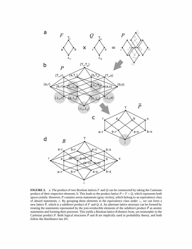
FIGURE 2. a. The product of two Boolean latticesF andQ can be constructed by taking the Cartesianproduct of their respective elements. b. This leads to the product latticeP= F ×Q, which represents bothspaces jointly. However,P contains seven statements (gray circles), which belong to an equivalence classof absurd statements. c. By grouping these elements in the equivalence class under⊥, we can form anew latticeP, which is a subdirect product ofF andQ. d. An alternate lattice structure can be formed bytreating the statements represented by the join-irreducible elements of the subdirect productP as atomicstatements and forming their powerset. This yields a Boolean latticeB distinct from, yet isomorphic to theCartesian productP. Both logical structuresP andB are implicitly used in probability theory, and bothfollow the distributive lawD1.

stands for the truism, which is a logical statement that says‘ It is an apple or a banana!’,which we write symbolically as⊤F = a∨b. The bottom is the absurdity which says ‘Itis an apple and a banana!’, written ⊥F = a∧b. The lattice is clearly Boolean as thecomplement ofa is b, and vice versa (i.e.a∧b = ⊥F anda∨b = ⊤F ).

Similarly, what is known about the quality of the fruit can bedescribed by the latticeQ generated by the atomic assertions

r = ‘It is ripe!’

s= ‘It is spoiled!’.

These assertions generate the center lattice in Figure 2a, which is also Boolean (isomor-phic to22).

We can combine these two lattices by taking thelattice product. Graphically, this canbe constructed by fixing one of the two lattices, and placing copies of the other overeach element of the former. In Figure 2a, I fix the latticeQ and place copies of the latticeF over each element ofQ. The elements of the product latticeP = F ×Q are foundby forming the Cartesian product of the elements of the two lattices. For example, theelement(a, r) represents the logical statement that says ‘The fruit is an apple and it isripe!’ Two elements ofF ×Q, ( f1,q1) and( f2,q2), can be ordered coordinate-wise [9,p.42], so that

( f1,q1) ≤ ( f2,q2) when f1 ≤ f2 and q1 ≤ q2, (60)

which leads to a coordinate-wise definition of∨ and∧

( f1,q1)∨ ( f2,q2) = ( f1∨ f2,q1∨q2) (61)

( f1,q1)∧ ( f2,q2) = ( f1∧ f2,q1∧q2). (62)

The result is the Boolean latticeP in Figure 2b, which is isomorphic to22× 22 = 24.I should make the meaning of some of these statements more explicit. For example,(⊤F , r) is a statement that says ‘It is an apple or a banana and it is ripe!’ Similarly,(b,⊤Q) is a statement that says ‘It is a banana that is either ripe or spoiled!’

The lattice product is associative, so that for three latticesJ, K, andL

J× (K ×L) = (J×K)×L. (63)

This associativity translates to the associativity of the meet of the Cartesian products ofthe elements, which is consistent with the fact that the lattice product of two lattices is alattice.

What is interesting is that there are seven elements (gray circles) that involve at leastone of the two absurdities. These seven elements,(⊤F ,⊥Q), (⊥F ,⊤Q), (⊥F , r), (a,⊥Q),(b,⊥Q), (⊥F ,s), and(⊥F ,⊥F) each belong to anequivalence classof logically absurdstatements as they say things like ‘It is ripe and spoiled!’ and ‘It is an apple and abanana!’ If we group these absurd statements together under a new symbol ⊥, we canconstruct the latticeP in Figure 2c. I have simplified the element labels so that theelementb stands for(b,⊤Q), which can be read as ‘The fruit is a banana!’, andsstandsfor (⊤F ,s), which can be read as ‘The fruit is spoiled!’ The lattice P is a subdirect

productof the latticesF andQ sinceP can be embedded into their Cartesian productP,and its projections onto bothF andQ are surjective (onto, but not one-to-one).

The symbol∧ again represents the meet in the subdirect productP, so that the meetof a ands gives the elementa∧ s, which is equivalent to a spoiled apple(a,s). In thisway we see that the meet in the subdirect product lattice behaves like the meet in theoriginal hypothesis space, while simultaneously implementing the Cartesian product.However, there are some key differences. First,P is not Boolean. For example, there isno unique complement to the statementa∧ s, as bothb andr satisfy the requirementsfor the complement

(a∧s)∨b= ⊤(a∧s)∧b= ⊥

and(a∧s)∨ r = ⊤(a∧s)∧ r = ⊥

A more important difference is the fact that the meet inP follows both distributivelawsD1 andD2, whereas the meet inP follows only D1. To demonstrate this considerthe following in the context ofP

a∧ (r ∨s) = a∧⊤ = a, (64)

and(a∧ r)∨ (a∧s) = a, (65)

which is consistent withD1

a∧ (r ∨s) = (a∧ r)∨ (a∧s). (66)

Now considera∨ (r ∧s) = a∨⊥ = a, (67)

whereas(a∨ r)∧ (a∨s) = ⊤∧⊤ = ⊤, (68)

which is inconsistent withD2, which is distributivity of∨ over∧. The difficulty hereis clear. In the Cartesian productP and the subdirect productP, statements likea∨ randa∨s do not have distinct interpretations since one cannot use the Cartesian productto form the statement ‘It is an apple or the fruit is ripe!’ Another way to look at theloss of propertyD2 is to notice that because we have identified the bottom elements inthe equivalence relation we lose distributivity of∨ over∧ (propertyD2), and maintaindistributivity of ∧ over∨ (propertyD1). Had we identified the top elements we wouldhave obtained the dual situation.

There is one last important construction we can perform. We can construct anotherlattice by considering the join-irreducible statements ofthe subdirect product differently.If we let a∧ r, a∧s, b∧ r, b∧s represent an atomic set of exhaustive mutually exclusivestatements rather than a Cartesian product of statements, then all other elements in thelattice can be formed from the joins of these atoms. The result is a Boolean latticeB thatis isomorphic to the lattice productP, so thatB ∼ P ∼ 24. In this lattice the atomic

statements, such asa∧ r, do not represent Cartesian products, but instead representelementary statements like ‘It is a ripe apple!’. For this reason,B contains logicalstatements not included in the Cartesian productP or the subdirect productP. Forexample, we can construct statements like(b∧ r)∨ (a∧ s), which state ‘It is either aripe banana or a spoiled apple!’ Lattices formed this way naturally follow bothD1 andD2, as they are Boolean.

The important point here is that we use each of these constructs in different applica-tions of probability theory without explicit consideration. Most relevant is the fact thateach of these three lattice constructsP, P, andB follows D1. Thus if we require that ourcalculus satisfies distributivity of∧ over∨ then we will have a rule that is consistentwith properties of each of the logical constructs we have considered here.

Deriving the Product Rule

The product rule is important as it gives us a way to compute the degree of inclusionfor meets of elements in a lattice constructed from the product of two distributive lattices.We look for a functionP that allows us to write the degree to which the meet of twoelementsx∧y includes a third elementt without relying on the joinx∨y. Cox chose theform

ν(x∧y, t) = P(ν(x, t),ν(y,x∧ t)), (69)

which was later shown by Tribus [23] and Smith & Erickson [24]to be the onlyfunctional form that satisfies consistency with associativity of ∧. 5

Consider the elementsa and b wherea∧ b = ⊥, and the elementsr and s wherer ∧s= ⊥. We reproduce Caticha’s derivation [11] and consider distributivity D1 of themeet over the join in the lattice product

(a,(r ∨s))≡ a∧ (r ∨s) = (a∧ r)∨ (a∧s). (70)

This equation gives us two different ways to express the sameposet element. Consis-tency with distributivityD1 requires that the same value is associated with each of thesetwo expressions. Using the sum rule (24) and the form ofP consistent with associativity(69), we find that distributivity requires that

P(ν(a, t),ν(r ∨s,a∧ t)) = ν(a∧ r, t)+ν(a∧s, t), (71)

which further simplifies to

P(ν(a, t),ν(r,a∧ t)+ν(s,a∧ t))= P(ν(a, t),ν(r,a∧ t))+P(ν(a,t),ν(s,a∧ t)). (72)

If we let u= ν(a, t), v= ν(r,a∧t), andw= ν(s,a∧t), the equation above can be writtenmore concisely as

P(u,v+w) = P(u,v)+P(u,w). (73)

5 I use the sum rule in the following derivation, which requires that I use the mappingν rather thanφ .

This is a functional equation for the functionP, which captures the essence of distribu-tivity. By working with this equation, we will obtain the functional form ofP.

The idea is to show thatP(u,v+w) is linear in its second argument. If we letz= w+v,and write (73) as

P(u,z) = P(u,v)+P(u,w), (74)

we can look at the second derivative with respect toz. Using the chain rule we find that

∂∂v

=∂z∂v

∂∂z

=∂∂z

. (75)

This can be done also forw giving

∂∂v

=∂

∂w=

∂∂z

. (76)

Writing the second derivative with respect toz as

∂ 2

∂z2 =∂∂v

∂∂w

, (77)

we find that∂ 2

∂z2P(u,z) = ∂∂v

∂∂w(P(u,v)+P(u,w))

= ∂∂v(

∂∂wP(u,w))

= ∂∂w( ∂

∂vP(u,w))= 0,

(78)

which means that the functionP is linear in its second argument

P(u,v) = A(u)v+B(u). (79)

If (79) is substituted back into (73) we find thatB(u) = 0.We can useD1 another way by considering(a∨b)∧ r. This leads to a condition that

looks likeP(v+w,u) = P(v,u)+P(w,u), (80)

whereu, v, w are appropriately redefined. Following the approach above,we find thatPis also linear in its first argument

P(u,v) = A(v)u. (81)

Together with (79), the general solution is

P(u,v) = Cuv, (82)

whereC is an arbitrary constant. Thus, we have theproduct rule

ν(x∧y, t) = Cν(x, t)ν(y,x∧ t), (83)

which tells us the degree to which the new elementx∧ y includes the elementt. Thislooks more familiar if we setC= 1 and re-write the rule in probability-theoretic notation,

p(x∧y|t) = p(x|t)p(y|x∧ t). (84)

If the lattice we are working in is formed by the lattice product, (83) can be rewrittenusing the Cartesian product notation

ν((x,y),(tx, ty)) = Cν((x,⊤y),(tx, ty))ν((⊤x,y),(x∧ tx, ty)), (85)

wherex∧y≡ (x,y), t ≡ (tx, ty), x≡ (x,⊤y), andy≡ (⊤x,y). Simplifying, we see that

ν((x,y),(tx, ty)) = Cν(x, tx)ν(y, ty), (86)

whereν(x, tx) is computed in one lattice andν(y, ty) in the other.

BAYES’ THEOREM

The origin of Bayes’ Theorem is perhaps the most well-known.It derives directly fromthe product rule and consistency with commutativity of the meet. When it is true thatx∧y = y∧x, one can write the product rule two ways

ν(x∧y, t) = Cν(x, t)ν(y,x∧ t)

andν(y∧x, t) = Cν(y, t)ν(x,y∧ t).

Consistency with commutativity requires that these two results are equal. Setting themequal and rearranging the terms leads toBayes’ Theorem

ν(x,y∧ t) =ν(x, t)ν(y,x∧ t)

ν(y, t). (87)

This will look more familiar if we letx ≡ h be a logical statement representing ahypothesis, and lety ≡ d be a new piece of data, and change notation to that used inprobability theory

p(h|d∧ t) =p(h|t)p(d|h∧ t)

p(d|t). (88)

This makes more sense now that it is clear that the two statementsh andd come fromdifferent lattices. This is whyd represents anewpiece of data, it represents informationwe were not privy to when we implicitly constructed the lattice including the hypothesish. The statementsh andd belong to two different logical structures and Bayes’ Theoremtells us how to do the computation when we combine them. To perform this computation,we need to first make assignments. The prior assignmentp(h|t) is made in the originallattice of hypotheses, whereas the likelihood assignmentp(d|h∧ t) is made in theproduct lattice. The evidence, while usually not assigned,refers to an assignment thatwould take place in the original data lattice.

LAWS FROM ORDER

Why is all this important? Because, the sum rules are associated with all lattices, andsum and product rules are not just associated with Boolean algebra, but with distributivealgebras. This is a much wider range of application than was ever considered by Cox, asthe following examples demonstrate.

Information Theory from Order

Most relevant to Cox is the further development of the calculus of inquiry [25, 26,27, 8, 6], which appears to be a natural generalization of information theory. Theextension of Cox’s methodology to distributive lattices ingeneral is extremely importantto this development, as the lattice structure of questions is not a Boolean lattice, butis instead thefree distributive lattice[8, 6]. This free distributive lattice of questionsis generated from the ordered set of down-sets of its corresponding Boolean lattice ofassertions. A probability measure on the Boolean assertionlattice induces a valuation,which we callrelevanceor bearing, on the question lattice. I will show in a future paper[28] that the join-irreducible questions, calledelementary questionsby Fry [26], haverelevances that are equal to−plogp, called thesurprise, wherep is the probability ofthe assertion defining the elementary question. Joins of these elementary questions formreal questions, which via the sum rule have valuations formed from sums of surprises,or entropy. Going further up the question lattice, one uses the generalized sum rule,which results in mutual information, and eventually generalized entropy [4], also calledco-information [21]. The lattice structure is given by the algebra of questions, and thegeneralized entropies are the valuations induced on the question lattice by the probabilitymeasure assigned to the Boolean algebra of assertions. Exactly how these valuations areinduced, manipulated, and used in calculations regarding questions will be discussedelsewhere [28].

Geometry from Order

Perhaps more interesting is the fact that much of geometry can be derived from theseorder-theoretic concepts. There has been much work done in this area, which is calledgeometric probability. This invariably calls up thoughts of Buffon’s Needle problem, butthe range of applications is much greater. I have found the introductory book by Klainand Rota [15] to be very useful, and below I discuss several illustrative examples fromtheir text.

The Lattice of Parallelotopes

Imagine a Cartesian coordinate system inn-dimensions. We will consider orthogonalparallelotopes, which are rectangular boxes with sides parallel to the coordinate axes.

FIGURE 3. An illustration of the join and meet of two orthogonal parallelotopes.

By taking finite unions (joins) and intersections (meets) ofthese parallelotopes, we canconstruct the lattice (or equivalently the algebra) ofn-dimensional parallelotopesPar(n)[15, p.30]. In one dimension, the parallelotope is simply a closed interval on the realline.

To extend the algebra to a calculus, to each parallelotopeP we will assign a valuation6

µ(P), which is invariant with respect to geometric symmetries relevant toPar(n), suchas invariance with respect to translations along the coordinate system and permutationsof the coordinate labels. Assigning valuations that are consistent with these importantgeometric symmetries is analogous to Jaynes’ use of group invariance to derive priorprobabilities [29].

Before looking at these invariant valuations in more detail, Figure 3 shows the join oftwo parallelotopesP1 andP2. Since this lattice is distributive, the sum rule can be usedto compute the valuation of the joinP1∨P2

µ(P1∨P2) = µ(P1)+ µ(P2)−µ(P1∧P2). (89)

Again we see the familiar inclusion-exclusion principle.

6 Note that one can considerµ(P)≡ µ(P,T), whereT refers to a parallelotope to which the measure is insome sense normalized.

A Basis Set of Invariant Valuations

At this point, you have probably already identified a valuation that will satisfy invari-ance with respect to translation and coordinate label permutation. One obvious valuationfor three-dimensional parallelotopes suggested by the illustration isvolume

µ3(x) = x1x2x3, (90)

wherex1, x2 andx3 are the side-lengths of the parallelotope. Surprisingly, this is not theonly valuation that satisfies the invariance properties we are considering. There is also avaluation, which is proportional to thesurface area

µ2(x) = x1x2 +x2x3+x3x1, (91)

which is easily shown to satisfy both the invariance properties as well as the sum rule. Infact, there is a basis set of invariant valuations, which in the case of three-dimensionalparallelotopes consists of the volume, surface area,mean width

µ1(x) = x1 +x2+x3, (92)

and theEuler characteristicµ0, which for parallelotopes is equal to one for non-emptyparallelotopes and zero otherwise. The fact that these valuations form a basis means thatwe can write any valuation as a linear combination of these basis valuations

µ = aµ3 +bµ2 +cµ1 +dµ0. (93)

In general, it is not clear under which invariance conditions one obtains a basis setof valuations rather than a unique functional form. This is an extremely importantissue when we consider the issue of assigning prior probabilities in probability theory.Jaynes’ demonstrated how to derive priors that are consistent with certain invariances,and cautioned that if the number of parameters in the transformation group is less thanthe number of model parameters, then the prior will only be partially determined [29].How to consistently assign priors in this case is an open problem.

Furthermore, the Euler characteristic is interesting in that it takes on discrete ratherthan continuous values. This is something that is not seen inmeasure theory indicatingthat this development is more general than the typical measure-theoretic approaches. Animportant example of this has been identified within the context of information theory.Aczél [30] showed that the Hartley entropy [31], which takeson only discrete values,has certain ‘natural’ properties shared only with the Shannon entropy [32]. Thiswillalso be discussed in more detail elsewhere [28].

The Euler Characteristic

The Euler characteristic appears in other lattices and is perhaps best known from thelattice of convex polyhedra where it satisfies the followingformula

µ0 = F −E +V, (94)

whereF is the number of faces,E is the number of edges, andV is the number of vertices[14]. For all convex polyhedra in three-dimensions,µ0 = 2. For example, if we considera cube, we see that it has 6 faces, 12 edges, and 8 vertices, so that 6−12+8 = 2. Again,this is an example of the inclusion-exclusion principle, which comes from the sum rule.In the lattice of simplicial complexes, a face is a 2-simplex, an edge is a 1-simplex, anda vertex is a 0-simplex. To compute the characteristic, we add at one level, subtract atthe next, and add at the next and so on. This geometric law derives directly from ordertheory via the sum rule.

Spherical Triangles

The connections with order theory do not stop with polyhedra, but extend into con-tinuous geometry. Klain & Rota [15, p.158] show that the solid angle subtended bya triangle inscribed on a sphere, called thespherical excess, can be found using theinclusion-exclusion principle

Ω(∆) = α +β + γ −π (95)

whereα,β ,γ ∈ [0,π] denote the angles of the spherical triangle. Such examples high-light the degree to which order theory dictates laws.

Statistical Physics from Order

Up to this point, probability theory and geometry have been the main examples bywhich I have demonstrated the use of order-theoretic principles to derive a calculusfrom an algebra. Thanks to the efforts of Ed Jaynes [33], Myron Tribus [34] and others,I am able to wave my hands and state that statistical physics derives from order-theoreticprinciples. In one important respect this argument is a sham, and that is where entropyis concerned. Theprinciple of maximum entropy[33, 35], which is central to statisticalphysics, lies just beyond the scope of this order-theoreticframework. It is possible thata fully-developed calculus of inquiry [28] will provide useful insights. With entropiesbeing associated with the question lattice, application ofthe principle of maximumentropy to enforce consistency with known constraints may in some sense be dual to themaximum a posterioriprocedure in probability theory. However, at this stage it is certainthat the probability-based features of the theory of statistical physics derive directly fromthese order-theoretic principles.

Quantum Mechanics from Order

Most surprising is Ariel Caticha’s realization that the rules for manipulating quantummechanical amplitudes in slit experiments derive from consistency with associativityand distributivity of experimental setups [11]. Each experimental setup describes anidealized experiment that describes a particle prepared atan initial point and detected

at a final point. These experimental setups are simplified so that the only observableconsidered is that of position. The design of each setup constrains the statements thatone can make about the particle.

These setups can be combined in two ways, which I will show areessentiallymeetsand joins of elements of a poset. However, there are additional constraints on theseoperations imposed by the physics of the problem. We will seethat the meets are notcommutative, and this makes these algebraic operations significantly different from theAND and OR of propositional logic. This lack of commutativity means that there is noBayes’ Theorem analog for quantum mechanical amplitudes. Furthermore, the operationof negation is never introduced—nor is it necessary. This sets Caticha’s approach apartfrom other quantum logic approaches where the negation of a quantum mechanicalproposition remains a necessary concept.

Caticha considers a simple case where the only experiments that can be performedare those that detect the local presence or absence of a particle. He considers a particle,which is prepared at timeti at positionxi and is later detected at timet f at positionxf . Experimental setups of this sort will test statements like‘ the particle moved fromxi to xf ’. The physics becomes interesting when we place obstacles in the path ofthe particle. For example, we can place a barrier with a single slit at positionx1.The detector atxf will only detect the particle if it moves fromxi to x1 and thenonward toxf , whereti < t1 < t f . 7 This barrier with a slit imposes a constraint onthe particles that can be detected. The central idea is that experimental setups can becombined in two ways: increasing the number of constraints on the particle behavior, orby decreasing the number of constraints. This allows one to impose an ordering relationon the experimental setups, and by considering the set of allpossible setups where theparticle is prepared atxi and detected atxf we have a poset of experimental setups.

Setups with fewer constraints give greater freedom to the possible behavior of thedetected particle. Of course, the ordering relation we choose can be defined in terms ofthe constraints on the particle’s behavior or, dually, on the freedom that the setup allowsthe particle. Each relation will lead to a poset, which is dual to the poset ordered by itsdual ordering relation. Maintaining a positive attitude, Iwill use the ordering relationthat describes the freedom that the setup allows, so that setups with greater freedom willinclude setups that allow only a portion of this freedom. Thus at the top of this poset(Figure 4) is the setup⊤ that has no obstructions placed betweenxi andxf . The particlehaving been prepared atxi and detected atxf is free to have taken any path during itstraversal. Caticha uses a concise notation to describe setups. The top setup can be writtenas⊤ ≡ [xf ,xi ], which reading right to left states that the particle is known to start atxiand is known to arrive atxf .

The most constrained setup is the one at the bottom,⊥ , as it is completely filled withobstructions.8 This setup is analogous to the logical absurdity in the sensethat there isno way for a particle prepared atxi to be detected atxf . More interesting are the join-

7 These paths are in space-time. For simplicity, I will often omit reference to the time coordinate.8 All setups with obstructions that provide no way for a particle to travel fromxi to xf belong to the sameequivalence class of obstructed setups and are representedby ⊥. This includes setups with obstructedpathways.

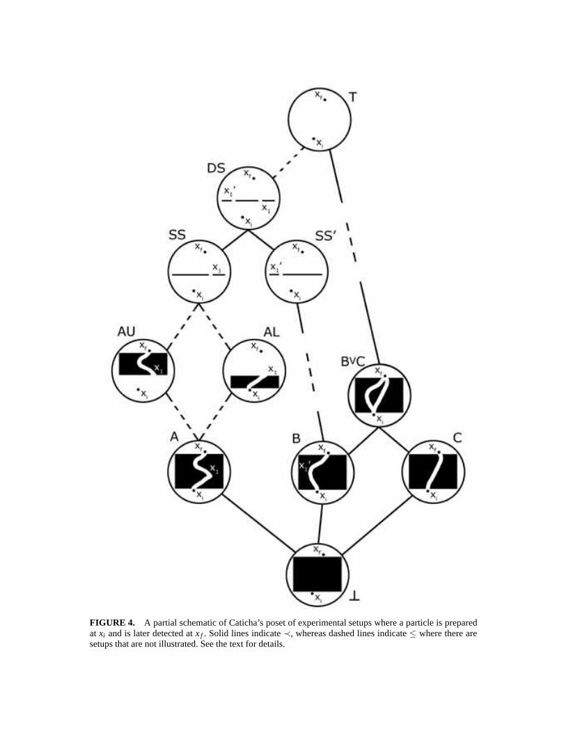
FIGURE 4. A partial schematic of Caticha’s poset of experimental setups where a particle is preparedat xi and is later detected atxf . Solid lines indicate≺, whereas dashed lines indicate≤ where there aresetups that are not illustrated. See the text for details.

irreducible setups that cover⊥. These are the setups that allow only a single path fromxi to xf . Three examplesA,B, andC can be seen in Figure 4.

All the setups in the poset can be generated by joining the join-irreducible setups. AsCaticha, defined his poset in terms of an algebra, we must lookat this algebra carefully toidentify the complete set of join-irreducible setups. Obviously the atomic setups, whichare the setups with a single path fromxi to xf , are join-irreducible. However, Catichadefined the join of two setups only for cases where the two setups differ by at most onepoint at one time. Thus we must work through his algebra usingthe poset structure todiscover how to perform the join in more general cases. Consider the two setupsSSandSS′ in Figure 4. The setupSSis a single-slit experiment where the particle is known tohave been prepared atxi , is known to have gone through the slit atx1 and was detectedat xf , written concisely asSS= [xf ,x1,xi ]. Similarly, SS′ is a different single-slit setupwrittenSS′ = [xf ,x′1,xi]. Their join is a double-slit setup

DS= SS∨SS′ (96)

found byDS= [xf ,x1,xi ]∨ [xf ,x

′1,xi], (97)

which is written concisely as

DS= [xf ,(x1,x′1),xi ]. (98)

This can be read as: ‘The particle was prepared at xi , is known to have passed througheither the slit at x1 or the slit at x′1, and was detected at xf ’. This definition describes thejoin of two setups differing at only one point. Before generalizing the join, we will firstexamine the meet.

Caticha describes the simplest instance of a meet [11, Eqn. 2], which is

[xf ,x1]∧ [x1,xi ] = [xf ,x1,xi ], (99)

giving the single-slit experimentSSin Figure 4. This equation is interesting, becauseneither setup on the left-hand side of (99) is a valid setup inour poset, since the particleis not always prepared atxi and it is not always detected atxf . Instead, what is going onhere is that this meet represents the Cartesian product of two setups. Two smaller setupposets are being combined to create a larger setup poset. This is demonstrated by themeet of AU and AL in Figure 4, each of which has a single path on one side ofx1 and isfree of obstructions on the other side. AU is the Cartesian product of the top setup in theset of posets describing particles prepared atxi and detected atx1, which I write as⊤1i ,and a setup consisting of a single path in the set of posets describing particles preparedatx1 and detected atxf . We can write these posets coordinate-wise

AL ≡ (⊤ f 1,A1i)AU ≡ (Af 1,⊤1i)

(100)

whereA1i is the setup where the particle is prepared atxi and is detected atx1 and isconstrained to follow that portion of the path in the single-path setupA. SetupsAf 1

and⊤ f 1 are defined similarly. Their meet is found trivially, since for each coordinate,x∧⊤ = x for all x. Thus

AU∧AL = (Af 1,A1i) (101)

which is a valid expression for the entire single-path setupA

A = (Af 1,A1i), (102)

and is consistent with Caticha’s definition in (99). This interpretation, which shouldbe compared to our earlier discussion on the lattice product, also provides insight intohow one can decompose the single-path setupsA, B, andC into a series of infinitesimaldisplacements. Each infinitesimal displacement of a particle can be described using asetup in a smaller poset. Using the Cartesian product, thesesetups can be combinedto form larger and larger displacements. Thus the single-path setups can be seen torepresent meets of many shorter single-path segment setups.

We can use what we have learned from the product space exampleto better understandthe join of two experimental setups. We can join the setupsAL and AU using theCartesian product notation. Since⊤ is the top element of the poset, when joined withany other element of the poset the result is always the top, i.e.⊤∨ x = ⊤, for anyx inthe poset. Thus we see that

AU∨AL = (Af 1,⊤1i)∨ (⊤ f 1,A1i)= (Af 1∨⊤ f 1,⊤1i ∨A1i)= (⊤ f 1,⊤1i)≡ SS.

(103)

The interpretation of the two posets forming this Cartesianproduct is key to betterunderstanding the join. The result states that the particleis prepared atxi and is freeto travel however it likes to be detected atx1, and that it is prepared atx1 and is freeto travel however it likes resulting in a detection atxf . The result is a particle that isprepared atxi , passes throughx1 and is detected atxf . Thus their join is the single slitexperiment,AU∨AL= SS. This result extends Caticha’s algebraic definition of the join.

Two setups with non-intersecting paths can also be joined. This must be the case sincethe top setup in this poset is obstacle-free and includes allsingle-path setups. Consider asetup divided by the straight line connectingxi andxf . Two setups can be formed fromthis, one by filling the left half with an obstacle, call itL, and the other by filling the righthalf R. Clearly, their join must be the top element, as one setup prevents the particle frombeing to the left of the line and the other one prevents it frombeing to the right. This canbe extended by considering two setups each with paths that donot intersect one another.This example is shown in Figure 4, as the join of two single-path setupsB andC, whichresults in a two-path setupB∨C.

At this stage, it is not completely clear to me how to handle setups with two pathsthat intersect at multiple points. Clearly, two paths that intersect at a single medianpoint, such asx1, can be considered to be the product of two setups each with two non-intersecting paths. Again, consistency will be the guidingprinciple. What is importantto this present development is that we know enough of the algebra to see what kindof laws we can derive from order theory by generalizing from order-theoretic inclusion

to degrees of inclusion. First, Caticha showed that the joinis associative. This impliesthat there exists a sum rule. Second, he showed that when the setups exist the meetis associative and distributes over the join. This leads to aproduct rule. By measuringdegrees of inclusion among experimental setups with complex numbers, Caticha showedthat the sum and product rules applied to complex-valued valuations are consistent withthe rules used to manipulate quantum amplitudes. By lookingat the join of setupsB andC one can visualize how application of the sum rule leads to Feynman path integrals [36],which can be used to compute amplitudes for setups likeB∨C, and by iterating acrossthe poset,SSand⊤. Also, the amplitude corresponding to a setup representingany finitedisplacement can be decomposed into a product of amplitudesfor setups representingsmaller successive displacements. Last, it should be notedthat the lack of commutativityof the meet implies that there is no Bayes’ Theorem analog forquantum amplitudes.

Furthermore, using these rules Caticha showed that that theonly consistent way todescribe time evolution is by a linear Schrödinger equation. This is a truly remarkableresult, as no information about the physics of the particle was used in this derivation ofthe setup calculus—only order theory! The physics comes in when one assigns valuesto the setups in the poset. This is done by assigning values tothe infinitesimal setups,which is equivalent to assigning the priors in probability theory. At the stage of assigningamplitudes, we can now only rely on symmetry, constraints, and consistency with otheraspects of the problem. The calculus of setup amplitudes will handle the rest. The factthat these assignments rely on the Hamiltonian and that theyare complex-valued arenow the key issues. Looking more closely at the particular symmetries, constraints andconsistencies that result in the traditional assignments independent of the setup calculuswill provide deeper insight into quantum mechanics and willteach us much about howto extend this new methodology into other areas of science and mathematics.

DISCUSSION

Probability theory is often summarized by the statement ‘probability is a sigma algebra’,which is a concise description of the mathematical properties of probability. However,descriptions like this can limit the way in which one thinks about probability in much thesame way that the statement ‘gravity is a vector field’ limits the way one thinks aboutgravitation. To gain new understanding in an area of study, the foundations need tobe re-explored. Richard Cox’s investigations into the roleof consistency of probabilitytheory with Boolean algebra were a crucial step in this new exploration. While Cox’stechnique has been celebrated in several circles within thearea of probability theory[33, 23, 37], the deeper connections to order theory discussed here have not yet beenfully recognized. The exception is the area of geometric probability where Gian-CarloRota has championed the importance of valuations on posets giving rise to an area ofmathematics which ties together number theory, combinatorics, and geometry. Simplerelations, such as the inclusion-exclusion principle, actas beacons signalling that ordertheory lies not far beneath.

Order theory dictates the way in which we can extend an algebra to a calculus byassigning numerical values to pairs of elements of a poset todescribe the degree to which

one element includes another. Consistency here is the guiding principle. The sum rulederives directly from consistency with associativity of the join operation in the algebra.Whereas, the product rule derives from consistency with associativity of the meet, andconsistency with distributivity of the meet over the join.

It is clear that the basic methodology of extending an algebra to a calculus, which ispresently explicitly utilized in probability theory and geometric probability, is implicitlyutilized in information theory, statistical mechanics, and quantum mechanics. The order-theoretic foundations suggest that this methodology mightbe used to extend any class ofproblems where partial orderings (or rankings) can be imposed to a full-blown calculus.One new example explored at this meeting is theranking of preferencesin decisiontheory, which is explored in Ali Abbas’ contribution to thisvolume [38]. More obviousis the relevance of this methodology to the development of the calculus of inquiry[25, 26, 8, 6], as well as Bob Fry’s extension of this calculusto cybernetic control[27]. A serious study of the relationship between order theory and geometric algebra,recognized and noted by David Hestenes [39, 40], is certain to yield important newresults. With the aid of geometric algebra, an examination of projective geometry in thisorder-theoretic context may provide new insights into Carlos Rodríguez’s observationthat the cross-ratio of projective geometry acts like Bayes’ Theorem [5].

ACKNOWLEDGMENTS

This work supported by the NASA IDU/IS/CICT Program and the NASA AerospaceTechnology Enterprise. I am deeply indebted to Ariel Caticha, Bob Fry, Carlos Ro-dríguez, Janos Aczél, Ray Smith, Myron Tribus, David Hestenes, Larry Bretthorst, Jef-frey Jewell, Domhnull Granquist-Fraser, and Bernd Fischerfor insightful and inspiringdiscussions, and many invaluable remarks and comments.

REFERENCES

1. Boole, G.,Dublin Mathematical Journal, 3, 183–198 (1848).2. Boole, G.,An Investigation of the Laws of Thought, Macmillan, London, 1854.3. Cox, R. T.,Am. J. Physics, 14, 1–13 (1946).4. Cox, R. T.,The Algebra of Probable Inference, Johns Hopkins Press, Baltimore, 1961.5. Rodríguez, C. C., “From Euclid to entropy,” inMaximum Entropy and Bayesian Methods, Laramie

Wyoming 1990, edited by W. T. Grandy and L. H. Schick, Kluwer, Dordrecht, 1991, pp. 343–348.6. Knuth, K. H.,Phil. Trans. Roy. Soc. Lond. A, 361, 2859–2873 (2003).7. Graham, R. L., Knuth, D. E., and Patashnik, O.,Concrete Mathematics, 2nd ed., Addison-Wesley,

Reading, Massachusetts, 1994.8. Knuth, K. H., “What is a question?,” inBayesian Inference and Maximum Entropy Methods in Sci-

ence and Engineering, Moscow ID, USA, 2002, edited by C. Williams, AIP Conference Proceedings659, American Institute of Physics, New York, 2003, pp. 227–242.

9. Davey, B. A., and Priestley, H. A.,Introduction to Lattices and Order, Cambridge Univ. Press,Cambridge, 2002.

10. Birkhoff,Lattice Theory, American Mathematical Society, Providence, 1967.11. Caticha, A.,Phys. Rev. A, 57, 1572–1582 (1998).12. Aczél, J.,Lectures on Functional Equations and Their Applications, Academic Press, New York,

1966.

13. Rota, G.-C.,Studies in Pure Mathematics, (Presented to Richard Rado), Academic Press, London,1971, chap. On the combinatorics of the Euler characteristic, pp. 221–233.

14. Rota, G.-C.,The Mathematical Intelligencer, 20, 11–16 (1998).15. Klain, D. A., and Rota, G.-C.,Introduction to Geometric Probability, Cambridge Univ. Press,

Cambridge, 1997, ISBN 0-521-59654-8.16. Rota, G.-C.,Zeitschrift für Wahrscheinlichkeitstheorie und Verwandte Gebiete, 2, 340–368 (1964).17. Krishnamurthy, V.,Combinatorics: Theory and Application, John Wiley & Sons, New York, 1986,

ISBN 0-470-20345-5.18. Barnabei, M., and Pezzoli, E.,Gian-Carlo Rota on combinatorics, Birkhauser, Boston, 1995, chap.

Möbius functions, pp. 83–104.19. Möbius, A. F.,J. reine agnew. Math., 9, 105–123 (1832).20. McGill, W. J.,IEEE Trans. Info. Theory, 4, 93–111 (1955).21. Bell, A. J., “The co-information lattice,” inProceedings of the Fifth International Workshop on

Independent Component Analysis and Blind Signal Separation: ICA 2003, edited by S. Amari,A. Cichocki, S. Makino, and N. Murata, 2003.

22. Pölya, G., and Szegö, G.,Aufgaben und Lehrsätze aus der Analysis, 2 vols., Springer, Berlin, 1964,3rd edn.

23. Tribus, M.,Rational Descriptions, Decisions and Designs, Pergamon Press, New York, 1969.24. Smith, C. R., and Erickson, G. J., “Probability theory and the associativity equation,” inMaximum

Entropy and Bayesian Methods, Dartmouth USA, 1989, edited by P. F. Fougère, Kluwer, Dordrecht,1990, pp. 17–30.

25. Cox, R. T., “Of inference and inquiry, an essay in inductive logic,” in The Maximum EntropyFormalism, edited by R. D. Levine and M. Tribus, The MIT Press, Cambridge, 1979, pp. 119–167.

26. Fry, R. L.,Maximum entropy and Bayesian methods, Johns Hopkins University (1999), electronicCourse Notes (525.475).

27. Fry, R. L., “Cybernetic systems based on inductive logic,” in Bayesian Inference and MaximumEntropy Methods in Science and Engineering, Gif-sur-Yvette, France 2000, edited by A. Mohammad-Djafari, AIP Conference Proceedings 568, American Institute of Physics, New York, 2001, pp. 106–119.

28. Knuth, K. H. (2004), in preparation. The calculus of inquiry.29. Jaynes, E. T.,IEEE Trans. Syst. Sci. Cyb., SSC-4, 227 (1968).30. Aczél, J., Forte, B., and Ng, C. T.,Adv. Appl. Prob., 6, 131–146 (1974).31. Hartley, R. V.,Bell System Tech. J., 7, 535–563 (1928).32. Shannon, C. F., and Weaver, W.,The Mathematical Theory of Communication, Univ. of Illinois Press,

Chicago, 1949.33. Jaynes, E. T.,Physical Review, 106, 620–630 (1957).34. Tribus, M.,Thermostatics and Thermodynamics, D. Van Nostrand Co., Inc., Princeton, 1961.35. Jaynes, E. T., “Where do we stand on maximum entropy,” inThe Maximum Entropy Formalism,

edited by R. D. Levine and M. Tribus, The MIT Press, Cambridge, 1979, pp. 15–118.36. Feynman, R. P.,Rev. Mod. Phys., 20, 367–387 (1948).37. Jaynes, E. T.,Probability Theory: The Logic of Science, Cambridge univ. Press, Cambridge, 2003.38. Abbas, A. E., “An information theory for preferences,” in Bayesian Inference and Maximum Entropy

Methods in Science and Engineering, Jackson Hole WY, USA 2003, edited by G. J. Erickson,American Institute of Physics, New York, 2003.

39. Hestenes, D., and Ziegler, R.,Acta Appl. Math., 23, 25–63 (1991).40. Hestenes, D.,Acta Appl. Math., 23, 65–93 (1991).