Optimizing Large Join Queries in Mediation Systems

Ramana Yerneni, Chen Li, Je�rey Ullman, Hector Garcia-Molina

Department of Computer Science

Stanford University

fyerneni, chenli, ullman, hectorg@cs.stanford.edu

Abstract

In data integration systems, queries posed to a mediator need to be translated into a sequence ofqueries to the underlying data sources. In a heterogeneous environment, with sources of diverseand limited query capabilities, not all the translations are feasible. In this paper, we studythe problem of �nding feasible and e�cient query plans for mediator systems. We considerconjunctive queries on mediators and model the source capabilities through attribute-bindingadornments. We use a simple cost model that focuses on the major costs in mediation systems,those involved with sending queries to sources and getting answers back. Under this metric, wedevelop two algorithms for source query sequencing { one based on a simple greedy strategy andanother based on a partitioning scheme. The �rst algorithm produces optimal plans in somescenarios, and we show a linear bound on its worst case performance when it misses optimalplans. The second algorithm generates optimal plans in more scenarios, while having no boundon the margin by which it misses the optimal plans. We also report on the results of theexperiments that study the performance of the two algorithms.

1 Introduction

Integration systems based on a mediation architecture [31] provide users with seamless access to

data from many heterogeneous sources. Examples of such systems are TSIMMIS [3], Information

Manifold [14], Garlic [8], and DISCO [26]. In these systems, mediators de�ne integrated views

based on the data provided by the sources. They translate user queries on integrated views into

source queries and postprocessing operations on the source query results. The translation process

can be quite challenging when integrating a large number of heterogeneous sources.

One of the important challenges for integration systems is to deal with the diverse capabilities

of sources in answering queries [8,15,19]. This problem arises due to the heterogeneity in sources

ranging from simple �le systems to full- edged relational databases. The problem we address in

this paper is how to generate e�cient mediator query plans that respect the limited and diverse

capabilities of data sources. In particular, we focus our attention on the kind of queries that are

the most expensive in mediation systems, large join queries. We propose e�cient algorithms to

�nd good plans for such queries.

1.1 Cost Model

In many applications, the cost of query processing in mediator systems is dominated by the cost

of interacting with the sources. Hence, we focus on the costs associated with issuing queries to

1

sources. Our results are �rst stated using a very simple cost model where we count the total

number of source queries in a plan as its cost. In spite of the simplicity of the cost model, the

optimization problem we are dealing with remains NP-hard. Later in the paper, we show how to

extend our main results to a more complex cost model that charges a �xed cost per query plus a

variable cost that is proportional to the amount of data transferred.

1.2 Capabilities-Based Plan Generation

We consider mediator systems, where users pose conjunctive queries over integrated views provided

by the mediator. These queries are translated into conjunctive queries over the source views to

arrive at logical query plans. The logical plans deal only with the content descriptions of the sources.

That is, they tell the mediator which sources provide the relevant data and what postprocessing

operations need to be performed on this data. The logical plans are later translated into physical

plans that specify details such as the order in which the sources are contacted and the exact queries

to be sent. Our goal in this paper is to develop algorithms that will translate a mediator logical

plan into an e�cient, feasible (does not exceed the source capabilities) physical plan. We illustrate

the process of translating a logical plan into a physical plan by an example.

EXAMPLE 1.1 Consider three sources that provide information about movies, and a mediator

that provides an integrated view:

Source Contents Must Bind

S1 R(studio, title) either studio or title

S2 S(title, year) title

S3 T(title, stars) title

Mediator View:

Movie(studio,title,year,stars) :- R(studio,title), S(title,year), T(title,stars)

The \Must Bind" column indicates what attributes must be speci�ed at a source. For instance,

queries sent to S1 must either provide the title or the studio. Suppose the user asks for the titles

of all movies produced by Paramount in 1955 in which Gregory Peck starred. That is,

ans(title) :- Movie(`Paramount', title, `1955', `Gregory Peck')

The mediator would translate this query to the logical plan:

ans(title) :- R(`Paramount', title), S(title, `1955'), T(title, `Gregory Peck')

The logical plan states the information the mediator needs to obtain from the three sources

and how it needs to postprocess this information. In this example, the mediator needs to join the

results of the three source queries on the title attribute. There are many physical plans that

correspond to this logical plan (based on various join orders and join methods). Some of these

plans are feasible while others are not. Here are three physical plans for this logical plan:

� Plan P1: Send query R(`Paramount', title) to S1; send query S(title, `1955') to S2;

and send query T(title, `Gregory Peck') to S3. Join the results of the three source queries

on the title attribute and return the title values to the user.

2

� Plan P2: First get the titles of movies produced by Paramount from source S1. For each

returned title t, send a query to S2 to get its year and check if it is `1955.' If so, send a query

to S3 to get the stars of movie t. If the set of stars contains `Gregory Peck,' return t to the

user.

� Plan P3: This plan is similar to P2, except that we reverse the S2 and S3 queries. That is,

after getting the titles of Paramount movies, we get their stars from S3. If stars contains

`Gregory Peck,' then we send a query to S2 to get the year of the movie. If the year is `1955,'

we return this title to the user.

Among the three physical plans, the �rst one is not feasible because the queries to sources S2and S3 do not provide a binding for title. The other two plans are feasible. It may be that plan

P2 is more e�cient than plan P3. In that case, the mediator may execute plan P2. 2

As illustrated by the example, we need to solve the following problems:

1. Given a logical plan and the description of the source capabilities, �nd feasible physical plans

for the logical plan. The central problem is to determine the evaluation order for logical plan

subgoals, so that attributes are appropriately bound.

2. Among all the feasible physical plans, pick the most e�cient one.

1.3 Related Work

The problem of ordering subgoals to �nd the best feasible sequence can be viewed as the well known

join-order problem. More precisely, we can assign in�nite cost to infeasible sequences and then �nd

the best join order.

The join-order problem has been extensively studied in the literature, and many solutions have

been proposed. Some solutions perform a rather exhaustive enumeration of plans, and hence do

not scale well [1,2,4,5,8,15,17,19,20,22,29]. In particular, we are interested in Internet scenarios

with many sources and subgoals, so these schemes are too expensive. Some other solutions reduce

the search space through techniques like simulated annealing, random probes, or other heuristics

[6,11,12,16,18,23,24,25]. While these approaches may generate e�cient plans in some cases, they

do not have any performance guarantees in terms of the quality of plans generated (i.e., the plans

generated by them can be arbitrarily far from the optimal one). Many of these techniques may

even fail to generate a feasible plan, while the user query does have a feasible plan.

The remaining solutions [10,13,21] use speci�c cost models and clever techniques that exploit

them to produce optimal join orders e�ciently. While these solutions are very good for the join-

order problem where those cost models are appropriate, they are hard to adopt in our context

because of two di�culties. The �rst is that it is not clear how to model the feasibility of mediator

query plans in their frameworks. A direct application of their algorithms to the problem we are

studying may end up generating infeasible plans, when a feasible plan exists. The second di�culty

is that when we use cost models that emphasize the main costs in mediator systems, the optimality

guarantees of their algorithms may not hold.

3

1.4 Our Solution

In this paper, we use a simple cost model that focuses on the major costs in mediator query

processing, that of getting the relevant data from the sources. In this cost model, we develop

two algorithms that can �nd good feasible plans rapidly. The �rst algorithm runs in O(n2) time,

where n is the number of subgoals in the logical plan. We also provide a linear bound on the

margin by which this algorithm can miss the optimal plan. Our second algorithm can guarantee

optimal plans in more scenarios than the �rst, although there is no bounded optimality for its plans.

Both our algorithms are guaranteed to �nd a feasible plan, if the user query has a feasible plan.

Furthermore, we show through experiments that our algorithms have excellent running time pro�les

in a variety of scenarios, and very often �nd optimal or close-to-optimal plans. This combination

of e�cient, scalable algorithms that generate provably good plans is not achieved by previously

known approaches.

1.5 Paper Organization

The paper is organized as follows. In Section 2, we introduce the cost model and our notation. We

present an e�cient algorithm named CHAIN in Section 3, and prove its n-competitiveness (i.e.,

bounded optimality). In Section 4, we describe our second algorithm, called PARTITION, and

discuss its ability to �nd optimal feasible plans. The results of our performance analysis of the two

algorithms are reported in Section 5. Finally, in Section 6, we discuss how the main results of this

paper can be extended to cost models other than the one introduced in Section 2.

2 Preliminaries

In this section, we introduce the notation we use throughout the paper. We also discuss the cost

model used in our optimization algorithms.

2.1 Source Relations and Logical Plans

Let S1, . . . , Sm be m sources in an integration system. To simplify the presentation, we assume

that sources provide their data in the form of relations. If sources have other data models, one

could use wrappers [9] to create the simple relational view of data. Each source is assumed to

provide a single relation. If a source provides multiple relations, we can model it in our framework

as a set of logical sources, all having the same physical source. Example 1.1 showed three sources

S1, S2 and S3 providing three relations R, S and T respectively.

A query to a source speci�es atomic values to a subset of the source relation attributes and

obtains the corresponding set of tuples. A source supports a set of access templates on its re-

lation that specify binding adornment requirements for source queries.1 In Example 1.1, source

S2 had one access template: Sbf(title; year), while source S1 had two: Rbf(studio; title) and

Rfb(studio; title).

1We consider source-capabilities described as bf adornment patterns that distinguish bound (b) and free (f) argu-ment positions [27]. The techniques developed in this paper can also be employed to solve the problem of mediatorquery planning when other source capability description languages are used.

4

User queries to the mediator are conjunctive queries on the integrated views provided by the

mediator. Each integrated view is de�ned as a set of conjunctive queries over the source relations.

The user query is translated into a logical plan, which is a set of conjunctive queries on the source

relations. The answer to the user query is the union of the results of this set of conjunctive queries.

Example 1.1 showed a user query that was a conjunctive query over the Movie view, and it was

translated into a conjunctive query over the source relations.

In order to �nd the best feasible plan for a user query, we assume that the mediator processes

the logical plan one conjunctive query at a time (as in [3,8,14]). Thus, we reduce the problem of

�nding the best feasible plan for the user query to the problem of �nding the best feasible plan for

a conjunctive query in the logical plan. In a way, from now on, we assume without loss of generality

that a logical plan has a single conjunctive query over the source relations.

Let the logical plan be H : � C1; C2; : : : ; Cn. We call each Ci a subgoal. Each subgoal speci�es

a query on one of the source relations by binding a subset of the attributes of the source relation.

We refer to the attributes of subgoals in the logical plan as variables. In Example 1.1, the logical

plan had three subgoals with four variables, three of which were bound.

2.2 Binding Relations and Source Queries

Given a sequence of n subgoals C1; C2; : : : ; Cn, we de�ne a corresponding sequence of n+1 binding

relations I0; I1; : : : ; In. I0 has as its schema the set of variables bound in the logical plan, and it

has a single tuple, denoting the bindings speci�ed in the logical plan. The schema of I1 is the union

of the schema of I0 and the schema of the source relation of C1. Its instance is the join of I0 and

the source relation of C1. Similarly, we de�ne I2 in terms of I1 and the source relation of C2, and

so on. The answer to the conjunctive query is de�ned by a projection operation on In.

In order to compute a binding relation Ij , we need to evaluate Ij�1 1 Cj . There are two ways

to do this evaluation:

1. Use I0 to send a query to the source of Cj (by binding a subset of its attributes); perform

the join of the result of this source query with Ij�1 at the mediator to obtain Ij .

2. For j � 2, use Ij�1 to send a set of queries to the source relation of Cj (by binding a subset

of its attributes); union the results of these source queries; perform the join of this union

relation with Ij�1 to obtain Ij .

We call the �rst kind of source query a block query and the second kind a parameterized query.

Obviously, answering Cj through the �rst method takes a single source query, while answering it

by the second method can take many source queries. The main reason why we need to consider

parameterized queries is that it may not be possible to answer some of the subgoals in the logical

plan through block queries. This may be because the access templates for the corresponding source

relations require bindings of variables that are not available in the logical plan. In order to answer

these subgoals, we must use parameterized queries by executing other subgoals and collecting

bindings for the required parameters of Cj .

5

2.3 The Plan Space

The space of all possible plans for a given user query is de�ned �rst by considering all sequences of

subgoals in its logical plan. In a sequence, we must then decide on the choice of queries for each

subgoal (among the set of block queries and parameterized queries available for the subgoal). We

call a plan in this space feasible if all the queries in it are answerable by the sources. Note that the

number of feasible physical plans, as well as the number of all plans, for a given logical plan can be

exponential in the number of subgoals in the logical plan.

Note that the space of plans we consider is similar to the space of left-deep-tree executions of

a join query. As stated in the following theorem, we do not miss feasible plans by not considering

bushy-tree executions.

Theorem 2.1 We do not miss feasible plans by considering only left-deep-tree executions of the

subgoals. 2

Proof: Given any feasible execution of the logical plan based on a bushy tree of subgoals, we constructanother feasible execution based on a left-deep tree of subgoals. The constructed left-deep tree will have thesame leaf order as the given bushy tree.

Consider a feasible plan P based on the bushy tree of subgoals. We will derive a feasible plan P 0 fromthe left-deep tree constructed above. If a subgoal is answered by a block query in P , it is also answered by ablock query in P 0. If it is answered by parameterized queries in P , it can also be answered by parameterizedqueries in P 0. Note that this is always possible because the left-deep-tree execution keeps the cumulativebindings of all the variables of all the subgoals to the left of the subgoal under consideration. This observationis similar to the bound-is-easier assumption of [28].

Thus, we conclude that if a bushy tree of subgoals has a feasible plan, we are guaranteed to �nd a feasible

plan by considering only left-deep-tree executions.

2.4 The Formal Cost Model

Our cost model is de�ned as follows:

1. The cost of a subgoal in a feasible plan is the number of source queries needed to answer the

subgoal.

2. The cost of a feasible plan is the sum of the costs of all the subgoals in the plan.

We develop the main results of the paper in the simple cost model presented above. Later, in

Section 6, we will show how to extend these results to more complex cost models. Here, we note

that even in the simple cost model that counts only the number of source queries, the problem of

�nding the optimal feasible plan is quite hard.

Theorem 2.2 The problem of �nding the feasible plan with the minimum number of source queries

is NP-hard. 2

Proof: We reduce the Vertex Cover problem ([7]) to our problem. Since the Vertex Cover problem isNP-complete, our problem is NP-hard.

6

Given a graph G with n vertices V1; : : : ; Vn, we construct a database and a logical plan as follows.Corresponding to each vertex Vi we de�ne a relation Ri. For all 1 � i � j � n, if Vi and Vj are connectedby an edge in G, Ri and Rj include the attribute Aij . In addition, we de�ne a special attribute X and twospecial relations R0 and Rn+1. In all, we have a total of m + 1 attributes, where m is the number of edgesin G. The special attribute X is in the schema of all the relations. The special relation Rn+1 also has allthe attributes Aij. That is, R0 has only one attribute and Rn+1 has m + 1 attributes. Each relation hasa tuple with a value of 1 for each of its attributes. In addition, all relations except Rn+1 include a secondtuple with a value of 2 for all their attributes. Each relation has a single access template: R0 has no bindingrequirements, R1 through Rn require the attribute X to be bound, and Rn+1 requires all of the attributesto be bound. Finally, the logical plan consists of all the n+ 2 relations, with no variables bound.

It is obvious that the above construction of the database and the logical plan takes time that is polynomialin the size of G. Now, we show that G has a vertex cover of size k if and only if the logical plan has a feasiblephysical plan that requires (n+ k + 3) source queries.

Suppose G has a vertex cover of size k. Without loss of generality, let it be V1; : : : ; Vk. Consider the physi-cal plan P that �rst answers the subgoal R0 with a block query, then answers R1; : : : ; Rk; Rn+1; Rk+1; : : : ; Rn

using parameterized queries. P is a feasible plan because R0 has no binding requirements, R1; : : : ; Rk needX to be bound and X is available from R0, and R1; : : : ; Rk will bind all the variables (since V1; : : : ; Vk isa vertex cover). In P , R0 is answered by a single source query, R1; : : : ; Rk and Rn+1 are answered by twosource queries each, and Rk+1; : : : ; Rn are answered by one source query each. This gives a total of (n+k+3)source queries for this plan. Thus, we see that if G has a vertex cover of size k, we have a feasible plan with(n+ k + 3) source queries.

Suppose, there is a feasible plan P 0 with f source queries. In P 0, the �rst relation must be R0, andthis subgoal must be answered by a block query (because the logical plan does not bind any variables). Allthe other subgoals must be answered by parameterized queries. Consider the set of subgoals in P 0 that areanswered before Rn+1 is answered. Let j be the size of this set of subgoals (excluding R0). Since Rn+1

needs all attributes to be bound, the union of the schemas of these j subgoals must be the entire attributeset. That is, the vertices corresponding to these j subgoals form a vertex cover in G. In P 0, each of thesej subgoals takes two source queries, along with Rn+1, while the rest of (n� j) subgoals in R1; : : : ; Rn takeone source query each. That is, f = 1+ 2� j+ 2+ (n� j). From this, we see that we can �nd a vertex coverfor G of size (f � n� 3).

Hence, G has a vertex cover of size k if and only if there is a feasible plan with (n+k+3) source queries.

That is, we have reduced the problem of �nding the minimum vertex cover in a graph to our problem of

�nding a feasible plan with minimum source queries.

Recall that the space of plans we consider does not include bushy-tree executions of the set of

subgoals. It turns out that in our cost model, we can safely (without missing the optimal plan)

restrict our attention to plans based on left-deep-tree executions of the set of subgoals.

Theorem 2.3 We do not miss the optimal plan by not considering the executions of the logical

plan based on bushy trees of subgoals. 2

Proof: The proof is similar to that of Theorem 2.1. Once again, given any physical plan based on a bushytree of subgoals, we can construct an physical plan based on a left-deep tree of subgoals (with the same leaforder) that is at least as good.

If a subgoal is answered by a block query in the bushy-tree plan, it will also be answered by a blockquery in the left-deep-tree plan. This subgoal will have the same cost (of 1) in both the plans. If a subgoalis answered by parameterized queries in the bushy-tree plan, it is also answered by parameterized queries inthe left-deep-tree plan. Note that by using cumulative binding relations in the left-deep-tree plan, we canonly reduce the number of distinct values for the parameters (to the queries) of the subgoal. Thus, the costof the subgoal in the left-deep-tree plan can be at most equal to that in the bushy-tree plan. So, the planbased on the constructed left-deep tree is at least as cheap as the plan based on the bushy tree.

7

Hence, by considering only left-deep trees of subgoals, we do not miss the optimal plan.

2.5 Subgoal Sequences and Physical Plans

We extend the notion of cost and feasibility of physical plans to sequences of subgoals in the

logical plan. For each sequence of subgoals, we associate a set of physical plans with it by making

the choices of source queries (block queries and parameterized queries) for the subgoals. A given

sequence of subgoals is feasible if there is a feasible plan in the set of physical plans associated with

that sequence. The cost of a given sequence of subgoals is the cost of the cheapest physical plan

associated with that sequence. The cost of a subgoal in a sequence is the cost of the subgoal in the

best physical plan for the sequence.

Sequences of subgoals satisfy some interesting properties stated by the following lemmas.

Lemma 2.1 Given a sequence of subgoals, one can ascertain its feasibility in O(n) time, where n

is the number of subgoals. 2

Lemma 2.2 Given a sequence of subgoals, one can �nd its cost in O(n) time, where n is the

number of subgoals. 2

Lemma 2.3 Given a sequence of subgoals, one can �nd the best physical plan for the sequence in

O(n) time, where n is the number of subgoals. 2

Lemma 2.4 Postponing the processing of an answerable subgoal in a sequence can not make it

unanswerable. 2

Lemma 2.5 Postponing the processing of an answerable subgoal in a sequence can not increase its

cost. 2

2.6 Problem Statement

The problem we are addressing in this paper is how to �nd e�cient, feasible physical plans for

given logical plans. As noted above, given a sequence of subgoals, one can easily compute the

best plan for that sequence. Because it is easy to go from a sequence of subgoals to its best plan,

we sometimes refer to our problem as �nding the best sequence of subgoals. In particular, the

algorithms of Section 3 and Section 4 actually �nd the best sequence of subgoals and then translate

it into the best physical plan.

3 The CHAIN Algorithm

In this section, we present the CHAIN algorithm for �nding the best feasible query plan. This

algorithm is based on a greedy strategy of building a single sequence of subgoals that is feasible

and e�cient. First, we describe the algorithm formally. Then we analyze its complexity as well as

its ability to generate e�cient, feasible plans.

8

The CHAIN Algorithm

Input: Logical plan { subgoals and bound variables.Output: Feasible physical plan.

� Initialize:S fC1; C2; : : : ; Cng /*set of subgoals in the logical plan*/

B set of bound variables in the logical plan

L � /* start with an empty sequence */

� Construct the sequence of subgoals:while (S 6= � ) doM in�nity;

N null;

for each subgoal Ci in S do /* �nd the cheapest subgoal */if (Ci is answerable with B) thenc CostL(Ci); /* get the cost of this subgoal in sequence L */

if ( c < M ) thenM c;

N Ci;

If no next answerable subgoal, declare no feasible plan ...

if (N = null) /* no feasible plan */return(�);

Add next subgoal to plan ....

L L+N ;

S S � fNg;

B B [ fvariables of Ng;

� Return the feasible plan:return(Plan(L)); /* construct plan from sequence L */

Figure 1: Algorithm CHAIN

The algorithm is shown in Figure 1. The essential idea behind CHAIN is as follows. CHAIN

�nds all subgoals that are answerable with the initial bindings in the logical plan, and picks the

one with the least cost. It computes the additional variables that are now bound due to the chosen

subgoal. It repeats the process of �nding answerable subgoals, picking the cheapest among them

and updating the set of bound variables, until no more subgoals are left or some subgoals are left

but none of them is answerable. If there are subgoals left over, CHAIN declares that there is no

feasible plan. Otherwise it outputs the plan it has constructed.

3.1 Feasible Plan Generation

Lemma 3.1 If a logical plan has feasible physical plans, CHAIN will not fail to generate a feasible

plan. 2

Proof: If CHAIN fails to generate a feasible plan, there are some left over subgoals in the logical plan

for which the initial bindings along with the variables of the other subgoals are not su�cient. This can only

9

Rbff (A;B;D) Sbf (B;E) T bf (D;F )(1, 1, 1) (1, 1) (4, 1)(1, 2, 2) (2, 1) (5, 1)(1, 3, 3) (3, 1) (6, 1)(1, 1, 4) (4, 1) (7, 1)

Table 1: Proof of Lemma 3.4: Data of 3 Sources

be possible if there is no feasible physical plan for the logical plan. Otherwise, consider the �rst subgoal

in a feasible physical plan that is one of the left over subgoals in CHAIN. Since all the subgoals preceding

this subgoal in the feasible plan are accumulated in the sequence built by CHAIN (before it gave up), this

subgoal will also be deemed answerable by CHAIN. So, it cannot be one of the left over subgoals. Hence, it

is not possible for the feasible physical plan to exist.

3.2 Complexity of CHAIN

Lemma 3.2 CHAIN runs in O(n2) time where n is the number of subgoals in the logical plan.2 2

Proof: There can be at most n iterations in CHAIN as in each iteration it adds a subgoal to the plan

it constructs. Each iteration takes O(n) time as it examines at most n subgoals to �nd the next cheapest

answerable subgoal. Thus, CHAIN takes a total of O(n2) time.

3.3 Optimality of Plans Generated by CHAIN

Lemma 3.3 If the result of the user query is nonempty, and the number of subgoals in the logical

plan is less than 3, CHAIN is guaranteed to �nd the optimal plan. 2

Proof: If there is only one subgoal, CHAIN will obviously �nd the optimal plan consisting of the lone

subgoal. If there are two subgoals, we have two cases: (i) both can be executed using block queries, (ii) only

one of them can be executed using a block query (the other one needs parameterized queries). In the �rst

case, the cost of the plan chosen by CHAIN is 2, and this is same as the cost of the optimal plan. In the

second case, there is only one feasible sequence of subgoals, and so CHAIN will end up with the optimal

plan.

Lemma 3.4 CHAIN can miss the optimal plan if the number of subgoals in the logical plan is

greater than 2. 2

Proof: We construct a logical plan with 3 subgoals and a database instance that result in CHAINgenerating a suboptimal plan.

Consider a logical plan H : �R(1; B;D); S(B;E); T (D;F ) and the database instance shown in Table 1.

For this logical plan and database, CHAIN will generate the plan: R ! S ! T , with a total cost of

2We are assuming here that �nding the cost of a subgoal following a partial sequence takes O(1) time.

10

1 + 3 + 4 = 8. We observe that a cheaper feasible plan is: R! T ! S, with a total cost of 1 + 4 + 1 = 6.

Thus, CHAIN misses the optimal plan in this case.

It is not di�cult to �nd situations in which CHAIN misses the optimal plan. However, surpris-

ingly, there is a linear upper bound on how far its plan can be from the optimal. In fact, we prove

a stronger result in Lemma 3.5.

Lemma 3.5 Suppose P c is the plan generated by CHAIN for a logical plan with n subgoals; P o is

the optimal plan, and Emax is the cost of the most expensive subgoal in P o. Then,

Cost(P c) � n� Emax

2

C1 m1C Cm2

Cm2Cm1:P

o

Cmk= n

Cmk= n ...

...C +1m1:P

c...

... ...

...

...

...

Figure 2: Proof for Lemma 3.5

Proof: Without loss of generality, suppose the sequence of subgoals in P c is C1; C2; : : : ; Cn. As shown inFigure 2, let the �rst subgoal in P o be Cm1

. Let G1 be the pre�x of P c, such that G1 = C1 : : :Cm1. When

CHAIN chooses C1, the subgoal Cm1is also answerable. This implies that the cost of C1 in P c is less than

or equal to the cost of Cm1in P o. After processing C1 in P c, the subgoal Cm1

remains answerable (seeLemma 2.4) and its cost of processing cannot increase (see Lemma 2.5). So, if CHAIN has chosen anothersubgoal C2 instead of Cm1

, once again we can conclude that the cost of C2 in P c is not greater than the costof Cm1

in P o. Finally, at the end of G1, when Cm1is processed in P c, we note that the cost of Cm1

in P c isno more than the cost of Cm1

in P o. Thus, the cost of each subgoal of G1 is less than or equal to the costof Cm1

in P o.

We call Cm1the �rst pivot in P o. We de�ne the next pivot Cm2

in P o as follows. Cm2is the �rst subgoal

after Cm1in P o such that Cm2

is not in G1. Now, we can de�ne the next subsequence G2 of Pc such that

the last subgoal of G2 is Cm2. The cost of each subgoal in G2 is less than or equal to the cost of Cm2

.

We continue �nding the rest of the pivots Cm3; : : :Cmk

in P o and the corresponding subsequencesG3; : : : ; Gk in P c. Based on the above argument, we have:

8Ci 2 Gj : (cost of Ci in Pc) � (cost of Cmj

in P o)

From this, it follows that

Cost(P c) =kX

j=1

X

Ci2Gj

(cost of Ci in Pc) �

kX

j=1

jGjj � (cost of Cmjin P o) � n�Emax

Theorem 3.1 CHAIN is n-competitive. That is, the plan generated by CHAIN can be at most n

times as expensive as the optimal plan, where n is the number of subgoals. 2

11

Proof: Follows from Lemma 3.5, by observing that Emax � cost of P o.

The cost of the plan generated by CHAIN can be arbitrarily close to the cost of the optimal plan

multiplied by the number of subgoals. In this sense, the linear bound on optimality for CHAIN is

tight. However, in many situations CHAIN yields optimal plans or plans whose cost is very close

to that of the optimal plan. In Section 5, we study the quality of plans generated by CHAIN in a

wide range of scenarios.

4 The PARTITION Algorithm

We present another algorithm called PARTITION for �nding e�cient, feasible plans. PARTITION

takes a very di�erent approach to solve the plan generation problem. It is guaranteed to generate

optimal plans in more scenarios than CHAIN but has a worse running time. First, we formally

present the PARTITION algorithm and discuss its ability to generate e�cient, feasible plans.

Towards the end of the section, we describe two variations of PARTITION that speci�cally target

the generation of optimal plans and the e�ciency of the plan generation process respectively.

4.1 PARTITION

PARTITION organizes the subgoals into clusters based on the capabilities of the sources. Then

it performs local optimization within each cluster, and builds the feasible plan by merging the

subplans from all the clusters.

As shown in Figure 3, PARTITION has two phases. The �rst phase organizes the set of subgoals

in the logical plan into a list of clusters. The property satis�ed by the clusters is as follows. All the

subgoals in the �rst cluster are answerable by block queries; all the subgoals in each subsequent

cluster are answerable by parameterized queries that use attribute bindings from the subgoals of

the earlier clusters. In the second phase, PARTITION �nds the best subplan for each cluster of

subgoals. It then combines all these subplans to arrive at the best feasible plan for the user query.

Now, let us describe the algorithm in more detail. Let and S denote the list of clusters and

the set of subgoals respectively. Initially, is empty and S contains all the subgoals in the logical

plan. S will become smaller as more subgoals are removed from it. Let � denote the new cluster

that would be generated in each round by adding more feasible subgoals.

Let B denote the cumulative set of bound variables in the process of �nding clusters. Initially,

B contains the set of variables that are bound in the logical plan. Using this B, PARTITION �nds

the set of subgoals that are answerable and collects them into �. When all the subgoals that are

answerable at this stage have been added to �, this cluster is added to , and the bound variables

of these subgoals are added to B. Given the new B, some new subgoals will become feasible in the

second round, and they are put into the second cluster. This process is repeated until one of two

cases happens:

1. No subgoals are left (S is empty), and we end up with a complete list of clusters.

2. Some subgoals are left in S, and no more new clusters can be formed.

In case 2, PARTITION declares that there is no feasible sequence for this logical plan. In case

12

The PARTITOIN Algorithm

Input: Logical plan { subgoals and bound variables.Output: Feasible physical plan.

� Initialize:S fC1; C2; : : : ; Cng /* set of subgoals in the logical plan */

B set of bound variables in the logical plan

� /* start with the empty list of clusers */

� Phase 1: Construct the list of clusters ...while (S 6= � ) do� null;

for each subgoal Ci in S doif (Ci is answerable with B) then� � [ fCig;

S S � fCig

If no next cluster, declare no feasible plan ...

if (� = null) thenreturn(�);

Add new cluster to the list of clusters ...

+ �;

B B [ f variables in subgoals of �g;

� Phase 2: Construct the sequence of subgoals ...L � /* start with an empty sequence */

for each cluster � in doL0 the best subsequence of subgoals in �;

L L jj L0;

� Return the feasible plan:return(Plan(L)); /* construct plan from sequence L */

Figure 3: Algorithm PARTITION

13

1, PARTITION will perform its second phase to generate the best feasible plan. For each cluster

of subgoals, the algorithm performs local optimization by trying all the possible permutations of

these subgoals. Then it will combine all the local subplans and create the global plan for the user

query.

EXAMPLE 4.1 Consider a logical plan with four subgoals:

H : � R(A;B); S(A;D); T (B;E); U(D;B)

Initially, assume no attribute in the query has been bound. Let there be four source relations to

answer these subgoals:

Rff(A;B); Sbf(A;D); T bf(B;E); U bf(D;B)

Since, each subgoal has a di�erent predicate, we refer to the predicates (R, S, etc.) as subgoals. Let

us consider the �rst phase of PARTITION. Initially, only one subgoal, R, is answerable. Therefore,

the �rst cluster contains only subgoal R. After R is answered, variables A and B are bound.

Then, subgoals S and T will both become feasible, and they are put into the second cluster.

After S and T have been answered, variables D and E are also bound, and subgoal U becomes

feasible. It is the only subgoal in the third cluster. So the clusters generated by PARTITION are:

< fRg; fS; Tg; fUg>.

In the second phase, PARTITION considers the two feasible subsequences in �2, and picks the

one with the lower cost, say S ! T . The plan output by PARTITION would be R! S ! T ! U .

Essentially, PARTITION considers two possible sequences: R ! S ! T ! U and R! T ! S !

U . 2

4.2 Feasible Plan Generation

Lemma 4.1 If feasible physical plans exist for a given logical plan, PARTITION is guaranteed to

�nd a feasible plan. 2

Proof: If PARTITION fails to �nd a feasible plan, there must be some subgoals in the logical plan that

are not answerable with respect to the set of variables that are initially bound or that occur in the other

subgoals. If there is a feasible physical plan, it is not possible to have such unanswerable subgoals in the

logical plan. Hence, PARTITION will not fail to �nd a feasible plan when feasible plans exist.

Lemma 4.2 If the number of clusters generated is less than 3, and the result of the query is not

empty, then PARTITION will �nd the optimal plan. 2

Proof: We proceed by a simple case analysis. There are two cases to consider.

The �rst case is when there is only one cluster �1. PARTITION �nds the best sequence among all thepermutations of the subgoals in �1. Since �1 contains all the subgoals of the logical plan, PARTITION will�nd the best possible sequence.

The second case is when there are two clusters �1 and �2. Let P be the optimal feasible plan. We willshow how we can transform P into a plan in the plan space of PARTITION that is at least as good as P .

Let Ci be a subgoal in �1. There are two possibilities:

1. Ci is answered in P by using a block query;

14

2. Ci is answered in P by using parameterized queries.

If Ci is answered by a block query, we make no change to P . Otherwise, we modify P as follows. Asthe result of the query is not empty, the cost of subgoal Ci (using parameterized queries) in P must be atleast 1. Since Ci is in the �rst cluster, it can be answered by using a block query. So we can modify P byreplacing the parameterized queries for Ci with the block query for Ci. Since the cost of a block query canbe at most 1, this modi�cation cannot increase the cost of the plan. For all subgoals in �1, we repeat theabove transformation until we get a plan P 0, in which all the subgoals in �1 are answered by using blockqueries.

We apply a second transformation to P 0 with respect to the subgoals in �1. Since all these subgoalsare answered by block queries in P 0, we can move them to the beginning of P 0 to arrive at a new plan P 00.Moving these subgoals ahead of the other subgoals will preserve the feasibility of the plan (see Lemma 2.4).It is also true that this transformation cannot increase the cost of the plan. This is because it does notchange the cost of these subgoals, and it cannot increase the cost of the other subgoals in the sequence (seeLemma 2.5). Hence, P 00 cannot be more expensive than P 0.

After the two-step transformation, we get a plan P 00 that is as good as the optimal plan. Finally, we

note that P 00 is in the plan space of PARTITION, and so the plan generated by PARTITION cannot be

worse than P 00. Thus, the plan found by PARTITION must be as good as the optimal plan.

Lemma 4.3 If the number of subgoals in the logical plan does not exceed 3, and the result of the

query is not empty, then PARTITION will always �nd the optimal plan. 2

Proof: If the number of subgoals in the logical plan does not exceed 3, the number of clusters generated isat most 3. In Lemma 4.2, we proved that if the number of clusters is 1 or 2, PARTITION �nds the optimalplan. Now, we show that in the case where there are three clusters with 1 subgoal each, PARTITION will�nd the optimal plan.

Without loss of generality, let the clusters generated be �1 = fC1g, �2 = fC2g, �3 = fC3g. Then the

only feasible sequence of subgoals is (C1; C2; C3), and this precisely is what PARTITION will output.

It is not true that PARTITION can generate the optimal plan in all the cases. One can construct

logical plans with as few as 4 subgoals that lead the algorithm to generate suboptimal plans. We

also note that PARTITION can miss the optimal plan by a margin that is unbounded by the query

parameters.

Lemma 4.4 For any k > 0, there exists a logical plan and a database for which PARTITION

generates a plan that is at least k times as expensive as the optimal plan. 2

Proof: Consider Example 4.1. Suppose the tables of the four sources are as shown in Table 2. PARTITIONessentially considers two plans: R ! S ! T ! U; R ! T ! S ! U . In the �rst sequence: cost of R is1, cost of S is 1, cost of T is 10000, cost of U is 1. So the cost of the �rst plan is 10003. For the secondsequence: cost of R is 1, cost of T is 10000, cost of S is 1, cost of U is 1. So the cost of the second plan is10003. PARTITION picks one of these two plans as the �nal physical plan with a cost of 10003.

Notice that after S has been answered, subgoal U becomes feasible. By answering U before T , all the

tuples whose B value is not 2 will be �ltered, so they don't need to be parameterized to answer subgoal T .

Based on this, we can de�ne the following plan: R ! S ! U ! T , in which cost of R is 1, cost of S is 1,

cost of U is 1 and cost of T is 1, for a total cost of 4. But PARTITION misses this plan. Thus, the ratio of

the cost of the PARTITION plan to the optimal cost is at least 10003=4. We can make this ratio arbitrarily

large by having the appropriate number of tuples in R. Thus, PARTITION can generate plans that are k

times as expensive as optimal plans, for any k > 0.

15

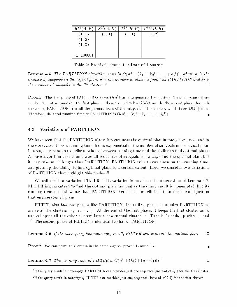
Rff(A;B) Sbf(A;D) T bf(B;E) U bf (D;B)

(1, 1) (1, 1) (1, 1) (1, 2)(1, 2)(1, 3). . .

(1, 10000)

Table 2: Proof of Lemma 4.4: Data of 4 Sources

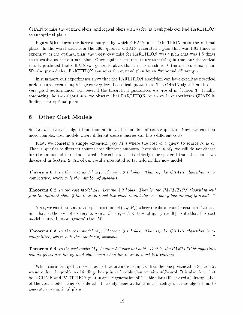
Lemma 4.5 The PARTITION algorithm runs in O(n2 + (k1! + k2! + : : :+ kp!)), where n is the

number of subgoals in the logical plan, p is the number of clusters found by PARTITION and ki is

the number of subgoals in the ith cluster. 32

Proof: The �rst phase of PARTITION takes O(n2) time to generate the clusters. This is because there

can be at most n rounds in the �rst phase and each round takes O(n) time. In the second phase, for each

cluster �i, PARTITION tries all the permutations of the subgoals in the cluster, which takes O(ki!) time.

Therefore, the total running time of PARTITION is O(n2 + (k1! + k2! + : : :+ kp!)).

4.3 Variations of PARTITION

We have seen that the PARTITION algorithm can miss the optimal plan in many scenarios, and in

the worst case it has a running time that is exponential in the number of subgoals in the logical plan.

In a way, it attempts to strike a balance between running time and the ability to �nd optimal plans.

A naive algorithm that enumerates all sequences of subgoals will always �nd the optimal plan, but

it may take much longer than PARTITION. PARTITION tries to cut down on the running time,

and gives up the ability to �nd optimal plans to a certain extent. Here, we consider two variations

of PARTITION that highlight this trade-o�.

We call the �rst variation FILTER. This variation is based on the observation of Lemma 4.2.

FILTER is guaranteed to �nd the optimal plan (as long as the query result is nonempty), but its

running time is much worse than PARTITION. Yet, it is more e�cient than the naive algorithm

that enumerates all plans.

FILTER also has two phases like PARTITION. In its �rst phase, it mimics PARTITION to

arrive at the clusters �1;�2; : : : ;�p. At the end of the �rst phase, it keeps the �rst cluster as is,

and collapses all the other clusters into a new second cluster �0. That is, it ends up with �1 and

�0. The second phase of FILTER is identical to that of PARTITION.

Lemma 4.6 If the user query has nonempty result, FILTER will generate the optimal plan. 2

Proof: We can prove this lemma in the same way we proved Lemma 4.2.

Lemma 4.7 The running time of FILTER is O(n2 + (k1! + (n� k1)!).4

2

3If the query result in nonempty, PARTITION can consider just one sequence (instead of k1!) for the �rst cluster.

4If the query result in nonempty, FILTER can consider just one sequence (instead of k1!) for the �rst cluster.

16

Proof: FILTER takes O(n2) time to generate all the clusters. It then takes an additional O(n) time to

merge clusters �2; : : : ;�p into �0. Now, it will have two clusters �1 with k1 subgoals and �0 with (n � k1)

subgoals. In the second phase, FILTER tries all permutations of subgoals in �1 and all permutations of

subgoals in �0. This takes O(k1!) and O((n� k1)!) time, respectively. So the total running time of FILTER

is O(n2 + k1 ! + (n � k1)!).

The second variation of PARTITION is called SCAN. This variation focuses on e�cient plan

generation. The main idea here is to simplify the second phase of PARTITION so that it can

run e�ciently. The penalty is that SCAN may not generate optimal plans in many cases where

PARTITION does.

SCAN also has two phases of processing. The �rst phase is identical to that of PARTITION.

In the second phase, SCAN picks an order for each cluster without searching over all the possible

orders. This leads to a second phase that runs in O(n) time. Note that since it does not search

over the space of subsequences for each cluster, SCAN tends to generate plans that are inferior to

those of PARTITION.

Lemma 4.8 SCAN runs in O(n2) time, where n is the number of subgoals in the logical plan. 2

Proof: The �rst phase of SCAN takes O(n2) like the �rst phase of PARTITION. The second phase takes

O(n) time. So the running time complexity of SCAN is O(n2).

5 Performance Analysis

In this section, we address the following questions regarding the performance of CHAIN and PAR-

TITION: How often do CHAIN and PARTITION �nd the optimal plan? When they miss the

optimal plan, what is the expected margin by which they miss? We attempt to answer these

questions by way of performance analysis of the algorithms in a simulated environment.

5.1 Simulation Parameters

In our experiments, we had a test bed of 15 sources, which participated in the integrated views on

which user queries could be posed. The source size distribution was 30% small, 60% medium and

10% large. Each source in our test bed had two access templates, each requiring that a di�erent

attribute be bound.

We employed randomly generated user queries that created logical plans over a subset of the 15

sources in the test bed. We varied the subset size from 1 to 10. For each query, we computed the

plans generated by the CHAIN algorithm and the PARTITION algorithm. We also exhaustively

searched for the optimal plan for the query. The cost of the three plans was computed based on

the model of Section 2.

5.2 Results of the Experiments

For each number of subgoals in the logical plan n, we generated 100 user queries, and studied the

performance of the algorithms on these queries. Figure 4 plots the number of query subgoals (on

17

0

2

4

6

8

10

1 2 3 4 5 6 7 8 9 10Av

erag

e D

iffer

ence

from

Opt

imal

Pla

n (%

)Number of Subgoals (n)

CHAINPARTITION

Figure 4: Average Cost

0

5

10

15

20

25

30

35

40

45

50

1 2 3 4 5 6 7 8 9 10

Frac

tion

of N

onop

timal

Pla

ns (%

)

Number of Subgoals (n)

CHAINPARTITION

(a) Fraction of non-optimal plan

0

0.2

0.4

0.6

0.8

1

1.2

1.4

1 2 3 4 5 6 7 8 9 10

Max

((C-C

o)/C

o)

Number of Subgoals (n)

PARTITIONCHAIN

(b) Worst case miss

Figure 5: Optimality of Each Algorithm

the horizontal axis) vs. the average margin by which generated plans miss the optimal plan (on

the vertical axis). Both CHAIN and PARTITION found near-optimal plans in the entire range of

inputs (a total of 1000 randomly generated queries) and, on the average, missed the optimal plan

by less than 10%.

Figure 4 also shows that as n increased, the average cost of the plan didn't necessarily increase.

Even though this is a bit surprising, we realize that it is because more subgoals in a logical plan

means more chances to choose some subgoals that have low cost, and thereby decrease the cost of

other expensive subgoals.

We also conducted experiments that measured the fraction of the queries for which the algo-

rithms found optimal plans, and the maximum margin by which the algorithms missed the optimal

plans. The results of these experiments are shown in Figure 5.

Figure 5(a) shows how often CHAIN and PARTITION found optimal plans. Over the entire

set of 1000 queries with n ranging from 1 to 10, CHAIN found the optimal plans more than 80%

of the time, while PARTITION found the optimal plans more than 95% of the time. This result is

surprising because we had proved in Section 3 that logical plans with as few as 3 subgoals can lead

18

CHAIN to miss the optimal plans, and logical plans with as few as 4 subgoals can lead PARTITION

to suboptimal plans.

Figure 5(b) shows the largest margin by which CHAIN and PARTITION miss the optimal

plans. In the worst case, over the 1000 queries, CHAIN generated a plan that was 1.95 times as

expensive as the optimal plan; the worst case miss for PARTITION was a plan that was 1.5 times

as expensive as the optimal plan. Once again, these results are surprising in that our theoretical

results predicted that CHAIN can generate plans that cost as much as 10 times the optimal plan.

We also proved that PARTITION can miss the optimal plan by an \unbounded" margin.

In summary, our experiments show that the PARTITION algorithm can have excellent practical

performance, even though it gives very few theoretical guarantees. The CHAIN algorithm also has

very good performance, well beyond the theoretical guarantees we proved in Section 3. Finally,

comparing the two algorithms, we observe that PARTITION consistently outperforms CHAIN in

�nding near-optimal plans.

6 Other Cost Models

So far, we discussed algorithms that minimize the number of source queries. Now, we consider

more complex cost models where di�erent source queries can have di�erent costs.

First, we consider a simple extension (say M1) where the cost of a query to source Si is ei.

That is, queries to di�erent sources cost di�erent amounts. Note that in M1, we still do not charge

for the amount of data transferred. Nevertheless, it is strictly more general than the model we

discussed in Section 2. All of our results presented so far hold in this new model.

Theorem 6.1 In the cost model M1, Theorem 3.1 holds. That is, the CHAIN algorithm is n-

competitive, where n is the number of subgoals. 2

Theorem 6.2 In the cost model M1, Lemma 4.2 holds. That is, the PARTITION algorithm will

�nd the optimal plan, if there are at most two clusters and the user query has nonempty result. 2

Next, we consider a more complex cost model (sayM2) where the data transfer costs are factored

in. That is, the cost of a query to source Si is ei + fi � (size of query result). Note that this cost

model is strictly more general than M1.

Theorem 6.3 In the cost model M2, Theorem 3.1 holds. That is, the CHAIN algorithm is n-

competitive, where n is the number of subgoals. 2

Theorem 6.4 In the cost modelM2, Lemma 4.2 does not hold. That is, the PARTITIONalgorithm

cannot guarantee the optimal plan, even when there are at most two clusters. 2

When considering other cost models that are more complex than the one presented in Section 2,

we note that the problem of �nding the optimal feasible plan remains NP-hard. It is also clear that

both CHAIN and PARTITION guarantee the generation of feasible plans (if they exist), irrespective

of the cost model being considered. The only issue at hand is the ability of these algorithms to

generate near optimal plans.

19

We observe that the n-competitiveness of CHAIN holds in any cost model with the following

property: the cost of a subgoal in a plan does not increase by postponing its processing to a

later time in the plan. Both M1 and M2 have this property and so CHAIN is n-competitive in

those models. We also note that the PARTITION algorithm with two clusters will always �nd the

optimal plan (assuming the query has nonempty result) if block queries cannot cost more than the

corresponding parameterized queries. This property holds, for instance, in model M1 and not in

model M2.

When one considers cost models other than those discussed here, the properties noted above may

hold in those models and consequently CHAIN and PARTITION may yield very good results. Even

when the properties do not hold, the strategies employed by the two algorithms may act as good

heuristics and help them generate e�cient plans. For instance, in the cost model M2, PARTITION

cannot guarantee the generation of optimal plans even when there are only two clusters. In our

simulation experiments we studied the performance of PARTITION in this cost model and found

that it continues to �nd plans that are very close to optimal.

7 Conclusion

In this paper, we considered the problem of query planning in heterogeneous data integration

systems based on the mediation approach. We employed a cost model that focuses on the main

costs in mediation systems. In this cost model, we developed two algorithms that guarantee the

generation of feasible plans (when they exist). We showed that the problem at hand is NP-hard.

One of our algorithms runs in polynomial time. It generates optimal plans in many cases and in

other cases it has a linear bound on the worst case margin by which it misses the optimal plans.

The second algorithm �nds optimal plans in more scenarios, but has no bound on the margin of

missing the optimal plans in the bad scenarios. We analyzed the performance of our algorithms

using simulation experiments and extended our results to more complex cost models.

References

[1] P. Apers, A. Hevner, S. Yao. Optimization Algorithms for Distributed Queries. In IEEE

Trans. Software Engineering, 9(1), 1983.

[2] P. Bernstein, N. Goodman, E. Wong, C. Reeve, J. Rothnie. Query Processing in a System for

Distributed Databases (SDD-1). In ACM Trans. Database Systems, 6(4), 1981.

[3] S. Chawathe, H. Garcia-Molina, J. Hammer, K. Ireland, Y. Papakonstantinou, J. Ullman,

J. Widom. The TSIMMIS Project: Integration of Heterogeneous Information Sources. In

IPSJ, Japan, 1994.

[4] S. Cluet, G. Moerkotte. On the Complexity of Generating Optimal Left-deep Processing Trees

with Cross Products. In ICDT Conference, 1995.

[5] R. Epstein, M. Stonebraker. Analysis of Distributed Database Strategies. In VLDB Conference,

1980.

[6] C. Galindo-Legaria, A. Pellenkoft, M. Kersten. Fast, Randomized Join Order Selection { Why

Use Transformations? In VLDB Conference, 1994.

20

[7] M. Garey, D. Johnson. Computers and Intractability: A Guide to the Theory of NP-

Completeness. Freeman, San Francisco, 1979.

[8] L. Haas, D. Kossman, E.L. Wimmers, J. Yang. Optimizing Queries Across Diverse Data

Sources. In VLDB Conference, 1997.

[9] J. Hammer, H. Garcia-Molina, S. Nestorov, R. Yerneni, M. Breunig, V. Vassalos. Template-

Based Wrappers in the TSIMMIS System. In SIGMOD Conference, 1997.

[10] T. Ibaraki, T. Kameda. On the Optimal Nesting Order for Computing N-relational Joins. In

ACM Trans. Database Systems, 9(3), 1984.

[11] Y. Ioannidis, Y. Kang. Randomized Algorithms for Optimizing Large Join Queries. In SIG-

MOD Conference, 1990.

[12] Y. Ioannidis, E. Wong. Query Optimization by Simulated Annealing. In SIGMOD Conference,

1987.

[13] R. Krishnamurthy, H. Boral, C. Zaniolo. Optimization of Non-recursive Queries. In VLDB

Conference, 1986.

[14] A. Levy, A. Rajaraman, J. Ordille. Querying Heterogeneous Information Sources Using Source

Descriptions. In VLDB Conference, 1996.

[15] C. Li, R. Yerneni, V. Vassalos, H. Garcia-Molina, Y. Papakonstantinou, J. Ullman, M. Valiveti.

Capability Based Mediation in TSIMMIS. In SIGMOD Conference, 1998.

[16] K. Morris. An Algorithm for Ordering Subgoals in NAIL!. In ACM PODS, 1988.

[17] K. Ono, G. Lohman. Measuring the Complexity of Join Enumeration in Query Optimization.

In VLDB Conference, 1990.

[18] C. Papadimitriou, K. Steiglitz. Combinatorial Optimization: Algorithms and Complexity.

Prentice-Hall, 1982.

[19] Y. Papakonstantinou, A. Gupta, L. Haas. Capabilities-based Query Rewriting in Mediator

Systems. In PDIS Conference, 1996.

[20] A. Pellenkoft, C. Galindo-Legaria, M. Kersten. The Complexity of Transformation-Based Join

Enumeration. In VLDB Conference, 1997.

[21] W. Scheufele, G. Moerkotte. On the Complexity of Generating Optimal Plans with Cross

Products. In PODS Conference, 1997.

[22] P. Selinger, M. Adiba. Access Path Selection in Distributed Databases Management Systems.

In Readings in Database Systems. Edited by M. Stonebraker. Morgan-Kaufman Publishers,

1994.

[23] M. Steinbrunn, G. Moerkotte, A. Kemper. Heuristic and Randomized Optimization for the

Join Ordering Problem. In VLDB Journal, 6(3), 1997.

[24] A. Swami. Optimization of Large Join Queries: Combining Heuristic and Combinatorial

Techniques. In SIGMOD Conference, 1989.

21

[25] A. Swami, A. Gupta. Optimization of Large Join Queries. In SIGMOD Conference, 1988.

[26] A. Tomasic, L. Raschid, P. Valduriez. Scaling Heterogeneous Databases and the Design of

Disco. In Int. Conf. on Distributed Computing Systems, 1996.

[27] J. Ullman. Principles of Database and Knowledge-base Systems, Volumes I, II. Computer

Science Press, Rockville MD.

[28] J. Ullman, M. Vardi. The Complexity of Ordering Subgoals. In ACM PODS, 1988.

[29] B. Vance, D. Maier. Rapid Bushy Join-Order Optimization with Cartesian Products. In

SIGMOD Conference, 1996.

[30] V. Vassalos, Y. Papakonstantinou. Describing and Using Query Capabilities of Heterogeneous

Sources. In VLDB Conference, 1997.

[31] G. Wiederhold. Mediators in the Architecture of Future Information Systems. In IEEE Com-

puter, 25:38-49, 1992.

22