Accessing Queries through Microsoft Excel:
237
FOUNDATION software AUG. 5-7 — CLEVELAND, OH CONSTRUCTION CPA CONFERENCE Foundation Software’s 3 rd Annual FOUNDATION COLLEGE Microsoft ® Excel Form Design Using Microsoft Query DELIVERY METHOD: Group Live PROGRAM LEVEL: Intermediate CPE CREDIT: up to 18 PRESENTER: Scott Kern
-
Upload
khangminh22 -
Category
Documents
-
view
1 -
download
0
Transcript of Accessing Queries through Microsoft Excel:

FOUNDATIONsoftware
AUG. 5-7 — CLEVELAND, OH
CONSTRUCTIONCPA CONFERENCE
Foundation Software’s 3rd Annual
FOUNDATION COLLEGEMicrosoft® Excel Form
Design Using Microsoft Query
DELIVERY METHOD: Group LivePROGRAM LEVEL: IntermediateCPE CREDIT: up to 18PRESENTER: Scott Kern


Microsoft Excel and Query Building Custom Form Creation through MS Query
Scott Kern
Senior Consultant
Foundation Software
- 1 -
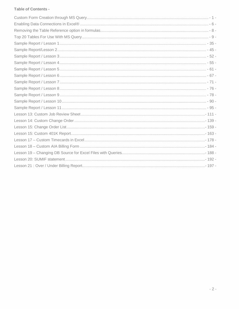
Table of Contents -
Custom Form Creation through MS Query ............................................................................................................ - 1 - Enabling Data Connections in Excel® .................................................................................................................. - 6 - Removing the Table Reference option in formulas ................................................................................................ - 8 - Top 20 Tables For Use With MS Query ................................................................................................................ - 9 - Sample Report / Lesson 1 .................................................................................................................................. - 35 - Sample Report/Lesson 2 .................................................................................................................................... - 45 - Sample Report / Lesson 3 .................................................................................................................................. - 52 - Sample Report / Lesson 4 .................................................................................................................................. - 55 - Sample Report / Lesson 5 .................................................................................................................................. - 61 - Sample Report / Lesson 6 .................................................................................................................................. - 67 - Sample Report / Lesson 7 .................................................................................................................................. - 71 - Sample Report / Lesson 8 .................................................................................................................................. - 76 - Sample Report / Lesson 9 .................................................................................................................................. - 78 - Sample Report / Lesson 10 ................................................................................................................................ - 90 - Sample Report / Lesson 11 ................................................................................................................................ - 95 - Lesson 13: Custom Job Review Sheet ..............................................................................................................- 111 - Lesson 14: Custom Change Order ....................................................................................................................- 139 - Lesson 15: Change Order List ...........................................................................................................................- 159 - Lesson 15: Custom 401K Report .......................................................................................................................- 163 - Lesson 17 – Custom Timecards in Excel ...........................................................................................................- 178 - Lesson 18 – Custom AIA Billing Form ...............................................................................................................- 184 - Lesson 19 – Changing DB Source for Excel Files with Queries..........................................................................- 188 - Lesson 20: SUMIF statement ............................................................................................................................- 192 - Lesson 21 : Over / Under Billing Report .............................................................................................................- 197 -
- 2 -

Preface: A Brief Explanation of Database Structure and Queries
(From Searchsqlserver.com)
http://searchsqlserver.techtarget.com/sDefinition/0,,sid87_gci212885,00.html
“Definition- A relational database is a collection of data items organized as a set of formally-described tables from which data can be accessed or reassembled in many different ways without having to reorganize the database tables. The relational database was invented by E. F. Codd at IBM in 1970.
The standard user and application program interface to a relational database is the structured query language (SQL). SQL statements are used both for interactive queries for information from a relational database and for gathering data for reports.
In addition to being relatively easy to create and access, a relational database has the important advantage of being easy to extend. After the original database creation, a new data category can be added without requiring that all existing applications be modified.
A relational database is a set of tables containing data fitted into predefined categories. Each table (which is sometimes called a relation) contains one or more data categories in columns. Each row contains a unique instance of data for the categories defined by the columns.”
A quick preview of how FOUNDATION’s Job table relates to the Customer table:
The Job table houses most of the fields on the Job Record. The Customer table houses the information from the Customer Record. Individual tables relate to each other by common fields within the tables. If you have a Job Record in FOUNDATION, chances are you have a customer attached to that Job Number. FOUNDATION’S database uses the field named customer_no to join these two tables. This way, we can access the Job table, and then pull in all associated information (fields) stored in the Customer table.
We will see more examples later, but each individual table stores minimal data related to other tables to reduce database size and overhead. The customer_no (customer number) is stored in the Job table, but the customer name, address, contact information, etc. is not. The specific customer details are stored in the Customer table. The link between the two tables joins the information together when it is queried from the source.
Fields
Tables
- 3 -
A note on field names: One item that needs to be addressed early is the definition of fields that contain “_no” vs. “_id” . Almost every table includes fields that are designated as “key identifiers.” Some examples are as follows:
• Customers: customer_no / customer_id
• G/L Accounts: account_no / account_id
• Jobs: job_no / job_id
• Vendors: vendor_no / vendor_id
• Employees: employee_no / employee_id
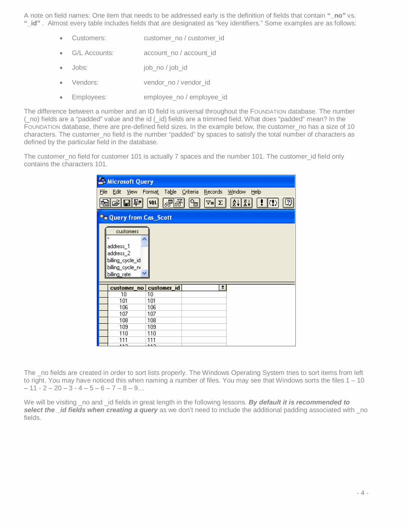
The difference between a number and an ID field is universal throughout the FOUNDATION database. The number (_no) fields are a “padded” value and the id (_id) fields are a trimmed field. What does “padded” mean? In the FOUNDATION database, there are pre-defined field sizes. In the example below, the customer_no has a size of 10 characters. The customer_no field is the number “padded” by spaces to satisfy the total number of characters as defined by the particular field in the database.
The customer_no field for customer 101 is actually 7 spaces and the number 101. The customer_id field only contains the characters 101.
The _no fields are created in order to sort lists properly. The Windows Operating System tries to sort items from left to right. You may have noticed this when naming a number of files. You may see that Windows sorts the files 1 – 10 – 11 - 2 – 20 – 3 - 4 – 5 – 6 – 7 – 8 – 9…
We will be visiting _no and _id fields in great length in the following lessons. By default it is recommended to select the _id fields when creating a query as we don’t need to include the additional padding associated with _no fields.
- 4 -

(From www.About.com:)
http://databases.about.com/od/specificproducts/a/whatisadatabase.htm
“Queries are the primary mechanism for retrieving information from a database and consist of questions presented to the database in a predefined format.”
There is a lot of good reading on the subject from beginning to advanced topics on these websites.
Actually locating the correct tables and fields in any database takes time and patience. The easiest queries to write access a single table. These are typically queries against maintenance type records (employee files, job files, vendor files). Some queries require calculations to sum amounts or return minimum or maximum values from a particular table (timecard history, job history). Other queries require the linking of multiple tables in order to return the desired information (job budgets/change orders/costs/income).
We will visit many of these options and show some of the more readily accessed tables in the following lessons.
Excel Resources on the Web
Mr. Excel – An excellent forum. Many Google searches return topics answered in these forums.
http://www.mrexcel.com/forum/index.php
Contextures – A well-organized menu of Excel tips and tricks.
http://www.contextures.com/tiptech.html
Microsoft Office Online – A good resource. (Some may find this site difficult to navigate/search.)
http://office.microsoft.com/en-us/excel/FX100646961033.aspx
University of Wisconsin – A well-documented source with many screen shots.
http://www.uwec.edu/help/excel03.htm
Allen Wyatt’s Excel Tips – Nicely formatted for different versions of Excel.
http://exceltips.vitalnews.com/
WikiHow – User Edited “how to” site (start your search with “excel”).
http://www.wikihow.com
Ozgrid.com
http://www.ozgrid.com/Excel/
Google– Everything I learned, I learned with the help of Google. Search for what you are looking for and you will find most of the answers with Google’s help. Many searches return data from the sites listed above. I find it easier to start searching with Google as opposed to visiting a specific website.
- 5 -

Enabling Data Connections in Excel® In Excel, heightened security settings have been enabled as a default. Before performing a query, you will need to change a few settings in order to pull data into Excel Worksheets. This setting will need to be modified for any and all workstations that are going to make use of the spreadsheets that are linked to a query.
1. In Excel 2007, c lick on the office button in the upper left hand corner and select “Excel Options. In Excel 2010 / 2013 / 365, click on the “File” tab and select “Options”
2007 2010 / 2012 / 365
2. Click on the “Trust Center” option in the left hand column, then click [Trust Center Settings…] in the lower right hand corner.
- 6 -

3. Click on “External Content” in the left hand column.
4. Select the Security Setting appropriate for the level of confidence you have in the users of the Excel application.
• If you choose Disable all Data Connections, please close the book, turn off your computer, and we thank you for attending.
• If you select Prompt user about Data Connections, every time you open a workbook with a query, Excel will warn you with the following:
• The last option is to Enable all Data Connections. This is the best choice IF you trust the source of all Excel files in your office. If you are busy downloading Excel files off the internet, or opening Excel Files that came as attachments on emails from complete strangers, this option may not be the best for you.
- 7 -

Removing the Table Reference option in formulas We will also be making extensive use of tables with all of our queries. By default, Excel is set to use table names in formulas. Advanced users may want to keep this option enabled, but most users will want to shut this option off.
Here is an example of the TABLE NAME REFERENCE in formulas.
1. Access the Excel Options again. In Excel 2007, this toggle is under the Popular option in the left hand column. In Excel 2010, it is under the Formulas section (shown below)
2. With the Use table names in formulas checkbox disabled, you will see the more familiar cell reference in formulas.
- 8 -

Top 20 Tables For Use With MS Query There are over 2,000 individual tables in FOUNDATION’S database.
The following list of Foundation Software Database tables is a representation of the most commonly sought after tables when creating reports through queries.
These tables break down into two simple categories; maintenance-related tables and history-related tables.
The easiest way to start is by creating the list.
For a simple Chart of Accounts, look for the G/L Account List. In the database, this table is known as …Accounts. There are 52 fields within this table. What is important is the ability to match the table.field name to the screen item in FOUNDATION.
This table is created as a reference so you may get familiar with identifying table and field names within the database as they relate to the more “public” face of Foundation Software.
When reviewing the “Top 20” tables, we will look at the most used fields within the tables as well.
company_no account_no description debit_credit apply_subdivision inc_exp_type overhead_percent overhead_formula_percent force_job_costing jc_income_expense cash_flag bonding_class record_status row_modified_by row_modified_on row_unique_id ovhd_alloc_income_expense percent_to_allocate overhead_weight_factor account_id company_id direct_deposit_format dir_dep_exp_dsg_report_no direct_deposit_pr_file ach_dest_routing_num ach_dest_name
ach_origin_routing_num ach_origin_name ach_origin_reference_code ach_company_name ach_company_id ach_pr_entry_desc ach_pr_discretionary_data ach_pr_emp_identifier ach_pr_emp_name_format dir_dep_exp_dsg_report_id condense_on_cash_rec statement_category_no bank_account_num bank_account_type ach_balanced_file statement_category_id include_in_canned_financials ach_origin_dfi_id positive_pay_exp_dsg_report_no positive_pay_export_file positive_pay_exp_dsg_report_id ach_use_origin_routing_bal_dfi ach_use_dest_routing_bal_dfi ach_origin_type account_type gl_history_report_rollup
- 9 -

Table Name: Accounts
FOUNDATION Location: General Ledger > Maintenance > Accounts
In a Query window, the most common fields used in the accounts table are:
account_id Account number
description G/L account name
debit_credit The “type” of account it is
#1
- 10 -

Table Name: Vendors
FOUNDATION Location: Accounts Payable > Maintenance > Vendors
vendor_id Vendor number
name Vendor description/name
address_1 First line address
address_2 Additional address line
city City
state State
zip_code Zip code
Additional vendor fields of interest:
wc_certificate Y or N to “W/C Certificate on file”
wc_date_expires W/C insurance certificate expiration date
ins_certificate Y or N to “Insurance Certificate on file”
ins_date_expires Insurance certificate expiration date
default_gl_account Uhhhhh…. the default G/L account
tax_id Default sales tax authority
#2
- 11 -

Table Name: Customers
FOUNDATION Location: Accounts Receivable > Maintenance > Customers
customer_id customer number
name customer description / name
address_1 First line address
address_2 Additional address line
city City
state State
zip_code Zip code
phone_voice Phone number
Additional customer fields of interest:
client_since How long client has been an active customer
income_type_id Default income type for A/R invoicing
tax_id Default A/R sales tax ID
default_tax_type Sales/Use/N/A
#3
- 12 -

Table Name: Jobs
FOUNDATION Location: Job Costing > Maintenance > Jobs
job_id Job number
description Job description / name
address_1, 2, city, state, zip_code Address information per other tables
customer_id Default customer number on job record
job_status Active/inactive/closed/overhead
completion_date Job end date from the “Addl” tab
geo_are_id Geographic area number
project_manager_id Project manager number
project_class_id Project class number
Associated tables:
• customers: contains customer name and addition customer related information • geographic_areas: Geographic area descriptions • project_managers: Project manager descriptions • project_classes: Project class descriptions
Additional job fields of interest:
original_contract Original contract amount on “General” tab original_cost Original estimated cost amount on “General” tab
#4
- 13 -

Table Name: Items
FOUNDATION Location: Inventory > Maintenance > Items
item_id Inventory item number
description Item name
stocking_unit_id Stocking unit of measure
standard_cost Standard cost
primary_item_category_id Primary item category
Additional item fields of interest:
item_2_category_id, item_3_category_id, etc. Additional categories 2 -6
last_cost Last cost transaction from receipt function
last_date_purchased Last date received from receipts function
bin_location_id Bin number
#5
- 14 -
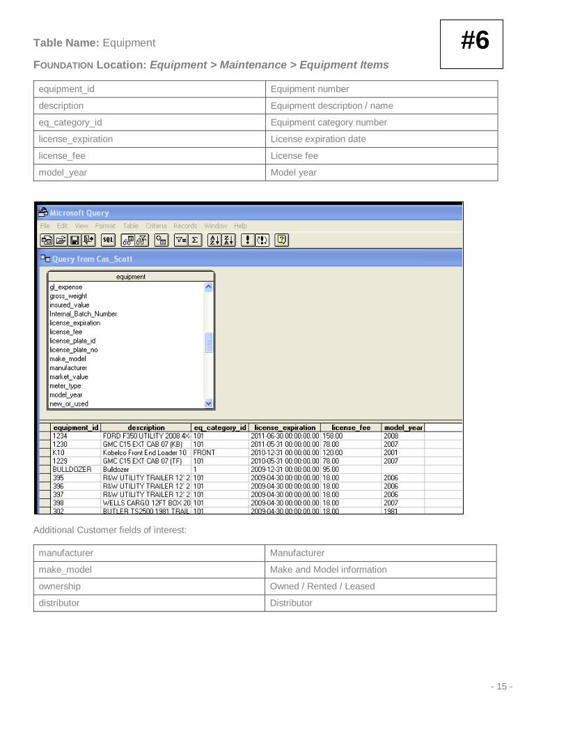
Table Name: Equipment
FOUNDATION Location: Equipment > Maintenance > Equipment Items
equipment_id Equipment number
description Equipment description / name
eq_category_id Equipment category number
license_expiration License expiration date
license_fee License fee
model_year Model year
Additional Customer fields of interest:
manufacturer Manufacturer
make_model Make and Model information
ownership Owned / Rented / Leased
distributor Distributor
#6
- 15 -
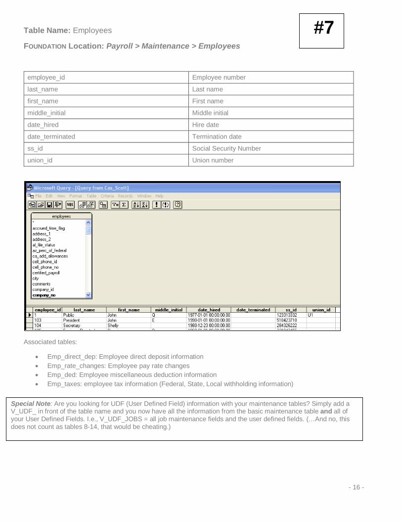
Table Name: Employees
FOUNDATION Location: Payroll > Maintenance > Employees
employee_id Employee number
last_name Last name
first_name First name
middle_initial Middle initial
date_hired Hire date
date_terminated Termination date
ss_id Social Security Number
union_id Union number
Associated tables:
• Emp_direct_dep: Employee direct deposit information • Emp_rate_changes: Employee pay rate changes • Emp_ded: Employee miscellaneous deduction information • Emp_taxes: employee tax information (Federal, State, Local withholding information)
#7
Special Note: Are you looking for UDF (User Defined Field) information with your maintenance tables? Simply add a V_UDF_ in front of the table name and you now have all the information from the basic maintenance table and all of your User Defined Fields. I.e., V_UDF_JOBS = all job maintenance fields and the user defined fields. (…And no, this does not count as tables 8-14, that would be cheating.)
- 16 -

Table Name: job_budgets
FOUNDATION Location: Job Cost > Maintenance > Jobs > “Budget” Tab
job_id Job number
cost_code_id Cost code number
cost_class_id Cost class number
orig_est_dollars Original estimated dollars (per code and class)
orig_est_units Original estimated units
Associated tables:
• Jobs, cost_codes, cost_classes: all tables used to pull in descriptions for associated items • Additional job_budgets fields of interest:
phase_id For phased companies
#8
- 17 -
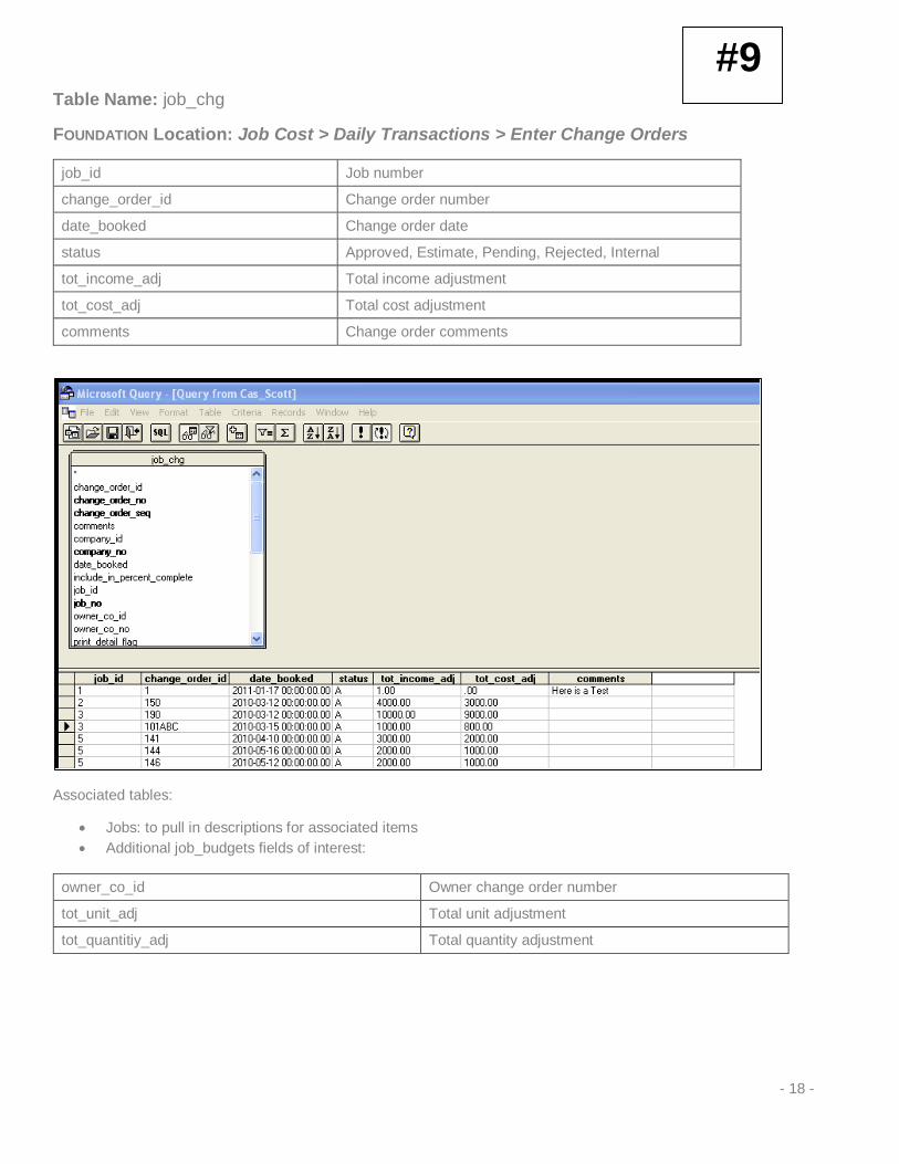
Table Name: job_chg
FOUNDATION Location: Job Cost > Daily Transactions > Enter Change Orders
job_id Job number
change_order_id Change order number
date_booked Change order date
status Approved, Estimate, Pending, Rejected, Internal
tot_income_adj Total income adjustment
tot_cost_adj Total cost adjustment
comments Change order comments
Associated tables:
• Jobs: to pull in descriptions for associated items • Additional job_budgets fields of interest:
owner_co_id Owner change order number
tot_unit_adj Total unit adjustment
tot_quantitiy_adj Total quantity adjustment
#9
- 18 -

Table Name: job_chg_budgets
FOUNDATION Location: Job Cost > Daily Transactions > Enter Change Orders > “Distribution” tab
job_id Job number
change_order_id Change order number
cost_code_id Cost code number
cost_class_id Cost class number
cost_adj Cost adjustment per code and class
unit_adj Unit adjustment
Associated tables:
• Job_chg, Jobs, Cost_codes, cost_classes: all tables used to pull in descriptions for associated items • Additional Job_chg_budgets fields of interest:
Phase_id For phased companies
#10
- 19 -
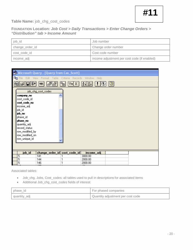
Table Name: job_chg_cost_codes
FOUNDATION Location: Job Cost > Daily Transactions > Enter Change Orders > “Distribution” tab > Income Amount
job_id Job number
change_order_id Change order number
cost_code_id Cost code number
income_adj income adjustment per cost code (if enabled)
Associated tables:
• Job_chg, Jobs, Cost_codes: all tables used to pull in descriptions for associated items • Additional Job_chg_cost_codes fields of interest:
phase_id For phased companies
quantity_adj Quantity adjustment per cost code
#11
- 20 -

Table Name: v_job_history
FOUNDATION Location: Job Cost > Reports > Job History Detail
Job_id Job number
Job_description Job description
Cost_code_id Cost code number
Cost_code_description Cost code description
Cost_class_id Cost class number
Cost_class_description Cost class description
Cost Cost
Units Units/Hours
Date_booked Date posted to G/L & job cost
Associated tables:
• None – all of the associated data is in this table – YEAH!!! • Additional v_job_history fields of interest :
Too many to mention. Basically, if it is cost-related and shows up on a Job History Detail Report, it is in this table. Employee names, inventory items, equipment items, journal descriptions, source module, earn codes, departments, vendors – all of the IDs and descriptions for these items are contained within this table.
#12
- 21 -

Table Name: ap_invoice_d
FOUNDATION Location: Accounts Payable > Daily Transactions > Posted Invoice Distribution Detail
Voucher_id A/P invoice transaction number
Account_id Basic G/L account number (no divisions)
Job_id Job number
Cost_code_id Cost code number
Cost_class_id Cost class number
Amount $ amount from A/P invoice distribution
Associated tables:
• Ap_invoice_h: This table carries the vendor, invoice, and posting date information – pretty much required if you want to make any sense out of the ap_invoice_d table.
• Jobs, cost_codes, cost_classes, accounts: All tables used to pull in descriptions for associated items.
Additional ap_invoice_d fields of interest:
Div_level_1 – 4 Division for G/L posting
Equip_id & eq_wo_id Equipment module posting information
Full_account_id Full G/L account number with divisions
Sales_tax_amount Sales tax from distribution
#13
- 22 -
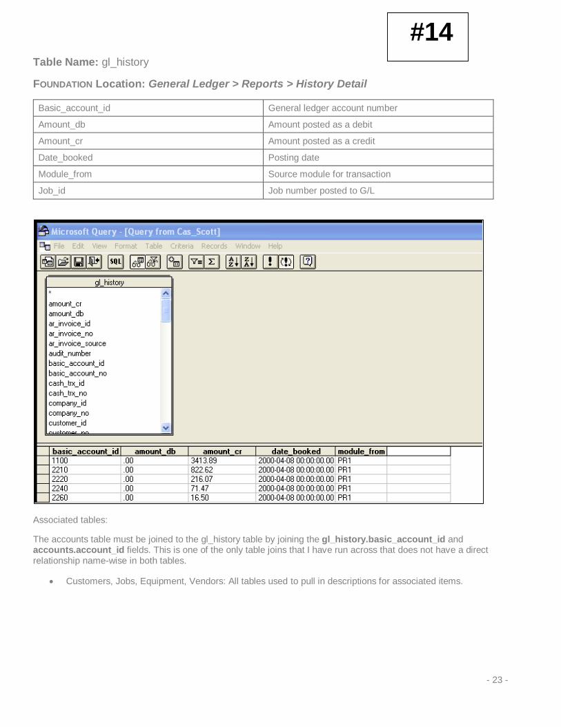
Table Name: gl_history
FOUNDATION Location: General Ledger > Reports > History Detail
Basic_account_id General ledger account number
Amount_db Amount posted as a debit
Amount_cr Amount posted as a credit
Date_booked Posting date
Module_from Source module for transaction
Job_id Job number posted to G/L
Associated tables:
The accounts table must be joined to the gl_history table by joining the gl_history.basic_account_id and accounts.account_id fields. This is one of the only table joins that I have run across that does not have a direct relationship name-wise in both tables.
• Customers, Jobs, Equipment, Vendors: All tables used to pull in descriptions for associated items.
#14
- 23 -

Table Name: gl_history_pr_dtl
FOUNDATION Location: General Ledger > Reports > History Detail > drilldown to Payroll History within G/L History
Basic_account_id G/L account number
Job_id Job number
Amount_db Amount posted as debit
Amount_cr Amount posted as credit
Employee_id Employee number
Date_booked Date posted to general ledger
Associated tables:
• Jobs, Employees, Accounts: all tables used to pull in descriptions for associated items • Additional gl_history_pr_dtl fields of interest:
Check_id P/R check number for the posting
Full_account_id G/L account including division
Gl_cash Cash account used for check posting
#15
- 24 -
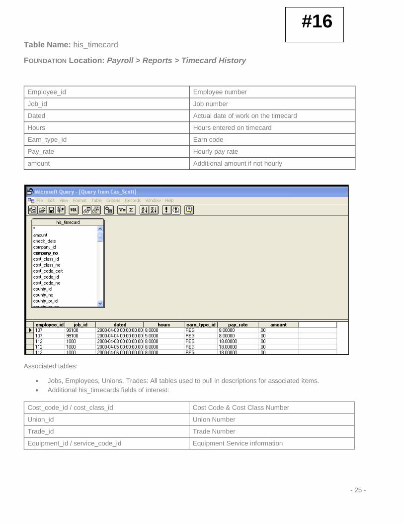
Table Name: his_timecard
FOUNDATION Location: Payroll > Reports > Timecard History
Employee_id Employee number
Job_id Job number
Dated Actual date of work on the timecard
Hours Hours entered on timecard
Earn_type_id Earn code
Pay_rate Hourly pay rate
amount Additional amount if not hourly
Associated tables:
• Jobs, Employees, Unions, Trades: All tables used to pull in descriptions for associated items. • Additional his_timecards fields of interest:
Cost_code_id / cost_class_id Cost Code & Cost Class Number
Union_id Union Number
Trade_id Trade Number
Equipment_id / service_code_id Equipment Service information
#16
- 25 -

Table Name: his_misc
FOUNDATION Location: Payroll > Reports > Miscellaneous Deduction History
Employee_id Employee number
Deduction_id Miscellaneous deduction number / code
Deduction_amount Amount withheld for this deduction code
P401K_earnings 401K Earnings (401K codes only)
P401K_matching 401K matching amount
Dated Date posted to payroll history (most likely check date)
Associated tables:
• Employees (and other earning history tables): All tables used to pull in descriptions for associated items.
Additional his_misc fields of interest:
Integration_type For A/P integration
Vendor_id Vendor number (for integration)
#17
- 26 -

Table Name: his_earn_hours
FOUNDATION Location: Payroll > Reports > Earnings Detail
Employee_id Employee number
Earn_type_id Earn code
Hours Number of hours worked per earn code
Dollars Summed value of dollars per earn code
Dated Date posted (most likely check date)
Associated tables:
• Employees: Used to pull in descriptions for associated items.
#18
- 27 -

Table Name: his_earn_additional
FOUNDATION Location: Payroll > Reports > Earnings Detail
Employee_id Employee number
Earn_type_id Earn code
Additional_dollars Additional earning amount
Dated Date posted (most likely check date)
Associated tables:
• Employees: Used to pull in descriptions for associated items.
#19
- 28 -
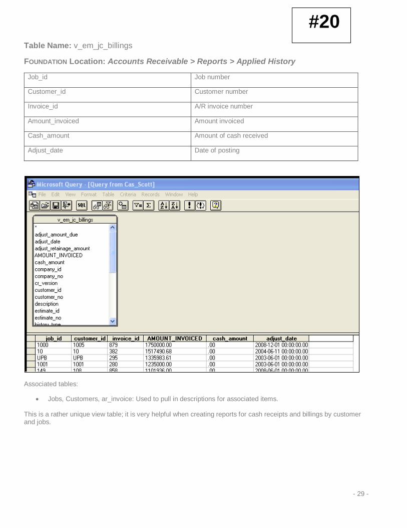
Table Name: v_em_jc_billings
FOUNDATION Location: Accounts Receivable > Reports > Applied History
Job_id Job number
Customer_id Customer number
Invoice_id A/R invoice number
Amount_invoiced Amount invoiced
Cash_amount Amount of cash received
Adjust_date Date of posting
Associated tables:
• Jobs, Customers, ar_invoice: Used to pull in descriptions for associated items.
This is a rather unique view table; it is very helpful when creating reports for cash receipts and billings by customer and jobs.
#20
- 29 -

Additional Tables of Use
The following tables are helpful when creating custom forms with the MS Query tool. This book would be over 2700 pages long if all available tables were listed. These tables are offered as a guide to help locate data that is used often by clients of Foundation Software.
For the most part, these tables will have some common names. Specifically, there are many items in FOUNDATION that contain “_H” (Header) and “_D” (Detail/Distribution) tables. As a general rule, if you need to right-click and add a line on a window within FOUNDATION, that data will be located in a separate table.
Some items, like the change order, may have more than a header and detail table. The change order table also has a “Printable” tab that has data stored in a separate table.
Change Orders
The “General” tab information is contained in the job_chg table.
The “Distribution” tab information is contained in the job_chg_budgets tab.
The “Printable” tab information is in the job_chg_printable table.
- 30 -

For the most part, the structure of the tables within the FOUNDATION database follow this same layout. More examples to follow:
Purchase Orders/Subcontracts:
FOUNDATION Location: Database Table Name:
PO/Sub “General” tab PO_SUB_H
PO/Sub Distribution (on “General” tab) PO_SUB_D
PO/Sub “Item Detail” tab PO_SUB_ITEM_D
- 31 -
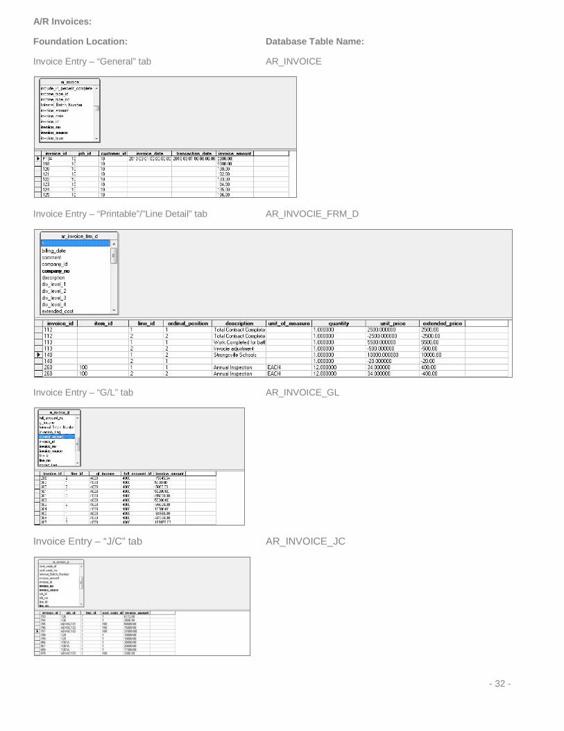
A/R Invoices:
Foundation Location: Database Table Name:
Invoice Entry – “General” tab AR_INVOICE
Invoice Entry – “Printable”/”Line Detail” tab AR_INVOCIE_FRM_D
Invoice Entry – “G/L” tab AR_INVOICE_GL
Invoice Entry – “J/C” tab AR_INVOICE_JC
- 32 -
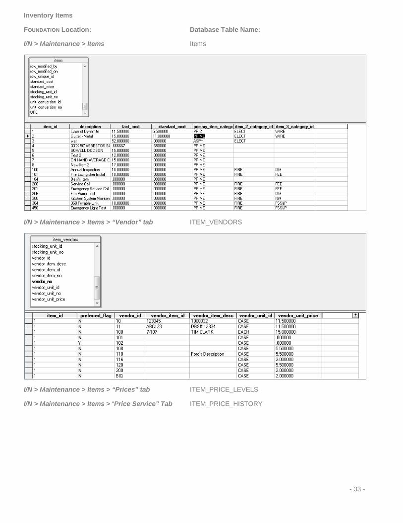
Inventory Items
FOUNDATION Location: Database Table Name:
I/N > Maintenance > Items Items
I/N > Maintenance > Items > “Vendor” tab ITEM_VENDORS
I/N > Maintenance > Items > “Prices” tab ITEM_PRICE_LEVELS
I/N > Maintenance > Items > “Price Service” Tab ITEM_PRICE_HISTORY
- 33 -

Employees:
FOUNDATION Location: Database Table Name:
Employee Record > General Tab EMPLOYEES
Employee Record > Deductions / Tax info EMP_TAXES
Employee Record > Deductions / Misc Ded EMP_DED
Employee Record > Direct Deposit EMP_DIRECT_DEPOSIT
Employee Record > History Tab EMP_RATE_CHANGES
Employee Record > Accruals Tab EMP_ACCRUALS
- 34 -

Sample Report / Lesson 1 Employee Phone List
Tasks
• Accessing Data Through MS Query • Formatting Queried Data in Excel • Editing Queries • Sorting data within MS Query
- 35 -

1. Click on the “Data” tab on the ribbon and select Get External Data Group > From Other Sources > From Microsoft Query.
2. Select the database that you want to query. This should be the primary database that houses the information for Foundation Software. Disable the option to Use the Query Wizard to create/edit queries. Once you have selected the database, click [OK] in the upper right-hand corner.
- 36 -

3. On the SQL Server Login window, enter your dba login and password (or your FOUNDATION user ID and password).
You have now accessed the Microsoft Query function. This is where we will build the queries, by selecting the appropriate tables and fields. Once the selection process is complete we will then return the data to Excel.
- 37 -

4. For this first example, we will access the employee table. Scroll down to the “employees” table.
5. Highlight it, and click [Add]. You will notice that the table appears in the upper left hand corner of the window. Click the [Close] button on the Add Tables dialog box.
6. To see more of the fields within the table, click and hold on the separator line and drag the top portion of the window to make more room.
Click here and drag the line down.
Click here to expand the size of the table box.
- 38 -
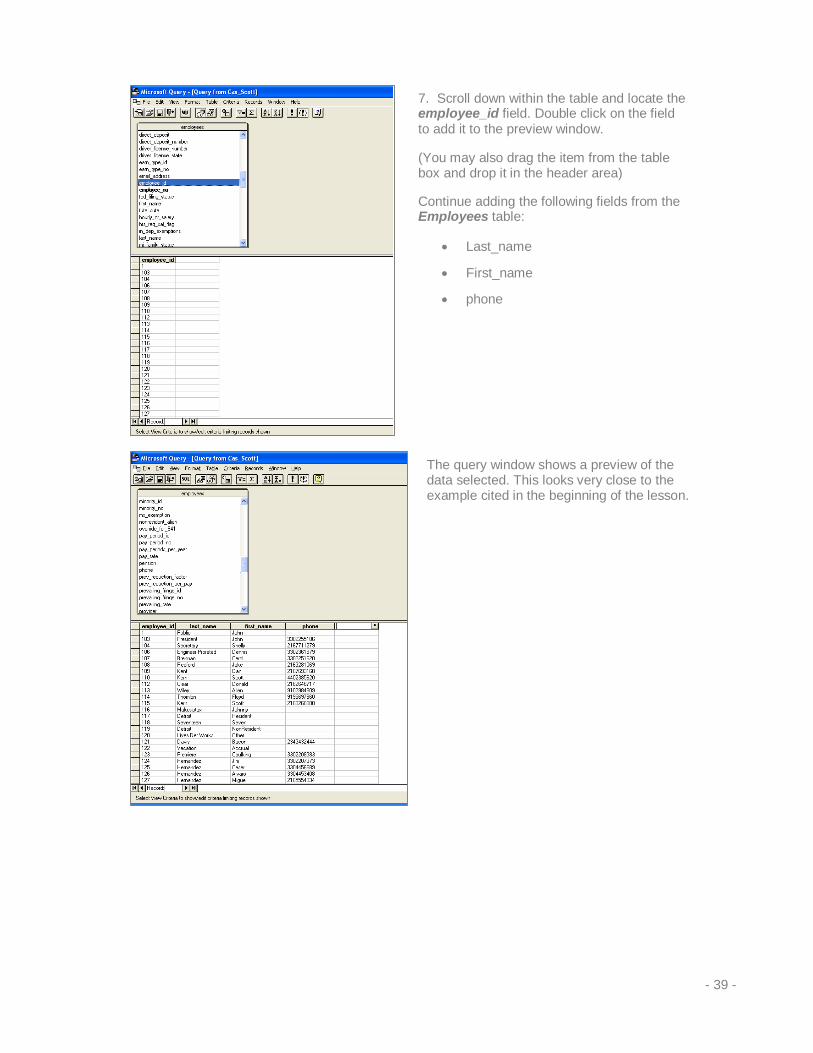
7. Scroll down within the table and locate the employee_id field. Double click on the field to add it to the preview window.
(You may also drag the item from the table box and drop it in the header area)
Continue adding the following fields from the Employees table:
• Last_name
• First_name
• phone
The query window shows a preview of the data selected. This looks very close to the example cited in the beginning of the lesson.
- 39 -
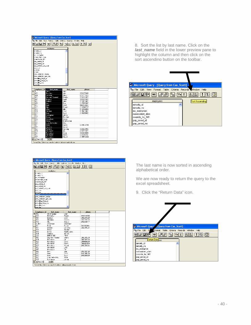
The last name is now sorted in ascending alphabetical order.
We are now ready to return the query to the excel spreadsheet.
9. Click the “Return Data” icon.
8. Sort the list by last name. Click on the last_name field in the lower preview pane to highlight the column and then click on the sort ascending button on the toolbar.
- 40 -

10. Excel will now ask where you want to return the data on the spreadsheet. In most cases, you will want to start the data in cell A1. Click [OK] to accept the selection.
Congratulations, some of you have completed your first query! …. Then reality sets in.
- 41 -
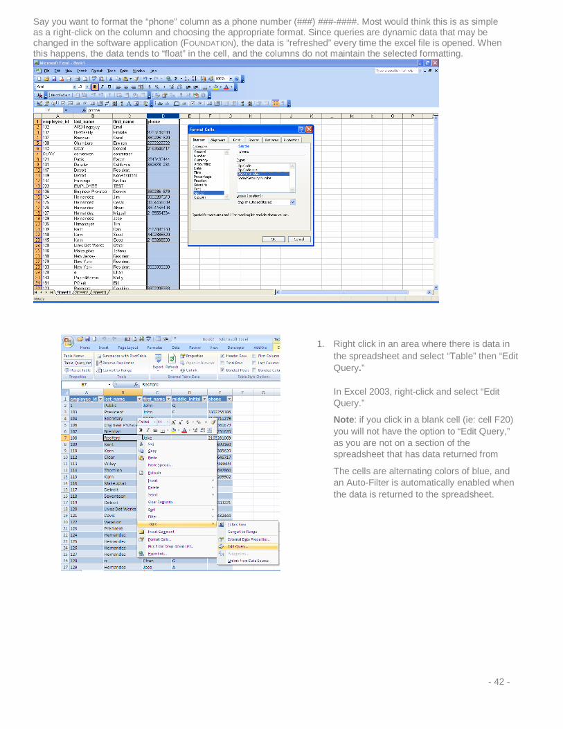
Say you want to format the “phone” column as a phone number (###) ###-####. Most would think this is as simple as a right-click on the column and choosing the appropriate format. Since queries are dynamic data that may be changed in the software application (FOUNDATION), the data is “refreshed” every time the excel file is opened. When this happens, the data tends to “float” in the cell, and the columns do not maintain the selected formatting.
1. Right click in an area where there is data in the spreadsheet and select “Table” then “Edit Query.” In Excel 2003, right-click and select “Edit Query.”
Note: if you click in a blank cell (ie: cell F20) you will not have the option to “Edit Query,” as you are not on a section of the spreadsheet that has data returned from
The cells are alternating colors of blue, and an Auto-Filter is automatically enabled when the data is returned to the spreadsheet.
- 42 -

We are now returned to the Query editing mode.
2. Double click the header of the phone column to access the Edit Column box.
3. In the Field…ummm field, type the following: abs(phone)
This will return the absolute value of the data to the spreadsheet. Click [OK] and return the data to Excel.
Double click
- 43 -
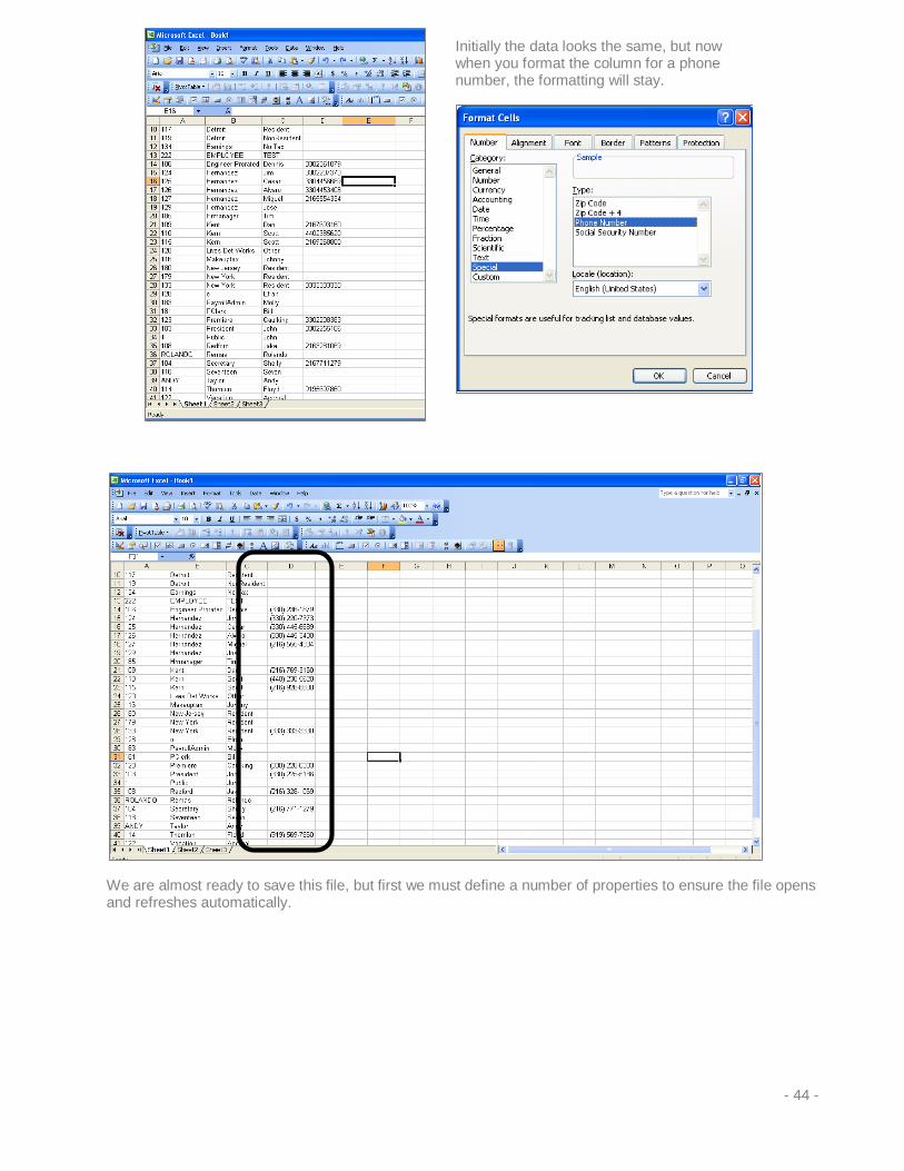
We are almost ready to save this file, but first we must define a number of properties to ensure the file opens and refreshes automatically.
Initially the data looks the same, but now when you format the column for a phone number, the formatting will stay.
- 44 -

Sample Report/Lesson 2 Employee Phone List
Tasks
• Saving Password in MS Query • Enabling Automatic Refresh
- 45 -
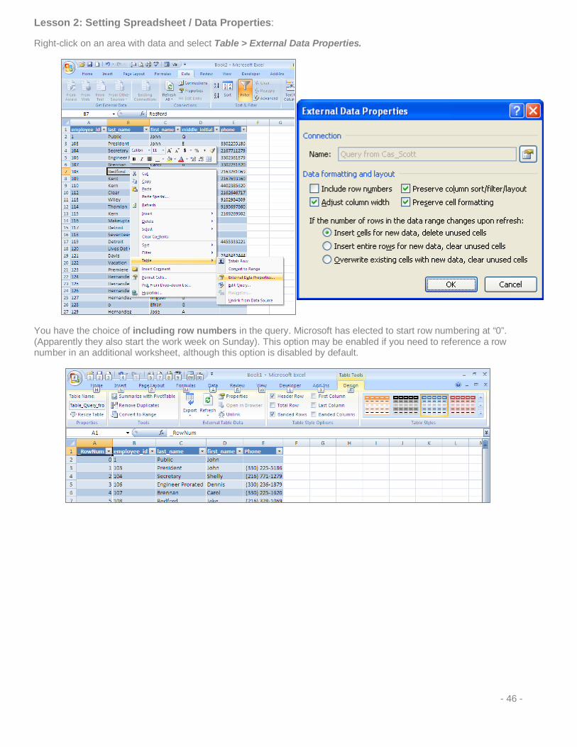
Lesson 2: Setting Spreadsheet / Data Properties:
Right-click on an area with data and select Table > External Data Properties.
You have the choice of including row numbers in the query. Microsoft has elected to start row numbering at “0”. (Apparently they also start the work week on Sunday). This option may be enabled if you need to reference a row number in an additional worksheet, although this option is disabled by default.
- 46 -

Preserve Column Sort/Filter/Layout
This option will allow you to preserve the column page layout if you select to sort on the Excel sheet. Please note that we demonstrated sorting in the MS Query mode. If you choose to sort the page once the data is returned to Excel and this checkbox is enabled, it will follow the sort criteria defined on the Excel worksheet.
The Layout option will be very important in later lessons. If you add columns to your query after creating an initial layout, you will want to disable this box before you edit the query. If I need to add the middle initial to my query, here is an example of what happens after editing the query with the Preserve Column Sort/Filter/Layout checkbox enabled.
Access the query and find the middle_initial field in the employee table. Click – hold – and drag-and-drop the field in the desired position in the preview window below.
When you return the data to Excel, you may be surprised to find where the middle initial appears. This is because of the Preserve Column Sort/Filter/Layout option. Since this option was enabled, it wants to maintain the original “look” of the spreadsheet.
- 47 -

To correct this issue, you may:
Disable this option before you edit the query, or refresh the Query with this option disabled.
1. First, right-click on a cell within the table, select Table > External Data Properties.
4. Right-click on a cell within the table again and choose “Refresh.” This will refresh the query and pull in the data from the FOUNDATION database again.
The columns should now be in the “order” that we desire. Access the External Data Properties dialog box again and enable the Preserve Column Sort/Filter/Layout checkbox to ensure you maintain the layout as it appears on screen.
2. Disable the Preserve Column Sort/Filter/Layout checkbox.
3. Click [OK] to close the dialog box.
- 48 -
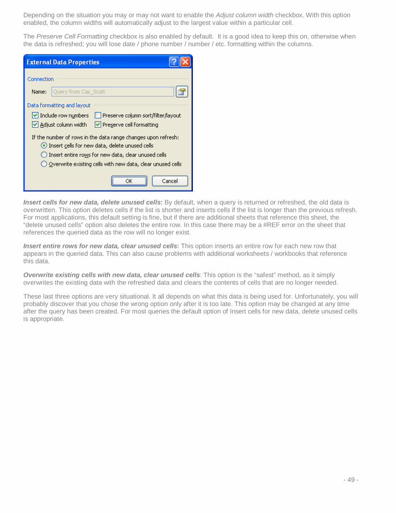
Depending on the situation you may or may not want to enable the Adjust column width checkbox. With this option enabled, the column widths will automatically adjust to the largest value within a particular cell.
The Preserve Cell Formatting checkbox is also enabled by default. It is a good idea to keep this on, otherwise when the data is refreshed; you will lose date / phone number / number / etc. formatting within the columns.
Insert cells for new data, delete unused cells: By default, when a query is returned or refreshed, the old data is overwritten. This option deletes cells if the list is shorter and inserts cells if the list is longer than the previous refresh. For most applications, this default setting is fine, but if there are additional sheets that reference this sheet, the “delete unused cells” option also deletes the entire row. In this case there may be a #REF error on the sheet that references the queried data as the row will no longer exist.
Insert entire rows for new data, clear unused cells: This option inserts an entire row for each new row that appears in the queried data. This can also cause problems with additional worksheets / workbooks that reference this data.
Overwrite existing cells with new data, clear unused cells: This option is the “safest” method, as it simply overwrites the existing data with the refreshed data and clears the contents of cells that are no longer needed.
These last three options are very situational. It all depends on what this data is being used for. Unfortunately, you will probably discover that you chose the wrong option only after it is too late. This option may be changed at any time after the query has been created. For most queries the default option of Insert cells for new data, delete unused cells is appropriate.
- 49 -
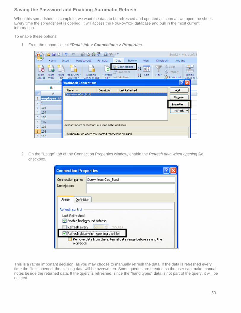
Saving the Password and Enabling Automatic Refresh
When this spreadsheet is complete, we want the data to be refreshed and updated as soon as we open the sheet. Every time the spreadsheet is opened, it will access the FOUNDATION database and pull in the most current information.
To enable these options:
1. From the ribbon, select “Data” tab > Connections > Properties.
2. On the “Usage” tab of the Connection Properties window, enable the Refresh data when opening file checkbox.
This is a rather important decision, as you may choose to manually refresh the data. If the data is refreshed every time the file is opened, the existing data will be overwritten. Some queries are created so the user can make manual notes beside the returned data. If the query is refreshed, since the “hand typed” data is not part of the query, it will be deleted.
- 50 -

Saving the password:
1. Click on the “Definition” tab of the Connection Properties dialog box, and enable the Save Password checkbox.
2. You will receive a warning from Microsoft about saving passwords within the Excel file. Click [Yes] to close this dialog box (more on this later).
- 51 -
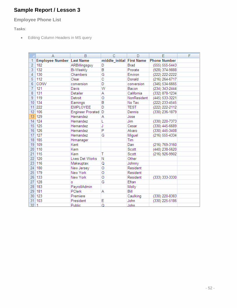
Sample Report / Lesson 3
Employee Phone List
Tasks:
• Editing Column Headers in MS query
- 52 -

Lesson 3: Editing column Headings
We like the results, but we want to tweak some of the items to make the list look more presentable.
Notice the column headings:
These are the field names from the query, and the “phone” column heading is altogether gone.
1. We need to access the query mode once again. Right-click, select Table > edit query.
2. Double click the column heading that you want to change.
3. In the Edit Column dialog box, note the Column Heading field. We will type a more appropriate heading here.
- 53 -
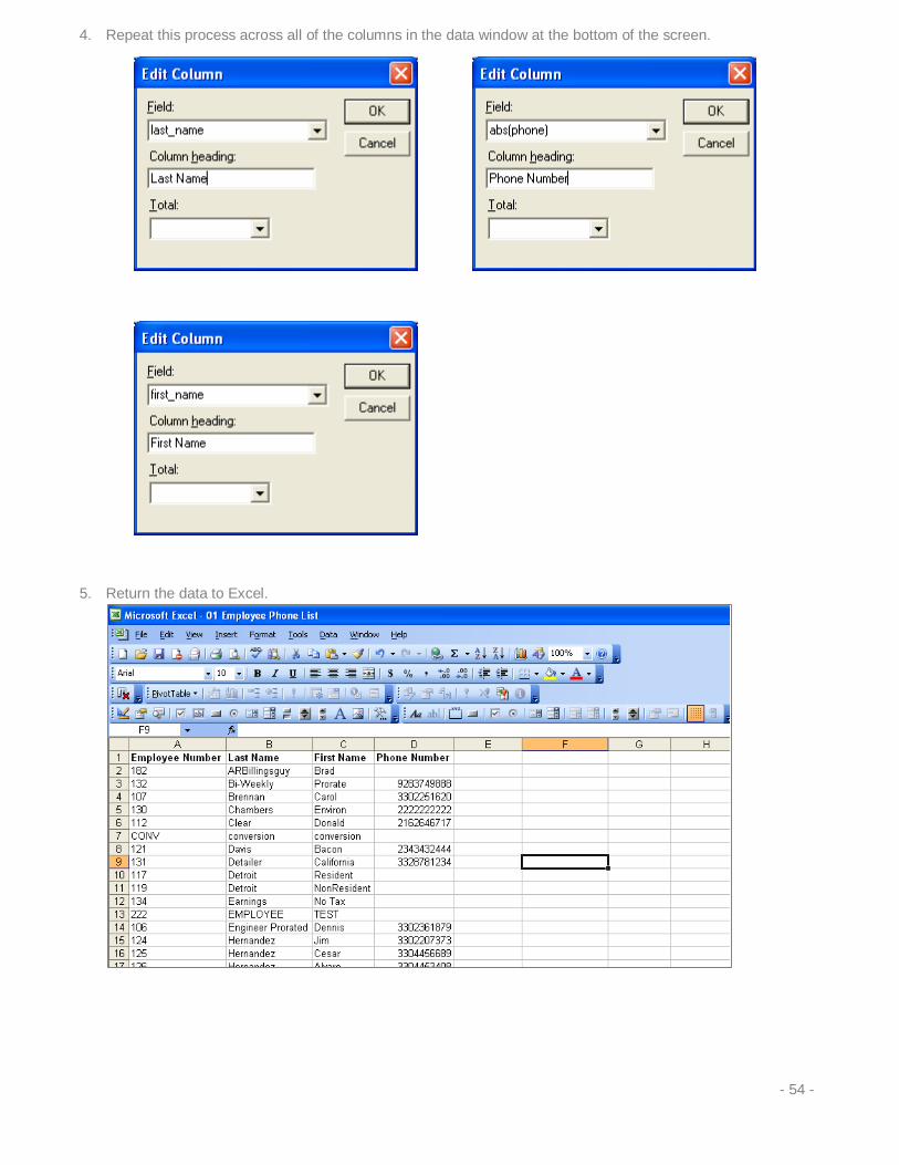
4. Repeat this process across all of the columns in the data window at the bottom of the screen.
5. Return the data to Excel.
- 54 -
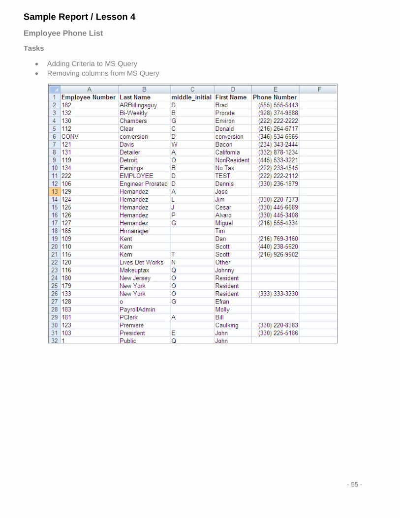
Sample Report / Lesson 4
Employee Phone List
Tasks
• Adding Criteria to MS Query • Removing columns from MS Query
- 55 -

Lesson 4: Adding Criteria to the Query:
Imagine that I do not want terminated employees to show on the phone list. We need to tell the query to ignore, or suppress, the terminated employees.
This is where a good amount of thought may be required for queries. What to include or exclude on a list or report. Much like FOUNDATION “Criteria” tabs on reports, we will assign filters to show only the data we request.
1. Once again, access the MS Query tool. 2. On the toolbar, select View > Criteria.
You will notice a criteria Field section is now available in the query designer.
- 56 -

3. Click and drag the “date_terminated” field into the criteria toolbar.
4. Double click the empty Value field to the right of the word “Value” to open the Edit Criteria dialog box.
5. Put on the thinking caps and try to remember your statistics class from 9th grade. What do we want to determine? In this case we only want to show employees who are not terminated. The “Operator” in this example would be:
Yes… “is Null”, or is blank. If the employee terminated date is blank, we want him to show up on the current phone list.
- 57 -

You may notice that the data in the preview window at the bottom flickers for a second as the terminated employees are removed from the query.
6. If you want to verify this information, drag the date_terminated into the last column in the preview pane. Based on our criteria, this column should be blank.
- 58 -
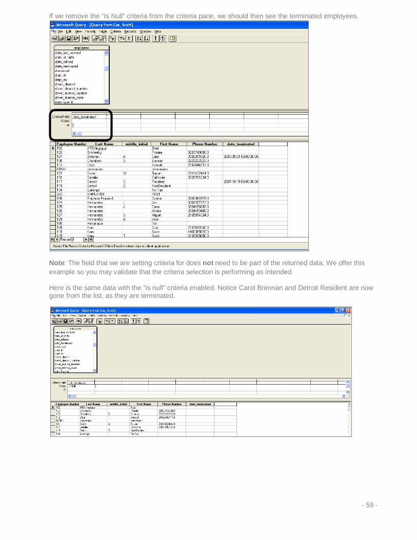
If we remove the “Is Null” criteria from the criteria pane, we should then see the terminated employees.
Note: The field that we are setting criteria for does not need to be part of the returned data. We offer this example so you may validate that the criteria selection is performing as intended.
Here is the same data with the “is null” criteria enabled. Notice Carol Brennan and Detroit Resident are now gone from the list, as they are terminated.
- 59 -

7. After validating the data, click on the date_terminated column to highlight it, and hit the <Delete> key on the keyboard. This will remove the column from the query, but it will not remove the criteria we set a few moments ago.
After Pressing <Delete> on the Keyboard
8. Once again return the data to Excel and save the file.
- 60 -
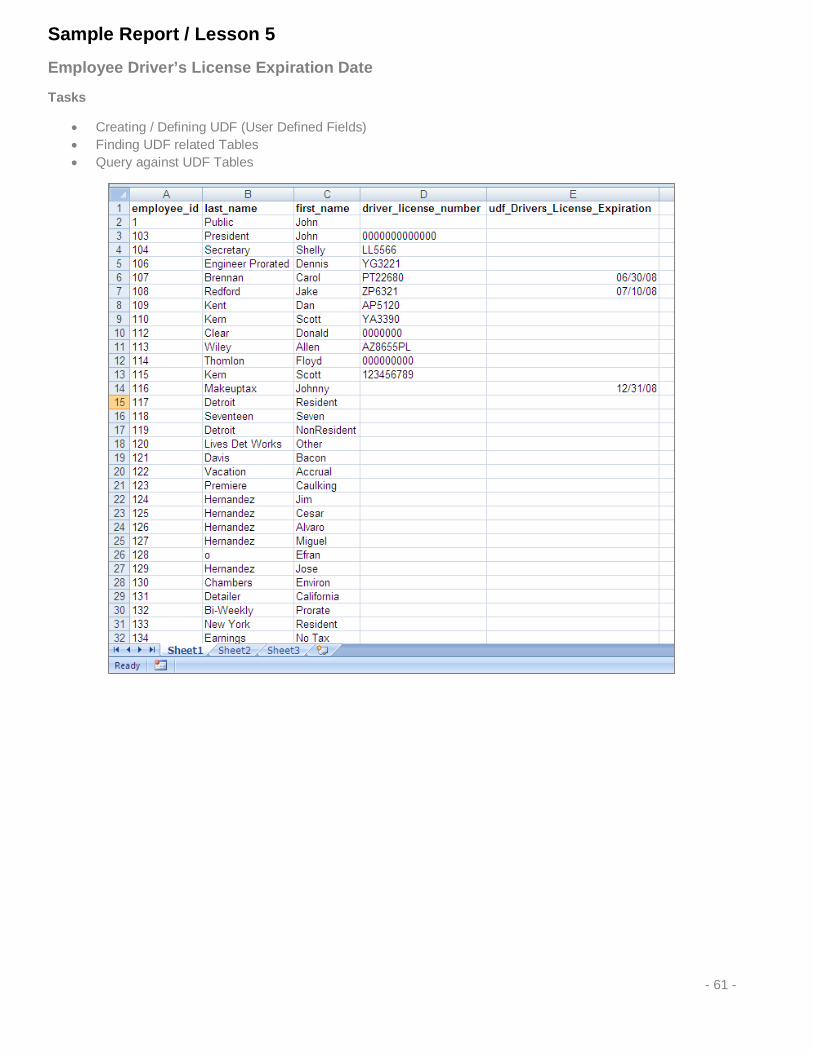
Sample Report / Lesson 5
Employee Driver’s License Expiration Date
Tasks
• Creating / Defining UDF (User Defined Fields) • Finding UDF related Tables • Query against UDF Tables
- 61 -

Lesson 5: Creating queries accessing User Defined Fields(UDFs)
UDFs are available in most maintenance tables across the FOUNDATION database.
In this example, we will create a list of driver’s license numbers and their associated expiration dates.
1. Log into FOUNDATION and select Tools > User Defined Fields. Scroll down to the Employees table.
2. Click [New] to add whatever type of field you want. A number of fields are noted here, but some other examples are: • Certification Dates • Drug Test Dates • Spouse’s Name and Contact Information • Nextel Direct Connect Numbers • Work Permit Expiration Dates
Once the fields are added in the tools menu, they become fields in the FOUNDATION program and FOUNDATION database. If they are part of the database, we can query the information for a custom list.
- 62 -

When executing a query that accesses User Defined Fields, we need to look to special tables in order to find the data. Since UDFs are “user defined”, no two FOUNDATION users will have the same tables. When you create a UDF, FOUNDATION creates a “view” or virtual table to store the complete data. These virtual tables are easily located because they are named as follows:
V_UDF_EMPLOYEES
This “View” contains all of the information that the employees table has, plus the user defined fields.
3. To create a custom query/list of employee’s driver’s license numbers and expiration dates, we need to access a new query and select the V_UDF_EMPLOYEES table.
Note: All of the UDF name fields are at the bottom of this table.
All other items are in alphabetical order, just like the “employees” table
- 63 -

4. If we add a date to an Employee Record in FOUNDATION and refresh the query, we can see the data on our preview screen.
Data has been added to FOUNDATION, and the record has been saved.
5. Click the Query Now button (an exclamation point) on the query toolbar to refresh the data in the query mode.
- 64 -
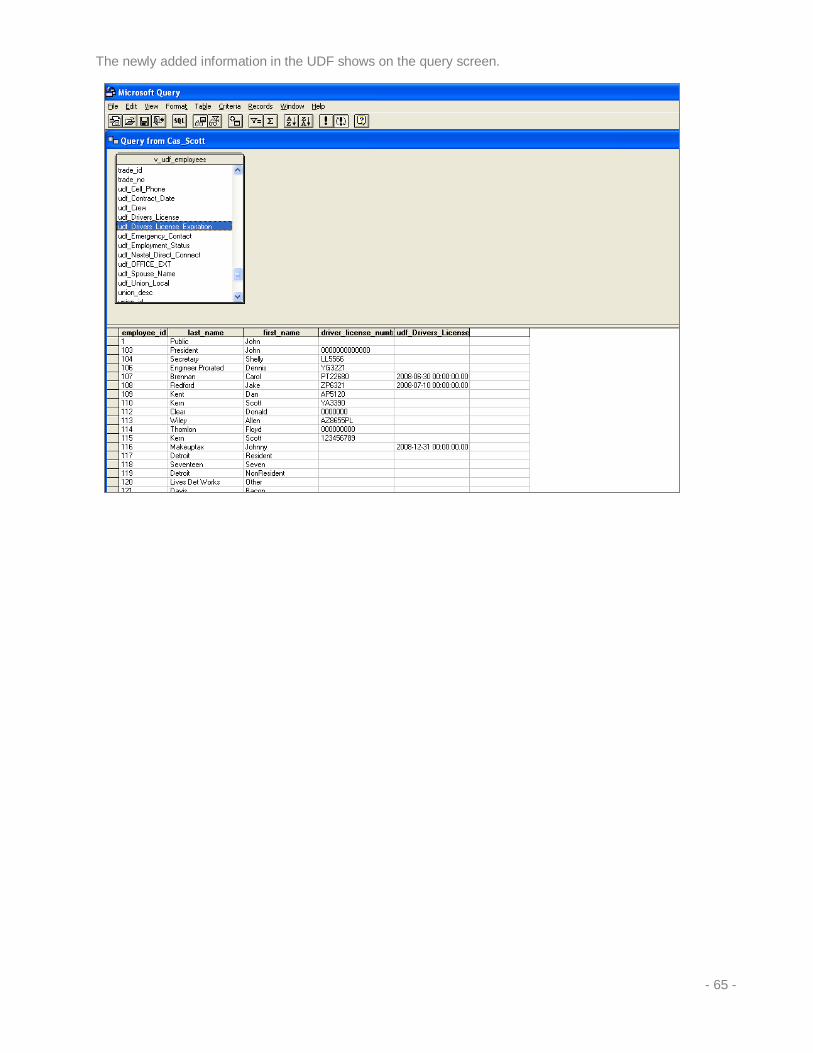
The newly added information in the UDF shows on the query screen.
- 65 -
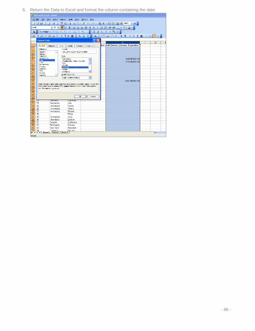
6. Return the Data to Excel and format the column containing the date:
- 66 -
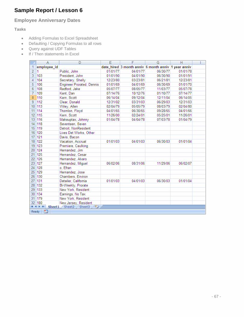
Sample Report / Lesson 6
Employee Anniversary Dates
Tasks
• Adding Formulas to Excel Spreadsheet • Defaulting / Copying Formulas to all rows • Query against UDF Tables • If / Then statements in Excel
- 67 -
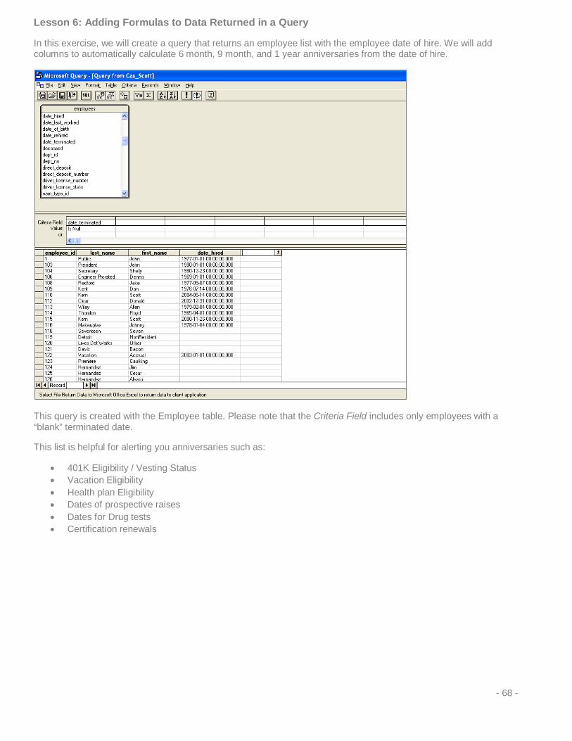
Lesson 6: Adding Formulas to Data Returned in a Query
In this exercise, we will create a query that returns an employee list with the employee date of hire. We will add columns to automatically calculate 6 month, 9 month, and 1 year anniversaries from the date of hire.
This query is created with the Employee table. Please note that the Criteria Field includes only employees with a “blank” terminated date.
This list is helpful for alerting you anniversaries such as:
• 401K Eligibility / Vesting Status • Vacation Eligibility • Health plan Eligibility • Dates of prospective raises • Dates for Drug tests • Certification renewals
- 68 -

Once the data is returned to Excel, we can add a formula next to the date to calculate a certain number of days from the date of hire.
The formula to “add” days to a current date is simple. Take the cell plus the number of days you want to add. (For 3 months, we add 90, 6 months, we add 180, for one year, we add 365.)
Here, the calculation fields are “exposed.” You can show all of the calculation fields on an Excel spreadsheet by pressing CTL + ` (Grave accent – located in the upper left hand corner of the keyboard above the tilde). For those of you who are wondering what the numbers in column “D” represent… that is the number of days from Excel’s “default” date. Excel recognizes dates as a number. Day “number 1” is 01/01/1900, so 01/01/1977 is 28,126 days from 01/01/1900. When we write equations against cells that contain dates, behind the scenes, Excel is simply calculating a number and then formatting the date based on the number of days from “day 1.”
If this type of information excites you, congratulations, you may be a nerd.
Here is the data viewed in a more familiar format:
As with all queries, we want to enable the Save Password and Refresh Data on File Open options.
Excel will automatically copy the formulas down to all rows within a particular column.
- 69 -

What is to be done with the employees that have no date of hire in their Employee Record? This field is important, and it should be filled in when an Employee Record is created. (There is a control file setting that will require you to enter this date when creating an Employee Record).
Should there be a blank item in a query that has an equation written against it, we can suppress the equation result with a simple “IF / THEN / ELSE ” statement.
If / Then / Else statements are easily written if you say them out loud or write them down before trying to write them as an function in Excel.
In this example, we would say “IF the date is blank, THEN return a blank, ELSE perform the calculation (adding 90 days to the date).
In the formula toolbar, we see the equation written as:
= IF(D2=””,””,D2+90)
We would repeat the IF / THEN logic across all of the columns for all of the equations. Once the query is refreshed, the dates that are blank will not have the calculation performed against the empty cells.
- 70 -

Sample Report / Lesson 7
Employee Anniversary Dates
Tasks
• Concatenate function within excel • Hiding columns in Excel
- 71 -

Lesson 7: Concatenate function:
“Concatenating” data in the Excel spreadsheet. Yes, when I heard this word for the first time, I too thought, “they are literally making words up for this stuff...”
For the layman, “concatenate” is a fancy term for combing multiple cells into a single cell. It differs from merging cells in the fact that you may insert additional formatting to the cells such as commas or dashes.
Imagine in our employee lists if I wanted to see names formatted as Kern, Scott as opposed to the first and last name residing in two separate cells.
1. Insert a new column into the spreadsheet to the right of the “first_name” column. 2. In the formula toolbar for cell D2, start typing: =concatenate(
3. At this point, click the fx button to the left of the formula toolbar. This will open up a dialog box that will assist
in creating the desired data format.
- 72 -

4. The Function Arguments box will open, and ask what cell is to be used as the first part of the joined data. • In the Text1 field, select the cell that contains the last name. • In the Text2 field, enter a comma and a space. • In the Text3 field, select the cell that contains the first name.
Notice the preview of the Joined data on the right hand side of the screen. You can join up to 255 different text and field strings if you so desire. Previous version of Excel only allowed 30 strings to be joined.
5. Click [OK] to return the formula results.
- 73 -
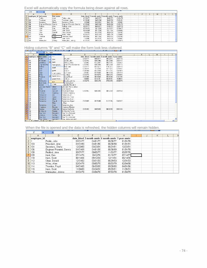
Excel will automatically copy the formula being down against all rows.
Hiding columns “B” and “C” will make the form look less cluttered.
When the file is opened and the data is refreshed, the hidden columns will remain hidden.
- 74 -
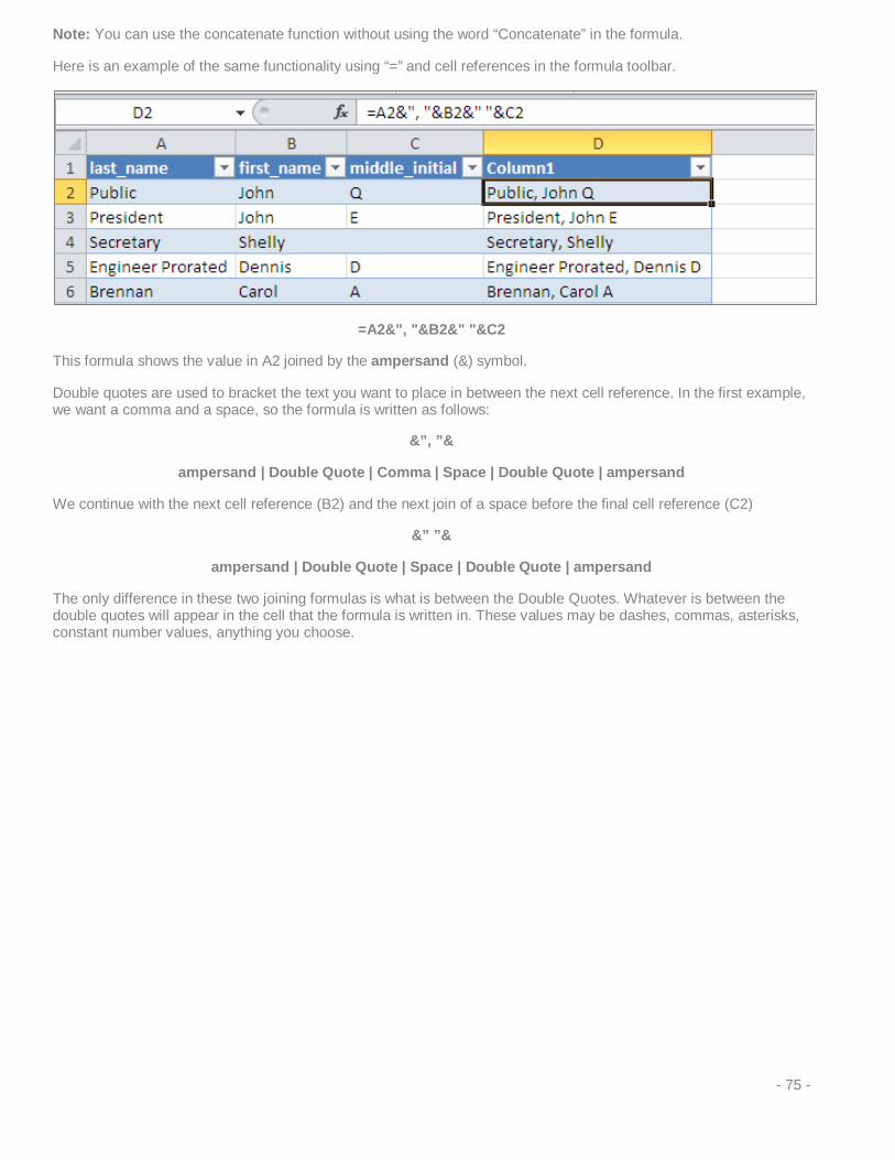
Note: You can use the concatenate function without using the word “Concatenate” in the formula.
Here is an example of the same functionality using “=” and cell references in the formula toolbar.
=A2&", "&B2&" "&C2
This formula shows the value in A2 joined by the ampersand (&) symbol.
Double quotes are used to bracket the text you want to place in between the next cell reference. In the first example, we want a comma and a space, so the formula is written as follows:
&”, ”&
ampersand | Double Quote | Comma | Space | Double Quote | ampersand
We continue with the next cell reference (B2) and the next join of a space before the final cell reference (C2)
&” ”&
ampersand | Double Quote | Space | Double Quote | ampersand
The only difference in these two joining formulas is what is between the Double Quotes. Whatever is between the double quotes will appear in the cell that the formula is written in. These values may be dashes, commas, asterisks, constant number values, anything you choose.
- 75 -

Sample Report / Lesson 8
Employee Anniversary Dates
Tasks
• Concatenating data (joining FIELDS) in MS Query
- 76 -

Lesson 8: Concatenate Function in MS Query
Now that you have learned how to concatenate cells within Excel, let’s take time to explore options on combining and formatting data fields in the query mode. This way, data is returned in the desired format, and columns do not have to be hidden.
1. In query mode with the employee table selected, click on the first column header in the data preview area and type: last_name+’, ‘+first_name.
Just when you thought you were getting the hang of it… Microsoft changes the game again. In query mode, you do not use the ampersand and double quotes. You must use the plus sign (+) and a single quote to bracket the data / field names. Programmers – go figure.
2. Tab out of the field to view the results.
This is only the beginning…
Combining text fields is one option, you can write rather complex calculations against numeric data from tables.
This is not recommended for the faint of heart, as the formula logic in Excel does not always relate to writing a formula in the Query mode.
A lot of trial and error will be needed in order to create the desired results. If you are better at writing formulas in Excel, by all means, return the data to Excel, perform the calculations on the spreadsheet and hide unneeded columns. (You may thank me later)
- 77 -
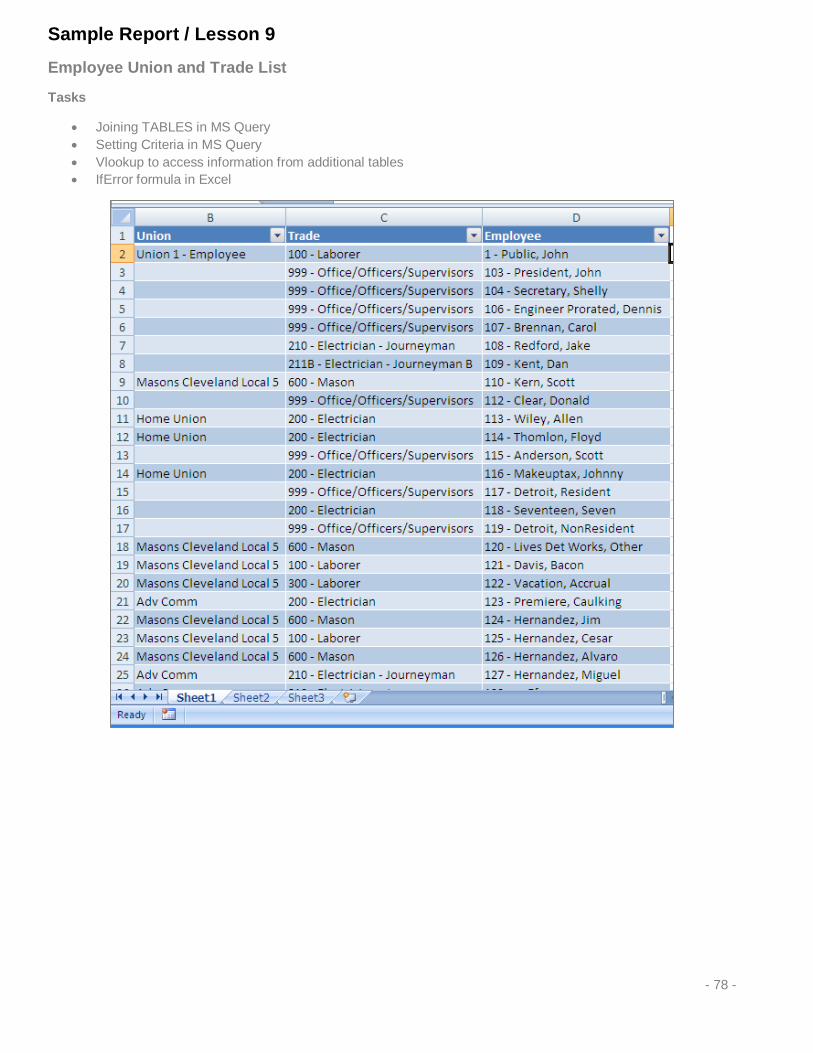
Sample Report / Lesson 9
Employee Union and Trade List
Tasks
• Joining TABLES in MS Query • Setting Criteria in MS Query • Vlookup to access information from additional tables • IfError formula in Excel
- 78 -

Lesson 9: Joining Tables within a Query.
So far, we have created queries that access a single table. Now we will explore queries that access and link multiple tables within the database. We will also look at the limitations inherent with the MS Query tool when attempting to join multiple tables.
In this example, we are going to create a simple list that shows the employee list by union and trade as defined on the Employee Record.
We will be accessing 3 tables for this query: The employee table, the trades table and the union table.
We start the query by accessing the employee table in the query. In this example, we will create a single column that joins the employee_id field along with the last_name and first_name of the employee.
The equation to accomplish this is written as follows:
employee_id+' - '+last_name+', '+first_name
Note: Any text contained between the +’ and ‘+ will appear in the field(s) that you are joining.
Double-click the column heading to edit the properties. In the Column Heading field, type “Employee.”
- 79 -

Adding tables to the Query
In this list, we want to reference the union and trade entered on the Employee Record.
1. Add the union_id and trade_id from the employee table to the preview window.
You will notice that the trade description and the union description do not reside in the “employees” table. We must add the tables that house this information in order to pull the details.
2. To add a new table, select the “Add Table” button on the toolbar.
3. You will be prompted to select the table(s) with the same dialog box that appears when you start a new
query.
- 80 -

When the Trades table is added to the query, you will notice that the tables are “joined” by lines between similar fields within the table.
In this case, the Employees table and the Trades table are joined by company_no and trade_no.
You will notice fields in certain tables that are bold. In the Trades table, these fields are company_no and trade_no.
These fields are bold, because they are defined as “Key Identifiers.” Basically, these are the fields that relate to other fields in other tables.
The Trade table is “linked” to the Employee table via the trade_no.
In this example, every employee has a trade, so we can add the description field from the trades table.
When the description is added to the query, the trade description matches with the associated trade_no from the Employee table.
- 81 -

Good news so far… Now we are going to add the Unions table to the query. Click the Add Tables button on the toolbar and select the table titled “Unions.”
You will notice that something has changed in the preview pane of the MS Query window. You have “lost” all employees that do not have a union defined on their record. (This may be a good thing, depending on what data you want to show or hide). In this example, we want to see every record, regardless of whether or not the employee is a union employee.
MS Query has “linked” the Unions table to the Employees table via the union_no field. A perfectly logical join, except it wants to report or return data that satisfies all of the links in the associated tables. In other words, if there is no union_no on the employee record, it has nothing to link to the Unions table, therefore, the query ignores this data. When the query ignores the data, it simply drops the record from the resulting data set.
It is always a good idea to reference the number of records in a query before (and after) adding more tables.
This example shows the employees and the trades table only.
Scroll down to the bottom of the list and click in a cell on the last record.
The lower left hand corner of the query window will show you how many records are returned.
In this example there are 42 records.
- 82 -

When the Unions table is added, and we look at the resulting records, the number is different. We only have 24 records returned.
In this case, there are 18 Employee Records that do not have a default union. Again – the query tool drops all records that do not satisfy all of the linked fields.
Some of you may know about left and right inner and outer joins. Certain programs allow you to resolve this with a little bit of creative coding. By default, the MS query tool only allows inner or outer joins on a query with 2 tables. If you are familiar with inner and outer joins, please feel free to explore these options on your own. There are other ways to rectify this that will be discussed later. We will discuss the benefits of not using the inner and outer joins.
In order to rectify this situation, we will delete the Unions table from the query.
1. Click on the Unions table at the top of the screen 2. Hit the <Delete> key on your keyboard. Once again all employees are now on the list.
- 83 -
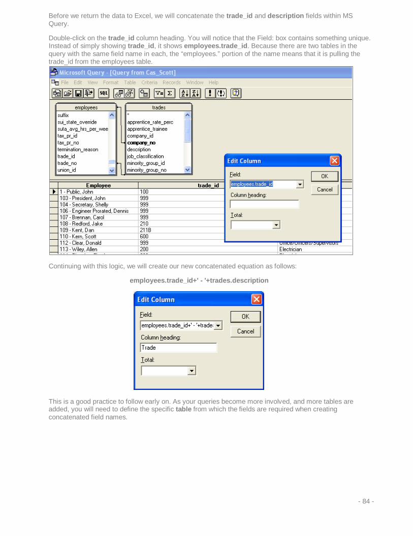
Before we return the data to Excel, we will concatenate the trade_id and description fields within MS Query.
Double-click on the trade_id column heading. You will notice that the Field: box contains something unique. Instead of simply showing trade_id, it shows employees.trade_id. Because there are two tables in the query with the same field name in each, the “employees.” portion of the name means that it is pulling the trade_id from the employees table.
Continuing with this logic, we will create our new concatenated equation as follows:
employees.trade_id+' - '+trades.description
This is a good practice to follow early on. As your queries become more involved, and more tables are added, you will need to define the specific table from which the fields are required when creating concatenated field names.
- 84 -
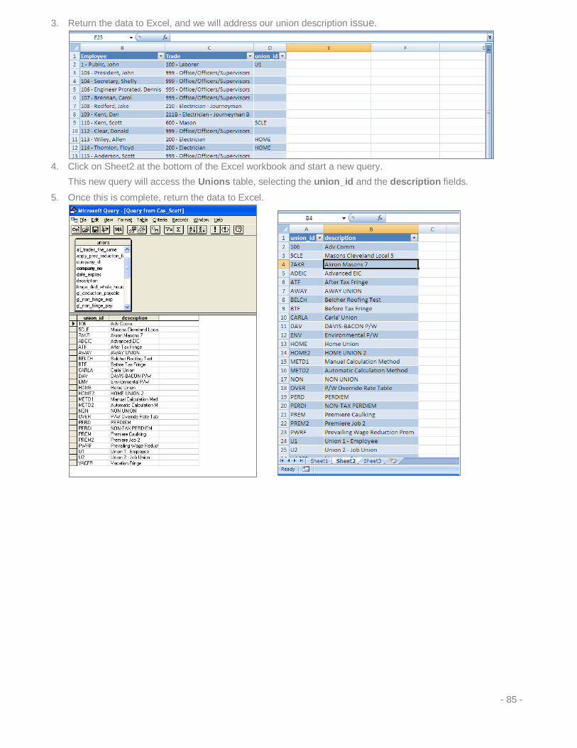
3. Return the data to Excel, and we will address our union description issue.
4. Click on Sheet2 at the bottom of the Excel workbook and start a new query.
This new query will access the Unions table, selecting the union_id and the description fields.
5. Once this is complete, return the data to Excel.
- 85 -
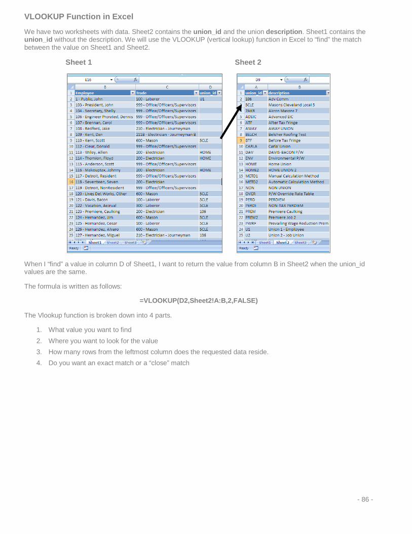
VLOOKUP Function in Excel
We have two worksheets with data. Sheet2 contains the union_id and the union description. Sheet1 contains the union_id without the description. We will use the VLOOKUP (vertical lookup) function in Excel to “find” the match between the value on Sheet1 and Sheet2.
Sheet 1 Sheet 2
When I “find” a value in column D of Sheet1, I want to return the value from column B in Sheet2 when the union_id values are the same.
The formula is written as follows:
=VLOOKUP(D2,Sheet2!A:B,2,FALSE)
The Vlookup function is broken down into 4 parts.
1. What value you want to find 2. Where you want to look for the value 3. How many rows from the leftmost column does the requested data reside. 4. Do you want an exact match or a “close” match
- 86 -

In the Formula editor these 4 Items are broken down as follows:
The Lookup_value is the cell on the spreadsheet that you want to pull information from. Although the help dialog state that it must be a value from the “leftmost column of a table”, this is not true, you may create a vlookup anywhere in a spreadsheet.
The table_array is the selected columns from which to look for the associated value defined in the first step. In this example, our array is on Sheet2, columns A:B. Even though we are only looking to an array with 2 columns, these arrays can be much larger.
The Col_index_num is the number of columns from the first column in the array to locate the required data. In this case, the array is A:B. We are looking to return the data from column B. Column B is the second column from column A, so we enter a 2 in the Col_index_num field.
The Range_Lookup is the most illogical “logical”’ value Excel offers. To find an exact match between the fields on the two sheets, you will select “false.” To find the first, or closest match, enter “true”. 99.99% of the time, you will want to enter “false”.
- 87 -

When the formula is written properly, you will see that Sheet1 has the associated union description pulled from the table on Sheet2.
Everything looks great, except for the #N/A errors in the rows where employees have no union_id identified.
Excel 2007 has a nice formula to address any and all errors in calculated cells. This new formula is called =IfError
If we append the original equation with the following:
=IfError(VLOOKUP(D2,Sheet2!A:B,2,FALSE),””)
This formula states that if there is an error with the specified formula, return “” (two sets of double quotes = blank). For calculated numbers, such as a #DIV/0 error, you may want to use a 0 in place of the “”.
Resulting data:
- 88 -
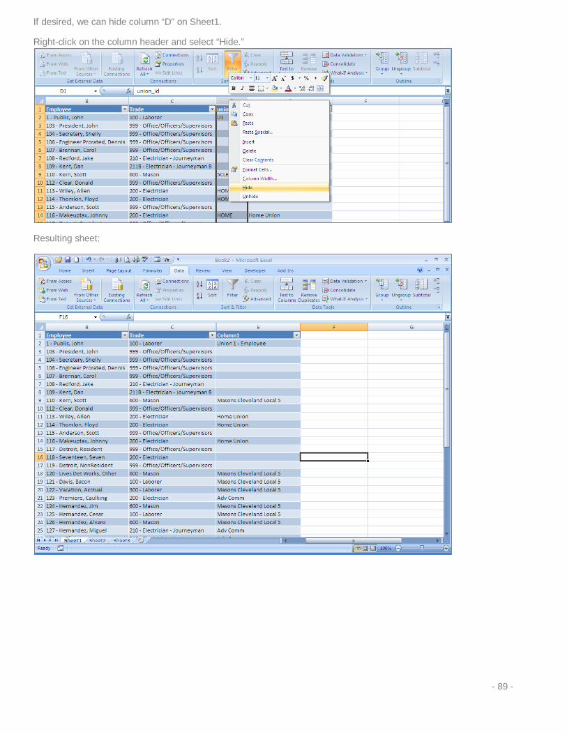
If desired, we can hide column “D” on Sheet1.
Right-click on the column header and select “Hide.”
Resulting sheet:
- 89 -
Sample Report / Lesson 10
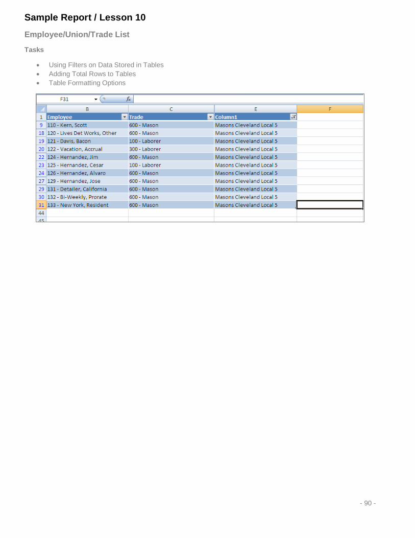
Employee/Union/Trade List
Tasks
• Using Filters on Data Stored in Tables • Adding Total Rows to Tables • Table Formatting Options
- 90 -

Data returned from an MS query is automatically entered into a table within Excel. These tables have default filters that can be used to limit data returned based on particular criteria.
In the example below, I have chosen to show only those members of the Cleveland Local 5 Masons union.
Click on the appropriate dropdown arrow in the desired column heading. If you disable the Select All checkbox, and then select a single item, only that item will show up. You may also select multiple items from a single column filter.
You may also select additional filter options from additional columns. In this example, only Local 5 Masons who have a trade of “Laborer.”
- 91 -

Note on the Dangers of Filtering: If a filter is enabled, it limits the data that is viewable on the list or report. The only representation you have to know that a column is filtered is a different icon at the column heading.
Solid Dropdown Choice = No Filter Enabled
“Filter” Icon = Filter Enabled.
When you click on the dropdown to select a filter, you may also select “Clear Filters From ‘X’” to reset the column.
Adding Total Rows to a Table
If you click on a cell within the table, you will notice a new tab on the top of the screen. The tab is titled “Table Tools / Design.”
Click on this tab for additional options.
- 92 -
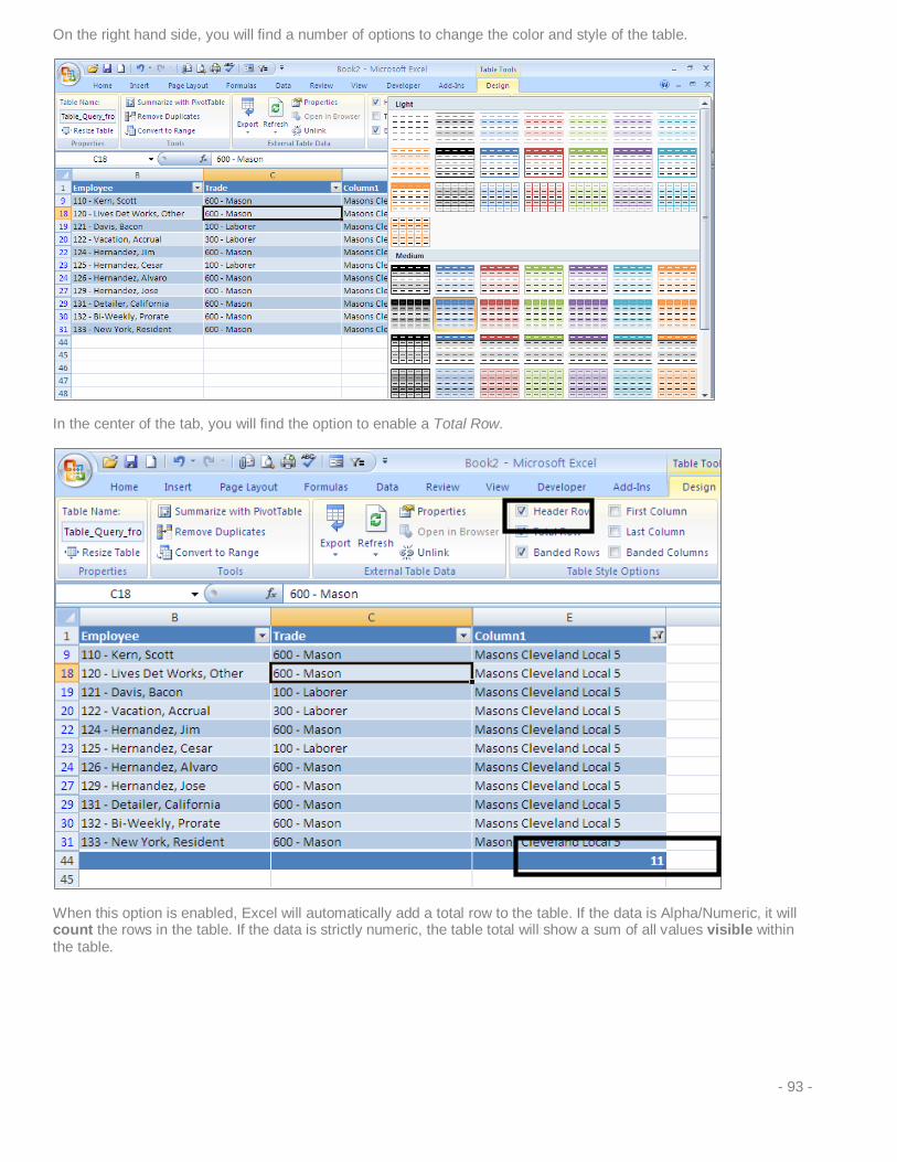
On the right hand side, you will find a number of options to change the color and style of the table.
In the center of the tab, you will find the option to enable a Total Row.
When this option is enabled, Excel will automatically add a total row to the table. If the data is Alpha/Numeric, it will count the rows in the table. If the data is strictly numeric, the table total will show a sum of all values visible within the table.
- 93 -
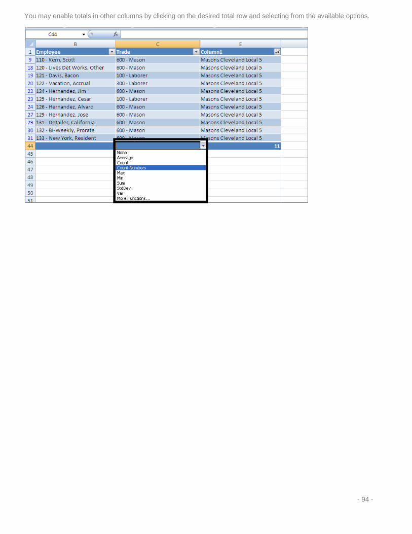
You may enable totals in other columns by clicking on the desired total row and selecting from the available options.
- 94 -
Sample Report / Lesson 11
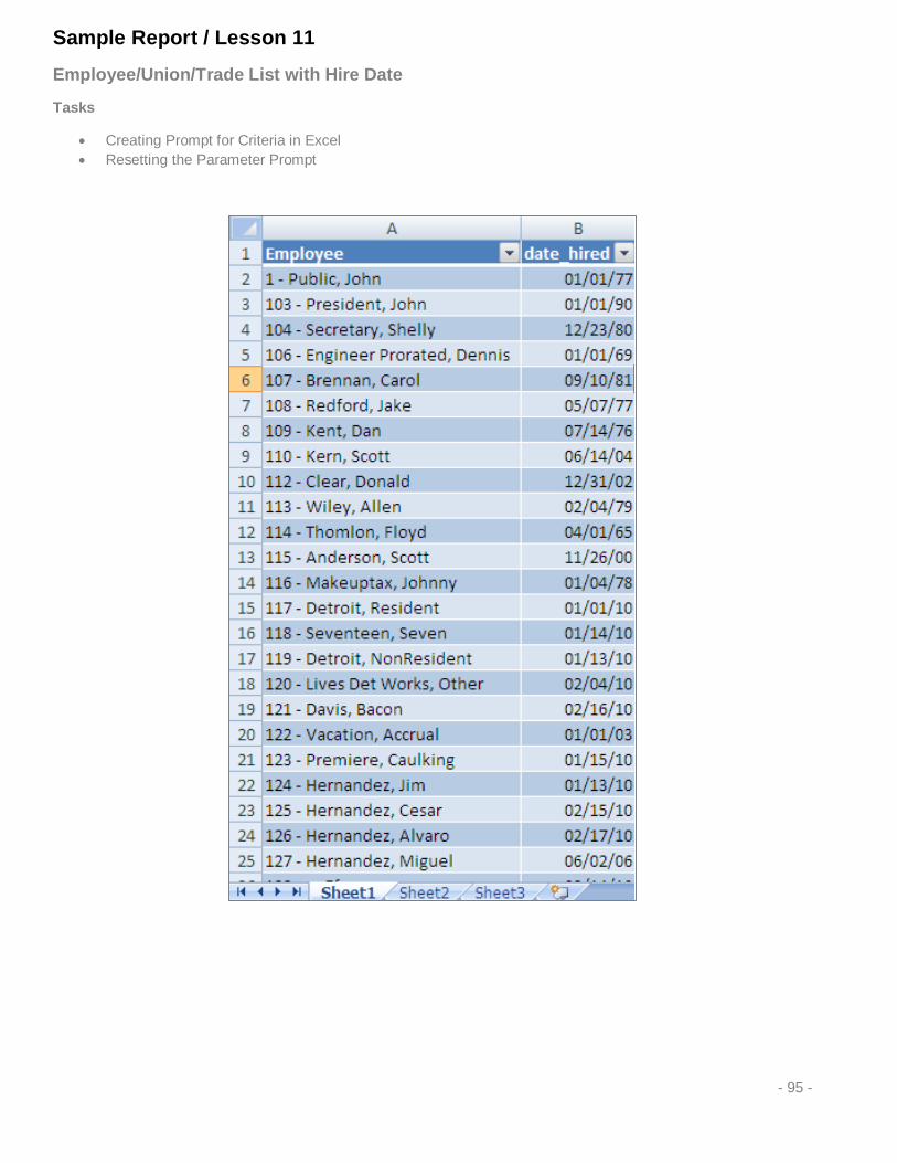
Employee/Union/Trade List with Hire Date
Tasks
• Creating Prompt for Criteria in Excel • Resetting the Parameter Prompt
- 95 -

Lesson 11: Adding Criteria That Will Prompt for Values When Spreadsheet is Opened
Let us start by creating a query that includes the employees and their respective hire date.
1. From the toolbar, select View > Criteria.
- 96 -

This will enable the Criteria pane in the MS Query screen.
In a previous lesson, we excluded employees who were terminated. In this lesson we will include employees who have a hired date between a defined date range.
This parameter will be based on the date_hired field from the Employees table.
2. Double click on the Value field to pull up the Edit Criteria dialog box. 3. In the Operator field, select “is between.”
- 97 -

4. In the Value Field, type the following: [Start Date],[End Date] This will be used as a prompt to limit the data returned in the query.
5. Click [OK]. The first prompt will appear. 6. Enter the starting date for the parameter. If this value is a date field, it must be entered in the following format
MM/DD/YY or MM/DD/YYY. The forward slashes are required.
7. Click [OK ]. You will be prompted for the next value (End Date) :
You will now see data for employees that match the criteria entered. In this example, employees hired between 01/01/10 and 03/31/10.
- 98 -

8. Return the data to Excel and we will review additional options using table filters.
If the value in a table is a date, and you select to filter on the date column, you will have an option to select by year, month, and ultimately date. This is a very useful feature with the tables in Excel.
Employees hired in the month of January 2010 only. The count function has been enabled on the total row as well.
- 99 -
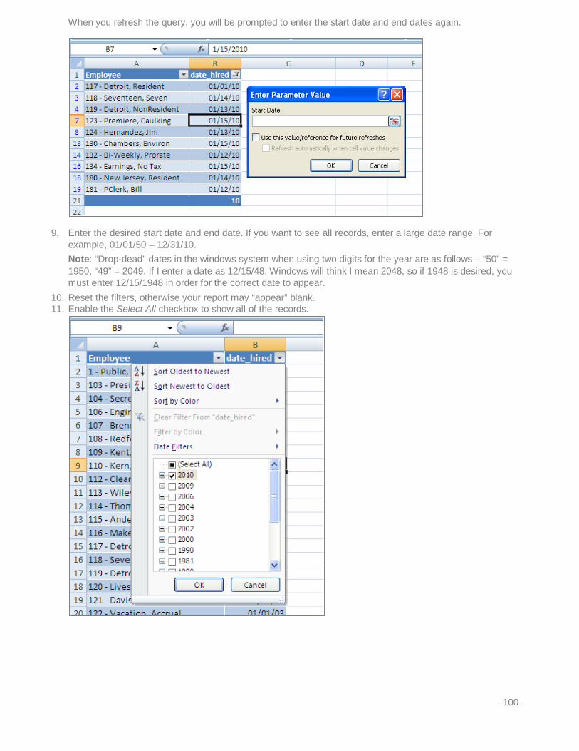
When you refresh the query, you will be prompted to enter the start date and end dates again.
9. Enter the desired start date and end date. If you want to see all records, enter a large date range. For example, 01/01/50 – 12/31/10. Note: “Drop-dead” dates in the windows system when using two digits for the year are as follows – “50” = 1950, “49” = 2049. If I enter a date as 12/15/48, Windows will think I mean 2048, so if 1948 is desired, you must enter 12/15/1948 in order for the correct date to appear.
10. Reset the filters, otherwise your report may “appear” blank. 11. Enable the Select All checkbox to show all of the records.
- 100 -
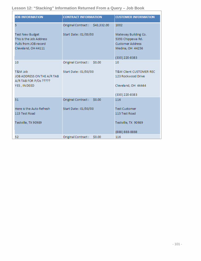
Lesson 12: “Stacking” Information Returned From a Query – Job Book
- 101 -
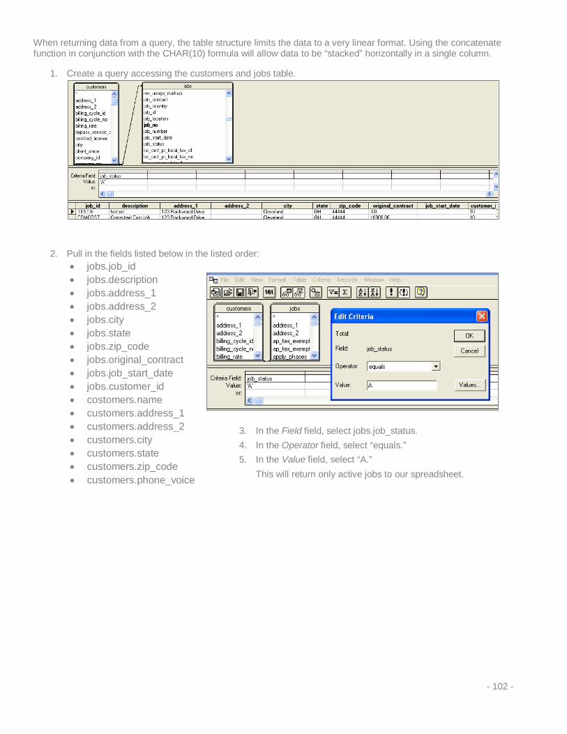
When returning data from a query, the table structure limits the data to a very linear format. Using the concatenate function in conjunction with the CHAR(10) formula will allow data to be “stacked” horizontally in a single column.
1. Create a query accessing the customers and jobs table.
2. Pull in the fields listed below in the listed order: • jobs.job_id • jobs.description • jobs.address_1 • jobs.address_2 • jobs.city • jobs.state • jobs.zip_code • jobs.original_contract • jobs.job_start_date • jobs.customer_id • costomers.name • customers.address_1 • customers.address_2 • customers.city • customers.state • customers.zip_code • customers.phone_voice
3. In the Field field, select jobs.job_status. 4. In the Operator field, select “equals.” 5. In the Value field, select “A.”
This will return only active jobs to our spreadsheet.
- 102 -
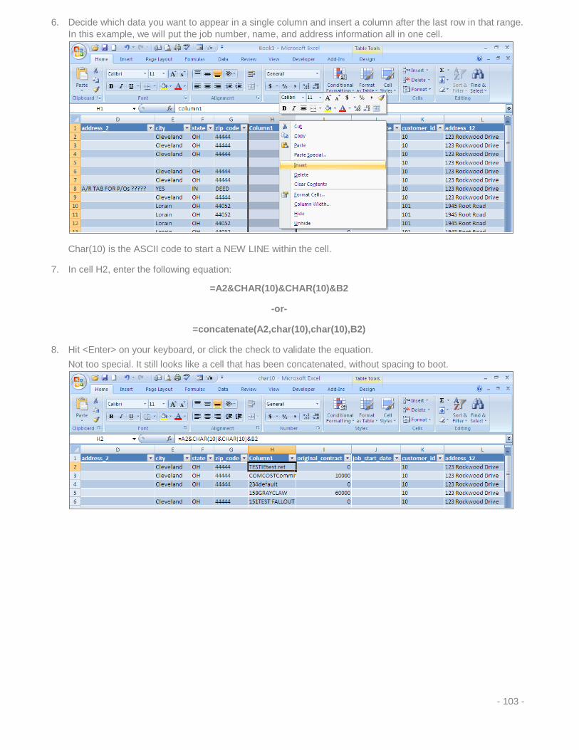
6. Decide which data you want to appear in a single column and insert a column after the last row in that range. In this example, we will put the job number, name, and address information all in one cell.
Char(10) is the ASCII code to start a NEW LINE within the cell.
7. In cell H2, enter the following equation:
=A2&CHAR(10)&CHAR(10)&B2
-or-
=concatenate(A2,char(10),char(10),B2)
8. Hit <Enter> on your keyboard, or click the check to validate the equation. Not too special. It still looks like a cell that has been concatenated, without spacing to boot.
- 103 -
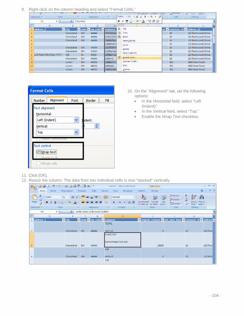
9. Right-click on the column heading and select “Format Cells.”
11. Click [OK]. 12. Resize the column. The data from two individual cells is now “stacked” vertically.
10. On the “Alignment” tab, set the following options: • In the Horizontal field, select “Left
(Indent)” • In the Vertical field, select “Top.” • Enable the Wrap Text checkbox.
- 104 -

13. Continue writing the equation to include columns A – G. 14. Separate each cell reference with the char(10) code to produce a line feed between the cell references.
=A2&CHAR(10)&CHAR(10)&B2&CHAR(10)&C2&CHAR(10)&D2&CHAR(10)&E2&", "&F2&" "&G2
Pay attention to the change in cells E2, F2, and G2. This is the city, state and zip code information. These will not be separated by a line feed. These cells are separated by text designated/defined by the text in between double quotes.
Once the formula is written, press enter or validate the formula with the check mark to the left of the formula bar.
Your row height should now be resized to the largest value in a particular column (in this case, the data contained in column H.
15. Highlight and hide columns A – G.
Click in the upper-most “cell” on top of the row numbers and to the left of the column letters to select the entire sheet.
Double click the line that separates the rows. You will know when to double click when the pointer changes to .
- 105 -
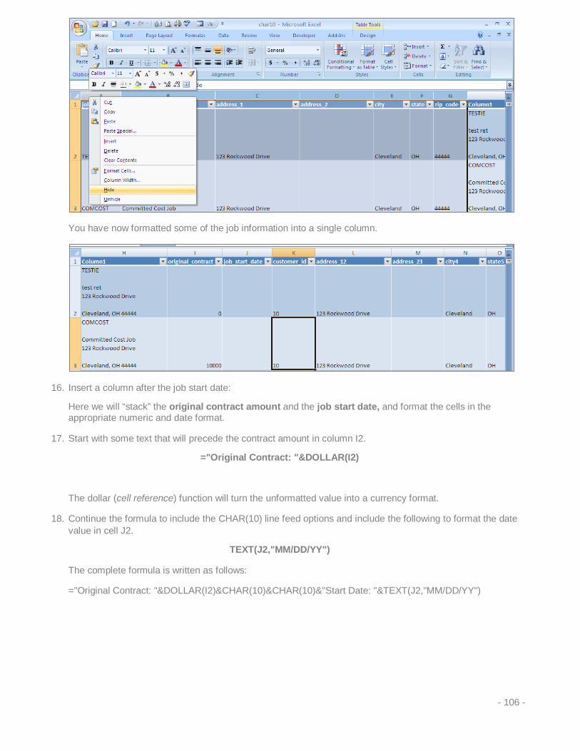
You have now formatted some of the job information into a single column.
16. Insert a column after the job start date:
Here we will “stack” the original contract amount and the job start date, and format the cells in the appropriate numeric and date format.
17. Start with some text that will precede the contract amount in column I2.
="Original Contract: "&DOLLAR(I2)
The dollar (cell reference) function will turn the unformatted value into a currency format.
18. Continue the formula to include the CHAR(10) line feed options and include the following to format the date value in cell J2.
TEXT(J2,"MM/DD/YY")
The complete formula is written as follows:
="Original Contract: "&DOLLAR(I2)&CHAR(10)&CHAR(10)&"Start Date: "&TEXT(J2,"MM/DD/YY")
- 106 -

19. Format column K in the same manner as column H by selecting the appropriate settings on the Alignment tab.
What happens when I want to format a phone number within a cell formula?
This is the formula to be written in Cell S2:
="("&LEFT(R2,3)&") "&MID(R2,4,3)&"-"&RIGHT(R2,4)
Looks complicated, but if you break down the individual components between the ampersands (&) – the logic becomes clear:
The first part of the equation is the left parenthesis preceding the area code:
=”(“
Then we use the leftmost three digits from cell R2. = LEFT(Cell reference, number of characters)
LEFT(R2,3)
Complete the area code formatting with a right side parenthesis and a space.
“) “
Next, to separate the middle characters in the 4th, 5th, and 6th position, use the MID function. MID(cell reference, starting character, number of characters from the starting character).
MID(R2,4,3)
Add the Dash between the first three digits.
“-“
And the final 4 characters of the 7 digit phone number. RIGHT(Cell reference, number of characters)
RIGHT(R2,4)
- 107 -

Ultimately we will combine the phone number in a “stacked” column to return all the data for the Customer into a single column:
=L2&CHAR(10)&CHAR(10)&M2&CHAR(10)&N2&CHAR(10)&O2&", "&P2&" "&Q2&CHAR(10)&CHAR(10)&"("&LEFT(R2,3)&") "&MID(R2,4,3)&"-"&RIGHT(R2,4)
20. Hide the columns that are represented in the equation above and you will see the fruits of your labor:
- 108 -
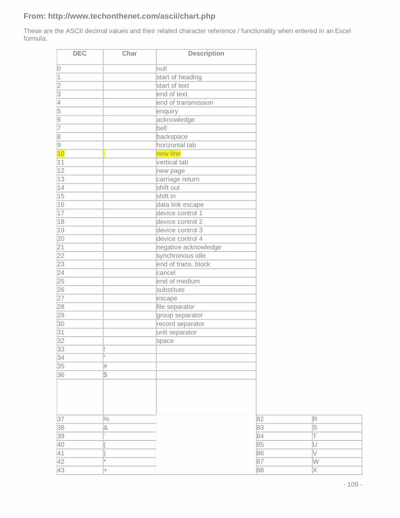
From: http://www.techonthenet.com/ascii/chart.php
These are the ASCII decimal values and their related character reference / functionality when entered in an Excel formula.
DEC Char Description
0 null 1 start of heading 2 start of text 3 end of text 4 end of transmission 5 enquiry 6 acknowledge 7 bell 8 backspace 9 horizontal tab 10 new line 11 vertical tab 12 new page 13 carriage return 14 shift out 15 shift in 16 data link escape 17 device control 1 18 device control 2 19 device control 3 20 device control 4 21 negative acknowledge 22 synchronous idle 23 end of trans. block 24 cancel 25 end of medium 26 substitute 27 escape 28 file separator 29 group separator 30 record separator 31 unit separator 32 space 33 ! 34 " 35 # 36 $
37 % 82 R 38 & 83 S 39 ' 84 T 40 ( 85 U 41 ) 86 V 42 * 87 W 43 + 88 X
- 109 -

44 , 89 Y 45 - 90 Z 46 . 91 [ 47 / 92 \ 48 0 93 ] 49 1 94 ^ 50 2 95 _ 51 3 96 ` 52 4 97 a 53 5 98 b 54 6 99 c 55 7 100 d 56 8 101 e 57 9 102 f 58 : 103 g 59 ; 104 h 60 < 105 i 61 = 106 j 62 > 107 k 63 ? 108 l 64 @ 109 m 65 A 110 n 66 B 111 o 67 C 112 p 68 D 113 q 69 E 114 r 70 F 115 s 71 G 116 t 72 H 117 u 73 I 118 v 74 J 119 w 75 K 120 x 76 L 121 y 77 M 122 z 78 N 123 { 79 O 124 | 80 P 125 }
- 110 -

Lesson 13: Custom Job Review Sheet Most of the queries that we have been looking at have been presented in a very “database” structure. Rows and rows and columns and columns of data on a spreadsheet. Pivot Tables are an excellent way of consolidating and subtotaling the data into a more user-friendly format.
What happens when you want a report that has a static layout? Can a query be used in these reports? The answer is yes.
The most important aspect of this exercise is that the format of the report is known before you start pulling data.
Here is an example of a hard coded form that we will be creating:
Again, this is a report that I created before I even looked at querying data.
The next step is determining what tables and fields we need to bring into the queries in order to populate the data in the report.
- 111 -

Another really good idea is identifying the cells that will be pulled form a query and what cells are populated with simple formulas within Excel.
In this sample, the fields in green are the cells that will be pulled from the queried data, and the fields in orange are calculated fields based on the queried (or green) fields.
- 112 -
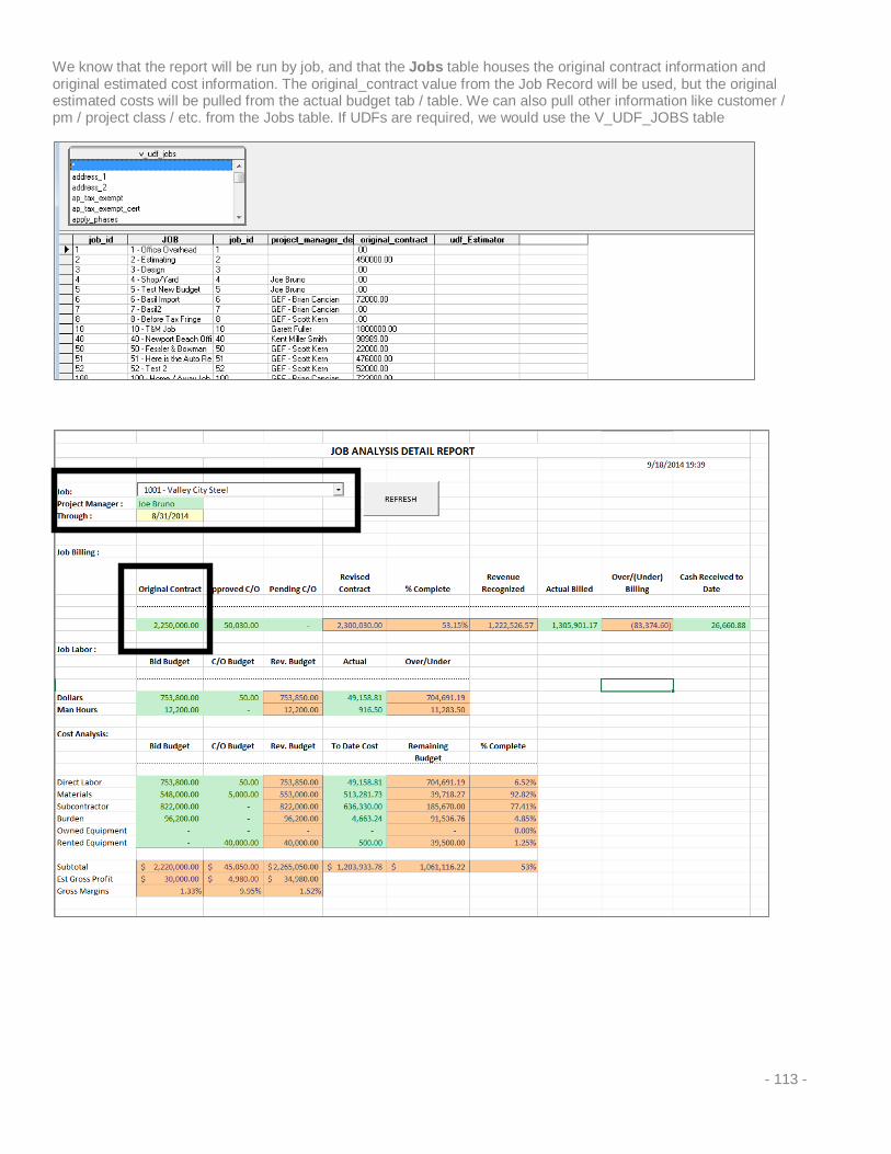
We know that the report will be run by job, and that the Jobs table houses the original contract information and original estimated cost information. The original_contract value from the Job Record will be used, but the original estimated costs will be pulled from the actual budget tab / table. We can also pull other information like customer / pm / project class / etc. from the Jobs table. If UDFs are required, we would use the V_UDF_JOBS table
- 113 -

The next component is the change orders to income (or change orders to contract). These items are pulled from the following table:
• job_chg
We also have a change order date (date_booked) as a criteria field. This will allow us to show change orders with a date less than or equal to a particular date. I have also included a status field to separate “approved” and “pending” change orders in the query.
- 114 -

We also need to identify the amount billed and cash received to date. This information is pulled from the v_em_jc_billings table.
- 115 -
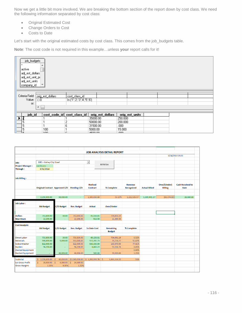
Now we get a little bit more involved. We are breaking the bottom section of the report down by cost class. We need the following information separated by cost class:
• Original Estimated Cost • Change Orders to Cost • Costs to Date
Let’s start with the original estimated costs by cost class. This comes from the job_budgets table.
Note: The cost code is not required in this example…unless your report calls for it!
- 116 -

Next we look at change order to cost information based on job and cost class. This information is found in the following table(s): job_chg and job_chg_budgets.
The job_chg table is used for the Job and Date fields, and the job_chg_budgets is used for the cost and unit adjustments by cost class.
- 117 -
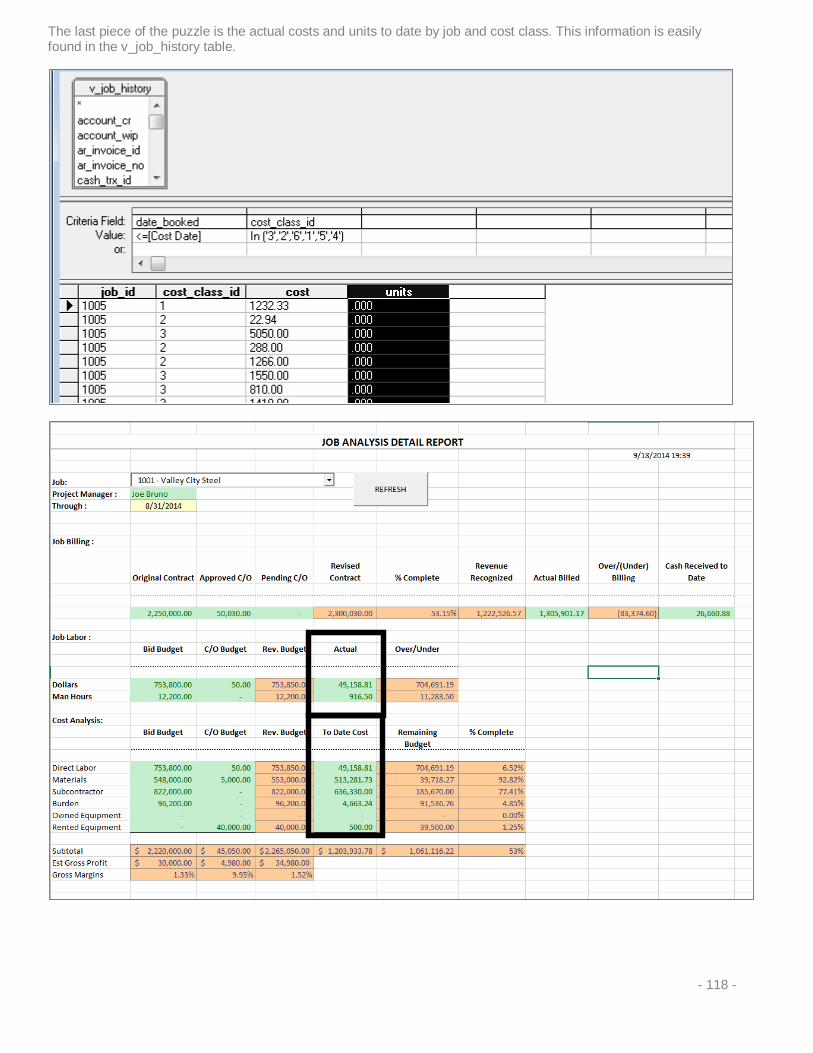
The last piece of the puzzle is the actual costs and units to date by job and cost class. This information is easily found in the v_job_history table.
- 118 -
Now that all of the tables are identified, we can start creating the report.
Ultimately, it is easiest to have a report on screen that you are overwriting the formulas in the cells. If you are trying to create the report and write the formulas at the same time, it will be more difficult.
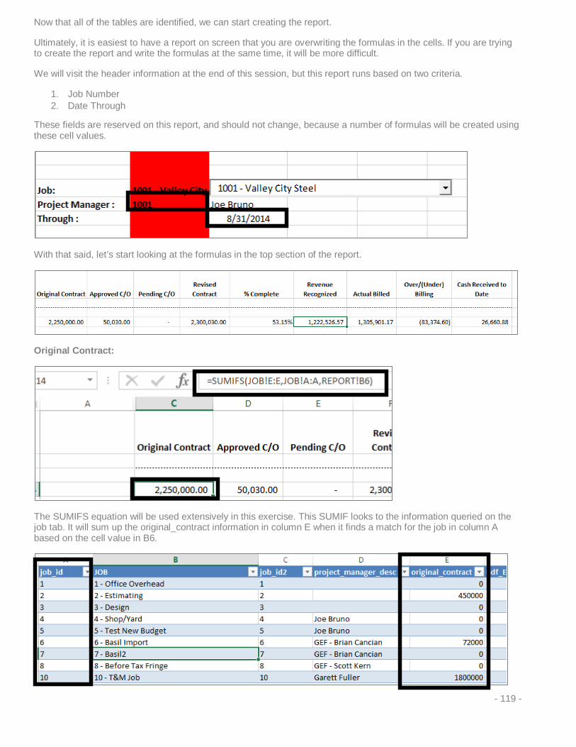
We will visit the header information at the end of this session, but this report runs based on two criteria.
1. Job Number 2. Date Through
These fields are reserved on this report, and should not change, because a number of formulas will be created using these cell values.
With that said, let’s start looking at the formulas in the top section of the report.
Original Contract:
The SUMIFS equation will be used extensively in this exercise. This SUMIF looks to the information queried on the job tab. It will sum up the original_contract information in column E when it finds a match for the job in column A based on the cell value in B6.
- 119 -
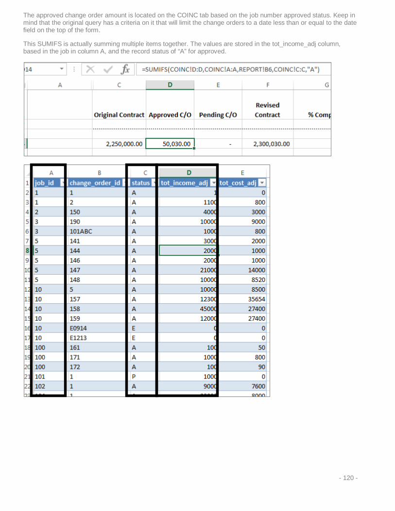
The approved change order amount is located on the COINC tab based on the job number approved status. Keep in mind that the original query has a criteria on it that will limit the change orders to a date less than or equal to the date field on the top of the form.
This SUMIFS is actually summing multiple items together. The values are stored in the tot_income_adj column, based in the job in column A, and the record status of “A” for approved.
- 120 -

Pending change orders. Cheating is highly encouraged in this report. The pending change orders are identical to the approved change orders with one exception – the status is “P” (for Pending) instead of “A.”
We can “cheat” by copying the formula from the previous cell to the adjacent cell.
Again, this is the exact same formula used for the approved change orders, the only difference is the status of “P” for Pending.
The revised contract amount is simple math; you just add the original contract amount to the approved change orders.
- 121 -

We will now move on to the middle section of the report to get information that is needed to complete the Job Billing section.
The Job Labor section calls for the estimated labor dollars and estimated labor hours (or units).
The estimated labor dollars comes from the budget tab. his information is based on the budgeted dollars based on the job and cost class 1 (labor).
- 122 -

The budgeted labor hours is similar, based on the job and cost class pulled from the same tab/query – budget.
- 123 -
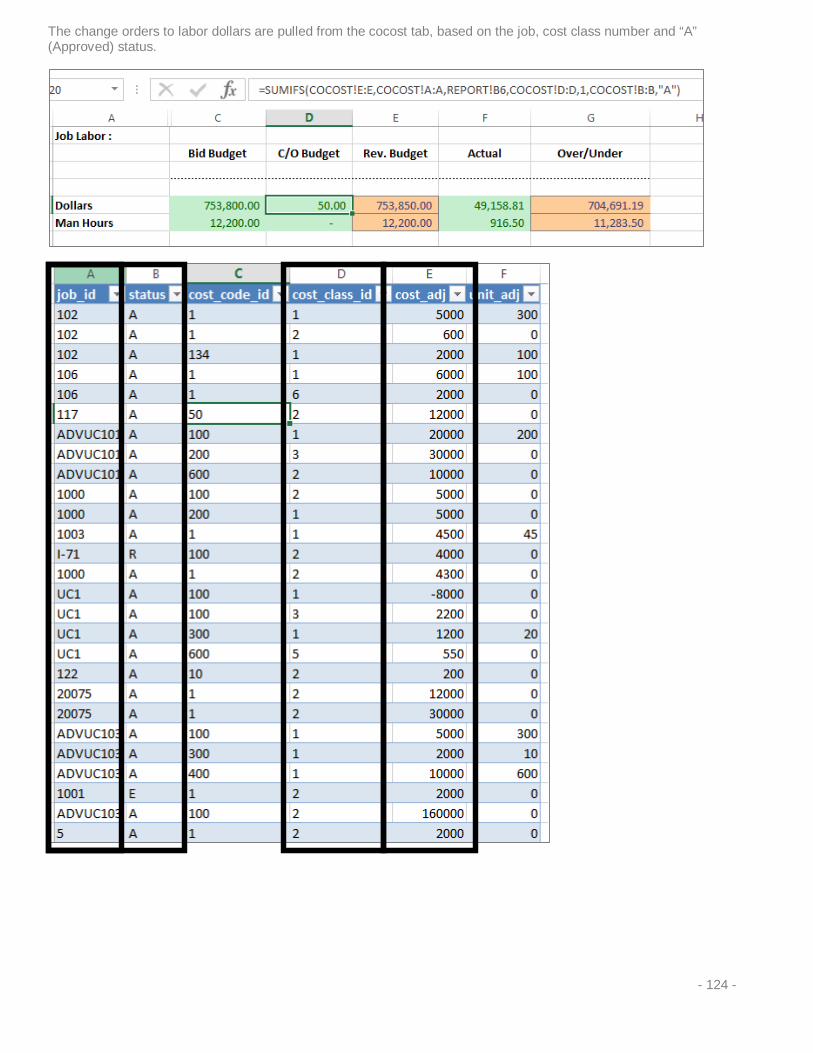
The change orders to labor dollars are pulled from the cocost tab, based on the job, cost class number and “A” (Approved) status.
- 124 -
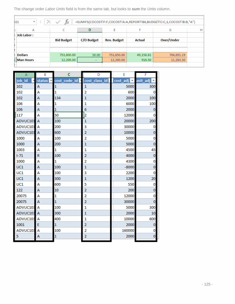
The change order Labor Units field is from the same tab, but looks to sum the Units column.
- 125 -

The revised labor budget figure and revised estimated units figure are simple equations in Excel; just add the bid budget to the co budget.
Actual labor costs are pulled from the cost tab/query based on the job number and cost class 1 (labor).
Actual labor units are pulled from the same tab, but using the units column.
- 126 -
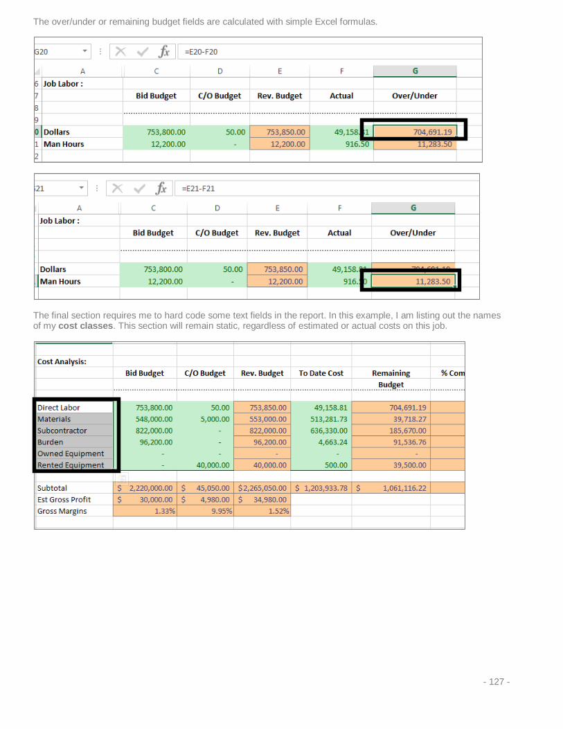
The over/under or remaining budget fields are calculated with simple Excel formulas.
The final section requires me to hard code some text fields in the report. In this example, I am listing out the names of my cost classes. This section will remain static, regardless of estimated or actual costs on this job.
- 127 -

The bid budget information is based on the job and individual cost class from the budget tab/query.
These formulas are redundant, with the only things that changes being the cost class number.
Cost Class 1 for Labor
Cost Class 2 for Material
Cost Class 3 for Subcontracts
- 128 -

Repeat this process for any and all cost classes required for your report.
The equation for the change order budget amounts is similar, but we pull the information from the cocost tab/query and add the “a” for approved change orders to the formula.
Materials Cost Approved Change Orders
Repeat these equations for all of the cost classes referenced in the far left column.
The revised budget amount = the values form the bid budget plus the c/o budget amounts.
- 129 -

To date costs…Same theory, different tab. Costs are based on the job number and the cost class.
Materials Example – Cost class reference is changed in the SUMIFS equation.
Skipping a few lines to show an example of the rented equipment costs.
- 130 -
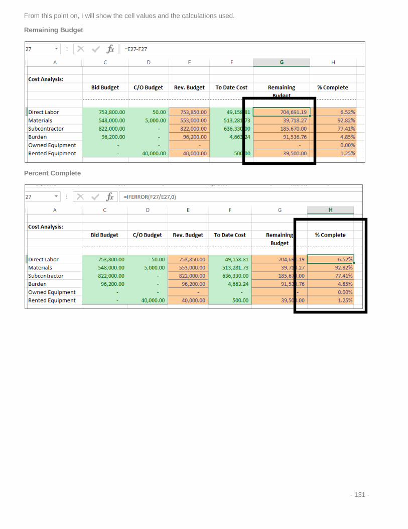
From this point on, I will show the cell values and the calculations used.
Remaining Budget
Percent Complete
- 131 -
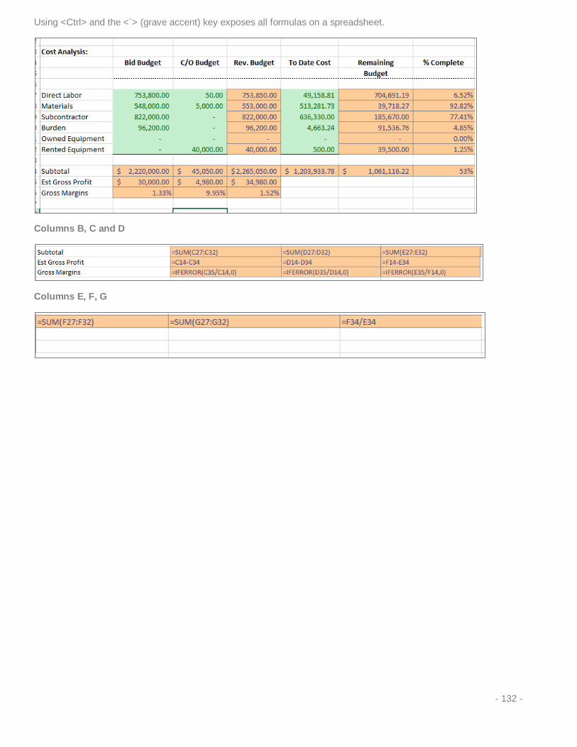
Using <Ctrl> and the <`> (grave accent) key exposes all formulas on a spreadsheet.
Columns B, C and D
Columns E, F, G
- 132 -
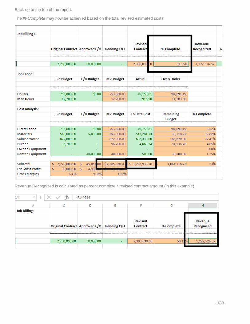
Back up to the top of the report.
The % Complete may now be achieved based on the total revised estimated costs.
Revenue Recognized is calculated as percent complete * revised contract amount (in this example).
- 133 -

The Actual Billed amount is based on a SUMIFS from the invoice tab/query based on job number.
Over/Under Billing is an equation.
And the Cash Received to Date is a SUMIFS using the data from the invoice tab/query.
- 134 -

Creating the Dropdown Box for the Job Selection
The first thing we need to do is create a “named range.”
1. Access the job tab and highlight the entire contents of column “B”. 2. From the “Formulas” tab, select “Define Name.”
3. When the dialog box appears, name the range something appropriate. In this case, we will call the named
range “JOB.”
- 135 -

4. On the “Report” tab, access the “Developer” tab and select Insert > Active X Controls > Combo Box. It is the second item in the first row under the Active X Control options.
5. “Draw” the box by dragging the mouse.
6. Right-click on the box and access “Properties.”
- 136 -

We are going to link a cell to the choice in the dropdown box and also determine the list fill range identified by the previously defined named range.
The linked cell will be B5 and the ListFillRange will be JOB.
7. Close the Properties dialog box and click on “Design Mode” to turn it off.
- 137 -
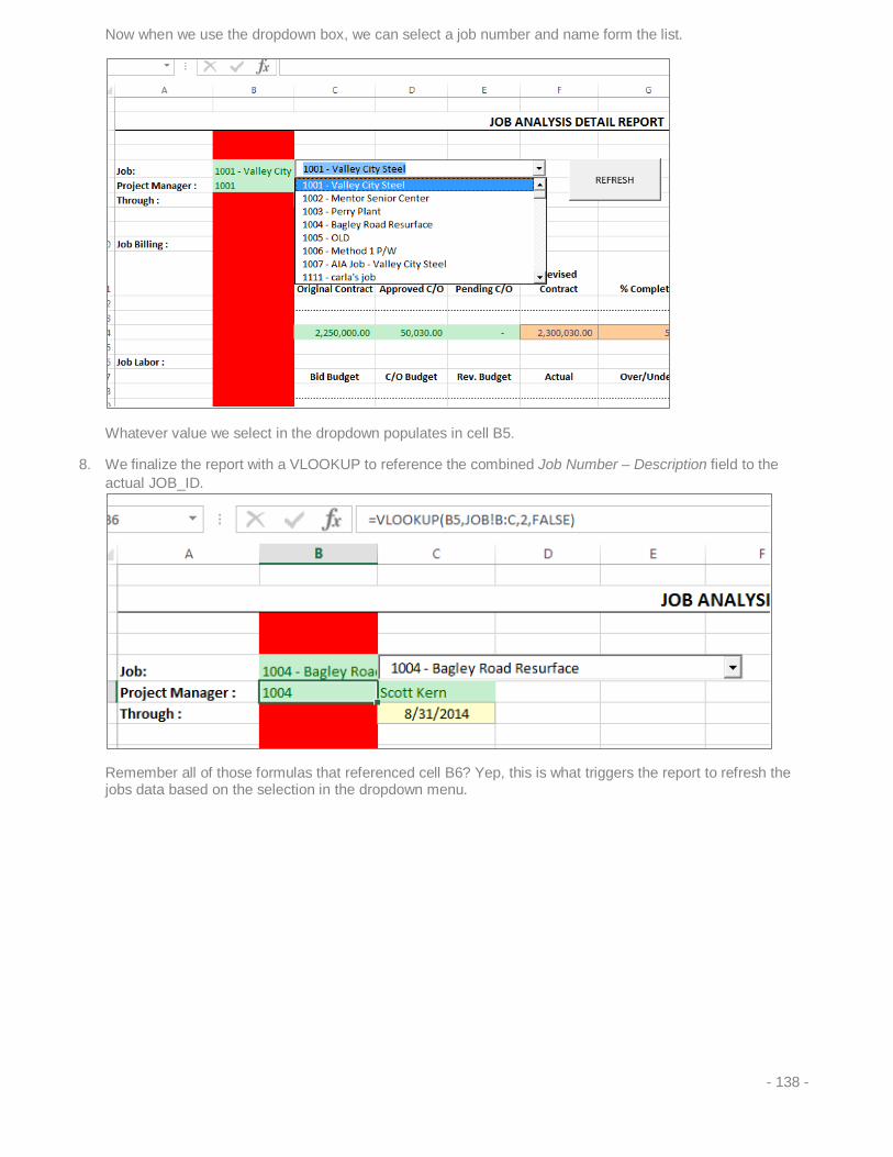
Now when we use the dropdown box, we can select a job number and name form the list.
Whatever value we select in the dropdown populates in cell B5.
8. We finalize the report with a VLOOKUP to reference the combined Job Number – Description field to the actual JOB_ID.
Remember all of those formulas that referenced cell B6? Yep, this is what triggers the report to refresh the jobs data based on the selection in the dropdown menu.
- 138 -

Lesson 14: Custom Change Order
- 139 -
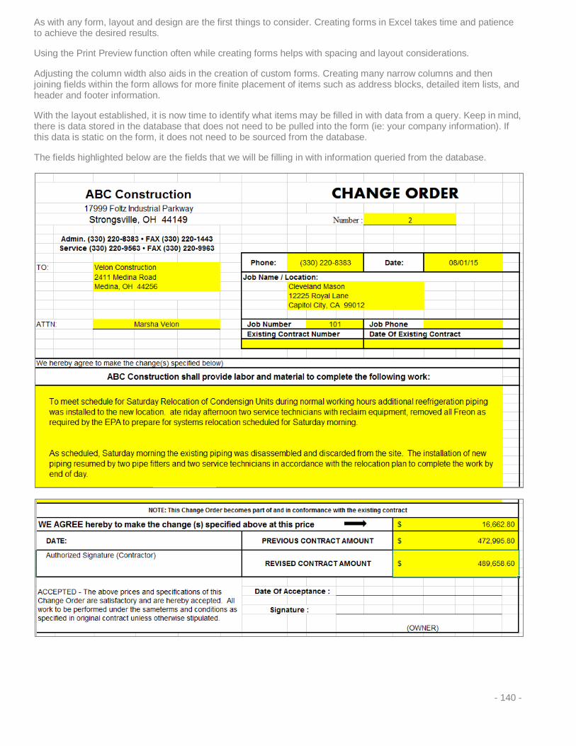
As with any form, layout and design are the first things to consider. Creating forms in Excel takes time and patience to achieve the desired results.
Using the Print Preview function often while creating forms helps with spacing and layout considerations.
Adjusting the column width also aids in the creation of custom forms. Creating many narrow columns and then joining fields within the form allows for more finite placement of items such as address blocks, detailed item lists, and header and footer information.
With the layout established, it is now time to identify what items may be filled in with data from a query. Keep in mind, there is data stored in the database that does not need to be pulled into the form (ie: your company information). If this data is static on the form, it does not need to be sourced from the database.
The fields highlighted below are the fields that we will be filling in with information queried from the database.
- 140 -

We will start with the header information on the form. This data is contained in three tables:
• JOB_CHANGE The “General” tab of the Change Order Record.
• JOBS / V_UDF_JOBS Job Record information. Use the v_udf_jobs table if
Data stored in the “UDF” tab is required on the form.
• CUSTOMERS Customer Record information (address / contact)
1. Create the query with these tables and remove the company_no links if you only have a single company in the selected database.
2. From these tables, we will select the following fields:
• job_chg.job_id • job_chg.change_order_id • job_chg.comments • v_udf_jobs.description • v_udf_jobs.address_1 • v_udf_jobs.address_2 • v_udf_jobs.city • v_udf_jobs.state • v_udf_jobs.zip_code • v_udf_jobs.job_contact • v_udf_jobs.customer_order_id • v_udf_jobs.customer_id • customers.name • customers.address_1 • customers.address_2 • customers.city • customers.state • customers.zip_code • customers.contact • abs(customers.phone_voice) • v_udf_jobs.original_contract • v_udf_jobs.order_number • v_udf_jobs.order_date
- 141 -
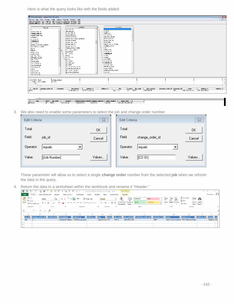
Here is what the query looks like with the fields added:
3. We also need to enable some parameters to select the job and change order number.
These parameter will allow us to select a single change order number from the selected job when we refresh the data in the query.
4. Return the data to a worksheet within the workbook and rename it “Header.”
- 142 -
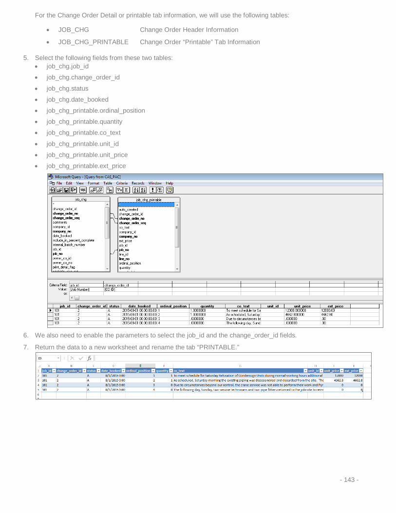
For the Change Order Detail or printable tab information, we will use the following tables:
• JOB_CHG Change Order Header Information
• JOB_CHG_PRINTABLE Change Order “Printable” Tab Information
5. Select the following fields from these two tables: • job_chg.job_id
• job_chg.change_order_id
• job_chg.status
• job_chg.date_booked
• job_chg_printable.ordinal_position
• job_chg_printable.quantity
• job_chg_printable.co_text
• job_chg_printable.unit_id
• job_chg_printable.unit_price
• job_chg_printable.ext_price
6. We also need to enable the parameters to select the job_id and the change_order_id fields.
7. Return the data to a new worksheet and rename the tab “PRINTABLE.”
- 143 -

Finally, for the footer information, we need to pull all of the approved change orders to add to the original contract amount. This information will be presented at the bottom of the change order.
We will access a single table for this information: JOB_CHG
8. From that table we will pull the following fields: • job_id • change_order_id • total_income_adj
9. Parameters will be enabled for the specific job_id, but we want to select only “A” (or approved) change orders from the Status field.
10. Return the data to a new worksheet and rename it “APP COS” (for Approved Change Orders).
- 144 -

With all of the data queried from our database, we can start to fill in the form. Many of these options will be single cell references from the other worksheets that contain queried data.
11. Let us start with the change order number. This information will come from cell B2 in the “Header” tab.
= HEADER!B2
Note: It is easiest to type in the “=” sign, then click the worksheet/cell reference you want to choose and then hit <Enter>.
12. We will follow up with the customer name and address_1.
- 145 -
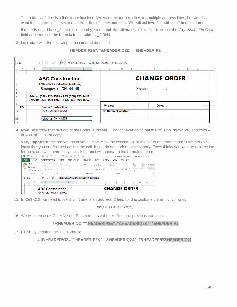
The address_2 line is a little more involved. We want the form to allow for multiple address lines, but we also want it to suppress the second address line if it does not exist. We will achieve this with an if/then statement.
If there is no address_2, then use the city, state, and zip. Ultimately it is easier to create the City, State, Zip Code field and then use the formula in the address_2 field.
13. Let’s start with the following concatenated data field:
=HEADER!P2&", "&HEADER!Q2&" "&HEADER!R2
14. Now, let’s copy that text out of the Formula toolbar. Highlight everything but the “=” sign, right-click, and copy – or – <Ctrl + C> for copy.
Very Important: Before you do anything else, click the checkmark to the left of the formula bar. This lets Excel know that you are finished editing the cell. If you do not click the checkmark, Excel thinks you want to replace the formula, and whatever cell you click on next will appear in the formula toolbar.
15. In Cell C12, we need to identify if there is an address_2 field for this customer. Start by typing in:
=if(HEADER!O2=””,
16. We will then use <Ctrl + V> (for Paste) to paste the text from the previous equation.
= IF(HEADER!O2="",HEADER!P2&", "&HEADER!Q2&" "&HEADER!R2
17. Finish by creating the “then” clause.
= IF(HEADER!O2="",HEADER!P2&", "&HEADER!Q2&" "&HEADER!R2,HEADER!O2)
- 146 -

18. Looks great, but we now have a duplication of the address field. An If/then added to the address field will solve this issue.
=IF(HEADER!O2="","",HEADER!P2&", "&HEADER!Q2&" "&HEADER!R2)
19. Add the ATTN, PHONE and DATE fields.
- 147 -

20. The Job Address section is similar to the Customer Address section, but it references different cells from the header tab.
- 148 -
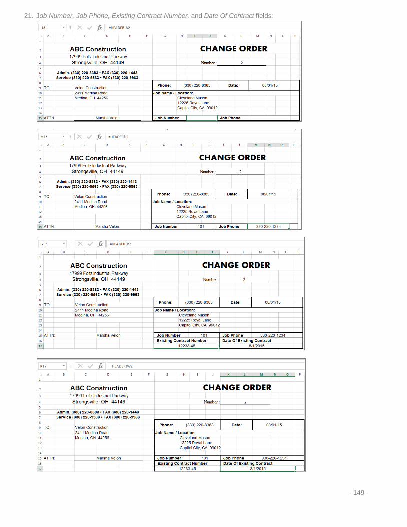
21. Job Number, Job Phone, Existing Contract Number, and Date Of Contract fields:
- 149 -

The detail information will be pulled from the PRINTABLE tab. We want to combine the data from multiple lines in the query into a single (merged) field within our form.
22. We will use the CHAR(10) function in the formula toolbar to combine the data.
=CHAR(10)&PRINTABLE!G2&CHAR(10)&CHAR(10)&PRINTABLE!G3&CHAR(10)&CHAR(10)&PRINTABLE!G4&CHAR(10)&CHAR(10)&PRINTABLE!G5&CHAR(10)&CHAR(10)&PRINTABLE!G6&CHAR(10)&CHAR(10)&PRINTABLE!G7&CHAR(10)&CHAR(10)&PRINTABLE!G8&CHAR(10)&CHAR(10)&PRINTABLE!G9&CHAR(10)&CHAR(10)&PRINTABLE!G10
This formula is involved, but not difficult, as most of the functions are repeated, only referencing different cells. In these situations, use of the copy and paste function will aid in creating the equation more efficiently.
- 150 -

23. For the summary information, we will pull data from a few tabs, the “Header” tab, the “Printable” tab, and the “APP COS” tab.
24. The total amount of the change order will come from the “Printable” tab. We will sum all of the values in the ext_price field.
25. The equation in the total line must include all rows from column J.
26. The previous contract amount will be a total of the original contract amount and the approved change orders.
27. The revised contract amount is the addition of these two previously defined formulas.
- 151 -
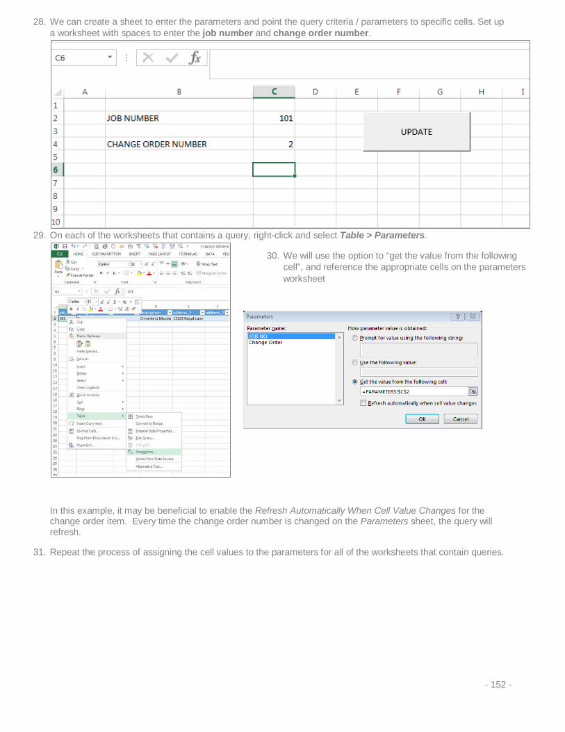
28. We can create a sheet to enter the parameters and point the query criteria / parameters to specific cells. Set up a worksheet with spaces to enter the job number and change order number.
29. On each of the worksheets that contains a query, right-click and select Table > Parameters.
In this example, it may be beneficial to enable the Refresh Automatically When Cell Value Changes for the change order item. Every time the change order number is changed on the Parameters sheet, the query will refresh.
31. Repeat the process of assigning the cell values to the parameters for all of the worksheets that contain queries.
30. We will use the option to “get the value from the following cell”, and reference the appropriate cells on the parameters worksheet
- 152 -

Refresh Macro and Button
1. Enable the “Developer” tab.
Excel 2007 Only: First we must enable a feature in Excel by accessing the Office button in the upper left hand corner of Excel. In the Popular section, enable the Show Developer tab in the Ribbon.
Excel 2010/2013/365 Only: Select File > Options > Customize Ribbon. Enable the Developer checkbox.
- 153 -

2. Click on the “Developer” tab and select Insert > Form Controls > Button.
3. “Draw” the button in the desired location. You will be prompted to assign a Macro to this button. If you are afraid
of Macros, don’t be. A Macro is a simple name for “I will record your key strokes and play them back for you.” On the other hand…. You should be very afraid of the VB code that a macro creates. I try to stick to recording and playing macros.
4. When the “Assign Macro” prompt comes up, let the macro name default to whatever is available and click the [Record] button.
- 154 -
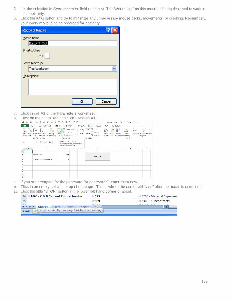
5. Let the selection in Store macro in: field remain at “This Workbook,” as this macro is being designed to work in this book only.
6. Click the [OK] button and try to minimize any unnecessary mouse clicks, movements, or scrolling. Remember… your every move is being recorded for posterity!
7. Click in cell A1 of the Parameters worksheet, 8. Click on the “Data” tab and click “Refresh All.”
9. If you are prompted for the password (or passwords), enter them now. 10. Click in an empty cell at the top of the page. This is where the cursor will “land” after the macro is complete. 11. Click the little “STOP” button in the lower left hand corner of Excel.
- 155 -

12. Test your Macro by pressing the button. If it does not work, or you get undesired results, you can delete the Macro and start over.
Note: Only if you need to delete the macro, click on the “Developer” tab and click on “Macros.” In the Macro dialog box, highlight the desired macro and click [Delete].
You may also reassign and delete the macro from this option if need arises.
13. We can rename the button by right-clicking the button and choosing “Edit Text.” The word “Refresh” is a nice option.
- 156 -
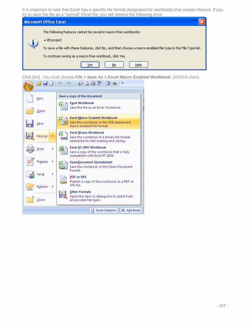
It is important to note that Excel has a specific file format designated for workbooks that contain Macros. If you try to save the file as a “normal” Excel file, you will receive the following error:
Click [No]. You must choose File > Save As > Excel Macro Enabled Workbook. (XXXXX.xlsm).
- 157 -

Another option when creating forms is to define separate rows for the data to display. In the previous exercise, we used a number of merged cells and the concatenate function to combine the data into a single cell.
Below, you will see an example of a Change Order formatted to allow multiple line items as separate lines.
This method may be in favor if you have a number of rows that exceeds the rows on Page 1 of the form.
The formula in each row is rather simple, it references the PRINTABLE tab information and is sequenced by a single row number for each row on the form.
The same is true for the Amount column on the form.
- 158 -
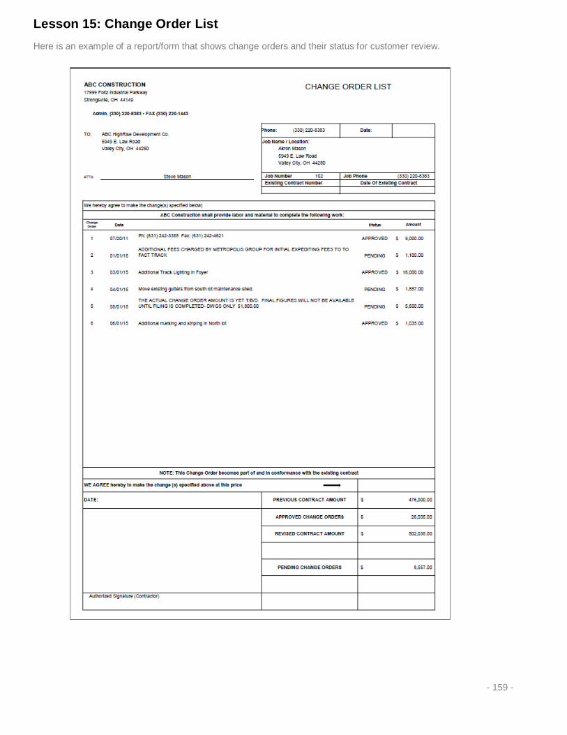
Lesson 15: Change Order List Here is an example of a report/form that shows change orders and their status for customer review.
- 159 -

We will create a header file that pulls information for all change orders for a single job, including the status and amount of each change order.
Here is the query and the list of tables and field names:
• job_chg.job_id • customers.name
• job_chg.change_order_id • customers.address_1 • job_chg.comments • customers.address_2
• jobs.description • customers.city
• jobs.address_1 • customers.state • jobs.address_2 • customers.zip_code
• jobs.city • customers.contact
• jobs.state • abs(customers.phone_voice)
• jobs.zip_code • jobs.original_contract
• jobs.job_contact • job_chg.date_booked • jobs.customer_order_id • job_chg.tot_income_adj
• jobs.customer_id • job_chg.status
Once we create a parameter for the job number and return the data to Excel, we will need to add a formula to change the status field into an actual word.
=IF(X2="A","APPROVED",IF(X2="P","PENDING",""))
- 160 -

The header information is sourced from the same fields / worksheets as the previous lesson.
The body of the form changes up a bit.
The first column shows the change order number. When creating forms with specific rows defined, you must remember to put an IF/THEN statement in to hide the values that do not, or may not, exist. These reports are dynamic, and the first job may have 10 change orders, whereas the next job only has 3. The form must be created to accept and report varying data sets.
The logic is the same for all of the columns, it says, “If the value on the header page is blank, then return a blank cell, otherwise, show me the value in that cell.” Repeat this formula for all of the appropriate columns.
The formulas in the footer are rather straightforward. The original contract amount is pulled from only one of the cells in the header worksheet. It is best to choose the first row after the header row, as you will be sure to always have at least one change order on this form (or you would not be using it).
- 161 -
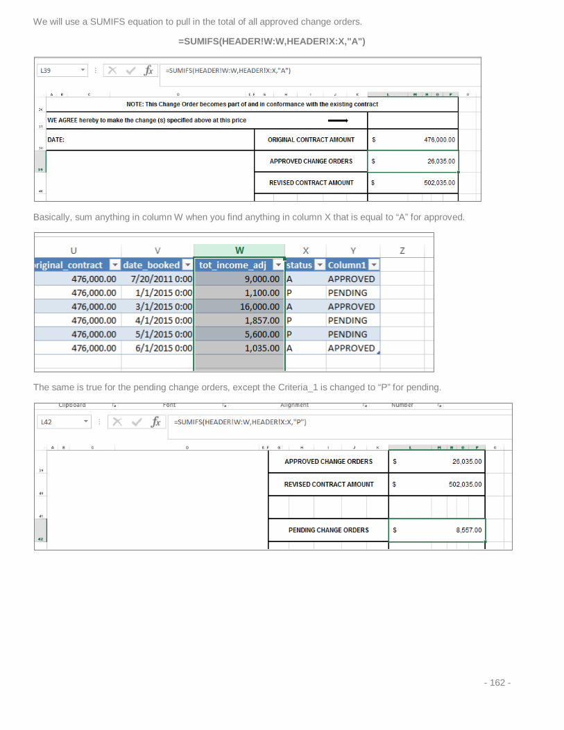
We will use a SUMIFS equation to pull in the total of all approved change orders.
=SUMIFS(HEADER!W:W,HEADER!X:X,"A")
Basically, sum anything in column W when you find anything in column X that is equal to “A” for approved.
The same is true for the pending change orders, except the Criteria_1 is changed to “P” for pending.
- 162 -
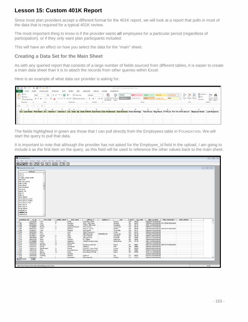
Lesson 15: Custom 401K Report Since most plan providers accept a different format for the 401K report, we will look at a report that pulls in most of the data that is required for a typical 401K review.
The most important thing to know is if the provider wants all employees for a particular period (regardless of participation), or if they only want plan participants included.
This will have an effect on how you select the data for the “main” sheet.
Creating a Data Set for the Main Sheet
As with any queried report that consists of a large number of fields sourced from different tables, it is easier to create a main data sheet than it is to attach the records from other queries within Excel.
Here is an example of what data our provider is asking for.
The fields highlighted in green are those that I can pull directly from the Employees table in FOUNDATION. We will start the query to pull that data.
It is important to note that although the provider has not asked for the Employee_id field in the upload, I am going to include it as the first item on the query, as this field will be used to reference the other values back to the main sheet.
- 163 -
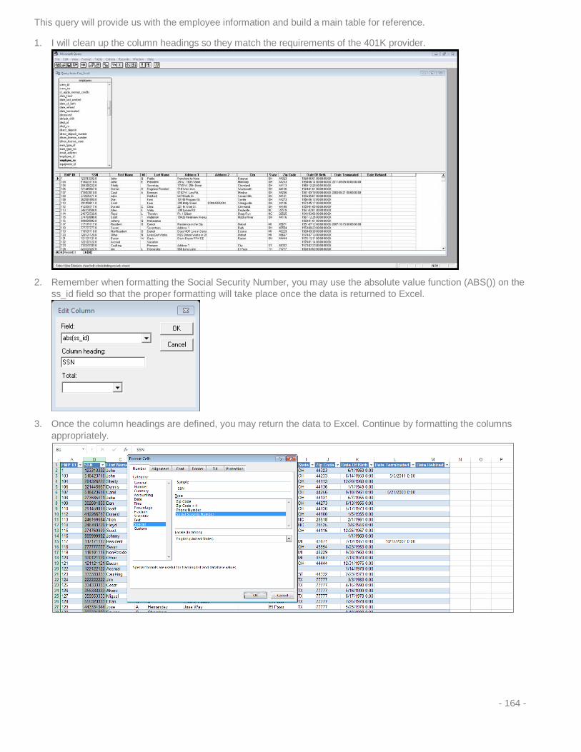
This query will provide us with the employee information and build a main table for reference.
1. I will clean up the column headings so they match the requirements of the 401K provider.
2. Remember when formatting the Social Security Number, you may use the absolute value function (ABS()) on the
ss_id field so that the proper formatting will take place once the data is returned to Excel.
3. Once the column headings are defined, you may return the data to Excel. Continue by formatting the columns
appropriately.
- 164 -

4. If your provider only requires the last 4 digits of the Social Security Number, you may use a formula in the query to show the last 4 digits.
The formula is written the same as in Excel:
RIGHT(ss_id,4)
This tells the field to show the last 4 digits on the right of the selected field.
Here is how the data looks with the RIGHT function written into the query.
The method you choose to use to format these values will depend on the requirements from your plan provider.
Now that we have the appropriate employee list created, we need to pull some queries from payroll history to populate the rest of the report.
5. There is a single table that may give us all of the information we need for this report. The table is titled PAY_SUMMARY. From this table, we will pull the following fields:
• Employee_id • Check_date • Regular_hours • Overtime_hours • Regular_earnings • Overtime_earnings • Additional_taxable • Additional_non_taxable • Deductions_401K
- 165 -

6. In the Operator field on the Edit Criteria dialog box, select “is between” for the check_date field.
7. Once the data is sourced from the query, return the values to Excel.
Now we need to link the data from the earnings summary to the main sheet. Remember that we included the reference to the employee_id on the main sheet to use as a reference to all other data on the other sheets.
8. We will start with the gross earnings value. This amount is stored in column H of the “Earnings” tab. We did pull over additional information in case your provider needs a breakdown between regular and overtime earnings.
- 166 -

9. We will use the SUMIFS formula to pull the information together.
=sumifs(EARNINGS!H:H,EARNINGS!A:A,MAIN!A2)
This will sum anything in column H from the “Earnings” tab if the value in column A from the “Earnings” tab equals the value in cell A2 on the main sheet (in this example, the individual employee_id).
10. For the Total Hours column, we will actually sum the REG Hours and OVT Hours from the “Earnings” tab and add them together on the main sheet.
11. REG Hours are summed together from column C on the “Earnings” tab.
12. OVT Hours are summed from column D on the “Earnings” tab.
- 167 -

13. The Total Hours column is a simple equation; just add the REG and OVT hours together.
14. Continuing on, we add the 401K deduction amount. This value is found in our his_summary/”Earnings” tab of the
spreadsheet in column J.
15. At this point it is a good idea to compare the values in the query against the values in the FOUNDATION 401K
Report for the same time period. Depending on the requirements of your plan provider, the amounts that come from the his_summary table may or may not be what they are looking for.
Let’s look at a single employee:
Notice his gross earnings are very different than his 401K earnings on the 401K report in FOUNDATION.
The 401K report is showing 401K earnings while the employee was eligible for the plan. Again, your plan provider may want both amounts on the report – requirements will vary.
- 168 -

16. In order to get the values for the 401K earnings separate from total gross earnings, we need to access another table.
The table we will use is his_misc. It carries the history of the miscellaneous deductions within FOUNDATION.
This table will have a dual purpose. It will allow us to pull in the isolated 401K earnings and the 401K matching value(s). We can also use this table to pull in values for a 401K loan repayment based on the miscellaneous deduction code.
17. In this example, I have used the employee_id as my reference, and I included the deduction_id code to reference the amount withheld for the particular deduction code. I have also included the p401K_earnings and p401K_matching fields.
Note: You may also include the deduction_amount field in this query. It should be the same as the amount in the deductions_401K field from the his_summary table. We will also enable date criteria based on the dated field.
By adding criteria on the deduction_id field, we can limit the values returned only to the codes that are 401K related. These may include: 401K, Roth 401K, Safe Harbor 401K, and 401K loans. Your setup in FOUNDATION will determine what codes you need for the report.
Here are the results showing the selected codes.
- 169 -

18. We will now return the data to Excel.
19. We will add a column to the main report tab for the 401K earnings amount from the “401” tab. This is a SUMIFS
formula.
Again, care must be taken in determining the values for the report. This corrects the values for Employee 109 – “Davis Bacon”
But we now have a very different value in place for employee 103 – John President. Looking at the 401 tab that contains the 401K earnings, we see there are amounts for multiple miscellaneous deduction codes. There are earnings recorded in the table against the 401K code and the Roth 401K code.
20. We need to tweak out SUMIFS statement on the MAIN page to reflect earnings for the 401K code only.
=SUMIFS('401'!C:C,'401'!A:A,MAIN!A2,'401'!B:B,"401")
This formula now says, pull all the p401K_earnings amounts when the employee_id = “X” and the specific miscellaneous deduction code is “401K”.
Again, depending on the number of 401K codes you have setup, the formulas will vary from company to company.
- 170 -
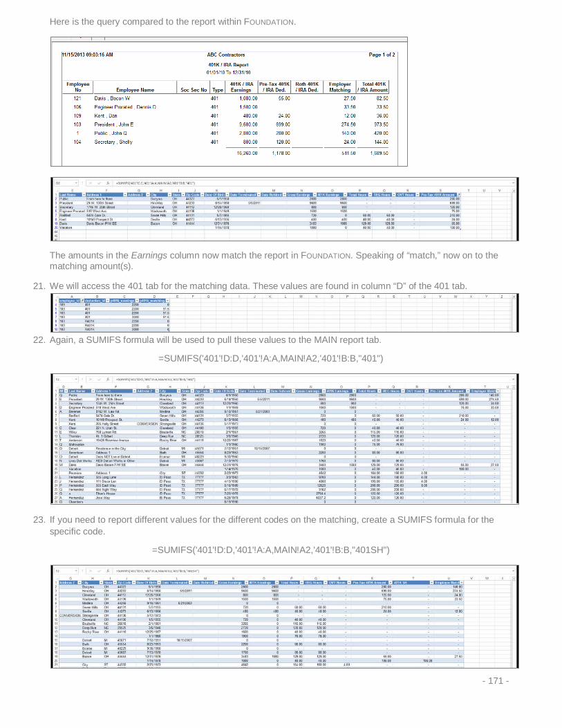
Here is the query compared to the report within FOUNDATION.
The amounts in the Earnings column now match the report in FOUNDATION. Speaking of “match,” now on to the matching amount(s).
21. We will access the 401 tab for the matching data. These values are found in column “D” of the 401 tab.
22. Again, a SUMIFS formula will be used to pull these values to the MAIN report tab.
=SUMIFS('401'!D:D,'401'!A:A,MAIN!A2,'401'!B:B,"401")
23. If you need to report different values for the different codes on the matching, create a SUMIFS formula for the specific code.
=SUMIFS('401'!D:D,'401'!A:A,MAIN!A2,'401'!B:B,"401SH")
- 171 -

24. Finally, we will insert a column for the 401K Loan repayments. In order to do this, we need to add the deduction_amount field from the his_misc query.
25. Then we create a SUMIFS formula to pull in data based on the employee_id and the desired miscellaneous
deduction code.
=SUMIFS('401'!E:E,'401'!A:A,MAIN!A2,'401'!B:B,"401KL")
26. It might be a good idea to create a “Date” tab to set the parameters for all of the queries. This tab is just a simple tab with cells referencing state and end dates for the reports.
27. Access one of the tabs with a query, right click on a cell within the table, and choose Table > Parameters.
- 172 -
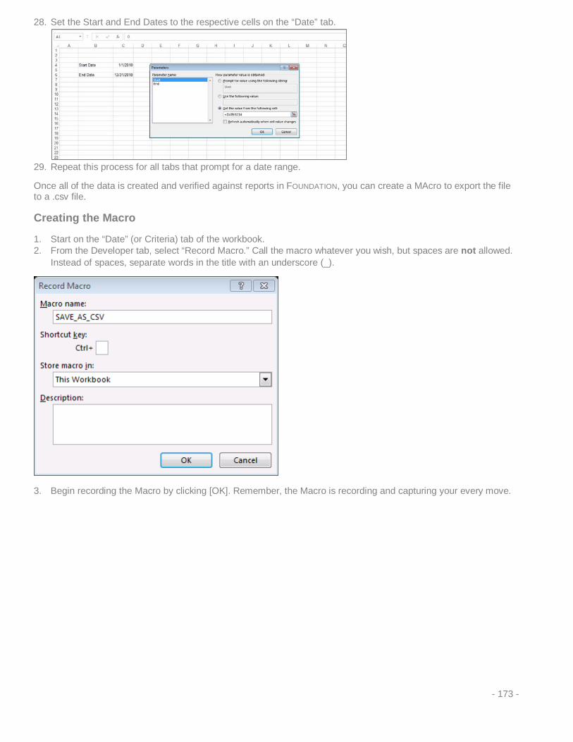
28. Set the Start and End Dates to the respective cells on the “Date” tab.
29. Repeat this process for all tabs that prompt for a date range.
Once all of the data is created and verified against reports in FOUNDATION, you can create a MAcro to export the file to a .csv file.
Creating the Macro
1. Start on the “Date” (or Criteria) tab of the workbook. 2. From the Developer tab, select “Record Macro.” Call the macro whatever you wish, but spaces are not allowed.
Instead of spaces, separate words in the title with an underscore (_).
3. Begin recording the Macro by clicking [OK]. Remember, the Macro is recording and capturing your every move.
- 173 -
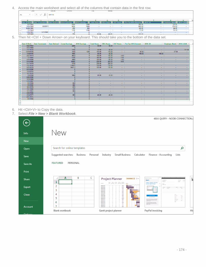
4. Access the main worksheet and select all of the columns that contain data in the first row.
5. Then hit <Ctrl + Down Arrow> on your keyboard. This should take you to the bottom of the data set.
6. Hit <Ctrl+V> to Copy the data. 7. Select File > New > Blank Workbook.
- 174 -
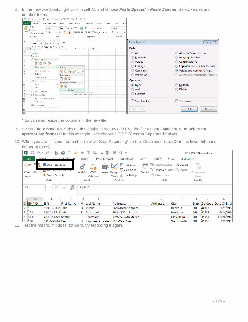
8. In the new workbook, right-click in cell A1 and choose Paste Special > Paste Special. Select values and number formats.
You can also resize the columns in the new file.
9. Select File > Save As. Select a destination directory and give the file a name. Make sure to select the appropriate format !! In this example, let’s choose “.CSV” (Comma Separated Values).
10. When you are finished, remember to click “Stop Recording” on the “Developer” tab. (Or in the lower left hand corner of Excel) .
11. Test the macro. If it does not work, try recording it again.
- 175 -

Macro Code
If we look at the Macro code, we can start to figure out what is going on.
1. On the “Developer” tab, select “Macros” in the upper left. This will show you the list of Macros stored in all open workbooks, your personal Excel Workbook, and the Current Workbook. Show “Macros in This Workbook” to minimize the amount of Macros shown.
2. Select the newly created macro and click “Edit” to display the code that was created for you.
- 176 -

Once you start poking around Macros, they are not all that difficult to understand.
Let’s break this one down.
Sub SAVE_AS_CSV()
'
' SAVE_AS_CSV Macro
'
'
‘ SELECTS THE “MAIN” SHEET AND HIGHLIGHTS ROW 1 A-V
Sheets("MAIN").Select
Range("A1:V1").Select
‘ SELECTS ALL ROWS WITHIN THE RANGE
Range(Selection, Selection.End(xlDown)).Select
‘ COPIES THE SELECTION
Selection.Copy
‘ ADDS A NEW WORKBOOK AND PASTES THE VALUES
Workbooks.Add
Selection.PasteSpecial Paste:=xlPasteValuesAndNumberFormats, Operation:= _
xlNone, SkipBlanks:=False, Transpose:=False
‘ AUTO FITS THE COLUMNS
Cells.Select
Cells.EntireColumn.AutoFit
Range("A1").Select
Application.CutCopyMode = False
‘ SELECTS THE DIRECTORY NA D NAMES THE FILE AND TYPE FOR SAVING
ChDir "C:\Users\stk.FOUNDATIONSOFT\Desktop"
ActiveWorkbook.SaveAs Filename:= _
"C:\Users\stk.FOUNDATIONSOFT\Desktop\401K EXPORT.csv", FileFormat:=xlCSV, _
CreateBackup:=False
End Sub
- 177 -
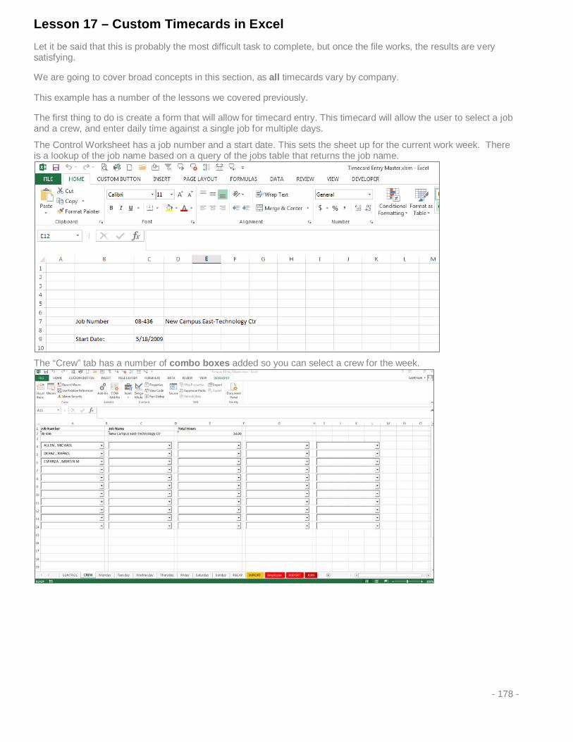
Lesson 17 – Custom Timecards in Excel Let it be said that this is probably the most difficult task to complete, but once the file works, the results are very satisfying.
We are going to cover broad concepts in this section, as all timecards vary by company.
This example has a number of the lessons we covered previously.
The first thing to do is create a form that will allow for timecard entry. This timecard will allow the user to select a job and a crew, and enter daily time against a single job for multiple days.
The Control Worksheet has a job number and a start date. This sets the sheet up for the current work week. There is a lookup of the job name based on a query of the jobs table that returns the job name.
The “Crew” tab has a number of combo boxes added so you can select a crew for the week.
- 178 -
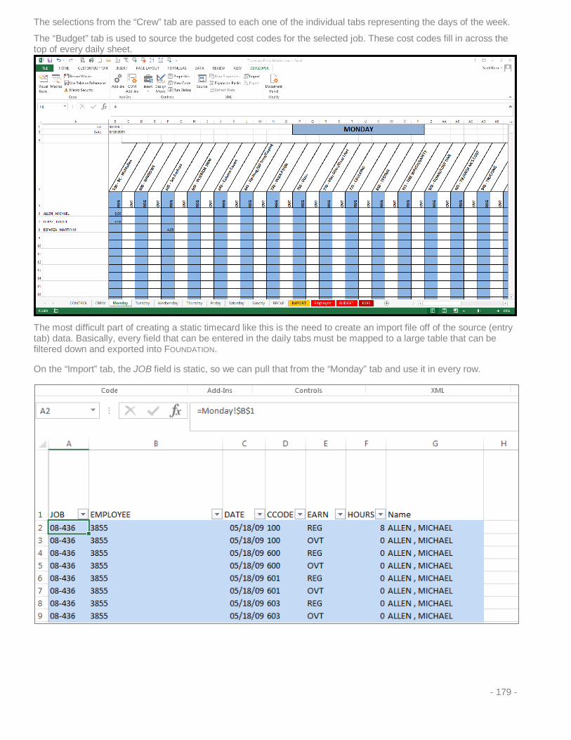
The selections from the “Crew” tab are passed to each one of the individual tabs representing the days of the week.
The “Budget” tab is used to source the budgeted cost codes for the selected job. These cost codes fill in across the top of every daily sheet.
The most difficult part of creating a static timecard like this is the need to create an import file off of the source (entry tab) data. Basically, every field that can be entered in the daily tabs must be mapped to a large table that can be filtered down and exported into FOUNDATION.
On the “Import” tab, the JOB field is static, so we can pull that from the “Monday” tab and use it in every row.
- 179 -
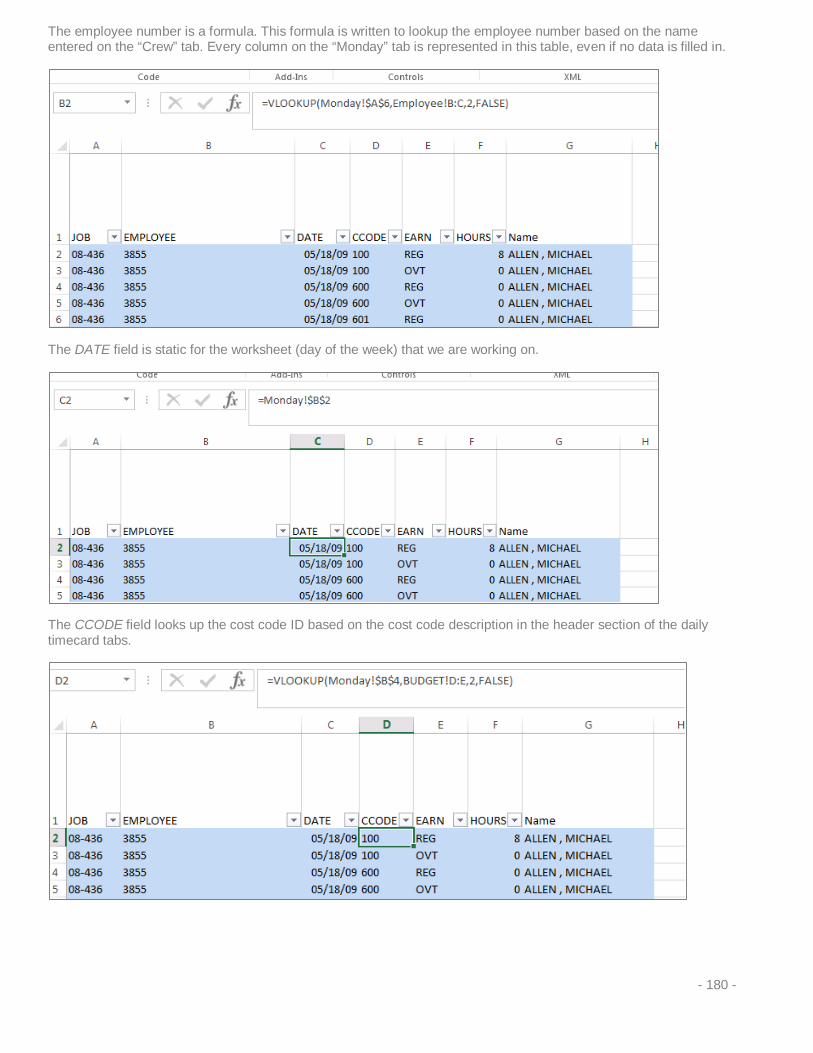
The employee number is a formula. This formula is written to lookup the employee number based on the name entered on the “Crew” tab. Every column on the “Monday” tab is represented in this table, even if no data is filled in.
The DATE field is static for the worksheet (day of the week) that we are working on.
The CCODE field looks up the cost code ID based on the cost code description in the header section of the daily timecard tabs.
- 180 -

Since the positions of the earn codes do not change, these may be set as absolute references for each daily tab as well.
The Hours fields need to be mapped individually for each cell on each of the daily tabs.
The final column is a simple reference for troubleshooting.
This is a lookup of the employee number, returning the employee name.
- 181 -

Once you have mapped a single day, you can then copy that range and paste below the existing range. Make sure to note where the old range ends and the new range starts
You can use the Find/Replace function to replace all of the “Monday” references with “Tuesday.”
Make sure you select only the range of cells that you want to replace, otherwise you will overwrite all of the references.
This will replace all of the values for “Monday” with “Tuesday.” Repeat for as many sections as you need.
Once complete, we can enable filters on the column headers and record a macro to filter out all of the values that have “0” hours present, leaving only the items that have time entered. The macro can then create the .CSV file and save the timecard record.
- 182 -

Sample MACRO Code
Sub SAVE_TC_CSV() ' ' SAVE_TC_CSV Macro ' ' ' CLEARS ALL FILTERS Rows("1:1").Select ActiveSheet.Range("$A$1:$F$23401").AutoFilter Field:=6 Range("A1").Select ' REAPPLIES FILTERS TO REMOVE 0 VALUES Range("A1").Select ActiveSheet.Range("$A$1:$F$23401").AutoFilter Field:=6, Criteria1:="<>0", _ Operator:=xlAnd ' SELECTS VISIBLE RANGE Range("A2:G2").Select Range(Selection, Selection.End(xlDown)).Select Selection.Copy ' ADDS NEW WORKBOOK Workbooks.Add ' PASTES DATA INTO WORKSHEET Range("A1").Select Selection.PasteSpecial Paste:=xlPasteValues, Operation:=xlNone, SkipBlanks _ :=False, Transpose:=False Columns("C:C").Select Application.CutCopyMode = False Selection.NumberFormat = "mm/dd/yy;@" Cells.Select Cells.EntireColumn.AutoFit Range("A1").Select ' DEFINES DIRECTORY TO SAVE FILE ChDir "C:\Timecards" ThisFile = Range("A1").Value TCDate = Range("C1").Value LValue = Format(TCDate, "mmddyy") strPath = "C:\Timecards\" MyFileName = ThisFile & "_" & LValue ActiveWorkbook.SaveAs Filename:=strPath & MyFileName, FileFormat _ :=xlCSV, CreateBackup:=False End Sub - 183 -

Lesson 18 – Custom AIA Billing Form We have developed a query that pulls data from posted AIA documents in FOUNDATION.
This is a form that offers all of the data presented in an AIA document, but allows the user to define the printable format.
The sample shown has the standard G702 and G703 information available. Using what you have learned in this class, you will be able to add tabs to this query and create custom AIA billing formats.
Again – this is like the Wild West, because everyone will have a different need and different form that they are required to use. The following examples are not gospel, only examples.
We start by adding tabs to the existing form. If you are fortunate enough to have the desired format in Excel, you may copy that worksheet into this file as well.
Once the billing form is resident within the spreadsheet, it is all about mapping references to the correct cells on the queery sheets.
- 184 -

Here is where the data is stored within the spreadsheet.
On the “JOBCUST” tab, we have pertinent job and customer information including the following:
The “TOTALS” tab includes data which is typically presented on the Header (or G702 page)
job_id Job Name Job Address1 Job Address2 Job CY ST ZP city state zip_code JOB PM ID PM JOB Customer Job# JOB Customer Order # JOBS Customer Contact customer_id Customer Name address_1 address_2 CUSTOMER CY ST ZP city2 state3 zip_code4 CUSTOMER contact
All of this information is relevant to the header of an invoice. (Who is being billed, and where the invoice should go, etc.)
Keep in mind, you may edit the query to include additional information, even adding UDF fields with the appropriate v_jobs_UDF or v_UDF_customers table(s).
The calculations have been done for you on this page.
No need to recreate the wheel. Use these values on a header page.
- 185 -

The “ITEMS” tab includes information that is typically presented on the G703 tab.
aia_item_id item_type Column1 description ordinal_position row_heading SCHED VAL PREV APP COMP THIS PER ORIG CON PREV ORIG CON CUR ORIG CON TD ADD C/O's PREV ADD C/O CUR ADD C/O CTD ADD C/O DED C/Os PREV DED C/O CUR DED C/O TD DED C/O STORED MAT COMP STORED % COMP BALANCE RETAINAGE STORED MAT RET
- 186 -
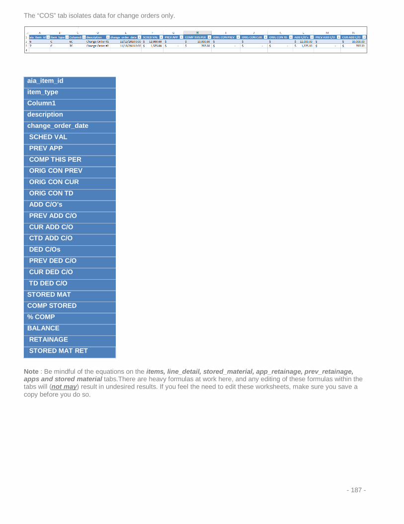
The “COS” tab isolates data for change orders only.
Note : Be mindful of the equations on the items, line_detail, stored_material, app_retainage, prev_retainage, apps and stored material tabs.There are heavy formulas at work here, and any editing of these formulas within the tabs will (not may) result in undesired results. If you feel the need to edit these worksheets, make sure you save a copy before you do so.
aia_item_id item_type Column1 description change_order_date SCHED VAL PREV APP COMP THIS PER ORIG CON PREV ORIG CON CUR ORIG CON TD ADD C/O's PREV ADD C/O CUR ADD C/O CTD ADD C/O DED C/Os PREV DED C/O CUR DED C/O TD DED C/O STORED MAT COMP STORED % COMP BALANCE RETAINAGE STORED MAT RET
- 187 -
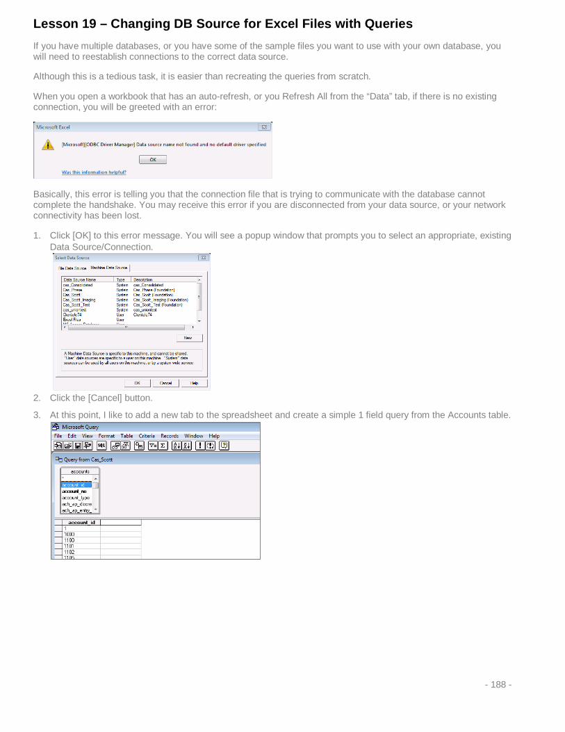
Lesson 19 – Changing DB Source for Excel Files with Queries If you have multiple databases, or you have some of the sample files you want to use with your own database, you will need to reestablish connections to the correct data source.
Although this is a tedious task, it is easier than recreating the queries from scratch.
When you open a workbook that has an auto-refresh, or you Refresh All from the “Data” tab, if there is no existing connection, you will be greeted with an error:
Basically, this error is telling you that the connection file that is trying to communicate with the database cannot complete the handshake. You may receive this error if you are disconnected from your data source, or your network connectivity has been lost.
1. Click [OK] to this error message. You will see a popup window that prompts you to select an appropriate, existing Data Source/Connection.
2. Click the [Cancel] button.
3. At this point, I like to add a new tab to the spreadsheet and create a simple 1 field query from the Accounts table.
- 188 -
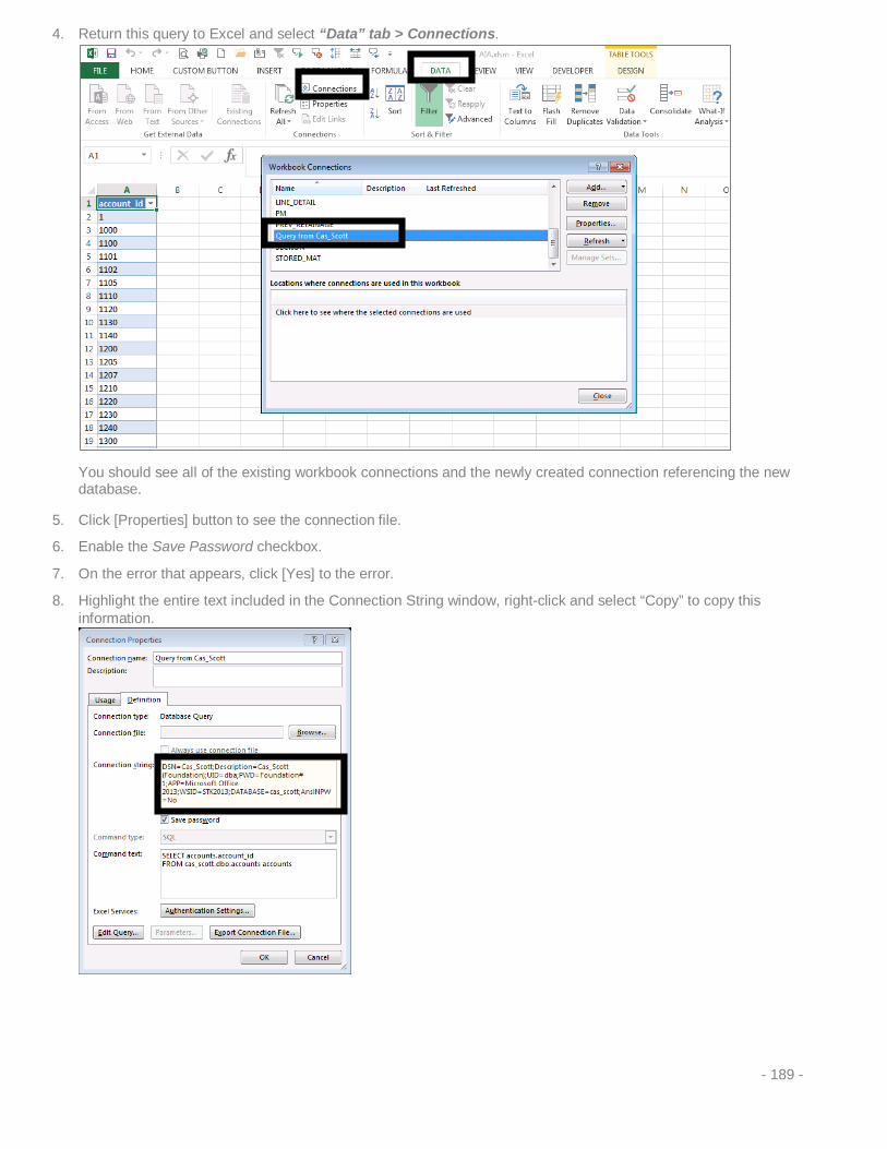
4. Return this query to Excel and select “Data” tab > Connections.
You should see all of the existing workbook connections and the newly created connection referencing the new database.
5. Click [Properties] button to see the connection file.
6. Enable the Save Password checkbox.
7. On the error that appears, click [Yes] to the error.
8. Highlight the entire text included in the Connection String window, right-click and select “Copy” to copy this information.
- 189 -

9. We now have our new connection string information on the clipboard. We have to open each one of the Workbook Connections and paste our connection string over the existing connection.
10. Connection String replaced. Do not click [OK]! We now have to edit the Command Text section.
- 190 -
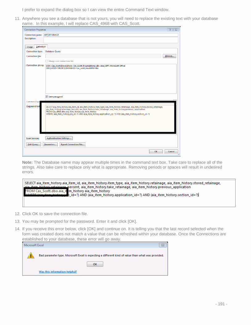
I prefer to expand the dialog box so I can view the entire Command Text window.
11. Anywhere you see a database that is not yours, you will need to replace the existing text with your database name. In this example, I will replace CAS_4968 with CAS_Scott.
Note: The Database name may appear multiple times in the command text box. Take care to replace all of the strings. Also take care to replace only what is appropriate. Removing periods or spaces will result in undesired errors.
12. Click OK to save the connection file.
13. You may be prompted for the password. Enter it and click [OK].
14. If you receive this error below, click [OK] and continue on. It is telling you that the last record selected when the form was created does not match a value that can be refreshed within your database. Once the Connections are established to your database, these error will go away.
- 191 -

Lesson 20: SUMIF statement The SUMIF statement is loosely related to the Vlookup statement. The Vlookup statement has to be used when text based fields are involved. Vlookup may be used on numeric fields, but what if we need to return more than one value from a column? Imagine we need to sum the numbers in a particular column if the criterion in an adjacent column is met.
Here is an example. In columns D and E, we have a month and an associated dollar amount for sales within that month. If we need to total the amounts from the array based on the month, we can use the Sumif statement.
The SUMIF statement is comprised of 3 items:
1. The range of data we want evaluated (Range) 2. What key we are looking for and where it is (Criteria) 3. What is the range of cells that needs to be summed up and where is it (sum_range)
- 192 -

The 3 items in the formula are broken down as follows:
Range: Define the range of cells in which you want to look for a particular value defined by the…
Criteria: The criteria in this formula is a cell reference. In some cases it can be a text or number string depending on your requirements. So far the Sumif statement is looking up and down column D for the value “JAN.” When it finds the value of JAN, it needs to SUM the values from …
SUM_RANGE: Just as the help says. The sum range is the range of cells you wish to evaluate, or sum.
- 193 -
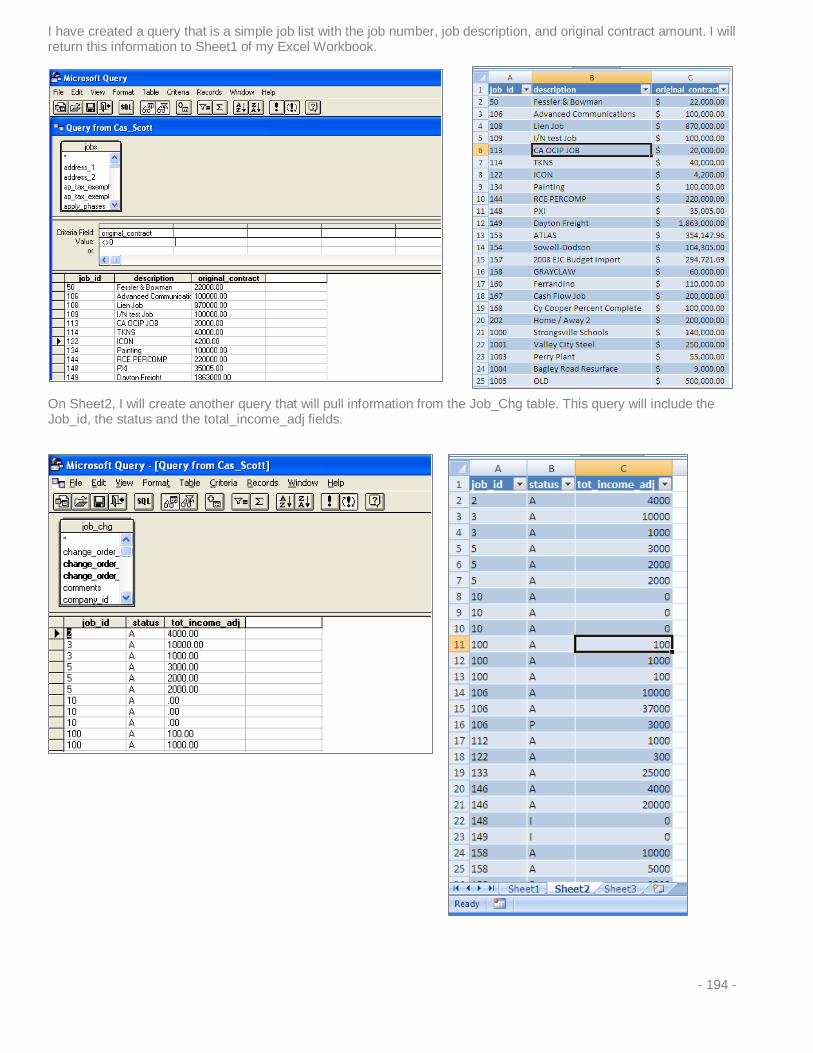
I have created a query that is a simple job list with the job number, job description, and original contract amount. I will return this information to Sheet1 of my Excel Workbook.
On Sheet2, I will create another query that will pull information from the Job_Chg table. This query will include the Job_id, the status and the total_income_adj fields.
- 194 -

Sheet1 – Job_id, description, original contract
Sheet2 – job_id, status, total_income_adj
The SUMIF equation to sum the values in Sheet2, column C, based on the values in Sheet2 column A that meet the same criteria as Sheet1 cell A2 is:
=sumif(Sheet2!A:A,Sheet1!A2,Sheet2!C:C)
If you need a moment, read the above again…and again, and again. It will eventually make sense.
The nice thing about the SUMIF equations is that there are no “wrong” results, no #N/A errors. (So we do not need to use the iferror formula to make our sheet look nice. The SUMIF formula only works with numeric values. We would not be able to use the SUMIF formula with the first example in this lesson (finding the project_manager description).
- 195 -

EXTRA – SUMIFs
Sumifs statement (available in Excel 2007 ONLY). This will allow for multiple criteria within a Sumif statement.
The =sumifs formula may be used to sum values if multiple criteria are met. (A total of 127 criteria may be defined in a sumifs statement.)
This example shows that we want to separate by Job_id and by status of A for approved, P for pending, and I for internal change orders.
• Column D: =SUMIFS(Sheet2!C:C,Sheet2!A:A,Sheet1!A4,Sheet2!B:B,"A") • Column E: =SUMIFS(Sheet2!C:C,Sheet2!A:A,Sheet1!A4,Sheet2!B:B,"P") • Column F: =SUMIFS(Sheet2!C:C,Sheet2!A:A,Sheet1!A4,Sheet2!B:B,"I")
- 196 -

Lesson 21 : Over / Under Billing Report In this session we will cover the ability to create a custom Over / Under Billing Report using the MS Query tool and Excel.
First, we will create a sheet with a complete job list. This is done because we are not sure that all jobs have all of the information contained within the O/U Report (ie: contract, estimated cost, change orders, cost and billing). We will pull this information from additional queries and link the data together in a single spreadsheet.
Job List
1. Access the Jobs table from the MS Query tool. 2. Select the following fields:
• JOB_STATUS • PROJECT_MANAGER_ID • JOB_ID • JOB_ID+’ – ‘+DESCRIPTION • CUSTOMER_ID • ORIGINAL_CONTRACT • ORIGINAL_COST
3. We will enable criteria to not include “O” (overhead jobs) based on the Job_Status field.
The Original_Contract and Original_Cost fields are the information entered on the “General” tab of the Job Record.
4. Return the Data to Excel, rename the tab “JOB” and access the second tab.
- 197 -

Customer Information
We will access the customer data from the Customers table. Remember that if all jobs do not have a customer coded to them, they would drop off of the Jobs table query if both the Jobs and Customers tables were included in a single query.
1. Select the following fields: • CUSTOMER_ID • CUSTOMER_ID+’ – ‘+NAME as CUSTOMER
2. Return the data to Excel and name this tab “CUSTOMERS.”
- 198 -

Change Orders
On the third tab, we will query change order information. This will include changes in contract amount and changes in estimated cost.
1. The table we will use is titled JOB_CHG. Select the following fields. • JOB_ID • CHANGE_ORDER_ID • TOT_INCOME_ADJ • TOT_COST_ADJ
2. We will also enable some criteria to select change orders with a status of A for approved and E for estimate only. 3. Add criteria to include Change Orders dated on or before a particular date using the date_booked field.
If you prefer, you may SUM these values. I like to keep the change orders separate, and reference the CHANGE_ORDER_ID in case I have to look up a record in question.
4. Return this data to the second tab, rename the tab “CO.”
- 199 -

Billings
On the fourth tab, we will create a sheet for the billings and cash received per job.
1. For this query, we will use the V_EM_JC_BILLINGS table. Pull the following fields from the table: • JOB_ID • AMOUNT_INVOICED • CASH_AMOUNT
2. Criteria will be added based on the ADJUST_DATE field to show billings on or before a particular date. 3. We can also SUM the total of amount_invoiced field into a single line per job.
4. Return the data to the third tab, rename the tab to “BILL.”
- 200 -
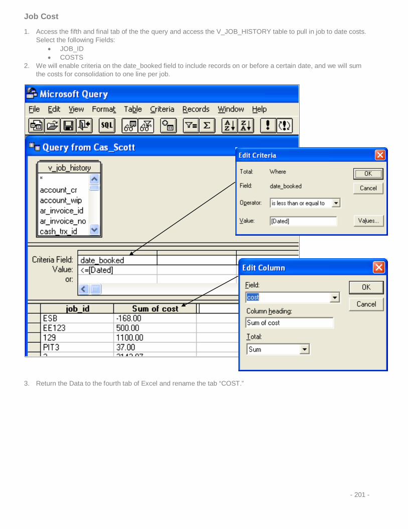
Job Cost
1. Access the fifth and final tab of the the query and access the V_JOB_HISTORY table to pull in job to date costs. Select the following Fields:
• JOB_ID • COSTS
2. We will enable criteria on the date_booked field to include records on or before a certain date, and we will sum the costs for consolidation to one line per job.
3. Return the Data to the fourth tab of Excel and rename the tab “COST.”
- 201 -
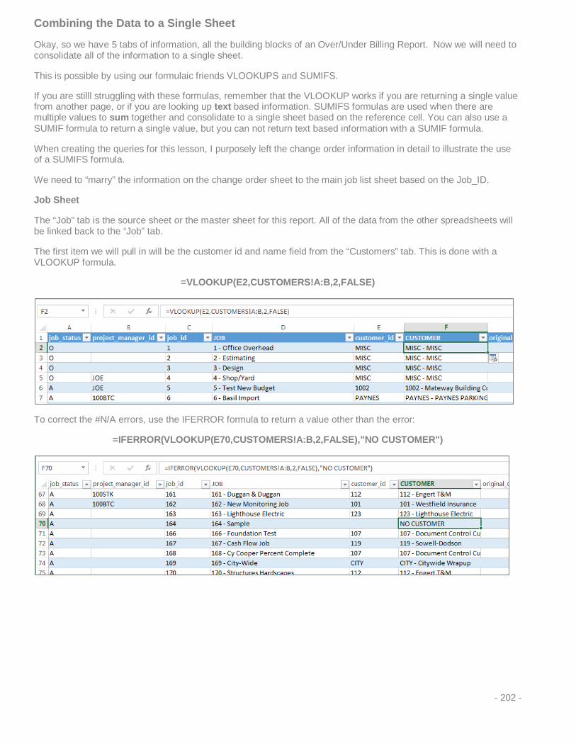
Combining the Data to a Single Sheet
Okay, so we have 5 tabs of information, all the building blocks of an Over/Under Billing Report. Now we will need to consolidate all of the information to a single sheet.
This is possible by using our formulaic friends VLOOKUPS and SUMIFS.
If you are stilll struggling with these formulas, remember that the VLOOKUP works if you are returning a single value from another page, or if you are looking up text based information. SUMIFS formulas are used when there are multiple values to sum together and consolidate to a single sheet based on the reference cell. You can also use a SUMIF formula to return a single value, but you can not return text based information with a SUMIF formula.
When creating the queries for this lesson, I purposely left the change order information in detail to illustrate the use of a SUMIFS formula.
We need to “marry” the information on the change order sheet to the main job list sheet based on the Job_ID.
Job Sheet
The “Job” tab is the source sheet or the master sheet for this report. All of the data from the other spreadsheets will be linked back to the “Job” tab.
The first item we will pull in will be the customer id and name field from the “Customers” tab. This is done with a VLOOKUP formula.
=VLOOKUP(E2,CUSTOMERS!A:B,2,FALSE)
To correct the #N/A errors, use the IFERROR formula to return a value other than the error:
=IFERROR(VLOOKUP(E70,CUSTOMERS!A:B,2,FALSE),"NO CUSTOMER")
- 202 -
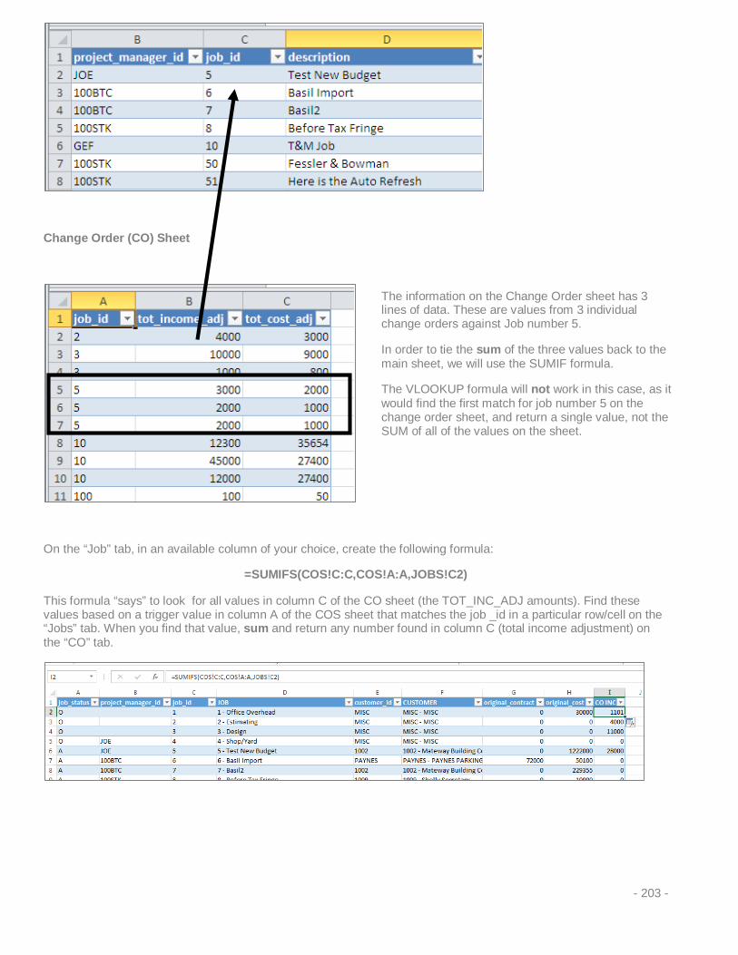
Change Order (CO) Sheet
On the “Job” tab, in an available column of your choice, create the following formula:
=SUMIFS(COS!C:C,COS!A:A,JOBS!C2)
This formula “says” to look for all values in column C of the CO sheet (the TOT_INC_ADJ amounts). Find these values based on a trigger value in column A of the COS sheet that matches the job _id in a particular row/cell on the “Jobs” tab. When you find that value, sum and return any number found in column C (total income adjustment) on the “CO” tab.
The information on the Change Order sheet has 3 lines of data. These are values from 3 individual change orders against Job number 5.
In order to tie the sum of the three values back to the main sheet, we will use the SUMIF formula.
The VLOOKUP formula will not work in this case, as it would find the first match for job number 5 on the change order sheet, and return a single value, not the SUM of all of the values on the sheet.
- 203 -

This sum represents the total income adjustments to the particular job.
Create a similar formula to sum the total cost adjustments from the change orders.
The formula is identical except for the last parameter that tells the formula to look in Column C for the values to sum.
=SUMIFS(COS!D:D,COS!A:A,JOBS!C2)
Add two more columns to the Job sheet titled Revised Contract and Revised Cost.
These are simple additions that add the original contract and the changes to contract and the original costs to the changes in cost.
- 204 -
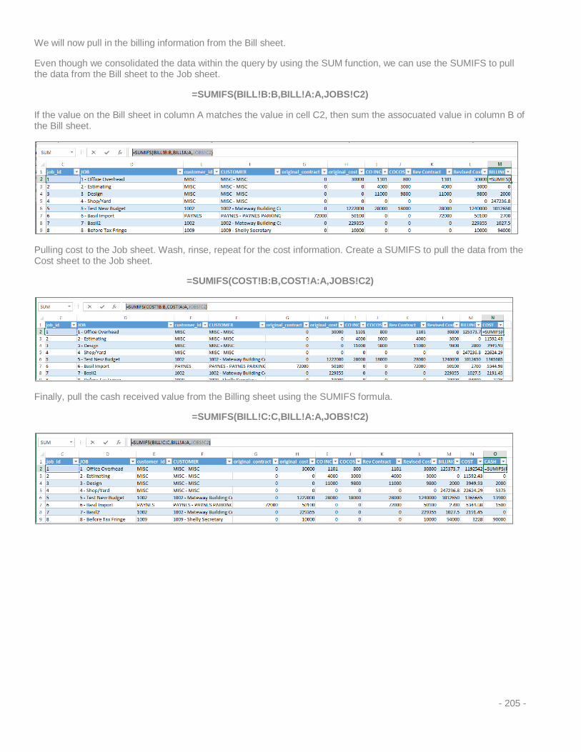
We will now pull in the billing information from the Bill sheet.
Even though we consolidated the data within the query by using the SUM function, we can use the SUMIFS to pull the data from the Bill sheet to the Job sheet.
=SUMIFS(BILL!B:B,BILL!A:A,JOBS!C2)
If the value on the Bill sheet in column A matches the value in cell C2, then sum the assocuated value in column B of the Bill sheet.
Pulling cost to the Job sheet. Wash, rinse, repeat for the cost information. Create a SUMIFS to pull the data from the Cost sheet to the Job sheet.
=SUMIFS(COST!B:B,COST!A:A,JOBS!C2)
Finally, pull the cash received value from the Billing sheet using the SUMIFS formula.
=SUMIFS(BILL!C:C,BILL!A:A,JOBS!C2)
- 205 -
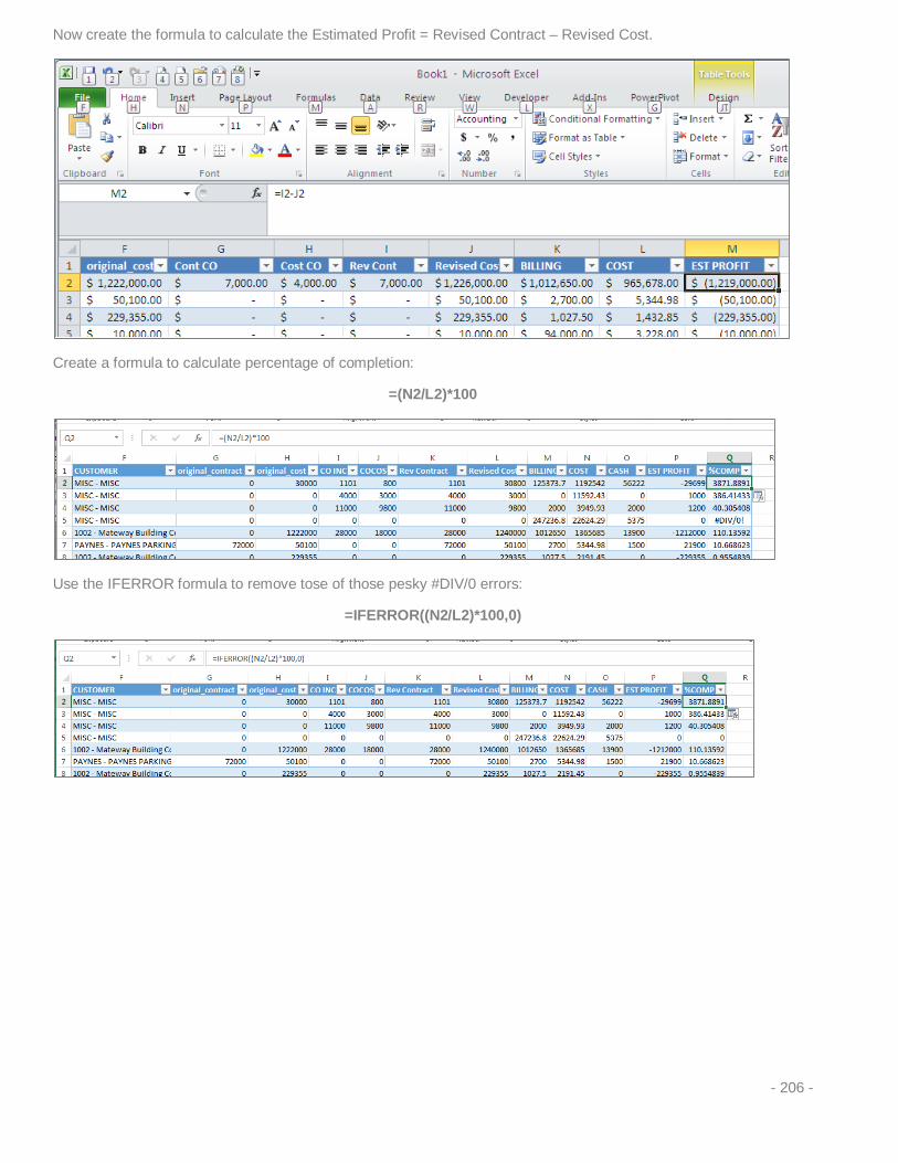
Now create the formula to calculate the Estimated Profit = Revised Contract – Revised Cost.
Create a formula to calculate percentage of completion:
=(N2/L2)*100
Use the IFERROR formula to remove tose of those pesky #DIV/0 errors:
=IFERROR((N2/L2)*100,0)
- 206 -

Next, we will calculate the Earned Revenue amount:
(Percentage of Completion * Revised Contract Amount)/100
=Q2*K2/100
Note: The earned revenue calculation shown in this example is not the “gospel.” Many companies calculate the earned revenue figure in different manner (ie: Earned Profit + Cost To Date). You may use whatever calculation you choose when creating these reports.
Calculation for over billing:
If Billing to Date – Earned Revenue > 0, Billing to Date – Earned Revenue otherwise 0.
=IF(M2-R2>0,M2-R2,0)
This formula states that if you have billed more than the earned revenue amount, you are overbilled by the amount of the billing less the earned revenue amount. If you are not overbilled, then show a $0.00 value in the column.
Calculation for under billing:
This caclulation computes if you have billed less than the earned revenue figure. If Earned Revenue – Billing to Date > 0, Earned Revenue to Date – Billing to Date otherwise 0.
=IF(R2-M2>0,R2-M2,0)
- 207 -

We now have all the components to create the over/under billing report.
We needed to include the % of completion caclulation within our database table, but we will have to rewrite the equation in the Pivot Table, as we do not want the % of completion amounts to add up, we would like to see an overall percentage of completion amount for all of the jobs on the report.
We will insert a pivot table based on the data collected within the new table on the “Job” tab. The pivot table will be created on a new spreadsheet. Access the “Insert” tab on the toolbar and select “Pivot Table.”
Format the pivot table with your desired criteria.
Note: Do not include percentage of completion from the data source as one of the value fields. We will create a calculated field later.
Drag and drop fields into the rows and values section of the designer.
- 208 -

Right-click a cell within the pivot table and select “Pivot Table Options.” On the “Display” tab, enable the Classic Pivot Table layout checkbox.
When creating a Pivot Table, the VALUES headings default to “Sum Of FIELD NAME” (assuming your source data is formatted as a number).
To change the VALUES column headings to a more appropriate name, double click on a VALUES column.
If you simply delete the “Sum Of” from the Custom Name, you will be greeted with an error.
- 209 -
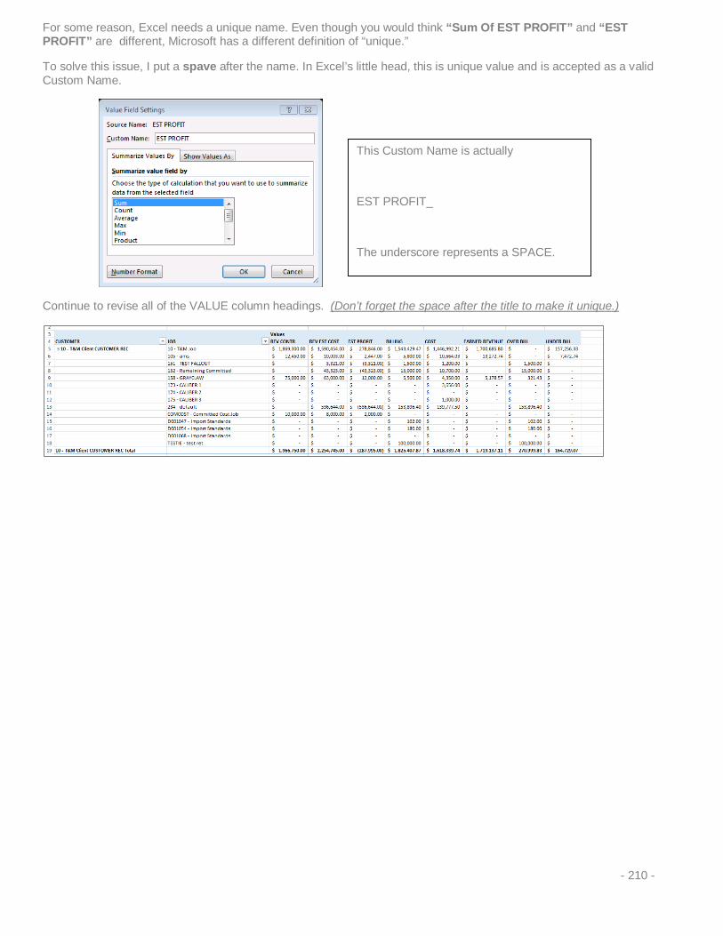
For some reason, Excel needs a unique name. Even though you would think “Sum Of EST PROFIT” and “EST PROFIT” are different, Microsoft has a different definition of “unique.”
To solve this issue, I put a spave after the name. In Excel’s little head, this is unique value and is accepted as a valid Custom Name.
Continue to revise all of the VALUE column headings. (Don’t forget the space after the title to make it unique.)
This Custom Name is actually
EST PROFIT_
The underscore represents a SPACE.
- 210 -

Creating a Custom Calculation Within the Pivot Table
1. On the “Pivot Table Tools / Analyze” tab, choose Fields, Items & Sets > Calculated Field.
2. Percent Complete: =IF('Revised Cost'=0,0,(COST/'Revised Cost')*100), the IF statement is written to
removepotential #DIV/O errors when there are no estimated costs.
3. Click [OK] to save the formula to save and place the new calculation in the desired column within the pivot table
report.
- 211 -

4. Double click the column header for the % Comp and change the Custom Name and Number Format.
I prefer the “Accounting” format, as it shows zero values a a dash instead of a zero. The options are available to show the data how you choose.
- 212 -

If you use the “Percentage” option in the Number Format, you will have to change the Calculated Field and remove the *100 from the equation.
5. From the top ribbon, select Pivot Table Tools > Analyze > Fields, Items & Sets > Calculated Field.
6. Use the dropdown menu to select the Calculated Field.
7. Edit the formula and click [OK] to save. You may now use the percentage number format.
8. You may quickly change the criteria for the Over/Under Billing report via the column headings:
Add the PM in the Filters area of the Pivot Table. Here is an example of the O/U Billing Report for a different Project Manager.
Note: We pulled in data from the Jobs table that included job_status and project_manager_ID. You may wish to sort this by Project Class, Geographic Area, even the Payroll Local Tax field. Remember to plan the report first, and add these fields when creating the first “Job List” tab in this lesson.
You may also sort and filter this report using user defined ields. With this option, the sorting and filtering possibilies are endless.
- 213 -
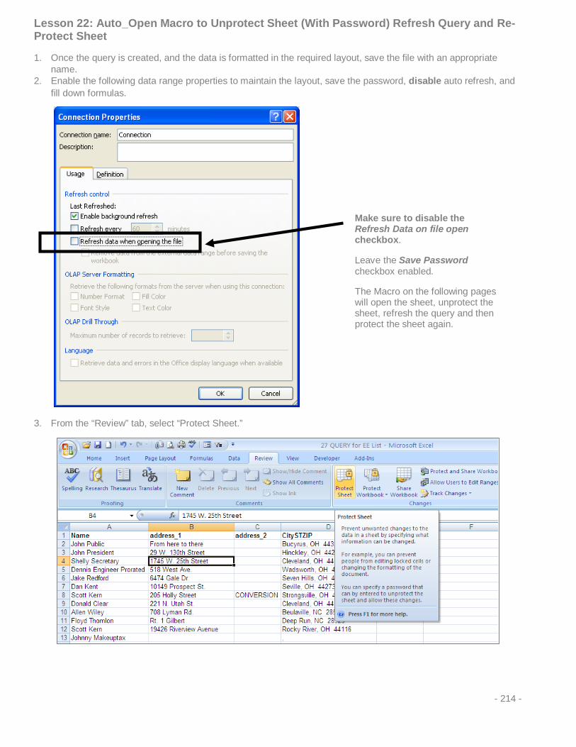
Lesson 22: Auto_Open Macro to Unprotect Sheet (With Password) Refresh Query and Re-Protect Sheet
1. Once the query is created, and the data is formatted in the required layout, save the file with an appropriate name.
2. Enable the following data range properties to maintain the layout, save the password, disable auto refresh, and fill down formulas.
3. From the “Review” tab, select “Protect Sheet.”
Make sure to disable the Refresh Data on file open checkbox.
Leave the Save Password checkbox enabled.
The Macro on the following pages will open the sheet, unprotect the sheet, refresh the query and then protect the sheet again.
- 214 -
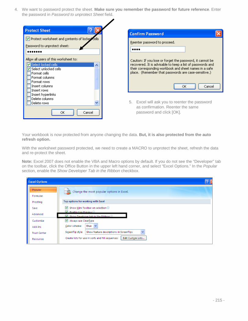
4. We want to password protect the sheet. Make sure you remember the password for future reference. Enter the password in Password to unprotect Sheet field.
Your workbook is now protected from anyone changing the data. But, it is also protected from the auto refresh option.
With the worksheet password protected, we need to create a MACRO to unprotect the sheet, refresh the data and re-protect the sheet.
Note: Excel 2007 does not enable the VBA and Macro options by default. If you do not see the “Developer” tab on the toolbar, click the Office Button in the upper left hand corner, and select “Excel Options.” In the Popular section, enable the Show Developer Tab in the Ribbon checkbox.
5. Excel will ask you to reenter the password as confirmation. Reenter the same password and click [OK].
- 215 -

You will also have to enable the Macros in Excel 2007.
1. In Excel Options, in the Trust Center group on the left, select Trust Center Settings > Macro Settings > Enable all macros.
2. From the “Developer” tab, click Visual Basic Editor.
- 216 -

3. Make sure the VBAProject (“workbookname”) – Microsoft Excel Objects – Sheet1 (Sheet1) is highlighted.
VBAProject (WORKBOOK NAME): This is the name of the workbook you are working in. In this example, the file is named: 01 Employee Phone List auto protect. If you have not saved the file, it will be titled “Book1.”
Sheet1 (Sheet1): The name of the worksheet you are on. If the name has been changed on the worksheet tab, the change will be reflected here.
4. Right-click on the Microsoft Excel Objects and select Insert > Module.
- 217 -

5. Double click on “Module 1.”
Here is the text for the Macro
Sub Auto_open()
'
Worksheets("sheet1").Unprotect Password:="1234"
Selection.ListObject.QueryTable.Refresh BackgroundQuery:=False
Worksheets("Sheet1").Protect Password:="1234"
End Sub
6. Enter this text into your VBA editor.
7. Replace “Sheet1” with the name of the worksheet that the query data resides in.
8. Replace “1234” with the password needed to unprotect and protect the worksheet.
Note: The double quotes are required around the sheet name and the password.
- 218 -

Your VBA Project should now look like the example below:
9. Click the “Save” icon in the upper left hand corner, and close out of the Visual Basic Editor.
- 219 -

If you try to modify any of the cells in the worksheet, you will receive the following error:
You will also notice that the RERESH ICON is not available.
Save the file and then re-open the file. When you re-open the file, the Macro will auto-run: unprotect the worksheet, refresh the query and protect the worksheet again.
We Now Need to Protect the Macro from Editing
1. Access “Macros” from the “Developer” tab
- 220 -
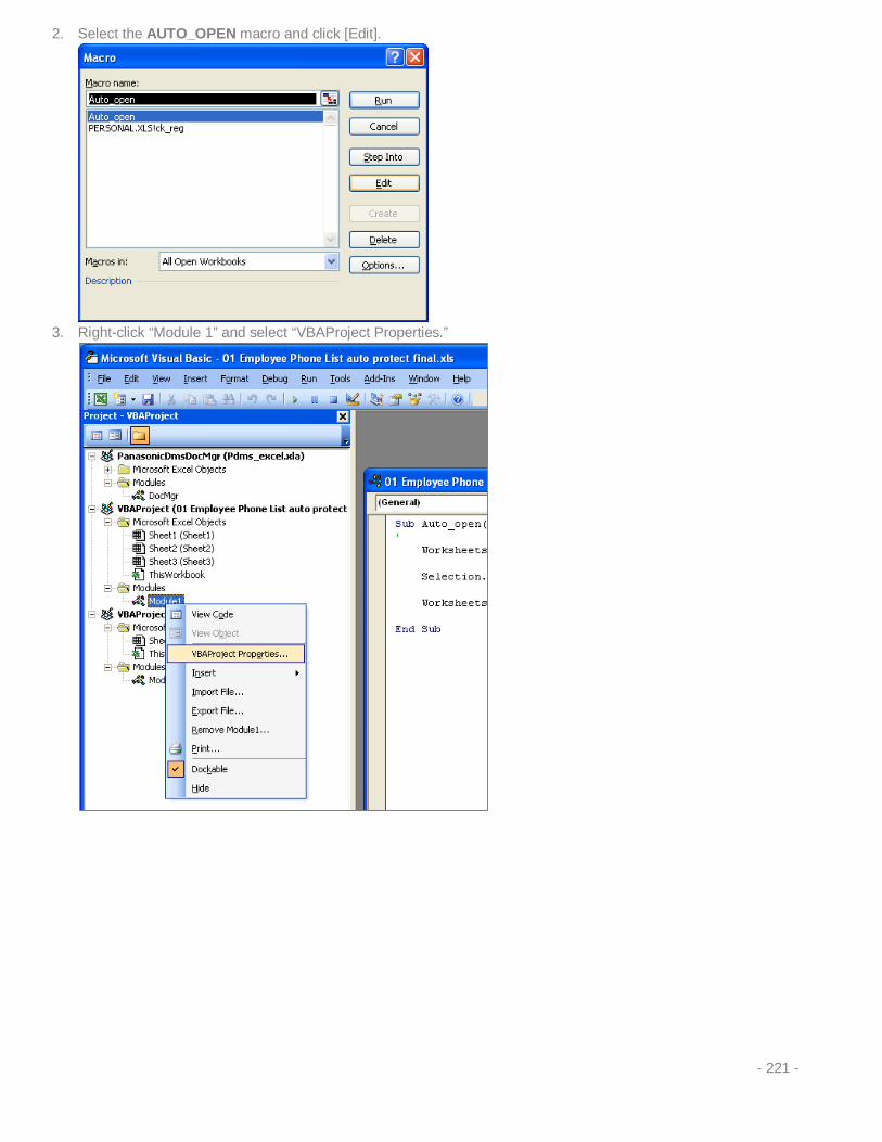
2. Select the AUTO_OPEN macro and click [Edit].
3. Right-click “Module 1” and select “VBAProject Properties.”
- 221 -

4. Select the “Protection” tab, enable the Lock project for viewing checkbox, and enter the password to protect the Macro.
5. Click [OK], save the VBA project, and close out of the VBA Editor.
6. Save the Excel file and close.
7. The Macro runs every time you open the file. If you try to access the Macro through Tools > Macro > Macros, you will notice that there is no option to edit the macro.
We have now successfully locked out the ability to edit the Macro, and we have disabled the ability to edit the query. If you RUN the macro from here, it will unprotect the sheet, refresh the data and re-protect the sheet.
- 222 -
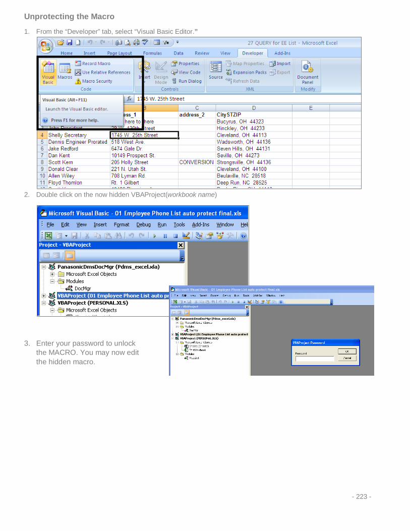
Unprotecting the Macro
1. From the “Developer” tab, select “Visual Basic Editor.”
2. Double click on the now hidden VBAProject(workbook name)
3. Enter your password to unlock the MACRO. You may now edit the hidden macro.
- 223 -
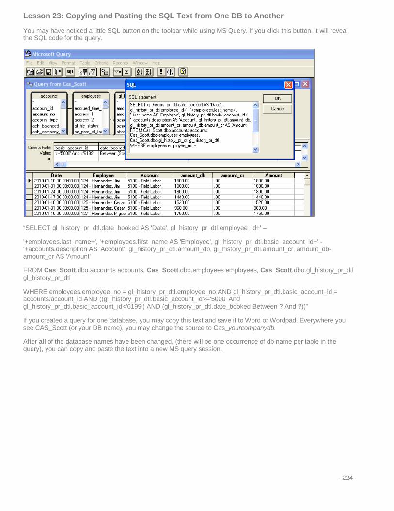
Lesson 23: Copying and Pasting the SQL Text from One DB to Another
You may have noticed a little SQL button on the toolbar while using MS Query. If you click this button, it will reveal the SQL code for the query.
“SELECT gl_history_pr_dtl.date_booked AS 'Date', gl_history_pr_dtl.employee_id+' –
'+employees.last_name+', '+employees.first_name AS 'Employee', gl_history_pr_dtl.basic_account_id+' - '+accounts.description AS 'Account', gl_history_pr_dtl.amount_db, gl_history_pr_dtl.amount_cr, amount_db-amount_cr AS 'Amount'
FROM Cas_Scott.dbo.accounts accounts, Cas_Scott.dbo.employees employees, Cas_Scott.dbo.gl_history_pr_dtl gl_history_pr_dtl
WHERE employees.employee_no = gl_history_pr_dtl.employee_no AND gl_history_pr_dtl.basic_account_id = accounts.account_id AND ((gl_history_pr_dtl.basic_account_id>='5000' And gl_history_pr_dtl.basic_account_id<'6199') AND (gl_history_pr_dtl.date_booked Between ? And ?))”
If you created a query for one database, you may copy this text and save it to Word or Wordpad. Everywhere you see CAS_Scott (or your DB name), you may change the source to Cas_yourcompanydb.
After all of the database names have been changed, (there will be one occurrence of db name per table in the query), you can copy and paste the text into a new MS query session.
- 224 -

1. Open a new Excel Workbook. 2. When the Select Database option comes up, select the new database name you wish to query and click [OK].
3. When the Add Tables window opens, click [Close] without selecting any tables.
4. Click the SQL button on the toolbar. In the SQL Statement window, right-click and paste the text from the SQL
statement with the correct database name.
- 225 -

Lesson 24: EXCEPTIONS and ERRORS When Using Date Range and SUM Criteria in MS Query
From time-to-time, you will run into a very frustrating series of events that will seemingly render your query inoperable. Let’s look at an example below.
This is a simple query built with the Jobs table and the Job_History table.
1. Add criteria to pull data between a certain date range. I have also added criteria to show data from
Cost_class_id = ‘1’.
- 226 -

So far – no problems.
2. If you want to sum a column within the query after you have added a date range parameter and any other parameter, you may run into problems.
3. When you click [OK], the following error may appear.
- 227 -

Frustration ensues, and depending on how you answer the next couple of questions, you may lose the entire query right before your eyes.
To get through the error, do the following:
4. Click OK on this message.
5. Enter a valid start date and click [OK].
6. Enter a valid end date and click [OK].
7. The Edit Column prompt will still be on screen. Click [Cancel] on this prompt, as the SUM function is what is causing this error.
- 228 -

How to solve this issue:
It all boils down to how the SQL text is created as the query is generated.
Here is the SQL script before it is SUMMED.
1. In order to solve this problem, remove the date_booked parameter and apply the SUM function to the desired
columns.
- 229 -
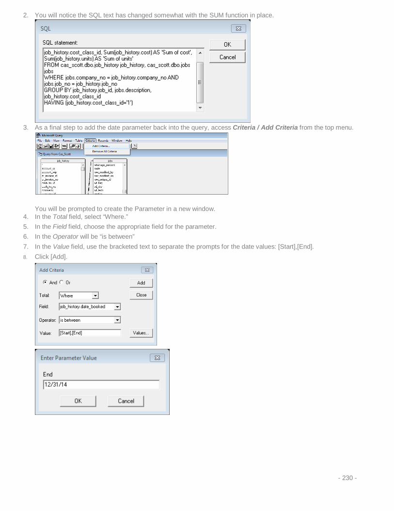
2. You will notice the SQL text has changed somewhat with the SUM function in place.
3. As a final step to add the date parameter back into the query, access Criteria / Add Criteria from the top menu.
You will be prompted to create the Parameter in a new window.
4. In the Total field, select “Where.” 5. In the Field field, choose the appropriate field for the parameter. 6. In the Operator will be “is between” 7. In the Value field, use the bracketed text to separate the prompts for the date values: [Start],[End]. 8. Click [Add].
- 230 -
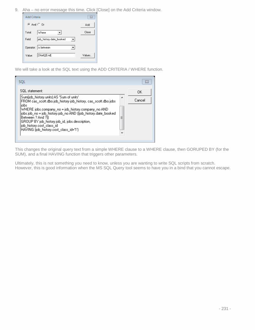
9. Aha – no error message this time. Click [Close] on the Add Criteria window.
We will take a look at the SQL text using the ADD CRITERIA / WHERE function.
This changes the original query text from a simple WHERE clause to a WHERE clause, then GORUPED BY (for the SUM), and a final HAVING function that triggers other parameters.
Ultimately, this is not something you need to know, unless you are wanting to write SQL scripts from scratch. However, this is good information when the MS SQL Query tool seems to have you in a bind that you cannot escape.
- 231 -
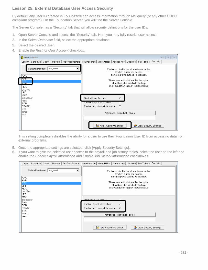
Lesson 25: External Database User Access Security
By default, any user ID created in FOUNDATION can access information through MS query (or any other ODBC compliant program). On the Foundation Server, you will find the Server Console.
The Server Console has a “Security” tab that will allow security definitions for the user IDs.
1. Open Server Console and access the “Security” tab. Here you may fully restrict user access. 2. In the Select Database field, select the appropriate database. 3. Select the desired User. 4. Enable the Restrict User Account checkbox.
This setting completely disables the ability for a user to use their Foundation User ID from accessing data from external programs.
5. Once the appropriate settings are selected, click [Apply Security Settings]. 6. If you want to give the selected user access to the payroll and job history tables, select the user on the left and
enable the Enable Payroll Information and Enable Job History Information checkboxes.
- 232 -

The [Advanced – Individual Tables] button allows you to define specific tables that the user will have access to.
In most cases, this is a nice option to give users access to individual tables.
• Vendors • Customers • Jobs • Equipment Items • Inventory Items
This user would have access to the vendors table only.
The ability to restrict access to tables allows users to query individual items and create custom lists without accessing sensitive history information in other modules.
Use this feature for granting access for creating labels and simple lists in the MS query tool.
- 233 -


17999 Foltz Industrial Parkway, Strongsville, OH 44149www.foundationsoft.com | (800) 246-0800 | [email protected]
©2015 Foundation Software, Inc. FOUNDATION® is a registered trademark of Foundation Software, Inc.Windows® is a registered trademark of Microsoft Corporation in the United States and other countries.
THANKS FOR ATTENDING!