Ordering Pareto-Optima ThroughMajority Voting¤

Herv¶e Crµes

HEC School of Management

Mich Tvede

University of Copenhagen

Abstract

A commodity is shared between some individuals: There is an initial alloca-tion; some selection procedures are used to choose an alternative allocation

and; individuals decide between keeping the initial allocation or shifting to thealternative allocation. The selection procedures are supposed to involve an el-

ement of randomness in order to re°ect uncertainty about economic, socialand political processes. It is shown that for every allocation, ¸, there exists a

number, ³(¸) 2 [0; 1], such that, if the number of individuals tends to in¯nity,then the probability that a proportion of the population smaller (resp. larger)

than ³(¸) prefers an allocation chosen by the selection procedure converges to1 (resp. 0). The index ³(¸) yields a complete order in the set of Pareto op-

timal allocations. Illustrations and interpretations of the selection proceduresare provided.

Keywords: Pareto-optimal allocations, Infra-majority voting.

JEL-classi¯cation: D31, D72.

Correspondence: Herv¶e Crµes, HEC School of Management, D¶epartement Finance etEconomie, 78 351, Jouy-en-Josas, France. Tel: 33 1 39 67 94 12; fax: 33 1 39 67 70 85.

Email: cres@hec.fr.

¤We are grateful to Edi Karni and Herv¶e Moulin for valuable discussions and helpful comments.

1

1 Introduction

The present paper investigates the general question of whether social choice rules, es-pecially voting rules, can be used to distinguish and even better rank Pareto-optimal

allocations. The present framework is too simple to yield a general answer to this ques-tion. Nevertheless it provides a partial positive answer. For the sake of clarity, and in

order to ¯x ideas it might be helpful to give a short introduction to the framework as wellas the main results of the present paper before entering into its motivation.

A family of simple models is considered: The set of divisions of one unit of a commoditybetweenm individuals. A division of the commodity is thus a vector ¸ withm nonnegative

coordinates that sum up to one, i.e. it is a point in the (m-1){simplex and it is called anallocation throughout the paper. Individuals are assumed to care only about their own

share of the commodity so obviously all allocations are Pareto-optimal.Fix the number of individuals, m, an allocation, ¸, and an integer, n, n 2 f1; : : : ;mg.

The main aim of the paper is to compute the \number" of other allocations, ¸0, thatare such that at least n individuals are better o® with ¸0 than with ¸. Since we have

a continuum of allocations, the natural way to count this \number" of allocations is tocompute their volume or Lebesgue measure. Clearly this volume is 1 for n = 1 and 0 for

n = m because all allocations are Pareto optimal. The main result is the following: Thereexists a number, ³(¸) 2 [0; 1], such that these volumes converge to 1 for n=m < ³(¸) and

to 0 for n=m > ³(¸) as the number of individuals tends to in¯nity. As an example, for theegalitarian allocation, ¸ = (1=m; : : : ; 1=m), the threshold value converges to e¡1 ¼ 0:37

as the number of individuals tends to in¯nity1. Of course the number, ³(¸), dependson how volumes of allocations are measured as well as the allocation therefore a family

of measures, all related to the Lebesgue measure, are considered. For every measure inthis family a simple model is obtained and the same threshold phenomenon as for the

Lebesgue measure is observed.The occurence of this threshold e®ect as the number of individuals tends to in¯nity

constitutes the main result of the paper. It is derived quite \mechanically" from compu-tations in the sense that it is based on a purely parametric approach, where the Lebesgue

measure in accordance with Laplace's advice is taken as the most neutral and naturalmeasure. It should be noted that the case of a ¯nite (but large) number of individuals

1Volume of the set of allocations that are better than the egalitarian allocation for a proportion largerthan ½ of the population: For ½ = 0:5, it is 2 ¢10¡5 for m = 100 and 2 ¢10¡9 for m = 200 and; for ½ = 0:4,it is 0:08 for m = 100 and 0:03 for m = 200.

2

is of course the most interesting case; actually, going to the limit with a continuum ofindividuals, where the threshold is clear-cut, is a mean to extract information for the

¯nite case. Therefore the paper also contains results about the strength of the thresholde®ect for the ¯nite case.

The motivation for this parametric approach and the computation of those volumes isclear: Starting from an allocation, ¸, it is obviously very easy to ¯nd another allocation,

¸0, that makes all individuals but one better o®: We just have to take the share of oneindividual and split it between the others. Thus, if most social choice rules behave as

Maxwell's devil and select alternative allocations that are exactly in this almost zero-measure set where all individuals but one are better o® then the parametric approach

followed in the present paper would be gratuitous and the main result would be a merecuriosity. However there are many upstream economic, social and political reasons why

this is not the case. Indeed, uncertainty about characteristics, outcomes of social as wellas political processes may be major reasons why Maxwell's devil is less relevant.

Even though it is beyond the primary concern of the present paper some attempts tojustify the parametric approach by yielding microeconomic illustrations of why Maxwell's

devil is less relevant and macroeconomic interpretations of the parametric approach's con-sequences are made. Of course our aim is to argue against Maxwell's devil-like arguments

and, more boldly, to advocate for the interest of interpreting the Lebesgue measure as aprobability distribution over the set of allocations as representing how alternative allo-

cations are selected. The ¯rst two illustrations are very simple non-coorperative gameswhere m individuals have to share one unit of a commodity. The ¯rst game being a one-

shot game and the second game being bargaining a la Rubinstein. The last illustrationis a pure exchange economy with consumption externalities involving two consumers and

one good.It is an implicit conjecture in the present paper that numerous upstream mechanisms

to divide a commodity generate (and can be identi¯ed with) probability distributions overthe (m-1){simplex of allocations2 as soon as they involve an element of randomness whichis a fair assumption in case of uncertainty about characteristics, outcomes of social as well

as political processes. We conjecture that the nature of the result (the threshold e®ect)will appear very often in large populations. The paper focuses on a family of special

distributions but ongoing research seeks to qualify \often".2The induced distribution might be degenerate: A way to share a commodity could be to pull out knifes

and give it to the surviving guy; the distribution is concentrated on the vertices of the (m-1){simplex,1=m chance for everybody provided that there are no strong (wo)men.

3

Indeed, natural and easy interpretations of these distributions are given in termsof wealth distributions by use of a simple urn model that dates back to Polya and

Eggenberger3. So the interest of the Lebesgue measure goes beyond the brutal para-metric approach with the belief that Maxwell's devil does not strike too often.

The paper is organized as follows. Section 2 introduces the framework. Section 3illustrates the choice of the Lebesgue measure as a selection mechanism. In Section 4 the

main results are stated; it mainly contains the de¯nition of the index ³ and the study ofits asymptotic properties. The family of selection mechanisms at scope in the paper are

given an interpretation in Section 5. Finally section 6 o®ers interpretations of the resultstogether with some concluding comments. All proofs are gathered in the appendix, which

starts with a section on urn models, with emphasize on the notion of occupancy. Indeed,urn models turn out to be very helpful for the computation of the various probabilities,

on which the proposed ranking of allocations is based.

2 The framework

Some commodity is allocated betweenm individuals and the preferences of each individual

depends on his share only. Allocations are represented by points in the (m-1){simplex

Sm¡1 =(¸ = (¸1; : : : ; ¸m) 2 Rm+ j

mX

i=1¸i = 1

);

where the i'th coordinate is the share of the i'th individual. Clearly, indi®erence sets forthe i'th individual are linear manifolds indexed by the i'th coordinate.4

Generally, as argued in the introduction, uncertainty about characteristics, outcomesof social as well as economic processes introduces an element of randomness in the selection

of allocations - some illustrations are provided in the next section. Therefore selectionprocedures are identi¯ed with probability measures over the set of allocations, Sm¡1. In

the present paper, the Lebesgue measure { called indi®erently the uniform distribution {is studied so that computing probabilities merely reduces to computing volumes. But in

order to study di®erent selection procedures, the uniform distribution is considered over3The literature on preference formation in a voting population facing a set of candidates has made

extensive use of these Polya-Eggenberger urn models, see Berg (1985) and Berg & Gehrlein (1992).4In Karni & Safra (1995) a similar framework is considered, but the commodity is supposed to be

indivisible and points in the (m-1){simplex are probability distributions, where the i'th coordinate is theprobability that the i'th individual gets the commodity. However Karni & Safra is concerned with theexistence of social welfare functions, while the present paper is concerned with allocative stability.

4

the set of all possible divisions of the commodity into cm pieces (with c 2 N), so that allindividuals get c pieces. For di®erent values of c, the uniform distribution over the set of

divisions of the commodity into cm pieces induces di®erent probability distributions overthe set of allocations. Indeed, divisions induce allocations as described hereafter.

For a ¯xed c, divisions are represented by points in the (cm-1){simplex

Scm¡1 =

8<:Ã = (Ã1; : : : ; Ãcm) 2 Rcm+ j

cmX

j=1Ãj = 1

9=; ;

where the j'th coordinate is the size of the j'th piece, and the (cm-1){simplex is endowedwith the Lebesgue measure. Given a division of the commodity, the share of an individual

consists of c pieces with subsequent index, thus the share of the i'th individual is

¸i =ciX

j=c(i¡1)+1

Ãj :

Clearly, indi®erence sets for the i'th individual in the (cm-1){simplex are linear manifolds

which are indexed by the sum of the individual's pieces. A probability measure over theset of allocations is induced by the Lebesgue measure over the set of divisions and the

\projection" of the (cm-1){simplex on the (m-1){simplex, ¼ : Scm¡1 ! Sm¡1, de¯ned by

¼(Ã1; : : : ; Ãcm) =

0@cX

j=1Ãj ; : : : ;

cmX

j=(c¡1)m+1

Ãj

1A :

The density of the induced probability measure on Sm¡1 can easily be computed.

Lemma 1 The Lebesgue measure on Scm¡1 induces a probability measure on Sm¡1 with

density

pc(¸) =(cm¡ 1)![(c¡ 1)!]m

mY

i=1¸c¡1i :

Remark Consider the egalitarian allocation, ¸ = (1=m; : : : ; 1=m) and another allocation¸0 6= ¸. Then

limc!1

pc(¸0)pc(¸)

= 0:

Therefore, the induced probability measure on Sm¡1 converges to the Dirac measure with

support on the egalitarian allocation as c tends to in¯nity { the notion of convergence leftunde¯ned. This can be caught intuitively by remembering that c is the number of pieces

that every individual gets and that the more pieces individuals get the more are sharesaveraged.

5

3 Illustration of the Lebesgue measure

3.1 Example of a simple game

A population ofm individuals want to share one unit of a commodity: A cake, represented

by the uniform unit disk. The individuals might simply decide to share the cake evenly.There are a lot of more or less complicated mechanisms proposed in the literature. This

section introduces one that is quite simple and moreover can result in any member of thefamily of distributions with densities (pc)c2N.

The basic game: The m individuals choose simultaneously a point on the unit circle;µ 2 [0; 2¼]. Thus m points are chosen: (µi)mi=1. There exists a permutation of the agents,

¾, such that0 · µ¾(1) · µ¾(2) · : : : · µ¾(m) · 2 ¼:

The share of agent i is the slice of the cake contained between the radii de¯ned by his

chosen point µi and the ¯rst one encountered counterclock-wise: suppose i = ¾(k), it isthe portion (µ¾(k); µ¾(k+1)), with the convention that ¾(m+ 1) = ¾(1). For this game it is

a Nash equilibrium in mixed strategies that all individuals choose their points on the unitcircle according to the uniform distribution. It is shown that the induced distribution

over the (m-1){simplex of shares is the uniform distribution.

Proposition 1 If all individuals choose their points on the unit circle according to theuniform distribution over the interval [0; 2¼], then the game induces the uniform distribu-

tion over the (m-1){simplex of allocations.

Proof Follows from Tovey (1997). Q.E.D.

Corollary 1 Suppose that ¯rst individuals divide the commodity into c small pieces of

equal size (each of them represented as a uniform unit disk) second they share every pieceby playing the described game. Then for the Nash equilibrium in mixed strategies where

all individuals choose their points on the unit circle according to the uniform distributionthe induced distribution over the (m-1){simplex of shares has density pc.

3.2 Example of a less simple game

As in the previous game a population of m individuals want to share one unit of a

commodity. There is an initial allocation and individuals can decide by voting whetherthey keep their initial shares or they enter into bargaining a la Rubinstein in order to

6

select another allocation. However as explained in Osborne & Rubinstein (1990) and vanDamme (1991) all allocations can be supported as subgame perfect equilibria provided

that there are more than two individuals, m ¸ 3. Thus the outcome of bargaining ischaracterized by indeterminacy, so unless individuals coordinate their strategies it is far

from obvious how individuals should play.Individuals can coordinate their strategies through some extrinsic random variable

such that all individuals observe this variable and coordinate their strategies on it. Indeedsuppose that all individuals believe that the choices of strategies of all other individuals

depend on a random variable on the (m-1){simplex such that if the random variabletakes the value ¸ then they play strategies that make the allocation ¸ a subgame perfect

equilibrium. Then all individuals play strategies that make the allocation ¸ a subgameperfect allocation. All distributions of the random variable seem to be equally reasonable,

in particular the family of distributions with densities (pc)c2N is just as reasonable as allother distributions. Perhaps the uniform distribution is a natural prior, because if all

allocations are equally reasonable then the uniform distribution over the set of allocationsseems to be a neutral belief.

In order to complete the description of the game suppose that the random variableis drawn from a distribution with density pc for c 2 N and that ¯rst the value of the

random variable is revealed and second individuals vote about keeping their initial sharesor entering into bargaining. For this game the main result of the present paper is that for

any initial allocation, ¸, there exists a number, ³c(¸) 2 [0; 1], such that the probabilitythat there is a n=m proportion that prefers an allocation selected according to the extrinsic

random variable converges to 1 for n=m < ³c(¸) and to 0 for n=m > ³c(¸) as m tends toin¯nity.

It should be remarked that the coordination of individuals' strategies by some extrinsicrandom variable implies that sunspots matter, see Cass & Shell (1983) and Shell (1987).

However in games with indeterminacy it seems quite natural that players coordinate theirstrategies { at least to some degree { and they can only coordinate on an extrinsic randomvariable.

3.3 Example of a market mechanism

A general model of consumption externalities was introduced in Arrow (1969) and ex-

tensively studied in Crµes (1996). Consider an economy with 1 commodity and 2 con-sumers where agents in°ict negative consumption externalities to each other. Let x1

7

(resp. x2) denote the consumption of consumer 1 (resp. consumer 2). Consumer 1's, re-spectively consumer 2's, utility function is given by U1(x1; x2) = log x1 ¡ x2, respectivelyU2(x1; x2) = log x2 ¡ x1. Externalities are individualized as in Arrow (1969) throughmarkets: There are, beside the usual market for the proper commodity, also markets

for externalities. Consumers face individualized prices on all markets, behave as price-takers and express demands for both their proper and external consumptions. Prices clear

markets.Both consumers are endowed with 1 unit of the commodity. Moreover, beside these

endowments in physical consumption good, legal entitlements are distributed to the con-sumers that represent, in a Coasian world, the initial juridical situation from where they

can trade on external e®ects; this legal entitlement, denoted ! is the same for bothconsumers, to respect the symmetry between them. In this example, we consider the

parametric family of economies where ! is taken, to ¯x idea, in [¡1; 1]. No value of! sounds more \reasonable" or probable than another. So that assuming the Lebesgue

measure on this parametric family seems a fair assumption.The system of equilibrium equations of this market economy is equivalent to the system

of equilibrium equations derived from the usual planner's program, with the addition ofconsumer 1's budget constraint. Consumer 1's consumption x1 can be expressed as a

function of its welfare weight t 2 [0; 1]:

x1(t) =1

2(1 ¡ 2t)

³3 ¡ 4t¡

p32t2 ¡ 32t+ 9

´

and of course x2(t) = x1(1 ¡ t) = 2 ¡ x1(t). Both x1(t) and U1(x1(t); x2(t)) are increas-ing function of t. For any value of the legal entitlement !, there exists a symmetric

equilibrium where the consumers are treated equally by the market; it is described by:x1 = x2 = 1, t = 1=2. But if ! 2 [¡1;¡0:5] (this corresponds to the case where the legal

authority wants to compensate for the negative externality through the legal entitlement),there exists also a pair of asymmetric equilibria. Thus we know that for ! 2 [¡1;¡0:5],

there exists a corresponding value t(!) 6= 1=2 and x1 6= x2; the equilibrium allocationsare (x1(t(!)); x2(t(!))) and (x1(1 ¡ t(!)); x2(1 ¡ t(!))). It is easy to compute, for an

asymmetric welfare weight t 6= 1=2, the reciprocal function !(t):

!(t) =1

1 ¡ 2t

Ã1 ¡ 2t+ tx1(t) ¡ t

x1(t)

!:

Plotting this function yields the following curve: The curve being almosty linear, the uni-form distribution over the set of parameters ! 2 [¡1; 1] generates a distribution over the

8

t

!

Welfare Weight at Equilibrium

¡1

¡0:5

0:5-

6

1{simplex of welfare weights a distribution which is close to be uniform. Either there are

no asymmetric equilibria (! 2 [¡0:5; 1]) or there are, and then they are evenly distributedin the 1{simplex of welfare weights. Suppose this example can be, to some extent, gen-

eralized: there are m consumers in°icting external e®ects on each other. Economies areparametrized by endowments and/or legal entitlements. Suppose that welfare weights

yield reasonable ordinal comparisons of the utility level of the consumers5. Suppose theLebesgue measure induces, on the (m-1){simplex of welfare weights, a distribution whose

density is close to pc; since for any c, the value of ³c at the center of the simplex issmaller than 0.5, it can be asserted that for most economies the symmetric equilibrium

defeats asymmetric equilibria by pairwise comparison through majority voting: it is thena Condorcet winner.

This example is not introduced to lead to such an hypothetic statement. Its mainvirtue is to provide an example of a microeconomic model that generates a distribution

over the simplex which is close to the uniform distribution. The starting point consistsin considering a parametric model in which assuming the Lebesgue measure is the most

neutral and natural assumption.5This is true in the example: U1(x1(t); x2(t)) is an increasing function of t. But it is di±cult to admit it

is still the case when there are more than 2 consumers: utility levels depend on all welfare weights; at mostit can be conjectured that for nice enough classes of utility functions, even though \indi®erence surfaces"in the (m-1){simplex of welfare weights are not hyperplanes, they can be straightened by application ofa di®eomorphism.

9

4 Main results

For ¸; ¸0 2 Sm¡1 let N(¸; ¸0) ½ M = f1; : : : ;mg be the set of indices for which ¸i < ¸0i.Let Tn(¸) ½ Sm¡1 be the set of points ¸0 for which N(¸; ¸0) contains exactly n elements

and; Un(¸) ½ Sm¡1 be the set of points for which N(¸; ¸0) contains at least n elements.Hence Tn(¸) is the set of allocations which are prefered by exactly n individuals to the

allocation ¸, and Un(¸) is the set of allocations which are prefered by at least n individualsto the allocation ¸.

Proposition 2 The measures of Tn(¸) ½ Sm¡1 and Un(¸) ½ Sm¡1 are

tc;n(¸) =m¡nX

j=0(¡1)m¡n¡j

0@ m¡ j

n

1AQc;j(¸)

uc;n(¸) =m¡nX

j=0(¡1)m¡n¡j

0@ m¡ j ¡ 1

n¡ 1

1AQc;j(¸) (1)

where

Qc;j(¸) =X

J2Mj

c¡1X

k1=0¢ ¢ ¢

c¡1X

km¡j=0

0@ cm¡ 1

k1; : : : ; km¡j

1A

ÃX

i2J¸i

!cm¡1¡k 0@m¡jY

h=1¸khih

1A

k =m¡jX

i=1ki

M n J = fi1; : : : ; im¡jg

and Mj is the set of all subsets of M with j elements.

Remark As shown and developped in the appendix, the quantities tc;n(¸) and uc;n(¸)are known in discrete probability theory. Consider m urns and (cm ¡ 1) balls which are

allocated into the m urns according to the probability distribution ¸ over the urns (i.e.every ball is allocated to urn i with probability ¸i). Then tc;n(¸) is the probability that

exactly n urns contain less than c balls and uc;n(¸) is the probability that at least n urnscontain less than c balls.

Clearly

1 = uc;1(¸) ¸ : : : ¸ uc;n(¸) ¸ uc;n+1(¸) ¸ : : : ¸ uc;m(¸) = 0;

10

because Pareto optimal allocations are only considered. The quantity uc;n(¸) is the prob-ability that an allocation chosen by the selection procedure is prefered to the initial allo-

cation ¸ by at least n individuals. On the one hand if uc;n(¸) is small for some small ration=m, then ¸ is stable in the sense that it is quite unlikely that an alternative allocation

that is chosen by the selection procedure is preferred by a r-majority for r ¸ n=m. On theother hand if uc;n(¸) is large for some large ratio n=m, then ¸ is unstable in the sense that

it is quite likely that an alternative allocation that is chosen by the selection procedure ispreferred by a r-majority for r · n=m. Of course it is pretty subjective whether a ratio

is small or large, but in order to ¯x ideas it is helpful to think of small ratios as beingsigni¯cantly smaller than 1=2 and large ratios as being signi¯cantly larger than 1=2.

De¯nition 1 Let ¸; ¸0 2 Sm¡1 then ¸ is at least as stable as ¸0 if and only if

uc;n(¸) · uc;n(¸0)

for all n 2M .

Hence in order to compare the stability of the two allocations ¸ and ¸0, the two

\curves", (n=m; uc;n(¸))mn=1 and (n=m; uc;n(¸0))mn=1, have to be compared, but these twocurves may or may not cross. Indeed let c = 1, m = 4 and

¸ =µ 32100;32100;32100;

4100

¶; ¸0 =

µ 37100;37100;13100;13100

¶; ¸00 = (1; 0; 0; 0)

thenu1;2(¸) ¼ 0:730 and u1;3(¸) ¼ 0:098

u1;2(¸0) ¼ 0:716 and u1;3(¸0) ¼ 0:104

u1;2(¸00) = 1 and u1;3(¸00) = 1:

Thus ¸ and ¸0 are both at least as stable as ¸00 but they cannot be ranked. On the one

hand, if the curves do not cross then the allocation with the curve to the left is at leastas stable as the other one { see ¯gure 1.a. On the other hand, if the curves do cross then

the allocations cannot be ranked { see ¯gure 1.b.

4.1 The index

In order to study asymptotic properties of the ranking of allocations relative to their

stability, the relation between allocations for m individuals and allocations for m + 1individuals has to be considered.

11

n

uc;n

n

uc;n

m

1

m

1

Figure 1.a Figure 1.b

-

6

-

6

Hence let ¸ be a probability measure on the Borel sets of the unit interval then ¸induces an allocation, ¸m = (¸m;1; : : : ; ¸m;m) 2 Sm¡1, for all m 2 N by

¸m;i = ¸(Im;i)

Im;1 =·0;

1m

¸and Im;i =

¸i¡ 1m;im

¸for all other i 2M

Let ® be the Lebesgue measure then a probability measure, ¯, is absolutely continuous ifand only if ¯(A) = 0 , ®(A) = 0 and it is singular if there exists B such that ¯(B) = 1

and ®(B) = 0. According to the Lebesgue decomposition theorem (see Ito (1984)) thereexists a unique decomposition of ¸ into a convex combination of an absolutely continuous

probability measure, °, and a singular probability measure, ±, such that

¸ = w° + (1 ¡ w)±

where w 2 [0; 1].

With the present relation between allocations and individuals the study of the asymp-totic properties of the ranking of allocations relative to their stability reduces to the study

of asymptotic properties of sequences of curves, ((n=m; uc;m;n(¸m))mn=1)m2N.

Theorem 1 For all ¸, all c and all (nm)m2N

limm!1uc;m;nm(¸) =

8>>>><>>>>:

1 for lim supm!1

nmm

< ³c(¸)

0 for lim infm!1

nmm

> ³c(¸)

12

where

³c(¸) =c¡1X

a=0

Z

[0;1]

(cw°(r))a

a!e¡cw°(r)dr:

For ¸ the associated sequence of curves, ((n=m; uc;m;n(¸m)mn=1)m2N, converges point-

wise to the following correspondence

dc(¸; r) =

8>>>>>>>>><>>>>>>>>>:

1 for r < ³c(¸)

[0; 1] for r = ³c(¸)

0 for r > ³c(¸):

according to theorem 1. Since curves are decreasing the largest deviations between curves,((n=m; uc;m;n(¸m)mn=1)m2N, and correspondences, dc, are for the smallest deviations be-

tween n=m and ³c(¸).

Observation 1 For all m 2 N and all c 2 N

uc;m;n(¸m) ¸ (n=m¡ ³c;m(¸m))2(n=m¡ ³c;m(¸m))2 + bc;m

for n=m · ³c;m(¸m)

uc;m;n(¸m) · bc;m(n=m¡ ³c;m(¸m))2 + bc;m

for n=m ¸ ³c;m(¸m)

where

³c;m(¸m) =1m

c¡1X

a=0

mX

i=1

0@ cm¡ 1

a

1A¸am;i(1 ¡ ¸m;i)cm¡1¡a

andbc;m = c2

Ã1m

+(2(c¡ 1))2c

cm¡ 1

!:

Remark Note thatlimm!1 ³c;m(¸m) = ³c(¸)

limm!1 bc;m = 0:

Moreover the proof of observation 1 reveals that bc;m comes from a very conservative

approximation, perhaps bc;m can be replace by a constant, which does not depend on c.

By an application of observation 1 it is possible to discuss how complete the ranking

by stability is, i.e. for which relative sizes of groups is it possible to rank two allocations

13

and for which relative sizes is it not possible to rank them? Consider two allocations, ¸and ¸0, then

uc;m;n(¸m)>< uc;m;n(¸0m) if and only if ³c;m(¸m)

>< ³c;m(¸0m)

provided that

nm

¸ ³c;m(¸m) + ³c;m(¸0m)2

¡vuut

óc;m(¸m) ¡ ³c;m(¸0m)

2

!2

¡ bc;m

ornm

· ³c;m(¸m) + ³c;m(¸0m)2

+

vuutóc;m(¸m) ¡ ³c;m(¸0m)

2

!2

¡ bc;m

Hence the ranking of allocations by their stability becomes \more and more" complete asthe number of individuals tends to in¯nity. Indeed if ³c(¸) < ³c(¸0) then the associated

curves can only cross for n=m closer and closer to ³c;m(¸m), where the curve for ¸0mconverges to one, or ³c;m(¸0m), where the curve for ¸m converges to zero, as m tends to

in¯nity because bc;m converges to zero and ³c;m converges to ³c as m tends to in¯nity.

De¯nition 2 For m 2 N and all c 2 N the index of an allocation, ¸m 2 Sm¡1, is

³c;m(¸m).

The index of an allocation is the expected relative size of the group of individuals who

prefer an allocation chosen by the selection procedure to the allocation in question asshown in the appendix. To pursue the translation in terms of occupancy, as it is shown in

the appendix, the index is the expected ratio of urns that are allocated less than c ballswhen allocating (cm¡ 1) balls into m urns according to the probability distribution ¸.

Observation 2 For all m 2 N and all c 2 N

³c;m(¸m) =1m

mX

n=1uc;m;n(¸m) =

1m

+1m

mX

n=1(n¡ 1)tc;m;n(¸m):

Hence, the index is a weighted sum of the probabilities that either exactly or at least

n individuals prefer an allocation chosen by the selection procedure to the allocation inquestion. Observation 1 shows that the index contains relevant information with respect

to ranking by stability, while observation 2 shows that the index has a reasonable inter-pretation. For an allocation, ¸, in Sm¡1 consider m¡ 2 hypersurfaces of Sm¡1 through ¸

de¯ned by uc;n(¸0) = uc;n(¸) for n 2 f2; : : : ;mg. If these m¡2 level surfaces coincide thenranking by stability is complete, but as shown after de¯nition 1 it is not. Observation 2 is

14

a ¯rst step toward showing that the iso-index hypersurface (de¯ned by ³c;m(¸) = ³c;m(¸0))are \in between" the m¡ 2 level surfaces. As an illustration reconsider the example after

de¯nition 1, then ¯gure 2.a and ¯gure 2.b illustrate this construction. The level curveson ¯gure 2.a, §2 and §3, are the sections of the two hypersurfaces de¯ned respectively

by u1;2(¸¤) = u1;2(¸) and u1;3(¸¤) = u1;3(¸) by the hyperplane ¸4 = 1=5 (the triangle {here a 2-simplex of size 4/5 { is of course the section of the 3-simplex S3 by the same

hyperplane). On ¯gure 2.a, the six small stripes of space in between §2 and §3 are theallocations that cannot be compared with ¸ using the ranking by stability.

Figure 2.a Figure 2.b

§2

§3

It is easy to check that ¸0 is in one of these stripes. On ¯gure 2.b the iso-index curveis added and it is between §2 and §3, and to some extent sums up the information that

they both give in terms of ranking by stability.In case c = 1 the index takes the form

³1;m(¸m) =1m

mX

i=1(1 ¡ ¸m;i)m¡1

and

limm!1 ³1;m(¸m) = ³1(¸) =

Z

[0;1]e¡w°(r)dr:

Consider the egalitarian allocation, where all individuals share the commodity, then

³1(¸) = e¡1 ¼ 0:37:

Therefore the expected number of individuals who prefer an allocation chosen by theselection procedure is approximately 0:37m for m large. For the egalitarian allocation:

u1;40 = 0:08 and u1;50 = 2 ¢ 10¡5

15

for m = 100 andu1;80 = 0:03 and u1;100 = 2 ¢ 10¡9

for m = 200.Consider an allocation, where two thirds of the individuals share the commodity and

one third of the individuals get nothing, then

³1(¸) =Z

[0;2=3]e¡

32dr +

Z

]2=3;1]1dr =

23e¡

32 +

13

¼ 0:48:

Therefore the expected number of individuals who prefer an allocation chosen by theselection procedure is approximately 0:48m for m large. Hence the egalitarian allocation

is more stable than the other allocation, where two thirds of the individuals share thecommodity and one third of the individuals get nothing.

In case c = 3 the index takes the form

³3;m(¸m) =2X

a=0

mX

i=1

0@ 3m¡ 1

a

1A¸am;i(1 ¡ ¸i;m)3m¡1¡k

and

limm!1 ³3;m(¸m) = ³3(¸) =

2X

a=0

(3w°(r))a

a!

Z

[0;1]e¡3w°(r)dr:

For the egalitarian allocation, ³3(¸) ¼ 0:423 and for an allocation, where ten eleventhof the individuals share the commodity and one eleventh of the individuals get nothing,

³3(¸) ¼ 0:418. Hence the allocation, where ten eleventh of the individuals share thecommodity and one eleventh of the individuals get nothing, is more stable than the

egalitarian allocation for m large - even though it is not much. Recall that c is thenumber of pieces that individuals get and the more pieces that individuals get the more

are shares averaged, therefore individuals, who have more than 1=m of the commodity,tend to prefer the allocation in question rather than an allocation chosen by the selection

procedure.Suppose that ¸ = w° + (1 ¡ w)± where ° is an absolutely continuous probability

measure and ± is a singular probability measure then Dw³c(¸) < 0 according to somestraight forward calculations. So, if ¸ minimizes ³c(¸) then ¸ is absolutely continuous.

Let

fc(x) =c¡1X

a=0

(cx)a

a!e¡cx and gc(x) = 1 ¡ 1

x(1 ¡ fc(x)):

Then fc(x) is the marginal contribution to the index of an individual who gets x and

gc(x) is the index of an allocation where some group of size 1¡1=x gets nothing and some

16

group of size 1=x shares the commodity. fc(x) is strictly decreasing on [0;1[, strictlyconcave on [0; (c¡ 1)=c] and strictly convex on [(c¡ 1]=c;1[ according to some straight

forward calculations. Therefore, in order to minimize ³c(¸), individuals should get either0 or (c¡ 1)=c provided that they get something in [0; (c¡ 1)=c] and individuals should all

get the same provided that they get something in [(c¡ 1)=c;1[. So, if ¸ minimizes ³c(¸)then there exists x 2 [(c ¡ 1)=c;1[ { actually x ¸ 1 { such that some group of size 1=x

shares the commodity and the rest gets nothing. Therefore, the solution to

min gc(x)

s.t. x ¸ 1

characterizes the allocations that minimize ³c(¸) in the sense that if x solves the problem

then some group of size 1=x should share the commodity and some group of size 1 ¡ 1=xshould get nothing. In order to study whether the egalitarian allocation minimizes ³c(¸),

the derivative of gc(x) could be evaluated at x = 1 where

Dxgc(x) =1x2

Ã1 ¡

à cX

a=0

(cx)a

a!+ (1 ¡ c)(cx)

c

c!

!e¡cx

!

=1x2e¡cx

0@

1X

a=c+1

(cx)a

a!+ (1 ¡ c)(cx)

c

c!

1A

according to some straight forward calculations. We conjecture that Dxgc(1) < 0 for all

c ¸ 3 which implies that the egalitarian allocations does not minimize ³c(¸) for c ¸ 3 butwe have not been able to prove this conjecture.

4.2 Interpretation of the Lebesgue measure

The selection procedures studied in the present paper are taken to be the uniform dis-tribution over the set of divisions, i.e. the (cm-1){simplex, or equivalently the induced

family of probability distributions on the set of allocations, i.e. the (m-1){simplex. Theseprobability distributions can be generated by the P¶olya-Eggenberger urn models that give

an alternative interpretation of the selection procedures. Indeed in this alternative inter-pretation \equalitarianism", i.e. the extent to which it is easier for a wealthy individual

than for a poor individual to become wealthier, becomes important.The structure of P¶olya-Eggenberger urn models6 is the following: An urn contains cm

balls of m di®erent colours, c balls of each colour; balls are drawn at random and after6In Berg (1985) and Gehrlein and Berg (1992) P¶olya-Eggenberger distributions are used to model

17

each draw it is put back into the urn with s more balls of the same color; k draws aremade. Hence P¶olya-Eggenberger urn models are parametrized by c and s.

Let ki be the number of times balls of color i have been drawn then the probability of(ki)mi=1 with

Pmi=1 ki = k is (see Johnson and Kotz (1978))

Pr[k1; : : : ; km] =k!

k1! : : : km!

mY

i=1

(c + s(ki ¡ 1)) : : : c(cm+ s(k ¡ 1)) : : : cm

(2)

For s = c = 1 the uniform probability measure on distributions of balls is generated

Pr[k1; : : : ; km] =k!

(m+ k ¡ 1) : : :m=

0@ m+ k ¡ 1

m¡ 1

1A¡1

Let ¸i = ki=k then (¸i)mi=1 is a point in the (m-1){simplex (ki)mi=1. Clearly the probabilitymeasures on allocations of balls induces a probability measure on the (m-1){simplex, but

only 0@ m+ k ¡ 1

m¡ 1

1A

points are in the support of the probability measure. Indeed the selection procedures con-sidered in the present paper can be obtained as limits of P¶olay-Eggenberger urn models.

Proposition 3 If s = 1 and k tends to in¯nity then the induced probability measure onthe (m-1){simplex converges to a probability measure with density

pc(¸) =(cm¡ 1)![(c¡ 1)!]m

mY

i=1¸c¡1i

in the weak topology.

Proof For s = 1, equation (2) is

P [k1; : : : ; km] =

0@ cm+ k ¡ 1

cm¡ 1

1A¡1mY

i=1

0@ c+ ki ¡ 1

c¡ 1

1A

forPmi=1 ki = k. Let ¸ = (¸i)mi=1 2 Sm¡1 and suppose that

limk!1

ki;kk

= ¸i:

homogeneity of a voting population, i.e. the degree of \similarity" of preferences of voters in a ¯xedpopulation.

18

Then

pc[¸] = limk!1

(m¡ 1)!

0@ m+ k ¡ 1

m¡ 1

1APr[k1;k; : : : ; km;k]

=(cm¡ 1)![(c¡ 1)!]m

mY

i=1¸c¡1i

because the Lebesgue measure of Sm¡1 is 1=(m¡1)! if it is projected on m¡1 coordinates.Q.E.D.

Remark According to lemma 1 the induced probability measure on the Sm¡1 simplex

is identical to the probability measure on allocations induced by the uniform probabilitydistribution on divisions into cm pieces.

P¶olya-Eggenberger urn models lead to an alternative interpretation of probability dis-tributions on allocations: The commodity is divided into k pieces of equal size and; every

time a ball of color i is drawn individual i receives a piece of the commodity. Recall thatif a ball of color i is drawn then it is put back into the urn with s more balls of the same

color. Therefore if s=c is small then the initial distribution of balls is important comparedwith the number of balls that are put into the urn after the draws and if s=c is large thenthe number of balls that are put into the urn after the draws are important compared

with the the initial distribution of balls. Hence s=c seems to be a natural measure of thedegree of equalitarianism, i.e. the extent to which it is easier for a wealthy individual

than for a poor individual to become wealthier.On the one hand, if s = 0 then the probability, that a ball of color i is drawn, does

not depend on the history of draws. In this case the multinomial distribution is obtained

Pr[k1; : : : ; km] =1mk

k!k1! : : : km!

;

that converges to the Dirac measure concentrated on the egalitarian allocation as k tends

to in¯nity. On the other hand, if s is very large then the ¯rst draw almost completely de-termines the allocation. In this case the probability distribution obtained is concentrated

on the m vertices of the Sm¡1 simplex hence it corresponds to a kind of \winner takesit all" selection procedure. Neither case seems to be relevant from an empirical point

of view because they result in trivial distributions where one individual gets everythingwhile the others get nothing. This is the main reason to exclude these cases from the

present paper.

19

5 Concluding Comments

In the present paper the stability of allocations has been studied from a combinatorialpoint of view in a quite simple model where power of groups is related to their size as

in voting. Allocations were ranked according to their stability unfortunately this rankingturned out not to be complete. However as the number of individual tends to in¯nity the

ranking becomes more and more complete. Indeed it was shown that every allocation canbe associated with an index such that the ranking of allocations by this index converge

to the ranking of allocations by stability in the sense that these two rankings deviateonly for groups of smaller and smaller or larger and larger relative size as the number of

individuals tends to in¯nity.All allocations are unstable provided that groups of small relative size are allowed to

in°uence as in infra-majority voting, i.e. there is always somebody who wants anotherallocation. Similarly all allocations are stable provided that groups of large relative size

are allowed to in°uence as in supra-majority voting, i.e. there is never unanimity to wantanother allocation. Therefore if respect for minorities is interpreted as allowing groups of

small relative size to in°uence then there is a trade-o® between stability and respect forminorities. The index for an allocation is more or less the in¯mum of the relative sizes

of groups that can be allowed to in°uence while keeping the allocation stable. Indeed ifthe index for an allocation is close to zero then the allocation is stable even if groups of

very small relative size are allowed to in°uence and if the index is close to one then theallocation is stable only if groups of very large relative size are allowed to in°uence. Hence

the index of an allocation is a measure of the degree of the trade-o® between stability andrespect for minorities.

Clearly the assumptions, i.e. the uniform distribution on the set of divisions, are veryimportant for the results of the present paper. The robustness of the results with regard

to other distributions, especially that the ranking of allocations by stability becomes moreand more complete as the number of individuals tends to in¯nity, remains to be explored.

6 References

Arrow, K., The Organization of Economic Activity: Issues Pertinent to Market versusNon-Market Analysis, \The Analysis and Evaluation of Public Expenditure: The

PPBS System", Congress Joint Economic Committee, Washington D.C., 1969, 47-64.

20

Balasko, Y., Equivariant General Equilibrium Theory, Journal of Economic Theory 52(1990), 18-44.

Berg, S., Paradox of Voting under an Urn Model: The E®ect of Homogeneity, PublicChoice 47 (1985), 377-87.

Berg, S. & W. V. Gehrlein, The E®ect of Social Homogeneity on Coincidence Proba-bilities for Pairwise Proportional Lottery and Simple Majority Rules, Social Choice

and Welfare 9 (1992), 361-372.

Cass, D., & K. Shell, Do Sunspots Matter? Journal of Political Economy 91 (1983),

193-227.

Champsaur, P., Symmetry and Continuity Properties of Lindhal Equilibria. Journal of

Mathematical Economy 3 (1976), 19-36.

Crµes, H., Symmetric Smooth Consumption Externalities. Journal of Economic Theory

69 (1996), 334-366.

Ito, K., Introduction to Probability Theory, Cambridge University Press, Cambridge,

UK, 1984.

Johnson, N. L., & S. Kotz, Continuous Univariate Distributions, volume 1, Houghton

Mi²in, Boston, MA, 1970.

Johnson, N. L., & S. Kotz, Urn Models and Their Application: An Approach to Modern

Discrete Probability Theory, Wiley, New York, NY, 1978.

Karni, E. & Z Safra, Individual Sense of Justice and Social Welfare Functions, mimeo,

1995.

Kolchin, V. F., B. A. Sevast'yanov & V. P. Chistyakov, Random Allocations, Winston,

Washington D.C., 1978.

Malinvaud, E., Markets for an Exchange Economy with Individual Risks. Econometrica

41, (1973), 383-410.

Osborne, M. & A. Rubinstein, Bargaining and Markets, Academic Press, San Diego,

CA, 1990.

21

Shell, K., Sunspot Equilibrium, in J. Eatwell, M. Milgate & P. Newman, The NewPalgrave Dictionary of Economics, MacMillan, London, UK, 1987.

Tovey, C., Probabilities of Preferences and Cycles with Super-Majority Rules, Journalof Economic Theory 70 (1997), 471-479.

Van Damme, E., Stability and Perfection of Nash Equilibria, Springer-Verlag, Berlin, D,1991.

22

7 AppendixAs noted in the remark to proposition 2 and section 4, urn models are very useful in relation to thepresent paper. First urn models are introduced and studied with emphasize on the notion of occupancyand asymptotic properties. Second results in the present paper are established.

7.1 Urn Models and OccupancyThis subsection of the appendix is mainly expository (see Kolchin, Sevast'yanov & Chistyakov (1978)and Johnson & Kotz (1978) for more details) and all results that are not established are stated andestablished in either Kolchin, Sevast'yanov & Chistyakov (1978) or Johnson & Kotz (1978). Let m ¸ 2be a natural number and let M = f1; : : : ;mg. Moreover let Mj be the set of all subsets of M with j 2 M

elements then there are

Ãmj

!subsets in Mj .

For m distiguishable urns let ¹ = (pi)i2M be a probability measure on the set of urns, i.e. pi 2 R+

for all i 2 M and X

i2M

pi = 1;

and consider random distributions of r indistinguishable balls into the urns. The balls are supposed tobe distributed independently according to ¹, i.e. pi is the probability that a ball is assigned to the i'thurn.

7.1.1 Empty Urns

For distributions of balls into urns, some urns are empty and some urns are occupied. Let X0 be thenumber of empty urns, then the probability that n urns are empty is

Pr[X0 = n] =m¡nX

j=0

(¡1)m¡n¡j

Ãm ¡ j

n

!P r

j (¹)

where

P rj (¹) =

X

J2Mj

ÃX

i2J

pi

!r

;

as shown by an application of the inclusion-exclusion principle7, and the probability that at least n urnsare empty is

Pr[X0 ¸ n] =m¡nX

j=0

(¡1)m¡n¡j

Ãm ¡ j ¡ 1

n ¡ 1

!P r

j (¹):

7See the proof of proposition 2

23

The expected value and variance of the occupancy distribution are

E[X0] =X

i2M

(1 ¡ pi)r

V ar[X0] = E[X0] ¡X

i2M

(1 ¡ 2pi)r

+X

i2M

X

j2M

((1 ¡ pi ¡ pj)r ¡ (1 ¡ pi)r(1 ¡ pj)r)

Clearly the expected value attains its minimum in the symmetric case where pi = 1=m for all i 2 M , thiscase is called the classical occupancy distribution Pn(r;m) and

Pr[X0 = n] = Pn(r;m) =m¡nX

j=0

(¡1)m¡n¡j

Ãmn; j

!µjm

¶r

;

where Ãmn; j

!=

m!n! j! (m ¡ n ¡ j)!

is a trinomial number. Obviously for the classical occupancy distribution

E[X0] = mµ

1 ¡ 1m

¶r

V ar[X0] = mµ

1 ¡ 1m

¶r

+ m(m ¡ 1)µ

1 ¡ 2m

¶r

¡ m2µ

1 ¡ 1m

¶2r

:

7.1.2 Occupied Urns

Let Xa be the number of urns that contain exactly a balls after the distribution of r balls. In particular,the expected value and the variance of the random variable Xa are

E[Xa] =

Ãra

! X

i2M

pai (1 ¡ pi)r¡a

V ar[Xa] =

Ãra

! X

i2M

pai (1 ¡ pi)r¡a

Ã1 ¡

Ãra

! X

i2M

pai (1 ¡ pi)r¡a

!

+

Ãr

a; b

! X

i2M

X

j 6=i

pai pa

j (1 ¡ pi ¡ pj)n¡2a

¡Ã

ra

!2 X

i2M

X

j 6=i

pai pa

j (1 ¡ pi)n¡a(1 ¡ pj)n¡a:

Let Yc be the sum of c random variables, X0, ..., Xc¡1, Yc = X0 + : : : + Xc¡1.

24

Lemma 2 The expected number of urns that contain less than c balls each is

E[Yc] =c¡1X

a=0

mX

i=1

Ãra

!pa

i (1 ¡ pi)r¡a

where c · r.

Lemma 3 The probabilitiy that there are exactly n urns that contain less than c balls each is

P [Yc = n] =m¡nX

j=0

(¡1)m¡n¡j

Ãm ¡ j

n

!Qr

c;j(¹); (3)

and the probabilitiy that there are at least n urns with less than c balls is

P [Yc ¸ n] =m¡nX

j=0

(¡1)m¡n¡j

Ãm ¡ j ¡ 1

n ¡ 1

!Qr

c;j(¹); (4)

where

Qrc;j(¹) =

X

J2Mj

c¡1X

k1=0

¢ ¢ ¢c¡1X

km¡j=0

Ãr

k1; : : : ; km¡j

!ÃX

i2J

pi

!r¡k m¡jY

h=1

pkhih

k =m¡jX

i=1

ki

M n J = fi1; : : : ; im¡jg

Proof Only the probability that all urns in a speci¯ed subset of m ¡ j urns contain less than c balls hasto be computed because the probability that exactly m ¡ j urns contain less than c balls each followsfrom an application of the inclusion-exclusion principle.

Consider m ¡ j urns then the probability that they contain less than c balls each is computed asthe sum over (khi)

m¡ji=1 2 f0; : : : ; c ¡ 1gm¡j of the probabilities that there are khi balls in the hi'th urn

for all i 2 f1; : : : ;m ¡ jg. For (khi)m¡ji=1 the probability that there are khi balls in the hi'th urn for all

i 2 f1; : : : ;m ¡ jg is

c¡1X

k1=0

¢ ¢ ¢c¡1X

km¡j=0

Ãr

k1; : : : ; km¡j

!ÃX

i2J

pi

!r¡k m¡jY

h=1

(pih)kh

where

k =m¡jX

i=1

ki

M n J = fi1; : : : ; im¡jg

Ãr

k1; k2; : : : ; km¡j

!=

rk1! : : : km¡j ! (r ¡ (k1 + : : : km¡j))!

where the multinomial coe±cient is the number of possible distributions such that the hi'th urn containkhi urns for all i 2 f1; : : : ;m ¡ jg. Q.E.D.

25

Lemma 4 Suppose that r · cm ¡ 1 then

m¡1X

n=2

Pr[Yc ¸ n] = ¡1 + Qrc;m¡1(¹):

Proof On the one hand for r · cm ¡ 1 and n = 0 the occupancy formula (3) implies that

1 +m¡1X

j=1

(¡1)m¡jQrc;j(¹) = 0; (5)

provided that Qrc;m(¹) = 1. Hence if less than cm balls are distributed, then the probability that no urn

contain less than c balls is zero.On the other hand

m¡1X

n=2

Pr[Yc ¸ n] =m¡1X

n=2

m¡nX

j=1

(¡1)m¡n¡j

Ãm ¡ j ¡ 1

n ¡ 1

!Qr

c;j(¹)

=m¡2X

j=1

(¡1)m¡jQrc;j(¹)

m¡jX

n=2

(¡1)n

Ãm ¡ j ¡ 1

n ¡ 1

!

=m¡2X

j=1

(¡1)m¡jQrc;j(¹)

pX

k=1

Ãpk

!

=m¡2X

j=1

(¡1)m¡jQrc;j(¹)

= ¡1 + Qrc;m¡1(¹)

for p = m ¡ j ¡ 1 becausepX

k=0

(¡1)k+1

Ãpk

!= 0:

according to Johnson & Kotz (1978). Q.E.D.

7.1.3 Asymptotic Properties

Let Za(m) be the normalized random variables of Xa(m), i.e. Za(m) = Xa(m)=m and let Vc(m) be thesum of c normalized random variables, i.e. Vc(m) = Yc(m)=m =

Pc¡1a=0 Za(m) then E[Za] = m¡1E[Xa]

and V ar[Za] = m¡2V ar[Xa]. In order to study the asymptotic properties of the Za(m)'s and theVc(m)'s as m converge to in¯nity the relation between the number of urns, the number of balls and thedistributions of balls has to be considered. Hence, let ¹ be a probability measure on the Borel sets of theunit interval and pi(m) = ¹(Ii(m)) where

I1(m) =·0;

1m

¸and Ii(m) =

¸i ¡ 1m

;im

¸

for all other i 2 M and all M 2 N. Let ® be the Lebesgue measure then a probability measure, ¯, isabsolutely continuous if and only if ¯(A) = 0 , ®(A) = 0 and it is singular if there exists B such that

26

¯(B) = 1 and ®(B) = 0. According to the Lebesgue decomposition theorem (see Ito (1984)) there existsa unique decomposition of ¹ into a convex combination of an absolutely continuous probability measure,°, and a singular probability measure, ±, i.e.

¹ = w° + (1 ¡ w)±

where w 2 [0; 1].

Lemma 5 Suppose that

limm!1

r(m)m

= s 2 R+ [ f1g

thenlim

m!1E[Za(m)] =

Z

[0;1]

(sw°(t))a

a!e¡sw°(t)dt

lim supm!1

mV ar[Za(m)] · 1 +(2a)2(a+1)

s:

Proof The mean values and the variances are treated in two separate parts.

\Mean Values" Suppose that t 2 Ii(m)(m) for all m 2 N then

lim supm!1

m¹(Ii(m)(m)) = lim infm!1

m¹(Ii(m)(m)) = w°(t) 2 R+

for almost all t 2 [0; 1] (see Ito (1984)). Therefore

limm!1

E[Za(m)] =Z

[0;1]

(sw°(t))a

a!e¡sw°(t)dt

because

E[Za(m)] =1m

Ãr(m)

a

! X

i2M

pi(m)a(1 ¡ pi(m))r(m)¡a

=1m

Ãr(m)

a

!1

ma

X

i2M

(mpi(m))a(1 ¡ pi(m))r(m)¡a

and

limm!1

Ãr(m)

a

!1

ma =sa

a!

limm!1(mpi(m)(m)) = w°(t)

limm!1(1 ¡ pi(m)(m))r(m)¡a = e¡sw°(t):

27

\Variances" The variance can be bounded

V ar[Xa(m)] ·Ã

ra

! X

i2M

pai (1 ¡ pi)r(m)¡a

+

Ãr(m)a; b

! X

i2M

X

j 6=i

pai pa

j (1 ¡ pi ¡ pj)r(m)¡2a

¡Ã

r(m)a; b

! X

i2M

X

j 6=i

pai pa

j (1 ¡ pi)r(m)¡2a(1 ¡ pj)r(m)¡2a

+

Ãr(m)

a

!2 X

i2M

X

j 6=i

pai pa

j (1 ¡ pi)r(m)¡2a(1 ¡ pj)r(m)¡2a

¡Ã

r(m)a

!2 X

i2M

X

j 6=i

pai pa

j (1 ¡ pi)r(m)¡a(1 ¡ pj)r(m)¡a:

The ¯rst term is less than E[Xa(m)], the sum of the second term and the third term is negative, because

(1 ¡ pi ¡ pj) · (1 ¡ pi ¡ pj + pipj) = (1 ¡ pi)(1 ¡ pj);

and the sum of the fourth term and the ¯fth term is less than

m2 (2a)2(a+1)

r(m)

µ1 ¡ a

r(m)

¶2(r(m)¡2a)

:

Therefore

V ar[Za(m)] · 1m

+(2a)2(a+1)

r(m)

µ1 ¡ a

r(m)

¶2(r(m)¡2a)

;

thus

lim supm!1

mV ar[Za(m)] · 1 +(2a)2(a+1)

s:

Hence V ar[Za(m)] = O(m) for s 2 R++.In order to show that the sum of the fourth and the ¯fth term is less than

m2 (2a)2(a+1)

r(m)

µ1 ¡ a

r(m)

¶2(r(m)¡2a)

;

¯rst note that1 ¡ (1 ¡ pi)a(1 ¡ pj)a · a(pi + pj)

secondly note that if pi and pj solve

max pai pa

j (pi + pj)(1 ¡ pi)r(m)¡2a(1 ¡ pj)r(m)¡2a

s.t pi; pj 2 [0; 1]

thena

r(m)· pi = pj =

2a + 12(r(m) ¡ a) + 1

· 2ar(m)

for r(m) ¸ 2a and thirdly use these bounds on the pi's to ¯nd an upper bound the sum of the fourth andthe ¯fth term. Q.E.D.

28

Corollary 2 Suppose that

limm!1

r(m)m

= s 2 R+ [ f1g

then

limm!1

E[Vc(m)] =c¡1X

a=0

Z

[0;1]

(sw°(t))a

a!e¡sw°(t)dt

lim supm!1

mV ar[Vc(m)] · c2µ

1 +(2(c ¡ 1))2c

s

¶:

Proof First

limm!1

E[c¡1X

a=0

Za(m)] =c¡1X

a=0

Z

[0;1]

(sw°(t))a

a!e¡sw°(t)dt

because E[V + W ] = E[V ] + E[W ]. Secondly

V ar[c¡1X

a=0

Za(m)] ·c¡1X

a=0

c¡1X

b=0

pV ar[Za(m)]V ar[Yb(m)]

· c2µ

1m

+(2(c ¡ 1))2c

r(m)

¶;

therefore

lim supm!1

mV ar[c¡1X

a=0

Za(m)] · c2µ

1 +(2(c ¡ 1))2c

s

¶:

Hence V ar[c¡1X

a=0

Za(m)] = O(m) for s 2 R++. Q.E.D.

If s > 0 then the corollary implies that for a ¯xed probability distribution on the unit interval thedistribution of Vc(m) converges to a degenerate distribution because the variance converges to zero. Hence(Pr[Vc · z])z2[0;1] converges to the following \function"

dc(¹; z) =

8>>>>>>><>>>>>>>:

0 for z < E[Vc]

[0; 1] for z = E[Vc]

1 for z > E[Vc]

Hence for ¯xed c 2 N di®erent probability measures on the unit interval can be ranked by stochasticdominance by comparing the mean values of the induced, normalized random variables. However form 2 N the induced probability measures on the unit interval cannot be ranked only by comparingthe mean values of the induced, normalized random variables because their distribution need not bedegenerate.

7.1.4 Comparisions of Distributions

Consider two probability measures on the unit interval, ¹ and º, by use of the construction in the previoussubsection these probability measures induces two distributions for every m 2 N. Clearly if m 2 N islarge compared to c 2 N then the distributions can be ranked by stochastic dominance { almost.

29

Lemma 6 Suppose that a random variable, T 2 R, has mean value E 2 R and variance V 2 R++ thenthe distribution, Pr : R ! [0; 1], satis¯es the following inequalities

Pr[T · t] · VV + (E ¡ t)2

for t · E

Pr[T · t] ¸ (E ¡ t)2

V + (E ¡ t)2for t ¸ E:

Proof Suppose that u · 0 and Pr[T ¡ E · u]u + (1 ¡ Pr[T ¡ E · u])v = 0 then V ¸ Pr[T ¡ E ·u]u2 + (1 ¡ Pr[T ¡ E · u])v2 therefore

Pr[T ¡ E · u] · VV + u2 :

Suppose that u ¸ 0 and (1 ¡ Pr[T ¡ E · u])u + Pr[T ¡ E · u]v = 0 then V ¸ Pr[T ¡ E ·u]u2 + (1 ¡ Pr[T ¡ E · u])v2 therefore

Pr[T ¡ E · u] ¸ u2

V + u2 :

Q.E.D.

Corollary 3 Suppose that two random variables, S; T 2 R, have mean values ES; ET 2 R with ES · ET

and variances VS; VT 2 R++. If(ES ¡ t)2(ET ¡ t)2 ¸ VSVT

thenPr[T · t] ¸ Pr[S · t]

for t 2]ES ;ET [.

Proof Follows from

Pr[S · u] ¸ (u ¡ ES)2

VS + (u ¡ ES)2¸ VT

VT + (u ¡ ET )2¸ Pr[T · u]

by simple manipulations. Q.E.D.

Remark Consider two probability measures on the unit interval, ¹ and º, and c 2 N and suppose thatE[Z¹;c(m)] · E[Zº;c(m)]. If

(t ¡ E[Z¹;c(m)])(E[Zº;c(m)] ¡ t) ¸ 1m

+(2a)2(a+1)

r(m)

thenPr[Z¹;c(m) · t] ¸ Pr[Zº;c(m) · t]

for t 2 [E[Z¹;c(m)]; E[Zº;c(m)]]. Hence for two probability measures on the unit interval if the mean valuesof the two induced normalized random variables and m as well as r(m) are large then the distributionscan be ranked by stochastic dominance { almost.

30

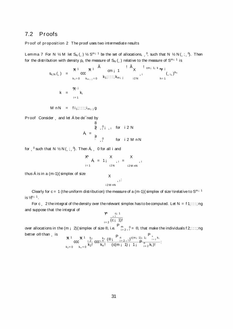
7.2 ProofsProof of proposition 2 The proof uses two intermediate results

Lemma 7 For N ½ M let SN(¸) ½ Sm¡1 be the set of allocations, ¸0, such that N ½ N(¸; ¸0). Thenfor the distribution with density pc the measure of SN(¸) relative to the measure of Sm¡1 is

sc;N(¸) =c¡1X

k1=0

¢ ¢ ¢c¡1X

km¡j=0

Ãcm ¡ 1

k1; : : : ; km¡j

!ÃX

i2N

¸i

!cm¡1¡k m¡jY

h=1

(¸ih)kh

k =m¡jX

i=1

ki

M n N = fi1; : : : ; im¡jg

Proof Consider ¸ and let Á be de¯ned by

Ái =

8>><>>:

¸0i ¡ ¸i for i 2 N

¸0i for i 2 M n N

for ¸0 such that N ½ N(¸; ¸0). Then Ái ¸ 0 for all i and

mX

i=1

Ái = 1 ¡X

i2N

¸i =X

i2MnN

¸i

thus Á is in a (m-1){simplex of size X

i2MnN

¸i:

Clearly for c = 1 (the uniform distribution) the measure of a (m-1){simplex of size ½ relative to Sm¡1

is ½m¡1.For c ¸ 2 the integral of the density over the relevant simplex has to be computed. Let N = f1; : : : ; ng

and suppose that the integral ofmY

i=2

¸c¡1i

(c ¡ 1)!

over allocations in the (m ¡ 2){simplex of size ®, i.e.Pm

i=2 ¸0i = ®, that make the individuals f2; : : : ; ng

better o® than ¸ isc¡1X

k2=0

¢ ¢ ¢c¡1X

kn=0

¸k22

k2!¢ ¢ ¢ ¸kn

nkn!

(® ¡ Pni=2 ¸i)

c(m¡1)¡1¡Pn

i=2ki

(c(m ¡ 1) ¡ 1 ¡ Pni=2 ki)!

:

31

Then the measure of the allocations in the (m-1){simplex of size ¯, which is de¯ned byPm

i=1 ¸0i = ¯,

that make the individuals f1; : : : ; ng better o® is (® = ¯ ¡ ¸1)

c¡1X

k2=0

¢ ¢ ¢c¡1X

kn=0

¸k22

k2!¢ ¢ ¢ ¸kn

n

kn!

Z ¯¡Pn

i=2ki

¸1

c¡1X

k1=0

¸01

(c ¡ 1)!(¯ ¡ ¸0

1 ¡ Pni=2 ¸i)c(m¡1)¡1¡

Pn

i=2ki

(c(m ¡ 1) ¡ 1 ¡ Pni=2 ki)!

d¸01

=

c¡1X

k1=0

¢ ¢ ¢c¡1X

kn=0

¸k11

k1!¢ ¢ ¢ ¸kn

nkn!

(¯ ¡ Pni=1 ¸i)

cm¡1¡Pn

i=1ki

(cm ¡ 1 ¡ Pni=1 kn)!

:

It remains to be shown that the integral of

mY

i=2

¸c¡1i

(c ¡ 1)!

over allocations in the (m ¡ 2){simplex of size ®, i.e.Pm

i=2 ¸0i = ®, that make the individuals f2; : : : ; ng

better o® than ¸ isc¡1X

k2=0

¢ ¢ ¢c¡1X

kn=0

¸k22

k2!¢ ¢ ¢ ¸kn

n

kn!(® ¡ Pn

i=2 ¸i)c(m¡1)¡1¡Pn

i=2ki

(c(m ¡ 1) ¡ 1 ¡ Pni=2 ki)!

:

First note that the integral ofi=mY

i=n+1

¸0c¡1i

(c ¡ 1)!

over the (m ¡ n ¡ 1){simplex de¯ned byPi=m

i=n+1 ¸0i = ® ¡ ¸n is

(® ¡ ¸n)c(m¡n¡1)¡1

(c(m ¡ n ¡ 1) ¡ 1)!:

Second a computation of the integral of

¸0c¡1n

(c ¡ 1)!(® ¡ ¸0

n)c(m¡n¡1)¡1

(c(m ¡ n ¡ 1) ¡ 1)!

over the set ¸0n 2 [¸n; ®] gives the result. Q.E.D.

Lemma 8iX

k=0

(¡1)k

Ãn + in + k

!Ãn + k ¡ 1

k

!= 1:

Proof First the preceding formula may be rewritten as

iX

k=0

(¡1)k

Ãn + ii ¡ k

!Ãn + k ¡ 1

n ¡ 1

!

32

second exchange k with k0 = i ¡ k

iX

k0=0

(¡1)i¡k0Ã

n + ik0

!Ãn + i ¡ 1 ¡ k0

n ¡ 1

!:

If the standard binomial formula,

iX

k=0

(¡1)k

Ãb ¡ kb ¡ i

!Ãak

!=

Ãb ¡ a

i

!;

is applied with a = n + i, b = n + i ¡ 1 then

iX

k0=0

(¡1)i¡k0Ã

n + ik0

!Ãn + i ¡ 1 ¡ k0

n ¡ 1

!= (¡1)i

á1i

!:

The basic identity, ári

!= (¡1)i

Ãr + i ¡ 1

i

!;

gives the result for r = 1. Q.E.D.

Proposition 2 can be established by use of lemma 7 and lemma 8. First the formula for uc;n(¸) has to beestablished. The proof follows from the principle of inclusion and exclusion as in the original problem ofoccupancy8 and it depends on induction on the index j.

The set Tn(¸) is the union of all sets SN(¸) for all N 2 Mn, i.e. Tn(¸) = [N2MnSN(¸). If therelative pc-measures of these sets are added then the ¯rst element of expression (1) is obtained,

X

J2Mm¡n

sc;MnJ(¸); (6)

but these sets intersect, so some parts of are counted more than once. As an example, let N 0 be a set of(n + 1) integers then it contains Ã

n + 1n

!

sets of n integers. Therefore the volume of the set SN0(¸) has then to be discounted

Ãn + 1

n

!¡ 1 =

Ãn1

!times then second element of expression (1) is obtained,

¡Ã

n1

! X

J2Mm¡n¡1

ÃX

i2J

¸i

!m¡1

: (7)

8Any standard proof of this result would hold here by noticing that, for any ¯xed subset N 2 M , theprobability that all urn in N contains less than c balls is equal to the probability that all families in Nend up being better o® when choosing an alternative allocation according to the density pc, given theidenti¯cation pi = ¸i. However since the principle of inclusion-exclusion is crucial in the present paper,it seems adequate to give the argument.

33

The induction hypothesis is that the volume corresponding to a set of (n + i ¡ 1) elements has to bediscounted

(¡1)i¡1

Ãn + i ¡ 2

i ¡ 1

!

times from the initial quantity (expresion 6). Then the volume corresponding to a set of (n + i) integerswas counted

Ãn + i

n

!

| {z }in (6)

¡Ã

n + in + 1

!Ãn1

!

| {z }in (7)

+ : : : + (¡1)i

Ãn + i

n + i ¡ 1

!Ãn + i ¡ 2

i ¡ 1

!

times that is equal to

1 ¡ (¡1)i

Ãn + i ¡ 1

i

!

times according to lemma (8). Hence a volume corresponding to a set of (n+i) integers has to be counted

(¡1)i

Ãn + i ¡ 1

i

!times more in order to be counted exactly one time.

This implies that

uc;n(¸) =m¡nX

i=0

(¡1)i

Ãn + i ¡ 1

i

!0@ X

I2Mm¡n¡i

sc;MnI(¸)

1A

hence if j = m ¡ n ¡ i the expression of proposition 2 is obtained. The volume of tc;n(¸) follows directlybecause tc;n(¸) = uc;n(¸) ¡ uc;n+1(¸), thus9

m¡nX

j=0

(¡1)m¡n¡j

ÃÃm ¡ j ¡ 1

n ¡ 1

!+

Ãm ¡ j ¡ 1

n

!!

| {z }

=

Ãm ¡ j

n

!

0@ X

J2Mj

sc;MnI(¸)

1A :

Hence the expression of proposition 2 is obtained. Q.E.D.

Proposition 2 implies that the results on urn models can be applied in order to establish theorem1, observation 1 and observation 2. Thus if ¹ is replaced by ¸ and Pr[Vc(m) ¸ n] is replaced withuc;m;n(¸m) then the proofs are applications of results on urn models.

Proof of theorem 1 Apply corollary 2. Q.E.D.

Proof of observation 1 Apply lemma 6. Q.E.D.

Proof of observation 2 Apply lemma 4. Q.E.D.

9Note that by convention

Ãab

!= 0 for a · b ¡ 1.

34