Eur. Phys. J. C (2022) 82:26https://doi.org/10.1140/epjc/s10052-021-09893-0

Regular Article - Experimental Physics

Determining the neutrino mass ordering and oscillationparameters with KM3NeT/ORCA

KM3NeT Collaboration

S. Aiello1, A. Albert2,55, S. Alves Garre3, Z. Aly4, A. Ambrosone5,6, F. Ameli7, M. Andre8, G. Androulakis9,M. Anghinolfi10, M. Anguita11, G. Anton12, M. Ardid13, S. Ardid13, J. Aublin14, C. Bagatelas9, B. Baret14,S. Basegmez du Pree15, M. Bendahman16, F. Benfenati17,18, E. Berbee15, A. M. van den Berg19, V. Bertin4,S. Biagi20, M. Bissinger12, M. Boettcher21, M. Bou Cabo22, J. Boumaaza16, M. Bouta23, M. Bouwhuis15, C. Bozza24,H. Brânzas25, R. Bruijn15,26, J. Brunner4, R. Bruno1, E. Buis27, R. Buompane5,28, J. Busto4, B. Caiffi10, D. Calvo3,A. Capone7,29, V. Carretero3, P. Castaldi17,30, S. Celli7,29, M. Chabab31, N. Chau14, A. Chen32, S. Cherubini20,33,V. Chiarella34, T. Chiarusi17, M. Circella35, R. Cocimano20, J. A. B. Coelho14, A. Coleiro14, M. Colomer Molla3,14,R. Coniglione20, P. Coyle4, A. Creusot14, A. Cruz36, G. Cuttone20, R. Dallier37, B. De Martino4, M. De Palma35,38,M. Di Marino39, I. Di Palma7,29, A. F. Díaz11, D. Diego-Tortosa13, C. Distefano20, A. Domi10,40, C. Donzaud14,D. Dornic4, M. Dörr41, D. Drouhin2,55, T. Eberl12, A. Eddyamoui16, T. van Eeden15, D. van Eijk15,I. El Bojaddaini23, D. Elsaesser41, A. Enzenhöfer4, V. Espinosa13, P. Fermani7,29, G. Ferrara20,33, M. D. Filipovic42,F. Filippini17,18, L. A. Fusco4, T. Gal12, A. Garcia Soto15, F. Garufi5,6, Y. Gatelet14, N. Geißelbrecht12,L. Gialanella5,28, E. Giorgio20, S. R. Gozzini7,44, R. Gracia15, K. Graf12, D. Grasso56, G. Grella39, D. Guderian57,C. Guidi10,40, J. Haefner12, S. Hallmann12,a, H. Hamdaoui16, H. van Haren45, A. Heijboer15, A. Hekalo41,L. Hennig12, J. J. Hernández-Rey3, J. Hofestädt12,b, F. Huang4, W. Idrissi Ibnsalih5,28, G. Illuminati3,14,C. W. James36, M. de Jong15, P. de Jong15,26, B. J. Jung15, M. Kadler41, P. Kalaczynski46, O. Kalekin12, U. F. Katz12,N. R. Khan Chowdhury3, G. Kistauri47, F. van der Knaap27, P. Kooijman26,58, A. Kouchner14,48, M. Kreter21,V. Kulikovskiy10, R. Lahmann12, M. Lamoureux14, G. Larosa20, C. Lastoria4, R. Le Breton14, S. Le Stum4,O. Leonardi20, F. Leone20,33, E. Leonora1, N. Lessing12, G. Levi17,18, M. Lincetto4, M. Lindsey Clark14,T. Lipreau37, F. Longhitano1, D. Lopez-Coto49, L. Maderer14, J. Manczak3, K. Mannheim41, A. Margiotta17,18,A. Marinelli5, C. Markou9, L. Martin37, J. A. Martínez-Mora13, A. Martini34, F. Marzaioli5,28, S. Mastroianni5,K. W. Melis15, G. Miele5,6, P. Migliozzi5, E. Migneco20, P. Mijakowski46, L. S. Miranda50, C. M. Mollo5,M. Morganti56,59, M. Moser12, A. Moussa23, R. Muller15, M. Musumeci20, L. Nauta15, S. Navas49, C. A. Nicolau7,B. Ó. Fearraigh15,26, M. O’Sullivan36, M. Organokov2, A. Orlando20, J. Palacios González3, G. Papalashvili47,R. Papaleo20, C. Pastore35, A. M. Paun25, G. E. Pavalas25, C. Pellegrino18,60, M. Perrin-Terrin4,c ,V. Pestel15, P. Piattelli20, C. Pieterse3, K. Pikounis9, O. Pisanti5,6, C. Poirè13, V. Popa25, T. Pradier2, G. Pühlhofer51,S. Pulvirenti20, O. Rabyang21, F. Raffaelli56, N. Randazzo1, S. Razzaque50, D. Real3, S. Reck12, G. Riccobene20,A. Romanov10, A. Rovelli20, F. Salesa Greus3, D. F. E. Samtleben15,52, A. Sánchez Losa35, M. Sanguineti10,40,A. Santangelo51, D. Santonocito20, P. Sapienza20, J. Schnabel12, M. F. Schneider12, J. Schumann12, H. M. Schutte21,J. Seneca15, I. Sgura35, R. Shanidze47, A. Sharma53, A. Sinopoulou9, B. Spisso5,39, M. Spurio17,18, D. Stavropoulos9,S. M. Stellacci5,39, M. Taiuti10,40, Y. Tayalati16, E. Tenllado49, H. Thiersen21, S. Tingay36, V. Tsourapis9,E. Tzamariudaki9, D. Tzanetatos9, V. Van Elewyck14,48, G. Vasileiadis43, F. Versari17,18, D. Vivolo5,28,G. de Wasseige14, J. Wilms54, R. Wojaczynski46, E. de Wolf15,26, T. Yousfi23, S. Zavatarelli10, A. Zegarelli7,29,D. Zito20, J. D. Zornoza3, J. Zúñiga3, N. Zywucka21

1 INFN, Sezione di Catania, Via Santa Sofia 64, 95123 Catania, Italy2 Université de Strasbourg, CNRS, IPHC UMR 7178, 67000 Strasbourg, France3 IFIC-Instituto de Física Corpuscular (CSIC-Universitat de València), c/Catedrático José Beltrán, 2, 46980 Paterna, Valencia, Spain4 Aix Marseille Univ, CNRS/IN2P3, CPPM, Marseille, France5 INFN, Sezione di Napoli, Complesso Universitario di Monte S. Angelo, Via Cintia ed. G,

80126 Naples, Italy6 Università di Napoli “Federico II”, Dip. Scienze Fisiche “E. Pancini”, Complesso Universitario di Monte S. Angelo, Via Cintia ed. G,

80126 Naples, Italy7 INFN, Sezione di Roma, Piazzale Aldo Moro 2, 00185 Rome, Italy8 Laboratori d’Aplicacions Bioacústiques, Centre Tecnològic de Vilanova i la Geltrú, Universitat Politècnica de Catalunya, Avda. Rambla

Exposició, s/n, 08800 Vilanova i la Geltrú, Spain

123

26 Page 2 of 16 Eur. Phys. J. C (2022) 82 :26

9 Institute of Nuclear and Particle Physics, NCSR Demokritos, Ag. Paraskevi Attikis, 15310 Athens, Greece10 INFN, Sezione di Genova, Via Dodecaneso 33, 16146 Genoa, Italy11 Department of Computer Architecture and Technology/CITIC, University of Granada, 18071 Granada, Spain12 Friedrich-Alexander-Universität Erlangen-Nürnberg, Erlangen Centre for Astroparticle Physics, Erwin-Rommel-Straße 1, 91058 Erlangen,

Germany13 Instituto de Investigación para la Gestión Integrada de las Zonas Costeras, Universitat Politècnica de València, C/ Paranimf, 1, 46730 Gandia,

Spain14 Astroparticule et Cosmologie, Université de Paris, CNRS, 75013 Paris, France15 Nikhef, National Institute for Subatomic Physics, PO Box 41882, 1009 DB Amsterdam, The Netherlands16 Faculty of Sciences, University Mohammed V in Rabat, 4 av. Ibn Battouta, B.P. 1014, R.P. 10000 Rabat, Morocco17 INFN, Sezione di Bologna, v.le C. Berti-Pichat, 6/2, 40127 Bologna, Italy18 Dipartimento di Fisica e Astronomia, Università di Bologna, v.le C. Berti-Pichat, 6/2, 40127 Bologna, Italy19 KVI-CART University of Groningen, Groningen, The Netherlands20 Laboratori Nazionali del Sud, INFN, Via S. Sofia 62, 95123 Catania, Italy21 Centre for Space Research, North-West University, Private Bag X6001, Potchefstroom 2520, South Africa22 Instituto Español de Oceanografía, Unidad Mixta IEO-UPV, C/ Paranimf, 1, 46730 Gandia, Spain23 Faculty of Sciences, University Mohammed I, BV Mohammed VI, B.P. 717, R.P. 60000 Oujda, Morocco24 Dipartimento di Matematica, Università di Salerno e INFN Gruppo Collegato di Salerno, Via Giovanni Paolo II 132, 84084 Fisciano, Italy25 ISS, Atomistilor 409, 077125 Magurele, Romania26 Institute of Physics/IHEF, University of Amsterdam, PO Box 94216, 1090 GE Amsterdam, The Netherlands27 Technical Sciences, TNO, PO Box 155, 2600 AD Delft, The Netherlands28 Dipartimento di Matematica e Fisica, Università degli Studi della Campania “Luigi Vanvitelli”, viale Lincoln 5, 81100 Caserta, Italy29 Dipartimento di Fisica, Università La Sapienza, Piazzale Aldo Moro 2, 00185 Rome, Italy30 Dipartimento di Ingegneria dell’Energia Elettrica e dell’Informazione “Guglielmo Marconi”, Università di Bologna, Via dell’Università 50,

47522 Cesena, Italy31 Physics Department, Faculty of Science Semlalia, Cadi Ayyad University, Av. My Abdellah, P.O.B. 2390, 40000 Marrakech, Morocco32 School of Physics, University of the Witwatersrand, Private Bag 3, Wits, Johannesburg 2050, South Africa33 Dipartimento di Fisica e Astronomia “Ettore Majorana”, Università di Catania, Via Santa Sofia 64, 95123 Catania, Italy34 INFN, LNF, Via Enrico Fermi, 40, 00044 Frascati, Italy35 INFN, Sezione di Bari, Via Amendola 173, 70126 Bari, Italy36 International Centre for Radio Astronomy Research, Curtin University, Bentley, WA 6102, Australia37 Subatech, IMT Atlantique, IN2P3-CNRS, Université de Nantes, 4 rue Alfred Kastler-La Chantrerie, BP 20722, 44307 Nantes, France38 University of Bari, Via Amendola 173, 70126 Bari, Italy39 Dipartimento di Fisica, Università di Salerno e INFN Gruppo Collegato di Salerno, Via Giovanni Paolo II 132, 84084 Fisciano, Italy40 Università di Genova, Via Dodecaneso 33, 16146 Genoa, Italy41 University Würzburg, Emil-Fischer-Straße 31, 97074 Würzburg, Germany42 School of Computing, Engineering and Mathematics, Western Sydney University, Locked Bag 1797, Penrith, NSW 2751, Australia43 Laboratoire Univers et Particules de Montpellier, Place Eugène Bataillon-CC 72, 34095 Montpellier Cédex 05, France44 Physics Department, University La Sapienza, Roma, Piazzale Aldo Moro 2, 00185 Rome, Italy45 NIOZ (Royal Netherlands Institute for Sea Research), PO Box 59, Den Burg, 1790 AB Texel, The Netherlands46 National Centre for Nuclear Research, 02-093 Warsaw, Poland47 Department of Physics, Tbilisi State University, 3, Chavchavadze Ave., 0179 Tbilisi, Georgia48 Institut Universitaire de France, 1 rue Descartes, 75005 Paris, France49 Dpto. de Física Teórica y del Cosmos & C.A.F.P.E., University of Granada, 18071 Granada, Spain50 Department Physics, University of Johannesburg, PO Box 524, Auckland Park 2006, South Africa51 Institut für Astronomie und Astrophysik, Eberhard Karls Universität Tübingen, Sand 1, 72076 Tübingen, Germany52 Leiden Institute of Physics, Leiden University, PO Box 9504, 2300 RA Leiden, The Netherlands53 Dipartimento di Fisica, Università di Pisa, Largo Bruno Pontecorvo 3, 56127 Pisa, Italy54 Friedrich-Alexander-Universität Erlangen-Nürnberg, Remeis Sternwarte, Sternwartstraße 7, 96049 Bamberg, Germany55 Université de Strasbourg, Université de Haute Alsace, GRPHE, 34, Rue du Grillenbreit, 68008 Colmar, France56 INFN, Sezione di Pisa, Largo Bruno Pontecorvo 3, 56127 Pisa, Italy57 Institut für Kernphysik, University of Münster, Wilhelm-Klemm-Str. 9, 48149 Münster, Germany58 Department of Physics and Astronomy, Utrecht University, PO Box 80000, 3508 TA Utrecht, The Netherlands59 Accademia Navale di Livorno, Viale Italia 72, 57100 Livorno, Italy60 INFN, CNAF, v.le C. Berti-Pichat, 6/2, 40127 Bologna, Italy

Received: 19 March 2021 / Accepted: 30 November 2021 / Published online: 11 January 2022© The Author(s) 2022

123

Eur. Phys. J. C (2022) 82 :26 Page 3 of 16 26

Abstract The next generation of water Cherenkov neu-trino telescopes in the Mediterranean Sea are under con-struction offshore France (KM3NeT/ORCA) and Sicily(KM3NeT/ARCA). The KM3NeT/ORCA detector featuresan energy detection threshold which allows to collect atmo-spheric neutrinos to study flavour oscillation. This paperreports the KM3NeT/ORCA sensitivity to this phenomenon.The event reconstruction, selection and classification aredescribed. The sensitivity to determine the neutrino massordering was evaluated and found to be 4.4σ if the true order-ing is normal and 2.3σ if inverted, after 3 years of data taking.The precision to measure Δm2

32 and θ23 were also estimatedand found to be 85.10−6 eV2 and (+1.9

−3.1)◦ for normal neu-

trino mass ordering and, 75.10−6 eV2 and (+2.0−7.0)

◦ for invertedordering. Finally, a unitarity test of the leptonic mixing matrixby measuring the rate of tau neutrinos is described. Threeyears of data taking were found to be sufficient to exclude↪ ↩ντ event rate variations larger than 20% at 3σ level.

1 Introduction

The standard framework of three neutrino flavour eigenstates(νe, νμ, ντ ), which are superpositions of the three mass eigen-states (ν1, ν2, ν3) with masses (m1, m2, m3), has been estab-lished with more than two decades of neutrino oscillationphysics research. By convention, ν1 is the mass eigenstatewith the largest νe component, and ν3 is the one with thesmallest. The ordering of the neutrino mass eigenstates isnot yet resolved, and it can be either m1 < m2 < m3 (‘nor-mal ordering’, NO) or m3 < m1 < m2 (‘inverted ordering’,IO). The question of the neutrino mass ordering (NMO) isone of the main drivers of neutrino oscillation physics.

Neutrino mixing is described by the Pontecorvo–Maki–Nakagawa–Sakata (PMNS) matrix, U , [1–3] with

να =3∑

i=1

Uαiνi , (1)

where α = e, μ, τ and i = 1, 2, 3. Under the assumptionthat the mixing matrixU is unitary, it is usually parametrisedin terms of three mixing angles θ12, θ13 and θ23, and a CP-violating phase δCP [4]. Neutrino oscillations are sensitiveto mass-squared differences Δm2

i j = m2i − m2

j (i, j =1, 2, 3). From the three neutrino mass eigenstates two inde-pendent mass-squared differences can be constructed, which

Deceased: Giorgos Androulakis.

a e-mail: steffen.hallmann@fau.de (corresponding author)b e-mail: jannik.hofestaedt@fau.de (corresponding author)c e-mail: mathieu.perrin-terrin@cppm.in2p3.fr (corresponding author)

we choose as Δm212 and ± ∣∣Δm2

23

∣∣, where the sign of thelatter is positive for NO and negative for IO.

Global fits of the available data form a coherent pictureand provide values for θ12, θ13, θ23, Δm2

12 and∣∣Δm2

23

∣∣ withfew-percent level precision [5–7]. However, some questionsremain: the determination of the value of δCP, the octant ofθ23 (i.e. whether θ23 is greater or smaller than π/4) and theneutrino mass ordering (i.e. the sign of Δm2

23). The currentstatus is that global fits [8,9] indicate a mild preference forNO over IO, second octant of θ23 and δCP ≈ π to 3

2π . Theexperiments driving the NMO sensitivity results are T2K[10], NOvA [11], MINOS [12], Super-Kamiokande [13] andIceCube/DeepCore [14]. Notably, the hints for NO tend toweaken in the light of combined analyses [8,9] using thelatest results from T2K [15] and NOvA [16].

Deriving strong experimental constraints on the unitarityof the 3 × 3 PMNS mixing matrix is challenging, as directobservations of ↪ ↩νμ → ↪ ↩ντ are difficult and the τ rest-masssuppresses the ↪ ↩ντ interaction cross section. Appearance of ↪ ↩ντ

has been directly observed at the long baseline CNGS neu-trino beam by OPERA [17,18]. Evidence for ↪ ↩ντ appearancehas also been found on a statistical basis in the atmosphericneutrino flux by Super-Kamiokande [19] and IceCube [20].However, the uncertainty on the normalisation of the ↪ ↩ντ sig-nal is currently too large to probe the unitarity of the PMNSmixing matrix. Non-unitarity would imply the incomplete-ness of the 3×3 flavour paradigm and could point to the exis-tence of additional neutrino flavours. A statistically highly-significant detection of ↪ ↩ντ appearance from ↪ ↩νμ → ↪ ↩ντ oscil-lations of atmospheric neutrinos could make an importantcontribution to further constrain the PMNS matrix elementsinvolving ↪ ↩ντ .

The NMO can be determined by measuring the energy andzenith angle dependent oscillation pattern of few-GeV atmo-spheric neutrinos that have traversed the Earth [21]. Matter-induced modifications [22,23] of the oscillation probabilitieslead to an enhancement of the ↪ ↩νμ ↔ ↪ ↩νe transition for neu-trinos in the case of NO, and anti-neutrinos in the case of IO.Earth matter effects are due to coherent neutrino electron for-ward scattering. They arise mainly below Eν � 15 GeV anddepend on the electron density of the medium. The largesteffects appear around 7 GeV for neutrinos passing throughthe Earth’s mantle and around 3 GeV for neutrinos passingthrough the Earth’s core. The oscillation pattern for neutri-nos with respect to anti-neutrinos is flipped between the twomass orderings.

In case of detectors that cannot distinguish between neutri-nos and anti-neutrinos on an event-by-event basis, the deter-mination of the NMO can be based on the observation ofa net difference in the event rates of atmospheric neutrinos,resulting from a higher interaction cross section (factor ∼ 2)and the existing atmospheric flux difference (factor ∼ 1.1)for neutrinos with respect to anti-neutrinos. Due to this event

123

26 Page 4 of 16 Eur. Phys. J. C (2022) 82 :26

rate difference, the strength of the observed matter effects,i.e. the enhancement of the ↪ ↩νμ ↔ ↪ ↩νe transition, is largerfor NO compared to IO. This is the experimental signatureexploited by KM3NeT/ORCA and other atmospheric neu-trino experiments to determine the NMO.

KM3NeT is a large research infrastructure that will consistof a network of deep-sea neutrino detectors in the Mediter-ranean Sea. Two underwater neutrino telescopes, calledARCA and ORCA, are currently under construction [24].ARCA (Astroparticle Research with Cosmics in the Abyss) isa sparsely instrumented gigaton-scale detector optimised forTeV–PeV neutrino astronomy. ORCA (Oscillation Researchwith Cosmics in the Abyss) is a more densely instrumenteddetector optimised for measuring the oscillation of few-GeVatmospheric neutrinos in order to determine the neutrinomass ordering.

With atmospheric neutrino data, ORCA can also performa precise measurement of θ23 and Δm2

23 as well as a high-statistics measurement of ↪ ↩ντ appearance in the atmosphericneutrino flux, which allows to probe deviations from theunitarity assumption of the 3-neutrino mixing. Sensitivityfor tau-neutrino appearance mainly comes from atmosphericneutrinos with energy � 15 GeV and therefore has only aweak dependence on the still undetermined neutrino massordering.

A first estimation of the sensitivity of ORCA to the NMOas well as to other oscillation parameters was published inthe ‘Letter of Intent for KM3NeT 2.0’ (LoI) [24]. Sincethen, the detector and the analysis methods have been furtheroptimised. First, the detector geometry has been updated. Inaddition, significant improvements in the neutrino detectionefficiency as well as reconstruction performance have beenachieved as illustrated in Sect. 2.4. The event classificationprocedure has been significantly improved as well. We usenow three event classes and hit features are included, this isdiscussed in Sect. 2.5. At the same time the analysis has beenrefined. The detector response is modeled in greater detail anda more complete list of systematic effects is now considered.These effects partly compensate the expected gain in sensitiv-ity from the improvements mentioned above but make themat the same time more realistic. The updated sensitivities arepresented in this paper.

This paper is organised as follows. Section 2 describesthe detector design and the simulations performed to obtainthe detector response to atmospheric neutrinos, atmosphericmuons as well as optical background noise. Then, the algo-rithms used for event reconstruction and for high flavourpurity event classification are described. In Sect. 3, the meth-ods used to analyse these samples and derive the sensitivity tothe NMO, the atmospheric oscillation parameters and the ↪ ↩ντ

appearance are presented together with the results. Finally,Sect. 4 summarises the main detector and analysis updatesand the expected sensitivity to neutrino oscillations.

2 ORCA detector response

The ORCA detector design comprises a 3-dimensional arrayof photosensors that register the Cherenkov light producedby relativistic charged particles emerging from neutrino-induced interactions. The arrival time of the Cherenkov pho-tons and the position of the sensors are used to reconstructthe energy and direction of the incoming neutrino as well asthe event topology.

2.1 Detector design

The ORCA detector design consists of an array of 115 ver-tical detection units (DUs) featuring 18 digital optical mod-ules (DOMs) each. Each DOM is a pressure-resistant glasssphere, housing 31 photomultiplier tubes (PMTs) of 3-inchdiameter and the related electronics. The KM3NeT PMTsare characterised in [25].

The detector is located at the KM3NeT-France site and thebase container of each DU is placed at about 2450 m depth.The DUs are arranged in a circular footprint with a radiusof about 115 m with an average spacing between the DUs of20 m. Along a DU, the vertical spacing between the DOMsvaries between 8.7 m to 10.9 m (due to technical constraintsfrom the deployment procedure) with an average of 9.3 m.The first DOM is at a distance of about 30 m from the seabed[26]. In total, a volume of about 6.7 × 106 m3 (equivalentto 7.0 Mt of sea water) is instrumented. This detector con-figuration is the outcome of an optimisation study using thesensitivity to the NMO as figure of merit.

2.2 Simulation

Detailed Monte Carlo (MC) simulations are used to evaluatethe detector response to atmospheric neutrinos, atmosphericmuons and optical background noise. The simulation chainused for the analysis presented in this paper is similar to theone described in [24].

Neutrino induced interactions in sea water are simulatedwith gSeaGen [27], a software package based on the widelyused GENIE (version 2.12.10) code [28,29]. Neutrinos andantineutrinos in the energy range from 1 to 100 GeV aresimulated and weighted to reproduce the conventional atmo-spheric neutrino flux following the Honda model [30]. Allparticles emerging from neutrino interactions are propagatedwith the GEANT4-based software package KM3Sim [31].Using this software, Cherenkov photons are generated fromprimary and secondary particles, tracked through the seawater taking into account absorption and scattering, anddetected by the PMTs.

Atmospheric muon events are generated using theMUPAGE package [32]. The KM3 package [33,34] is then

123

Eur. Phys. J. C (2022) 82 :26 Page 5 of 16 26

used for tracking the muons in sea water and the subsequentCherenkov light production.

The PMT response and the readout are simulated usingcustom KM3NeT software. The digitised PMT output sig-nal is typically called a hit. In this step, the optical back-ground due to Cherenkov light from β-decays of 40K in thesea water is also added: an uncorrelated hit rate of 10 kHzper PMT as well as time-correlated noise on multiple PMTson each DOM (600 Hz twofold, 60 Hz threefold, 7 Hz four-fold, 0.8 Hz fivefold and 0.08 Hz sixfold). The simulatedtime-correlated noise rate is taken from the data of the firstdeployed DUs [35]. Finally, the simulated data is filteredby dedicated trigger algorithms to identify events inducedby energetic particles. The trigger algorithms are designedto search for large clusters of causally-connected hits. Thesame trigger algorithms are applied to both simulated andreal data.

Compared to the LoI [24], significant improvements havebeen made in the triggering of faint events with only a fewtens of detected photons [36]. A new trigger algorithm hasbeen developed for the needs of ORCA. It is based on onlyone local coincidence (photons recorded on two or morePMTs of the same DOM within 10 ns) and a tunable num-ber of causally-connected single hits on DOMs in the vicin-ity. A minimum of seven additional hits distributed over atleast three different DOMs are required. This new algorithmsignificantly increases the trigger efficiency in the few-GeVneutrino energy range, while still satisfying the bandwidthrequirements of the data acquisition system.

The total trigger rate due to atmospheric muons is about50 Hz and noise events add about 54 Hz, while atmosphericneutrinos are triggered with a rate of about 8 mHz. In total,1.4 days of noise events, 14 days of atmospheric muons andmore than 15 years of atmospheric neutrinos are simulated.These event samples are sufficient to probe a percent-levelbackground contamination (see Sect. 2.5). In future analysisof real data, the background will be included based on run-by-run simulations [34], accounting for the detector and data-taking conditions.

2.3 Event topologies

Two distinct event topologies can be distinguished in thedetector: track-like and shower-like. In the few-GeV energyrange, muons are the only particles that can be confidentlyidentified, because they are the only particles that appear astracks in the detector, with a track length proportional to themuon energy (∼ 4 m/GeV). Electrons and hadrons initiateparticle showers that develop over distances of a few metres.Compared to elongated muon tracks, these showers appear aslocalised light sources in the detector. All neutrino-inducedevents producing a muon with sufficient energy are calledtrack-like, i.e. ↪ ↩νμ charged-current (CC) events and ↪ ↩ντ CC

1 2 3 4 5 6 7 8 910 20 30 40 50neutrino energy [GeV]

0

1

2

3

4

5

6

7

8

9

10]3ef

fect

ive

volu

me

[Mm CCμν CCμν

CCeν CCeν CCτν CCτν

NCν NCν

KM3NeT

Fig. 1 Effective detector volume as a function of true neutrino energyEν for different neutrino flavours and interactions. Events are weightedaccording to the Honda atmospheric neutrino flux model and averagedover the zenith angle. Only events reconstructed and selected as upgoingare used. The dashed black line indicates the instrumented volume ofthe detector

events with muonic τ decays. All other neutrino-inducedevents are called shower-like, i.e. ↪ ↩νe,μ,τ neutral-current (NC)events, ↪ ↩νe CC events and ↪ ↩ντ CC events with non-muonic τ

decays.

2.4 Event reconstruction and event selection

Dedicated reconstruction algorithms are applied for track-like and shower-like events as well as an event topologyclassification algorithm. The track and shower reconstruc-tion algorithms are described in [37,38], respectively. Bothreconstruction algorithms are maximum likelihood fits andreconstruct the energy and direction as well as interactionvertex position and time. Events reconstructed as upgoing,i.e. with a negative cosine zenith angle, are selected based onthe reconstruction quality and containment. The containmentcriteria are based on the event position and direction insidethe instrumented detector volume [36]. The goal of the eventpreselection is to fulfil two main purposes: suppress back-ground events and select well-reconstructed events with agood reconstruction accuracy.

The effective detector volume after the event preselectionis shown in Fig. 1 for upgoing neutrinos weighted accord-ing to the Honda atmospheric neutrino flux model [30]. Theeffective detector volume reaches a plateau and is nearlyas large as the instrumented detector volume for ↪ ↩νe,μ CCwith Eν � 15 GeV, while 50% efficiency is reached forEν ∼ 4 GeV. Compared to the LoI [24], the turn-on regionof the effective detector volume is shifted by about 20% tolower energies due to improvements in event triggering andreconstruction. Indeed, as discussed in Sect. 2.2, additionalmethods have been developed to record events with a lower

123

26 Page 6 of 16 Eur. Phys. J. C (2022) 82 :26

2 3 4 5 6 7 8 10 20 30 40neutrino energy [GeV]

2

3456

10

20

304050

reco

nstru

cted

ene

rgy

[GeV

]

3−10

2−10

1−10

1KM3NeT

CCeν + eνshower sample50%

15%

85%

2 3 4 5 6 7 8 10 20 30 40neutrino energy [GeV]

2

3456

10

20

304050

reco

nstru

cted

ene

rgy

[GeV

]

3−10

2−10

1−10

1KM3NeT

CCμν + μνtrack sample

50%

15%

85%

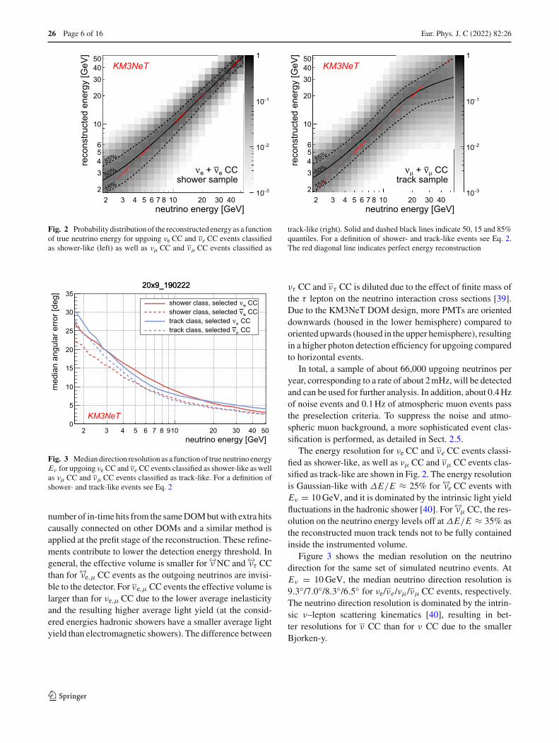
Fig. 2 Probability distribution of the reconstructed energy as a functionof true neutrino energy for upgoing νe CC and νe CC events classifiedas shower-like (left) as well as νμ CC and νμ CC events classified as

track-like (right). Solid and dashed black lines indicate 50, 15 and 85%quantiles. For a definition of shower- and track-like events see Eq. 2.The red diagonal line indicates perfect energy reconstruction

2 3 4 5 6 7 8 910 20 30 40 50neutrino energy [GeV]

0

5

10

15

20

25

30

35

med

ian

angu

lar e

rror

[deg

]

20x9_190222

CCeνshower class, selected CCeνshower class, selected

CCμνtrack class, selected CCμνtrack class, selected

KM3NeT

20x9_190222

Fig. 3 Median direction resolution as a function of true neutrino energyEν for upgoing νe CC and νe CC events classified as shower-like as wellas νμ CC and νμ CC events classified as track-like. For a definition ofshower- and track-like events see Eq. 2

number of in-time hits from the same DOM but with extra hitscausally connected on other DOMs and a similar method isapplied at the prefit stage of the reconstruction. These refine-ments contribute to lower the detection energy threshold. Ingeneral, the effective volume is smaller for ↪ ↩ν NC and ↪ ↩ντ CCthan for ↪ ↩νe,μ CC events as the outgoing neutrinos are invisi-ble to the detector. For νe,μ CC events the effective volume islarger than for νe,μ CC due to the lower average inelasticityand the resulting higher average light yield (at the consid-ered energies hadronic showers have a smaller average lightyield than electromagnetic showers). The difference between

ντ CC and ντ CC is diluted due to the effect of finite mass ofthe τ lepton on the neutrino interaction cross sections [39].Due to the KM3NeT DOM design, more PMTs are orienteddownwards (housed in the lower hemisphere) compared tooriented upwards (housed in the upper hemisphere), resultingin a higher photon detection efficiency for upgoing comparedto horizontal events.

In total, a sample of about 66,000 upgoing neutrinos peryear, corresponding to a rate of about 2 mHz, will be detectedand can be used for further analysis. In addition, about 0.4 Hzof noise events and 0.1 Hz of atmospheric muon events passthe preselection criteria. To suppress the noise and atmo-spheric muon background, a more sophisticated event clas-sification is performed, as detailed in Sect. 2.5.

The energy resolution for νe CC and νe CC events classi-fied as shower-like, as well as νμ CC and νμ CC events clas-sified as track-like are shown in Fig. 2. The energy resolutionis Gaussian-like with ΔE/E ≈ 25% for ↪ ↩νe CC events withEν = 10 GeV, and it is dominated by the intrinsic light yieldfluctuations in the hadronic shower [40]. For ↪ ↩νμ CC, the res-olution on the neutrino energy levels off at ΔE/E ≈ 35% asthe reconstructed muon track tends not to be fully containedinside the instrumented volume.

Figure 3 shows the median resolution on the neutrinodirection for the same set of simulated neutrino events. AtEν = 10 GeV, the median neutrino direction resolution is9.3◦/7.0◦/8.3◦/6.5◦ for νe/νe/νμ/νμ CC events, respectively.The neutrino direction resolution is dominated by the intrin-sic ν–lepton scattering kinematics [40], resulting in bet-ter resolutions for ν CC than for ν CC due to the smallerBjorken-y.

123

Eur. Phys. J. C (2022) 82 :26 Page 7 of 16 26

0 0.2 0.4 0.6 0.8 1

atmospheric muon score

5−10

4−10

3−10

2−10

1−10

1fra

ctio

natm. muonsatm. neutrinosnoise

KM3NeT

0 2 4 6 8 10 12 14

atmospheric muon background contamination [%]

80

82

84

86

88

90

92

94

96

98

100

neut

rino

effic

ienc

y [%

]

all neutrinos CC, 5 GeV μν + μν CC, 15 GeV μν + μν CC, 5 GeV eν + eν CC, 15 GeV eν + eνKM3NeT

Fig. 4 Left: Distribution of the atmospheric muon score variable for the RDF trained to separate between neutrinos and atmospheric muons, for themain classes of events. Right: Fraction of remaining neutrinos weighted with an oscillated atmospheric flux versus atmospheric muon contaminationin the final sample

0 0.2 0.4 0.6 0.8 1

noise score

5−10

4−10

3−10

2−10

1−10

1

fract

ion

atm. muonsatm. neutrinosnoise

KM3NeT

0 2 4 6 8 10 12 14

noise background contamination [%]

98

98.2

98.4

98.6

98.8

99

99.2

99.4

99.6

99.8

100

neut

rino

effic

ienc

y [%

]

all neutrinos CC, 5 GeV μν + μν CC, 15 GeV μν + μν CC, 5 GeV eν + eν CC, 15 GeV eν + eνKM3NeT

Fig. 5 Left: Distribution of the noise score variable for the RDF aimed to separate between neutrinos and pure noise, for the main classes of events.Right: Fraction of remaining atmospheric neutrinos versus noise event contamination in the final sample

2.5 Event classification

For event classification, random decision forests (RDFs) [41]are used, which consist of an ensemble of binary decisiontrees.

Two RDFs are trained individually for selecting neutrinocandidates against each of the two dominant classes of back-ground – atmospheric muons and noise events – and a thirdone is trained to distinguish track-like from shower-like eventtopologies.

To train the classifiers, ↪ ↩νμ CC events have been used torepresent track-like event topologies. For showers ↪ ↩νe CC and↪ ↩ν NC events have been used. The neutrino event distributionswere flattened in log10 of neutrino energy and the numbersof events per class were balanced between tracks and show-ers. In contrast, background was fed with the expected truespectra.

Each trained classifier yields a score variable (atmospheric_muon_score, noise_score, track_score).These represent the fraction of trees voting for the respectiveresult class. The individual score parameters allow to sep-arately optimise the suppression of the atmospheric muonand noise components using selection cuts and to divide theremaining events into different classes for analysis.

In the training, only events which pass the preselectionrequirements for either tracks or showers were used. Theclassifiers were trained independently of each other. Con-sequently, no further selection based on the resulting scorefrom one of the other classifiers and none of the resultingscore variables is used to train the RDFs. In the training, aforest size of 101 trees,1 and 50,000 events per class (25,000for noise suppression due to smaller available statistics after

1 The uneven number was chosen for practical purposes only and sim-plifies consistency of event selection across different analyses (> vs.≥).

123

26 Page 8 of 16 Eur. Phys. J. C (2022) 82 :26

3 4 5 6 7 8 910 20 30 40 50neutrino energy [GeV]

0

0.1

0.2

0.3

0.4

0.5

0.6

0.7

0.8

0.9

1fra

ctio

n

shower class

intermediate class

track class

KM3NeT CCμν CCμν

3 4 5 6 7 8 910 20 30 40 50neutrino energy [GeV]

0

0.1

0.2

0.3

0.4

0.5

0.6

0.7

0.8

0.9

1

fract

ion

shower class

intermediate class

track class

KM3NeT

CCeν CCeν

3 4 5 6 7 8 910 20 30 40 50neutrino energy [GeV]

0

0.1

0.2

0.3

0.4

0.5

0.6

0.7

0.8

0.9

1

fract

ion

shower class

intermediate class

track class

KM3NeT

CCτν CCτν

3 4 5 6 7 8 910 20 30 40 50neutrino energy [GeV]

0

0.1

0.2

0.3

0.4

0.5

0.6

0.7

0.8

0.9

1

fract

ion

shower class

intermediate class

track class

KM3NeT

NCν NCν

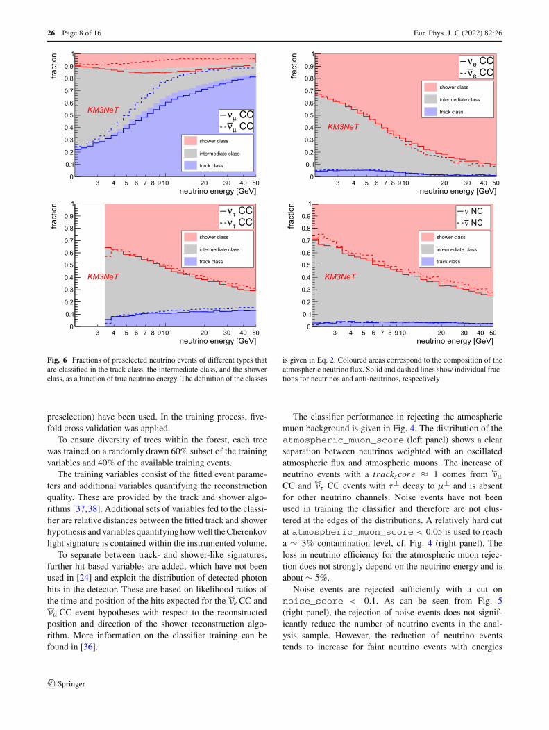
Fig. 6 Fractions of preselected neutrino events of different types thatare classified in the track class, the intermediate class, and the showerclass, as a function of true neutrino energy. The definition of the classes

is given in Eq. 2. Coloured areas correspond to the composition of theatmospheric neutrino flux. Solid and dashed lines show individual frac-tions for neutrinos and anti-neutrinos, respectively

preselection) have been used. In the training process, five-fold cross validation was applied.

To ensure diversity of trees within the forest, each treewas trained on a randomly drawn 60% subset of the trainingvariables and 40% of the available training events.

The training variables consist of the fitted event parame-ters and additional variables quantifying the reconstructionquality. These are provided by the track and shower algo-rithms [37,38]. Additional sets of variables fed to the classi-fier are relative distances between the fitted track and showerhypothesis and variables quantifying how well the Cherenkovlight signature is contained within the instrumented volume.

To separate between track- and shower-like signatures,further hit-based variables are added, which have not beenused in [24] and exploit the distribution of detected photonhits in the detector. These are based on likelihood ratios ofthe time and position of the hits expected for the ↪ ↩νe CC and↪ ↩νμ CC event hypotheses with respect to the reconstructedposition and direction of the shower reconstruction algo-rithm. More information on the classifier training can befound in [36].

The classifier performance in rejecting the atmosphericmuon background is given in Fig. 4. The distribution of theatmospheric_muon_score (left panel) shows a clearseparation between neutrinos weighted with an oscillatedatmospheric flux and atmospheric muons. The increase ofneutrino events with a trackscore ≈ 1 comes from ↪ ↩νμ

CC and ↪ ↩ντ CC events with τ± decay to μ± and is absentfor other neutrino channels. Noise events have not beenused in training the classifier and therefore are not clus-tered at the edges of the distributions. A relatively hard cutat atmospheric_muon_score < 0.05 is used to reacha ∼ 3% contamination level, cf. Fig. 4 (right panel). Theloss in neutrino efficiency for the atmospheric muon rejec-tion does not strongly depend on the neutrino energy and isabout ∼ 5%.

Noise events are rejected sufficiently with a cut onnoise_score < 0.1. As can be seen from Fig. 5(right panel), the rejection of noise events does not signif-icantly reduce the number of neutrino events in the anal-ysis sample. However, the reduction of neutrino eventstends to increase for faint neutrino events with energies

123

Eur. Phys. J. C (2022) 82 :26 Page 9 of 16 26

Fig. 7 Comparison of the classifier performance as a function of trueneutrino energy in terms of the separation power metric as defined inEq. 3. Separation power for training with (solid) and without (dashed)hit-based features is shown

near the detection threshold. The proposed cuts on theatmospheric_muon_score and noise_score val-ues reduce the muon and noise contamination of the selectedevent sample to a level which can be safely neglected in thesensitivity study.

The training of track- versus shower-like neutrino eventsignatures results in atrack_score variable, representingthe fraction of trees voting for the candidate event to be track-like. Using this variable, events can be split in three eventclasses based on the following criteria:

shower class: passes shower preselection

and (track_score ≤ 0.3),

intermediate class: passes shower preselection

and (0.3 < track_score ≤ 0.7),

track class: passes track preselection

and (track_score > 0.7). (2)

The performance of the event type classifier for neutrinosis shown in Fig. 6, where the fractions of events ending upin the respective class are presented as a function of neutrinoenergy.

The fraction of correctly classified events increasessteeply in the energy region up to ∼ 15 GeV, where lessthan 5% of ↪ ↩νe CC and ↪ ↩ν NC are mis-classified as tracks.At ∼ 15 GeV, 85% νμ CC and 70% of νμ CC are correctlyclassified as tracks. The better classification performance forνμ CC compared to νμ CC is due to the different Bjorken-ydistribution resulting in longer tracks of the final state muonfor νμ CC. The fraction of ↪ ↩ντ CC events classified as tracksis higher compared to ↪ ↩νe CC and ↪ ↩ν NC reflecting the 17%branching ratio for muonic tau decays.

To quantify the gain in classification performance whenincluding the additional variables based on the expected hitdistributions for ↪ ↩νμ CC and ↪ ↩νe CC, the separation power, S,is used. It quantifies the overlap in the distribution of thetrack_score between ↪ ↩νμ CC and ↪ ↩νe CC events by usingthe correlation coefficient, C , and is defined as:

S(ΔE) = 1−C(ΔE)

= 1−∑

i P↪↩νμ

i,score(ΔE) · P↪↩νei,score(ΔE)

√∑

i

(P

↪↩νμ

i,score(ΔE))2 · ∑

i

(P

↪↩νei,score(ΔE)

)2.

(3)

The separation power is calculated in slices of neutrinoenergy ΔE by summing over binned probabilities for thetrack_score values, Pi,score. The resulting quantity isshown as a function of neutrino energy in Fig. 7. The eventtype classification reaches 50% separation power at 20%lower neutrino energies when including hit-based variablesin the classifier.

3 Sensitivity calculation

3.1 Method

The neutrino oscillation parameters are studied by analysingthe expected bi-dimensional distributions – reconstructedenergy, reconstructed cosine zenith angle – of the neutrinocandidates in the three event classes (track, intermediate andshower).

These distributions are obtained based on the true energyand cosine zenith angle event distributions split by neutrinointeraction type (νe CC, νe CC , νμ CC, νμ CC,ντ CC, ντ CC,ν NC, ν NC). The true distributions are derived from the neu-trino flux [30], the neutrino cross section [42], the proba-bility for each neutrino flavour to oscillate while traversingthe Earth computed with the OscProb software [43] and abi-dimensional parametric description of the detector effec-tive volume. The latter is obtained based on the simulationsdescribed in Sect. 2.2.

Each of the eight true energy and cosine zenith angle dis-tributions are then split in the three event classes (track, inter-mediate and shower), resulting in 24 distributions. The frac-tions of the distribution classified in each category, given thetrue neutrino energy, is obtained using parametric functions,derived from simulations.

The distributions of the reconstructed quantities areobtained from these 24 distributions using two sets of para-metric functions that describe, first, the probability for a neu-trino to be reconstructed at any energy given the true neutrinoenergy and, second, the probability for a neutrino to be recon-

123

26 Page 10 of 16 Eur. Phys. J. C (2022) 82 :26

structed at any zenith angle given the true neutrino energy andtrue zenith angle.

These 24 distributions are merged to form the three finaldistributions of observables (reconstructed energy and cosinezenith angle) for events classified as track, intermediate andshower.

These three final distributions are used as an Asimov dataset [44] to derive the median sensitivity to the oscillationparameters under study. A distribution obtained with a givenset of oscillation parameters, the null hypothesis, is con-fronted with other sets, the alternate hypotheses, using LL0,the Poisson likelihood χ2 [45], defined as:

LL0 =∑

i∈[Erec, cosθ recz ]

LL0,i

=∑

i∈[Erec, cosθ recz ]

−2.0 ·(nnulli − nalt

i − nnulli ln

nnulli

nalti

),

(4)

where nnulli and nalt

i are the expected numbers of eventsunder the null and alternate hypotheses, respectively, in thei th region of the reconstructed energy – cosine zenith angleplane.

Relevant external information on the neutrino oscillationparameters [6] and model uncertainties are taken into accountby adding to LL0 extra contributions measuring the dis-crepancy between the parameter value, pobsi , and the oneexpected, pexpi , in standard deviation unit, σi :

LLeff = LL0 +∑

i∈parameters

(pexpi − pobs

i )2

σ 2i

. (5)

The sensitivity to the parameters under study (described inthe next sections) is obtained from the LLeff , minimised overall remaining parameters, as

√LLeff,min.

A first set of model parameters reflecting the currentknowledge on the neutrino flux are considered using theuncertainties reported in [46]:

1. the spectral index of the neutrino flux energy distributionis allowed to vary without constraint,

2. the ratio of upgoing to horizontally-going neutrinos,n↪↩νup/n↪↩νhori z , is allowed to vary with a standard deviationof 2% of the parameter’s nominal value,

3. the ratio between the total number of ↪ ↩νe and ↪ ↩νμ, n↪↩νe/n↪↩νμ,

is allowed to vary with a standard deviation of 2% of theparameter’s nominal value,

4. the ratio between the total number of νe and νe, nνe/nνe ,is allowed to vary with a standard deviation of 7% of theparameter’s nominal value,

5. the ratio between the total number of νμ and νμ, nνμ/nνμ ,is allowed to vary with a standard deviation of 5% of theparameter’s nominal value.

In addition, two uncertainties on the neutrino cross sectionare considered:

6. the number of NC events is scaled by a factor nNC towhich no constraint is applied,

7. the number of ↪ ↩ντ CC is scaled by a factor nCCτ to whichno constraint is applied.

Then three uncertainties on the detector response are takeninto account:

8. the absolute energy scale of the detector depends onthe knowledge of the PMT efficiencies and the wateroptical properties, as shown in [24] (section 3.4.6). Thetime dependent PMT efficiencies are monitored perma-nently with high fidelity, using coincidence signals from40K decays, as demonstrated in ANTARES [47]. Sev-eral methods are under study to monitor in-situ the wateroptical properties, exploiting both Cherenkov light fromatmospheric muons and 40K decays as well as signalsfrom artificial light sources. The combination of thesemethods will allow to constrain the energy scale uncer-tainty to a few percent. In the study presented here, theenergy scale of the detector is allowed to vary with astandard deviation of 5% around its nominal value,

9. the light yield in hadronic showers, Had. Energy Scaleis allowed to vary with a standard deviation of 6% of theparameter’s nominal value, as obtained while comparingtwo different simulation software packages Gheisha andFluka [40],

10. the number of events in the three classes is allowed tovary without constraints via three scaling factors nTracks,nIntermediate, nShowers.

Previous studies [24,48] showed that the uncertainty on theEarth model had negligible effects on the NMO sensitivityand is thus ignored in this study. Systematics 2 and 4–10 werenot included in the previous analysis [24]. Table 1 reports allthe parameters and the external constraints applied to them.

3.2 NMO sensitivity

The sensitivity to the neutrino mass ordering is obtained as afunction of θ23 using the method described in Sect. 3.1. Forevery θ23 value, each mass ordering hypothesis – the nullhypothesis – is confronted with the reversed one – the alter-nate hypothesis. The oscillation parameters used for the nullhypothesis are reported in Table 2 as well as the constraintsapplied to them in the minimisation procedure.

123

Eur. Phys. J. C (2022) 82 :26 Page 11 of 16 26

Table 1 Parameter values minimising the LL obtained for 3 years ofdata taking with NO (IO) as null hypothesis and IO (NO) as alter-nate hypothesis and using the oscillation parameters from Table 2. The

parameter uncertainties are defined as the values by which the parame-ter has to vary to increase LL by 1.0. For each parameter value scanned,LL is minimised over the other free parameters

Parameter Null hypothesis Dataset value Value at Min. Prior

Δm232 [eV2] NO 2.528 × 10−3 (2.51+0.11

−0.11) × 10−3 Free

IO 2.436 × 10−3 (2.43+0.10−0.08) × 10−3

Δm221 [eV2] NO 7.39 × 10−5 7.39 × 10−5 Fixed

IO

δCP [◦] NO 221.0 162 ± 180 Free

IO 282.0 190 ± 180

θ13 [◦] NO 8.60 8.63 ± 0.40 0.13

IO 8.64 8.62 ± 0.29

θ12 [◦] NO 33.82 33.82 Fixed

IO

θ23 [◦] NO 48.6 49.4+2.3−3.9 Free

IO 48.8 41.5+3.8−1.9

Spectral index NO 1.0 1.00 ± 0.02 Free

IO 1.01 ± 0.02

n↪↩νup/n↪↩νhori z NO 1.0 1.01 ± 0.01 0.02

IO 1.00 ± 0.01

n↪↩νe/n↪↩νμNO 1.0 1.02 ± 0.06 0.02

IO 1.00+0.05−0.04

nνe/nνe NO 1.0 1.02+0.22−0.21 0.07

IO 1.00 ± 0.16

nνμ/nνμ NO 1.0 0.98+0.15−0.14 0.05

IO 1.00+0.12−0.11

Energy scale NO 1.0 1.02 ± 0.05 0.06

IO 0.99 ± 0.04

Had. energy scale NO 1.0 0.96+0.13−0.10 0.05

IO 1.00+0.11−0.08

nNC NO 1.0 1.02+0.42−0.37 Free

IO 0.89+0.32−0.28

nCCτ NO 1.0 1.05+0.19−0.20 Free

IO 1.03+0.13−0.14

nIntermediate NO 1.0 1.00+0.05−0.06 Free

IO 1.02 ± 0.04

nTracks NO 1.0 0.98 ± 0.04 Free

IO 1.00 ± 0.03

nShowers NO 1.0 1.01+0.09−0.08 Free

IO 1.03+0.07−0.06

The distributions of selected events after 3 years of datataking for the null hypothesis assuming NO, nnull

i , obtainedwith the parametric detector response are shown in Fig. 8using a 40×40 grid of energy, equally logarithmically spacedbetween 2 and 100 GeV, and cosine zenith angle equallyspaced between 0 and −1. Around 51d3 events are expectedfor the track-class, 63d3 for the intermediate-class and 64d3

for the shower-class. Figure 8 shows also the LL0,i,min

obtained confronting these distributions with the alternatehypothesis ones.

The sensitivity to the NMO after 3 years of data taking isreported as a function of θ23 for both NMO in Fig. 9a. Assum-ing the current best estimates for θ23 (see Table 2), the NMOsensitivity is 4.4σ if the true NMO is NO and 2.3σ if it is IO.

123

26 Page 12 of 16 Eur. Phys. J. C (2022) 82 :26

Table 2 Oscillation parametersvalues used for differentanalyses for the null hypothesisand constraints applied duringthe LLef f minimisation. Thevalues are taken from [6] exceptthe ones identified by a dagger(†) which are extra θ23 and δCPtest points used for the NMOsensitivity

Parameter Null hypothesis values Constraints

Δm221 7.39 × 10−5 eV2 Fixed

θ12 33.82◦ Fixed

θ13

NO 8.60◦ ±0.13◦

IO 8.64◦

Δm231

NO 2.528 × 10−3 eV2 Free

IO 2.436 × 10−3eV2

θ23

NO 48.6◦, [40◦−50◦]† Free

IO 48.8◦, [40◦−50◦]†δCP

NO 221.0◦, 0◦†, 180.0◦† Free

IO 282.0◦, 0◦†, 180.0◦†

Fig. 8 (Left) Expected eventdistributions for NO after3 years of data taking for eventsclassified as track (top),intermediate (middle), andshower (bottom). (right) Signedbinned Poisson likelihood χ2

derived using these distributionsand the ones obtainedminimising LLeff with the IOhypothesis. If more events areexpected for NO than for IO, thevalue plotted is LL0,i which, asdefined in Eq. 4, is positive.Otherwise, the value plotted is−LL0,i

123

Eur. Phys. J. C (2022) 82 :26 Page 13 of 16 26

(a)

(b)

Fig. 9 a Sensitivity to NMO after 3 years of data taking, as a func-tion of the true θ23 value, for both normal (red upward pointing trian-gles) and inverted ordering (blue downward pointing triangles) underthree assumptions for the δCP value: the world best fit point for NO,IO reported in Table 2 (plain line), 0◦ (dotted line) or 180◦ (dashedline). The coloured shaded areas represent the sensitivity that 68%of the experiment realisation would yield, according to the Asimovapproach [44]. b Sensitivity to NMO as a function of data taking timefor both normal (red upward pointing triangles) and inverted ordering(blue downward pointing triangles) and assuming the oscillation param-eters reported in Table 2

Table 1 illustrates the fit results at one test point for oscilla-tion parameters reported in Table 2. None of the systematicuncertainties exhibits a strong pull in this wrong-hierarchy fit,demonstrating that degeneracies between the NMO choiceand systematic uncertainties are generally small.

Figure 9b shows the sensitivity for both NMO as a functionof data taking time. The NMO can be determined at 3σ levelafter 1.3 years if the true NMO is NO, and after 5.0 years ifit is IO.

3.3 Sensitivity to Δm232 and θ23

The sensitivity to Δm232 and θ23 is obtained using the method

described in Sect. 3.1. The null hypothesis, assuming the lat-est oscillation parameter values, reported in Table 2, is con-fronted with a set of alternate hypotheses, one for each pointin the Δm2

32, θ23 plane. The NMO is kept fixed in the LLeff

minimisation. All (Δm232, θ23) points for which the result-

(a)

(b)

Fig. 10 Expected measurement precision of Δm232 and θ23 for both NO

(a) and IO (b) after 3 years of data taking at 90% confidence level (red)overlaid with results from other experiments [10–14] and the oscillationparameters reported in Table 2 (black cross)

ing LLeff,min exceeds by 4.61 [4] the LLeff minimum in the(Δm2

32, θ23) plane are excluded with 90% confidence level.The oscillation parameters used and the constraints appliedduring the LLeff minimisation are reported in Table 2. Theresulting 90% confidence level contours for both NMO areshown in Fig. 10. The 90% confidence level interval on Δm2

32and θ23 are 85.10−6 eV2 and (+1.9

−3.1)◦ for NO and, 75.10−6 eV2

and (+2.0−7.0)

◦ for IO.The same analysis allows to calculate the significance to

determine the octant of θ23. The alternate hypothesis is nowthe minimal LLeff for θ23 in the opposite octant with respectto the true θ23 value. The results are shown in Fig. 11, whichillustrates the needed data taking time to reach a 1, 2 and3σ octant significance as a function of the true value of θ23.Dashed lines ignore the NMO, while for solid lines the NMOis assumed to be known. KM3NeT/ORCA can constrain theoctant with better than 95% confidence level after 6 years ofdata taking for

∣∣sin2θ23 − 0.5∣∣ < 0.05.

3.4 Sensitivity to ↪ ↩ντ appearance

The appearance of ↪ ↩ντ is determined by measuring the nor-malisation factor n↪↩ντ

of the ↪ ↩ντ contribution. For this study,NO is assumed. As in the analyses above, the oscillation

123

26 Page 14 of 16 Eur. Phys. J. C (2022) 82 :26

(a)

(b)

Fig. 11 Expected sensitivity to determine the θ23 octant at 1 (blue), 2(green) or 3σ (red) as a function of data taking time for both NO (a)and IO (b) assuming the true NMO is known (solid line) or unknown(dashed line). The dashed lines differ from the plain ones when theLLeff minimisation converges to the wrong NMO

parameter values are taken from Table 2 and the normalisa-tion is fixed to n↪↩ντ

≡ 1 for the null hypothesis. The latter isexpected if the commonly accepted picture of unitary 3 × 3neutrino mixing is complete and, in addition, the assumedstandard model cross sections are correct. A measurementin tension with n↪↩ντ

≡ 1 would therefore provide a model-independent test for new physics. Two choices to scale the ↪ ↩ντ

contribution are possible for the alternate hypotheses. Thefirst is to vary only the ↪ ↩ντ CC contribution, leaving the NCcontribution fixed to unity. The second allows for a combinedCC+NC scaling of the ↪ ↩ντ flux. Note, that the CC-only casecorrelates directly with a scaling of the ↪ ↩ντ CC cross section.Both choices, CC-only and CC+NC normalisation scaling,have been adopted in previous experiments ( [18,19] and[20], respectively).

The sensitivity is evaluated using the method described inSect. 3.1 extended by the additional scaling parameter n↪↩ντ

,affecting the ↪ ↩ντ CC flux and in case of CC + NC scalingalso the NC fraction that has oscillated into the ↪ ↩ντ channel.While oscillations of the NC do not need to be consideredif the overall flux remains unchanged, this is different forn↪↩ντ

�= 1. In this case the procedure to populate the eventdistributions is modified and includes the oscillated fractions

(a)

(b)

Fig. 12 Sensitivity to ↪ ↩ντ appearance for CC and CC+NC normalisa-tion scaling after 1 and 3 years of operation (a). Measurements fromother experiments [18–20] at 1σ level are shown for comparison. In b,↪ ↩ντ appearance sensitivity for CC scaling is presented as a function ofdata taking period

of each flavour, which allows to scale the ↪ ↩ντ contributionaccordingly.

The sensitivity to ↪ ↩ντ appearance after 1 and 3 years ofoperation for CC and CC+NC normalisation scaling is shownfor a scan in n↪↩ντ

in Fig. 12a. In Fig. 12b, the sensitivity forCC-only scaling is presented as a function of operation time.

KM3NeT/ORCA will already be able to confirm theexclusion of non-appearance with high statistical signifi-cance with few months of data-taking. For CC the nor-malisation can be constrained to ±30% at 3σ -level andto ±10% at 1σ -level after 1 year of data taking. After3 years, the normalisation can be constrained to ±20% at3σ -level, and to ±7% at 1σ -level. The measured ↪ ↩ντ nor-malisation is robust against an incorrectly assumed sign ofthe still undetermined NMO. This enables KM3NeT/ORCAto measure ↪ ↩ντ appearance already during an early phase ofconstruction [49].

123

Eur. Phys. J. C (2022) 82 :26 Page 15 of 16 26

4 Conclusions

The importance of an independent study of neutrino oscil-lations, notably the determination of the NMO, has recentlybeen reinforced as earlier hints, which favoured NO, are fad-ing away in the light of latest combined results [8,9].

The KM3NeT/ORCA sensitivity to atmospheric neu-trino oscillation has been updated accounting for an opti-mised detector geometry and major improvements in neu-trino trigger and reconstruction algorithms, and data analysis.The trigger algorithm has been improved allowing to moreefficiently collect neutrinos in the few-GeV energy range.The algorithms to select neutrino flavour-enriched sampleshave been optimised using multivariate analysis techniques.Finally, the models used in the statistical analysis have beenrefined with a realistic description of the systematic uncer-tainties.

The sensitivity to determine the NMO after 3 years of datataking was found to be 4.4 (2.3)σ if the true NMO is NO(IO) and the other oscillation parameters are set to the currentbest estimates [6]. The measurement precision on Δm2

32 andθ23 are 85.10−6 eV2 and (+1.9

−3.1)◦ for NO, and 75.10−6 eV2

and (+2.0−7.0)

◦ for IO. Finally, the unitary 3×3 neutrino mixingparadigm can be assessed by confronting the ↪ ↩ντ event rateto the expectation in this model. With 3 years of data taking,↪ ↩ντ event rate variation larger than 20% can be excluded atthe 3σ level.

Acknowledgements The authors acknowledge the financial supportof the funding agencies: Agence Nationale de la Recherche (contractANR-15-CE31-0020), Centre National de la Recherche Scientifique(CNRS), Commission Européenne (FEDER fund and Marie CurieProgram), Institut Universitaire de France (IUF), LabEx UnivEarthS(ANR-10-LABX-0023 and ANR-18-IDEX-0001), Paris Île-de-FranceRegion, France; Shota Rustaveli National Science Foundation of Geor-gia (SRNSFG, FR-18-1268), Georgia; Deutsche Forschungsgemein-schaft (DFG), Germany; The General Secretariat of Research andTechnology (GSRT), Greece; Istituto Nazionale di Fisica Nucleare(INFN), Ministero dell’Università e della Ricerca (MIUR), PRIN2017 program (Grant NAT-NET 2017W4HA7S) Italy; Ministry ofHigher Education Scientific Research and Professional Training, ICTPthrough Grant AF-13, Morocco; Nederlandse organisatie voor Weten-schappelijk Onderzoek (NWO), the Netherlands; The National Sci-ence Centre, Poland (2015/18/E/ST2/00758); National Authority forScientific Research (ANCS), Romania; Ministerio de Ciencia, Inno-vación, Investigación y Universidades (MCIU): Programa Estatal deGeneración de Conocimiento (refs. PGC2018-096663-B-C41, -A-C42,-B-C43, -B-C44) (MCIU/FEDER), Severo Ochoa Centre of Excel-lence and MultiDark Consolider (MCIU), Junta de Andalucía (ref.SOMM17/6104/UGR), Generalitat Valenciana: Grisolía (ref. GRISO-LIA/2018/119) and GenT (ref. CIDEGENT/2018/034 and CIDE-GENT/2019/043) programs, La Caixa Foundation (ref. LCF/BQ/IN17/11620019), EU: MSC program (ref. 713673), Spain.

DataAvailability Statement This manuscript has no associated data orthe data will not be deposited. [Authors’ comment: This study is basedon simulations. The hypotheses used for the simulations are describedin the article.]

Open Access This article is licensed under a Creative Commons Attri-bution 4.0 International License, which permits use, sharing, adaptation,distribution and reproduction in any medium or format, as long as yougive appropriate credit to the original author(s) and the source, pro-vide a link to the Creative Commons licence, and indicate if changeswere made. The images or other third party material in this articleare included in the article’s Creative Commons licence, unless indi-cated otherwise in a credit line to the material. If material is notincluded in the article’s Creative Commons licence and your intendeduse is not permitted by statutory regulation or exceeds the permit-ted use, you will need to obtain permission directly from the copy-right holder. To view a copy of this licence, visit http://creativecommons.org/licenses/by/4.0/.Funded by SCOAP3.

References

1. B. Maki, M. Nakagawa, S. Sakata, Prog. Theor. Phys. 28, 870(1962). https://doi.org/10.1143/PTP.28.870

2. B. Pontecorvo, Sov. Phys. JETP 26, 984 (1968)3. V. Gribov, B. Pontecorvo, Phys. Lett. B 28, 493 (1969). https://doi.

org/10.1016/0370-2693(69)90525-54. M. Tanabashi et al. (Particle Data Group), Phys. Rev. D 98(3),

030001 (2018). https://doi.org/10.1103/PhysRevD.98.0300015. P.F. de Salas, D.V. Forero, C.A. Ternes, M. Tórtola, J.W.F. Valle,

Phys. Lett. B 782, 633 (2018). https://doi.org/10.1016/j.physletb.2018.06.019

6. I. Esteban, M.C. Gonzalez-Garcia, A. Hernandez-Cabezudo, M.Maltoni, T. Schwetz, J. High Energy Phys. 01, 106 (2019). https://doi.org/10.1007/JHEP01(2019)106

7. F. Capozzi, E. Lisi, A. Marrone, A. Palazzo, Prog. Part. Nucl. Phys.102, 48 (2018). https://doi.org/10.1016/j.ppnp.2018.05.005

8. I. Esteban, M.C. Gonzalez-Garcia, M. Maltoni, T. Schwetz,A. Zhou, JHEP 09, 178 (2020). https://doi.org/10.1007/JHEP09(2020)178

9. K.J. Kelly, P.A. Machado, S.J. Parke, Y.F. Perez Gonzalez, R.Zukanovich-Funchal, Phys. Rev. D 103(1), 013004 (2021). https://doi.org/10.1103/PhysRevD.103.013004

10. K. Abe et al. (T2K Collaboration), Nature 580(7803), 339 (2020).https://doi.org/10.1038/s41586-020-2177-0

11. M.A. Acero et al. (NOvA Collaboration), Phys. Rev. Lett. 123(15),151803 (2019). https://doi.org/10.1103/PhysRevLett.123.151803

12. A. Aurisano, Recent results from MINOS and MINOS+, XXVIIIInternational Conference on Neutrino Physics and Astrophysics(2018). https://doi.org/10.5281/zenodo.1286760

13. K. Abe et al. (Super-Kamiokande Collaboration), Phys. Rev.D 97(7), 072001 (2018). https://doi.org/10.1103/PhysRevD.97.072001

14. M.G. Aartsen et al. (IceCube Collaboration), Phys. Rev. Lett.120(7), 071801 (2018). https://doi.org/10.1103/PhysRevLett.120.071801

15. P. Dunne, Latest neutrino oscillation results from T2K, XXIX Inter-national Conference on Neutrino Physics and Astrophysics (2020).https://doi.org/10.5281/zenodo.4154355

16. A. Himmel, New oscillation results from the NOvA experiment.XXIX International Conference on Neutrino Physics and Astro-physics (2020). https://doi.org/10.5281/zenodo.3959581

17. N. Agafonova et al. (OPERA Collaboration), Phys. Rev. Lett.115(12), 121802 (2015). https://doi.org/10.1103/PhysRevLett.115.121802

18. N. Agafonova et al. (OPERA Collaboration), Phys. Rev. Lett.120(21), 211801 (2018). https://doi.org/10.1103/PhysRevLett.120.211801 [Erratum: Phys. Rev. Lett. 121, 139901 (2018)]

123

26 Page 16 of 16 Eur. Phys. J. C (2022) 82 :26

19. Z. Li et al. (Super-Kamiokande Collaboration), Phys. Rev. D 98(5),052006 (2018). https://doi.org/10.1103/PhysRevD.98.052006

20. M.G. Aartsen et al. (IceCube Collaboration), Phys. Rev. D 99(3),032007 (2019). https://doi.org/10.1103/PhysRevD.99.032007

21. E.K. Akhmedov, S. Razzaque, A.Yu. Smirnov, J. High EnergyPhys. 02, 82 (2013). https://doi.org/10.1007/JHEP02(2013)082

22. L. Wolfenstein, Phys. Rev. D 17, 2369 (1978). https://doi.org/10.1103/PhysRevD.17.2369

23. S.P. Mikheyev, A.Y. Smirnov, Sov. J. Nucl. Phys. 42, 913 (1985)24. S. Adrián-Martínez et al., KM3NeT Collaboration. J. Phys. G

43(8), 084001 (2016). https://doi.org/10.1088/0954-3899/43/8/084001

25. S. Aiello et al. (KM3NeT Collaboration), JINST 13(05), P05035(2018). https://doi.org/10.1088/1748-0221/13/05/P05035

26. S. Aiello et al. (KM3NeT Collaboration), JINST 15(11), P11027(2020). https://doi.org/10.1088/1748-0221/15/11/P11027

27. S. Aiello (KM3NeT Collaboration), Comput. Phys. Commun. 256,107477 (2020). https://doi.org/10.1016/j.cpc.2020.107477

28. C. Andreopoulos et al., Nucl. Instrum. Methods A 614, 87 (2010).https://doi.org/10.1016/j.nima.2009.12.009

29. C. Andreopoulos et al., The GENIE neutrino Monte Carlo genera-tor: physics and user manual (2015). arXiv:1510.05494 [hep-ph]

30. M. Honda, M.S. Athar, T. Kajita, K. Kasahara, S. Midorikawa,Phys. Rev. D 92, 023004 (2015). https://doi.org/10.1103/PhysRevD.92.023004

31. A.G. Tsirigotis, A. Leisos, S.E. Tzamarias, Nucl. Instrum. MethodsA 626–627, S185 (2011). https://doi.org/10.1016/j.nima.2010.06.258

32. G. Carminati, A. Margiotta, M. Spurio, Comput. Phys. Commun.179, 915 (2008). https://doi.org/10.1016/j.cpc.2008.07.014

33. D. Bailey, Monte Carlo tools and analysis methods for understand-ing the ANTARES experiment and predicting its sensitivity to darkmatter. Ph.D. thesis, University of Oxford (2002)

34. A. Albert et al. (ANTARES Collaboration), JCAP 01, 064 (2021).https://doi.org/10.1088/1475-7516/2021/01/064

35. M. Ageron et al. (KM3NeT Collaboration), Eur. Phys. J. C 80(2),99 (2020). https://doi.org/10.1140/epjc/s10052-020-7629-z

36. S. Hallmann, Sensitivity to atmospheric tau-neutrino appear-ance and all-flavour search for neutrinos from the FermiBubbles with the deep-sea telescopes KM3NeT/ORCA andANTARES. Ph.D. thesis, Friedrich-Alexander-UniversitätErlangen-Nürnberg (FAU) (2021). https://nbn-resolving.org/urn:nbn:de:bvb:29-opus4-157495

37. L. Quinn, Neutrino mass hierarchy determination withKM3Net/ORCA. Ph.D. thesis, Aix-Marseille University (2018).http://hal.in2p3.fr/tel-02265297

38. J. Hofestädt, Measuring the neutrino mass hierarchy withthe future KM3NeT/ORCA detector. Ph.D. thesis, Friedrich-Alexander-Universität Erlangen-Nürnberg (FAU) (2017). https://nbn-resolving.org/urn:nbn:de:bvb:29-opus4-82770

39. Y.S. Jeong, M.H. Reno, Phys. Rev. D 82, 033010 (2010). https://doi.org/10.1103/PhysRevD.82.033010

40. S. Adrián-Martínez et al. (KM3NeT Collaboration), JHEP 05, 008(2017). https://doi.org/10.1007/JHEP05(2017)008

41. L. Breiman, Mach. Learn. 45(1), 5 (2001). https://doi.org/10.1023/A:1010933404324

42. J.A. Formaggio, G.P. Zeller, Rev. Mod. Phys. 84, 1307 (2012).https://doi.org/10.1103/RevModPhys.84.1307

43. J. Coelho, OscProb neutrino oscillation calculator. https://github.com/joaoabcoelho/OscProb

44. G. Cowan, K. Cranmer, E. Gross, O. Vitells, Eur. Phys. J. C71, 1554 (2011). https://doi.org/10.1140/epjc/s10052-011-1554-0[Erratum: Eur. Phys. J. C 73, 2501 (2013)]

45. S. Baker, R.D. Cousins, Nucl. Instrum. Methods 221, 437 (1984).https://doi.org/10.1016/0167-5087(84)90016-4

46. G.D. Barr, T.K. Gaisser, S. Robbins, T. Stanev, Phys. Rev. D 74,094009 (2006). https://doi.org/10.1103/PhysRevD.74.094009

47. A. Albert et al. (ANTARES Collaboration), Eur. Phys. J. C 78(8),669 (2018). https://doi.org/10.1140/epjc/s10052-018-6132-2

48. A.M. Dziewonski, D.L. Anderson, Phys. Earth Planet. Inter. 25,297 (1981). https://doi.org/10.1016/0031-9201(81)90046-7

49. B. Strandberg, S. Hallmann, PoS ICRC2019, 1019 (2019). https://doi.org/10.22323/1.358.1019

123