ANTARESI:

the first undersea neutrino telescope

M. Agerona, J.A. Aguilarb, I. Al Samaraia, A. Albertc, F. Amelid,M. Andree, M. Anghinolfif, G. Antong, S. Anvarh, M. Ardidi, K. Arnauda,

E. Aslanidesa, A.C. Assis Jesusj, T. Astraatmadjaj,1, J.-J. Auberta,R. Auerg, E. Barbaritok, B. Baretl, S. Basam, M. Bazzottin,o, Y. Becherinip,

J. Beltramellih, A. Bersanif, V. Bertina, S. Beurtheya, S. Biagin,o,C. Bigongiarib, M. Billaulta, R. Blaesc, C. Bogazzij, N. de Bottonp,

M. Bou-Caboi, B. Boudahefq, M.C. Bouwhuisj, A.M. Browna, J. Brunnera,2,J. Bustoa, L. Caillata, A. Calzasa, F. Camarenai, A. Caponed,r,

L. Caponettos, C. Carloganut, G. Carminatin,o, E. Carmonab, J. Carra,P.H. Cartonh, B. Cassanok, E. Castorinaq,u, S. Cecchinio, A. Ceresk,

Th. Chaleilh, Ph. Charvisv, P. Chauchotw, T. Chiarusio, M. Circellak,∗∗,C. Comperew, R. Coniglionex, X. Coppolanih, A. Cosquera, H. Costantinif,

N. Cottinip, P. Coylea, S. Cuneof, C. Curtila, C. D’Amatox, G. Damyw,R. van Dantzigj, G. De Bonisd,r, G. Decockh, M.P. Decowskij, I. Dekeysery,

E. Delagnesh, F. Desages-Ardellierh, A. Deschampsv, J.-J. Destellea,F. Di Mariag, B. Dinkespilera, C. Distefanox, J.-L. Dominiqueh,

C. Donzaudl,p,z, D. Dornica,b, Q. Dorostiaa, J.-F. Drogouab, D. Drouhinc,F. Druilloleh, D. Durandh, R. Durandh, T. Eberlg, U. Emanueleb,

J.J. Engelenj, J.-P. Ernenweina, S. Escoffiera, E. Falchiniq,u, S. Favarda,F. Fehrg, F. Feinsteina,p, M. Ferrii, S. Ferryp, C. Fiorellok, V. Flaminioq,u,

F. Folgerg, U. Fritschg, J.-L. Fuday, S. Galataa, S. Galeottiq,u, P. Gayt,F. Gensolena, G. Giacomellin,o, C. Gojaka, J.P. Gomez-Gonzalezb,

IAstronomy with a Neutrino Telescope and Abyss environmental RESearch∗Corresponding author. Postal address: CE Saclay, Bat.141, 91191 Gif-sur-Yvette,

France∗∗Corresponding author. Postal address: INFN Sezione di Bari, via Amendola 173,

70126 Bari, ItalyEmail addresses: Marco.Circella@ba.infn.it (M. Circella),

jean-pierre.schuller@cea.fr (J.-P. Schuller)1Also at University of Leiden, the Netherlands2On leave at DESY, Platanenallee 6, D-15738 Zeuthen, Germany3Now at Bergische Universitt Wuppertal, Fachbereich C - Mathematik und Naturwissenschaften, 42097

Wuppertal4Now at IRFU/DSM/CEA, CE Saclay, 91191 Gif-sur-Yvette, France5Deceased (December 2010).

Preprint submitted to Nuclear Instruments & Methods in Physics Research Section AApril 11, 2011

arX

iv:1

104.

1607

v1 [

astr

o-ph

.IM

] 8

Apr

201

1

Ph. Goretac, K. Grafg, G. Guillardad, G. Halladjiana, G. Hallewella,H. van Harenae, B. Hartmanng, A.J. Heijboerj, E. Heinej, Y. Hellov,S. Henrya, J.J. Hernandez-Reyb, B. Heroldg, J. Hoßlg, J. Hogenbirkj,C.C. Hsuj, J.R. Hubbardp, M. Jaqueta, M. Jaspersj,af, M. de Jongj,1,D. Jourdeh, M. Kadlerag, N. Kalantar-Nayestanakiaa, O. Kaleking,

A. Kappesg, T. Kargg,3, S. Karkara, M. Karolakh, U. Katzg, P. Kellera,P. Kestenerh, E. Kokj, H. Kokj, P. Kooijmanj,af,ah, C. Kopperg,

A. Kouchnerp,l, W. Kretschmerg, A. Kruijerj, S. Kuchg, V. Kulikovskiyf,ai,D. Lachartreh, H. Lafouxp, P. Lagiera, R. Lahmanng,

C. Lahonde-Hamdounh, P. Lamareh, G. Lambarda, J.-C. Languillath,G. Larosai, J. Lavallea, Y. Le Guenw, H. Le Provosth, A. LeVanSuua,

D. Lefevrey, T. Legoua, G. Lelaizanta, C. Levequeab, G. Limj,af,D. Lo Prestiaj, H. Loehneraa, S. Loucatosp, F. Louish, F. Lucarellid,r,V. Lyashukak, P. Magnierh, S. Manganob, A. Marcelh, M. Marcelinm,

A. Margiottan,o, J.A. Martinez-Morai, R. Masullor, F. Mazeasw,A. Mazurem, A. Melig, M. Melissasa, E. Mignecox, M. Mongellik,

T. Montarulik,al, M. Morgantiq,u, L. Moscosol,p, H. Motzg, M. Musumecix,C. Naumannp, M. Naumann-Godog,4, M. Neffg, V. Niessa,

G.J.L. Noorenj,ah, J.E.J. Oberskij, C. Olivettoa, N. Palanque-Delabrouillep,D. Palioselitisj, R. Papaleox, G.E. Pavalasam, K. Payetp, P. Payrea,5,

H. Peekj, J. Petrovicj, P. Piattellix, N. Picot-Clementea, C. Picqp, Y. Pireth,J. Poinsignonh, V. Popaam, T. Pradierad, E. Presanij, G. Pronoh, C. Raccac,

G. Raiax, J. van Randwijkj, D. Realb, C. Reedj, F. Rethorea,P. Rewiersmaj, G. Riccobenex, C. Richardtg, R. Richterg, J.S. Ricola,V. Rigaudab, V. Rocab, K. Roenschg, J.-F. Rolinw, A. Rostovtsevak,

A. Rotturaf, J. Rouxa, M. Rujoiuam, M. Ruppik, G.V. Russoaj, F. Salesab,K. Salomong, P. Sapienzax, F. Schmittg, F. Schockg, J.-P. Schullerp,∗,

F. Schusslerp, D. Scilibertoaj, R. Shanidzeg, E. Shirokovai, F. Simeoned,A. Sottorivaj,o,af, A. Spiesg, T. Sponag, M. Spurion,o, J.J.M. Steijgerj,Th. Stolarczykp, K. Streebg, L. Sulaka, M. Taiutif,an, C. Tamburiniy,

C. Taoa,p, L. Tascam, G. Terreniq, D. Teziera, S. Toscanob, F. Urbanob,P. Valdyab, B. Vallagep, V. Van Elewyckl, G. Vannonip, M. Vecchia,r,G. Venekampj, B. Verlaatj, P. Verninp, E. Viriqueh, G. de Vriesj,ah,

R. van Wijkj, G. Wijnkerj, G. Wobbeg, E. de Wolfj,af, Y. Yakovenkoai,H. Yepesb, D. Zaborovak, H. Zacconep, J.D. Zornozab, J. Zunigab

aCPPM, Aix-Marseille Universite, CNRS/IN2P3, Marseille, FrancebIFIC - Instituto de Fısica Corpuscular, Edificios Investigacion de Paterna, CSIC - Universitat de

Valencia, Apdo. de Correos 22085, 46071 Valencia, Spain

2

cGRPHE - Institut universitaire de technologie de Colmar, 34 rue du Grillenbreit BP 50568,68008 Colmar, France

dINFN -Sezione di Roma, P.le Aldo Moro 2, 00185 Roma, ItalyeTechnical University of Catalonia, Laboratory of Applied Bioacoustics, Rambla Exposicio,

08800 Vilanova i la Geltru, Barcelona, SpainfINFN - Sezione di Genova, Via Dodecaneso 33, 16146 Genova, Italy

gFriedrich-Alexander-Universitat Erlangen-Nurnberg, Erlangen Centre for Astroparticle Physics,Erwin-Rommel-Str. 1, 91058 Erlangen, Germany

hDirection des Sciences de la Matiere - Institut de recherche sur les lois fondamentales de l’Univers -Service d’Electronique des Detecteurs et d’Informatique, CEA Saclay,

91191 Gif-sur-Yvette Cedex, FranceiInstitut d’Investigacio per a la Gestio Integrada de Zones Costaneres (IGIC) - Universitat Politecnica

de Valencia. C/ Paranimf 1. , 46730 Gandia, Spain.jNikhef, Science Park, Amsterdam, The Netherlands

kINFN - Sezione di Bari, Via E. Orabona 4, 70126 Bari, ItalylAPC - Laboratoire AstroParticule et Cosmologie, UMR 7164 (CNRS, Universite Paris 7 Diderot,

CEA, Observatoire de Paris), 10 rue Alice Domon et Leonie Duquet, 75205 Paris Cedex 13, FrancemLAM - Laboratoire d’Astrophysique de Marseille, Pole de l’Etoile Site de Chateau-Gombert,

rue Frederic Joliot-Curie 38, 13388 Marseille Cedex 13, FrancenDipartimento di Fisica dell’Universita, Viale Berti Pichat 6/2, 40127 Bologna, Italy

oINFN - Sezione di Bologna, Viale Berti Pichat 6/2, 40127 Bologna, ItalypDirection des Sciences de la Matiere - Institut de recherche sur les lois fondamentales de l’Univers -

Service de Physique des Particules, CEA Saclay, 91191 Gif-sur-Yvette Cedex, FranceqINFN - Sezione di Pisa, Largo B. Pontecorvo 3, 56127 Pisa, Italy

rDipartimento di Fisica dell’Universita La Sapienza, P.le Aldo Moro 2, 00185 Roma, ItalysINFN - Sezione di Catania, Viale Andrea Doria 6, 95125 Catania, Italy

tLaboratoire de Physique Corpusculaire, IN2P3-CNRS, Universite Blaise Pascal,Clermont-Ferrand, France

uDipartimento di Fisica dell’Universita, Largo B. Pontecorvo 3, 56127 Pisa, ItalyvGeoazur - Universite de Nice Sophia-Antipolis, CNRS/INSU, IRD, Observatoire de la Cote d’Azur et

Universite Pierre et Marie Curie, BP 48, 06235 Villefranche-sur-mer, FrancewIFREMER - Centre de Brest, BP 70, 29280 Plouzane, France

xINFN - Laboratori Nazionali del Sud (LNS), Via S. Sofia 62, 95123 Catania, ItalyyCOM - Centre d’Oceanologie de Marseille, CNRS/INSU et Universite de la Mediterranee,

163 Avenue de Luminy, Case 901, 13288 Marseille Cedex 9, FrancezUniversite Paris-Sud , 91405 Orsay Cedex, France

aaKernfysisch Versneller Instituut (KVI), University of Groningen, Zernikelaan 25,9747 AA Groningen, The Netherlands

abIFREMER - Centre de Toulon/La Seyne Sur Mer, Port Bregaillon, Chemin Jean-Marie Fritz,83500 La Seyne sur Mer, France

acDirection des Sciences de la Matiere - Institut de recherche sur les lois fondamentales de l’Univers -Service d’Astrophysique, CEA Saclay, 91191 Gif-sur-Yvette Cedex, France

adIPHC-Institut Pluridisciplinaire Hubert Curien - Universite de Strasbourg et CNRS/IN2P3,23 rue du Loess, BP 28, 67037 Strasbourg Cedex 2, France

aeRoyal Netherlands Institute for Sea Research (NIOZ), Landsdiep 4,1797 SZ ’t Horntje (Texel), The Netherlands

afUniversiteit van Amsterdam, Instituut voor Hoge-Energiefysika, Science Park 105,1098 XG Amsterdam, The Netherlands

agDr. Remeis-Sternwarte Bamberg, Sternwartstrasse 7, 96049 Bamberg, GermanyahUniversiteit Utrecht, Faculteit Betawetenschappen, Princetonplein 5,

3584 CC Utrecht, The NetherlandsaiMoscow State University,Skobeltsyn Institute of Nuclear Physics,Leninskie gory,

119991 Moscow, RussiaajDipartimento di Fisica ed Astronomia dell’Universita, Viale Andrea Doria 6, 95125 Catania, Italy

akITEP - Institute for Theoretical and Experimental Physics, B. Cheremushkinskaya 25,117218 Moscow, Russia

alUniversity of Wisconsin - Madison, 53715, WI, USA

3

amInstitute for Space Sciences, R-77125 Bucharest, Magurele, RomaniaanDipartimento di Fisica dell’Universita, Via Dodecaneso 33, 16146 Genova, Italy

Abstract

The ANTARES Neutrino Telescope was completed in May 2008 and is thefirst operational Neutrino Telescope in the Mediterranean Sea. The mainpurpose of the detector is to perform neutrino astronomy and the apparatusalso offers facilities for marine and Earth sciences. This paper describes thedesign, the construction and the installation of the telescope in the deep sea,offshore from Toulon in France. An illustration of the detector performanceis given.

Keywords: neutrino, astroparticle, neutrino astronomy, deep sea detector,marine technology, DWDM, photomultiplier tube, submarine cable, wetmateable connector.

Contents1

1 Introduction 92

2 Basic concepts 113

2.1 Detection principle . . . . . . . . . . . . . . . . . . . . . . . . 114

2.2 General description of the detector . . . . . . . . . . . . . . . 115

2.2.1 Detector layout . . . . . . . . . . . . . . . . . . . . . . 116

2.2.2 Detector architecture . . . . . . . . . . . . . . . . . . . 127

2.2.3 Master clock system . . . . . . . . . . . . . . . . . . . 148

2.2.4 Positioning system . . . . . . . . . . . . . . . . . . . . 159

2.2.5 Timing calibration systems . . . . . . . . . . . . . . . . 1610

2.3 Detector design considerations . . . . . . . . . . . . . . . . . . 1611

3 Line structure 1812

3.1 Optical modules . . . . . . . . . . . . . . . . . . . . . . . . . . 1813

3.1.1 Photo detector requirements . . . . . . . . . . . . . . . 1914

3.1.2 Optical module components . . . . . . . . . . . . . . . 1915

3.1.2.1 Photomultiplier tube . . . . . . . . . . . . . . 1916

3.1.2.2 Glass sphere . . . . . . . . . . . . . . . . . . 2117

4

3.1.2.3 Optical gel . . . . . . . . . . . . . . . . . . . 2218

3.1.2.4 Magnetic shield . . . . . . . . . . . . . . . . . 2219

3.1.2.5 HV power supply . . . . . . . . . . . . . . . . 2320

3.1.2.6 Internal LED . . . . . . . . . . . . . . . . . . 2321

3.1.2.7 Link with the electronics container . . . . . . 2422

3.1.2.8 Final assembly and tests . . . . . . . . . . . . 2423

3.1.3 OM support . . . . . . . . . . . . . . . . . . . . . . . . 2524

3.2 Storey . . . . . . . . . . . . . . . . . . . . . . . . . . . . . . . 2625

3.2.1 Optical module frame . . . . . . . . . . . . . . . . . . . 2626

3.2.2 Local control module . . . . . . . . . . . . . . . . . . . 2727

3.2.2.1 Container . . . . . . . . . . . . . . . . . . . . 2728

3.2.2.2 Electronics . . . . . . . . . . . . . . . . . . . 2829

3.3 Electro-optical mechanical cable (EMC) . . . . . . . . . . . . 3230

3.4 Bottom string structure . . . . . . . . . . . . . . . . . . . . . 3631

3.4.1 Dead weight . . . . . . . . . . . . . . . . . . . . . . . . 3632

3.4.2 Release system . . . . . . . . . . . . . . . . . . . . . . 3733

3.4.3 Recoverable part . . . . . . . . . . . . . . . . . . . . . 3734

3.5 Top buoy . . . . . . . . . . . . . . . . . . . . . . . . . . . . . 3935

3.6 Mechanical behaviour of a line . . . . . . . . . . . . . . . . . . 4036

3.7 Timing calibration devices . . . . . . . . . . . . . . . . . . . . 4137

3.7.1 LED beacons . . . . . . . . . . . . . . . . . . . . . . . 4138

3.7.2 Laser beacons . . . . . . . . . . . . . . . . . . . . . . . 4339

3.8 Positioning devices . . . . . . . . . . . . . . . . . . . . . . . . 4440

3.9 Instrumentation line . . . . . . . . . . . . . . . . . . . . . . . 4541

3.10 Acoustic detection system AMADEUS . . . . . . . . . . . . . 4642

4 Detector infrastructure 4743

4.1 Interlink cable . . . . . . . . . . . . . . . . . . . . . . . . . . . 4744

4.2 Junction box . . . . . . . . . . . . . . . . . . . . . . . . . . . 4845

4.2.1 Junction box mechanical layout . . . . . . . . . . . . . 4846

4.2.2 Junction box cabling . . . . . . . . . . . . . . . . . . . 4947

4.2.3 Junction box slow control electronics . . . . . . . . . . 5048

4.2.4 Fibre optic signal distribution in the junction box . . . 5249

4.3 Main electro-optical cable . . . . . . . . . . . . . . . . . . . . 5350

4.3.1 Cable . . . . . . . . . . . . . . . . . . . . . . . . . . . 5351

4.3.2 Power supply to the junction box . . . . . . . . . . . . 5552

4.4 Shore facilities . . . . . . . . . . . . . . . . . . . . . . . . . . . 5653

5

5 Construction 5754

5.1 Generalities . . . . . . . . . . . . . . . . . . . . . . . . . . . . 5755

5.2 Quality assurance and quality control . . . . . . . . . . . . . . 5856

5.3 Assembly . . . . . . . . . . . . . . . . . . . . . . . . . . . . . 5957

5.3.1 Control module integration . . . . . . . . . . . . . . . . 5958

5.3.2 Line integration . . . . . . . . . . . . . . . . . . . . . . 5959

5.3.3 Deployment preparation . . . . . . . . . . . . . . . . . 6060

5.4 Line deployments and connections . . . . . . . . . . . . . . . . 6061

5.5 Maintenance . . . . . . . . . . . . . . . . . . . . . . . . . . . . 6162

6 Operation 6263

6.1 Apparatus control . . . . . . . . . . . . . . . . . . . . . . . . . 6264

6.2 Data acquisition . . . . . . . . . . . . . . . . . . . . . . . . . . 6365

6.3 Trigger . . . . . . . . . . . . . . . . . . . . . . . . . . . . . . . 6466

6.4 Calibration . . . . . . . . . . . . . . . . . . . . . . . . . . . . 6767

6.4.1 Position determination . . . . . . . . . . . . . . . . . . 6768

6.4.2 Timing calibration . . . . . . . . . . . . . . . . . . . . 7069

6.4.3 Amplitude calibration . . . . . . . . . . . . . . . . . . 7370

6.5 Performance of the apparatus . . . . . . . . . . . . . . . . . . 7571

7 Conclusions 7972

6

Acronyms and abbreviations73

ADCP Acoustic Doppler Current Profiler74

ARS Analogue Ring Sampler75

AS Acoustic Storey76

AVC Amplitude to Voltage Converter77

BSS Bottom String Socket78

CTD Conductivity Temperature Depth sensor79

DAQ Data Acquisition80

DP Dynamic Positioning81

DSP Digital Signal Processor82

DWDM Dense Wavelength Division Multiplexer83

EMC (vertical) Electro Mechanical Cable84

GCN Gamma-ray bursts Coordinates Network85

GUI Graphical User Interface86

HFLBL High Frequency Long Base Line87

ID Inner Diameter88

IL InterLink89

IL07 Instrumented Line (deployed in the year 2007)90

JB Junction Box91

LCM Local Control Module92

LDPE Low Density PolyEthylene93

LFLBL Low Frequency Long Base Line94

LPB Local Power Box95

LQS Local Quality Supervisor96

MEOC Main Electro Optical Cable97

MLCM Master Local Control Modul98

NWB Non-Water-Blocking99

OD Outer Diameter100

OM Optical Module101

OMF Optical Module Frame102

7

PBS Product Breakdown Structure103

PETP PolyEthylene TerePhthalate104

PMT Photo Multiplier Tube105

PU PolyUrethane106

QA/QC Quality Assurance / Quality Control107

ROV Remote Operated Vehicle108

SC Slow Control109

SCM String Control Module110

SPE Single Photo Electron111

SPM String Power Module112

SV Sound Velocimeter113

TS TimeStamp114

TVC Time to Voltage Converter115

TTS Transit Time Spread116

VNC Virtual Network Computing117

WB Water-Blocking118

WDM Wavelength Division Multiplexer119

WF WaveForm sampling120

8

1. Introduction121

Neutrino Astronomy is a new and unique method to observe the Universe.122

The weakly interacting nature of the neutrino make it a complementary cos-123

mic probe to other messengers such as multi-wavelength light and charged124

cosmic rays: the neutrino can escape from sources surrounded with dense125

matter or radiation fields and can travel cosmological distances without being126

absorbed. This specificity of the neutrino astronomy means that in addition127

to knowledge on cosmic accelerators seen by other messengers, it may lead to128

the discovery of objects hitherto unknown. For known high energy sources129

such as active galactic nuclei, gamma ray bursters, microquasars and super-130

nova remnants, neutrinos will allow to distinguish unambiguously between131

hadronic and electronic acceleration mechanisms and to localize the acceler-132

ation sites more precisely than charged cosmic ray detectors. The ability of133

neutrinos to exit dense sources means that new compact acceleration sites134

might be discovered. Furthermore, this feature gives an exclusive signal for135

indirect searches of dark matter based on the detection of high energy prod-136

ucts from the annihilation of dark matter particles which might have been137

accumulated in the cores of dense objects such as the Sun, Earth and the138

centre of the Galaxy. Although the search for a diffuse flux of neutrinos from139

unresolved distant sources is in the research program of neutrino telescopes,140

the main emphasis of the program is to search for distinct point sources of141

neutrinos such as the examples mentioned above. In this matter, the angu-142

lar resolution of the neutrino telescope is of particular importance: not only143

to resolve and correlate sources with other instruments using other messen-144

gers, but also because it plays an important role in rejecting background.145

The flux of neutrinos from interactions of cosmic rays with the atmosphere146

(“atmospheric neutrinos”) is an irreducible source of background which only147

differs from the neutrino signal from distant objects in the energy spectrum.148

To distinguish a signal from point sources in this background, good angu-149

lar resolution greatly improves the telescope sensitivity. At a given energy,150

this angular resolution depends on the optical scattering properties of the151

medium and on the size of the detector.152

The ANTARES detector, located 40 km offshore from Toulon at 2475153

m depth6, was completed on 29 May 2008, making it the largest neutrino154

telescope in the northern hemisphere and the first to operate in the deep sea.155

64248N, 610E

9

The technological developments made for ANTARES have extensively been156

built on the experience of the pioneer DUMAND project [1] as well as the157

operational BAIKAL [2] detector in Siberia. Some features of the ANTARES158

design are common with the AMANDA/ICECUBE [3] detector at the South159

Pole.160

The detector infrastructure has 12 mooring lines holding light sensors de-161

signed for the measurement of neutrino induced charged particles based on162

the detection of Cherenkov light emitted in water. The ANTARES telescope163

extends in a significant way the reach of neutrino astronomy in a complemen-164

tary region of the Universe to the South Pole experiments, in particular the165

central region of the local galaxy. Furthermore, due to its location in the deep166

sea, the infrastructure provides opportunities for innovative measurements in167

Earth and sea sciences. An essential attribute of the infrastructure is the per-168

manent connection to shore with the capacity for high-bandwidth acquisition169

of data, providing the opportunity to install sensors for sea parameters giving170

continuous long-term measurements. Instruments for research in marine and171

Earth sciences are distributed on the 12 optical lines of the detector and are172

also located on a 13th line specifically dedicated to the monitoring of the sea173

environment.174

Another project benefiting from the deep sea infrastructure is an R&D175

system of hydrophones which investigates the detection of ultra-high energy176

neutrinos using the sound produced by their interaction in water. This sys-177

tem called AMADEUS (Antares Modules for the Acoustic Detection Under178

the Sea) is a feasibility study for a prospective future large scale acoustic179

detector. This technique aimes to detect neutrinos with energies exceeding180

100 PeV. The advantage of the acoustic technique is the attenuation length181

which is about 5 km for the peak spectral density of the generated sound182

waves around 10 kHz while the attenuation of Cherenkov light in water is183

about 60 m.184

This paper describes the design, construction and operation of the AN-185

TARES Neutrino Telescope with emphasis on the aspects of the infrastruc-186

ture important for neutrino astronomy. The scope of the present paper is187

to describe the detector as it was built, the extensive experience obtained in188

developing this technology will be described in other documents. The marine189

and Earth sciences aspects of the project are described in other places [4, 5, 6]190

as is the AMADEUS acoustic detection system [7].191

Following a summary of the basic concepts of the neutrino detection tech-192

nique and of the detector architecture, the detector elements are described.193

10

For some aspects of the detector separate papers have been published and194

for these the present paper will give a short overview with appropriate refer-195

ences. Those features of the detector which are not described elsewhere are196

covered in more details. Finally, this paper summarizes the construction and197

sea deployment of the detector and ends with a description of the detector198

operation including some performance characteristics.199

2. Basic concepts200

2.1. Detection principle201

The telescope is optimised to detect upward going high energy neutri-202

nos by observing the Cherenkov light produced in sea water from secondary203

charged leptons which originate in charged current interactions of the neutri-204

nos with the matter around the instrumented volume. Due to the long range205

of the muon, neutrino interaction vertices tens of kilometres away from the206

detector can be observed. Other neutrino flavours are also detected, though207

with lower efficiency and worse angular precision because of the shorter range208

of the corresponding leptons. In the following the description of the detection209

principle will concentrate on the muon channel.210

To detect the Cherenkov light, the neutrino telescope comprises a ma-211

trix of light detectors, in the form of photomultipliers contained in glass212

spheres, called Optical Modules (OM), positioned on flexible lines anchored213

to the seabed. The muon track is reconstructed using the measurements of214

the arrival times of the Cherenkov photons on the OMs of known positions.215

With the chosen detector dimensions, the ANTARES detector has a low216

energy threshold of about 20 GeV for well reconstructed muons. The Monte-217

Carlo simulations indicate that the direction of the incoming neutrino, almost218

collinear with the secondary muon at high energy, can be determined with219

an accuracy better than 0.3 for energies above 10 TeV. Figure 1 illustrates220

the principle of neutrino detection with the undersea telescope.221

2.2. General description of the detector222

2.2.1. Detector layout223

The basic detection element is the optical module housing a photomulti-224

plier tube (PMT). The nodes of the three-dimensional telescope matrix are225

called storeys. Each storey is the assembly of a mechanical structure, the226

Optical Module Frame (OMF), which supports three OMs, looking down-227

wards at 45, and a titanium container, the Local Control Module (LCM),228

11

Figure 1: Principle of detection of high energy muon neutrinos in an underwater neutrinotelescope. The incoming neutrino interacts with the material around the detector to createa muon. The muon gives Cherenkov light in the sea water which is then detected by amatrix of light sensors. The original spectrum of light emitted from the muon is attenuatedin the water such that the dominant wavelength range detected is between 350 and 500nm.

housing the offshore electronics and embedded processors. In its nominal229

configuration, a detector line is formed by a chain of 25 OMFs linked with230

Electro-Mechanical Cable segments (EMC). The distance is 14.5 m between231

storeys and 100 m from the seabed to the first storey. The line is anchored232

on the seabed with the Bottom String Socket (BSS) and is held vertical by a233

buoy at the top. The full neutrino telescope comprises 12 lines, 11 with the234

nominal configuration, the twelfth line being equipped with 20 storeys and235

completed by devices dedicated to acoustic detection (Section 3.10). Thus,236

the total number of the OMs installed in the detector is 885. The lines are237

arranged on the seabed in an octagonal configuration and is illustrated in238

Figure 2. It is completed by the Instrumentation Line (IL07) which sup-239

ports the instruments used to perform environmental measurements. The240

data communication and the power distribution to the lines are done via241

an infrastructure on the seabed which consists of Inter Link cables (IL), the242

Junction Box (JB) and the Main Electro-Optical Cable (MEOC).243

2.2.2. Detector architecture244

The Data Acquisition system (DAQ) is based on the “all-data-to-shore”245

concept [8]. In this mode, all signals from the PMTs that pass a preset246

threshold (typically 0.3 Single Photo Electron (SPE)) are digitized in a cus-247

12

Figure 2: Schematic view of the ANTARES detector.

tom built ASIC chip, the Analogue Ring Sampler (ARS) [9], and all digital248

data are sent to shore where they are processed in real-time by a farm of249

commodity PCs. The data flow ranges from a couple of Gb s−1 to several250

tens of Gb s−1, depending on the level of the submarine bioluminescent ac-251

tivity. To cope with this large amount of data, the readout architecture of252

the detector has a star topology with several levels of multiplexing. The first253

level is in the LCM of each storey of the detector, where the data acquisition254

card containing an FPGA and a microprocessor outputs the digitised data of255

the three optical modules. The card is also equipped with dedicated memory256

to allow local data storage and it manages the delayed transmission of data257

in order to avoid network congestion. The transmission is done through a258

13

bi-directional optical fibre to the Master Local Control Module (MLCM),259

a specific LCM located every fifth storey. It is equipped with an Ethernet260

switch which gathers the data from the local OMs and from the four con-261

nected storeys. Such a group of 5 storeys is called a sector. The switch of262

each sector is connected via a pair of uni-directional fibres to a Dense Wave-263

length Division Multiplexing (DWDM) system in an electronics container,264

the String Control Module (SCM), situated on the BSS at the bottom of265

each line. The DWDM system is then connected to the junction box on the266

seabed via the interlink cables. In the junction box the outputs from up to267

16 lines are gathered onto the MEOC and sent to the shore station. In the268

shore station, the data are demultiplexed and treated by a PC farm where269

they are filtered and then sent via the commercial fibre optic network to be270

stored remotely at a computer centre in Lyon7. A schematic view of the271

readout architecture is shown in Figure 3.272

The electrical supply system has a similar architecture to the readout sys-273

tem. The submarine cable supplies up to 4400 VAC, 10 A to a transformer274

in the junction box. The sixteen independent secondary outputs from the275

transformer provide up to 500 VAC, 4 A to the lines via the interlink cables.276

At the base of each line a String Power Module (SPM) power supply dis-277

tributes up to 400 VDC to each sector. The MLCM and LCMs of the sector278

are fed in parallel and the power is used by a Local Power Box (LPB) in279

each storey to provide the various low voltages required by each electronics280

board.281

2.2.3. Master clock system282

Precise timing resolution for the recorded PMT signals, of order 1 ns, is283

required to maintain the angular resolution of the telescope. An essential284

element to achieve this precision is a 20 MHz master clock system, based285

onshore, which delivers a common reference time to all the offshore electronics286

in the LCMs. This system delivers a timestamp, derived from GPS time, via287

a fibre optic network from the shore station to the junction box and then288

to each line base and each LCM. The master clock system is self calibrating289

and periodically measures the time path from shore to the LCM by echoing290

signals received in the LCM back to the shore station.291

7http://cc.in2p3.fr

14

Figure 3: Schematic view of the data acquisition system. The dashed line boxes refer tohardware devices, the ellipses correspond to processes running on those devices. The linesbetween processes indicate the exchange of information (commands, data, messages, etc.).

2.2.4. Positioning system292

The detector lines connecting the OMs are flexible and are moving con-293

tinually in the sea current. In order to ensure optimal track reconstruction294

accuracy, it is necessary to monitor the relative positions of all OMs with295

15

accuracy better than 20 cm, equivalent to the 1 ns precision of the timing296

measurements. The reconstruction of the muon trajectory and the determi-297

nation of its energy also require the knowledge of the OM orientation with a298

precision of a few degrees. In addition, a precise absolute orientation of the299

whole detector has to be achieved in order to find potential neutrino point-300

sources in the sky. To attain a suitable precision on the overall positioning301

accuracy, a constant monitoring with two independent systems is used:302

• A High Frequency Long Base Line acoustic system (HFLBL) giving303

the 3D position of hydrophones placed along the line. These positions304

are obtained by triangulation from emitters anchored in the base of the305

line plus autonomous transponders on the sea floor.306

• A set of tiltmeter-compass sensors giving the local tilt angles of each307

storey with respect to the vertical line (pitch and roll) as well as its308

orientation with respect to the Earth magnetic north (heading).309

2.2.5. Timing calibration systems310

The timing calibration of the detector was performed during the construc-311

tion and is continually verified and adjusted during operation on a weekly312

basis. The master clock system measures the time delays between the shore313

station and the LCMs leaving only the short delays between the electronics314

in the LCM and the photon arrival at the PMT photocathode as a time315

offset requiring further calibration. These offsets are first measured after316

line assembly on shore and then again in the sea after deployment. This317

in situ calibration uses a system of external light sources (optical beacons)318

distributed throughout the detector. There are two types of optical beacons:319

LED beacons located in four positions on each detector line and laser beacons320

located on the bottom of two particular lines. In addition, there is an LED321

inside each optical module which is used to monitor changes in the transit322

time of the photomultiplier.323

2.3. Detector design considerations324

The detector location on the seabed at a depth of 2475 m imposes many325

constraints on the detector design. All components must withstand a hydro-326

static pressure between 200 and 256 bar and resist corrosion or degradation327

in the sea water of 46 mS cm−1 conductivity. The seabed environment has328

a stable temperature around 13 C and little risk of shock or variable me-329

chanical stress. The detector lines sway in the sea current which is typically330

16

10 cm s−1 with variations up to a maximum value of 30 cm s−1. The detector331

components were designed to take into account possible shocks, vibrations332

and high temperatures during construction, transport and deployment. All333

components were chosen with the objective of a minimum detector life time334

of 10 years.335

The materials to be in contact with the sea water were selected accord-336

ing to their known resistance to corrosion: glass, titanium alloys (grade337

2 and 5), anode protected carbon steel, polyethylene (LDPE and PETP),338

polyurethane, aramid and glass-epoxy (syntactic foam and fibre composite).339

Stainless steel and aluminium alloys were not used due to their reduced cor-340

rosion resistance. In addition to this material selection, special attention was341

paid to prevent any parasitic electrical currents able to induce electrolytic342

corrosion. Isolating interfaces were used between metals of different nature343

and the electrical power distribution system was designed to prevent any344

current leak to the water.345

Avoiding water leaks during operation imposed many constraints on the346

detector design. When possible, O-rings in containers, made of Viton8 or347

nitrile material were implemented in two seals in a redundant way. The348

O-ring material hardness, its cross section diameter, the shape and the sur-349

face roughness of the groove as well as the characteristics of the matching350

parts were specified following the recommendations of the manufacturer for351

the in situ pressure. Tests under pressure were performed on all the major352

containers (JB container and glass spheres) and EMC sections. Electron-353

ics containers have been tested by sampling. Some tests were performed by354

the manufacturer of the component (glass spheres and short sections of the355

EMC ) and others were performed by the collaboration at IFREMER9, at356

the COMEX10 and Ring-O Valve11 companies (JB and electronics contain-357

ers, the rest of the EMC sections). The pressure tests were based on the358

IFREMER rules for undersea vessels for a working pressure of 256 bar: a359

cycle up to 310 bar for 24 h and ten cycles up to 256 bar for 1h with all the360

pressure changes made at a rate of ± 12 bar per minute. The criterion of361

success for the acceptance test was the integrity of the tested element, the362

absence of water inside the containers and the electro-optical continuity of363

8Vitonr, http://www.dupontelastomers.com/products/viton/9IFREMER, www.ifremer.fr

10COMEX, www.comex.fr11Ring-O Valve SpA, 23823 Colico, Italy.

17

the cable under static pressure conditions.364

The maximum static tension along the line is expected to occur during365

the line deployment in the section below the first storey, which has to sustain366

the weight in water of the full anchor (BSS + deadweight): ≈ 3 tons. Dy-367

namic load may reach higher values during the deployment, due to the swell.368

Since the total mass of the line is 7 tons, an upward acceleration of 1 g, for369

instance, will add a tension of 70 kN in the top part of the line during the370

descent. In order to minimise the risks of high dynamic loads, the deploy-371

ment of the lines were required to be performed in quiet sea state (≤ 3 on372

the Beaufort scale, corresponding to waves of ≈ 60 cm high). However, since373

the conditions are difficult to predict accurately for the ≈ 8 hours needed for374

a deployment or a recovery, the general dimensioning rules recommended by375

IFREMER for deployments in the sea from a surface boat were imposed:376

Breaking Load > Static Load× A (1)

where A = 1.5 for metal parts (BSS, OMF and buoy equipment) and 4 for377

organic fibres (the Aramid braid of the vertical EMC). This rule results in a378

breaking load of more than 7 tons for the OMF and 18 tons for the EMC.379

3. Line structure380

A line is the assembly of an anchor sitting on the seabed, 25 storeys and381

a top buoy linked by electro-optical mechanical cables. A storey consists of382

three optical modules, the metal structure that supports them and provides383

interfaces with the EMCs, the electronics container and additional instru-384

mentation. In order to limit the number of single point failures for a full385

line, a line is divided in 5 sectors of 5 successive storeys each. The sectors386

are independent for the power distribution and the data transmission. The387

distribution of power and routing of clock and acquisition signals toward each388

sector are performed in electronics containers fixed on the BSS.389

3.1. Optical modules390

The optical module, the basic sensor element of the telescope, is the391

assembly of a pressure resistant glass sphere housing a photomultiplier tube,392

its base and other components. A detailed description of the ANTARES OM393

can be found in [10].394

18

3.1.1. Photo detector requirements395

The search for a highly sensitive light detector led to the choice of pho-396

tomultiplier tubes with a photocathode area as large as possible combined397

with a large angular acceptance. Regarding these criteria, the best candi-398

dates are large hemispherical tubes. However, the PMT size is limited by399

some characteristics which increase with the photocathode area:400

- the transit time spread (TTS) which has to be small enough to ensure401

the required time resolution,402

- the dark count rate which must be negligible compared to photon back-403

ground rate.404

In summary, the main requirements for the choice of the ANTARES405

PMTs are:406

photocathode area > 500 cm2407

quantum efficiency > 20 %408

collection efficiency > 80%409

TTS < 3 ns410

dark count rate < 10 kHz (threshold at 1/3 SPE, including glass411

sphere)412

peak/valley ratio > 2413

peak width (FWHM)/peak position < 50%414

gain of 5×107 reached with HV < 2000 V415

pre-pulse rate < 1%416

after-pulse rate < 15%417

3.1.2. Optical module components418

Figure 4 shows a schematic view of an optical module with its main419

components. The following sections describe the different components and,420

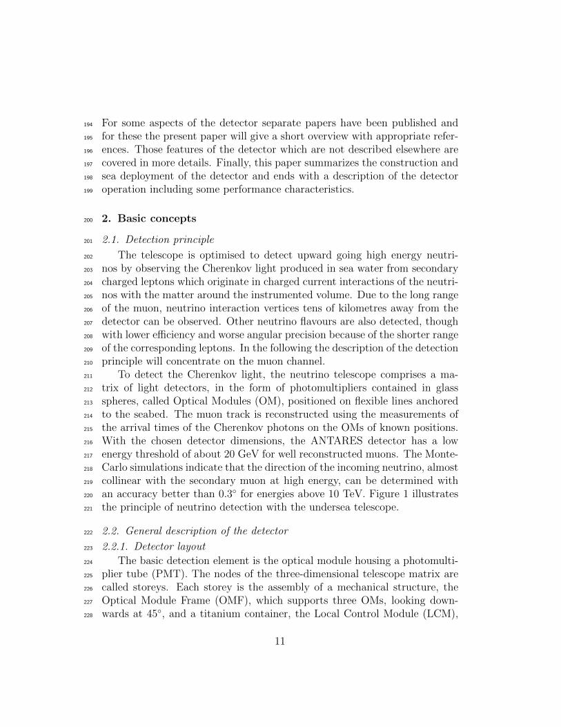
when relevant, the assembly process.421

3.1.2.1. Photomultiplier tube.422

In the R&D phase, an extensive series of tests were performed on several423

commercially available models of large hemispherical photomultipliers. A424

summary of this study is presented in [11]. The R7081-20, a 10” hemispheri-425

cal tube from Hamamatsu12, was chosen. The full sample of delivered PMTs426

has been tested with a dedicated test bench in order to calibrate the sensors427

and to check the compliance with the specifications. The number of rejected428

12Hamamatsu Photonics, Electron tube division, http://www.hamamatsu.com

19

Figure 4: Schematic view of an optical module

tubes was small (17, their peak/valley ratio being too low), these tubes were429

replaced by the manufacturer. To illustrate the homogeneity of the produc-430

tion, Figure 5 shows the measured values of dark noise rate (top) and of the431

peak/valley ratio (bottom). During the testing process, the working point of

Figure 5: Results of dark count rate (top) and peak/valley ratio (bottom) for the full setof tested PMTs.

432

each PMT, i.e. the high voltage needed to obtain a gain of 5× 107 ± 10 %,433

was determined by measuring the value of the SPE pulse height. The results434

20

of these measurements are illustrated in Figure 6.

Figure 6: Measured mean pulse height of single photoelectrons for each PMT at nominalgain.

435

3.1.2.2. Glass sphere.436

The protective envelope of the PMT is a glass sphere of a type rou-437

tinely used by sea scientists for buoyancy and for instrument housing. These438

spheres, because of their mechanical resistance to a compressive stress and of439

their transparency, provide a convenient housing for the photodetectors. Ta-440

ble 1 summarizes the main characteristics of the Vitrovexr glass spheres13441

used. The sphere is provided as two hemispheres: one, referred to as “back

Outer diameter 432 mm (17”)

Wall thickness 15 mm

Type of glass Borosilicate

Refractive index 1.47

Light transmission above 350 nm >95%

Density 2.23 g cm−3

Pressure of qualification test 700 bar (70 MPa)

Diameter shrinking at 250 bar 1.25 mm (0.3%)

Absolute internal air pressure 0.7 bar (70 kPa)

Hole diameters 20 mm, 5 mm

(penetrator and vacuum port)

Table 1: Data on the OM glass sphere.

13Nautilus Marine Service GmbH, http://www.nautilus-gmbh.de

21

442

hemisphere” is painted black on its internal surface and the other, “front443

hemisphere” is transparent. The front hemisphere houses the PMT and the444

magnetic shielding held in place by the optical gel. The back hemisphere445

has two drilled holes to accommodate the electrical connection via a pene-446

trator and a vacuum port. Around both holes a flat surface is machined on447

the outside of the sphere for the contact of the single O-ring ensuring water448

tightness. The back hemisphere is also equipped with a manometer readable449

from the outside. The two glass halves have precisely machined flat equato-450

rial surfaces in direct contact (glass/glass) without any gasket or interface.451

The risk of implosion and the consequences on the structure were consid-452

ered since its potential energy is of the order of a megajoule (200 g of TNT)453

at the depth of the detector. Based on tests performed by DUMAND [12]454

and further tests performed off Corsica in the year 2000 by the ANTARES455

Collaboration, it has been concluded that the implosion of a glass sphere at456

the ANTARES depth would provoke the loss of the two other spheres of the457

same storey (at centre distances of 770 mm) but not of spheres on adjacent458

storeys (at a distance of 14.5 m), and would not cut or damage the cable.459

The rigid storey mechanical frame would be distorted but not destroyed by460

the implosion.461

3.1.2.3. Optical gel.462

The optical coupling between the glass sphere and the PMT is achieved463

with optical gel. The chosen gel is a two-component silicon rubber provided464

by the Wacker company14. The mixture of the components is made in the465

ratio 100:60. After curing and polymerization, lasting 4 hours at ambient466

temperature, the optical gel reaches an elastic consistency soft enough to467

absorb the sphere diameter reduction by the deep sea pressure (1.2 mm)468

and stiff enough to hold the PMT in position in the sphere. The optical469

properties of the gel have been measured in the laboratory: the absorption470

length is 60 cm and the refractive index is 1.404 for wavelengths in the blue471

domain.472

3.1.2.4. Magnetic shield.473

At the ANTARES site, the Earth’s magnetic field has a magnitude of474

approximately 46 µT and points downward at 31.5 from the vertical. Un-475

14Silgel 612 A/B; Wacker-Chemie AG, http://www.wacker.com

22

corrected, the effect of this field would be a significant degradation of the476

TTS, of the collection efficiency and of the charge amplification of the PMT.477

A magnetic shield is implemented by surrounding the bulb of the PMT with478

a hemispherical grid made of wires of µ-metal15 closed by a flat grid on the479

rear of the bulb. This provides a magnetic shielding for the collection space480

and for the first stages of the amplification cascade. The efficiency of the481

screening becomes larger as the size of the mesh is reduced and/or the wire482

diameter is increased, however the drawback is a shadowing effect on the483

photocathode. The compromise adopted by the ANTARES Collaboration, a484

mesh of 68 × 68 mm2 and wire diameter of 1.08 mm, results in a shadowing485

of less than 4 % of the photocathode area while reducing the magnetic field486

by a factor of three. Measurements performed in the laboratory show that487

this shielding provides a reduction of 0.5 ns on the TTS and a 7 % increase488

on the collected charge with respect to a naked, uniformly illuminated PMT.489

3.1.2.5. HV power supply.490

To limit the power consumption of the HV power supply a high voltage491

generator based on the Cockroft-Walton [13] scheme is adopted. The HV492

generator chosen for the ANTARES detector is derived from the model de-493

veloped for the AMANDA experiment16, and is manufactured by the iseg494

company17. It has two independent high-voltage chains. The first chain495

produces a constant focusing voltage (800 V) to be applied between photo-496

cathode and first dynode. The second chain gives the amplification voltage,497

which can be adjusted from 400 V to 1600 V by an external DC voltage.498

The HV generator is powered by a 48 V DC power supply and has a typical499

consumption of 300 mW.500

The signals of the anode, of the last dynode and of the last-but-two dyn-501

ode of the PMT are routed to the electronics container together with the502

PMT ground. A low level voltage image of the actual HV is provided for503

monitoring purpose.504

3.1.2.6. Internal LED.505

On the rear part of the bulb of the PMT, a blue LED is glued in such506

a way to illuminate the pole of the photocathode through the aluminium507

15Sprint Metal, Ugitech, http://www.ugitech.com16http://icecube.wisc.edu/17PHQ7081-20; iseg Spezialelektronik GmbH, http://www.iseg-hv.de

23

coating, which acts as a filter of large optical density (optical density ≈ 5).508

This LED is excited by an externally driven pulser circuit and is used to509

monitor the internal timing of the OM.510

3.1.2.7. Link with the electronics container.511

The electrical connection of the OM to the electronics container is made512

with a penetrator18 (Ti socket with polyurethane over moulding). The as-513

sociated cable contains shielded twisted pairs for the transmission of power,514

the control of the LED pulser and the setting and monitoring of the DC515

command voltage of the PMT base. One pair is used to transmit the an-516

ode and the last dynode signals. This pseudo differential transmission pair517

has the advantage of reducing the noise and enhancing the output signal by518

approximately a factor of two when the subtraction is done at the readout519

electronics. The last pair is used to transmit signals from the last-but-two520

dynode, together with the ground, for the treatment of very high amplitude521

signals.522

3.1.2.8. Final assembly and tests.523

The assembly starts with the pouring of the gel into the front hemisphere524

and a precise sequence of out-gasing is applied in order to avoid the appear-525

ance of bubbles during the polymerization phase. Then, the cage and the526

PMT are positioned by tools which ensure a defined position with respect527

to marks on the hemisphere. These marks are also used to mount the OM528

on its support structure, giving each PMT a well-defined and reproducible529

orientation with respect to the storey mechanical structure.530

After the gluing of the LED, the cabling of the base to the pig-tail of the531

penetrator and the connection of the PMT, the back hemisphere is placed532

in contact with the front one. Closure is obtained by establishing an un-533

derpressure of ≈ 300 mbar inside the sphere. The equatorial seam is sealed534

externally with butyl rubber sealant which is protected by a sealant tape.535

Figure 7 shows an assembled OM. The same test bench as for the naked536

PMT is used to test the OM. Dark count rate, gain and LED functionality537

are checked.538

18EurOceanique S.A., part of MacArtney Underwater Technology,http://www.macartney.com

24

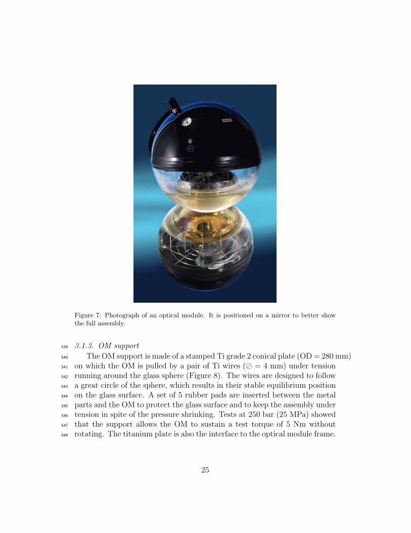
Figure 7: Photograph of an optical module. It is positioned on a mirror to better showthe full assembly.

3.1.3. OM support539

The OM support is made of a stamped Ti grade 2 conical plate (OD = 280 mm)540

on which the OM is pulled by a pair of Ti wires ( = 4 mm) under tension541

running around the glass sphere (Figure 8). The wires are designed to follow542

a great circle of the sphere, which results in their stable equilibrium position543

on the glass surface. A set of 5 rubber pads are inserted between the metal544

parts and the OM to protect the glass surface and to keep the assembly under545

tension in spite of the pressure shrinking. Tests at 250 bar (25 MPa) showed546

that the support allows the OM to sustain a test torque of 5 Nm without547

rotating. The titanium plate is also the interface to the optical module frame.548

25

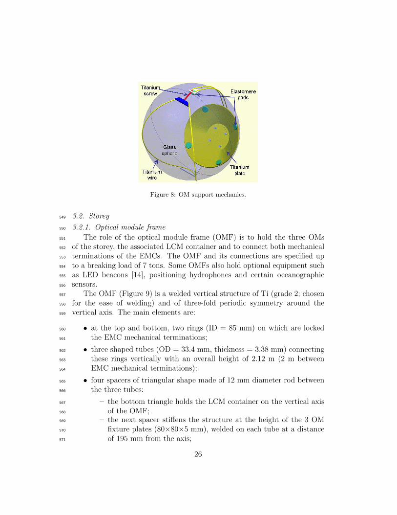
Figure 8: OM support mechanics.

3.2. Storey549

3.2.1. Optical module frame550

The role of the optical module frame (OMF) is to hold the three OMs551

of the storey, the associated LCM container and to connect both mechanical552

terminations of the EMCs. The OMF and its connections are specified up553

to a breaking load of 7 tons. Some OMFs also hold optional equipment such554

as LED beacons [14], positioning hydrophones and certain oceanographic555

sensors.556

The OMF (Figure 9) is a welded vertical structure of Ti (grade 2; chosen557

for the ease of welding) and of three-fold periodic symmetry around the558

vertical axis. The main elements are:559

• at the top and bottom, two rings (ID = 85 mm) on which are locked560

the EMC mechanical terminations;561

• three shaped tubes (OD = 33.4 mm, thickness = 3.38 mm) connecting562

these rings vertically with an overall height of 2.12 m (2 m between563

EMC mechanical terminations);564

• four spacers of triangular shape made of 12 mm diameter rod between565

the three tubes:566

– the bottom triangle holds the LCM container on the vertical axis567

of the OMF;568

– the next spacer stiffens the structure at the height of the 3 OM569

fixture plates (80×80×5 mm), welded on each tube at a distance570

of 195 mm from the axis;571

26

Figure 9: OMF equipped with the 3 OMs, the LCM and an LED beacon. The mechanicalparts used for fixing cables toward the upper and the lower storeys are omitted.

– the two top spacers are used to hold the optional LED beacon.572

All OMFs were validated by applying a traction load of 80 kN, which is573

in fact higher than the load resulting from the design rule of 7 tons.574

3.2.2. Local control module575

3.2.2.1. Container.576

The housing of the readout electronics is a Ti grade 5 container made577

of a hollow cylinder (600 mm long, 179 mm outer diameter and 22 mm578

wall thickness) closed by two end caps (30 mm thick). The top end cap579

accommodates the two large penetrators of the EMC linking the storey to580

its upper and lower adjacent storey. The bottom end cap accommodates581

three connectors linking the LCM to its three optical modules. In some of582

the LCMs, a 4th connector is needed for additional equipment. The fixation583

of the end caps on the cylinder and of the whole container on the OMF is584

27

made with three external threaded rods of 6 mm diameter in Ti grade 2.585

The thickness of the cylinder and of the end-caps was optimised by Finite586

Element Method analysis with the goal to stay within the yield strength587

of the material at an external pressure of 310 bars. The calculations were588

tested by the collapse under pressure of an Al alloy container of the same589

configuration. Ti grade 5 was chosen for its yield strength around 900 MPa,590

compared to that of grade 2 which is around 300 MPa.591

3.2.2.2. Electronics.592

In order to optimally fill the cylindrical volume offered by the container,593

a dedicated crate was developed. This crate accepts circular shaped printed594

circuit boards plugged on a backplane which distributes the signals as well595

as the DC power supplied by the local power box. The crate was designed596

to ensure that its mechanical structure acts as a medium that transfers the597

heat produced by the electronics to the Ti cylinder in contact with the water.598

After evaluating different metals, the final choice was made for aluminium599

which can guarantee good performance with light weight and at an affordable600

price. Furthermore, boards having high power consumption are equipped601

with metal cooling bases which are in thermal contact with the crate.602

Most of the LCMs contain the same set of electronics cards. However, due603

to the segmentation of a line in sectors, one in five LCMs, called Master LCM604

or MLCM, acts as a master for other LCMs of the same sector and houses605

additional boards. Other differences between individual LCMs are due to606

electronics necessary for optional equipment on the storey (hydrophone, LED607

beacon, ...).608

A standard LCM contains the following elements:609

• LPB. Fixed on the crate, the local power box is fed by the 400 V DC610

from the bottom of the line, and provides the 48 V for the optical611

modules and several different low voltages for the electronics boards.612

An embedded micro-controller allows the monitoring of the voltages,613

the temperatures and the current consumptions as well as the remote614

setting of the 48 V for the OMs.615

• CLOCK. The clock reference signal coming from shore reaches the bot-616

tom of the line where it is repeated and sent to each sector. Within617

a sector, the clock signal is daisy-chained between LCMs. The role of618

the CLOCK card is to receive the clock signal from the lower LCM,619

to distribute it on the backplane and to repeat it toward the upper620

28

LCM of the sector. It also has the capability to pass commands on the621

backplane which are coded within the clock signal.622

• ARS MB (Figure 10). The ARS motherboards host the front-end elec-623

tronics of the OMs (one board per OM). This front-end electronics con-624

sists of a custom-built Analogue Ring Sampler (ARS) chip [9] which

Figure 10: The ARS MB board with the 2 ARSs (labelled 16 and 15). The 3rd one (topright, labelled 12) is foreseen for trigger purposes.

625

digitizes the charge and the time of the analogue signal coming from626

the PMTs, provided its amplitude is larger than a given threshold.627

The level of this threshold is tuneable by slow-control commands. The628

analogue signal is integrated by an AVC (Amplitude to Voltage Con-629

verter) to obtain the charge which is digitized by an ADC. The ARS630

can also operate like a flash-ADC using analog memories with a sam-631

pling tuneable down to sub-nanosecond values. The output consists of632

a waveform of 128 amplitude samples. The arrival time is determined633

from the signal of the clock system in the LCM and from a TVC (Time634

to Voltage Converter) which provides a sub-nanosecond resolution. To635

minimise the dead time induced by the digitization, each ARS MB card636

is equipped with 2 ARSs working in a token ring scheme. For a storey637

with an optical beacon, a 4th ARS MB is installed to digitize the signals638

sent by the internal PMT of the beacon.639

29

• DAQ/SC (Figure 11). The DAQ/Slow-Control card host the local pro-640

cessor and memory. The processor is a Motorola MPC860P which641

runs the VxWorks real time operating system19 and hosts the software642

processes [8]. These processes are used to handle the data from the643

ARS chips and from the slow control, respectively. The processor has644

a fast Ethernet controller (100 Mb s−1) that is optically connected to645

an Ethernet switch in the MLCM of the corresponding sector. Three

Figure 11: The DAQ/SC board holding the processor (centre), the FPGA (left) and theoptical link to the MLCM (right).

646

serial ports, two with RS485 links and one with RS232 links, using the647

MODBUS protocol20 are used to handle the slow control signals. The648

specific hardware for the readout of the ARS chips and data format-649

ing is implemented in a high density field programmable gate array21.650

The data are temporarily stored in a high capacity memory (64 MB651

SDRAM) allowing a de-randomisation of the data flow.652

• COMPASS MB (Figure 12). The compass motherboard hosts a TCM22653

sensor which provides heading, pitch and roll of the LCM (i.e. of the654

19Wind River, http://www.windriver.com20http://www.modbus.org21Virtex-EXCV1000E, http://www.xilinx.com22PNI Sensor Corp., http://www.pnicorp.com

30

OMF) used for the reconstruction of the line shape and PMT positions.655

The heading is measured with an accuracy of 1 over the full cycle and656

the tilts with an accuracy of 0.2 over a range of ±20. The same657

card supports two micro-controllers dedicated to the slow control: they658

control the measurements of various temperatures and the humidity,659

and set and monitor the PMT high voltages.

Figure 12: The COMPASS MB equipped with a TCM2 sensor on a raised daughter card.

660

For LCMs performing acoustic functions (cf. Section 3.8), there are three661

additional cards: one housing a pre-amplifier, one a CPU and the third a662

digital signal processor. These cards are commercial products from ECA23,663

re-shaped to fit in the crate.664

An MLCM holds the following additional cards:665

• BIDICON. It communicates via bi-directional optical fibres with the666

four other LCMs of the sector, and performs the electrical↔optical con-667

version of signals transmitted via the backplane to or from the SWITCH668

card.669

• SWITCH. An Ethernet switch which consists of a combination of eight670

100 Mb s−1 ports and two 1 Gb s−1 ports24. One of the 100 Mb s−1 ports671

is connected to the processor of the MLCM and four to the BIDICON672

card via the backplane. One of the two Gb s−1 ports is connected to a673

Dense Wavelength (De)-Multiplexer (DWDM) transceiver.674

23ECA S.A., http://www.eca.fr24Allayer AL121 and AL1022 respectively.

31

• DWDM (Figure 13). The role of the transceiver is to perform the675

electrical↔optical conversion for the full sector and to communicate676

with the shore via the SCM located at the bottom of the line. It677

is electrically connected to the SWITCH card via coaxial cables and678

optically to the SCM via two uni-directional optical fibres (Rx and Tx)679

at a connection speed of 1 Gb s−1. For each MLCM (i.e. sector) of a680

line, the laser mounted on the card has a specific frequency chosen in681

the range from 192.1 to 194.9 THz, the frequency spacing being 400682

GHz.

Figure 13: The DWDM board.

683

Figure 14 shows an MLCM crate equipped with the full set of the elec-684

tronics cards. A description of the components in the SPM/SCM container685

will be given later in the BSS Section 3.4.3.686

3.3. Electro-optical mechanical cable (EMC)687

The EMC cable has three roles:688

• optical data link: 21 single mode optical fibres (=9/125/250 µm) run689

along the cable;690

• power distribution: 9 electrical conductors (Cu section = 1 mm2 with691

insulation = 2.5 mm);692

• mechanical link: breaking tension above 177 kN.693

32

Figure 14: The crate of an MLCM equipped with the electronics boards.

To facilitate the line handling and deployment with its cumulative length694

of ≈ 480 m, the minimal allowed radius of curvature of the cable was specified695

to be less than 300 mm (180 mm for the naked core).696

The cable, developed under the responsibility of EurOceanique18 is assem-697

bled in successive layers as shown in Figure 15. The two internal layers are

ARAMID BRAID

FILLING BODY

CONDUCTOR

FIBRE TUBE

PU

LDPE

Figure 15: Cross section of the EMC. From centre to outside one can distinguish the layerwith 3 tubes, each housing 7 optical fibres, the layer with 9 copper conductors, the LDPEjacket, the aramid braid and the polyurethane sheath. The external diameter is 30 mm.

698

assembled with silicon compound filling the space between the elements. Wa-699

ter can penetrate through the 2 external layers, while the inner polyethylene700

jacket acts as a water barrier. The polyurethane (PU) sheath is in contact701

33

with the water. Its role is to protect the aramid braid and the cable be-702

fore and during deployment. The two outer layers end inside the mechanical703

termination where the aramid braid is firmly held by a cone locking-system704

and the rest of the cable, called the “core”, continues for a few meters to705

the LCM penetrators. Each section sustained a static test tension of 50 kN.706

During this test, the insulation of electrical conductors and the attenuation707

on the optical fibres are controlled. The cable length between the mechanical708

terminations is 98 m for the bottom cable section and 12.5 m for the 25 other709

sections of a line (including the passive section linking the top storey to the710

buoy), resulting in a pitch between optical modules of 14.5 m. The actual711

length of each section delivered was measured under a tension of one ton,712

with an accuracy of ±5 mm, and the results were recorded in a database as713

input to the line shape reconstruction. Figure 16 gives a schematic view of714

the top and bottom mechanical terminations and their PU bending limitors.715

TOP BOTTOM

EMCCore

Bending limitor(PU)

Locking grooveCore EMC

holding pointDeployment hook

(PU)Bending limitor

Locking groove

Figure 16: Mechanical termination of an EMC.

716

Two different types of LCM penetrators are mounted at the ends of the717

core: a pair of water-blocking (WB) penetrators for the sections located718

between sectors and a less expensive pair of non-water-blocking (NWB) pen-719

34

etrators elsewhere. In case of a flooded cable, the WB type stops the prop-720

agation of the water along the cable and thus limits the flooded part of the721

line to one sector (the WB penetrator only stops water propagation from the722

cable to the container and not in the opposite direction). Figure 17 gives723

a schematic view of the NWB penetrator (left) and of the WB penetrator724

(right). In both cases, the fibre tubes are mechanically blocked in an epoxy725

moulding, itself blocked in the penetrator body to avoid extrusion when the726

cable is subject to water pressure.

Figure 17: EMC penetrators of the LCM container. Left: non water blocking. Right:water blocking. For clarity, the 3rd fibre tube and the 9 conductors are not shown.

727

When subjectted to a uniform horizontal sea current, as present at the728

ANTARES site, the 3-fold periodic symmetry of the storey induces a torque729

which is a function of the actual azimuth of the storey. The storey is in stable730

equilibrium when one of the three OMs is upstream of the current. From731

measurements performed in a pool, the torque was found to be proportional732

to the square of the current with a proportionality constant of 9.47 N s2 m−1.733

Between two adjacent storeys, the EMC acts as a torsion spring tending to734

keep them at the same relative angle. This torque was measured as a function735

of the cable tension on a prototype and found to be proportional to the736

cable torsion angle per unit length and to the tension with a proportionality737

constant of 1.3 × 10−3 m2 rad−1. In order to specify the minimum torsion738

strength of the cable, the torsion behaviour of the line was simulated using739

the above data and for very unfavorable environmental conditions: uniform740

35

sea current at 30 cm s−1 slowly increasing in the azimuth angle for several741

turns. The resulting specification was a maximum torsion angle change per742

unit length of ± 45 m−1.743

3.4. Bottom string structure744

The function of the BSS (Figure 18) is to anchor the line to the seabed745

with the capability of a recovery. The BSS is made of two parts: an unre-746

coverable dead weight laid on the seabed and a recoverable part sitting on747

top. The two parts are connected by a release system remotely controlled by748

acoustic signals.

Figure 18: The ANTARES Bottom String Stucture.

749

3.4.1. Dead weight750

The dead weight is a horizontal square plate made of 50 mm thick carbon751

steel. The line stability requires a dead weight of 1270 kg in water, which752

means 1.5 tons of steel. Therefore, the dimension of the square side is 1.8 m,753

resulting in a ground pressure of 4 kPa, while the seabed is believed to754

sustain safely a pressure up to 5 kPa. Four steel “wings” are welded below755

the square plate to improve the anchoring in the seabed sediment. The total756

wet surface of steel is 9.5 m2. To avoid the galvanic corrosion of this large757

surface in contact with the sea water, 9 plates of Al-Zn-In alloy, the so-called758

36

sacrificial anodes25, are welded on the steel surface with a total mass of 68 kg.759

The line is linked to the junction box by the interlink cable (IL), an760

electro-optical cable laying on the seabed and connected to the line at the761

level of the BSS by an underwater mateable connector:, developed by ODI762

company26.763

The remote line release implies an automatic disconnection system for764

the IL cable: the plug of the IL is fixed to the dead weight while the socket765

is located on the recoverable part of the BSS, at the end of a pivoting arm in766

such a way that it is extracted from the plug at the beginning of the ascent.767

In order to slow down the speed of extraction (≤ 5 cm s−1 as recommended768

by the manufacturer) and to guide the disconnection phase of the ascent,769

two vertical damping systems are mounted between the two parts of the770

BSS: a pair of pistons on the dead weight matching a pair of cylinders on the771

recoverable part. These parts are in LDPE and/or PETP, the piston has a772

diameter of 150 mm and a used height of 670 mm. The damping effect was773

adjusted in pool tests. Finally, the piston/cylinder gap was set to 0.8 mm774

and a set of grooves was machined along the pistons to avoid suction effect775

in water and water inlets were drilled through the cylinder.776

3.4.2. Release system777

The BSS holds two lithium battery powered transponders27 in Ti cylinders778

which are equipped with release mechanism. The releases are mounted on the779

recoverable part of the BSS in a redundant system which includes a chain,780

made of Ti and steel, engaged inside a steel part belonging to the dead weight.781

The chain is pre-tensioned to avoid a gap between the two components of782

the BSS. The acoustic beacon capability of the transponders is employed783

in the Low Frequency Long Baseline (LFLBL) positioning and navigation784

system to monitor the position of the line anchor during its deployment and785

to determine its geodetic location with a precision of ≈ 1 m.786

3.4.3. Recoverable part787

In addition to the already mentioned transponders, the recoverable part788

of the BSS holds various equipment:789

25BAC Corrosion Control A/S, http://www.bacbera.dk26Ocean Design Inc. (ODI), http://www.odi.com27Type RT 861 B2T; IXSEA/Oceano, http://www.ixsea.com

37

• a 1.8 m long Ti container housing the power module and the control790

electronics (SPM/SCM) of the line;791

• a high resolution pressure meter, used for line positioning;792

• an acoustic transceiver at the top of a 3.6 m long rod of glass-epoxy,793

used as a reference emitter for the High Frequency Long Base Line794

(HFLBL) positioning system;795

• optional sound velocimeter, laser beacon, seismometer depending on796

the line [15];797

• a weight to keep the line vertical and under enough tension after release,798

even when the buoy reaches the sea surface.799

The recoverable part of the BSS is a welded Ti (grade 2) structure sitting800

on top of a square steel weight (950 mm side length and 160 mm thickness)801

of 1140 kg total mass (9.6 kN weight in water) and with 2.5 m2 wet surface802

of steel. Depending on the actual equipment of the line, this mass is ad-803

justable by a set of steel plates welded on the weight. The steel parts are804

anode protected in the same way as the dead weight, with three anodes with805

a total mass of 30 kg. After two years of immersion of prototypes, the anode806

consumption rate was measured to be ≈ 300 g per year and per square meter807

of wet steel. This value can be extrapolated to an approximate lifetime of808

the anodes of 40 years.809

The SPM/SCM electronics container is the assembly of two cylinders sim-810

ilar to those of the LCMs and is fixed vertically on the structure (Figure 18).811

The SPM part, at the top, contains transformers/rectifiers which deliver the812

five 400 V DC supplies needed for the sectors, starting from the 480 V AC813

provided by the junction box. An embedded micro-controller operates the re-814

mote powering of sectors. Voltages, temperatures and current consumptions815

are monitored. The micro-controller can also detect anomalies and is pro-816

grammed to turn off the power in case of over-consumption. Like a standard817

LCM container, the SCM cylinder houses a crate equipped with COMPASS,818

CLOCK and DAQ cards. In order to perform the distribution of the clock819

signal to the sectors, the SCM crate houses specific boards called:820

• SCM WDM (Wavelength Division Multiplexing) (Figure 19) which re-821

ceives the 20 MHz clock signal via an optical link from the shore and822

converts it to an electrical signal which is distributed on the backplane.823

For redundancy, the clock is transmitted on two fibres from the shore824

38

and in case of failure of one fibre, the WDM card automatically switches825

to the other.

Figure 19: The SCM WDM board.

826

• REP: its role is to operate the reverse conversion. It is equipped with827

three fibre outputs and two such cards are needed to distribute the828

clock signals to the five sectors.829

To communicate with the shore, the SCM is equipped with a DWDM830

board similar to the MLCM one but working at 100 Mb s−1 and using its own831

DWDM channel. The pair of fibres of this DWDM is connected, as well as832

the 5 pairs of fibres coming from the sectors to 6 channels of a 1-to-8 passive833

optical mux/demux28 performing the merging/separation of the 6 colours.834

The BSS being equipped with an acoustic transceiver, the appropriate cards835

are present in the SCM crate.836

3.5. Top buoy837

The top buoy29 is made of syntactic foam qualified for a depth of 3000 m838

and with a density around 0.5 g cm−3. The foam is moulded into an oval839

shape (horizontal diameter = 1347 mm, height = 1530 mm) with a hole along840

the vertical axis where a Ti rod is inserted. The buoy is held on the rod by841

28Multi-Channel Mux/Demux Module 400 GHz spacing; JDS Uniphase Corp.,http://www.jdsu.com

29TRELLEBORG CRP, http://www.trelleborg.com/en/offshore

39

a pair of Ti disks. The last EMC section is fixed on the bottom end of this842

rod and, for the deployment, a releasable transponder is fixed to the top end.843

The mass of the equipped buoy is 782 kg and its buoyant force 6.7 kN.844

3.6. Mechanical behaviour of a line845

Three rules govern the stability of a line.846

1. The line must remain firmly anchored on the seabed and must be held847

close to vertical even in the presence of the strongest sea current con-848

sidered (30 cm s−1). In all situations, the horizontal displacement of849

any part of the line must be smaller than the horizontal line spacing (60850

m) to avoid any possible contact between two lines. The fact that, in a851

uniform sea current, two adjacent lines will lean in the same direction852

gives an extra safety factor.853

2. The tension in the release chain while the line is on the seabed, must854

be above 4 kN in order to overcome any possible blocking of the release855

systems and in order to reach the surface in one hour or less.856

3. During the recovery, while the buoy is floating on the surface, the EMC857

tension must be above 2 kN everywhere along the line to allow a safe858

operation of an automatic hook system which must slide down along859

the EMC.860

The buoyancy is provided by the top buoy but also by the storeys, since861

each OM has a buoyant force of 0.22 kN. A sector of five storeys with their862

cables has a buoyant force of 1.42 kN. The weight is mainly provided by863

the BSS recoverable part and, until the release, its dead weight. The global864

recovery force is the small difference between two large quantities: the weight865

in air of the line (without the dead weight) which amounts to 5.5 tons and the866

weight of the sea water displaced by the line (6 tons). To limit the uncertainty867

on this force to 10%, a measurement of the mass and of the volume of all the868

line components within 0.5% is required. Table 2 summarises the resulting869

tension along the line for three static periods of the life of a line without sea870

current:871

• during the deployment, held by the deep sea cable of the surface boat872

(maximum stress conditions);873

• in operation on the seabed (rule 2 above applies);874

• during the recovery, while the buoy floats at the surface (rule 3 applies).875

40

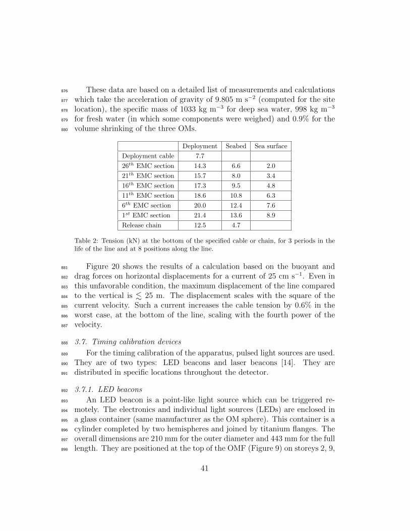
These data are based on a detailed list of measurements and calculations876

which take the acceleration of gravity of 9.805 m s−2 (computed for the site877

location), the specific mass of 1033 kg m−3 for deep sea water, 998 kg m−3878

for fresh water (in which some components were weighed) and 0.9% for the879

volume shrinking of the three OMs.880

Deployment Seabed Sea surface

Deployment cable 7.7

26th EMC section 14.3 6.6 2.0

21th EMC section 15.7 8.0 3.4

16th EMC section 17.3 9.5 4.8

11th EMC section 18.6 10.8 6.3

6th EMC section 20.0 12.4 7.6

1st EMC section 21.4 13.6 8.9

Release chain 12.5 4.7

Table 2: Tension (kN) at the bottom of the specified cable or chain, for 3 periods in thelife of the line and at 8 positions along the line.

Figure 20 shows the results of a calculation based on the buoyant and881

drag forces on horizontal displacements for a current of 25 cm s−1. Even in882

this unfavorable condition, the maximum displacement of the line compared883

to the vertical is . 25 m. The displacement scales with the square of the884

current velocity. Such a current increases the cable tension by 0.6% in the885

worst case, at the bottom of the line, scaling with the fourth power of the886

velocity.887

3.7. Timing calibration devices888

For the timing calibration of the apparatus, pulsed light sources are used.889

They are of two types: LED beacons and laser beacons [14]. They are890

distributed in specific locations throughout the detector.891

3.7.1. LED beacons892

An LED beacon is a point-like light source which can be triggered re-893

motely. The electronics and individual light sources (LEDs) are enclosed in894

a glass container (same manufacturer as the OM sphere). This container is a895

cylinder completed by two hemispheres and joined by titanium flanges. The896

overall dimensions are 210 mm for the outer diameter and 443 mm for the full897

length. They are positioned at the top of the OMF (Figure 9) on storeys 2, 9,898

41

Figure 20: Line shape for a sea current velocity of 25 cm s−1 velocity. The horizontal scaleis enhanced to better illustrate the line shape.

15 and 21 (numbering from the bottom storey) of each line. The pulsed light899

source is composed of 36 blue30 LEDs in groups of six on 6 printed circuit900

boards (Figure 21). These boards are assembled into a hexagon configuration901

and contain the pulser circuits and components to allow an individual tuning902

of the timing for each LED. The geometrical arrangement of the LEDs is such903

that the emitted light is almost isotropic in azimuth. The number of boards904

as well as the number of LEDs flashing can be varied. A pencil PMT31 sits905

in the centre of the hexagon and is exposed to the emitted light in order to906

provide the precise pulse time.907

30HLMP-CB15; Agilent Technologies Inc., http://www.agilent.com31H6780-03; Hamamatsu, http://www.hamamatsu.com

42

Figure 21: The electronic boards and light sources of an LED beacon.

3.7.2. Laser beacons908

Due to their positions, LED beacons are not efficient for the timing cal-909

ibration of the lowest storeys of the lines and between lines. Hence, they910

are complemented by light sources sitting on the BSS. However, because of911

the larger distances, the required light intensity demands the use of a laser.912

This laser32 is housed in a cylindrical titanium container 705 mm in length913

and 170 mm in diameter (Figure 22). Inside the container, an aluminium914

inner frame holds the laser and its associated electronics. The laser beam915

points upwards and leaves the container through a flat disk diffuser coupled916

by bonding to a quartz cylinder (n = 1.54). This output window configu-917

ration is needed in order to minimize transmission losses due to underwater918

sedimentation and biofouling which affect mainly horizontal surfaces. The919

actual time of laser emission is obtained from a fast photodiode integrated920

into the laser head. Two lines located in a central position in the detector921

are equipped with laser beacons.922

32NG-10120-120; Nanolase, presently part of JDS Uniphase Corp., http://www.jdsu.com

43

Figure 22: Components of the laser beacon.

3.8. Positioning devices923

Each ANTARES detector line is equipped with an acoustic transceiver924

(RxTx module) fixed on its anchor and receiving hydrophones (Rx modules)925

fixed on storeys 1, 8, 14, 19 and 25. There are five Rx modules per line, one926

is placed on the bottom storey and one on the top storey. The others are927

distributed in order to obtain a larger density of hydrophones in the top third928

part of the line, where the maximum curvature of the line shape is expected.929

The RxTx module is composed of a transducer (emitting and receiving hy-930

drophone) placed at the top of a pole on the line anchor and six electronic931

boards (preamplification, CPU, two DSPs, power, emission) integrated in932

the SCM. It emits the acoustic signals in emission mode and acts as an Rx933

module in reception mode. The Rx module is composed of a receiving hy-934

drophone placed on the storey and three electronic boards (preamplification,935

DSP, CPU) included in the LCM. Since the position measurements are based936

on the travel time of acoustic signals, the knowledge of the sound velocity in937

situ is mandatory: sound velocimeters are distributed on some lines. Data938

from these devices are used to reconstruct by triangulation the positions939

of the hydrophones. In order to obtain the optical modules positions, the940

following complementary information is used:941

• orientation of the OMFs provided by the COMPASS MB sitting in each942

LCM;943

• a model for the line shape, see Section 6.4.1.944

44

3.9. Instrumentation line945

The instrumentation line has evolved in time from the “MILOM” line946

[15], which was operational from March 2005 to June 2007 to the “IL07” line947

which has been operational since December 2007.948

This IL07 instrumentation line has six storeys of which three house el-949

ements of the acoustic detection system, which will be described in Sec-950

tion 3.10. The storeys of the line house various oceanographic instruments:951

Acoustic Doppler Current Profilers (ADCP) to monitor the intensity and di-952

rection of the underwater flow; a sound velocimeter to record the local value953

of the sound velocity; probes to measure the conductivity and temperature954

(CT) of the sea water; transmissiometers to monitor the light attenuation of955

the water (C-STAR); a dissolved oxygen sensor (O2) widely used by physical956

oceanographers to characterize mixing and ventilation of water masses and957

two cameras continuously connected in order to record images of biolumines-958

cent organisms. A schematic layout of the instruments on the line is shown959

in Figure 23 and details of the instruments are given in Table 3.960

StoreyHeightaboveseabed

Device type Manufacturer Model Measured parameters

6 305 m6 hydrophones HTI HTI-90-U sound level, transients

CTD SEABIRD SBE37-SMPconductivity, temper-ature

5 290 m

Optical module ANTARES custom light level

ADCP TeledyneRD Workhorse sea current velocity

Camera AXIS AXIS221 images

4 210 m

Transmissometer WETLabs C-Star water transparency

SV GENISEA/ECAQUUX-3A(A)

sound velocity

O2 probe AANDERAA Optode 3830 oxygen level

3 195 m6 hydrophones Erlangen custom sound level, transients

CTD SEABIRD SBE37-SMPconductivity, temper-ature

2 180 m6 hydrophones HTI HTI-90-U sound level, transients

Transmissometer WETLabs C-Star water transparency

1 100 m

Optical module ANTARES custom light level

ADCP TeledyneRD Workhorse sea current velocity

Camera AXIS AXIS221 images

BSS 0 mpressure sensor GENISEA/ECA pressure

Transponder IXSEA RT661B2T acoustic positioning

Table 3: List of the instruments on the line IL07.

45

Figure 23: The instrumentation line IL07. Elements are indicated schematically; notdrawn to scale.

3.10. Acoustic detection system AMADEUS961

The acoustic neutrino detection is integrated into ANTARES in the form962

of Acoustic Storeys (AS) which are modified standard storeys with the PMTs963

replaced by acoustic sensors with custom-designed electronics for signal pro-964

cessing. AMADEUS consists of six ASs, three of them located on the instru-965

mentation line and three on Line 12. Each AS comprises six acoustic sensors966

that are arranged at distances of roughly 1 m from each other. The ASs967

46

on the instrumentation line IL07 are located at 180 m, 195 m, and 305 m968

above the seabed, respectively. Line 12 is anchored at a horizontal distance969

of about 240 m from the IL07, with the ASs positioned at heights of 380 m,970

395 m, and 410 m. With this setup, the maximum distance between two ASs971

is 340 m.972

4. Detector infrastructure973

The infrastructure required to power and control the offshore detector974

includes the onshore buildings to house the electronics for monitoring and975

data acquisition, the main electro-optical cable providing the electrical power976

and the data link between the detector and the shore, the junction box and977

the interlink cables to distribute the power and the optical fibres to the 13978

lines.979

4.1. Interlink cable980

The connection between the JB and each line is provided by the inter-981

link cables. These cables, produced by the ODI company26, contain four982

monomode optical fibres and two electrical conductors. A complete link be-983

tween the JB and a line is composed of three parts: two short cables at each984

end (jumpers) and the IL itself as shown in Figure 24. Each jumper is termi-985

nated at one end by a penetrator equipped with a water blocking system and986

at the other end by a socket fixed on a strong mechanical structure. Whereas987

the mounting of the jumpers is performed on shore, the completion of the988

connection is realised by a Remotely Operated underwater Vehicle (ROV)989

which lays the IL on the seabed, plugs it on the JB side then on the line side.990

After each step of the connection operation, both the electrical and optical991

contacts are checked from shore to be within specifications.992

In order to compensate for failures experienced in some of the 16 out-993

puts of the JB, interlink cables of a special design are used in the seabed994

infrastructure. Each of these special cables connects two separate lines of995

the detector with one single JB output. Due to their particular shape, these996

cables are denoted as “Y” links. In this configuration, the cable coming from997

the JB is split and then linked to the two lines with the same system that is998

used for the other lines. The two connected lines share the power provided by999

the JB output. Their DWDM systems are tuned on two different frequency1000

domains. The splitting of the electrical conductors and the splicing of the1001

47

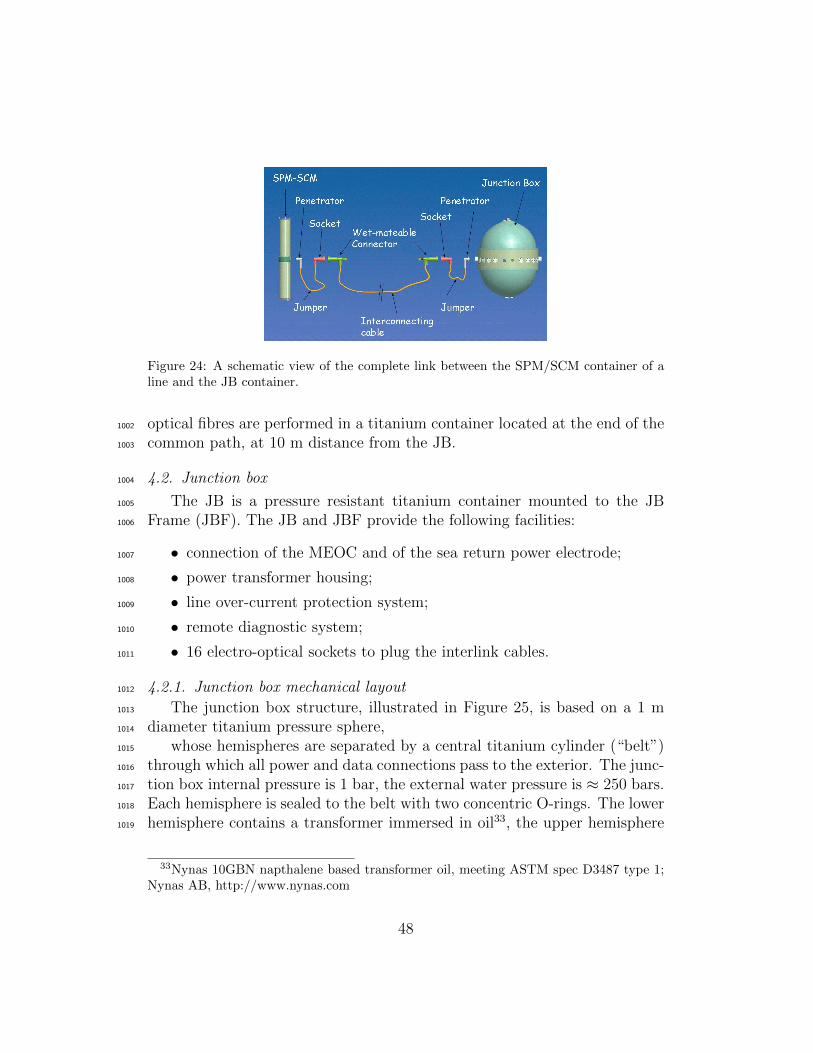
Figure 24: A schematic view of the complete link between the SPM/SCM container of aline and the JB container.

optical fibres are performed in a titanium container located at the end of the1002

common path, at 10 m distance from the JB.1003

4.2. Junction box1004

The JB is a pressure resistant titanium container mounted to the JB1005

Frame (JBF). The JB and JBF provide the following facilities:1006

• connection of the MEOC and of the sea return power electrode;1007

• power transformer housing;1008

• line over-current protection system;1009

• remote diagnostic system;1010

• 16 electro-optical sockets to plug the interlink cables.1011

4.2.1. Junction box mechanical layout1012

The junction box structure, illustrated in Figure 25, is based on a 1 m1013

diameter titanium pressure sphere,1014

whose hemispheres are separated by a central titanium cylinder (“belt”)1015

through which all power and data connections pass to the exterior. The junc-1016

tion box internal pressure is 1 bar, the external water pressure is ≈ 250 bars.1017

Each hemisphere is sealed to the belt with two concentric O-rings. The lower1018

hemisphere contains a transformer immersed in oil33, the upper hemisphere1019

33Nynas 10GBN napthalene based transformer oil, meeting ASTM spec D3487 type 1;Nynas AB, http://www.nynas.com

48

Figure 25: The junction box container and its support frame.

contains the power system slow control electronics. Following component1020

installation, the junction box sphere was qualified in a 24 hour pressure test1021

at 310 bar (20 % overpressure) in a 2.5 m diameter caisson10.1022

The sphere is supported within a rectangular titanium transit frame. The1023

cage incorporates an acoustic transponder to allow triangulation of the junc-1024

tion box position during deployment, an electrode for the return of the cur-1025

rent to shore, and an entry guide to protect the undersea cable from scuffing1026

during the deployment procedure and bending too sharply. In addition, it1027

is equipped with a plug board with 16 deep sea wet mateable electro-optical1028

sockets for the interlink cable connections. Figure 26 shows the junction1029

box on the deck of the deployment ship. The sphere, the cable penetrations1030

through the belt and the plug board of wet-mateable connectors are visible.1031

1032

4.2.2. Junction box cabling1033

The junction box is equipped with 16 outputs for connection of the de-1034

tection and instrumentation lines. The typical power drawn for a detection1035

line is around 1 kW. The junction box outputs are galvanically separated1036

through a transformer with 16 individual secondaries rated at 500 V. Two1037

additional windings rated at 240 V power the junction box internal slow1038

control systems. Each output is protected by a thermo-magnetic breaker341039

set to a 5 A threshold. In addition, each breaker can be rearmed or opened1040

34PKZ2/ZN6 with RE-PZK2 remote control block; Moeller, http://www.moeller.fr

49

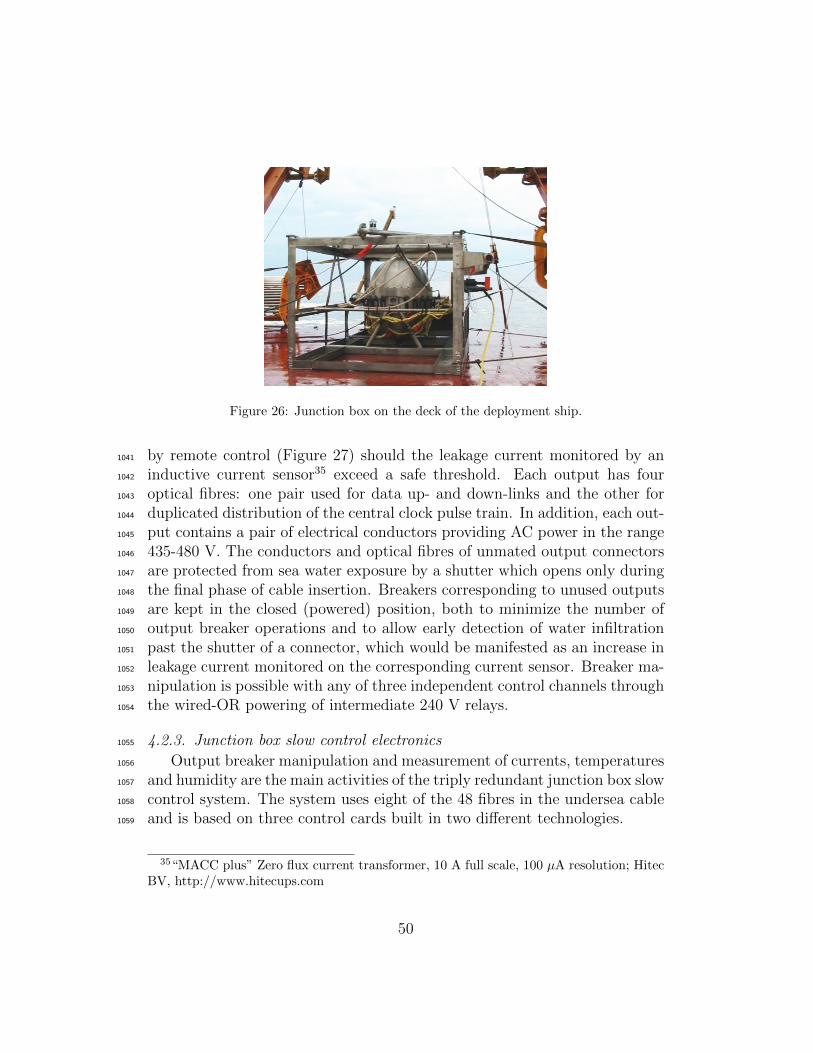
Figure 26: Junction box on the deck of the deployment ship.

by remote control (Figure 27) should the leakage current monitored by an1041

inductive current sensor35 exceed a safe threshold. Each output has four1042

optical fibres: one pair used for data up- and down-links and the other for1043

duplicated distribution of the central clock pulse train. In addition, each out-1044

put contains a pair of electrical conductors providing AC power in the range1045

435-480 V. The conductors and optical fibres of unmated output connectors1046

are protected from sea water exposure by a shutter which opens only during1047

the final phase of cable insertion. Breakers corresponding to unused outputs1048

are kept in the closed (powered) position, both to minimize the number of1049

output breaker operations and to allow early detection of water infiltration1050

past the shutter of a connector, which would be manifested as an increase in1051

leakage current monitored on the corresponding current sensor. Breaker ma-1052

nipulation is possible with any of three independent control channels through1053

the wired-OR powering of intermediate 240 V relays.1054

4.2.3. Junction box slow control electronics1055

Output breaker manipulation and measurement of currents, temperatures1056

and humidity are the main activities of the triply redundant junction box slow1057

control system. The system uses eight of the 48 fibres in the undersea cable1058

and is based on three control cards built in two different technologies.1059

35“MACC plus” Zero flux current transformer, 10 A full scale, 100 µA resolution; HitecBV, http://www.hitecups.com

50

Figure 27: Junction box output breaker management.

In the first of these, two identical cards communicate with the shore sta-1060

tion through 160 Mb s−1 links, using a transmitter/receiver chip set36 with1061

the Photon Techno PT5543-13-3-SC laser emitter and PT6143-155-SC re-1062

ceiver operating at 1550 nm. Associated firmware is embedded in FPGAs37.1063

Each card can simultaneously stream 16-bit digitized data from 48 inter-1064

nal temperature and humidity sensors, and 24-bit data at 2.6 kHz sampling1065

from a group of 4 “MACC plus” inductive current sensors. This latter data1066

is passed onshore to a DSP38 and used for sinusoid reconstruction and RMS1067

current calculation. A third card, designed for ultra-low power operation and1068

powered by lithium batteries39, is based on a microcontroller40 with 60 kbyte1069

flash and 2048 byte RAM memory equipped with eight 12-bit ADC entries1070

and 45 digital I/O ports. This card communicates,even in case of JB power1071

failure, at very low speed (1200 Baud) using an NDL7701 laser uplink oper-1072

ating at 1550nm and an LPD80 pin diode receiver. This channel has a power1073

consumption of 5µA in sleep mode and 60µA when active. When the uplink1074

is transmitting, the maximum power consumption of the card is 100 mA for1075

short periods.1076

A hermetic stainless steel diaphragm separates the lower transformer com-1077

36HDMP-1022/1024; Agilent Technologies Inc., http://www.agilent.com377256S; Altera Corp., http://www.altera.com38TMS320C5510 200 MHz; Texas Instruments, http://www.ti.com39Eight SAFT LSH20 Lithium elements of 3.6 V, 13 Ah each.40MSP430F149; Texas Instruments, http://www.ti.com

51

partment from the hemisphere containing the slow control system and fibre1078

optic routing devices. The electronics is mounted on an aluminium heat1079

sink disk (Figure 28) making thermal contact with the titanium belt of the1080

junction box. The diaphragm and heat spreader disk sandwich a thermal

Figure 28: View inside the open JB: heat-spreader disk, transformer connections andprimary circuit current sensor, passive fibre optic splitters and cassettes protecting fibrefusion splices.

1081

insulation blanket of silica aerogel41 which also serves as a getter for water1082

vapour.1083

4.2.4. Fibre optic signal distribution in the junction box1084

Each junction box output connector contains four optical fibres with the1085

following functions:1086

• DAQ Rxn (data downlink from shore; n=1→16);1087

• DAQ Txn (data uplink to shore; n=1→16);1088

• Clock channel A;1089

• Clock channel B.1090

DAQ Tx and Rx are specific to each line, and are accommodated using 321091

fibres in the undersea cable, which are point-to-point spliced in the junction1092

box hub to their respective fibres in the 16 output connectors.1093

41Spaceloftr; Aspen Aerogels Inc., http://www.aerogel.com

52

The central clock signal, vital for time referencing of photomultiplier data1094

to subnanosecond precision, is transmitted with a 4-fold redundancy. Pulse1095

trains from two independent, identical clock transmitters at the shore station1096

are split for broadcast on four undersea fibres. In the junction box they are1097

routed via dual-input 16-way passive splitters so that clock pulse trains from1098

either or both transmitters are available on every output connector. All1099

internal fibre connections are made by fusion splicing, resulting in an optical1100

loss of around 0.01 dB per joint. The laser diode intensity in the shore based1101

clock system is sufficient to maintain an optical power margin of 12 dB over1102

the attenuation in the undersea cable and passive splitters.1103

4.3. Main electro-optical cable1104

The main electro-optical cable provides the electrical power link and the1105

optical data link between the shore station and the detector. The selected1106

cable, a standard telecommunications type, satisfies the electrical and optical1107

transmission specifications as well as the environmental and mechanical cri-1108

teria such as temperature tolerance, bending radius and mechanical strength.1109

4.3.1. Cable1110

Prior to deployment of the MEOC, surveys by a ROV have been carried1111

out to select the best possible offshore site for the apparatus in terms of1112

flatness of the sea bottom and the absence of obstacles. The MEOC has1113

been deployed from the site to the shore by a specialized cable-laying ship1114

and crew under the responsibility of Alcatel. The cable was tested for op-1115

tical and power transmission prior to the deployment operation. Figure 291116

shows the structure of the different cable sections used at different depths1117

and Table 4 gives the main characteristics of the undersea cable42, which con-1118

tains 48 monomode optical fibres43 in a stainless steel tube surrounded by1119

a “pressure vault” of two windings of steel armour wires. A tubular copper1120

power conductor surrounds the vault and delivers current up to a maximum1121

of 10 A to the junction box. A standard undersea cable configuration with a1122

single conductor (normally used for series powering of repeaters in long-haul1123

cables) was chosen to minimize the cable cost and weight. The use of the sea1124

for current return reduces ohmic losses by a factor 4 compared with a cable1125

sharing equivalent cross-section between supply and return conductors.1126

42Alcatel URC3 Type 4 (unrepeatered); Alcatel-Lucent, http://www.alcatel-lucent.com43Type G24B DE 1302XB (BBO) WB B1, = 125 µm.

53

Figure 29: Sections of the undersea cable.

Electrical resistance 1 Ω km−1

Fibre attenuation 0.18 dB km−1

Fibre chromatic dispersion 21 ps nm−1 km−1

Table 4: Characteristics of the undersea cable.

On the deep, smooth seabed the cable exterior terminates in a 21 mm1127

diameter polyethylene sheath (“Light-Weight” configuration). An additional1128

polypropylene jacket (LWP) protects the cable in the zone of shelving seabed.1129

In shallower water with risk of damage from fishing or boat anchors, the cable1130

has an additional single layer of armour wires (SA) and a coating of tarred1131

polyurethane yarn. The final short section in very shallow water has an1132

additional armour layer (DA). This sequence with cable sections lengths and1133

water depths is summarized in Table 5. On the sea side, the cable terminates1134

in a titanium shell dry-mated electro-optical connector44 (Figure 30) mating1135

with a receptacle in the junction box belt. The overall weight of the deployed1136

cable is 88 tons for a total length of 41.3 km.1137

The central electrical conductor connects with the HV pole of the primary1138

winding of the junction box transformer. The LV pole returns the current1139

through an external sea electrode45 to the power hut, which has receiving1140

44SeaCon Europe Ltd, http://www.seaconbrantner.com45Titanium with Keramoxr coating, of length 1.6 m and diameter 40 mm; Magneto

54

LW Length 17.4 km

’Light-Weight’ Depth > 2300 m

LWP Length 10.2 km

’LW-Protected’ Depth 422 to 2300 m

SA Length 12.1 km

’Single Armoured’ Depth 27 to 422 m

DA Length 1.6 km

’Double Armoured’ Depth < 27 m

Table 5: Layout of the undersea cable.

Figure 30: Electro-optical plug and receptacle for connection of the undersea cable to thejunction box.

electrodes buried in the nearby ground.1141

4.3.2. Power supply to the junction box1142

Figure 31 illustrates the power system of the detector up to the outputs1143

of the junction box. The detector shore power supply draws 400 V 50 Hz1144

AC power from the electricity grid. The power supply located in a build-1145

ing (the Power Hut) near the cable landing beach raises the voltage to the1146

range 3700-4100 V for passage through the undersea cable to the junction1147

BV, http://www.magneto.nl

55

Figure 31: Power distribution system from the shore to the underwater junction box.

box. The voltage at the cable input is adjusted using a motor driven variable1148

transformer, depending on the load requirement (i.e. the number of lines to1149

be powered). The 50 Hz AC power system was chosen as the best compro-1150

mise for power delivery over the 42 km transmission length. Although direct1151

and indirect losses are increased relative to a DC system having the same1152

voltage and current limits, the AC option was preferred since it allows for1153

more reliable variation of the cable entry voltage, using passive (transformer)1154

elements. It also has a greater simplicity and reliability at the seabed distri-1155

bution node through the use of a transformer with multiple windings in the1156

junction box. The 9 µF cable capacitance needs to be compensated; this is1157

largely achieved through the use of a 1.4 H self inductance at the shore end1158

of the cable. The self inductance strongly reduces the reactive component1159

produced by the cable capacitance. The dissipation in the cable is there-1160

fore mostly resistive and corresponds to about 10% of the 36 kW (9.6 A at1161

3800 V) leaving the shore station.1162

4.4. Shore facilities1163

The onshore infrastructure consists of two separate buildings, the Shore1164

Station housing control and data management infrastructure and providing1165

space for onsite personnel, and the Power Hut devoted to power distribution1166

requirements. The shore station is situated at La Seyne-sur-Mer.1167

The building has three rooms dedicated to the operation of the ANTARES1168

experiment: a computer room, a control room, and a service room. The1169

56

computer room hosts the racks for the clock crate, the 13 onshore DWDM1170

crates (counterparts of the DWDM boards of the 13 lines) and the PC farm1171

for data filtering and storage. The control room contains various computers1172

for apparatus control and status monitoring.1173

The Power Hut is located near to the MEOC landing point at Les Sablettes,1174

and is connected to the latter with a fibre optical link 1.5 km long. The1175

Power Hut is connected to the 60 kVA, 400 V three-phase electrical distribu-1176

tion from Electricite de France. The building has been adapted to house the1177

transformer 400/4000 V, the MEOC to shore link rack as well as the return1178

current electrodes.1179

5. Construction1180

5.1. Generalities1181

The construction of the apparatus started in 2001 with the installation of1182

the long distance electro-optical cable. In late 2002 the underwater junction1183

box was installed; the deep sea end of the cable was recovered for this purpose,1184

the junction box dry connected to it, tested on the deck of the ship and finally1185

deployed. During the following years several prototype lines were installed1186

and operated in situ, allowing the validation and optimization of their design,1187

as well as the evaluation of possible long-term effects. The first detection line1188

was installed in early 2006 and the last two lines of the apparatus were put1189

into operation in May 2008. A European-wide effort was mobilized for the1190

construction of the detector. While all optical modules were assembled in just1191

one laboratory, the production of different mechanical parts and electronics1192

boards was performed by a number of laboratories in different countries.1193

A large effort was subsequently devoted to the assembly of the electronics1194

modules and of the complete lines. Three sites fabricated electronics modules1195

in order to feed two laboratories which worked independently on the assembly1196

of new lines. When running at full speed, two lines were produced every three1197

months.1198

Since the same integration tasks had to be performed at different sites,1199

special care was devoted to the development of dedicated tools, the definition1200

of detailed procedures and the distribution of the expertise among the differ-1201

ent teams, under a unified Quality Control approach. A coherent scenario of1202

tests to be performed at the different integration levels made it possible to1203

identify faulty components in order to avoid delays in the integration of the1204

57

lines. Logistics was an important issue; the Cellule Logistique of IN2P3461205

was used for managing the transportations.1206

5.2. Quality assurance and quality control1207

The organization of the Quality Assurance/Quality Control activities was1208

based on the methodologies defined by the rules of ISO 9001:200047, with an1209

effort to guarantee a high level of adaptability and flexibility. The construc-1210

tion project of ANTARES was structured as a set of processes performed by1211

an ensemble of institutes and persons under different authorities and respon-1212

sibilities. The flow of products to be assembled into the apparatus defined1213

the relationships between providers and clients, who could be located in-1214

side the same laboratory or at different sites. The specifications that each1215

product had to fulfil were carefully defined in written documents, all doc-1216

uments being stored in a centralised repository and accessible through a1217

password-protected website. Rules for proper management of the documen-1218

tation were defined, with different levels of approval established for the most1219

critical documents, such as the integration and test procedures. Problems1220

and changes in the organization were traced through appropriate documents:1221

a Non-Conformity Report was the tool used to report the problems found1222

at all levels in the construction of the apparatus. Improvements of the or-1223

ganization were sometimes defined after the treatment of such reports, and1224

implemented in response to a Design Change Request.1225

A key document for the construction of the apparatus was the Risk Anal-1226

ysis, whose output of served as the basis, first for the implementation of1227

detailed prototyping campaigns and later for the definition of the test cri-1228

teria to be adopted during the construction of the apparatus. A general1229

Quality Plan was then put in place, defining the main guidelines for Qual-1230

ity management in the Collaboration, and all laboratories participating in1231

the construction of the apparatus were required to define their local Quality1232

Plans. A Quality Plan was also required from the external providers at the1233

time of placing the orders.1234

A central database was used for collecting traceability information and,1235

when applicable, calibration data of all products, which were individually1236

identified by a bar-code label built according to a well defined Product Break-1237

down Structure of the apparatus and a serial number. Detailed information1238

46ULISSE, http://ulisse.in2p3.fr47http://www.iso.org/iso/catalogue detail?csnumber=21823

58

of which products were integrated in which parts of the apparatus was also1239

stored in this DB, so that all necessary information for the configuration of1240

the apparatus at the time of operation was immediately available.1241

A Local Quality Supervisor (LQS) was appointed at each laboratory par-1242

ticipating in the construction of the apparatus, with the general task to1243

ensure that the Quality rules were respected. A program of audit activities1244

was also set up for all laboratories in order to continually improve the system.1245

5.3. Assembly1246

5.3.1. Control module integration1247

Construction of the electronics modules required a very high level of reli-1248

ability since the failure of one module could lead to the loss of functionality1249

of a whole sector of a line.1250

The integration of the electronics modules was a delicate task because1251

of the design of the mechanical crate, the fact that electronics boards were1252

densely packed inside it and the need to have careful handling of optical fibres1253

at all times. Detailed procedures were therefore defined and dedicated tools1254

developed. A full functionality test was performed on all integrated modules1255

in order to find and cure all possible problems. Calibration of the front-end1256

electronics was also performed during these tests.1257

5.3.2. Line integration1258

Line integration took place at two different sites. The sharing of expertise,1259

the usage of the same tools and procedures and the respect of quality rules1260

ensured that the level of quality was the same in the two laboratories. This1261

was confirmed by a cross calibration between the two sites. The lines were1262

integrated from the bottom to the top. Optical splices were used on all optical1263

fibre connections for maximum reliability. Once a sector was completed,1264

a calibration in a dedicated dark room (or in dark boxes) for the optical1265

modules was performed. Simultaneously, the integration of a new sector1266

started. The purpose of the tests in the dark room was to verify the full1267

functionality of the sector, as well as to provide an initial time and charge1268

calibration for all optical modules in the final configuration of the line. A1269

calibration of the tiltmeters in each storey was also performed. Then, the1270

storeys were arranged on a line transportation pallet. The optical modules1271

were temporarily connected to their storeys for the tests, but were then1272

removed and transported separately from the line for maximum safety.1273

59

5.3.3. Deployment preparation1274

The final steps of integration took place in a dedicated hangar at the1275

port of La Seyne-sur-Mer. Here, a final functionality test of the lines was1276

performed. Then, in preparation for deployment, the storeys were arranged1277

on wheeled carts, equipped with the optical modules and the instrumenta-1278

tion and moved onto a deployment pallet. The top buoy and the bottom1279

deadweight were finally added. An integrated line was arranged on a single1280

pallet which was then installed on the deck of the ship for the deployment.1281

5.4. Line deployments and connections1282

The vessel Castor of the Foselev Marine Company was used for installa-1283

tion of all ANTARES lines.1284

The deployment of a line proceeds as follows: once the ship reaches the1285

site, the first package to be launched under the boat frame winch is the1286

heavy BSS. Then, the storeys are put into the water one by one until the1287

top buoy of the line. Two 5-ton winches are used on the deployment ship,1288

each equipped with a specially designed remote release hook which made it1289

possible to avoid the use of divers during the deployment. Once the top1290

buoy is in water it is connected to the deep sea cable winch through a hook1291

equipped with an acoustic release. The transponders mounted on the BSS1292

are localized while paying out cable until the seabed is reached. The ship1293

then adjusts its position using its Dynamic Positioning (DP) capabilities in1294

order to place the BSS on the target location. This procedure allows the1295

positioning of the lines within a few metres from their target points.1296

A team of 12 people from the Collaboration is needed for a line deploy-1297

ment in addition to the 4 deck crew. The typical duration of activities on site,1298

including DP station tests, acoustic position tests, launch and deployment of1299

the line and cable recovery is about 8 hours.1300

As explained previously, the connection between the junction box and1301

the lines is made with electro-optical cables of suitable length (ranging from1302

120 to 350 m), equipped with a wet-mateable connector at each end. These1303

interlink cables are prepared on turrets which are deposited on the seabed,1304

either being deployed with the deep sea cable winch or in free falling mode.1305

An underwater vehicle is then used for the subsequent actions: it moves the1306

turret close to the JB and connects one end of the cable to a free output of1307

the JB. Once a good connection is established at the level of the junction1308

box, the underwater vehicle moves the turret towards the base of the line to1309

be connected, while routing the cable on the seabed. Finally, the connection1310

60

to the BSS is performed. Each operation is monitored from the shore station1311

where tests are made in order to test electrical and optical continuity.1312

All connection operations were performed by means of the ROV Victor of1313

IFREMER, except the connection of the second line of the apparatus which1314

was performed with the manned submersible Nautile of IFREMER.1315

The weather conditions permitting the safe operation of an underwater1316

vehicle depend on the support vessel used. Wind limits of 20 knots48 were1317

found when Victor was operated onboard Castor, while larger vessels allowed1318

operation with winds up to around 35 kts. The seabed conditions have also1319

to be acceptable, since operation of the ROV becomes difficult when the sea1320

current exceeds 10 cm s−1.1321

The ROV was also used during the detector construction for other tasks,1322

such as:1323

• inspection and test of the outputs of the junction box;1324

• survey of optical modules;1325

• deployment of the seismograph;1326

• measurement of the electrical current and visual survey of the MEOC;1327

• survey of the acoustic transponders installed around the apparatus;1328

• change of the interlink cables.1329

5.5. Maintenance1330

A simplified scheme of the construction organization is still operating1331

today for maintenance of the apparatus. The possibility of recovering lines is1332

foreseen in case of severe functionality problems while no routine maintenance1333

of the offshore apparatus is scheduled. A recovery operation is performed as1334

follows: once the ship is on site, the hook holding the BSS to its deadweight1335

is opened by means of a release command issued acoustically from onboard.1336

Once the deadweight is released, the line comes up to the surface freely in1337

about 40 minutes. In order to perform this operation safely, the sea current1338

conditions must be suitable with deep sea currents not exceeding 5 cm s−11339

in order to prevent the released line from colliding with the other lines of the1340

detector. When the top buoy of the line reaches the surface, it is dragged1341

481 knot = 1.852 km h−1.

61

to the ship. Then, the recovery of the rest of the line takes place in a way1342

similar to a reversed deployment procedure.1343

A set of spare components for all different products is available, so that1344

generally the lines could be repaired without delays for new productions of1345

elements. The different laboratories remain, however, in charge of the prod-1346

ucts they have originally provided, in case new productions must be launched,1347

so components would be provided with the same quality level as during the1348

construction. One laboratory is still active for assembly of new electronics1349

modules while another laboratory is still active for line dismounting and re-1350

integration. A line recovery gives also the opportunity to inspect all parts of1351

the lines for any effects induced by the long-term operation at large depth.1352

6. Operation1353

6.1. Apparatus control1354

Control of the apparatus is performed from the shore station in Institute1355

Michel Pacha, which is manned during the day for this purpose, although full1356

control can also be performed remotely from all institutes participating in the1357

experiment by means of a VNC (Virtual Network Computing) application49.1358

All information for apparatus control is stored in the central database of the1359

experiment, located together with the resources for mass storage of data at1360

the IN2P3 Centre de Calcul in Lyon50. The Oracle database is also regularly1361

updated with the slow control information from the data acquisition system1362

so as to maintain a detailed record of the performance of each element of the1363

apparatus.1364

The operator controls the data acquisition operations by means of two1365

main programs, both provided with a Graphical User Interface (GUI), one for1366

monitoring and control of the power delivery system, and the second one for1367

control of the data acquisition. The former program is capable of delivering1368

the commands set by the operator to the onshore power system facility or1369

directly to the junction box, as appropriate. It can also be used to retrieve1370

monitoring data from all sensors of the junction box. The sensor data are1371

converted into engineering units for on-screen presentation and are written1372

at regular intervals into the database. The environmental conditions inside1373

49http://www.realvnc.com50http://cc.in2p3.fr

62

the power distribution hut are also monitored and recorded regularly. Alarm1374

thresholds are set for each sensor in the database so as to define different1375

levels, and priorities, of alarms: low priority alarms alert the operator with1376

on-screen messages while higher priority alarms can also generate SMS text1377

messages, and depending on the criticality of the sensor, may trigger a power1378

shutdown after a predetermined delay.1379

In total, the data acquisition control system involves about 750 processes1380

(300 offshore processes for data acquisition, 300 offshore processes for slow1381

control, and about 120 processes running on the onshore computers for data1382

processing and filtering, monitoring and user interface). These processes1383

implement the same state machine diagram [8]. Transitions between dif-1384

ferent states are decided by the operator and handled by the main control1385

GUI. All relevant configuration information is extracted from the database.1386

A message logging system keeps track of all operations in a designated file1387

(that is archived regularly); warnings generated by any process are captured,1388

recorded in the same file and shown on the computer screen for operator1389

alert. In order to archive data efficiently, the main control GUI updates the1390

run number regularly. The database system is also used to keep track of1391

the history of the detector integration and the data taking. A number of1392

monitoring programs have been developed to monitor different data com-1393

ing from the apparatus so that the operator can have a detailed view of1394

the working conditions in the apparatus at a glance; this is very important1395

for an undersea apparatus, since depending on the optical background con-1396

ditions, the user has to choose the best data taking configuration in order1397

to maximise the data quality. Monitored quantities include environmental1398

conditions inside the electronics modules (temperature, humidity), position1399

information retrieved by the compasses and tiltmeters inside the electronics1400

modules, PMT hit rates, the measured sea current direction and speed. A1401

fraction of the data is reconstructed online and reconstructed events are also1402

displayed.1403

6.2. Data acquisition1404

The operations onshore are optimized so as to maximize the time devoted1405

to data taking. The data collected offshore are temporarily stored in high1406

capacity buffers on the LCMs which allow a de-randomisation of the data1407

flow. The data are packed offshore as arrays of hits of predefined time frame1408

duration of about 100 ms. Depending on the hit rate of the PMTs, the size1409

of these data packets amounts to 60–200 kB. The data are then sent to shore1410

63

in such a way that the data collected for the full detector for the same time1411

frame are sent to a single data filter process in the onshore data processing1412

system. The data flow to the different data filter processes is staggered to1413

avoid network congestion.1414

The onshore data processing system consists of about 50 PCs running1415

the GNU/Linux operating system. To make optimal use of the multi-core1416

technology, four data filter processes run on each PC. The physics events1417

are filtered from the data by the data filter process using a fast algorithm,1418

as described in the next subsection. For one processor, the typical time1419

needed to process 100 ms of raw data amounts to 500 ms. The available time1420

allows the application of concurrent software triggers to the same data. On1421

average, the data flow is reduced by a factor of about 10,000. The filtered1422

data are written to disk in ROOT51 format by a central data writing process1423

and copied every night to the computer centre in Lyon. The count rate1424

information of every PMT is stored together with the physics data. The1425

sampling frequency of these rate measurements is about 10 Hz.1426

The data from the readout of the various instruments are transferred as1427

an array of parameter values and stored in the database via a single process.1428

The readout of the various deep sea instruments is scheduled via read requests1429

that are sent from shore by a designated process. The frequency of these read1430

requests is defined in the database. A general purpose data server based on1431

the tagged data concept is used to route messages and data [16]. For instance,1432

there is one such server to route the physics events to the data writer which1433

is also used for online monitoring.1434

6.3. Trigger1435

The data filter algorithm applied onshore is based on different trigger1436

criteria, including a general purpose muon trigger, a directional trigger, muon1437

triggers based on local coincidences, a minimum bias trigger for monitoring1438

the data quality, and dedicated triggers for multi-messenger investigations.1439

The general purpose (“standard”) muon trigger makes use of the general1440

causality relation:1441

|ti − tj| ≤ rij ×n

c(2)

51http://root.cern.ch

64

where ti (tj) refers to the time of hit i (j), rij to the distance between PMTs1442

i and j, c is the speed of light and n the index of refraction of the sea water1443

(Figure 32, left). The direction of the muon, and hence of the neutrino,

Figure 32: Definitions of the symbols used in equation 2 (left) and in equation 3 (right).

1444

being not used, this trigger is sensitive to muons covering the full sky. To1445

limit the rate of accidental correlations (i.e. to increase the purity of the1446

event samples), the hits have to be preselected. This preselection provides1447

the L1 signals, i.e. either coincidences in a time window of 20 ns between1448

two neighbouring PMTs in the same storey or the occurrence of large pulses1449

(number of photoelectrons typically greater than 3 in a single PMT). Then,1450

the trigger criteria consist either in a set of at least 5 L1 hits that are causality1451

related or in a local cluster of neighbouring L1 hits. The efficiency and1452

the purity of this trigger have been determined with a simulation of the1453

detector response to muons and accounting for the observed background [8].1454

The efficiency grows fast above 10 detected photons and reaches ≈ 1 at1455

40 detected photons. The typical threshold for the neutrino energy is a few1456

hundred GeV. The purity is of the order of 90%, the remaining impurity being1457

mainly due to (low-energy) muons which in combination with the random1458

background produce a trigger; only a small fraction of the events ( 1%)1459

is found to be due to accidental correlations. The observed trigger rate is1460

thus dominated by the background of atmospheric muons and amounts to1461

5–10 Hz (depending on the trigger conditions). The standard trigger can1462

operate with hit rates in each PMT up to about 250 kHz.1463

In addition to the standard trigger, a directional trigger has been imple-1464

mented to maximize the detection efficiency of tracks coming from predefined1465

directions. Currently, this trigger is used to look for events coming from the1466

Galactic centre. This trigger makes use of the following direction specific1467

65

causality relation:1468

(zi − zj)−Rij tan θC

≤ c(ti − tj) ≤ (zi − zj) +Rij tan θC (3)

where zi refers to the position of hit i along the neutrino direction, Rij1469

refers to distance between the positions of hits i and j in the plane per-1470

pendicular to the neutrino direction and θC is the Cherenkov angle in water1471

(Figure 32, right). Compared to equation 2, this condition is more stringent1472

because the 2-dimensional distance Rij is always smaller than the corre-1473

sponding 3-dimensional distance. Furthermore, this distance corresponds to1474

the distance travelled by the photon (and not by the muon). Hence, it can1475

be limited to several absorption lengths without loss of detection efficiency.1476

This restriction reduces the combinatorics significantly. As a consequence,1477

all hits can be considered for the directional trigger and not only the prese-1478

lected hits used for the standard trigger, without compromising the purity of1479

the physics events. In a field of view of about 10 degrees around the selected1480

direction and for neutrino energy below 1 TeV, the detection efficiency with1481

the directional trigger is 2 times higher than that obtained with the standard1482

trigger.1483

Additional trigger schemes have been implemented to allow multi-messenger1484

searches. The onshore data processing system is linked to the Gamma-ray1485

bursts Coordinates Network (GCN)52. There are about 1 to 2 GCN alerts1486

distributed per day and half of them correspond to a real gamma-ray burst.1487

For each alert, all raw data are saved to disk during a preset period (presently1488

2 minutes). The buffering of the data in the data filter processors is used1489

to save the data up to about one minute before the actual alert. Further-1490

more, ANTARES is capable of distributing proper event alerts to external1491

detectors. A collaboration with the TAROT [17] optical telescope has been1492

recently established in this respect. The direction of interesting neutrino1493

triggers (two neutrinos within 3 degrees within a time window of 15 minutes1494

or a single event of very high energy) are sent to the TAROT telescope in1495

Chile in order that a series of optical follow-up images can be taken. Such1496

procedures are well-suited to maximize the sensitivity for transient sources1497

such as gamma-ray bursters or flaring sources.1498

52http://gcn.gsfc.nasa.gov/

66

6.4. Calibration1499

6.4.1. Position determination1500

Accurate position information for each OM is needed for good event re-1501

construction (cf. Section 2.2.4). The shape of each line is reconstructed by1502

performing a fit based on all the available measurements: positions coming1503

from the acoustic positioning system, headings provided by the compasses1504

and tilt angles provided by the tiltmeters. These measurements are per-1505

formed every two minutes. The relative positions of the OMs are then de-1506

duced from the reconstructed line shape and from the known geometry of the1507

storeys: a hydrophone is mounted on a storey offset from the centre of the1508

storey. The acoustic positioning system described below allows to determine1509

the position of the hydrophone. Combining the hydrophone position with1510

the tilt and heading information of the same storey one obtains the position1511

and the orientation of that storey. Five storeys of a line are equipped with1512

hydrophones. From the position and orientation of these five storeys and1513

from the tilt and heading measured in the other storeys, the shape of the1514

line can be reconstructed and the position of every OM can be determined.1515

The reconstruction of the line shape is based on a model which predicts1516

the mechanical behaviour of the line under the influence of the sea water1517

flow taking into account the weight and drag coefficients of all elements of1518

the line. The zenith angle Θ in one point of the line can be computed from1519

the vertical forces Fz (buoyancy minus weight) and the horizontal drag forces1520

F⊥ = ρ CWAv2 / 2, where ρ is the water density, A is the cross-section area1521

of the element considered, v is the sea current velocity, and CW is the drag1522

coefficient. The drag coefficient was determined by a hydro-dynamical study1523

of the storey in the IFREMER pool facility. Since tan(Θ) = dr/dz, the radial1524

displacement r as a function of the vertical coordinate z can be obtained by1525

integration along the line, resulting in the expression:1526

r(z) = av2z − bv2 ln[1− cz], (4)

where a, b and c are known constants, and the horizontal components of the1527

sea current velocity v2 = v2x + v2y are treated as free fitting parameters. The1528

values of sea current velocity inferred from the reconstructed shapes of the1529

different lines can be compared among themselves and to the measurements1530

provided by the ADCP installed on the instrumentation line in order to have1531

a test of the accuracy of the reconstruction procedure.1532

The measurements with the acoustic positioning system are performed as1533

follows. Acoustic sinusoidal wave packets of short duration (typically 2 ms)1534

67

are broadcasted from the emitters at the bottom of each line and detected1535

by the hydrophones installed on all lines. Various fixed frequencies between1536

40 and 60 kHz are used in turn to differentiate the sound emissions and to1537

avoid possible interference due to successive emissions of acoustic waves with1538

the same frequency. Detection of the acoustic signal by the hydrophones is1539

done by comparison of the amplitude of the numerically filtered signal to a1540

preset threshold. The gain of the preamplification as well as the detection1541

threshold are set for each receiver depending on the emission cycle, the emis-1542

sion frequency and the attenuation due to the distances travelled. In this1543

way the travel time between the emitter and the receiver can be determined1544

independently. Knowing the sound velocity profile, the distance between1545

one emitter and one receiver is deduced from the travel time measurement.1546

Positions of all hydrophones and transducers are then computed from the1547

measured distances using the triangulation principle and a least-mean-square1548

minimization procedure.1549

Prior to positioning measurements, configuration messages are sent from1550

the shore station to all acoustic modules. The configuration defines whether1551

modules will act as receivers or, in the case of the devices at the bottom of the1552

lines, as emitters for a given measurement cycle. In addition the frequency1553

and the detection gain are set. The emission of acoustic signals is triggered by1554

a synchronization signal sent by the master clock system. The timestamp of1555

each detected signal is obtained by starting a counter in the acoustic module1556

with the synchronization signal, and by stopping the counter when the signal1557

is detected. The accuracy of this counter is 100 ns.1558

Autonomous transponders installed around the detector are used in the1559

measurements in order to enlarge the triangulation basis. These transponders1560

are autonomous emitter-receiver beacons fixed on pyramidal structures an-1561

chored on the seabed and powered by batteries. Each transponder responds1562

at one unique frequency whilst the interrogation occurs at a common commu-1563

nication frequency. The transponders can thus be activated and de-activated1564

by a transceiver using an acoustic modem dialogue.1565

The acoustic travel times have to be corrected for the delays of the signal1566

due to emission and detection delays including the frequency-matching nu-1567

merical filter. Such delays depend on the ratio between the detection thresh-1568

old and the measured signal amplitude. The global delay has been measured1569

and found to be in the range from 140 to 180 µs. They can be modelled1570

according to a third-order polynomial. This polynomial correction is then1571

applied to the detection timestamp. The accuracy of the acoustic travel time1572

68

measurement is primarily determined by the jitter of the detected signal.1573

This jitter has been measured to be less than 4 µs corresponding to a dis-1574

tance of 6 mm for a sound velocity of 1500 m s−1, even in the presence of a1575

30 dB white-noise background.1576

For the determination of distances from the measurement of the acoustic1577

travel time, the knowledge of the sound velocity within the detector is needed.1578

The detector is equipped with several Sound Velocimeters (SV) placed at1579

different locations along the detector lines, in order to determine the sound1580

velocity and its variations. In sea water, the sound velocity depends on ther-1581

modynamic parameters such as the conductivity, the temperature and the1582

pressure, which depend on the depth. Sound velocity can be inferred by1583

combined measurements of these quantities performed with a CTD detec-1584

tor (conductivity, temperature and depth probes), according to the Chen &1585

Millero model [18, 19]. One SV-CTD has been also installed in the apparatus1586

in order to have independent sound velocity determination, and also to get1587

an estimation of the salinity and temperature gradients within the detector.1588

The behaviour of the positioning system using the first ANTARES data is1589

described in [20, 21]. As an example, Figure 33 shows the x-y displacement in1590

the horizontal plane of the five hydrophones at different heights along a line1591

as a function of time for a period of 6 months (from July to December 2007).1592

A detailed analysis of the system performance indicates that the resolution1593

is better than the 20 cm specification at which value it does not degrade the1594

angular resolution.

Figure 33: Displacements in the horizontal plane of the five storeys equipped with posi-tioning hydrophones of a line as determined by the positioning system.

1595

69

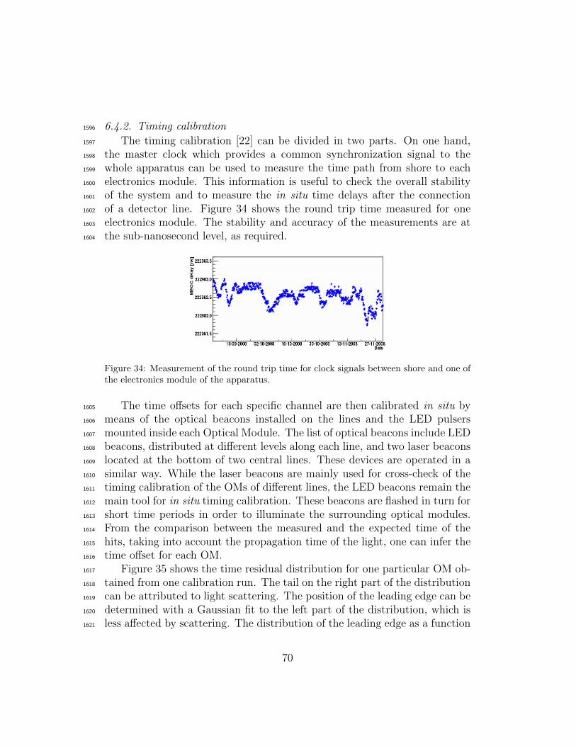
6.4.2. Timing calibration1596

The timing calibration [22] can be divided in two parts. On one hand,1597

the master clock which provides a common synchronization signal to the1598

whole apparatus can be used to measure the time path from shore to each1599

electronics module. This information is useful to check the overall stability1600

of the system and to measure the in situ time delays after the connection1601

of a detector line. Figure 34 shows the round trip time measured for one1602

electronics module. The stability and accuracy of the measurements are at1603

the sub-nanosecond level, as required.1604

Figure 34: Measurement of the round trip time for clock signals between shore and one ofthe electronics module of the apparatus.

The time offsets for each specific channel are then calibrated in situ by1605

means of the optical beacons installed on the lines and the LED pulsers1606

mounted inside each Optical Module. The list of optical beacons include LED1607

beacons, distributed at different levels along each line, and two laser beacons1608

located at the bottom of two central lines. These devices are operated in a1609

similar way. While the laser beacons are mainly used for cross-check of the1610

timing calibration of the OMs of different lines, the LED beacons remain the1611

main tool for in situ timing calibration. These beacons are flashed in turn for1612

short time periods in order to illuminate the surrounding optical modules.1613

From the comparison between the measured and the expected time of the1614

hits, taking into account the propagation time of the light, one can infer the1615

time offset for each OM.1616

Figure 35 shows the time residual distribution for one particular OM ob-1617

tained from one calibration run. The tail on the right part of the distribution1618

can be attributed to light scattering. The position of the leading edge can be1619

determined with a Gaussian fit to the left part of the distribution, which is1620

less affected by scattering. The distribution of the leading edge as a function1621

70

Figure 35: Time residual distribution of the signals in an OM located two storeys abovea flashing LED Beacon. The curve is a Gaussian fit with a sigma of 0.5 ns.

of the distance (or, equivalently, the storey number) shows a linear trend,1622

which is ascribed to the “early-photon effect”. This effect is due to the du-1623

ration of the light pulse (FWHM ≈ 4 ns) and the intensity of the detected1624

light. The closer the OM, the more light it receives and therefore the sooner1625

the PMT signal passes the preset threshold of the ARS, an effect which is1626

further emphasized by time walk. A straight line fit is then applied to the1627

data and deviations from this fit are understood as the corrections to be1628

made on the time offsets obtained by the calibration onshore. An example1629

is given in Figure 36. In most cases these corrections are small, and only for1630

≈ 15% of cases they are larger than 1 ns. This method provides an average1631

improvement of ≈ 0.5 ns over the timing calibration performed onshore.1632

The time offset variations of each optical module, due to variations in1633

the transit time of the photomultiplier for instance, can be monitored by1634

operating the LED pulser placed in each optical module. These data show a1635

good stability of the time delays when the HV of the PMT and the settings1636

of the ARS are not changed.1637

An additional check of the timing calibration accuracy may come from1638

the detection of coincidences of PMT signals induced by Potassium-40 decays1639

(40K). This radioactive isotope is naturally present in the sea water. From1640

71

Figure 36: Time residual peak position as a function of the distance between a flashingLED beacon and the OMs along seven storeys above. The three points at each distancecorrespond to the three OMs in each storey. The additional delay with distance is due tothe early photon effect.

its decay, electrons with a kinetic energy up to 1.3 MeV are produced. This1641

energy exceeds the Cherenkov threshold for electrons in water (0.26 MeV),1642

and is sufficient to produce up to 150 Cherenkov photons. If the decay occurs1643

in the vicinity of a detector storey, a coincident signal may be recorded by a1644

pair of PMTs. In Figure 37 the distribution of the measured time difference1645

between hits in neighbouring PMTs of one storey is shown. The peak around1646

0 ns is mainly due to single 40K decays producing coincident signals. The1647

fit to the data is the sum of a Gaussian distribution and a flat background.1648

The full width at half maximum of the Gaussian function is about 9 ns. This1649

width is mainly due to the spatial distribution of the 40K decays around the1650

storey. The positions of the peaks of the time distributions for different pairs1651

of PMTs in the same storey are used to cross-check the time offsets computed1652

with the timing calibration. This is illustrated in Figure 38 which shows a1653

comparison of the time offsets calculated from the optical beacon calibration1654

and those extracted from the analysis of 40K coincidences.The rms of the1655

distribution is about 0.6 ns.1656

The coincidences induced by 40K decays provide also a powerful tool for1657

monitoring the relative efficiencies of the individual OM, with an accuracy1658

of about 5%.1659

72

Figure 37: Time difference between signals measured by a pair of PMTs in storey 1 of line1. The peak is due to single 40K decays , whereas the flat background is due to accidentalcoincidences of 40K decays and bioluminescence. The solid line is a fit of the sum of aGaussian distribution and a flat background to the data.

Figure 38: Differences between the time offsets inferred from the calibrations with theLED beacons and independently determined by the 40K coincidence method for all pho-tomultiplier tubes.

6.4.3. Amplitude calibration1660

Amplitude calibration of each channel is routinely performed. During1661

special runs, the output signal of the PMT is digitized at random times.1662

This allows for a measurement of the corresponding pedestal value of the1663

73

AVC channel. The single photoelectron peak is studied with minimum bias1664

events. The optical activity due the 40K decays and bioluminescent bacteria1665

produces primarily single photons at the photocathode level. The knowledge1666

of the position of the single photoelectron peak and of the pedestal is used to1667

determine the charge conversion over the full dynamical range of the ADC.1668

The charge measurements, performed inside the ARS, appear to be influenced1669

by the time measurements in the TVC channel (the inverse effect does not1670

apply). This cross-talk effect is corrected on an event-by-event basis. The1671

maximal size of this correction amounts to 0.2 photoelectrons. The effect is1672

thought to be due to a coupling between the capacitors inside the pipeline in1673

the chips. This correction is inferred with in situ measurements of the AVC1674

value versus the TVC value.1675

Once the cross-talk correction is made, the charge calibration is applied1676

to reconstruct the amplitude of the individual signals detected from the op-1677

tical modules. As shown in Figure 39, this distribution is peaked at one1678

photoelectron as expected from 40K decay and bioluminescence.1679

Figure 39: Calibrated charge distribution combining all PMTs in the detector.

The front-end chip has also the capability to perform full waveform sam-1680

pling (WF) of the PMT signal in addition to the charge measurement of1681

the PMT pulse and its arrival time. This functionality is primarily meant1682

for recording double pulses or large amplitude signals. However, it is also1683

exploited during the calibration in order to cross-check the computation of1684

the charge by the integrator circuit of the front-end chip and for determining1685

the shape of the SPE signals in order to correct for the so-called walk effect1686

(i.e., the dependence of the threshold crossing time on the signal amplitude).1687

74

6.5. Performance of the apparatus1688

There are a number of criteria which can be considered for assessing the1689

performance of a complex apparatus like ANTARES. The first criterion con-1690

cerns stability of the operating conditions. The junction box has the longest1691

operation history since it was installed in December 2002. Temperature and1692

relative humidity inside the junction box have been continuously logged dur-1693

ing this period by a battery-powered monitor system. A sample of such1694

measurements, taken during the first years of operation, is shown in Fig-1695

ure 40. The relative humidity is seen to plateau at 50% when the detector1696

is not powered and to drop during periods when the junction box is warm1697

with the transformer powered for the operation of prototype detection lines.1698

Figure 40: Long-term monitor of relative humidity (RH) (top curve) and temperature(bottom curves) in the underwater junction box over a period of eight years. From 2002to 2005, during the prototyping phase, the detector was powered off a large part of thetime while from 2006, with operational detector lines, the power was mostly on. The twotemperature curves come from probes located at different positions in the junction box.

Another important parameter for assessing the apparatus performance1699

is the fraction of time dedicated to data taking. This should be as high as1700

possible in order to maximize the statistics of events collected and to allow for1701

a maximum probability of detecting transient phenomena. Since the start1702

75

of the operation of the detector in March 2006, the data taking live time1703

has been better than 90 %, the larger fractions of dead time being due to1704

construction/maintenance activities (≈ 4%) and calibrations (≈ 3%). The1705

trigger rate, which is dominated by cosmic ray muons, is at the level of a few1706

tens of Hz. Neutrino events are recorded at a rate of about four per day.1707

Detection efficiency and angular resolution are the parameters which1708

mainly determine the apparatus sensitivity to neutrino sources; neutrino en-1709

ergy resolution is also significant, as it helps to discriminate between neu-1710

trinos of astrophysical origin and those created in cosmic ray showers in1711

the atmosphere. These three parameters have been studied using a detailed1712

Monte Carlo simulation of the detector response to muons and neutrinos. The1713

performance of the apparatus has been reported in references [23, 24, 25].1714

Angular resolution, which is a key element for separating a point source1715

neutrino signal from the atmospheric neutrino background, depends on the1716

timing resolution, the accuracy of the OM positioning system and the water1717

scattering properties. Detection efficiency is affected by different factors,1718

the most significant being the light transmission parameters in water and1719

the OM detection efficiency; the latter in turn depends on several factors1720

such as light transmission losses, photocathode quantum efficiency, electron1721

collection efficiency and the threshold setting.1722

An example of an energetic upgoing neutrino candidate event, observed1723

on eight ANTARES detector lines is shown in Figure 41. For each detector1724

line, a panel shows the vertical position (y-axis) and the arrival time of the1725

hits (x-axis). In this coordinates system, the hits must lie on a hyperbola.1726

A reconstruction algorithm [27] is applied and the curves show the results of1727

the best fit. The “aperture” of the asymptotes is related to the angle of the1728

muon with respect to the detector line and the “summit” gives the altitude1729

of the closest approach of the muon to the line.1730

In Figure 42 the time residuals of the track fits for data and Monte Carlo1731

simulation are shown. A minimum number of 15 hits used in the fit is1732

required. Good agreement can be seen between the data and the simulation1733

with a core timing resolution of 2 ns, obtained by fitting a Gaussian to the1734

data in a range of values between residuals from -4 ns to 4 ns. The tail of1735

late hits is attributed to light scattering and to the presence of showers in1736

the track sample.1737

In the absence of a point-like source, demonstration of the experimental1738

angular resolution and absolute pointing of the detector can be provided by1739

observation of the moon shadow with cosmic rays. However several years of1740

76

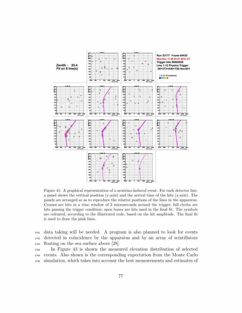
Figure 41: A graphical representation of a neutrino-induced event. For each detector line,a panel shows the vertical position (y-axis) and the arrival time of the hits (x-axis). Thepanels are arranged so as to reproduce the relative positions of the lines in the apparatus.Crosses are hits in a time window of 3 microseconds around the trigger; full circles arehits passing the trigger condition; open boxes are hits used in the final fit. The symbolsare coloured, according to the illustrated code, based on the hit amplitude. The final fitis used to draw the pink lines.

data taking will be needed. A program is also planned to look for events1741

detected in coincidence by the apparatus and by an array of scintillators1742

floating on the sea surface above [28].1743

In Figure 43 is shown the measured elevation distribution of selected1744

events. Also shown is the corresponding expectation from the Monte Carlo1745

simulation, which takes into account the best measurements and estimates of1746

77

Figure 42: Time residuals for tracks of neutrino candidate events as measured from thedata (black crosses) and as expected from the simulation (red histogram).

the contributions to detector efficiency mentioned above. The overall agree-1747

ment between data and Monte Carlo is well within the estimated systematic1748

uncertainties of about 20 % for the detector effects and an additional 30 %1749

of uncertainty on the absolute flux of atmospheric particles.1750

Figure 43: Elevation distribution of events.

A further check of the efficiency assumptions in the Monte Carlo, inde-1751

pendently of the absolute flux of particles, is shown in Figure 44. Here the1752

number of hits associated to the fitted tracks is compared to the Monte Carlo1753

78

expectation for the upward going events of Figure 43. A good agreement be-1754

tween data and Monte Carlo is observed.

Figure 44: Number of hits in neutrino candidate events as measured from the data (blackcrosses) and as expected from the simulation (red histogram). The two distributions havebeen normalized to the same event count.

1755

7. Conclusions1756

After an extensive period of R&D and prototyping, the construction of1757

ANTARES has been successfully completed. The high energy neutrino tele-1758

scope consisting of 12 lines holding optical modules is deployed on the seabed1759

off the Toulon coast at 2475 m depth. Since the deployment of the first line1760

in 2006, data taking has proceeded essentially continuously.1761

The methods and the procedures to control such a novel detector have1762

been developed including in situ timing calibration, acoustic positioning of1763

the detector elements and charge calibration.1764

All the design goals of the detector have been attained. The measure-1765

ments of the position of the optical modules is achieved to accuracy better1766

than 20 cm and the expected time resolution of 1 ns is reached. This allows1767

the reconstruction of the events with the desired angular resolution.1768

ANTARES has demonstrated that undersea neutrino telescopes are fea-1769

sible and manageable from the onshore infrastructure. The successful oper-1770

ation of ANTARES represents an important step towards a future km3-scale1771

79

high-energy neutrino observatory and marine sciences infrastructure.1772

1773

We dedicate this paper to the memory of our colleague and friend Patrice1774

Payre, who passed away during the preparation of this paper.1775

Acknowledgements1776

The authors acknowledge the financial support of the funding agencies:1777

Centre National de la Recherche Scientifique (CNRS), Commissariat a l’energie1778

atomique et aux energies alternatives (CEA), Agence Nationale de la Recherche1779

(ANR), Commission Europeenne (FEDER fund and Marie Curie Program),1780

Region Alsace (contrat CPER), Region Provence-Alpes-Cote d’Azur, Depar-1781

tement du Var and Ville de La Seyne-sur-Mer, France; Bundesministerium1782

fur Bildung und Forschung (BMBF), Germany; Istituto Nazionale di Fisica1783

Nucleare (INFN), Italy; Stichting voor Fundamenteel Onderzoek der Materie1784

(FOM), Nederlandse organisatie voor Wetenschappelijk Onderzoek (NWO),1785

the Netherlands; Council of the President of the Russian Federation for young1786

scientists and leading scientific schools supporting grants, Russia; National1787

Authority for Scientific Research (ANCS), Romania; Ministerio de Ciencia e1788

Innovacion (MICINN), Prometeo of Generalitat Valenciana and MultiDark,1789

Spain. We also acknowledge the technical support of Ifremer, AIM and Fos-1790

elev Marine for the sea operation and the CC-IN2P3 for the computing fa-1791

cilities.1792

80

List of Figures1793

1 Principle of detection of high energy muon neutrinos in an un-1794

derwater neutrino telescope. The incoming neutrino interacts1795

with the material around the detector to create a muon. The1796

muon gives Cherenkov light in the sea water which is then de-1797

tected by a matrix of light sensors. The original spectrum of1798

light emitted from the muon is attenuated in the water such1799

that the dominant wavelength range detected is between 3501800

and 500 nm. . . . . . . . . . . . . . . . . . . . . . . . . . . . . 121801

2 Schematic view of the ANTARES detector. . . . . . . . . . . . 131802

3 Schematic view of the data acquisition system. The dashed1803

line boxes refer to hardware devices, the ellipses correspond1804

to processes running on those devices. The lines between pro-1805

cesses indicate the exchange of information (commands, data,1806

messages, etc.). . . . . . . . . . . . . . . . . . . . . . . . . . . 151807

4 Schematic view of an optical module . . . . . . . . . . . . . . 201808

5 Results of dark count rate (top) and peak/valley ratio (bot-1809

tom) for the full set of tested PMTs. . . . . . . . . . . . . . . 201810

6 Measured mean pulse height of single photoelectrons for each1811

PMT at nominal gain. . . . . . . . . . . . . . . . . . . . . . . 211812

7 Photograph of an optical module. It is positioned on a mirror1813

to better show the full assembly. . . . . . . . . . . . . . . . . . 251814

8 OM support mechanics. . . . . . . . . . . . . . . . . . . . . . 261815

9 OMF equipped with the 3 OMs, the LCM and an LED beacon.1816

The mechanical parts used for fixing cables toward the upper1817

and the lower storeys are omitted. . . . . . . . . . . . . . . . . 271818

10 The ARS MB board with the 2 ARSs (labelled 16 and 15).1819

The 3rd one (top right, labelled 12) is foreseen for trigger pur-1820

poses. . . . . . . . . . . . . . . . . . . . . . . . . . . . . . . . 291821

11 The DAQ/SC board holding the processor (centre), the FPGA1822

(left) and the optical link to the MLCM (right). . . . . . . . . 301823

12 The COMPASS MB equipped with a TCM2 sensor on a raised1824

daughter card. . . . . . . . . . . . . . . . . . . . . . . . . . . 311825

13 The DWDM board. . . . . . . . . . . . . . . . . . . . . . . . . 321826

14 The crate of an MLCM equipped with the electronics boards. 331827

81

15 Cross section of the EMC. From centre to outside one can1828

distinguish the layer with 3 tubes, each housing 7 optical fi-1829

bres, the layer with 9 copper conductors, the LDPE jacket,1830

the aramid braid and the polyurethane sheath. The external1831

diameter is 30 mm. . . . . . . . . . . . . . . . . . . . . . . . . 331832

16 Mechanical termination of an EMC. . . . . . . . . . . . . . . . 341833

17 EMC penetrators of the LCM container. Left: non water1834

blocking. Right: water blocking. For clarity, the 3rd fibre1835

tube and the 9 conductors are not shown. . . . . . . . . . . . 351836

18 The ANTARES Bottom String Stucture. . . . . . . . . . . . . 361837

19 The SCM WDM board. . . . . . . . . . . . . . . . . . . . . . 391838

20 Line shape for a sea current velocity of 25 cm s−1 velocity.1839

The horizontal scale is enhanced to better illustrate the line1840

shape. . . . . . . . . . . . . . . . . . . . . . . . . . . . . . . . 421841

21 The electronic boards and light sources of an LED beacon. . . 431842

22 Components of the laser beacon. . . . . . . . . . . . . . . . . . 441843

23 The instrumentation line IL07. Elements are indicated schemat-1844

ically; not drawn to scale. . . . . . . . . . . . . . . . . . . . . 461845

24 A schematic view of the complete link between the SPM/SCM1846

container of a line and the JB container. . . . . . . . . . . . . 481847

25 The junction box container and its support frame. . . . . . . . 491848

26 Junction box on the deck of the deployment ship. . . . . . . . 501849

27 Junction box output breaker management. . . . . . . . . . . . 511850

28 View inside the open JB: heat-spreader disk, transformer con-1851

nections and primary circuit current sensor, passive fibre optic1852

splitters and cassettes protecting fibre fusion splices. . . . . . . 521853

29 Sections of the undersea cable. . . . . . . . . . . . . . . . . . . 541854

30 Electro-optical plug and receptacle for connection of the un-1855

dersea cable to the junction box. . . . . . . . . . . . . . . . . 551856

31 Power distribution system from the shore to the underwater1857

junction box. . . . . . . . . . . . . . . . . . . . . . . . . . . . 561858

32 Definitions of the symbols used in equation 2 (left) and in1859

equation 3 (right). . . . . . . . . . . . . . . . . . . . . . . . . 651860

33 Displacements in the horizontal plane of the five storeys equipped1861

with positioning hydrophones of a line as determined by the1862

positioning system. . . . . . . . . . . . . . . . . . . . . . . . . 691863

34 Measurement of the round trip time for clock signals between1864

shore and one of the electronics module of the apparatus. . . . 701865

82

35 Time residual distribution of the signals in an OM located two1866

storeys above a flashing LED Beacon. The curve is a Gaussian1867

fit with a sigma of 0.5 ns. . . . . . . . . . . . . . . . . . . . . 711868

36 Time residual peak position as a function of the distance be-1869

tween a flashing LED beacon and the OMs along seven storeys1870

above. The three points at each distance correspond to the1871

three OMs in each storey. The additional delay with distance1872

is due to the early photon effect. . . . . . . . . . . . . . . . . . 721873

37 Time difference between signals measured by a pair of PMTs1874

in storey 1 of line 1. The peak is due to single 40K decays ,1875

whereas the flat background is due to accidental coincidences1876

of 40K decays and bioluminescence. The solid line is a fit of1877

the sum of a Gaussian distribution and a flat background to1878

the data. . . . . . . . . . . . . . . . . . . . . . . . . . . . . . . 731879

38 Differences between the time offsets inferred from the calibra-1880

tions with the LED beacons and independently determined by1881

the 40K coincidence method for all photomultiplier tubes. . . . 731882

39 Calibrated charge distribution combining all PMTs in the de-1883

tector. . . . . . . . . . . . . . . . . . . . . . . . . . . . . . . . 741884

40 Long-term monitor of relative humidity (RH) (top curve) and1885

temperature (bottom curves) in the underwater junction box1886

over a period of eight years. From 2002 to 2005, during the1887

prototyping phase, the detector was powered off a large part1888

of the time while from 2006, with operational detector lines,1889

the power was mostly on. The two temperature curves come1890

from probes located at different positions in the junction box. 751891

41 A graphical representation of a neutrino-induced event. For1892

each detector line, a panel shows the vertical position (y-axis)1893

and the arrival time of the hits (x-axis). The panels are ar-1894

ranged so as to reproduce the relative positions of the lines1895

in the apparatus. Crosses are hits in a time window of 3 mi-1896

croseconds around the trigger; full circles are hits passing the1897

trigger condition; open boxes are hits used in the final fit. The1898

symbols are coloured, according to the illustrated code, based1899

on the hit amplitude. The final fit is used to draw the pink1900

lines. . . . . . . . . . . . . . . . . . . . . . . . . . . . . . . . . 771901

83

42 Time residuals for tracks of neutrino candidate events as mea-1902

sured from the data (black crosses) and as expected from the1903

simulation (red histogram). . . . . . . . . . . . . . . . . . . . 781904

43 Elevation distribution of events. . . . . . . . . . . . . . . . . . 781905

44 Number of hits in neutrino candidate events as measured from1906

the data (black crosses) and as expected from the simulation1907

(red histogram). The two distributions have been normalized1908

to the same event count. . . . . . . . . . . . . . . . . . . . . . 791909

List of Tables1910

1 Data on the OM glass sphere. . . . . . . . . . . . . . . . . . . 211911

2 Tension (kN) at the bottom of the specified cable or chain, for1912

3 periods in the life of the line and at 8 positions along the line. 411913

3 List of the instruments on the line IL07. . . . . . . . . . . . . 451914

4 Characteristics of the undersea cable. . . . . . . . . . . . . . . 541915

5 Layout of the undersea cable. . . . . . . . . . . . . . . . . . . 551916

References1917

[1] H. Hanada et al., A Highly Sensitive Optical Detector for a Use in Deep1918

Underwater, Nucl. Instr. and Meth. A408 (1998) 425-437.1919

[2] G. V. Domogatsky et al., [Baikal Collaboration], The Lake Baikal Deep1920

Underwater Detector, Nucl. Phys. Proc. Suppl. 19 (1991) 388-395.1921

[3] E. Andres et al., The AMANDA neutrino telescope: principle of opera-1922

tion and first results, Astrop. Phys. 13 (2000) 1-20.1923

[4] J.A. Aguilar et al., Background light in potential sites for the ANTARES1924

undersea neutrino telescope, Astrop. Phys. 13 (2000) 127-136, astro-1925

ph/9910170.1926

[5] J.A. Aguilar et al., Sedimentation and Fouling of Optical Surfaces at the1927

ANTARES Site, Astrop. Phys. 17 (2003) 253-267, astro-ph/0206454.1928

[6] J.A. Aguilar et al., Transmission of light in deep sea water at the site of1929

the Antares neutrino telescope, Astrop. Phys. 23 (2005) 131-155, astro-1930

ph/0412126.1931

84

[7] J.A. Aguilar et al., AMADEUS The Acoustic Neutrino Detection Test1932

System of the ANTARES DeepSea Neutrino Telescope, accepted for1933

publication in Nucl. Instr. and Meth., doi:10.1016/j.nima.2010.09.053,1934

arXiv:1009.4179.1935

[8] J.A. Aguilar et al., The data acquisition system for the ANTARES neu-1936

trino telescope, Nucl. Instr. and Meth. A570 (2007) 107-116.1937

[9] J.A. Aguilar et al., Performance of the front-end electronics of the AN-1938

TARES neutrino telescope, Nucl. Instr. and Meth. A622 (2010) 59-73,1939

arXiv:1007.2549.1940

[10] M. Amram et al., The ANTARES optical module, Nucl. Instr. and Meth.1941

A484 (2002) 369-383.1942

[11] J.A. Aguilar et al., Study of large hemispherical photomultiplier tubes for1943

the ANTARES neutrino telescope, Nucl. Instr. and Meth. A555 (2005)1944

132-141.1945

[12] P.W. Gorham et al., Mechanical and Acoustic1946

Studies of Deep Ocean Glass Sphere Implosions,1947

http://www.phys.hawaii.edu/∼dumand/implopp.ps.1948

[13] Cockcroft J.D. and Walton E.T.S. (1932). Proc. R. Soc. London1949

A137:229.1950

[14] M. Ageron et al., The Antares optical beacon system, Nucl. Instr. and1951

Meth. A578 (2007) 498-509, astro-ph/0703335.1952

[15] J.A. Aguilar et al., First results of the Instrumentation Line for the1953

deep-sea ANTARES neutrino telescope, Astroparticle Physics 26 (2006)1954

314-324, astro-ph/0606229.1955

[16] R. Gurin and A. Maslennikov, Controlhost: Distributed data handling1956

package. Technical report, CASPUR Inter-University Computing Con-1957

sortium Rome, 1995.1958

[17] M. Bringer et al., The TAROT observatory data management, Astron.1959

Astrophys. Suppl. Ser. 138 (1999) 581-582.1960

[18] C-T. Chen and F.J. Millero, Speed of sound in seawater at high pressures,1961

(1977) J. Acoust. Soc. Am. 62(5) 1129-1135.1962

85

[19] The Practical Salinity Scale 1978 and the International Equation of State1963

of Seawater 1980, UNESCO technical papers in marine science 36.1964

[20] P. Keller (for the ANTARES Collaboration), Acoustic Positioning Sys-1965

tem for the Deep-sea ANTARES Neutrino Telescope, in Proc. UNWAT1966

- SENSORCOMM Conf., Valencia, 2007, 243-247.1967

[21] M. Ardid (for the ANTARES Collaboration), Positioning system of the1968

ANTARES neutrino telescope, Nucl. Instr. and Meth. A602 (2009) 174-1969

176.1970

[22] J.A. Aguilar et al., Time Calibration of the ANTARES Neutrino Tele-1971

scope, Astrop. Phys. 34 (2011) 539-549, [arXiv:1012.2204]1972

[23] M. Ageron et al., Performance of the First ANTARES Detector Line,1973

Astrop. Phys. 31, 4 (2009) 277-283.1974

[24] J.A. Aguilar et al., Measurement of the atmospheric muon flux with a1975

4 GeV threshold in the ANTARES neutrino telescope, Astrop. Phys. 331976

(2010) 86-90, astro-ph/0910.4843.1977

[25] J.A. Aguilar et al., Zenith distribution and flux of atmospheric muons1978

measured with the 5-line ANTARES detector, Astrop. Phys. 34 (2010)1979

179-184, arXiv:0910.4843.1980

[26] M. Ageron et al., Studies of a full scale mechanical prototype line for1981

the ANTARES neutrino telescope and tests of a prototype instrument1982

for deep-sea acoustic measurements, Nucl. Instr. and Meth. A581(2007)1983

695-708.1984

[27] J.A. Aguilar et al., A Fast Algorithm for Muon Track Reconstruction and1985

its Application to the ANTARES Neutrino Telescope, to be published in1986

Astrop. Phys.1987

[28] J.-P. Ernenwein, A. Tsirigotis and S. Tzamarias, Study of the calibra-1988

tion potential of HELYCON detectors with ANTARES, Nucl. Instr. and1989

Meth. A602 (2009), 88-90.1990

86