Muon Neutrino to Electron Neutrino Oscillation in NOνA - CERN
223
Muon Neutrino to Electron Neutrino Oscillation in NOν A A THESIS SUBMITTED TO THE FACULTY OF THE GRADUATE SCHOOL OF THE UNIVERSITY OF MINNESOTA BY Kanika Sachdev IN PARTIAL FULFILLMENT OF THE REQUIREMENTS FOR THE DEGREE OF Doctor of Philosophy Prof. Daniel Cronin-Hennessy & Prof. Gregory Pawloski August, 2015
-
Upload
khangminh22 -
Category
Documents
-
view
0 -
download
0
Transcript of Muon Neutrino to Electron Neutrino Oscillation in NOνA - CERN

Muon Neutrino to Electron Neutrino Oscillation in NOνA
A THESIS
SUBMITTED TO THE FACULTY OF THE GRADUATE SCHOOL
OF THE UNIVERSITY OF MINNESOTA
BY
Kanika Sachdev
IN PARTIAL FULFILLMENT OF THE REQUIREMENTS
FOR THE DEGREE OF
Doctor of Philosophy
Prof. Daniel Cronin-Hennessy & Prof. Gregory Pawloski
August, 2015

c© Kanika Sachdev 2015
ALL RIGHTS RESERVED

Acknowledgements
I want to begin with thanking my undergraduate teacher, Adarsh Shroff- I would not
be a physicist had it not been for your encouragement.
Thank you, to my advisers, Daniel Cronin-Hennessy and Gregory Pawloski, for your
guidance, support, and patience, and for sharing your intuition in Physics with me.
Thank you, Mayly Sanchez and Patricia Vahle, for your trust and encouragement.
Thank you, NOνA graduate students at Minnesota- Dominick, Jan, Minerba, Nick
and Susan, for helping me learn the ropes early on and teaching me how to stand on
my own two feet.
Thank you, Gavin Davies, Chris Backhouse and Evan Niner, with whom I shared this
nerve-wracking, life-changing and thrilling experience of bringing a new experiment
online and extracting the first physics results from it. I wouldn’t choose different
friends if I had to do it all over again.
Thank you, mom, dad, Maggi and Larry, for everything; this journey would be
unimaginable without you.
i

Dedication
To my parents, Ravi and Archana, my sister, Maggi, and Larry.
ii
Abstract
NOvA is a long-baseline neutrino oscillation experiment optimized for electron neu-
trino (νe) appearance in the NuMI beam, a muon neutrino (νµ) source at Fermilab.
It consists of two functionally identical, nearly fully-active liquid-scintillator tracking
calorimeters. The near detector (ND) at Fermilab is used to study the neutrino beam
spectrum and composition before oscillation, and measure background rate to the νe
appearance search. The far detector, 810 km away in Northern Minnesota, observes the
oscillated beam and is used to extract oscillation parameters from the data. NOνA’s
long baseline, combined with the ability of the NuMI beam to operate in the anti-
neutrino mode, makes NOνA sensitive to the last unmeasured parameters in neutrino
oscillations- mass hierarchy, CP violation and the octant of mixing angle θ23. This thesis
presents the search for νe appearance in the first data collected by the NOνA detectors
from October 2013 till May 2015.
Studies of the NuMI neutrino data collected in the NOνA near detector are also
presented, which show large discrepancies between the ND simulation and data. Muon-
removed electron (MRE) events, constructed by replacing the muon in νµ charged cur-
rent interactions by a simulated electron, are used to correct the far detector νe appear-
ance prediction for these discrepancies.
In the analysis of the first data, a total of 6 νe candidate events are observed in
the far detector on a background of 1, a 3.46 σ excess, which is interpreted as strong
evidence for νe appearance. The results are consistent with our expectation, based on
constraints from other neutrino oscillation experiments.
The result presented here differs from the officially published νe appearance result
from the NOνA experiment where the systematic error is assumed to cover the MRE
correction.
iii

Contents
Acknowledgements i
Dedication ii
Abstract iii
List of Tables x
List of Figures xii
1 Neutrino Physics 1
1.1 Neutrinos in the Standard Model . . . . . . . . . . . . . . . . . . . . . 1
1.1.1 Weak Interaction . . . . . . . . . . . . . . . . . . . . . . . . . . . 2
1.1.2 Free Neutrinos . . . . . . . . . . . . . . . . . . . . . . . . . . . . 3
1.2 Extending the Standard Model . . . . . . . . . . . . . . . . . . . . . . . 4
1.2.1 Majorana Mass of Neutrinos . . . . . . . . . . . . . . . . . . . . 4
1.3 Neutrino Oscillations . . . . . . . . . . . . . . . . . . . . . . . . . . . . . 6
1.3.1 Oscillations in Vacuum . . . . . . . . . . . . . . . . . . . . . . . 6
1.3.2 Oscillations in Matter . . . . . . . . . . . . . . . . . . . . . . . . 8
2 Status of Neutrino Oscillation Measurements 12
2.1 Conventions and Nomenclature . . . . . . . . . . . . . . . . . . . . . . . 12
iv

2.2 Oscillation Parameter Measurements . . . . . . . . . . . . . . . . . . . . 13
2.2.1 θ12 and ∆m221 Measurements . . . . . . . . . . . . . . . . . . . . 13
2.2.2 θ23 and |∆m232| Measurements . . . . . . . . . . . . . . . . . . . 16
2.2.3 θ13 Measurements . . . . . . . . . . . . . . . . . . . . . . . . . . 17
2.3 Unknown Parameters . . . . . . . . . . . . . . . . . . . . . . . . . . . . . 18
2.3.1 Mass Hierarchy . . . . . . . . . . . . . . . . . . . . . . . . . . . . 18
2.3.2 CP Violation . . . . . . . . . . . . . . . . . . . . . . . . . . . . . 20
2.3.3 θ23 Octant . . . . . . . . . . . . . . . . . . . . . . . . . . . . . . . 21
2.4 νµ → νe on Long Baseline . . . . . . . . . . . . . . . . . . . . . . . . . . 21
2.4.1 Experimental Observation . . . . . . . . . . . . . . . . . . . . . . 24
3 The NOνA Experiment 25
3.1 The NuMI Beam . . . . . . . . . . . . . . . . . . . . . . . . . . . . . . . 27
3.1.1 The Accelerator Complex . . . . . . . . . . . . . . . . . . . . . . 30
3.1.2 Slip-Stacking . . . . . . . . . . . . . . . . . . . . . . . . . . . . . 31
3.1.3 The NuMI Beamline . . . . . . . . . . . . . . . . . . . . . . . . . 31
3.2 The NOνA Detector Design . . . . . . . . . . . . . . . . . . . . . . . . . 32
3.2.1 The NOνA Unit Cell . . . . . . . . . . . . . . . . . . . . . . . . . 32
3.2.2 Liquid Scintillator . . . . . . . . . . . . . . . . . . . . . . . . . . 33
3.2.3 Optical Fiber . . . . . . . . . . . . . . . . . . . . . . . . . . . . . 35
3.2.4 Avalanche Photodiode (APD) . . . . . . . . . . . . . . . . . . . . 36
3.2.5 PVC Modules . . . . . . . . . . . . . . . . . . . . . . . . . . . . . 37
3.2.6 Detector Assembly . . . . . . . . . . . . . . . . . . . . . . . . . . 40
4 Data Acquisition and Triggering Systems 43
4.1 Overview of NOνA DAQ System . . . . . . . . . . . . . . . . . . . . . . 43
4.2 Clock and Triggering . . . . . . . . . . . . . . . . . . . . . . . . . . . . . 44
4.3 Readout . . . . . . . . . . . . . . . . . . . . . . . . . . . . . . . . . . . . 46
4.3.1 APD Sag and Ringing . . . . . . . . . . . . . . . . . . . . . . . . 47
v

4.4 Timing Peak . . . . . . . . . . . . . . . . . . . . . . . . . . . . . . . . . 48
4.4.1 Far Detector . . . . . . . . . . . . . . . . . . . . . . . . . . . . . 48
4.4.2 Near Detector . . . . . . . . . . . . . . . . . . . . . . . . . . . . . 50
5 νe Appearance Analysis Overview 52
5.1 Oscillation Analysis Steps . . . . . . . . . . . . . . . . . . . . . . . . . . 52
5.1.1 Blind Analysis . . . . . . . . . . . . . . . . . . . . . . . . . . . . 52
5.1.2 Cosmic Background Estimate . . . . . . . . . . . . . . . . . . . . 53
5.1.3 Beam Background Estimate . . . . . . . . . . . . . . . . . . . . . 54
5.1.4 Extrapolation . . . . . . . . . . . . . . . . . . . . . . . . . . . . . 55
5.1.5 Final Fit . . . . . . . . . . . . . . . . . . . . . . . . . . . . . . . 55
5.2 NOνA’s First Data . . . . . . . . . . . . . . . . . . . . . . . . . . . . . . 55
5.2.1 Treatment of 64 µs Delayed Peak in Pre-Shutdown Data . . . . . 56
5.3 Simple Oscillations . . . . . . . . . . . . . . . . . . . . . . . . . . . . . . 57
6 Simulation 59
6.1 Particle Simulation . . . . . . . . . . . . . . . . . . . . . . . . . . . . . . 59
6.1.1 Beam . . . . . . . . . . . . . . . . . . . . . . . . . . . . . . . . . 59
6.1.2 Neutrinos . . . . . . . . . . . . . . . . . . . . . . . . . . . . . . . 60
6.1.3 Particles in Detector . . . . . . . . . . . . . . . . . . . . . . . . . 61
6.2 Detector Response Simulation . . . . . . . . . . . . . . . . . . . . . . . . 62
6.2.1 Photon Transport . . . . . . . . . . . . . . . . . . . . . . . . . . 62
6.2.2 Readout Simulation . . . . . . . . . . . . . . . . . . . . . . . . . 63
6.3 Tuning to Data . . . . . . . . . . . . . . . . . . . . . . . . . . . . . . . . 64
6.3.1 APD Sag Simulation . . . . . . . . . . . . . . . . . . . . . . . . . 65
6.3.2 Scintillator Quenching . . . . . . . . . . . . . . . . . . . . . . . . 65
6.3.3 Diblock and Bad Channel Masking . . . . . . . . . . . . . . . . . 68
vi
7 Event and Energy Reconstruction 70
7.1 Calibration . . . . . . . . . . . . . . . . . . . . . . . . . . . . . . . . . . 70
7.1.1 Attenuation Correction . . . . . . . . . . . . . . . . . . . . . . . 71
7.1.2 Absolute Energy Scale . . . . . . . . . . . . . . . . . . . . . . . . 73
7.1.3 Timing resolution . . . . . . . . . . . . . . . . . . . . . . . . . . 74
7.2 Reconstruction Steps . . . . . . . . . . . . . . . . . . . . . . . . . . . . . 75
7.3 Slicing Algorithm . . . . . . . . . . . . . . . . . . . . . . . . . . . . . . . 77
7.4 νe Reconstruction . . . . . . . . . . . . . . . . . . . . . . . . . . . . . . . 80
7.4.1 Hough Transform . . . . . . . . . . . . . . . . . . . . . . . . . . . 80
7.4.2 Elastic Arms Vertex . . . . . . . . . . . . . . . . . . . . . . . . . 82
7.4.3 Fuzzy-k Prong Reconstruction . . . . . . . . . . . . . . . . . . . 83
7.4.4 νe Event Energy Reconstruction . . . . . . . . . . . . . . . . . . 85
7.5 νµ Reconstruction Chain . . . . . . . . . . . . . . . . . . . . . . . . . . . 86
8 νe Event Selection 89
8.1 νe Selection Cuts . . . . . . . . . . . . . . . . . . . . . . . . . . . . . . . 89
8.1.1 Data Quality Cuts . . . . . . . . . . . . . . . . . . . . . . . . . . 89
8.1.2 Preselection and Cosmic Rejection Cuts . . . . . . . . . . . . . . 92
8.1.3 Performance of Preselection . . . . . . . . . . . . . . . . . . . . . 98
8.2 νe Particle Identification . . . . . . . . . . . . . . . . . . . . . . . . . . 101
8.2.1 Likelihood-based Particle Identification . . . . . . . . . . . . . . 101
8.3 Final Cosmic Background Prediction . . . . . . . . . . . . . . . . . . . . 108
9 Near Detector Data 112
9.1 Near Detector Data-MC Comparisons . . . . . . . . . . . . . . . . . . . 113
9.1.1 ND νe Event Selection . . . . . . . . . . . . . . . . . . . . . . . 113
9.1.2 ND νµ Event Selection . . . . . . . . . . . . . . . . . . . . . . . . 119
9.2 Interpretation . . . . . . . . . . . . . . . . . . . . . . . . . . . . . . . . . 122
9.2.1 Fitting For Interaction Type . . . . . . . . . . . . . . . . . . . . 123
vii

9.2.2 Fitting For Interaction Mode . . . . . . . . . . . . . . . . . . . . 125
10 Muon Removed Electron Events 134
10.1 MRE Event Generation . . . . . . . . . . . . . . . . . . . . . . . . . . . 134
10.1.1 Muon Removal . . . . . . . . . . . . . . . . . . . . . . . . . . . . 135
10.1.2 Muon and Hadron Energy Disentaglement . . . . . . . . . . . . 136
10.1.3 Performance of Muon-Removal . . . . . . . . . . . . . . . . . . . 139
10.1.4 Insertion of Simulated Electron . . . . . . . . . . . . . . . . . . . 141
10.2 MRE ND Data-MC Comparison . . . . . . . . . . . . . . . . . . . . . . 141
10.2.1 MRE Event Selection . . . . . . . . . . . . . . . . . . . . . . . . 141
10.2.2 MRE with Interaction Mode Scaling . . . . . . . . . . . . . . . . 145
10.3 MRE Correction On Signal Prediction . . . . . . . . . . . . . . . . . . . 147
10.3.1 Efficiency by Shower and Hadronic Energy . . . . . . . . . . . . 147
11 Decomposition and Extrapolation 155
11.1 Decomposition . . . . . . . . . . . . . . . . . . . . . . . . . . . . . . . . 156
11.1.1 Proportional Decomposition . . . . . . . . . . . . . . . . . . . . . 156
11.1.2 Decomposition, Upon Scaling by Interaction Type . . . . . . . . 156
11.1.3 Decomposition, Upon Scaling by Interaction Mode . . . . . . . . 156
11.1.4 Summary of Decomposition . . . . . . . . . . . . . . . . . . . . . 157
11.2 Background Extrapolation . . . . . . . . . . . . . . . . . . . . . . . . . 157
11.3 Signal Extrapolation . . . . . . . . . . . . . . . . . . . . . . . . . . . . . 160
11.4 Results of Extrapolation . . . . . . . . . . . . . . . . . . . . . . . . . . . 163
12 Error Estimates 167
12.1 Calibration Error . . . . . . . . . . . . . . . . . . . . . . . . . . . . . . . 167
12.2 Interaction Model Uncertainties . . . . . . . . . . . . . . . . . . . . . . . 169
12.2.1 Beam Flux Errors . . . . . . . . . . . . . . . . . . . . . . . . . . 170
12.2.2 Neutrino Interaction Model Uncertainty . . . . . . . . . . . . . . 171
viii

12.3 Birks Suppresion . . . . . . . . . . . . . . . . . . . . . . . . . . . . . . . 172
12.4 Decomposition Uncertainty . . . . . . . . . . . . . . . . . . . . . . . . . 172
12.5 Uncertainty on MRE Correction . . . . . . . . . . . . . . . . . . . . . . 173
12.6 Other Smaller Effects . . . . . . . . . . . . . . . . . . . . . . . . . . . . 176
12.6.1 Containment and Rock Contamination . . . . . . . . . . . . . . . 176
12.6.2 Simulation Statistics and Normalization . . . . . . . . . . . . . . 177
12.6.3 Alignment . . . . . . . . . . . . . . . . . . . . . . . . . . . . . . . 177
12.6.4 Light Level . . . . . . . . . . . . . . . . . . . . . . . . . . . . . . 178
12.7 Summary . . . . . . . . . . . . . . . . . . . . . . . . . . . . . . . . . . . 178
13 Results of νe Appearance Analysis 180
13.1 PID Sideband . . . . . . . . . . . . . . . . . . . . . . . . . . . . . . . . . 181
13.2 νe Appearance Result . . . . . . . . . . . . . . . . . . . . . . . . . . . . 181
13.3 Analysis of the Result . . . . . . . . . . . . . . . . . . . . . . . . . . . . 187
13.3.1 Significance of Observation: Simple Treatment . . . . . . . . . . 191
13.3.2 Fit to Oscillation Parameters . . . . . . . . . . . . . . . . . . . . 192
13.3.3 Feldman-Cousins Method for Confidence Interval . . . . . . . . . 195
13.3.4 Result from Alternative PID, LEM . . . . . . . . . . . . . . . . . 198
13.3.5 Comparison with Official NOνA νe Appearance Result . . . . . . 198
13.4 Future Analyses of NOνA Data . . . . . . . . . . . . . . . . . . . . . . . 198
References 200
ix

List of Tables
5.1 Far detector exposure and livetime . . . . . . . . . . . . . . . . . . . . . 56
8.1 Containment cuts in ND . . . . . . . . . . . . . . . . . . . . . . . . . . . 97
8.2 νe selection cut flow in the FD . . . . . . . . . . . . . . . . . . . . . . . 99
8.3 Summary of νe preselection cuts applied in the far detector . . . . . . . 100
8.4 Performance of LID . . . . . . . . . . . . . . . . . . . . . . . . . . . . . 110
8.5 Cut flow on cosmic ray background in out-of-time NuMI data . . . . . . 110
9.1 Near detector νe selection cuts . . . . . . . . . . . . . . . . . . . . . . . 113
9.2 νe event selection efficiency in Near Detector . . . . . . . . . . . . . . . 114
9.3 νµ CC selection criteria in the ND . . . . . . . . . . . . . . . . . . . . . 120
9.4 Description of interaction type and mode . . . . . . . . . . . . . . . . . 123
9.5 Result of fit for NC, νµ CC and beam νe CC scales in ND . . . . . . . . 124
9.6 Result of fit for QE, resonance and DIS scales in ND . . . . . . . . . . . 128
10.1 Cut flow of ND MRE data and MC . . . . . . . . . . . . . . . . . . . . . 142
11.1 Result of decomposition of νe selected data in the near detector . . . . . 157
11.2 Extrapolated signal and background predictions for νe appearance anal-
ysis of NOνA’s first data . . . . . . . . . . . . . . . . . . . . . . . . . . . 164
11.3 Predictions with different oscillation scenarios . . . . . . . . . . . . . . . 164
12.1 Calibration systematic error . . . . . . . . . . . . . . . . . . . . . . . . . 170
12.2 Decomposition Error . . . . . . . . . . . . . . . . . . . . . . . . . . . . . 173
x

12.3 Change in MRE corrected extrapolated νe signal production due to dif-
ferent selection cuts on the MRE parent νµ CC interaction . . . . . . . . 174
12.4 Change in MRE corrected extrapolated νe signal production due to dif-
ferent parent matching efficiency cuts on the MRE slice. . . . . . . . . . 176
12.5 Final systematic error (in percentages) on the combined background and
signal in the Far Detector. . . . . . . . . . . . . . . . . . . . . . . . . . . 179
13.1 Expected signal and background for NOνA first data along with the
systematic and statistical errors on the predictions. . . . . . . . . . . . . 180
13.2 LID sideband event counts expectation in the far detector . . . . . . . . 181
13.3 Significance of observation . . . . . . . . . . . . . . . . . . . . . . . . . . 191
xi

List of Figures
1.1 Masses of fundamental particles in the Standard Model . . . . . . . . . 4
1.2 Allowed coherent scattering modes for neutrinos passing through the
earth matter . . . . . . . . . . . . . . . . . . . . . . . . . . . . . . . . . 9
2.1 Predicted solar neutrino spectrum [1] . . . . . . . . . . . . . . . . . . . 14
2.2 Mass hierarchy in neutrinos . . . . . . . . . . . . . . . . . . . . . . . . . 19
2.3 Values of effective Majoarana mass as a function of the lightest neutrino
mass . . . . . . . . . . . . . . . . . . . . . . . . . . . . . . . . . . . . . . 20
3.1 νµ to νe oscillation probability for the NuMI beam at the location of the
NOνA far detector under different hierarchy hypotheses. . . . . . . . . . 26
3.2 P (νµ → νe) versus P (ν̄µ → ν̄e) for NOνA . . . . . . . . . . . . . . . . . 27
3.3 The neutrino energy spectra and flux as a function of the pion energy for
different off-axis angles, θ. . . . . . . . . . . . . . . . . . . . . . . . . . 28
3.4 Simulated neutrino energy spectra at the NOνA far detector baseline of
810 km. The off-axis location of NOνA suppress the high neutrino energy
tail . . . . . . . . . . . . . . . . . . . . . . . . . . . . . . . . . . . . . . . 29
3.5 Schematic of the Fermilab accelerator complex, with upgrades imple-
mented for NOνA . . . . . . . . . . . . . . . . . . . . . . . . . . . . . . 30
3.6 The NuMI Beamline [2] . . . . . . . . . . . . . . . . . . . . . . . . . . . 32
3.7 A cell and a cut-out of the NOνA detectors indicating the orthogonal
arrangment of cells in adjacent planes. . . . . . . . . . . . . . . . . . . . 33
xii

3.8 The emission spectrum of the NOνA scintillator. The figure is from [3]. 34
3.9 The absorption and emission spectra of the NOνA WLS fiber . . . . . . 35
3.10 Schematic of the APD and front-end electronics. . . . . . . . . . . . . . 37
3.11 Profile of the PVC extrusion showing scalloped corners in the inner and
outer walls of the extrusion . . . . . . . . . . . . . . . . . . . . . . . . . 38
3.12 Schematic of the APD and front-end electronics. . . . . . . . . . . . . . 39
3.13 Block pivoter during the installation of a block in the far detector hall . 41
4.1 DCM lay out in FD . . . . . . . . . . . . . . . . . . . . . . . . . . . . . 44
4.2 Single- and multi-point point readout . . . . . . . . . . . . . . . . . . . . 47
4.3 Readout traces illustrating APD sag. . . . . . . . . . . . . . . . . . . . . 48
4.4 Far detector timing peak, over the full 500 µs window, with all data upto
February 16, 2015. . . . . . . . . . . . . . . . . . . . . . . . . . . . . . . 49
4.5 Near detector timing peak, over the full 500 µs window, and zoomed in
to show the NuMI beam structure. . . . . . . . . . . . . . . . . . . . . . 51
5.1 Timing sideband . . . . . . . . . . . . . . . . . . . . . . . . . . . . . . . 54
5.2 Timing sideband in pre-shutdown data . . . . . . . . . . . . . . . . . . . 57
6.1 FLUGG’s neutrino flux prediction by flavor and sign for the NOνA de-
tectors in the forward horn current mode . . . . . . . . . . . . . . . . . 60
6.2 Particle simulation steps in NOνA . . . . . . . . . . . . . . . . . . . . . 62
6.3 Light collection rate estimate from the ray tracing algorithm . . . . . . 63
6.4 Comparison of raw pulse-heights in FD and ND cosmic ray data . . . . 65
6.5 PE/cm per plane measured in near detector data compared with MC
with no sag and sag . . . . . . . . . . . . . . . . . . . . . . . . . . . . . 66
6.6 dE/dx comparison between ND data and MC for candidate proton track 67
6.7 POT exposure in each diblock configuration in data and simulation . . . 69
7.1 Selection of tri-cells associated with a track . . . . . . . . . . . . . . . . 71
7.2 Attenuation correction of a far detector cell, and the residual of the fit . 73
xiii

7.3 dE/dx as a function of distance from the muon stopping point as mea-
sured in FD cosmic ray data . . . . . . . . . . . . . . . . . . . . . . . . . 74
7.4 Absolute energy calibration in the far detector . . . . . . . . . . . . . . 74
7.5 Timing resolution as a function of PE in FD and ND . . . . . . . . . . . 75
7.6 Neutrino interactions of different types in the NOνA detectors . . . . . 76
7.7 ND and FD data from a single spill reconstructed into separate slices . . 79
7.8 Efficiency and purity of slices in ND simulation . . . . . . . . . . . . . . 80
7.9 νe reconstruction chain . . . . . . . . . . . . . . . . . . . . . . . . . . . . 81
7.10 Resolution of reconstructed vertex for νe CC events . . . . . . . . . . . . 82
7.11 Efficiency and purity of reconstructed prongs . . . . . . . . . . . . . . . 85
7.12 Reconstructed energy resolution of preselected νe charged-current inter-
actions. . . . . . . . . . . . . . . . . . . . . . . . . . . . . . . . . . . . . 86
7.13 Muon neutrino energy resolution for quasi-elastic CC interactions. . . . 87
8.1 An FD spill with DCM synchronization problem . . . . . . . . . . . . . 92
8.2 Flashing of multiple APDs in the FD cosmic data . . . . . . . . . . . . . 94
8.3 Neutron interaction depth in the FD . . . . . . . . . . . . . . . . . . . . 95
8.4 Minimum distance of events in the far detector from the top and the back
faces of the detector . . . . . . . . . . . . . . . . . . . . . . . . . . . . . 96
8.5 Transverse momentum fraction of the far detector events with respect to
the beam direction . . . . . . . . . . . . . . . . . . . . . . . . . . . . . . 97
8.6 Energy distribution of FD events after preselection . . . . . . . . . . . . 98
8.7 Efficiency of νe preselection cuts as a function of number of detector
diblocks in the FD, as measured in real conditions MC. . . . . . . . . . 99
8.8 Fuzzy-K prongs are reclustered to better fit the electron shower shape. . 102
8.9 Transverse dE/dx per electron energy as a function of distance from the
shower core. The distribution is fit with 8.2 . . . . . . . . . . . . . . . . 102
8.10 Muon and electron dE/dx in the second and the tenth plane from the
start point . . . . . . . . . . . . . . . . . . . . . . . . . . . . . . . . . . . 104
xiv

8.11 Longitudinal and transverse likelihood difference for electron, neutral pi-
ons and muons . . . . . . . . . . . . . . . . . . . . . . . . . . . . . . . . 105
8.12 Distribution of ANN input variables for signal(red) and background (blue)107
8.13 Distribution of LID for different neutrino interactions . . . . . . . . . . 109
8.14 Efficiency of selecting νe appearance signal and purity as a function of
LID cut . . . . . . . . . . . . . . . . . . . . . . . . . . . . . . . . . . . . 109
9.1 Near detector fiducial and containment bounds for νe selection . . . . . 112
9.2 Data and MC comparison of ND νe preselected events. . . . . . . . . . . 115
9.3 Data and MC comparison of ND νe preselected events . . . . . . . . . . 116
9.4 Data and MC comparison of ND νe preselected events. . . . . . . . . . . 117
9.5 Data and MC comparison of ND LID selected events. . . . . . . . . . . 118
9.6 Data and MC comparison of ND LID selected events . . . . . . . . . . . 119
9.7 Reconstructed quantities for νµ selected events in the ND . . . . . . . . 121
9.8 Performance of ReMID, the νµ CC PID, on the ND data and MC. . . . 122
9.9 χ2 distributions of fit for NC, νµ CC and beam νe CC scales in ND. . . 124
9.10 Result of scaling interaction types in ND MC . . . . . . . . . . . . . . . 125
9.11 Hadronic energy in ND preselected events, split by interaction mode . . 127
9.12 Cross-section as a function of neutrino energy in different modes. For
further description of the plot, see [4] . . . . . . . . . . . . . . . . . . . . 129
9.13 Result of scaling interaction modes in ND MC . . . . . . . . . . . . . . 130
9.14 Result of scaling interaction modes in ND MC . . . . . . . . . . . . . . 131
9.15 Result of scaling interaction modes in ND MC . . . . . . . . . . . . . . 132
10.1 MRE event creation process . . . . . . . . . . . . . . . . . . . . . . . . 136
10.2 dE/dx of muons with and without hadronic contamination. . . . . . . . 137
10.3 Variables to measure the performance of muon removal . . . . . . . . . 140
10.4 Comparison of MRE events in ND data and MC . . . . . . . . . . . . . 143
10.5 Comparison of MRE events in ND data and MC . . . . . . . . . . . . . 144
10.6 MRE in MC with interaction mode scaled by factor from 9.6 . . . . . . 146
xv

10.7 LID selection efficiency of MRE events in the ND . . . . . . . . . . . . . 149
10.8 Efficiency ratio of MRE selection efficiency in data and simulation . . . 150
10.9 Shower multiplicity as a function of primary shower and hadronic energy
in MRE events . . . . . . . . . . . . . . . . . . . . . . . . . . . . . . . . 151
10.10Shower multiplicity as a function of primary shower and hadronic energy
in MRE events . . . . . . . . . . . . . . . . . . . . . . . . . . . . . . . . 151
10.11A cartoon of hadronic showers of same energy but different multiplicity 152
10.12Impact of MRE correction on FD simulated νe signal . . . . . . . . . . . 153
11.1 Reconstructed energy of NC and νµ CC backgrounds in the near detector
and extrapolated spectra in the far detector. . . . . . . . . . . . . . . . . 159
11.3 Extraction of a predicted νe reconstructed energy spectrum from FD true
to reconstructed νe energy map and ND true energy spectra for data and
MC. . . . . . . . . . . . . . . . . . . . . . . . . . . . . . . . . . . . . . . 162
11.2 Reconstructed energy to true energy conversion of the ND data νµ CC
events . . . . . . . . . . . . . . . . . . . . . . . . . . . . . . . . . . . . . 165
11.4 Reconstructed energy of νµ selected events in the ND, with and without
mode scaling. . . . . . . . . . . . . . . . . . . . . . . . . . . . . . . . . . 166
12.1 Evidence of miscalibration in near and far detectors. . . . . . . . . . . . 169
12.2 Beam systematic error on ND Spectra . . . . . . . . . . . . . . . . . . . 171
12.3 Change in νe selection of MRE events upon changing the νµ selection of
the parent interactions. . . . . . . . . . . . . . . . . . . . . . . . . . . . 175
12.4 Summary of signal and background uncertainties . . . . . . . . . . . . . 178
13.1 νe Appearance candidates in FD NuMI beam data. The gray events are
are out-of-time cosmics. . . . . . . . . . . . . . . . . . . . . . . . . . . . 183
13.2 Timing distribution of FD signal events. The blue line indicate the NuMI
beam window boundaries. The two out of time events are cosmic back-
ground. . . . . . . . . . . . . . . . . . . . . . . . . . . . . . . . . . . . . 183
xvi

13.3 νe Appearance candidates in FD NuMI beam data. The gray events are
are out-of-time cosmics. . . . . . . . . . . . . . . . . . . . . . . . . . . . 184
13.4 νe Appearance candidates in FD NuMI beam data. The gray events are
are out-of-time cosmics. . . . . . . . . . . . . . . . . . . . . . . . . . . . 185
13.5 νe Appearance candidates in FD NuMI beam data. The gray events are
are out-of-time cosmics. . . . . . . . . . . . . . . . . . . . . . . . . . . . 186
13.6 Distributions of signal events in the NuMI beam window in the FD data. 187
13.7 Vertex distributions of candidate events . . . . . . . . . . . . . . . . . . 188
13.8 dE/dx by plane number from the shower start in the longitudinal and
transverse directions for leading showers in the νe candidate events . . . 189
13.9 dE/dx by plane number from the shower start in the longitudinal and
transverse directions for leading showers in the νe candidate events . . . 190
13.10A fit to θ13 and CP violation phase, δ, based on the observation of 6
events in the νe appearance channel . . . . . . . . . . . . . . . . . . . . 193
13.11−2∆ logL as a function of δ with sin2 2θ13 fixed at the reactor value of
0.086 . . . . . . . . . . . . . . . . . . . . . . . . . . . . . . . . . . . . . . 194
13.12Critical value of χ2 in sin2 2θ13 vs δ space for normal and inverted hier-
archies. . . . . . . . . . . . . . . . . . . . . . . . . . . . . . . . . . . . . 196
13.13Feldman-Cousins contours for 68% and 90% confidence interval in θ13
and δ space, based on the observation of 6 events in the νe appearance
channel . . . . . . . . . . . . . . . . . . . . . . . . . . . . . . . . . . . . 197
xvii

Chapter 1
Neutrino Physics
In 1933, three years after Pauli postulated the existence of the neutrino, a particle that
he feared “can not be detected”, Enrico Fermi proposed a theory of β decay which
involved the interaction of four fermions at a single point in space. One of these was
a massless neutrino. Fortunately, neutrinos only proved to be elusive, but not unde-
tectable. They were experimentally observed in inverse β decay interactions, in an
experiment led by Cowan and Reines in 1956. And experimental work over the next
half century revealed that they are not massless either.
In the following sections we review how neutrinos fit into the current Standard Model
of Particle Physics, focusing on the Electroweak sector, since leptons are altogether
indifferent to the Strong interaction.
1.1 Neutrinos in the Standard Model
The Standard Model of Particle Physics consists of six leptons, which are naturally
grouped into three pairs, such that each charged lepton has a neutrino partner: e
νe
µ
νµ
τ
ντ
(1.1)
1

Neutrinos, in the original Standard Model model are massless particles that are neutral
to the electromagnetic and strong forces, and interact only via the weak force. The
flavor of neutrinos is dynamically defined by the lepton that pairs with them in the W±
mediated charged current weak interactions. For instance, the neutrino that is produced
in the weak decay of a charged pion to a muon (eg: π− → µ− + ν̄µ) is a muon flavored
(anti-)neutrino.
1.1.1 Weak Interaction
To account for the experimentally observed parity violation in weak interactions, the
weak current is given a V − A structure and written as jµ ∼ ψ̄lγµ(1 − γ5)ψν + h.c.,
where ψl and ψν are the charged lepton and the partner neutrino’s wave-functions. As
a consequence of this, the charged-current weak force only couples to ψL, while ψR is
eliminated from this interaction. Here, ψL and ψR are the left and the right chiral
projections of the fermion field:
ψL =1− γ5
2ψ, ψR =
1 + γ5
2ψ (1.2)
This also indicates that a left-handed charged lepton and its left-handed partner
neutrino form a weak isospin doublet, with z−projection, IWz (νL) = 1/2 and IWz (eL) =
−1/2, where IW denotes the weak isospin.
The right-handed components in this model are iso-singlets, with IW = 0. Neutral
current weak interactions do couple with left as well right-handed particles. However,
the coupling of the right-handed particles to the Z0 is −Q sin2 θW , where θW is the
Weinberg angle and Q is the electric charge, which for neutrinos is 0. Therefore, the
right-handed neutrino is neutral to the weak neutral current interaction as well.
2

1.1.2 Free Neutrinos
The Dirac Lagrangian for a free massless fermion is:
L = ψ̄iγµ∂µψ (1.3)
which yields the Weyl equation of motion:
iγµ∂µψ = 0 (1.4)
Using the Weyl basis and representation of the γ matrices, the above equation decouples
into two independent equations,
EψL = −~σ · ~pψL
EψR = +~σ · ~pψR(1.5)
Equations 1.5 show that ψL is the negative helicity state, with the spin aligned in the
direction opposite to the particle’s momentum, and vice versa for ψR. Thus, in the
absence of mass, helicity coincides with chirality, and is a Lorentz invariant property of
the particle. The left and the right chirality states are independent.
For particles with non-zero mass, the Dirac Lagrangian has this additional mass
term
mψ̄ψ = m(ψ̄LψR + ψ̄RψL)
The Dirac mass term always connects the opposite chirality states of a fermion field. If
either ψL or ψR field does not exist, the Dirac mass of the particle is automatically 0.
Conversely, if the mass of a particle is 0, it is not necessary for both ψL and ψR to exist.
Therefore, the right-handed neutrino is neutral to all standard model forces, and
combined with the assumption of masslessness of neutrinos, has no bearing on observable
phenomena. It is for these reasons that it does not appear in the Standard Model of
Particle Physics.
3

1.2 Extending the Standard Model
It is apparent from the previous section that attributing a Dirac mass to neutrinos
requires the existence of a right-handed neutrino. Mass in the Standard Model is gen-
erated by interaction with the Higgs field, mD1 = Cν〈v〉/
√2, where 〈v〉 is the vacuum
expectation value of the Higgs field, and Cν is the Yukawa coupling of the neutrino
field to the Higgs. Since neutrino masses are very small, the coupling Cν is aberrantly
small when compared to couplings of other Standard Model particles to the Higgs, a
feature that warrants some theoretical explanation. A popular model for doing so is to
introduce a Majorana mass for the neutrinos.
Figure 1.1: Masses of fundamental particles in the Standard Model. Neutrino masses
are anomalously small when compared to other particles. [5]
1.2.1 Majorana Mass of Neutrinos
Electrically neutral fermions can either be Dirac particles, in which case the particle
and its anti-particle are distinct from each other, or they may be Majorana particles. If
neutrinos are Majorana fields then, ψc, neutrino’s charge-conjugate field, is the same as
the neutrino field, except with opposite chirality. In addition to ψ̄ψ term, a Majorana
field has other possibilities for constructing mass terms, such as ψ̄cψ and ψ̄ψc2.
1The subscript D is to distinguish the Dirac mass due to interaction with the Higgs field from the
Majorana mass discussed in the next section.2Note that these additional terms violate lepton number conservation, since ∆L for them is 2.
4

Enumerating all the possible mass terms allowed for neutrinos results in the following
mass term in the Lagrangian:
Lm =1
2(mDψ̄RψL +mDψ̄cRψ
cL +mLψ̄L
cψL +mRψ̄R
cψR) + h.c. (1.6)
which can be represented more compactly as follows:
(ψ̄cL ψcR
)mL mD
mD mR
ψ̄LψR
(1.7)
This suggests that the left and the right chiral components of neutrino flavor eigen-
states do not have a definite mass because of the existence of the off-diagonal Dirac
mass. Diagonalizing this matrix reveals the masses of the neutrino mass eigenstates as
m1,2 =1
2
((mL +mR)±
√(mL −mR)2 − 4m2
D
)(1.8)
mL is required to be 0 in the standard model . This is because ψL destroys a left-
handed neutrino with weak isospin 1/2 and ψ̄Lc
creates a right-handed neutrino with
weak isospin −1/2 which would require a Higgs field with weak isospin of 1. If we
assume that mR is very large (mR >> mD), then the mass eigenvalues simplify as
m1 ∼m2D
mR(1.9)
m2 ∼ mR
(1 +
m2D
m2R
)∼ mR (1.10)
The mass m1 is suppressed by 1/mR, so if mR, and therefore m2, is very large, m1
becomes very small. This is known as the see-saw mechanism and provides a natural
explanation for the smallness of the observed neutrino masses, in comparison with other
Standard Model fermions. For instance, if mD is O(MeV ), as it is for other charged
leptons, and mR ∼ 1015eV , m1 is in the meV range, consistent with current limits.
In summary, if we need to introduce a Dirac mass mD for neutrinos in the Standard
Model Lagrangian, we are forced to introduce a sterile right-handed neutrino, which
5

has no known interaction with matter (except with Higgs). If neutrinos are Majorana
particles, they are their own anti-particles. This possibility violates lepton number
conservation, but provides a mechanism to explain the smallness of neutrino masses in
relation to the others.
1.3 Neutrino Oscillations
What convinces us of the need to include neutrino masses in the Standard Model is the
observation of neutrino oscillation. The quantum mechanical phenomenon of oscillation
occurs when the state that a particle is produced in is not a mass eigenstate. In the
case of neutrinos, the state they are produced in is a weak flavor eigenstate while the
state that propagates is an eigenstate of the free neutrino Hamiltonian, ie, the mass
eigenstate.
1.3.1 Oscillations in Vacuum
A neutrino with flavor l at time t = 0 can be expressed in terms of the neutrino mass
eigenstates νj as follows:
|να(0)〉 =3∑j=0
Uαj |νj(0)〉 (1.11)
where Uαj are elements of a 3 × 3 unitary matrix that encodes the mixing parameters
and is known as the Pontecorvo-Maki-Nakagawa-Sakata or PMNS matrix [6]. At a later
time t, the above state evolves to
|να(t)〉 =
3∑j=0
Uαj |νj(t)〉 =
3∑j=0
Uαje−iEjt |νj(0)〉 (1.12)
Ej are the energies of the individual mass states. If we assume neutrino masses to be
small in comparison to their total energy,
Ej =√p2j +m2
j ' Ej
(1 +
m2j
2E2j
)' E
(1 +
m2j
2E2
)
6

Since neutrinos are ultra-relativistic, t ∼ L, where L is the propagation distance of the
neutrino, or in the language neutrino oscillation experiments, the baseline. Therefore,
the probability of transition of the neutrino that began its life in flavor state α, to a
flavor state β is given by:
Pα→β(E,L) = |〈νβ|να(t)〉|2
=
∣∣∣∣∣∣∑j
e−im2jL
2E U∗βjUαj
∣∣∣∣∣∣2
For the case of only two neutrino generations, the oscillation probability reduces to this
simpler form:
Pα→β(E,L) = sin2 2θ sin2
(∆m2L
4E
)(1.13)
since U is just the 2D rotation matrix,
U =
cos θ sin θ
− sin θ cos θ
(1.14)
θ is the angle with which the mass and the flavor bases are rotated with respect to
one another and ∆m2 is the mass-squared difference, m22 − m2
1. This simple analysis
highlights a few important features of neutrino oscillations: oscillation probability is
dependent on the ratio of the distance the neutrinos travel (L, baseline) to the neutrino
energy (E), the mass squared difference of the mass states and θ, the angle by which the
mass basis is rotated with respect to the weak basis for neutrinos. The sin2
(∆m2
4
L
E
)term is what ascribes the oscillatory character to this phenomenon.
If the mixing angle, θ or the mass-squared difference, ∆m2 is zero, oscillations would
not be observed. Thus, for neutrino oscillations to be an observable effect, not only must
neutrinos have mass, but the masses must also be non-degenerate.
Generalizing the 2-flavor oscillations to 3-flavors, we pick up two additional rotation
angles, bringing the total to 3: θ13, θ23 and θ12, and a complex phase, δ. The full 3× 3
PMNS matrix is conventionally expressed as:
7

c13c12 c13s12 s13e
−iδ
−c23s12 − s13s23c12eiδ c23c12 − s13s23s12e
iδ c13s23
s23s12 − s13c23c12eiδ −s23c12 − s13c23s12e
iδ c13c23
(1.15)
where cij and sij are the cosine and sine of the mixing angle θij .
The oscillation probability, considering three flavors is:
Pα→β(E,L) = δαβ − 4∑j>k
<(U∗βjUβkUαjU
∗αk
)sin2
(∆m2
jkL
4E
)+
2∑j>k
=(U∗βjUβkUαjU
∗αk
)sin
(∆m2
jkL
2E
) (1.16)
Where ∆m2jk is m2
j−m2k. If the mixing matrix U is real, ie δ = 0, the second term in the
oscillation probability is zero and oscillations are time-reversible, that is, Pα→β = Pβ→α
for α 6= β. Since CPT is observed to be an exact symmetry, a non-zero value of δ
implies breaking of T symmetry and therefore, the violation of CP symmetry. For this
reason, δ is termed the CP -violating phase.
1.3.2 Oscillations in Matter
In realistic experiments, neutrinos pass through matter, and not through vacuum, and
in doing so, interact with it. Interactions with matter that maintain the coherence of the
neutrino state allow for interference between the scattered and the unscattered wave-
functions and result in observable effects in neutrino oscillations. Incoherent interactions
are a negligible effect due to the smallness of neutrino interaction cross-sections. There-
fore, the only interactions that are interesting are forward elastic scattering of neutrinos
on protons, neutrons and electrons that constitute matter. This section presents the
correction to the free neutrino Hamiltonian due to the presence of matter. We closely
follow Ho-Kim’s treatment of the problem in [7].
The Z0 mediated neutral current interactions on p, n and e are identical for νe, νµ
and ντ . However, only νe can have W mediated elastic charged-current interaction on
8
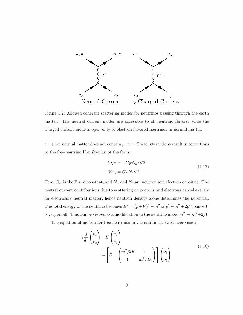
Figure 1.2: Allowed coherent scattering modes for neutrinos passing through the earth
matter. The neutral current modes are accessible to all neutrino flavors, while the
charged current mode is open only to electron flavored neutrinos in normal matter.
e−, since normal matter does not contain µ or τ . These interactions result in corrections
to the free-neutrino Hamiltonian of the form:
VNC = −GFNn/√
2
VCC = GFNe
√2
(1.17)
Here, GF is the Fermi constant, and Nn and Ne are neutron and electron densities. The
neutral current contributions due to scattering on protons and electrons cancel exactly
for electrically neutral matter, hence neutron density alone determines the potential.
The total energy of the neutrino becomes E2 = (p+V )2 +m2 ' p2 +m2 +2pV , since V
is very small. This can be viewed as a modification to the neutrino mass, m2 → m2+2pV
The equation of motion for free-neutrinos in vacuum in the two flavor case is
id
dt
ν1
ν2
=H
ν1
ν2
=
E +
m21/2E 0
0 m22/2E
ν1
ν2
(1.18)
9
To transform this to the flavor basis, H → H ′ = UHU †,
id
dt
νeνµ
=H ′
νeνµ
=
E +m2
1 +m22
4E+
∆m2
4E
− cos 2θ sin 2θ
sin 2θ cos 2θ
νeνµ
(1.19)
Correcting the free Hamiltonian for interactions with matter adds VNC to the effective
masses of νe as well as νµ. VCC , however, adds only to the mass of νe and therefore adds
to H ′00 element of the mixing matrix. Diagonalizing this new matrix leads to corrections
to the vacuum ∆m2 and mixing angle θ.
sin 2θmat =sin 2θ
Amat
∆m2mat = ∆m2Amat
where, Amat =
√(2EVCC∆m2
− cos 2θ
)2
+ sin2 2θ
(1.20)
The form of Amat indicates a resonance behavior for
VCC =√
2GFNe =∆m2 cos 2θ
2E(1.21)
=⇒ Nres =∆m2 cos 2θ
2√
2GFE= 6.56× 10³ ∆m2[eV2]
E[GeV]cos 2θ NA (1.22)
That is, at certain electron densities, matter effect causes even small mixing angles to
become nearly 45◦, resulting in an amplification in oscillation probabilities. This effect
is known as the Mikheyev-Smirnov-Wolfenstein or MSW effect. It can be a significant
effect where neutrinos pass through a very dense medium, for instance the core of a
star.
Even for neutrinos passing through earth crust where Ne ∼ 1.3NA3/cm3 [8] matter
effects can play a crucial role. For instance, for ∆m2 ∼ 10−3eV2 and neutrino energies
∼ 1 GeV, a vacuum mixing angle θ = 10◦ becomes ∼ 12◦ in matter. The oscillation
probability depends on sin2 2θ, which changes from ∼ 0.34 to ∼ 0.42, a ∼ 20% effect.
3NA is the Avogadro number, 6.023 × 10²³
10

Summary
Neutrinos, that were thought to be massless, undetectable particles at the time of their
conception, have proved to be neither. Neutrino oscillations require neutrinos to have
non-zero masses and are one of the few signs of physics beyond the Standard Model.
Neutrino masses are known to be very small (< eV ) compared to other Standard Model
fermions which might indicate that their nature is different from other SM particles. In
particular, the possibility of neutrinos having a Majorana mass has been discussed here
which provides a natural explanation for the smallness of the observed neutrino masses.
Oscillations are an interesting way of probing the physics of neutrino masses, which
is largely inaccessible otherwise, due to their small masses. The next chapter lays
out the current state of knowledge of the neutrino oscillation parameter space and the
experiments instrumental in making some of the measurements.
11

Chapter 2
Status of Neutrino Oscillation
Measurements
In modern experiments, neutrinos continue to pose a difficulty in detection as they
only interact rarely, via the weak interaction. While they are regularly produced in
collisions at collider experiments, they escape undetected and are more or less dismissed
as “missing energy”.
However, the discovery of neutrino oscillations has led to a rich program in exper-
imental neutrino physics in the last three decades. Neutrino oscillation measurements
have been made on a variety of neutrino sources, such as solar and atmospheric neutri-
nos, and reactor and accelerator neutrinos. These sources produce neutrinos of different
flavors and in different energy regimes, making them sensitive to different oscillation
parameters.
2.1 Conventions and Nomenclature
In the three neutrino flavor scenario, there are two independent mass-squared differences
constructed from the three mass eigenvalues m1, m2 and m3. The third degree of
freedom is the sign of one of the mass-squared differences. The convention is to set m1
12

to be smaller than m2, ie ∆m221 = m2
2 −m21 is positive definite.
The analysis of the oscillation experiments data indicated that one mass-squared
difference is much smaller than the other (∆m221 ' 3× 10⁻²× ∆m2
32). This means that
the L/E factor at which an experiment is sensitive to ∆m221, it is insensitive to ∆m2
32,
and 2-flavor oscillation formalism provides a good description of the phenomenology
to within a few percent. The angle and mass-squared difference that govern the solar
oscillations to leading order are θ12 and ∆m221. The atmospheric oscillation parameters
then are ∆m232 and θ23. This leaves θ13, which controls the amplitude of the electron-
neutrino disappearance channel in reactor neutrino experiments.
2.2 Oscillation Parameter Measurements
2.2.1 θ12 and ∆m221 Measurements
The nuclear chain reactions that occur in the core of the sun produce a large flux
of electron flavored neutrinos. The energy spectrum of neutrinos depends upon the
core temperature, composition of the sun, cross-sections of nuclear reactions involved,
opacity of the sun, etc. These factors were studied in detail by Bahcall and collaborators,
and encapsulated in the Standard Solar Model (SSM). The model, in addition to other
measurables, predicts a solar neutrino spectrum that can be observed on earth. Most
of these neutrinos, close to 91%, are produced in proton-proton fusion reactions:
p+ p→ d+ e+ + νe
However, the maximum energy of the neutrinos produced in this interaction is 0.4 MeV,
making detection very challenging. Higher energy neutrinos, with maximum energy of
14 MeV [9] are produced in the decay of Boron in the sun and contribute to less than
13

1% of the total flux:
d+ p→ 3He+ γ
3He+ 3He→ 4He+ 2p
3He+ 4He→ 7Be+ γ
7Be+ p→ 8B + γ
8B → 8Be+ e+ + νe
Figure 2.1: Predicted solar neutrino spectrum [1]
The first experiment to directly detect solar neutrinos was conducted by Raymond
Davis Jr. and collaborators [10], using electron neutrino capture on 37Cl to produce
37Ar in liquid C2Cl4 at the Homestake Mine in South Dakota. Helioseismological mea-
surements are in good agreement with the SSM [11], but the solar neutrino observation
experiments have consistently measured a neutrino flux significantly below the SSM pre-
diction. An interesting, chronological account of the unravelling of this so-called Solar
14

Neutrino Problem can be found in [12]. The solution to the problem is now understood
in the context of neutrino oscillations.
A series of solar neutrino detection experiments, such as GALLEX, GNO and SAGE
[13][14][15], used neutrino absorption on Gallium for detection and observed similar
deficits. Gallium has a threshold of 233 keV and therefore, enabled observation of νe
resulting from p− p fusion. The resolution, however, came from the Sudbury Neutrino
Observatory (SNO), a heavy water Cherenkov experiment in Canada, that measured
the rate of both, the NC and CC interactions of solar neutrinos resulting from Boron
decay:
νe + d→ e− + p+ p
ν + d→ ν + p+ n
The measurement of the flavor agnostic neutral current interactions made the exper-
iment sensitive to the total neutrino flux, independent of flavors. Their sensitivity to
the νe charged current interaction allowed them to measure the flux of electron-flavored
neutrinos alone. They observed that the total, flavor-independent neutrino flux was in
agreement with the SSM prediction, while the νe flux was only 1/3 of the predicted
value [16].
While travelling from the core of the sun to the surface, the electron neutrinos
encounter, to a good approximation, exponentially varying density of electrons. In the
core, for the higher energy neutrinos (E > 4− 5 MeV), the electron density is close to
the resonance density, Nres, discussed in the previous chapter. The νe state transitions
to mostly ν2,mat state, ie the heavier mass state in matter, in such conditions. If the
electron density in the sun changes adiabatically, the state ν2,mat smoothly transitions
15

to ν2, the heavier mass state in vacuum, at the surface of the sun. Given that
|ν2〉 = sin θ|νe〉+ cos θ|νx〉
P (νe → νe) = sin2 θ
For neutrinos with energies less than 4,5 MeV, θmat ' θ, and P (νe → νe) = 1− 1
2sin2 θ.
The best fit of current data from low and higher energy solar neutrino experiments
results in a value of θ12 ∼ 33.4◦ and ∆m221 ∼ 7.53 × 10⁻⁵ eV2. The θ12 angle is a
measure of the overlap of the νe flavor state with ν2. So these results mean that the
mass state ν1 is about 2/3 νe and ν2 is ∼ 1/3 νe.
2.2.2 θ23 and |∆m232| Measurements
Collision of cosmic rays with nuclei in the earth’s atmosphere produce showers of
hadrons. Pions being the lightest hadrons, are produced in large numbers and their
decay to muons produces muon neutrinos. The resulting muons further decay to pro-
duce an electron and a muon neutrino:
π+ → µ+ + νµ
µ+ → e+ + νe + ν̄µ
From this decay chain, the ratio of muon flavored to electron flavored neutrinos is ex-
pected to be 2:1. Various experiments had evidence of atmospheric neutrino oscillations
before Super Kamiokande (Super K) established it statistically [17]. What stands the
Super K experiment apart from its predecessors is that the detector is a massive 50 kilo-
ton water Cherenkov tank instrumented with photo-multiplier tubes. The Cherenkov
rings produced by energetic particles passing through the detector allow real-time event
energy and angle reconstruction. The angle reconstruction was especially important
in building confidence that the neutrinos were indeed atmospheric. The collaboration
recorded the νµ and νe CC interactions as a function of the zenith-angle, and found the
rate of νµ CC interactions due to neutrinos coming from below (having passed through
16

the earth) was signicantly lower than the rate of those coming from above. No such
discrepancy was observed in the νe CC rates. The leading interpretation was that the
disappearance of νµ was predominantly due to νµ → ντ transition.
The accelerator neutrino beams are obtained in much the same way as the atmo-
spheric neutrinos, except that the pions are produced by colliding energetic protons on a
stationary target. The K2K experiment in Japan and MINOS experiment at Fermilab,
USA, used such beams of muon neutrinos to observe νµ disappearance. The neutrinos
produced in this manner have energies of O(GeV ) and require baselines of 100’s of kilo-
meters. These beams of neutrinos travel through the earth’s crust and are sensitive to
matter effects.
The current best fit value of the global data is ∆m232 ∼ 2.44 × 10⁻³ eV2 (normal
hierarchy) and sin2 2θ23 ∼ 1.
2.2.3 θ13 Measurements
Nuclear power reactors are powerful sources of low energy electron anti-neutrinos, with
average energy of about 3 to 4 MeV. By choosing a baseline of about 1 km, the ex-
periments are sensitive to |∆m232| governed νe disappearance channel. At these L/E
values, the oscillation terms due to ∆m221 may be ignored to a good approximation. The
amplitude of this oscillation is dependent on the mixing-angle θ13, and the ν̄e survival
probability in the two-flavor approximation is:
P (ν̄e → ν̄e) ' 1− sin2 2θ13 sin2
(∆m2
32L
4E
)θ13 is the smallest and the last neutrino mixing-angle to be measured. It parameter-
izes the size of the νe component in the m3 mass state. CHOOZ was the first to make
this measurement using reactor neutrinos and they measured sin2 2θ13 < 0.15 [18], ie
their measurement was consistent with zero. A non-zero value of θ13 is crucial to the
measurement of CP violation in neutrinos (see equation 1.15).
17

The first results reporting evidence of non-zero value of θ13 were announced in 2012
by Double CHOOZ [19] in France, Daya Bay in China [20] and RENO [21] in Korea.
The three detectors are very similar. They contain Gadolinium doped liquid scintillator
that produces a flash of light due to annihilation of a positron resulting from anti-
neutrino absorption on a proton (ν̄e+p+ → e+ +n0). The free neutron thermalizes and
is eventually absorbed by a Gd nucleus, producing a delayed signal. The coincidence
of the prompt and delayed signals help reject backgrounds efficiently. The Daya Bay
experiment, which consists of 8 detectors in the vicinity of 6 commercial nuclear power
reactors has the world’s most precise measurement of this parameter.
Higher statistics analyses from the reactor experiments have since been published.
The current global fit value is θ13 ∼ 8.9◦. The θ13 parameter also controls the amplitude
of the leading term in the νµ to νe appearance channel. T2K and NOνA are the leading
experiments in this channel which is discussed in more detail later.
2.3 Unknown Parameters
2.3.1 Mass Hierarchy
As hinted before, oscillation experiments so far have not been able to resolve the sign
of ∆m232 and ∆m2
31. Neutrino oscillation experiments tell us that ∆m221 ' 3 × 10⁻²×
∆m232. Therefore, if |∆m2
32| is positive, m3 >> m2,m1, ie there are two light neutrinos
and one heavier neutrino, a scenario known as Normal Hierarchy (NH). If the sign is
negative, we have two heavier neutrinos, and a lighter one. This scenario is called
Inverted Hierarchy1. The vacuum oscillation probabilities only depend on the sine-
squared of the mass-squared differences and are not sensitive to the mass hierarchy.
1Another scenario is that the splittings between neutrino masses are much smaller than the neutrino
masses, so that the neutrino masses are degenerate. However, since oscillations are not sensitive to the
absolute mass scale, this case is not discussed here.
18

Figure 2.2: Mass hierarchy in neutrinos
The normal ordering of neutrino masses is considered normal because the electron-
flavored neutrino state comprises 2/3 of the ν1 mass state, and it is natural to expect
the lightest mass state to correspond to the first generation flavor state. The mass
hierarchy is also of critical importance in the searches for neutrino-less double-beta
(denoted as 0νββ) decay. The rate of lepton number violating 0νββ depends on the
square of < mββ >, the effective Majorana mass of the neutrino.
< mββ >= | cos2 θ13 cos2 θ12m1 + ei∆α21 cos2 θ13 sin2 θ12m2 + ei∆α21 sin2 θ13m3|2
where ∆αi1 are physically relevant Majorana phases (see section on neutrino-less double
beta decay in [6]). The effective Majorana mass can be computed as a function of the
lightest neutrino mass as shown in figure 2.3. At small enough neutrino masses, the
rate of 0νββ decay becomes sensitive to the neutrino mass hierarchy. So hierarchy
determination would help clarify the results from upcoming 0νββ experiments and help
in evaluating the sensitivity and in the design of the next generation of experiments.
19

Figure 2.3: Values of effective Majoarana mass, mββ , as a function of the lightest
neutrino mass. At small values of neutrino masses, mββ is sensitive to neutrino mass
hierarchy. Plot from [22].
2.3.2 CP Violation
The violation of T, and therefore CP symmetry arises from the complex phase, δ in the
PMNS matrix. If CP is violated, it implies that P (να → νβ) 6= P (νβ → να) for α 6= β.
Since changing the flavor of the source neutrinos is not feasible, experimental searches
for CP violation are carried out by changing the neutrino source to an anti-neutrino
source. The size of the difference between the neutrino and anti-neutrino oscillation
probabilities can be obtained with the help of equation 1.16:
P (να → νβ)− P (νβ → να) =P (να → νβ)− P (ν̄α → ν̄β)
=4∑j>k
=(U∗βjUβkUαjU
∗αk
)sin
(∆m2
jkL
2E
)(2.1)
Note that the above difference is zero for survival probability, P (να → να), because
this is a T invariant and therefore, a CP invariant process.
20

2.3.3 θ23 Octant
The current measurements of θ23 are consistent with 45◦. θ23 angle primarily determines
the admixture of the mass state ν3. If θ23 is exactly 45◦, all mass states contain equal
proportions of νµ and ντ . This might indicate a symmetry in the neutrino sector that
has not yet been accounted for in our theoretical framework. This scenario is known
as maximal-mixing. An accurate measurement of the νµ disappearance probability can
tell us if the mixing is maximal or non-maximal. But determining the octant of θ23, ie
whether θ23 less or more than 45◦, from νµ disappearance is difficult because the leading
order term in probability of this channel is given by:
P (νµ → νµ) ' 1− sin2 2θ23 sin
(∆m2
32L
4E
)That is, the leading term in the νµ disappearance probability depends on sin2 2θ23, which
is close to or equal to 1. The probability is the same for 2θ23 . 90◦ and 2θ23 & 90◦
2.4 νµ → νe on Long Baseline
νe appearance in a νµ beam on a long baseline is the most promising and relatively easy
to access oscillation channel to measure the remaining unknown parameters of neutrino
oscillations. The full three-flavor νµ → νe oscillation probability in vacuum is [23]
P (( )
ν µ →( )
ν e) = P1 + P2 + P3 + P4
P1 = sin2 2θ13 sin2 θ23 sin2 ∆m232L
4E
P2 = sin2 2θ13 cos2 θ23 sin2 ∆m221L
4E
P3 =(+)− J sin δ sin
∆m232L
4E
P4 =J cos δ cos∆m2
32L
4E
(2.2)
where
J = cos θ31 sin 2θ13 sin 2θ23 sin 2θ21 sin∆m2
32L
4Esin
∆m221L
4E(2.3)
21
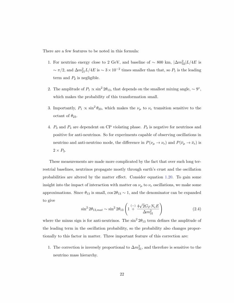
There are a few features to be noted in this formula:
1. For neutrino energy close to 2 GeV, and baseline of ∼ 800 km, |∆m232|L/4E is
∼ π/2, and ∆m221L/4E is ∼ 3×10⁻² times smaller than that, so P1 is the leading
term and P2 is negligible.
2. The amplitude of P1 ∝ sin2 2θ13, that depends on the smallest mixing angle, ∼ 9◦,
which makes the probability of this transformation small.
3. Importantly, P1 ∝ sin2 θ23, which makes the νµ to νe transition sensitive to the
octant of θ23.
4. P3 and P4 are dependent on CP violating phase. P3 is negative for neutrinos and
positive for anti-neutrinos. So for experiments capable of observing oscillations in
neutrino and anti-neutrino mode, the difference in P (νµ → νe) and P (ν̄µ → ν̄e) is
2× P3.
These measurements are made more complicated by the fact that over such long ter-
restrial baselines, neutrinos propagate mostly through earth’s crust and the oscillation
probabilities are altered by the matter effect. Consider equation 1.20. To gain some
insight into the impact of interaction with matter on νµ to νe oscillations, we make some
approximations. Since θ13 is small, cos 2θ13 ∼ 1, and the denominator can be expanded
to give
sin2 2θ13,mat ∼ sin2 2θ13
(1
(−)+
4√
2GFNeE
∆m231
)(2.4)
where the minus sign is for anti-neutrinos. The sin2 2θ13 term defines the amplitude of
the leading term in the oscillation probability, so the probability also changes propor-
tionally to this factor in matter. Three important feature of this correction are:
1. The correction is inversely proportional to ∆m231, and therefore is sensitive to the
neutrino mass hierarchy.
22

2. For normal hierarchy ∆m231 is positive, and the matter effect leads to an enhance-
ment in νµ to νe oscillation probability and to a suppression in ν̄µ to ν̄e oscillation
probability. The effect is just the opposite in case of inverted hierarchy.
3. The matter effect increases linearly with energy. Because neutrino oscillations are
a function of L/E, this implies that the longer the baseline of an experiment, more
the effect of matter interactions on the oscillation probability.
A more accurate expansion of νµ to νe oscillation probability is given in [23], and
amounts to:
P (( )
ν µ →( )
ν e) ∼ sin2 2θ13 sin2 θ23sin2((1−A)∆)
(1−A)2
+ α sin 2θ13 cos θ13 sin 2θ12 sin 2θ23sin(A∆)
Asin((1−A)∆)
(1−A)[cos δ cos ∆− sin δ sin ∆]
+ α2 cos θ223 sin2 2θ12
sin2(A∆)
A2
(2.5)
where A = ±2√
2GFNeE/∆m231, α = ∆m2
21/∆m231 and ∆ = ∆m2
31L/4E
The salient features of this more complicated form are consistent with those described
above for the simplification. It is worth pointing out that due to the presence of matter
effects, any difference between neutrino and anti-neutrino oscillation probabilities can
not be interpreted crisply as a violation of CP symmetry, since the matter effects can
alone produce such a difference. Therefore, all the interpretations of the parameters
extracted from this mode are as a function of the CP violation phase, δ and the mass
hierarchy.
The degeneracy between these parameters can be helped somewhat by making this
measurement at different baselines, since that would change the contribution due to
matter effects.
23

2.4.1 Experimental Observation
There are three current experiments capable of making this measurement: NOνA, which
is the subject of this dissertation, T2K and MINOS.
The MINOS detectors are made of alternating planes of steel and solid scintillator
and the neutrino baseline is about 735 km. The experiment was optimized for the
νµ disappearance measurement and is not very sensitive to νe appearance. But with
sophisticated analysis techniques, they produced their first νe appearance result in 2013
and a combined νµ disappearance and νe appearance result that mildly favors δ = 3π/2.
[24].
The T2K experiment uses the Super-K water Cherenkov detector to detect accel-
erator neutrinos from the J-PARC accelerator complex. The neutrino energy peak is
0.6 GeV and the baseline is 295 km long. Because of the shorter baseline, the effect
of interactions with matter is appreciably smaller for T2K. The experiment has been
collecting data since 2010. Their most recent result was published in April 2014, with
the observation of 28 νe candidate events and disfavors 0.35π(0.09π) < δ < 0.63π(0.9π)
at 90% CL for normal (inverted) mass hierarchy.
The NOνA experiment is discussed in detail in the remaining length of this docu-
ment.
24

Chapter 3
The NOνA Experiment
NOνA is the NuMI Off-axis νe Appearance experiment, designed to measure oscillations
of muon neutrinos in the NuMI beam at Fermilab. The power of the NOνA experimental
setup comes from its location, capabilities of the NuMI beam and the NOνA detector
design. The location of the far detector is at a distance of 810 km from the neutrino
source, near International Falls in Northern Minnesota, which enhances the matter effect
(recall that the matter effect is more pronounced at higher energies, and therefore, at
longer baselines). Figure 3.1 shows the νµ to νe oscillation probability at a baseline
of 810 km, and its dependence, through matter effect, on the neutrino mass hierarchy.
The oscillation probability peaks around 2 GeV neutrino energy. To match the neutrino
beam’s energy peak to the νµ to νe oscillation probability, the NOνA detectors are placed
14 milliradians off-axis from the NuMI beam (see section 3.1).
NuMI can run in neutrino as well as anti-neutrino mode which enables measurements
of P (νµ → νe) and P (ν̄µ → ν̄e). Figures 3.2 shows P (νµ → νe) versus P (ν̄µ → ν̄e) for
varying CP violation phase, mass hierarchy and values of θ23 at 2 GeV energy and a
baseline of 810 km. To first order, NOνA will measure a point in this plane. The
knowledge of parameters from other oscillation experiments constrains the range of
possible observations by NOνA to a set of ellipses. Due to the significantly large matter
25

E (GeV)0 1 2 3 4 5
)eν
→ µν
P(
0
0.1
0.2
0.3
0.4Baseline = 809 km
3Matter density = 2.76 g/cm-3| = 2.5 x 10²
32∆|-5 = 7.53 x 10²
21∆ = 123θ22sin = 0.84612θ22sin = 0.09313θ22sin
/2π = 3δ
< 0232 m∆
> 0232 m∆
No matter effect
Figure 3.1: Location of the NOνA detectors. The dotted black line indicates the axis of
the NuMI beam, while the red line is 14 mrad off-axis from the beam. The plot shows
the impact of matter effect on the νe appearance probability at NOνA’s baseline.
effect, the ellipses are disparate for normal and inverted hierarchies. The amplitude of
appearance probabilities is modulated by sin2 θ23. If sin2 2θ23 is different from 1, the
set of ellipses splits in two, one for θ23 > π/4 and the other for θ23 < π/4. The farther
apart the point that NOνA measures is from the alternative hypotheses, the tighter the
constraints from the measurements.
The NOνA detectors are optimized for νe identification. The νe appearance signal
is charged current interactions of the electron neutrino which produces an electron in
the final state. NOνA detectors have been designed with low Z materials. This allows
electromagnetic showers due to electrons to develop over many planes and cells and
provide enough information for their identification.
NOνA consists of two functionally identical detectors: a 0.3 kT near detector (ND)
about 1km from the neutrino source at Fermilab and a 14 kT far detector (FD) situated
near International Falls, Minnesota. The purpose of the near detector is to measure
the neutrino beam composition and energy spectrum close to the source, before neu-
trino oscillations set in. The far detector observes an oscillated neutrino beam and by
26

1 and 2 σ Contours for Starred Point
0
0.01
0.02
0.03
0.04
0.05
0.06
0.07
0.08
0.09
0 0.02 0.04 0.06 0.08
NOνAContours 3 yr ν and 3 yr ν̄|Δm32
2| = 2.32 10-3 eV2
sin2(2θ13) = 0.095sin2(2θ23) = 1.00
P(νe)
P(ν̄
e)
δ =0δ = π/2δ = πδ = 3π/2
-- Δm2<0— Δm2>0
1 and 2 σ Contours for Starred Point
0
0.01
0.02
0.03
0.04
0.05
0.06
0.07
0.08
0.09
0 0.02 0.04 0.06 0.08
NOνAContours 3 yr ν and 3 yr ν̄|∆m32
2| = 2.32 10-3 eV2
sin2(2θ13) = 0.095sin2(2θ23) = 0.97
P(νe)
P(ν̄
e)δ = 0δ = π/2δ = πδ = 3π/2
∆m2 < 0
∆m2 > 0
Figure 3.2: P (νµ → νe) versus P (ν̄µ → ν̄e) as a function of δ for the normal and inverted
hierarchies. The star point is a possible measurement scenario that NOνA may observe.
The contours are representative statistical errors on the measurement.
comparing the beam composition and spectrum between the two detectors, oscillation
parameters can be extracted. The near detector is 100 m below the surface in a cavern
at Fermilab, and the far detector is on surface.
3.1 The NuMI Beam
The NuMI beam is a muon neutrino source operated by Fermilab in Batavia, Illinois.
The neutrinos are produced by colliding high energy protons on a fixed target. The
collisions produce a large number of charged pions and kaons. These hadrons are focused
forward into a decay pipe, where their decays produce muon neutrinos: π+ → µ+ + νµ
(branching ratio 99.98%) and K+ → µ+ + νµ (branching ratio 63.55%). The beam
can be converted into an anti-muon neutrino beam by changing the polarity of the
27

focusing horns and focusing negatively charged hadrons towards the decay pipe. The
neutrino mode of the beam is called Forward Horn Current mode (FHC) and the anti-
neutrino mode is called Reverse Horn Current mode (RHC). The spectrum of neutrinos
obtained in this manner is reconstructed from K/π production data, decay kinematics
and simulation of the target-hall elements.
Figure 3.3: The neutrino energy spectra and flux as a function of the pion energy for
different off-axis angles, θ.
Since pions and kaons are spinless, their decay in the rest frame is isotropic. Using
relativistic kinematics, it can be shown that the neutrino energy and flux as a function
of the angle with respect to the beam axis in the lab-frame is given by
Eν =aEh
1 + θ2γ2
F =
(2γ
1 + θ2γ2
)2 A
4πL2
where h denotes the decaying hadron, and a =
(1−
m2µ
m2h
). γ is the hadron’s boost,
A is the detector cross-section and θ is the angle between the hadron’s and the decay
neutrino’s directions. It is clear from figure 3.3 that placing the NOνA detectors 14
28

milliradians off-axis from the beam ensures a narrow band beam with the neutrino
energy peaked at about 2 GeV, which is close to the νµ to νe oscillation probability
maximum for a baseline of 810 km. The narrowness of the spectrum reduces feed-down
from the neutral current background.
Figure 3.4: Simulated neutrino energy spectra at the NOνA far detector baseline of 810
km. The off-axis location of NOνA suppress the high neutrino energy tail
The beam does have an intrinsic νe component resulting from µ+ → e+ + νe + ν̄µ
and K+ → π0 + e+ + νe (branching ratio 5.07%). Since these decays are three-body
decays, the energy spectrum of the resulting νe is much broader than the very narrow
muon neutrino spectrum due to the off-axis location of NOνA. The electron neutrinos
resulting from kaon decays are higher in energy, so the νe beam background for NOνA
is mostly due to muons decaying in the decay pipe. In the energy region of interest to
NOνA (1-3 GeV), our simulations show that the νe contamination is sub-1% level. The
beam has a small wrong-sign contamination too, ie anti-muon neutrinos in the neutrino
beam and vice versa. The estimate for these components from simulation is < 2% in
neutrino mode and ∼ 10% in the anti-neutrino mode.
29

3.1.1 The Accelerator Complex
The Fermilab accelerator complex consists of two main accelerator rings. The Booster
ring is fed protons from a linear accelerator and accelerates protons to 8 GeV. In the
original design of the NuMI beamline, the proton batches from the Booster were trans-
ferred to the Main Injector ring, where they were accelerated to 120 GeV energy. The
beam in this configuration was used by the MINOS experiment for νµ disappearance
measurements and delivered a power ∼ 350 kW.
Figure 3.5: Schematic of the Fermilab accelerator complex, with upgrades implemented
for NOνA
To increase the beam power for the NOνA experiment, a series of upgrades have
been implemented in the accelerator complex. The Main Injector cycle-time has been
reduced from 2.2 seconds to 1.33 seconds. In the new scheme, the anti-proton storage
ring from the Tevatron days has been converted into the Recycler ring. Protons from
the Booster are now transferred first to the Recycler, which is used as a pre-injector to
the Main Injector. This reduces the proton injection time from the Main Injector.
30

3.1.2 Slip-Stacking
Another improvement is to slip-stack all the batches in the Recycler to improve the
intensity of the NuMI beam. Fermilab uses two RF systems to implement slip-stacking.
The details can be found in [25]; what follows is a brief qualitative description.
Six batches, with 4 to 5 ×10¹² protons each, are fed one after the other from the
Booster into the Recycler. The Recycler is seven times larger than the Booster in
circumference, which means that there is space in the Recycler for an extra batch.
The first six batches in the Recycler are first decelerated, by gradually reducing the
frequency of the RF cavity, and fall into a lower momentum orbit. A seventh batch is
then introduced from the Booster into the Recycler, in the seventh, empty slot. Since
the seventh batch is at a different momentum than the earlier six batches, the batches
slip with respect to one another. The RF voltages are tuned such that the batches
stay bunched, and before the next injection occurs, the seventh batch slips out of the
seventh slot and lines up azimuthally with the sixth batch. The eighth batch is then
introduced into the once again empty seventh slot. This process is repeated until all
six batches have twice the number of protons, albeit at slightly different energies. The
recycler beam is then extracted into the Main Injector altogether, so that the intensity
of each Main Injector spill is close to 5× 10¹³ protons and it lasts for 10 µs.
3.1.3 The NuMI Beamline
The protons extracted from the main injector are directed 3◦
downwards in order to aim
the resulting neutrinos towards the MINOS far detector. The target for the NOνA era
is a series of graphite fins mounted between two stainless steel pipes that circulate water
for cooling. The target is 2 pion interaction lengths, to provide sufficient probability of
proton interaction, while avoiding absorption of low energy pions that are needed for
neutrino production. The charged hadrons produced at the target are focused towards
the decay pipe by two pulsed magnetic horns whose inner conductors are parabolic
31

Figure 3.6: The NuMI Beamline [2]
in shape. The magnetic horns act like lenses with a focal length proportional to the
pion momentum. The pions that are not focused by the first horn may be focused by
the second horn downstream. The decay pipe is 675 m long and 1 m in radius and
maintained at a very low pressure (5× 10⁻⁵ atm). A water cooled Aluminium hadron
absorber is placed at the end of the decay pipe, followed by three ionization chambers
to monitor the outgoing muons.
3.2 The NOνA Detector Design
The NOνA detectors are close to 65% active calorimeters, optimized for development
of well-formed electromagnetic showers. Each of the detector components is described
briefly in the following sections. This chapter draws heavily from the NOνA Technical
Design Report [25] which may be consulted for greater detail.
3.2.1 The NOνA Unit Cell
The NOνA detectors are composed of PVC modules extruded to form tube-like cells
with rectangular cross-section (∼ 4 cm × 6 cm). A layer of cells forms one plane of
the detector. The cells in adjacent planes are orthogonallly rotated with respect to one
another to allow for 3-D reconstruction of particle positions. Each cell is filled with
32

Figure 3.7: A cell and a cut-out of the NOνA detectors indicating the orthogonal
arrangment of cells in adjacent planes.
liquid scintillator and there is a loop of optical fiber to catch the scintillation light (see
figure 3.7). The light from 32 such cells is read out by 32 pixels of an Avalanche Photo
Diode chip. The cells are 3.6 cm wide and 5.6 cm deep. This defines the granularity of
the NOνA detectors. A cell is 15.5 m long in the FD and 4 m long in the ND. These
long fiber lengths mean that light attenuation is a significant effect in NOνA. There are
384 cells per plane in the FD, and 48 in ND.
3.2.2 Liquid Scintillator
The scintillator used in NOνA consists of three components: a scintillator that emits
light in the UV region when charged particles pass through, wave-length shifters (WLS)
that absorb the light emitted by the scintillator and emit longer wave-length radiation
that can be picked up by the optical fiber and mineral oil as solvent, that blends these
components into a stable solution.
33

Figure 3.8: The emission spectrum of the NOνA scintillator. The figure is from [3].
The scintillating agent used in NOνA is pseudocumene (1,2,4- Trimethylbenzene)
that emits photons in the range 270 - 320 nm. These photons emitted by pseudocumene
excite the wave-length shifter PPO (2,5-Diphenyloxazole) that de-excites by emitting
photons of wavelength in range 340 - 380 nm. These photons excite the second wave-
length shifter in the NOνA blend, bis-MSB (1,4-bis-(o-methyl-styryl-)-benzene). This
WLS de-excites through emission in the range 390 - 440 nm [3].
The NOνA scintillator is close to 95% mineral oil and 5% pseudocumene, with
sub-percent level of WLS agents. The scintillator also contains an anti-static agent
(Stadis-425) at 3 ppm to make it semi-conducting and less of a fire-hazard from charge
build-up and sparking during filling. In addition, Vitamin E is added to the blend
as an anti-oxidant to prevent yellowing of the scintillator, which would degrades its
transparency over time.
65% of the total mass of the NOνA detectors is in liquid scintillator.
34

3.2.3 Optical Fiber
The optical fiber used in the NOνA detectors also contains wave-length shifting agents.
The Y11 die in the fiber is excited by the violet light (∼ 425 nm) emitted by the
NOνA scintillator. The dye emits blue-green light in the wave-length range 450-650
nm. Due to the overlap between the absorption and emission spectrum of the dye,
the wavelengths below 520 nm are severely attenuated in the fiber. The fiber core is
Figure 3.9: The absorption and emission spectra of the NOνA WLS fiber. Due to the
overlap between the two, the light with wavelengths below 520 nm are highly attenuated.
made of polystyrene, which has a refractive index of 1.59. The core is encased in an
inner acrylic cladding (n=1.49) and an outer fluorinated-polymer cladding (n=1.42).
The inner cladding improves the acceptance angle for total internal reflection of light in
the core and also provides an additional layer of protection for the core. In the NOνA
cells, the fiber is placed in a loop, with its plane oriented along the diagonal of the cell
cross-section. The bending radius of the fiber has to be as little as 3 cm. For this reason
the fiber has a radius of 7 mm, which is much finer than the 1.2 mm fiber used in the
MINOS detectors. The looped fiber provides twice the light-collection fraction than a
single strand. It is also more efficient than two separate strands of fiber because it does
not suffer from imperfect reflection from the fiber ends.
The two ends of the fiber in a single cell terminate at one pixel of a 32 pixel avalanche
photo diode (APD) array.
35

3.2.4 Avalanche Photodiode (APD)
APDs are photo-sensitive avalanche diodes that are operated with a high reverse bias
voltage. Under such conditions, the electron and hole pairs excited by photons are
accelerated in the strong internal electric field. As these highly energetic electrons move,
they strike other electrons and cause them to be freed. These secondary electrons and
holes are themselves accelerated and strike more electrons free and so on. This process
is called impact-ionization and an avalanche of charge carriers in the diode leads to a
significant amplification of the photocurrent.
APDs were favored over Photomultiplier Tubes (PMT) for light detection in NOνA
for two reasons: the quantum efficiency of APDs (85%) is about eight times higher than
that for PMTs (∼ 10− 20%) and is much flatter over the range of wavelengths of light
that NOνA WLS fiber transmits (500-550 nm). The high quantum efficiency of APDs
is a necessity for NOνA because it allows the observation of faint light signal from the
end of 15 m long modules in the FD. The APDs used by NOνA are manufactured by
Hamamtsu and have a custom design to accommodate two ends of the fiber loop per
cell on a single pixel. Each NOνA APD array consists of 32 pixels, where each pixel
reads out a single cell.
For APDs to effectively detect signal from the far end in a 15 m long cell, the noise
must be kept low. To minimize the dark current (current in absence of light) due to
thermally created electron-hole pairs, APDs are operated at a temperature of −15◦C.
Each APD carries its own thermoelectric cooler (TEC) to maintain this operational
temperature. To remove heat from the TECs, a water cooling system has been designed
which circulates water chilled to 15◦C. The APD surface must be kept clean and dry
for safe operation and to minimize surface currents. To achieve this, the surface of the
APD is coated with Parylene, a transparent epoxy, and it is ventilated with dry-air to
prevent accumulation of moisture.
36

In addition, the statistical nature of the avalanche process generates current fluctua-
tions and the APD performance is further degraded by what is known as an excess noise
factor. The excess noise is a function of the gain and the carrier ionization ratio, k,
defined as the ratio of ionization probabilities of holes to electrons, which in the NOνA
APDs is about 1:50. The APDs are operated at a voltage close to 425V which is known
to produce a gain of about a 100. The excess noise factor is well-modeled and is included
to some extent in our simulation. The operational conditions have been designed and
demonstrated to produce a signal to noise ratio of 10:1 or better for majority of the
APDs.
Figure 3.10: Schematic of the APD and front-end electronics.
The signal received from each APD pixel is further amplified through individual
integrated circuits custom designed for NOνA. After amplification and pulse-shaping,
the signal from eight cells is multiplexed into an ADC. The APD, and all the other
components described here are mounted on a front-end board or FEB (see figure 3.10).
The APDs are operated continuously and do not require any external triggering.
3.2.5 PVC Modules
The PVC modules are the structural elements of the NOνA detector and primary con-
tainment for the liquid scintillator. PVC is close to 30% of the total NOνA detector
37

mass. The high light-yield of NOνA is in part due to the reflectivity of the PVC modules,
which is boosted substantially by adding anatase titanium dioxide (TiO2) to it. The
reflectivity attained in this manner is about 90% at the peak wavelength of scintillator
emission (430 nm).
The shape of the PVC extrusions is optimized for easy and reliable extrusion, mini-
mum PVC stress and light reflectivity. The outer extrusion walls are 4.8 mm thick and
the inner walls between cells are 3.3 mm thick. The outer wall of the modules is scal-
loped at the cell boundaries due to the requirements of the extrusion process (see figure
3.11). The corners of the cells are rounded or scalloped too. This reduce PVC stress
concentration on corners and makes the cell wall thickness constant which assists in
uniform cooling in the extrusion process. The ratio of the inner to outer wall thickness
is at the recommendation of the extruders for reliable extrusion.
Figure 3.11: Profile of the PVC extrusion showing scalloped corners in the inner and
outer walls of the extrusion
The PVC extrusions were extruded in groups of 16 cells and shipped, upon in-
spection, to the Module Factory at University of Minnesota, Minneapolis, where the
extrusions and other components were assembled into NOνA modules. This is done
due to the expense and technical challenges involved in extruding 32 cell extrusions.
For the assembly of the modules, adhesive epoxies that are inert to the liquid scintil-
lator were used. The first step in the process is to glue two extrusions to form 32 cell
extrusions. The cells are strung with loops of optical fiber. The end of the loop is
mounted on a plastic ring, with a groove to hold the fiber in place, that is aligned along
the diagonal of the cell’s cross-section. At the top end of the modules, the two fiber
ends from each of the 32 cells are embedded into the grooves of the fiber raceways. The
38

raceway routes the fiber ends to the optical connector that contains 32 holes through
which the fiber ends from the cells in the module are threaded. Each of the holes on the
connector maps to a single channel on the APD. The handling of the fiber is a delicate
process and tests were done to check the quality of the fiber at each stage of the process.
Figure 3.12: Schematic of the APD and front-end electronics.
The end of the module is sealed with an end plate, which is injection-molded from the
same PVC as the extrusions. It has walls that cover the outside edge of the extrusions.
Side seals are designed to take up the tolerance in the width of the module. End plate,
center and side seals together seal the end of the module.
The top of the module is sealed with the manifold cover and the snout. The snout
houses the optical connector and the fiber raceway ends and supports the APD and FEB
mounted on the optical connectors. It also contains a port for filling the module with
scintillator and another for ventilation. The manifold cover has a more complex shape
than the end plate in order to accommodate the raceways. The shape of the manifold
39

is with a step at the top to accommodate the snout from the adjacent module in the
same plane. The fiber cover, raceways, manifold cover and snouts are all composed
of black injection plastic to minimize light reflection. This reduces cross-talk between
fibers from different cells in the module.
Once the modules are fully assembled, they are tested to detect any leaks. If a
leak is found and the attempts to fix it prove unfruitful, the module is discarded. The
fully tested modules are shipped to the far detector hall or to Fermilab to assemble the
detectors.
3.2.6 Detector Assembly
Far Detector
In the far detector, each plane consists of 12 32-cell modules. The detector is assembled
in units of blocks, each consisting of 32 planes glued together in alternating vertical and
horizontal orientations. The fully assembled detector consists of 28 such blocks and has
896 planes in total. The south-end of the far detector hall is the assembly area where
modules that are shipped from the module factory are stacked, reassessed for damage
during shipping and prepared for assembly. Empty modules are vacuum lifted using an
overhead crane. An automatic glue dispenser applies and spreads the glue on the surface
of the modules. The modules are then moved into place on the block for adhesion. The
bottom of the blocks is fitted with stiff steel pellets that provide structural support.
The assembly of the blocks takes place on a movable horizontal platform, known
as the block pivoter. Upon completion of the block, the block pivoter moves on rails
down the hall to the position where the block is to be installed. The horizontal platform
pivots to a vertical position, installs the block in place, returns in a horizontal position
to the assembly area, where the assembly of the next block commences.
40

Figure 3.13: Block pivoter during the installation of a block in the far detector hall
The first block is installed against a concrete bookend that is capable of supporting
the detector in case of buckling due to structural failures in the detector blocks. The
subsequent blocks are installed against the already installed blocks. After the last block
is installed, the block pivoter is pivoted against it and permanently left in that position,
to provide support.
The blocks are filled with scintillator one at a time, starting first with the lowest
horizontal modules. Once the horizontal modules are filled, the filling of vertical modules
follows. Once the block is filled, the modules are outfitted with APDs and FEBs.
Near Detector
The processes involved in the assembly of the near detector are the same as those for
the far detector with a few modifications. The near detector has three modules per
plane and 24 planes (12 horizontal and 12 vertical) per block and contains 8 such blocks
in total. In addition, the downstream end of the ND has a muon catcher to range out
muons.
41

The muon catcher contains ten planes of steel, each of which is 4.03 inches in thick-
ness, as wide as three module-widths and as tall as two module-widths, giving them a
rectangular shape. The steel planes are interspersed with three vertical and two hori-
zontal PVC planes for detecting muons. The vertical PVC modules are also 2/3 their
usual height to match the steel planes. Therefore, the total number of active, scintillator
filled PVC planes in the ND is 214.
Once a near detector block is assembled, it is erected into an upright position. A
cradle is then built around it for safe transportation to the underground detector cavern.
The blocks arrive at the MINOS surface building at Fermilab and are lowered down the
the MINOS shaft. The detector blocks are on wheels which are a part of the cradle.
Once underground, they are wheeled into place in the NOνA near detector hall.
Summary
The NOνA detectors are composed of liquid scintillator filled PVC modules. Wave-
length shifting fiber and APD’s are the light-detection elements in the detector design.
The detectors are now fully constructed. The far detector has been taking data since
October 2013 and the near detector, since August 2014.
42

Chapter 4
Data Acquisition and Triggering
Systems
The NOνA detector design presents unique challenges in data acquisition. The far
detector is located 810 km from the NuMI beamline so triggering the readout in advance
of a NuMI beam spill is difficult. Using an activity based trigger to record NuMI data
is also difficult because the FD is located on surface and there is a very large flux of
cosmic rays, at 120 kHz . These problems are circumvented by operating the detector
in continuous readout mode which is outlined in this chapter.
4.1 Overview of NOνA DAQ System
The pulses from 32 channels of an APD (Avalanche Photodiode) are readout by a Front-
end Board (FEB) that time stamps and shapes the signal. Data from 64 FEBs (and
therefore 64 modules, with 32 cells each) are aggregated by a Data Concentrator Module
or DCM, which is a custom built computer. It organizes data into 50 µs long units, or
microslices. These 50 µs units are aggregated by an event builder module, running on
the DCM, into 5 ms long chunks, or millislices. The durations of these data aggregation
units are optimized for transmission over the internal bus and on the ethernet. All the
43

DCMs dispatch their 5 ms millislices to a pool of buffer nodes, such that the data from
the same 5 ms window from all DCMs arrives at the same buffer node.
Two consecutive modules in 32 consecutive planes from the same view are read
out by a single DCM. Since each block contains only 16 modules per view, a DCM
encompasses two blocks, a unit we call diblock. Therefore, while the NOνA detectors
are installed in units of blocks, the readout is organized in units of diblocks. A diblock
contains 64 planes, 32 in each view. It is instrumented with 12 DCMs, 6 for horizontal
and 6 for vertical view (recall that there are 12 modules per plane). In figure 4.1, DCMs
are outline in green. The mass of a single diblock is about 1 kT, and there are 14 of
them in the completed NOνA far detector.
Figure 4.1: DCM layout in FD. The green boxes indicate the readout domain of an
individual DCM.
4.2 Clock and Triggering
All the readout components in NOνA are synchronized to an external wall clock through
the timing chain at the head of which is a Master Timing Distribution Unit (MTDU).
44

The MTDU is connected to a high-precision GPS receiver to drive the master clock.
The MTDU drives slave TDUs (STDU), each of which synchronizes a diblock, or 1kT
of the NOνA detector. This results in all the detector channels being synchronized with
each other. The detector is operated in a free running mode where all the channels that
register an above-threshold energy deposit record a hit with a time stamp.
The MTDU at Fermilab is connected to the accelerator network. When a beam
spill occurs at Fermilab, it decodes the accelerator time stamp into NOνA time, and
the spill is transmitted to both near and far detectors, after correcting for the time of
flight of neutrinos through the earth. When the spill information is received by the spill
receiver, the buffer nodes search in millislices for hits that occurred in the beam spill
time and the selected hits are stored to permanent storage. Note that the far detector
beam spills are recorded in 500 µs windows, centered around the beam spill time. This
is because the exact location of the spills was not known with enough accuracy and
has since been determined using the far detector data (see section 4.4.1). Moreover,
recording beam-spills with ample padding on either side allows for cosmic background
estimation from these side-bands. The buffer nodes are capable of storing up to 20
minutes of far detector data and the spill messages are received between 2-10 seconds
after the occurrence of the spill.
Additionally, we also run a cosmic pulsar trigger at the far detector, that triggers
at regular intervals and records 500 µs of cosmic data at a time. In the near detector,
the cosmic trigger is an activity based trigger. The cosmic data is used for calibration,
to determine timing resolution and study detector response and also, to study cosmic
background to the neutrino oscillation analyses. More details on the NOνA timing and
triggering systems can be found in [26].
45

4.3 Readout
The front-end board (FEB) that an APD is mounted on houses an ASIC (Application
Specific Integrated Circuit) to shape the signal and an ADC (Analog to Digital Con-
verter) to digitize it. The far detector FEBs are driven by a 16 MHz clock and the
ASIC uses 8:1 multiplexing to readout the 32 channels of an APD. This means that
each APD channel is readout with a 2 MHz frequency. The far detector ASIC shapes
the pulse with a 460 ns rise-time and a 7000 ns fall-time. These shaping parameters are
determined from measuring the APD leakage current and shot noise to get a signal to
noise ratio of 10:1 from the far end of the cell.
The near detector, due to its proximity to the neutrino beamline, records multiple
interactions per beam spill. The separation of hits arising from different neutrino inter-
actions requires a more precise timing resolution in the near detector than in the FD.
The ND ASIC uses 2:1 multiplexing, so the sampling frequency of each APD channel is
increased to 8 Mz. In addition, a pulse in the near detector is shaped with a rise-time
of 140 ns and a fall time of 4500 ns.
The FEBs use a dual correlated sampling (DCS) algorithm to determine if a pulse
is signal or not. In this algorithm, the FEB processes the difference between the ADC
counts of the si sample and the ADC count from the sample three clock-ticks prior, si−3.
If this difference is above a pre-determined threshold value, the baseline subtracted ADC
value of the si sample and its time, ie the TDC (Time to Digital Converter) value are
recorded as a hit. This mode is known as the single-point mode. We can also store
multiple samples, si−3 to si, which we may fit offline to more precisely estimate the
hit time from the rising edge of the pulse. This readout mode is called the multi-point
readout. The near detector has always been operated in the multi-point mode. The
far detector was operated in single-point mode until October 2014, and in multi-point
mode since. Figure 4.2 shows a cartoon of a typical pulse shape. In the single point
readout mode, the timing resolution of the far and near detectors are (tsample/√
12 =)
46

144 ns and 36 ns, respectively.
Figure 4.2: Single- and multi-point readout. In single-point readout, the charge and
time of the baseline subtracted, above threshold ith sample is saved, while in multi-
point mode, a pulse-shape is fitted to the trace to derive the time and charge of the
hit.
4.3.1 APD Sag and Ringing
Benchtop charge-injection tests of APDs have shown that when any particular channel
on an APD is triggered, the other 31 channels exhibit a negative pulse, ie a drop in the
output. The observed pulse on the triggered channel itself is diminished by the same
magnitude as the drop in other channels. The scale of the drop is found to be linearly
correlated with the amount of charge injected on a channel, and is about 1.86% of the
injected charge. When multiple channels are triggered, the drop in the baseline across
all channels is found to be 1.86% of the total charge deposited in the APD. The cause of
this drop is not well understood. Simulated waveforms of channels triggered in a single
APD in the ND are shown in figure 4.3. Notice the black trace of a channel that sags
below zero due to the presence of charge on other channels.
A repercussion of APD baseline sag is APD ringing or flashing. When the baseline
of untriggered channels recovers from sag by returning to the nominal baseline, if the
47

Time [ns]0.215 0.22 0.225 0.23 0.235
610×
AD
C
0
1
2
3
4
310×
Figure 4.3: Simulated readout traces of channels on a single APD exhibiting sag. The
black trace is of a channel that had no energy deposited in it, but the baseline sags due
to triggering of other channels on the APD.
difference between any pairs of samples separated by three clock-ticks exceeds the ADC
threshold of that channel, the Dual-Correlated Sampling (DCS) algorithm triggers a
hit. Since the sag is larger when the the initial charge deposited on the APD is high,
this flashing of an APD is observed after a very a highly ionizing interaction takes place.
Bench top tests show sag induced triggering to occur with charge deposits of 250X the
threshold in FD and 700X in ND. This translates to ∼300 MeV and ∼500 MeV of energy
deposited in a far and near detector APD, respectively. APD flashes usually happen
several microseconds after the initial charge deposition and therefore are well-separated
from the main event in time.
4.4 Timing Peak
4.4.1 Far Detector
In the far detector, the data are dominated by cosmic rays. We apply a series of cuts
to reject cosmic rays and select neutrino-like interactions. The timing distribution of
selected events is used to determine the location of the NuMI peak. The cuts employed
48
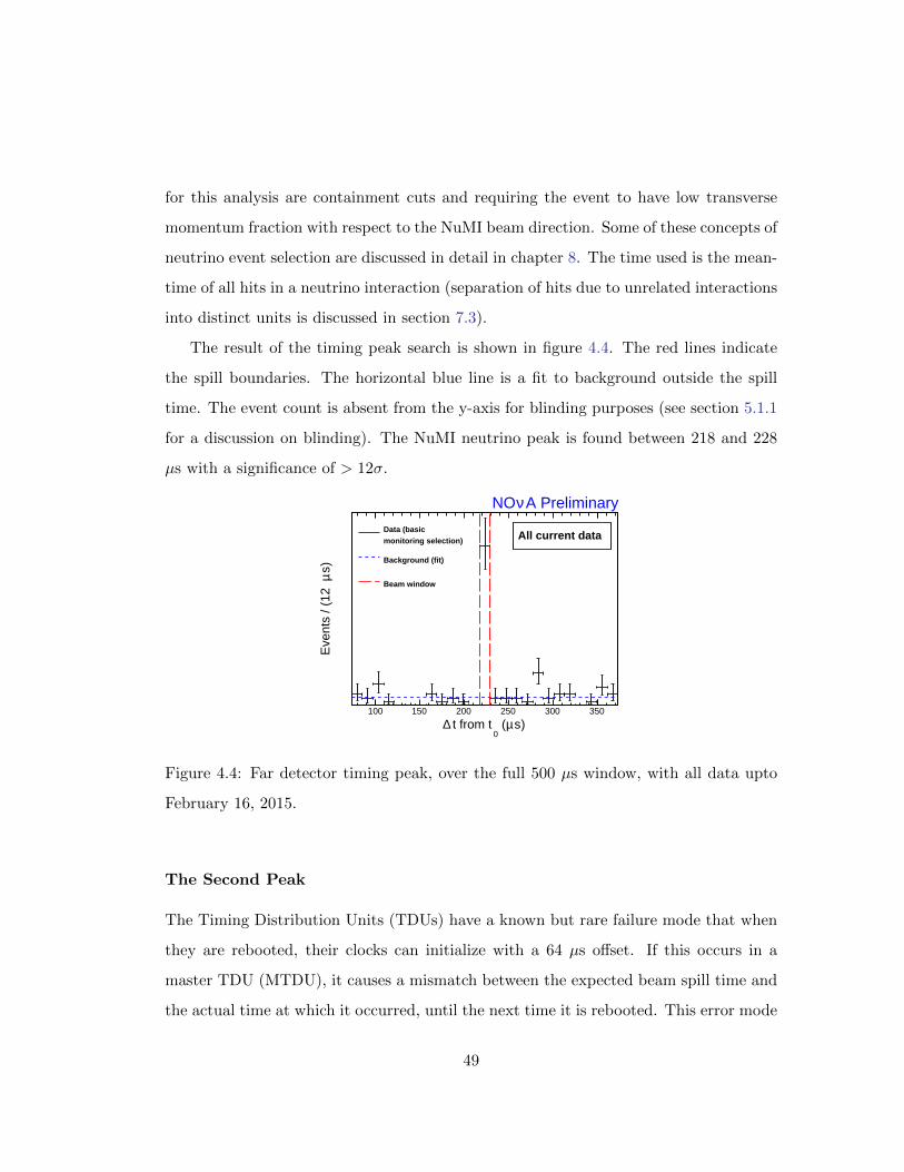
for this analysis are containment cuts and requiring the event to have low transverse
momentum fraction with respect to the NuMI beam direction. Some of these concepts of
neutrino event selection are discussed in detail in chapter 8. The time used is the mean-
time of all hits in a neutrino interaction (separation of hits due to unrelated interactions
into distinct units is discussed in section 7.3).
The result of the timing peak search is shown in figure 4.4. The red lines indicate
the spill boundaries. The horizontal blue line is a fit to background outside the spill
time. The event count is absent from the y-axis for blinding purposes (see section 5.1.1
for a discussion on blinding). The NuMI neutrino peak is found between 218 and 228
µs with a significance of > 12σ.
)sµ (0
t from t∆100 150 200 250 300 350
)sµ
Eve
nts
/ (12
monitoring selection)Data (basic
Background (fit)
Beam window
A PreliminaryνNO
All current data
Figure 4.4: Far detector timing peak, over the full 500 µs window, with all data upto
February 16, 2015.
The Second Peak
The Timing Distribution Units (TDUs) have a known but rare failure mode that when
they are rebooted, their clocks can initialize with a 64 µs offset. If this occurs in a
master TDU (MTDU), it causes a mismatch between the expected beam spill time and
the actual time at which it occurred, until the next time it is rebooted. This error mode
49

is easy to monitor for in the near detector, since the neutrino peak moves visibly. In
the far detector, these cases were not identified at the time, but in retrospect, we see
compelling evidence of this shift in the far detector for at least some part of the data
collected thus far. This can be seen in the timing peak in figure 4.4, where a smaller
peak 64 µs after the expected peak at 218 µs, at 282 µs is visible.
The far detector was only susceptible to this failure before the October beam shut-
down. During the shutdown, a Timing Calibration Reference (TCR) was installed at
each detector. The TCRs have an independent GPS antenna and receivers that gen-
erate a stable 1Hz pulse. MTDUs receive these signals and time stamp them. If the
MTDU version of time is different from expected, an automated synchronization process
is started.
The treatment of this additional timing window at 282 µs and its consequences to
the analysis of those data are discussed in the next chapter.
4.4.2 Near Detector
Observing the timing peak in the near detector is trivial in comparison to the far
detector. It is 100 m underground, and the cosmic interaction rate in the detector
is negligible. Therefore, the activity that is registered in the detector is mostly due
to the interaction of neutrinos. Electronic noise is evenly distributed in time, while
the neutrino interactions occur within the 10 µs NuMI spill. The NuMI beam peak is
discernible by just plotting the hit times within the 500µs NuMI trigger window, with
no cuts applied. The peak can be observed after collecting a few spills of NuMI data.
The location of the spill in the 500 µs trigger window is found to be consistent with the
expectation of 218 - 228 µs.
Because of the large statistics and reasonably precise timing, we are also able to
observe (figure 4.5) the batch structure in NuMI spills (recall that the NuMI spill is
composed of six batches of protons, see 3.1.2).
50

Figure 4.5: Near detector timing peak, over the full 500 µs window, and zoomed in to
show the NuMI beam structure.
51

Chapter 5
νe Appearance Analysis Overview
The analysis presented in this report is an observation of νe appearance in the muon
neutrino NuMI beam in the NOνA experiment. This chapter lays out the steps involved
in this analysis and attempts to provide some context for the chapters that follow.
Section 5.2 is dedicated to describing the data analyzed in this thesis.
5.1 Oscillation Analysis Steps
In a two-detector oscillation experiment such as NOνA, the neutrino data collected
in the near detector are used as a control sample. Given that the neutrinos are 2
GeV in energy at the off-axis location of NOνA, the propagation distance of neutrinos
from the source to the near detector (∼ 1 km) is much smaller than the oscillation
length. Therefore the ND neutrino data contains no νe appearance signal and is a pure
background-only sample. The use of the ND data and other steps and concepts used in
the appearance analysis are described below.
5.1.1 Blind Analysis
The oscillation analyses in NOνA are blind analyses, which means that all cuts, back-
ground and error estimates etc are finalized prior to looking at the far detector neutrino
52

data. Blinding is achieved by obscuring relevant information about the events in the
NuMI trigger data that relate to the oscillation probabilities.
The purpose of blinding is to avoid any bias in our oscillation results. The two pieces
of information that are sufficient for the oscillation analysis are the flavor of the neutrino
and the energy of the interaction. So the particle identification (PID) information and
energy are naturally blinded. Other variables from which event energy or identity may
be deduced, such as the leading shower energy or length, number of planes and cells
in slice, PID input variables etc, are also blinded. Blinding is only applied to the far
detector data events with reconstructed energy between 0.8 and 3 GeV, that fall within
the 10 µs beam window in the NuMI trigger stream. Leaving beam events that do not
bias our oscillation results unblinded allows the study of sidebands that offer valuable
sanity checks of our reconstruction and PID on the far detector data. It is worth noting
that the near detector data are not subject to blinding which lets us put our simulation
to more severe tests against the neutrino data.
5.1.2 Cosmic Background Estimate
As described in the previous chapter, we have a dedicated cosmic trigger in the far
detector, which records the data collected over a 500 µs window at regular intervals.
The data from this trigger stream was used to tune the cosmic rejection cuts. The NuMI
trigger windows are also 500 µs in duration, while the beam only lasts for 10 µs, from 218
to 228 µs. NuMI trigger data outside of the time range 217 - 229 µs is called the timing
sideband and is used to estimate the cosmic background for the final analysis. Using the
NuMI trigger ensures that the detector configuration and data-taking conditions used
in cosmic background estimates are identical to that of the neutrino data.
Figure 5.1 is a diagramatic representation of how a NuMI trigger is split. The NuMI
spill times are padded by 1 µs so neutrino data is not lost due to slight miscalibration
of our timing system. For cosmic background estimate, we get further away from the
beam spill and use data in the two sidebands between 25 and 208 µs and 238 and 475
53

µs. Any cosmic events in the sidebands that pass the νe selection cuts are scaled by a
factor of 12/( (208-25)+(475-238)) = 12/420 to scale to the livetime of the NuMI beam
spill for a final estimate of the cosmic background.
sideband sideband
| |<--------------------->| |numi| |<----------------------->| |
0 25 208 217 219 238 475 500
|<---------------------------------------------------------------------->|
numi trigger window
Figure 5.1: Diagram showing the timing sideband in NuMI trigger windows. The num-
bers are times in µs since the start of the NuMI trigger window. The sidebands are
used to estimate cosmic background.
5.1.3 Beam Background Estimate
Since there is no νe appearance signal in the near detector, any events that pass the
νe selection cuts represent background to the νe appearance analysis. However, event
counts alone are not sufficient. The background selected in the ND must be broken down
by event type so that they may be properly treated in oscillation. For instance, neutral
current interactions are flavor independent and therefore, unaffected by oscillations,
while muon neutrinos oscillate, therefore the contribution of νµ CC events to background
in FD will be greatly diminished to that in the ND.
The estimation of the contribution of different components to the observed back-
ground in the near detector is known as decomposition. This is discussed in more detail
in chapter 11
54

5.1.4 Extrapolation
The ND data is used not only for beam background estimates, but also for prediction of
the νe appearance signal. The observed νµ CC interaction rate in the ND is essentially a
measurement of the beam at t, L = 0 and translates to an expectation of νe appearance
signal in the FD. It gives us a handle on any beam flux differences in data and MC that
would impact the νe appearance signal.
The conversion of the observed interaction rates in various channels in the near
detector to a prediction of signal and background in the far detector is known as ex-
trapolation. The extrapolation method is discussed in detail in chapter 11.
5.1.5 Final Fit
The signal expected (see chapter 11) from the analysis of the first NOνA data is small,
so we have opted for a simple cut-and-count analysis. That is, our measurement of
oscillation parameters is based solely on the number of events observed in the FD, and
not their underlying energy distribution. Extrapolation of beam background and cosmic
background estimate from the NuMI timing sidebands gives us an estimate of the event
counts expected in the absence of muon to electron neutrino oscillation. Any excess
observed over this total background estimate will be interpreted as an observation of νe
appearance and the result will be reported as a significance of appearance and values
of oscillation parameters that favor the observed event counts. The fitting framework,
estimates of systematic errors and the final results are discussed in chapter 13.
5.2 NOνA’s First Data
NOνA’s first data, which are analyzed here, are the data taken from February 06, 2014
till May 15, 2015 in the far detector and from August 16, 2014 till March 13, 2015 in the
near detector. Data taken prior to these periods were when the respective detector was
being commissioned and therefore are not analyzed for an oscillation result. The near
55

detector data span a shorter duration than the far detector data because it was built
later than the far detector, and within a short period of time gathered enough statistics
required for the analysis. The ND data period from March 13, 2015 to May 15, 2015 is
not included because the data could not be processed in time for use in this analysis.
In this analysis, we only consider FD data taken with 4 or more contiguous diblocks.
We define the far detector exposure as mass in kilotons times POT collected, to be
able to compare the relative exposure in different diblock configurations. The first FD
data are equivalent to 32.1 × 10²⁰ POT × kT. Livetime exposure is expressed in mass
times seconds for the same reason and is based on the assumption of a 10 µs beam spill
with 1 µs padding at each end.
The Fall 2014 NuMI beam shutdown (from September 01, 2014 to October 30, 2014)
divides the first data in two parts, pre- and post-shutdown data. The shutdown was used
as an opportunity to update and improve various detector systems. Timing Calibration
References (TCR) were installed at the detectors and far detector readout was switched
to multi-point mode.
Pre-shutdown Post-shutdown Total
POT (×1020) 1.27 2.25 3.52
Exposure (POT × kT ×1020 ) 7.3 24.8 32.1
Livetime (s) 131.85 102.23 234.09
Livetime Exposure (s × kT) 759 1123 1882
Table 5.1: Far detector exposure and livetime
5.2.1 Treatment of 64 µs Delayed Peak in Pre-Shutdown Data
As discussed in section 4.4.1, before the installation of the TCRs during the shutdown,
the 64 µs offset in MTDUs went unnoticed, and there may have been several periods
when the data were taken in this state. So for pre-shutdown data in FD, there is no
56

way for us to know whether the beam spills occurred at the usual 218 to 228 µs from
the start of the trigger window or 64 µs later, ie 282 µs onwards. The pre-shutdown
data represent 23% of our exposure in first data. Instead of throwing the pre-shutdown
data away, it was decided to treat it as if it contains two NuMI beam windows, with a
structure shown in figure 5.2. Cosmic background to νe analysis (see table 8.5) is reduced
to a very small number, so the gain in exposure from including the pre-shutdown data
far outweighs the penalty due to doubling of the cosmic background for this period.
The livetime figure reported in table 5.1 accounts for the doubled time window in the
pre-shutdown data.
sideband sideband sideband
| |<---------------->| |numi| |<---------->|numi|<------------->| |
0 25 208 217 219 238 281 293 475 500
|<----------------------------------------------------------------------->|
numi trigger window
Figure 5.2: Diagram showing the timing sideband in NuMI trigger windows in pre-
shutdown data. A second NuMI window is opened from 281 to 293 µs in order not to
miss any neutrino data due to the 64 µs offset failure mode of TDUs.
5.3 Simple Oscillations
The size of the νe appearance signal in the far detector is a function of the oscillation
parameters. Since it becomes tedious to quote all numbers for every likely oscillation
scenario in all cases, in this document nearly all numbers are quoted on applying, what
we call, simple oscillations. In this scheme, the CP violation phase δ = 0 and the
oscillations are assumed to be maximal (θ23 = 45◦). Additionally, matter effects are
ignored (effectively, earth’s crust density ρ is set to 0), so the signal is independent of
57

hierarchy. We also only consider the leading term in the oscillation probability :
Psimp = sin2 θ23 sin2 2θ13 sin2
(∆m2
32L
4E
)(5.1)
Recall that the two extreme oscillation scenarios for NOνA are δ = 3π/2 for normal
hierarchy (NH) where the signal will be the largest and δ = π/2 for inverted hierarchy
(IH), where the signal will be the smallest. The simple oscillations are in between these
two extremes, closer to the δ = 3π/2, NH case. The results assuming these two extreme
cases are also presented where appropriate.
58

Chapter 6
Simulation
This chapter describes the simulation used in the first-analysis of the NOνA data.
Several improvements that have been made since have not been included here.
6.1 Particle Simulation
6.1.1 Beam
The NOνA simulation chain begins with the simulation of hadron production and decay
in the NuMI beamline. This simulation is done with FLUGG, which uses FLUKA2011
for simulating the physics of particle interactions and decays and GEANT4 to simulate
the geometry, ie the environment that the particles interact in and with. The geometry
consists of the graphite target and relevant elements of the target hall, the horns and the
decay pipe. FLUKA simulates hadron production in the NuMI target and tracks them
until they decay into neutrinos or are absorbed by the hadron monitors downstream.
NOνA beam simulation is similar to the one MINOS uses as described in [27]1.
Hadron production simulation is a time consuming process. Since the decay of spin
0 hadrons is isotropic in their rest frame, the probability of the decay neutrino passing
1Note that NOνA beam simulation does not have a 1GeV threshold for hadron tracking, since the
detectors are off-axis and see a lower energy beam than MINOS.
59

(a) Far Detector (b) Near Detector
Figure 6.1: FLUGG’s neutrino flux prediction by flavor and sign for the NOνA detectors
in the forward horn current mode. The ND peak is broader since NuMI beamline is a
line source of neutrinos as such a close distance. FD sees it as a point source.
through the detector is just the fractional solid angle that the detector subtends at the
point of the hadron’s decay. So it suffices to save kinematic properties of the neutrino
parents in flux files that can later be used and reused to generate neutrinos to interact
in the NOνA detectors. The availability of neutrino parent information in flux files also
allows us to reweight the parent, and therefore the resulting neutrino spectra, for the
purpose of assessing beam related systematic errors.
6.1.2 Neutrinos
Interaction of beam neutrinos in the NOνA detector environment is done with GENIE
event generator [28] that reads in FLUKA generated flux files. GENIE uses Bodek and
Ritchie version of the Relativistic Fermi Gas (RFG) nuclear model that has been mod-
ified to include short range nucleon-nucleon correlations. GENIE uses the flux and the
total cross-section model to determine the energies of the neutrinos that will interact. It
then uses interaction-specific cross-section models to decide which interaction type (QE,
DIS etc) will occur and then the differential cross-section models to produce the final
60

state kinematics. The nature of the final state particles and their kinematics is deter-
mined by the hadronization model. GENIE also simulates the interaction of final state
hadrons while they are still inside the nucleus in a subpackage called INTRANUKE.
The final state interaction (FSI) rates are derived from the free hadron cross-sections
and the density of nucleons. Because these measurements are difficult to make, there
are large uncertainties on these models which directly impact the observed energy of
neutrinos in experiments.
Cosmic rays in NOνA are simulated using the CRY (Cosmic RaY) generator [29].
It generates primary cosmic ray particles between 1 GeV and 100 TeV and secondaries
between 1 MeV to 100 TeV.
6.1.3 Particles in Detector
The geometry of the NOνA detectors, detector halls and the surrounding earth is en-
coded in CERN’s GDML (Geometry Description Markup Language) which is parsed by
ROOT’s geometry classes. Once GENIE and CRY create the particles from a neutrino
interaction and cosmic showers, their propagation and energy loss in the NOνA detector,
and possible decays, are simulated by GEANT4 [30]. It simulates particle propagation
step-by-step, and various process are categorized as those that occur at rest, or during
a step or after a step is completed. Processes that happen continuously such as energy
loss in media fall in the second category, decay at rest falls in the first and generation
of secondary particles due to decay or multiple-scattering fall in the third. All possible
process that can occur in these categories propose a step size based on their interaction
length. GEANT takes the step which has the smallest length. Which physics processes
are considered and how they are modeled is decided by the Physics List. In NOνA, we
use the QGSP_BERT_HP list. This list consists of quark gluon string (QGS) model for
modelling high-energy hadrons with Bertini cascade model for hadrons with less than
10 GeV energy. In addition, it has a high-precision (HP) neutron model that tracks
thermal neutrons (< 20 MeV) accurately.
61

(a) Simulation of neutrino interactions with GENIE
(b) Simulation of particle propagation in detector with GEANT
Figure 6.2: Particle simulation steps in NOνA. Figure 6.2a shows the output from
GENIE. The lines are the momentum vectors of the generated particles. The dotted
line is due to the incoming neutrino, while the solid lines are for the charged daughter
particles. This information is relayed to GEANT that propagates these particles in
the detector. The dots are the cells where the simulated particle deposited energy. The
colored cells are energy depositions that, upon photon transport and readout simulation,
were registered as above threshold hits. The scattered hits, with small charges, in the
background are simulated noise for 500 µs.
6.2 Detector Response Simulation
6.2.1 Photon Transport
GEANT creates energy deposits that must be turned into photons that scatter, reflect
and are absorbed by the fiber. A ray-tracing algorithm has been developed to compute
the expected light collection rate ahead of time. It uses the measured NOνA scintillator
response, PVC reflectivity and the measured absorption spectrum of the fiber and the
result is shown in figure 6.3. All the cells in a detector are treated identically at this
62

stage, since the working assumption is that all cell to cell variations in scintillator and
fiber response are taken out during calibration.
Figure 6.3: Light collection rate estimate from the ray tracing algorithm
Each side of the fiber loop gets half the collected light. The light loss in the fiber
is simulated according to the average light attenuation measured in the fiber during
detector construction. At this step, different cells in a module are treated differently,
since the length of fiber in the manifold cover is different for each cell.
6.2.2 Readout Simulation
We model the APD to have a flat 85% quantum efficiency and a gain of 100 with 5%
variation. The photo-electron pulse is shaped and smeared in time, to model the CR-RC
circuit response in data as:
f(t) = NpeF
F −R(e−(t−t0)/F − e−(t−t0)/R) (6.1)
where R and F are respectively the rise and fall times, t0 is the time at which the
pulse occurred and Npe is the number of photo-electrons collected. The shaped pulse
is distorted to simulate current and voltage variations (see [31]) and converted in ADC
based on a pre-determined PE to ADC conversion factor from charge-injection studies.
The baseline is determined from pedestal data and clock-ticks simulated to finally arrive
63

at the ADC value of ADCi −ADCi−3. A hit is registered if this difference is above the
threshold value for the cell. Threshold distribution is obtained from data from the two
detectors and randomly sampled for simulation. For cells that have physics hits in them,
the ADC trace is simulated for the full 500 µs window.
We also insert noise in cells with no physics hits in them. The noise rate and ADC
distribution is derived from pedestal scan data from the two detectors.
6.3 Tuning to Data
To tune the simulation to the raw detector response, we use cosmic trigger data and
simulation. The pulse height per cell, per path length through cell as a function of
distance from the APD in simulation is pegged at the distribution from data to tune
the absolute scintillator light level. The results of this tuning are shown in figure 6.4 for
both near and far detector. The peaks of the distribution match well while the modeling
of saturation in MC does not quite agree with data.
Since the near detector beam data is not blinded and is high-statistics, it allows us
to put our simulation to more varied and rigorous tests. Data-MC comparisons in the
near detector revealed two major effects whose adequate simulation was missing from
our MC. These are discussed in more detail below.
64

(a) FD (b) ND
Figure 6.4: Comparison of raw pulse-heights in FD and ND cosmic ray data
6.3.1 APD Sag Simulation
APD sag discussed in 4.3.1 was thought to be a small effect and not included in the
simulation of readout. But comparisons of path-length normalized pulse heights in
muons in the near detector data showed a clear and non-negligible effect. This is shown
in figure 6.5. If a muon leaves multiple hits in a plane, the d(PE)/dx in the plane for
the muon drops evidently. The drop observed is 1.87% of the total charge deposited on
the APD, summed over all the triggered cells, and is consistent with the benchtop APD
charge injection studies [32]. Including this effect in simulation brings the data and MC
response in good agreement. And because for hits with physics activity in them, the
trace is simulated for the full 500 µs window, we are also able to observe retriggering or
flashing of APD in these cells.
6.3.2 Scintillator Quenching
It is well known that when the ionization density due to the passage of a charged particle
through organic scintillators becomes very high, the light output of the scintillator is
no longer proportional to the dE/dx of the particle due to quenching of the primary
fluorescence process. The parameterization of this suppression was put forth by Birks
65

Number of Hits in Module0 10 20 30
PE
/cm
0
20
40
60
80
DataBase MCNominal Sag2x Nominal Sag
Number of Hits in Module0 10 20 30
Rat
io
0.6
0.8
1
1.2
1.4
Figure 6.5: PE/cm per plane measured in near detector data compared with MC with
no sag, 1.86% sag and 2× 1.86%. The bench top measurement of 1.86% appears to be
representative of the data.
[33] as:dL
dx= S
dE
dx
1
1 + kBdEdx
(6.2)
where dL/dx is the light output per path length for energy deposition per path length,
dE/dx. S is the absolute scintillator efficiency and kB is the Birks suppression constant.
The value of kB depends on the type of scintillator and is of the order 10−2 g/ MeV cm2.
Scintillator quenching was simulated in NOνA MC, but the magnitude of kB was too
low. Comparison of dE/dx of candidate protons in ND data with MC clearly showed an
anomaly. This study was done with the shorter of the two tracks in a two-track sample
of neutrino interactions, where the primary track was identified as the muon. In figure
6.6 the dE/dx is plotted for the last six planes of the candidate proton tracks and shows
that MC dE/dx is systematically higher than the observation in data.
66

Figure 6.6: dE/dx comparison between ND data and MC for last six planes of the
candidate proton tracks. The schintillator was not quenched adequately (blue) and
the MC dE/dx was consistently higher than data. Properly tuning the suppression
parameters in the MC now gives good agreement (red) with data (black).
Our data is modeled well with an extension of the Birks’ suppression law proposed
by Chou [34], which has a second order correction term:
dL
dx= S
dE
dx
1
1 + kBdEdx + c
(dEdx
)2 (6.3)
where c is the Chou constant. Tuning kB and c to ND data gives us values of 0.04
and −0.0005 respectively. With this large of a Birks suppression, the energy in the
last plane would be over-suppressed; the negative contribution from the Chou constant
remedies this over-quenching. These parameter values have been included in the final
first-analysis simulation.
67

6.3.3 Diblock and Bad Channel Masking
The first analysis dataset consists of data from a period when the detector was still
under-construction or being commissioned. Since the data acquisition systems for di-
blocks are independent, we are able to turn off any particular diblock which needs
hardware repairs, while taking data on the others. Because of this, the dataset consists
of many different diblock configurations. This information about which diblocks are
active during a run is stored in the database and is associated with the run number.
Also, the far detector consists of just over 344,000 cells. In any subrun, roughly
0.5% of them are masked off because of high noise levels or lower than acceptable data
rate. The channel mask information is stored in the database on a subrun basis.
To make our simulation as close as possible to the real running conditions of the
detector, the far detector MC used in the first-analysis predictions is generated with
diblock configurations from data. How often each configuration is generated is weighted
by the amount of POT collected in that configuration in data. The simulation also has
the same channel masks applied as in data for both, near and far detectors. This means
that the MC properly handles the changing fiducial mass and we are able to estimate
the fiducial volume dependent selection efficiency and arrive at a reasonable estimate of
the expected signal counts for any set of oscillation parameters.
68

Figure 6.7: Relative exposure in each diblock configuration in data and simulation. Red
is simulation and black is data. The simulation is area normalized to data.
Summary
NOνA simulation chain uses GENIE, CRY and GEANT, which are third-party, generic
particle simulation packages. The light propagation and front-end simulation is done
using custom tools developed by the NOνA collaboration. The simulation has been
tested against far detector cosmic ray data and the neutrino beam data in the near
detector. Several improvement have been made to the simulation to better model the
detector conditions observed in data, including varying detector mass, which is crucial
to arrive at a reasonable prediction.
69
Chapter 7
Event and Energy Reconstruction
An above threshold charge deposit in a detector cell, or electronic noise that appears
as such, is recorded as a hit. Since NOνA cells are long tubes, a hit can only give 2-D
information about the particle trajectory. The plane gives the z coordinate and the
cell gives the x coordinate if it is vertical and y coordinate if it is horizontal. To learn
where along the depth of the cell the particle passed through, an x view cell must be
correlated with a cell from the y view and vice versa. This is the task of reconstruction–
to associate hits in the detector that arise from the same particle and organize them
into track or cluster objects, as appropriate.
Once the distance of the particle from the readout is determined, an attenuation
correction to the pulse-height can be applied to derive the true energy that the particle
deposited in the cell. This process of converting pulse-height into energy is handled by
the calibration framework.
7.1 Calibration
Calibration in the NOvA detectors is done using cosmic ray data. A simple tracking
algorithm is used to reconstruct the cosmic rays and several quality cuts are applied
to ensure that the tracks belong to muons. The energy deposited in a cell belonging
70

to the reconstructed track is normalized by the path-length in a cell and this channel
response is then calibrated. Since path-length on a cell-by-cell basis can be difficult to
estimate due to reconstruction effects, most of calibration uses tri-cells, that is, cellhits
where both the adjacent cells in the plane were also triggered by the same cosmic ray
as shown in figure 7.1. This selection ensures that the particle entered through the top
wall and exited through the bottom wall in that cell and constrains the path-length to
be cell-height, corrected by the direction cosine in that view.
Figure 7.1: Selection of tri-cells associated with a track. The dark red cell is a tricell
because its neighbors are triggered by the same cosmic ray. The path-length in cell is
given by Ly/cy
In many of the calibration procedures, W is used to denote the depth in cell. W is
aligned along the length of the cell and has a value of 0 cm at the center of the cell.
Therefore, the range of W for a FD cell is about −775 cm (farthest from the APD) to
775 cm (closest to the APD).
7.1.1 Attenuation Correction
Light attenuates as it travels through the optical fiber in a NOvA cell. The attenua-
tion correction converts the pulse-height recorded in ADC to corrected photo electrons
(PECorr) units. An energy deposit expressed in PECorr is independent of the distance
71

from the APD at which it was deposited. This calibration is done individually for each
channel in the detector.
The ADC/cm is recorded for a given cell as a function of W in a two-dimensional
histogram. The histogram must have at least 5000 entries in it to be used for calibration.
The profile of this histogram is constructed by taking the median value in each W bin
and is fit to an exponential function of the form:
y = C +A(eW/L + e−W
′/L)
(7.1)
where W ′ is the longer path around the fiber, given by (W + 1.5× cell-length) and
C is an arbitrary constant scale factor. Hits close to the beginning and the end of the
cell exhibit different behavior than from the bulk of the cell. This is likely because in
the bulk of the cell, most of the light that hits the white PVC cell walls is reflected back
into the scintillator; the manifold cover at the top of the cell is composed of a black
plastic which isn’t nearly as reflective and results in greater light loss. To correct for
this effect, a polynomial function is added to the above exponential form at the two
ends of the cell. The roll-off is empirically determined to follow the following form:
y =
1− αR(W −WR)4 : W > WR
1− αL(W −WL)4 : W < −WL
The full fit to each channel is a product of 7.1 and the above. The seven free-
parameters from these two functions are stored in a database table for access by later
reconstruction.
In some cells, large residuals are observed. This may result from fiber performance
variation. In such cases, the exponential function does not correctly describe the re-
sponse. To deal with this problem, a LOWESS (Locally Weighted Scatter plot Smooth-
ing) fit is done on the residuals from the exponential fit to smooth the cell response.
72

Distance from center (cm)-500 0 500
Mea
n P
E /
cm
0
10
20
30A PreliminaryνNO
FD cosmic data - plane 84 (horizontal), cell 100
Distance from center (cm)-500 0 500
Rat
io to
fit
0.8
0.9
1
1.1
1.2FD cosmic data - plane 84 (horizontal), cell 100
A PreliminaryνNO
Figure 7.2: Attenuation correction of a far detector cell, and the residual of the fit
7.1.2 Absolute Energy Scale
The purpose of the absolute energy calibration is to convert the attenuation corrected
response into energy units, ie MeV or GeV. We use cosmic muons that enter from outside
and stop in the detector for this because they deposit energy in a well-understood way,
according to the Bethe-Bloch curve. The dE/dx information in a 1 m long window on
the track, 1 m away from the stopping point of the muon, shown in figure 7.3, is used to
measure the detector response, as the dE/dx is approximately flat in this region. The
corrected photo-electrons per length (PECorr/cm) distribution derived from this region
is used to determine the scale factor between the data and simulation. That scale factor
is then used to convert the PECorr/cm in data to MeV/cm
73

Figure 7.3: dE/dx as a function of distance from the muon stopping point measured in
the cosmic sample in the NOνA far detector. The hits between the two red lines marking
a 1 m long window, 1 m away from the muon end, are used for absolute calibration.
Figure 7.4: The attenuation corrected dE/dx response is different between data and
MC and this scale factor is used to determine the PECorr → MeV conversion factor for
data.
7.1.3 Timing resolution
The timing resolution is determined empirically for both the detectors. The sample
used in this calibration is through-going muons from cosmics in the far detector and
from neutrino interactions in the rock preceding the detector in the near detector. Hits
are first corrected for time of flight of the muon and time of light propagation in the
74

fiber to APD. After these corrections, all hits within the same DCM must occur at the
same time, within the timing resolution. To compute the resolution, the post correction
time difference between all pairs of hits in the same DCM is plotted as a function of the
photoelectrons when the PE of the hits is within 25 photoelectrons of each other. The
profile is fit with the following functional form to determine the timing resolution as a
function of photo-electrons, npe, in the cells:
σt =p0
p1 + np2pe+ p3
where σt is the timing resolution. The others are free parameters in the fit.
Figure 7.5: Timing resolution as a function of PE for the far and the near detector.
Due to multi-point readout and faster sampling rate in the near detector, the timing
resolution is much bettter than in the far detector.
7.2 Reconstruction Steps
The reconstruction tools used in νµ disappearance and νe appearance analyses are some-
what different since the interactions produce very different signatures (see figure 7.6).
The signature of a νµ charged current interaction is a muon which produces a narrow
track along its trajectory; a νe charged current interaction produces an electron which
produces an electromagnetic shower that is more suitably reconstructed with cluster-
ing, rather than tracking algorithms. The following sections explain the reconstruction
75

algorithms used in the NOνA νe analysis in some detail. The νµ reconstruction chain
is also described, but only briefly, since that is not the focus of this thesis.
Muon
Proton
Michel e-
Electron
Proton
π0 (→γγ)
νμ + n → μ + p
νe + n → e + p
ν + X → ν + X'Proton
1m
1m
νμ Charged Current
νe Charged Current
Neutral Current
Figure 7.6: Profile of νµ and νe CC interactions. Muons form compact tracks while
electrons produce wide showers. The bottom panel shows a particular, in no way typical,
neutral current interaction that acts as a background to the νe appearance analysis due
to the presence of EM showers.
The raw data coming out of the detector is organized into cellhits, that contain plane,
cell, time and charge information about the hit. In addition to hit time, the timing
resolution for the hit, based on its charge and determined by the procedure described in
section 7.1.3 is also saved. Hits that are spatially and temporally correlated with each
other are clustered together into slices. A slice in NOνA is treated as an independent,
self-contained interaction and all further reconstruction, for νe as well as νµ analyses, is
76

done on hits that belong within the same slice 1.
The process of reconstructing a neutrino interaction within a slice for the νe analysis
is split into three separate algorithms. The first is a two-point Hough Transform which
identifies lines that serve as seeds. The next step uses the lines to reconstruct a neutrino
interaction vertex using an Elastic Arms algorithm. The third step uses the Hough lines
and the vertex information to cluster hits in the slice into prongs. For the νµ analysis,
the hits inside a slice are fitted into tracks using a Kalman Filter algorithm.
If the reconstruction works as designed, a slice corresponds to a single neutrino or
cosmic ray interaction and each prong or track within the slice corresponds to a separate
particle resulting from the interaction.
7.3 Slicing Algorithm
Slicing in NOνA is based on the DBSCAN (Density-Based Spatial Clustering of Appli-
cation with Noise) algorithm [35] which groups together points that are closely packed
in some parameter space, marking points that lie alone in low density regions as noise.
In the DBSCAN algorithm, if a point p contains more than a certain minimum
number of points, MinPts, within a distance ε from itself, it is considered to be a
core-point; the points within its ε neighborhood are its neighbors and are said to be
directly-reachable from p. The points on the edges of clusters do not have the minimum
number of hits in their ε neighborhood but are neighbors of core-points and are known
as border points. A border point q is reachable from a core point p, if all the points
that connect q to p are directly-reachable from p, ie are core-points themselves. Points
that belong to neither of these categories are loners and are treated as noise.
Clustering begins by scanning all points and calculating the number of points in
their ε neighborhoods. If a core-point is found, a cluster is formed by finding all the
1There are some exceptions where hits outside of a slice are of interest, for instance in Michel electron
finding algorithms
77

points that are directly-reachable from the seed point. The expansion of the cluster
terminates when all the branches end in a border point. The algorithm then returns
to the original list of points and finds the next core-point that is not yet assigned to a
cluster.
In this algorithm, ε and MinPts are free parameters that are tuned based on the
density of clusters and noise in the particular problem. One is also free to define the
distance function based on which it is determined if two points are each other’s neighbor
or not. In NOνA, we use the following definition of the distance function for two hits
in the same view:
D =
(∆T −∆~r/c
Tres
)2
+
(∆Z
Dpen
)2
+
(∆XorY
Dpen
)2
+
(PEpenPE
)5
(7.2)
Tres is the timing resolution of the two hits added in quadrature. ∆~r is the 2-dimensional
distance between two hits. ∆Z and ∆XorY are the one dimensional distances between
the hits in Z and X/Y directions. The PE in the last term is a sum in quadrature
of the number of photoelectrons in the two hits. Since hits due to electronic noise are
typically low in energy, this term works to suppress addition of noise into the clusters.
Dpen and PEpen are free parameters. The term is raised to the fifth power because the
noise spectrum falls off as PE−2.5. For hits that are not in the same view, ∆XorY is 0
and the denominator in the ∆Z term is smaller, since ideally hits would be in adjacent
planes. The free parameters in slicer are tuned separately for the near and far detectors
to meet the challenges of different event rates. The requirement from slicer is that
each slice should contain a single interaction and it should contain all of it. We define
two variables, efficiency and purity, shown in fig. 7.8, to measure the performance of
slicer. The efficiency is a measure of the fraction of hits from an interaction that are
contained in a slice and purity is the fraction of hits in a slice that come from the leading
interaction in the slice. All the slicer free-parameters have been tuned to maximize the
number of slices that score high on both efficiency and purity.
78

Figure 7.7: A near detector spill where the display is zoomed in on the 10 µs time window
to display neutrino activity and a far detector 500 µs time window shows cosmic rays.
The dots in the same color indicate hits that have been clustered together in the same
slice by slicer.
79

0.5 0.6 0.7 0.8 0.9 1 1.10
0.5
1
1.5
2
310× Slice Efficiency in ND
0.5 0.6 0.7 0.8 0.9 1 1.10
1
2
3
4
5
310×Slice Purity in ND
Figure 7.8: Efficiency and purity of slices in ND simulation. Over 80% slices have > 90%
efficiency and over 95% have > 90% purity.
7.4 νe Reconstruction
7.4.1 Hough Transform
The first step in the νe reconstruction chain is to identify lines that represent features in
a slice. We use a modified Hough Transform [36] to achieve this end. In this algorithm,
lines are parameterized in a polar space (ρ, θ) in order to naturally deal with vertical
lines. The lines are fit separately in the XZ and YZ views. The line passing through
each pair of points in the slice is recorded with a Gaussian smear vote
vote = e− (ρ−ρ0)
2
2σρ2 e− (θ−θ0)
2
2σθ
σρ =3√12
σθ =3
d√
6
where d is the distance between the two hits. 3 cm is roughly the width of the cell
and σρ is just the uncertainty due to a top-hat distribution. Pairs of hits that belong
80

Figure 7.9: νe reconstruction chain. A neutrino interaction is first isolated into a slice
of its own. Hough transform then finds global event features in terms of lines. Elastic
arms uses hough lines to fit the event vertex. Fuzzy-K finds tracks that arise from it.
to true lines produces peaks in the Hough space of (ρ, θ) and can be grouped together
into a line whose ρ and θ are represented by a weighted mean around the peak. Peaks
in the Hough-space that fall below a certain threshold are not reconstructed into a line.
The current threshold is set at the average bin height in the Hough space for the slice.
We use an iterative line finding process, such that the points that belong to the most
prominent Hough line are removed from the list in the next iteration to create a new
Hough map. This ensures that very prominent lines in a slice do not interfere with the
reconstruction of the less obvious ones that also arise from physics, for instance short
81

proton tracks.
Figure 7.10: Resolution of the reconstructed vertex for νe charged current events mea-
sured with respect to the true neutrino interaction point. The resolution in the x and
y directions are identical, so only one is shows.
7.4.2 Elastic Arms Vertex
The assumption of the version of Elastic Arms reconstruction used in NOνA is that all
activity in a slice has a common origin, the event vertex, and prongs or tracks, or arms
extend from this vertex. The algorithm uses Hough lines as seeds for finding the global
event vertex and arm directions. In an Elastic Arms algorithm [37], otherwise known
as the method of deformable templates, once an event vertex is found, the arms that
reconstruct the particles may be deformed or adjusted to better represent the event.
The seed vertex and arm directions are assessed using the following energy function
E =N∑i
n∑a
Viadia + λ
N∑i
(
n∑a
Via − 1)2 +2
λv
n∑a
Da (7.3)
The first term is a measure of how well the arms describe the hits and the second is a
penalty term for hits that are not assigned to any arm. The third term, which is specific
to NOνA’s implementation of this algorithm, assigns a penalty to arms that start more
than a distance λv away from the event vertex, where λv = 7/9Xo, the photon radiation
length.
82

In the first term, dia is the distance of the ith hit from the ath arm, normalized by
the detector spatial resolution. n and N are the total number of arms and hits in slice,
respectively. Via is a measure of the strength of association of the ith hit with the ath
arm, and is given by:
Via =e−βdia
e−βλ +∑n
b=1 e−βdib
The factor e−βλ parameterizes the likelihood that the hit is noise. The parameter β
represents the range of influence of the arms and can be viewed as inverse of temperature.
All the vertex seeds and arm directions are scanned and the set that minimize eq.7.3 is
used in the final minimization step using root’s MINUIT class. The fit procedure begins
at low values of β to avoid local minima in the energy function, and β is gradually tuned
up to close-in on the final event vertex.
7.4.3 Fuzzy-k Prong Reconstruction
While Elastic Arms algorithm works well to find the event vertex, its ability to deduce
the correct number of arms or prongs in the event, and correctly associate hits with
them is found to be inadequate. For this reason, Fuzzy-k follows Elastic Arms in the
reconstruction chain and is designed to cluster hits that arise from different particles
into separate prongs. Fuzzy-k clusters hits separately in the XZ and YZ views, so it
begins with a 2-D problem. The algorithm treats the vertex from Elastic Arms as the
origin of the event and assumes that all particles, ie prongs, appear as peaks of energy
distributions in the angular space viewed from the event vertex, thereby reducing the
problem to a 1-D problem.
The module is based on a possibilistic Fuzzy-K Means [38, 39] clustering algorithm.
An extension of this algorithm [40] allows its application to situations where the total
number of clusters is unknown to begin with. The method allows a hit to belong to
more than one cluster and therefore, the boundaries of a cluster are fuzzy. The term
possibilistic refers to the fact that the sum of a cell’s membership across all clusters is
83
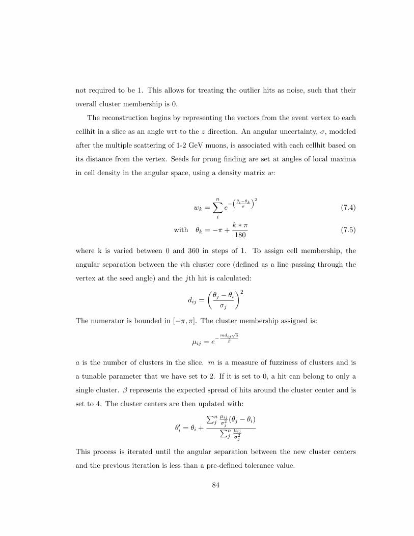
not required to be 1. This allows for treating the outlier hits as noise, such that their
overall cluster membership is 0.
The reconstruction begins by representing the vectors from the event vertex to each
cellhit in a slice as an angle wrt to the z direction. An angular uncertainty, σ, modeled
after the multiple scattering of 1-2 GeV muons, is associated with each cellhit based on
its distance from the vertex. Seeds for prong finding are set at angles of local maxima
in cell density in the angular space, using a density matrix w:
wk =
n∑i
e−(θi−θkσ
)2
(7.4)
with θk = −π +k ∗ π180
(7.5)
where k is varied between 0 and 360 in steps of 1. To assign cell membership, the
angular separation between the ith cluster core (defined as a line passing through the
vertex at the seed angle) and the jth hit is calculated:
dij =
(θj − θiσj
)2
The numerator is bounded in [−π, π]. The cluster membership assigned is:
µij = e−mdij
√a
β
a is the number of clusters in the slice. m is a measure of fuzziness of clusters and is
a tunable parameter that we have set to 2. If it is set to 0, a hit can belong to only a
single cluster. β represents the expected spread of hits around the cluster center and is
set to 4. The cluster centers are then updated with:
θ′i = θi +
∑njµijσ2j
(θj − θi)∑njµijσ2j
This process is iterated until the angular separation between the new cluster centers
and the previous iteration is less than a pre-defined tolerance value.
84

Figure 7.11: Efficiency and purity of reconstructed Fuzzy-K prongs that correspond to
true electrons are > 80% for the region of interest for νe appearance analysis. The drop
in efficiency and purity is due to the rise in the non-quasielastic modes of neutrino inter-
action. These produce significant hadronic showers that can contaminate the electron
showers and make clustering difficult.
The final task is to match 2-D clusters in XZ and YZ views to form 3-D prongs. To
do this, a 2-D cluster in one view is matched with each of the 2-D clusters in the other
view. The cumulative energy as a function of distance from the prong start is computed
for the prongs in each of the two views. If the 2-D prong is correctly matched to its
counterpart in the other view, the energy profile should be very similar between the
two views. To find the best match for the prong, a Kuiper metric, K = min(D+, D−)
is used, where D+ and D− are the largest negative or positive distances between the
profiles.
7.4.4 νe Event Energy Reconstruction
The νe energy reconstruction used for the first analysis is very simple. Since NOνA is
a calorimeter with 65% detector mass in scintillator, we would expect close to 65% of
the true energy to be visible in the detector. In reality, the visible energy fraction is
lower than that. Threshold effects and low energy particles suppress the visible energy
to about 56%. The rest of the energy is deposited in dead material, ie PVC, and is not
85

visible.
To reconstruct the νe energy, we sum up the calorimetric energy of all the hits in
a slice and scale it by a factor of 1.78 (=1/0.56). This factor has been determined
from the simulation of charged current interactions of electron neutrinos and yields an
energy resolution of ∼ 10%. More sophisticated energy reconstruction algorithms that
treat the hadronic and electromagnetic energies separately are also available, but the
resulting energy resolution is comparable to this simpler method, therefore we decided
to not introduce unnecessary complexity.
/ ndf 2χ 388.2 / 12
Constant 7.913e+01± 3.516e+04
Mean 0.000197±0.008598 −
Sigma 0.00023± 0.09271
true)/Ereco-E
true(E
1− 0.5− 0 0.5 1
Eve
nts
0
10
20
30
310×
/ ndf 2χ 388.2 / 12
Constant 7.913e+01± 3.516e+04
Mean 0.000197±0.008598 −
Sigma 0.00023± 0.09271
CC Energy Resolutioneν
Figure 7.12: Reconstructed energy resolution of preselected νe charged-current interac-
tions.
7.5 νµ Reconstruction Chain
νµ reconstruction uses a tracker based Kalman Filter [41] in order to accommodate tracks
that curve due to multiple scattering of particles. Tracking first begins by assuming that
all adjacent hits in a slice are tracks. A Kalman Filter subroutine is used to propagate
tracks forward, plane by plan. Hits that are consistent with the track are added to it,
86

while others are ignored. The consistency of a hit with the developing track is measured
in terms of the change in χ2 of the track upon inclusion of the hit. If the hit is added,
the track fit is updated by performing a weighted average fit over the hits. These tracks
are formed separately in XZ and YZ views. Once all the 2-D tracks are found, a process
to merge them into 3-D track is run. The merging mechanism relies on the tracks in
the two views arising from the same particle to have similar start and end points in the
z direction within some tolerance.
Fractional Energy Resolution-0.4 -0.2 0 0.2 0.4
Fra
ctio
nal E
vent
s
0.00
0.02
0.04
0.06
CC Eventsµν Mean = -0.021RMS = 0.06 Fit Parameters: Mean = -0.0085Sigma = 0.042
A SimulationνNO2 = 2.4e-3 eV32
2m∆ = 0.5 23θ2sin
Mode, 14 kton: QE Sampleν
Figure 7.13: Muon neutrino energy resolution for quasi-elastic CC interactions.
To identify νµ CC interactions, each reconstructed Kalman track is tested for like-
ness to a muon. A k-nearest neighbor algorithm based identifier named ReMId (Recon-
structed Muon ID) has been developed for this purpose. It uses log-likelihood based on
dE/dx along the track in the longitudinal view as an input variable. The main back-
ground to muons are charged pions that are also minimum ionizing. However, pions
may interact strongly and undergo hard scatters which distinguish them from muons.
So length of the track and the scattering likelihood are also used as inputs.
The energy of the muons in νµ CC candidate interactions is computed from range.
The hadronic energy in the event is taken to be the sum of the calorimetric energy of
all the hits that do not belong to the muon track, corrected by a scale factor to account
for energy deposition below threshold or in dead material. The muon neutrino energy
87

is a sum of the muon and the hadronic energies.
88

Chapter 8
νe Event Selection
For the selection of νe appearance signal and rejection of beam and cosmic backgrounds,
we use a combination of simple cuts and more complicated particle identifiers. The sim-
ple cuts are aimed at rejecting low quality data due to occasional electronic failures and
to exploit some obvious topological differences between signal and background events.
The intent is to keep selection cuts identical between the near and the far detectors,
which helps minimize systematics on the far over near ratio. But, in some cases, the
vastly different sizes and data rates in the two detectors force small differences.
In section 8.1 of this chapter, we focus on selection cuts. The νe analysis has two
main PID algorithms, LID and LEM. The LID algorithm builds on the reconstruction
chain discussed in chapter 7 and section 8.2 takes a detailed look at this algorithm as
LID is the PID used for this thesis.
8.1 νe Selection Cuts
8.1.1 Data Quality Cuts
Data quality cuts ensure that the detector and beam were in a reliable state at the time
of data taking.
89

Beam Quality
Beam quality cuts are applied on a spill by spill basis. The information on beam related
metrics is hosted centrally in the intensity frontier database (IFDB) from where it can
be retrieved by all the experiments on the NuMI beam. We apply the following cuts to
both, near and far detector spills:
1. The event time recorded by NOνA must be within 0.5 s of the spill time as recorded
in the IFDB (note that the spills are 1.33 µs apart)
2. Number of protons on target (POT) in the spill must be greater than 2 × 10¹².
Spills with POT smaller than this are usually used for target scans and do not
guarantee good beam.
3. The horn current, in the forward horn current configuration, must be between
-202 and -198 kA
4. Beam spot position requirements: 0.02 mm < x, y positions < 2.00 mm
5. Beam spot size requirements: 0.57 mm < x, y widths < 1.58 mm
The beam quality cuts remove less than 1% of the POT collected in the first-analysis
datasets.
Subrun Quality
The subrun quality metrics are designed to remove data in case of significant or repeated
failures of hardware during the span of a subrun. For a subrun to pass these cuts, it
must have a livetime of at least 1 second. It must have at least two consecutive good
diblocks in FD and all good diblocks in ND. A diblock is considered good if all the
DCMs in it are operating optimally, that is, they have fewer than 9 misbehaving APDs.
An APD is good if less than 7 of its pixels have a hit rate outside an acceptable range
of 100.5 Hz to 103.5 Hz. Response of channels with hit rates outside of this range is
90

found to be unreliable. They are masked off and information from them is not visible
to further offline analysis. These bad channel masks are generated on a subrun basis.
In addition, we require MIP (minimum ionizing particle) hit rate and reconstructed
slice rate normalized by the number of active channels to be in a nominal range. The
cut values on these metrics are different for ND and FD due to very different data rates.
In FD, the hit rates are dominated by cosmics while in ND, due its location under-
ground, nearly all the hits come from the beam. The ND subruns have an additional
cut to monitor the location of the beam peak in the 500 µs window.
In the first data-taking period, close to 11% of the total POT is lost to subrun quality
cuts in the FD, and about 8% in the ND. The first data overlap with the commissioning
period for both detectors when the failure rate of front-end electronics or other detector
systems was high and the electronic parameters were still being optimized. The current
FD data-taking is significantly more stable and we disqualify less than 1% of the data
due to subrun quality cuts.
Spill Data Quality
While subrun cuts are essential for weeding out data where significant failures occurred,
they are not fine enough to pick up on more local and smaller duration failures that
nevertheless undermine the quality of reconstruction and identification. For this purpose
a set of spill quality cuts has been designed. Events that fail spill quality cuts are
not analyzed and the POT corresponding to such events is not counted towards our
exposure.
Because of certain failures in the DAQ, there are short durations of time, typically
lasting a few seconds, ie over several spills, when a subset of DCMs fail to report any
data at all. This can be troublesome, because if hits from a DCM on the edge of the
detector are missing, a cosmic ray entering from outside can appear to be contained.
For this reason, we reject data from spills where any of the active DCMs is missing, ie
reports no hits over the full 500 µs trigger window.
91

NOvA - FNAL E929
Run: 16660 / 0Event: 5 / --
UTC Thu Aug 7, 201421:13:5.546601280 sec)µt (
0 100 200 300 400 500
hits
110
210
q (ADC)10 210 310
hits
110
210310410
0 1000 2000 3000 4000 5000 6000
x (c
m)
500−
0
500
z (cm)0 1000 2000 3000 4000 5000 6000
y (c
m)
500−
0
500
Figure 8.1: A far detector data event where a large number of DCMs are unsynchronized.
The green boxes indicate DCM boundaries. Hits are colored by time.
Similar DAQ problems can sometimes cause a large number of DCMs to become
unsynchronized with respect to other DCMs. This particular problem is only known to
occur in the far detector because of the large number of readout channels, and therefore
high data rates that can strain the DAQ system. The signature of such events is that
a large number of cosmic tracks appear to terminate on DCM edges, as fig 8.1 shows.
The metric designed to reject these events is the fraction of the number of hits on DCM
edges that have adjacent hits in adjoining DCM. Hits on detector edges or at the edges
of uninstrumented DCMs are not counted towards this ratio.
8.1.2 Preselection and Cosmic Rejection Cuts
Preselection and cosmic rejection cuts are applied to every slice and identically to data
and Monte Carlo simulation. The cuts, the rationale behind them and their impact are
discussed below.
92

Skim Cuts
To speed up the processing time of data and simulation files, we apply two skim cuts
during file production: 20 < number of hits in slice < 200 and longest prong length
< 500 cm. These essentially cut out no νe appearance signal, while rejecting a large
fraction of cosmic rays and higher energy neutrino interactions that can take a long
time to reconstruct. No showers are reconstructed for events that do not pass the skim
cuts.
Reconstruction Quality Cuts
Since LID, the likelihood based νe identifier, depends on the reconstruction of vertices
and prongs, we require that there be a reconstructed vertex and at least one recon-
structed shower, with more than 5 hits in each view, in the slice.
If a large number of channels in a region of the detector are masked out of the
analysis or are low in efficiency, the quality of reconstruction in such regions may suffer.
A reconstructed prong may get broken into two or more prongs, with the vertex placed
either in the middle of the fragments, or at the start of the most upstream prong. In
case the vertex is in the middle, one of the prongs is reconstructed as backward going,
and we can reject such events by requiring cos θ > −0.95 between the two showers. If
the vertex is at the most upstream end in z, the distance of the start of the downstream
prong from the vertex is large and can mostly be rejected if we require this distance to
be less than 100 cm. Additionally, the asymmetry in the leading shower between the x
and y views, defined as |xhits − yhits|/(xhits + yhits) should be less than 40%.
Another slice level feature that needs to rejected is the ringing of APDs after large
charge depositions as was discussed in the section 4.3.1. Such slices are characterized
by a large number of APDs being nearly fully triggered, ie close to 32 pixels reporting
hits. We can reject them efficiently by requiring fewer than 8 hits per plane.
All the cuts listed above are only applied to the far detector. In the near detector,
93

Figure 8.2: Flashing of multiple APDs in an FD data event because of high energy
deposits. The gray hits preceded and likely caused the flashing
because of the smaller size of the detector, and nearly 0 cosmic background, we only
need simple quality cuts, requiring at least one vertex and one reconstructed shower in
the slice, in addition to rejecting APD flashes.
Containment Cuts
NOνA is a fully active detector, so any charged particle entering or leaving the detector
leaves a track close to the detector edges. Hence containment cuts are not only a way to
make sure that the neutrino interacted inside the detector, but they are also a powerful
tool in rejecting cosmic ray background.
The far detector dataset contains different diblock configurations, so a statically
defined set of containment cuts is not sufficient. In every subrun, we define edges of the
detector that are live, ie active in data taking, for that subrun. Shower start and stop
points are required to be at least 10 cm away from the live west and bottom detector
faces. Our optimization prefers a slightly tighter cut on the east edge of the detector,
requiring a distance greater than 15 cm to the edge. The east edge is at the far end with
respect to the APDs in the horizontal view, so the light has to travel the full length of
the cell to produce a hit. Hits due to a cosmic ray entering the east face of the detector
may fall below threshold, hence the preference for a tighter cut. The distance from front
of the detector is required to be more than 35 cm.
94

Figure 8.3: Neutron interaction depth in the FD. The data is from the cosmic trigger
and the particles were identified as neutron candidates during hand scanning.
Most cosmic rays enter from the top face of the detector. While charged cosmic
particles are easy to reject with lenient containment cuts, neutral particles can reach
quite deep into the detector before depositing any energy (see figure 8.3). The optimized
cut for the minimum distance of the leading shower from the top face is 150 cm. Another
tricky background to reject is cosmic ray photons. The overburden on the FD contains
barite which is very effective in absorbing photons. At the north end of the detector,
the overburden is thin and let’s more cosmic photons in. The block-pivoter absorbs
photons and helps mitigate the problem somewhat, but as an additional safeguard, the
maximum z of the leading shower is required to be more than 200 cm from the back
face. Figure 8.4 shows the distributions of the minimum distance from top and back
faces of the detector after preselection and loose PID cuts.
Containment is more straightforward in the near detector because the detector con-
figuration does not change. The containment cuts used in ND are listed in the table
below. To cut out activity due to neutrino interactions in the rock preceding the front
face of the near near detector, we reject slices with any activity in the first 6 near
detector planes.
95

Figure 8.4: Minimum distance of the leading shower in the slice from the top and the
back faces of the far detector. Most charged particles in cosmic rays deposit energy close
to the boundary of the detector and can be rejected with containment cuts. In these
figures, all preselection cuts , along with a loose LID cut of > 0.7, have been applied
except for the y and z containment cuts (respectively).
Additional Cosmic Rejection Cut
While most cosmic rays are rejected by containment cuts, cosmic neutrons, or those
produced by the interaction of cosmic rays in the overburden, are much more difficult to
reject, because there is no tell-tale track close to the detector edge. However, cosmic rays
tend to align with the azimuth, ie along the y direction in the NOνA detector coordinate
system, while the direction of the NuMI beam in the NOνA detector coordinates is
roughly horizontal, along the z axis. The transverse momentum fraction with respect
to the beam direction, which folds in this information, has proved very effective in
separation of cosmic rays from neutrino interactions in such cases. This variable also
provides some separation of charged current neutrino interactions from neutral currents,
because the invisible final state neutrino in NCs can causes an imbalance in the observed
transverse momentum.
96

Variable Allowed Range [cm]
Vertex X, Y (-140, 140)
Vertex Z (100, 700)
Shower start, stop X, Y (-180, 180)
Shower start, stop Z (25, 1225)
Table 8.1: Containment cuts in ND
Figure 8.5: Transverse momentum fraction computed with respect to the beam direc-
tion, which is nearly horizontal along detector z axis. Cosmics are usually vertical and
therefore cluster close to 1. We cut on this variable at a value of 0.65. In this plot, all
preselection cuts , along with a loose LID cut of > 0.7, have been applied, other than
the cut on pT /p
Energy-related Cuts
NC interactions of high energy neutrinos have low visible energy because of the missing
visible energy of the final state neutrino. At NOνA’s location, the NuMI beam has a
narrow peak at 2 GeV and a highly suppressed high-energy tail. This reduces the feed-
down from high-energy neutrino NC interactions in the νe appearance signal region.
97

These interactions, along with cosmic rays, tend to have visible energy less than 1 GeV.
The energy cuts on FD events are 1.5 GeV < E < 2.7 GeV. Rejecting events with
reconstructed energy > 2.7 GeV or number of cells in slice > 115, cuts out higher energy
beam νe CC interactions which otherwise have the same signature as the νe appearance
signal. Additionally, we require the leading shower in the event to have a length between
140 and 500 cm.
Figure 8.6: Energy distribution with all preselection applied, except for energy cut. The
νe appearance signal is well-bounded between 1 and 3 GeV while cosmic background
clusters at lower energy
In the near detector, energy cuts are looser than in the far detector. The intent is
to select events in a wider energy range and extrapolate to FD, because the neutrino
energy spectra are similar but not identical for the two detectors.
8.1.3 Performance of Preselection
Table 8.3 summarizes the preselection cuts applied in the far detector and table 8.2
shows the performance of these cuts in a sequential manner. The event counts are for real
conditions FD MC scaled to 3.516× 10²⁰ POT to reflect the first-analysis expectation,
weighted by simple oscillations (see section 5.3). The cosmic background figures are
98

from FD cosmic trigger data normalized to the first analysis livetime exposure. The
cosmic figures in bracket are raw event count prior to the livetime scaling.
Note that the preselection efficiency changes with the number of diblocks because of
the varying fiducial to detector mass ratio, which directly impacts containment efficiency,
as figure 8.7 shows. This effect was studied in the real conditions simulation where POT-
weighted diblock masks from data have been applied to the MC to imitate the changing
detector mass in the first-analysis dataset.
Cut νe Signal νµ CC NC Beam νe CC Cosmics
After data quality 20.56 314.64 15.30 211.16 5.75 ×10⁶ (4.43 ×10⁸)
Reconstruction Quality 15.18 31.05 6.10 65.73 3.55 ×10⁵ (2.74 ×10⁷)
Cosmic Rejection 12.73 23.64 5.11 54.93 1.54 ×10⁴ (1.19 ×10⁶)
Containment 11.95 21.43 4.98 45.86 307.25 (23685)
Energy-related 9.16 11.32 1.12 11.52 22.09 (1703)
Table 8.2: Event counts on sequential selection before PID cut. The numbers in bracket
in the cosmics column are the event counts prior to scaling to the first data livetime.
Figure 8.7: Efficiency of νe preselection cuts as a function of number of detector diblocks
in the FD, as measured in real conditions MC.
99

Cut Description
Skim Cuts 20 < number of hits in slice < 200
Longest prong length < 500cm
Reconstruction quality Number of vertices in slice > 0
At least one shower with > 5 hits in each view
If number of showers is 2, cos θ > −0.95 between showers
Vertex to shower start gap < 100 cm
Shower asymmetry, |xhits − yhits|/(xhits + yhits) < 40%
Containment Dist. of leading shower start and stop to west face < 10 cm
Dist. of leading shower start and stop to bottom face < 10 cm
Dist. of leading shower start and stop to east face < 15 cm
Dist. of leading shower start and stop to front face < 35 cm
Dist. of leading shower start and stop to top face < 150 cm
Dist. of leading shower start and stop to back face < 200 cm
Cosmic rejection Transverse momentum fraction pT /p < 0.65
Energy-related cuts 20 < number of hits in slice < 115
140 cm < Longest prong length < 500 cm
1.5 GeV < Event energy < 2.7 GeV
Table 8.3: Summary of νe preselection cuts applied in the far detector
It is clear that preselection does not get us a pure enough sample of νe CC signal
events for the appearance analysis. The final signal to background separation is done
by the particle identification algorithms, as we will discuss next.
100

8.2 νe Particle Identification
We have two main approaches to identifying νe appearance signal. The Likelihood-based
particle ID, or LID, in particular looks for an electron-induced electromagnetic shower
in the event. This section describes LID method of νe identification in detail.
An alternative approach to LID has been implemented in the form of Library Event
Matching, or LEM . It consists of a vast library of simulated νe signal and background
interactions. A candidate event is compared against all library events to identify the
class of events that the candidate is most akin to. The properties of the 1000 best
matches found from the library are fed into an ensemble of decision trees to obtain a
PID value. This method is reported in detail in [42].
8.2.1 Likelihood-based Particle Identification
The energy deposited per unit length, dE/dx, by a particle, along its trajectory is
a characteristic of the particle. LID uses this information to compute the likelihood
that the candidate particle is an electron. These likelihood variables, along with other
topological information about the event are used as input to an Artificial Neural Network
or ANN to construct a particle ID. The steps involved in achieving that end are described
below.
Fine-tuning the reconstruction
LID uses prongs made by the Fuzzy-K algorithm, but these prongs are not reconstructed
or shaped to fit any particular particle hypothesis. LID performs some reclustering of
the Fuzzy-K prongs to conform to the shape expected of an electron shower. A typical
prong due to an electron is narrow close to the vertex, where the electron is minimum
ionizing and has not yet begun to radiate. Once a brehmsstrahlung photon is emitted,
the shower commences and the prong broadens. The reclustering in LID labels all hits
within a radius of 2.5 cell widths of the shower core in the first 8 planes and 20 cell
101

widths for the rest of the planes as belonging to the shower. The smaller radius at the
start of the shower also reduces contamination of the shower by other hadronic activity
close to the vertex.
Figure 8.8: Fuzzy-K prongs are reclustered to better fit the electron shower shape.
As discussed before, Fuzzy-K allows hits to be associated with multiple prongs. LID
performs cell-energy deconvolution to ensure that a cell’s energy is not double counted
towards the event energy. For a cell common to multiple shower, its energy contribution
to the ith shower is set to:
Ecelli =PEcell
ai.PEshoweri × e−Di/λ∑j PE
showerj e−Dj/λ
(8.1)
A Monte CarloνNO
Distance to shower core (cm)0 10 20 30 40
/cm
)3
(1
0show
er
(Tra
nsvers
e d
E/d
x)/
E
0
0.5
1
1.5
Figure 8.9: Transverse dE/dx per electron energy as a function of distance from the
shower core. The distribution is fit with 8.2
102

Here, PEcell is the number of photo-electrons in that cell and PEshower is the total
PE in the ith shower. ai is the attenuation calibration factor to convert PE to GeV,
based on the average distance of the ith shower from the readout. Di is the distance of
the hit from the ith shower core and λ is a constant that describes the shower lateral
profile in the medium, ie the transverse dE/dx as a function of distance from the shower
core isdE
dx(w) = AEe−w/λ (8.2)
where E is the shower energy, A is a normalization constant and w the distance from
the shower core. Based on simulated electron showers, λ is determined to be 3.05 cm,
as shown in fig.8.9.
Particle Likelihood
After reclustering and energy deconvolution, the most energetic shower in the event
is picked for identification. The particle hypothesis that LID tests the leading shower
against are e, µ, p, n, π±, π0 and γ. To construct likelihoods, the dE/dx information is
recorded in longitudinal and transverse views. The longitudinal view is along the length
of the shower and transverse view is perpendicular to the direction of the shower and
summed over all planes in the shower.
In the longitudinal view, the dE/dx is recorded for every detector plane that the
particle passes through. The transverse view is a measure of how concentrated the
energy deposition is in the core of the shower. Therefore, the dE/dx is recorded radially,
as a function of the number of cell-widths from the core of the shower. Figure 8.10 shows
an example of how different particles differ in dE/dx.
Template histograms of the expected plane-by-plane dE/dx and transverse view
depositions are created for all the particle hypotheses using simulated neutrino interac-
tions. These histograms are normalized to form probability distribution functions. The
energy depositions of a prong of unknown identity are compared against these template
histograms. For instance, if an unknown particle deposits energy Ei in the ith plane
103

Plane dE/dx (GeV/cm)
0.00 0.01 0.02 0.03 0.04 0.05
Ev
en
ts
0
200
400
600
800
1000
Plane idx = 2
e
µ
Plane dE/dx (GeV/cm)
0.00 0.01 0.02 0.03 0.04 0.05
Ev
en
ts
0
200
400
600
800
1000
1200
1400 Plane idx = 10
e
µ
Figure 8.10: Muon and electron dE/dx in the second and tenth plane from the shower
start. In most cases, by the second plane, the electron has begin to shower and behaves
as a minimum ionizing particle, just as the muon does. By the tenth plane, it is very
likely that the EM shower has begun to develop.
from the start of the prong, the probability, Pi of various particle hypotheses depositing
energy in this manner is read from the template histograms for the ith plane. The
logarithms of these probabilities are then summed over all planes in the prong and used
to construct a likelihood for that particle hypothesis:
LL(e−) =
N∑i
log(Pi(e−))/N
where LL(e−) is the likelihood of the unknown particle being an electron. N is the total
number of planes in case of longitudinal likelihood and total number of transverse cells
in transverse likelihood. Likelihood differences are found to be more useful quantities
since they are relative probabilities. So the likelihood difference LL(e−)−LL(µ−) would
be clustered towards higher values for electron showers and towards lower values for true
muon tracks. Figure 8.11 shows the discriminating power of these likelihood ratios for
simulated electron, muons and neutral pions.
104

Figure 8.11: Longitudinal and transverse likelihood difference LL(e−) − LL(π0) for
electrons and neutral pions, and LL(e−) − LL(µ) for electrons and muons. While the
lateral profile of π0 and electrons do not show much separation, the transverse likelihood
ratio is better separated. This is because π0 EM showers often contain two overlapping
decay photons. Muons and electrons are well-separated in both views.
The Neural Net
LID uses ROOT’s TMultiLayerPerceptron class which is an implementation of a feed-
forward neural network. Neural networks are a computational method of approximating
a non-linear functional mapping between input variables and an output. The network is
presented with input variables for a training sample for which the signal and background
populations are known, and it learns what combinations of inputs maps to signal and
105

to background.
A neural network consists of an input an output layer of neurons and one or more
hidden layers where the computation takes place. The number of neurons in the input
layers corresponds to the number of input variables to the network. It passes on the
input to the first hidden layer. The neurons in hidden layers are characterized by a bias
and weighted connections to neurons in the next layer, called synapses. Each neuron in
a hidden layer receives a linear combination of the output of neurons from the previous
layers, and makes independent calculations. Each has a pre-defined activation function,
which it uses to compute its output, based on the inputs it received. The activation
functions are usually sigmoids. For each training event, the network compares the
output to the correct answer and readjusts the neuron biases to reduce the error.
Additional LID Variables
The goal of νe particle identification is to select νe CC appearance signal with high
efficiency and purity. The νe appearance signal is expected to peak between 1 and 3
GeV.
The presence of an obvious muon track makes νµ CC interactions relatively easy to
separate from the signal and the likelihood variables are very efficient at doing so. νµ
CC’s may be a background when the interaction is highly inelastic (high hadronic-y)
and the hadronic shower contains an EM-like shower, though the rate of this background
is sufficiently small.
Neutral currents are more difficult to separate, since there is no muon track for easy
separation, and these interactions often produce neutral pions whose decay (π0 → γγ)
produces electromagnetic showers that are a potential background. Showers induced by
photons are different from those produced by electrons, since electrons being charged,
deposit energy right away. The photon may travel some distance before converting and
producing a shower. LID uses a reconstructed π0 invariant mass and the distance of
the shower start to the event vertex to help reject this background. Moreover, neutral
106

currents have a neutrino in the final state which is not visible. So the angular distribution
of EM-like showers in NC’s is also different. We use cos θ, the angle of the leading shower
with respect to the beam direction, as a variable in LID to exploit this properly. This
variable is also useful for cosmic background rejection in FD since cosmics are mostly
vertical. Additionally, NC interactions that are a background to the appearance signal
are usually highly inelastic and have a smaller fraction of event energy contained in the
leading shower. This too is an input variable to the ANN.
egLLL
1.0 0.5 0.0 0.5 1.0
Even
ts
0
5000
10000
15000
20000
25000
30000
35000
40000
45000
egLLT
2 1 0 1 2
Even
ts
0
5000
10000
15000
20000
25000
30000
35000
40000
emuLLL
4 2 0 2 4E
ven
ts
0
2000
4000
6000
8000
10000
12000
14000
16000
18000
emuLLT
2 0 2 4
Even
ts
0
5000
10000
15000
20000
25000
epi0LLL
1.0 0.5 0.0 0.5 1.0
Ev
ents
0
2000
4000
6000
8000
10000
12000
14000
16000
18000
20000
22000
24000
epi0LLT
2 0 2 4
Ev
ents
0
5000
10000
15000
20000
25000
30000
35000
epLLL
2 1 0 1 2
Ev
ents
0
2000
4000
6000
8000
10000
12000
14000
16000
epLLT
2 0 2 4
Ev
ents
0
5000
10000
15000
20000
25000
30000
35000
enLLL
2 1 0 1 2
Even
ts
0
2000
4000
6000
8000
10000
12000
14000
16000
18000
20000
enLLT
2 0 2 4
Even
ts
0
10000
20000
30000
40000
50000
epiLLL
2 1 0 1 2
Even
ts
0
2000
4000
6000
8000
10000
12000
14000
epiLLT
2 0 2 4
Even
ts
0
5000
10000
15000
20000
25000
30000
35000
pi0mass
0.0 0.5 1.0 1.5
Even
ts
0
5000
10000
15000
20000
25000
shE
0.0 0.5 1.0 1.5 2.0 2.5
Even
ts
0
1000
2000
3000
4000
5000
vtxgev
0.0 0.5 1.0 1.5
Even
ts
0
2000
4000
6000
8000
10000
12000
14000
16000
gap
0 20 40 60 80 100
Even
ts
0
10000
20000
30000
40000
50000
60000
Figure 8.12: Distribution of ANN input variables for signal(red) and background (blue)
The intrinsic beam νe component is an irreducible background since these interac-
tions are identical to the νe appearance signal. The only handle that we have to reject
the intrinsic νe component is that the energy distribution of the two samples is different-
the νe appearance signal is a narrow peak around 2 GeV, while the beam νe’s are a much
more spread out higher energy distribution. The energy cuts discussed earlier in the
107

chapter are efficient at reducing this ‘background’.
To summarize, in addition to the particle likelihoods, LID uses the following addi-
tional input variables for identification:
1. Shower energy fraction: shower energy divided by the total event energy.
2. π0 mass: The invariant mass of the most energetic shower with all the other
showers in the slice is computed and the one closest to the π0 mass is saved
3. Vertex energy: The calorimetric energy within ±8 planes from the event vertex
4. Gap: The distance of the start point of the shower from the event vertex.
5. cos θ: Angle of the leading shower with respect to the beam direction
The cut on PID value has been optimized to maximize two statistical figures of merit
(FoM). The FoM s/√b is appropriate for a νe appearance search on a large background,
and the PID value tuned to maximize it gives a value of 0.95. Optimizing to maximize
s/√
(s+ b) gives a value of 0.61. The PID shape and selected event counts are given
in figure 8.13 and table 8.4. A combination of preselection and PID cuts reduces the
enormous cosmic background from 5.75 ×10⁶((4.43 × 10⁸) events to 0.04(3) events for
the livetime equivalent to the first data exposure. As before, the figures in the bracket
are the counts before scaling. The beam backgrounds continue to be the bigger problem
and work aiming towards future NOνA analyses is under way to polish our selections
and improve beam background rejection efficiency.
8.3 Final Cosmic Background Prediction
The νe selection and cosmic rejection cuts presented thus far have been tuned on a
combination of cosmic trigger data and the oscillated NuMI beam simulation. Once
the cuts were tested and found to perform optimally, they were applied to the NuMI
out-of-time sideband to get the final estimate of cosmic background to the appearance
108

LID0 0.2 0.4 0.6 0.8 1
Eve
nts
0
0.2
0.4
0.6
0.8
1
LID (FHC)
signaleν
NC background
backgroundµν
backgroundeνBeam
Figure 8.13: LID distribution for νe appearance signal and beam backgrounds. The
distributions are weighted by oscillation probability with no matter effect and scaled
to the expected event count for 1.9 × 10²⁰ Protons on Target (POT). The two arrows
indicate the cuts that maximize the figure of merit s/√b (light green) and s/
√s+ b
(dark green)
LID0 0.2 0.4 0.6 0.8 1
Effi
cien
cy (
%)
0
20
40
60
80
100
Efficiency vs Cut Value
LID0 0.2 0.4 0.6 0.8 1
Pur
ity (
%)
0
20
40
60
80
Purity vs Cut Value
Figure 8.14: Efficiency of LID selection and purity of selected sample as a function of
LID cut. The dotted green line is the cut optimized for maximum s/√s+ b and and
the red for maximum s/√b. The efficiency is measured with respect to preselection.
analysis of first data. The event counts of cosmics in NuMI sideband are presented in
table 8.5, along with those in cosmic trigger data for reference.
109

Cut νe sig Tot bg NC νµ CC Beam νe Sig eff Puritys√b
opt 0.95 4.36 0.82 0.33 0.05 0.44 47.57% 84.10%
s√s+ b
opt 0.61 6.97 3.08 1.82 0.47 0.79 76.08% 69.36%
Table 8.4: Performance of LID for cut optimized to maximize the figure of merit in two
different ways. All selection cuts discussed in section 8.1 have been applied. Signal effi-
ciency is measured with respect to the preselected sample. Event counts are normalized
to first data exposure
Cut Cosmic Trigger NuMI Out-of-time Sideband
After data quality 5.75 ×10⁶ (4.43 ×10⁸) 5.86 ×10⁶ (1.59 ×10⁸)
Reconstruction quality 3.55 ×10⁵ (2.74 ×10⁷) 3.62 ×10⁵ (1.00 ×10⁷)
Containment 1.54 ×10⁴ (1.19 ×10⁶) 1.56 ×10⁴ (4.40 ×10⁵)
Cosmic Rejection 307.25 (23685) 312.16 (8403)
Energy-related Cuts 22.09 (1703) 23.24 (642)
LID 0.04 (3) 0.06 (2)
Table 8.5: Cut flow on cosmic ray background in out-of-time NuMI data. Event counts
in bracket are prior to scaling the livetime to first data.
To summarize, in the NuMI out-of-time sideband, only two cosmic ray events survive
all νe selection. Scaling to the total NuMI spill livetime in the first data, this results in
a cosmic background estimate of 0.06 events for this analysis, a background negligible
in comparison to other beam neutrino backgrounds. This finding is consistent with the
background count obtained from the cosmic trigger data at the 0.41 σ level.
110

Summary
In the νe analysis, we use a combination of simple, well-motivated cuts to control data
quality and to reject some of the backgrounds. The fully active nature of the detector
allows the use of detector edges as a veto region and makes cosmic rejection a manageable
task. The angular separation of beam from cosmics is also found to be a useful variable.
Other topological variables such as prong length and event energy help in rejecting some
of the beam backgrounds too.
We rely on more complex neural-network based techniques to separate the appear-
ance signal from harder to separate backgrounds. We are able to select νe CC appearance
signal with an efficiency of 47.57% (with respect to preselected sample) and achieve a
signal purity of 84.1%. The cosmic background is also reduced to a negligible level,
where we achieve a suppression of 95.8 million to 1.
111

Chapter 9
Near Detector Data
The near detector (ND) is a 0.3 kT version of the NOνA far detector located 1 km from
the neutrino source at Fermilab. Being located this close to the source, the ND records
multiple neutrinos per beam spill and the ND data comprise a high statistics sample of
neutrino interactions. They helps us understand how our detectors respond to events
that we are most interested in and how well we simulate them. This chapter presents
the studies that have been conducted thus far to comprehend the ND data and some
discussion on how the data might be interpreted for future analyses.
Figure 9.1: Near detector fiducial and containment bounds for νe selection
112

Cut name Value
Data quality Hits per plane ≥ 8 (reject APD flash)
Reconstruction Quality Number of vertices, 3D prongs, shower > 0
Fiducial cut |Vertex x, y| < 140 cm, 100 cm < Vertex z < 700 cm
Containment cut | shower start, stop x, y| < 180 cm, 25 cm < shower start stop z < 1225 cm
Front Planes Minimum distance of slice to front face > 6 planes
Slice hits and Ecal 20 < hits in slice < 200, Ecal < 5
Shower length 140 cm < longest prong length < 500 cm
Gap Leading shower start distance to vertex < 100 cm
νe PID LID > 0.95
Table 9.1: Near detector νe selection cuts
9.1 Near Detector Data-MC Comparisons
It was discussed earlier (chapter 6) that studies of the near detector data prompted
the incorporation of APD sag and Birks-Chou suppression into our simulation, which
went a long way in improving data-MC agreement in the ND. All those refinements are
included in the simulation that is compared with the data in this section.
9.1.1 ND νe Event Selection
The selection cuts applied in the near detector have previously been considered in chap-
ter 8; nonetheless they are reviewed here in table 9.1. Figure 9.1 is a diagram of the
ND with event containment boundaries shown. The selection efficiencies for each cut
level are in table 9.2. The event counts are normalized by POT equivalent to the first
ND data exposure of 1.66× 10²⁰ POT.
Prior to any cuts, MC has only a 0.8% excess over data, so the integrated flux ×
cross-section simulation is remarkably good. After all preselection cuts are applied,
however, this excess increases to 5.9%, while after applying the final PID cut, it is the
data that have a 3% excess over MC. According to the simulation, the final νe selected
events in the ND comprise 16% νµ CC, 52.3 % beam νe CC and 31.7 % NC interactions.
Figures 9.2, 9.3 and 9.4 show distributions of some key variables after all cuts listed
113

Total MC Efficiency νµ CC νe CC NC Data Efficiency
No cut 30049057 100.00% 25742957 364671 3941430 29802297 100.00%
Data quality 29139394 96.97% 25132969 339183 3667242 29015588 97.36%
Reconstruction 16338569 54.37% 13577267 229803 2531499 15996841 53.68%
Fiducial 1139793 3.79% 758778 20924 360091 1025407 3.44%
Containment 478835 1.59% 253650 10236 214949 424518 1.42%
Front planes 461975 1.54% 243569 9815 208592 413242 1.39%
Slice hits and Ecal 323131 1.08% 177970 5437 139724 301019 1.01%
Shower length 236834 0.79% 145944 4859 86030 222046 0.75%
Gap 230475 0.77% 100.00% 142987 4755 82732 217656 0.73% 100.00%
LID 2471 0.01% 1.07% 396 1292 783 2579 0.01% 1.18%
Table 9.2: νe event selection efficiency in Near Detector for simulation, split by interac-
tion type and data.
in table 9.1 except for PID are applied. The preselected events are dominated by νµ
CC interactions (62%). Figure 9.2a shows the reconstructed energy of the interactions;
the data peak lower than the simulation by about 15%. The energy per hit in slice
and energy of the leading shower (figures 9.2b and 9.3a, respectively) are also biased
low in data, but the degree of disagreement is smaller. It is clear from figure 9.3b that
most of the disagreement in the event energy between data and MC arises from the
poorly modeled hadronic energy in simulation. The hadronic energy is defined here as
all the energy in the event that is not on the leading shower. Since no νe or νµ PID
cut has been applied at this stage, the leading shower or track is not guaranteed to
be an electron or a muon. So the hadronic energy after preselection may have some
non-hadronic component.
Further, figure 9.3c shows a large disagreement in the number of reconstructed show-
ers or the observed multiplicity in the events. The electron-muon log-likelihood differ-
ence in figure 9.3d has two distributions. The peak to the left, at negative values of
the difference, is dominated by νµ CC interactions where the leading shower is the
muon, and therefore, very unlike the electron. The one on the right consists of neutral
currents and νµ CC interactions where a hadron is the primary shower. The beam νe
114

CC populate the region further to the right, at higher values of the difference. From
this distribution too it appears that hadronic component of neutrino interactions is not
modeled properly in our simulation. Such modeling problems have a direct impact on
the behavior of higher level variables such as the PID which is shown in figures 9.4a and
9.4b. LID shows an excess in data in the signal region (LID > 0.95), but everywhere
else, the data are 5− 10% lower than MC.
calE0 1 2 3 4 5
Eve
nts
2000
4000
6000
8000
Near Detector Data & MC, POT Normalized
DataTotal MCNC
CCeνBeam CCµν
calE0 1 2 3 4 5
Dat
a / M
C
0.5
1
1.5
2
(a) Reconstructed neutrino energy
Calorimetric energy / hit (GeV)0 0.01 0.02 0.03 0.04
Eve
nts
10000
20000
30000
Near Detector Data & MC, POT Normalized
DataTotal MCNC
CCeνBeam CCµν
Calorimetric energy / hit (GeV)0 0.01 0.02 0.03 0.04
Dat
a / M
C
0.5
1
1.5
2
(b) Energy per hit in slice
Figure 9.2: Data and MC comparison of ND νe preselected events.
115

Primary shower calorimetric energy (GeV)0 0.5 1 1.5 2 2.5 3
Eve
nts
5000
10000
15000
20000
25000
Near Detector Data & MC, POT Normalized
DataTotal MCNC
CCeνBeam CCµν
Primary shower calorimetric energy (GeV)0 0.5 1 1.5 2 2.5 3
Dat
a / M
C
0.5
1
1.5
2
(a) Reconstructed energy of the leading
shower in the event
(Slice - Shower) calorimetric energy (GeV)0 0.5 1 1.5
Eve
nts
5000
10000
15000
Near Detector Data & MC, POT Normalized
DataTotal MCNC
CCeνBeam CCµν
(Slice - Shower) calorimetric energy (GeV)0 0.5 1 1.5
Dat
a / M
C
0.5
1
1.5
2
(b) Energy in slice that is not on the leading
shower, or the hadronic energy in the event.
Number of showers0 2 4 6 8 10
Eve
nts
20000
40000
60000
Near Detector Data & MC, POT Normalized
DataTotal MCNC
CCeνBeam CCµν
Number of showers0 2 4 6 8 10
Dat
a / M
C
0.5
1
1.5
2
(c) Number of reconstructed 3D showers in
event.
LLLµe/1− 0 1 2 3
Eve
nts
2000
4000
6000
8000
10000
12000
14000
Near Detector Data & MC, POT Normalized
DataTotal MCNC
CCeνBeam CCµν
LLLµe/1− 0 1 2 3
Dat
a / M
C
0.5
1
1.5
2
(d) Electron-muon longitudinal log-
likelihood difference
Figure 9.3: Data and MC comparison of ND νe preselected events. The MC is broken
down by interaction type. 116

LID0 0.2 0.4 0.6 0.8 1
Eve
nts
20000
40000
60000
Near Detector Data & MC, POT Normalized
DataTotal MCNC
CCeνBeam CCµν
LID0 0.2 0.4 0.6 0.8 1
Dat
a / M
C
0.5
1
1.5
2
(a) LID
LID0.96 0.98 1 1.02 1.04
Eve
nts
100
200
300
Near Detector Data & MC, POT Normalized
DataTotal MCNC
CCeνBeam CCµν
LID0.96 0.98 1 1.02 1.04
Dat
a / M
C
0.5
1
1.5
2
(b) LID zoomed in on the signal region
Figure 9.4: Data and MC comparison of ND νe preselected events.
The distributions in figures 9.2 and 9.3 are repeated in figures 9.5 and 9.6 after
applying the PID cut of LID > 0.95. The data-MC agreement is much better once
the PID cut is applied and it is ensured that there is some electromagnetic activity in
the event. The hadronic energy in the interaction and the event multiplicity, however,
continue to be discrepant between data and MC (figure 9.5d).
117

calE0 1 2 3 4 5
Eve
nts
20
40
60
80
100
Near Detector Data & MC, POT Normalized
DataTotal MCNC
CCeνBeam CCµν
calE0 1 2 3 4 5
Dat
a / M
C
0.5
1
1.5
2
(a) Reconstructed neutrino energy
Calorimetric energy / hit (GeV)0 0.01 0.02 0.03 0.04
Eve
nts
100
200
300
400
Near Detector Data & MC, POT Normalized
DataTotal MCNC
CCeνBeam CCµν
Calorimetric energy / hit (GeV)0 0.01 0.02 0.03 0.04
Dat
a / M
C
0.5
1
1.5
2
(b) Energy per hit in slice
Primary shower calorimetric energy (GeV)0 0.5 1 1.5 2 2.5 3
Eve
nts
50
100
150
200
Near Detector Data & MC, POT Normalized
DataTotal MCNC
CCeνBeam CCµν
Primary shower calorimetric energy (GeV)0 0.5 1 1.5 2 2.5 3
Dat
a / M
C
0.5
1
1.5
2
(c) Reconstructed energy of the leading
shower in the event
(Slice - Shower) calorimetric energy (GeV)0 0.5 1 1.5
Eve
nts
100
200
300
400
500
Near Detector Data & MC, POT Normalized
DataTotal MCNC
CCeνBeam CCµν
(Slice - Shower) calorimetric energy (GeV)0 0.5 1 1.5
Dat
a / M
C
0.5
1
1.5
2
(d) Energy in slice that is not on the leading
shower, or the hadronic energy in the event.
Figure 9.5: Data and MC comparison of ND LID selected events.
118

Number of showers0 2 4 6 8 10
Eve
nts
200
400
600
800
1000
1200
Near Detector Data & MC, POT Normalized
DataTotal MCNC
CCeνBeam CCµν
Number of showers0 2 4 6 8 10
Dat
a / M
C
0.5
1
1.5
2
(a) Number of reconstructed 3D showers in
event.
LLLµe/1− 0 1 2 3
Eve
nts
100
200
300
Near Detector Data & MC, POT Normalized
DataTotal MCNC
CCeνBeam CCµν
LLLµe/1− 0 1 2 3
Dat
a / M
C
0.5
1
1.5
2
(b) Electron-muon longitudinal log-
likelihood difference
Figure 9.6: Data and MC comparison of ND LID selected events. The MC is broken
down by interaction type.
9.1.2 ND νµ Event Selection
The prediction of the νµ to νe oscillation signal in the far detector is based on the
observed νµ CC spectrum in the near detector. Any data-MC disagreement observed in
the νµ population is used to correct the ND and FD MC (see chapter 11).
The νµ CC selection criteria in the ND are listed in table 9.3. Unlike the νe selection,
the selection of νµ’s in the ND in an energy range relevant to oscillations requires the use
of the muon catcher. The reconstructed muon track length and energy (figure 9.7a and
9.7b) are in reasonably good agreement. The reconstructed νµ CC energy and hadronic
energy in νµ events are shows in figures 9.7c and 9.7d respectively and exhibit similar
data-MC discrepancies to those outlined in section 9.1.1.
Figure 9.8 is the distribution of the νµ PID, ReMID for all ND events that pass
119

νµ preselection. The low ReMID values are dominated by neutral currents and highly
inelastic νµ CC interactions where the muon is not prominent. Here too, the data and
simulation differ in shape.
Cut Value
Quality At least one reconstructed Kalman track,
number of hits in slice > 20,
number of contiguous planes with hits in slice > 4
Containment Number of cells from edge > 1,
first and last plane in slice > 1 and < 212 resp.
start z of the most muon-like track < 1275 cm (not in muon catcher)
visible hadronic energy in muon catcher < 0.03 GeV
Projected distance to detector edge of the most muon-like track :
in the forward direction > 4 cells
in the backward direction > 8 cells
νµ PID ReMID > 0.75
Table 9.3: νµ CC selection criteria in the ND
120

Track Length [cm]µ0 200 400 600 800 1000
Eve
nts
2000
4000
6000
8000
10000
Near Detector Data & MC, POT Normalized
DataTotal MCNC
CCeνBeam CCµν
Track Length [cm]µ0 200 400 600 800 1000
Dat
a / M
C
0.5
1
1.5
2
(a) Length of the candidate muon track
Energy [GeV]µ0 1 2 3 4 5
Eve
nts
10000
20000
30000
Near Detector Data & MC, POT Normalized
DataTotal MCNC
CCeνBeam CCµν
Energy [GeV]µ0 1 2 3 4 5
Dat
a / M
C
0.5
1
1.5
2
(b) Reconstructed energy of the candidate
muon
Energy [GeV]µν0 1 2 3
Eve
nts
10000
20000
30000
40000
Near Detector Data & MC, POT Normalized
DataTotal MCNC
CCeνBeam CCµν
Energy [GeV]µν0 1 2 3
Dat
a / M
C
0.5
1
1.5
2
(c) Reconstructed neutrino energy of νµ CC
selected events
Hadronic Energy [GeV]µν0 0.5 1 1.5 2 2.5
Eve
nts
20000
40000
60000
Near Detector Data & MC, POT Normalized
DataTotal MCNC
CCeνBeam CCµν
Hadronic Energy [GeV]µν0 0.5 1 1.5 2 2.5
Dat
a / M
C
0.5
1
1.5
2
(d) Reconstructed hadronic energy in νµ
CC selected events
Figure 9.7: Reconstructed quantities for candidate muon tracks and νµ CC selected
events in the near detector data and MC.
121

ReMID0 0.2 0.4 0.6 0.8 1
Eve
nts
50
100
150
200
250
310×Near Detector Data & MC, POT Normalized
DataTotal MCNC
CCeνBeam CCµν
ReMID0 0.2 0.4 0.6 0.8 1
Dat
a / M
C
0.5
1
1.5
2
Figure 9.8: Performance of ReMID, the νµ CC PID, on the ND data and MC.
9.2 Interpretation
From previous discussions, it is evident that the ND data differ from simulation in
some fundamental way that is not yet completely understood. For the low statistics
analysis that is presented in this thesis, such differences do not bear too heavily on the
sensitivity of the final result. However, for future analyses with larger data samples,
systematic errors will become important and these problems will need to be addressed.
This section presents two approaches that have so far been explored as an explanation
of the observed differences: adjusting the interaction type scales and adjusting the
interaction mode scales in the simulation (see table 9.4).
122

Interaction Type Neutral Current (NC),
Beam νe CC
νµ CC
Interaction Mode Quasi-elastic (QE),
Resonance (Res),
Deep-inelastic (DIS)
Coherent
Table 9.4: Description of interaction type and mode
9.2.1 Fitting For Interaction Type
The LID distribution in data disagrees in shape with the simulation. The data has
fewer events than simulation in the low-LID region, and more events than simulation
in the high signal region. The low PID region in LID is dominated by NC and νµ CC
interactions while the very high PID region consists mostly of beam νe CC interactions.
We proceeded with the assumption that the NC, νµ CC and beam νe CC interactions
are modeled correctly but the relative proportions (flux × cross-section) are not correct.
The events selected by cuts 0.6 <LID< 0.8, contain very little beam νe CC, so this
component is held fixed. The neutrino energy distribution of these events (figure 9.10a)
was used to fit for the scale of NC and the νµ CC components in the MC by minimizing
the χ2 for a Poisson distribution:
−2 logL = −2
N∑i=1
oi log ei − ei − log oi!
=⇒ χ2 ' 2N∑i=1
oi log
(oiei
)+ ei − oi
where oi and ei are the observed and expected event counts in the ith bin. The scale
123
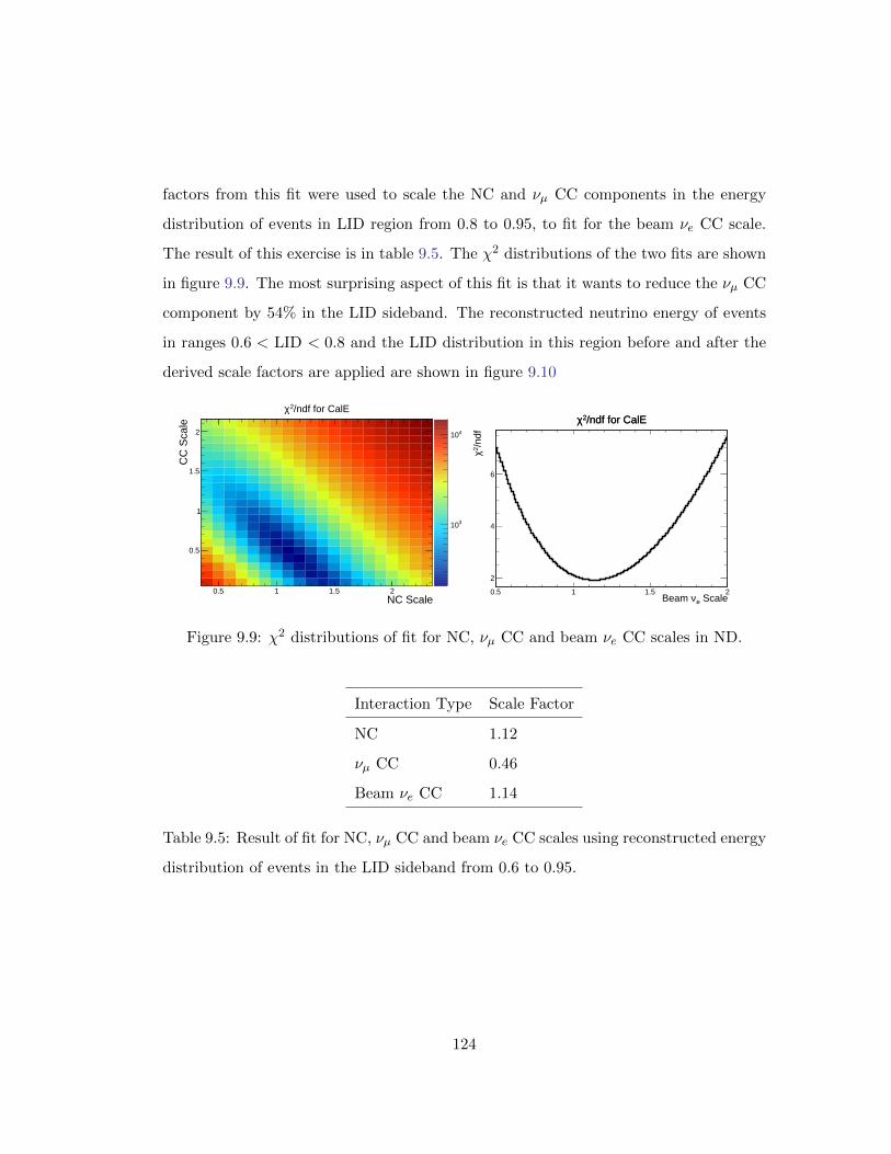
factors from this fit were used to scale the NC and νµ CC components in the energy
distribution of events in LID region from 0.8 to 0.95, to fit for the beam νe CC scale.
The result of this exercise is in table 9.5. The χ2 distributions of the two fits are shown
in figure 9.9. The most surprising aspect of this fit is that it wants to reduce the νµ CC
component by 54% in the LID sideband. The reconstructed neutrino energy of events
in ranges 0.6 < LID < 0.8 and the LID distribution in this region before and after the
derived scale factors are applied are shown in figure 9.10
NC Scale0.5 1 1.5 2
CC
Sca
le
0.5
1
1.5
2
310
410
/ndf for CalE2χ
Scaleeν Beam 0.5 1 1.5 2
/ndf
2 χ
2
4
6
/ndf for CalE2χ /ndf for CalE2χ
Figure 9.9: χ2 distributions of fit for NC, νµ CC and beam νe CC scales in ND.
Interaction Type Scale Factor
NC 1.12
νµ CC 0.46
Beam νe CC 1.14
Table 9.5: Result of fit for NC, νµ CC and beam νe CC scales using reconstructed energy
distribution of events in the LID sideband from 0.6 to 0.95.
124

Calorimetric Energy [GeV]0 1 2 3 4 5
Eve
nts
0
100
200
300
400
0.6 <= LID < 0.8
Data
Total MC
NC
CCeνBeam
CCµν
0.6 <= LID < 0.8
(a) Reconstructed neutrino energy of events
with 0.6 <= LID<= 0.8, before interaction
types are scaled
Calorimetric Energy [GeV]0 1 2 3 4 5
Eve
nts
0
100
200
300
400
0.6 <= LID < 0.8
Data
Total MC
NC
CCeνBeam
CCµν
0.6 <= LID < 0.8
(b) Reconstructed neutrino energy of
events with 0.6 <= LID <= 0.8, after in-
teraction types are scaled
LID0.6 0.7 0.8 0.9 1 1.1
Eve
nts
100
200
300
400
500
Data
Total MC
NC
CCeνBeam
CCµν
(c) LID, before interaction types are scale
LID0.6 0.7 0.8 0.9 1 1.1
Eve
nts
100
200
300
400
500
Data
Total MC
NC
CCeνBeam
CCµν
(d) LID, after interaction types are scale
Figure 9.10: Result of scaling interaction types in MC by the factors in table 9.5.
9.2.2 Fitting For Interaction Mode
Neutrino interactions with nucleons are broadly divided into elastic and inelastic. The
recoiling nucleus remains intact in case of elastic interactions, which dominate at low
momentum transfer (Q2). In case of charged-current, an interaction can not be elas-
tic because some energy is converted to the mass of the final-state lepton and there is
an exchange of charge. These interactions are called quasi-elastic (QE), and are char-
acterized by a track or a shower due to the primary lepton, and a small amount of
125
hadronic activity. At high momentum transfer, the neutrino interacts with the con-
stituent quarks of a nucleon, which breaks apart as a consequence of the interaction.
These are deep-inelastic (DIS) interactions and are usually characterized by significant
hadronic activity. Inelastic interactions at low Q2 usually proceed via excitation of nu-
cleons into resonances such as ∆. If the nucleus as a whole recoils due to interaction
with a neutrino, it is known as coherent scattering.
Interaction modes are a convenient conceptual tool in understanding interactions of
neutrinos with nucleons, but there are no distinct boundaries that separate one process
from another in practice. The neutrino-nucleon interactions occur with a continuum of
inelasticity as the momentum transfer rises. Final state hadrons can also interact in the
nuclear medium as they exit the nucleus, so that the apparent final state appears very
different from the one produced. All of this put together makes for a very challenging
problem in modeling and measuring interaction mode cross-sections.
The near detector data and simulation strongly differ in the behavior of the hadronic
component of the interactions. As a measure of hadronic energy, we subtract the energy
of the electron shower candidate from the event energy. The data prefer, on average,
lower hadronic energy and multiplicity. The hadronic energy distribution differs signifi-
cantly for different interaction modes. From figure 9.11a, it appears that the data favor
fewer DIS and more QE interactions.
126

(Slice - Shower) Energy [GeV]0 0.5 1 1.5 2 2.5 3
Eve
nts
5000
10000
15000
ND Data and MC
MC
MC QE
MC Res
MC Dis
MC Coh
Data
(Slice - Shower) Energy [GeV]0 0.5 1 1.5 2 2.5 3
Dat
a/M
C
0.5
1
1.5
2
(a) Hadronic energy in preselected ND
events, MC split by mode
(Slice - Shower) Energy [GeV]0 0.5 1 1.5 2 2.5 3
Eve
nts
5000
10000
15000
ND MC Scaled by Mode
MC
MC QE
MC Res
MC DIS
MC Coh
Data
(Slice - Shower) Energy [GeV]0 0.5 1 1.5 2 2.5 3
Dat
a/M
C
0.5
1
1.5
2
(b) Hadronic energy in preselected ND
events, after fitting, MC split by interac-
tion type
Figure 9.11: Hadronic energy in ND preselected events, split by interaction mode, before
and after the fit to interaction mode scales.
A fit to the hadronic energy distribution of νe preselected events was performed
to obtain QE, Res and DIS scale factors that best represent the data. Since coherent
interactions are such a small fraction of the total, their scale was kept fixed. The result
of this fit are shown in table 9.6.
127

Interaction Mode Scale Factor
Quasi-elastic 1.86
Resonance 0.97
Deep-inelastic 0.74
Coherent 1.00 (fixed)
Table 9.6: Result of fit for QE, resonance and DIS scales using reconstructed hadronic
energy distribution of νe preselected events in the ND.
The fit favors a near doubling of the QE interactions in the MC. The fitted scale
factors perform remarkably well in bringing the simulation closer to the data across a
variety of very different variables (see figures 9.13, 9.14 and 9.15), which gives some
confidence that this is a step in the right direction. Neutrino cross-sections are not
very well-measured in general. The energy range of interest to NOνA, around 2 GeV
neutrino energy, is still less understood due to the falling QE and rising resonance
and DIS cross-sections (see figure 9.12). Nevertheless, such a large discrepancy in the
simulation is surprising. It is unlikely that the quasi-elastic cross-section is nearly a
factor of two lower in the simulation and the high scale factor more likely indicates that
the number of interactions from DIS with low hadronic activity is underrepresented.
However, we are not concerned here with determining the correct relative cross-sections
of various modes, but we are concerned with finding a model that adequately describes
our data. This appears to be achieved to some degree with the fit discussed here. More
careful studies of interaction modes and comparisons with other neutrino experiments
are necessary to further shed light on this topic.
128

Figure 9.12: Cross-section as a function of neutrino energy in different modes. For
further description of the plot, see [4]
129

Slice CalE [GeV]0 1 2 3 4 5
Eve
nts
5000
10000
15000
ND Data and MC
MC
MC QE
MC Res
MC Dis
MC Coh
Data
Slice CalE [GeV]0 1 2 3 4 5
Dat
a/M
C
0.5
1
1.5
2
(a) Reconstructed neutrino energy, before
scaling by mode
Slice CalE [GeV]0 1 2 3 4 5
Eve
nts
5000
10000
15000
ND MC Scaled by Mode
MC
MC QE
MC Res
MC DIS
MC Coh
Data
Slice CalE [GeV]0 1 2 3 4 5
Dat
a/M
C
0.5
1
1.5
2
(b) Reconstructed neutrino energy, after
scaling by mode
# of Showers0 2 4 6 8 10
Eve
nts
20000
40000
60000
ND Data and MC
MC
MC QE
MC Res
MC Dis
MC Coh
Data
# of Showers0 2 4 6 8 10
Dat
a/M
C
0.5
1
1.5
2
(c) Number of reconstructed showers per
event, before scaling by mode
# of Showers0 2 4 6 8 10
Eve
nts
20000
40000
60000
ND MC Scaled by Mode
MC
MC QE
MC Res
MC DIS
MC Coh
Data
# of Showers0 2 4 6 8 10
Dat
a/M
C
0.5
1
1.5
2
(d) Number of reconstructed showers per
event, after scaling by mode
Figure 9.13: Data and MC comparison of ND νe preselected events. The distributions
on the left are base simulation, split by interaction mode and those on the right have
the scale factors in table 9.6 applied, and are split by interaction type.
130

LLLµe/1− 0 1 2 3
Eve
nts
2000
4000
6000
8000
10000
12000
14000
ND Data and MC
MC
MC QE
MC Res
MC Dis
MC Coh
Data
LLLµe/1− 0 1 2 3
Dat
a/M
C
0.5
1
1.5
2
(a) Log-likelihood difference between elec-
tron and muon hypothesis, before scaling
by mode
LLLµe/1− 0 1 2 3
Eve
nts
2000
4000
6000
8000
10000
12000
14000
ND MC Scaled by Mode
MC
MC QE
MC Res
MC DIS
MC Coh
Data
LLLµe/1− 0 1 2 3
Dat
a/M
C
0.5
1
1.5
2
(b) Log-likelihood difference between elec-
tron and muon hypothesis, after scaling by
mode
LID0 0.2 0.4 0.6 0.8 1
Eve
nts
20
40
60
80
100
120
310×ND Data and MC
MC
MC QE
MC Res
MC Dis
MC Coh
Data
LID0 0.2 0.4 0.6 0.8 1
Dat
a/M
C
0.5
1
1.5
2
(c) LID, before scaling by mode
LID0 0.2 0.4 0.6 0.8 1
Eve
nts
20
40
60
80
100
120
310×ND MC Scaled by Mode
MC
MC QE
MC Res
MC DIS
MC Coh
Data
LID0 0.2 0.4 0.6 0.8 1
Dat
a/M
C
0.5
1
1.5
2
(d) LID, after scaling by mode
Figure 9.14: Data and MC comparison of ND νe preselected events. The distributions
on the left are base simulation, split by interaction mode and those on the right have
the scale factors in table 9.6 applied, and are split by interaction type.
131

/pT
p0 0.2 0.4 0.6 0.8 1
Eve
nts
2000
4000
6000
8000
ND Data and MC
MC
MC QE
MC Res
MC Dis
MC Coh
Data
/pT
p0 0.2 0.4 0.6 0.8 1
Dat
a/M
C
0.5
1
1.5
2
(a) Transverse momentum fraction, before
scaling by mode
/pT
p0 0.2 0.4 0.6 0.8 1
Eve
nts
2000
4000
6000
8000
ND MC Scaled by Mode
MC
MC QE
MC Res
MC DIS
MC Coh
Data
/pT
p0 0.2 0.4 0.6 0.8 1
Dat
a/M
C
0.5
1
1.5
2
(b) Transverse momentum fraction, after
scaling by mode
Vertex Energy [GeV]0 0.1 0.2 0.3 0.4 0.5
Eve
nts
5000
10000
15000
ND Data and MC
MC
MC QE
MC Res
MC Dis
MC Coh
Data
Vertex Energy [GeV]0 0.1 0.2 0.3 0.4 0.5
Dat
a/M
C
0.5
1
1.5
2
(c) Energy within 8 planes of the vertex,
before scaling by mode
Vertex Energy [GeV]0 0.1 0.2 0.3 0.4 0.5
Eve
nts
5000
10000
15000
20000ND MC Scaled by Mode
MC
MC QE
MC Res
MC DIS
MC Coh
Data
Vertex Energy [GeV]0 0.1 0.2 0.3 0.4 0.5
Dat
a/M
C
0.5
1
1.5
2
(d) Energy within 8 planes of the vertex,
after scaling by mode
Figure 9.15: Data and MC comparison of ND νe preselected events. The distributions
on the left are base simulation, split by interaction mode and those on the right have
the scale factors in table 9.6 applied, and are split by interaction type.
132

Summary
The near detector data are a large statistic sample of neutrino interactions that can
be scrutinized to test assumptions in our simulation of neutrino interactions. When
fairly loose selection (νe preselection cuts) is applied to the ND data and MC, there
are significant differences. There are indications that the main source of deviations is
the simulation of hadronic showers. These data-Monte Carlo anomalies are similarly
observed in the νµ selected sample too. Once νe PID cut, that nearly guarantees the
presence of electromagnetic activity in the event, is applied, the data-MC differences
are smaller.
To bring the simulation in better agreement with data, two independent approaches
have been attempted. One is to fit for the interaction type scales in the MC (NC,
νµ CC and beam νe CC), the other is to fit for the scales of interaction modes (QE,
resonance, DIS). While both approaches show promising results, the latter appears to
get to the root of the problem better than the former, and will be used later in this
thesis. The results of both approaches are somewhat surprising. A systematic review of
the simulation configuration, comparisons with data from other neutrino experiments,
and further analysis of the NOνA near detector data in the coming months should help
clarify the matter further.
133

Chapter 10
Muon Removed Electron Events
The near detector data allows a close look at the neutrino backgrounds to the νe ap-
pearance signal, but offers little information about what may be expected of the signal
events. Muon removed electron, or MRE, events are a construct that remedy this. These
events are constructed from obvious νµ CC interactions by removing the primary muon
track and simulating an electron in its place, as shown in figure 10.1. This procedure
can be performed on both, data and simulation. This combines electron showers, that
we simulate well, with hadronic shower from data, which are not well simulated, and
helps understand how the mismodeling of hadronic showers impacts νe selection.
In this chapter, the construction of MRE events is described in some detail, followed
by data and MC comparisons of MRE samples and its implications for the νe appearance
signal.
10.1 MRE Event Generation
The MRE events are built from νµ CC events where the muon is removed from the
event. This intermediate stage is called Muon Removed Charged Current, or MRCC.
134

10.1.1 Muon Removal
The removal of muon information is done at the most basic level of data, the cell hits.
The hits in each channel that belong to the muon are removed from the event. In
case the muon and a hadron resulting from the interaction are in the same horizontal or
vertical plane, it is possible that part of the energy deposited in a cell on the muon track
is from a non-muon source. In such a cell, the hit must not be completely removed.
Instead, the ADC value for a hit on the muon track is scaled down as follows:
newADC = originalADC × (1−muonWeight) (10.1)
Here muonWeight is the fraction of the total energy deposited in the cell by the
muon. If all the energy in a cell is due to the muon, then muonWeight must be 1 and
newADC = 0. If the newADC is 0 or below threshold, the hit is removed from the list
of mrcc hits.
135

(a) A candidate νµ CC interaction in ND data
(b) The muon removed or MRCC version of the event
(c) A simulated electron is inserted in place of the muon to make an MRE event.
Figure 10.1: MRE event creation process
10.1.2 Muon and Hadron Energy Disentaglement
Muons lose energy in a medium mostly via ionization of atoms along their trajectory.
The mean energy deposited by a muon per unit length is a characteristic of the medium
and the kinematics. The dE/dx of muons at energies typical in NOνA is close to the
minimum of the Bethe-Bloch curve which is used as an energy unit equivalent. This
unit is termed Minimum Ionizing Particle energy equivalent or MIP. The muon removal
algorithm takes advantage of this property of muons to dis-entangle the energy deposited
136

by the muon in a cell from that deposited by a hadron in the same cell.
The region at the start of the muon candidate track is often characterized by high
activity as the scattering nucleon breaks apart and it becomes likely that the muon
and the hadrons deposit energy in the same cells. This region where the hadronic
contamination of the muon track is very likely is called the vertex-region. If one or more
particles other than the muon deposit energy in a cell on the muon track, the dE/dx in
that plane would be more than that expected from the muon alone. The plot in figure
10.2a shows the dE/dx distribution of planes with energy due to the muon only and
those with energy from non-muon sources.
dE/dx [GeV/cm]0 1 2 3 4 5
-310×0
10
20
30
40-310×
Area Normalized
Muon dE/dx
Shared hits dE/dx
Area Normalized
Muon dE/dx
Shared hits dE/dx
(a) dE/dx per plane on the muon track. The
blue lines mark the muon dE/dx cut range.
Planes from Track Start0 10 20 30
in G
eV/cm
dxdE
0
2
4
6
8
10
-310×
in a planedxdE
over 3 planesdxdE Avg
Vertex Region Cut
Event 17
(b) dE/dx profile of a muon in a νµ CC in-
teraction. The red line marks the end of the
vertex region
Figure 10.2: dE/dx of muons with and without hadronic contamination.
Determination of Vertex-Region
The removal algorithm determines the vertex-region dynamically for every event. Since
the muon track may be highly contaminated in one view while it is very pure in the other
view, the determination of vertex-region is done independently for each detector view.
From the start of the muon track, the dE/dx values for each set of three consecutive
137

planes in the same view (i, i+ 1 and i+ 2 ) are averaged. If the averaged dE/dx values
drop to values consistent with a MIP, and stay low for the next three averaged values,
the vertex-region is considered to be over. 10.2b shows the dE/dx profile for a muon
track in a νµ CC interaction. The red line marks the end of the vertex region as found by
this procedure. The blue lines in figure 10.2a mark the dE/dx range that is considered
to be compatible with the muon.
Determination of muonWeight
The muonWeight for all hits on the muon track outside the vertex region is set to 1.
Inside the vertex region, if the dE/dx value in a given plane is within the range 0.0008–
0.0022 GeV/cm, the plane is consistent with MIP assumption for the muon and the
muonWeight for the hits in the plane is set to 1.
If the dE/dx in a plane is greater than 0.0022 GeV/cm, the following steps are
taken:
1. The hits in that plane on the track are ordered by their closeness to the track in
that plane.
2. These hits are looped over, starting with the one closest to the trajectory point.
The energy of the cells is summed and the dE/dx recalculated for every cell-energy
added and checked for consistency with the MIP range.
3. If consistency with MIP range is attained, the rest of the hits in the plane get a
muon weight of 0.
4. If the dE/dx is greater than the MIP range upper-bound, the hit then gets a
muonWeight that would be just enough to make the dE/dx equal the MIP peak.
The rest of the hits in the plane get a muonWeight of 0.
5. If the dE/dx is less than the MIP range lower-bound, the next closest hit energy
is added.
138

If the dE/dx in a plane is less than 0.0008 GeV/cm, the following steps are taken:
1. The hits in that plane in the same slice but not on the muon track, and within
5 cells from the muon track, are ordered by their closeness to the track in that
plane.
2. Starting from the closest such hit, its energy is added to the plane energy.
3. If consistency with MIP range is attained, the muonWeight of that hit is set to 1.
4. If the dE/dx is less than the MIP range lower-bound, the next closest hit energy
is added.
5. If the dE/dx is greater than the MIP range upper bound, the hit then gets a
muonWeight that would be just enough to make the dE/dx equal the MIP peak.
Cumulatively, this procedure correctly tags ∼ 76% of hits with hadronic energy, and
wrongly tags ∼ 24% of pure muon hits as having hadronic contribution.
10.1.3 Performance of Muon-Removal
If muon removal works perfectly, it should remove only and all the energy left by the
muon in the detector, while leaving the hadronic energy in the event untouched. The
metrics that can assess the performance of muon removal are : fraction of muon energy
left behind after removal, muFrac and fraction of hadronic energy removed in the process
of muon removal, hadFrac. Both of these quantities should be zero in case of perfect
muon-removal and are defined as follows:
muFrac =
∑µ Hits
(Eµ − Etot × ADC-Removed
ADC-Original
)Total Eµ
hadFrac =
∑had Hits
(Ehad − Etot × ADC-MRCC
ADC-Original
)Total Ehad
Here, Etot refers to the sum of all the true energy deposited in a cell, Eµ and Ehad are all
the true energy deposited in a cell by only the muon and only the hadrons respectively.
139

ADC-Original is the ADC value of the hit before removal, while ADC-MRCC is the
ADC value left behind after removal; ADC-Removed is the difference of the two and is
a measure of the energy attributed to the muon in the cell.
The performance of muon- removal in terms of these metrics is illustrated by figure
10.3. The distributions are strongly peaked at 0 for the metrics, with small scatter,
indicating that muon-removal is performing well. 2-D plots of muFrac and hadFrac
with respect to true muon and hadronic energies respectively indicate that most of the
long tail about 0 in the fractions arises at very low energies where Poisson fluctuations
can be significant.
(a) Fraction of muon left behind after re-
moval, muFrac
(b) Fraction of hadrons removed during muon
removal, hadFrac
Energy Fraction Remainingµ-1 -0.5 0 0.5 1
Muo
n E
nerg
y [G
eV]
0
5
10
15
0
1000
2000
3000
4000
(c) muFrac vs muon energy
Hadronic Energy Fraction Removed-1 -0.5 0 0.5 1
Had
roni
c E
nerg
y [G
eV]
0
2
4
6
8
10
0
500
1000
1500
2000
2500
(d) hadFrac vs hadronic energy
Figure 10.3: Variables to measure the performance of muon removal
140

10.1.4 Insertion of Simulated Electron
The most muon-like track is removed from every slice and for each muon removed from
the spill, an electron is generated in its place. The information about the muon that is
passed on to GEANT is the start point of the muon track, the direction of the muon ie
(p̂x, p̂y, p̂z) and the energy reconstructed from range of the muon. Thus, the resulting
electron has the same energy as the removed muon, but a different momentum. It also
begins in the same place and travels in the same direction as the muon.
Once the simulated electron hits are generated, they are overlaid with the hits of
the MRCC event to get the final MRE event. In case the electron produced a hit in a
cell where an MRCC hit already exists, the pedestal subtracted ADC of the electron
and the MRCC hit are added together to make a single hit.
10.2 MRE ND Data-MC Comparison
10.2.1 MRE Event Selection
When an MRE event is created, no cut is applied on the original interaction. The most
muon like track, ie the track with the highest ReMID (see section 7.5) value is simply
removed from the event. The cuts on the original event, to ensure that it is a νµ CC
interaction, are applied at the time of analysis. This allows the flexibility of changing
the νµ selection cuts for optimization and systematic studies after the files are generated.
Since each spill in the ND consists of multiple neutrino interactions, and therefore,
multiple slices, an MRE slice must first be matched to its parent slice. The original
slice with which an MRE slice has maximum overlap in terms of cellhits, ie for which
the fraction of hits in MRE slice that are in common with the original parent slice is
the highest, is called the MRE parent slice. In addition to applying νµ selection cuts to
the parent slice, we need to safeguard against the loss of too many hadronic hits when
the MRE interaction is being sliced. Even if the hadronic hits are not assigned to the
141

same slice as the electron, where they belong, they exist in the list of all hits in a given
spill. We define MRE slicing efficiency as the number of overlapping hits between the
parent and MRE slices divided by number of overlapping hits between the parent slice
and all the MRE hits in a spill. This slicing efficiency is required to be more than 80%.
An MRE interaction whose parent passes νµ selection criteria, and the MRE slice
efficiency cut, is then subject to all the νe selection criteria developed for the ND. The
cut flow efficiencies of MRE events in ND MC and data are shown in table 10.1. The
efficiency of the νe selection cuts is measured with respect to events that pass all parent
matching and selection criteria.
Total MC Efficiency Data Efficiency
No Cut 31415264 100.00% 28012242 100.00%
νµ Quality 21570177 68.66% 20914155 74.66%
νµ Containment 1042575 3.32% 1041643 3.72%
νµ PID 489857 1.56% 513569 1.83%
MRE slicing efficiency 459449 1.46% 409132 1.46%
All parent cuts 459449 100.00% 409132 100.00%
Data quality 457467 99.57% 406306 99.31%
Reconstruction 441542 96.10% 393939 96.29%
Fiducial 182518 39.73% 158696 38.79%
Containment 155612 33.87% 138317 33.81%
Front planes 154458 33.62% 137499 33.61%
Slice hits and Ecal 153531 33.42% 135965 33.23%
Shower length 152217 33.13% 134176 32.80%
Gap 150988 32.86% 100.00% 133175 32.55% 100.00%
LID 44254 9.63% 29.31% 47289 11.56% 35.51%
Table 10.1: Cut flow of ND MRE data and MC
142

After the νµ selection criteria are applied, the MC has 4.7% fewer events than data.
The MRE slicing efficiency is very different in data and MC and applying a cut on this
quantity causes there to be more events in MC than data by 12.3%. The efficiencies of
νe preselection cuts on MRE data and MC are consistent with each other to sub-percent
level. Since these events imitate νe CC interactions, a large fraction of them pass the
νe selection cuts.
LID0 0.2 0.4 0.6 0.8 1
Eve
nts
5
10
15
20
25
310×ND MRE Data and MC, Area Normalized
DataMCMC QEMC ResMC DISMC Coh
LID0 0.2 0.4 0.6 0.8 1
Dat
a/M
C
0.5
1
1.5
2
(a) LID distribution of MRE data and MC
Slice CalE [GeV]0 1 2 3 4 5
Eve
nts
2
4
6
8
10
310×ND MRE Data and MC, Area Normalized
DataMCMC QEMC ResMC DISMC Coh
Slice CalE [GeV]0 1 2 3 4 5
Dat
a/M
C
0.5
1
1.5
2
(b) Reconstructed neutrino energy of MRE
data and MC
Figure 10.4: Comparison of MRE νe preselected events in ND data and MC. MC is area
normalized to the data to emphasize the shape difference.
143

Shower CalE [GeV]0 1 2 3 4 5
Eve
nts
2
4
6
8
10
310×ND MRE Data and MC, Area Normalized
DataMCMC QEMC ResMC DISMC Coh
Shower CalE [GeV]0 1 2 3 4 5
Dat
a/M
C
0.5
1
1.5
2
(a) Reconstructed primary shower energy
of MRE data and MC
(Slice - Shower) Energy [GeV]0 0.5 1 1.5 2 2.5 3
Eve
nts
5
10
15
20
310×ND MRE Data and MC, Area Normalized
DataMCMC QEMC ResMC DISMC Coh
(Slice - Shower) Energy [GeV]0 0.5 1 1.5 2 2.5 3
Dat
a/M
C0.5
1
1.5
2
(b) Reconstructed hadronic energy of MRE
data and MC
# of Showers0 2 4 6 8 10
Eve
nts
10
20
30
40
50
310×ND MRE Data and MC, Area Normalized
DataMCMC QEMC ResMC DISMC Coh
# of Showers0 2 4 6 8 10
Dat
a/M
C
0.5
1
1.5
2
(c) Shower multiplicity of MRE data and
MC
/pT
p0 0.2 0.4 0.6 0.8 1
Eve
nts
2
4
6
8
310×ND MRE Data and MC, Area Normalized
DataMCMC QEMC ResMC DISMC Coh
/pT
p0 0.2 0.4 0.6 0.8 1
Dat
a/M
C
0.5
1
1.5
2
(d) Transverse momentum fraction of MRE
data and MC
Figure 10.5: Comparison of MRE νe preselected events in ND data and MC. MC is area
normalized to the data to emphasize the shape difference.
144

However, the LID selection efficiency on MRE data (35.5%) is higher by 17.5% than
in MC (29.3%). This can be seen in figure 10.4a. Note that the LID distributions
for MRE data and MC show similar features to those in the standard data and MC
(see figure 9.4a); in the intermediate region of LID, there are fewer data events than
in MC, while in the LID signal region, the opposite is true. Figure 10.4b shows that
the reconstructed neutrino energy of MRE events in MC is systematically higher than
the MRE data. The hadronic energy distribution (figure 10.5b) also exhibits the same
features as the standard data and MC disagreement. This points to the possibility that
the data and MC difference in MRE and the standard events have a common source –
the incorrect modeling of the hadronic system in simulated neutrino interactions. This
notion is explored further in the next section.
10.2.2 MRE with Interaction Mode Scaling
In the previous chapter, section 9.2.2, it was observed that the hadronic energy discrep-
ancy in the ND data and MC could be arising from simulating an excess of deep-inelastic
(DIS) interactions and not enough quasi-elastics (QE). A fit to hadronic energy distri-
bution of νe preselected events for scales of interaction modes gave a factor of 1.86 for
QE, 0.97 for resonance and 0.74 for DIS. Applying these scale factors to the MC im-
proved the agreement with data of many distributions. These scale factors have now
been applied to the MRE events in simulation and the results are in figure 10.6.
145

LID0 0.2 0.4 0.6 0.8 1
Eve
nts
5
10
15
20
25
310×MRE MC Scaled by Mode, Area Normalized
DataMCMC QEMC ResMC DISMC Coh
LID0 0.2 0.4 0.6 0.8 1
Dat
a/M
C
0.5
1
1.5
2
(a) LID distribution of MRE events, MC
with interaction mode scaling
Hadronic Energy [GeV]0 0.5 1 1.5 2 2.5 3
Eve
nts
5
10
15
20
310×MRE MC Scaled by Mode, Area Normalized
DataMCMC QEMC ResMC DISMC Coh
(Slice - Shower) Energy [GeV]0 0.5 1 1.5 2 2.5 3
Dat
a/M
C0.5
1
1.5
2
(b) Hadronic energy in MRE events, MC
with interaction mode scaling
# of Showers0 2 4 6 8 10
Eve
nts
10
20
30
40
50
310×MRE MC Scaled by Mode, Area Normalized
DataMCMC QEMC ResMC DISMC Coh
# of Showers0 2 4 6 8 10
Dat
a/M
C
0.5
1
1.5
2
(c) Shower multiplicity in MRE events, MC
with interaction mode scaling
Neutrino Energy [GeV]0 1 2 3 4 5
Eve
nts
2
4
6
8
10
310×MRE MC Scaled by Mode, Area Normalized
DataMCMC QEMC ResMC DISMC Coh
Slice CalE [GeV]0 1 2 3 4 5
Dat
a/M
C
0.5
1
1.5
2
(d) Neutrino energy of MRE events, MC
with interaction mode scaling
Figure 10.6: MRE in MC with interaction mode scaled by factor from 9.6
146

Figure 10.6a shows that after scaling the interaction modes in MC with factors
from table 9.6, the LID shapes of MRE data and MC agree remarkably well. The
other distributions in 10.6 also show some minor improvements. The MRE selection
efficiency in scaled MC is 34.9%, which is only different by 1.7% from that in data of
35.5%, compared to the difference of 17.5% without the scaling.
10.3 MRE Correction On Signal Prediction
There is strong evidence from MRE events in ND that the νe selection efficiency is
much higher in data than in MC. Furthermore, the effect appears to arise from detector
response to hadrons or the physics model of hadrons in neutrino interactions, or a
combination of both. Since the neutrino simulator is configured the same way for
both, near and far detector simulations, these issues must also be present in the far
detector simulation. It is therefore necessary to correct the νe prediction in the far
detector to account for this higher efficiency. However, the correction may not be
applied directly. The vastly different sizes of the near and far detectors impose different
kinematic constraints on the selected events which we will need to correct for. Moreover,
the MRE events are constructed from νµ selected events, so they are already subjected to
a selection which has its own biases in the kinematic phase-space that aren’t necessarily
the same as those of the νe selection. The scheme that has been developed to circumvent
these issues is described below.
10.3.1 Efficiency by Shower and Hadronic Energy
The hadronic showers in the ND data and simulation are known to disagree in energy
scale and multiplicity and are the likely cause of the difference in behavior of LID in
the standard data and MC. The LID νe identifier uses the most energetic shower in
the event to measure the likelihood of the electron hypothesis. Therefore, two of the
important kinematic variables that impact the response of LID are the energy of the
147

primary shower and the hadronic energy component of the event.
The MRE selection efficiency in the near detector data and simulation is computed in
the 2D space of leading shower energy and the hadronic energy in the event. Efficiency
here is defined as the fraction of preselected MRE events (figures 10.7a and 10.7b) that
pass the LID cut (figures 10.7c and 10.7d). These efficiency maps for data and MC are
shown in figures 10.7e and 10.7f. The sparsely populated bins are combined together to
reduce statistical fluctuations.
148

Hadronic Energy [GeV]0 0.5 1 1.5
Sho
wer
Ene
rgy
[GeV
]
0
1
2
3
4
5
10
15
310× Preselection, MRE Dataeν
(a) MRE Events that pass νe preselection
in data
Hadronic Energy [GeV]0 0.5 1 1.5
Sho
wer
Ene
rgy
[GeV
]
0
1
2
3
4
5
10
15
20
25
310× Preselection, MRE MCeν
(b) MRE Events that pass νe preselection
in MC
Hadronic Energy [GeV]0 0.5 1 1.5
Sho
wer
Ene
rgy
[GeV
]
0
1
2
3
4
1
2
3
4
310× Preselection + LID > 0.95, MRE Dataeν
(c) MRE Events that pass LID in addition
to νe preselection in data
Hadronic Energy [GeV]0 0.5 1 1.5
Sho
wer
Ene
rgy
[GeV
]
0
1
2
3
4
1
2
3
310× Preselection + LID > 0.95, MRE MCeν
(d) MRE events that pass LID in addition
to νe preselection in MC
Hadronic Energy [GeV]0 0.5 1 1.5
Sho
wer
Ene
rgy
[GeV
]
0
1
2
3
4
0.2
0.4
0.6
0.8
MRE Selection Efficiency in Data
(e) MRE selection efficiency in data
Hadronic Energy [GeV]0 0.5 1 1.5
Sho
wer
Ene
rgy
[GeV
]
0
1
2
3
4
0.2
0.4
0.6
0.8
MRE Selection Efficiency in MC
(f) MRE selection efficiency in MC
Figure 10.7: MRE events in data and MC after preseletion and LID cuts are used to
construct a LID efficiency map in the primary shower and hadronic energy space.
149

Hadronic Energy [GeV]0 0.5 1 1.5
Sho
wer
Ene
rgy
[GeV
]
0
1
2
3
4
1.1
1.2
1.3
1.4
MRE Selection Efficiency Data/MC Ratio
Figure 10.8: Efficiency ratio of MRE selection efficiency in data and simulation
The data to MC ratio of efficiencies in this 2D space (figure 10.8) is then used
to reweight the far detector signal events that pass all νe selection criteria to give a
corrected prediction. This procedure is, by design, insensitive to the physics model of
shower and hadronic energy. The efficiency ratio shows that the MRE selection efficiency
in the data and simulation are comparable when the leading shower is energetic (∼ 2
GeV) and there is little hadronic energy in the event. As the balance shifts towards
higher fraction of hadronic energy in the event, the selection efficiency in data exceeds
that in the MC.
150

Hadronic Energy [GeV]0 0.5 1 1.5
Sho
wer
Mul
tiplic
ity
2
3
4
5
Preselection eνMRE Events after
MRE MC
MRE Data
(a) Shower multiplicity as a function of
hadronic energy in MRE events
Primary Shower Energy [GeV]0 1 2 3 4
Sho
wer
Mul
tiplic
ity
1.5
2
2.5
3
3.5
4
PreselectioneνMRE Events after
MRE MC
MRE Data
(b) Shower multiplicity as a function of pri-
mary shower energy in MRE events
Figure 10.9: Shower multiplicity as a function of primary shower and hadronic energy in
MRE events. MRE MC on average has higher shower multiplicity than data uniformly
across a wide range of hadronic and leading shower energies.
Hadronic Energy [GeV]0 0.5 1 1.5
Sho
wer
Mul
tiplic
ity
2
2.5
3
3.5 MRE MC
MRE Data
MRE Events, LID > 0.95
(a) Shower multiplicity as a function of
hadronic energy in MRE events
Primary Shower Energy [GeV]0 1 2 3 4
Sho
wer
Mul
tiplic
ity
1.5
2
2.5
MRE MC
MRE Data
MRE Events, LID > 0.95
(b) Shower multiplicity as a function of pri-
mary shower energy in MRE events
Figure 10.10: Shower multiplicity as a function of primary shower and hadronic energy
in MRE events. MRE MC on average has higher shower multiplicity than data uniformly
across a wide range of hadronic and leading shower energies.
Recall that the MRE data has a significantly higher proportion of events with low
151

multiplicity (1 or 2 reconstructed shower in event) as shown in 10.5c. Figure 10.9 further
shows that MC on average has a higher multiplicity than data uniformly across a wide
range of hadronic and shower energies. The average multiplicity and the difference in
average multiplicity in data and simulation are smaller after applying the LID cut (figure
10.10) indicating that LID preferentially selects lower multiplicity events. If the same
amount of hadronic energy is split across many rather than a few particles, the overlap
of a hadron track or shower with the primary shower becomes more likely (see figure
10.11). This distorts the measured plane dE/dx from the values typical of an electron
shower, making it harder to correctly identify them as electrons. This is at least one
way of interpreting the observed selection efficiency difference between MRE data and
MC.
Figure 10.11: A cartoon of hadronic showers (black lines) of same energy but different
multiplicity. The higher multiplicity shower is more likely to overlap with the EM shower
(blue)
The application of this correction to the extrapolated far detector prediction is
discussed in chapter 11. Here, in figure 10.12, the correction is simply applied to the far
detector simulation to illustrate the size of the effect. The number of expected signal
events in the FD simulation for the dataset analyzed in this document is 4.37. Upon
correction due to MRE, the expectation rises to 5.06 events, an increase of 15.7%.
152

Shower Energy [GeV]0 0.5 1 1.5 2 2.5 3
Eve
nts
0.2
0.4
0.6
Shower Energy, LID > 0.95
Nominal FD MC
MRE Corrected FD MC
(a) Shower energy of νe signal events in FD
simulation
Hadronic Energy [GeV]0 0.5 1 1.5
Eve
nts
0.2
0.4
0.6
0.8
1
Hadronic Energy, LID > 0.95
Nominal FD MC
MRE Corrected FD MC
(b) Hadronic of νe signal events in FD sim-
ulation
Neutrino Energy [GeV]1 1.5 2 2.5 3
Eve
nts
0.2
0.4
0.6
Neutrino Energy, LID > 0.95
Nominal FD MC
MRE Corrected FD MC
(c) Neutrino energy of νe signal events in
FD simulation
Figure 10.12: Energy distributions of νe selected signal events in FD simulation before
and after MRE efficiency correction has been applied
Summary
MRE events are constructed by removing muon tracks from νµ CC interactions in ND
data and MC and replacing them with simulated electrons with same kinematics (origin,
direction and energy). Therefore, these events combine electron showers that are well-
simulated with hadronic showers in data, that have much larger uncertainties on them,
to give a real-world-like sample of νe CC interactions. MRE samples have been used
153

to study the impact of the observed hadronic shower difference in ND data and MC on
νe selection efficiency. The νe PID selection efficiency of MRE data is higher than that
in MC by 17.5%. This difference appears to arise from hadronic energy and particle
multiplicity differences in data and MC, an effect that we also expect to be present
in the FD simulation and data. Therefore, a scheme to use the MRE efficiency to
correct for this difference has been presented in this chapter. The correction leads to a
significant rise of 15.7% in the expected signal events in the FD based on simulation.
The difference in signal that we expect for δ = π/2 and δ = π is about ∼ 16% in
case of normal hierarchy and maximal mixing. So the MRE correction to efficiency is
comparable to the size of physics effects that we would like to measure. Finding the
source of this large difference between simulation and data is one of the most important
problems to tackle before future analyses of NOνA data.
The MRE correction of the final extrapolated signal prediction is presented in chap-
ter 11 and the systematic error on the MRE correction is treated in chapter 12.
154

Chapter 11
Decomposition and Extrapolation
The near detector contains no νµ to νe appearance signal, therefore all the events that
pass νe selection represent background to the appearance signal. Decomposition is
the process of estimating the fractions of NC, νµ CC and beam νe CC background
interactions in the νe selected sample in the near detector. The purpose of extrapolation
is to derive a far detector event rate prediction based on the observed event rates in
different channels in the near detector. In simple terms, we use far over near ratio from
simulation and correct it by the near detector data, to obtain a far detector estimate.
The advantage of this approach is that many systematics that affect the two detectors
in similar ways cancel out in the far over near ratio and results in a smaller error on
the measurement. In this chapter we first discuss decomposition of the ND data, the
method used for extrapolation of background and signal and then finally, the far detector
prediction resulting from this exercise.
155

11.1 Decomposition
11.1.1 Proportional Decomposition
In this decomposition method, the simulation is trusted to correctly simulate the relative
rates of the NC, νµ CC and beam nue CC interaction rates in the νe selected sample in
the ND, but relies on data for the absolute normalization. From the final row of table
9.2, after applying all νe selection cuts, MC has 2471 events, which contains 31.7% NC,
16% νµ CC and 52.3% beam νe CC interactions. In the data, however, 2579 survive νe
selection, 4.4% higher than MC. It is assumed that MC scale is uniformly low and all
the three interaction types are scaled up by 4.4% so that the MC is consistent with data
in norm. This does not change the fraction of NC, νµ CC and beam νe CC interactions
in the ND MC.
11.1.2 Decomposition, Upon Scaling by Interaction Type
In section 9.2.1, the NC and νµ CC scale factors were derived from fitting the recon-
structed neutrino energy of ND events in the intermediate LID region. These scale
factors were then used to fit for the scale of beam νe CC interactions in the neutrino
energy distribution of events in the high intermediate region of LID. The fit scales are
1.12 for NC, 0.46 for beam νe CC and 1.14 for beam νe CC. This changes the proportion
of interactions in the ND MC to 34.6% NC, 7.2% νµ CC and 58.2% beam νe CC. The
MC is again normalized to data to give the decomposed background counts.
11.1.3 Decomposition, Upon Scaling by Interaction Mode
In section 9.2.2, the relative proportions of QE, resonance and DIS interaction modes
that best describe the data were found by fitting the hadronic energy distribution. The
quasi-elastic interactions that pass νe selection in the ND are usually due to charged
current scattering of beam νe whereas the νµ CC’s that are a background to νe appear-
ance are usually deep-inelastic. The neutral currents that pass νe selection are mostly
156

deep-inelastic or coherent scatterings. Scaling the interaction modes by the derived fac-
tors changes the relative proportion of ND MC such that it contains 24.4% NC, 11.5%
νµ CC and 64.1% beam νe CC.
11.1.4 Summary of Decomposition
Table 11.1 summarizes the result of the decomposition methods discussed above. For
this analysis, the result from the proportional decomposition will be used for the back-
ground estimate. The results of decomposition from scaling by typing and mode will be
used to estimate the error on the background prediction.
Method NC νµ CC Beam νe CC
ND MC 783 (31.7%) 396 (16%) 1292 (52.3%)
Proportional 817 (31.7%) 413 (16%) 1348 (52.3%)
Proportional, Scaled by type 892 (34.6%) 187 (7.3%) 1500 (58.2%)
Proportional, Scaled by mode 629 (24.4%) 300 (11.6%) 1650 (64.0%)
Table 11.1: Result of decomposition of νe selected data in the near detector
11.2 Background Extrapolation
The beam background components predicted by extrapolation are neutral current, νµ
CC and intrinsic beam νe CC. ντ CC background is known to be very small, so we have
opted to estimate it directly by using far detector simulation, rather than extrapolating
it. We apply the νe selection cuts to the data and simulation in the near detector.
The reconstructed energy spectrum of the selected events is decomposed into the three
different components- NC, beam νe (and beam ν̄e) CC and νµ (and ν̄µ) CC. The far
detector estimate of these background components is obtained by scaling the νe selected
background in each channel in the far detector simulation by the data-MC ratio of that
157

component in the near detector, and weighting by the oscillation probability.
F (Erecoj )|pred = F (Erecoj )|sim ×N(Erecoj )|dataN(Erecoj )|sim
× P (νx → νy) (11.1)
where j is a bin in reconstructed neutrino energy, F denotes the event counts in FD and
N in ND. The oscillation weight for neutral currents is 1. The near detector data and
MC spectra and the far detector simulated and predicted spectra for the three beam
backgrounds are shown in figure 11.1.
158

Calorimetric Energy (GeV)0 1 2 3 4 5
Eve
nts
0
20
40
60
80
100
120
Data
MC
ND Reco Spectrumµν → µν
(a) Reconstructed energy spectrum of νµ CC
background in ND
Calorimetric Energy (GeV)1 2 3
Eve
nts
0
0.02
0.04
0.06
0.08
0.1
0.12 Extrapolated
MC
FD Reco Spectrumµν → µν
(b) Reconstructed energy spectrum of νµ CC
background in FD
Calorimetric Energy (GeV)0 1 2 3 4 5
Eve
nts
0
50
100
150
200Data
MC
NC ND Reco Spectrum→NC
(c) Reconstructed energy spectrum of NC
background in ND
Calorimetric Energy (GeV)1 2 3
Eve
nts
0
0.02
0.04
0.06
0.08
0.1
0.12
0.14Extrapolated
MC
NC FD Reco Spectrum→NC
(d) Reconstructed energy spectrum of NC
background in FD
Calorimetric Energy (GeV)0 1 2 3 4 5
Eve
nts
0
50
100
150
200Data
MC
ND Reco Spectrumeν → eν
(e) Reconstructed energy spectrum of beam νe
CC background in ND
Calorimetric Energy (GeV)0.5 1 1.5 2 2.5 3 3.5
Eve
nts
0
0.05
0.1
0.15 Extrapolated
MC
FD Reco Spectrumeν → eν
(f) Reconstructed energy spectrum of beam νe
CC background in FD
Figure 11.1: Reconstructed energy of NC and νµ CC backgrounds in the near detector
and extrapolated spectra in the far detector.
159

11.3 Signal Extrapolation
The νµ to νe appearance signal expected in the far detector must be constrained by
the flux of νµ’s observed in the near detector. In the near detector, for selection of
νe background events, we ignore the muon catcher, but to contain νµ CC interactions
that are representative of the oscillating population, ie with energy around 2 GeV,
muon catcher is necessary to range out muons. Due to this, we can not use the simple
calorimetric energy reconstruction for νµ’s as we use in the νe analysis, as that does not
properly account for energy loss in steel. Instead, we use the νµ energy reconstruction
that is used in the disappearance analysis where the muon energy estimated from range
is summed with all other energy in the slice corrected for loss in dead material etc
(see section 7.5). Since the energy of the νµ CC interactions that the νe signal is
extrapolated from is reconstructed in a different way and has a different resolution, the
signal extrapolation is done in true neutrino energy.
We select a pure sample of νµ CC interactions in the near detector using ReMID,
the νµ CC PID (see section 7.5). νµ selection cuts in the ND are listed is table 9.3.
The selection applied to the simulation and data are identical. Using the simulation, a
matrix Mµ is constructed to map a reconstructed νµ CC energy to the true νµ energy
in the form of a 2D histogram. Using this matrix, the observed νµ energy spectrum in
the near detector data is converted into an underlying true νµ energy distribution as
follows:
N(Etruei )data =∑j
Mµij
N(Erecoj,µ )data
N(Erecoj,µ )sim(11.2)
That is, the row corresponding to a true energy is corrected by the data/MC ratio in bins
of reconstructed energy, and summed to get an event count at that true energy in data.
The νµ CC energy distributions in the near detector data and MC, the reconstructed
to true energy conversion matrix, and the estimated true energy distributions of ND νµ
events are shown in figure 11.2
160

A similar true↔ reconstructed energy matrix, M e is constructed using the far detec-
tor simulation, to convert a true electron neutrino energy spectrum to a reconstructed
one. This matrix is corrected by the true ND data and ND MC νµ energy distributions.
M eij,corr = M e
ij ×N(Etruei )dataN(Etruei )sim
(11.3)
Finally, the corrected true↔ reconstructed νe energy matrix is projected, and weighted
by νµ to νe oscillation probability, to obtain a prediction of the νe CC signal.
F (Erecoj,e )pred =∑i
M eij,corrPνµ→νe(E
truei ) (11.4)
Plots that show this progression into a predicted spectrum are shown in figure 11.3.
161

Calorimetric Energy (GeV)0.5 1 1.5 2 2.5 3 3.5
Tru
e E
nerg
y (G
eV)
1
2
3 Eve
nts
0
1
2
3
4
FD True To Reco Spectrum (MC)eν → µν
(a) Reconstructed to true energy map of νe
CC selected events in FD MC
True Energy (GeV)1 2 3
Eve
nts
0
2
4
6
8
10
12
14
Extrapolated
MC
FD True Energy Spectrumeν → µν
(b) True energy of νe CC selected events in
FD corrected by the ND distributions.
Calorimetric Energy (GeV)0.5 1 1.5 2 2.5 3 3.5
Eve
nts
0
10
20
30 Extrapolated
MC
FD Reco Spectrumeν → µν
(c) Reconstructed energy distribution of the
predicted νe appearance signal in FD.
Figure 11.3: Extraction of a predicted νe reconstructed energy spectrum from FD true
to reconstructed νe energy map and ND true energy spectra for data and MC.
As shown in 11.2, the reconstructed energy of νµ CC interactions in the ND data
peaks about 5% lower than in the ND MC (1.77 GeV in data compared with 1.87 GeV
in MC). The reconstructed energy in data maps to a lower true energy (figure 11.4b)
and this directly impacts the oscillation probability and the predicted νe appearance
signal energy spectrum. If the mode scale factors discussed in section 9.2.2 are applied
to the νµ sample, an improvement in the data-MC agreement in the neutrino energy is
observed (figure 11.4). However, the disagreement in ND data and MC in νµ energy has
162

little impact on the total number of predicted signal events (< 0.2%), and therefore, is
not pursued any further in this document.
11.4 Results of Extrapolation
The prediction of signal and different beam background components in the far detector
for this analysis are shown in table 11.2 for simple oscillations (see section 5.3). The
predictions for the two extreme oscillation combinations of hierarchies and δ are in
table 11.3. The estimates are based on real-conditions far detector simulation and near
detector data and simulation.
Since the near detector data has a ∼ 4% excess over simulation after applying νe
selection, the background event counts from extrapolation are higher than those from
the far detector simulation. There are 4.7% more νµ CC interaction in data than in
MC, therefore the signal expectation also rises on extrapolation. The extrapolated
signal prediction is 1.1% higher than the FD simulation prediction. The MRE correc-
tion, discussed in detail in section 10.3, produces a much larger effect of increasing the
extrapolated signal from 4.41 to 5.1, ie by 15.8%.
To conclude this chapter, in the absence of νµ to νe oscillation, we expect to observe
about 1 event, while in the presence of oscillations, the selected event count is expected
to be close to 6 events for simple oscillations. The expected signal changes significantly
with different oscillation parameters, but the background is relatively stable against
such changes. The next chapter discusses the errors on these estimates.
163

νe Signal Total BG NC νµ CC Beam νe CC ντ CC Cosmics
FD MC 4.36 0.91 0.34 0.05 0.44 0.02 0.06
FD MC with MRE 5.06 0.91 0.34 0.05 0.44 0.02 0.06
FD Extrap 4.41 0.97 0.36 0.05 0.47 0.02 0.06
FD Extrap with MRE 5.10 0.97 0.36 0.05 0.47 0.02 0.06
FD Extrap, by type 5.10 1.04 0.41 0.02 0.51 0.02 0.06
FD Extrap, by mode 5.10 0.99 0.28 0.04 0.60 0.02 0.06
Table 11.2: Extrapolated signal and background predictions for νe appearance analysis
of NOνA’s first data using simple oscillations. The highlighted row is the main predic-
tion. The first two rows are from the far detector simulation directly. The bottom two
rows are from using different ways of decomposing the background spectrum in ND
Osc. Parameters νe Signal Total BG NC νµ CC Beam νe CC ντ CC Cosmics
Simple Osc, Extrap 5.10 0.97 0.36 0.05 0.47 0.02 0.06
IH, δ = π/2, Extrap 2.59 0.96 0.36 0.05 0.48 0.02 0.06
NH, δ = 3π/2, Extrap 6.57 0.94 0.36 0.05 0.47 0.02 0.06
Table 11.3: Predictions with different oscillation scenarios. NH and IH refer to normal
and inverted hierarchies, that is ∆m232 > 0 and ∆m2
32 < 0 cases respectively. It can be
seen in figure 3.2, that the bottom two rows represent the two most extreme oscillation
scenarios in NOνA. All the oscillations listed above are maximal, that is θ23 = π/4
164

Numu CC Energy Estimator (GeV)0.5 1 1.5 2 2.5 3 3.5
Tru
e E
nerg
y (G
eV)
1
2
3 Eve
nts
0
2
4
6
310× ND Reco to True Spectrum (MC)eν → µν
(a) Reconstructed to true energy map of νµ
CC selected events in ND MC
Numu CC Energy Estimator (GeV)0.5 1 1.5 2 2.5 3 3.5
Eve
nts
0
10
20
30
40
50
310×
Data
MC
ND Reco Spectrumeν → µν
(b) Reconstructed energy of νµ CC selected
events in ND for data and MC.
True Energy (GeV)1 2 3
Eve
nts
0
10
20
30
40
310×
Reweighted
MC
ND True Energy Spectrumeν → µν
(c) True energy distribution for the observed
reconstructed νµ energy spectrum in ND data
Figure 11.2: Reconstructed energy to true energy conversion of the ND data νµ CC
events
165

Neutrino Energy [GeV]0 1 2 3 4 5
Eve
nts
10
20
30
40
310×
DataMCMC QEMC ResMC DISMC Coh
Energy [GeV]µν0 1 2 3 4 5
Dat
a/M
C
0.5
1
1.5
2
(a) Reconstructed energy of νµ CC selected
events in ND for data and MC
Neutrino Energy [GeV]0 1 2 3 4 5
Eve
nts
10
20
30
40
310×MC Scaled by Mode
DataMCMC QEMC ResMC DISMC Coh
Energy [GeV]µν0 1 2 3 4 5
Dat
a/M
C
0.5
1
1.5
2
(b) Reconstructed energy of νµ CC selected
events in ND for data and MC scaled by mode
Figure 11.4: Reconstructed energy of νµ selected events in the ND, with and without
mode scaling.
166

Chapter 12
Error Estimates
The NOνA near and far detectors are functionally identical and many systematic errors
are reduced or canceled in the far over near extrapolation described in chapter 11. To
study the effect of systematic errors, we reweight the events, or generate systematically
shifted far and near detector simulations, where possible, and derive new event rate
predictions based on extrapolation using the shifted simulation. The errors considered
for this analysis, their treatment and size of effect are considered in this chapter.
12.1 Calibration Error
The error due to miscalibration was expected to be one of the larger errors, because
despite being identically built, the two detectors are calibrated separately. In the far
detector, a large statistics sample of cosmic ray muon tracks that are used for calibration
is easily available. Near detector is underground and the cosmic ray rate is significantly
lower. The muons that reach the near detector have to be high in energy and are likely
to emit bremsstrahlung radiation which can bias the calibration sample.
The effect of error due to miscalibration was assessed by deliberately miscalibrating
the far and near detector simulations in a few different ways and finding the change in
signal and background event counts. The different miscalibrations and their motivations
167

are listed below:
Energy Scale
For this error, the calibrated energy scale in the simulation was changed by ±5%
of the nominal. The value of 5% is used because comparisons of the energy scale of
some samples between data and MC show them to be different by 5%. The most
important of these for the νe analysis is the measurement of the energy spectrum
of the decay electron of muon, or the Michel electron. The mean of the energy
distribution of Michel electrons in data and MC in the near detector are 40.6 MeV
and 42.4 MeV, respectively, which are different by ∼ 5% (see figure 12.1a). The
Michel energy scale has been tested in the FD as well, but the response is more
complicated. The data is lower than MC at the end closer to the APD, and higher
than the MC at the far end. This distance dependent response is considered next.
The energy scale error could be present in both detectors, or only in one. The
extrapolation was performed using the ND data and systematically shifted sets
of near and far detector simulated samples, and the results were compared to
the nominal extrapolation, to get an estimate of error due to miscalibrating both
the detectors by the same amount. To estimate the relative error, systematically
shifted ND simulation was used for extrapolation, instead of ND data, along with
nominal ND and FD simulations.
Response Slope
In the far detector it has been found that the calibrated detector response behaves
differently in data and MC along the length of a cell. A polynomial was fit to
the data/MC ratio of response as a function of cell depth in the far detector as
shown in figure 12.1b, and the resulting function was used to change the calibrated
response as a function of the distance from readout in the far detector. This shifted
FD MC was used in extrapolation in place of the nominal, to gauge the impact
on predictions.
168

(a) Michel electron energy spectrum measured in
data and ND MC.
w [cm] y-view-500 0 500
Nor
mal
ised
det
. res
p. (
data
/MC
)
1
1.1
1.2input
/NDF: 3.702χfit
(b) Difference in calibrated response as a
function of cell depth in FD cosmic data
and MC.
Figure 12.1: Evidence of miscalibration in near and far detectors.
Random Miscalibration
The detector response changes and is calibrated cell by cell in the data. There is no
such cell to cell variation in the simulation. To test the impact of this variation, a
FD simulation sample was generated with randomly shifted response in each cell
of the detector. The shifts have a Gaussian distribution with 1σ = 8%, which
far exceeds the observed variation seen in the far detector data, which is ∼ 1%.
Despite that, random miscalibration is demonstrated to be a very small effect on
our selection.
12.2 Interaction Model Uncertainties
Improperly modeling particle interactions can not only cause us to rely on unrealistic
models of neutrino interactions, but also skew the simulation of the neutrino beam
spectrum and flux. These two effects are considered separately below.
169

νe Signal (%) Tot bg. (%) νµ CC (%) NC (%) Beam νe CC (%)
Absolute 5.98 0.76 8.45 10.81 10.89
Relative 4.36 3.72 12.07 15.65 6.39
Random -0.93 -0.39 1.47 1.47 1.87
Slope 1.33 2.27 2.94 10.51 3.92
Total 7.58 4.44 15.10 21.78 13.35
Table 12.1: Calibration systematic errors
12.2.1 Beam Flux Errors
The model of the neutrino beam used is the same for both, the near and the far detectors,
and the uncertainties in the model are expected to cancel to a large extent in the far over
near ratio. The cancellation is not expected to be exact because the NuMI beamline is
a line source at the location of the near detector, but it is effectively a point source for
the far detector.
The beam uncertainties relate to the uncertainties in the operating conditions of the
beam such as the horn and target positions, horn current, etc and these are grouped
under beam transport errors. The other, bigger, source of error is the modeling of pion
and kaon production rates at the target and their spectra, the uncertainties due to which
are grouped under hadron production errors.
To estimate the errors from these sources, the beam transport and hadron production
variables were changed by 1σ from their central value and alternative near and far
beam flux simulations were produced. The ratios of varied to nominal fluxes in bins
of true neutrino energy were used to reweight the νe selected events. The uncertainty
on a single detector is obtained by adding in quadrature the variations in event counts
corresponding to variations in beam parameters. Figure 12.2 shows the size of beam
systematic errors on the near detector energy and LID spectra.
170
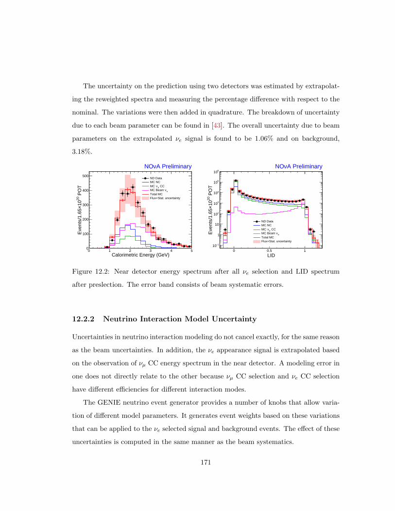
The uncertainty on the prediction using two detectors was estimated by extrapolat-
ing the reweighted spectra and measuring the percentage difference with respect to the
nominal. The variations were then added in quadrature. The breakdown of uncertainty
due to each beam parameter can be found in [43]. The overall uncertainty due to beam
parameters on the extrapolated νe signal is found to be 1.06% and on background,
3.18%.
Calorimetric Energy (GeV)0 1 2 3 4 5
PO
T20
10×E
vent
s/1.
65
0
100
200
300
400
500
A PreliminaryνNO
ND DataMC NC
CCµνMC
eνMC Beam Total MCFlux+Stat. uncertainty
LID0 0.5 1
PO
T20
10×E
vent
s/1.
65
1−10
1
10
210
310
410
510
610A PreliminaryνNO
ND DataMC NC
CCµνMC
eνMC Beam Total MCFlux+Stat. uncertainty
Figure 12.2: Near detector energy spectrum after all νe selection and LID spectrum
after preslection. The error band consists of beam systematic errors.
12.2.2 Neutrino Interaction Model Uncertainty
Uncertainties in neutrino interaction modeling do not cancel exactly, for the same reason
as the beam uncertainties. In addition, the νe appearance signal is extrapolated based
on the observation of νµ CC energy spectrum in the near detector. A modeling error in
one does not directly relate to the other because νµ CC selection and νe CC selection
have different efficiencies for different interaction modes.
The GENIE neutrino event generator provides a number of knobs that allow varia-
tion of different model parameters. It generates event weights based on these variations
that can be applied to the νe selected signal and background events. The effect of these
uncertainties is computed in the same manner as the beam systematics.
171

The complete list of parameters whose effect was studied can be found in [43]. The
total uncertainty from this source on νe signal is 7.28% and on background is 2.14%. The
error on signal is dominated by the uncertainty on the axial mass MA in the quasi-elastic
CC interactions for reasons touched upon earlier.
12.3 Birks Suppresion
It was noted in chapter 6 that tuning the scintillator quenching effect using the near
detector data gives us a Birks Suppression constant value of kB = 0.04 g / MeV cm2.
This is 4 times higher than the typical values published in literature [44], although
the negative contribution due to the second order Chou suppression mitigates over
suppression to some extent. There is, however, some concern that with our measurement
of Birks suppression, we are compensating for other unknown detector effects that result
in loss of visible energy. We have taken the uncertainty on Birks suppression constants
as a systematic to account for our ignorance of the exact parameterization of this effect.
We produced far and near simulation samples with Birks suppression parameters
found in literature (kB = 0.01 g / MeV cm2 and kC = 0.0 g2 / MeV2 cm4) and
compared the extrapolation predictions from these samples with those from nominal
samples.
12.4 Decomposition Uncertainty
In this analysis, we have opted to rely on the simulation to correctly model the ratio of
different components in the νe selected background in the near detector. The excess in
data is then proportionally distributed among the three beam background components.
However, there is some indication that this isn’t the case. In section 11.1, two alternative
methods of decomposition were discussed. In one method, the NC, νµ CC and beam
νe CC scales were determined from energy distribution of events in the LID sideband.
In the second method, the quasi-elastic, resonance and deep-inelastic interaction scales
172

were determined from fitting the hadronic energy distribution of preselected events.
Scaling interaction modes changes the relative rates of NC, νµ CC and beam νe CC
interactions and this was introduced as a second method of decomposition. Table 11.1
shows the results in ND and table 11.2 shows the extrapolated background results in FD
based on these decompositions. The error on decomposition is taken to be the largest
deviation from the proportional decomposition, which is 7.22% based on table 12.2.
Method Tot bg. (%) NC (%) νµ CC (%) Beam νe CC (%)
Scaled by type 7.22 13.89 -60.00 8.51
Scaled by mode 2.06 -22.22 20.00 27.66
Table 12.2: Percentage difference in predicted background with respect to the nominal
proportional decomposition.
12.5 Uncertainty on MRE Correction
The MRE correction to the νe selection efficiency leads to a 15.6% increase in the ex-
pected appearance signal. The possible sources of error on this correction are evaluated
here.
νµ Selection
The MRE events are reconstructed from νµ CC interactions and the selection
efficiency of νµ’s is a smoothly rising function of the true neutrino energy. To
evaluate the impact of changing the νµ selection efficiency on the νe selection of
MRE events, the cut on ReMID, the νµ PID, was changed from the nominal and
the new MRE efficiency corrections applied to the extrapolated appearance signal.
It is found that this has very little effect on the MRE selection efficiency in the
ND. Changing the νµ selection cut largely only changes the background region of
LID for MRE events as is seen in figure 12.3. Nevertheless, the MRE efficiency
173

corrections after these changes were applied to the far detector appearance pre-
diction and the size of the effect is taken as a systematic. Table 12.3 summarizes
this.
νµ Cut Extrapolate νe Signal Difference
Nominal, ReMID > 0.75 5.1 0
Low, ReMID > 0.55 5.07 0.59%
High, ReMID > 0.95 5.17 1.37%
Table 12.3: Change in MRE corrected extrapolated νe signal production due to different
selection cuts on the MRE parent νµ CC interaction. The last column is the percentage
difference with respect to the nominal cut of ReMID > 0.75.
174

LID0 0.2 0.4 0.6 0.8 1
Eve
nts
5000
10000
15000
20000
25000
MRE ND Data and MC
MC
Data
LID0 0.2 0.4 0.6 0.8 1
Dat
a/M
C
0.5
1
1.5
2
(a) LID distribution of MRE events, with
ReMID > 0.55 cut applied to parent inter-
action
LID0 0.2 0.4 0.6 0.8 1
Eve
nts
5000
10000
15000
20000
25000
MRE ND Data and MC
MC
Data
LID0 0.2 0.4 0.6 0.8 1
Dat
a/M
C
0.5
1
1.5
2
(b) LID distribution of MRE events, with
ReMID > 0.95 cut applied to parent inter-
action
LID0 0.2 0.4 0.6 0.8 1
Eve
nts
5000
10000
15000
20000
25000
MRE ND Data and MC
MC
Data
LID0 0.2 0.4 0.6 0.8 1
Dat
a/M
C
0.5
1
1.5
2
(c) LID distribution of MRE events, with
the nominal ReMID > 0.75 cut applied to
parent interaction
Figure 12.3: Change in νe selection of MRE events upon changing the νµ selection of
the parent interactions.
175

MRE to Parent Slice Matching Efficiency
It was noted in chapter 10 that the MRE to parent slice matching efficiency is
discrepant between data and MC. To check if this has any bearing on the MRE
correction, the efficiency cut was changed. Table 12.4 is a summary of these and
their impact on the extrapolated signal prediction.
Efficiency Cut Extrapolate νe Signal Difference
Nominal, Eff > 0.8 5.10 0
Eff > 0.00 5.16 1.18%
Eff > 0.50 5.16 1.18%
Eff > 0.95 4.97 2.55%
Table 12.4: Change in MRE corrected extrapolated νe signal production due to different
parent matching efficiency cuts on the MRE slice. The last column is the percentage
difference with respect to the nominal cut of efficiency > 0.8.
The maximum of the errors on the MRE correction are added in quadrature and
the total error amounts to 2.89%.
12.6 Other Smaller Effects
12.6.1 Containment and Rock Contamination
The NuMI beam is a line source of neutrinos for the near detector. The off-axis loca-
tion of the detector leads to a non-uniform flux of neutrinos along the detector face.
Moreover, the detector, being underground, is surrounded by rock where most beam
neutrinos interact. Neutrino interactions in the rock preceding the front face of the
detector often lead to activity in the front part of the detector. To study all these ef-
fects, the near detector was divided into octants, with each axes divided in half and the
near detector data was extrapolated independently from each quadrant. The maximum
176

variation produced in the background prediction from this exercise is of 2.7%.
To reduce the time required in simulation of rock interactions that leave activity
in the detector, a simplification in the simulation process is used. A large set of rock
interactions is generated and overlaid with interaction of neutrinos in the detector. The
reuse rate of a simulated rock interaction in the near detector simulation set used in
this analysis is close to 350 times. If a single interaction passes selection cuts, it is likely
to pass them for all the repetitions. This has been incorporated as a systematic, the
size of which was determined by extrapolating without any rock interactions at all. The
change in total background is 0.1%.
12.6.2 Simulation Statistics and Normalization
The predictions for the analysis are made from limited simulation statistics. The error
on the prediction due to this is 3.47% on background and 0.9% on signal.
Normalization errors arise from two source - POT counting and detector mass. The
POT counting error is 0.5% [45]. The detector mass uncertainty is computed from
tolerances on the size, mass and densities of the detector components and adds up to
0.7% of the detector mass [46]. Also, a difference of 0.8% in the neutrino event rate is
observed in the near detector data and MC before any cuts are applied. It is not clear
whether this applies equally to the far detector as well. Therefore, it is treated as a
normalization systematic. Additionally, the diblock configurations in real conditions far
detector simulation are not identical to the data; this contributes another 0.7% to the
normalization systematic. All these uncertainties add up to 1.37%.
12.6.3 Alignment
The analysis simulation samples use a perfectly aligned geometry of the near and far
detectors. The installation of the blocks is indeed not perfect and they are staggered
with respect to one another. Small samples of near and far detector simulations were
generated with this imperfect alignment and it was shown to have a small effect on
177

reconstruction and selection efficiencies. The error due to this is 0.73% on signal and
1.73 % on background.
12.6.4 Light Level
It was discussed earlier that the far detector calibrated response shows different shapes
between data and MC as a function of distance from readout. The suspicion is that the
scintillator light yield is not properly tuned in the simulation. The impact of this effect
on the energy reconstruction is accounted for in the calibration systematic. However, a
mistuned light level can lead to second order effects, such as hits below threshold, that
never triggered. The number of hits in a slice shifts by about 5% in the response slope
simulated sample. This 5% shift results in a 1% change in the signal selection efficiency,
while there is no noticeable effect on background efficiency.
12.7 Summary
Many different sources of error have been considered for this analysis. The largest of
errors on signal arise from uncertainty in calibration, neutrino interaction model and
Birks suppression parameters. The errors are tabulated in table 12.5.
Figure 12.4: Summary of signal and background uncertainties
178

Total BG Syst. (%) Signal Syst. (%)
Beam 3.18 1.06
Birks 5.14 7.22
Calibration 4.44 7.58
Light Level n/a 1.00
Neutrino Interaction 2.14 7.28
Containment 1.84 n/a
Rock contamination 0.10 n/a
Decomposition 7.22 n/a
ND Data & MC Stats 3.47 0.6
Normalization 1.37 1.37
MRE Correction n/a 2.89
Total 11.41 13.24
Table 12.5: Final systematic error (in percentages) on the combined background and
signal in the Far Detector. The last row is the sum in quadrature of all errors in this
table.
179

Chapter 13
Results of νe Appearance Analysis
The last two chapters discussed in detail the predicted signal and background in the
νe appearance analysis of NOνA’s first data and the errors on these predictions. The
predictions are reviewed again in table 13.1.
Signal Stat Syst Total Bg Stat Syst Total Events
Simple Osc 5.10 2.26 0.68 0.97 0.98 0.11 6.07
IH, δ = π/2, θ23 = π/4 2.59 1.61 0.34 0.96 0.98 0.11 3.55
NH, δ = 3π/2, θ23 = π/4 6.57 2.56 0.87 0.94 0.97 0.11 7.54
Table 13.1: Expected signal and background for NOνA first data along with the sys-
tematic and statistical errors on the predictions.
This chapter presents the results of νe appearance analysis performed on the first
data collected with the NOνA detectors. The first section presents a sideband study
that was done prior to unblinding the main signal region, as a final check of the analysis
chain. The second section presents the main result and its statistical treatment. The
final section is a discussion of the outlook for future analyses of NOνA data.
180

13.1 PID Sideband
The signal events for this analysis are those that pass all νe preselection cuts and have a
LID value greater than 0.95. To test the analysis chain and check that the PID behaves
as expected on data, the LID sideband from 0.7 to 0.95 was unblinded ahead of the
final analysis. The event counts expected from extrapolation for this region in the FD
beam data are listed in table 13.2. The MRE correction has been applied to the signal
prediction here. The correction was determined separately using MRE events with LID
values between 0.7 and 0.95.
Osc,. Params Signal Beam BG Cosmic BG Tot. Events
Simple osc. 2.33 1.50 0.38 4.21
IH , δ = π/2 1.22 1.51 0.38 3.11
NH, δ = 3π/2 3.01 1.48 0.38 4.87
Table 13.2: LID sideband event counts expectation in the far detector
In the FD data, 5 events have been observed in the sideband, which is consistent
with the expectations listed in table 13.2. All the events observed appear neutrino-like
and the PID performance seems well-behaved on the FD data.
13.2 νe Appearance Result
In the far detector NuMI beam data, 6 events have been observed in the signal region.
The event displays of these 6 candidates follow in figures 13.3, 13.4 and 13.5. All
the observed candidates have very convincing electron neutrino characteristics, with
a well-defined electromagnetic shower. Figure 13.1 shows the cumulative event count
as a function of time during the data taking period along with the integrated exposure
expressed in mass × POT. The Kolmogorov-Smirnov (KS) statistic test of the integrated
event count with the exposure as a reference has a probability of 31%, indicating that
181

the observed event rate is consistent with exposure.
Figure 13.2 shows the time distribution of the candidate events. The blue lines mark
the edges of the NuMI timing windows and the two out-of-time events are the cosmic
background. Interestingly, no νe candidates are found in the delayed 64 µs time window
in the pre-shutdown data. Figure 13.6 shows distributions of event energy, cosine of
angle wrt to NuMI beam direction and electron log-likelihoods of the signal candidates
overlaid on the prediction from simulation. These distributions show no unexpected
behavior in the candidates observed in the FD data. Figure 13.7 shows the vertex
distributions of the candidates. With the exception of one event, which is very close to
the front face of the detector, all events are well contained within the fiducial volume
of the detector.
Figures 13.8 and 13.9 are the longitudinal and transverse dE/dx profiles of the can-
didate events overlaid on the dE/dx probability distribution constructed from electrons
in simulated νe CC interactions. The events follow the trademark electron shower de-
velopment, with energy deposition consistent with a MIP in the first few planes and
with an electromagnetic shower in the following planes.
182

Figure 13.1: νe Appearance candidates in FD NuMI beam data. The gray events are
are out-of-time cosmics.
Figure 13.2: Timing distribution of FD signal events. The blue line indicate the NuMI
beam window boundaries. The two out of time events are cosmic background.
183

Figure 13.3: νe Appearance candidates in FD NuMI beam data. The gray events are
are out-of-time cosmics.
184

Figure 13.4: νe Appearance candidates in FD NuMI beam data. The gray events are
are out-of-time cosmics.
185

Figure 13.5: νe Appearance candidates in FD NuMI beam data. The gray events are
are out-of-time cosmics.
186

(a) Cosine of angle with respect to the beam
direction.
(b) Energy distribution of neutrinos. Each ar-
row indicates the observed candidate events in
the FD data
(c) Longitudinal electron log-likelihood (d) Transverse electron log-likelihood
Figure 13.6: Distributions of signal events in the NuMI beam window in the FD data.
13.3 Analysis of the Result
In the analysis presented here, the only information used to infer neutrino oscillation
parameters is the number of candidate events observed in the FD NuMI data. No energy
shape information is utilized. This section discusses a simple method of analyzing the
results in the first subsection, followed by a more sophisticated statistical treatment.
187

(a) Vertex distribution of
candidate events in XY
plane
(b) Vertex distribution of candidate events in XZ plane
(c) Vertex distribution of candidate events in YZ plane
Figure 13.7: Vertex distributions of candidate events. The dotted red lines indicate the
containment boundaries.
188

(a) dE/dx in longitudinal direction vs plane
number from shower start for νe candidate
event in run 15330
(b) dE/dx in transverse direction vs cell
number from shower core for νe candidate
event in run 15330
(c) dE/dx in longitudinal direction vs plane
number from shower start for νe candidate
event in run 17103
(d) dE/dx in transverse direction vs cell
number from shower core for νe candidate
event in run 17103
(e) dE/dx in longitudinal direction vs plane
number from shower start for νe candidate
event in run 19165
(f) dE/dx in transverse direction vs cell
number from shower core for νe candidate
event in run 19165
Figure 13.8: dE/dx by plane number from the shower start in the longitudinal and
transverse directions for leading showers. The points are the data and the color scale is
the dE/dx probability distribution for electrons in simulated νe CC events.
189

(a) dE/dx in longitudinal direction vs plane
number from shower start for νe candidate
event in run 19193
(b) dE/dx in transverse direction vs cell
number from shower core for νe candidate
event in run 19193
(c) dE/dx in longitudinal direction vs plane
number from shower start for νe candidate
event in run 19264
(d) dE/dx in transverse direction vs cell
number from shower core for νe candidate
event in run 19264
(e) dE/dx in longitudinal direction vs plane
number from shower start for νe candidate
event in run 19578
(f) dE/dx in transverse direction vs cell
number from shower core for νe candidate
event in run 19578
Figure 13.9: dE/dx by plane number from the shower start in the longitudinal and
transverse directions for leading showers. The points are the data and the color scale is
the dE/dx probability distribution for electrons in simulated νe CC events.
190

13.3.1 Significance of Observation: Simple Treatment
In the far detector data, 6 events have been observed in the νe appearance channel.
Recall that the estimated background is 0.97 event with a systematic error of 11.64%.
The probability that 6 or more events may be observed due to Poisson fluctuation of
this background, rather than due to νµ to νe oscillation is given by :
p =∞∑x=6
∫ −∞−∞
Poisson(x,b)×Gauss(b, b0, σbb0)× 1
σbb0db (13.1)
Here, b0 and σb are the expected background and the relative systematic error on the
background, respectively. The Gaussian varies the background with a width equal to
the systematic error and the Poisson function fluctuates it around the new central value.
If simple oscillations are used, with no matter effects or CP violation, the probability
of 6 events being an upward fluctuation of the background is 5.5×10⁻⁴, which translates
to a significance of rejection of no-oscillation hypothesis at 3.46 σ.
To see which of the two extreme hierarchy and CP violation scenarios are favored
by our data, we perform the same calculation as above (eq. 13.1) except that the
background and background error are replaced by the expected total event count for
the particular oscillation hypothesis and the total error. From this computation, the
inverted hierarchy with CP violation phase δ = π/2 parameters are disfavored at 1.28
σ, while the normal hierarchy with δ = 3π/2 is disfavored at 0.73 σ. Therefore, our
data mildly favor the normal hierarchy with δ = 3π/2 at 1.05 σ.
Deviation from... Significance in σ
No-oscillation hypothesis 3.46
IH, δ = π/2 1.28
NH, δ = 3π/2 0.74
Table 13.3: Significance of observation
191

13.3.2 Fit to Oscillation Parameters
The oscillation fits here are performed in the 2D space of sin2 2θ13 versus CP violation
phase δ. Mass hierarchy can also produce an enhancement or suppression of oscillations,
but since it can only take on of two values (∆m232 > 0 for normal hierarchy and ∆m2
32 < 0
for inverted hierarchy), the fit values are computed and plotted separately for the two
hierarchy hypotheses. The systematic uncertainty on the signal and the background
are treated as additional uncertainty along with the statistical error. Since statistical
uncertainty in this analysis is fairly large, treating systematics as nuisance parameters
is found to make little difference.
In the fit for sin2 2θ13, a marginalization is performed over the atmospheric and solar
oscillation parameters. The atmospheric parameter measurements are taken from the
T2K experiment result in [47] because the dependence of their result on hierarchy is
small due to a much shorter baseline. The solar oscillation parameters are from [6]. The
results of this fit are in figure 13.10.
Figure 13.10 shows that the νe appearance result from NOνA data is well in agree-
ment with the value of sin2 2θ13 measured by the reactor neutrino experiments. The
best fit point in the normal hierarchy case is at sin2 2θ13 = 0.092 and δ/π = 0.31. For
inverted hierarchy, the best fit is at sin2 2θ13 = 0.10 and δ/π = 1.64. There is a slight
tension with the reactor results for sin2 2θ13 (1 − 2σ) in case of inverted hierarchy, CP
violation phase δ ∼ π/2, where larger values of sin2 2θ13 are favored by our observation
of 6 events. For the normal hierarchy, the result is consistent with the reactor constraint
for all values of δ within 1σ.
Since the sin2 2θ13 parameter is precisely measured in reactor neutrino experiments,
it can be used as a constraint to check which values of CP violating phase our data
are most consistent with. This is shown in figure 13.11a where the likelihood difference
with respect to best fit is plotted as a function of δ. This also points towards a greater
consistency with the normal hierarchy compared to inverted. In IH case, a δ value
192

Figure 13.10: A fit to θ13 and CP violation phase, δ, based on the observation of 6
events in the νe appearance channel, where the expected background is 0.97 event.
The dotted blue lines enclose the 68% confidence interval and the solid red lines are
90% confidence interval. The solid gray lines show the sin22θ13 measurement from the
reactor experiments. 193
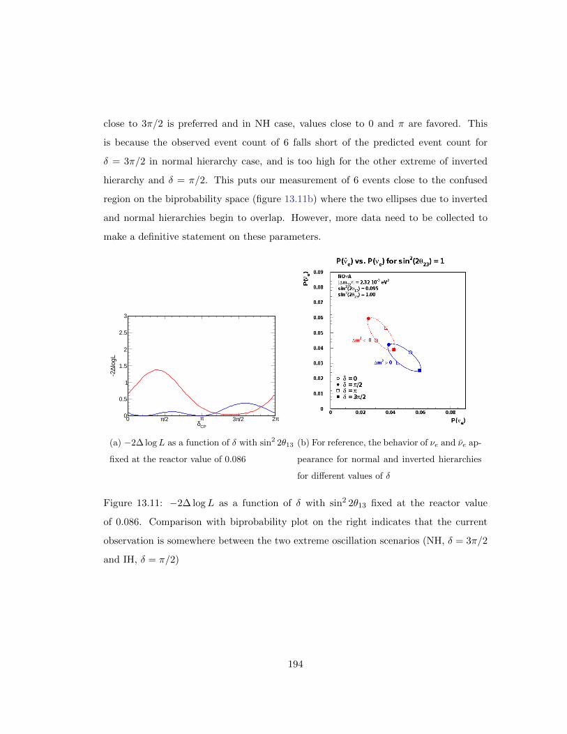
close to 3π/2 is preferred and in NH case, values close to 0 and π are favored. This
is because the observed event count of 6 falls short of the predicted event count for
δ = 3π/2 in normal hierarchy case, and is too high for the other extreme of inverted
hierarchy and δ = π/2. This puts our measurement of 6 events close to the confused
region on the biprobability space (figure 13.11b) where the two ellipses due to inverted
and normal hierarchies begin to overlap. However, more data need to be collected to
make a definitive statement on these parameters.
CPδ
logL
∆-2
0
0.5
1
1.5
2
2.5
3
0 /2π π /2π3 π2
(a) −2∆ logL as a function of δ with sin2 2θ13
fixed at the reactor value of 0.086
(b) For reference, the behavior of νe and ν̄e ap-
pearance for normal and inverted hierarchies
for different values of δ
Figure 13.11: −2∆ logL as a function of δ with sin2 2θ13 fixed at the reactor value
of 0.086. Comparison with biprobability plot on the right indicates that the current
observation is somewhere between the two extreme oscillation scenarios (NH, δ = 3π/2
and IH, δ = π/2)
194

13.3.3 Feldman-Cousins Method for Confidence Interval
The oscillation parameters like sin2 θ13 have a well-defined physical range, in this case
0 to 1. However, the Gaussian errors on such parameters can sometimes extend beyond
the physical range, where they have no natural interpretation. If these cases are not
carefully dealt with, the quoted confidence intervals can often lead to under- or over-
coverage. The complete presentation of the subtleties involved in the analysis of such
parameters can be found in the original Feldman-Cousins (FC) publication [48]; what
follows is a brief description of their proposed method to circumvent these problems.
In an ensemble of experiments with an observable x that depends on a parameter
µ, a confidence interval [µ1, µ2] on the parameter µ is defined as a subset that satisfies
P (x|µ ∈ [µ1, µ2]) = α (13.2)
Therefore, the interval contains the true value µt of the parameter µ in α fraction
of the experiments. To determine the confidence interval, the outcomes are added in
the decreasing order of probability, starting with P (x|µmp), where µmp maximizes the
probability of the observed outcome, until the summed probability reaches the desired
level α. In the FC method, the best fit value µmp is constrained to be within its physical
range. Moreover, the order in which probabilities are added, to construct a confidence
interval is instead determined by the likelihood ratio P (x|µ)/P (x|µmp). Since in the
Gaussian regime, −2 lnP ∼ χ2, the likelihood ratio can be replaced by the difference
between the χ2 at a given value of µ and that at µmp, which we call χ2mp.
Prior to looking at the data, for each point in the oscillation phase space, an ensemble
of statistical experiments is generated and the difference ∆χ2 = χ2 − χ2mp is computed
for each experiment. The critical value of the difference , ∆χ2crit, is defined as the one
for which α fraction of the experiments at that combination of oscillation parameters
have ∆χ2 < ∆χ2crit. Once the data are known, the difference between χ2 for each set
of oscillation parameters and the best fit χ2 is computed. The points for which ∆χ2 of
data are is than ∆χ2crit are included in the confidence interval with coverage α.
195

The Feldman-Cousins critical values of χ2 are shows in figure 13.12. The contours
derived using these critical χ2 values are shown in figure 13.13. Note that this method
does not change the best fit value, it only changes the region of phase space included
in the confidence interval. The FC contours are noticeably less smooth than those in
figure 13.10 that were based on Gaussian assumption. This is due to the limited number
of experiments (10 million) that was run to produce this result, rather than anything
inherent to the FC method.
(a) Normal Hierarchy
(b) Inverted Hierarchy
Figure 13.12: Critical value of χ2 in sin2 2θ13 vs δ space for normal and inverted hier-
archies.
196

Figure 13.13: Feldman-Cousins contours for 68% and 90% confidence interval in θ13 and
δ space, based on the observation of 6 events in the νe appearance channel, where the
expected background is 0.97 event. The dotted blue lines enclose the 68% confidence
interval and the solid red lines are 90% confidence interval. The solid gray lines show
the sin2 2θ13 measurement from the reactor experiments.
197

13.3.4 Result from Alternative PID, LEM
As mentioned before, LEM is an alternative PID developed for νe identification in
NOνA. It matches every candidate event against a library of simulated neutrino in-
teractions and deduces its identity based on the characteristics of the best matched
simulated events in the library. For completeness, the LEM PID selects 11 events in
the NOνA first data. All 6 events selected by LID are also selected by LEM. Of the 5
additional events that LEM selects, 3 are in the LID sideband from 0.7 to 0.95. Given
the estimated correlation (62%) between the two PIDs, the probability of observing 5
events in LEM that are not selected by LID, and no events in LID that are not selected
by LEM, and other less likely combinations is 9.2%.
13.3.5 Comparison with Official NOνA νe Appearance Result
The officially presented and published νe appearance result from the NOνA collabora-
tion do not apply the MRE correction to the far detector signal estimate. The ∼ 12%
systematic error in the official analysis on the νe signal estimate is meant to cover the
MRE correction. Since the expected signal count in far detector is ∼ 15% lower than
the MRE corrected signal count, this changes the interpretation of the observed 6 can-
didate events. Without the MRE correction, for normal hierarchy and CP violating
phase, δ = 3π/2, the expected total event count (signal + background) is 5.62 events,
which is consistent with the observation of 6 events, so this scenario is favored in the
official result.
13.4 Future Analyses of NOνA Data
The analysis presented here uses roughly 8% of the exposure planned for the full age
of the NOνA experiment. While higher statistics will play a large role in improving
the power of future NOνA νe appearance results, many aspects of the analysis will
need substantial improvement to keep systematic errors relatively low. The hadronic
198

energy discrepancy that has been discussed at some length in this thesis is one of the
highest priority issues to resolve over the next few months. There is evidence that
the disagreement arises from under-representing quasi-elastic-like interactions in the
simulation. A simple fit for scale factors of interaction types has been presented here;
however, since the cross-sections of different modes are a function neutrino energy, an
energy based fit might provide additional power. Applying external constraints, such as
the neutrino cross-section measurements by the MINERνA experiment might also aid
in resolving this discrepancy.
Cosmic background rejection in the far detector costs a considerable loss in efficiency
of νe signal selection. For this analysis, a simple cut-based approach was used for cosmic
rejection as proof of concept. The cuts were optimized to maximize the significance of
νe appearance. For future analyses, multi-variate techniques can be explored for cosmic
rejection to improve efficiency. Minimizing systematic error while tuning cuts such as
the neutrino energy cut might also help to make the measurements more robust.
While many avenues of improvement remain open for exploration, the detectors are
already performing remarkably well. The level of detail with which neutrino interactions
can be observed is unparalleled for a detector of this size. As the NuMI beam continues
to ramp up in power, the NOνA data are making the remaining unmeasured neutrino
oscillation parameters more accessible. T2K has recently presented their first data in
the anti-neutrino mode, although it is too early to definitively claim ν̄e appearance [49].
Over the next year, plans to run the NuMI beam in anti-neutrino mode will be finalized
as well. The following years promise to be very interesting in the field of neutrino
physics.
199

References
[1] Davide D’Angelo. Low Energy Neutrino Measurements. Pramana, 79:757–780,
2012, 1211.5359.
[2] Robert M. Zwaska. Accelerator System and Instrumentation for the NuMI Neutrino
Beam. PhD thesis, University of Texas, Austin, 2005.
[3] S. Mufson, B. Baugh, C. Bower, T. Coan, J. Cooper, et al. Liquid scintillator
production for the NOvA experiment. 2015, 1504.04035.
[4] Fundamental Physics at the Intensity Frontier, 2012, 1205.2671.
[5] P. Hernandez. Neutrino physics. 2010, 1010.4131.
[6] K.A. Olive et al. Review of Particle Physics. Chin.Phys., C38:090001, 2014.
[7] Quang Ho-Kim and Pham Xuan Yem. Elementary Particles and Their Interactions.
Springer, 1998.
[8] Don L Anderson. Theory of the Earth. Blackwell Scientific Publications , Boston,
MA, 1989.
[9] J. N. Bahcall, W. A. Fowler, I. Iben, Jr., and R. L. Sears. Solar Neutrino Flux.
The Astrophysical Journal, 137:344–346, January 1963.
[10] Raymond Davis, Don S. Harmer, and Kenneth C. Hoffman. Search for neutrinos
from the sun. Phys. Rev. Lett., 20:1205–1209, May 1968.
200

[11] John N. Bahcall, M. H. Pinsonneault, Sarbani Basu, and J. Christensen-Dalsgaard.
Are standard solar models reliable? Phys. Rev. Lett., 78:171–174, Jan 1997.
[12] John N. Bahcall and Jr. Raymond Davis. The evolution of neutrino astronomy.
Publications of the Astronomical Society of the Pacific, 112(770):pp. 429–433, 2000.
[13] F. Kaether, W. Hampel, G. Heusser, J. Kiko, and T. Kirsten. Reanalysis of the
gallex solar neutrino flux and source experiments. Phys. Lett., B685:47–54, 2010,
1001.2731.
[14] M. Altmann et al. Complete results for five years of gno solar neutrino observations.
Phys. Lett., B616:174, 2005, hep-ex/0504037.
[15] J. N. Abdurashitov et al. Measurement of the solar neutrino capture rate with
gallium metal, part iii. Phys. Rev., C80:015807, 2009, 0901.2200.
[16] B. Ananthanarayan and Ritesh K. Singh. Direct observation of neutrino oscillations
at the sudbury neutrino observatory. Curr. Sci., 83:553, 2002, physics/0208096.
[17] Y. Fukuda et al. Evidence for oscillation of atmospheric neutrinos. Phys. Rev.
Lett., 81:1562–1567, 1998, hep-ex/9807003.
[18] M. Apollonio et al. Search for neutrino oscillations on a long base-line at the chooz
nuclear power station. Eur. Phys. J., C27:331, 2003, hep-ex/0301017.
[19] Y. Abe et al. Reactor electron antineutrino disappearance in the double chooz
experiment. Phys. Rev., D86:052008, 2012, 1207.6632.
[20] F.P. An et al. Observation of electron-antineutrino disappearance at daya bay.
Preprint, 2012.
[21] Kim Soo-Bong et al. Observation of reactor electron antineutrino disappearance in
the reno experiment. 2012.
201

[22] S. M. Bilenky and Carlo Giunti. Neutrinoless double-beta decay: A brief review.
Mod. Phys. Lett., A27:1230015, 2012, 1203.5250.
[23] A. Cervera, A. Donini, M.B. Gavela, J.J. Gomez Cdenas, P. Hernndez, O. Mena,
and S. Rigolin. Golden measurements at a neutrino factory. Nuclear Physics B,
579(12):17 – 55, 2000.
[24] P. Adamson et al. Combined analysis of νµ disappearance and νµ → νe appearance
in minos using accelerator and atmospheric neutrinos. Phys.Rev.Lett., 112:191801,
2014, 1403.0867.
[25] D.S. Ayres et al. The nova technical design report. Technical report, Fermilab,
Batavia, Illinois, 2007.
[26] E. Niner, P. Adamson, G. Deuerling, R. Kwarciany, H. Meyer, et al. Synchro-
nization of the 14 kTon NOνA neutrino detector with the Fermilab NuMI beam.
J.Phys.Conf.Ser., 513:012028, 2014.
[27] Alexander Radovic. Measuring the Disappearance of Muon Neutrinos with the
MINOS Detector. PhD thesis.
[28] C. Andreopoulos et al. The GENIE Neutrino Monte Carlo Generator. Nucl. In-
strum. Meth., A614:87–104, 2010, 0905.2517.
[29] Chris Hagmann et al. Cosmic-ray Shower Library (CRY).
[30] S. Agostinelli et al. GEANT4: A Simulation toolkit. Nucl.Instrum.Meth.,
A506:250–303, 2003.
[31] A Aurisano et al. The nova simulation chain. Submitted to Journal of Physics:
Conference Series.
[32] Jonathan Liu. Quantifying croscross in avalanche photodiodes used in nova. NOvA
internal document database.
202

[33] J.B. Birks. The theory and practice of scintillation counting. International series
of monographs on electronics and instrumentation. Macmillan, 1964.
[34] C. N. Chou. The nature of the saturation effect of fluorescent scintillators. Phys.
Rev., 87:904–905, Sep 1952.
[35] Martin Ester, Hans peter Kriegel, Jrg S, and Xiaowei Xu. A density-based algo-
rithm for discovering clusters in large spatial databases with noise. pages 226–231.
AAAI Press, 1996.
[36] L. Fernandes and M. Oliveira. Real-timelinedetectionthroughanimprovedhoughtransform
votingscheme. Pattern Recognition, 41:299–314, 2008.
[37] Mattias Ohlsson. Extensions and explorations of the elastic arms algorithm. Com-
puter Physics Communications, 77(1):19 – 32, 1993.
[38] J. C. Dunn. A fuzzy relative of the isodata process and its use in detect-
ing compact well-separated clusters. Journal of Cybernetics, 3(3):32–57, 1973,
http://dx.doi.org/10.1080/01969727308546046.
[39] R. Krishnapuram and J.M. Keller. A possibilistic approach to clustering. Fuzzy
Systems, IEEE Transactions on, 1(2):98–110, May 1993.
[40] Miin-Shen Yang and Kuo-Lung Wu. Unsupervised possibilistic clustering. Pattern
Recogn., 39(1):5–21, January 2006.
[41] Rudolph Emil Kalman. A new approach to linear filtering and prediction problems.
Transactions of the ASME–Journal of Basic Engineering, 82(Series D):35–45, 1960.
[42] C. Backhouse and R. B. Patterson. Library event matching event classification algo-
rithm for electron neutrino interactions in the nova detectors. Nucl.Instrum.Meth.,
A778:31–39, 2015, 1501.00968.
203

[43] Gavin Davies et al. Position paper: Nue systematics. NOvA In-
ternal Document Database 13597 http://nova-docdb.fnal.gov:8080/cgi-
bin/ShowDocument?docid=13597.
[44] V.I. Tretyak. Semi-empirical calculation of quenching factors for ions in scintilla-
tors. Astroparticle Physics, 33(1):40 – 53, 2010.
[45] Hongyue Duyang et al. A technote describing the derivation and size of numi flux
uncertainties used in the first nova analyse. NOvA internal Document Database
13584, http://nova-docdb.fnal.gov:8080/cgi-bin/ShowDocument?docid=13584.
[46] Nicholas Raddatz. Fiducial mass systematic. NOvA Internal Document Database
13237 http://nova-docdb.fnal.gov:8080/cgi-bin/ShowDocument?docid=13237.
[47] K. Abe et al. Measurements of neutrino oscillation in appearance and disappear-
ance channels by the T2K experiment with 6.61020 protons on target. Phys. Rev.,
D91(7):072010, 2015, 1502.01550.
[48] Gary J. Feldman and Robert D. Cousins. Unified approach to the classical statis-
tical analysis of small signals. Phys. Rev. D, 57:3873–3889, Apr 1998.
[49] Melody RAVONEL. Antineutrino oscillations with t2k. 2015. EPS HEP 2015.
204