
Performance Studies for the KM3NeT Neutrino Telescope
162
Performance Studies for the KM3NeT Neutrino Telescope Der Naturwissenschaftlichen Fakult¨ at der Friedrich-Alexander-Universit¨ at Erlangen-N¨ urnberg zur Erlangung des Doktorgrades vorgelegt von Claudio Kopper aus Erlangen
-
Upload
khangminh22 -
Category
Documents
-
view
1 -
download
0
Transcript of Performance Studies for the KM3NeT Neutrino Telescope

Performance Studies for theKM3NeT Neutrino Telescope
Der Naturwissenschaftlichen Fakultat
der Friedrich-Alexander-Universitat Erlangen-Nurnberg
zur Erlangung des Doktorgrades
vorgelegt von
Claudio Kopper
aus Erlangen

Als Dissertation genehmigt von der Naturwissenschaftlichen Fakultatder Friedrich-Alexander-Universitat Erlangen-Nurnberg
Tag der mundlichen Prufung: 12. Marz 2010
Vorsitzender der Promotionskommission: Prof. Dr. Eberhard BanschErstberichterstatter: Prof. Dr. Ulrich KatzZweitberichterstatter: Prof. Dr. Christian Stegmann

Meinen Eltern


Contents
Introduction 9
I Basics 13
1 High energy cosmic neutrinos 151.1 Neutrinos in the Standard Model . . . . . . . . . . . . . . . . . . . . 151.2 Cosmic accelerators . . . . . . . . . . . . . . . . . . . . . . . . . . . . 16
1.2.1 The cosmic ray spectrum . . . . . . . . . . . . . . . . . . . . 161.2.2 Particle acceleration . . . . . . . . . . . . . . . . . . . . . . . 171.2.3 Neutrino production . . . . . . . . . . . . . . . . . . . . . . . 201.2.4 Source candidates . . . . . . . . . . . . . . . . . . . . . . . . 21
2 Neutrino telescopes 252.1 Detection mechanism . . . . . . . . . . . . . . . . . . . . . . . . . . . 25
2.1.1 Neutrino interaction . . . . . . . . . . . . . . . . . . . . . . . 252.1.2 Cherenkov radiation from charged particles . . . . . . . . . . 292.1.3 Muon propagation . . . . . . . . . . . . . . . . . . . . . . . . 292.1.4 Electromagnetic and hadronic cascades . . . . . . . . . . . . 302.1.5 Light propagation . . . . . . . . . . . . . . . . . . . . . . . . 312.1.6 Light detection . . . . . . . . . . . . . . . . . . . . . . . . . . 322.1.7 Triggering . . . . . . . . . . . . . . . . . . . . . . . . . . . . . 332.1.8 Muon track reconstruction . . . . . . . . . . . . . . . . . . . . 332.1.9 Background . . . . . . . . . . . . . . . . . . . . . . . . . . . . 34
2.2 Existing neutrino telescopes . . . . . . . . . . . . . . . . . . . . . . . 382.2.1 Baikal . . . . . . . . . . . . . . . . . . . . . . . . . . . . . . . 382.2.2 IceCube . . . . . . . . . . . . . . . . . . . . . . . . . . . . . . 392.2.3 ANTARES . . . . . . . . . . . . . . . . . . . . . . . . . . . . 40
2.3 The KM3NeT project . . . . . . . . . . . . . . . . . . . . . . . . . . 422.3.1 Overview . . . . . . . . . . . . . . . . . . . . . . . . . . . . . 422.3.2 Design possibilities . . . . . . . . . . . . . . . . . . . . . . . . 422.3.3 Detector sites . . . . . . . . . . . . . . . . . . . . . . . . . . . 44
5

Contents
II Methodology 45
3 Software simulation and reconstruction tools 473.1 Legacy software tools from ANTARES . . . . . . . . . . . . . . . . . 473.2 Software frameworks . . . . . . . . . . . . . . . . . . . . . . . . . . . 50
3.2.1 The concept of a software framework . . . . . . . . . . . . . . 503.2.2 The IceTray framework . . . . . . . . . . . . . . . . . . . . . 523.2.3 Simulation and analysis tools for KM3NeT within the IceTray
framework - “SeaTray” . . . . . . . . . . . . . . . . . . . . . . 52
4 A new KM3NeT simulation and reconstruction chain 554.1 Overview and Incentive . . . . . . . . . . . . . . . . . . . . . . . . . 554.2 Simulation of neutrino interactions using ANIS . . . . . . . . . . . . 55
4.2.1 Event weights . . . . . . . . . . . . . . . . . . . . . . . . . . . 574.3 Simulation of atmospheric muons with CORSIKA . . . . . . . . . . 584.4 Propagation of muons to the detection volume . . . . . . . . . . . . 59
4.4.1 Modifications for KM3NeT . . . . . . . . . . . . . . . . . . . 594.5 Muon propagation and Cherenkov light generation . . . . . . . . . . 59
4.5.1 Detailed simulation . . . . . . . . . . . . . . . . . . . . . . . . 604.5.2 Speedup of the Cherenkov light tracking algorithm for unscat-
tered light . . . . . . . . . . . . . . . . . . . . . . . . . . . . . 634.6 Fast cascade light generation and propagation . . . . . . . . . . . . . 63
4.6.1 Angular light distribution . . . . . . . . . . . . . . . . . . . . 634.6.2 Total photon yield . . . . . . . . . . . . . . . . . . . . . . . . 654.6.3 Scattering table generation . . . . . . . . . . . . . . . . . . . 654.6.4 Light generation at optical modules . . . . . . . . . . . . . . 684.6.5 Optimisation for unscattered photons . . . . . . . . . . . . . 714.6.6 Longitudinal light distribution . . . . . . . . . . . . . . . . . 71
4.7 Adaptation of the cascade simulation approach to muons . . . . . . 734.7.1 Spatial segmentation . . . . . . . . . . . . . . . . . . . . . . . 744.7.2 Table generation . . . . . . . . . . . . . . . . . . . . . . . . . 744.7.3 Light generation at optical modules . . . . . . . . . . . . . . 76
4.8 A unified cascade/muon simulation . . . . . . . . . . . . . . . . . . . 764.9 Simulation of light near and in optical modules . . . . . . . . . . . . 77
4.9.1 ANTARES-style modules . . . . . . . . . . . . . . . . . . . . 774.9.2 MultiPMT modules . . . . . . . . . . . . . . . . . . . . . . . 79
4.10 Light detection . . . . . . . . . . . . . . . . . . . . . . . . . . . . . . 834.10.1 PMT simulation . . . . . . . . . . . . . . . . . . . . . . . . . 834.10.2 Readout electronics simulation using the “ARS” chip . . . . . 844.10.3 A time-over-threshold approach . . . . . . . . . . . . . . . . . 844.10.4 Hit coincidence triggering . . . . . . . . . . . . . . . . . . . . 85
6

Contents
4.11 Muon track reconstruction strategies . . . . . . . . . . . . . . . . . . 864.11.1 The standard ANTARES reconstruction strategy . . . . . . . 864.11.2 A new reconstruction algorithm for multiPMT detectors . . . 87
5 Analysis techniques 975.1 Angular resolution . . . . . . . . . . . . . . . . . . . . . . . . . . . . 975.2 Neutrino effective area . . . . . . . . . . . . . . . . . . . . . . . . . . 975.3 Point-source sensitivity and discovery potential . . . . . . . . . . . . 99
5.3.1 Discovery potential . . . . . . . . . . . . . . . . . . . . . . . . 995.3.2 Sensitivity . . . . . . . . . . . . . . . . . . . . . . . . . . . . . 100
III Results 103
6 Comparison between simulation chains 1056.1 Detector design, environment and simulation parameters . . . . . . . 1056.2 Basic quantities before reconstruction . . . . . . . . . . . . . . . . . 1076.3 Quality cut distribution . . . . . . . . . . . . . . . . . . . . . . . . . 1096.4 Angular resolution . . . . . . . . . . . . . . . . . . . . . . . . . . . . 1126.5 Effective area . . . . . . . . . . . . . . . . . . . . . . . . . . . . . . . 1146.6 Point-source sensitivity . . . . . . . . . . . . . . . . . . . . . . . . . . 116
7 Performance of different detector designs 1197.1 Angular resolution . . . . . . . . . . . . . . . . . . . . . . . . . . . . 1207.2 Effective area . . . . . . . . . . . . . . . . . . . . . . . . . . . . . . . 1227.3 Point-source sensitivity . . . . . . . . . . . . . . . . . . . . . . . . . . 1247.4 Effect of the atmospheric muon background on the multiPMT design 124
8 Scaling of the multiPMT design 1298.1 Doubling the number of strings . . . . . . . . . . . . . . . . . . . . . 1298.2 Effects of varying string distances . . . . . . . . . . . . . . . . . . . . 134
8.2.1 Angular resolution . . . . . . . . . . . . . . . . . . . . . . . . 1348.2.2 Effective area . . . . . . . . . . . . . . . . . . . . . . . . . . . 1348.2.3 Point-source sensitivity . . . . . . . . . . . . . . . . . . . . . 1348.2.4 Discovery potential for SNR RX J1713.7–3946 . . . . . . . . 139
Summary and conclusions 141
Zusammenfassung und Ausblick 145
Bibliography 151
7


Introduction
It is impressive how extensive our knowledge about the universe and its contentshas become by just looking at the night sky. Astronomy has come a long wayfrom its beginnings with observations using the naked eye to modern times, wheresophisticated instruments are used to record the information reaching us from thestars, galaxies and from the host of other amazing things that exist out there. Untilrecent times, this information has almost exclusively been measured by detectingphotons, either at optical wavelengths or at other bands including radio, x-rays andγ-rays.
There are, however, other particles that reach us, that, until recently, have notbeen used to look at the universe. One example is the flux of charged, high-energyprotons and nuclei that are continuously hitting our atmosphere. As it is the caseso often, the discovery of these particles1 (being a major part of what has beencalled “cosmic rays”), posed more new questions than it answered: Where do theseparticles come from? How are they accelerated to the extremely high energies thatwe observe?
This thesis was written to be part of a tiny step towards answering these questions.Even though it is impossible to deduce the origin of most of these charged particleswhen they arrive at Earth because their trajectories have been altered by interstellarmagnetic fields, it is nevertheless possible to “see” cosmic ray sources by using twoother types of messengers that are produced in association with them: TeV-γ-raysand neutrinos. Both of them being uncharged, they can be used to deduce theirsource’s origin and, thus, the origin of cosmic rays. TeV-γ-ray astronomy has comea long way in the recent years, especially thanks to the H.E.S.S. experiment whichwas able to produce whole sky maps of sources, some of them corresponding to analready known object, some of them being entirely new ones. There are, however,fundamental problems when only looking for sources emitting γ-rays with energiesof a few TeV. One of these problems is that the sources may be too dense andthus may possibly absorb most of their emitted γ-rays. Another problem is thatthe observed TeV-γ-ray spectra could either be produced through leptonic effects(inverse compton scattering of photons from relativistic electrons and synchrotronradiation) or by the decay of neutral pions, produced by the interaction of high-energy protons. Proving that it is really hadronic interactions that produce themeasured γ-ray spectra and thus showing that these sources are the accelerators ofcosmic rays is extremely hard by only looking at photons.
1The discovery was made by Victor Hess in 1912 during a balloon flight.
9

The other kind of uncharged particles from cosmic ray sources that are able toreach us are neutrinos. As they are only weakly interacting, they are not absorbedon their way to us, making them a unique tool for gathering more insight intosources of cosmic rays, of both galactic and extragalactic origin. It is, however,exactly these properties that make them so hard to detect. Their extremely lowcross sections require huge amounts of target material to be able to detect them insignificant numbers. As detectors with their target material in containers or cavernshave a certain limit in size, both due to monetary and technological constraints,high-energy neutrinos are usually detected using natural resources as a target. Thecharged particles produced by a neutrino interaction are detected using light emittedfrom them due to the Cherenkov effect, making a naturally occurring large volumeof a transparent medium a requirement for building a neutrino detector. The onlyresource available in the required abundance is water, either in its liquid state, i.e.sea or lake water, or as ice in the glaciers of Antarctica. Deploying a light-detectinginstrumentation into these media allows to detect neutrinos in the energy rangefrom a few GeV up to the EeV region. Detecting neutrinos from a cosmic ray sourcewould be a “smoking gun” evidence for disentangling between hadronic and leptonicacceleration.
Several experiments, starting with the DUMAND project in 1976 aimed to buildsuch a detector with the goal of eventually using it as a neutrino telescope. Today,the BAIKAL experiment is the longest-running neutrino detector, operating since1993. AMANDA and its km3-sized successor IceCube have been taking data foryears at the South Pole. In the meantime, AMANDA has already been shut down,with IceCube’s construction being almost complete. The remaining projects are allsituated in the Mediterranean Sea, two of them (NESTOR and NEMO) performingpreliminary studies and in-sea testing.2 The third project, ANTARES, has finishedbuilding a neutrino detector with a size comparable to AMANDA and has beensuccessfully taking data for several years. Unfortunately, none of these detectorscould yet find a source of cosmic neutrinos, but predictions from TeV-γ-ray sourcesshow that there is a good chance of detecting high-energy neutrinos with km3-scaledetectors.
This work is concerned with the KM3NeT project, a joint effort of the NESTOR,NEMO and ANTARES collaborations, with the aim to build a neutrino telescopein the Mediterranean Sea which will surpass IceCube’s sensitivity. The KM3NeTConsortium has just finished writing the Technical Design Report (TDR), whichis currently in press, and thus has concluded its “Design-Study” phase associatedwith planning for the actual detector construction. This effort required extensiveamounts of simulation in order to optimise the detector design, including detectorgeometries and sensor designs.
2NEMO is an R&D study for a km3 neutrino telescope, whereas NESTOR does aim tobuild a full detector.
10

This thesis is part of the effort to study the performance of various detectordesigns and determine their physics performance. Its goal is to compare differentdesign options that were being discussed for KM3NeT with a focus on one of thenewer detector design options, which did not receive as much attention up to nowbecause of the lack of a dedicated reconstruction algorithm. To achieve these means,a new simulation software chain, consisting of tools developed by the IceCube col-laboration and of tools developed specifically for KM3NeT as part of this work wasimplemented.
The document is split into three parts: The first one introduces the physics ofneutrino production and detection and presents the detection method common toall neutrino telescopes. It also introduces the currently working neutrino detectorsand the KM3NeT project.
The second part gives a detailed description of the methods developed for study-ing different KM3NeT detector designs. It includes descriptions of all the alreadyexisting tools that were used for this study, among them the neutrino event gen-erators from ANTARES and IceCube that both can be used for KM3NeT. It alsopresents the large number of algorithms that have been developed as part of thisthesis and presents a software framework that was introduced for KM3NeT as partof this work.3 The algorithms presented include a new muon propagation code and aCherenkov light simulation for both muons and cascades induced by neutrinos. Ad-ditionally, a new reconstruction technique inspired by methods used for the IceCubeneutrino telescope is introduced. Finally, the most common analysis techniques forneutrino point-sources are presented.
The third part of the document shows the results obtained for different KM3NeTdesigns using the new simulation chain introduced previously. Results obtained withthis new chain are first compared to those produced with the old ANTARES tools.The new chain is then used to compare different detector design possibilities forKM3NeT. The remainder of the document then focusses on one of these possibilitiesand explores the effects of scaling the detector in various ways. At the very end ofthe thesis, the results and conclusions obtained earlier are summarised.
3When this work was started, KM3NeT and ANTARES did not use any kind of softwareframeworks, a point that often lead to confusion and hard-to-find software bugs.
11


Part I
Basics
13


1 High energy cosmic neutrinos
Physics isn’t a religion. If itwere, we’d have a mucheasier time raising money.
(Leon Lederman)
At first sight, neutrinos seem to be rather dull particles; they are virtually massless,do not have an electric charge and only interact weakly. It is exactly these proper-ties, however, that make them so valuable for astroparticle physics. Unlike chargedparticles, they are not influenced by cosmic magnetic fields, so that any neutrinomeasured on Earth will point back to its source. And, unlike photons, neutrinosare not absorbed by interstellar matter due to their extremely low interaction cross-section.1 They are also not influenced by photon fields and can escape very densesource environments.
This chapter will first provide a very brief history of the discovery of the neutrinoand introduce its basic properties within the Standard Model. It will then describepossible cosmic sources of high energy neutrinos and a mechanism for particle accel-eration within these sources.
1.1 Neutrinos in the Standard Model
The (electron) neutrino was first postulated by Pauli in 1930 in his famous letterto Lise Meitner et al. [1], to explain the continuous spectrum of electrons seen fromradioactive beta decays. Unwilling to give up momentum conservation on the sub-atomic scale, he proposed to add a third, massless and uncharged particle to thefinal state of the decay
n→ p + e− + νe. (1.1)
This does not only explain the observed electron energy spectrum, but also ensuresthat the conservation of angular momentum is not violated. It took another 26 yearsuntil the actual discovery of the electron (anti-)neutrino by Reines and Cowan [2] in1956 in their water and cadmium-chloride-based scintillation detector.
1This is only true up to a certain neutrino energy.
15

1 High energy cosmic neutrinos
Since then, two more neutrino flavours have been discovered, namely the muon [3]and tau [4]2 neutrino. Together with their charged partners, these particles enteredthe Standard Model as three lepton families, corresponding to the three generationsof quarks. In the Standard Model, neutrinos are assumed to be massless and onlycouple to other particles via the weak interaction, i.e. via the W and Z bosons.
In an extension to the Standard Model, neutrinos are allowed to have a smallnon-vanishing mass to explain the occurrence of neutrino oscillations [6]. Thiseffect explains the solar neutrino deficit [7], where the number of electron neutrinosreaching the earth from the sun is too low to be explained by common solar models.However, when combining the neutrino flux of all three flavours, the measured fluxbecomes compatible with these models. This behaviour is explained by oscillations ofneutrinos between different flavour eigenstates. This is possible because the flavoureigenstates are not identical to the mass eigenstates of the three neutrino generationsand because these mass eigenstates are not identical.
This thesis will be primarily concerned with muon neutrinos, as their signaturein neutrino detectors provides the best pointing to potential sources. More on thesignatures of the different neutrino flavours in a neutrino telescope can be found insection 2.1.
1.2 Cosmic accelerators
Each high energy cosmic neutrino measured in an earth-based detector originatesfrom a certain source. Though there are a number of different possible productionmechanisms, the currently favoured one is the acceleration of protons within a sourceand their subsequent conversion into neutrinos through pion decay.
This section describes an acceleration mechanism that is capable of producingextremely high non-thermal energies that are already seen in cosmic rays [8, 9]and which are thus also expected for neutrinos. It outlines neutrino production at asource and gives a short overview of the most probable astrophysical objects capableof neutrino production.
1.2.1 The cosmic ray spectrum
Since Victor Hess opened a new window for astronomical observations by detect-ing the first cosmic rays in 1912 [10], a multitude of experiments have providedknowledge about their energy spectrum and composition. To our current knowledge,cosmic rays mainly consist of protons and heavier nuclei in addition to small amounts
2The referenced paper describes the actual direct measurement of the tau neutrino thatwas achieved in 2000. Indirect measurements from collider experiments have given strongevidence to its existence long before [5].
16

1.2 Cosmic accelerators
of electrons and positrons. Their energy spectrum spans several orders of magnitudeand follows, to a very good approximation, a power law. Thus, the differential fluxcan be written as
dNdE∝ E−γ , (1.2)
with γ being the so-called spectral index. Today, the highest recorded energies are ofthe order of about 1011 GeV. Figure 1.1 shows the measured cosmic ray spectrumincluding two points where the spectral index abruptly changes, known as the kneeand the ankle. The knee at about 3 · 106 GeV corresponds to a change of spectralindex from γ ≈ 2.7 to approximately γ ≈ 3. The spectrum stays at this steeperslope up to the ankle at about 3 · 109 GeV, where the spectral index changes again,back to γ ≈ 2.7. The even higher energies, the interaction of cosmic ray protonswith the 2.7 K black body radiation of the cosmic microwave background leads toa cutoff in the spectrum at about 6 · 1010 GeV. This effect has been called the
“GZK-cutoff” [11, 12].
1.2.2 Particle acceleration
A proposed mechanism that allows particles to be accelerated up to very high en-ergies is the so-called first-order Fermi acceleration [18–21], which sometimes isreferred to as shock acceleration. The basic idea is that particles are accelerated ata shock front between two colliding plasmas. For an overview of phenomena thatcould cause such a shock, see section 1.2.4.
The acceleration process itself can be sketched using a simple two-dimensionalargument. Consider a shock front moving with the velocity vS relative to the sur-rounding medium, which is considered to be at rest. If one assumes magnetic inho-mogeneities on both sides of the shock front that randomise the directions of chargedparticles, these particles can be elastically scattered between these two sides multipletimes. For each scattering iteration, a particle will gain energy until it finally leavesthe shock front region.
In more detail, the argument can be the following: the shocked plasma behindthe shock front travels with a lower speed vP, which is related to vS by shock hydro-dynamics as
vP =34vS. (1.3)
A particle with an initial energy E1 crosses the shock front from downstream toupstream at an angle θ1 (cf. figure 1.2 for an illustration). Transforming E1 to thenew reference frame yields
E′1 = γE1 (1− β cos θ1) , (1.4)
17

1 High energy cosmic neutrinos
102 103 104 105 106 107 108 109 1010 1011 1012
Energy [GeV]
100
101
102
103
104
105
Flu
xdΦ/dE·( E G
eV
) 2.5[m−
2sr−
1G
eV−
1s−
1]
ProtonYakustkHaverah ParkAkenoFly’s Eye
Figure 1.1 The energy spectrum of cosmic rays compiled from various ex-periments. Data provided by the author of [13], which was in turn compiledfrom [14–17].
with β := vPc−1 and γ :=
(1− β2
)− 12 . The particle is now scattered elastically at
magnetic irregularities so that it crosses the shock front again, back to its down-stream side. Thus, its energy in the shocked reference frame is unchanged E′2 = E′1,whereas its direction is randomised so that it crosses the boundary at an angle of θ′2.
The transformation back to the initial frame can be written as
E2 = γE′2(1 + β cos θ′2
). (1.5)
Therefore, the particle’s new energy after crossing the shock front twice is
E2 = γ2E1
[1− β (cos θ1 − cos θ′2
)− β2 cos θ1 cos θ′2]− 1. (1.6)
Assuming isotropic scattering on both sides of the shock front, the average valuesof the crossing angle cosines can be calculated as 〈cos θ′2〉 = −〈cos θ1〉 = 2
3 . Using
18

1.2 Cosmic accelerators
Figure 1.2 Illustration of a particle crossing a shock front from the unshockedmedium into the shocked one. The particle’s direction is randomised in magneticirregularities until it crosses the front again. The shock front is travelling witha speed of vS, whereas the plasma behind it has a lower speed of vP.
(1.6), this immediately allows to derive the average energy change per cycle:
〈∆E〉 = 〈E2 − E1〉 ≈ E1
[1− β (〈cos θ1〉 −
⟨cos θ′2
⟩)]− E1 =43βE1. (1.7)
Terms proportional to β2 have been neglected. After n cycles, the particle’s averageenergy will then be En = E1 (1 + ε)n, where ε := 4
3β . Solving this for the numberof cycles needed to reach a given energy E yields
n =ln (E/E1)ln (1 + ε)
. (1.8)
Assuming that the escape probability of a particle during one cycle is Pesc, theprobability of crossing the shock at least n times is P (Ncross ≥ n) = (1− Pesc)
n.The integral energy spectrum of particles escaping the shock region is proportionalto this number:
Q(≥ E) ∝ (1− Pesc)n . (1.9)
Substituting (1.8) yields3
Q(≥ E) ∝ E−Γ, (1.10)
19

1 High energy cosmic neutrinos
where Γ := − ln(1−Pesc)ln(1+ε) . Assuming both ε and Pesc are small, Γ will be of the order
of 1. The differential energy spectrum thus looks like
Q(E) =dNdE∝ E−2. (1.15)
The derivation of this power-law spectrum does however rely on a number ofsimplifications and assumptions and are only valid up to a certain energy. Morerealistic calculations [22] yield indices in the range of γ ∈ [2.1, 2.4]. The actualmeasured spectral index of γ ≈ 2.7 can be explained by taking into account theenergy-dependent leakage of cosmic rays from the galaxy.
1.2.3 Neutrino production
The conventional models for neutrino production are based on interactions of accel-erated protons and nuclei with photon or matter fields near or in the astrophysicalsource. The primary reaction produces neutral and charged pions
p + p/γ→ π+ + π− + π0 + X. (1.16)
Whereas neutral pions mainly decay into photons, which can subsequently be de-tected by imaging air-shower cherenkov telescopes, charged pion decays yield neutri-nos.
π+ → µ+ + νµ → e+ + νe + νµ + νµ (1.17)π− → µ− + νµ → e− + νe + νµ + νµ (1.18)π0 → 2γ (1.19)
In these decays, the fraction of energy carried by the resulting neutrinos is approx-imately independent from the mesons’ energies. The neutrino spectrum thus closelyresembles the proton spectrum. Ignoring the distinction between neutrinos and anti-
3The equation can be transformed as follows:
Q(≥ E) = A (1− Pesc)n (1.11)
⇒ lnQ(≥ E) = A+ln (E/E1)ln (1 + ε)
ln (1− Pesc) (1.12)
⇒ lnQ(≥ E) = B − Γ lnE (1.13)⇒ Q(≥ E) ∝ E−Γ, (1.14)
where A and B are constants and Γ := − ln(1−Pesc)ln(1+ε) .
20

1.2 Cosmic accelerators
neutrinos4, the neutrino flux ratios are expected to be νe : νµ : ντ = 1 : 2 : 0. Dueto neutrino oscillations, this ratio is changed to 1 : 1 : 1.5
1.2.4 Source candidates
This section summarises the most important source candidates that are thought beable to produce cosmic rays and therefore high-energy neutrinos. For details see thereviews in [22, 23].
Active Galactic Nuclei (AGN)
Galaxies with a supermassive black hole in their centre and an accretion disc sur-rounding it are classified as “Active Galactic Nuclei” (AGNs). As the matter fromthe accretion disc spirals inwards, it is finally ejected perpendicular to the disc inrelativistic jets. It is along these jets that emission of high-energy neutrinos is ex-pected. AGNs are already known to emit high-energy gamma rays, especially alongtheir jets.
Depending on their jet’s direction and thus their appearance from our point ofview, different names are given to AGNs: Seyfert galaxies, radio galaxies, quasars,blazars and so on.
It is not entirely clear today which acceleration model leads to the observed AGNspectra. In one model, the leptonic acceleration model, low-energy synchrotronradiation from relativistic electrons is (inverse) Compton scattered on the electronpopulation and can thus reach higher energies, a process called Synchroton Self-Compton (SSC). A competing model, the hadronic acceleration model, assumes thathadrons are accelerated to very high energies in the jet. They eventually interactwith photons, producing π0. The gamma rays from these pions would then lead tothe observed gamma ray flux. Detection of neutrinos from an AGN could play animportant role in resolving the question which of these models is actually valid.
Gamma Ray Bursts (GRB)
Gamma Ray Bursts are transient phenomena with a lifetime of up to several hundredseconds, emitting a gamma ray flux that outshines all other gamma ray sources.They are randomly distributed on the sky, so current models assume them to beextragalactic objects. Currently, GRBs are associated either with the core collapseof a very massive star leading to the formation of a black hole (so called long-softGRBs) or with the merger of binary systems consisting of two neutron stars or a
4This assumption is possible because neutrino telescopes cannot distinguish between neu-trinos and anti-neutrinos.
5This assumption is true for sources with an extent larger than the oscillation length.
21

1 High energy cosmic neutrinos
neutron star and a black hole (short-hard GRBs). In both cases, matter is ejectedfrom the object in ultra-relativistic jets.
The model that is currently best able to describe GRBs is the so-called fireballmodel, which is based on shock fronts at relativistically expanding spherical shells.Along with the gamma rays, emission of high-energy neutrinos is expected fromthese objects.[24]
Starburst Galaxies
Galaxies with a high rate of star formations, the so-called “starburst galaxies”, havebeen suggested to emit neutrinos. Observations of synchrotron radiation at radiowavelengths and of TeV γ-rays from their dense core regions [25] imply the existenceof relativistic electrons. Assuming that protons are accelerated along with theseelectrons, the dense core regions with high matter densities can act as proton beam-dumps. Neutrinos from the resulting p-p interactions could potentially be detectedby km3-sized neutrino telescopes like IceCube or KM3NeT [26].
Supernova Remnants (SNR)
One possible source of Galactic cosmic rays and therefore presumably of neutrinosare the remnants of supernovae, i.e. the material emitted from the initial explosionthat encounters the interstellar medium and builds a shock front. The measuredgamma ray spectra from SNRs can be used to calculate approximate neutrino ratesfrom these objects, making detection of neutrinos from these sources possible withkm3-scale detectors [27]. As a concrete example, the analysis of RXJ1713.7-3946measured by H.E.S.S. favours hadronic acceleration, which should lead to a measur-able neutrino flux [28].
Pulsar Wind Nebulae
Whenever the axis of a neutron star’s magnetic field points into our direction, wepossibly observe the object as a pulsar. Particles are accelerated to relativisticenergies, and they can subsequently react with the surrounding matter. Some ofthe brightest sources in TeV gamma rays are pulsar wind nebulae, among them theCrab and Vela pulsars [29, 30]. Though the gamma acceleration process is usuallyassumed to be leptonic, it has been suggested that there may be a hadronic part inthe pulsar wind, which makes production of neutrinos possible [31].
Microquasars
Microquasars are another candidate for neutrino production. They are binary sys-tems consisting of a neutron star or black hole of approximately a solar mass and a
22
1.2 Cosmic accelerators
single star. The compact object accretes mass from the star and produces a relativis-tic jet perpendicular to the accretion disc. It has been shown that these objects mayemit high energy neutrinos [32, 33]. It has been argued that γ-rays emitted frommicroquasars may be heavily absorbed inside the source. Neutrino fluxes for thesesources could thus be much higher than predicted from their TeV-γ-ray spectra [34].
Other neutrino sources
There is a multitude of other suggested neutrino sources, among them various darkmatter models and more exotic ‘top-down’ models suggesting that neutrinos may beproduced by super-massive relic particles from the Big Bang. These other sourceswill not be considered in this work.
23


2 Neutrino telescopes
One neutrino is a signal.Two neutrinos are aspectrum.
(Francis Halzen)
Single-photo detection techniques and fast readout electronics have made it possibleto build large-scale neutrino telescopes able to reconstruct the particles producedin neutrino interactions. This chapter shall describe the detection mechanisms cur-rently used by neutrino telescopes and give an overview of different backgroundsources that overlay the signal of cosmic neutrinos.1 In addition, currently runningneutrino telescope projects and the KM3NeT design study are presented.
2.1 Detection mechanism
Because of their very low interaction cross-section and their lack of charge, neutrinoscan not be detected directly. However, the products of a neutrino interacting witha nucleon of the surrounding matter can be detected. Neutrino telescopes use theCherenkov light emitted by muons (and other charged particles) to reconstruct theseparticle’s tracks. At high energies, due to the kinematics of the interaction, a muontrack will point in approximately the same direction as the original neutrino. Thiseventually allows to reconstruct the astronomical position of a potential neutrinosource.
2.1.1 Neutrino interaction
Neutrinos are weakly interacting, so the only available interaction channels are viaexchange of W± or Z vector bosons, i.e. via charged current (CC) or neutral current(NC) reactions, respectively. In neutrino telescopes, the interactions will alwaysoccur with nucleons of the surrounding matter, usually water or rock.
1When numbers are quoted in this section that depend on the detector material (ice orwater) or on the detector site, they will be given for the ANTARES detector site inthe Mediterranean sea as an example. This is done to give the reader a feeling for theapproximate magnitude of these values. The overall principle, however, is the same forin-ice or in-water detection.
25

2 Neutrino telescopes
(a) NC (b) CC e± (c) CC µ± (d) CC τ±
Figure 2.1 Illustration of the neutrino interaction channels visible to neutrinotelescopes. A neutral current reaction resulting in a hadronic cascade and aninvisible outgoing neutrino is shown in (a). Electron neutrinos reacting viathe charged current yield an electron that immediately showers and forms anelectromagnetic cascade overlaid to the hadronic one (b). Production of muonsvia CC is shown in (c), whereas (d) shows the reaction of tau neutrinos and theeventual decay of the τ into a hadronic cascade.
Due to flavour and charge conservation, the products of CC interactions dependon the flavour of the initial neutrino. The charged lepton’s flavour in the final statewill always be the same as the initial neutrino’s flavour. So a νµ will yield a µ−, aninteracting νe will produce an electron and a ντ will produce a τ−. This is of coursealso true for the respective anti-particles. In general, CC interactions can be writtenas
(–)
ν f +X → f± +X ′ (2.1)
where f denotes the neutrino flavour andX stands for an arbitrary nucleon. The finalstate of this reaction includes the charged lepton and a hadronic part X ′ which willimmediately lead to a particle cascade localised at the interaction vertex. Figure 2.1shows (pseudo-)Feynman diagrams for these interactions.
The detector signatures of the three different neutrino flavours are therefore:
electron neutrino (νe) The resulting electron/positron only has a short free pathlength in matter and will produce high energy photons via bremsstrahlung.These photons can in turn interact with matter and again produce electronsand positrons via pair-production. This leads to an electromagnetic cascadewhich overlays the hadronic cascade. Such showers contain the whole energyof the neutrino and can be used for calorimetric measurements of the neutrinoenergy if they are located within the detector.
26

2.1 Detection mechanism
101 102 103 104 105 106 107
energy [GeV]
100
101
102
103
104
105
106
leng
th[m
]
muontauelectromagnetic cascadehadronic cascade
Figure 2.2 Mean Muon (µ) and tau (τ) path lengths and mean cascade lengthsfor electromagnetic and hadronic cascades in water. Data taken from [35].
muon neutrino (νµ) At energies of a few GeV, the path length of the resultingmuon in water will be of the order of metres. It increases to over a fewkilometres at about 1 TeV. The energy-dependence of muon path lengths isshown in figure 2.2. This means that most of the muon tracks visible in aneutrino telescope will have their vertex far outside the instrumented volume,which reduces energy resolution, but provides a much larger effective detectionvolume than the geometrical volume of the detector.
tau neutrino (ντ) The main signature of tau neutrinos is the so called double-bangstructure, where a first particle shower is due to the hadronic cascade at theinteraction vertex, followed by a second shower due to the decay of the tau.In case these two showers are by an appropriate distance separated, they canbe detected individually.
As NC interactions are mediated by the neutral Z boson, the leptonic part of thefinal state has to be a neutrino with unchanged flavour.
(–)
ν f +X → (–)
ν f +X ′ (2.2)
27

2 Neutrino telescopes
101 102 103 104 105 106 107 108 109 1010 1011 1012
energy [GeV]
10−38
10−37
10−36
10−35
10−34
10−33
10−32
10−31
10−30σ
(νN
)[c
m2]
νN totalνN CCνN NC
Figure 2.3 Cross sections for ν-nucleon-interactions according to the CTEQ5parton distributions. Data taken from [36].
As the outgoing neutrino does not have a visible signature in the detector, only thehadronic cascade X ′ is seen, regardless of the neutrino flavour.
The following sections will only focus on CC reactions of muon neutrinos, asthe design of neutrino telescopes is primarily focused on the detection of muons.Detection of all other interaction channels is possible, but because of their long leverarm, muon tracks provide the best angular resolution and therefore the best pointingaccuracy.
Note that there is a small angle between the neutrino’s direction and the resultingmuon caused by the reactions kinematics. This angle does, however, decrease withenergy, so that the angular resolution of the telescope above energies of a few 10 TeVis fully dependent on the reconstruction quality. Below this energy, the angularresolution is dominated by the neutrino interaction kinematics.
Figure 2.3 shows the neutrino cross-section in the energy range relevant for neu-trino telescopes.2
2The Glashow resonance (i.e. W-production in anti-neutrino-electron scattering) atabout 6.3 PeV is not included in the plot.
28

2.1 Detection mechanism
2.1.2 Cherenkov radiation from charged particles
Charged particles travelling through a transparent medium with a speed greaterthan the speed of light in that medium emit Cherenkov light [37]. It is this effectthat allows neutrino telescopes to actually reconstruct muon track directions.
Cherenkov light is emitted on a cone with the emitting particle on its tip and witha characteristic opening angle θC depending on the particle’s speed β = v
c and themedium’s refractive index n:
cos θC =1βn
(2.3)
For sea water with n ≈ 1.35 and for highly relativistic particles (i.e. β ≈ 1) theCherenkov angle approaches θC = 42 and becomes independent of the particle’senergy.
When neglecting changes in refractive index, the Cherenkov radiation’s intensityis proportional to the emitted photon’s frequency. As water is only transparent in anarrow band within the visible spectrum, most of the Cherenkov light is visible inthe ultraviolet and visible range.
The number of photons emitted from a charged particle per path length can bewritten as
d2N
dxdλ=
2παλ2
(1− 1
n2β2
), (2.4)
where λ is the Cherenkov photon’s wavelength and α is the fine-structure constant.In the wavelength range relevant for water-based neutrino telescopes of about 300 nmto 600 nm, the number of photons per track length is approximately
dNdx
= 3.4 · 104 m−1. (2.5)
2.1.3 Muon propagation
A muon propagating through the detector volume can lose energy via ionisation,bremsstrahlung, pair-production and nuclear interactions. See figure 2.4 for anoverview of the relative energy loss levels at different muon energies. Note the onsetof the non-ionisation processes at an energy of about 1 TeV. Below this threshold,the muon energy loss is dominated by ionisation, which, at the resolution of currentneutrino detectors, manifests as a quasi-continuous process along the muon track [39].This energy loss mechanism does not have a strong dependence on the muon’s energyand can be treated as a correction to the number of Cherenkov photons per tracklength (cf. (2.5)).
Starting at about 1 TeV, the muon starts to lose energy via bremsstrahlung andpair-production. At sufficiently high energies, these so-called catastrophic energylosses are visible as distinct electromagnetic showers along the muon track. It is
29

2 Neutrino telescopes
102 103 104 105 106
energy [GeV]
10−4
10−3
10−2
10−1
100
101en
ergy
loss
[GeV/cm
]
totalionisationpair productionbremsstrahlungphotonuclear interaction
Figure 2.4 Energy losses of muons in water. The plot shows the losses byionisation and by the stochastic processes (i.e. pair production, bremsstrahlungand photo-nuclear interaction). Data taken from [38].
specifically this type of energy loss that makes it possible to reconstruct a muon’senergy as it passes through the detector.
2.1.4 Electromagnetic and hadronic cascades
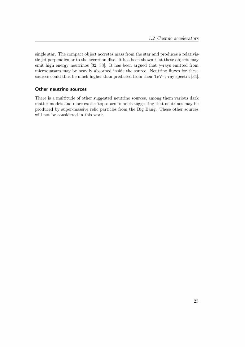
As particle cascades consist of many particles with each of them having a rathershort path length, their signature in Cherenkov light is different from that of muons:the Cherenkov cones of all charged particles within the shower overlap and lead toan effective angular light distribution that still peaks at 42 but is much broaderthan for muons. See figure 2.5 for an example. In addition, as the total length ofshowers is considerably shorter than that of muons, they will appear as point-likebursts of light in the detector, at least in first approximation.
Looking more closely, the total photon yield of a cascade and its mean length areproportional to its total energy E or to logE, respectively. The energy dependenceallows “calorimetric” energy measurements, which can help to determine a cascade’senergy. Details on these parameterisations will be shown later in section 4.6.6.
The signature of hadronic cascades in the detector is very similar to that of elec-tromagnetic ones. In first approximation, when applying simple corrections [39],
30
2.1 Detection mechanism
−1.0 −0.5 0.0 0.5 1.0
cos(α)
104
105
106
107
108
a.u.∝
num
ber
ofph
oton
s
Figure 2.5 Angular profile of an electromagnetic cascade simulated withGeant4.
they can be treated like electromagnetic cascades, especially when parametric sim-ulations are used that only simulate the shower according to its longitudinal andangular profiles.
2.1.5 Light propagation
As the position of measured photons and their arrival times are the only handles aneutrino telescope has on a muon track or shower, it becomes necessary to under-stand the influence of the surrounding medium on the Cherenkov light. Two effectsneed to be considered: absorption of light and scattering of light.
Absorption
Light absorption is characterised by the wavelength-dependent absorption length λa.It corresponds to the total track length at which the survival probability of photonshas dropped to e−1. Deep-sea water has its maximal transparency at about 470 nm.At this wavelength, measurements yield typical values of λa ≈ 60 m [40].
Low absorption lengths necessitate a certain density of the detector instrumenta-tion, as particles passing through sparsely instrumented detectors can simply be lost
31

2 Neutrino telescopes
due to the fact that all their Cherenkov light is absorbed before it even reaches thedetector.
Scattering
Scattered photons are one of the challenges in muon track reconstruction, as they willnot be on the Cherenkov cone and thus do not point back to their emitting particle.The scattering properties of water are commonly described by a scattering length λs
and a scattering angle distribution β(θ). For deep-sea water, these properties havebeen measured and parameterised. At a wavelength of about 470 nm, the scatteringlength is λs ≈ 50 m.3 The scattering angle distribution (or phase function) can bedescribed by a mixture of Rayleigh scattering and scattering on larger particles (Miescattering). For details on the measured properties for the ANTARES site refer tosection 2.2.3.
Speed of light in water/ice
As the arrival times of photons in the detector are crucial in reconstructing tracks,the speed of light in the respective medium needs to be known. The relevant speedis the light’s group velocity, which is related to the medium’s refractive index n by
vg =c
n+ λ
c
n2
dndλ. (2.6)
Sometimes, a group refractive index ng is defined, so that vg = cng
. Substitutingin (2.6) yields
ng =n
1 + λn
dndλ
. (2.7)
Refractive indices in sea water have to be measured and depend on temperature,salinity and water pressure at a certain point. At 470 nm, typical values are n ≈ 1.35and ng ≈ 1.42 (see [41]).
2.1.6 Light detection
Light detection in neutrino telescopes is typically done using a number of opticalmodules (OMs) consisting of photomultiplier tubes (PMTs) (and possibly readoutelectronics) in a spherical glass housing. The glass sphere protects the PMT frompressure and other environmental influences like salt water, while allowing Cherenkovlight to get to the PMT’s photocathode, where photons are subsequently convertedinto electrons. After an amplification stage, detected photons lead to an electrical
3This scattering length should not be confused with “effective” scattering lengths whereaveraging over scattering angles is included.
32

2.1 Detection mechanism
charge pulse which is read out using dedicated electronics. Detected photons arethus converted into a time and charge signature which is called a hit.
OMs are located on horizontal structures commonly called strings. They typicallyconsist of a cable for mechanical support and data transport which has a numberof OMs fixed to it. Depending on the level of expected optical background hits fora certain medium (see section 2.1.9), OMs are grouped in pairs, triples or othermultiples on so-called floors or storeys. By looking for coincident hits within thesenearby OMs, high background rates can be very well suppressed. This is especiallytrue for all detectors located in sea water, as Cherenkov light from electrons producedby decays of 40K lead to significant background rates.4 For detectors in ice, a singleOM per floor is sufficient, as there is no considerable background from radioactivedecays.
More detailed information on the OM designs and readout schemes used by exist-ing and planned telescopes can be found in sections 2.2 and 2.3.2.
2.1.7 Triggering
The readout of thousands of optical modules creates a huge amount of data thathas to be filtered before it can be written to permanent storage for analysis. Forthis reason, trigger algorithms are applied. Such algorithms either operate on thecontinuous data stream arriving from the detector on shore or are implemented inthe off-shore hardware. A trigger algorithm has to fulfil two requirements: it hasto be able to split the data stream into discrete events and it has to filter all databetween events that are not likely to contain any useful information.
There are a multitude of algorithms for triggering data. A simple, yet powerfulalgorithm, which looks for coincident clusters of hits in nearby floors will be describedin section 4.10.4.
2.1.8 Muon track reconstruction
The information available for reconstruction of a muon track is a triggered eventcontaining a set of hits. Each hit consists of a position in space (i.e. the positionof the OM that recorded the hit), a timestamp and a pulse amplitude, commonlymeasured in multiples of the single photoelectron level.
Using information like the fixed Cherenkov angle and the speed of muons andlight in water, the task of any reconstruction algorithm is to find a track that fitsthe given hit distribution.
There are several classes of track reconstruction algorithms:
4Another detector design possibility is to use more than a single PMT per OM be ableto reduce background hits by using coincidences. Such a design will be presented insection 2.3.2.
33
2 Neutrino telescopes
Maximum likelihood fits Algorithms of the class use a probability density function(PDF) that, according to a given track assumption, assigns a likelihood valueto each recorded hit. Calculating the product of all likelihood values yields anoverall likelihood for a certain track assumption.5 The algorithm then variesthe track parameters in order to find the highest possible likelihood value. Itfinally returns the track with the best parameters as the reconstructed track.
The most important part in a PDF is the difference between the theoreticalhit time calculated from the track assumption and the recorded hit time. Butother data like hit amplitudes and OM directions can also be used to furtherimprove the quality of the reconstructed tracks.
χ2 fits These algorithms work similar to maximum likelihood methods in that theyminimise a function that depends on a certain track assumption. In this casethe function is a quadratic sum over time differences between recorded andhypothetical hit times, with each time difference divided by its uncertainty.
χ2 =∑i
(trec. − thypoth.)2
σ2i
(2.8)
A minimisation algorithm then finds a minimal value of χ2 by varying thetrack parameters. The track with these parameters is returned and used asthe fit result.
geometrical fits/pre-fits These algorithms are usually used for pre-fits, with theirresults being used as a starting point for the likelihood or χ2 minimisationroutines. Most geometrical fits simplify the procedure by, for example, assum-ing that a track responsible for a hit goes exactly through the OM in question.This allows for a fast first-guess track estimate, which is usually not very goodbut better than a purely arbitrary starting point.
2.1.9 Background
No measurement can be free of background, which is especially true for neutrinotelescopes. The rate of hits that are not due to cosmic neutrinos is much larger thanthe number of hits produced from the signal events.
Background light can be due to various sources. The most important of thesesources will be described in this section, together with possible measures to reducetheir contribution.
5For numerical reasons, most algorithms do not calculate the product of all likelihoodvalues Pi but rather the sum of logPi. Hence, these algorithms are sometimes calledlog-likelihood methods.
34

2.1 Detection mechanism
Optical noise
An overall optical noise rate is the main background source for unfiltered data insea-water-based detectors. This noise is due to two sources:
40K decays The salt contained in sea-water includes a small amount of the radioac-tive isotope Potassium-40 (40K), which decays through β-decay with a branch-ing ratio of 89.3% (40K → 40Ca + νe + e−). The resulting electrons have anenergy of about 1 MeV, which is sufficient to produce Cherenkov light. A sec-ond decay channel with a branching ratio of 10.5% is the decay to 40Ar, eitherby electron-capture or by positron emission. The resulting 40Ar nucleus is inan excited state and can thus emit a photon with an energy of about 1.5 MeV,which in turn can produce electrons via compton-scattering. These electronscan also possibly create Cherenkov light if their energy is high enough. Thesedecays add up to a total rate of about 100 Hz per cm2 of photocathode area.
Bioluminescence As the deep sea is by no means a dead environment, it containsa large number of life forms, ranging from microscopic life-forms to largeranimals including fish. Several of these organisms emit light in a broad rangeof wavelengths. This light is seen in the detector’s PMTs as two differentcontributions. One is a slowly-changing baseline rate that causes noise hitsthat just overlay the 40K noise. On top of this, bursts of noise with durationsof up to a few seconds can be seen. The ANTARES collaboration measuresa baseline noise rate in the range of about 60 to 120 kHz with rates of over aMHz during bursts.
Bioluminescence is subject to a noticeable seasonal variation, depending on seacurrents and the vertical movement of nutrient-rich water from warmer layersdown to the depths of a detector [42]. During spring, baseline rates of up toseveral MHz have been measured by ANTARES. However, as these rates havenot been measured each year during the operation of ANTARES, seasonalvariations do not seem to be the only factor influencing the bioluminescencerate.
Optical noise can affect the reconstruction performance of neutrino telescopes, asthe chance of a series of noise hits accidentally looking like a muon event rises withthe noise rate per PMT. This is especially true for muons with energies below 1 TeV,where only a few photons are seen. In addition to such fake events, an excessiveamount of noise hits can mask hits from a real event.
One way to suppress noise hits is to look for coincidences in neighbouring PMTs,as already described in section 2.1.6. The probability for random coincidences by40K or bioluminescence hits is low. Another possibility is to only use hits above acertain amplitude threshold: photons from 40K decays generally have amplitudes
35

2 Neutrino telescopes
corresponding to a single photoelectron, whereas signal hit amplitudes can havehigher amplitudes, at least at higher muon energies. This basically corresponds toa coincidence within a single PMT. The actual probability for a noise coincidenceleading to a hit with higher amplitude depends on the length of the integration timewindow defined by the readout electronics.
Atmospheric muons
Cosmic rays reaching earth’s atmosphere with enough energy will produce extensiveair showers. Due to their hadronic nature, these cascades will contain a significantnumber of muons, many of them reaching the detector from above. The flux ofthese muons is significantly higher than the expected flux of muons due to neutrinointeractions.
As a an air shower usually produces more than one muon, most of these muonsarrive at the detectors in bundles. This background type is the main reason to buildneutrino detectors at deep sea sites, as the sea water above the detector acts as ashield against these muons. But, even at large depths, atmospheric muons are themost common events seen in the detector.
Therefore, neutrino telescopes predominantly look at up-going muons, thus usingthe whole planet as a muon shield. This requires a robust track reconstructionalgorithm which minimises the fraction of mis-reconstructed tracks. Bundles ofmuons or even two coincident muons from separate air showers can lead to signaturesin the detector that closely resemble these of up-going muon tracks.
Looking downwards will only work up to an energy of about 1 PeV, as abovethis energy, the earth starts to become opaque for neutrinos. See figure 2.6 foran overview of the neutrino interaction lengths vs. energy compared to the earthdiameter. Simulations for the ANTARES detector [45] show, however, that theatmospheric background rate is low enough at these energies to allow reconstructionof such high-energetic tracks even if they are only seen from above the horizon.
Atmospheric neutrinos
Hadronic air showers do not only produce muons. Decays of charged pions and kaonsalso yield a large flux of high-energetic neutrinos, which will be visible to a neutrinodetector on top of the flux of cosmic neutrinos signal. These atmospheric neutri-nos present an irreducible background for the measurement of any cosmic neutrino.However, as can be seen from figure 2.7, the energy spectrum of atmospheric neutri-nos is much softer than the signal spectrum expected from cosmic sources. In thatway, signal events will manifest as an excess of events measured at higher energies.For point-source searches, the expected neutrino direction is already known, so a
36

2.1 Detection mechanism
101 102 103 104 105 106 107 108 109 1010 1011 1012
neutrino energy Eν [GeV]
102
103
104
105
106
107
108
109
inte
ract
ion
leng
thL
int
[km
w.e
.]
earth diameterν: total interaction lengthν: CC interaction lengthν: NC interaction lengthν: total interaction lengthν: CC interaction lengthν: NC interaction length
Figure 2.6 Interaction lengths for (anti-)neutrino-nucleon interactions in kmwater equivalent. Data taken from [43]. The earth diameter has been calculatedusing the earth density profile cited in [44].
large amount of background events can be eliminated by simply requiring events tobe contained in a pre-defined space angle around the source direction.
In addition to the conventional neutrino flux due to pions and kaons, there is asecondary flux component due to decay of charm particles called the prompt flux.Whereas the different models for the conventional flux are more or less in agreementwith each other, this is not true for the prompt flux models. Note that, beginningfrom approximately 100 TeV, the prompt flux component starts to dominate. As thisis the energy region where diffuse neutrino flux searches are focused, a calculateddetector sensitivity will depend on the choice of flux model. This work uses thebartol model [46] for the conventional flux and the Naumov RQPM model [47] forthe prompt flux. This particular prompt flux model yields rather high fluxes and isthus conservative.
37

2 Neutrino telescopes
101 102 103 104 105 106 107
neutrino energy Eν [GeV]
10−25
10−23
10−21
10−19
10−17
10−15
10−13
10−11
10−9
10−7
10−5
flux
[GeV−
1cm−
2s−
1sr−
1]
“source” flux (5 · 10−8(E
GeV
)−2)
conventional only (ν)conventional & prompt (ν)
Figure 2.7 Atmospheric neutrino spectrum calculated using the“bartol”modelwith and without a prompt contribution according to the “Naumov RQPM”model. The anti-neutrino spectrum looks similar and is thus not shown forclarity. An E−2 “source” spectrum is included for comparison.
2.2 Existing neutrino telescopes
This section will give an overview of the currently existing and operational neutrinotelescopes. However, before introducing the currently running neutrino telescopes,the DUMAND project [48] has to be mentioned. It was the first deep-sea neutrinotelescope project, starting its planning phase around 1976. The detector location wasin the Pacific Ocean near Hawaii’s Big Island. Although the project’s funding waseventually cancelled in 1995 due to technical difficulties with their deployed hardwareand the detector was never fully built, DUMAND did a lot of fundamental work forthe neutrino astronomy community.
2.2.1 Baikal
The neutrino telescope in Lake Baikal [49] started with 36 OMs on three detectorstrings which were deployed in 1993. Deployment and detector maintenance is gen-erally done in winter, when the lake freezes over. This allows cost-effective access tothe detector with winterproof vehicles. The second advantage of using Lake Baikal
38

2.2 Existing neutrino telescopes
Figure 2.8 The Baikal neutrino telescope “NT200+” as of 2008 with its com-pact centre array (“NT200”) several extra peripheral strings. Taken from [49].
as detector site is the low concentration of 40K in its water. It is a fresh water lakeas there are several rivers draining into it and one river coming out of the lake. Thelower optical noise is however outweighed by the rather short light absorption length(< 20 m) when compared to deep-sea sites. Additionally, the relatively low depth ofthe detector site of only about one km leads to a high flux of atmospheric muons.
Nevertheless, the Baikal experiment was the first deep-water neutrino telescope todetect several neutrinos. It has been continuously extended with additional strings.Its current iteration NT-200+ is shown in figure 2.8.
2.2.2 IceCube
The IceCube detector [50], currently under construction at the south pole, is the firstneutrino detector with a volume approaching 1 km3. At the time of this writing, morethan half of the detector is completed and data-taking is well underway. Sharing itsSouth Pole site, IceCube’s predecessor AMANDA pioneered in-ice neutrino detectionand is integrated with the IceCube data acquisition system. However, AMANDAhas recently been turned off, leaving IceCube as the only neutrino telescope in theSouthern hemisphere.
39
2 Neutrino telescopes
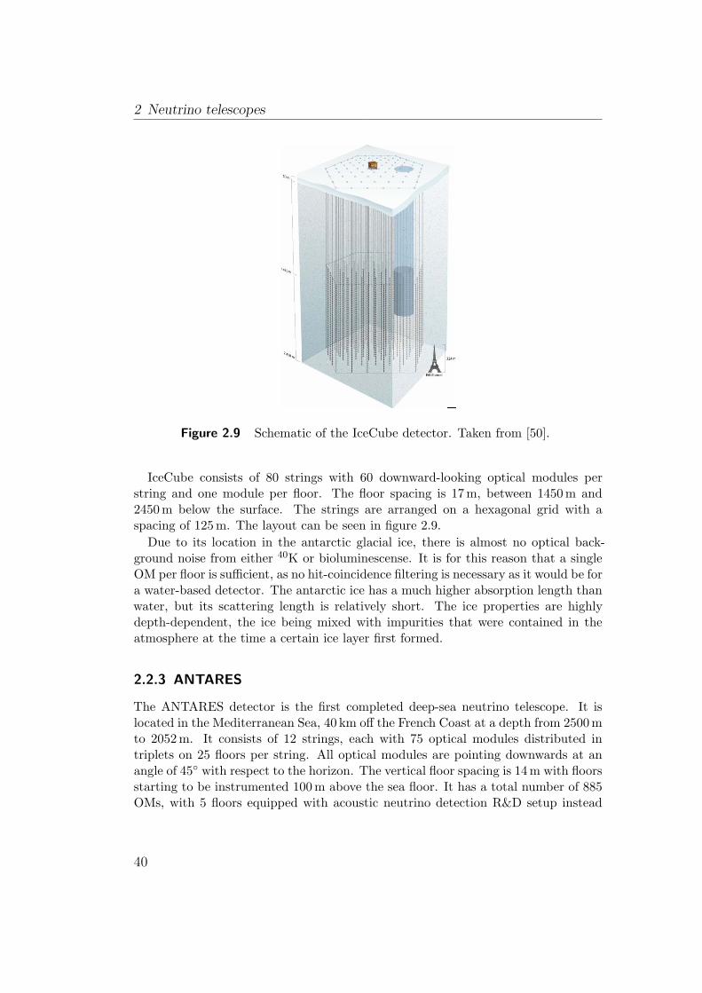
Figure 2.9 Schematic of the IceCube detector. Taken from [50].
IceCube consists of 80 strings with 60 downward-looking optical modules perstring and one module per floor. The floor spacing is 17 m, between 1450 m and2450 m below the surface. The strings are arranged on a hexagonal grid with aspacing of 125 m. The layout can be seen in figure 2.9.
Due to its location in the antarctic glacial ice, there is almost no optical back-ground noise from either 40K or bioluminescense. It is for this reason that a singleOM per floor is sufficient, as no hit-coincidence filtering is necessary as it would be fora water-based detector. The antarctic ice has a much higher absorption length thanwater, but its scattering length is relatively short. The ice properties are highlydepth-dependent, the ice being mixed with impurities that were contained in theatmosphere at the time a certain ice layer first formed.
2.2.3 ANTARES
The ANTARES detector is the first completed deep-sea neutrino telescope. It islocated in the Mediterranean Sea, 40 km off the French Coast at a depth from 2500 mto 2052 m. It consists of 12 strings, each with 75 optical modules distributed intriplets on 25 floors per string. All optical modules are pointing downwards at anangle of 45 with respect to the horizon. The vertical floor spacing is 14 m with floorsstarting to be instrumented 100 m above the sea floor. It has a total number of 885OMs, with 5 floors equipped with acoustic neutrino detection R&D setup instead
40

2.2 Existing neutrino telescopes
Figure 2.10 Schematic overview of the ANTARES detector. OfficialANTARES plot.
of optical modules. See figure 2.10 for a schematic of the detector. The detectoris connected with a shore station using an electro-optical telecommunications cable,capable of transmitting multiple optical GBit feeds.
The ANTARES collaboration performed detailed site studies, leading to a fairunderstanding of the detector medium. It is these water properties that have beenused in all simulation studies for this work. Refer to section 4.5.1 for the actualmedium property values.
The ANTARES readout is performed by a application-specific readout chip, the“analogue ring sampler” (ARS) [51]. This chip reads out the integrated photomulti-plier signal once it rises above a certain configurable threshold. The default integra-tion time is 33 ns with a consecutive dead time of 250 ns. To compensate for this, thechip contains a second, similar channel with the same integration and dead times,which is used if the first channel is processing data. There is a short switching timefrom one ARS channel to the other of 7 ns. The default pulse integration thresholdis at a level of about 0.3 photoelectrons. The ANTARES readout is equipped with
41

2 Neutrino telescopes
an optional waveform pulse readout, which is currently only used for calibrationpurposes.
The detector’s trigger scheme uses an all-data-to-shore strategy, i.e. all hits abovethe integration threshold are sent to shore without any further filtering. The actualevent building and triggering is done in an on-shore computer cluster. This allowsfor a rather flexible trigger design, as no hardware changes are necessary in case animproved triggering algorithm becomes available.
2.3 The KM3NeT project
2.3.1 Overview
The KM3NeT project is a joint effort of the ANTARES collaboration and theother collaborations currently designing Mediterranean neutrino telescopes, namelyNEMO [52] and NESTOR [53, 54]. The project’s aim is to construct a detector witha volume larger than 1 km3 in the Mediterranean Sea to complement the IceCubeproject in the Southern hemisphere. At the time of this writing, the project is com-pleting its initial Design Study Phase, a “Conceptual Design Report” (CDR) hasbeen written [55] and a final “Technical Design Report” (TDR), describing optionsfor the final detector design, is in press.
This work is concerned with the development of a new simulation toolchain, inde-pendent of the original ANTARES tools, which have been used for a large fractionof the studies on KM3NeT. It is currently not clear which final design choices will bemade for KM3NeT, so the simulations are performed for several example detectorswhich were design possibilities at the time of this writing.
As the TDR was not in existence when the simulations for this work were started,the following design choices may not coincide with the choices finally made forKM3NeT. Thus, none of the results in this work were either endorsed by the KM3NeTConsortium nor do they represent any official result.
2.3.2 Design possibilities
From a technical point of view, there are three competing overall detector designchoices that are possible for KM3NeT, re-using part of the knowledge gained fromthe respective predecessor projects.
The “string” design
The “string” design used in this work shares most of the detector properties withthe original ANTARES detector. To achieve a larger detector size at manageablecost, the string and floor distances have to be increased with respect to ANTARES.
42

2.3 The KM3NeT project
Common floor distances are of the order of 30 m to 40 m, whereas string distancesare increased to be larger than 100 m. As the hit coincidence condition is based onthe OM distances on a floor, it does not need to be changed from its ANTARESvalues. In fact, the whole ANTARES readout simulation scheme can be used as-is,including the two-channel ARS chip.
The “tower” design
An alternative design is to fix the optical modules on large metal bars, a designchoice pioneered by the NEMO collaboration. In the design that will be used forthis work, three pairs of optical modules will be fixed on both ends and in the middleof each bar with a length of 8 m. As in this design each vertical detection unit looksmore like a tower of bars instead of a string of OMs, the name “tower” design will beadopted for it from now on. Like the “string” design, the ANTARES concept witha single photomultiplier per OM is used.
Building tower-like detectors with only OM pairs instead of triplets decreases thenumber of detected hit coincidences for each pair. However, it has a non-negligibleadvantage at high tower distances, as the three pairs of optical modules on each barare indistinguishable from three separate closely-spaced strings if shadowing effectsare not taken into account. Thus, at low muon energies, where the track lengthsare short and a single line may not be sufficient to fully reconstruct a track, thetower design provides a gain in detection efficiency while at the same time keepingtechnical deployment problems with closely spaced strings at a minimum. In thiswork, the OMs used for the tower design are the same as for the string design. Thisincludes the PMT type and readout choices.
The “multiPMT” design
The third design tries to change the “single-PMT-per-OM” paradigm by using anumber of smaller PMTs per OM instead. The specific “multiPMT” design [56]used in this work has 31 PMTs with an effective diameter of 76 mm fitted into anOM sphere with a diameter of 432 mm, the same size currently used for ANTARES.In this design, the use of multiple OMs per floor becomes unnecessary, so it onlyconsists of single OMs per floor, similar to IceCube.
Due to its simplicity with only one OM per floor, strings for the multiPMT designare cheaper to build, which allows to deploy more of them. This compensates for thelower total photocathode area per string in these designs. Additionally, the numberof under-water connectors is minimised in this design, eliminating a potential sourceof failure during the detector’s lifetime. Having such a large number of small PMTs ina single OM also allows the detector to have a finer-grained single photon resolution.Finally, it may even be possible to reconstruct a Cherenkov light front’s direction
43

2 Neutrino telescopes
from the data of just a single OM. The readout scheme used for such multiPMTOMs is a time-over-threshold approach, which will be described in more detail insection 4.10.3.
2.3.3 Detector sites
As each of the predecessor projects of KM3NeT performed site studies in differentplaces around the Mediterranean Sea, three different site possibilities emerged: offthe French coast near Toulon (depth 2475 m), at the Capo Passero site near Catania(depth 3500 m) and near Pylos in the East Ionian Sea (depth between 3750 m and5200 m). These sites have very different maximum depths, influencing the atmo-spheric muon background rate. The studies for this work have all been done for adepth of 3500 m.
44

Part II
Methodology
45


3 Software simulation and reconstruction tools
Computer Science is nomore about computers thanastronomy is abouttelescopes.
(Edsger W. Dijkstra)
Neutrino detectors would not be possible without computer-based simulation andreconstruction tools. As the sheer amount of data collected by any telescope cannotpossibly be handled by hand, sophisticated filtering, triggering and reconstructionalgorithms have to be implemented in software to reduce and convert the recordedraw data to datasets suitable for a physics analysis. In addition, Monte Carlo sim-ulation tools are necessary for understanding the effect of detector systematics andto be finally able to interpret the data recorded by a detector. Especially during thedesign phase of KM3NeT, where no real working detector does exist, Monte Carlosimulations are the only way to properly compare different possible design optionsand to evaluate their physics potential.
This chapter describes the Monte Carlo simulation tools used to produce all datapresented in this work. First, the legacy software toolchain from the ANTARESproject, which is currently in use for most KM3NeT studies, is presented. The re-mainder of this chapter introduces the concept of a software framework and presentsIceTray, a framework developed by IceCube. During the course of this work, IceTraywas adapted for KM3NeT and ANTARES. This chapter covers all direct ports ofANTARES algorithms to IceTray and the most important modules that could be re-used from IceCube without major changes. Note that some of the simulation-centricIceCube modules are covered in more detail in chapter 4.
3.1 Legacy software tools from ANTARES
The software that has been in use by ANTARES for the last decade consists of asuite of independent software tools [57] loosely linked by an ASCII-based text fileformat [58, 59]. Data processed by one tool is written to disk in a common fileformat that can then be read by the next tool in the processing chain. The relevanttools for simulation and reconstruction of muon neutrinos are:
gendet, a tool for detector layout generation [60, 61]. It takes a set of sea floor co-ordinates and a string template description. The template contains the floor
47

3 Software simulation and reconstruction tools
positions on the string and a floor description specifying the OM positions onthe floor and their orientations. From these data, it generates a detector filecontaining the position and orientation of each OM in the detector. Optionally,a sea current which distorts the strings from their vertical orientations can besimulated. The gendet tool does not directly support non-string detector lay-outs (i.e. “tower”-type detectors). Such layouts can, however, be generated byconfiguring bar-like floors on each string. In this way, the final OM positionswill be compatible with the “tower”-layout as long as no sea current is simu-lated. Because all further simulation and reconstruction steps only work onthe OM level and do not use the string cable positions, this approximation issufficient for KM3NeT studies.
genhen, a neutrino event generator [62–67]. Neutrinos are generated with a user-defined energy spectrum and propagated to a cylindrical volume around thedetector called the generation volume. Inside this volume, each neutrino isforced to interact and the actual interaction probability is recorded. All muonsresulting from these interactions are then propagated, taking into accounttheir energy losses in rock and water. The generation volume is chosen asa cylinder encompassing all strings (the instrumented volume) and extendedby the maximum muon length at the maximum neutrino energy used for thesimulation, limited by the sea surface.
In case one of these muons reaches a second, smaller cylindrical volume aroundthe detector, the whole reaction including neutrino and muon is recorded as anevent. The size of this sensitive volume has to be chosen so that muons that donot intersect it will only have an extremely small probability of being seen bythe detector. The standard ANTARES approach is to extend the instrumentedvolume by three Cherenkov light absorption lengths. The sensitive volume issometimes called the can in ANTARES jargon.
The genhen generator simulates neutrino interactions with LEPTO [68]/CTEQ6and RSQ [69], for deep inelastic scattering and for resonant/quasi-elasticevents, respectively. Muons are transported to the can using either the MU-SIC [70], MUM [71, 72] or PropMu [73] algorithm.
The implementation of genhen is generic and can be used for KM3NeT detec-tors with only minor technical changes.
km3, a muon and Cherenkov light propagation implementation [74, 75]. The km3package performs muon tracking within the sensitive volume, takes care ofgenerating Cherenkov photons and of propagating them to the optical mod-ules. Muon tracking is performed by the MUSIC library [70], which provideskm3 with information about the energy loss profile along the particle’s track.Electromagnetic showers are then placed along the track according to this
48

3.1 Legacy software tools from ANTARES
profile. In a second step, light from the “bare” muon and from each of theshowers is propagated to the detector’s OMs, taking into account scatteringand absorption of light in sea water.
As simulating each single photon would take far too much CPU time to befeasible for Monte Carlo mass productions, an alternative approach using pre-simulated photon tables is used: Photons are only simulated once using theGeant3 [76] based helper tool gen, which records the light output of a shortmuon segment (with a length of about 1 to 2 m) or of an electromagneticshower on concentric spheres. Several of these spheres are placed aroundthe emitters at different distances. All photons intersecting the spheres arerecorded. A second helper tool, hit, subsequently divides these spheres intoangular bins and converts the photon fields into tables containing hit prob-abilities. These probabilities include the OMs’ characteristics such as theirangular acceptance and their wavelength-dependent quantum efficiency. Thus,the photon tables produced by hit contain the full set of OM properties andhave to be re-calculated for each type of OM that is to be simulated.
The actual km3 program then takes care of calling the MUSIC library topropagate muons and of creating hits according to the pre-generated tablesfrom hit. The muon segments are combined into a whole muon track. Eachtime the energy loss is above a configurable limit (which is set to the ionisationloss), a secondary shower is placed at this position on the track. Hits oneach OM are sampled from the tabulated probability distributions for eachsegment and shower. Optionally a white noise background per OM can beadded, approximating the 40K and bioluminescence rate. All OM hits canadditionally be converted into readout pulses using a simplified PMT andelectronics simulation targeted at ANTARES OMs. See [74] for more detailson the actual implementation of the km3 suite of simulation tools.
geasim, a full tracking Monte Carlo code based on Geant3 [76]. This tool providesthe same functionality as km3, with the exception of light scattering. It doesnot use a table-based approach, but rather simulates each particle using thefull Geant3 engine. To be reasonably fast, light is only propagated in straightlines, which enables the code to speed up processing by a fair amount, as mostphotons can simply be rejected by simple geometric considerations: a photonwith a straight path that can never hit an OM can be rejected early in thecode. This is of course only true if light scattering is neglected. As geasim isstill quite slow when simulating very long muon tracks, it is mainly used forthe hadronic part of neutrino interactions near the vertex. It can be combinedwith km3 by using a special mode where only the hadronic component issimulated by geasim, whereas the muon is simulated by km3.
49

3 Software simulation and reconstruction tools
reco, a track reconstruction tool containing a number of reconstruction algorithms,including the current standard ANTARES reconstruction strategy [77]. Thisstrategy has been ported to the software framework described in the followingsections. It consists of a chain of likelihood-based fitting routines. A detaileddescription can be found in section 4.11.1.
As they were initially designed for use with ANTARES, several of these toolsrequired minor technical modifications to be usable for simulations of KM3NeTdetectors. This included changing of some hard-coded numbers and array sizes andthe implementation of dynamic OM types [78].
3.2 Software frameworks
A major physics experiment like the KM3NeT neutrino telescope requires an im-mense amount of hardware development effort. However, to make use of the tele-scope, software that allows running the experiment and, most importantly, to trans-form the raw data to high-level physics information is also needed. Such softwarecannot be written by a single person, but has to be created in a collaborative effort.
A software developer should not need to know every single line of code of a partic-ular program to be able to extend it. Most of the time, the task is to implement orchange a single algorithm only, without modifying the rest of the reconstruction soft-ware. It is thus necessary to write modular code with a predefined data flow from thevery beginning. Such program modularisation and the definition of a correspondingdata flow are the essential elements provided by a software framework [79].
3.2.1 The concept of a software framework
A possible definition of a software framework can be: a software framework is a setof rules, interfaces and services provided to a software developer, who can use it toperform a set of tasks.
In a modular framework, the user should only have to change a few lines in asteering file to modify an analysis chain. This is illustrated in figure 3.1: An existinganalysis is changed by adding a further module.
Frameworks should not be confused with class libraries. A class library, like aframework, provides a set of interfaces and services. It does not, however, enforcea particular program structure and leaves it to the individual programmer’s codeto specify the structure. A framework defines an overall program pattern, whichmakes it easy to extend: a developer implements algorithms, whereas the frameworkspecifies how their implementations interact.
Typically, frameworks enforce this overall design. At the same time, they mustavoid being too restrictive, to allow for the necessary freedom to developers and
50

3.2 Software frameworks
data/lereader
data/lewriter
muontrack
recon-structor
data/lereader
muontrack
recon-structor
event lter
data/lewriter
event lter
Figure 3.1 Simplified reconstruction chains consisting of modules, with dataflowing from one module to the next one. The first chain consists of threemodules. In a framework, tasks like adding modules can easily be performed.In this example, an event filter is inserted at a particular point in the first chain.The resulting reconstruction chain is shown below the dashed line.
end-users.1 This is achieved by using a modular approach, where each subsystemcan be modified, added or replaced without altering the others.
Using a framework saves the physicist a lot of time in learning how to use aparticular software package every time s/he wants to perform a new task on a set ofdata. All algorithms are implemented in modules having the exact same structure.This makes the code easier to read and understand. The software user can thus startto work on physics problems with a significantly shorter learning period.
A modular structure also leads to more flexibility. Systematic analyses can beperformed more easily, as the high-level program flow and all fine-grained moduleparameters are always visible to and changeable by the framework user.
Finally, frameworks facilitate the collaboration between different groups doingsoftware development. As all modules have the same format, they can be easilyexchanged. This is especially advantageous when doing cross-checks and also helpsimplementing an overall quality control scheme: Code that is broken down into smallindependent units can be more easily reviewed by others than a single monolithicprogram.
1In an object-oriented language like C++, a particular design can be enforced by using theconcept of encapsulation: the inner workings of a class should always be hidden fromother classes. Another important concept, called polymorphism, allows the framework tobe extended in a well-defined way: only a small set of abstract classes is exposed fromthe framework. These classes are then overwritten when implementing an algorithm.
51

3 Software simulation and reconstruction tools
3.2.2 The IceTray framework
IceTray [80], the software framework developed and used by the IceCube collabo-ration [50], provides all the features mentioned in the previous section. Developerscreate modules, which can be dynamically linked into the framework. They containthe actual algorithms responsible for event reconstruction or simulation. Data ispassed from module to module in data containers called frames. Each frame typ-ically describes a single event. A frame consists of a list of name-object tuples.Except for an I/O method, there are no requirements imposed on the objects storedin a frame. This design decision makes the framework easily extendable.
The framework already provides modules for reading and writing of data. Thesemodules can be used at any time in the reconstruction chain, so that data canbe written out at any stage. Though IceTray uses its own data format based onroutines from the boost.org libraries [81], it is possible to write reader modules forany other data format. This has been demonstrated by providing a reader modulefor standard ANTARES ROOT-files as produced by the current ANTARES onlinedata acquisition (DAQ) system [82]. It should be noted that, in principle, theframework does not require to write out any intermediate data, as data input andoutput is done in dedicated modules. A full Monte Carlo simulation of events andtheir reconstruction can thus be done in IceTray without ever writing temporaryfiles to disk. Of course it is still possible to produce intermediate data files.
The order of modules can be defined when initialising the framework. This istypically done using the Python scripting language [83]. In addition to Python,compiled C++ code can be used to control IceTray module chains.
IceTray comes with dataclasses, containing class definitions usable for storing posi-tions, directions, particle tracks, optical module (OM) properties and all other datanecessary during event reconstruction and simulation. These classes are usable forKM3NeT with only minor modifications. These modifications are mostly necessarybecause the developers of IceTray assumed that all OMs would look either verticallydownwards or upwards. This is true for IceCube, but assumedly not for KM3NeT.
A few simple non-physics modules, such as a generic event selector template anda ROOT tree writer can also be re-used for KM3NeT. None of these helper modulescontain any physics-relevant code.
3.2.3 Simulation and analysis tools for KM3NeT within the IceTrayframework - “SeaTray”
To enable IceTray to work with the data that is currently available, a considerablefraction of the code from the ANTARES experiment, was modularised during thecourse of this work. Most of these modules can also be used for KM3NeT withoutmajor changes, although some modules are targeted specifically to ANTARES and
52
3.2 Software frameworks
were only implemented to show the feasibility of using IceTray for water-based de-tectors. They are, however currently in active use for other projects [84–86]. Thework done on the framework and the implementation of all modules has ultimatelyled to the adoption of IceTray as the official software framework for both ANTARESand KM3NeT.
In addition to straight ports from ANTARES, new modules have been imple-mented which are targeted specifically to the simulation of different proposed KM3-NeT detector designs. The whole distribution of the framework core together withall KM3NeT/ANTARES modules is referred to as“SeaTray”, whereas the frameworkitself is still called IceTray.2
This section will give an overview of all modules that could be re-used fromIceCube and of all modules that were ported or re-written from existing ANTAREScode. It will not cover modules that were developed specifically for this work, asthese are presented in full detail in chapter 4.
Ports and rewrites from the ANTARES toolchain
As part of this work, several modules have been ported to IceTray from their originalimplementation in the ANTARES toolchain. This includes a DAQ file reader moduletogether with database access services necessary for reading real detector data files.These modules were implemented to demonstrate the applicability of IceTray toneutrino detectors beside IceCube and can be disregarded for this work.
In addition to that, a module that permits reading the standard ANTARES MonteCarlo file format was developed. It enables the user to read data produced by thestandard ANTARES Monte Carlo packages described in section 3.1. Thus, all of thecurrently existing Monte Carlo tools can be used with IceTray.
Environmental background hits (from 40K decays and bioluminescence) at the de-tector site are generated with a fixed user-configurable rate per OM. Alternatively,the noise rate per OM can be taken from real data. A module providing this function-ality was re-written to be compatible with the previous ANTARES implementation.
To be able to compare Monte Carlo events to real data, full simulations of theOM’s digitisation electronics are needed. The ANTARES code for these simula-tions has been encapsulated into modules: The OM simulator uses a parameterisedapproach to simulate the transit time spread and the amplitude smearing of thePMTs. The simulation of the PMT signal digitisation is fully compatible with theone currently in use by ANTARES. A second simulation for a time-over-thresholdreadout scheme was developed from scratch. Both simulations will be described insections 4.10.2 and 4.10.3 respectively.
2For reasons of pronounciability, it was decided to use the name “SeaTray”, despite the factthat “KM3Tray” would be a more correct name, as the “Ice” in IceTray does not refer tothe detector’s medium but rather to its name.
53

3 Software simulation and reconstruction tools
When using Monte Carlo data, it is necessary to simulate different detector triggerconditions. For this purpose, the complete ANTARES core trigger code was encap-sulated into an IceTray module. This module receives the current event data andconverts it into the format used internally by the ANTARES trigger. The originaltrigger code can thus be used unchanged, which allows for easy maintenance andupdates in case new trigger algorithms are added to the ANTARES DAQ. Aftercalling the trigger routines, the module converts all results back to a data formatcompatible with IceTray and passes all information to the next module.
The ANTARES standard reconstruction strategy has also been ported to IceTrayfrom its reco implementation mentioned in section 3.1. A full description can befound in section 4.11.1. In addition, two more reconstruction algorithms were portedto IceTray, namely the χ2-based BBFit algorithm [87] and the scanfit algorithm [88].Porting of the latter was not done as part of this work but rather during anotherPhD thesis [85]. As these algorithms are not suited for KM3NeT in their currentstate, they have not been used for the studies presented later on.
Modules provided by the IceCube collaboration
Events can not only be produced by the ANTARES Monte Carlo packages, butalso by using other event generators like ANIS [36] (neutrino events) and COR-SIKA [89] (atmospheric muons). Both of them are also in use for IceCube andalready exist as IceTray modules. Once events have been generated, the resultingparticles need to be tracked through the detector volume and their Cherenkov lightneeds to be simulated. Muons, being the main detection channel of neutrino tele-scopes, can either be tracked by the MMC [90] package which was modularised byIceCube or by a custom tracking code based on Geant4 [91] developed specificallyfor KM3NeT in the context of this work (see section 4.5).
54

4 A new KM3NeT simulation and reconstructionchain
++++++++++[>+++++++>++++++++++>+++>+<<<<-]>++.>+.+++++++..+++.>++.<<+++++++++++++++.>.+++.------.--------.>+.>.
(example code)
This chapter presents a new simulation chain that was developed within the frameof this work. It consists of a combination of tools that have already been in use bythe IceCube collaboration and new tools developed specifically for KM3NeT.
4.1 Overview and Incentive
The tools that have been used for most of the simulation work for KM3NeT aretaken over from the ANTARES pilot project and have been successfully in use therefor over a decade.
This fact, however, also leads to problems: until now, no independent toolchainwas in existence, which would have been necessary to perform cross-checks of thecurrent tools. Additionally, all ANTARES simulation code is written in FORTRANin a highly non-modular style and is thus hard to maintain. This is especially truefor modern operating systems where FORTRAN compilers do not have as high animportance as they did a few years ago.
It is thus desirable to develop an alternative simulation chain based on moremodern programming languages. For this work, such a chain has been implementedon top of the IceTray framework.
4.2 Simulation of neutrino interactions using ANIS
The first step in a simulation chain for a neutrino telescope has to be the generationof neutrino events according to a spectrum defined by the user. Here, an event isdefined as the combination of the neutrino’s energy, its direction, the reaction vertex,the reaction’s final state and an event weight. The weight is necessary as typically, allneutrinos are forced to interact within a certain volume around the detector. Their
55

4 A new KM3NeT simulation and reconstruction chain
interaction probability and the initial energy spectrum are combined into a weightthat has to be applied to each reconstructed event to obtain a physical neutrinoevent rate.
An existing tool providing exactly these features is ANIS [36], originally developedfor AMANDA/IceCube. Therefore, a modularised version for IceTray is alreadyavailable. ANIS can be used to simulate neutrinos of all flavours, though only muonneutrinos will be covered in this document. It includes tabulated cross-sectionsfor neutrinos and anti-neutrinos and is able to simulate both CC and NC events.The νN structure functions are chosen according to CTEQ5 [92] (cf. figure 2.3).Generation of neutrino events starts at the surface of the Earth. From there, theyare propagated to the detector along straight lines, neglecting small angle neutrinoscattering. The density profile of the earth is chosen according to the PreliminaryEarth Model [93]. In case of an interaction on the way to the detector, an appropriateinteraction channel is chosen and the neutrino is either absorbed or regenerated.Once a neutrino reaches the pre-defined volume around the detector, it is forced tointeract within the volume and its interaction probability is stored. Additionally, thefinal state of the reaction is generated as a particle vector. As neutrino telescopescannot distinguish between different types of hadrons, no hadronisation is performed.All hadronic energy is written out as a single particle type reserved especially for thispurpose, whereas the leptonic part is fully stored as independent particles. In thecase of muon neutrinos this is either a muon for CC reactions or a muon neutrinofor NC reactions. For the purposes of event simulation the NC neutrinos can bediscarded, as they will not be seen as part of the event.
The most important input parameters to the ANIS simulation are the neutrinospectrum (specified as the spectral index γ of a power law spectrum E−γ), theneutrino energy range [Emin, Emax], the zenith range and the neutrino flavour. ANISalways simulates neutrinos and anti-neutrinos as well as NC and CC events in asingle run. Additionally, the interaction volume size around the detector and thedetector depth needs to be specified. The interaction volume is defined as a cylinder,anchored at the detector centre with its axis parallel to the neutrino direction. Itsradius and height can be chosen by the user. See figure 4.1 for an illustration.
Almost no modifications were necessary to use ANIS in its modularised form froKM3NeT. The hard-coded detector medium density and the fixed rock depth of3000 m which are used for IceCube simulations were made user-configurable. Thedetector medium density can now be changed from its default value for polar ice tothat of sea water. Apart from that, no changes were necessary to be able to use thecode for KM3NeT simulations.
56

4.2 Simulation of neutrino interactions using ANIS
x
detector
radius r
+height height
μν
y
z
Figure 4.1 The ANIS geometry. The cylinder shown is the final/detectionvolume defined by two heights (before and after the detector centre) and aradius. This radius defines the generation area. The cylinder is rotated to haveits axis in parallel with the neutrino direction. The actual detector volume isshown as a box around the coordinate origin. Taken from [36].
4.2.1 Event weights
ANIS stores event weights with its final events [93]. The most important weight isthe interaction probability in the final volume Pint, which is being calculated from thecross-section for every event. Together with the knowledge of the input spectrum’sspectral index γ and the simulation parameters described previously, an event ratefor an arbitrary spectrum
dΦ′(E)dE
(4.1)
can be calculated. The generation spectrum is defined to be
Φ(E) = (E/GeV)−γ[GeV−1cm−2sr−1s−1
]. (4.2)
Neutrinos are sampled uniformly across the generation area A and isotropicallyin Ω, so that the total rate of incoming neutrinos can be written as
Rincoming =∫ Emax
Emin
Φ(E)dE ·A · Ω, (4.3)
where A is the generation area and Ω is the integrated generation solid angle.
57

4 A new KM3NeT simulation and reconstruction chain
For a sample of Ngen generated events, the rate of interacting neutrinos due tothe flux Φ(E) is
Rint =1
Ngen
Ngen∑i=1
∫ Emax
Emin
Φ(E)dE ·A · Ω · Pint,i . (4.4)
Re-weighting event-wise to Φ′(E) yields
R′int =1
Ngen
Ngen∑i=1
Φ′(Ei)Φ(Ei)
∫ Emax
Emin
Φ(E)dE ·A · Ω · Pint,i (4.5)
=1
Ngen
Ngen∑i=1
Φ′(Ei)E−γi
∫ Emax
Emin
E−γdE ·A · Ω · Pint,i (4.6)
=1
Ngen
Ngen∑i=1
Φ′(Ei) · wi , (4.7)
with wi being defined as
wi :=1
E−γi
∫ Emax
Emin
E−γdE ·A · Ω · Pint,i . (4.8)
For convenience, this derived weight wi is stored with every event during thegeneration step. This weight is practical, as it can be used to weight events withoutknowing about simulation parameters such as the generated energy range, the energyspectrum, the zenith angle range and the generation volume radius.1
4.3 Simulation of atmospheric muons with CORSIKA
In addition to a neutrino flux, the atmospheric muon background has to be simu-lated. The muons’ lateral and energy distributions are generated using the COR-SIKA extensive air shower Monte Carlo tool [89] in a version originally modified forAMANDA [94]2.
CORSIKA simulates air showers induced by a cosmic ray flux of protons andnuclei. Muons produced in these showers are stored at the sea surface level. Theycan then be propagated to the detector as described in section 4.4.
1The weight wi was given the name “OneWeight” by the IceCube collaboration.2dCORSIKA is available from http://icecube.wisc.edu/~jkelley/simulation/dcorsika.html.
58
4.4 Propagation of muons to the detection volume
4.4 Propagation of muons to the detection volume
Muons produced near the detector (either by ANIS on the surface of the generationvolume or by CORSIKA at the sea level) need to be propagated to the actual detectorvolume. This is done using the MMC simulation code [90]3. The JAVA-based codehas already been wrapped as an IceTray module by IceCube, which makes it easyto use. MMC propagates muons (and optionally tauons) through matter whilesimulating their energy losses. For the simulation chain presented here, MMC isonly used to find the position of the muon on the surface of the sensitive volume ofthe detector and to calculate the muon’s energy at this point. The sensitive volumeis defined as an upright cylinder containing the instrumented detector, extended bythree light absorption lengths.4 As muons can propagate over long distances, it isimportant to calculate their energy losses with good accuracy. As this was one ofthe design goals of MMC, it was chosen as the primary muon propagator.
4.4.1 Modifications for KM3NeT
MMC allows to define a lower cut-off energy, which is set to the energy at whichCherenkov light ceases to be emitted. The refractive index used to calculate thisenergy was hard-coded and has been changed from its original value of nice = 1.31 tonwater = 1.35. Additionally, an already existing definition of the element compositionof water at the ANTARES site was bug-fixed (see table 4.1 for the actual composi-tion). Together with a new medium definition containing the KM3NeT detector sitedepths, these were the only changes necessary for adaptation to KM3NeT. Note thatthe bug concerning the element composition only affects a pre-defined “ANTARESwater” medium type and thus has no effects on simulations using other mediumtypes.
4.5 Muon propagation and Cherenkov light generation
Once a muon has reached the detector, it has to be propagated through its sensitivevolume. At the same time, secondary particles from the muon need to be trackedand all Cherenkov light needs to be propagated through the detector medium. Asimulation code based on Geant4 [91] was developed for this purpose. The codeperforms a full tracking simulation of every particle inside the sensitive volume.This includes the simulation of every single Cherenkov photon. This approach takesan immense amount of computing time, but it provides accurate event simulationsusable for cross-checks of parameterised simulations.
3MMC is available from http://dima.lbl.gov/~dima/work/MUONPR/.4This is the same definition as used in the ANTARES simulation tools, see section 3.1.
59

4 A new KM3NeT simulation and reconstruction chain
4.5.1 Detailed simulation
Geant4 provides algorithms for simulation of almost all of the“standard”physics pro-cesses needed for tracking of muons, electrons and other particles through a medium,among them all muon energy loss processes described in section 2.1.3. Hadronic pro-cesses, which can result from either nuclear interactions of the muon or from theprimary hadronic cascade, are simulated according to the QGSC model. In Geant4,a large set of hadronic models is made available to the users, each one tuned to differ-ent energy ranges and applications. The QGSC model is one of the hadronic modelsrecommended by the Geant4 authors for high-energy applications and is valid upto 100 TeV. Electromagnetic processes can be simulated with much higher energies,although care should be taken, as for example the LPM effect is not yet properlyimplemented in Geant4 for all processes. Geant4 can not only track high-energycascades and muons, it can also directly simulate Cherenkov photons and propagatethem through a medium.
Medium definition
To be able to track particles, all media surrounding the detector have to be definedin terms of their element composition and density. For the current application, thetwo important media are sea water and rock. Medium properties have been chosento be compatible to the ones used in the ANTARES simulation tools: sea wateris mainly composed of H2O with a salinity of 3.84% and a density of 1.039 g cm−3.The bedrock layer composition is chosen to be compatible with standard rock asdefined in [95]. This definition assumes a material with a density of 2.65 g cm−3. Asthe definition uses an average atomic weight (〈Z/A〉 = 0.5) which is not properlysupported by Geant4, the known chemical composition of Gran Sasso rock as definedfor example in [96] was used instead.5 As this step of the simulation is not meantto be used to propagate muons over long distances, this choice should not influencesimulation results.6 Note that only the chemical composition was changed from theoriginal standard rock definition, the density is chosen as defined originally. Seetable 4.1 for the exact chemical composition used for the simulation.
Simulation of optical photons needs a few more medium specifications like thewavelength dependent refractive indices, absorption lengths and scattering lengths.These specifications were chosen to be compatible with measurements from theANTARES site. To be able to compare results, all medium descriptions are takenfrom the geasim/km3 tools from the ANTARES software chain. Figure 4.2 showsall these water properties.
5The Geant4 authors specifically warn about using average atomic weights with their code.6Propagation of muons over long distances is done using MMC in the previous simulation
step. MMC includes a proper parametrisation of standard rock.
60

4.5 Muon propagation and Cherenkov light generation
medium element fraction of massANTARES sea water Hydrogen 10.74%
Oxygen 85.41%Chlorine 2.37%Sodium 1.32%Magnesium 0.15%
bedrock Oxygen 52%Calcium 27%Carbon 12%Magnesium 9%
Table 4.1 Composition of sea water at the ANTARES site and of standard rockas used in the Geant4-based muon propagation and Cherenkov light generationcode.
300 360 420 480 540 600
wavelength λ[nm]
1.34
1.36
1.38
1.40
1.42
1.44
1.46
refr
acti
vein
dexn
nphasengroup
300 360 420 480 540 600
wavelength λ[nm]
0
10
20
30
40
50
60
70
abso
rpti
onle
ngth
[m]
300 360 420 480 540 600
wavelength λ[nm]
10
20
30
40
50
60
70
80
90
scat
teri
ngle
ngth
[m]
Figure 4.2 Water properties of the ANTARES site used in the simulation. Theplots show, from left to right, the refractive index, the absorption length andthe scattering length as a function of wavelength. Taken from the km3 code [74].The group refractive index is calculated as defined in section 2.1.5.
61

4 A new KM3NeT simulation and reconstruction chain
0 20 40 60 80 100 120 140 160 180
scattering angle θ[]
10−3
10−2
10−1
100
101
102
103
104β
Mie
(θ)
Figure 4.3 Scattering angular distribution βMie(θ) for the“partic-0.0075”watermodel used for water at the ANTARES site.
For light scattering, a scattering angle distribution is needed in addition to thescattering length. The algorithm for calculation of scattering angles was portedfrom the original FORTRAN implementation in km3 and implemented as a Geant4process. This was possible due to the modular design of Geant4 which allows addingnew particles and processes as derived classes. There are multiple scattering modelsimplemented in the original ANTARES software. The model currently in use iscalled “partic-0.0075” and is implemented as a mixture of Rayleigh scattering andscattering on particles (Mie Scattering). For each scattering event, the type ofscattering is decided randomly so that the fraction of Rayleigh scattering events isη. All other scattering events will be Mie scatters, described by a scattering angledistribution (or phase function) βMie(θ). Figure 4.3 shows the angular distributions.The value used for η in the “partic-0.0075” model is 0.17. The Rayleigh scatteringangle distribution is described by the parameterisation given by [97] for sea water:
βRayleigh(θ) = 0.06225(1 + 0.853 cos2(θ)
)(4.9)
62

4.6 Fast cascade light generation and propagation
4.5.2 Speedup of the Cherenkov light tracking algorithm for unscatteredlight
Simulating each single particle generated by an incident muon is a rather time-consuming process. Depending on their energy, single events can take days to sim-ulate on modern CPUs. Even muons with low energies need processing times of atleast a few minutes. This is due to the huge number of photons being generatedby a single track. In the wavelength range relevant to water Cherenkov telescopes(between 300 nm and 600 nm), approximately 5·104 m−1 are generated by low muonsand their secondary particles. At higher energies, starting at about 1 TeV, this num-ber starts to grow, as the probability of producing larger electromagnetic showersalong the muon track increases. Considering muon track lengths of the order of 100meters or more, a simulation algorithm tracking each photon will always be ratherslow.
Most of these simulated photons, however, will never reach an optical module, asa neutrino detector is only sparsely instrumented. In a way, most of the processingtime is wasted on the simulation of photons that will never be seen. An easy solutionto this problem can be found if optical scattering of photons is neglected. In thiscase, the simulation code can decide if a photon will never reach an optical moduleby purely geometric calculations before even starting the tracking code. Wholesegments of a muon track can be skipped in the simulation, as unscattered lightfrom these segments would never reach any optical module. Note that, in a MonteCarlo tracking simulation, this is only possible when light scattering is neglected,because the code cannot know if a photon that would not reach an OM on its directpath could eventually reach it after one or more scatters.
The speedup provided by this solution is substantial, but neglecting scatteringcan distort results, especially for detector designs where the string distance is largerthan the scattering length.
4.6 Fast cascade light generation and propagation
As the source of most of the Cherenkov light are cascades (either induced by themuon or by the neutrino itself), a starting point for improvement of simulation timescan be to parameterise the light output of electromagnetic or hadronic cascades andoptionally include light scattering in this parameterisation.
4.6.1 Angular light distribution
Parameterisations of the angular light output of showers (which are assumed to bepoint-like for this argument) have been used in previous simulation codes [98, 99].These parameterisations make use of the fact that the basic shape of the angular
63

4 A new KM3NeT simulation and reconstruction chain
−1.0 −0.5 0.0 0.5 1.0
cos(α)
104
105
106
107
108a.
u.∝
num
ber
ofph
oton
s
geasimfixed θCh
fixed n
realistic
0.72 0.73 0.74 0.75 0.76
cos(α)
107
a.u.∝
num
ber
ofph
oton
s
Figure 4.4 The angular light distribution of an electromagnetic cascade withan energy of 100 GeV. The plots show the distribution for a full Geant4 sim-ulation (“realistic”), for a Geant4 simulation with fixed refractive index n butvariable β = v/c and for a Geant4 simulation with fixed Cherenkov angle θCh, i.e.fixed n and fixed β = v/c. The corresponding distribution used for simulationswith the Geant3-based geasim tool is shown for comparison. The left plot showsthe full angular range, whereas the right plot shows a zoomed in portion of theplot around the Cherenkov peak.
light distribution is the same over a large range of primary shower particle energies.Figure 4.4 shows the angular distribution used in the geasim package compared to thedistribution for showers simulated with Geant4 in the ANTARES sea-water definedpreviously in section 4.5. During the simulation process, each generated opticalphoton was killed (i.e. its simulation process was aborted and the particle wasremoved from the simulation stack). Before removing a photon, the angle betweenthe shower axis and its direction vector was recorded in a histogram. The resultscan be seen in figure 4.4.
As expected from previous work, the distribution peaks at the Cherenkov angleof about 42. At angles far away from the peak, these new distributions differ fromthe distributions used by the original ANTARES software. This is due to the factthat previous implementations used a fixed Cherenkov angle for all particle energies,i.e. they assumed that β/c ≈ 1 and n = const. When changing this behaviour in
64

4.6 Fast cascade light generation and propagation
100 101 102 103 104 105
cascade energy E [GeV]
105
106
107
108
109
1010
mea
nnu
mbe
rof
phot
onsN
phot
best fit: Nphot = (1.74± 0.01) · 107 E100 GeV
simulation
Figure 4.5 The total number of photons produced by cascades of a specificenergy in the wavelength range [290 nm, 610 nm] as simulated with Geant4.
the Geant4 simulation code, the original distributions are reproduced more closely.The peak itself has a certain width in the new simulation. This is caused by the useof a realistic refractive index distribution instead of the approximation of using aconstant refractive index.
4.6.2 Total photon yield
Figure 4.5 shows the total number of photons generated by a cascade with respect toits primary particle’s energy. The dependence on energy is linear over the consideredrange. A best fit over a range of energies from 1 GeV to 100 TeV yields
Nphotons ≈ 1.74 · 107 · Eshower
100 GeV. (4.10)
4.6.3 Scattering table generation
The most time-consuming process of the simulation chain is the propagation ofphotons through the detector medium including the simulation of scattering and ab-
65

4 A new KM3NeT simulation and reconstruction chain
sorption of photons. This process can be sped up by sampling a multi-dimensionalprobability distribution that describes the probability to see a photon at a certainposition with a certain direction and wavelength together with the photon’s traveltime. As there is no good analytical model for this distribution, it is usually calcu-lated using Monte-Carlo methods and stored in large lookup tables. The km3 andphotonics simulation packages [99] use this method.
For this work, however, a different method is used: the space around a showeris divided into spherical segments. A number of photons is propagated from theshower and tracked through the medium using a full Monte Carlo simulation. If aphoton enters a segment it is recorded at the position where it crosses the surfacewith its full properties, including position, direction and energy. All photon recordsare stored in a database (the “scattering table”) where they can be accessed later onduring the actual simulation of a shower. In this way, given that the segment sizesare chosen small enough, photons do not need to be propagated all the way fromthe shower to the optical module. They can rather be randomly chosen from tablesof pre-propagated photons at the nearest segment surfaces.
Figure 4.6 shows the segmentation of the medium around a shower as it is usedin the actual implementation: the medium is divided into concentrical sphere shellsaround a shower. Each shell has two photons tables associated with it that arestored in the photon database: one for the inner boundary and one for the outerone. As the whole space around a shower needs to be covered, each shell (except theinnermost and outermost one) shares its boundaries with exactly two other spheres.However, the two tables associated with a shared boundary are still distinct: onecontains photons entering a shell from the space outside its maximum radius, theother contains photons entering a shell from inside its minimal radius.
To exploit as many symmetries as possible, the shower is assumed to be point-like,i.e. photons are only emitted from a single point in space which is chosen to be atthe origin during the simulation process. Additionally, showers are assumed to havea rotational symmetry around their axis. In the following description, this showeraxis is arbitrarily defined to be the z-axis. During the table generation process, itis sufficient to emit photons only with directions in the x-z-plane, provided that anarbitrary rotation around the z-axis is performed whenever such a photon is usedlater on.
However, even when only photons emitted in the x-z-plane are used, the numberof photons that need to be pre-propagated to be able to fully describe only a sin-gle cascade is still too large to be effectively handled by a current computer. Tofurther minimise the number of photons that need to be stored, photons are onlypre-propagated in the range θi = 0..α, where θi is the angle between a photon’s di-rection and the z-axis and α is a sufficiently small constant angle (see figure 4.6(b)).For the implementation used in this work, α was chosen to be 1. When using thisoptimisation, the cascade’s angular emission probability is not used during table
66

4.6 Fast cascade light generation and propagation
(a) basic principle (b) optimised photon direction range
Figure 4.6 Segmentation of the medium around a shower when building aphoton table. The space around a shower is divided into spherical shells. Theshower shown in the centre is assumed to be point-like; the extended showerprofile is only shown for illustration purposes. Photons (yellow lines) are emittedfrom the shower. Each time a photon crosses a sphere boundary (red dots), itsfull properties are recorded in a database. The basic principle is illustratedin (a), whereas (b) shows the optimised photon direction range actually usedduring the table generation process. Note that photons are only generated inthe x-z-plane. They can, however, leave this plane after they are scattered.
generation but rather during the actual simulation process described in the nextsection. For each photon, θi is chosen from a flat distribution.
For each simulated photon, the following data are saved in the scattering table:
1. θsphere, the zenith angle with respect to the shower axis of the point where thephoton track intersects the sphere boundary
2. θdir, the zenith angle of the photon’s direction vector at the sphere
3. ϕdir, the azimuth angle of the photon’s direction vector at the sphere
4. λ, the photon’s wavelength
5. t, the time it takes the photon to travel from its emission to the sphere
67

4 A new KM3NeT simulation and reconstruction chain
6. Nscat, the number of scatters the photon has undergone on its way to the sphere(This value is not needed for the actual simulation process and is stored forinformational reasons only.)
Note that the azimuth angle of the photon’s intersection point with the sphereboundary is not stored in the table. This is because scattering is assumed to havea rotational symmetry around the photon’s direction. The azimuthal position cantherefore be generated during the simulation phase by adding a random rotationaround the photon’s initial direction. As photons are only generated with directionsnear the z-axis, the rotation can be performed around that axis instead. This yieldsan approximate result without having to store the actual initial direction of eachphoton.
4.6.4 Light generation at optical modules
With a table of pre-propagated photons as described in the previous section, thealgorithm to generate light at a optical module can be split into two parts. First,a list of photons corresponding to a shower is generated at the segment boundariessurrounding the optical module. Then each of these photons is propagated withinthe segment until it reaches the optical module or it leaves the segment.
Generation of photons at the segment boundaries
Generation of photons at segment boundaries is done by randomly choosing photonsfrom the pre-generated table. If an optical module is fully contained within a seg-ment, photons only have to be chosen from the tables describing the inner and outershell of this segment. In case an optical module overlaps more than one segment,the photon tables from different segments have to be combined.
As the tabulated photons are only generated with zenith angles in the rangeθi ∈ [0;α[ (see section 4.6.3), this process needs to be repeated Rα = 180
α timesfor each shower. For each iteration j ∈ [0;Rα[, the selected photons are rotated byan angle j · α around the y-axis.7 For each iteration j, the simulated zenith anglerange is therefore [jα; (j + 1)α[. The number of photons to be simulated Nsim;j isdetermined by integrating the angular photon distribution in the current range.
Nsim;j =Narriving
Ngenerated
∫ (j+1)α
jαdphot(θ)dθ (4.11)
Here, Ngenerated is the total number of photons used for the table generation andNarriving is the number of generated photons actually arriving at the segment bound-
7To be able to cover the whole zenith range up to 180, α needs to be chosen so thatRα ∈ N.
68

4.6 Fast cascade light generation and propagation
(a) first step (b) second step (c) third step
Figure 4.7 Rotations applied to each photon read from the photon databaseduring the simulation phase. Solid lines represent the geometry before the rota-tion, dashed lines indicate the position after the rotation. In the actual imple-mentation, the first rotation is not applied around the initial photon directionbut around the z-axis. This optimisation can be used because the initial photondirections are always near the z-axis.
ary. The angular photon distribution dphot is normalised to the total photon yieldof the shower as described in section 4.6.2.
Now, Nsim;j photons are chosen randomly from the pre-generated table. For eachphoton i, three rotations are performed: (see figure 4.7 for an illustration)
1. A random rotation around the z-axis (the shower axis) to account for the miss-ing scattering azimuth angle. As photons are only produced with directionsnear the z-axis, this is approximately correct. The rotation angle is chosenrandomly from the range [0; 180[.
2. A rotation around the y-axis to account for the currently simulated zenithangle. The rotation angle is jα.
3. Another random rotation around the z-axis to account for the fact that pho-tons were only emitted in the x-z-plane. Again, the rotation angle is chosenrandomly from the range [0; 180[.
At this point, a photon is fully propagated to the boundary of a segment and isready to be propagated to an OM. Similar to the km3 simulation code, the maximumsegment distance was set to 250 m for the results presented in this work. However,this value is a configurable option and thus can easily be changed.
69

4 A new KM3NeT simulation and reconstruction chain
OM
Figure 4.8 Propagation of photons from a segment boundary to an OM. Pho-tons stored at segment boundaries are indicated as black arrows, their propaga-tion tracks are shown as dashed lines. Once a photon hits the OM sphere, it isstored for further processing, indicated as a small black dot on the OM surface.
Propagation of photons inside a segment
To save computation time, scattering is neglected at this point. Scattered photonsare treated as if they were absorbed, so in fact the scattering and absorption lengthsare combined into an attenuation length λatt with
λatt :=(λ−1
abs + λ−1scat
)−1 (4.12)
This length is used to describe the mean length after which a photon cannot beobserved by an optical module. This is of course an approximation, but if segmentsizes are kept small enough, absorption and scattering should be sufficiently rare.
As photons can only travel in straight paths at this point, they can be describedby line segments with a starting point ~ai and a length li. The starting point isalready known from the previous step. The length li is sampled from an exponentialdistribution with the attenuation length as its mean. In case the line described bythese quantities leaves the segment, it is clipped to stay inside by shortening li. Thissimply means that all photons that leave the segment without hitting an OM areimmediately removed from the simulation.
In this way, finding the list of photons that hit a spherical OM becomes equivalentto the problem of finding intersections of line segments (~ai, li) with a sphere, whichis computationally cheaper than a full scattering simulation. See figure 4.8 for anillustration of the tracking process from the segment boundary to an OM.
The output of this simulation step is a list of photons that hit the OM sphere,which can then be converted into actual hits.
70

4.6 Fast cascade light generation and propagation
4.6.5 Optimisation for unscattered photons
This section describes a further optimisation technique that can be used to storemore photons in a single table while keeping its size manageable. This increases thestatistics available for simulation.
In the algorithm described until now, direct (i.e. unscattered) photons are treatedin the same way as photons that have undergone one or more scattering events.Direct photons, however, do not necessarily need to be stored in the table oneby one as their position and direction on each sphere are known a priori. Theonly information missing is the wavelength-dependent survival probability on eachsegment boundary. Using this fact, the table generation algorithm can be changedto prevent all direct photons from being stored. Instead, an entry to a wavelengthhistogram is added for each photon intersecting the sphere boundary that has not yetbeen absorbed or scattered. This histogram is then stored along with the databaseof scattered photons.
During the simulation step, direct photons on the segment boundaries now haveto be generated separately. This is done by sampling the histogram, which leads toa correct distribution of photon wavelengths for the corresponding distance from theshower. The photon directions and positions are chosen according to the shower’sangular profile. Because the segments were chosen to be spherical, the photon po-sition vectors are always parallel to their direction vectors. Once all direct photonshave been generated at the sphere boundaries, the algorithm can continue to trackthem to an OM in the same way as described in the previous section.
4.6.6 Longitudinal light distribution
In the simulation process described up to now, showers were treated as point-likelight sources. Using the assumption that the angular light distribution is approx-imately independent from the shower energy, a shower’s longitudinal light distri-bution can be approximated by distributing its total light output to a number ofsub-showers. These sub-showers are then placed along the shower axis according tothe longitudinal shower profile.
Figure 4.9 shows such a longitudinal shower profile for a cascade induced byan electron with an energy of 100 GeV. It also shows a best fit using a gammadistribution
p(x, a, b) := xa−1 e−x/b
baΓ(a). (4.13)
Because the profile changes with energy, this fit has been performed for differentenergies. The fit parameters are shown in figure 4.10. It can be seen that the scaleparameter b is approximately constant, whereas the shape parameter a varies linearly
71

4 A new KM3NeT simulation and reconstruction chain
0 2 4 6 8 10longitudinal position [m]
0.0
0.1
0.2
0.3
0.4
0.5
0.6
0.7
0.8em
issi
onpr
obab
ility
1 GeV10 GeV100 GeV1 TeV10 TeV100 TeV
Figure 4.9 Longitudinal light distribution for cascades with different ener-gies. The parameterisation given in (4.13) is overlaid using the parametersfrom (4.14).
with logE. Thus, the following parameterisation has been found:
a = 1.85 + 0.62 · ln E
1 GeV(4.14)
b = 0.54 (4.15)
72

4.7 Adaptation of the cascade simulation approach to muons
10−1 100 101 102 103 104 105 106
cascade energy [GeV]
0
2
4
6
8
10
12
para
met
erva
lue
shapefit: a = a0 + a1 ln (E); a0 = 1.85± 0.08, a1 = 0.62± 0.01
scalefit: b = 0.540± 0.003 = const.
Figure 4.10 Fits of the shape and scale parameters a and b from the longitu-dinal cascade shape parameterisation (4.13).
4.7 Adaptation of the cascade simulation approach tomuons
The method for shower photon simulation described in the previous section can onlybe used for point-like light sources as it relies on the spherical symmetry of thesource.
However, the basic idea of using a database of pre-propagated photons for fastlookup can be extended to muons (or any other track-like light source), too. Thissection describes a spatial segmentation that can be used for this problem.
To be able to exploit as many symmetries as possible, the following assumptionsare made:
• During database generation, muon tracks are assumed to have infinite length.An extension to the algorithm that allows simulation of muons with finitelength will be presented in section 4.7.3.
• Muons travel with a constant speed of c.
• Muons are simulated as “bare” muons, i.e. any secondary particle created bythe muon that has an energy above a certain threshold Ethresh is not regarded
73

4 A new KM3NeT simulation and reconstruction chain
as part of the muon. During the database creation phase, these particlesare removed from the simulation immediately, whereas during the simulationphase, they are treated as separate showers distinct from the muon. Suchshowers are then simulated independently from the muon in a second step,using the algorithm described in section 4.6.
• The mean light output of a muon during its traversal through the detector isassumed to be constant. Energy losses are not taken into account for purposesof light generation.
• Rotational symmetry is assumed around the muon track.
The coordinate system for this algorithm is chosen so that the z-axis is parallel tothe direction of the muon. Because of the rotational symmetry of the problem, thex- and y-axes can be chosen arbitrarily as long as they are orthogonal to the z-axisand to each other.
4.7.1 Spatial segmentation
Using these assumptions, a muon track does not only have a rotational symmetryaround its axis, it also has a translational symmetry along the axis, as long as thephoton arrival times are adjusted accordingly. A photon seen in the x-y-plane attime t is equivalent to a photon recorded in any other plane parallel to the x-y-planeas long as the photon time is corrected to be t′ := t+ ∆t with
∆t :=∆zc, (4.16)
where ∆z is the distance of the shifted plane from the original x-y-plane. See fig-ure 4.11(a) for an illustration. It is therefore sufficient to record photons only in(or near) the x-y-plane. Due to the rotational symmetry, segments only have to bestored around an arbitrary axis in this plane.
For these reasons, segments are chosen to be “tube segments”, each with a certaininner radius Rinner, an outer radius Router, a height h and an angular (azimuth)range ∆ϕ (see figure 4.11(c)).
4.7.2 Table generation
Photon tables are generated by propagating a muon from a position on the z-axisthat is sufficiently far away from the origin to look like an infinite muon. The currentimplementation uses a distance of d = 600 m. The muon is propagated along the z-axis until it has traveled a distance of l = 2d. In case a secondary particle producedby it has an energy higher than a certain threshold Ethresh, it is immediately removed
74

4.7 Adaptation of the cascade simulation approach to muons
(a) translational symmetry (b) rotational symmetry (c) a tube segment
Figure 4.11 Rotational and translation symmetry of a muon track and a pos-sible spatial segmentation using “tube segments”, i.e. cylindrical segments witha certain radial width ∆R, a height h and an angular range ∆ϕ.
from the simulation and does thus not produce any light. The threshold energy isset to Ethresh = 500 MeV in the current implementation.
The tube segments are placed along the x-axis with a radial length of Router −Rinner = 1 m; the segment height is h = 1 m. For each radial segment, its azimuthalrange is chosen so that an OM sphere with a diameter of 2rOM := 1 m fully fitsinside the segment, i.e. ∆ϕ := atan( 2rOM
Rinner).
All photons produced by the muon or its secondaries below Ethresh are propagatedthrough the medium using Geant4. In case a photon crosses a segment boundary,it is recorded and stored in the photon table for this segment. Each photon recordstores the particle’s position, direction, wavelength and its emission time from themuon. As the muon is assumed to travel with constant speed c, a photon’s emissiontime can easily be converted into the position along the muon track where it wasemitted.
The data from all tables is saved to an on-disk database after the muon has trav-elled for the pre-defined length l = 2d. To increase photon statistics, this procedureis performed with a number of muons. The tables for these muons are then mergedinto a single table which is eventually used for simulation. Table merging is done byconcatenating all photon records from multiple muons belonging to the same radialsegment bin. In case a table exceeds a certain amount of entries, photon recordsare randomly deleted from the table. The mean number of photons Nphot recordedper muon is stored along with each table, which allows to select the right number ofphotons during the actual simulation process.
75
4 A new KM3NeT simulation and reconstruction chain
4.7.3 Light generation at optical modules
Before generating photons at an OM for a certain muon, the reference frame isrotated and translated so that the muon’s direction is parallel to the z-axis and itsinitial position is on this axis. A time offset for the muon is calculated so that theOM’s centre lies on the x-y-plane. This offset is later added to the arrival times ofall photons hitting the OM. The simulation then starts within this new referenceframe which is compatible to the frame in which the photon database was generated.
Generation of hits at optical modules is then performed in the same way as forshowers: photons are randomly selected on the boundaries of the segments surround-ing an OM. All these photons are then propagated inside their segments until theyeither leave the segment or hit a sphere around the OM. All photons intersecting thesphere are then returned from the simulation and can be used to generate hit sig-natures for this OM. This approach is analogous to that used for showers describedin section 4.6.4. It differs from it in that no random rotations of photon positionsand directions are needed during the simulation stage. This is because the segmentsare much smaller than the ones used for the shower tables. In this way, most ofthe photons that are generated on a segment boundary actually hit the OM sphere.This helps keeping the photon database much smaller.
The photons generated up to now are compatible with the assumption of a muontrack with infinite length. As each photon also has information about the time atwhich it was emitted from the muon, all photons hitting the OM sphere that wereemitted before or after the muon really existed can easily be omitted during thegeneration process. In this way muon tracks with finite lengths can be simulatedeasily.
4.8 A unified cascade/muon simulation
The method of using photon databases with the “tube segments” spatial segmenta-tion as presented in the previous section (4.7) can also be adapted to be used forsimulation of cascades. This section describes this adapted method which can beused as an alternative to the algorithm presented in section 4.6.4.
The basic idea is to use the exact same spatial segmentation as for muons.8 Show-ers are again regarded as point-like objects during the table generation and initialsimulation process. The algorithm presented in section 4.6.6 is then used to constructcascades with a longitudinal extent.
In contrast to a muon track where photons are emitted during the whole lifetimeof the particle, shower photons are all emitted at approximately the same point in
8For cascades with their spherical symmetry, sphere segments instead of tube segmentswould have been the more logical choice. By using tube segments, however, the most ofthe algorithms developed for muons could be re-used.
76

4.9 Simulation of light near and in optical modules
time. It is therefore not necessary to store the emission time for shower photons.As a good approximation, their emission time can be set to the interaction time ofthe shower’s primary particle. Cascades also do not have a translational symmetryalong their axis, however, they can be assumed to be point-like objects. The latterproperty can be used to generate photon tables in almost the same way as for muonsby placing the shower in the reference frame’s origin. In order not to be dependenton the shower’s direction, light is generated isotropically from this point. For eachphoton, the initial direction vector is stored along with all of its other properties.This allows to weight photons later during the simulation phase according to theshower’s angular profile and its direction. All other aspects of the database creationprocess are kept exactly the same as already described for muons.
During the simulation phase, the reference frame is rotated so that the shower tobe simulated is in the frame’s origin and the detecting OM is on the x-axis and thusenclosed in one or more segments.
4.9 Simulation of light near and in optical modules
Once light has been propagated to each optical module, the module’s response mustbe simulated. This includes all effects of the glass housing and of the actual PMT.In this step, photons are propagated through the OM until they are either absorbedor hit the PMT’s photocathode. For technical reasons, this step also includes theconversion of photons into photoelectrons (p.e.’s) at the photocathode and propaga-tion to the first dynode, which is described by the so-called “collection efficiency”.Everything else, including the propagation of photoelectrons through the PMT isdone in a separate step described in the next section (section 4.10).
This section first describes the simulation of the ANTARES-style optical mod-ule with a single PMT per module. This is the design already used by all existingneutrino telescopes like ANTARES, IceCube and Baikal. The second part coversan alternative design where each OM houses multiple small PMTs, called the “mul-tiPMT” design.
4.9.1 ANTARES-style modules
The essential part of this simulation step is to determine if a photon arriving on anOM is converted into a photoelectron at the PMT’s photocathode. There are severalfactors determining the probability of measuring a photon:
• The photon must not be absorbed in the OM’s glass sphere. This is describedby a wavelength-dependent transmission probability pglass(λ), where λ is thephoton’s wavelength.
77

4 A new KM3NeT simulation and reconstruction chain
• The photon must not be absorbed in the optical gel connecting the OM glassto the PMT. This can again be described by a transmission probability pgel(λ).
• The photon must arrive at the photocathode to be detected. This is describedby a geometrical factor pgeom corresponding to the ratio of OM area and thePMT area, both projected on a plane which is perpendicular to the PMTdirection dPMT (i.e. the axis of rotational symmetry of the PMT).
pgeom =AOM,proj.
APMT,proj.=
πR2OM
πR2PMT
=R2
OM
R2PMT
(4.17)
The factor pgeom describes the ratio of the area projections for photons inci-dent anti-parallel to the PMT direction, i.e. for photons with α = 0, whereα = −acos(~dphot · ~dPMT). For photons from all other directions, the loweredacceptance can be described by including an angular acceptance factor pang(α)with pang(0) = 1.9
• The photon must be converted into a photoelectron at the photocathode. Thisis described by the PMT’s quantum efficiency pqe(λ).
• The photoelectron must arrive at the PMT’s first dynode. This probabilityis described by the “collection efficiency” pcoll. In the current implementationthis factor does neither depend on α nor on λ.
Combining all these probabilities yields an overall detection probability for theconversion of an incident photon into a hit that is measured by a PMT:
pdetect(λ, α) := pglass(λ) · pgel(λ) · pgeom · pang(α) · pqe(λ) · pcoll (4.18)
Note that for each OM, the glass and gel transmission probabilities are not storeddirectly, but are rather split into an absorption length lglass/gel(λ) and a glass/gelthickness dglass/gel. The respective transmission probabilities can then be calculatedas
pglass/gel(λ) = e−dglass/gel·lglass/gel(λ). (4.19)
Splitting this value into a material property and a geometrical factor allows forgreater flexibility when different OM designs are studied. Figure 4.12 shows theindividual transmission probabilities and the quantum efficiency for the standardANTARES OMs used for all single-PMT simulations in this work. Note that the
9The reason for defining the angular acceptance like this is to stay compatible with previousANTARES code which uses the same definition. Note that for a flat photocathode theangular acceptance becomes pang(α) = cos(α) if scattering and reflection processes inthe OM are neglected.
78

4.9 Simulation of light near and in optical modules
320 400 480 560
wavelength λ[nm]
0.0
0.2
0.4
0.6
0.8
1.0
1.2
1.4
1.6
abso
rpti
onle
ngthd
gla
ss[m
]
320 400 480 560
wavelength λ[nm]
0.0
0.2
0.4
0.6
0.8
1.0
1.2
abso
rpti
onle
ngthd
gel
[m]
320 400 480 560
wavelength λ[nm]
0.00
0.05
0.10
0.15
0.20
0.25
0.30
0.35
0.40
quan
tum
effici
encyp
qe
oldnew
Figure 4.12 Various properties of an ANTARES-style optical module with asingle PMT. The PMTs used in all simulations in this work (labelled“new”) havea higher quantum efficiency than the ones used in the existing ANTARES design(labelled “old”). The new quantum efficiency is scaled up from the ANTARESvalues to have a peak value of 35%. The original values have been extractedfrom the ANTARES simulation tools km3 and geasim.
quantum efficiency has been scaled from the original ANTARES values to have apeak value of 35%. This was done to be comparable with newer PMT photocathodecoatings the have become available since ANTARES was designed. The PMT’sangular acceptance is shown in figure 4.13. All other properties are summarised intable 4.2.
Having defined the overall detection probability pdetect(λ, α), the photon-to-hitconversion process is reduced to sampling a random value u1 from an uniform distri-bution in the interval [1, 0[ for each photon. A photon is rejected if pdetect(λ, α) ≤ u1,otherwise it is converted into a hit and passed to the PMT and readout simulationalgorithm.
4.9.2 MultiPMT modules
Simulation of multiPMT OMs is done in much the same way as for ANTARES-style OMs. However, as the angular acceptance cannot be parameterised for thewhole OM, photons first need to be tracked to determine if they hit a PMT and ifyes, which one of the set. This is accomplished with a simple ray-tracing approach.Photons are first tracked through the glass and gel layers neglecting the respectivetransmission probabilities. PMTs are assumed to be discs with pre-defined radii in auser-definable spatial configuration. In case the photon track does not intersect anyPMT disc, it is discarded. In case a PMT is hit, the algorithm described for single-
79

4 A new KM3NeT simulation and reconstruction chain
−1.0 −0.5 0.0 0.5 1.0
cos(α)
0.0
0.2
0.4
0.6
0.8
1.0
angu
lar
acce
ptan
cep
ang
0 30 60 90 120 150 180
α []
0.0
0.2
0.4
0.6
0.8
1.0
angu
lar
acce
ptan
cep
ang
Figure 4.13 Angular acceptance of the ANTARES-style optical modules asused in the simulations done for this work. The angle α is defined as α =−acos(~dphot · ~dPMT), where ~dphot is the direction of the incident light and ~dPMT isthe direction vector of the PMT. The ANTARES collaboration defined variousangular acceptance parameterisations. When simulations for this work weredone, the one accepted as best fitting real optical modules was the so-called
“Genova” parameterisation [100] shown in this plot.
number of PMTs 1OM sphere diameter 432 mm
PMT diameter when projected in OM direction 9.3′′ = 236.22 mmglass thickness dglass 14 mm
gel thickness dgel 2 mmglass absorption length lglass see figure 4.12
gel absorption length lgel see figure 4.12glass refractive index nglass 1.472
gel refractive index ngel 1.44quantum efficiency pqe peak at 35%, see figure 4.12
collection efficiency pcoll 90%angular acceptance pang see figure 4.13
Table 4.2 Constant properties of the ANTARES-style OM containing a singlePMT as used for all simulations in this work. Compiled from [101].
80

4.9 Simulation of light near and in optical modules
320 400 480 560
wavelength λ[nm]
0.0
0.2
0.4
0.6
0.8
1.0
1.2
1.4
1.6
abso
rpti
onle
ngthd
gla
ss[m
]
320 400 480 560
wavelength λ[nm]
0.0
0.2
0.4
0.6
0.8
1.0
1.2
abso
rpti
onle
ngthd
gel
[m]
320 400 480 560
wavelength λ[nm]
0.00
0.05
0.10
0.15
0.20
0.25
0.30
0.35
0.40
0.45
quan
tum
effici
encyp
qe
Figure 4.14 Various properties of an multiPMT-style optical module with 31small PMTs. The OM glass sphere and optical gel properties are exactly thesame as for the single PMT optical module (cf. figure 4.12), the PMT’s quantumefficency pqe is different. Values taken from [56].
PMT OMs in the previous section is applied, now taking into account absorption inthe glass and gel layers.
Note that the detection probability defined in (4.18) needs to be slightly changeddue to the fact that the ray-tracing process already accounts for the angular accep-tance for a flat PMT photocathode (∝ cos(α)). It therefore becomes
pdetect(λ, α) := pglass(λ) · pgel(λ) · pgeom · pang(α)cos(α)
· pqe(λ) · pcoll. (4.20)
For all subsequent results, the following OM design has been used: each PMT’sangular acceptance in a multiPMT design is assumed to be pang(α) = cos(α) (cf. fig-ure 4.13). This corresponds to the purely geometrical angular acceptance. ThePMT’s effective diameter is 76 mm and its collection efficiency is 90%. The quan-tum efficiency is shown in figure 4.14. An OM contains 31 PMTs, distributed evenlywithin the glass sphere (with the exception of the sphere’s top, which cannot con-tain a PMT as it is used for the cable breakout, OM electronics and cooling). ThePMT positions and direction are summarised in table 4.3. The OM’s glass sphereproperties (including the optical gel) are exactly the same as for the ANTARESmodules (cf. figure 4.13).
81

4 A new KM3NeT simulation and reconstruction chain
px [m] py [m] pz [m] dx dy dz0.000 0.000 -0.200 0.000 0.000 -1.0000.092 0.053 -0.169 0.460 0.266 -0.8470.000 0.106 -0.169 0.000 0.531 -0.847-0.092 0.053 -0.169 -0.460 0.266 -0.847-0.092 -0.053 -0.169 -0.460 -0.266 -0.847-0.000 -0.106 -0.169 0.000 -0.531 -0.8470.092 -0.053 -0.169 0.460 -0.266 -0.8470.166 0.000 -0.111 0.831 0.000 -0.5570.083 0.144 -0.111 0.415 0.719 -0.557-0.083 0.144 -0.111 -0.415 0.719 -0.557-0.166 0.000 -0.111 -0.831 0.000 -0.557-0.083 -0.144 -0.111 -0.415 -0.719 -0.5570.083 -0.144 -0.111 0.415 -0.719 -0.5570.165 0.096 -0.059 0.827 0.478 -0.2960.000 0.191 -0.059 0.000 0.955 -0.296-0.165 0.096 -0.059 -0.827 0.478 -0.296-0.165 -0.095 -0.059 -0.827 -0.477 -0.296-0.000 -0.191 -0.059 0.000 -0.955 -0.2960.165 -0.096 -0.059 0.827 -0.478 -0.2960.191 0.000 0.059 0.955 0.000 0.2970.096 0.165 0.059 0.478 0.827 0.297-0.095 0.165 0.059 -0.477 0.827 0.297-0.191 0.000 0.059 -0.955 0.000 0.297-0.096 -0.165 0.059 -0.478 -0.827 0.2970.095 -0.165 0.059 0.477 -0.827 0.2970.144 0.083 0.111 0.719 0.415 0.5570.000 0.166 0.111 0.000 0.830 0.557-0.144 0.083 0.111 -0.719 0.415 0.557-0.144 -0.083 0.111 -0.719 -0.415 0.5570.000 -0.166 0.111 0.000 -0.830 0.5570.144 -0.083 0.111 0.719 -0.415 0.557
Table 4.3 Positions and directions of the 31 photomultiplier tubes in the mul-tiPMT OM design used in this work. The position is specified relative to the OMcentre as the three components of the position vector ~p = (px, py, pz). The di-rection is given in a similar manner as (dx, dy, dz). All PMTs are facing radiallyaway from the OM centre.
82

4.10 Light detection
−1.0 −0.5 0.0 0.5 1.0
cos(α)
0.0
0.2
0.4
0.6
0.8
1.0
1.2
angu
lar
acce
ptan
cep
ang
0 30 60 90 120 150 180
α []
0.0
0.2
0.4
0.6
0.8
1.0
angu
lar
acce
ptan
cep
ang
Figure 4.15 Angular acceptance of the multiPMT-style PMTs as used in thesimulations done for this work. The acceptance profile shown here (∝ cos θ)corresponds to a flat photocathode with uniform acceptance regardless of thephoton’s angle of impact. The factor cos θ is purely geometrical.
4.10 Light detection
During the previous step, photons were propagated through the optical module to itsPMT’s first dynode. For technical reasons, the conversion into photoelectrons wasalready performed during the OM simulation step. The input of this step are thus
“hits” that need to be converted into measured electrical pulses, read out by the OM’selectronics. Finally, the event consisting of all detected pulses in the whole detectorneeds to be evaluated by a trigger algorithm, which decides whether it should berecorded or not.
4.10.1 PMT simulation
The current PMT pulse height and transit time spread (TTS) simulation algorithmsassume a very simple model for the simulation of pulse heights and start times frominput photoelectrons. All PMT pulses are generated from single photoelectronstaken from the previous OM simulation step. The pulse amplitude is generatedfrom a gaussian centred at 1 p.e., i.e. charge calibration is assumed to already beperformed. The gaussian’s width is set according to the PMT type to be simulated.For the large ANTARES PMTs, this value is 0.3, for the smaller PMTs used in themultiPMT OMs it is 0.25.
The pulse start time is simulated in a similar manner. The photon arrival timeis smeared with a gaussian distribution with a configurable width, the TTS. For asingle photoelectron, this value is assumed to be 1.5 ns for the large PMTs and 1 ns
83

4 A new KM3NeT simulation and reconstruction chain
for the small ones. The TTS is practically proportional to 1/√nphot, where nphot isthe number of photoelectrons per pulse [102].
4.10.2 Readout electronics simulation using the “ARS” chip
The readout for singlePMT PMTs used in this work is compatible to the originalimplementation in ANTARES:10 The signal is read out using a chip design calledanalogue ring sampler (ARS). The chip reads out two channels and is used in anintegrating configuration. Once a configurable threshold (0.3 p.e. in this case) isreached, the signal is integrated for 40 ns.11 The resulting value is then sent toshore together with a timestamp value. After each readout event, the correspondingchannel is dead for 250 ns. During this time, the second channel can record hits. Inthe event that both channels are dead, incoming hits are lost.
4.10.3 A time-over-threshold approach
At the time of this writing, the readout scheme for multiPMT OMs is planned to be atime-over-threshold (TOT) approach. PMT pulses are sampled at a regular intervalof the order of 1 ns. In each of the resulting time bins, the electronics check if thePMT signal is above a certain threshold. The threshold value is currently assumedto be 0.3 p.e. The data that is sent to shore is a continuous bitstream from which thepulse start times can be extracted. Additionally, as the pulse widths are correlatedto their heights, amplitudes can be extracted. Figure 4.16(a) shows a typical pulseshape, which in this case is modelled as a falling exponential convoluted with agaussian to include the rising pulse edge. A pulse can thus be characterised by itswidth (e.g., the time over threshold for 1 p.e.) and by its rise time from amplitudezero to its peak. The single photon pulses (amplitude 1.0) as used in the followingsimulation have a rise time of 2 ns and a time-over-threshold of 20 ns. The samplingtime is 1 ns.
Once a pulse has been identified in the bitstream as a number of consecutivebins, the number of bins is converted back to an amplitude using a fast, lookup-table based calibration code, which includes a time-walk correction. In its currentimplementation, the calibration tables have to be re-calculated in case the pulseshape or the binning time is changed. Figure 4.16(b) shows the calibration table asa function of the number of bins. The resulting value is the most probable amplitudefor this number.
10This may not be the readout solution used in a final KM3NeT detector design, but at thetime this work was started, it was the only solution in existence.
11This does not correspond exactly to the behaviour of the ARS chip in ANTARES, wherethe integration window is only 33 ns, followed by a short dead time of 7 ns needed toswitch to the other channel.
84

4.10 Light detection
0 5 10 15 20 25 30 35time [ns]
0.0
0.2
0.4
0.6
0.8
1.0
norm
alis
edpu
lse
ampl
itud
e
thresh. = 0.3TOT := 20 nstmax = 6.73 nstrise := 2 ns
(a) pulse shape
10 20 30 40 50 60 70number of consecutive bins
100
101
mos
tpr
obab
leam
plit
ude
(b) calibration
Figure 4.16 Pulse shape and calibration used for the time-over-threshold sim-ulation. The pulse’s falling edge is an exponential, which is convoluted with agaussian for the rising edge. The rise time is defined as the time from the 10%to the 90% level. The calibration plot (b) shows the most probable amplitudefor a given number of consecutive 1 ns bins that are over the threshold level. Upto a level of 32 bins, the calibration includes charge smearing and binning effectsand was done for a realistic photon number distribution.
4.10.4 Hit coincidence triggering
Real in-water detectors have a high optical noise rate and thus need to use somekind of trigger algorithm to reduce the data rate. This algorithm needs to determineif a number of hits could correspond to an actual event. For the studies in this work,no particular trigger algorithm is necessary as computation time and data rate arenot an issue. Every possible event is sent to the reconstruction and the decisionwhether to keep it or not is made using a set of quality criteria available after thereconstruction. In this way, the reconstruction algorithm becomes the actual trigger.This is a solution that may be not practical in a real detector, but one that is possibleassuming that adequate computational power is available.
Nevertheless, for comparison with other works, a simple trigger algorithm is used.It is based on coincident “L1 hits” on neighbouring floors on the same string. An L1
85

4 A new KM3NeT simulation and reconstruction chain
hit is defined as a coincidence of hits in neighbouring PMTs. In the string and towerdesigns, these PMTs will be in neighbouring OMs on the same floor, whereas in themultiPMT design, both PMTs will be contained in the same OM. The coincidencetime window is 20 ns for the single-PMT designs, the same value that is currentlyin use for the ANTARES detector. For the multiPMT design, where all PMTs arespaced much more closely, a smaller time of 10 ns was chosen.12
In the list of all L1 hits, coincidences are found on either neighbouring floors ornext-to-neighbour floors, the event is triggered. The trigger can be made more strictby requesting two non-overlapping coincidences instead of one within a single eventand/or by not taking into account next-to-neighbour coincidences. The ANTARESnaming convention for this trigger is nTm, where n is the number of non-overlappingcoincidences and m is 2 for only neighbouring floors and 3 for neighbouring and next-to-neighbour floors. The coincidence time window for neighbouring floors is set to180 ns for a floor distance of 30 m, which is the value used in all of the simulationsin this work. For next-to-neighbour coincidences, the time window is doubled.
4.11 Muon track reconstruction strategies
Once light has been detected, converted into hits and possibly passed the trigger,the hit distribution has to be converted back into a particle track. This task can beperformed by different reconstruction algorithms, two of which shall be presented inthis section. The first one is the algorithm currently used by ANTARES with someminor modifications for KM3NeT-sized detectors. The other one is a reconstructionstrategy aimed specifically at multiPMT detectors, based on ideas taken from theIceCube reconstruction algorithm [103]. This second algorithm has been developedas part of this work.
4.11.1 The standard ANTARES reconstruction strategy
The standard reconstruction algorithm used for the ANTARES experiment uses alarge number of hit selections, a linear pre-fit and several log-likelihood fit stages [77].It has previously been modified for use with KM3NeT detectors [104, 105]. Thissection gives a very brief outline of the algorithm that has been re-implemented tobe usable with the IceTray framework for this work. For the details of the algorithm,refer to [77, 104, 105].
The algorithm starts with a hit filter that is used to clean the hit sample fromas much optical noise as possible, while at the same time retaining most of thesignal hits. This selection has been modified for KM3NeT to be a bit more relaxedcompared to its ANTARES version. Overall, this leads to a slightly worse angular
12This value was not optimised and was only used as a first guess.
86

4.11 Muon track reconstruction strategies
resolution, but provides better efficiency, i.e. more tracks are visible to the algorithmthan with its ANTARES counterpart.
These hits are then used in a linear prefit which has been optimised to includethe mean distance of tracks from optical modules as a function of the hit amplitude.Tracks are thus not forced to go through the optical module, but rather through apoint that is a certain distance away from the OM. This distance is determined byMonte Carlo simulations and hard-coded as part of the algorithm.13
The resulting track is transformed (shifted and translated from the original track)eight times. Each of these tracks (including the original track) are then used asinput for an “M-Estimator” fit14 which is used to bring the track estimate nearer toits true value. The result is put through another fit stage using a simple probabilitydensity function (PDF).
The best fit result out of the nine tracks considered is then used for a final fitstep, using a highly optimised PDF. This function was fitted to Monte Carlo datafor ANTARES and has not been changed for KM3NeT.
The final result is a track estimate together with some quality parameters. Theones used here are the number of compatible tracks Ncomp, defined as the numberof tracks out of the nine translated ones that ended up within an angular range of1. A second parameter is the quality parameter Λ defined as
Λ :=Lfinal
NDOF−Ncomp · 0.1, (4.21)
where NDOF is the number of degrees of freedom used for the final fit and Lfinal isthe value of the log-likelihood function of the final fit.
4.11.2 A new reconstruction algorithm for multiPMT detectors
When reconstructing events from multiPMT detectors, it became clear that theANTARES reconstruction strategy was not usable for that design. This is primarilydue to the fact that the optical module design is fundamentally different. Neithertreating each PMT as its own OM in the reconstruction nor combining all hits ona OM into a single hit list proved successful. Especially the final fit PDF, which isheavily tuned to the ANTARES optical module design does only yield successful re-sults if the previous fit step result is already extremely near the actual result. Quitepossibly, this is due to the tuning of the PDF to the average hit amplitude distri-butions and the angular acceptance of large PMTs which is of course different forthe smaller ones. Figure 4.17 shows the reconstruction results using the ANTARES
13The actual values have been determined for ANTARES and were not changed forKM3NeT.
14M-Estimators are solutions to a generalised form of maximum likelihood estimation, wherethe probability density function is replaced with a more general function.
87

4 A new KM3NeT simulation and reconstruction chain
−3 −2 −1 0 1 2log10(ΨMC[])
0
1
2
3
4
5
even
tspe
rye
aran
dbi
n
no cut (all upgoing reconstructed events)cuts: Λ ≥ −7.00, Ncomp ≥ 1
cuts: Λ ≥ −6.00, Ncomp ≥ 1
cuts: Λ ≥ −5.50, Ncomp ≥ 1
cuts: Λ ≥ −5.00, Ncomp ≥ 1
Figure 4.17 Reconstruction results using the standard ANTARES reconstruc-tion algorithm for a multiPMT detector. The plot show the angular error Ψ, i.e.the space angle between the Monte Carlo track and the reconstructed track. Tobe able to better see the whole angular range, log10 Ψ is shown, with Ψ in unitsof degrees. Varying the cut level Λ should cut away tracks with large errorswhile retaining well-reconstructed tracks. It is evident that the cut does notwork correctly, as it removes bad tracks as well as good ones. Additionally, alarge amount of tracks is reconstructed with a large angular error while only asmall amount of tracks ends up with small errors.
algorithm before and after the standard quality cut for a generic multiPMT detec-tor design. It is evident that rejecting events due to this parameter cuts away manywell-reconstructed events while at the same time it does not reject enough of theevents with large angular reconstruction errors.
To achieve good reconstruction results for multiPMT detectors, a new reconstruc-tion algorithm was developed as part of this work. The aim was not to achieve thebest possible angular resolution using a heavily tuned PDF, but rather to imple-ment a robust algorithm with a good reconstruction efficiency and a usable qualityparameter.
This new reconstruction algorithm is inspired by work published by IceCube. Ituses the“Pandel”PDF parameterisation for photon arrival time residuals that is alsocurrently used by IceCube [106], re-fitted to water MC data. Additionally, a track
88
4.11 Muon track reconstruction strategies
reconstruction error estimator used by IceCube as described in [107] was adaptedfor KM3NeT.
The “Pandel” parameterisation
The Pandel parameterisation [103, 106] is a semi-physical function with 3 free pa-rameters that need to be fitted to Monte Carlo data to represent the time residualdistribution at various distances from point light sources. Despite the fact that itonly has a small number of free parameters, it can be fitted to results from a largerange of different water and OM properties. It is for this reason that it can also beused for muon tracks, which in principle have a different light emission profile thanpoint sources (i.e. cascades). It should be noted that using the Pandel parameter-isation for muons should be a better approximation in scattering-dominated medialike ice, compared to water with its much larger scattering lengths. It is assumedthat this is one reason for the slightly worse angular resolution obtained from thetrack reconstructions algorithm presented in this section.
The function itself is a gamma distribution and can be written as
p(d, tres) :=1
N(d)τ−d/λscatt
d/λscat−1res
Γ(d/λscat)· e−(tres(1/τ+cmedium/λabs)+d/λabs) (4.22)
N(d) := e−d/λabs
(1 +
τcmedium
λabs
)−d/λscat
, (4.23)
where N(d) is a normalisation factor so that∫∞−∞ p(d, tres)dtres = 1. The function’s
parameters are the absorption length λabs, the scattering length λscat and the timeparameter τ . Note that these parameters are effective values obtained as fit results toMonte Carlo data and do not necessarily represent the real scattering and absorptionlengths of the medium. The function depends on the distance from the light sourced and on the time residuals tres, i.e. the differences between the expected andmeasured photon arrival times. For muons, d is not the perpendicular distancefrom the track, but rather the path length of an unscattered photon. It is, however,linearly dependent on the perpendicular distance d⊥ and can be calculated assuminga constant Cherenkov angle θC:
d =d⊥
sin θC. (4.24)
For this work, the fit to Monte Carlo data was only intended to show this function’sgeneral applicability to the KM3NeT track fit problem and not to be at its absoluteoptimum. Therefore, in order to reduce the degrees of freedom in the fit procedure,the value for λabs was chosen to be at the real peak absorption length at 470 nm, i.e.λabs = 62.5 m.
89

4 A new KM3NeT simulation and reconstruction chain
For small distances, the Pandel function has a pole at tres = 0. It is also undefinedfor negative time delays. In order to account for PMT transit-time-spread andreadout uncertainties, it can be convoluted with a gaussian with width σ. Thiswidth should correspond to the timing accuracy of each PMT. It is non-trivial tocalculate this convolution with the high accuracy that is needed for log-likelihoodalgorithms. However, by splitting the function into different distance and time delayranges and using different approximations, these problems can be averted [108]. Theoptimal value of σ for the multiPMT OMs with the readout presented earlier wasfound to be σ ≈ 1.4 ns.
The time-residual distributions for Cherenkov light are different for different PMTorientations with respect to the muon track. These differences can be accounted forby replacing the distance from the muon track d with an effective distance deff , whichincludes the angle at which the PMT sees the Cherenkov light [103]:
deff := ad+ b , (4.25)
where b := b(cos η), with η being the angle between the expected direction of unscat-tered Cherenkov light from the track and the reverse PMT orientation vector, i.e.η = 0 for direct light from the track hitting the PMT head-on. The function b(cos η)includes scattering effects and the effects from the PMTs angular acceptance andhas to be fitted to Monte Carlo data. The constant a was chosen to be 1 and thefunction b(cos η) was chosen with the boundary condition b(cos(0)) ≈ 0. Slight de-viations from b(cos(0)) = 0 were allowed during the fit process in order to accountfor systematic uncertainties. In this way, the time residual distributions could firstbe fitted for head-on photons (i.e. η ≈ 0). The angular dependencies were thenfitted in a second step.
Photon survival probability
The parameterisation is constructed so that the normalisation factorN(d) (cf. (4.23))represents the total photon survival probability as a function of the photon pathlength d independent of photon arrival time. The exponential term describes theabsorption component whereas the second term can be seen as a correction to includescattering processes. Fitting this function to Monte Carlo data can help to resolvethe large correlation between the λscat and τ parameters that is present at shortdistances.
Fit to Monte Carlo data for head-on photons
A full fit of λscat and τ over a large range of distances and time differences forphotons with cos η > 0.9 yielded λscat = 66.89 m and τ = 163.55 ns. The resulting
90
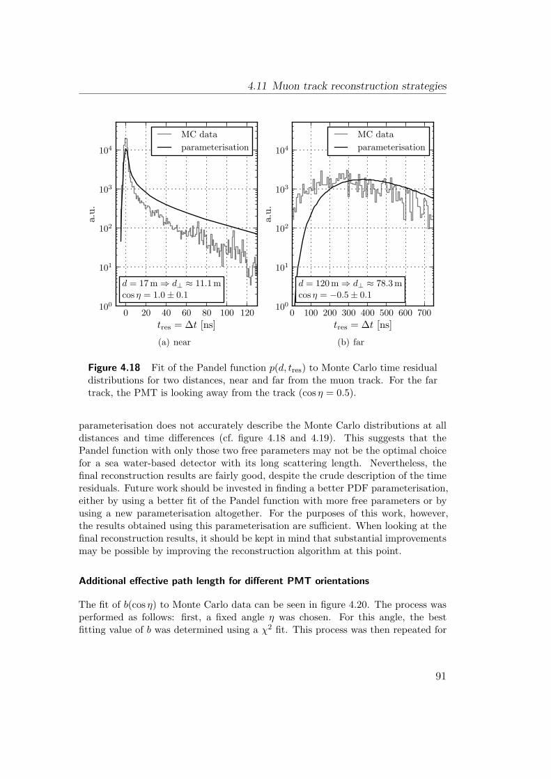
4.11 Muon track reconstruction strategies
0 20 40 60 80 100 120tres = ∆t [ns]
100
101
102
103
104
a.u.
d = 17 m⇒ d⊥ ≈ 11.1 mcos η = 1.0± 0.1
MC dataparameterisation
(a) near
0 100 200 300 400 500 600 700tres = ∆t [ns]
100
101
102
103
104
a.u.
d = 120 m⇒ d⊥ ≈ 78.3 mcos η = −0.5± 0.1
MC dataparameterisation
(b) far
Figure 4.18 Fit of the Pandel function p(d, tres) to Monte Carlo time residualdistributions for two distances, near and far from the muon track. For the fartrack, the PMT is looking away from the track (cos η = 0.5).
parameterisation does not accurately describe the Monte Carlo distributions at alldistances and time differences (cf. figure 4.18 and 4.19). This suggests that thePandel function with only those two free parameters may not be the optimal choicefor a sea water-based detector with its long scattering length. Nevertheless, thefinal reconstruction results are fairly good, despite the crude description of the timeresiduals. Future work should be invested in finding a better PDF parameterisation,either by using a better fit of the Pandel function with more free parameters or byusing a new parameterisation altogether. For the purposes of this work, however,the results obtained using this parameterisation are sufficient. When looking at thefinal reconstruction results, it should be kept in mind that substantial improvementsmay be possible by improving the reconstruction algorithm at this point.
Additional effective path length for different PMT orientations
The fit of b(cos η) to Monte Carlo data can be seen in figure 4.20. The process wasperformed as follows: first, a fixed angle η was chosen. For this angle, the bestfitting value of b was determined using a χ2 fit. This process was then repeated for
91

4 A new KM3NeT simulation and reconstruction chain
0 30 60 90 120 150 180 210 240photon path length d [m]
10−3
10−2
10−1
100ph
oton
arri
val
prob
abili
ty
MC dataN(d)
e− dλabs
Figure 4.19 Photon survival probability vs. photon path length. The plotshows Monte Carlo data overlaid with the fit of N(d) (cf. (4.23)). Additionally,an exponential containing only the absorption length is shown for comparison.
a number of angles. The results can be seen as data points in figure 4.20. Note thekink in the distribution at cos η ≈ 0.14. This is attributed to the angular acceptanceof the PMTs used in the simulation which is linear in cos η for light coming from thefront but zero for light coming from the back. It is therefore not differentiable atcos η = 0 (cf. figure 4.13), an effect that seems to be visible in this fit. Starting fromthe kink, almost all light hitting a PMT is scattered, whereas for smaller angles, asubstantial amount of direct light is left. For these reasons, the fit function b(cos η)was composed of two parts
b(cos η) :=
b0 + bfrac
cos η+bshiftfor cos η ≥ k
b1 + b2 cos η for cos η < k(4.26)
with the condition to be continuous at cos η = k. Note that this is a purely empiricaldefinition which was chosen to best fit the Monte Carlo data.
92

4.11 Muon track reconstruction strategies
−1.0 −0.5 0.0 0.5 1.0cos η
0
50
100
150
200
250
300
b(co
sη)
[m]
cos η = k = 0.14
b1 + b2 cos η
b0 + bfrac
cos η+bshift
b0 = −8.37bfrac = 8.81bshift = −0.06b1 = 117.99b2 = −141.25
fit valuesparameterisation
Figure 4.20 Angular dependency of the additional track length b(cos η) in-cluded in the effective distance deff (see (4.25)). The function corresponds to aneffective additional path length for PMT orientations that face away from thedirection of direct light. For larger values of η (i.e. lower values of cos η), moreand more scattered light with a larger track length reaches the PMT. The datapoints with error bars correspond to fits to Monte Carlo data at a particularvalue of cos η, the solid line is the parameterisation used in the reconstructioncode (see (4.26)).
Minimiser algorithms and first guess
When the Pandel PDF is finally used in a log-likelihood track reconstruction process,some kind of minimisation algorithm needs to be used. In the current implementa-tion, the minimisation process consists of two steps: first, a minimum is determinedusing the downhill simplex algorithm [109] as implemented in the MINUIT packageusing the result of a simple linear fit as a starting point.15 As this algorithm can pos-sibly converge into a local minimum and miss the global one, a second minimisationprocess is performed, taking the simplex result as a starting point. It uses the exactsame likelihood function as before, but finds the optimal value using the CMA-ES
15This linear fit assumes that the track goes directly through all hit PMTs. The algorithmfinds the optimal value analytically.
93

4 A new KM3NeT simulation and reconstruction chain
−2 −1 0 1 2log10(ΨMC[])
0
2
4
6
8
10
12
even
tspe
rye
aran
dbi
n
linear prefit, no cut, upgoingPandel fit (Simplex) no cut, upgoingPandel fit (CMA-ES) no cut, upgoingPandel fit (Paraboloid) error estimate could be determined, upgoing
Figure 4.21 Angular error after the four fit stages for an example multiPMTdetector with a E−2 neutrino energy spectrum. The first log-likelihood stepafter the initial linear fit improves the angular error substantially, whereas thesecondary CMA-ES optimisation only finds the minimum for some tracks wherethe Simplex minimiser failed. The fourth fit is performed during the pointingaccuracy determination step (“paraboloid”).
evolutionary algorithm [110]. Though these methods are usually aimed at higher-dimensional search spaces, this algorithm nevertheless improves the reconstructionfor tracks where the global minimum was only closely missed. Figure 4.21 showsthe angular error after each of the three fit stages: the preliminary linear fit, thePandel PDF as minimised by the Simplex algorithm and the fit after the additionalCMA-ES minimisation. The fourth stage shown is for the track direction after thepointing accuracy estimation presented in the following section, which may re-fit thetrack.
Hit filtering
To provide the reconstruction algorithm with less optical noise hits, a simple hitfiltering algorithm, developed as part of another work [111], is used before the ac-tual fitting process. The algorithm starts with the whole set of hits. Each hit is
94
4.11 Muon track reconstruction strategies
then compared to all remaining hits on the same, the neighbouring and the next-to-neighbouring floors on the same string. Any combination with a time differencesmaller than 300 ns is stored as part of a potential hit cluster containing a number ofhits Nclust in addition to the initial hit. Within each cluster, the angle θi := atan ∆ti
∆ziis calculated for each of cluster hit with respect to the initial hit. Here, ∆ti and∆zi are the differences in hit time and z-coordinate, respectively. Now, hits areiteratively removed from the cluster until the RMS of θ is smaller than a pre-definedthreshold (which was chosen as 1 in this case). In each iteration the hit with thelargest deviation from the mean is removed. All hits in clusters where the remainingnumber of hits is larger than a threshold are retained and marked as selected. Thisthreshold was chosen to be Nclust, sel. ≥ 4.
A measure for track pointing accuracy
If the likelihood function’s shape is assumed to be Gaussian (at least locally aroundits maximum), the track reconstruction error can be estimated from the gaussian’swidth σ. A gaussian maximum in the likelihood function becomes a minimum ofa paraboloid in the negative log-likelihood space. For the one-dimensional case,the width σ thus is the distance from the minimum of the negative log-likelihoodfunctionto the point where this function has changed by 1
2 , i.e.
∆ (− logL) =12. (4.27)
This track reconstruction error can be used as a powerful quality estimator. Animplementation for IceCube, where the width is calculated in the two-dimensionalangular space (zenith and azimuth), is discussed in [107, 112]. To reduce the 5-dimensional problem (with three dimensions for the track position and two dimen-sions for its direction) to a two-dimensional problem, the following algorithm isused: first, fixed track directions are defined around the previously determined mini-mum in the log-likelihood space. These directions are on concentrical circles aroundthe optimal direction in zenith and azimuth16. For each of these directions, thelog-likelihood function is optimised by varying the track position while leaving thedirection fixed. The resulting log-likelihood values are used to analytically determinethe optimal two-dimensional paraboloid. Under the condition given in (4.27), thisyields an error ellipse with two width parameters, one for each axis of the ellipse(σ1 and σ2). Also resulting from this procedure is a new track direction estimate(i.e. the centre of the ellipse), which is used as the new fit direction. In case theanalytical determination of the ellipse failed, the fit is rejected.
16To avoid distortions for directions near the poles, the coordinate system is rotated for thecalculations of the minimum’s width, so that the track direction is facing towards theequator, i.e. an zenith of 90.
95

4 A new KM3NeT simulation and reconstruction chain
For this work, the IceCube algorithm has been re-implemented. Although boththe σ1 and the σ2 parameters are available, for reasons of simplicity only theirgeometrical mean
σ :=
√σ2
1 + σ22
2(4.28)
has been used as a quality parameter. Further studies should investigate the separatetreatment of both direction errors.
The track estimation results after this step can be seen in figure 4.21, wheresome badly reconstructed tracks are missing after the “paraboloid” stage due to therejection step. Unfortunately, there seem to be slight problems with the paraboloiddetermination, as the peak of the angular error histogram is slightly shifted to worseangular errors. Due to time constraints, this shift could not be investigated yet.
96

5 Analysis techniques
I reject your reality andsubstitute my own.
(Adam Savage)
Reconstructed tracks can now be subjected to different analysis steps. Some ofthe most important benchmark analysis techniques for neutrino telescopes will bepresented in this chapter. There are certainly more analyses that can be performedthan those presented in this chapter (including searches for diffuse fluxes). Forthe preliminary studies done for KM3NeT, the following detector properties wereconsidered.
5.1 Angular resolution
One very important quality of a neutrino telescope is its angular resolution. A goodangular resolution allows the detector to resolve track directions with a small errorand thus enables it to detect point-sources. The angular resolution is influencedby several factors, amongst them the geometrical layout of the detector, its totalphotocathode area and density and of course the quality of the track reconstructiontechnique that is used. Most commonly the value that is presented is the medianspace angle Ψ between the Monte Carlo track direction ~dMC and the reconstructeddirection ~dreco
Ψ = acos(~dMC · ~dreco
), (5.1)
where ~dMC and ~dreco are assumed to be unit vectors. Optionally, the angular differ-ence can be expressed in two dimensions, leading to a 2D point-spread function.
5.2 Neutrino effective area
The effective area of a neutrino telescope is a way to define the fraction of particlesincident on the detector that can be reconstructed without being dependent on thethe actual detector’s size. When used as a function of energy, it is also independentof the incident spectrum. It includes all possible effects like absorption in the earth,the interaction probability in or near the detector and its actual detection probability,possibly after reconstruction quality cuts. For this work, the “neutrino effective area”Aeff; ν(Eν, θν) will be used exclusively, i.e. it will be defined in terms of neutrino
97

5 Analysis techniques
103 104 105 106
neutrino energy Eν [GeV]
10−1
100
101
102
103
neut
rino
effec
tive
area
[m2] zenith ranges
90 – 100
100 – 120
120 – 140
140 – 160
160 – 180
Figure 5.1 Typical example of effective areas for a neutrino detector for dif-ferent zenith ranges. Note that due to neutrino absorption in the earth at highenergies, the effective area above Eν ≈ 104 GeV decreases significantly withincreasing zenith angle and thus increasing neutrino path lengths through theearth.
energy Eν and the neutrino zenith angle θν.1 The event rate Nν for a certainneutrino flux dΦν
dEνθνcan then be calculated from the effective area:
Nν =∫Aeff; ν(Eν, θν)
dΦν
dEνθνdEνdΩν. (5.2)
Typically, the effective area is highly energy-dependent, ranging from tiny areasat low energies (at about Eν ≤ 10 GeV) where only a small amount of light isproduced by the generated muon, up to a few hundred metres at higher energiesabove Eν ≈ 100 TeV.2 When looking downwards, the effective area will fall off atthese high energies due to absorption of neutrinos in the earth. This effect is notvisible when looking upwards. Effective areas are usually given in units of metresas a function of energy for a specific zenith range. Examples of effective areas canbe seen in figure 5.1. Note that, when results are given later on in this work, theeffective are will always be for upgoing tracks, i.e. for a zenith range of [90; 180].
1Other effective area types like the muon effective area will not be discussed here. The term“effective area” will be used in the following to consistently refer to “neutrino effectivearea”.
2These approximate values are for km3-sized telescopes.
98

5.3 Point-source sensitivity and discovery potential
5.3 Point-source sensitivity and discovery potential
Searching for point-like sources of neutrino emission is one of the most importanttasks of a neutrino telescope. Therefore, many techniques exist to look for pointsources in the recorded data and to set exclusion limits in the case that no pointsources are found. The algorithm used in this work to determine such detectorsensitivities and discovery potentials is based on a binned point-source search. Themore complex technique of unbinned searches will not be considered here.
The two basic questions are: can a source be seen with at least a certain signif-icance (e.g. 5σ) in a given amount of hypothetical experiments (e.g. 50%)? And,if no source is discovered, what is the source flux that can be excluded at a givenconfidence level (e.g. 90%)? The answer to the first question yields the detector’sdiscovery potential [113], whereas the second question leads to the detector’s sensi-tivity [114].
Both calculations require the expected number of signal events nsig and the num-ber of background events nbkg seen from the direction of a certain source. As thelocation of a source is assumed to be known, nbkg can be kept low by only usingevents with directions that are near the actual source’s direction, i.e. by using aso-called search cone with a defined opening angle θcone. Additionally, the relativenumber of signal and background events can be influenced by various track qualitycuts. The cuts leading to optimal values for discovery potential and sensitivity willusually be different and have to be found using an optimisation process.
As the signal and background fluxes vary for different zenith angles due to earthabsorption processes, the analysis has to be performed for a range of different zenithbins. For KM3NeT, the rotation of the earth has to be taken into account to convertfrom event numbers in zenith bins to event numbers for different declination bins.This can be achieved by distributing the event rates according to the fraction of timea certain zenith direction is visible in a certain declination band. The total visibilityper year of each declination is shown in figure 5.2. In all these analyses, the fluxesare assumed to have an azimuthal symmetry.
5.3.1 Discovery potential
The discovery potential of a detector can be determined by calculating the “leastdetectable signal”µlds(nbkg), assuming a given number of background events accord-ing to [113]: given an expected number of background events nbkg, the Poissonianprobability of observing more than a certain number of events P (≥ nobs|nbkg) canbe calculated. In case this number is very small, e.g. P (≥ nobs|nbkg) < α, somethinginteresting might have been detected. As an example, for a 5σ detection (area in aone-sided gaussian tail), α would be chosen as α = 2.87 · 10−7. For a given α, thecritical number of events ncrit, where P (≥ ncrit|nbkg) < α can be calculated. This is
99

5 Analysis techniques
−50 0 50declination δ []
0.0
0.2
0.4
0.6
0.8
1.0vi
sibi
lity
(fra
ctio
nof
year
)
Figure 5.2 Source visibility versus declination δ. Sources are regarded as visi-ble if they are below the horizon. The shown values are for a detector located inthe Mediterranean at E 6 10′ N 42 48′ (grid WGS84), i.e. the ANTARES site.
the number of events that need to be observed in order to report a detection, in thiscase with 5σ. In the presence of a real signal nsig, the probability (statistical power1− β) that ncrit or more events are observed is 1− β = P (≥ ncrit|nbkg + nsig). The
“least detectable signal” µlds is then defined as the value of nsig where this equalityis satisfied for a given value of 1− β.
Finding the minimum of the parameter µlds/nsig, yields an optimal set of cuts fordiscovering the source at significance level α with probability 1−β. This parameteris often called the “model discovery factor” (MDF). In the following, α is chosen fora 5σ detection with a probability of 1− β = 50%.
5.3.2 Sensitivity
If no signal source is found, an upper limit for a certain source flux can be given [115].The method is similar to the one presented in the last section, only the least de-tectable signal has to be replaced with an “average upper limit” µC.L.(nbkg) for a cer-tain confidence level (C.L.) calculated using the Feldman-Cousins approach [114]: inabsence of a measured signal nobs, the Feldman-Cousins upper limit µC.L.(nobs, nbkg)needs to be averaged for a certain background expectation nbkg. This is done byweighting the upper limits by their Poisson probability of occurrence:
µC.L. =∞∑
nobs=0
µC.L.(nobs, nbkg)(nbkg)nobs
(nobs)!exp (−nbkg) (5.3)
100

5.3 Point-source sensitivity and discovery potential
Again, the optimal set of cuts can be found by minimising the parameter µC.L./nsig,called the “model rejection factor” (MRF). The detector’s flux sensitivity can thenbe written as (
dΦdE
)sens
:=µC.L.
nsig
(dΦdE
)source
, (5.4)
where (dΦ/dE)source is the assumed source flux yielding the signal expectation usedto calculate the MRF. The resulting flux is the largest flux that can be excluded bythe detector with the given C.L. In the following, the confidence level is chosen tobe 90%.
101


Part III
Results
103


6 Comparison between simulation chains
People are very open-mindedabout new things — as longas they’re exactly like the oldones.
(Charles F. Kettering)
This chapter presents results obtained for a single reference detector design (basedon the singlePMT floor layout), simulated with the two different simulation chainsavailable: the legacy ANTARES toolchain and the new simulation chain developed inthis work. To determine if the results from the two simulation chains are compatible,data simulated with both of them have been reconstructed using the same algorithm.This shows the influence of different approaches and approximations made in thesimulation on the final results.
6.1 Detector design, environment and simulationparameters
For this analysis, a small reference detector design based on the “string” detectordesign (ANTARES-like) floor layout with a volume of approximately 0.5 km3 waschosen. It consists of 154 strings in a hexagonal seafloor layout (cf. figure 6.1) withan inter-string distance of dstring = 91 m. The strings have an instrumented lengthof 570 m with 20 floors per string. This corresponds to a vertical floor distance of30 m. The distance from the seabed to the first floor is 100 m with the seabed beingat a depth of 3500 m.
All simulations have been performed with an optical background rate of 75 kHz(per 9.3′′ PMT) in the “ANTARES water” medium defined in section 4.5.1. Themuon neutrino signal has been simulated as a full sky sample (Ω = 4π) with anE−1 spectrum and then re-weighted to an E−2 benchmark flux with the followingnormalisation:
dφνµ
dE= 1.0 · 10−8
(E
GeV
)−2
GeV−1cm−2s−1 (6.1)
This flux is distributed evenly to neutrinos and anti-neutrinos. The backgroundsignal corresponds to the atmospheric flux described in section 2.1.9. Neutrinoshave been simulated in an energy range from 102 GeV to 107 GeV. The simulations
105

6 Comparison between simulation chains
−600 −400 −200 0 200 400 600x coordinate [m]
−600
−400
−200
0
200
400
600
yco
ordi
nate
[m]
dstring = 91 m
Figure 6.1 Hexagonal sea floor layout with 154 strings and a string distance of91 m as used for the comparison between simulation chains. Each dot representsa detector string.
do not include atmospheric muon background at this point. Muon propagationand photon tracking is done using the km3 tool for the old simulation chain. Thenew simulation chain uses the unified shower/muon simulation presented earlier insection 4.8.
As the neutrino sample simulated with the new algorithm was also used for other,larger detectors to obtain results presented later on, the light generation (“active”)volume for the detector was chosen substantially larger than the detector’s instru-mented volume. In contrast to that, all data produced with the legacy ANTAREScode uses its default active volume definition for the muon propagation, i.e. a cylin-der around the instrumented volume, extended by three absorption lengths.
In the old ANTARES simulation chain, the hadronic cascade at the interactionvertex is simulated using the“geasim”tool which does not take light scattering effectsinto account. Therefore, for the sake of comparability of the two simulation chains,light from the vertex cascade was removed from both simulations.1
1Note that in all of the following sections, where only the new simulation chain is used,light from the hadronic cascade at the vertex is fully included.
106

6.2 Basic quantities before reconstruction
6.2 Basic quantities before reconstruction
Before reconstructing tracks, distributions of the most important hit-related quanti-ties of the muon and photon-propagation step have been compared between the twosimulations chains (cf. figure 6.2). For the results presented in this section, in orderto be independent of effects due to the event generator, the genhen tool has beenused as a generator for both simulation chains. For all other results, the ANIS eventgenerator has been used as part of the new simulation chain. The upper plot showsthe distribution of the cosine of the angle θ between the expected photon directionwith respect to the Monte Carlo muon track and the OM axis. Below, the distri-bution of the distance dtrack between the Monte Carlo track and the OM recordingthe photon is shown. The two lower plots show the time residual distribution andthe distribution of the recorded charges, respectively. The step in the dtrack distribu-tion at dtrack = 100 m corresponds to a hit selection done as part of the ANTARESreconstruction strategy. The step in the time residual distribution at tres = 40 nscorresponds to the integration time of the first ARS channel. After this time, thesecond channel can take over.
The only notable difference between the two simulations is the time residual dis-tribution, where the peak around tres = 0 is slightly broader for the new simulationchain. This is due to differences in light dispersion simulation between the twochains. Whereas the new simulation includes a full simulation of photons with thecorrect spectrum and thus automatically includes light dispersion because of theincluded refractive index distribution, the old simulation uses a single wavelengthfor the simulation of its photon tables. Only in the very last step of km3, the lightdispersion is included as a smearing in time according to pre-generated distributions.These distributions do not seem to fully reproduce the results obtained with the fullsimulation performed as part of the new algorithm developed for this work.
107

6 Comparison between simulation chains
−1.0 −0.5 0.0 0.5 1.0cos θ
0500
1000150020002500
a.u.
km3 (ANTARES simulation)new simulation
0 20 40 60 80 100 120dtrack [m]
101
102
103
104
a.u.
−50 0 50 100 150 200 250tres [ns]
100101102103104105
a.u.
100 101
hit amplitude [p.e.]
101
102
103
a.u.
Figure 6.2 Distributions of basic hit-related quantities. The hits used to gen-erate the distributions shown here are the ones selected for the final step of theANTARES reconstruction strategy. From top to bottom, the plots show distri-butions of the cosine of the angle between the expected photon direction andthe OM axis, the distance from the Monte Carlo track, of the time residuals andthe hit amplitudes.
108

6.3 Quality cut distribution
6.3 Quality cut distribution
One of the interesting quantities to study after the reconstruction algorithm hasbeen used on simulated data, is the reconstruction quality variable. To this end,simulated neutrinos from both software chains have been reconstructed using thedefault ANTARES algorithm (with KM3NeT modifications, cf. sec. 4.11.1).2
During its development, the algorithm’s final PDF has been heavily optimised tothe MC results obtained from the old ANTARES simulation toolchain, especiallyto the photon output of the km3 tool. When comparing the distribution of the Λquality parameter defined in (4.21), small differences are visible only at high energies(Eν > 106 GeV), (see figure 6.3). The overall shape of the distributions is compatiblefor both simulation chains: there are two overlapping peaks, one containing well-reconstructed tracks, the other one mainly containing badly reconstructed ones. Thelocation of the peak containing the “good” tracks is shifted starting at energies ofabout Eν ≈ 103.5 GeV; it starts out at about Λ ≈ −5 for low energies and is locatedat Λ ≈ −4.5 above that threshold.
Only for the new simulation, another minute shift of the peak becomes visible atthe highest energies (Eν ≈ 106 GeV). A possible explanation for this behaviour canbe found in the differences in the simulation algorithms for cascades along muontracks: the km3 tool distributes pre-simulated cascades obtained from a full Geant3simulation along the muon track, but only has a limited range of cascade energiesup to 100 GeV at its disposal. Higher energies are simulated by superimposing thesecascades. In the new simulation algorithm, cascades of any energy are simulated,with their energy range not limited by the lack of photon tables. The price forthis, however, is that cascades are only simulated according to parameterised angu-lar and longitudinal distributions. Differences between these two approaches shouldonly be visible at the highest energies. Because these differences may lead to differ-ences between the simulated hit distribution and the distribution expected by thereconstruction’s PDF, such a shift is at least plausible.
Overall, the new simulation chain yields about 5% more events, an effect thatseems to get larger with higher energies. This effect can be attributed to the ANISgenerator, as it is not visible when tracks generated by the old ANTARES genhentool are propagated with the new muon simulation code instead of km3. This isconsistent with the previous observation in section 6.2: when using the same events,the low level hit distributions are unchanged except at time residuals near zero, aneffect that is independent of muon energy. The reason for this difference could notbe found, but it is believed that this is either due to the different parameterisations
2Note that in contrast to the previous section, the event generator that has been usedas part of the new software chain is now ANIS. This is also true for all results shownfrom now on. The genhen generator was still used to generate the results for the oldANTARES software chain.
109

6 Comparison between simulation chains
of the νN structure functions (CTEQ5 for ANIS and CTEQ6 for genhen) or due tothe fact that the genhen “can” size is chosen too small for such high energy events.
The optimal cut levels for each simulation chain have been determined, each oneby optimising for best E−2 flux point-source sensitivity, albeit without contributionsfrom atmospheric muons. This type of background was omitted as it would haverequired extensive amounts of computation time to include, which was not availablein the frame of this work. The primary objective, however, was to compare the twosimulation chains which was possible without the inclusion of atmospheric muons.The following sections show the angular resolution, effective area and point sourcesensitivity achievable with these cuts.
110

6.3 Quality cut distribution
0
1
2
3
4
5
6
7
8
even
tsp
eryea
ran
db
in
old sim. (all upgoing)old sim. (up, ΨMC ≤ 1)
new sim. (all upgoing)new sim. (up, ΨMC ≤ 1)
total events [all energies]
76.380.4
0.00.20.40.60.8
evts
.[b
in−
1yr−
1]
EMC < 103.5 GeV
10.110.3
012345
evts
.[b
in−
1yr−
1]
103.5 ≤ EMC/GeV < 106
62.465.5
−11 −10 −9 −8 −7 −6 −5 −4Λ quality parameter
0.00.10.20.30.40.50.6
evts
.[b
in−
1yr−
1]
EMC ≥ 106 GeV
3.94.5
Figure 6.3 Distribution of the Λ quality parameter for both simulation chains.The top plot shows the overall distribution for an E−2 spectrum, whereas thelower plots show three different energy ranges. The lighter coloured lines corre-spond to the total distribution, the dark lines are distributions obtained after acut on the Monte Carlo angular reconstruction error.
111

6 Comparison between simulation chains
6.4 Angular resolution
Comparing the angular error of reconstructed tracks (cf. figure 6.4), the distributionsare similar in shape and position. The only difference visible is an excess of well-reconstructed events for the new simulation. This is already expected from theprevious plots, where more events were seen, too.
As expected, the highly optimised reconstruction algorithm yields an excellentangular resolution with a median angular error of about 0.07. The cuts were op-timised for best E−2 sensitivity, so some kind of energy estimator was needed todistinguish between the low energy atmospheric neutrino background and the highenergy neutrinos from the signal flux. The cut chosen here (and in all followinganalyses) is the number of PMTs with L1 hits (NPMT). This parameter depends onthe track’s energy due to the higher number of cascades from catastrophic energylosses accompanying them, leading to a higher photon count.
If optimising this cut together with the Λ quality parameter, the optimal valuesturn out to be Λ ≥ −5.5 andNPMT ≥ 15 for both simulation chains. When looking atthe amount of mis-reconstructed events with ΨMC & 1, it is evident that these cutsare not probably enough to suppress the atmospheric muon background, althoughthe plots were only made for upgoing events. Because of the immensely high rate ofatmospheric muons, when compared to neutrino fluxes, having even a small amountof mis-reconstructed tracks with angular errors of the order of 90 or higher causes alarge amount of atmospheric muon events to “spill over” below the horizon. Hardercuts will be needed to drastically lower the number of mis-reconstructed muons.
112

6.4 Angular resolution
−3 −2 −1 0 1 2log10(ΨMC[])
0
1
2
3
4
5
6
even
tspe
rye
aran
dbi
n
no cut (all upgoing reconstructed events) [median = 0.43]
cuts for best E−2 sensitivity: Λ ≥ −5.50, NPMT ≥ 15 [median = 0.07]
quality cut only to reach same resolution: Λ ≥ −5.30 [median = 0.07]
∫dΨMC
140.765.869.8
(a) old simulation chain
−3 −2 −1 0 1 2log10(ΨMC[])
0
1
2
3
4
5
6
even
tspe
rye
aran
dbi
n
no cut (all upgoing reconstructed events) [median = 0.43]
cuts for best E−2 sensitivity: Λ ≥ −5.50, NPMT ≥ 15 [median = 0.07]
quality cut only to reach same resolution: Λ ≥ −5.30 [median = 0.07]
∫dΨMC
148.470.173.4
(b) new simulation chain
Figure 6.4 Angular error w.r.t. the muon direction for the old (a) and new(b) simulation chains, with no cut at all (i.e. all upgoing tracks that werereconstructable, without any quality cuts), with cuts optimised for best E−2
flux point-source sensitivity (using the Λ quality parameter and the number ofPMTs with L1 hits, NPMT, as a crude energy estimator) and with the Λ cutonly. In the last case, the cut level was chosen as to obtain the same medianresolution as for the combined Λ and NPMT cuts.
113

6 Comparison between simulation chains
6.5 Effective area
The effective areas for the two simulations (cf. figure 6.5) are similar, but show apeculiar behaviour at high energies (EMC & 106 GeV): the effective area for recon-structed events does not follow the shape of the area obtained when asking for recon-structible events — for the ANTARES reconstruction strategy, this corresponds toNhits ≥ 6, where Nhits is the number of hits selected for the final reconstruction step.Instead, the ratio of the two areas gets smaller again. This is due to the distributionof the Λ parameter at this energy range, which is broader than for lower energies.A constant cut on Λ thus removes more and more muons with well reconstructedtracks, thereby reducing the effective area. This difference can thus be attributed tothe reconstruction strategy which was never designed for these high-energy eventsin km3-scale detectors. The differences at very low energies (Eν < 103 GeV) can beattributed to a lack of statistics. In this region, over 95% of all simulated events areremoved by the quality cuts, thus leaving only a small amount of samples to deter-mine the effective area3. This, combined with the fact that the simulated spectrumis E−1 in both cases and thus produces lower statistics at low energies anyway, canvery well lead to the observed differences.
3In the energy range 103 GeV ≤ Eν ≤ 106 GeV only about 50% of the simulated eventsare removed.
114

6.5 Effective area
10−4
10−3
10−2
10−1
100
101
102
103
area
[m2]
(a)
Nhit,reco ≥ 6 [old sim.]
Λ ≥ −5.50, NPMT ≥ 15
Λ ≥ −5.30 (same 〈Ψ〉 ≈ 0.07)Nhit,reco ≥ 6 [new sim.]
Λ ≥ −5.50, NPMT ≥ 15
Λ ≥ −5.30 (same 〈Ψ〉 ≈ 0.07)
trig.: 2T3 [old sim.]trig.: 2T3 [new sim.]
0.00.51.01.5
rati
o
(b)
0.00.51.01.5
rati
o
(c)
0.00.51.01.5
rati
o
(d)
0.0
0.5
1.0
rati
o
(e)
103 104 105 106
neutrino energy [GeV]
0.0
0.5
1.0
rati
o
(f)
Figure 6.5 The top plot (a) shows the neutrino effective area for the twosimulation chains for three different cut levels: all tracks that have at least 6hits for the final reconstruction step (dashed), all hits surviving the cuts for bestE−2 sensitivity and all hits for a cut yielding the same median angular resolutionas the sensitivity cut, but using only the Λ parameter. For comparison, theeffective areas for the 2T3 trigger level have been included. The lower plots(b-f) show ratios of the effective areas using the same colour scheme as in thetop plot. Note that no trigger is used during the actual reconstruction.
115

6 Comparison between simulation chains
6.6 Point-source sensitivity
The point-source sensitivity for an E−2 flux at different declinations δ (cf. figure 6.6)reveals differences between the two simulations at the extreme declination values cor-responding to almost horizontal tracks (δ & 20). The sensitivity calculated from thenew simulation chain is slightly better over the whole range of declinations, exceptfor declinations δ . −60. This corresponds to upgoing tracks, where very high neu-trino energies cannot contribute due to their absorption in the earth. The differenceis therefore due to neutrinos with very high energies of the order of Eν ≈ 106 GeVor higher. The flux of these neutrinos can influence the sensitivity as the simulatedE−2 spectrum does not have any cutoff at high energies (except for the one imposedby the simulation which stops at Eν = 107 GeV). When plotting the sensitivityas a function of zenith angle in the detector’s local system instead of declination(cf. figure 6.7), the effect gets disentangled from the declination “smearing” due tothe Earth’s rotation: starting from upgoing tracks at a zenith angle of 180 to about120, the sensitivities from both simulation chains are compatible. Only at zenithangles near the horizon, where neutrinos of extremely high energies can contributebecause of their shorter path through the earth, the two sensitivities begin to de-viate. This is compatible with the previous observation that an excess of events isobserved at higher energies with the new simulation chain when compared to theold chain.
116

6.6 Point-source sensitivity
10−9
10−8
(E/G
eV)2
dφ/dE
[GeV−
1cm−
2s−
1]
(a)
old sim. (sensitivity 90% C.L.)old sim. (5σ discovery potential [50% of experiments])new sim. (sensitivity 90% C.L.)new sim. (5σ discovery potential [50% of experiments])
0.0
0.5
1.0
1.5
2.0
mea
nN
sig/bkg
calculated for dφ/dE = 10−9 (E/GeV)−2 GeV−1cm−2s−1
(b)
0.150.200.250.300.350.400.45
searc
hb
in[
]
(c)
−7.0
−6.5
−6.0
−5.5
−5.0
Λcu
t
(d)
−80 −60 −40 −20 0 20 40
declination δ []
5101520253035
NP
MT
cut
(e)
Figure 6.6 Point-source sensitivity and discovery potential for one year for theold and new simulation chains. The top plot (a) shows the final detectable/ex-cludable fluxes, whereas the lower plots show the individual cut levels (c-e) andthe mean number of signal and background events per year (b). The number ofbackground events is indicated using a dashed line in (b). The search bin size in(c) is given as the radius. As the correlation between the parameters in (c-d) ishigh and their behaviour can therefore be erratic, the values have been smoothedusing a sliding window to better indicate the parameters’ general behaviour.
117
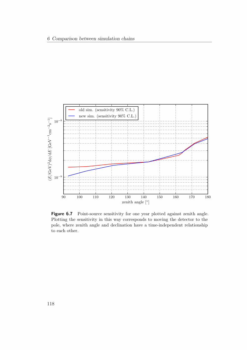
6 Comparison between simulation chains
90 100 110 120 130 140 150 160 170 180
zenith angle []
10−9
10−8
(E/G
eV)2
dφ/dE
[GeV−
1cm−
2s−
1]
old sim. (sensitivity 90% C.L.)new sim. (sensitivity 90% C.L.)
Figure 6.7 Point-source sensitivity for one year plotted against zenith angle.Plotting the sensitivity in this way corresponds to moving the detector to thepole, where zenith angle and declination have a time-independent relationshipto each other.
118

7 Performance of different detector designs
It is common sense to take amethod and try it. If it fails,admit it frankly and tryanother. But above all, trysomething.
(Franklin D. Roosevelt)
In this chapter, the three different detector types introduced earlier in section 2.3.2will be compared. The detector sizes are still “small”, i.e. 154 strings for the “string”and “multiPMT” designs and 80 strings for the “tower” design. The string distancefor the former two detectors is 91 m, whereas it is 130 m for the latter. This choiceyields approximately the same photocathode area for each of the designs, while stillretaining a hexagonal layout and approximately the same detector volume and thusmakes them comparable. This choice was made because the sensitivity of neutrinodetectors mainly scales with photocathode area [78]. In this way, the designs’ per-formance can be disentangled from the effect achieved by simply adding more OMs.Note that the average cost per optical module may be different for each design.
From now on, all simulations were made using the new simulation chain developedin this work. The input tracks used for all detectors are exactly the same, i.e. thesame ANIS run is used for all of them. The only difference is in the muon trackingand light propagation step, which uses a different random seed for each detector type,and in the PMT and OM simulations. As before, the optical noise level for the single-PMT designs was chosen to be 75 kHz per OM. This translates to a background rateof 5.2 kHz per PMT for the “multiPMT” design. This value has been determinedusing a dedicated photon tracking simulation taking into account all of the OMparameters given in section 4.9.2.1
All data simulated for the “tower” and “string” detectors were reconstructed usingthe standard ANTARES reconstruction strategy, whereas for the“multiPMT”design,the new reconstruction algorithm presented in section 4.11.2 was used.
1The simulation was set-up in such a way as to retain the value of 75 kHz when applied tothe single-PMT OMs.
119

7 Performance of different detector designs
7.1 Angular resolution
As in the previous chapter, the cut levels have been optimised for best E−2 point-source sensitivity. As expected, the angular resolution determined for the “string”design is almost the same as the one shown in the previous chapter (cf. figure 7.1(a)).There is only a single parameter that has been changed, which is the inclusion oflight from the hadronic cascade at the interaction vertex. Interestingly, this changeleads to a slight drop in the median angular resolution from 0.07 to 0.08 whenreconstructing exactly the same events.
As expected, the angular resolution determined for the “multiPMT” design isworse than that of the other two designs (cf. figure 7.1(c)). This, however, is notdue to the detector’s inferior design, but rather due to the fact that the recon-struction algorithm used for this type of detector is not as refined as the standardANTARES strategy. Large improvements in both detection efficiency and angularresolution can be expected once the new algorithm gets more refined. For the othertwo detector types, where the algorithm is already heavily adapted to single-PMTlight detection in sea-water only smaller improvements are expected when optimisingthe reconstruction algorithm. In this way, all results presented for the “multiPMT”design are to be taken as worst-case scenarios, where no optimisation has been doneon the reconstruction algorithm.
The “tower” design has a good angular resolution but the detection efficiency isworse than that of the “string” design. This seems to be due to the sparser detectorwhich allows more muons to pass it undetected. If, however, the cost of deploying onetower structure is not much more expensive than the cost of deploying a single string,a denser “tower” detector with more OMs will certainly outperform a “string”-typedetector of similar cost.
120

7.1 Angular resolution
0
1
2
3
4
5
6
even
tspe
rye
aran
dbi
n
“string” design
no cut (all upgoing reconstructed events) [median = 0.56]
cuts for best E−2 sensitivity: Λ ≥ −5.50, NPMT ≥ 15 [median = 0.08]
quality cut only to reach same resolution: Λ ≥ −5.30 [median = 0.08]∫dΨMC
159.973.774.8
0
1
2
3
4
5
6
even
tspe
rye
aran
dbi
n
“tower” design
no cut (all upgoing reconstructed events) [median = 5.83]
cuts for best E−2 sensitivity: Λ ≥ −5.90, NPMT ≥ 33 [median = 0.08]
quality cut only to reach same resolution: Λ ≥ −5.28 [median = 0.08]∫dΨMC
157.959.159.5
−3 −2 −1 0 1 2log10(ΨMC[])
0
1
2
3
4
5
6
even
tspe
rye
aran
dbi
n
“multiPMT” design
no cut (all upgoing reconstructed events) [median = 1.36]
cuts for best E−2 sensitivity: σpara < 0.50, NPMT ≥ 45 [median = 0.31]
quality cut only to reach same resolution: σpara < 0.32 [median = 0.31]∫dΨMC
123.542.250.2
Figure 7.1 Angular error w.r.t. the muon direction for the “string” (a), the“tower” (b) and the “multiPMT” (c) designs, with no cut (i.e. all upgoing tracksthat were reconstructable, without any quality cuts), with cuts optimised forbest E−2 flux point-source sensitivity (using the Λ quality parameter and thenumber of PMTs with L1 hits NPMT as a crude energy estimator) and with theΛ cut only. In the last case, the cut level was chosen to obtain the same medianresolution as for the E−2 cuts.
121

7 Performance of different detector designs
7.2 Effective area
When comparing the effective areas of the three detector designs shown in figure 7.2,it is apparent that the effective area obtained for the “multiPMT” design is a factor0.3 smaller than the one for the “string” design. This is visible over the whole rangeof energies for the case where no additional energy cut was introduced in additionto the fit quality cut (Λ for the single-PMT designs and σpara for the “multiPMT”design). To achieve the best E−2 point-source sensitivity, the “multiPMT” designwith its worse angular resolution due to the unoptimised reconstruction algorithmneeds a high energy cut. This can be seen at energies Eν < 104 GeV (lighter colours).This cut could have been chosen at a lower level if the angular resolution had beenbetter.
Interestingly, the drop in effective area at very high energies visible for tracksreconstructed with the ANTARES algorithm is not visible for the “multiPMT” de-tectors using a different algorithm. This backs up the point made before that thisdrop is an artefact of the ANTARES track reconstruction algorithm.
122

7.2 Effective area
10−4
10−3
10−2
10−1
100
101
102
103
area
[m2]
(a)
Nhit,reco ≥ 6 [string]
Λ ≥ −5.50, NPMT ≥ 15
Λ ≥ −5.30 (same 〈Ψ〉 ≈ 0.08)
Nhit,reco ≥ 6 [tower]
Λ ≥ −5.90, NPMT ≥ 33
Λ ≥ −5.28 (same 〈Ψ〉 ≈ 0.08)
Nhit,reco ≥ 6 [multiPMT]
σpara < 0.50, NPMT ≥ 45
σpara < 0.32 (same 〈Ψ〉 ≈ 0.31)
trig.: 2T3 [string]
trig.: 2T3 [tower]
trig.: 2T3 [multiPMT]
0.00.51.01.5
rati
o (b)
0.00.51.01.5
rati
o (c)
0.00.51.01.5
rati
o (d)
0.0
0.5
1.0
rati
o (e)
0.0
0.5
1.0
rati
o (f)
102 103 104 105 106
neutrino energy [GeV]
0.0
0.5
1.0
rati
o (g)
Figure 7.2 The top plot (a) shows the neutrino effective area for the “string”,“tower” and “multiPMT” detector designs with three different cut levels: alltracks that have at least 6 hits for the final reconstruction step (dashed), allhits surviving the cuts for best E−2 sensitivity and all hits for a cut yieldingthe same median angular resolution as the sensitivity cut, but using only theΛ/σ quality parameter. The lower plots (b-g) show ratios of the of the effectiveareas using the same colour scheme as in the top plot. Note that no trigger isused during the actual reconstruction.
123

7 Performance of different detector designs
7.3 Point-source sensitivity
It is no surprise that the point-source sensitivity for an E−2 flux is worse for the“multiPMT” design than for the two other detector types. This is due to the slightlyworse effective area and to the worse angular resolution obtained with the unrefinedreconstruction algorithm. Figure 7.3 shows the point-source sensitivity and thediscovery potential for the “multiPMT”, “tower” and “string” detector designs alongwith the cut levels, search bin sizes and event numbers that are used to calculate thesevalues. Despite the comparable effective areas of the “multiPMT” ad “tower” designs,the “tower” design has a better senistivity due to its better angular resolution.
7.4 Effect of the atmospheric muon background on themultiPMT design
Up to now, no atmospheric muon background was included in the sensitivity studies.The reason for this is the immense computational time needed to simulated a samplewith adequate statistics. For point-source studies where the detector is looking belowthe horizon, only mis-reconstructed atmospheric muons surviving the quality cutsare of interest. As the atmospheric muon flux is a factor of 106 higher than theatmospheric neutrino flux, it is very time-consuming to generate such a sample foreach detector design with the appropriate statistics. Unfortunately, this time wasnot available during this study.
For this reason, a different approach was taken: a number of atmospheric muonevents was generated for the “multiPMT” design, as this is the design choice thatwill be further explored in the remainder of this work. For two example reconstruc-tion quality cut levels, the minimum energy cut level needed in order to suppressthe atmospheric muon background to a level of 10% of the atmospheric neutrinobackground was determined. The assumption made here is that when this level isreached, the atmospheric muon background can effectively be neglected. As withthe previous results, the energy cut was performed by requiring a minimum numberof PMTs with at least one L1 hit NPMT.
Because the simulated atmospheric muon sample did not have the necessary statis-tics, an extrapolation to the 10% level was performed. The results can be seen infigure 7.4(a). In this case, the reconstruction quality cut was fixed to σpara = 0.55,which is the approximate cut value yielded by the E−2 sensitivity optimisations.When increasing the NPMT cut, the number of mis-reconstructed atmospheric muonevents is falling faster than the number of atmospheric neutrino background events.Unfortunately, at NPMT ≈ 43, all of the simulated atmospheric muon events arecut away. At this point, this background type is still a magnitude higher than theneutrino background. However, when linearly extrapolating the curve, it can be seen
124

7.4 Effect of the atmospheric muon background on the multiPMT design
10−9
10−8
10−7
(E/G
eV)2
dφ/dE
[GeV−
1cm−
2s−
1]
(a)
string design (sensitivity 90% C.L.)string design (5σ discovery potential [50% of experiments])tower design (sensitivity 90% C.L.)tower design (5σ discovery potential [50% of experiments])multiPMT design (sensitivity 90% C.L.)multiPMT design (5σ discovery potential [50% of experiments])
0.0
0.5
1.0
1.5
2.0
mea
nN
sig/bkg
calculated for d φ/dE = 10−9 (E/GeV)−2 GeV−1cm−2s−1
(b)
0.2
0.4
0.6
0.8
1.0
sear
chbi
n[
]
(c)
−7.0−6.5−6.0−5.5−5.0Λcu
t
(d)
0.30.40.50.60.7
σcu
t[
]
(e)
−80 −60 −40 −20 0 20 40
declination []
1020304050607080
NP
MT
cut
(f)
Figure 7.3 Point-source sensitivity and discovery potential for one year for the“string”, “tower” and “multiPMT” design options. The top plot (a) shows thefinal detectable/excludable fluxes, the lower one the individual cut levels (c-f)and the mean number of signal and background events (b). The number ofbackground events is indicated using a dashed line in (b).
125

7 Performance of different detector designs
30 35 40 45 50 55 60 65
cut parameter (NPMT ≥)
10−1
100
101
102
103
104
105
106
107
108
even
tsaf
ter
cut
(upg
oing
,pe
rye
ar)
misreconstructed atm. µreconstructed atm. νratio Nµ/Nν
(a) loose cut σpara = 0.55
30 35 40 45 50 55 60 65
cut parameter (NPMT ≥)
10−1
100
101
102
103
104
105
106
107
108
even
tsaf
ter
cut
(upg
oing
,pe
rye
ar)
misreconstructed atm. µreconstructed atm. νratio Nµ/Nν
(b) tight cut σpara = 0.3
Figure 7.4 Extrapolation of the NPMT energy cut to a level where the atmo-spheric muon background is 10% of the atmospheric neutrino background. Theupper plot (a) uses a looser track quality cut, requiring a higher number of hitPMTs in order to suppress enough atmospheric muons. In the lower plot (b), atighter quality cut was chosen, yielding a lower NPMT requirement.
126

7.4 Effect of the atmospheric muon background on the multiPMT design
that the 10% level is reached at NPMT ≥ 62. Thus, assuming the dependence stayslinear until this point, the necessary cut level is found. This energy cut is rather highwhen compared to the necessary NPMT level determined by the previous sensitivityoptimisations of about NPMT & 45. It is, however, lower than the cutoff provided byan optimisation for best discovery potential. Thus, when tightening the energy cutto the determined level, the point-source sensitivity will get slightly worse, whereasthe discovery potential will stay virtually unchanged. This behaviour can be seen infigure 7.5.
A second NPMT cut level was determined for a tighter reconstruction quality cutof σpara = 0.3. The reason for this is, that the previous energy cut may certainly beusable for source spectra which extend up to very high energies (like the pure E−2
benchmark spectrum used up to now), but is not especially suited for spectra witha lower energy cutoff, where very high energy neutrinos are not emitted. Choosinga tighter reconstruction quality cut will lead to a lower energy cutoff that retainsmore of the events from a particular source. The results can be seen in figure 7.4(b).The energy cut level is now NPMT ≥ 55. This “low-energy” cut will be used later onduring the determination of discovery potentials for a real source (RX J1713.7–3946)instead of the pure E−2 spectrum (see section 8.2.4).
127
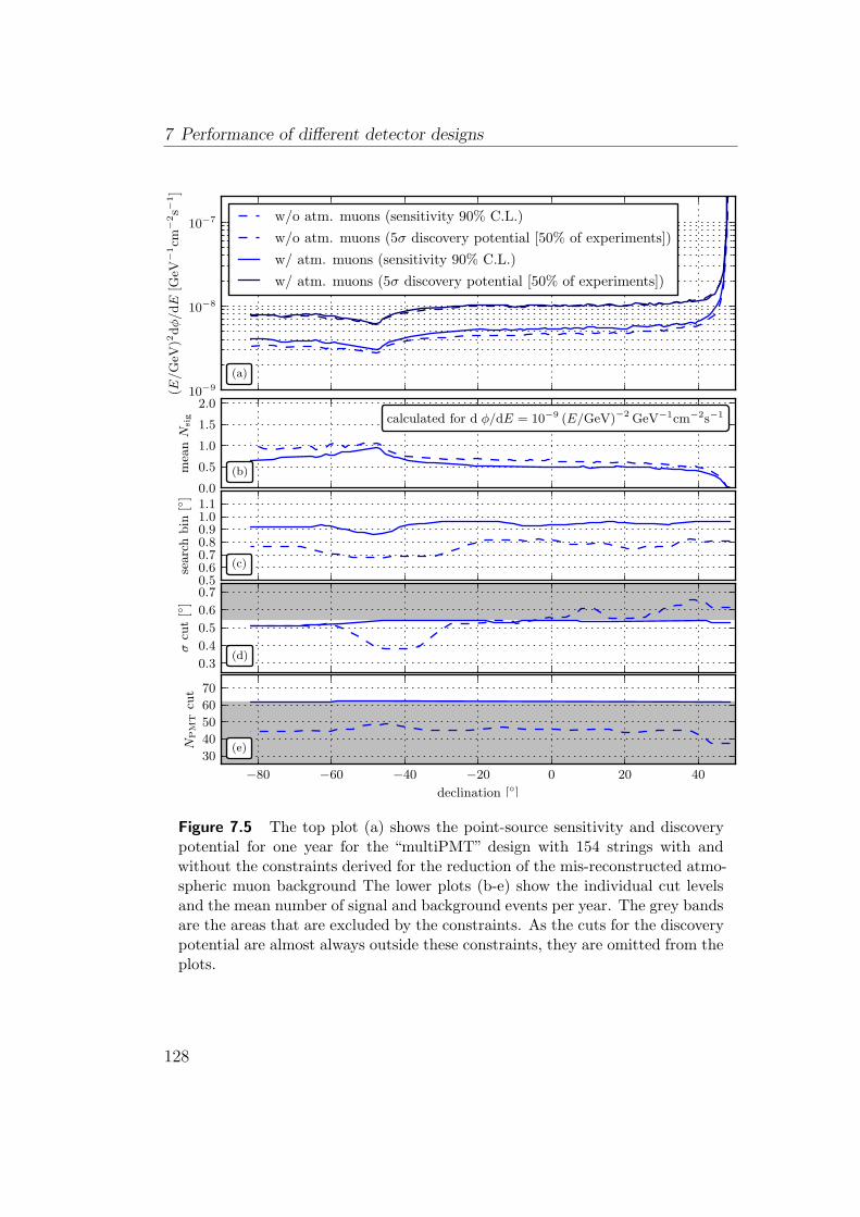
7 Performance of different detector designs
10−9
10−8
10−7
(E/G
eV)2
dφ/dE
[GeV−
1cm−
2s−
1]
(a)
w/o atm. muons (sensitivity 90% C.L.)w/o atm. muons (5σ discovery potential [50% of experiments])w/ atm. muons (sensitivity 90% C.L.)w/ atm. muons (5σ discovery potential [50% of experiments])
0.0
0.5
1.0
1.5
2.0
mea
nN
sig calculated for d φ/dE = 10−9 (E/GeV)−2 GeV−1cm−2s−1
(b)
0.50.60.70.80.91.01.1
searc
hb
in[
]
(c)
0.3
0.4
0.5
0.6
0.7
σcu
t[
]
(d)
−80 −60 −40 −20 0 20 40
declination []
30
40
50
60
70
NP
MT
cut
(e)
Figure 7.5 The top plot (a) shows the point-source sensitivity and discoverypotential for one year for the “multiPMT” design with 154 strings with andwithout the constraints derived for the reduction of the mis-reconstructed atmo-spheric muon background The lower plots (b-e) show the individual cut levelsand the mean number of signal and background events per year. The grey bandsare the areas that are excluded by the constraints. As the cuts for the discoverypotential are almost always outside these constraints, they are omitted from theplots.
128

8 Scaling of the multiPMT design
Two is not equal to three -not even for very largevalues of two.
(Grabel’s Law)
The remainder of this work shall focus on the “multiPMT” detector design andexplore the effects of varying the number of string and the inter-string distance.
8.1 Doubling the number of strings
An interesting question to ask is: how does the sensitivity of a detector behave whenincreasing the number of strings? This section will explore part of this question bylooking at the effects of doubling the number of strings of the previous detector designfrom 154 strings to 308 (or 310) strings. When not changing the layout of each singlestring and keeping the string distance constant, the number of strings can be doubledin two ways. One possibility is to simply build two identical detectors at two separatesites, so that the chance of observing the same event in two detectors becomesnegligible. In this case, no new simulation is necessary to determine the sensitivityor discovery potential as the detectors are fully independent. The observed numbersof background and signal events can simply be doubled. The other possibility is tobuild a single, larger detector with twice the number of strings. Such a detector hasbeen simulated, however with 310 instead of 308 strings. The reason for this is thata hexagonal seafloor string layout is only possible with 310 strings and not with 308.The systematical error introduced by this is negligible.
Figures 8.1 and 8.2 shows the E−2 point-source sensitivities and discovery poten-tials for both cases, respectively. For the chosen benchmark flux, there is almostno difference between a single, large or two smaller detectors. When looking at thediscovery potential for a E−2 point-source flux, it even seems to be better to buildtwo smaller detectors. Note that the atmospheric muon constraints derived in sec-tion 7.4 have been imposed on the sensitivity and discovery potential calculations.Also note that the NPMT cut derived for the 154-string detector is assumed to alsobe valid for the 310-string version, as, unfortunately, a new atmospheric muon simu-
129

8 Scaling of the multiPMT design
10−9
10−8
(E/G
eV)2
dφ/dE
[GeV−
1cm−
2s−
1]
(a)
1x154 strings2x154 strings1x310 strings
0.00.51.01.52.0
〈Nsi
g〉
(b)
0.00.20.40.60.8
〈Nbkg〉
(c)
0.50.60.70.80.91.0
sear
chbi
n[
]
(d)
0.460.480.500.520.540.56
σcu
t[
]
(e)
−80 −60 −40 −20 0 20 40
declination []
55
60
65
70
75
NP
MT
cut
(f)
Figure 8.1 Point-source sensitivity (90% C.L.) for one year for the“multiPMT”design with 154 strings, 2x154 strings and 310 strings. The top plot (a) showsthe final detectable/excludable fluxes, whereas the lower plots (b-f) show theindividual cut levels and the mean number of signal and background events peryear. The grey bands represent the atmospheric muon constraints imposed onthe cut levels.
130

8.1 Doubling the number of strings
10−8
(E/G
eV)2
dφ/dE
[GeV−
1cm−
2s−
1]
(a)
1x154 strings2x154 strings1x310 strings
0.00.51.01.52.0
〈Nsi
g〉
(b)
0.00.20.40.60.8
〈Nbkg〉
(c)
0.3
0.4
0.5
0.6
0.7
sear
chbi
n[
]
(d)
0.250.300.350.400.450.500.55
σcu
t[
]
(e)
−80 −60 −40 −20 0 20 40
declination []
60708090
100110120
NP
MT
cut
(f)
Figure 8.2 Point-source 5σ discovery potential for 50% of experiments in oneyear for the “multiPMT” design with 154 strings, 2x154 strings and 310 strings.The top plot (a) shows the final detectable/excludable fluxes, whereas the lowerplots (b-f) show the individual cut levels and the mean number of signal andbackground events per year. The grey bands represent the atmospheric muonconstraints imposed on the cut levels.
131

8 Scaling of the multiPMT design
lation could not be performed for this detector type due to the required generationtime.1
This is, however, an effect of the unbroken E−2 benchmark spectrum. Here, veryhigh energy neutrinos play an important role. As the generated muons have very longtracks, the“effective”volume for such tracks is larger when building two independentdetectors. In a way, at very high energies, the detector becomes “surface”-dominatedinstead of “volume”-dominated. Thus, when introducing an energy cutoff Ecut intothe benchmark spectrum, the single, large detector should perform better startingat a certain cutoff. This is shown in figure 8.3(b). The benchmark spectrum waschanged to include a cutoff term to look like
dφνµ
dE:= 10−8
(E
GeV
)−2
exp
(−√
E
Ecut
)GeV−1cm−2s−1. (8.1)
Example spectra are shown in figure 8.3(a). Note that no neutrinos were simulatedabove Eν = 107 GeV, which also represents a hard cutoff. This energy region ismarked with a grey background in figure 8.3(a). When varying Ecut, it can be seenthat a single, large detector starts to yield better sensitivities for Ecut . 107 GeV.For Ecut . 105 GeV, the discovery potential obtained for a single, large detectorbecomes better than the one for two smaller detectors, as well.
This result raises an important issue when optimising detector designs for pureE−2 point-source fluxes. Real neutrino sources will always have an energy cutoffat a certain point, so that a single-minded optimisation for this benchmark sourcespectrum may yield a different optimal detector design than what would be obtainedfor more realistic spectra. When building a neutrino detector, it will always be moresuited to one type of spectrum than to another. The expected spectra from Galacticsources, e.g. SNRs, show lower cutoffs, while the spectra from extragalactic sourceslike GRBs have higher ones. It is thus important not only to optimise for one extremecase, like a pure E−2 spectrum, and to keep in mind that other source spectra shouldbe detectable after a practical amount of observation time, too.
1In the rather “flat” detector designs looked at here, with heights of 570 m compared todiameters of over 1 km, downgoing, low-energy muons should only hit a low number ofstrings, anyway. This number will not change significantly when adding more stringswhile leaving the detector height constant.
132

8.1 Doubling the number of strings
101 102 103 104 105 106 107 108 109
neutrino Energy E [GeV]
10−30
10−28
10−26
10−24
10−22
10−20
10−18
10−16
10−14
10−12
10−10
10−8
dφ/dE
[GeV−
1cm−
2s−
1]
dφdE
:= 10−8(E
GeV
)−2exp
(−√
EEcut
)GeV−1cm−2s−1
Ecut =∞Ecut = 109 GeV
Ecut = 108 GeV
Ecut = 107 GeV
Ecut = 106 GeV
Ecut = 105 GeV
Ecut = 104 GeV
(a) E−2 fluxes with energy cutoffs
10−1
100
101
102
103
MR
Fan
dM
DF
@−6
0 MRF (2x154 strings)MDF (2x154 strings)MRF (1x310 strings)MDF (1x310 strings)
102 103 104 105 106 107 108
cutoff energy Ecut [GeV]
0.90
0.95
1.00
1.05
1.10
1.15
1.20
rati
o
MRF(2x154)MRF(1x310)
MDF(2x154)MDF(1x310)
(b) model discovery and rejection factors vs. Ecut
Figure 8.3 Behaviour of the sensitivity and discovery potential on an energycutoff in the source neutrino flux for a source at δ ≈ −60. The upper plot (a)shows the simulated spectra used to calculate the MRF and MDF values shownin (b).
133
8 Scaling of the multiPMT design
8.2 Effects of varying string distances
In this section, the effects of increasing the string distance from 91 m to largerdistances is explored for a “multiPMT” detector with 310 strings. For historicalreasons, these distances were chosen to be 100 m, 130 m and 150 m. As before,for each of these distances, the angular resolution and effective areas have beendetermined using cut values from a sensitivity optimisation to an E−2 point-sourceflux. The atmospheric muon cuts derived in section 7.4 are also used for thesecalculations.
8.2.1 Angular resolution
The angular reconstruction errors for each of the simulated detectors is shown in fig-ure 8.4. Not surprisingly, the median angular error get slightly worse with increasingstring distance, starting at 0.28 for 91 m up to 0.35 for 150 m string distance. Thelower amount of light reaching the OMs in a less dense detector and the increasedtiming error for long photon paths introduce a higher uncertainty when reconstruct-ing a muon track.
8.2.2 Effective area
Comparing the effective areas obtained for the four different distances, the expectedbehaviour can be observed: at low energies, short string distances are advantageous,because muon tracks will be short and do not emit a large amount of light. Incontrast, at higher energies, the amount of light produced by a muon track will beenough to illuminate a sufficient amount of optical modules, even if they are faraway from a light source. Hence, the string spacing does not have to be as small asfor low energies.
The effective areas plotted against neutrino energy seen in figure 8.5 show exactlythis behaviour. At about Eν ≈ 2 · 104 GeV, the effective area is independent fromthe string spacing. For lower energies, smaller string distances are favourable, abovethis point, higher string distances yield better effective areas. The objective is tofind a string distance that finds the best balances between both.
8.2.3 Point-source sensitivity
Detectors with large string distances seem to be better suited for the detection of anE−2 point-source flux, as can be seen in figures 8.6 and 8.7. Especially at declina-tions where near-horizontal high-energy neutrinos play a larger role, the sensitivitybecomes better when the string distance is increased. At declinations near −90, cor-responding to up-going tracks where extremely high-energy neutrinos are absorbedby the Earth, these differences are less pronounced.
134

8.2 Effects of varying string distances
log10(ΨMC[])02468
101214
even
tspe
rye
aran
dbi
n
dstring = 91 m
no cut (all upgoing, reconstructed) [median = 1.11]cuts for best E−2 sensitivity: σpara < 0.55, NPMT ≥ 62 [median = 0.28]quality cut only to reach same resolution: σpara < 0.29 [median = 0.28]∫
dΨMC
219.3
74.6
93.0
log10(ΨMC[])02468
101214
even
tspe
rye
aran
dbi
n
dstring = 100 m
no cut (all upgoing, reconstructed) [median = 1.40]cuts for best E−2 sensitivity: σpara < 0.55, NPMT ≥ 62 [median = 0.31]quality cut only to reach same resolution: σpara < 0.33 [median = 0.31]∫
dΨMC
243.2
76.8
102.9
log10(ΨMC[])02468
101214
even
tspe
rye
aran
dbi
n
dstring = 130 m
no cut (all upgoing, reconstructed) [median = 3.50]cuts for best E−2 sensitivity: σpara < 0.55, NPMT ≥ 62 [median = 0.33]quality cut only to reach same resolution: σpara < 0.31 [median = 0.33]∫
dΨMC
319.2
79.6
104.2
−2 −1 0 1 2log10(ΨMC[])
02468
101214
even
tspe
rye
aran
dbi
n
dstring = 150 m
no cut (all upgoing, reconstructed) [median = 5.36]cuts for best E−2 sensitivity: σpara < 0.55, NPMT ≥ 62 [median = 0.35]quality cut only to reach same resolution: σpara < 0.30 [median = 0.35]∫
dΨMC
367.7
84.2
104.3
Figure 8.4 Distribution of angular reconstruction errors w.r.t. the muon direc-tion for four 310-string“multiPMT”-type detectors with varying string distances.The subplot contents are analogous to the plots shown on the previous pages.
135

8 Scaling of the multiPMT design
10−4
10−3
10−2
10−1
100
101
102
103
area
[m2] Nhit,reco ≥ 6 [string dist. 91m]
σpara < 0.55, NPMT ≥ 62
σpara < 0.29 (same 〈Ψ〉 ≈ 0.28)Nhit,reco ≥ 6 [string dist. 100m]
σpara < 0.55, NPMT ≥ 62
σpara < 0.33 (same 〈Ψ〉 ≈ 0.31)
trig.: 2T3 [91m]
trig.: 2T3 [100m]
10−4
10−3
10−2
10−1
100
101
102
103
area
[m2] Nhit,reco ≥ 6 [string dist. 130m]
σpara < 0.55, NPMT ≥ 62
σpara < 0.31 (same 〈Ψ〉 ≈ 0.33)Nhit,reco ≥ 6 [string dist. 150m]
σpara < 0.55, NPMT ≥ 62
σpara < 0.30 (same 〈Ψ〉 ≈ 0.35)
trig.: 2T3 [130m]
trig.: 2T3 [150m]
1.01.52.0
rati
o
0.51.01.5
rati
o
0.51.01.5
rati
o
0.0
0.5
1.0
rati
o
0.0
0.5
1.0
rati
o
0.0
0.5
1.0
rati
o
103 104 105 106
neutrino energy [GeV]
0.0
0.5
1.0
rati
o
Figure 8.5 Effective area for 310-string “multiPMT” detectors with four differ-ent string distances. The subplot contents are analogous to the plots shown onthe previous pages.
136

8.2 Effects of varying string distances
10−9
10−8
(E/G
eV)2
dφ/dE
[GeV−
1cm−
2s−
1]
(a)
dstring = 91 m
dstring = 100 m
dstring = 130 m
dstring = 150 m
0.00.51.01.52.0
〈Nsi
g〉
(b)
0.00.51.01.5
〈Nbkg〉
(c)
0.5
0.6
0.7
0.8
0.9
1.0
sear
chbi
n[
]
(d)
0.440.460.480.500.520.540.56
σcu
t[
]
(e)
−80 −60 −40 −20 0 20 40
declination []
60
65
70
75
80
NP
MT
cut
(f)
Figure 8.6 Point-source sensitivity (90% C.L.) for one year for the“multiPMT”designs with 310 strings and four different string distances. The subplot contentsare analogous to the plots shown on the previous pages.
137

8 Scaling of the multiPMT design
10−9
10−8
(E/G
eV)2
dφ/dE
[GeV−
1cm−
2s−
1]
(a)
dstring = 91 m
dstring = 100 m
dstring = 130 m
dstring = 150 m
0.00.51.01.52.0
〈Nsi
g〉
(b)
0.000.050.100.150.200.25
〈Nbkg〉
(c)
0.40.50.60.70.80.91.0
sear
chbi
n[
]
(d)
0.35
0.40
0.45
0.50
0.55
σcu
t[
]
(e)
−80 −60 −40 −20 0 20 40
declination []
60708090
100110120130
NP
MT
cut
(f)
Figure 8.7 5σ Point-source discovery potential (50% of exp.) for one year forthe“multiPMT”designs with 310 strings and four different string distances. Thesubplot contents are analogous to the plots shown on the previous pages.
138

8.2 Effects of varying string distances
8.2.4 Discovery potential for SNR RX J1713.7–3946
In order to not only optimise to an artificial E−2 benchmark flux, but to a realobject with a predicted neutrino spectrum, the SNR RX J1713.7–3946 at declinationδ = −39.46, shall be considered.
The assumed neutrino flux, based on observations in TeV-γ-rays, taken from [27],using updated values [116], is
dφνµ
dE:= k
(E
TeV
)−γexp
(−√E
ε
), (8.2)
with
k := 16.80 · 10−12TeV−1cm−2s−1 (8.3)γ := 1.78 (8.4)ε := 2.10 TeV. (8.5)
RX J1713 is an extended source, so this fact had to be incorporated into the sim-ulation. As an approximation, all neutrino source directions have been uniformlysmeared on a disc with radius 0.65, centred on the given source location.
With this spectrum, the time to reach an MDF of 1.0 has been determined foreach of the four available string distances. At that time, the source will have beendetected in 50% of the experiments with a significance of 5σ. The sensitivity and dis-covery potential optimisations were done using the “low-energy” atmospheric muonconstraints presented in section 7.4, because for this source, very high energy neutri-nos are unlikely because of its spectrum’s rather low cutoff.
Figure 8.8 shows the MDF as a function of time. When compared to the previousresults for the E−2 benchmark flux, the behaviour is reversed again: detectors withsmaller string distances will detect the predicted flux earlier. This, however, isexpected for sources with an energy cutoff, as already explained in section 8.1. Thetime until detection/rejection is summarised in table 8.1, which also includes themean signal and background event numbers at the detection time.
Unfortunately, the time until a detection on the 5σ level is possible is quite long,over 14 years for any of the detector designs. Be reminded, however, that the trackreconstruction algorithm used to get to these results is by no means fully optimised.These results, like all before them, should be regarded as worst-case scenarios.
139

8 Scaling of the multiPMT design
0 10 20 30 40 50 60 70 80
number of years
10−1
100
101
MR
For
MD
F
dstring = 91 m (MDF)
dstring = 91 m (MRF)
dstring = 100 m (MDF)
dstring = 100 m (MRF)
dstring = 130 m (MDF)
dstring = 130 m (MRF)
dstring = 150 m (MDF)
dstring = 150 m (MRF)
Figure 8.8 MDF and MRF for a predicted neutrino flux from the SNR RXJ1713.7–3946 versus observation time.
sensitivity (90% C.L.) 5σ discovery (50% of exp.)string distance time nsig nbkg time nsig nbkg
91 m 2.5 yr 5.14 4.72 14.5 yr 25.96 19.01100 m 3.0 yr 5.78 5.03 15.0 yr 26.35 19.57130 m 3.5 yr 5.01 4.37 20.0 yr 25.99 19.00150 m 4.0 yr 4.79 3.86 22.5 yr 23.52 15.28
Table 8.1 Observation time necessary to reach an MRF or MDF of one for theSNR RX J1713.7–3946. This time is the time necessary to exclude the sourcewith a C.L. of 90% or to detect it with 5σ in 50% of experiments, respectively.Additionally, the mean number of observed signal and background events isgiven.
140

Summary and conclusions
The aim of this thesis was to study the performance of different detector design pos-sibilities for the KM3NeT telescope, with the focus on a new design using multiplephotomultiplier tubes within a single spherical optical module (the “multiPMT” de-sign). For that purpose, a new Monte Carlo simulation chain was developed withina software framework (IceTray). This chain was then used to perform all simulationwork.
The necessary software tools have been implemented as a mixture of freshly cre-ated and pre-existing code. The pre-existing code consists of the neutrino eventgenerator ANIS and the lepton propagator MMC, originally developed for IceCube.Due to their good design and the use of a software framework, these tools could eas-ily be re-purposed for KM3NeT. Amongst the algorithms implemented specificallyfor this work are a full muon and Cherenkov photon propagation algorithm basedon Geant4, including a new way to store photon tables for a fast, detailed simula-tion of light scattering in water. For the “multiPMT” design, a new photomultiplier,readout and electronics simulation has been developed. Additionally, auxiliary codefrom the original ANTARES software was integrated into the IceTray frameworkwhere necessary.
This new toolchain has been compared to the original ANTARES toolchain, re-vealing minor differences at very high energies. These were attributed to the eventgeneration process at the detector site, i.e. differences between the ANIS generatorpackage and the corresponding tool within the ANTARES toolset, genhen. Otherthan that, no major differences were observed; the two chains yield compatible re-sults.
The new software chain has then been used to simulate three different hypotheticalKM3NeT detectors, starting with small volumes of only about 0.5 km3. Each of thesedetectors was built according to one of the three possible design options that werediscussed for KM3NeT when this thesis was written:2
• An ANTARES-like“string”design, with triplets of optical modules per floor on154 strings. Each string contains 20 floors. The floor spacing is 30 m, the stringspacing is 91 m with strings on a hexagonal grid. This design uses the sameoptical module design as the ANTARES detector, a single photomultipliertube per optical module with a diameter of 9.3′′ (236.22 mm). It also uses
2Since then, the details of the design options have been slightly changed, but their basicfeatures are still retained. For example, the current “tower” design uses smaller 8” PMTsand the readout scheme has been changed to an alternative design.
141

the same readout scheme as ANTARES, an integrating two-channel on-chipdesign with an all-data-to-shore approach.
• A “tower” design that uses floors made from large metal frame bars with threepairs of optical modules mounted on them. The same optical module designand readout scheme as for the “string” design was used for this detector type.Each tower contains 20 floors with a spacing of 30 m. Because a tower floorcontains twice the number of OMs as a floor in the “string” design, the numberof towers was chosen to be 80 with a spacing of 130 m. In that way, the pho-tocathode area and average detector instrumentation density are comparable.The 80 strings are still arranged on a hexagonal grid.
• The “multiPMT” design only uses a single optical module per floor, but in-stead of placing a single, large photomultiplier inside each optical module, 31smaller PMTs are mounted inside of each one. Their diameter is approxi-mately 3′′ (76 mm). Like the “string” design, 154 strings with 20 OMs perstring are used with the same spacings as for that design. This yields approxi-mately the same photocathode area as for the other two designs. The readoutscheme used for is different from the other two. It is implemented using a time-over-threshold approach, sending a full time-binned“over-threshold”bitstreamto shore.
All data simulated for the two single-PMT designs have been reconstructed using thesame modified version of the standard ANTARES reconstruction strategy that haspreviously been used for other KM3NeT studies. This algorithm is heavily optimisedfor the single-PMT design and yields excellent angular resolutions of about 0.07
for an incoming E−2 flux. It does, however, not yield satisfactory results for the“multiPMT” design. Therefore, a dedicated algorithm, inspired by published workfrom IceCube, was developed. The new algorithm is far from being optimised andis only a first step to a full dedicated “multiPMT” reconstruction strategy. Theangular resolutions obtained for an E−2 spectrum with this design are of the orderof 0.3. It is believed that large improvements to this value are possible by refiningthe reconstruction algorithm.
In terms of neutrino effective area after reconstruction and applying cuts optimisedfor E−2 point-source flux sensitivity, it is the “string” design that does perform best.Both, the “tower” and the “multiPMT” design have worse effective areas, with theexception of the highest energies above 106 GeV, where all designs perform similarly.For the “tower” design, this can be explained with the lesser number of verticalstructures, effectively leading to a less dense detector in terms of strings per seafloorarea. However, it may very well be that the total deployment cost per optical moduleis cheaper for the “tower” design, thus allowing to use more than the 80 towers thatwere simulated. This would bring the “tower” design on par with the “string” one.
142

For the “multiPMT” design, the worse effective area can be accounted for throughthe non-refined track reconstruction strategy. With its angular resolution being afactor four worse than for the other two designs, much harder cuts have to be usedto optimise for E−2 point-source flux sensitivity. Especially for this design, largeimprovements are to be expected after refinement of the reconstruction algorithm.All results presented for this design should thus be seen as worst-case scenarios.3
Comparing the E−2 point-source flux sensitivities and discovery potentials yieldsthe same behaviour as for the effective areas: the “string” design performs best,followed closely by the “tower” design. Despite the lower effective area and worseangular resolution, the “multiPMT” design performs fairly good when comparedto the other two designs. During these and all following sensitivity and discoverypotential calculations, cuts an the reconstruction quality parameters and on thenumber of PMTs with at least one hit were used. The latter one is a crude energycut that had to be used in the absence of a dedicated energy reconstruction algorithmfor KM3NeT.
From this point on, the focus was on the “multiPMT” design. This design possi-bility has not been studied before as much as the others, especially due to the factthat no satisfactory track reconstruction algorithm existed up to now.
Up to this point, the only background flux used for the sensitivity calculationswas the one of atmospheric neutrinos. The reason for this is the immense com-putational time needed to simulate an atmospheric muon flux with the necessarystatistics. Using a small sample of atmospheric muon background events, simulatedfor the “multiPMT” design, the effect of these events on the point-source sensitiv-ity and discovery potential has been studied by extrapolating constraints on theenergy cut level for different quality cut levels. The imposed requirement was toreduce the atmospheric muon background to 10% of the atmospheric neutrino back-ground. These constraints have a visible impact on the point-source flux sensitivity,but hardly change the discovery potential. This is because the discovery potentialcut optimisation already yields optimal cut levels that fulfil the atmospheric muonconstraints. The constraints derived for this detector type were then used for all thefollowing results.
Scaling of the “multiPMT” detector from its initial number of strings (154) todouble its size was examined. This was done in two different ways: the performanceof having two identical smaller detectors at different sites was compared to a sin-gle, large detector. This larger detector, was chosen to consist of 310 strings on ahexagonal seafloor grid. The string design was kept unchanged. For an E−2 fluxwithout a cutoff, two smaller detectors yield better point-source sensitivity. When,however, introducing a cutoff into the spectrum, the single large detector performsbetter. This is because of neutrinos with very high energies Eν & 106 GeV, produc-
3This is of course also true for the other designs, but the improvements will probably beless for them.
143

ing high-energy muons with very long track lengths. For them, the smaller detectordesign is still surface-dominated. As spectrum cutoffs are expected for almost allsources, building a single large detector seems to be the favourable choice.
Keeping the string number constant at a value of 310, the effects of varying thestring distance and thus the detector density was studied. In addition to the stringdistance of 91 m that was used before, three new detectors with string distances of100 m, 130 m and 150 m were considered. All other parameters were kept unchanged.For an unbroken E−2 flux, the 150 m detector turns out to be optimal in terms ofsensitivity and discovery potential, especially at track directions near the horizonwhere neutrino absorption in the Earth at the highest energies does not play a largerole yet.
Injecting the neutrino spectrum predicted for a known TeV-γ-ray source yieldsdifferent results. The chosen spectrum was for the supernova remnant RXJ1713.7-3946 under the assumption of hadronic acceleration. Due to its spectrum’s energycutoff, the two detectors with smaller string distances (91 m and 100 m) yield bettersensitivities and discovery potentials. With one of these detectors, a 5σ detectionof the source would be possible after 15 years. Keep in mind, however, that theseresults were obtained using a non-optimised reconstruction algorithm and with onlya crude cut on energy. Additionally, improvements are to be expected by using anunbinned analysis technique instead of the binned one used in this work. During thelast phase of this work, it became clear that detectors with even more strings werea serious possibility. The currently discussed possibilities are detectors with over600 strings. Taking all these points into account, KM3NeT has a very good chanceto detect Galactic neutrino sources. A detector with a string distance of about100 m should also be able to detect extragalactic sources with higher energy cutoffsand harder spectra. Taking into account higher neutrino energies, the differencesbetween a detector with this string distance and the ones with larger distances arenot too pronounced. Of course, there is also the possibility of neutrino sources wherethe emitted γ-rays are heavily absorbed within the source itself. Should they exist,their discovery would present an important step forward in neutrino and cosmic rayastronomy.
Building the KM3NeT neutrino telescope presents an important opportunity forthe whole field of astroparticle physics, including many aspects that were not eventouched in this thesis. Having a complementary neutrino telescope to IceCube onthe Northern Hemisphere and a more sensitive instrument at the same time willcertainly lead to a lot of exciting discoveries. Most of them will probably be entirelyunexpected.
144

Zusammenfassung und Ausblick
Ziel dieser Arbeit war es, die Effizienz verschiedener Design-Optionen fur das Neu-trinoteleskop der nachsten Generation im Mittelmeer, ”KM3NeT“, zu untersuchen.Der Fokus lag dabei auf einem neuen Design, bei welchem mehrere Photomultiplierinnerhalb eines optischen Moduls angebracht sind (dem sog. ”MultiPMT“-Design).Zu diesem Zweck wurde eine neue Monte Carlo-Simulationskette innerhalb einesSoftware-Frameworks (”IceTray“) entwickelt. Mittels dieser Kette wurden dann alleSimulationen durchgefuhrt.
Die benotigte Software wurde als eine Mischung aus neu entwickeltem und be-reits vorhandenem Code implementiert. Der bereits existierende Code besteht ausdem Neutrino-Ereignisgenerator ANIS und dem Lepton-Propagator MMC. BeideWerkzeuge wurden ursprunglich fur IceCube entwickelt. Aufgrund ihres guten De-signs und durch die Benutzung eines Software-Framworks konnten sie sehr leichtfur KM3NeT verwendet werden. Speziell fur diese Arbeit wurde eine vollstandigeMyon- und Cherenkov-Photonen-Simulation auf Basis von Geant4 implementiert.Diese beinhaltet einen neuen Algorithmus zur Speicherung von Photonentabellen zurschnellen und detaillierten Simulation von Streuung in Wasser. Fur das ”MultiPMT“-Design wurde ein neuer Algorithmus zur Simulation der Photomultiplier und derAusleseelektronik entwickelt. Falls erforderlich, wurde Code aus der Software desbestehenden Neutrino-Detektors ANTARES in das IceTray-Framework integriert.
Diese neue Simulationskette wurde mit der bestehenden ANTARES-Simulations-kette verglichen, wobei kleine Unterschiede bei sehr hohen Energien festgestellt wur-den. Diese lassen sich auf Unterschiede zwischen dem Ereignisgenerator ANIS unddem entsprechenden Tool aus der ANTARES-Simulationskette (”genhen“) zuruck-fuhren. Weiterhin wurden keine bedeutenden Unterschiede festgestellt; beide Simu-lationsketten liefern vergleichbare Ergebnisse.
Mittels der neuen Simulationskette wurden nun drei verschiedene hypothetischeKM3NeT-Detektoren simuliert, wobei anfangs ein relativ kleines Volumen von 0.5 km3
gewahlt wurde. Jeder dieser Detektoren entspricht einer der drei moglichen Design-Optionen, die wahrend der Anfertigung dieser Arbeit diskutiert wurden:4
• Das ”String“-Design basiert weitgehend auf der Konstruktion des bisherigenANTARES-Detektors. Auf jedem Stockwerk befinden sich drei, um 45 vonder Horizontalen nach unten geneigte, optische Module. Jeweils 20 von diesen
4Seitdem haben sich die Parameter dieser Optionen leicht geandert, ihre grundlegendenEigenschaften blieben aber unverandert. So wurde zum Beispiel beim ”Tower“-Designdie Große der Photomultiplier auf 8 Zoll angepasst und die Auslesemethode verandert.
145

Stockwerken mit einem Abstand von 30 m bilden einen vertikalen ”String“.Der gesamte Detektor besteht aus 154 dieser Strings, welche im Abstand von91 m auf einem hexagonalen Gitter angeordnet sind. Der Aufbau der opti-schen Module entspricht dem des ANTARES-Detektors, d.h. einem einzelnenPhotomultiplier mit 9.3′′ (236.22 mm) Durchmesser pro Modul. Auch die Aus-leseelektronik ist analog zum ANTARES-Detektor simuliert: Das gemesseneSignal wird auf einem zwei-kanaligen Chip integriert und zur Kustenstationgeschickt, wo es weiter verarbeitet wird.
• Beim ”Tower“-Design bestehen die Detektor-Stockwerke aus großen Metall-gerust-Balken, an deren Enden und Mitte jeweils Paare von optischen Mo-dulen angebracht sind. Fur diesen Detektor-Typ wurde in der Simulation diegleiche Auslese-Elektronik wie fur das ”String“-Design simuliert. Jeder ”Tower“besteht aus 20 Stockwerken in einem Abstand von jeweils 30 m. Da jedesStockwerk, verglichen mit dem vorhergehenden Design, die doppelte Anzahlvon optischen Modulen besitzt, besteht der simulierte Detektor nur aus 80dieser Einheiten. Diese haben einen horizontalen Abstand von 130 m, wieder-um angeordnet auf einem hexagonalen Gitter. Dadurch bleiben die Photoka-thodenflache und die mittlere Instrumentierungsdichte der beiden Detektorenvergleichbar.
• Das ”MultiPMT“-Design besteht aus nur einem optischen Modul pro Stock-werk, welches nun allerdings 31 kleinere Photomultiplier mit Durchmessernvon 3′′ (76 mm) enthalt. Wie beim ”String“-Design besteht der Detektor aus154 Strings mit jeweils 20 Stockwerken pro String. Dadurch erhalt man in et-wa die gleiche Photokathodenflache wie bei den beiden anderen Designs. DieAusleseelektronik ist hier mittels eines ”Time-over-threshold“-Ansatzes imple-mentiert, wobei ein durchgehender, zeitlich unterteilter Bit-Strom zur Kusten-station gesendet wird.
Alle simulierten Daten fur die beiden erstgenannten Designs wurden mittels dessel-ben Algorithmus rekonstruiert, der auch bereits zuvor fur eine Vielzahl von KM3NeT-Studien verwendet wurde. Es handelt sich hierbei um eine leicht modifizierte Versiondes Standard-ANTARES-Rekonstruktionsalgorithmus. Da dieser stark auf Detekto-ren optimiert ist, die denselben optischen Modul-Typ wie ANTARES verwenden,ergeben sich sehr gute Winkelauflosungen von ca. 0.07 fur das rekonstruierte My-on bei einem simulierten E−2-Fluss. Fur das ”MultiPMT“-Design hingegen wurdendamit keine zufriedenstellenden Ergebnisse erzielt. Daher wurde eigens hierfur einRekonstruktions-Algorithmus entwickelt, der auf veroffentlichten Beschreibungen ei-nes IceCube-Algorithmus basiert. Dieser neue Algorithmus ist noch nicht optimiertund daher nur als erster Schritt zu einer vollstandigen ”MultiPMT“-Rekonstruktionanzusehen. Die erreichte Winkelauflosung fur Myonen fur einen E−2-Fluss bewegt
146

sich um 0.3. Dieser Wert sollte sich durch Weiterentwicklung des Rekonstruktions-Algorithmus stark verbessern lassen.
Betrachtet man die effektiven Flachen fur Neutrinos nach der Spurrekonstruktionund optimiert die Qualitatsschnitte auf bestmogliche Punktquellen-Sensitivitat fureinen angenommenen E−2-Fluss, so schneidet der ”String“-Detektor am Besten ab.Sieht man vom Energiebereich uber 106 GeV ab, so sind die effektive Flachen deranderen beiden Detektoren etwas kleiner. Dies kann beim ”Tower“-Design mit dergeringeren Anzahl an vertikalen Strukturen erklart werden, welche zu einer kleine-ren Dichte, bezogen auf ”Strings pro Meeresbodenflache“, fuhrt. Allerdings ist esgut moglich, dass die Gesamtkosten pro optischem Modul einschließlich der Auf-baukosten fur das ”Tower“-Design kleiner sind, so dass in diesem Fall mehr als diesimulierten 80 Strings benutzt werden konnten.
Beim ”MultiPMT“-Design kann man die kleinere effektive Flache mit dem nochnicht vollstandig optimierten Spurrekonstruktions-Algorithmus erklaren. Aufgrundder um einen Faktor vier schlechteren Winkelauflosung im Vergleich zu den anderenbeiden Designs, fuhrt eine Optimierung auf Punktquellen-Sensitivitat zu sehr vielharteren Schnitten. Es ist daher insbesondere bei diesem Design mit großen Verbesse-rungen in der Rekonstruktionseffizienz nach einer Optimierung des Rekonstruktions-Algorithmus zu rechnen.5
Betrachtet man die Sensitivitaten und Entdeckungspotentiale fur Punktquellenmit einem E−2-Fluss, so ergibt sich dasselbe Bild: Das ”String“-Design schneidetknapp vor dem ”Tower“-Design am Besten ab. Trotzdem sind die Ergebnisse auch furdas ”MultiPMT“-Design relativ gut. Fur diese und alle folgenden Berechnungen wur-den Schnitte auf die Rekonstruktions-Qualitat und auf die Energie des den Detektordurchquerenden Teilchens angewendet. Da kein geeigneter Energierekonstruktions-Algorithmus zur Verfugung stand, wurde der Energieschnitt auf die Anzahl der Pho-tomultiplier mit mindestens einem Treffer gelegt, einer Wert, der grob mit der Ener-gie des Teilchens korreliert ist.
Von nun an lag der Fokus der Arbeit auf dem ”MultiPMT“-Design. Dieses wurdein vorhergehenden Arbeiten nicht in derselben Ausfuhrlichkeit untersucht wie diebeiden anderen Designs, was zum großen Teil auf das Fehlen einer leistungsfahigenSpurrekonstruktion zuruckzufuhren sein durfte.
In den bisherigen Betrachtungen bestand der simulierte Untergrund einzig ausatmospharischen Neutrinos; falschlicherweise als nach oben laufend rekonstruier-te atmospharische Myonen wurden vernachlassigt. Der Grund hierfur liegt in derimmensen Rechenzeit, die benotigt wird, um ausreichende Statistik zu generieren.Die Auswirkungen auf Punktquellen-Sensitivitaten wurden daher aus einer kleine-ren Menge an simulierten Ereignissen extrapoliert. Die sich ergebenden Einschran-
5Naturlich lassen sich die Ergebnisse auch fur die anderen beiden Detektor-Designs durchOptimierung des Rekonstruktions-Algorithmus verbessern, allerdings ist zu erwarten,dass die Verbesserungen fur diese kleiner ausfallen.
147

kungen an die Qualitats- und Energie-Schnitte wurden so gewahlt, dass die Anzahlder Untergrundereignisse aus atmospharischen Myonen weniger als 10% der Anzahlder Ereignisse aus atmospharischen Neutrinos betragt. Die harteren Schnitte habensichtbaren Einfluss auf die Punktquellen-Sensitivitaten. Dagegen andern sich dieEntdeckungspotentiale kaum. Der Grund hierfur ist, dass die optimierten Schnittein diesem Fall schon die Einschrankungen zur Unterdruckung des atmospharischenMyon-Untergrundes erfullen. Fur alle weiteren Studien wurden nun diese Einschran-kungen an die Schnitte benutzt.
Weiterhin wurden die Auswirkungen einer Verdoppelung der Anzahl der Stringseines ”MultiPMT“-Detektors untersucht. Die Effizienz eines einzelnen, großen Detek-tors wurde mit derjenigen von zwei identischen, kleineren, an verschiedenen Stellengebauten Detektoren verglichen. Der große Detektor bestand aus 310 Strings (ver-glichen mit 154 beim kleineren). Der Abstand der Strings wurde beibehalten. Furein E−2-Spektrum ergibt sich eine bessere Sensitivitat fur zwei kleine Detektoren.Fuhrt man in das simulierte Quellspektrum allerdings einen Energie-Cutoff ein, soschneidet der große Detektor besser ab. Dies lasst sich mit Neutrinos hoher Energie(Eν & 106 GeV) erklaren, welche zu sehr langen Myon-Spuren fuhren. Detektorenmit großerer Oberflache sind hier von Vorteil, was zur besseren Sensitivitat von zweikleinen Detektoren fuhrt. Da reale Quellspektren im Allgemeinen aber einen Cutoffbesitzen, ist der Bau eines großen Detektors die vorzuziehende Alternative.
Nun wurden die Auswirkungen der Anderung des String-Abstands fur Detekto-ren mit 310 Strings untersucht. Zusatzlich zum bereits betrachteten Detektor miteinem Abstand von 91 m wurden noch solche mit Abstanden von 100 m, 130 m und150 m simuliert. Fur ein E−2-Spektrum ohne Cutoff erscheint der großte Detektormit einem Abstand von 150 m als optimal in Bezug auf Sensitivitat und Entdeckungs-potential, insbesondere fur Spuren nahe dem Horizont, bei denen die Absorption vonhochstenergetischen Neutrinos in der Erde noch keine große Rolle spielt.
Simuliert man ein erwartetes Neutrino-Spektrum fur eine bekannte TeV-γ-Strahl-ungsquelle, so erhalt man abweichende Ergebnisse. Hier wurde ein erwartetes Spek-trum fur den Supernova-Uberrest RXJ1713.7-3946 benutzt. Aufgrund des Energie-Cutoffs dieses Spektrums erhalt man bessere Sensitivitaten fur Detektoren mit klei-neren String-Abstanden (91 m und 100 m). Mit einem dieser Detektoren ist eineEntdeckung der Quelle auf 5σ-Niveau nach 15 Jahren moglich. Dabei sollte aberbeachtet werden, dass dieses Ergebnis mit einer noch nicht optimalen Rekonstruk-tion und einem nur groben Energieschnitt bestimmt wurde. Zusatzlich sind Verbes-serungen durch die Benutzung einer ”ungebinnten“ Analyse (im Gegensatz zu der
”gebinnten“ Analyse, welche in dieser Arbeit verwendet wurde) zu erwarten. In derEndphase der Entstehung dieser Arbeit wurde weiterhin klar, dass der Bau von De-tektoren mit weit mehr als den bisher betrachteten 310 Strings ernsthaft in Betrachtgezogen wird. Nimmt man all diese Punkt zusammen, so ruckt die Entdeckung vongalaktischen Neutrino-Quellen mit KM3NeT in greifbare Nahe. Ein Detektor mit
148

einem String-Abstand von 100 m sollte zudem weiterhin extragalaktische Quellenmit einem hoheren Energie-Cutoff und harteren Spektren detektieren konnen. Na-turlich besteht auch die Moglichkeit fur Neutrino-Quellen, deren γ-Strahlen stark inder Quelle selbst absorbiert sind. Sollten sie existieren, so ware ihre Entdeckung einwichtiger Schritt fur die Neutrino-Astronomie und die Astronomie der kosmischenStrahlung im Allgemeinen.
Der Bau des KM3NeT-Neutrinoteleskops stellt eine einzigartige Chance fur dasgesamte Feld der Astroteilchenphysik dar und bietet Moglichkeiten, die weit uberdas in dieser Arbeit Beschriebene hinausgehen. Ein zu IceCube komplementaresNeutrinoteleskop auf der Nordhalbkugel, welches zudem noch sensitiver ist, wirdmit Sicherheit zu spannenden Entdeckungen fuhren. Die meisten davon werden wohlvollig unerwartet sein.
149


Bibliography
[1] R. Kronig and V. F. Weisskopf, editors. Wolfgang Pauli: Collected scientificpapers, volume 2. Interscience Publishers, New York, 1964. (Cited on page 15.)
[2] C. L Cowan, F Reines, F. B Harrison, et al. Detection of the Free Neutrino:A Confirmation. Science, 124:103, 1956. (Cited on page 15.)
[3] G Danby, J.-M Gaillard, K Goulianos, et al. Observation of High-EnergyNeutrino Reactions and the Existence of Two Kinds of Neutrinos. PhysicalReview Letters, 9:36, 1962. (Cited on page 16.)
[4] DONUT Collaboration, K Kodama, N Ushida, et al. Observation of tau neu-trino interactions. Physics Letters B, 504:218, 2001. (Cited on page 16.)
[5] LEP Collaborations. A Combination of Preliminary Electroweak Measure-ments and Constraints on the Standard Model. CERN Document PPE/96-183,pages 96–183, 1996. (Cited on page 16.)
[6] Q R Ahmad, R. C Allen, T. C Andersen, et al. Measurement of the Rateof νe + d → p + p + e− Interactions Produced by 8B Solar Neutrinos atthe Sudbury Neutrino Observatory. Physical Review Letters, 87:71301, 2001.(Cited on page 16.)
[7] Raymond Davis. Nobel Lecture: A half-century with solar neutrinos. Reviewsof Modern Physics, 75:985, 2003. (Cited on page 16.)
[8] M Nagano and A. A Watson. Observations and implications of the ultrahigh-energy cosmic rays. Reviews of Modern Physics, 72:689, 2000. (Cited onpage 16.)
[9] Gunter Sigl. Ultrahigh-Energy Cosmic Rays: Physics and Astrophysics atExtreme Energies. Science, 291:73, 2001. (Cited on page 16.)
[10] V F Hess. Uber Beobachtungen der durchdringenden Strahlung bei siebenFreiballonfahrten. Phys. Z., 13:1084–1091, 1912. (Cited on page 16.)
[11] Kenneth Greisen. End to the Cosmic-Ray Spectrum? Physical Review Letters,16:748, 1966. (Cited on page 17.)
151

Bibliography
[12] G. T Zatsepin and V. A Kuz’min. Upper Limit of the Spectrum of CosmicRays. ZhETF Pis ma Redaktsiiu, 4:114, 1966. (Cited on page 17.)
[13] J. W Cronin, T. K Gaisser, and S. P Swordy. Cosmic rays at the energyfrontier. Sci. Am., 276(1):32–37, 1997. (Cited on page 18.)
[14] D. J Bird, S. C Corbato, H. Y Dai, et al. The cosmic-ray energy spectrumobserved by the Fly’s Eye. Astrophys. J, 424:491, 1994. (Cited on page 18.)
[15] M. A Lawrence, R. J. O Reid, and A. A Watson. The cosmic ray energyspectrum above 4 × 10¹⁷ eV as measured by the h Park array. Journal ofPhysics G: Nuclear and Particle Physics, 17:733, 1991. (Cited on page 18.)
[16] M Nagano, M Teshima, Y Matsubara, et al. Energy spectrum of primarycosmic rays above 1017.0 eV determined from extensive air shower experimentsat Akeno. Journal of Physics G: Nuclear and Particle Physics, 18:423, 1992.(Cited on page 18.)
[17] E. S Seo, J. F Ormes, R. E Streitmatter, et al. Measurement of cosmic-rayproton and helium spectra during the 1987 solar minimum. Astrophys. J, 378:763, 1991. (Cited on page 18.)
[18] W. I Axford, E Leer, and G Skadron. The Acceleration of Cosmic Rays byShock Waves. Proceedings of the 15th International Cosmic Ray Conference,11:132, 1977. (Cited on page 17.)
[19] A. R Bell. The acceleration of cosmic rays in shock fronts. I. Royal Astronom-ical Society, 182:147, 1978. (Cited on page 17.)
[20] R. D Blandford and J. P Ostriker. Particle acceleration by astrophysical shocks.Astrophys. J, 221:L29, 1978. (Cited on page 17.)
[21] G. F Krymskii. A regular mechanism for the acceleration of charged particleson the front of a shock wave. Akademiia Nauk SSSR, 234:1306, 1977. (Citedon page 17.)
[22] John G Learned and Karl Mannheim. High-Energy Neutrino Astrophysics.Annual Reviews of Nuclear and Particle Science, 50:679, 2000. (Cited onpages 20 and 21.)
[23] Julia K Becker. High-energy neutrinos in the context of multimessenger astro-physics. Physics Reports, 458:173, 2008. (Cited on page 21.)
[24] Eli Waxman and John Bahcall. High energy neutrinos from astrophysicalsources: An upper bound. Phys. Rev. D, 59:23002, 1999. (Cited on page 22.)
152

Bibliography
[25] VERITAS Collaboration, V. A Acciari, E Aliu, et al. A connection betweenstar formation activity and cosmic rays in the starburst galaxy M82. Nature,462:770, 2009. (Cited on page 22.)
[26] Abraham Loeb and Eli Waxman. The cumulative background of high energyneutrinos from starburst galaxies. Journal of Cosmology and AstroparticlePhysics, 05:003, 2006. (Cited on page 22.)
[27] Alexander Kappes, Jim Hinton, Christian Stegmann, et al. Potential neutrinosignals from galactic gamma-ray sources. Astrophys. J, 656(2):870–878, 2007.(Cited on pages 22 and 139.)
[28] J Alvarez-Muniz and F Halzen. Possible High-Energy Neutrinos from theCosmic Accelerator RX J1713.7-3946. The Astrophysical Journal, 576:L33,2002. (Cited on page 22.)
[29] Felix A Aharonian, A. G Akhperjanian, A. R Bazer-Bachi, et al. Observationsof the Crab nebula with HESS. Astronomy and Astrophysics, 457:899, 2006.(Cited on page 22.)
[30] Felix A Aharonian, A. G Akhperjanian, A. R Bazer-Bachi, et al. First detec-tion of a VHE gamma-ray spectral maximum from a cosmic source: HESSdiscovery of the Vela X nebula. Astronomy and Astrophysics, 448:L43, 2006.(Cited on page 22.)
[31] W Bednarek. Neutrinos from the pulsar wind nebulae. Astronomy and Astro-physics, 407:1, 2003. (Cited on page 22.)
[32] Anna Balenzano, Fiorella Burgio, and Teresa Montaruli. Review of models ofgalactic sources and rate estimates in ANTARES: young supernova remnants,plerions, magnetars and microquasars. ANTARES internal note, 2004. (Citedon page 23.)
[33] C Distefano, D Guetta, Eli Waxman, et al. Neutrino Flux Predictions forKnown Galactic Microquasars. The Astrophysical Journal, 575:378, 2002.(Cited on page 23.)
[34] Felix A Aharonian, L Anchordoqui, D Khangulyan, et al. Microquasar LS5039: a TeV gamma-ray emitter and a potential TeV neutrino source. Journalof Physics: Conference Series, 39:408, 2006. (Cited on page 23.)
[35] Franck Bernard. Caracterisation des performances d’un telescope sous-marina neutrinos pour la detection du cascades contenues dans le cadre du projectANTARES. PhD thesis, Universite de la Mediterranee, 2000. (Cited onpage 27.)
153

Bibliography
[36] A Gazizov and Marek Kowalski. ANIS: High energy neutrino generator for neu-trino telescopes. Comput. Phys. Commun., 172:203, 2005. (Cited on pages 28,54, 56, and 57.)
[37] P. A Cerenkov. Visible Radiation Produced by Electrons Moving in a Mediumwith Velocities Exceeding that of Light. Physical Review, 52:378, 1937. (Citedon page 29.)
[38] Cristina Carloganu. Muon Interactions at High Energies. ANTARES internalnote, 1998. (Cited on page 30.)
[39] C. H Wiebusch. The Detection of Faint Light in Deep Underwater NeutrinoTelescopes. PhD thesis, RWTH Aachen, 1995. (Cited on pages 29 and 30.)
[40] N Palanque-Delabrouille. Light transmission in the ANTARES site Measure-ment in blue light (Analysis of Test 3’ data). ANTARES internal note, 1999.(Cited on page 31.)
[41] David J.L Bailey. The effect of the group velocity and dispersion on photon ar-rival times in the ANTARES detector. ANTARES internal note, 2001. (Citedon page 32.)
[42] Stephanie Escoffier and Anne-Sophie Cussatlegras. Correlations between biolu-minescence and environmental parameters with ANTARES data in 2003 (PSL)and 2005 (MILOM). ANTARES internal note, 2006. (Cited on page 35.)
[43] Raj Gandhi, Chris Quigg, Mary Hall Reno, et al. Neutrino interactions atultrahigh energies. Phys. Rev. D, 58:93009, 1998. (Cited on page 37.)
[44] Raj Gandhi, Chris Quigg, Mary Hall Reno, et al. Ultrahigh-energy neutrinointeractions. Astropart. Phys., 5:81, 1996. (Cited on page 37.)
[45] S Cecchini, E Korolkova, A Margiotta, et al. Atmospheric muon backgroundin the ANTARES detector. Proceedings of the 29th International Cosmic RayConference, 5, 2005. (Cited on page 36.)
[46] GD Barr, TK Gaisser, Paolo Lipari, et al. Three-dimensional calculation ofatmospheric neutrinos. Phys. Rev. D, 70(2):023006, 2004. (Cited on page 37.)
[47] G Fiorentini, VA Naumov, and FL Villante. Atmospheric neutrino flux sup-ported by recent muon experiments. Physics Letters B, 510(1-4):173–188, 2001.(Cited on page 37.)
154

Bibliography
[48] Arthur Roberts. The birth of high-energy neutrino astronomy: A personalhistory of the DUMAND project. Reviews of Modern Physics, 64:259, 1992.(Cited on page 38.)
[49] V Aynutdinov, A Avrorin, V Balkanov, et al. The BAIKAL neutrino experi-ment — Physics results and perspectives. Nucl. Instr. Meth. A, 602:14, 2009.(Cited on pages 38 and 39.)
[50] Spencer R Klein. IceCube: A Cubic Kilometer Radiation Detector. IEEETransactions on Nuclear Science, 56:1141, 2009. (Cited on pages 39, 40,and 52.)
[51] ANTARES Collaboration. Performance of the front-end electronics of theANTARES neutrino telescope. 2009. (Cited on page 41.)
[52] E Migneco, S Aiello, A Aloisio, et al. Recent achievements of the NEMOproject. Nucl. Instr. Meth. A, 588:111, 2008. (Cited on page 42.)
[53] Nestor Collaboration, E. G Anassontzis, A. E Ball, et al. Operation andperformance of the NESTOR test detector. Nucl. Instr. Meth. A, 552:420,2005. (Cited on page 42.)
[54] Nestor Collaboration, G Aggouras, E. G Anassontzis, et al. A measurement ofthe cosmic-ray muon flux with a module of the NESTOR neutrino telescope.Astropart. Phys., 23:377, 2005. (Cited on page 42.)
[55] KM3NeTConsortium. KM3NeT Conceptual Design for a Deep-Sea ResearchInfrastructure Incorporating a Very Large Volume Neutrino Telescope in theMediterranean Sea. KM3NeT CDR, 2008. (Cited on page 42.)
[56] Paul Kooijman. SeaWiet — SEnsor Architecture for a WIde Energy rangeTelescope. KM3NeT internal report, 2009. (Cited on pages 43 and 81.)
[57] Jurgen Brunner. Antares simulation tools. ANTARES internal note, 2003.(Cited on page 47.)
[58] Jurgen Brunner. General purpose data format for ANTARES simulation andreconstruction. ANTARES internal note, 1998. (Cited on page 47.)
[59] Jurgen Brunner. Updated tag list fot the new ANTARES event format.ANTARES internal note, 1999. (Cited on page 47.)
[60] F Cassol. GENDET 1.0: a program to generate detector files. ANTARESinternal note, 1999. (Cited on page 47.)
155

Bibliography
[61] Franca Cassol-Brunner. GENDET 1.2: cards and tags. ANTARES internalnote, 2000. (Cited on page 47.)
[62] David J.L Bailey. Extension of Genneu to v3r0. ANTARES internal note,2000. (Cited on page 48.)
[63] David J.L Bailey. Genhen v3r1: Further optimisation for large energy ranges.ANTARES internal note, 2000. (Cited on page 48.)
[64] David J.L Bailey. Genhen v5r1: Software Documentation. ANTARES internalnote, 2002. (Cited on page 48.)
[65] Jurgen Brunner. Event generators for ANTARES nu oscillation search.ANTARES internal note, 1998. (Cited on page 48.)
[66] Konstantin Kuzmin, Teresa Montaruli, and Igor A Sokalski. GENHEN v6r3:implementation of the Glashow resonance and of the MUSIC transport code.ANTARES internal note, 2004. (Cited on page 48.)
[67] Annalisa L’Abbate, Teresa Montaruli, and Igor A Sokalski. GENHEN v6:ANTARES neutrino generator extension to all neutrino flavors and inclusionof propagation through the Earth. ANTARES internal note, 2004. (Cited onpage 48.)
[68] G Ingelman, A Edin, and J Rathsman. LEPTO 6.5 — A Monte Carlo generatorfor deep inelastic lepton-nucleon scattering. Comput. Phys. Commun., 101:108,1997. (Cited on page 48.)
[69] Giles David Barr. The Separation of Signals and Background in a NucleonDecay Experiment. PhD thesis, University of Oxford, 1987. (Cited on page 48.)
[70] P Antonioli, C Ghetti, E. V Korolkova, et al. A three-dimensional code formuon propagation through the rock: MUSIC. Astropart. Phys., 7:357, 1997.(Cited on page 48.)
[71] Edgar V Bugaev, Igor A Sokalski, and S. I Klimushin. Simulation accuracyof long range muon propagation in medium: analysis of error sources. arXiv,hep-ph, 2000. (Cited on page 48.)
[72] Igor A Sokalski, Edgar V Bugaev, and Sergey I Klimushin. MUM: Flexibleprecise Monte Carlo algorithm for muon propagation through thick layers ofmatter. Phys. Rev. D, 64:74015, 2001. (Cited on page 48.)
[73] Paolo Lipari and Todor Stanev. Propagation of multi-TeV muons. Phys. Rev.D, 44:3543, 1991. (Cited on page 48.)
156

Bibliography
[74] David J.L Bailey. KM3 v2r1: User Guide. ANTARES internal note, 2002.(Cited on pages 48, 49, and 61.)
[75] Sergio Navas and L. F Thompson. KM3 User Guide and Reference Manual.ANTARES internal note, 1999. (Cited on page 48.)
[76] Computing Application Software Group and Networks Division. GEANT De-tector Description and Simulation Tool. CERN Program Library Long Writeup,W5013, 1993. (Cited on page 49.)
[77] A Heijboer. Track Reconstruction and Point Source Searches with ANTARES.PhD thesis, Universiteit van Amsterdam, 2004. (Cited on pages 50 and 86.)
[78] Sebastian Kuch. Design studies for the KM3NeT Neutrino Telescope. PhDthesis, Universitat Erlangen, 2007. (Cited on pages 50 and 119.)
[79] Claudio Kopper, Thomas Eberl, and Alexander Kappes. A software frameworkfor KM3NeT. Proceedings of the 31st International Cosmic Ray Conference,2009. (Cited on page 50.)
[80] T de Young. IceTray: A Software Framework for IceCube. Interna-tional Conference on Computing in High-Energy Physics and Nuclear Physics(CHEP2004), 2004. (Cited on page 52.)
[81] available from http: // www. boost. org/ . (Cited on page 52.)
[82] J A Aguilar, A Albert, F Ameli, et al. The data acquisition system for theANTARES neutrino telescope. Nucl. Instr. Meth. A, 570:107, 2007. (Cited onpage 52.)
[83] see http: // www. python. org/ . (Cited on page 52.)
[84] Ralf Auer. PhD thesis, Erlangen Centre for Astroparticle Physics (ECAP),Universitat Erlangen, 2010. In preparation. (Cited on page 53.)
[85] Felix Fehr. Systematic studies, calibration, and software development for eventreconstruction and data analysis using the ANTARES deep-sea neutrino tele-scope. PhD thesis, Erlangen Centre for Astroparticle Physics (ECAP), Univer-sitat Erlangen, 2010. (Cited on pages 53 and 54.)
[86] Friederike Schock. PhD thesis, Erlangen Centre for Astroparticle Physics(ECAP), Universitat Erlangen, 2010. In preparation. (Cited on page 53.)
[87] Jurgen Brunner. The BBfit Reconstruction algorithm. ANTARES internalnote, 2009. (Cited on page 54.)
157

Bibliography
[88] Ronald Bruijn. The Antares Neutrino Telescope: Performance Studies andAnalysis of First Data. PhD thesis, Universiteit van Amsterdam, 2008. (Citedon page 54.)
[89] D Heck, J Knapp, J. N Capdevielle, et al. CORSIKA: a Monte Carlo code tosimulate extensive air showers. CORSIKA: a Monte Carlo code to simulateextensive air showers., 1998. (Cited on pages 54 and 58.)
[90] Dmitry Chirkin and Wolfgang Rhode. Propagating leptons through matterwith Muon Monte Carlo (MMC). arXiv, 2004. (Cited on pages 54 and 59.)
[91] Geant4 Collaboration, S Agostinelli, J Allison, et al. Geant4 — a simulationtoolkit. Nucl. Instr. Meth. A, 506:250, 2003. (Cited on pages 54 and 59.)
[92] H. L Lai, J Huston, S Kuhlmann, et al. Global QCD analysis of partonstructure of the nucleon: CTEQ5 parton distributions. The European PhysicalJournal C, 12, 2000. (Cited on page 56.)
[93] R Gandhi, Chris Quigg, Mary Hall Reno, et al. Ultrahigh-energy neutrinointeractions, 1996. (Cited on pages 56 and 57.)
[94] Dmitry Chirkin. dCORSIKA update. (Cited on page 58.)
[95] DE Groom, NV Mokhov, and SI Striganov. Muon stopping power and rangetables 10 MeV-100 TeV. Atom Data Nucl Data, 78(2):183–356, 2001. (Citedon page 60.)
[96] M Ambrosio, R Antolini, G Auriemma, et al. Vertical muon intensity measuredwith MACRO at the gran sasso laboratory. Phys. Rev. D, 52(7):3793–3802,1995. (Cited on page 60.)
[97] C D Mobley. Light and Water. Radiative Transfer in Natural Waters. Aca-demic, New York, 1994. (Cited on page 62.)
[98] Jurgen Brunner. Cherenkov light from HE electromagnetic and hadronic show-ers. ANTARES internal note, 2002. (Cited on page 63.)
[99] J Lundberg, P Miocinovic, K Woschnagg, et al. Light tracking through ice andwater — Scattering and absorption in heterogeneous media with PHOTONICS.Nucl. Instr. Meth. A, 581:619, 2007. (Cited on pages 63 and 66.)
[100] M Anghinolfi, H Costantini, K Fratini, et al. New measurement of the angularacceptance of the Antares Optical Module. ANTARES internal note, 2008.(Cited on page 80.)
158

Bibliography
[101] ANTARES Collaboration, P Amram, M Anghinolfi, et al. The ANTARESoptical module. Nucl. Instr. Meth. A, 484:369, 2002. (Cited on page 80.)
[102] S-O Flyckt and Carole Marmonier. Photomultiplier tubes, principles and ap-plications. Photonis, Brive, France, 2002. (Cited on page 84.)
[103] J Ahrens, X Bai, R Bay, et al. Muon track reconstruction and data selectiontechniques in AMANDA. Nucl. Instr. Meth. A, 524:169, 2004. (Cited onpages 86, 89, and 90.)
[104] D Zaborov. Simulation of ANTARES KM3 detector. ANTARES internal note,2002. (Cited on page 86.)
[105] D Zaborov. Updated results of Monte-Carlo simulation of km3-scale waterCherenkov detectors. ANTARES internal note, 2004. (Cited on page 86.)
[106] Dirk Pandel. Bestimmung von Wasser- und Detektorparametern und Rekon-struktion von Myonen bis 100 TeV mit dem Baikal-Neutrinoteleskop NT-72.Diplomarbeit, Humboldt-Universitat zu Berlin, 1996. (Cited on pages 88and 89.)
[107] Till Neunhoffer. Die Entwicklung eines neuen Verfahrens zur Suche nachkosmischen Neutrino-Punktquellen mit dem AMANDA-Neutrinoteleskop. PhDthesis, Johannes-Gutenberg-Universitat in Mainz, 2003. (Cited on pages 89and 95.)
[108] N van Eijndhoven, O Fadiran, and G Japaridze. Implementation of a Gaussconvoluted Pandel PDF for track reconstruction in neutrino telescopes. As-tropart. Phys., 28:456, 2007. (Cited on page 90.)
[109] J A Nelder and R Mead. A Simplex Method for Function Minimization. TheComputer Journal, 7(4):308–313, 1965. (Cited on page 93.)
[110] N Hansen and S Kern. Evaluating the CMA evolution strategy on multimodaltest functions, 2004. (Cited on page 94.)
[111] Holger Motz. PhD thesis, Erlangen Centre for Astroparticle Physics (ECAP),Universitat Erlangen, 2010. In preparation. (Cited on page 94.)
[112] Till Neunhoffer. Estimating the angular resolution of tracks in neutrino tele-scopes based on a likelihood analysis. Astropart. Phys., 25:220, 2006. (Citedon page 95.)
159

Bibliography
[113] G.C Hill, J Hodges, B Hughey, et al. Examining the balance between opti-mising an analysis for best limit setting and best discovery potential. Proc. ofPHYSTAT 2005, 2005. (Cited on page 99.)
[114] GJ Feldman and RD Cousins. Unified approach to the classical statisticalanalysis of small signals. Phys. Rev. D, 57(7):3873–3889, 1998. (Cited onpages 99 and 100.)
[115] GC Hill and K Rawlins. Unbiased cut selection for optimal upper limits inneutrino detectors: the model rejection potential technique. Astropart. Phys.,19(3):393–402, 2003. (Cited on page 100.)
[116] Alexander Kappes. private communication. (Cited on page 139.)
160

Acknowledgements
All the work done for this thesis would certainly not have been possible without thehelp and contributions from lots of different people. I cannot name all of them andhope that no one feels left out.
Let me first thank my supervisor Uli Katz for the opportunity to work on such aninteresting topic and for giving me a free hand with my research. Thank you, Uli,for always having an open door and for even having time for questions and advicewhen you did not have time at all! I am also extremely thankful for the invaluablediscussions with Alexander Kappes. Without his feedback I would not have beenable to finish this thesis in its current form. I had a lot of help with the technicalwork from fellow PhD student and systems administrator colleague Ralf Auer, whois currently on “leave” at the South Pole deploying lots of IceCube strings. I am alittle jealous..
I would like to thank the entire ANTARES&KM3NeT group at the ErlangenCentre for Astroparticle Physics (ECAP) for the good atmosphere and the incredibleworking environment. Of all the other groups at ECAP, I have to especially thank thewhole novel detector group. Thank you for accepting me into your “Kaffeezimmer”when our group did not have one yet. Without the daily coffee breaks I would havegone mad (and probably would have slept through most of my work day). I alsowould have missed the opportunity to get to know a lot of people and to make a lotof friends. As much as I would like to, I cannot mention everyone individually, butthere are a few whom I would especially like to thank: Annelen, Bjorn, Ulle, Mike,Markus, Florian and Kati.
A large part of my work has been made so much easier because of contributionsfrom the IceCube collaboration. I don’t know if I could have achieved any of thiswithout their software framework IceTray, which they let us use and which, in themeantime, has even become the official framework of ANTARES and KM3NeT.Thank you, Troy and Erik, for even encouraging us to use it!
Furthermore, I would like to thank all the colleagues of the ANTARES andKM3NeT collaborations I have met during my work. Let’s keep ANTARES runningas successful as possible and get the big one built! Thanks to Kati Kania, AlexanderKappes, Thomas Eberl and my brother Sandro for proofreading the manuscript.
And, finally, I owe a lot to my family for encouraging and supporting me theentire time. None of this would have been possible without them and I do not knowhow to thank them enough.
161