The Golden Channel at a Neutrino Factory revisited: improved

sensitivities from a Magnetised Iron Neutrino Detector

R. Bayes, A. Laing, and F.J.P. Soler

School of Physics & Astronomy, University of Glasgow, Glasgow, UK.

A. Cervera Villanueva, J.J. Gomez Cadenas, P. Hernandez, and J. Martın-Albo

IFIC, CSIC & Universidad de Valencia, Valencia, Spain.

J. Burguet-Castell

Universitat de les Illes Balears, Spain.

This paper describes the performance and sensitivity to neutrino mixing parame-

ters of a Magnetised Iron Neutrino Detector (MIND) at a Neutrino Factory with a

neutrino beam created from the decay of 10 GeV muons. Specifically, it is concerned

with the ability of such a detector to detect muons of the opposite sign to those

stored (wrong-sign muons) while suppressing contamination of the signal from the

interactions of other neutrino species in the beam. A new more realistic simulation

and analysis, which improves the efficiency of this detector at low energies, has been

developed using the GENIE neutrino event generator and the GEANT4 simulation

toolkit. Low energy neutrino events down to 1 GeV were selected, while reducing

backgrounds to the 10−4 level. Signal efficiency plateaus of ∼60% for νµ and ∼70%

for νµ events were achieved starting at ∼5 GeV. Contamination from the νµ → ντ

oscillation channel was studied for the first time and was found to be at the level

between 1% and 4%. Full response matrices are supplied for all the signal and back-

ground channels from 1 GeV to 10 GeV. The sensitivity of an experiment involving

a MIND detector of 100 ktonnes at 2000 km from the Neutrino Factory is calculated

for the case of sin2 2θ13 ∼ 10−1. For this value of θ13, the accuracy in the measure-

ment of the CP violating phase is estimated to be ∆δCP ∼ 3 − 5, depending on

the value of δCP , the CP coverage at 5σ is 85% and the mass hierarchy would be

determined with better than 5σ level for all values of δCP .

PACS numbers: 14.60.Ef,14.60.Pq,29.20.D-,29.40.-n,29.40.Mc

arX

iv:1

208.

2735

v2 [

hep-

ex]

31

Aug

201

2

2

Keywords: Neutrino Factory; Golden Channel; Magnetised Iron Neutrino Detector, MIND,

CP violation

3

I. INTRODUCTION

The Neutrino Factory, a new type of accelerator facility in which a neutrino beam is

created from the decay of muons in flight in a storage ring, is perhaps the most promising

facility design to resolve the problem of CP violation in the neutrino sector. The physics

potential of this facility was first described by Geer [1]. The expected absolute flux and

spectrum of neutrinos from such a facility can be calculated with smaller systematic errors

than those associated with the beams of alternate facilities due to the ability to measure the

muon beam flux and the highly accurate measurement of muon decay kinematics [2]. Since,

in principle, both µ+ and µ− can be created with the same systematic uncertainties on the

flux, any oscillation channel can be studied with both neutrinos and antineutrinos, improving

sensitivity to CP violation. Table I shows the oscillation channels that will contribute to

the flux at any far site due to the decay of µ+.

TABLE I: Oscillation channels contributing to flux from the decay of µ+.

νe origin νµ origin

νe → νe (νe disappearance channel) νµ → νµ (νµ disappearance channel)

νe → νµ (Golden channel) νµ → ντ (Dominant oscillation)

νe → ντ (Silver channel) νµ → νe (Platinum channel)

The sub-dominant νe → νµ oscillation [3] was identified as the most promising channel

to explore CP violation at a Neutrino Factory. The charged current interactions of the

“Golden Channel” νµ produce muons of the opposite charge to those stored in the storage

ring (wrong-sign muons) and these can be detected with a large magnetised iron detector [4].

The original analyses were carried out assuming a Neutrino Factory storing 50 GeV muons

and, as such, were optimised for high energy using a detector with 4 cm thick iron plates

and 1 cm scintillator planes. However, subsequent phenomenological studies carried out as

part of the International Scoping Study (ISS) for future neutrino facilities [5, 6] favoured

a stored muon energy of 25 GeV and showed the importance of neutrinos with energies

below 5 GeV. The Magnetised Iron Neutrino Detector (MIND) is a large scale iron and

scintillator sampling calorimeter, similar to MINOS [7], which was re-optimized from the

4

original studies motivated by these findings [8–10]. The performance obtained indicated

that the combination of two Magnetised Iron Neutrino Detectors at 4000 km and 7500 km

would give optimum sensitivity to the mixing parameters [11].

The studies of MIND mentioned above evaluated the performance of the detector us-

ing deep inelastic scattering events only, with a simplified simulation, reconstruction and

kinematic analysis. The performance needed to be evaluated and improved using a full sim-

ulation and analysis of all physical processes. As part of the International Design Study for

a Neutrino Factory [12, 13], a software framework to perform these studies has been devel-

oped. Pattern recognition and analysis algorithms were developed and first applied to data

generated using the same simulation as was used in the ISS studies. The development of

the algorithm and the results of its application were described in [14] and [15], where it was

shown that under these conditions the efficiency and background could be maintained at a

similar level to that achieved in the ISS studies. This paper introduces the full spectrum of

possible neutrino interactions generated using the neutrino event generator GENIE [16] and

a comparison with another event generator, NUANCE [17]. These interactions were tracked

through a new GEANT4 simulation [18, 19] with full hadron shower development and a new

detector digitisation not present in previous studies. The events were then subject to the

pattern recognition algorithm presented in [15], reoptimised for the new simulation. Finally

a likelihood based analysis was used to further suppress backgrounds. A preliminary ver-

sion of this analysis using the NUANCE package has been published in the Interim Design

Report of the IDS-NF [20]. This paper includes the full GENIE simulation, a comparison to

NUANCE, an estimate of systematic errors, and sensitivity calculations for θ13, the neutrino

mass hierarchy (sign of ∆m213 = m2

1 −m23) and the CP violating phase δCP .

Recent results from the reactor experiments Daya Bay, RENO and Double Chooz [21–23],

as well as evidence from T2K [24] and MINOS [25], have demonstrated that the value of

θ13 is large (with a combined average of sin2 2θ13 = 0.097 ± 0.012). These results increase

the likelihood of a discovery of CP violation and the determination of the mass hierarchy in

neutrinos. It was shown in the Interim Design Report of the IDS-NF [20] that at a value of

sin2 2θ13 ∼ 0.1 the optimum Neutrino Factory configuration is achieved with a muon energy

of 10 GeV and with a far detector at a distance of 2000 km. While the Neutrino Factory

was designed to discover CP violation for a large range of values of θ13 (down to values of

sin2 2θ13 ∼ 10−4), it will be shown in this paper that it also offers the best chance to discover

5

CP violation and the mass hierarchy at large values of θ13, regardless of whether ∆m213 is

positive or negative (inverted or normal mass hierarchy).

This paper is organised as follows. Section II introduces the relevant backgrounds and

contaminations of the golden signal and describes the required suppressions. Section III

describes the simulation tools and gives a description of MIND and the assumptions still

made for this study. The analysis is described in Section IV, with a detailed demonstration

of all variables and functions used to identify signal from background. The results from this

analysis, including signal efficiencies, background rejection capabilities and performance to

the νµ → ντ oscillation signal, are presented in Section V. A discussion of some of the

systematic errors of the analysis is described in Section VI. Finally, full sensitivity to θ13,

δCP and the neutrino mass hierarchy will be presented in Section VIII. Response (migration)

matrices of this detector system for all signal and background will be shown in the Appendix.

II. SOURCES OF IMPURITY IN THE GOLDEN SAMPLE

The primary sources of background to the wrong-sign muon search come from the Charged

Current (CC) and Neutral Current (NC) interactions of the non-oscillating neutrinos present

in the beam. Specifically, the CC interactions of νµ (νµ) being reconstructed as νµ (νµ), NC

from all neutrino types in the beam being reconsructed as νµ (νµ) and the CC interactions of

νe (νe) being reconstructed as νµ (νµ). Since these interactions are in far greater abundance

than those of the signal channel and contain little or no discernible information about the

key parameters θ13 and δCP , they must be suppressed sufficiently so that the statistical

error on the background is smaller than the expected signal level. This corresponds to a

suppression of at least 10−3 for each channel in the signal region.

In addition to the golden channel appearance oscillation there are three other appearance

channels that will introduce neutrinos to the flux incident on the far detectors (shown

in table I). The dominant oscillation, νµ(νµ) → ντ (ντ ), which must be considered when

fitting for the νµ (νµ) disappearance signal, should not pose a problem for fitting the golden

channel since, at large θ13, the dependence of this channel on this mixing angle is very

small and the interaction would have to be reconstructed with the opposite charge to that

of the true primary lepton. See [26] for a detailed discussion of tau contamination in the

disappearance channel. The platinum channel, νµ(νµ) → νe(νe), should pose no problem

6

since the number of interactions should be similar to that produced by the golden channel

and νe interactions produce a penetrating muon-like track in only a small fraction of cases.

However, the silver channel oscillation, νe(νe)→ ντ (ντ ), would be expected to contribute a

similar amount of ντ to the flux as the golden channel does to νµ, and since the primary τ

decays with a ∼ 17.65% probablility via channels containing muons, a significant proportion

of these interactions would be expected to pass the analysis cuts. As discussed in [27],

fitting the observed spectrum without accounting for the presence of these ντ interactions

leads to significantly reduced accuracy in the fits. However, since this oscillation contains

complimentary information about both θ13 and δCP , handling this ‘contamination’ correctly

has the potential to perhaps improve the fit accuracy compared to using an analysis which

attempts to remove it from the sample.

III. SIMULATION AND RECONSTRUCTION OF MIND

In previous studies [4, 10, 15], only deep inelastic scattering (DIS) events generated with

LEPTO 6.1 [28] were considered. However, at energies below 5 GeV there are large contri-

butions from quasi-elastic (QE), single pion production (1π) and other resonant production

(RES) events. QE and 1π events are expected to exhibit lower multiplicity in the detector

output, which makes candidate muon reconstruction simpler. This should improve recon-

struction efficiency in low energy CC interactions but also potentially increase low energy

backgrounds, particularly from NC 1π interactions. Other nuclear resonant events, produc-

ing two or three pions, as well as diffractive and coherent production, have much smaller

contributions. Moreover, the presence of QE interactions allows for the calculation of neu-

trino energy without hadron shower reconstruction, improving neutrino energy resolution.

A. Neutrino event generation and detector simulation

Generation of all types of interaction was performed using the GENIE framework [17].

The exclusive event samples generated by GENIE are shown in figure 1, where ‘other’

interactions include the resonant, coherent and diffractive processes other than single pion

production. The relative rates below 1 GeV are included for completeness, but will have

negligible effect at a Neutrino Factory. GENIE also includes a treatment to simulate the

7

effect of re-interaction within the participant nucleon, which is particularly important for

low energy interactions in high-Z targets such as iron.

A new simulation of MIND using the GEANT4 toolkit [19] (G4MIND) was developed

to provide flexibility to the definition of the geometry, to carry out full hadron shower

development and to perform a proper digitisation of the events. This allows optimisation

of all aspects of the detector, such as the dimensions and spacing of all scintillator and iron

pieces, external dimensions of the detector and detector readout considerations.

The detector transverse dimensions (x and y axes) and length in the beam direction (z

axis), transverse to the detector face, are controlled from a parameter file. A fiducial cross

section of 14 m×14 m, including 3 cm of iron for every 2 cm of polystyrene extruded plastic

scintillator (1 cm of scintillator per view), was assumed. A constant magnetic field of 1 T

is oriented in the positive y direction throughout the detector volume. Events generated for

iron and scintillator nuclei are selected according to their relative weights in the detector and

the resultant particles are tracked from a vertex randomly positioned in three dimensions

within a randomly selected piece of the appropriate material. Physics processes are modelled

using the QGSP BERT physics lists provided by GEANT4 [29].

Secondary particles are required to travel at least 30 mm from their production point

or to cross a material boundary between the detector sub-volumes to have their trajectory

fully tracked. Generally, particles are only tracked down to a kinetic energy of 100 MeV.

However, gammas and muons are excluded from this cut. The end-point of a muon track is

important for muon pattern recognition.

A simplified digitisation model was considered for this simulation. Two-dimensional

boxes – termed voxels – represent view-matched x and y readout positions. Any deposit

which falls within a voxel has its energy deposit added to the voxel total raw energy deposit.

The thickness of two centimetres of scintillator per plane assumes 1 cm per view. Voxels

with edge lengths of 3.5 cm were chosen to match the required point resolution of 1 cm

(3.5/√

12), assuming a uniform hit distribution along the width of the scintillator bar. The

response of the scintillator bars is derived from the raw energy deposit in each voxel, read

out using wavelength shifting (WLS) fibres with attenuation length λ = 5 m, as reported

by the MINERvA collaboration [30]. Assuming that approximately half of the energy will

come from each view, the deposit is halved and the remaining energy at each edge in x and

y is calculated. This energy is then smeared according to a Gaussian with σ/E = 6% to

8

True Neutrino Energy0 1 2 3 4 5 6 7 8 9 10

Fra

ctio

na

l C

on

ten

t

0

0.2

0.4

0.6

0.8

1

1.2 Quasi elastics

Deep inelastic scattering

πSingle

Others

(a) νµ CC

True Neutrino Energy0 1 2 3 4 5 6 7 8 9 10

Fra

ctio

na

l C

on

ten

t

0

0.2

0.4

0.6

0.8

1

1.2 Quasi elastics

Deep inelastic scattering

πSingle

Others

(b) νe CC

True Neutrino Energy0 1 2 3 4 5 6 7 8 9 10

Fra

ctio

na

l C

on

ten

t

0

0.2

0.4

0.6

0.8

1

1.2 Quasi elastics

Deep inelastic scattering

πSingle

Others

(c) νµ CC

True Neutrino Energy0 1 2 3 4 5 6 7 8 9 10

Fra

ctio

na

l C

on

ten

t

0

0.2

0.4

0.6

0.8

1

1.2 Quasi elastics

Deep inelastic scattering

πSingle

Others

(d) νe CC

True Neutrino Energy0 1 2 3 4 5 6 7 8 9 10

Fra

ctio

na

l C

on

ten

t

0

0.2

0.4

0.6

0.8

1

1.2 Quasi elastics

Deep inelastic scattering

πSingle

Others

(e) νµ NC

True Neutrino Energy0 1 2 3 4 5 6 7 8 9 10

Fra

ctio

na

l C

on

ten

t

0

0.2

0.4

0.6

0.8

1

1.2 Quasi elastics

Deep inelastic scattering

πSingle

Others

(f) νµ NC

FIG. 1: Proportion of total number of interactions of different ν interaction processes for

events generated using GENIE and passed to the G4MIND simulation.

9

Z position-4600 -4400 -4200 -4000 -3800 -3600 -3400 -3200

X p

osit

ion

-400

-200

0

200

400

600

Graph

Raw deposits

Voxels

Clusters

Z position-4600 -4400 -4200 -4000 -3800 -3600 -3400 -3200

Y p

osit

ion

1200

1400

1600

1800

2000

2200

Graph

Y position1500 1600 1700 1800 1900 2000

X p

osit

ion

50

100

150

200

250

300

350

Graph

FIG. 2: The digitisation and voxel clustering of an example event: (top left) bending plane

view, (top right) non bending plane, (bottom) an individual scintillator plane. The

individual hits are small dots (in red), the blue squares are the voxels and the black

asterisks represent the centroid positions of the clusters.

represent the response of the electronics and then recombined into x, y and total = x + y

energy deposit per voxel. An output wavelength of 525 nm, a photo-detector quantum

efficiency of ∼30% and a threshold of 4.7 photo electrons (pe) per view (as in MINOS [7])

were assumed. Any voxel in which the two views do not make this threshold is cut. If only

one view is above threshold, then only the view below the cut is excluded (see section III B).

The digitisation of an example event is shown in figure 2.

B. Event reconstruction

The reconstruction package was described in detail in [15]. We present here an update of

the reconstruction based on the MIND simulation generated using GENIE and GEANT4.

Many traversing particles, particularly hadrons, deposit energy in more than one voxel.

10

Forming clusters of adjacent voxels reduces event complexity and can improve pattern recog-

nition in the region of the hadron shower. The clustering algorithm is invoked at the start of

each event. The voxels of every plane in which energy has been deposited are considered in

sequence. Where an active voxel is in contact with no other active voxel, this voxel becomes

a cluster. If there are adjacent voxels, the voxel with the largest total deposit (at scintillator

edge) is sought and all active voxels in the surrounding 3×3 area are considered part of

the cluster. Adjacent deposits that do not fall into this area are considered separate. The

cluster position is calculated independently in the x and y views as the energy-weighted sum

of the individual voxels. One voxel, two voxel and three voxel clusters were found to have

position resolutions of 9.4 mm, 8.0 mm and 7.2 mm, respectively. The improved resolution

due to clusters with multiple voxels is due to the charge sharing between voxels. The clusters

formed from the hit voxels of an event are then passed to the reconstruction algorithm.

The separation of candidate muons from hadronic activity is achieved using two methods:

a Kalman filter algorithm provided by RecPack [31] and a cellular automaton method (based

on [32]), both algorithms are described in detail in [15]. The Kalman filter method requires

a section of at least five planes where only one cluster is present in the highest z region

of the event that is associated with particle tracks. Between 85% and 95% of νµ (νµ) CC

interactions and ∼2.5% of NC interactions fall into this category. This section is used to

form a seed, which is projected back through the high occupancy planes using a helix model.

Events which do not have such a section (generally high Q2 or low neutrino energy events) are

subject to the cellular automaton which tests a number of possible tracks to find a potential

muon candidate. Between 5% and 13% of νµ (νµ) CC interactions and ∼83% of NC are

presented to the cellular automaton for consideration. NC events produce a candidate muon

which is successfully fitted as such in ∼60% of cases sent to the Kalman filter. Of the ∼28%

νµ (νµ) CC events sent to the cellular automaton method 99% of νµ and 45% of νµ are

successfully fitted.

Compared to the method used and described in detail in [15], an additional step has

been added to the reconstruction method to take into account that fully-contained muons

(particularly µ−) can have additional deposits at their endpoint due to captures on nuclei or

due to decays. Long, well defined tracks can be rejected if there is added energy deposited

at the muon end point, since this can be interpreted as hadronic activity and rejected by the

Kalman filter method, thereby confusing the track finding algorithm of the cellular automa-

11

FIG. 3: Muon candidate hit purity for νµ CC (top) and νµ CC (bottom) interactions

extracted using (left) Kalman filter method and (right) cellular automaton method.

ton. Therefore, after sorting clusters into increasing z position, an additional algorithm is

used to identify such activity and extract the track section for seeding and projection. The

details of this algorithm can be found in [33], but it relies on identifying isolated muon-like

hits at the end of a track and removing the high activity region in the choice of seeds to

perform the track fit.

The complete pattern-recognition chain using these algorithms leads to candidate purity

(fraction of candidate hits of true muon origin) for νµ (νµ) CC events as shown in figure 3. A

cluster is considered to be of muon origin if greater than 80% of the raw deposits contained

within the cluster were recorded as muon deposits.

Fitting of the candidates proceeds using a Kalman filter to fit a helix to the candidate,

using an initial seed estimated by a quartic fit, and then refitting any successes. Projecting

12

momentum (GeV/c)µ

0 5 10 15 20 25

/1/p

1/p

σ

0.15

0.2

0.25

0.3

0.35

0.4

0.45

0.5

0.55Measured resolution

Best fit parameterisation

FIG. 4: Pull on the reconstructed momentum (the difference between the true and

reconstructed momentum divided by the measured error) (left) and momentum resolution

(right).

successful trajectories back to the true vertex z position, the quality of the fitter can be

estimated by comparing to the pull distribution of the reconstructed momentum, defined as

the difference in true and reconstructed momentum, divided by the measured error in the

momentum from the fit (see figure 4). The error in the momentum pull is as expected, but

the mean pull has a bias (+0.68), due to an incomplete energy-loss model in the Kalman

filter. This small bias is taken into account in the migration matrices derived for this

analysis (see Appendix). Further improvements to the energy-loss model within Recpack

are being carried out and should reduce any residual bias. An empirical parametrisation of

the momentum resolution is also shown in figure 4, which can be written as follows:

σ1/p1/p

= 0.18 +0.28

p(GeV )− 1.17× 10−3p(GeV ). (1)

Neutrino energy is generally reconstructed as the sum of the muon and hadronic energies,

with hadronic reconstruction currently performed using a smear on the true quantities as

described in ref. [15]. The reconstruction of the hadronic energy Ehad assumes a resolution

δEhad from the MINOS CalDet testbeam [7, 34]:

δEhadEhad

=0.55√Ehad

⊕ 0.03. (2)

The hadronic shower direction vector was also smeared according to the angular resolution

13

found by the Monolith test-beam [35]:

δθhad =10.4√Ehad

⊕ 10.1

Ehad. (3)

In the case of QE interactions, where there is no hadronic jet, the neutrino energy recon-

struction was carried out using the formula:

Eν =mNEµ + 1

2

(m2N ′ −m2

µ −m2N

)mN − Eµ + |pµ| cosϑ

; (4)

where ϑ is the angle between the muon momentum vector and the beam direction, mN is

the mass of the initial state nucleon, and mN ′ is the mass of the outgoing nucleon for the

interactions νµ + n → µ− + p and νµ + p → µ+ + n (see for example [36]). The current

algorithm only uses this formula for the case of events consisting of a single unaccompanied

track, however, its use could be extended by selecting QE interactions using their distribution

in ϑ and their event-plane occupancy among other parameters. Should the use of equation 4

result in a negative value for the energy, it is recalculated as the total energy of a muon with

its reconstructed momentum.

IV. ANALYSIS OF POTENTIAL SIGNAL AND BACKGROUND

There are four principal sources of background to the wrong sign muon search: charge

mis-identification of the primary muon in νµ charged current (CC) interactions, wrong sign

muons from hadron decay in νµ CC events, neutral current (NC) from all species and νe CC

events wrongly identified as νµ CC. Typically, a νµ charged current event has greater length

in the beam direction than a NC or νe CC event, due to the penetrating muon. Any muons

produced from the decay of primary interaction hadrons will tend to be less isolated from

other hadronic activity. Additionally, the νe spectrum at a Neutrino Factory has a lower

average energy than the νµ spectrum which results in reduced probability of producing a

high energy particle in the interaction.

The previous general principles are used to define a series of offline cuts that reject the

dominant background while maintaining good signal efficiency. These can be organised in

three categories: 1) track quality cuts; 2) charged current selection cut; and 3) kinematic

cuts. We will describe these cuts in detail in sub-sections IV A, IV B and IV C. A summary

of the performance of each of the cuts on signal and background will be presented in sub-

section IV D and table II.

14

Fitted Clusters/Candidate Clusters0 0.2 0.4 0.6 0.8 1 1.2

Pro

po

rtio

n o

f R

em

ain

ing

Eve

nts

­310

­210

­110

1 Signal

µν

Backgroundeν

NC Backgroundµ

ν

Backgroundτ

ν

Contaminationτν

Fitted Clusters/Candidate Clusters0 0.2 0.4 0.6 0.8 1 1.2

Pro

po

rtio

n o

f R

em

ain

ing

Eve

nts

­310

­210

­110

1 Signal

µν

Backgroundeν

NC Backgroundµ

ν

Backgroundτν

Contaminationτ

ν

FIG. 5: Distribution of the proportion of clusters fitted in the trajectory for νµ appearance

(left) and νµ appearance (right), normalised to total remaining events individually for each

interaction type.

A. Track quality cuts

The quality of the reconstruction and the error on the momentum parameter of the

Kalman filter are powerful handles in the rejection of backgrounds. We commence by im-

posing the reconstruction criteria from the previous section to guarantee fully reconstructed

neutrino events. We then proceed to impose a fiducial cut requiring that z1, which is the

cluster with the lowest z in the candidate, be at least 2 m from the end of the detector

(z1 − zend ≥ 2000 mm), to reduce the mis-identification of candidates originating at high

z. Additionally, a maximum value for the reconstructed muon momentum is imposed at

16 GeV to improve energy resolution and remove backgrounds caused by very straight par-

ticles, which confuse the fitter.

Tracks dominated by multiple scattering or incorporating deposits made by particles not

left by a muon can contribute significantly to backgrounds. However, these tracks will tend

to be fitted only partially or with a larger error on the momentum variables. As such, cuts

on these variables can be used to reduce the effect of these backgrounds. The distribution

of the ratio of the candidate clusters which are fitted with respect to the total number of

candidate clusters for signal and background is shown in figure 5. Accepting only those

events in which a candidate has more than 60% of its clusters fitted reduces the background

levels.

Further reduction is achieved by performing a cut related to the relative error in the mo-

15

q/pL­5 ­4 ­3 ­2 ­1 0 1 2 3 4 5

En

trie

s

1

10

210

310

410

510

610

CC Signalµ

ν

CCµ

ν Identified as µ

ν

CC Backgroundeν

NC Backgroundµ

ν

CC Backgroundτ

ν

CC Contaminationτ

ν

q/pL­5 ­4 ­3 ­2 ­1 0 1 2 3 4 5

En

trie

s

1

10

210

310

410

510

610

CC Signalµ

ν

CCµ

ν Identified as µ

ν

CC Backgroundeν

NC Backgroundµ

ν

CC Backgroundτ

ν

CC Contaminationτ

ν

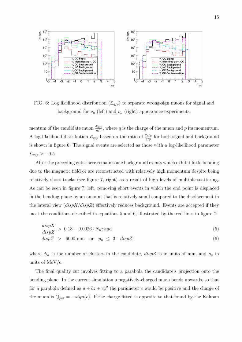
FIG. 6: Log likelihood distribution (Lq/p) to separate wrong-sign muons for signal and

background for νµ (left) and νµ (right) appearance experiments.

mentum of the candidate muonσq/pq/p

, where q is the charge of the muon and p its momentum.

A log-likelihood distribution Lq/p based on the ratio ofσq/pq/p

for both signal and background

is shown in figure 6. The signal events are selected as those with a log-likelihood parameter

Lσ/p > −0.5.

After the preceding cuts there remain some background events which exhibit little bending

due to the magnetic field or are reconstructed with relatively high momentum despite being

relatively short tracks (see figure 7, right) as a result of high levels of multiple scattering.

As can be seen in figure 7, left, removing short events in which the end point is displaced

in the bending plane by an amount that is relatively small compared to the displacement in

the lateral view (dispX/dispZ) effectively reduces background. Events are accepted if they

meet the conditions described in equations 5 and 6, illustrated by the red lines in figure 7:

dispX

dispZ> 0.18− 0.0026 ·Nh ; and (5)

dispZ > 6000 mm or pµ ≤ 3 · dispZ ; (6)

where Nh is the number of clusters in the candidate, dispZ is in units of mm, and pµ in

units of MeV/c.

The final quality cut involves fitting to a parabola the candidate’s projection onto the

bending plane. In the current simulation a negatively-charged muon bends upwards, so that

for a parabola defined as a + bz + cz2 the parameter c would be positive and the charge of

the muon is Qpar = −sign(c). If the charge fitted is opposite to that found by the Kalman

16

No. Clusters in Candidate0 50 100 150 200 250 300 350 400 450 500

Dis

pla

ce

me

nt

in X

/ D

isp

lace

me

nt

in Z

0

0.1

0.2

0.3

0.4

0.5

0.6

0.7

0.8

0.9

1

Displacement in Z (m)0 2 4 6 8 10 12 14 16 18 20

Mo

me

ntu

m (

Ge

V/c

)µ

Re

c.

0

5

10

15

20

25

30

35

40

No. Clusters in Candidate0 50 100 150 200 250 300 350 400 450 500

Dis

pla

ce

me

nt

in X

/ D

isp

lace

me

nt

in Z

0

0.1

0.2

0.3

0.4

0.5

0.6

0.7

0.8

0.9

1dispX_back

Entries 10781Mean x 69.23Mean y 0.1788RMS x 65.89RMS y 0.1629

dispX_back

Entries 10781Mean x 69.23Mean y 0.1788RMS x 65.89RMS y 0.1629

Displacement in Z (m)0 2 4 6 8 10 12 14 16 18 20

Mo

me

ntu

m (

Ge

V/c

)µ

Re

c.

0

5

10

15

20

25

30

35

40

FIG. 7: Distributions of displacement and momentum with cut levels: (top left) relative

displacement in the bending plane to the z direction against candidate hits for signal

events, (top right) reconstructed momentum against displacement in z for signal events

and (bottom) as top for νµ (νµ) CC backgrounds. The red lines represent the cuts from

equations 5 and 6.

filter, the quality of the fit is assessed using the variable:

qppar =

∣∣∣∣σcc∣∣∣∣ , if Qpar = Qkal ;

−∣∣∣∣σcc

∣∣∣∣ , if Qpar = −Qkal ;

(7)

where Qkal is the charge fitted by the Kalman filter fit. Defining the parameter in this way

ensures that the cut is independent of the initial fitted charge. Events with no charge change

(qppar > 0.0) are accepted as signal. Additionally, those fitted badly with a charge change

(qppar < −1.0) are also accepted. In this way, background events which have remained in the

sample due to local variations affecting the Kalman fitter can be removed without rejecting

viable events in which the Kalman fitter ignored a section after a high angle scatter. The

17

)par

Refit Charge Relative Error (qp­2 ­1.5 ­1 ­0.5 0 0.5 1

Pro

po

rtio

n o

f R

em

ain

ing

Eve

nts

­510

­410

­310

­210

­110

1 CC Signalµν

CCµν Identified as µν

CC Backgroundeν

NC Backgroundµν

CC Backgroundτν

CC Contaminationτ

ν

)par

Refit Charge Relative Error (qp­2 ­1.5 ­1 ­0.5 0 0.5 1

Pro

po

rtio

n o

f R

em

ain

ing

Eve

nts

­510

­410

­310

­210

­110

1 CC Signalµν

CCµν Identified as µν

CC Backgroundeν

NC Backgroundµν

CC Backgroundτ

ν

CC Contaminationτν

FIG. 8: Distribution of the qppar variable, with the region where the parameter is < 0

representing those candidates fitted with charge opposite to the initial Kalman filter for νµ

(left) and νµ appearance experiments. The distributions are normalised to the total

remaining events, individually, for each interaction type.

distribution of qppar is shown in figure 8.

B. Charged current selection

Selection of charged currents and rejection of neutral current events is most efficiently

performed by exploiting the propertiy that νµ CC events tend to have greater length in z

than NC events, since a true muon only interacts electromagnetically where a pion or kaon

of similar momentum can interact via the strong force and will tend to stop after a shorter

distance. Hence, the number of hits, lhit, was used to generate Probability Density Functions

(PDF) for charged and neutral current events (see figure 9). One can see that the NC events

have fewer reconstructed clusters than the equivalent νµ CC events. For the event selection,

candidates with greater than 150 clusters are considered signal, otherwise, the log likelihood

rejection parameter:

L1 = log

(lCChitlNChit

); (8)

is used, which is shown in figure 10. Allowing only those candidates where the log parameter

is L1 > 1.0 to remain in the sample ensures that the sample is pure. This analysis is similar,

but simpler, than that employed by MINOS [37]. The effect of the CC event selection is to

reduce the background by one order of magnitude (see table II) while having minimal effect

18

Number of Clusters in Trajectory0 20 40 60 80 100 120 140

Pro

ba

bili

ty0

0.1

0.2

0.3

0.4

0.5

0.6

CCµν

NCµν

CCµ

ν

NCµ

ν

FIG. 9: Distribution of the number of fit clusters in candidate track used to calculate the

log likelihood based charged current selection.

1L

­6 ­4 ­2 0 2 4 6 8 10 12 14

En

trie

s

210

310

410

510

610

710

CC Signalµν

CCµ

ν Identified as µ

ν

CC Backgrounde

ν

NC Backgroundµν

CC Backgroundτ

ν

CC Contaminationτν

(a) Distribution for νµ detection

1L

­6 ­4 ­2 0 2 4 6 8 10 12 14

En

trie

s

210

310

410

510

610

710

CC Signalµ

ν

CCµ

ν Identified as µ

ν

CC Backgroundeν

NC Backgroundµ

ν

CC Backgroundτν

CC Contaminationτ

ν

(b) Distribution for νµ detection

FIG. 10: Distribution of L1 likelihood ratios used to reject NC and other background

signals.

on the signal efficiency.

C. Kinematic cuts

Kinematic cuts based on the momentum and isolation of the candidate, in relation to

the reconstructed energy of the event Erec, can be used to reduce backgrounds from hadron

decays. The isolation of the candidate muon is described by the variable Qt = pµ sin2 θ,

where θ is the angle between the muon candidate and the hadronic-jet vector. The muon

from a true CC event is generally isolated from the hadronic jet so, on average, the Qt is

larger for CC events than for NC events, in which a hadron associated with the hadronic

19

jet decays to a muon. Cuts based on this variable and on the reconstructed momentum

compared to the reconstructed energy are an effective way to reduce all of the relevant beam

related backgrounds. The distributions after the application of the preceding cuts are shown

in figure 11, where the red lines illustrate the acceptance conditions defined in equations 9

and 10:

Erec ≤ 5 GeV or Qt > 0.25 GeV/c and ; (9)

Erec ≤ 7 GeV or pµ ≥ 0.3 · Erec . (10)

QE like events (see section III B) and those events passing the conditions of equation 9 must

also pass the conditions of equation 10 to remain in the data-set for the next series of cuts.

The effect of these cuts is to reduce the background by a further order of magnitude, while

only having a modest effect on the signal efficiency, as can be seen in table II.

D. Cut summary

In summary, after tuning the cuts described in the previous sub-sections to a test statistic,

these were applied to independent simulated data leading to an absolute efficiency of 51%

for νµ selection and 62% for νµ selection, while reducing the background to a level below

10−3. A summary of all the cuts, with their effect on the signal and absolute background,

can be found in Table II. The species which would be expected to contribute the greatest

amount of background interactions for an example oscillation parameter set is also identified

at each level.

V. MIND RESPONSE TO THE GOLDEN CHANNEL

Using a data-set of 3× 106 events each of νµ CC, νµ CC, νe CC, νe CC and 7× 106 NC

interactions from neutrinos and anti-neutrinos generated using GENIE and tracked through

the GEANT4 representation of MIND, the expected efficiency and background suppression

for the reconstruction and analysis of the golden channel in MIND have been evaluated for

both νµ and νµ appearance. Additionally, the expected level of contamination of the signal

from other appearance oscillation channels is considered.

20

Energy (GeV)νReconstructed 0 2 4 6 8 10 12 14 16

Mo

me

ntu

m (

Ge

V/c

)µ

Re

co

nstr

ucte

d

0

2

4

6

8

10

12

Energy (GeV)νReconstructed 0 2 4 6 8 10 12 14 16

(G

eV

/c)

tQ

0

0.2

0.4

0.6

0.8

1

1.2

1.4

1.6

Energy (GeV)νReconstructed 0 2 4 6 8 10 12 14 16

Mo

me

ntu

m (

Ge

V/c

)µ

Re

co

nstr

ucte

d

0

2

4

6

8

10

12

Energy (GeV)νReconstructed 0 2 4 6 8 10 12 14 16

(G

eV

/c)

tQ

0

0.2

0.4

0.6

0.8

1

1.2

1.4

1.6

Energy (GeV)νReconstructed 0 2 4 6 8 10 12 14 16

Mo

me

ntu

m (

Ge

V/c

)µ

Re

co

nstr

ucte

d

0

2

4

6

8

10

12

Energy (GeV)νReconstructed 0 2 4 6 8 10 12 14 16

(G

eV

/c)

tQ

0

0.2

0.4

0.6

0.8

1

1.2

1.4

1.6

Energy (GeV)νReconstructed 0 2 4 6 8 10 12 14 16

Mo

me

ntu

m (

Ge

V/c

)µ

Re

co

nstr

ucte

d

0

2

4

6

8

10

12

Energy (GeV)νReconstructed 0 2 4 6 8 10 12 14 16

(G

eV

/c)

tQ

0

0.2

0.4

0.6

0.8

1

1.2

1.4

1.6

FIG. 11: Distributions of kinematic variables: (left) Reconstructed muon momentum with

reconstructed neutrino energy for (top→bottom) νµ (νµ) signal, νµ (νµ) CC background,

NC background, νe (νe) CC background and (right) Qt variable (in the same order). The

red lines represent the cuts from equations 9 and 10.

21

TABLE II: Summary of cuts applied to select the golden channel appearance signals. The

level of absolute efficiency and, for a 100 ktonne MIND 2000 km from the NF and

θ13 = 9.0 and δCP = 45, the proportion of the total non-golden channel interactions

remaining in the sample after each cut are also shown, along with the species contributing

the greatest number of interactions.

Cut Acceptance level Eff. after cut background (×10−3)

νµ νµ νµ νµ

successful pattern rec. and fit 0.91 0.93 419 (νe) 153 (νµNC)

Fiducial z1− zend ≤ 2000 mm 0.88 0.90 400 (νe) 147 (νµNC)

Max. momentum Pµ ≤ 16 GeV 0.85 0.89 158 (νe) 108 (νe)

Fitted proportion Nfit/Nh ≥ 0.6 0.81 0.87 74.4 (νe) 71.3 (νe)

Track quality Lq/p > −0.5 0.70 0.76 13.6 (νe) 20.3 (ντ )

Displacement dispX/dispZ > 0.18− 0.0026Nh 0.65 0.72 13.6 (νµ NC) 10.9 (ντ )

dispZ > 6000 mm or Pµ ≤ 3dispZ

Quadratic fit qppar < −1.0 or qppar > 0.0 0.65 0.72 10.3 (νµ NC) 10.9 (ντ )

CC selection L1 > 1.0 0.63 0.70 2.1 (νµ NC) 3.0 (ντ )

Kinematic Erec ≤ 5 GeV or Qt > 0.25 0.51 0.62 0.3 (νµ NC) 0.9 (ντ )

Erec ≤ 7 GeV or Pµ ≥ 0.3Erec

A. Signal efficiency and beam neutrino background suppression

The resultant efficiencies for both polarities and the corresponding background levels

expected for the appearance channels are summarised in Figs. 12 – 15. Numeric response

matrices for each of the channels may be found in the Appendix. As can be seen in figure

12 the expected level of background from CC mis-identification is around 10−4, which is

significantly below 10−3 at all energies for the new simulation and re-optimised analysis.

This is also below the background levels achieved in [15], mainly due to the additional

quality cuts.

The background from neutral current interactions lies at or below the 10−3 level, with the

high energy region exhibiting a higher level than the low-energy region due to the dominance

22

True Neutrino Energy (GeV)0 1 2 3 4 5 6 7 8 9 10

Fra

ctio

na

l B

ackg

rou

nd

0

0.02

0.04

0.06

0.08

0.1

0.12

0.14

0.16

0.18

­310×

True Neutrino Energy (GeV)0 1 2 3 4 5 6 7 8 9 10

Fra

ctio

na

l B

ackg

rou

nd

0

0.05

0.1

0.15

0.2

0.25

­310×

FIG. 12: Background from mis-identification of νµ (νµ) CC interactions as the opposite

polarity. (left) νµ CC reconstructed as νµ CC, (right) νµ CC reconstructed as νµ CC as a

function of true energy.

True Neutrino Energy (GeV)0 1 2 3 4 5 6 7 8 9 10

Fra

ctional B

ackgro

und

0

0.1

0.2

0.3

0.4

0.5

0.6

­310×

True Neutrino Energy (GeV)0 1 2 3 4 5 6 7 8 9 10

Fra

ctional B

ackgro

und

0

0.02

0.04

0.06

0.08

0.1

0.12

­310×

FIG. 13: Background from mis-identification of NC interactions as νµ (νµ) CC

interactions. (left) NC reconstructed as νµ CC, (right) NC reconstructed as νµ CC as a

function of true energy.

of DIS interactions. The increased particle multiplicity and greater likelihood of producing

a penetrating pion that can mimic a primary muon are the primary reasons for this increase.

As expected, the NC background tends to be reconstructed at low energy due to the missing

energy (see appendix X).

The background from νe (νe) CC interactions is once again expected to constitute a very

low level addition to the observed signal. This background is particularly well suppressed due

23

True Neutrino Energy (GeV)0 1 2 3 4 5 6 7 8 9 10

Fra

ctional B

ackgro

und

0

10

20

30

40

50

60

70

80

90

­610×

True Neutrino Energy (GeV)0 1 2 3 4 5 6 7 8 9 10

Fra

ctional B

ackgro

und

0

10

20

30

40

50

60

70

80

90

­610×

FIG. 14: Background from mis-identification of νe (νe) CC interactions as νµ (νµ) CC

interactions. (left) νe CC reconstructed as νµ CC, (right) νe CC reconstructed as νµ CC as

a function of true energy.

True Neutrino Energy (GeV)0 1 2 3 4 5 6 7 8 9 10

Fra

ctio

na

l E

ffic

ien

cy

0

0.1

0.2

0.3

0.4

0.5

0.6

True Neutrino Energy (GeV)0 1 2 3 4 5 6 7 8 9 10

Fra

ctio

na

l E

ffic

ien

cy

0

0.1

0.2

0.3

0.4

0.5

0.6

0.7

FIG. 15: Efficiency of reconstruction of νµ (νµ) CC interactions. (left) νµ CC efficiency,

(right) νµ CC efficiency as a function of true energy.

to the electron shower overlapping with the hadron shower. If a particle from the hadronic

jet decays into a wrong-sign muon, it has a lower energy and is less isolated than in the NC

case, so the kinematic cuts suppress this background more.

The efficiency of detection of the two νµ polarities has a threshold lower than that seen

in previous studies due to the presence of non-DIS interactions in the Monte Carlo sample.

The efficiencies expected for the current analysis are shown in figure 15.

A comparison of the resultant νµ and νµ efficiency can be made with that extracted in

24

previous studies. Analyses performed in 2000 [4] and 2005 [38] assumed a 50 GeV Neutrino

Factory, so were optimised for high energy and low values of θ13. The background rejection

achieved was at the level of 10−6, but at the expense of signal efficiency, especially below

10 GeV. A more recent analysis [9] was the first attempt at re-optimzing for a 25 GeV

Neutrino Factory, while that in 2010 [15] was still based on a GEANT3 model, but included

full event reconstruction and a likelihood based analysis for the first time. There exists an

improvement in threshold for the current analysis, between 2–3 GeV, due to the inclusion

of QE and resonance events, since these events are easier to reconstruct (see figure 20).

The difference in efficiency between the two polarities is effectively described by the

difference in the inelasticity of neutrino and anti-neutrino CC interactions. Neutrino DIS

interactions with quarks have a flat distribution in the Bjorken variable:

y =Eν − ElEν

, (11)

with El the scattered-lepton energy. However, anti-neutrinos interacting with quarks follow

a ∝ (1 − y)2 distribution [39]. For this reason, neutrino interactions generally involve a

greater energy transfer to the target. The efficiencies for the two species as a function of y

can be seen from figure 16-(left). The shape of the efficiency curves is a consequence of the

ratio of DIS to non-DIS events in the event samples. Neutrino and anti-neutrino efficiencies

are very similar, showing that the Bjorken y of each event is the dominant contributor to

the efficiency. The difference in neutrino and anti-neutrino efficiencies, when translated into

true neutrino-energy, can be explained by the greater abundance of neutrino events at high

y. However, since the cross section for the interaction of neutrinos is approximately twice

that for anti-neutrinos, it is not expected that this reduced efficiency will affect the fit to

the observed spectrum significantly.

B. Contamination from oscillation channels containing ντ or ντ

Three million events of both ντ and ντ interactions were generated using the GENIE

framework [16] and passed through the GEANT4 simulation of MIND. These events were

then subject to the same digitization, reconstruction and analysis as the main beam back-

grounds. Matrices were extracted describing the expected level of contamination in the

golden channel data-set for the situation when a viable muon candidate from a ντ (ντ ) in-

teraction is reconstructed as a νµ (νµ) candidate with the same and opposite charge to the

25

y0 0.1 0.2 0.3 0.4 0.5 0.6 0.7 0.8 0.9 1

Fra

ctio

na

l E

ffic

ien

cy

0

0.1

0.2

0.3

0.4

0.5

0.6

0.7

0.8

µν

µν

y0 0.1 0.2 0.3 0.4 0.5 0.6 0.7 0.8 0.9 1

Pro

port

ion o

f E

vents

0

5

10

15

20

25

­310×

FIG. 16: νµ CC and νµ CC signal detection efficiency as a function of y (left) and the

normalised distribution of all events considered in each polarity as a function of y (right).

true primary τ . As can be seen in figure 17, between 1% and 3% of the ντ (ντ ) interactions

True Neutrino Energy (GeV)0 1 2 3 4 5 6 7 8 9 10

Fra

ctio

na

l E

ffic

ien

cy

0

5

10

15

20

25

30

­310×

True Neutrino Energy (GeV)0 1 2 3 4 5 6 7 8 9 10

Fra

ctio

na

l E

ffic

ien

cy

0

5

10

15

20

25

30

35

­310×

FIG. 17: Expected level of contamination from ντ (ντ ) CC interactions due to the

platinum channel. (left) ντ CC reconstructed as νµ CC, (right) ντ CC reconstructed as νµ

CC as a function of true energy.

are expected to be identified as the golden νµ (νµ) interactions. Considered properly, this

contamination should not weaken the extraction of the oscillation parameters (see [27]).

Contamination from the dominant oscillation (which requires reconstruction with the oppo-

site primary lepton charge) is expected to be below the 10−3 level (as shown in figure 18).

This contamination is taken into account, but does not deteriorate the δCP fits, since the

dominant oscillation is less sensitive to this parameter for large values of θ13.

26

True Neutrino Energy (GeV)0 1 2 3 4 5 6 7 8 9 10

Fra

ctional B

ackgro

und

0

0.1

0.2

0.3

0.4

0.5

0.6

0.7

0.8­3

10×

True Neutrino Energy (GeV)0 1 2 3 4 5 6 7 8 9 10

Fra

ctional B

ackgro

und

0

0.02

0.04

0.06

0.08

0.1

0.12

­310×

FIG. 18: Expected level of contamination from ντ (ντ ) CC interactions due to the

dominant oscillation. (left) ντ CC reconstructed as νµ CC, (right) ντ CC reconstructed as

νµ CC as a function of true energy.

C. Interaction expectation for 1021 muon decays

Using the response matrices extracted using the analysis described in the preceding sec-

tions it is possible to make a prediction of the expected contribution to the Monte Carlo

sample from each of the neutrino types in the beam. Figure 19 shows the expected num-

ber of events for the best fit values of the currently measured parameters taken from [40]:

θ12 = 33.5, θ23 = 45, ∆m221 = 7.65× 10−5 eV2, ∆m2

32 = 2.4× 10−3 eV2 for δCP = 45 and

calculating matter effects using the PREM model [41]. The number of interactions were

calculated for a 100 ktonne MIND at a distance of 2000 km from the NF for a value of

θ13 = 9.0, for an integrated flux due to 1021 decays of each polarity in the straight sections

of the decay pipes.

VI. STUDY OF SYSTEMATIC UNCERTAINTIES

The efficiencies and backgrounds described above will be affected by several systematic

effects. There will be many contributing factors including uncertainty in the determina-

tion of the parameters used to form the cuts in the analysis, uncertainty in the exclusive

cross-sections, uncertainty in the determination of the hadronic shower energy and direction

resolution, and any assumptions in the representation of the detector and readout. While

27

Energy (GeV)νRec. 0 1 2 3 4 5 6 7 8 9 10

Expecte

d R

econstr

ucte

d E

vents

­110

1

10

210

310

410

510

Energy (GeV)νRec. 0 1 2 3 4 5 6 7 8 9 10

Expecte

d R

econstr

ucte

d E

vents

­110

1

10

210

310

410

510

Golden Channel Interaction

Like­sign Muon Background

Electron Neutrino Background

ContaminationτPlatinum Channel

BackgroundτDominant Osc.

Neutral Current Background

FIG. 19: Expected interactions in a 100 ktonne MIND 2000 km from the Neutrino Factory

for θ13 = 9.0. Left column for νµ appearance and right for νµ appearance.

exact determination of the overall systematic error in the efficiencies is complicated, an es-

timate of the contribution of different factors can be obtained by setting certain variables

to the extremes of their errors.

The exclusive QE, DIS and ‘other’ cross-sections in the data sample could have a signifi-

cant effect on the signal efficiencies and backgrounds. The efficiencies for the reconstruction

of true QE and true DIS interactions are compared to the nominal efficiency in figure 20

where the dominance of DIS interactions in the backgrounds is clear. Although experimen-

tal data are available, confirming the presence of non-DIS interactions in the energy region

of interest, there are significant errors in the transition regions (see for example [42, 43]).

These errors lead to an uncertainty in the proportion of the different types of interaction

that can affect the efficiencies. In order to study the systematic error associated with this

effect, events of certain types were randomly removed from the data-set and the mean effect

quantified. As an illustration of the method, consider the contribution from QE interactions.

Taking the binned errors on the cross-section measurements from [42, 43], a run to reduce

the QE content would exclude a proportion of events in a bin so that instead of contribut-

ing the proportionNQENtot

, where NQE and Ntot are the number of QE interactions and the

total number of interactions in the bin of interest, it would instead contribute:NQE−σQENQENtot−σQENQE

,

where σQE is the proportional error on the QE cross section for the bin. Since the data-set is

finite and an actual increase in the number of QE interactions is not possible, the equivalent

run to increase the QE contribution reduces the contribution of the “rest” by an amount

28

True Neutrino Energy0 1 2 3 4 5 6 7 8 9 10

Fra

ctio

na

l Effic

ien

cy

0

0.1

0.2

0.3

0.4

0.5

0.6

0.7

0.8

0.9

Full Interaction Spectrum

QE Interactions

DIS Interactions

True Neutrino Energy0 1 2 3 4 5 6 7 8 9 10

Fra

ctio

na

l Effic

ien

cy

0

0.1

0.2

0.3

0.4

0.5

0.6

0.7

0.8

0.9

Full Interaction Spectrum

QE Interactions

DIS Interactions

True Neutrino Energy0 1 2 3 4 5 6 7 8 9 10

Fra

ctio

na

l Ba

ckg

rou

nd

0

0.1

0.2

0.3

0.4

0.5

0.6­3

10×

Full Interaction Spectrum

QE Interactions

DIS Interactions

True Neutrino Energy0 1 2 3 4 5 6 7 8 9 10

Fra

ctio

na

l Ba

ckg

rou

nd

0

0.1

0.2

0.3

0.4

0.5

0.6­3

10×

Full Interaction Spectrum

QE Interactions

DIS Interactions

True Neutrino Energy0 1 2 3 4 5 6 7 8 9 10

Fra

ctio

na

l Ba

ckg

rou

nd

0

0.1

0.2

0.3

0.4

0.5

0.6­3

10×

Full Interaction Spectrum

DIS Interactions

True Neutrino Energy0 1 2 3 4 5 6 7 8 9 10

Fra

ctio

na

l Ba

ckg

rou

nd

0

0.1

0.2

0.3

0.4

0.5

0.6­3

10×

Full Interaction Spectrum

DIS Interactions

True Neutrino Energy0 1 2 3 4 5 6 7 8 9 10

Fra

ctio

na

l Ba

ckg

rou

nd

0

0.02

0.04

0.06

0.08

0.1

0.12

0.14

­310×

Full Interaction Spectrum

DIS Interactions

True Neutrino Energy0 1 2 3 4 5 6 7 8 9 10

Fra

ctio

na

l Ba

ckg

rou

nd

0

0.02

0.04

0.06

0.08

0.1

0.12

0.14

­310×

Full Interaction Spectrum

DIS Interactions

FIG. 20: Efficiencies for a pure DIS sample compared to the nominal case. (top) Signal

efficiency, (second line) νµ (νµ) CC background, (third line) NC background and (bottom)

νe (νe) CC background. νµ appearance on the left and νµ appearance on the right.

29

calculated to give the corresponding proportional increase in QE interactions:

NQE + σQENQE

Ntot + σQENQE

=NQE

Ntot − εNrest

; (12)

where Nrest is the total number of non-QE interactions in the bin and ε is the required

proportional reduction in the ‘rest’ to simulate an appropriate increase in QE. Solving for ε

yields the required reduction:

ε =σQE

1 + σQE. (13)

The 1σ systematic error can be estimated as the mean difference between the nominal

efficiency and the increase due to a higher QE proportion or decrease due to exclusion.

The errors in the true νµ and νµ efficiencies extracted using this method that varies the

contribution of QE, 1π and other non-DIS interactions are shown in figure 21. Errors for

1π resonant reactions are estimated to be ∼20% below 5 GeV (as measured by the K2K

near detector [44]) and at 30% above. Due to the large uncertainty, both theoretically and

experimentally, on the models describing other resonances, coherent, diffractive and elastic

processes, a very conservative error of 50% is taken when varying the contribution of the

“others”. As can be seen in figure 21, the systematic effect is less than 1% for neutrino

energies between 3 GeV and 10 GeV increasing to 4% near 1 GeV, with increased QE

and 1π interactions generally increasing the efficiency and increased contribution of the

“other” interactions having the effect of decreasing efficiency. This last result is likely to be

predominantly due to resonances producing multiple tracks. The effect on backgrounds is

expected to be minimal, as was also shown in figure 20. At the time of a Neutrino Factory,

the cross-section uncertainties should be much smaller than the ones assumed here, so we

expect the systematic error to be below 1% for all energies.

Another important source of systematic uncertainty is due to the error in the muon mo-

mentum and the hadron shower energy used to reconstruct the total neutrino energy. The

muon is fully reconstructed, but the hadron shower reconstruction is performed assuming

a parametrisation to the hadron energy and angular resolution. The particular choice of

this parametrisation introduces a systematic error on the resulting signal and background

efficiencies that should be studied. Taking a 6% error as quoted for the energy scale uncer-

tainty assumed by the MINOS collaboration [7] and varying the constants of the energy and

direction smears by this amount, it can be seen (blue bands in figure 22) that, to this level,

30

True Neutrino Energy0 1 2 3 4 5 6 7 8 9 10

Effic

ien

cy E

rro

r

­50

­40

­30

­20

­10

0

10

20

30

40

50­3

10×

Increased QE proportion

productionπIncreased Resonant

Increased ’other’ proportion

True Neutrino Energy0 1 2 3 4 5 6 7 8 9 10

Effic

ien

cy E

rro

r

­50

­40

­30

­20

­10

0

10

20

30

40

50­3

10×

Increased QE proportion

productionπIncreased Resonant

Increased ’other’ proportion

True Neutrino Energy0 1 2 3 4 5 6 7 8 9 10

Effic

ien

cy E

rro

r

­50

­40

­30

­20

­10

0

10

20

30

40

50­3

10×

Decreased QE proportion

productionπDecreased Resonant

Decreased ’other’ proportion

True Neutrino Energy0 1 2 3 4 5 6 7 8 9 10

Effic

ien

cy E

rro

r

­50

­40

­30

­20

­10

0

10

20

30

40

50­3

10×

Decreased QE proportion

productionπDecreased Resonant

Decreased ’other’ proportion

FIG. 21: Calculated error on signal efficiencies on increasing (top) and decreasing

(bottom) the proportion of non-DIS interactions in the data-set. (left) Errors on true

energy νµ CC efficiency and (right) errors on true energy νµ CC efficiency

the hadronic resolutions have little effect on the true neutrino-energy efficiencies. However,

the hadronic direction resolution is likely to have far greater uncertainty and would be very

sensitive to noise in the readout electronics. Also shown in figure 22 are the efficiencies

when the hadronic energy resolution parameters are 6% larger but with a 50% increase in

the angular resolution parameters. We expect in a real detector to measure the hadronic

angular resolution with a precision of better than 50%, even though we cannot quantify this

precision yet. However, even at this level, the observed difference in efficiency is only at

the level of 1% above 7-8 GeV. A combination of the exclusive cross-sections and hadronic

energy uncertainties implies a total systematic uncertainty for the measurement efficiency

of order 1% over the neutrino energy range above 2 GeV.

31

True Neutrino Energy0 1 2 3 4 5 6 7 8 9 10

Fra

ctio

na

l E

ffic

ien

cy

0.45

0.5

0.55

0.6

0.65

0.7Nominal level

6% energy and angular variation

50% worse angular res.

True Neutrino Energy0 1 2 3 4 5 6 7 8 9 10

Fra

ctio

na

l E

ffic

ien

cy

0.5

0.55

0.6

0.65

0.7

0.75

0.8Nominal level

6% energy and angular variation

50% worse angular res.

True Neutrino Energy0 1 2 3 4 5 6 7 8 9 10

Fra

ctio

na

l E

ffic

ien

cy

0

0.05

0.1

0.15

0.2

0.25

0.3

0.35

0.4­3

10×

Nominal level

6% energy and angular variation

50% worse angular res.

True Neutrino Energy0 1 2 3 4 5 6 7 8 9 10

Fra

ctio

na

l E

ffic

ien

cy

0

0.1

0.2

0.3

0.4

0.5

0.6

0.7

0.8­3

10×

Nominal level

6% energy and angular variation

50% worse angular res.

FIG. 22: Variation of signal efficiency (top) and NC backgrounds (bottom) due to a 6%

variation in the hadron shower energy and direction resolution and a more pessimistic 50%

reduction in angular resolution (focused on region of greatest variation).

VII. COMPARISON BETWEEN EVENT GENERATORS

The above analysis uses the GENIE event generator to simulate the interaction of events

with matter in the detector. This generator was assumed to bring this effort in line with

current experiments, such as MINOS, where good agreement with data has been achieved. It

is useful to compare to a previous version of this analysis with the NUANCE event generator

[20]. A comparison of the neutrino charge current detection efficiencies appears in figure 23.

This shows that the GENIE derived analysis produces smaller positive identification of

charge current events. This loss of performance is linear with respect to neutrino energy for

energies greater than 5 GeV, so that the analysis of the GENIE simulation is 20% less efficient

32

True Neutrino Energy0 5 10 15 20 25

Fra

ctio

na

l E

ffic

ien

cy

0

0.1

0.2

0.3

0.4

0.5

0.6

0.7

0.8

Simulation with GENIE

Simulation with NUANCE

(a) GENIE and NUANCE νµCC efficiency

True Neutrino Energy0 5 10 15 20 25

Fra

ctio

na

l E

ffic

ien

cy

0

0.1

0.2

0.3

0.4

0.5

0.6

0.7

0.8

Simulation with GENIE

Simulation with NUANCE

(b) GENIE and NUANCE νµCC efficiency

True Neutrino Energy0 5 10 15 20 25F

ractio

na

l d

iffe

ren

ce

of

Effic

ien

cie

s

­0.8

­0.7

­0.6

­0.5

­0.4

­0.3

­0.2

­0.1

0

0.1

0.2

(c) Fractional difference between GENIE and

NUANCE νµ CC efficiencies

True Neutrino Energy0 5 10 15 20 25F

ractio

na

l d

iffe

ren

ce

of

Effic

ien

cie

s

­0.8

­0.7

­0.6

­0.5

­0.4

­0.3

­0.2

­0.1

0

0.1

0.2

(d) Fractional difference between GENIE and

NUANCE νµCC efficiencies

FIG. 23: The Golden channel analysis efficiencies from simulations of charge current

neutrino events in a MIND detector generated using GENIE and NUANCE neutrino

generators. The differences between the efficiencies as fractions of the GENIE efficiency are

also shown.

than that of the NUANCE simulation. This difference is partially ascribed to differences in

the parton distribution functions used by each generator and should not be interpreted as a

systematic error of the analysis, since the measured event rates in a future experiment will

be cross-checked against the simulations, so the efficiencies will be determined much more

accurately than the difference between generators. We assume that GENIE, which has been

benchmarked against recent neutrino experiments, serves as a more realistic estimator for

the efficiency of the analysis.

33

VIII. MIND SENSITIVITY

The Neutrino Factory is required to measure the CP-violating phase δCP simulaneously

with θ13 while removing ambiguity caused by degenerate solutions. Extracting the oscillation

parameters from the observed signal at the far detectors requires the accurate prediction

of the expected flux without oscillation, which is used along with the calculated oscillation

probabilities to fit the observed signal for the best value of θ13 and δCP . Due to the large

distance to the far detectors, the flux spectra expected from the decay rings of the Neutrino

Factory are accurately approximated by the flux from a point source of muons travelling with

appropriate Lorentz boost in the direction of the detector. Using this flux or, alternatively,

a projection of the spectra observed in the near detector, the number of true interactions

expected in MIND as a function of energy can be calculated for each value of θ13 and δ.

These spectra can then be multiplied by the response matrices shown in the Appendix to

calculate the observed golden channel interaction spectrum expected for some hypothetical

values of the oscillation parameters.

A Neutrino Factory storing muons of energy 10 GeV is assumed, of which 5.0×1020 per

year of each species decay in the straight sections pointing towards the MIND far detector

of 100 ktonnes mass placed at a distance of 2000 km from the facility.

A. The NuTS framework

The Neutrino tool suite (NuTS) was developed for the studies presented in [45–47]. It

provides a framework for the generation of appropriate fluxes for different neutrino accelera-

tor facilities along with the necessary infrastructure to calculate the true neutrino oscillation

probabilities for all channels. In addition, using the parametrisation of the total interaction

spectra calculated in section III A, the expected number of events in a given energy bin

can be calculated. Using this framework and the response matrices extracted for MIND,

simulated data for an experiment can be generated as

Datai,jsim = smear

(M i

sigNi,jsig +

∑k

M i,kbkgN

i,j,kbkg

), (14)

for each polarity and detector baseline of interest, where M isig is the response matrix for

MIND for a particular signal channel i (stored µ+ or µ−), N i,jsig is the 100% efficiency inter-

action spectrum in true ν energy bins for a channel i at a detector baseline j (in this case,

34

there is only one baseline at 2000 km), M i,kbkg is the response matrix for a background k (mis-

identification of CC interactions from other neutrino species or from NC) to the appearance

channel i, N i,j,kbkg is the 100% expectation spectrum for a background k to an appearance

signal i at a detector baseline j and these expected values are used to calculate an observed

number of interactions following a Poisson distribution.

B. Fitting for θ13 and δCP simultaneously

Due to the correlation between θ13 and δCP , a simultaneous fit is necessary. Defining a

grid of θ13 and δCP values the χ2 of a fit to Datai,jsim can be calculated using the function

χ2 =∑j

2×Eµ∑e

(AjxjN

e+,j(θ13, δCP )− ne+,j + ne+,j log

(ne+,j

AjxjNe+,j(θ13,δCP )

)

+AjNe−,j(θ13, δCP )− ne−,j + ne−,j log

(ne−,j

AjNe−,j(θ13,δCP )

))+

(Aj − 1)2

σA+

(xj − 1)2

σx

, (15)

where nei,j is the simulated data (Datai,jsim) for an energy bin e, N ei,j(θ13, δCP ) is the pre-

dicted spectrum for the values of θ13 and δCP represented by the grid point (calculated as

in equation 14 but without a smear) and j represents the baseline as in equation 14. The

uncertainty in the expected number of interactions and expected ratio in interactions be-

tween neutrinos and antineutrinos are represented by the additional free parameters Aj and

xj respectively and their corresponding errors.

We made two assumptions regarding the overall event normalisation: one assumes a

conservative error of σA = 0.025 and the other assumes a more optimistic (but realistic)

assumption for a neutrino factory of σA = 0.01. The uncertainty in the ratio of cross

sections between neutrinos and antineutrinos is maintained fixed at σx = 0.01, which is

the level to which a near detector would seek to measure the interaction cross-sections at

the time of a neutrino factory. The minimisation of the parameters A and x is performed

analytically for each predicted dataset to leading order. The contours at χ2min + 9 represent

approximately the 3σ level of understanding and those at χ2min+25 represent 5σ. In such a fit,

the experimentally determined oscillation parameters [40] are considered fixed. While there

would be some systematic error associated with uncertainty in these parameters, systematics

35

13θ22sin

0.07 0.08 0.09 0.1 0.11 0.12 0.13 0.14 0.15

(deg

)C

Pδ

­150

­100

­50

0

50

100

150 sensitivityσ1

sensitivityσ3

sensitivityσ5

sensitivityσ1

sensitivityσ3

sensitivityσ5

sensitivityσ1

sensitivityσ3

sensitivityσ5

sensitivityσ1

sensitivityσ3

sensitivityσ5

sensitivityσ1

sensitivityσ3

sensitivityσ5

sensitivityσ1

sensitivityσ3

sensitivityσ5

sensitivityσ1

sensitivityσ3

sensitivityσ5

sensitivityσ1

sensitivityσ3

sensitivityσ5

FIG. 24: Examples of 1σ, 3σ and 5σ fits to simulated data for the 10 GeV Neutrino

Factory, for sin2 2θ13 = 0.096.

from the normalisation and cross-section uncertainties are expected to dominate. Some

examples for such fits, assuming sin2 2θ13 = 0.096, are shown in figure 24.

C. Sensitivity to the mass hierarchy

Distinguishing between the two possible mass hierarchies is important for the understand-

ing of the neutrino mass sector. The sensitivity to the true mass hierarchy is defined here as

when the true sign of ∆m213 can be distinguished from the opposite sign to the appropriate

nσ level, that is

χ2min(−∆m2

13)− χ2min(∆m2

13) ≥ n2. (16)

Sensitivity to the mass hierarchy up to 5σ covers the whole region down to sin2 2θ13 < 10−4,

so the Neutrino Factory would be able to cover easily the current value of sin2 2θ13 ∼ 0.1.

D. Sensitivity to δCP

Sensitivity to the measurement of δCP is defined as when the difference between the

minimum χ2 with respect to the minimum obtained by fitting with CP conserving cases is

36

13

θ22sin0 0.02 0.04 0.06 0.08 0.1 0.12 0.14 0.16

(deg)

CP

δ

­150

­100

­50

0

50

100

150 sensitivityσ3

sensitivityσ5

sensitivityσ10

13θDaya Bay

13

θ22sin0 0.02 0.04 0.06 0.08 0.1 0.12 0.14 0.16

(deg)

CP

δ

­150

­100

­50

0

50

100

150 sensitivityσ3

sensitivityσ5

sensitivityσ10

13θDaya Bay

13θ2

2sin

0 0.02 0.04 0.06 0.08 0.1 0.12 0.14

Fra

ction

CP

δ

0

0.2

0.4

0.6

0.8

1

13θ2

2sin

0 0.02 0.04 0.06 0.08 0.1 0.12 0.14

Fra

ction

CP

δ

0

0.2

0.4

0.6

0.8

1

FIG. 25: δCP 3σ, 5σ and 10σ measurements (top) and δCP 5σ coverage to measure CP

violation (bottom) as a function of sin2 2θ13 for true normal hierarchy (left) and true

inverted hierarchy (right). The vertical lines represent the range of possible values of

sin2 2θ13.

greater than the appropriate nσ level, that is

min(χ2(δCP = 0), χ2(δCP = 180), χ2(δCP = −180))− χ2min ≥ n2. (17)

The δCP measurement and δCP coverage plots to measure CP violation by the 10 GeV

Neutrino Factory are shown in figure 25 for the normal mass hierarchy (left) and for the

inverted mass hierarchy (right). The CP coverage to measure δCP at the 5σ level for both

normal and inverted mass hierarchy is ∼85% in the range of the currently measured values

of sin2 2θ13. These results improve those presented by the Interim Design Report [20].

The accuracy achieved in the measurement of δCP is an increasingly important parameter

to determine the performance of a facility [48]. The 1σ error ∆δCP for θ13 = 9 is shown

in figure 26 (left), under two assumptions of the overall normalisation and cross-section

37

(Deg)CP

δ

­200 ­150 ­100 ­50 0 50 100 150 200

(D

eg)

CP

δ∆

0

2

4

6

8

10

12

14=1%

Aσ=1%,

Xσ

=3.0%A

σ=2.5%, X

σ

(Deg)δ∆

0 2 4 6 8 10

Fra

ction

δ

0

0.1

0.2

0.3

0.4

0.5

0.6

0.7

0.8

0.9

1

FIG. 26: Left: Precision in the value of δCP as a function of δCP under two different

assumptions: top line (3.0% normalisation and 2.5% cross-section error), bottom line (1%

normalisation and cross-section error). Right: δCP fraction coverage that can be achieved

above each value of ∆δCP for 3.0% and 2.5% errors (right curve) and for 1% and 1% errors

(left curve).

systematic errors: (σA, σx) = (3.0%,2.5%) and (1.0%,1.0%). Depending on the value of

δCP and the level of systematic error, the accuracy in ∆δCP is between 2.5% and 5%.

Figure 26 (right) shows the δ fraction coverage that can be achieved above the value of ∆δCP

determined at a Neutrino Factory for each of the two assumptions about the systematic error.

IX. CONCLUSIONS

A new GEANT4 simulation of the Magnetised Iron Neutrino Detector (MIND), using

GENIE as the neutrino event generator, has been developed to determine the performance

of MIND at a Neutrino Factory. Considering the spectrum of neutrino interactions in the

energy region 0-25 GeV produced by the GENIE generator, this simulation has been used

to study the efficiency and the background rejection of MIND. A detector of 100 ktonne

at 2000 km was used to determine the expected sensitivity to δCP and the mass hierarchy

at a Neutrino Factory for a value of sin2 θ13 ∼ 0.1, as determined recently by reactor and

accelerator neutrino oscillation experiments.

The proportions of quasi-elastic, single pion production and deep inelastic events obtained

from GENIE have been benchmarked with experiments and a parametrisation of the total

38

interaction spectrum, in agreement with data, was used for the simulation. Digitisation of

the events tracked through the simulation assumed read-out of the scintillator using WLS

fibres and electronics with 30% QE and a standard deviation on signal response of 6%.

Both assumptions should be achievable and could, perhaps, turn out to be conservative if

the current trend in photon detectors and electronics performance continues. These events

have been used to study the efficiency and background suppression of MIND in a search

for wrong sign muons at a Neutrino Factory storing both muon polarities. A re-optimised

reconstruction algorithm and a new analysis applied to data-sets comprising several million

νµ (νµ) and νe (νe) CC and NC events, resulted in response matrices describing the expected

response of the detector. MIND showed an efficiency plateau from 5 GeV in true neutrino

energy at ∼60% for νµ and ∼70% for νµ and thresholds at ∼2 GeV. All beam inherent

backgrounds were simultaneously suppressed at a level around 10−4. The difference in

efficiencies for the two polarities has been studied and found to be predominantly due to the

difference in the inelasticity spectrum expected for neutrino and anti-neutrino interactions.

We expect the dominant systematic errors to be due to the hadronic energy resolution and

due to the different neutrino interaction types. Each contribute an expected systematic error

on the signal efficiency of around 1%.

The response of MIND and a parametrisation of the total neutrino and antineutrino cross-

sections, calculated from the output of the GENIE event generator, were used to study the

sensitivity of two MIND detectors at the Neutrino Factory. The obtained measurement of

key parameters of the PMNS matrix indicate that such an experiment would determine the

mass hierarchy, irrespective of the value of δCP , at a level better than 5σ, could perform

measurements of δCP with an accuracy between 3% and 5% and would have an 85% δCP

coverage for the currently preferred value of θ13 ∼ 9.0.

ACKNOWLEDGMENTS

The authors acknowledge the support of the European Community under the European

Commission Framework Programme 7 Design Study: EUROnu, Project Number 212372.

The work was supported by the Science and Technology Facilities Council (UK) and by the

Spanish Ministry of Education and Science.

39

[1] S. Geer, Phys. Rev. D57, 6989 (1998), hep-ph/9712290.

[2] A. Hillairet et al. (TWIST Collaboration), Phys.Rev. D85, 092013 (2012), arXiv:1112.3606

[hep-ex].

[3] A. De Rujula, M. B. Gavela, and P. Hernandez, Nucl. Phys. B547, 21 (1999), arXiv:hep-

ph/9811390.

[4] A. Cervera et al., Nucl. Phys. B579, 17 (2000), arXiv:hep-ph/0002108.

[5] A. Bandyopadhyay et al. (ISS Physics Working Group), Rept. Prog. Phys. 72, 106201 (2009),

arXiv:0710.4947 [hep-ph].

[6] The ISS Accelerator Working Group et al., JINST 4, P07001 (2009).

[7] D. G. Michael et al. (MINOS), Nucl. Instrum. Meth. A596, 190 (2008), arXiv:0805.3170

[physics.ins-det].

[8] A. Cervera, F. Dydak, and J. Gomez Cadenas, Nucl. Instrum. Meth. A451, 123 (2000).

[9] A. Cervera-Villanueva, AIP Conf. Proc. 981, 178 (2008).

[10] T. Abe et al. (ISS Detector Working Group), JINST 4, T05001 (2009), arXiv:0712.4129

[physics.ins-det].

[11] S. K. Agarwalla, P. Huber, J. Tang, and W. Winter, JHEP 1101, 120 (2011), arXiv:1012.1872

[hep-ph].

[12] “The International Design Study for the Neutrino Factory,” URL: https://www.ids-

nf.org/wiki/FrontPage.

[13] “EUROnu: A High Intensity Neutrino Oscillation Facility in Europe,” URL:

http://www.euronu.org/.

[14] A. Cervera and A. Laing, PoS Nufact08, 042 (2008).

[15] A. Cervera, A. Laing, J. Martin-Albo, and F. J. P. Soler, Nucl. Instrum. Meth. A624, 601

(2010), arXiv:1004.0358 [hep-ex].

[16] C. Andreopoulos et al., Nucl. Instrum. Meth. A614, 87 (2010), arXiv:0905.2517 [hep-ph].

[17] D. Casper, Nucl. Phys. Proc. Suppl. 112, 161 (2002), arXiv:hep-ph/0208030.

[18] S. Agostinelli et al. (GEANT4), Nucl. Instrum. Meth. A506, 250 (2003).

[19] J. Apostolakis and D. H. Wright (Geant4), AIP Conf. Proc. 896, 1 (2007).

40

[20] S. Choubey et al. (IDS-NF), (2011), arXiv:1112.2853 [hep-ex].

[21] F. An et al. (DAYA-BAY Collaboration), Phys.Rev.Lett. 108, 171803 (2012), arXiv:1203.1669

[hep-ex].

[22] J. Ahn et al. (RENO collaboration), Phys.Rev.Lett. 108, 191802 (2012), arXiv:1204.0626

[hep-ex].

[23] Y. Abe et al. (DOUBLE-CHOOZ Collaboration), Phys.Rev.Lett. 108, 131801 (2012),

arXiv:1112.6353 [hep-ex].

[24] K. Abe et al. (T2K Collaboration), Phys.Rev.Lett. 107, 041801 (2011), arXiv:1106.2822 [hep-

ex].

[25] P. Adamson et al. (MINOS Collaboration), Phys.Rev.Lett. 107, 181802 (2011),

arXiv:1108.0015 [hep-ex].

[26] D. Indumathi and N. Sinha, Phys. Rev. D80, 113012 (2009), arXiv:0910.2020 [hep-ph].

[27] A. Donini, J. J. Gomez Cadenas, and D. Meloni, JHEP 02, 095 (2011), arXiv:1005.2275

[hep-ph].

[28] G. Ingelman, A. Edin, and J. Rathsman, Computer Physics Communications 101, 108 (1997).

[29] “Geant4 Physics Reference Manual,” http://cern.ch/geant4/UserDocumentation/UsersGuides/

PhysicsReferenceManual/html/.

[30] A. Pla-Dalmau, A. D. Bross, V. V. Rykalin, and B. M. Wood (MINERvA), “Extruded plastic

scintillator for MINERvA,” (2005), proceedings of 2005 IEEE Nuclear Science Symposium

and Medical Imaging Conference, El Conquistador Resort, Puerto Rico, 23-29 Oct 2005.

[31] A. Cervera-Villanueva, J. J. Gomez-Cadenas, and J. A. Hernando, Nucl. Instrum. Meth.

A534, 180 (2004).

[32] D. Emeliyanov, I. Gorbounov, and I. Kisel, “OTR/ITR-CATS: Tracking Based on Cellular

Automaton and Kalman Filter,” (2001), HERA-B note 01-137.

[33] A. Laing, PhD thesis, University of Glasgow (2010).

[34] P. Adamson et al., Nucl. Instrum. Meth. A556, 119 (2006).

[35] G. Bari et al., Nucl. Instrum. Meth. A508, 170 (2003).

[36] A. Blondel, M. Campanelli, and M. Fechner, Nucl. Instrum. Meth. A535, 665 (2004).

[37] P. Adamson et al. (MINOS), Phys. Rev. D 77, 072002 (2008), arXiv:0711.0769 [hep-ex].

[38] A. Cervera-Villanueva, Nucl. Phys. Proc. Suppl. 149, 201 (2005).

[39] K. Zuber, Neutrino physics (IOP, 2003).

41

[40] T. Schwetz, M. A. Tortola, and J. W. F. Valle, New J. Phys. 10, 113011 (2008),

arXiv:0808.2016 [hep-ph].

[41] A. M. Dziewonski and D. L. Anderson, Phys. Earth Planet. Interiors 25, 297 (1981).

[42] V. Lyubushkin et al. (NOMAD), Eur. Phys. J. C63, 355 (2009), arXiv:0812.4543 [hep-ex].

[43] A. A. Aguilar-Arevalo et al. (MiniBooNE), Phys. Rev. D81, 092005 (2010), arXiv:1002.2680.

[44] A. Rodriguez et al. (K2K), Phys. Rev. D78, 032003 (2008), arXiv:0805.0186 [hep-ex].

[45] J. Burguet-Castell, M. B. Gavela, J. J. Gomez-Cadenas, P. Hernandez, and O. Mena, Nucl.

Phys. B608, 301 (2001), arXiv:hep-ph/0103258.

[46] J. Burguet-Castell, M. B. Gavela, J. J. Gomez-Cadenas, P. Hernandez, and O. Mena, Nucl.

Phys. B646, 301 (2002), arXiv:hep-ph/0207080.

[47] J. Burguet-Castell, D. Casper, E. Couce, J. J. Gomez-Cadenas, and P. Hernandez, Nucl.

Phys. B725, 306 (2005), arXiv:hep-ph/0503021.

[48] P. Coloma, A. Donini, E. Fernandez-Martinez, and P. Hernandez, JHEP 1206, 073 (2012),

arXiv:1203.5651 [hep-ph].

42

X. APPENDIX

This appendix summarizes the response matrices of signal (wrong sign νµ and νµ appear-

ance) and all backgrounds. (νµ and νµ CC, νe and νe CC, ντ and ντ CC, and NC) in bins

of true and reconstructed neutrino energy relevant to an oscillation analysis. Each entry in

the table is the survival probability for each species. In all tables, columns represent the

true neutrino energy in GeV and rows the reconstructed energy, also in GeV. The overflow

bin in reconstructed energy represents all events with a reconstructed energy greater than

the known maximum.

A. νµ appearance

0.0-1.0 1.0-2.0 2.0-3.0 3.0-4.0 4.0-5.0 5.0-6.0 6.0-7.0 7.0-8.0 8.0-9.0 9.0-10.0

0.0-1.0 0 1.392 3.940 2.052 2.402 1.323 0.3669 0.2460 0.3710 0.1218

1.0-2.0 0 222.0 243.6 45.87 28.82 21.65 9.660 6.519 1.608 2.679

2.0-3.0 0 149.4 1238 568.5 144.5 68.80 34.73 22.63 14.10 7.551

3.0-4.0 0 14.13 807.9 1790 813.2 270.8 110.4 60.52 41.31 26.79

4.0-5.0 0 1.392 162.0 1340 1848 859.0 318.7 146.9 81.87 57.24

5.0-6.0 0 0.1070 14.64 375.5 1516 1695 805.7 339.7 152.2 83.54

6.0-7.0 0 0.1070 1.914 62.40 593.3 1630 1616 841.6 369.3 178.8

7.0-8.0 0 0 0.3378 7.725 123.1 744.8 1563 1462 783.8 347.1

8.0-9.0 0 0 0 0.7242 18.37 200.4 836.3 1547 1360 771.6

9.0-10.0 0 0 0.1126 0.3621 2.402 35.24 277.6 891.3 1454 1289

10.0-11.0 0 0 0 0 0.6004 8.059 83.52 474.8 1520 3014

TABLE III: Golden channel νµ appearance signal efficiency. All values ×10−4.

43

0.0-1.0 1.0-2.0 2.0-3.0 3.0-4.0 4.0-5.0 5.0-6.0 6.0-7.0 7.0-8.0 8.0-9.0 9.0-10.0

0.0-1.0 0 0 0 0 0 0 0 0 0 0

1.0-2.0 0 0 0 0 0 0 0 0 0 0

2.0-3.0 0 0 0 0 0 0.1203 0.1218 0 0 0.1198

3.0-4.0 0 0 0 0 0 0.2406 0 0 0.1220 0.1198

4.0-5.0 0 0 0 0 0 0 0.2437 0.2439 0 0.1198

5.0-6.0 0 0 0 0 0 0 0 0 0.1220 0

6.0-7.0 0 0 0 0 0 0 0 0.1220 0.1220 0.2396

7.0-8.0 0 0 0 0 0 0.1203 0 0.1220 0 0.2396

8.0-9.0 0 0 0 0 0 0 0 0 0 0.1198

9.0-10.0 0 0 0 0 0 0 0.1218 0 0 0

10.0-11.0 0 0 0 0 0 0 0 0 0 0.1198

TABLE IV: µ− background from charge mis-identified νµ CC events All values ×10−4.

0.0-1.0 1.0-2.0 2.0-3.0 3.0-4.0 4.0-5.0 5.0-6.0 6.0-7.0 7.0-8.0 8.0-9.0 9.0-10.0

0.0-1.0 0 0 0 0 0 0 0 0 0 0

1.0-2.0 0 0 0 0 0 0 0 0 0 0

2.0-3.0 0 0 0 0 0 0 0 0 0 0

3.0-4.0 0 0 0 0 0.0596 0 0 0 0 0

4.0-5.0 0 0 0 0.0596 0 0 0.0614 0 0 0

5.0-6.0 0 0 0 0 0 0 0 0 0 0.0610

6.0-7.0 0 0 0 0 0 0 0 0 0 0

7.0-8.0 0 0 0 0 0 0 0 0 0 0

8.0-9.0 0 0 0 0 0 0 0 0 0 0

9.0-10.0 0 0 0 0 0 0 0 0 0 0

10.0-11.0 0 0 0 0 0 0 0 0 0 0.0610

TABLE V: µ− background from νe CC events. All values ×10−4.

44

0.0-1.0 1.0-2.0 2.0-3.0 3.0-4.0 4.0-5.0 5.0-6.0 6.0-7.0 7.0-8.0 8.0-9.0 9.0-10.0

0.0-1.0 0 0 0 0 0 0 0 0 0 0

1.0-2.0 0 0 0 0.1729 0.0581 0.3538 0.0602 0.1221 0 0.0612

2.0-3.0 0 0 0.1068 0 0.3488 0.2359 0.1807 0.4272 0.3680 0.1224

3.0-4.0 0 0 0 0.2305 0.8138 0.8844 0.8431 0.6713 0.6133 0.8566

4.0-5.0 0 0 0 0.1152 0.5232 0.7076 1.144 1.098 0.9812 0.9178

5.0-6.0 0 0 0 0.0576 0.0581 0.5307 0.3011 0.5492 0.6746 0.6119

6.0-7.0 0 0 0 0 0 0.1769 0.3011 0.4272 0.5519 0.4895

7.0-8.0 0 0 0 0 0 0 0.0602 0.4272 0.2453 0.4283

8.0-9.0 0 0 0 0 0 0 0 0.0610 0.1840 0.4283

9.0-10.0 0 0 0 0 0 0 0 0 0 0.1836

10.0-11.0 0 0 0 0 0 0 0 0 0 0.1836

TABLE VI: µ− background from νµ NC events. All values ×10−4.

0.0-1.0 1.0-2.0 2.0-3.0 3.0-4.0 4.0-5.0 5.0-6.0 6.0-7.0 7.0-8.0 8.0-9.0 9.0-10.0

0.0-1.0 0 0 0 0 0.5833 0 0 0.3747 0 0.1426

1.0-2.0 0 0 0 14.70 8.750 8.569 12.33 8.992 9.264 6.845

2.0-3.0 0 0 0 49.97 51.33 54.27 65.98 67.44 52.33 45.35

3.0-4.0 0 0 0 38.21 51.92 58.08 71.91 76.06 78.66 79.71

4.0-5.0 0 0 0 11.76 18.08 38.08 47.49 57.32 61.27 70.16

5.0-6.0 0 0 0 0 5.833 16.19 28.77 32.41 33.32 42.78

6.0-7.0 0 0 0 0 0 3.808 12.33 17.23 18.69 25.67

7.0-8.0 0 0 0 0 0 1.587 4.109 10.30 10.89 13.69

8.0-9.0 0 0 0 0 0 0 1.142 2.810 5.526 7.986

9.0-10.0 0 0 0 0 0 0 0.2283 0.3747 2.113 4.278

10.0-11.0 0 0 0 0 0 0 0 0 1.788 2.139

TABLE VII: µ− reconstructed from ντ CC events. All values ×10−4.

45

0.0-1.0 1.0-2.0 2.0-3.0 3.0-4.0 4.0-5.0 5.0-6.0 6.0-7.0 7.0-8.0 8.0-9.0 9.0-10.0

0.0-1.0 0 0 0 0 0 0 0 0 0 0

1.0-2.0 0 0 0 0 0 0 0 0 0 0

2.0-3.0 0 0 0 0 0 0 0 0 0 0

3.0-4.0 0 0 0 0 0 0 0 0.1637 0.4287 0

4.0-5.0 0 0 0 0 0 0 0 0.1637 0.2858 0

5.0-6.0 0 0 0 0 0 0 0 0 0 0

6.0-7.0 0 0 0 0 0 0 0 0 0 0

7.0-8.0 0 0 0 0 0 0 0 0 0 0

8.0-9.0 0 0 0 0 0 0 0 0 0 0

9.0-10.0 0 0 0 0 0 0 0 0 0 0

10.0-11.0 0 0 0 0 0 0 0 0 0 0

TABLE VIII: µ− background from ντ CC events. All values ×10−4.

B. νµ appearance

0.0-1.0 1.0-2.0 2.0-3.0 3.0-4.0 4.0-5.0 5.0-6.0 6.0-7.0 7.0-8.0 8.0-9.0 9.0-10.0

0.0-1.0 0 4.606 22.28 14.26 9.296 3.729 1.340 0.3659 0 0.7188

1.0-2.0 0 85.70 262.9 93.41 54.43 26.11 18.15 9.025 4.757 1.318

2.0-3.0 0 84.87 1565 656.4 116.1 51.85 39.48 28.05 20.61 12.94

3.0-4.0 0 5.304 990.1 2364 795.4 164.5 63.85 49.15 46.11 38.57

4.0-5.0 0 0.1396 161.9 1904 2513 880.2 226.6 89.76 66.35 54.63

5.0-6.0 0 0 10.52 477.7 2145 2218 851.9 246.6 97.94 64.45

6.0-7.0 0 0 0 60.02 801.6 2221 2032 842.4 283.0 111.5

7.0-8.0 0 0 0.1238 3.751 152.5 1022 2181 1896 840.2 307.4

8.0-9.0 0 0 0 0.6252 19.33 263.2 1169 2108 1738 832.3

9.0-10.0 0 0 0 0.1250 1.223 47.28 355.9 1230 1996 1633

10.0-11.0 0 0 0 0.1250 0.3670 8.301 98.33 603.4 2024 4033

TABLE IX: Golden channel νµ appearance signal efficiency. All values ×10−4.

46

0.0-1.0 1.0-2.0 2.0-3.0 3.0-4.0 4.0-5.0 5.0-6.0 6.0-7.0 7.0-8.0 8.0-9.0 9.0-10.0

0.0-1.0 0 0 0 0 0 0 0 0 0 0

1.0-2.0 0 0 0 0 0 0 0 0 0 0

2.0-3.0 0 0 0 0 0 0 0 0 0 0

3.0-4.0 0 0 0.3378 0.6035 0 0.2406 0.1223 0.1230 0 0

4.0-5.0 0 0 0.2252 0.8449 0.3602 0.2406 0 0 0 0.2436

5.0-6.0 0 0 0 0.1207 0.2402 0 0.1223 0.3690 0.1237 0.1218

6.0-7.0 0 0 0 0 0 0.1203 0.2446 0 0.1237 0

7.0-8.0 0 0 0 0 0 0.2406 0.1223 0.1230 0 0

8.0-9.0 0 0 0 0.1207 0 0 0 0 0 0

9.0-10.0 0 0 0 0 0 0 0 0.1230 0.1237 0.1218

10.0-11.0 0 0 0 0 0 0.1203 0.2446 0.2460 0 0.3654

TABLE X: µ+ background from charge mis-identified νµ CC events All values ×10−4.

0.0-1.0 1.0-2.0 2.0-3.0 3.0-4.0 4.0-5.0 5.0-6.0 6.0-7.0 7.0-8.0 8.0-9.0 9.0-10.0

0.0-1.0 0 0 0 0 0 0 0 0 0 0

1.0-2.0 0 0 0 0 0 0 0 0 0 0

2.0-3.0 0 0 0 0 0 0.0605 0.0608 0 0 0

3.0-4.0 0 0 0.0613 0 0.0609 0 0 0.1221 0.1215 0.0602

4.0-5.0 0 0 0 0.0627 0.1218 0.1211 0.2431 0.1832 0.1215 0.1204

5.0-6.0 0 0 0 0 0 0 0 0.0611 0 0

6.0-7.0 0 0 0 0 0.0609 0 0 0.1221 0 0

7.0-8.0 0 0 0 0 0 0 0 0 0 0

8.0-9.0 0 0 0 0 0 0 0 0 0 0.0602

9.0-10.0 0 0 0 0 0 0 0 0.0611 0.0608 0.0602

10.0-11.0 0 0 0 0 0 0 0 0 0 0

TABLE XI: µ+ background from νe CC events. All values ×10−4.

47

0.0-1.0 1.0-2.0 2.0-3.0 3.0-4.0 4.0-5.0 5.0-6.0 6.0-7.0 7.0-8.0 8.0-9.0 9.0-10.0

0.0-1.0 0 0 0 0 0 0 0 0 0 0

1.0-2.0 0 0 0 0 0 0.0586 0 0.0607 0 0

2.0-3.0 0 0 0 0.1167 0 0.1173 0 0.0607 0 0.0606

3.0-4.0 0 0 0 0 0 0.1759 0.0597 0.1213 0.1210 0.2422

4.0-5.0 0 0 0 0 0 0.0586 0.1194 0.2427 0.1814 0.0606

5.0-6.0 0 0 0 0 0 0 0.0597 0.0607 0.1210 0.1817

6.0-7.0 0 0 0 0 0 0 0 0.0607 0.1814 0.0606

7.0-8.0 0 0 0 0 0 0 0 0 0.0605 0

8.0-9.0 0 0 0 0 0 0 0 0 0 0

9.0-10.0 0 0 0 0 0 0 0 0 0 0.0606

10.0-11.0 0 0 0 0 0 0 0 0 0 0

TABLE XII: µ+ background from νµ NC events. All values ×10−4.

0.0-1.0 1.0-2.0 2.0-3.0 3.0-4.0 4.0-5.0 5.0-6.0 6.0-7.0 7.0-8.0 8.0-9.0 9.0-10.0

0.0-1.0 0 0 0 15.53 1.498 2.763 3.066 2.128 1.857 2.020

1.0-2.0 0 0 0 0 22.47 33.16 31.88 27.66 25.29 23.99

2.0-3.0 0 0 0 62.11 64.41 77.99 74.19 75.28 67.44 59.34

3.0-4.0 0 0 0 54.35 63.67 68.47 66.62 61.70 73.59 69.82

4.0-5.0 0 0 0 15.53 28.46 42.99 54.36 55.15 55.15 53.91

5.0-6.0 0 0 0 0 5.243 19.65 36.17 36.99 41.29 43.43

6.0-7.0 0 0 0 0 3.745 5.220 11.44 20.62 27.01 26.39

7.0-8.0 0 0 0 0 0 0.6141 4.292 12.27 16.72 18.94

8.0-9.0 0 0 0 0 0 0 1.635 2.619 5.430 10.48

9.0-10.0 0 0 0 0 0 0 0.4087 1.964 3.572 5.555

10.0-11.0 0 0 0 0 0 0.3070 0.2044 0.4910 1.286 5.176

TABLE XIII: µ+ reconstructed from ντ CC events. All values ×10−4.

48

0.0-1.0 1.0-2.0 2.0-3.0 3.0-4.0 4.0-5.0 5.0-6.0 6.0-7.0 7.0-8.0 8.0-9.0 9.0-10.0

0.0-1.0 0 0 0 0 0 0 0 0 0 0

1.0-2.0 0 0 0 0 0 0 0.6849 0.1873 0.6501 0.2852

2.0-3.0 0 0 0 0 0 0.3174 0.2283 0.9367 0.4876 0.9982

3.0-4.0 0 0 0 0 0.5833 0 0.2283 0.3747 0.9751 1.426

4.0-5.0 0 0 0 0 0 0 0 0.3747 0.4876 0.7130

5.0-6.0 0 0 0 0 0 0 0 0 0.3250 0.8556

6.0-7.0 0 0 0 0 0 0 0 0 0 0.1426

7.0-8.0 0 0 0 0 0 0 0 0 0 0

8.0-9.0 0 0 0 0 0 0 0 0 0 0

9.0-10.0 0 0 0 0 0 0 0 0 0 0

10.0-11.0 0 0 0 0 0 0 0 0 0 0

TABLE XIV: µ+ background from ντ CC events. All values ×10−4.