New parameterizations and sensitivities for simple climate models

JOURNAL OF GEOPHYSICAL RESEARCH, VOL. 98, NO. D3, PAGES 5025-5036, MARCH 20, 1993

New Parameterizations and Sensitivities for Simple Climate Models

CHARLES E. GRAVES, 1 WAN-HO LEE, AND GERALD R. NORTH

Climate System Research Program, College of Geosciences, Texas A&M University, College Station

This paper presents a reexamination of the Earth radiation budget' parameterization of energy balance climate models in light of data collected over the last 12 years. The study consists of three parts: (1) an examination of the infrared terrestrial radiation to space and its relationship to the surface temperature field on time scales from 1 month to 10 years; 2) an examination of the albedo of the Earth with special attention to the seasonal cycle of snow and clouds; (3) solutions for the seasonal cycle using the new parameterizations with special attention to changes in sensitivity. While the infrared parameterization is not dramatically different from that used in the past, the albedo in the new data suggest that a stronger latitude dependence be employed. After retuning the diffusion coefficient the simulation results for the present climate generally show only a slight dependence on the new parameters. Also, the sensitivity parameter for the model is still about the same (1.25øC for a 1% increase of solar constant) for the linear models and for the nonlinear models that include a seasonal snow line albedo feedback (1.34øC). One interesting feature is that a clear-sky planet with a snow line albedo feedback has a significantly higher sensitivity (2.57øC) due to the absence of smoothing normally occurring in the presence of average cloud cover.

1. INTRODUCTION

Energy balance climate models (EBMs) have been used extensively in the last two decades for conceptual studies of the large-scale climate [e.g., Budyko, 1968, 1969; Sellers, 1969; North et al., 1981, 1983; Hyde et al., 1989, 1990; Kim and North, 1991]. The models rely on simple formulas relating various energy fluxes to the surface temperature. Typically, the model surface temperature field T is the solution of

c(e) OT

ot V . D(x)VT + A + BT: QS(x, t)a[x, T(•, t)]

(1)

where • is a unit vector from the center of the Earth pointing to the point on the Earth being considered; t is the time; x is the sine of latitude; C(•) is the space-dependent heat capacity per unit area, which takes on different constant values dependent on whether the local surface is land, sea or sea ice;D(x) is a horizontal thermal diffusion coefficient, dependent quadratically on x2; A and B are empirical parameters relating the outgoing infrared flux to the surface temperature to be determined from data (these are part of the subject of this study); Q is the solar constant divided by 4; S(x, t) is the normalized seasonal distribution of heat flux entering the top of the atmosphere; and a[x, T(•, t)] is the coalbedo, which may be dependent on the local temperature as well as position (also a subject of the present study). In solving the equation we require the boundary condition that the horizontal heat flux into the poles vanish.

When the temperature dependence of the coalbedo is held fixed, the model is linear and it is convenient to use the discrete Fourier representation since the harmonics are uncoupled. The nonlinearity stemming from the temperature

•Currently at Department of Earth and Atmospheric Sciences, St. Louis University, St. Louis, Missouri.

Copyright 1993 by the American Geophysical Union.

Paper number 92JD02666. 0148-0227/93/92JD-02666505.00

dependence of the albedo is sufficiently mild that even when it is included the harmonic representation is often a useful approximation. Most of the studies have concentrated on applications that exploit the ability of the linear version of the model to reproduce the ensemble average seasonal cycle in the present and altered climates [Hyde et al., 1990; Crowley and North, 1988; Short et al., 1991; Baum and Crowley, 1991]. In addition, some studies have introduced noise forcing to simulate fluctuations at frequencies away from the forced seasonal cycle and its harmonics [North and Cahalan, 1982; Leung and North, 1990; Leung and North, 1991; Kim and North, 1991]. All of these studies have relied

on parameterizations derived from satellite data taken from the 1970s [cf. North and Coakley, 1979].

Nonlinearity enters the model as the snowcover (and possibly cloud) movements alter the albedo leading to a feedback which can increase climate sensitivity and even induce bifurcations with occasionally bizarre effects [e.g., Lin and North, 1990]. There are especially interesting effects near the poles that are associated with the small ice cap instability [North, 1984]. These are of special interest because they might be relevant to some paleoclimatic transitions [e.g., Crowley and North, 1990; Suarez and Held, 1979; Watts and Hayder, 1984; Lin and North, 1990; Huang and Bowman, 1991 ].

An interesting feature of EBMs is that under present conditions they produce an isolated subfreezing Greenland in summer even in the absence of snow-albedo feedback.

Was the glaciation of Greenland sudden? Are there sudden transitions across the Arctic Ocean that could remove the

perennial ice cover there? Are there any sudden transitions that could be related to the large-scale Laurentide Continen- tal glaciations that have repeated themselves many times in phase with orbital element changes on astronomical time scales? The northern hemisphere problem is much more problematic than that in the southern. It is likely that ice-albedo feedback is not the whole story as suggested by Huang and Bowman [1991]. Deblonde and Peltier [1990] have coupled the linear EBM to a dynamical ice sheet model and while their ice sheets are very realistic, they point out

5025

5026 GRAVES ET AL.' NEW PARAMETERIZATIONS AND SENSITIVITIES

B , 10 YF_I•R$

4•N

180W sow o •o• look

(B)

CORRELAT I ON COEFF., 10 YEARS

180W 90W 0

. ) 4ss

:: 90S 90E 180E

Fig. 1. The estimated value for (a) B and (b) the accompanying correlation coefficient from the 10-year data set. The contours of B are in units of W m -2 øC-1 and the contours of correlation are multiplied by a factor of 10.

that the simulations still produce too much ice in the western part of North America and that this could possibly be related to moisture budget considerations which are beyond the scope of present simple EBMs.

In view of the extensive observing program that has been in place over the last decade it is time to reexamine the empirical relations used in these models to make sure there are no surprises. In addition to updating with later and more accurate data we can now use many more realizations of the seasonal cycle to increase our confidence in the parameters that have to be estimated. Hence the purpose of this study is to take advantage of the 10 years of data from Nimbus 6 and 7 as well as the first year of data taken from the Earth Radiation Budget Experiment (ERBE) to examine the con- sequences in typical EBMs.

The paper falls naturally into three parts: (1) outgoing longwave parameterization; (2) albedo parameterization; (3) model simulations with the new parameters. We take advantage of the analysis that has been conducted by the ERBE

experiment team [Barkstrom, 1984] to present results for both the clear-sky and the average-sky conditions. This leads to some interesting conclusions about the role of clouds in determining climate sensitivity.

2. OUTGOING LONGWAVE PARAMETERIZATION

Most recent EBM studies have relied on the simple formula

I = A + BT s (2)

which relates the outgoing infrared radiation flux (W/m 2) to the local contemporaneous surface temperature, T(•, t) as indicated in (2). The parameters A and B must be determined by regression from the two separately collected contemporaneous data sets. Previous studies such as Short et al.

[1984] used the annual cycle as a means of finding the regression coefficients. This was in part because at the time they only had 1 year of Nimbus 6 data. We are interested not

GRAVES ET AL..' NEW PARAMETERIZATIONS AND SENSITIVITIES 5027

300

._o

:• 250

> -

o 200 --

.N

0 -

o 150 --

ß oT4

Scatter plot for OLR vs T (10 years)

•F..•

::::::::::. :: .

---- :-:-:b-•. ..:.:

........... i!ig ...... ' • ....... .: ........... .

,• • ,• ......... . .......... •[•i ';':[ :-:•:•. . // :•=:'::•':'•"•:: =:si::.• •;'...•

ß E:>;•.•:::::-::: •::;•

I ' I ' I ' I ' I ' I ' I '

-40 -30 -20 -10 0 10 20

Surface Temperature (in C)

I

0.0%

1.0%

Fig. 2. Scatter plot of OLR versus surface temperature from 30øN to 90øN from the 10-year data set. The scale on the right indicates the percent of total. Note that there is a cosine of latitude weighting to account for the differing grid point areas.

only in the response of the IR to the surface temperature at the annual frequency but at lower and higher frequencies as well, since there is always the possibility of bias entering that is peculiar to the systematic poleward and equatorward motions of cloud patterns.

2.1. OLR Data and Method of Analysis

Most of our analysis was conducted with 10 years of OLR data (July 1975 through June 1985) which were deconvoluted from the wide field-of-view radiometers aboard the Nimbus

6 and 7 satellites. The details on the construction of this data

set have been discussed by Bess and Smith [ 1987a, b; Bess et al., 1992]. There were 4 missing months in the data set (July 1978 through October 1978) which were replaced by the 9-year mean for those calendar months. The data were obtained in spherical harmonic format truncated triangularly at degree 12, although OLR gridded fields were computed by expansion on to a 15 ø x 15 ø grid.

We also analyzed an additional 9 months of OLR data from the ERBE mission (February, March, May, June, July, September, October, November, of 1985 and January 1986), which were provided by NESDIS.

Monthly mean surface temperature climatology as well as anomalies analyzed in this study were obtained from the National Center for Atmospheric Research. The temperature anomalies are from those used by Jones et al. [ 1986] and Jones [1988]. The missing temperature anomalies were filled using spatial linear interpolation. The interpolation was more extensive in the southern hemisphere so we concentrate our discussion on the northern hemisphere results. The temperature data were obtained on a 5 ø x 5 ø but were smoothed to

15 ø x 15 ø to match spatial resolution of the OLR data. Additionally, only those months for which the OLR data were available were analyzed.

The analysis is based on the linear regression given by (2),

where the regression coefficients are computed for a variety of filtered I and T s time series. The parameter B is of most concern in this study since it is inversely proportional to the sensitivity of temperature anomalies to radiative cooling. That is, the larger the value of B the faster temperature anomalies are radiatively damped. In the absence of feedbacks such as snow-albedo B -] is also a measure of a climate model's sensitivity to changes in external control parameters. When the regression was done at a particular grid point, no area weighting was applied, however when large regional estimates of B were obtained, the analysis included area weighting (i.e., a cosine of latitude weighting at each grid point).

2.2. OLR Analysis

2.2.1. The 10-year mean. The regression analysis was first applied to each grid point for the entire 10 years (120 months). A map of the locally computed regression coefficient B and the corresponding correlation coefficient are shown in Figure 1. As with all plots in this study, some nearest neighbor averaging was applied to smooth out the contours. A pronounced difference between the tropics and middle latitudes can be observed in both the values of B and

the correlation coefficient in Figure 1. In much of the middle and high latitudes the value of B is near 2.0 W m-2 øC-•, and the transition region tends to follow the position of the climatological storm tracks along the east coasts of the two northern hemisphere land masses. In middle and high latitudes the correlation coefficient is more zonally symmetric with values greater than 0.6.

In the tropics, the value of B is highly longitude dependent reflecting the strong regional cloud-surface temperature dependence in the tropics. Of course, the dynamic range of T is also very small in the tropics. The three locations with large negative values of B are in the vicinity of regions of


2 •

1

Sudace Temperature

Outgoing Longwave Radiation

OLR vs Sudace Temperature

0.75

0.50

0.25

0.00

1 2 3 4 5

Frequency (1/year)

Fig. 3. Spectra and squared coherence averaged over 54 land grid points from the 10-year data set. Spectra density graphs are shown with the vertical axis on a logarithmic scale.

quasi-permanent cloud cover. This effect is easily explained [Short et al., 1984] since tropical convection migrates to spots of local surface temperature maxima, and the corresponding local cloud tops are cold radiating surfaces. It follows that a single linear form relating I and T s does not hold in the tropics. Fortunately, it has been shown that the IR and albedo effects of tropical clouds nearly cancel [Ra- manathan et al., 1990]. This suggests that if we ignore the departures from the mid-latitude parameterization in the tropics in both the IR and albedo formulations the near- perfect cancellation will not lead to serious error in EBM seasonal cycle computations.

As shown in Figure 1, the value of B even in the mid-

latitudes is not perfectly uniform. Figure 2 employs a two- dimensional histogram to illustrate this variability with data taken from the latitude band 30øN to 90øN. The histogram shows the fractional area (number of grid points weighted by cosine of latitude) that falls within each bin. The values shown alongside the key in Figure 2 are normalized and indicate the percent of the total area.

Consistent with earlier findings, Figure 2 reveals a strong relationship between OLR and Ts. The solid line through the data represents the (area weighted) least squares fit to A + BT s and as indicated the estimate of B is 1.90 W M -2 øC-• (the correlation coefficient is 0.90). This value of B is very close to the estimate reported by Short et al. [1984] of 1.93 W m -2 C 2 from a similar analysis with only 1 year of data. Scatter about the linear fit in Figure 2 indicates a small quadratic bias. Since the extremes account for only a small fraction of the total counts, the bias while more noticeable in this plot is actually a rare occurrence The curvature appears to be cloud related as will be discussed in a later section.

2.2.2. Spectral Analysis. Most of the variability of monthly averages for both the OLR and the temperature over the 10-year span is contained in a narrow band of frequencies about the annual cycle. It is conceivable that the relationship between OLR and T s might be different at forced frequencies than at other frequencies where the system is presumably undergoing natural fluctuations. We proceed with an investigation of the frequency dependence of this relationship by cross-spectral analysis.

Some examples of spectral products are shown in Figure 3. These sample spectral densities were obtained by squaring the Fourier amplitudes from all land locations between 30øN and 90øN (54, 15 ø x 15 ø locations) and averaging them together. The annual cycle is an exact harmonic of the time series length so that power at that frequency does not contaminate adjacent bands.

Both I and T s spectra have dominant peaks at the annual cycle. The T s spectrum contains more prominent harmonics of the annual cycle, otherwise both spectra are red. The (squared) coherency, also shown in Figure 3, is likewise strongest at the annual cycle while only marginally signifi- cant at the other frequencies.

The relationship between I and Ts at the annual cycle time scale is quite stable with both fields in phase. At the other frequencies the relationship is less sharp and more of the I variability is left unexplained by Ts. Consequently, the most appropriate time scale at which to model I linearly by T s is the annual cycle.

With the annual cycle dominating the foregoing results, we specifically removed the annual and semiannual components of both the OLR and T s and examined their relationship away from the seasonally forced frequencies. As expected, the relationship between I and Ts was less correlated (0.32), but with a slope of 1.80 W m -2 C- • in reasonable agreement with the results at the forced frequencies. A major problem with this estimate was that the dynamic range of natural fluctuations is very small, leading to large signal-to-noise problems.

2.2.3. ERBE Analysis of OLR. At the time of this analysis, 9 months of ERBE data were available. The ERBE products analyzed here are the average-sky and clear-sky OLR. The estimates of B for both of these products are shown in Figure 4. (More smoothing was applied to these data because of the smaller sample.) The average-sky esti-

GRAVES ET AL.' NEW PARAMETERIZATIONS AND SENSITIVITIES 5029

B , ERBE (AVERAr_.,E SKY) 90N

0 •OE

4•N

EO

4;$

90$ 18014

b , ERBE (CLEAR SKY)

(B) i ',,-' ..... :

, ; 4SN

..

• ...... 4 4sS

' ' 90S l BOW 9061 0 90E 1BOE

Fig. 4. The IR parameter B as shown in Figure la but for the (a) ERBE average sky and the (b) ERBE clear-sky cases.

mates of B are very similar to those from the entire 10-year analysis (Figure 1). Most of the large-scale patterns in Figure 1 are also apparent in Figure 4a. In the northern hemisphere, B does not exceed 2.0 W m -2 C -], and in the tropics the local minima are not as deep.

The clear-sky estimates of B shown in Figure 4b are radically different from previous results, (e.g., much of the tropical variability is gone). With the effects of clouds removed the I-T s relationship in the tropics has moved closer to the upper latitude values. Additional changes can be observed in the scatterplot in Figure 5, which is similar to Figure 2 but for the ERBE clear sky I. There is an overall increase in the mean B to 2.26 W m -2 C -] (with a correlation of 0.96). This estimate is more in line with the radiative transfer calculations of B • 2.2 W m -2 C -1 [Cess, 1974]. The quadratic trend previously observed is less noticeable, suggesting that clouds tend to increase the OLR away from a linear trend at extreme temperatures.

Also the extremes in both the average-sky and clear-sky

scatterplots (Figures 2 and 5) are in the same OLR and T s range. This suggests that the extreme OLR and T s values occur in clear-sky (or nearly clear sky) conditions. In contrast, Ramanathan and Collins [1991] suggest that in the tropics the extreme surface temperatures over the ocean should be associated with cloudy (high cirrus) conditions. Since our analysis strictly excludes the tropics, the apparent discrepancy may reflect the differing climatic regions.

3. ALBEDO PARAMETERIZATION

We made use of the 9 months of ERBE data available as of this study. We did not make use of albedo estimates from the earlier data sets because of the difficulties in obtain-

ing reliable values due to angular effects. Special attention was given to the angular effects in the ERBE making use of all three satellites when they were simultaneously available (see Barkstrom [1984], Barkstrom and Smith [1986], and Harrison et al. [1988] for details and examples of ERBE products).


]

250-

200 --

-

150 --

Scatter plot of OLR vs T (ERBE Clear Sky)

ß aT4 '"*

,, ............ •-•,•••

/ ,, :

......

I " I " I " I ' I ' I ' I " I "

-40 -30 -20 -10 0 10 20 30

SuHace Temperature (in C)

Fi•. 5. A scattot plot similar to that in Fi•uro 2, but

1.0%

The ERBE Science Team also report the albedo for "clear sky." This data set was produced by searching through the month in a given grid box and finding as many as possible measurements that were "cloud free" and reporting the albedo for these measurements alone [Wielicki and Green, 1989]. Presumably, this procedure removed the effect of clouds and the difference between the two data sets (IR as well as albedo) can be used to estimate the so-called cloud radiative forcing.

After examining both the clear- and average-sky albedo we have adopted the following parameterization:

a(x, t) = a o + aiPi(x) + a2P2(x) + a I (3)

where x is the sine of latitude and P, is the nth-order Legrendre polynomial. The coefficients a0, a i, and a2 represent the background albedo, which characterizes the U-shaped dependence of the albedo. These parameters also contain the time dependence of the parameterization, since they vary from month to month. The coefficient a i represents the change in albedo in the presence of snow cover.

In the following sections we justify this parameterization by examining the seasonal dependence and regional changes in the albedo.

The albedo has a seasonal cycle for a combination of reasons. First, the solar zenith angle changes with season and the albedo of the whole column of atmosphere and surface have a strong zenith angle dependence. Second, cloud and water vapor, which reflect and absorb sunlight, have systematic variations with season because of shifts of stormy regions and because of thermal changes with season, which can induce more water vapor in the atmospheric column. Finally, snow and sea ice cover change significantly with season and these surface features exhibit a very strong albedo contrast with neighboring snow- and ice-free surfaces. The thin solid line in Figure 6 shows the zonally averaged albedo for the average sky for 4 different months as revealed in the first year of ERBE data. The albedo exhibits

a mild seasonal cycle with a rather U-shaped dependence on latitude. Also prominent is a bump in albedo in the tropics presumably associated with the Intertropical Convergence Zone (ITCZ).

The zonally averaged clear-sky albedo is also presented in Figure 6 by the thick solid line. The clear-sky albedo has a much weaker latitudinal dependence, which suggests that most of the zenith angle dependence in the average-sky case comes from clouds. Also note the clear-sky albedo contains essentially step function albedo jumps at the ice and snowcover edges.

For the purpose of modeling the seasonal climate we fitted the zonal mean albedo for each month to a quadratic in x (missing months were filled in by averaging neighbors). The monthly values of the coefficients are given in Table 1. The time dependences of the coefficients a0, a l, and a2 are due to such effects as zenith angle dependence and cloud/snow line migrations with the seasonal march. The dependence is especially large in the north-south antisymmetric term a•, since this term captures the main dependence of the seasonal cycle [North and Coakley, 1979]. The quality of the fits is indicated also in Figure 6 by the dashed lines. However, the regions above the snow line where not included in estimating the fit. Also note that the fits still do not capture the ITCZ feature along the equator. On the other hand, it is suggested by Ramanathan et al. [1990] that the cloud radiative forcing due to tropical convection nearly vanishes. Hence in EBMs if we ignore the ITCZ in the IR and in the albedo, we will make almost no error. This is fortunate since the temperature parameterization of the IR fails utterly in the ITCZ region.

Figure 7 shows the July zonal average albedo from ERBE data alongside the parameterization that has been used in previous climate simulations with EBMs [e.g., Hyde et al., 1991]. The old albedo parameterization in the absence of snow is given by the simple formula a = 0.25 + 0.18x 2 . We note that the latitude dependence even below snow latitudes

GRAVES ET AL.' NEW PARAMETERIZATIONS AND SENSITIVITIES 5031

BACKOROUNO ALBEDO PARAMETERI ZAT I ON

SOL I O , OBSERVAT I ON

DOTTED, BACKOROUNO THIN ,AVERAOE SKY

TH I CK, CLEAR SKY

• 40- b=l

..I . (3:

' FEB

•0-

.

l::3 40-

..I .

20-

L•T I TUDE ( N-$ )

$EP

60

CD E3 40- b=l

..I . CI:

ZO-

C:) E3 40- b.I

_1 -

20-

JUN

60 30 o -3o -•o

l;::l T I TUOE ( N-$ )

NOV

:', '1 I I I I ..... : -60 tSO 313 0 -::•3 -$0

LI::IT I TUOE ( N-$ ) LI::I T I TUOE ( N-$ )

Fig. 6. The observed and background albedo for the 12 months of ERBE data. The background albedo does not contain the jump in albedo from snowcover (see equation (3)). The thick lines denote the clear-sky data, while the thin lines denote the average-sky data. Dashed lines indicate the parametric fit adopted for the EBM.

is much too mild. Hence it is clear that EBMs need to

incorporate this new albedo information in order to create more realistic seasonal climate simulations and to properly calculate sensitivities.

Also of interest is the albedo as a function of latitude at a

particular longitude, since considerable smoothing of discontinuities is likely to occur in the zonal averaging process The Jan ß Feb strength of local albedo discontinuities is known to be very Mar important in the small ice cap phenomena [North, 1984]. Apr This discontinuity is contained in the parameter a/which as May discussed below is temperature dependent in the nonlinear Jun model. Jul

Aug Determining a/ is actually a two part process. First, the Sep

size of the albedo change must be estimated and second, the Oct temperature at which this change occurs must also be Nov determined. The selected parameters in the snow-albedo Dec Mean feedback are presented in Table 2 for both clear and average conditions. These values have been determined by examin-

TABLE 1. Values of the Background Albedo Parameterization From Both Average-Sky and Clear-Sky ERBE Data

Average Sky Clear Sky

ao al a2 ao al a2

0.667 -0.080 -0.267 0.843 -0.032 -0.053 0.667 -0.080 -0.267 0.843 -0.032 -0.053 0.667 -0.040 -0.267 0.843 -0.032 -0.053 0.680 -0.000 -0.240 0.843 -0.032 -0.053 0.687 0.034 -0.227 0.843 0.000 -0.033

0.687 0.048 -0.227 0.853 0.000 -0.033 0.687 0.048 -0.227 0.853 0.000 -0.033 0.693 0.045 -0.213 0.853 0.000 -0.033 0.693 0.019 -0.213 0.853 0.000 -0.033 0.687 -0.020 -0.227 0.853 -0.020 -0.033

0.673 -0.038 -0.253 0.843 -0.032 -0.053 0.667 -0.080 -0.267 0.843 -0.032 -0.053 0.679 -0.012 -0.241 0.848 -0.020 -0.045

The coefficients correspond to those in equation (3).


ZONAL MEAN ALBEDO (JULY)

•l 40- bJ

=J 02 •0-

'70 OBSERVAT I ON 7o ............... NEW MODEL

ß o- -- ........ OLD MODEL -gO

- ', 7: /

-._....... ..... zo

1o

o ! i i t i i i i i I i o •0 30 0

LAT I TUDE

Fig. 7. The albedo from the ERBE average sky data for the month of July. The previous albedo parameterization is shown by the dotted-dashed line, while the new albedo parameterization is shown by the dashed line.

ing data as presented in Figure 8. Figure 8a contains the observed albedo at 105 W for both the clear- (thick solid line) and the average-sky (thin solid line) conditions. The location of the snowline is most easily determined from the clear sky and in this particular case happens near 45øN and 65øS. The jump in albedo in the northern hemisphere in clear-sky conditions is nearly 0.40 while in average sky conditions is much less, about 0.20. Accompanying the albedo data on this figure are the observed temperatures indicated by the dotted-dashed line. Consequently, the locations of the albedo jumps can also be associated with a temperature. In both hemispheres the temperature is in between 0øC and -10øC (the temperature scale is shown on the right side of the figure). Figure 8b is equivalent to Figure 8a but for the month of July. The overall results are nearly the same but the differences provide an indication of the variability in the parameters. Also presented in Figures 8c and 8d are average conditions; Figure 8c reveals the albedo and temperature for the 12-month average at 105øW, while Figure 8d shows the 12-month and zonal average conditions. The same general conclusions hold for these averages, however, determining

TABLE 2. Snow Line Rule for Albedo for the Average-Sky and Clear-Sky Cases

Average Sky Clear Sky

Critical temperature Land -2.0C -5.0C Ocean -7.0C - 12.0C

Albedo jump Land -0.14 -0.50 Ocean -0.07 -0.25

The critical temperature is the value when the albedo changes (due to snow) and the net change in albedo is given by the jump value.

the location of the snowline is masked by the averaging process.

Final tuning of the critical temperature and of the magni- tude of the albedo jump was accomplished by solving the EBM and determining the model albedo curve. These simulated albedos are also shown in Figure 8 by the dashed lines. (The details on the model runs are presented in the next section). After numerous runs with slightly differing snow albedo feedback parameters, the best fit appears to be obtained with the parameters given in Table 2. The fit of the albedo parameterization especially in the average (both 12 month and zonal, Figures 8c and 8d) are quite good.

4. MODEL SIMULATIONS

In this section we report the results of simulations for several model types. In each case the parameters in the diffusion coefficient, D(x) = Do(1 + D2 x2 + D4 x4) are adjusted to give the correct amplitude and phase of the annual cycle over middle Asia. While trying to match the annual cycle over central Asia, we also tried to eliminate D 4, or at least minimize its value. This last is in line with our

philosophy that the number of adjustable parameters should be as few as possible. In some cases we purposely sacrifice a better fit to achieve this aim. Accomplishing this required adjustment of the heat capacity over land and sea ice (C•. and C/respectively). In fact, only the ocean heat capacity has a physically based computable value; the others are traditionally adjusted to obtain the proper seasonal cycle lags (see North et al. [1983] for details). Our present adjustment resulted in smaller values for C/ and C•. than previously used. The values are presented in Table 3 along with previous values. As pointed out by Huang and Bowman [1992], one can take very small values of these and still obtain good simulations of the seasonal cycle. The reason is that the large value over oceans gets smeared into continen-

GRAVES ET AL..' NEW PARAMETERIZATIONS AND SENSITIVITIES 5033

OBSERVED AND SIMULATED ALBEDO WITH OBSERVED TEMPERATURE

SOL ! D , OBSERVED ALBEDO TH ! N, AVERACE SKY DOTTED,SIMULATED ALBEDO THICK,CLEAR SKY

OBSERVED TEMPERATURE

Fig. 8. The albedo and surface temperature (a) for January along 105W, (b) for July along 105W, (c) for 12-month average along 105W, and (d) for the zonal average. The albedo scale is shown on the left, and the temperature scale is shown on the right. The thick lines denote the clear-sky data, while the thin lines denote the average-sky data. Dashed lines indicate the parametric fit adopted for the nonlinear EBM including the snow-albedo feedback.

TABLE 3. Adopted Parameters for the EBM Simulations Discussed in the Text

Linear Nonlinear Previous

Models Average (LA) Clear (LC) Average (NA) Clear (NC)

C(r) Ocean 9.70 9.70 9.70 9.70 9.70 Land 0.08 0.016 0.016 0.016 0.016 Ice 0.97 0.10 0.10 0.10 0.10

D(x) D O 1.01 1.175 1.494 1.175 1.331 D 2 - 1.33 -0.957 -2.344 -0.957 -2.258 D 4 0.67 0.00 1.756 0.00 1.616 A 203.3 211.2 255.0 212.8 249.8 B 2.094 1.90 2.26 1.90 2.26

Global temperature 15.41 14.36 14.33 14.49 14.30 Climate sensitivity 1.57 1.25 1.27 1.34 2.57

Also presented are the parameters from work by Hyde et al. [1990]. Climate sensitivity is the difference in global mean temperature between the simulation with a 1% increase in the solar constant from the present-day conditions (i.e., T(Q = 1.01) - T(Q = 100)).

$034 GR4VES ET AL.' NEW PARAMETERIZATIONS AND SENSITIVITIES

AREA T < -2C ½NH,JUL)

o.• o.• o.• o

i iii

III1"" NONE I NEAR MODEL OLD PARAMETERS

i I I .... I .... i .... i .... i ....

• 0.•0 O.eJ$ 1.00 1.13•

NORMAL I ZED SOLAR ½ON•'I'I=•I'I'

1oo

1o

L I NEAR MODEL AVERROE SKY

............ I .... I .... I .... ...... I ....

L I NEAR MODEL CLEAR SKY

............ I .... I .... I .... I .... I ....

!11111 NONE I NEAR MODEL AVERROE SKY

. ........... ', .... I .... I .... I .... I ....

NONL I NEAR MODEL

CLEAR SKY

0.70 0.7S 0.1•0 0.• 0.90 0.95 1.00

NORM;:tL I ZIED $OLIClR CONSTIClNT

1130

1130

0

-40 -

-60 .

.

,

loo

l .o• t. to

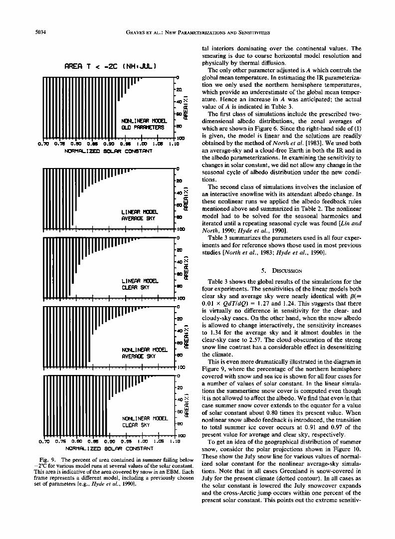
Fig. 9. The percent of area contained in summer falling below -2øC for various model runs at several values of the solar constant.

This area is indicative of the area covered by snow in an EBM. Each frame represents a different model, including a previously chosen set of parameters [e.g., Hyde et al., 1990].

tal interiors dominating over the continental values. The smearing is due to coarse horizontal model resolution and physically by thermal diffusion.

The only other parameter adjusted is A which controls the global mean temperature. In estimating the IR parameterization we only used the northern hemisphere temperatures, which provide an underestimate of the global mean temperature. Hence an increase in A was anticipated; the actual value of A is indicated in Table 3.

The first class of simulations include the prescribed two- dimensional albedo distributions, the zonal averages of which are shown in Figure 6. Since the right-hand side of (1) is given, the model is linear and the solutions are readily obtained by the method of North et al. [1983]. We used both an average-sky and a cloud-free Earth in both the IR and in the albedo parameterizations. In examining the sensitivity to changes in solar constant, we did not allow any change in the seasonal cycle of albedo distribution under the new conditions.

The second class of simulations involves the inclusion of

an interactive snowline with its attendant albedo change. In these nonlinear runs we applied the albedo feedback rules mentioned above and summarized in Table 2. The nonlinear

model had to be solved for the seasonal harmonics and

iterated until a repeating seasonal cycle was found [Lin and North, 1990; Hyde et al., 1990].

Table 3 summarizes the parameters used in all four experiments and for reference shows those used in most previous studies [North et al., 1983; Hyde et al., 1990].

5. DISCUSSION

Table 3 shows the global results of the simulations for the four experiments. The sensitivities of the linear models both clear sky and average sky were nearly identical with /3(-= 0.01 x QdT/dQ) - 1.27 and 1.24. This suggests that there is virtually no difference in sensitivity for the clear- and cloudy-sky cases. On the other hand, when the snow albedo is allowed to change interactively, the sensitivity increases to 1.34 for the average sky and it almost doubles in the clear-sky case to 2.57. The cloud obscuration of the strong snow line contrast has a considerable effect in desensitizing the climate.

This is even more dramatically illustrated in the diagram in Figure 9, where the percentage of the northern hemisphere covered with snow and sea ice is shown for all four cases for

a number of values of solar constant. In the linear simula-

tions the summertime snow cover is computed even though it is not allowed to affect the albedo. We find that even in that

case summer snow cover extends to the equator for a value of solar constant about 0.80 times its present value. When nonlinear snow albedo feedback is introduced, the transition to total summer ice cover occurs at 0.91 and 0.97 of the

present value for average and clear sky, respectively. To get an idea of the geographical distribution of summer

snow, consider the polar projections shown in Figure 10. These show the July snow line for various values of normalized solar constant for the nonlinear average-sky simulations. Note that in all cases Greenland is snow-covered in

July for the present climate (dotted contour). In all cases as the solar constant is lowered the July snowcover expands and the cross-Arctic jump occurs within one percent of the present solar constant. This points out the extreme sensitiv-

GRAVES ET AL.'. NEW PARAMETERIZATIONS AND SENSITIVITIES 5035

NH SUMMER

SNOW L I NE CHANGE -2C I NONLINEAR AVERAGE SKY

SH SUMMER

Fig. 10. The location of the snowline during (a) July for the northern hemisphere and (b) January for the southern hemisphere. Each contour indicates the snow line location for different normalized solar constants from the nonlinear EBM model with the newest parameterizations. The current solar content location is denoted by a dashed line.

ity of the perennial sea ice in the Arctic. It is not clear whether the present climate is on one side of this jump or the other. Actually, it is probably not a jump but a strong transition over a short but finite interval of solar constant as

pointed out by Huang and Bowman [1991]. Note that this transition is not due solely to nonlinearity since a similar phenomenon occurs in the linear models as well. It is a property of the land-sea geography in the Arctic region, and the effect is simply amplified by the snow feedback.

6. CONCLUSION

The analysis of ERB6, ERB7, and ERBE data for the purpose of retuning the seasonal EBMs has resulted in several interesting insights. In the case of the IR we found that outside the tropics a very strong linear relationship exists between the surface temperature and the outgoing IR flux. This is especially valid for the clear-sky component of the radiation. The slope of the regression curve is about 1.90 Wm -2 (øC)-l for the average-sky case and 2.26 Wm -2 (øC)-l for the clear-sky case. These values are important since they tend to be inversely proportional to the sensitivity of the model in the absence of other feedbacks. Using 10 years of data, we were able to examine the relationship at frequencies other than the annual cycle. While not conclu- sive because of the low amplitude of fluctuations away from the annual cycle and its harmonics, it appears that the linear relationship with the same slope holds at other so-called unforced frequencies as well. The slope found in the new data for average sky is rather close to that normally used (within 10%) and do not cause any concern. In other words, the IR study is consistent with previous use.

The albedo derived from the first year of the ERBE experiment has a stronger latitude dependence than has been

used in most EBM experiments over the last decade. Incor- poration of the new albedo parameterization into the EBMs with a corresponding adjustment of the diffusion coefficient to restore the present climate simulation, does not lead to dramatically different results from those previously found. For example, in linear simulations the sensitivity parameter (the change in global temperature of a 1% increase in solar constant) is still about 1.24øC.

One interesting finding in the nonlinear simulations that include snow line feedback is that if we try to simulate a cloud-free planet using the clear-sky albedo and the clear- sky IR parameterization we find a dramatically increased sensitivity (2.57øC) as compared to that for an average-sky planet (1.34øC). This comes about because in the average- sky case the albedo contrast across a snow boundary is so much weakened by the presence of cloud.

Acknowledgments. We gratefully acknowledge the support of a NASA grant through the Langley Research Center for partial support of this work. Some support was also utilized from the National Science Foundation Climate Dynamics Section. It is also a pleasure to thank our colleagues T. J. Crowley and K.-Y. Kim of the Applied Research Corporation and G. L. Smith of NASA/Langley Research Center for their encouragement and helpful conversations.

REFERENCES

Barkstrom, B. R., The Earth radiation budget experiment (ERBE), Bull. Amer. Meteorol., Soc., 65, 1170-1185, 1984.

Barkstrom, B. R., and C. L. Smith, The Earth radiation budget experiment: Science and implementation, Rev. Geophys., 24, 977-985, 1986.

Baum, S. K., and T. J. Crowley, Seasonal Snowline instability in a climate model with realistic geography: Application to carbonif- erous (•300 Ma) glaciation, Geophys. Res. Lett., 18, 1719-1722, 1991.

5036 GRAVES ET AL..' NEW PARAMETERIZATIONS AND SENSITIVITIES

Bess, T. D., and G. L. Smith, Altas of wide-field-of-view outgffoing longwave radiation derived from nimbus 6 Earth radiation budget data set--July 1975 to June 1978, NASA Res. Proj., RP-1185, 1987a.

Bess, T. D., and G. L. Smith, Altas of wide-field-of-view outgffoing long-wave radiation derived from nimbus 7 Earth radiation budget data set--November 1978 to October 1985, NASA Res. Proj., RP-1186, 1987b.

Bess, T. D., G. L. Smith, T. P. Chadock, and F. C. Rose, Annual and interannual variations of Earth-emitted radiation based on a

10-year data set, J. Geophys. Res., 97, 12,825-12,836, 1992. Budyko, M. I., On the origin of glacial epochs, Meteorol. Gidrol., 2,

3-8, 1968. Budyko, M. I., The effect of solar radiation variations on the climate

of earth, Tellus, 21,611-619, 1969. Cess, R. D., Radiative transfer due to atmospheric water vapor:

Global considerations of the Earth's energy balance, J. Quant. Spectrosc. Radiat. Transfer, 21,861-871, 1974.

Crowley, T. J., and G. R. North, Abrupt climate change and extinction events in earth history, Science, 240, 996-1002, 1988.

Crowley, T. J., and G. R. North, Modeling onset of glaciation, Ann. Glaciol., 11, 39-42, 1990.

Deblonde, G., and W. R. Peltier, A model of late pleistocene ice sgheety growth with realistic geography and simplified crydynam- ics and geodynamics, Clim. Dyn., 5, 103-110, 1990.

Harrison, E. F., D. R. Brooks, P. Minnis, B. A. Wielicki, W. F. Staylor, G. G. Gibson, D. F. Young, F. M. Denn, and the ERBE Science Team, First estimates of the diurnal variation of longwave radiation from the multiple-satellite Earth radiation budget experiment (ERBE), Bull. Am. Meteorol. Soc., 69, 1144-1151, 1988.

Huang, J., and K. P. Bowman, The small ice cap instability in seasonal energy balance models, Clim. Dyn., 7, 205-215, 1992.

Hyde, W. T., T. J. Crowley, K-Y. Kim, and G. R. North, Compar- ison of GCM and energy balance model simulations of seasonal temperature changes over the past 18,000 years, J. Clim., 2, 864-887, 1989.

Hyde, W. T., K-Y. Kim, and T. J. Crowley, On the relation between polar coninentality and climate: Studies with a nonlinear seasonal energy balance model, J. Geophys. Res., 95, 18,653-18,668, 1990.

Jones, R. D., Hemispheric surface air temperature variations: Recent trends and an update to 1987, J. Clint., 1,654-660, 1988.

Jones, R. D., S.C. B. Raper, R. S. Bradley, H. F. Diaz, P.M. Kelly, and T. M. L. Wigley, Northern hemisphere surface air temperature variations 1851-1984, J. Clim. Appl. Meteorol., 25, 161-179, 1986.

Kim, K-Y., and G. R. North, Surface temperature fluctuations in a stochastic climate model, J. Geophys. Res., 96, 18,573-18,580, 1991.

Leung, L-Y., and G. R. North, Information theory and climate prediction. J. Clim., 3, 5-14, 1990.

Leung, L-Y., and G. R. North, Atmospheric variability on a zonally symmetric all land planet, J. Clim., 4, 753-765, 1991.

Lin, R-Q., and G. R. North, A study of abrupt climate change in a simple nonlinear climate model, Clim. Dyn., 4, 253-261, 1990.

North, G. R., The small ice cap instability in diffusive climate models, J. Atmos. Sci., 41, 3390-3395, 1984.

North, G, R., and R. F. Cahalan, Predictability in a solvable stochatic climate model, J. Atmos. Sci., 38, 504-513, 1982.

North, G. R., and J. A. Coakley, Jr., Differences between seasonal and mean annual energy balance model calculations of climate and climate sensitivity, J. Atmos. Sci., 36, 1189-1204, 1979.

North, G. R., R. F. Cahalan, and J. A. Coakley, Jr., Energy balance climate models, Rev. Geophys., 19, 91-121, 1981.

North, G. R., J. G. Mengel, and D. A. Short, Simple energy balance model resolving the seasons and the continents: Applications to the astronomical theory of the ice ages, J. Geophys. Res., 88, 6576-6586, 1983.

Ramanathan, V., and W. Collins, Thermodynamic regulation of ocean warming by cirrus clouds deduced from observations of the 1987 E1 Nifio, Nature, 351, 27-32, 1991.

Ramanathan, V., B. R. Barkstrom, and E. F. Harrison, Climate and the Earth's radiation budget, Phys. Today, 42, 22-32, 1989.

Sellers, W. D., A climate model based on the energy balance of the Earth-atmosphere system, J. Appl. Meteorol., 8, 392-400, 1969.

Short, D. A., G. R. North, T. D. Bess, and G. L. Smith, Infrared parameterization and simple climate models, J. Clim. Appl. Meteorol., 23, 1222-1233, 1984.

Short, D. A., J. G. Mengel, T. J. Crowley, W. T. Hyde, and G. R. North, Filtering of Milankovitch cycles by Earth's geography, Quat. Res. N.Y., 35, 157-173, 1991.

Suarez, M. J., and I. M. Held, The sensitivity of an energy-balance climate model to variations in the orbital parameters, J. Geophys. Res., 84, 4825-4836, 1979.

Watts, R. G., and M. E. Hayder, The effect of land-sea distribution on ice-sheet formation (abstract), Ann. Glaciol., 5,234-236, 1984.

Wielicki, B. A., and R. N. Green, Cloud identification for ERBE radiation flux retrieval, J. Appl. Meteorol., 28, 1133-1146, 1989.

C. E. Graves, Department of Earth and Atmospheric Sciences, St. Louis University, St. Louis, MO 63103.

W-H. Lee and G. R. North, Climate System Research Program, College of Geosciences, Texas A&M University, College Station, TX 77843.

(Received January 16, 1992; revised October 13, 1992;

accepted November 6, 1992.)

New parameterizations and sensitivities for simple climate models

Documents

Transcript of New parameterizations and sensitivities for simple climate models