Sensitivities of Corporate Investment and Financing Decisions to the ...

Sensitivities of Corporate Investment andFinancing Decisions to the Implied Cost of

Capital

Soku Byoun∗ David Ng† and Kai Wu‡

August 2015§

∗Hankamer School of Business, Baylor University, One Bear Place, #98004, Waco, TX 76798-8004. Email:Soku [email protected]. Phone: (254)710-7849. Fax: (710)710-1092.†Dyson School of Applied Economics and Management, Cornell University. Email: [email protected].

Phone: (607)255-0145.‡Dyson School of Applied Economics and Management, Cornell University. Email: [email protected].

Phone: (607)379-1678.§We would like to thank Andrew Karolyi, George Gao, Byoung-Hyoun Hwang, Hyunseob Kim, Murillo

Campello, Zhongjin Lu, Zhaoxia Xu for helpful comments and discussions. We also thank seminar par-ticipants at Cornell University, Baylor University and Ulsan National Institute of Science and Technology(UNIST).

Sensitivities of Corporate Investment and Financing Decisions to the ImpliedCost of Capital

AbstractMost textbooks suggest factor models like Capital Asset Pricing Model and the Fama andFrench (1992, 1993) model to estimate the cost of equity. Recent studies question this prac-tice. We examine the attributes of the implied cost of capital (ICC) as an alternative costof equity measure. Our results show that the ICC has negative effects on investment andequity issuance, whereas the factor model estimates have opposite effects on these decisions.We find that such opposite effects of the CAPM and FFM estimates on investment andfinancing decisions are attributed to the way in which stock prices reflect cash flow news anddiscount rate news. Moreover, the ICC exhibits the properties of the cost of equity regardingequity dependence, private information, and capital supply shocks, whereas the factor modelestimates fail to do so. Our findings lend support for the ICC as the cost of equity in thecapital budgeting process.

JEL Classification: G31; G32

Keywords: Implied Cost of Capital; Corporate Investment; Cash Flow News; Discount RateNews

1 Introduction

Among the most fundamental tasks for corporate managers is to decide when to raise capital

and which investment project to undertake. Having a good estimate for the cost of capital

is an essential component for the capital budgeting decision. The CAPM and the Fama and

French (1992, 1993) model (FFM) are currently the standard textbook choice for estimating

the cost of equity (COE). Yet, Fama and French (1997) contend that the uncertainty about

risk premiums and risk loadings for the CAPM and the FFM implies “woefully imprecise

estimates” of the COE.1 Levi and Welch (2014) show that the CAPM and the FFM fail

to adjust for term and risk premia and do not predict subsequent rates of return. They

conclude that the CAPM and the FFM are “useless for capital budgeting purposes.”

This raises the question of what other COE estimates should be used for capital bud-

geting.2 Recently, Frank and Shen (Forthcoming) find that cost of capital based on CAPM

predict positively subsequent corporate investment, suggesting that CAPM model prediction

is not even directionally correct. They also find that cost of capital estimated based on the

implied cost of capital (ICC) approach at least gets the direction right in that it negatively

predicts subsequent corporate investment. Their finding leaves open the possibility that ICC

can potentially serve as a reasonable COE proxy.

The implied cost of capital is the internal rate of return obtained by equating the stock

price to the present value of expected future cash flows. The ICC has been used in various

asset pricing contexts.3 In particular, Lee, So, and Wang (2014) show that the ICC predicts

1Their estimates suggest that the 95-percent confidence interval of the market risk premium ranges fromless than zero to more than 10%.

2Levi and Welch (2014) suggest using the same cost of capital for all projects, which is not very satisfying.3For example, previous papers use the ICC to study: the unconditional equity premium (Claus and

1

the realized returns better than the CAPM and FFM. Li, Ng, and Swaminathan (2013) also

show that the aggregate ICC predicts the future market returns. Both argue that ICC serves

as a good proxy for expected returns. Thus, it is useful to see if the ICC would be a good

proxy for COE estimate in corporate financial decision.

A useful COE estimate should not only predict future investment negatively, but it should

also possess other qualities. The COE proxy should predict future financing activities in ad-

dition to future investment. Meanwhile, the sensitivity of investment to the COE should

vary depending on the level of equity dependence and the amount of private information.

Additionally, a shock in the supply of capital should affect COE. Our paper examines the

characteristics of the ICC to see whether it can be a good COE proxy, especially in compar-

ison to the CAPM and FFM estimates.

To that end, we do the following. First, we test the theoretical prediction that firms

increase equity financing as well as investment when facing lower cost of equity.4 Second,

while Frank and Shen (Forthcoming) leave it as a puzzle why ICC is at least directionally

correct in predicting future investment while CAPM is not, we examine how COE estimates

reflect the cash flow news and discount rate news. Third, we examine the sensitivities of

investment to COE proxies conditional on the degree of equity dependence. The sensitivity

of investment to the COE is expected to be greater for firms with greater equity dependence

Thomas (2001) and Fama and French (2002)); stock market return predictability (Li, Ng, and Swaminathan(2013)); theories on betas (Kaplan and Ruback (1995), Botosan (1997), Gebhardt, Lee, and Swaminathan(2001), Gode and Mohanram (2003), Brav, Lehavy, and Michaely (2005), and Easton and Monahan (2005));international asset pricing (Lee, Ng, and Swaminathan (2009)); default risk (Chava and Purnanandam(2010)); cross-sectional expected returns (Hou and Van Dijk (2010), Botosan, Plumlee, and Wen (2011));stock return volatility (Friend, Westerfield, and Granito (1978)); and the cost of equity (Burgstahler, Hail,and Leuz (2006), Botosan and Plumlee (2005), and Hughes, Liu, and Liu (2009)).

4Taggart (1977),Marsh (1982) and Baker and Wurgler (2002) suggest that firms prefer to issue equitywhen equity prices are relatively high.

2

(Baker, Stein, and Wurgler (2003)). Fourth, we examine the sensitivities of investment to

COE proxies conditional on the amount of private information. Chen, Goldstein, and Jiang

(2007) and Bakke and Whited (2010) suggest that investment decisions respond to stock

prices as firms are informed about their investments from the stock market. In light of these

studies, the COE is expected to have a larger impact on investment for firms with greater

private information. Finally, we examine the effect of supply shocks in equity capital from

natural experiments. A positive (negative) shock in the supply of capital is expected to have

a negative (positive) effect on the COE.

We find that the ICC has significantly negative impacts on corporate investment and

net equity issuance, while the CAPM and FFM estimates have the opposite effects. We

demonstrate that such opposite effects are attributed to the way in which stock prices reflect

cash flow and discount rate news. Specifically, the ICC is positively correlated with discount

rate news, and negatively with cash flow news. On the contrary, the CAPM and FFM

estimates are negatively correlated with discount rate news (a wrong direction) and positively

correlated with cash flow news, resulting in their positive effects on investment.

Our results show that the sensitivities of investment to the COE proxies are affected

by both equity dependence and private information from the stock market. Specifically,

lower ICC induces additional investment for firms with high equity dependence and greater

private information. The CAPM and FFM estimates, however, have insignificant effects

on investment for firms with high equity dependence and greater private information, while

showing positive and significant effect for firms with low equity dependence and less private

information. We also find that the ICC tends to increase (decrease), while the CAPM and

3

FFM estimates tend to decrease (increase), when facing a negative (positive) supply shock

in equity capital. These findings indicate that the ICC displays the properties of the COE,

whereas the CAPM and FFM estimates do not exhibit such properties.

Our study has important implications for finance instructors and researchers. Managers

determine the optimal level of investment through their experience after observing the stock

price. What we find out is that the ICC is close to the COE they come up with after

considering the market conditions. In contrast, the CAPM and the FFM estimates are

neither consistent with the theory nor relevant to the real world practice. Thus, we need

to reconsider our practice of teaching students to use the CAPM and the FFM in capital

budgeting. Also, applying the CAPM or FFM estimates as the COE in empirical corporate

finance research can result in misleading conclusions. In this regard, we demonstrate that

the ICC, as a COE estimate, is not only theoretically sound but also relevant to corporate

financial decisions.

Our study is also linked to the q-model with the interdependence of investment and

financing decisions in Bolton, Chen, and Wang (2011). Bolton, Chen, and Wang (2011)

show that external financing costs due to asymmetric information and managerial incentive

problems have impact on investment beyond q. Consistent with the prediction of their

model, our findings suggest that the ICC is highly informative about the risk of investment

opportunities particularly for equity dependent firms.

Our study also contributes to the literature on private information in stock price for

investment decisions. For example, previous studies show that the stock market affects

corporate investment as it informs managers about real variables (Dow and Gorton (1997),

4

Subrahmanyam and Titman (1999), Dow and Rahi (2003), Chen, Goldstein, and Jiang

(2007), and Goldstein and Guembel (2008)) or as irrational movements in stock prices make

the effective cost of equity lower relative to other capital sources (Baker, Stein, and Wurgler

(2003)).5 Yet, previous findings do not tell what kind of private information firms gather

from the stock market. Our findings suggest that the discount rate implied by the stock

price is particularly important information for managers to assess investment and financing

decisions. The ICC appears to be informative about the project risk: managers learn about

the market’s assessment of the firm’s project risk, which they incorporate in their investment

decisions.

The remainder of the paper proceeds as follows: Section 2 presents the investment model

that highlights the role of cost of equity beyond cash flow and Tobins q. In Section 3, we

describe the data, sample construction, and the methodology for measuring the COE and

return decomposition. Section 4 presents the empirical results on the relation between the

COE and corporate investment and financing behaviors, and provides the possible channel

through which alternative COE proxies affect corporate investment differently. Section 5

explores the stock market feedback effects. Section 6 examines the effect of supply shocks

in equity capital on COE proxies. Section 7 carries out a battery of conventional robustness

checks including alternative estimation methods, sub-sample analysis, variable definitions,

and control variables. Section 8 concludes.

5Bond and Goldstein (2011) provides an excellent review on the real effects of financial markets and theirimplications.

5

2 An Investment Model with External Financing Costs

Abel and Blanchard (1986) develop a model to show that an increase in expected future cash

flows is associated with the higher marginal return on investment today, while an increase

in discount rates is associated with the lower marginal return on investment. We use their

model to define a firm value as given by the discounted value of maximized net cash flows

as follows:

Vt = Et

∞∑j=0

j∏i=1

(1 + rt+i)−1Ct+j(Kt+j, It+j(1 + θt+j)), (1)

where Et is the expectation operator conditional on information at time t, rt+i is the discount

rate at time t+ i, Kt+j and It+j are capital stock and investment, θt+j ∈ (−1, 1) is the effect

of external financing costs, and Ct+j(Kt+j, It+j) is cash flow at time t + j. The external

financing costs are broadly defined to include the effects of asymmetric information and

agency problem; i.e., they include the possibility of mispricing or feedback from private

information embedded in stock price about the firm’s investment opportunities. Bolton,

Chen, and Wang (2011) explicitly show that such external financing costs have an impact

on investment beyond q. Similar to their approach, we modify the q-model to show that

the marginal cost of investment is no longer equal to q in the presence of external financing

costs.

The firm value changes when expected cash flows change, or when discount rates change.

The firm maximizes Vt subject to the following condition:

Kt+1 = (1− δ)Kt + It (2)

6

where δ is the depreciation rate. The first order conditions maximizing the firm value at t

implies:

∂L

∂Kt

= Et

∞∑j=0

{j∏i=1

(1 + rt+i)−1

}∂Ct+j∂Kt+j

(1− δ)j − qt = 0 (3)

∂L

∂It= Et

∂Ct∂It

(1 + θt) + qt = 0 (4)

where Lagrange multiplier qt represents the marginal rate of return on investment at time t.

The first order conditions imply the following:

qt = Et

∞∑j=0

{j∏i=1

Rt+i

}ct+j (5)

MCIt = −Et∂Ct∂It

=qt

1 + θt(6)

Thus, equation (6) suggests that the marginal cost of investment (MCIt) can deviate from

the expected present value of marginal returns to capital (qt). In case of no external financing

costs (θt = 0), we obtain qt = MCIt.

3 Data and Methodology

3.1 Sample Construction

Our initial sample consists of US firms from the Center for Research in Security Prices (CR-

SP)/Compustat Merged Database from 1985 to 2013. We obtain the stock price, the number

of shares outstanding, the SIC code, and monthly returns from CRSP, firm-level annual ac-

7

counting data from Compustat, analysts’ earnings forecasts from I/B/E/S, and the nominal

GDP growth rates from the Bureau of Economic Analysis. We exclude firms operating in

regulated utilities (SIC code 4000-4999) and financial (SIC code 6000-6999) industries. We

further drop firm-year observations with negative sales or total assets. Since computing ICCs

requires analysts’ earnings forecasts, the number of firms with valid information are reduced

to 40,123 firm-year observations.

3.2 The Proxies for the Cost of Equity

There is no consensus about the computing procedure of the ICC in the literature. Each

study makes its own specific assumptions to facilitate the computation of the ICC. We

compute three ICCs for each firm, following the procedures utilized by Claus and Thomas

(2001), Gebhardt, Lee, and Swaminathan (2001), and Li, Ng, and Swaminathan (2013),

respectively. For comparison, we also estimate the COE using the CAPM, the Fama and

French (1992, 1993) 3-factor model (FF3M), and the 4-factor model (FF4M, Carhart (1997)).

We provide the detailed estimation procedures in Appendix A

3.3 Return Decomposition

In order to examine the relative effects of the discount rate and cash flow on corporate

investment, following the methodology of Chen, Da, and Zhao (2013), we decompose the

realized return into two components: (1) cash flow news (CFN), defined as the price change

holding the discount rate constant, and (2) discount rate news (DRN), defined as the price

change holding the cash flow forecasts constant. Specifically, the stock return between month

8

t and t+ 1 can be written as follows:

ri,t =Pi,t+1 − Pi,t

Pi,t=f (ci,t+1, di,t+1)− f (ci,t, di,t)

Pi,t

= CFN i,t −DRN i,t (7)

where f (·) is the discounted cash flow function, and ci,t, di,t is the cash flow forecast and the

ICC of firm i at month t, respectively. The cash flow news (CFN) and discount rate news

(DRN) could be expressed as

CFNi,t =1

2

[f (ci,t+1, di,t+1)− f (ci,t, di,t+1)

Pi,t+f (ci,t+1, di,t)− f (ci,t, di,t)

Pi,t

](8)

DRNi,t = −1

2

[f (ci,t, di,t+1)− f (ci,t, di,t)

Pi,t+f (ci,t+1, di,t+1)− f (ci,t+1, di,t)

Pi,t

](9)

We then compound the monthly CFN andDRN to annualize them over the firm’s fiscal year.

According to the Abel and Blanchard (1986) model, CFN is expected to have positive effect,

while DRN is expected to has negative effect, on investment. The return decomposition

should shed light on the fundamental question of whether cash flow or discount rate news is

the main driver of corporate investment.

We also follow the methodology of Campbell and Shiller (1988) to decompose the return

into CFN (related to future dividends) andDRN (related to the discount rate). Particularly,

omitting the firm subscript i, the unexpected return can be expressed as

rt − Et−1 (rt) = CFNt −DRNt (10)

9

To estimate the components of equation (10), we assume a system of log-linear dynamic equa-

tions for market returns, return on equity and any other variables assumed to affect market

returns and return on equity (Callen and Segal (2010)). The VAR system is formulated as

follows:

rt = α1rt−1 + α2roet−1 + α3bmt−1 + η1t (11)

roet = β1rt−1 + β2roet−1 + β3bmt−1 + η2t (12)

bmt = γ1bmt−1 + γ2roet−1 + γ3bmt−1 + η3t. (13)

Following Vuolteenaho (2002), we estimate earnings news residually and discount rate news

directly.

3.4 Summary Statistics

Panel A in Table 1 provides the summary statistics for the sample. The average (median)

capital expenditure (CAPX) and is 6.8% (4.6%) of total assets. The average net equity

issuance is 11.2% of total assets and the median is mere 0.8%. Thus, the firms’ capital

investment activities are fairly active, while equity issuing activities are lumpy and less

frequent. The average ICC ranges from 9.8% (ICC-GLS) to 14% (ICC-LNS), while the

factor-model-based estimates range from 11% to 12.1%.

(Insert Table 1 about here)

10

We report the correlations matrix for our estimates in Panel B. The CAPM and FFM

estimates and ICCs show positive and significant correlations with one another but ICCs

and the factor-model-based estimates are more highly correlated among themselves. ICCs

have significant and positive correlations with the discount rate news. The CAPM estimate

also shows positive correlation with the discount rate news. However, the FFM estimates

show little correlation with the discount rate news.

4 Empirical Results

4.1 The Cost of Equity and Corporate Investment

In order to investigate the effect of each of the cost-of-equity proxies on corporate investment,

we start with the following baseline regression model:

Ii,t = α0 + α1Rei,t−1 + α2CFi,t + α3qi,t−1 + ηt + θi + εi,t, (14)

where i and t represent firm and time, respectively. I is investment (capital expenditure

scaled by beginning-of-the-year assets), Re is the COE proxy, CF is cash flow divided by

total assets. We also include firm fixed effects θi and year effects ηt in order to control for

firm-specific characteristics and general economic trends. Detailed definitions of variables

are provided in Appendix B.

Table 2 reports the estimation results of investment regression (14). The coefficient

estimates on all ICCs are significant and negative, suggesting that firms invest less when

11

the COE is higher. However, the coefficient estimates on the CAPM and FFM estimates

are positive and significant, suggesting that firms invest more when the COE is higher. The

results also show that CF and q have significant and positive effects on investment, consistent

with previous results.


In order to examine whether the ICC absorbs the explanatory power of the factor-model-

based estimates, or vice versa, we simultaneously include both the ICC and the factor-model-

based estimates in columns (8)-(10). The results with the ICC-LNS show that both the ICC

and the factor-model estimate have independent and opposite effects on investment.

4.2 The Cost of Equity and Net Equity Issuance

In Table 3, we also investigate the effect of the COE on net equity issuance using the

same regression model of (14) with the dependent variable replaced by net equity issuance.

The coefficient estimates on ICCs are all significant and negative, which suggests that firms

issue more shares when the COE is low. In contrast, the coefficient estimates on the CAPM

and FFM estimates are positive and significant. The results also suggest that CF and q

have positive effects on net equity issuance.


If the COE serves as the ex-ante required rate of return on equity in the capital bud-

geting decision, ceteris paribus, the company is expected to increase its equity issuance and

investment when the COE is low. Our findings of the negative relations between ICCs and

12

investment/net equity issuance is consistent with this argument. The CAPM and FFM es-

timates, however, appear to reflect the opposite effects of profitability and the discount rate

on investment so as to produce positive association with investment and net equity issuance.

4.3 The Effects of Cash Flow News and Discount Rate News

In order to understand the contradicting effects of the factor-based estimates and ICCs, we

examine their relations with the cash flow news (CFN) and discount rate news (DRN). We

first examine how CFN and DRN affect investment and net equity issuance based on the

following regression model:

Ii,t = β0 + β1CFi,t + β2qi,t−1 + β3CFNi,t−1 + β4DRNi,t−1 + ηt + θi + εi,t. (15)

Table 4 reports the estimation result for both investment and equity issuance. In all

regressions, the coefficient estimates on CFN are positive and significant, while those on

DRN are negative and significant. The results are similar whether we use the Chen, Da,

and Zhao (2013) or Campbell and Shiller (1988) approach for the return composition. Thus,

these findings confirm that CFN has positive effects, while DRN having negative effects, on

investment and equity issuance decisions.


We also run the following regressions to examine the relation between alternative COE

13

proxies and CFN/DRN:

Rei,t = α0 + α1CFNi,t + α2DRNi,t + εi,t. (16)

Table 5 reports similar results on Panel A (Chen, Da, and Zhao (2013) return decompo-

sition) and on Panel B (Campbell and Shiller (1988) approach). ICCs reflect both the CFN

and DRN . The coefficient estimates on DRN are positive and significant, while those on

CFN are negative and significant, which suggests that the higher discount rate is associated

with higher ICC. Thus, the negative relation between ICCs and investment is consistent

with the idea that investment should be lower when facing a low marginal rate of return on

investment and relatively high cost of capital. However, for the FFM estimates, the coeffi-

cient estimates on DRN are negative and significant, while those on CFN are positive and

significant. For the CAPM estimate, the coefficient estimates on both DRN and CFN are

not significant.


The results in Table 5 suggest that the effects of profitability and discount rate news

on investment are partly captured by the CAPM and FFM estimates. The factor-model-

based estimates appear to reflect the expected future investments affected by profitability

and discount rate news. To add up a bit, note that, subject to the transversality condition,

equation (5) implies:

Et(1 + rt+1) =Et(qt+1 + ct+1)

qt. (17)

This equation suggests that the expected return is high when the expected future cash flows

14

(ct+1) and the marginal rate of return on investment (qt+1) are high. Both high expected

future cash flows and low discount rate increase the marginal return on investment, which

will induce firms to increase investment. Expected increase in investment will also increase

expected return. This will show as the positive relation between the cash flow news and the

expected return and the negative relation between the discount rate news and the expected

return, which is consistent with our findings for the CAPM and FFM estimates.

Thus, the positive effects of the CAPM and FFM estimates can be attributed to their

forward-looking nature into future investments. Unlike the CAPM and FFM estimates, the

ICC reflects the market’s assessment of the firm’s discount rate for its long-term cash flows.

Thus, the ICC serves as a proper proxy for the COE in the firm’s investment and financing

decisions. The CAPM and FFM estimates, however, fail to reflect the effect of the COE on

investment.

5 Feedback Effects from the Stock Market

The effects of the COE on corporate investment and equity issuance beyond q can reflect

feedback from the stock market. The literature documents two channels through which the

stock market affects investment. On one hand, Baker, Stein, and Wurgler (2003), Gilchrist,

Himmelberg, and Huberman (2005), and Polk and Sapienza (2009) find significant effects

of mis-pricing on investment. On the other hand, Chen, Goldstein, and Jiang (2007) and

Bakke and Whited (2010) find that firms’ investment decisions respond to stock prices as

firms are informed about their investments from the stock market. We explore these stock-

15

market-feedback channels below.

5.1 Equity Dependence and Investment Sensitivity

Campbell and Shiller (1988) suggest that “investor sentiment can directly affect discount

rates, but cannot directly affect cash flows.” Since overpriced stock implies a lower COE for

given cash flows, the COE may better reflect the nonfundamental component of the stock

price. Baker, Stein, and Wurgler (2003) suggest that equity-dependent firms’ investment

is especially sensitive to mispricing in the stock market. Thus, the effect of mispricing on

investment is more likely to be captured by the sensitivity of investment to the COE for firms

with greater equity dependence. This leads to the hypothesis that equity-dependent firms

display a more negative sensitivity of investment to the COE than do non-equity-dependent

firms.

Based on the above hypothesis, we compare the performance of alternative COE proxies

between high and low equity-dependent firms. Following Baker, Stein, and Wurgler (2003),

we use the KZ index to measure equity dependence:

KZi,t = −1.002CFi,t − 39.368DIVit − 1.315CASHi,t + 3.139LEVi,t. (18)

We define firms with the top 30% KZ index as high equity-dependent and firms with the

bottom 30% KZ index as low equity-dependent. We expect to find stronger effects of COE

proxies on investment for high equity-dependent firms than for low equity-dependent firms.

Table 6 presents the results. For high equity-dependent firms on Panel A, we find that

16

the coefficient estimates on ICCs are all negative and highly significant, while those on

factor-based COE proxies are all insignificant. For low equity-dependent firms on Panel B,

the coefficient estimates on ICCs are insignificant, while those on factor-based COE proxies

exhibit strong positive effects on corporate investment. To the extent that ICCs are driven

by mispricing, our results suggest that equity-dependent firms’ investment is particularly

sensitive to stock mispricing. In contrast, the CAPM and FFM estimates show significant

positive effects only for non-equity-dependent firms.


5.2 Price Informativeness and Investment Sensitivity

We also examine if COE proxies convey new information about the firm’s investment, es-

pecially regarding the risk of investment reflected on the discount rate. Such information

feedback is expected to be more pronounced for firms with greater private information in

their stock prices. Accordingly, we examine the sensitivities of investment to COE proxies,

conditional on the amount of private information. We measure the amount of private infor-

mation by the price nonsynchronicity calculated as one minus R-square from the time-series

regression of daily return on market and 3-digit SIC industry portfolio returns over the fiscal

year.6 Chen, Goldstein, and Jiang (2007) suggest that a weak correlation of a firm’s stock

return with the market and industry returns indicates more firm specific information which

is useful for the firm’s investment decision. Based on the price nonsynchronicity measure, we

6This measure was first suggested by Roll (1988) and later developed by Morck, Yeung, and Yu (2000),Durnev, Morck, Yeung, and Zarowin (2003), Durnev, Morck, and Yeung (2004), and Chen, Goldstein, andJiang (2007).

17

define the top 30% as large private information firms and the bottom 30% as small private

information firms. For the estimation of price nonsynchronicity, we require that firms have

at least 150 days of non-missing returns during the given year.

Table 7 presents the results. The coefficient estimates on ICCs are all negative and signif-

icant for firms with large private information on Panel A, whereas the coefficient estimates

on ICCs are all insignificant for firms with small private information on Panel B. In contrast,

the coefficient estimates on the CAPM and FFM estimates are all insignificant for firms with

large private information on Panel A, whereas they are all positive and significant for firms

with small private information on Panel B. These findings suggest that a firm’s investment is

particularly sensitive to the ICC when there is greater amount of private information in the

stock price. Thus, the ICC appears to contain information about the market’s assessment

of project risk beyond what is reflected in q. However, results for the CAPM and FFM es-

timates suggest that firms with low private information tend to have more investment when

the COE is higher.


Overall, our findings suggest that both mispricing and private information are affecting

the investment-ICC sensitivity. The takeaway from this exercise is that lower ICC, whether

it is driven by mispricing or reflecting private information, induces additional investment

for firms, which is an important property of the COE. In contrast, the CAPM and FFM

estimates show significant and positive effects on investment for firms with less mispricing

or private information. The CAPM and FFM estimates appear to reflect the positive effect

of upcoming investment on the stock price especially when the firm’s stock price reflects

18

more fundamental information and moves more synchronously with the industry and market

trends.

6 Effects of Capital Supply Shocks

In this section, we further evaluate the validity of COE proxies based on another property

of the COE: i.e., the COE will be higher (lower) when there is a negative (positive) supply

shock in equity capital. To this end, we examine the effects of negative supply shocks during

recessions and positive supply shocks following legislation granting capital gains tax cuts.

6.1 Behavior of the Cost of Equity Estimates during Recessions

We plot the time trends of the COE proxies in Figure 1. ICCs tend to increase during the

highlighted recession periods, while the CAPM and FFM estimates show the opposite trend.

Thus, ICCs indicate that the COE becomes higher during recessions, whereas the CAPM

and FFM estimates indicate that the COE becomes lower during recessions. ICCs appear to

reflect the hightened uncertainty and risk aversion of investors during recessions (Gonzalez-

Hermosillo (2008), Coudert and Gex (2007), and Frank and Goyal (2009)), whereas the

CAPM and FFM estimates appear to reflect diminishing profitability and high discount

rate. The results for the CAPM and FFM estimates are consistent with the forward-looking

nature of the expected return.

(Insert Figure 1 about here)

19

6.2 Natural Experiment

Taxpayer Relief Act of 1997 (TRA) and the Jobs and Growth Tax Relief Reconciliation Act

of 2003 (JGTRRA) provide tax cuts in capital gains, raising the effective after-tax return

for equity investors and thereby the supply of equity capital (Dai, Shackelford, Zhang, and

Chen (2013)). The effect of the tax cut on the COE will depend on the elasticity of capital

demand: with perfectly inelastic demand, the COE will be reduced by the tax cut; with

perfectly elastic demand, the COE will not change. Using financial constraint as a proxy

for the demand elasticity of equity capital, we hypothesize that financially constrained firms

have low demand elasticity of equity capital and experience a larger reduction in the COE

following the tax cuts.

We test the hypothesis with the following difference-in-difference (DID) regression:

Rei,t = α0 + α1Postt + α2HFCi + α3Postt ×HFCi + εit, (19)

where Post is a dummy variable that takes 1 if it is the third quarter of 1997 or 2003, and

0 if it is the first quarter of 1997 or 2003 (skipping the announcement quarter). HFC is a

dummy variable which takes value of 1 if the firm is on the top 30% of financial constraint

at the beginning of the year, defined as in Hadlock and Pierce (2010):7

FCi,t = Pr (Financial Constraint) = 1− 1

1 + exp (β′Xi,t − 0.454), (20)

7We also try the KZ index as an alternative measure of financial constraint. The results are similar andnot reported.

20

where

β′Xi,t = 0.737× Sizei,t+0.043× Size2i,t−0.04× Firmagei,t. (21)

Table 8 presents the estimation results of the DID regressions. The coefficient estimates

on Post are negative and significant for all three ICC measures, indicating that the COE

becomes lower following the positive supply shock in equity capital. The significant and

negative coefficient estimates on Post ∗HFC for ICC measures also suggest that after the

adoption of TRA and JGTRRA, the COE decreased significantly more for low demand

elasticity firms than for high demand elasticity firms. For factor-model-based estimates,

however, the coefficient estimates on Post and Post ∗HFC are all significant and positive,

suggesting that the COE is higher following positive supply shocks in equity capital and

especially for low demand elasticity firms. To recapitulate, using exogenous shocks from tax

reforms, we show that the ICC demonstrate the property of the COE, while the CAPM and

FFM estimates show the property of the forward-looking expected return.


7 Robustness Checks

7.1 Erickson and Whited Error-in-Variable GMM

Erickson and Whited (2000, 2002, 2012) suggest that the measurement error in Tobin’s q has

a significant effect on coefficient estimates. It is possible that our results for the COE proxies

21

are also driven by measurement errors. Accordingly, we implement their measurement-error

consistent GMM technique to correct for measurement errors in q and the COE estimates.

The results (Table A1 in the Online Appendix) show that our findings remain quantitatively

and qualitatively the same. Thus, we rule out the potential effect of measure error for our

findings.

7.2 Controlling for Fundamentals

Morck, Shleifer, and Vishny (1990) suggest that the positive correlation between stock price

and investment reflects fundamentals. We examine if the effect of the COE on investmen-

t still holds when we incorporate firm fundamentals in q. Cummins, Hassett, and Oliner

(2006) suggest that Tobin’s q constructed using analysts’ forecast earnings better reflects

fundamentals important for investment spending. In particular, using the analysts’ forecast

earnings-based q, they find no evidence that investment is sensitive to cash flow. Conse-

quently, we also examine if our results are altered when the fundamental q is used.

The results (in Table A2 in the Online Appendix) show that all coefficient estimates on

ICCs remain negative and highly significant, whereas those on the CAPM and FFM expected

returns are still positive and significant. The ICC appears to inform firms about the risk of

investment, beyond q and CF .

7.3 Is the Result Driven by Growth Firms?

Growth firms may face higher COEs and have large investment opportunities. This may re-

sult in the positive association between the COE and investment. To examine this possibility,

22

we run regressions of capital expenditures on COE proxies excluding growth firms.

The results (in Table A3 in the Online Appendix)excluding firms with B/M ratios in

the bottom 30%. The results remain qualitatively the same. Specifically, on one hand, the

coefficient estimates on ICCs are all significant and negative except for the result on ICC-CT.

On the other hand, factor-based COE proxies are all significant and positive.

7.4 Other Firm Characteristics

We also investigate the effect of the COE on corporate investment while controlling for other

firm characteristics, which should mitigate the concern that our COE proxies simply capture

some firm characteristics not reflected in q. For this exercise, we estimate regression (14)

including the following additional control variables: leverage (Lev), firm size (Size), cash

dividend (Div), fixed assets (FA), and cash holdings (Cash). Table 9 reports the results.

The signs and significance of all coefficient estimates for COE proxies remain the same as

previously reported results.


7.5 Recession Periods

Given the opposite patterns between ICCs and factor-model-based estimates during recession

periods in Figure 1, We check if their opposite effects on investment are driven by recession

periods. To this end, we run separate regressions for recession and non-recession periods.

The results (in Table A4 in the Online Appendix) show that the coefficient estimates

on ICCs are significant and positive for non-recession periods, but none of the estimates

23

are significant during recession periods. The insignificant results for the recession periods

may reflect the distortion of firms’ investment activities due to uncertainty shocks (Bloom,

Floetotto, Jaimovich, Saporta-Eksten, and Terry (2014)). The coefficient estimates on the

CAPM and FFM estimates show mixed results. Thus, we verify that the negative effect of

the ICC on corporate investment is not driven by its particular behavior during recession

periods.

7.6 Research and Development (R&D) and Mergers and Acquisi-

tions (M&A)

For our main results, our sample did not include firms with R&D and M&As. In this

section, we examine the relation between COE proxies and corporate investment including,

R&D and M&As. Specifically, we estimate our investment regressions with the dependent

variable defined as the sum of capital expenditure (CAPX) plus R&D and M&A scaled

by beginning-of-the-year total assets. The results (in Table A5 in the Online Appendix)

show that all coefficient estimates on ICC measures remain negative and highly significant,

whereas those on the CAPM and FFM expected returns all become insignificant. These

findings reinforce the preponderance of the ICC as a measure of the COE.

7.7 Long-term Effects

Given that some capital projects involve long-term planning and implementation, there may

be a time gap between the time of estimating the COE and the actual investment for a

24

project. In order to check the potential effect of this time gap, we try longer (up to two-

year) lags of the COE proxies.

The estimation results with the second-year lags of the COE proxies (in Table A6 in the

Online Appendix) show that the long-term effects are not significant except for the two-year

lagged FF4M expected return which has positive and significant effect. Thus, our findings

suggest that the long-term effects of the proxies are limited.

8 Conclusion

When the market assesses low risk for a firm’s investment opportunities, the effective cost of

equity (COE) becomes lower. As a result, the firm is likely to take on more investment. One

of the puzzling result from empirical literature on the effect of the COE on investment is the

apparent positive relation between investment and the COE, as proxied by the CAPM and

the Fama-French model. We find strong empirical evidence that the implied cost of capital

is negatively related to both investment and equity issuance. We also show that cash flow

news has a positive effect on investment and equity issuance, whereas discount rate news

has a negative effect on these decisions. The ICC, reflecting discount rate news and cash

flow news properly, show unequivocally negative effect on investment and equity issuance.

The CAPM and FFM expected returns, reflecting the effects of cash flow and discount rate

news on investment and financing, tend to show mixed or positive effect on investment and

equity issuance. Moreover, the ICC exhibits stronger effect on corporate investment for firms

with more equity dependence and greater private information, which is consistent with the

25

prediction that firms invest more when the market perceives lower COE whether rationally

or irrationally. Furthermore, our results suggest that the ICC increases (decreases) following

negative (positive) supply shocks in equity capital, particularly when the demand is not

elastic, whereas the CAPM and FFM estimates have the opposite effects.

In conclusion, our results lend strong support for the application of the ICC in the capital

budgeting process. The preponderance of the ICC over the traditional factor-model-based

proxies comes from the fact that ICC captures cash flow news and discount rate news in the

way that is consistent with the theoretical prediction.

26

ReferencesAbel, Andrew B., and Oliver J. Blanchard, 1986, The present value of profits and cyclical

movements in investment, Econometrica 54, 249–273.

Baker, M., J. Stein, and J. Wurgler, 2003, When does the market matter? stock prices andthe investment of equity-dependent firms, Quarterly Journal of Economics 118, 969–1006.

Baker, M., and J. Wurgler, 2002, Market timing and capital structure, Journal of Finance57, 1–32.

Bakke, Tor-Erik, and Toni M. Whited, 2010, Which firms follow the market? an analysis ofcorporate investment decisions, Journal of Financial Studies 23, 1941–1980.

Bloom, Nicholas, Max Floetotto, Nir Jaimovich, Itay Saporta-Eksten, and Stephen J Terry,2014, Really uncertain business cycles, Technical report, US Census Bureau, Center forEconomic Studies.

Bolton, P., H. Chen, and N. Wang, 2011, A unified theory of tobin’sq, corporate investment,financing, and risk management, Journal of Finance 66, 1545–1578.

Bond, Alex Edmans, Philip, and Itay Goldstein, 2011, The real effects of financial markets,National Bureau of Economic Research Working Paper 17719.

Botosan, Christine A, 1997, Disclosure level and the cost of equity capital, Accounting Review323–349.

Botosan, Christine A, and Marlene A Plumlee, 2005, Assessing alternative proxies for theexpected risk premium, The Accounting Review 80, 21–53.

Botosan, Christine A, Marlene A Plumlee, and He Wen, 2011, The relation between expectedreturns, realized returns, and firm risk characteristics, Contemporary Accounting Research28, 1085–1122.

Brav, Alon, Reuven Lehavy, and Roni Michaely, 2005, Using expectations to test assetpricing models, Financial management 34, 31–64.

Burgstahler, David C, Luzi Hail, and Christian Leuz, 2006, The importance of reportingincentives: Earnings management in european private and public firms, The AccountingReview 81, 983–1016.

Callen, Jeffrey L, and Dan Segal, 2010, A variance decomposition primer for accountingresearch, Journal of Accounting, Auditing and Finance 25, 121–142.

Campbell, John Y., and R. J. Shiller, 1988, The dividend-price ratio and expectations offuture dividends and discount factors, Review of Financial Studies 1, 195–228.

Carhart, Mark M, 1997, On persistence in mutual fund performance, The Journal of Finance52, 57–82.

Chava, Sudheer, and Amiyatosh Purnanandam, 2010, Is default risk negatively related tostock returns?, Review of Financial Studies 2523–2559.

Chen, Long, Zhi Da, and Xinlei Zhao, 2013, What drives stock price movements?, Review ofFinancial Studies 26, 841–876.

27

Chen, Qi, Itay Goldstein, and Wei Jiang, 2007, Price informativeness and investment sensi-tivity to stock price, Review of Financial Studies 20, 619–650.

Claus, James, and Jacob Thomas, 2001, Equity premia as low as three percent? evidencefrom analysts’ earnings forecasts for domestic and international stock markets, Journal ofFinance 56, 1629–1666.

Coudert, Virginie, and Mathieu Gex, 2007, Does risk aversion drive financial crises? Testingthe predictive power of empirical indicators, Journal of Empirical Finance 15, 167–184.

Cummins, Jason G, Kevin A Hassett, and Stephen D Oliner, 2006, Investment behavior,observable expectations, and internal funds, The American Economic Review 96, 796–810.

Dai, Zhonglan, Douglas A Shackelford, Harold H Zhang, and Chongyang Chen, 2013, Doesfinancial constraint affect the relation between shareholder taxes and the cost of equitycapital?, The Accounting Review 88, 1603–1627.

Dow, J., and R. Rahi, 2003, Informed trading, investment, and economic welfare, Journal ofBusiness 76, 430–454.

Dow, James, and Gary Gorton, 1997, Stock market efficiency and economic efficiency: Isthere a connection?, Journal of Finance 52, 1087–1129.

Durnev, Art, Randall Morck, and Bernard Yeung, 2004, Value-enhancing capital budgetingand firm-specific stock return variation, The Journal of Finance 59, 65–105.

Durnev, Artyom, Randall Morck, Bernard Yeung, and Paul Zarowin, 2003, Does greater firm-specific return variation mean more or less informed stock pricing?, Journal of AccountingResearch 797–836.

Easton, Peter D, and Steven J Monahan, 2005, An evaluation of accounting-based measuresof expected returns, The Accounting Review 80, 501–538.

Erickson, Timothy, and Toni M. Whited, 2000, Measurement error and the relationshipbetween investment and q, Journal of Political Economy 108, 1027–1057.

Erickson, Timothy, and Toni M. Whited, 2002, Two-step gmm estimation of the errors-in-variables model using high-order moments, Econometric Theory 18, 776–799.

Erickson, Timothy, and Toni M. Whited, 2012, Treating measurement error in tobin’s q,Review of Financial Studies 25, 1286–1329.

Fama, E. F., and K. R. French, 1992, The cross-section of expected returns, Journal ofFinance 47, 427–465.

Fama, E. F., and K. R. French, 1997, Industry costs of equity, Journal of Financial Eco-nomics 43, 153–193.

Fama, E. F., and K. R. French, 2002, Testing tradeoff and pecking order predictions aboutdividends and debt, Review of Financial Studies 15, 1–33.

Fama, Eugene F, and Kenneth R French, 1993, Common risk factors in the returns on stocksand bonds, Journal of Financial Economics 33, 3–56.

28

Frank, M. Z., and Vidhan K. Goyal, 2009, Capital structure decisions: Which factors arereliably important?, Financial Management 38, 1–37.

Frank, M. Z., and Tao Shen, Forthcoming, Investment and the weighted average cost ofcapital, Journal of Financial Economics .

Friend, Irwin, Randolph Westerfield, and Michael Granito, 1978, New evidence on the capitalasset pricing model, The Journal of Finance 33, 903–917.

Gebhardt, W., C. Lee, and B. Swaminathan, 2001, Toward an implied cost of capital, Journalof Accounting Research 39, 135–176.

Gilchrist, Simon, Charles P Himmelberg, and Gur Huberman, 2005, Do stock price bubblesinfluence corporate investment?, Journal of Monetary Economics 52, 805–827.

Gode, Dan, and Partha Mohanram, 2003, Inferring the cost of capital using the ohlson–juettner model, Review of Accounting Studies 8, 399–431.

Goldstein, I., and A. Guembel, 2008, Manipulation and the allocation role of prices, Reviewof Economic Studies 75, 133–164.

Gonzalez-Hermosillo, Brenda, 2008, Investors’ risk appetite and global financial market con-ditions, International Monetary Fund Working paper.

Hadlock, Charles J, and Joshua R Pierce, 2010, New evidence on measuring financial con-straints: Moving beyond the kz index, Review of Financial Studies 23, 1909–1940.

Hou, Kewei, and Mathijs A Van Dijk, 2010, Profitability shocks and the size effect in thecross-section of expected stock returns, Technical report.

Hughes, John, Jing Liu, and Jun Liu, 2009, On the relation between expected returns andimplied cost of capital, Review of Accounting Studies 14, 246–259.

Kaplan, Steven N, and Richard S Ruback, 1995, The valuation of cash flow forecasts: Anempirical analysis, The Journal of Finance 50, 1059–1093.

Lee, Charles, David Ng, and Bhaskaran Swaminathan, 2009, Testing international asset pric-ing models using implied costs of capital, Journal of Financial and Quantitative Analysis44, 307–335.

Lee, Charles M.C., Eric C. So, and Charles C. Y. Wang, 2014, Evaluating firm-level expected-return proxies, Harvard Business School working paper.

Levi, Yaron, and Ivo Welch, 2014, Long-term capital budgeting, UCLA working paper.

Li, Y., D. T. Ng, and B. Swaminathan, 2013, Predicting market returns using aggregateimplied cost of capital, Journal of Financial Economics 110, 419–436.

Marsh, P., 1982, The choice between equity and debt: An empirical study, Journal of Finance37, 121–144.

Morck, Randall, Andrei Shleifer, and Robert W Vishny, 1990, Do managerial objectives drivebad acquisitions?, Journal of Finance 45, 31–48.

29

Morck, Randall, Bernard Yeung, and Wayne Yu, 2000, The information content of stockmarkets: Why do emerging markets have synchronous stock price movements?, Journalof Financial Economics 58, 215–260.

Polk, Christopher, and Paola Sapienza, 2009, The stock market and corporate investment:A test of catering theory, Review of Financial Studies 22, 187–217.

Roll, Richard, 1988, R2, The Journal of Finance 43, 541–566.

Subrahmanyam, A., and S. Titman, 1999, The going-public decision and the developmentof financial markets, Journal of Finance 54, 1045–1082.

Taggart, Robert A, 1977, A model of corporate financing decisions, The Journal of Finance32, 1467–1484.

Vuolteenaho, Tuomo, 2002, What drives firm-level stock returns, Journal of Finance 57,233–264.

30

.006

.008

.01

.012

.014

1985m11993m52001m92010m12018m5

ICC_li Recession

.004

.006

.008

.01

.012

1985m11993m52001m92010m12018m5

ICC_gls Recession

.006

.008

.01

.012

.014

1985m11993m52001m92010m12018m5

ICC_ct Recession

-.01

0.0

1.0

2.0

3

1985m11993m52001m92010m12018m5

CPAM Recession

-.01

0.0

1.0

2.0

3

1985m11993m52001m92010m12018m5

FF3 Recession-.

005

0.0

05.0

1.0

15.0

2

1985m11993m52001m92010m12018m5

FF4 Recession

Figure 1: Times Series Patterns of the Cost-of-Equity Proxies

31

Table 1: Descriptive Statistics and Variable Correlations

The Panel A of Table 1 provides the summary statistics for the variables used in the study. The sampleconsists of US firms from 1985 to 2013. For each variable, we report the number of observations (N), mean(Mean), standard deviation (Std), 25th percentile, median and 75th percentile. The Panel B of Table 1provides Pearson correlation matrix of cost-of-equity proxies and return components. ICC-LNS, ICC-GLSand ICC-CT are the implied cost of equity estimates following the methods of Li, Ng, and Swaminathan(2013), Claus and Thomas (2001), and Gebhardt, Lee, and Swaminathan (2001), respectively. Eret-CAPM,Eret-FF3, and Eret-FF4 are expected returns based on the CAPM, the FF3M, and the FF4M. CFN-Chenand DRN-Chen are cash flow news and discount rate news following the method of Chen, Da, and Zhao(2013). Detailed definitions of the variables are provided in Appendix B. ***, ** and * denote statisticalsignificance at the 1%, 5% and 10% levels, respectively.

Panel A. Summary StatisticsVariable N Mean Std 25% Median 75%

CAPX 40,053 0.068 0.071 0.024 0.046 0.084CAPX + R&D 40,053 0.109 0.098 0.041 0.081 0.144Issuance 37,929 0.112 0.332 -0.003 0.008 0.038CF 40,053 0.097 0.112 0.054 0.102 0.153Q 40,057 1.843 1.166 1.120 1.468 2.1121-R2 40,123 0.753 0.209 0.634 0.812 0.919ICC-LNS 40,123 0.140 0.071 0.093 0.120 0.170ICC-GLS 40,123 0.098 0.029 0.079 0.095 0.113ICC-CT 40,123 0.110 0.063 0.078 0.097 0.123Eret-CAPM 40,123 0.110 0.094 0.028 0.112 0.170Eret-FF3 40,123 0.121 0.098 0.054 0.114 0.181Eret-FF4 40,123 0.110 0.108 0.039 0.104 0.175CFN-Chen 39,752 0.067 0.608 -0.390 0.090 0.584CFN-CS 37,751 0.045 0.613 -0.424 0.092 0.531DRN-Chen 39,752 -0.027 0.626 -0.566 -0.048 0.498DRN-CS 37,751 -0.004 0.534 -0.224 0.019 0.178

Panel B. CorrelationICC-LNS

ICC-GLS

ICC-CT Eret-CAPM

Eret-FF3

Eret-FF4

CFN-Chen

DRN-Chen

ICC-LNS 1.00ICC-GLS 0.50* 1.00ICC-CT 0.57* 0.58* 1.00Eret-CAPM 0.12* 0.09* 0.12* 1.00Eret-FF3 0.08* 0.06* 0.07* 0.59* 1.00Eret-FF4 0.03* 0.01 0.05* 0.47* 0.85* 1.00CFN-Chen 0.15* -0.03* 0.03* 0.00 0.00 0.00 1.00DRN-Chen 0.21* 0.06* 0.08* 0.02* 0.00 0.00 0.84* 1.00

32

Tab

le2:

Est

imati

on

Resu

lts

of

Invest

ment

Regre

ssio

ns

Th

ista

ble

pro

vid

eses

tim

atio

nre

sult

sfr

omp

anel

regre

ssio

ns.

Th

esa

mp

leco

nsi

sts

of

US

firm

sfr

om

1985

to2013.

Th

ed

epen

den

tva

riab

les

are

cap

ital

exp

endit

ure

s(C

AP

X)

scal

edby

beg

inn

ing-o

f-ye

ar

tota

lass

ets

(AT

).IC

C-L

NS,

ICC

-GL

San

dIC

C-C

Tare

the

imp

lied

cost

of

equ

ity

esti

mat

esfo

llow

ing

the

met

hod

sof

Li,

Ng,

an

dS

wam

inath

an

(2013),

Cla

us

an

dT

hom

as

(2001),

an

dG

ebh

ard

t,L

ee,

an

dS

wam

inath

an

(200

1),

resp

ecti

vely

.E

ret-

CA

PM

,E

ret-

FF

3,an

dE

ret-

FF

4are

exp

ecte

dre

turn

sb

ase

don

the

CA

PM

,th

eF

F3M

,an

dth

eF

F4M

.A

llth

eco

st-o

f-eq

uit

yp

roxie

sar

em

easu

red

atth

eb

egin

nin

gof

the

yea

r.Q

isT

ob

in’s

qat

the

beg

inn

ing

of

the

year

an

dCF

isco

ncu

rren

tfr

eeca

shfl

ow.

All

regr

essi

ons

incl

ud

eye

aran

dfi

rmfi

xed

effec

ts.

Det

ail

edd

efin

itio

ns

of

vari

ab

les

are

pro

vid

edin

Ap

pen

dix

B.

Th

ero

bu

stst

an

dard

erro

rsad

just

edfo

rfi

rm-l

evel

clu

ster

ing

are

rep

ort

edin

pare

nth

eses

.***,

**

an

d*

den

ote

stati

stic

al

sign

ifica

nce

at

the

1%

,5%

an

d10%

leve

ls,

resp

ecti

vel

y.

(1)

(2)

(3)

(4)

(5)

(6)

(7)

(8)

(9)

(10)

CF

0.10

2∗∗∗

0.10

7∗∗∗

0.106∗∗∗

0.1

05∗∗∗

0.1

05∗∗∗

0.1

04∗∗∗

0.1

04∗∗∗

0.1

10∗∗∗

0.1

09∗∗∗

0.1

09∗∗∗

(0.0

1)(0

.01)

(0.0

1)

(0.0

1)

(0.0

1)

(0.0

1)

(0.0

1)

(0.0

1)

(0.0

1)

(0.0

1)

Q0.

007∗∗∗

0.00

6∗∗∗

0.006∗∗∗

0.0

07∗∗∗

0.0

07∗∗∗

0.0

07∗∗∗

0.0

07∗∗∗

0.0

06∗∗∗

0.0

06∗∗∗

0.0

06∗∗∗

(0.0

0)(0

.00)

(0.0

0)

(0.0

0)

(0.0

0)

(0.0

0)

(0.0

0)

(0.0

0)

(0.0

0)

(0.0

0)

ICC

-LN

S-0

.036∗∗∗

-0.0

34∗∗∗

-0.0

34∗∗∗

-0.0

34∗∗∗

(0.0

1)(0

.01)

(0.0

1)

(0.0

1)

ICC

-GL

S-0

.065∗∗∗

(0.0

2)

ICC

-CT

-0.0

12∗

(0.0

1)

Ere

t-C

AP

M0.0

31∗∗∗

0.0

34∗∗∗

(0.0

1)

(0.0

1)

Ere

t-F

F3

0.0

12∗∗

0.0

16∗∗∗

(0.0

0)

(0.0

1)

Ere

t-F

F4

0.0

14∗∗∗

0.0

15∗∗∗

(0.0

0)

(0.0

0)

Yea

rF

EY

esY

esY

esY

esY

esY

esY

esY

esY

esY

esF

irm

FE

Yes

Yes

Yes

Yes

Yes

Yes

Yes

Yes

Yes

Yes

N40

050

3809

338180

37503

37176

37176

37176

35420

35420

35420

Ad

j-R

20.

154

0.16

20.1

61

0.1

61

0.1

55

0.1

55

0.1

55

0.1

63

0.1

63

0.1

63

33

Table 3: Estimation Results of Net Equity Issuance Regressions

This table provides estimation results from panel regression. The sample consists of US firms from 1985to 2013. The dependent variable is Issuance, defined as the difference of log adjusted shares outstandingbetween fiscal year t and t − 1. ICC-LNS, ICC-GLS and ICC-CT are the implied cost of equity estimatesfollowing the methods of Li, Ng, and Swaminathan (2013), Claus and Thomas (2001), and Gebhardt, Lee,and Swaminathan (2001), respectively. Eret-CAPM, Eret-FF3, and Eret-FF4 are expected returns basedon the CAPM, the FF3M, and the FF4M. All the cost-of-equity proxies are measured at the beginning ofthe year. Q is Tobin’s q at the beginning of the year and CF is concurrent free cash flow. All regressionsinclude year and firm fixed effects. Detailed definitions of variables are provided in Appendix B. The robuststandard errors adjusted for firm-level clustering are reported in parentheses. ***, ** and * denote statisticalsignificance at the 1%, 5% and 10% levels, respectively.

Dependent Variable: Net Equity Issuance(1) (2) (3) (4) (5) (6)

CF 0.489∗∗∗ 0.480∗∗∗ 0.480∗∗∗ 0.473∗∗∗ 0.470∗∗∗ 0.470∗∗∗

(0.03) (0.03) (0.03) (0.03) (0.03) (0.03)Q 0.030∗∗∗ 0.031∗∗∗ 0.033∗∗∗ 0.031∗∗∗ 0.031∗∗∗ 0.031∗∗∗

(0.00) (0.00) (0.00) (0.00) (0.00) (0.00)ICC-LNS -0.182∗∗∗

(0.03)ICC-GLS -0.214∗∗

(0.09)ICC-CT -0.046∗

(0.03)Eret-CAPM 0.087∗

(0.04)Eret-FF3 0.093∗∗∗

(0.03)Eret-FF4 0.082∗∗∗

(0.02)Year FE Yes Yes Yes Yes Yes YesFirm FE Yes Yes Yes Yes Yes YesN 36103 36188 35563 35238 35238 35238Adj-R2 0.068 0.066 0.067 0.064 0.064 0.064

34

Table 4: Sensitivities of Investments and Net Equity Issuance to Cash Flow andDiscount Rate News

This table provides estimation results from panel regression. The sample consists of US firms from 1985to 2013. The dependent variables are capital expenditures (CAPX) scaled by beginning-of-year total assets(AT); and Issuance, defined as the difference of log adjusted shares outstanding between fiscal year t andt− 1. CFN-Chen and DRN-Chen are cash flow news and discount rate news, respectively, according to theChen, Da, and Zhao (2013)’s approach. CFN-CS and DRN-CS are cash flow news and discount rate news,respectively, according to Campbell and Shiller (1988) approach. All the cost of equity proxies are measuredat the beginning of the year. Q is Tobin’s q at the beginning of the year and CF is concurrent free cash flow.All regressions include year and firm fixed effects. Detailed definitions of variables are provided in AppendixB. The robust t-statistics adjusted for firm-level clustering are reported in parentheses. ***, ** and * denotestatistical significance at the 1%, 5% and 10% levels, respectively.

(1) (2) (3) (4)CAPX Issuance CAPX Issuance

CF 0.105∗∗∗ 0.425∗∗∗ 0.094∗∗∗ 0.382∗∗∗

(0.01) (0.03) (0.01) (0.03)Q 0.006∗∗∗ 0.021∗∗∗ 0.006∗∗∗ 0.021∗∗∗

(0.00) (0.00) (0.00) (0.00)CFN-Chen 0.009∗∗∗ 0.145∗∗∗

(0.00) (0.01)DRN-Chen -0.008∗∗∗ -0.143∗∗∗

(0.00) (0.01)CFN-CS 0.014∗∗∗ 0.132∗∗∗

(0.00) (0.01)CFN-CS -0.014∗∗∗ -0.118∗∗∗

(0.00) (0.01)Year FE Yes Yes Yes YesFirm FE Yes Yes Yes YesN 37774 35802 37698 35672Adj-R2 0.164 0.084 0.160 0.076

35

Table 5: Sensitivities of Cost-of-Equity Proxies to Cash Flow News and DiscountRate News

This table provides estimation results from Fama-Macbeth regression. The sample consists of US firms from1985 to 2013. The dependent variables include implied cost of capital measures ICC-LNS, ICC-GLS, ICC-CTand factor-based COE proxies Eret-CAPM, Eret-FF3 and Eret-FF4. Explanatory variables are cash flownews CFN −Chen and discount rate news DRN −Chen following Chen, Da, and Zhao (2013) in Panel Aand cash flow news CFN −CS and discount rate news DRN −CS following Campbell and Shiller (1988) inPanel B. Detailed variable definitions are provided in the Appendix B. The reported R2 the the time-seriesaverage of R2 from cross-sectional regressions. The robust t-statistics adjusted for autocorrelation up to 12years are reported in parentheses. ***, ** and * denote statistical significance at the 1%, 5% and 10% levels,respectively.

Panel A. Chen, Da, and Zhao (2013) Return Decomposition(1) (2) (3) (4) (5) (6)

ICC-LNS ICC-GLS ICC-CT Eret-CAPM Eret-FF3 Eret-FF4CFN-Chen -0.010∗∗∗ -0.012∗∗∗ -0.011∗∗∗ 0.000 0.004∗∗ 0.008∗∗∗

(0.00) (0.00) (0.00) (0.00) (0.00) (0.00)DRN-Chen 0.031∗∗∗ 0.012∗∗∗ 0.017∗∗∗ -0.001 -0.005∗∗∗ -0.008∗∗∗

(0.00) (0.00) (0.00) (0.00) (0.00) (0.00)N 39752 39752 39752 39752 39752 39752R2 0.047 0.027 0.012 0.009 0.003 0.003

Panel B. Campbell and Shiller (1988) Return Decomposition(1) (2) (3) (4) (5) (6)

ICC-LNS ICC-GLS ICC-CT Eret-CAPM Eret-FF3 Eret-FF4CFN-CS -0.024∗∗∗ -0.017∗∗∗ -0.015∗∗∗ -0.003 0.006∗∗∗ 0.008∗∗∗

(0.00) (0.00) (0.00) (0.00) (0.00) (0.00)DRN-CS 0.024∗∗∗ 0.017∗∗∗ 0.015∗∗∗ 0.004 -0.007∗ -0.011∗∗∗

(0.01) (0.00) (0.00) (0.00) (0.00) (0.00)N 37751 37751 37751 37751 37751 37751R2 0.017 0.046 0.010 0.012 0.006 0.007

36

Table 6: Equity Dependence and Investment Sensitivity to COE Proxies

This table provides estimation results from panel regression. The sample consists of US firms from 1985 to2013. The dependent variable is capital expenditures (CAPX) scaled by beginning-of-year total assets (AT).Panel A includes firms with equity dependence index on the top 30%, and Panel B includes firms with equitydependence index on the bottom 30%. The equity dependence is measured by KZ index, defined as

KZi,t = −1.002CFi,t − 39.368DIVit − 1.315CASHi,t + 3.139LEVi,t

ICC-LNS, ICC-GLS and ICC-CT are the implied cost of equity estimates following the methods of Li,Ng, and Swaminathan (2013), Claus and Thomas (2001), and Gebhardt, Lee, and Swaminathan (2001),respectively. Eret-CAPM, Eret-FF3, and Eret-FF4 are expected returns based on the CAPM, the FF3M,and the FF4M. All the cost-of-equity proxies are measured at the beginning of the year. Q is Tobin’s q atthe beginning of the year and CF is concurrent free cash flow. All regressions include year and firm fixedeffects. Detailed definitions of variables are provided in Appendix B. The robust standard errors adjustedfor firm-level clustering are reported in parentheses. ***, ** and * denote statistical significance at the 1%,5% and 10% levels, respectively.

37

Panel A: High Equity-dependent Firms(1) (2) (3) (4) (5) (6)

CF 0.121∗∗∗ 0.122∗∗∗ 0.124∗∗∗ 0.133∗∗∗ 0.132∗∗∗ 0.132∗∗∗

(0.01) (0.01) (0.01) (0.01) (0.01) (0.02)Q 0.022∗∗∗ 0.020∗∗∗ 0.021∗∗∗ 0.020∗∗∗ 0.021∗∗∗ 0.021∗∗∗

(0.01) (0.00) (0.00) (0.01) (0.01) (0.01)ICC-LNS -0.040∗∗∗

(0.01)ICC-GLS -0.121∗∗∗

(0.04)ICC-CT -0.023∗∗

(0.01)Eret-CAPM 0.025

(0.02)Eret-FF3 -0.003

(0.01)Eret-FF4 -0.002


Panel B: Low Equity-dependent Firms(1) (2) (3) (4) (5) (6)

CF 0.080∗∗∗ 0.078∗∗∗ 0.071∗∗∗ 0.069∗∗∗ 0.068∗∗∗ 0.068∗∗∗

(0.01) (0.01) (0.01) (0.01) (0.01) (0.01)Q 0.004∗∗∗ 0.004∗∗∗ 0.005∗∗∗ 0.004∗∗∗ 0.004∗∗∗ 0.004∗∗∗

(0.00) (0.00) (0.00) (0.00) (0.00) (0.00)ICC-LNS -0.009

(0.01)ICC-GLS 0.025

(0.03)ICC-CT 0.012

(0.01)Eret-CAPM 0.047∗∗∗

(0.01)Eret-FF3 0.025∗∗∗

(0.01)Eret-FF4 0.026∗∗∗


38

Table 7: Price Informativeness and Investment Sensitivity

This table provides estimation results from panel regressions. The sample consists of US firms from 1985 to2013. The dependent variable is capital expenditures (CAPX) scaled by beginning-of-year total assets (AT).Panel A includes firms with price nonsynchronicity measure in the top 30%, and Panel B includes firms withprice non-synchronicity measure in the bottom 30%. The price nonsynchronicity is calculated as 1-R2, whereR2 is the R-square of time-series regression of daily stock returns on market and 3-digit SIC industry returnsat year t. ICC-LNS, ICC-GLS and ICC-CT are the implied cost of equity estimates following the methods ofLi, Ng, and Swaminathan (2013), Claus and Thomas (2001), and Gebhardt, Lee, and Swaminathan (2001),respectively. Eret-CAPM, Eret-FF3, and Eret-FF4 are expected returns based on the CAPM, the FF3M,and the FF4M. All the cost-of-equity proxies are measured at the beginning of the year. Q is Tobin’s q atthe beginning of the year, and CF is concurrent free cash flow. All regressions include year and firm fixedeffects. Detailed definitions of variables are provided in Appendix B. The robust standard errors adjustedfor firm-level clustering are reported in parentheses. ***, ** and * denote statistical significance at the 1%,5% and 10% levels, respectively.

39

Panel A: Large Private Information Firms(1) (2) (3) (4) (5) (6)

CF 0.110∗∗∗ 0.109∗∗∗ 0.105∗∗∗ 0.102∗∗∗ 0.102∗∗∗ 0.102∗∗∗

(0.01) (0.01) (0.01) (0.01) (0.01) (0.01)Q 0.005∗∗∗ 0.005∗∗∗ 0.006∗∗∗ 0.005∗∗∗ 0.005∗∗∗ 0.005∗∗∗

(0.00) (0.00) (0.00) (0.00) (0.00) (0.00)ICC-LNS -0.039∗∗∗

(0.01)ICC-GLS -0.065∗∗

(0.03)ICC-CT -0.017∗

(0.01)Eret-CAPM 0.020

(0.02)Eret-FF3 0.008

(0.01)Eret-FF4 0.013


Panel B: Small Private Information Firms(1) (2) (3) (4) (5) (6)

CF 0.160∗∗∗ 0.158∗∗∗ 0.157∗∗∗ 0.166∗∗∗ 0.161∗∗∗ 0.161∗∗∗

(0.01) (0.01) (0.01) (0.01) (0.01) (0.01)Q 0.007∗∗∗ 0.007∗∗∗ 0.007∗∗∗ 0.007∗∗∗ 0.007∗∗∗ 0.007∗∗∗

(0.00) (0.00) (0.00) (0.00) (0.00) (0.00)ICC-LNS -0.023

(0.01)ICC-GLS 0.023

(0.04)ICC-CT 0.006

(0.02)Eret-CAPM 0.096∗∗∗

(0.02)Eret-FF3 0.039∗∗∗

(0.01)Eret-FF4 0.032∗∗∗


40

Table 8: Difference-in-Difference Estimation for Cost-of-Equity Proxies

This table provides estimation results of the difference-in-difference (DID) regression. The sample consistsof US firms in 1997 and 2003. The dependent variables are six cost-of-equity measures. ICC-LNS, ICC-GLSand ICC-CT are the implied cost of equity estimates following the method of Li, Ng, and Swaminathan(2013), Claus and Thomas (2001) and Gebhardt, Lee, and Swaminathan (2001), respectively. Factor-basedCOE proxies are Eret-CAPM, Eret-FF3 and Eret-FF4, where beta and expected factor premiums are bothestimated using rolling regression in five-year window. We estimate the following DID regression:

Rei,t = α0 + α1Postt + α2HFCi + α3Postt ×HFCi + εit,

where Post is a dummy variable that takes 1 if it is the third quarter of 1997 or 2003, and 0 if it is the firstquarter of 1997 or 2003. HFC is a dummy variable which takes value of 1 if the firm is on the top 30% offinancial constraint in the last year. The measure of financial constraint is defined as

FCi,t = Pr (Financial Constraint) = 1− 1

1 + exp (β′Xi,t − 0.454)

andβ′Xi,t = 0.737× Sizei,t+0.043× Size2i,t−0.04× Firmagei,t

Detailed variables definitions are provided in the Appendix B. The robust t-statistics adjusted for firm-levelclustering are reported in parentheses. ***, ** and * denote statistical significance at the 1%, 5% and 10%levels, respectively.

(1) (2) (3) (4) (5) (6)ICC-LNS ICC-GLS ICC-CT Eret-CAPM Eret-FF3 Eret-FF4

Post -0.004∗ -0.007∗∗∗ -0.009∗∗∗ 0.021∗∗∗ 0.026∗∗∗ 0.034∗∗∗

(0.00) (0.00) (0.00) (0.00) (0.00) (0.00)HFC 0.028∗∗∗ 0.014∗∗∗ 0.014∗∗∗ -0.026∗∗∗ -0.027∗∗∗ -0.037∗∗∗

(0.00) (0.00) (0.00) (0.00) (0.01) (0.01)Post*HFC -0.008∗∗ -0.005∗∗∗ -0.007∗∗ 0.010∗∗∗ 0.031∗∗∗ 0.035∗∗∗

(0.00) (0.00) (0.00) (0.00) (0.00) (0.00)N 2638 2638 2638 2638 2638 2638Adj-R2 0.032 0.082 0.018 0.022 0.044 0.046

41

Table 9: Estimation Results of Investment Regressions with Additional Controls

This table provides estimation results from panel regressions. The sample consists of US firmss from 1985 to 2013. The dependentvariable is capital expenditures (CAPX) scaled by beginning-of-year total assets (AT). ICC-LNS, ICC-GLS and ICC-CT arethe implied cost of equity estimates following the methods of Li, Ng, and Swaminathan (2013), Claus and Thomas (2001), andGebhardt, Lee, and Swaminathan (2001), respectively. Eret-CAPM, Eret-FF3, and Eret-FF4 are expected returns based onthe CAPM, the FF3M, and the FF4M. All the cost-of-equity proxies are measured at the beginning of the year. Q is Tobin’s qat the beginning of the year, CF is concurrent free cash flow. Additional control variables include: Lev = Book value of debt/market value of asset, where the book value of debt equals long-term debt (DLTT) plus debt in current liabilities(DLC) and themarket value of asset (MVA) equals total asset (AT) plus closing stock price (PRCC) times common shares outstanding(CSHO)minus common equity(CEQ) minus deferred taxes(TXDB); MB = Market-to-book asset ratio defined as the market value ofassets divided by the book value of assets; SIZE =Natural log of total assets, where total assets is inflated to 1996 dollarsusing the GDP deflator; Div = Cash dividend divided by total assets; FA = Net plant, property, and equipment scaled bytotal assets; and Cash = Cash and short-term investments over total assets. Detailed definitions of variables are provided inAppendix B. The robust standard errors adjusted for firm-level clustering are reported in parentheses. ***, ** and * denotestatistical significance at the 1%, 5% and 10% levels, respectively.

(1) (2) (3) (4) (5) (6)CF 0.096∗∗∗ 0.095∗∗∗ 0.094∗∗∗ 0.094∗∗∗ 0.093∗∗∗ 0.094∗∗∗

(0.01) (0.01) (0.01) (0.01) (0.01) (0.01)Q 0.006∗∗∗ 0.006∗∗∗ 0.006∗∗∗ 0.006∗∗∗ 0.006∗∗∗ 0.006∗∗∗

(0.00) (0.00) (0.00) (0.00) (0.00) (0.00)Lev -0.005 -0.005 -0.005 -0.005 -0.005 -0.005

(0.00) (0.00) (0.00) (0.00) (0.00) (0.00)Size -0.011∗∗∗ -0.011∗∗∗ -0.011∗∗∗ -0.010∗∗∗ -0.010∗∗∗ -0.010∗∗∗

(0.00) (0.00) (0.00) (0.00) (0.00) (0.00)Div -0.029∗∗∗ -0.032∗∗∗ -0.032∗∗∗ -0.023∗ -0.023∗ -0.023∗

(0.01) (0.01) (0.01) (0.01) (0.01) (0.01)FA 0.033∗∗∗ 0.033∗∗∗ 0.032∗∗∗ 0.020∗∗ 0.020∗∗ 0.020∗∗

(0.01) (0.01) (0.01) (0.01) (0.01) (0.01)Cash 0.001 0.002 0.002 0.001 0.001 0.001

(0.00) (0.00) (0.00) (0.00) (0.00) (0.00)ICC-LNS -0.040∗∗∗

(0.01)ICC-GLS -0.072∗∗∗

(0.02)ICC-CT -0.019∗∗∗

(0.01)Eret-CAPM 0.033∗∗∗

(0.01)Eret-FF3 0.012∗∗

(0.00)Eret-FF4 0.014∗∗∗


42

Appendix A. Estimation Procedures for the Cost of E-

quity

A.1. Factor Model Cost-of-Equity Proxies

Our factor-model-based COE proxies include the expected returns estimated by the CAPM

(Eret-CAPM), the FF3M (Eret-FF3) and the FF4M (Eret-FF4).8 Specifically, at the end of

each month for each firm, the expected monthly return is estimated as

Et [ri,t+1] = rf,t+1 +J∑j=1

βiEt [fj,t] (22)

Et [ri,t+1] is expected return for t+1, rf,t+1 is the risk-free rate for t+1, βi is the factor loadings

and Et [fj,t] is the expected factor premiums at time t, and J = 1, 3, 4 according to different

model specifications. The factor loadings are estimated through time-series regression using

past five years of monthly stock returns. Factor premiums are the means of factor returns

over the same five-year period. Finally, the monthly expected returns are compounded into

an annual return for a given fiscal year.

A.2. Implied Cost of Capital

Following Li, Ng, and Swaminathan (2013), we assume that the steady-state earning growth

rate (gt) will be a rolling average of annual GDP growth rate after 15 years: e.g. gt =

8For the FF3M ((Fama and French, 1993)) and the FF4M ((Carhart, 1997)) monthly factor premiums,RM −Rf , SMB, HML, and UMD, are obtained from Ken French’s data library.

43

ICCt × bt, where bt is the constant retention ratio after year 15. Given the first two years’

forecast earnings (FE), the initial growth rate (gt+2) is given by: gt+2 = FEt+2

FEt+1− 1. This

implies that gt+2 exp{ggt × 15} = gt with ggt being the growth rate of growth rate gt+2,

which yields ggt = ln(

gtgt+2

)/15. Now we can construct FEt+k for the next 15 years as

FEt+k = FEt+2 × (1 + gt+2 exp{ggt × (k − 2)}) for 3 ≤ k ≤ 16.

The retention rate is assumed to revert linearly to the constant rate bt = gtICCt

by year

16. Thus, we have bt+k = bt+1 −(bt+1− gt

ICCt)

15× (k − 1) for 2 ≤ k ≤ 16. The initial retention

ratio is estimated as bt+1 = [1- Cash Dividendt /Net Incomet].

Now we construct the stream of dividends as Dt+k = FEt+k × (1 − bt+k) for 1 ≤ k ≤

15. For the terminal value of remaining cash dividends after year 15, we have: FEt+16 ×

(1 − bt)/(ICCt − gt). Putting all terms together, we estimate ICC-LNS from the following

equation.

Pt =15∑k=1

FEt+k × [1− bt+1 +(bt+1− gt

ICCt)

15× (k − 1)]

(1 + ICCt)k+

FEt+15 × (1− bt)(ICCt − gt)(1 + ICCt)15

. (23)

This equation is equivalent to equation (4) in Following Li, Ng, and Swaminathan (2013).

We consider an alternative model following the Claus and Thomas (2001) approach. For

this, we can obtain the initial forecast value of equity as BEt+1 = BEt +FEt+1× (1− bt+1),

where BEt is the book equity value per share at t. We then obtain ICC-CT based on the

44

economic profit for shareholders as in the following equation:

Pt = BEt +5∑

k=1

FEt+k − ICCt ×BEt+k−1

(1 + ICCt)k+

(FEt+5 − ICCt ×BEt+4)(1 + gt)

(ICCt − gt)(1 + ICCt)5(24)

where the growth rate after 5 years, g, is estimated by inflation rate. The advantage of using

the Claus and Thomas (2001) approach relative to the previous approach is that it does not

require future payout ratios. However, this approach is sensitive to the estimated growth

rate g.

As the last approach, we follow the Gebhardt, Lee, and Swaminathan (2001) and estimate

ICC-GLS as follows:

Pt = BEt +12∑k=1

(ROEt+k − ICCt)BEt+k−1

(1 + ICCt)k+

(ROEt+12 − ICCt)BEt+11

ICCt(1 + ICCt)12(25)

where ROEt+k is the return on equity at t + k which is assumed to fade linearly to the

median industry ROE (based on 10 years of past data for 48 Fama and French industries,

excluding firms with losses) by year t + 12. The book value of equity is given by BEt+k =

BEt+k−1 + FEt+k × (1 − bt+k). This approach mitigates the sensitivity of the ICC to the

estimated growth rate in the Claus and Thomas (2001) approach.

The sample includes firms with I/B/E/S earnings forecasts for up to five years and a

long-term growth forecast. We also require non-missing data for the prior year’s book value,

earnings, and dividends. When explicit forecasts are unavailable, we obtain forecasts by

projecting the long-term growth rate on the prior year’s earnings forecast.

45

Appendix B. Variable Definitions

Variable Definitions

Dependent VariablesCAPX Capital expenditure (CPAX) over beginning-of-year total assets (AT)CAPX +R&D Capital expenditure plus R&D (XRD) over beginning-of-year total assets (AT)CAPX+R&D+M&A Capital expenditure plus R&D (XRD) and M&A (AQC) over beginning-of-year total

assets (AT)Issuance Log difference of adjusted shares outstanding between year t and t − 1, where ad-

justed shares outstanding is shares outstanding (SHROUT) divided by total factor(CFACSHR).

Explanatory VariablesICC − LNS Internel rate of return that equates a stock’s current price to the present value of its

expected future free cash flows. Following the methodology of Li, Ng, and Swami-nathan (2013))

ICC −GLS Following the methogology of Gebhardt, Lee, and Swaminathan (2001))ICC − CT Following the methogology of Claus and Thomas (2001))

Eret− CAPM Monthly expected returns estimated by CAPM. RetCAPMi,t+1 = Rf,t+1+ β1E [Mktrft].β is the slope coefficient of time-series regression using past five years of monthly stockreturns, and Mktrf is the expected factor risk premium calculated as the averagevalue in the past five years.

Eret− FF3 Monthly expected returns estimated by Fama-French three-factor model. RetFF3i,t+1 =

Rf,t+1 + β1E [Mktrft] + β2E [SMBt] + β3E [HMLt]. β is estimated by past fiveyears of monthly stock return, and Mktrf , SMB, HML are the expected factor riskpremiums calculated as the average value in the past five years.

Eret− FF4 Monthly expected returns estimated by Fama-French-Carhart four-factor model.RetCAPMi,t+1 = Rf,t+1 + β1E [SMBt] + β2E [HMLt] + β3E [HMLt] + β4E [UMDt].β is estimated by past five years of monthly stock return, and Mktrf , SMB, HML,UMD are the expected factor risk premiums calculated as the average value in thepast five years.

Tobin′s Q Total assets (AT) plus market capitalization (CSHO*PRC) minus common equity(CEQ) over total assets (AT)

CF Income before extraordinary items (IB) + depreciation and amortization (DP) overtotal assets (AT)

B/M Book-to-market ratio, defined as BE/ME, where the market value of equity MEis close price (PRCC)*common shares outstanding (CSHO), and the book value ofequity BE is total assets (AT) plus deferred taxes and investment (TXDITC) minuspreferred stock (PSTKL).

1−R2 Price nonsynchronicity, calculated as 1-R2, where R2 is the R-square of time-seriesregression of daily stock returns on market and 3-digit SIC industry returns at yeart.

Equity Dependence Measured by KZ Index, which is calculated as KZi,t = −1.002CFi,t−39.368DIVit−1.315CASHi,t + 3.139LEVi,t

FC Following Hadlock and Pierce (2010), financial constraint is defined as FCi,t =

Pr (Financial Constraint) = 1 − 11+exp(β′Xi,t−0.454)

and β′Xi,t = 0.737 ×

Sizei,t+0.043× Size2i,t−0.04× Firmagei,t.

Size Natural log of total assets (AT)Lev [long-term debt (DLTT) + debt in current liabilities(DLC)] / [long-term debt (DLTT)

+ debt in current liabilities(DLC)+ Stockholders’ Equity (SEQ)Div Cash dividend (DV) / total assets (AT)FA Net plant, property, and equipment (PPENT) / total assets (AT)Cash Cash and short-term investments (CHE) / total assets (AT)

46

Unpublished Online Appendix

Table A1: Erickson & Whited Errors-in-Variables GMM

This table provides estimation results from Erickson-Whited Errors-in-Variables GMM regression. Thesample consists of US firms from 1985 to 2013. The dependent variable is capital expenditures (CAPX)scaled by beginning-of-year total assets (AT). ICC-LNS, ICC-GLS and ICC-CT are the implied cost ofequity estimates following the methods of Li, Ng, and Swaminathan (2013), Claus and Thomas (2001), andGebhardt, Lee, and Swaminathan (2001), respectively. Eret-CAPM, Eret-FF3, and Eret-FF4 are expectedreturns based on the CAPM, the FF3M, and the FF4M. All the cost-of-equity proxies are measured atthe beginning of the year. Q is Tobin’s q at the beginning of the year and CF is concurrent free cashflow. All regressions include year and firm fixed effects. Detailed definitions of variables are provided inAppendix B. We treat Tobin’s q and cost-of-equity proxies as misspecified variables, and use fifth-ordercumulants. We performance within transformation at both firm and year dimension before estimation. Therobust standard errors adjusted for firm-level clustering are reported in parentheses. ***, ** and * denotestatistical significance at the 1%, 5% and 10% levels, respectively.

Dependent Variable: CAPX(1) (2) (3) (4) (5) (6)

CF 0.119∗∗∗ 0.125∗∗∗ 0.118∗∗∗ 0.127∗∗∗ 0.130∗∗∗ 0.124∗∗∗

(0.01) (0.01) (0.01) (0.01) (0.01) (0.01)Q 0.005∗∗∗ 0.003∗∗∗ 0.006∗∗∗ 0.002∗∗∗ 0.001 0.003∗∗

(0.00) (0.00) (0.00) (0.00) (0.00) (0.00)ICC-LNS -0.037∗∗

(0.02)ICC-GLS -0.128∗∗∗

(0.04)ICC-CT -0.048∗∗

(0.02)Eret-CAPM 0.102∗∗∗

(0.02)Eret-FF3 0.117∗∗∗

(0.02)Eret-FF4 0.032

(0.03)Year FE Yes Yes Yes Yes Yes YesFirm FE Yes Yes Yes Yes Yes YesN 38093 38180 37503 37176 37176 37176rho 0.085 0.076 0.082 0.080 0.072 0.073

47

Table A2: Controlling for Cummins, Hassett, and Oliner (2006)’s Real Q

This table provides estimation results from panel regression. The sample consists of US firms from 1985to 2013. The dependent variable is capital expenditures (CAPX) scaled by beginning-of-year total assets(AT). ICC-LNS, ICC-GLS and ICC-CT are the implied cost of equity estimates following the methods ofLi, Ng, and Swaminathan (2013), Claus and Thomas (2001), and Gebhardt, Lee, and Swaminathan (2001),respectively. Eret-CAPM, Eret-FF3, and Eret-FF4 are expected returns based on the CAPM, the FF3M,and the FF4M. All the cost-of-equity proxies are measured at the beginning of the year. Real Q is Cummins,Hassett, and Oliner (2006)’s q at the beginning of the year and CF is concurrent free cash flow. All regressionsinclude year and firm fixed effects. Detailed definitions of variables are provided in Appendix B. The robuststandard errors adjusted for firm-level clustering are reported in parentheses. ***, ** and * denote statisticalsignificance at the 1%, 5% and 10% levels, respectively.


CF 0.138∗∗∗ 0.137∗∗∗ 0.140∗∗∗ 0.144∗∗∗ 0.143∗∗∗ 0.143∗∗∗

(0.01) (0.01) (0.01) (0.01) (0.01) (0.01)Real Q 0.002∗∗∗ 0.002∗∗∗ 0.002∗∗∗ 0.002∗∗∗ 0.002∗∗∗ 0.002∗∗∗

(0.00) (0.00) (0.00) (0.00) (0.00) (0.00)ICC-LNS -0.059∗∗∗

(0.01)ICC-GLS -0.152∗∗∗

(0.02)ICC-CT -0.029∗∗∗

(0.01)Eret-CAPM 0.043∗∗∗

(0.01)Eret FF3 0.018∗∗∗

(0.01)Eret-FF4 0.020∗∗∗


48

Table A3: Estimation Results of Investment Regressions Excluding Growth Firms

This table provides estimation results from panel regressions. The sample consists of US firms from 1985to 2013. The dependent variable is capital expenditures (CAPX) scaled by beginning-of-year total assets(AT). ICC-LNS, ICC-GLS and ICC-CT are the implied cost of equity estimates following the methods ofLi, Ng, and Swaminathan (2013), Claus and Thomas (2001), and Gebhardt, Lee, and Swaminathan (2001),respectively. Eret-CAPM, Eret-FF3, and Eret-FF4 are expected returns based on the CAPM, the FF3M,and the FF4M. All the cost-of-equity proxies are measured at the beginning of the year. Q is Tobin’s q atthe beginning of the year and CF is concurrent free cash flow. All regressions include year and firm fixedeffects. Detailed definitions of variables are provided in Appendix B. The robust standard errors adjustedfor firm-level clustering are reported in parentheses. ***, ** and * denote statistical significance at the 1%,5% and 10% levels, respectively.


CF 0.114∗∗∗ 0.113∗∗∗ 0.113∗∗∗ 0.113∗∗∗ 0.112∗∗∗ 0.112∗∗∗

(0.01) (0.01) (0.01) (0.01) (0.01) (0.01)Q 0.014∗∗∗ 0.013∗∗∗ 0.014∗∗∗ 0.013∗∗∗ 0.013∗∗∗ 0.013∗∗∗

(0.00) (0.00) (0.00) (0.00) (0.00) (0.00)ICC-LNS -0.028∗∗∗

(0.01)ICC-GLS -0.055∗∗

(0.02)ICC-CT -0.007

(0.01)Eret-CAPM 0.028∗∗∗

(0.01)Eret-FF3 0.010∗

(0.01)Eret-FF4 0.011∗∗


49

Table A4: The Performance of COE Proxies in Recession / Non-Recession Period

This table provides estimation results from panel regressions. The sample consists of US firms from 1985to 2013. The dependent variable is capital expenditures (CAPX) scaled by beginning-of-year total assets(AT). ICC-LNS, ICC-GLS and ICC-CT are the implied cost of equity estimates following the methods ofLi, Ng, and Swaminathan (2013), Claus and Thomas (2001), and Gebhardt, Lee, and Swaminathan (2001),respectively. Eret-CAPM, Eret-FF3, and Eret-FF4 are expected returns based on the CAPM, the FF3M,and the FF4M. All the cost-of-equity proxies are measured at the beginning of the year. Q is Tobin’s q atthe beginning of the year and CF is concurrent free cash flow. All regressions include year and firm fixedeffects. Detailed definitions of variables are provided in Appendix B. The robust standard errors adjustedfor firm-level clustering are reported in parentheses. ***, ** and * denote statistical significance at the 1%,5% and 10% levels, respectively.

50

Panel A: Non-Recession Period(1) (2) (3) (4) (5) (6)

CF 0.112∗∗∗ 0.111∗∗∗ 0.108∗∗∗ 0.109∗∗∗ 0.108∗∗∗ 0.108∗∗∗

(0.01) (0.01) (0.01) (0.01) (0.01) (0.01)Q 0.006∗∗∗ 0.006∗∗∗ 0.007∗∗∗ 0.006∗∗∗ 0.007∗∗∗ 0.006∗∗∗

(0.00) (0.00) (0.00) (0.00) (0.00) (0.00)ICC-LNS -0.039∗∗∗

(0.01)ICC-GLS -0.075∗∗∗

(0.02)ICC-CT -0.014∗

(0.01)Eret-CAPM 0.030∗∗∗

(0.01)Eret-FF3 0.007

(0.01)Eret-FF4 0.012∗∗∗


Panel B: Recession Period(1) (2) (3) (4) (5) (6)

CF 0.099∗∗∗ 0.100∗∗∗ 0.100∗∗∗ 0.103∗∗∗ 0.103∗∗∗ 0.102∗∗∗

(0.01) (0.01) (0.01) (0.01) (0.01) (0.01)Q 0.007∗∗∗ 0.008∗∗∗ 0.008∗∗∗ 0.007∗∗∗ 0.007∗∗∗ 0.007∗∗∗

(0.00) (0.00) (0.00) (0.00) (0.00) (0.00)ICC-LNS -0.015

(0.02)ICC-GLS 0.022

(0.05)ICC-CT -0.013

(0.02)Eret-CAPM 0.036∗∗

(0.02)Eret-FF3 0.032∗∗∗

(0.01)Eret-FF4 0.018


51

Table A5: Estimation Results of Investment Regressions Including R&D and M&AExpenses

This table provides estimation results from panel regressions. The sample consists of US firms from1985 to 2013. The dependent variable is capital expenditures (CAPX) plus R&D expenses (XRD) andM&A expenses (AQC) scaled by beginning-of-year total assets (AT). ICC-LNS, ICC-GLS and ICC-CTare the implied cost of equity estimates following the methods of Li, Ng, and Swaminathan (2013), Clausand Thomas (2001), and Gebhardt, Lee, and Swaminathan (2001), respectively. Eret-CAPM, Eret-FF3,and Eret-FF4 are expected returns based on the CAPM, the FF3M, and the FF4M. All the cost-of-equityproxies are measured at the beginning of the year. Q is Tobin’s q at the beginning of the year, and CF isconcurrent free cash flow. All regressions include year and firm fixed effects. Detailed definitions of variablesare provided in Appendix B. The robust standard errors adjusted for firm-level clustering are reported inparentheses. ***, ** and * denote statistical significance at the 1%, 5% and 10% levels, respectively.

Dependent Variable: CAPX+R&D+M&A(1) (2) (3) (4) (5) (6)

CF 0.189∗∗∗ 0.182∗∗∗ 0.180∗∗∗ 0.182∗∗∗ 0.182∗∗∗ 0.182∗∗∗

(0.01) (0.01) (0.01) (0.01) (0.01) (0.01)Q 0.014∗∗∗ 0.014∗∗∗ 0.015∗∗∗ 0.016∗∗∗ 0.016∗∗∗ 0.016∗∗∗

(0.00) (0.00) (0.00) (0.00) (0.00) (0.00)ICC-LNS -0.093∗∗∗

(0.01)ICC-GLS -0.156∗∗∗

(0.03)ICC-CT -0.046∗∗∗

(0.01)Eret-CAPM -0.005

(0.02)Eret-FF3 -0.005

(0.01)Eret-FF4 0.002


52

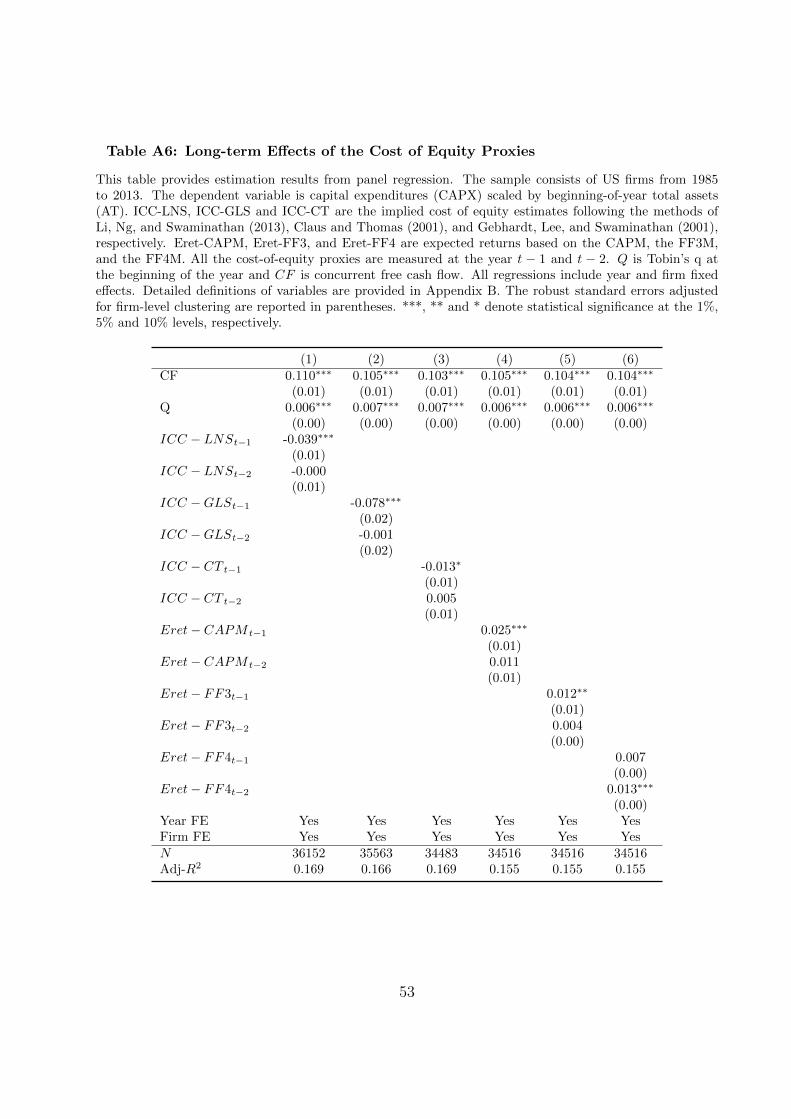
Table A6: Long-term Effects of the Cost of Equity Proxies

This table provides estimation results from panel regression. The sample consists of US firms from 1985to 2013. The dependent variable is capital expenditures (CAPX) scaled by beginning-of-year total assets(AT). ICC-LNS, ICC-GLS and ICC-CT are the implied cost of equity estimates following the methods ofLi, Ng, and Swaminathan (2013), Claus and Thomas (2001), and Gebhardt, Lee, and Swaminathan (2001),respectively. Eret-CAPM, Eret-FF3, and Eret-FF4 are expected returns based on the CAPM, the FF3M,and the FF4M. All the cost-of-equity proxies are measured at the year t − 1 and t − 2. Q is Tobin’s q atthe beginning of the year and CF is concurrent free cash flow. All regressions include year and firm fixedeffects. Detailed definitions of variables are provided in Appendix B. The robust standard errors adjustedfor firm-level clustering are reported in parentheses. ***, ** and * denote statistical significance at the 1%,5% and 10% levels, respectively.

(1) (2) (3) (4) (5) (6)CF 0.110∗∗∗ 0.105∗∗∗ 0.103∗∗∗ 0.105∗∗∗ 0.104∗∗∗ 0.104∗∗∗

(0.01) (0.01) (0.01) (0.01) (0.01) (0.01)Q 0.006∗∗∗ 0.007∗∗∗ 0.007∗∗∗ 0.006∗∗∗ 0.006∗∗∗ 0.006∗∗∗

(0.00) (0.00) (0.00) (0.00) (0.00) (0.00)ICC − LNSt−1 -0.039∗∗∗

(0.01)ICC − LNSt−2 -0.000

(0.01)ICC −GLSt−1 -0.078∗∗∗

(0.02)ICC −GLSt−2 -0.001

(0.02)ICC − CT t−1 -0.013∗

(0.01)ICC − CT t−2 0.005

(0.01)Eret− CAPM t−1 0.025∗∗∗

(0.01)Eret− CAPM t−2 0.011

(0.01)Eret− FF3t−1 0.012∗∗

(0.01)Eret− FF3t−2 0.004

(0.00)Eret− FF4t−1 0.007

(0.00)Eret− FF4t−2 0.013∗∗∗


53

Sensitivities of Corporate Investment and Financing Decisions to the ...

Documents

Transcript of Sensitivities of Corporate Investment and Financing Decisions to the ...