Working Paper | SRA 19-01 | April 9, 2019

Variable Annuities: Underlying Risks and Sensitivities Imad Chahboun, Nathaniel Hoover

Supervisory Research and Analysis Unit

© 2019 Federal Reserve Bank of Boston. All rights reserved.

Supervisory Research and Analysis (SRA) Working Papers present economic, financial and policy-related research conducted by staff in the Federal Reserve Bank of Boston’s Supervisory Research and Analysis Unit. SRA Working Papers can be downloaded without charge at: http://www.bostonfed.org/publications/sra/

The views expressed in this paper are those of the author and do not necessarily represent those of the Federal Reserve Bank of Boston or the Federal Reserve System.

1  

Variable Annuities: Underlying Risks and 

Sensitivities 

Imad Chahboun1 and Nathaniel Hoover April 2019 

AbstractandmotivationThis paper presents a quantitative model designed to understand the sensitivity of variable annuity 

(VA)  contracts  to  market  and  actuarial  assumptions  and  how  these  sensitivities  make  them  a 

potentially important source of risk to insurance companies during times of stress. VA contracts often 

include  long  dated  guarantees  of  market  performance  that  expose  the  insurer  to  multiple  non‐

diversifiable risks. Our modeling framework employs a Monte Carlo simulation of asset returns and 

policyholder behavior to derive fair prices for variable annuities in a risk neutral framework and to 

estimate  sensitivities of  reserve  requirements under a  real‐world probability measure.   Simulated 

economic scenarios are applied to four hypothetical insurance company VA portfolios to assess the 

sensitivity of portfolio pricing and reserve levels to portfolio characteristics, modelling choices, and 

underlying economic assumptions.  Additionally, a deterministic stress scenario, modeled on Japan 

beginning in the mid‐90s, is used to estimate the potential impact of a severe, but plausible, economic 

environment  on  the  four  hypothetical  portfolios.  The  main  findings  of  this  exercise  are:  (1) 

interactions  between  market  risk  modeling  assumptions  and  policyholder  behavior  modeling 

assumptions can significantly impact the estimated costs of providing guarantees, (2) estimated VA 

prices and reserve requirements are sensitive to market price discontinuities and multiple shocks to 

asset prices, (3) VA prices are very sensitive to assumptions related to interest rates, asset returns, 

and  policyholder  behavior,  and  (4)  a  drawn‐out  period  of  low  interest  rates  and  asset  under‐

performance, even if not accompanied by dramatic equity losses, is likely to result in significant losses 

in VA portfolios. 

 

Keywords: insurance risk, market risk, variable annuities, derivative pricing, policyholder behavior JEL Classification: C15, G12, G17, G22, G23 

   

                                                            1 E‐mail: imad.chahboun@bos.frb.org (corresponding author). For helpful comments and guidance, we thank Jose Fillat, Matt Pritsker, Michal Kowalik, Patrick DeFontnouvelle, Patricia Valley, James Bohn, Richard Rosen, Bret Howlett, John Mara and all participants at the Boston Federal Reserve seminar series that provided valuable feedback and guidance. We also thank Dan Smith and Mark Manion for their help in running model simulations. The views expressed herein are those of the authors and do not necessarily reflect those of the Federal Reserve Bank of Boston or the Federal Reserve System .Any remaining errors are ours. 

2  

A. Introduction 

In the period leading up to the financial crisis of 2008, variable annuities (VAs) emerged as an important 

and high‐growth offering for U.S. life insurance companies.  During the 1998 to 2007 period, VA sales grew 

at a 6.9% annualized rate, reaching $182 Billion in 20072.  At the same time, the VA product was evolving 

from  one  that  offered  relatively  straight‐forward  guaranteed  death  benefits  to  one  that  offered 

increasingly complex living‐benefit guarantees.  The rapid growth in these guarantees resulted in insurers 

assuming substantial, non‐diversifiable exposures to equities and bond markets within their VA portfolios.  

After substantial losses and a contraction following the financial crisis of 2007‐2008, the VA market has 

seen  renewed  growth  in  recent  years  driven  by  the  aging  of  the  baby  boomers  and  strong  recent 

performance  of  the  equities  markets.    As  of  December  2015,  the  value  of  separate  account  assets 

associated with guaranteed variable annuities have grown to approximately $1.7 trillion. 

This paper examines the sensitivity of the prices and reserves related to guarantees associated with VAs 

to market and actuarial assumptions and whether these guarantees may become an important source of 

risk  to  insurance  companies  during  times  of  stress.   We  develop  a  quantitative model,  calibrated  to 

industry  data,  to  examine  the  sensitivities  of  VA  fair  pricing  and  reserve  requirements  to  various 

underlying risks.  Our model expands upon existing literature by simultaneously incorporating, within a 

single Monte Carlo simulation framework, several essential aspects of financial markets and policyholder 

behavior that have previously been examined in isolation.   

We apply our model to derive fair prices for various VA guarantees and to estimate reserve and capital 

requirements  for  firm‐level  proxy  portfolios  (derived  from  regulatory  reported  data)  under  simulated 

economic scenarios.  Using these results, we evaluate the sensitivities of VA guarantee prices and reserve 

requirements  to  modeling  choices  related  to  macroeconomic  scenario  generation  and  policyholder 

behavior.  It is important to note that our model does not incorporate a rigorous accounting of VA hedging 

strategy.  For this reason, our estimates of absolute levels of prices and reserve requirements are unlikely 

to be representative of those observed in the market by firms that hedge a considerable amount of risk.  

However, while we do not draw conclusions about the levels of reserves associated with a portfolio of 

VAs, we can offer insight into how those levels are likely to be impacted by various modeling assumptions. 

Additionally,  a  deterministic  stress  scenario,  modeled  on  Japan  beginning  in  the mid‐90s,  is  used  to 

estimate the potential impact of a severe, but plausible, economic environment on the four portfolios. 

The  main  findings  of  this  exercise  are:  (1)  VA  guarantee  prices  and  reserves  are  very  sensitive  to 

assumptions related to interest rates, asset returns, and policyholder behavior, (2) assumptions interact 

with each other to produce impacts that are highly non‐linear and, (3) a drawn‐out period of low interest 

rates  and  asset  under‐performance,  even  if  not  accompanied  by  dramatic  equity  losses,  results  in 

significant losses in VA portfolios.    

The remainder of this paper will proceed in the following manner.  Section B provides an overview of the 

structure of VA contracts and their features that we incorporate into our model.   Section C provides a 

description of the types of risks inherent to insurance firms’ VA portfolios that we attempt to assess within 

                                                            2  U.S. Individual Annuities Sales Survey, LIMRA   

3  

our model.  In section D we provide a brief overview of the academic literature related to the pricing of 

VA contracts and guarantees and the impact of modeling choices related to financial market features and 

policyholder behavior.  We present our modeling framework in section E.  Section F presents results of 

sensitivity testing of prices and reserves related to various contract, financial market, and policyholder 

feature  assumptions.    The  application  of  the  model  to  four  hypothetical  VA  portfolios  derived  from 

statutory filings at individual firms is presented in section G under a large number of simulated economic 

scenarios.  Finally in section H we consider the impact of a deterministic economic scenario modeled after 

Japan in the 1994‐2017 period and conclude in section I. 

B. OverviewofVariableAnnuities 

Before we present our model, we describe the characteristics and types of VAs offered.  This will allow us 

to better highlight the features of VAs that we are modeling. 

Variable  annuities  are  long‐term  insurance  contracts,  used  by  individuals  for  saving  and  guaranteed 

income purposes.  Initial premiums are paid up‐front by the policyholder who then receives contractually 

guaranteed payments from the insurer in the future.  The underlying assets of a VA (i.e. the premium paid 

by the policyholder less origination fees) are invested in mutual funds.    The policyholder typically pays 

fees, in addition to the initial premium amount, related to optional guarantees embedded into the VA, 

administrative fees, and investment management fees.  The policyholder may also be charged additional 

fees for exiting the contract before a pre‐established holding period elapses.   

Variable annuities have a lifecycle consisting of three phases:  an accumulation phase, a withdrawal phase, 

and an insured phase.  During the accumulation phase, the account value is allocated across, and its value 

varies with, investment options provided by the insurer.  The policyholder determines the fund allocation 

across the investment options (subject to restrictions placed on the investments by contract).   

In the withdrawal phase guaranteed cash flows are paid out to the policyholder.  The withdrawal rates 

are generally established at the contract inception and are guaranteed by the insurer.  The payments may 

be a lump sum or a recurring percentage of the benefit base.  The benefits base, which is discussed in 

more  detail  below,  is  determined  by  the  performance  of  the  underlying  investments  during  the 

accumulation phase and any additional guarantees that the customer may have purchased to reduce the 

investment risk associated with the underlying account during the accumulation period.   

Cash flows during the withdrawal phase are first paid out of the underlying account value of the VA (and 

thus reduce the underlying account value).  If the underlying account value is insufficient to support the 

guaranteed payments (generally owing to poor investment returns experienced during the accumulation 

phase), then the insurer is responsible for covering any shortfalls.  If at some point the insurer becomes 

responsible  for  making  guaranteed  payments  to  a  policyholder  (i.e.  the  underlying  account  value  is 

insufficient to support the payments), then the VA is said to have entered the insured phase.  

4  

PaymentGuarantees:Variable annuities are sold with various types of guarantees.  These guarantees provide the policyholders 

with assurance that they will receive certain future cash flows.  These cash flows may be either recurring 

or  lump  sum  payments.    There  are  four  main  types  of  guarantees  (death,  income,  withdrawal,  and 

accumulation) that insurers sell with VAs.   

GMDB  riders  provide  guaranteed  certain  lump‐sum payment  at  the  time  of  the  policyholder’s  death, 

regardless of the account value. Guaranteed Minimum Income Benefit (GMIB) riders provides the account 

holder the right to convert the underlying account value into a fixed annuity that provides a lifetime fixed 

payment.  The annuity payment amount will be equal to a percentage, established at the time of the initial 

VA sale, of the benefit base.  The timing of the conversion is determined by the policyholder, assuming 

that an initial waiting period has elapsed.   

Guaranteed Minimum Accumulation Benefit  (GMAB)  riders guarantee  the policyholder a certain  lump 

sum payment amount on a  certain date,  regardless of  the  investment performance of  the underlying 

account. 

GMWB and Guaranteed Lifetime Withdrawal Benefit (GLWB) riders provide assurance that a policyholder 

will be able to make withdrawals that are less than or equal to a fixed percentage of the benefits base for 

a fixed number of years. For example, the policyholder may be guaranteed the right to withdraw up to 5 

percent of the benefit base annually for 20 years, even if the payment amount exceeds the account value 

at any point.  In this example, the policyholder is guaranteed withdrawals that total, at a minimum, the 

original amount of the benefit base, regardless of the performance of the underlying account.  The GLWB 

extends the withdrawal period to encompass the policyholder’s lifetime, rather than a fixed interval. 

BenefitBaseContractProvisions:Benefit payments are calculated in reference to a “benefit base.”  The benefit base is an amount that is 

related to, but separate from, the underlying account value.  Differences between the benefit base and 

the account value arise when the policyholder elects (in exchange for paying additional fees) to receive 

protection against poor performance of the investment funds selected for the underlying assets.   

Return of principle  (RoP)  guarantees ensure  that  the policyholder will  not  incur any  losses below  the 

original account value (adjusted for fees and withdrawals) due to underperformance of the underlying 

funds that the account is invested in.   

Roll‐ups are a contract provisions that protect the policyholder from underperformance of the underlying 

account value relative to a baseline growth rate.  When a roll‐up provision is in place, the benefit base will 

be the greater of the actual account value (reflective of  investment returns) and a value derived from 

applying  a  pre‐specified minimum  rate  to  the original  account  value.    A  roll‐up  guarantee,  therefore, 

establishes  a minimum  growth  rate  for  the  benefit  base,  but  does  not  limit  upside  potential  for  the 

policyholder. 

A ratchet is a contract feature that establishes the benefit base as the maximum value of the underlying 

asset account value in a specified period.  Ratchets are evaluated at pre‐established intervals during the 

accumulation period (annually, quarterly, or monthly) and offer protection against short‐term downward 

5  

movement in the underlying account value.  For example, an annual ratchet would set the benefit base 

to the highest between account values observed at prior year, the current account value, and the past 

values of the benefit base that have been set by the application of the ratchet in prior periods.  In the case 

that the account values were to fall over the course of the upcoming year, the benefit base would remain 

at the “high‐water” mark observed at the ratchet reset date or “anniversary”.     

The  insurer  offers  these  contract  features  to  customers  purchasing  VAs  with  all  types  of  cash  flow 

guarantees, in exchange for an additional rider charge that is typically established as percentage of the 

account value.  A particular policy may include multiple benefit base guarantees simultaneously (e.g. a 

roll‐up and a ratchet), if the policyholder elects to purchase multiple guarantees. 

A final contract feature of VAs is the right for the policyholder to withdraw more than the guaranteed 

withdrawal amount or  to withdraw the value of  the underlying account and terminate  the policy.   By 

withdrawing  excess  funds  from  the  account,  the  policyholder  relinquishes  the  guarantees  that  were 

included in the VA contract for the withdrawn amount.  The embedded guarantees are primarily designed 

to protect the policyholder from downside moves in the account value.  Thus, lapsing may be rational for 

the policyholder if the account value has increased significantly, and is therefore far above the guaranteed 

value.  In this case, the policyholder may benefit from forfeiting the now relatively low‐value (or a portion 

of it) guarantees and removing the underlying account value for other uses (e.g. purchasing a new VA that 

offers  downside  protection  relative  to  the  new,  higher  account  value).    Typically,  surrender  fees  are 

waived if the policy has been in force for some prespecified period of time.  If a policyholder surrenders, 

all guarantees associated with the contract are relinquished.   

C. MainUnderlyingRisks 

In this section, we discuss the main type of risks that are present for insurance companies with VA contract 

liabilities.  The risks described here, are the exposures that our model attempts to quantify under various 

economic conditions. At the end of the section, we explain why we refrain from modelling the cost to 

hedge these contracts. 

MarketRisk:Market risk is the risk of adverse price movement that impacts guaranteed payments or required reserve 

levels  due  to  changes  in market  factors,  and  it  includes  interest  rate  risk,  equity market  risk,  foreign 

exchange risk and credit risk.  

When  pricing  and  reserving  for  variable  annuity  products,  insurers  make  assumptions  about  the 

performance  of  several  capital market  factors.   Market  risk  exists  to  the  extent  that  capital markets 

perform in different way than assumed in pricing and reserving calculations.  

The  main  market  risks  that  variable  annuities  involve  are  equity  and  interest  rate  risks.  Declines  in 

policyholder account values due to equity price declines or shifts in the interest rate environment increase 

the exposure of VA  issuer  to  the  risk  that  the account value may be  insufficient  to  cover  the  level of 

guarantees  promised  by  the  contract  which  increases  expected  living  benefit  future  claims.  Further, 

6  

declining  interest  rates  increases  the present value of  the  long‐term  income provided by  the contract 

guarantees. A change in capital markets can result in increases or decreases in the required reserves and 

the capital  that a VA  issuer has to set aside to meet  its commitments to policyholders and regulatory 

requirements. If market risk is managed inappropriately, it can lead to significant balance‐sheet volatility 

and solvency risk for VA issuers. In the current framework, we focus on equity and interest rate risks as 

these are the main market risks.  

Insurancerisk:Longevity risk reflects the risk that mortality assumptions are not as expected and policyholders live longer 

than expected resulting in increased duration of guarantee payments associated with living benefits. This 

risk impacts the living benefits (GMWB, GMIB, GMAB and GLWB). 

Mortality assumptions are derived from actuarial studies. Such studies involve long periods of time and 

large population which creates a high degree of precision and confidence in their estimate.  

However, longevity risk is still present as holders of these insurance products may not exactly match the 

overall population expectations, due to many different factors, resulting in different mortality experiences 

within a given VA portfolio population than the population used to derive the tables. Causal factors may 

include  population  health  improvements,  medical  enhancements,  and  different  demographic  profile. 

There may also be adverse selection and moral hazard aspects related to insurance risk. Customers who 

buy individual annuities may tend to be those that are expected to live longer than average. On the other 

hand,  customers  with  shorter  life  expectancy  would  find  a  VA  based  on  average  mortality  to  be 

unfavorably priced. 

By  contrast,  living  benefit  contract  holders might  change  their  habits  and  live  longer  than  previously 

expected by the insurer. Such changes in policyholder behavior after VA issuances is purchased is referred 

to as moral hazard.  

To manage longevity risks, insurers design products with age restrictions on both receiving guaranteed 

benefits and on income commencement. Other tools available to insurers are risk pooling and product 

diversification where large pools of contracts are  likely to behave in terms of mortality, on average as 

expected. A mix of guaranteed death and living benefit contracts is a natural hedge against mortality and 

longevity risk. 

PolicyholderRisk:Policyholder  risk  is  the  risk  that  policyholder  behavior  in  terms  of  benefit  utilization  and  contract 

surrender doesn’t align with insurer’s expectation or past experience resulting in unexpectedly high or 

low utilization of benefits.  Insurers make assumptions regarding the frequency and magnitude of contract 

lapse rates and benefit utilization. For example, insurers can assume a static lapse rate of 5% annually and 

90% of benefit utilization (90% of the withdrawal in the case of guaranteed withdrawals). Assumptions 

made  by  VA  issuers  vary  based  on  the  types  of  guarantees  offered,  as  well  as  internal  and  external 

policyholder behavior studies. Such studies3, generally based on limited data, show that surrender rate 

and utilization are becoming  increasingly dynamic.  Several  factors  contribute  to  shaping  this  dynamic 

                                                            3 SOA/LIMRA, Variable Annuity Guaranteed Living Benefits Utilization, 2013 

7  

behavior, including policyholder characteristics (age, gender), contract size (retail vs institutional), and the 

moneyness of the guaranteed benefit. The dynamic nature of these assumptions is generally linked to the 

gap between the guaranteed benefit amount and the VA account value. For instance, a large difference 

between these two values where the guaranteed amount exceeds the account value can lead to low lapse 

rates. Rational holder’s behavior suggests keeping risk with the insurer when market is declining (lower 

lapse rates) and seek better opportunities when market is rising (higher lapse rates). 

As  for  insurance  risk,  product  design  can  also  help mitigate  risks  arising  from  policyholder  behavior. 

Insurers can design VA contracts that penalize lapses within the first 5 or 7 years of contract life. Typically 

insurers will  apply  penalties  on  early  surrenders  during  this window. Consequently,  policyholders will 

modify their surrender behavior to avoid penalties.  Lapsing penalties are effective at reducing the rate of 

lapses during the early years of contracts, but do not offset the dynamic lapsing effect with relation to 

contract moneyness. Pricing is another component of product design where VA issuers may adopt prudent 

assumptions with regards to policyholder behavior and in order to avoid unexpected changing behavior. 

As will be shown later in this paper, failure to model moneyness‐based dynamic lapsing poses a serious 

risk to VA providers; as dynamic lapsing exacerbates the impact on VA price (reserve or capital) or market 

risk shocks.   This  illustrates that market and policyholder risks are multiplicative,  rather  than additive. 

Furthermore,  there  is  an  increasing  awareness,  in  policy  behavior  studies,  of  the  moneyness‐based 

utilization of VA benefits. Such changing behavior from static to dynamic utilization will likely to expose 

VA providers to further risks and increase the cost of guaranteed benefits, reserves and capital. 

HedgeRisks:Hedge risk is the risk that hedging strategies do not perform as intended, creating basis risk, or the risk 

that a hedge provider defaults on  its obligation, creating counterparty risk. VA  issuers rely on hedging 

strategies to neutralize (or reduce) residual risks that are inherent to the product design or emerging due 

to changes in underlying assumptions. Hedging strategies are also used to mitigate the required levels of 

reserve and capital. There are several aspects characterizing hedging strategies such as the risks that need 

to be hedged, which include sensitivity to changes in the underlying portfolio price (Delta), sensitivity to 

changes in interest rate (Rho) or sensitivity to guarantee value to changes in the implied volatility of the 

underlying  asset  (Vega).  Hedging  strategies  also  include  cross  Greek  sensitivities  and  sensitivity  to 

convexity risk (variation of Delta and Rho). Hedging strategies are based on a variety of instruments where 

equity  risk  is managed mainly via equity  future contracts while  interest  rate  risk  is managed primarily 

using interest rate futures contracts. Volatility is generally hedged using equity put options and swaptions. 

Due  to  the  long duration of VA contracts, hedging  strategies  require  frequent  rebalancing  in order  to 

maintain hedging efficiency at  targeted  levels. The cost of hedging  is  in general  included  in guarantee 

prices in cases where hedging is part of product design. 

Continuous rebalancing associated with dynamic hedging results in high costs. A study by PIMCO4 on the 

cost of delta hedge from December 2005 to June 2011 show hedge cost ranging from a few basis points 

(prior to 2008) and near 200 basis points during 2008 financial crisis. 

                                                            4 PIMCO, Viewpoints November 2011 

8  

In this paper, we do not model the cost of hedging VA guarantees.  There are several difficulties inherent 

to modeling  the  impact of hedging.   Simulating the  impact of a hedging strategy on cash flows would 

require us to make assumptions about the hedge objective, the guarantees that firms are hedging, and 

firms’ risk tolerances.  In addition, we would need to assume whether firms were employing static hedges, 

dynamic hedges, or partial hedges.  Given the wide variety of approaches and risk tolerances that could 

reasonably be adopted, the large number of assumptions that would need to be made, and the significant 

impact on results, we opt rather to focus on evaluating sensitivities in prices, and reserve requirements 

rather than attempting to establish these values net of the effect of hedging. 

Given that our model quantifies VA price under risk neutral measure, we expect the cost of lifetime hedges 

to be equivalent  to VA  fair  value produced by our model. A  hedge  cost  index produced by Milliman5 

confirms this fact and shows a cost for hedging a hypothetical GMWB spanning between 100 and 172bps 

during September 2014 to September 2016 period. These values are equivalent to the 150bps VA price 

produced by our model for scenario 1. 

D. Literaturereview 

Our  paper  extends  the  existing  literature  in  several  dimensions:    (a)  our  model  is  designed  to  price 

contracts that include various combinations of guarantees and features whereas the literature has largely 

focused on pricing  individual  guarantees,  (b)  our model  includes  several  features  of  realistic  financial 

markets that have not been  incorporated  in much of the prior work on VA pricing,  (c) we  incorporate 

several important features of policyholder behavior that have been shown to play an important role in 

accurately modeling contract cash flows and, (d) we apply our model to proxy portfolios developed using 

industry data.  This allows us to evaluate the interaction between market risk factors, insurance factors, 

and various combinations of contract features simultaneously, rather than in isolation.  In addition, we 

apply these results to evaluating the expected impact on industry‐representative portfolios, rather than 

on individual VAs in isolation.   

While our model  is  implemented using a Monte Carlo simulation  framework,  it  is  related  to  the early 

literature  on  VA  pricing  that  focused  primarily  on  deriving  closed‐form  solutions  for  the  pricing  and 

valuation of  guarantees.    Closed‐form pricing models  are generally  limited  to pricing  specific  types of 

guarantees  independently,  as  combinations  of  guarantees  do  not  generally  admit  exact  closed‐form 

solutions.  Aase and Persson (1994) applied tools typically used for pricing financial products, such as no‐

arbitrage  pricing  and  martingale  theory,  to  derive  the  optimal  pricing  for  traditional  life  insurance 

products.   

Milevsky  and  Salisbury  (2001,  2002) were  early  examples  of  the  application  of  closed‐form pricing of 

guarantees  associated with  variable  annuities.    The  authors  employed  option  pricing  theory  to  value 

Guaranteed Minimum Death Benefit  (GMDB)  and Guaranteed Minimum Withdrawal  Benefit  (GMWB) 

guarantees using a static approach that assumed policies did not lapse and withdrawals are made exactly 

as specified in riders.  Milevsky and Salisbury (2006) expanded this framework to incorporate Guaranteed 

                                                            5 The Milliman Hedge Cost Index 

9  

Lifetime Withdrawal Benefit (GLWB) and dynamic withdrawal behavior.  Their results generally show that 

guarantees were, at the time, underpriced in the market.  However, approaches that rely on closed‐form 

pricing solutions are limited because of the complexity of contracts that can be priced and must generally 

assume relatively simple models related to behavior of the underlying assets.   

Several papers have provided analytical pricing  formulas  for  specific  individual guarantee  types under 

stochastic interest rates and stochastic mortality.  A relevant example is Krayzler et al (2012) for GMDB 

guarantees that incorporate various riders such as roll‐ups and ratchets, though Krayzler and coauthors 

only model a single asset.  

Our work extends the literature that discusses the pricing of various types of guarantees together.  Sun 

(2006)  studied  the  impact  of  combining  multiple  products  while  incorporating  dynamic  policyholder 

behavior  related  to  lapsing,  the  “annuitization”  decision,  and  withdrawal  rates  utilizing  a  set  of  pre‐

defined economic scenarios.  Sun shows that incorporating policyholder behavior that is conditional on 

the economic scenario can have a dramatic effect on pricing.  However, Sun’s approach does not result in 

prices that are consistent with market expectations related to asset behavior. 

Bauer et al (2008) developed a framework that could consistently price contracts that include multiple 

guarantees using a stochastic economic scenario generator.  Their model uses a Monte Carlo framework 

to simulate asset returns using Geometric Brownian Motion and imposes a deterministic mortality model 

while assuming that policyholders follow an optimal strategy related to surrender and withdrawal.  While 

able to price multiple guarantees simultaneously, their approach relied on relatively simple models for 

asset returns and policyholder behavior. 

Several authors have worked to expand this general framework to incorporate various riders, dynamic 

policyholder  behavior,  and multiple  assets.    Bacinello  et  al  (2011)  developed  a  dynamic  approach  to 

policyholder behavior.  Their model incorporates stochastic interest rates as well as stochastic mortality 

into a Monte Carlo framework to price VAs with multiple guarantees simultaneously.  The authors derive 

pricing under a solution for optimal withdrawal strategy for rational policyholder. Holz et al (2007) applied 

a  framework  similar  to  the one employed  in Bauer  (2006)  to GLWBs while  incorporating  roll‐ups  and 

ratchets.  Kling et al. (2010) further expand on this framework by applying stochastic rates and volatilities 

rather  than  log‐normal  returns.    Chen  et  al.  (2009)  incorporates  asset  jumps  and  dynamic,  but  sub‐

optimal, policyholder behavior in order to extend research to better reflect the observed behavior of both 

asset returns and lapsing experiences.   

While  the  literature  has  increasingly  moved  towards  simultaneously  modeling  multiple  guarantees, 

dynamic policyholder behavior, and realistic asset returns, our model contributes to the understanding of 

the risks inherent in VAs to firms by incorporating each of these modeling features and applying them to 

representative  firm  portfolios  derived  using  data  included  in  regulatory  reporting.    This  allows  us  to 

examine the sensitivity of firms’ VA portfolios to various risk factors and to estimate the potential impact 

of various counterfactual economic scenarios on the performance of these portfolios. 

10  

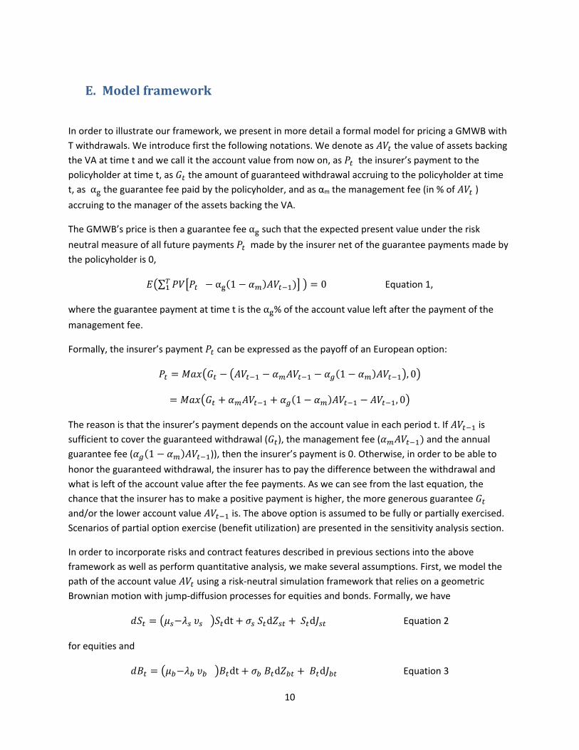
E. Modelframework 

In order to illustrate our framework, we present in more detail a formal model for pricing a GMWB with 

T withdrawals. We introduce first the following notations. We denote as   the value of assets backing 

the VA at time t and we call it the account value from now on, as    the insurer’s payment to the 

policyholder at time t, as   the amount of guaranteed withdrawal accruing to the policyholder at time 

t, as  α  the guarantee fee paid by the policyholder, and as αm the management fee (in % of   ) 

accruing to the manager of the assets backing the VA.  

The GMWB’s price is then a guarantee fee α  such that the expected present value under the risk 

neutral measure of all future payments    made by the insurer net of the guarantee payments made by 

the policyholder is 0,  

∑ α 1 0    Equation 1, 

where the guarantee payment at time t is the α % of the account value left after the payment of the 

management fee.  

Formally, the insurer’s payment   can be expressed as the payoff of an European option: 

1 , 0  

1 , 0  

The reason is that the insurer’s payment depends on the account value in each period t. If   is 

sufficient to cover the guaranteed withdrawal ( ), the management fee (  and the annual 

guarantee fee ( 1 )), then the insurer’s payment is 0. Otherwise, in order to be able to 

honor the guaranteed withdrawal, the insurer has to pay the difference between the withdrawal and 

what is left of the account value after the fee payments. As we can see from the last equation, the 

chance that the insurer has to make a positive payment is higher, the more generous guarantee    

and/or the lower account value   is. The above option is assumed to be fully or partially exercised. 

Scenarios of partial option exercise (benefit utilization) are presented in the sensitivity analysis section.  

In order to incorporate risks and contract features described in previous sections into the above 

framework as well as perform quantitative analysis, we make several assumptions. First, we model the 

path of the account value   using a risk‐neutral simulation framework that relies on a geometric 

Brownian motion with jump‐diffusion processes for equities and bonds. Formally, we have  

dt   d d              Equation 2 

for equities and 

dt   d d      Equation 3 

11  

for bonds, where   and    are values of equities and bonds indices at time t,    and   are drifts,   

and   are volatilities, d  and d  are correlated Brownian motion processes, and  d  and d  are 

stochastic jump processes. Drifts have the starting risk free rates of 0.7% as of June 2016. The bond 

portfolio is assumed to be actively managed and follow an index which supports the use of GBM 

process. The probability of having at least one jump is assumed to be 1% each month corresponding to 

one in eight years event. Historically, market price jumps occurred, on average, with one in seven years 

frequency. Our model framework assumes frequency of jumps to follow a Poisson distribution with 

intensity . 

Pr X k!           Equation 4 

The jump size is assumed to follow a lognormal distribution calibrated to the 1% most severe monthly 

historical drops of equity and bond indices. Jump size is drawn from lognormal distributions ( ,  

and  ,  for equity and bond respectively.   and   the jump‐adjusted drifts 

for equities and bonds where: 

exp 0.5 )       and  exp 0.5 ) 

In our baseline calculation we assume a typical 60%/40% distribution between equity and bonds, 

implying   =0.6.  + 0.4 . However, our framework allows for varying this asset allocation (such as 

the 80%/20% allocation presented in the sensitivity analysis section).Next we assume that interest rates 

evolve according to a Vasicek6 model: 

a dt          Equation 5 

where  is a Brownian motion process under the risk‐neutral framework and is correlated with equity 

and bond processes (  and  , b is the long‐term mean level of risk free rate, a is the speed at which 

interest rate path reverts to level b, and   is the instantaneous interest rate volatility.  Calibration of 

the Vasicek model results in an estimated long‐run equilibrium rate of 1.63%, volatility of 14.2% and a 

reversion speed of 0.99%. 

We calibrate the equity process using monthly data on the S&P500 from 1999 to 2016, the bond process 

using Merrill Corporate Bond Total Return Indices from 1999 to 2016, and the interest rate process using 

3‐months treasury rates from 1982 to 2016.  The calibration period spans back to the 80s in order to 

reflect life benefit’s long guaranteed period (30 years or higher) and capture the levels of interest rates 

observed in the early 80s. Moreover, we allow for correlations between equity, bond and interest rate 

processes. We use the Cholesky transformation to generate correlated random processes with 

correlations calibrated to 1999‐2016 data period.  

The rest of the assumptions cover those specific for the insurance contracts. First, we model 

mortality/longevity risk in a deterministic fashion7 based on the most recent life tables by age, gender 

and date of birth. However, we assessed the potential impact of longevity risk by conducting sensitivity 

                                                            6 Vasicek, Oldrich (1977). "An Equilibrium Characterisation of the Term Structure". Journal of Financial Economics 7 We abstract from stochastic mortality since E Marceau, P‐A Veilleux, GMWB Guarantee: Hedge Efficiency & Longevity Analysis, 2015 and a study led by Milliman demonstrated that it has limited impact on VA prices. 

12  

analyses on VA prices in response to changes in mortality rates and found limited impact. In addition, we 

abstract from any correlation between mortality/longevity and financial risks. 

To assess the impact of policyholder behavior, we allow for static and dynamic lapsing of contracts. As 

mentioned in section B, VA contracts allow policyholders to withdraw a percentage of the account value 

in excess of guaranteed withdrawal. Under static lapsing, we assume that this percentage is fixed at 5%. 

Under dynamic lapsing we assume that this percentage is a function of the VA contract’s moneyness 

( ) and other policyholder’s characteristics.   is the in‐the‐money indicator at time t and is 

defined as the ratio of the account value over the guaranteed annual withdrawal, 

ITM                                 Equation 6 

A variable annuity contract is considered in the money if the present value of future guaranteed benefits 

( )  is  below  the  account  value  ( )  oftheunderlying  asset  at  time  t  (ITM   =>1).  To  calibrate 

policyholder behavior we use data from Milliman’s dynamic lapse study.8 We then use a cubic polynomial 

function to regress lapse rate on the “in‐the‐moneyness” indicator , 

                         Equation 7  

Figure 1 shows calibration results of observed versus fitted lapse rates as a function of ITM. 

Figure 1: Lapse Rate Calibration 

 

Second, we assume the following pattern of lapsing penalties for the first seven years of the contract: 7%, 

6%, 5%, 4%, 3%, 2% and 1% of the account value. In addition to moneyness calibration, the framework 

                                                            8 Milliman, Variable annuity dynamic lapse study: A data mining approach, June 2011. 

13  

adjusts lapse rates to the levels observed before and after the surrender penalty period (9). Figure 2 shows 

the lapse rate adjustment reflecting policyholder behavior of relatively lower lapsing during the penalty 

period (first 7 years). To reflect this policyholder behavior before and after the penalty period, we adjust 

lapse rate from Equation 7 with the surrender rate adjustment (Equation 8). 

                      Equation 8 

Figure 2: VA Surrender Experience by Years Remaining to Maturity 

 

Finally, our model allows using ratchets and roll‐ups as performance guarantees of the benefit base. The 

benefit base which is the sum of all guaranteed withdrawals (including the death benefit) is guaranteed 

to grow regardless of market performance. The Ratchet feature guarantees the greater of a return of 

benefit base or the highest “anniversary” account value adjusted for withdrawals. The “anniversary” 

decides the frequency of the ratchet (monthly, semiannually, annually, etc.). An annual ratchet will 

recalculate the base benefit once a year by taking the maximum of previous benefit base and the 

account value at the end of a chosen month of the year. The rollup feature guarantees a minimum 

return of the account value where the benefit base at   will be equal to the maximum of  and 1 .05 ∗ 1 if we assume 5% rollup rate. 

F. ModelResultsandPricesensitivity:ApplicationtoStandardGMWBContract

In this section we first present the results from pricing of a VA contract with a GMWB using the 

framework described in the previous section. We price the GMWB using a set of parameters reflecting 

average contract features and financial conditions. Next, we analyze the sensitivity of the GMWB price 

to changes in these assumed parameters. 

                                                            9 Society Of Actuaries, What is the Market Price of Policyholder Behavior? May 2015. 

0

0.5

1

1.5

2

2.5

3

3.5

7 6 5 4 3 2 1 0 ‐1 ‐2 ‐3 (‐4 ormore)

Surrender Rate Adjustment

Years Remaining in Surrender Charge Period

14  

1) ResultsTable 1 summarizes all contract features, financial conditions and assumptions on policyholder behavior 

we use to price the GMWB in the baseline scenario 1. Parameters on contract features reflect average 

contract features described in the literature10. Financial inputs are obtained using calibration 

approaches described in the previous section.  

Table 1: Model Inputs 

   Model Input  Scenario 1  Source 

   Policyholder age  55  Assumed contract feature 

Insurance Inputs 

Contract maturity  15  Assumed contract feature 

Accumulation period  5  Assumed contract feature 

Acquisition fee  5%  Assumed contract feature 

Management fee  1% Contract feature/Assumed based 

on literature 

Fee base  Account value  Assumed contract feature 

Death guarantee  N  Assumed contract feature 

Roll‐up guarantee  N  Assumed contract feature 

Guaranteed roll‐up rate  2% Contract feature/Assumed based 

on literature 

Ratchet at accumulation  N  Assumed contract feature 

Frequency of ratchet at accumulation  once a year  Assumed contract feature 

Ratchet at distribution  N  Assumed contract feature 

Frequency of ratchet at distribution  once a year  Assumed contract feature 

Static lapse rate  5% Contract feature/Assumed based 

on literature 

Dynamic lapsing  N  Assumed contract feature 

Financial Inputs 

Equity vs bond weight  60/40  Assumed contract feature 

Equity volatility  13.4%  Calibrated 

Bond volatility  4.5%  Calibrated 

Correlation equity/bond  15%  Calibrated 

Correlation equity/rate  ‐10.40%  Calibrated 

Correlation bond/rate  ‐0.15%  Calibrated 

Starting short rate  0.70%  Observed 

Interest rate model  Vasicek (14.2%, 1.63%, 0.99%)  Calibrated 

Jump frequency‐monthly  1%  Calibrated/Assumed 

Jump size equity   lognormal(‐0.156,0.044)  Calibrated 

Jump size bond  lognormal(‐0.062,0.031)  Calibrated 

 

We  assume  constant  correlation  between  stock  and  bond  indices.  This  is  a  limitation  to  the  model 

framework  since  correlation  can  vary  over  time and be market  state dependent. US  stock‐bond  yield 

correlations  have  been  consistently  positive  since  the  late  90s,  increased  significantly  during  2008 

financial crisis and stayed at a high level for a long period thereafter. We perform, however, sensitivity on 

                                                            10 Variable Annuity Guaranteed Living Benefit Utilization, SOA/LIMRA, 2013 

15  

the assumed correlation by testing a constant negative correlation of ‐15% between stock and bond. This 

sensitivity test shows limited impact on guarantee price from change of correlation. 

The fair price of the GMWB is a guarantee fee for which the contract’s expected PV given by equation 1 

under scenario 1 is equal to 0. To obtain the contract’s expected PV we simulate 10000 times the path of 

market  conditions  and  policyholder  behavior  based  on  a  given  realization  of  stochastic  processes  of 

equity, bond, interest rate and jumps over the duration of the contract. Figure 3 shows the distribution of 

contract’s present values generated from 10000 simulated paths of scenario 1 for a guarantee fee set at 

150bps. Here a guarantee fee of 150bps is chosen because it is the fee that, when charged, results in an 

expected PV of 0 for the guarantee.  

Figure  3:  Contract  Present  Value  Distribution  for Guarantee Fee of 150 bps. 

Figure 4: Typical GMWB Valuation: Average Path.  

Figure 5: Typical GMWB Valuation: Good Path 

 

Figure 6: Typical GMWB Valuation: Bad Path 

 

Figure 4‐6 present  three  cases  for patterns of payments  to  the policyholders  that are  covered by  the 

account value (yellow) and the out‐of‐pocket payments that the insurer has to make in case the account 

value  is  not  enough  (purple).  The  patterns  of  payments  differ  across  the  pictures  depending  on  the 

realization of  the  simulated paths  of  account  values  for  benefit  base  equal  to  the  initial  value of  the 

account  (100).  Because  the  annual withdrawal  is  calculated  as  a  fraction of  the benefit  base  and  the 

withdrawal duration is 15 years, the annual withdrawal is around 6.7% of the benefit base. 

-30 -20 -10 0 10 20 30 400

0.005

0.01

0.015

0.02

0.025

0.03

0.035

0.04

0.045

0.05

55 60 65 70 75

Age

0

20

40

60

80

100

120

140

Account valueBenefit BaseWithdrawalGuaranteed payment

55 60 65 70 75

Age

0

20

40

60

80

100

120

140

160

180

Account valueBenefit BaseWithdrawalGuaranteed payment

55 60 65 70 75

Age

0

20

40

60

80

100

120

Account valueBenefit BaseWithdrawalGuaranteed payment

16  

Figure 4 depicts the case in which future market conditions and policyholder behavior are such that the 

contract’s PV is zero. In this case the insurance company makes only three out‐of‐pocket payments at the 

end of contract’s life at the age of 73 after 13 payments that were fully covered by the account value. 

Figure  5  presents  the  case  where  the  performance  of  the  underlying  assets  cover  all  guaranteed 

withdrawal benefits without a need of out‐of‐pocket payments. The contract’s present value is positive 

and  insurers  make  profit  on  this  contract.  In  contrast,  Figure  6  presents  a  poor  performance  of  the 

underlying assets and early out‐of‐pocket guarantee payments. Benefit payments are paid by the insurer 

due to insufficient account value for covering the guaranteed amount for 12 out of 15 total guaranteed 

withdrawals. 

 

2) SensitivityAnalysis 

In this section we present sensitivity analysis of guarantee price to varying insurance and financial inputs. 

We use scenario 1 shown in Table 1 as a base case for the sensitivity analysis. 

We  first  analyze  the  sensitivity  of  guarantee  price  to  insurance  factors.  The  results  are  in  Figure  7. 

Incorporating dynamic  lapsing behavior  in  the model has  the  largest  impact on  the price of  a GMWB 

contract. Incorporating more realistic modeling of policyholder behavior in the form of dynamic lapsing 

(calibrated to observed lapsing behavior) results in break‐even guarantee costs that are around 280bps 

higher than those calculated using an assumed static  lapsing rate of 5%. Adding roll‐ups as a contract 

feature has a significant impact with an incremental cost around 190 bps. Adding a death guarantee to a 

GMWB increases the guarantee cost by around 100bps. Except the sensitivity tests related to initial value 

based  fee,  longer maturity  and  lower utilization, other  insurance  features have  increasing but  limited 

impact on the guarantee price. Longer maturity lowers the likelihood of triggering withdrawal guarantee, 

because it decreases the maximum annual withdrawal  . Lower policyholder age (50 instead of 55) will 

increase  contract  exposure  to  market  risk  given  that  relatively  more  policyholders  will  survive  until 

maturity and increases contract price by 30 bps.  Assuming lower benefit utilization (from 100% to 70%) 

will decrease guarantee price by around 130 bps as it lowers the likelihood of out‐of‐pocket payments. 

Insurance companies generally assume that utilization is static and is lower than the guaranteed benefit.  

However a SOA/LIMRA recent study11 shows that the assumption of static utilization is increasingly less 

realistic and that increasingly utilization is a function of contract’s moneyness.  We also believe, as shown 

with dynamic  lapsing,  that modeling utilization dynamically as a  function of contract’s moneyness will 

further increases the cost of the guarantee. Public data on levels of VA guarantee utilization is limited and 

doesn’t allow further modelling. 

Similarly, calculating guarantee fee as a percentage of initial account value as opposed to a percentage of 

current account value decreases guarantee price by up to 50 bps. Using initial account value as fee’s base 

lowers  issuer’s  inflows  in market upturn but also  lowers  issuer’s outflows (out‐of‐pocket payments)  in 

market downturn. Initial account value based fees constitute a natural hedge against low returns on the 

underlying assets. The fee is flat over the duration of the contract.  An increase in the management fee 

                                                            11 SOA/LIMRA, Variable Annuity Guaranteed Living Benefits Utilization, 2013 

17  

will result in an equal increase in the price given that the fee reduces the issuer’s inflows in all market 

conditions by the amount of the fee.  

Figure 7: Sensitivity of Guarantee Price to Insurance Factors (% of Account Value) 

  

Figure 8 presents the results of the sensitivity analysis performed on financial factors. The inclusion of 

jumps in equity and bond prices is the most impactful factor on guarantee price, followed by changes to 

long‐run interest rates, changes in equity volatilities and changes in portfolio composition (equity/bond). 

Incorporating negative correlation reflected in observed historical levels of correlation between equities 

and bonds, and higher bond volatility have intuitive, but limited (less than 10 bps), impacts on guarantee 

price. We also note that the sensitivity to financial factors is not symmetrical, meaning that the impact on 

price of  increasing equity  volatility  is  higher  than  that  for decreasing  volatility.  The  same observation 

applies  to  changes  in  the  long‐run  rate  assumption.  In  terms  of  allocation  of  the  underlying  assets 

(equity/bond), increasing equity allocation from 60% to 80% increases guarantee price by 40 bps due to 

higher equity volatility and jump size. 

It is therefore important to highlight that the assumption of the long‐run risk free rate and the inclusion 

of  jumps in asset paths  in the modeling framework have significant  impact on the modeled guarantee 

price. More importantly, the reversion speed to long‐run interest rate which is the speed at which spot 

rate converge to long‐run risk free rate is the most impactful factor. As seen in Figure 8, an increase of the 

reversion speed from around 1% (base value) to 3% increases guarantee prices by 180 bps. An increase of 

rate volatility from 14% (base value) to 30% lowers guarantee prices by 30bps only. 

In the implementation of this framework, we assume price discontinuity (jumps) consistent with empirical 

evidence12 and the lengthy literature on price discontinuities. We assume a jump frequency of 1 each 8‐9 

                                                            12 Rama Cont and Peter Tankov, Financial Modelling With Jump Processes, 2004 

18  

years, which is calibrated to long‐run data.   The observed frequency of market price jumps since 1980 

exhibits a slightly higher frequency of jumps with a jump occurring once approximately every seven years.    

Moreover, we test a combination of no jump assumption and a relatively higher long‐run risk free rate of 

3.75%.  The  resulting  guarantee  price  is  120bps  lower  than  scenario1  (priced  at  150bp).  Note  that  in 

scenario 1 we assume price discontinuity and a long‐run risk free rate of 1.6% (calibrated to market data 

spanning from the 80s). 

Figure 8: Sensitivity of Guarantee Price to Market Factors (% of Account Value) 

 

  

 

Guarantee price sensitivity under dynamic lapsing assumption: 

Since we found that dynamic lapsing has the most pronounced impact on the guarantee price, we 

compare the sensitivity of the guarantee price to the changes in the inputs between the cases of static 

and dynamic lapsing. In order to do so, we calculate differences in guarantee price before and after 

applying the shock (change in underlying input) for both static and dynamic lapsing scenario. For a single 

shock i the impact is as follow: 

 

              Equation 9 

       Equation 10 

 

In  terms of  combined effect of dynamic  lapsing and changes  in  insurance  inputs,  Figure 9  shows  that 

GMWB prices are significantly more sensitive to changes in insurance features when dynamic lapsing is 

considered.   The cost of “richer” contracts  is higher when dynamic  lapsing behavior  is  included  in  the 

model. For example, the cost of combined death guarantee and dynamic lapsing is considerably higher 

‐1.5 ‐1 ‐0.5 0 0.5 1 1.5 2

Long run rate (3.75%)+ No jump

No Jump

Long run rate (+1 sigma)

Less frequent jumpa (0.7%)

rate vol 30%

Equity vol  (‐2 sigma)

Equity vol (‐1 sigma)

Negative equity‐bond corr (‐15%)

Scenario 1 (150 bps)

Bond vol (+2 sigma)

rate vol 20%

Equity vol (+1 sigma)

Higher eqyuity weight (80/20)

More frequent jumps (1.3%)

Equity vol (+2 sigma)

rate speed rev 2%

Long run rate (‐1 sigma)

rate speed rev 3%

19  

than the sum of death guarantee cost and dynamic lapsing cost. Dynamic lapsing has an aggravating effect 

when combined to other  insurance features. The residual cost of a death guarantee or roll‐up are less 

than 200bps under static lapsing condition but more than 500bps under dynamic lapsing. The dynamic 

lapsing  condition  also  exacerbates  the  price  reduction  impact  from  lower  benefit  utilization  where 

assuming benefit utilization of 70% instead of 100% reduces guarantee price by 4% which illustrates that 

guarantee price is very sensitive to policyholder behavior both in terms of level of benefit utilization and 

dynamic  lapsing.  This  suggests  that  pricing  variable  annuity  guarantees  without  accounting  for  the 

interaction effect of dynamic lapsing and other insurance features will likely lead to significant estimate 

bias and potentially to underestimating guarantee fees. Changes in other insurance features such as lower 

age  of  policyholder  at  issuance,  higher  acquisition  fee  and  shorter  accumulation  period  have  also 

significant impact on guarantee price under dynamic lapsing compared to static lapsing. 

 

Figure 9: Sensitivity of Guarantee Price to Insurance Factors Conditional on Dynamic Lapsing  

(% of Account Value) 

  

Similar to insurance factors, sensitivities to financial factors (Figure 10) are also amplified when dynamic 

lapsing  is  included  in  the model.  The  sensitivities  to  long‐run  interest  rate  and  jump  parameters  are 

significantly higher if dynamic lapsing is included in the model. Reducing equity volatility shock magnitude, 

changing  the equity‐bond correlation, and altering bond volatilities do not have significant  interaction 

with dynamic  lapsing behavior. However the most pronounced effect  is from lower  long term interest 

rates whereas the impact on guarantee price under static versus dynamic lapsing increases from 70bps to 

430bps.  The  low  interest  rate  environment  and  a more  frequent market  price  discontinuity  have  an 

extreme impact on VA guarantee value when measured under dynamic policyholder behavior. 

GMWB  pricing  depends  mainly  on  assumptions  of  policyholder  behavior,  long‐run  interest  rate 

environment, discontinuity of asset prices and to lesser extent on equity volatility and allocation of the 

underlying asset investments. 

20  

 

Figure 10: Sensitivity of Guarantee Price to Financial Factors Conditional on Dynamic Lapsing (% of 

Account Value) 

  

Figure 11 shows that VA reserves calculated as the 70th conditional tail expectation (CTE70)  of guaratee’s 

cash  flow  are most  sensitive  to  rate  reversion  speed,  long‐run  interest  rate,  increased  volatility  and 

portfolio composition (higher concentration i equity). These results are similar to the those observed for 

price sensitivity to market factors. Bond volatility and correlation have an intuitive, but limited, impact on 

reserves.  Price discontinuity  (jump)  shows  less  impact on  reserve  as opposed  to  guarantee price.  For 

example, an increase of rate reversion speed from 0.99% (base value) to 2% increases required reserves 

by 6% which is a 61% increase from its base value of 9.8%. We also note that while assuming no price 

discontinuity reduces gurantee price by around 50% it reduces guarantee reserve by only 20%. 

21  

Figure 11: Sensitivity of Guarantee Reserve (in %) to Market Factors 

 

G. ApplicationtofourhypotheticalVAportfolios 

We now apply our framework to data that are representative of real‐world insurance VA portfolios.  In 

particular,  using  our  Monte  Carlo  simulation  framework,  we  estimate  the  model  price  and  reserve 

requirements of four proxy portfolios created for four firms using regulatory reports. 

1) DataWe created four stylized portfolios designed to reflect the risk exposure of four of the largest VA issuers 

by  combining  a  number  of  publicly  available  data  sources.    The  first  of  these  are  the  2015  annual 

statement general interrogatories (life interrogatories) for each firm.  These data are filed by firms (at the 

legal entity level) with state insurance regulators and provide high‐level data regarding the amount and 

types of VA liabilities held by the firm.  Firms provide data grouped by contract types (i.e. death guarantee 

benefit type, living guarantee benefit type, and by rider type).  For example, a particular line item in this 

data may include data on the value of separate account assets associated with contracts with a 5% rollup 

GMDB and a GMAB with 5% rollup and 1 year ratchet with one year remaining on the waiting period. 

These data provide a reasonable, but not complete, source of data regarding the scope and nature of a 

firm’s VA liabilities.  Clearly, in order to facilitate presenting these data in regulatory reports, there is a fair 

degree of aggregation among contract  features.   For the purposes of reporting,  firms aggregate some 

contracts with similar, but slightly different characteristics (e.g. contracts with 4%, 5% and 6% rollup rates) 

into a single line item which is designated as “5% roll‐up”).  Thus, we are working with data that has had 

some detail removed regarding contract features.  This will naturally introduce some uncertainty into our 

approximation of firm‐specific risk as some contracts are simulated using average values (for example the 

‐4 ‐2 0 2 4 6 8 10 12 14 16 18

Equity vol  (‐2 sigma)

No jump

Rate vol 30%

Long run rate (+1 sigma)

Equity vol (‐1 sigma)

Negative equity‐bond corr (‐15%)

Less frequent jumps 0.7%

Scenario 1 (9.8%)

Rate vol 20%

More fequent jumps 1.3%

Bond vol (+2 sigma)

Equity vol (+1 sigma)

Long run rate (‐1 sigma)

Higher eqyuity weight (80/20)

Equity vol (+2 sigma)

Rate speed reversion 2%

Rate speed reversion 3%

22  

4% rollup contracts being simulated as 5% rollups based on their  inclusion on this  line  item). Without 

access to confidential contract‐level data, our data are the best source of data regarding the exposures 

within firms. 

Additionally the general interrogatory data does not include some data that is required to generate results 

within our simulation framework.   These data include: age and gender of policyholder, and GLWB and 

GMWB withdrawal rates.  To address this, we supplement regulatory data with data from a joint study 

sponsored  by  SOA  and  LIMRA13.    This  study  surveyed  20  firms  regarding  VA  contracts  and  their 

policyholders.  The data covered 4.7 million contracts in force in 2013.  These data are analyzed to provide 

industry‐representative data of policies and policyholders.  For each VA type, the authors calculate the 

age distribution of policyholders and the portion of policyholders that are male and female, across all 

firms. Within  a particular  type of  guarantee,  the portion of  contracts  that  include  certain  features or 

guarantees—in particular,  the portion  of  contracts  that were  issued with  each withdrawal  rates—are 

provided. 

These data are crossed with the firm‐level data to create a proxy for contract‐level data.  For example, if 

$100 million in separate account assets are associated with GMAB guarantees and in the industry‐level 

data 49% of GMAB policyholders are male, we assume  that  at  the  firm  level,  $49 million of  separate 

account assets that are associated with GMAB contracts that are held by males.  Using this process we are 

able to define VA and policyholder characteristics at a policy level for data that are not included in the 

general  interrogatory.    This  process  assumes  independence  between  the  observed  characteristics  of 

contracts and the industry‐level proxies.  

2) ProxyPortfolioDescriptionsFigure 12: Risk Profile by Hypothetical Portfolio 

 

                                                            13 Variable Annuity Guaranteed Living Benefits Utilization: 2013 Experience 

23  

The four selected firms that provide a basis for our proxy portfolios have large guaranteed VA portfolios 

on their balance sheets as measured by separate account assets as a portion of total assets. Products 

offered are primarily GMIB, GMWB and GLWB.  GMDB and GMAB constitute smaller portions of the 

sample portfolios.  

Figure 12 shows the size of the proxy portfolios across each type of offered guarantee and the average 

price as estimated by our model (i.e. the fair price result). For example, 59% of portfolio 1’s VA is made 

up of GMIBs with an average guarantee price of 6.43%. Our results show that the modeled price of GMABs 

is higher than the other guarantee types followed by GMWB, GMIB/GLWB and GMDB.  

Figure 18 to Figure 22 (in the appendix) provide the descriptions of the proxy VA portfolios in terms of 

guarantee type composition, and roll‐up and ratchet features. More than 80% of offered contacts provide 

guaranteed roll‐up (Figure 19).  Ratchets which are intra‐annual performance guarantees are offered in 

relatively lower scale except for firm 1 (Figure 20) where 60% of the VA portfolio are guaranteed intra‐

annual ratchets. Offered roll‐rates are mostly between 0% and 5%.  Here a 0% roll‐up rate corresponds to 

a “return‐of‐principle” guarantee that protects against decreases  in the value of  the underlying assets 

while a 5% roll‐up guarantees an annual increase in the value of the benefits base of 5% regardless of the 

returns on the underlying portfolio.  

Based on these data, we constructed a sample of 1414 contracts representative of those held in the VA 

portfolios at the four companies and covering most of the observed contract features combinations. This 

sample  is  used  to  generate  results  for  these  firms  and  assess  guarantee  prices  and  reserves.  In  the 

following section, we discuss the guarantee price results and in section 4) we present model results on 

guarantee reserves. 

3) ModelResults‐ApplicationtoProxyPortfoliosFor  each  contract  in  the  proxy  portfolios,  we  run  10000  simulations  and  solve  for  the  “breakeven” 

guarantee  fee.  Simulations  are  run  for multiple  guarantee  fees  and  the  guarantee  fee  leading  to  an 

expected 0 present value is determined to be the fair price for the contract. Table 2 shows VA price results 

from the model summarized by firm and product.  Our model results are presented as a range of values 

where the lower boundary is obtained when guarantee fee is modeled as a percentage of initial account 

value  and  the  higher  boundary  represents  contracts modeled with  guarantee  fee  as  a  percentage  of 

current  account  value. As  shown  in  the  sensitivity  analysis  section,  the  guarantee price  of  scenario  1 

(GMWB contract) is 150bps and 430bps if priced under dynamic lapsing assumption. 

Our model results show that GMABs are the most expensive product, followed by GMIBs and GMWBs 

(Table 2).   In table 2, fees are presented as a range a lower bound when calculated using initial account 

value and an upper bound given by the fee calculated using current account value.   GMLB with GMDB are 

the least expensive. Such results are intuitive knowing that GMABs have longer duration on average, and 

thus have greater exposure to market risk over the life of the contract, while GMWB and GMIB are more 

sensitive to combined effect of financial risks and policyholder’s dynamic behavior.  

24  

Table 2: Fair Value Fees Calculated as a Percentage of Initial or current Account Value 

Model Results:  (Lower values are Fees as % of Initial account value, 

Upper values are Fees as a % of current value) 

GMDB  GLWB  GMIB  GMWB  GMAB 

Firm 1  3.2‐5.7     3.2‐9.6  2.9‐10+    

Firm 2  3.2‐5.7  3.7‐9.614     7.2‐13.6 

Firm 3  3.2‐5.7     2.8‐8.3  3‐10+  7.4‐13.8 

Firm 4  3.2‐5.8  2.3‐6.9  3.8‐11.2  3.3‐10+    

 

Beyond the fact that our model contains a lot of simplifying assumptions in modelling the hypothetical 

portfolios,  there  are  several  factors  that may  explain  the  differences  between our modeled  fees  and 

market fees: 

‐ Reported  fees  may  be  specific  to  limited  guarantees  and  reflect  guarantee  price  instead  of 

contract price that combines living and death benefits. 

‐ Firms may price these guarantees using real world measures as shown in the 2015 NAIC QIS where 

87%  of  firms  assumed  equity  returns  of  more  than  4%  through  VA  contract  duration.  Such 

assumption significantly reduces the guarantee price. 

‐ Firms may not incorporate dynamic lapsing and multiple shocks. Or may use static rates and lower 

than historically observed volatilities. They may also model these differently using internal data 

and assumptions. 

As a result of these different modelling approaches and assumptions, our model outputs aren’t not 

directly comparable to market reported fees. Results from our model aim primarily to quantify 

sensitivities to risk coverage, modelling approaches, inputs and assumption. 

4) EstimatingVAReserves.This section discusses reserve quantification for the 1414 contracts in our sample. Reserves are estimated 

by calculating the conditional tail expectation at 70th percentile (CTE70) of the P&L at the contract level 

and aggregated to the guarantee type and proxy portfolio levels. Reserves are calculated using real world 

valuation by assuming an equity return premium over risk free rate and discounting cash‐flows using firms’ 

funding cost proxy curves. 

 

For equity returns, we adjust modelled stochastic risk free rates (OIS‐based) by adding an equity return 

premium  (ERP). A  study by Modugno 201215  shows  that historically  ERP  ranges  from 2.67%  to 7.62% 

depending on the chosen period and the underlying index. In this framework, we assume a 3.5% ERP such 

that asset drift in the geometric Brownian process is set to stochastic risk free rate plus 3.5% ERP.  This 

                                                            14 Portfolio 2 is generated using a combined GLWB and GMIB portfolios because of the optionality of annuitization or guaranteed withdrawal as this is the reporting method for this firm. 15 Victor Modugno, Estimating Equity Risk Premium, SOA 2012 

25  

rate is observed to roughly correspond to the median ERP in the Modugno study.  The discount curve is 

selected to match the funding cost for the four selected insurance firms. To that end, we use 20‐year CMT 

(constant maturity treasury) to calibrate firms’ stochastic funding cost. We also explored a two other yield 

curve tenors 0.5 to 20 years and 0.5 to 50 years HQM discounting curves. Furthermore, we noted that 

CMT  is  discussed  in  industry  literature  as  an  appropriate  choice  of  a  discounting  curve  for  reserve 

deterministic scenario.16 Vasicek interest rate models are applied to all three discounting curves. 

Figure 13, Figure 23 and Figure 24 present modelled reserves as percentages of current value for the three 

different  discounting  scenarios  (CMT20  and  HQM50,  HQM20)  and  for  six  assumed  charged  fees.  In 

addition to the fair price produced by our model, values assumed for charged fees are 20, 100, 150, 200 

and 300 bps. Fair price values are specific to each contract  in the portfolio and vary buy contact type, 

features and “richness”. Other assumed fees (20 to 300bps) are set flat for each contract in the portfolio. 

Note that if fair price is charged, the required reserves (from our model) are below 4% across the different 

guarantee types.  

Reserves calculated at CTE70 reflect the shape of the guarantee P&L distribution.  The probability of large 

losses is higher for GMABs which show relatively higher CTE70 compared to GMIBs and GMWBs.  Due to 

lower withdrawal rates, GLWBs also show lower reserve requirements.  As seen in the previous sections, 

GMDBs are relatively less expensive and require limited reserves if priced above 100bps. 

Figure 13: Modeled Reserves (% Current AV) – Discount Curve calibrated to 20‐year CMT yield curve. 

 

Vasicek Model Parameters for 20‐year CMT: 

Initial rate  1.57% 

Theta  3.12% 

Kappa  14.56% 

Eta  0.22% 

 

The Vasicek model calibrated to the 20‐year CMT shows different parameters compared to our risk neutral 

model where the starting  rate  is 7.57% (higher  than 0.7%),  the equilibrium rate  is 3.12%  (higher  than 

1.63%), similar rate volatility (14.56%) but lower speed reversion (0.22% vs 0.99%). The HQM20 is most 

optimistic scenario with an equilibrium rate of 6.53% and a reversion to equilibrium speed of 2%. Note 

                                                            16 NAIC VA Reserve and Capital Reform, Recommended Revisions to AG43 and C3P2, August 2016 

0

5

10

15

20

GLWB GMAB GMDB GMIB GMWB

20 bps

100 bps

150 bps

200 bps

300 bps

Fair price

26  

that we showed in the sensitivity analysis section that these two parameters are the most impactful on 

guarantee price and reserve. 

There are several features regarding reserving practices at firms that may result in reserve requirements 

that are significantly different than those represented here: 

‐ As shown  in  figure 13,  required reserves are conditional on contract pricing practices.   To  the 

extent that firms employ pricing that differs from our modeled fair value prices, calculated reserve 

requirements will differ as well. 

‐ Firms may not incorporate dynamic lapsing and multiple shocks. Or may use static rates and lower 

than historically observed volatilities. They may also model these differently using internal data 

and assumptions. 

‐ Firms determine reserves net of any impact of hedging, which we do not consider in our modeling. 

‐ There is a standard scenario floor used to established reserves which may require firms to post 

reserves beyond those specified in AG 43. 

 

Given the differences stated above, our model results are not directly comparable to firms’ reported 

reserves. Our model results show that reserves are very sensitive and inversely proportional to VA price 

(the lower the fee, the higher the reserve). 

H. StressingVAportfolioIn addition to pricing and reserving for VAs, our model can be used to stress‐test the portfolio of VAs with 

guarantees.  In this section we provide a hypothetical example of applying a stress scenario to hypothetical 

VA portfolios. 

As described above, variable annuities guarantees are long dated liabilities with present values depending 

on long‐term market factor assumptions such as 20 to 30 years projections of interest rates and equity 

returns. Variable annuities are also sensitive to market discontinuity and to multiple (versus single) market 

shocks within contract lifetime.  A meaningful stress test of these liabilities should assume a stressful, but 

plausible,  macroeconomic  scenario  for  the  duration  of  VA  contracts.  As  our  model  shows,  variable 

annuities are most vulnerable to a macroeconomic scenario that includes a low interest rate environment 

and a protracted equity/bond decline. 

As an example of a possible meaningful scenario, we propose the Japanese macroeconomic conditions 

observed between December 1994 and April 2017 (269 months).  We use the Japanese 3‐month LIBOR 

rate and the return on the NIKKEI 225 as proxies for risk free rates and equity returns. The VA portfolio 

composition as described in section G is used as the base for stressed cash flow projections. December 

1994 is chosen as a starting date for the Japanese proxy scenario because of the comparability to US rates 

as of today. Note that the Japanese stock market was stable and with near 0% average return during the 

selected period (Figure 15).    Beyond the 269 months form Japan scenario, rates and returns revert to 

stochastic values calibrated from US experience (same as used in calculating guarantee fair price).  

27  

Within  this  deterministic  scenario  we  keep  insurance  and  policyholder  behavior  risks  unstressed. 

However, the policyholder behavior in our model framework is tied to market performance via the lapsing 

versus moneyless relationship (see section 0). 

Figure 14: Japan 3M LIBOR 1994‐2017 

 

In December 1994 JPY 3M LIBOR was about 2.3% (Figure 14) and dropped to near zero levels for a long 

period of time. Rates recovered during a brief period between August 2006 and August 2008. Returns on 

equity as proxied by NIKKEI 225 (Figure 15) do not appear to be stressful during this same period with an 

average return of 0.1%. 

Figure 15: NIKKEI 225; 1994‐2017 

 

In order  to project cash  flows, we need to assume a value  for  the  fees  that are charged by  insurance 

companies  for VA  contracts.  First we assume  that VA contacts  are  fairly  priced by  the  four  insurance 

companies using the risk neutral framework simulation outputs shown in prior section related to model 

price results.  We also run the Japan scenario assuming two average guarantee prices of 150 and 100 bps. 

Note that 150 bps is the price we presented in the “standard scenario”. 

 

‐0.5

0.0

0.5

1.0

1.5

2.0

2.5

3.0

1994‐12‐…

1995‐12‐…

1996‐12‐…

1997‐12‐…

1998‐12‐…

1999‐12‐…

2000‐12‐…

2001‐12‐…

2002‐12‐…

2003‐12‐…

2004‐12‐…

2005‐12‐…

2006‐12‐…

2007‐12‐…

2008‐12‐…

2009‐12‐…

2010‐12‐…

2011‐12‐…

2012‐12‐…

2013‐12‐…

2014‐12‐…

2015‐12‐…

2016‐12‐…

% Rate

JPY 3M LIBOR; 1994‐2017

0

5000

10000

15000

20000

25000

12/1/1994

11/1/1995

10/1/1996

9/1/1997

8/1/1998

7/1/1999

6/1/2000

5/1/2001

4/1/2002

3/1/2003

2/1/2004

1/1/2005

12/1/2005

11/1/2006

10/1/2007

9/1/2008

8/1/2009

7/1/2010

6/1/2011

5/1/2012

4/1/2013

3/1/2014

2/1/2015

1/1/2016

12/1/2016

NKKEI 225; 1994‐2017

28  

1) JapanDeterministicScenario(1994‐2017)underafairpriceassumption:Based on our model, Figure 16 shows the cumulative discounted gain/loss generated from the overall 

proxy  portfolio  made  of  the  four  individual  proxy  portfolios  after  applying  the  stress  scenario.  The 

cumulative gain will reach its maximum after 6 years from the beginning of the stress and then starts to 

decrease as the early losses begin offsetting previous gain. The portfolio loses all its previous gain at year 

16 and shows 10% cumulative loss in year 24 with a maximum expected cumulative loss of 20%. 

Such scenario applied to the overall VA industry ($1.7 trillion) could generate a cumulative loss of over 

$300 billion. Results from this stress analysis are sensitive to the assumed guarantee price. In Figure 16, 

we assume that VA guarantees are fair‐value priced. Figure 25 and Figure 27 present stress results for 

guarantee prices of 150bps and 100bps respectively and show that pricing below fair value lead to earlier 

and more severe cumulative losses.    

Note that all Japan scenarios do not assume replenishment of the portfolio as we attempt to estimate 

losses generated from the current portfolio. However, this analysis aims to produce stress losses (under 

different price assumptions) for different guarantee profiles that can be used to allocate stress losses to 

future portfolio acquisition or replacement.  

Figure 16: Portfolio Cumulative Losses under Japan Scenario and Fair Price Assumption17 

 

 

Figure 17 below shows the 5th percentile, the mean, and the 95th percentile of cumulative losses at the 

contract level. Contract losses below the 5th percentile do not manifest until year 25, while contracts with 

losses above 95th percentile are observed starting from year 9. This means that 5% of portfolio contracts 

                                                            17 The “sawtooth” observed in the gain area (green zone) is due to cash flow timing mismatch; death claims occur anytime within a year while withdrawals and fee payments are annual. 

‐25

‐20

‐15

‐10

‐5

0

5

10

15

20

25

1 3 5 7 9 11 13 15 17 19 21 23 25 27 29 31 33 35 37 39

% In

itial V

alue

Years

Gain

Loss

29  

will start seeing losses before year 9. Contracts below the 5th percentile can be described as the least risky 

(i.e.  less sensitive  to  Japan scenario) among all  contracts  from the  four  firms. Contract above the 95th 

percentile are the riskier (and more sensitive to Japan scenario) contract that likely to show losses the 

earliest. These least risky contracts will not report losses until year 24. 

Figure 17: Cumulative Contract Level Losses under Japan Scenario and Fair Price Assumption 

 

 

2) JapanDeterministicScenario(1994‐2017)under150and100bpsaverageprices

Given that firms’ specific guarantee prices are not public, we assume average prices across firms using 

prices  reported  by  industry  reports  and  literature.  Therefore  we  run  also  the  Japan  stress  scenario 

assuming VA guarantees priced at 150 bps and 100 bps (Figure 25 and Figure 27, respectively). Contracts 

priced at 150 bps and subjected to “Japan deterministic scenario”, will incur losses starting from year 10 

and cumulative losses will reach 10% of portfolio initial value by year 16. The overall cumulative loss for 

this case nears 30% of initial value. Assuming guarantee price at 100 bps, losses will be incurred starting 

from  year  8  and  will  reach  a  cumulative  loss  of  5%  of  portfolio  initial  value  by  year  11.  The  overall 

cumulative losses for contracts priced at 100 bps under “Japan deterministic scenario” will exceed 30% of 

portfolio initial value. Note that these cumulative losses are portfolio losses and single contacts may incur 

more or less severe losses than average depending on contract features and guaranteed benefits. 

In Figure 26 we present percentiles (5th, mean and 95th) of cumulative losses at contract level under the 

150 bps price assumption. Contracts with 5% lower losses will not observe losses until year 23 while, 95th 

percentile contracts will observe losses starting from year 4.  

In Figure 28 we present percentiles (5th, mean and 95th) of cumulative losses at contract level under the 

100 bps price assumption. Contracts with 5% lower losses will not observe losses until year 21, while 95th 

percentile contracts will observe losses as early as year 3.  

As shown in Figure 28, stress losses increase with lower guarantee prices and firms may observe losses in 

some underpriced contracts as early as the first or second year of the stress test horizon. Under 100bps 

‐60

‐40

‐20

0

20

40

1 3 5 7 9 11

13

15

17

19

21

23

25

27

29

31

33

35

37

% In

itial V

alue

Year

Cumulative Loss at Fair Price: 5th percentile, mean and 95th percentile

30  

price assumption, more than 5% of the four firms’ contracts will see losses within the first three years of 

the stress horizon. 

3) JapanDeterministicScenario (1994‐2017)under150bpsaverageprices:StressLossesbyGuaranteeType

In this section we apply the “Japan deterministic Scenario” to four types of guarantees: GMWB, GMIB, 

GMAB and GMDB assuming they are priced at 150 bps. 

From prior sections, we observed that for contracts from the four firms that we analyzed, GMAB, GMIB 

and GMWB are (on average) relatively riskier in terms of fair prices. Note that most living benefit 

contracts at these firms include death benefits which, when offered alone, have lower fair prices than 

living benefit guarantees. We also noted that GMABs are relatively longer duration contracts that 

typically include supplementary guarantees such as rollups and ratchets. Thus, GMAB contracts are both 

“rich” and face longer exposure to market risks. Figure 29 shows the 5th percentile, the mean, and the 

95th percentile of losses among GMAB contracts with 95th riskier contracts observing losses as early as 

year 4 and a lifetime cumulative losses over 50% of initial value. Less risky contracts do not realize losses 

until year 19 which reflects the variety of “richness” of these contracts within the four analyzed 

companies. GMWBs (Figure 30) shows 5th, mean and 95th percentile of stressed losses under the Japan 

scenario and a 150 bps price assumption. The 5% riskier contracts observe losses just before year 4 and 

have a lifetime cumulative loss of more than 30%. Lifetime cumulative losses are reached at year 15 

relatively earlier than other guarantee types. This is due to the fact that most GMWBs are offered for 15 

years duration. GMIBs (Figure 31) which guarantee lifetime income exhibit the most losses under the 

Japan scenario and under the 150 bps assumption. Lifetime cumulative losses range from 20% to 60% 

(5th and 95th percentiles). As noted before, most of these contracts offer death benefit and guarantee 

lifetime income which is equivalent to a long series of put options exercised over a long period. GMDBs 

(Figure 32) are the least impacted by Japan scenario where no contract observes losses before year 11 

and contract lifetime losses between 25% and 30%. Our results show that GMIB and GMAB are more 

vulnerable to prolonged low interest rate due to their longer duration compared to GMDB and GMWB 

where claims occur in general relatively earlier in contract life. 

Our results from the Japan stress test corroborate conclusions reached by the Financial Services Agency 

of  Japan  (JFSA)  in a  study on  the  impact of  low  interest  rate environment on  the  Japanese  insurance 

sector18. The study found that life insurance bankruptcies were caused by a persistent “negative spread” 

(guaranteed interest rate minus investment yield) which resulted in 7 life insurers failing between 1997 

and 2001 with negative equity ranging from 11% to 30% of total assets. These firms were guaranteeing 

returns above 5% prior to failing.  

                                                            18 Impact of interest rate environment on Japanese insurance sector, JFSA, Nov 2016 

31  

I. ConclusionThis paper develops a Monte Carlo model that is used to examine the sensitivities of VA fair pricing and 

reserve  requirements  to various underlying  risks and applies  this model  to  several proxy portfolios  to 

examine the risks associated with a portfolio of VAs and the impact of a stress scenario on potential losses 

associated  with  these  portfolios.    We  expand  upon  the  existing  literature  by  incorporating  several 

essential  aspects of  financial markets  and policyholder behavior  simultaneously within a Monte Carlo 

simulation  framework  that  allows  us  to  examine  the  risks  and  sensitivities  associated with  portfolios 

designed to mimic those that currently exist within four large insurers.  

 

Our examination of the pricing and reserving sensitivity of VA contracts to underlying risks confirms the 

results of previous research that features that incorporating elements such as asset return correlation and 

jump processes has a material  impact on pricing.    Similarly, VA prices can exhibit  large sensitivities  to 

extended periods of sub‐par returns or to multiple periods of shocks and recovers.   The findings have 

important implication for evaluating both the stochastic economic scenario generation framework and 

for evaluating the deterministic scenarios that are both used by insurers. 

 

Our  results  illustrate  the  sensitivity  of  pricing  and  reserving  calculations  to  underlying  assumptions 

regarding the economic scenario generation and policyholder behavior modeling.  In particular, the choice 

of discount curve has a large impact on fair‐value pricing and reserve requirements, with the use of risk‐

adjusted  discount  curves with  higher  long‐run  equilibrium  rate  assumptions  dramatically  reduces  the 

modeled reserve requirements conditional on a given price.  Additionally, the incorporation of dynamic 

lapsing behavior has a large impact on results as well.   Our findings indicate that realistic assumptions 

regarding these modeling features will be critical in developing reliable pricing and reserve estimates. 

  

Finally, applying our model to a deterministic stress scenario, modeled on Japan beginning in the mid‐90s, 

shows significant cumulative losses of up to 25% of the initial contract value. Cumulative losses vary by 

contract type and can reach more than 40% for some types of GMIB and GMAB contracts. 

32  

J. References

1) Bauer, Daniel, Alexander Kling, and Jochen Russ. "A universal pricing framework for guaranteed 

minimum benefits in variable annuities." ASTIN Bulletin: The Journal of the IAA 38.2 (2008): 621‐

651. 

2) Bacinello, Anna Rita, et al. "Variable annuities: A unifying valuation approach." Insurance: 

Mathematics and Economics 49.3 (2011): 285‐297. 

3) Chen, Hua, and Samuel H. Cox. "Modeling mortality with jumps: Applications to mortality 

securitization." Journal of Risk and Insurance 76.3 (2009): 727‐751. 

4) E Marceau, P‐A Veilleux, GMWB Guarantee: Hedge Efficiency & Longevity Analysis, 2015 

5) Holz, Daniela, Alexander Kling, and Jochen Ruß. "GMWB for life an analysis of lifelong 

withdrawal guarantees." Zeitschrift für die gesamte Versicherungswissenschaft 101.3 (2012): 

305‐325. 

6) Krayzler, Mikhail. "Pricing of Guaranteed Minimum Benefits in Variable Annuities." ACTUARIAL 

AND FINANCIAL MATHEMATICS CONFERENCE. 2012. 

7) LIMRA Secure Retirement Institute, U.S. Individual Annuity Sales Survey (2015, 4th quarter) 

8) Milevsky, Moshe A., and Thomas S. Salisbury. "The real option to lapse a variable annuity: Can 

surrender charges complete the market." Conference Proceedings of the 11th Annual 

International AFIR Colloquium. Vol. 1. 2001. 

9) Milevsky, Moshe A., and Tom S. Salisbury. "The real option to lapse and the valuation of death‐

protected investments." (2002). 

10) Milevsky, Moshe A., and Thomas S. Salisbury. "Financial valuation of guaranteed minimum 

withdrawal benefits." Insurance: Mathematics and Economics 38.1 (2006): 21‐38. 

11) Milliman, Variable annuity dynamic lapse study: A data mining approach, June 2011. 

12) Morgan Stanley Research, Life Insurance Primer 2016 

13) NAIC VA Reserve and Capital Reform, Recommended Revisions to AG43 and C3P2, August 2016 

14) Persson, Svein‐Arne. "Valuation of a multistate life insurance contract with random 

benefits." Scandinavian Journal of Management 9 (1993): S73‐S86. 

15) PIMCO, Viewpoints November 2011 

16) Rama Cont and Peter Tankov, Financial Modelling With Jump Processes, 2004 

17) Society of Actuaries, What is the Market Price of Policyholder Behavior? May 2015. 

18) Sun, Feng. "Pricing and risk management of variable annuities with multiple guaranteed 

minimum benefits." (2006). 

19) Variable Annuity Guaranteed Living Benefits Utilization, SOA/LIMRA, 2013. 

20) Victor Modugno, Estimating Equity Risk Premium, SOA 2012 

 

33  

K. Appendix 

Figure 18: Firm Portfolio Composition by Guarantee 

 

Figure 19: Proportion of VA contracts with Roll‐Up by firm 

 

Figure 20: Proportion of VA contracts with Ratchet by firm 

 

 ‐

 0.10

 0.20

 0.30

 0.40

 0.50

 0.60

 0.70

 0.80

 0.90

GMDB GMIB GMWB GMAB GMDB GMIB GMAB GMDB GMIB GMWB GLWB GMDB GMIB GMWB

firm1 firm2 firm3 firm4

 ‐

 0.20

 0.40

 0.60

 0.80

 1.00

 1.20

Y N Y N Y N Y

firm1 firm2 firm3 firm4

 ‐

 0.20

 0.40

 0.60

 0.80

 1.00

N Y N Y N Y N Y

firm1 firm2 firm3 firm4

34  

Figure 21: Proportion of VA contracts with Roll‐Up and Ratchet by firm 

 

Figure 22: Roll‐Up rate by firm 

 

Figure 23: Modeled Reserves (% Current AV) – Discount Curve calibrated to 0.5‐50 years HQM yield curve. 

 

Vasicek Model Parameters for 0.5‐50 years HQM yield curve: 

Initial rate  0.60% 

Theta  5.07% 

Kappa  23.37% 

Eta  1.00% 

 

 ‐

 0.20

 0.40

 0.60

 0.80

 1.00

N Y N Y N Y N Y

firm1 firm2 firm3 firm4

Roll‐up + Ratchet

 ‐

 0.20

 0.40

 0.60

 0.80

 1.00

0 0.05 0 0.05 0 0.05 0 0.05

firm1 firm2 firm3 firm4

Roll up Rates

0

2

4

6

8

10

12

14

GLWB GMAB GMDB GMIB GMWB

20 bps

100 bps

150 bps

200 bps

300 bps

Fair price

35  

Figure 24: Modeled Reserves (% Current AV) – Discount Curve calibrated to 0.5‐20 years HQM yield curve. 

 

Vasicek Model Parameters for 0.5‐20 years HQM yield curve: 

Initial rate  0.60% 

Theta  6.53% 

Kappa  12.27% 

Eta  2.09% 

 

Figure 25: Portfolio Cumulative Losses under Japan Scenario and 150 bps Price 

 

 

0

2

4

6

8

10

12

14

16

18

GLWB GMAB GMDB GMIB GMWB

20 bps

100 bps

150 bps

200 bps

300 bps

Fair price

‐10

‐5

0

5

10

15

20

25

30

35

1 3 5 7 9 11 13 15 17 19 21 23 25 27 29 31 33 35 37 39

% In

itial V

alue

Years

Cumulative loss: Price= 150bps

Gain

Loss

36  

Figure 26: Cumulative Contract Level Losses under Japan Scenario and 150 bps Price 

 

 

Figure 27: Portfolio Cumulative Losses under Japan Scenario and 100 bps Price 

 

‐20

‐10

0

10

20

30

40

50

1 3 5 7 9 11

13

15

17

19

21

23

25

27

29

31

33

35

37

39

41

43

% In

itial V

alue

Year

Cumulative Loss at 150 bps: 5th percentile, mean and 95th percetime

‐5

0

5

10

15

20

25

30

35

1

21

41

61

81

101

121

141

161

181

201

221

241

261

281

301

321

341

361

381

401

421

441

461

481

% In

itial V

alue

Months

Cumulative Loss: Price = 100 bps

Gain

Loss

37  

Figure 28: Cumulative Contract Level Losses under Japan Scenario and 100 bps Price 

 

 

Figure 29: GMAB Contracts Cumulative Losses at 150 bps: 5th and 95th percentiles 

 

 

‐10

0

10

20

30

40

50

1 2 3 4 5 6 7 8 9 10

11

12

13

14

15

16

17

18

19

20

21

22

23

24

25

26

27

28

29

30

31

32

% In

itial V

alue

Year

Cumulative Loss at 100 bps: 5th percentile, mean and 95th percentile

‐30

‐20

‐10

0

10

20

30

40

50

60

1 2 3 4 5 6 7 8 9 10 11 12 13 14 15 16 17 18 19 20 21 22 23 24

% In

itial V

alue

Year

38  

Figure 30: GMWB Contracts Cumulative Losses at 150 bps: 5th and 95th percentiles 

 

 

Figure 31: GMIB Contracts Cumulative Losses at 150 bps: 5th and 95th percentiles 

 

 

‐15

‐10

‐5

0

5

10

15

20

25

30

35

1 2 3 4 5 6 7 8 9 10 11 12 13 14 15 16 17

% In

itial V

alue

Year

‐20

‐10

0

10

20

30

40

50

60

70

1 2 3 4 5 6 7 8 9 10 11 12 13 14 15 16 17 18 19 20 21 22 23 24 25 26 27 28 29 30 31 32 33 34 35 36 37 38 39 40

% In

itial V

alue

Year

39  

Figure 32: GMDB Contracts Cumulative Losses at 150 bps: 5th and 95th percentiles 

 

 

 

 

 

 

‐10

‐5

0

5

10

15

20

25

30

35

1 3 5 7 9 11 13 15 17 19 21 23 25 27 29 31 33 35 37 39

% In

itial V

alue

Year