Risks - Feature Papers 2020 - MDPI

RisksFeature Papers 2020

Printed Edition of the Special Issue Published in Risks

www.mdpi.com/journal/risks

Mogens SteffensenEdited by

Risks • Mogens Steffensen

Risks: Feature Papers 2020

Risks: Feature Papers 2020

Editor

Mogens Steffensen

MDPI • Basel • Beijing • Wuhan • Barcelona • Belgrade • Manchester • Tokyo • Cluj • Tianjin

Editor

Mogens Steffensen

University of Copenhagen

Denmark

Editorial Office

MDPI

St. Alban-Anlage 66

4052 Basel, Switzerland

This is a reprint of articles from the Special Issue published online in the open access journal

Risks (ISSN 2227-9091) (available at: https://www.mdpi.com/journal/risks/special issues/Risks

Feature Papers).

For citation purposes, cite each article independently as indicated on the article page online and as

indicated below:

LastName, A.A.; LastName, B.B.; LastName, C.C. Article Title. Journal Name Year, Volume Number,

Page Range.

ISBN 978-3-0365-0712-5 (Hbk)

ISBN 978-3-0365-0713-2 (PDF)

© 2021 by the authors. Articles in this book are Open Access and distributed under the Creative

Commons Attribution (CC BY) license, which allows users to download, copy and build upon

published articles, as long as the author and publisher are properly credited, which ensures maximum

dissemination and a wider impact of our publications.

The book as a whole is distributed by MDPI under the terms and conditions of the Creative Commons

license CC BY-NC-ND.

Contents

About the Editor . . . . . . . . . . . . . . . . . . . . . . . . . . . . . . . . . . . . . . . . . . . . . . vii

Preface to ”Risks: Feature Papers 2020” . . . . . . . . . . . . . . . . . . . . . . . . . . . . . . . . . ix

Alexander J. McNeil

Modelling Volatile Time Series with V-Transforms and CopulasReprinted from: Risks 2021, 9, 14, doi:10.3390/risks9010014 . . . . . . . . . . . . . . . . . . . . . . 1

Jean-Philippe Aguilar, Justin Lars Kirkby and Jan Korbel

Pricing, Risk and Volatility in Subordinated Market ModelsReprinted from: Risks 2020, 8, 124, doi:10.3390/risks8040124 . . . . . . . . . . . . . . . . . . . . . 27

Susanna Levantesi and Gabriella Piscopo

The Importance of Economic Variables on London Real Estate Market: A Random Forest ApproachReprinted from: Risks 2020, 8, 112, doi:10.3390/risks8040112 . . . . . . . . . . . . . . . . . . . . . 55

Lane P. Hughston and Leandro Sanchez-Betancourt

Pricing with Variance Gamma InformationReprinted from: Risks 2020, 8, 105, doi:10.3390/risks8040105 . . . . . . . . . . . . . . . . . . . . . 73

Arianna Agosto and Paolo Giudici

A Poisson Autoregressive Model to Understand COVID-19 Contagion DynamicsReprinted from: Risks 2020, 8, 77, doi:10.3390/risks8030077 . . . . . . . . . . . . . . . . . . . . . . 95

Steffen Volkenand, Gunther Filler and Martin Odening

Price Discovery and Market Reflexivity in Agricultural Futures Contracts with Different MaturitiesReprinted from: Risks 2020, 8, 75, doi:10.3390/risks8030075 . . . . . . . . . . . . . . . . . . . . . . 103

Thomas C. Chiang

Risk and Policy Uncertainty on Stock–Bond Return Correlations: Evidence from the US MarketsReprinted from: Risks 2020, 8, 58, doi:10.3390/risks8020058 . . . . . . . . . . . . . . . . . . . . . . 121

Veronika Kalouguina and Joel Wagner

How Do Health, Care Services Consumption and Lifestyle Factors Affect the Choice of HealthInsurance Plans in Switzerland?Reprinted from: Risks 2020, 8, 41, doi:10.3390/risks8020041 . . . . . . . . . . . . . . . . . . . . . . 137

v

About the Editor

Mogens Steffensen is professor of Life Insurance Mathematics at the University of Copenhagen.

He earned his Ph.D. degree from the same university in 2001. After visiting positions in Germany,

England, and the USA, he became a professor in 2008. He has contributed to the development of

market-based valuation methods in insurance. His research also covers various decision-making

problems within insurance and finance, and, recently, he is mainly interested in integrating insurance

and pension decisions into classical consumption–investment problems. He has written 45 articles

and 2 monographs in the areas of actuarial science and mathematical finance. He participates actively

in industrial discussions about accounting, solvency, and risk management, and he has taken part in

several research projects together with partners in the Danish pension industry. He is member of the

Solvency and Accounting Committee under the Danish Actuarial Association. He is member of the

board of directors and the audit committee of PFA Pension, the largest Danish commercial pension

fund and the 10th largest pension fund in Europe.

vii

Preface to ”Risks: Feature Papers 2020”

The advancements and applications of risk modeling, and the impact on individual, institutional,

and national decision-making is the broad scope of Risks. Actuarial mathematics and mathematical

finance is at the core of this area, where institutional is in reference to insurance and financial

institutions. But around this core we find, more generally, actuarial science and financial economics.

Actuarial science can be thought of as combining economic and other social scientific elements with

actuarial mathematics, expanding the insurance domain beyond its formalizations. Further away

from the core, but still within the scope of acturial mathematics and mathematical finance, we find

other branches that either draw on the advances in risk modeling, or relate to the insurance and

financial decision-making with new insights and ideas but not necessarily advancements in risk

modeling itself.

This book contains eight articles that explore advancements that are being developed across the

diverse range that this area touches upon, all encompassed within the description of the scope above.

Advancements of probabilistic models beyond the standard, and their impact on pricing and hedging,

is at the core of mathematical finance. Such studies are, currently, rarely found in finance journals but

frequently, and most appropriately, found in Risks. Much of financial research over the past decade

has evolved into taking more standard models and drawing new insights from the financial data, and

such research is certainly also welcome in Risks. Real estate and agricultural economics is also about

effectively pricing assets, the financial contracts written on those prices, and the understanding of

the dynamics of observed prices. The methods of machine learning, their predictive power, and the

statistical assumptions and methods behind them, are tools that will inevitably find their place in the

market. Modeling pandemic risk is, for obvious reasons, topical in health science, but its applications

in health and life insurance are similarly of keen interest at the moment. Finally, understanding the

behavior of health insurance policy holders is a core aspect of actuarial science. We hope you enjoy

this collection of feature articles and find it insightful!

Mogens Steffensen

Editor

ix

risks

Article

Modelling Volatile Time Series with V-Transformsand Copulas

Alexander J. McNeil

The York Management School, University of York, Freboys Lane, York YO10 5GD, UK;[email protected]

Received: 29 November 2020; Accepted: 29 December 2020; Published: 5 January 2021

Abstract: An approach to the modelling of volatile time series using a class of uniformity-preservingtransforms for uniform random variables is proposed. V-transforms describe the relationship betweenquantiles of the stationary distribution of the time series and quantiles of the distribution of apredictable volatility proxy variable. They can be represented as copulas and permit the formulationand estimation of models that combine arbitrary marginal distributions with copula processes for thedynamics of the volatility proxy. The idea is illustrated using a Gaussian ARMA copula process andthe resulting model is shown to replicate many of the stylized facts of financial return series and tofacilitate the calculation of marginal and conditional characteristics of the model including quantilemeasures of risk. Estimation is carried out by adapting the exact maximum likelihood approach tothe estimation of ARMA processes, and the model is shown to be competitive with standard GARCHin an empirical application to Bitcoin return data.

Keywords: time series; volatility; probability-integral transform; ARMA model; copula

1. Introduction

In this paper, we show that a class of uniformity-preserving transformations for uniform randomvariables can facilitate the application of copula modelling to time series exhibiting the serial dependencecharacteristics that are typical of volatile financial return data. Our main aims are twofold: to establishthe fundamental properties of v-transforms and show that they are a natural fit to the volatilitymodelling problem; to develop a class of processes using the implied copula process of a GaussianARMA model that can serve as an archetype for copula models using v-transforms. Although theexisting literature on volatility modelling in econometrics is vast, the models we propose have someattractive features. In particular, as copula-based models, they allow the separation of marginal andserial dependence behaviour in the construction and estimation of models.

A distinction is commonly made between genuine stochastic volatility models, as investigated byTaylor (1994) and Andersen (1994), and GARCH-type models as developed in a long series of papersby Engle (1982), Bollerslev (1986), Ding et al. (1993), Glosten et al. (1993) and Bollerslev et al. (1994),among others. In the former an unobservable process describes the volatility at any time point while inthe latter volatility is modelled as a function of observable information describing the past behaviourof the process; see also the review articles by Shephard (1996) and Andersen and Benzoni (2009). Thegeneralized autoregressive score (GAS) models of Creal et al. (2013) generalize the observation-drivenapproach of GARCH models by using the score function of the conditional density to model timevariation in key parameters of the time series model. The models of this paper have more in commonwith the observation-driven approach of GARCH and GAS but have some important differences.

In GARCH-type models, the marginal distribution of a stationary process is inextricably linkedto the dynamics of the process as well as the conditional or innovation distribution; in most cases,it has no simple closed form. For example, the standard GARCH mechanism serves to create

Risks 2021, 9, 14; doi:10.3390/risks9010014 www.mdpi.com/journal/risks1

Risks 2021, 9, 14

power-law behaviour in the marginal distribution, even when the innovations come from a lighter-taileddistribution such as Gaussian (Mikosch and Stărică 2000). While such models work well for manyreturn series, they may not be sufficiently flexible to describe all possible combinations of marginaland serial dependence behaviour encountered in applications. In the empirical example of this paper,which relates to log-returns on the Bitcoin price series, the data appear to favour a marginal distributionwith sub-exponential tails that are lighter than power tails and this cannot be well captured by standardGARCH models. Moreover, in contrast to much of the GARCH literature, the models we proposemake no assumptions about the existence of second-order moments and could also be applied to veryheavy-tailed situations where variance-based methods fail.

Let X1, . . . , Xn be a time series of financial returns sampled at (say) daily frequency and assumethat these are modelled by a strictly stationary stochastic process (Xt) with marginal distributionfunction (cdf) FX. To match the stylized facts of financial return data described, for example, byCampbell et al. (1997) and Cont (2001), it is generally agreed that (Xt) should have limited serialcorrelation, but the squared or absolute processes

(X2

t

)and (|Xt|) should have significant and persistent

positive serial correlation to describe the effects of volatility clustering.In this paper, we refer to transformed series like (|Xt|), in which volatility is revealed through

serial correlation, as volatility proxy series. More generally, a volatility proxy series (T(Xt)) is obtainedby applying a transformation T : R �→ R which (i) depends on a change point μT that may be zero, (ii)is increasing in Xt − μT for Xt ≥ μT and (iii) is increasing in μT −Xt for Xt ≤ μT.

Our approach in this paper is to model the probability-integral transform (PIT) series (Vt) of avolatility proxy series. This is defined by Vt = FT(X)(T(Xt)) for all t, where FT(X) denotes the cdf ofT(Xt). If (Ut) is the PIT series of the original process (Xt), defined by Ut = FX(Xt) for all t, then av-transform is a function describing the relationship between the terms of (Vt) and the terms of (Ut).Equivalently, a v-transform describes the relationship between quantiles of the distribution of Xt andthe distribution of the volatility proxy T(Xt). Alternatively, it characterizes the dependence structureor copula of the pair of variables (Xt, T(Xt)). In this paper, we show how to derive flexible, parametricfamilies of v-transforms for practical modelling purposes.

To gain insight into the typical form of a v-transform, let x1, . . . , xn represent the realized datavalues and let u1, . . . , un and v1, . . . , vn be the samples obtained by applying the transformationsvt = F(|X|)

n (|xt|) and ut = F(X)n (xt), where F(X)

n (x) = 1n+1∑n

t=1 I{xt≤x} and F(|X|)n (x) = 1

n+1∑n

t=1 I{|xt |≤x}denote scaled versions of the empirical distribution functions of the xt and |xt| samples, respectively.The graph of (ut, vt) gives an empirical estimate of the v-transform for the random variables (Xt, |Xt|).In the left-hand plot of Figure 1 we show the relationship for a sample of n = 1043 daily log-returns ofthe Bitcoin price series for the years 2016–2019. Note how the empirical v-transform takes the form ofa slightly asymmetric ‘V’.

Figure 1. Scatterplot of vt against ut (left), sample acf of raw data xt (centre) and sample acf of

zt = Φ−1(vt) (right). The transformed data are defined by vt = F(|X|)n (|xt|) and ut = F(X)n (xt) where F(X)

n

and F(|X|)n denote versions of the empirical distribution function of the xt and |xt| values, respectively.The sample size is n = 1043 and the data are daily log-returns of the Bitcoin price for the years 2016–2019.

2

Risks 2021, 9, 14

The right-hand plot of Figure 1 shows the sample autocorrelation function (acf) of the data givenby zt = Φ−1(vt) where Φ is the standard normal cdf. This reveals a persistent pattern of positive serialcorrelation which can be modelled by the implied ARMA copula. This pattern is not evident in the acfof the raw xt data in the centre plot.

To construct a volatility model for (Xt) using v-transforms, we need to specify a process for (Vt).In principle, any model for a series of serially dependent uniform variables can be applied to (Vt). Inthis paper, we illustrate concepts using the Gaussian copula model implied by the standard ARMAdependence structure. This model is particularly tractable and allows us to derive model propertiesand fit models to data relatively easily.

There is a large literature on copula models for time series; see, for example, the review papersby Patton (2012) and Fan and Patton (2014). While the main focus of this literature has beenon cross-sectional dependencies between series, there is a growing literature on models of serialdependence. First-order Markov copula models have been investigated by Chen and Fan (2006),Chen et al. (2009) and Domma et al. (2009) while higher-order Markov copula models using D-vinesare applied by Smith et al. (2010). These models are based on the pair-copula apporoach developedin Joe (1996), Bedford and Cooke (2001, 2002) and Aas et al. (2009). However, the standard bivariatecopulas that enter these models are not generally effective at describing the typical serial dependenciescreated by stochastic volatility, as observed by Loaiza-Maya et al. (2018).

The paper is structured as follows. In Section 2, we provide motivation for the paper byconstructing a symmetric model using the simplest example of a v-transform. The general theory ofv-transforms is developed in Section 3 and is used to construct the class of VT-ARMA processes andanalyse their properties in Section 4. Section 5 treats estimation and statistical inference for VT-ARMAprocesses and provides an example of their application to the Bitcoin return data; Section 6 presentsthe conclusions. Proofs may be found in the Appendix A.

2. A Motivating Model

Given a probability space (Ω,F , P), we construct a symmetric, strictly stationary process (Xt)t∈N\{0}such that, under the even transformation T(x)=|x|, the serial dependence in the volatility proxy series(T(Xt)) is of ARMA type. We assume that the marginal cdf FX of (Xt) is absolutely continuous and thedensity fX satisfies fX(x) = fX(−x) for all x > 0. Since FX and F|X| are both continuous, the propertiesof the probability-integral (PIT) transform imply that the series (Ut) and (Vt) given by Ut = FX(Xt)

and Vt = F|X|(|Xt|) both have standard uniform marginal distributions. Henceforth, we refer to (Vt) asthe volatility PIT process and (Ut) as the series PIT process.

Any other volatility proxy series that can be obtained by a continuous and strictly increasingtransformation of the terms of (|Xt|), such as

(X2

t

), yields exactly the same volatility PIT process.

For example, if Vt = FX2

(X2

t

), then it follows from the fact that FX2(x) = F|X|

(+√

x)

for x ≥ 0 that

Vt = FX2

(X2

t

)= F|X|(|Xt|) = Vt. In this sense, we can think of classes of equivalent volatility proxies,

such as (|Xt|),(X2

t

), (exp

∣∣∣Xt∣∣∣) and (ln(1+|Xt|)). In fact, (Vt) is itself an equivalent volatility proxy to

(|Xt|) since F|X| is a continuous and strictly increasing transformation.The symmetry of fX implies that F|X|(x) = 2FX(x)− 1 = 1− 2FX(−x) for x ≥ 0. Hence, we find that

Vt = F|X|(|Xt|) ={

F|X|(−Xt) = 1− 2FX(Xt) = 1− 2Ut, ifXt < 0F|X|(Xt) = 2FX(Xt) − 1 = 2Ut − 1, ifXt ≥ 0

which implies that the relationship between the volatility PIT process (Vt) and the series PIT process(Ut) is given by

Vt = V(Ut) = |2Ut − 1| (1)

whereV(u)=|2u− 1| is a perfectly symmetric v-shaped function that maps values of Ut close to 0 or1 to values of Vt close to 1, and values close to 0.5 to values close to 0. V is the canonical example

3

Risks 2021, 9, 14

of a v-transform. It is related to the so-called tent-map transformation T (u) = 2 min(u, 1− u) byV(u) = 1−T (u).

Given (Vt), let the process (Zt) be defined by setting Zt = Φ−1(Vt) so that we have the followingchain of transformations:

XtFX→ Ut

V→ VtΦ−1→ Zt. (2)

We refer to (Zt) as a normalized volatility proxy series. Our aim is to construct a process (Xt) suchthat, under the chain of transformations in (2), we obtain a Gaussian ARMA process (Zt) with meanzero and variance one. We do this by working back through the chain.

The transformationV is not an injection and, for any Vt > 0, there are two possible inverse values,12 (1−Vt) and 1

2 (1 + Vt). However, by randomly choosing between these values, we can ‘stochasticallyinvert’V to construct a random variable Ut such thatV(Ut) = Vt, This is summarized in Lemma 1,which is a special case of a more general result in Proposition 4.

Lemma 1. Let V be a standard uniform variable. If V = 0, set U = 12 . Otherwise, let U = 1

2 (1−V) withprobability 0.5 and U = 1

2 (1 + V) with probability 0.5. Then, U is uniformly distributed andV(U) = V.

This simple result suggests Algorithm 1 for constructing a process (Xt) with symmetric marginaldensity fX such that the corresponding normalized volatility proxy process (Zt) under the absolutevalue transformation (or continuous and strictly increasing functions thereof) is an ARMA process.We describe the resulting model as a VT-ARMA process.

It is important to state that the use of the Gaussian process (Zt) as the fundamental building blockof the VT-ARMA process in Algorithm 1 has no effect on the marginal distribution of (Xt), which is FX

as specified in the final step of the algorithm. The process (Zt) is exploited only for its serial dependencestructure, which is described by a family of finite-dimensional Gaussian copulas; this dependencestructure is applied to the volatility proxy process.

Algorithm 1:

1. Generate (Zt) as a causal and invertible Gaussian ARMA process of order (p, q) with mean zero andvariance one.

2. Form the volatility PIT process (Vt) where Vt = Φ(Zt) for all t.3. Generate a process of iid Bernoulli variables (Yt) such that P(Yt = 1) = 0.5.

4. Form the PIT process (Ut) using the transformation Ut = 0.5(1−Vt)I{Yt=0} (1 + Vt)

I{Yt=1} .5. Form the process (Xt) by setting Xt = F−1

X (Ut).

Figure 2 shows a symmetric VT-ARMA(1,1) process with ARMA parameters α1 = 0.95 andβ1 = −0.85; such a model often works well for financial return data. Some intuition for this observationcan be gained from the fact that the popular GARCH(1,1) model is known to have the structure of anARMA(1,1) model for the squared data process; see, for example, McNeil et al. (2015) (Section 4.2) formore details.

4

Risks 2021, 9, 14

Figure 2. Realizations of length n = 500 of (Xt) and (Zt) for a VT-ARMA(1,1) process with a marginalStudent t distribution with ν = 3 degrees of freedom and ARMA parameters α = 0.95 and β = −0.85.ACF plots for (Xt) and (|Xt|) are also shown.

3. V-Transforms

To generalize the class of v-transforms, we admit two forms of asymmetry in the constructiondescribed in Section 2: we allow the density fX to be skewed; we introduce an asymmetricvolatility proxy.

Definition 1 (Volatility proxy transformation and profile). Let T1 and T2 be strictly increasing, continuousand differentiable functions on R+ = [0,∞) such that T1(0) = T2(0). Let μT ∈ R. Any transformationT : R→ R of the form

T(x) ={

T1(μT − x) x ≤ μT

T2(x− μT) x > μT(3)

is a volatility proxy transformation. The parameter μT is the change point of T and the associated functiongT : R+ → R+ , gT(x) = T−1

2 ◦ T1(x) is the profile function of T.

By introducing μT, we allow for the possibility that the natural change point may not be identicalto zero. By introducing different functions T1 and T2 for returns on either side of the change point, weallow the possibility that one or other may contribute more to the volatility proxy. This has a similareconomic motivation to the leverage effects in GARCH models (Ding et al. 1993); falls in equity pricesincrease a firm’s leverage and increase the volatility of the share price.

Clearly, the profile function of a volatility proxy transformation is a strictly increasing, continuousand differentiable function on R+ such that gT(x) = 0. In conjunction with μT, the profile contains allthe information about T that is relevant for constructing v-transforms. In the case of a volatility proxytransformation that is symmetric about μT, the profile satisfies gT(x) = x.

The following result shows how v-transforms V = V(U) can be obtained by considering differentcontinuous distributions FX and different volatility proxy transformations T of type (3).

5

Risks 2021, 9, 14

Proposition 1. Let X be a random variable with absolutely continuous and strictly increasing cdf FX on R andlet T be a volatility proxy transformation. Let U = FX(X) and V = FT(X)(T(X)). Then, V = V(U) where

V(u) =

⎧⎪⎪⎨⎪⎪⎩ FX(μT + gT

(μT − F−1

X (u)))− u, u ≤ FX(μT)

u− FX(μT − g−1

T

(F−1

X (u) − μT))

, u > FX(μT) .(4)

The result implies that any two volatility proxy transformations T and T which have the samechange point μT and profile function gT belong to an equivalence class with respect to the resultingv-transform. This generalizes the idea that T(x)=|x| and T(x) = x2 give the same v-transform inthe symmetric case of Section 2. Note also that the volatility proxy transformations T(V) and T(Z)

defined byT(V)(x) = FT(X)(T(x)) = V(FX(x))T(Z)(x) = Φ−1

(T(V)(x)

)= Φ−1(V(FX(x)))

(5)

are in the same equivalence class as T since they share the same change point and profile function.

Definition 2 (v-transform and fulcrum). Any transformationV that can be obtained from Equation (4) bychoosing an absolutely continuous and strictly increasing cdf FX on R and a volatility proxy transformation T isa v-transform. The value δ = FX(μT) is the fulcrum of the v-transform.

3.1. A Flexible Parametric Family

In this section, we derive a family of v-transforms using construction (4) by taking a tractableasymmetric model for FX using the construction proposed by Fernández and Steel (1998) and bysetting μT = 0 and gT(x) = kxξ for k > 0 and ξ > 0. This profile function contains the identity profilegT(x) = x (corresponding to the symmetric volatility proxy transformation) as a special case, butallows cases where negative or positive returns contribute more to the volatility proxy. The choices wemake may at first sight seem rather arbitrary, but the resulting family can in fact assume many of theshapes that are permissible for v-transforms, as we will argue.

Let f0 be a density that is symmetric about the origin and let γ > 0 be a scalar parameter. Fernandezand Steel suggested the model

fX(x;γ) =

⎧⎪⎪⎪⎨⎪⎪⎪⎩2γ

1+γ2 f0(γx) x ≤ 02γ

1+γ2 f0(

xγ

)x > 0 .

(6)

This model is often used to obtain skewed normal and skewed Student distributions for use asinnovation distributions in econometric models. A model with γ > 1 is skewed to the right whilea model with γ < 1 is skewed to the left, as might be expected for asset returns. We consider theparticular case of a Laplace or double exponential distribution f0(x) = 0.5 exp(−|x|) which leads toparticularly tractable expressions.

Proposition 2. Let FX(x;γ) be the cdf of the density (6) when f0(x) = 0.5 exp(−|x|). Set μT = 0 and letgT(x) = kxξ for k, ξ > 0. The v-transform (4) is given by

Vδ,κ,ξ(u) =

⎧⎪⎪⎪⎪⎨⎪⎪⎪⎪⎩1− u− (1− δ) exp

(−κ(− ln(

uδ

))ξ)u ≤ δ,

u− δ exp(−κ−1/ξ

(− ln(

1−u1−δ))1/ξ

)u > δ,

(7)

where δ = FX(0) =(1 + γ2

)−1∈ (0, 1) and κ = k/γξ+1 > 0.

6

Risks 2021, 9, 14

It is remarkable that (7) is a uniformity-preserving transformation. If we set ξ = 1 and κ = 1,we get

Vδ(u) ={

(δ− u)/δ u ≤ δ,(u− δ)/(1− δ) u > δ

(8)

which obviously includes the symmetric modelV0.5(u) = |2u− 1|. The v-transformVδ(u) in (8) is avery convenient special case, and we refer to it as the linear v-transform.

In Figure 3, we show the v-transformVδ,κ,ξ when δ = 0.55, κ = 1.4 and ξ = 0.65. We will use thisparticular v-transform to illustrate further properties of v-transforms and find a characterization.

Figure 3. An asymmetric v-transform from the family defined in (7). For any v-transform, if v = V(u)and u∗ is the dual of u, then the points (u, 0), (u, v), (u∗, 0) and (u∗, v) form the vertices of a square.For the given fulcrum δ, a v-transform can never enter the gray shaded area of the plot.

3.2. Characterizing v-Transforms

It is easily verified that any v-transform obtained from (4) consists of two arms or branches,described by continuous and strictly monotonic functions; the left arm is decreasing and the rightarm increasing. See Figure 3 for an illustration. At the fulcrum δ, we have V(δ) = 0. Every pointu ∈ [0, 1]\{δ} has a dual point u∗ on the opposite side of the fulcrum such that V(u∗) = V(u). Dualpoints can be interpreted as the quantile probability levels of the distribution of X that give rise to thesame level of volatility.

We collect these properties together in the following lemma and add one further importantproperty that we refer to as the square property of a v-transform; this property places constraints on theshape that v-transforms can take and is illustrated in Figure 3.

Lemma 2. A v-transform is a mappingV : [0, 1]→ [0, 1] with the following properties:

1. V(0) = V(1) = 1;2. There exists a point δ known as the fulcrum such that 0 < δ < 1 andV(δ) = 0;3. V is continuous;

7

Risks 2021, 9, 14

4. V is strictly decreasing on [0, δ] and strictly increasing on [δ, 1];5. Every point u ∈ [0, 1]\{δ} has a dual point u∗ on the opposite side of the fulcrum satisfyingV(u) = V(u∗)

and |u∗ −u∣∣∣= V(u) (square property).

It is instructive to see why the square property must hold. Consider Figure 3 and fix apoint u ∈ [0, 1]\{δ} with V(u) = v. Let U ∼ U(0, 1) and let V = V(U). The events {V ≤ v} and{min(u, u∗) ≤ U ≤ max(u, u∗)

}are the same and hence the uniformity of V under a v-transform

implies thatv = P(V ≤ v) = P(min(u, u∗) ≤ U ≤ max(u, u∗)) = |u∗ − u| . (9)

The properties in Lemma 2 could be taken as the basis of an alternative definition of a v-transform.In view of (9), it is clear that any mapping V that has these properties is a uniformity-preservingtransformation. We can characterize the mappingsV that have these properties as follows.

Theorem 1. A mappingV : [0, 1]→ [0, 1] has the properties listed in Lemma 2 if and only if it takes the form

V(u) =

⎧⎪⎪⎨⎪⎪⎩ (1− u) − (1− δ)Ψ(

uδ

)u ≤ δ,

u− δΨ−1(

1−u1−δ)

u > δ,(10)

where Ψ is a continuous and strictly increasing distribution function on [0, 1].

Our arguments so far show that every v-transform must have the form (10). It remains to verifythat every uniformity-preserving transformation of the form (10) can be obtained from construction (4),and this is the purpose of the final result of this section. This allows us to view Definition 2, Lemma 2,and the characterization (10) as three equivalent approaches to the definition of v-transforms.

Proposition 3. Let V be a uniformity-preserving transformation of the form (10) and FX a continuousdistribution function. Then,V can be obtained from construction (4) using any volatility proxy transformationwith change point μT = F−1

X (δ) and profile

gT(x) = F−1X (FX(μT − x) +V(FX(μT − x))) − μT, x ≥ 0. (11)

Henceforth, we can view (10) as the general equation of a v-transform. Distribution functionsΨ on [0, 1] can be thought of as generators of v-transforms. Comparing (10) with (7), we see that ourparametric familyVδ,κ,ξ is generated by Ψ(x) = exp(−κ(−(ln x)ξ)). This is a 2-parameter distributionwhose density can assume many different shapes on the unit interval including increasing, decreasing,unimodal, and bathtub-shaped forms. In this respect, it is quite similar to the beta distribution whichwould yield an alternative family of v-transforms. The uniform distribution function Ψ(x) = x givesthe family of linear v-transformsVδ.

In applications, we construct models starting from the building blocks of a tractable v-transformV such as (7) and a distribution FX; from these, we can always infer an implied profile function gT

using (11). The alternative approach of starting from gT and FX and constructing V via (4) is alsopossible but can lead to v-transforms that are cumbersome and computationally expensive to evaluateif FX and its inverse do not have simple closed forms.

3.3. V-Transforms and Copulas

If two uniform random variables are linked by the v-transform V = V(U), then the jointdistribution function of (U, V) is a special kind of copula. In this section, we derive the form of thecopula, which facilitates the construction of stochastic processes using v-transforms.

8

Risks 2021, 9, 14

To state the main result, we use the notationV−1 andV′ for the the inverse function and the gradientfunction of a v-transformV. Although there is no unique inverseV−1(v) (except when v = 0), the factthat the two branches of a v-transform mutually determine each other allows us to defineV−1(v) to be theinverse of the left branch of the v-transform given by V−1 : [0, 1]→ [0, δ], V−1(v) = inf

{u :V(u) = v

}.

The gradientV′(u) is defined for all points u ∈ [0, 1]\{δ}, and we adopt the convention thatV′(δ) isthe left derivative as u→ δ .

Theorem 2. Let V and U be random variables related by the v-transform V = V(U).

1. The joint distribution function of (U, V) is given by the copula

C(u, v) = (U ≤ u, V ≤ v) =

⎧⎪⎪⎪⎨⎪⎪⎪⎩0 u <V−1(v)

u−V−1(v) V−1(v) ≤ u <V−1(v) + vv u ≥ V−1(v) + v .

(12)

2. Conditional on V = v, the distribution of U is given by

U =

⎧⎪⎪⎪⎨⎪⎪⎪⎩V−1(v) withprobabilityΔ(v)i f v � 0V−1(v) + v withprobability1− Δ(v)ifv � 0

δ i f v = 0(13)

whereΔ(v) = − 1

V′(V−1(v)). (14)

3. E(Δ(V)) = δ.

Remark 1. In the case of the symmetric v-transform V(u)=|1− 2u|, the copula in (12) takes the formC(u, v) = max

(min(u + v

2 −12 , v), 0). We note that this copula is related to a special case of the tent map copula

family CTθ

in Rémillard (2013) by C(u, v) = u−CT1 (u, 1− v).

For the linear v-transform family, the conditional probability Δ(v) in (14) satisfies Δ(v) = δ. Thisimplies that the value of V contains no information about whether U is likely to be below or above thefulcrum; the probability is always the same regardless of V. In general, this is not the case and thevalue of V does contain information about whether U is large or small.

Part (2) of Theorem 2 is the key to stochastically inverting a v-transform in the general case. Basedon this result, we define the concept of stochastic inversion of a v-transform. We refer to the function Δas the conditional down probability ofV.

Definition 3 (Stochastic inversion function of a v-transform). LetV be a v-transform with conditionaldown probability Δ. The two-place function V−1 : [0, 1] × [0, 1]→ [0, 1] defined by

V−1(v, w) =

{V−1(v) i f w ≤ Δ(v)

v +V−1(v) i f w > Δ(v).(15)

is the stochastic inversion function ofV.

The following proposition, which generalizes Lemma 1, allows us to construct general asymmetricprocesses that generalize the process of Algorithm 1.

Proposition 4. Let V and W be iid U(0, 1) variables and let V be a v-transform with stochastic inversionfunctionV. If U =V−1(V, W), thenV(U) = V and U ∼ U(0, 1).

9

Risks 2021, 9, 14

In Section 4, we apply v-transforms and their stochastic inverses to the terms of time seriesmodels. To understand the effect this has on the serial dependencies between random variables, weneed to consider multivariate componentwise v-transforms of random vectors with uniform marginaldistributions and these can also be represented in terms of copulas. We now give a result whichforms the basis for the analysis of serial dependence properties. The first part of the result shows therelationship between copula densities under componentwise v-transforms. The second part showsthe relationship under the componentwise stochastic inversion of a v-transform; in this case, weassume that the stochastic inversion of each term takes place independently given V so that all serialdependence comes from V.

Theorem 3. LetV be a v-transform and let U = (U1, . . . , Ud)′ and V = (V1, . . . , Vd)

′ be vectors of uniformrandom variables with copula densities cU and cV, respectively.

1. If V = (V(U1), . . . ,V(Ud))′, then

cV(v1, . . . , vd) =2∑

j1=1

· · ·2∑

jd=1

cU(u1 j1 , . . . , udjd

) d∏i=1

Δ(vi)I{ ji=1}(1− Δ(vi))

I{ ji=2} (16)

where ui1 = V−1(vi) and ui2 = V−1(vi) + vi for all i ∈ {1, . . . , d}.2. If U =

(V−1(V1, W1), . . . ,V−1(Vd, Wd)

)′where W1, . . . , Wd are iid uniform random variables that are

also independent of V1, . . . , Vd, then

cU(u1, . . . , ud) = cV(V(u1), . . . ,V(ud)). (17)

4. VT-ARMA Copula Models

In this section, we study some properties of the class of time series models obtained by thefollowing algorithm, which generalizes Algorithm 1. The models obtained are described as VT-ARMAprocesses since they are stationary time series constructed using the fundamental building blocks of av-transformV and an ARMA process.

We can add any marginal behaviour in the final step, and this allows for an infinitely rich choice. Wecan, for instance, even impose an infinite-variance or an infinite-mean distribution, such as the Cauchydistribution, and still obtain a strictly stationary process for (Xt). We make the following definitions.

Definition 4 (VT-ARMA and VT-ARMA copula process). Any stochastic process (Xt) that can be generatedusing Algorithm 2 by choosing an underlying ARMA process with mean zero and variance one, a v-transformV,and a continuous distribution function FX is a VT-ARMA process. The process (Ut) obtained at the penultimatestep of the algorithm is a VT-ARMA copula process.

Figure 4 gives an example of a simulated process using Algorithm 2 and the v-transformVδ,κ,ξ

in (7) with κ = 0.9 and MA parameter ξ = 1.1. The marginal distribution is a heavy-tailed skewedStudent distribution of type (6) with degrees-of-freedom ν = 3 and skewness γ = 0.8, which gives riseto more large negative returns than large positive returns. The underlying time series model is anARMA(1,1) model with AR parameter α = 0.95 and MA parameter β = −0.85. See the caption of thefigure for full details of parameters.

10

Risks 2021, 9, 14

Figure 4. Top left: realization of length n = 500 of (Xt) for a process with a marginal skewed Studentdistribution (parameters: ν = 3, γ = 0.8, μ = 0.3, σ = 1) a v-transform of the form (7) (parameters:δ = 0.50, κ = 0.9, ξ = 1.1) and an underlying ARMA process (α = 0.95, β = −0.85, σε = 0.95). Topright: the underlying ARMA process (Zt) in gray with the conditional mean (μt) superimposed inblack; horizontal lines at μt = 0.5 (a high value) and μt = −0.5 (a low value). The correspondingconditional densities are shown in the bottom figures with the marginal density as a dashed line.

Algorithm 2:

1. Generate (Zt) as a causal and invertible Gaussian ARMA process of order (p, q) with mean zero andvariance one.

2. Form the volatility PIT process (Vt) where Vt = Φ(Zt) for all t.3. Generate iid U(0, 1) random variables (Wt).

4. Form the series PIT process (Ut) by taking the stochastic inverses Ut =V−1(Vt, Wt).5. Form the process (Xt) by setting Xt = F−1

X (Ut) for some continuous cdf FX.

In the remainder of this section, we concentrate on the properties of VT-ARMA copula processes(Ut) from which related properties of VT-ARMA processes (Xt) may be easily inferred.

4.1. Stationary Distribution

The VT-ARMA copula process (Ut) of Definition 4 is a strictly stationary process since the jointdistribution of

(Ut1 , . . . , Utk

)for any set of indices t1 < · · · < tk is invariant under time shifts. This

property follows easily from the strict stationarity of the underlying ARMA process (Zt) according tothe following result, which uses Theorem 3.

Proposition 5. Let (Ut) follow a VT-ARMA copula process with v-transformV and an underlying ARMA(p,q)structure with autocorrelation function ρ(k). The random vector

(Ut1 , . . . , Utk

)for k ∈ N has joint density

11

Risks 2021, 9, 14

cGaP(t1,...,tk)

(V(u1), . . . ,V(uk)), where cGaP(t1,...,tk)

denotes the density of the Gaussian copula CGaP(t1,...,tk)

and

P(t1, · · · , tk) is a correlation matrix with (i, j) element given by ρ(∣∣∣tj − ti

∣∣∣).An expression for the joint density facilitates the calculation of a number of dependence measures

for the bivariate marginal distribution of (Ut, Ut+k). In the bivariate case, the correlation matrix of theunderlying Gaussian copula CGa

P(t,t+k)contains a single off-diagonal value ρ(k) and we simply write

CGaρ(k)

. The Pearson correlation of (Ut, Ut+k) is given by

ρ(Ut, Ut+k)= 12∫ 1

0

∫ 1

0u1u2cGa

ρ(k)(V(u1),V(u2))du1du2 − 3 . (18)

This value is also the value of the Spearman rank correlation ρS(Xt, Xt+k) for a VT-ARMA process(Xt) with copula process (Ut) (since the Spearman’s rank correlation of a pair of continuous randomvariables is the Pearson correlation of their copula). The calculation of (18) typically requires numericalintegration. However, in the special case of the linear v-transform Vδ in (8), we can get a simplerexpression as shown in the following result.

Proposition 6. Let (Ut) be a VT-ARMA copula process satisfying the assumptions of Proposition 5 with linearv-transformVδ. Let (Zt) denote the underlying Gaussian ARMA process. Then,

ρ(Ut, Ut+k) = (2δ− 1)2ρS(Zt, Zt+k) =6(2δ−1)2 arcsin

(ρ(k)

2

)π . (19)

For the symmetric v-transformV0.5, Equation (19) obviously yields a correlation of zero so that,in this case, the VT-ARMA copula process (Ut) is a white noise with an autocorrelation function thatis zero, except at lag zero. However, even a very asymmetric model with δ = 0.4 or δ = 0.6 givesρ(Ut, Ut+k) = 0.04ρS(Zt, Zt+k) so that serial correlations tend to be very weak.

When we add a marginal distribution, the resulting process (Xt) has a different auto-correlationfunction to (Ut), but the same rank autocorrelation function. The symmetric model of Section 2 is awhite noise process. General asymmetric processes (Xt) are not perfect white noise processes but haveonly very weak serial correlation.

4.2. Conditional Distribution

To derive the conditional distribution of a VT-ARMA copula process, we use the vector notationUt = (U1, . . . , Ut)

′ and Zt = (Z1, . . . , Zt)′ to denote the history of processes up to time point t and ut and

zt for realizations. These vectors are related by the componentwise transformation Zt = Φ−1(V(Ut)).We assume that all processes have a time index set given by t ∈ {1, 2, . . .}.

Proposition 7. For t > 1, the conditional density fUt |Ut−1(u | ut−1) is given by

fUt |Ut−1(u | ut−1) =φ(

Φ−1(V(u))−μtσε

)σεφ(Φ−1(V(u)))

(20)

where μt = E(Zt | Zt−1 = Φ−1(V(ut−1))

)and σε is the standard deviation of the innovation process for the

ARMA model followed by (Zt).

When (Zt) is iid white noise μt = 0, σε = 1 and (20) reduce to the uniform densityfUt |Ut−1(u | ut−1) = 1 as expected. In the case of the first-order Markov AR(1) model Zt = α1Zt−1 + εt,the conditional mean of Zt is μt = α1Φ−1(V(ut−1)) and σ2

ε = 1 − α21. The conditional density (20)

12

Risks 2021, 9, 14

can be easily shown to simplify to fUt |Ut−1(u | ut−1) = cGaα1(V(u),V(ut−1)) where cGa

α1(V(u1),V(u2))

denotes the copula density derived in Proposition 5. In this special case, the VT-ARMA model fallswithin the class of first-order Markov copula models considered by Chen and Fan (2006), although thecopula is new.

If we add a marginal distribution FX to the VT-ARMA copula model to obtain a model for (Xt) anduse similar notational conventions as above, the resulting VT-ARMA model has conditional density

fXt |Xt−1(x | xt−1) = fX(x) fUt |Ut−1(FX(x) | FX(xt−1)) (21)

with fUt |Ut−1 as in (20). An interesting property of the VT-ARMA process is that the conditional density(21) can have a pronounced bimodality for values of μt in excess of zero that is in high volatilitysituations where the conditional mean of Zt is higher than the marginal mean value of zero; in lowvolatility situations, the conditional density appears more concentrated around zero. This phenomenonis illustrated in Figure 4. The bimodality in high volatility situations makes sense: in such cases, it islikely that the next return will be large in absolute value and relatively less likely that it will be close tozero.

The conditional distribution function of (Xt) is FXt |Xt−1(x | xt−1) = FUt |Ut−1(FX(x) | FX(xt−1)) andhence the ψ-quantile xψ,t of FXt |Xt−1 can be obtained by solving

ψ = FUt |Ut−1

(FX(xψ,t)| FX(xt−1)

). (22)

For ψ < 0.5, the negative of this value is often referred to as the conditional (1−ψ)-VaR(value-at-risk) at time t in financial applications.

5. Statistical Inference

In the copula approach to dependence modelling, the copula is the object of central interestand marginal distributions are often of secondary importance. A number of different approachesto estimation are found in the literature. As before, let x1, . . . , xn represent realizations of variablesX1, . . . , Xn from the time series process (Xt).

The semi-parametric approach developed by Genest et al. (1995) is very widely used in copulainference and has been applied by Chen and Fan (2006) to first-order Markov copula models in the timeseries context. In this approach, the marginal distribution FX is first estimated non-parametrically usingthe scaled empirical distribution function F(X)

n (see definition in Section 1) and the data are transformedonto the (0, 1) scale. This has the effect of creating pseudo-copula data ut = rank(xt)/(n + 1) whererank(xt) denotes the rank of xt within the sample. The copula is fitted to the pseudo-copula data bymaximum likelihood (ML).

As an alternative, the inference-functions-for-margins (IFM) approach of Joe (2015) could beapplied. This is also a two-step method although in this case a parametric model FX is estimated underan iid assumption in the first step and the copula is fitted to the data ut = FX(xt) in the second step.

The approach we adopt for our empirical example is to first use the semi-parametric approach todetermine a reasonable copula process, then to estimate marginal parameters under an iid assumption,and finally to estimate all parameters jointly using the parameter estimates from the previous steps asstarting values.

We concentrate on the mechanics of deriving maximum likelihood estimates (MLEs). The problemof establishing the asymptotic properties of the MLEs in our setting is a difficult one. It is similar to, butappears to be more technically challenging than, the problem of showing consistency and efficiencyof MLEs for a Box-Cox-transformed Gaussian ARMA process, as discussed in Terasaka and Hosoya(2007). We are also working with a componentwise transformed ARMA process, although, in our case,the transformation (Xt)→ (Zt) is via the nonlinear, non-increasing volatility proxy transformation

13

Risks 2021, 9, 14

T(Z)(x) in (5), which is not differentiable at the change point μT. We have, however, run extensivesimulations which suggests good behaviour of the MLEs in large samples.

5.1. Maximum Likelihood Estimation of the VT-ARMA Copula Process

We first consider the estimation of the VT-ARMA copula process for a sample of data u1, . . . , un.Let θ(V) and θ(A) denote the parameters of the v-transform and ARMA model, respectively. It followsfrom Theorem 3 (part 2) and Proposition 5 that the log-likelihood for the sample u1, . . . , un is simply thelog density of the Gaussian copula under componentwise inverse v-transformation. This is given by

L(θ(V),θ(A) | u1, . . . , un

)= L∗

(θ(A) | Φ−1

(Vθ(V) (u1)

), . . . , Φ−1

(Vθ(V) (un)

))−

n∑t=1

lnφ(Φ−1(Vθ(V) (ut)

)) (23)

where the first term L∗ is the log-likelihood for an ARMA model with a standard N(0,1) marginaldistribution. Both terms in the log-likelihood (23) are relatively straightforward to evaluate.

The evaluation of the ARMA likelihood L∗(θ(A) | z1, . . . , zn) for parameters θ(A) and data z1, . . . , zn

can be accomplished using the Kalman filter. However, it is important to note that the assumptionthat the data z1, . . . , zn are standard normal requires a bespoke implementation of the Kalman filter,since standard software always treats the error variance σ2

ε as a free parameter in the ARMA model. Inour case, we need to constrain σ2

ε to be a function of the ARMA parameters so that var(Zt) = 1. Forexample, in the case of an ARMA(1,1) model with AR parameter α1 and MA parameter β1, this meansthat σ2

ε = σ2ε(α1, β1) =

(1− α2

1

)/(1 + 2α1β1 + β2

1

). The constraint on σ2

ε must be incorporated into thestate-space representation of the ARMA model.

Model validation tests for the VT-ARMA copula can be based on residuals

rt = zt − μt, zt = Φ−1(Vθ(V) (ut)) (24)

where zt denotes the implied realization of the normalized volatility proxy variable and where anestimate μt of the conditional mean μt = E(Zt | Zt−1 = zt) may be obtained as an output of the Kalmanfilter. The residuals should behave like an iid sample from a normal distribution.

Using the estimated model, it is also possible to implement a likelihood-ratio (LR) test for thepresence of stochastic volatility in the data. Under the null hypothesis that θ(A) = 0, the log-likelihood(23) is identically equal to zero. Thus, the size of the maximized log-likelihood L(θ(V), θ(A) ; u1, . . . , un)

provides a measure of the evidence for the presence of stochastic volatility.

5.2. Adding a Marginal Model

If FX and fX denote the cdf and density of the marginal model and the parameters are denotedθ(M), then the full log-likelihood for the data x1, . . . , xn is simply

Lfull(θ | x1, . . . , xn) =n∑

t=1ln fX

(xt ; θ(M)

)+L(θ(V),θ(A) | FX

(x1 ; θ(M)

), . . . , FX

(xn ; θ(M)

)) (25)

where the first term is the log-likelihood for a sample of iid data from the marginal distribution FX andthe second term is (23).

When a marginal model is added, we can recover the implied form of the volatility proxytransformation using Proposition 3. If δ is the estimated fulcrum parameter of the v-transform, thenthe estimated change point is μT = F−1

X (δ; θ(M)) and the implied profile function is

gT(x) = F−1X

(FX(μT − x) −Vθ(V)

(FX(μT − x)

))− μT. (26)

14

Risks 2021, 9, 14

Note that is is possible to force the change point to be zero in a joint estimation of marginalmodel and copula by imposing the constraint FX(0;θ(M)) = δ on the fulcrum and marginal parametersduring the optimization. However, in our experience, superior fits are obtained when these parametersare unconstrained.

5.3. Example

We analyse n = 1043 daily log-returns for the Bitcoin price series for the period 2016–2019;values are multiplied by 100. We first apply the semi-parametric approach of Genest et al. (1995)using the log-likelihood (23) which yields the results in Table 1. Different models are referred to byVT(n)-ARMA(p, q), where (p, q) refers to the ARMA model and n indexes the v-transform: 1 is thelinear v-transformVδ in (8); 3 is the three-parameter transformVδ,κ,ξ in (7); 2 is the two-parameterv-transform given byVδ,κ := Vδ,κ,1. In unreported analyses, we also tried the three-parameter familybased on the beta distribution, but this had negligible effect on the results.

Table 1. Analysis of daily Bitcoin return data 2016–2019. Parameter estimates, standard errors (belowestimates) and information about the fit: SW denotes Shapiro–Wilks p-value; L is the maximized valueof the log-likelihood and AIC is the Akaike information criterion.

Model α1 β1 δ κ ξ SW L AIC

VT(1)-ARMA(1,0) 0.283 0.460 0.515 37.59 −71.170.026 0.001

VT(1)-ARMA(1,1) 0.962 −0.840 0.416 0.197 92.91 −179.810.012 0.028 0.004

VT(2)-ARMA(1,1) 0.965 −0.847 0.463 0.920 0.385 94.73 −181.450.011 0.026 0.001 0.131

VT(3)-ARMA(1,1) 0.962 −0.839 0.463 0.881 0.995 0.407 94.82 −179.640.012 0.028 0.001 0.123 0.154

The column marked L gives the value of the maximized log-likelihood. All values are large andpositive showing strong evidence of stochastic volatility in all cases. The model VT(1)-ARMA(1,0) is afirst-order Markov model with linear v-transform. The fit of this model is noticeably poorer than theothers suggesting that Markov models are insufficient to capture the persistence of stochastic volatilityin the data. The column marked SW contains the p-value for a Shapiro–Wilks test of normality appliedto the residuals from the VT-ARMA copula model; the result is non-significant in all cases.

According to the AIC values, the VT(2)-ARMA(1,1) is the best model. We experimented withhigher order ARMA processes, but this did not lead to further significant improvements. Figure 5provides a visual of the fit of this model. The pictures in the panels show the QQplot of the residualsagainst normal, acf plots of the residuals and squared residuals and the estimated conditional meanprocess (μt), which can be taken as an indicator of high and low volatility periods. The residuals andabsolute residuals show very little evidence of serial correlation and the QQplot is relatively linear,suggesting that the ARMA filter has been successful in explaining much of the serial dependencestructure of the normalized volatility proxy process.

We now add various marginal distributions to the VT(2)-ARMA(1,1) copula model and estimateall parameters of the model jointly. We have experimented with a number of location-scale familiesincluding Student-t, Laplace (double exponential), and a double-Weibull family which generalizes theLaplace distribution and is constructed by taking back-to-back Weibull distributions. Estimation resultsare presented for these three distributions in Table 2. All three marginal distributions are symmetricaround their location parameters μ, and no improvement is obtained by adding skewness using theconstruction of Fernández and Steel (1998) described in Section 3.1; in fact, the Bitcoin returns in thistime period show a remarkable degree of symmetry. In the table, the shape and scale parameters of thedistributions are denoted η and σ, respectively; in the case of Student, an infinite-variance distribution

15

Risks 2021, 9, 14

with degree-of-freedom parameter η = 1.94 is fitted, but this model is inferior to the models withLaplace and double-Weibull margins; the latter is the favoured model on the basis of AIC values.

Figure 5. Plots for a VT(2)-ARMA(1,1) model fitted to the Bitcoin return data: QQplot of the residualsagainst normal (upper left); acf of the residuals (upper right); acf of the absolute residuals (lower left);estimated conditional mean process (μt) (lower right).

Table 2. VT(2)-ARMA(1,1) model with three different margins: Student-t, Laplace, double Weibull.Parameter estimates, standard errors (alongside estimates) and information about the fit: SW denotesShapiro–Wilks p-value; L is the maximized value of the log-likelihood and AIC is the Akaikeinformation criterion.

Student Laplace dWeibull

α1 0.954 0.012 0.953 0.012 0.965 0.021β1 −0.842 0.026 −0.847 0.025 −0.847 0.035δ 0.478 0.001 0.480 0.002 0.463 0.000κ 0.790 0.118 0.811 0.129 0.939 0.138η 1.941 0.005 0.844 0.022μ 0.319 0.002 0.315 0.002 0.192 0.001σ 2.427 0.003 3.194 0.004 2.803 0.214

SW 0.585 0.551 0.376L −2801.696 −2791.999 −2779.950AIC 5617.392 5595.999 5573.899

Figure 6 shows some aspects of the joint fit for the fully parametric VT(2)-ARMA(1,1) model withdouble-Weibull margin. A QQplot of the data against the fitted marginal distribution confirms that thedouble-Weibull is a good marginal model for these data. Although this distribution is sub-exponential(heavier-tailed than exponential), its tails do not follow a power law and it is in the maximum domainof attraction of the Gumbel distribution (see, for example, McNeil et al. 2015, Chapter 5).

16

Risks 2021, 9, 14

Figure 6. Plots for a VT(2)-ARMA(1,1) model combined with a double Weibull marginal distributionfitted to the Bitcoin return data: QQplot of the data against fitted double Weibull model (upper left);estimated volatility proxy profile function gT (upper right); estimated v-transform (lower left); impliedrelationship between data and volatility proxy variable (lower right).

Using (26), the implied volatility proxy profile function gT can be constructed and is found to lie justbelow the line y = x as shown in the upper-right panel. The change point is estimated to be μT = 0.06.We can also estimate an implied volatility proxy transformation in the equivalence class defined by gT

and μT. We estimate the transformation T = T(Z) in (5) by taking T(x) = Φ−1(Vθ(V) (FX(x; θ(M)))). Inthe lower-left panel of Figure 6, we show the empirical v-transform formed from the data (xt, T(xt))

together with the fitted parametric v-transform Vθ(V) . We recall from Section 1 that the empirical

v-transform is the plot (ut, vt) where ut = F(X)n (xt) and vt = F(T(X))

n (T(xt)). The empirical v-transformand the fitted parametric v-transform show a good degree of correspondence. The lower-right panel ofFigure 6 shows the volatility proxy transformation T(x) as a function of x superimposed on the points(xt, Φ−1(vt)

). Using the curve, we can compare the effects of, for example, a log-return (× 100) of −10

and a log-return of 10. For the fitted model, these are 1.55 and 1.66 showing that the up movement isassociated with slightly higher volatility.

As a comparison to the VT-ARMA model, we fit standard GARCH(1,1) models using Student-tand generalized error distributions for the innovations; these are standard choices available in thepopular rugarch package in R. The generalized error distribution (GED) contains normal and Laplaceas special cases as well as a model that has a similar tail behaviour to Weibull; note, however, that, bythe theory of Mikosch and Stărică (2000), the tails of the marginal distribution of the GARCH decayaccording to a power law in both cases. The results in Table 3 show that the VT(2)-ARMA(1,1) modelswith Laplace and double-Weibull marginal distributions outperform both GARCH models in terms ofAIC values.

Figure 7 shows the in-sample 95% conditional value-at-risk (VaR) estimate based on theVT(2)-ARMA(1,1) model which has been calculated using (22). For comparison, a dashed lineshows the corresponding estimate for the GARCH(1,1) model with GED innovations.

17

Risks 2021, 9, 14

Table 3. Comparison of three VT(2)-ARMA(1,1) models with different marginal distributions with twoGARCH(1,1) models with different innovation distributions.

Parameters AIC

VT-ARMA(Student) 7 5617.39

VT-ARMA(Laplace) 6 5596.00

VT-ARMA(dWeibull) 7 5573.90

GARCH(Student) 5 5629.02

GARCH (GED) 5 5611.53

Figure 7. Plot of estimated 95% value-at-risk (VaR) for Bitcoin return data superimposed on log returns.Solid line shows VaR estimated using the VT(2)-ARMA(1,1) model combined with a double-Weibullmarginal distribution; the dashed line shows VaR estimated using a GARCH(1,1) model with GEDinnovation distribution.

Finally, we carry out an out-of-sample comparison of conditional VaR estimates using the sametwo models. In this analysis, the models are estimated daily throughout the 2016–2019 period using a1000-day moving data window and one-step-ahead VaR forecasts are calculated. The VT-ARMA modelgives 47 exceptions of the 95% VaR and 11 exceptions of the 99% VaR, compared with expected numbersof 52 and 10 for a 1043 day sample, while the GARCH model leads to 57 and 12 exceptions; both modelspass binomial tests for these exception counts. In a follow-up paper (Bladt and McNeil 2020), weconduct more extensive out-of-sample backtests for models using v-transforms and copula processesand show that they rival and often outperform forecast models from the extended GARCH family.

6. Conclusions

This paper has proposed a new approach to volatile financial time series in which v-transformsare used to describe the relationship between quantiles of the return distribution and quantilesof the distribution of a predictable volatility proxy variable. We have characterized v-transforms

18

Risks 2021, 9, 14

mathematically and shown that the stochastic inverse of a v-transform may be used to constructstationary models for return series where arbitrary marginal distributions may be coupled withdynamic copula models for the serial dependence in the volatility proxy.

The construction was illustrated using the serial dependence model implied by a Gaussian ARMAprocess. The resulting class of VT-ARMA processes is able to capture the important features offinancial return series including near-zero serial correlation (white noise behaviour) and volatilityclustering. Moreover, the models are relatively straightforward to estimate building on the classicalmaximum-likelihood estimation of an ARMA model using the Kalman filter. This can be accomplishedin the stepwise manner that is typical in copula modelling or through joint modelling of the marginaland copula process. The resulting models yield insights into the way that volatility responds to returnsof different magnitude and sign and can give estimates of unconditional and conditional quantiles(VaR) for practical risk measurement purposes.

There are many possible uses for VT-ARMA copula processes. Because we have complete controlover the marginal distribution, they are very natural candidates for the innovation distribution inother time series models. For example, they could be applied to the innovations of an ARMA model toobtain ARMA models with VT-ARMA errors; this might be particularly appropriate for longer intervalreturns, such as weekly or monthly returns, where some serial dependence is likely to be present in theraw return data.

Clearly, we could use other copula processes for the volatility PIT process (Vt). The VT-ARMAcopula process has some limitations: the radial symmetry of the underlying Gaussian copula means thatthe serial dependence between large values of the volatility proxy must mirror the serial dependencebetween small values; moreover, this copula does not admit tail dependence in either tail and it seemsplausible that very large values of the volatility proxy might have a tendency to occur in succession.

To extend the class of models based on v-transforms, we can look for models for the volatility PITprocess (Vt) with higher dimensional marginal distributions given by asymmetric copulas with uppertail dependence. First-order Markov copula models as developed in Chen and Fan (2006) can giveasymmetry and tail dependence, but they cannot model the dependencies at longer lags that we findin empirical data. D-vine copula models can model higher-order Markov dependencies and Bladt andMcNeil (2020) show that this is a promising alternative specification for the volatility PIT process.

Funding: This research received no external funding.

Data Availability Statement: The analyses were carried out using R 4.0.2 (R Core Team, 2020) and the tscopulapackage (Alexander J. McNeil and Martin Bladt, 2020) available at https://github.com/ajmcneil/tscopula. The fullreproducible code and the data are available at https://github.com/ajmcneil/vtarma.

Acknowledgments: The author is grateful for valuable input from a number of researchers including HansjoergAlbrecher, Martin Bladt, Valérie Chavez-Demoulin, Alexandra Dias, Christian Genest, Michael Gordy, Yen HsiaoLok, Johanna Nešlehová, Andrew Patton, and Ruodu Wang. Particular thanks are due to Martin Bladt forproviding the Bitcoin data and advice on the data analysis. The paper was completed while the author was aguest at the Forschungsinstitut für Mathematik (FIM) at ETH Zurich.

Conflicts of Interest: The author declares no conflict of interest.

Appendix A. Proofs

Appendix A.1. Proof of Proposition 1

We observe that, for x ≥ 0,

FT(X)(x) = P(μT − T−1

1 (x) ≤ Xt ≤ μT + T−12 (x)

)= FX

(μT + T−1

2 (x))− FX

(μT − T−1

1 (x)).

19

Risks 2021, 9, 14

{Xt ≤ μT

}⇔ {U ≤ FX(μT)}

and in this case

V = FT(X)(T(Xt)) = FT(X)(T1(μT −Xt))= FX(μT + T−1

2 (T1(μT −Xt)))− FX(Xt)

= FX(μT + gT

(μT − F−1

X (U)))−U.

{Xt > μT

}⇔ {U > FX(μT)}

and in this case

V = FT(X)(T(Xt)) = FT(X)(T2(Xt − μT))= FX(Xt) − FX(μT − T−1

1 (T2(Xt − μT)))

= U − FX(μT − g−1

T

(F−1

X (U) − μT))

.


The cumulative distribution function F0(x) of the double exponential distribution is equal to 0.5ex

for x ≤ 0 and 1− 0.5e−x if x > 0. It is straightforward to verify that

FX(x;γ) =

⎧⎪⎪⎨⎪⎪⎩ δeγx x ≤ 0

1− (1− δ)e−xγ x > 0

andF−1X (u;γ) =

⎧⎪⎪⎨⎪⎪⎩1γ ln(

uδ

)u ≤ δ

−γ ln(

1−u1−δ)

u > δ .

When gT(x) = kxξ, we obtain for u ≤ δ that

Vδ,κ,ξ(u) = FX

(kγξ

(ln(δu

)ξ);γ)− u= 1− u− (1− δ) exp

(− kγξ+1

(− ln(uδ

))ξ).

For u > δ, we make a similar calculation.

Appendix A.3. Proof of Theorem 1

It is easy to check that Equation (10) fulfills the list of properties in Lemma 2. We concentrate onshowing that a function that has these properties must be of the form (10). It helps to consider thepicture of a v-transform in Figure 3. Consider the lines v = 1− u and v = δ− u for u ∈ [0, δ]. The areasabove the former and below the latter are shaded gray.

The left branch of the v-transform must start at (0, 1), end at (δ, 0), and lie strictly between theselines in (0, δ). Suppose, on the contrary, that v = V(u) ≤ δ− u for u ∈ (0, δ). This would imply that thedual point u∗ given by u∗ = u + v satisfies u∗ ≤ δ which contradicts the requirement that u∗ must be onthe opposite side of the fulcrum. Similarly, if v = V(u) ≥ 1− u for u ∈ (0, δ), then u∗ ≥ 1 and this isalso not possible; if u∗ = 1, then u = 0, which is a contradiction.

Thus, the curve that links (0, 1) and (δ, 0) must take the form

V(u) = (δ− u)Ψ(uδ

)+ (1− u)

(1−Ψ

(uδ

))= (1− u) − (1− δ)Ψ

(uδ

)where Ψ(0) = 0, Ψ(1) = 1 and 0 < Ψ(x) < 1 for x ∈ (0, 1). Clearly, Ψ must be continuous to satisfy theconditions of the v-transform. It must also be strictly increasing. If it were not, then the derivative wouldsatisfyV′(u) ≥ −1, which is not possible: if at any point u ∈ (0, δ), we haveV′(u) = −1, then the oppositebranch of the v-transform would have to jump vertically at the dual point u∗, contradicting continuity; ifV′(u) > −1, thenV would have to be a decreasing function at u∗, which is also a contradiction.

Thus, Ψ fulfills the conditions of a continuous, strictly increasing distribution function on [0, 1],and we have established the necessary form for the left branch equation. To find the value of the rightbranch equation at u > δ, we invoke the square property. SinceV(u) = V(u∗) = V(u−V(u)), weneed to solve the equation x = V(u− x) for x ∈ [0, 1] using the formula for the left branch equationof V. Thus, we solve x = 1 − u + x − (1− δ)Ψ

(u−xδ

)for x, and this yields the right branch equation

as asserted.

20

Risks 2021, 9, 14


Let gT(x) be as given in (11) and let u(x) = FX(μT − x). For x ∈ R+, u(x) is a continuous, strictlydecreasing function of x starting at u(0) = δ and decreasing to 0. Since Ψ is a cumulative distributionfunction, it follows that

u∗(x) = u(x) +V(u(x)) = 1− (1− δ)Ψ(

u(x)δ

)

is a continuous, strictly increasing function starting at u∗(0) = δ and increasing to 1. Hence,gT(x) = F−1

X (u∗(x)) − μT is continuous and strictly increasing on R+ with gT(0) = 0 as required of theprofile function of a volatility proxy transformation. It remains to check that, if we insert (11) in (4), werecoverV(u), which is straightforward.


1. For any 0 ≤ v ≤ 1, the event {U ≤ u, V ≤ v} has zero probability for u <V−1(v). For u ≥ V−1(v),we have

{U ≤ u, V ≤ v} ={V−1(v) ≤ U ≤ min

(u,V−1(v) + v

)}and hence P(U ≤ u, V ≤ v) = min

(u,V−1(v) + v

)−V−1(v) and (12) follows.

2. We can write P(U ≤ u, V ≤ v) = C(u, v), where C is the copula given by (12). It follows from thebasic properties of a copula that

P(U ≤ u, V = v) =d

dvC(u, v) =

⎧⎪⎪⎪⎨⎪⎪⎪⎩0 u <V−1(v)

− ddvV−1(v) V−1(v) ≤ u <V−1(v) + v

1 u ≥ V−1(v) + v

This is the distribution function of a binomial distribution, and it must be the case that Δ(v) =− d

dvV−1(v). Equation (14) follows by differentiating the inverse.3. Finally, E(Δ(V)) = δ is easily verified by making the substitution x = V−1(v) in the integral

E(Δ(V)) = −∫ 1

01

V′(V−1(v))dv.


It is obviously true thatV(V−1(v, W)

)= v for any W. Hence,V(U) = V

(V−1(V, W)

)= V. The

uniformity of U follows from the fact that

P(V−1(V, W) = V−1(v) | V = v

)= P(W ≤ Δ(v) | V = v) = P(W ≤ Δ(v)) = Δ(v) .

Hence, the pair of random variables (U, V) has the conditional distribution (13) and is distributedaccording to the copula C in (12).


1. Since the event {Vi ≤ vi} is equal to the event{V−1(vi) ≤ Ui ≤ V−1(vi) + vi

}, we first compute the

probability of a box [a1, b1] × · · · × [ad, bd] where ai = V−1(vi) ≤ V−1(vi) + vi = bi. The standardformula for such probabilities implies that the copulas CV and CU are related by

CV(v1, . . . , vd) =2∑

j1=1

· · ·2∑

jd=1

(−1) j1+···+ jd CU(u1 j1 , . . . , udjd

);

21

Risks 2021, 9, 14

see, for example, McNeil et al. (2015), p. 221. Thus, the copula densities are related by

cV(v1, . . . , vd) =2∑

j1=1

· · ·2∑

jd=1

cU(u1 j1 , . . . , udjd

) d∏i=1

ddvi

(−1) ji ui ji ,

and the result follows if we use (14) to calculate that

ddvi

(−1) juij =

⎧⎪⎪⎨⎪⎪⎩d

dvi

(−V−1(vi)

)= Δ(vi) if j = 1,

ddvi

(vi +V−1(vi)

)= 1− Δ(vi) if j = 2.

2. For the point (u1, . . . , ud) ∈ [0, 1]d, we consider the set of events Ai(ui) defined by

Ai(ui) =

{{Ui ≤ ui} ifui ≤ δ{Ui > ui} ifui > δ

The probability P(A1(u1), . . . , Ad(ud)) is the probability of an orthant defined by the point(u1, . . . , ud) and the copula density at this point is given by

cU(u1, . . . , ud) = (−1)∑d

i=1 I{ui>δ}dd

du1 · · ·dudP

⎛⎜⎜⎜⎜⎜⎝d⋂

i=1

Ai(ui)

⎞⎟⎟⎟⎟⎟⎠ .

The event Ai(ui) can be written

Ai(ui) =

{ {Vi ≥ V(ui), Wi ≤ Δ(Vi)

}ifui ≤ δ{

Vi >V(ui), Wi > Δ(Vi)}

ifui > δ

and hence we can use Theorem 2 to write

P(

d⋂i=1

Ai(ui)

)=∫ 1V(u1)

· · ·∫ 1V(ud)

cV(v1, . . . , vd)d∏

i=1Δ(vi)

I{ui≤δ}(1− Δ(vi))I{ui>δ}dv1 · · ·dvd .

The derivative is given by

dd

du1···dudP(

d⋂i=1

Ai(ui)

)= (−1)dcV(V(u1), . . . ,V(ud))

d∏i=1

p(ui)I{ui≤δ}(1− p(ui))

I{ui>δ}V′(ui)

where p(ui) = Δ(V(ui)) and hence we obtain

cU(u1, . . . , ud) = cV(V(u1), . . . ,V(ud))d∏

i=1

(−p(ui))I{ui≤δ}(1− p(ui))

I{ui>δ}V′(ui).

It remains to verify that each of the terms in the product is identically equal to 1. For ui ≤ δ, thisfollows easily from (14) since−p(ui) = −Δ(V(ui)) = 1/V′(ui). For ui > δ, we need an expressionfor the derivative of the right branch equation. SinceV(ui) = V(ui −V(ui)), we obtain

V′(ui) = V′(ui −V(ui))(1−V′(ui)) = V′(u∗i)(1−V′(ui)) =⇒V′(ui) =

V′(u∗i)

1 +V′(u∗i)

22

Risks 2021, 9, 14

implying that

1− p(ui) = 1− Δ(V(ui)) = 1− Δ(V(u∗i))= 1 +

1

V′(u∗i) = 1 +V′

(u∗i)

V′(u∗i) =

1V′(ui)

.


Let Vt = V(Ut) and Zt = Φ−1(Vt) as usual. The process (Zt) is an ARMA process with acf ρ(k)and hence

(Zt1 , . . . , Ztk

)are jointly standard normally distributed with correlation matrix P(t1, . . . , tk).

This implies that the joint distribution function of(Vt1 , . . . , Vtk

)is the Gaussian copula with density

cGaP(t1,...,tk)

and hence by Part 2 of Theorem 3 the joint distribution function of(Ut1 , . . . , Utk

)is the copula

with density cGaP(t1,...,tk)

(V(u1), . . . ,V(uk)).


We split the integral in (18) into four parts. First, observe that, by making the substitutionsv1 = V(u1) = 1− u1/δ and v2 = V(u2) = 1− u2/δ on [0, δ] × [0, δ], we get

∫ δ0

∫ δ0

u1u2cGaρ(k)(V(u1),V(u2))du1du2= δ

4∫ 1

0

∫ 1

0(1− v1)(1− v2)cGa

ρ(k)(v1, v2)dv1dv2

= δ4E((1−Vt)(1−Vt+k))

= δ4(1− E(Vt) − E(Vt+k) + E(VtVt+k)) = δ4E(VtVt+k)

where (Vt, Vt+k) has joint distribution given by the Gaussian copula CGaρ(k)

. Similarly, by making the

substitutions v1 = V(u1) = 1− u1/δ and v2 = V(u2) = (u2 − δ)/(1− δ) on [0, δ] × [δ, 1], we get

∫ δ0

∫ 1δ

u1u2cGaρ(k)

(V(u1),V(u2))du1du2

=∫ 1

0

∫ 10 δ

2(1− δ)(1− v1)(δ+ (1− δ)v2)cGaρ(k)

(v1, v2)dv1dv2

= δ3(1− δ)E(1−Vt) + δ2(1− δ)2E((1−Vt)Vt+k) =δ2(1−δ)

2 − δ2(1− δ)2E(VtVt+k)

and the same value is obtained on the quadrant [δ, 1] × [0, δ]. Finally, making the substitutionsv1 = V(u1) = (u1 − δ)/(1− δ) and v2 = V(u2) = (u2 − δ)/(1− δ) on [δ, 1] × [δ, 1], we get

∫ 1δ

∫ 1δ

u1u2cGaρ(k)

(V(u1),V(u2))du1du2

=∫ 1

0

∫ 10 (1− δ)2(δ+ (1− δ)v1)(δ+ (1− δ)v2)cGa

ρ(k)(v1, v2)dv1dv2

=∫ 1

0

∫ 10 (1− δ)2

(δ2 + δ(1− δ)v1 + δ(1− δ)v2 + (1− δ)2v1v2

)cGaρ(k)

(v1, v2)dv1dv2

= δ2(1− δ)2 + δ(1− δ)3E(Vt) + δ(1− δ)3E(Vt+k) + (1− δ)4E(VtVt+k)

= δ(1− δ)2 + (1− δ)4E(VtVt+k)

Collecting all of these terms together yields

∫ 1

0

∫ 1

0u1u2cGa

ρ(k)(V(u1),V(u2))du1du2= δ(1− δ) + (2δ− 1)2E(VtVt+k)

23

Risks 2021, 9, 14

and, since ρS(Zt, Zt+k) = 12E(VtVt+k) − 3, it follows that

ρ(Ut, Ut+k) = 12E(UtUt+k) − 3 = 12∫ 1

0

∫ 10 u1u2cGa

ρ(k)(V(u1),V(u2))du1du2 − 3

= 12δ(1− δ) + 12(2δ− 1)2E(VtVt+k) − 3= 12δ(1− δ) + (2δ− 1)2(ρS(Zt, Zt+k) + 3) − 3= (2δ− 1)2ρS(Zt, Zt+k) .

The value of Spearman’s rho ρS(Zt, Zt+k) for the bivariate Gaussian distribution is well known;see, for example, McNeil et al. (2015).


The conditional density satisfies

fUt |Ut−1(u | ut−1) =cUt (u1,...,ut−1,u)cUt−1 (u1,...,ut−1)

=cGa

P(1,...,t)(V(u1),...,V(ut−1),V(u))

cGaP(1,...,t−1)

(V(u1),...,V(ut−1)).

The Gaussian copula density is given in general by

cGaP (v1, . . . , vd) =

fZ(Φ−1(v1), . . . , Φ−1(vd)

)∏d

i=1 φ(Φ−1(vi))

where Z is a multivariate Gaussian vector with standard normal margins and correlation matrix P.Hence, it follows that we can write

fUt |Ut−1(u | ut−1) =fZt(Φ−1(V(u1)),...,Φ−1(V(ut−1)),Φ−1(V(u)))

fZt−1 (Φ−1(V(u1)),...,Φ−1(V(ut−1)))φ(Φ−1(V(u)))

=fZt |Zt−1(Φ−1(V(u))|Φ−1(V(ut−1)))

φ(Φ−1(V(u)))

where fZt |Zt−1 is the conditional density of the ARMA process, from which (20) follows easily.

References

Aas, Kjersti, Claudia Czado, Arnoldo Frigessi, and Henrik Bakken. 2009. Pair-copula constructions of multipledependence. Insurance: Mathematics and Economics 44: 182–98. [CrossRef]

Andersen, Torben G. 1994. Stochastic autoregressive volatility: A framework for volatility modeling. MathematicalFinance 4: 75–102.

Andersen, Torben G., and Luca Benzoni. 2009. Stochastic Volatility. In Complex Systems in Finance and Econometrics.Edited by Robert A. Meyers. New York: Springer.

Bedford, Tim, and Roger M. Cooke. 2001. Probability density decomposition for conditionally independentrandom variables modeled by vines. Annals of Mathematics and Artificial Intelligence 32: 245–68. [CrossRef]

Bedford, Tim, and Roger M. Cooke. 2002. Vines—A new graphical model for dependent random variables. Annalsof Statistics 30: 1031–68. [CrossRef]

Bladt, Martin, and Alexander J. McNeil. 2020. Time series copula models using d-vines and v-transforms: Analternative to GARCH modelling. arXiv arXiv:2006.11088.

Bollerslev, Tim. 1986. Generalized autoregressive conditional heteroskedasticity. Journal of Econometrics 31: 307–27.[CrossRef]

Bollerslev, Tim, Robert F. Engle, and Daniel B. Nelson. 1994. ARCH models. In Handbook of Econometrics. Editedby Robert F. Engle and Daniel L. McFadden. Amsterdam: North-Holland, vol. 4, pp. 2959–3038.

Campbell, John Y., Anrew W. Lo, and A. Craig MacKinlay. 1997. The Econometrics of Financial Markets. Princeton:Princeton University Press.

Chen, Xiaohong, and Yanqin Fan. 2006. Estimation of copula-based semiparametric time series models. Journal ofEconometrics 130: 307–35. [CrossRef]

24

Risks 2021, 9, 14

Chen, Xiaohong, Wei Biao Wu, and Yanping Yi. 2009. Efficient estimation of copula-based semiparametric Markovmodels. Annals of Statistics 37: 4214–53. [CrossRef]

Cont, Rama. 2001. Empirical properties of asset returns: stylized facts and statistical issues. Quantitative Finance 1:223–36. [CrossRef]

Creal, Drew, Siem Jan Koopman, and André Lucas. 2013. Generalized autoregressive score models withapplications. Journal of Applied Econometrics 28: 777–95. [CrossRef]

Ding, Zhuanxin, Clive W. Granger, and Robert F. Engle. 1993. A long memory property of stock market returnsand a new model. Journal of Empirical Finance 1: 83–106. [CrossRef]

Domma, Filippo, Sabrina Giordano, and Pier Francesco Perri. 2009. Statistical modeling of temporal dependencein financial data via a copula function. Communications if Statistics: Simulation and Computation 38: 703–28.[CrossRef]

Engle, Robert F. 1982. Autoregressive conditional heteroskedasticity with estimates of the variance of UnitedKingdom inflation. Journal of the Econometric Society 50: 987–1008. [CrossRef]

Fan, Yanqin, and Andrew J. Patton. 2014. Copulas in econometrics. Annual Review of Economics 6: 179–200. [CrossRef]Fernández, Carmen, and Mark F. J. Steel. 1998. On Bayesian modeling of fat tails and skewness. Journal of the

American Statistical Association 93: 359–71.Genest, Christian, Kilani Ghoudi, and Louis-Paul Rivest. 1995. A semi-parametric estimation procedure of

dependence parameters in multivariate families of distributions. Biometrika 82: 543–52. [CrossRef]Glosten, Lawrence R., Ravi Jagannathan, and David E. Runkle. 1993. On the relation between the expected value

and the volatility of the nominal excess return on stocks. The Journal of Finance 48: 1779–801. [CrossRef]Joe, Harry. 1996. Families of m-variate distributions with given margins and m(m − 1)/2 bivariate dependence

parameters. In Distributions with Fixed Marginals and Related Topics. Edited by Ludger Rüschendorf,Berthold Schweizer and Michael D. Taylor. Lecture Notes–Monograph Series; Hayward: Institute ofMathematical Statistics, vol. 28, pp. 120–41.

Joe, Harry. 2015. Dependence Modeling with Copulas. Boca Raton: CRC Press.Loaiza-Maya, Rubén, Michael S. Smith, and Worapree Maneesoonthorn. 2018. Time series copulas for

heteroskedastic data. Journal of Applied Econometrics 33: 332–54. [CrossRef]McNeil, Alexander J., Rüdiger Frey, and Paul Embrechts. 2015. Quantitative Risk Management: Concepts, Techniques

and Tools, 2nd ed. Princeton: Princeton University Press.Mikosch, Thomas, and Catalin Stărică. 2000. Limit theory for the sample autocorrelations and extremes of a

GARCH(1,1) process. The Annals of Statistics 28: 1427–51.Patton, Andew J. 2012. A review of copula models for economic time series. Journal of Multivariate Analysis 110:

4–18. [CrossRef]Rémillard, Bruno. 2013. Statistical Methods for Financial Engineering. London: Chapman & Hall.Shephard, Neil. 1996. Shephard, Neil 1996. Statistical aspects of ARCH and stochastic volatility. In Time

Series Models in Econometrics, Finance and Other Fields. Edited by David R. Cox, David V. Hinkley and OleE. Barndorff-Nielsen. London: Chapman & Hall, pp. 1–55.

Smith, Michael S., Aleksey Min, Carlos Almeida, and Claudia Czado. 2010. Modeling Longitudinal Data Using aPair-Copula Decomposition of Serial Dependence. Journal of the American Statistical Association 105: 1467–79.[CrossRef]

Taylor, Stephen J. 1994. Modeling stochastic volatility: A review and comparative study. Mathematical Finance 4:183–204. [CrossRef]

Terasaka, Takahiro, and Yuzo Hosoya. 2007. A modified Box-Cox transformation in the multivariate ARMAmodel. Journal of the Japan Statistical Society 37: 1–28. [CrossRef]

Publisher’s Note: MDPI stays neutral with regard to jurisdictional claims in published maps and institutionalaffiliations.

© 2021 by the author. Licensee MDPI, Basel, Switzerland. This article is an open accessarticle distributed under the terms and conditions of the Creative Commons Attribution(CC BY) license (http://creativecommons.org/licenses/by/4.0/).

25

risks

Article

Pricing, Risk and Volatility in SubordinatedMarket Models

Jean-Philippe Aguilar 1,*, Justin Lars Kirkby 2 and Jan Korbel 3,4,5,6

1 Covéa Finance, Quantitative Research Team, 8-12 rue Boissy d’Anglas, FR75008 Paris, France2 School of Industrial and Systems Engineering, Georgia Institute of Technology, Atlanta, GA 30318, USA;

[email protected] Section for the Science of Complex Systems,

Center for Medical Statistics, Informatics, and Intelligent Systems (CeMSIIS), Medical University of Vienna,Spitalgasse 23, 1090 Vienna, Austria; [email protected]

4 Complexity Science Hub Vienna, Josefstädterstrasse 39, 1080 Vienna, Austria5 Faculty of Nuclear Sciences and Physical Engineering, Czech Technical University, 11519 Prague, Czech Republic6 The Czech Academy of Sciences, Institute of Information Theory and Automation, Pod Vodárenskou Veží 4,

182 00 Prague 8, Czech Republic* Correspondence: [email protected]

Received: 26 October 2020; Accepted: 13 November 2020; Published: 17 November 2020

Abstract: We consider several market models, where time is subordinated to a stochastic process.These models are based on various time changes in the Lévy processes driving asset returns, or onfractional extensions of the diffusion equation; they were introduced to capture complex phenomena suchas volatility clustering or long memory. After recalling recent results on option pricing in subordinatedmarket models, we establish several analytical formulas for market sensitivities and portfolio performancein this class of models, and discuss some useful approximations when options are not far from the money.We also provide some tools for volatility modelling and delta hedging, as well as comparisons withnumerical Fourier techniques.

Keywords: Lévy process; subordination; option pricing; risk sensitivity; stochastic volatility; Greeks;time-change

1. Introduction

In this opening section, we provide a general introduction to the class of subordinated market models;we also present the key points investigated in the paper, as well as the work’s overall structure.

1.1. Time Subordination in Financial Modelling

Among the most striking patterns that are observable in financial time series are the phenomena ofregime switching, clustering, and long memory or autocorrelation (see e.g., Cont (2007) and referencestherein). Such stylized facts have been evidenced for several decades, Mandelbrot famously remarkingin Mandelbrot (1963) that large price changes tend to cluster together (“large changes tend to be followedby large changes, of either sign, and small changes tend to be followed by small changes”), thus creatingperiods of market turbulence (high volatility) alternating with periods of relative calm (low volatility).These empirical observations can be described, among other approaches, by agent based models focusingon economic interpretation, such as Lux and Marchesi (2000); Niu and Wang (2013), by tools from statistical

Risks 2020, 8, 124; doi:10.3390/risks8040124 www.mdpi.com/journal/risks

27

Risks 2020, 8, 124

mechanics and econophysics (Krawiecki et al. 2002), or by the introduction of multifractals (Calvet andFischer 2008).

Another prominent approach to describe this subtle volatility behavior consists of introducing a timechange in the stochastic process driving the market prices. Besides stochastic volatility, time changedmarket models also capture several stylized facts, like non-Normality of returns (the presence of jumps,asymmetry) and negative correlation between the returns and their volatility (see a complete overviewin Carr and Wu (2004)). They are motivated by the observation that market participants do not operateuniformly through a trading period, but, on the contrary, the volume, and frequency of transactions greatlyvary over time. Following the terminology of Geman (2009), the time process is called the stochastic clock,or business time, while the stochastic process for the underlying market (a Brownian motion, or a moregeneral Lévy process) is said to evolve in operational time.

Historically, the first introduction of a time change in a diffusion process goes back to Bochner(1949); it was first applied to financial modeling in Clark (1973) in the context of the cotton futuresmarket and for a continuous-time change. During the late 1990s and early 2000s, the approach wasextended to discontinuous time changes, with the introduction of subordinators (i.e., non-negativeLévy processes, see the theoretical details in Bertoin (1999)). In other words, the business time nowadmits increasing staircase-like realizations, describing peak periods of activity (following, for instance,earning announcements, central bank reports, or major political events) alternating with less busy periods.Perhaps the best-known subordinators are the Gamma process, like in the Variance Gamma (VG) modelby Madan et al. (1998), and the inverse Gaussian process, like in the Normal inverse Gaussian (NIG) modelby Barndorff-Nielsen (1997). Let us also mention that subordination has been successfully applied in manyother fields of applied science. For instance, Gamma subordination has been employed for modeling thedeterioration of production equipment in order to optimize their maintenance (see de Jonge et al. (2017) andreferences therein), and inverse Gaussian subordination was originally introduced in Barndorff-Nielsen(1977) to model the influence of wind on dunes and beach sands.

Recently, a new type of time subordination, based on fractional calculus, has emerged. Indeed,Lévy processes are closely related to fractional calculus because, for many of them (including stable andtempered stable processes), their probability densities satisfy a space fractional diffusion equation (seedetails and applications to option pricing in Cartea and del-Castillo-Negrete (2007) and in Luchko et al.(2019)). By also allowing the time derivative to be fractional, as, e.g., in Jizba et al. (2018); Kleinert andKorbel (2016); Korbel and Luchko (2016); Tarasov (2019); Tomovski et al. (2020), it provides a new type ofsubordinated models: while the order of the space fractional derivative controls the heavy tail behaviorof the distribution of returns, the order of the time fractional derivative acts as a temporal subordinationparameter whose purpose is to capture time-related phenomena, such as temporal risk redistribution. Thismodel, which we shall refer to as the fractional diffusion (FD) model, is an alternative to time-changemodels, or to subordinated random walks (Gorenflo et al. 2006).

Regarding the practical implementation and valuation of financial derivatives within subordinatedmarket models, the literature is dominated by numerical techniques. In time changed models notably, toolsfrom Fourier transform (Lewis 2001) or Fast Fourier transform (Carr and Madan 1999), and their manyrefinements, such as the COS method by Fang and Osterlee (2008) or the PROJ method by Kirkby (2015).These methods are popular, notably because such models’ characteristic functions are known in relativelysimple closed-forms. Similarly, Cui et al. (2019) provides a numerical pricing framework for a generaltime changed Markov processes, and Li and Linetsky (2014) employs eigenfunction expansion techniques.However, recently, closed-form pricing formulas have been derived, for the VG model in Aguilar (2020a)and for the NIG model in Aguilar (2020b). The technique has also been employed in the FD model,for vanilla payoffs in Aguilar et al. (2018) and for more exotic options in Aguilar (2020c).

28

Risks 2020, 8, 124

In this paper, we extend these pricing tools to the calculation of risk sensitivities and to profit-and-loss(P&L) explanation, and we provide comparisons between time changed models (such as the NIG andthe VG models) and the FD model. Like for the pricing case, risk sensitivities in the context of timechanged market models (and of Lévy market models in general) are traditionally evaluated by means ofnumerical methods based on Fourier inversion (Eberlein et al. 2010; Takahashi and Yamazaki 2008); in thepresent paper, we will therefore show that they can be expressed in a tractable way, under the form offast convergent series whose terms explicitly depend on the model parameters. This will allow for us toconstruct and compare the performance of option based portfolios, and discuss, both quantitatively andqualitatively, the impact on the parameters on risks and P&L. Related topics, such as volatility modeling,will also be discussed.

1.2. Contributions of the Paper

Our purpose in the present work is to investigate and provide details on the following key points:

(a) demonstrate that the recent pricing formulas for the VG, NIG and FD models are precise and fastconverging, and can be successfully used for other applications (e.g., calculations of volatility curve);

(b) provides efficient closed-form formulas for first and second-order risk sensitivities (Delta, Gamma)and compare them with numerical techniques; and,

(c) deduce from these formulas several practical features regarding delta-hedging policies and portfolioperformance.

1.3. Structure of the Paper

The paper is organized as follows: in Section 2 we recall some fundamental concepts on Lévyprocesses and option pricing and, in Section 3, we introduce the class of subordinated market models andtheir main implications in financial modeling.Subsequently, in Section 4, we mention the various closedpricing formulas that have been obtained for this class of models. Approximating these formulas whenoptions are not far from the money, we establish formulas for computing the market volatility in thisconfiguration, thus generalizing the usual Black-Scholes implied volatility. In Section 5 (resp. Section 6),we derive the expressions for the first (resp. second) order market sensitivities, and for the P&L of adelta-hedged portfolio; the impact of the subordination parameter is discussed, and a comparison withnumerical techniques is provided. Last, Section 7 is dedicated to concluding remarks.

2. Exponential Lévy Processes

Let us start by recalling some fundamentals on Lévy processes (see full details in Sato (1999) andin Cont and Tankov (2004) for their applications to financial modeling) and, following the classical setupof Schoutens (2003), how they are implemented for the purpose of option pricing.

2.1. Basics of Lévy Processes

Let (Ω,F , {Ft}t≥0,P) be a probability space that is equipped with its natural filtration. Recallthat a Lévy process {Xt}t≥0 is a stochastically continuous process satisfying X0 = 0 (P-almost surely),and whose increments are independent and stationary. This implies that the characteristic functionΨ(u, t) := EP [eiuXt ] of a Lévy process has a semi-group structure and it admits an infinitesimal generatorψ(u), called Lévy symbol or characteristic exponent, which satisfies

Ψ(u, t) = etψ(u), ψ(u) := log Ψ(u, 1). (1)

29

Risks 2020, 8, 124

The characteristic exponent is entirely determined by the triplet (a, b, Π(dx)), which corresponds toLévy–Khintchine representation

ψ(u) = a iu − 12

b2u2 +

+∞∫−∞

(eiux − 1 − iux {|x|<1}

)Π(dx), (2)

where a is the drift and is b the Brownian (or diffusion) component. The measure Π(dx), assumed to beconcentrated on R\{0} and satisfy

+∞∫−∞

min(1, x2)Π(dx) < ∞, (3)

is called the Lévy measure of the process, and determines its tail behavior and the distribution ofjumps. When Π(R) < ∞, one speaks of a process with finite activity (or intensity); this is the casefor jump-diffusion processes, like in the Kou Model (Kou 2002) or the Merton model (Merton 1976),where only a finite number of jumps can occur on each time interval. When Π(R) = ∞, one speaks of aprocess with infinite activity (or intensity); this class is far richer, because an infinite number of jumpscan occur on any finite time interval and, as a consequence, no Brownian component b is even neededto generate a very complex dynamics. A prominent model with infinite activity is the Variance Gammaprocess, introduced in Madan et al. (1998). When Π(R−) = 0 (i.e., the process has only positive jumps),one speaks of a subordinator.

An important class of Lévy measures, which will be of particular interest to us in this paper,corresponds to the so-called class of tempered stable processes:

Π(dx) :=

[c+e−λ+x

x1+α+ {x>0} +c−e−λ−|x|

|x|1+α− {x<0}

]dx. (4)

This class contains several sub-classes, such as the tempered stable subordinators (c− = 0) or thestable processes (λ+ = λ− = 0). When c+ = c− := C, α+ = α− := Y, λ− := G and λ+ := M, one speaksof a CGMY process (introduced in Carr et al. (2002)). By requiring the further restriction that Y = 0,we obtain the Variance Gamma process of Madan et al. (1998); the symmetric case G = M was consideredearlier in Madan and Seneta (1990). We also note that the CGMY (and VG) models are members of theKoBoL family, see Boyarchenko and Levendorskii (2000).

2.2. Exponential Lévy Motions

Let T > 0 and S : t ∈ [0, T] → St be the market price of some financial asset, seen as the realization ofa time dependent random variable {St}t∈[0,T] on the canonical space Ω = R+. We assume that there existsa risk-neutral measure Q under which the instantaneous variations of St can be written down as:

dSt

St= (r − q)dt + dXt (5)

where r ∈ R is the risk-free interest rate and q ≥ 0 is the dividend yield (both being assumed tobe deterministic and continuously compounded), and where {Xt}t∈[0,T] is a Lévy process. Under thedynamics (5), the terminal market price is given by

ST = Ste(r−q+ω)τ+Xτ , (6)

30

Risks 2020, 8, 124

where τ := T − t is the time horizon and ω is the martingale adjustment (also called convexity adjustment,or compensator), which is determined by the martingale condition

EQ [ST | Ft] = e(r−q)τSt. (7)

Given the form of the exponential process (6), the condition (7) is equivalent to:

ω = −ψ(−i) = − logEP[eX1

]. (8)

2.3. Option Pricing

Given a path-independent payoff function P , i.e., a positive function depending only on the terminalvalue ST of the market price and on some strike parameters K1, . . . , KN > 0, then the value at time t of acontingent claim delivering a payoff P at its maturity is equal to the following risk-neutral expectation:

C = EQ [e−rτP(ST , K1, . . . , Kn) | Ft

]. (9)

If the Lévy process {Xt}t∈[0,T] admits a density f (x, t), then the conditional expectation (9) can beachieved by integrating all possible realizations for the payoff over the Lévy density, thus resulting in:

C = e−rτ

+∞∫−∞

P(St e(r−q+ω)τ + x, K1, . . . , Kn) f (x, τ)dx. (10)

3. Subordinated Models

In this section, we introduce the class of subordinated market models, which is, models for whichtime is driven by a particular subordinator. We also provide a review of their main financial applications.

3.1. Exponential VG Model

3.1.1. Model Characteristics

In the exponential VG model by (Madan et al. 1998), one chooses the Lévy process in (5) to be a VGprocess; this process is defined by

X(VG)t := θGt + σWGt (11)

where Wt is the standard Wiener process, and γ(t, 1, ν) is a Gamma process (i.e., a process whose incrementsγ(t + h, 1, ν)− γ(t, 1, ν) follow a Gamma distribution with mean 1 × h and variance ν × h). It follows fromdefinition (11) that the VG process is actually distributed according to a so-called Normal variance–meanmixture (see Barndorff-Nielsen et al. (1982)), where the mixing distribution is the Gamma distribution;this distribution materializes the business time, and it is a particular case of a tempered stable subordinator,as it admits the following Lévy measure (see Sato (1999) for instance):

ΠG(dx) =1ν

e− 1ν x

x {x>0} dx. (12)

It follows from (12) that ΠG(R) = ∞, which means that the Gamma process has infinite activity;note also that the Gamma measure (12) is concentrated around 0, which means that most jumps inthe business time are small, and become bigger in the high ν regime. The VG process is actually a

31

Risks 2020, 8, 124

tempered stable process itself (and, more precisely, a CGMY process), its Lévy measure admitting thefollowing representation:

ΠVG(dx) =e

θxσ2

ν|x| e−

√θ2σ2 + 2

ν

σ |x| dx. (13)

Note that (13) is symmetric around the origin when θ = 0 (i.e., positive and negative jumps in assetprices occur with the same probability). The density function of the VG process is obtained by integratingthe normal density conditionally to the Gamma time-change, and it reads:

fVG(x, t) =2eθ x

σ2

νtν√

2πσΓ( tν )

(x2

2σ2

ν + θ2

) t2ν − 1

4

K tν − 1

2

(1σ2

√2σ2

ν+ θ2|x|

)(14)

where Ka(X) denotes the modified Bessel function of the second kind, sometimes also called MacDonaldfunction (see definition and properties in Abramowitz and Stegun (1972)). The Lévy symbol is known inthe exact form:

ψVG(u) = −1ν

log(

1 − iθνu +σ2ν

2u2

), (15)

allowing for a simple representation for the VG martingale adjustment:

ωVG = −ψVG(−i) =1ν

log(

1 − θν − σ2ν

2

). (16)

Remark 1. Note that, when θ = 0 and ν → ∞, then ωVG → − σ2

2 , which is the usual Gaussian adjustment,and, in this limit, the exponential VG model degenerates into the Black–Scholes model (Black and Scholes 1973).

The limiting regime, VG(σ, ν, 0) ν→0−→ BS(σ), is illustrated in Figure 1 for decreasing ν. In particular, ν directlycontrols the excess kurtosis for the VG model.

-1.5 -1 -0.5 0 0.5 1 1.50

0.5

1

1.5

2

2.5

Figure 1. Black–Scholes (circles) as the limit of VG(σ, ν, 0) ν→0−→ BS(σ).

32

Risks 2020, 8, 124

3.1.2. Financial Applications

As already noted, the presence of the subordination parameter ν is particularly attractive for modelingtime-induced phenomena, as it allows for a non-uniform passage of time. When ν is small, realizationsof the Gamma subordinator are quasi-linear, which corresponds to a situation where the business timeis the same as the operational time. On the contrary, for bigger values of ν, realizations of the Gammaprocess are highly discontinuous and staircase-like (because the process is non decreasing), capturing thealternation of intense and quieter trading periods.

The exponential VG model has been successfully tested on real market data and shown to performbetter than Black–Scholes or Jump-Diffusion models in multiple situations, e.g., for European-style optionson the HSI index in Lam et al. (2002) or for currency options in Madan and Dual (2005). Several extensionsof the model have been subsequently developed, such as the generalization of the subordination toa bivariate or multivariate Brownian motion (Luciano and Schoutens 2006; Semeraro 2008) (with anapplication to basket options calibration in Linders and Stassen (2015)). Other recent extensions includethe possibility of negative jumps in the linear drift rate of the price process in Ivanov (2018). Last, let usalso mention that the exponential VG model has also found its way to applications in other fields ofquantitative finance, such as credit risk in Fiorani et al. (2007).

3.2. Exponential NIG Model


In the exponential NIG model (see Barndorff-Nielsen (1997)), one chooses the Lévy process in (5) tobe the NIG process, defined by

X(NIG)t = βδ2 It + δWIt (17)

where {It}t∈[0,T] follows an Inverse Gamma distribution of shape δ√

α2 − β2 and mean rate 1. α > 0 isa tail or steepness parameter controlling the kurtosis of the NIG distribution; the large α regime givesbirth to light tails, while small α corresponds to heavier tails. β ∈ (−α, α − 1) is the skewness parameter:β < 0 (resp. β > 0) implies that the distribution is skewed to the left (resp. the right), and β = 0 that thedistribution is symmetric. δ > 0 is the scale parameter and it plays an analogous role to the variance termσ2 in the Normal distribution. Let us mention that a location parameter μ ∈ R can also be incorporated,but it has no impact on option prices (see e.g., Aguilar (2020b)), and, therefore, we will assume that it isequal to 0. Let us also note that, again, we are in the presence of a tempered stable subordination, as theLévy measure of the Inverse Gamma process {It}t∈[0,T] satisfies

ΠIG(dx) =e−

δ2(α2−β2)2 x

x32

{x>0} dx, (18)

while the Lévy measure of the NIG process itself is given by

ΠNIG(dx) :=αδ

πeβx K1(α|x|)

|x| dx. (19)

It follows from definition (17) that, like in the VG case, the NIG process is also distributed accordingto a Normal variance-mean mixture, where the mixing distribution is now the IG distribution; this mixtureis a particular case of the more general class of hyperbolic processes (see discussion and applications tofinance in Eberlein and Keller (1995)), the mixing distributions in that case being the Generalized Inverse

33

Risks 2020, 8, 124

Gaussian (GIG) distribution. The probability density function for the NIG process is obtained by anintegration of the Normal density over the IG distribution and it reads

fNIG(x, t) :=αδtπ

eδt√

α2−β2+β(x−μt)K1

(α√(δt)2 + (x − μt)2

)√(δt)2 + (x − μt)2

, (20)

and its Lévy symbol is given by

ψNIG(u) = − δ

(√α2 − (β + iu)2 −

√α2 − β2

). (21)

It follows that the NIG convexity adjustment reads

ωNIG = −ψNIG(−i) = δ

(√α2 − (β + 1)2 −

√α2 − β2

). (22)

Remark 2. When α → ∞ (large steepness regime), then ωNIG → − σ2

2 (1+ 2β) where σ2 := δα ; when, furthermore,

β = 0 (symmetric process) then one recovers the usual Gaussian adjustment − σ2

2 and the exponential NIG modeldegenerates into the Black–Scholes model.


The exponential NIG model has been proved to provide a distinguished fitting to financial datamany times. Let us mention, among others, initial tests for daily returns on Danish and German marketsin Rydberg (1997) and, subsequently, on the FTSE All-share index (also known as “Actuaries index”)in Venter and de Jongh (2002). More recently, the impact of high-frequency trading has also been taken intoaccount, and calibrations have been performed on intraday returns, e.g., in Figueroa-López et al. (2012) fordifferent sampling frequencies. Like in the VG case, multivariate extensions have also been considered(see Luciano and Semeraro (2010) and references therein), and applications to credit risk have also beenprovided (Luciano 2009).

In Figure 2, we display the log-return density for a VG and NIG example, each being recoveredfrom their characteristic functions while using the method of Kirkby (2015). While both models exhibitheavy-tails, the VG model is characterized by a pronounced cusp, especially for shorter maturities.This near singular behavior presents challenges for Fourier pricing methods, and techniques, such asspectral filtering, have been proposed as a remedy Cui et al. (2017); Phelan et al. (2019); Ruijter et al. (2015).In contrast, the closed form pricing formulas presented here exhibit smooth exponential convergencewithout special handling, as demonstrated in Section 4.

34

Risks 2020, 8, 124

-2 -1.5 -1 -0.5 0 0.5 1 1.5 20

1

2

3

4

5

6

710-3

-3 -2 -1 0 1 2 30

0.5

1

1.5

2

2.5

3

3.5

4

4.5

510-3

Figure 2. Log-return densities for several maturities τ, for the VG(0.3, 0.5, 0) model (Left) and theNIG(9.0, 0, 1.2) model (Right).

3.3. Fractional Diffusion Model

The FD model by Kleinert and Korbel (2016); Korbel and Luchko (2016) aims at generalizing theLévy stable model by introducing a time-fractional derivative in the equation governing the probabilitydensities, whose order will be interpreted as a subordination parameter. Before introducing the model andits characteristics, we briefly recall some basics of stable distributions and their link with fractional calculus.

3.3.1. Lévy-Stable Processes and Fractional Derivatives

Taking λ+ = λ− = 0 and α+ = α− := α ∈ (0, 2) in (4) yields the Lévy measure of the stable(or α-stable) process {X(stable)

t }t∈[0,T]:

Πstable(x) =c−

|x|1+α {x<0} +c+

x1+α {x>0}. (23)

It is known that, when using Feller’s parametrization,⎧⎪⎨⎪⎩σα := −(c+ + c−)Γ(−α) cos

πα

2

β :=c+ − c−c+ + c−

(24)

then the Lévy symbol of the stable process can be written as

ψstable(u) = σα|u|α(

1 − iβ tanαπ

2sgnu

)+ iau (25)

where the drift term a equals the expectation EQ[X(stable)t ] as soon as α ∈ (1, 2), that is, for the class of

stable Paretian distributions. This class is the one with the greatest financial meaning and historicalimportance, with initial calibrations going back to Mandelbrot (1963) with α � 1.7 for cotton prices; see acomprehensive overview of these distributions in Zolotarev (1986), and of their financial applicationsin Mittnik and Rachev (2000). However, we may note that, due to the polynomial decay of (23) on thepositive axis, the moment generating function and moments of all order do not exist unless c+ = 0, or,

35

Risks 2020, 8, 124

equivalently, in terms of the parametrization (24), β = −1. This condition, which is known as the maximalnegative asymmetry (or skewness) hypothesis, is the key assumption in the Finite Moment Log Stable(FMLS) model by Carr and Wu (2003); it follows from (25) that the FMLS martingale adjustment is

ωFMLS =

(σ√2

)α

cos πα2

=1π

Γ(

1 − α

2

)Γ

(1 + α

2

) (σ√2

)α

(26)

where we have introduced the√

2 normalization, so as to recover the Gaussian adjustment when α = 2,and where the second equality is a consequence of the reflection formula for the Gamma function; in thelimiting case α = 2, the stable distribution degenerates into the Normal one, and, therefore, the FMLSmodel recovers the Black–Scholes model.

Another consequence of the characteristic exponent (25) with β = −1 is that the FMLS probabilitydensity fFMLS(x, t) satisfies the space fractional diffusion equation

∂ fFMLS∂t

+ ωα Dαx fFMLS(x, t) = 0, x ∈ R, t ∈ [0, T], (27)

where Dαx :=α−2 Dα

x is a particular case of the Riesz–Feller derivative defined (via its Fourier transform) by

θDαx f (u) = |k|αei(signu)θπ/2 f (u) , |θ| ≤ min{α, α − 2}. (28)

Remark 3. When θ = 0, the Riesz–Feller derivative is simply called Riesz derivative (as the operator inverse tothe Riesz potential, see all details and definitions e.g., in the classical monograph Samko et al. (1993)); the choiceθ = α − 2 in Equation (27) is the fractional calculus analogue to the maximal negative asymmetry hypothesisβ = −1. When α = 2 then the Riesz-Feller derivative degenerates into the usual second derivative; in that case,(27) becomes the usual heat equation, whose fundamental solution (the heat kernel) is the probability density of theWiener process.


The FD model generalizes the FMLS model, by allowing the time derivative in the Equation (27) forthe probability density to be fractional as well:(∗Dγ

t + ωFD Dαx)

fFD(x, t) = 0, x ∈ R, t ∈ [0, T], (29)

where α ∈ (1, 2], γ ∈ (0, α] and ∗Dtγ denotes the Caputo fractional derivative (see the definitions and

properties in Li et al. (2011) for instance); when γ = 1, it coincides with the usual first-order derivative.The fundamental solution to (29) has been determined in Mainardi et al. (2001) and admits the

following Mellin–Barnes representation

fFD(x, t) =1

αx

c+i∞∫c−i∞

(G∗+(s) {x>0} + G∗−(s) {x<0}

) (|x|

(−μα,γtγ)1α

)sds

2iπ, (30)

where we have defined

G∗+(s) :=

Γ(1 − s)Γ(1 − γ s

α ), G∗−(s) :=

Γ( s

α

)Γ

(1 − s

α

)Γ(1 − s)

Γ(1 − γ

α s)

Γ(

α−1α s

)Γ

(1 − α−1

α s) . (31)

36

Risks 2020, 8, 124

By analogy with (10), the price of a contingent claim C delivering a path independent payoff P at itsmaturity is defined to be

C = e−rτ

+∞∫−∞

P(St e(r−q+ωFD)τ + x, K1, . . . , Kn) fFD(x, τ)dx (32)

and the martingale adjustment is defined in terms of the cumulant generating function by

ωFD = − log+∞∫

−∞

ex fFD(x, 1)dx. (33)

It has been shown in Aguilar et al. (2018) that ωFD can be conveniently expressed in the form ofa series

ωFD = − log∞

∑n=0

(−1)n

n!Γ(1 + αn)

Γ(1 + γαn)ωn

FMLS (34)

where ωFMLS is the FMLS martingale adjustment that is defined in (26), and under the condition thatγ ∈ (1 − 1

α , α); using a first-order Taylor expansion for log(1 + u) and the expression (26), we obtain theuseful approximation:

ωFD =1π

Γ(1 + α)Γ(

1−α2

)Γ

(1+α

2

)Γ(1 + γα)

(σ√2

)α

+ O(

σ2α)

. (35)

Remark 4. When α = 2, we are left with

ωFD = − σ2

Γ(1 + 2γ)+ O

(σ4

)(36)

which coincides with the Black–Scholes adjustment − σ2

2 when γ = 1; we call the situation α = 2 and γ ∈ (0, 2]the “subordinated Black-Scholes” (sub-BS) model. This is a slight abuse of terminology, because we are notdirectly in the presence of a subordinating process (i.e., a non decreasing Lévy process) like in the VG and theNIG cases; subordination is achieved here via the introduction of a fractional time derivative whose order γ actsas a supplementary degree of freedom in the time dynamics. When γ = 1, then the sub-BS model recovers theBlack–Scholes model, like the VG model with ν → 0 and the NIG model with α → ∞; we summarize the situationin Table 1.

Table 1. Some subordinated market models, and their limiting cases. Time changed models (exponentialVG and NIG), FD, and sub-BS models recover the Black–Scholes (BS) model for specific values of theirsubordination parameters.

Subordinated Model Limiting Regimes

VG(σ, ν, θ) VG(σ, ν, 0) ν→0−→ BS(σ)NIG(α, β, δ) NIG(α, 0, δ)

α→∞−→ BS(√

δ/α)

FD(σ, α, γ) FD(σ, α, γ)γ→1−→ FMLS(σ, α)

α→2−→ BS(σ)

sub-BS(σ,γ) := FD(σ, 2, γ) sub-BS(σ, γ)γ→1−→ BS(σ)

37

Risks 2020, 8, 124


The purpose of the FD model is to allow more flexibility in the risk redistribution of returns. When thetail index α departs from 2, the model shifts the returns towards more significant losses due to thepresence of the left fat tail. Similarly, when the order of the fractional derivative γ is different from 1,the risk is shifted either towards shorter (γ < 1) or longer (γ > 1) maturities: for instance, when γ < 1,the prices of short term options increase while the prices of long term options slightly decrease (seedetails, e.g., in Korbel and Luchko (2016)). This behavior is particularly relevant in periods of stressedmarket conditions: for instance, it has been observed during the 2020 market turmoils (consecutive tothe COVID19 pandemics) that short-term implied volatility on the Euro Stoxx 50 index had increasedsharply while remaining more stable for long-term options. Several calibrations have been made, notablyon market data from turbulent times; in particular, in Kleinert and Korbel (2016), the FD model has beencalibrated on data from S&P 500 options traded during November 2008. Such calibrations have shownthat α could be quite different from 2: typically, α � 1.6–1.7, that turns out to be quite remote from thelog-normal hypothesis (α = 2), but relatively close to the initial Mandelbrot estimate for the stable law oncotton futures market (Mandelbrot 1963). Moreover, it has been noted that both fractional parameters α

and γ appeared to vary simultaneously and in the same direction, leaving the diffusion scaling exponentγ/α relatively stable.

4. Pricing and Volatility Modelling

In this section, we first recall the pricing formulas that were obtained in recent works for the VG, NIG,and FD models, in the case of a European option C delivering a payoff equal to [ST − K]+ at maturity.Then, we discuss some volatility properties when asset prices are not far from the money. In all of thefollowing, we will denote the forward strike price and the log-forward moneyness by

F := Ke−rτ , k := logSt

K+ (r − q)τ. (37)

We will also use the notations

kVG := k + ωVGτ , kNIG := k + ωNIGτ , kFD := k + ωFDτ (38)

and, in the specific case of the VG model, we will denote

τν :=τ

ν− 1

2σν := σ

√ν

2. (39)

We will assume that the underlying VG (resp. NIG) processes are symmetric, which is, θ = 0(resp. β = 0); this is to simplify the notations, but also because symmetric time-changed models extendthe Black–Scholes setup (see Table 1). Therefore, we will be better able to compare the results with usualformulas known in the Black-Scholes model. We will also assume that τν /∈ Q; note that this conditionis not restrictive, due to the density of Q in R: if τν ∈ Q, it is easy to make τν irrational by adding anarbitrary small perturbation, for instance, τν → τν + e/1010). Last, whenever the exponential NIG modelis concerned, we will always assume that

|kNIG|δτ

< 1 (40)

to ensure the convergence of the series. Please note that this condition is automatically satisfied whenoptions are not far from the money because, in this case, kNIG is small. When St is far from K, condition (40)necessitates a restriction on options maturities in order to be satisfied; for a typical set of parameters,

38

Risks 2020, 8, 124

maturities shorter than two or three months should be excluded, which remains a reasonable limitation(see details in Aguilar (2020b)).

For convenience, we summarize the pricing formulas for a European call option.

Formula 1 (European call: pricing formulas).(i) The value at time t of a European call option in the exponential VG model is:

- (OTM price) If kVG < 0,

C−VG(kVG, σν) =

F2Γ( τ

ν )

∞

∑n1=0n2=1

(−1)n1

n1!

[Γ(−n1+n2+1

2 + τν)

Γ(−n1+n22 + 1)

(−kVGσν

)n1

σn2ν

+ 2Γ(−2n1 − n2 − 1 − 2τν)

Γ(−n1 +12 − τν)

(−kVGσν

)2n1+1+2τν

(−kVG)n2

]. (41)

- (ITM price) If kVG > 0,C+

VG(kVG, σν) = Ste−qτ − F − C−VG(kVG,−σν). (42)

- (ATM price) If kVG = 0,

C−VG(kVG, σν) = C+

VG(kVG, σν) =F

2Γ( τν )

∞

∑n=1

Γ( n+12 + τν)

Γ( n2 + 1)

σnν . (43)

(ii) The value at time t of a European call option in the exponential NIG model is:

CNIG =Fαeαδτ

√π

∞

∑n1=0n2=1

kn1NIG

n1!Γ(1 + −n1+n22 )

K n1−n2+12

(αδτ)

(δτ

2α

)−n1+n2+12

. (44)

(iii) The value at time t of a European call option in the FD model is:

CFD =Fα

∞

∑n1=0n2=1

kn1FD

n1!Γ(1 + γ−n1+n2α )

(−ωFDτγ)−n1+n2

α . (45)

Proof. (i) is proved in Aguilar (2020a), (ii) is proved in Aguilar (2020b) and (iii) in Aguilar et al. (2018).

The pricing formulas in Formula (1) converge exponentially fast to the true prices, as exhibited inFigure 3 for the VG model (Left). The reference prices are obtained with N = 50 terms, and they are

verified by the method of Kirkby (2015). Recalling Remark 1, VG(σ, ν, 0) ν→0−→ BS(σ), and fewer terms arerequired to accurately price the option as ν → 0. A nearly identical convergence profile is observed forNIG (Right), displayed for several values of α. Recalling that NIG(α, 0, δ)

α→∞−→ BS(√

δ/α) (see Table 1),we again see that fewer terms are required in order to accurately price under NIG for larger α.

39

Risks 2020, 8, 124

0 2 4 6 8 10 12 14 16-14

-12

-10

-8

-6

-4

-2

0

2

4

0 2 4 6 8 10 12 14 16-14

-12

-10

-8

-6

-4

-2

0

2

4

Figure 3. Exponential convergence of pricing Formula (1) for a call option: τ = 1, St = K =

4000, r = 0.01, q = 0. (Left) VG(σ, ν, 0) with σ = 0.3. (Right) NIG(α, 0, δ) with δ = 1.2. Here N = n1 = n2

is the number of terms in the truncated series.

4.1. At-the-Money Forward Approximations

Let us assume that options are at-the-money forward (ATMF), that is, St = F (or, equivalently, k = 0).If we approximate the European call price in the exponential VG model by the first term of the series (41),which is, the term for n1 = 0, n2 = 1, we obtain (recall that Γ(3/2) =

√π/2):

C−VG =

St√2π

Γ( 12 + τ

ν )

Γ( τν )

σ√

ν. (46)

Using the Stirling approximation for the Gamma function, we know that

Γ(

12 + τ

ν

)Γ

(τν

) ∼ν→0

√τ

ν, (47)

and, therefore, in the low variance regime, we recover the well-known approximation for the ATMFBlack–Scholes price

CBS � St√2π

σ√

τ. (48)

The approximation (48) is often known to market practitioners under the form C � 0.4Sσ√

τ,because 1/

√2π = 0.399 . . . , and it was first derived in Brenner and Subrahmanyam (1994).

In a similar way, the ATMF price in the exponential NIG model can be approximated by the first termof the series (44), resulting in

CNIG =Stδτeαδτ

πK0(αδτ). (49)

Using the large argument behavior of the Bessel function (see Abramowitz and Stegun (1972))

K0(αδτ) ∼α→∞

√π

2αδτe−αδτ , (50)

40

Risks 2020, 8, 124

it is immediate to see that (49) also recovers the approximation (48) in the large steepness regime,with σ2 := δ/α. Likewise, in the FD model, the ATMF price is approximated by the first term of theseries (45), resulting in

CFD =St

α

1Γ(1 + γ

α )(−ωFDτγ)

1α . (51)

Taking α = 2 and using (36), the ATMF price in the sub-BS model becomes

Csub−BS =St

21

Γ(1 + γ2 )

√Γ(1 + 2γ)

στγ2 (52)

which recovers (48) when γ → 1.

4.2. Implied Volatility

One key benefit of the subordinated models is their ability to capture the heavy-tails that wereobserved in financial markets. For the VG model, ν directly controls the tail-heaviness, as illustrated inFigure 4. In particular, large values of ν lead to steep implied volatility smiles. The ATMF prices that areobtained in Section 4.1 are helpful to approximate the implied volatility σI of the subordinated models,when St is close to F. Denoting by Ct the market price of an ATMF European call option at time t andinverting (46), we immediately see that the VG implied volatility is

σVG =

√2π

ν

Γ( τν )

Γ( 12 + τ

ν )

Ct

St, (53)

and, similarly, inverting Equation (52), the sub-BS implied volatility is

σsub−BS =2√

Γ(1 + 2γ)Γ(1 + γ2 )

τγ2

Ct

St. (54)

As expected, VG and sub-BS both implied volatilities recover the BS implied volatility in their limitingregimes (ν → 0 and γ → 1):

σBS =

√2π

τ

Ct

St. (55)

In the NIG case, things are a bit more complicated, because one has to solve

Stδτeαδτ

πK0(αδτ) = Ct (56)

for which there is no exact solution in an analytical form. Nevertheless, an analytical approximation can bedetermined by using Hankel’s expression for the Bessel function (see Andrews (1992) or any monographon special functions), which goes, as follows: define, for ρ ∈ R,⎧⎪⎨⎪⎩

a0(ρ) = 1

ak(ρ) =(4ρ2 − 12)(4ρ2 − 32) . . . (4ρ2 − (2k − 1)2)

k!8k , k ≥ 1,(57)

41

Risks 2020, 8, 124

then, for large z and fixed ρ, we have:

Kρ(z) =z→∞

√π

2ze−z

∞

∑k=0

ak(ρ)

zk . (58)

0.5 0.6 0.7 0.8 0.9 1 1.1 1.2 1.3 1.4 1.50.15

0.2

0.25

0.3

0.35

0.4

0.45

0.5

0.55

0.6

Figure 4. Implied volatility smiles of VG(σ, ν, 0) obtained by Formula (1). Params: σ = 0.3, τ = 0.2,r = 1%, q = 0%, St = 4000. The moneyness is determined by F := St exp((r − q)τ).

In particular, when 4ρ2 − 1 = 0, i.e., when ρ = 12 , all the ak(ρ) are null in definition (57) when k ≥ 1,

and we are left with:

K 12(z) =

√π

2ze−z (59)

for all z. Using (58) up to k = 1 for z = αδτ and inserting into (56), we are left with the quadratic equation

X2 − α√

2πCt

StX − 1

8= 0 (X :=

√αδτ), (60)

whose positive solution reads

X =12

(α√

2πCt

St+

√2πα2 C2

tS2

t+

12

). (61)

Taylor expanding for large α and turning back to the δ variable, we obtain

δ =2πα

τ

C2t

S2t+

14ατ

+ O(

1α3

)(62)

which, at first order, recovers (55) for σ2 := δ/α. We summarize these results in Table 2.

42

Risks 2020, 8, 124

Table 2. Volatility modelling for ATMF options in various subordinated models, and their limiting cases.

ATMF Implied Volatility (European Options)

Exponential VG σVG =√

2πν

Γ( τν )

Γ( 12 +

τν )

CtSt

Low variance regime (ν → 0):

σVG →√

2πτ

CtSt

Exponential NIG Solve Stδτeαδτ

π K0(αδτ) = CtLarge steepness regime (α → ∞):

δ = 2πατ

C2t

S2t+ 1

4ατ + O(

1α2

)At order α0:

σNIG :=√

δα =

√2πτ

CtSt

sub-BS σFD =2√

Γ(1+2γ)Γ(1+ γ2 )

τγ2

CtSt

Non-fractional regime (γ → 1):

σFD →√

2πτ

CtSt

5. First-Order Sensitivities

The sensitivity of a contingent claim C to the underlying asset, often denoted Delta or Δ, is definedby Δ := ∂C/∂St; by deriving Formula (1) with respect to St and re-arranging the terms, we obtain thefollowing expressions for European options in subordinated market models:

Formula 2 (European call: Delta).(i) The Delta at time t of a European call option in the exponential VG model is:

- (OTM sensitivity) If kVG < 0,

Δ−VG(kVG, σν) =

F2StΓ( τ

ν )

∞

∑n1=0n2=1

(−1)n1

n1!

[−n1Γ(−n1+n2+1

2 + τν)

Γ(−n1+n22 + 1)

(−kVGσν

)n1−1σn2−1

ν

+ 2Γ(−2n1 − n2 − 2τν)

Γ(−n1 +12 − τν)

(−kVGσν

)2n1+1+2τν

(−kVG)n2−1

]. (63)

- (ITM sensitivity) If kVG > 0,

Δ+VG(kVG, σν) = e−qτ − Δ−

VG(kVG,−σν). (64)

- (ATM sensitivity) If kVG = 0,

Δ−VG(kVG, σν) = Δ+

VG(kVG, σν) =F

2StΓ( τν )

∞

∑n=1

Γ( n2 + τν)

Γ( n+12 )

σn−1ν . (65)

(ii) The Delta at time t of a European call option in the exponential NIG model is:

ΔNIG =Fαeαδτ

St√

π

∞

∑n1=0n2=1

kn1NIG

n1!Γ(−n1+n2+12 )

K n1−n22 +1

(αδτ)

(δτ

2α

)−n1+n22

. (66)

43

Risks 2020, 8, 124

(iii) The Delta at time t of a European call option in the FD model is:

ΔFD =F

αSt

∞

∑n1=0n2=0

kn1FD

n1!Γ(1 + γ−n1+n2α )

(−ωFDτγ)−n1+n2

α . (67)

For illustration, in Figure 5 we compare the Delta of VG(σ, ν, 0) while using Formula (2) with that ofBS(σ). Similarly, we compare the Dollar Gamma using Formula (3). Figure 6 provides a comparison forNIG(α, 0, δ). For both models, we can see the substantial impact of the heavy-tailed assumption and itsimplications for hedging. In the next section, we discuss delta hedging in more detail, and provide somesimplified approximations for the ATMF case.

1500 2000 2500 3000 3500 4000 4500 5000 5500 6000 6500 70000

0.1

0.2

0.3

0.4

0.5

0.6

0.7

0.8

0.9

1

2000 3000 4000 5000 6000 7000 80000

1000

2000

3000

4000

5000

6000

7000

8000

Figure 5. Delta (Left) and Dollar Gamma (Right) of a call option under VG(σ, ν, 0) using Formula (2)and Formula (3). Greeks of BS(σ) are provided for reference (dash lines). Params: σ = 0.3, τ = 1,r = 1%, q = 0%, K = 4000.

1500 2000 2500 3000 3500 4000 4500 5000 5500 6000 6500 70000

0.1

0.2

0.3

0.4

0.5

0.6

0.7

0.8

0.9

1

2000 3000 4000 5000 6000 7000 8000 9000 10000 110000

500

1000

1500

2000

2500

Figure 6. Delta (Left) and Dollar Gamma (Right) of a call option under NIG(α, 0, δ) using Formulas (2)and (3). Greeks of BS(σ = 0.3) are provided for reference (dash lines). Params: δ = 1.2, τ = 1, r = 1%,q = 0%, K = 4000.

44

Risks 2020, 8, 124

5.1. Delta Hedging

The leading term for the Delta of the European option in the exponential VG case is given forn1 = n2 = 1 in (63) and it reads:

Δ−VG =

F2StΓ( τ

ν )

[Γ

(12+ τν

)− 2

Γ(−3 − 3τν)

Γ(− 12 − τν)

(−kVGσν

)−3+2τν]

; (68)

In the ATMF situation (St = F, i.e., k = 0), we can re-write the martingale adjustment and Taylorexpand for small σ

kVG = ωVGτ = −σ2

2τ + O

(σ4

)(69)

and, recalling τν = τν − 1

2 , we obtain

Δ−VG =

12+ O

(σ4(τν+1)

). (70)

It is interesting to note that, in the ATMF situation, Δ−VG � 1

2 , which is, it suffices to be long one unitof the asset S and short two units of an European call written on this asset, to offset the impact of thevariations of S on a portfolio; this fact is well-known in the usual Black–Scholes theory, and is thereforepreserved in the exponential VG model. The same observation actually also holds for the exponential NIGmodel: indeed, the leading term in the series (66) (obtained for n1 = 0, n2 = 1) reads

Fαeαδτ

St√

πK 1

2(αδτ)

√δτ

2α=

F2St

(71)

where we have used the particular value of the Bessel function of index 12 (59) in order to simplify

the expression; when F = St, we obtain ΔNIG = 12 , which, again, turns out to be similar to the usual

Black–Scholes behavior. This effect is clearly illustrated in Figures 5 and 6. We can conclude that in both theexponential VG and NIG models, the presence of a time subordination does not modify the delta hedgingpolicy, at least when options are not far from the money. In contrast, the option Gamma is significantlyinfluenced by time subordination, and it is discussed further in Section 6.

In the FD model, things are a bit different; keeping only the leading term (n1 = n2 = 0) in (67) yields

ΔFD =F

αSt

St→F−→ 1α

(72)

which explicitly depends on the tail parameter α and resumes to 12 in the sub-BS model, for any

subordination parameter γ. Again, the subordination parameter plays no role in the delta-hedgingpolicy of the portfolio, which is entirely governed by the tail parameter α; in other words, it suffices to belong one unit of the underlying asset S and short α European calls to offset the effect of the variations of Son the portfolio’s value.

5.2. Comparisons with Numerical Techniques

In this subsection, we show that the series formulas for the first order sensitivity Δ providedby Formula (2) are a very efficient alternative to Fourier-based computations. Such calculations aretypically based on a representation for the price of an European call in terms of Arrau–Debreu securities(see e.g., Lewis (2001))

EQ [e−rτ(ST − K)+ | St

]= Ste−qτΠ1 − Ke−rτΠ2, (73)

45

Risks 2020, 8, 124

where e−qτΠ1 is the option’s Delta. This quantity is known to admit a convenient representation in theFourier space:

Δ = e−qτΠ1 =12+

1π

∞∫0

Re

[eiukΨ(u − i, τ)

iu

]du (74)

where k is the log forward moneyness defined in (37), and the “risk-neutralized” characteristic function isdefined by:

Ψ(u, t) := eiuωtΨ(u, t) = e(iuω+ψ(u))t (75)

In the case of the exponential VG and NIG models, the integral in (74) can be easily carried out byinserting the expressions for the Lévy symbol ψ(u) and the martingale adjustment ω, and by evaluatingthe integral by any classical recursive algorithm (such as a simple trapezoidal rule, for instance). In Table 3,we compare the results of such numerical evaluations, with several truncations of the series in Formula (2),and for various market configurations. We can observe that the convergence is extremely accurate andfast, notably in the ATM region: this is because, in that case, k � 0, which tends to accelerate the overallconvergence of the series.

Table 3. First order sensitivity (Delta) of European call options in the exponential VG and NIG models,obtained by truncations of Formula (2), and by a numerical evaluation of (74). Here, N = n1 = n2 is thenumber of terms in the truncated series. Parameters: K = 4000, r = 1%, q = 0%, τ = 1.

Exponential VG Model [σ = 0.2, ν = 0.85]

Formula (2) Lewis (74)

N = 3 N = 5 N = 10 N = 15

Deep OTM (St = 3000) 2.1823 0.6347 0.0941 0.0940 0.0940OTM (St = 3500) 0.4113 0.2567 0.2455 0.2455 0.2455ATM (St = 4040.90) 0.5703 0.5718 0.5719 0.5719 0.5719ITM (St = 4500) 0.7569 0.8113 0.8134 0.8134 0.8134Deep ITM (St = 5000) 0.4729 0.8589 0.9206 0.9206 0.9206

Exponential NIG Model [α = 9, δ = 1.2]

Formula (2) Lewis (74)

N = 3 N = 5 N = 10 N = 15

Deep OTM (St = 3000) 0.2921 0.2722 0.2747 0.2748 0.2748OTM (St = 3500) 0.4289 0.4309 0.4311 0.4311 0.4311ATM (St = 4234.09) 0.6336 0.6410 0.6412 0.6412 0.6412ITM (St = 4500) 0.6936 0.7030 0.7033 0.7033 0.7033Deep ITM (St = 5000) 0.7827 0.7966 0.7971 0.7971 0.7971

6. Second-Order Sensitivities and Portfolio Performance

6.1. Gamma, Dollar Gamma

The second order derivative of a contingent claim C with respect to St is often denotedby Γ := ∂2C/∂S2

t . It is closely related to the performance, or Profit and Loss (P&L) of a portfolio: if t2 > t1

are two trading days, then the P&L between t1 and t2 is

P&L = Θ Δt + market P&L , Δt := t2 − t1, (76)

46

Risks 2020, 8, 124

where Θ is the time sensitivity of the portfolio, and the market P&L is, at order 2:

market P&L := Δ(ΔSt) +12

Γ(ΔSt)2 ΔSt := St2 − St1 . (77)

Assuming that the portfolio has been delta-hedged, then we are left with

market P&L = $Γ(

ΔSt

St

)2(78)

where the Dollar Gamma has been defined by $Γ := 12 S2

t Γ; relation (78) is widely employed in financialengineering, because it allows for expressing the performance of the portfolio as a simple function of therealized variance of the underlying S. In the usual Black–Scholes theory, it is well known that the DollarGamma of the European call is

$ΓBS =St

2σ√

2πτ. (79)

Remarkably, as shown by Formula (3), the Gamma of European options admits a simple form insubordinated market models: while the series expansion for the price or the first-order sensitivity isexpressed in terms of a double sum, the Gamma can be expressed as a sum over a single index.

Formula 3 (European call: Gamma).(i) The Gamma at time t of a European call option in the exponential VG model is:

- (OTM sensitivity) If kVG < 0,

Γ−VG(kVG, σν) =

F2S2

t σνΓ( τν )

∞

∑n=0

(−1)n

n!

[Γ(− n

2 + τν)

Γ(−n+12 )

(−kVGσν

)n

+ 2Γ(−2n − 2τν)

Γ(−n + 12 − τν)

(−kVGσν

)2n+2τν]

. (80)

- (ITM sensitivity) If kVG > 0,Γ+

VG(kVG, σν) = −Γ−VG(kVG,−σν). (81)

- (ATM sensitivity) If kVG = 0,

Γ−VG(kVG, σν) = Γ+

VG(kVG, σν) =F

2√

πS2t σνΓ( τ

ν )

Γ(τν − 12 )

Γ( τν )

. (82)

(ii) The Gamma at time t of a European call option in the exponential NIG model is:

ΓNIG =Fαeαδτ

S2t√

π

∞

∑n=0

knNIG

n!Γ(−n+12 )

K n2 +1(αδτ)

(δτ

2α

)− n2

. (83)

(iii) The Gamma at time t of a European call option in the FD model is:

ΓFD =F

αS2t

∞

∑n=0

knFD

n!Γ(1 − γα (n + 1))

(−ωFDτγ)−n+1

α . (84)

47

Risks 2020, 8, 124

Proof. The formulas are all straightforward to obtain, by deriving the series in Formula (2) with respect toSt and making an appropriate change of variables. For instance, in the NIG case, we have

ΓNIG =Fαeαδτ

S2t√

π

⎡⎢⎢⎣− ∞

∑n1=0n2=1

kn1NIG

n1!Γ(−n1+n2+12 )

K n1−n22 +1

(αδτ)

(δτ

2α

)−n1+n22

+∞

∑n1=1n2=1

kn1−1NIG

(n1 − 1)!Γ(−n1+n2+12 )

K n1−n22 +1

(αδτ)

(δτ

2α

)−n1+n22

⎤⎥⎥⎦ . (85)

Performing the change of variables n1 := n1 + 1, n2 → n2 + 1 in the second sum shows that only theterms for n2 = 0 survive; renaming n1 := n yields Formula (83).

6.2. Properties and Particular Cases

Let us discuss some useful approximations and qualitative properties of Formula (3). First, in the VGcase, the leading term (n = 0) in (80) is

F2S2

t σνΓ( τν )

[Γ(τν)√

π+ 2

Γ(−2τν)

Γ( 12 − τν)

(− kVG

σν

)2τν]

. (86)

Taylor expanding the VG martingale adjustment for small ν and assuming that we are not far fromthe money forward (St → F), we have

kVG ∼ν→0

k − σ2

2τ ∼

St→F−σ2

2τ, (87)

therefore, the Gamma writes, at first order:

Γ−VG =

12√

πStσν

Γ( τν − 1

2 )

Γ( τν )

(88)

and the Dollar Gamma immediately follows:

$Γ−VG =

St

4√

πσν

Γ( τν − 1

2 )

Γ( τν )

. (89)

While using the functional relation Γ(z + 1) = zΓ(z) and the Stirling approximation (47), we have:

Γ( τν − 1

2 )

Γ( τν )

=1

τν − 1

2

Γ( τν + 1

2 )

Γ( τν )

∼ν→0

√ν

τ(90)

and, therefore, we obtain the behavior of (89) in the low variance regime:

$Γ−VG

ν→0−→ St

2σ√

2πτ, (91)

thus recovering the Black–Scholes Dollar Gamma (79) in this limit. It is interesting to note that, contrary tothe first order sensitivity Delta (70), which appeared to be independent of ν; this is no longer the case with

48

Risks 2020, 8, 124

the second order sensitivity Gamma (89) that explicitly depends on the subordination parameter. In otherwords, while the subordination parameter does not modify the Delta Hedging policy of the portfolio(when not far from the money), it directly impacts its performance. This observation also holds in theexponential NIG model; indeed, the leading term in (83) for St → F reads

ΓNIG =αeαδτ

πStK1(αδτ) (92)

and therefore the Dollar Gamma is

$ΓNIG =αSteαδτ

2πK1(αδτ). (93)

Using the asymptotic behavior for large argument (58) for the Bessel function, we know that

K1(αδτ) ∼α→∞

√π

2αδτe−αδτ (94)

and, therefore

$ΓNIGα→∞−→ St

2σ√

2πτ, σ2 :=

δ

α, (95)

recovering the Black–Scholes Dollar Gamma (79). Last in the FD model, the leading term in the series (84)for St → F is

ΓFD =1

αSt

(−ωFDτγ)− 1α

Γ(1 − γα )

, (96)

and, in the sub-BS model (α = 2), using the approximation (36) for the martingale adjustment,

Γsub−BS =1

2St

√Γ(1 + 2γ)

Γ(1 − γ2 )στ

γ2

. (97)

Therefore, the Dollar Gamma in the sub-BS model is

$Γsub−BS =St

4

√Γ(1 + 2γ)

Γ(1 − γ2 )στ

γ2

. (98)

and, in the non fractional limit (γ → 1), we have, again,

$Γsub−BSγ→1−→ St

2σ√

2πτ. (99)

In Table 4, we summarize these observations, as well as the properties that are discussed for thefirst-order sensitivity in Section 5.

49

Risks 2020, 8, 124

Table 4. First and second order market sensitivities (ATMF situation) for European call options in varioussubordinated models, and their limiting cases. Time subordination does not affect the Delta, but it directlyimpacts the Gamma of options.

1st Order (Δ) 2nd Order (Γ)

Exponential VG 12

12√

πStσν

Γ( τν − 1

2 )Γ( τ

ν )

Low variance regime (ν → 0):1

Stσ√

2πτ

Exponential NIG 12

αeαδτ

πStK1(αδτ)

Large steepness regime (α → ∞):1

Stσ√

2πτ, σ2 := δ

α

FD 1α

1αSt

(−ωFDτγ)− 1α

Γ(1− γα )

sub-BS 12

12St

√Γ(1+2γ)

Γ(1− γ2 )στ

γ2

Non fractional regime (γ → 1):1

Stσ√

2πτ

7. Concluding Remarks

In this article, we have provided a review of several subordinated market models and recalled theirmain properties. We have also recalled recent formulas while used for European option pricing in thiscontext. Our main conclusions are the following:

(a) The pricing formulas are smooth and fast converging, and provide excellent agreement with efficientnumerical techniques (such as the PROJ method). Moreover, these formulas can provide usefulapproximations for at-the-money options, and allow for the construction of volatility curves.

(b) We have derived several analytical formulas for risk sensitivities and shown that they also provideexcellent agreement with standard numerical (Fourier) evaluations.

(c) Thanks to these formulas, we were able to show that the presence of a time subordination in the VG,NIG, and FD models has a minimal impact on the delta hedging policy of an at-the-money option,but, on the contrary, has a direct impact on the P&L of the delta hedged portfolio.

Future work should include extending the pricing and sensitivities formulas to path-dependentinstruments or to options written on several assets. It would also be interesting to determine whether theseanalytical results could be extended if the risk-neutral hypothesis is replaced, for instance, by approachesbased on optimal quadratic hedging or utility functions.

Author Contributions: J.-P.A. and J.L.K. performed conceptualization and calculations and prepared the originalmanuscript draft. J.-P.A., J.L.K. and J.K. reviewed and finalized the manuscript. All authors have read and agreed tothe published version of the manuscript.

Funding: J. K. acknowledges support from Grant Agency of the Czech Republic, grant No. 19-16066S, and grantNo. 20-17295S.

Conflicts of Interest: The authors declare no conflict of interest.

References

Abramowitz, Milton, and Irene Stegun. 1972. Handbook of Mathematical Functions. Mineola: Dover Publications.Aguilar, Jean-Philippe. 2020a. Some pricing tools for the Variance Gamma model. International Journal of Theoretical and

Applied Finance 23: 2050025.

50

Risks 2020, 8, 124

Aguilar, Jean-Philippe. 2020b. Explicit option valuation in the exponential NIG model. arXiv arXiv:2006.04659.Aguilar, Jean-Philippe. 2020c. Pricing Path-Independent Payoffs with Exotic Features in the Fractional Diffusion

Model. Fractal Fract 4: 2.Aguilar, Jean-Philippe, Cyril Coste, and Jan Korbel. 2018. Series representation of the pricing formula for the European

option driven by space-time fractional diffusion. Fractional Calculus and Applied Analysis 21: 981–1004.Andrews, Larry. 1992. Special Functions of Mathematics for Engineers. New York: McGraw & Hill.Barndorff-Nielsen, Ole. 1977. Exponentially decreasing distributions for the logarithm of particle size. Proceedings of

the Royal Society of London 353: 401–19.Barndorff-Nielsen, Ole, John Kent, and Michael Sørensen. 1982. Normal Variance-Mean Mixtures and z Distributions.

International Statistical Review 50: 145–59.Barndorff-Nielsen, Ole. 1997. Normal inverse Gaussian distributions and stochastic volatility models. Scandinavian Journal

of Statistics 24: 1–133.Bertoin, Jean. 1999. Subordinators: Examples and Applications. In Lectures on Probability Theory and Statistics. Lecture

Notes in Mathematics. Edited by Bernard Pierre. Berlin and Heidelberg: Springer, vol. 1717.Black, Fischer, and Myron Scholes. 1973. The Pricing of Options and Corporate Liabilities. The Journal of

Political Economy 81: 637–54.Bochner, Salomon. 1949. Diffusion equation and stochastic processes. Proceedings of the National Academy of Science of

the United States of America 35: 368–70.Boyarchenko, Svetlana, and Sergei Levendorskii. 2000. Option pricing for truncated Lévy Processes.

International Journal of Theoretical and Applied Finance 3: 549–52.Brenner, Menahem, and Marti G. Subrahmanyam. 1994. A simple approach to option valuation and hedging in the

Black-Scholes Model. Financial Analysts Journal 50: 25–28.Calvet, Laurent, and Adlai Fischer. 2008. Multifractal Volatility: Theory, Forecasting and Pricing. Burlington:

Academic Press.Carr, Peter, and Dilip Madan. 1999. Option valuation using the Fast Fourier Transform. Journal of Computational Finance

2: 61–73.Carr, Peter, Hélyette Geman, Dilip Madan, and Marc Yor. 2002. The Fine Structure of Asset Returns: An Empirical

Investigation. Journal of Business 75: 305–32.Carr, Peter, and Liurn Wu. 2003. The Finite Moment Log Stable Process and Option Pricing. The Journal of Finance

58: 753–77.Carr, Peter, and Liuren Wu. 2004. Time-changed Lévy processes and option pricing. Journal of Financial Economics

71: 113–41.Cartea, Alavaro, and Diego del-Castillo-Negrete. 2007. Fractional diffusion models of option prices in markets with

jumps. Physica A 374: 749–63.Cont, Rama, and Peter Tankov. 2004. Financial Modelling with Jump Processes. New York: Chapman & Hall.Cont, Rama. 2007. Volatility Clustering in Financial Markets: Empirical Facts and Agent-Based Models. In Long

Memory in Economics. Edited by Teyssière Gilles and Kirman Alan. Berlin and Heidelberg: Springer.Clark, Peter K. 1973. A subordinated stochastic process model with fixed variance for speculative prices. Econometrica

41: 135–55.Cui, Zhenyu, Justin L. Kirkby, and Duy Nguyen. 2017. Equity-linked annuity pricing with cliquet-style guarantees in

regime-switching and stochastic volatility models with jumps. Insurance: Mathematics and Economics 74: 46–62.Cui, Zhenyu, Justin L. Kirkby, and Duy Nguyen. 2019. A general framework for time-changed Markov processes and

applications. European Journal of Operational Research 273: 785–800.de Jonge, Bram, Ruud Teunter, and Tiedo Tinga. 2017. The influence of practical factors on the benefits of

condition-based maintenance over time-based maintenance. Reliability Engineering & System Safety 158: 21–30.Eberlein, Ernst, and Ulrich Keller. 1995. Hyperbolic distributions in finance. Bernoulli 1: 281–99.Eberlein, Ernst, Kathrin Glau, and Antonis Papapantoleon. 2010. Analysis of Fourier Transform Valuation Formulas

and Applications. Applied Mathematical Finance 17: 211–40.

51

Risks 2020, 8, 124

Fang, Fang, and Cornelis W. Oosterlee. 2008. A novel pricing method for European options based on Fourier cosineseries expansions. SIAM Journal on Scientific Computing 31: 826–48.

Figueroa-López, José E., Steven R. Lancette, Kiseop Lee, and Yanhui Mi. 2012. Estimation of NIG and VG models forhigh frequency financial data. In Handbook of Modeling High-Frequency Data in Finance. Edited by Viens Frederi,Mariani Maria and Florescu Ionut. Hoboken: John Wiley & Sons.

Fiorani, Filippo, Elisa Luciano, and Patrizia Semeraro. 2007. Single and Joint Default in a Structural Model with PurelyDiscontinuous Assets. Carlo Alberto Notebooks Working Paper 41. Available online: https://EconPapers.repec.org/RePEc:cca:wpaper:41 (accessed on 8 November 2020).

Geman, Hélyette. 2009. Stochastic Clock and Financial Markets. Handbook of Numerical Analysis 15: 649–63.Gorenflo, Rudolf, Francesco Mainardi, and Alessandro Vivoli. 2006. Discrete and Continuous Random Walk Models

for Space-Time Fractional Diffusion. Journal of Mathematical Sciences 132: 614–28.Ivanov, Roman. 2018. Option pricing in the variance-gamma model under the drift jump. International Journal of

Theoretical and Applied Finance 21: 1–19.Jizba, Petr, Jan Korbel, Hynek Lavicka, Martin Prokš, Václav Svoboda, and Christian Beck. 2018. Transition between

superstatistical regimes: Validity, breakdown and applications. Physica A 493: 29–46.Kirkby, Justin L. 2015. Efficient Option Pricing by Frame Duality with the Fast Fourier Transform. SIAM Journal on

Financial Mathematics 6: 713–47.Kleinert, Hagen, and Jan Korbel. 2016. Option Pricing Beyond Black-Scholes Based on Double-Fractional Diffusion.

Physica A 449: 200–14.Korbel, Jan, and Yuri Luchko. 2016. Modeling of financial processes with a space-time fractional diffusion equation of

varying order. Fractional Calculus and Applied Analysis 19: 1414–33.Kou, Steven. 2002. A jump-diffusion model for option pricing. Management Science 48: 1086–101.Krawiecki, Andrzej, Janusz A. Holyst, and Dirk Helbing. 2002. Volatility Clustering and Scaling for Financial Time

Series due to Attractor Bubbling. Physical Review Letters 89: 158701.Lam, Kin, Eric Chang, and Matthew C. Lee. 2002. An empirical test of the variance gamma option pricing model.

Pacific-Basin Finance Journal 10: 267–85.Lewis, Alan. 2001. A Simple Option Formula for General Jump-Diffusion and Other Exponential Lévy Processes.

SSRN. SSRN 282110. Available online: https://ssrn.com/abstract=282110 (accessed on 8 November 2020).Li, Changpin, Deliang Qian, and YangQuan Chen. 2011. On Riemann-Liouville and Caputo Derivatives.

Discrete Dynamics in Nature and Society 2011: 562494.Li, Lingfei, and Vadim Linetsky. 2014. Time-Changed Ornstein-Uhlenbeck processes and their applications in

commodity derivative models. Mathematical Finance 24: 289–330.Linders, Daniel, and Ben Stassen. 2015. The multivariate Variance Gamma model: Basket option pricing and calibration.

Quantitative Finance 16: 555–72.Luchko, Yuri, Jean-Philippe Aguilar, and Jan Korbel. 2019. Applications of the Fractional Diffusion Equation to Option

Pricing and Risk Calculations. Mathematics 7: 796.Luciano, Elisa, and Wim Schoutens. 2006. A multivariate jump-driven financial asset model. Quantitative Finance

6: 385–402.Luciano, Elisa. 2009. Business Time and New Credit Risk Models. Convegno Economia e Incertezza. Available online:

https://ideas.repec.org/p/icr/wpmath/16-2010.html#download (accessed on 1 October 2020).Luciano, Elisa, and Patrizia Semeraro. 2010. Multivariate time changes for Lévy asset models: Characterization and

calibration. Journal of Computational and Applied Mathematics 223: 1937–53.Lux, Thomas, and Michele Marchesi. 2000. Volatility Clustering in Financial Markets: A MicroSimulation of Interacting

Agents. International Journal of Theoretical and Applied Finance 3: 675–702.Madan, Dilip, Peter Carr, and Eric Chang. 1998. The Variance Gamma Process and Option Pricing. European Finance

Review 2: 79–105.Madan, Dilip, and Eugene Seneta. 1990. The Variance Gamma (V.G.) Model for Share Market Returns. The Journal of

Business 63: 511–24.

52

Risks 2020, 8, 124

Madan, Dilip, and Elton A. Daal. 2005. An Empirical Examination of the Variance Gamma Model for Foreign CurrencyOptions. The Journal of Business 78: 2121–52.

Mainardi, Francesco, Yuri Luchko, and Gianni Pagnini. 2001. The fundamental solution of the space-time fractionaldiffusion equation. Fractional Calculus and Applied Analysis 4: 153–92.

Mandelbrot, Benoit. 1963. The Variation of Certain Speculative Prices. The Journal of Business 36: 384–419.Merton, Robert. 1976. Option pricing when underlying stock returns are discontinuous. Journal of Financial Economics

3: 125–44.Mittnik, Svetlozar, and Stefan Rachev. 2000. Stable Paretian Models in Finance. Hoboken: John Wiley & Sons.Niu, Hongli, and Jun Wang. 2013. Volatility clustering and long memory of financial time series and financial price

model. Digital Signal Processing 23: 489–98.Phelan, Carolyn E., Daniele Marazzina, Gianluca Fusai, and Guido Germano. 2019. Hilbert transform, spectral filters

and option pricing. Annals of Operations Research 282: 273–98.Ruijter, Marjon, Mark Versteegh, and Cornelis W. Oosterlee. 2015. On the application of spectral filters in a Fourier

option pricing technique. Journal of Computational Finance 19: 76–106.Rydberg, Tina Hviid. 1997. The Normal inverse Gaussian Lévy process: Simulation and approximation.

Communications in Statistics. Stochastic Models 13: 887–910.Samko, Stefan, Anatoly A. Kilbas, and Oleg Marichev. 1993. Fractional Integrals and Derivatives, Theory and

Applications. Yverdon: Gordon and Breach Science Publishers.Sato, Ken-iti. 1999. Lévy Processes and Infinitely Divisible Distributions. Cambridge: Cambridge University Press.Schoutens, Wim. 2003. Lévy Processes in Finance: Pricing Financial Derivatives. Hoboken: Wiley & Sons.Semeraro, Patrizia. 2008. A multivariate Variance Gamma model for financial applications. International Journal of

Theoretical and Applied Finance 11: 1–18.Takahashi, Akihiko, and Akira Yamazaki. 2008. Efficient static replication of European options under exponential

Lévy models. The Journal of Futures Markets 29: 1–15.Tarasov, Vasily E. 2019. On history of mathematical economics: Application of fractional calculus. Mathematics 7: 509.Tomovski, Živorad, Johan L. A. Dubbeldam, and Jan Korbel. 2020. Applications of Hilfer-Prabhakar operator to option

pricing financial model. Fractional Calculus and Applied Analysis 23: 996–1012.Venter, Johannes, and Riaan de Jongh. 2002. Risk estimation using the Normal inverse Gaussian distribution.

The Journal of Risks 2: 1–25.Zolotarev, Vladimir. 1986. One-dimensional Stable Distributions. Providence: American Mathematical Soc.


© 2020 by the authors. Licensee MDPI, Basel, Switzerland. This article is an open access articledistributed under the terms and conditions of the Creative Commons Attribution (CC BY)license (http://creativecommons.org/licenses/by/4.0/).

53

risks

Article

The Importance of Economic Variables on LondonReal Estate Market: A Random Forest Approach

Susanna Levantesi 1 and Gabriella Piscopo 2,*

1 Department of Statistics, Sapienza University of Rome, 00161 Rome, Italy; [email protected] Department of Economics and Statistical Science, University of Naples Federico II, 80138 Naples, Italy* Correspondence: [email protected]

Received: 6 August 2020; Accepted: 12 October 2020; Published: 21 October 2020

Abstract: This paper follows the recent literature on real estate price prediction and proposes to takeadvantage of machine learning techniques to better explain which variables are more important indescribing the real estate market evolution. We apply the random forest algorithm on London realestate data and analyze the local variables that influence the interaction between housing demand,supply and price. The variables choice is based on an urban point of view, where the main forcedriving the market is the interaction between local factors like population growth, net migration,new buildings and net supply.

Keywords: house price prediction; real estate; machine learning; random forest

JEL Classification: R31; G170

1. Introduction

Urban economy and real estate markets are two interconnected fields of research. They overlapin so far as the real estate price evolution is analyzed under an urban approach: it has been shownthat less than 8% of the variation in price levels across cities can be accounted for by national effectsGlaeser et al. (2014), while the remaining part is explained by local factors. In other words, nationalmacroeconomic variables such as population growth, global migration, interest rates or nationalincome, have really tiny power in explaining the real estate market, comparing with the macroeconomicvariables accounted at a local level, such as the city population, the migration towards a particularcity or the opportunities of jobs in a given urban area, that directly press on built environment andhousing demand. On the other hand, the local real estate market influences the urban economy as longas it offers advantageous investment opportunities and facilities able to attract w orkers and economicactivities: according to Arvanitidis (2014), the property market institution has a pivotal role throughwhich local economic potential can be realized and served. In this sense, urban economy and realestate market influence each other.

Recently, some phenomena are affecting both urban economy and real estate market evolution.According to the United Nations (2019), the world’s population is expected to grow by 5.9 billionby the end of the century, and about the 80% of which is expected to live in or move toward cities,due to economic and political motivations. Moreover, the population is aging and the proportionof elderly who remains to live in the city is increasing, thanks to alternative pension productsbased on the property value, like home equity plan and reverse mortgages Di Lorenzo et al. (2020a).In Europe, 25% of the population is already aged 60 years and the proportion who lives in city isgrowing: by 2050, two-thirds of the world population are expected to live in cities Lopez-Alcala (2016).A complete overview of the urban situation has to take into account data on migration: according tothe International Organization of Migration, in 2015 in Europe there have been one million migrants,and many of them stay i n cities McKinsey (2016). As population grows and the urbanization goes on,


Risks 2020, 8, 112

real estate markets have to face pressure on prices and affordability van Doorn et al. (2019), caused bythe mismatch between demand and supply: inflows of people in cities are pressing and asking for newbuildings. On the other hand, the increase of working population into metropolitan areas are bearinglong-term opportunities for investors. In this context, understanding real estate market evolution iscrucial for various real estate stakeholders such as house owners, investors, banks, insurances andother institutional investors like real estate funds. The housing demand is supported by both theneed of a house to live in and the research of competitive yields. As highlighted by the emergingtrend in Real Estate Europe survey Morrison et al. (2019), real estate has grown as a proportionof the balance sheets of many institutional investors because it has provided the yield and returnsthat other asset types have not. In particular, in the last decade we have experienced geopoliticaluncertainty and decrease in the interest rate and this has reinforced the longing of secure and profitablelong-term income. Moreover, many financial intermediaries offer financial and insurance productswhose valuation is influenced by the expectation on the real estate market, like mortgages or reversemortgages Di Lorenzo et al. (2020a). The link between real estate markets and financial market isevident from the recent world economic crisis. Moreover, real estate property represents a majorpart of the individual wealth Arvanitidis (2014), so it is clear that real estate pricing mechanism is animportant driver of the economy.

In light of these considerations, the importance of a precise awareness of the inner workings inthe real estate market and an accurate price prediction is evident. The academic literature on this topicis fervent. In order to describe the dynamics of the market and produce predictions, the features thatinfluence the real estate price have to be identified. Gao et al. (2019) grouped these features into twocategories: non-geographical factors, that concern the peculiarities of the house, such as the number ofbedrooms or the floor space area; and geographical factors, such as the distance to the city center and tomain services like the schools. Rahadi et al. (2015) divide the variables explanatory of the house priceinto three groups: physical conditions, concept and location Chica-Olmo (2007). Physical conditionsare properties possessed by the house; the concept concerns internalized ideas of home like minimalisthome or healthy and green environment (Ozdenerool et al. 2007; Miller et al. 2009; Coen et al. 2018).Another point of view is the macroeconomic perspective Grum and Govekar (2016), according towhich many factors drive the behavior of the real estate market, such as interest rates, governmentregulation, economic growth, political instability and so on. However, Glaeser et al. (2014) presentsan urban approach and show how most variation in housing price changes is local and not national.The empirical evidence confirms that the most important factors driving the value of a house are thesize and the location: (Bourassa et al. 2010; Case et al. 2004; Gerek 2014 and Montero et al. 2018) showhow different locations have a strong impact on their prices. Spatial location broadly aims to analyzethe role of geography and location in economic phenomena, and a particular strand of research isdevoted to the analysis of real estate market fluctuations as one of the economic phenomenon in aparticular geographic area.

Once the explanatory variables have been chosen, the prediction model has to be identified.The hedonic pricing model has proposed extensively in the literature of house price prediction (Krol 2013;Selim et al. 2009; Del Giudice et al. 2017b). It is essentially used for analyzing the relationship between houseprice and house features through classical regression methods, assuming that the value of a house is thesum of all its attributes value Liang et al. (2015). Manjula et al. (2017) uses multivariate regression models.Some related works Greenstein et al. (2015) are concerned with trying to estimate the health of a real estatemarket using the housing index price. Alfiyatin et al. (2017) model house price combine regression analysisand particle swarm optimization. In the last few years, with the diffusion of the application of artificialintelligence in various fields and in the context of real estate Zurada et al. (2011), many authors have usedmachine learning algorit hms to gain a better fitting of the models. House price predictions have beenproduced through machine learning (Baldominos et al. 2018; Winson 2018) and deep learning methods,such as artificial neural networks (Nghiep et al. 2001; Selim et al. 2009; Yacim et al. 2016; Yacim et al. 2018;Di Lorenzo et al. 2020b), support vector machine (Gu et al. 2011; Wang et al. 2014) and adaptive boosting

56

Risks 2020, 8, 112

Park and Bae (2015). Other contributions deepen the expert systems based on fuzzy logic (Sarip et al. 2016;Del Giudice et al. 2017a; Guan et al. 2008). Guan et al. (2014) propose adaptive neuro-fuzzy inferencesystems for real estate appraisal. Park and Bae (2015) analyze the problem of classification of aninvestment in worthy or not, performing different algorithms: decision trees, Naive Bayes and AdaBoost.Manganelli et al. (2007) study the sales of residential property in a city in the Campania region in Italyusing linear programming to analyze the real estate da ta. Del Giudice et al. (2017b) predict house pricethrough a Markov chain hybrid Monte Carlo method, and test neural networks, multiple regressionanalysis and penalized spline semiparametric method. Gao et al. (2019) describe a multi task learningapproach to predict location centered house price.

This paper follows the recent developments of the literature on real estate and proposes to takeadvantage of the random forest algorithm to better explain which variables have more importance indescribing the evolution of the house price following an urban approach. To this aim, we focus on agiven city, and analyze the local variables that influences the interaction between housing demand andsupply and the price. We perform random forest on real estate data of London, that already in the 1990swas attracting literature attention for the economy of its agglomeration Crampton and Evans (1992)and continues to stimulate the international debate for having experienced in the three last decadesan extraordinary building boom National Geographic (2018). The novelty of our paper consists indeepening a machine learning (ML) technique for real estate price prediction under an urban approach.In order to achieve this goal, we insert in the algorithm the house price in London as output variable,and some local urban economic variables as input variables. The random forest provides usefulsupport for understanding the relationships between information variables and the target variable andhighlighting the importance of each factor. There is a lot of research articles that employ the randomforest approach. For instance, it has been considered in early warning systems that signal a country’svulnerability to financial crises. Tanaka et al. (2016) proposed a novel random forests-based earlywarning system for predicting bank failures. Tanaka et al. (2019) developed a vulnerability analysis bybuilding bankruptcy models for multiple industries using random forests to predict the probabilityof firm bankruptcy. Beutel et al. (2019) compared the predictive performance of different machinelearning (including random forest) models applied to early warning for systemic banking crises.

In the research concerning real estate, several articles use different ML algorithms to calculatehousing prices, such as (Antipov and Pokryshevskaya 2012; Ceh et al. 2018; Hong et al. 2020 andPai and Wang 2020).

Moreover, we use different explanatory variables with respect to those previously listed.The variables choice is based on an urban point of view, where the main force driving the market is theinteraction between local demand and supply, explained by factors like the population growth or thenet migration for the demand side, and new buildings and net supply.

The paper is structured as follows. Section 2 describes the regression tree architecture, the randomforest technique and the variable importance measure. In Section 3 we present the case study based onthe London real estate market. Final remarks are provided in Section 4.

2. The Model

In this section we introduce machine learning techniques for regression problems. In Section 2.1we briefly describe the regression tree architecture on which the random forest algorithm is based.In Section 2.2 we illustrate the functioning of the random forest and in Section 2.3 we present thevariable importance measure used in the case study to catch the importance of each predictor inpredicting the target variable.

Machine learning is generally used to perform classification or regression over large datasets.However, it is also proved useful in small datasets to identify hidden patterns that are difficult todetect through more traditional regression techniques such as Generalized Linear Models (GLMs) andGeneralized Additive Models (GAMs).

57

Risks 2020, 8, 112

Consider a generic regression problem to estimate the relationship between a target (or response)variable, Y, and a set of predictors (or features), X1, X2, . . . , Xp:

Y = f (X1, X2, . . . , Xp) + ε (1)

where ε is the error term. The quantity E(Y − Y)2 represents the expected squared prediction error.It can rewritten as the sum of the reducible error E[ f (X1, X2, . . . , Xp) − f (X1, X2, . . . , Xp)]2 and theirreducible error Var(ε). A machine learning technique aims at estimating f by minimizing thereducible error.

Among the machine learning algorithms, we refer to the random forest that falls into the categoryof the ensemble methods. It allows obtaining the error decrease by reducing the prediction variance,maintaining the bias, which is the difference between the model prediction and the real value of thetarget variable.

2.1. Regression Tree Architecture

The random forest algorithm is founded on the regression tree architecture. The regression treesenable attaining the best function approximation f (X1, X2, . . . , Xp) through a procedure consisting inthe following steps Loh (2011):

• The predictor space (i.e., the set of possible values for X1, X2, . . . , Xp) is divided into J distinctand non-overlapping regions, R1, R2, . . . , RJ .

• For each observation that falls into the region Rj, the algorithm provides the same prediction,which is the mean of the response values for the training observations in Rj.

As described in James et al. (2017), the fundamental concept is to split the predictors’ space intorectangles, identifying the regions R1, . . . , RJ that minimize the Residual Sum of Squares (RSS):

J

∑j=1

∑i∈Rj

(yi − yRj)2

Once building the regions R1, . . . , RJ , the response is predicted for a given test observation usingthe mean of the training observations in the region to which that test observation appertain.

The consideration of all the possible partitions of the feature is computationally infeasible, thus weuse a top-down approach through a recursive binary partition Quinlan (1986): the algorithm starts atthe top of the tree, where all values of the target variable stand in a single region, and then successivelypartitions the predictors’ space. The best split is identified according to the entropy or the index ofGini that is a homogeneity measure for every node. The highest homogeneity (or purity) is achievedwhen only one class of the target variable is attending the node.

Breiman (2001) has listed the most interesting properties of regression tree-based methods.They belong to non-parametric methods able to catch tricky relations between inputs and outputs,without involving any a-priori assumption. They manage miscellaneous data by applying featuresselection so as to be robust to not significant or noisy variables. They are also robust to outliers ormissing values and easy to be unfolded.

2.2. Random Forest

The random forest (RF) algorithm creates a collection of decision trees from a casually variant ofthe tree. Once one specific learning set is defined, the RF presents a random perturbation to the learningprocedure and in this way a differentiation among the trees is produced. Successively the predictions ofall these trees is derived through the impelementation of aggregation techniques. The first aggregationprocedure was described by Breiman (1996); the authors proposed the well know bagging based onrandom bootstrap copies of the original data to assemble different trees. Later in 2001 the same authors

58

Risks 2020, 8, 112

Breiman (2001) proposed the random forest as an extention of the procedure of the bagging suchthat it combines the bootstrap with randomization of the input variables to separate internal nodes t.This means that the algorithm does not identify the best split st = s∗ among all variables, but firstlycreates a random subset of K variables for each node and among them determines the best split.

The RF estimator of the target variable yRj is a function of the regression tree estimator, f tree(X) =

∑j∈J yRj 1{X∈Rj}, where X = (X1, X2, . . . , Xp) is the vector of the predictors, 1{.} represents the indicatorfunction and (Rj)j∈J are the regions of the predictors space obtained by minimizing RSS. It is identifiedby the average values of the variable belonging to the same region Rj. Therefore, denoting the numberof bootstrap samples by B and the decision tree estimator developed on the sample b ∈ B by f tree(X|b),the RF estimator is defined as follows:

f RF(x) =1B

B

∑b=1

f tree(X|b) (2)

The choice of the number of trees to include in the forest should be done carefully, in order toreach the highest percentage of explained variance and the lowest mean of squared residuals (MSR).

2.3. Variable Importance

ML algorithms are usually viewed as a black-box, as the large number of trees makes theunderstanding of the prediction rule hard. To get from the algorithm interpretable informationon the contribution of different variables we follow the common approach consisting in the calculationof the variable importance measures.

Variable importance is determined according to the relative influence of each predictor,by measuring the number of times a predictor is selected for splitting during the tree building process,weighted by the squared error improvement to the model as a result of each split, and averaged overall trees.

According to the definition provided by Breiman (2001), the RF variable importance is a measureproviding the importance of a variable in the RF prediction rule. These measures are often able todetect the interaction effects, i.e., when the predictor variables interact with each other, without any apriori specification Wright et al. (2016).

A weighted impurity measure has been proposed in Breiman (2001) for evaluating the importanceof a variable Xm in predicting the target Y, for all nodes t averaged over all NT trees in the forest.Among the variants of the variable importance measures, we refer to the Gini importance, obtainedassigning the Gini index to the impurity i(t) index. This measure is often called Mean Decrease Gini,here denoted by IncNodePurity:

IncNodePurity(Xm) =1

NT∑T

∑t∈T:v(st)=Xm

p(t)Δi(st, t, tl , tr) (3)

where v(st) is the variable used in split st and Δi(st, t, tl , tr) is the impurity decrease of a binary split st

dividing node t into a left node tl and a right node tr:

Δi(st, t, tl , tr) = i(t)− Ntl

Nt· i(tl)− Ntr

Nt· i(tr) (4)

where N is the sample size, p(t) = NtN the proportion of samples reaching t, and p(tl) =

NtlN and

p(tr) =NtrN are the proportion of samples reaching the left node tl and the right node tr respectively.

The IncNodePurity(Xm) defined in Equation (3) provides the importance of feature Xm,which takes into account the number of splits enclosing the variable. The study of the importance ofthe feature provides more insight into the learning mode of the algorithm.

59

Risks 2020, 8, 112

3. Case Study

As highlighted in Section 1, in this research we look for the urban explanatory variables of thehouse price starting from the consideration that the main force driving the market is the interactionbetween demand and supply. For this reason, we select some local variables that influence the need ofhouse and its the demand, like the population growth or the net migration, and other linked to supply,like new buildings and net supply.

3.1. Data Description

We consider data on survey “Housing in London 2018”, collected by the Greater London AuthorityCity Hall Survey (2018), that provides the average house price (AHP) and the following set ofexplanatory variables over the period 1997–2016 that are the input of our regression model:

• POP: historic London population• OO: annual trend in household tenure owned outright• OM: annual trend in household tenure owned with mortgage• NB: new build homes• NS: net housing supply• NM: net migration (domestic and international)• TJ: trend of jobs in London

The output variable is the average price across the whole of London. The data considered arepurposely generic to highlight the generality of the approach used; it is evident that further ad hocanalyzes can be conducted for individual neighborhoods or areas to obtain more specific results. In thisapplication we are not interested so much in explaining the real estate market of a specific area as inhighlighting the results of the application of RF to real estate market. For the precise description of allpredictors we refer to Survey (2018).

The Survey (2018) describes the urban situation of London: the London’s population has reacheda new peak in 2016, becoming estimated equal to 8.8 million. London’s population boom has beendriven by both net international migration and natural change due the annual surplus of births overdeaths. Net international migration has risen from around 50,000 a year in 1996 to over 100,000 ayear in 2016 and also has explained a part of the increase in natural change, because reducing theaverage age of London’s population. Moreover net domestic migration has been less volatile thannet international migration and has been negative throughout the last 20 years with a net outflowfrom London equal to 93,000 in 2016. In the same year, more homes than households have beenrecorded, in contrast to the first half of the 20th century, because the number of people for everyhome has risen, while falling across the rest of the country. We are attending the declining share ofmortgagors for ho me ownership and the growth in people living in a shared private rented home.The number of homes built in London in 2017 is the highest since 1977, but in the same time thepopulation is projected to be equal to 10.5 in 2035, so two thirds of Londoners say they would supportnew homes being built. Another aspect that detects the home demand is its composition, that ischanging: the proportion of households that own their home with a mortgage fell from 38% in 2000 to29% in 2011, while the proportion that rent privately rose from 15% to 25%. In particular, in 2017 22%of households in London owned their home outright, 29% had a mortgage, 27% rented privately and21% were in social housing. Another factor that has influenced the urbanization of London has beenits flourishing economy. Since 1997, both London’s population and economy have grown consistently.In the last two decades, the number of jobs in London grew by 42%, while the population grew by26%. However, this rap id economic and demographic growth was not matched by an increase in thehousing stock: the new buildings have increased the number of homes by 16% over the same period.The constructions of new buildings are expected to further increase to satisfy the growing demand.

60

Risks 2020, 8, 112

3.2. Regression Model and Main Statistics

In order to understand how this scenario influences the house price, the regression problem isthen formulated as follows:

AHP ∼ YEAR + POP + OO + OM + NB + NS + NM + TJ (5)

Table 1 shows the summary statistics for the input variables in the data. In addition to mean(μ) and standard deviation (σ), we also show the coefficient of variation (CV), or relative standarddeviation, that is a standardized measure of dispersion of frequency distribution. It shows the extentof variability in relation to the mean of the average house price (cv = σ

μ ).

Table 1. Summary statistics across years 1997–2016.

Variable Summary Statistics

POP μ = 7,776,538.90 σ = 554,808 CV = 7.13%OO μ = 21.56 σ = 1.00 CV = 4.64%OM μ = 33.33 σ = 3.96 CV = 11.88%NB μ = 18,385.00 σ = 3695.46 CV = 20.10%NS μ = 27,314.00 σ = 7929.26 CV = 29.03%NM μ = 23,752.40 σ = 24,129.15 CV = 101.59%TJ μ = 4,857,200.00 σ = 424,621.52 CV = 8.74%AHP μ = 320,045.95 σ = 89,380.52 CV = 27.93%

In addition, we show in Figure 1 a graphical display of the correlation matrix. Positive correlationsare depicted in blue and negative correlations in red color. The color intensity and the size of the circleare proportional to the correlation coefficients. We observe strong correlations between some of thefeatures. The average house price (AHP) is positively strongly correlated with YEAR and then withthe population (POP) and trend of jobs (TJ) while it is negatively correlated with the annual trend inhousehold tenure—owned with mortgage (OM). Moreover, POP is in turn positively correlated withTJ and YEAR and negatively correlated with OM.

-1

-0.8

-0.6

-0.4

-0.2

0

0.2

0.4

0.6

0.8

1

YEAR

POP

OO

OM

NB

NS

NM

TJ AHP

YEAR

POP

OO

OM

NB

NS

NM

TJ

AHP

Figure 1. Correlation matrix.

61

Risks 2020, 8, 112

3.3. RF Estimation of AHP

We solve Equation (5) through the random forest algorithm presented in Section 2. We denoteAHP the random forest estimator, obtained by applying the random forest algorithm implemented inthe R package randomForest Liaw (2018) to the London average house prices.

A machine learning algorithm provides different outcomes when changing the seed and thenumber of trees. Therefore, we initially consider a set of 1000 random seeds for the pseudo-randomgenerator used in the RF algorithm, as well as a set of reasonable number of trees (≤50) and wechoose the combination of seed/number of trees producing the lowest mean of squared residuals,MSR. This allows to obtain a high percentage of variance explained and avoid model’s over-fitting.Therefore, the algorithm’s parameters have been set as follows: number of trees (ntrees) equal to 21 andthe number of input variables to be used in each node (mtry) equal to 3. The percentage of varianceexplained by the random forest algorithm, RSS, and the level of MSR resulting from the application ofthe RF algorithm to the dataset are given in Table 2.

Table 2. Residual Sum of Squares (RSS) and mean of squared residuals (MSR) by the random forestalgorithm. Years 1997–2016.

Indicator Value

RSS 94.01%MSR 454,451,969

In order to find the best model explaining our data, we have to balance bias and variance.Models with high bias simplify the relationship between target variable and predictors, providing ahigh error on both training and test set. Meanwhile, models with high variance, focusing too much onthe training set, lose the generalization capacity providing a very low error on the training set andvery high error on the test set. Models trained on small datasets could result in high variance and higherror on the test set, giving rise to overfitting. This can be avoided by reducing the maximum depth soimproving the model’s ability to disregard patterns that do not exist. To this purpose, we calculatethe distribution of the mean minimal depth, illustrated in Figure 2. The mean value placed at thevertical bar indicates the mean minimal depth: the smaller its value, the more important the variableis. The rainbow gradient provides the minimum and maximum minimal depth for each predictor.The higher the width of red blocks, more frequently the variable is the root of a tree. As missing valuesappears when a feature is not used for tree splitting, the higher the width gray blocks, less frequentlythe variable is used for splitting trees.

3.67

3.55

3.32

2.34

3.86

1.65

2.7

2.37

3.67

3.55

3.32

2.34

3.86

1.65

2.7

2.37

OO

NB

NM

NS

TJ

YEAR

OM

POP

0 5 10 15 20Number of trees

Variable

Minimal depth

0

1

2

3

4

5

6

7

NA

Figure 2. Distribution of minimal depth and its mean.

62

Risks 2020, 8, 112

The values of the mean decrease Gini of features attributed by the algorithm, in descendingorder from top to bottom, are depicted in Figure 3. It allows to identify which predictor are the mostimportant to understand the underlying process that is the average house price. Despite the decline inthe proportion of households that own their home with a mortgage Survey (2018), the annual trend inhousehold tenure owned with mortgage (OM) is the one of most explanatory variables of the houseprice between those selected. Quite the opposite, annual trend in household tenure owned outright(OO) is one of the less important variable, supporting by the data according to which the proportion ofhouseholds owned their home outright is very low. We can note that RF algorithm selects POP as themost explicative variable, but since it is strongly positively correlated with YEAR the two variableshave the same explicative power in the description of the output. Consequently, the algorithm includesjust one of these latter variables among those having a greater importance. Instead, since POP and OMare negatively correlated, they offer different information in the prediction of AHP, so they are bothselected as important.

NM

OO

NB

YEAR

TJ

NS

OM

POP

0.0 1.0 10 2.0 3.0

Figure 3. Mean decrease Gini values of features.

Figure 4 shows the marginal effect of the three most important predictors on the the target variableaveraged over the joint values of the other predictors. These plots are called partial dependence plots.We show the effect of the population, annual trend in household tenure—owned with mortgage andnet housing supply on the London average house price.

Figure 4. Single variable partial dependence plot. Predictors: POP, OM and NS.

All these variables clearly show non-linear pattern, further confirming the choice of the RF model.In fact, in case of linear pattern a simple linear (or logistic for binary target variables) regressionmodel should be preferable to more complex ones. While, if the data shows non-linear and irregularpattern, like in our dataset, then random forest can be widely considered a very good choice, as wewill demonstrate in the following.

63

Risks 2020, 8, 112

3.4. Sensitivity to Predictor

As shown in the previous sub-section, the IncNodePurity, measuring the importance of thevariables, provides the highest value of node purity for POP, which therefore represents the mostimportant variable in the RF (Figure 3). In this sub-section we perform a predictors sensitivity analysisby progressively adding one predictor in modeling AHP, aiming at measuring the contribution ofeach predictor to refine the model accuracy. Then, we combine the selected predictors two by two.We consider the first three predictors in terms of importance. Table 3 shows the values of AHP obtainedby RF algorithm in a regression model based on one/two predictors. While, Figure 5 reports theresiduals of these models. Looking at the panels with POP, NS, POP + NS and OM + NS predictors,the highest values of residuals correspond to years 1997 and 2003, when the London population datashow two inflection points (Figure 6).

Table 3. RF estimation of AHP according to different predictors.

YEAR POP OM NS POP + OM POP + NS OM + NS Obs.

1997 183,781 177,594 220,706 177,349 199,614 202,211 149,6161998 193,924 173,391 225,909 157,184 214,491 198,730 170,7201999 211,542 212,472 208,978 198,043 202,130 229,106 179,8882000 217,570 178,742 201,503 203,084 195,192 187,088 217,6912001 236,617 205,580 199,442 237,029 228,907 208,593 243,0622002 264,721 317,158 190,907 328,907 254,313 273,101 272,5492003 271,452 301,789 215,949 275,967 261,350 262,067 322,9362004 331,517 342,420 354,699 339,730 352,269 342,233 332,4062005 348,727 334,189 346,321 331,844 341,708 332,266 342,1732006 346,830 347,434 349,716 353,006 352,616 339,709 344,8872007 343,530 351,773 377,760 354,995 377,016 368,037 369,2252008 361,114 363,370 373,558 359,544 357,437 354,736 395,8032009 364,396 365,626 350,713 355,699 349,910 353,876 335,0082010 352,958 345,881 344,328 343,831 341,911 340,788 357,0042011 351,097 346,328 340,926 348,378 339,996 354,018 349,730

1998 2000 2002 2004 2006 2008 2010

-0.4

-0.2

0.0

0.2

Predictor: POP

Year

AHP

1998 2000 2002 2004 2006 2008 2010

-0.4

-0.2

0.0

0.2

Predictor: OM

Year

AHP

1998 2000 2002 2004 2006 2008 2010

-0.4

-0.2

0.0

0.2

Predictor: NS

Year

AHP

1998 2000 2002 2004 2006 2008 2010

-0.4

-0.2

0.0

0.2

Predictor: POP+OM

Year

AHP

1998 2000 2002 2004 2006 2008 2010

-0.4

-0.2

0.0

0.2

Predictor: POP+NS

Year

AHP

1998 2000 2002 2004 2006 2008 2010

-0.4

-0.2

0.0

0.2

Predictor: OM+NS

Year

AHP

Figure 5. Residuals of the RF model based on different predictors.

64

Risks 2020, 8, 112

Figure 6. Historic London population. Years 1997–2011.

As shown in Table 4, the results of RF prediction confirm that POP is the most explicative featurewith a percentage of explained variance (RSS) equal to 91.29%, followed by OM with 86.74%.

Table 4. RF estimation of AHP according to different predictors: % of explained variance (RSS).

Predictor RSS

POP 91.29%OM 86.74%NS 69.08%POP + OM 87.53%POP + NS 84.77%OM + NS 82.41%

3.5. RF Predictive Performance and Comparison with GLM

To perform the prediction we partition the dataset into training set (1997–2011) and testing set(2012–2016). The data have been randomly partitioned, however there are a set of popular data splittingmethods that could potentially work well with alternative data. Among them, cross-validation (CC)1,bootstrapping, bootstrapped Latin partition, Kennard-Stone algorithm (KS) and sample set partitioningbased on joint X-Y distances algorithm (SPXY) (see e.g., Xu and Goodacre (2018) for further details).

The ability of the RF algorithm to predict the average house price according to our sample iscompared to the performance of a GLM.

In a GLM, the explanatory variables, X = (X1, X2, . . . , Xp), are related to the response variable, Y,via a link function, g(). Denoting η = g(E(Y)) the linear predictor, the following equation describeshow the mean of the response variable depends on the linear predictor:

η = β0 + β1X1 + ... + βpXp (6)

where β1, . . . , βp are the regression coefficients that need to be estimated and β0 is the intercept.We assume a Gaussian distribution for Y and an identity for the link function, so that: η = E(Y).To assess the importance of variables, we measure the significance of the predictors by the Wald testwith the null hypothesis: H0 : β = 0. The GLM performance and the estimate of the regression

coefficients are reported in Table 5, where z = β

SE(β)is the value of the Wald test, Pr(> |z|) is the

corresponding p-value, and SE(β) is the standard error of the model.

1 e.g., k-fold cross-validation where the original sample is randomly partitioned into k equal size subsamples, leave-p-outcross-validation (LpOCV) which considers p observations as the validation set and the remaining observations as thetraining set, or Leave-one-out cross-validation (LOOCV) that is a particular case of the previous method with p = 1)

65

Risks 2020, 8, 112

Table 5. GLM results.

Coefficient β SE(β) z Value Pr(> |z|)(Intercept) −1.004 × 108 3.099 × 107 −3.239 0.00789 **YEAR 5.092 × 104 1.542 × 104 3.302 0.00705 **POP −2.961 × 10−1 1.932 × 10−1 −1.533 0.15363OO −1.094 × 104 1.240 × 104 −0.882 0.39640OM 1.972 × 104 2.287 × 104 0.862 0.40706NB 1.606 3.738 0.430 0.67569NS −8.192 × 10−1 2.453 −0.334 0.74467NM −4.009 × 10−1 3.267 × 10−1 −1.227 0.24538TJ 8.134 × 10−2 1.138 × 10−1 0.715 0.48958

Significance codes: p < 0.1, ** p < 0.01.

Apart from the intercept, the GLM assigns the greatest importance to the predictor YEAR.This result differs from that obtained through the RF algorithm, which ascribes greater importance tothe variables population and household tenure owned with mortgage (POP and OM).

We measure the goodness of prediction through the root mean square error (RMSE) and meanabsolute percent error (MAPE), respectively defined as:

RMSE =∑i(yi − yi)

2

n(7)

MAPE =100N ∑

i

∣∣∣yi − yiyi

∣∣∣ (8)

The resulting values of RMSE and MAPE are shown in Table 6 for RF and GLM: the improvementin the prediction obtained by applying RF with respect to the traditional GLM is strong, reducing theMAPE from 5.75% to 1.68%.

Table 6. RMSE and MAPE on predicted values, years 2012–2016.

Measure RF GLM

RMSE 8505 24,416MAPE 1.68% 5.75%

Figure 7 illustrates the predicted average house prices obtained by the random forest algorithmcompared to the values predicted by GLM. We can observe that GLM overestimates the AHP values inthe period 2012–2014 and underestimates them in 2015–2016. The RF algorithm turns out to be moreflexible, characterized by a better adaptive capacity.

In addition, we apply the Diebold–Mariano test (Diebold and Mariano 1995) for comparing theaccuracy of forecast performance between RF and GLM. We define the forecast error eit as:

eit = yit − yt i = 1, 2 (9)

where yit and yt are the predicted and actual values at time t, respectively. The loss associated withforecast i is assumed to be a function of the forecast error and is denoted by g(eit). We assumeg(eit) = e2

it. The two forecasts have equal accuracy if and only if the loss differential between the twoforecasts, dt = g(e1t)− g(e2t), has zero expectation for all t.

The DM test statistic is defined as follows:

DM =d√

sN

(10)

66

Risks 2020, 8, 112

where d is the sample mean of the loss differential, s is the variance, and N the sample size. The nullhypothesis of this test is that the models have the same forecast accuracy, i.e., H0 : E[dt] = 0, ∀t,while the alternative hypothesis is that H1 : E[dt] �= 0, ∀t. If H0 is true, then the DM statistic isasymptotically distributed as a normal standard normal distribution with 0 mean and standarddeviation equal to 1.

Figure 7. AHP: predicted (RF, GLM) versus observed values (Obs), years 2012–2016.

According to the DM test, since DM = −2.416 with p-value = 0.0365, the null hypothesis isrejected at the 5% level of significance, indicating that the observed differences between RF and GLMare significant and the forecasting accuracy of RF is better than that of GLM.

At the end of this section we briefly focus on a problem often ignored by the literature:the endogeneity of predictors that produces bias in the forecast results of regression algorithms.In our case, for instance, newly built homes may certainly affect home prices, but also the oppositecould be true as well. The endogeneity could generate bias in the regression models and impacts onstatistical significance of the coefficients. In the ordinary least square regression the bootstrappingmethod is used to reduce the bias of the coefficients. However, nonlinear methods in machine learningcannot provide coefficients of each feature, and thus it is not possible to bias correct the nonlinearregression. Recently, to overcome this problem Ghosal (2018) develop the one-step boost random forestfor bias correction.

4. Conclusions

In this paper we have implemented a machine learning algorithm, RF, to predict houses pricewith an application to UK real estate data. In particular, we have analyzed the average house price ofthe center of London, taking in consideration urban explicative variables of the demand and supply ofthe houses. The point of view offered is different and complementary with respect to the literature onthe field, which considers features attaining the buildings like size and location, and is based on anurban perspective to explain the evolution of the local real estate market. This is the main reason ourdata set has been selected. Despite the dataset size being small, the numerical results show a betterprediction improvement by RF with respect to the traditional regression approach based on GLM.The use of RF in small datasets is common among data scientists as the bootstrapping, on which RF isbased, allows the algorithm to perform well anyway. RF is relatively easy to build and does not requireexpensive hyperparameters tuning. Besides, to avoid overfitting that generally affects the modelstrained on small datasets, we control both the number of trees and the maximum depth. This improvesthe model’s ability to do not see patterns that do not exist. As regard to the importance of variables,the algorithm selects the local population as the most predictive variable. This result confirms that the

67

Risks 2020, 8, 112

demand size is the main driver of the real estate market. The space for further works is twofold: on onehand the model presented is flexible and can be easily extended to combine variables related to supplyand demand with others attaining to the physical features of the house, on the other hand, differentmachine learning algorithms, like that deals with the problem of the endogeneity of predictors and thebias of results, can be implemented and compared. The research conducted can be reproduced for theanalysis of other real estate dataset. A more accurate forecast of the evolution of real estate marketprices must exploit not only variables relating to local characteristics of the market, but also combinethem with different information sources such as macroeconomic ones. The improvements achievedcan show practical feedback for the whole society. As population and urbanization grow, the needfor models able to catch the possible evolution of the real estate market concerns more stakeholders,from homeowners to real estate companies to insurance companies and so on. In modern society weare witnessing the growth of the elderly “cash poor house rich”, those who own a home but haveretirement incomes so low that they cannot ensure a decent survival and the necessary medical care.Faced with this phenomenon, the insurance market of Reverse Mortgage is developing considerably.In this context, the role that data play will be at the core of the forecasting of assets future value interms of real-world evaluation and of the cost of insurance contracts related to house valuation.

Author Contributions: The authors have equally contributed to the paper. All authors have read and agreed tothe published version of the manuscript.



References

Alfiyatin, Adyan Nur, Ruth Ema Febrita, Hilman Taufiq, and Wayan Firdaus Mahmudy. 2017. Modeling HousePrice Prediction using Regression Analysis and Particle Swarm Optimization Case Study: Malang, East Java,Indonesia. International Journal of Advanced Computer Science and Applications 8. [CrossRef]

Antipov, Evgeny A., and Elena B. Pokryshevskaya. 2012. Mass appraisal of residential apartments: An applicationof Random forest for valuation and a CART-based approach for model diagnostics. Expert Systems withApplications 39: 1772–78. [CrossRef]

Arvanitidis, Pachalis A. 2014. The Economics of Urban Property Markets: An Institutional Economics Analysis. Series:Routledge Studies in the European Economy. London and New York: Routledge, Taylor & Francis Group.ISBN 9780415426824.

Baldominos, Alejandro, Ivan Blanco, Antonio José Moreno, Rubén Iturrarte, Oscar Bernardez, and Carlos Alfonso.2018. Identifying Real Estate Opportunities Using Machine Learning. Applied Science 8. [CrossRef]

Beutel, Johannes, Sophia List, and Gregor von Schweinitz. 2019. Does machine learning help us predict bankingcrises? Journal of Financial Stability 45. [CrossRef]

Bourassa, Steven C., Eva Cantoni, and Martin Hoesli. 2010. Predicting house prices with spatial dependence:A comparison of alternative methods. Journal of Real Estate Research 32: 139–59.

Breiman, Leo. 1996. Bagging predictors. Machine Learning 24: 123–40. [CrossRef]Breiman, Leo. 2001. Random forests. Machine Learning 45: 5–32. [CrossRef]Case, Bradford, John Clapp, Robin Dubin, and Mauricio Rodriguez. 2004. Modeling spatial and temporal house

price patterns: A comparison of four models. The Journal of Real Estate Finance and Economics 29: 167–91.[CrossRef]

Ceh, Marian, Milan Kilibarda, Anka Lisec, and Branislav Bajat. 2018. Estimating the Performance of RandomForest versus Multiple Regression for Predicting Prices of the Apartments. ISPRS International Journal ofGeo-Information 7: 168. [CrossRef]

Chica-Olmo, Jorge. 2007. Prediction of Housing Location Price by a Multivariate Spatial Method. Cokriging,Journal of Real Estate Research 29: 91–114.

Coen, Alan, Patrick Lecomte, and Dorra Abdelmoula. 2018. The Financial Performance of Green Reits Revisited.Journal of Real Estate Portfolio Management 24: 95–105. [CrossRef]

68

Risks 2020, 8, 112

Crampton, Graham, and Alan Evans. 1992. The economy of an agglomeration: The case of London. Urban Studies29: 259–71. [CrossRef]

Del Giudice, Vincenzo, Pierfrancesco de Paola, and Giovanni Battista Cantisani. 2017a. Valuation of Real EstateInvestments through Fuzzy Logic. Buildings 7: 26. [CrossRef]

Del Giudice, Vincenzo, Benedetto Manganelli, and Pierfrancesco de Paola. 2017b. Hedonic analysis of housingsales prices with semiparametric methods. International Journal of Agricoltural and Environmental InformationSystem 8: 65–77. [CrossRef]

Diebold, Francis X., and Roberto S. Mariano. 1995. Comparing Predictive Accuracy. Journal of Business andEconomic Statistics 13: 253–63.

Di Lorenzo, Emilia, Gabriella Piscopo, Marilena Sibillo, and Roberto Tizzano. 2020a. Reverse Mortgages: Risks andOpportunities. In Demography of Population Health, Aging and Health Expenditures. Edited by Christos Skiadasand Charilaos Skiadas. Springer Series on Demographic Methods and Population Analysis. Cham: Springer,pp. 435–42. ISBN 978-3-030-44695-6.

Di Lorenzo, Emilia, Gabriella Piscopo, Marilena Sibillo, and Roberto Tizzano. 2020b. Reverse mortgagesthrough artificial intelligence: New opportunities for the actuaries. Decision in Economics and Financedoi:10.1007/s10203-020-00274-y. [CrossRef]

Gao, Guangliang, Zhifeng Bao, Jie Cao, A. K. Quin, and Timos Sellis. 2019. Location Centered House PricePrediction: A Multi-Task Learning Approach. arXiv arXiv:1901.01774.

Gerek, Ibrahim Halil. 2014. House selling price assessment using two different adaptive neuro fuzzy techniques.Automation in Construction 41: 33–39. [CrossRef]

Ghosal, Indrayudh, and Giles Hooker. 2018. Boosting random forests to reduce bias; One step boosted forest andits variance estimate. arXiv arXiv:1803.08000.

Glaeser, Edward L., Joseph Gyourko, Eduardo Morales, and Charles G. Nathanson. 2014. Housing dynamics:An urban approach. Journal of Urban Economics 81: 45–56. [CrossRef]

Greater London Authority, Housing in London. 2018. The Evidence Base for the Mayor’s Housing Strategy. London:Greater London Authority, City Hall.

Greenstein, Shane M., Catherine E. Tucker, Lynn Wu, and Erik Brynjolfsson. 2015. The Future of Prediction:How Google Searches Foreshadow Housing Prices and Sales. In Economic Analysis of the Digital Economy.Chicago: The University of Chicago Press, pp. 89–118.

Grum, Bojan, and Darja Kobe Govekar. 2016. Influence of Macroeconomic Factors on Prices of Real Estate inVarious Cultural Environments: Case of Slovenia, Greece, France, Poland and Norway. Procedia Economicsand Finance 39: 597–604. [CrossRef]

Gu, Jirong, Mingcang Zhu, and Jiang Liuguangyan. 2011. Housing price forecasting based on genetic algorithmand support vector machine. Expert Systems with Applications 38: 3383–86. [CrossRef]

Guan, Jian, Jozef M. Zurada, and Alan S. Levitan. 2008. An Adaptive Neuro-Fuzzy Inference System BasedApproach to Real Estate Property Assessment. Journal of Real Estate Research 30: 395–422.

Guan, Jian, Donghui Shi, Jozef M. Zurada, and Alan S. Levitan. 2014. Analyzing Massive Data Sets: An AdaptiveFuzzy Neural Approach for Prediction, with a Real Estate Illustration. Journal of Organizational Computingand Electronic Commerce 24: 94–112. [CrossRef]

Hong, Jengei, Heeyoul Choi, and Woo-sung Kim. 2020. A house price valuation based on the random forestapproach: The mass appraisal of residential property in South Korea. International Journal of Strategic PropertyManagement 24: 140–52. [CrossRef]

James, Gareth, Daniela Witten, Trevor Hastie, and Robert Tibshirani. 2017. An Introduction to Statistical Learning:With Applications in R. Springer Texts in Statistics. Cham: Springer Publishing Company, Incorporated.ISBN 10: 1461471370.

Krol, Anna. 2013. Application of hedonic methods in modelling real estate prices in Poland. In Data Science,Learning by Latent Structures and Knowledge Discovery. Berlin: Springer, pp. 501–11.

Liang, Jiang, Peter C. B. Phillips, and Jun Yu. 2015. A New Hedonic Regression for Real Estate Prices Applied tothe Singapore Residential Market. Journal of Banking and Finance 61: 121–31.

Liaw, Andy. 2018. Package. Randomforest. Available online: https://cran.r-project.org/web/packages/randomForest/randomForest.pdf (accessed on 20 April 2020).

Loh, Wei-Yin. 2011. Classification and regression trees. Wiley Interdisciplinary Reviews: Data Mining and KnowledgeDiscovery 1. [CrossRef]

69

Risks 2020, 8, 112

Lopez-Alcala, Mario. 2016. The Crisis of Affordability in Real Estate. London: MSCI. McKinsey Global Institute.Manganelli, Benedetto, Pierfrancesco de Paola, and Vincenzo Del Giudice. 2016. Linear Programming in a

Multi-Criteria Model for Real Estate Appraisal. Paper presented at the International Conference onComputational Science and Its Applications, Part I, Beijing, China, July 4–7.

Manjula, Raja, Shubham Jain, Sharad Srivastava, and Pranav Rajiv Kher. 2017. Real estate value prediction usingmultivariate regression models. In IOP Conf. Ser.: Materials Science and Engineering. Bristol: IOP Publishing.

McKinsey Global Institute. 2016. People on the Move: Global Migration’s Impact and Opportunity. London: McKinseyGlobal Institute.

Miller, Norm G., Dave Pogue, Quiana D. Gough, and Susan M. Davis. 2009. Green Buildings and Productivity.Journal of Sustainable Real Estate 1: 65–89.

Montero, José Maria, Roman Minguez, and Gema Fernandez Avilés. 2018. Housing price prediction: Parametricversus semiparametric spatial hedonic models. Journal of Geographical Systems 20: 27–55. [CrossRef]

Morrison, Doug, Adam Branson, Mike Phillips, Jane Roberts, and Stuart Watson. 2019. Emerging Trend in RealEstate. Creating an Impact. Washington: PwC and Urban Land Institute.

National Geographic. 2018. How London became the centre of the world. National Geographic, October 27.Nghiep, Nguyen, and Al Cripps. 2001. Predicting Housing Value: A Comparison of Multiple Regression Analysis

and Artificial Neural Networks. Journal of Real Estate Research 22: 313–36.Ozdenerol, Esra, Ying Huang, Farid Javadnejad, and Anzhelika Antipova. 2015. The Impact of Traffic Noise on

Housing Values. Journal of Real Estate Practice and Education 18: 35–54. [CrossRef]Pai, Ping-Feng, and Wen-Chang Wang. 2020. Using Machine Learning Models and Actual Transaction Data for

Predicting Real Estate Prices. Applied Sciences 10: 5832. [CrossRef]Park, Byeonghwa, and Jae Kwon Bae. 2015. Using machine learning algorithms for housing price prediction:

The case of fairfax county, virginia housing data. Expert Systems with Applications 42: 2928–34. [CrossRef]Quinlan, John Ross 1986. Induction of decision trees. Machine Learning 1: 81–106. [CrossRef]Rahadi, Raden Aswin, Sudarso Wiryono, Deddy Koesrindartotoor, and Indra Budiman Syamwil. 2015. Factors

influencing the price of housing in Indonesia. International Journal of House Market Analysis 8: 169–88.[CrossRef]

Sarip, Abdul Ghani, Muhammad Burhan Hafez, and Md Nasir Daud. 2016. Application of Fuzzy RegressionModel for Real Estate Price Prediction. The Malaysian Journal of Computer Science 29: 15–27. [CrossRef]

Selim, Hasan. 2009. Determinants of house prices in turkey: Hedonic regression versus artificial neural network.Expert Systems with Applications 36: 2843–52. [CrossRef]

Tanaka, Katsuyuki, Takuo Higashide, Takuji Kinkyo, and Shigeyuki Hamori. 2019. Analyzing industry-levelvulnerability by predicting financial bankruptcy. Economic Inquiry 57: 2017–34. [CrossRef]

Tanaka, Katsuyuki, Takuo Kinkyo, and Shigeyuki Hamori. 2016. Random Forests-based Early Warning System forBank Failures. Economics Letters 148: 118–21. [CrossRef]

United Nations. 2019. World Population Prospects: The 2017 Revision, Key Findings & Advance Tables. Working PaperNo. ESA/P/WP/248. New York: United Nations.

Van Doorn, Lisette, Amanprit Arnold, and Elizabeth Rapoport. 2019. In the Age of Cities: The Impact ofUrbanisation on House Prices and Affordability. In Hot Property. Edited by Rob Nijskens, Melanie Lohuis,Paul Hilbers and Willem Heeringa. Cham: Springer.

Wang, Xibin, Junhao Wen, Yihao Zhang, and Yubiao Wang. 2014. Real estate price forecasting based on svmoptimized by pso. Optik-International Journal for Light and Electron Optics 125: 1439–43. [CrossRef]

Winson Geideman, Kimberly. 2018. Sentiments and Semantics: A Review of the Content Analysis Literature in theEra of Big Data. Journal of Real Estate Literature 26: 1–12.

Wright, Marvin, Andreas Ziegler, and Inke König. 2016. Do little interactions get lost in dark random forests?BMC Bioinformatics 17: 145. [CrossRef]

Xu, Yun, and Roystone Goodacre. 2018. On Splitting Training and Validation Set: A Comparative Study ofCross-Validation, Bootstrap and Systematic Sampling for Estimating the Generalization Performance ofSupervised Learning. Journal of Analysis and Testing 2: 249–62. [CrossRef] [PubMed]

Yacim, Joseph Awoamim, and Douw Boshoff. 2018. Impact of Artificial Neural Networks Training Algorithms onAccurate Prediction of Property Values. Journal of Real Estate Research 40: 375–418.

70

Risks 2020, 8, 112

Yacim, Joseph Awoamim, Douw Boshoff, and Abdullah Khan. 2016. Hybridizing Cuckoo Search with LevenbergMarquardt Algorithms in Optimization and Training Of ANNs for Mass Appraisal of Properties. Journal ofReal Estate Literature 24: 473–92.

Zurada, Jozef, Alan Levitan, and Jian Guan. 2011. A Comparison of Regression and Artificial Intelligence Methodsin a Mass Appraisal Context. Journal of Real Estate Research 33: 349–87.


© 2020 by the authors. Licensee MDPI, Basel, Switzerland. This article is an open accessarticle distributed under the terms and conditions of the Creative Commons Attribution(CC BY) license (http://creativecommons.org/licenses/by/4.0/).

71

risks

Article

Pricing with Variance Gamma Information

Lane P. Hughston 1,* and Leandro Sánchez-Betancourt 2

1 Department of Computing, Goldsmiths University of London, New Cross, London SE14 6NW, UK2 Mathematical Institute, University of Oxford, Oxford OX2 6GG, UK;

[email protected]* Correspondence: [email protected]

Received: 11 September 2020; Accepted: 30 September 2020; Published: 10 October 2020

Abstract: In the information-based pricing framework of Brody, Hughston & Macrina, the marketfiltration {Ft}t≥0 is generated by an information process {ξt}t≥0 defined in such a way that at somefixed time T an FT-measurable random variable XT is “revealed”. A cash flow HT is taken to dependon the market factor XT , and one considers the valuation of a financial asset that delivers HT at timeT. The value of the asset St at any time t ∈ [0, T) is the discounted conditional expectation of HTwith respect to Ft, where the expectation is under the risk neutral measure and the interest rate isconstant. Then ST− = HT , and St = 0 for t ≥ T. In the general situation one has a countable numberof cash flows, and each cash flow can depend on a vector of market factors, each associated with aninformation process. In the present work we introduce a new process, which we call the normalizedvariance-gamma bridge. We show that the normalized variance-gamma bridge and the associatedgamma bridge are jointly Markovian. From these processes, together with the specification of amarket factor XT , we construct a so-called variance-gamma information process. The filtration is thentaken to be generated by the information process together with the gamma bridge. We show that theresulting extended information process has the Markov property and hence can be used to developpricing models for a variety of different financial assets, several examples of which are discussedin detail.

Keywords: information-based asset pricing; Lévy processes; gamma processes; variance gammaprocesses; Brownian bridges; gamma bridges; nonlinear filtering

1. Introduction

The theory of information-based asset pricing proposed by Brody et al. (2007, 2008a, 2008b) andMacrina (2006) is concerned with the determination of the price processes of financial assets from firstprinciples. In particular, the market filtration is constructed explicitly, rather than simply assumed, as itis in traditional approaches. The simplest version of the model is as follows. We fix a probability space(Ω, F ,P). An asset delivers a single random cash flow HT at some specified time T > 0, where time0 denotes the present. The cash flow is a function of a random variable XT , which we can thinkof as a “market factor” that is in some sense revealed at time T. In the general situation there willbe many factors and many cash flows, but for the present we assume that there is a single factorXT : Ω → R such that the sole cash flow at time T is given by HT = h(XT) for some Borel functionh : R → R+. For simplicity we assume that interest rates are constant and that P is the risk neutralmeasure. We require that HT should be integrable. Under these assumptions, the value of the asset attime 0 is

S0 = e−r T E [h(XT)] , (1)


Risks 2020, 8, 105

where E denotes expectation under P and r is the short rate. Since the single “dividend” is paid attime T, the value of the asset at any time t ≥ 0 is of the form

St = e−r (T−t) 1{t<T} E[h(XT)

∣∣ Ft]

, (2)

where {Ft}t≥0 is the market filtration. The task now is to model the filtration, and this will bedone explicitly.

In traditional financial modelling, the filtration is usually taken to be fixed in advance.For example, in the widely-applied Brownian-motion-driven model for financial markets, the filtrationis generated by an n-dimensional Brownian motion. A detailed account of the Brownian frameworkcan be found, for example, in Karatzas and Shreve (1998). In the information-based approach, however,we do not assume the filtration to be given a priori. Instead, the filtration is constructed in a way thatspecifically takes into account the structures of the information flows associated with the cash flows ofthe various assets under consideration.

In the case of a single asset generating a single cash flow, the idea is that the filtration shouldcontain partial or “noisy” information about the market factor XT , and hence the impending cashflow, in such a way that XT is FT-measurable. This can be achieved by allowing {Ft} to be generatedby a so-called information process {ξt}t≥0 with the property that for each t such that t ≥ T therandom variable ξt is σ{XT}-measurable. Then by constructing specific examples of cádlàg processeshaving this property, we are able to formulate a variety of specific models. The resulting modelsare finely tuned to the structures of the assets that they represent, and therefore offer scope for auseful approach to financial risk management. In previous work on information-based asset pricing,where precise definitions can be found that expand upon the ideas summarized above, such modelshave been constructed using Brownian bridge information processes (Brody et al. (2007, 2008a, 2009,2010, 2011), Filipovic et al. (2012), Hughston and Macrina (2012), Macrina (2006), Mengütürk (2013),Rutkowski and Yu (2007)), gamma bridge information processes (Brody et al. (2008b)), Lévy randombridge information processes (Hoyle (2010), Hoyle et al. (2011, 2015, 2020), Mengütürk (2018))and Markov bridge information processes (Macrina (2019)). In what follows we present a new modelfor the market filtration, based on the variance-gamma process. The idea is to create a two-parameterfamily of information processes associated with the random market factor XT . One of the parameters isthe information flow-rate σ. The other is an intrinsic parameter m associated with the variance gammaprocess. In the limit as m tends to infinity, the variance-gamma information process reduces to the typeof Brownian bridge information process considered by Brody et al. (2007, 2008a) and Macrina (2006).

The plan of the paper is as follows. In Section 2 we recall properties of the gamma process,introducing the so-called scale parameter κ > 0 and shape parameter m > 0. A standard gammasubordinator is defined to be a gamma process with κ = 1/m. The mean at time t of a standard gammasubordinator is t. In Theorem 1 we prove that an increase in the shape parameter m results in a transferof weight from the Lévy measure of any interval [c, d] in the space of jump size to the Lévy measure ofany interval [a, b] such that b − a = d − c and c > a. Thus, roughly speaking, an increase in m resultsin an increase in the rate at which small jumps occur relative to the rate at which large jumps occur.This result concerning the interpretation of the shape parameter for a standard gamma subordinator isnew as far as we are aware.

In Section 3 we recall properties of the variance-gamma process and the gamma bridge, and inDefinition 1 we introduce a new type of process, which we call a normalized variance-gamma bridge.This process plays an important role in the material that follows. In Lemmas 1 and 2 we work outvarious properties of the normalized variance-gamma bridge. Then in Theorem 2 we show that thenormalized variance-gamma bridge and the associated gamma bridge are jointly Markov, a propertythat turns out to be crucial in our pricing theory. In Section 4, at Definition 2, we introduce the so-called

74

Risks 2020, 8, 105

variance-gamma information process. The information process carries noisy information about thevalue of a market factor XT that will be revealed to the market at time T, where the noise is representedby the normalized variance-gamma bridge. In Equation (58) we present a formula that relates thevalues of the information process at different times, and by use of that we establish in Theorem 3 thatthe information process and the associated gamma bridge are jointly Markov.

In Section 5, we consider a market where the filtration is generated by a variance gammainformation process along with the associated gamma bridge. In Lemma 3 we work out a version ofthe Bayes formula in the form that we need for asset pricing in the present context. Then in Theorem 4we present a general formula for the price process of a financial asset that at time T pays a singledividend given by a function h(XT) of the market factor. In particular, the a priori distribution of themarket factor can be quite arbitrary, specified by a measure FXT (dx) on R, the only requirement beingthat h(XT) should be integrable. In Section 6 we present a number of examples, based on variouschoices of the payoff function and the distribution for the market factor, the results being summarizedin Propositions 1–4. We conclude with comments on calibration, derivatives, and how one determinesthe trajectory of the information process from market prices.

2. Gamma Subordinators

We begin with some remarks about the gamma process. Let us as usual write R+ for thenon-negative real numbers. Let κ and m be strictly positive constants. A continuous random variableG : Ω → R+ on a probability space (Ω, F , P) will be said to have a gamma distribution with scaleparameter κ and shape parameter m if

P [G ∈ dx] = 1{x>0}1

Γ[m]κ−m xm−1 e−x/κ dx , (3)

whereΓ[a] =

∫ ∞

0xa−1 e−x dx (4)

denotes the standard gamma function for a > 0, and we recall the relation Γ[a + 1] = aΓ[a].A calculation shows that E [G] = κ m, and Var[G] = κ2 m. There exists a two-parameter familyof gamma processes of the form Γ : Ω ×R+ → R+ on (Ω, F , P). By a gamma process with scaleκ and shape m we mean a Lévy process {Γt}t≥0 such that for each t > 0 the random variable Γt isgamma distributed with

P [Γt ∈ dx] = 1{x>0}1

Γ[m t]κ−m t xm t−1 e−x/κ dx . (5)

If we write (a)0 = 1 and (a)k = a(a + 1)(a + 2) · · · (a + k − 1) for the so-called Pochhammersymbol, we find that E[Γn

t ] = κn(mt)n. It follows that E[Γt] = μ t and Var[Γt] = ν2 t, where μ = κ mand ν2 = κ2 m, or equivalently m = μ2/ν2, and κ = ν2/μ.

The Lévy exponent for such a process is given for α < 1 by

ψΓ(α) =1t

logE [exp(αΓt)] = −m log (1 − κα) , (6)

and for the corresponding Lévy measure we have

νΓ(dx) = 1{x>0} m1x

e−x/κ dx . (7)

One can then check that the Lévy-Khinchine relation

75

Risks 2020, 8, 105

ψΓ(α) =∫R

(eαx − 1 − 1{|x|<1} αx

)νΓ(dx) + pα (8)

holds for an appropriate choice of p (Kyprianou 2014, Lemma 1.7).By a standard gamma subordinator we mean a gamma process {γt}t≥0 for which κ = 1/m.

This implies that E[γt] = t and Var[γt] = m−1 t. The standard gamma subordinators thus constitute aone-parameter family of processes labelled by m. An interpretation of the parameter m is given bythe following:

Theorem 1. Let {γt}t≥0 be a standard gamma subordinator with parameter m. Let νm[a, b] be the Lévymeasure of the interval [a, b] for 0 < a < b. Then for any interval [c, d] such that c > a and d − c = b − athe ratio

Rm(a, b ; c, d) =νm[a, b]νm[c, d]

(9)

is strictly greater than one and strictly increasing as a function of m.

Proof. By the definition of a standard gamma subordinator we have

νm[a, b] =∫ b

am

1x

e−m x dx . (10)

Let δ = c − a > 0 and note that the integrand in the right hand side of (10) is a decreasing function ofthe variable of integration. This allows one to conclude that

νm[a + δ, b + δ] =∫ b+δ

a+δm

1x

e−m x dx <∫ b

am

1x

e−m x dx , (11)

from which it follows that 0 < νm[c, d] < νm[a, b] and hence Rm(a, b ; c, d) > 1. To show thatRm(a, b; c, d) is strictly increasing as a function of m we observe that

νm[a, b] = m∫ ∞

a

1x

e−m x dx − m∫ ∞

b

1x

e−m x dx = m (E1[m a]− E1[m b]) , (12)

where the so-called exponential integral function E1(z) is defined for z > 0 by

E1(z) =∫ ∞

z

e−x

xdx . (13)

See Abramowitz and Stegun (1972), Section 5.1.1, for properties of the exponential integral. Next,we compute the derivative of Rm(a, b ; c, d), which gives

∂

∂mRm(a, b ; c, d) =

1m (E1[m c]− E1[m d])

e−m a(

1 − e−m Δ) (

Rm(a, b ; c, d)− em(c−a))

, (14)

whereΔ = d − c = b − a . (15)

We note that1

m (E1[m c]− E1[m d])e−m a

(1 − e−m Δ

)> 0 , (16)

which shows that the sign of the derivative in (14) is strictly positive if and only if

Rm(a, b ; c, d) > em(c−a). (17)

76

Risks 2020, 8, 105

But clearly ∫ Δ m

0

e−u

u + a mdu >

∫ Δ m

0

e−u

u + c mdu (18)

for c > a, which after a change of integration variables and use of (15) implies

em a∫ b m

a m

e−x

xdx > em c

∫ d m

c m

e−x

xdx, (19)

which is equivalent to (17), and that completes the proof.

We see therefore that the effect of an increase in the value of m is to transfer weight from the Lévymeasure of any jump-size interval [c, d] ⊂ R+ to any possibly-overlapping smaller-jump-size interval[a, b] ⊂ R+ of the same length. The Lévy measure of such an interval is the rate of arrival of jumps forwhich the jump size lies in that interval.

3. Normalized Variance-Gamma Bridge

Let us fix a standard Brownian motion {Wt}t≥0 on (Ω, F , P) and an independent standardgamma subordinator {γt}t≥0 with parameter m. By a standard variance-gamma process withparameter m we mean a time-changed Brownian motion {Vt}t≥0 of the form

Vt = Wγt . (20)

It is straightforward to check that {Vt} is itself a Lévy process, with Lévy exponent

ψV(α) = −m log(

1 − α2

2 m

). (21)

Properties of the variance-gamma process, and financial models based on it, have been investigatedextensively in Madan (1990), Madan and Milne (1991), Madan et al. (1998), Carr et al. (2002) and manyother works.

The other object we require going forward is the gamma bridge (Brody et al. (2008b),Emery and Yor (2004), Yor (2007)). Let {γt} be a standard gamma subordinator with parameterm. For fixed T > 0 the process {γtT}t≥0 defined by

γtT =γt

γT(22)

for 0 ≤ t ≤ T and γtT = 1 for t > T will be called a standard gamma bridge, with parameter m,over the interval [0, T]. One can check that for 0 < t < T the random variable γtT has a beta distribution(Brody et al. 2008b, pp. 6–9). In particular, one finds that its density is given by

P [γtT ∈ dy] = 1{0<y<1}ymt−1(1 − y)m(T−t)−1

B[mt, m(T − t)]dy , (23)

where

B[a, b] =Γ[a] Γ[b]Γ[a + b]

. (24)

It follows then by use of the integral formula

B[a, b] =∫ 1

0ya−1(1 − y)b−1dy (25)

77

Risks 2020, 8, 105

that for all n ∈ N we have

E [γntT ] =

B[mt + n, m(T − t)]B[mt, m(T − t)]

, (26)

and hence

E [γntT ] =

(mt)n

(mT)n. (27)

Accordingly, one has

E[γtT ] = t/T , E[γ2tT ] = t(mt + 1)/T(mT + 1) (28)

and therefore

Var[γtT ] =t(T − t)

T2(1 + mT). (29)

One observes, in particular, that the expectation of γtT does not depend on m, whereas thevariance of γtT decreases as m increases.

Definition 1. For fixed T > 0, the process {ΓtT}t≥0 defined by

ΓtT = γT− 1

2 (Wγt − γtT WγT ) (30)

for 0 ≤ t ≤ T and ΓtT = 0 for t > T will be called a normalized variance gamma bridge.

We proceed to work out various properties of this process. We observe that ΓtT is conditionallyGaussian, from which it follows that E [ΓtT | γt, γT ] = 0 and E

[Γ2

tT | γt, γT]

= γtT (1 − γtT).Therefore E[ΓtT ] = 0 and E[Γ2

tT ] = E[γtT ]−E[γ2tT ] ; and thus by use of (28) we have

Var [ΓtT ] =mt (T − t)T (1 + mT)

. (31)

Now, recall (Yor (2007), Emery and Yor (2004)) that the gamma process and the associated gammabridge have the following fundamental independence property. Define

G ∗t = σ {γs/γt, s ∈ [0, t]} , G +

t = σ {γu, u ∈ [t, ∞)} . (32)

Then, for every t ≥ 0 it holds that G ∗t and G+

t are independent. In particular γst and γu areindependent for 0 ≤ s ≤ t ≤ u and t > 0. It also holds that γst and γuv are independent for0 ≤ s ≤ t ≤ u ≤ v and t > 0. Furthermore, we have:

Lemma 1. If 0 ≤ s ≤ t ≤ u and t > 0 then Γst and γu are independent.

Proof. We recall that if a random variable X is normally distributed with mean μ and variance ν2 then

P [X < x] = N(

x − μ

ν

), (33)

where N : R → (0, 1) is defined by

N(x) =1√2π

∫ x

−∞exp

(−1

2y2

)dy . (34)

78

Risks 2020, 8, 105

Since ΓtT is conditionally Gaussian, by use of the tower property we find that

FΓst , γu(x, y) = E[1{Γst≤x} 1{γu≤y}

]= E

[E

[1{Γst≤x} 1{γu≤y}

∣∣∣ γs , γt , γu

]]= E

[1{γu≤y} E

[1{Γst≤x}

∣∣∣ γs , γt , γu

]]= E

[1{γu≤y} N

(x (γst (1 − γst))

− 12)]

= E[1{γu≤y}

]E

[N

(x (γst (1 − γst))

− 12)]

,

(35)

where the last line follows from the independence of γst and γu.

By a straightforward extension of the argument we deduce that if 0 ≤ s ≤ t ≤ u ≤ v and t > 0then Γst and γuv are independent. Further, we have:

Lemma 2. If 0 ≤ s ≤ t ≤ u ≤ v and t > 0 then Γst and Γuv are independent.

Proof. We recall that the Brownian bridge {βtT}0≤t≤T defined by

βtT = Wt − tT

WT (36)

for 0 ≤ t ≤ T and βtT = 0 for t > T is Gaussian with E [βtT ] = 0, Var [βtT ] = t (T − t)/T,and Cov [βsT , βtT ] = s(T − t)/T for 0 ≤ s ≤ t ≤ T. Using the tower property we find that

FΓst , Γuv(x, y) = E[1{Γst≤x} 1{Γuv≤y}

]= E

[E

[1{Γst≤x} 1{Γuv≤y}

∣∣∣ γs , γt , γu , γv

]]= E

[E

[1{Γst≤x}

∣∣∣ γs , γt , γu , γv

]E

[1{Γuv≤y}

∣∣∣ γs , γt , γu , γv

]]= E

[N

(x ((1 − γst) (γst))

− 12)]

E[

N(

y ((1 − γuv) (γuv))− 1

2)]

, (37)

where in the final step we use (30) along with properties of the Brownian bridge.

A straightforward calculation shows that if 0 ≤ s ≤ t ≤ u and t > 0 then

Γsu = (γtu)12 Γst + γst Γtu . (38)

With this result at hand we obtain the following:

Theorem 2. The processes {ΓtT}0≤t≤T and {γtT}0≤t≤T are jointly Markov.

Proof. To establish the Markov property it suffices to show that for any bounded measurable functionφ : R×R → R, any n ∈ N, and any 0 ≤ tn ≤ tn−1 ≤ . . . ≤ t1 ≤ t ≤ T, we have

E[φ(ΓtT , γtT)

∣∣ Γt1T , γt1T , Γt2T , γt2T , . . . , ΓtnT , γtnT]

= E[φ(ΓtT , γtT)

∣∣ Γt1T , γt1T]

. (39)

79

Risks 2020, 8, 105

We present the proof for n = 2. Thus we need to show that

E[φ(ΓtT , γtT)

∣∣ Γt1T , γt1T , Γt2T , γt2T]

= E[φ(ΓtT , γtT)


. (40)

As a consequence of (38) we have

E[φ(ΓtT , γtT)

∣∣ Γt1T , γt1T , Γt2T , γt2T]

= E[φ(ΓtT , γtT)

∣∣ Γt1T , γt1T , Γt2t1 , γt2t1

]. (41)

Therefore, it suffices to show that

E[φ(ΓtT , γtT)


]= E

[φ(ΓtT , γtT)


. (42)

Let us writef ΓtT , γtT , Γt1T , γt1T , Γt2t1 , γt2t1

(x, y, a, b, c, d) (43)

for the joint density of ΓtT , γtT , Γt1T , γt1T , Γt2t1 , γt2t1 . Then for the conditional density of ΓtT and γtTgiven Γt1T = a, γt1T = b, Γt2t1 = c, γt2t1 = d we have

g ΓtT , γtT (x, y, a, b, c, d) =f ΓtT , γtT , Γt1T , γt1T , Γt2t1 , γt2t1

(x, y, a, b, c, d)

f Γt1T , γt1T , Γt2t1 , γt2t1(a, b, c, d)

. (44)

Thus,

E[φ(ΓtT , γtT)


]=

∫R

∫R

φ(x, y) g ΓtT , γtT (x, y, Γt1T , γt1T , Γt2t1 , γt2t1)dx dy . (45)

Similarly,

E[φ(ΓtT , γtT)


=∫R

∫R

φ(x, y) g ΓtT , γtT (x, y, Γt1T , γt1T)dx dy , (46)

where for the conditional density of ΓtT and γtT given Γt1T = a, γt1T = b we have

g ΓtT , γtT (x, y, a, b) =f ΓtT , γtT , Γt1T , γt1T (x, y, a, b)

f Γt1T , γt1T (a, b). (47)

Note that the conditional probability densities that we introduce in formulae such as those aboveare “regular” conditional densities (Williams 1991, p. 91). We shall show that

g ΓtT , γtT (x, y, Γt1T , γt1T , Γt2t1 , γt2t1) = g ΓtT , γtT (x, y, Γt1T , γt1T) . (48)

Writing

FΓtT , γtT , Γt1T , γt1T , Γt2t1 , γt2t1(x, y, a, b, c, d)

= E[1{ΓtT<x}1{γtT<y} 1{Γt1T<a}1{γt1T<b} 1{Γt2t1<c}1{γt2t1<d}

](49)

80

Risks 2020, 8, 105

for the joint distribution function, we see that


= E[1{ΓtT<x}1{γtT<y} 1{Γt1T<a}1{γt1T<b} 1{Γt2t1<c}1{γt2t1<d}

]= E

[E

[1{ΓtT<x} 1{γtT<y} 1{Γt1T<a} 1{γt1T<b} 1{Γt2t1<c}1{γt2t1<d}

∣∣∣ γt2 , γt1 , γt, γT

]]= E

[1{γtT<y} 1{γt1T<b} 1{γt2t1<d} E

[1{ΓtT<x} 1{Γt1T<a} 1{Γt2t1<c}

∣∣∣ γt2 , γt1 , γt, γT

]]= E

[E

[1{ΓtT<x} 1{γtT<y} 1{Γt1T<a} 1{γt1T<b}

∣∣∣ γt1 , γt, γT

]× N

(c√

(1 − γt2t1) (γt2t1)

)1{γt2t1<d}

],

(50)

where the last step follows as a consequence of Lemma 2. Thus we have


= E

[1{ΓtT<x} 1{γtT<y} 1{Γt1T<a} 1{γt1T<b} N

(c√

(1 − γt2t1) (γt2t1)

)1{γt2t1<d}

]

= E[1{ΓtT<x} 1{γtT<y} 1{Γt1T<a} 1{γt1T<b}

]E

[N

(c√

(1 − γt2t1) (γt2t1)

)1{γt2t1<d}

]= FΓtT , γtT , Γt1T , γt1T (x, y, a, b)× FΓt2t1 , γt2t1

(c, d) ,

(51)

where the next to last step follows by virtue of the fact that Γst and γuv are independent for 0 ≤ s ≤t ≤ u ≤ v and t > 0. Similarly,

FΓt1T , γt1T , Γt2t1 , γt2t1(a, b, c, d)

= E[1{Γt1T<a}1{γt1T<b} 1{Γt2t1<c}1{γt2t1<d}

]= E

[E

[1{Γt1T<a}1{γt1T<b} 1{Γt2t1<c}1{γt2t1<d}

∣∣∣ γt2 , γt1 , γT

]]= E

[1{γt1T<b} 1{γt2t1<d} E

[1{Γt1T<a} 1{Γt2t1<c}

∣∣∣ γt2 , γt1 , γT

]],

(52)

and hence

FΓt1T , γt1T , Γt2t1 , γt2t1(a, b, c, d)

= E

⎡⎣N

⎛⎝ a√(1 − γt1T

) (γt1T

)⎞⎠ 1{γt1T<b} N

(c√

(1 − γt2t1) (γt2t1)

)1{γt2t1<d}

⎤⎦= E

⎡⎣N

⎛⎝ a√(1 − γt1T

) (γt1T

)⎞⎠ 1{γt1T<b}

⎤⎦ E

[N

(c√

(1 − γt2t1) (γt2t1)

)1{γt2t1<d}

]

= FΓt1T , γt1T (a, b)× FΓt2t1 , γt2t1(c, d) .

(53)

81

Risks 2020, 8, 105

Thus we deduce that

f ΓtT , γtT , Γt1T , γt1T , Γt2t1 , γt2t1(x, y, a, b, c, d) (54)

= f ΓtT , γtT , Γt1T , γt1T (x, y, a, b)× f Γt2t1 , γt2t1(c, d) , (55)

and

f Γt1T , γt1T , Γt2t1 , γt2t1(a, b, c, d) = f Γt1T , γt1T (a, b)× fΓt2t1 , γt2t1

(c, d) , (56)

and the theorem follows.

4. Variance Gamma Information

Fix T > 0 and let {ΓtT} be a normalized variance gamma bridge, as defined by (30). Let {γtT}be the associated gamma bridge defined by (22). Let XT be a random variable and assume that XT ,{γt}t≥0 and {Wt}t≥0 are independent. We are led to the following:

Definition 2. By a variance-gamma information process carrying the market factor XT we mean a process{ξt}t≥0 that takes the form

ξt = ΓtT + σ γtT XT (57)

for 0 ≤ t ≤ T and ξt = σXT for t > T, where σ is a positive constant.

The market filtration is assumed to be the standard augmented filtration generated jointly by {ξt}and {γtT}. A calculation shows that if 0 ≤ s ≤ t ≤ T and t > 0 then

ξs = Γst (γtT)12 + ξt γst . (58)

We are thus led to the following result required for the valuation of assets.

Theorem 3. The processes {ξt}0≤t≤T and {γtT}0≤t≤T are jointly Markov.

Proof. It suffices to show that for any n ∈ N and 0 < t1 < t2 < · · · < tn we have

E[φ(ξt, γtT)

∣∣ ξt1 , ξt2 , . . . , ξtn , γt1T , γt2T , . . . , γtnT]= E

[φ(ξt, γtT)

∣∣ ξt1 , γt1T]

. (59)

We present the proof for n = 2. Thus, we propose to show that

E[φ(ξt, γtT)

∣∣ ξt1 , ξt2 , γt1T , γt2T]= E

[φ(ξt, γtT)

∣∣ ξt1 , γt1T]

. (60)

By (58), we have

E[φ(ξt, γtT)

∣∣ ξt1 , ξt2 , γt1T , γt2,T]

= E[φ(ξt, γtT)

∣∣ ξt1 , ξt2 , γt1T , γt2t1

]= E

[φ(ξt, γtT)

∣∣ ξt1 , Γt2t1 , γt1T , γt2t1

]= E

[φ(ΓtT + γtT σ XT , γtT)

∣∣ Γt1T + γt1T σ XT , Γt2t1 , γt1T , γt2t1

].

(61)

82

Risks 2020, 8, 105

Finally, we invoke Lemma 2, and Theorem 2 to conclude that

E[φ(ξt, γtT)|ξt1 , ξt2 , γt1T , γt2,T

]= E

[φ(ΓtT + γtT σ XT , γtT)

∣∣ Γt1T + γt1T σ XT , γt1T]

= E[φ(ξt, γtT)|ξt1 , γt1T

].

(62)

The generalization to n > 2 is straightforward.

5. Information Based Pricing

Now we are in a position to consider the valuation of a financial asset in the setting just discussed.One recalls that P is understood to be the risk-neutral measure and that the interest rate is constant.The payoff of the asset at time T is taken to be an integrable random variable of the form h(XT) forsome Borel function h, where XT is the information revealed at T. The filtration is generated jointly bythe variance-gamma information process {ξt} and the associated gamma bridge {γtT}. The value ofthe asset at time t ∈ [0, T) is then given by the general expression (2), which on account of Theorem 3reduces in the present context to

St = e−r (T−t) E [h(XT) | ξt, γtT ] , (63)

and our goal is to work out this expectation explicitly.Let us write FXT for the a priori distribution function of XT . Thus FXT : x ∈ R → FXT (x) ∈ [0, 1]

and we haveFXT (x) = P (XT ≤ x) . (64)

Occasionally, it will be typographically convenient to write F(x)XT

in place of FXT (x), and similarlyfor other distribution functions. To proceed, we require the following:

Lemma 3. Let X be a random variable with distribution {FX(x)}x∈R and let Y be a continuous randomvariable with distribution {FY(y)}y∈R and density { fY(y)}y∈R. Then for all y ∈ R for which fY(y) �= 0we have

F(x)X|Y=y =

∫u∈(−∞,x] f (y)Y|X=u dF(u)

X∫u∈(−∞,∞) f (y)Y|X=u dF(u)

X

, (65)

where F(x)X|Y=y denotes the conditional distribution P (X ≤ x | Y = y), and where

f (y)Y|X=u =d

dyP (Y ≤ y | X = u) . (66)

Proof. For any two random variables X and Y it holds that

P (X ≤ x, Y ≤ y) = E[1{X≤x} 1{Y≤y}

]= E

[E

[1{X≤x}

∣∣Y]1{Y≤y}

]= E

[F(x)

X|Y 1{Y≤y}]

. (67)

83

Risks 2020, 8, 105

Here we have used the fact that for each x ∈ R there exists a Borel measurable function Px : y ∈R → Px(y) ∈ [0, 1] such that E

[1{X≤x}

∣∣Y]= Px(Y). Then for y ∈ R we define

F(x)X|Y=y = Px(y) . (68)

Hence

P (X ≤ x, Y ≤ y) =∫

v∈(−∞,y]F(x)

X|Y=v dF(v)Y . (69)

By symmetry, we have

P (X ≤ x, Y ≤ y) =∫

u∈(−∞,x]F(y)

Y|X=u dF(u)X , (70)

from which it follows that we have the relation∫u∈(−∞,x]

F(y)Y|X=u dF(u)

X =∫

v∈(−∞,y]F(x)

X|Y=v dF(v)Y . (71)

Moving ahead, let us consider the measure FX|Y=y(dx) on (R,B) defined for each y ∈ R by setting

FX|Y=y(A) = E[1{X∈A}

∣∣Y = y]

(72)

for any A ∈ B. Then FX|Y=y(dx) is absolutely continuous with respect to FX(dx). Indeed, suppose

that FX(B) = 0 for some B ∈ B. Now, FX|Y=y(B) = E[1{X∈B}

∣∣Y = y]. But if E

[1{X∈B}

]= 0, then

E[E

[1{X∈B}

∣∣Y]]= 0, and hence E

[1{X∈B}

∣∣Y]= 0, and therefore E

[1{X∈B}

∣∣Y = y]= 0. Thus

FX|Y=y(B) vanishes for any B ∈ B for which FX(B) vanishes. It follows by the Radon-Nikodymtheorem that for each y ∈ R there exists a density {gy(x)}x∈R such that

F(x)X|Y=y =

∫u∈(−∞,x]

gy(u)dF(u)X . (73)

Note that {gy(x)} is determined uniquely apart from its values on FX-null sets. Inserting (73) into (71)we obtain ∫

u∈(−∞,x]F(y)

Y|X=u dF(u)X =

∫v∈(−∞,y]

∫u∈(−∞,x]

gv(u)dF(u)X dF(v)

Y , (74)

and thus by Fubini’s theorem we have∫u∈(−∞,x]

F(y)Y|X=u dF(u)

X =∫

u∈(−∞,x]

∫v∈(−∞,y]

gv(u)dF(v)Y dF(u)

X . (75)

It follows then that {F(y)Y|X=x}x∈R is determined uniquely apart from its values on FX-null sets,

and we have

F(y)Y|X=x =

∫v∈(−∞,y]

gv(x)dF(v)Y . (76)

This relation holds quite generally and is symmetrical between X and Y. Indeed, we have notso far assumed that Y is a continuous random variable. If Y is, in fact, a continuous random variable,then its distribution function is absolutely continuous and admits a density { f (y)Y }y∈R. In that case,(76) can be written in the form

84

Risks 2020, 8, 105

F(y)Y|X=x =

∫v∈(−∞,y]

gv(x) f (v)Y dv , (77)

from which it follows that for each value of x the conditional distribution function {F(y)Y|X=x}y∈R is

absolutely continuous and admits a density { f (y)Y|X=x}y∈R such that

f (y)Y|X=x = gy(x) f (y)Y . (78)

The desired result (65) then follows from (73) and (78) if we observe that

f (y)Y =∫

u∈(−∞,∞)f (y)Y|X=u dF(u)

X , (79)

and that concludes the proof.

Armed with Lemma 3, we are in a position to work out the conditional expectation that leads tothe asset price, and we obtain the following:

Theorem 4. The variance-gamma information-based price of a financial asset with payoff h(XT) at time T isgiven for t < T by

St = e−r (T−t)∫

x∈Rh(x)

e(σ ξt x− 12 σ2 x2 γtT) (1−γtT)

−1∫y∈R e(σ ξt y− 1

2 σ2 y2 γtT) (1−γtT)−1

dF(y)XT

dF(x)XT

. (80)

Proof. To calculate the conditional expectation of h(XT), we observe that

E [h(XT) | ξt, γtT ] = E

[E [h(XT) | ξt, γtT , γT ]

∣∣∣∣ ξt, γtT

], (81)

by the tower property, where the inner expectation takes the form

E [h(XT) | ξt = ξ, γtT = b, γT = g] =∫

x∈Rh(x)dF(x)

XT |ξt=ξ, γtT=b, γT=g . (82)

Here by Lemma 3 the conditional distribution function is

F(x)XT |ξt=ξ, γtT=b, γT=g =

∫u∈(−∞, x ] f (ξ)

ξt | XT=u, γtT=b ,γT=g dF(u)XT | γtT=b ,γT=g∫

u∈R f (ξ)ξt | XT=u, γtT=b ,γT=g dF(u)

XT | γtT=b ,γT=g

=

∫u∈(−∞, x ] f (ξ)

ξt | XT=u, γtT=b ,γT=g dF(u)XT∫

u∈R f (ξ)ξt | XT=u, γtT=b ,γT=g dF(u)

XT

=

∫u∈(−∞, x ] e(σ ξ u− 1

2 σ2 u2 b) (1−b)−1dF(u)

XT∫R e(σ ξ u− 1

2 σ2 u2 b) (1−b)−1dF(u)

XT

. (83)

85

Risks 2020, 8, 105

Therefore, the inner expectation in Equation (81) is given by

E [h(XT) | ξt, γtT , γT ] =∫

x∈Rh(x)


−1∫y∈R e(σ ξt y− 1

2 σ2 y2 γtT) (1−γtT)−1

dF(y)XT

dF(x)XT

. (84)

But the right hand side of (84) depends only on ξt and γtT . It follows immediately that

E [h(XT) | ξt, γtT ] =∫

x∈Rh(x)


−1∫y∈R e(σ ξt y− 1

2 σ2 y2 γtT) (1−γtT)−1

dF(y)XT

dF(x)XT

, (85)

which translates into Equation (80), and that concludes the proof.

6. Examples

Going forward, we present some examples of variance-gamma information pricing for specificchoices of (a) the payoff function h : R → R+ and (b) the distribution of the market factor XT .In the figures, we display sample paths for the information processes and the corresponding prices.These paths are generated as follows. First, we simulate outcomes for the market factor XT . Second,we simulate paths for the gamma process {γt}t≥0 over the interval [0, T] and an independent Brownianmotion {Wt}t≥0. Third, we evaluate the variance gamma process {Wγt}t≥0 over the interval [0, T] bysubordinating the Brownian motion with the gamma process, and we evaluate the resulting gammabridge {γtT}0≤t≤T . Fourth, we use these ingredients to construct sample paths of the informationprocesses, where these processes are given as in Definition 2. Finally, we evaluate the pricing formulain Equation (80) for each of the simulated paths and for each time step.

Example 1: Credit risky bond. We begin with the simplest case, that of a unit-principal credit-riskybond without recovery. We set h(x) = x, with P(XT = 0) = p0 and P(XT = 1) = p1, wherep0 + p1 = 1. Thus, we have

FXT (x) = p0δ0(x) + p1δ1(x) , (86)

where

δa(x) =∫

y∈(−∞,x]δa(dy) , (87)

and δa(dx) denotes the Dirac measure concentrated at the point a, and we are led to the following:

Proposition 1. The variance-gamma information-based price of a unit-principal credit-risky discount bondwith no recovery is given by

St = e−r (T−t) p1 e(σ ξt − 12 σ2 γtT) (1−γtT)

−1

p0 + p1 e(σ ξt − 12 σ2 γtT) (1−γtT)

−1 . (88)

Now let ω ∈ Ω denote the outcome of chance. By use of Equation (57) one can check rather directlythat if XT(ω) = 1, then limt→T St = 1, whereas if XT(ω) = 0, then limt→T St = 0. More explicitly,we find that

St

∣∣∣∣XT(w)=0

= e−r(T−t)p1 exp

[σ

(γ−1/2

T (Wγt − γtT WγT )− 12 σ γtT

)(1 − γtT)

−1]

p0 + p1 exp[σ

(γ−1/2

T (Wγt − γtT WγT )− 12 σ γtT

)(1 − γtT)−1

] , (89)

86

Risks 2020, 8, 105

whereas

St

∣∣∣∣XT(w)=1

= e−r(T−t)p1 exp

[σ

(γ−1/2

T (Wγt − γtT WγT ) +12 σ γtT

)(1 − γtT)

−1]

p0 + p1 exp[σ

(γ−1/2

T (Wγt − γtT WγT ) +12 σ γtT

)(1 − γtT)−1

] , (90)

and the claimed limiting behaviour of the asset price follows by inspection. In Figures 1 and 2 weplot sample paths for the information processes and price processes of credit risky bonds for variousvalues of the information flow-rate parameter. One observes that for σ = 1 the information processesdiverge, thus distinguishing those bonds that default from those that do not, only towards the end ofthe relevant time frame; whereas for higher values of σ the divergence occurs progressively earlier,and one sees a corresponding effect in the price processes. Thus, when the information flow rate ishigher, the final outcome of the bond payment is anticipated earlier, and with greater certainty. Similarconclusions hold for the interpretation of Figures 3 and 4.

Figure 1. Credit-risky bonds with no recovery. The panels on the left show simulations of trajectoriesof the variance gamma information process, and the panels on the right show simulations of thecorresponding price trajectories. Prices are quoted as percentages of the principal, and the interest rateis taken to be zero. From top to bottom, we show trajectories having σ = 1, 2, respectively. We takep0 = 0.4 for the probability of default and p1 = 0.6 for the probability of no default. The value of m is100 in all cases. Fifteen simulated trajectories are shown in each panel.

87

Risks 2020, 8, 105

Figure 2. Credit-risky bonds with no recovery. From top to bottom we show trajectories havingσ = 3, 4, respectively. The other parameters are the same as in Figure 1.

Figure 3. Log-normal payoff. The panels on the left show simulations of the trajectories of theinformation process, whereas the panels on the right show simulations of the corresponding priceprocess trajectories. From the top to bottom, we show trajectories having σ = 1, 2, respectively.The value for m is 100. We take μ = 0, ν = 1, and show 15 simulated trajectories in each panel.

88

Risks 2020, 8, 105

Figure 4. Log-normal payoff. From the top row to the bottom, we show trajectories having σ = 3, 4,respectively. The other parameters are the same as those in Figure 3.

Example 2: Random recovery. As a somewhat more sophisticated version of the previous example,we consider the case of a defaultable bond with random recovery. We shall work out the case whereh(x) = x and the market factor XT takes the value c with probability p1 and XT is uniformly distributedover the interval [a, b] with probability p0, where 0 ≤ a < b ≤ c. Thus, for the probability measure ofXT we have

FXT (dx) = p0 1{a≤x<b} dx + p1 δc(dx) , (91)

and for the distribution function we obtain

FXT (x) = p0 x 1{a≤x<b} + 1{x≥c} . (92)

The bond price at time t is then obtained by working out the expression

St = e−r (T−t) p0∫ b

a x e(σ ξt x− 12 σ2 x2 γtT) (1−γtT)

−1dx + p1 c e(σ ξt − 1

2 σ2 γtT) (1−γtT)−1

p0∫ b

a e(σ ξt x− 12 σ2 x2 γtT) (1−γtT)

−1dx + p1 e(σ ξt − 1

2 σ2 γtT) (1−γtT)−1 , (93)

and it should be evident that one can obtain a closed-form solution. To work this out in detail, it willbe convenient to have an expression for the incomplete first moment of a normally-distributed randomvariable with mean μ and variance ν2. Thus we set

N1(x, μ, ν) =1√

2 π ν2

∫ x

−∞y exp

(−1

2(y − μ)2

ν2

)dy , (94)

and for convenience we set

N0(x, μ, ν) =1√

2 π ν2

∫ x

−∞exp

(−1

2(y − μ)2

ν2

)dy . (95)

89

Risks 2020, 8, 105

Then we have

N1(x, μ, ν) = μ N(

x − μ

ν

)− ν√

2 πexp

(−1

2(x − μ)2

ν2

), (96)

and of course

N0(x, μ, ν) = N(

x − μ

ν

), (97)

where N( · ) is defined by (34). We also set

f (x, μ, ν) =1√

2 π ν2exp

(−1

2(x − μ)2

ν2

). (98)

Finally, we obtain the following:

Proposition 2. The variance-gamma information-based price of a defaultable discount bond with auniformly-distributed fraction of the principal paid on recovery is given by

St =e−r (T−t) p0(

N1(b, μ, ν)− N1(a, μ, ν))+ p1 c f (c, μ, ν)

p0(

N0(b, μ, ν)− N0(a, μ, ν))+ p1 f (c, μ, ν)

, (99)

where

μ =1σ

ξt

γtT, ν =

1σ

√1 − γtT

γtT. (100)

Example 3: Lognormal payoff. Next we consider the case when the payoff of an asset at time T islog-normally distributed. This will hold if h(x) = ex and XT ∼ Normal(μ, ν2). It will be convenientto look at the slightly more general payoff obtained by setting h(x) = eq x with q ∈ R. If we recallthe identity

1√2 π

∫ ∞

−∞exp

(−1

2Ax2 + Bx

)dx =

1√A

exp(

12

B2

A

), (101)

which holds for A > 0 and B ∈ R, a calculation gives

It(q) :=∫ ∞

−∞eq x 1√

2 π νexp

[−1

2(x − μ)2

ν2 +1

1 − γtT

(σ ξt x − 1

2σ2 x2 γtT

) ]dx

=1

ν√

Atexp

(12

B2t

At− C

), (102)

where

At =1 − γtT + ν2σ2 γtT

ν2(1 − γtT), Bt = q +

μ

ν2 +σ ξt

1 − γtT, C =

12

μ2

ν2 . (103)

For q = 1, the price is thus given in accordance with Theorem 4 by

St = e−r(T−t) It(1)It(0)

. (104)

Then clearly we have

S0 = e−r T exp[

μ +12

ν2]

, (105)

90

Risks 2020, 8, 105

and a calculation leads to the following:

Proposition 3. The variance-gamma information-based price of a financial asset with a log-normally distributedpayoff such that log (ST−) ∼ Normal(μ, ν2) is given for t ∈ (0, T) by

St = er t S0 exp[

ν2 σ2 γtT (1 − γtT)−1

1 + ν2 σ2 γtT (1 − γtT)−1

(1

σ γtTξt − μ − 1

2ν2

)]. (106)

More generally, one can consider the case of a so-called power-payoff derivative for which

HT = (ST−)q , (107)

where ST− = limt→T St is the payoff of the asset priced above in Proposition 3. See Bouzianis andHughston (2019) for aspects of the theory of power-payoff derivatives. In the present case if we write

Ct = e−r (T−t) Et[(ST−)q] (108)

for the value of the power-payoff derivative at time t, we find that

Ct = er t C0 exp[

ν2 σ2 γtT (1 − γtT)−1

1 + ν2 σ2 γtT (1 − γtT)−1

(q

σ γtTξt − q μ − 1

2q2 ν2

)], (109)

where

C0 = e−r T exp[

q μ +12

q2 ν2]

. (110)

Example 4: Exponentially distributed payoff. Next we consider the case where the payoff isexponentially distributed. We let XT ∼ exp(λ), so P [XT ∈ dx] = λ e−λ x dx, and take h(x) = x.A calculation shows that∫ ∞

0x exp

[−λ x +

(σ ξt x − 1

2σ2 x2 γtT

)(1 − γtT)

−1]

dx =μ − N1(0, μ, ν)

f (0, μ, ν), (111)

where we set

μ =1σ

ξt

γtT− λ

σ21 − γtT

γtT, ν =

1σ

√1 − γtT

γtT, (112)

and ∫ ∞

0exp

[−λ x +

(σ ξt x − 1

2σ2 x2 γtT

)(1 − γtT)

−1]

dx =1 − N0(0, μ, ν)

f (0, μ, ν). (113)

As a consequence we obtain:

Proposition 4. The variance-gamma information-based price of a financial asset with an exponentiallydistributed payoff is given by

St =μ − N1(0, μ, ν)

1 − N0(0, μ, ν), (114)

where N0 and N1 are defined as in Example 2.

91

Risks 2020, 8, 105

7. Conclusions

In the examples considered in the previous section, we have looked at the situation where thereis a single market factor XT , which is revealed at time T, and where the single cash flow occurringat T depends on the outcome for XT . The value of a security St with that cash flow is determined bythe information available at time t. Given the Markov property of the extended information process{ξt, γtT} it follows that there exists a function of three variables F : R× [0, 1]×R+ → R+ such thatSt = F(ξt, γtT , t), and we have worked out this expression explicitly for a number of different cases,given in Examples 1–4. The general valuation formula is presented in Theorem 4.

It should be evident that once we have specified the functional dependence of the resulting assetprices on the extended information process, then we can back out values of the information processand the gamma bridge from the price data. So in that sense the process {ξt, γtT} is “visible” in themarket, and can be inferred directly, at any time, from a suitable collection of prices. This means,in particular, that given the prices of a certain minimal collection of assets in the market, we can thenwork out the values of other assets in the market, such as derivatives. In the special case we have justbeen discussing, there is only a single market factor; but one can see at once that the ideas involvedreadily extend to the situation where there are multiple market factors and multiple cash flows, as oneexpects for general securities analysis, following the principles laid out in Brody et al. (2007, 2008a),where the merits and limitations of modelling in an information-based framework are discussed insome detail.

The potential advantages of working with the variance-gamma information process, rather thanthe highly tractable but more limited Brownian information process should be evident—these includethe additional parametric freedom in the model, with more flexibility in the distributions of returns,but equally important, the scope for jumps. It comes as a pleasant surprise that the resulting formulaeare to a large extent analytically explicit, but this is on account of the remarkable properties of thenormalized variance-gamma bridge process that we have exploited in our constructions. Keep inmind that in the limit as the parameter m goes to infinity our model reduces to that of the Brownianbridge information-based model considered in Brody et al. (2007, 2008a), which in turn contains thestandard geometric Brownian motion model (and hence the Black-Scholes option pricing model) as aspecial case. In the case of a single market factor XT , the distribution of the random variable XT canbe inferred by observing the current prices of derivatives for which the payoff is of the form

HT = erT1XT≤K, (115)

for K ∈ R. The information flow-rate parameter σ and the shape parameter m can then be inferred fromoption prices. When multiple factors are involved, similar calibration methodologies are applicable.

Author Contributions: The authors have made equal contributions to the work. Both have read and agreed tothe published version of the manuscript.

Funding: This research has received no external funding.

Acknowledgments: The authors wish to thank G. Bouzianis and J. M. Pedraza-Ramírez for useful discussions.LSB acknowledges support from (a) Oriel College, Oxford, (b) the Mathematical Institute, Oxford, (c) ConsejoNacional de Ciencia y Tenconología (CONACyT), Ciudad de México, and (d) LMAX Exchange, London. We aregrateful to the anonymous referees for a number of helpful comments and suggestions.


92

Risks 2020, 8, 105

References

Abramowitz, Milton, and Irene A. Stegun, eds. 1972. Handbook of Mathematical Functions with Formulas, Graphs,and Mathematical Tables. United State Department of Commerce, National Bureau of Standards, AppliedMathematics Series 55. Washington: National Bureau of Standards.

Bouzianis, George, and Lane P. Hughston. 2019. Determination of the Lévy Exponent in Asset Pricing Models.International Journal of Theoretical and Applied Finance 22: 1950008. [CrossRef]

Brody, Dorje C., Lane P. Hughston, and Andrea Macrina. 2007. Beyond Hazard Rates: A New Framework forCredit-Risk Modelling. In Advances in Mathematical Finance. Edited by Michael C. Fu, Robert A. Jarrow,Ju-Yi J. Yen and Robert J. Elliot. Basel: Birkhäuser.

Brody, Dorje C., Lane P. Hughston, and Andrea Macrina. 2008a. Information-Based Asset Pricing. InternationalJournal of Theoretical and Applied Finance 11: 107–42. [CrossRef]

Brody, Dorje C., Lane P. Hughston, and Andrea Macrina. 2008b. Dam Rain and Cumulative Gain. Proceeding of theRoyal Society A 464: 1801–22. [CrossRef]

Brody, Dorje C., Mark H. A. Davis, Robyn L. Friedman, and Lane P. Hughston. 2009. Informed Traders. Proceedingsof the Royal Society A 465: 1103–22. [CrossRef]

Brody, Dorje C., Lane P. Hughston, and Andrea Macrina. 2010. Credit Risk, Market Sentiment andRandomly-Timed Default. In Stochastic Analysis in 2010. Edited by Dan Crisan. Berlin: Springer-Verlag.

Brody, Dorje C., Lane P. Hughston, and Andrea Macrina. 2011. Modelling Information Flows in Financial Markets.In Advanced Mathematical Methods for Finance. Edited by Giulia Di Nunno and Bernt Øksendal. Berlin:Springer-Verlag.

Carr, Peter, Hélyette Geman, Dilip B. Madan, and Marc Yor. 2002. The Fine Structure of Asset Returns: An EmpiricalInvestigation. Journal of Business 75: 305–32. [CrossRef]

Émery, Michel, and Marc Yor. 2004. A Parallel between Brownian Bridges and Gamma Bridges. Publications of theResearch Institute for Mathematical Sciences, Kyoto University 40: 669–88. [CrossRef]

Filipovic, Damir, Lane P. Hughston, and Andrea Macrina. 2012. Conditional Density Models for Asset Pricing.International Journal of Theoretical and Applied Finance 15: 1250002. [CrossRef]

Hoyle, Edward. 2010. Information-Based Models for Finance and Insurance. Ph.D. Thesis, Imperial CollegeLondon, UK.

Hoyle, Edward, Lane P. Hughston, and Andrea Macrina. 2011. Lévy Random Bridges and the Modelling ofFinancial Information. Stochastic Processes and their Applications 121: 856–84. [CrossRef]

Hoyle, Edward, Lane P. Hughston, and Andrea Macrina. 2015. Stable-1/2 Bridges and Insurance. In Advancesin Mathematics of Finance. Edited by Andrzej Palczewski and Lukasz Stettner. Warsaw: Polish Academy ofSciences.

Hoyle, Edward, Andrea Macrina, and Levent A. Mengütürk. 2020. Modulated Information Flows in FinancialMarkets. International Journal of Theoretical and Applied Finance 23: 2050026. [CrossRef]

Hughston, Lane P., and Andrea Macrina. 2012. Pricing Fixed-Income Securities in an Information-BasedFramework. Applied Mathematical Finance 19: 361–79. [CrossRef]

Karatzas, Ioannis, and Steven E. Shreve. 1998. Methods of Mathematical Finance. New York: Springer-Verlag.Kyprianou, Andreas E. 2014. Fluctuations of Lévy Processes with Applications, 2nd ed. Berlin: Springer-Verlag.Macrina, Andrea. 2006. An Information-Based Framework for Asset Pricing: X-factor Theory and Its Applications.

Ph.D. Thesis, King’s College London, UK.Macrina, Andrea, and Jun Sekine. 2019. Stochastic Modelling with Randomized Markov Bridges. Stochastics 19:

1–27. [CrossRef]Madan, Dilip, and Eugene Seneta. 1990. The Variance Gamma (VG) Model for Share Market Returns. Journal of

Business 63: 511–24. [CrossRef]Madan, Dilip, and Frank Milne. 1991. Option Pricing with VG Martingale Components. Mathematical Finance 1:

39–55. [CrossRef]Madan, Dilip, Peter Carr, and Eric C. Chang. 1998. The Variance Gamma Process and Option Pricing. European

Finance Review 2: 79–105. [CrossRef]

93

Risks 2020, 8, 105

Mengütürk, Levent A. 2013. Information-Based Jumps, Asymmetry and Dependence in Financial Modelling.Ph.D. Thesis, Imperial College London, UK.

Mengütürk, Levent A. 2018. Gaussian Random Bridges and a Geometric Model for Information Equilibrium.Physica A 494: 465–83. [CrossRef]

Rutkowski, Marek, and Nannan Yu. 2007. An Extension of the Brody-Hughston-Macrina Approach to Modelingof Defaultable Bonds. International Journal of Theoretical and Applied Finance 10: 557–89. [CrossRef]

Williams, David. 1991. Probability with Martingales. Cambridge, UK: Cambridge University Press.Yor, Marc. 2007. Some Remarkable Properties of Gamma Processes. In Advances in Mathematical Finance. Edited by

Michel C. Fu, Robert A. Jarrow, Ju-Yi J. Yen and Robert J. Elliot. Basel: Birkhäuser.


94

risks

Communication

A Poisson Autoregressive Model to UnderstandCOVID-19 Contagion Dynamics

Arianna Agosto and Paolo Giudici *

Department of Economics and Management, University of Pavia, 27100 Pavia, Italy; [email protected]* [email protected]

Received: 9 June 2020; Accepted: 11 July 2020; Published: 16 July 2020

Abstract: We present a statistical model which can be employed to understand the contagiondynamics of the COVID-19, which can heavily impact health, economics and finance. The model is aPoisson autoregression of the daily new observed cases, and can reveal whether contagion has a trend,and where is each country on that trend. Model results are exemplified from some observed series.

Keywords: poisson autoregressive models; contagion; predictive monitoring

1. Motivation

The spread of the COVID-19 virus at the beginning of 2020 caught many countries andgovernments by surprise and unveiled a widespread lack of pandemic preparedness at the global andnational level.

Currently, given the absence of a vaccine and the incomplete information about several aspectsof contagion, such as the role of different risk factors, the dynamics of transmission and the roleof asymptomatic transmission, governments operate under significant uncertainty. Against thisbackground, data from countries where the virus has initially spread (notably China) are a precioussource of information for the countries that are fighting against the virus. The more data becomesavailable, the more policies can be formulated with the backing of evidence as regards the “curve” andthe “peak” of the contagion.

Early attempts to model the contagion curve of the COVID-19 include (Danon et al. 2020),which predicted that the outbreak would peak 126 to 147 days (around 4 months) after the startof person-to-person transmission in England and Wales, at a time in which the virus had beenfound in just 25 countries; and (Kucharski et al. 2020), which combines a stochastic transmissionmodel with four datasets on cases of COVID-19 originated in Wuhan to estimate how transmissionvaried over time, and calculate the probability that newly introduced cases might generate outbreaksin other areas. In Imperial College COVID-19 Response Team (2020), researchers modified anindividual-based simulation model developed to support pandemic influenza planning to explorescenarios for COVID-19 in Great Britain.

Particularly relevant studies for our work are Gu et al. (2020) and Giordano et al. (2020) which,while mathematically expressing the current practices in the modelling on the global spread of diseases,draw policy making suggestions. We follow the same line of research, combining mathematical rigourwith attention to drawing results that can be useful for policy makers. Specifically, our contributionis a new statistical model for disease spread which, by taking dependence between daily contagioncounts into account, can better capture the contagion curve dynamics and, thus, can draw further lighton the understanding of its possible future path.

Our approach is connected to the exponential growth models employed in the SIR literature(Biggerstaff et al. 2014), to which we contribute by including an autoregressive component in thegrowth dynamics.


Risks 2020, 8, 77

2. Methodology

We aim to build a monitoring model which can provide support to policy makers engaged incontrasting the spread of the COVID-19, and their economical consequences. To this aim, we propose astatistical model that can estimate when the peak of contagion is reached, so that preventive measures(such as mobility restrictions) can be applied and/or relaxed.

To be built the model requires, for each country (or region), the daily count of new infections. In thestudy of epidemics, it is usually assumed that infection counts follow an exponential growth, driven bythe reproduction number R (see, e.g., Biggerstaff et al. 2014). The latter can be estimated by the ratiobetween the new cases arising in consecutive days: a short-term dependence. This procedure, however,may not be adequate: incubation time is quite variable among individuals and data occurrence andmeasurement is not uniform across different countries (and, sometimes, along time): these aspectsinduce a long-term dependence.

From the previous considerations, it follows that it would be ideal to model newly infected countsas a function of both a short-term and a long-term component. A model of this kind has been recentlyproposed by Agosto et al. (2016), in the context of financial contagion. We propose to adapt this modelto the COVID-19 contagion.

Formally, resorting to the log-linear version of Poisson autoregression, introduced by Fokianosand Tjøstheim (2011), we assume that the statistical distribution of new cases at time (day) t, conditionalon the information up to t − 1, is Poisson, with a log-linear autoregressive intensity, as follows:

yt|Ft−1 ∼ Poisson(λt)

log(λt) = ω + α log(1 + yt−1) + β log(λt−1),

where Ft−1 denotes the σ-field generated by {y0, ..., yt}, yt ∈ N, ω ∈ R, α ∈ R, β ∈ R. Note that theinclusion of log(1 + yt−1), rather than log(yt−1), allows to deal with zero values.

In the model, ω is the intercept term, whereas α and β express the dependence of the expectednumber of new infections, λt, on the past counts of new infections. Specifically, the α componentrepresents the short-term dependence on the previous time point. The β component representsa trend component, that is, the long-term dependence on all past values of the observed process.The inclusion of the β component is analogous to moving from an ARCH (Engle 1982) to a GARCH(Engle and Bollerslev 1986) model in Gaussian processes, and allows to capture long memory effects.The advantage of a log-linear intensity specification, rather than the linear one known as integer-valuedGARCH (see, e.g., Ferland et al. 2006), is that it allows for negative dependence. From an inferentialviewpoint, Fokianos and Tjøstheim (2011) show that the model can be estimated by a maximumlikelihood method.

3. Results

The model can be applied to any country, region, and in different time periods. We exemplifyits usage, without loss of generality, using data available until 31 March 2020. The data source is thedaily World Health Organisation reports (see World Health Organisation 2020), from which we haveextracted the “Total confirmed new cases”. Figure 1 presents the observed evolution of the daily newcases of infection: for China (starting from 20 January), Iran, South Korea and Italy (starting from21 February). We choose to consider data until the end of March (Figure 1) and make predictionsfor the beginning of April because at that time contagion counts in the analysed countries were stillhigh and predictions challenging. Being the count response variable a Poisson, its variance dependson the number of observed counts, a number which has been declining in the considered countries,from April onwards, when not before.

96

Risks 2020, 8, 77

Figure 1. Observed infection counts.

Figure 1 shows that, as of 31 March 2020, COVID-19 contagion in China has completed a fullcycle, with an upward trend, a peak, and a downward trend. South Korea seems to have had asimilar situation, with a smaller intensity. Italy has followed a similar path, with a larger intensity.The contagion dynamics in Iran is more difficult to interpret, and is still quite erratic.

The application of our model can better qualify these conclusions. The estimated model parametersfor China, using all data available until 31 March, are shown in Table 1.

Table 1. Model estimates for China, with standard errors and p-values.

Parameter Estimate Std Error (p-Value)

ω 0.337 0.247 (0.177)α 0.823 0.069 (0.000)β 0.133 0.062 (0.016)

Table 1 shows that all estimated autoregressive coefficients are significant, confirming thepresence of both a short-term dependence and a long-term trend. From an interpretational viewpoint,the estimate of α shows that, if the expectation of new cases for yesterday was close to 0, 100 new casesobserved yesterday generate about 40 new expected cases today. According to the value estimated forβ, an expectation of 100 new cases for yesterday generates instead about 2 new expected cases today,if no cases were observed yesterday.

With the aim of better interpreting the time series of the other countries, which on 31 Marchseem not to have completed their contagion cycle yet, we repeatedly fit the model to the Chinese data,using increasing amounts of data, in a retrospective way. More precisely, we first fit the model on the

97

Risks 2020, 8, 77

first 15 counts from China (a minimal requirement for statistical consistency of the results), then on thefirst 16, and so on. For each fit we plot the estimated α and β parameters in Figure 2.

Figure 2. Evolution of the α and β parameters for Chinese daily infection counts.

Figure 2 shows that, until February 11th (the 23rd day reported) β is greater than α, indicatingthe presence of a still increasing trend (the β component) that absorbs the short-term component.After that time, downward trend data is accumulated, β starts decreasing and α increasing. The resultsapproximate the values in Table 1 around 20 February: after this date the estimated parameters becomestable, as the difference between subsequent estimates becomes lower than 0.01.

What obtained from the Chinese data suggests to use the PAR model to assess at which stagethe contagion cycle is in the other countries. We thus estimate the model parameters for the otherthree countries, using the data available until 31 March. Our results show that, for Iran, on that datethe α parameter prevails, with an estimated value equal to 0.96, indicating a process mainly drivenby a short-term dependence on the previous time points. However, further analyses reveal that theparameters estimated for Iran are very unstable. The estimated β parameter for South Korea is notsignificant, indicating absence of a trend effect on the daily counts, consistently with what observedin Figure 1. For Italy, instead, α is about 0.51, higher than β 0.38, similarly to China but with a lowerdifference between the two parameters, indicating that, at the end of March, the trend componentis weakening.

To conclude, we believe that our model can constitute a useful statistical tool for decision makers:in each country, once a minimal series of data is collected (we suggest 15 days) the values of α and β

can be monitored along time, to reveal at which stage the contagion dynamics is: well beyond the peak(as in China and South Korea); close to or right after the peak (as Italy on 31 March); or in a situationthat could indicate that the peak has been reached, but which needs more data to be understood(as Iran at the end of March).

98

Risks 2020, 8, 77

The full reproducibility of our model can easily extend its application to more countries and timeperiods as data becomes available.

To better understand the advantages of our proposed specification and, at the same time, to showits possible improvement, we now compare it with two alternative models, one simpler and onemore complex.

The first one is a classic exponential growth model, that is a regression of the number of dailynew cases on the time, expressed as days since the outbreak:

log(yt) = κ0 + κ1t. (1)

The second alternative model we consider is a PARX model Agosto et al. (2016), that is a Poissonautoregressive model with a covariate. As a covariate we use time: the number of days since theoutbreak, as in the classical exponential model. Thus, we extend the PAR model as follows:

log(λt) = ω + α log(1 + yt−1) + β log(λt−1) + γt,

We now apply the three models-estimated using data until the end of March - to make 10-dayahead predictions of the daily new cases. The results obtained for South Korea, Iran and Italy areshown in Figures 3–5.

Figure 3. Daily infection counts in South Korea: observed and predicted values.

99

Risks 2020, 8, 77

Figure 4. Daily infection counts in Iran: observed and predicted values.

Figure 5. Daily infection counts in Italy: observed and predicted values.

100

Risks 2020, 8, 77

Figures 3–5 all show the limits of the exponential model, which, being a “static” model, cannotcapture time variations in the contagion dynamics, differently from both the PAR and the PARX.The latter, being dynamic models, can better adapt to disease count variations, without the need tooften adjust the estimates and find a saturation point, as it would be the case for the exponential model.

To compare the models in terms of out-of-sample predictive performance, in Table 2 wereport the value of Root Mean Squared Error (RMSE) and Mean Percentage error (MPE) for thethree specifications.

Table 2. Out-of-sample error measures.

South Korea Iran Italy

Model RMSE MPE RMSE MPE RMSE MPE

PAR 19.48 −31.04% 2426.2 −0.29% 551.79 −7.69%PARX 14.18 −14.44% 6996.1 −49.33% 2633.4 59.63%Exponential 47.28 −103.1% 8399.5 −156.30% 13,441 −269.17%

The results in Table 2 show that the PAR model always outperforms the other two,except in the case of South Korea, for which the preferable specification turns out to be Poissonautoregression including the time since outbreak as a covariate. This finding is consistent with whatobserved in Figures 3–5 and confirms the superiority of Poisson autoregressive models over theexponential growth model. This advantage explains the potential impact of our proposal, which issuccessfully implemented and weekly updated in the infographic website of the Center for EuropeanPolicy Studies1.

Author Contributions: All authors have read and agreed to the published version of the manuscript.


Acknowledgments: The work of the Authors is receiving support from the European Union’s Horizon 2020training and innovation programme “FIN-TECH”, under the grant agreement No. 825215 (Topic ICT-35-2018,Type of actions: CSA). The paper is the result of the joint collaboration between the two authors.

Conflicts of Interest: The authors declare no conflicts of interest.

References

Agosto, Arianna, Giuseppe Cavaliere, Dennis Kristensen, and Anders Rahbek. 2016. Modeling CorporateDefaults: Poisson Autoregressions with Exogenous Covariates (PARX). Journal of Empirical Finance 38: 640–63.[CrossRef]

Biggerstaff, Matthew, Simon Cauchemez, Carrie Reed, Manoj Gambhir, and Lyn Finelli. 2014. Estimates of thereproduction number for seasonal, pandemic, and zoonotic influenza: A systematic review of the literature.BMC Infectious Diseases 14: 480. [CrossRef] [PubMed]

Danon, Leon, Ellen Brooks-Pollock, Mick Bailey, and Matt J. Keeling. 2020. A Spatial Model of CoVID-19Transmission in England and Wales: Early Spread and Peak Timing. Available online: https://www.medrxiv.org/content/10.1101/2020.02.12.20022566v1 (accessed on 30 April 2020).

Engle, Robert F. 1982. Autoregressive Conditional Heteroscedasticity with Estimates of the Variance of U. K.Inflation. Econometrica: Journal of the Econometric Society 50: 987–1008. [CrossRef]

Engle, Robert F., and Tim Bollerslev. 1986. Modelling the persistence of conditional variances. Econometric Reviews5: 1–50. [CrossRef]

Ferland, René, Alain Latour, and Driss Oraichi. 2006. Integer-valued GARCH processes. Journal of Time SeriesAnalysis 27: 923–42. [CrossRef]

1 https://infogram.com/covid-1hd12y0d0dpw6km?live.

101

Risks 2020, 8, 77

Fokianos, Konstantinos, and Dag Tjøstheim. 2011. Log-linear Poisson autoregression. Journal of MultivariateAnalysis 102: 563–78. [CrossRef]

Giordano, Giulia, Franco Blanchini, Raffaele Bruno, Patrizio Colaneri, Alessandro Di Filippo, Angela Di Matteo,and Marta Colaneri. 2020. Modelling the COVID-19 epidemic and implementation of population wideinterventions in Italy. Nature Medicine 26: 855–60. [CrossRef] [PubMed]

Gu, Chenlin, Wei Jiang, Tianyuan Zhao, and Ban Zheng. 2020. Mathematical Recommendations to Fight againstCOVID-19. Available online: https://papers.ssrn.com/sol3/papers.cfm?abstract_id=3551006 (accessed on30 April 2020).

Imperial College COVID-19 Response Team. 2020. Impact of Non-Pharmaceutical Interventions(NPIs) to Reduce COVID19 Mortality and Healthcare Demand. Available online: https://www.imperial.ac.uk/media/imperial-college/medicine/sph/ide/gida-fellowships/Imperial-College-COVID19-NPI-modelling-16-03-2020.pdf (accessed on 30 April 2020).

Kucharski, Adam J., Timothy W. Russell, Charlie Diamond, Yang Liu, John Edmunds, Sebastian Funk, Rosalind M.Eggo, Fiona Sun, Mark Jit, James D Munday, et al. 2020. Early Dynamics of Transmission and Control ofCOVID-19: A Mathematical Modelling Study. Centre for Mathematical Modelling of Infectious DiseasesCOVID-19 Working Group. Available online: http://docplayer.fr/11284694-Tables-de-probabilites-et-statistique.html (accessed on 30 April 2020).

World Health Organisation. 2020. Novel Coronavirus (2019-nCoV) Situation Reports. pp. 1–49. Available online:https://apps.who.int/iris/bitstream/handle/10665/330762/nCoVsitrep23Jan2020-eng.pdf (accessed on 30April 2020).


102

risks

Article

Price Discovery and Market Reflexivity inAgricultural Futures Contracts withDifferent Maturities

Steffen Volkenand *, Günther Filler and Martin Odening

Department of Agricultural Economics, Humboldt-Universität zu Berlin, 10099 Berlin, Germany;[email protected] (G.F.); [email protected] (M.O.)* Correspondence: [email protected]

Received: 12 May 2020; Accepted: 8 July 2020; Published: 11 July 2020

Abstract: The purpose of this paper is to analyze market reflexivity in agricultural futures contractswith different maturities. To this end, we apply a four-dimensional Hawkes model to storable andnon-storable agricultural commodities. We find market reflexivity for both storable and non-storablecommodities. Reflexivity accounts for about 50 to 70% of the total trading activity. Differences betweennearby and deferred contracts are less pronounced for non-storable than for storable commodities.We conclude that the co-existence of exogenous and endogenous price dynamics does not changequalitative characteristics of the price discovery process that have been observed earlier without theconsideration of market reflexivity.

Keywords: agricultural commodity futures; price discovery; market reflexivity; Hawkes process

JEL Classification: G14; C49

1. Introduction

Prices of commodity futures contracts with different maturities are linked through the forwardcurve. Understanding of the shape and the characteristics of the term structure is of utmost importancefor storage decisions, hedging and roll-over strategies as well as calendar spread trading. Severalstrands of literature address this topic. The theoretical underpinning of the forward curve goes backto Working’s (1949) theory of storage that establishes an equilibrium relation between nearby anddistant futures contracts and explains storage under backwardation by the concept of convenienceyield (Brennan 1958). In contrast, Keynes’ theory of normal backwardation decomposes a futures priceinto an expected future spot price and an expected risk premium that risk-averse hedgers grant tospeculators (Fama and French 1987). The statistical modelling of the forward curve has benefitted fromNelson and Siegel’s (1987) proposal to describe the term structure parsimoniously in terms of level,slope and curvature. A dynamic version of this model has been introduced by Diebold and Li (2006).Applications to commodity futures can be found in Karstanje et al. (2017). An alternative method usesa set of state variables (factors), particularly spot price, convenience yield, and interest rate, to derive theforward curve under no-arbitrage conditions (Gibson and Schwartz 1990; Schwartz 1997). Applicationsof this approach to agricultural futures include Geman and Nguyen (2005) and Sorensen (2002),among others.

With the rise of the modern market microstructure, interest has shifted from the estimation ofequilibrium relations towards the understanding of price discovery, i.e., the question of how newinformation is absorbed in asset prices and how this information is transferred along the forwardcurve. Since there is no explicit market microstructure theory designed for commodity futures withdifferent maturities, most studies in this area are non-structural and try to identify empirical patterns in


Risks 2020, 8, 75

data. Mallory et al. (2015) use contemporaneous and time-lagged correlations of nearby and deferredfutures contracts for corn to investigate the speed at which liquidity providers revise their beliefs inresponse to the occurrence of an information event. They find that the correlation of price revisionsdisappears even for short time lags and conclude that new information to the market is immediatelytransmitted across all contract maturities. Hu et al. (2017) pursue a similar objective, but instead ofsimple correlations, they apply co-integration techniques to explore price discovery among nearbyand deferred futures contracts of corn and live cattle. They report a larger share of price discovery innearer to maturity contracts. The dominance of nearer contracts, however, is less pronounced for livecattle than for corn, which is explained by differences in the storability of these commodities. Recently,Volkenand et al. (2019) investigate the duration dependence among agricultural futures with differentmaturities, exploiting the fact that the time between market events (transactions or price changes)carries information (Easley and O’Hara 1992). They apply an autoregressive conditional duration(ACD) model to price durations for corn, wheat, live cattle, and lean hog. The authors report linkagesbetween nearby and deferred futures contracts. They conclude that information is quickly processedalong the forward curve.

The aforementioned studies rest on a traditional view of the price discovery mechanism accordingto which price revisions are driven by the arrival of exogenous information. This view has beenchallenged by the concept of market reflexivity (Soros 1987) which assumes that trading activityis also endogenously driven by positive feedback mechanisms. Sources of potential endogeneityencompass informational cascades leading to herding, as well as speculation based on technicalanalysis (e.g., momentum trading) and algorithmic trading (Filimonov et al. 2014). Furthermore,hedging strategies combined with portfolio execution rules can lead to self-excitement of price moves(Kyle and Obizhaev 2019). While this co-existence of exogenous and endogenous price dynamicscontradicts the efficient market hypothesis (Fama 1970), it can be helpful to understand puzzlingphenomena on financial markets, such as “flash crashes” or excess volatility (Hardiman et al. 2013).The concept of market reflexivity has originally been introduced in a narrative, non-technical manner,but since then it experienced an underpinning by statistical methods that allow one to disentangleexogenous and endogenous sources of market activities and thus measure the degree of marketreflexivity. More specifically, self-exiting Hawkes processes have been proposed as a device to quantifyreflexivity (e.g., Filimonov and Sornette 2012). Bacry et al. (2016), for example, find that less than 5%of the price changes in the DAX (German stock index) and BUND (German Bond) futures marketsare driven by external sources. In the context of commodity futures markets, Filimonov et al. (2014)find that reflexivity has increased since the mid-2000s to 70%. They trace this back to the increasein automated trading in the course of the transition to an electronic trading environment. In fact,automated trading generated about 40% of the total futures volume traded in the grain and oilseedmarkets between 2012 and 2014 (Haynes and Roberts 2015).

Despite the increasing interest in market reflexivity as an alternative to the prevalent tenet ofmarket efficiency and rational expectations, there exists no empirical study applying this conceptto the forward curve of commodities. Against this backdrop, our objective is to examine pricediscovery in nearby and deferred agricultural futures contracts while explicitly taking into accountpotential market reflexivity. We apply a four-dimensional Hawkes model to storable and non-storableagricultural commodities. The Hawkes model allows us to divide the intensity of the trading activityin a futures contract with a certain maturity into three parts: a reaction on external sources like newinformation, market reflexivity, and reactions on trading activity in contracts of different maturities.Using this approach, we review previous findings regarding price discovery in nearby and deferredfutures contracts. In particular, we examine whether nearby contracts dominate deferred contractsin price discovery while accounting for potential market reflexivity (e.g., Gray and Rutledge 1971).We also explore whether price discovery and potential market reflexivity differ between storableand non-storable commodities. In line with Hu et al. (2017), we expect that dominance of nearbycontracts in price discovery is more pronounced for storable commodities. Moreover, we conjecture

104

Risks 2020, 8, 75

that commodities with a high share of automated trading, such as grains and oilseeds, show a higherlevel of endogeneity. Since market microstructure theory emphasizes the importance of the directionof the transactions in the price discovery process (cf. Glosten and Milgrom 1985), we differentiatebetween buyer- and seller-initiated transactions in our analyses.

The remainder of the paper is organized as follows: Section 2 explains the statistical methodsused in the analyses. Section 3 presents the dataset and the results of the empirical application andSection 4 concludes.

2. Methodology

The price discovery process has been mainly examined using two measures: The Hasbrouckinformation share (Hasbrouck 1995) and the Harris–McInish–Wood component share (Harris et al. 2002).Both measures are derived from a reduced form vector error correction model that is estimated basedon equidistant time intervals. However, Easley and O’Hara (1992) show that liquidity providersalso consider the time between market events within the price setting process. Since the timingof transactions and the frequency in which they occur have information value of their own,fixed-interval aggregation schemes lead to a loss of information (cf. Bauwens and Hautsch 2007).Taking into account the irregular occurrence of transactions requires one to consider the data as apoint process. The simplest type of point process is the homogeneous Poisson process. Since thehomogeneous Poisson process assumes independently distributed events, it is not suited todescribe well-known structures such as correlations and clustering of transactions. The ACD model(Engle and Russell 1998), in contrast, accounts for correlation structures in the data and can be used tomodel the time between transactions. However, in a multivariate framework, the asynchronous arrivalof transactions renders the application of the ACD model difficult and dynamic intensity models arepreferable. In autoregressive conditional intensity (ACI) models (Russell 1999), the intensity is directlymodeled in terms of an autoregressive process. On the other hand, Hawkes processes (Hawkes 1971)describe the intensity in terms of an additive structure and can be regarded as clusters of Poissonprocesses. According to this view, all events belong to one of two classes—immigrants and descendants.The exogenous immigrants can trigger clusters of descendants, each of whom in turn can trigger owndescendants. In this branching process, the so-called branching ratio is defined as the average numberof daughter events per mother event. Hautsch (2004), Bowsher (2007), and Large (2007) confirm thatHawkes processes model the dynamics in financial point processes remarkably well. Since the linearstructure of the Hawkes model allows one to separate external influences on the process from internalfeedback mechanisms, it is well suited to examine price discovery and potential market reflexivity.Technically speaking, Hawkes processes refer to a class of models for stochastic self-exciting andmutually exciting point processes (Hawkes 1971). These can be regarded as non-homogeneous Poissonprocesses whose intensity depends on both time t and the history of the process. The intensity functionλi(t) of a Hawkes process is defined as:

λi(t) = μi +D∑

j=1

∑tjk<t

φi j(t− tj

k

),∀i, j ∈ [1 . . .D] (1)

where D is the number of dimensions in the process. The non-negative parameter μ is the baselineintensity and commonly assumed to be constant. The baseline intensity describes the arrival rate ofevents triggered by external sources. In our analysis, we use μ to examine how futures contracts ofdifferent maturities react to new information. The non-negative kernel function, φ, describes the arrivalrate of events that are triggered by previous events within the process. Various kernel functions can befound in the literature. The most widely used are power-law and exponential parameterizations of thekernel function. In our analysis, we follow Bacry et al. (2017) and choose the following exponentialparametrization of the kernel functions:

||φ ||i j(t) = αi jβi jexp(−βi jt

)1t>0 (2)

105

Risks 2020, 8, 75

where α and β > 0. In this parametrization, α describes the degree of influence of past points on theintensity process and β determines the time decay of the influence of past points on the intensityprocess. From the chosen parametrization, it follows∫ ∞

0φ(t)dt = α = ||φ ||1 (3)

where ||φ ||1 is a matrix of kernel norms. Each matrix element describes the total impact that events ofthe type defined by a column of the matrix has on events of the type defined by a row of the matrix.According to the population representation of a Hawkes process (Hawkes and Oakes 1974), the processis considered stable if ||φ ||1 < 1. For a stable Hawkes process, a kernel norm ||φii||1 stands for theaverage number of events of type i that is directly triggered by a past event of the same type i. In ouranalysis, we use ||φii||1 to measure market reflexivity in futures contracts with different maturities.On the other hand, a kernel norm ||φi j||1 with i � j stands for the average number of events of type i thatis directly triggered by an event of a different type j. We use ||φi j||1 to measure price discovery betweenfutures contracts with different maturities. Furthermore, following Bacry et al. (2016), the ratio betweenthe baseline intensity μi and the average intensity γi describes an exogeneity ratio, i.e., the ratio betweenthe number of events that is triggered by external sources and the total number of events of type i:

Ri =μi

γi(4)

where the average intensities can be derived by

γ = (I − ||φ ||1)−1μ (5)

with I as the identity matrix.Various methods to estimate Hawkes processes have been proposed in the literature. Estimation

procedures include maximum likelihood estimation (Ogata 1998) and the resolution of a Wiener–Hopfsystem (Bacry et al. 2016). In our analysis, we follow Bacry et al. (2017) and estimate the Hawkesprocess with least-squares. To assess the goodness-of-fit of the estimated Hawkes model, we carryout a residual analysis according to Ogata (1989). Ogata’s residual analysis of point process data isbased on the random time change theorem by Meyer (1971). The random time change theorem statesthat a point process is transformed into a homogeneous Poisson process by its compensator Λ(t). Thecompensator is determined by the Doob–Meyer decomposition of a point process and is described bythe following monotonically increasing function:

Λ(t) =∫ t

0λ(t)dt. (6)

In accordance with Ogata (1989), we use the compensator with the conditional intensity λ ofthe estimated Hawkes model to transform the observed data and regard the resulting process as aresidual process. In line with the random time change theorem, if the residual process behaves likea homogeneous Poisson process, then the conditional intensity λ of the estimated Hawkes model isa good approximation to the true intensity λ of the observed point process. To check whether theresidual process behaves similar to a homogeneous Poisson process, we apply Kolmogorov–Smirnovand Ljung–Box tests. On the one hand, the Kolmogorov–Smirnov test examines the null hypothesisthat the distribution of the residuals is a homogeneous Poisson distribution. On the other hand,the Ljung–Box test examines the null hypothesis that the residuals are independently distributed. Ifthe null hypothesis of both the Kolmogorov–Smirnov test and the Ljung–Box test cannot be rejected atthe 5% significance level, we conclude that the estimated Hawkes process is a good approximation ofthe observed point process.

106

Risks 2020, 8, 75

3. Empirical Application

3.1. Data

Empirical analyses of market reflexivity can be conducted for different time horizons. Long termanalyses are useful if the development of endogeneity and its determinants over time are of interest.Long-term reflexivity is expected to be caused mainly by herding. In this paper, however, we focus onthe analysis of short-term reflexivity. Short-term reflexivity is expected to be caused by algorithmictrading (Filimonov et al. 2014) that is supposed to distort the price discovery process in electroniccommodity futures markets (cf. Tang and Xiong 2012; Bicchetti and Maystre 2013). For our analysiswe utilize the Chicago Mercantile Exchange (CME) Group’s best-bid–best-offer (BBO) futures data.We focus on corn, wheat, live cattle and lean hog. These commodities represent the most activelytraded storable and non-storable agricultural futures contracts, respectively. The analysis is based onfutures contracts of the first two maturities, i.e., the nearest (front contract) and the next to nearest (backcontract).1 We confine our analysis to the daytime trading session because the trading activity is muchhigher compared to the evening trading session. At the beginning of the daytime trading session, ordersthat have accumulated in the previous night are processed (cf. Gurgul and Syrek 2017), which can leadto a distorted picture of the price discovery process. Therefore, we exclude the first hour of the daytimetrading session. Furthermore, to ensure stationarity of the parameters of the estimated Hawkes process,we follow Filimonov et al. (2014) and base our estimations on intervals of 10 min. Intervals of 10 minare considered to contain a sufficient number of events for reliable estimation. It can be assumed that inshort intervals of 10 min, market reflexivity is not caused by behavioral mechanisms, such as herding,but instead is mainly caused by automated trading. The observation period covers all trading days inMarch 2016, which corresponds to 528 intervals of 10 min. March has been chosen as the observationperiod, because we want to exclude a rollover of contracts and the effect of a new harvest. On the otherhand, we are interested in the effect of a release of three public reports on the short-term reflexivity:a World Agricultural Supply and Demand Estimates (WASDE) report on world agricultural supplyand demand estimations, the United States Department of Agriculture (USDA) report on prospectiveplantings, and a National Agricultural Statistics Service (NASS) report on grain stocks. BBO datacontain top-of-book quotes, transactions, and corresponding time stamps with a resolution of onesecond. In line with the above-mentioned market microstructure models, we regard the trading activityas the starting point of the price formation process and base our analyses on transactions. However,many transactions share the same time stamp. Therefore, to take all transactions into account, we followWang et al. (2016) and simulate sub-second time stamps. In addition, BBO data do not include thedirection of transactions. Therefore, to distinguish between buyer- and seller-initiated transactions,we apply the trade classification algorithm proposed by Lee and Ready (1991). To summarize,we analyze a four-dimensional point process whose dimensions are buyer- and seller-initiatedtransactions in a futures front and back contract for corn, wheat, live cattle and lean hog.

3.2. Descriptive Statistics

Table 1 contains descriptive statistics for the considered commodities. The total number of buyer-and seller-initiated transactions is considerably higher in the front contract than in the back contract forcorn and wheat. In contrast, the total number of transactions is similar in the front and back contractfor live cattle and lean hog. The number of seller-initiated transactions is higher than the number ofbuyer-initiated transactions in both the front and back contract for corn. In contrast, the number ofseller-initiated transactions is lower than the number of buyer-initiated transactions in both the front

1 An inclusion of further contracts with longer maturities would be desirable to obtain a clearer picture of price discoveryalong the entire term structure curve. However, this comes at the cost of increasing the dimension of the Hawkes model.Moreover, the number of transactions becomes rather small for futures contracts with longer maturity, which renders theestimation unreliable.

107

Risks 2020, 8, 75

and back contract for live cattle. The coefficients of variation show that the number of transactionsvaries more widely over the intervals for storable than for non-storable commodities.

Table 1. Descriptive statistics.

Variable

Commodity Corn Wheat

Contract Front Back Front Back

Type Buy Sell Buy Sell Buy Sell Buy Sell

Number ofTransactions

Total 102,778 105,822 30,607 31,762 80,038 77,586 22,873 23,273Min. 14 34 1 4 12 11 1 1Mean 194.655 200.420 58.078 60.155 145.524 141.065 41.815 42.469Max. 2127 2519 946 889 1237 1392 349 277

Std Dev 177.603 191.665 67.799 66.629 129.876 127.539 37.675 36.888CV 1.096 1.046 0.857 0.903 1.120 1.106 1.110 1.151

Volume(number ofcontracts)

Min. 149 110 4 12 50 84 8 4Mean 1991 2083 402 434 781 763 180 175Max. 22,131 29,561 5926 7546 6771 6,206 2127 1468

Std Dev 2009 2467 516 596 775 714 197 174CV 1.009 1.185 1.284 1.372 0.993 0.937 1.099 0.995

Mid-quotes(cents per

bushel)

Min. 348 352 446 453Mean 364 369 466 472Max. 373 377 479 486

Std Dev 5.683 5.594 8.199 8.341CV 0.016 0.015 0.018 0.018

Variable

Commodity Live Cattle Lean Hog


Type Buy Sell Buy Sell Buy Sell Buy Sell

Number ofTransactions

Total 35,801 35,474 36,426 35,025 25,077 26,892 25,160 23,845Min. 1 1 1 1 1 1 1 1Mean 70.061 69.285 71.424 68.811 49.364 52.833 49.237 46.755Max. 426 373 532 584 371 371 261 328

Std Dev 52.744 50.727 52.819 54.116 44.705 43.991 36.408 34.376CV 1.328 1.366 1.352 1.272 1.104 1.201 1.352 1.360

Volume(number ofcontracts)

Min. 2 2 2 2 0 0 0 0Mean 248 249 237 232 171 179 152 142Max. 2532 1512 1962 2416 1586 1661 106 1343

Std Dev 225 210 209 214 181 179 135 128CV 0.905 0.842 0.882 0.922 1.058 1.003 0.883 0.898

Mid-quotes(cents per

pound)

Min. 131 123 68 80Mean 137 127 70 82Max. 142 131 73 84

Std Dev 2.553 2.131 0.937 1.040CV 0.019 0.017 0.013 0.013

The trading volume is much higher for storable than for non-storable commodities. Moreover,the trading volume is significantly higher in the front contract than in the back contract for corn and forwheat. In contrast, the trading volume is similar in both the front and back contract for live cattle andlean hog. Furthermore, the imbalance between the buy-and-sell volume is larger for corn and wheatthan for live cattle and lean hog. A high coefficient of variation indicates that the trading volume variesconsiderably over the intervals. The coefficient of variation is highest for corn.

To avoid bid–ask bounce effects, our descriptive statistics are based on mid-quotes rather thantransaction prices. The mid-quotes are higher in the back contract than in the front contract for corn,wheat, and lean hog. This points to a normal forward curve during the observation period. In contrast,mid-quotes are higher in the front contract than in the back contract for live cattle. This points to aninverted forward curve during the observation period. The standard deviation of the mid-quotes ishigher for storable than for non-storable commodities. However, low coefficients of variation for allcommodities indicate that prices exhibit little volatility during the observation period.

108

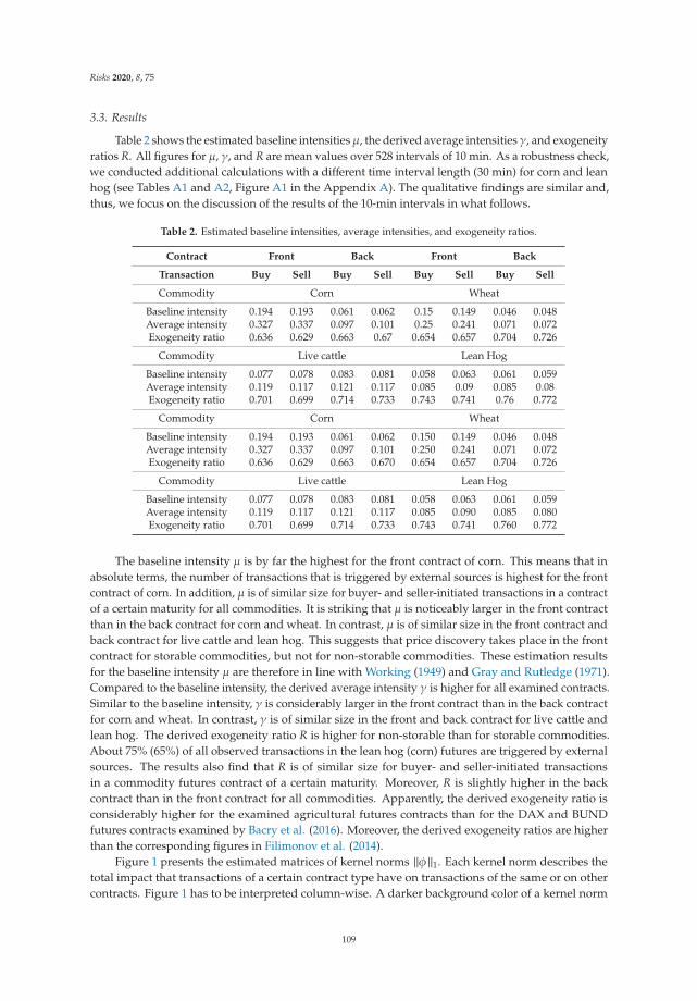
Risks 2020, 8, 75

3.3. Results

Table 2 shows the estimated baseline intensities μ, the derived average intensities γ, and exogeneityratios R. All figures for μ, γ, and R are mean values over 528 intervals of 10 min. As a robustness check,we conducted additional calculations with a different time interval length (30 min) for corn and leanhog (see Tables A1 and A2, Figure A1 in the Appendix A). The qualitative findings are similar and,thus, we focus on the discussion of the results of the 10-min intervals in what follows.

Table 2. Estimated baseline intensities, average intensities, and exogeneity ratios.


Transaction Buy Sell Buy Sell Buy Sell Buy Sell


Baseline intensity 0.194 0.193 0.061 0.062 0.15 0.149 0.046 0.048Average intensity 0.327 0.337 0.097 0.101 0.25 0.241 0.071 0.072Exogeneity ratio 0.636 0.629 0.663 0.67 0.654 0.657 0.704 0.726

Commodity Live cattle Lean Hog






The baseline intensity μ is by far the highest for the front contract of corn. This means that inabsolute terms, the number of transactions that is triggered by external sources is highest for the frontcontract of corn. In addition, μ is of similar size for buyer- and seller-initiated transactions in a contractof a certain maturity for all commodities. It is striking that μ is noticeably larger in the front contractthan in the back contract for corn and wheat. In contrast, μ is of similar size in the front contract andback contract for live cattle and lean hog. This suggests that price discovery takes place in the frontcontract for storable commodities, but not for non-storable commodities. These estimation resultsfor the baseline intensity μ are therefore in line with Working (1949) and Gray and Rutledge (1971).Compared to the baseline intensity, the derived average intensity γ is higher for all examined contracts.Similar to the baseline intensity, γ is considerably larger in the front contract than in the back contractfor corn and wheat. In contrast, γ is of similar size in the front and back contract for live cattle andlean hog. The derived exogeneity ratio R is higher for non-storable than for storable commodities.About 75% (65%) of all observed transactions in the lean hog (corn) futures are triggered by externalsources. The results also find that R is of similar size for buyer- and seller-initiated transactionsin a commodity futures contract of a certain maturity. Moreover, R is slightly higher in the backcontract than in the front contract for all commodities. Apparently, the derived exogeneity ratio isconsiderably higher for the examined agricultural futures contracts than for the DAX and BUNDfutures contracts examined by Bacry et al. (2016). Moreover, the derived exogeneity ratios are higherthan the corresponding figures in Filimonov et al. (2014).

Figure 1 presents the estimated matrices of kernel norms ||φ ||1. Each kernel norm describes thetotal impact that transactions of a certain contract type have on transactions of the same or on othercontracts. Figure 1 has to be interpreted column-wise. A darker background color of a kernel norm

109

Risks 2020, 8, 75

illustrates a larger impact than a lighter color. A kernel norm ||φ ii||1 on the diagonals of the matricesdescribes the impact that transactions of a certain type have on transactions of the same type. A kernelnorm ||φi j||1 on the off-diagonals of the matrices describes the impact that transactions of a certaintype have on transactions of a different type. In general, the kernel norm values are higher for storablethan for non-storable commodities. According to the population representation of the Hawkes process,each buyer-initiated (seller-initiated) transaction directly triggers 0.3102 buyer-initiated transactions(0.3147 seller-initiated) on average in the front contract for corn. The respective values for othercommodities are slightly smaller. Apparently, the kernel norm values on the diagonals of the matrixare considerably higher compared to those on the off-diagonals for all commodities. This indicates thata substantial part of the observed transactions is endogenously driven and points to the presence ofmarket reflexivity for all commodities. In addition, the kernel norm values on the diagonals of thematrix are higher in the front contract than in the back contract for corn and wheat. In contrast, thekernel norm values on the diagonals are of similar size in the front and back contract for live cattle andlean hog. As expected, the estimation results for the matrices of kernel norms ||φ ||1 show that differencesbetween front and back contracts are less pronounced for non-storable than for storable commodities.

Corn Front Back

Wheat Front Back

Buy Sell Buy Sell Buy Sell Buy Sell

Front

Buy 0.3102 0.0315 0.0128 0.0100

Front

Buy 0.2868 0.0288 0.0152 0.0106

Sell 0.0284 0.3147 0.0094 0.0138 Sell 0.0344 0.2828 0.0091 0.0136

Back

Buy 0.0531 0.0375 0.2434 0.0252

Back

Buy 0.0570 0.0389 0.1946 0.0206

Sell 0.0363 0.0596 0.0186 0.2301 Sell 0.0421 0.0634 0.0228 0.1787

Live cattle

Front Back Lean hog

Front Back Buy Sell Buy Sell Buy Sell Buy Sell

Front

Buy 0.2132 0.0170 0.0488 0.0184

Front

Buy 0.1925 0.0179 0.0377 0.0172

Sell 0.0197 0.2490 0.0136 0.0236 Sell 0.0163 0.2012 0.0191 0.0272

Back

Buy 0.0675 0.0181 0.2046 0.0169

Back

Buy 0.0359 0.0188 0.1718 0.0199

Sell 0.0186 0.0269 0.0165 0.2137 Sell 0.0161 0.0405 0.0156 0.1611

Figure 1. Estimated matrices of kernel norms.

The kernel norms on the off-diagonals show that in the cases of corn and wheat, the impactof front contracts on back contracts is larger than vice versa. This relationship, however, is notprevalent for live cattle and lean hog. Thus, our results are in line with Hu et al. (2017), who showthat nearby futures contracts dominate deferred futures contracts in price discovery for storablecommodities, but not for non-storable commodities. No differences can be identified between buyer-and seller-initiated transactions.

110

Risks 2020, 8, 75

Table 3 contains the results of the residual analyses of the estimated Hawkes processes. For morethan about 80% of the 10-min intervals, the Kolmogorov–Smirnov test does not reject the null hypothesisthat the distribution of the residuals is homogeneous Poisson at the 5% significance level for theconsidered commodities. Except for the front contracts of corn and wheat, for more than approximately90% of the 10-min intervals, the Ljung–Box test does not reject the null hypothesis that the residuals areindependently distributed at the 5% significance level. We can therefore conclude that the estimatedHawkes process with the chosen parameterization of the kernel function is a good approximation ofthe observed point process.

Table 3. Residual analyses.




Kolmogorov–Smirnov 0.84 0.84 0.88 0.89 0.87 0.83 0.89 0.89Ljung–Box 0.64 0.67 0.94 0.92 0.78 0.80 0.94 0.94



Figure 2 displays the evolution of the average intensity γ over the whole observation period.The figure is based on daily mean values of the average intensity. In general, the evolution of γ for thefront contract is similar to the evolution of γ for the back contract for all commodities. In particular, γis higher for the front contract than for the back contract throughout the whole observation periodfor corn and wheat. In contrast, for live cattle and lean hog, γ is higher for the front contract thanfor the back contract in the first half of the observation period only. In addition, the evolution of theaverage intensity of buyer-initiated transactions is similar to the evolution of the average intensity ofseller-initiated transactions in a contract of a certain maturity for all commodities.

In general, the average intensity shows a relatively constant progression for all commodities;however, γ increases around certain days where public information became available. For instance,the average intensity increases for all commodities on 9 March 2016 when the USDA released itsmonthly WASDE report (USDA 2016b). Furthermore, γ increases for live cattle on 22 March 2016following a USDA cattle on feed report (USDA 2016c). Most notably, γ increases considerably towardsthe end of the observation period for corn and wheat on 31 March 2016. On this day (11:00 a.m.),the USDA reported an unexpected increase in the corn acreage (USDA 2016a). On the same day, theUSDA published its quarterly grain stocks reports (USDA 2016d). This may explain why the increase inaverage intensities is rather pronounced at that time. Overall, Figure 2 documents that the publicationof USDA reports affects not only volatility and trading volume, but also the intensity of trading activity.

111

Risks 2020, 8, 75

0.00.20.40.60.81.01.2

3/1/16 3/11/16 3/21/16 3/31/16

Buy transactions [corn]

0.00.20.40.60.81.01.2

3/1/16 3/11/16 3/21/16 3/31/16

Sell transactions [corn]

front contractback contract

0.0

0.2

0.4

0.6

0.8

3/1/16 3/11/16 3/21/16 3/31/16

Buy transactions [wheat] front contractback contract

0.0

0.2

0.4

0.6

0.8

3/1/16 3/11/16 3/21/16 3/31/16

Sell transactions [wheat]front contractback contract

0.0

0.1

0.2

0.3

3/1/16 3/11/16 3/21/16 3/31/16

Buy transactions [cattle]front contractback contract

0.0

0.1

0.2

0.3

3/1/16 3/11/16 3/21/16 3/31/16

Sell transactions [cattle]front contractback contract

0.0

0.1

0.2

3/1/16 3/11/16 3/21/16 3/31/16

Buy transactions [hog]front contractback contract

0.0

0.1

0.2

3/1/16 3/11/16 3/21/16 3/31/16

Sell transactions [hog]front contractback contract

Figure 2. Evolution of average intensities (y-axis) in both buy and sell transactions for corn, wheat, livecattle, and lean hog in March 2016.

Figure 3 depicts the evolution of the baseline intensity μ on 31 March 2016 for corn. The figureis based on 24 intervals of 10 min. The baseline intensity μ increases considerably at the time of

112

Risks 2020, 8, 75

the publication of the USDA report for transactions in both the front and back contract. Moreover,the evolution of μ for seller-initiated transactions is similar to the evolution of μ for buyer-initiatedtransactions at the time of the publication of the USDA report for the front contract. In contrast, forthe back contract, the evolution of μ for seller-initiated transactions differs from the evolution of μ forbuyer-initiated transactions at the time of the publication of the USDA report.

0

0.4

0.8

1.2

1.6

2

2.4

9:30

AM

9:40

AM

9:50

AM

10:0

0 A

M10

:10

AM

10:2

0 A

M10

:30

AM

10:4

0 A

M10

:50

AM

11:0

0 A

M11

:10

AM

11:2

0 A

M11

:30

AM

11:4

0 A

M11

:50

AM

12:0

0 PM

12:1

0 PM

12:2

0 PM

12:3

0 PM

12:4

0 PM

12:5

0 PM

1:00

PM

1:10

PM

1:20

PM

Buy front Sell front Buy back Sell back

Figure 3. Evolution of the baseline intensity (y-axis) for corn on 31 March 2016.

The evolution of the baseline intensity for corn on 31 March 2016 suggests that new information isquickly incorporated into market prices through trading activity. Moreover, it is becoming clearer thatnew information does not only affect nearby futures contracts, but also affects deferred futures contracts.

Figure 4 presents the estimated matrix of kernel norms ||φ ||1 for corn on 31 March 2016. The figuresare mean values over 24 intervals of 10 min.

Corn Front Back (March 31, 2016) Buy Sell Buy Sell

Front

Buy 0.3770 0.0290 0.0170 0.0130

Sell 0.0360 0.4380 0.0120 0.0290

Back

Buy 0.0370 0.0420 0.2660 0.0260

Sell 0.0120 0.1090 0.0200 0.2990

Figure 4. Estimated matrix of kernel norms for corn on 31 March 2016.

Compared to the whole observation period, the kernel norm values ||φii||1 on the diagonal ofthe matrix are considerably higher for corn on 31 March 2016. This indicates an increase in market

113

Risks 2020, 8, 75

reflexivity on the publication day of the USDA report. Moreover, compared to the whole observationperiod, the kernel norm values ||φi j||1 on the off-diagonal of the matrix are higher for the back contractfor corn on 31 March 2016. This indicates an increase in the impact that transactions in the back contracthave on transactions in both the front and back contract on the publication day of the USDA report.

To gain an overall picture of the price formation process in agricultural futures contracts withdifferent maturities, Figure 5 illustrates the composition of the estimated intensity of the trading activityin both the front and back contract exemplarily for corn and live cattle. The figure is based on meanvalues of 528 intervals of 10 min. It shows the relative contribution of the estimated baseline intensityμi and the kernel norms ||φii||1 and ||φi j||1 to the total intensity λi.

Figure 5. Composition of the estimated intensity for corn and live cattle.

The relative contribution of the baseline intensity μi to the total intensity λi is largest for thefront contract of corn. It amounts to approximately 30%. This means that external sources, such asnew information, account for approximately 30% of the total intensity of both buyer-initiated andseller-initiated transactions for the front contract of corn. Moreover, the relative contribution of μiis noticeably larger in the front contract than in the back contract for corn. In contrast, the relativecontribution of μi is of similar size in the front and back contract for live cattle. Therefore, in line withWorking Working (1949) and Gray and Rutledge (1971), the composition of the estimated intensitysuggests that nearby futures contracts dominate deferred futures contracts in price discovery forstorable commodities, but not for non-storable commodities.

Compared to the relative contribution of μi, the relative contribution of the kernel norms ||φii||1 tothe total intensity is considerably larger. More specifically, the relative contribution of ||φii||1 to the totalintensity is largest for the back contract of corn. It amounts to roughly 70%, which means that marketreflexivity accounts for about 70% of the total intensity of both buyer-initiated and seller-initiatedtransactions for the back contract of corn. Moreover, the relative contribution of ||φii||1 is clearly larger

114

Risks 2020, 8, 75

in the back contract than in the front contract for corn. In contrast, the relative contribution of ||φii||1 isof similar size in the front and back contract for live cattle.

As expected, the composition of the estimated intensity shows that differences between frontand back contracts in the degree of market reflexivity are less pronounced for live cattle than for corn.Compared to the relative contribution of ||φii||1 , the relative contribution of the kernel norms ||φi j||1to the total intensity is considerably smaller. More specifically, the relative contribution of ||φi j||1 tothe total intensity is higher for live cattle than for corn. It is shown that buyer-initiated transactionsin the back contract account for almost 20% of the total intensity of buyer-initiated transactions inthe front contract for live cattle. On the other hand, buyer-initiated transactions in the back contractaccount for approximately 10% of the total intensity of buyer-initiated transactions in the front contractfor corn. Therefore, in line with Kendall (1982), the composition of the estimated intensity suggeststhat interdependencies of current and subsequent supply might link futures contracts of differentmaturities to non-storable commodities.

4. Conclusions

This paper is the first to examine price discovery in nearby and deferred agricultural commoditiesfutures contracts while explicitly considering potential market reflexivity. For this purpose, we applya four-dimensional Hawkes model with an exponential parametrization of the kernel functions tostorable and non-storable agricultural commodities. We find market reflexivity for both storableand non-storable commodities. Reflexivity accounts for about 50 to 70% of the total trading activity,irrespective of whether transactions have been buyer- or seller-initiated. Storable commodities show ahigher level of reflexivity than non-storable commodities and differences between nearby and deferredcontracts are less pronounced for non-storable commodities than for storable ones. We conjecturethat the degree of reflexivity is related to the trading intensity and the amount of automated trading.Endogeneity results from backward-looking trading strategies, which exploit information from previoustrading activities. Most likely, this source of endogeneity is more prevalent in liquid markets thanin thin markets. Storable commodities are more frequently traded compared with non-storablecommodities, but this holds only for the front contract (c.f. Table 1). Moreover, grains show a highershare of automated trading than livestock contracts (e.g., Haynes and Roberts 2015; Couleau et al. 2019).It appears that these differences are reflected in the endogeneity of the price formation process.

What are the implications of these findings for the price discovery process in agriculturalcommodity futures? The presence of market reflexivity seems to contradict the efficient markethypothesis, and Filimonov et al. (2014) argue that reflexivity is likely to result in a less efficient pricediscovery process. Though our analysis does not allow an evaluation of the presence of reflexivity,we can at least compare our results with previous empirical findings on price discovery in agriculturalcommodity futures markets and screen them for irregularities. Regarding the relation between nearbyand deferred futures contracts, our results are in line with Mallory et al. (2015), who find that newinformation to the market is immediately transmitted across all contract maturities. Moreover, we canreplicate the finding of Hu et al. (2017) that nearby contracts are dominant in price discovery for storablecommodities, but not for non-storable commodities. Finally, we observe an increased baseline intensityat the time of a USDA publication, suggesting that external information is quickly incorporated intomarket prices through trading activity despite the presence of market reflexivity. From these findings,we conclude that the co-existence of exogenous and endogenous price dynamics does not changequalitative characteristics of the price discovery process that have been observed earlier without theconsideration of market reflexivity.

Some aspects could be incorporated in further empirical analyses to obtain a clearer picture aboutprice discovery in agricultural commodity futures in the presence of market reflexivity. The empiricalbasis could be broadened by including additional commodities. Moreover, price discovery and marketreflexivity should be examined over a longer observation period covering, for example, markets innormal backwardation and in contango. From a methodological point of view, the Hawkes model

115

Risks 2020, 8, 75

can be extended and amended in several ways. Covariates such as order imbalances between buyer-and seller-initiated transactions can be included into the intensity function. Other parameterizationsof the kernel function such as power-law parameterizations or other estimation methods such asnon-parametric estimation techniques can be applied to check the robustness of the results. Finally,methods allowing the assessment of the direct impact of market reflexivity on the price formationprocess need to be explored.

Author Contributions: Conceptualization, S.V., G.F. and M.O.; data curation, S.V. and G.F.; formal analysis, S.V.;methodology, S.V. and G.F.; software, S.V.; supervision, M.O.; validation, S.V. and G.F.; visualization, S.V. and G.F.;writing—original draft, S.V., G.F. and M.O.; writing—review and editing, S.V., G.F. and M.O. All authors haveread and agreed to the published version of the manuscript.


Acknowledgments: We thank three anonymous reviewers for helpful comments and suggestions.


Appendix A

Table A1. Estimated baseline intensities, average intensities, and exogeneity ratios (corn, lean hog) fora 30-min interval.



Commodity Corn (30-min interval) Lean Hog (30-min interval)


Table A2. Residual analyses (corn, lean hog) for a 30-min interval.



Commodity Corn (30-min interval) Lean Hog (30-min interval)


Corn 30 min

Front Back Lean Hog 30 min

Front Back

Buy Sell Buy Sell Buy Sell Buy Sell

Front Buy 0.3696 0.0403 0.0103 0.0079

Front Buy 0.2294 0.0210 0.0520 0.0274

Sell 0.0369 0.3727 0.0082 0.0126

Sell 0.0188 0.2331 0.0241 0.0486

Back Buy 0.0585 0.0434 0.2766 0.0275

Back Buy 0.0552 0.0287 0.2183 0.0216

Sell 0.0315 0.0570 0.0152 0.2747

Sell 0.0252 0.0488 0.0247 0.1951

Figure A1. Estimated matrices of kernel norms (corn, lean hogs) for a 30-min interval.

116

Risks 2020, 8, 75

References

Bacry, Emmanuel, Martin Bompaire, Stéphane Gaıffas, and Soren Poulsen. 2017. Tick: A Python library forstatistical learning, with a particular emphasis on time-dependent modeling. arXiv, 1707.03003.

Bacry, Emmanuel, Thibault Jaisson, and Jean–François Muzy. 2016. Estimation of slowly decreasing Hawkeskernels: Aplication to high-frequency order book dynamics. Quantitative Finance 16: 1179–201. [CrossRef]

Bauwens, Luc, and Nikolaus Hautsch. 2007. Modelling Financial High Frequency Data Using Point Processes.SFB 649 Discussion Paper 2007-066. Available online: http://sfb649.wiwi.hu-berlin.de/papers/pdf/SFB649DP2007-066.pdf (accessed on 29 October 2018).

Bicchetti, David, and Nicolas Maystre. 2013. The synchronized and long-lasting structural change on commoditymarkets: Evidence from high frequency data. Algorithmic Finance 2: 233–39. [CrossRef]

Bowsher, Clive G. 2007. Modelling Security Markets in Continuous Time: Intensity-based, Multivariate PointProcess Models. Journal of Econometrics 141: 876–912. [CrossRef]

Couleau, Anabelle, Teresa Serra, and Philip Garcia. 2019. Microstructure noise and realized variance in the livecattle futures market. American Journal of Agricultural Economics 101: 563–78. [CrossRef]

Brennan, M. J. 1958. The supply of storage. American Economic Review 48: 50–72.Diebold, Francis X., and Canlin Li. 2006. Forecasting the term structure of government bond yields. Journal of

Econometrics 130: 337–64. [CrossRef]Easley, David, and Maureen O’Hara. 1992. Time and the process of security price adjustment. Journal of Finance 47:

577–604. [CrossRef]Engle, Robert F., and Jeffrey R. Russell. 1998. Autoregressive conditional duration: A new model for irregularly

spaced transaction data. Econometrica 66: 1127–62. [CrossRef]Fama, Eugene F. 1970. Efficient capital markets: A review of theory and empirical work. The Journal of Finance 25:

383–417. [CrossRef]Fama, Eugene F., and Kenneth R. French. 1987. Commodity Futures Prices: Some Evidence on Forecast Power,

Premiums, and the Theory of Storage. The Journal of Business 60: 55–73. [CrossRef]Filimonov, Vladimir, and Didier Sornette. 2012. Quantifying reflexivity in financial markets: Toward a prediction

of flash crashes. Physical Review E 85: 056108. [CrossRef]Filimonov, Vladimir, David Bicchetti, Nicolas Maystre, and Didier Sornette. 2014. Quantification of the high level

of endogeneity and of structural regime shifts in commodity markets. Journal of International Money andFinance 42: 174–92. [CrossRef]

Geman, Helyette, and Vu-Nhat Nguyen. 2005. Soybean Inventory and Forward Curve Dynamics. ManagementScience 51: 1076–91. [CrossRef]

Gibson, Rajna, and Eduardo S. Schwartz. 1990. Stochastic Convenience Yield and the Pricing of Oil ContingentClaims. Journal of Finance 45: 959–76. [CrossRef]

Glosten, Lawrence R., and Paul R. Milgrom. 1985. Bid, Ask, and Transaction Prices in a Specialist Market withHeterogeneously Informed Agents. Journal of Financial Economics 14: 71–100. [CrossRef]

Gray, Roger W., and David J. S. Rutledge. 1971. The economics of commodity futures markets: A survey. Review ofMarketing and Agricultural Economics 39: 57–108.

Gurgul, Henryk, and Robert Syrek. 2017. Trading volume and volatility patterns across selected Central Europeanstock markets from microstructural perspective. Managerial Economics 18: 87. [CrossRef]

Hardiman, Stephen J., Nicolas Bercot, and Jean-Philippe Bouchard. 2013. Critical reflexivity in financial markets:A Hawkes process analysis. The European Physical Journal B 86: 442. [CrossRef]

Harris, Frederick H. deB., Thomas H. McInish, and Robert A. Wood. 2002. Security price adjustment acrossexchanges: An investigation of common factor components for Dow stocks. Journal of Financial Markets 5:277–308. [CrossRef]

Hasbrouck, Joel. 1995. One Security, Many Markets: Determining the Contributions to Price Discovery. The Journalof Finance 50: 1175–95. [CrossRef]

Hautsch, Nikolaus. 2004. Modelling Irregularly Spaced Financial Data. Berlin: Springer.Hawkes, Alan G. 1971. Point spectra of some mutually-exciting point processes. Journal of the Royal Statistical

Society 33: 438–43. [CrossRef]Hawkes, Alan G., and David Oakes. 1974. A cluster process representation of a self-exciting process. Journal of

Applied Probability 11: 493–503. [CrossRef]

117

Risks 2020, 8, 75

Haynes, Richard, and John S. Roberts. 2015. Automated Trading in Futures Markets. CFTC White Paper. Availableonline: https://www.cftc.gov/sites/default/files/idc/groups/public/@economicanalysis/documents/file/oce_automatedtrading.pdf (accessed on 25 October 2019).

Hu, Zhepeng, Mindy Mallory, Teresa Serra, and Philip Garcia. 2017. Measuring Price Discovery between Nearbyand Deferred Contracts in Storable and Non-Storable Commodity Futures Markets. arXiv, 1711.03506.

Karstanje, Dennis, Michel van der Wel, and Dick J. C. van Dijk. 2017. Common Factors in Commodity FuturesCurves. SSRN Working Paper. [CrossRef]

Kendall, David Laurence. 1982. Intertemporal Price Relationships in Noninventory Futures Markets. Ph.D. thesis,North Carolina State University, Raleigh, NC, USA.

Kyle, Albert S., and Anna Obizhaev. 2019. Large Bets and Stock Market Crashes. Working Paper. Available online:https://ssrn.com/abstract=2023776 (accessed on 25 October 2019).

Large, Jeremy. 2007. Measuring the Resiliency of an Electronic Limit Order Book. Journal of Financial Markets 10:1–25. [CrossRef]

Lee, Charles M. C., and Mark J. Ready. 1991. Inferring trade direction from intraday data. The Journal of Finance 46:733–46. [CrossRef]

Mallory, Mindy, Philip Garcia, and Teresa Serra. 2015. Nearby and Deferred Quotes: What They Tell Us aboutLinkages and Adjustments to Information. Proceedings of the NCCC-134 Conference on Applied CommodityPrice Analysis, Forecasting, and Market Risk Management. Available online: http://www.farmdoc.illinois.edu/nccc134/conf_2015/pdf/Mallory_Garcia_Serra_NCCC_134_2015.pdf (accessed on 25 October 2019).

Meyer, Paul-André. 1971. Démonstration simplifiée d’un théorème Knight. Lecture Notes in Mathematics 191:191–95.

Nelson, Charles R., and Andrew F. Siegel. 1987. Parsimonious modeling of yield curve. Journal of Business 60:473–89. [CrossRef]

Ogata, Yosihiko. 1989. Statistical Models for Earthquake Occurrences and Residual Analysis for Point Processes.Journal of the American Statistical Association 83: 9–27. [CrossRef]

Ogata, Yosihiko. 1998. Space-time point-process models for earthquake occurrences. Annals of the Institute ofStatistical Mathematics 50: 379–402. [CrossRef]

Russell, Jeffrey R. 1999. Econometric Modeling of Multivariate Irregularly-Spaced High-Frequency Data. WorkingPaper, University of Chicago. Available online: http://citeseerx.ist.psu.edu/viewdoc/download?doi=10.1.1.202.486&rep=rep1&type=pdf (accessed on 5 November 2018).

Schwartz, Eduardo S. 1997. The Stochastic Behavior of Commodity Prices: Implications for Valuation and Hedging.The Journal of Finance 52: 923–73. [CrossRef]

Sorensen, Carsten. 2002. Modeling seasonality in agricultural commodity futures. The Journal of Futures Markets22: 393–426. [CrossRef]

Soros, George. 1987. The Alchemy of Finance: Reading the Mind of the Market. New York: John Wiley & Sons.Tang, Ke, and Wei Xiong. 2012. Index investment and the financialization of commodities. Financial Analysts

Journal 68: 54–74. [CrossRef]USDA. 2016a. Prospective Plantings (March 2016). United States Department of Agriculture, National Agricultural

Statistics Service. Available online: https://downloads.usda.library.cornell.edu/usda-esmis/files/x633f100h/9c67wq58w/rx913s37m/ProsPlan-03-31-2016.pdf (accessed on 25 October 2019).

USDA. 2016b. United States Department of Agriculture, National Agricultural Statistics Service. Availableonline: https://downloads.usda.library.cornell.edu/usda-esmis/files/3t945q76s/zs25x8827/d504rk71k/wasde-03-09-2016.pdf (accessed on 25 October 2019).

USDA. 2016c. United States Department of Agriculture, National Agricultural Statistics Service. Available online:https://downloads.usda.library.cornell.edu/usda-esmis/files/m326m174z/8623j006q/q524jq148/CattOnFe-03-18-2016.pdf (accessed on 25 October 2019).

USDA. 2016d. United States Department of Agriculture, National Agricultural Statistics Service. Available online:https://downloads.usda.library.cornell.edu/usda-esmis/files/xg94hp534/08612q46m/fj236409h/GraiStoc-03-31-2016.pdf (accessed on 25 October 2019).

Volkenand, Steffen, Günther Filler, Marlene Kionka, and Martin Odening. 2019. Duration dependence amongagricultural futures with different maturities. Applied Economics Letters. [CrossRef]

118

Risks 2020, 8, 75

Wang, Xiaoyang, Philip Garcia, and Scott H. Irwin. 2016. Are agricultural futures getting noisier? The impactof high frequency quoting in the corn market. Working paper, University of Illinois, Urbana-Champaign.Available online: https://legacy.farmdoc.illinois.edu/irwin/research/Wang_Garcia_Irwin_Oct%202016.pdf(accessed on 25 October 2019).

Working, Hoolbrock. 1949. The theory of price of storage. The American Economic Review 39: 1254–62.


119

risks

Article

Risk and Policy Uncertainty on Stock–Bond ReturnCorrelations: Evidence from the US Markets

Thomas C. Chiang

Department of Finance, LeBow College of Business, Drexel University, Philadelphia, PA 19104, USA;[email protected]

Received: 4 May 2020; Accepted: 27 May 2020; Published: 1 June 2020

Abstract: This paper investigates dynamic correlations of stock–bond returns for different stockindices and bond maturities. Evidence in the US shows that stock–bond relations are time-varyingand display a negative trend. The stock–bond correlations are negatively correlated with impliedvolatilities in stock and bond markets. Tests show that stock–bond relations are positively correlatedwith economic policy uncertainty, however, are negatively correlated with the monetary policy andfiscal policy uncertainties. Correlation coefficients between stock and bond returns are positivelyrelated to total policy uncertainty for returns of the Dow-Jones Industrial Average (DJIA) and theS&P 500 Value stock index (VALUE), but negatively correlated with returns of S&P500 (Total market),the NASDAQ Composite Index (NASDAQ), and the RUSSELL 2000 (RUSSELL).

Keywords: stock–bond correlation; VIX; economic policy uncertainty; monetary policy uncertainty;fiscal policy uncertainty

JEL Classification: C12; C13; G10; G11

1. Introduction

The investigation on correlations of stock and bond returns has long been a key concern ofportfolio managers and financial market strategists (Connolly et al. 2005; Panchenko and Wu 2009;Baur and Lucey 2009; Li et al. 2019, among others). This is because the derived parametric relationscould provide useful guidance in portfolio selection, dynamic asset allocation, and risk management.For most of this time, two questions have dominated the literature. First, are stock returns and bondreturns positively or negatively correlated? Second, what are the factors that cause correlations tovary over time? The theoretical claim of the first issue contends that both required rates of returnfor stock and bond yields are viewed as part of a discount factor to calculate the future cash flowsof investments. This argument is based on the valuation model that has been adopted and used inthe “Fed model” (Kwan 1996; Yardeni 1997). It is observed that any economic shocks, such as income,inflation rate, policy innovation, or external shock that disturb an existing equilibrium, will causeinvestors to reallocate their funds between assets with lower returns to ones with higher returns.An efficient arbitrage will eliminate the return differentials and establish return parity conditions afterexecuting full adjustment (Tobin 1969). This view focuses on economic fundamentals analyzed over along-run perspective.

However, evidence of the decoupling phenomenon observed by Gulko (2002) finds a negativesign for the correlation that obviously occurred in the crisis period; this finding reflects a short run“flight-to-quality” process (Baur and Lucey 2009). To advance the study, Connolly et al. (2005) examinethe US market and discover that the implied stock volatility (VIX) spikes during periods of marketturmoil leads to decline in stock prices (Whaley 2009). It is argued that the VIX variable has a powerin predicting stock returns (Connolly et al. 2005) and find that VIX displays a negative effect on the


Risks 2020, 8, 58

stock–bond correlation. Further study by Chiang et al. (2015) documents that both implied volatilityof stock and conditional volatility of bond returns have significantly negative effects on variations instock–bond returns.

To distinguish their work from previous models, some researchers identify economic policyuncertainty (EPU) as a key factor that dictates the time-varying correlations between stock and bondreturns (Antonakakis et al. 2013; Jones and Olson 2013; Li et al. 2015). Antonakakis et al. (2013) showthat the dynamic correlation between EPU and S&P500 returns is consistently negative over time, withexception of a financial crisis period. Li et al. (2015) report that innovations in EPU have a negative andasymmetrical impact on subsequent stock–bond correlations, since a rise in EPU will likely prompt riskaverse investors to sell off risky stocks and purchase lower risk bonds, leading to a negative correlation.1

Considering the above evidence of risk/uncertainty on stock returns, this paper attempts tocontribute to the study of the effects of policy uncertainty on stock–bond relations. This study differsfrom existing models in the following ways. First, this study focus on broad information in developingmeasures of financial risks such as VIX, Merrill Lynch Option Volatility Estimate (MOVE) anduncertainty (EMU) to explain the time-varying correlations between stock and bond returns. Second,in addition to EPU, this study investigates the impact of categorical policy uncertainties, including bothfiscal policy uncertainty (FPU) and monetary policy uncertainty (MPU). The testing result suggeststhat the FPU and MPU give rise to different effects vis-à-vis that of EPU. Third, instead of testing acorrelation coefficient derived from a single measure of aggregate stock returns that covaries with aspecific bond yield, this study conducts tests on the return correlations involving different measures ofaggregate stock returns and a spectrum of bond yields for different maturities. Thus, the estimatedresults will provide broad coverage of dynamic correlation behavior. Fourth, the net effect of variouspolicy uncertainty is summarized in total policy uncertainty (TPU). Evidence demonstrates that theresults are mixed due to the different impact, which the income and substitution effects have onstock–bond return correlations.

The remainder of the paper is structured as follows. Section 2 describes a dynamic correlation modeland derives the time-varying correlations. Section 3 provides rationales for using risk and uncertaintyvariables to explain the time-varying behavior of stock–bond return correlation. Section 4 describes thesample data. Section 5 reports the estimates developed from the use of policy uncertainty to explain thedynamic stock–bond correlations. Section 6 provides robustness tests. Section 7 concludes the paper.

2. The Relationship between Stock Returns and Bond Returns

As mentioned earlier, stock and bond returns are positively correlated since both stock and bondmarkets commonly react to economic news, such as changes in inflation rate, economic growth, the realinterest rate, and business cycle, in similar ways. When investors perceive that economic prospectsare good, demand for bonds increase, as does demand for stocks, leading to a positive correlation.Experience from the late 1990s suggests that an upward shift in the wealth effect encourages investorsto hold both types of assets simultaneously. Campbell and Ammer (1993), Kwan (1996), and d’Addonaand Kind (2006) document this phenomenon.

Historical experience also reveals a negative correlation between stock–bond returns, which isespecially noticeably in the stock market during a downturn period or a financial crisis. When the stockmarket plummets, risk averse investors may move funds from the stock market to safer assets andincrease the demand for bond market, forming a “flight-to-quality” phenomenon (Baur and Lucey 2009;Hakkio and Keeton 2009). On the contrary, when the economy recovers and stock prices start to rally,investors become less risk averse and opt to switch back to stock market, leading to a “flight-from-quality”

1 Li et al. (2015) argue that when EPU declines, a flight from quality could also occur, resulting in a reduction in the correlations.However, the reduction in EPU can signify an improvement in the market environment, which would raise investors’ demandfor both stocks and bonds, thereby pushing up their correlations. This could produce an asymmetric effect.

122

Risks 2020, 8, 58

phenomenon. Thus, the correlation between stock and bond returns displays a negative relation.Evidence by Gulko (2002), Connolly et al. (2005), Baur and Lucey (2009), and Chiang et al. (2015) supportthis hypothesis.

Despite their contributions, which use VIX as a measure to explain the time-varying correlation ofstock–bond returns, their work appears to inadequately capture all the necessary information associatedwith uncertainty. For instance, President Trump revealed in the first week of October that high-level tradenegotiations between the US and China had concluded in a “very substantial phase one deal” and thatphase two would start almost immediately after phase one was signed. This statement, a sure sign ofreduced uncertainty, would be expected to improve investors’ sentiment, and indeed, Wall Street stocksclosed higher on 11 October 2019 as the S&P 500 gained 32.14 points (or 1.09%), DJIA moved ahead319.92 points (or 1.21%) and Nasdaq 106.26 advanced points (1.34%). This episode motivates this study toinvestigate the role of economic policy uncertainty on asset prices. In addition, the impacts of monetarypolicy uncertainty (MPU) and fiscal policy uncertainty (FPU) are also included to the test equation as away of differentiating the impact of dynamic correlation behavior of stock–bond returns.

It is generally recognized that a sudden rise in EPU is likely to impede the smoothness of operationsin economic activities and hence cause income uncertainty, which tamps down liquidity (Brunnermeierand Pedersen 2009) and leads to a decline in demand for assets (Bloom 2009, 2014; Chiang 2019).This phenomenon may be called the income uncertainty effect. Conversely, as EPU lessens, investorsfeel less uncertain about the future and more encouraged to increase their demand for assets, driving apositive correlation between stock and bond returns (Hong et al. 2014).

On the other hand, the substitution effect describes a phenomenon in which stock and bond returnsmove in opposite directions as uncertainty about economic activity changes in the market. This occursas uncertainty heightens; investors then sell off their riskier assets (stock) and move their funds intosafer assets (bond). This shift results in a negative relation between stock and bond returns. Further, asuncertainty declines, investors then switch from lower return assets (bond) to higher return assets (stocks),causing a negative relation between stock and bond returns (Li et al. 2015). Thus, the substitution effecttends to produce a negative relation between stock and bond returns. In fact, the concept of income effectis essentially derived from Tobin (1969) and then applied by Barsky (1989), Hong et al. (2014), and Li et al.(2015) to analyze the impact of economic uncertainty, triggered by economic policy uncertainty, on assetreturns. The analysis can be extended to examine the impacts of monetary policy uncertainty (MPU) andfiscal policy uncertainty (FPU). As stated above, the impacts of MPU and FPU on stock return and bondreturn could also be attributed to the income effect and substitution effect; the ultimate impact on thereturns of these two asset classes depends on the relative influence of these two forces.

3. A Dynamic Conditional Correlation Model

To derive the dynamic correlation series, the literature follows a seminal study by Engle (2002)who proposes a dynamic conditional correlation model, which is designed to estimate asset marketreturns (de Goeij and Marquering 2004; Chiang et al. 2007; Yu et al. 2010; Antonakakis et al. 2013; Jonesand Olson 2013; Li et al. 2015; Ehtesham and Siddiqui 2019; Allard et al. 2019). This model is frequentlyused because of its ability to capture a vector of return correlations and describe the volatility clusteringphenomenon. Moreover, it could alleviate the heteroscedasticity problem (Forbes and Rigobon 2002).In this study, {Rt} represents a bivariate return series, expressed as

Rt = μt + ut (1)

where Rt = [R1,t R2,t]′ is a 2 × 1 vector for stock market returns, μt is the mean value of asset 1 or 2,

which has the conditional expectation of multivariate time series properties2, ut|Ft−1 = [u1,tu2,t]′ ∼

2 Some researchers use domestic macroeconomic factors, such as inflation rate, business cycle patterns, and policy stance, onthe stock–bond correlation (Ilmanen 2003; Yang et al. 2009; Dimic et al. 2016; Pericoli 2018).

123

Risks 2020, 8, 58

N(0, Ht), Ft−1 is the information set up for (and including) time t − 1. In the context of this study,it is convenient to treat R1,t as the return on stocks and R2,t as the bond return for one of the bondinstruments. In the multivariate DCC-GARCH structure, the conditional variance-covariance matrixHt is assumed to be

Ht = DtPtDt (2)

where Dt = diag{Ht}−1/2 is the 2 × 2 diagonal matrix of time-varying standard deviations fromunivariate models, and Pt is the time-varying conditional correlation matrix, which satisfies thefollowing conditions:

Pt= diag{Qt}−1/2Qtdiag{Qt}−1/2 (3)

Now Pt in Equation (3) is a correlation matrix with ones on the diagonal and off-diagonal elementsthat have an absolute value less than one. Use of an asymmetric DCC model recognizes a shockdynamic adjustment of correlation for negative shock may be different than it is for a positive outcome(Cappiello et al. 2006; Engle 2009).3 In this expression, it can be written as:

Qt = Ω + a εt−1ε′t−1 + γηt−1η

′t−1 + βQt−1 (4)

where the Qt is positive definite and ηt−1 = min[εt , 0].The product of ηi,tη j,t will be nonzero; only these two variables are negative. Thus, a positive

value of γ indicates that correlations increase more in response to market falls than they do to marketrises. The equation is written as

Ω = (1− α− β)Q− γN (5)

where Qt =(Qij,t)

is the 2 × 2 time-varying covariance matrix of εt, Q = E[εtε′t ] is the 2 × 2 unconditional

variance matrix of εt (where εi,t = ui,t/√

hii,t, i = 1 and 2), N = E[γηtη′t

]is the 2 × 2 unconditional

variance matrix of ηt; a, β, and γ are non-negative scalar parameters satisfying (1− α− β− γ) > 0.The substitution of Equation (5) for four yields

ρi j,t =Qij,t√

Qii,t√

Qjj,t(6)

which can be used to calculate the correlations for the two assets. As proposed by Engle (2002, 2009)and Cappiello et al. (2006), the asymmetric dynamic correlation (ADCC) model can be estimated byusing a two-stage approach to maximize the log-likelihood function.

4. Data

The data in this study cover the US aggregate stock market index (TTMK-US$RI) for the monthlyobservations spanning from January 1990 through June 2019. To measure the risks in the stock andbond markets, I use the implied stock market volatility (VIXt) obtained from the S&P 500 index optionsand MOVEt, the one-month Merrill Lynch Option Volatility Estimate of bond volatility. To conductrobustness tests, the US aggregate stock market indices also include the Dow-Jones Industrial Average(DJIA), the NASDAQ Composite Index (NASDAQ), the RUSSELL 2000 (RUSSELL), and the S&P 500Value stock index (VALUE). For bond markets, the data cover the bond price indices of maturitiesfor 30 years, 10 years, seven years, five years, and two years. The data for the total stock market,VIX, MOVE, and bond markets indices are obtained from Thomson Reuters’ Datastream. Returns areconstructed by taking the log-difference of the price indices times 100.

The data for the categorical uncertainty indices are equivalent to the economic policy uncertainty(EPU) data used by Baker et al. (2016). The construction of the EPU index is based on the followingcomponents: newspaper coverage of policy-related economic uncertainty, which is based on 10 large

3 This section follows closely to Engle (2009, pp. 45–49).

124

Risks 2020, 8, 58

newspapers; the number of federal tax code provisions set to expire in future years; and disagreementsamong economic forecasters, which are used as a proxy for uncertainty. Based on a similar procedure,Baker, Bloom, and Davis (BBD) construct categorical indices, including the MPU and FPU indices.Of these indices, the MPU and FPU are based on several dimensions of information: (i) the AccessWorld News database of over 2000 newspapers; (ii) a balanced panel of 10 major national andregional US papers, including a broader set of terms designed to capture domestic and foreignsources of monetary policy and fiscal policy uncertainties; and (iii) data scaled by the total numberof articles. The term sets for economic policy, monetary policy, and fiscal policy uncertainty indicesare given in the Appendix A. These data can be downloaded from the link given below: http://www.policyuncertainty.com/categorical_terms.html.

Note that the choice of the US data is based on the rationale that these data can be used to constructa dynamic correlation between stocks and bonds with combinations of different stock indices andmaturities of bonds. More importantly, our goal is to use policy uncertainty, including economicpolicy uncertainty, fiscal policy uncertainty and monetary policy uncertainty to explain the dynamiccorrelations. These data are more consistently available in the US market and not as accessible in othermarkets. The data constraint limits our research scope.

5. Empirical Estimations

5.1. Estimated Stock–Bond Dynamic Correlations

Table 1 provides different correlation matrices of stock returns, bond returns, risk and uncertainty.Panel A. reports the correlations of total stock market (TTMK) return and bond returns withdifferent maturities. The statistics show negative correlation coefficients ranging from −0.12 to −0.15.The corresponding t-ratios are statistically significant, the only exception is the coefficient of a two-yearbond. The other elements in this table are the correlations of bond returns, which range between 0.59and 0.98. Panel B presents the correlations among different measures of stock returns and range from0.74 to 0.95 (VALUE and DJIA). Due to the high correlation in both types of assets, most researcherstend to use only one type of stock measure, i.e., total market return, and one type of bond return,i.e., 10-year bond, to engage empirical analysis. Panel C provides a correlation matrix that illustratesthe correlation of VIX and different categorical policy uncertainties. It shows that FPU and MPU arehighly correlated with EPU, and VIX has the highest correlation with MOVE. To visually demonstrate,Figure 1 presents time varying correlations for VIX, MOVE, EPU, FPU, and MPU in the US market.Panel D reports the summary of statistics for VIX and uncertainty variables. Among them, the FPUsurprisingly has the highest standard deviation, while the VIX has the lowest. The information is notusually observable by the public.

Table 1. Correlation matrices of stock returns, bond returns, risk, and uncertainty.

Correlation (t-Statistic) Rm_TTMK Rb_30Y Rb_10Y Rb_7Y Rb_5Y Rb_2Y

Rm_TTMK 1—–

Rb_30Y −0.1209 1−2.28 —–

Rb_10Y −0.1191 0.9215 1−2.24 44.39 —–

Rb_7Y −0.1191 0.8638 0.9809 1−2.24 32.08 94.42 —–

Rb_5Y −0.1456 0.7798 0.9407 0.9701 1−2.75 23.31 51.87 74.76 —–

Rb_2Y −0.1544 0.5934 0.7764 0.8278 0.9073 1−0.15 13.79 23.05 27.60 40.37 —–

Panel A. Correlations of bond index returns.

125

Risks 2020, 8, 58

Table 1. Cont.

Correlation (t-Statistic) Rm_TTMK R_DJIA R_Nasdaq R_Russell R_Value

Rm_TTMK 1—–

R_DJIA 0.9333 148.70 —–

R_Nasdaq 0.8752 0.7391 133.90 20.56 —–

R_Russell 0.8466 0.7543 0.8552 129.80 21.52 30.92 —–

R_Value 0.9447 0.9451 0.7350 0.8101 153.96 54.19 20.31 25.89 —–

Panel B. Correlations of stock index returns.

Correlation (t-Statistic) VIX MOVE EPU FPU MPU

VIX 1—–

MOVE 0.5969 113.84 —–

EPU 0.4099 0.2997 18.36 5.84 —–

FPU 0.2945 0.1490 0.8974 15.73 2.80 37.84 —–

MPU 0.3803 0.3020 0.7659 0.5515 17.65 5.89 22.16 12.30 —–

Panel C. Correlations of financial risk and categorical uncertainty.

Statistics VIX MOVE EPU FPU MPU

Mean 19.32 93.84 96.74 101.71 87.58Median 17.40 91.30 85.92 81.96 71.37

Maximum 59.89 213.90 271.83 374.31 407.94Minimum 9.51 46.20 37.27 23.05 16.57Std. Dev. 7.44 27.16 41.05 63.54 56.14Skewness 1.72 0.95 1.18 1.59 1.80Kurtosis 7.60 5.24 4.26 5.68 8.06

Observations 348.00 348.00 348.00 348.00 348.00

Panel D. Summary of statistics of risk and uncertainty.

Figure 1. Time-varying VIX, MOVE, EPU, FPU, and MPU in the US market.

126

Risks 2020, 8, 58

5.2. Estimated Stock–Bond Correlation Coefficients

Table 2 contains parametric estimates of the covariance between stock and various bond returnsusing the ADCC-GARCH model as represented by the system of Equations (1)–(5). Estimates in Table 2are pairwise covariances between TTMK stock returns and one of the bond returns from 30 year to twoyear bonds, hij(RmR30y

b ), hij(RmR10yb ), hij(RmR7y

b ), hij(RmR5yb ), and hij(RmR2y

b ). The reported statistics forconditional variances indicate that the lagged conditional variance, βi j, and the lagged shock squared,αi j, are largely statistically significant except for α11. This result indicates that the GARCH-type modelis relevant. Turning to the asymmetric impact of shocks on conditional variance, we find that most ofthe estimated coefficients in the stock and bond markets

(γi j)

are highly significant. The exception isγ11, which is not consistent with the expected sign. Judging from the estimated coefficient and theassociated t-statistics, the variance equation is apparently dominated by the predictive power from the

lagged variance term.4 Having estimated hij(Rm, Rb), it can derive: ρi j,t =hij,t√

hii,t√

hjj,t.

Table 2. Estimates of the asymmetric dynamic correlation (ADCC) models parameters for stock–bondreturn correlations.

Parameters hij(RmR30yb ) hij(RmR10y

b ) hij(RmR7yb ) hij(RmR5y

b ) hij(RmR2yb )

ω11 0.708 2.21 1.281 2.70 1.357 2.62 1.169 2.35 1.280 2.68ω12 0.030 0.80 0.002 0.02 −0.066 −1.05 −0.088 −2.09 0.002 0.02ω22 0.865 2.44 0.325 1.81 0.121 1.41 0.050 1.30 0.325 1.79α11 0.082 1.57 0.094 1.42 0.099 1.29 0.120 1.54 0.094 1.39α12 0.022 4.03 0.138 4.83 0.094 2.79 0.067 2.46 0.138 4.21α22 0.136 3.03 0.096 2.79 0.106 2.41 0.103 2.29 0.096 2.70γ11 0.070 1.40 0.175 2.33 0.192 2.31 0.133 1.67 0.175 2.30γ12 −0.052 −3.71 −0.057 −1.50 0.033 0.52 0.073 1.36 −0.058 −0.92γ22 −0.206 −3.71 −0.149 −3.55 −0.150 −2.88 −0.118 −2.40 −0.149 −3.39β11 0.844 19.49 0.743 12.38 0.728 11.35 0.746 11.49 0.743 12.38β12 0.998 17.63 0.823 23.69 0.843 21.83 0.859 24.09 0.823 23.68β22 0.898 21.75 0.897 17.83 0.918 19.57 0.914 18.19 0.897 17.62

LLF −1844 −1672 −1594 −1488 −1673

Note: This table estimate the parameters for conditional variance and covariance between totalstock returns and various bond returns. For an ADCC(RmR10y

b ) model, the model is given by:⎡⎢⎢⎢⎢⎢⎢⎣h11,th12,th22,t

⎤⎥⎥⎥⎥⎥⎥⎦ =⎡⎢⎢⎢⎢⎢⎢⎣ω11ω12ω22

⎤⎥⎥⎥⎥⎥⎥⎦+⎡⎢⎢⎢⎢⎢⎢⎣α11 0 00 α12 00 0 α22

⎤⎥⎥⎥⎥⎥⎥⎦⎡⎢⎢⎢⎢⎢⎢⎢⎣

ε21,t−1

ε1,t−1ε2,t−1ε2

2,t−1

⎤⎥⎥⎥⎥⎥⎥⎥⎦+⎡⎢⎢⎢⎢⎢⎢⎣γ11 0 00 γ12 00 0 γ22

⎤⎥⎥⎥⎥⎥⎥⎦⎡⎢⎢⎢⎢⎢⎢⎢⎣

η21,t−1

η1,t−1η2,t−1η2

2,t−1

⎤⎥⎥⎥⎥⎥⎥⎥⎦for (η1,t−1 < 0, η2,t−1 < 0)

+

⎡⎢⎢⎢⎢⎢⎢⎣β11 0 00 β12 00 0 β22

⎤⎥⎥⎥⎥⎥⎥⎦⎡⎢⎢⎢⎢⎢⎢⎣

h11,t−1h12,t−1h22,t−1

⎤⎥⎥⎥⎥⎥⎥⎦.

The estimated result for ADCC(RmR10yb ) model is given by:

⎡⎢⎢⎢⎢⎢⎢⎢⎢⎢⎣h11,t

h12,t

h22,t

⎤⎥⎥⎥⎥⎥⎥⎥⎥⎥⎦ =⎡⎢⎢⎢⎢⎢⎢⎢⎢⎢⎣

1.2800.0020.325

⎤⎥⎥⎥⎥⎥⎥⎥⎥⎥⎦+⎡⎢⎢⎢⎢⎢⎢⎢⎢⎢⎣

0.094 0 00 0.138 00 0 0.096

⎤⎥⎥⎥⎥⎥⎥⎥⎥⎥⎦⎡⎢⎢⎢⎢⎢⎢⎢⎢⎢⎢⎣

ε21,t−1

ε1,t−1ε2,t−1

ε22,t−1

⎤⎥⎥⎥⎥⎥⎥⎥⎥⎥⎥⎦+⎡⎢⎢⎢⎢⎢⎢⎢⎢⎢⎣

0.175 0 00 −0.057 00 0 −0.149

⎤⎥⎥⎥⎥⎥⎥⎥⎥⎥⎦⎡⎢⎢⎢⎢⎢⎢⎢⎢⎢⎢⎣

η21,t−1

η1,t−1η2,t−1

η22,t−1

⎤⎥⎥⎥⎥⎥⎥⎥⎥⎥⎥⎦+

⎡⎢⎢⎢⎢⎢⎢⎢⎢⎢⎣0.743 0 0

0 0.823 00 0 0.897

⎤⎥⎥⎥⎥⎥⎥⎥⎥⎥⎦⎡⎢⎢⎢⎢⎢⎢⎢⎢⎢⎣

h11,t−1

h12,t−1

h22,t−1

⎤⎥⎥⎥⎥⎥⎥⎥⎥⎥⎦

4 To illustrate the model, in the footnote of Table 2, one can plug the estimated parameters into the model using hij(RmR10yb ).

127

Risks 2020, 8, 58

The parameter hij,t is the variance and covariance of asset i and j in the estimated equation(subscripts i = (Rm) and j = (Rb), which stand for stock and bond returns, respectively); ω, α, and βare the parameters for the conditional variance equation; and γ is an asymmetric parameter. The firstcolumn is the estimated parameters and the second column is the t-statistics. The critical values at the1%, 5%, and 10% are 2.60, 1.97, and 1.65, respectively. LLF denotes the log-likelihood function.

Figure 2 shows time series plots of dynamic conditional correlations for the monthly data betweenTTMK return and bond returns with different maturities based on Equation (6). Correlations betweenthe returns of the two assets display noticeable variations throughout the sample period. In general,the plots clearly show a downward slope up to the time of 2004. During the beginning of the 2000swhen the US market suffered from the dotcom collapse, the stock market dropped dramatically,and there was less of a decline in bond returns, causing the correlation to move downward as shownin the Figure 2 in this period. These results are consistent with the findings of Connolly et al. (2005),Chiang et al. (2015), and Li et al. (2015). However, during the global financial crisis period in 2008–2010,the stock market plummeted again, and the correlation coefficient also deepened in this period. Afterthis crisis time the relationships become stationary and fluctuate around a very mild negative regime.A special feature derived from this study is that despite of their common movement around turningpoints, the dynamic paths show that the stock–bond return correlations vary with different bondmaturities, which reflect different market conditions and preferences for bond maturities with differentbondholders. These results suggest that the path of ρSB,t is based on only one stock return and one bondreturn, as is the case in conventional studies, which could produce a misleading and biased estimator.

Figure 2. Dynamic correlations between stock (TTMK) and various bond returns in the US.

5.3. The Role of Uncertainty

Early studies by Connolly et al. (2005), Andersson et al. (2008), and Chiang et al. (2015) stressthe notion of using volatility measure as a proxy for uncertainty. Connolly et al. (2005) find that thecorrelation between stock and bond returns declines during periods with substantial increases in VIX.Andersson et al. (2008), Chiang et al. (2015), and Dimic et al. (2016) report that periods of elevatedstock market uncertainty cause a decoupling between the relation of stock and bond returns, whichis consistent with the “flight-to-quality” phenomenon. Antonakakis et al. (2013) and Li et al. (2015)employ the economic policy uncertainty in modeling the dynamic correlations. The current studyextends this approach by adding monetary policy uncertainty and fiscal policy uncertainty in thetest equation to explain the dynamic correlations between stock and bond returns. This notion issummarized in the regression model as follows:

128

Risks 2020, 8, 58

ρ∗Sb,t= ϕ0 + ϕ1VIXt−1+ϕ2MOVEt−1+ϕ3EPUt−1+ϕ4MPUt−1+ϕ5FPUt−1+ϕ6Trend + εt (7)

where ρ∗Sb,t is a Fisher transformation of stock–bond correlation coefficient, ρSB,t, that is, ρ∗Sb,t =

12 ln[ 1+ρSB,t

1−ρSB,t] and is bound to interval [−1,+1]. VIXt−1 and MOVEt−1 are the 1-month implied volatility

in stock and bond markets, respectively. The EPUt−1 is the economic policy uncertainty at time t − 1,while MPUt−1 and FPUt−1 are the monetary policy and fiscal policy uncertainties at time t − 1. Twospecial features are included in Equation (7). First, the financial risk and uncertainty are treated asindependent factors to explain the stock–bond return correlations; second, in addition to the EPUt−1, thecategorical policy impacts, such as the MPUt−1 and FPUt−1, are included to highlight their distinctiveeffects. In the last term, the trend factor is added to capture of the presence of non-stationarity.

Table 3 presents consistent estimates (Newey and West 1987) of Equation (7) without includingEPUt−1, MPUt−1 and FPUt−1, while Table 4 shows results for this equation where the restriction ofϕ3 = ϕ4 = ϕ5 = 0 has been relaxed. Both models perform very well, the adjusted R-squares for theunrestricted model, which range from 0.48 to 0.81, are notably higher than those of the restricted model,indicating that the inclusion of the uncertainty variables helps to increase their explanatory power.Since the results in Table 3 are nested in Table 4, our interpretations focus on Table 4. Several pointsare noteworthy.

Table 3. Estimates of aggregate and categorical EPU, FPU, and MPU and on stock (TTMK)–bondreturn correlations.

PI = TTMK ^ρ∗t(RmR30y

b )^ρ∗t(RmR10y

b )^ρ∗t(RmR7y

b )^ρ∗t(RmR5y

b )^ρ∗t(RmR2y

b )

C 0.945 14.34 0.668 8.80 0.642 5.26 0.673 13.27 0.781 12.79VIXt−1 −0.006 −2.52 −0.005 −1.73 0.001 0.25 0.001 0.56 −0.005 −2.33

MOVEt−1 −0.002 −2.15 −0.003 −3.10 −0.001 −1.33 −0.002 −3.74 −0.003 −5.30Trend −0.004 −24.65 −0.003 −14.28 −0.003 −10.93 −0.003 −27.75 −0.002 −15.42

R2 0.68 0.41 0.71 0.72 0.48

Note: This table presents evidence of VIX and MOVE on ρ∗t , the Fisher transformation of ρt, which is the dynamic

correlations between value stock–bond returns. That is, ρ∗Sb,t(· · · ) =12 ln[ 1+ρt

1−ρt]). The subscript “sb” is suppressed to

save space in table. For each model, the first column reports the estimated coefficients, the second column containsthe estimated t-statistics. The critical values of t-distribution at the 1%, 5%, and 10% levels of significance are 2.60,

1.98, and 1.66, respectively. The numbers in the brackets are the p-values. R2

is the adjusted R-squared.

Table 4. Estimates of aggregate and categorical EPU, FPU, and MPU, and on stock (TTMK)–bondreturn correlations.

PI = TTMK ^ρ∗t(RmR30y

b )^ρ∗t(RmR10y

b )^ρ∗t(RmR7y

b )^ρ∗t(RmR5y

b )^ρ∗t(RmR2y

b )

C 0.000 0.00 0.370 1.91 −0.680 −5.91 −0.444 −3.66 0.513 3.13VIXt−1 −0.007 −2.00 −0.003 −1.00 −0.002 −1.73 −0.001 −0.99 −0.005 −2.12

MOVEt−1 −0.001 −1.40 −0.002 −2.97 −0.001 −3.82 −0.002 −5.27 −0.003 −5.54EPUt−1 0.857 6.15 0.674 5.43 0.766 10.79 0.715 9.34 0.406 3.96FPUt−1 −0.409 −4.59 −0.415 −6.11 −0.231 −5.67 −0.250 −5.79 −0.203 −3.57MPUt−1 −0.254 −4.55 −0.222 −5.01 −0.236 −9.25 −0.217 −8.18 −0.157 −4.60

Trend −0.004 −11.98 −0.002 −11.93 −0.003 −28.00 −0.003 −27.70 −0.002 −14.60χ2(3) 38.12 [0.00] 18.30 [0.00] 197.92 [0.00] 127.64 [0.00] 21.86 [0.00]χ2(2) 29.81 [0.00] 17.60 [0.00] 91.81 [0.00] 74.36 [0.00] 21.85 [0.00]

R2 0.73 0.48 0.81 0.79 0.51

Note: This table presents evidence of financial risk and policy uncertainty on ρ∗Sb,t, the Fisher transformation of ρt,

which is the dynamic correlations between TTMK stock–bond returns. That is, ρ∗Sb,t(· · · ) =12 ln[ 1+ρt

1−ρt]. The subscript

“sb” is suppressed to save space in the table. For each model, the first column reports the estimated coefficients, thesecond column contains the estimated t-statistics. The critical values of t-distribution at the 1%, 5%, and 10% levelsof significance are 2.60, 1.98, and 1.66, respectively. The numbers in the brackets are the p-values. R

2is the adjusted

R-squared.

129

Risks 2020, 8, 58

First, the coefficients of the trend factor are negative, indicating that in general the correlationsbetween stock and bond returns slope downward, although feathering in the stochastic process is present.This result is consistent with the findings reported by Connolly et al. (2005) and Chiang et al. (2015).

Second, the risk variables of VIXt−1 and MOVEt−1 are negative, revealing that investors are activelyswitching between stock and bond depending on the level of risk in the market. This movementresembles a flight-to-quality as risk increases and flight-from-quality as risk declines. This finding isconsistent with the results in the literature (Gulko 2002; Connolly et al. 2005; Andersson et al. 2008;Chiang et al. 2015).

Third, the estimated coefficients of EPUt−1 are positive and highly significant. This conforms witha market phenomenon in which a sudden rise in uncertainty impedes prospects for economic activities,thereby dampening output production and future cash flows. Facing weakening liquidity, investorstend to sell off stocks and bonds. The dominance of this income effect will lead to a positive movementbetween stock and bond prices, a reaction that is consistent with a study by Hong et al. (2014), whichemphasizes the response to market volatile.

Fourth, the estimated coefficients for FPUt−1 and MPUt−1 are negative and significant at the onepercent level. This should not be surprising, since a rise in MPU tends to increase uncertainty ininterest rate, which is more likely to create a strong substitution effect that causes a shift from highuncertainty asset-stocks to relatively low uncertainty asset-bonds and leads to a decoupling of stockand bond returns. A similar shift also holds true for an upward shift in FPU, especially in the case ofbond financing of government deficits. It is recognized that an increase in FPUt−1 and MPUt−1 couldcreate an income effect; however, the negative coefficients imply that the substitution effect dominatesthe income effect.

Fifth, the estimated results favor the inclusion of uncertainty variables as incremental variables.This can be seen in the reported χ2(3) statitic, which tests the joint significance of the coefficients withϕ3 = ϕ4 = ϕ5 = 0. The p-values of the Chi-squared test, which are in brackets, indicate the rejection ofthe null, suggesting that the inclusion of the uncertainty variables helps to improve the explanation ofthe dynamic correlations between stock and bond returns. Evidence thus indicates that the exclusion ofuncertainty variables in the literature (Connolly et al. 2005; Andersson et al. 2008; Chiang et al. 2015) issubject to an omitted variable problem. In addition, the χ2(2) statistic for testing equality of coefficientsfor ϕ4 = ϕ5 = 0 against alternatives is also significant in all of cases, this test indicates the exclusion ofcategorical uncertainty even in the case of EPU (Antonakakis et al. 2013; Li et al. 2015) suffers from amissing variable problem.

In summary, this study contributes to the literature in two ways. First, the effect of risk is separatedfrom the uncertainty effect, showing both types of variables contribute to the variations of stock–bondcorrelations. Second, unlike the EPU, evidence shows the coefficients of FPU and MPT are negative,which provides an incremental contribution in the ability to predict time-varying correlations of stockand bond returns, ρ∗Sb,t. These categorical uncertainty variables have not been explored in the literature.

6. Robustness Tests

6.1. Difference of Stock Indices

Despite of successful outcomes of the time-varying behavior of ρ∗Sb,t in relation to therisk/uncertainty, it is important to examine the robustness of the parametric relations, which can bedone by using alternative measures of stock indices. In this section, the test equations apply to stockindices including the DJIA, NASDAQ, RUSSELL, and VALUE. Pairings of stock returns with bondreturns of maturities of 30 years, 10 years, seven years, five years, and two years are used to deriveρ∗Sb,t(·). The estimated equations are reported in Tables 5–8, and the test results are summarizedas follows.

130

Risks 2020, 8, 58

Table 5. Estimates of aggregate and categorical EPU, FPU, and MPU and on stock (DJIA)–bondreturn correlations.

PI = DJIA ^ρ∗t(RmR30y

b )^ρ∗t(RmR10y

b )^ρ∗t(Rm(RmR7y

b )^ρ∗t(RmR5y

b )^ρ∗t(RmR2y

b )

C −1.148 −4.66 −1.116 −9.04 −1.019 −9.09 −0.834 −7.19 0.100 0.93VIXt−1 −0.016 −4.62 0.000 −0.04 −0.004 −3.08 0.003 2.59 0.000 0.11


Trend −0.004 −10.01 −0.004 −23.49 −0.003 −24.63 −0.003 −21.82 −0.002 −16.65χ2(3) 76.80 [0.00] 216.77 [0.00] 232.68 [0.00] 130.12 [0.00] 15.60 [0.00]χ2(2) 28.91 [0.00] 74.98 [0.00] 53.30 [0.00] 62.22 [0.00] 15.52 [0.00]

R2 0.73 0.82 0.84 0.77 0.61

Note: This table presents evidence of financial risk and policy uncertainty on ρ∗Sb,t, the Fisher transformation of ρt,

which is the dynamic correlations between DJIA stock–bond returns. That is, ρ∗Sb,t(· · · ) =12 ln[ 1+ρt

1−ρt]. The subscript

“sb” is suppressed to save space in the table. For each model, the first column reports the estimated coefficients,the second column contains the estimated t-statistics. The critical values of t-distribution at the 1%, 5%, and 10%levels of significance are 2.60, 1.98, and 1.66, respectively. The numbers in the brackets are the p-values. R

2is the

adjusted R-squared.

Table 6. Estimates of aggregate and categorical EPU, FPU and MPU and on stock (NASDAQ)–bondreturn correlations.

PI = NASD ^ρ∗t(RmR30y

b )^ρ∗t(RmR10y

b )^ρ∗t(RmR7y

b )^ρ∗t(RmR5y

b )^ρ∗t(RmR2y

b )

C −0.641 −4.21 0.100 0.76 0.056 0.46 0.182 1.51 0.307 2.76VIXt−1 0.003 1.29 0.003 1.27 0.003 1.71 0.002 1.20 0.001 0.76


Trend −0.003 −7.14 −0.002 −11.36 −0.001 −9.84 −0.001 −11.66 −0.002 −13.7χ2(3) 20.07 [0.00] 50.21 [0.00] 44.47 [0.00] 30.44 [0.00] 29.01 [0.00]χ2(2) 11.36 [0.00] 40.53 [0.00] 36.68 [0.00] 24.90 [0.00] 19.78 [0.00]

R2 0.67 0.48 0.41 0.46 0.52

Note: This table presents evidence of financial risk and policy uncertainty on ρ∗Sb,t, the Fisher transformation

of ρt, which is the dynamic correlations between NASDAQ stock–bond returns. That is, ρ∗Sb,t(· · · ) =12 ln[ 1+ρt

1−ρt]).

The subscript “sb” is suppressed to save space in the table. For each model, the first column reports the estimatedcoefficients, the second column contains the estimated t-statistics. The critical values of t-distribution at the 1%, 5%,and 10% levels of significance are 2.60, 1.98, and 1.66, respectively. The numbers in the brackets are the p-values. R

2


First, the evidence clearly indicates that the coefficients of stock–bond return correlations slopedownward as indicated by the negative sign and are statistically significant. However, the coefficientsof VIXt−1 have mixed signs. Although most of them are negative, yet, the coefficients of VIXt−1 inthe NASDAQ and RUSSELL stock returns are positive, reflecting the possibility that investors withdifferent stocks holding have different degrees of sensitivity to financial shock and react differently.From an econometric point of view, this may also result from a spurious correlation. Another financialrisk variable, MOVEt−1, however, presents consistent results. Except ρ∗t(RmR7y

b ) (in Tables 7 and 8),the coefficients show negative signs and are statistically significant.

131

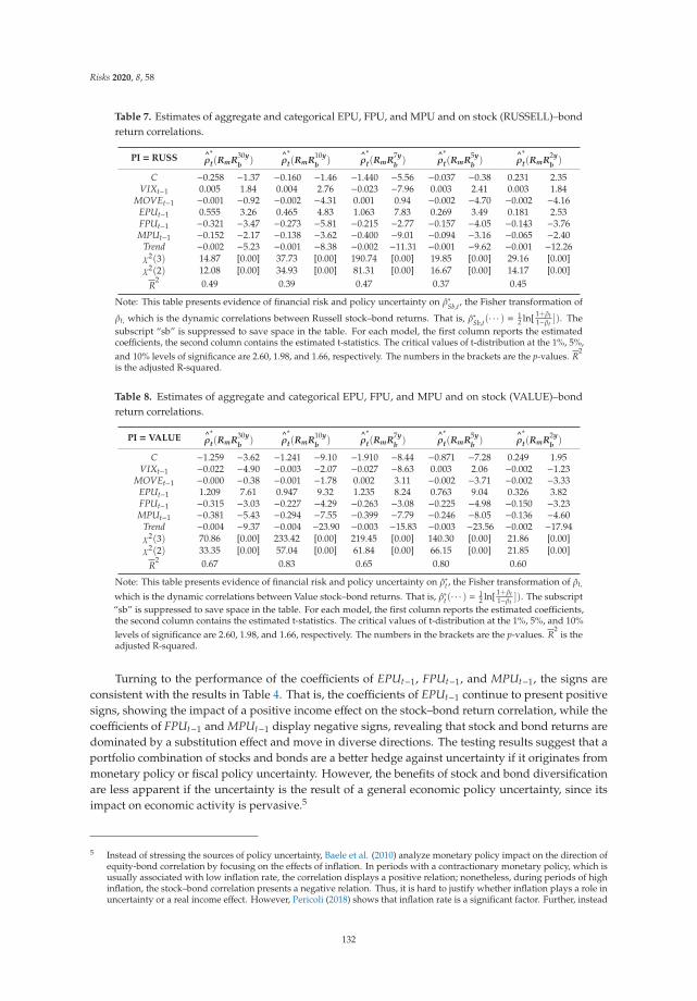
Risks 2020, 8, 58

Table 7. Estimates of aggregate and categorical EPU, FPU, and MPU and on stock (RUSSELL)–bondreturn correlations.

PI = RUSS ^ρ∗t(RmR30y

b )^ρ∗t(RmR10y

b )^ρ∗t(RmR7y

b )^ρ∗t(RmR5y

b )^ρ∗t(RmR2y

b )

C −0.258 −1.37 −0.160 −1.46 −1.440 −5.56 −0.037 −0.38 0.231 2.35VIXt−1 0.005 1.84 0.004 2.76 −0.023 −7.96 0.003 2.41 0.003 1.84

MOVEt−1 −0.001 −0.92 −0.002 −4.31 0.001 0.94 −0.002 −4.70 −0.002 −4.16EPUt−1 0.555 3.26 0.465 4.83 1.063 7.83 0.269 3.49 0.181 2.53FPUt−1 −0.321 −3.47 −0.273 −5.81 −0.215 −2.77 −0.157 −4.05 −0.143 −3.76MPUt−1 −0.152 −2.17 −0.138 −3.62 −0.400 −9.01 −0.094 −3.16 −0.065 −2.40

Trend −0.002 −5.23 −0.001 −8.38 −0.002 −11.31 −0.001 −9.62 −0.001 −12.26χ2(3) 14.87 [0.00] 37.73 [0.00] 190.74 [0.00] 19.85 [0.00] 29.16 [0.00]χ2(2) 12.08 [0.00] 34.93 [0.00] 81.31 [0.00] 16.67 [0.00] 14.17 [0.00]

R2 0.49 0.39 0.47 0.37 0.45

Note: This table presents evidence of financial risk and policy uncertainty on ρ∗Sb,t, the Fisher transformation of

ρt, which is the dynamic correlations between Russell stock–bond returns. That is, ρ∗Sb,t(· · · ) =12 ln[ 1+ρt

1−ρt]). The

subscript “sb” is suppressed to save space in the table. For each model, the first column reports the estimatedcoefficients, the second column contains the estimated t-statistics. The critical values of t-distribution at the 1%, 5%,and 10% levels of significance are 2.60, 1.98, and 1.66, respectively. The numbers in the brackets are the p-values. R

2


Table 8. Estimates of aggregate and categorical EPU, FPU, and MPU and on stock (VALUE)–bondreturn correlations.

PI = VALUE ^ρ∗t(RmR30y

b )^ρ∗t(RmR10y

b )^ρ∗t(RmR7y

b )^ρ∗t(RmR5y

b )^ρ∗t(RmR2y

b )

C −1.259 −3.62 −1.241 −9.10 −1.910 −8.44 −0.871 −7.28 0.249 1.95VIXt−1 −0.022 −4.90 −0.003 −2.07 −0.027 −8.63 0.003 2.06 −0.002 −1.23

MOVEt−1 −0.000 −0.38 −0.001 −1.78 0.002 3.11 −0.002 −3.71 −0.002 −3.33EPUt−1 1.209 7.61 0.947 9.32 1.235 8.24 0.763 9.04 0.326 3.82FPUt−1 −0.315 −3.03 −0.227 −4.29 −0.263 −3.08 −0.225 −4.98 −0.150 −3.23MPUt−1 −0.381 −5.43 −0.294 −7.55 −0.399 −7.79 −0.246 −8.05 −0.136 −4.60

Trend −0.004 −9.37 −0.004 −23.90 −0.003 −15.83 −0.003 −23.56 −0.002 −17.94χ2(3) 70.86 [0.00] 233.42 [0.00] 219.45 [0.00] 140.30 [0.00] 21.86 [0.00]χ2(2) 33.35 [0.00] 57.04 [0.00] 61.84 [0.00] 66.15 [0.00] 21.85 [0.00]

R2 0.67 0.83 0.65 0.80 0.60

Note: This table presents evidence of financial risk and policy uncertainty on ρ∗t , the Fisher transformation of ρt,

which is the dynamic correlations between Value stock–bond returns. That is, ρ∗t(· · · ) =12 ln[ 1+ρt

1−ρt]). The subscript

“sb” is suppressed to save space in the table. For each model, the first column reports the estimated coefficients,the second column contains the estimated t-statistics. The critical values of t-distribution at the 1%, 5%, and 10%levels of significance are 2.60, 1.98, and 1.66, respectively. The numbers in the brackets are the p-values. R

2is the

adjusted R-squared.

Turning to the performance of the coefficients of EPUt−1, FPUt−1, and MPUt−1, the signs areconsistent with the results in Table 4. That is, the coefficients of EPUt−1 continue to present positivesigns, showing the impact of a positive income effect on the stock–bond return correlation, while thecoefficients of FPUt−1 and MPUt−1 display negative signs, revealing that stock and bond returns aredominated by a substitution effect and move in diverse directions. The testing results suggest that aportfolio combination of stocks and bonds are a better hedge against uncertainty if it originates frommonetary policy or fiscal policy uncertainty. However, the benefits of stock and bond diversificationare less apparent if the uncertainty is the result of a general economic policy uncertainty, since itsimpact on economic activity is pervasive.5

5 Instead of stressing the sources of policy uncertainty, Baele et al. (2010) analyze monetary policy impact on the direction ofequity-bond correlation by focusing on the effects of inflation. In periods with a contractionary monetary policy, which isusually associated with low inflation rate, the correlation displays a positive relation; nonetheless, during periods of highinflation, the stock–bond correlation presents a negative relation. Thus, it is hard to justify whether inflation plays a role inuncertainty or a real income effect. However, Pericoli (2018) shows that inflation rate is a significant factor. Further, instead

132

Risks 2020, 8, 58

6.2. Total Policy Uncertainty

The above tests suggest that the EPUt−1 has a positive effect, while FPUt−1 and MPUt−1have anegative effect on the ρ∗Sb,t(·). It is natural to pool all the uncertainty information together regardless ofthe sources of uncertainty. To this end, I define TPUt = EPUt + FPUt +MPUt as total policy uncertainty(TPUt). Table 9 reports the estimates of the test equation, which uses TPUt as a measure of uncertainty.Consistent with previous findings, the coefficients of VIXt−1 have mixed signs. However, the signs forMOVEt−1 consistently present negative signs and most of them are statistically significant.

Table 9. Estimates of correlations of total stock market returns and 10-year bond returns in response tofinancial risk and total policy uncertainty.

Indpt.Variable

TTMK DJIA NASDAQ RUSSELL VALUE

^ρ∗t(RmR10y

b )^ρ∗t(RmR10y

b )^ρ∗t(RmR10y

b )^ρ∗t(RmR10y

b )^ρ∗t(RmR10y

b )

C 1.239 7.59 −0.207 −1.77 0.704 6.87 0.427 3.96 −0.270 −2.06VIXt−1 −0.001 −0.47 0.000 0.04 0.004 1.78 0.005 3.34 −0.003 −1.68

MOVEt−1 −0.002 −2.80 −0.002 −2.89 −0.002 −4.23 −0.002 −4.10 −0.001 −1.37TPUt−1 −0.048 −4.23 0.060 7.28 −0.032 −4.49 −0.023 −3.18 0.074 8.18Trend −0.003 −13.08 −0.003 −19.94 −0.002 −12.61 −0.001 −9.15 −0.004 −20.60

R2 0.43 0.73 0.42 0.33 0.75

Notes: This table presents evidence of financial risk and policy uncertainty on ρ∗Sb,t, the Fisher transformation of ρt,

which is the dynamic correlations between Value stock–bond returns. That is, ρ∗Sb,t(· · · ) =12 ln[ 1+ρt

1−ρt]). The subscript

“sb” is suppressed to save space in the table. For each model, the first column reports the estimated coefficients, thesecond column contains the estimated t-statistics. The critical values of t-distribution at the 1%, 5%, and 10% levelsof significance are 2.60, 1.98, and 1.66, respectively. R

2is the adjusted R-squared.

With respect to the sign of TPUt−1, evidence shows that the coefficients on TTMK, NASDAQ, andRUSSELL exhibit negative signs and are statistically significant. This result is consistent with marketbehavior of investors who during a rise in TPUt−1 tend to sell offmore uncertain stock and move theirfunds to bonds, effectively exhibiting the substitution effect. However, the coefficients of TPUt−1 for theDJIA and VALUE stocks are positive and statistically significant, indicating a dominance of the incomeeffect. A review of the S&P 500 Value index, which has a style-concentrated index designed to trackthe performance of stocks that exhibit the strongest value, shows that the value of these stocks is verymuch in line with that of the DJIA. In sum, estimates of correlations between total stock market returnsand 10-year bond returns show different signs in response to total policy uncertainty is essentiallyexecuted under different degrees of force from income effect and substitution effect.

7. Conclusions

This paper examines the impact of financial market risk and policy uncertainties on the correlationbetween stock and bond returns. Analyzing the financial data of US markets for the period January1990–June 2019, I derive several important empirical conclusions. First, empirical estimations basedon the asymmetric dynamic correlation model (ADCC) suggest that stock–bond correlations aretime-varying and display a negative relation overtime, especially for the period before 2002.

Second, evidence confirms that the stock–bond relationship is negatively correlated with theimplied volatility in stock market (VIX), suggesting a higher market risk would cause a “flight-to-safety.”This phenomenon appears in stock markets of TTMK and VALUE. However, for indices such as theDJIA (with two-year and five-year bonds), the NASDAQ and RUSSELL, the sign turns out to be positive.The mixed results reflect differing attitudes toward risks of investors who hold different stock portfolios.This finding suggests that the use of a single stock index to measure stock returns and one specific

of using government bonds, one might use junk bonds to trace the dynamic correlations (Glassman 2018), which will be thesubject of future research.

133

Risks 2020, 8, 58

form of bond maturity (10-year bond) as was done in the previous research (Connolly et al. 2005) couldproduce a biased estimator and hence a misleading statistical inference.

Third, with respect to the performance of implied bond volatility (MOVEt−1), this study arrivesat more consistent results. In this case, the coefficients tend to have negative signs with a coupleof exceptions. For this reason, we can reach a more concrete conclusion that a rise in MOVEt−1

leads to a decoupling of stock and bond returns. Thus, MOVEt−1 to some extent reflects differentmarket information and complementarily contributes to explaining movements in stock and bondreturn correlations.

Fourth, this study find evidence that estimated coefficient of the EPUt−1 has a positive andsignificant effect on the stock–bond return correlation. This result is consistent with a dominant incomeeffect resulting from a rise in economic policy uncertainty that impedes economic activities and leadsto a decline in income. This decline brings about a decrease in liquidity and in turn weakens demandfor both stocks and bonds. Therefore, both stock and bond prices move in the same direction.

Fifth, testing results conclude that the estimated coefficients for both FPUt−1 and MPUt−1 arenegative and highly significant. The negative sign of this policy uncertainty is mainly due to thedominance of the substitution effect, which prompts investors to replace higher uncertainty assets withlower uncertainty assets due to an upward shift in policy uncertainty. This occurs because of a policystance that causes a sudden rise in MPUt−1 (or FPUt−1 in bond financing) and increases uncertaintyin interest rates, prompting a selloff in stocks and a flight-to-quality phenomenon. Note that thismarket action essentially stems from a heightened fear from policy uncertainty rather than somethingof inherent in the asset’s return. It is possible that a rise in MPUt−1 (or FPUt−1) could threaten thefuture cash flow and reduce the demand for both stocks and bonds. However, the evidence of anegative coefficient indicates the dominant force of the substitution effect. An implication of a negativecoefficient suggests that a portfolio can benefit from a combination of stocks and bonds as a way ofdiversification and hedging against monetary policy or fiscal policy uncertainty.

Sixth, by testing the total policy uncertainty on the dynamic correlations between stock–bondreturns, the evidence turns out to display mixed signs. For DJIA and VALUE stocks, the correlationcoefficients present positive signs, indicating the dominance of an income effect attributable to generaleconomic policy uncertainty; however, correlations of the TTMK, NASDAQ, and RUSSELL stockswith bond returns display negative signs, suggesting the dominance of a substitution effect, resultingfrom the reallocation of assets from ones with higher uncertainty to those with lower uncertainty inresponse to a rise in total policy uncertainty.

In sum, this paper provides significant empirical evidence to support the impact of MPUt−1 andFPUt−1 on stock–bond correlations. In addition to the VIXt−1, MOVEt−1 and EPUt−1, our Chi-squaredstatistics consistently suggest the rejection of the null, MPUt−1 = FPUt−1 = 0, and support the incrementalsignificance of MPUt−1 and FPUt−1 in the test equation. This evidence has not previously been shownin the literature to explain the stock–bond return correlation.

Further, this study has practical implications for investment firms by tracing the time-varyingcorrelations and is distinct from more commonly taken approaches by calculating the individual,constant correlations (Forbes and Rigobon 2002) within a given period of time. This study identifiescategorical policy uncertainties as factors to explain the change in stock–bond correlations over time.Given the model parameters, firms can access information via newspapers to make projections relatedto stock–bond dynamics.


Conflicts of Interest: The author declares no conflict of interest.

134

Risks 2020, 8, 58

Appendix A

Table A1. Some major term sets for policy category uncertainty indices.

Variable Description Source

EPUt

Economic policy uncertainty index involves: “economic” or “economy”;“uncertain” or “uncertainty”; and one or more of “Congress,” “deficit,” “FederalReserve,” “legislation,” “regulation,” or “White House” in 10 major newspapers.

Baker et al.(2016) *

FPUt

Fiscal policy uncertainty index involves terms of “government budget” ordiscretionary fiscal policy”, “government revenue”, “tax” or “Taxation”,

“government deficit”, “government spending” or “government expenditure”,“social security expenditures”, “defense spending”, “Legislation”, “public debt”

or “government debt”, “National bonds”, among others.

Davis (2016) **

MPUt

Monetary policy uncertainty index involves terms of “monetary policy”,monetary easing”, quantitative easing”, “negative interest rate”, “officialdiscount rate”, “monetary operation(s)”, “inflation target”, among others.

Davis (2016) **

* Baker et al. (2016). http://www.policyuncertainty.com. ** Source: ‘Measuring Economic Policy Uncertainty’ byScott Baker, Nicholas Bloom and Davis, S.J. at www.PolicyUncertainty.com.

References

Allard, Anne-Florence, Leonardo Iania, and Kristien Smedts. 2019. Stock–Bond Return Correlations: Movingaway from ‘One-Frequency-Fits-All’ by Extending the DCC-MIDAS Approach. Available online: https://ssrn.com/abstract=3190071 (accessed on 29 May 2020).

Andersson, Magnus, Elizaveta Krylova, and Sami Vähämaa. 2008. Why does the correlation between stock andbond returns vary over time? Applied Financial Economics 18: 139–51. [CrossRef]

Antonakakis, Nikolaos, Ioannis Chatziantoniou, and George Filis. 2013. Dynamic co-movements of stock marketreturns, implied volatility and policy uncertainty. Economics Letters 120: 87–92. [CrossRef]

Baele, Lieven, Geert Bekaert, and Inghelbrecht Koen. 2010. The determinants of stock and bond returncomovements. Review of Financial Studies 23: 2374–428. [CrossRef]

Baker, Scott R., Nicholas Bloom, and Steven J. Davis. 2016. Measuring economic policy uncertainty. QuarterlyJournal of Economics 131: 1593–636. [CrossRef]

Barsky, R. 1989. Why don’t the prices of stocks and bonds movetogether? American Economic Review 79: 1132–45.Baur, Dirk, and Brian Lucey. 2009. Flight and contagion—An empirical analysis of stock–bond correlations. Journal

of Financial Stability 5: 339–52. [CrossRef]Bloom, Nicholas. 2009. The impact of uncertainty shocks. Econometrica 77: 623–85.Bloom, Nicholas. 2014. Fluctuations in Uncertainty. Journal of Economic Perspectives 28: 153–76. [CrossRef]Brunnermeier, Markus, and Lasse H. Pedersen. 2009. Market liquidity and funding liquidity. Review of Financial

Studies 22: 2201–38. [CrossRef]Campbell, John Y., and John Ammer. 1993. What moves the stock and bond markets? A variance decomposition

for long-term asset returns. Journal of Finance 48: 3–37. [CrossRef]Cappiello, Lorenzo, Robert F. Engle, and Kevin Sheppard. 2006. Asymmetric dynamics in the correlations of

global equity and bond returns. Journal of Financial Econometrics 4: 537–72. [CrossRef]Chiang, Thomas Chinan. 2019. Economic policy uncertainty, risk and stock returns: Evidence from G7 stock

markets. Finance Research Letters 29: 41–49. [CrossRef]Chiang, Thomas Chinan, Bang Nam Jeon, and Huimin Li. 2007. Dynamic correlation analysis of financial

contagion: Evidence from Asian markets. Journal of International Money and Finance 26: 1206–28. [CrossRef]Chiang, Thomas Chinan, Jiandong Li, and Sheng-Yung Yang. 2015. Dynamic stock–bond return correlations and

financial market uncertainty. Review of Quantitative Finance and Accounting 45: 59–88. [CrossRef]Connolly, Robert A., Chris T. Stivers, and Licheng Sun. 2005. Stock market uncertainty and the stock–bond return

relation. Journal of Financial and Quantitative Analysis 40: 161–94. [CrossRef]d’Addona, Stefano, and Axel H. Kind. 2006. International stock–bond correlations in a simple affine asset pricing

model. Journal of Banking and Finance 30: 2747–65. [CrossRef]

135

Risks 2020, 8, 58

de Goeij, Peter, and Wessel Marquering. 2004. Modeling the conditional covariance between stock and bondreturns: A multivariate GARCH approach. Journal of Financial Econometrics 2: 531–64. [CrossRef]

Dimic, Nabojsa, Jarmo Kivisha, Vanja Piljak, and Janne Äijö. 2016. Impact of financial market uncertainty andmacroeconomic factors on stock–bond correlation in emerging markets. Research in International Business andFinance 36: 41–51. [CrossRef]

Ehtesham, Qurat, and Danish Siddiqui. 2019. Analyzing Stock–bond Correlation in Emerging Markets. Researchin Applied Economics. Available online: https://www.researchgate.net/publication/336283757_Analyzing_Stock--bond_Correlation_in_Emerging_Markets (accessed on 29 May 2020).

Engle, Robert F. 2002. Dynamic conditional correlation: A simple class of multivariate generalized autoregressiveconditional heteroskedasticity models. Journal of Business and Economic Statistics 20: 339–50. [CrossRef]

Engle, Robert F. 2009. Anticipating Correlations: A New Paradigm for Risk Management. Princeton: PrincetonUniversity Press.

Forbes, Kristin, and Roberto Rigobon. 2002. No contagion, only interdependence: measuring stock marketcomovements. Journal of Finance 57: 2223–61. [CrossRef]

Glassman, Barry. 2018. The Most Confused Identity in Your Portfolio: High Yield Bonds. Availableonline: https://www.forbes.com/sites/advisor/2018/03/13/the-most-confused-identity-in-your-portfolio-high-yield-bonds/#cccd5ea2b8b6 (accessed on 30 May 2020).

Gulko, Les. 2002. Decoupling. Journal of Portfolio Management 28: 59–66. [CrossRef]Hakkio, Craig S., and William R. Keeton. 2009. Financial stress: What is it, how can it be measured, and why does

it matter? Federal Reserve Bank of Kansas City Economic Review 2: 5–50.Hong, GWangheou, Youngsoo Kim, and Bong-Soo Lee. 2014. Correlations between stock returns and bond returns:

income and substitution effects. Quantitative Finance 14: 1999–2018. [CrossRef]Ilmanen, Antti. 2003. Stock–bond correlations. Journal of Fixed Income 13: 55–66. [CrossRef]Jones, Paul M., and Eric Olson. 2013. The time-varying correlation between uncertainty, output, and inflation:

Evidence from a DCC-GARCH model. Economic Letters 118: 33–37. [CrossRef]Kwan, Simon H. 1996. Firm-specific information and the correlation between individual stocks and bonds. Journal

of Financial Economics 40: 63–80. [CrossRef]Li, Xiao-Ming, Bing Zhang, and Ruzhao Gao. 2015. Economic policy uncertainty shocks and stock–bond

correlations: Evidence from the US market. Economics Letters 132: 191–96. [CrossRef]Li, Erica X.N., Tao Zha, Ji Zhang, and Hao Zhou. 2019. Active Monetary or Fiscal Policy and Stock–bond

Correlation. Available online: http://abfer.org/media/abfer-events-2019/annualconference/cebra/AC19P1019_Active_Monetary_or_Fiscal_Policy_and_Stock--bond_Correlation.pdf (accessed on 29 May 2020).

Newey, Whitney K., and Kenneth D. West. 1987. A simple, positive semi-definite, heteroskedasticity andautocorrelation consistent covariance matrix. Econometrica 55: 703–8. [CrossRef]

Panchenko, Valentyn, and Eliza Wu. 2009. Time-varying market integration and stock and bond return concordancein emerging markets. Journal of Banking and Finance 33: 1014–21. [CrossRef]

Pericoli, Marcello. 2018. Macroeconomics Determinants of the Correlation between Stocks and Bonds. Bank ofItaly Working Paper No. 1198. Available online: https://ssrn.com/abstract=3429148 (accessed on 31 May2020).

Tobin, James. 1969. A general equilibrium approach to monetary theory. Journal of Money Credit and Banking 1:15–29. [CrossRef]

Whaley, Robert E. 2009. Understanding the VIX. Journal of Portfolio Management 35: 98–105. [CrossRef]Yang, Jian, Yinggang Zhou, and Zijun Wang. 2009. The stock–bond correlation and macroeconomic conditions:

One and a half centuries of evidence. Journal of Banking and Finance 33: 670–80. [CrossRef]Yardeni, Edward. 1997. Fed’s Stock Market Model Finds Overvaluation. US Equity Research, Deutsche Morgan

Grenfell. Available online: http://www.yardeni.com/premiumdata/t_970825.pdf (accessed on 29 May 2020).Yu, IP-Win, Kang-Por Fung, and Chi-Sang Tam. 2010. Assessing financial market integration in Asia—Equity

markets. Journal of Banking and Finance 34: 2874–85. [CrossRef]

© 2020 by the author. Licensee MDPI, Basel, Switzerland. This article is an open accessarticle distributed under the terms and conditions of the Creative Commons Attribution(CC BY) license (http://creativecommons.org/licenses/by/4.0/).

136

risks

Article

How Do Health, Care Services Consumption andLifestyle Factors Affect the Choice of HealthInsurance Plans in Switzerland?

Veronika Kalouguina 1 and Joël Wagner 1,2,*

1 Department of Actuarial Science, University of Lausanne, Faculty HEC, Extranef, 1015 Lausanne,Switzerland; [email protected]

2 Swiss Finance Institute, University of Lausanne, 1015 Lausanne, Switzerland* Correspondence: [email protected]

Received: 10 March 2020; Accepted: 25 April 2020; Published: 27 April 2020

Abstract: In compulsory health insurance in Switzerland, policyholders can choose two main features,the level of deductible and the type of plan. Deductibles can be chosen among six levels, which rangefrom CHF 300 to 2500. While the coverage and benefits are identical, insurers offer several planswhere policyholders must first call a medical hotline, consult their family doctor, or visit a doctorfrom a defined network. The main benefit of higher deductibles and insurance plans with limitationsis lower premiums. The insureds’ decisions to opt for a specific cover depend on observed andunobserved characteristics. The aim of this research is to understand the correlation betweeninsurance plan choices and lifestyle through the state of health and medical care consumptionin the setting of Swiss mandatory health insurance. To do so, we account for individual health andmedical health care consumption as unobserved variables employing structural equation modeling.Our empirical analysis is based on data from the Swiss Health Survey wherein lifestyle factors likethe body mass index, diet, physical activity, and commuting mode are available. From the 9301recorded observations, we find a positive relationship between having a “healthy” lifestyle, a lowconsumption of doctors’ services, and choosing a high deductible, as well as an insurance plan withrestrictions. Conversely, higher health care services’ usage triggers the choice of lower deductiblesand standard insurance plans.

Keywords: medical services’ consumption; lifestyle factors; insurance plan; structural equation model

1. Introduction

Health insurers try to foster healthy lifestyles among their insureds by promoting exercise,supporting fitness center memberships, and more recently, the use of wearable connected devices.The data collected from the latter permit insurance companies to track the individual’s physical activity,diet, or sleep patterns for instance. Subsequently, insureds carrying on a healthy lifestyle benefit frompremium discounts or other kinds of monetary rewards. Why health insurers promote a healthylifestyle is not unfounded. There is a strand of medical literature assessing the effect of the lifestyleon health documenting that a healthier lifestyle leads to better health, relating to lower medical costs(Johansson and Sundquist 1999; Andersen et al. 2000; Lee and Skerrett 2001; Joshipura et al. 2001;Penedo and Dahn 2005; Dauchet et al. 2006; Inyang and Okey-Orji 2015; Miller et al. 2017). However,the relationship between health and health insurance decisions has been sparsely investigated.While there is a clearly demonstrated link between lifestyle and health in the medical literature,this relation has not been used in actuarial science, leaving the field with little or no evidence of theeffect of lifestyle on health insurance decisions.


Risks 2020, 8, 41

In our study, using data from the Swiss Health Survey (SHS), we aim to seize the indirect effect oflifestyle—encompassed by the body mass index (BMI), diet, physical activity and commuting mode—onhealth insurance decisions, i.e., the choice of the plan and the level of deductible. We consider that thedecisions are mediated through latent variables linked to health and health care consumption. We set upa structural equation modeling (SEM) framework that allows capturing such indirect effects. We definehealth as a latent variable embodied by the self-assessed health, as well as chronic and limiting dailyactivities health conditions. Thereby, the latter offer an objective measure. Further, health directly impactshealth care consumption, our second latent variable captured by the number of doctor visits and hospitalstays. Additionally, the model is able to account for the bidirectional relationship between health careconsumption and the choice of the insurance plan and the deductible level.

The results from our model provide empirical support for the correlation between health insurancechoice and lifestyle via health and health care consumption. Using 9301 observations obtained from theSHS dataset, we control the choice of deductible and insurance plan for socio-economic characteristics(gender, nationality, education, income, number of children in the household, importance of freedomof choice of the specialist doctor, linguistic region, and urbanization) and allow for the two endogenousvariables to correlate. We show that an increase in age and BMI correlates with a decrease in health,whereas an increase in the number of portions of fruits and vegetables eaten per day, the number ofphysical activities performed in a week, and the usage of a bike to commute correlates with an increasein health. Further results display a negative correlation between health and health care consumption,where the latter variable is positively associated with the choice of a standard, i.e., non-restricting,health insurance plan. Similarly, an increase in health care consumption correlates positively witha low level of deductible. Linking our results, we obtain the indirect effect of lifestyle on insurancedecisions. Thereby, an increase in age and BMI is associated with having a low deductible and optingfor a standard insurance plan whereas, having a “healthy” lifestyle (good diet and physical activity)correlates with having a high deductible and preferring a more restrictive insurance plan at lower cost.

The remainder of this paper is organized as follows: In Section 2, we briefly review the Swisshealth insurance system, as well as the literature related to the development of our research hypotheses.In Section 3, we pursue the setup of the model. Results are displayed along with a discussion inSection 4. Finally, we conclude in Section 5.

2. Background Information and Research Hypotheses

2.1. Insurance Plans and Deductibles in the Swiss Health System

Before developing our research, we expose some basic features of the Swiss health insurancesystem that are relevant for the matter of this study. Basic health insurance in Switzerland is mandatoryand regulated by Federal law, which sets up the reimbursement policies. Under Federal law, basichealth insurance coverage is compulsory for all residents and organized through private insurancecompanies. All insurance companies proposing basic health insurance are obliged to accept anyindividual independently of the health status. Premiums are calculated by the insurers, are determinedby regions along cantons and urbanicity, and are validated by the Swiss government. Note that pricesare the same for all individuals within the three age classes: up to 18 years, 19 to 25 years, and 26 yearsor more. Thus, insurers are not allowed to take into account other variables like gender, exact age,or health status. Beyond the basic plan, individuals can subscribe to private complementary healthinsurance. Regarding the catalog of reimbursements, on the one hand, the basic plan covers basichealth risks, but does not extend to dental treatments, to alternative medicine techniques, nor to glassesor lens purchases, with exceptions made for some specific medical conditions. On the other hand,complementary health policies cover the costs that go beyond the basic insurance scheme. In this study,we focus on the decisions on basic health insurance by individuals aged 18 years and older. Theseindividuals face several choices for their insurance plan and deductible level.

138

Risks 2020, 8, 41

2.1.1. Insurance Plans

The insurance policies currently offered in Switzerland can be grouped into four families. The firstplan is the “standard” plan, and it is chosen by most individuals. This policy offers the freedom ofchoice to visit any doctor or specialist and presents no specific restriction. This plan has the highestpremium. The second most popular plan is the so-called “family doctor” model. Its peculiarity lies inthe importance of the general practitioner (GP) that acts as a gatekeeper and centralizes informationof the individual. Indeed, holders of this type of policy commit to always consulting the same GPin case of any health issues. They have to chose their doctor in advance from a list of recognizedGPs provided by their health insurer. As a gatekeeper, the GP transfers the patient to a specialist ifnecessary. This plan typically displays premiums that are 15 to 20% lower than those of standard plans.The third most common plan is known as “CallMed”. As its name suggests, this model brings theconstraint of calling a medical hotline prior to physically seeking advice from a doctor. Depending onthe specific policy rules, there may be an unrestricted choice of the doctor after the phone consultation.Policyholders from this scheme profit from premium reductions of up to 20%. Finally, there is the“HMO” model where the acronym stands for health maintenance organization. Under this model,the insureds commit to always pass through a doctor affiliated with the selected HMO group fora first consultation. Like in the CallMed model, if necessary, the following consultation may take placeoutside of the HMO medical team, depending on the health insurer. This last type of plan can comewith premiums up to 25% below the standard plan.

2.1.2. Deductible Levels

In all insurance plans and on a yearly basis, policyholders chose a deductible. Here, the decisionenvironment is less complex. With amounts regulated by the health insurance law, there exist six levelsof deductibles, namely CHF 300, 500, 1000, 1500, 2000, and 2500. Once medical costs up to the chosenlevel are paid out-of-pocket, there only remains a co-payment of 10% up to CHF 700 on the additionalcosts, whereafter the health insurer entirely reimburses the spending.

2.2. Literature Review and Development of the Hypothesis

While partial insights into our research can be gained by studying descriptive statistics, we proposeto structure our analyses around selected conjectures and embed the latter in the body of existingliterature. A recent study conducted by Li et al. (2018) identified five health risk-reducing lifestylefactors. Among them, three characteristics are of particular interest for our study. Indeed, three lifestyleindicators are found to play a role in mortality. More specifically, life expectancy increases with a BMIranging between 18.5 and 24.9, 30 min or more per day of exercising, and a healthy diet. In addition tothese measures, we considered in our research another factor: the commuting mode. This variable hasbeen found to be a relevant factor for health conditions in the literature (Oja et al. 1991; Pucher et al. 2010and Riiser et al. 2018). Since these factors are relatively easily trackable and modifiable, as opposed to,for example, alcohol or tobacco consumption, we used them as determinants for lifestyle.

2.2.1. BMI

The effect of BMI on health outcomes has been extensively studied, and the results are unambiguous.In reports published as early as 1959, the Society of Actuaries has assessed this link by studying therelationship between mortality rates and weight (Society of Actuaries 1959; Courtland C. and Edward A.1979). It was found that as weight increases, so does the mortality rate. Following studies have confirmedand extended the negative effect of a high BMI on health. Indeed, a higher BMI is associated with a higherrisk for coronary heart disease (CHD), cardiovascular disease (CVD), and for congestive health failure(Hubert et al. 1983; Jousilahti et al. 1996). An increase in BMI also increases the vulnerability to endometrial,sigmoidal, colorectal, and hormone-related cancer and type II diabetes (non-insulin dependent diabetesmellitus; see Pi-Sunyer 1991; Le Marchand et al. 1992; World Health Organization 2000; Stommel and

139

Risks 2020, 8, 41

Schoenborn 2010). Overall, a higher BMI is associated with higher incidence rates of diseases (see also, e.g.,Felson et al. 1992; Stommel and Schoenborn 2010).

2.2.2. Diet

The old adage “You are what you eat” has been proven right in multiple stances. Two literaturereviews (Block et al. 1992; Steinmetz and Potter 1996) assessed the incidence of fruit and vegetableintake on several cancers, reporting their protective effect. A healthier diet composed of a greaternumber of fruits and vegetables decreases the likelihood of cancers like esophagus, pancreas, and breastcancer. Other studies focused on the beneficial impact of an increase of fruit and vegetable consumptionon CHD or CVD and reported a lower incidence, as well as lower mortality related to heart deficiencies(Joshipura et al. 2001; Bazzano et al. 2002; Dauchet et al. 2006; Oyebode et al. 2014; Miller et al. 2017).

2.2.3. Physical Activity

Similar to the effect of the diet on health, the positive effect of physical activity on health iswell established. A literature review conducted by Warburton et al. (2006) assessed 152 studies andhighlighted that increased levels of physical activity were found to reduce relative risks of death by20 to 35%; inversely, individuals in the lowest quantiles of physical activity had an increased riskof death from any cause compared to those in the top quantiles. They also accounted for a reducedincidence of type II diabetes in those individuals who reported weekly physical activity. Other studiesalso investigated this relationship and backed up the review of Warburton et al. (2006). Johansson andSundquist (1999), Lee and Skerrett (2001), and Matthews et al. (2007) associated a higher frequencyof physical activity to a reduced mortality rate and better overall health, while Gerhardsson et al.(1988), Thune et al. (1997), Thune and Furberg (2001), and Penedo and Dahn (2005) related a less activelifestyle to increased risks of colon, breast, prostate, and colorectal cancers.

2.2.4. Commuting Mode

The mode of commuting most frequently used to go to work, to school, for grocery shopping,or other activities is an integral part of the lifestyle definition. The medical literature has especiallyaimed its attention at walking and cycling as a means of transportation. Most papers pool togetherindividuals who walk or cycle to commute; when a distinction was made, the results may presentslight differences, but overall, they pointed to similar effects. For instance, Oja et al. (1991) andRiiser et al. (2018) both found a positive effect of walking or cycling on health measures such as havinga high level of good cholesterol (HDL) or a decreased heart rate and systolic tension. The authors alsoidentified an inverse relationship between walking or cycling to work and the risk of having diabetes,results that were equally found by Pucher et al. (2010). Aside from these pooled analyses, the literaturereview by Oja et al. (1991) focused on the effect of cycling on health. Of the 16 cycling-specific studiesconsidered therein, all but two showed that cycling provided a health benefit and particularly for CVDand CHD risks.

Conjecture 1. An increase in BMI negatively influences health, while an increase in fruit andvegetable intake and an increase in physical activity frequency positively relate to health. Walking andcycling for commuting also enhance health.

2.2.5. Health Care Utilization

The usage of health care services is most often approximated by the number of doctor visits (GPand specialist), outpatient and inpatient hospitalization, or drug use. In the literature from the medicaland economics fields, health care seeking has been studied under several perspectives, theoreticallyand empirically (to cite a few, Grossman 1972; Pohlmeier and Ulrich 1995; Ang 2010). Many of themaddressed the demand for health care from a socio-economic, including from an insurance, point ofview. However, health, as a determinant, has seldom been investigated, as the relationship may seem

140

Risks 2020, 8, 41

trivial. Fylkesnes (1993) found that self-rated health was the most important driver of health careutilization.

Another factor that could lead to the increase in health care consumption is the enrollment inhealth insurance. This incentive effect has been extensively studied, and the conclusion was sharedamong the literature reviews of Schmitz (2012) and Prinja et al. (2017): insurance take up leads toan increase in health care services’ utilization. Schmitz (2012) specified that insurance plans witha deductible had lower consumption compared to plans without such a feature. Gardiol et al. (2005)performed this analysis in Switzerland and outlined that 25% of health care expenditures couldbe attributable to the incentive effect linked to deductibles. Further, alternative plans have beenintroduced in Switzerland to contain health costs by limiting doctors’ visits through the primary usageof telephone hotlines and directing patients to the most efficient doctors’ networks. Thus, we expectedhealth care utilization to be negatively linked to alternative insurance plans.

Conjecture 2. Health is the most important driver of health care consumption. As health improves,health care consumption declines. Further, a low deductible and standard insurance plan shouldincentivize health care consumption.

2.2.6. Insurance Demand

The empirical literature on health insurance demand is relatively limited. Firstly, health asa component of the decision-making process has been less exploited, probably due to the endogeneityit may present and the difficulty to deal with it. Secondly, papers rather address the demand forcomplementary (private) health insurance through expected health care expenditures. In our context,we focused on the choices made in a compulsory health insurance environment. Finally, we note thatother socio-economic variables have nonetheless been used as drivers of health insurance demand:e.g., gender, age, marital status, country of origin, education, occupation, or income (Van de Ven andVan Praag 1981; Cameron et al. 1988). Among these covariates, it is the effect of income that has beenthe most extensively estimated (see Schneider 2004 for a literature review). It is needless to emphasizethe lack of empirical evidence linking health and health insurance demand, let alone the effect oflifestyle. Our research aims at providing an instance of the relationship between lifestyle and healthinsurance demand via the health and health care consumption channels.

Conjecture 3. The effect of socio-economic covariates, namely gender, education, and income,on decisions for the insurance plan and the deductible is significant.

Linking the arguments on health, health care utilization, and insurance demand, we furtherpropose the following conjecture:

Conjecture 4. The effect of health through health care consumption is believed to be significantfor the health insurance decisions. Higher health care usage is associated with a low deductible anda standard insurance plan.

Finally, it is interesting to consider Conjectures 2 and 4 together. When reconsidering Conjecture 2,we can state that riskier individuals, i.e., unhealthy individuals, come along with higher health careconsumption, which, in line with Conjecture 4, is associated with choosing a standard insurancecontract with a low insurance deductible. This is aligned with the common contributions in theinsurance economics literature (Zweifel and Eisen 2012). In our model framework, we will considerthe bidirectional relationship between health care consumption and insurance decisions. Indeed,while our main interest is on how one’s own health and health care consumption trigger insurancedecisions (deductible, insurance plan). We know from the economics literature that a given insurancecoverage will also have an impact on the consumption (cf. the presence of moral hazard; see the abovediscussion in the section “Health Care Utilization”).

141

Risks 2020, 8, 41

3. Model Framework and Available Data

3.1. Structural Equation Model

To study the above questions and conjectures, the choice of SEM was guided by the severaladvantages that this technique presents. Health is a difficult concept to quantify and is oftentimesestimated by its outcomes, namely chronic disease occurrence or mortality rates. This method, however,does not provide a complete, nor a sufficient picture of the individual’s state of physical and mentalwell-being. In view of these elements, in our SEM model, we let health be a latent variable, influencedby the lifestyle. Doing so, we avoided at the same time any reporting bias and measurement errors ofhealth-related variables (on which Crossley and Kennedy (2002) shed light). Indeed, some authorsused the self-assessed health of the individual as a proxy for the unobserved health, especially in thelabor market field (see Haan and Myck 2009; Strully 2009; Böckerman and Ilmakunnas 2009, for a fewexamples). The issue in this procedure lies in the unobserved characteristics such as risk aversion,which may, for instance, affect both one’s own health perception and health insurance demand. Solelyrelying on the self-reported health at face value is also prone to severe measurement biases highlightedin the literature (mostly attributed to social desirability, discussed in Huang et al. 1998 and Van deMortel et al. 2008). In an SEM setting, on the contrary, health can be captured by several more objectivemeasures called manifest variables and, by this means, minimize the bias. The same rationale applies tothe latent variable of health care seeking. Like health, the unobservable variable of the demand ofhealth care services is a difficult notion to grasp by a single variable or even a set (as for instance inBourne et al. 2009) and may be subject to omitted variables’ bias. Again, SEM is well suited for usingseveral variables at once to define the concept.

Additionally, in dealing with the above issues, SEM can indicate simultaneous direct relationshipscalled paths. These paths can be specified as well between exogenous as between endogenous variables,thus allowing for a more thorough and exhaustive analysis. Because of this convenient ability of themodel to assess the simultaneous relationship between multiple unobserved variables and observedoutcomes, SEM frameworks have been widely used in the sociology- and psychology-related literature(Sobel 1987; Cuttance and Ecob 2009; MacCallum and Austin 2000; Martens 2005). Moreover, we notethat usual econometric methodologies like fixed effects regressions cannot be applied in our context dueto the cross-sectional nature of data from surveys. In an SEM, the estimation of the parameters comesfrom a maximization of likelihood between the actual covariance matrices of the relationships betweenvariables and the estimated covariance matrices of the model (for more information, see Bollen 1989).

Our research aims to assess the relationship between lifestyle and health insurance decisions.Figure 1 gives a graphical representation of the model that we employed. We measured lifestylefrom four behaviors, namely BMI (BMI), diet (DIT), sports (SPT), and commuting modes (CMW,CMB, CMP, CMV), while we controlled for age (AGE). In our model, however, lifestyle was notassumed to have a direct effect on insurance decisions (insurance plan PLN and deductible DED),but rather an indirect one mediated via health (HLT) and health care consumption (HCC). Healthwas hypothesized to play a role in health care usage, which in turn was conjectured to drive healthinsurance decisions, thus creating a bridge to lifestyle. Finally, the health insurance choice wascontrolled by socio-demographic characteristics (gender SEX, nationality NAT, education EDU andincome INC levels, number of children in the household KID, freedom of choice for specialist doctorsSPE, language region LNR, and urbanicity RUR). Further, health was measured using information onself-reported health SRH, chronic health conditions CHR, and limiting health conditions LIM, whilehealth care consumption was evaluated from GP visits (GPV), specialist and gynecologist visits (SPV),and hospital stays (HOS). In Table 1, we summarize and describe the variables that we used.

142

Risks 2020, 8, 41

Figure 1. Illustration of the path diagram of the structural equation model.

Table 1. Description of the variables used in the model.

Variables Type Description Values

AGE Exogenous Age integer (19+)BMI Exogenous BMI according to the WHO scale categories: 0–18.4, 18.5–24.9, 25–29.9, 30+DIT Exogenous Diet, portions of fruits and vegetables categories: 0–2, 3–4, 5+consumed on average per daySPT Exogenous Sports sessions with perspiration, per week categories: 0, 1–2, 3+CMW Exogenous Commuting mode: walking no, yesCMB Exogenous Commuting mode: biking no, yesCMP Exogenous Commuting mode: public transportation no, yesCMV Exogenous Commuting mode: motorized vehicle no, yesHLT Latent Health –SRH Manifest Self-reported health, (Likert scale) 0 (very bad), 0.25 (bad), 0.5 (average),

0.75 (good), 1 (very good)CHR Manifest Chronic health conditions lasting no, yesat least 6 monthsLIM Manifest Limiting health conditions no, yesin everyday activitiesHCC Latent Health care consumption –GPV Manifest Number of general practitioner and family integerdoctor visits in the past 12 monthsSPV Manifest Specialist and gynecologist visits integerin the past 12 monthsHOS Manifest Any hospital stays of at least one night no, yesSEX Exogenous Gender male, femaleNAT Exogenous Nationality Swiss, otherEDU Exogenous Level of education primary, secondary (professional and general),

tertiary (professional and general)INC Exogenous Level of income in CHF categories: 0–3000, 3001–4500, 4501–6000, 6001+KID Exogenous Number of children in household < 18 y.o. categories: 0, 1, 2, 3, 4+SPE Exogenous Freedom of choice of specialist important no, yesLNR Exogenous Language region German, French, ItalianRUR Exogenous Rural region no, yesPLN Endogenous Insurance plan standard, other (HMO, family doctor,

telmed, other)DED Endogenous Deductible in CHF high (2500), low (300)

143

Risks 2020, 8, 41

3.1.1. Measurement of Health

To run the analysis, we designed our model with health (HLT) as a latent variable. This latentvariable was measured by three observed variables: the self-rated health (SRH), having or having hada chronic health condition lasting at least six months (CHR), and having health conditions limitingdaily activities during the past six months (LIM). These three indicators were assumed to correlateperfectly with the unobserved health variable. We considered the following set of equations:

SRHi = κSRH HLTi + εSRH,i

CHRi = κCHR HLTi + εCHR,i

LIMi = κLIM HLTi + εLIM,i

(1)

In the system of Equation (1), κSRH , κCHR, and κLIM are the loading factors. ε ·,i are the errorterms for the individual i linked to each of the indicator variables. For our modeling, we assumed theerror terms to be uncorrelated with each other and with the latent variable HLT, as well as having anexpectation value of zero.

3.1.2. Regression Model for Health

The following Equation (2) describes the regression of health on the lifestyle variables includinga control for age as depicted in the left-hand part of the graph in Figure 1.

HLTi = β0 + βAGE AGEi + βBMI BMIi + βDIT DITi + βSPTSPTi + βCMWCMWi

+ βCMBCMBi + βCMPCMPi + βCMVCMVi + εHLT,i(2)

The respective β0 and β· coefficients correspond to the baseline, respectively the regressioncoefficients linked to the variables. The error term εHLT,i was assumed to have a zero expected valueand to be uncorrelated with the error terms in the other submodels.

3.1.3. Measurement of Health Care Consumption

Our second latent variable was the individual’s inherent health care consumption (HCC).Three variables were used to approximate this behavior: the number of GP or family doctor visits (GPV),the number of specialists visits (SPV), and whether the respondent had an inpatient hospitalization(HOS). All three variables were accounted for during the past 12 months and were assumed to correlateperfectly with our unobserved health variable.

GPVi = λGPV HCCi + εGPV,i,

SPVi = λSPV HCCi + εSPV,i,

HOSi = λHOSHCCi + εHOS,i

(3)

In the system of Equation (3), λGPV , λSPV , and λHOS are the loading factors. ε ·,i denote the errorterms for the individual i in each indicator variable. The errors were assumed to be uncorrelated witheach other and with the latent variable HCC. Errors were supposed to have an expected value of zero.

3.1.4. Regression Model for Health Care Consumption

The following Equation (4) is the regression of health care consumption on health (HLT) and theinsurance characteristics (plan PLN and deductible DED):

HCCi = δ0 + δHLT HLTi + δPLN PLNi + δDEDDEDi + εHCC,i (4)

144

Risks 2020, 8, 41

The respective δ0 and δ· coefficients correspond to the baseline, respectively the variables’regression coefficients. The error term εHCC,i was assumed to have a zero expected value and tobe uncorrelated with other error terms.

3.1.5. Regression Models for Health Insurance Decisions

The two following regressions express the choice of the insurance plan (PLN) and deductiblelevel (DED) according to health care consumption and socio-demographic characteristics. The variablePLN takes the value of one if the respondent chooses an alternative plan (HMO, family doctor, telmed,other) and zero for the standard plan. Concerning the deductible levels DED, if the individual hasopted for a yearly deductible of CHF 300, the variable takes the value of zero. The value is one ifthe chosen deductible is CHF 2500. Here, we built a simple model by selecting only the two extremevalues because we considered that they unveiled a clear choice towards the highest versus the lowestcoverage. We disregarded all individuals with other choices. The resulting respective probit models(choices 0 and 1) were modeled through latent variables. Indeed, for our SEM, we supposed thereexisted auxiliary random variables PLN∗ and DED∗ such that:

PLN∗i = γPLN

0 + γPLNHCC · HCCi + γPLN

SEX · SEXi + γPLNNAT · NATi + γPLN

EDU · EDUi + γPLNINC · INCi

+ γPLNKID · KIDi + γPLN

SPE · SPEi + γPLNLNR · LNRi + γPLN

RUR · RURi + εPLN,i(5)

and:

DED∗i = γDED

0 + γDEDHCC · HCCi + γDED

SEX · SEXi + γDEDNAT · NATi + γDED

EDU · EDUi + γDEDINC · INCi

+ γDEDKID · KIDi + γDED

SPE · SPEi + γDEDLNR · LNRi + γDED

RUR · RURi + εDED,i(6)

for which we had PLN and DED variables acting as indicators:

PLNi =

{1 if PLN∗

i > 0

0 otherwise(7)

and:

DEDi =

{1 if DED∗

i > 0

0 otherwise(8)

The values γPLN0 and γPLN· , respectively γDED

0 and γDED· , follow the standard notations forregression coefficients. Further, the error terms εPLN,i and εDED,i were assumed to come from a standardnormal distribution and were allowed to correlate with each other.

3.2. Swiss Health Survey Data

We based our study on data obtained from the Swiss Health Survey, a cross-sectional nation-widesurvey (Swiss Federal Statistical Office 2019; Swiss Federal Statistical Office 2018).1 The survey wascarried out by the Swiss Federal Statistical Office on behalf of the Federal Council every five yearssince 1992. In the following, we used the wave of 2017, which was the sixth and most recent one.The survey responses were firstly collected via computer-assisted telephone interviews and followedup by an additional written questionnaire available in the three official Swiss languages (German,French, and Italian). The included population was aged 15 years or over and lived in Switzerlandin a private household. The total sample of 2017 included 22,134 telephone interviews and 18,832subsequently completed and returned questionnaires. The information collected concerned the state ofhealth of each individual (e.g., physical and mental well-being, health conditions, health limitations),

1 For more information, see https://www.bfs.admin.ch/bfs/fr/home/statistiques/sante/enquetes/sgb.html.

145

Risks 2020, 8, 41

the use of health care (e.g., doctor consultations, hospitalization, use of drugs), the health insurancestatus (e.g., insurance plan, deductible, purchase of complementary insurance), behaviors susceptibleto have an influence on health (e.g., alcohol intake, drug consumption), and socio-demographiccharacteristics (e.g., employment status, income, nationality).

To conduct our empirical analysis, we extracted a sample of “complete” answers comprising 9301observations. The completeness of an observation was defined by the absence of entries that were notavailable (NA). We could consider that the NAs were distributed randomly across the original datasince our extracted sample was not markedly different from the original one. Regrading the lifestyleindicators, our final sample had a slightly higher median age, i.e., 52 versus 49 years. As concernedthe BMI, the diet (number of portions of fruits and vegetables eaten per day) or the frequency ofphysical activity2, and commuting, the average values and shares were very close. Regarding theother exogenous variables, the original sample displayed the same level of self-rated health (good),and a smaller percentage had health conditions limiting daily activities, which was most probably dueto a lower proportion of individuals aged over 50 years; our final sample contained a higher numberof individuals with chronic health conditions. Overall, we considered that our extracted sample didnot present any selection bias thanks to the sampling performed beforehand by the Swiss FederalStatistical Office and the relatively large sample size when compared to other surveys (where thenumber of observations is often considerably smaller).

3.3. Descriptive Statistics

3.3.1. Exogenous Characteristics Affecting Health

In Table 2, we present some descriptive statistics based on our data along with the variablesappearing in our hypotheses. The lifestyle was conjectured to have an effect on health, which wasdefined in our model by the self-rated health (SRH), the past or ongoing existence of a chronic diseaselasting for six months or more (CHR), and a health condition coming with a limitation in daily activities(LIM). Subsequently, through health, they impacted health care consumption, gauged in our modelby the number of GP visits (GPV), the number of specialists visits (SPV, gynecologists excluded, toavoid pregnancy-related bias), and the individual’s hospital stays of one night or over (HOS). The firstcolumn in Table 2 counts the number of observations N per category in each variable, while the secondrepresents the corresponding share from the whole sample of 9301 observations (total N). The othersix columns display the mean for each manifest variable. Over the total sample (cf. the last row ofthe table), the mean self-rated health was at 0.81, that is good health on average; 35% of the sample’spopulation reported chronic, and 21% health conditions limiting daily activities. Alongside this, theaverage number of GP visits was 2.27, and the number of visits to specialists was 1.99. Finally, 18% ofthe sampled individuals stayed in a hospital for more than one night during the 12 months precedingthe survey.

Concerning the lifestyle variables, when grouping individuals by BMI categories, we decipheredthe pattern that was documented in the literature, i.e., respondents with a BMI comprised between18.5 and 24.9 declared the highest self-rated health (0.84) and the lowest propensity of having a chronicor a limiting health condition (0.31 and 0.18). Additionally, as the BMI increased, the SRH decreased(from 0.84 to 0.72 for the category with highest BMI), and the proportion of individuals havingchronic or limiting health conditions increased (moving from 0.31 and 0.18 to 0.50 and 0.30 for CHR,respectively LIM, in the group with the highest BMI), thus matching observations from the literature(cf. Section 2.2). An increase in BMI was also positively associated with health care services’ utilization.According to our descriptive statistics, the effect of the diet on the health and health care usage proxieswas mitigated. Two associations could be made: an increase in the number of fruits and vegetables

2 Note that we excluded individuals not being able to walk at least 200 m by themselves.

146

Risks 2020, 8, 41

eaten on average per day came with an increase in self-rated health (0.80 to 0.83), but also withan increase of visits to specialists (1.33 to 1.66). Further analysis, including the study of significance,was performed in our SEM. When it came to physical activity, however, the relationship seemedindisputable. As the frequency of sports activities increased, the data presented a clear increase in theself-rated health variable (0.74 to 0.85), coupled with a decrease in the occurrence of health conditions(0.42 to 0.30 for CHR and 0.26 to 0.18 for LIM). This beneficial association continued on health careseeking through all indicators where we observed declining consumption. Concerning the effecton the commuting mode, we observed that it largely depended on the type. Biking as a means oftransportation exhibited the most notable link to our indicators: individuals who bike reported ahigher self-rated health (0.85 against 0.80) and a lower in-group propensity to have a chronic or limitinghealth condition (0.33 versus 0.36 for CHR and 0.19 versus 0.21 for LIM). By the same token, thenumber of GP visits dropped from 2.42 to 1.82 on average, the number of visits to specialists from1.48 to 1.32, and the inpatient stays going down by three percentage points. Finally, age displayed theexpected effect, that is as age increased, the self-rated health decreased, and the propensity in eachcategory of having a chronic or a limiting health condition increased, along with the frequency of allmedical visits. Finally, to supplement our descriptive statistics, we document in Table 3 the correlationcoefficients between our proxy variables, as well as their standard deviations.

Table 2. Descriptive statistics of the exogenous characteristics affecting health.

N (%) SRH CHR LIM GPV SPV HOS

BMI0–18.4 260 (2.8) 0.82 0.35 0.20 2.10 1.72 0.1218.5–24.9 5075 (54.6) 0.84 0.31 0.18 1.99 1.37 0.1025.0–29.9 2973 (32.0) 0.79 0.37 0.22 2.36 1.42 0.1230.0+ 993 (10.7) 0.72 0.50 0.30 3.42 1.76 0.17

Diet0–2 portions per day 4309 (46.3) 0.80 0.35 0.21 2.33 1.30 0.123–4 portions per day 3043 (32.7) 0.82 0.35 0.20 2.15 1.49 0.115+ portions per day 1949 (21.0) 0.83 0.35 0.21 2.30 1.66 0.11

SportsNo activity 2947 (31.7) 0.74 0.42 0.26 2.91 1.72 0.141–2 times per week 3641 (39.1) 0.84 0.33 0.18 1.92 1.24 0.103+ times per week 2713 (29.2) 0.85 0.30 0.18 2.02 1.39 0.11

Commuting: walkingNo 4732 (50.9) 0.81 0.34 0.20 2.28 1.46 0.11Yes 4569 (49.1) 0.81 0.36 0.21 2.25 1.42 0.11

Commuting: bikingNo 6892 (74.1) 0.80 0.36 0.21 2.42 1.48 0.12Yes 2409 (25.9) 0.85 0.33 0.19 1.82 1.32 0.09

Commuting: public transportNo 6000 (64.5) 0.81 0.34 0.20 2.30 1.38 0.12Yes 3301 (35.5) 0.81 0.36 0.22 2.21 1.54 0.11

Commuting: motorized vehicleNo 3092 (33.2) 0.81 0.35 0.21 2.23 1.50 0.11Yes 6209 (66.8) 0.81 0.35 0.21 2.28 1.41 0.11

Age19–26 568 (6.1) 0.87 0.21 0.14 1.95 1.20 0.0825–40 2117 (22.8) 0.87 0.23 0.13 1.80 1.38 0.1141–50 1732 (18.6) 0.83 0.29 0.17 1.86 1.15 0.0951–60 1840 (19.8) 0.79 0.38 0.21 2.28 1.71 0.1061–70 1552 (16.7) 0.77 0.46 0.26 2.58 1.55 0.1371–80 1173 (12.6) 0.75 0.48 0.31 3.06 1.61 0.1781+ 319 (3.4) 0.72 0.45 0.36 3.55 1.06 0.15

Total 9301 (100.0) 0.81 0.35 0.21 2.27 1.99 0.18

147

Risks 2020, 8, 41

Table 3. Correlation coefficients and standard deviation of the indicator variables.

SRH CHR LIM GPV SPV HOS

SRH 1.00 −0.58 −0.50 −0.53 −0.46 −0.31CHR −0.58 1.00 0.49 0.35 0.27 0.14LIM −0.50 0.49 1.00 0.27 0.18 0.15GPV −0.53 0.35 0.27 1.00 0.51 0.39SPV −0.46 0.27 0.18 0.51 1.00 0.33HOS −0.31 0.14 0.15 0.39 0.33 1.00

Std. dev. 0.19 0.48 0.40 3.85 3.86 0.32

3.3.2. Exogenous Characteristics Affecting Health Insurance Decisions

In the following Table 4, we provide an overview of the distribution of the observations alongthe second set of exogenous variables, i.e., the socio-demographic characteristics, linked to insurancedecisions. We provide the shares of individuals along the insurance plan and deductible choices.In addition to the control variables, we present the distribution along the health and health careutilization indicator variables.

Firstly, when comparing the statistics of health insurance decisions based on socio-demographicvariables, we observed several trends. Between both genders, we noted one important differencewith women being more likely to choose a lower deductible when compared to men (65.9% of thewomen, 52.2% of the men). Regarding the nationality, Swiss nationals tended to opt more often foran alternative plan, whereas non-Swiss individuals rather went for the standard one. Education,income, and the number of children in the household seemed to demonstrate differences. As thelevel of education, income, or the number of children increased, the majority switched from the lowto the high level of deductible. Moreover, increasing education levels came along with a favor foralternative insurance plans. Along the two other variables, the majority already favored alternativeplans with a slight increase in the share as income and number of children became higher. Finally, thelast markedly different result with respect to the socio-demographic variables was the specificity ofGerman-speaking respondents regarding the choice of the insurance plan: most individuals from theGerman-speaking language area tended towards alternative models, which was not the case in theFrench- and Italian-speaking regions.

Secondly, when focusing on health-related variables, we observed that higher levels of self-ratedhealth went along with individuals that had chosen the high level deductible, as well as an alternativeinsurance plan. This observation was not at odds with economic logic as an individual with a lowerself-rated health may expect to have higher yearly expenses and hence would prefer to pick a modelwith a higher coverage. The same observation could be drawn for individuals disclosing chronic orother limiting health conditions. The distribution of individuals who did not report having or havinghad any chronic health conditions was fairly even among both models (43.3% standard) and deductiblelevels (49.7% low). For individuals with a limiting health condition, the figures were still very similar.When focusing on people reporting any chronic or limiting health conditions, the shares regarding themodel choices remained in fact relatively stable, but presented a strong increase in the share opting forthe low deductible, i.e., 77.8% for CHR and 78.5% for LIM.

Finally, concerning our manifest variables accounting for health care consumption, the observationsmet the economic intuition. Regarding the models, the relationship was constant: as the number ofvisits, disregarding the type of doctor, increased, health care consumption did as well. Respondentstypically favor an alternative insurance plan. Strong differences appeared with regard to the deductible.As an example, individuals not reporting any visits to a GP were 36.6% in the low deductible category;this percentage rose to 84.4% for those reporting four visits or more during the past 12 months. The samepattern could be observed throughout all three variables.

148

Risks 2020, 8, 41

Table 4. Descriptive statistics of the exogenous characteristics affecting insurance decisions.

Insurance Plan Deductible

N (%) Std. (%) Oth. (%) Low (%) High (%)

GenderMale 4343 (46.7) 43.9 56.1 52.2 47.8Female 4958 (53.3) 43.1 56.9 65.9 34.1

Nationality (baseline: Swiss)Swiss 7633 (82.1) 40.7 59.3 60.3 39.7Other 1668 (17.9) 55.8 44.2 55.6 44.4

EducationPrimary 1152 (12.4) 55.2 44.8 83.4 16.6Secondary: professional 3384 (36.4) 44.6 55.4 68.0 32.0Secondary: general 1213 (13.0) 43.9 56.1 57.0 43.0Tertiary: professional 1280 (13.8) 33.8 66.2 50.9 49.1Tertiary: general 2261 (24.3) 40.6 59.4 40.7 59.3

Income0–3000 3502 (37.7) 45.8 54.2 70.1 29.93001–4500 1949 (21.0) 45.9 54.1 64.5 35.54501–6000 1738 (18.7) 39.8 60.2 54.0 46.06001+ 2112 (22.7) 40.2 59.8 41.7 58.3

Children in household0 6 720 (72.3) 45.6 54.4 65.9 34.11 354 (3.8) 42.1 57.9 56.8 43.22 774 (8.3) 42.4 57.6 45.1 54.93 220 (2.4) 43.6 56.4 47.3 52.74+ 1233 (13.3) 32.5 67.5 36.4 63.6

Freedom of choice of specialist importantNo 2436 (26.2) 33.9 66.1 52.4 47.6Yes 6865 (73.8) 46.8 53.2 62.0 38.0

Language regionGerman 6273 (67.4) 39.0 61.0 60.1 39.9French 2295 (24.7) 52.6 47.4 58.8 41.2Italian 733 (7.9) 53.1 46.9 56.3 43.7

Rural regionNo 6412 (68.9) 44.6 55.4 59.5 40.5Yes 2889 (31.1) 40.9 59.1 59.4 40.6

Self-rated healthVery bad 32 (0.3) 46.9 53.1 87.5 12.5Bad 212 (2.3) 57.5 42.5 93.4 6.6Average 1020 (11.0) 51.9 48.1 90.3 9.7Good 4218 (45.3) 43.2 56.8 66.6 33.4Very good 3819 (41.1) 40.6 59.4 41.2 58.8

Chronic health conditionsNo 6062 (65.2) 43.3 56.7 49.7 50.3Yes 3239 (34.8) 43.7 56.3 77.8 22.2

Limiting health conditionsNo 7385 (79.4) 43.2 56.8 54.5 45.5Yes 1916 (20.6) 44.5 55.5 78.5 21.5

Visits to general practitioner0 2623 (28.2) 43.0 57.0 36.6 63.41 2459 (26.4) 41.7 58.3 54.0 46.02–3 2503 (26.9) 43.9 56.1 71.5 28.54+ 1716 (18.4) 45.9 54.1 84.8 15.2

Visits to specialist0 5111 (55.0) 42.7 57.3 50.0 50.01 1977 (21.3) 42.1 57.9 64.9 35.12–3 1265 (13.6) 44.6 55.4 74.6 25.44+ 948 (10.2) 48.6 51.4 78.7 21.3

Hospital inpatient stayNo 8243 (88.6) 43.3 56.7 57.3 42.7Yes 1058 (11.4) 44.3 55.7 76.5 23.5

Total 9301 (100.0) 59.5 40.5 43.4 56.6

149

Risks 2020, 8, 41

4. Model Results and Discussion

In this section, we document the SEM results for our health measurement for the model definedthrough Equation (1), followed by the regression model for health, i.e., the coefficients of the lifestyleeffects on health (see Equation (2)), the health care consumption measurement as modeled throughEquation (3), succeeded by the health care consumption regression (Equation (4)). Finally, we presentthe results for the regression models on health insurance demand for both insurance plan (Equation (5))and deductible (Equation (6)).

We estimated the SEM using diagonally weighted least squares, which best fits binary observedvariables as it does not make any distributional assumptions, nor consider continuity contrary to themaximum likelihood method (for more information, see Muthén 1984 or Li 2016). To run our empiricalanalysis, we made use of the lavaan package in R (Rosseel 2012). Before presenting the model resultsand coefficients, we lay out the goodness-of-fit measures. The measures and indicators calculatedfor the overall model were the following. We obtained a comparative fit index (CFI) of 0.959 anda Tucker–Lewis index (TLI) of 0.995 for the incremental fit measures and a root mean squared errorof the approximation (RMSEA) of 0.028 and a standardized root mean squared residual (SRMR) of0.043 for the absolute fit indices. According to the cut-off values of Hooper et al. (2008), our modelpresented a good fit, and an RMSEA lower than 0.03, as in our case, was indicative of an excellent fit.In the following paragraphs and Tables 5–9, we display our results.

4.1. Measurement of Health

Our first results were on the establishment of the health latent variable. We set the loading factorκSRH to one as it set the scale of the HLT variable. The model results in Table 5 lay out that, expectedly,as individuals reported chronic or limiting health conditions, their health significantly decreased.Indeed, both variables CHR and LIM were highly significant at the 0.001 p-level, and the related κ

coefficients were negative.

Table 5. Results for the measurement of health (Equation (1)).

Health Measurement

κ Sig.

SRHi ∼ κSRH HLTi 1.000CHRi ∼ κCHR HLTi −1.760 ***LIMi ∼ κLIM HLTi −1.047 ***

Note: *** p < 0.001.

4.2. Regression Model for Health

In Table 6, we report the coefficients stemming from the regression Equation (2), i.e., the results forthe effect of lifestyle-defining behavior on the latent health variables. The first variable of interest wasthe BMI, and the displayed results were in line with the existing literature. The baseline category wasa BMI ranging from 18.5 and 24.9 and showing no statistical difference with the lower category of BMI.However, when moving to higher categories, the obtained regression coefficients suggested that thenegative effect on health became more salient: the value of the coefficient was multiplied by a factorof three between the third and last group, both coefficients being highly significant at the 0.001 level.Regarding the diet variable, which was characterized by the number of fruits and vegetables eatenon average per day, there was no strong effect in our sample. The only change in health may occurfrom an increase from 0–2 portions per day to 3–4 resulting in an increase with a 0.1 significance level.This result was somehow expected from our descriptive statistics where no striking differences betweenthe several categories were observed. Sports activities when compared to the baseline of no activitywere significantly linked to better health. When comparing individuals performing 1–2 sessions or 3+sessions per week with the baseline, we observed very similar coefficient values. That is, an increase in

150

Risks 2020, 8, 41

the number of sessions enhanced health rather similarly between both categories with a coefficient of0.053 (1–2 sessions), respectively 0.057 (3+ sessions). We note that our findings concerning diet andsports were found to follow the same pattern as in Blanchard et al. (2004). Indeed, they found thatamong cancer survivors, individuals following the five fruits and vegetables per day recommendationdid not witness an increase in their health-related quality of life contrary to individuals who performedphysical activities. If we classified the commuting modes according to their impact on health, bikingwould be the most interesting way of transportation in this regard, and walking would come second.The stronger effect of biking rather than walking was also documented by Matthews et al. (2007).Using a motorized vehicle was still linked to better health, but with a lower significance (p-value of 0.1);using public transport was linked to worse health (significance level of 0.1). Finally, with increasingage, individuals had worse health levels. Overall, having a BMI lower than 25, eating three to fourportions of fruits and vegetables per day on average, exercising with perspiration at least once perweek, and biking or walking as a way to commute represented a lifestyle relating to better health. Inthe opposite manner, having a high BMI, a greens-deprived diet, as well as a sedentary lifestyle werelinked to worse health levels. These results supported and specified our first conjecture.

Table 6. Results for the regression model for health (Equation (2)).

Health

β Sig.

BMI category (baseline: 18.5–24.9)0–18.4 −0.01625.0–29.9 −0.032 ***30.0+ −0.090 ***

Diet (baseline: 0–2 portions per day)3–4 portions per day 0.007 .5+ portions per day 0.002

Sports (baseline: No activity)1–2 times per week 0.053 ***3+ times per week 0.057 ***

Commuting mode: walking (baseline: No)Yes 0.010 *

Commuting mode: biking (baseline: No)Yes 0.016 ***

Commuting mode: public transport (baseline: No)Yes −0.008 .

Commuting mode: motorized vehicle (baseline: No)Yes 0.008 .

Age (baseline: 25–40)19–24 −0.00141–50 −0.029 ***51–60 −0.061 ***61–70 −0.080 ***71–80 −0.103 ***81+ −0.107 ***

Note: . p < 0.1, * p < 0.05, *** p < 0.001.

4.3. Measurement of Health Care Consumption

Moving to the second latent variable construction defined in Equation (3), we set the loadingfactor λGPV to one defining the scale of the health care consumption variable HCC. From the results inTable 7, one can observe a positive relationship between the number of visits to specialist doctors orinpatient stays and health care consumption (both with a p-level of 0.001).

151

Risks 2020, 8, 41

Table 7. Results for the measurement of health care consumption (Equation (3)).

Health Care Consumption Measurement

λ Sig.

GPVi ∼ λGPV HCCi 1.000SPVi ∼ λSPV HCCi 0.828 ***HOSi ∼ λHOS HCCi 0.042 ***

Note: *** p < 0.001.

Regression Model for Health Care Consumption

In Table 8, we display the results of the variables conjectured to affect health care consumption.Undoubtedly, health had the strongest impact on health care consumption. Indeed, the health variablewas highly significant at the 0.001 p-value level and showed a negative sign, i.e., better health camewith lower care consumption. This confirmed the first part of the second conjecture.

Table 8. Results for the regression model for health care consumption (Equation (4)).

Health Care Consumption

δ Sig.

Health−14.109 ***

Insurance plan (baseline: standard)Other 0.096 .

Deductible (baseline: Low)High 0.284 *

Note: . p < 0.1, * p < 0.05, *** p < 0.001.

Further, we found that the type of plan, as well as the level of deductible played some role inthe amount of health care services used. Our results suggested that an alternative insurance planand a high level of deductible were related to higher health care consumption. These results werecounterintuitive since higher deductibles and alternative insurance plans were thought to diminishcare service utilization (see our Conjecture 2 and Gardiol et al. 2005; Schmitz 2012; Prinja et al. 2017).First, care must be taken when concluding since significance levels for both variables were much lessstrong then the one for the health variable. Second, the results contradicted our findings from the“reverse” regression models in Equations (5) and (6) where health care consumption was a predictor forinsurance decisions (see below). Finally, the observed relationship linking the high deductible to higherconsumption might be that individuals who already experienced expenses reaching the deductible maywant “to make the most out of it” and use more services that they have been postponing beforehand.Thus, individuals with a low deductible may have less incentives to “overuse” health care services.More research, beyond the data available to us, is needed to resolve this issue.

At this stage, we remained with the one conclusion that health status was probably the singleprimary driver for health care consumption.

4.4. Regression Models for Health Insurance Decisions

Finally, we now turn to the probit regression models defined in Equations (5) and (6) linking thepreviously discussed variables and results to health insurance decisions. The results are presented inTable 9. We considered two insurance decisions. The first column of the table reports the coefficientsof the model related to the decision of choosing an alternative or “other” insurance plan (versus thebaseline of the standard plan). The second part of the table relates to choosing the high deductible(versus the baseline of the low deductible). The first and foremost result concerned health careconsumption. For both the alternative insurance plan and the high level of deductible choices,

152

Risks 2020, 8, 41

HCC displayed a negative sign with statistical significance above 0.001. This meant that highercare utilization went along with the choice of the standard insurance plan and the low deductible.This confirmed our fourth conjecture. It is noteworthy that both coefficients were statistically verystrong (as was for example the case of health on health care consumption in Table 8). Assemblingthe results from the entire model, we could put forward the following reasoning: when we defineda healthy lifestyle as having a low BMI, a diet of 3+ portions of fruits and vegetables per day, practicingsports or commuting by bike or walking, such a lifestyle enhanced health; higher levels of healthwere associated with lower health care consumption, which in turn correlated with the choice ofan alternative insurance model and a high deductible.

Table 9. Results for regression models for health insurance demand (Equations (5) and (6)).

“Other” “High”Insurance Plan Deductible

γ Sig. γ Sig.

Health care consumption−0.030 *** −0.308 ***

Gender (baseline: Male)Female 0.059 . −0.405 ***

Nationality (baseline: Swiss)Other −0.362 *** −0.060

Education (baseline: primary)Secondary: professional 0.198 *** 0.462 ***Secondary: general 0.105 * 0.271 ***Tertiary: professional 0.314 *** 0.486 ***Tertiary: general 0.191 *** 0.627 ***

Income (baseline: 0–3000)3001–4500 0.003 −0.0014501–6000 0.064 0.0526001+ −0.004 0.229 ***

Children in household (baseline: 0)1 0.067 -0.1082 0.058 0.0213 −0.005 0.0394+ 0.201 *** 0.115 *

Freedom of choice of specialist important (baseline: No)Yes −0.317 *** −0.268 ***

Language region (baseline: German)French −0.284 *** 0.064 .Italian −0.235 *** 0.258 ***

Rural region (baseline: No)Yes 0.059 . 0.099 **

Note: . p < 0.1, * p < 0.05, ** p < 0.01, *** p < 0.001.

Regarding the further control variables, we found several significant relationships that supportedConjecture 3. For example, we observed that women rather tended to prefer a low level of deductiblewhen compared to men. Another notable difference lied in the choice of the insurance planregarding the nationality: non-Swiss individuals rather selected a standard insurance plan whileSwiss individuals, who might be more knowledgeable about the system and have a family doctor,rather went for other plans (p-value of 0.001). Next, an increase in the level of education correlated withthe choice of an alternative insurance plan and a higher level of deductible. This might correlate withbetter system understanding or potentially an interaction with better health. Similarly, individuals fromvery high income classes rather selected a higher deductible. This somewhat unexpected observationabout wealthier families opting for the higher level of deductible may be explained by two factors.Firstly, in Switzerland, health insurance subsidies are commonplace, and they may incentivize theuptake of a lower deductible. The second element could be the diminishing level of risk aversion with

153

Risks 2020, 8, 41

wealth. As highlighted by, e.g., Schneider (2004), less wealthy households may be more risk averse thanwealthier ones as unexpected medical expenses could push them into financial distress. Concerningthe number of children in the household, only the last category was markedly different with largerhouseholds going for the less expensive alternative plan and the high deductible. Further, we foundthat respondents for whom the freedom of choice for the specialist doctor was important preferred thestandard insurance plan and a low level of deductible. This was intuitive. Finally, our model includedgeographical control variables, as well as a variable controlling for urbanicity. We observed regionaldifferences between German-speaking respondents and French- or Italian-speaking ones. The latterrather chose a standard insurance plan, but a high deductible (as seen already from the descriptivestatistics). Regarding rural regions, individuals were more prone to choose an alternative insuranceplan coupled with a high deductible.

5. Concluding Remarks

Using data from the Swiss Health Survey, we successfully established the relationship betweenlifestyle-defining behavior and decisions in a compulsory health insurance environment. Employinga structural equation model with health and health care consumption characterized by latent variables,we gave proof for the following conjectures. Firstly, we empirically demonstrated that an increasein BMI was negatively correlated with health, whereas an increase in fruit and vegetable intake,as well as an increase in the number of sports sessions with perspiration were linked to better health.Additionally, we found that biking and walking for commuting were also related to better health.Secondly, our results indicated health as being the most significant driver of health care consumption.In a third step, we confirmed that socio-economic, as well as geographic covariates played a role inhealth insurance decisions. Finally, we were able to document the positive relationship between thechoice of an alternative health insurance plan coupled with a high deductible in the case where healthcare consumption was lower. Bridging the different findings, we understood that health-enhancingbehavior correlated with decreased health care services’ consumption, the choice of an alternativehealth insurance plan, and a high level of deductible.

Our research bound medical and actuarial aspects to provide a better understanding of healthinsurance. Most of the results were intuitive, but have not been researched so far for significance ina regression framework. Our results, although, were very specific to the Swiss health insurance scheme,and conclusions have to be drawn carefully. For further comprehension of the decision process, it maybe interesting to perform analyses under other insurance environments, as well as make use of paneldata, where available, for the implementation of other econometric techniques.

Author Contributions: Conceptualization, V.K. and J.W.; methodology, V.K. and J.W.; formal analysis, V.K.;writing–original draft preparation, V.K.; writing–review and editing, J.W.; supervision, J.W.; funding acquisition,J.W. All authors have read and agreed to the published version of the manuscript.

Funding: Financial support from the Swiss National Science Foundation (SNSF, Grant No. CRSII5_180350).


References

Andersen, Lars Bo, Peter Schnohr, Marianne Schroll, and Hans Ole Hein. 2000. All-cause mortality associatedwith physical activity during leisure time, work, sports, and cycling to work. Archives of Internal Medicine 160:1621–28. [CrossRef] [PubMed]

Ang, James B. 2010. The determinants of health care expenditure in Australia. Applied Economics Letters 17: 639–44.[CrossRef]

Bazzano, Lydia A., Jiang He, Lorraine G. Ogden, Catherine M. Loria, Suma Vupputuri, Leann Myers, and Paul K.Whelton. 2002. Fruit and vegetable intake and risk of cardiovascular disease in US adults: The first NationalHealth and Nutrition Examination Survey Epidemiologic Follow-up Study. The American Journal of ClinicalNutrition 76: 93–99. [CrossRef] [PubMed]

154

Risks 2020, 8, 41

Blanchard, Chris M., Kevin D. Stein, Frank Baker, Mary F. Dent, Maxine M. Denniston, Kerry S. Courneya, and EricNehl. 2004. Association between current lifestyle behaviors and health-related quality of life in breast,colorectal, and prostate cancer survivors. Psychology & Health 19: 1–13.

Block, Gladys, Blossom Patterson, and Amy Subar. 1992. Fruit, vegetables, and cancer prevention: A review ofthe epidemiological evidence. Nutrition and Cancer 18: 1–29. [CrossRef]

Böckerman, Petri, and Pekka Ilmakunnas. 2009. Unemployment and self-assessed health: Evidence from paneldata. Health Economics 18: 161–79. [CrossRef]

Bollen, Kenneth A. 1989. Structural Equations with Latent Variables. New York: Wiley.Bourne, Paul Andrew. 2009. Socio-demographic determinants of health care-seeking behaviour, self-reported

illness and self-evaluated health status in Jamaica. International Journal of Collaborative Research on InternalMedicine & Public Health 1: 101–30.

Cameron, A. Colin, Pravin K. Trivedi, Frank Milne, and John Piggott. 1988. A microeconometric model ofthe demand for health care and health insurance in Australia. The Review of Economic Studies 55: 85–106.[CrossRef]

Courtland C., Smith, and Lew Edward A. 1979. New investigation of build and blood pressure. The Actuary 13:7–8.

Crossley, Thomas F., and Steven Kennedy. 2002. The reliability of self-assessed health status. Journal of HealthEconomics 21: 643–58. [CrossRef]

Cuttance, Peter, and Russell Ecob. 2009. Structural Modeling by Example: Applications in Educational, Sociological,and Behavioral Research. Cambridge: Cambridge University Press.

Dauchet, Luc, Philippe Amouyel, Serge Hercberg, and Jean Dallongeville. 2006. Fruit and vegetable consumptionand risk of coronary heart disease: A meta-analysis of cohort studies. The Journal of Nutrition 136: 2588–93.[CrossRef]

Felson, David T., Yuqing Zhang, John M. Anthony, Allan Naimark, and Jennifer J. Anderson. 1992. Weight lossreduces the risk for symptomatic knee osteoarthritis in women: The Framingham Study. Annals of InternalMedicine 116: 535–39. [CrossRef] [PubMed]

Fylkesnes, Knut. 1993. Determinants of health care utilization—Visits and referrals. Scandinavian Journal of SocialMedicine 21: 40–50. [CrossRef] [PubMed]

Gardiol, Lucien, Pierre-Yves Geoffard, and Chantal Grandchamp. 2005. Separating Selection and Incentive Effects inHealth Insurance. Working Paper No. 2005-5380. London: Centre for Economic Policy Research.

Gerhardsson, Maria, Birgitta Floderus, and Staffan E. Norell. 1988. Physical activity and colon cancer risk.International Journal of Epidemiology 17: 743–46. [CrossRef]

Grossman, Michael. 1972. On the concept of health capital and the demand for health. Journal of PoliticalEconomy 80: 223–55. [CrossRef]

Haan, Peter, and Michal Myck. 2009. Dynamics of health and labor market risks. Journal of Health Economics 28:1116–25. [CrossRef]

Hooper, Daire, Joseph Coughlan, and Michael R. Mullen. 2008. Structural equation modelling: Guidelines fordetermining model fit. Electronic Journal of Business Research Methods 6: 53–60.

Huang, Chiou-Yan, Hsin-Ya Liao, and Sue-Hwang Chang. 1998. Social desirability and the Clinical Self-ReportInventory: Methodological reconsideration. Journal of Clinical Psychology 54: 517–28. [CrossRef]

Hubert, Helen B., Manning Feinleib, Patricia M. McNamara, and William P. Castelli. 1983. Obesity as anindependent risk factor for cardiovascular disease: A 26-year follow-up of participants in the FraminghamHeart Study. Circulation 67: 968–77. [CrossRef]

Inyang, Mfrekemfon P., and Stella Okey-Orji. 2015. Sedentary Lifestyle: Health Implications. IOSR Journal ofNursing and Health Science Ver. I 4: 20–25. [CrossRef]

Johansson, Sven-Erik, and Jan Sundquist. 1999. Change in lifestyle factors and their influence on health statusand all-cause mortality. International Journal of Epidemiology 28: 1073–80. [CrossRef] [PubMed]

Joshipura, Kaumudi J., Frank B. Hu, JoAnn E. Manson, Meir J. Stampfer, Eric B. Rimm, Frank E. Speizer, GrahamColditz, Alberto Ascherio, Bernard Rosner, Donna Spiegelman, and et al. 2001. The effect of fruit andvegetable intake on risk for coronary heart disease. Annals of Internal Medicine 134: 1106–14. [CrossRef][PubMed]

155

Risks 2020, 8, 41

Jousilahti, Pekka, Jaakko Tuomilehto, Erkki Vartiainen, Juha Pekkanen, and Pekka Puska. 1996. Body weight,cardiovascular risk factors, and coronary mortality: 15-year follow-up of middle-aged men and women ineastern Finland. Circulation 93: 1372–79. [CrossRef] [PubMed]

Le Marchand, Loïc, Lynne R. Wilkens, and Ming-Pi Mi. 1992. Obesity in youth and middle age and risk ofcolorectal cancer in men. Cancer Causes & Control 3: 349–54.

Lee, I-Min, and Patrick J. Skerrett. 2001. Physical activity and all-cause mortality: What is the dose-responserelation? Medicine and Science in Sports and Exercise 33 (Suppl. 6): S459–71.

Li, Cheng-Hsien. 2016. Confirmatory factor analysis with ordinal data: Comparing robust maximum likelihoodand diagonally weighted least squares. Behavior Research Methods 48: 936–49. [CrossRef] [PubMed]

Li, Yanping, An Pan, Dong D. Wang, Xiaoran Liu, Klodian Dhana, Oscar H. Franco, Stephen Kaptoge, EmanueleDi Angelantonio, Meir Stampfer, Walter C. Willett, and et al. 2018. Impact of healthy lifestyle factors on lifeexpectancies in the US population. Circulation 138: 345–55. [CrossRef]

MacCallum, Robert C., and James T. Austin. 2000. Applications of structural equation modeling in psychologicalresearch. Annual Review of Psychology 51: 201–26. [CrossRef]

Martens, Matthew P. 2005. The use of structural equation modeling in counseling psychology research. TheCounseling Psychologist 33: 269–98. [CrossRef]

Matthews, Charles E., Adriana L. Jurj, Xiao-ou Shu, Hong-Lan Li, Gong Yang, Qi Li, Yu-Tang Gao, and WeiZheng. 2007. Influence of exercise, walking, cycling, and overall nonexercise physical activity on mortalityin Chinese women. American Journal of Epidemiology 165: 1343–50. [CrossRef]

Miller, Victoria, Andrew Mente, Mahshid Dehghan, Sumathy Rangarajan, Xiaohe Zhang, Sumathi Swaminathan,Gilles Dagenais, Rajeev Gupta, Viswanathan Mohan, Scott Lear, and et al. 2017. Fruit, vegetable, and legumeintake, and cardiovascular disease and deaths in 18 countries (pure): A prospective cohort study. TheLancet 390: 2037–49. [CrossRef]

Muthén, Bengt. 1984. A general structural equation model with dichotomous, ordered categorical, and continuouslatent variable indicators. Psychometrika 49: 115–32. [CrossRef]

Oja, Pekka, Ari Tapio Mänttäri, Ari Heinonen, K. Kukkonen-Harjula, Raija Laukkanen, M. Pasanen,and Ilkka Vuori. 1991. Physiological effects of walking and cycling to work. Scandinavian Journal ofMedicine & Science in Sports 1: 151–57.

Oyebode, Oyinlola, Vanessa Gordon-Dseagu, Alice Walker, and Jennifer S. Mindell. 2014. Fruit and vegetableconsumption and all-cause, cancer and CVD mortality: Analysis of Health Survey for England data. JournalEpidemiology Community Health 68: 856–62. [CrossRef] [PubMed]

Penedo, Frank J., and Jason R. Dahn. 2005. Exercise and well-being: A review of mental and physical healthbenefits associated with physical activity. Current Opinion in Psychiatry 18: 189–93. [CrossRef]

Pi-Sunyer, F. Xavier. 1991. Health implications of obesity. The American Journal of Clinical Nutrition 53: 1595S–603S.[CrossRef]

Pohlmeier, Winfried, and Volker Ulrich. 1995. An econometric model of the two-part decisionmaking process inthe demand for health care. Journal of Human Resources 30: 339–61. [CrossRef]

Prinja, Shankar, Akashdeep Singh Chauhan, Anup Karan, Gunjeet Kaur, and Rajesh Kumar. 2017. Impact ofpublicly financed health insurance schemes on healthcare utilization and financial risk protection in India:A systematic review. PLoS ONE 12: e0170996. [CrossRef]

Pucher, John, Ralph Buehler, David R. Bassett, and Andrew L. Dannenberg. 2010. Walking and cycling to health:A comparative analysis of city, state, and international data. American Journal of Public Health 100: 1986–92.[CrossRef]

Riiser, Amund, Ane Solbraa, Anne Karen Jenum, Kåre I. Birkeland, and Lars Bo Andersen. 2018. Cycling andwalking for transport and their associations with diabetes and risk factors for cardiovascular disease. Journalof Transport & Health 11: 193–201.

Rosseel, Yves. 2012. Lavaan: An R package for structural equation modeling and more. Version 0.5–12 (BETA).Journal of Statistical Software 48: 1–36. [CrossRef]

Schmitz, Hendrik. 2012. More health care utilization with more insurance coverage? Evidence from a latent classmodel with german data. Applied Economics 44: 4455–68. [CrossRef]

Schneider, Pia. 2004. Why should the poor insure? Theories of decision-making in the context of health insurance.Health Policy and Planning 19: 349–55. [CrossRef]

156

Risks 2020, 8, 41

Sobel, Michael E. 1987. Direct and indirect effects in linear structural equation models. Sociological Methods &Research 16: 155–76.

Society of Actuaries. 1959. Build and Blood Pressure Study. Schaumburg: Society of Actuaries, vol. 1.Steinmetz, Kristi A., and John D. Potter. 1996. Vegetables, fruit, and cancer prevention: A review. Journal of the

American Dietetic Association 96: 1027–39. [CrossRef]Stommel, Manfred, and Charlotte A. Schoenborn. 2010. Variations in BMI and prevalence of health risks in

diverse racial and ethnic populations. Obesity 18: 1821–26. [CrossRef]Strully, Kate W. 2009. Job loss and health in the US labor market. Demography 46: 221–46. [CrossRef]Swiss Federal Statistical Office. 2018. Enquête Suisse sur la Santé 2017. Vue d’ensemble. Neuchâtel: Swiss Federal

Statistical Office.Swiss Federal Statistical Office. 2019. L’enquête Suisse sur la Santé 2017 en Bref. Conception, Méthode, Réalisation.

Neuchâtel: Swiss Federal Statistical Office.Thune, Inger, Tormod Brenn, Eiliv Lund, and Maria Gaard. 1997. Physical activity and the risk of breast cancer.

New England Journal of Medicine 336: 1269–75. [CrossRef]Thune, Inger, and Anne-Sofie Furberg. 2001. Physical activity and cancer risk: Dose-response and cancer, all sites

and site-specific. Medicine and Science in Sports and Exercise 33 (Suppl. 6): S530–50.Van de Mortel, Thea F. 2008. Faking it: Social desirability response bias in self-report research. The Australian

Journal of Advanced Nursing 25: 40.Van de Ven, Wynand P. M. M., and Bernard M. S. Van Praag. 1981. The demand for deductibles in private health

insurance: A probit model with sample selection. Journal of Econometrics 17: 229–52. [CrossRef]Warburton, Darren E. R., Crystal Whitney Nicol, and Shannon S. D. Bredin. 2006. Health benefits of physical

activity: The evidence. CMAJ 174: 801–9. [CrossRef]World Health Organization. 2000. Obesity: Preventing and Managing the Global Epidemic. Number 894. Geneva:

World Health Organization.Zweifel, Peter, and Roland Eisen. 2012. Insurance Economics. Springer Texts in Business and Economics.

Berlin/Heidelberg: Springer. [CrossRef]


157

MDPISt. Alban-Anlage 66

4052 BaselSwitzerland

Tel. +41 61 683 77 34Fax +41 61 302 89 18

www.mdpi.com

Risks Editorial OfficeE-mail: [email protected]

www.mdpi.com/journal/risks

MDPI St. Alban-Anlage 66 4052 Basel Switzerland

Tel: +41 61 683 77 34 Fax: +41 61 302 89 18

www.mdpi.com ISBN 978-3-0365-0713-2

Risks - Feature Papers 2020 - MDPI

Documents

Transcript of Risks - Feature Papers 2020 - MDPI