Sesam Feature Description - NTNU
224
SAFER, SMARTER, GREENER FEATURE DESCRIPTION Sesam Software suite for hydrodynamic and structural analysis of ships and offshore structures
-
Upload
khangminh22 -
Category
Documents
-
view
2 -
download
0
Transcript of Sesam Feature Description - NTNU
SAFER, SMARTER, GREENER
FEATURE DESCRIPTION
Sesam Software suite for hydrodynamic and structural analysis
of ships and offshore structures

Last revised: March 12, 2019
Prepared by DNV GL – Digital Solutions
© DNV GL AS. All rights reserved
This publication or parts thereof may not be reproduced or transmitted in any form or by any means, including copying or recording, without the prior written consent of DNV GL AS.

TABLE OF CONTENTS
Introduction to Sesam .................................................................................................................. 5
Sesam packages 6
Sesam Manager 10
Applications Version Manager (AVM) 11
Sesam Interface Files 12
Import and export features of Sesam 14
Hardware and operating systems 14
GeniE ....................................................................................................................................... 16
Beam, plate and surface modelling 18
Finite elements and features for meshing 24
Modelling for structural analysis in Sestra 36
Modelling for wave and wind analysis in Wajac 37
Modelling for wave and motion analysis in HydroD/Wadam 40
Modelling for pile-soil analysis in Splice 40
Explicit (point, line, surface) load modelling 43
Post-processing and reporting 45
Member and tubular joint code checking – requires extension CCBM 48
Supported standards for member and tubular joint checking 50
Plate code checking – requires extension CCPL 53
Import and export data in GeniE 54
HydroD ..................................................................................................................................... 55
General features 56
Features for hydrostatic analysis 58
Features for hydrodynamic analysis (Wadam and Wasim) 63
Sima ........................................................................................................................................ 67
DeepC ...................................................................................................................................... 74
Presel ....................................................................................................................................... 80
Submod .................................................................................................................................... 84
Wadam ..................................................................................................................................... 87
Model types 88
Analyses 90
Transfer of load to structural analysis 91
Theory and formulation 92
Wasim ...................................................................................................................................... 94
Model types 95
Analyses 97
Transfer of load to structural analysis 98
Theory and formulation 99
Waveship ................................................................................................................................ 101
Wajac ..................................................................................................................................... 104
Types of analysis 105
Details on certain features 107
Installjac ................................................................................................................................ 110
Simo ...................................................................................................................................... 112
Sestra .................................................................................................................................... 116
Types of analysis 117
Elements, properties and loads 121
Equation solvers 124
Additional features 127
Splice ..................................................................................................................................... 129
Usfos ...................................................................................................................................... 134
Vivana .................................................................................................................................... 137
Mimosa ................................................................................................................................... 139
Riflex ..................................................................................................................................... 142
Postresp ................................................................................................................................. 145
RAO ....................................................................................................................................... 151
Xtract ..................................................................................................................................... 153
Structural analysis results 154
Hydrodynamic analysis results 154
Other results 154
Main features 155
Models and results for presentation in Xtract 161
Hierarchical organisation of results 164
Result cases 166
Complex results 167
Animation of dynamic behaviour 169
Exporting data for further processing and reporting 169
Framework .............................................................................................................................. 171
Stofat ..................................................................................................................................... 178
Platework................................................................................................................................ 184
Cutres .................................................................................................................................... 187
Fatigue Manager ...................................................................................................................... 190
PET ........................................................................................................................................ 195
FatFree ................................................................................................................................... 199
OS-F101 ................................................................................................................................. 203
RP-F101 ................................................................................................................................. 206
SimBuck ................................................................................................................................. 209
StableLines ............................................................................................................................. 212
Helica ..................................................................................................................................... 215
Cross-sectional load sharing analysis 216
Short-term fatigue analysis 219
Long-term fatigue analysis 221
Extreme analysis 221
VIV fatigue analysis 222
Validation 223

Sesam Feature Description – Introduction to Sesam Page 5
Introduction to Sesam Sesam is a software suite for hydrodynamic and structural analysis of ships and offshore structures. It is
based on the displacement formulation of the finite element method. An overview of Sesam is shown
below. The four groups of programs: preprocessors, hydrodynamic analysis programs, structural
analysis programs and postprocessors, are bound together by a set of Sesam Interface Files, the
green “H” in the figure. All major inter-program communication goes via this well-defined set of files.
Sesam Manager at top of the figure is the master control program of Sesam. Analysis workflows
including any of the Sesam programs and of any complexity may be set up and run.
The main tools GeniE, HydroD, Sima and DeepC are through their features for modelling and
controlling execution of analysis programs entry points to Sesam packages for specific industries.
Typically, programs in the hydrodynamics and structural groups are run from GeniE, DeepC and HydroD.
Sesam overview
This introduction to Sesam is organised in sections:
• Sesam packages – About the industry specific packages of Sesam
• Sesam Manager – About the master control program of Sesam
• Application Version Manager (AVM) – About the version control manager of Sesam
• Sesam Interface File – About the files binding Sesam together
• Import and export features of Sesam – About import from/export to CAE/CAD
• Hardware and operating systems – Sesam computer recommendations
Sesam Feature Description – Introduction to Sesam Page 6
Sesam packages
For specific industry applications, Sesam packages are available as described below. More details for the
programs included in the packages are found in separate sections of this document.
PACKAGE DESCRIPTION
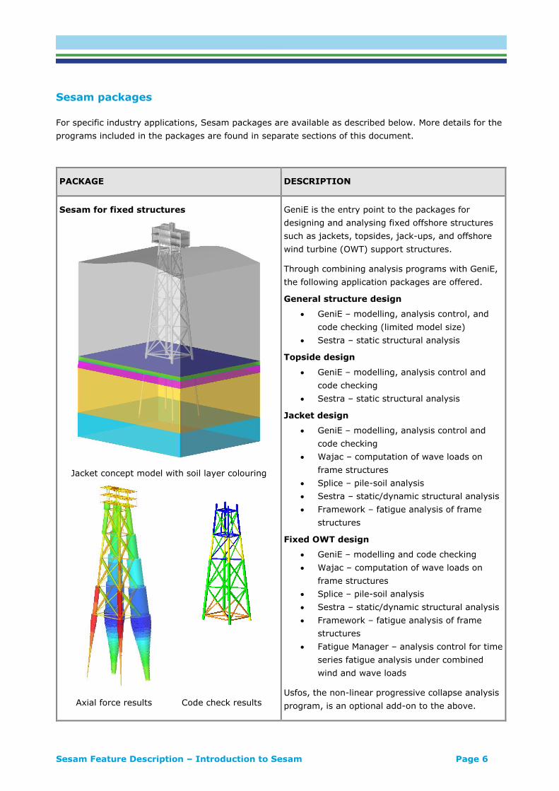
Sesam for fixed structures
Jacket concept model with soil layer colouring
Axial force results Code check results
GeniE is the entry point to the packages for
designing and analysing fixed offshore structures
such as jackets, topsides, jack-ups, and offshore
wind turbine (OWT) support structures.
Through combining analysis programs with GeniE,
the following application packages are offered.
General structure design
• GeniE – modelling, analysis control, and
code checking (limited model size)
• Sestra – static structural analysis
Topside design
• GeniE – modelling, analysis control and
code checking
• Sestra – static structural analysis
Jacket design
• GeniE – modelling, analysis control and
code checking
• Wajac – computation of wave loads on
frame structures
• Splice – pile-soil analysis
• Sestra – static/dynamic structural analysis
• Framework – fatigue analysis of frame
structures
Fixed OWT design
• GeniE – modelling and code checking
• Wajac – computation of wave loads on
frame structures
• Splice – pile-soil analysis
• Sestra – static/dynamic structural analysis
• Framework – fatigue analysis of frame
structures
• Fatigue Manager – analysis control for time
series fatigue analysis under combined
wind and wave loads
Usfos, the non-linear progressive collapse analysis
program, is an optional add-on to the above.

Sesam Feature Description – Introduction to Sesam Page 7
Sesam for floating structures
Ship hull with pressures viewed from underneath
Semisubmersible motion animation and
hydrodynamic pressures
Semisubmersible panel model with load sections
HydroD and GeniE are the entry points to the
packages for floating structures. By combining
analysis programs with HydroD and GeniE, the
following application packages are offered.
Stability analysis
• HydroD – modelling and stability analysis
Stability analysis extended
• GeniE Panel – floater modelling
• HydroD – modelling and stability analysis
Linear hydrodynamics
• HydroD – modelling and analysis control
• Wadam – freq. domain hydrodynamics
• Wasim – time domain hydrodynamics
• Postresp – statistical postprocessing
Linear hydrodynamics with forward speed
• HydroD – modelling and analysis control
• Wasim – hydrodynamics including forward
speed
• Postresp – statistical postprocessing
Advanced hydrodynamics (add-on to above)
• Wadam – 2nd order hydrodynamics,
wave/current interaction and multi-body
• Wasim – non-linear hydrodynamics
including forward speed
Structural design
• GeniE – modelling, analysis control and
plate code checking
• Sestra – static/dynamic structural analysis
• Xtract – FE results post-processing
Structural design extended
• GeniE – modelling, analysis control, and
beam and plate code checking
• Presel – superelement modelling
• Submod – sub-modelling
• Wadam – wave load transfer extension
• Wasim – wave load transfer extension
• Presel – superelement modelling
• Sestra – static/dynamic structural analysis
• Stofat – fatigue of stiffened plates/shells
• Cutres – sectional results presentation
• Xtract – FE results post-processing
Xtract extension for animation is an optional add-
on to the hydrodynamics and structural packages.

Sesam Feature Description – Introduction to Sesam Page 8
Sesam for marine systems
Sima is the entry point to packages for analysing
and visualising marine systems in 3D.
Through combining analysis programs with Sima
the following application packages are offered.
Marine operations
• Sima – modelling, analysis control and
results presentation
• Simo – simulation of motions
Marine dynamics
• Sima – modelling, analysis control and
results presentation
• Simo – simulations of motions
• Riflex – analysis of moorings
Marine dynamics extended
• Sima – modelling, analysis control and
results presentation
• Simo – simulation of motions
• Riflex – analysis of moorings
• Vivana – vortex induced vibration analysis
Floating OWT design
• Sima – modelling, analysis control and
results presentation
• Simo – simulation of motions
• Riflex – analysis of moorings
Hydrodynamic coefficients
• HydroD – modelling and analysis control
• Wadam – frequency domain motion
analysis to output mass/damping
coefficients and RAOs
Vivana is an optional add-on to all packages
except Hydrodynamic coefficients for which GeniE
Panel is an optional add-on.

Sesam Feature Description – Introduction to Sesam Page 9
Sesam for moorings and risers
DeepC is the entry point to this package for
mooring and riser design. Through combining
analysis programs with DeepC, the following
application packages are offered.
Mooring and riser design
• DeepC – modelling, analysis control and
results presentation
• Simo – simulation of motions
• Riflex – analysis of mooring lines
Hydrodynamic coefficients *
• HydroD – modelling, analysis control and
results presentation
• Wadam – frequency domain motion
analysis to output mass/damping
coefficients and RAOs
* Offered as an optional add-on to the Mooring
and riser design package together with GeniE
Panel.
Helica, Mimosa, Sima and Vivana are optional add-
on programs to the Mooring and riser design
package.
Sesam for pipelines
Sesam for pipelines is a set of independent
programs.
• PET (Pipeline Engineering Tool) for early
phase pipeline assessment covering
different aspects of pipeline design.
• StableLines for pipeline on-bottom stability
based on DNV Recommended Practice
DNV-RP-F109.
• FatFree for analysis of free spanning
pipelines according to the DNV
Recommended Practice, RP-F105.
• OS-F101 Code Compliance is related to the
re-issue of the DNV Offshore Standard for
Submarine Pipeline Systems.
• RP-F101 Spreadsheet for assessment of
corroded pipelines in compliance with
DNV-RP-F101
• SimBuck for simplified global buckling
analysis of submarine pipelines

Sesam Feature Description – Introduction to Sesam Page 10
Sesam Manager
Last revised: January 8, 2019. Describing version 6.6-02.
Sesam Manager manages Sesam analyses of any kind, from the simplest to the most comprehensive.
An analysis job is Sesam programs (applications) organised as activities in a workflow. The workflow
may be of any length and complexity. Any other program/application may also be added to the
workflow, e.g. your own program or an MS Office application.
Sesam Manager
Sesam Manager takes care of the data flow between the Sesam programs. The default file operation is
transparent and can be modified to meet special requirements. Any document and file, e.g. analysis
specifications and reports, may be attached to the job.
Taking advantage of the JavaScript® scripting language of Sesam Manager a job may be exported,
edited and imported to establish a new revised job. A built-in ZIP import/export functionality allows jobs
to be transferred between users whether they are in progress or completed.
In short, the purpose of Sesam Manager is to:
• Be a common starting point for all Sesam programs
• Ease the execution of Sesam programs and establish parts of the input
• Organise execution of the Sesam programs in the proper sequence for the task at hand
• Manage the files involved in an analysis project
• Establish workflow templates for analysis tasks of any complexity
• Provide easy archiving of an analysis job with its input and results files plus attachments
Sesam Feature Description – Introduction to Sesam Page 11
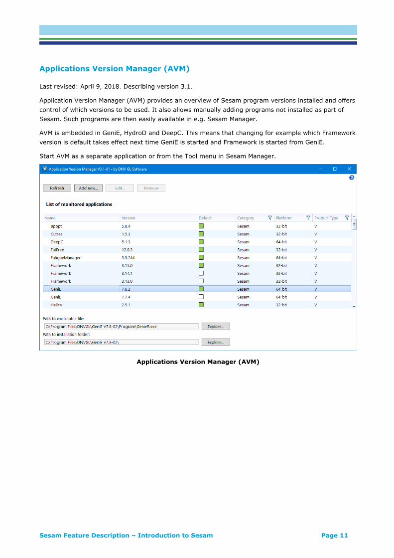
Applications Version Manager (AVM)
Last revised: April 9, 2018. Describing version 3.1.
Application Version Manager (AVM) provides an overview of Sesam program versions installed and offers
control of which versions to be used. It also allows manually adding programs not installed as part of
Sesam. Such programs are then easily available in e.g. Sesam Manager.
AVM is embedded in GeniE, HydroD and DeepC. This means that changing for example which Framework
version is default takes effect next time GeniE is started and Framework is started from GeniE.
Start AVM as a separate application or from the Tool menu in Sesam Manager.
Applications Version Manager (AVM)

Sesam Feature Description – Introduction to Sesam Page 12
Sesam Interface Files
The Sesam Interface Files are comprised of a set of files for which the most commonly used names are
T1.FEM, L1.FEM and R1.SIN. These are shown in the simplified Sesam overview figure below.
Sesam overview with focus on Sesam Interface Files
The Sesam Interface Files are comprised of the following:
• Input Interface Files – e.g. T1.FEM, T3.FEM, T21.FEM, etc.
The model created by the preprocessors is contained in these files. The number in the file name
can be any number from 1 to 9999 and is used to distinguish separate models (e.g. panel mesh
for hydrodynamic analysis and FE mesh for structural analysis, different versions of the same
model, different superelements, etc.). The short names T-file and FEM file are often used for
these files. The contents of the file are:
o FE/panel model with nodes, elements, material, boundary conditions and loads
o 2nd or higher level superelements when using the multilevel superelement technique
• Loads Interface Files – e.g. L1.FEM, L3.FEM, etc.
Hydrodynamic loads computed by environmental programs are stored in these files. They pertain
to corresponding Input Interface Files: L1.FEM belongs to T1.FEM, L3.FEM belongs to T3.FEM,
etc. The contents of the file are:
o Hydrodynamic beam line and surface pressure loads, deterministic or transfer functions
o Inertia and gravity loads
o Point loads from anchor or TLP elements
• Matrix Interface Files – e.g. M21.SIF (or M21.SIU or M21.SIN)
These files are for exchange of matrix data like stiffness, mass, damping and loads. The most
common usage is exchange of data between Sestra and Splice. The contents of the file are:

Sesam Feature Description – Introduction to Sesam Page 13
o Stiffness, mass and damping matrices
o Load vectors
o Nodal displacements
• Structural Results Interface Files – e.g. R21.SIN (or R21.SIF or R21.SIU)
Structural (FE) analysis results are stored in these files ready for further processing by a
postprocessor. The short names R-file and SIN file are often used for this file. The contents of
the file are:
o FE model (= Input Interface File)
o Nodal displacements
o Beam forces
o Element stresses
• Hydrodynamic Results Interface Files – typically named G1.SIF (or G1.SIU or G1.SIN)
Hydrodynamic rigid body motion results are stored in these files. The short name G-file is often
used for this file. The contents of the file are:
o Transfer functions for rigid body motion of floating structure
o Hydrodynamic coefficients
o Sea surface elevation and off-body kinematics
o Transfer functions for base shear and overturning moments for fixed frame structure
o Transfer functions for sectional loads
o Transfer functions for forces and stresses in selected elements
Tools for conversion between Sesam and other formats, i.e. CAE and CAD programs, is covered in
section Import and export features of Sesam below.
There are also auxiliary tools for manipulating the Sesam Interface Files:
• Loads Interface Files may be manipulated in various ways by the auxiliary program Waloco:
o Merge two and more files from different Wajac/Wadam/Wasim runs
o Renumber the load cases
o Conversion between formatted and unformatted (FEM extension for both)
• Results Interface Files may be manipulated in various ways by the auxiliary program Prepost:
o Merge two and more files from different Sestra runs
o Copy data from one file to another
o Conversion between formatted (SIF), unformatted (SIU) and database format (SIN)
o Result combinations may be created (alternatively to creating combinations in GeniE)
o Extraction of transfer functions for selected elements and results and storage on
Hydrodynamic Results Interface Files (G-file)
Sesam Feature Description – Introduction to Sesam Page 14
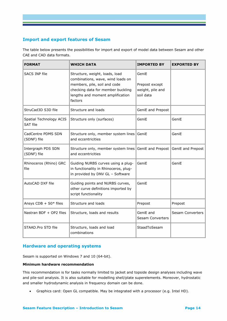
Import and export features of Sesam
The table below presents the possibilities for import and export of model data between Sesam and other
CAE and CAD data formats.
FORMAT WHICH DATA IMPORTED BY EXPORTED BY
SACS INP file Structure, weight, loads, load
combinations, wave, wind loads on
members, pile, soil and code
checking data for member buckling
lengths and moment amplification
factors
GeniE
Prepost except
weight, pile and
soil data
StruCad3D S3D file Structure and loads GeniE and Prepost
Spatial Technology ACIS
SAT file
Structure only (surfaces) GeniE GeniE
CadCentre PDMS SDN
(SDNF) file
Structure only, member system lines
and eccentricities
GeniE GeniE
Intergraph PDS SDN
(SDNF) file
Structure only, member system lines
and eccentricities
GeniE and Prepost GeniE and Prepost
Rhinoceros (Rhino) GRC
file
Guiding NURBS curves using a plug-
in functionality in Rhinoceros, plug-
in provided by DNV GL – Software
GeniE GeniE
AutoCAD DXF file Guiding points and NURBS curves,
other curve definitions imported by
script functionality
GeniE
Ansys CDB + S0* files Structure and loads Prepost Prepost
Nastran BDF + OP2 files Structure, loads and results GeniE and
Sesam Converters
Sesam Converters
STAAD.Pro STD file Structure, loads and load
combinations
StaadToSesam
Hardware and operating systems
Sesam is supported on Windows 7 and 10 (64-bit).
Minimum hardware recommendation
This recommendation is for tasks normally limited to jacket and topside design analyses including wave
and pile-soil analysis. It is also suitable for modelling shell/plate superelements. Moreover, hydrostatic
and smaller hydrodynamic analysis in frequency domain can be done.
• Graphics card: Open GL compatible. May be integrated with a processor (e.g. Intel HD).
Sesam Feature Description – Introduction to Sesam Page 15
• Memory: 4 GB
• Processor: Dual core
• 64-bit version of Windows operating system
• Storage: 200 GB
• Display: 17” supporting 1280x1024, alternatively laptop 15” supporting 1280x1024
Preferred hardware recommendation
This recommendation is for all types of Sesam analysis.
• Graphics card: Separate Open GL compatible graphics card (NVIDIA or ATI) with 512 MB
graphics memory. If OpenGL is not supported, then use DX9 as provided in the Sesam
installation.
• Memory: 16 GB
• Processor: Quad core
• 64-bit version of Windows operating system
• Storage: 500 GB
• Display: 24” supporting 1900x1200 (or-1080), alternatively laptop 17” supporting 1900x1200
(or-1080)
Graphics driver
By “graphics driver” below is meant the system level software provided by your Graphics Card supplier
(most likely Intel, NVIDIA or ATI) to interface between Windows and the GPU. This is supplied with your
operating system or graphics card.
By “GeniE graphics driver” below is meant the software used by GeniE to interface with the graphics
driver defined above.
Use of DX9
DirectX 9.0 (DX9) is the preferred GeniE graphics driver and it is the default on installation.
DirectX 9.0c Runtime version 9.27.1734 distributed on June 2010 or a later version of DirectX 9 must be
installed on your system. The Sesam installer will install DirectX 9.0c.
Windows 7 comes with DirectX 9 pre-installed. However, GeniE uses extra components so DirectX 9
must be explicitly installed using the Sesam installer or an installer from the Microsoft website.
The GeniE DX9 driver is supported on any DirectX 9.0 compliant graphics hardware (Microsoft Shader
Model 3) with the latest vendor-supplied drivers.
DirectX 9.0c was first released in August 2004 so older systems will not support the DX9 driver.
Use of OpenGL
GeniE supports two different OpenGL drivers. The standard GeniE OpenGL driver is a legacy driver that
attempts to support all OpenGL 1.1 hardware.
The GeniE OpenGL2 driver is a shader-based driver that is offered as an alternative should a user
encounter problems with other drivers. It attempts to support all OpenGL 2.0+ hardware.

Sesam Feature Description – GeniE Page 16
GeniE CONCEPT MODELLING OF BEAM, PLATE AND SHELL STRUCTURES,
ANALYSIS WORKFLOWS AND CODE CHECKING
Last revised: January 8, 2019. Describing version 7.11 (64-bit).
GeniE is a tool for concept (high level geometry) modelling of beams and stiffened plates and shells
(curved surfaces). Load modelling includes equipment (with automatic load transfer), explicit loads
(point, line and surface) and wind loads. The model is transferred to Sestra for structural analysis, to
Wajac and Wadam for hydrodynamic analysis, to Splice for pile-soil analysis and to Installjac for
launching and upending analysis. GeniE includes predefined analysis set-ups (workflows) involving
Sestra, Wajac and Splice. General basic results presentation can be carried out as well as code checking
of members and tubular joints.
Sesam Feature Description – GeniE Page 17
FEATURES OF GENIE
The features of GeniE are organised in sections:
• Beam, plate and surface modelling
• Finite elements and features for meshing
• Modelling for structural analysis in Sestra
• Modelling for wave and wind analysis in Wajac
• Modelling for wave and motion analysis in HydroD/Wadam
• Modelling for pile-soil analysis in Splice
• Explicit (point, line, surface) load modelling
• Post-processing and reporting
• Member and tubular joint code checking – requires extension CCBM
• Supported standards for member and tubular joint checking
• Plate code checking – requires extension CCPL
• Import and export data in GeniE
GeniE has several extensions, i.e. features screened off for users of the basic version of the program.
Access to an extension is subject to agreement and a valid license file. These extensions are:
CGEO – curved geometry modelling, includes partial meshing and all mesh editing except features
covered by the REFM extension
REFM – refined meshing, includes refine mesh for grid, edge and box, detail box for refined meshing and
convert beam to plate
CCBM – code checking beams
CCPL – code checking stiffened plates
There is also a special version that is the same as GeniE including extensions CGEO, CCBM and CCPL
only limited to 10,000 finite elements and 500 beam concepts. Wave loads (Wajac) and pile-soil analysis
(Splice) is not included.

Sesam Feature Description – GeniE Page 18
Beam, plate and surface modelling
FEATURE DESCRIPTION
Unit support
m? mm? inch?
Units may be mixed throughout the modelling. The
data logging (scripting) ensures that re-creating
the model gives the same result.
Unit information is stored on the Sesam Input
Interface File (FEM file).
Flat plates and beams
By default, there is connectivity between beams
and plates that geometrically connect at their
centre lines/planes. The user may, however,
disconnect structural components. Beams
connected to plates may be flushed (given
offsets/eccentricities) so as to become plate
stiffeners. Beams and plates may be created in
GeniE or imported from other CAE systems. A flat
plate may be changed to a membrane (no bending
stiffness).
Thickness
The thickness is applied to a flat plate (membrane
or shell) or a surface (shell).
Beam cross sections (profiles)
The user may define profiles for pipe, I/H
(symmetrical and unsymmetrical), channel, angle,
massive bar, box, tubular cone and of type
general. Derived properties (area, moment of
inertia, section modulus) based on geometry may
be modified. In addition, GeniE includes section
libraries from AISC, EURONORM, Norwegian
Standard and BS in addition to typical ship
libraries.

Sesam Feature Description – GeniE Page 19
Beam classification
Beams may optionally be assigned beam
classifications primary, secondary, tertiary and
auxiliary. This eases keeping the most important
structural components in focus.
In later versions, this classification will be used to
auto setup code checking parameters.
Segmented beams
A segmented beam is a beam split into multiple
parts. Segmented beams are typically used for
modelling beams with variable section and/or
material. The automatic tubular joint modelling of
cans, stubs and cone also involves segmented
modelling.
Overlapping beams
Overlapping beams are typically used to define pile
in leg and other cases of double beams.
By default, overlapping geometry is prevented so a
particular command is used to create overlapping
beams.
Grouted members
Easy definition of outer leg and inner pile to define
overlapping beams including the connectivity
(fixed, free, stiffness) along the member length.
The stiffness of grout between pile and leg may
thus be included in a linear analysis. The mass of
grout must be added to the overlapping member.
Overlapping beams with connectivity may be
modelled either in a single operation (grouted
beam modelling) or by first modelling a normal
beam and thereafter adding overlapping beam,
inner beam and mesh properties.
Sesam Feature Description – GeniE Page 20
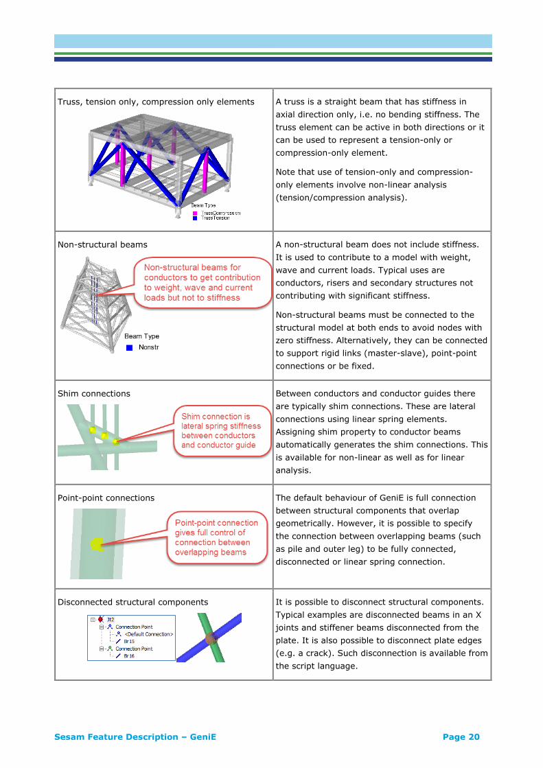
Truss, tension only, compression only elements
A truss is a straight beam that has stiffness in
axial direction only, i.e. no bending stiffness. The
truss element can be active in both directions or it
can be used to represent a tension-only or
compression-only element.
Note that use of tension-only and compression-
only elements involve non-linear analysis
(tension/compression analysis).
Non-structural beams
A non-structural beam does not include stiffness.
It is used to contribute to a model with weight,
wave and current loads. Typical uses are
conductors, risers and secondary structures not
contributing with significant stiffness.
Non-structural beams must be connected to the
structural model at both ends to avoid nodes with
zero stiffness. Alternatively, they can be connected
to support rigid links (master-slave), point-point
connections or be fixed.
Shim connections
Between conductors and conductor guides there
are typically shim connections. These are lateral
connections using linear spring elements.
Assigning shim property to conductor beams
automatically generates the shim connections. This
is available for non-linear as well as for linear
analysis.
Point-point connections
The default behaviour of GeniE is full connection
between structural components that overlap
geometrically. However, it is possible to specify
the connection between overlapping beams (such
as pile and outer leg) to be fully connected,
disconnected or linear spring connection.
Disconnected structural components
It is possible to disconnect structural components.
Typical examples are disconnected beams in an X
joints and stiffener beams disconnected from the
plate. It is also possible to disconnect plate edges
(e.g. a crack). Such disconnection is available from
the script language.

Sesam Feature Description – GeniE Page 21
Tubular joints
Tubular joints may automatically be refined to
include gaps (brace offsets ensuring proper plane-
wise gaps), cans, stubs and cones according to API
and Norsok rules for joint design. The rules may
be modified. The braces may be flushed to the
chord wall to more accurately represent mass and
buoyancy. The braces may be coupled to the chord
by spring stiffness connections according to the
Buitrago formulae (geometric or load path). It is
also possible to use hinges to represent the joint
stiffness.
X joints and offsets/eccentricities
Offsets for an X brace typically cause the X joint to
be offset from the topology lines. A brace added to
the X joint should connect to the structural joint
and not to the intersection of the topology lines.
In the example to the left the diagonal braces
have large offsets in their upper ends. The braces
from the X joint to the legs should remain
connected to the structural joint – and also remain
perpendicular to the leg if relevant – when the
brace offsets are introduced or changed.
General offsets/eccentricities
The offset/eccentricity feature used for flushing
plate stiffeners and ensuring proper gaps in
tubular joints is quite general. In addition to the
automatic flush and gap features, any offset may
be manually specified in the two ends.
An example of use is a structural joint with internal
stiffeners making it so stiff that the flexible beam
should not extend all the way to the FE node in the
middle of the joint.
Sesam Feature Description – GeniE Page 22
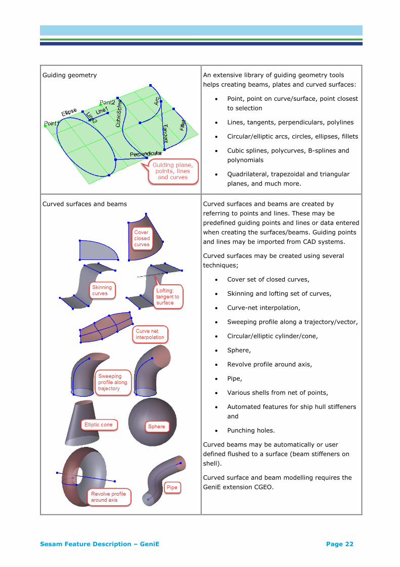
Guiding geometry
An extensive library of guiding geometry tools
helps creating beams, plates and curved surfaces:
• Point, point on curve/surface, point closest
to selection
• Lines, tangents, perpendiculars, polylines
• Circular/elliptic arcs, circles, ellipses, fillets
• Cubic splines, polycurves, B-splines and
polynomials
• Quadrilateral, trapezoidal and triangular
planes, and much more.
Curved surfaces and beams
Curved surfaces and beams are created by
referring to points and lines. These may be
predefined guiding points and lines or data entered
when creating the surfaces/beams. Guiding points
and lines may be imported from CAD systems.
Curved surfaces may be created using several
techniques;
• Cover set of closed curves,
• Skinning and lofting set of curves,
• Curve-net interpolation,
• Sweeping profile along a trajectory/vector,
• Circular/elliptic cylinder/cone,
• Sphere,
• Revolve profile around axis,
• Pipe,
• Various shells from net of points,
• Automated features for ship hull stiffeners
and
• Punching holes.
Curved beams may be automatically or user
defined flushed to a surface (beam stiffeners on
shell).
Curved surface and beam modelling requires the
GeniE extension CGEO.

Sesam Feature Description – GeniE Page 23
Hole
Holes may be defined as objects, i.e. a hole
overlapping a plate involves that there is a hole in
the plate. This differs from deleting an area in a
plate in that deleting the hole patches up the
plate.
Holes are defined by punching a plate by a closed
guide curve or a profile.
General about topology modelling
When inserting, moving or deleting beams and
surfaces the connectivity between structural
objects is kept updated. This means that if two
objects geometrically coincide they will be
connected. Hence there is no need to manually
define or delete connections.
Beams and surfaces may be split at intersections
thereby enabling trimming (deleting protruding
parts) to flush parts.
Compartment modelling
Compartments may automatically be created for
volumes enclosed by surfaces. The compartments
may be filled with liquid and solid matter in GeniE
or from Nauticus Hull. The compartment contents
will contribute with loads (e.g. weight) in a
structural analysis. Compartment contents may
also be used by Sesam HydroD in hydro-static and
hydrodynamic analyses.
Non-structural plates
A non-structural plate has no mass or stiffness. Its
sole purpose is to close a volume in case there are
openings in the enclosing surfaces. A typical
example is an open compartment in a bulk ship.
Point masses
Point masses may be inserted at given positions
along a beam or a plate edge. The point mass may
be of type uniform (mass is specified) or generic
(properties for all 6 degrees of freedom are
specified).

Sesam Feature Description – GeniE Page 24
Loads converted to mass
Various features for converting explicit loads and
load combinations including load factors to mass
for dynamic analysis.
Mass scaling
A named set (a group of structural components)
may be defined to have a designated mass. GeniE
will scale the material density for the set to hit the
target mass. That way the centre of gravity is
maintained.
Finite elements and features for meshing
FEATURE DESCRIPTION
Finite element types
GeniE can create the following finite element
types:
• Truss, including tension-only and
compression-only
• Two node beam
• Three node beam (GeniE term: second
order)
• Three node triangular flat plate
• Four node quadrilateral flat plate
• Six node triangular curved shell (GeniE
term: second order)
• Eight node quadrilateral curved shell
(GeniE term: second order)

Sesam Feature Description – GeniE Page 25
Hinges
Hinges may be inserted at beam ends to fully or
partly release their connection to the node of the
joint. Each of the six degrees of freedom may be
fixed, released or connected with spring stiffness
to the node.
Command: Properties > Hinges > New Hinge
Mesh always reflects geometry
Basic geometry (beams, plates and shells)
determines the FE mesh. Where geometry
intersects, there will be mesh points (nodes) and
lines. There is no need for ensuring mesh
connectivity.
Mesh part of structure
A set containing a part of the model may be
meshed as a separate FE model. This could be to
create a superelement (for superelement analysis)
or to create a sub-model (for sub-modelling
analysis). The boundary conditions at the cut
planes (super for superelement analysis and
prescribed displacements for sub-modelling) are
contained in the set.
Any number of such part FE models may be
created.
The example to the left shows a part of a model
meshed as a separate FE model with boundary
conditions.
Command: Right-click meshing activity | Edit Mesh
Activity

Sesam Feature Description – GeniE Page 26
Meshing algorithms
Advancing front mesher Quad mesher
GeniE supports two different meshing algorithms.
The first option is a quad mesh algorithm (the
Sesam quad mesher) that will give the best mesh
in the middle of a surface – it is thus intended for
regular structures like topsides and rectangular
parts of a floating structure. The other option is an
advancing front mesher (also known as paver
meshing) that gives the best mesh along edges –
this is best for details and irregular structural parts
such as a joint, a hole or the fore or aft part of a
vessel. It is possible to use both options in a
model.
Command: Edit | Rules | Meshing
Mesh density
The density or size of elements is determined by
mesh properties:
• Mesh density specifying length of element
edge
• Number of elements along a line or plate
edge
Any number of such properties are defined and
assigned to various parts of the model. One of the
mesh properties may also be set as default, i.e.
valid where no particular property has been
assigned.
Command: Edit | Properties | Mesh Property
Mesh transition
With different mesh densities for various parts
there will be a mesh transition zone from fine to
coarse mesh. By default, the extent of the
transition zone will be as short as possible. The
user may extend the transition zone by specifying
a growth rate for a mesh density.

Sesam Feature Description – GeniE Page 27
Feature edges for mesh control
So-called feature edges may be inserted to control
the mesh. Where there is a feature edge crossing
a plate, there will be a mesh line in same way as
for a beam stiffener.
The example to the left shows how introducing a
feature edge alters the mesh: there is a mesh line
along the feature edge.
Command: Structure | Features and Holes |
Feature Edge
Meshing rules
The mesh creation is subject to several user
defined rules:
• Various idealisations of topology to
improve mesh
• Preferences re. regular (mxn) mesh,
triangular elements and more
• Max/min angle of element corner
• Max relative and minimum Jacobian
determinant
• Elimination of short edges to avoid
degenerated mesh
• Etc.
Command: Edit | Rules | Meshing
Overrule general rules and settings
Meshing rules and meshing algorithm (Sesam
quad or advancing front) may be specified for
individual parts thereby overruling general (global)
rules and settings.
For the example to the left advancing front mesh
is generally used to get a proper mesh for holes
and cavities. But the Sesam quad mesher is
assigned to the right part as this is a better choice
for rectangular parts.
Command: Edit | Properties | Mesh Option

Sesam Feature Description – GeniE Page 28
Option for ignoring holes
Holes may optionally be ignored in the mesh
creation.
Command: Edit | Properties | Mesh Option
Control mesh around holes/cavities
There is a feature for easy offsetting guide curves
around holes, cavities and similar details by
constant values. This may be used to improve the
mesh in such critical areas.
Command: Right-click model curve at hole edge |
Offset
Prioritized meshing
To achieve an optimal mesh for important parts
the meshing can be prioritized. I.e. important
parts are meshed first (priority 1) and less
important parts are meshed later. Any number of
priority levels may be specified, each priority level
is assigned plates/shells. The priority levels may
easily be reordered.
The example to the left shows three perpendicular
planes with different mesh densities. The plate
with the highest priority gets a regular mxn mesh.
Command: Utilities | Mesh Priorities | New Mesh
Priority
Sesam Feature Description – GeniE Page 29
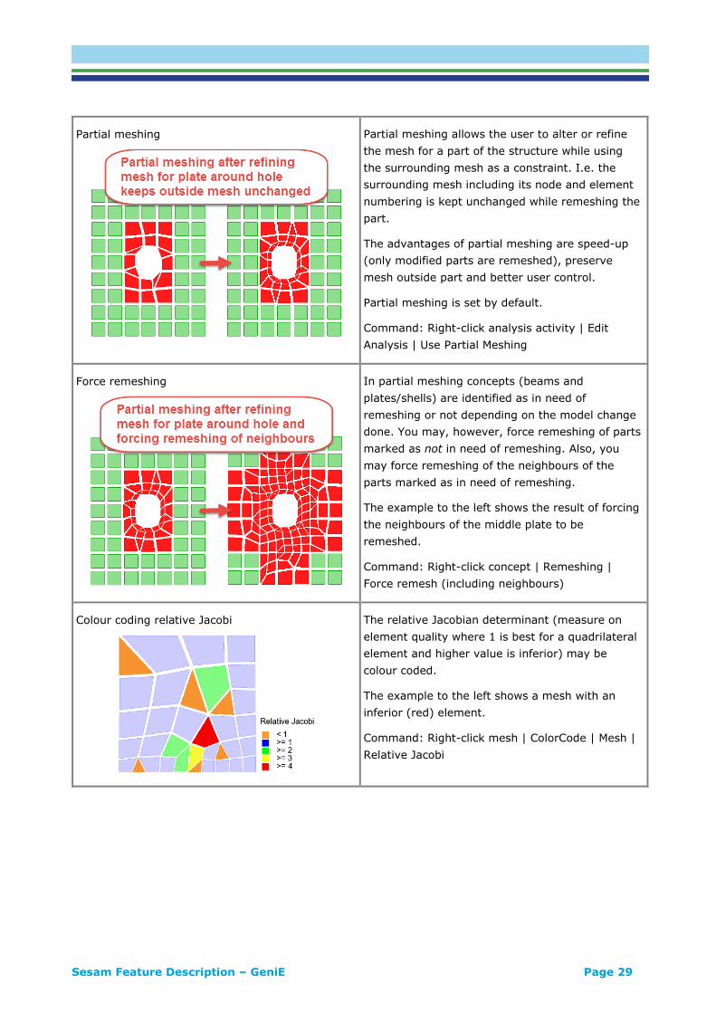
Partial meshing
Partial meshing allows the user to alter or refine
the mesh for a part of the structure while using
the surrounding mesh as a constraint. I.e. the
surrounding mesh including its node and element
numbering is kept unchanged while remeshing the
part.
The advantages of partial meshing are speed-up
(only modified parts are remeshed), preserve
mesh outside part and better user control.
Partial meshing is set by default.
Command: Right-click analysis activity | Edit
Analysis | Use Partial Meshing
Force remeshing
In partial meshing concepts (beams and
plates/shells) are identified as in need of
remeshing or not depending on the model change
done. You may, however, force remeshing of parts
marked as not in need of remeshing. Also, you
may force remeshing of the neighbours of the
parts marked as in need of remeshing.
The example to the left shows the result of forcing
the neighbours of the middle plate to be
remeshed.
Command: Right-click concept | Remeshing |
Force remesh (including neighbours)
Colour coding relative Jacobi
The relative Jacobian determinant (measure on
element quality where 1 is best for a quadrilateral
element and higher value is inferior) may be
colour coded.
The example to the left shows a mesh with an
inferior (red) element.
Command: Right-click mesh | ColorCode | Mesh |
Relative Jacobi

Sesam Feature Description – GeniE Page 30
Mesh editing: Manipulate triangle
The manipulate triangle feature has two options:
• Moving a triangular element to a new
position where it possibly may be merged
with another triangular element into a
quadrilateral element
• Splitting a quadrilateral element into two
triangular elements
Button:
Mesh editing: Move node
Drag any node to a new position and see while
dragging the colour coding of maximum relative
Jacobian determinant changes. Release node at
the optimal position.
The example to the left shows how the inferior
(red) element is improved by moving a node.
Button:
Mesh editing: Align nodes in element grid
An irregular mxn element grid may be aligned by
dragging the mouse diagonally over the area.
Button:
Mesh editing: Align nodes along line and move by
constant vector
Aligned nodes may be shifted sideways by a given
value. First select the aligned nodes by two clicks
and then move sideways by a third.
Button:
Mesh editing: Split edge
Split an element edge by creating a new node
there and new elements.
Button:
Sesam Feature Description – GeniE Page 31
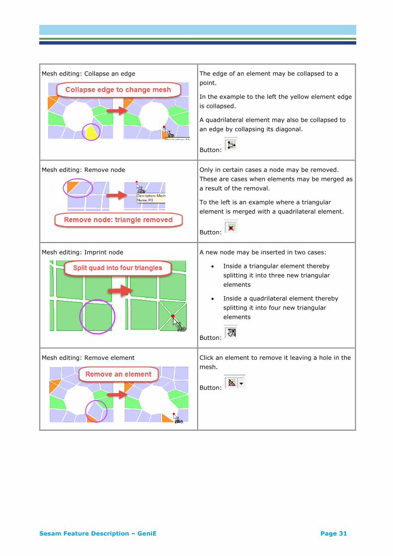
Mesh editing: Collapse an edge
The edge of an element may be collapsed to a
point.
In the example to the left the yellow element edge
is collapsed.
A quadrilateral element may also be collapsed to
an edge by collapsing its diagonal.
Button:
Mesh editing: Remove node
Only in certain cases a node may be removed.
These are cases when elements may be merged as
a result of the removal.
To the left is an example where a triangular
element is merged with a quadrilateral element.
Button:
Mesh editing: Imprint node
A new node may be inserted in two cases:
• Inside a triangular element thereby
splitting it into three new triangular
elements
• Inside a quadrilateral element thereby
splitting it into four new triangular
elements
Button:
Mesh editing: Remove element
Click an element to remove it leaving a hole in the
mesh.
Button:

Sesam Feature Description – GeniE Page 32
Mesh editing: Add plate element
Add an element by clicking its corners.
Button:
Mesh editing: Enhance quality
The mesh resulting from the automatic generation
may be enhanced by merely clicking single
elements or sweeping mouse over several
elements.
The example to the left shows how clicking the
inferior element of the example above enhances it.
The example to the left shows the result of
sweeping the mouse over all elements.
Button:
Sesam Feature Description – GeniE Page 33
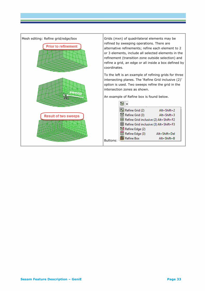
Mesh editing: Refine grid/edge/box
Grids (mxn) of quadrilateral elements may be
refined by sweeping operations. There are
alternative refinements; refine each element to 2
or 3 elements, include all selected elements in the
refinement (transition zone outside selection) and
refine a grid, an edge or all inside a box defined by
coordinates.
To the left is an example of refining grids for three
intersecting planes. The ‘Refine Grid inclusive (2)’
option is used. Two sweeps refine the grid in the
intersection zones as shown.
An example of Refine box is found below.
Buttons:
Sesam Feature Description – GeniE Page 34
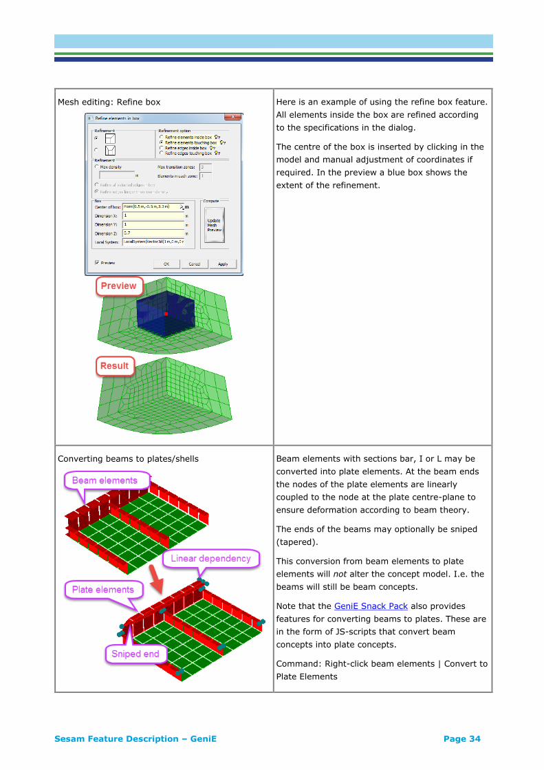
Mesh editing: Refine box
Here is an example of using the refine box feature.
All elements inside the box are refined according
to the specifications in the dialog.
The centre of the box is inserted by clicking in the
model and manual adjustment of coordinates if
required. In the preview a blue box shows the
extent of the refinement.
Converting beams to plates/shells
Beam elements with sections bar, I or L may be
converted into plate elements. At the beam ends
the nodes of the plate elements are linearly
coupled to the node at the plate centre-plane to
ensure deformation according to beam theory.
The ends of the beams may optionally be sniped
(tapered).
This conversion from beam elements to plate
elements will not alter the concept model. I.e. the
beams will still be beam concepts.
Note that the GeniE Snack Pack also provides
features for converting beams to plates. These are
in the form of JS-scripts that convert beam
concepts into plate concepts.
Command: Right-click beam elements | Convert to
Plate Elements

Sesam Feature Description – GeniE Page 35
Detail box for refined meshing
A box may be defined enclosing a part of a model
with the purpose of creating a refined mesh inside
the box. The box is defined by its centre and
extent in X, Y and Z (optionally in a local
coordinate system). The box definition includes a
mesh density, how to handle holes and whether
beams shall be converted into plate/shell
elements.
The example to the left shows how a part of the
rounded box model has a refined mesh.
Some of the elements are shown in the bottom
figure. Beams inside the detail box are converted
to plate elements, beams outside not.
Command: Right-click Structure > Details folder |
New Detail Box
Identify inferior elements
Inferior elements may be identified based on
several criteria:
• Max/min angle of element corner
• Max relative and minimum Jacobian
determinant
• Maximum aspect ratio
• Warping (twisting)
• Etc.
Command: Tools | Analysis | Locate FE

Sesam Feature Description – GeniE Page 36
Modelling for structural analysis in Sestra
FEATURE DESCRIPTION
Materials
GeniE supports linear isotropic material, isotropic
shear material and orthotropic material (material
axes are aligned with the global axis system).
Plates with shear material are typically used for
connecting pile sleeve and leg.
Hinges
Hinges may be inserted at beam ends to fully or
partly release their connection to the node of the
joint. Each of the six degrees of freedom may be
fixed, released or connected with spring stiffness
to the node.
Boundary conditions
Boundary conditions (or supports) may be of type
fixed, free, spring-to-ground or spring matrix.
Furthermore, it is also possible to specify
prescribed displacements for each load case.
Corrosion addition
Corrosion additions are applied to a plate, surface
or beam to reduce the thickness to be used in the
structural analysis. The corrosion addition is
specific to an analysis which means that it is
possible to run several analyses with alternative
corrosion additions.
Analysis types
There are built-in analyses running analysis
programs in the background:
• Linear static structural analysis (in Sestra)
• Eigenvalue analysis (in Sestra)
• Time/frequency domain dynamic analysis,
direct or Modal Superposition (in Sestra)
• Non-linear tension-compression analysis
(in Sestra)
• Wave load calculation (in Wajac)
• Wave load plus integrated structure-pile-
soil analysis (Wajac, Sestra, Splice)
Sesam Manager is used to run non-linear analysis
(in Usfos) where the model is created in GeniE.
E ε σ
1

Sesam Feature Description – GeniE Page 37
Modelling for wave and wind analysis in Wajac
FEATURE DESCRIPTION
Flooding
Flooding is used to specify which members are
filled with water. Members are by default non-
flooded. Flooding involves that only the steel
volume contributes to buoyancy.
Buoyancy
Buoyancy may be combined with the wave forces
or singled out as a separate case. The buoyancy
accounts for the steel sectional area plus
entrapped air (unless flooded). The buoyancy may
be switched off for selected members.
A buoyancy area may optionally be defined to
override the area computed by Wajac for tubular
or non-tubular sections for use in the buoyancy
calculation.
The buoyancy is calculated up to the wave
crest/trough in deterministic analysis.
The buoyancy may be computed as:
• Line load perpendicular to the member
plus concentrated forces in the ends
(rational method)
• Vertical line load (marine method)
Morison coefficients for wave loads
The Morison coefficients (Cm and Cd) may be
defined in several ways: constant value, function
of diameter, function of Roughness/Reynolds
number, function of Roughness/KC number, by
rule (API RP 2A-WSD 21st edition) and directionally
dependent.
Marine growth
By adding marine growth, the hydrodynamic
diameter is increased. In addition, the mass and
added mass of the marine growth is included in
the analysis. The weight of the marine growth may
optionally be included in the hydrostatic buoyancy
calculation.

Sesam Feature Description – GeniE Page 38
Hydrodynamic diameter
The hydrodynamic diameter is used to manually
override the diameter computed by Wajac for
tubular or non-tubular sections for use in wave
load calculation.
An application may be to substitute the equivalent
diameter, the diagonal, for a box section with a
more suitable value.
Conductor shielding
Reduce drag and inertia coefficients for conductor
arrays due to shielding effects (conductor shielding
factor) according to API (API RP 2A-WSD 21st
edition).
Element refinement
A member is by default divided into two segments
for calculation of the wave loads. Only the
submerged part is considered. Using the element
refinement property, a member may be divided
into up to 20 segments for more precise wave load
analysis.
Air drag
The Morison coefficient Cd for wind load calculation
may be defined as a constant or as a function of
Reynolds number. Wind shielding is achieved by
setting Cd = 0.
Wind load area
Wind load area is an area defined by the user for
computation of wind loads. A wind load area can
be a surface, a dummy wall connected to
members, or a side wall of an equipment.
Water depth
The water depth is used to define the location of
the sea surface. It is possible to include multiple
sea surface elevations in one analysis.

Sesam Feature Description – GeniE Page 39
Wave theory
The selection of wave theory (Airy, Stokes 5th
order, Cnoidal and Stream Function) to be used in
Wajac is done in GeniE.
For more information see Wajac.
Current The current may be defined to act in the same
direction as the wave or in any specified direction.
Wave load analysis
Deterministic wave load analysis (stepping a wave)
may be performed by using GeniE’s built-in
analysis activity. All model and execution data are
generated in GeniE. Wajac computes and stores
for subsequent structural analysis the wave plus
current loads for all wave steps or for only steps of
maximum/minimum base shear and/or
overturning moment.
Short term sea state simulation (time domain) and
frequency domain wave load analyses may be
executed by using model data given in GeniE plus
manually edited additional Wajac input data. Such
Wajac analyses may also be part of a workflow
established in Sesam Manager.
Wind profile
Several wind profiles may be defined. There are
two user defined profiles (normal and general) and
two profiles according to API, the 1st edition
(termed Extreme) and 21st edition (termed
Extreme API21).
Wind load analysis
A wind load analysis may be performed separately
or in combination with a wave load analysis. As for
a wave load analysis, the loads are stored for a
subsequent structural analysis. All model and
execution data are generated in GeniE. Wind loads
are a combination of member (beam) loads and
area loads. The member wind load calculation is
done in Wajac while wind loads on areas, surfaces
and equipments are calculated in GeniE.
Sesam Feature Description – GeniE Page 40
Modelling for wave and motion analysis in HydroD/Wadam
FEATURE DESCRIPTION
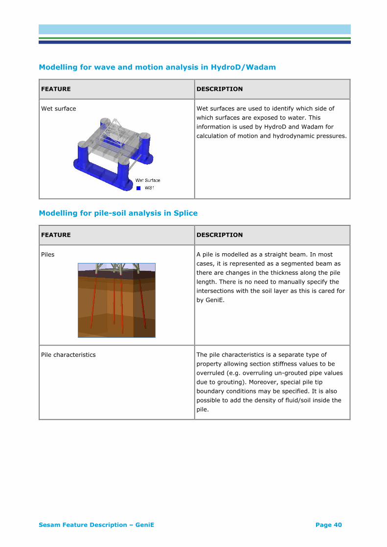
Wet surface
Wet surfaces are used to identify which side of
which surfaces are exposed to water. This
information is used by HydroD and Wadam for
calculation of motion and hydrodynamic pressures.
Modelling for pile-soil analysis in Splice
FEATURE DESCRIPTION
Piles
A pile is modelled as a straight beam. In most
cases, it is represented as a segmented beam as
there are changes in the thickness along the pile
length. There is no need to manually specify the
intersections with the soil layer as this is cared for
by GeniE.
Pile characteristics The pile characteristics is a separate type of
property allowing section stiffness values to be
overruled (e.g. overruling un-grouted pipe values
due to grouting). Moreover, special pile tip
boundary conditions may be specified. It is also
possible to add the density of fluid/soil inside the
pile.

Sesam Feature Description – GeniE Page 41
Soil type sand and clay
The sand property is defined by specifying angle of
internal friction, mass density and other
geotechnical parameters.
The clay property is defined by specifying
undrained shear strengths, mass density and other
geotechnical parameters.
Scour
Scour is specified as consisting of two
components:
• General scour (i.e. for the whole sea
bottom around the structure)
• Local scour around the piles (depth and
slope)
Soil data Soil data is a property with additional soil
characteristics like the initial value of soil shear
modulus, soil Poisson’s ratio and details for skin
friction and tip resistance.
Soil curves
Soil curves are properties that control the
generation of the:
• P-Y (lateral stiffness)
• T-Z (skin friction stiffness)
• Q-Z (tip stiffness)
They can be generated based on a set of pre-
defined curves or by manual input of data.
Soil utility tool
Easy conversion of soil data from a design premise
report into analysis data format
Sesam Feature Description – GeniE Page 42
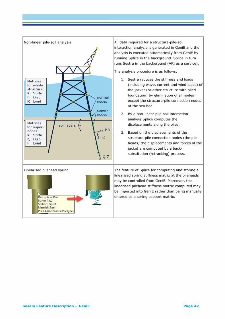
Non-linear pile-soil analysis
All data required for a structure-pile-soil
interaction analysis is generated in GeniE and the
analysis is executed automatically from GeniE by
running Splice in the background. Splice in turn
runs Sestra in the background (API as a service).
The analysis procedure is as follows:
1. Sestra reduces the stiffness and loads
(including wave, current and wind loads) of
the jacket (or other structure with piled
foundation) by elimination of all nodes
except the structure-pile connection nodes
at the sea bed.
2. By a non-linear pile-soil interaction
analysis Splice computes the
displacements along the piles.
3. Based on the displacements of the
structure-pile connection nodes (the pile
heads) the displacements and forces of the
jacket are computed by a back-
substitution (retracking) process.
Linearised pilehead spring
The feature of Splice for computing and storing a
linearised spring stiffness matrix at the pileheads
may be controlled from GeniE. Moreover, the
linearised pilehead stiffness matrix computed may
be imported into GeniE rather than being manually
entered as a spring support matrix.

Sesam Feature Description – GeniE Page 43
Explicit (point, line, surface) load modelling
FEATURE DESCRIPTION
Point loads
A force or a moment applied at a given position.
Must be connected to a beam or a plate edge.
Line loads
A line load (constant or linearly varying) applied
along the whole or part of a beam. May be applied
to segmented beams and individual parts of
overlapping beams.
Surface loads
A surface load may be specified as X, Y and Z
component pressure, normal pressure and
traction. The variation of these may be constant,
linearly varying and any variation as given by a
JavaScript function.
The load may be applied to any part of any
surface.
Temperature loads Temperature intensities may be applied along a
beam – constant or linearly varying.
Acceleration loads
Accelerations are used to generate inertia forces
based on structural mass and user defined
masses. Constant acceleration fields in X, Y or Z
directions may be defined.
In addition, rotational acceleration fields may be
defined. The angular velocity and acceleration of
the rotational field may be given directly or in
terms of a harmonic (wave induced) motion giving
angular motion and period. The latter method is
used for analysis of structures resting on a barge
or ship with known motion.

Sesam Feature Description – GeniE Page 44
Equipment
Equipments are used to create:
• Point or line loads on beams for use in
static analysis and
• Masses for use in eigenvalue and dynamic
analysis.
The equipment includes user control of size and
location, footprint, mass, method for calculation of
forces and how to handle mass in dynamic
analysis. Equipments may be resting on top or
hanging below a deck, it may be resting on an
inclined deck and be hanging on a vertical wall.
Load interface
The load interface is used to limit equipment
loading to certain beams, e.g. girders only.
Wind loads
Wind loads are combinations of member loads and
area loads. The area loads are generated in GeniE
and combined with member loads from Wajac. The
area loads are computed based on user defined
areas, surfaces or equipment walls that are
exposed to wind.
Load combinations
LComb1 = LCGrav*1.2 + LCBuoy*1.0 +
LCWave*1.6 + LCWind*1.6
Load combinations may be nested, i.e. a load
combination may include another load
combination. Load combinations can include loads
from hydrodynamic and wind load analysis and
they can be designated as an operation or storm
condition for use by the API member code check.

Sesam Feature Description – GeniE Page 45
Post-processing and reporting
FEATURE DESCRIPTION
Displacements
Displacements for beams and plates are shown as
contour plots in a 3D view. The deformed model
may be viewed together with the un-deformed
model. For a beam a cubic interpolation between
the beam ends may be performed by including end
rotations – this gives a realistic deformation
pattern with a single beam element along a
member.
Beam deflections
Deflections along a member may be computed and
presented in a 3D view and a 2D graph. It is also
possible to do a check against the AISC provision
of maximum deflection 1/180, 1/240 and 1/360 of
the span. Envelopes (maxima and minima) over
result cases may be presented in the 2D graph.
Plate and shell stresses
GeniE presents element stresses (G-stress) for
plates and shells as contour plots in 3D view.
These are stresses extrapolated and interpolated
from the result points within the individual
elements. There is no averaging between adjoining
elements. Stress components (sigxx, sigyy,
tauxy, …), von Mises stress and principal stresses
(P1, P2, P3) may be presented. More post-
processing capabilities for stresses are available in
Xtract that can be started from the GeniE user
interface.
Principal plate and shell stress vectors
Principal stresses P1, P2 and P3 may be shown as
vectors on top of a contour plot of any
displacement or stress component.

Sesam Feature Description – GeniE Page 46
Beam forces and moments
Beam forces and moments may be presented as a
coloured wireframe in 3D view. Optionally, and for
better identification of high values, the lines of the
wireframe may be displayed as cylinders with
diameter in proportion to the absolute value of the
force/moment.
Beam forces and moments may also be shown as
diagrams in a 3D view.
Finally, beam forces and moments may be
presented in a 2D graph together with other beam
results. The 2D graph allows envelopes (maxima
and minima) over result cases to be presented.
Beam stresses
Beam stresses are presented for selected
members in a 2D graph. Envelopes (maxima and
minima) over result cases may be presented.
Reaction forces
Reaction forces in the support points may be
shown as numeric values in a 3D view.

Sesam Feature Description – GeniE Page 47
Save graphics
Graphics of the 3D view may be saved to
alternative formats: gif, png, jpg, ps, bmp, tga, tif,
pdf, hsf, hmf, obj and ply. The resolution of the
graphics file is controlled by specifying number of
pixels.
The 2D graph may be copied as a bitmap to the
clipboard for pasting into a document.
Tabular report1
A tabular report can be saved to alternative
formats: txt, html, MS Word (xml) and MS Excel
(xml and csv).
The user has full control of the content of the
report. The report content is stored in the
database so that it is easy to reproduce the report
after model changes.
The report may include:
• Model data:
o Beam and plate data
o Properties
o Masses
o Loads
• FE analysis results
• Code checking results
• Graphics
• Your own text added

Sesam Feature Description – GeniE Page 48
Member and tubular joint code checking – requires extension CCBM
FEATURE DESCRIPTION
Code check analysis
The following code checks are performed:
• Member check
• Hydrostatic collapse
• Punching shear
• Conical transition
Code checks are performed for section profiles:
• Pipe
• Symmetrical/un-symmetrical I/H
• Channel
• Box
• Massive bar
• Angle
• General
• Torsion warping included for non-tubulars
Code checking model
The capacity model is generated in GeniE and
normally includes code checking parameters such
as member buckling length and buckling factors,
chord, can, stub and cone.
Code checking parameters
Each standard has its own set of code checking
parameter values. These values are the default
values in GeniE but the user can manually override
them if desired. The implementation of each code
check standard is described in technical notes that
are part of the GeniE installation.
Sesam Feature Description – GeniE Page 49
Member redesign
The redesign tool allows the user to modify
parameters like section size, material quality and
buckling length and immediately see the effect on
the code check result. Multiple members may be
evaluated at the same time. Such redesign is
based on the assumption of no redistribution of
forces caused by the redesign.
Final code check results based on redistribution of
forces are generated by transferring redesign
changes back to the model, re-running the
structural analysis, generating code check results
and updating the report(s). This is available from a
single action in GeniE.
Tubular joint – chord thickness requirement For API WSD 2005 GeniE will report the chord
thickness required to pass the code check (i.e.
utilisation factor less than 1.0).
Complex results
Complex results from a frequency domain analysis
may also be code checked. A combination of a
static (non-complex) and a complex result case is
code checked at given phase step intervals:
F(∝) = Static + R∙cos(∝) – I∙sin(∝)
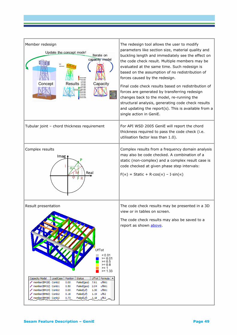
Result presentation
The code check results may be presented in a 3D
view or in tables on screen.
The code check results may also be saved to a
report as shown above.
Sesam Feature Description – GeniE Page 50
Supported standards for member and tubular joint checking
FEATURE DESCRIPTION
American offshore standards
API-WSD 2002 – Offshore structures
• Tubular: American Petroleum Institute RP 2A-WSD
(21st edition December 2000, Errata and Supplement
1, December 2002)
• Non-tubular: American National Standard;
Specification for Structural Steel Buildings, AISC 360-
xx (Steel Construction Manual 13th, 14th and 15th
editions)
API-WSD 2005 – Offshore structures
• Tubular: American Petroleum Institute RP 2A-WSD
(21st edition December 2000, Errata and Supplement
2, October 2005)
• Non-tubular: American National Standard;
Specification for Structural Steel Buildings, AISC 360-
xx (Steel Construction Manual 13th, 14th and 15th
editions)
API-WSD 2014 – Offshore structures
• Tubular: American Petroleum Institute RP 2A-WSD
(22nd edition November 2014)
• Non-tubular: American Institute of Steel Construction,
Allowable Stress Design and Plastic Design, AISC 9th
(June 1, 1989)
API-LRFD 2003 – Offshore structures
• Tubular: American Petroleum Institute LRFD (1st
Edition/July 1, 1993/ Reaffirmed, May 16, 2003)
• Non-tubular: American National Standard;
Specification for Structural Steel Buildings, AISC 360-
xx (Steel Construction Manual 13th, 14th and 15th
editions)

Sesam Feature Description – GeniE Page 51
NORSOK offshore standards
NORSOK 2004 and 2013 – Offshore structures
• Tubular: NORSOK STANDARD N-004, Rev. 2, October
2004, and Rev. 3, February 2013. Design of steel
structures
• Non-tubular: EUROCODE 3, EN 1993 Part 1-1: General
rules and rules for buildings. It is also possible to
select the preferences according to the Norwegian and
Danish National Annexes
ISO offshore standards
ISO 19902 2007 – Offshore structures
• Tubular: INTERNATIONAL STANDARD ISO 19902,
Petroleum and natural gas industries — Fixed steel
offshore structures (First edition 1 December 2007)
• Non-tubular: EUROCODE 3, EN 1993 Part 1-1: General
rules and rules for buildings. It is also possible to
select the preferences according to the Norwegian and
Danish National Annexes
American onshore standards
AISC 360-05, 360-10 and 360-16 – Onshore structures:
• Tubular and non-tubular: American National Standard;
Specification for Structural Steel Buildings”, versions
from March 9 2005, June 22 2010 and July 7 2016.
These versions are supported by AISC Steel
Construction Manual 13th, 14th and 15th editions. The
check covers design/utilisation of members according
to the provisions for Load and Resistance Factor
Design (LRFD) or to the provisions for Allowable
Strength Design (ASD).
AISC 335-89 – Onshore structures
• Tubular and non-tubular: American National Standard;
Specification for Structural Steel Buildings”, June 1
1989. This version is supported by AISC Steel
Construction Manual 9th edition. The check covers
design/utilisation of members according to the
provisions for Allowable Stress Design and Plastic
Design (ASD).
EUROCODE onshore standard
EUROCODE 3 – Onshore structures
• Tubular and non-tubular: EUROCODE 3, EN 1993 Part
1-1: General rules and rules for buildings. It is also
possible to select the preferences according to the
Norwegian and Danish National Annexes

Sesam Feature Description – GeniE Page 52
Danish onshore and offshore standard
DANISH STANDARD 412 / 449 – Onshore and offshore
structures
• Tubular profiles only in both DS 412 and DS 449

Sesam Feature Description – GeniE Page 53
Plate code checking – requires extension CCPL
FEATURE DESCRIPTION
Code check analysis For CSR Bulk both panel yielding and buckling are assessed.
For CSR panel buckling according to PULS is assessed.
Code checking model The capacity model is generated in GeniE. There are three
different ways to create the panel capacity models.
Supported standards CSR Bulk: Common Structural Rules for Bulk Carriers, IACS,
January 2006
CSR Tank – July 2008: Common Structural Rules for Double
Hull Oil Tankers with Length 150 Metres and Above, IACS, July
2008
Redesign The user may add local details to the code checking models
such as stiffener locations. For refined design of panels
according to the PULS standard it is possible to export the
data to a separate tool (requires an installation of Nauticus
Hull). By this tool, it is possible to modify all parameters like
load, thickness, material, section type, locations and boundary
conditions.
Result presentation The code check results may be presented in a 3D view or in
tables.
Fatigue for floating structures Fatigue screening and calculations
Sesam Feature Description – GeniE Page 54
Import and export data in GeniE
FEATURE DESCRIPTION
Section library GeniE includes section libraries for the AISC, Euronorm &
Norwegian and the British Standards. There are also several
hull specific profiles for angle, bulb, flatbar and tbar. Users
may create their own libraries for sharing and re-use.
Material library GeniE comes with a material library consisting of about 70
material types. Users may also create their own libraries.
GeniE XML file The XML (eXtended Markup Language) is the most complete
storage format for GeniE models. It contains all definitions to
recreate structure, loads, analysis set-ups and member code
checking. It is the most secure source of data export and
import. It is also used when upgrading model data to a newer
release of GeniE.
GeniE JS file The js file based on JavaScript and is a log of all user
commands except graphic manipulations. It can be edited and
used as input. Utilizing the power of the JavaScript the js file
can be used for parametric modelling.
GeniE condensed JS file GeniE may export a condensed js file (also referred to as
“clean JS file”). This is a file for recreating the model as is
without the steps of its creation. The exported js file is
intended for use in jacket and topside modelling as it does not
cover curved surfaces or punched plates/surfaces.
Sesam Input Interface File
also termed FEM file
and T file
This file includes the finite element data. It is used by the
other Sesam analysis tools. The FEM file can also be imported
into GeniE for modification. This file is used for converting old
Sesam models to GeniE format. Note that a curved surface is
represented as facetted elements in a FEM file and will be
imported as such.
Wajac.INP
Wajac analysis control (input) file
GeniE will export a Wajac.inp file for use by the wave and wind
load analysis in Wajac. GeniE may also import data from a
Wajac.inp file.
Gensod.INP
Gensod input file
GeniE will export a Gensod.inp file for use by the pile-soil
analysis. GeniE may also import data from a Gensod.inp file.
For import and export towards external software and formats see subsection ‘Import and Export
Features of Sesam’ in section ‘Introduction to Sesam’.

Sesam Feature Description – HydroD Page 55
HydroD HYDRODYNAMIC AND HYDROSTATIC ANALYSIS
Last revised: January 9, 2019. Describing versions 4.10-01 (32-bit) and 5.1-07 (64-bit).
HydroD is a tool for:
• Hydrostatic and stability analysis (version 5.1-07)
• Hydrodynamic (wave load and motion response) analysis (version 4.10-01)
As concerns hydrodynamics, the environment is modelled in HydroD while the hydrodynamic analysis is
performed by running Wadam (linear frequency domain theory) or Wasim (non-linear time domain
theory) in the background. The panel model is normally created in GeniE but will in certain cases be
created in HydroD. HydroD provides analysis workflows for execution of Wadam and Wasim. Multiple
floating equilibrium positions can be computed depending on mass and compartment filling.

Sesam Feature Description – HydroD Page 56
FEATURES OF HYDROD
General features
FEATURE DESCRIPTION
Analysis types - stability
HydroD provides the following stability analysis
types:
• Hydrostatic balancing
• Stability analysis
• Maximum KG analysis
• Strength analysis
• Watertight and weathertight surfaces
Analysis types - hydrodynamics
HydroD provides the following hydrodynamic
analysis types:
• Frequency domain analysis of stationary
floating or fixed rigid bodies (Wadam)
• Deterministic analysis of floating or fixed
rigid bodies (Wadam)
• Time domain analysis of floating or fixed
rigid bodies (Wasim)
• Time domain analysis of ships with forward
speed, with conversion to frequency
domain (Wasim)
Unit support
m? mm? inch?
The user may mix units throughout the modelling.
The data logging (scripting) ensures that re-
creating the model gives the same result.

Sesam Feature Description – HydroD Page 57
Wizards
Wizards are available for guiding the user through
all necessary steps to set up the following
analyses:
• Stability
• Linear hydrodynamic analysis in Wadam
• Non-linear hydrodynamic analysis in
Wasim
Colour coding properties
All properties may be displayed in separate colours
for verification purposes.
Save Clean JS
Save a complete and cleaned-up JS script file
containing all the objects in your workspace in a
defined sequence.
Read Command File (JS file)
A JS script file may be edited and used as input.
HydroD 5.1 and later can read a JS file also from
HydroD 4.10.

Sesam Feature Description – HydroD Page 58
Graph control
Many of the dialogs utilize a graph control allowing
manipulation of the graph.
Features for hydrostatic analysis
Hydrostatic and stability computations may be run for both intact and damage conditions. HydroD will
compute the draught and heel/trim angles to ensure equilibrium. Compartments may be flooded or
balanced by HydroD. A wind heeling moment, user defined or calculated by HydroD, may be included.
FEATURE DESCRIPTION
Hydrostatic data
Hydrostatic data are computed:
• Displaced volume
• Mass with and without compartment fluid
• Centre of gravity and centre of buoyancy
• Centre of flotation
• Metacentre
• Trim moment
• Compartment information
Compartments
• Compartments are employed in hydrostatic
and stability computations
• The free surface inside compartments is
always horizontal
• The free surface in damaged
compartments is always at the free surface
level.
Hydrostatic balancing of compartments HydroD may calculate the filling ratio of
compartments necessary to obtain equilibrium of
gravity and buoyancy forces.
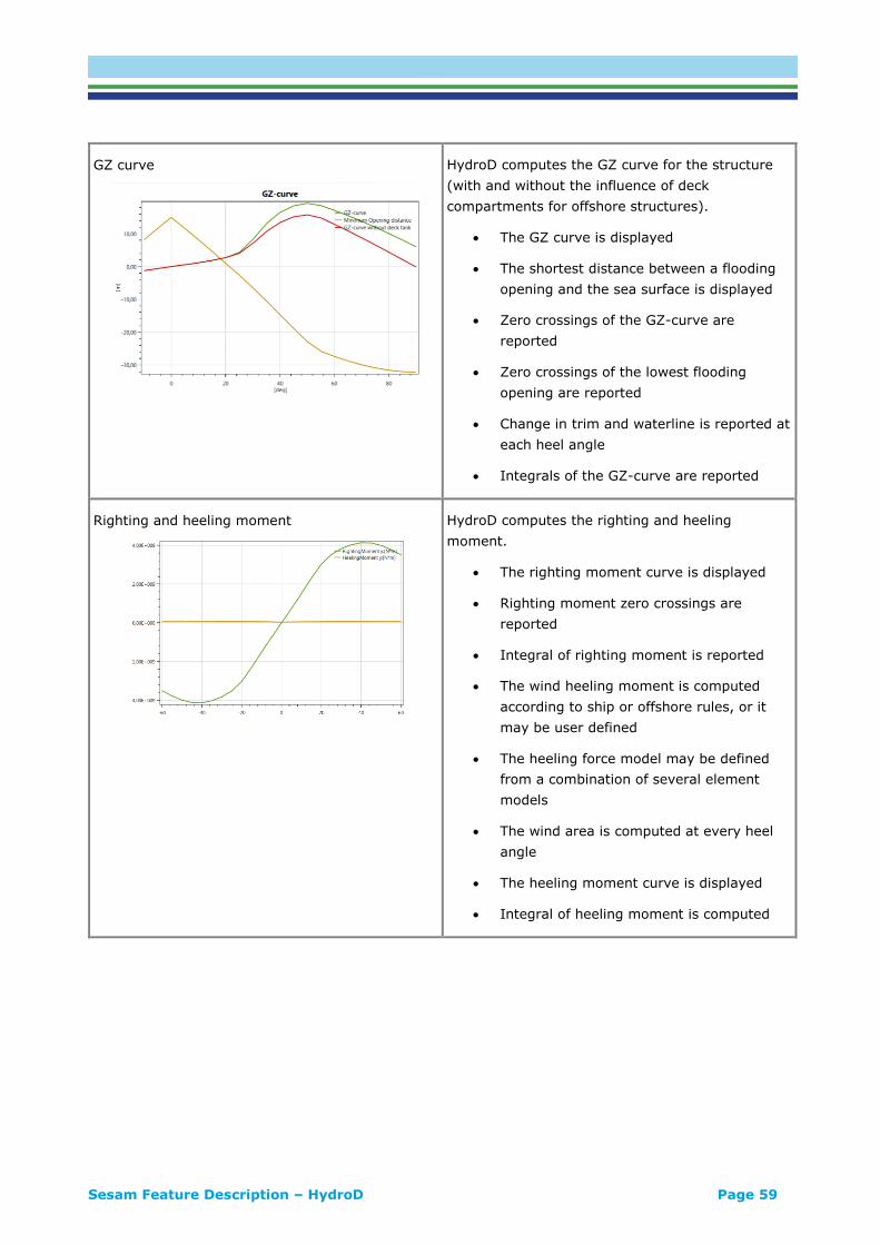
Sesam Feature Description – HydroD Page 59
GZ curve
HydroD computes the GZ curve for the structure
(with and without the influence of deck
compartments for offshore structures).
• The GZ curve is displayed
• The shortest distance between a flooding
opening and the sea surface is displayed
• Zero crossings of the GZ-curve are
reported
• Zero crossings of the lowest flooding
opening are reported
• Change in trim and waterline is reported at
each heel angle
• Integrals of the GZ-curve are reported
Righting and heeling moment
HydroD computes the righting and heeling
moment.
• The righting moment curve is displayed
• Righting moment zero crossings are
reported
• Integral of righting moment is reported
• The wind heeling moment is computed
according to ship or offshore rules, or it
may be user defined
• The heeling force model may be defined
from a combination of several element
models
• The wind area is computed at every heel
angle
• The heeling moment curve is displayed
• Integral of heeling moment is computed

Sesam Feature Description – HydroD Page 60
Openings
Flooding openings in the hull may be defined at
selected locations.
• Openings can be Unprotected,
Weathertight or Watertight
• Heeling angle of intersection with the
waterline is printed
• An unprotected opening may be connected
to a compartment, making this flooded
when the opening becomes submerged
Strength analysis
HydroD computes the sectional loads in the still
water condition on the specified side of the defined
cross sections.
• Cross sectional loads, forces and moments,
may be both displayed, e.g. longitudinal
bending moment, and printed
• Mass and buoyancy distribution may also
be displayed

Sesam Feature Description – HydroD Page 61
Hydrostatic rule checks
HydroD may check the analysis results against
rules defined by internationally recognised codes:
• IMO general
• MARPOL (tanker) intact
• MARPOL (tanker) damage
• IGC (liquefied gas in bulk) damage
• IBC (chemicals in bulk) damage
• NMD (mobile offshore units) intact
• NMD (mobile offshore units) damage
• DNV GL intact
• DNV GL damage
• IMO MODU (mobile offshore units) intact
• IMO MODU (mobile offshore units) damage
• ABS MODU (mobile offshore units) intact
• ABS MODU (mobile offshore units) damage
• User defined
Maximum KG analysis
HydroD can perform an AVCG/MaximumKG
analysis based on the following rules
• IMO general
• MARPOL (tanker) intact
• MARPOL (tanker) damage
• IGC (liquefied gas in bulk) damage
• IBC (chemicals in bulk) damage
• NMD (mobile offshore units) intact
• NMD (mobile offshore units) damage
• DNV GL intact
• DNV GL damage
• IMO MODU (mobile offshore units) intact
• IMO MODU (mobile offshore units) damage
• ABS MODU (mobile offshore units) intact
• ABS MODU (mobile offshore units) damage

Sesam Feature Description – HydroD Page 62
Limit surfaces
Watertight and weathertight integrity surfaces can
be computed and displayed.
Beach lines
Beach lines, intersection of a horizontal plane and
a limit surface, can be computed and displayed.
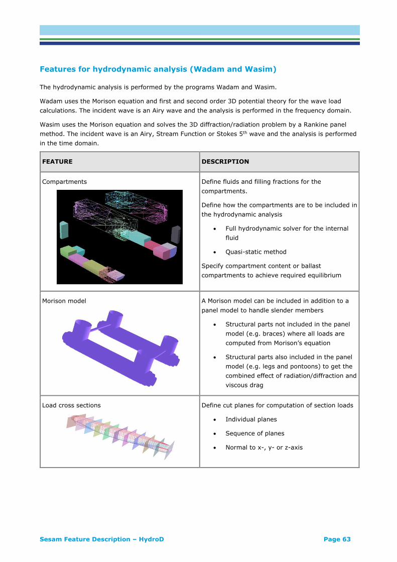
Sesam Feature Description – HydroD Page 63
Features for hydrodynamic analysis (Wadam and Wasim)
The hydrodynamic analysis is performed by the programs Wadam and Wasim.
Wadam uses the Morison equation and first and second order 3D potential theory for the wave load
calculations. The incident wave is an Airy wave and the analysis is performed in the frequency domain.
Wasim uses the Morison equation and solves the 3D diffraction/radiation problem by a Rankine panel
method. The incident wave is an Airy, Stream Function or Stokes 5th wave and the analysis is performed
in the time domain.
FEATURE DESCRIPTION
Compartments
Define fluids and filling fractions for the
compartments.
Define how the compartments are to be included in
the hydrodynamic analysis
• Full hydrodynamic solver for the internal
fluid
• Quasi-static method
Specify compartment content or ballast
compartments to achieve required equilibrium
Morison model
A Morison model can be included in addition to a
panel model to handle slender members
• Structural parts not included in the panel
model (e.g. braces) where all loads are
computed from Morison’s equation
• Structural parts also included in the panel
model (e.g. legs and pontoons) to get the
combined effect of radiation/diffraction and
viscous drag
Load cross sections
Define cut planes for computation of section loads
• Individual planes
• Sequence of planes
• Normal to x-, y- or z-axis

Sesam Feature Description – HydroD Page 64
Multi-body model
Create a multi-body model. The model can include
different bodies or multiple occurrences of the
same body, possibly with different loading
conditions.
Global response
A global response analysis may include:
• First order wave excitation forces and
moments
• Second order wave excitation forces and
moments (used to model springing effects,
low frequency forces etc.)
• Hydrodynamic added mass and damping
• First and second order rigid body motions
• Sectional forces and moments
• Steady drift forces and moments
• Wave drift damping
• Sectional load components (mass, added
mass, damping and excitation forces)
• Panel pressures
• Fluid particle kinematics (for gap
calculations and free surface animation)
• Second order free surface elevations
• Calculation of selected global responses of
a multi-body system
Transfer of structural loads
Transfer of structural loads to a finite element (FE)
model may include:
• Inertia loads
• Line loads on beam elements from Morison
model
• Point loads from pressure areas, anchor
elements etc. from Morison model
• Pressure loads on plate/shell/solid
elements
• Internal tank pressure in compartments

Sesam Feature Description – HydroD Page 65
Environment
Define the environment that is to be used in a
hydrodynamic analysis.
• Frequency domain condition for
computation of transfer functions
• Regular wave set for time domain
simulation
• Irregular time domain condition (a
realization of a given sea state)
Section model
A set of curves describing the hull. Can be
imported from a “pln-file” (Sesam internal format)
or DXF file with curves given as polylines.
HydroD can make a panel model from a section
model.
Automatic creation of mesh from section model
Create mesh on hull for Wadam (panel model)
and/or create mesh on hull and free surface for
Wasim.
Free surface mesh can also be used for Wadam
wave/current interaction or wave elevation
animation.

Sesam Feature Description – HydroD Page 66
Interactive creation of free surface meshes
A separate tool, HydroMesh version 3.1-01, is
started from HydroD to create free surface meshes
for:
• Damping lids for single or multi-body
problems
• Internal lids for irregular frequency
removal
• Free surface mesh for wave elevation
animation
• Free surface mesh for second-order
analysis or wave/current interaction and
wave drift damping analysis
• Free surface mesh for Wasim analysis if
the automatically created mesh is not good
enough
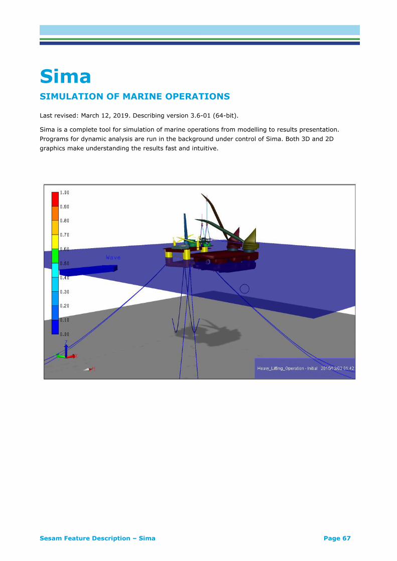
Sesam Feature Description – Sima Page 67
Sima SIMULATION OF MARINE OPERATIONS
Last revised: March 12, 2019. Describing version 3.6-01 (64-bit).
Sima is a complete tool for simulation of marine operations from modelling to results presentation.
Programs for dynamic analysis are run in the background under control of Sima. Both 3D and 2D
graphics make understanding the results fast and intuitive.

Sesam Feature Description – Sima Page 68
FEATURES OF SIMA
FEATURE DESCRIPTION
GUI for Simo, Riflex and Vivana
Sima supports various types of analysis. Sima is
used as the general GUI and platform for various
calculation programs such as Simo, Riflex and
Vivana.
Wave, swell, current and wind
Wave, swell, current and wind can be specified with
different spectrums and profiles. They can have
either collinear or different incoming directions.
Hydrodynamic coefficients
Hydrodynamic coefficients can be read into Sima
directly, i.e. added mass and damping coefficients,
first and second order wave forces, etc.
Retardation function can also be calculated.
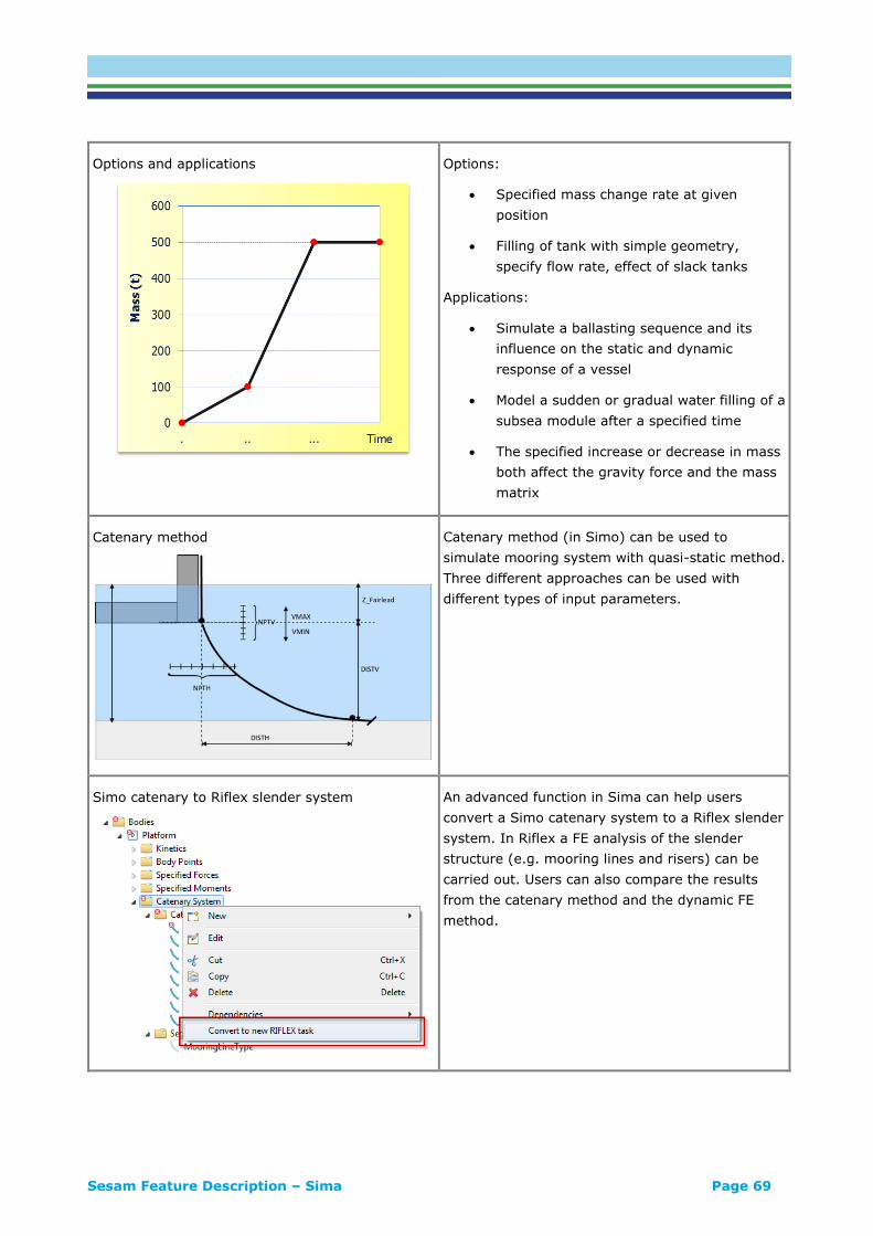
Sesam Feature Description – Sima Page 69
Options and applications
Options:
• Specified mass change rate at given
position
• Filling of tank with simple geometry,
specify flow rate, effect of slack tanks
Applications:
• Simulate a ballasting sequence and its
influence on the static and dynamic
response of a vessel
• Model a sudden or gradual water filling of a
subsea module after a specified time
• The specified increase or decrease in mass
both affect the gravity force and the mass
matrix
Catenary method
Catenary method (in Simo) can be used to
simulate mooring system with quasi-static method.
Three different approaches can be used with
different types of input parameters.
Simo catenary to Riflex slender system
An advanced function in Sima can help users
convert a Simo catenary system to a Riflex slender
system. In Riflex a FE analysis of the slender
structure (e.g. mooring lines and risers) can be
carried out. Users can also compare the results
from the catenary method and the dynamic FE
method.
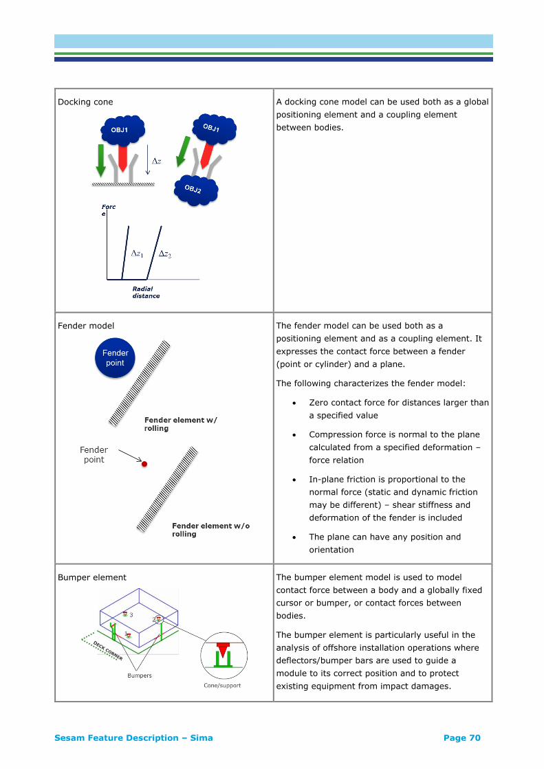
Sesam Feature Description – Sima Page 70
Docking cone
A docking cone model can be used both as a global
positioning element and a coupling element
between bodies.
Fender model
The fender model can be used both as a
positioning element and as a coupling element. It
expresses the contact force between a fender
(point or cylinder) and a plane.
The following characterizes the fender model:
• Zero contact force for distances larger than
a specified value
• Compression force is normal to the plane
calculated from a specified deformation –
force relation
• In-plane friction is proportional to the
normal force (static and dynamic friction
may be different) – shear stiffness and
deformation of the fender is included
• The plane can have any position and
orientation
Bumper element
The bumper element model is used to model
contact force between a body and a globally fixed
cursor or bumper, or contact forces between
bodies.
The bumper element is particularly useful in the
analysis of offshore installation operations where
deflectors/bumper bars are used to guide a
module to its correct position and to protect
existing equipment from impact damages.
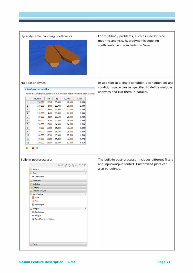
Sesam Feature Description – Sima Page 71
Hydrodynamic coupling coefficients
For multibody problems, such as side-by-side
mooring analysis, hydrodynamic coupling
coefficients can be included in Sima.
Multiple analyses
In addition to a single condition a condition set and
condition space can be specified to define multiple
analyses and run them in parallel.
Built-in postprocessor
The built-in post-processor includes different filters
and input/output control. Customized plots can
also be defined.

Sesam Feature Description – Sima Page 72
Floating wind turbine
A floating wind turbine can also be simulated in
Sima. The blades, turbine and control system can
either be specified in Sima or be given by link to
an external controller. The hydrodynamics of the
floating substructure can be read from general
hydrodynamic analysis programs. The mooring
system is defined in Sima. The whole system can
be analysed in time domain by a fully coupled
method.
Aquaculture
Sima also provides modelling possibilities for fish
nets and fish cages. The floating ring, bottom ring
etc. have formulations for partial submergence of
horizontal slender structures. The net is modelled
as a slender structure, where the user inputs the
flow reduction factor manually.
Fish net models can be combined with other Simo
and Riflex elements, e.g. mooring system,
connection cables and vessels.

Sesam Feature Description – Sima Page 73
Workflows
Workflows can be set up in Sima to prepare input,
run Sima models, do post-processing and store
results in various formats. A workflow can contain
other workflows (nesting), post-processors and
external programs, visualized as flowcharts.
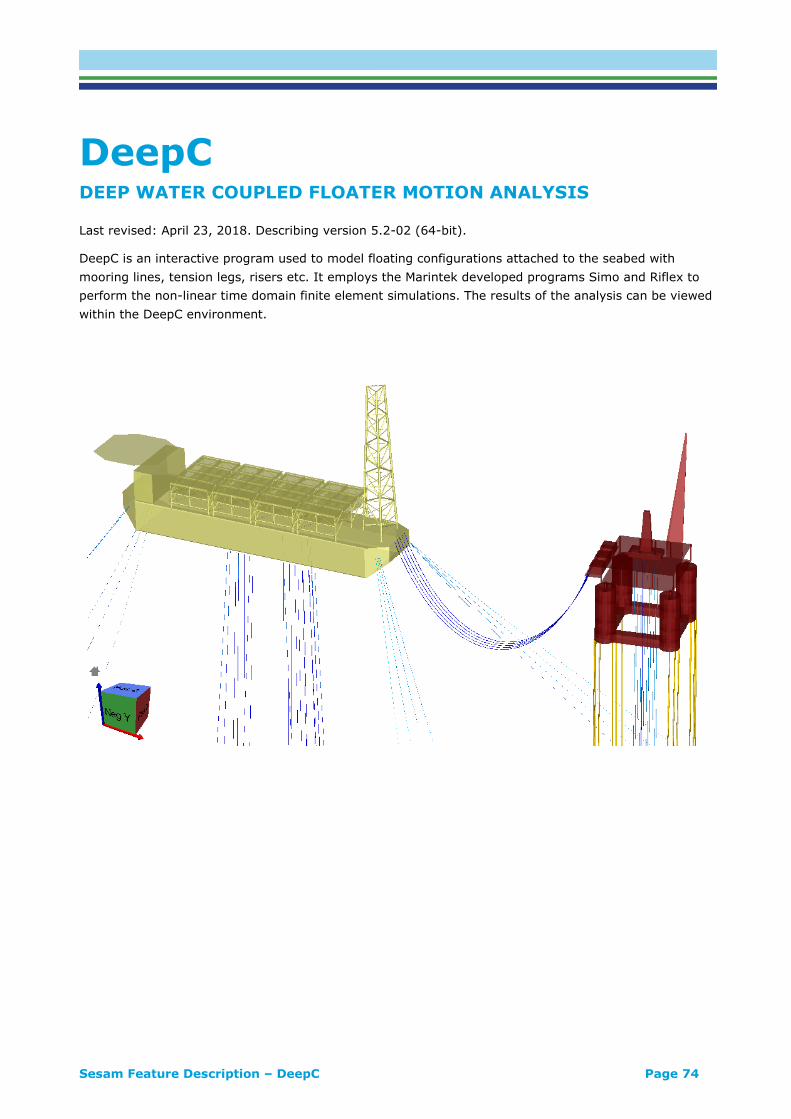
Sesam Feature Description – DeepC Page 74
DeepC DEEP WATER COUPLED FLOATER MOTION ANALYSIS
Last revised: April 23, 2018. Describing version 5.2-02 (64-bit).
DeepC is an interactive program used to model floating configurations attached to the seabed with
mooring lines, tension legs, risers etc. It employs the Marintek developed programs Simo and Riflex to
perform the non-linear time domain finite element simulations. The results of the analysis can be viewed
within the DeepC environment.

Sesam Feature Description – DeepC Page 75
FEATURES OF DEEPC
FEATURE DESCRIPTION
Unit support
m? mm? inch?
The user may mix units throughout the modelling.
The data logging (scripting) ensures that re-
creating the model gives the same result.
Locations and environments
Environment modelling includes:
• Current and wind profiles
• Wave and wind spectra
• Seafloor properties (stiffness, friction)
• Locations (site specific data such as water
depth, gravity, water density, seabed etc.)
• Regular time conditions including current
• Irregular time conditions including wind
data, wind generated wave data, swell and
current
• Scatter diagrams and discretization
Floaters definition
Any number of vessels may be modelled and
employed in the analysis. Main parameters include:
• Hydrodynamic coefficients read in from
HydroD
o Added mass and potential damping
o 1st and 2nd order wave excitation
o RAOs
o Etc.
• Wind and current coefficients
• Vessel damping coefficients
• Additional viscous force elements used to
capture the Morison forces on the beam
structure
• Specified point forces
DeepC automatically calculates retardation
functions from added mass and damping
coefficients.

Sesam Feature Description – DeepC Page 76
Slender structure properties
Structure properties describe common attributes
on geometrical entities.
Sections: Different kinds of cross sections for
segments and stress joints (pipe, axi-symmetric
etc.)
Load Interfaces: Contains Morison coefficients,
segment external wrapping and segment marine
growth properties.
Materials: Contains material definitions.
Mesh Densities: Contains mesh density properties
for segments and stress joints.
Slender Components: Internal fluid, buoy
common properties, rotation hinge properties,
stress concentration factors, SN-curves and
section stress parameters.
Combined Loading: Contains material, pipe cross
section and fluid properties for combined loading
analyses only.
Fatigue: Contains SN-curve, stress concentration
factor and cross sectional properties for fatigue
analyses only.
Slender structures
Various slender structures, including mooring and
riser, tendon, jumper, etc. can be modelled by:
• Segmented lines (any number of
segments)
• Stress joints (lines with piecewise linearly
varying tubular cross section)
• Ball joints, buoys, flex joints
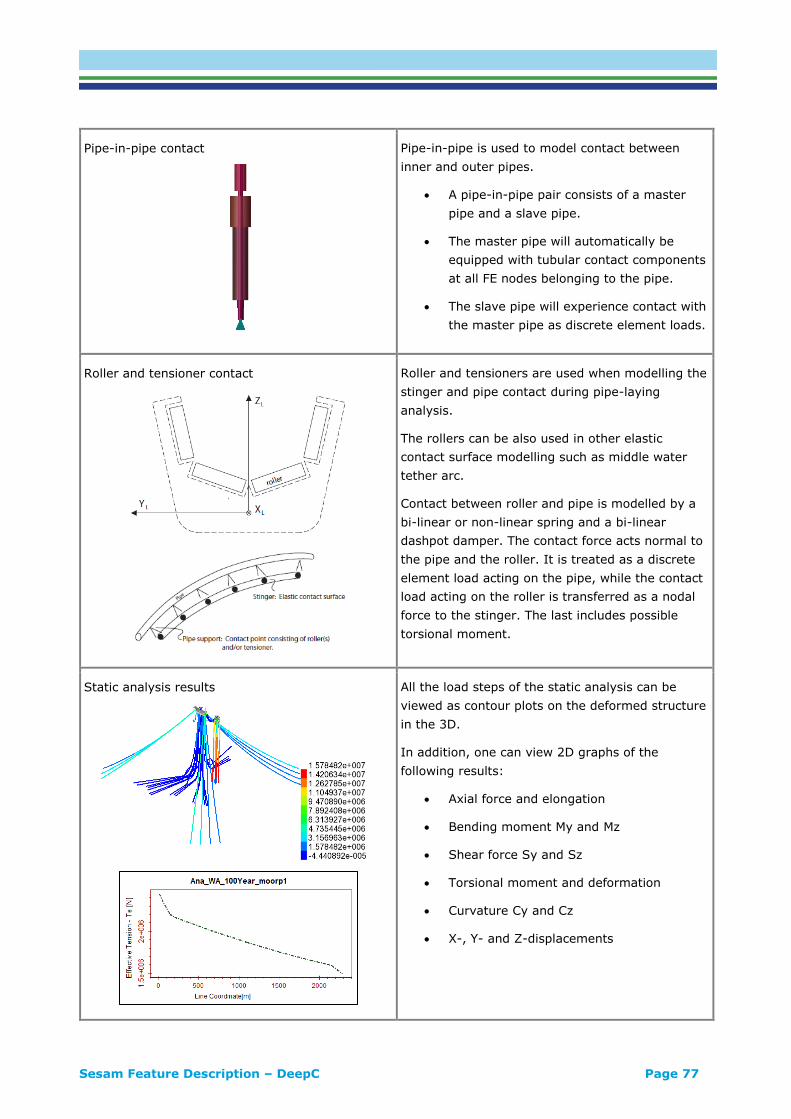
Sesam Feature Description – DeepC Page 77
Pipe-in-pipe contact
Pipe-in-pipe is used to model contact between
inner and outer pipes.
• A pipe-in-pipe pair consists of a master
pipe and a slave pipe.
• The master pipe will automatically be
equipped with tubular contact components
at all FE nodes belonging to the pipe.
• The slave pipe will experience contact with
the master pipe as discrete element loads.
Roller and tensioner contact
Roller and tensioners are used when modelling the
stinger and pipe contact during pipe-laying
analysis.
The rollers can be also used in other elastic
contact surface modelling such as middle water
tether arc.
Contact between roller and pipe is modelled by a
bi-linear or non-linear spring and a bi-linear
dashpot damper. The contact force acts normal to
the pipe and the roller. It is treated as a discrete
element load acting on the pipe, while the contact
load acting on the roller is transferred as a nodal
force to the stinger. The last includes possible
torsional moment.
Static analysis results
All the load steps of the static analysis can be
viewed as contour plots on the deformed structure
in the 3D.
In addition, one can view 2D graphs of the
following results:
• Axial force and elongation
• Bending moment My and Mz
• Shear force Sy and Sz
• Torsional moment and deformation
• Curvature Cy and Cz
• X-, Y- and Z-displacements

Sesam Feature Description – DeepC Page 78
Dynamic analysis results
Users can plot and export time-series results of
different forces and displacement, including:
• Vessel 6-DOF motions
• Wave forces
• Effective tension
• Bending moment about local y- and z-axes
• Resulting bending moment
• Decomposed line end forces in global X-,
Y- and Z-directions
• Nodal displacement in global X-, Y- and Z-
directions
• Element curvature
• Etc.
Animation
3D animations of vessels and lines displacements
with contour colour of forces or bending moments
on the lines.
These are displayed in Xtract.

Sesam Feature Description – DeepC Page 79
Post-processing
DeepC also provides in-built post-processing
calculation for all kinds of time series including:
• Energy spectra
• Cumulative distributions
• Cumulative distribution function on Weibull
paper
• High and low frequency filtering
• Range curves of effective tension showing
max/min/mean and standard deviation
along the lines
Fatigue evaluation
For both regular and irregular time condition
analyses DeepC can perform fatigue calculations
by rainflow counting and Miner-Palmgren
summation.
Fatigue results include 3D contour plots of fatigue
life and 2D graphs of fatigue life along the lines.
Code check for metallic risers
Based on regular or irregular time domain riser
analysis combined loading capacity analysis may
be performed. Available codes are DNV OS-F201
and ISO 13628-7.
Combined loading results include 3D contour plots
and 2D graphs of utilization factor along riser.

Sesam Feature Description – Presel Page 80
Presel PREPROCESSOR FOR ASSEMBLING SUPERELEMENTS
Last revised: August 22, 2017. Describing version 7.5-01.
Presel is Sesam’s tool for assembling superelements to form the complete model. A superelement is
basically a finite element (FE) model of a part of the complete structure. The Sesam preprocessors GeniE
and Patran-Pre are used for creating first level superelements, i.e. part models comprised of finite
elements like beams, shells, etc. Presel puts these parts together to form superelement assemblies. First
level superelements are typically assembled to form second level superelement assemblies, these are in
turn assembled to form third level superelement assemblies, and so on until the complete model — the
top level superelement assembly — is formed.

Sesam Feature Description – Presel Page 81
FEATURES OF PRESEL
Assembling a superelement consists of two steps:
• Assemble superelements (assemble geometry)
• Assemble or combine loads
These two steps are repeated for all higher level (from 2 and up) superelements created in Presel.
FEATURE DESCRIPTION
Assembling superelements
All 1st level superelements (created by GeniE and
Patran-Pre) may be assembled into a 2nd level
superelement.
Or they may be assembled through any number of
levels to form the complete model.
Any superelement at any level may be repeatedly
included in an assembly. This may be done for
geometrically identical parts.
Include by transformation
When including a superelement into an assembly it
may be:
• Translated
• Rotated
• Mirrored
• Fitted by referring to two sets of three
nodes to be matched
Print superelement hierarchy
Assembling superelements to form the complete
model results in a superelement hierarchy. This
may be printed for verification.
Display of superelement
Any superelement at any level from 1st level
superelements created by GeniE and Patran-Pre to
the top level superelement, the complete model,
may be displayed with colours distinguishing the
individual superelements.

Sesam Feature Description – Presel Page 82
Boundary conditions
Boundary conditions may be added to higher level
superelements (from 2nd level and up). 1st level
superelements may not be modified in Presel:
• Fixed
• Prescribed
• Super
Load combination
The load combination may be done in two ways:
• Manually by specifying all loads of included
superelements contributing to the
combination
• A group of loads combined one-to-one into
a group of load combinations. This is
useful for loads created by Wajac and
Wadam.
Loads Nodal loads may be added to any higher level
superelement.
Sets Sets of nodes may be defined. These are available
in the postprocessors (Framework, Stofat, and
Xtract).
Node triplet
Nodes are referred to by so-called triplets, i.e.
three numbers being the superelement number,
the superelement index and the node number. The
superelement index is a number starting at 1 and
incremented each time the same superelement is
included.
Label Node symbols and node numbers may be added to
the display:
• Boundary conditions
• Coupled nodes (where superelements join)
• Non-coupled nodes
• Node symbols (yellow diamond for free,
blue octagon for super)
• Node numbers
• Origin symbol

Sesam Feature Description – Presel Page 83
Linear dependency Linear dependencies by making one or more
degrees of freedom (dofs) linearly dependent on
one or more other (independent) dofs.
Plot
CGM →
The display may be sent to a file in alternative
graphics formats:
• CGM-Binary (Computer Graphics Metafile
which may be imported into MS Office)
• Postscript
Or the display may be sent directly to an on-line
printer.
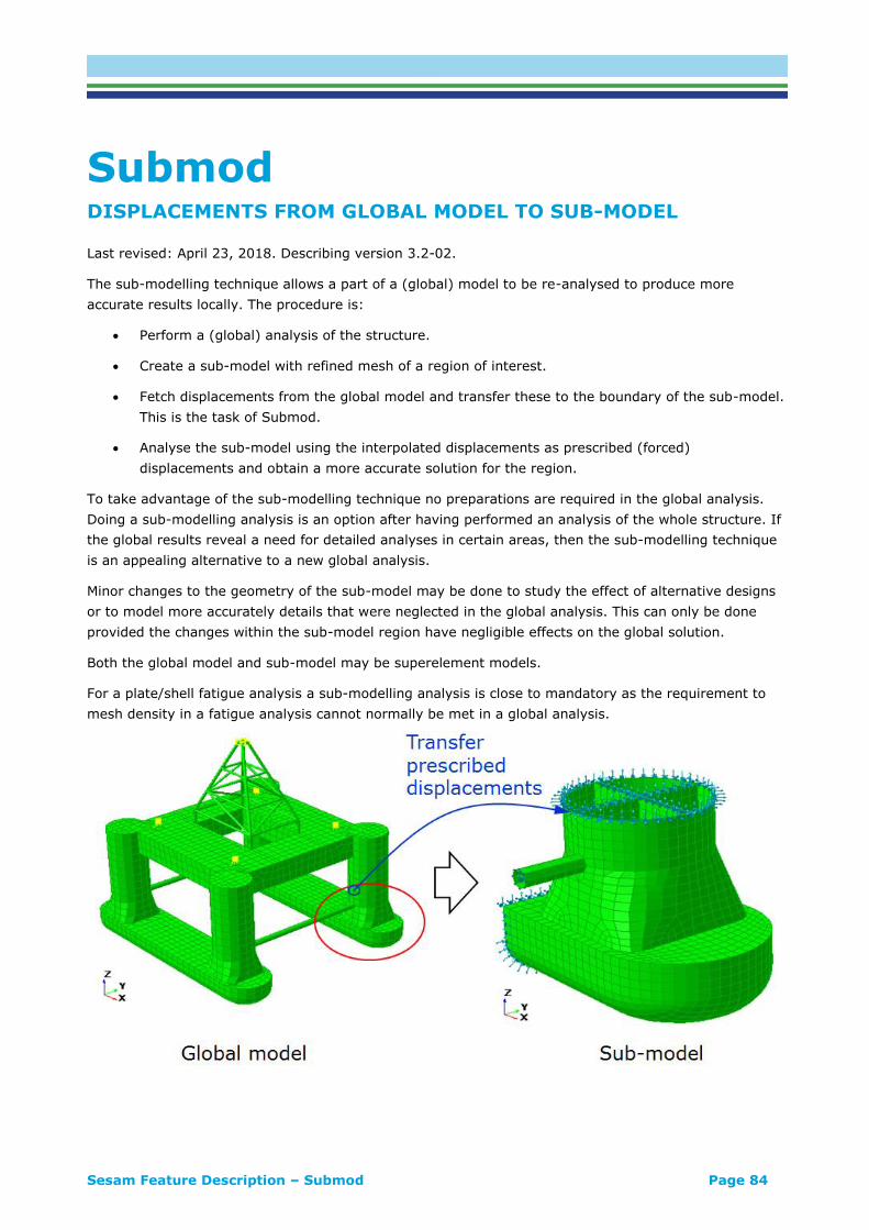
Sesam Feature Description – Submod Page 84
Submod DISPLACEMENTS FROM GLOBAL MODEL TO SUB-MODEL
Last revised: April 23, 2018. Describing version 3.2-02.
The sub-modelling technique allows a part of a (global) model to be re-analysed to produce more
accurate results locally. The procedure is:
• Perform a (global) analysis of the structure.
• Create a sub-model with refined mesh of a region of interest.
• Fetch displacements from the global model and transfer these to the boundary of the sub-model.
This is the task of Submod.
• Analyse the sub-model using the interpolated displacements as prescribed (forced)
displacements and obtain a more accurate solution for the region.
To take advantage of the sub-modelling technique no preparations are required in the global analysis.
Doing a sub-modelling analysis is an option after having performed an analysis of the whole structure. If
the global results reveal a need for detailed analyses in certain areas, then the sub-modelling technique
is an appealing alternative to a new global analysis.
Minor changes to the geometry of the sub-model may be done to study the effect of alternative designs
or to model more accurately details that were neglected in the global analysis. This can only be done
provided the changes within the sub-model region have negligible effects on the global solution.
Both the global model and sub-model may be superelement models.
For a plate/shell fatigue analysis a sub-modelling analysis is close to mandatory as the requirement to
mesh density in a fatigue analysis cannot normally be met in a global analysis.

Sesam Feature Description – Submod Page 85
FEATURES OF SUBMOD
FEATURE DESCRIPTION
Fetch and transfer displacements
The sub-model must have prescribed type of
boundary condition at its edges where it is cut out
of the global model.
Submod compares geometrically the global model
and sub-model to determine the position of
prescribed nodes within the elements of the global
model.
Node-to-element match
Submod fetches displacements by interpolation
inside the elements using the shape functions of
the elements:
• Any plate/shell element (3, 4, 6 and 8
node)
o Interpolation may be in the
thickness direction
• Any solid element
• 2 and 3 node beam elements but only
along neutral axis
The global model and sub-model may have
different element types.
Node-to-node match Alternatively to interpolating within elements, the
displacements may be fetched from the nearest
node. This is normally not the preferred option.

Sesam Feature Description – Submod Page 86
Verification of results
Submod’s transfer of displacements may be
verified using Xtract.

Sesam Feature Description – Wadam Page 87
Wadam WAVE ANALYSIS BY DIFFRACTION AND MORISON THEORY
Last revised: January 9, 2019. Describing version 9.5-03 (64-bit).
Wadam is an analysis program for calculation of wave-structure interaction for fixed and floating
structures of arbitrary shape, e.g. semi-submersible platforms, tension-leg platforms, gravity-base
structures and ship hulls. Wadam performs hydrodynamic analysis in the frequency domain. The
program is based on the radiation diffraction methodology for large volume structures. For slender
structures the Morison formulation is used to account for the drag effects of such structures. Wadam can
handle a very small forward speed/current. Wadam uses input data generated by HydroD.
The Wadam results are presented directly as complex transfer functions. The loads on the finite element
model can also be given in this way, but they may alternatively be converted to deterministic results for
a specified sequence of phase angles of the incident wave. For fixed structures Morison’s equation may
also be used with deterministic output option to calculate drag forces due to time independent current.
The same analysis model may be applied to both the calculation of global responses in Wadam and the
subsequent structural analysis. For shell and solid element models Wadam also provides automatic
mapping of pressure loads from a panel model to a differently meshed structural finite element model.

Sesam Feature Description – Wadam Page 88
FEATURES OF WADAM
The features of Wadam are summarised below.
Model types
FEATURE DESCRIPTION
Model types
There are three main model types:
• Hydro model used to calculate
hydrodynamic forces
• Structural model onto which hydrodynamic
and hydrostatic loads are transferred
• Mass model for floating structures being
either a model or a mass matrix
Hydro models
The hydro model may be:
• Panel model for potential theory
computations
• Morison model for computation by the
Morison equation
• Composite model being a combination of a
panel and a Morison model for use when
potential theory and the Morison equation
are applied for different parts of the hydro
model
Mass model
The mass can be provided in any of the two forms
• Global mass data
• A file describing the mass distribution
A description of the mass distribution is needed for
computation of sectional loads.
Panel model
The panel model may be a single superelement or a
hierarchy of superelements. It may describe either
the entire wet surface or take advantage of one or
two planes of symmetry.

Sesam Feature Description – Wadam Page 89
Morison model
Morison elements:
• 2D Morison elements for loads on 2 node
beam elements
• 3D Morison elements for loads in three
directions in nodes
• Pressure area elements for loads at the
ends of 2D Morison elements
• Dry Morison elements for beams on which
no load is to be computed
• Anchor and TLP elements for restoring
contributions in nodes. These elements can
be used to provide a simplified model of the
moorings and risers. The element is a
linear spring with pretension.
Composite model
Hydrodynamic forces on a composite model are
computed from potential theory for the panel
model and from the Morison equation for the
Morison model. The hydrodynamic exciting forces
and matrices from both theories are accumulated in
the equations of motion for the composite model.
Multi-body
Hydrodynamic and mechanical interaction between
several structures can be analysed. The
hydrodynamic interaction is computed from the
potential theory as applied for a single structure
with the extension that the number of degrees of
freedom is increased from 6 to 6N where N is the
number of structures. A multi-body model can
contain both fixed and floating bodies.

Sesam Feature Description – Wadam Page 90
Analyses
FEATURE DESCRIPTION
Forward speed/Wave current interaction The effect of a small current or forward speed can
be accounted for. The speed limit is case
dependent, but is typically in the range 1-2 m/s.
The current can be in any direction.
Hydrostatic Calculation of hydrostatic data and inertia
properties
Global response
Global response is calculated including:
• First order wave excitation forces and
moments
• Second order wave excitation forces and
moments (used to model springing effects,
low frequency forces etc.)
• Hydrodynamic added mass and damping
• First and second order rigid body motions
• Sectional forces and moments
• Steady drift forces and moments
• Wave drift damping coefficients
• Sectional load components (mass, added
mass, damping and excitation forces)
• Panel pressures
• Fluid particle kinematics (for gap
calculations and free surface animation)
• Second order free surface elevations

Sesam Feature Description – Wadam Page 91
Transfer of load to structural analysis
FEATURE DESCRIPTION
Load transfer
Panel mesh FE mesh
Automatic load transfer to a finite element model
for subsequent structural analysis including:
• Inertia loads
• Line loads on beam elements from Morison
model
• Point loads from pressure areas, anchor
elements etc. from Morison model
• Pressure loads on plate/shell/solid
elements
• Internal tank pressure in compartments
Load transfer in frequency domain The computed load transfer functions are mapped
onto a finite element model. For the shell/solid
part the mesh need not be the same as the mesh
used in the hydrodynamic analysis (the panel
model). For the beams the model must be identical
in the hydrodynamic and structural analysis.
Deterministic load transfer The loads may alternatively be extracted as real
load cases at specified phase angles during the
wave cycle. In this case a wave amplitude must
also be specified and the load transfer function is
multiplied with this wave amplitude. The loads will
be used in a quasi-static structural analysis.

Sesam Feature Description – Wadam Page 92
Theory and formulation
FEATURE DESCRIPTION
Morison equation
The Morison equation is used for slender (beam)
structures.
Potential theory
𝛻2𝜑(𝑥, 𝑦, 𝑧, 𝑡) = 0
First and second order 3D potential theory is used
for large volume structures. The solution is based
on using the Green’s function formulation.
The Morison equation and potential theory
combined
The forces from Morison equation and potential
theory are added when the structure comprises of
both slender and large volume parts.
Removal of irregular frequencies
Irregular frequencies may be removed from the
radiation-diffraction solution. This method is based
on a modified integral equation obtained by
including a panel model of the internal water
plane.

Sesam Feature Description – Wadam Page 93
Damping lids
The wave elevation in areas where resonance may
happen can be controlled by including a damping
lid on the free surface in those areas.
Tank pressures Tank pressures may be computed
• Quasi-statically
• Dynamically
Roll damping Viscous roll damping included in different ways:
• By using the roll damping models of
Tanaka and Kato
• By using the ITTC roll damping model
• By prescribing a linear and a quadratic
damping coefficient
• By using a Morison model
Additional damping and restoring matrices Additional damping and restoring matrices can be
specified. This can be used for including damping
or restoring from moorings and risers and/or
viscous damping
Pressure loads up to free surface
Panel pressures calculated by first order potential
theory may be extrapolate to the free surface.
Correspondingly, dry elements below the still
water level receive no loads. This is done by
stretching pressures above the still water level.
This option is only for deterministic load transfer.
Reduced pressure around the free surface
This is a recommended option for fatigue analysis
and follows DNV GL Class not 30.7. The pressure is
modified around the waterline. The method should
only be applied on that part of the vessel which
has vertical intersection with the free surface.

Sesam Feature Description – Wasim Page 94
Wasim LINEAR AND NON-LINEAR SEA-KEEPING AND WAVE LOADS ON
VESSELS WITH FORWARD SPEED
Last revised: January 9, 2019. Describing version 5.5-09 (64-bit).
Wasim is an analysis program for calculation of wave-structure interaction for fixed and floating
structures. Wasim performs hydrodynamic analysis in time domain, but also includes an option for
conversion to frequency domain. The program is based on the radiation diffraction methodology for large
volume structures. For slender structures the Morison formulation is used to account for the drag effects
of such structures. Wasim can handle any forward speed from zero to very high as long as the vessel is
not planing. Wasim uses input data generated by HydroD. The forward speed problem may alternatively
be regarded as a wave/current interaction problem with the forward speed replaced by a uniform current
in the opposite direction.
The same analysis model may be applied to both the calculation of global responses in Wasim and the
subsequent structural analysis. For shell and solid element models Wasim also provides automatic
mapping of pressure loads from a panel model to a differently meshed structural finite element model.
The 3D potential theory in Wasim is based on a Rankine formulation. This means that both the hull and
free surface must be meshed. HydroD has tools for meshing the free surface.
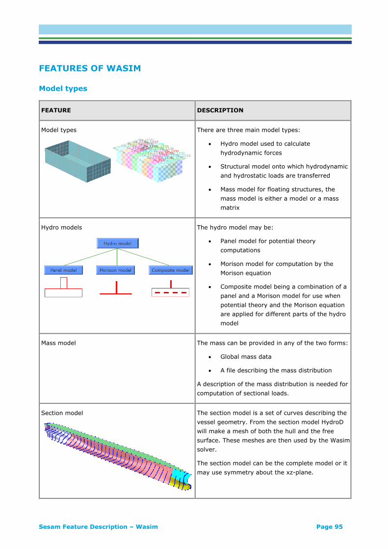
Sesam Feature Description – Wasim Page 95
FEATURES OF WASIM
Model types
FEATURE DESCRIPTION
Model types
There are three main model types:
• Hydro model used to calculate
hydrodynamic forces
• Structural model onto which hydrodynamic
and hydrostatic loads are transferred
• Mass model for floating structures, the
mass model is either a model or a mass
matrix
Hydro models
The hydro model may be:
• Panel model for potential theory
computations
• Morison model for computation by the
Morison equation
• Composite model being a combination of a
panel and a Morison model for use when
potential theory and the Morison equation
are applied for different parts of the hydro
model
Mass model The mass can be provided in any of the two forms:
• Global mass data
• A file describing the mass distribution
A description of the mass distribution is needed for
computation of sectional loads.
Section model
The section model is a set of curves describing the
vessel geometry. From the section model HydroD
will make a mesh of both the hull and the free
surface. These meshes are then used by the Wasim
solver.
The section model can be the complete model or it
may use symmetry about the xz-plane.

Sesam Feature Description – Wasim Page 96
Panel model
The Rankine solver requires a mesh on both hull
and free surface. Both meshes are created by
HydroD from the section model.
The free surface mesh can be automatically or
interactively created.
Morison model
Morison elements:
• 2D Morison elements for loads on 2 node
beam elements
• Pressure area elements for loads at the
ends of 2D Morison elements
• Dry Morison elements for beams on which
no load is to be computed
• Anchor and TLP elements for restoring
contributions in nodes. These elements can
be used to provide a simplified model of
the moorings and risers. The element is a
linear spring with pretension.
Composite model
Hydrodynamic forces on a composite model are
computed from potential theory for the panel
model and from the Morison equation for the
Morison model. The hydrodynamic excitation
forces and matrices from both theories are
accumulated in the equations of motion for the
composite model.
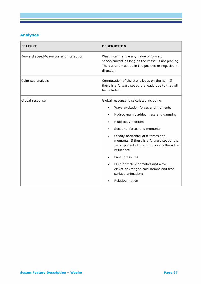
Sesam Feature Description – Wasim Page 97
Analyses
FEATURE DESCRIPTION
Forward speed/Wave current interaction Wasim can handle any value of forward
speed/current as long as the vessel is not planing.
The current must be in the positive or negative x-
direction.
Calm sea analysis Computation of the static loads on the hull. If
there is a forward speed the loads due to that will
be included.
Global response Global response is calculated including:
• Wave excitation forces and moments
• Hydrodynamic added mass and damping
• Rigid body motions
• Sectional forces and moments
• Steady horizontal drift forces and
moments. If there is a forward speed, the
x-component of the drift force is the added
resistance.
• Panel pressures
• Fluid particle kinematics and wave
elevation (for gap calculations and free
surface animation)
• Relative motion

Sesam Feature Description – Wasim Page 98
Transfer of load to structural analysis
FEATURE DESCRIPTION
Load transfer
Panel mesh FE mesh
Automatic load transfer to a finite element model
for subsequent structural analysis including:
• Inertia loads
• Line loads on beam elements from Morison
model
• Point loads from pressure areas, anchor
elements etc. from Morison model
• Pressure loads on plate/shell/solid
elements
• Internal tank pressure in compartments
Load transfer in frequency domain The time histories of the loads are converted into
frequency domain by Fourier analysis and then
applied to the finite element model to be used in a
quasi-static or frequency domain structural
analysis.
Load transfer in time domain A selected part of the time histories is applied as
time domain loads on the finite element model to
be used in a time domain (dynamic) structural
analysis.
Snapshot loads Loads at selected points in time are applied as
static loads on the finite element model to be used
in a quasi-static structural analysis.
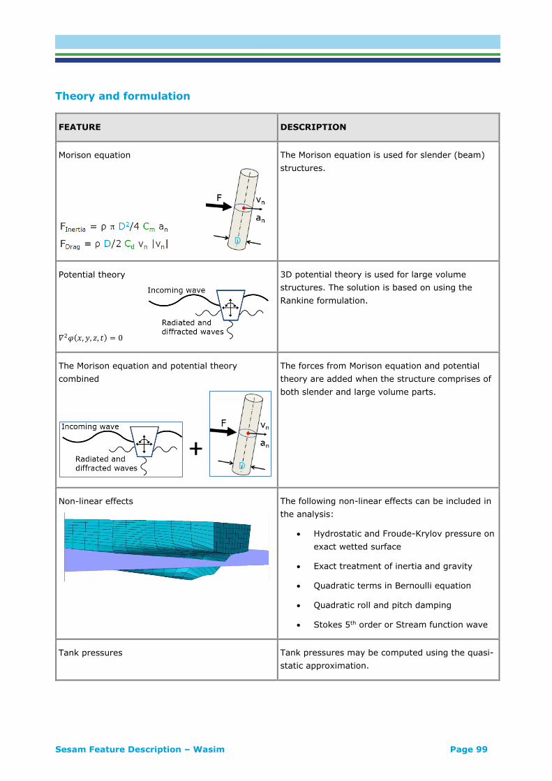
Sesam Feature Description – Wasim Page 99
Theory and formulation
FEATURE DESCRIPTION
Morison equation
The Morison equation is used for slender (beam)
structures.
Potential theory
𝛻2𝜑(𝑥, 𝑦, 𝑧, 𝑡) = 0
3D potential theory is used for large volume
structures. The solution is based on using the
Rankine formulation.
The Morison equation and potential theory
combined
The forces from Morison equation and potential
theory are added when the structure comprises of
both slender and large volume parts.
Non-linear effects
The following non-linear effects can be included in
the analysis:
• Hydrostatic and Froude-Krylov pressure on
exact wetted surface
• Exact treatment of inertia and gravity
• Quadratic terms in Bernoulli equation
• Quadratic roll and pitch damping
• Stokes 5th order or Stream function wave
Tank pressures Tank pressures may be computed using the quasi-
static approximation.

Sesam Feature Description – Wasim Page 100
Viscous damping Viscous damping in roll and pitch can be modelled
by prescribing a linear and a quadratic damping
coefficient.
Alternatively, the effect can be included by using a
Morison model.
Additional damping and restoring matrices Additional damping and restoring matrices can be
specified. This can be used for including damping
or restoring from moorings and risers and/or
viscous damping.
Pressure loads up to free surface In a non-linear analysis loads are computed on the
exact wetted surface.
Reduced pressure around the free surface
This is a recommended option for fatigue analysis
and follows DNV GL Class note 30.7. The pressure
is modified around the waterline. The method
should only be applied on that part of the vessel
which has vertical intersection with the free
surface.
Time series input
Wasim can read and utilize any combination of the
following time series inputs:
• Wave elevation at a prescribed point
• Motion, velocity and acceleration of the
structure
• Forces (and optionally also moments)
acting in specified points

Sesam Feature Description – Waveship Page 101
Waveship SEA-KEEPING OF SLENDER VESSELS
Last revised: August 22, 2017. Describing version 6.2-05.
Waveship is a frequency domain hydrodynamic analysis program for calculation of wave loading and
response for ships and other slender marine structures, with and without forward speed. The Waveship
results are presented directly as complex transfer functions.
Waveship is using strip theory. This is in many cases a good approximation for obtaining global
responses but is less reliable for local responses (i.e. pressure distribution).
The most typical approximation of Waveship is to compute global results on slender structures at zero to
moderate speed. When applicable these results can be obtained with a very small computational effort.

Sesam Feature Description – Waveship Page 102
FEATURES OF WAVESHIP
FEATURE DESCRIPTION
Strip model
The strip model is the basis for the hydrodynamic
solver. A 2D problem is solved in the planes
defined by each curve (yz-plane).
The strip model covers one half of the vessel so only
vessels with xz-symmetry can be analysed.
Mass model The mass can be provided in any of the two forms:
• Global mass data
• Sectional mass matrices
Sectional mass matrices are needed for
computation of sectional loads.
Mooring elements A simplified model of moorings and risers can be
given in the form of linear springs with pretension.
Forward speed Waveship can handle moderate forward speeds.
The results are best at zero speed and becomes
gradually less reliable with increasing speed.
Global response Global response is calculated including:
• Wave excitation forces and moments
• Hydrodynamic added mass and damping
• Rigid body motions
• Mean drift force
• Sectional forces and moments
Mean drift force and sectional loads are less
reliable than the global quantities since it requires
computation of the pressure distribution.

Sesam Feature Description – Waveship Page 103
Load transfer Automatic load transfer to a finite element model
for subsequent structural analysis including:
• Inertia loads
• Pressure loads on plate/shell/solid
elements
The pressure loads may have significant
uncertainty and should be used with care. Load
transfer from Waveship is therefore in general only
recommended for load transfer to the cargo in a
transportation analysis, i.e. transfer only of inertia
loads.
Tank pressures Tank pressures may be computed using the quasi-
static approximation.
Roll damping Viscous roll damping from hull and bilge keel can
be included by using the roll damping models of
Tanaka and Kato.
Pressure loads up to free surface
Panel pressures calculated by first order potential
theory may be extrapolate to the free surface.
Correspondingly, dry elements below the still
water level receive no loads. This is done by
stretching pressures above the still water level.

Sesam Feature Description – Wajac Page 104
Wajac WAVE AND CURRENT LOADS ON FIXED RIGID FRAME
STRUCTURES
Last revised: February 1, 2019. Describing version 7.4.
Wajac calculates wind, wave and current loads on fixed and rigid frame structures. Typical examples of
such structures are offshore jacket platforms and jack-up rigs. The loads are calculated according to
Morison’s equation (plus optionally MacCamy-Fuchs) in the time domain (deterministic), frequency
domain or in a short-term time domain simulation. Loads are transferred to structural analysis in Sestra
and statistical post-processing in Postresp.

Sesam Feature Description – Wajac Page 105
FEATURES OF WAJAC
The features of Wajac are summarised below in sections:
• Types of Analysis
• Details on Certain Features
Types of analysis
FEATURE DESCRIPTION
Deterministic load calculation
Deterministic load calculation is performed in the
time domain (wave stepping through structure) and
is generally used for design purposes in an ultimate
limit state analysis. Several wave theories are
available including Stokes 5th, Stream Function and
Cnoidal. Multiple water depths may be specified.
Such an analysis is the basis for:
• Static analysis in Sestra
• Deterministic fatigue analysis (FLS) in
Framework
• Code checking (ULS) in GeniE
Print of transfer functions for base shear and
overturning moment allows graphing in Excel.
Spectral (frequency domain) load calculation
This involves calculation of wave force transfer
functions in the frequency domain. Such an
analysis is the basis for:
• Frequency domain dynamic or quasi-static
analysis in Sestra
• Stochastic (spectral) fatigue analysis (FLS)
in Framework
Print of transfer functions for base shear and
overturning moment allows graphing in Excel.
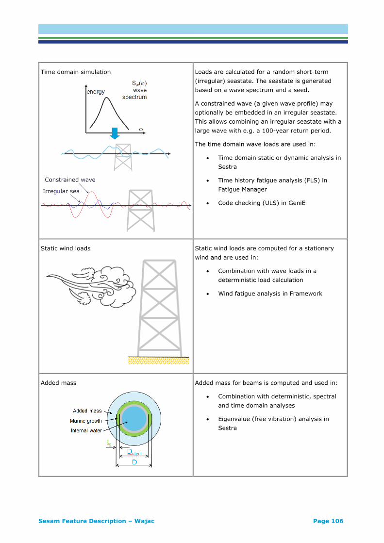
Sesam Feature Description – Wajac Page 106
Time domain simulation
Loads are calculated for a random short-term
(irregular) seastate. The seastate is generated
based on a wave spectrum and a seed.
A constrained wave (a given wave profile) may
optionally be embedded in an irregular seastate.
This allows combining an irregular seastate with a
large wave with e.g. a 100-year return period.
The time domain wave loads are used in:
• Time domain static or dynamic analysis in
Sestra
• Time history fatigue analysis (FLS) in
Fatigue Manager
• Code checking (ULS) in GeniE
Static wind loads
Static wind loads are computed for a stationary
wind and are used in:
• Combination with wave loads in a
deterministic load calculation
• Wind fatigue analysis in Framework
Added mass
Added mass for beams is computed and used in:
• Combination with deterministic, spectral
and time domain analyses
• Eigenvalue (free vibration) analysis in
Sestra

Sesam Feature Description – Wajac Page 107
Details on certain features
FEATURE DESCRIPTION
Load calculation
All loads calculated by Wajac are based on
Morison’s equation:
F = ρ ∏ D2/4 Cm an + ρ D/2 Cd vn |vn|
Hydrodynamic coefficients
The hydrodynamic coefficients Cm (inertia) and Cd
(drag) may be specified in alternative ways:
• Constant
o Different constant values to
different parts of structure
• Function of diameter
• Function of roughness and Reynolds
number
• Function of roughness and Keulegan-
Carpenter number
• By API rule
Marine growth
Marine growth may contribute to:
• Drag force
• Inertia force and added mass
• Weight and buoyancy
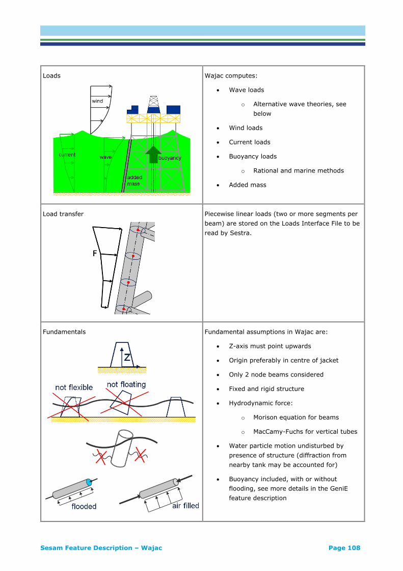
Sesam Feature Description – Wajac Page 108
Loads
Wajac computes:
• Wave loads
o Alternative wave theories, see
below
• Wind loads
• Current loads
• Buoyancy loads
o Rational and marine methods
• Added mass
Load transfer
Piecewise linear loads (two or more segments per
beam) are stored on the Loads Interface File to be
read by Sestra.
Fundamentals
Fundamental assumptions in Wajac are:
• Z-axis must point upwards
• Origin preferably in centre of jacket
• Only 2 node beams considered
• Fixed and rigid structure
• Hydrodynamic force:
o Morison equation for beams
o MacCamy-Fuchs for vertical tubes
• Water particle motion undisturbed by
presence of structure (diffraction from
nearby tank may be accounted for)
• Buoyancy included, with or without
flooding, see more details in the GeniE
feature description
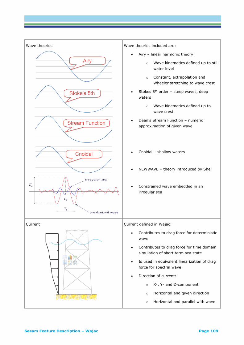
Sesam Feature Description – Wajac Page 109
Wave theories
Wave theories included are:
• Airy – linear harmonic theory
o Wave kinematics defined up to still
water level
o Constant, extrapolation and
Wheeler stretching to wave crest
• Stokes 5th order – steep waves, deep
waters
o Wave kinematics defined up to
wave crest
• Dean’s Stream Function – numeric
approximation of given wave
• Cnoidal – shallow waters
• NEWWAVE – theory introduced by Shell
• Constrained wave embedded in an
irregular sea
Current
Current defined in Wajac:
• Contributes to drag force for deterministic
wave
• Contributes to drag force for time domain
simulation of short term sea state
• Is used in equivalent linearization of drag
force for spectral wave
• Direction of current:
o X-, Y- and Z-component
o Horizontal and given direction
o Horizontal and parallel with wave

Sesam Feature Description – Installjac Page 110
Installjac LAUNCHING AND UPENDING ANALYSIS
Last revised: August 22, 2017. Describing version 8.2-00.
Installjac simulates the installation launch and upending of a jacket. The program provides a
comprehensive assessment of the hydrostatic and hydrodynamic properties of the jacket during the
installation simulations.
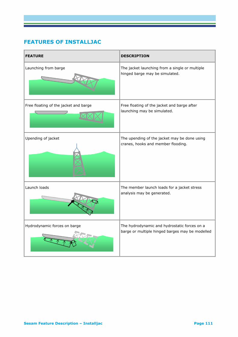
Sesam Feature Description – Installjac Page 111
FEATURES OF INSTALLJAC
FEATURE DESCRIPTION
Launching from barge
The jacket launching from a single or multiple
hinged barge may be simulated.
Free floating of the jacket and barge
Free floating of the jacket and barge after
launching may be simulated.
Upending of jacket
The upending of the jacket may be done using
cranes, hooks and member flooding.
Launch loads
The member launch loads for a jacket stress
analysis may be generated.
Hydrodynamic forces on barge
The hydrodynamic and hydrostatic forces on a
barge or multiple hinged barges may be modelled

Sesam Feature Description – Simo Page 112
Simo COMPLEX MULTIBODY CALCULATIONS
Last revised: March 12, 2019. Describing version 4.14-00 (64-bit).
Simo is for simulation of motions and station-keeping behaviour of complex systems of floating vessels
and suspended loads. Essential features are:
• Flexible modelling of multimode systems
• Non-linear time domain simulation of wave frequency as well as low frequency forces
• Environmental forces due to wind, waves and current
• Passive and active control forces
• Interactive or batch simulation
Simo is run from the Sima GUI.
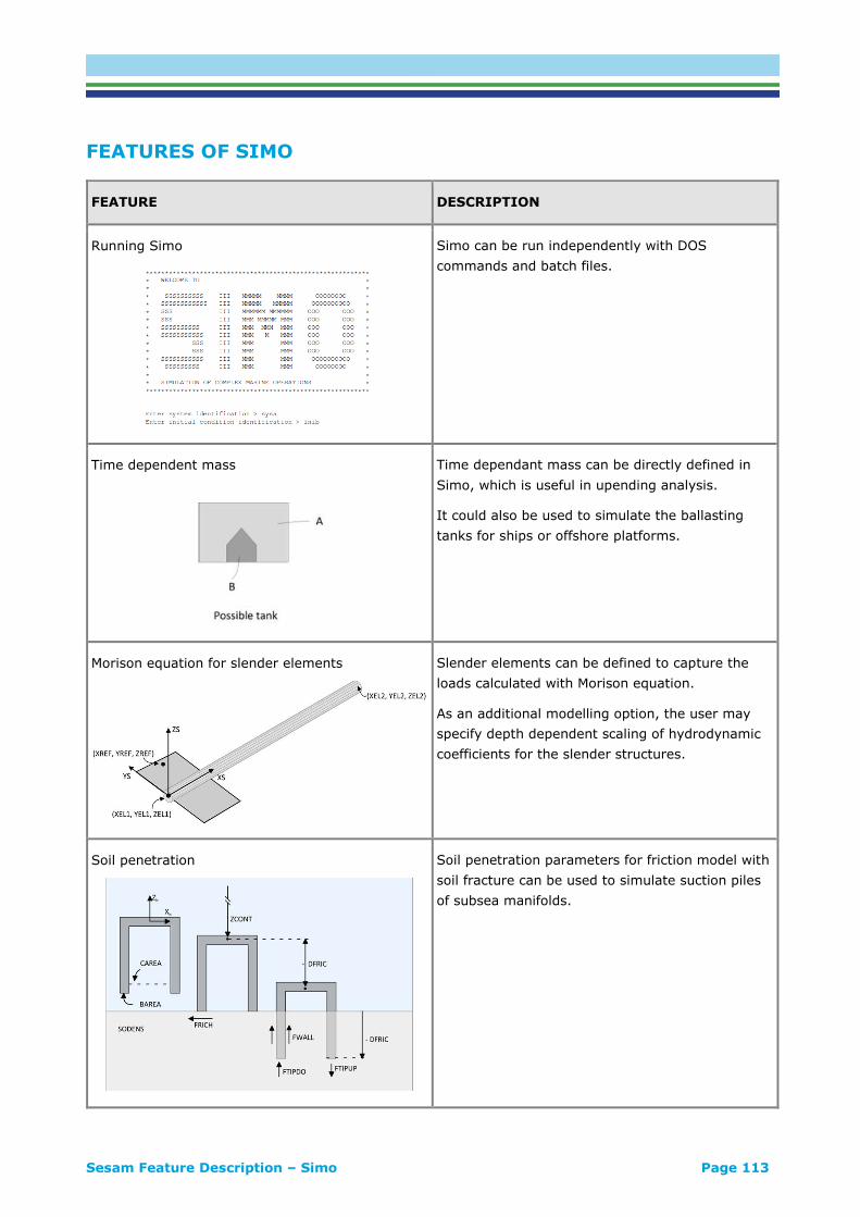
Sesam Feature Description – Simo Page 113
FEATURES OF SIMO
FEATURE DESCRIPTION
Running Simo
Simo can be run independently with DOS
commands and batch files.
Time dependent mass
Time dependant mass can be directly defined in
Simo, which is useful in upending analysis.
It could also be used to simulate the ballasting
tanks for ships or offshore platforms.
Morison equation for slender elements
Slender elements can be defined to capture the
loads calculated with Morison equation.
As an additional modelling option, the user may
specify depth dependent scaling of hydrodynamic
coefficients for the slender structures.
Soil penetration
Soil penetration parameters for friction model with
soil fracture can be used to simulate suction piles
of subsea manifolds.
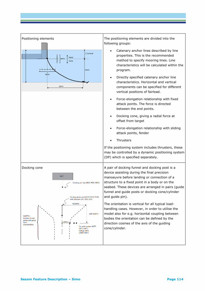
Sesam Feature Description – Simo Page 114
Positioning elements
The positioning elements are divided into the
following groups:
• Catenary anchor lines described by line
properties. This is the recommended
method to specify mooring lines. Line
characteristics will be calculated within the
program.
• Directly specified catenary anchor line
characteristics. Horizontal and vertical
components can be specified for different
vertical positions of fairlead.
• Force-elongation relationship with fixed
attack points. The force is directed
between the end points.
• Docking cone, giving a radial force at
offset from target
• Force-elongation relationship with sliding
attack points, fender
• Thrusters
If the positioning system includes thrusters, these
may be controlled by a dynamic positioning system
(DP) which is specified separately.
Docking cone
A pair of docking funnel and docking post is a
device assisting during the final precision
manoeuvre before landing or connection of a
structure to a fixed point in a body or on the
seabed. These devices are arranged in pairs (guide
funnel and guide posts or docking cone/cylinder
and guide pin).
The orientation is vertical for all typical load-
handling cases. However, in order to utilise the
model also for e.g. horizontal coupling between
bodies the orientation can be defined by the
direction cosines of the axis of the guiding
cone/cylinder.
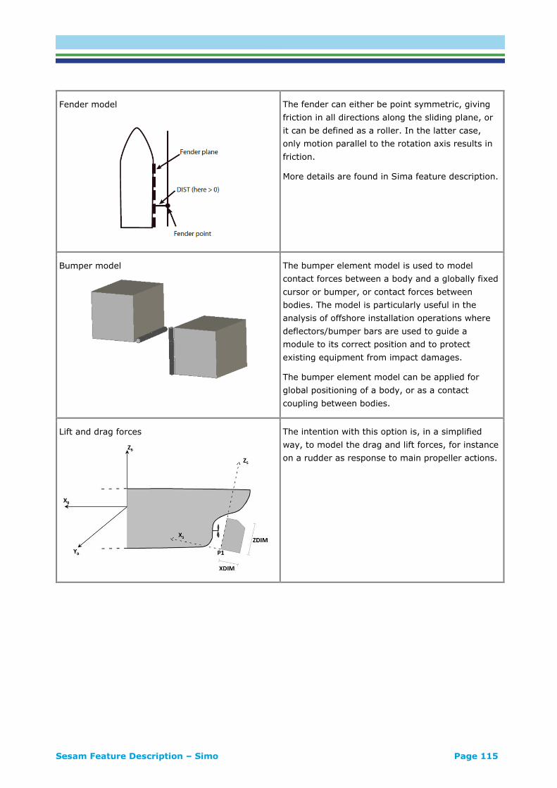
Sesam Feature Description – Simo Page 115
Fender model
The fender can either be point symmetric, giving
friction in all directions along the sliding plane, or
it can be defined as a roller. In the latter case,
only motion parallel to the rotation axis results in
friction.
More details are found in Sima feature description.
Bumper model
The bumper element model is used to model
contact forces between a body and a globally fixed
cursor or bumper, or contact forces between
bodies. The model is particularly useful in the
analysis of offshore installation operations where
deflectors/bumper bars are used to guide a
module to its correct position and to protect
existing equipment from impact damages.
The bumper element model can be applied for
global positioning of a body, or as a contact
coupling between bodies.
Lift and drag forces
The intention with this option is, in a simplified
way, to model the drag and lift forces, for instance
on a rudder as response to main propeller actions.
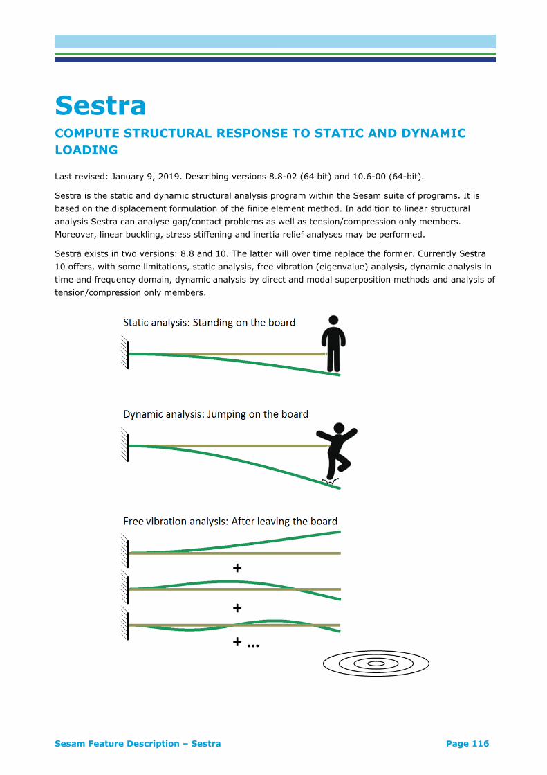
Sesam Feature Description – Sestra Page 116
Sestra COMPUTE STRUCTURAL RESPONSE TO STATIC AND DYNAMIC
LOADING
Last revised: January 9, 2019. Describing versions 8.8-02 (64 bit) and 10.6-00 (64-bit).
Sestra is the static and dynamic structural analysis program within the Sesam suite of programs. It is
based on the displacement formulation of the finite element method. In addition to linear structural
analysis Sestra can analyse gap/contact problems as well as tension/compression only members.
Moreover, linear buckling, stress stiffening and inertia relief analyses may be performed.
Sestra exists in two versions: 8.8 and 10. The latter will over time replace the former. Currently Sestra
10 offers, with some limitations, static analysis, free vibration (eigenvalue) analysis, dynamic analysis in
time and frequency domain, dynamic analysis by direct and modal superposition methods and analysis of
tension/compression only members.

Sesam Feature Description – Sestra Page 117
FEATURES OF SESTRA
Types of analysis
The types of analysis illustrated and explained in the table below are:
• Linear static analysis
• Linear free vibration analysis
• Linear dynamic analysis in frequency as well as time domain
• Linear frequency domain static analysis
• Gap/contact analysis
• Tension/compression only member analysis
• Linear buckling analysis
• Stress stiffening analysis
• Axi-symmetric analysis
FEATURE DESCRIPTION
Linear static analysis
The loads are (more or less) constant and the
structural response is linear. Linear response
means that it is proportional to the load: Double
the load and the displacements are doubled.
Equation of equilibrium being solved:
Kr = R
K is stiffness matrix, r is displacement vector, R is
load vector
Linear free vibration analysis
An analysis to determine the free vibration of the
structure when there are no loads and no
damping. The mode shapes (eigenmodes) and
natural frequencies (eigenfrequencies) are
computed.
Equation of equilibrium being solved:
Ma + Kr = 0
M is mass matrix, a is acceleration vector, K is
stiffness matrix,
r is displacement vector
Assuming r = Φ sin(ωt) the equation turns into the
eigenvalue problem:
(K – ω2M)Φ = 0
ω is angular frequency (=2f), Φ is mode shape
(eigenvector)
See below for information on eigenvalue solvers
offered by Sestra.
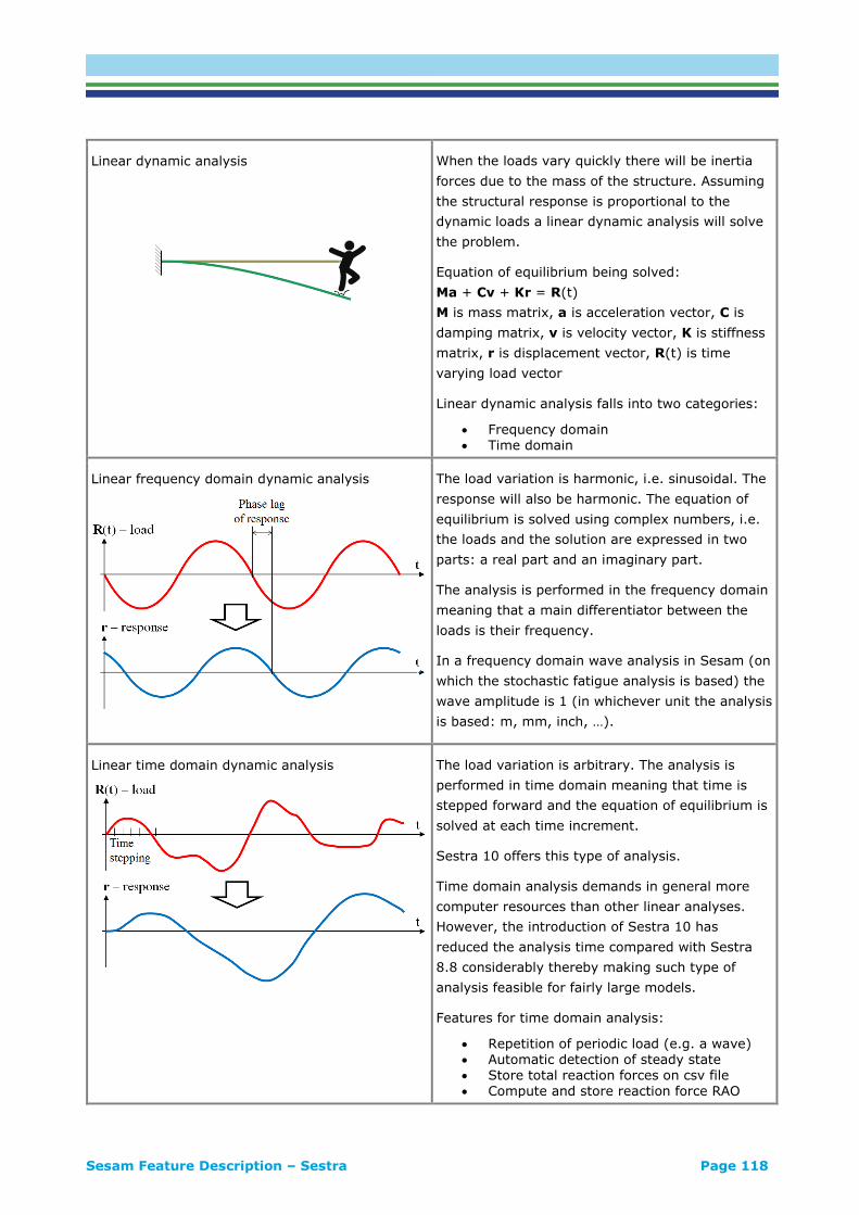
Sesam Feature Description – Sestra Page 118
Linear dynamic analysis
When the loads vary quickly there will be inertia
forces due to the mass of the structure. Assuming
the structural response is proportional to the
dynamic loads a linear dynamic analysis will solve
the problem.
Equation of equilibrium being solved:
Ma + Cv + Kr = R(t)
M is mass matrix, a is acceleration vector, C is
damping matrix, v is velocity vector, K is stiffness
matrix, r is displacement vector, R(t) is time
varying load vector
Linear dynamic analysis falls into two categories:
• Frequency domain • Time domain
Linear frequency domain dynamic analysis
The load variation is harmonic, i.e. sinusoidal. The
response will also be harmonic. The equation of
equilibrium is solved using complex numbers, i.e.
the loads and the solution are expressed in two
parts: a real part and an imaginary part.
The analysis is performed in the frequency domain
meaning that a main differentiator between the
loads is their frequency.
In a frequency domain wave analysis in Sesam (on
which the stochastic fatigue analysis is based) the
wave amplitude is 1 (in whichever unit the analysis
is based: m, mm, inch, …).
Linear time domain dynamic analysis
The load variation is arbitrary. The analysis is
performed in time domain meaning that time is
stepped forward and the equation of equilibrium is
solved at each time increment.
Sestra 10 offers this type of analysis.
Time domain analysis demands in general more
computer resources than other linear analyses.
However, the introduction of Sestra 10 has
reduced the analysis time compared with Sestra
8.8 considerably thereby making such type of
analysis feasible for fairly large models.
Features for time domain analysis:
• Repetition of periodic load (e.g. a wave) • Automatic detection of steady state • Store total reaction forces on csv file • Compute and store reaction force RAO
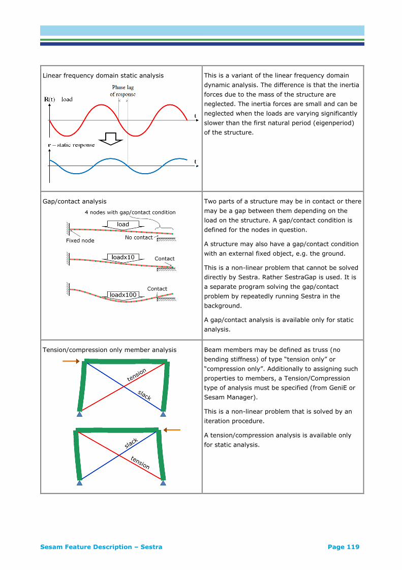
Sesam Feature Description – Sestra Page 119
Linear frequency domain static analysis
This is a variant of the linear frequency domain
dynamic analysis. The difference is that the inertia
forces due to the mass of the structure are
neglected. The inertia forces are small and can be
neglected when the loads are varying significantly
slower than the first natural period (eigenperiod)
of the structure.
Gap/contact analysis
Two parts of a structure may be in contact or there
may be a gap between them depending on the
load on the structure. A gap/contact condition is
defined for the nodes in question.
A structure may also have a gap/contact condition
with an external fixed object, e.g. the ground.
This is a non-linear problem that cannot be solved
directly by Sestra. Rather SestraGap is used. It is
a separate program solving the gap/contact
problem by repeatedly running Sestra in the
background.
A gap/contact analysis is available only for static
analysis.
Tension/compression only member analysis
Beam members may be defined as truss (no
bending stiffness) of type “tension only” or
“compression only”. Additionally to assigning such
properties to members, a Tension/Compression
type of analysis must be specified (from GeniE or
Sesam Manager).
This is a non-linear problem that is solved by an
iteration procedure.
A tension/compression analysis is available only
for static analysis.

Sesam Feature Description – Sestra Page 120
Linear buckling analysis
A linear buckling analysis determines the scaling of
a load required to reach linear buckling.
This is an automatic two step procedure:
• Static analysis to find forces and stresses.
A geometric stiffness matrix Kg is
computed based on these results.
• Solve eigenvalue problem:
(K – Kg)Φ = 0
is eigenvalue or stability factor, Φ is
buckling modes.
Only the first buckling mode is of interest.
Load times is the critical buckling load.
Second order (P-) effects are not accounted for.
This limitation plus the fact that structural
imperfections may not be properly accounted for
involves that a linear buckling analysis
overestimates the real buckling load.
Stress stiffening analysis
A stress stiffening analysis takes the stiffening
effect of tension and softening effect of
compression into account when computing e.g. the
free vibration of the structure.
This is an automatically performed two step
procedure:
• Static analysis to find the initial stress
level. A geometric stiffness matrix Kg is
computed based on these initial stresses.
Kg is added to the stiffness matrix K
thereby adding/subtracting stiffness to the
ordinary stiffness.
• A new analysis is done based on the
updated stiffness matrix. This analysis may
be a static, free vibration or forced
response dynamic analysis.
Axi-symmetric analysis
A rotational symmetric model may be analysed as
a 2D problem thereby reducing the size of the
problem to a fraction compared to a full 3D
analysis.

Sesam Feature Description – Sestra Page 121
Elements, properties and loads
Presented below are essential features related to the types of analysis presented above.
FEATURE DESCRIPTION
Element types
1 and 2 node spring
Truss
2 node beam
3 node beam
The library of elements in Sestra covers all types
of structures:
• 1 and 2-node spring
• Damper
• Mass
• Truss
• 2 node beam, with offset (eccentricities) in
nodes
• 3 node beam
• 3 and 4 node membrane
• 6 and 8 node membrane
• 3 and 4 node plate
• 6 and 8 node shell
• Axi-symmetric volume
• 6 and 8 node volume (solid)
• 10, 15 and 20 node volume (solid)
• Transition element between 6/8 node shell
and 15/20 node volume (solid)

Sesam Feature Description – Sestra Page 122
Hinge
Hinge, optionally with flexibility, is available for 2
node beam elements. The hinge is general in that
it can be defined for all six degrees of freedom, i.e.
translational as well as rotational hinges.
Damping properties
Depending on the type of dynamic analysis being
performed there are alternative damping models
available:
• Modal damping as fraction of critical
damping
A viscous damping where fractions of
critical damping λ for the modes used in
Modal Superposition are given.
• Proportional damping or Rayleigh damping
A viscous damping where a damping
matrix is specified as a linear combination
of the stiffness and mass matrices:
C = 1M + 2K
• Structural damping
This is a damping proportional to the
displacements and in phase with the
velocity. It is relevant only for frequency
domain analysis.
Dashpots and axial dampers
Dashpots and axial dampers may be specified by
the preprocessors for inclusion in the viscous
damping matrix. It is relevant only for direct
methods, i.e. not Modal Superposition.
Material properties
There are two linear material properties available:
• Isotropic
Anisotropic (of which orthotropic is a special case)
Different properties in two directions
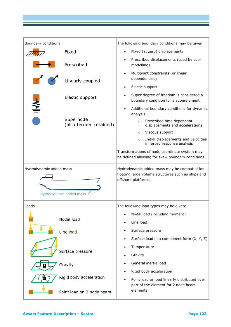
Sesam Feature Description – Sestra Page 123
Boundary conditions
The following boundary conditions may be given:
• Fixed (at zero) displacements
• Prescribed displacements (used by sub-
modelling)
• Multipoint constraints (or linear
dependencies)
• Elastic support
• Super degree of freedom is considered a
boundary condition for a superelement
• Additional boundary conditions for dynamic
analysis:
o Prescribed time dependent
displacements and accelerations
o Viscous support
o Initial displacements and velocities in forced response analysis
Transformations of node coordinate system may
be defined allowing for skew boundary conditions.
Hydrodynamic added mass
Hydrodynamic added mass may be computed for
floating large volume structures such as ships and
offshore platforms.
Loads
The following load types may be given:
• Nodal load (including moment)
• Line load
• Surface pressure
• Surface load in a component form (X, Y, Z)
• Temperature
• Gravity
• General inertia load
• Rigid body acceleration
• Point load or load linearly distributed over
part of the element for 2 node beam
elements

Sesam Feature Description – Sestra Page 124
Equation solvers
Presented below are solvers related to the types of analysis presented above.
FEATURE DESCRIPTION
Superelement analysis
Sestra features a multilevel superelement
technique applicable for static analysis. This
technique involves splitting the structure to be
analysed into part models, superelements, and
assembling these to form the complete model. Not
only Sestra but the whole Sesam suite of programs
incorporates the superelement technique:
• GeniE creates 1st level superelements
• Presel assembles superelements through
any number of levels to form the complete
model
• Wajac and Wadam computes loads and
motion for superelement assemblies
• Sestra analyses superelement assemblies
• Postprocessors (Xtract, Framework, Stofat,
etc.) handle superelement assemblies
Whereas the computer power and technology of
today no longer makes the superelement
technique a necessity it is still useful:
• Different teams can work on different
superelements
• Previously analysed model may be added
as a superelement to a new model
• A huge results file for a very big model
may be split thereby facilitating
postprocessing work
• Allows highly efficient non-linear analysis
when the non-linearity is limited to
regions, examples:
o Structure-pile-soil analysis, Sestra
for linear structure, Splice for non-
linear pile-soil
o Contact/gap analysis, Sestra for
linear structure, SestraGap for
non-linear contact/gap region
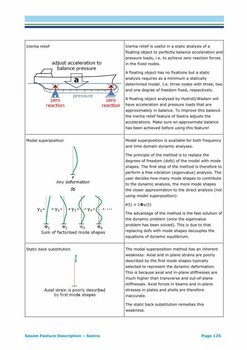
Sesam Feature Description – Sestra Page 125
Inertia relief
Inertia relief is useful in a static analysis of a
floating object to perfectly balance acceleration and
pressure loads, i.e. to achieve zero reaction forces
in the fixed nodes.
A floating object has no fixations but a static
analysis requires as a minimum a statically
determined model. I.e. three nodes with three, two
and one degree of freedom fixed, respectively.
A floating object analysed by HydroD/Wadam will
have acceleration and pressure loads that are
approximately in balance. To improve this balance
the inertia relief feature of Sestra adjusts the
accelerations. Make sure an approximate balance
has been achieved before using this feature!
Modal superposition
Modal superposition is available for both frequency
and time domain dynamic analyses.
The principle of the method is to replace the
degrees of freedom (dofs) of the model with mode
shapes. The first step of the method is therefore to
perform a free vibration (eigenvalue) analysis. The
user decides how many mode shapes to contribute
to the dynamic analysis, the more mode shapes
the closer approximation to the direct analysis (not
using model superposition):
r(t) ≈ Φiyi(t)
The advantage of the method is the fast solution of
the dynamic problem (once the eigenvalue
problem has been solved). This is due to that
replacing dofs with mode shapes decouples the
equations of dynamic equilibrium.
Static back substitution
The modal superposition method has an inherent
weakness: Axial and in-plane strains are poorly
described by the first mode shapes typically
selected to represent the dynamic deformation.
This is because axial and in-plane stiffnesses are
much higher than transverse and out-of-plane
stiffnesses. Axial forces in beams and in-plane
stresses in plates and shells are therefore
inaccurate.
The static back substitution remedies this
weakness.

Sesam Feature Description – Sestra Page 126
Eigenvalue solvers
The eigenvalue solvers available in Sestra are:
• Multifront Lanczos
An implicitly restarted Lanczos’ method
combined with a multifrontal solver, this is
a very efficient solver
• Lanczos’ method
Suitable for big problems but not when
there are un-constrained stiff body
motions
• Subspace Iteration
This is suitable for big problems and when
the eigenvalues are dense
• Householder’s method
This is suitable for small problems and
many eigenvalues
Component mode synthesis
Component mode synthesis is a reduction
technique for dynamic analysis resembling the
superelement technique for static analysis.
The principle of the method is to split the model
into part models (seen from a modelling point of
view: superelements) and for each part replace
the degrees of freedom (dofs) with mode shapes.
The first step of the method is therefore to
perform free vibration analyses of all part models.
When proceeding from a static analysis by use of
the superelement technique to a dynamic analysis
then the component mode synthesis technique is
an attractive choice.
Master-Slave
Master-Slave is a reduction technique for dynamic
analysis.
The principle of the method is to define selected
degrees of freedom (dofs) as masters (seen from a
modelling point of view: super-dofs) and then do
the same condensation of the mass and damping
matrices as done for a stiffness matrix in a static
condensation. The consequence of this is a
lumping of mass and damping to the master-dofs.
The Master-Slave technique also provides a way of
eliminating soft areas (due to approximate
modelling?) from the dynamic analysis.
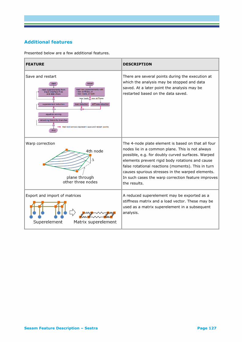
Sesam Feature Description – Sestra Page 127
Additional features
Presented below are a few additional features.
FEATURE DESCRIPTION
Save and restart
There are several points during the execution at
which the analysis may be stopped and data
saved. At a later point the analysis may be
restarted based on the data saved.
Warp correction
The 4-node plate element is based on that all four
nodes lie in a common plane. This is not always
possible, e.g. for doubly curved surfaces. Warped
elements prevent rigid body rotations and cause
false rotational reactions (moments). This in turn
causes spurious stresses in the warped elements.
In such cases the warp correction feature improves
the results.
Export and import of matrices
A reduced superelement may be exported as a
stiffness matrix and a load vector. These may be
used as a matrix superelement in a subsequent
analysis.
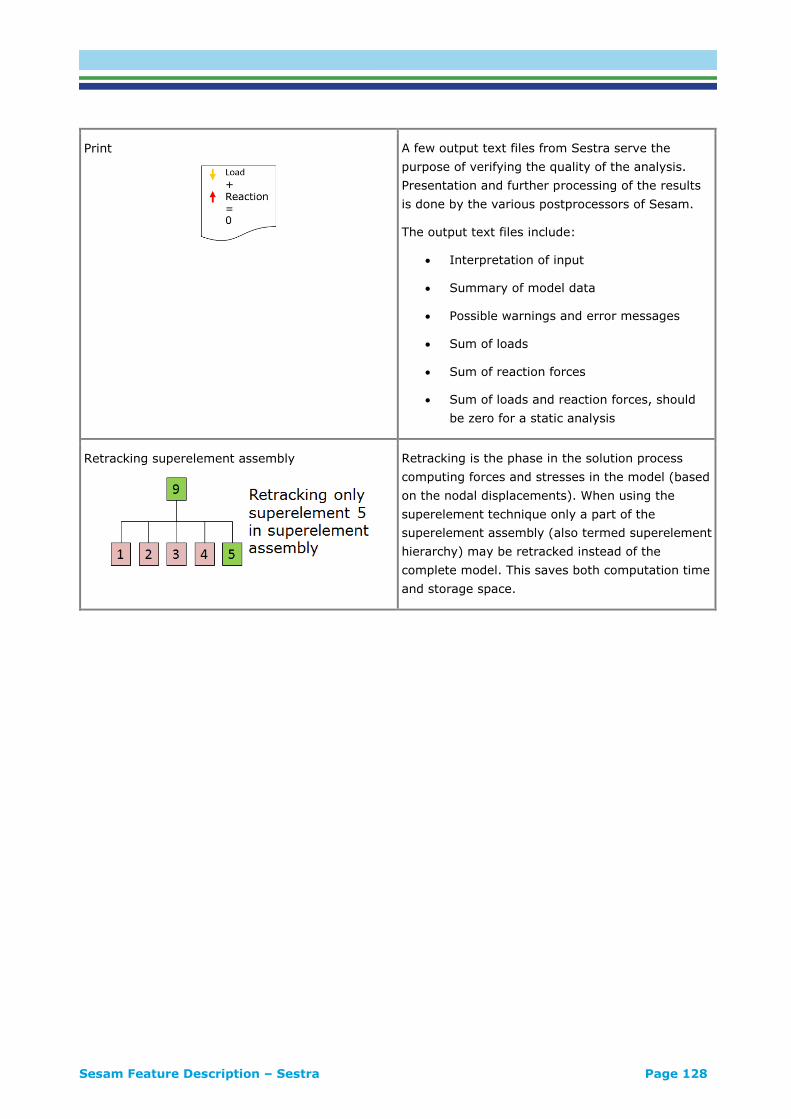
Sesam Feature Description – Sestra Page 128
A few output text files from Sestra serve the
purpose of verifying the quality of the analysis.
Presentation and further processing of the results
is done by the various postprocessors of Sesam.
The output text files include:
• Interpretation of input
• Summary of model data
• Possible warnings and error messages
• Sum of loads
• Sum of reaction forces
• Sum of loads and reaction forces, should
be zero for a static analysis
Retracking superelement assembly
Retracking is the phase in the solution process
computing forces and stresses in the model (based
on the nodal displacements). When using the
superelement technique only a part of the
superelement assembly (also termed superelement
hierarchy) may be retracked instead of the
complete model. This saves both computation time
and storage space.

Sesam Feature Description – Splice Page 129
Splice STRUCTURE-PILE-SOIL INTERACTION ANALYSIS
Last revised: April 23, 2018. Describing version 7.5-00 (64-bit).
Splice is a program for non-linear analysis of the structure-pile-soil interaction problem of typically a
jacket supported by piles driven into the sea bed. The programs Pilgen and Gensod belong to Splice, the
former for pile modelling and the latter for generation of non-linear soil stiffnesses. Pilgen is, however,
normally not used since the pile modelling is done as part of the jacket modelling in GeniE. The non-
linear soil stiffnesses are generated by Gensod based on soil modelling performed in GeniE. While Splice
analyses the non-linear pile-soil interaction it runs Sestra in the background for analysing the linear
jacket.
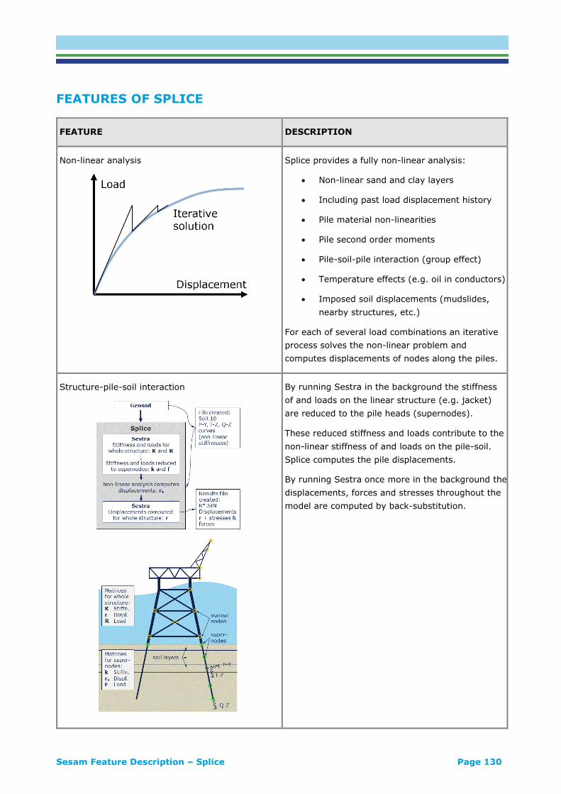
Sesam Feature Description – Splice Page 130
FEATURES OF SPLICE
FEATURE DESCRIPTION
Non-linear analysis
Splice provides a fully non-linear analysis:
• Non-linear sand and clay layers
• Including past load displacement history
• Pile material non-linearities
• Pile second order moments
• Pile-soil-pile interaction (group effect)
• Temperature effects (e.g. oil in conductors)
• Imposed soil displacements (mudslides,
nearby structures, etc.)
For each of several load combinations an iterative
process solves the non-linear problem and
computes displacements of nodes along the piles.
Structure-pile-soil interaction
By running Sestra in the background the stiffness
of and loads on the linear structure (e.g. jacket)
are reduced to the pile heads (supernodes).
These reduced stiffness and loads contribute to the
non-linear stiffness of and loads on the pile-soil.
Splice computes the pile displacements.
By running Sestra once more in the background the
displacements, forces and stresses throughout the
model are computed by back-substitution.
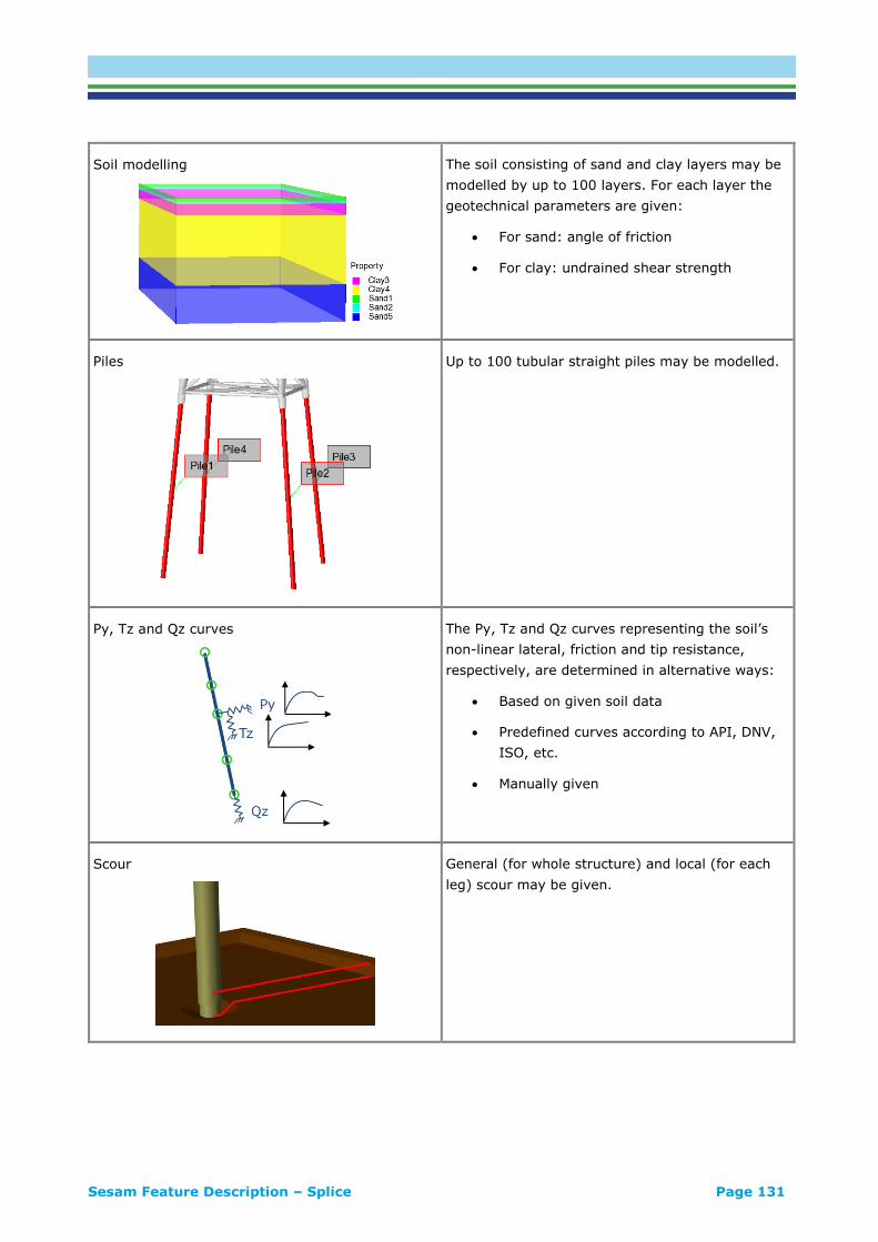
Sesam Feature Description – Splice Page 131
Soil modelling
The soil consisting of sand and clay layers may be
modelled by up to 100 layers. For each layer the
geotechnical parameters are given:
• For sand: angle of friction
• For clay: undrained shear strength
Piles
Up to 100 tubular straight piles may be modelled.
Py, Tz and Qz curves
The Py, Tz and Qz curves representing the soil’s
non-linear lateral, friction and tip resistance,
respectively, are determined in alternative ways:
• Based on given soil data
• Predefined curves according to API, DNV,
ISO, etc.
• Manually given
Scour
General (for whole structure) and local (for each
leg) scour may be given.

Sesam Feature Description – Splice Page 132
Pile tip modelling
There are alternatives for handling the pile tip:
• Free
• Fixed
• Pile is assumed to be infinitely long
beneath real tip or beneath given level
Pile group
Pile group effects (one pile influences a
neighbouring pile) are handled based on the
Mindlin equation.
Second order effects
Second order effects for the piles may be
accounted for
Pile capacity
Calculation of the capacity curves based on
allowable maximum deflections
• Pile penetration depth based on maximum
axial capacity
Compare with geotechnical report

Sesam Feature Description – Splice Page 133
Pile code check
Piles may be code checked according to:
• Norsok N-004 2013
• ISO 19902 2007
• API RP 2A 21st & 22nd editions
Linearization of pile-soil
The linearization of the pile-soil foundation
required for free vibration analysis of the structure
as well as for structural fatigue analysis may be
done automatically based on a selected loading
condition and pile.
Local buckling

Sesam Feature Description – Usfos Page 134
Usfos NON-LINEAR STATIC AND DYNAMIC ANALYSIS OF SPACE FRAME
STRUCTURES
Last revised: April 23, 2018. Describing version 8.8-01 (64-bit).
Usfos is used for ultimate strength, progressive collapse and accident analysis of space frame structures,
e.g. jackets in intact and damaged conditions. Extreme and accidental scenarios like earthquake,
explosion, fire, ship collision, dropped object etc. are analysed using Usfos.
ULS (ultimate limit state) analysis in Usfos is performed using a coarse beam and plate mesh equal to
the one used in linear analysis. Linear analysis models may therefore be used in Usfos with little or no
modifications. Yielding, plastic hinges, buckling, local buckling, joint yielding and fracture are accounted
for using a single beam element between joints.

Sesam Feature Description – Usfos Page 135
FEATURES OF USFOS
The analysis program Usfos comes with a front end graphical user interface named Xact in which input
specification and analysis control is done. The utility tool Struman for converting models from GeniE,
Sacs, Staad and Abaqus is run from Xact. And the graphical presentation of results is done in Xact.
Usfos is interfaced with Fahts (Fire And Heat Transfer Simulations). Fahts has an interface to the CFD
tool Kameleon FireEx KFX. Fahts prepares temperature data for structural response analysis in Usfos.
FEATURE DESCRIPTION
Pushover analysis
A pushover analysis is carried out for a combination
of static loads plus wave and wind loads.
The finite element model may be imported from
GeniE along with explicit loads or it may be
modelled in Usfos via a text file. Wave loads and
pile-soil data may be imported from Wajac and
Splice or generated in Usfos.
Initial imperfections may be defined according to
various curves recommended by codes (standards)
and by manual input data. The geometric stiffness
matrix is updated after each load step based on the
deflected nodal coordinates. Two surface plasticity
models are used to simulate the material non-
linearity.
Joint checks according to API, ISO, NORSOK etc.
are integrated parts of the analysis
Boat impact analysis
A boat impact analysis requires definition of impact
energy. The impact energy is transferred into dent
growth of the impacted tube, deformation of
member being hit, global deformation of the
structure and energy absorption of the ship.
After unloading the boat impact a 100-year design
wave may be stepped through the piled jacket
structure to document its strength according to
different codes.
A boat impact analysis may also be simulated by a
dynamic analysis in which non-linear springs
transfer the kinetic energy from a point mass with
a given velocity.
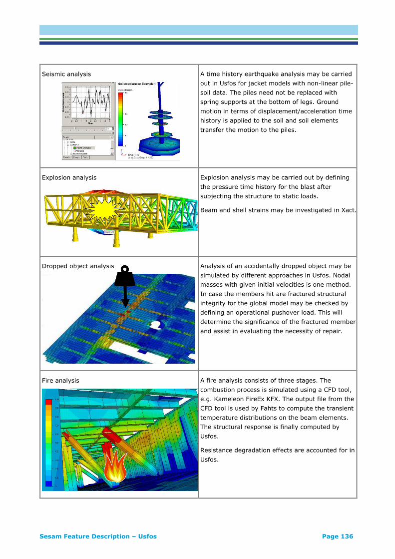
Sesam Feature Description – Usfos Page 136
Seismic analysis
A time history earthquake analysis may be carried
out in Usfos for jacket models with non-linear pile-
soil data. The piles need not be replaced with
spring supports at the bottom of legs. Ground
motion in terms of displacement/acceleration time
history is applied to the soil and soil elements
transfer the motion to the piles.
Explosion analysis
Explosion analysis may be carried out by defining
the pressure time history for the blast after
subjecting the structure to static loads.
Beam and shell strains may be investigated in Xact.
Dropped object analysis
Analysis of an accidentally dropped object may be
simulated by different approaches in Usfos. Nodal
masses with given initial velocities is one method.
In case the members hit are fractured structural
integrity for the global model may be checked by
defining an operational pushover load. This will
determine the significance of the fractured member
and assist in evaluating the necessity of repair.
Fire analysis
A fire analysis consists of three stages. The
combustion process is simulated using a CFD tool,
e.g. Kameleon FireEx KFX. The output file from the
CFD tool is used by Fahts to compute the transient
temperature distributions on the beam elements.
The structural response is finally computed by
Usfos.
Resistance degradation effects are accounted for in
Usfos.

Sesam Feature Description – Vivana Page 137
Vivana VORTEX INDUCED VIBRATIONS OF SLENDER MARINE
STRUCTURES
Last revised: March 12, 2019. Describing version 4.14-00.
Vivana is a computer tool for calculation of vortex induced vibrations (VIV) of slender marine structures
such as risers, free span pipelines and cables subjected to ocean current. This response type may in
many cases be decisive for the design and operation of marine systems.
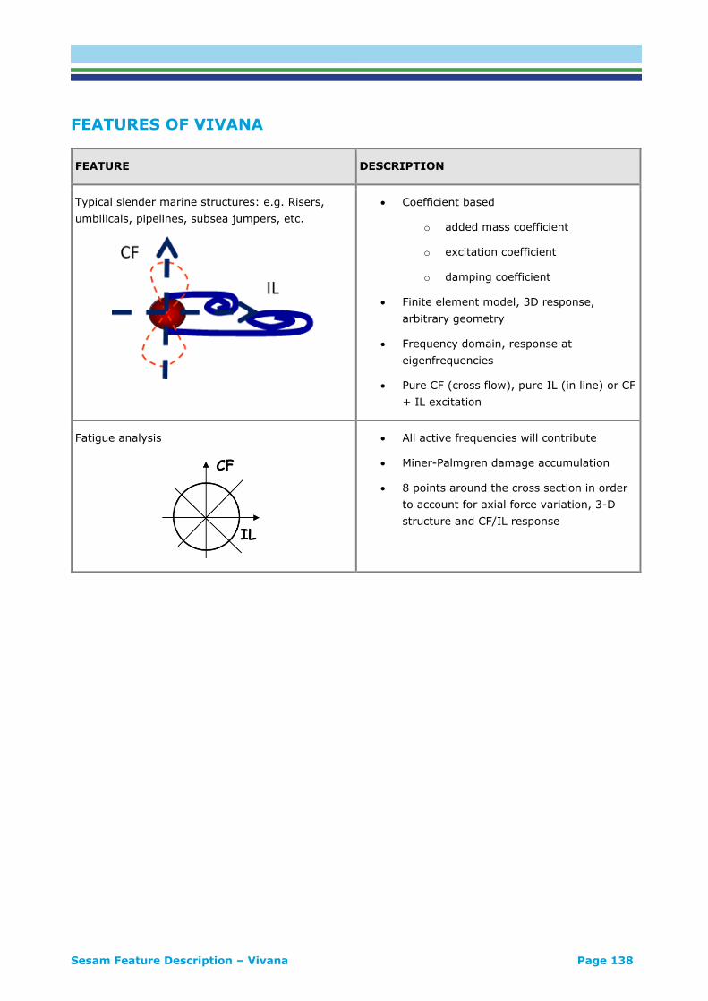
Sesam Feature Description – Vivana Page 138
FEATURES OF VIVANA
FEATURE DESCRIPTION
Typical slender marine structures: e.g. Risers,
umbilicals, pipelines, subsea jumpers, etc.
• Coefficient based
o added mass coefficient
o excitation coefficient
o damping coefficient
• Finite element model, 3D response,
arbitrary geometry
• Frequency domain, response at
eigenfrequencies
• Pure CF (cross flow), pure IL (in line) or CF
+ IL excitation
Fatigue analysis
• All active frequencies will contribute
• Miner-Palmgren damage accumulation
• 8 points around the cross section in order
to account for axial force variation, 3-D
structure and CF/IL response

Sesam Feature Description – Mimosa Page 139
Mimosa MOORING LINES ANALYSIS
Last revised: April 23, 2018. Describing version 6.3-08.
Mimosa is an interactive program for static and dynamic analysis of moored vessels. It computes static
and dynamic environmental loads, corresponding displacements and motions of the vessel and static and
dynamic mooring tensions.

Sesam Feature Description – Mimosa Page 140
FEATURES OF MIMOSA
FEATURE DESCRIPTION
Static and dynamic mooring system analysis
Mimosa offers a variety of options such as
calculation of the vessel’s wave frequency and low-
frequency motions and mooring line tensions.
Several options are available for analysis of the
properties of the mooring system and individual
mooring lines.
Static and dynamic environmental forces due to
wind, waves and current
• 4 wind spectra, incl. ISO 19901-1 (NPD)
and API
• 5 wave spectra, wave spreading
• Vertically varying current profile
Tension optimization
Optimum distribution of tension based on either
minimising the maximum tension in the mooring
system or least squares minimisation including
thrusters.
1st-order wave-induced motions (wave frequency,
WF)
Wave induced motion in the WF range solved in
frequency domain, using transfer functions for
vessel and wave spectrum, ensuring computer
efficient computations.
Slow-drift motions (low frequency, LF)
Maximum slow drift motion and maximum dynamic
mooring tension based on non-Gaussian statistics.
Gaussian and non-Gaussian statistics of extremes
Combining WF and LF motion to compute the
extremes of the combined WF and LF motion
Dynamic line models 1. Simplified analytic model
2. Finite element model
3. External motion-to-tension transfer
functions

Sesam Feature Description – Mimosa Page 141
Transient motion after line breakage
Transient motion after a line breakage or thruster
failure in terms of time traces of motion and
tension, motion trajectory, maximum excursion of
any given point on the vessel, and maximum
mooring tension. This also includes free drift (DP
blackout).
Automatic thruster assistance
Static and dynamic forces from thrusters under
dynamic positioning control.
Stability analysis
Stability of the vessel in single-point mooring or
turret mooring checked by eigenvalue analysis.
Long term simulation
Long term simulation results based on using a
macro command facility for running a set of
environmental conditions and producing
corresponding sets of results, covering e.g. 5-20
years of operation

Sesam Feature Description – Riflex Page 142
Riflex RISER ANALYSIS
Last revised: March 12, 2019. Describing version 4.14-00 (64-bit).
Riflex was developed as a tool for analysis of flexible marine riser systems but is just as well suited for
any type of slender structure such as mooring lines, umbilicals, steel pipelines and conventional risers.
These slender structures are characterized by:
• Small bending stiffness
• Large deflection
• Large upper end motion excitation
• Nonlinear cross section properties
• Complex cross section structure
Riflex is run via Sima.
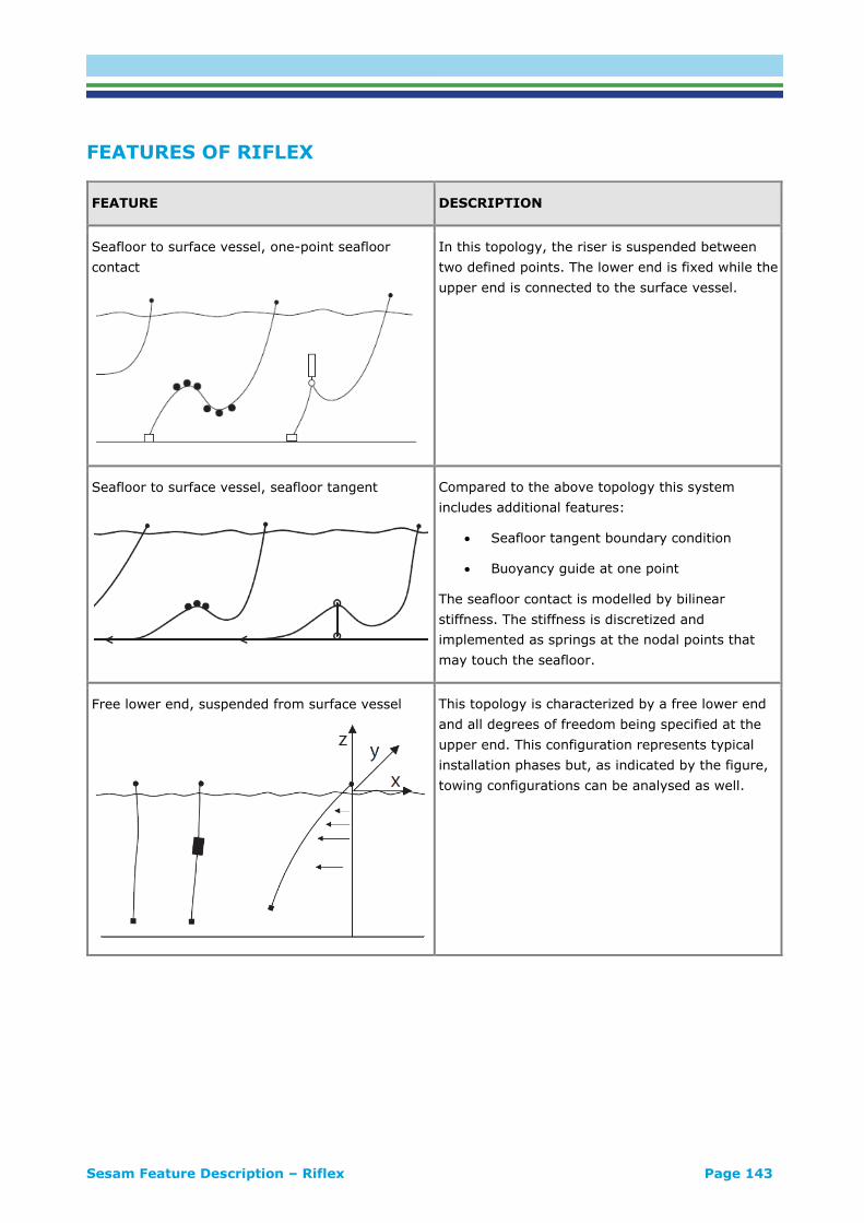
Sesam Feature Description – Riflex Page 143
FEATURES OF RIFLEX
FEATURE DESCRIPTION
Seafloor to surface vessel, one-point seafloor
contact
In this topology, the riser is suspended between
two defined points. The lower end is fixed while the
upper end is connected to the surface vessel.
Seafloor to surface vessel, seafloor tangent
Compared to the above topology this system
includes additional features:
• Seafloor tangent boundary condition
• Buoyancy guide at one point
The seafloor contact is modelled by bilinear
stiffness. The stiffness is discretized and
implemented as springs at the nodal points that
may touch the seafloor.
Free lower end, suspended from surface vessel
This topology is characterized by a free lower end
and all degrees of freedom being specified at the
upper end. This configuration represents typical
installation phases but, as indicated by the figure,
towing configurations can be analysed as well.

Sesam Feature Description – Riflex Page 144
Free upper end, single line
In this topology, a single line is connected to the
seafloor at its lower end and has a free upper end.
Wind turbine with floating substructure
A wind turbine with floating substructure can be
calculated in Riflex. More details please refer to
Sima chapter.
Elastic contact
Elastic contact can be calculated in Riflex. For
more details please refer to the DeepC feature
description.

Sesam Feature Description – Postresp Page 145
Postresp POSTPROCESSOR FOR STATISTICAL RESPONSE CALCULATIONS
Last revised: January 08, 2019. Describing version 6.7-04.
Postresp is an interactive graphic postprocessor for processing and presentation of responses in terms of
transfer functions in the frequency domain. The transfer functions are usually generated by one of the
hydrodynamic analysis programs in Sesam but they may also be transfer functions for any other kind of
response.
In this description, the term “transfer functions” is used. In Sesam the terms “response variables” and
“response amplitude operators” are also used with the same meaning.
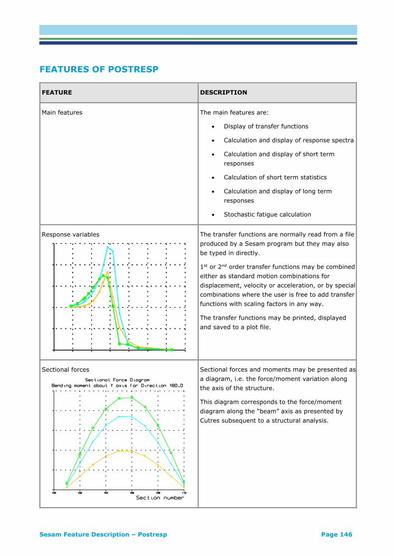
Sesam Feature Description – Postresp Page 146
FEATURES OF POSTRESP
FEATURE DESCRIPTION
Main features The main features are:
• Display of transfer functions
• Calculation and display of response spectra
• Calculation and display of short term
responses
• Calculation of short term statistics
• Calculation and display of long term
responses
• Stochastic fatigue calculation
Response variables
The transfer functions are normally read from a file
produced by a Sesam program but they may also
be typed in directly.
1st or 2nd order transfer functions may be combined
either as standard motion combinations for
displacement, velocity or acceleration, or by special
combinations where the user is free to add transfer
functions with scaling factors in any way.
The transfer functions may be printed, displayed
and saved to a plot file.
Sectional forces
Sectional forces and moments may be presented as
a diagram, i.e. the force/moment variation along
the axis of the structure.
This diagram corresponds to the force/moment
diagram along the “beam” axis as presented by
Cutres subsequent to a structural analysis.
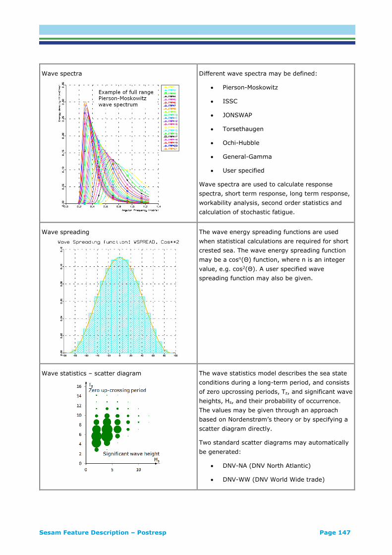
Sesam Feature Description – Postresp Page 147
Wave spectra
Different wave spectra may be defined:
• Pierson-Moskowitz
• ISSC
• JONSWAP
• Torsethaugen
• Ochi-Hubble
• General-Gamma
• User specified
Wave spectra are used to calculate response
spectra, short term response, long term response,
workability analysis, second order statistics and
calculation of stochastic fatigue.
Wave spreading
The wave energy spreading functions are used
when statistical calculations are required for short
crested sea. The wave energy spreading function
may be a cosn(Θ) function, where n is an integer
value, e.g. cos2(Θ). A user specified wave
spreading function may also be given.
Wave statistics – scatter diagram
The wave statistics model describes the sea state
conditions during a long-term period, and consists
of zero upcrossing periods, Tz, and significant wave
heights, Hs, and their probability of occurrence.
The values may be given through an approach
based on Nordenstrøm’s theory or by specifying a
scatter diagram directly.
Two standard scatter diagrams may automatically
be generated:
• DNV-NA (DNV North Atlantic)
• DNV-WW (DNV World Wide trade)
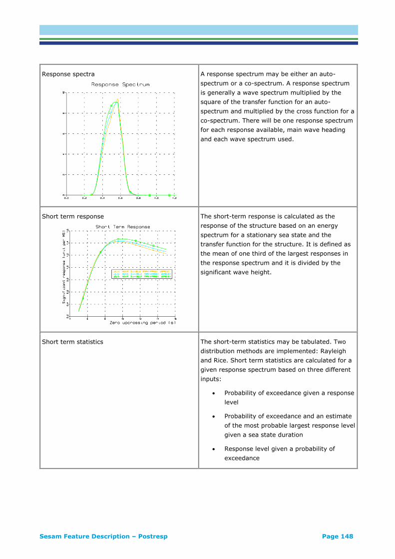
Sesam Feature Description – Postresp Page 148
Response spectra
A response spectrum may be either an auto-
spectrum or a co-spectrum. A response spectrum
is generally a wave spectrum multiplied by the
square of the transfer function for an auto-
spectrum and multiplied by the cross function for a
co-spectrum. There will be one response spectrum
for each response available, main wave heading
and each wave spectrum used.
Short term response
The short-term response is calculated as the
response of the structure based on an energy
spectrum for a stationary sea state and the
transfer function for the structure. It is defined as
the mean of one third of the largest responses in
the response spectrum and it is divided by the
significant wave height.
Short term statistics The short-term statistics may be tabulated. Two
distribution methods are implemented: Rayleigh
and Rice. Short term statistics are calculated for a
given response spectrum based on three different
inputs:
• Probability of exceedance given a response
level
• Probability of exceedance and an estimate
of the most probable largest response level
given a sea state duration
• Response level given a probability of
exceedance
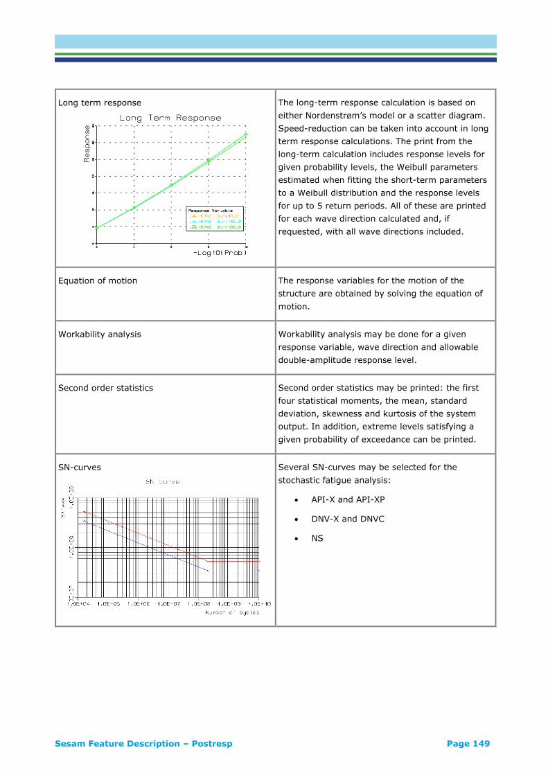
Sesam Feature Description – Postresp Page 149
Long term response
The long-term response calculation is based on
either Nordenstrøm’s model or a scatter diagram.
Speed-reduction can be taken into account in long
term response calculations. The print from the
long-term calculation includes response levels for
given probability levels, the Weibull parameters
estimated when fitting the short-term parameters
to a Weibull distribution and the response levels
for up to 5 return periods. All of these are printed
for each wave direction calculated and, if
requested, with all wave directions included.
Equation of motion The response variables for the motion of the
structure are obtained by solving the equation of
motion.
Workability analysis Workability analysis may be done for a given
response variable, wave direction and allowable
double-amplitude response level.
Second order statistics Second order statistics may be printed: the first
four statistical moments, the mean, standard
deviation, skewness and kurtosis of the system
output. In addition, extreme levels satisfying a
given probability of exceedance can be printed.
SN-curves
Several SN-curves may be selected for the
stochastic fatigue analysis:
• API-X and API-XP
• DNV-X and DNVC
• NS

Sesam Feature Description – Postresp Page 150
Stochastic fatigue calculation Stochastic fatigue calculations are available:
• Short term fatigue calculation based on
short term duration of a given sea state
and assuming Rayleigh distribution of the
stress ranges
• Long term fatigue calculation either based
directly on a scatter diagram where
Rayleigh distributions are assumed for
each cell or based on a Weibull-fit from a
long-term response calculation of the
significant responses (stress ranges) of the
cells.

Sesam Feature Description – RAO Page 151
RAO RESPONSE AMPLITUDE OPERATORS
Last revised: December 20, 2016. Describing version 1.0-00.
The console program RAO reads sets of user defined response amplitude operators, calculates the
corresponding accelerations (real part and imaginary part) and writes the results to Sestra input files,
S#.FEM and L#.FEM. Fluctuating gravity and forward speed (in terms of the Froude number) are
accounted for.
The data on the output file have the same format and structure as the corresponding loads computed by
the hydrodynamic solvers (Wadam and Wasim).

Sesam Feature Description – RAO Page 152
FEATURES OF RAO
FEATURE DESCRIPTION
Load file creation
Provided motion RAO’s are converted into
accelerations and combined with gravity. The result
is written on BRIGAC cards in the L-file
Sestra file creation
The frequencies and headings corresponding to the
load case numbers on the L-file are written to the
S-file in the same way as what is done by the
hydrodynamics solvers
Forward speed
The effect of forward speed is included in the
creation of the loads and the data on the S-file

Sesam Feature Description – Xtract Page 153
Xtract POSTPROCESSOR FOR PRESENTATION, ANIMATION AND
REPORTING OF RESULTS
Last revised: January 28, 2019. Describing version 5.2 (64-bit).
Xtract is the model and results visualisation program of Sesam. Xtract is owned and developed by
Ceetron AS and marketed by DNV GL - Software. It offers general-purpose features for extracting,
further processing, displaying, tabulating and animating results from static and dynamic structural
analysis as well as results from various types of hydrodynamic analysis. Its intuitive and high-
performance 3D graphics enables easy and efficient interactive rotation, zooming and panning of the
model with results.
The user interface operations are logged (journaled) as command equivalents. This log may be edited
and used as input to a new session for automated extraction and presentation of results.

Sesam Feature Description – Xtract Page 154
FEATURES OF XTRACT
Structural analysis results
Xtract presents results for truss, beam, membrane, plate, shell and solid models. These results may be:
• Displacements, velocities and accelerations
• Forces
• Stresses
Xtract may create combinations and scan over result cases and combinations for highest and lowest
values.
The graphic results presentation may be printed directly or saved to various graphic file formats for
inclusion in reports. Tabulated data may be exported to file for importing into spreadsheets for
customised results manipulation.
A 3D model with (animated) results may even be exported and opened in free tools for interactive 3D
viewing:
• Xtract Viewer (free program)
• PowerPoint slideshow (with free GLview 3D Plugin embedded)
• Word (with free GLview 3D Plugin embedded)
This allows a Sesam user to prepare data and send to a non-Sesam user who may view the data in an
Xtract-like environment.
Hydrodynamic analysis results
The animation feature of Xtract is especially useful for presenting results from hydrodynamic analyses.
The motion of a vessel in waves may for example be animated superimposed by the corresponding hull
stresses.
Other results
Various programs can store results on a VTF file that may be opened for postprocessing in Xtract:
• Wasim: Time domain results for a vessel and sea surface
• Installjac: Time domain results for a launching/floating stability/upending process of a jacket
• Riflex: Time domain results for conductors, risers and anchor lines
• Stofat: Stochastic fatigue results for a stiffened plate
• ShellDesign (a product of Dr. Techn. Olav Olsen): Steel reinforced concrete shell design results
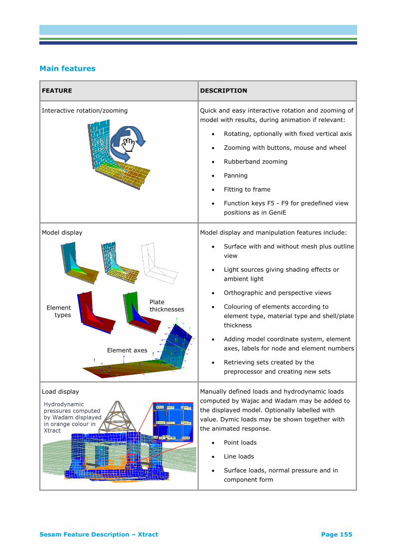
Sesam Feature Description – Xtract Page 155
Element axes
Main features
FEATURE DESCRIPTION
Interactive rotation/zooming
Quick and easy interactive rotation and zooming of
model with results, during animation if relevant:
• Rotating, optionally with fixed vertical axis
• Zooming with buttons, mouse and wheel
• Rubberband zooming
• Panning
• Fitting to frame
• Function keys F5 - F9 for predefined view
positions as in GeniE
Model display
Model display and manipulation features include:
• Surface with and without mesh plus outline
view
• Light sources giving shading effects or
ambient light
• Orthographic and perspective views
• Colouring of elements according to
element type, material type and shell/plate
thickness
• Adding model coordinate system, element
axes, labels for node and element numbers
• Retrieving sets created by the
preprocessor and creating new sets
Load display
Manually defined loads and hydrodynamic loads
computed by Wajac and Wadam may be added to
the displayed model. Optionally labelled with
value. Dymic loads may be shown together with
the animated response.
• Point loads
• Line loads
• Surface loads, normal pressure and in
component form
Element
types
Plate
thicknesses
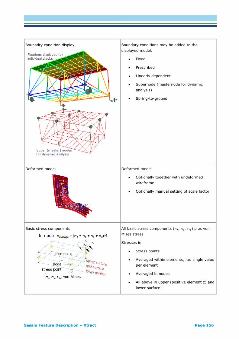
Sesam Feature Description – Xtract Page 156
Bounadry condition display
Boundary conditions may be added to the
displayed model:
• Fixed
• Prescribed
• Linearly dependent
• Supernode (masternode for dynamic
analysis)
• Spring-to-ground
Deformed model
Deformed model
• Optionally together with undeformed
wireframe
• Optionally manual setting of scale factor
Basic stress components
All basic stress components (x, y, xy) plus von
Mises stress.
Stresses in:
• Stress points
• Averaged within elements, i.e. single value
per element
• Averaged in nodes
• All above in upper (positive element z) and
lower surface

Sesam Feature Description – Xtract Page 157
Derived stresses
Derived stresses are based on the basic stress
components:
• Basic stress components decomposed into
membrane (M) and bending (B) stresses
• Basic stresses integrated through thickness
gives stress resultants (also termed direct
stresses)
• Principal stresses, P1 is the highest stress
in main stress direction, P2 is lowest stress
perpendicular to main stress direction
Colour contouring
Colour contouring (filling) for all types of results
User control of the contour levels and legend:
• Number of levels between min and max
• Specified min and max
• Selected values
Numerics in display
Numeric values superimposed on whole model:
• All values
• Limited to ranges (min – max)
• Only peak (maximum and minimum)
values
• Label with and without background box
• Font size control
• Number of digits control

Sesam Feature Description – Xtract Page 158
Numerics in display for selected elements/nodes
Numeric values superimposed for selected:
• Elements (Shift+Ctrl+click)
• Nodes (Ctrl+click)
Mouseover/hover box
Feedback label with node/element information
including results shown by hovering the mouse.

Sesam Feature Description – Xtract Page 159
Vector presentation
Vector presentation of.
• Principal stresses P1, P2, P3 on top of
colour contouring of one of them
• Deformation
Stress transformation
Transformation of stresses to a user defined
coordinate system may be done for shell, plate
and membrane elements. The user gives a rotation
about the normal axis.
Graph
A graph in Xtract may be shown in a separate view
or transparently superimposed on the model.
Graph can be shown for:
• Nodes – results graphed over a series of
nodes
• Beams – results graphed along several
beams
• Occurrences – results in a node graphed
over result cases, e.g. time
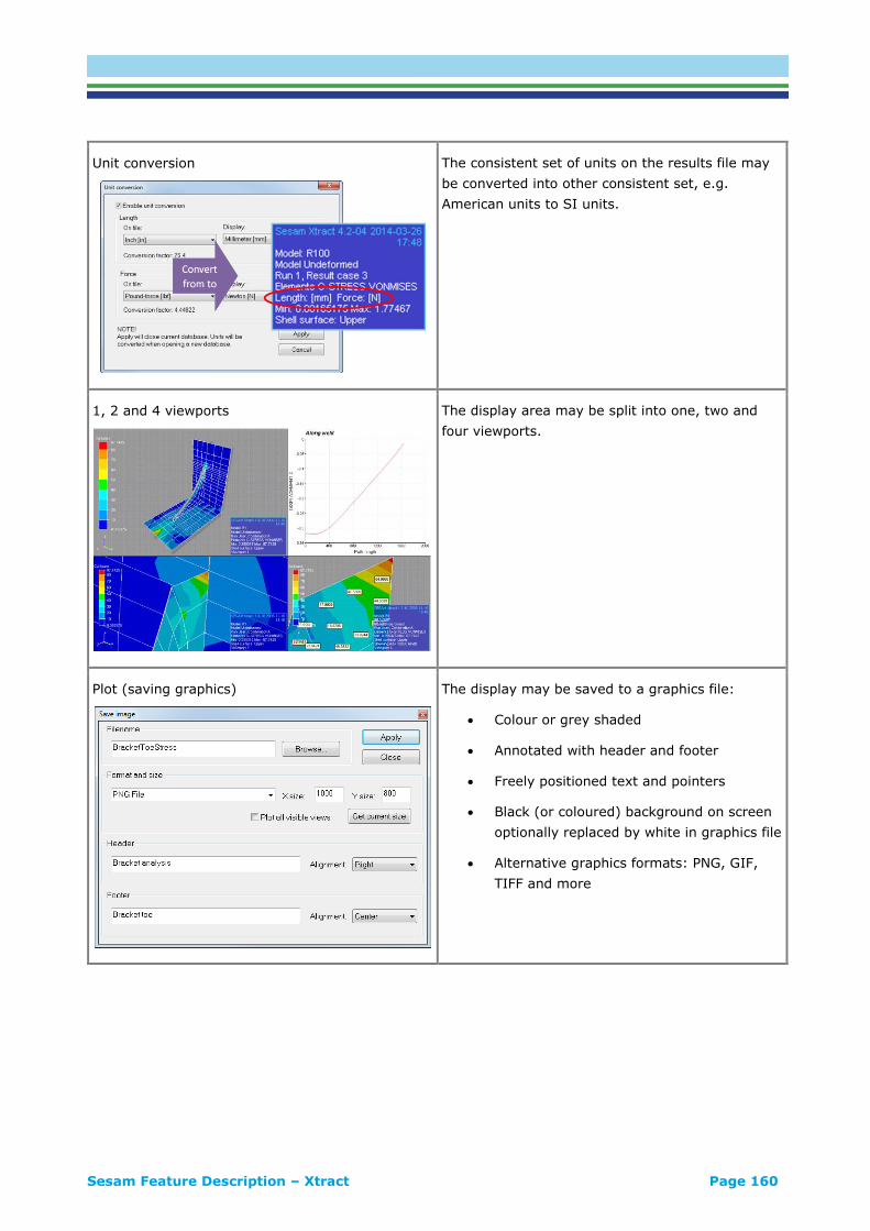
Sesam Feature Description – Xtract Page 160
Unit conversion
The consistent set of units on the results file may
be converted into other consistent set, e.g.
American units to SI units.
1, 2 and 4 viewports
The display area may be split into one, two and
four viewports.
Plot (saving graphics)
The display may be saved to a graphics file:
• Colour or grey shaded
• Annotated with header and footer
• Freely positioned text and pointers
• Black (or coloured) background on screen
optionally replaced by white in graphics file
• Alternative graphics formats: PNG, GIF,
TIFF and more

Sesam Feature Description – Xtract Page 161
Models and results for presentation in Xtract
Xtract may present analysis results from different programs. A list of files for processing is provided
below. The required program extension is also given.
FEATURE DESCRIPTION
Structural Results Postprocessing
R#.SIN file
The R#.SIN (or R#.SIU or R#.SIF) file is typically
generated by Sestra. Its contents are:
• FE model
• Nodal displacements
• Beam forces
• Element stresses
Program extension required: STRU
Hydrodynamic & Structural Results Postprocessing
R#.SIN + Gn.SIF
The R#.SIN file: see above.
The Gn.SIF file is typically generated by Wadam,
Wajac or Prepost. Its contents are:
• Transfer functions for rigid body motion of
floating structure (Wadam)
• Sea surface elevation (Wadam)
• Transfer functions for base shear and
overturning moments for fixed frame
structure (Wajac)
• Transfer functions for forces and stresses
in selected elements (Prepost)
Program extension required: STRU
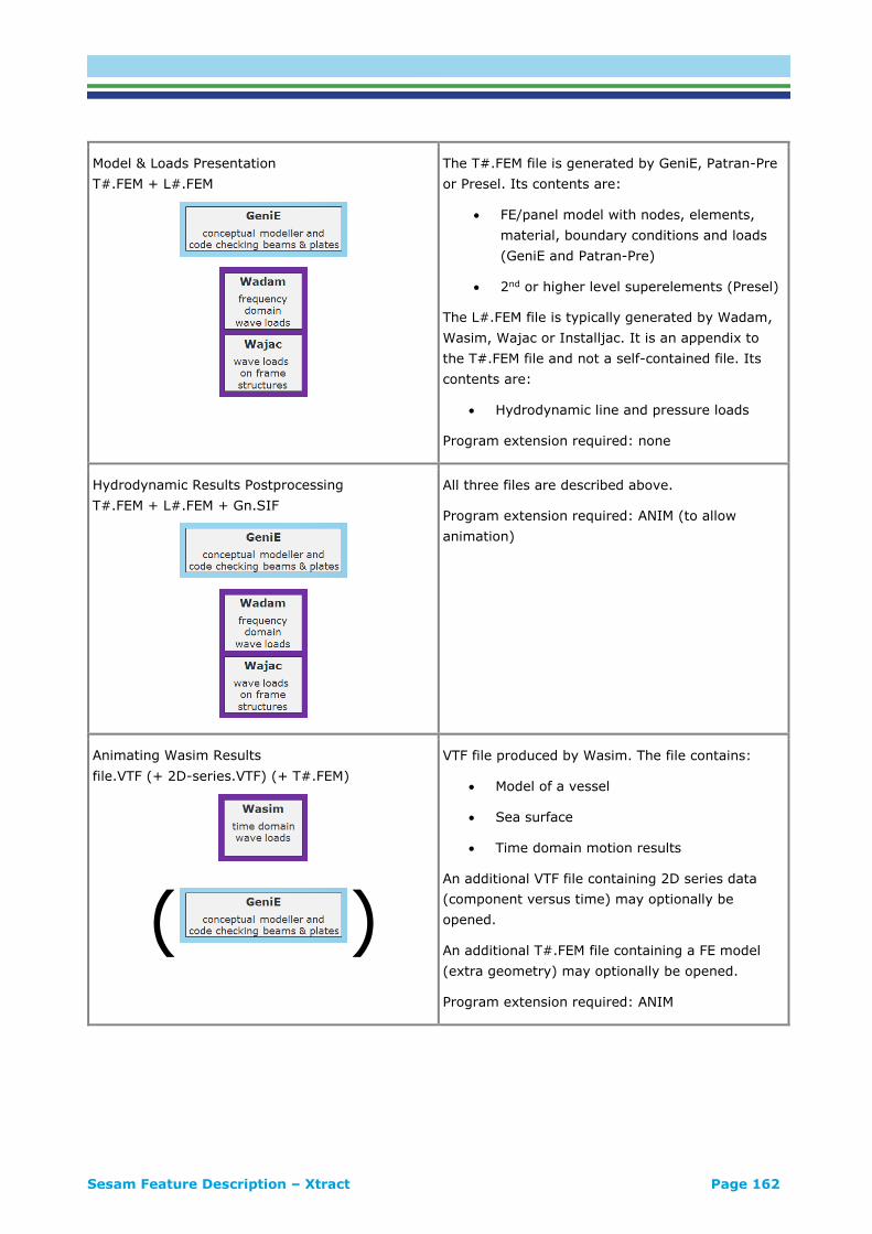
Sesam Feature Description – Xtract Page 162
Model & Loads Presentation
T#.FEM + L#.FEM
The T#.FEM file is generated by GeniE, Patran-Pre
or Presel. Its contents are:
• FE/panel model with nodes, elements,
material, boundary conditions and loads
(GeniE and Patran-Pre)
• 2nd or higher level superelements (Presel)
The L#.FEM file is typically generated by Wadam,
Wasim, Wajac or Installjac. It is an appendix to
the T#.FEM file and not a self-contained file. Its
contents are:
• Hydrodynamic line and pressure loads
Program extension required: none
Hydrodynamic Results Postprocessing
T#.FEM + L#.FEM + Gn.SIF
All three files are described above.
Program extension required: ANIM (to allow
animation)
Animating Wasim Results
file.VTF (+ 2D-series.VTF) (+ T#.FEM)
( )
VTF file produced by Wasim. The file contains:
• Model of a vessel
• Sea surface
• Time domain motion results
An additional VTF file containing 2D series data
(component versus time) may optionally be
opened.
An additional T#.FEM file containing a FE model
(extra geometry) may optionally be opened.
Program extension required: ANIM

Sesam Feature Description – Xtract Page 163
Animating Installjac Results
file.VTF (+ 2D-series.VTF)
VTF file produced by Installjac. The file contains:
• Models of jacket, barge and sea surface
• Time domain motion results of the
launching/floating stability/upending
process
An additional VTF file containing 2D series data
(component versus time) may optionally be
opened.
Program extension required: ANIM
Animating Riflex Results
file.VTF (+ 2D-series.VTF) (+ T#.FEM)
( )
VTF file produced by Riflex. The file contains:
• Time domain results for conductors, risers
and anchor lines
An additional VTF file containing 2D series data
(component versus time) may optionally be
opened.
An additional T#.FEM file containing a FE model
(extra geometry) may optionally be opened.
Program extension required: ANIM
Presenting Stofat Results
file.VTF
VTF file produced by Stofat. The file contains:
• Stiffened plate model with stochastic
fatigue analysis results
An additional VTF file containing 2D series data
may optionally be opened.
Program extension required: ANIM
Presenting ShellDesign results
file.VTF
VTF file produced by ShellDesign (a product of Dr.
Techn. Olav Olsen). The file contains:
• Steel reinforced concrete shell design
results
Program extension required: SHDS
ShellDesign
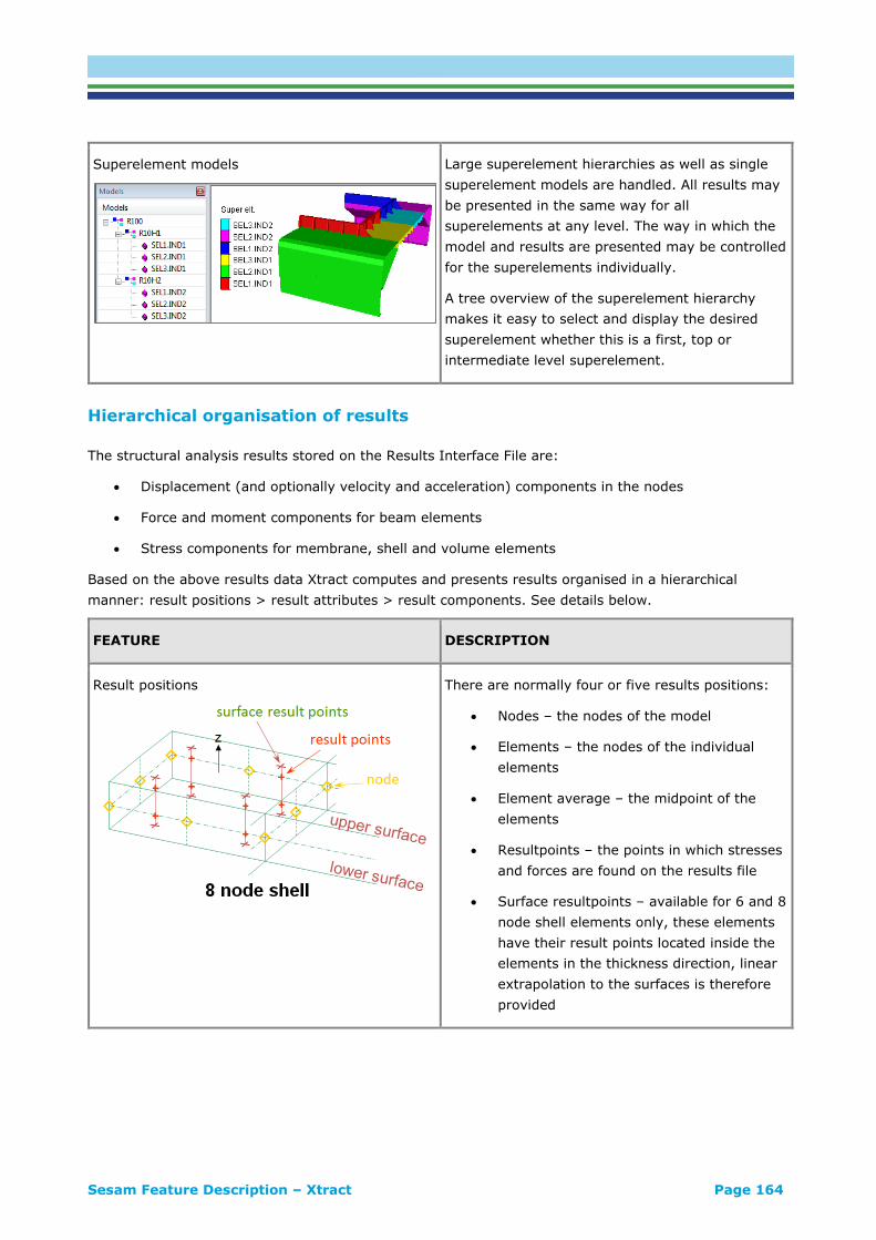
Sesam Feature Description – Xtract Page 164
Superelement models
Large superelement hierarchies as well as single
superelement models are handled. All results may
be presented in the same way for all
superelements at any level. The way in which the
model and results are presented may be controlled
for the superelements individually.
A tree overview of the superelement hierarchy
makes it easy to select and display the desired
superelement whether this is a first, top or
intermediate level superelement.
Hierarchical organisation of results
The structural analysis results stored on the Results Interface File are:
• Displacement (and optionally velocity and acceleration) components in the nodes
• Force and moment components for beam elements
• Stress components for membrane, shell and volume elements
Based on the above results data Xtract computes and presents results organised in a hierarchical
manner: result positions > result attributes > result components. See details below.
FEATURE DESCRIPTION
Result positions
There are normally four or five results positions:
• Nodes – the nodes of the model
• Elements – the nodes of the individual
elements
• Element average – the midpoint of the
elements
• Resultpoints – the points in which stresses
and forces are found on the results file
• Surface resultpoints – available for 6 and 8
node shell elements only, these elements
have their result points located inside the
elements in the thickness direction, linear
extrapolation to the surfaces is therefore
provided

Sesam Feature Description – Xtract Page 165
Result attributes
Each result position has its own set of result
attributes being a selection of the following:
• DISPLACEMENT – nodal displacements
• VELOCITY – nodal velocities
• ACCELERATION – nodal accelerations
• REACTION-FORCE – reaction forces in
supported (fixed or prescribed) nodes
• G-STRESS – general stresses (found on
the results file)
• P-STRESS – principal stresses
• PM-STRESS – principal membrane stresses
• D-STRESS – decomposed stresses for shell
elements
• R-STRESS – stresses integrated through
the thickness
• G-FORCE – general forces for beam
elements
• B-STRESS – beam stresses
Result components
Each attribute has its own set of result
components. Examples of components:
• DISPLACEMENT: X, Y, Z, RX, RY, RZ and
ALL
• G-STRESS: SIGXX, SIGYY, TAUXY, etc.
• P-STRESS: P1, P2 and P3.
• PM-STRESS: P1 and P2.
• D-STRESS: SIGMX, SIGMY, TAUMXY, etc.
• G-FORCE: NXX, NXY, NXZ, MXX, etc.
• REACTION-FORCE: X-FORCE, Y-FORCE, Z-
FORCE, RX-MOMENT, etc.
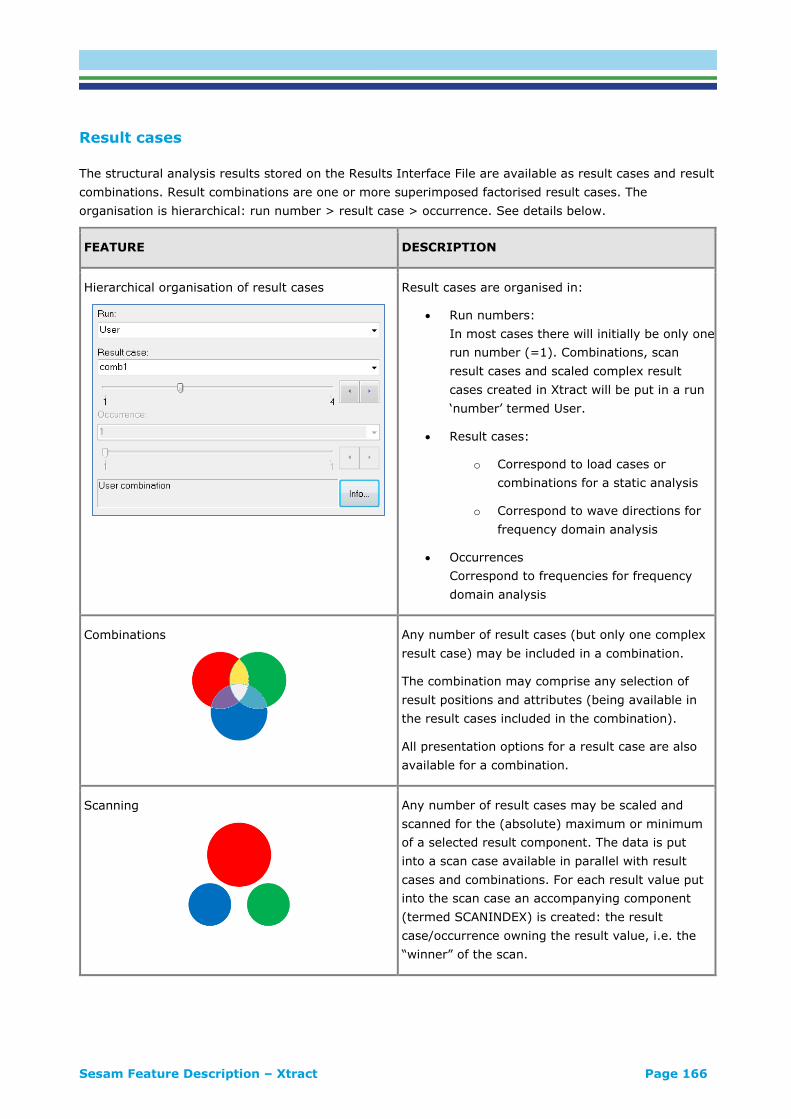
Sesam Feature Description – Xtract Page 166
Result cases
The structural analysis results stored on the Results Interface File are available as result cases and result
combinations. Result combinations are one or more superimposed factorised result cases. The
organisation is hierarchical: run number > result case > occurrence. See details below.
FEATURE DESCRIPTION
Hierarchical organisation of result cases
Result cases are organised in:
• Run numbers:
In most cases there will initially be only one
run number (=1). Combinations, scan
result cases and scaled complex result
cases created in Xtract will be put in a run
‘number’ termed User.
• Result cases:
o Correspond to load cases or
combinations for a static analysis
o Correspond to wave directions for
frequency domain analysis
• Occurrences
Correspond to frequencies for frequency
domain analysis
Combinations
Any number of result cases (but only one complex
result case) may be included in a combination.
The combination may comprise any selection of
result positions and attributes (being available in
the result cases included in the combination).
All presentation options for a result case are also
available for a combination.
Scanning
Any number of result cases may be scaled and
scanned for the (absolute) maximum or minimum
of a selected result component. The data is put
into a scan case available in parallel with result
cases and combinations. For each result value put
into the scan case an accompanying component
(termed SCANINDEX) is created: the result
case/occurrence owning the result value, i.e. the
“winner” of the scan.
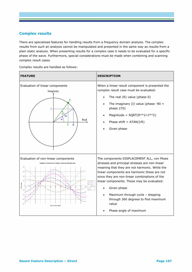
Sesam Feature Description – Xtract Page 167
Complex results
There are specialised features for handling results from a frequency domain analysis. The complex
results from such an analysis cannot be manipulated and presented in the same way as results from a
plain static analysis. When presenting results for a complex case it needs to be evaluated for a specific
phase of the wave. Furthermore, special considerations must be made when combining and scanning
complex result cases.
Complex results are handled as follows:
FEATURE DESCRIPTION
Evaluation of linear components
When a linear result component is presented the
complex result case must be evaluated:
• The real (R) value (phase 0)
• The imaginary (I) value (phase -90 =
phase 270)
• Magnitude = SQRT(R**2+I**2)
• Phase shift = ATAN(I/R)
• Given phase
Evaluation of non-linear components
The components DISPLACEMENT ALL, von Mises
stresses and principal stresses are non-linear
meaning that they are not harmonic. While the
linear components are harmonic these are not
since they are non-linear combinations of the
linear components. These may be evaluated:
• Given phase
• Maximum through cycle – stepping
through 360 degrees to find maximum
value
• Phase angle of maximum

Sesam Feature Description – Xtract Page 168
Combination
A combination may include a single complex result
case and any number of static (non-complex)
result cases. The complex result case may be
evaluated for the (absolute) maximum or
minimum of any result component as well as for
any user chosen phase of the wave.
Scanning
A scanning for the (absolute) maximum or
minimum value of a component may be done for
any number of complex result cases and any
number of static (non-complex) result cases. In
this process, each complex result case is
evaluated. The evaluation may be done for a given
phase or for the same criterion as the scanning
over the result cases. The latter evaluation is
normally the desired one and involves that if you
want to scan several result cases for the highest
von Mises stress then the complex result cases
need to be evaluated for the highest von Mises
stress also.
Scaling
A complex result case may be scaled. I.e. the real
and imaginary parts are simply multiplied by a
given factor.

Sesam Feature Description – Xtract Page 169
Animation of dynamic behaviour
FEATURE DESCRIPTION
Mode shape animation The mode shape (eigenmodes) may be animated.
The number of frames (time steps) through the
360-degree cycle is specified. The more frames the
smoother animation.
Frequency domain animation The harmonic motion of a structure may be
animated. The step interval in degrees is specified.
The shorter step the smoother animation.
Time domain animation The time domain motion of a structure may be
animated. Which time steps to include in the
animation is specified.
Animation speed The animation speed may be adjusted by setting
frames per second.
Saving animation An animation may be saved to alternative formats
for replaying outside Xtract.
Exporting data for further processing and reporting
By exporting data from Xtract you have access to even more presentation features.
FEATURE DESCRIPTION
Save tabulated data to file
Tabulated nodal and element results may be saved
to file for import into another program, e.g. Excel.
Optionally the table may be unwrapped to one line
per item with tab delimiters to ease further
processing in Excel.
Export graph data
Data graphed in Xtract may be exported to file for
import into e.g. Excel.

Sesam Feature Description – Xtract Page 170
3D model viewing outside Xtract
Xtract-like GUI in PowerPoint
A 3D model with results (and animation) may be
exported to a VTFx file. The VTFx file may be
opened for interactive 3D viewing in:
• Xtract Viewer (free program)
• PowerPoint slideshow (with free GLview 3D
Plugin embedded)
• Word (with free GLview 3D Plugin
embedded)
A Sesam user may thus prepare data and send to a
non-Sesam user who may view the data in an
Xtract-like environment.
Global model + sub-model
Two 3D models may be exported to a common
VTFx file. The feature is general but it is
particularly useful for comparing a sub-model with
the global model in a sub-modelling type of
analysis, i.e. involving use of the program
Submod. The deformed shape of the two models
may for instance be overlaid to verify that the
deformations at the outer boundary of the sub-
model match those of the global model. Such
match of deformations is an absolute demand in a
sub-modelling analysis.

Sesam Feature Description – Framework Page 171
Framework STEEL FRAME DESIGN
Last revised: October 5, 2018. Describing version 4.0-01.
Framework is a postprocessor for frame structures, i.e. 2 node beam elements, with the following
capabilities:
• Wave induced fatigue analysis
• Wind induced fatigue analysis
• Earthquake analysis including code checking

Sesam Feature Description – Framework Page 172
FEATURES OF FRAMEWORK
The processes in Sesam involved in the three most important wave induced types of fatigue analysis –
the deterministic, spectral and stochastic – is illustrated by the figure below.
A description of the main features of Framework follows below.
FEATURE DESCRIPTION
Wave induced deterministic fatigue
Required analyses in:
• Wajac: Several deterministic waves of
different heights, lengths and directions
• Sestra: Static analysis
The deterministic fatigue analysis method is for
dynamically insensitive structures in shallow to
medium water depths where non-linearities in the
wave force such as drag and variable submergence
are of importance. The energy content of the sea-
states is not directly represented in the method so
judgment and experience is required in selecting
the discrete waves to include in the analysis.
Framework Deterministic approach
Framework Spectral approach
Wajac Deterministic wave loads
Sestra
Static/dynamic time-stepping analysis
Wajac Frequency domain wave loads
Sestra Frequency domain static/dynamic analysis
Deterministic fatigue analysis Spectral fatigue analysis Stochastic fatigue analysis

Sesam Feature Description – Framework Page 173
Wave induced spectral fatigue
Required analyses in:
• Wajac: Several deterministic waves of
different heights, lengths and directions
• Sestra: Static or dynamic analysis
Spectral stress transfer functions are established
based on deterministic stress variations followed by
a spectral fatigue analysis.
The spectral fatigue analysis method is for
dynamically sensitive and insensitive structures in
shallow to medium water depths where non-
linearities in the wave force such as drag and
variable submergence are of importance. The
structural dynamic analysis, if required, may be
computer intensive. The method properly
represents the energy content of the sea-states.
Wave induced stochastic fatigue
Required analyses in:
• Wajac: Spectral (frequency domain) waves,
unit amplitude waves of different frequency
and direction
• Sestra: Dynamic or quasi-static analysis
The stochastic fatigue analysis method is for
dynamically sensitive and insensitive structures in
deep water where the non-linearities in the wave
force are less important. The method properly
represents the energy content of the sea-states.
This analysis is equivalent to the wave induced
stochastic fatigue analysis available for welded
plate and shell structures in Stofat.
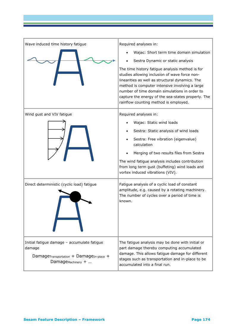
Sesam Feature Description – Framework Page 174
Wave induced time history fatigue
Required analyses in:
• Wajac: Short term time domain simulation
• Sestra Dynamic or static analysis
The time history fatigue analysis method is for
studies allowing inclusion of wave force non-
linearities as well as structural dynamics. The
method is computer intensive involving a large
number of time domain simulations in order to
capture the energy of the sea-states properly. The
rainflow counting method is employed.
Wind gust and VIV fatigue
Required analyses in:
• Wajac: Static wind loads
• Sestra: Static analysis of wind loads
• Sestra: Free vibration (eigenvalue)
calculation
• Merging of two results files from Sestra
The wind fatigue analysis includes contribution
from long term gust (buffeting) wind loads and
vortex induced vibrations (VIV).
Direct deterministic (cyclic load) fatigue
Fatigue analysis of a cyclic load of constant
amplitude, e.g. caused by a rotating machinery.
The number of cycles over a period of time is
known.
Initial fatigue damage – accumulate fatigue
damage
DamageTransportation + DamageIn-place +
DamageMachinery + …
The fatigue analysis may be done with initial or
part damage thereby computing accumulated
damage. This allows fatigue damage for different
stages such as transportation and in-place to be
accumulated into a final run.
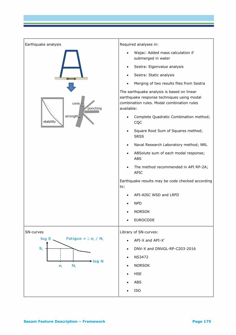
Sesam Feature Description – Framework Page 175
Earthquake analysis
Required analyses in:
• Wajac: Added mass calculation if
submerged in water
• Sestra: Eigenvalue analysis
• Sestra: Static analysis
• Merging of two results files from Sestra
The earthquake analysis is based on linear
earthquake response techniques using modal
combination rules. Modal combination rules
available:
• Complete Quadratic Combination method;
CQC
• Square Root Sum of Squares method;
SRSS
• Naval Research Laboratory method; NRL
• ABSolute sum of each modal response;
ABS
• The method recommended in API RP-2A;
APIC
Earthquake results may be code checked according
to:
• API-AISC WSD and LRFD
• NPD
• NORSOK
• EUROCODE
SN-curves
Library of SN-curves:
• API-X and API-X’
• DNV-X and DNVGL-RP-C203-2016
• NS3472
• NORSOK
• HSE
• ABS
• ISO

Sesam Feature Description – Framework Page 176
SCF – Stress Concentration Factors
Manual specification and parametric (formulas):
• Kuang for YT, K, KT / Wordsworth and
Smedley for X
• Efthymiou for X, YT, K and KT
• Lloyd’s Register for gap K and KT
• Smedley and Fisher for SCF ring stiffened
tubular joints
• NORSOK for SCFs at butt welds and conical
transitions
Fatigue check points
Eight points around the circumference of the
tubular sections are checked for fatigue, both on
the chord and brace sides of the weld. For each
point an SCF may be manually or parametrically
specified.
Wave height distribution
The long-term wave height distribution is defined
for deterministic fatigue analysis as:
• Linear
• Piecewise linear
Wave spectra
The wave spectra available for spectral and
stochastic fatigue are:
• Pierson-Moskowitz
• Jonswap
• General Gamma
• ISSC
• Ochi-Hubble
• Torsethaugen

Sesam Feature Description – Framework Page 177
Wave spreading
Wave energy spreading functions may be defined
to account for short crested sea in spectral and
stochastic fatigue analyses:
• Cosine power, e.g. cos2
• User defined
Wave statistics – scatter diagram
Wave statistics (scatter diagram) for long term sea
state conditions are defined for spectral and
stochastic fatigue:
• Manually
• Predefined (DNV-NA, DNV-WW)
Wave direction probability
Wave direction probabilities are defined for
spectral and stochastic fatigue to calculate
contributions from the wave directions to the
fatigue damage.
Graphic results presentation
Results may be presented graphically:
• Fatigue
• Code check (of earthquake)
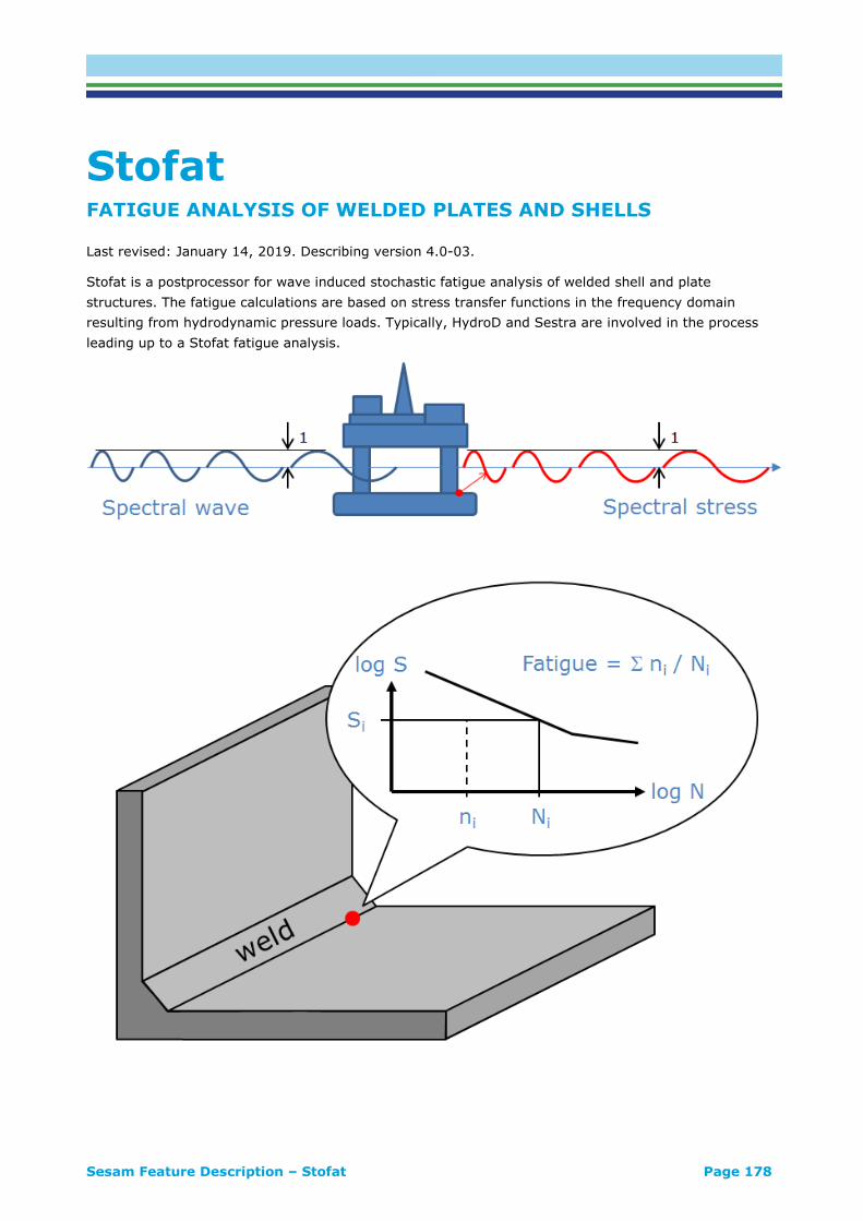
Sesam Feature Description – Stofat Page 178
Stofat FATIGUE ANALYSIS OF WELDED PLATES AND SHELLS
Last revised: January 14, 2019. Describing version 4.0-03.
Stofat is a postprocessor for wave induced stochastic fatigue analysis of welded shell and plate
structures. The fatigue calculations are based on stress transfer functions in the frequency domain
resulting from hydrodynamic pressure loads. Typically, HydroD and Sestra are involved in the process
leading up to a Stofat fatigue analysis.

Sesam Feature Description – Stofat Page 179
FEATURES OF STOFAT
FEATURE DESCRIPTION
Wave induced stochastic fatigue
Required analyses in:
• HydroD/Wadam: Spectral (frequency
domain) waves, unit amplitude waves of
different frequency and direction
• Sestra: Dynamic or quasi-static analysis
The stochastic fatigue analysis method is for
dynamically sensitive and insensitive structures in
deep water where the non-linearities in the wave
force are less important. The structural dynamic
analysis, if required, may be computer intensive.
The method properly represents the energy content
of the sea-states.
This analysis is equivalent to the wave induced
stochastic fatigue analysis available for frame
structures in Framework.
Time domain fatigue based on time history load
Required analyses in:
• HydroD/Wasim: Time domain wave load
analysis
• Sestra: Time domain dynamic analysis
The fatigue analysis is based on stress reversals
determined by a rainflow-counting algorithm.
Time domain fatigue based on FFT Based on Fast Fourier Transform (FFT) of spectral
data and rainflow-counting.
Long term stress calculation
The long-term stress calculation:
• Maximum and minimum stress
• Return period
• Probability level
• Exceedance
• Etc.

Sesam Feature Description – Stofat Page 180
SN-curves
Library of SN-curves:
• API-X and API-X’
• DNV-X and DNV RP-C203-2010, etc.
• NS3472
• NORSOK
• HSE
• ABS
Static stress accounted for
Static stress from still water is accounted for
according to DNV Classification Notes No. 30.7. I.e.
tension increases and compression reduces fatigue
damage.
Principal stress direction
Fatigue analysis is based on the principal stress
within ±45º of the weld normal line.
Wave spectra
The wave spectra available are:
• Pierson-Moskowitz
• Jonswap
• General Gamma
• ISSC
• Ochi-Hubble
• Torsethaugen
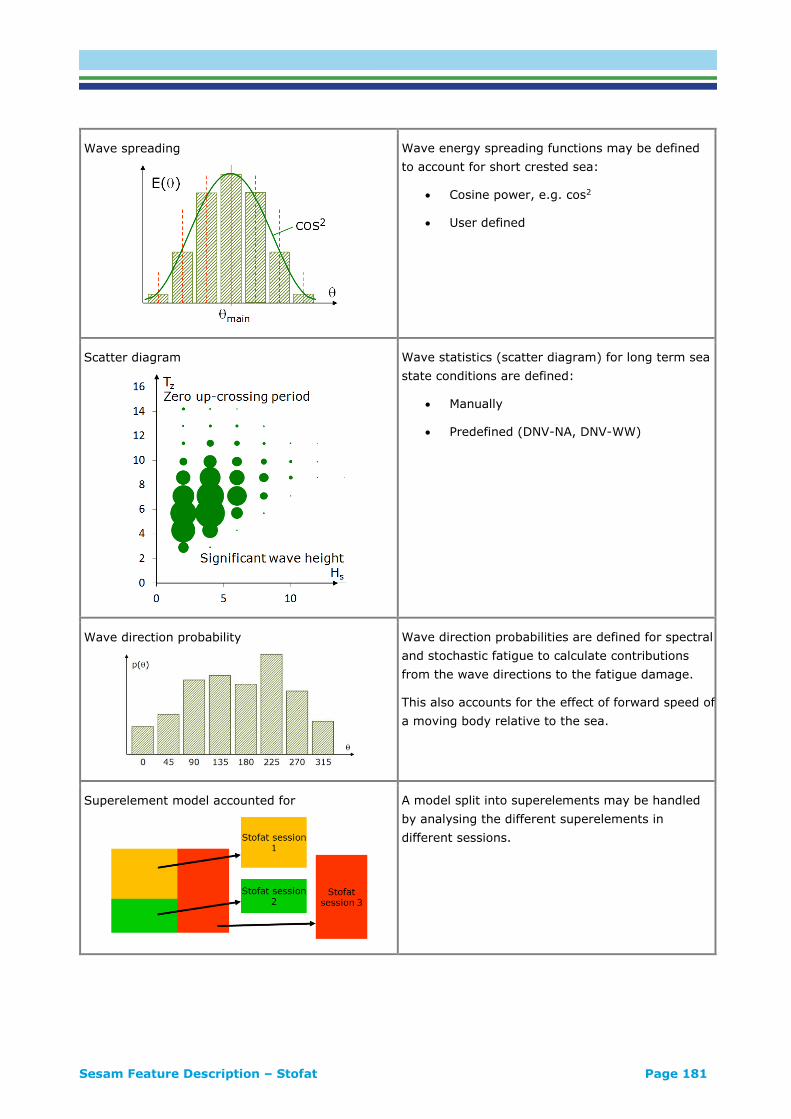
Sesam Feature Description – Stofat Page 181
Wave spreading
Wave energy spreading functions may be defined
to account for short crested sea:
• Cosine power, e.g. cos2
• User defined
Scatter diagram
Wave statistics (scatter diagram) for long term sea
state conditions are defined:
• Manually
• Predefined (DNV-NA, DNV-WW)
Wave direction probability
Wave direction probabilities are defined for spectral
and stochastic fatigue to calculate contributions
from the wave directions to the fatigue damage.
This also accounts for the effect of forward speed of
a moving body relative to the sea.
Superelement model accounted for
A model split into superelements may be handled
by analysing the different superelements in
different sessions.
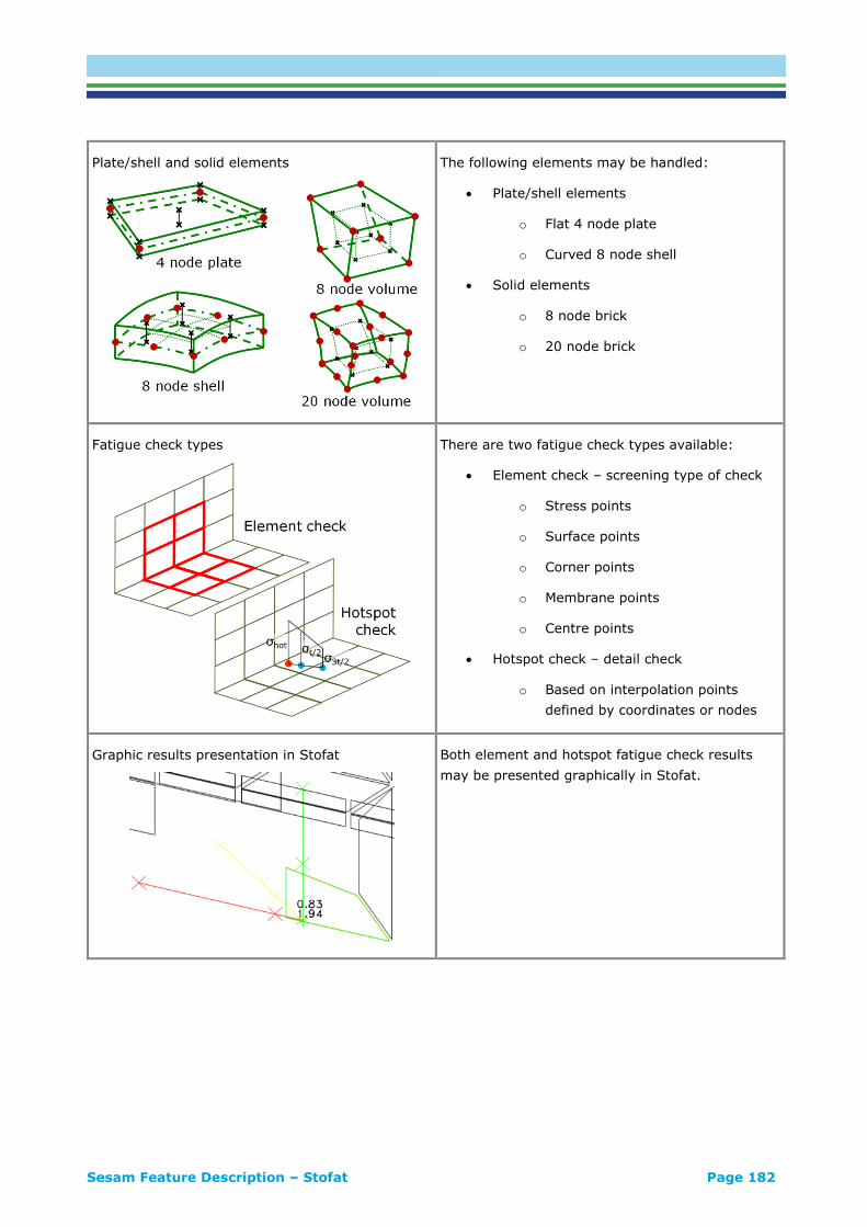
Sesam Feature Description – Stofat Page 182
Plate/shell and solid elements
The following elements may be handled:
• Plate/shell elements
o Flat 4 node plate
o Curved 8 node shell
• Solid elements
o 8 node brick
o 20 node brick
Fatigue check types
There are two fatigue check types available:
• Element check – screening type of check
o Stress points
o Surface points
o Corner points
o Membrane points
o Centre points
• Hotspot check – detail check
o Based on interpolation points
defined by coordinates or nodes
Graphic results presentation in Stofat
Both element and hotspot fatigue check results
may be presented graphically in Stofat.
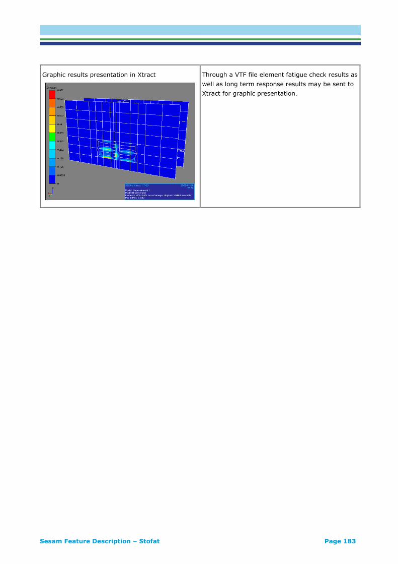
Sesam Feature Description – Stofat Page 183
Graphic results presentation in Xtract
Through a VTF file element fatigue check results as
well as long term response results may be sent to
Xtract for graphic presentation.
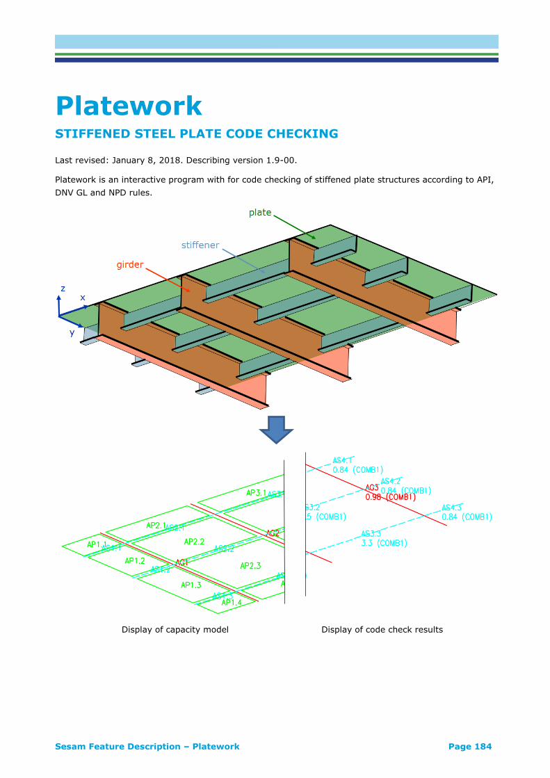
Sesam Feature Description – Platework Page 184
Platework STIFFENED STEEL PLATE CODE CHECKING
Last revised: January 8, 2018. Describing version 1.9-00.
Platework is an interactive program with for code checking of stiffened plate structures according to API,
DNV GL and NPD rules.
Display of capacity model Display of code check results

Sesam Feature Description – Platework Page 185
FEATURES OF PLATEWORK
FEATURE DESCRIPTION
Independent or FE use In addition to use in conjunction with a FE analysis
the program can be used as an independent tool to
assess stiffened plates with given loads.
Capacity models
The FE model is fully or semi-automatically split
into an assembly of capacity models:
• Simple unstiffened plate
• Stiffener
• Girder
• Uniaxially and orthogonally stiffened panel
(API)
Capacity models may be displayed as shown on the
previous page.
Capacity models for any FE mesh
The capacity model creation and code checking is
independent of the FE mesh. The only difference is
that a finer mesh will produce more accurate code
checking results.
Single or multiple superelements
The capacity model creation and code checking is
independent of division into superelements.

Sesam Feature Description – Platework Page 186
Capacity model loads
Each capacity model, plate, stiffener and girder,
has its set of capacity model loads on which the
code checking is performed.
The capacity model loads are automatically
established for all result cases.
Capacity model loads:
Code checking standards API – American Petroleum Institute
DNV – DNV GL
NPD – Norwegian Petroleum Directorate
Graphic results presentation
The code check results may be presented
graphically
Tabulated results presentation
Tabulated results may be sorted in several ways to
focus on the results of interest.
Alternative modelling of stiffeners
In the FE model the stiffeners may be modelled
as:
• Beams
• Plate elements for web and beams for
flange
• Plate elements for both web and flange
The same capacity model may be created and code
checked for all three cases.

Sesam Feature Description – Cutres Page 187
Cutres PRESENTATION OF SECTIONAL RESULTS
Last revised: April 23, 2018. Describing version 1.5-03.
Cutres is a postprocessor for presentation of results in terms of stresses, forces and moments in user
defined sections through a FE shell/plate model with beam stiffeners. This is primarily relevant for oblong
structures that may be regarded as beams, e.g. ship type structures and pontoons of semi-submersibles.
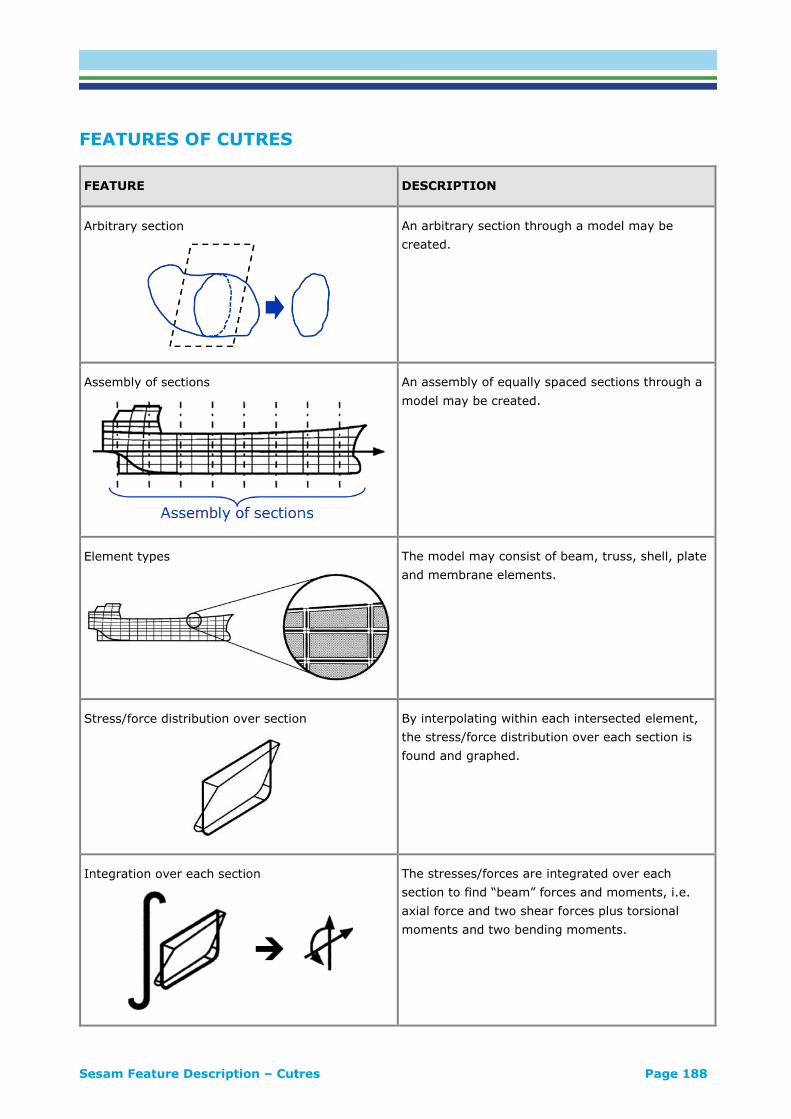
Sesam Feature Description – Cutres Page 188
FEATURES OF CUTRES
FEATURE DESCRIPTION
Arbitrary section
An arbitrary section through a model may be
created.
Assembly of sections
An assembly of equally spaced sections through a
model may be created.
Element types
The model may consist of beam, truss, shell, plate
and membrane elements.
Stress/force distribution over section
By interpolating within each intersected element,
the stress/force distribution over each section is
found and graphed.
Integration over each section
The stresses/forces are integrated over each
section to find “beam” forces and moments, i.e.
axial force and two shear forces plus torsional
moments and two bending moments.

Sesam Feature Description – Cutres Page 189
“Beam” forces/moments along axis
The “beam” forces/moments may be graphed and
tabulated along the “beam” axis.
Static or complex Complex results from a frequency domain analysis
may be handled as well as results from a static
analysis.
Direct or superelement analysis
Direct analysis
Superelement analysis
The model may be a multilevel superelement
model.
Handling part of a model
By specifying limiting coordinates or by selecting
sets a part of the model may be selected for
creation of sections.
This allows calculating “beam” forces/moments for
e.g. only a pontoon of a full semi-submersible
model and only one hull of a double-hull ship.
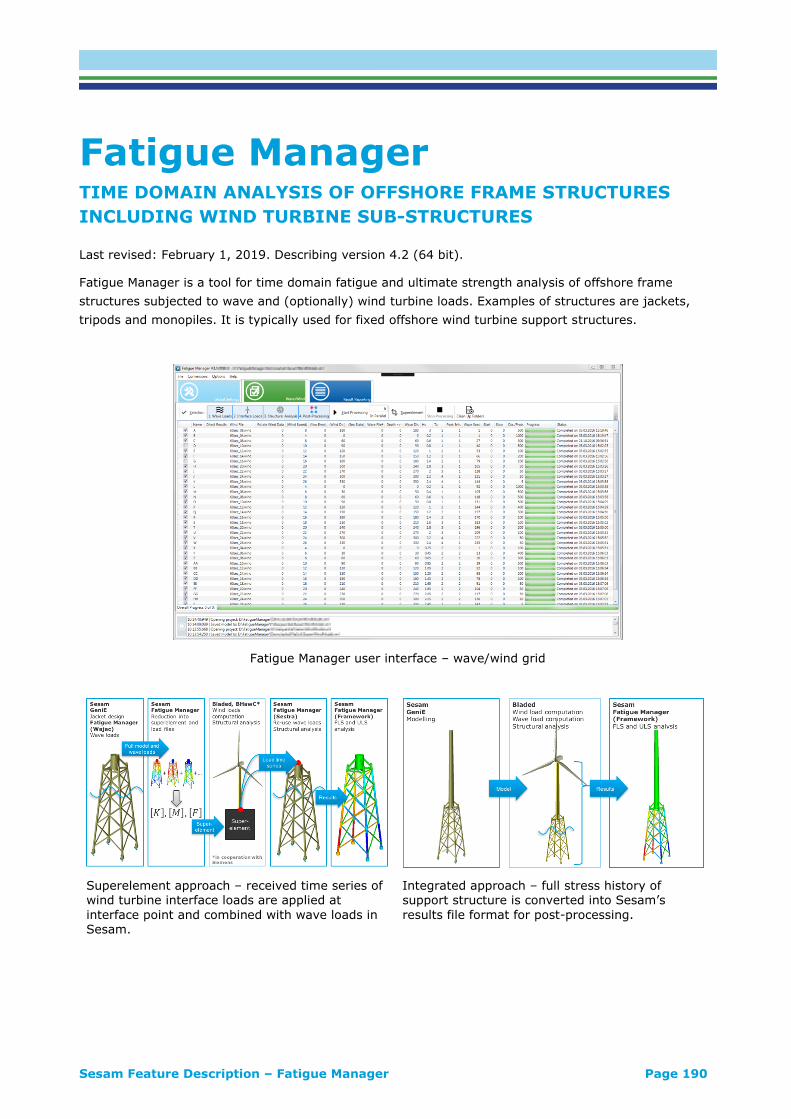
Sesam Feature Description – Fatigue Manager Page 190
Fatigue Manager TIME DOMAIN ANALYSIS OF OFFSHORE FRAME STRUCTURES
INCLUDING WIND TURBINE SUB-STRUCTURES
Last revised: February 1, 2019. Describing version 4.2 (64 bit).
Fatigue Manager is a tool for time domain fatigue and ultimate strength analysis of offshore frame
structures subjected to wave and (optionally) wind turbine loads. Examples of structures are jackets,
tripods and monopiles. It is typically used for fixed offshore wind turbine support structures.
Fatigue Manager user interface – wave/wind grid
Superelement approach – received time series of wind turbine interface loads are applied at
interface point and combined with wave loads in Sesam.
Integrated approach – full stress history of support structure is converted into Sesam’s
results file format for post-processing.
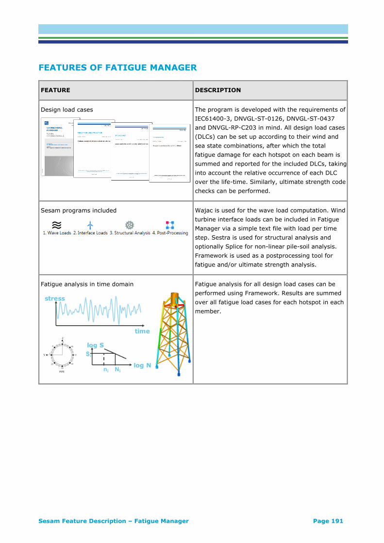
Sesam Feature Description – Fatigue Manager Page 191
FEATURES OF FATIGUE MANAGER
FEATURE DESCRIPTION
Design load cases
The program is developed with the requirements of
IEC61400-3, DNVGL-ST-0126, DNVGL-ST-0437
and DNVGL-RP-C203 in mind. All design load cases
(DLCs) can be set up according to their wind and
sea state combinations, after which the total
fatigue damage for each hotspot on each beam is
summed and reported for the included DLCs, taking
into account the relative occurrence of each DLC
over the life-time. Similarly, ultimate strength code
checks can be performed.
Sesam programs included
Wajac is used for the wave load computation. Wind
turbine interface loads can be included in Fatigue
Manager via a simple text file with load per time
step. Sestra is used for structural analysis and
optionally Splice for non-linear pile-soil analysis.
Framework is used as a postprocessing tool for
fatigue and/or ultimate strength analysis.
Fatigue analysis in time domain
Fatigue analysis for all design load cases can be
performed using Framework. Results are summed
over all fatigue load cases for each hotspot in each
member.

Sesam Feature Description – Fatigue Manager Page 192
Ultimate strength analysis in time domain
Ultimate strength analysis for all design load cases
can be performed using Framework.
The results for all design load cases are combined
into a single overview, showing the worst design
load case and utilisation factor for each beam in the
model.
Seismic (earthquake) analysis in time domain
Prescribed ground accelerations in time domain
may be added into the analysis and will contribute
to the total loading together with wave and wind
turbine loads.

Sesam Feature Description – Fatigue Manager Page 193
Superelement analysis
The modelling of the jacket is done in Sesam. The
model (and optionally the wave loads) are then
imported/converted into a superelement, and
linked to a wind turbine and tower model in
Bladed, BHawC, VTS/Flex5, or another wind
turbine load calculation tool. A structural analysis
is then performed in Bladed (or similar), after
which the forces and moments are extracted at the
interface point. These interface loads are then
applied to the model in Sesam, together with the
wave loads, and the structural analysis is run to
obtain the loads in the jacket. Fatigue and extreme
analysis is subsequently performed in Sesam.
Integrated analysis
The modelling of the jacket and tower is done in
Sesam. The model is then imported/converted into
Bladed format and linked to a wind turbine model
in Bladed. A structural analysis is then performed
in Bladed, after which time series of the resulting
forces and moments are extracted for every beam
in the structure. These results are then converted
into Sesam format. Fatigue and extreme analysis
is subsequently performed in Sesam.
Import and export functionalities for data
exchange
Converters exist for load import from Bladed,
BHawC, VTS/Flex5 and HawC2. In addition, time
series of wind turbine loads from any 3rd party tool
can easily be used in Sesam by outputting the
loads as a simple text file with columns of time
and loads in 6 degrees of freedom.
Besides this, export functionalities exist to Bladed
(integrated model or superelement+wave loads),
BHawC (superelement+wave loads) and VTS/Flex5
(superelement+wave loads).
Parallel computing
Sesam Fatigue Manager offers parallel computing,
thereby significantly speeding up running a large
set of design load cases (DLCs).

Sesam Feature Description – Fatigue Manager Page 194
Cloud computing
In addition to local parallel computing, Sesam
Fatigue Manager is cloud-enabled. This enables
analysing all DLCs in the Sesam Cloud allowing
fast and simultaneous running of many DLCs. The
status of the analyses can be monitored online and
results are downloaded automatically at run
completion.
Verification reports
The interfaces between Sesam and wind turbine
load calculation tools Bladed and BHawC have
been verified. Verification reports describing the
interfaces and verifying correct implementation are
available on request.

Sesam Feature Description – PET Page 195
PET PIPELINE ENGINEERING TOOL – THE DEFINITIVE TOOL FOR
EARLY PHASE PIPELINE DESIGN
Last revised: October 5, 2018. Describing version 4.1-00.
PET is a tool for the early design stage covering all significant design decisions in a simplified manner.
PET contains a wide set of easy to use calculation modules for quick assessments of offshore pipeline
designs.
In general, PET could be used for early design where all design checks are performed in a simplified way.
Later the other Pipeline Tools or other advanced tools can be used for more detailed design.

Sesam Feature Description – PET Page 196
FEATURES OF PET
FEATURE DESCRIPTION
Design checks in accordance with DNV GL ST F101
The calculation module performs calculation for the
following limit states (failure modes):
• Burst – during operation as well as during
system pressure test
• Collapse
• Propagating buckling
• Combined loading
Weight and volume
Calculates the volume, mass and dry weight of the
components that constitute a pipeline, i.e. steel,
coating layers and content. Volume, mass and dry
weight are calculated individually and totally, per
metre pipeline and totally for a given length of the
pipeline.
Expansion
Calculates end expansion due to temperature and
internal pressure. The virtual anchor length is also
calculated. These two results are presented for the
system pressure condition and the design condition.

Sesam Feature Description – PET Page 197
Upheaval buckling
Estimates the safety level with respect to upheaval
buckling for the given set of input, predicts the
temperature, internal pressure and imperfection
height that will trigger upheaval buckling and
estimates the cover height to prevent upheaval
buckling for a given safety level.
Stability calculations according to DNV-RP-F109
Estimates the safety level with respect to stability
for the given set of input, added weight coating and
wall thickness required to ensure stability for 10D
displacement criterion.
Free span calculations according to DNV-RP-F105
Calculates the allowable free span length
considering in-line and cross-flow vortex induced
vibrations. The module also gives the buckling
length (pinned-fixed condition) for the given
effective axial force.
Reel straining
Calculates maximum bending strain on the reel
including a code check according to DNV-OS-F101,
corresponding ovality and accumulated plastic
strain during reeling, unreeling, aligning and
straightening.
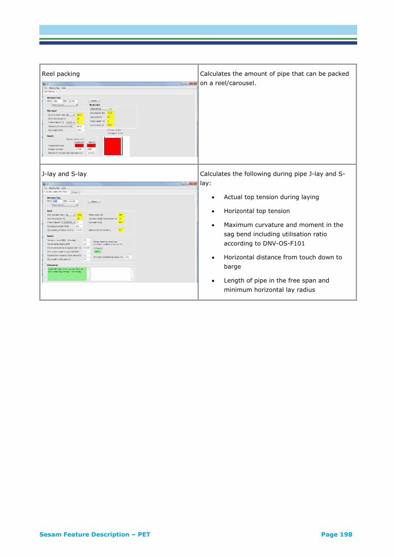
Sesam Feature Description – PET Page 198
Reel packing
Calculates the amount of pipe that can be packed
on a reel/carousel.
J-lay and S-lay
Calculates the following during pipe J-lay and S-
lay:
• Actual top tension during laying
• Horizontal top tension
• Maximum curvature and moment in the
sag bend including utilisation ratio
according to DNV-OS-F101
• Horizontal distance from touch down to
barge
• Length of pipe in the free span and
minimum horizontal lay radius

Sesam Feature Description – FatFree Page 199
FatFree FATIGUE ANALYSIS OF FREE SPANNING PIPELINES
Last revised: April 23, 2018. Describing version 12.0-03.
FatFree is a Microsoft Excel VBA spreadsheet for design and (re-)assessment of submarine pipeline spans
in compliance with DNV-RP-F105 “Free Spanning Pipelines”, issued February 2006.

Sesam Feature Description – FatFree Page 200
FEATURES OF FATFREE
FEATURE DESCRIPTION
Fatigue life FatFree calculates the fatigue life due to:
• Combined direct wave action and in-line
vortex induced vibrations (VIV)
• Cross-flow VIV based on environmental
description, i.e. directional long term
distribution for current and wave (in terms
of height and period)
• Free span scenario (water depth, span
geometry, soil conditions, etc.)
• Pipe characteristics (material, geometry,
SN-curve, etc.)
• Natural frequency and mode shape from FE
analyses or simplified beam theory
expressions
Main sheet
The main sheet contains all important input and
output except environmental data. It allows
definition of calculation modes and links to the
environmental data.
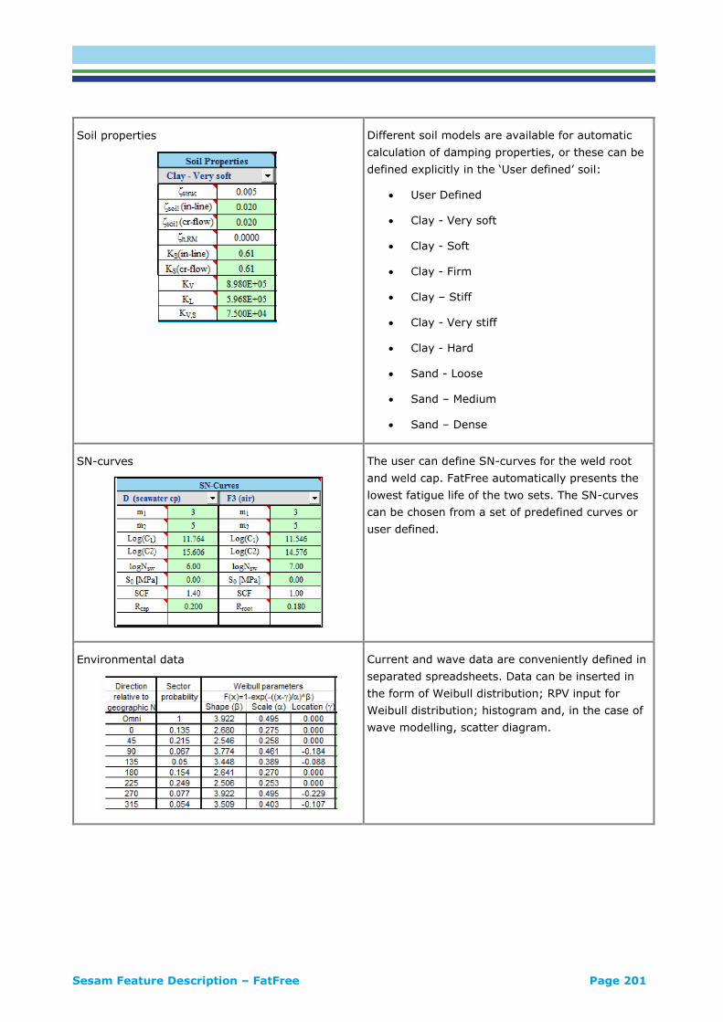
Sesam Feature Description – FatFree Page 201
Soil properties
Different soil models are available for automatic
calculation of damping properties, or these can be
defined explicitly in the ‘User defined’ soil:
• User Defined
• Clay - Very soft
• Clay - Soft
• Clay - Firm
• Clay – Stiff
• Clay - Very stiff
• Clay - Hard
• Sand - Loose
• Sand – Medium
• Sand – Dense
SN-curves
The user can define SN-curves for the weld root
and weld cap. FatFree automatically presents the
lowest fatigue life of the two sets. The SN-curves
can be chosen from a set of predefined curves or
user defined.
Environmental data
Current and wave data are conveniently defined in
separated spreadsheets. Data can be inserted in
the form of Weibull distribution; RPV input for
Weibull distribution; histogram and, in the case of
wave modelling, scatter diagram.
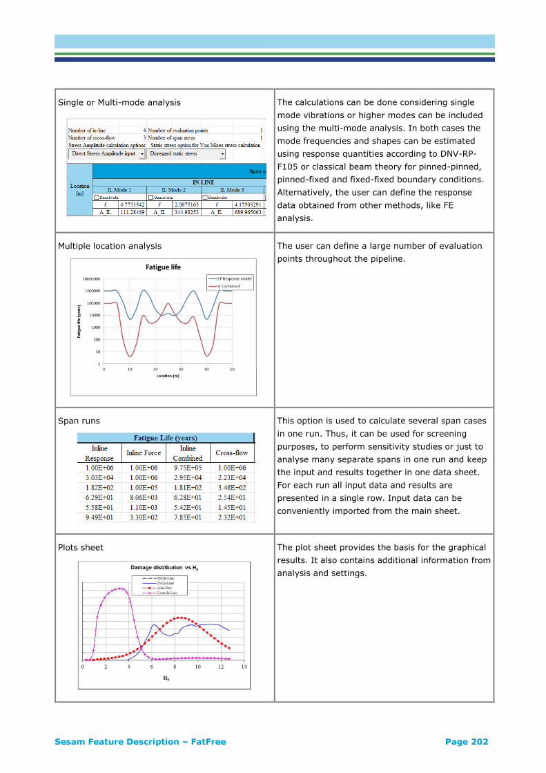
Sesam Feature Description – FatFree Page 202
Single or Multi-mode analysis
The calculations can be done considering single
mode vibrations or higher modes can be included
using the multi-mode analysis. In both cases the
mode frequencies and shapes can be estimated
using response quantities according to DNV-RP-
F105 or classical beam theory for pinned-pinned,
pinned-fixed and fixed-fixed boundary conditions.
Alternatively, the user can define the response
data obtained from other methods, like FE
analysis.
Multiple location analysis
The user can define a large number of evaluation
points throughout the pipeline.
Span runs
This option is used to calculate several span cases
in one run. Thus, it can be used for screening
purposes, to perform sensitivity studies or just to
analyse many separate spans in one run and keep
the input and results together in one data sheet.
For each run all input data and results are
presented in a single row. Input data can be
conveniently imported from the main sheet.
Plots sheet
The plot sheet provides the basis for the graphical
results. It also contains additional information from
analysis and settings.
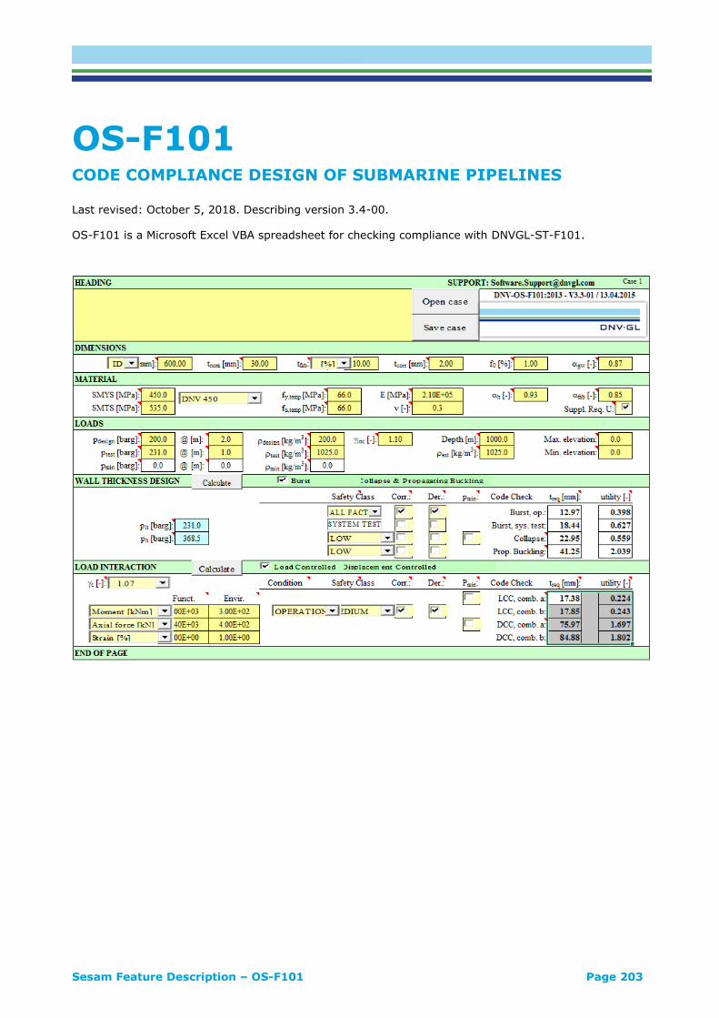
Sesam Feature Description – OS-F101 Page 203
OS-F101 CODE COMPLIANCE DESIGN OF SUBMARINE PIPELINES
Last revised: October 5, 2018. Describing version 3.4-00.
OS-F101 is a Microsoft Excel VBA spreadsheet for checking compliance with DNVGL-ST-F101.
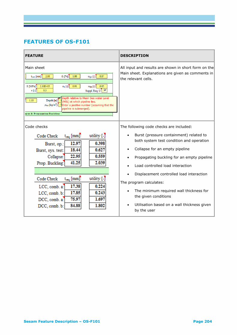
Sesam Feature Description – OS-F101 Page 204
FEATURES OF OS-F101
FEATURE DESCRIPTION
Main sheet
All input and results are shown in short form on the
Main sheet. Explanations are given as comments in
the relevant cells.
Code checks
The following code checks are included:
• Burst (pressure containment) related to
both system test condition and operation
• Collapse for an empty pipeline
• Propagating buckling for an empty pipeline
• Load controlled load interaction
• Displacement controlled load interaction
The program calculates:
• The minimum required wall thickness for
the given conditions
• Utilisation based on a wall thickness given
by the user

Sesam Feature Description – OS-F101 Page 205
Reported sheets
When calculation is done report sheets are created
automatically for all code checks (collapse and
propagation buckling are reported in a single
sheet).
These report sheets are meant for paper print-out
and inclusion in reports. They contain all relevant
input, some intermediate results (to ease external
verification) and the results from the code check.
Parametric studies
The program allows the user to perform parameter
studies/sensitivity studies on each case. E.g.
calculate minimum required wall thickness for
varying depths.
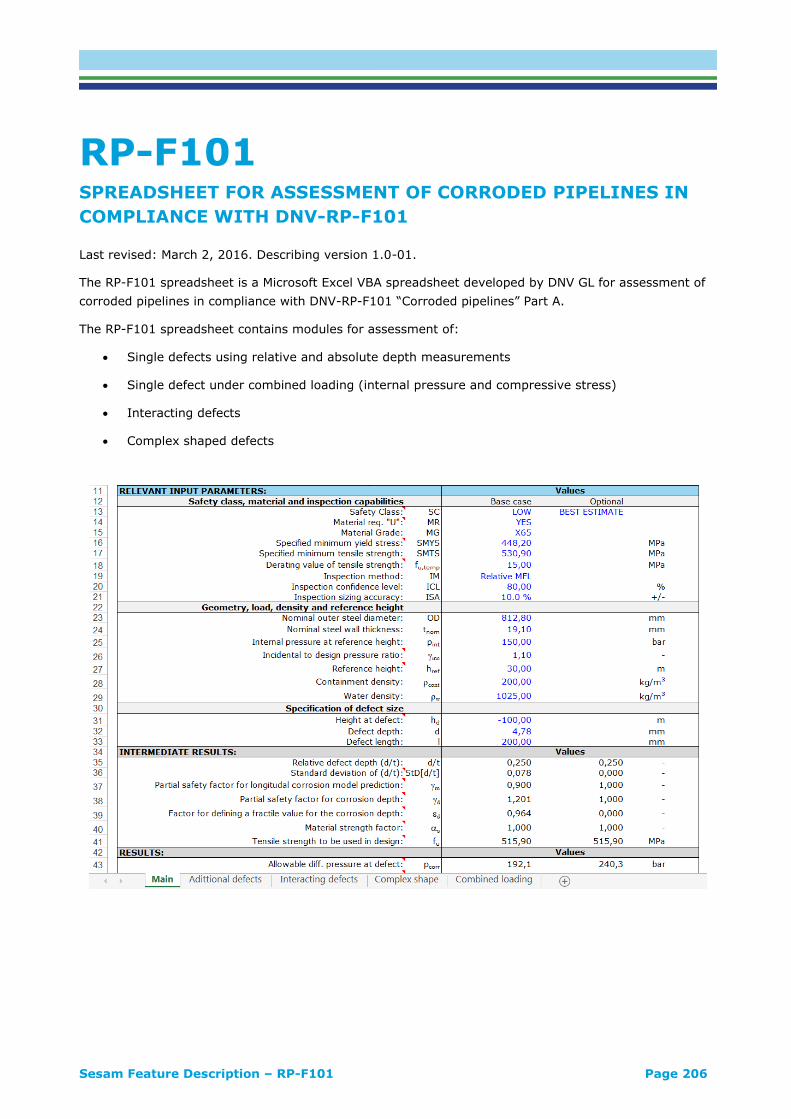
Sesam Feature Description – RP-F101 Page 206
RP-F101 SPREADSHEET FOR ASSESSMENT OF CORRODED PIPELINES IN
COMPLIANCE WITH DNV-RP-F101
Last revised: March 2, 2016. Describing version 1.0-01.
The RP-F101 spreadsheet is a Microsoft Excel VBA spreadsheet developed by DNV GL for assessment of
corroded pipelines in compliance with DNV-RP-F101 “Corroded pipelines” Part A.
The RP-F101 spreadsheet contains modules for assessment of:
• Single defects using relative and absolute depth measurements
• Single defect under combined loading (internal pressure and compressive stress)
• Interacting defects
• Complex shaped defects

Sesam Feature Description – RP-F101 Page 207
FEATURES OF RP-F101
FEATURE DESCRIPTION
Main sheet
Used for assessment of single defects.
There are two set of input parameters:
• Base case: All of the base case parameters
must be entered. All other features of the
RP-F101 spreadsheet make reference to
these values.
• Optional: This set of parameters is meant
for sensitivity study by comparison to the
base case input. Input that is left blank will
be equal to the base case input.
Additional defects sheet
An extension of the main sheet where multiple
defects can be assessed for the base case set of
parameters in the main sheet.
The calculations performed in the additional defects
sheet make use of the base case parameters in the
main sheet, but where the defect depth, defect
length and height at defect is changed to a list of
defects.
Interacting defects
Used for assessment of interacting defects as per
section 3.8 of DNV-RP-F101.
To assess the pressure resistance of a pipeline with
a set of interacting defects. The list of defects is
entered with start position, defect depth and
length. All defects in the defect list are projected
onto a projection line to obtain the wall thickness
profile. Overlapping of defects is handled
automatically by the spreadsheet.

Sesam Feature Description – RP-F101 Page 208
Complex shape
Used for assessment of complex shaped defects as
per section 3.9 of DNV-RP-F101.
To assess the pressure resistance using the
complex shape methodology, the wall thickness
profile is entered in the form of a list of position
and defect depth.
Combined loading
Used for assessment of a single longitudinal defect
with internal pressure and superimposed
longitudinal compressive stresses as per section
3.7.4 of DNV-RP-F101.

Sesam Feature Description – SimBuck Page 209
SimBuck SIMPLIFIED GLOBAL BUCKLING ANALYSIS OF SUBMARINE
PIPELINES
Last revised: August 22, 2017. Describing version 2.0-02.
SimBuck is a Microsoft Excel VBA spreadsheet developed by DNV GL for preliminary design and
verification of global buckling potential for submarine pipelines in compliance with DNV-RP-F110 ‘Global
Buckling of Submarine Pipelines – Structural Design due to High Temperature / High Pressure’, issued
October 2007.
SimBuck performs:
• Single buckle assessment for exposed pipeline on even seabed
• Multi-buckle assessment for exposed pipelines on even seabed
• Checks for upheaval buckling potential
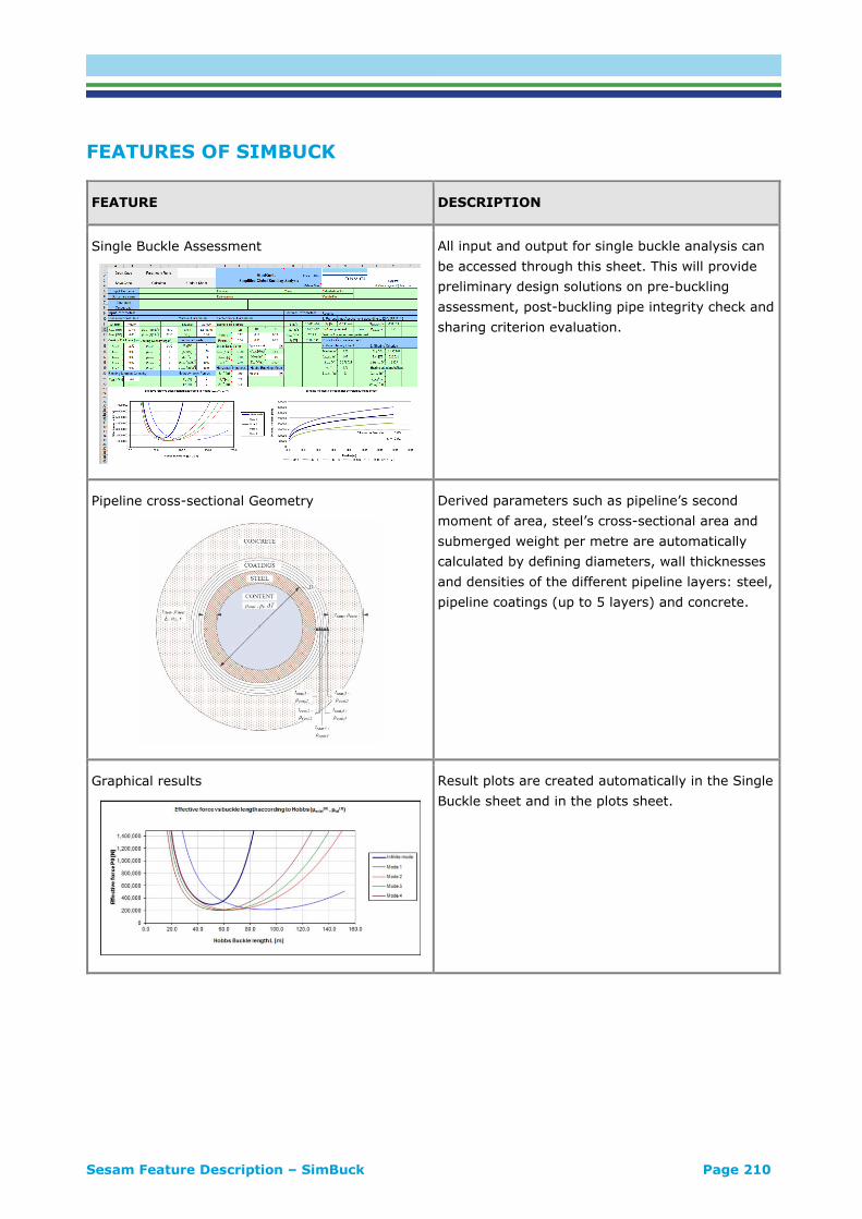
Sesam Feature Description – SimBuck Page 210
FEATURES OF SIMBUCK
FEATURE DESCRIPTION
Single Buckle Assessment
All input and output for single buckle analysis can
be accessed through this sheet. This will provide
preliminary design solutions on pre-buckling
assessment, post-buckling pipe integrity check and
sharing criterion evaluation.
Pipeline cross-sectional Geometry
Derived parameters such as pipeline’s second
moment of area, steel’s cross-sectional area and
submerged weight per metre are automatically
calculated by defining diameters, wall thicknesses
and densities of the different pipeline layers: steel,
pipeline coatings (up to 5 layers) and concrete.
Graphical results
Result plots are created automatically in the Single
Buckle sheet and in the plots sheet.

Sesam Feature Description – SimBuck Page 211
Parametric Runs
Used to run several lateral buckling cases (single
buckle), ideal for screening, performing sensitivity
analyses, or simply analysing many separate cases
and keeping all the input and output results
together on a single data sheet.
Multi Buckle Assessment
Provides additional functionality for analysing an
entire pipeline. Buckling triggers can either be
specified manually or calculated by SimBuck.
UHB Sheet
Assessment of upheaval buckling based on
deterministic approach according to DNV-RP-F110.
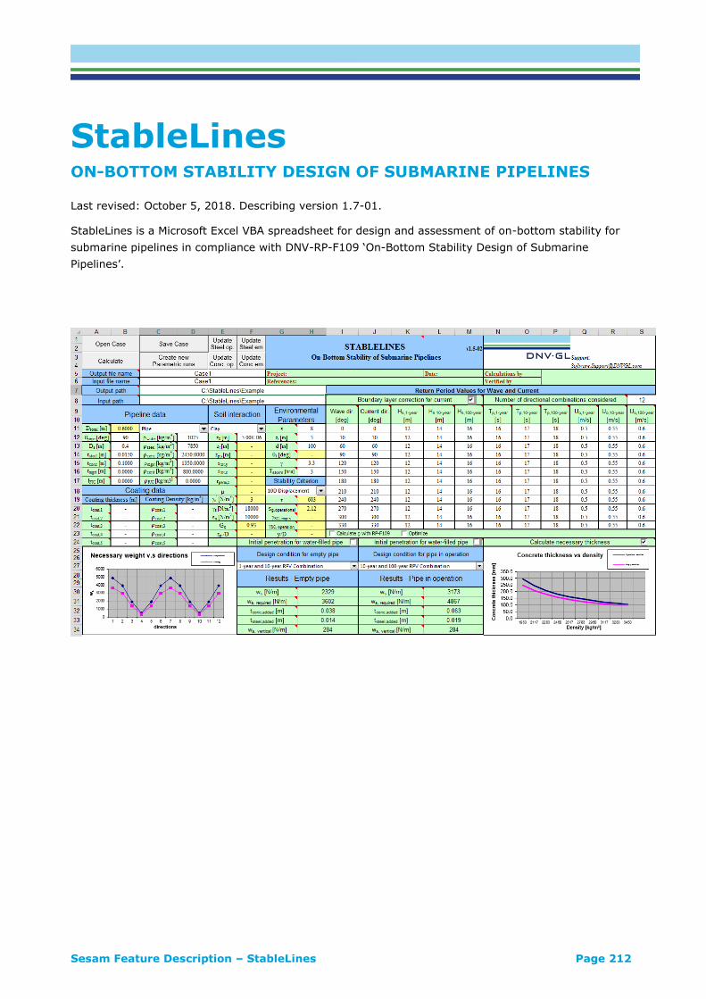
Sesam Feature Description – StableLines Page 212
StableLines ON-BOTTOM STABILITY DESIGN OF SUBMARINE PIPELINES
Last revised: October 5, 2018. Describing version 1.7-01.
StableLines is a Microsoft Excel VBA spreadsheet for design and assessment of on-bottom stability for
submarine pipelines in compliance with DNV-RP-F109 ‘On-Bottom Stability Design of Submarine
Pipelines’.
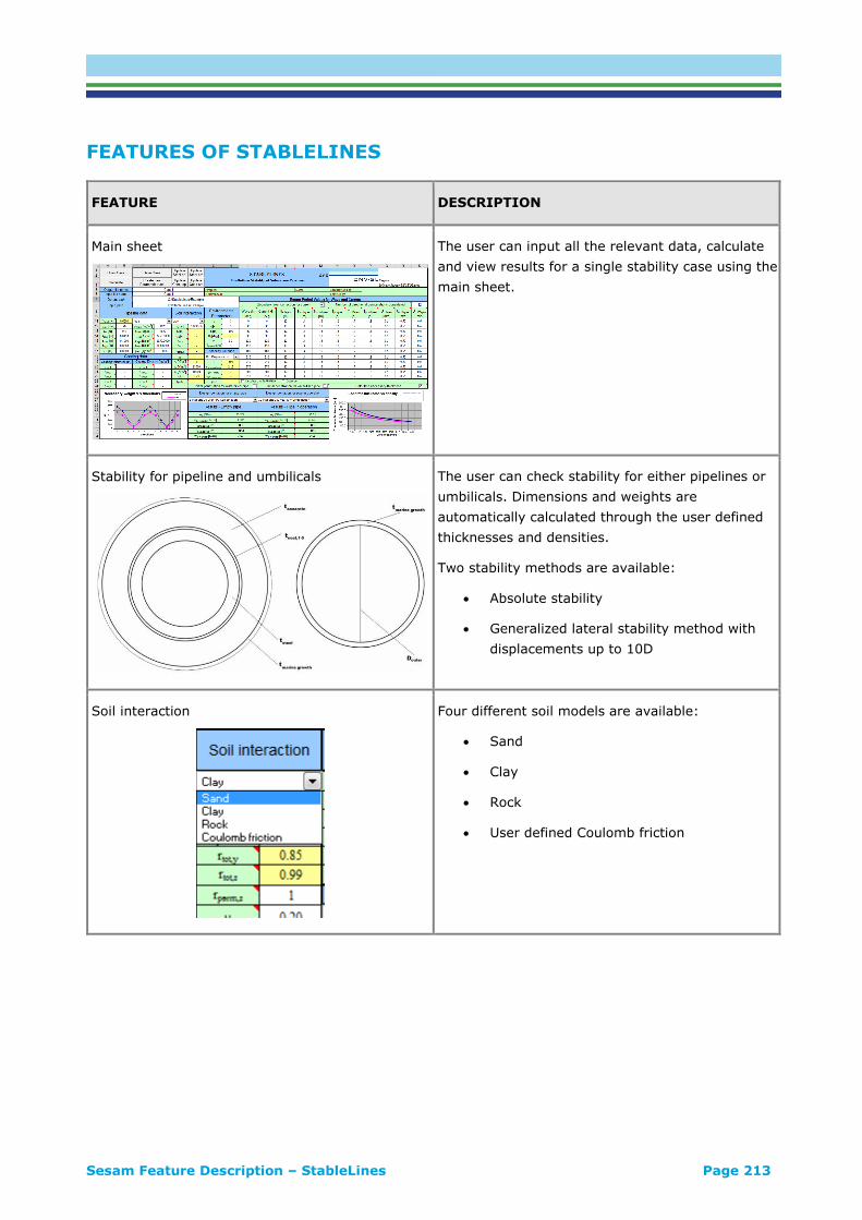
Sesam Feature Description – StableLines Page 213
FEATURES OF STABLELINES
FEATURE DESCRIPTION
Main sheet
The user can input all the relevant data, calculate
and view results for a single stability case using the
main sheet.
Stability for pipeline and umbilicals
The user can check stability for either pipelines or
umbilicals. Dimensions and weights are
automatically calculated through the user defined
thicknesses and densities.
Two stability methods are available:
• Absolute stability
• Generalized lateral stability method with
displacements up to 10D
Soil interaction
Four different soil models are available:
• Sand
• Clay
• Rock
• User defined Coulomb friction

Sesam Feature Description – StableLines Page 214
Results presentation
The user can check graphical representation of the
stability results such as (but not restricted to):
• Required submerged weight as function of
direction
• Required concrete thickness as function of
concrete density (pipeline mode)
• Required weight as a function of outer
diameter (umbilical mode)
StableLines also suggests added steel and
concrete/armour thicknesses to make unstable
pipelines stable.
Report Sheet
Report of final and intermediate results ready for
copy&paste into technical reports.
Parametric runs
Calculate several on-bottom stability cases in one
run. Can be used for screening purposes, to
perform sensitivity studies or just to analyse many
separate cases in one run and keep the input and
results together in one data sheet.

Sesam Feature Description – Helica Page 215
Helica CROSS-SECTIONAL ANALYSIS OF FLEXIBLE PIPES, UMBILICALS
AND POWER CABLES
Last revised: March 3, 2019. Describing version 3.0.
Helica is a stress analysis tool tailor made for cross-section analysis of flexible pipes, umbilicals and
power cables.
The main functionalities of the program are:
• Cross-sectional load sharing analysis
• Short-term fatigue analysis
• Long-term fatigue analysis
• Extreme analysis
• VIV fatigue analysis

Sesam Feature Description – Helica Page 216
FEATURES OF HELICA
Cross-sectional load sharing analysis
FEATURE DESCRIPTION
Stiffness and twist characteristics
Helica may consider one or more load cases, i.e.
combinations of tension, curvature and torque (left
or right) for various boundary conditions.
For each load case specified by the user, Helica
calculates stiffness characteristics and/or angle of
twist.
Axial load distribution
For a load case specified by the user, Helica
determines the axial load distribution between
layers in the cross-section.
Layer contact
For a load case specified by the user, Helica
determines the contact pressure on each layer
resulting from applied tension.
External (e.g. hydrostatic) pressure is accounted
for, if applicable.
Global responses
Group Response
BC Boundary condition, axial displ.
Boundary condition, torsion displ.
Axial Effective axial force [N]
End-cap force (pressure load) [N]
True axial force [N]
Axial displacement [mm]
Axial stiffness [N]
Torsion Torsional load [Nmm]
Torsional displacment (twist) [rad]
Torsional stiffness [Nmm/rad]
Torsional/axial displacement ratio
Bending Helix bending stiffness, axial, stick [Nmm2]
Helix bending stiffness, bending, stick and slip [Nmm2]
Cylinder layer bending stiffness [Nmm2]
Bending stiffness, full stick [Nmm2]
Bending stiffness, full slip [Nmm2]

Sesam Feature Description – Helica Page 217
Capacity curve
Capacity curves, considering inter-layer contact
and friction, may be established for allowable
utilization level(s) of material stress capacities
specified by the user.
Effects of internal and (uniform) external
pressures are considered, if applicable.
Magnitude and number of tension and curvature
levels to be considered are specified by the user to
facilitate finer discretization, if necessary.
Hierarcical calulation scheme allowing for capacity
curve calulation of bundle helix elements.
Non-linear bending performance
The non-linear bending characteristics of a cross-
section may be determined, considering stick/slip
effects, for an applied tension specified by the
user.
Contribution to bending stiffness
The relative contribution of each layer to the
bending stiffness of a cross-section may be
determined for both full stick and full slip
conditions.
Slip curvatures
The curvature at which slip of a helix layer is
initiated is determined, as well as the curvature
that represents full slip of the layer.

Sesam Feature Description – Helica Page 218
Layer types
Layers may be modelled in Helica as:
• Thin homogenous cylinder layers that do
not account for radial deformation
• Thick homogenous cylinder layers that
account for thickness and radial
deformation
• General cylinder layer, specified by
stiffness properties
• Helix layers that may be composed of
different types of helix components to
model e.g. layers of umbilicals with
several different elements in the same
layer
• Helix layers can be specified in terms of
helix lay angle or helix pitch length
Component types
The following component types are currently
available in Helica:
• Solid circular cross-section geometry
• Circular pipe cross-section geometry
• Solid rectangular cross-section geometry
• Arbitrary cross-section geometry (circular
cross-section with equivalent
homogeneous properties)
1rv2rv
vzv

Sesam Feature Description – Helica Page 219
Short-term fatigue analysis
FEATURE DESCRIPTION
Load case definition
The following is specified by the user:
• What helix element to be considered in the
fatigue analysis
• Hierarcical calulation scheme allowing for
fatigue analysis of 2nd order stick/slip
• What locations along riser/umbilical, e.g.
nodes in global model, to be considered
• Fatigue capacity data (S-N curve) and
stress concentration factor
• Method for mean stress correction
• Response conversion to obtain fatigue
stresses in MPa in compliance with units
applied in the global response calculations
• Filtering technique for processing of stress
data
• Method of computing fatigue stress in helix
elements, e.g. friction/no friction and
contact loads based on max or specified
tension
Specification of global loads
Short-term fatigue analyses may be performed
based on histograms or time series of tension and
curvature imported directly from global analyses.
Helica can be run in batch mode, thus facilitating
parallel processing if specified by the user.
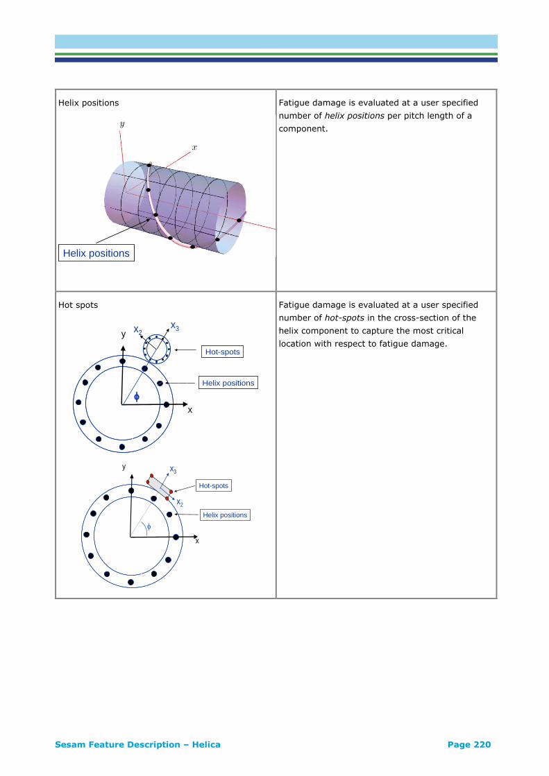
Sesam Feature Description – Helica Page 220
Helix positions
Fatigue damage is evaluated at a user specified
number of helix positions per pitch length of a
component.
Hot spots
Fatigue damage is evaluated at a user specified
number of hot-spots in the cross-section of the
helix component to capture the most critical
location with respect to fatigue damage.
Helix positions
x
yx2
x3
Helix positions
Hot-spots
y
x
x2
x3
Hot-spots
Helix positions

Sesam Feature Description – Helica Page 221
Long-term fatigue analysis
FEATURE DESCRIPTION
Accumulation of fatigue damage
Average long-term fatigue damage is found by
weighting the damage calculated for selected short-
term conditions by the probability of occurrence.
The load cases (e.g. locations along the riser) and
conditions (e.g. representing one or more offsets)
to be considered in the long-term fatigue analysis
are specified by the user.
Output
The output from the analysis is:
• accumulated long-term fatigue damage,
• long-term stress cycle distribution, and
• relative contributions from short-term
conditions to the long-term fatigue
damage.
Extreme analysis
FEATURE DESCRIPTION
Capacity check
The response from an extreme analysis may be
checked against the capacity curve of the cross-
section. The cross capacity curve may be
established by Helica or specified by the user.
Utilization time series are established by
interpolation of the cross-section capacity curve
according to the cross-section loading described by
time series of effective tension and curvature
components imported from a global time domain
dynamic analysis.
Tp 0 1 2 3 4 5 6 7 8 9 10 11 12 13 14 15 16 17 18 19 20 21 22
Hs 1 2 3 4 5 6 7 8 9 10 11 12 13 14 15 16 17 18 19 20 21 22 23
0 0.5 0.000182 0.001452 0.002493 0.002147 0.001329 0.000695 0.000336 0.000154 6.85E-05 3.08E-05 1.37E-05 6.85E-06 3.42E-06
0.5 1 0.000116 0.003709 0.016069 0.026727 0.026765 0.020158 0.012836 0.007384 0.00399 0.002075 0.001055 0.000531 0.000267 0.000134 6.51E-05 3.42E-05 1.71E-05 1.03E-05 3.42E-06 3.42E-06
1 1.5 1.03E-05 0.001226 0.011257 0.031275 0.044858 0.043649 0.033453 0.022025 0.013134 0.007336 0.003921 0.002038 0.001041 0.000524 0.000264 0.000134 6.51E-05 3.42E-05 1.71E-05 1.03E-05 3.42E-06 3.42E-06
1.5 2 0.000175 0.003456 0.016148 0.033207 0.041553 0.037995 0.028292 0.01835 0.010826 0.005983 0.003161 0.001617 0.000808 0.000401 0.000195 9.59E-05 4.79E-05 2.4E-05 1.03E-05 6.85E-06 3.42E-06
2 2.5 1.37E-05 0.000668 0.005528 0.016857 0.027758 0.03071 0.026063 0.018436 0.011483 0.006535 0.003483 0.001774 0.000873 0.000421 0.000199 9.25E-05 4.45E-05 2.05E-05 1.03E-05 3.42E-06 3.42E-06
2.5 3 8.9E-05 0.001394 0.006651 0.01497 0.02059 0.020282 0.015829 0.010473 0.006151 0.003308 0.001671 0.000805 0.000373 0.000171 7.53E-05 3.42E-05 1.37E-05 6.85E-06 3.42E-06
3 3.5 6.85E-06 0.000264 0.002099 0.006795 0.012052 0.014144 0.012408 0.008826 0.005384 0.002932 0.001466 0.000688 0.000308 0.000134 5.48E-05 2.4E-05 1.03E-05 3.42E-06
3.5 4 3.77E-05 0.000524 0.002599 0.00623 0.009014 0.009107 0.007082 0.004538 0.002517 0.00125 0.000572 0.000247 9.93E-05 4.11E-05 1.37E-05 6.85E-06 3.42E-06
4 4.5 3.42E-06 9.93E-05 0.000822 0.002819 0.005247 0.006295 0.005473 0.00374 0.00213 0.001055 0.000469 0.000192 7.53E-05 2.74E-05 1.03E-05 3.42E-06
4.5 5 1.37E-05 0.000209 0.001086 0.00274 0.004058 0.004055 0.00301 0.001784 0.000887 0.000387 0.000151 5.48E-05 1.71E-05 6.85E-06 3.42E-06
5 5.5 4.11E-05 0.000356 0.001295 0.002483 0.002949 0.002438 0.001527 0.000774 0.000329 0.000123 4.11E-05 1.37E-05 3.42E-06
5.5 6 6.85E-06 9.59E-05 0.000534 0.001397 0.002058 0.001956 0.001322 0.000688 0.000291 0.000103 3.08E-05 1.03E-05 3.42E-06
6 6.5 2.05E-05 0.000178 0.000682 0.001312 0.001486 0.001116 0.000606 0.000253 8.9E-05 2.4E-05 6.85E-06
6.5 7 3.42E-06 4.79E-05 0.000281 0.00075 0.001058 0.000911 0.000531 0.000226 7.53E-05 2.05E-05 3.42E-06
7 7.5 1.03E-05 9.59E-05 0.000373 0.000692 0.000712 0.000455 0.000199 6.51E-05 1.71E-05 3.42E-06
7.5 8 2.4E-05 0.000158 0.000408 0.000524 0.000384 0.000178 5.48E-05 1.37E-05 3.42E-06
8 8.5 3.42E-06 5.14E-05 0.000209 0.00036 0.000312 0.000158 5.14E-05 1.03E-05 3.42E-06
8.5 9 1.37E-05 9.25E-05 0.000223 0.000243 0.000137 4.45E-05 1.03E-05
9 9.5 3.42E-06 3.08E-05 0.00012 0.000178 0.000116 4.11E-05 6.85E-06
9.5 10 1.03E-05 5.48E-05 0.000116 9.93E-05 3.77E-05 6.85E-06
10 10.5 2.05E-05 6.85E-05 7.88E-05 3.42E-05 6.85E-06
10.5 11 6.85E-06 3.42E-05 5.82E-05 3.08E-05 6.85E-06
11 11.5 1.37E-05 3.77E-05 2.74E-05 6.85E-06
11.5 12 3.42E-06 2.05E-05 2.4E-05 6.85E-06
12 12.5 1.03E-05 1.71E-05 6.85E-06
12.5 13 3.42E-06 1.03E-05 6.85E-06
13 13.5 6.85E-06 6.85E-06
13.5 14 3.42E-06 3.42E-06
14 14.5 3.42E-06
14.5 15 3.42E-06
0.0 %
1.0 %
2.0 %
3.0 %
4.0 %
5.0 %
6.0 %
7.0 %
8.0 %
9.0 %
10.0 %
1 2 3 4 5 6 7 8 9 10 11 12 13 14 15 16 17 18 19 20 21 22 23 24 25 26 27 28 29 30 31 32 33 34 35 36 37
DAMAGE PER BLOCK
FAR

Sesam Feature Description – Helica Page 222
Statistical processing
In case of irregular wave loading, statistical
processing of the utilisation time series is
performed to establish extreme values.
Deterministic processing is applied in case of
regular wave loading.
VIV fatigue analysis
FEATURE DESCRIPTION
Short-term fatigue analysis
Modal damping may be calculated by Helica to
account for the amplitude dependant hysteretic
stick/slip behaviour of the cross-section in bending.
Fatigue stress calculations are performed in Helica
considering stick/slip of helix elements and the
exited modes and modal amplitudes determined in
the VIV analysis.
Result files from VIV analyses performed using
acknowledged software may be imported directly to
Helica.
Long-term fatigue analysis
Long-term fatigue damage may be calculated by
weighting the damage calculated for selected short-
term conditions by the probability of occurrence.
1.0E+00
1.0E+01
1.0E+02
1.0E+03
1.0E+04
1.0E+05
1.0E+06
1.0E+07
1.0E+08
1.0E+09
1.0E+10
1.0E+11
1.0E+12
1.0E+13
1.0E+14
1.0E+15
1.0E+16
0 200 400 600 800 1000 1200 1400 1600 1800 2000
Node #
Fati
gu
e l
ife [
years
]
Center tube
Inner tube layer
Outer tube layer
Outer armor layer
Inner armor layer
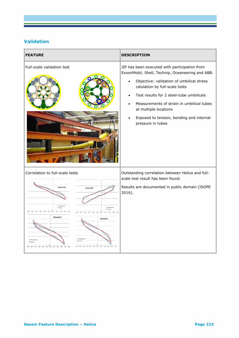
Sesam Feature Description – Helica Page 223
Validation
FEATURE DESCRIPTION
Full-scale validation test
JIP has been executed with participation from
ExxonMobil, Shell, Technip, Oceaneering and ABB.
• Objective: validation of umbilical stress
calulation by full-scale tests
• Test results for 2 steel-tube umbilicals
• Measurements of strain in umbilical tubes
at multiple locations
• Exposed to tension, bending and internal
pressure in tubes
Correlation to full-scale tests
Outstanding correlation between Helica and full-
scale test result has been found.
Results are documented in public domain (ISOPE
2016).

ABOUT DNV GL DNV GL is a global quality assurance and risk management company. Driven by our purpose of
safeguarding life, property and the environment, we enable our customers to advance the safety and
sustainability of their business. We provide classification, technical assurance, software and independent
expert advisory services to the maritime, oil & gas, power and renewables industries. We also provide
certification and supply chain services to customers across a wide range of industries. Operating in more
than 100 countries, our experts are dedicated to helping customers make the world safer, smarter and
greener.
DIGITAL SOLUTIONS DNV GL is a world-leading provider of digital solutions for managing risk and improving safety and asset
performance for ships, pipelines, processing plants, offshore structures, electric grids, smart cities and
more. Our open industry platform Veracity, cyber security and software solutions support business-
critical activities across many industries, including maritime, energy, and healthcare.