1American Institute of Aeronautics and Astronautics

Higher Order Sensitivities for Solving Nonlinear Two-Point Boundary-Value Problems

D. Todd Griffith*

Texas A&M University, College Station, Texas 77843-3141

James D. Turner†

Amdyn Systems, White GA 30184

S. R. Vadali‡ and John. L. Junkins§

Texas A&M University, College Station, Texas 77843-3141

In this paper, we consider new computational approaches for solving nonlinear Two-Point Boundary-Value Problems. The sensitivity calculations required in the solution utilize the automatic differentiation tool OCEA (Object Oriented Coordinate Embedding Method). OCEA has broad potential in this area and many other areas since the partial derivative calculations required for solving these problems are automatically computed and evaluated freeing the analyst from deriving and coding them. In this paper, we demonstrate solving nonlinear Two-Point Boundary Value Problems by shooting and direct methods using automatic differentiation. We demonstrate standard first-order algorithms and higher-order extensions. Additionally, automatic generation of co-state differential equations and second- and higher-order midcourse corrections are considered. Optimization of a sample Low-thrust, Mars-Earth trajectory is considered as an example. Computational issues related to domain of convergence and rate of convergence will be detailed.

I. IntroductionPPLICATIONS which require the solution to a Two-Point Boundary-Value Problem (TPBVP) occur in many engineering disciplines. The solution of the TPBVP determines states or functions of the states at two points,

usually the initial and final times, which satisfy the boundary conditions for a given mathematical problem. For linear problems, analytical solutions exist for determining the unknown initial or final conditions; however, for nonlinear problems we must resort to iterative methods. Many methods have been developed to solve nonlinear TPBVPs dealing with a wide range of issues, including stiffness of differential equations of motion, reduction in sensitivity, and speed of convergence.

One particular solution is obtained by the method of differential corrections1,2. Here a guess is made for the unknown states, the state differential equations are integrated until the final time, and the boundary conditions are checked to see if they are satisfied. When the constraint conditions are not satisfied, corrections to the unknown states are computed and the process is repeated until convergence criteria are met. Typically, these corrections are computed by using first order sensitivity calculations or at best, second order calculations using an approximate Hessian.

In this paper, we study the automatic generation of sensitivity equations for solving nonlinear TPBVPs. The Fortran 90 extension OCEA (Object Oriented Coordinate Embedding Method) will be used to perform the sensitivity calculations3-4. OCEA has been used to solve problems in optimization3-4, estimation5, and generation of equations of motion6. OCEA has broad potential in many areas since it is extremely useful for computing partial derivatives of scalar, vector, matrix, and higher order tensor functions.

Optimization of a sample Low-thrust, Mars-Earth trajectory will be considered as one example. Direct optimization using Differential Inclusions7 will be considered in a second example demonstrating OCEA’s

* Graduate Research Assistant, Department of Aerospace Engineering, 3141 TAMU, Student Member AIAA.† Adjunct Faculty, Department of Aerospace Engineering, and President Amdyn Systems.‡ Stewart & Stevenson-I Professor, Department of Aerospace Engineering, 3141 TAMU, Member AIAA.§ George Eppright Chair, Distinguished Professor, Department of Aerospace Engineering, 3141 TAMU, Fellow AIAA.

A

AIAA/AAS Astrodynamics Specialist Conference and Exhibit16 - 19 August 2004, Providence, Rhode Island

AIAA 2004-5404

Copyright © 2004 by D. Todd Griffith. Published by the American Institute of Aeronautics and Astronautics, Inc., with permission.

2American Institute of Aeronautics and Astronautics

capabilities. First through fourth order sensitivity calculations will be considered in each case. A number of results detailing performance will be presented.

II. Overview of OCEAThis approach uses the previously developed OCEA (Object Oriented Coordinate Embedding Method) extension

for FORTRAN90 (F90).3-4 The OCEA package is an object-oriented automatic differentiation equation manipulation package. Computer implementation of differentiation is typically accomplished by two distinct approaches – automatic differentiation and symbolic differentiation.8 The primary distinction of these approaches is that automatic differentiation invokes the chain automatically and takes place in the background. This allows for time and memory optimized differentiation. On the other hand, symbolic differentiation requires more user intervention. Typically, derivatives are computed using a symbolic differentiation program, such as Macsyma or Mathcad, and the derivatives then need to be either hand typed in a computer program or saved in a file that typically requires editing and compilation. There is an advantage here in that the computed derivative expressions can be viewed by the analyst; however, the resulting mathematical expressions can be so large that no physical insight can be gained from the effort.

OCEA defines embedded variables that represent abstract data types, where hidden dimensions (background arrays) are used for storing and manipulating partial derivative calculations. OCEA replaces each scalar variable in the problem with a differential n-tuple consisting of the following variables (second-order OCEA method):

2:f f f f = ∇ ∇ (1)

where ∇ and 2∇ denote symmetric first- and second-order gradient tensors with respect to a user-defined set of independent variables. The introduction of the abstract differential n-tuple allows the computer to continue to manipulate each scalar variable as a conventional scalar variable, even though the first and higher-order partial derivative are attached to the scalar variable in a hidden way. The individual objects are extracted, using OCEA’s

adopted notation, as follows: %f f E= , %f f V∇ = , and 2 %f f T∇ = . The automatic computation of the partial

derivatives is achieved by operator-overloading methodologies that redefine the intrinsic mathematical operators and functions using the rules of calculus. For example, addition and multiplication are redefined as follows.

2 2: + = + ∇ +∇ ∇ +∇ a b a b a b a b (2)

( ) ( )* : * * * = ∂ ∂ ∂ i j ia b a b a b a b (3)

Thus the “+” and “*” operators are overloaded so that coding the left side expressions of Eqs. (2) and (3) causes all

the right side computations to be carried out. More subtly, if 1z a b= + and 2 *z a b= , then computing

3 1 2z z z= + causes the results of Eqs. (2) and (3) to be propagated efficiently in the background to compute:

3 3 3* ( ) ( )i j iz a b a b z z = + + ∂ ∂ ∂ (4)

Additional operations for the standard mathematical library functions, such as trigonometric and exponential functions, are redefined to account for the known rules of differentiation. In essence, this approach pre-codes, once and for all, all of the partial derivatives required for any problem, and the chain rule is implemented automatically in background operations that the user neither derives nor codes. At compile time, and without user intervention, the OCEA-based approach links the subroutines and functions required for evaluating the partial derivative models.

III. The Optimal Control FormulationIn this section, we overview the formulation of the necessary conditions for the Optimal Control problem. One

of the problems we consider in this paper is a minimum time problem. Therefore, we also examine converting the minimum time problem to one in which the final time is fixed, and the unknown final time becomes a free parameter to be optimized.

3American Institute of Aeronautics and Astronautics

A. General FormulationConsider the minimization of the following function where ft is the final time:

0

( ( ), ( ), )ft

J L t t t dt= ∫ x u (5)

subject to the following dynamics:

( ( ), ( ), ) ( ( ), ( ), )TH L t t t f t t t= +x u λ x u (6)

In general, the Hamiltonian for the system is written as

( ( ), ( ), ) ( ( ), ( ), )TH L t t t f t t t= +x u λ x u (7)

For unconstrained control, the well-known necessary conditions along the trajectory required to minimize J are given by Eqs. (8-10)

H∂=∂

xλ

& (8)

-H∂∂

λ =x

& (9)

0H∂ =∂u

(10)

Furthermore, we consider the initial and final boundary conditions on the states and co-states. The necessary

boundary condition for an unspecified initial state, 0( )ix t , are 0( ) 0i tλ = , whereas initial co-states are unknown and

must be solved numerically when the corresponding initial state is specified. The problems considered in this paper are of the type in which the initial states are known and the desired terminal states are specified. Therefore, the objective of one of the numerical solutions, the Low-thrust Mars-Earth trajectory, is to determine the unknown

initial co-states. Also, when the final time is free we have ( ) 0fH t = as an additional necessary condition.

B. Converting to Fixed Final Time Free Parameter Type ProblemIn this section, we show how a free final time problem can be converted to fixed final time problem with

ft included in the formulation as a free parameter. A fixed final time problem has the obvious advantage of fixed

time limits for integrating any differential equations. The numerical algorithm for solving the TPBVP, which is outlined in subsequent sections, benefits since the unknown final time parameter appears explicitly in the state and co-state equations and ultimately appears explicitly in the sensitivity calculations.

Consider a new time variable, τ , defined as

; 0 1f

t

tτ τ= ≤ ≤ (11)

Differentiation of the states with respect to the new time variable (denoted with a prime) can be written as

4American Institute of Aeronautics and Astronautics

'f

d d dtt

d dt dτ τ= = = &

x xx x (12)

Therefore, in producing the new state equations for the fixed time problem we simply multiply Eq. (6) by the

parameter ft . Additionally, new co-state equations for the fixed time problem are computed in the same manner.

The cost function is rewritten as 10 fJ t dτ= ∫ , and the Hamiltonian is defined as

( ( ), ( ), )

1 ( ( ), ( ), )

T

f f

T

f

H t t t t t

t t t t

= +

= +

λ f x u

λ f x u(13)

Equations (8-10) are applied to the Hamiltonian in Eq. (13) to produce the fixed time problem necessary conditions

along the trajectory. However, here we must consider one additional necessary condition on the free parameter ft :

1

00

f

Hd

tτ∂ =

∂∫ (14)

In the next section, we describe the numerical procedures for solving the TPBVP.

IV. Development of Numerical AlgorithmsIn this section, we present the first- through fourth-order extension of the update equation required in the

numerical solution. Additionally, we overview two particular methods for solving nonlinear TPBVP using OCEA. These methods include the method of differential corrections and solution by Differential Inclusions. Many approaches have been developed to solve TPBVPs. Here we show that the automatic differentiation capability of OCEA is very efficient in solving TPBVPs by these methods, solving optimization problems in general, and extending the methods to higher-order.

A. Update Equation: Reversion of Series SolutionIn this section, we summarize the reversion of series solution for the update equation. More details can be found

in Reference 4. This solution provides the correction to be applied to the current guess of the unknown parameters in the iterative numerical procedure. The update equation is given by

2 3 4

2 3 4

1 1 1

2! 3! 4!guess guessg g g g

dx d x d x d xx x x

ds ds ds dsδ≈ + = − + − + (15)

where

( ) 1( )guess

g

dxG h x

ds

−= − ∇ (16)

( )2

1 22

g gg

d x dx dxG G

ds ds ds

−= − ∇ ∇ ⋅ ⋅ (17)

5American Institute of Aeronautics and Astronautics

( )

23 2

23

1

3 22

2

2g g g gg

g

g g

dx dx dx d x dxG G

ds ds ds ds dsd xG

ds dx d xG

ds ds

−

∇ ⋅ ⋅ ⋅ + ∇ ⋅ ⋅ +

= − ∇ ∇ ⋅ ⋅

(18)

( )

4

23

2

4 21 3

4 2

2 33 2

2 3

2 2 32 2

2 2 3

3

2

3

3

g g g g

g gg

g gg g

g g gg g

gg g g

dx dx dx dxG

ds ds ds ds

d x dx dxG

ds ds ds

d x dx d x dxG G

ds ds ds ds

dx dx d x d x dxG G

ds ds ds ds ds

d x d x dx d xG G

ds ds ds ds

−

∇ ⋅ ⋅ ⋅ ⋅ + ∇ ⋅ ⋅ ⋅ + = − ∇ ∇ ⋅ ⋅ ⋅ + ∇ ⋅ ⋅ ⋅ + ∇ ⋅ ⋅ +

∇ ⋅ ⋅ + ∇ ⋅ ⋅

(19)

where ( )guessh x is the error in the terminal boundary states and ( G∇ , 2G∇ , 3G∇ , and 4G∇ ) are symbolically the

first- through fourth-order sensitivities.In general, the solution given in Eqs. (15-19) provides a means for solving iterative problems in optimization

and estimation. When only considering the first-order term in Eq. (15), we have the multilinear version of Newton’s Method. Equation (15) can therefore be considered as the higher-order extension of Newton’s Method. The

gradient terms ( G∇ , 2G∇ , 3G∇ , and 4G∇ ) are understood to be taken with respect to the unknown parameters to be estimated. The correction term in Eq. (15) can be accomplished once the desired order of terms coming from Eqs. (16-19) are computed.

B. The Method of Differential Corrections The method of differential corrections is a shooting method. The numerical process entails guessing the

unknowns initial conditions, integrating the state and co-state equations along with the state transition matrix differential equations until the final time is reached, and then evaluating how well the terminal boundary conditions are met. If the terminal conditions are satisfied to some acceptable error, then we accept the estimate for the unknown initial conditions as the solution. Otherwise, we utilize sensitivity calculations (Eqs. 16-19) to update the guess for the unknowns at the initial time and repeat the process until the terminal conditions are satisfied.

When the objective is to reach a specified set of terminal states, the sensitivity matrices required to solve the problem by the method of differential corrections using Eq. (15) are simply the state transition matrices that relate the initial and terminal states. For illustration we show that, to first order, the relationship is written as

0 0 00

( )( ) ( , ) ( ); ( , )

( )f

f f f

tt t t t t t

tδ δ

∂= Φ Φ =

∂

xx x

x(20)

where 0( )tδ x and ( )ftδ x represent small state departures from the optimal solution and 0( , )ft tΦ is the first-order

state transition matrix that relates the departure state at the two times. Considering the procedure outlined above, it

6American Institute of Aeronautics and Astronautics

can be seen that Eq. (20) can be solved for 0( )tδ x in order to update the estimate for the initial states. This

solution corresponds to the first-order term given in Eq. (16).We can easily extend the procedure to include second- and higher-order terms. For example, considering up to

second-order terms in Eq. (15) we have as an update equation

{ }1 1 1 110 0 0 0 0 0 02( ) ( , ) ( ) ( , ) ( , , ) ( , ) ( ) ( , ) ( )f f f f f f f ft t t t t t t t t t t t t t tδ δ δ δ− − − −= Φ − Φ Φ Φ Φ� �x x x x (21)

where “�” represents a dot product operation and the second-order state transition matrix is defined as

2

0 00

( )( , , )

( )f

f

tt t t

t

∂Φ =

∂ 2

x

x.

The first- through fourth-order state transition matrix algorithms have been developed in Reference 5. Appendix A contains the first- through fourth-order state transition matrix differential equations. Note in the Appendix that automatic differentiation enables the analyst to completely avoid the most time-consuming and error prone task involved in solving the state transition matrix differential equations since OCEA computes and evaluates the partial derivatives of the function ( ( ), )t tf x automatically. The benefits are readily seen for the first-order case.

Extension to higher-order is easily accomplished since the partial derivatives are automatically computed and evaluated.

C. Differential InclusionsThe method of Differential Inclusions7 is a direct optimization approach for generating finite-dimensional

approximations to the solutions of optimal control problems. This method is used for rapid trajectory generation, and has the advantage that controls can be eliminated from the problem formulation. The differential equations are integrated implicitly resulting in a parameter optimization problem. There is no need to derive co-state and state transition matrix differential equations. Additionally, this method provides a means for approximating unknown parameters which can improve the starting guess for another solution effort, such as the method of differential corrections.

In this paper, we consider solving problems using Differential Inclusions of the following type

( ( ), ) ( )t t t= +x f x u& (22)

( )0

1

2

ft

T TJ x Qx u Ru dt= +∫ (23)

where the final time is fixed.The procedure entails discretizing the equations of motion. For the ith equation of Eq. (22) we have

( ) ( ) ( ) ( )( )1 1

( ) 2

i i i iik k k k

ki

x x x xf u+ + − +

− = ∆ (24)

where 0( )

( )( ) fi

t tiN

−∆ = and ( )iN is the number equally spaced time intervals chosen. The performance index of Eq.

(23) is also rewritten as

( )( )

( , ) ( ) ( ) ( , ) ( ) ( )12

1 1 1

im m Ni j i j i j i j

k k k ki j k

J q x x r u u= = =

= +

∑∑ ∑ (25)

7American Institute of Aeronautics and Astronautics

where m is the number of states ( mR∈x ).The expression on the left-hand side of Eq. (24) can be substituted into the performance index of Eq. (25) which

eliminates the control from the formulation. Therefore, the unknowns to be solved for are the discretized state

coordinates defined as ( ) ( ) ( ) ( )( ) ( )i i i i

k kx x t x k= = ∆ . This can be accomplished by minimization of the nonlinear

function that results from substituting the control into Eq. (25).The capability of OCEA to automatically compute the partial derivatives J makes this problem readily

solvable. The gradient of J produces the necessary conditions for a minimum. The Hessian of J provides the

required sensitivity matrix used to iteratively solve for the roots of the nonlinear equations defined by J∇ = 0 . These roots are the solution for the unknown discretized states. OCEA also enables higher-order optimization methods to be employed here by utilizing higher-order gradients of J .

Given the solution for the states, we can substitute them into Eq. (24) and solve for the control. With the control and state time histories, we can then compute the initial co-states for the Differential Inclusions solution. These can be used as an improved starting guess for another solution method.

V. Midcourse CorrectionsAn issue that must be addressed in any trajectory design is performing midcourse corrections when the vehicle

deviates from the reference path. Many times this correction is computed using a first-order state transition matrix

time history that is stored onboard. In order to illustrate the idea, a departure from the reference path at time *t will result in a first-order correction of the terminal error as given in the following expression:

** *

*

( )( )( ) ( , )

( )( )f

ff

ttt t t

tt

δδδ

δδ

= = Φ

rrx

vv(26)

where

*

* *

* *

( ) ( )( ) ( )

) ( )( ) ( )

( , )f

f f

f f

t tt t

t tt t

t t

∂ ∂∂ ∂

∂ ∂∂ ∂

Φ =

r rr v

v( vr v

The procedure is given by Battin in Reference 9. Suppose we wish to maintain the reference path, then we

choose ( )ftδ =r 0 and solve Eq. (26) for *( )tδ v , the instantaneous velocity correction to compensate for the

position error, *( )tδ r , at that time. The state transition matrix required in Eq. (26) can be computed by utilizing the

special “group” property of the first-order state transition matrices which hold in the general case:

3 1 3 2 2 1

13 2 1 2

( , ) ( , ) ( , )

( , ) ( , )

t t t t t t

t t t t −

Φ = Φ Φ

= Φ Φ (27)

Therefore, we can compute 1

0 0

* *( , ) ( , ) ( , )f ft t t t t t −Φ = Φ Φ using the forward integrated, stored history of state

transition matrices described by 0( , )t tΦ for 0 ft t t≤ ≤ and then solve Eq. (26). This property and the symplectic

property, which allows for matrix inversion to be replaced by a transpose operation and pre- and post-multiplication by an orthogonal matrix, of first-order state transition matrix are well known.

Now suppose that we desire to perform a second-order midcourse correction. Thus we write

* * *12( ) ( , ) ( ) ( , , ) ( ) ( )f f f f f ft t t t t t t t tδ δ δ δ= Φ + Φ � �x x x x (28)

8American Institute of Aeronautics and Astronautics

where *( , , )f ft t tΦ is a second order state transition matrix and is given by

*

2 * 2 *

2 2

2 * 2 *

2 2

( ) ( )( ) ( )

) ( )( ) ( )

( , , )f f

f f

f f

t tt t

t tt t

t t t

∂ ∂∂ ∂

∂ ∂∂ ∂

Φ =

r rr v

v( vr v

Again, choosing ( )ftδ =r 0 , we can solve Eq. (28) for ( )ftδ v

1*

*

1 1 1* 2 * * *

* *12 2

( )( ) ( )

( )

( ) ( ) ( ) ( )( ) ( )

( ) ( ) ( ) ( )

ff

f f f f

tt t

t

t t t tt t

t t t t

δ δ

δ δ

−

− − −

∂= ∂

∂ ∂ ∂ ∂ − ∂ ∂ ∂ ∂

rv r

v

r r r rr r

v v v v� �

(29)

and eliminate it from expression in order to compute *( )tδ v :

* 2 ** 1

2 2

( ) ( )( ) ( ) ( ) ( )

( ) ( )f f ff f

t tt t t t

t tδ δ δ δ∂ ∂= +

∂ ∂v v

v v v vv v

� � (30)

Equation (30) represents the velocity change required to maintain the reference path including up to second-order terms. We stop at second-order for no particular reason. Higher-order terms can easily be included if desired.

In the above developments it was shown that the first-order state transition matrix in Eq. (28) is readily computed from the onboard stored data. It is worth noting here that the second- and higher-order state transition matrices do not share the “group” property of first-order state transition matrices. This was verified for the second-order case and is clearly follows for higher-order as well. On the other hand, it can be seen that second- and higher-

order guidance laws can be accomplished by integrating backward from time ft in order to compute *( , , )f ft t tΦin Eq. (28). Higher-order guidance laws will increase the computations cost to some extent; however, the significance of a more accurate dynamical prediction cannot be overlooked since there is potential for reducing the magnitude and/or frequency of velocity corrections that are required to meet mission objectives.

VI. Automatic Generation of Co-state EquationsThe OCEA automatic differentiation facility enables the automatic generation of co-state equations. It can be

seen from Eq. (9) that by simply differentiating the Hamiltonian with respect to the states, we can produce the co-state differential equations. Additionally a numerical integration routine can readily solve the automatically generated co-state equations. Although a considerable amount of simplification can be performed in some optimal control problems (e.g. some co-states may be known to be zero for all time if a terminal state is a free unspecified parameter), the impact of automatically generated co-state equations results in time and programming savings especially for systems containing many states and/or complicated equations of motion.

VII. Numerical ExamplesA. Low-thrust Mars-Earth Transfer by Differential Corrections

In this example, we demonstrate two developments enabled by OCEA: 1) the automatic generation of co-state equations, and 2) higher-order sensitivity calculations. The problem to be considered is a minimum time Low-thrust Mars-Earth transfer. The performance index and the polar heliocentrical equations of motion are given by Eqs. (31-35). These equations are in the form of a fixed time problem with the final time as a free parameter.

9American Institute of Aeronautics and Astronautics

1

0 fJ t dτ= ∫ (31)

fr t u=' (32)

f

vt

rθ =' (33)

2

2

0

2sin

( )f

sp

v Pu t

r r I g m m

µ ε ατ

= − + +

'' (34)

0

2cos

( )f

sp

uv Pv t

r I g m m

ε ατ

− = + +

'' (35)

where the mass flow rate is given by

( )2' 2

f

sp

Pm t

I g

ε= −

and r is a radial distance from the sun, θ is the angle measured from a reference line, and α is the control angle.

The variables u and v are respectively, the velocities in radial and tangential directions. The initial mass is 0m , µis the gravitational parameter of the sun, g is the gravitational acceleration at sea level on Earth, P is the power, εis the engine efficiency, and spI is the specific impulse.

Equation (10) results in the following optimal control law

1tan u

v

λα

λ− −= −

(36)

From Eqs (31-35), the Hamiltonian for the system can be defined as

( )2

21 sin cosf r u v

v v uvH t u

r r r rθµλ λ λ γ α λ γ α

− = + + + − + + +

(37)

The co-state differential equations are automatically generated through Eq. (9) by differentiating the Hamiltonian given in Eq. (37). The system is comprised of 10 total equations including Eqs. (32-35), the four co-state

differential equations, and Eqs. (38-39). Here, ft is considered as a free parameter; therefore, we must satisfy an

additional necessary condition as described in Eq. (14). Eq. (39) is the differential equation representation of this integral boundary condition.

' 0ft = (38)

10American Institute of Aeronautics and Astronautics

'

f

Hz

t

∂∂

= (39)

For these solutions, the initial mass is 842.5 kg, the power is 10 kW, the engine efficiency is 0.661, and the specific impulse is 3945 sec.

The desired initial and terminal boundary conditions are given in Table 1. For this problem we are using astronomical units for distance and non-dimensional time units where 1 AU = 1.4959965e11 m and 1 TU = 5.0226757e6 sec.

Initial Time ( 0τ = ) Final Time ( 1τ = )

( )r AU 1.524 1

θ 0 Free

( / )u AU TU 0 0

( / )v AU TU 0.81 1

z 0 0

Table 1. Initial and Final Conditions

We could eliminate θλ from the Hamiltonian since it is zero for all times as a result of (1)θ being a free terminal

state. This would result in lower dimension solution; however, we retain this variable in the formulation for completeness in these developments.

In summary, we have four unknowns and four boundary and necessary conditions to satisfy in order to solve the

problem. The unknowns are the three initial unknown co-states and ft . The conditions to be met at the final time

are the four terminal conditions listed in Table 1. We begin the solution process by guessing the three unknown co-

states and ft . We have chosen to solve this problem by first- and second-order methods, and for two cases of initial

conditions. For Case I, we start with a relatively good initial guess and for Case II we start with a poor initial guess for the unknowns. Arising from the form of the optimal control, a good guess essentially implies that the ratio of the co-states are suitably scaled. For each case, we choose as a stopping criterion that the largest terminal error condition be less than 1e-12. This results in errors of the order of 10 centimeters and 10 centimeters/sec.

1. Case I: Good starting guess

Initial guess for unknowns: { } { }, , , 1.0,1.0,1.7,4.4r u v ftλ λ λ =

Iteration ( 1)rδ τ = ( 1)uδ τ = ( 1)vδ τ = ( 1)zδ τ = Tε = δ δ0 0.124285D-01 -0.412110D-01 -0.455149D-01 -0.850729D+00 0.727664D+001 0.552611D-02 -0.454643D-01 -0.232267D-01 0.668859D-02 0.268176D-022 -0.102705D-01 -0.102573D-01 0.458271D-02 0.155596D-02 0.234119D-033 0.551949D-03 0.248241D-03 -0.464508D-03 0.303631D-04 0.582962D-064 0.243315D-06 0.528947D-06 -0.263844D-06 0.518276D-07 0.411287D-125 -0.131073D-11 -0.239765D-12 0.113398D-11 0.916281D-13 0.306981D-236 0.888178D-15 0.891648D-15 -0.222045D-15 -0.393782D-15 0.178827D-29

Table 2. First-Order Solution Terminal Errors

First-order solution: { } { }, , , 6.822434207, 7.020330890, 10.852450714, 4.591579951 r u v ftλ λ λ =

11American Institute of Aeronautics and Astronautics

Iteration ( 1)rδ τ = ( 1)uδ τ = ( 1)vδ τ = ( 1)zδ τ = Tε = δ δ0 0.124285D-01 -0.412110D-01 -0.455149D-01 -0.850729D+00 0.727664D+001 0.552612D-02 -0.454643D-01 -0.232267D-01 0.668859D-02 0.268176D-022 -0.239727D-02 -0.177398D-02 0.140691D-02 0.239322D-03 0.109306D-043 0.182139D-06 0.361176D-07 -0.152295D-06 0.560773D-08 0.577045D-134 0.388578D-14 0.265933D-14 -0.155431D-14 -0.101048D-14 0.256083D-28

Table 3. First-and Second-Order Teaming Solution Terminal Errors

Teaming solution: { } { }, , , 6.822434200, 7.020330887, 10.852450689, 4.591579951 r u v ftλ λ λ =

Tables 2 and 3 show the results for the errors in the terminal boundary conditions and a norm error measure of these errors for a first-order method and a first- and second-order teaming method, respectively. In Table 2, bold indicates second-order. Rapid convergence is found when utilizing second-order sensitivity calculations after two iterations as shown in Table 3. The time required for the solutions in Tables 2 and 3 require 24 second and 1 min 50 seconds, respectively. Both solutions agree to 8 digits. The time of flight is 267 days.

2. Case II: Poor starting guess

Initial guess for unknowns: { } { }, , , 1.0,1.0,1.0, 4.0r u v ftλ λ λ =

Iteration ( 1)rδ τ = ( 1)uδ τ = ( 1)vδ τ = ( 1)zδ τ = Tε = δ δ0 -0.837031D-01 0.180058D+00 0.106202D+00 -0.884851D+00 0.833668D+001 0.140618D+00 0.261973D+00 -0.237773D-01 0.212807D+00 0.134255D+002 -0.588966D-01 0.171903D+00 0.345475D-01 0.219901D+00 0.825696D-013 -0.377342D+00 -0.228549D-01 0.251688D+00 0.852905D-01 0.213531D+004 -0.111856D+00 0.579959D-01 0.319013D-01 0.840541D-01 0.239580D-015 -0.612626D-01 -0.295134D-01 0.414676D-01 0.173395D-02 0.634671D-026 0.591566D-02 0.533004D-02 -0.548228D-02 0.350411D-03 0.935825D-047 0.234576D-04 0.153805D-03 0.410596D-05 0.449376D-05 0.242432D-078 -0.137822D-06 -0.116461D-06 0.895741D-07 0.244099D-08 0.405874D-139 0.132450D-12 0.121932D-12 -0.837108D-13 -0.490406D-13 0.418228D-25

Table 4. First-Order Solution Terminal Errors

First-order Solution: { } { }, , , 6.822434207, 7.020330890, 10.852450714, 4.591579951 r u v ftλ λ λ =

Iteration ( 1)rδ τ = ( 1)uδ τ = ( 1)vδ τ = ( 1)zδ τ = Tε = δ δ0 -0.837031D-01 0.180058D+00 0.106202D+00 -0.884851D+00 0.833668D+001 0.140618D+00 0.261973D+00 -0.237773D-01 0.212807D+00 0.134255D+002 -0.588966D-01 0.171903D+00 0.345475D-01 0.219901D+00 0.825696D-013 -0.377342D+00 -0.228549D-01 0.251688D+00 0.852905D-01 0.213531D+004 -0.111856D+00 0.579959D-01 0.319013D-01 0.840541D-01 0.239580D-015 -0.612626D-01 -0.295134D-01 0.414676D-01 0.173395D-02 0.634671D-026 0.591565D-02 0.533004D-02 -0.548228D-02 0.350412D-03 0.935825D-047 -0.623211D-05 -0.442036D-05 0.425097D-05 -0.599650D-06 0.768091D-108 0.666134D-14 0.221611D-14 -0.488498D-14 0.803177D-15 0.737927D-28

Table 5. First-and Second-Order Teaming Solution Terminal Errors

Teaming Solution: { } { }, , , 6.822434200, 7.020330887, 10.852450689, 4.591579951 r u v ftλ λ λ =

Tables 4 and 5 show the results for the errors in the terminal boundary conditions for a first-order method and a first-and second-order teaming method, respectively. Improved convergence is found when utilizing second-order

12American Institute of Aeronautics and Astronautics

sensitivity calculations after seven iterations as shown in Table 5. The time required for the solutions in Tables 4 and 5 require 42 second and 1 min 41 seconds, respectively.

3. Domain of Convergence Study

In this section we study the domain of convergence of the first- and second-order algorithms. Here, we simply vary the initial guess by scaling the known optimal solution. The results are given in Table 6. In these results, we choose either the first-order or second-order algorithm with no teaming solution as was done in the earlier test cases.

( ): guess optimalα α=x x First-order iteration count Second-order iteration count

0.50 Does not converge Does not converge0.60 7 Does not converge0.70 6 50.80 6 40.85 5 40.90 5 30.95 4 30.98 4 30.99 3 2

0.995 3 21.0 1 1

1.005 3 21.01 3 21.02 4 31.05 4 31.10 5 31.15 6 61.20 7 71.30 9 Does not converge1.40 Does not converge Does not converge1.50 Does not converge Does not converge

Table 6. Domain of Convergence Studies

The results of Table 6 detail the domain of convergence for the first- and second-order algorithms. We have investigated an interval of +/- 50% of the optimal solution. As expected, the second-order algorithm shows significant improvement in rate of convergence when near the solution, and the first-order algorithm has a larger domain of convergence although it is not significantly larger. These results are consistent with those results from the teaming solutions in Cases I and II. That is, the larger domain of convergence of the first-order algorithms provides a means to reach the domain of convergence of the second order algorithm. Once in this region, the second-order algorithm provides a superior rate of convergence.

4. Results SummaryIt should be kept in mind when examining these solutions that no partial derivatives were computed and coded

by hand in producing the co-state differential equations and the state transition matrix differential equations. Extending the method to second-order increased the computational burden; however, there is no increase in analyst effort in going to higher-order since no hand calculations or additional coding, other than the algorithm itself which is coded once and for all, are needed. The decrease in time for analytical developments more than offsets the increase in computational cost for the second-order algorithm. The OCEA automatic differentiation environment provides a means for focusing solely on new algorithm development – in this case, the evaluation of higher-order methods.

With the method of differential corrections, computation of second-order sensitivities results in an increase in the number of equations by a factor equal to the number of differential equations to be integrated (10 in this case). This is a drawback of the method since higher-order methods require integration of a larger number of equations. Due to coupling, the entire 10x10 first-order state transition matrix must be computed although only a 4x4 partition is needed to solve by the method of differential corrections. Significant reductions in computational cost related to

13American Institute of Aeronautics and Astronautics

symmetry and sparsity have not yet been exploited, and no advanced optimization techniques, incorporating line searching, has been attempted in these solutions.

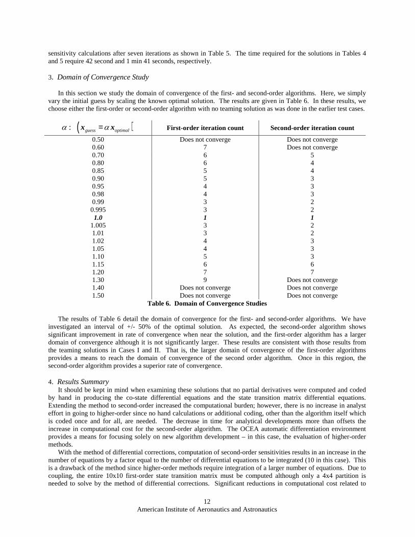
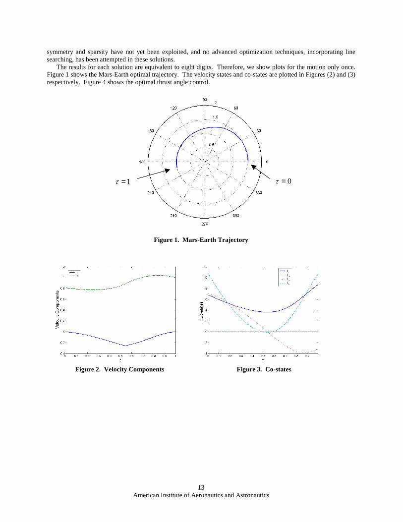
The results for each solution are equivalent to eight digits. Therefore, we show plots for the motion only once. Figure 1 shows the Mars-Earth optimal trajectory. The velocity states and co-states are plotted in Figures (2) and (3) respectively. Figure 4 shows the optimal thrust angle control.

Figure 1. Mars-Earth Trajectory

Figure 2. Velocity Components Figure 3. Co-states

0τ =1τ =

14American Institute of Aeronautics and Astronautics

Figure 4. Optimal Thrust Angle

B. An Example by Differential InclusionsHere we consider a simple nonlinear scalar system in order to illustrate the OCEA method in a direct

optimization example. Consider

3x x x uε= − + +& (40)

with performance index to be minimized given by

5 2

0

1

2J u dt= ∫ (41)

The discretized form of the equations of motion and performance index are then given by

3

1 1 1

2 2k k k k k k

k

x x x x x xuε+ + +− + + + + = ∆

(42)

and10

2

1

1

2 kk

J u=

= ∑ (43)

Here we choose ε =0.01 and, approximate the system by conveniently choosing 10 time intervals over the 5

second, thus ∆ = 0.5 seconds. We choose as boundary conditions 1 3x = and 11 0x = .

Once the relation for the control given in Eq. (42 is substituted into Eq. (43) we have the cost as a function of the unknown states as

( ); 2,3,...10kJ J x k= = (44)

A standard optimization procedure is employed now to solve for the nine unknown states. As mentioned earlier,

J∇ = 0 defines a set of nonlinear equations ( ( )kx = 0h ) which must be solved iteratively for the unknown states.

The Hessian of J, 2 J∇ , provides the matrix of first-order sensitivities ( 2G J= ∇ ) required for the solutions. OCEA’s automatic differentiation capability enables an efficient tool for computing and evaluating these partial derivatives, and higher-order partials if desired. A first-order correction to the unknown states can be written as

15American Institute of Aeronautics and Astronautics

1( ) ( )T TG G G−∆ =x h x (45)

We choose to solve this example using Matlab’s Symbolic Toolbox in order to compare the effort required in using OCEA and Matlab. Essentially, this is a test of symbolic and automatic differentiation methods. The difference comes when we need to compute and evaluate the derivatives of Eq. (44). With Matlab, we must type a command for each partial derivative required. In computing first- through third- order partials of the cost function, many ten’s of these commands are needed, at best, using Matlab. OCEA is ideally suited for solution of direct optimization problems such as the minimization of the expression given in Eq. (44). No coding effort is required beyond specifying the cost function since all required partial derivatives are automatically computed and evaluated. The implementation of higher-order solutions for direct optimization problems results in relatively small increase in the computational cost and no additional effort to derive or code partials for the higher-order terms using OCEA. Table 7 shows a comparison of solving the problem by first- and second-order methods. More rapid convergence is found for the second-order method.

Iteration count First-order error Second-order error1 1.4313e+002 1.4313e+002 2 2.1830e-001 1.8792e-0023 2.9154e-007 4.0911e-0124 2.6237e-018 8.6737e-0305 8.3470e-030

Table 7. Differential Inclusions Solution Errors

A comparison of the optimal solutions and that by Differential Inclusions is shown in Figure 5.

Figure 5. Optimal versus OCEA-Differential Inclusions

As expected, the Differential Inclusions solution provided a starting guess for the initial co-state that resulted in convergence to the optimal solution in only two iterations using Matlab’s fmincon function. On the other hand, blind guessing resulted in many unsuccessful attempts to choose a suitable starting guess. A check of the performance index of these two solutions shows that the approximate Differential Inclusions solution is sub-optimal as anticipated. Of course a larger number of time intervals can be chosen; however, the objective of this exercise is to demonstrate the utility of a computational tool which can reduce the time involved and coding effort involved in this and many other optimization applications.

16American Institute of Aeronautics and Astronautics

VI. ConclusionIn this paper, we demonstrated by several examples the solution of nonlinear Two-point Boundary Value

Problems using automatic differentiation. The automatic differentiation tool, OCEA, was utilized to compute the partial derivatives required in the solution of state transition matrix differential equations and the sensitivities required for solving discrete optimization problems. OCEA has the capability to compute higher-order sensitivities which enable extending traditional algorithms to higher-order for improving rate of convergence. Further uses of automatic differentiation result in automatically generating co-state differential equations and enabling second- and higher-order guidance laws.

VII. References1Bryson A.E., and Ho, Y., Applied Optimal Control, Taylor and Francis, Levittown, PA, 1975.2Junkins, J.L. and Turner, J.D., Optimal Spacecraft Rotational Maneuvers: Studies in Astronautics, Vol. 3,

Elsevier Science Publishers, Amsterdam, The Netherlands, 1986.3J. D. Turner, "Automated Generation Of High-Order Partial Derivative Models,” AIAA Journal, Vol. 41, No. 8

August 2003, pp. 1590-1598.4J. D. Turner, "Generalized Gradient Search And Newton's Methods For Multilinear Algebra Root-Solving And

Optimization Applications," Invited Paper No. AAS 03-261, To Appear In The Proceedings Of The John L. Junkins Astrodynamics Symposium, George Bush Conference Center, College Station, Texas, May 23-24, 2003.

5Griffith, D.T., Turner, J.D., and Junkins, J.L., “An Embedded Function Tool for Modeling and Simulating Estimation Problems in Aerospace Engineering”, AAS/AIAA Spaceflight Mechanics Meeting, Maui, Hawaii, February 8-12, 2004, AAS 04-148.

6Griffith, D.T, Sinclair, A.J., Turner, J.D., Hurtado, J.E., and Junkins, J.L., “Automatic Generation and Integration of Equations of Motion by Operator Over-Loading Techniques”, AAS/AIAA Spaceflight Mechanics Meeting, Maui, Hawaii, February 8-12, 2004, AAS 04-242.

7Seywald, H., “Trajectory Optimization Based on Differential Inclusions,” Journal of Guidance, Control, andDynamics, Vol. 17, No. 3, May-June 1994, pp. 480-487.

8Durrbaum, A., Klier, W., and Hahn, H., “Comparison of Automatic and Symbolic Differentiation in Mathematical Modeling and Computer Simulation of Rigid Body Systems”, Multibody System Dynamics, Vol. 7, pp. 331-355, 2002.

9Battin, Richard H., An Introduction to the Mathematics and Methods of Astrodynamics, AIAA Education Series, 1987.

17American Institute of Aeronautics and Astronautics

APPENDIX A: State Transition Matrix Differential EquationsThe state transition differential equations are here written in indicial notation. Note: All indices run from 1 to ns

where ns is the number of states. Initial conditions are the identity matrix for the first order state transition matrix differential equations, and zeros for second and higher order state transition matrix differential equations.

First order:

,ij i s sjfΦ = Φ& (A.1)

( )( , )

( )i

ij ij oj o

tt t

t

∂Φ = Φ =

∂x

x(A.2)

Second order:

, ,ijk i s sjk i st tk sjf fΦ = Φ + Φ Φ& (A.3)

( )2 ( )

, ,( ) ( )

iijk ijk o o

j o k o

tt t t

t t

∂Φ = Φ =

∂ ∂x

x x(A.4)

Third order:

, , ,

, ,

ijkl i s sjkl i su ul sjk i st tk sjl

i st tkl sj i stu ul tk sj

f f f

f f

Φ = Φ + Φ Φ + Φ Φ

+ Φ Φ + Φ Φ Φ

&(A.5)

( )3 ( )

, , ,( ) ( ) ( )

iijkl ijkl o o o

j o k o l o

tt t t t

t t t

∂Φ = Φ =

∂ ∂ ∂x

x x x(A.6)

Fourth order:

, ,

, , ,

, , ,

, , ,

, ,

ijklm i s sjklm i sv vm sjkl

i su ul sjkm i su ulm sjk i suv vm ul sjk

i st tk sjlm i st tkm sjl i stv vm tk sjl

i st tkl sjm i st tklm sj i stv vm tkl sj

i stu ul tk sjm i stu ul tkm s

f f

f f f

f f f

f f f

f f

Φ = Φ + Φ Φ

+ Φ Φ + Φ Φ + Φ Φ Φ

+ Φ Φ + Φ Φ + Φ Φ Φ

+ Φ Φ + Φ Φ + Φ Φ Φ

+ Φ Φ Φ + Φ Φ Φ

&

,

,

j i stu ulm tk sj

i stuv vm ul tk sj

f

f

+ Φ Φ Φ

+ Φ Φ Φ Φ

(A.7)

( )4 ( )

, , , ,( ) ( ) ( ) ( )

iijklm ijklm o o o o

j o k o l o m o

tt t t t t

t t t t

∂Φ = Φ =

∂ ∂ ∂ ∂x

x x x x(A.8)