Solving the stationary Liouville equation via a boundary elementmethod

David J. Chappell, Gregor Tanner

School of Mathematical Sciences, University of Nottingham, University Park, Nottingham NG7 2RD, UK

Abstract

Intensity distributions of linear wave fields are, in the high frequency limit, often approximatedin terms of flow or transport equations in phase space. Common techniques for solving the flowequations for both time dependent and stationary problems are ray tracing or level set methods.In the context of predicting the vibro-acoustic response of complex engineering structures, reducedray tracing methods such as Statistical Energy Analysis or variants thereof have found widespreadapplications. Starting directly from the stationary Liouville equation, we develop a boundary el-ement method for solving the transport equations for complex multi-component structures. Themethod, which is an improved version of the Dynamical Energy Analysis technique introduced re-cently by the authors, interpolates between standard statistical energy analysis and full ray tracing,containing both of these methods as limiting cases. We demonstrate that the method can be usedto efficiently deal with complex large scale problems giving good approximations of the energydistribution when compared to exact solutions of the underlying wave equation.

Keywords: Statistical energy analysis, high-frequency asymptotics, Liouville equation, boundaryelement method

1. Introduction

Many phenomena in physics and engineering can be accurately described or modelled in termsof linear wave equations. A large range of numerical methods has been developed for solvingwave problems, often making heavy use of the linearity of the underlying PDEs leading in generalto large, finite matrix equations. Popular tools include finite element or finite volume methods,boundary element methods and various spectral methods. There are, however, basic limitationswhen approximating the solutions of the wave equations directly: the size of the associated linearsystem increases with decreasing wavelength and numerical schemes become inefficient when thelocal wavelengths are orders of magnitude smaller than typical dimensions of the physical system.

In order to overcome this limitation, a range of high-frequency/ short wave length methodshave been devised such as the WKB or eikonal approach or semiclassical methods developed in thecontext of quantum chaos, see [1, 2, 3] for overviews. In particular, phase information is obtainedby solving the Hamilton-Jakobi equations for the action fields, whereas amplitude informationis calculated using transport equations. The actual methods can be quite intricate demandingan intimate knowledge of the classical phase space dynamics given by the Hamilton equations ofmotion for the underlying ray or classical dynamics. If one is prepared to omit phase information

Preprint submitted to Elsevier February 23, 2012

arX

iv:1

202.

4754

v1 [

phys

ics.

com

p-ph

] 2

1 Fe

b 20

12

altogether, the approximations amount to solving the transport or Liouville equation for phasespace densities.

In this paper, we will focus on efficient numerical methods for solving the Liouville equation(LE) for stationary problems. We will show how the solutions of the LE are related to both raytracing (see for example, [4, 5, 6]) and statistical energy analysis (SEA) [7, 8, 9], a popular methodin the engineering community for solving vibro-acoustic problems in the high-frequency limit.

The Liouville equation is an example of a PDE describing a conservation law [10]. Typicalsolution methods are based on characteristics or ray tracing. Ray tracing is the method of choicewhen considering propagation over relatively short times or length intervals. Prime examples includeweather forecasting, where data updates lead to regular re-initialisations of the density distributions[11], or room acoustics, where only very few reflections need to be considered [5]. More sophisticatedmethods related to tracking the time-dynamics of interfaces in phase space such as moment methodsand level set methods [12, 13, 14] have been developed only relatively recently, finding applicationsin acoustics, seismology and computer imaging. For an excellent recent overview, see Runborg [2].Numerical methods based on solving the time dependent Liouville equation directly on a mesh usingfinite volume or transfer operator methods, also referred to as Ulam methods, have been consideredin [15] and more recently in [16, 17]. Ray based and tracking methods often become inefficient whenconsidering frequency domain wave problems in bounded domains, for example, determining thewave field in a finite size cavity driven by a continuous, monochromatic excitation. Here, multiplereflections of the rays and complicated folding patterns of the associated level-surfaces often leadto an exponential increase in the number of branches that need to be considered.

In the engineering literature, these problems have been circumvented by subdividing the struc-ture into a set of substructures. Assuming ergodicity of the underlying ray dynamics and quasi-equilibrium conditions in each of the subsystems, that is, assuming that the density in each subsys-tem is approximately constant, greatly simplified SEA equations based only on coupling constantsbetween subsystems can be set up. The disadvantage of SEA is that the underlying assumptionsare often hard to verify a priori or are only justified when an additional averaging over ‘equivalent’subsystems is considered. These shortcomings have been addressed by Langley [18, 19] and morerecently in a series of papers by Le Bot [20, 21, 22]. A computational tool based on a Frobenius-Perron operator approach systematically interpolating between SEA and full ray tracing has beenintroduced first in [23] and further analysed in [24]. Its name, Dynamical Energy Analysis (DEA),points at the similarities with SEA but stresses at the same time the importance of dynamical cor-relations present in the ray-densities. Thus, in DEA, the solution in a subsystem of the structure istypically represented by a vector; this is in contrast to SEA where the solution in each subsystemis represented by a single number, the mean ray density in each subsystem.

The implementation of DEA as presented in [23, 24] corresponds to a spectral boundary integralmethod; the integral equations are expanded in orthogonal basis sets and the resulting matrixequations are solved for the coefficients of the basis expansion of the solution. It has been shownin [24] that the method works even in situations where a naive application of SEA fails. However,spectral methods can lead to slow convergence for the matrix elements in the DEA matrix, inparticular if the boundary is non-smooth. In this paper, we show that using a boundary elementmethod (BEM) for the spatial variable and a basis function expansion in the momentum componentleads to large efficiency gains. We will furthermore present a more in depth derivation of the actualboundary integral formulation.

The paper is structured as follows: in Sec. 2, we sketch the derivation of the Liouville transportequation from the underlying wave equation; we will then derive the boundary integral formulation

2

in Sec. 3 and give a description of the numerical implementation of DEA using the BEM/ basisfunction approach in Sec. 4. Numerical results will then be presented in the Sec. 5.

2. From wave dynamics to phase space densities

2.1. A time dependent formulation

In the following, we sketch the connection between linear wave equations and the Liouvilleequation via the Eikonal ansatz. We develop the theory in the time domain first and move to astationary formulation in the next section. We will restrict the discussion to the Helmholtz equationof acoustics; other wave problems such as electromagnetic waves, linear elasticity or Schrodinger’sequation can be treated along the same line with the obvious modifications. For a more in depthdiscussion of the Eikonal approach, see for example [2]. A nice derivation of the connection betweenwave transport equations and the Liouville equation based on Wigner transformation techniqueshas been given in [25].

We start from the wave equation for linear acoustics, that is,(∂2

∂t2−∇ · (c2∇)

)u(r, t) = 0 (1)

seeking solutions u(r, t) in some domain Ω with boundary Γ (u may express acoustic pressure inappropriate units). Furthermore, c = c(r) ≥ 0 is the local wave speed. We assume in whatfollows that the wave equation is not explicitly time dependent and that the walls act as passiveelements, that is, we have Dirichlet or Neumann boundary conditions, u(s) = 0 or ∂u/∂n(s) = 0for s ∈ Γ. Solutions are then determined uniquely in terms of initial conditions u(r, 0) = u0(r) and∂tu(r, 0) = u1(r) at t = 0.

We now make the usual Eikonal ansatz

u = Aeiωφ (2)

with real valued functions A = A(r, t), φ = φ(r, t) and ω acting as the large parameter here. Plugging(2) into (1) and collecting terms of the order ω2, we arrive at the Eikonal equation(

∂φ

∂t

)± c |∇φ| = 0. (3)

Terms of order ω yield a transport equation

2∂A

∂t

∂φ

∂t+A

∂2φ

∂t2− 2c2∇A · ∇φ− c2A∆φ− 2c∇ · (cA∇φ) = 0. (4)

Setting

ρ(r, t) = A2(r, t)∂φ

∂t(r, t) ,

we can write Eq. (4) in the form of a conservation law, that is,

∂ρ

∂t+∇ · (vρ) = 0 (5)

3

with “velocity field”

v(r, t) = −c2∇φ/∂φ∂t

(6)

determined through the phase function φ(r, t) alone.Solutions of the Eikonal equation (3) can readily be found using characteristics. Without re-

stricting the discussion we choose the “+” sign in (3); see also comments further down in the text.Setting

H(r, p) = c|p| with momentum p = ∇φ , (7)

one obtains solutions φ(r, t) along trajectories in phase space X(t) = (r(t), p(t)) by solving Hamil-ton’s equations of motion, that is,

r = ∇pH = cp

|p|(8)

p = −∇rH = |p|∇c .

Note that in deriving the Eikonal Eq. (3) and transport Eq. (4) we omitted terms of order O(ω0);neglecting the coupling terms between Eqs. (3), (4) leads to first order differential equations whichcan formally be solved by using only one of the initial conditions, that is, either u0(r) or u1(r).The ODEs (8) are thus solved by using, for example, initial conditions X(0) = (r0, p0 = ∇φ0(r0)).A solution for the phase φ is then obtained by integration, that is,

φ(r, t) = φ0(r0) +

∫ t

0

p r dτ

where the integral is taken along X(t) = ϕt(X0). Here ϕt(X0) is the phase space flow map obtainedfrom the pair of ODEs (8). In particular we integrate over trajectories starting at t = 0 at somepoint r0 with momentum p0 = ∇φ0(r0) and reaching the final point r at time t. Here, φ0 is theinitial phase corresponding to the initial conditions u0(r0) = A0(r0) exp(iωφ0(r0)) at t = 0. Ingeneral, there will be several such initial points from which a trajectory reaches the point r at timet. That is, the solution to the eikonal equation (3) at a point r has a multi-sheet structure with aset of N = N(r, t) branches, each giving rise to a phase

φj(r, t) = φ0(rj) +

∫ t

0

pj rjdτ, j = 1, ..., N . (9)

The integrals are taken over paths Xj , j = 1, ..., N , reaching r in time t with Xj(0) = (rj ,∇φ0(rj)).It is this multi-sheet structure which makes solving Eq. (3) difficult in practice [2]. In particular,the number of branches N(t) can increase rapidly with t and for chaotic ray dynamics N(t) actuallyincreases exponentially [1].

We would like to remark that choosing the “−” sign in (3) leads to a sign-change in (8) andgives time-reversed ray trajectories obtained through the time transformation t→ −t. The completesolution to the Eikonal equation is thus given by the set of characteristics travelling both in positiveand negative time.

We turn now to the solution of the transport Eq. (5); this equation is driven by the solutionφ(r, t) of the Eikonal Eq. (3). It thus suffers in principle from the same multi-valuedness problem asthe original equation. Note, however, that the solutions of the ray equations (8) in phase space are

4

determined uniquely for a given initial condition; it is the projection onto r - space which leads tothe multi-valuedness of the phase solution. It is thus advantageous to solve the transport equationin phase space. The corresponding equation is the Liouville equation (LE)

∂ρ

∂t+ H, ρ = 0 (10)

where · , · are the Poison brackets, and H(r, p) is the classical Hamilton function (7). The phasespace density

ρ(r, p, t) =

N(t)∑j=1

ρj(r, t)δ(p−∇φj(r, t)) (11)

indeed solves Eq. (10) if the branches φj(r, t) and ρj(r, t) obey the Eikonal and transport equations(3), (5), respectively. (This result can be obtained by inserting (11) into (10), see also [2].) A formalsolution of the LE is obtained in terms of a Frobenius-Perron operator

ρ(X, t) = Lt[ρ](X) =

∫δ(X − ϕt(Y ))ρ(Y, 0)dY = ρ(ϕ−t(X), 0), (12)

where the last relation is valid for Hamiltonian flows; this relation is used extensively in the raytracing approach.

The solution of the wave equation (1) is now formally obtained by summing over the solutionbranches in (9), that is,

u(r, t) =

N∑j=1

|Aj(r, t)|eiωφj(r,t)−iνjπ2 (13)

where νj are Maslov indices [1] due to caustics along the ray Xj(t). As we are not interested inphases in what follows, we will not discuss this issue any further here. An asymptotic treatmentof the wave equation using the Eikonal ansatz needs to keep track of the link between phases andamplitudes along the different solution branches. Ray tracing methods are often the only wayforward when finding solutions using the Eikonal ansatz. This may be an efficient method for shorttimes and in cases where only a few reflections occur. However, the rapid increase in the numberof paths makes ray tracing methods quite cumbersome for large times. The advantages behindthe original idea of the Eikonal ansatz, namely replacing a wave equation with highly oscillatorysolutions by differential equations for slowly varying quantities such as the amplitude and phase,are lost.

In many applications it is, however, sufficient to find the solution of the transport equations fora given set of initial conditions. The density ρ(X, t) contains a great deal of information about thewave solution, and this may often be sufficient for the required purpose. Classical ray tracing, thatis ray tracing without tracking phase information, is indeed used extensively in room acoustics.

2.2. Stationary formulation

In what follows, we will consider wave problems with time-harmonic forcing at a frequency ω.We can then separate out time by setting

u(r, t) = G(r)eiωt.

5

Let us consider problems with a forced excitation by a point source. The corresponding inhomoge-neous wave equation then has the form(

∇ · (c2∇) + ω2)G(r) = −c2δ(r − r0) , (14)

with the source point at r = r0. The solution G(r, r0) is the Green function and arbitrary forcedistributions can be recovered.

For an Eikonal approach, we proceed by splitting the solution into a homogeneous and aninhomogeneous (or direct) solution in the form

G(r, r0) = G0(r, r0) +Gh(r, r0),

where G0 is the free Green function and Gh solves the homogeneous Helmholtz Eq.(∇ · (c2∇) + ω2

)Gh(r) = 0 (15)

with appropriate boundary conditions. (For Dirichlet BC, that is G(s) = 0, we obtain Gh(s) =−G0(s) for s ∈ Γ). One finds for two-dimensional problems with c = const,

G0(r, r0) =i

4H1

0 (ω|r − r0|/c), (16)

where H10 is the 0th order Hankel function of the first kind. Proceeding with an Eikonal ansatz, we

set Gh = A exp(iωψ); we have then

φ(r, t) = ψ(r) + t and∂A

∂t= 0. (17)

The Eikonal and transport Eqs. (3), (5) reduce to

c|∇ψ| = 1 (18)

and∇ · (vρ) = 0 with v(r) = −c2∇ψ. (19)

We write the boundary conditions in the form

G0(s) = A0(s)eiωψ0(s) for s ∈ Γ .

In order to obtain an approximate solution of (18) at a point r ∈ Ω one needs to find those raysstarting from a boundary point s ∈ Γ with initial conditions X0 = (s, p = ∇ψ0(s)) which passthrough the point r following the equations of motion (8). The phase function ψ is then obtainedby integrating along this trajectory with an initial condition ψ(s) = ψ0(s); the phase function ψagain has a multi-sheet structure and there are in general infinitely many sheets intersecting withthe plane r = const in phase space. (A phase space description of the sheets can be given in termsof Lagrangian manifolds, see for example [26].) The various branches are calculated according to

ψj(r) = ψ0(sj) +

∫ r

sj

p dr

6

integrating along a trajectory with initial condition Xj = (sj , pj = ∇ψ0(sj)). The transportequation (19) is solved with initial conditions

j0(s) = −c2A2(s)∂ψ(s)

∂n(20)

where j0(s) is the incoming flux normal to the boundary. The total solution is then approximativelyobtained as

G(r) = G0(r) +∑j=1

|Aj(r)|eiωψj(r)−iµjπ/2 (21)

where µj are again Maslov phases and |Aj | is the amplitude transported along the trajectory fromXj to r; for alternative derivations of Eqs. (13), (21), see [1].

In applications, one is often interested in wave intensities (such as energy densities); the contri-butions arising from reflections from the boundary have the form

I(r) = |Gh(r)|2 =∑j,j′

|AjAj′ |eiω(ψj−ψj′ ) =∑j

ρj(r) +∑j 6=j′|AjAj′ |eiω(ψj−ψj′ ). (22)

Neglecting the oscillatory terms, which is justified after averaging over a small ω range or over anensemble of similar systems, one arrives at the ray tracing approximation

I(r) ≈ ρ(r) =∑j

ρj(r) =

∫ρ(r, p)dp (23)

where ρ(r, p) is a solution of the stationary Liouville equation with

H, ρ = 0 (24)

and boundary conditions given by (20) together with Snell’s law of reflection. Note that the totalintensity |G(r)|2 for r ∈ Ω may be estimated simply by adding |G0(r)|2 to ρ(r).

It is clear from the description above that a ray tracing approach is even more cumbersomein the stationary case than in the time-dependent case. The stationary solution is constructedfrom infinitely many branches which originate from reflections at boundaries. If we neglect phaseinformation, however, we can reconstruct the phase space densities using the Frobenius-Perronoperator, Eq. (12) [23, 24]. In the next section we will introduce an efficient algorithm for deter-mining solutions of the stationary Liouville equation even in the presence of multiple reflections,thus overcoming the limitations of the ray tracing approaches sketched above.

3. Boundary integral formulation of the Liouville equation

In order to solve the stationary Liouville equation (24), the ray tracing integral formula, Eq.(12), is rewritten in a boundary integral form using a boundary mapping technique. The boundarymapping procedure involves first mapping the ray density emanating continuously from the sourceonto the boundary Γ and then constructing a Frobenius-Perron operator for the boundary map.

We now give an explicit derivation of the initial density on the boundary arising from Eq. (14)for Dirichlet boundary conditions. The ray density emanating from a source point r0 ∈ Ω is given

7

by the square of the amplitude of the free space Green function. For Ω ⊂ R2, it is given by (16)and we have the following high frequency asymptotic form

|G0(r, r0)|2 ∼ c

8πω|r − r0|. (25)

Lifting the ray density to the full phase space, Eq. (25) corresponds to rays moving out fromthe source in all directions according to

ρ0(r, p; r0) =cδ(p− p0)

8πω|r − r0|, (26)

where p0 = |p|(r−r0)/|r−r0|. Note that from Eq. (18), the ray dynamics take place on the ‘energy’manifold c|p| = 1. To obtain the source density ρΓ

0 on the boundary Γ, we set

ρ0(r, p; r0) = ρΓ0 (s, ps)δ(c|p| − 1), (27)

where s parameterizes Γ and ps ∈ Bd−1|p| denotes the momentum component tangential to Γ at s

for fixed H(X) = c|p| = 1; here Bd−1|p| is an open ball in Rd−1 of radius |p| and centre s. Using

local coordinates on the boundary, that is, p = (ps, p⊥), then δ(p− p0) = δ(ps− ps0)δ(p⊥− p⊥0 ) and

|p|δ(p⊥ − p⊥0 ) = cp⊥δ(c|p| − 1). Combining these identities with (26) and (27) yields

ρΓ0 (s, ps; r0) =

c2 cos(θ(r(s), r0))δ(ps − ps0)

8πω|r(s)− r0|, (28)

where θ(r(s), r0) is the angle between the normal to Γ at r(s) and the ray from r0 to r(s). Theresulting boundary layer density ρΓ

0 is equivalent to a source density on the boundary producingthe same ray field in the interior as the original source field after one reflection.

The operator equivalent to the Frobenius-Perron operator (12), but now acting on boundarydensities ρΓ, is described in terms of a boundary integral operator B,

B ρΓ(Xs) =

∫∂Pw(Y s, ω)δ(Xs − γ(Y s))ρΓ(Y s)dY s (29)

where Xs = (s, ps), Ys = (s′, p′s) and γ is the invertible boundary map. Also, ∂P = Γ×Bd−1

|p| is the

phase space on the boundary at fixed “energy” H(X) = c|p|. The weight w contains factors dueto reflection/ transmission at interfaces within Ω and a damping term of the form exp (−µL(s, s′)),where L(s, s′) is the length of the trajectory between s and s′. Note that, depending on themodelling assumptions, the factors in w may depend on ω. A similar weight term also needs to beapplied in Eq. (28) since rays emanating from the source will also be subject to dissipation andpossible reflection/ transmission at interfaces. We assume uniform damping in the interior, thatis, the damping coefficient µ does not depend on r. The damping term does then not alter theunderlying ray dynamics [27]. Note that convexity is assumed to ensure γ is well defined; non-convex regions can be handled by introducing a cut-off function in the shadow zone as in Ref. [21]or by subdividing the regions further.

The stationary density on the boundary induced by the initial boundary distribution ρΓ0 (Xs, ω)

can then be obtained using

ρΓ(ω) =

∞∑n=0

Bn(ω)ρΓ0 (ω) = (I − B(ω))−1ρΓ

0 (ω), (30)

8

where Bn contains trajectories undergoing n reflections at the boundary.The resulting density distribution on the boundary ρΓ(Xs, ω) is then mapped back into the

interior region. Using Eq. (23), one can relate ρΓ to a wave energy density after projecting onto rspace, that is for Ω ⊂ R2 ,

ρ(r, ω) =

∫ρ(r, p)dp,

=

∫ ∫ρΓ(Xs, ω)δ(c|p| − 1)|p|d|p|dΘ,

(31)

where (|p|,Θ) is a polar coordinate system for p. One finally obtains

ρ(r, ω) =1

c2

∫ρΓ(Xs, ω)dΘ. (32)

Now performing a change of variables from Θ to s yields

ρ(r, ω) =1

c2

∫ρΓ(Xs, ω)

cos(θ(rs, r))

|r − rs|ds, (33)

where rs ∈ Γ is the point on Γ in Cartesian coordinates corresponding to s. For systems withdamping we must again apply a factor of the form exp (−µL(s, s′)) to the final density evaluation(33). The total intensity |G(r, r0;ω)|2 may be estimated simply by adding |G0(r, r0;ω)|2 to thevalue of ρ(r, ω) given by (33).

We remark in passing that our approach is akin to the infinitesimal generator technique presentedin [17] which aims at estimating the long term behaviour of the dynamics by numerically calculatingthe spectral properties of the generator of the Frobenius-Perron operator and extrapolating to longtimes.

4. Numerical implementation: basis approximations and boundary element tech-niques

The long term dynamics is contained in the operator (I − B)−1 and standard properties ofFrobenius-Perron operators ensure that the sum over n in Eq. (30) converges for dissipative oropen systems. In order to evaluate (I − B)−1, a finite dimensional approximation of the operatorB must be constructed. In Refs. [23, 24], basis expansions have been applied in both positionand momentum coordinates, which is straightforward to implement for Ω ⊂ R2 using univariateexpansions in each argument. In particular, in Ref. [23], a Fourier basis was employed globally oneach subsystem in both position and momentum. It is well known that the convergence rate of aFourier basis expansion depends on the smoothness of the approximant and also requires periodicboundary conditions [28]. The periodicity requirement will be fulfilled due to periodicity of theboundary curve and that the ray density corresponding to ps = ±|p| is zero giving periodicity inthe momentum coordinate. However, the smoothness criterion often fails if, for example, cornersare present in Γ; the initial density due to a point source is not then differentiable at the corners.

In Ref. [24] it was suggested to split up the spatial approximation at corners in Γ and applya basis approximation with no requirement for periodic boundary conditions in order to attainits optimal convergence properties. An approximation using a Chebyshev basis was implemented

9

since Chebyshev polynomials may be computed simply in terms of trigonometric functions andhave similar convergence properties to Fourier basis approximations without the periodicity re-quirement. Such an approach also has a natural and optimal (in terms of polynomial degrees thatcan be integrated exactly) quadrature choice for the associated integrals, namely, Gauss-Chebyshevquadrature. The improvement in computational efficiency brought about by this approach openedup the method to larger scale multi-component problems.

In this work we go further along this route by subdividing the boundary using a mesh. Thisintroduces greater flexibility into the numerical method making it possible to both increase thepolynomial order of the basis functions and to refine the mesh for the spatial coordinates. Theadvantage of refining the mesh is that additional degrees of freedom are introduced to the modelwhilst maintaining relatively low quadrature costs due to the lower order of the spatial basis ap-proximation. As such it is preferable to choose a basis which is orthogonal in the standard L2 innerproduct. (From previous experience using a Chebyshev basis, where the associated orthogonalinner product is weighted, we found that low order approximations were very poor). Due to themesh discretization procedure adopted here, the boundary conditions are not periodic and using aFourier basis is not advisable; hence an alternative L2−orthogonal basis choice is proposed, namely,Legendre polynomials.

The overall form of the proposed numerical scheme in 2D is therefore based on a Legendrepolynomial approximation in both position and momentum augmented with a boundary meshthrough which the spatial approximation may be localised. For an extension of the method to 3Dcavities, see [29]. Recall that ps ∈ (−|p|, |p|) and denote by ps a re-scaling of ps to (−1, 1). Let usalso denote

Pm(ps) =√

1/|p|Pm(ps).

An important special case of the scheme described above is when we fix the spatial basis approxima-tion at zero (constant) order and only refine the mesh, which essentially results in a scaled piecewiseconstant boundary element approximation. This type of approximation is also often referred to asUlam’s method [15, 16], although this would involve performing such an approximation in full phasespace, rather than just in its spatial component. The implementation of separate meshes and basisapproximations in both position and momentum would, however, complicate the procedure. Inaddition, our final computations will involve integration over spatial variables only. A spatial meshtherefore has the additional benefit of localising the integration regions, permitting the use of lowerorder quadrature rules.

The overall approximation is then of the form

ρΓ(Xs, ω) ≈n∑α=1

Ns∑l=0

Np∑m=0

ρα,l,mPα,l(s)Pm(ps), (34)

where Ns and Np are the orders of the position and momentum basis expansions, respectively, andn is the number of elements in the mesh. Also

Pα,l(s) =√

2/AαPl(sα)χα(s),

where sα parameterizes the αth element and is scaled to take values in (−1, 1), χα is the char-acteristic function for element α and Aα is the length of element α, α = 1, .., n. An analogousapproximation is also made for ρΓ

0 , the initial density, and the values of ρα,l,m are to be determined

10

by solving the resulting linear system. Note that the special case of piecewise constant bound-ary elements is reached by setting Ns = 0 above. The other limiting case, Np = 0, correspondsto a ‘diffusive’ reflection approximation, also denoted as Lambert’s law [5], which is equivalent tothe assumption that incoming rays are scattered uniformly in all directions after reflecting from aboundary. Equation (30) then becomes equivalent to the integral equations discussed in [21, 30].Note that the case Np = Ns = 0 and n = 1 corresponds to an SEA approximation for a singlesubsystem (n equals the number of substructures for multi-component systems ) [23].

The matrix approximation B of the linear operator B (29) is given by taking the inner product< ·, · > in L2(∂P):

Bm+1+Np(l+Ns(α−1)),b+1+Np(a+Ns(β−1)) =

(2m+ 1)(2l + 1)

4

⟨B(Pβ,a(s′)Pb(p

′s)), Pα,l(s)Pm(ps)

⟩=

(2m+ 1)(2l + 1)

4

∫∂P

∫∂Pw(Y s, ω)δ(Xs − γ(Y s))Pβ,a(s′)Pb(p

′s)Pα,l(s)Pm(ps)dY

sdXs =

(2m+ 1)(2l + 1)

4

∫∂Pw(Y s, ω)Pβ,a(s′)Pb(p

′s)Pα,l(γs(Y

s))Pm(γp(Ys))dY s.

(35)

Here we write γ = (γs, γp), to denote the splitting of the position and momentum parts of theboundary map. The boundary map can be very difficult to obtain in general, and hence we writethe operator in terms of trajectories with fixed start and end points s′ and s as follows

Bm+1+Np(l+Ns(α−1)),b+1+Np(a+Ns(β−1)) =

(2m+ 1)(2l + 1)

4

∫Γ

∫Γ

w(Y s, ω)Pm(ps(s, s′))Pα,l(s)Pb(p

′s(s, s

′))Pβ,a(s′)

∣∣∣∣∂p′s∂s∣∣∣∣ ds′ds. (36)

The resulting boundary integral formulation containing a pair of integrals over boundary coordi-nates bears a resemblance to standard variational Galerkin boundary integral formulations, see forexample [31].

5. Numerical results

In this section we consider a two-dimensional polygonal example whose boundary is meshed bysubdividing each side into equidistant sections governed by a mesh parameter ∆x. The number ofelements on any given side is computed using the integer part of the side length divided by ∆x.The Jacobian in Eq. (36) is written in the form∣∣∣∣∂p′s∂s

∣∣∣∣ =|p|(n · (r − r′))(n′ · (r − r′))

|r − r′|3, (37)

where n and n′ are the inward unit normal vectors to Γ at r and r′, respectively. In addition r andr′ are the Cartesian coordinate vectors corresponding to the boundary parameterised coordinatess and s′. In order to treat the corner singularities in (37), Gaussian quadrature is employed whereend-points are not included as quadrature points. The convergence of the quadrature rules is stillslow due to the peak in the integrand at corners. Telles’ transformation techniques are employedto speed up the convergence [32].

11

Source

Figure 1: Five cavity polygonal example geometry

12

A five cavity system is considered as shown in Fig. 1 with Dirichlet boundary conditions onthe outer boundary. The application of the method to multiple sub-domains is carried out usingthe same techniques as detailed in [24]. In general the configuration features irregular shaped, wellseparated pentagonal subsystems. In such a case one expects the wave energy to be fairly evenlydistributed within subsystems and the energy levels in each subsystem to be distinct and wellseparated. The one feature of the configuration where such trends may not hold is due to the directchannel running to the right of the source point leading to a corridor type effect and energy beinglocalised along this channel. Such dynamical features are likely to require higher order applicationsof our numerical algorithm to adequately resolve the behaviour.

Energy distributions have been studied as a function of the frequency with a hysteretic dampingfactor η = 0.01, where µ = ωη/(2c) throughout Ω. Here and in the remainder of this section thesubsystems (or cavities) are numbered 1, 2, ..., 5 from left to right. The wave speed is set to unity forsimplicity. Note that the method allows c (and thus µ) to vary between subsystems [24], but we donot make use of this in the examples considered here. Therefore the subsystem interface reflectionand transmission coefficients appearing in the weight term in (29) are simply 0 and 1, respectively.

Fig. 2 shows the energy distribution throughout the five subsystems compared with the resultsof a boundary element computation for the full wave problem. Explicitly we compute the squareof the energy norm

‖Gi‖2 :=

∫Ωi

|G(r, r0;ω)|2dr, i = 1, 2, .., 5. (38)

The lines show the approximate energy norms given by the Liouville equation model computed forf = (ω/(2π)) = 10, 13, 16, 19, ..., 70 with Np = 10, Ns = 0 and n = 627, and hence the spatialapproximation has been improved via mesh refinement rather than using higher order Legendrepolynomial basis expansions. This has the benefit that the quadrature costs are kept moderate andleads to considerable efficiency gains. The computations here took approximately 2.5 hours perfrequency compared with typical times of approximately 53 hours for a full tenth order Chebyshevbasis computation using the methods reported in [24]. Here the computations were performed usinga single core of a desktop PC with a 2.83 Ghz dual core processor. The circles each show the meanof 22 boundary element method computations, where the average is taken over a small range offrequencies centered around 10, 20,..., 70. The plus signs show the maxima and minima of theboundary element computations. The plot shows a good agreement between the solution of theLiouville equation and the mean of the full wave problem computations. In addition, the Liouvillesolution always lies within the range of the data for the full wave problem.

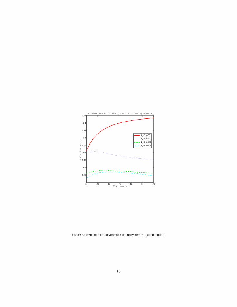
Fig. 3 shows the convergence of our numerical algorithm in subsystem 5 as the precision of theapproximation is increased by refining the mesh and simultaneously increasing the order of theLegendre basis approximation in direction space. The plot shows the relative error in the energynorm ‖G5‖2 compared against the value ‖Ge5‖2 computed with Np = 10, Ns = 0 and n = 627. Therelative error plotted is thus given by (‖Ge5‖2−‖G5‖2)/‖Ge5‖2. The trend of the energy increasing asthe precision of the numerical method is increased is shown by the error values all being positive andis expected since a low order implementation of our numerical scheme will not capture the directenergy channelled to the right of the source and into subsystem 5. Higher order basis functionsin direction space are required to capture such directivity patterns in the wave field. In additionthe plot shows the approximated solutions converging since the errors are getting closer to zeroas higher order approximations are employed. For the case Np = 2, n = 70 one sees the errorincreasing as the frequency and thus damping are increased. For high damping, the direct channel

13

0 10 20 30 40 50 60 70 8010

−7

10−6

10−5

10−4

10−3

10−2

10−1

Frequency (Hz)

||G||2

Energy Norm in each Subsystem Compared with BEM

Figure 2: Energy distribution in five coupled acoustic cavities. Subsystem: 1 - blue (dash-dot), 2 - red (dashed), 3 -green (thin solid), 4 - black (dotted), 5 - cyan (thick solid) (colour online)

14

10 20 30 40 50 60 700

0.05

0.1

0.15

0.2

0.25

0.3

0.35

0.4

0.45Convergence of Energy Norm in Subsysyem 5

Frequency

Relative Error

Np=2, n=70

Np=4, n=70

Np=6, n=150

Np=8, n=309

Figure 3: Evidence of convergence in subsystem 5 (colour online)

15

of energy (before reflection) from the source point will form a more significant part of the overallsolution. For the case Np = 4, n = 70, the higher order basis in direction space has been able tomodel the channelling effect more accurately and the error has become almost uniform across thefrequency range.

Fig. 4 shows the energy density |G(r, r0;ω)|2 plotted for r ∈ Ω and f = 15. The upper subplotshows the energy density approximated using a boundary element method for the full wave problem.The central subplot shows the average of 22 full wave solutions at different frequencies 13 < f < 17.One sees that the averaging reduces the influence of small scale fluctuations in the solution andproduces a generally smoother looking plot, showing more clearly the influence of the source point.The lower subplot shows the energy density approximated using the Liouville equation model withNp = 10, Ns = 0 and n = 627. Many similarities with the central subplot are apparent. Forexample, the direct energy channel to the right of the source and into subsystem 5, the locationof the source and the dip in energy in the second subsystem close to the interface are featurespresent in both plots. Also the energy channelled along the upper boundaries of subsystems 1 and4 is a common feature. This demonstrates that high frequency wave models based on the Liouvilleequation are indeed a powerful tool to obtain averaged solutions. Such an average solution can beobtained through averaging over an ensemble of similar structures or over a small frequency range.Applications are abundant in high frequency vibro-acoustics, where small changes in the domaindue to, for example, manufacturing tolerances lead to large variations in the response and thus asimulation of any one particular problem will only be of statistical significance. Indeed, replacinghighly oscillatory wave problems with smooth ray dynamical problems is often the only practicaloption in the high frequency regime.

6. Conclusion

The suitability of the Liouville equation as a model for high frequency wave problems has beendiscussed. A boundary integral approach has been proposed for its solution using the Frobenius-Perron operator. A numerical solution method has been implemented based on Legendre polynomialapproximations in phase space together with a spatial boundary mesh. The proposed method hasbeen verified by comparison with a BEM code for the full wave problem and numerical evidence ofconvergence has been shown.

ACKNOWLEDGEMENT

Support from the EPSRC (grant EP/F069391/1) and the EU (FP7IAPP grant MIDEA) isgratefully acknowledged. The authors also wish to thank InuTech Gmbh, Nurnberg for Diffpackguidance and licences, and Dmitrii Maksimov and Niels Søndergaard for stimulating discussions.

References

[1] Gutzwiller, M.C. Chaos in Classical and Quantum Mechanics. Springer, New York (1990).

[2] Runborg, O. Mathematical Models and Numerical Methods for High Frequency Waves. Com-mun. Comput. Phys. 2(5), (2007) 827-880.

16

[3] Tanner, G. & Søndergaard, N. Wave chaos in acoustics and elasticity. J. Phys. A 40, (2007)R443-R509.

[4] Glasser, A.S. An Introduction to Ray Tracing. Academic Press (1989).

[5] Kuttruff, H. Room Acoustics. 4th edn. Spon, London (2000).

[6] Cerveny, V. Seismic Ray Theory. Cambridge University Press 2001.

[7] Lyon, R.H. Statistical analysis of power injection and response in structures and rooms. J.Acoust. Soc. Am. 45, (1969) 545-565.

[8] Lyon, R.H. & DeJong, R.G. Theory and Application of Statistical Energy Analysis. 2nd edn.Butterworth-Heinemann, Boston, MA 1995.

[9] Craik, R.J.M Sound Transmission through Buildings using Statistical Energy Analysis. Gower,Hampshire 1996.

[10] LeVeque, R.J. Numerical Methods for Conservation Laws Birkhauser-Verlag, Basel 1990.

[11] Sommer, M.& Reich, S. Phase space volume conservation under space and time discretizationschemes for the shallow-water equations. Monthly Weather Review, 138, (2010) 4229-4236.

[12] Osher, S & Fedkiw, R.P. Level Set Methods: An Overview and Some Recent Results. J. Comp.Phys. 169, (2001) 463-502.

[13] Engquist, B. & Runborg, O. Computational high frequency waves propagation. Acta Numerica12, (2003) 181-266.

[14] Ying, L. & Candes, E.J. The phase flow method. J. Comp. Phys. 220, (2006) 184-215.

[15] Ding, J. & Zhou, A. Finite approximations of Frobenius-Perron operators. A solution of Ulam’sconjecture to multi-dimensional transformations. Physica D 92, (1996) 61-68.

[16] Junge, O. & Koltai, P. Discretization of the Frobenius-Perron operator using a sparse Haartensor basis - the Sparse Ulam method. SIAM J. Num. Anal., 47, (2009) 3464-3485.

[17] Froyland, G., Junge, O. & Koltai, P. Estimating long term behavior of flows without trajectoryintegration: the infinitesimal generator approach. Submitted to SIAM J. Num. Anal. (2011)(E-print arXiv:1101.4166).

[18] Langley, R.S. A wave intensity technique for the analysis of high frequency vibrations. J. Sound.Vib. 159, (1992) 483-502.

[19] Langley, R.S. & Bercin, A.N. Wave intensity analysis for high frequency vibrations. Phil. Trans.Roy. Soc. Lond. A 346, (1994) 489-499.

[20] Le Bot, A. A vibroacoustic model for high frequency analysis. J. Sound. Vib. 211, (1998)537-554.

[21] Le Bot, A. Energy transfer for high frequencies in built-up structures. J. Sound. Vib. 250,(2002) 247-275.

17

[22] Le Bot, A. Energy exchange in uncorrelated ray fields of vibroacoustics. J. Acoust. Soc. Am.120(3), (2006) 1194-1208.

[23] Tanner, G. Dynamical energy analysis- Determining wave energy distributions in vibro-acoustical structures in the high-frequency regime. J. Sound. Vib. 320, (2009) 1023-1038.

[24] Chappell, D.J., Giani, S. & Tanner, G. Dynamical energy analysis for built-up acoustic systemsat high frequencies. J. Acoust. Soc. Am. 130(3), (2011) 1420-1429.

[25] McDonald, S. Phase-space representations of wave equations with applications to the Eikonalapproximation for short-wavelength waves. Phys. Rep. 158, (1988) 337-416.

[26] Littlejohn, R.G. The semiclassical evolution of wave packets. Phys. Rep. 138, (1986) 193-291.

[27] Graefe, E.M. & Schubert, R. Wave packet evolution in non-Hermitain quantum systems.Phys.Rev.A 83 (2011) 060101(R).

[28] Boyd, J.P. Chebyshev and Fourier Spectral Methods.2nd edn. Dover, Mineola, NY 2000.

[29] Chappell, D.J., Tanner, G & Giani, S. Boundary element dynamical energy analysis: a versatilehigh-frequency method suitable for two or three dimensional problems. Submitted to J. Comp.Phys. (2011).

[30] Le Bot, A & Bocquillet, A. Comparison of an integral equation on energy and the ray tracingtechnique for room acoustics. J. Acoust. Soc. Am. 108, (2000) 1732-1740.

[31] Schmindlin, G. Lage, Ch. & Schwab, Ch. Rapid solution of first kind boundary integral equa-tions in R3. Engineering Analysis with Boundary Elements 27, (2003) 469-490.

[32] Telles, J.C.F. A self-adaptive co-ordinate transformation for efficient numerical evaluation ofgeneral boundary element integrals. Int. J. Num. Meth. Eng. 24, (1987) 959-973.

18

Figure 4: Energy density compared against the full wave solution: upper subplot shows the full wave solution, centralsubplot shows the full wave solution averaged over a small frequency band, lower subplot shows the Liouville equationmodel (colour online)

19