Solving ordinary differential equations

07/05/2016 Solving ordinary differential equations — Sage Reference Manual v7.1: Symbolic Calculus

http://doc.sagemath.org/html/en/reference/calculus/sage/calculus/desolvers.html 1/13

Solving ordinary differential equationsThis file contains functions useful for solving differential equations which occur commonly in a 1st semester differentialequations course. For another numerical solver see the ode_solver() function and the optional package Octave.

Solutions from the Maxima package can contain the three constants _C, _K1, and _K2 where the underscore is used todistinguish them from symbolic variables that the user might have used. You can substitute values for them, and makethem into accessible usable symbolic variables, for example with var("_C").

Commands:

desolve Compute the “general solution” to a 1st or 2nd order ODE via Maxima.desolve_laplace Solve an ODE using Laplace transforms via Maxima. Initial conditions are optional.desolve_rk4 Solve numerically IVP for one first order equation, return list of points or plot.desolve_system_rk4 Solve numerically IVP for system of first order equations, return list of points.desolve_odeint Solve numerically a system of firstorder ordinary differential equations using odeint fromscipy.integrate module.desolve_system Solve any size system of 1st order odes using Maxima. Initial conditions are optional.eulers_method Approximate solution to a 1st order DE, presented as a table.eulers_method_2x2 Approximate solution to a 1st order system of DEs, presented as a table.eulers_method_2x2_plot Plot the sequence of points obtained from Euler’s method.

AUTHORS:

David Joyner (32006) Initial version of functionsMarshall Hampton (72007) Creation of Python module and testingRobert Bradshaw (102008) Some interface cleanup.Robert Marik (102009) Some bugfixes and enhancementsMiguel Marco (062014) Tides desolvers

sage.calculus.desolvers.desolve(de, dvar, ics=None, ivar=None, show_method=False, contrib_ode=False)Solves a 1st or 2nd order linear ODE via maxima. Including IVP and BVP.

Use desolve? <tab> if the output in truncated in notebook.

INPUT:

de an expression or equation representing the ODEdvar the dependent variable (hereafter called y)ics (optional) the initial or boundary conditions

for a firstorder equation, specify the initial x and yfor a secondorder equation, specify the initial x, y, and dy/dx, i.e. write for a secondorder boundary solution, specify initial and final x and y boundary conditions, i.e. write

.gives an error if the solution is not SymbolicEquation (as happens for example for a Clairaut equation)

ivar (optional) the independent variable (hereafter called x), which must be specified if there is more thanone independent variable in the equation.show_method (optional) if true, then Sage returns pair [solution, method], where method is the string describingthe method which has been used to get a solution (Maxima uses the following order for first order equations:linear, separable, exact (including exact with integrating factor), homogeneous, bernoulli, generalizedhomogeneous) use carefully in class, see below for the example of the equation which is separable but thisproperty is not recognized by Maxima and the equation is solved as exact.contrib_ode (optional) if true, desolve allows to solve Clairaut, Lagrange, Riccati and some other equations.This may take a long time and is thus turned off by default. Initial conditions can be used only if the result isone SymbolicEquation (does not contain a singular solution, for example)

OUTPUT:

In most cases return a SymbolicEquation which defines the solution implicitly. If the result is in the form y(x)=...(happens for linear eqs.), return the righthand side only. The possible constant solutions of separable ODE’s areomitted.

EXAMPLES:

[ , y( ), ( )]x0 x0 y′ x0

[ , y( ), , y( )]x0 x0 x1 x1

http://doc.sagemath.org/html/en/reference/calculus/sage/gsl/ode.html#sage.gsl.ode.ode_solver



sage: x = var('x') sage: y = function('y')(x) sage: desolve(diff(y,x) + y ‐ 1, y) (_C + e^x)*e^(‐x)

sage: f = desolve(diff(y,x) + y ‐ 1, y, ics=[10,2]); f (e^10 + e^x)*e^(‐x)

sage: plot(f) Graphics object consisting of 1 graphics primitive

We can also solve secondorder differential equations.:

sage: x = var('x') sage: y = function('y')(x) sage: de = diff(y,x,2) ‐ y == x sage: desolve(de, y) _K2*e^(‐x) + _K1*e^x ‐ x

sage: f = desolve(de, y, [10,2,1]); f ‐x + 7*e^(x ‐ 10) + 5*e^(‐x + 10)

sage: f(x=10) 2

sage: diff(f,x)(x=10)1

sage: de = diff(y,x,2) + y == 0 sage: desolve(de, y) _K2*cos(x) + _K1*sin(x)

sage: desolve(de, y, [0,1,pi/2,4]) cos(x) + 4*sin(x)

sage: desolve(y*diff(y,x)+sin(x)==0,y) ‐1/2*y(x)^2 == _C ‐ cos(x)

Clairaut equation: general and singular solutions:

sage: desolve(diff(y,x)^2+x*diff(y,x)‐y==0,y,contrib_ode=True,show_method=True) [[y(x) == _C^2 + _C*x, y(x) == ‐1/4*x^2], 'clairault']

For equations involving more variables we specify an independent variable:

sage: a,b,c,n=var('a b c n') sage: desolve(x^2*diff(y,x)==a+b*x^n+c*x^2*y^2,y,ivar=x,contrib_ode=True) [[y(x) == 0, (b*x^(n ‐ 2) + a/x^2)*c^2*u == 0]]

sage: desolve(x^2*diff(y,x)==a+b*x^n+c*x^2*y^2,y,ivar=x,contrib_ode=True,show_method=True) [[[y(x) == 0, (b*x^(n ‐ 2) + a/x^2)*c^2*u == 0]], 'riccati']

Higher order equations, not involving independent variable:

sage: desolve(diff(y,x,2)+y*(diff(y,x,1))^3==0,y).expand() 1/6*y(x)^3 + _K1*y(x) == _K2 + x

sage: desolve(diff(y,x,2)+y*(diff(y,x,1))^3==0,y,[0,1,1,3]).expand() 1/6*y(x)^3 ‐ 5/3*y(x) == x ‐ 3/2

sage: desolve(diff(y,x,2)+y*(diff(y,x,1))^3==0,y,[0,1,1,3],show_method=True) [1/6*y(x)^3 ‐ 5/3*y(x) == x ‐ 3/2, 'freeofx']

Separable equations Sage returns solution in implicit form:

sage: desolve(diff(y,x)*sin(y) == cos(x),y) ‐cos(y(x)) == _C + sin(x)

sage: desolve(diff(y,x)*sin(y) == cos(x),y,show_method=True) [‐cos(y(x)) == _C + sin(x), 'separable']



sage: desolve(diff(y,x)*sin(y) == cos(x),y,[pi/2,1]) ‐cos(y(x)) == ‐cos(1) + sin(x) ‐ 1

Linear equation Sage returns the expression on the right hand side only:

sage: desolve(diff(y,x)+(y) == cos(x),y) 1/2*((cos(x) + sin(x))*e^x + 2*_C)*e^(‐x)

sage: desolve(diff(y,x)+(y) == cos(x),y,show_method=True) [1/2*((cos(x) + sin(x))*e^x + 2*_C)*e^(‐x), 'linear']

sage: desolve(diff(y,x)+(y) == cos(x),y,[0,1]) 1/2*(cos(x)*e^x + e^x*sin(x) + 1)*e^(‐x)

This ODE with separated variables is solved as exact. Explanation factor does not split in Maxima into :

sage: desolve(diff(y,x)==exp(x‐y),y,show_method=True) [‐e^x + e^y(x) == _C, 'exact']

You can solve Bessel equations, also using initial conditions, but you cannot put (sometimes desired) the initialcondition at x=0, since this point is a singular point of the equation. Anyway, if the solution should be bounded atx=0, then _K2=0.:

sage: desolve(x^2*diff(y,x,x)+x*diff(y,x)+(x^2‐4)*y==0,y) _K1*bessel_J(2, x) + _K2*bessel_Y(2, x)

Example of difficult ODE producing an error:

sage: desolve(sqrt(y)*diff(y,x)+e^(y)+cos(x)‐sin(x+y)==0,y) # not tested Traceback (click to the left for traceback) ... NotImplementedError, "Maxima was unable to solve this ODE. Consider to set option contrib_ode to True."

Another difficult ODE with error moreover, it takes a long time

sage: desolve(sqrt(y)*diff(y,x)+e^(y)+cos(x)‐sin(x+y)==0,y,contrib_ode=True) # not tested

Some more types of ODE’s:

sage: desolve(x*diff(y,x)^2‐(1+x*y)*diff(y,x)+y==0,y,contrib_ode=True,show_method=True) [[y(x) == _C*e^x, y(x) == _C + log(x)], 'factor']

sage: desolve(diff(y,x)==(x+y)^2,y,contrib_ode=True,show_method=True) [[[x == _C ‐ arctan(sqrt(t)), y(x) == ‐x ‐ sqrt(t)], [x == _C + arctan(sqrt(t)), y(x) == ‐x + sqrt(t)]], 'lagrange']

These two examples produce an error (as expected, Maxima 5.18 cannot solve equations from initial conditions).Maxima 5.18 returns false answer in this case!:

sage: desolve(diff(y,x,2)+y*(diff(y,x,1))^3==0,y,[0,1,2]).expand() # not tested Traceback (click to the left for traceback) ... NotImplementedError, "Maxima was unable to solve this ODE. Consider to set option contrib_ode to True."

sage: desolve(diff(y,x,2)+y*(diff(y,x,1))^3==0,y,[0,1,2],show_method=True) # not tested Traceback (click to the left for traceback) ... NotImplementedError, "Maxima was unable to solve this ODE. Consider to set option contrib_ode to True."

Second order linear ODE:

sage: desolve(diff(y,x,2)+2*diff(y,x)+y == cos(x),y) (_K2*x + _K1)*e^(‐x) + 1/2*sin(x)

sage: desolve(diff(y,x,2)+2*diff(y,x)+y == cos(x),y,show_method=True) [(_K2*x + _K1)*e^(‐x) + 1/2*sin(x), 'variationofparameters']

sage: desolve(diff(y,x,2)+2*diff(y,x)+y == cos(x),y,[0,3,1]) 1/2*(7*x + 6)*e^(‐x) + 1/2*sin(x)

sage: desolve(diff(y,x,2)+2*diff(y,x)+y == cos(x),y,[0,3,1],show_method=True)

ex−y exey



[1/2*(7*x + 6)*e^(‐x) + 1/2*sin(x), 'variationofparameters']

sage: desolve(diff(y,x,2)+2*diff(y,x)+y == cos(x),y,[0,3,pi/2,2]) 3*(x*(e^(1/2*pi) ‐ 2)/pi + 1)*e^(‐x) + 1/2*sin(x)

sage: desolve(diff(y,x,2)+2*diff(y,x)+y == cos(x),y,[0,3,pi/2,2],show_method=True) [3*(x*(e^(1/2*pi) ‐ 2)/pi + 1)*e^(‐x) + 1/2*sin(x), 'variationofparameters']

sage: desolve(diff(y,x,2)+2*diff(y,x)+y == 0,y) (_K2*x + _K1)*e^(‐x)

sage: desolve(diff(y,x,2)+2*diff(y,x)+y == 0,y,show_method=True) [(_K2*x + _K1)*e^(‐x), 'constcoeff']

sage: desolve(diff(y,x,2)+2*diff(y,x)+y == 0,y,[0,3,1]) (4*x + 3)*e^(‐x)

sage: desolve(diff(y,x,2)+2*diff(y,x)+y == 0,y,[0,3,1],show_method=True) [(4*x + 3)*e^(‐x), 'constcoeff']

sage: desolve(diff(y,x,2)+2*diff(y,x)+y == 0,y,[0,3,pi/2,2]) (2*x*(2*e^(1/2*pi) ‐ 3)/pi + 3)*e^(‐x)

sage: desolve(diff(y,x,2)+2*diff(y,x)+y == 0,y,[0,3,pi/2,2],show_method=True) [(2*x*(2*e^(1/2*pi) ‐ 3)/pi + 3)*e^(‐x), 'constcoeff']

TESTS:

trac ticket #9961 fixed (allow assumptions on the dependent variable in desolve):

sage: y=function('y')(x); assume(x>0); assume(y>0) sage: sage.calculus.calculus.maxima('domain:real') # needed since Maxima 5.26.0 to get the answer as below real sage: desolve(x*diff(y,x)‐x*sqrt(y^2+x^2)‐y == 0, y, contrib_ode=True) [x ‐ arcsinh(y(x)/x) == _C]

trac ticket #10682 updated Maxima to 5.26, and it started to show a different solution in the complex domain for theODE above:

sage: forget() sage: sage.calculus.calculus.maxima('domain:complex') # back to the default complex domain complex sage: assume(x>0) sage: assume(y>0) sage: desolve(x*diff(y,x)‐x*sqrt(y^2+x^2)‐y == 0, y, contrib_ode=True) [x ‐ arcsinh(y(x)^2/(x*sqrt(y(x)^2))) ‐ arcsinh(y(x)/x) + 1/2*log(4*(x^2 + 2*y(x)^2 + 2*x*sqrt((x^2*y(x)^2 + y(x)^4)/x^2))/x^2) == _C]

trac ticket #6479 fixed:

sage: x = var('x') sage: y = function('y')(x) sage: desolve( diff(y,x,x) == 0, y, [0,0,1]) x

sage: desolve( diff(y,x,x) == 0, y, [0,1,1]) x + 1


sage: x = var('x') sage: y = function('y')(x) sage: desolve(diff(y,x,2)+y*(1‐y^2)==0,y,[0,‐1,1,1]) Traceback (most recent call last):... NotImplementedError: Unable to use initial condition for this equation (freeofx).


sage: x=var('x'); f=function('f')(x); k=var('k'); assume(k>0) sage: desolve(diff(f,x,2)/f==k,f,ivar=x) _K1*e^(sqrt(k)*x) + _K2*e^(‐sqrt(k)*x)

http://trac.sagemath.org/9961








sage: forget() sage: y = function('y')(x) sage: desolve(diff(y, x) == sqrt(abs(y)), dvar=y, ivar=x) sqrt(‐y(x))*(sgn(y(x)) ‐ 1) + (sgn(y(x)) + 1)*sqrt(y(x)) == _C + x

AUTHORS:

David Joyner (12006)Robert Bradshaw (102008)Robert Marik (102009)

sage.calculus.desolvers.desolve_laplace(de, dvar, ics=None, ivar=None)Solve an ODE using Laplace transforms. Initial conditions are optional.

INPUT:

de a lambda expression representing the ODE (eg, de = diff(y,x,2) == diff(y,x)+sin(x))dvar the dependent variable (eg y)ivar (optional) the independent variable (hereafter called x), which must be specified if there is more thanone independent variable in the equation.ics a list of numbers representing initial conditions, (eg, f(0)=1, f’(0)=2 is ics = [0,1,2])

OUTPUT:

Solution of the ODE as symbolic expression

EXAMPLES:

sage: u=function('u')(x) sage: eq = diff(u,x) ‐ exp(‐x) ‐ u == 0 sage: desolve_laplace(eq,u) 1/2*(2*u(0) + 1)*e^x ‐ 1/2*e^(‐x)

We can use initial conditions:

sage: desolve_laplace(eq,u,ics=[0,3]) ‐1/2*e^(‐x) + 7/2*e^x

The initial conditions do not persist in the system (as they persisted in previous versions):

sage: desolve_laplace(eq,u) 1/2*(2*u(0) + 1)*e^x ‐ 1/2*e^(‐x)

sage: f=function('f')(x) sage: eq = diff(f,x) + f == 0 sage: desolve_laplace(eq,f,[0,1]) e^(‐x)

sage: x = var('x') sage: f = function('f')(x) sage: de = diff(f,x,x) ‐ 2*diff(f,x) + f sage: desolve_laplace(de,f) ‐x*e^x*f(0) + x*e^x*D[0](f)(0) + e^x*f(0)

sage: desolve_laplace(de,f,ics=[0,1,2]) x*e^x + e^x

TESTS:

Trac #4839 fixed:

sage: t=var('t') sage: x=function('x')(t) sage: soln=desolve_laplace(diff(x,t)+x==1, x, ics=[0,2]) sage: soln e^(‐t) + 1

sage: soln(t=3) e^(‐3) + 1




AUTHORS:

David Joyner (12006,82007)Robert Marik (102009)

sage.calculus.desolvers.desolve_mintides(f, ics, initial, final, delta, tolrel=1e16, tolabs=1e16)Solve numerically a system of first order differential equations using the taylor series integrator implemented inmintides.

INPUT:

f – symbolic function. Its first argument will be the independent variable. Its output should be de derivatives ofthe deppendent variables.ics – a list or tuple with the initial conditions.initial – the starting value for the independent variable.final – the final value for the independent value.delta – the size of the steps in the output.tolrel – the relative tolerance for the method.tolabs – the absolute tolerance for the method.

OUTPUT:

A list with the positions of the IVP.

EXAMPLES:

We integrate a periodic orbit of the Kepler problem along 50 periods:

sage: var('t,x,y,X,Y') (t, x, y, X, Y) sage: f(t,x,y,X,Y)=[X, Y, ‐x/(x^2+y^2)^(3/2), ‐y/(x^2+y^2)^(3/2)] sage: ics = [0.8, 0, 0, 1.22474487139159] sage: t = 100*pi sage: sol = desolve_mintides(f, ics, 0, t, t, 1e‐12, 1e‐12) # optional ‐tides sage: sol # optional ‐tides # abs tol 1e‐5 [[0.000000000000000, 0.800000000000000, 0.000000000000000, 0.000000000000000, 1.22474487139159], [314.159265358979, 0.800000000028622, ‐5.91973525754241e‐9, 7.56887091890590e‐9, 1.22474487136329]]

ALGORITHM:

Uses TIDES.

REFERENCES:

A. Abad, R. Barrio, F. Blesa, M. Rodriguez. Algorithm 924. ACM Transactions on Mathematical Software , 39(1), 128.(http://www.unizar.es/acz/05Publicaciones/Monografias/MonografiasPublicadas/Monografia36/IndMonogr36.htm)A. Abad, R. Barrio, F. Blesa, M. Rodriguez. TIDES tutorial: Integrating ODEs by using the Taylor SeriesMethod.

sage.calculus.desolvers.desolve_odeint(des, ics, times, dvars, ivar=None, compute_jac=False, args=(), rtol=None,atol=None, tcrit=None, h0=0.0, hmax=0.0, hmin=0.0, ixpr=0, mxstep=0, mxhnil=0, mxordn=12, mxords=5,printmessg=0)

Solve numerically a system of firstorder ordinary differential equations using odeint from scipy.integrate module.

INPUT:

des – right hand sides of the systemics – initial conditionstimes – a sequence of time points in which the solution must be founddvars – dependent variables. ATTENTION: the order must be the same as in des, that means:d(dvars[i])/dt=des[i]ivar – independent variable, optional.

http://www.unizar.es/acz/05Publicaciones/Monografias/MonografiasPublicadas/Monografia36/IndMonogr36.htm



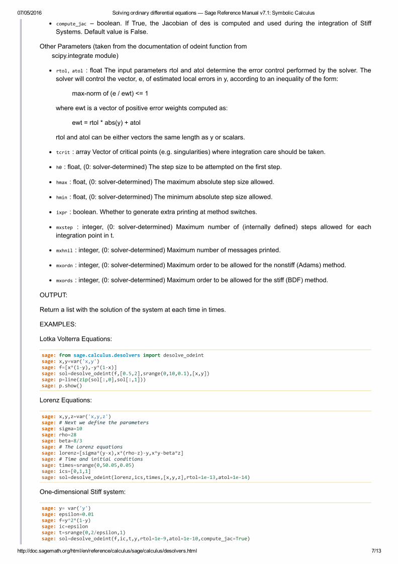
compute_jac – boolean. If True, the Jacobian of des is computed and used during the integration of StiffSystems. Default value is False.

Other Parameters (taken from the documentation of odeint function fromscipy.integrate module)

rtol, atol : float The input parameters rtol and atol determine the error control performed by the solver. Thesolver will control the vector, e, of estimated local errors in y, according to an inequality of the form:

maxnorm of (e / ewt) <= 1

where ewt is a vector of positive error weights computed as:

ewt = rtol * abs(y) + atol

rtol and atol can be either vectors the same length as y or scalars.

tcrit : array Vector of critical points (e.g. singularities) where integration care should be taken.

h0 : float, (0: solverdetermined) The step size to be attempted on the first step.

hmax : float, (0: solverdetermined) The maximum absolute step size allowed.

hmin : float, (0: solverdetermined) The minimum absolute step size allowed.

ixpr : boolean. Whether to generate extra printing at method switches.

mxstep : integer, (0: solverdetermined) Maximum number of (internally defined) steps allowed for eachintegration point in t.

mxhnil : integer, (0: solverdetermined) Maximum number of messages printed.

mxordn : integer, (0: solverdetermined) Maximum order to be allowed for the nonstiff (Adams) method.

mxords : integer, (0: solverdetermined) Maximum order to be allowed for the stiff (BDF) method.

OUTPUT:

Return a list with the solution of the system at each time in times.

EXAMPLES:

Lotka Volterra Equations:

sage: from sage.calculus.desolvers import desolve_odeint sage: x,y=var('x,y') sage: f=[x*(1‐y),‐y*(1‐x)] sage: sol=desolve_odeint(f,[0.5,2],srange(0,10,0.1),[x,y]) sage: p=line(zip(sol[:,0],sol[:,1])) sage: p.show()

Lorenz Equations:

sage: x,y,z=var('x,y,z') sage: # Next we define the parameters sage: sigma=10 sage: rho=28 sage: beta=8/3 sage: # The Lorenz equations sage: lorenz=[sigma*(y‐x),x*(rho‐z)‐y,x*y‐beta*z] sage: # Time and initial conditions sage: times=srange(0,50.05,0.05) sage: ics=[0,1,1] sage: sol=desolve_odeint(lorenz,ics,times,[x,y,z],rtol=1e‐13,atol=1e‐14)

Onedimensional Stiff system:

sage: y= var('y') sage: epsilon=0.01 sage: f=y^2*(1‐y) sage: ic=epsilon sage: t=srange(0,2/epsilon,1) sage: sol=desolve_odeint(f,ic,t,y,rtol=1e‐9,atol=1e‐10,compute_jac=True)



sage: p=points(zip(t,sol)) sage: p.show()

Another Stiff system with some optional parameters with no default value:

sage: y1,y2,y3=var('y1,y2,y3') sage: f1=77.27*(y2+y1*(1‐8.375*1e‐6*y1‐y2)) sage: f2=1/77.27*(y3‐(1+y1)*y2) sage: f3=0.16*(y1‐y3)sage: f=[f1,f2,f3] sage: ci=[0.2,0.4,0.7] sage: t=srange(0,10,0.01) sage: v=[y1,y2,y3] sage: sol=desolve_odeint(f,ci,t,v,rtol=1e‐3,atol=1e‐4,h0=0.1,hmax=1,hmin=1e‐4,mxstep=1000,mxords=17)

AUTHOR:

Oriol Castejon (052010)

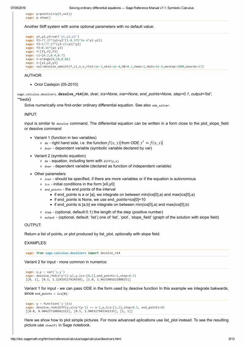
sage.calculus.desolvers.desolve_rk4(de, dvar, ics=None, ivar=None, end_points=None, step=0.1, output='list',**kwds)

Solve numerically one firstorder ordinary differential equation. See also ode_solver.

INPUT:

input is similar to desolve command. The differential equation can be written in a form close to the plot_slope_fieldor desolve command

Variant 1 (function in two variables)de right hand side, i.e. the function from ODE dvar dependent variable (symbolic variable declared by var)

Variant 2 (symbolic equation)de equation, including term with diff(y,x)dvar dependent variable (declared as function of independent variable)

Other parametersivar should be specified, if there are more variables or if the equation is autonomousics initial conditions in the form [x0,y0]end_points the end points of the interval

if end_points is a or [a], we integrate on between min(ics[0],a) and max(ics[0],a)if end_points is None, we use end_points=ics[0]+10if end_points is [a,b] we integrate on between min(ics[0],a) and max(ics[0],b)

step (optional, default:0.1) the length of the step (positive number)output (optional, default: ‘list’) one of ‘list’, ‘plot’, ‘slope_field’ (graph of the solution with slope field)

OUTPUT:

Return a list of points, or plot produced by list_plot, optionally with slope field.

EXAMPLES:

sage: from sage.calculus.desolvers import desolve_rk4

Variant 2 for input more common in numerics:

sage: x,y = var('x,y') sage: desolve_rk4(x*y*(2‐y),y,ics=[0,1],end_points=1,step=0.5) [[0, 1], [0.5, 1.12419127424558], [1.0, 1.461590162288825]]

Variant 1 for input we can pass ODE in the form used by desolve function In this example we integrate bakwards,since end_points < ics[0]:

sage: y = function('y')(x) sage: desolve_rk4(diff(y,x)+y*(y‐1) == x‐2,y,ics=[1,1],step=0.5, end_points=0) [[0.0, 8.904257108962112], [0.5, 1.909327945361535], [1, 1]]

Here we show how to plot simple pictures. For more advanced aplications use list_plot instead. To see the resultingpicture use show(P) in Sage notebook.

f (x, y) = f (x, y)y′



sage: x,y = var('x,y') sage: P=desolve_rk4(y*(2‐y),y,ics=[0,.1],ivar=x,output='slope_field',end_points=[‐4,6],thickness=3)

ALGORITHM:

4th order RungeKutta method. Wrapper for command rk in Maxima’s dynamics package. Perhaps could be fasterby using fast_float instead.

AUTHORS:

Robert Marik (102009)

sage.calculus.desolvers.desolve_rk4_determine_bounds(ics, end_points=None)Used to determine bounds for numerical integration.

If end_points is None, the interval for integration is from ics[0] to ics[0]+10If end_points is a or [a], the interval for integration is from min(ics[0],a) to max(ics[0],a)If end_points is [a,b], the interval for integration is from min(ics[0],a) to max(ics[0],b)

EXAMPLES:

sage: from sage.calculus.desolvers import desolve_rk4_determine_bounds sage: desolve_rk4_determine_bounds([0,2],1) (0, 1)

sage: desolve_rk4_determine_bounds([0,2]) (0, 10)

sage: desolve_rk4_determine_bounds([0,2],[‐2]) (‐2, 0)

sage: desolve_rk4_determine_bounds([0,2],[‐2,4]) (‐2, 4)

sage.calculus.desolvers.desolve_system(des, vars, ics=None, ivar=None)Solve any size system of 1st order ODE’s. Initial conditions are optional.

Onedimensional systems are passed to desolve_laplace().

INPUT:

des list of ODEsvars list of dependent variablesics (optional) list of initial values for ivar and vars. If ics is defined, it should provide initial conditions for eachvariable, otherwise an exception would be raised.ivar (optional) the independent variable, which must be specified if there is more than one independentvariable in the equation.

EXAMPLES:

sage: t = var('t') sage: x = function('x')(t) sage: y = function('y')(t) sage: de1 = diff(x,t) + y ‐ 1 == 0 sage: de2 = diff(y,t) ‐ x + 1 == 0 sage: desolve_system([de1, de2], [x,y]) [x(t) == (x(0) ‐ 1)*cos(t) ‐ (y(0) ‐ 1)*sin(t) + 1, y(t) == (y(0) ‐ 1)*cos(t) + (x(0) ‐ 1)*sin(t) + 1]

Now we give some initial conditions:

sage: sol = desolve_system([de1, de2], [x,y], ics=[0,1,2]); sol [x(t) == ‐sin(t) + 1, y(t) == cos(t) + 1]

sage: solnx, solny = sol[0].rhs(), sol[1].rhs() sage: plot([solnx,solny],(0,1)) # not tested sage: parametric_plot((solnx,solny),(0,1)) # not tested

TESTS:

Check that trac ticket #9823 is fixed:




sage: t = var('t') sage: x = function('x')(t) sage: de1 = diff(x,t) + 1 == 0 sage: desolve_system([de1], [x]) ‐t + x(0)


sage: t = var('t') sage: x = function('x')(t) sage: y = function('y')(t) sage: de1 = diff(x,t) + y ‐ 1 == 0 sage: de2 = diff(y,t) ‐ x + 1 == 0 sage: des = [de1,de2] sage: ics = [0,1,‐1] sage: vars = [x,y] sage: sol = desolve_system(des, vars, ics); sol [x(t) == 2*sin(t) + 1, y(t) == ‐2*cos(t) + 1]

sage: solx, soly = sol[0].rhs(), sol[1].rhs() sage: RR(solx(t=3)) 1.28224001611973

sage: P1 = plot([solx,soly], (0,1))sage: P2 = parametric_plot((solx,soly), (0,1))

Now type show(P1), show(P2) to view these plots.


sage: t = var('t') sage: epsilon = var('epsilon') sage: x1 = function('x1')(t) sage: x2 = function('x2')(t) sage: de1 = diff(x1,t) == epsilon sage: de2 = diff(x2,t) == ‐2sage: desolve_system([de1, de2], [x1, x2], ivar=t) [x1(t) == epsilon*t + x1(0), x2(t) == ‐2*t + x2(0)] sage: desolve_system([de1, de2], [x1, x2], ics=[1,1], ivar=t) Traceback (most recent call last):... ValueError: Initial conditions aren't complete: number of vars is different from number of dependent variables. Got ics = [1, 1], vars = [x1(t), x2(t)]

AUTHORS:

Robert Bradshaw (102008)Sergey Bykov (102014)

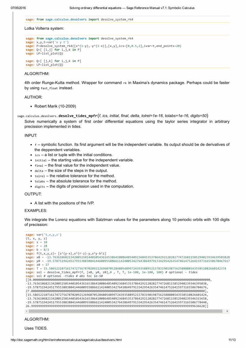
sage.calculus.desolvers.desolve_system_rk4(des, vars, ics=None, ivar=None, end_points=None, step=0.1)Solve numerically a system of firstorder ordinary differential equations using the 4th order RungeKutta method.Wrapper for Maxima command rk. See also ode_solver.

INPUT:

input is similar to desolve_system and desolve_rk4 commands

des right hand sides of the systemvars dependent variablesivar (optional) should be specified, if there are more variables or if the equation is autonomous and theindependent variable is missingics initial conditions in the form [x0,y01,y02,y03,....]end_points the end points of the interval

if end_points is a or [a], we integrate on between min(ics[0],a) and max(ics[0],a)if end_points is None, we use end_points=ics[0]+10if end_points is [a,b] we integrate on between min(ics[0],a) and max(ics[0],b)

step – (optional, default: 0.1) the length of the step

OUTPUT:

Return a list of points.

EXAMPLES:





sage: from sage.calculus.desolvers import desolve_system_rk4

Lotka Volterra system:

sage: from sage.calculus.desolvers import desolve_system_rk4 sage: x,y,t=var('x y t') sage: P=desolve_system_rk4([x*(1‐y),‐y*(1‐x)],[x,y],ics=[0,0.5,2],ivar=t,end_points=20) sage: Q=[ [i,j] for i,j,k in P] sage: LP=list_plot(Q)

sage: Q=[ [j,k] for i,j,k in P] sage: LP=list_plot(Q)

ALGORITHM:

4th order RungeKutta method. Wrapper for command rk in Maxima’s dynamics package. Perhaps could be fasterby using fast_float instead.

AUTHOR:

Robert Marik (102009)

sage.calculus.desolvers.desolve_tides_mpfr(f, ics, initial, final, delta, tolrel=1e16, tolabs=1e16, digits=50)Solve numerically a system of first order differential equations using the taylor series integrator in arbitraryprecission implemented in tides.

INPUT:

f – symbolic function. Its first argument will be the independent variable. Its output should be de derivatives ofthe deppendent variables.ics – a list or tuple with the initial conditions.initial – the starting value for the independent variable.final – the final value for the independent value.delta – the size of the steps in the output.tolrel – the relative tolerance for the method.tolabs – the absolute tolerance for the method.digits – the digits of precission used in the computation.

OUTPUT:

A list with the positions of the IVP.

EXAMPLES:

We integrate the Lorenz equations with Salztman values for the parameters along 10 periodic orbits with 100 digitsof precission:

sage: var('t,x,y,z') (t, x, y, z) sage: s = 10 sage: r = 28 sage: b = 8/3 sage: f(t,x,y,z)= [s*(y‐x),x*(r‐z)‐y,x*y‐b*z] sage: x0 = ‐13.7636106821342005250144010543616538641008648540923684535378642921202827747268115852940239346395038284sage: y0 = ‐19.5787519424517955388380414460095588661142400534276438649791334295426354746147526415973165506704676171sage: z0 = 27 sage: T = 15.586522107161747275678702092126960705284805489972439358895215783190198756258880854355851082660142374 sage: sol = desolve_tides_mpfr(f, [x0, y0, z0],0 , T, T, 1e‐100, 1e‐100, 100) # optional ‐ tides sage: sol # optional ‐tides # abs tol 1e‐50 [[0.000000000000000000000000000000000000000000000000000000000000000000000000000000000000000000000000000, ‐13.7636106821342005250144010543616538641008648540923684535378642921202827747268115852940239346395038, ‐19.5787519424517955388380414460095588661142400534276438649791334295426354746147526415973165506704676, 27.0000000000000000000000000000000000000000000000000000000000000000000000000000000000000000000000000], [15.5865221071617472756787020921269607052848054899724393588952157831901987562588808543558510826601424, ‐13.7636106821342005250144010543616538641008648540923684535378642921202827747268115852940239346315658, ‐19.5787519424517955388380414460095588661142400534276438649791334295426354746147526415973165506778440, 26.9999999999999999999999999999999999999999999999999999999999999999999999999999999999999999999636628]]

ALGORITHM:

Uses TIDES.



Warning: This requires the package tides.

REFERENCES:

sage.calculus.desolvers.eulers_method(f, x0, y0, h, x1, algorithm='table')This implements Euler’s method for finding numerically the solution of the 1st order ODE y' = f(x,y), y(a)=c. The “x”column of the table increments from x0 to x1 by h (so (x1‐x0)/h must be an integer). In the “y” column, the new yvalue equals the old yvalue plus the corresponding entry in the last column.

For pedagogical purposes only.

EXAMPLES:

sage: from sage.calculus.desolvers import eulers_method sage: x,y = PolynomialRing(QQ,2,"xy").gens() sage: eulers_method(5*x+y‐5,0,1,1/2,1) x y h*f(x,y) 0 1 ‐2 1/2 ‐1 ‐7/4 1 ‐11/4 ‐11/8

sage: x,y = PolynomialRing(QQ,2,"xy").gens() sage: eulers_method(5*x+y‐5,0,1,1/2,1,algorithm="none") [[0, 1], [1/2, ‐1], [1, ‐11/4], [3/2, ‐33/8]]

sage: RR = RealField(sci_not=0, prec=4, rnd='RNDU') sage: x,y = PolynomialRing(RR,2,"xy").gens() sage: eulers_method(5*x+y‐5,0,1,1/2,1,algorithm="None") [[0, 1], [1/2, ‐1.0], [1, ‐2.7], [3/2, ‐4.0]]

sage: RR = RealField(sci_not=0, prec=4, rnd='RNDU') sage: x,y=PolynomialRing(RR,2,"xy").gens() sage: eulers_method(5*x+y‐5,0,1,1/2,1) x y h*f(x,y) 0 1 ‐2.0 1/2 ‐1.0 ‐1.7 1 ‐2.7 ‐1.3

sage: x,y=PolynomialRing(QQ,2,"xy").gens() sage: eulers_method(5*x+y‐5,1,1,1/3,2) x y h*f(x,y) 1 1 1/3 4/3 4/3 1 5/3 7/3 17/9 2 38/9 83/27

sage: eulers_method(5*x+y‐5,0,1,1/2,1,algorithm="none") [[0, 1], [1/2, ‐1], [1, ‐11/4], [3/2, ‐33/8]]

sage: pts = eulers_method(5*x+y‐5,0,1,1/2,1,algorithm="none") sage: P1 = list_plot(pts) sage: P2 = line(pts) sage: (P1+P2).show()

AUTHORS:

David Joyner

sage.calculus.desolvers.eulers_method_2x2(f, g, t0, x0, y0, h, t1, algorithm='table')This implements Euler’s method for finding numerically the solution of the 1st order system of two ODEs

x' = f(t, x, y), x(t0)=x0.

y' = g(t, x, y), y(t0)=y0.

The “t” column of the table increments from to by (so must be an integer). In the “x” column,the new xvalue equals the old xvalue plus the corresponding entry in the next (third) column. In the “y” column, thenew yvalue equals the old yvalue plus the corresponding entry in the next (last) column.


EXAMPLES:

t0 t1 h f rac − ht1 t0



sage: from sage.calculus.desolvers import eulers_method_2x2 sage: t, x, y = PolynomialRing(QQ,3,"txy").gens() sage: f = x+y+t; g = x‐y sage: eulers_method_2x2(f,g, 0, 0, 0, 1/3, 1,algorithm="none") [[0, 0, 0], [1/3, 0, 0], [2/3, 1/9, 0], [1, 10/27, 1/27], [4/3, 68/81, 4/27]]

sage: eulers_method_2x2(f,g, 0, 0, 0, 1/3, 1) t x h*f(t,x,y) y h*g(t,x,y) 0 0 0 0 0 1/3 0 1/9 0 0 2/3 1/9 7/27 0 1/27 1 10/27 38/81 1/27 1/9

sage: RR = RealField(sci_not=0, prec=4, rnd='RNDU') sage: t,x,y=PolynomialRing(RR,3,"txy").gens() sage: f = x+y+t; g = x‐y sage: eulers_method_2x2(f,g, 0, 0, 0, 1/3, 1) t x h*f(t,x,y) y h*g(t,x,y) 0 0 0.00 0 0.00 1/3 0.00 0.13 0.00 0.00 2/3 0.13 0.29 0.00 0.043 1 0.41 0.57 0.043 0.15

To numerically approximate , where , , , using 4 steps of Euler’smethod, first convert to a system: , ; , .:

sage: RR = RealField(sci_not=0, prec=4, rnd='RNDU') sage: t, x, y=PolynomialRing(RR,3,"txy").gens() sage: f = y; g = (x‐y)/(1+t^2) sage: eulers_method_2x2(f,g, 0, 1, ‐1, 1/4, 1) t x h*f(t,x,y) y h*g(t,x,y) 0 1 ‐0.25 ‐1 0.50 1/4 0.75 ‐0.12 ‐0.50 0.29 1/2 0.63 ‐0.054 ‐0.21 0.19 3/4 0.63 ‐0.0078 ‐0.031 0.11 1 0.63 0.020 0.079 0.071

To numerically approximate y(1), where , , :

sage: t,x,y=PolynomialRing(RR,3,"txy").gens() sage: f = y; g = ‐x‐y*t sage: eulers_method_2x2(f,g, 0, 1, 0, 1/4, 1) t x h*f(t,x,y) y h*g(t,x,y) 0 1 0.00 0 ‐0.25 1/4 1.0 ‐0.062 ‐0.25 ‐0.23 1/2 0.94 ‐0.11 ‐0.46 ‐0.17 3/4 0.88 ‐0.15 ‐0.62 ‐0.10 1 0.75 ‐0.17 ‐0.68 ‐0.015

AUTHORS:

David Joyner

sage.calculus.desolvers.eulers_method_2x2_plot(f, g, t0, x0, y0, h, t1)Plot solution of ODE.

This plots the soln in the rectangle (xrange[0],xrange[1]) x (yrange[0],yrange[1]) and plots using Euler’s method thenumerical solution of the 1st order ODEs , , , .


EXAMPLES:

sage: from sage.calculus.desolvers import eulers_method_2x2_plot

The following example plots the solution to , , . Type P[0].show() to plot thesolution, (P[0]+P[1]).show() to plot and :

sage: f = lambda z : z[2]; g = lambda z : ‐sin(z[1]) sage: P = eulers_method_2x2_plot(f,g, 0.0, 0.75, 0.0, 0.1, 1.0)

y(1) (1 + ) + − y = 0t2 y″ y′ y(0) = 1 (0) = −1y′

=y′1 y2 (0) = 1y1 =y′

2

f rac − 1 +y1 y2 t2

(0) = −1y2

+ t + y = 0y″ y′ y(0) = 1 (0) = 0y′

= f (t, x, y)x ′ x(a) = x0 = g(t, x, y)y′ y(a) = y0

+ sin(θ) = 0θ″ θ(0) = 34 (0) = 0θ ′

(t, θ(t)) (t, (t))θ ′

Solving ordinary differential equations

Documents

Transcript of Solving ordinary differential equations