A comparison of numerical methods for solving diffusion-reaction equations in air quality models

mMS ID: CVS001

26 October 1999 8:06 CET

Comput Visual Sci 2: 1–13 (1999) Computing andVisualization in Science Springer-Verlag 1999

Regular article

A comparison of numerical methods for solving diffusion-reaction equationsin air quality models

G. Barone1,2, P. D’Ambra2, D. di Serafino2,3, G. Giunta2,4,∗, A. Riccio1

1 Department of Chemistry, University of Naples “Federico II”, Via Mezzocannone 4, I-80134 Naples, Italy2 Center for Research on Parallel Computing and Supercomputers (CPS) - CNR, Complesso Monte S. Angelo, Via Cintia, I-80126 Naples, Italy3 Department of Mathematics, the Second University of Naples, Piazza Duomo, I-81100 Caserta, Italy4 Institute of Mathematics, Faculty of Environmental Science, Naval University, Via de Gasperi 5, I-80133, Naples, Italy

Received: 28 January 1998 / Accepted: 26 April 1999

Communicated by: G. Wittum

Abstract. In this paper we analyze the efficiency of some stiffODE solvers, applied to the coupled solution of vertical tur-bulent diffusion and chemical kinetics in Air Quality Models.We consider four general-purpose solvers, based onBDF orRosenbrock methods, and two special-purpose solvers, de-veloped for ODEs from atmospheric chemistry, and com-pare their performance on three test problems using differ-ent chemical models. The general-purpose solvers have beenmodified to take advantage of the sparsity of the Jacobianmatrices arising in the application of implicit methods. Theobtained results show that general-purpose solvers, providedwith suitable sparse matrix techniques, perform generally bet-ter than special-purpose ones. Our analysis extends to thediffusion-reaction equations the recent work of other researchgroups, comparingODE solvers on atmospheric chemical ki-netics equations.

1 Introduction

One of the main computational kernels arising in the numer-ical solution of Air Quality Models (AQMs) is the followingsystem of diffusion-reaction equations:

∂c

∂t= ∂

∂z

(K(t, z)

∂c

∂z

)+ R(t, c), (1)

t ≥ t0, 0≤ z≤ H,

where c(t, z) = (c(1)(t, z), . . . , c(N)(t, z))Tis the vector of

the concentrations ofN chemical species,K(t, z) is a giventurbulent diffusivity tensor,R(t, c) is the transformation ratedue to chemical reactions, and the space domain[0, H] rep-resents an air column of heightH . The above system isusually provided with the following initial and boundary

∗ Correspondence to: [email protected]

conditions:

c(t0, z)= c0(z), 0≤ z≤ H,

−K(t,0)∂c

∂z(t,0)= E(t)−vd(t)c(t,0), t ≥ t0

∂c

∂z(t, H)= 0, t ≥ t0 ,

whereE(t) is the emission term andvd is the deposition vel-ocity of the chemical species.

In a typical AQM, system (1) arises from the 3D atmo-spheric transport-chemistry system of equations, by apply-ing a time-splitting technique that decouples advection andhorizontal diffusion from vertical diffusion and chemistry.Generally, it is not advisable to split chemistry and verticaldiffusion in (1), since the reaction rate of some species canhave the same magnitude as the transport rate of the verti-cal turbulent diffusion. In such a case, the error introducedin treating vertical diffusion and chemistry decoupled can begreater than 1%, which is widely accepted as a reference levelin AQMs. In [16] it is shown that splitting vertical diffusionfrom chemistry in (1) gives good results if all the reactionrates are greater than the transport rates. Otherwise, smalltime-splitting intervals have to be chosen, leading to manyrestarts of the solvers and hence increasing the solution time.Numerical experiments, reported in Sect. 6 have confirmedthis behaviour. Taking into account the above considerations,advancedAQMs implement the coupled solution of the diffu-sion and chemistry operators [5, 15, 19].

The integration of system (1) is often the most compu-tational demanding part in air quality simulations, thus re-quiring effective numerical methods and software. Chemicalreactions introduce a high degree of stiffness in the system,since the life times of the chemical species span over a widerange, that can exceed 10 orders of magnitude. Therefore,the effective numerical solution of large air pollution modelsis a very time-consuming problem, requiring the exploitationof the powerful computational resources of parallel comput-ers [4, 5, 7]. In this case the 3D simulation domain is usuallysubdivided into vertical columns of grid cells and system (1)must be solved, concurrently, in all the vertical columns. This

mMS ID: CVS001


2 G. Barone et al.

emphasizes the need of effective sequential algorithms andsoftware also in a parallel computing environment.

In this paper we analyze the performance (accuracy ver-sus execution time) of four general-purpose stiffODE solvers,based on implicit methods, applied to the non-linearODEsystem arising from a semidiscretization of (1). We considerVODE [2] and VODPK [3], implementing variable-coefficientBackward Differentiation Formulas (BDF), and ROS3 [24]andROS2 [31], based on Rosenbrock methods. We also com-pare the above solvers with two special-purpose solvers de-veloped for atmospheric chemistry problems,TWOSTEP[26]andCHEMEQ [25, 33], that exploit the particular form of thereaction term to treat the chemistry explicitly. Our analysis iscarried out using three chemical models fromAQM, namelyEUSMOG [17], LCC [15] andAL [18]. These models involvea different number of chemical species and reactions and havebeen chosen because we are also interested in analyzing theperformance of the previous solvers with respect to the sizeof the chemistry model. This work follows an approach pro-posed in [27] and extends to the diffusion-reaction equationsthe comparison work presented in [23, 24] for the chemicalreaction equations.

In Sect. 2 we describe the semidiscretization applied tosystem (1) and give some details of the underlying physicaland chemical parameterizations. In Sect. 3 we introduce theproblem of sparsity exploitation in the linear systems arisingfrom implicit solvers. The stiffODE solvers considered in thiswork are described in Sect. 4. The numerical experiments andthe testing methodology are presented in Sect. 5 and the re-sults are analyzed in Sect. 6. Some conclusions are reportedin Sect. 7.

2 The semidiscrete model

In air quality simulations system (1) is usually discretizedin space using a non-uniform grid, so that the region closeto the terrain can be resolved accurately. To this aim, az-coordinate transformation with a one-dimensional stretchingfunction can be applied and system (1) becomes:

∂χ

∂t= 1

g′∂

∂ζ

(κ

g′∂χ

∂ζ

)+ R(t, χ), (2)

t> t0, 0≤ ζ ≤ 1,

whereχ(t, ζ)= c(t, z), κ(t, ζ)= K(t, z) andz= g(ζ), with gsatisfyingg(0)= 0 andg(1)= H . We have used the follow-ing stretching function [10]:

g(ζ)= H

(Qζ + (1−Q)

1− tanh(R(1− ζ))tanh(R)

),

whereQ and R are two parameters that regulate the stretch-ing of the grid, set to 0.01 and 2.0 respectively. In our case, theheightH of the vertical domain has been set to 2000 meters.

System (2) has been discretized using a vertical grid with10 layers, i.e. withM = 11 points. Letζk = (k−1)h, whereh = 1/(M−1) and 1≤ k≤ M; the diffusion term has beenapproximated by the following second-order scheme:

Dk = 1

h2g′k

(κ+k (χ(t, ζk+1)−χ(t, ζk)) (3)

−κ−k (χ(t, ζk)−χ(t, ζk−1)))

where

κ±k =κ (t, (ζk+ ζk±1)/2)g′ ((ζk+ ζk±1)/2)

.

The boundary conditions have been discretized using a first-order approximation; however, this does not affect signifi-cantly the accuracy, since the turbulent diffusion coefficient isvery small at the boundaries.

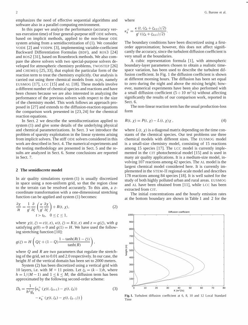
A cubic representation formula [1], with atmosphericboundary-layer parameters chosen to obtain a realistic time-space variation, has been used to describe the turbulent dif-fusion coefficient. In Fig. 1 the diffusion coefficient is shownat different morning hours. The diffusion has been set equalto zero during the night and above the mixing height; how-ever, numerical experiments have been also performed witha small diffusion coefficient (5÷10 m2/s) without affectingsignificantly the results of our comparison work, reported inSect. 6.

The non-linear reaction term has the usual production-lossform

R(t, χ)= P(t, χ)− L(t, χ)χ , (4)

whereL(t, χ) is a diagonal matrix depending on the time con-stants of the chemical species. Our test problems use threechemical models with different sizes. TheEUSMOG modelis a small-size chemistry model, consisting of 15 reactionsamong 15 species [17]. TheLCC model is currently imple-mented in theCIT photochemical model [15] and is used inmany air quality applications. It is a medium-size model, in-volving 107 reactions among 42 species. TheAL model is thelargest chemical model considered here. It is currently im-plemented in theSTEM-II regional-scale model and describes178 reactions among 84 species [18]. It is well suited for thestudy of both highly polluted urban and rural areas.EUSMOGand AL have been obtained from [11], whileLCC has beenextracted fromCIT.

The initial concentrations and the hourly emission ratesat the bottom boundary are shown in Table 1 and 2 for the

0 10 20 30 40 50 60 70 800

100

200

300

400

500

600

700

800

900

1000

K (m^2/s)

heig

ht (

m)

Diffusion coefficient

Fig. 1. Turbulent diffusion coefficient at 6, 8, 10 and 12 Local StandardTime

mMS ID: CVS001


A comparison of numerical methods for solving diffusion-reaction equations in air quality models 3

three models. They are typical of a polluted urban atmo-sphere. The initial concentrations at the remaining grid pointshave been calculated by linear interpolation from the ground-level concentrations and the null concentration at the max-imum mixing height (≈ 1000 meters). Emissions have beenincorporated into the ground-level boundary condition1. Fur-thermore, the deposition has been not taken into account inour simulations, i.e. the deposition velocity has been set equalto zero, since we are not considering the whole air pollutionmodel, but only the vertical diffusion and chemistry module.

Identical atmospheric conditions have been set at eachgrid point, except the variable turbulent diffusion coefficient,i.e. the same chemical reactions, photolysis rates, tempera-ture, etc., have been considered at each grid point. Physicalparameters are also reported in Tables 1 and 2.

The above semi-discretization of system (1) leads to thefollowing non-linear stiffODE system ofMN equations:

d

dtck(t)= Fk(t, c) (5)

= Dk(t, ζ, c)+ P(t, ck)− L(t, ck)ck,

t> t0, 1≤ k≤ M

wherec(t) is the complete concentration grid function2, ck(t)is the concentration vector at grid pointk, and Dk is thediscretized diffusion operator defined in (3). Note that the re-action term couples the different chemical species at each gridpoint, while the diffusion term introduces no coupling amongdifferent species, but couples values of the same concentra-tion at different grid points.

3 Linear algebra issues in implicit solvers

The general-purpose solvers considered in this work arebased onBDF [13] or Rosenbrock methods [14]. We now fo-cus our attention on the solution of the linear systems arising

1 They could have been equivalently included in the differential equationas a source term in the ground-level cells.

2 For simplicity of notations, the concentrations are denoted again byc.

Table 1. Initial concentrations, hourly emission values and physical param-eters for theEUSMOGmodel

SpeciesInitial Concentration(ppb)

Emission(ppb/hour)

CO 200 2.5NO 20 0.125NO2 10 –O3 30 –NO3 25 –C2H6 25 0.04C4H10 25 0.1C2H4 2 0.03C3H6 2 0.01XYL 2 0.03CH4 4000 –ISO 2 0.01

Latitude 41 (north)Longitude 14 (east)Temperature 298 KDate 15 AugustRelative humidity 60%

Table 2. Initial concentrations, hourly emission values and physical pa-rameters for theLCC and AL models. The concentrations of fixed speciesare [O2] = 2.1×108 ppb, [CO2] = 5.0×107 ppb, [H2] = 500 ppb, and[CH4] = 2.2 ppb for LCC only

SpeciesInitial Concentration(ppb)

Emission(ppb/hour)

CO 200 2NO 20 1NO2 10 0.2O3 30 –ETHE 4 0.2ALKE 8 1ALKA 50 2TOLU(LCC only) 10 0.2AROM 10 0.2HCHO 7 0.2ALD2 7 0.2ISOP 10 1

Latitude 41 (north)Longitude 14 (east)Temperature 298 KDate 15 AugustRelative humidity 80%

from the application of these methods. A short description ofeach solver is given in Sect. 4.

The genericp-th orderBDF formula applied to system (5)can be written as:

cn =p∑

i=1

αi cn−i + τγF(tn, c

n) , (6)

wheren is the current time level,τ is the time step size and theindexk in (5) has been dropped for convenience. Therefore,the solution of a system of non-linear equations is requiredat each step, due to the non-linearity of the chemical reactionterm, which is usually a quadratic polynomial. This systemcan be solved using a modified Newton iteration, leading tothe solution of linear systems of the form:(I − τγJ

)∆cn(m+1)= G(tn, c

n(m)) (7)

whereJ is the Jacobian matrix of the functionF evaluated ata suitable point(ti , ci ),∆cn(m+1)= cn(m+1)−cn(m), andG(tn, cn(m))= τγF(tn, cn(m))−cn(m)+an, with an involv-ing past valuescn−k.

One of the general-purpose solvers used in this work isthe well-known packageVODE [2], whereBDF methods areimplemented within a predictor-corrector scheme. An explicitpredictor is used to get an initial approximation to an implicitcorrector, that requires the solution of a non-linear system;solving this system by modified Newton iterations leads tolinear systems of the form (7) (for more details see [6]).

Rosenbrock methods are linearly implicit methods, thatcan be derived with a linearization of diagonally implicitRunge-Kutta methods [14]. Ans-stage Rosenbrock methodfor the non-autonomous system (5) takes the form:

cn = cn−1+s∑

i=1

bi l i ,

mMS ID: CVS001


4 G. Barone et al.

l i = τF(tn−1+αi τ, c

n−1+i−1∑j=1

αij l j

)(8)

+γiτ2∂F(tn−1, cn−1)

∂t+ τJ(tn−1, c

n−1)

i∑j=1

γij l j ,

where the computation of eachl i requires the solution ofa linear system with coefficient matrixI − τγii J, that is a lin-ear system of the same form as (7). We consider Rosenbrockmethods withγii = γ , hence all the systems have the same co-efficient matrix I − τγJ. These methods are implemented inthe solversROS3 [24] andROS2 [31], used in our work.

If the components of the unknown grid functionc areordered first respect to the chemical species and then re-spect to the grid points, theNM×NM matrix J can be ex-pressed as

J = JR+ JD , (9)

whereJR depends only on the discrete chemical operator andJD only on the discrete diffusion operator. More precisely,

JR= diag(J1, . . . , JM) ,

where Jk is the N×N Jacobian matrix of the chemical ki-netics term at thek-th grid point, which is usually sparseunstructured, with sparsity ranging from 10% to 20%, and

JD = D⊗ IN ,

whereD is the M×M matrix corresponding to the discretediffusion operatorDk, IN is the identity matrix of orderNand⊗ is the tensor product. In other words,JD is a bandedmatrix with half-bandwidthM, but only three non-zero di-agonals.I − τγJ is therefore a block-tridiagonal matrix, withsparse unstructured blocks on the main diagonal and lowerand upper blocks that are diagonal matrices.

An efficient solution of the above linear systems is a keypoint in the solution of theODE system (5). Direct methodsprovided with sparse matrix techniques have been efficientlyused whenJ ≡ JR, that is when diffusion and chemistry op-erators are splitted [23, 24]. TheKinetic Pre-Processor(KPP)software tool has been developed to reduce the cost of solvinglinear systems [8].KPP reorders the unknowns to minimizethe fill-in arising from the LU factorization, builds data struc-tures to perform the factorization and producesad hocloop-free codes for the forward and backward substitution routines.Using this tool, the efficiency of implicitODE integrators onvarious chemical models has been increased by a factor of 2.5to 4 [22].

The straightforward application of the above techniquesto the matrix J = JR+ JD turns out to be inefficient, be-cause of the fill-in due to upper and lower blocks withnon-zero entries only on their main diagonals. An alterna-tive approach is to use iterative solvers. In [27] a MultigridV-cycle with a damped block-Jacobi smoother was appliedto linear systems arising from a second-order two-stepBDFmethod. A single V-cycle with one pre-relaxation and onepost-relaxation was executed, that is iterations were not per-formed until a convergence criterion was satisfied and theerror detection was left to the modified Newton iteration andstep size control strategies. We have used a similar approach

with the general-purpose solversVODE, ROS3 andROS2, i.e.a block-Jacobi scheme has been applied to the linear systemsarising fromBDF or Rosenbrock methods and sparse directsolvers obtained withKPPhave been used in dealing at blocklevel. Let

JD = diag(JD)+off(JD) , (10)

denote the splitting ofJD into two matrices, containing themain and the upper/lower block-diagonals respectively. Thefollowing block-Jacobi scheme has been considered:(

I − τγ(JR+diag(JD)))

x(m+1)= b+ τγoff(JD)x(m) ,

(11)

wherex andb denote the solution and the right-hand-side ofsystem (7) or (8).

The matrixA= I −τγ(JR+diag(JD)) is a block-diagonalmatrix, where the entries of each block come from the entriesof the Jacobian matrix of the reaction operator at the samegrid point and from the entries of the main diagonal of the dif-fusion operator. Therefore, the linear systems involving eachblock of A can be solved with direct methods using the samesparse matrix techniques as for the caseJ ≡ JR, that is apply-ing KPP. As an example, the dimension of a generic diagonalblock of A and the maximum number of non-zero entries, be-fore and after the LU factorization usingKPP, are reported inTable 3, for the three chemical models. Note thatKPPdoes notsupport pivoting. However, according to [23, 29], we have notobserved any significant loss of accuracy arising from suchan approach. Details about the number of iterations and thebehaviour of the ODE solvers are given in Secs. 4 and 6.

We observe that in the above block-Jacobi iterationsJR istreated implicitly, together with the main diagonal of the diag-onally dominant matrixJD, as usually required in the solutionof stiff systems. Moreover, when the turbulent diffusion coef-ficient is equal to zero,J ≡ JR and the block-Jacobi methodreduces to the direct solution of a block-diagonal system.

We have also used a different iterative method for thesolution of system (6). We solved theODE system (5) withthe packageVODPK [3], a modification ofVODE which im-plements a preconditioned Krylov-projection method to dealwith the linear sytems arising from Newton iterations. In thiscase, theKPP tool is applied to the preconditioning matricesto obtainad hocroutines for the corresponding LU factoriza-tions and back/forward substitutions.

4 The ODE solvers

We briefly describe the four general-purpose solversVODE,VODPK, ROS3, andROS2 and the two special-purpose solvers

Table 3. Dimension and maximum number of non-zero entries in a block ofA before and after the LU factorization withKPP

Chemical model EUSMOG LCC AL

Dimension 15 42 84Non-zeros before LU 57 364 674Non-zeros after LU 57 418 768

mMS ID: CVS001



TWOSTEPand CHEMEQ, well known in theAQM literature.The general-purpose solvers have been modified to take ad-vantage of the sparsity of the Jacobian matrices, as explainedin Sect. 3. These matrices are computed using their analyt-ical expressions, via user-supplied routines. All the solvers,exceptROS2, have variable step sizes, automatically selectedusing local error estimates and two tolerance parameters,atolandrtol , for the absolute and the relative error respectively. Atthe end of each splitting interval,clipping is applied, i.e. nega-tive concentration values are set equal to zero, to guaranteethe positivity of the chemical species.

4.1 VODE

VODE is a well-knownODE solver for stiff and non-stiff prob-lems. For stiff problems it implements variable-coefficientBDF methods of orders one through five, that are stiffly sta-ble, with an automatic technique for the selection of order andstep size; details are given in [2] and in the references therein.

To solve the linear systems arising from modified New-ton iterations,VODE performs an LU factorization followedby back and forward substitutions, using routines fromLIN -PACK [9]. These routines have been substituted with routinesperforming block-Jacobi iterations, incorporating the sparsematrix routines provided byKPP to treat the diagonal blocksof the matrixI − τγJ.

ITERS CPU SDA1 SDAmin STEPS JACS NEWTS NFAILS TFAILS

VODE on EUSMOG1 4.51 2.54 1.81 2084 102 2839 18 662 4.62 2.53 1.69 1951 63 2445 0 683 4.93 2.36 1.33 1948 63 2433 0 674 5.23 2.83 1.93 1932 62 2391 0 64

VODE on LCC

1 8.63 2.93 1.71 1754 137 2632 14 742 9.94 2.80 1.57 1768 113 2459 2 773 11.22 2.77 1.50 1706 109 2358 2 714 12.98 2.64 1.30 1714 85 2387 2 72

VODE on AL

1 16.66 2.67 1.55 2133 121 3017 13 472 19.25 2.74 1.35 2004 92 2639 1 453 22.80 2.69 1.26 1998 91 2637 1 424 27.10 2.73 1.33 2012 91 2674 1 49

Table 4.Statistics about the application ofVODEwith different numbers of block-Jacobi itera-tions. ITERS is the number of iterations for eachlinear system; CPU is the execution time (secs.);SDA1 and SDAmin are the mean and mini-mum number of correct digits; STEPS, JACS,NEWTS, NFAILS and TFAILS are the num-ber of time steps, Jacobian updates, Newtoniterations, Newton step failures and time stepfailures, respectively.

Splitting Solver CPU SDA1 SDAmin STEPS JACS NEWTS NFAILS TFAILS

VODE on EUSMOG

60 min. modif. 4.51 2.54 1.81 2084 102 2839 18 6660 min. standard 8.14 2.78 1.95 1914 62 2382 0 6515 min. modif. 6.04 2.16 1.45 2757 204 3431 1 8015 min. standard 15.53 2.27 1.43 2726 203 3387 1 74

VODE on LCC


VODE on AL


Table 5. Comparison between standard andmodified VODE. For the legend see the captionof Table 4

By numerical experiments, we found more efficient per-forming a small fixed number of block-Jacobi iterations perNewton step rather than repeating block-Jacobi iterations un-til a convergence criterion is satisfied. As shown in Sect. 6.1,one iteration per Newton step, that is a “direct sequence” ofblock-Jacobi steps to solve the non-linear equations, resultedto be the most efficient choice for our problems. This cor-responds to solve the linear system (7) with a direct method,neglecting the off-diagonal blocks ofI − τγJ. The error con-trol has been left to the modified Newton iteration and stepsize control strategies. Numerical experiments reported inSect. 6.1 (see Table 5) show that this choice does not increasesignificantly the number of time steps and Jacobian updates.Further experiments with a greater diffusion coefficient, i.e.k×10, have led to the choice of two block-Jacobi iterationsper Newton step.

4.2 VODPK

VODPK is a modification ofVODE, that uses an iterativeKrylov-projection method to solve the linear systems arisingfrom modified Newton iterations. It implements a scaled pre-conditioned incomplete version of theGMRES (GeneralizedMinimum RESidual) method, with left and right precondition-ers supplied by the user [3].

mMS ID: CVS001


6 G. Barone et al.

We applied two different preconditioning strategies, oneusing the following left and right preconditioners:

Pl = I − τγJR , (12)Pr = I − τγJD ,

and the other using only the left preconditioner

Pl = I − τγ(JR+diag(JD)). (13)

VODPK has been modified by introducing routines generatedby KPP for the LU factorization of the sparse unstructuredmatrix Pl and the corresponding back and forward substitu-tions.

4.3 ROS3

TheROS3 solver is based on an embedded pair of Rosenbrockmethods, of orders three and two. It involves three stages,requiring the solution of three linear systems with the samecoefficient matrixI −τγJ. The third-order method isL-stableand the second-order one isA-stable. They are combinedto obtain a local error estimate in the step selection stategy.ROS3 has been proposed in [24] to solve atmospheric chem-istry problems.

The one-step nature of Rosenbrock methods can be an ad-vantage with respect toBDF multistep methods, when they areused in a time-splitting context. Due to fictitious transients,BDF methods select very small step sizes at the beginning ofeach splitting interval, leading to a large linear algebra over-head. Indeed, in [24] it has been shown thatROS3 is ableto select very large time step and performs better than manyother solvers, including solvers based onBDF methods, whentheODE system modeling only the chemical kinetics (J≡ JR)is considered.

The solution of the linear systems inROS3 has been car-ried out by using the block-Jacobi method and theKPP sparsematrix techniques, as described in Sect. 3. Two different con-vergence criteria have been tested with the block-Jacobi itera-tions. One is the same criterion used inVODE for the modifiedNewton iterations, that is:

‖(x(m)− x(m−1))w‖RMS≤ αβ

(14)

where x( j) is the approximate solution of system (11) atthe j -th iteration, w = (wik) with wik = 1/(rtol |cn−1

ik | +atol), (i = 1, . . . , N, k= 1, . . . ,M), rtol and atol are theabsolute and relative error tolerances mentioned at the be-ginning of Sect. 4,‖ · ‖RMS is the root mean square norm,αis a constant experimentally chosen andβ is an estimate ofthe convergence rate constant of the block-Jacobi iterationprocess. The other choice of the convergence criterion is:

‖r(m)‖2‖b‖2 ≤ εatol+ rtol‖cn−1‖2

‖cn−1‖2 (15)

wherer(m) is the residual vector at them-th iteration, andεhas been setequal to 0.1.

4.4 ROS2

The ROS2 solver, proposed in [31], is based on aL-stablesecond-order two-stage Rosenbrock method.ROS2 usesa constant step size, allowed by the stability properties ofthe Rosenbrock method. As pointed out in [31], this choicecan be efficient when a 3D atmospheric transport-chemistryproblem is solved in a parallel environment andODE compu-tations are performed concurrently in different air columns,since it avoids the load imbalance due to different step sizesin different columns.

The block-Jacobi iteration strategy and the convergencecriteria used inROS2 are the same as inROS3.

4.5 TWOSTEP

The TWOSTEP solver, proposed in [26], exploits the pro-duction-loss form of the chemical reaction term in system (5).It is based on a second-orderBDF method, that, when appliedto system (5), takes the following form [27]:

cnk = Cn−1

k + τγDk+ τγPnk − τγLn

kcnk , (16)

1≤ k≤ M ,

whereCn−1k is a term depending oncn−1

k and cn−2k , Dk is

the discretized diffusion operator defined in (3), andPnk =

P(tn, cnk) and Ln

k = L(tn, cnk) are the production and loss

terms. As a starting method, the first-order backward Eulermethod is used. System (16) can be rewritten as

cn = (I − τγD+ τγLn)−1(Cn−1+ τγPn) , (17)

whereD is the matrix corresponding to the discrete diffusionoperator defined in (5),Pn = diag

(Pn

1 , . . . , PnM

)and Ln =

diag(Ln

1, . . . , LnM

). System (17) is solved with a Gauss-

Seidel type method, as explained in [27]. A fixed numberof iterations per time step can be considered satisfactory, asshown in [27, 28]); for our problems two iterations per timestep have been chosen experimentally. The same step sizecontrol strategy as in [30] has been used.

4.6 CHEMEQ

The CHEMEQ solver is based on a modified version of thehybrid algorithmby Young and Boris [33], described, for ex-ample, in [21]. It is currently used in the well-knownCIT [15]and CALGRID [32] mesoscaleAQMs. This solver separatesthe chemical species into slow, medium and fast species, ac-cording to the relative sizes of their life times with respectto the step size. Slow and medium species are treated withexplicit predictor-corrector schemes, while fast species aretreated using a steady-state assumption. The backward Eu-ler and the trapezoidal method are used for the slow species,while special-purpose methods, exploiting the production-loss form of Eq. (4), are used as predictor and corrector for themedium species. We use the implementation ofCHEMEQpro-vided in theCIT, modifying the step size selection as follows:

τnew= τold max(

2,min(0.1,0.9/√

err)),

whereerr is an estimate of the relative error in the computedchemical concentrations,as described in [25].

mMS ID: CVS001



5 Numerical experiments and testing methodology

All the numerical experiments have been performed as ina time splitting procedure, where advection and horizontaldiffusion are decoupled from vertical diffusion and chem-istry. Therefore, the total simulation time has been dividedinto L intervals and the solvers have been re-initializedat the beginning of each interval. We have chosen twotime splitting intervals, of 15 and 60 minutes, typical ofurban and regionalAQMs, respectively, The diffusion co-efficient has been updated every 60 minutes. The integra-tion has been performed for a total simulation time of twodays.

The error control has been based on two parameters,rtolandatol, for the relative and the absolute error, respectively.In all the simulationsatol has been set to 10−10 ppb, corres-ponding to about 2 molecules/cm3, to avoid that meaninglessconcentrations could influence the error control estimationand the step size selection strategy;rtol has been varied toobtain solutions with different relative accuracies.

A minimum and a maximum step size have also been con-sidered. Since the kinetic models involve reactions with lifetimes of 10−8÷10−9 seconds, the automatic step selectionprocedures usually lead to very small step sizes. However,these step sizes are not effectively required, because mean-ingful life times in chemistry models are of the order ofseconds, and species with smaller life times almost instanta-neously get their steady states. Therefore, a suitable choiceof a minimum step size improves the efficiency of theODEsolvers. In our experiments, a minimum step size variable be-tween 10−3 and 10−8 sec. has been chosen, depending onthe solver used. On the other hand, too large step sizes canreduce the accuracy of the computed solutions; therefore,a maximum step size of 5 minutes has been chosen experi-mentally.

ROS2 has been run with three constant step sizes, 1,5 and 10 minutes. The last one is greater than the max-imum step size allowed for the otherODE solvers, but ithas been considered to see the performance ofROS2 witha constant step size much larger than those generally usedin atmospheric chemistry integrations. The error tolerancesatol and rtol are used here only in the block-Jacobi con-vergence criteria; andrtol has been set to 10−3 for con-vergence criterion (14) and to 10−2 for convergence crite-rion (15), as explained in Sec. Refs:results:jac. Note that theimplementation ofROS2 is the same for both the splitting in-tervals.

The tests have been carried out on a IBM RISC/6000workstation, model 550. The solvers, written in Fortran 77using double precision, have been compiled with the F77compiler.

The performance of theODE solvers has been evaluatedin terms of accuracy versus execution time. The executiontime has been obtained using themclockfunction providedby the Fortran compiler. To evaluate the accuracy, the com-puted solutions have been compared with the reference so-lution obtained with the solverLSODE [20], widely used inAQMs to compute reference solutions of chemical kineticsproblems, called with strict error tolerances (rtol = 10−12 andatol= 10−11 ppb).

The accuracy has been measured as follows. Letclik indi-

cate the computed solution of thei -th chemical species at the

k-th grid point and at the end of thel -th splitting interval, andcl

ik the corresponding reference solution. We have first com-puted the following root mean square measure of the relativeerror:

ERi =√√√√ 1

LM·

L∑l=1

M∑k=1

∣∣∣∣clik− cl

ik

clik

∣∣∣∣2 (18)

(actually, only valuesclik greater than 10−10 ppb have been

considered in (18), to avoid that meaningless concentrationscould influence the error estimate); then we have used twomeasures of accuracy, that is the mean number of correct sig-nificant digits in the computed solution:

SDA1=− log10

(1

N

N∑i=1

ERi

),

and the minimum number of correct significant digits:

SDAmin =− log10

(max

1≤i≤NERi

).

Note thatSDA1 andSDAmin have been set to zero if they hadnegative values.

6 Results

Before comparing the performance of the sixODE solvers, weanalyze the effectiveness of the block-Jacobi method withinVODE, ROS3 andROS2. Finally, we give some results whichsupport the choice of a coupled solution of diffusion andchemistry for our test problems.

6.1 Effectiveness of the block-Jacobi iterations

As noted in Sect. 4.1, a key issue for an efficient implemen-tation of VODE is the choice of the number of block-Jacobiiterations. A large number of iterations to solve system (7)could turn out to be inefficient, because of the computa-tional cost of back/forward substitutions concerning diag-onal blocks, althoughKPP is applied to exploit sparsity. Onthe other hand, a small number of iterations could result ina higher number of failures in the modified Newton pro-cedure or of step size rejections. However, we have foundthat one iteration generally suffices for our problems. Statis-tics about the application ofVODE with 1 to 4 block-Jacobiiterations are shown in Table 4. These results have been ob-tained withrtol = 10−3, atol= 10−10 ppb and a time splittinginterval of 60 minutes; however similar results hold for dif-ferent error tolerances and splitting intervals. As the numberof iterations increases, the number of time steps, Jacobianupdates, Newton iterations, Newton step failures and timestep failures generally decreases, the only exception beingthe case of 4 iterations onLCC and AL . However, the ex-ecution time always increases, while the mean number ofcorrect digits is kept approximately the same. The reasonfor this behaviour can be explained by the following con-siderations. The value ofcn(0) provided by the predictorscheme implemented inVODE is fairly accurate; therefore

mMS ID: CVS001


8 G. Barone et al.

one iteration in the correctionx(m)= ∆cn(m) usually suf-fices, as noted in [12]. The diffusion coefficients are zeroduring the night and at the grid points above the mixingheight, therefore in these cases one block-Jacobi iteration cor-responds to a direct factorization method. Moreover,VODE isable to select very large time step (limited only by the max-imum step size), though the high degree of stiffness of theproblem.

We have also compared our implementation ofVODE withthe original version. Table 5 shows the results obtained withatol= 10−10 ppb,rtol = 10−3 and both sizes of splitting inter-vals (15 and 60 minutes). The numerical behaviour ofVODEdoes not seem to be greatly influenced by the block-Jacobi it-eration strategy; the number of extra time steps and Jacobianupdates is relatively small, keeping about the same accuracy.On the other hand, the execution time is considerably lower;in particular, the time saving is about 80% for theAL model,the largest chemistry model used in this work.

These results confirm that the use ofad hocroutines forthe forward and backward substitutions, implementing loop-free codes without pivoting and exploiting the sparsity of theJacobian matrix, seems to be effective for the numerical solu-tion of diffusion-chemistry models in air quality modeling, asalready stated in [22].

We now turn to the application of block-Jacobi itera-tions in theROS3 andROS2 solvers. In this case, system (8)has to be solved with the level of accuracy prescribed bycriterion (14) or criterion (15). Statistics about the applica-tion of ROS3 with both convergence criteria are shown inTable 6. The reported data have been obtained using a split-ting interval of 60 minutes,atol= 10−10 pbb, rtol = 10−3

with criterion (14) andrtol = 10−2 with criterion (15). Dif-ferent values ofrtol have been chosen for the two conver-

CRIT CPU SDA1 SDAmin STEPS TFAILS ITERS

ROS3 on EUSMOG

(14) 12.31 2.59 2.16 2081 27 11924(15) 7.52 2.54 1.46 1164 24 6581

ROS3 on LCC

(14) 13.92 3.00 2.26 1075 39 6166(15) 12.02 3.36 2.46 826 26 5212

ROS3 on AL

(14) 29.22 2.50 1.11 1250 44 7257(15) 24.34 2.81 1.13 946 71 571

Table 6. Statistics about the application ofROS3. For the legend see the caption of Table 4;here CRIT is the convergence criterion used inthe block-Jacobi method and ITERS is the totalnumber of block-Jacobi iterations

CRIT CPU SDA1 SDAmin STEPS ITERS

ROS2 on EUSMOG

(14) 2.80 0.40 0 576 1152(15) 4.34 1.55 0.72 576 3725

ROS2 on theLCC

(14) 5.81 0.48 0 576 1152(15) 9.31 1.10 0.72 576 3382

ROS2 on theAL

(14) 9.91 0 0 576 1152(15) 19.02 0.67 0.10 576 3495

Table 7. Statistics about the application ofROS2with a constant step size of 5 minutes. For thelegend see the caption of Table 4; here CRITis the convergence criterion used in the block-Jacobi method and ITERS is the total number ofblock-Jacobi iterations

gence criteria to obtain about the same accuracy in the so-lution of the ODES (experiments have shown that more ac-curate solutions are computed byROS3 with criterion (15)if rtol = 10−3 is used). We have found that the solutionof system (8) does not require a large number of iterationswhen a low accuracy is required. For example, on theLCCmodel ROS3 with criterion (14) employs 1075+39= 1114time steps; reminding that this solver involves three stages,the linear system (8) must be solved at least 1114×3= 3342times, and therefore the mean number of iterations is about6166/3342≈ 1.8, i.e. it is lower than 2. With the same rea-soning we see that the mean number of block-Jacobi it-erations executed byROS3 with criterion (15) on theLCCmodel is 5212/2556≈ 2. We have also verified that in theworst caseROS3 employs at most 3 iterations. Similar con-clusions can be drawn for theEUSMOG and AL models.However, it is worthwhile to note that these conclusionsare no longer valid if a high accuracy is required. Indeed,as it will be shown in Sect. 6.2, the performance ofROS3quickly deteriorates if more than three accurate digits arerequired. We note that the mean number of block-Jacobi it-erations inROS3 with criterion (15) is slightly greater thanin ROS3 with criterion (14), but the number of time stepsis smaller and hence the execution time is smaller. More-over, the accuracy provided byROS3 with criterion (15) isgenerally slightly higher. Therefore, onlyROS3 with crite-rion (15) has been considered in the comparison with theother solvers (see Sect. 6.2).

ROS2 uses a constant step size; therefore, it does not em-ploy any error control strategy, and the parametersrtol andatol are used only for the convergence of the block-Jacobimethod, according to criterion (14) or criterion (15). Statis-tics about the application ofROS2 are shown in Table 7

mMS ID: CVS001



for a step size of 5 minutes and the same values ofatoland rtol used with ROS3. We note thatROS2 requiresa smaller execution time thanROS3, but the mean num-ber of correct significant digits is less than 0.5 with cri-terion (14) (no correct digits are obtained onAL ) and isapproximately 1 with criterion (15). Since two linear sys-tems are solved per time step, the number of block-Jacobiiterations is 1 with criterion (14) and is around 3 with cri-terion (15). Due to the poor accuracy provided byROS2with criterion (14), onlyROS2 with criterion (15) has beenconsidered in the comparison with the other solvers (seeSect. 6.2).

6.2 Comparison of theODE solvers

The results of the performance comparison of the six solversare shown in Figs. 2, 3 and 4, for theEUSMOG, LCC andALmodels, respectively. The behaviour of the six solvers is simi-lar for all the chemical models. The general-purpose solversgenerally perform better than the special-purpose ones. Thisresult agrees with that reported in [23, 24].

Among the general-purpose solvers,VODE generallyshows the best performance. In [23] it has been shown thatROS3 outperformsVODE in solving ODEs modeling onlychemical kinetics. The different behaviour on diffusion-reaction equations can be attributed to the effectiveness ofthe block-Jacobi iteration strategy withinVODE. Also withonly one iteration per linear system, the solver continues toselect large time steps without any significant loss of accu-racy and the extra number of rejected time steps is very small.

100

101

102

103

0

1

2

3

4

5

6EUSMOG, splitting interval = 60 min.

SD

A_1

execution time (sec.)

100

101

102

103

0

1

2

3

4

5


SD

A_1


100

101

102

103

0

1

2

3

4

5


SD

A_m

in


100

101

102

103

0

1

2

3

4

5


SD

A_m

in


Fig. 2. Accuracy vs. execution time of thesix solvers for theEUSMOG model, withsplitting intervals of 60 min. (top) and15 min. (bottom). VODE: solid with ‘x’;VODPK with left and right precondition-ing: solid with ‘o’; VODPK with left pre-conditioning: solid with ‘*’; ROS3: dashwith ‘x’; ROS2: dashwith ‘o’; TWOSTEP:dot with ‘x’; CHEMEQ: dot with ‘o’

On the other hand,ROS3 performs block-Jacobi iterations un-til a convergence criterion is satisfied, thus requiring moreexecution time.

VODPK with only left preconditioning generally performsbetter thanVODPK with left and right preconditioning; how-ever we note thatROS3 andVODE often compare favourablywith VODPK, indicating that there is room for an optimizedimplementation of general-purpose solvers with respect tospecial-purpose solvers inAQMs. ROS3 outperformsVODPKwhen up to about three correct digits are required, but it fallsbehindVODPK at higher accuracies.VODPK suffers to a lessextent from greater accuracy requirements, because it canuse up to fifth-orderBDF formulas, whileROS3 can use onlya third-order Rosenbrock method and selects smaller timesteps when a high accuracy is demanded. However, it mustbe remembered that inAQMs only a 1% relative accuracy isgenerally required.

At low accuracyROS2 is faster thanROS3 and VODPK;this is mainly becauseROS2 use a constant step size and hasnot to be restarted at the beginning of each splitting interval.However, its performance deteriorates for large step sizes. FortheLCC andAL models, it does not compute any correct digitwith a 10 minutes time step, therefore the corresponding re-sults have not been reported in Figs. 3 and 4. This behaviouris due to the fact that the linear system (8) has been solvedwith a low accuracy, so that only few correct digits wereexpected.

Among the special purpose solvers,TWOSTEPcomparesfavourably withCHEMEQ on theLCC andAL models, whilethe two solvers show a similar performance on theEUSMOG

mMS ID: CVS001


10 G. Barone et al.

100

101

102

103

0

1

2

3

4

5

6LCC, splitting interval = 60 min.

SD

A_1


100

101

102

103

0

1

2

3

4

5


SD

A_1


100

101

102

103

0

1

2

3

4

5


SD

A_m

in


100

101

102

103

0

1

2

3

4

5


SD

A_m

in


Fig. 3. Accuracy vs. execution time ofthe six solvers for theLCC model, withsplitting intervals of 60 min. (top) and15 min. (bottom). VODE: solid with ‘x’;VODPK with left and right precondition-ing: solid with ‘o’; VODPK with left pre-conditioning: solid with ‘*’; ROS3: dashwith ‘x’; ROS2: dashwith ‘o’; TWOSTEP:dot with ‘x’; CHEMEQ: dot with ‘o’

100

101

102

103

0

1

2

3

4

5

6AL, splitting interval = 60 min.

SD

A_1


100

101

102

103

0

1

2

3

4

5


SD

A_1


100

101

102

103

0

1

2

3

4

5


SD

A_m

in


100

101

102

103

0

1

2

3

4

5


SD

A_m

in


Fig. 4. Accuracy vs. execution time ofthe six solvers for theAL model, withsplitting intervals of 60 min. (top) and15 min. (bottom). VODE: solid with ‘x’;VODPK with left and right precondition-ing: solid with ‘o’; VODPK with left pre-conditioning: solid with ‘*’; ROS3: dashwith ‘x’; ROS2: dashwith ‘o’; TWOSTEP:dot with ‘x’; CHEMEQ: dot with ‘o’

mMS ID: CVS001



model. This finding is in line with the results reported in [23].Note thatCHEMEQ has been used for a long time in many airquality models (see for example [15, 32]), and has been gen-erally preferred to implicit solvers because it was erroneuoslyjudged faster. However our results confirm that if the com-parison is made in terms of accuracy versus execution time,CHEMEQusually performs worst. We also note thatTWOSTEPperforms better thanVODPK in the low accuracy region forour test problems.

Comparing the results obtained with splitting intervals of15 and 60 minutes, we see that the six solvers show about thesame behaviour. However, with intervals of 15 minutes, theperformances ofROS3 and VODE are closer, andROS3 out-performsVODE in some regions of accuracy. This behaviouris due to the fact that bothVODE and ROS3 select smalltime steps at the beginning of the splitting interval, butROS3,based on Rosenbrock formulas, is able to adapt its time stepmore rapidly thanVODE, based onBDF formulas (see also[23, 24]).

We have also compared theODE solvers on theLCC modelusing a greater diffusion coefficient, i.e.k×10, to see theeffects of a higher diffusion on the block-Jacobi iteration pro-cess. In this case, numerical experiments have shown thatVODE achieves its best performance when two block-Jacobiiterations per Newton step are performed, while using onlyone iteration increases significantly the number of time stepsand hence the execution time. Therefore,VODE with twoblock-Jacobi iterations has been considered.

The comparison plots in Fig. 5 show thatVODE gener-ally outperforms the other solvers.VODPK is faster thanROS3 when a splitting interval of 60 minutes is used, while

100

101

102

103

0

1

2

3

4

5


SD

A_1


100

101

102

103

0

1

2

3

4

5


SD

A_1


100

101

102

103

0

1

2

3

4

5


SD

A_m

in


100

101

102

103

0

1

2

3

4

5


SD

A_m

in


Fig. 5. Accuracy vs. execution time of thesix solvers for the diffusion coefficientk×10 and theLCC model, with splittingintervals of 60 min. (top) and 15 min.(bottom). VODE: solid with ‘x’; VODPK

with left and right preconditioning:solidwith ‘o’; VODPK with left precondition-ing: solid with ‘*’; ROS3: dashwith ‘x’;ROS2: dashwith ‘o’; TWOSTEP: dot with‘x’; CHEMEQ: dot with ‘o’

it is slower with a splitting interval of 15 minutes. More-over, as with the original diffusion coefficient,VODE andROS3 have closer performances with an interval of 15 min-utes. Therefore,ROS3 shows again its capability of increasingthe time step more rapidly than theBDF solvers, at the be-ginning of each splitting interval.ROS2 has been used withstep sizes of 5, 2.5 and 1 minutes. In this caseROS2 re-sults slower than all the other solvers, exceptCHEMEQ. Theperformance ofTWOSTEP is much closer to that ofVODE,VODPK andROS3 than it was with the original diffusion co-efficient, andTWOSTEPoutperforms the other solvers whenabout one correct significant digit is required in the solu-tion.

Finally, we are interested in comparing the efficiency ofthe six ODE solvers with respect to the size of the chem-istry model. As it has been noted in [23], if the originalimplementations of the general-purpose solvers were used,their linear algebra costs, due to banded LU solutions, wouldhave been proportional toM×N3, while for TWOSTEPthiscost is proportional to toM× N only. In our implementa-tions, the general-purpose solvers perform better than thespecial-purpose ones, as our results illustrate, indicating thatthe use of sparse linear algebra routines effectively pays.Their execution time approximately scales linearly with thesize of the chemistry model; for example, looking at theperformances ofVODE and ROS3 in the low accuracy re-gion, with the original diffusion coefficient and a splittinginterval of 60 minutes, we see that they employ about 4,10 and 20 seconds for the solution of theEUSMOG, LCCand AL models, involving 15, 42 and 84 chemical speciesrespectively.

mMS ID: CVS001


12 G. Barone et al.

Table 8. Mean (SDA1) and minimum (SDAmin) number of correct digits inthe decoupled treatment of vertical diffusion and chemistry with differentsplitting intervals

Splitting SDA1 SDAmin

60 min 0 015 min 0.77 05 min 1.35 01 min 2.13 0.52

6.3 Some results on the decoupled treatment of diffusion andchemistry

We have also performed a few experiments to see the ef-fects of a decoupled and explicit treatment of diffusive trans-port in our test problems. A symmetric time splitting hasbeen applied with different splitting intervals; a second-orderRunge-Kutta method (Heun) has been used for the diffu-sion, while LSODE with very strict tolerances (rtol = 10−9

andatol= 10−11 ppb) has been used for the chemistry reac-tions.

Due to the stability constraint of the Runge-Kutta method(τ max(2K/∆z2)≤ 1) a maximum time step of about 1minute is allowed in the diurnal hours. In Table 8, the meanand the minimum number of accurate digits are reported forthe LCC chemical model; similar results hold for the othertwo models. Note that a splitting interval of 1 minute must beused to compute a solution with two correct digits. However,in AQMs a small splitting interval is not desirable because itleads to a large number of restarts, hence reducing the ef-ficiency of an explicit treatment. Similar results have beenobtained in [16].

7 Conclusions

This work extends to the diffusion-reaction equations aris-ing in AQMs the results obtained in [23, 24] for the reac-tion equations. We show that variable-step general-purposesolvers generally perform better than special-purpose ones,when provided with suitable sparse matrix methods. This isvalid for different chemical models, of small, medium andlarge sizes.

In particular, we see that the modified version ofVODEperforms better thanROS3 on the diffusion-reaction equa-tions, while the results reported in [24] show thatROS3is superior on the reaction equations alone. This behaviourcan be attributed to the different block-Jacobi iterationstrategies introduced in the two solvers to exploit the spar-sity of the linear systems arising from diffusion-reactionequations.

Finally, the performance ofROS2 in the low accuracyrange shows that this solver can be a suitable choice inAQMswith moderate diffusion coefficients, and its effectiveness ina parallel computing environment should be investigated.

Acknowledgements.We thank J.H. Seinfeld and D. Dabdub, from CalTech,for giving us theCIT code, from which theLCC chemical model has beenextracted. We also thank J.G. Verwer, from CWI, for suggesting us to testROS2 and for providing related material.

References

1. O’ Brien, J.J.: A note on the vertical structure of the eddy exchangecoefficient in the planetary boundary layer. J. Atmos. Sci. 27, 1213–1215 (1970)

2. Brown, P.N., Byrne, G.D., Hyndmarsh, A.C.: VODE: a variable coeffi-cient ODE solver. SIAM J. Sci. Stat. Comput. 10, 1038–1051 (1989)

3. Brown, P.N., Hyndmarsh, A.C.: Reduced storage matrix methods instiff ODE systems. J. Appl. Math. Comp. 31, 40–91 (1989)

4. Brown, J., Wasniewski, J., Zlatev, Z.: Running air pollution models onmassively parallel machines. Parallel Computing 21, 971–991 (1995)

5. Bruegge, B., Riedel, E., Russell, A., Segall, E., Steenkiste, P.: Het-erogeneous Distributed Environmental Modeling. SIAM News. 28,(1995)

6. Byrne, G.D., Hyndmarsh, A.C.: A Polyalgorithm for the NumericalSolution of Ordinary Differential Equations. ACM Trans. Math. Soft.1, 71–96 (1975)

7. Dabdub, D., Seinfeld, J.H.: Parallel Computation in AtmosphericChemical Modeling. Parallel Computing. 22, 111–130 (1996)

8. Damian-Iordache, V., Sandu, A.: KPP - A Symbolic preprocessor forchemistry kinetics – User’s guide. Center for Global and RegionalEnvironmental Research. (University of Iowa, Internal Report 1995)

9. Dongarra, J.J., Moler, C.B., Bunch, J.R., Stewart, G.W.: LINPACKUsers’ Guide (SIAM, Philadelphia 1979)

10. Fletcher, C.A.J.: Computational Techniques for Fluid Dynamics.Vol. II, 2nd edn. (Springer, Berlin 1991)

11. ftp.cgrer.uiowa.edu. Ftp site at the Center for Global and RegionalEnvironmental Research. University of Iowa (cd pub/Ode-benchmark)

12. Gear, C.W., Saad, Y.: Iterative Solution of Linear Equations inODE

Codes. SIAM J. Sci. Stat. Comput. 4, 583–601 (1983)13. Hairer, E., Norsett, S.P., Wanner G.: Solving Ordinary Differential

Equations I, Nonstiff Problems (Springer, Berlin 1987)14. Hairer, E., Wanner, G.: Solving Ordinary Differential Equations II,

Stiff and Differential-Algebraic Problems. (Springer, Berlin 1991)15. Harley, R.A., Russell, A.G., McRae, G.J., Cass, G.R., Seinfelds, J.H.:

Photochemical modeling of the Southern California Air Quality Study.Environ. Sci. Technol. 27, 378–388 (1993)

16. Kim, J., Cho, S.Y.: Computation accuracy and efficiency of the time-splitting method in solving atmospheric transport/chemistry equations.Atmos. Environ. 31, 2215–2224 (1997)

17. van Loon, M.: Numerical smog prediction I: The physical and chem-ical model. CWI Report NM-R9411 (1995)

18. Lurmann, F.W., Loyd, A.C., Atkinson, R.D.: A chemical mechanismfor use in long-range transport/acid deposition computer modeling.J. Geophys. Res. 91, 10905–10936 (1986)

19. Moussiopoulos, N., Sahm, P., Kessler, C.H.: Numerical Simulation ofPhotochemical Smog Formation in Athens, Greece – A Case Study.Atmos. Environ. 29, 3619–3632 (1995)

20. ODEPACK. A systemized collection ofODE solvers. Availablethrough http://www.netlib.org

21. Odman, R.T., Kumar, N., Russell, A.G.: A comparison of fast chemicalkinetics solvers for air quality modeling. Atmos. Environ. 26, 1783–1789 (1992)

22. Sandu, A., Potra, F.A., Charmichael, G.R., Damian, V.: Efficient imple-mentation of fully implicit methods for atmospheric chemical kinetics.J. Comput. Phys. 129, 101–110 (1996)

23. Sandu, A., Verwer, J.G., van Loon, M., Carmichael, G.R., Potra, F.,Dabdub, D., Seinfeld, J.H.: Benchmarking stiffODE solvers for atmo-spheric chemistry problems I: implicit versus explicit. Atmos. Environ.31, 3151–3166 (1997)

24. Sandu, A., Verwer, J.G., van Loon, M., Carmichael, G.R., Potra, F.,Dabdub, D., Seinfeld, J.H.: Benchmarking stiffODE solvers for atmo-spheric chemistry problems II: Rosenbrock solvers. Atmos. Environ.31, 3459–3472 (1997)

25. Saylor, R.D., Ford, G.D.: On the comparison of numerical methodsfor the integration of kinetic equations in atmospheric chemistry andtransport models. Atmos. Environ. 29, 2585–2593 (1995)

26. Verwer, J.G.: Gauss–Seidel iteration for stiffODEs from chemical ki-netics. SIAM J. Sci. Comp. 15, 1243–1250 (1994)

27. Verwer, J.G., Blom, J.B: On the coupled solution of diffusion andchemistry in air pollution models. In: Kreuzer, E., Mahrenholtz, O.eds. Proceedings of the Third International Congress on Industrial andApplied Mathematics (ICIAM/GAMM 95), ZAMM 4 Applied Sci-

mMS ID: CVS001



ences, especially Mechanics 454–457, Akademie Verlag (1996)28. Verwer, J.G., Blom, J.B., Hunsdorfer, W.: An implicit-explicit ap-

proach for atmospheric transport-chemistry problems. CWI ReportNM-R9501 (1995)

29. Verwer, J.G., Blom, J.G., van Loon, M., Spee, E.J.: A comparison ofstiff ODE solvers for atmospheric chemistry problems. Atmos. Envi-ron. 30, 49–58 (1996)

30. Verwer, J.G., Simpson, D.: Explicit methods for stiffODEs fromatmospheric chemistry. Appl. Numerical Math. 18, 413–430 (1995)

31. Verwer, J.G., Spee, E.J., Blom, J.B.,Hunsdorfer, W.: A Second OrderRosenbrock Method Applied to Photochemical Dispersion Problems.CWI Report MAS-R9717 (1997)

32. Yamartino, R., Scire, J., Carmichael, G.R., Chang, Y.S.: The CAL-GRID mesoscale photochemical grid model. Atmos. Environ. 26,1493–1512 (1992)

33. Young, T.R., Boris, J.P.: A numerical technique for solving stiffODEsassociated with the chemical kinetics of reactive flow problems.J. Phys. Chem. 81, 2424–2427 (1977)

A comparison of numerical methods for solving diffusion-reaction equations in air quality models

Documents

Transcript of A comparison of numerical methods for solving diffusion-reaction equations in air quality models