
Applications to Solving Equations Involving Fractional powers ...
66
arXiv:1910.13865v1 [math.NA] 30 Oct 2019 The Best Uniform Rational Approximation: Applications to Solving Equations Involving Fractional powers of Elliptic Operators S. Harizanov, R.D. Lazarov, S. Margenov, P. Marinov Institute of Information and Communication Technologies, Bulgarian Academy of Sciences, Sofia, Bulgaria E-mail address : [email protected] Department of Mathematics, Texas A&M University, College Station, TX 77843 E-mail address : [email protected] Institute of Information and Communication Technologies, Bulgarian Academy of Sciences, Sofia, Bulgaria E-mail address : [email protected] Institute of Information and Communication Technologies, Bulgarian Academy of Sciences, Sofia, Bulgaria E-mail address : [email protected]
-
Upload
khangminh22 -
Category
Documents
-
view
0 -
download
0
Transcript of Applications to Solving Equations Involving Fractional powers ...
arX
iv:1
910.
1386
5v1
[m
ath.
NA
] 3
0 O
ct 2
019
The Best Uniform Rational Approximation:
Applications to Solving Equations Involving Fractional
powers of Elliptic Operators
S. Harizanov, R.D. Lazarov, S. Margenov, P. Marinov
Institute of Information and Communication Technologies, Bulgarian Academyof Sciences, Sofia, Bulgaria
E-mail address: [email protected]
Department of Mathematics, Texas A&M University, College Station, TX 77843E-mail address: [email protected]
Institute of Information and Communication Technologies, Bulgarian Academyof Sciences, Sofia, Bulgaria
E-mail address: [email protected]
Institute of Information and Communication Technologies, Bulgarian Academyof Sciences, Sofia, Bulgaria
E-mail address: [email protected]
Abstract. In this paper we consider one particular mathematical problem of this large area offractional powers of self-adjoined elliptic operators, defined either by Dunford-Taylor-like integralsor by the representation through the spectrum of the elliptic operator.
Due to the mathematical modeling of various non-local phenomena using such operators re-cently a number of numerical methods for solving equations involving operators of fractional orderwere introduced, studied, and tested. Here we consider the discrete counterpart of such problemsobtained from finite difference or finite element approximations of the corresponding elliptic prob-
lems. In short, these are linear equations for uh ∈ RN of the type A
αuh = fh or uh = A−αfh,
where α ∈ (0, 1), and A ∈ RN×N is an SPD matrix.
Among the existing methods is a method based on the best uniform rational approximation(BURA) introduced and analyzed in [17, 19]. In fact, the method of Bonito and Pasciak, [4, 7, 8],which uses exponentially convergent sinc-quadratures for the Dunford-Taylor integrals, results in arational approximation of the corresponding kernel. Thus theoretically, the BURA approach shouldbe as good as the method of Bonito-Pasciak.
In the simplest case, to implement the BURA method one needs to generate the best uniform
rational approximation of t−α on the spectrum of A. In order to make the method feasible, instead
we seek the BURA on the interval [λ1, λN ], where λ1 ≤ · · · ≤ λN are the eigenvalues of A. This is
further simplified by rescaling the system so the solution is sought in the form uh = (λ−1
1A)−αλα
1 fh,so we need the find the BURA of t−α on [1, λN/λ1]. If we introduce a parameter 0 ≤ δ ≤ λ1/λN ,
an estimate of the ratio λ1/λN from below, we can avoid the necessity to know the spectrum of A.In this report we provide all necessary information regarding the best uniform rational ap-
proximation (BURA) rk,α(t) := Pk(t)/Qk(t) of tα on [δ, 1] for various α, δ, and k. The results are
presented in 160 tables containing the coefficients of Pk(t) and Qk(t), the zeros and the poles ofrk,α(t), the extremal point of the error tα − rk,α(t), the representation of rk,α(t) in terms of partialfractions, etc. In short, we provide all necessary data to compute efficiently the approximation
wh = rk,α((λ−1
1A)−1)λ−α
1fh of the exact solution uh = (λ−1
1A)−αλα
1 fh. Moreover, we provide linksto the files with the data that characterize rk,α(t) which are available with enough significant digitsso one can use them in his/her own computations. The presented numerical results use Remezalgorithm for computing BURA, see, e.g. [12, 27]. It is well known that this method is highly sen-sitive to the computer arithmetics precision, so precomputing (or off-line computations) of BURAseems to be an important and necessary step, [12, 27]. Here we report the results in performingthis step and we provide the data associated with handling this problem.
Further, similar data (the poles, the extreme points, the the partial fraction representation)is generated and presented for the BURA of the function g(q, δ, α; t) = tα/(1 + q tα) (of threeparameters q, δ, α, such that 0 ≤ q, 0 ≤ δ < 1, 0 < α < 1 and a variable t ∈ [δ, 1]). The informationis organized in the way as the case BURA of tα. In the end on two examples of model problems we gothrough all necessary steps of extracting the necessary information in order to solve approximatelythe problems.
Contents
Chapter 1. Theoretical background 51. Introduction 52. Examples of problems involving fractional powers of elliptic operators 63. Semi-discrete approximations of equations involving fractional powers of elliptic
operators 74. Brief review of methods for solving equations involving fractional powers of elliptic
operators 105. Fully discrete schemes 11
Chapter 2. Tables 171. Description of the data provided by our numerical experiments 172. Tables type (a-b) for BURA-errors and BURA-extreme points 183. Tables type (c) for BURA-poles 254. Tables type (d) for the coefficients of partial fractions representation of BURA 345. Tables type (e) for 0-URA-poles 396. Tables type (f) for 0-URA-decomposition coefficients 437. Tables type (g) for 1-URA-poles 508. Tables type (h) for 1-URA-decomposition coefficients 529. How to access the BURA data from the repository 54Acknowledgments 62
Bibliography 65
3


CHAPTER 1
Theoretical background
1. Introduction
1.1. General comments. ”Fractional” order differential operators appear naturally in manyareas in mathematics and physics, e.g. trace theory of functions in Sobolev classes (Sobolev imbed-ding, elliptic type), the theory of special classes analytic functions (Dzhrbashyan, [11], Riemann-Liouville fractional derivative, [25, 31]), modeling various phenomena, e.g. particle movementin heterogeneous media, [28] and/or modeling dynamics in fractal media (Tarasov, [36]), model-ing materials with memory (e.g. viscoelasticity, Bagley-Torvik equation, [38]) heavily tailed Levyflights of particles, [22], peridynamics (deformable media with fractures), image reconstruction us-ing non-local operators, [16], etc. The most important property of these operators is that they arenon-local.
There are two main definitions of ”fractional Laplacian” (and more general steady-state sub-diffusion problem) used modeling of various non-local diffusion-like problems. For a reveling andthorough discussion on this topic we refer to [26]. Here we shall consider the case of so-calledspectral fractional Laplacian.
In this work we consider numerical methods and algorithms for solving equations involvingfractional powers of self-adjoined elliptic operators, defined either by Dunford-Taylor-like integralsor by the representation through the eigenvalues and the eigenfunctions of the elliptic operator.The numerical methods are done in two basic steps:(1) approximation of the corresponding elliptic operator by finite elements in a finite dimensionspace Vh (of dimension N) or similar approximation by finite differences on a rectangular meshleading to a matrix acting in the Euclidean space R
N ; this results in a semi-discrete scheme;(2) approximation of the fractional powers of the discretized elliptic operator using the best uniformrational approximation (BURA) of a certain function on [0, 1], which results in a fully discretescheme.
1.2. Semi-discrete and fully discrete approximations in the elliptic case. First, inSubsection 2.1 we consider systems of equations generated by fractional powers of elliptic operatorsof the type Aαu = f . The fractional powers of A are defined by Dunford-Taylor integrals, whichcan be transformed when α ∈ (0, 1) to the Balakrishnan integral (5). Further we also consider other
problems like Aαu+ bu = f and initial value problem ∂u(t)∂t +Aαu(t) = f(t), t > 0, with u(0) = v.
The approximation is done in two steps. In the first step we discretize the elliptic operatorA. In the case of finite element approximation we get a symmetric and positive definite operatorA : Vh → Vh, that results in an operator equation A
αuh = fh for fh ∈ Vh given and uh ∈ Vhunknown. In the case of finite difference approximation we get a symmetric and positive definite
matrix A ∈ RN×N and a vector fh ∈ R
N , so that the approximate solution uh ∈ RN satisfies
Aαuh = fh. The fractional powers of the operator A
α and the matrix Aα are defined by (5) or
(6) (with finite summation), correspondingly. These equations generate the so-called semi-discretesolutions
uh = A−αfh or/and uh = A
−αfh.
5
6 1. THEORETICAL BACKGROUND
In the second step we essentially approximate the Balakrishnan integral (5). This is done byintroducing the rational function rk,α(t), which is the best uniform rational approximation (BURA)of tα on [0, 1] and apply it to produce the fully discrete approximations, see (39),
wh = λ−α1 rα,k(λ1A
−1)fh and wh = λ−α1 rα,k(λ1A
−1)fh.
The paper is devoted to the characterization of the rational functions rk,α(t) and providing theirextremal point, poles, partial fraction representation, etc.
Semi-discrete and fully discrete approximations in the parabolic sub-diffusion case. Further, inSections 2.2 and 2.3 we apply the same strategy to the sub-diffusion-reaction problem (7) andtime-stepping procedure for the transient sub-diffusion problem (8). Both results in solving thefollowing type semi-discrete problem (21):
uh = (Aα + bI)−1fh.
In this case, we consider two possible fully discrete schemes. The first one is based on the BURAof the function tα/(1 + qtα) on the interval [δ, 1]. The second fully discrete scheme is based ona rational approximation of the same function, but NOT the best one, see Subsection 5.6 andDefinition 5.2 and call further URA-method.
2. Examples of problems involving fractional powers of elliptic operators
2.1. Spectral fractional powers of elliptic operators. In this paper we consider the fol-lowing second order elliptic equation with homogeneous Dirichlet data:
(1)−∇ · (a(x)∇v(x)) + b(x)u = f(x), for x ∈ Ω,
v(x) = 0, for x ∈ ∂Ω.
Here Ω is a bounded domain in Rd, d ≥ 1. We assume that 0 < a0 ≤ a(x) and b(x) ≥ 0 for x ∈ Ω.
The fractional powers of the elliptic operator associated with the problem (1) are defined interms of the weak form of (1), namely, v(x) is the unique function in V = H1
0 (Ω) satisfying
(2) a(v, θ) = (f, θ) for all θ ∈ V.
Here
a(w, θ) :=
∫
Ω(a(x)∇w(x) · ∇θ(x) + bwθ) dx and (w, θ) :=
∫
Ωw(x)θ(x) dx.
For f ∈ L2(Ω) := X, (2) defines a solution operator Tf := v. Following [24], we define anunbounded operator A on X as follows. The operator A with domain
D(A) = Tf : f ∈ Xis defined by
(3) Av = g ∀v ∈ D(A), where g ∈ X with Tg = v.
The operator A is well defined as T is injective.Thus, the focus of our work in this paper is numerical approximation and algorithm development
for the equation:
(4) Aαu = f with a solution u = A−αf.
Here A−α = Tα for α > 0 is defined by Dunford-Taylor integrals which can be transformed whenα ∈ (0, 1), to the Balakrishnan integral, e.g. [3]: for f ∈ X,
(5) u = A−αf =sin(πα)
π
∫ ∞
0µ−α(µI +A)−1f dµ.
3. SEMI-DISCRETE APPROXIMATIONS OF EQUATIONS INVOLVING FRACTIONAL POWERS OF ... 7
This definition is sometimes referred to as the spectral definition of fractional powers. One can alsouse an equivalent definition through the expansion with respect to the eigenfunctions ψj and theeigenvalues λj of A, e.g. [26, 2]:
(6) Aαu =
∞∑
j=1
λαj (u, ψj)ψj so that u =
∞∑
j=1
λ−αj (f, ψj)ψj
Since the bilinear form a(·, ·) is symmetric on V × V and A is a unbounded operator we can showthat λj are real and positive and limj→∞ λj = ∞.
Remark 2.1. An operator A is positivity preserving if Af ≥ 0 when f ≥ 0. We note that by
the maximum principle, (µI + A)−1 is a positivity preserving operator for µ ≥ 0 and the formula
(5) shows that A−α is also. In many applications, it is important that the discrete approximations
share this property.
2.2. Sub-diffusion-reaction problems. Another possible model of sub-diffusion reaction isgive by the operator equation: find u ∈ V s.t.
(7) Aαu+ bu = f where b = const ≥ 0.
2.3. Transient sub-diffusion-reaction problems. For time dependent problems one canconsider: find u(t) ∈ V for t ∈ (0, tmax] such that
(8)∂u(t)
∂t+Aαu(t) = f(t) and u(0) = v,
with v given initial data, tmax > 0 is a given number, and the finite dimensional operator (matrix)A defined by (3).
3. Semi-discrete approximations of equations involving fractional powers of ellipticoperators
We study approximations to u = A−αf defined in terms of finite difference or finite elementapproximation of the operator T . We shall use the following convention regarding the approximatesolutions by the finite element, [14], and finite difference, [33], methods.
The finite element solutions are functions in Vh, an N -dimensional space of continuous piece-wise linear functions over a partition Th of the domain. Such functions will be denoted by uh, vh,etc. Also we shall denote by A, I, etc operators acting on the elements uh, θh, etc in the finitedimensional space of functions Vh. When a nodal basis of the finite element space is introduced,then the vectors coefficients in this basis are denoted uh, vh, etc. Under this convention operator
equations in Vh such as Auh = fh will be written as a system of linear algebraic equations Auh = fhin R
N .In the finite difference case, discrete solutions are vectors in R
N and are also denoted uh, vh,
etc. Then the corresponding counterparts of operators action on these vectors are denoted by A, I,etc.
3.1. The finite difference approximation. In this case the approximation uh ∈ RN of u is
given by
(9) Aαuh = Ihf := fh, or equivalently uh = A
−αfh,
where A is an N × N symmetric and positive definite matrix coming from a finite difference ap-proximation to the differential operator appearing in (1), uh is the vector in R
N of the approximate
solution at the interior N grid points, and Ihf := fh ∈ RN denotes the vector of the values of the
data f at the grid points.
8 1. THEORETICAL BACKGROUND
Example 1. We first consider the one-dimensional equation (1) with variable coefficient, namely,we study the following boundary value problem −(a(x)u′)′ = f(x), u(0) = 0, u(1) = 0, for0 < x < 1, where a(x) is uniformly positive function on [0, 1]. On a uniform mesh xi = ih,i = 0, . . . , N+1, h = 1/(N +1), we consider the three-point approximation of the second derivative
(a(xi)u′(xi))
′ ≈ 1
h
(ai+ 1
2
u(xi+1)− u(xi)
h− ai− 1
2
u(xi)− u(xi−1)
h
)
Here ai− 1
2
= a(xi − h/2) or ai− 1
2
= 1h
∫ xi
xi−1a(x)dx. Note that the former is the standard finite
difference approximation obtained from the balanced method (see, e.g. [33, pp. 155–157]).Then the finite difference approximation of the differential equation −(a(x)u′(x))′ = f(x) is
given by the matrix equation (9) with
(10) A =1
h2
a 1
2
+ a 3
2
−a 3
2
−a 3
2
a 3
2
+ a 5
2
−a 5
2
· · · · · · · · · · · · · · ·−ai− 1
2
ai− 1
2
+ ai+ 1
2
ai+ 1
2
· · · · · · · · · · · · · · ·−aN− 1
2
aN− 1
2
+ aN+ 1
2
,
The eigenvalues λi of the matrix A are all real and positive and satisfy
4π2 minxa(x) ≤ λi ≤ 4max
xa(x)/h2, i = 1, . . . , N.
3.2. The finite element approximation. The approximation in the finite element case isdefined in terms of a conforming finite dimensional space Vh ⊂ V of piece-wise linear functions overa quasi-uniform partition Th of Ω into triangles or tetrahedrons. Note that the construction (5)of negative fractional powers carries over to the finite dimensional case, replacing V and X by Vhwith a(·, ·) and (·, ·) unchanged.
The discrete operator A is defined to be the inverse of Th : Vh → Vh with Thgh := vh wherevh ∈ Vh is the unique solution to
(11) a(vh, θh) = (gh, θh), for all θh ∈ Vh.
The finite element approximation uh ∈ Vh of u is then given by
(12) Aαuh = πhf, or equivalently uh = A
−απhf := A−αfh,
where πh denotes the L2(Ω) projection into Vh. In this case, N denotes the dimension of the spaceVh and equals the number of (interior) degrees of freedom. The operator A in the finite elementcase is a map of Vh into Vh so that Avh := gh, where gh ∈ Vh is the unique solution to
(13) (gh, θh) = a(vh, θh), for all θh ∈ Vh.
Let φj denote the standard “nodal” basis of Vh. In terms of this basis
(14) A corresponds to the matrix A = M−1
S, where Si,j = a(φi, φj), Mi,j = (φi, φj).
In the terminology of the finite element method, M and S are the mass (consistent mass) andstiffness matrices, respectively.
Obviously, if θ = Aη and θ, η ∈ RN are the coefficient vectors corresponding to θ, η ∈ Vh, then
θ = Aη. Now, for the coefficient vector fh corresponding to fh = πhf we have fh = M−1F , where
F is the vector with entries
Fj = (f, φj), for j = 1, 2, . . . , N.
3. SEMI-DISCRETE APPROXIMATIONS OF EQUATIONS INVOLVING FRACTIONAL POWERS OF ... 9
Then using vector notation so that uh is the coefficient vector representing the solution uh throughthe nodal basis, we can write the finite element approximation of (1) in the form of an algebraicsystem
(15) Auh = M−1F which implies Suh = F .
Consequently, the finite element approximation of the sub-diffusion problem (12) becomes
(16) MAαuh = F or uh = A
−αM
−1F .
3.3. The lumped mass finite element approximation. We shall also introduce the finiteelement method with “mass lumping” for two reasons. First, it leads to positivity preserving fullydiscrete methods. Second, it is well known that on uniform meshes lumped mass schemes for linearelements are equivalent to the simplest finite difference approximations. This will be used to studythe convergence of the finite difference method for solving the problem (4), an outstanding issue inthis area.
We introduce the lumped mass (discrete) inner product (·, ·)h on Vh in the following way (see,e.g. [37, pp. 239–242]) for d-simplexes in R
d:
(17) (z, v)h =1
d+ 1
∑
τ∈Th
d+1∑
i=1
|τ |z(Pi)v(Pi) and Mh = (φi, φk)hNi,k.
Here P1, . . . , Pd+1 are the vertexes of the d-simplex τ and |τ | is its d-dimensional measure. The
matrix Mh is called lumped mass matrix. Simply, the “lumped mass” inner product is defined byreplacing the integrals determining the finite element mass matrix by local quadrature approxima-tion, specifically, the quadrature defined by summing values at the vertices of a triangle weightedby the area of the triangle.
In this case, we define A by Avh := gh where gh ∈ Vh is the unique solution to
(18) (gh, θh)h = a(vh, θh), for all θh ∈ Vh
so that
(19) A corresponds to the matrix A = M−1h S, Mh = (φi, φk)hNi,k.
Here Mh is the lumped mass matrix which is diagonal with positive entries. We also replace πh byIh so that the lumped mass semi-discrete approximation is given by
(20) uh = A−αIhf := A
−αfh or uh = A−αF .
Here F is the coefficient vector in the representation of the function Ihf with respect to the nodalbasis in Vh. We shall call uh in (9) and uh in (12) and (20) semi-discrete approximations of u.
3.4. Discretization of sub-diffusion-reaction problem (7). If we use (9), a finite differ-
ence approximation A of the operator A, then the corresponding discrete problem is: find uh ∈ RN
such that (Aα + bI
)uh = fh.
In a similar way one can introduce the corresponding finite element discretizations of the prob-lem (7):
(21) (Aα + bI) uh = fh,
where A is defined by (13) and I : Vh → Vh is the identity operator in Vh. Using consistent mass
matrix evaluation the operator I has matrix representation M defined by (14), while using lumped
mass evaluation, the operator I is represented by the lumped mass matrix Mh defined by (17).
10 1. THEORETICAL BACKGROUND
By using these matrix representations this equation can be written as a system of linear al-gebraic equations in R
N . Taking into account the matrix representation of the operator A weget the following systems, corresponding to the consistent mass and lumped mass finite elementsapproximations of the L2-inner product in Vh:
M
(Aα + bI
)uh = F or Mh
(Aαh + bI
)uh = fh.
3.5. Time-dependent problems. Similarly, the discretization of the time-dependent prob-lem (8) with implicit Euler approximation in time, for tn = nτ , n = 1, 2, . . . ,M , τ = tmax/M andunh ∈ Vh an approximation of u(tn), will lead to the operator equation
(22)
(1
τI+ A
α
)unh =
1
τun−1h + fnh , n = 1, . . . ,M,
where fnh is the L2-projection of f(tn) on Vh. Denoting by vnh = 1τ u
n−1h + fnh , we have the following
representation of the solution unh:
(23) unh =
(1
τI+ A
α
)−1
vnh .
Having in mind the matrix representations (14) (for the consistent mass FEM), (17) (for thelumped-mass FEM), and (19) of the operator A : Vh → Vh we get the following systems of algebraicequations:
(1
τM+ S
α
)unh =
1
τMun−1
h + Fn and
(1
τMh + S
α
)unh =
1
τMhu
n−1h + Fn,
for the standard and lumped mass FEM, correspondingly.
4. Brief review of methods for solving equations involving fractional powers ofelliptic operators
We note that computing the solutions of (12), (16), (23) involves inverting fractional powers ofelliptic operators or their shifts. This is a computationally intensive task and the aim of this paperis to provide a methodology that results in fast and efficient methods. Further in the paper theseare called fully discrete schemes.
Due to the serious interest of the computational mathematics and physics communities inmodeling and simulations involving fractional powers of elliptic operators, a number of approachesand algorithms has been developed, studied and tested on various problems, [1, 29, 30, 23]. Wesurvey some of these approaches by splitting them into four basic categories. These are methodsbased on:
(1) An extension of the problem from Ω ⊂ Rd to a problem in Ω × (0,∞) ⊂ R
d+1, see, e.g.[9]. Nochetto and co-authors in [29, 30] developed efficient computational method basedon finite element discretization of the extended problem and subsequent use of multi-gridtechnique. The main deficiency of the method is that instead of problem in R
d one needs towork in a domain in one dimension higher which adds to the complexity of the developedalgorithms.
(2) Reformulation of the problem as a pseudo-parabolic on the cylinder (0, 1) × Ω by addinga time variable t ∈ (0, 1). Such methods were proposed, developed, and tested byVabishchevich in [39, 40]. As shown in the numerical experiments in [23], while us-ing uniform time stepping, this method is very slow. However, the improvement made in[13, 10] makes the method quite competitive.

5. FULLY DISCRETE SCHEMES 11
(3) Approximation of the Dunford-Taylor integral representation of the solution of equationsinvolving fractional powers of elliptic operators, proposed in the pioneering paper of Bonitoand Pasciak [7]. Further the idea was extended and augmented in various directions in[8, 6, 5]. These methods use exponentially convergent sinc quadratures and are the mostreliable and accurate in the existing literature.
(4) Best uniform rational approximation of the function tα on [0, 1], proposed in [21, 17], andfurther developed in [20, 18, 19] and called BURA methods.
As shown recently in [23], these methods, though entirely different, are interrelated and all seemto involve certain rational approximation of the fractional powers of the underlying elliptic operator.As such, from mathematical point of view, those based on the best uniform rational approximationshould be the best. However, one should realize that BURA methods involve application of theRemez method of finding the best uniform rational approximation, [27, 12], a numerical algorithmfor solving certain min-max problem that is highly nonlinear and sensitive to the precision of thecomputer arithmetic. For example, in [41] the errors of the best uniform rational approximationof tα for six values of α ∈ [0, 1] are reported for degree k ≤ 30 by using computer arithmetic with200 significant digits.
5. Fully discrete schemes
5.1. Explicit representation of the solution of uh = A−αfh. Now consider the spectral
properties of the operator A:
Aψj = λjψj or in matrix form Aψj = λjψj, j = 1, . . . , N.
Note that if A is defined from the finite difference approximation, then this results in a standardmatrix eigenvalue problem. In case of finite element approximation (14) or (19) this results incorresponding generalized eigenvalue problems
(24) Sψj = λjMψj or Sψj = λjMhψj , j = 1, . . . , N.
Using the eigenvalues and the eigenfunctions we have explicit representation of the solution of theoperator equation:
(25) uh =N∑
j=1
λ−αj (fh, ψj)ψj .
This representation can be used as a direct method for solving the equation uh = A−αfh. Moreover,
using FFT-like technique, in the cases when possible (rectangular domain and constant coefficients),this could be an efficient numerical method. However, this will limit substantially the applicabilityof such approach.
Similarly, the solution of the problem resulting in time-stepping method (23) can be expressedthrough the eigenvalues and the eigenfunctions we have
(26) unh =N∑
j=1
(λαj +
1
τ
)−1
(vnh , ψj)ψj =N∑
j=1
λ−αj
(1 +
1
τλ−αj
)−1
(vnh , ψj)ψj .
5.2. The idea of the fully discrete schemes. To explain our approach we consider Pk(t),the polynomial of degree k that approximates tα on the interval [1/λN , 1/λ1] in the maximumnorm. Then the vector wh defined by
wh =
N∑
j=1
Pk(λ−1j )(fh, ψj)ψj is an approximation of uh =
N∑
j=1
λ−αj (fh, ψj)ψj .
12 1. THEORETICAL BACKGROUND
Moreover, we can express the error of this approximation through the approximation properties ofPk(t) [15]:
‖uh − wh‖ ≤ maxt=λ1,...,λN
|t−α − Pk(t−1)|‖fh‖ = max
t=1/λN ,...,1/λ1
|tα − Pk(t)|‖fh‖.
Once we have the polynomial Pk(t) then we can find its roots ξi, i = 1, . . . , k, so that we have
Pk(t−1) = c0
k∏
i=1
(t−1 − ξ−1i )
and consequently
wh = c0
k∏
i=1
(A−1 − ξ−1i I)fh := c0
k∏
i=1
w(i)h .
Thus, to find wh we need to find w(i)h = (A−1 − ξ−1
i I)fh, i = 1, . . . , k which results in solving k
systems Aw(i)h = (I− ξ−1
i A)fh.This idea will produce a computable approximate solution, but will not lead to an efficient
method since the required polynomial degree k will depend on the spectral condition numberκ(A) = λN/λ1. Namely, the best uniform polynomial approximation of tα, t ∈ [1/λN , 1/λ1], is
given by the scaled and shifted Chebyshev polynomial Pk(t). Then, the error estimate
maxt=λ1,...,λN
|t−α − Pk(t)| < 2
(√κα + 1√κα − 1
)k
holds true, and therefore a polynomial of degree k ≈ 2κα2 log 2
ǫ will be needed to guarantee the therelative error less than ǫ of ‖uh − wh‖. Note, that the matrix A defined by (10) has a conditionnumber κ(A) = O
(max a(x)/min a(x)h−2
)and the degree of the polynomial of best uniform
approximation will grow as 1/hα/2 as h→ 0.Our aim is to produce a method that involves much smaller k, so we need to solve fewer systems
of the type (A− ξiI)v = f with ξi ≤ 0.
5.3. Fundamental properties of BURA of tα on (0, 1]. Instead of polynomial approxima-tion, we shall seek a rational approximation of the function t−α. In order to make the computationsuniform and to use the known results for the approximation theory, we first rewrite the solution ofthe (9) in the form
(27) uh = λ−α1 (λ1A
−1)αfh.
The scaling by λ1 maps the eigenvalues of λ1A−1 to the interval (λ1/λN , 1] := (δ, 1] ⊂ (0, 1]. Here
δ = λ1/λN is a small parameter. Often below we shall take even δ = 0.Similarly, the solution (26) of the time dependent problem after the scaling by λ1 maps the
eigenvalues of λ1A−1 to the interval (λ1/λN , 1] := [δ, 1] ⊂ (0, 1]. Then
unh =
N∑
j=1
λ−αj (1 + bλ−α
j )−1(vnh , ψj)ψj =(bλ−α
1 (λ−11 A)−α + I
)−1(λ−1
1 A)−αλ−α1 vnh .
Introducing the parameters q = bλ−11 and defining the function g(t) := g(q, δ, α; t) = tα
1+qtα for t ∈(λ1/λN , 1] we get
(28) unh = g(λ1A−1)λ−α
1 vnh =
N∑
j=1
g(λj)λ−α1 (vnh , ψj)ψj .
5. FULLY DISCRETE SCHEMES 13
Now we consider BURA along the diagonal of the Walsh table and take Rk to be the set ofrational functions
Rk =r(t) : r(t) = Pk(t)/Qk(t), Pk ∈ Pk, and Qk ∈ Pk, monic
with Pk set of algebraic polynomials of degree k.The best discrete uniform rational approximation (discrete BURA) of tα is the rational function
Rα,k ∈ Rk satisfying
(29) Rα,k(t) := argmins(t)∈Rk
maxt∈ λ1
λN,λ2λN
,...,1|s(t)− tα|.
Unfortunately, such approximation depends of the knowledge of the eigenvalues, something wewould like to avoid. Now we shall show how to avoid in our computation such dependence for bothsolutions defined by (27) and (28).
To find a computable approximation to (27) we introduce the following best uniform rationalapproximation (BURA) rδ,α,k(t) of t
α on [δ, 1]
rδ,α,k(t) := argmins(t)∈Rk
supt∈[δ,1]
|s(t)− tα|.
Obviously we havemax
t∈ λ1λN
,λ2λN
,...,1|s(t)− tα| ≤ sup
t∈[δ,1]|s(t)− tα|.
Often, for practical considerations, we would like to get rid of the parameter δ = λ1/λN byusing the best uniform rational approximation rα,k(t) of t
α on the whole interval [0, 1], namely
(30) rα,k(t) := argmins(t)∈Rk
maxt∈[0,1]
|s(t)− tα| = argmins(t)∈Rk
‖s(t)− tα‖L∞(0,1).
The problem (30) has been studied extensively in the past, e.g. [32, 34, 41]. Denoting theerror by
(31) Eα,k := ‖rα,k(t)− tα‖L∞[0,1],
and applying Theorem 1 of [34] we conclude that there is a constant Cα > 0, independent of k,such that
(32) Eα,k ≤ Cαe−2π
√kα.
Thus, the BURA error converges exponentially to zero as k becomes large.It is known that the best rational approximation rα,k(t) = Pk(t)/Qk(t) of tα for α ∈ (0, 1) is
non-degenerate, i.e., the polynomials Pk(t) and Qk(t) are of full degree k. Denote the roots of Pk(t)and Qk(t) by ζ1, . . . , ζk and d1, . . . , dk, respectively. It is shown in [32, 35] that the roots are real,interlace and satisfy
(33) 0 > ζ1 > d1 > ζ2 > d2 > · · · > ζk > dk.
We then have
(34) rα,k(t) = bk∏
i=1
t− ζit− di
where, by (33) and the fact that rα,k(t) is a best approximation to a non-negative function, b > 0and Pk(t) > 0 and Qk(t) > 0 for t ≥ 0.
Knowing the poles di, i = 1, . . . , k we can give an equivalent representation of (34) as a sum ofpartial fractions, namely
(35) rα,k(t) = c0 +k∑
i=1
cit− di
14 1. THEORETICAL BACKGROUND
where c0 > 0 and ci < 0 for i = 1, . . . , k.Now changing the variable ξ = 1/t in rα,k(t) we get a rational function rα,k(ξ) defined by
(36) rα,k(ξ) := rα,k(1/t) =P (ξ)
Q(ξ).
Here Pk(ξ) = tkPk(t−1) and Qk(ξ) = tkQk(t
−1) and hence their coefficients are defined by reversingthe order of the coefficients in Pk and Qk appearing in rα,k(t). In addition, (33) implies that we
have the following properties for the roots of Pk and Qk, di = 1/di and ζi = 1/ζi, respectively.
(37) 0 > dk > ζk > dk−1 > ζk−1 · · · > d1 > ζ1.
Remark 5.1. For α ∈ (0, 1),
(38) rα,k(ξ) = c0 +
k∑
i=1
ci/(ξ − di)
where
c0 = c0 −k∑
i=1
cidi = rα,k(0) = Eα,k > 0 with ci = −cid−2i = −cid2i > 0, i = 1, . . . , k.
Indeed,
rα,k(ξ) = rα,k(1/ξ) = c0 +
k∑
i=1
ci1/ξ − di
= c0 −k∑
i=1
cid−1i −
k∑
i=1
cid−2i
ξ − d−1i
and having in mind that di = 1/di, we get (38).
5.4. Fully discrete schemes based on BURA. Now we introduce the fully discrete ap-
proximations: wh ∈ Vh of the finite element approximation uh ∈ Vh, defined by (27), and wh ∈ RN
of the finite difference approximation uh ∈ RN by
(39) wh = λ−α1 rα,k(λ1A
−1)fh and wh = λ−α1 rα,k(λ1A
−1)fh.
Here A and fh are as in (12) or (20) and A and fh are as in (9).In the paper [19], we studied the error of these fully discrete solutions. For the finite element
case we obtain the error estimate
(40) ‖uh − wh‖ ≤ λ−α1 Eα,k‖fh‖
with ‖ · ‖ denoting the norm in L2(Ω). In the finite difference case, we have
(41) ‖uh − wh‖ℓ2 ≤ λ−α1 Eα,k‖fh‖ℓ2 ,
where the norm ‖ · ‖ℓ2 denotes the Euclidean norm in RN .
5.5. BURA approximation of tα
1+q tα on [δ, 1]. Now we consider the solution (28) and in-
troduce the function g(q, δ, α; t), of the variable t on [δ, 1], 0 ≤ δ < 1 and two parameters q ∈ [0,∞)and 0 < α < 1:
gq,δ,α(t) := g(q, δ, α; t) =tα
1 + q tαon t ∈ [δ, 1].
Note that for q = 1/τ we get the corresponding problem from time-discretization of sub-diffusionequation (22). The role of this function is clear from the representation of the solution by (28).As before, our goal is to approximate this function using the best uniform rational approximation
(BURA). To find BURA of g(q, δ, α; t) we employ Remez algorithm, cf. [27].
5. FULLY DISCRETE SCHEMES 15
Definition 5.1. The best uniform rational approximation rq,δ,α,k(t) ∈ Rk of g(q, δ, α; t) on
[δ, 1], called further (q, δ, α, k)-BURA, is the rational function
(42) rq,δ,α,k(t) := argmins∈Rk
‖g(q, δ, α; t) − s(t)‖L∞[δ,1] .
Then the error-function is denoted by
(43) ε(q, δ, α, k; t) = rq,δ,α,k(t)− g(q, δ, α; t),
and its L∞-norm is denoted by
(44) Eq,δ,α,k = supt∈[δ,1]
|g(q, δ, α; t) − rq,δ,α,k(t)| = ‖ε(q, δ, α, k; t)‖L∞[δ,1] .
We observe that the zeros and poles of rq,δ,α,k are again real, nonnegative, and interlacingfor all considered choices of the four parameters q, δ, α, k. Furthermore, there seem to be 2k + 2(the theoretically maximal possible number) points where ε(q, δ, α, k; t) achieves its extremal value±Eq,δ,α,k. However, we are not aware of a theoretical proof for any of the above observations inthe general setting q > 0 and/or δ > 0, which is not covered by Section 5.3.
Obviously, for ξ = 1/t, 0 < t < 1,
(45) ε(q, δ, α, k; ξ) := ε(q, δ, α, k; t), ξ ∈ [1, 1/δ]
we haveEq,δ,α,k = ‖ε(q, δ, α, k; t)‖L∞(δ,1) = ‖ε(q, δ, α, k; ξ)‖L∞(1,1/δ) .
5.6. URA approximation of g(q, δ, α; t) = tα
1+q tα on t ∈ [δ, 1]. Now we shall introduce a
rational approximations of function g(t) that has simpler appearance and that is based on theBURA of tα = g(0, δ, α; t).
Definition 5.2. The function
(46) rq,δ,α,k(t) :=r0,δ,α,k(t)
1 + q r0,δ,α,k(t)∈ Rk
is an approximation of g(q, δ, α; t) on [δ, 1]. Then the error-function is defined as
ε(q, δ, α, k; t) = g(q, δ, α; t) − rq,δ,α,k(t)
andEq,δ,α,k = ‖g(q, δ, α; t) − rq,δ,α,k(t)‖L∞[δ,1) = max
t∈[δ,1]|ε(q, δ, α, k; t)| .
The rational function rq,δ,α,k(t) will be called (q, δ, α, k)-0-URA approximation of g(q, δ, α; t).
Further, we present this rational function as a sum of partial fractions
(47) rq,δ,α,k(t) = c0 +k∑
i=1
cit− di
where ci > 0 and di are the poles, i = 0, 1, . . . , k.As shown in [18, Theorem 2.4] the approximation error Eq,δ,α,k and Eq,δ,α,k are related by
Eq,δ,α,k/(1 + q)2 < Eq,δ,α,k < Eq,δ,α,k.
The importance of this approximation is that by using corresponding BURA of tα we reduce thenumber of the parameters involved.
Remark 5.2. Now consider q > q0 > 0 and take rq0,δ,α,k(t) as (q0, δ, α, k; t)-0-URA approxima-
tion of g(q0, δ, α; t). Then
rq,δ,α,k(t) =rq0,δ,α,k(t)
1 + (q − q0)rq0,δ,α,k(t)=
r0,δ,α,k(t)
1 + q r0,δ,α,k(t).
16 1. THEORETICAL BACKGROUND
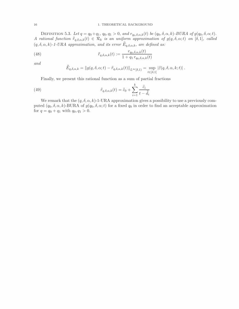
Definition 5.3. Let q = q0+q1, q0, q1 > 0, and rq0,δ,α,k(t) be (q0, δ, α, k)-BURA of g(q0, δ, α; t).A rational function ¯rq,δ,α,k(t) ∈ Rk is an uniform approximation of g(q, δ, α; t) on [δ, 1], called
(q, δ, α, k)-1-URA approximation, and its error ¯Eq,δ,α,k, are defined as:
(48) ¯rq,δ,α,k(t) :=rq0,δ,α,k(t)
1 + q1 rq0,δ,α,k(t)
and¯Eq,δ,α,k = ‖g(q, δ, α; t) − ¯rq,δ,α,k(t)‖L∞[δ,1) = sup
t∈[δ,1]|¯ε(q, δ, α, k; t)| .
Finally, we present this rational function as a sum of partial fractions
(49) ¯rq,δ,α,k(t) = ¯c0 +
k∑
i=1
¯ci
t− ¯di
We remark that the (q, δ, α, k)-1-URA approximation gives a possibility to use a previously com-puted (q0, δ, α, k)-BURA of g(q0, δ, α; t) for a fixed q0 in order to find an acceptable approximationfor q = q0 + q1 with q0, q1 > 0.
CHAPTER 2
Tables
1. Description of the data provided by our numerical experiments
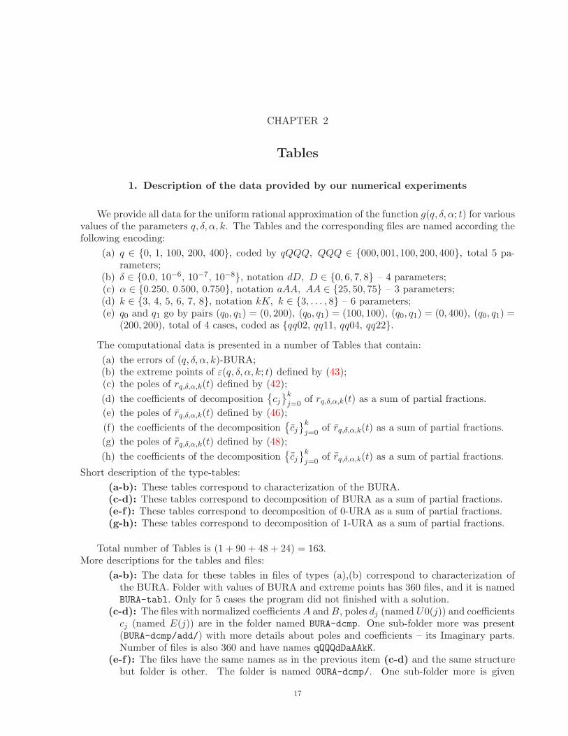
We provide all data for the uniform rational approximation of the function g(q, δ, α; t) for variousvalues of the parameters q, δ, α, k. The Tables and the corresponding files are named according thefollowing encoding:
(a) q ∈ 0, 1, 100, 200, 400, coded by qQQQ, QQQ ∈ 000, 001, 100, 200, 400, total 5 pa-rameters;
(b) δ ∈ 0.0, 10−6, 10−7, 10−8, notation dD, D ∈ 0, 6, 7, 8 – 4 parameters;(c) α ∈ 0.250, 0.500, 0.750, notation aAA, AA ∈ 25, 50, 75 – 3 parameters;(d) k ∈ 3, 4, 5, 6, 7, 8, notation kK, k ∈ 3, . . . , 8 – 6 parameters;(e) q0 and q1 go by pairs (q0, q1) = (0, 200), (q0, q1) = (100, 100), (q0, q1) = (0, 400), (q0, q1) =
(200, 200), total of 4 cases, coded as qq02, qq11, qq04, qq22.
The computational data is presented in a number of Tables that contain:
(a) the errors of (q, δ, α, k)-BURA;(b) the extreme points of ε(q, δ, α, k; t) defined by (43);(c) the poles of rq,δ,α,k(t) defined by (42);
(d) the coefficients of decompositioncjkj=0
of rq,δ,α,k(t) as a sum of partial fractions.
(e) the poles of rq,δ,α,k(t) defined by (46);
(f) the coefficients of the decompositioncjkj=0
of rq,δ,α,k(t) as a sum of partial fractions.
(g) the poles of ¯rq,δ,α,k(t) defined by (48);
(h) the coefficients of the decomposition¯cjkj=0
of ¯rq,δ,α,k(t) as a sum of partial fractions.
Short description of the type-tables:
(a-b): These tables correspond to characterization of the BURA.(c-d): These tables correspond to decomposition of BURA as a sum of partial fractions.(e-f): These tables correspond to decomposition of 0-URA as a sum of partial fractions.(g-h): These tables correspond to decomposition of 1-URA as a sum of partial fractions.
Total number of Tables is (1 + 90 + 48 + 24) = 163.More descriptions for the tables and files:
(a-b): The data for these tables in files of types (a),(b) correspond to characterization ofthe BURA. Folder with values of BURA and extreme points has 360 files, and it is namedBURA-tabl. Only for 5 cases the program did not finished with a solution.
(c-d): The files with normalized coefficients A andB, poles dj (named U0(j)) and coefficientscj (named E(j)) are in the folder named BURA-dcmp. One sub-folder more was present(BURA-dcmp/add/) with more details about poles and coefficients – its Imaginary parts.Number of files is also 360 and have names qQQQdDaAAkK.
(e-f): The files have the same names as in the previous item (c-d) and the same structurebut folder is other. The folder is named 0URA-dcmp/. One sub-folder more is given
17
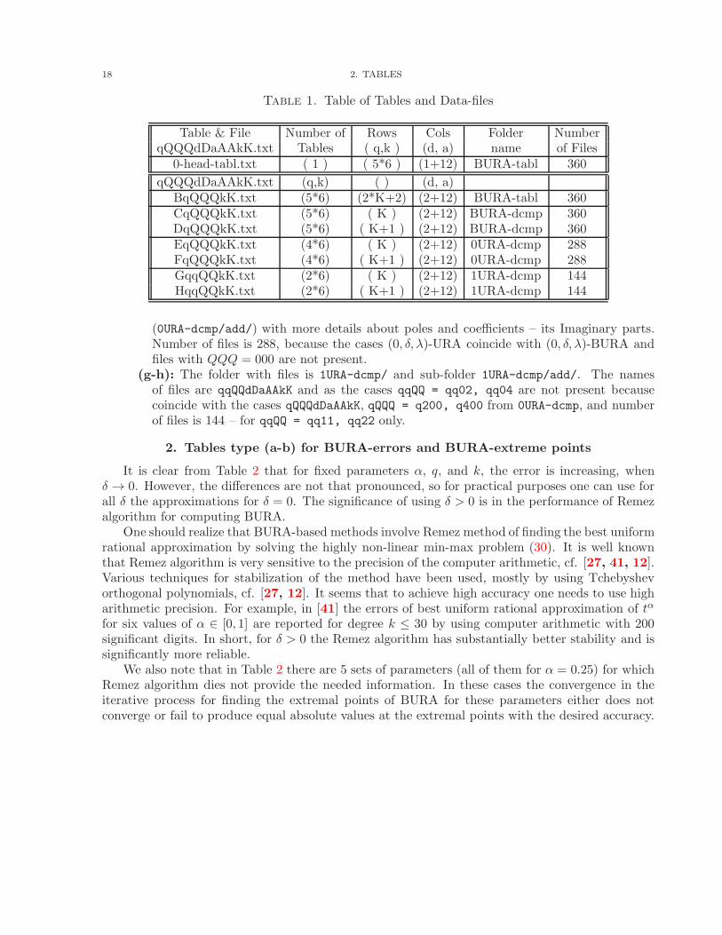
18 2. TABLES
Table 1. Table of Tables and Data-files
Table & File Number of Rows Cols Folder NumberqQQQdDaAAkK.txt Tables ( q,k ) (d, a) name of Files
0-head-tabl.txt ( 1 ) ( 5*6 ) (1+12) BURA-tabl 360
qQQQdDaAAkK.txt (q,k) ( ) (d, a)BqQQQkK.txt (5*6) (2*K+2) (2+12) BURA-tabl 360CqQQQkK.txt (5*6) ( K ) (2+12) BURA-dcmp 360DqQQQkK.txt (5*6) ( K+1 ) (2+12) BURA-dcmp 360EqQQQkK.txt (4*6) ( K ) (2+12) 0URA-dcmp 288FqQQQkK.txt (4*6) ( K+1 ) (2+12) 0URA-dcmp 288GqqQQkK.txt (2*6) ( K ) (2+12) 1URA-dcmp 144HqqQQkK.txt (2*6) ( K+1 ) (2+12) 1URA-dcmp 144
(0URA-dcmp/add/) with more details about poles and coefficients – its Imaginary parts.Number of files is 288, because the cases (0, δ, λ)-URA coincide with (0, δ, λ)-BURA andfiles with QQQ = 000 are not present.
(g-h): The folder with files is 1URA-dcmp/ and sub-folder 1URA-dcmp/add/. The namesof files are qqQQdDaAAkK and as the cases qqQQ = qq02, qq04 are not present becausecoincide with the cases qQQQdDaAAkK, qQQQ = q200, q400 from 0URA-dcmp, and numberof files is 144 – for qqQQ = qq11, qq22 only.
2. Tables type (a-b) for BURA-errors and BURA-extreme points
It is clear from Table 2 that for fixed parameters α, q, and k, the error is increasing, whenδ → 0. However, the differences are not that pronounced, so for practical purposes one can use forall δ the approximations for δ = 0. The significance of using δ > 0 is in the performance of Remezalgorithm for computing BURA.
One should realize that BURA-based methods involve Remez method of finding the best uniformrational approximation by solving the highly non-linear min-max problem (30). It is well knownthat Remez algorithm is very sensitive to the precision of the computer arithmetic, cf. [27, 41, 12].Various techniques for stabilization of the method have been used, mostly by using Tchebyshevorthogonal polynomials, cf. [27, 12]. It seems that to achieve high accuracy one needs to use higharithmetic precision. For example, in [41] the errors of best uniform rational approximation of tα
for six values of α ∈ [0, 1] are reported for degree k ≤ 30 by using computer arithmetic with 200significant digits. In short, for δ > 0 the Remez algorithm has substantially better stability and issignificantly more reliable.
We also note that in Table 2 there are 5 sets of parameters (all of them for α = 0.25) for whichRemez algorithm dies not provide the needed information. In these cases the convergence in theiterative process for finding the extremal points of BURA for these parameters either does notconverge or fail to produce equal absolute values at the extremal points with the desired accuracy.
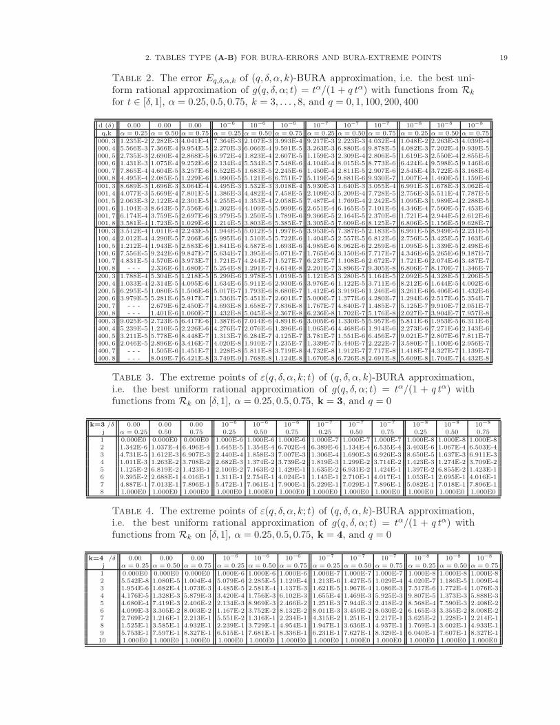
2. TABLES TYPE (A-B) FOR BURA-ERRORS AND BURA-EXTREME POINTS 19
Table 2. The error Eq,δ,α,k of (q, δ, α, k)-BURA approximation, i.e. the best uni-form rational approximation of g(q, δ, α; t) = tα/(1 + q tα) with functions from Rk
for t ∈ [δ, 1], α = 0.25, 0.5, 0.75, k = 3, . . . , 8, and q = 0, 1, 100, 200, 400
d (δ) 0.00 0.00 0.00 10−6 10−6 10−6 10−7 10−7 10−7 10−8 10−8 10−8
q,k α = 0.25 α = 0.50 α = 0.75 α = 0.25 α = 0.50 α = 0.75 α = 0.25 α = 0.50 α = 0.75 α = 0.25 α = 0.50 α = 0.75000, 3 1.235E-2 2.282E-3 4.041E-4 7.364E-3 2.107E-3 3.993E-4 9.217E-3 2.223E-3 4.032E-4 1.048E-2 2.263E-3 4.039E-4000, 4 5.566E-3 7.366E-4 9.954E-5 2.270E-3 6.066E-4 9.591E-5 3.263E-3 6.880E-4 9.878E-5 4.082E-3 7.202E-4 9.939E-5000, 5 2.735E-3 2.690E-4 2.868E-5 6.972E-4 1.823E-4 2.607E-5 1.159E-3 2.309E-4 2.806E-5 1.619E-3 2.550E-4 2.855E-5000, 6 1.431E-3 1.075E-4 9.252E-6 2.134E-4 5.534E-5 7.548E-6 4.104E-4 8.015E-5 8.773E-6 6.424E-4 9.598E-5 9.146E-6000, 7 7.865E-4 4.604E-5 3.257E-6 6.522E-5 1.683E-5 2.245E-6 1.450E-4 2.811E-5 2.907E-6 2.545E-4 3.722E-5 3.168E-6000, 8 4.495E-4 2.085E-5 1.229E-6 1.990E-5 5.121E-6 6.751E-7 5.119E-5 9.881E-6 9.930E-7 1.007E-4 1.460E-5 1.159E-6001, 3 8.689E-3 1.696E-3 3.064E-4 4.495E-3 1.532E-3 3.018E-4 5.930E-3 1.640E-3 3.055E-4 6.991E-3 1.678E-3 3.062E-4001, 4 4.077E-3 5.669E-4 7.801E-5 1.386E-3 4.482E-4 7.458E-5 2.109E-3 5.209E-4 7.728E-5 2.756E-3 5.511E-4 7.787E-5001, 5 2.063E-3 2.122E-4 2.301E-5 4.255E-4 1.353E-4 2.058E-5 7.487E-4 1.769E-4 2.242E-5 1.095E-3 1.989E-4 2.288E-5001, 6 1.104E-3 8.643E-5 7.556E-6 1.302E-4 4.109E-5 5.999E-6 2.651E-4 6.165E-5 7.101E-6 4.346E-4 7.560E-5 7.453E-6001, 7 6.174E-4 3.759E-5 2.697E-6 3.979E-5 1.250E-5 1.789E-6 9.366E-5 2.164E-5 2.370E-6 1.721E-4 2.944E-5 2.612E-6001, 8 3.581E-4 1.723E-5 1.029E-6 1.214E-5 3.803E-6 5.385E-7 3.305E-5 7.609E-6 8.125E-7 6.806E-5 1.156E-5 9.628E-7100, 3 3.512E-4 1.011E-4 2.243E-5 1.944E-5 5.012E-5 1.997E-5 3.953E-5 7.387E-5 2.183E-5 6.991E-5 8.949E-5 2.231E-5100, 4 2.012E-4 4.290E-5 7.266E-6 5.995E-6 1.510E-5 5.722E-6 1.404E-5 2.557E-5 6.812E-6 2.756E-5 3.425E-5 7.163E-6100, 5 1.212E-4 1.943E-5 2.583E-6 1.841E-6 4.587E-6 1.693E-6 4.985E-6 8.962E-6 2.259E-6 1.095E-5 1.339E-5 2.498E-6100, 6 7.556E-5 9.242E-6 9.847E-7 5.634E-7 1.395E-6 5.071E-7 1.765E-6 3.150E-6 7.717E-7 4.346E-6 5.265E-6 9.187E-7100, 7 4.831E-5 4.570E-6 3.973E-7 1.721E-7 4.244E-7 1.527E-7 6.237E-7 1.108E-6 2.672E-7 1.721E-6 2.074E-6 3.487E-7100, 8 - - - 2.336E-6 1.680E-7 5.254E-8 1.291E-7 4.614E-8 2.201E-7 3.896E-7 9.305E-8 6.806E-7 8.170E-7 1.346E-7200, 3 1.788E-4 5.304E-5 1.218E-5 5.299E-6 1.978E-5 1.019E-5 1.121E-5 3.280E-5 1.164E-5 2.092E-5 4.328E-5 1.206E-5200, 4 1.033E-4 2.314E-5 4.095E-6 1.634E-6 5.911E-6 2.930E-6 3.976E-6 1.122E-5 3.711E-6 8.212E-6 1.644E-5 4.002E-6200, 5 6.295E-5 1.080E-5 1.506E-6 5.017E-7 1.793E-6 8.680E-7 1.412E-6 3.919E-6 1.246E-6 3.261E-6 6.406E-6 1.432E-6200, 6 3.979E-5 5.281E-6 5.917E-7 1.536E-7 5.451E-7 2.601E-7 5.000E-7 1.377E-6 4.280E-7 1.294E-6 2.517E-6 5.354E-7200, 7 - - - 2.679E-6 2.450E-7 4.693E-8 1.658E-7 7.836E-8 1.767E-7 4.840E-7 1.485E-7 5.125E-7 9.910E-7 2.051E-7200, 8 - - - 1.401E-6 1.060E-7 1.432E-8 5.045E-8 2.367E-8 6.236E-8 1.702E-7 5.176E-8 2.027E-7 3.904E-7 7.957E-8400, 3 9.025E-5 2.723E-5 6.417E-6 1.387E-6 7.014E-6 4.891E-6 3.005E-6 1.330E-5 5.957E-6 5.811E-6 1.953E-5 6.311E-6400, 4 5.239E-5 1.210E-5 2.226E-6 4.276E-7 2.076E-6 1.396E-6 1.065E-6 4.468E-6 1.914E-6 2.273E-6 7.271E-6 2.143E-6400, 5 3.211E-5 5.778E-6 8.448E-7 1.313E-7 6.284E-7 4.125E-7 3.781E-7 1.551E-6 6.456E-7 9.021E-7 2.807E-6 7.811E-7400, 6 2.046E-5 2.896E-6 3.416E-7 4.020E-8 1.910E-7 1.235E-7 1.339E-7 5.440E-7 2.222E-7 3.580E-7 1.100E-6 2.956E-7400, 7 - - - 1.505E-6 1.451E-7 1.228E-8 5.811E-8 3.719E-8 4.732E-8 1.912E-7 7.717E-8 1.418E-7 4.327E-7 1.139E-7400, 8 - - - 8.049E-7 6.421E-8 3.749E-9 1.768E-8 1.124E-8 1.670E-8 6.726E-8 2.691E-8 5.609E-8 1.704E-7 4.432E-8
Table 3. The extreme points of ε(q, δ, α, k; t) of (q, δ, α, k)-BURA approximation,i.e. the best uniform rational approximation of g(q, δ, α; t) = tα/(1 + q tα) withfunctions from Rk on [δ, 1], α = 0.25, 0.5, 0.75, k = 3, and q = 0
k=3 /δ 0.00 0.00 0.00 10−6 10−6 10−6 10−7 10−7 10−7 10−8 10−8 10−8
j α = 0.25 0.50 0.75 0.25 0.50 0.75 0.25 0.50 0.75 0.25 0.50 0.751 0.000E0 0.000E0 0.000E0 1.000E-6 1.000E-6 1.000E-6 1.000E-7 1.000E-7 1.000E-7 1.000E-8 1.000E-8 1.000E-82 1.342E-6 1.037E-4 6.496E-4 1.645E-5 1.354E-4 6.702E-4 6.389E-6 1.134E-4 6.535E-4 3.403E-6 1.067E-4 6.503E-43 4.731E-5 1.612E-3 6.907E-3 2.440E-4 1.858E-3 7.007E-3 1.306E-4 1.690E-3 6.926E-3 8.650E-5 1.637E-3 6.911E-34 1.011E-3 1.263E-2 3.708E-2 2.682E-3 1.374E-2 3.739E-2 1.819E-3 1.299E-2 3.714E-2 1.423E-3 1.274E-2 3.709E-25 1.125E-2 6.819E-2 1.423E-1 2.100E-2 7.163E-2 1.429E-1 1.635E-2 6.931E-2 1.424E-1 1.397E-2 6.855E-2 1.423E-16 9.395E-2 2.688E-1 4.016E-1 1.311E-1 2.754E-1 4.024E-1 1.145E-1 2.710E-1 4.017E-1 1.053E-1 2.695E-1 4.016E-17 4.887E-1 7.013E-1 7.896E-1 5.472E-1 7.061E-1 7.900E-1 5.229E-1 7.029E-1 7.896E-1 5.082E-1 7.018E-1 7.896E-18 1.000E0 1.000E0 1.000E0 1.000E0 1.000E0 1.000E0 1.000E0 1.000E0 1.000E0 1.000E0 1.000E0 1.000E0
Table 4. The extreme points of ε(q, δ, α, k; t) of (q, δ, α, k)-BURA approximation,i.e. the best uniform rational approximation of g(q, δ, α; t) = tα/(1 + q tα) withfunctions from Rk on [δ, 1], α = 0.25, 0.5, 0.75, k = 4, and q = 0
k=4 /δ 0.00 0.00 0.00 10−6 10−6 10−6 10−7 10−7 10−7 10−8 10−8 10−8
j α = 0.25 α = 0.50 α = 0.75 α = 0.25 α = 0.50 α = 0.75 α = 0.25 α = 0.50 α = 0.75 α = 0.25 α = 0.50 α = 0.751 0.000E0 0.000E0 0.000E0 1.000E-6 1.000E-6 1.000E-6 1.000E-7 1.000E-7 1.000E-7 1.000E-8 1.000E-8 1.000E-82 5.542E-8 1.080E-5 1.004E-4 5.079E-6 2.285E-5 1.129E-4 1.213E-6 1.427E-5 1.029E-4 4.020E-7 1.186E-5 1.009E-43 1.954E-6 1.682E-4 1.073E-3 4.485E-5 2.581E-4 1.137E-3 1.621E-5 1.967E-4 1.086E-3 7.517E-6 1.772E-4 1.076E-34 4.176E-5 1.328E-3 5.879E-3 3.420E-4 1.756E-3 6.102E-3 1.655E-4 1.469E-3 5.925E-3 9.807E-5 1.373E-3 5.888E-35 4.680E-4 7.419E-3 2.406E-2 2.134E-3 8.969E-3 2.466E-2 1.251E-3 7.944E-3 2.418E-2 8.568E-4 7.590E-3 2.408E-26 4.099E-3 3.305E-2 8.003E-2 1.167E-2 3.752E-2 8.132E-2 8.011E-3 3.459E-2 8.030E-2 6.165E-3 3.355E-2 8.008E-27 2.769E-2 1.216E-1 2.213E-1 5.551E-2 1.316E-1 2.234E-1 4.315E-2 1.251E-1 2.217E-1 3.625E-2 1.228E-1 2.214E-18 1.525E-1 3.585E-1 4.932E-1 2.239E-1 3.729E-1 4.954E-1 1.947E-1 3.636E-1 4.937E-1 1.769E-1 3.602E-1 4.933E-19 5.753E-1 7.597E-1 8.327E-1 6.515E-1 7.681E-1 8.336E-1 6.231E-1 7.627E-1 8.329E-1 6.040E-1 7.607E-1 8.327E-110 1.000E0 1.000E0 1.000E0 1.000E0 1.000E0 1.000E0 1.000E0 1.000E0 1.000E0 1.000E0 1.000E0 1.000E0
20 2. TABLES
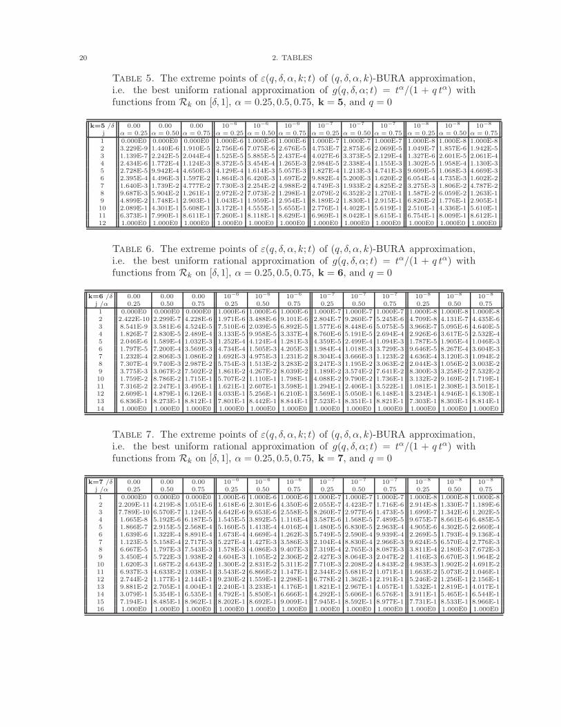
Table 5. The extreme points of ε(q, δ, α, k; t) of (q, δ, α, k)-BURA approximation,i.e. the best uniform rational approximation of g(q, δ, α; t) = tα/(1 + q tα) withfunctions from Rk on [δ, 1], α = 0.25, 0.5, 0.75, k = 5, and q = 0
k=5 /δ 0.00 0.00 0.00 10−6 10−6 10−6 10−7 10−7 10−7 10−8 10−8 10−8
j α = 0.25 α = 0.50 α = 0.75 α = 0.25 α = 0.50 α = 0.75 α = 0.25 α = 0.50 α = 0.75 α = 0.25 α = 0.50 α = 0.751 0.000E0 0.000E0 0.000E0 1.000E-6 1.000E-6 1.000E-6 1.000E-7 1.000E-7 1.000E-7 1.000E-8 1.000E-8 1.000E-82 3.229E-9 1.440E-6 1.910E-5 2.756E-6 7.075E-6 2.676E-5 4.753E-7 2.875E-6 2.069E-5 1.049E-7 1.857E-6 1.942E-53 1.139E-7 2.242E-5 2.044E-4 1.525E-5 5.885E-5 2.437E-4 4.027E-6 3.373E-5 2.129E-4 1.327E-6 2.601E-5 2.061E-44 2.434E-6 1.772E-4 1.124E-3 8.372E-5 3.454E-4 1.265E-3 2.984E-5 2.338E-4 1.155E-3 1.302E-5 1.958E-4 1.130E-35 2.728E-5 9.942E-4 4.650E-3 4.129E-4 1.614E-3 5.057E-3 1.827E-4 1.213E-3 4.741E-3 9.609E-5 1.068E-3 4.669E-36 2.395E-4 4.496E-3 1.597E-2 1.864E-3 6.420E-3 1.697E-2 9.882E-4 5.200E-3 1.620E-2 6.054E-4 4.735E-3 1.602E-27 1.640E-3 1.739E-2 4.777E-2 7.730E-3 2.254E-2 4.988E-2 4.749E-3 1.933E-2 4.825E-2 3.275E-3 1.806E-2 4.787E-28 9.687E-3 5.904E-2 1.261E-1 2.972E-2 7.073E-2 1.298E-1 2.079E-2 6.352E-2 1.270E-1 1.587E-2 6.059E-2 1.263E-19 4.899E-2 1.748E-1 2.903E-1 1.043E-1 1.959E-1 2.954E-1 8.189E-2 1.830E-1 2.915E-1 6.826E-2 1.776E-1 2.905E-110 2.089E-1 4.301E-1 5.608E-1 3.172E-1 4.555E-1 5.655E-1 2.776E-1 4.402E-1 5.619E-1 2.510E-1 4.336E-1 5.610E-111 6.373E-1 7.990E-1 8.611E-1 7.260E-1 8.118E-1 8.629E-1 6.969E-1 8.042E-1 8.615E-1 6.754E-1 8.009E-1 8.612E-112 1.000E0 1.000E0 1.000E0 1.000E0 1.000E0 1.000E0 1.000E0 1.000E0 1.000E0 1.000E0 1.000E0 1.000E0
Table 6. The extreme points of ε(q, δ, α, k; t) of (q, δ, α, k)-BURA approximation,i.e. the best uniform rational approximation of g(q, δ, α; t) = tα/(1 + q tα) withfunctions from Rk on [δ, 1], α = 0.25, 0.5, 0.75, k = 6, and q = 0
k=6 /δ 0.00 0.00 0.00 10−6 10−6 10−6 10−7 10−7 10−7 10−8 10−8 10−8
j /α 0.25 0.50 0.75 0.25 0.50 0.75 0.25 0.50 0.75 0.25 0.50 0.751 0.000E0 0.000E0 0.000E0 1.000E-6 1.000E-6 1.000E-6 1.000E-7 1.000E-7 1.000E-7 1.000E-8 1.000E-8 1.000E-82 2.422E-10 2.299E-7 4.228E-6 1.971E-6 3.488E-6 9.101E-6 2.804E-7 9.260E-7 5.245E-6 4.709E-8 4.131E-7 4.435E-63 8.541E-9 3.581E-6 4.524E-5 7.510E-6 2.039E-5 6.892E-5 1.577E-6 8.448E-6 5.075E-5 3.966E-7 5.095E-6 4.640E-54 1.826E-7 2.830E-5 2.489E-4 3.133E-5 9.958E-5 3.337E-4 8.760E-6 5.191E-5 2.694E-4 2.926E-6 3.617E-5 2.532E-45 2.046E-6 1.589E-4 1.032E-3 1.252E-4 4.124E-4 1.281E-3 4.359E-5 2.499E-4 1.094E-3 1.787E-5 1.905E-4 1.046E-36 1.797E-5 7.200E-4 3.569E-3 4.734E-4 1.505E-3 4.205E-3 1.984E-4 1.018E-3 3.729E-3 9.646E-5 8.267E-4 3.604E-37 1.232E-4 2.806E-3 1.086E-2 1.692E-3 4.975E-3 1.231E-2 8.304E-4 3.666E-3 1.123E-2 4.636E-4 3.120E-3 1.094E-28 7.307E-4 9.740E-3 2.987E-2 5.754E-3 1.513E-2 3.283E-2 3.247E-3 1.195E-2 3.063E-2 2.044E-3 1.056E-2 3.003E-29 3.775E-3 3.067E-2 7.502E-2 1.861E-2 4.267E-2 8.039E-2 1.189E-2 3.574E-2 7.641E-2 8.300E-3 3.258E-2 7.532E-210 1.759E-2 8.786E-2 1.715E-1 5.707E-2 1.110E-1 1.798E-1 4.088E-2 9.790E-2 1.736E-1 3.132E-2 9.169E-2 1.719E-111 7.316E-2 2.247E-1 3.495E-1 1.621E-1 2.607E-1 3.598E-1 1.294E-1 2.406E-1 3.522E-1 1.081E-1 2.308E-1 3.501E-112 2.609E-1 4.879E-1 6.126E-1 4.033E-1 5.256E-1 6.210E-1 3.569E-1 5.050E-1 6.148E-1 3.234E-1 4.946E-1 6.130E-113 6.836E-1 8.273E-1 8.812E-1 7.801E-1 8.442E-1 8.844E-1 7.523E-1 8.351E-1 8.821E-1 7.303E-1 8.303E-1 8.814E-114 1.000E0 1.000E0 1.000E0 1.000E0 1.000E0 1.000E0 1.000E0 1.000E0 1.000E0 1.000E0 1.000E0 1.000E0
Table 7. The extreme points of ε(q, δ, α, k; t) of (q, δ, α, k)-BURA approximation,i.e. the best uniform rational approximation of g(q, δ, α; t) = tα/(1 + q tα) withfunctions from Rk on [δ, 1], α = 0.25, 0.5, 0.75, k = 7, and q = 0
k=7 /δ 0.00 0.00 0.00 10−6 10−6 10−6 10−7 10−7 10−7 10−8 10−8 10−8
j /α 0.25 0.50 0.75 0.25 0.50 0.75 0.25 0.50 0.75 0.25 0.50 0.751 0.000E0 0.000E0 0.000E0 1.000E-6 1.000E-6 1.000E-6 1.000E-7 1.000E-7 1.000E-7 1.000E-8 1.000E-8 1.000E-82 2.209E-11 4.219E-8 1.051E-6 1.618E-6 2.301E-6 4.350E-6 2.055E-7 4.423E-7 1.716E-6 2.914E-8 1.330E-7 1.189E-63 7.789E-10 6.570E-7 1.124E-5 4.642E-6 9.653E-6 2.558E-5 8.260E-7 2.977E-6 1.473E-5 1.699E-7 1.342E-6 1.202E-54 1.665E-8 5.192E-6 6.187E-5 1.545E-5 3.892E-5 1.116E-4 3.587E-6 1.568E-5 7.489E-5 9.675E-7 8.661E-6 6.485E-55 1.866E-7 2.915E-5 2.568E-4 5.160E-5 1.413E-4 4.016E-4 1.480E-5 6.830E-5 2.963E-4 4.905E-6 4.302E-5 2.660E-46 1.639E-6 1.322E-4 8.891E-4 1.673E-4 4.669E-4 1.262E-3 5.749E-5 2.590E-4 9.939E-4 2.269E-5 1.793E-4 9.136E-47 1.123E-5 5.158E-4 2.717E-3 5.227E-4 1.427E-3 3.586E-3 2.104E-4 8.830E-4 2.966E-3 9.624E-5 6.570E-4 2.776E-38 6.667E-5 1.797E-3 7.543E-3 1.578E-3 4.086E-3 9.407E-3 7.319E-4 2.765E-3 8.087E-3 3.811E-4 2.180E-3 7.672E-39 3.450E-4 5.722E-3 1.938E-2 4.604E-3 1.105E-2 2.306E-2 2.427E-3 8.064E-3 2.047E-2 1.416E-3 6.670E-3 1.964E-210 1.620E-3 1.687E-2 4.643E-2 1.300E-2 2.831E-2 5.311E-2 7.710E-3 2.208E-2 4.843E-2 4.983E-3 1.902E-2 4.691E-211 6.937E-3 4.633E-2 1.038E-1 3.543E-2 6.866E-2 1.147E-1 2.344E-2 5.681E-2 1.071E-1 1.663E-2 5.073E-2 1.046E-112 2.744E-2 1.177E-1 2.144E-1 9.230E-2 1.559E-1 2.298E-1 6.778E-2 1.362E-1 2.191E-1 5.246E-2 1.256E-1 2.156E-113 9.881E-2 2.705E-1 4.004E-1 2.240E-1 3.233E-1 4.176E-1 1.821E-1 2.967E-1 4.057E-1 1.532E-1 2.819E-1 4.017E-114 3.079E-1 5.354E-1 6.535E-1 4.792E-1 5.850E-1 6.666E-1 4.292E-1 5.606E-1 6.576E-1 3.911E-1 5.465E-1 6.544E-115 7.194E-1 8.485E-1 8.962E-1 8.202E-1 8.692E-1 9.009E-1 7.945E-1 8.592E-1 8.977E-1 7.731E-1 8.533E-1 8.966E-116 1.000E0 1.000E0 1.000E0 1.000E0 1.000E0 1.000E0 1.000E0 1.000E0 1.000E0 1.000E0 1.000E0 1.000E0
2. TABLES TYPE (A-B) FOR BURA-ERRORS AND BURA-EXTREME POINTS 21
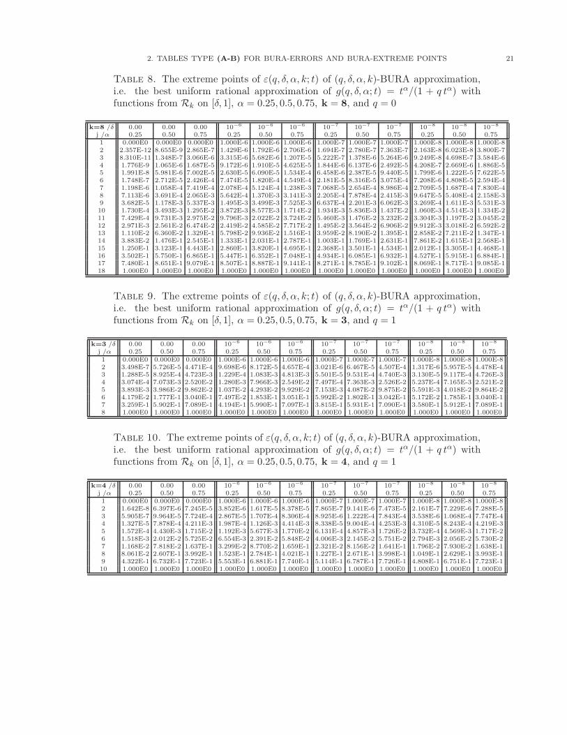
Table 8. The extreme points of ε(q, δ, α, k; t) of (q, δ, α, k)-BURA approximation,i.e. the best uniform rational approximation of g(q, δ, α; t) = tα/(1 + q tα) withfunctions from Rk on [δ, 1], α = 0.25, 0.5, 0.75, k = 8, and q = 0
k=8 /δ 0.00 0.00 0.00 10−6 10−6 10−6 10−7 10−7 10−7 10−8 10−8 10−8
j /α 0.25 0.50 0.75 0.25 0.50 0.75 0.25 0.50 0.75 0.25 0.50 0.751 0.000E0 0.000E0 0.000E0 1.000E-6 1.000E-6 1.000E-6 1.000E-7 1.000E-7 1.000E-7 1.000E-8 1.000E-8 1.000E-82 2.357E-12 8.655E-9 2.865E-7 1.429E-6 1.792E-6 2.706E-6 1.694E-7 2.780E-7 7.363E-7 2.163E-8 6.023E-8 3.800E-73 8.310E-11 1.348E-7 3.066E-6 3.315E-6 5.682E-6 1.207E-5 5.222E-7 1.378E-6 5.264E-6 9.249E-8 4.698E-7 3.584E-64 1.776E-9 1.065E-6 1.687E-5 9.172E-6 1.910E-5 4.625E-5 1.844E-6 6.137E-6 2.492E-5 4.208E-7 2.669E-6 1.886E-55 1.991E-8 5.981E-6 7.002E-5 2.630E-5 6.090E-5 1.534E-4 6.458E-6 2.387E-5 9.440E-5 1.799E-6 1.222E-5 7.622E-56 1.748E-7 2.712E-5 2.426E-4 7.474E-5 1.820E-4 4.549E-4 2.181E-5 8.316E-5 3.075E-4 7.208E-6 4.808E-5 2.594E-47 1.198E-6 1.058E-4 7.419E-4 2.078E-4 5.124E-4 1.238E-3 7.068E-5 2.654E-4 8.986E-4 2.709E-5 1.687E-4 7.830E-48 7.113E-6 3.691E-4 2.065E-3 5.642E-4 1.370E-3 3.141E-3 2.205E-4 7.878E-4 2.415E-3 9.647E-5 5.408E-4 2.158E-39 3.682E-5 1.178E-3 5.337E-3 1.495E-3 3.499E-3 7.525E-3 6.637E-4 2.201E-3 6.062E-3 3.269E-4 1.611E-3 5.531E-310 1.730E-4 3.493E-3 1.295E-2 3.872E-3 8.577E-3 1.714E-2 1.934E-3 5.836E-3 1.437E-2 1.060E-3 4.514E-3 1.334E-211 7.429E-4 9.731E-3 2.975E-2 9.796E-3 2.022E-2 3.724E-2 5.460E-3 1.476E-2 3.232E-2 3.304E-3 1.197E-2 3.045E-212 2.971E-3 2.561E-2 6.474E-2 2.419E-2 4.585E-2 7.717E-2 1.495E-2 3.564E-2 6.906E-2 9.912E-3 3.018E-2 6.592E-213 1.110E-2 6.360E-2 1.329E-1 5.798E-2 9.936E-2 1.516E-1 3.959E-2 8.190E-2 1.395E-1 2.858E-2 7.211E-2 1.347E-114 3.883E-2 1.476E-1 2.545E-1 1.333E-1 2.031E-1 2.787E-1 1.003E-1 1.769E-1 2.631E-1 7.861E-2 1.615E-1 2.568E-115 1.250E-1 3.123E-1 4.443E-1 2.860E-1 3.820E-1 4.695E-1 2.368E-1 3.501E-1 4.534E-1 2.012E-1 3.305E-1 4.468E-116 3.502E-1 5.750E-1 6.865E-1 5.447E-1 6.352E-1 7.048E-1 4.934E-1 6.085E-1 6.932E-1 4.527E-1 5.915E-1 6.884E-117 7.480E-1 8.651E-1 9.079E-1 8.507E-1 8.887E-1 9.141E-1 8.271E-1 8.785E-1 9.102E-1 8.069E-1 8.717E-1 9.085E-118 1.000E0 1.000E0 1.000E0 1.000E0 1.000E0 1.000E0 1.000E0 1.000E0 1.000E0 1.000E0 1.000E0 1.000E0
Table 9. The extreme points of ε(q, δ, α, k; t) of (q, δ, α, k)-BURA approximation,i.e. the best uniform rational approximation of g(q, δ, α; t) = tα/(1 + q tα) withfunctions from Rk on [δ, 1], α = 0.25, 0.5, 0.75, k = 3, and q = 1
k=3 /δ 0.00 0.00 0.00 10−6 10−6 10−6 10−7 10−7 10−7 10−8 10−8 10−8
j /α 0.25 0.50 0.75 0.25 0.50 0.75 0.25 0.50 0.75 0.25 0.50 0.751 0.000E0 0.000E0 0.000E0 1.000E-6 1.000E-6 1.000E-6 1.000E-7 1.000E-7 1.000E-7 1.000E-8 1.000E-8 1.000E-82 3.498E-7 5.726E-5 4.471E-4 9.698E-6 8.172E-5 4.657E-4 3.021E-6 6.467E-5 4.507E-4 1.317E-6 5.957E-5 4.478E-43 1.288E-5 8.925E-4 4.723E-3 1.229E-4 1.083E-3 4.813E-3 5.501E-5 9.531E-4 4.740E-3 3.130E-5 9.117E-4 4.726E-34 3.074E-4 7.073E-3 2.520E-2 1.280E-3 7.966E-3 2.549E-2 7.497E-4 7.363E-3 2.526E-2 5.237E-4 7.165E-3 2.521E-25 3.893E-3 3.986E-2 9.862E-2 1.037E-2 4.293E-2 9.929E-2 7.153E-3 4.087E-2 9.875E-2 5.591E-3 4.018E-2 9.864E-26 4.179E-2 1.777E-1 3.040E-1 7.497E-2 1.853E-1 3.051E-1 5.992E-2 1.802E-1 3.042E-1 5.172E-2 1.785E-1 3.040E-17 3.259E-1 5.902E-1 7.089E-1 4.194E-1 5.990E-1 7.097E-1 3.815E-1 5.931E-1 7.090E-1 3.580E-1 5.912E-1 7.089E-18 1.000E0 1.000E0 1.000E0 1.000E0 1.000E0 1.000E0 1.000E0 1.000E0 1.000E0 1.000E0 1.000E0 1.000E0
Table 10. The extreme points of ε(q, δ, α, k; t) of (q, δ, α, k)-BURA approximation,i.e. the best uniform rational approximation of g(q, δ, α; t) = tα/(1 + q tα) withfunctions from Rk on [δ, 1], α = 0.25, 0.5, 0.75, k = 4, and q = 1
k=4 /δ 0.00 0.00 0.00 10−6 10−6 10−6 10−7 10−7 10−7 10−8 10−8 10−8
j /α 0.25 0.50 0.75 0.25 0.50 0.75 0.25 0.50 0.75 0.25 0.50 0.751 0.000E0 0.000E0 0.000E0 1.000E-6 1.000E-6 1.000E-6 1.000E-7 1.000E-7 1.000E-7 1.000E-8 1.000E-8 1.000E-82 1.642E-8 6.397E-6 7.245E-5 3.852E-6 1.617E-5 8.378E-5 7.865E-7 9.141E-6 7.473E-5 2.161E-7 7.229E-6 7.288E-53 5.905E-7 9.964E-5 7.724E-4 2.867E-5 1.707E-4 8.306E-4 8.925E-6 1.222E-4 7.843E-4 3.538E-6 1.068E-4 7.747E-44 1.327E-5 7.878E-4 4.211E-3 1.987E-4 1.126E-3 4.414E-3 8.338E-5 9.004E-4 4.253E-3 4.310E-5 8.243E-4 4.219E-35 1.572E-4 4.430E-3 1.715E-2 1.192E-3 5.677E-3 1.770E-2 6.131E-4 4.857E-3 1.726E-2 3.732E-4 4.569E-3 1.717E-26 1.518E-3 2.012E-2 5.725E-2 6.554E-3 2.391E-2 5.848E-2 4.006E-3 2.145E-2 5.751E-2 2.794E-3 2.056E-2 5.730E-27 1.168E-2 7.818E-2 1.637E-1 3.299E-2 8.770E-2 1.659E-1 2.321E-2 8.156E-2 1.641E-1 1.796E-2 7.930E-2 1.638E-18 8.061E-2 2.607E-1 3.992E-1 1.523E-1 2.784E-1 4.021E-1 1.227E-1 2.671E-1 3.998E-1 1.049E-1 2.629E-1 3.993E-19 4.322E-1 6.732E-1 7.723E-1 5.553E-1 6.881E-1 7.740E-1 5.114E-1 6.787E-1 7.726E-1 4.808E-1 6.751E-1 7.723E-110 1.000E0 1.000E0 1.000E0 1.000E0 1.000E0 1.000E0 1.000E0 1.000E0 1.000E0 1.000E0 1.000E0 1.000E0

22 2. TABLES
Table 11. The extreme points of ε(q, δ, α, k; t) of (q, δ, α, k)-BURA approximation,i.e. the best uniform rational approximation of g(q, δ, α; t) = tα/(1 + q tα) withfunctions from Rk on [δ, 1], α = 0.25, 0.5, 0.75, k = 5, and q = 1
k=5 /δ 0.00 0.00 0.00 10−6 10−6 10−6 10−7 10−7 10−7 10−8 10−8 10−8
j /α 0.25 0.50 0.75 0.25 0.50 0.75 0.25 0.50 0.75 0.25 0.50 0.751 0.000E0 0.000E0 0.000E0 1.000E-6 1.000E-6 1.000E-6 1.000E-7 1.000E-7 1.000E-7 1.000E-8 1.000E-8 1.000E-82 1.060E-9 8.967E-7 1.424E-5 2.372E-6 5.717E-6 2.124E-5 3.725E-7 2.076E-6 1.569E-5 7.213E-8 1.233E-6 1.452E-53 3.775E-8 1.397E-5 1.522E-4 1.135E-5 4.360E-5 1.879E-4 2.686E-6 2.305E-5 1.600E-4 7.789E-7 1.684E-5 1.537E-44 8.273E-7 1.104E-4 8.348E-4 5.672E-5 2.450E-4 9.630E-4 1.800E-5 1.557E-4 8.637E-4 6.937E-6 1.253E-4 8.407E-45 9.531E-6 6.199E-4 3.443E-3 2.641E-4 1.114E-3 3.812E-3 1.042E-4 7.959E-4 3.528E-3 4.879E-5 6.794E-4 3.461E-36 8.766E-5 2.813E-3 1.178E-2 1.156E-3 4.360E-3 1.269E-2 5.481E-4 3.386E-3 1.199E-2 3.018E-4 3.010E-3 1.182E-27 6.370E-4 1.099E-2 3.519E-2 4.766E-3 1.524E-2 3.714E-2 2.636E-3 1.261E-2 3.564E-2 1.651E-3 1.155E-2 3.528E-28 4.120E-3 3.828E-2 9.395E-2 1.878E-2 4.855E-2 9.759E-2 1.194E-2 4.229E-2 9.480E-2 8.371E-3 3.969E-2 9.413E-29 2.367E-2 1.204E-1 2.253E-1 7.023E-2 1.415E-1 2.310E-1 5.072E-2 1.288E-1 2.267E-1 3.931E-2 1.234E-1 2.256E-110 1.242E-1 3.335E-1 4.744E-1 2.410E-1 3.654E-1 4.808E-1 1.980E-1 3.465E-1 4.759E-1 1.695E-1 3.382E-1 4.747E-111 5.139E-1 7.299E-1 8.140E-1 6.551E-1 7.515E-1 8.172E-1 6.114E-1 7.389E-1 8.148E-1 5.779E-1 7.332E-1 8.141E-112 1.000E0 1.000E0 1.000E0 1.000E0 1.000E0 1.000E0 1.000E0 1.000E0 1.000E0 1.000E0 1.000E0 1.000E0
Table 12. The extreme points of ε(q, δ, α, k; t) of (q, δ, α, k)-BURA approximation,i.e. the best uniform rational approximation of g(q, δ, α; t) = tα/(1 + q tα) withfunctions from Rk on [δ, 1], α = 0.25, 0.5, 0.75, k = 6, and q = 1
k=6 /δ 0.00 0.00 0.00 10−6 10−6 10−6 10−7 10−7 10−7 10−8 10−8 10−8
j /α 0.25 0.50 0.75 0.25 0.50 0.75 0.25 0.50 0.75 0.25 0.50 0.751 0.000E0 0.000E0 0.000E0 1.000E-6 1.000E-6 1.000E-6 1.000E-7 1.000E-7 1.000E-7 1.000E-8 1.000E-8 1.000E-82 8.636E-11 1.487E-7 3.227E-6 1.807E-6 3.078E-6 7.729E-6 2.433E-7 7.452E-7 4.164E-6 3.764E-8 3.006E-7 3.419E-63 3.061E-9 2.316E-6 3.452E-5 6.142E-6 1.650E-5 5.602E-5 1.192E-6 6.319E-6 3.957E-5 2.726E-7 3.550E-6 3.559E-54 6.631E-8 1.830E-5 1.897E-4 2.360E-5 7.678E-5 2.663E-4 6.037E-6 3.745E-5 2.086E-4 1.823E-6 2.469E-5 1.938E-45 7.541E-7 1.028E-4 7.859E-4 8.907E-5 3.078E-4 1.010E-3 2.823E-5 1.762E-4 8.426E-4 1.047E-5 1.285E-4 7.982E-46 6.784E-6 4.661E-4 2.710E-3 3.235E-4 1.098E-3 3.283E-3 1.232E-4 7.070E-4 2.857E-3 5.427E-5 5.532E-4 2.742E-37 4.795E-5 1.820E-3 8.221E-3 1.128E-3 3.569E-3 9.526E-3 5.033E-4 2.519E-3 8.561E-3 2.557E-4 2.079E-3 8.295E-38 2.978E-4 6.352E-3 2.255E-2 3.804E-3 1.076E-2 2.524E-2 1.956E-3 8.178E-3 2.326E-2 1.127E-3 7.041E-3 2.270E-29 1.634E-3 2.027E-2 5.679E-2 1.242E-2 3.041E-2 6.180E-2 7.265E-3 2.460E-2 5.812E-2 4.670E-3 2.193E-2 5.708E-210 8.305E-3 5.987E-2 1.320E-1 3.936E-2 8.086E-2 1.403E-1 2.599E-2 6.909E-2 1.343E-1 1.849E-2 6.346E-2 1.325E-111 3.909E-2 1.632E-1 2.816E-1 1.193E-1 2.003E-1 2.930E-1 8.867E-2 1.799E-1 2.846E-1 6.945E-2 1.698E-1 2.822E-112 1.690E-1 3.959E-1 5.345E-1 3.299E-1 4.438E-1 5.459E-1 2.770E-1 4.181E-1 5.376E-1 2.394E-1 4.048E-1 5.352E-113 5.771E-1 7.707E-1 8.433E-1 7.277E-1 7.982E-1 8.486E-1 6.869E-1 7.838E-1 8.447E-1 6.536E-1 7.760E-1 8.436E-114 1.000E0 1.000E0 1.000E0 1.000E0 1.000E0 1.000E0 1.000E0 1.000E0 1.000E0 1.000E0 1.000E0 1.000E0
Table 13. The extreme points of ε(q, δ, α, k; t) of (q, δ, α, k)-BURA approximation,i.e. the best uniform rational approximation of g(q, δ, α; t) = tα/(1 + q tα) withfunctions from Rk on [δ, 1], α = 0.25, 0.5, 0.75, k = 7, and q = 1
k=7 /δ 0.00 0.00 0.00 10−6 10−6 10−6 10−7 10−7 10−7 10−8 10−8 10−8
j /α 0.25 0.50 0.75 0.25 0.50 0.75 0.25 0.50 0.75 0.25 0.50 0.751 0.000E0 0.000E0 0.000E0 1.000E-6 1.000E-6 1.000E-6 1.000E-7 1.000E-7 1.000E-7 1.000E-8 1.000E-8 1.000E-82 8.427E-12 2.812E-8 8.172E-7 1.533E-6 2.136E-6 3.909E-6 1.884E-7 3.856E-7 1.433E-6 2.539E-8 1.060E-7 9.458E-73 2.980E-10 4.380E-7 8.743E-6 4.034E-6 8.309E-6 2.183E-5 6.776E-7 2.401E-6 1.194E-5 1.299E-7 1.006E-6 9.465E-64 6.417E-9 3.461E-6 4.809E-5 1.252E-5 3.197E-5 9.298E-5 2.715E-6 1.213E-5 6.000E-5 6.764E-7 6.307E-6 5.086E-55 7.252E-8 1.943E-5 1.995E-4 3.969E-5 1.123E-4 3.297E-4 1.056E-5 5.141E-5 2.356E-4 3.222E-6 3.076E-5 2.080E-46 6.454E-7 8.812E-5 6.899E-4 1.236E-4 3.620E-4 1.024E-3 3.923E-5 1.910E-4 7.857E-4 1.423E-5 1.265E-4 7.128E-47 4.499E-6 3.440E-4 2.104E-3 3.751E-4 1.085E-3 2.882E-3 1.391E-4 6.415E-4 2.332E-3 5.844E-5 4.594E-4 2.159E-38 2.738E-5 1.200E-3 5.828E-3 1.110E-3 3.059E-3 7.496E-3 4.738E-4 1.986E-3 6.326E-3 2.270E-4 1.515E-3 5.948E-39 1.463E-4 3.833E-3 1.493E-2 3.210E-3 8.183E-3 1.824E-2 1.558E-3 5.753E-3 1.593E-2 8.383E-4 4.620E-3 1.517E-210 7.188E-4 1.138E-2 3.575E-2 9.089E-3 2.090E-2 4.184E-2 4.972E-3 1.574E-2 3.762E-2 2.976E-3 1.321E-2 3.621E-211 3.267E-3 3.177E-2 8.044E-2 2.520E-2 5.109E-2 9.068E-2 1.544E-2 4.090E-2 8.362E-2 1.019E-2 3.567E-2 8.122E-212 1.406E-2 8.355E-2 1.697E-1 6.809E-2 1.191E-1 1.852E-1 4.658E-2 1.009E-1 1.746E-1 3.375E-2 9.106E-2 1.709E-113 5.704E-2 2.048E-1 3.320E-1 1.758E-1 2.606E-1 3.515E-1 1.345E-1 2.328E-1 3.382E-1 1.069E-1 2.171E-1 3.335E-114 2.126E-1 4.492E-1 5.831E-1 4.122E-1 5.125E-1 6.008E-1 3.536E-1 4.820E-1 5.888E-1 3.094E-1 4.640E-1 5.846E-115 6.271E-1 8.012E-1 8.649E-1 7.809E-1 8.335E-1 8.724E-1 7.441E-1 8.184E-1 8.673E-1 7.126E-1 8.091E-1 8.655E-116 1.000E0 1.000E0 1.000E0 1.000E0 1.000E0 1.000E0 1.000E0 1.000E0 1.000E0 1.000E0 1.000E0 1.000E0
2. TABLES TYPE (A-B) FOR BURA-ERRORS AND BURA-EXTREME POINTS 23
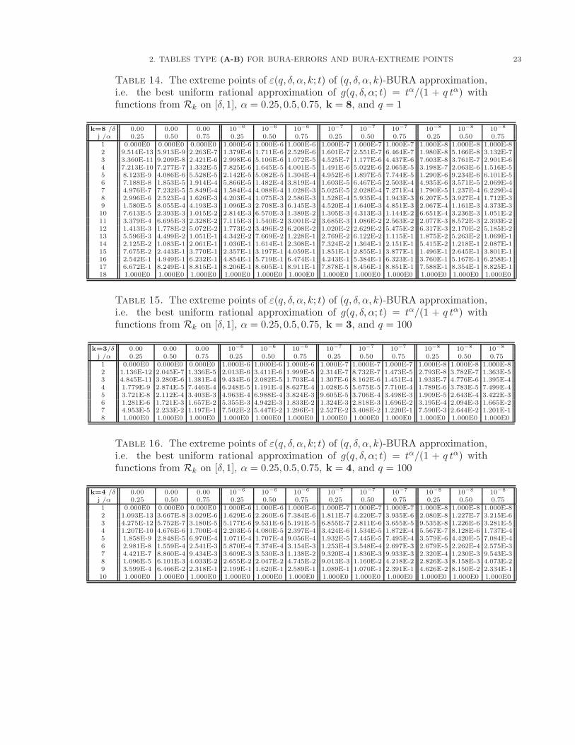
Table 14. The extreme points of ε(q, δ, α, k; t) of (q, δ, α, k)-BURA approximation,i.e. the best uniform rational approximation of g(q, δ, α; t) = tα/(1 + q tα) withfunctions from Rk on [δ, 1], α = 0.25, 0.5, 0.75, k = 8, and q = 1
k=8 /δ 0.00 0.00 0.00 10−6 10−6 10−6 10−7 10−7 10−7 10−8 10−8 10−8
j /α 0.25 0.50 0.75 0.25 0.50 0.75 0.25 0.50 0.75 0.25 0.50 0.751 0.000E0 0.000E0 0.000E0 1.000E-6 1.000E-6 1.000E-6 1.000E-7 1.000E-7 1.000E-7 1.000E-8 1.000E-8 1.000E-82 9.514E-13 5.913E-9 2.263E-7 1.379E-6 1.711E-6 2.529E-6 1.601E-7 2.551E-7 6.464E-7 1.980E-8 5.166E-8 3.132E-73 3.360E-11 9.209E-8 2.421E-6 2.998E-6 5.106E-6 1.072E-5 4.525E-7 1.177E-6 4.437E-6 7.603E-8 3.761E-7 2.901E-64 7.213E-10 7.277E-7 1.332E-5 7.825E-6 1.645E-5 4.001E-5 1.491E-6 5.022E-6 2.065E-5 3.198E-7 2.063E-6 1.516E-55 8.123E-9 4.086E-6 5.528E-5 2.142E-5 5.082E-5 1.304E-4 4.952E-6 1.897E-5 7.744E-5 1.290E-6 9.234E-6 6.101E-56 7.188E-8 1.853E-5 1.914E-4 5.866E-5 1.482E-4 3.819E-4 1.603E-5 6.467E-5 2.503E-4 4.935E-6 3.571E-5 2.069E-47 4.976E-7 7.232E-5 5.849E-4 1.584E-4 4.088E-4 1.028E-3 5.025E-5 2.028E-4 7.271E-4 1.790E-5 1.237E-4 6.229E-48 2.996E-6 2.523E-4 1.626E-3 4.203E-4 1.075E-3 2.586E-3 1.528E-4 5.935E-4 1.943E-3 6.207E-5 3.927E-4 1.712E-39 1.580E-5 8.055E-4 4.193E-3 1.096E-3 2.708E-3 6.145E-3 4.520E-4 1.640E-3 4.851E-3 2.067E-4 1.161E-3 4.373E-310 7.613E-5 2.393E-3 1.015E-2 2.814E-3 6.570E-3 1.389E-2 1.305E-3 4.313E-3 1.144E-2 6.651E-4 3.236E-3 1.051E-211 3.379E-4 6.695E-3 2.328E-2 7.115E-3 1.540E-2 3.001E-2 3.685E-3 1.086E-2 2.563E-2 2.077E-3 8.572E-3 2.393E-212 1.413E-3 1.778E-2 5.072E-2 1.773E-2 3.496E-2 6.208E-2 1.020E-2 2.629E-2 5.475E-2 6.317E-3 2.170E-2 5.185E-213 5.596E-3 4.499E-2 1.051E-1 4.342E-2 7.669E-2 1.228E-1 2.769E-2 6.122E-2 1.115E-1 1.875E-2 5.263E-2 1.069E-114 2.125E-2 1.083E-1 2.061E-1 1.036E-1 1.614E-1 2.308E-1 7.324E-2 1.364E-1 2.151E-1 5.415E-2 1.218E-1 2.087E-115 7.675E-2 2.443E-1 3.770E-1 2.357E-1 3.197E-1 4.059E-1 1.851E-1 2.855E-1 3.877E-1 1.496E-1 2.645E-1 3.801E-116 2.542E-1 4.949E-1 6.232E-1 4.854E-1 5.719E-1 6.474E-1 4.243E-1 5.384E-1 6.323E-1 3.760E-1 5.167E-1 6.258E-117 6.672E-1 8.249E-1 8.815E-1 8.206E-1 8.605E-1 8.911E-1 7.878E-1 8.456E-1 8.851E-1 7.588E-1 8.354E-1 8.825E-118 1.000E0 1.000E0 1.000E0 1.000E0 1.000E0 1.000E0 1.000E0 1.000E0 1.000E0 1.000E0 1.000E0 1.000E0
Table 15. The extreme points of ε(q, δ, α, k; t) of (q, δ, α, k)-BURA approximation,i.e. the best uniform rational approximation of g(q, δ, α; t) = tα/(1 + q tα) withfunctions from Rk on [δ, 1], α = 0.25, 0.5, 0.75, k = 3, and q = 100
k=3/δ 0.00 0.00 0.00 10−6 10−6 10−6 10−7 10−7 10−7 10−8 10−8 10−8
j /α 0.25 0.50 0.75 0.25 0.50 0.75 0.25 0.50 0.75 0.25 0.50 0.751 0.000E0 0.000E0 0.000E0 1.000E-6 1.000E-6 1.000E-6 1.000E-7 1.000E-7 1.000E-7 1.000E-8 1.000E-8 1.000E-82 1.136E-12 2.045E-7 1.336E-5 2.013E-6 3.411E-6 1.999E-5 2.314E-7 8.732E-7 1.473E-5 2.793E-8 3.782E-7 1.363E-53 4.845E-11 3.280E-6 1.381E-4 9.434E-6 2.082E-5 1.703E-4 1.307E-6 8.162E-6 1.451E-4 1.933E-7 4.776E-6 1.395E-44 1.779E-9 2.874E-5 7.446E-4 6.248E-5 1.191E-4 8.627E-4 1.028E-5 5.675E-5 7.710E-4 1.789E-6 3.783E-5 7.499E-45 3.721E-8 2.112E-4 3.403E-3 4.963E-4 6.988E-4 3.824E-3 9.605E-5 3.706E-4 3.498E-3 1.909E-5 2.643E-4 3.422E-36 1.281E-6 1.721E-3 1.657E-2 5.355E-3 4.942E-3 1.833E-2 1.324E-3 2.818E-3 1.696E-2 3.195E-4 2.094E-3 1.665E-27 4.953E-5 2.233E-2 1.197E-1 7.502E-2 5.447E-2 1.296E-1 2.527E-2 3.408E-2 1.220E-1 7.590E-3 2.644E-2 1.201E-18 1.000E0 1.000E0 1.000E0 1.000E0 1.000E0 1.000E0 1.000E0 1.000E0 1.000E0 1.000E0 1.000E0 1.000E0
Table 16. The extreme points of ε(q, δ, α, k; t) of (q, δ, α, k)-BURA approximation,i.e. the best uniform rational approximation of g(q, δ, α; t) = tα/(1 + q tα) withfunctions from Rk on [δ, 1], α = 0.25, 0.5, 0.75, k = 4, and q = 100
k=4 /δ 0.00 0.00 0.00 10−6 10−6 10−6 10−7 10−7 10−7 10−8 10−8 10−8
j /α 0.25 0.50 0.75 0.25 0.50 0.75 0.25 0.50 0.75 0.25 0.50 0.751 0.000E0 0.000E0 0.000E0 1.000E-6 1.000E-6 1.000E-6 1.000E-7 1.000E-7 1.000E-7 1.000E-8 1.000E-8 1.000E-82 1.093E-13 3.667E-8 3.029E-6 1.629E-6 2.260E-6 7.384E-6 1.811E-7 4.220E-7 3.935E-6 2.080E-8 1.227E-7 3.215E-63 4.275E-12 5.752E-7 3.180E-5 5.177E-6 9.531E-6 5.191E-5 6.855E-7 2.811E-6 3.655E-5 9.535E-8 1.226E-6 3.281E-54 1.207E-10 4.676E-6 1.700E-4 2.203E-5 4.080E-5 2.397E-4 3.424E-6 1.534E-5 1.872E-4 5.567E-7 8.128E-6 1.737E-45 1.858E-9 2.848E-5 6.970E-4 1.071E-4 1.707E-4 9.056E-4 1.932E-5 7.445E-5 7.495E-4 3.579E-6 4.420E-5 7.084E-46 2.981E-8 1.559E-4 2.541E-3 5.870E-4 7.374E-4 3.154E-3 1.253E-4 3.548E-4 2.697E-3 2.679E-5 2.262E-4 2.575E-37 4.421E-7 8.860E-4 9.434E-3 3.609E-3 3.530E-3 1.138E-2 9.320E-4 1.836E-3 9.933E-3 2.320E-4 1.230E-3 9.543E-38 1.096E-5 6.101E-3 4.033E-2 2.655E-2 2.047E-2 4.745E-2 9.013E-3 1.160E-2 4.218E-2 2.826E-3 8.158E-3 4.073E-29 3.599E-4 6.466E-2 2.318E-1 2.199E-1 1.620E-1 2.589E-1 1.089E-1 1.070E-1 2.391E-1 4.626E-2 8.150E-2 2.334E-110 1.000E0 1.000E0 1.000E0 1.000E0 1.000E0 1.000E0 1.000E0 1.000E0 1.000E0 1.000E0 1.000E0 1.000E0
24 2. TABLES
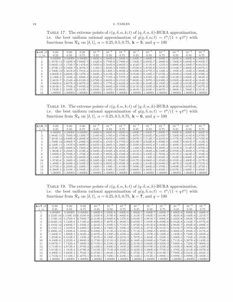
Table 17. The extreme points of ε(q, δ, α, k; t) of (q, δ, α, k)-BURA approximation,i.e. the best uniform rational approximation of g(q, δ, α; t) = tα/(1 + q tα) withfunctions from Rk on [δ, 1], α = 0.25, 0.5, 0.75, k = 5, and q = 100
k=5 /δ 0.00 0.00 0.00 10−6 10−6 10−6 10−7 10−7 10−7 10−8 10−8 10−8
j /α 0.25 0.50 0.75 0.25 0.50 0.75 0.25 0.50 0.75 0.25 0.50 0.751 0.000E0 0.000E0 0.000E0 1.000E-6 1.000E-6 1.000E-6 1.000E-7 1.000E-7 1.000E-7 1.000E-8 1.000E-8 1.000E-82 1.357E-14 7.520E-9 7.680E-7 1.432E-6 1.770E-6 3.790E-6 1.556E-7 2.695E-7 1.368E-6 1.730E-8 5.683E-8 8.935E-73 5.084E-13 1.173E-7 8.147E-6 3.505E-6 5.584E-6 2.065E-5 4.454E-7 1.311E-6 1.121E-5 5.898E-8 4.340E-7 8.841E-64 1.273E-11 9.346E-7 4.407E-5 1.118E-5 1.922E-5 8.592E-5 1.653E-6 5.873E-6 5.521E-5 2.544E-7 2.468E-6 4.667E-55 1.706E-10 5.381E-6 1.791E-4 4.021E-5 6.536E-5 2.983E-4 6.829E-6 2.377E-5 2.122E-4 1.195E-6 1.163E-5 1.869E-46 2.066E-9 2.600E-5 6.127E-4 1.560E-4 2.215E-4 9.241E-4 3.053E-5 9.108E-5 7.015E-4 6.058E-6 4.936E-5 6.339E-47 2.138E-8 1.164E-4 1.928E-3 6.452E-4 7.715E-4 2.727E-3 1.468E-4 3.478E-4 2.159E-3 3.313E-5 2.026E-4 1.984E-38 2.481E-7 5.254E-4 6.013E-3 2.878E-3 2.862E-3 8.151E-3 7.803E-4 1.397E-3 6.639E-3 2.050E-4 8.601E-4 6.164E-39 3.066E-6 2.607E-3 2.007E-2 1.389E-2 1.177E-2 2.624E-2 4.613E-3 6.244E-3 2.190E-2 1.442E-3 4.052E-3 2.052E-210 6.204E-5 1.576E-2 7.685E-2 7.355E-2 5.606E-2 9.593E-2 3.211E-2 3.323E-2 8.265E-2 1.284E-2 2.304E-2 7.827E-211 1.763E-3 1.343E-1 3.513E-1 3.850E-1 3.107E-1 3.995E-1 2.461E-1 2.249E-1 3.667E-1 1.386E-1 1.760E-1 3.551E-112 1.000E0 1.000E0 1.000E0 1.000E0 1.000E0 1.000E0 1.000E0 1.000E0 1.000E0 1.000E0 1.000E0 1.000E0
Table 18. The extreme points of ε(q, δ, α, k; t) of (q, δ, α, k)-BURA approximation,i.e. the best uniform rational approximation of g(q, δ, α; t) = tα/(1 + q tα) withfunctions from Rk on [δ, 1], α = 0.25, 0.5, 0.75, k = 6, and q = 100
k=6 /δ 0.00 0.00 0.00 10−6 10−6 10−6 10−7 10−7 10−7 10−8 10−8 10−8
j /α 0.25 0.50 0.75 0.25 0.50 0.75 0.25 0.50 0.75 0.25 0.50 0.751 0.000E0 0.000E0 0.000E0 1.000E-6 1.000E-6 1.000E-6 1.000E-7 1.000E-7 1.000E-7 1.000E-8 1.000E-8 1.000E-82 1.984E-15 1.700E-9 2.129E-7 1.316E-6 1.519E-6 2.479E-6 1.407E-7 2.032E-7 6.245E-7 1.530E-8 3.414E-8 2.979E-73 7.261E-14 2.649E-8 2.269E-6 2.681E-6 3.825E-6 1.030E-5 3.287E-7 7.514E-7 4.221E-6 4.177E-8 1.970E-7 2.735E-64 1.708E-12 2.098E-7 1.238E-5 6.953E-6 1.101E-5 3.775E-5 9.818E-7 2.822E-6 1.938E-5 1.440E-7 9.601E-7 1.415E-55 2.129E-11 1.187E-6 5.069E-5 2.025E-5 3.206E-5 1.208E-4 3.259E-6 9.905E-6 7.145E-5 5.409E-7 4.016E-6 5.609E-56 2.254E-10 5.499E-6 1.726E-4 6.285E-5 9.274E-5 3.479E-4 1.148E-5 3.290E-5 2.269E-4 2.141E-6 1.513E-5 1.870E-47 1.962E-9 2.256E-5 5.219E-4 2.040E-4 2.692E-4 9.355E-4 4.241E-5 1.062E-4 6.539E-4 8.876E-6 5.365E-5 5.573E-48 1.690E-8 8.709E-5 1.473E-3 6.910E-4 7.985E-4 2.433E-3 1.651E-4 3.435E-4 1.785E-3 3.911E-5 1.864E-4 1.558E-39 1.419E-7 3.343E-4 4.083E-3 2.446E-3 2.470E-3 6.356E-3 6.806E-4 1.149E-3 4.832E-3 1.843E-4 6.608E-4 4.287E-310 1.374E-6 1.348E-3 1.166E-2 9.106E-3 8.129E-3 1.729E-2 3.017E-3 4.096E-3 1.354E-2 9.555E-4 2.490E-3 1.217E-211 1.499E-5 6.049E-3 3.592E-2 3.560E-2 2.905E-2 5.059E-2 1.444E-2 1.610E-2 4.094E-2 5.487E-3 1.042E-2 3.731E-212 2.575E-4 3.236E-2 1.236E-1 1.439E-1 1.139E-1 1.615E-1 7.569E-2 7.206E-2 1.370E-1 3.669E-2 5.075E-2 1.273E-113 6.286E-3 2.210E-1 4.584E-1 5.251E-1 4.558E-1 5.243E-1 3.906E-1 3.585E-1 4.834E-1 2.657E-1 2.929E-1 4.656E-114 1.000E0 1.000E0 1.000E0 1.000E0 1.000E0 1.000E0 1.000E0 1.000E0 1.000E0 1.000E0 1.000E0 1.000E0
Table 19. The extreme points of ε(q, δ, α, k; t) of (q, δ, α, k)-BURA approximation,i.e. the best uniform rational approximation of g(q, δ, α; t) = tα/(1 + q tα) withfunctions from Rk on [δ, 1], α = 0.25, 0.5, 0.75, k = 7, and q = 100
k=7 /δ 0.00 0.00 0.00 10−6 10−6 10−6 10−7 10−7 10−7 10−8 10−8 10−8
j /α 0.25 0.50 0.75 0.25 0.50 0.75 0.25 0.50 0.75 0.25 0.50 0.751 0.000E0 0.000E0 0.000E0 1.000E-6 1.000E-6 1.000E-6 1.000E-7 1.000E-7 1.000E-7 1.000E-8 1.000E-8 1.000E-82 3.253E-16 4.158E-10 6.353E-8 1.243E-6 1.373E-6 1.896E-6 1.312E-7 1.692E-7 3.618E-7 1.403E-8 2.440E-8 1.221E-73 1.174E-14 6.476E-9 6.786E-7 2.213E-6 2.908E-6 6.137E-6 2.634E-7 4.981E-7 1.936E-6 3.232E-8 1.082E-7 9.858E-74 2.664E-13 5.122E-8 3.719E-6 4.909E-6 7.207E-6 1.963E-5 6.659E-7 1.595E-6 8.059E-6 9.354E-8 4.523E-7 4.877E-65 3.191E-12 2.883E-7 1.533E-5 1.221E-5 1.849E-5 5.751E-5 1.872E-6 4.951E-6 2.803E-5 2.963E-7 1.692E-6 1.889E-56 3.141E-11 1.316E-6 5.249E-5 3.224E-5 4.746E-5 1.550E-4 5.559E-6 1.471E-5 8.551E-5 9.815E-7 5.787E-6 6.206E-57 2.490E-10 5.229E-6 1.583E-4 8.838E-5 1.215E-4 3.913E-4 1.711E-5 4.229E-5 2.369E-4 3.360E-6 1.856E-5 1.817E-48 1.846E-9 1.896E-5 4.362E-4 2.497E-4 3.130E-4 9.433E-4 5.450E-5 1.197E-4 6.129E-4 1.193E-5 5.729E-5 4.895E-49 1.276E-8 6.533E-5 1.135E-3 7.257E-4 8.199E-4 2.221E-3 1.797E-4 3.403E-4 1.522E-3 4.406E-5 1.745E-4 1.253E-310 9.100E-8 2.222E-4 2.880E-3 2.173E-3 2.211E-3 5.233E-3 6.168E-4 9.898E-4 3.734E-3 1.711E-4 5.387E-4 3.143E-311 6.687E-7 7.742E-4 7.389E-3 6.715E-3 6.210E-3 1.263E-2 2.213E-3 3.002E-3 9.322E-3 7.030E-4 1.728E-3 7.988E-312 5.713E-6 2.872E-3 1.978E-2 2.143E-2 1.836E-2 3.185E-2 8.358E-3 9.670E-3 2.433E-2 3.103E-3 5.909E-3 2.120E-213 5.613E-5 1.181E-2 5.679E-2 7.015E-2 5.751E-2 8.502E-2 3.323E-2 3.366E-2 6.775E-2 1.478E-2 2.211E-2 6.027E-214 8.290E-4 5.620E-2 1.764E-1 2.274E-1 1.884E-1 2.376E-1 1.372E-1 1.273E-1 2.013E-1 7.700E-2 9.241E-2 1.845E-115 1.715E-2 3.112E-1 5.467E-1 6.313E-1 5.748E-1 6.243E-1 5.144E-1 4.812E-1 5.808E-1 3.939E-1 4.099E-1 5.582E-116 1.000E0 1.000E0 1.000E0 1.000E0 1.000E0 1.000E0 1.000E0 1.000E0 1.000E0 1.000E0 1.000E0 1.000E0

3. TABLES TYPE (C) FOR BURA-POLES 25
Table 20. The extreme points of ε(q, δ, α, k; t) of (q, δ, α, k)-BURA approximation,i.e. the best uniform rational approximation of g(q, δ, α; t) = tα/(1 + q tα) withfunctions from Rk on [δ, 1], α = 0.25, 0.5, 0.75, k = 8, and q = 100
k=8 /δ 0.00 0.00 0.00 10−6 10−6 10−6 10−7 10−7 10−7 10−8 10−8 10−8
j /α 0.25 0.50 0.75 0.25 0.50 0.75 0.25 0.50 0.75 0.25 0.50 0.751 0.000E0 0.000E0 1.000E-6 1.000E-6 1.000E-6 1.000E-7 1.000E-7 1.000E-7 1.000E-8 1.000E-8 1.000E-82 1.087E-10 2.018E-8 1.192E-6 1.282E-6 1.596E-6 1.247E-7 1.496E-7 2.507E-7 1.318E-8 1.949E-8 6.184E-83 1.692E-9 2.158E-7 1.921E-6 2.374E-6 4.180E-6 2.231E-7 3.661E-7 1.054E-6 2.660E-8 6.855E-8 4.179E-74 1.338E-8 1.185E-6 3.773E-6 5.191E-6 1.169E-5 4.941E-7 1.018E-6 3.912E-6 6.684E-8 2.474E-7 1.930E-65 7.516E-8 4.902E-6 8.284E-6 1.196E-5 3.128E-5 1.218E-6 2.830E-6 1.267E-5 1.847E-7 8.323E-7 7.181E-66 3.416E-7 1.687E-5 1.932E-5 2.785E-5 7.882E-5 3.170E-6 7.646E-6 3.677E-5 5.334E-7 2.607E-6 2.301E-57 1.342E-6 5.114E-5 4.667E-5 6.478E-5 1.881E-4 8.519E-6 2.007E-5 9.803E-5 1.583E-6 7.710E-6 6.613E-58 4.747E-6 1.408E-4 1.156E-4 1.507E-4 4.293E-4 2.348E-5 5.167E-5 2.444E-4 4.816E-6 2.186E-5 1.748E-49 1.562E-5 3.607E-4 2.922E-4 3.529E-4 9.491E-4 6.627E-5 1.319E-4 5.794E-4 1.503E-5 6.041E-5 4.340E-410 4.918E-5 8.792E-4 7.536E-4 8.372E-4 2.062E-3 1.919E-4 3.378E-4 1.330E-3 4.838E-5 1.655E-4 1.032E-311 1.522E-4 2.088E-3 1.984E-3 2.029E-3 4.476E-3 5.711E-4 8.801E-4 3.017E-3 1.611E-4 4.574E-4 2.407E-312 4.757E-4 4.951E-3 5.339E-3 5.055E-3 9.856E-3 1.753E-3 2.360E-3 6.895E-3 5.587E-4 1.297E-3 5.625E-313 1.543E-3 1.201E-2 1.468E-2 1.304E-2 2.233E-2 5.564E-3 6.586E-3 1.619E-2 2.026E-3 3.835E-3 1.348E-214 5.340E-3 3.047E-2 4.113E-2 3.493E-2 5.254E-2 1.830E-2 1.933E-2 3.965E-2 7.752E-3 1.202E-2 3.373E-215 2.026E-2 8.193E-2 1.159E-1 9.694E-2 1.284E-1 6.198E-2 6.000E-2 1.020E-1 3.127E-2 4.042E-2 8.920E-216 8.635E-2 2.314E-1 3.136E-1 2.704E-1 3.169E-1 2.096E-1 1.941E-1 2.704E-1 1.315E-1 1.459E-1 2.459E-117 3.955E-1 6.172E-1 7.095E-1 6.656E-1 7.008E-1 6.118E-1 5.823E-1 6.585E-1 5.050E-1 5.130E-1 6.333E-118 1.000E0 1.000E0 1.000E0 1.000E0 1.000E0 1.000E0 1.000E0 1.000E0 1.000E0 1.000E0 1.000E0
Table 21. The extreme points of ε(q, δ, α, k; t) of (q, δ, α, k)-BURA approximation,i.e. the best uniform rational approximation of g(q, δ, α; t) = tα/(1 + q tα) withfunctions from Rk on [δ, 1], α = 0.25, 0.5, 0.75, k = 3, and q = 200
k=3 /δ 0.00 0.00 0.00 10−6 10−6 10−6 10−7 10−7 10−7 10−8 10−8 10−8
j /α 0.25 0.50 0.75 0.25 0.50 0.75 0.25 0.50 0.75 0.25 0.50 0.751 0.000E0 0.000E0 0.000E0 1.000E-6 1.000E-6 1.000E-6 1.000E-7 1.000E-7 1.000E-7 1.000E-8 1.000E-8 1.000E-82 7.673E-14 5.630E-8 5.903E-6 1.922E-6 2.490E-6 1.106E-5 2.115E-7 4.920E-7 6.978E-6 2.376E-8 1.572E-7 6.120E-63 3.286E-12 9.051E-7 6.095E-5 8.531E-6 1.212E-5 8.523E-5 1.086E-6 3.697E-6 6.648E-5 1.413E-7 1.720E-6 6.209E-54 1.222E-10 7.992E-6 3.299E-4 5.497E-5 6.304E-5 4.196E-4 8.108E-6 2.357E-5 3.509E-4 1.199E-6 1.292E-5 3.342E-45 2.594E-9 5.980E-5 1.534E-3 4.338E-4 3.601E-4 1.866E-3 7.449E-5 1.501E-4 1.612E-3 1.236E-5 8.935E-5 1.550E-36 9.325E-8 5.073E-4 7.786E-3 4.723E-3 2.603E-3 9.290E-3 1.033E-3 1.166E-3 8.143E-3 2.060E-4 7.277E-4 7.861E-37 3.798E-6 7.250E-3 6.395E-2 6.800E-2 3.132E-2 7.437E-2 2.038E-2 1.541E-2 6.646E-2 5.061E-3 1.007E-2 6.448E-28 1.000E0 1.000E0 1.000E0 1.000E0 1.000E0 1.000E0 1.000E0 1.000E0 1.000E0 1.000E0 1.000E0 1.000E0
Table 22. The extreme points of ε(q, δ, α, k; t) of (q, δ, α, k)-BURA approximation,i.e. the best uniform rational approximation of g(q, δ, α; t) = tα/(1 + q tα) withfunctions from Rk on [δ, 1], α = 0.25, 0.5, 0.75, k = 4, and q = 200
k=4 /δ 0.00 0.00 0.00 10−6 10−6 10−6 10−7 10−7 10−7 10−8 10−8 10−8
j /α 0.25 0.50 0.75 0.25 0.50 0.75 0.25 0.50 0.75 0.25 0.50 0.751 0.000E0 0.000E0 0.000E0 1.000E-6 1.000E-6 1.000E-6 1.000E-7 1.000E-7 1.000E-7 1.000E-8 1.000E-8 1.000E-82 7.638E-15 1.067E-8 1.408E-6 1.583E-6 1.869E-6 4.909E-6 1.712E-7 2.934E-7 2.123E-6 1.875E-8 6.576E-8 1.557E-63 2.997E-13 1.675E-7 1.476E-5 4.829E-6 6.463E-6 2.991E-5 6.006E-7 1.551E-6 1.843E-5 7.581E-8 5.396E-7 1.557E-54 8.537E-12 1.367E-6 7.883E-5 2.004E-5 2.489E-5 1.305E-4 2.866E-6 7.575E-6 9.211E-5 4.102E-7 3.277E-6 8.181E-55 1.327E-10 8.402E-6 3.247E-4 9.640E-5 9.927E-5 4.808E-4 1.584E-5 3.485E-5 3.659E-4 2.539E-6 1.712E-5 3.340E-46 2.176E-9 4.693E-5 1.202E-3 5.279E-4 4.250E-4 1.678E-3 1.022E-4 1.640E-4 1.329E-3 1.870E-5 8.699E-5 1.231E-37 3.319E-8 2.769E-4 4.627E-3 3.269E-3 2.081E-3 6.240E-3 7.655E-4 8.666E-4 5.062E-3 1.628E-4 4.846E-4 4.726E-38 8.824E-7 2.046E-3 2.121E-2 2.446E-2 1.277E-2 2.779E-2 7.595E-3 5.816E-3 2.301E-2 2.047E-3 3.421E-3 2.163E-29 3.160E-5 2.539E-2 1.455E-1 2.088E-1 1.146E-1 1.783E-1 9.618E-2 6.171E-2 1.548E-1 3.562E-2 3.961E-2 1.476E-110 1.000E0 1.000E0 1.000E0 1.000E0 1.000E0 1.000E0 1.000E0 1.000E0 1.000E0 1.000E0 1.000E0 1.000E0
3. Tables type (c) for BURA-poles
Now we provide the data about the poles of the BURA element rq,δ,α,k(t):
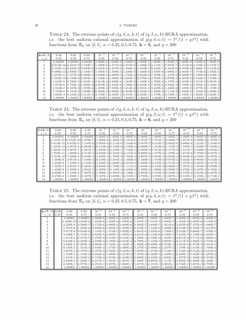
26 2. TABLES
Table 23. The extreme points of ε(q, δ, α, k; t) of (q, δ, α, k)-BURA approximation,i.e. the best uniform rational approximation of g(q, δ, α; t) = tα/(1 + q tα) withfunctions from Rk on [δ, 1], α = 0.25, 0.5, 0.75, k = 5, and q = 200
k=5 /δ 0.00 0.00 0.00 10−6 10−6 10−6 10−7 10−7 10−7 10−8 10−8 10−8
j /α 0.25 0.50 0.75 0.25 0.50 0.75 0.25 0.50 0.75 0.25 0.50 0.751 0.000E0 0.000E0 0.000E0 1.000E-6 1.000E-6 1.000E-6 1.000E-7 1.000E-7 1.000E-7 1.000E-8 1.000E-8 1.000E-82 9.914E-16 2.321E-9 3.740E-7 1.406E-6 1.571E-6 2.915E-6 1.499E-7 2.141E-7 8.567E-7 1.614E-8 3.740E-8 4.747E-73 3.723E-14 3.622E-8 3.963E-6 3.335E-6 4.217E-6 1.358E-5 4.043E-7 8.434E-7 6.325E-6 4.970E-8 2.300E-7 4.515E-64 9.388E-13 2.890E-7 2.140E-5 1.040E-5 1.308E-5 5.246E-5 1.440E-6 3.358E-6 2.988E-5 2.004E-7 1.174E-6 2.346E-55 1.267E-11 1.671E-6 8.689E-5 3.698E-5 4.200E-5 1.744E-4 5.824E-6 1.270E-5 1.121E-4 9.060E-7 5.198E-6 9.318E-56 1.558E-10 8.159E-6 2.985E-4 1.428E-4 1.388E-4 5.293E-4 2.578E-5 4.705E-5 3.670E-4 4.505E-6 2.140E-5 3.158E-47 1.643E-9 3.726E-5 9.524E-4 5.914E-4 4.836E-4 1.563E-3 1.239E-4 1.788E-4 1.137E-3 2.452E-5 8.751E-5 9.991E-48 1.974E-8 1.742E-4 3.058E-3 2.653E-3 1.833E-3 4.780E-3 6.642E-4 7.327E-4 3.584E-3 1.530E-4 3.795E-4 3.192E-39 2.554E-7 9.167E-4 1.076E-2 1.293E-2 7.858E-3 1.614E-2 3.991E-3 3.430E-3 1.243E-2 1.100E-3 1.877E-3 1.119E-210 5.733E-6 6.121E-3 4.509E-2 6.968E-2 4.009E-2 6.403E-2 2.859E-2 1.980E-2 5.114E-2 1.023E-2 1.165E-2 4.666E-211 1.856E-4 6.433E-2 2.511E-1 3.745E-1 2.533E-1 3.151E-1 2.294E-1 1.579E-1 2.729E-1 1.185E-1 1.069E-1 2.569E-112 1.000E0 1.000E0 1.000E0 1.000E0 1.000E0 1.000E0 1.000E0 1.000E0 1.000E0 1.000E0 1.000E0 1.000E0
Table 24. The extreme points of ε(q, δ, α, k; t) of (q, δ, α, k)-BURA approximation,i.e. the best uniform rational approximation of g(q, δ, α; t) = tα/(1 + q tα) withfunctions from Rk on [δ, 1], α = 0.25, 0.5, 0.75, k = 6, and q = 200
k=6 /δ 0.00 0.00 0.00 10−6 10−6 10−6 10−7 10−7 10−7 10−8 10−8 10−8
j /α 0.25 0.50 0.75 0.25 0.50 0.75 0.25 0.50 0.75 0.25 0.50 0.751 0.000E0 0.000E0 0.000E0 1.000E-6 1.000E-6 1.000E-6 1.000E-7 1.000E-7 1.000E-7 1.000E-8 1.000E-8 1.000E-82 1.531E-16 5.552E-10 1.079E-7 1.300E-6 1.405E-6 2.101E-6 1.371E-7 1.751E-7 4.489E-7 1.457E-8 2.590E-8 1.767E-73 5.613E-15 8.652E-9 1.150E-6 2.585E-6 3.114E-6 7.534E-6 3.057E-7 5.413E-7 2.665E-6 3.666E-8 1.213E-7 1.518E-64 1.327E-13 6.857E-8 6.264E-6 6.573E-6 8.149E-6 2.549E-5 8.809E-7 1.813E-6 1.157E-5 1.190E-7 5.269E-7 7.649E-65 1.665E-12 3.887E-7 2.561E-5 1.892E-5 2.233E-5 7.742E-5 2.862E-6 5.913E-6 4.117E-5 4.311E-7 2.049E-6 2.984E-56 1.783E-11 1.809E-6 8.712E-5 5.838E-5 6.244E-5 2.157E-4 9.969E-6 1.877E-5 1.278E-4 1.671E-6 7.376E-6 9.847E-57 1.574E-10 7.499E-6 2.644E-4 1.892E-4 1.789E-4 5.700E-4 3.667E-5 5.934E-5 3.643E-4 6.863E-6 2.556E-5 2.927E-48 1.388E-9 2.951E-5 7.548E-4 6.419E-4 5.331E-4 1.482E-3 1.430E-4 1.919E-4 9.974E-4 3.024E-5 8.864E-5 8.242E-49 1.202E-8 1.169E-4 2.142E-3 2.283E-3 1.680E-3 3.941E-3 5.936E-4 6.535E-4 2.751E-3 1.437E-4 3.201E-4 2.317E-310 1.226E-7 4.955E-4 6.365E-3 8.560E-3 5.709E-3 1.111E-2 2.664E-3 2.418E-3 8.000E-3 7.587E-4 1.254E-3 6.839E-311 1.429E-6 2.398E-3 2.091E-2 3.382E-2 2.138E-2 3.436E-2 1.298E-2 1.006E-2 2.566E-2 4.476E-3 5.587E-3 2.230E-212 2.828E-5 1.448E-2 7.967E-2 1.388E-1 8.991E-2 1.196E-1 6.985E-2 4.918E-2 9.442E-2 3.125E-2 3.010E-2 8.407E-213 8.278E-4 1.258E-1 3.597E-1 5.167E-1 4.039E-1 4.512E-1 3.750E-1 2.873E-1 3.967E-1 2.418E-1 2.105E-1 3.712E-114 1.000E0 1.000E0 1.000E0 1.000E0 1.000E0 1.000E0 1.000E0 1.000E0 1.000E0 1.000E0 1.000E0 1.000E0
Table 25. The extreme points of ε(q, δ, α, k; t) of (q, δ, α, k)-BURA approximation,i.e. the best uniform rational approximation of g(q, δ, α; t) = tα/(1 + q tα) withfunctions from Rk on [δ, 1], α = 0.25, 0.5, 0.75, k = 7, and q = 200
k=7 /δ 0.00 0.00 0.00 10−6 10−6 10−6 10−7 10−7 10−7 10−8 10−8 10−8
j /α 0.25 0.50 0.75 0.25 0.50 0.75 0.25 0.50 0.75 0.25 0.50 0.751 0.000E0 0.000E0 1.000E-6 1.000E-6 1.000E-6 1.000E-7 1.000E-7 1.000E-7 1.000E-8 1.000E-8 1.000E-82 1.429E-10 3.334E-8 1.232E-6 1.302E-6 1.706E-6 1.287E-7 1.531E-7 2.895E-7 1.354E-8 2.029E-8 8.152E-83 2.226E-9 3.560E-7 2.153E-6 2.496E-6 4.868E-6 2.492E-7 3.894E-7 1.351E-6 2.922E-8 7.475E-8 5.986E-74 1.761E-8 1.950E-6 4.696E-6 5.685E-6 1.439E-5 6.104E-7 1.122E-6 5.268E-6 8.018E-8 2.789E-7 2.851E-65 9.917E-8 8.024E-6 1.154E-5 1.374E-5 3.992E-5 1.681E-6 3.236E-6 1.756E-5 2.452E-7 9.666E-7 1.078E-56 4.538E-7 2.744E-5 3.029E-5 3.395E-5 1.035E-4 4.931E-6 9.145E-6 5.196E-5 7.952E-7 3.134E-6 3.483E-57 1.811E-6 8.271E-5 8.279E-5 8.516E-5 2.543E-4 1.509E-5 2.550E-5 1.410E-4 2.691E-6 9.711E-6 1.008E-48 6.633E-6 2.284E-4 2.338E-4 2.180E-4 6.043E-4 4.799E-5 7.124E-5 3.605E-4 9.511E-6 2.946E-5 2.701E-49 2.326E-5 5.995E-4 6.808E-4 5.745E-4 1.422E-3 1.586E-4 2.029E-4 8.953E-4 3.521E-5 8.973E-5 6.941E-410 8.135E-5 1.551E-3 2.046E-3 1.575E-3 3.396E-3 5.477E-4 5.999E-4 2.227E-3 1.379E-4 2.813E-4 1.769E-311 2.957E-4 4.107E-3 6.357E-3 4.536E-3 8.422E-3 1.983E-3 1.874E-3 5.718E-3 5.744E-4 9.314E-4 4.631E-312 1.166E-3 1.154E-2 2.044E-2 1.388E-2 2.213E-2 7.587E-3 6.302E-3 1.559E-2 2.588E-3 3.342E-3 1.287E-213 5.231E-3 3.552E-2 6.753E-2 4.554E-2 6.258E-2 3.068E-2 2.329E-2 4.625E-2 1.267E-2 1.340E-2 3.912E-214 2.846E-2 1.228E-1 2.217E-1 1.591E-1 1.901E-1 1.296E-1 9.607E-2 1.511E-1 6.863E-2 6.209E-2 1.326E-115 2.028E-1 4.575E-1 6.251E-1 5.337E-1 5.664E-1 5.017E-1 4.181E-1 5.081E-1 3.716E-1 3.295E-1 4.759E-116 1.000E0 1.000E0 1.000E0 1.000E0 1.000E0 1.000E0 1.000E0 1.000E0 1.000E0 1.000E0 1.000E0
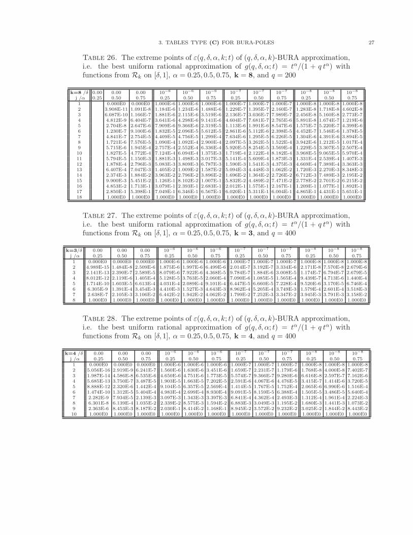
3. TABLES TYPE (C) FOR BURA-POLES 27
Table 26. The extreme points of ε(q, δ, α, k; t) of (q, δ, α, k)-BURA approximation,i.e. the best uniform rational approximation of g(q, δ, α; t) = tα/(1 + q tα) withfunctions from Rk on [δ, 1], α = 0.25, 0.5, 0.75, k = 8, and q = 200
k=8 /δ 0.00 0.00 0.00 10−6 10−6 10−6 10−7 10−7 10−7 10−8 10−8 10−8
j /α 0.25 0.50 0.75 0.25 0.50 0.75 0.25 0.50 0.75 0.25 0.50 0.751 0.000E0 0.000E0 1.000E-6 1.000E-6 1.000E-6 1.000E-7 1.000E-7 1.000E-7 1.000E-8 1.000E-8 1.000E-82 3.908E-11 1.091E-8 1.184E-6 1.234E-6 1.488E-6 1.229E-7 1.395E-7 2.160E-7 1.283E-8 1.718E-8 4.602E-83 6.087E-10 1.166E-7 1.881E-6 2.115E-6 3.519E-6 2.136E-7 3.036E-7 7.989E-7 2.456E-8 5.160E-8 2.773E-74 4.812E-9 6.404E-7 3.641E-6 4.298E-6 9.141E-6 4.604E-7 7.681E-7 2.765E-6 5.891E-8 1.674E-7 1.219E-65 2.704E-8 2.647E-6 7.909E-6 9.366E-6 2.319E-5 1.113E-6 1.991E-6 8.547E-6 1.575E-7 5.220E-7 4.399E-66 1.230E-7 9.100E-6 1.832E-5 2.096E-5 5.612E-5 2.861E-6 5.112E-6 2.398E-5 4.452E-7 1.546E-6 1.378E-57 4.841E-7 2.754E-5 4.409E-5 4.756E-5 1.299E-4 7.634E-6 1.295E-5 6.226E-5 1.304E-6 4.391E-6 3.894E-58 1.721E-6 7.576E-5 1.090E-4 1.092E-4 2.900E-4 2.097E-5 3.262E-5 1.522E-4 3.942E-6 1.212E-5 1.017E-49 5.715E-6 1.945E-4 2.757E-4 2.552E-4 6.336E-4 5.920E-5 8.254E-5 3.569E-4 1.229E-5 3.307E-5 2.507E-410 1.827E-5 4.772E-4 7.124E-4 6.094E-4 1.375E-3 1.719E-4 2.122E-4 8.182E-4 3.968E-5 9.065E-5 5.970E-411 5.794E-5 1.150E-3 1.881E-3 1.498E-3 3.017E-3 5.141E-4 5.609E-4 1.873E-3 1.331E-4 2.539E-4 1.407E-312 1.878E-4 2.796E-3 5.083E-3 3.809E-3 6.787E-3 1.590E-3 1.541E-3 4.375E-3 4.669E-4 7.389E-4 3.363E-313 6.407E-4 7.047E-3 1.405E-2 1.009E-2 1.587E-2 5.094E-3 4.448E-3 1.062E-2 1.720E-3 2.270E-3 8.348E-314 2.374E-3 1.884E-2 3.963E-2 2.796E-2 3.896E-2 1.696E-2 1.364E-2 2.726E-2 6.712E-3 7.489E-3 2.195E-215 9.900E-3 5.451E-2 1.126E-1 8.102E-2 1.007E-1 5.832E-2 4.489E-2 7.471E-2 2.778E-2 2.701E-2 6.215E-216 4.853E-2 1.713E-1 3.079E-1 2.393E-1 2.683E-1 2.012E-1 1.575E-1 2.167E-1 1.209E-1 1.077E-1 1.892E-117 2.850E-1 5.398E-1 7.049E-1 6.346E-1 6.567E-1 6.020E-1 5.311E-1 6.004E-1 4.865E-1 4.431E-1 5.651E-118 1.000E0 1.000E0 1.000E0 1.000E0 1.000E0 1.000E0 1.000E0 1.000E0 1.000E0 1.000E0 1.000E0
Table 27. The extreme points of ε(q, δ, α, k; t) of (q, δ, α, k)-BURA approximation,i.e. the best uniform rational approximation of g(q, δ, α; t) = tα/(1 + q tα) withfunctions from Rk on [δ, 1], α = 0.25, 0.5, 0.75, k = 3, and q = 400
k=3/δ 0.00 0.00 0.00 10−6 10−6 10−6 10−7 10−7 10−7 10−8 10−8 10−8
j /α 0.25 0.50 0.75 0.25 0.50 0.75 0.25 0.50 0.75 0.25 0.50 0.751 0.000E0 0.000E0 0.000E0 1.000E-6 1.000E-6 1.000E-6 1.000E-7 1.000E-7 1.000E-7 1.000E-8 1.000E-8 1.000E-82 4.989E-15 1.484E-8 2.509E-6 1.875E-6 1.997E-6 6.499E-6 2.014E-7 3.192E-7 3.334E-6 2.171E-8 7.570E-8 2.679E-63 2.141E-13 2.390E-7 2.589E-5 8.079E-6 7.922E-6 4.368E-5 9.784E-7 1.884E-6 3.008E-5 1.174E-7 6.794E-7 2.679E-54 8.012E-12 2.119E-6 1.405E-4 5.128E-5 3.763E-5 2.060E-4 7.090E-6 1.085E-5 1.565E-4 9.439E-7 4.713E-6 1.440E-45 1.714E-10 1.603E-5 6.613E-4 4.031E-4 2.089E-4 9.101E-4 6.447E-5 6.660E-5 7.228E-4 9.520E-6 3.170E-5 6.746E-46 6.305E-9 1.391E-4 3.454E-3 4.410E-3 1.527E-3 4.643E-3 8.962E-4 5.205E-4 3.749E-3 1.579E-4 2.601E-4 3.518E-37 2.638E-7 2.105E-3 3.106E-2 6.442E-2 1.942E-2 4.062E-2 1.799E-2 7.252E-3 3.347E-2 3.945E-3 3.791E-3 3.158E-28 1.000E0 1.000E0 1.000E0 1.000E0 1.000E0 1.000E0 1.000E0 1.000E0 1.000E0 1.000E0 1.000E0 1.000E0
Table 28. The extreme points of ε(q, δ, α, k; t) of (q, δ, α, k)-BURA approximation,i.e. the best uniform rational approximation of g(q, δ, α; t) = tα/(1 + q tα) withfunctions from Rk on [δ, 1], α = 0.25, 0.5, 0.75, k = 4, and q = 400
k=4 /δ 0.00 0.00 0.00 10−6 10−6 10−6 10−7 10−7 10−7 10−8 10−8 10−8
j /α 0.25 0.50 0.75 0.25 0.50 0.75 0.25 0.50 0.75 0.25 0.50 0.751 0.000E0 0.000E0 0.000E0 1.000E-6 1.000E-6 1.000E-6 1.000E-7 1.000E-7 1.000E-7 1.000E-8 1.000E-8 1.000E-82 5.056E-16 2.919E-9 6.241E-7 1.560E-6 1.630E-6 3.451E-6 1.659E-7 2.231E-7 1.179E-6 1.768E-8 4.000E-8 7.402E-73 1.987E-14 4.586E-8 6.535E-6 4.650E-6 4.751E-6 1.773E-5 5.574E-7 9.366E-7 9.280E-6 6.616E-8 2.597E-7 7.162E-64 5.685E-13 3.750E-7 3.487E-5 1.903E-5 1.663E-5 7.202E-5 2.591E-6 4.067E-6 4.476E-5 3.415E-7 1.414E-6 3.720E-55 8.888E-12 2.320E-6 1.442E-4 9.104E-5 6.357E-5 2.569E-4 1.414E-5 1.767E-5 1.752E-4 2.065E-6 6.990E-6 1.516E-46 1.474E-10 1.312E-5 5.404E-4 4.983E-4 2.699E-4 8.930E-4 9.091E-5 8.159E-5 6.388E-4 1.505E-5 3.486E-5 5.640E-47 2.282E-9 7.934E-5 2.139E-3 3.097E-3 1.343E-3 3.397E-3 6.841E-4 4.362E-4 2.493E-3 1.312E-4 1.961E-4 2.224E-38 6.301E-8 6.139E-4 1.035E-2 2.339E-2 8.575E-3 1.594E-2 6.883E-3 3.049E-3 1.195E-2 1.680E-3 1.441E-3 1.073E-29 2.363E-6 8.453E-3 8.187E-2 2.030E-1 8.414E-2 1.168E-1 8.945E-2 3.572E-2 9.232E-2 3.025E-2 1.844E-2 8.443E-210 1.000E0 1.000E0 1.000E0 1.000E0 1.000E0 1.000E0 1.000E0 1.000E0 1.000E0 1.000E0 1.000E0 1.000E0
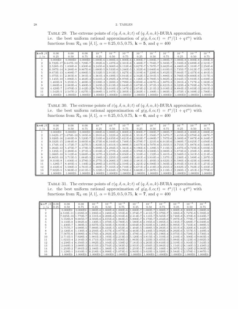
28 2. TABLES
Table 29. The extreme points of ε(q, δ, α, k; t) of (q, δ, α, k)-BURA approximation,i.e. the best uniform rational approximation of g(q, δ, α; t) = tα/(1 + q tα) withfunctions from Rk on [δ, 1], α = 0.25, 0.5, 0.75, k = 5, and q = 400
k=5 /δ 0.00 0.00 0.00 10−6 10−6 10−6 10−7 10−7 10−7 10−8 10−8 10−8
j /α 0.25 0.50 0.75 0.25 0.50 0.75 0.25 0.50 0.75 0.25 0.50 0.751 0.000E0 0.000E0 0.000E0 1.000E-6 1.000E-6 1.000E-6 1.000E-7 1.000E-7 1.000E-7 1.000E-8 1.000E-8 1.000E-82 6.722E-17 6.647E-10 1.729E-7 1.392E-6 1.437E-6 2.331E-6 1.468E-7 1.794E-7 5.583E-7 1.550E-8 2.689E-8 2.521E-73 2.528E-15 1.038E-8 1.830E-6 3.245E-6 3.368E-6 9.153E-6 3.827E-7 5.787E-7 3.602E-6 4.486E-8 1.310E-7 2.256E-64 6.397E-14 8.288E-8 9.867E-6 1.000E-5 9.533E-6 3.246E-5 1.332E-6 2.046E-6 1.610E-5 1.735E-7 5.912E-7 1.145E-55 8.673E-13 4.808E-7 4.006E-5 3.532E-5 2.913E-5 1.027E-4 5.319E-6 7.229E-6 5.852E-5 7.664E-7 2.437E-6 4.491E-56 1.075E-11 2.365E-6 1.381E-4 1.361E-4 9.439E-5 3.044E-4 2.342E-5 2.591E-5 1.888E-4 3.766E-6 9.666E-6 1.517E-47 1.145E-10 1.096E-5 4.462E-4 5.641E-4 3.292E-4 8.978E-4 1.126E-4 9.780E-5 5.862E-4 2.044E-5 3.910E-5 4.838E-48 1.403E-9 5.255E-5 1.469E-3 2.539E-3 1.269E-3 2.799E-3 6.059E-4 4.067E-4 1.887E-3 1.281E-4 1.717E-4 1.582E-39 1.860E-8 2.883E-4 5.400E-3 1.245E-2 5.613E-3 9.844E-3 3.673E-3 1.971E-3 6.821E-3 9.323E-4 8.793E-4 5.787E-310 4.429E-7 2.070E-3 2.442E-2 6.765E-2 3.016E-2 4.187E-2 2.674E-2 1.211E-2 3.018E-2 8.894E-3 5.833E-3 2.601E-211 1.542E-5 2.547E-2 1.627E-1 3.688E-1 2.107E-1 2.395E-1 2.202E-1 1.100E-1 1.903E-1 1.073E-1 6.169E-2 1.706E-112 1.000E0 1.000E0 1.000E0 1.000E0 1.000E0 1.000E0 1.000E0 1.000E0 1.000E0 1.000E0 1.000E0 1.000E0
Table 30. The extreme points of ε(q, δ, α, k; t) of (q, δ, α, k)-BURA approximation,i.e. the best uniform rational approximation of g(q, δ, α; t) = tα/(1 + q tα) withfunctions from Rk on [δ, 1], α = 0.25, 0.5, 0.75, k = 6, and q = 400
k=6 /δ 0.00 0.00 0.00 10−6 10−6 10−6 10−7 10−7 10−7 10−8 10−8 10−8
j /α 0.25 0.50 0.75 0.25 0.50 0.75 0.25 0.50 0.75 0.25 0.50 0.751 0.000E0 0.000E0 0.000E0 1.000E-6 1.000E-6 1.000E-6 1.000E-7 1.000E-7 1.000E-7 1.000E-8 1.000E-8 1.000E-82 1.042E-17 1.670E-10 5.185E-8 1.291E-6 1.322E-6 1.822E-6 1.351E-7 1.556E-7 3.347E-7 1.415E-8 2.078E-8 1.067E-73 3.926E-16 2.603E-9 5.520E-7 2.533E-6 2.635E-6 5.621E-6 2.933E-7 4.080E-7 1.707E-6 3.389E-8 7.887E-8 8.348E-74 9.332E-15 2.064E-8 3.005E-6 6.373E-6 6.344E-6 1.740E-5 8.279E-7 1.221E-6 6.913E-6 1.060E-7 3.025E-7 4.056E-65 1.174E-13 1.172E-7 1.227E-5 1.823E-5 1.651E-5 4.989E-5 2.657E-6 3.707E-6 2.355E-5 3.755E-7 1.087E-6 1.546E-56 1.264E-12 5.475E-7 4.173E-5 5.608E-5 4.494E-5 1.341E-4 9.196E-6 1.129E-5 7.113E-5 1.437E-6 3.723E-6 5.033E-57 1.125E-11 2.288E-6 1.271E-4 1.816E-4 1.277E-4 3.482E-4 3.376E-5 3.500E-5 2.000E-4 5.873E-6 1.258E-5 1.488E-48 1.006E-10 9.142E-6 3.668E-4 6.167E-4 3.824E-4 9.056E-4 1.318E-4 1.132E-4 5.481E-4 2.588E-5 4.341E-5 4.214E-49 8.865E-10 3.715E-5 1.064E-3 2.198E-3 1.225E-3 2.449E-3 5.491E-4 3.916E-4 1.537E-3 1.236E-4 1.589E-4 1.207E-310 9.310E-9 1.636E-4 3.278E-3 8.277E-3 4.268E-3 7.130E-3 2.481E-3 1.493E-3 4.622E-3 6.596E-4 6.423E-4 3.689E-311 1.128E-7 8.405E-4 1.140E-2 3.288E-2 1.657E-2 2.318E-2 1.221E-2 6.506E-3 1.563E-2 3.954E-3 3.011E-3 1.271E-212 2.432E-6 5.596E-3 4.761E-2 1.360E-1 7.355E-2 8.710E-2 6.671E-2 3.418E-2 6.255E-2 2.832E-2 1.762E-2 5.235E-213 7.922E-5 5.963E-2 2.611E-1 5.122E-1 3.624E-1 3.795E-1 3.662E-1 2.287E-1 3.113E-1 2.280E-1 1.451E-1 2.779E-114 1.000E0 1.000E0 1.000E0 1.000E0 1.000E0 1.000E0 1.000E0 1.000E0 1.000E0 1.000E0 1.000E0 1.000E0
Table 31. The extreme points of ε(q, δ, α, k; t) of (q, δ, α, k)-BURA approximation,i.e. the best uniform rational approximation of g(q, δ, α; t) = tα/(1 + q tα) withfunctions from Rk on [δ, 1], α = 0.25, 0.5, 0.75, k = 7, and q = 400
k=7 /δ 0.00 0.00 0.00 10−6 10−6 10−6 10−7 10−7 10−7 10−8 10−8 10−8
j /α 0.25 0.50 0.75 0.25 0.50 0.75 0.25 0.50 0.75 0.25 0.50 0.751 0.000E0 0.000E0 1.000E-6 1.000E-6 1.000E-6 1.000E-7 1.000E-7 1.000E-7 1.000E-8 1.000E-8 1.000E-82 4.510E-11 1.658E-8 1.226E-6 1.248E-6 1.555E-6 1.274E-7 1.411E-7 2.379E-7 1.326E-8 1.747E-8 5.592E-83 7.025E-10 1.770E-7 2.121E-6 2.200E-6 3.916E-6 2.414E-7 3.141E-7 9.565E-7 2.748E-8 5.370E-8 3.640E-74 5.558E-9 9.685E-7 4.582E-6 4.655E-6 1.063E-5 5.806E-7 8.170E-7 3.454E-6 7.297E-8 1.779E-7 1.649E-65 3.133E-8 3.982E-6 1.120E-5 1.070E-5 2.780E-5 1.580E-6 2.195E-6 1.095E-5 2.185E-7 5.688E-7 6.040E-66 1.436E-7 1.360E-5 2.927E-5 2.563E-5 6.910E-5 4.604E-6 5.923E-6 3.128E-5 6.995E-7 1.745E-6 1.909E-57 5.757E-7 4.099E-5 7.989E-5 6.334E-5 1.652E-4 1.404E-5 1.608E-5 8.283E-5 2.351E-6 5.220E-6 5.442E-58 2.126E-6 1.136E-4 2.256E-4 1.617E-4 3.877E-4 4.463E-5 4.446E-5 2.092E-4 8.292E-6 1.557E-5 1.449E-49 7.567E-6 3.008E-4 6.576E-4 4.292E-4 9.135E-4 1.478E-4 1.271E-4 5.196E-4 3.075E-5 4.738E-5 3.736E-410 2.711E-5 7.928E-4 1.981E-3 1.193E-3 2.213E-3 5.120E-4 3.815E-4 1.310E-3 1.210E-4 1.506E-4 9.663E-411 1.021E-4 2.164E-3 6.171E-3 3.510E-3 5.636E-3 1.863E-3 1.223E-3 3.455E-3 5.084E-4 5.123E-4 2.602E-312 4.238E-4 6.356E-3 1.992E-2 1.104E-2 1.538E-2 7.181E-3 4.263E-3 9.810E-3 2.319E-3 1.916E-3 7.543E-313 2.049E-3 2.089E-2 6.615E-2 3.754E-2 4.583E-2 2.931E-2 1.656E-2 3.084E-2 1.154E-2 8.146E-3 2.438E-214 1.253E-2 7.991E-2 2.186E-1 1.380E-1 1.503E-1 1.255E-1 7.349E-2 1.100E-1 6.397E-2 4.126E-2 9.083E-215 1.128E-1 3.610E-1 6.218E-1 4.998E-1 5.073E-1 4.945E-1 3.623E-1 4.320E-1 3.584E-1 2.578E-1 3.887E-116 1.000E0 1.000E0 1.000E0 1.000E0 1.000E0 1.000E0 1.000E0 1.000E0 1.000E0 1.000E0 1.000E0
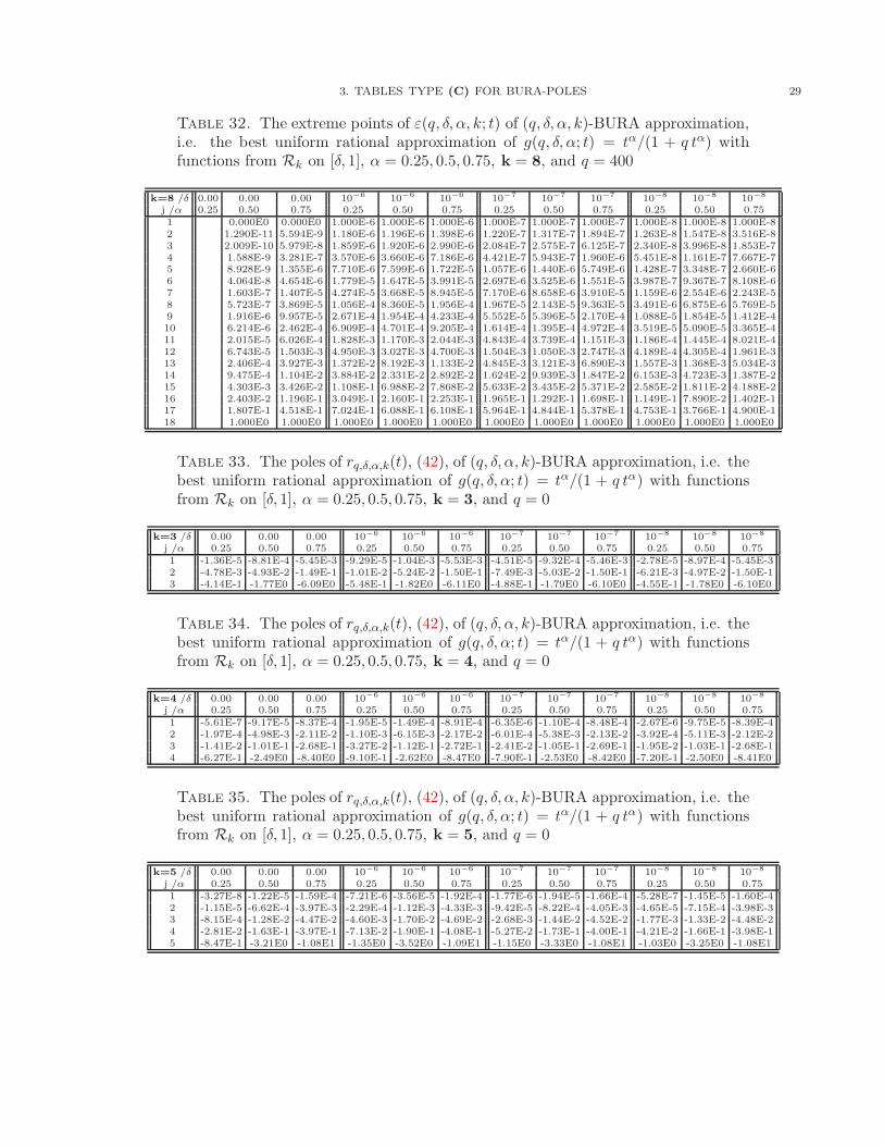
3. TABLES TYPE (C) FOR BURA-POLES 29
Table 32. The extreme points of ε(q, δ, α, k; t) of (q, δ, α, k)-BURA approximation,i.e. the best uniform rational approximation of g(q, δ, α; t) = tα/(1 + q tα) withfunctions from Rk on [δ, 1], α = 0.25, 0.5, 0.75, k = 8, and q = 400
k=8 /δ 0.00 0.00 0.00 10−6 10−6 10−6 10−7 10−7 10−7 10−8 10−8 10−8
j /α 0.25 0.50 0.75 0.25 0.50 0.75 0.25 0.50 0.75 0.25 0.50 0.751 0.000E0 0.000E0 1.000E-6 1.000E-6 1.000E-6 1.000E-7 1.000E-7 1.000E-7 1.000E-8 1.000E-8 1.000E-82 1.290E-11 5.594E-9 1.180E-6 1.196E-6 1.398E-6 1.220E-7 1.317E-7 1.894E-7 1.263E-8 1.547E-8 3.516E-83 2.009E-10 5.979E-8 1.859E-6 1.920E-6 2.990E-6 2.084E-7 2.575E-7 6.125E-7 2.340E-8 3.996E-8 1.853E-74 1.588E-9 3.281E-7 3.570E-6 3.660E-6 7.186E-6 4.421E-7 5.943E-7 1.960E-6 5.451E-8 1.161E-7 7.667E-75 8.928E-9 1.355E-6 7.710E-6 7.599E-6 1.722E-5 1.057E-6 1.440E-6 5.749E-6 1.428E-7 3.348E-7 2.660E-66 4.064E-8 4.654E-6 1.779E-5 1.647E-5 3.991E-5 2.697E-6 3.525E-6 1.551E-5 3.987E-7 9.367E-7 8.108E-67 1.603E-7 1.407E-5 4.274E-5 3.668E-5 8.945E-5 7.170E-6 8.658E-6 3.910E-5 1.159E-6 2.554E-6 2.243E-58 5.723E-7 3.869E-5 1.056E-4 8.360E-5 1.956E-4 1.967E-5 2.143E-5 9.363E-5 3.491E-6 6.875E-6 5.769E-59 1.916E-6 9.957E-5 2.671E-4 1.954E-4 4.233E-4 5.552E-5 5.396E-5 2.170E-4 1.088E-5 1.854E-5 1.412E-410 6.214E-6 2.462E-4 6.909E-4 4.701E-4 9.205E-4 1.614E-4 1.395E-4 4.972E-4 3.519E-5 5.090E-5 3.365E-411 2.015E-5 6.026E-4 1.828E-3 1.170E-3 2.044E-3 4.843E-4 3.739E-4 1.151E-3 1.186E-4 1.445E-4 8.021E-412 6.743E-5 1.503E-3 4.950E-3 3.027E-3 4.700E-3 1.504E-3 1.050E-3 2.747E-3 4.189E-4 4.305E-4 1.961E-313 2.406E-4 3.927E-3 1.372E-2 8.192E-3 1.133E-2 4.845E-3 3.121E-3 6.890E-3 1.557E-3 1.368E-3 5.034E-314 9.475E-4 1.104E-2 3.884E-2 2.331E-2 2.892E-2 1.624E-2 9.939E-3 1.847E-2 6.153E-3 4.723E-3 1.387E-215 4.303E-3 3.426E-2 1.108E-1 6.988E-2 7.868E-2 5.633E-2 3.435E-2 5.371E-2 2.585E-2 1.811E-2 4.188E-216 2.403E-2 1.196E-1 3.049E-1 2.160E-1 2.253E-1 1.965E-1 1.292E-1 1.698E-1 1.149E-1 7.890E-2 1.402E-117 1.807E-1 4.518E-1 7.024E-1 6.088E-1 6.108E-1 5.964E-1 4.844E-1 5.378E-1 4.753E-1 3.766E-1 4.900E-118 1.000E0 1.000E0 1.000E0 1.000E0 1.000E0 1.000E0 1.000E0 1.000E0 1.000E0 1.000E0 1.000E0
Table 33. The poles of rq,δ,α,k(t), (42), of (q, δ, α, k)-BURA approximation, i.e. thebest uniform rational approximation of g(q, δ, α; t) = tα/(1 + q tα) with functionsfrom Rk on [δ, 1], α = 0.25, 0.5, 0.75, k = 3, and q = 0
k=3 /δ 0.00 0.00 0.00 10−6 10−6 10−6 10−7 10−7 10−7 10−8 10−8 10−8
j /α 0.25 0.50 0.75 0.25 0.50 0.75 0.25 0.50 0.75 0.25 0.50 0.751 -1.36E-5 -8.81E-4 -5.45E-3 -9.29E-5 -1.04E-3 -5.53E-3 -4.51E-5 -9.32E-4 -5.46E-3 -2.78E-5 -8.97E-4 -5.45E-32 -4.78E-3 -4.93E-2 -1.49E-1 -1.01E-2 -5.24E-2 -1.50E-1 -7.49E-3 -5.03E-2 -1.50E-1 -6.21E-3 -4.97E-2 -1.50E-13 -4.14E-1 -1.77E0 -6.09E0 -5.48E-1 -1.82E0 -6.11E0 -4.88E-1 -1.79E0 -6.10E0 -4.55E-1 -1.78E0 -6.10E0
Table 34. The poles of rq,δ,α,k(t), (42), of (q, δ, α, k)-BURA approximation, i.e. thebest uniform rational approximation of g(q, δ, α; t) = tα/(1 + q tα) with functionsfrom Rk on [δ, 1], α = 0.25, 0.5, 0.75, k = 4, and q = 0
k=4 /δ 0.00 0.00 0.00 10−6 10−6 10−6 10−7 10−7 10−7 10−8 10−8 10−8
j /α 0.25 0.50 0.75 0.25 0.50 0.75 0.25 0.50 0.75 0.25 0.50 0.751 -5.61E-7 -9.17E-5 -8.37E-4 -1.95E-5 -1.49E-4 -8.91E-4 -6.35E-6 -1.10E-4 -8.48E-4 -2.67E-6 -9.75E-5 -8.39E-42 -1.97E-4 -4.98E-3 -2.11E-2 -1.10E-3 -6.15E-3 -2.17E-2 -6.01E-4 -5.38E-3 -2.13E-2 -3.92E-4 -5.11E-3 -2.12E-23 -1.41E-2 -1.01E-1 -2.68E-1 -3.27E-2 -1.12E-1 -2.72E-1 -2.41E-2 -1.05E-1 -2.69E-1 -1.95E-2 -1.03E-1 -2.68E-14 -6.27E-1 -2.49E0 -8.40E0 -9.10E-1 -2.62E0 -8.47E0 -7.90E-1 -2.53E0 -8.42E0 -7.20E-1 -2.50E0 -8.41E0
Table 35. The poles of rq,δ,α,k(t), (42), of (q, δ, α, k)-BURA approximation, i.e. thebest uniform rational approximation of g(q, δ, α; t) = tα/(1 + q tα) with functionsfrom Rk on [δ, 1], α = 0.25, 0.5, 0.75, k = 5, and q = 0
k=5 /δ 0.00 0.00 0.00 10−6 10−6 10−6 10−7 10−7 10−7 10−8 10−8 10−8
j /α 0.25 0.50 0.75 0.25 0.50 0.75 0.25 0.50 0.75 0.25 0.50 0.751 -3.27E-8 -1.22E-5 -1.59E-4 -7.21E-6 -3.56E-5 -1.92E-4 -1.77E-6 -1.94E-5 -1.66E-4 -5.28E-7 -1.45E-5 -1.60E-42 -1.15E-5 -6.62E-4 -3.97E-3 -2.29E-4 -1.12E-3 -4.33E-3 -9.42E-5 -8.22E-4 -4.05E-3 -4.65E-5 -7.15E-4 -3.98E-33 -8.15E-4 -1.28E-2 -4.47E-2 -4.60E-3 -1.70E-2 -4.69E-2 -2.68E-3 -1.44E-2 -4.52E-2 -1.77E-3 -1.33E-2 -4.48E-24 -2.81E-2 -1.63E-1 -3.97E-1 -7.13E-2 -1.90E-1 -4.08E-1 -5.27E-2 -1.73E-1 -4.00E-1 -4.21E-2 -1.66E-1 -3.98E-15 -8.47E-1 -3.21E0 -1.08E1 -1.35E0 -3.52E0 -1.09E1 -1.15E0 -3.33E0 -1.08E1 -1.03E0 -3.25E0 -1.08E1

30 2. TABLES
Table 36. The poles of rq,δ,α,k(t), (42), of (q, δ, α, k)-BURA approximation, i.e. thebest uniform rational approximation of g(q, δ, α; t) = tα/(1 + q tα) with functionsfrom Rk on [δ, 1], α = 0.25, 0.5, 0.75, k = 6, and q = 0
k=6 /δ 0.00 0.00 0.00 10−6 10−6 10−6 10−7 10−7 10−7 10−8 10−8 10−8
j /α 0.25 0.50 0.75 0.25 0.50 0.75 0.25 0.50 0.75 0.25 0.50 0.751 -2.45E-9 -1.95E-6 -3.52E-5 -3.62E-6 -1.28E-5 -5.49E-5 -7.44E-7 -5.05E-6 -3.98E-5 -1.74E-7 -2.90E-6 -3.62E-52 -8.61E-7 -1.06E-4 -8.75E-4 -7.42E-5 -2.93E-4 -1.10E-3 -2.41E-5 -1.72E-4 -9.30E-4 -9.22E-6 -1.28E-4 -8.87E-43 -6.11E-5 -2.03E-3 -9.65E-3 -1.06E-3 -3.74E-3 -1.10E-2 -4.90E-4 -2.70E-3 -1.00E-2 -2.60E-4 -2.27E-3 -9.73E-34 -2.07E-3 -2.40E-2 -7.40E-2 -1.22E-2 -3.47E-2 -8.01E-2 -7.43E-3 -2.84E-2 -7.56E-2 -4.98E-3 -2.56E-2 -7.44E-25 -4.58E-2 -2.30E-1 -5.32E-1 -1.26E-1 -2.85E-1 -5.58E-1 -9.40E-2 -2.53E-1 -5.39E-1 -7.46E-2 -2.39E-1 -5.34E-16 -1.07E0 -3.95E0 -1.31E1 -1.86E0 -4.52E0 -1.36E1 -1.57E0 -4.20E0 -1.32E1 -1.38E0 -4.04E0 -1.32E1
Table 37. The poles of rq,δ,α,k(t), (42), of (q, δ, α, k)-BURA approximation, i.e. thebest uniform rational approximation of g(q, δ, α; t) = tα/(1 + q tα) with functionsfrom Rk on [δ, 1], α = 0.25, 0.5, 0.75, k = 7, and q = 0
k=7 /δ 0.00 0.00 0.00 10−6 10−6 10−6 10−7 10−7 10−7 10−8 10−8 10−8
j /α 0.25 0.50 0.75 0.25 0.50 0.75 0.25 0.50 0.75 0.25 0.50 0.751 -2.24E-10 -3.58E-7 -8.75E-6 -2.17E-6 -6.05E-6 -2.05E-5 -3.98E-7 -1.84E-6 -1.17E-5 -7.97E-8 -7.90E-7 -9.40E-62 -7.85E-8 -1.94E-5 -2.17E-4 -3.21E-5 -1.03E-4 -3.45E-4 -8.69E-6 -4.79E-5 -2.52E-4 -2.70E-6 -2.94E-5 -2.25E-43 -5.57E-6 -3.72E-4 -2.39E-3 -3.42E-4 -1.09E-3 -3.18E-3 -1.30E-4 -6.56E-4 -2.61E-3 -5.65E-5 -4.80E-4 -2.44E-34 -1.89E-4 -4.34E-3 -1.77E-2 -3.10E-3 -8.76E-3 -2.13E-2 -1.56E-3 -6.26E-3 -1.88E-2 -8.72E-4 -5.11E-3 -1.80E-25 -4.08E-3 -3.80E-2 -1.08E-1 -2.51E-2 -5.94E-2 -1.21E-1 -1.58E-2 -4.79E-2 -1.12E-1 -1.08E-2 -4.21E-2 -1.09E-16 -6.66E-2 -3.01E-1 -6.71E-1 -1.97E-1 -3.96E-1 -7.24E-1 -1.48E-1 -3.46E-1 -6.87E-1 -1.17E-1 -3.20E-1 -6.75E-17 -1.30E00 -4.69E00 -1.55E01 -2.45E00 -5.64E00 -1.64E01 -2.05E00 -5.15E00 -1.58E01 -1.78E00 -4.88E00 -1.56E01
Table 38. The poles of rq,δ,α,k(t), (42), of (q, δ, α, k)-BURA approximation, i.e. thebest uniform rational approximation of g(q, δ, α; t) = tα/(1 + q tα) with functionsfrom Rk on [δ, 1], α = 0.25, 0.5, 0.75, k = 8, and q = 0
k=8 /δ 0.00 0.00 0.00 10−6 10−6 10−6 10−7 10−7 10−7 10−8 10−8 10−8
j /α 0.25 0.50 0.75 0.25 0.50 0.75 0.25 0.50 0.75 0.25 0.50 0.751 -2.39E-11 -7.35E-8 -2.38E-6 -1.45E-6 -3.45E-6 -9.54E-6 -2.47E-7 -8.67E-7 -4.20E-6 -4.45E-8 -2.86E-7 -2.82E-62 -8.37E-9 -3.98E-6 -5.93E-5 -1.69E-5 -4.52E-5 -1.33E-4 -3.97E-6 -1.71E-5 -8.07E-5 -1.04E-6 -8.49E-6 -6.47E-53 -5.95E-7 -7.62E-5 -6.50E-4 -1.41E-4 -3.97E-4 -1.10E-3 -4.56E-5 -2.00E-4 -7.91E-4 -1.66E-5 -1.24E-4 -6.87E-44 -2.01E-5 -8.89E-4 -4.79E-3 -1.04E-3 -2.79E-3 -6.84E-3 -4.41E-4 -1.72E-3 -5.47E-3 -2.08E-4 -1.24E-3 -4.97E-35 -4.34E-4 -7.65E-3 -2.79E-2 -6.99E-3 -1.67E-2 -3.55E-2 -3.73E-3 -1.19E-2 -3.05E-2 -2.17E-3 -9.55E-3 -2.86E-26 -6.88E-3 -5.44E-2 -1.44E-1 -4.40E-2 -9.13E-2 -1.69E-1 -2.85E-2 -7.28E-2 -1.53E-1 -1.97E-2 -6.28E-2 -1.47E-17 -8.99E-2 -3.75E-1 -8.13E-1 -2.83E-1 -5.23E-1 -9.06E-1 -2.13E-1 -4.51E-1 -8.46E-1 -1.69E-1 -4.10E-1 -8.22E-18 -1.53E00 -5.43E00 -1.79E01 -3.11E00 -6.88E00 -1.95E01 -2.58E00 -6.18E00 -1.85E01 -2.23E00 -5.78E00 -1.81E01
Table 39. The poles of rq,δ,α,k(t), (42), of (q, δ, α, k)-BURA approximation, i.e. thebest uniform rational approximation of g(q, δ, α; t) = tα/(1 + q tα) with functionsfrom Rk on [δ, 1], α = 0.25, 0.5, 0.75, k = 3, and q = 1
k=3 /δ 0.00 0.00 0.00 10−6 10−6 10−6 10−7 10−7 10−7 10−8 10−8 10−8
j /α 0.25 0.50 0.75 0.25 0.50 0.75 0.25 0.50 0.75 0.25 0.50 0.751 -3.53E-6 -4.86E-4 -3.78E-3 -4.67E-5 -6.08E-4 -3.87E-3 -1.89E-5 -5.25E-4 -3.80E-3 -9.90E-6 -4.98E-4 -3.79E-32 -1.43E-3 -2.61E-2 -9.83E-2 -4.41E-3 -2.84E-2 -9.90E-2 -2.88E-3 -2.69E-2 -9.84E-2 -2.17E-3 -2.64E-2 -9.83E-23 -1.49E-1 -5.52E-1 -9.17E-1 -2.37E-1 -5.71E-1 -9.20E-1 -1.97E-1 -5.58E-1 -9.18E-1 -1.76E-1 -5.54E-1 -9.17E-1
Table 40. The poles of rq,δ,α,k(t), (42), of (q, δ, α, k)-BURA approximation, i.e. thebest uniform rational approximation of g(q, δ, α; t) = tα/(1 + q tα) with functionsfrom Rk on [δ, 1], α = 0.25, 0.5, 0.75, k = 4, and q = 1
k=4 /δ 0.00 0.00 0.00 10−6 10−6 10−6 10−7 10−7 10−7 10−8 10−8 10−8
j /α 0.25 0.50 0.75 0.25 0.50 0.75 0.25 0.50 0.75 0.25 0.50 0.751 -1.66E-7 -5.43E-5 -6.06E-4 -1.26E-5 -9.98E-5 -6.56E-4 -3.57E-6 -6.86E-5 -6.16E-4 -1.28E-6 -5.88E-5 -6.08E-42 -6.21E-5 -2.94E-3 -1.53E-2 -5.87E-4 -3.85E-3 -1.59E-2 -2.82E-4 -3.25E-3 -1.54E-2 -1.63E-4 -3.04E-3 -1.53E-23 -5.06E-3 -5.62E-2 -1.75E-1 -1.68E-2 -6.42E-2 -1.78E-1 -1.11E-2 -5.90E-2 -1.76E-1 -8.30E-3 -5.72E-2 -1.75E-14 -2.51E-1 -7.73E-1 -1.13E00 -4.39E-1 -8.23E-1 -1.13E00 -3.61E-1 -7.91E-1 -1.13E00 -3.14E-1 -7.79E-1 -1.13E00
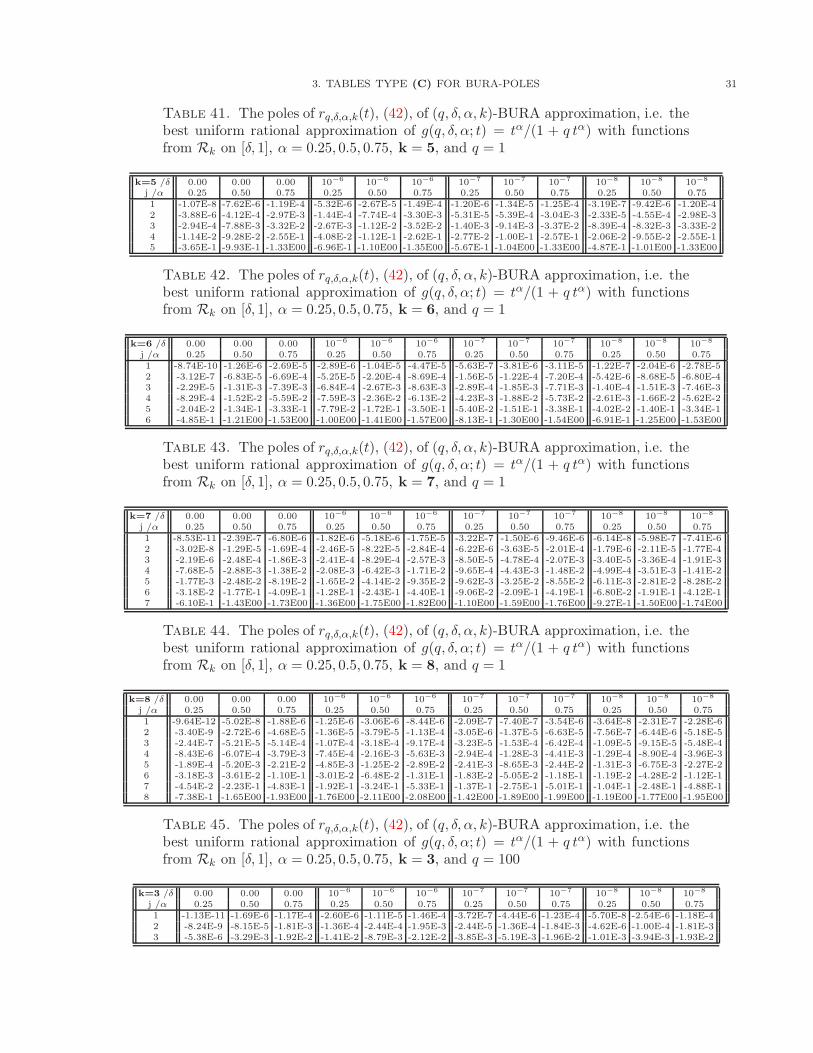
3. TABLES TYPE (C) FOR BURA-POLES 31
Table 41. The poles of rq,δ,α,k(t), (42), of (q, δ, α, k)-BURA approximation, i.e. thebest uniform rational approximation of g(q, δ, α; t) = tα/(1 + q tα) with functionsfrom Rk on [δ, 1], α = 0.25, 0.5, 0.75, k = 5, and q = 1
k=5 /δ 0.00 0.00 0.00 10−6 10−6 10−6 10−7 10−7 10−7 10−8 10−8 10−8
j /α 0.25 0.50 0.75 0.25 0.50 0.75 0.25 0.50 0.75 0.25 0.50 0.751 -1.07E-8 -7.62E-6 -1.19E-4 -5.32E-6 -2.67E-5 -1.49E-4 -1.20E-6 -1.34E-5 -1.25E-4 -3.19E-7 -9.42E-6 -1.20E-42 -3.88E-6 -4.12E-4 -2.97E-3 -1.44E-4 -7.74E-4 -3.30E-3 -5.31E-5 -5.39E-4 -3.04E-3 -2.33E-5 -4.55E-4 -2.98E-33 -2.94E-4 -7.88E-3 -3.32E-2 -2.67E-3 -1.12E-2 -3.52E-2 -1.40E-3 -9.14E-3 -3.37E-2 -8.39E-4 -8.32E-3 -3.33E-24 -1.14E-2 -9.28E-2 -2.55E-1 -4.08E-2 -1.12E-1 -2.62E-1 -2.77E-2 -1.00E-1 -2.57E-1 -2.06E-2 -9.55E-2 -2.55E-15 -3.65E-1 -9.93E-1 -1.33E00 -6.96E-1 -1.10E00 -1.35E00 -5.67E-1 -1.04E00 -1.33E00 -4.87E-1 -1.01E00 -1.33E00
Table 42. The poles of rq,δ,α,k(t), (42), of (q, δ, α, k)-BURA approximation, i.e. thebest uniform rational approximation of g(q, δ, α; t) = tα/(1 + q tα) with functionsfrom Rk on [δ, 1], α = 0.25, 0.5, 0.75, k = 6, and q = 1
k=6 /δ 0.00 0.00 0.00 10−6 10−6 10−6 10−7 10−7 10−7 10−8 10−8 10−8
j /α 0.25 0.50 0.75 0.25 0.50 0.75 0.25 0.50 0.75 0.25 0.50 0.751 -8.74E-10 -1.26E-6 -2.69E-5 -2.89E-6 -1.04E-5 -4.47E-5 -5.63E-7 -3.81E-6 -3.11E-5 -1.22E-7 -2.04E-6 -2.78E-52 -3.12E-7 -6.83E-5 -6.69E-4 -5.25E-5 -2.20E-4 -8.69E-4 -1.56E-5 -1.22E-4 -7.20E-4 -5.42E-6 -8.68E-5 -6.80E-43 -2.29E-5 -1.31E-3 -7.39E-3 -6.84E-4 -2.67E-3 -8.63E-3 -2.89E-4 -1.85E-3 -7.71E-3 -1.40E-4 -1.51E-3 -7.46E-34 -8.29E-4 -1.52E-2 -5.59E-2 -7.59E-3 -2.36E-2 -6.13E-2 -4.23E-3 -1.88E-2 -5.73E-2 -2.61E-3 -1.66E-2 -5.62E-25 -2.04E-2 -1.34E-1 -3.33E-1 -7.79E-2 -1.72E-1 -3.50E-1 -5.40E-2 -1.51E-1 -3.38E-1 -4.02E-2 -1.40E-1 -3.34E-16 -4.85E-1 -1.21E00 -1.53E00 -1.00E00 -1.41E00 -1.57E00 -8.13E-1 -1.30E00 -1.54E00 -6.91E-1 -1.25E00 -1.53E00
Table 43. The poles of rq,δ,α,k(t), (42), of (q, δ, α, k)-BURA approximation, i.e. thebest uniform rational approximation of g(q, δ, α; t) = tα/(1 + q tα) with functionsfrom Rk on [δ, 1], α = 0.25, 0.5, 0.75, k = 7, and q = 1
k=7 /δ 0.00 0.00 0.00 10−6 10−6 10−6 10−7 10−7 10−7 10−8 10−8 10−8
j /α 0.25 0.50 0.75 0.25 0.50 0.75 0.25 0.50 0.75 0.25 0.50 0.751 -8.53E-11 -2.39E-7 -6.80E-6 -1.82E-6 -5.18E-6 -1.75E-5 -3.22E-7 -1.50E-6 -9.46E-6 -6.14E-8 -5.98E-7 -7.41E-62 -3.02E-8 -1.29E-5 -1.69E-4 -2.46E-5 -8.22E-5 -2.84E-4 -6.22E-6 -3.63E-5 -2.01E-4 -1.79E-6 -2.11E-5 -1.77E-43 -2.19E-6 -2.48E-4 -1.86E-3 -2.41E-4 -8.29E-4 -2.57E-3 -8.50E-5 -4.78E-4 -2.07E-3 -3.40E-5 -3.36E-4 -1.91E-34 -7.68E-5 -2.88E-3 -1.38E-2 -2.08E-3 -6.42E-3 -1.71E-2 -9.65E-4 -4.43E-3 -1.48E-2 -4.99E-4 -3.51E-3 -1.41E-25 -1.77E-3 -2.48E-2 -8.19E-2 -1.65E-2 -4.14E-2 -9.35E-2 -9.62E-3 -3.25E-2 -8.55E-2 -6.11E-3 -2.81E-2 -8.28E-26 -3.18E-2 -1.77E-1 -4.09E-1 -1.28E-1 -2.43E-1 -4.40E-1 -9.06E-2 -2.09E-1 -4.19E-1 -6.80E-2 -1.91E-1 -4.12E-17 -6.10E-1 -1.43E00 -1.73E00 -1.36E00 -1.75E00 -1.82E00 -1.10E00 -1.59E00 -1.76E00 -9.27E-1 -1.50E00 -1.74E00
Table 44. The poles of rq,δ,α,k(t), (42), of (q, δ, α, k)-BURA approximation, i.e. thebest uniform rational approximation of g(q, δ, α; t) = tα/(1 + q tα) with functionsfrom Rk on [δ, 1], α = 0.25, 0.5, 0.75, k = 8, and q = 1
k=8 /δ 0.00 0.00 0.00 10−6 10−6 10−6 10−7 10−7 10−7 10−8 10−8 10−8
j /α 0.25 0.50 0.75 0.25 0.50 0.75 0.25 0.50 0.75 0.25 0.50 0.751 -9.64E-12 -5.02E-8 -1.88E-6 -1.25E-6 -3.06E-6 -8.44E-6 -2.09E-7 -7.40E-7 -3.54E-6 -3.64E-8 -2.31E-7 -2.28E-62 -3.40E-9 -2.72E-6 -4.68E-5 -1.36E-5 -3.79E-5 -1.13E-4 -3.05E-6 -1.37E-5 -6.63E-5 -7.56E-7 -6.44E-6 -5.18E-53 -2.44E-7 -5.21E-5 -5.14E-4 -1.07E-4 -3.18E-4 -9.17E-4 -3.23E-5 -1.53E-4 -6.42E-4 -1.09E-5 -9.15E-5 -5.48E-44 -8.43E-6 -6.07E-4 -3.79E-3 -7.45E-4 -2.16E-3 -5.63E-3 -2.94E-4 -1.28E-3 -4.41E-3 -1.29E-4 -8.90E-4 -3.96E-35 -1.89E-4 -5.20E-3 -2.21E-2 -4.85E-3 -1.25E-2 -2.89E-2 -2.41E-3 -8.65E-3 -2.44E-2 -1.31E-3 -6.75E-3 -2.27E-26 -3.18E-3 -3.61E-2 -1.10E-1 -3.01E-2 -6.48E-2 -1.31E-1 -1.83E-2 -5.05E-2 -1.18E-1 -1.19E-2 -4.28E-2 -1.12E-17 -4.54E-2 -2.23E-1 -4.83E-1 -1.92E-1 -3.24E-1 -5.33E-1 -1.37E-1 -2.75E-1 -5.01E-1 -1.04E-1 -2.48E-1 -4.88E-18 -7.38E-1 -1.65E00 -1.93E00 -1.76E00 -2.11E00 -2.08E00 -1.42E00 -1.89E00 -1.99E00 -1.19E00 -1.77E00 -1.95E00
Table 45. The poles of rq,δ,α,k(t), (42), of (q, δ, α, k)-BURA approximation, i.e. thebest uniform rational approximation of g(q, δ, α; t) = tα/(1 + q tα) with functionsfrom Rk on [δ, 1], α = 0.25, 0.5, 0.75, k = 3, and q = 100
k=3 /δ 0.00 0.00 0.00 10−6 10−6 10−6 10−7 10−7 10−7 10−8 10−8 10−8
j /α 0.25 0.50 0.75 0.25 0.50 0.75 0.25 0.50 0.75 0.25 0.50 0.751 -1.13E-11 -1.69E-6 -1.17E-4 -2.60E-6 -1.11E-5 -1.46E-4 -3.72E-7 -4.44E-6 -1.23E-4 -5.70E-8 -2.54E-6 -1.18E-42 -8.24E-9 -8.15E-5 -1.81E-3 -1.36E-4 -2.44E-4 -1.95E-3 -2.44E-5 -1.36E-4 -1.84E-3 -4.62E-6 -1.00E-4 -1.81E-33 -5.38E-6 -3.29E-3 -1.92E-2 -1.41E-2 -8.79E-3 -2.12E-2 -3.85E-3 -5.19E-3 -1.96E-2 -1.01E-3 -3.94E-3 -1.93E-2
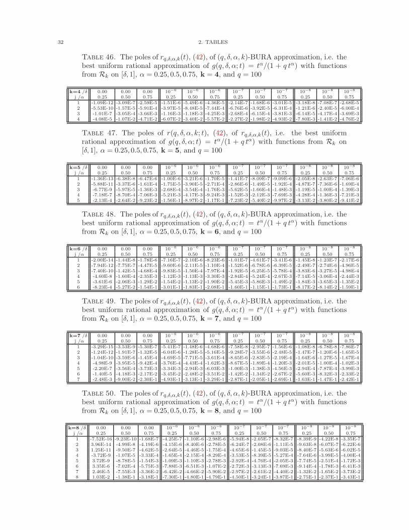
32 2. TABLES
Table 46. The poles of rq,δ,α,k(t), (42), of (q, δ, α, k)-BURA approximation, i.e. thebest uniform rational approximation of g(q, δ, α; t) = tα/(1 + q tα) with functionsfrom Rk on [δ, 1], α = 0.25, 0.5, 0.75, k = 4, and q = 100
k=4 /δ 0.00 0.00 0.00 10−6 10−6 10−6 10−7 10−7 10−7 10−8 10−8 10−8
j /α 0.25 0.50 0.75 0.25 0.50 0.75 0.25 0.50 0.75 0.25 0.50 0.751 -1.09E-12 -3.09E-7 -2.59E-5 -1.51E-6 -5.49E-6 -4.36E-5 -2.14E-7 -1.68E-6 -3.01E-5 -3.18E-8 -7.08E-7 -2.68E-52 -5.53E-10 -1.57E-5 -5.91E-4 -3.97E-5 -8.48E-5 -7.44E-4 -6.76E-6 -3.92E-5 -6.31E-4 -1.21E-6 -2.40E-5 -6.00E-43 -1.01E-7 -3.05E-4 -3.66E-3 -1.16E-3 -1.18E-3 -4.25E-3 -2.68E-4 -6.15E-4 -3.81E-3 -6.14E-5 -4.17E-4 -3.69E-34 -4.08E-5 -1.07E-2 -4.71E-2 -6.07E-2 -3.40E-2 -5.57E-2 -2.27E-2 -1.98E-2 -4.93E-2 -7.80E-3 -1.41E-2 -4.76E-2
Table 47. The poles of r(q, δ, α, k; t), (42), of rq,δ,α,k(t), i.e. the best uniformrational approximation of g(q, δ, α; t) = tα/(1 + q tα) with functions from Rk on[δ, 1], α = 0.25, 0.5, 0.75, k = 5, and q = 100
k=5 /δ 0.00 0.00 0.00 10−6 10−6 10−6 10−7 10−7 10−7 10−8 10−8 10−8
j /α 0.25 0.50 0.75 0.25 0.50 0.75 0.25 0.50 0.75 0.25 0.50 0.751 -1.36E-13 -6.38E-8 -6.47E-6 -1.00E-6 -3.21E-6 -1.70E-5 -1.41E-7 -8.09E-7 -9.09E-6 -2.05E-8 -2.63E-7 -7.06E-62 -5.88E-11 -3.37E-6 -1.61E-4 -1.75E-5 -3.90E-5 -2.71E-4 -2.86E-6 -1.49E-5 -1.92E-4 -4.87E-7 -7.36E-6 -1.69E-43 -6.77E-9 -5.97E-5 -1.36E-3 -2.68E-4 -3.54E-4 -1.76E-3 -5.62E-5 -1.66E-4 -1.48E-3 -1.19E-5 -1.00E-4 -1.39E-34 -7.18E-7 -8.70E-4 -7.06E-3 -5.21E-3 -4.17E-3 -9.24E-3 -1.52E-3 -2.12E-3 -7.69E-3 -4.28E-4 -1.36E-3 -7.21E-35 -2.13E-4 -2.64E-2 -9.23E-2 -1.56E-1 -8.97E-2 -1.17E-1 -7.23E-2 -5.40E-2 -9.97E-2 -3.13E-2 -3.80E-2 -9.41E-2
Table 48. The poles of rq,δ,α,k(t), (42), of (q, δ, α, k)-BURA approximation, i.e. thebest uniform rational approximation of g(q, δ, α; t) = tα/(1 + q tα) with functionsfrom Rk on [δ, 1], α = 0.25, 0.5, 0.75, k = 6, and q = 100
k=6 /δ 0.00 0.00 0.00 10−6 10−6 10−6 10−7 10−7 10−7 10−8 10−8 10−8
j /α 0.25 0.50 0.75 0.25 0.50 0.75 0.25 0.50 0.75 0.25 0.50 0.751 -2.00E-14 -1.44E-8 -1.78E-6 -7.16E-7 -2.10E-6 -8.23E-6 -1.01E-7 -4.61E-7 -3.41E-6 -1.45E-8 -1.23E-7 -2.17E-62 -7.94E-12 -7.75E-7 -4.47E-5 -9.60E-6 -2.11E-5 -1.10E-4 -1.52E-6 -6.78E-6 -6.39E-5 -2.49E-7 -2.74E-6 -4.96E-53 -7.40E-10 -1.42E-5 -4.68E-4 -9.83E-5 -1.50E-4 -7.97E-4 -1.92E-5 -6.25E-5 -5.78E-4 -3.83E-6 -3.27E-5 -4.98E-44 -4.60E-8 -1.60E-4 -2.35E-3 -1.12E-3 -1.13E-3 -3.30E-3 -2.84E-4 -5.24E-4 -2.67E-3 -7.14E-5 -3.06E-4 -2.44E-35 -3.61E-6 -2.06E-3 -1.29E-2 -1.54E-2 -1.13E-2 -1.90E-2 -5.45E-3 -5.86E-3 -1.49E-2 -1.84E-3 -3.65E-3 -1.35E-26 -8.23E-4 -5.27E-2 -1.54E-1 -3.01E-1 -1.83E-1 -2.08E-1 -1.60E-1 -1.15E-1 -1.73E-1 -8.17E-2 -8.14E-2 -1.59E-1
Table 49. The poles of rq,δ,α,k(t), (42), of (q, δ, α, k)-BURA approximation, i.e. thebest uniform rational approximation of g(q, δ, α; t) = tα/(1 + q tα) with functionsfrom Rk on [δ, 1], α = 0.25, 0.5, 0.75, k = 7, and q = 100
k=7 /δ 0.00 0.00 0.00 10−6 10−6 10−6 10−7 10−7 10−7 10−8 10−8 10−8
j /α 0.25 0.50 0.75 0.25 0.50 0.75 0.25 0.50 0.75 0.25 0.50 0.751 -3.29E-15 -3.53E-9 -5.30E-7 -5.41E-7 -1.48E-6 -4.68E-6 -7.58E-8 -2.95E-7 -1.56E-6 -1.08E-8 -6.78E-8 -7.86E-72 -1.24E-12 -1.91E-7 -1.32E-5 -6.04E-6 -1.28E-5 -5.16E-5 -9.28E-7 -3.55E-6 -2.48E-5 -1.47E-7 -1.20E-6 -1.65E-53 -1.04E-10 -3.59E-6 -1.45E-4 -4.69E-5 -7.71E-5 -3.61E-4 -8.65E-6 -2.83E-5 -2.19E-4 -1.64E-6 -1.27E-5 -1.67E-44 -4.98E-9 -3.95E-5 -9.42E-4 -3.76E-4 -4.43E-4 -1.62E-3 -8.67E-5 -1.89E-4 -1.20E-3 -2.01E-5 -1.00E-4 -1.02E-35 -2.20E-7 -3.56E-4 -3.73E-3 -3.34E-3 -2.94E-3 -6.03E-3 -1.00E-3 -1.38E-3 -4.56E-3 -2.94E-4 -7.87E-4 -3.99E-36 -1.40E-5 -4.18E-3 -2.17E-2 -3.45E-2 -2.48E-2 -3.51E-2 -1.42E-2 -1.34E-2 -2.67E-2 -5.60E-3 -8.32E-3 -2.33E-27 -2.48E-3 -9.00E-2 -2.30E-1 -4.93E-1 -3.13E-1 -3.29E-1 -2.87E-1 -2.05E-1 -2.69E-1 -1.63E-1 -1.47E-1 -2.42E-1
Table 50. The poles of rq,δ,α,k(t), (42), of (q, δ, α, k)-BURA approximation, i.e. thebest uniform rational approximation of g(q, δ, α; t) = tα/(1 + q tα) with functionsfrom Rk on [δ, 1], α = 0.25, 0.5, 0.75, k = 8, and q = 100
k=8 /δ 0.00 0.00 0.00 10−6 10−6 10−6 10−7 10−7 10−7 10−8 10−8 10−8
j /α 0.25 0.50 0.75 0.25 0.50 0.75 0.25 0.50 0.75 0.25 0.50 0.751 -7.52E-16 -9.23E-10 -1.68E-7 -4.25E-7 -1.10E-6 -2.98E-6 -5.94E-8 -2.05E-7 -8.32E-7 -8.39E-9 -4.22E-8 -3.35E-72 3.96E-14 -4.99E-8 -4.19E-6 -4.15E-6 -8.40E-6 -2.78E-5 -6.24E-7 -2.08E-6 -1.11E-5 -9.63E-8 -6.07E-7 -6.22E-63 1.25E-11 -9.50E-7 -4.62E-5 -2.64E-5 -4.46E-5 -1.75E-4 -4.65E-6 -1.45E-5 -9.03E-5 -8.40E-7 -5.63E-6 -6.02E-54 -3.72E-9 -1.07E-5 -3.33E-4 -1.65E-4 -2.15E-4 -8.29E-4 -3.53E-5 -8.39E-5 -5.27E-4 -7.64E-6 -3.99E-5 -4.00E-45 3.72E-9 -8.78E-5 -1.54E-3 -1.09E-3 -1.10E-3 -2.78E-3 -2.92E-4 -4.76E-4 -2.05E-3 -7.74E-5 -2.51E-4 -1.72E-36 3.35E-6 -7.02E-4 -5.75E-3 -7.88E-3 -6.51E-3 -1.07E-2 -2.72E-3 -3.13E-3 -7.69E-3 -9.14E-4 -1.78E-3 -6.41E-37 2.46E-5 -7.55E-3 -3.36E-2 -6.42E-2 -4.66E-2 -5.90E-2 -2.97E-2 -2.61E-2 -4.40E-2 -1.32E-2 -1.65E-2 -3.73E-28 1.03E-2 -1.38E-1 -3.18E-1 -7.30E-1 -4.80E-1 -4.79E-1 -4.50E-1 -3.24E-1 -3.87E-1 -2.75E-1 -2.37E-1 -3.43E-1

3. TABLES TYPE (C) FOR BURA-POLES 33
Table 51. The poles of rq,δ,α,k(t), (42), of (q, δ, α, k)-BURA approximation, i.e. thebest uniform rational approximation of g(q, δ, α; t) = tα/(1 + q tα) with functionsfrom Rk on [δ, 1], α = 0.25, 0.5, 0.75, k = 3, and q = 200
k=3 /δ 0.00 0.00 0.00 10−6 10−6 10−6 10−7 10−7 10−7 10−8 10−8 10−8
j /α 0.25 0.50 0.75 0.25 0.50 0.75 0.25 0.50 0.75 0.25 0.50 0.751 -7.62E-13 -4.65E-7 -5.18E-5 -2.21E-6 -5.95E-6 -7.36E-5 -2.87E-7 -1.99E-6 -5.68E-5 -3.87E-8 -9.21E-7 -5.28E-52 -5.67E-10 -2.24E-5 -7.69E-4 -1.17E-4 -1.16E-4 -8.72E-4 -1.85E-5 -5.15E-5 -7.94E-4 -2.92E-6 -3.22E-5 -7.74E-43 -3.98E-7 -9.78E-4 -9.03E-3 -1.24E-2 -4.63E-3 -1.08E-2 -3.00E-3 -2.15E-3 -9.44E-3 -6.48E-4 -1.37E-3 -9.12E-3
Table 52. The poles of rq,δ,α,k(t), (42), i.e. the best uniform rational approximationof g(q, δ, α; t) = tα/(1 + q tα) with functions from Rk on [δ, 1], α = 0.25, 0.5, 0.75,k = 4, and q = 200
k=4 /δ 0.00 0.00 0.00 10−6 10−6 10−6 10−7 10−7 10−7 10−8 10−8 10−8
j /α 0.25 0.50 0.75 0.25 0.50 0.75 0.25 0.50 0.75 0.25 0.50 0.751 -7.64E-14 -9.00E-8 -1.21E-5 -1.31E-6 -3.41E-6 -2.54E-5 -1.72E-7 -9.12E-7 -1.53E-5 -2.30E-8 -3.17E-7 -1.28E-52 -3.91E-11 -4.53E-6 -2.69E-4 -3.51E-5 -4.49E-5 -3.74E-4 -5.42E-6 -1.72E-5 -2.98E-4 -8.33E-7 -8.90E-6 -2.76E-43 -7.43E-9 -9.08E-5 -1.65E-3 -1.04E-3 -6.54E-4 -2.11E-3 -2.16E-4 -2.71E-4 -1.78E-3 -4.20E-5 -1.54E-4 -1.68E-34 -3.37E-6 -3.68E-3 -2.49E-2 -5.61E-2 -2.14E-2 -3.28E-2 -1.92E-2 -1.00E-2 -2.71E-2 -5.71E-3 -6.03E-3 -2.54E-2
Table 53. The poles of rq,δ,α,k(t), (42), of (q, δ, α, k)-BURA approximation, i.e. thebest uniform rational approximation of g(q, δ, α; t) = tα/(1 + q tα) with functionsfrom Rk on [δ, 1], α = 0.25, 0.5, 0.75, k = 5, and q = 200
k=5 /δ 0.00 0.00 0.00 10−6 10−6 10−6 10−7 10−7 10−7 10−8 10−8 10−8
j /α 0.25 0.50 0.75 0.25 0.50 0.75 0.25 0.50 0.75 0.25 0.50 0.751 -9.97E-15 -1.97E-8 -3.15E-6 -8.77E-7 -2.20E-6 -1.12E-5 -1.16E-7 -5.07E-7 -5.18E-6 -1.55E-8 -1.41E-7 -3.63E-62 -4.33E-12 -1.04E-6 -7.83E-5 -1.58E-5 -2.28E-5 -1.56E-4 -2.38E-6 -7.56E-6 -1.01E-4 -3.58E-7 -3.21E-6 -8.41E-53 -5.11E-10 -1.83E-5 -6.27E-4 -2.43E-4 -2.06E-4 -8.91E-4 -4.67E-5 -7.88E-5 -7.11E-4 -8.63E-6 -4.03E-5 -6.48E-44 -5.77E-8 -2.87E-4 -3.50E-3 -4.79E-3 -2.64E-3 -5.30E-3 -1.29E-3 -1.10E-3 -4.04E-3 -3.18E-4 -5.89E-4 -3.64E-35 -2.05E-5 -1.05E-2 -5.40E-2 -1.48E-1 -6.45E-2 -7.77E-2 -6.47E-2 -3.27E-2 -6.15E-2 -2.53E-2 -1.96E-2 -5.60E-2
Table 54. The poles of rq,δ,α,k(t), (42), of (q, δ, α, k)-BURA approximation, i.e. thebest uniform rational approximation of g(q, δ, α; t) = tα/(1 + q tα) with functionsfrom Rk on [δ, 1], α = 0.25, 0.5, 0.75, k = 6, and q = 200
k=6 /δ 0.00 0.00 0.00 10−6 10−6 10−6 10−7 10−7 10−7 10−8 10−8 10−8
j /α 0.25 0.50 0.75 0.25 0.50 0.75 0.25 0.50 0.75 0.25 0.50 0.751 -1.54E-15 -4.71E-9 -9.03E-7 -6.32E-7 -1.54E-6 -5.94E-6 -8.37E-8 -3.19E-7 -2.16E-6 -1.12E-8 -7.57E-8 -1.21E-62 -6.16E-13 -2.53E-7 -2.27E-5 -8.77E-6 -1.35E-5 -7.07E-5 -1.29E-6 -3.90E-6 -3.71E-5 -1.91E-7 -1.38E-6 -2.66E-53 -5.84E-11 -4.59E-6 -2.32E-4 -9.01E-5 -9.19E-5 -4.49E-4 -1.63E-5 -3.23E-5 -3.09E-4 -2.90E-6 -1.47E-5 -2.55E-44 -3.79E-9 -5.29E-5 -1.12E-3 -1.03E-3 -7.30E-4 -1.83E-3 -2.44E-4 -2.79E-4 -1.36E-3 -5.46E-5 -1.38E-4 -1.19E-35 -3.27E-7 -7.57E-4 -7.00E-3 -1.44E-2 -7.94E-3 -1.22E-2 -4.81E-3 -3.46E-3 -8.77E-3 -1.47E-3 -1.84E-3 -7.51E-36 -9.57E-5 -2.42E-2 -9.77E-2 -2.89E-1 -1.43E-1 -1.51E-1 -1.48E-1 -7.87E-2 -1.17E-1 -7.01E-2 -4.89E-2 -1.03E-1
Table 55. The poles of rq,δ,α,k(t), (42), of (q, δ, α, k)-BURA approximation, i.e. thebest uniform rational approximation of g(q, δ, α; t) = tα/(1 + q tα) with functionsfrom Rk on [δ, 1], α = 0.25, 0.5, 0.75, k = 7, and q = 200
k=7 /δ 0.00 0.00 0.00 10−6 10−6 10−6 10−7 10−7 10−7 10−8 10−8 10−8
j /α 0.25 0.50 0.75 0.25 0.50 0.75 0.25 0.50 0.75 0.25 0.50 0.751 -9.85E-15 -1.21E-9 -2.78E-7 -4.79E-7 -1.14E-6 -3.61E-6 -6.37E-8 -2.18E-7 -1.08E-6 -8.54E-9 -4.61E-8 -4.80E-72 -4.28E-12 -6.55E-8 -6.96E-6 -5.57E-6 -8.79E-6 -3.61E-5 -8.07E-7 -2.26E-6 -1.57E-5 -1.17E-7 -6.85E-7 -9.46E-63 -5.07E-10 -1.23E-6 -7.61E-5 -4.34E-5 -4.96E-5 -2.28E-4 -7.50E-6 -1.59E-5 -1.30E-4 -1.28E-6 -6.38E-6 -9.29E-54 1.65E-9 -1.35E-5 -4.68E-4 -3.49E-4 -2.92E-4 -9.06E-4 -7.56E-5 -1.04E-4 -6.39E-4 -1.57E-5 -4.78E-5 -5.26E-45 -5.79E-8 -1.28E-4 -1.89E-3 -3.14E-3 -2.07E-3 -3.74E-3 -8.89E-4 -8.18E-4 -2.56E-3 -2.36E-4 -3.99E-4 -2.10E-36 -2.05E-5 -1.71E-3 -1.27E-2 -3.28E-2 -1.88E-2 -2.45E-2 -1.29E-2 -8.74E-3 -1.72E-2 -4.68E-3 -4.73E-3 -1.41E-27 1.51E-3 -4.63E-2 -1.55E-1 -4.78E-1 -2.60E-1 -2.54E-1 -2.70E-1 -1.53E-1 -1.95E-1 -1.45E-1 -9.90E-2 -1.69E-1
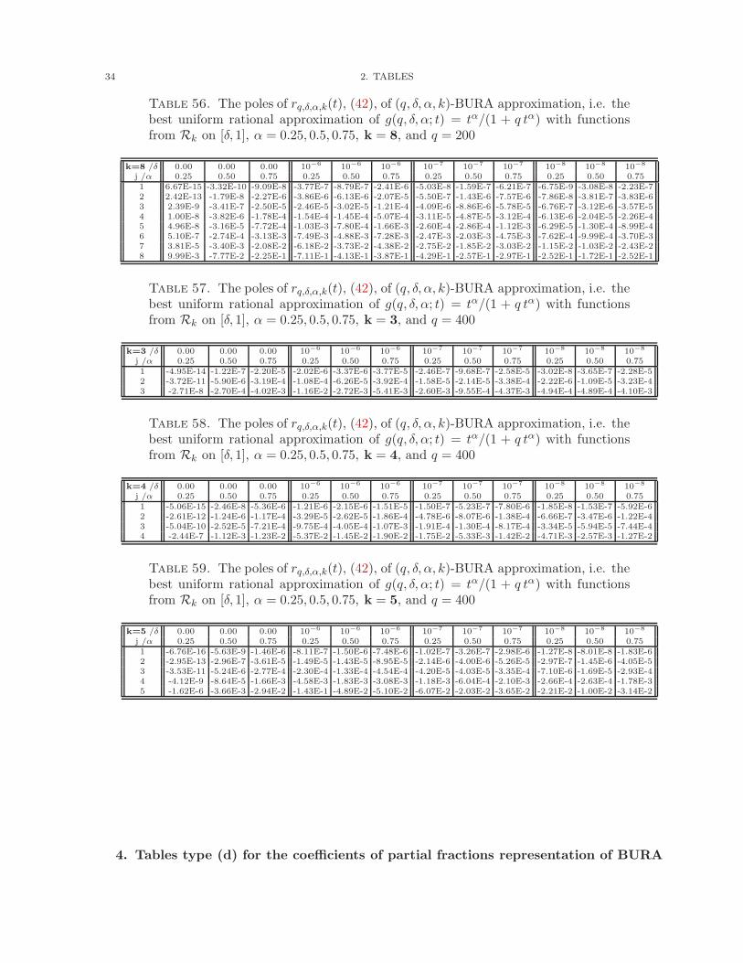
34 2. TABLES
Table 56. The poles of rq,δ,α,k(t), (42), of (q, δ, α, k)-BURA approximation, i.e. thebest uniform rational approximation of g(q, δ, α; t) = tα/(1 + q tα) with functionsfrom Rk on [δ, 1], α = 0.25, 0.5, 0.75, k = 8, and q = 200
k=8 /δ 0.00 0.00 0.00 10−6 10−6 10−6 10−7 10−7 10−7 10−8 10−8 10−8
j /α 0.25 0.50 0.75 0.25 0.50 0.75 0.25 0.50 0.75 0.25 0.50 0.751 6.67E-15 -3.32E-10 -9.09E-8 -3.77E-7 -8.79E-7 -2.41E-6 -5.03E-8 -1.59E-7 -6.21E-7 -6.75E-9 -3.08E-8 -2.23E-72 2.42E-13 -1.79E-8 -2.27E-6 -3.86E-6 -6.13E-6 -2.07E-5 -5.50E-7 -1.43E-6 -7.57E-6 -7.86E-8 -3.81E-7 -3.83E-63 2.39E-9 -3.41E-7 -2.50E-5 -2.46E-5 -3.02E-5 -1.21E-4 -4.09E-6 -8.86E-6 -5.78E-5 -6.76E-7 -3.12E-6 -3.57E-54 1.00E-8 -3.82E-6 -1.78E-4 -1.54E-4 -1.45E-4 -5.07E-4 -3.11E-5 -4.87E-5 -3.12E-4 -6.13E-6 -2.04E-5 -2.26E-45 4.96E-8 -3.16E-5 -7.72E-4 -1.03E-3 -7.80E-4 -1.66E-3 -2.60E-4 -2.86E-4 -1.12E-3 -6.29E-5 -1.30E-4 -8.99E-46 5.10E-7 -2.74E-4 -3.13E-3 -7.49E-3 -4.88E-3 -7.28E-3 -2.47E-3 -2.03E-3 -4.75E-3 -7.62E-4 -9.99E-4 -3.70E-37 3.81E-5 -3.40E-3 -2.08E-2 -6.18E-2 -3.73E-2 -4.38E-2 -2.75E-2 -1.85E-2 -3.03E-2 -1.15E-2 -1.03E-2 -2.43E-28 9.99E-3 -7.77E-2 -2.25E-1 -7.11E-1 -4.13E-1 -3.87E-1 -4.29E-1 -2.57E-1 -2.97E-1 -2.52E-1 -1.72E-1 -2.52E-1
Table 57. The poles of rq,δ,α,k(t), (42), of (q, δ, α, k)-BURA approximation, i.e. thebest uniform rational approximation of g(q, δ, α; t) = tα/(1 + q tα) with functionsfrom Rk on [δ, 1], α = 0.25, 0.5, 0.75, k = 3, and q = 400
k=3 /δ 0.00 0.00 0.00 10−6 10−6 10−6 10−7 10−7 10−7 10−8 10−8 10−8
j /α 0.25 0.50 0.75 0.25 0.50 0.75 0.25 0.50 0.75 0.25 0.50 0.751 -4.95E-14 -1.22E-7 -2.20E-5 -2.02E-6 -3.37E-6 -3.77E-5 -2.46E-7 -9.68E-7 -2.58E-5 -3.02E-8 -3.65E-7 -2.28E-52 -3.72E-11 -5.90E-6 -3.19E-4 -1.08E-4 -6.26E-5 -3.92E-4 -1.58E-5 -2.14E-5 -3.38E-4 -2.22E-6 -1.09E-5 -3.23E-43 -2.71E-8 -2.70E-4 -4.02E-3 -1.16E-2 -2.72E-3 -5.41E-3 -2.60E-3 -9.55E-4 -4.37E-3 -4.94E-4 -4.89E-4 -4.10E-3
Table 58. The poles of rq,δ,α,k(t), (42), of (q, δ, α, k)-BURA approximation, i.e. thebest uniform rational approximation of g(q, δ, α; t) = tα/(1 + q tα) with functionsfrom Rk on [δ, 1], α = 0.25, 0.5, 0.75, k = 4, and q = 400
k=4 /δ 0.00 0.00 0.00 10−6 10−6 10−6 10−7 10−7 10−7 10−8 10−8 10−8
j /α 0.25 0.50 0.75 0.25 0.50 0.75 0.25 0.50 0.75 0.25 0.50 0.751 -5.06E-15 -2.46E-8 -5.36E-6 -1.21E-6 -2.15E-6 -1.51E-5 -1.50E-7 -5.23E-7 -7.80E-6 -1.85E-8 -1.53E-7 -5.92E-62 -2.61E-12 -1.24E-6 -1.17E-4 -3.29E-5 -2.62E-5 -1.86E-4 -4.78E-6 -8.07E-6 -1.38E-4 -6.66E-7 -3.47E-6 -1.22E-43 -5.04E-10 -2.52E-5 -7.21E-4 -9.75E-4 -4.05E-4 -1.07E-3 -1.91E-4 -1.30E-4 -8.17E-4 -3.34E-5 -5.94E-5 -7.44E-44 -2.44E-7 -1.12E-3 -1.23E-2 -5.37E-2 -1.45E-2 -1.90E-2 -1.75E-2 -5.33E-3 -1.42E-2 -4.71E-3 -2.57E-3 -1.27E-2
Table 59. The poles of rq,δ,α,k(t), (42), of (q, δ, α, k)-BURA approximation, i.e. thebest uniform rational approximation of g(q, δ, α; t) = tα/(1 + q tα) with functionsfrom Rk on [δ, 1], α = 0.25, 0.5, 0.75, k = 5, and q = 400
k=5 /δ 0.00 0.00 0.00 10−6 10−6 10−6 10−7 10−7 10−7 10−8 10−8 10−8
j /α 0.25 0.50 0.75 0.25 0.50 0.75 0.25 0.50 0.75 0.25 0.50 0.751 -6.76E-16 -5.63E-9 -1.46E-6 -8.11E-7 -1.50E-6 -7.48E-6 -1.02E-7 -3.26E-7 -2.98E-6 -1.27E-8 -8.01E-8 -1.83E-62 -2.95E-13 -2.96E-7 -3.61E-5 -1.49E-5 -1.43E-5 -8.95E-5 -2.14E-6 -4.00E-6 -5.26E-5 -2.97E-7 -1.45E-6 -4.05E-53 -3.53E-11 -5.24E-6 -2.77E-4 -2.30E-4 -1.33E-4 -4.54E-4 -4.20E-5 -4.03E-5 -3.35E-4 -7.10E-6 -1.69E-5 -2.93E-44 -4.12E-9 -8.64E-5 -1.66E-3 -4.58E-3 -1.83E-3 -3.08E-3 -1.18E-3 -6.04E-4 -2.10E-3 -2.66E-4 -2.63E-4 -1.78E-35 -1.62E-6 -3.66E-3 -2.94E-2 -1.43E-1 -4.89E-2 -5.10E-2 -6.07E-2 -2.03E-2 -3.65E-2 -2.21E-2 -1.00E-2 -3.14E-2
4. Tables type (d) for the coefficients of partial fractions representation of BURA

4. TABLES TYPE (D) FOR THE COEFFICIENTS OF PARTIAL FRACTIONS REPRESENTATION OF BURA 35
Table 60. The poles of rq,δ,α,k(t), (42), of (q, δ, α, k)-BURA approximation, i.e. thebest uniform rational approximation of g(q, δ, α; t) = tα/(1 + q tα) with functionsfrom Rk on [δ, 1], α = 0.25, 0.5, 0.75, k = 6, and q = 400
k=6 /δ 0.00 0.00 0.00 10−6 10−6 10−6 10−7 10−7 10−7 10−8 10−8 10−8
j /α 0.25 0.50 0.75 0.25 0.50 0.75 0.25 0.50 0.75 0.25 0.50 0.751 -1.08E-16 -1.42E-9 -4.34E-7 -5.86E-7 -1.12E-6 -4.33E-6 -7.42E-8 -2.23E-7 -1.39E-6 -9.35E-9 -4.82E-8 -6.73E-72 -4.33E-14 -7.59E-8 -1.09E-5 -8.35E-6 -8.95E-6 -4.53E-5 -1.18E-6 -2.29E-6 -2.14E-5 -1.63E-7 -7.17E-7 -1.39E-53 -4.14E-12 -1.37E-6 -1.09E-4 -8.60E-5 -6.14E-5 -2.47E-4 -1.49E-5 -1.76E-5 -1.60E-4 -2.45E-6 -6.77E-6 -1.25E-44 -2.75E-10 -1.61E-5 -5.15E-4 -9.90E-4 -5.15E-4 -1.04E-3 -2.24E-4 -1.60E-4 -6.91E-4 -4.64E-5 -6.48E-5 -5.68E-45 -2.51E-8 -2.51E-4 -3.60E-3 -1.40E-2 -5.95E-3 -7.87E-3 -4.48E-3 -2.14E-3 -5.08E-3 -1.28E-3 -9.42E-4 -4.06E-36 -8.52E-6 -9.61E-3 -5.81E-2 -2.83E-1 -1.17E-1 -1.09E-1 -1.41E-1 -5.52E-2 -7.70E-2 -6.39E-2 -2.91E-2 -6.41E-2
Table 61. The poles of rq,δ,α,k(t), (42), of (q, δ, α, k)-BURA approximation, i.e. thebest uniform rational approximation of g(q, δ, α; t) = tα/(1 + q tα) with functionsfrom Rk on [δ, 1], α = 0.25, 0.5, 0.75, k = 7, and q = 400
k=7 /δ 0.00 0.00 0.00 10−6 10−6 10−6 10−7 10−7 10−7 10−8 10−8 10−8
j /α 0.25 0.50 0.75 0.25 0.50 0.75 0.25 0.50 0.75 0.25 0.50 0.751 9.05E-14 -3.83E-10 -1.38E-7 -4.45E-7 -8.62E-7 -2.79E-6 -5.67E-8 -1.62E-7 -7.58E-7 -7.20E-9 -3.20E-8 -2.93E-72 -1.37E-13 -2.06E-8 -3.47E-6 -5.32E-6 -6.13E-6 -2.52E-5 -7.43E-7 -1.45E-6 -9.86E-6 -1.01E-7 -3.97E-7 -5.34E-63 3.25E-13 -3.85E-7 -3.77E-5 -4.16E-5 -3.42E-5 -1.40E-4 -6.92E-6 -9.29E-6 -7.50E-5 -1.10E-6 -3.24E-6 -5.00E-54 4.90E-10 -4.22E-6 -2.21E-4 -3.36E-4 -2.10E-4 -5.11E-4 -6.99E-5 -6.17E-5 -3.32E-4 -1.36E-5 -2.36E-5 -2.60E-45 3.57E-9 -4.21E-5 -9.30E-4 -3.03E-3 -1.56E-3 -2.39E-3 -8.29E-4 -5.15E-4 -1.45E-3 -2.07E-4 -2.10E-4 -1.10E-36 7.90E-8 -6.29E-4 -7.01E-3 -3.20E-2 -1.50E-2 -1.72E-2 -1.22E-2 -5.95E-3 -1.09E-2 -4.21E-3 -2.73E-3 -8.34E-37 2.77E-4 -2.10E-2 -9.93E-2 -4.70E-1 -2.23E-1 -1.96E-1 -2.61E-1 -1.17E-1 -1.39E-1 -1.36E-1 -6.63E-2 -1.14E-1
Table 62. The poles of rq,δ,α,k(t), (42), of (q, δ, α, k)-BURA approximation, i.e. thebest uniform rational approximation of g(q, δ, α; t) = tα/(1 + q tα) with functionsfrom Rk on [δ, 1], α = 0.25, 0.5, 0.75, k = 8, and q = 400
k=8 /δ 0.00 0.00 0.00 10−6 10−6 10−6 10−7 10−7 10−7 10−8 10−8 10−8
j /α 0.25 0.50 0.75 0.25 0.50 0.75 0.25 0.50 0.75 0.25 0.50 0.751 1.55E-13 -1.10E-10 -4.66E-8 -3.51E-7 -6.88E-7 -1.94E-6 -4.49E-8 -1.23E-7 -4.65E-7 -5.73E-9 -2.27E-8 -1.49E-72 2.42E-11 -5.92E-9 -1.16E-6 -3.70E-6 -4.47E-6 -1.53E-5 -5.10E-7 -9.81E-7 -5.13E-6 -6.91E-8 -2.42E-7 -2.34E-63 -1.05E-10 -1.12E-7 -1.28E-5 -2.37E-5 -2.14E-5 -8.14E-5 -3.81E-6 -5.51E-6 -3.64E-5 -5.92E-7 -1.74E-6 -2.07E-54 3.87E-10 -1.25E-6 -8.93E-5 -1.49E-4 -1.06E-4 -3.00E-4 -2.90E-5 -2.97E-5 -1.77E-4 -5.37E-6 -1.07E-5 -1.23E-45 -3.93E-9 -1.05E-5 -3.71E-4 -9.94E-4 -5.94E-4 -1.03E-3 -2.44E-4 -1.83E-4 -6.18E-4 -5.56E-5 -7.02E-5 -4.62E-46 -1.59E-7 -9.78E-5 -1.65E-3 -7.29E-3 -3.88E-3 -5.05E-3 -2.33E-3 -1.38E-3 -2.95E-3 -6.84E-4 -5.79E-4 -2.13E-37 -1.55E-5 -1.37E-3 -1.23E-2 -6.06E-2 -3.12E-2 -3.26E-2 -2.64E-2 -1.36E-2 -2.07E-2 -1.06E-2 -6.57E-3 -1.55E-28 -3.37E-3 -3.93E-2 -1.52E-1 -7.01E-1 -3.66E-1 -3.13E-1 -4.17E-1 -2.08E-1 -2.24E-1 -2.39E-1 -1.25E-1 -1.81E-1
Table 63. The coefficients cj , j = 0, . . . , k of the partial fraction representationdefined by (35) of (q, δ, α, k)-BURA approximation for δ = 0, 10−6, 10−7, 10−8, α =0.25, 0.50, 0.75, k = 3, and q = 0
k=3 /δ 0.00 0.00 0.00 10−6 10−6 10−6 10−7 10−7 10−7 10−8 10−8 10−8
j /α 0.25 0.50 0.75 0.25 0.50 0.75 0.25 0.50 0.75 0.25 0.50 0.750 1.23E00 2.28E00 6.15E00 1.29E00 2.31E00 6.17E00 1.27E00 2.29E00 6.16E00 1.25E00 2.28E00 6.15E001 -1.40E-6 -4.18E-5 -9.88E-5 -1.12E-5 -5.15E-5 -1.01E-4 -5.10E-6 -4.48E-5 -9.92E-5 -3.02E-6 -4.28E-5 -9.88E-52 -1.37E-3 -1.20E-2 -2.39E-2 -2.99E-3 -1.29E-2 -2.41E-2 -2.19E-3 -1.23E-2 -2.39E-2 -1.80E-3 -1.21E-2 -2.39E-23 -3.44E-1 -3.52E00 -3.64E01 -4.60E-1 -3.65E00 -3.66E01 -4.07E-1 -3.56E00 -3.65E01 -3.79E-1 -3.54E00 -3.64E01
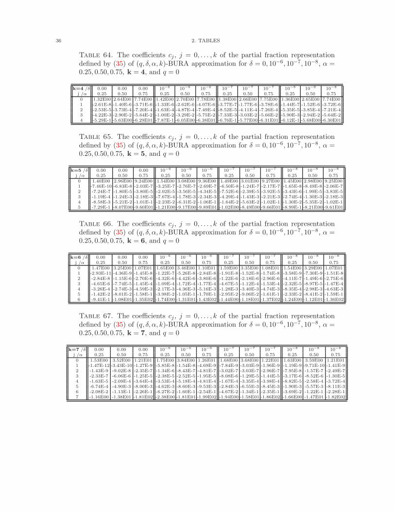
36 2. TABLES
Table 64. The coefficients cj , j = 0, . . . , k of the partial fraction representationdefined by (35) of (q, δ, α, k)-BURA approximation for δ = 0, 10−6, 10−7, 10−8, α =0.25, 0.50, 0.75, k = 4, and q = 0
k=4 /δ 0.00 0.00 0.00 10−6 10−6 10−6 10−7 10−7 10−7 10−8 10−8 10−8
j /α 0.25 0.50 0.75 0.25 0.50 0.75 0.25 0.50 0.75 0.25 0.50 0.750 1.32E00 2.64E00 7.74E00 1.42E00 2.70E00 7.78E00 1.38E00 2.66E00 7.75E00 1.36E00 2.65E00 7.74E001 -2.61E-8 -1.40E-6 -3.71E-6 -1.33E-6 -2.62E-6 -4.07E-6 -3.77E-7 -1.77E-6 -3.78E-6 -1.44E-7 -1.52E-6 -3.72E-62 -2.53E-5 -3.73E-4 -7.20E-4 -1.63E-4 -4.87E-4 -7.49E-4 -8.52E-5 -4.11E-4 -7.26E-4 -5.35E-5 -3.85E-4 -7.21E-43 -4.22E-3 -2.90E-2 -5.64E-2 -1.00E-2 -3.29E-2 -5.75E-2 -7.33E-3 -3.03E-2 -5.66E-2 -5.90E-3 -2.94E-2 -5.64E-24 -5.29E-1 -5.63E00 -6.29E01 -7.87E-1 -6.05E00 -6.38E01 -6.76E-1 -5.77E00 -6.31E01 -6.12E-1 -5.68E00 -6.30E01
Table 65. The coefficients cj , j = 0, . . . , k of the partial fraction representationdefined by (35) of (q, δ, α, k)-BURA approximation for δ = 0, 10−6, 10−7, 10−8, α =0.25, 0.50, 0.75, k = 5, and q = 0
k=5 /δ 0.00 0.00 0.00 10−6 10−6 10−6 10−7 10−7 10−7 10−8 10−8 10−8
j /α 0.25 0.50 0.75 0.25 0.50 0.75 0.25 0.50 0.75 0.25 0.50 0.750 1.40E00 2.96E00 9.24E00 1.54E00 3.08E00 9.36E00 1.49E00 3.01E00 9.27E00 1.45E00 2.98E00 9.25E001 -7.46E-10 -6.83E-8 -2.03E-7 -3.25E-7 -2.76E-7 -2.69E-7 -6.50E-8 -1.24E-7 -2.17E-7 -1.65E-8 -8.49E-8 -2.06E-72 -7.24E-7 -1.80E-5 -3.80E-5 -2.02E-5 -3.56E-5 -4.34E-5 -7.52E-6 -2.39E-5 -3.92E-5 -3.43E-6 -1.99E-5 -3.83E-53 -1.19E-4 -1.24E-3 -2.18E-3 -7.67E-4 -1.78E-3 -2.34E-3 -4.29E-4 -1.43E-3 -2.21E-3 -2.74E-4 -1.30E-3 -2.18E-34 -8.58E-3 -5.21E-2 -1.01E-1 -2.23E-2 -6.31E-2 -1.06E-1 -1.64E-2 -5.63E-2 -1.02E-1 -1.30E-2 -5.35E-2 -1.02E-15 -7.29E-1 -8.07E00 -9.60E01 -1.21E00 -9.17E00 -9.89E01 -1.02E00 -8.49E00 -9.66E01 -8.99E-1 -8.21E00 -9.61E01
Table 66. The coefficients cj , j = 0, . . . , k of the partial fraction representationdefined by (35) of (q, δ, α, k)-BURA approximation for δ = 0, 10−6, 10−7, 10−8, α =0.25, 0.50, 0.75, k = 6, and q = 0
k=6 /δ 0.00 0.00 0.00 10−6 10−6 10−6 10−7 10−7 10−7 10−8 10−8 10−8
j /α 0.25 0.50 0.75 0.25 0.50 0.75 0.25 0.50 0.75 0.25 0.50 0.750 1.47E00 3.25E00 1.07E01 1.65E00 3.46E00 1.10E01 1.59E00 3.35E00 1.08E01 1.54E00 3.29E00 1.07E011 -2.93E-11 -4.36E-9 -1.45E-8 -1.22E-7 -5.26E-8 -2.84E-8 -1.91E-8 -1.52E-8 -1.74E-8 -3.58E-9 -7.30E-9 -1.51E-82 -2.84E-8 -1.15E-6 -2.70E-6 -4.32E-6 -4.42E-6 -3.80E-6 -1.22E-6 -2.18E-6 -2.96E-6 -4.11E-7 -1.49E-6 -2.75E-63 -4.65E-6 -7.74E-5 -1.45E-4 -1.09E-4 -1.72E-4 -1.77E-4 -4.67E-5 -1.12E-4 -1.53E-4 -2.32E-5 -8.97E-5 -1.47E-44 -3.26E-4 -2.74E-3 -4.59E-3 -2.17E-3 -4.36E-3 -5.16E-3 -1.28E-3 -3.40E-3 -4.74E-3 -8.35E-4 -2.98E-3 -4.63E-35 -1.42E-2 -8.01E-2 -1.58E-1 -3.98E-2 -1.05E-1 -1.70E-1 -2.95E-2 -9.06E-2 -1.61E-1 -2.33E-2 -8.41E-2 -1.59E-16 -9.41E-1 -1.08E01 -1.35E02 -1.74E00 -1.31E01 -1.43E02 -1.44E00 -1.18E01 -1.37E02 -1.24E00 -1.12E01 -1.36E02
Table 67. The coefficients cj , j = 0, . . . , k of the partial fraction representationdefined by (35) of (q, δ, α, k)-BURA approximation for δ = 0, 10−6, 10−7, 10−8, α =0.25, 0.50, 0.75, k = 7, and q = 0
k=7 /δ 0.00 0.00 0.00 10−6 10−6 10−6 10−7 10−7 10−7 10−8 10−8 10−8
j /α 0.25 0.50 0.75 0.25 0.50 0.75 0.25 0.50 0.75 0.25 0.50 0.750 1.53E00 3.52E00 1.21E01 1.75E00 3.84E00 1.26E01 1.68E00 3.68E00 1.22E01 1.63E00 3.59E00 1.21E011 -1.47E-12 -3.43E-10 -1.27E-9 -5.85E-8 -1.54E-8 -4.69E-9 -7.84E-9 -3.03E-9 -1.96E-9 -1.19E-9 -9.71E-10 -1.41E-92 -1.43E-9 -9.02E-8 -2.35E-7 -1.34E-6 -8.43E-7 -4.81E-7 -3.02E-7 -3.03E-7 -2.96E-7 -7.95E-8 -1.57E-7 -2.49E-73 -2.33E-7 -6.06E-6 -1.25E-5 -2.38E-5 -2.52E-5 -1.95E-5 -8.08E-6 -1.29E-5 -1.44E-5 -3.17E-6 -8.52E-6 -1.30E-54 -1.63E-5 -2.09E-4 -3.64E-4 -3.53E-4 -5.18E-4 -4.81E-4 -1.67E-4 -3.35E-4 -3.98E-4 -8.82E-5 -2.58E-4 -3.72E-45 -6.74E-4 -4.90E-3 -8.00E-3 -4.62E-3 -8.60E-3 -9.53E-3 -2.84E-3 -6.55E-3 -8.45E-3 -1.90E-3 -5.57E-3 -8.11E-36 -2.08E-2 -1.13E-1 -2.26E-1 -6.27E-2 -1.60E-1 -2.54E-1 -4.67E-2 -1.34E-1 -2.35E-1 -3.69E-2 -1.22E-1 -2.28E-17 -1.16E00 -1.38E01 -1.81E02 -2.38E00 -1.81E01 -1.99E02 -1.94E00 -1.58E01 -1.86E02 -1.66E00 -1.47E01 -1.82E02
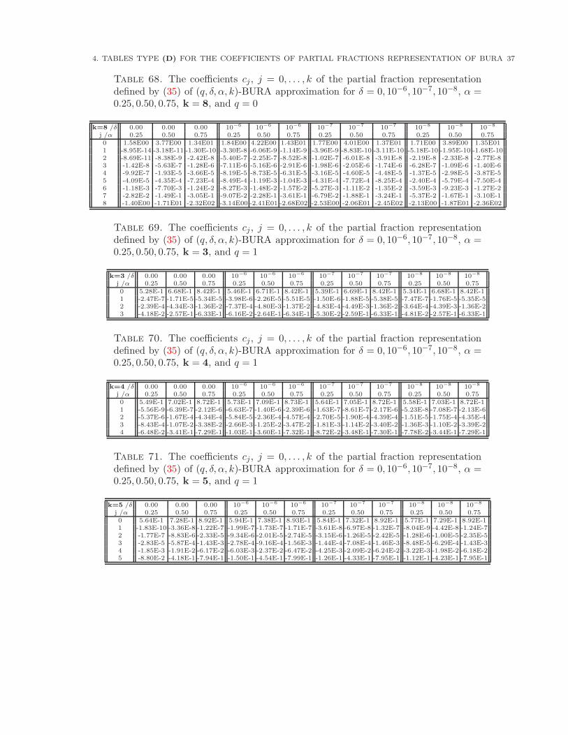
4. TABLES TYPE (D) FOR THE COEFFICIENTS OF PARTIAL FRACTIONS REPRESENTATION OF BURA 37
Table 68. The coefficients cj , j = 0, . . . , k of the partial fraction representationdefined by (35) of (q, δ, α, k)-BURA approximation for δ = 0, 10−6, 10−7, 10−8, α =0.25, 0.50, 0.75, k = 8, and q = 0
k=8 /δ 0.00 0.00 0.00 10−6 10−6 10−6 10−7 10−7 10−7 10−8 10−8 10−8
j /α 0.25 0.50 0.75 0.25 0.50 0.75 0.25 0.50 0.75 0.25 0.50 0.750 1.58E00 3.77E00 1.34E01 1.84E00 4.22E00 1.43E01 1.77E00 4.01E00 1.37E01 1.71E00 3.89E00 1.35E011 -8.95E-14 -3.18E-11 -1.30E-10 -3.30E-8 -6.06E-9 -1.14E-9 -3.96E-9 -8.83E-10 -3.11E-10 -5.18E-10 -1.95E-10 -1.68E-102 -8.69E-11 -8.38E-9 -2.42E-8 -5.40E-7 -2.25E-7 -8.52E-8 -1.02E-7 -6.01E-8 -3.91E-8 -2.19E-8 -2.33E-8 -2.77E-83 -1.42E-8 -5.63E-7 -1.28E-6 -7.11E-6 -5.16E-6 -2.91E-6 -1.98E-6 -2.05E-6 -1.74E-6 -6.28E-7 -1.09E-6 -1.40E-64 -9.92E-7 -1.93E-5 -3.66E-5 -8.19E-5 -8.73E-5 -6.31E-5 -3.16E-5 -4.60E-5 -4.48E-5 -1.37E-5 -2.98E-5 -3.87E-55 -4.09E-5 -4.35E-4 -7.23E-4 -8.49E-4 -1.19E-3 -1.04E-3 -4.31E-4 -7.72E-4 -8.25E-4 -2.40E-4 -5.79E-4 -7.50E-46 -1.18E-3 -7.70E-3 -1.24E-2 -8.27E-3 -1.48E-2 -1.57E-2 -5.27E-3 -1.11E-2 -1.35E-2 -3.59E-3 -9.23E-3 -1.27E-27 -2.82E-2 -1.49E-1 -3.05E-1 -9.07E-2 -2.28E-1 -3.61E-1 -6.79E-2 -1.88E-1 -3.24E-1 -5.37E-2 -1.67E-1 -3.10E-18 -1.40E00 -1.71E01 -2.32E02 -3.14E00 -2.41E01 -2.68E02 -2.53E00 -2.06E01 -2.45E02 -2.13E00 -1.87E01 -2.36E02
Table 69. The coefficients cj , j = 0, . . . , k of the partial fraction representationdefined by (35) of (q, δ, α, k)-BURA approximation for δ = 0, 10−6, 10−7, 10−8, α =0.25, 0.50, 0.75, k = 3, and q = 1
k=3 /δ 0.00 0.00 0.00 10−6 10−6 10−6 10−7 10−7 10−7 10−8 10−8 10−8
j /α 0.25 0.50 0.75 0.25 0.50 0.75 0.25 0.50 0.75 0.25 0.50 0.750 5.28E-1 6.68E-1 8.42E-1 5.46E-1 6.71E-1 8.42E-1 5.39E-1 6.69E-1 8.42E-1 5.34E-1 6.68E-1 8.42E-11 -2.47E-7 -1.71E-5 -5.34E-5 -3.98E-6 -2.26E-5 -5.51E-5 -1.50E-6 -1.88E-5 -5.38E-5 -7.47E-7 -1.76E-5 -5.35E-52 -2.39E-4 -4.34E-3 -1.36E-2 -7.37E-4 -4.80E-3 -1.37E-2 -4.83E-4 -4.49E-3 -1.36E-2 -3.64E-4 -4.39E-3 -1.36E-23 -4.18E-2 -2.57E-1 -6.33E-1 -6.16E-2 -2.64E-1 -6.34E-1 -5.30E-2 -2.59E-1 -6.33E-1 -4.81E-2 -2.57E-1 -6.33E-1
Table 70. The coefficients cj , j = 0, . . . , k of the partial fraction representationdefined by (35) of (q, δ, α, k)-BURA approximation for δ = 0, 10−6, 10−7, 10−8, α =0.25, 0.50, 0.75, k = 4, and q = 1
k=4 /δ 0.00 0.00 0.00 10−6 10−6 10−6 10−7 10−7 10−7 10−8 10−8 10−8
j /α 0.25 0.50 0.75 0.25 0.50 0.75 0.25 0.50 0.75 0.25 0.50 0.750 5.49E-1 7.02E-1 8.72E-1 5.73E-1 7.09E-1 8.73E-1 5.64E-1 7.05E-1 8.72E-1 5.58E-1 7.03E-1 8.72E-11 -5.56E-9 -6.39E-7 -2.12E-6 -6.63E-7 -1.40E-6 -2.39E-6 -1.63E-7 -8.61E-7 -2.17E-6 -5.23E-8 -7.08E-7 -2.13E-62 -5.37E-6 -1.67E-4 -4.34E-4 -5.84E-5 -2.36E-4 -4.57E-4 -2.70E-5 -1.90E-4 -4.39E-4 -1.51E-5 -1.75E-4 -4.35E-43 -8.43E-4 -1.07E-2 -3.38E-2 -2.66E-3 -1.25E-2 -3.47E-2 -1.81E-3 -1.14E-2 -3.40E-2 -1.36E-3 -1.10E-2 -3.39E-24 -6.48E-2 -3.41E-1 -7.29E-1 -1.03E-1 -3.60E-1 -7.32E-1 -8.72E-2 -3.48E-1 -7.30E-1 -7.78E-2 -3.44E-1 -7.29E-1
Table 71. The coefficients cj , j = 0, . . . , k of the partial fraction representationdefined by (35) of (q, δ, α, k)-BURA approximation for δ = 0, 10−6, 10−7, 10−8, α =0.25, 0.50, 0.75, k = 5, and q = 1
k=5 /δ 0.00 0.00 0.00 10−6 10−6 10−6 10−7 10−7 10−7 10−8 10−8 10−8
j /α 0.25 0.50 0.75 0.25 0.50 0.75 0.25 0.50 0.75 0.25 0.50 0.750 5.64E-1 7.28E-1 8.92E-1 5.94E-1 7.38E-1 8.93E-1 5.84E-1 7.32E-1 8.92E-1 5.77E-1 7.29E-1 8.92E-11 -1.83E-10 -3.36E-8 -1.22E-7 -1.99E-7 -1.73E-7 -1.71E-7 -3.61E-8 -6.97E-8 -1.32E-7 -8.04E-9 -4.42E-8 -1.24E-72 -1.77E-7 -8.83E-6 -2.33E-5 -9.34E-6 -2.01E-5 -2.74E-5 -3.15E-6 -1.26E-5 -2.42E-5 -1.28E-6 -1.00E-5 -2.35E-53 -2.83E-5 -5.87E-4 -1.43E-3 -2.78E-4 -9.16E-4 -1.56E-3 -1.44E-4 -7.08E-4 -1.46E-3 -8.48E-5 -6.29E-4 -1.43E-34 -1.85E-3 -1.91E-2 -6.17E-2 -6.03E-3 -2.37E-2 -6.47E-2 -4.25E-3 -2.09E-2 -6.24E-2 -3.22E-3 -1.98E-2 -6.18E-25 -8.80E-2 -4.18E-1 -7.94E-1 -1.50E-1 -4.54E-1 -7.99E-1 -1.26E-1 -4.33E-1 -7.95E-1 -1.12E-1 -4.23E-1 -7.95E-1
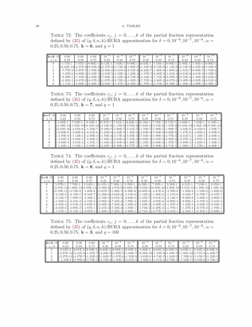
38 2. TABLES
Table 72. The coefficients cj , j = 0, . . . , k of the partial fraction representationdefined by (35) of (q, δ, α, k)-BURA approximation for δ = 0, 10−6, 10−7, 10−8, α =0.25, 0.50, 0.75, k = 6, and q = 1
k=6 /δ 0.00 0.00 0.00 10−6 10−6 10−6 10−7 10−7 10−7 10−8 10−8 10−8
j /α 0.25 0.50 0.75 0.25 0.50 0.75 0.25 0.50 0.75 0.25 0.50 0.750 5.77E-1 7.47E-1 9.06E-1 6.12E-1 7.62E-1 9.08E-1 6.02E-1 7.54E-1 9.06E-1 5.94E-1 7.50E-1 9.06E-11 -8.02E-12 -2.27E-9 -9.03E-9 -8.37E-8 -3.74E-8 -1.96E-8 -1.24E-8 -9.72E-9 -1.13E-8 -2.13E-9 -4.23E-9 -9.49E-92 -7.77E-9 -5.97E-7 -1.70E-6 -2.39E-6 -2.81E-6 -2.53E-6 -6.22E-7 -1.28E-6 -1.90E-6 -1.91E-7 -8.20E-7 -1.74E-63 -1.25E-6 -4.00E-5 -9.45E-5 -4.91E-5 -1.02E-4 -1.20E-4 -1.97E-5 -6.28E-5 -1.01E-4 -9.01E-6 -4.81E-5 -9.59E-54 -8.38E-5 -1.35E-3 -3.22E-3 -7.88E-4 -2.32E-3 -3.73E-3 -4.42E-4 -1.75E-3 -3.35E-3 -2.72E-4 -1.50E-3 -3.25E-35 -3.20E-3 -2.87E-2 -9.47E-2 -1.07E-2 -3.79E-2 -1.02E-1 -7.75E-3 -3.28E-2 -9.67E-2 -5.96E-3 -3.03E-2 -9.51E-26 -1.11E-1 -4.89E-1 -8.38E-1 -2.03E-1 -5.47E-1 -8.46E-1 -1.70E-1 -5.15E-1 -8.40E-1 -1.49E-1 -4.99E-1 -8.39E-1
Table 73. The coefficients cj , j = 0, . . . , k of the partial fraction representationdefined by (35) of (q, δ, α, k)-BURA approximation for δ = 0, 10−6, 10−7, 10−8, α =0.25, 0.50, 0.75, k = 7, and q = 1
k=7 /δ 0.00 0.00 0.00 10−6 10−6 10−6 10−7 10−7 10−7 10−8 10−8 10−8
j /α 0.25 0.50 0.75 0.25 0.50 0.75 0.25 0.50 0.75 0.25 0.50 0.750 5.88E-1 7.63E-1 9.16E-1 6.27E-1 7.81E-1 9.20E-1 6.16E-1 7.73E-1 9.17E-1 6.08E-1 7.68E-1 9.16E-11 -4.39E-13 -1.86E-10 -8.16E-10 -4.34E-8 -1.19E-8 -3.50E-9 -5.62E-9 -2.16E-9 -1.35E-9 -8.03E-10 -6.26E-10 -9.28E-102 -4.25E-10 -4.91E-8 -1.52E-7 -8.38E-7 -5.89E-7 -3.41E-7 -1.78E-7 -1.96E-7 -1.99E-7 -4.34E-8 -9.45E-8 -1.63E-73 -6.90E-8 -3.30E-6 -8.21E-6 -1.25E-5 -1.64E-5 -1.36E-5 -4.03E-6 -7.89E-6 -9.69E-6 -1.47E-6 -4.95E-6 -8.56E-64 -4.70E-6 -1.12E-4 -2.49E-4 -1.56E-4 -3.17E-4 -3.46E-4 -7.04E-5 -1.96E-4 -2.77E-4 -3.51E-5 -1.45E-4 -2.56E-45 -1.83E-4 -2.46E-3 -5.93E-3 -1.66E-3 -4.63E-3 -7.35E-3 -9.92E-4 -3.45E-3 -6.36E-3 -6.37E-4 -2.87E-3 -6.03E-36 -4.82E-3 -3.91E-2 -1.31E-1 -1.64E-2 -5.45E-2 -1.46E-1 -1.22E-2 -4.66E-2 -1.35E-1 -9.49E-3 -4.23E-2 -1.32E-17 -1.34E-1 -5.54E-1 -8.68E-1 -2.62E-1 -6.39E-1 -8.77E-1 -2.19E-1 -5.96E-1 -8.71E-1 -1.90E-1 -5.73E-1 -8.68E-1
Table 74. The coefficients cj , j = 0, . . . , k of the partial fraction representationdefined by (35) of (q, δ, α, k)-BURA approximation for δ = 0, 10−6, 10−7, 10−8, α =0.25, 0.50, 0.75, k = 8, and q = 1
k=8 /δ 0.00 0.00 0.00 10−6 10−6 10−6 10−7 10−7 10−7 10−8 10−8 10−8
j /α 0.25 0.50 0.75 0.25 0.50 0.75 0.25 0.50 0.75 0.25 0.50 0.750 5.97E-1 7.76E-1 9.24E-1 6.41E-1 7.98E-1 9.29E-1 6.29E-1 7.89E-1 9.26E-1 6.21E-1 7.83E-1 9.25E-11 -2.87E-14 -1.80E-11 -8.62E-11 -2.58E-8 -4.97E-9 -9.02E-10 -3.03E-9 -6.80E-10 -2.29E-10 -3.81E-10 -1.38E-10 -1.16E-102 -2.79E-11 -4.73E-9 -1.60E-8 -3.67E-7 -1.68E-7 -6.38E-8 -6.66E-8 -4.21E-8 -2.76E-8 -1.35E-8 -1.52E-8 -1.88E-83 -4.54E-9 -3.18E-7 -8.56E-7 -4.20E-6 -3.62E-6 -2.12E-6 -1.12E-6 -1.36E-6 -1.21E-6 -3.34E-7 -6.78E-7 -9.47E-74 -3.12E-7 -1.08E-5 -2.48E-5 -4.18E-5 -5.81E-5 -4.60E-5 -1.55E-5 -2.91E-5 -3.14E-5 -6.36E-6 -1.80E-5 -2.66E-55 -1.24E-5 -2.41E-4 -5.16E-4 -3.68E-4 -7.45E-4 -7.88E-4 -1.82E-4 -4.65E-4 -6.06E-4 -9.69E-5 -3.37E-4 -5.41E-46 -3.32E-4 -3.91E-3 -9.62E-3 -2.92E-3 -7.92E-3 -1.28E-2 -1.83E-3 -5.89E-3 -1.07E-2 -1.22E-3 -4.82E-3 -9.92E-37 -6.64E-3 -4.98E-2 -1.67E-1 -2.31E-2 -7.30E-2 -1.93E-1 -1.74E-2 -6.20E-2 -1.77E-1 -1.37E-2 -5.57E-2 -1.70E-18 -1.57E-1 -6.14E-1 -8.87E-1 -3.26E-1 -7.30E-1 -8.96E-1 -2.71E-1 -6.77E-1 -8.91E-1 -2.34E-1 -6.45E-1 -8.88E-1
Table 75. The coefficients cj , j = 0, . . . , k of the partial fraction representationdefined by (35) of (q, δ, α, k)-BURA approximation for δ = 0, 10−6, 10−7, 10−8, α =0.25, 0.50, 0.75, k = 3, and q = 100
k=3 /δ 0.00 0.00 0.00 10−6 10−6 10−6 10−7 10−7 10−7 10−8 10−8 10−8
j /α 0.25 0.50 0.75 0.25 0.50 0.75 0.25 0.50 0.75 0.25 0.50 0.750 9.55E-3 9.81E-3 9.93E-3 9.89E-3 9.86E-3 9.93E-3 9.86E-3 9.84E-3 9.93E-3 9.83E-3 9.82E-3 9.93E-31 -2.87E-14 -3.41E-9 -1.37E-7 -4.26E-9 -3.69E-8 -1.96E-7 -8.28E-10 -1.16E-8 -1.50E-7 -1.56E-10 -5.71E-9 -1.40E-72 -3.27E-11 -4.27E-7 -1.22E-5 -1.03E-7 -1.07E-6 -1.32E-5 -2.83E-8 -6.74E-7 -1.24E-5 -7.76E-9 -5.15E-7 -1.22E-53 -1.44E-8 -8.08E-6 -3.78E-5 -4.72E-6 -1.30E-5 -3.81E-5 -1.96E-6 -1.01E-5 -3.79E-5 -7.62E-7 -8.84E-6 -3.78E-5
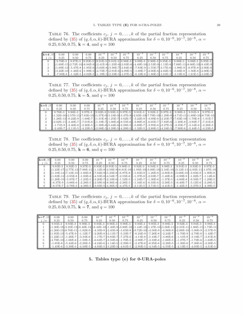
5. TABLES TYPE (E) FOR 0-URA-POLES 39
Table 76. The coefficients cj , j = 0, . . . , k of the partial fraction representationdefined by (35) of (q, δ, α, k)-BURA approximation for δ = 0, 10−6, 10−7, 10−8, α =0.25, 0.50, 0.75, k = 4, and q = 100
k=4 /δ 0.00 0.00 0.00 10−6 10−6 10−6 10−7 10−7 10−7 10−8 10−8 10−8
j /α 0.25 0.50 0.75 0.25 0.50 0.75 0.25 0.50 0.75 0.25 0.50 0.750 9.70E-3 9.87E-3 9.95E-3 9.91E-3 9.91E-3 9.96E-3 9.89E-3 9.90E-3 9.95E-3 9.88E-3 9.88E-3 9.95E-31 -1.69E-15 -2.73E-10 -8.94E-9 -2.41E-9 -1.23E-8 -2.03E-8 -4.49E-10 -2.53E-9 -1.13E-8 -7.88E-11 -8.06E-10 -9.43E-92 -1.69E-12 -5.47E-8 -1.95E-6 -3.02E-8 -3.38E-7 -2.84E-6 -7.83E-9 -1.55E-7 -2.17E-6 -1.98E-9 -8.97E-8 -2.00E-63 -3.22E-10 -1.26E-6 -1.99E-5 -4.73E-7 -2.91E-6 -2.09E-5 -1.68E-7 -2.00E-6 -2.02E-5 -5.68E-8 -1.56E-6 -2.00E-54 -7.00E-8 -1.42E-5 -4.02E-5 -1.19E-5 -2.33E-5 -4.07E-5 -6.43E-6 -1.86E-5 -4.04E-5 -3.18E-6 -1.61E-5 -4.03E-5
Table 77. The coefficients cj , j = 0, . . . , k of the partial fraction representationdefined by (35) of (q, δ, α, k)-BURA approximation for δ = 0, 10−6, 10−7, 10−8, α =0.25, 0.50, 0.75, k = 5, and q = 100
k=5 /δ 0.00 0.00 0.00 10−6 10−6 10−6 10−7 10−7 10−7 10−8 10−8 10−8
j /α 0.25 0.50 0.75 0.25 0.50 0.75 0.25 0.50 0.75 0.25 0.50 0.750 9.78E-3 9.90E-3 9.97E-3 9.92E-3 9.93E-3 9.97E-3 9.91E-3 9.92E-3 9.97E-3 9.90E-3 9.91E-3 9.97E-31 -1.32E-16 -2.57E-11 -7.63E-10 -1.57E-9 -5.18E-9 -3.47E-9 -2.83E-10 -7.79E-10 -1.29E-9 -4.71E-11 -1.69E-10 -8.73E-102 -1.28E-13 -6.22E-9 -1.68E-7 -1.31E-8 -1.25E-7 -4.02E-7 -3.22E-9 -4.09E-8 -2.25E-7 -7.63E-10 -1.70E-8 -1.81E-73 -2.02E-11 -2.40E-7 -7.01E-6 -1.19E-7 -1.06E-6 -9.55E-6 -3.86E-8 -6.05E-7 -7.82E-6 -1.20E-8 -3.93E-7 -7.21E-64 -1.71E-9 -2.46E-6 -2.26E-5 -1.30E-6 -5.44E-6 -2.28E-5 -5.69E-7 -3.95E-6 -2.27E-5 -2.35E-7 -3.14E-6 -2.26E-55 -2.43E-7 -2.11E-5 -4.22E-5 -2.08E-5 -3.39E-5 -4.29E-5 -1.32E-5 -2.80E-5 -4.24E-5 -7.90E-6 -2.44E-5 -4.23E-5
Table 78. The coefficients cj , j = 0, . . . , k of the partial fraction representationdefined by (35) of (q, δ, α, k)-BURA approximation for δ = 0, 10−6, 10−7, 10−8, α =0.25, 0.50, 0.75, k = 6, and q = 100
k=6 /δ 0.00 0.00 0.00 10−6 10−6 10−6 10−7 10−7 10−7 10−8 10−8 10−8
j /α 0.25 0.50 0.75 0.25 0.50 0.75 0.25 0.50 0.75 0.25 0.50 0.750 9.83E-3 9.92E-3 9.97E-3 9.93E-3 9.95E-3 9.98E-3 9.92E-3 9.94E-3 9.98E-3 9.91E-3 9.93E-3 9.97E-31 -1.22E-17 -2.77E-12 -7.88E-11 -1.12E-9 -2.59E-9 -8.81E-10 -1.95E-10 -3.09E-10 -2.16E-10 -3.12E-11 -4.93E-11 -1.07E-102 -1.18E-14 -7.12E-10 -1.60E-8 -7.04E-9 -5.23E-8 -6.97E-8 -1.65E-9 -1.26E-8 -2.86E-8 -3.68E-10 -3.83E-9 -1.90E-83 -1.82E-12 -3.85E-8 -1.03E-6 -4.55E-8 -4.54E-7 -2.55E-6 -1.37E-8 -2.03E-7 -1.48E-6 -3.99E-9 -1.02E-7 -1.14E-64 -1.20E-10 -5.87E-7 -1.25E-5 -3.20E-7 -2.10E-6 -1.52E-5 -1.24E-7 -1.36E-6 -1.37E-5 -4.60E-8 -9.56E-7 -1.29E-55 -6.37E-9 -3.88E-6 -2.28E-5 -2.59E-6 -8.36E-6 -2.28E-5 -1.34E-6 -6.33E-6 -2.28E-5 -6.49E-7 -5.12E-6 -2.28E-56 -6.57E-7 -2.78E-5 -4.38E-5 -3.03E-5 -4.36E-5 -4.47E-5 -2.11E-5 -3.71E-5 -4.41E-5 -1.42E-5 -3.27E-5 -4.39E-5
Table 79. The coefficients cj , j = 0, . . . , k of the partial fraction representationdefined by (35) of (q, δ, α, k)-BURA approximation for δ = 0, 10−6, 10−7, 10−8, α =0.25, 0.50, 0.75, k = 7, and q = 100
k=7 /δ 0.00 0.00 0.00 10−6 10−6 10−6 10−7 10−7 10−7 10−8 10−8 10−8
j /α 0.25 0.50 0.75 0.25 0.50 0.75 0.25 0.50 0.75 0.25 0.50 0.750 9.85E-3 9.93E-3 9.98E-3 9.93E-3 9.96E-3 9.98E-3 9.93E-3 9.95E-3 9.98E-3 9.92E-3 9.94E-3 9.98E-31 -1.30E-18 -3.35E-13 -9.40E-12 -8.42E-10 -1.46E-9 -3.00E-10 -1.44E-10 -1.47E-10 -5.06E-11 -2.21E-11 -1.86E-11 -1.73E-112 -1.26E-15 -8.76E-11 -1.82E-9 -4.33E-9 -2.45E-8 -1.65E-8 -9.72E-10 -4.58E-9 -4.96E-9 -2.06E-10 -1.06E-9 -2.57E-93 -1.95E-13 -5.47E-9 -1.12E-7 -2.20E-8 -2.11E-7 -5.33E-7 -6.24E-9 -7.26E-8 -2.24E-7 -1.70E-9 -2.79E-8 -1.42E-74 -1.22E-11 -1.26E-7 -3.34E-6 -1.17E-7 -9.83E-7 -7.27E-6 -4.14E-8 -5.43E-7 -4.86E-6 -1.41E-8 -3.18E-7 -3.81E-65 -4.78E-10 -1.06E-6 -1.59E-5 -6.64E-7 -3.34E-6 -1.70E-5 -2.98E-7 -2.33E-6 -1.66E-5 -1.27E-7 -1.72E-6 -1.62E-56 -1.85E-8 -5.44E-6 -2.28E-5 -4.24E-6 -1.14E-5 -2.29E-5 -2.47E-6 -8.95E-6 -2.28E-5 -1.36E-6 -7.36E-6 -2.28E-57 -1.45E-6 -3.39E-5 -4.50E-5 -4.03E-5 -5.23E-5 -4.61E-5 -2.95E-5 -4.54E-5 -4.55E-5 -2.13E-5 -4.05E-5 -4.51E-5
5. Tables type (e) for 0-URA-poles
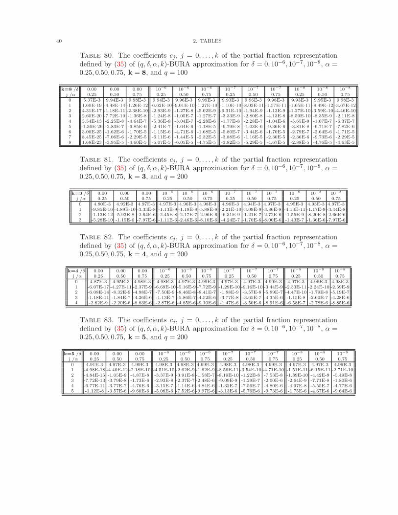
40 2. TABLES
Table 80. The coefficients cj , j = 0, . . . , k of the partial fraction representationdefined by (35) of (q, δ, α, k)-BURA approximation for δ = 0, 10−6, 10−7, 10−8, α =0.25, 0.50, 0.75, k = 8, and q = 100
k=8 /δ 0.00 0.00 0.00 10−6 10−6 10−6 10−7 10−7 10−7 10−8 10−8 10−8
j /α 0.25 0.50 0.75 0.25 0.50 0.75 0.25 0.50 0.75 0.25 0.50 0.750 5.37E-3 9.94E-3 9.98E-3 9.94E-3 9.96E-3 9.99E-3 9.93E-3 9.96E-3 9.98E-3 9.93E-3 9.95E-3 9.98E-31 1.60E-19 -4.48E-14 -1.26E-12 -6.62E-10 -9.01E-10 -1.27E-10 -1.10E-10 -8.03E-11 -1.57E-11 -1.65E-11 -8.49E-12 -3.67E-122 4.31E-17 -1.18E-11 -2.38E-10 -2.93E-9 -1.27E-8 -5.02E-9 -6.31E-10 -1.94E-9 -1.13E-9 -1.27E-10 -3.59E-10 -4.46E-103 2.60E-20 -7.72E-10 -1.36E-8 -1.24E-8 -1.05E-7 -1.27E-7 -3.33E-9 -2.80E-8 -4.13E-8 -8.59E-10 -8.35E-9 -2.11E-84 3.54E-13 -2.25E-8 -4.64E-7 -5.36E-8 -5.04E-7 -2.28E-6 -1.77E-8 -2.28E-7 -1.04E-6 -5.65E-9 -1.07E-7 -6.37E-75 -1.36E-26 -2.83E-7 -6.85E-6 -2.41E-7 -1.64E-6 -1.18E-5 -9.79E-8 -1.03E-6 -9.36E-6 -3.81E-8 -6.71E-7 -7.82E-66 3.00E-25 -1.62E-6 -1.70E-5 -1.15E-6 -4.71E-6 -1.68E-5 -5.80E-7 -3.44E-6 -1.70E-5 -2.79E-7 -2.64E-6 -1.71E-57 8.45E-25 -7.06E-6 -2.29E-5 -6.11E-6 -1.44E-5 -2.32E-5 -3.88E-6 -1.16E-5 -2.30E-5 -2.36E-6 -9.73E-6 -2.29E-58 1.68E-23 -3.95E-5 -4.60E-5 -5.07E-5 -6.05E-5 -4.75E-5 -3.82E-5 -5.29E-5 -4.67E-5 -2.88E-5 -4.76E-5 -4.63E-5
Table 81. The coefficients cj , j = 0, . . . , k of the partial fraction representationdefined by (35) of (q, δ, α, k)-BURA approximation for δ = 0, 10−6, 10−7, 10−8, α =0.25, 0.50, 0.75, k = 3, and q = 200
k=3 /δ 0.00 0.00 0.00 10−6 10−6 10−6 10−7 10−7 10−7 10−8 10−8 10−8
j /α 0.25 0.50 0.75 0.25 0.50 0.75 0.25 0.50 0.75 0.25 0.50 0.750 4.80E-3 4.92E-3 4.97E-3 4.97E-3 4.96E-3 4.98E-3 4.96E-3 4.94E-3 4.97E-3 4.95E-3 4.93E-3 4.97E-31 -9.85E-16 -4.89E-10 -3.33E-8 -1.13E-9 -1.19E-8 -5.88E-8 -2.21E-10 -3.09E-9 -3.86E-8 -4.13E-11 -1.17E-9 -3.44E-82 -1.13E-12 -5.93E-8 -2.64E-6 -2.45E-8 -2.17E-7 -2.96E-6 -6.31E-9 -1.21E-7 -2.72E-6 -1.55E-9 -8.20E-8 -2.66E-63 -5.28E-10 -1.15E-6 -7.97E-6 -1.11E-6 -2.46E-6 -8.10E-6 -4.24E-7 -1.70E-6 -8.00E-6 -1.43E-7 -1.36E-6 -7.97E-6
Table 82. The coefficients cj , j = 0, . . . , k of the partial fraction representationdefined by (35) of (q, δ, α, k)-BURA approximation for δ = 0, 10−6, 10−7, 10−8, α =0.25, 0.50, 0.75, k = 4, and q = 200
k=4 /δ 0.00 0.00 0.00 10−6 10−6 10−6 10−7 10−7 10−7 10−8 10−8 10−8
j /α 0.25 0.50 0.75 0.25 0.50 0.75 0.25 0.50 0.75 0.25 0.50 0.750 4.87E-3 4.95E-3 4.98E-3 4.98E-3 4.97E-3 4.99E-3 4.97E-3 4.97E-3 4.99E-3 4.97E-3 4.96E-3 4.98E-31 -6.07E-17 -4.27E-11 -2.37E-9 -6.69E-10 -5.16E-9 -7.72E-9 -1.29E-10 -9.16E-10 -3.44E-9 -2.33E-11 -2.24E-10 -2.59E-92 -6.08E-14 -8.32E-9 -4.98E-7 -7.50E-9 -8.46E-8 -8.41E-7 -1.88E-9 -3.57E-8 -5.89E-7 -4.47E-10 -1.79E-8 -5.19E-73 -1.18E-11 -1.84E-7 -4.26E-6 -1.13E-7 -5.86E-7 -4.52E-6 -3.77E-8 -3.65E-7 -4.35E-6 -1.15E-8 -2.60E-7 -4.28E-64 -2.82E-9 -2.20E-6 -8.83E-6 -2.87E-6 -4.85E-6 -9.10E-6 -1.47E-6 -3.50E-6 -8.91E-6 -6.58E-7 -2.78E-6 -8.85E-6
Table 83. The coefficients cj , j = 0, . . . , k of the partial fraction representationdefined by (35) of (q, δ, α, k)-BURA approximation for δ = 0, 10−6, 10−7, 10−8, α =0.25, 0.50, 0.75, k = 5, and q = 200
k=5 /δ 0.00 0.00 0.00 10−6 10−6 10−6 10−7 10−7 10−7 10−8 10−8 10−8
j /α 0.25 0.50 0.75 0.25 0.50 0.75 0.25 0.50 0.75 0.25 0.50 0.750 4.91E-3 4.97E-3 4.99E-3 4.98E-3 4.98E-3 4.99E-3 4.98E-3 4.98E-3 4.99E-3 4.97E-3 4.97E-3 4.99E-31 -4.98E-18 -4.40E-12 -2.18E-10 -4.51E-10 -2.62E-9 -1.62E-9 -8.56E-11 -3.54E-10 -4.71E-10 -1.51E-11 -6.15E-11 -2.71E-102 -4.84E-15 -1.05E-9 -4.87E-8 -3.37E-9 -3.91E-8 -1.58E-7 -8.19E-10 -1.22E-8 -7.53E-8 -1.89E-10 -4.42E-9 -5.49E-83 -7.72E-13 -3.79E-8 -1.73E-6 -2.93E-8 -2.37E-7 -2.48E-6 -9.09E-9 -1.29E-7 -2.00E-6 -2.64E-9 -7.71E-8 -1.80E-64 -6.77E-11 -3.77E-7 -4.76E-6 -3.15E-7 -1.14E-6 -4.84E-6 -1.32E-7 -7.56E-7 -4.80E-6 -4.97E-8 -5.55E-7 -4.77E-65 -1.12E-8 -3.57E-6 -9.60E-6 -5.08E-6 -7.52E-6 -9.97E-6 -3.13E-6 -5.76E-6 -9.73E-6 -1.75E-6 -4.67E-6 -9.64E-6
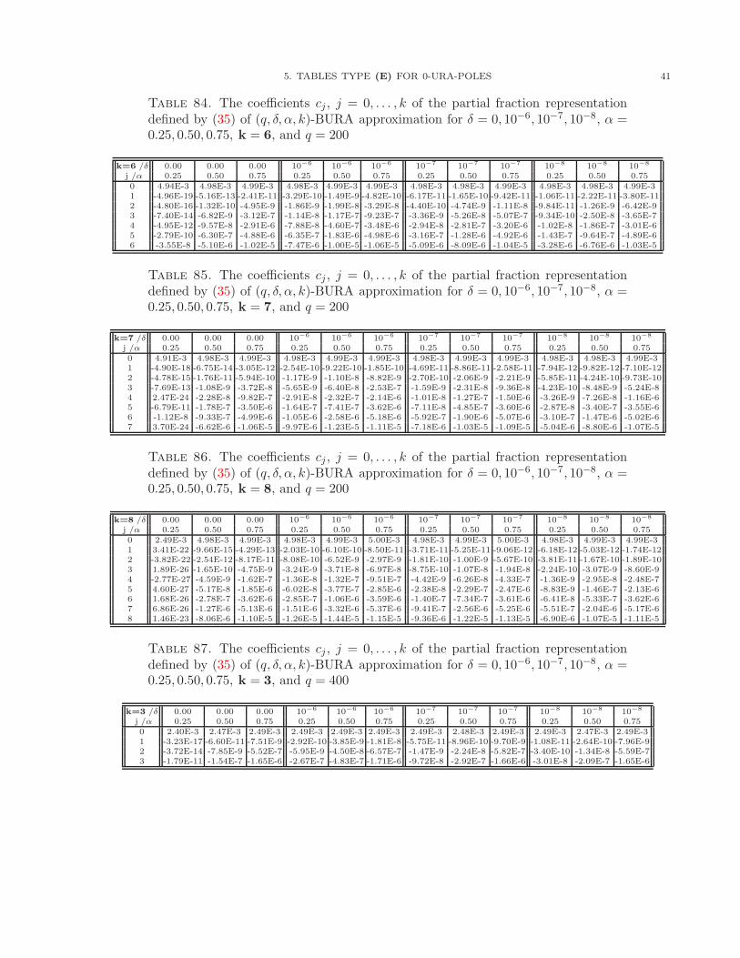
5. TABLES TYPE (E) FOR 0-URA-POLES 41
Table 84. The coefficients cj , j = 0, . . . , k of the partial fraction representationdefined by (35) of (q, δ, α, k)-BURA approximation for δ = 0, 10−6, 10−7, 10−8, α =0.25, 0.50, 0.75, k = 6, and q = 200
k=6 /δ 0.00 0.00 0.00 10−6 10−6 10−6 10−7 10−7 10−7 10−8 10−8 10−8
j /α 0.25 0.50 0.75 0.25 0.50 0.75 0.25 0.50 0.75 0.25 0.50 0.750 4.94E-3 4.98E-3 4.99E-3 4.98E-3 4.99E-3 4.99E-3 4.98E-3 4.98E-3 4.99E-3 4.98E-3 4.98E-3 4.99E-31 -4.96E-19 -5.16E-13 -2.41E-11 -3.29E-10 -1.49E-9 -4.82E-10 -6.17E-11 -1.65E-10 -9.42E-11 -1.06E-11 -2.22E-11 -3.80E-112 -4.80E-16 -1.32E-10 -4.95E-9 -1.86E-9 -1.99E-8 -3.29E-8 -4.40E-10 -4.74E-9 -1.11E-8 -9.84E-11 -1.26E-9 -6.42E-93 -7.40E-14 -6.82E-9 -3.12E-7 -1.14E-8 -1.17E-7 -9.23E-7 -3.36E-9 -5.26E-8 -5.07E-7 -9.34E-10 -2.50E-8 -3.65E-74 -4.95E-12 -9.57E-8 -2.91E-6 -7.88E-8 -4.60E-7 -3.48E-6 -2.94E-8 -2.81E-7 -3.20E-6 -1.02E-8 -1.86E-7 -3.01E-65 -2.79E-10 -6.30E-7 -4.88E-6 -6.35E-7 -1.83E-6 -4.98E-6 -3.16E-7 -1.28E-6 -4.92E-6 -1.43E-7 -9.64E-7 -4.89E-66 -3.55E-8 -5.10E-6 -1.02E-5 -7.47E-6 -1.00E-5 -1.06E-5 -5.09E-6 -8.09E-6 -1.04E-5 -3.28E-6 -6.76E-6 -1.03E-5
Table 85. The coefficients cj , j = 0, . . . , k of the partial fraction representationdefined by (35) of (q, δ, α, k)-BURA approximation for δ = 0, 10−6, 10−7, 10−8, α =0.25, 0.50, 0.75, k = 7, and q = 200
k=7 /δ 0.00 0.00 0.00 10−6 10−6 10−6 10−7 10−7 10−7 10−8 10−8 10−8
j /α 0.25 0.50 0.75 0.25 0.50 0.75 0.25 0.50 0.75 0.25 0.50 0.750 4.91E-3 4.98E-3 4.99E-3 4.98E-3 4.99E-3 4.99E-3 4.98E-3 4.99E-3 4.99E-3 4.98E-3 4.98E-3 4.99E-31 -4.90E-18 -6.75E-14 -3.05E-12 -2.54E-10 -9.22E-10 -1.85E-10 -4.69E-11 -8.86E-11 -2.58E-11 -7.94E-12 -9.82E-12 -7.10E-122 -4.78E-15 -1.76E-11 -5.94E-10 -1.17E-9 -1.10E-8 -8.82E-9 -2.70E-10 -2.06E-9 -2.21E-9 -5.85E-11 -4.24E-10 -9.73E-103 -7.69E-13 -1.08E-9 -3.72E-8 -5.65E-9 -6.40E-8 -2.53E-7 -1.59E-9 -2.31E-8 -9.36E-8 -4.23E-10 -8.48E-9 -5.24E-84 2.47E-24 -2.28E-8 -9.82E-7 -2.91E-8 -2.32E-7 -2.14E-6 -1.01E-8 -1.27E-7 -1.50E-6 -3.26E-9 -7.26E-8 -1.16E-65 -6.79E-11 -1.78E-7 -3.50E-6 -1.64E-7 -7.41E-7 -3.62E-6 -7.11E-8 -4.85E-7 -3.60E-6 -2.87E-8 -3.40E-7 -3.55E-66 -1.12E-8 -9.33E-7 -4.99E-6 -1.05E-6 -2.58E-6 -5.18E-6 -5.92E-7 -1.90E-6 -5.07E-6 -3.10E-7 -1.47E-6 -5.02E-67 3.70E-24 -6.62E-6 -1.06E-5 -9.97E-6 -1.23E-5 -1.11E-5 -7.18E-6 -1.03E-5 -1.09E-5 -5.04E-6 -8.80E-6 -1.07E-5
Table 86. The coefficients cj , j = 0, . . . , k of the partial fraction representationdefined by (35) of (q, δ, α, k)-BURA approximation for δ = 0, 10−6, 10−7, 10−8, α =0.25, 0.50, 0.75, k = 8, and q = 200
k=8 /δ 0.00 0.00 0.00 10−6 10−6 10−6 10−7 10−7 10−7 10−8 10−8 10−8
j /α 0.25 0.50 0.75 0.25 0.50 0.75 0.25 0.50 0.75 0.25 0.50 0.750 2.49E-3 4.98E-3 4.99E-3 4.98E-3 4.99E-3 5.00E-3 4.98E-3 4.99E-3 5.00E-3 4.98E-3 4.99E-3 4.99E-31 3.41E-22 -9.66E-15 -4.29E-13 -2.03E-10 -6.10E-10 -8.50E-11 -3.71E-11 -5.25E-11 -9.06E-12 -6.18E-12 -5.03E-12 -1.74E-122 -3.82E-22 -2.54E-12 -8.17E-11 -8.08E-10 -6.52E-9 -2.97E-9 -1.81E-10 -1.00E-9 -5.67E-10 -3.81E-11 -1.67E-10 -1.89E-103 1.89E-26 -1.65E-10 -4.75E-9 -3.24E-9 -3.71E-8 -6.97E-8 -8.75E-10 -1.07E-8 -1.94E-8 -2.24E-10 -3.07E-9 -8.60E-94 -2.77E-27 -4.59E-9 -1.62E-7 -1.36E-8 -1.32E-7 -9.51E-7 -4.42E-9 -6.26E-8 -4.33E-7 -1.36E-9 -2.95E-8 -2.48E-75 4.60E-27 -5.17E-8 -1.85E-6 -6.02E-8 -3.77E-7 -2.85E-6 -2.38E-8 -2.29E-7 -2.47E-6 -8.83E-9 -1.46E-7 -2.13E-66 1.68E-26 -2.78E-7 -3.62E-6 -2.85E-7 -1.06E-6 -3.59E-6 -1.40E-7 -7.34E-7 -3.61E-6 -6.41E-8 -5.33E-7 -3.62E-67 6.86E-26 -1.27E-6 -5.13E-6 -1.51E-6 -3.32E-6 -5.37E-6 -9.41E-7 -2.56E-6 -5.25E-6 -5.51E-7 -2.04E-6 -5.17E-68 1.46E-23 -8.06E-6 -1.10E-5 -1.26E-5 -1.44E-5 -1.15E-5 -9.36E-6 -1.22E-5 -1.13E-5 -6.90E-6 -1.07E-5 -1.11E-5
Table 87. The coefficients cj , j = 0, . . . , k of the partial fraction representationdefined by (35) of (q, δ, α, k)-BURA approximation for δ = 0, 10−6, 10−7, 10−8, α =0.25, 0.50, 0.75, k = 3, and q = 400
k=3 /δ 0.00 0.00 0.00 10−6 10−6 10−6 10−7 10−7 10−7 10−8 10−8 10−8
j /α 0.25 0.50 0.75 0.25 0.50 0.75 0.25 0.50 0.75 0.25 0.50 0.750 2.40E-3 2.47E-3 2.49E-3 2.49E-3 2.49E-3 2.49E-3 2.49E-3 2.48E-3 2.49E-3 2.49E-3 2.47E-3 2.49E-31 -3.23E-17 -6.60E-11 -7.51E-9 -2.92E-10 -3.85E-9 -1.81E-8 -5.75E-11 -8.96E-10 -9.70E-9 -1.08E-11 -2.64E-10 -7.96E-92 -3.72E-14 -7.85E-9 -5.52E-7 -5.95E-9 -4.50E-8 -6.57E-7 -1.47E-9 -2.24E-8 -5.82E-7 -3.40E-10 -1.34E-8 -5.59E-73 -1.79E-11 -1.54E-7 -1.65E-6 -2.67E-7 -4.83E-7 -1.71E-6 -9.72E-8 -2.92E-7 -1.66E-6 -3.01E-8 -2.09E-7 -1.65E-6
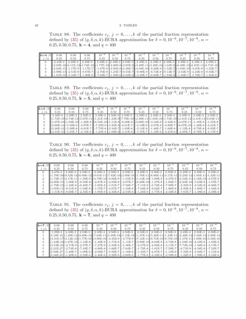
42 2. TABLES
Table 88. The coefficients cj , j = 0, . . . , k of the partial fraction representationdefined by (35) of (q, δ, α, k)-BURA approximation for δ = 0, 10−6, 10−7, 10−8, α =0.25, 0.50, 0.75, k = 4, and q = 400
k=4 /δ 0.00 0.00 0.00 10−6 10−6 10−6 10−7 10−7 10−7 10−8 10−8 10−8
j /α 0.25 0.50 0.75 0.25 0.50 0.75 0.25 0.50 0.75 0.25 0.50 0.750 2.44E-3 2.48E-3 2.49E-3 2.49E-3 2.49E-3 2.50E-3 2.49E-3 2.49E-3 2.49E-3 2.49E-3 2.49E-3 2.49E-31 -2.03E-18 -6.11E-12 -5.74E-10 -1.77E-10 -2.06E-9 -3.05E-9 -3.49E-11 -3.48E-10 -1.04E-9 -6.49E-12 -6.85E-11 -6.71E-102 -2.04E-15 -1.17E-9 -1.17E-7 -1.87E-9 -2.05E-8 -2.38E-7 -4.58E-10 -8.20E-9 -1.52E-7 -1.05E-10 -3.65E-9 -1.25E-73 -3.99E-13 -2.51E-8 -8.87E-7 -2.76E-8 -1.21E-7 -9.55E-7 -8.88E-9 -6.74E-8 -9.14E-7 -2.54E-9 -4.34E-8 -8.94E-74 -1.01E-10 -3.16E-7 -1.90E-6 -7.03E-7 -1.03E-6 -2.02E-6 -3.49E-7 -6.60E-7 -1.94E-6 -1.46E-7 -4.70E-7 -1.91E-6
Table 89. The coefficients cj , j = 0, . . . , k of the partial fraction representationdefined by (35) of (q, δ, α, k)-BURA approximation for δ = 0, 10−6, 10−7, 10−8, α =0.25, 0.50, 0.75, k = 5, and q = 400
k=5 /δ 0.00 0.00 0.00 10−6 10−6 10−6 10−7 10−7 10−7 10−8 10−8 10−8
j /α 0.25 0.50 0.75 0.25 0.50 0.75 0.25 0.50 0.75 0.25 0.50 0.750 2.46E-3 2.49E-3 2.50E-3 2.49E-3 2.50E-3 2.50E-3 2.49E-3 2.49E-3 2.50E-3 2.49E-3 2.49E-3 2.50E-31 -1.72E-19 -6.74E-13 -5.67E-11 -1.21E-10 -1.23E-9 -7.79E-10 -2.39E-11 -1.65E-10 -1.74E-10 -4.41E-12 -2.41E-11 -8.04E-112 -1.67E-16 -1.59E-10 -1.28E-8 -8.54E-10 -1.11E-8 -6.09E-8 -2.06E-10 -3.54E-9 -2.44E-8 -4.67E-11 -1.16E-9 -1.55E-83 -2.68E-14 -5.50E-9 -3.97E-7 -7.25E-9 -5.25E-8 -6.01E-7 -2.19E-9 -2.67E-8 -4.80E-7 -6.07E-10 -1.48E-8 -4.21E-74 -2.40E-12 -5.39E-8 -9.91E-7 -7.75E-8 -2.44E-7 -1.03E-6 -3.14E-8 -1.46E-7 -1.00E-6 -1.12E-8 -9.73E-8 -9.95E-75 -4.31E-10 -5.55E-7 -2.15E-6 -1.25E-6 -1.69E-6 -2.31E-6 -7.57E-7 -1.19E-6 -2.21E-6 -4.05E-7 -8.76E-7 -2.17E-6
Table 90. The coefficients cj , j = 0, . . . , k of the partial fraction representationdefined by (35) of (q, δ, α, k)-BURA approximation for δ = 0, 10−6, 10−7, 10−8, α =0.25, 0.50, 0.75, k = 6, and q = 400
k=6 /δ 0.00 0.00 0.00 10−6 10−6 10−6 10−7 10−7 10−7 10−8 10−8 10−8
j /α 0.25 0.50 0.75 0.25 0.50 0.75 0.25 0.50 0.75 0.25 0.50 0.750 2.47E-3 2.49E-3 2.50E-3 2.50E-3 2.50E-3 2.50E-3 2.49E-3 2.50E-3 2.50E-3 2.49E-3 2.49E-3 2.50E-31 -1.78E-20 -8.52E-14 -6.69E-12 -9.01E-11 -7.92E-10 -2.69E-10 -1.76E-11 -8.90E-11 -4.17E-11 -3.23E-12 -1.05E-11 -1.32E-112 -1.72E-17 -2.17E-11 -1.39E-9 -4.79E-10 -6.66E-9 -1.55E-8 -1.14E-10 -1.69E-9 -4.27E-9 -2.54E-11 -4.16E-10 -2.07E-93 -2.66E-15 -1.08E-9 -8.50E-8 -2.87E-9 -2.83E-8 -2.97E-7 -8.29E-10 -1.27E-8 -1.60E-7 -2.23E-10 -5.83E-9 -1.07E-74 -1.79E-13 -1.43E-8 -6.42E-7 -1.95E-8 -1.01E-7 -7.50E-7 -7.11E-9 -5.74E-8 -7.09E-7 -2.35E-9 -3.54E-8 -6.68E-75 -1.05E-11 -9.51E-8 -1.04E-6 -1.57E-7 -4.07E-7 -1.10E-6 -7.64E-8 -2.62E-7 -1.06E-6 -3.32E-8 -1.80E-7 -1.04E-66 -1.51E-9 -8.60E-7 -2.35E-6 -1.85E-6 -2.34E-6 -2.53E-6 -1.25E-6 -1.77E-6 -2.43E-6 -7.81E-7 -1.38E-6 -2.38E-6
Table 91. The coefficients cj , j = 0, . . . , k of the partial fraction representationdefined by (35) of (q, δ, α, k)-BURA approximation for δ = 0, 10−6, 10−7, 10−8, α =0.25, 0.50, 0.75, k = 7, and q = 400
k=7 /δ 0.00 0.00 0.00 10−6 10−6 10−6 10−7 10−7 10−7 10−8 10−8 10−8
j /α 0.25 0.50 0.75 0.25 0.50 0.75 0.25 0.50 0.75 0.25 0.50 0.750 1.39E-3 2.49E-3 2.50E-3 2.50E-3 2.50E-3 2.50E-3 2.50E-3 2.50E-3 2.50E-3 2.49E-3 2.50E-3 2.50E-31 3.10E-18 -1.20E-14 -8.99E-13 -7.03E-11 -5.39E-10 -1.15E-10 -1.37E-11 -5.30E-11 -1.33E-11 -2.49E-12 -5.32E-12 -2.90E-122 -4.31E-17 -3.12E-12 -1.77E-10 -3.06E-10 -4.25E-9 -4.77E-9 -7.12E-11 -8.75E-10 -9.75E-10 -1.57E-11 -1.69E-10 -3.56E-103 -1.24E-18 -1.87E-10 -1.12E-8 -1.43E-9 -1.71E-8 -1.11E-7 -3.99E-10 -6.63E-9 -3.74E-8 -1.04E-10 -2.43E-9 -1.83E-84 -3.53E-25 -3.71E-9 -2.57E-7 -7.27E-9 -5.33E-8 -5.46E-7 -2.47E-9 -2.82E-8 -4.11E-7 -7.74E-10 -1.56E-8 -3.17E-75 2.21E-27 -2.74E-8 -7.43E-7 -4.06E-8 -1.66E-7 -7.64E-7 -1.73E-8 -1.01E-7 -7.59E-7 -6.71E-9 -6.58E-8 -7.52E-76 2.50E-27 -1.49E-7 -1.09E-6 -2.60E-7 -5.92E-7 -1.18E-6 -1.45E-7 -4.07E-7 -1.13E-6 -7.33E-8 -2.92E-7 -1.11E-67 4.34E-25 -1.20E-6 -2.50E-6 -2.48E-6 -2.92E-6 -2.68E-6 -1.77E-6 -2.34E-6 -2.59E-6 -1.22E-6 -1.90E-6 -2.54E-6
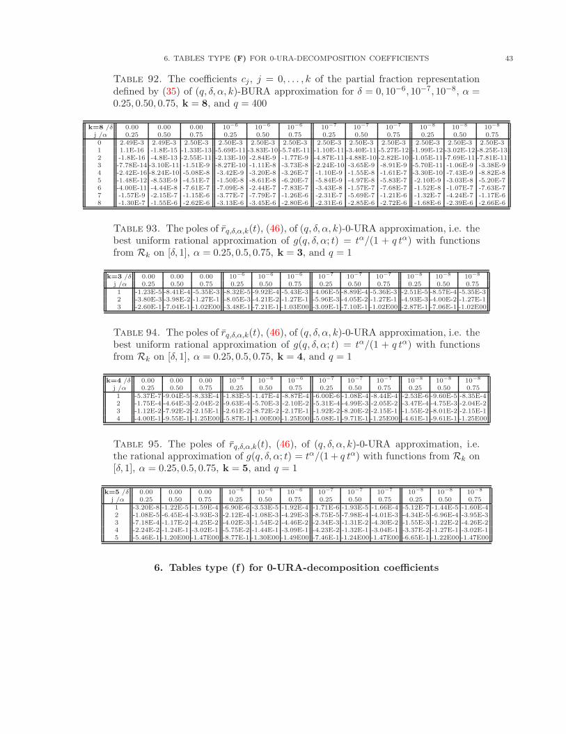
6. TABLES TYPE (F) FOR 0-URA-DECOMPOSITION COEFFICIENTS 43
Table 92. The coefficients cj , j = 0, . . . , k of the partial fraction representationdefined by (35) of (q, δ, α, k)-BURA approximation for δ = 0, 10−6, 10−7, 10−8, α =0.25, 0.50, 0.75, k = 8, and q = 400
k=8 /δ 0.00 0.00 0.00 10−6 10−6 10−6 10−7 10−7 10−7 10−8 10−8 10−8
j /α 0.25 0.50 0.75 0.25 0.50 0.75 0.25 0.50 0.75 0.25 0.50 0.750 2.49E-3 2.49E-3 2.50E-3 2.50E-3 2.50E-3 2.50E-3 2.50E-3 2.50E-3 2.50E-3 2.50E-3 2.50E-3 2.50E-31 1.1E-16 -1.8E-15 -1.33E-13 -5.69E-11 -3.83E-10 -5.74E-11 -1.10E-11 -3.40E-11 -5.27E-12 -1.99E-12 -3.02E-12 -8.25E-132 -1.8E-16 -4.8E-13 -2.55E-11 -2.13E-10 -2.84E-9 -1.77E-9 -4.87E-11 -4.88E-10 -2.82E-10 -1.05E-11 -7.69E-11 -7.81E-113 -7.78E-14 -3.10E-11 -1.51E-9 -8.27E-10 -1.11E-8 -3.73E-8 -2.24E-10 -3.65E-9 -8.91E-9 -5.70E-11 -1.06E-9 -3.38E-94 -2.42E-16 -8.24E-10 -5.08E-8 -3.42E-9 -3.20E-8 -3.26E-7 -1.10E-9 -1.55E-8 -1.61E-7 -3.30E-10 -7.43E-9 -8.82E-85 -1.48E-12 -8.53E-9 -4.51E-7 -1.50E-8 -8.61E-8 -6.20E-7 -5.84E-9 -4.97E-8 -5.83E-7 -2.10E-9 -3.03E-8 -5.20E-76 -4.00E-11 -4.44E-8 -7.61E-7 -7.09E-8 -2.44E-7 -7.83E-7 -3.43E-8 -1.57E-7 -7.68E-7 -1.52E-8 -1.07E-7 -7.63E-77 -1.57E-9 -2.15E-7 -1.15E-6 -3.77E-7 -7.79E-7 -1.26E-6 -2.31E-7 -5.69E-7 -1.21E-6 -1.32E-7 -4.24E-7 -1.17E-68 -1.30E-7 -1.55E-6 -2.62E-6 -3.13E-6 -3.45E-6 -2.80E-6 -2.31E-6 -2.85E-6 -2.72E-6 -1.68E-6 -2.39E-6 -2.66E-6
Table 93. The poles of rq,δ,α,k(t), (46), of (q, δ, α, k)-0-URA approximation, i.e. thebest uniform rational approximation of g(q, δ, α; t) = tα/(1 + q tα) with functionsfrom Rk on [δ, 1], α = 0.25, 0.5, 0.75, k = 3, and q = 1
k=3 /δ 0.00 0.00 0.00 10−6 10−6 10−6 10−7 10−7 10−7 10−8 10−8 10−8
j /α 0.25 0.50 0.75 0.25 0.50 0.75 0.25 0.50 0.75 0.25 0.50 0.751 -1.23E-5 -8.41E-4 -5.35E-3 -8.32E-5 -9.92E-4 -5.43E-3 -4.06E-5 -8.89E-4 -5.36E-3 -2.51E-5 -8.57E-4 -5.35E-32 -3.80E-3 -3.98E-2 -1.27E-1 -8.05E-3 -4.21E-2 -1.27E-1 -5.96E-3 -4.05E-2 -1.27E-1 -4.93E-3 -4.00E-2 -1.27E-13 -2.60E-1 -7.04E-1 -1.02E00 -3.48E-1 -7.21E-1 -1.03E00 -3.09E-1 -7.10E-1 -1.02E00 -2.87E-1 -7.06E-1 -1.02E00
Table 94. The poles of rq,δ,α,k(t), (46), of (q, δ, α, k)-0-URA approximation, i.e. thebest uniform rational approximation of g(q, δ, α; t) = tα/(1 + q tα) with functionsfrom Rk on [δ, 1], α = 0.25, 0.5, 0.75, k = 4, and q = 1
k=4 /δ 0.00 0.00 0.00 10−6 10−6 10−6 10−7 10−7 10−7 10−8 10−8 10−8
j /α 0.25 0.50 0.75 0.25 0.50 0.75 0.25 0.50 0.75 0.25 0.50 0.751 -5.37E-7 -9.04E-5 -8.33E-4 -1.83E-5 -1.47E-4 -8.87E-4 -6.00E-6 -1.08E-4 -8.44E-4 -2.53E-6 -9.60E-5 -8.35E-42 -1.75E-4 -4.64E-3 -2.04E-2 -9.63E-4 -5.70E-3 -2.10E-2 -5.31E-4 -4.99E-3 -2.05E-2 -3.47E-4 -4.75E-3 -2.04E-23 -1.12E-2 -7.92E-2 -2.15E-1 -2.61E-2 -8.72E-2 -2.17E-1 -1.92E-2 -8.20E-2 -2.15E-1 -1.55E-2 -8.01E-2 -2.15E-14 -4.00E-1 -9.55E-1 -1.25E00 -5.87E-1 -1.00E00 -1.25E00 -5.08E-1 -9.71E-1 -1.25E00 -4.61E-1 -9.61E-1 -1.25E00
Table 95. The poles of rq,δ,α,k(t), (46), of (q, δ, α, k)-0-URA approximation, i.e.the rational approximation of g(q, δ, α; t) = tα/(1 + q tα) with functions from Rk on[δ, 1], α = 0.25, 0.5, 0.75, k = 5, and q = 1
k=5 /δ 0.00 0.00 0.00 10−6 10−6 10−6 10−7 10−7 10−7 10−8 10−8 10−8
j /α 0.25 0.50 0.75 0.25 0.50 0.75 0.25 0.50 0.75 0.25 0.50 0.751 -3.20E-8 -1.22E-5 -1.59E-4 -6.90E-6 -3.53E-5 -1.92E-4 -1.71E-6 -1.93E-5 -1.66E-4 -5.12E-7 -1.44E-5 -1.60E-42 -1.08E-5 -6.45E-4 -3.93E-3 -2.12E-4 -1.08E-3 -4.29E-3 -8.75E-5 -7.98E-4 -4.01E-3 -4.34E-5 -6.96E-4 -3.95E-33 -7.18E-4 -1.17E-2 -4.25E-2 -4.02E-3 -1.54E-2 -4.46E-2 -2.34E-3 -1.31E-2 -4.30E-2 -1.55E-3 -1.22E-2 -4.26E-24 -2.24E-2 -1.24E-1 -3.02E-1 -5.75E-2 -1.44E-1 -3.09E-1 -4.23E-2 -1.32E-1 -3.04E-1 -3.37E-2 -1.27E-1 -3.02E-15 -5.46E-1 -1.20E00 -1.47E00 -8.77E-1 -1.30E00 -1.49E00 -7.46E-1 -1.24E00 -1.47E00 -6.65E-1 -1.22E00 -1.47E00
6. Tables type (f) for 0-URA-decomposition coefficients
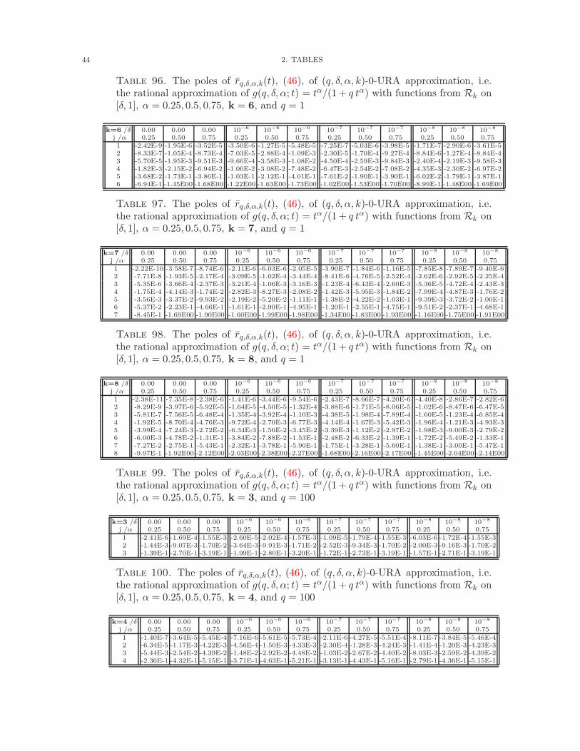
44 2. TABLES
Table 96. The poles of rq,δ,α,k(t), (46), of (q, δ, α, k)-0-URA approximation, i.e.the rational approximation of g(q, δ, α; t) = tα/(1 + q tα) with functions from Rk on[δ, 1], α = 0.25, 0.5, 0.75, k = 6, and q = 1
k=6 /δ 0.00 0.00 0.00 10−6 10−6 10−6 10−7 10−7 10−7 10−8 10−8 10−8
j /α 0.25 0.50 0.75 0.25 0.50 0.75 0.25 0.50 0.75 0.25 0.50 0.751 -2.42E-9 -1.95E-6 -3.52E-5 -3.50E-6 -1.27E-5 -5.48E-5 -7.25E-7 -5.03E-6 -3.98E-5 -1.71E-7 -2.90E-6 -3.61E-52 -8.33E-7 -1.05E-4 -8.73E-4 -7.03E-5 -2.88E-4 -1.09E-3 -2.30E-5 -1.70E-4 -9.27E-4 -8.84E-6 -1.27E-4 -8.84E-43 -5.70E-5 -1.95E-3 -9.51E-3 -9.66E-4 -3.58E-3 -1.08E-2 -4.50E-4 -2.59E-3 -9.84E-3 -2.40E-4 -2.19E-3 -9.58E-34 -1.82E-3 -2.15E-2 -6.94E-2 -1.06E-2 -3.08E-2 -7.48E-2 -6.47E-3 -2.54E-2 -7.08E-2 -4.35E-3 -2.30E-2 -6.97E-25 -3.68E-2 -1.73E-1 -3.86E-1 -1.03E-1 -2.12E-1 -4.01E-1 -7.61E-2 -1.90E-1 -3.90E-1 -6.02E-2 -1.79E-1 -3.87E-16 -6.94E-1 -1.45E00 -1.68E00 -1.22E00 -1.63E00 -1.73E00 -1.02E00 -1.53E00 -1.70E00 -8.99E-1 -1.48E00 -1.69E00
Table 97. The poles of rq,δ,α,k(t), (46), of (q, δ, α, k)-0-URA approximation, i.e.the rational approximation of g(q, δ, α; t) = tα/(1 + q tα) with functions from Rk on[δ, 1], α = 0.25, 0.5, 0.75, k = 7, and q = 1
k=7 /δ 0.00 0.00 0.00 10−6 10−6 10−6 10−7 10−7 10−7 10−8 10−8 10−8
j /α 0.25 0.50 0.75 0.25 0.50 0.75 0.25 0.50 0.75 0.25 0.50 0.751 -2.22E-10 -3.58E-7 -8.74E-6 -2.11E-6 -6.03E-6 -2.05E-5 -3.90E-7 -1.84E-6 -1.16E-5 -7.85E-8 -7.89E-7 -9.40E-62 -7.71E-8 -1.93E-5 -2.17E-4 -3.09E-5 -1.02E-4 -3.44E-4 -8.41E-6 -4.76E-5 -2.52E-4 -2.62E-6 -2.92E-5 -2.25E-43 -5.35E-6 -3.66E-4 -2.37E-3 -3.21E-4 -1.06E-3 -3.16E-3 -1.23E-4 -6.43E-4 -2.60E-3 -5.36E-5 -4.72E-4 -2.43E-34 -1.75E-4 -4.14E-3 -1.74E-2 -2.82E-3 -8.27E-3 -2.08E-2 -1.42E-3 -5.95E-3 -1.84E-2 -7.99E-4 -4.87E-3 -1.76E-25 -3.56E-3 -3.37E-2 -9.93E-2 -2.19E-2 -5.20E-2 -1.11E-1 -1.38E-2 -4.22E-2 -1.03E-1 -9.39E-3 -3.72E-2 -1.00E-16 -5.37E-2 -2.23E-1 -4.66E-1 -1.61E-1 -2.90E-1 -4.95E-1 -1.20E-1 -2.55E-1 -4.75E-1 -9.51E-2 -2.37E-1 -4.68E-17 -8.45E-1 -1.69E00 -1.90E00 -1.60E00 -1.99E00 -1.98E00 -1.34E00 -1.83E00 -1.93E00 -1.16E00 -1.75E00 -1.91E00
Table 98. The poles of rq,δ,α,k(t), (46), of (q, δ, α, k)-0-URA approximation, i.e.the rational approximation of g(q, δ, α; t) = tα/(1 + q tα) with functions from Rk on[δ, 1], α = 0.25, 0.5, 0.75, k = 8, and q = 1
k=8 /δ 0.00 0.00 0.00 10−6 10−6 10−6 10−7 10−7 10−7 10−8 10−8 10−8
j /α 0.25 0.50 0.75 0.25 0.50 0.75 0.25 0.50 0.75 0.25 0.50 0.751 -2.38E-11 -7.35E-8 -2.38E-6 -1.41E-6 -3.44E-6 -9.54E-6 -2.43E-7 -8.66E-7 -4.20E-6 -4.40E-8 -2.86E-7 -2.82E-62 -8.29E-9 -3.97E-6 -5.92E-5 -1.64E-5 -4.50E-5 -1.32E-4 -3.88E-6 -1.71E-5 -8.06E-5 -1.02E-6 -8.47E-6 -6.47E-53 -5.81E-7 -7.56E-5 -6.48E-4 -1.35E-4 -3.92E-4 -1.10E-3 -4.38E-5 -1.98E-4 -7.89E-4 -1.60E-5 -1.23E-4 -6.85E-44 -1.92E-5 -8.70E-4 -4.76E-3 -9.72E-4 -2.70E-3 -6.77E-3 -4.14E-4 -1.67E-3 -5.42E-3 -1.96E-4 -1.21E-3 -4.93E-35 -3.99E-4 -7.24E-3 -2.72E-2 -6.34E-3 -1.56E-2 -3.45E-2 -3.39E-3 -1.12E-2 -2.97E-2 -1.98E-3 -9.00E-3 -2.79E-26 -6.00E-3 -4.78E-2 -1.31E-1 -3.84E-2 -7.88E-2 -1.53E-1 -2.48E-2 -6.33E-2 -1.39E-1 -1.72E-2 -5.49E-2 -1.33E-17 -7.27E-2 -2.75E-1 -5.43E-1 -2.32E-1 -3.78E-1 -5.90E-1 -1.75E-1 -3.28E-1 -5.60E-1 -1.38E-1 -3.00E-1 -5.47E-18 -9.97E-1 -1.92E00 -2.12E00 -2.03E00 -2.38E00 -2.27E00 -1.68E00 -2.16E00 -2.17E00 -1.45E00 -2.04E00 -2.14E00
Table 99. The poles of rq,δ,α,k(t), (46), of (q, δ, α, k)-0-URA approximation, i.e.the rational approximation of g(q, δ, α; t) = tα/(1 + q tα) with functions from Rk on[δ, 1], α = 0.25, 0.5, 0.75, k = 3, and q = 100
k=3 /δ 0.00 0.00 0.00 10−6 10−6 10−6 10−7 10−7 10−7 10−8 10−8 10−8
j /α 0.25 0.50 0.75 0.25 0.50 0.75 0.25 0.50 0.75 0.25 0.50 0.751 -2.41E-6 -1.69E-4 -1.55E-3 -2.60E-5 -2.02E-4 -1.57E-3 -1.09E-5 -1.79E-4 -1.55E-3 -6.03E-6 -1.72E-4 -1.55E-32 -1.44E-3 -9.07E-3 -1.70E-2 -3.64E-3 -9.91E-3 -1.71E-2 -2.52E-3 -9.34E-3 -1.70E-2 -2.00E-3 -9.16E-3 -1.70E-23 -1.39E-1 -2.70E-1 -3.19E-1 -1.99E-1 -2.80E-1 -3.20E-1 -1.72E-1 -2.73E-1 -3.19E-1 -1.57E-1 -2.71E-1 -3.19E-1
Table 100. The poles of rq,δ,α,k(t), (46), of (q, δ, α, k)-0-URA approximation, i.e.the rational approximation of g(q, δ, α; t) = tα/(1 + q tα) with functions from Rk on[δ, 1], α = 0.25, 0.5, 0.75, k = 4, and q = 100
k=4 /δ 0.00 0.00 0.00 10−6 10−6 10−6 10−7 10−7 10−7 10−8 10−8 10−8
j /α 0.25 0.50 0.75 0.25 0.50 0.75 0.25 0.50 0.75 0.25 0.50 0.751 -1.40E-7 -3.64E-5 -5.45E-4 -7.16E-6 -5.61E-5 -5.73E-4 -2.11E-6 -4.27E-5 -5.51E-4 -8.11E-7 -3.84E-5 -5.46E-42 -6.34E-5 -1.17E-3 -4.22E-3 -4.56E-4 -1.50E-3 -4.33E-3 -2.30E-4 -1.28E-3 -4.24E-3 -1.41E-4 -1.20E-3 -4.23E-33 -5.44E-3 -2.54E-2 -4.39E-2 -1.48E-2 -2.92E-2 -4.48E-2 -1.03E-2 -2.67E-2 -4.40E-2 -8.03E-3 -2.59E-2 -4.39E-24 -2.36E-1 -4.32E-1 -5.15E-1 -3.71E-1 -4.63E-1 -5.21E-1 -3.13E-1 -4.43E-1 -5.16E-1 -2.79E-1 -4.36E-1 -5.15E-1
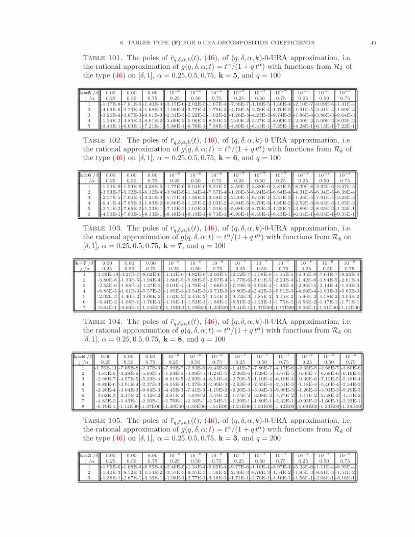
6. TABLES TYPE (F) FOR 0-URA-DECOMPOSITION COEFFICIENTS 45
Table 101. The poles of rq,δ,α,k(t), (46), of (q, δ, α, k)-0-URA approximation, i.e.the rational approximation of g(q, δ, α; t) = tα/(1 + q tα) with functions from Rk ofthe type (46) on [δ, 1], α = 0.25, 0.5, 0.75, k = 5, and q = 100
k=5 /δ 0.00 0.00 0.00 10−6 10−6 10−6 10−7 10−7 10−7 10−8 10−8 10−8
j /α 0.25 0.50 0.75 0.25 0.50 0.75 0.25 0.50 0.75 0.25 0.50 0.751 -1.17E-8 -7.81E-6 -1.40E-4 -3.15E-6 -2.02E-5 -1.67E-4 -7.36E-7 -1.18E-5 -1.46E-4 -2.10E-7 -9.09E-6 -1.41E-42 -4.09E-6 -2.23E-4 -1.68E-3 -1.09E-4 -3.77E-4 -1.79E-3 -4.13E-5 -2.76E-4 -1.70E-3 -1.91E-5 -2.41E-4 -1.69E-33 -3.26E-4 -3.67E-3 -9.61E-3 -2.31E-3 -5.22E-3 -1.02E-2 -1.26E-3 -4.23E-3 -9.74E-3 -7.86E-4 -3.86E-3 -9.64E-34 -1.24E-2 -4.85E-2 -8.01E-2 -3.69E-2 -5.96E-2 -8.34E-2 -2.60E-2 -5.27E-2 -8.09E-2 -2.00E-2 -5.00E-2 -8.03E-25 -3.40E-1 -6.03E-1 -7.21E-1 -5.88E-1 -6.76E-1 -7.38E-1 -4.89E-1 -6.31E-1 -7.25E-1 -4.28E-1 -6.13E-1 -7.22E-1
Table 102. The poles of rq,δ,α,k(t), (46), of (q, δ, α, k)-0-URA approximation, i.e.the rational approximation of g(q, δ, α; t) = tα/(1 + q tα) with functions from Rk ofthe type (46) on [δ, 1], α = 0.25, 0.5, 0.75, k = 6, and q = 100
k=6 /δ 0.00 0.00 0.00 10−6 10−6 10−6 10−7 10−7 10−7 10−8 10−8 10−8
j /α 0.25 0.50 0.75 0.25 0.50 0.75 0.25 0.50 0.75 0.25 0.50 0.751 -1.20E-9 -1.59E-6 -3.38E-5 -1.77E-6 -9.04E-6 -5.21E-5 -3.59E-7 -3.88E-6 -3.81E-5 -8.39E-8 -2.32E-6 -3.47E-52 -3.53E-7 -5.32E-5 -6.32E-4 -3.94E-5 -1.34E-4 -7.57E-4 -1.20E-5 -8.24E-5 -6.64E-4 -4.31E-6 -6.34E-5 -6.39E-43 -2.57E-5 -7.00E-4 -3.21E-3 -5.77E-4 -1.36E-3 -3.58E-3 -2.50E-4 -9.53E-4 -3.31E-3 -1.26E-4 -7.91E-4 -3.23E-34 -9.41E-4 -7.95E-3 -1.83E-2 -6.86E-3 -1.25E-2 -2.03E-2 -3.94E-3 -9.79E-3 -1.89E-2 -2.52E-3 -8.63E-3 -1.85E-25 -2.21E-2 -7.66E-2 -1.23E-1 -7.12E-2 -1.01E-1 -1.31E-1 -5.08E-2 -8.70E-2 -1.25E-1 -3.89E-2 -8.05E-2 -1.23E-16 -4.50E-1 -7.80E-1 -9.33E-1 -8.48E-1 -9.19E-1 -9.73E-1 -6.99E-1 -8.40E-1 -9.43E-1 -6.04E-1 -8.03E-1 -9.35E-1
Table 103. The poles of rq,δ,α,k(t), (46), of (q, δ, α, k)-0-URA approximation, i.e.the rational approximation of g(q, δ, α; t) = tα/(1 + q tα) with functions from Rk on[δ, 1], α = 0.25, 0.5, 0.75, k = 7, and q = 100
k=7 /δ 0.00 0.00 0.00 10−6 10−6 10−6 10−7 10−7 10−7 10−8 10−8 10−8
j /α 0.25 0.50 0.75 0.25 0.50 0.75 0.25 0.50 0.75 0.25 0.50 0.751 -1.39E-10 -3.27E-7 -8.62E-6 -1.14E-6 -4.82E-6 -2.00E-5 -2.12E-7 -1.58E-6 -1.15E-5 -4.35E-8 -7.04E-7 -9.26E-62 -3.80E-8 -1.33E-5 -1.94E-4 -1.86E-5 -5.98E-5 -2.97E-4 -4.77E-6 -3.01E-5 -2.23E-4 -1.42E-6 -1.94E-5 -2.01E-43 -2.53E-6 -1.68E-4 -1.37E-3 -2.01E-4 -4.79E-4 -1.68E-3 -7.19E-5 -2.90E-4 -1.46E-3 -2.96E-5 -2.14E-4 -1.39E-34 -8.85E-5 -1.61E-3 -5.57E-3 -1.85E-3 -3.54E-3 -6.73E-3 -8.80E-4 -2.42E-3 -5.91E-3 -4.69E-4 -1.93E-3 -5.65E-35 -2.02E-3 -1.40E-2 -3.00E-2 -1.52E-2 -2.41E-2 -3.51E-2 -9.12E-3 -1.85E-2 -3.15E-2 -5.96E-3 -1.58E-2 -3.04E-26 -3.41E-2 -1.08E-1 -1.70E-1 -1.18E-1 -1.53E-1 -1.88E-1 -8.51E-2 -1.29E-1 -1.75E-1 -6.53E-2 -1.17E-1 -1.71E-17 -5.64E-1 -9.60E-1 -1.15E00 -1.15E00 -1.19E00 -1.23E00 -9.41E-1 -1.07E00 -1.17E00 -8.06E-1 -1.01E00 -1.15E00
Table 104. The poles of rq,δ,α,k(t), (46), of (q, δ, α, k)-0-URA approximation, i.e.the rational approximation of g(q, δ, α; t) = tα/(1 + q tα) with functions from Rk on[δ, 1], α = 0.25, 0.5, 0.75, k = 8, and q = 100
k=8 /δ 0.00 0.00 0.00 10−6 10−6 10−6 10−7 10−7 10−7 10−8 10−8 10−8
j /α 0.25 0.50 0.75 0.25 0.50 0.75 0.25 0.50 0.75 0.25 0.50 0.751 -1.76E-11 -7.05E-8 -2.37E-6 -7.99E-7 -2.93E-6 -9.43E-6 -1.41E-7 -7.86E-7 -4.17E-6 -2.65E-8 -2.68E-7 -2.80E-62 -4.81E-9 -3.29E-6 -5.69E-5 -1.04E-5 -3.09E-5 -1.24E-4 -2.36E-6 -1.28E-5 -7.67E-5 -6.03E-7 -6.68E-6 -6.19E-53 -2.98E-7 -4.57E-5 -5.23E-4 -8.81E-5 -2.09E-4 -8.14E-4 -2.70E-5 -1.10E-4 -6.19E-4 -9.39E-6 -7.12E-5 -5.48E-44 -9.89E-6 -3.91E-4 -2.27E-3 -6.55E-4 -1.27E-3 -2.99E-3 -2.63E-4 -7.65E-4 -2.51E-3 -1.18E-4 -5.46E-4 -2.34E-35 -2.20E-4 -3.04E-3 -9.04E-3 -4.45E-3 -7.41E-3 -1.19E-2 -2.26E-3 -5.04E-3 -9.99E-3 -1.26E-3 -3.91E-3 -9.29E-36 -3.62E-3 -2.17E-2 -4.42E-2 -2.81E-2 -4.04E-2 -5.44E-2 -1.75E-2 -3.08E-2 -4.77E-2 -1.17E-2 -2.58E-2 -4.51E-27 -4.82E-2 -1.43E-1 -2.20E-1 -1.76E-1 -2.16E-1 -2.54E-1 -1.29E-1 -1.80E-1 -2.32E-1 -9.93E-2 -1.60E-1 -2.23E-18 -6.79E-1 -1.14E00 -1.37E00 -1.49E00 -1.50E00 -1.51E00 -1.21E00 -1.33E00 -1.42E00 -1.03E00 -1.23E00 -1.38E00
Table 105. The poles of rq,δ,α,k(t), (46), of (q, δ, α, k)-0-URA approximation, i.e.the rational approximation of g(q, δ, α; t) = tα/(1 + q tα) with functions from Rk ofthe type (46) on [δ, 1], α = 0.25, 0.5, 0.75, k = 3, and q = 200
k=3 /δ 0.00 0.00 0.00 10−6 10−6 10−6 10−7 10−7 10−7 10−8 10−8 10−8
j /α 0.25 0.50 0.75 0.25 0.50 0.75 0.25 0.50 0.75 0.25 0.50 0.751 -1.95E-6 -1.08E-4 -8.95E-4 -2.40E-5 -1.34E-4 -9.05E-4 -9.77E-6 -1.16E-4 -8.97E-4 -5.23E-6 -1.11E-4 -8.95E-42 -1.40E-3 -8.52E-3 -1.54E-2 -3.57E-3 -9.35E-3 -1.56E-2 -2.46E-3 -8.79E-3 -1.54E-2 -1.95E-3 -8.61E-3 -1.54E-23 -1.38E-1 -2.67E-1 -3.16E-1 -1.98E-1 -2.77E-1 -3.18E-1 -1.71E-1 -2.70E-1 -3.16E-1 -1.56E-1 -2.68E-1 -3.16E-1
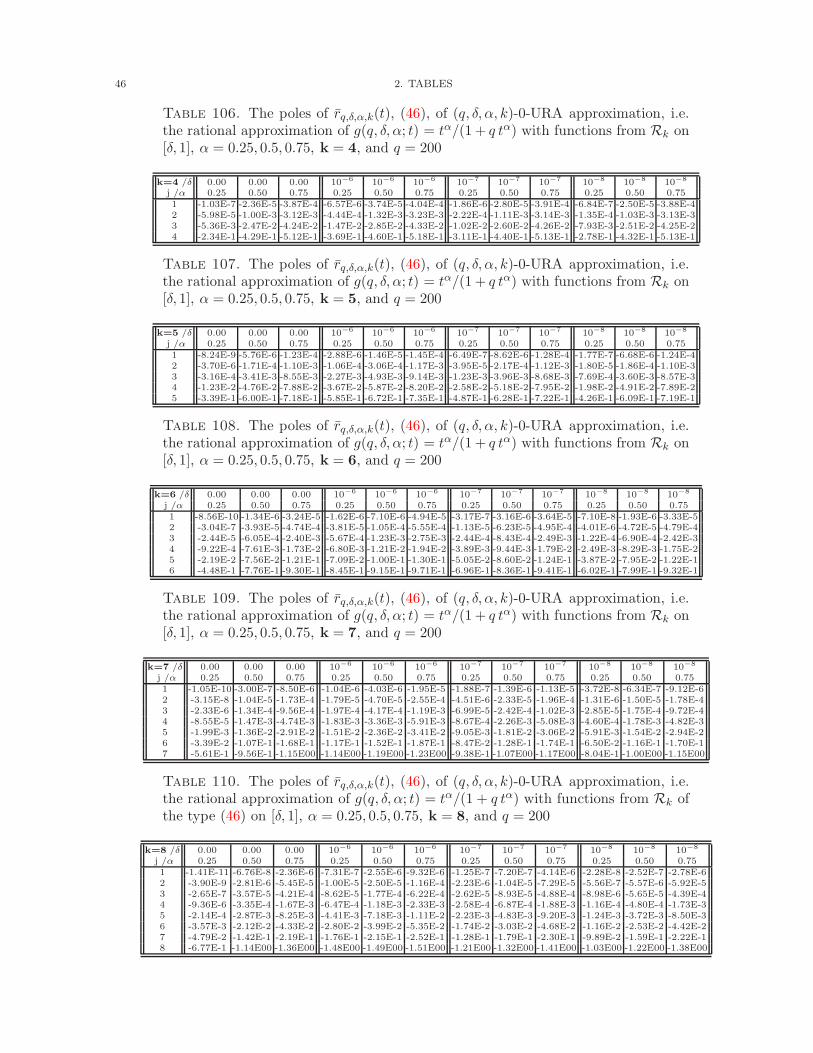
46 2. TABLES
Table 106. The poles of rq,δ,α,k(t), (46), of (q, δ, α, k)-0-URA approximation, i.e.the rational approximation of g(q, δ, α; t) = tα/(1 + q tα) with functions from Rk on[δ, 1], α = 0.25, 0.5, 0.75, k = 4, and q = 200
k=4 /δ 0.00 0.00 0.00 10−6 10−6 10−6 10−7 10−7 10−7 10−8 10−8 10−8
j /α 0.25 0.50 0.75 0.25 0.50 0.75 0.25 0.50 0.75 0.25 0.50 0.751 -1.03E-7 -2.36E-5 -3.87E-4 -6.57E-6 -3.74E-5 -4.04E-4 -1.86E-6 -2.80E-5 -3.91E-4 -6.84E-7 -2.50E-5 -3.88E-42 -5.98E-5 -1.00E-3 -3.12E-3 -4.44E-4 -1.32E-3 -3.23E-3 -2.22E-4 -1.11E-3 -3.14E-3 -1.35E-4 -1.03E-3 -3.13E-33 -5.36E-3 -2.47E-2 -4.24E-2 -1.47E-2 -2.85E-2 -4.33E-2 -1.02E-2 -2.60E-2 -4.26E-2 -7.93E-3 -2.51E-2 -4.25E-24 -2.34E-1 -4.29E-1 -5.12E-1 -3.69E-1 -4.60E-1 -5.18E-1 -3.11E-1 -4.40E-1 -5.13E-1 -2.78E-1 -4.32E-1 -5.13E-1
Table 107. The poles of rq,δ,α,k(t), (46), of (q, δ, α, k)-0-URA approximation, i.e.the rational approximation of g(q, δ, α; t) = tα/(1 + q tα) with functions from Rk on[δ, 1], α = 0.25, 0.5, 0.75, k = 5, and q = 200
k=5 /δ 0.00 0.00 0.00 10−6 10−6 10−6 10−7 10−7 10−7 10−8 10−8 10−8
j /α 0.25 0.50 0.75 0.25 0.50 0.75 0.25 0.50 0.75 0.25 0.50 0.751 -8.24E-9 -5.76E-6 -1.23E-4 -2.88E-6 -1.46E-5 -1.45E-4 -6.49E-7 -8.62E-6 -1.28E-4 -1.77E-7 -6.68E-6 -1.24E-42 -3.70E-6 -1.71E-4 -1.10E-3 -1.06E-4 -3.06E-4 -1.17E-3 -3.95E-5 -2.17E-4 -1.12E-3 -1.80E-5 -1.86E-4 -1.10E-33 -3.16E-4 -3.41E-3 -8.55E-3 -2.27E-3 -4.93E-3 -9.14E-3 -1.23E-3 -3.96E-3 -8.68E-3 -7.69E-4 -3.60E-3 -8.57E-34 -1.23E-2 -4.76E-2 -7.88E-2 -3.67E-2 -5.87E-2 -8.20E-2 -2.58E-2 -5.18E-2 -7.95E-2 -1.98E-2 -4.91E-2 -7.89E-25 -3.39E-1 -6.00E-1 -7.18E-1 -5.85E-1 -6.72E-1 -7.35E-1 -4.87E-1 -6.28E-1 -7.22E-1 -4.26E-1 -6.09E-1 -7.19E-1
Table 108. The poles of rq,δ,α,k(t), (46), of (q, δ, α, k)-0-URA approximation, i.e.the rational approximation of g(q, δ, α; t) = tα/(1 + q tα) with functions from Rk on[δ, 1], α = 0.25, 0.5, 0.75, k = 6, and q = 200
k=6 /δ 0.00 0.00 0.00 10−6 10−6 10−6 10−7 10−7 10−7 10−8 10−8 10−8
j /α 0.25 0.50 0.75 0.25 0.50 0.75 0.25 0.50 0.75 0.25 0.50 0.751 -8.56E-10 -1.34E-6 -3.24E-5 -1.62E-6 -7.10E-6 -4.94E-5 -3.17E-7 -3.16E-6 -3.64E-5 -7.10E-8 -1.93E-6 -3.33E-52 -3.04E-7 -3.93E-5 -4.74E-4 -3.81E-5 -1.05E-4 -5.55E-4 -1.13E-5 -6.23E-5 -4.95E-4 -4.01E-6 -4.72E-5 -4.79E-43 -2.44E-5 -6.05E-4 -2.40E-3 -5.67E-4 -1.23E-3 -2.75E-3 -2.44E-4 -8.43E-4 -2.49E-3 -1.22E-4 -6.90E-4 -2.42E-34 -9.22E-4 -7.61E-3 -1.73E-2 -6.80E-3 -1.21E-2 -1.94E-2 -3.89E-3 -9.44E-3 -1.79E-2 -2.49E-3 -8.29E-3 -1.75E-25 -2.19E-2 -7.56E-2 -1.21E-1 -7.09E-2 -1.00E-1 -1.30E-1 -5.05E-2 -8.60E-2 -1.24E-1 -3.87E-2 -7.95E-2 -1.22E-16 -4.48E-1 -7.76E-1 -9.30E-1 -8.45E-1 -9.15E-1 -9.71E-1 -6.96E-1 -8.36E-1 -9.41E-1 -6.02E-1 -7.99E-1 -9.32E-1
Table 109. The poles of rq,δ,α,k(t), (46), of (q, δ, α, k)-0-URA approximation, i.e.the rational approximation of g(q, δ, α; t) = tα/(1 + q tα) with functions from Rk on[δ, 1], α = 0.25, 0.5, 0.75, k = 7, and q = 200
k=7 /δ 0.00 0.00 0.00 10−6 10−6 10−6 10−7 10−7 10−7 10−8 10−8 10−8
j /α 0.25 0.50 0.75 0.25 0.50 0.75 0.25 0.50 0.75 0.25 0.50 0.751 -1.05E-10 -3.00E-7 -8.50E-6 -1.04E-6 -4.03E-6 -1.95E-5 -1.88E-7 -1.39E-6 -1.13E-5 -3.72E-8 -6.34E-7 -9.12E-62 -3.15E-8 -1.04E-5 -1.73E-4 -1.79E-5 -4.70E-5 -2.55E-4 -4.51E-6 -2.33E-5 -1.96E-4 -1.31E-6 -1.50E-5 -1.78E-43 -2.33E-6 -1.34E-4 -9.56E-4 -1.97E-4 -4.17E-4 -1.19E-3 -6.99E-5 -2.42E-4 -1.02E-3 -2.85E-5 -1.75E-4 -9.72E-44 -8.55E-5 -1.47E-3 -4.74E-3 -1.83E-3 -3.36E-3 -5.91E-3 -8.67E-4 -2.26E-3 -5.08E-3 -4.60E-4 -1.78E-3 -4.82E-35 -1.99E-3 -1.36E-2 -2.91E-2 -1.51E-2 -2.36E-2 -3.41E-2 -9.05E-3 -1.81E-2 -3.06E-2 -5.91E-3 -1.54E-2 -2.94E-26 -3.39E-2 -1.07E-1 -1.68E-1 -1.17E-1 -1.52E-1 -1.87E-1 -8.47E-2 -1.28E-1 -1.74E-1 -6.50E-2 -1.16E-1 -1.70E-17 -5.61E-1 -9.56E-1 -1.15E00 -1.14E00 -1.19E00 -1.23E00 -9.38E-1 -1.07E00 -1.17E00 -8.04E-1 -1.00E00 -1.15E00
Table 110. The poles of rq,δ,α,k(t), (46), of (q, δ, α, k)-0-URA approximation, i.e.the rational approximation of g(q, δ, α; t) = tα/(1 + q tα) with functions from Rk ofthe type (46) on [δ, 1], α = 0.25, 0.5, 0.75, k = 8, and q = 200
k=8 /δ 0.00 0.00 0.00 10−6 10−6 10−6 10−7 10−7 10−7 10−8 10−8 10−8
j /α 0.25 0.50 0.75 0.25 0.50 0.75 0.25 0.50 0.75 0.25 0.50 0.751 -1.41E-11 -6.76E-8 -2.36E-6 -7.31E-7 -2.55E-6 -9.32E-6 -1.25E-7 -7.20E-7 -4.14E-6 -2.28E-8 -2.52E-7 -2.78E-62 -3.90E-9 -2.81E-6 -5.45E-5 -1.00E-5 -2.50E-5 -1.16E-4 -2.23E-6 -1.04E-5 -7.29E-5 -5.56E-7 -5.57E-6 -5.92E-53 -2.65E-7 -3.57E-5 -4.21E-4 -8.62E-5 -1.77E-4 -6.22E-4 -2.62E-5 -8.93E-5 -4.88E-4 -8.98E-6 -5.65E-5 -4.39E-44 -9.36E-6 -3.35E-4 -1.67E-3 -6.47E-4 -1.18E-3 -2.33E-3 -2.58E-4 -6.87E-4 -1.88E-3 -1.16E-4 -4.80E-4 -1.73E-35 -2.14E-4 -2.87E-3 -8.25E-3 -4.41E-3 -7.18E-3 -1.11E-2 -2.23E-3 -4.83E-3 -9.20E-3 -1.24E-3 -3.72E-3 -8.50E-36 -3.57E-3 -2.12E-2 -4.33E-2 -2.80E-2 -3.99E-2 -5.35E-2 -1.74E-2 -3.03E-2 -4.68E-2 -1.16E-2 -2.53E-2 -4.42E-27 -4.79E-2 -1.42E-1 -2.19E-1 -1.76E-1 -2.15E-1 -2.52E-1 -1.28E-1 -1.79E-1 -2.30E-1 -9.89E-2 -1.59E-1 -2.22E-18 -6.77E-1 -1.14E00 -1.36E00 -1.48E00 -1.49E00 -1.51E00 -1.21E00 -1.32E00 -1.41E00 -1.03E00 -1.22E00 -1.38E00
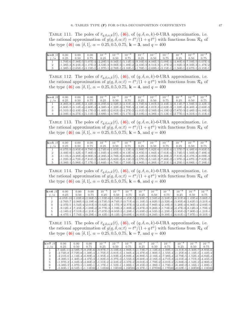
6. TABLES TYPE (F) FOR 0-URA-DECOMPOSITION COEFFICIENTS 47
Table 111. The poles of rq,δ,α,k(t), (46), of (q, δ, α, k)-0-URA approximation, i.e.the rational approximation of g(q, δ, α; t) = tα/(1 + q tα) with functions from Rk ofthe type (46) on [δ, 1], α = 0.25, 0.5, 0.75, k = 3, and q = 400
k=3 /δ 0.00 0.00 0.00 10−6 10−6 10−6 10−7 10−7 10−7 10−8 10−8 10−8
j /α 0.25 0.50 0.75 0.25 0.50 0.75 0.25 0.50 0.75 0.25 0.50 0.751 -1.70E-6 -7.38E-5 -5.07E-4 -2.29E-5 -9.56E-5 -5.14E-4 -9.16E-6 -8.06E-5 -5.09E-4 -4.80E-6 -7.59E-5 -5.07E-42 -1.38E-3 -8.24E-3 -1.47E-2 -3.53E-3 -9.06E-3 -1.48E-2 -2.43E-3 -8.51E-3 -1.47E-2 -1.92E-3 -8.33E-3 -1.47E-23 -1.38E-1 -2.65E-1 -3.15E-1 -1.97E-1 -2.76E-1 -3.16E-1 -1.70E-1 -2.69E-1 -3.15E-1 -1.56E-1 -2.67E-1 -3.15E-1
Table 112. The poles of rq,δ,α,k(t), (46), of (q, δ, α, k)-0-URA approximation, i.e.the rational approximation of g(q, δ, α; t) = tα/(1 + q tα) with functions from Rk ofthe type (46) on [δ, 1], α = 0.25, 0.5, 0.75, k = 4, and q = 400
k=4 /δ 0.00 0.00 0.00 10−6 10−6 10−6 10−7 10−7 10−7 10−8 10−8 10−8
j /α 0.25 0.50 0.75 0.25 0.50 0.75 0.25 0.50 0.75 0.25 0.50 0.751 -8.26E-8 -1.49E-5 -2.42E-4 -6.25E-6 -2.52E-5 -2.51E-4 -1.73E-6 -1.81E-5 -2.44E-4 -6.14E-7 -1.59E-5 -2.42E-42 -5.80E-5 -9.14E-4 -2.60E-3 -4.38E-4 -1.22E-3 -2.70E-3 -2.18E-4 -1.01E-3 -2.62E-3 -1.32E-4 -9.46E-4 -2.60E-33 -5.31E-3 -2.43E-2 -4.17E-2 -1.46E-2 -2.81E-2 -4.27E-2 -1.01E-2 -2.56E-2 -4.19E-2 -7.87E-3 -2.48E-2 -4.18E-24 -2.34E-1 -4.27E-1 -5.11E-1 -3.68E-1 -4.58E-1 -5.17E-1 -3.10E-1 -4.38E-1 -5.12E-1 -2.77E-1 -4.31E-1 -5.11E-1
Table 113. The poles of rq,δ,α,k(t), (46), of (q, δ, α, k)-0-URA approximation, i.e.the rational approximation of g(q, δ, α; t) = tα/(1 + q tα) with functions from Rk ofthe type (46) on [δ, 1], α = 0.25, 0.5, 0.75, k = 5, and q = 400
k=5 /δ 0.00 0.00 0.00 10−6 10−6 10−6 10−7 10−7 10−7 10−8 10−8 10−8
j /α 0.25 0.50 0.75 0.25 0.50 0.75 0.25 0.50 0.75 0.25 0.50 0.751 -6.07E-9 -3.85E-6 -9.78E-5 -2.74E-6 -1.01E-5 -1.13E-4 -5.99E-7 -5.82E-6 -1.01E-4 -1.57E-7 -4.48E-6 -9.85E-52 -3.49E-6 -1.42E-4 -7.46E-4 -1.04E-4 -2.68E-4 -8.13E-4 -3.85E-5 -1.84E-4 -7.61E-4 -1.74E-5 -1.56E-4 -7.49E-43 -3.11E-4 -3.28E-3 -8.06E-3 -2.26E-3 -4.78E-3 -8.66E-3 -1.22E-3 -3.83E-3 -8.20E-3 -7.61E-4 -3.47E-3 -8.09E-34 -1.22E-2 -4.72E-2 -7.81E-2 -3.66E-2 -5.82E-2 -8.13E-2 -2.57E-2 -5.14E-2 -7.88E-2 -1.97E-2 -4.87E-2 -7.82E-25 -3.38E-1 -5.98E-1 -7.17E-1 -5.84E-1 -6.70E-1 -7.34E-1 -4.86E-1 -6.26E-1 -7.21E-1 -4.25E-1 -6.08E-1 -7.18E-1
Table 114. The poles of rq,δ,α,k(t), (46), of (q, δ, α, k)-0-URA approximation, i.e.the rational approximation of g(q, δ, α; t) = tα/(1 + q tα) with functions from Rk ofthe type (46) on [δ, 1], α = 0.25, 0.5, 0.75, k = 6, and q = 400
k=6 /δ 0.00 0.00 0.00 10−6 10−6 10−6 10−7 10−7 10−7 10−8 10−8 10−8
j /α 0.25 0.50 0.75 0.25 0.50 0.75 0.25 0.50 0.75 0.25 0.50 0.751 -6.05E-10 -1.03E-6 -2.98E-5 -1.53E-6 -5.18E-6 -4.45E-5 -2.93E-7 -2.34E-6 -3.34E-5 -6.31E-8 -1.45E-6 -3.06E-52 -2.76E-7 -2.96E-5 -3.19E-4 -3.73E-5 -8.74E-5 -3.71E-4 -1.10E-5 -4.92E-5 -3.32E-4 -3.85E-6 -3.62E-5 -3.21E-43 -2.37E-5 -5.54E-4 -2.01E-3 -5.62E-4 -1.17E-3 -2.37E-3 -2.41E-4 -7.86E-4 -2.10E-3 -1.20E-4 -6.36E-4 -2.03E-34 -9.12E-4 -7.45E-3 -1.69E-2 -6.77E-3 -1.19E-2 -1.89E-2 -3.87E-3 -9.26E-3 -1.74E-2 -2.47E-3 -8.12E-3 -1.70E-25 -2.18E-2 -7.51E-2 -1.21E-1 -7.07E-2 -9.95E-2 -1.29E-1 -5.03E-2 -8.55E-2 -1.23E-1 -3.85E-2 -7.90E-2 -1.21E-16 -4.47E-1 -7.74E-1 -9.29E-1 -8.43E-1 -9.13E-1 -9.69E-1 -6.95E-1 -8.34E-1 -9.39E-1 -6.01E-1 -7.97E-1 -9.31E-1
Table 115. The poles of rq,δ,α,k(t), (46), of (q, δ, α, k)-0-URA approximation, i.e.the rational approximation of g(q, δ, α; t) = tα/(1 + q tα) with functions from Rk ofthe type (46) on [δ, 1], α = 0.25, 0.5, 0.75, k = 7, and q = 400
k=7 /δ 0.00 0.00 0.00 10−6 10−6 10−6 10−7 10−7 10−7 10−8 10−8 10−8
j /α 0.25 0.50 0.75 0.25 0.50 0.75 0.25 0.50 0.75 0.25 0.50 0.751 -7.44E-11 -2.58E-7 -8.25E-6 -9.87E-7 -3.10E-6 -1.86E-5 -1.73E-7 -1.12E-6 -1.09E-5 -3.31E-8 -5.30E-7 -8.85E-62 -2.73E-8 -7.72E-6 -1.39E-4 -1.75E-5 -3.81E-5 -1.94E-4 -4.37E-6 -1.80E-5 -1.55E-4 -1.25E-6 -1.13E-5 -1.42E-43 -2.21E-6 -1.14E-4 -6.80E-4 -1.95E-4 -3.83E-4 -8.89E-4 -6.88E-5 -2.16E-4 -7.38E-4 -2.79E-5 -1.52E-4 -6.94E-44 -8.39E-5 -1.40E-3 -4.37E-3 -1.82E-3 -3.27E-3 -5.55E-3 -8.60E-4 -2.18E-3 -4.71E-3 -4.55E-4 -1.71E-3 -4.45E-35 -1.97E-3 -1.34E-2 -2.86E-2 -1.51E-2 -2.34E-2 -3.37E-2 -9.01E-3 -1.79E-2 -3.01E-2 -5.88E-3 -1.52E-2 -2.90E-26 -3.38E-2 -1.07E-1 -1.68E-1 -1.17E-1 -1.52E-1 -1.86E-1 -8.45E-2 -1.28E-1 -1.73E-1 -6.48E-2 -1.16E-1 -1.69E-17 -5.60E-1 -9.54E-1 -1.14E00 -1.14E00 -1.19E00 -1.23E00 -9.37E-1 -1.07E00 -1.17E00 -8.02E-1 -1.00E00 -1.15E00
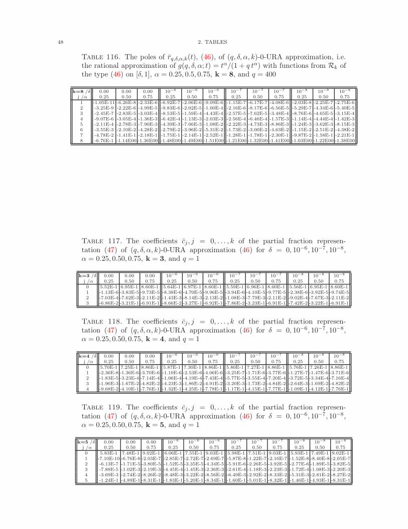
48 2. TABLES
Table 116. The poles of rq,δ,α,k(t), (46), of (q, δ, α, k)-0-URA approximation, i.e.the rational approximation of g(q, δ, α; t) = tα/(1 + q tα) with functions from Rk ofthe type (46) on [δ, 1], α = 0.25, 0.5, 0.75, k = 8, and q = 400
k=8 /δ 0.00 0.00 0.00 10−6 10−6 10−6 10−7 10−7 10−7 10−8 10−8 10−8
j /α 0.25 0.50 0.75 0.25 0.50 0.75 0.25 0.50 0.75 0.25 0.50 0.751 -1.05E-11 -6.26E-8 -2.33E-6 -6.92E-7 -2.06E-6 -9.09E-6 -1.15E-7 -6.17E-7 -4.08E-6 -2.03E-8 -2.25E-7 -2.75E-62 -3.25E-9 -2.22E-6 -4.99E-5 -9.83E-6 -2.02E-5 -1.00E-4 -2.16E-6 -8.17E-6 -6.56E-5 -5.29E-7 -4.34E-6 -5.40E-53 -2.45E-7 -2.83E-5 -3.03E-4 -8.53E-5 -1.59E-4 -4.43E-4 -2.57E-5 -7.62E-5 -3.48E-4 -8.76E-6 -4.65E-5 -3.15E-44 -9.07E-6 -3.05E-4 -1.36E-3 -6.42E-4 -1.13E-3 -2.03E-3 -2.56E-4 -6.46E-4 -1.57E-3 -1.14E-4 -4.44E-4 -1.42E-35 -2.11E-4 -2.78E-3 -7.90E-3 -4.39E-3 -7.06E-3 -1.08E-2 -2.22E-3 -4.73E-3 -8.86E-3 -1.24E-3 -3.62E-3 -8.15E-36 -3.55E-3 -2.10E-2 -4.28E-2 -2.79E-2 -3.96E-2 -5.31E-2 -1.73E-2 -3.00E-2 -4.63E-2 -1.15E-2 -2.51E-2 -4.38E-27 -4.78E-2 -1.41E-1 -2.18E-1 -1.75E-1 -2.14E-1 -2.52E-1 -1.28E-1 -1.78E-1 -2.30E-1 -9.87E-2 -1.58E-1 -2.21E-18 -6.76E-1 -1.14E00 -1.36E00 -1.48E00 -1.49E00 -1.51E00 -1.21E00 -1.32E00 -1.41E00 -1.03E00 -1.22E00 -1.38E00
Table 117. The coefficients cj , j = 0, . . . , k of the partial fraction represen-tation (47) of (q, δ, α, k)-0-URA approximation (46) for δ = 0, 10−6, 10−7, 10−8,α = 0.25, 0.50, 0.75, k = 3, and q = 1
k=3 /δ 0.00 0.00 0.00 10−6 10−6 10−6 10−7 10−7 10−7 10−8 10−8 10−8
j /α 0.25 0.50 0.75 0.25 0.50 0.75 0.25 0.50 0.75 0.25 0.50 0.750 5.52E-1 6.95E-1 8.60E-1 5.64E-1 6.97E-1 8.60E-1 5.59E-1 6.96E-1 8.60E-1 5.56E-1 6.95E-1 8.60E-11 -1.13E-6 -3.83E-5 -9.73E-5 -8.38E-6 -4.70E-5 -9.96E-5 -3.94E-6 -4.10E-5 -9.77E-5 -2.38E-6 -3.92E-5 -9.74E-52 -7.03E-4 -7.62E-3 -2.11E-2 -1.43E-3 -8.14E-3 -2.13E-2 -1.08E-3 -7.79E-3 -2.11E-2 -9.02E-4 -7.67E-3 -2.11E-23 -6.86E-2 -3.21E-1 -6.91E-1 -8.66E-2 -3.27E-1 -6.92E-1 -7.86E-2 -3.23E-1 -6.91E-1 -7.42E-2 -3.22E-1 -6.91E-1
Table 118. The coefficients cj , j = 0, . . . , k of the partial fraction represen-tation (47) of (q, δ, α, k)-0-URA approximation (46) for δ = 0, 10−6, 10−7, 10−8,α = 0.25, 0.50, 0.75, k = 4, and q = 1
k=4 /δ 0.00 0.00 0.00 10−6 10−6 10−6 10−7 10−7 10−7 10−8 10−8 10−8
j /α 0.25 0.50 0.75 0.25 0.50 0.75 0.25 0.50 0.75 0.25 0.50 0.750 5.70E-1 7.25E-1 8.86E-1 5.87E-1 7.30E-1 8.86E-1 5.80E-1 7.27E-1 8.86E-1 5.76E-1 7.26E-1 8.86E-11 -2.36E-8 -1.36E-6 -3.70E-6 -1.10E-6 -2.53E-6 -4.06E-6 -3.25E-7 -1.71E-6 -3.77E-6 -1.27E-7 -1.47E-6 -3.71E-62 -1.83E-5 -3.23E-4 -7.14E-4 -1.06E-4 -4.19E-4 -7.43E-4 -5.77E-5 -3.55E-4 -7.20E-4 -3.72E-5 -3.34E-4 -7.16E-43 -1.96E-3 -1.67E-2 -4.82E-2 -4.23E-3 -1.86E-2 -4.91E-2 -3.20E-3 -1.73E-2 -4.84E-2 -2.64E-3 -1.69E-2 -4.82E-24 -9.68E-2 -4.10E-1 -7.76E-1 -1.32E-1 -4.25E-1 -7.78E-1 -1.17E-1 -4.15E-1 -7.77E-1 -1.09E-1 -4.12E-1 -7.76E-1
Table 119. The coefficients cj , j = 0, . . . , k of the partial fraction represen-tation (47) of (q, δ, α, k)-0-URA approximation (46) for δ = 0, 10−6, 10−7, 10−8,α = 0.25, 0.50, 0.75, k = 5, and q = 1
k=5 /δ 0.00 0.00 0.00 10−6 10−6 10−6 10−7 10−7 10−7 10−8 10−8 10−8
j /α 0.25 0.50 0.75 0.25 0.50 0.75 0.25 0.50 0.75 0.25 0.50 0.750 5.83E-1 7.48E-1 9.02E-1 6.06E-1 7.55E-1 9.03E-1 5.98E-1 7.51E-1 9.03E-1 5.93E-1 7.49E-1 9.02E-11 -7.10E-10 -6.76E-8 -2.03E-7 -2.85E-7 -2.72E-7 -2.69E-7 -5.87E-8 -1.22E-7 -2.16E-7 -1.52E-8 -8.40E-8 -2.05E-72 -6.13E-7 -1.71E-5 -3.80E-5 -1.52E-5 -3.35E-5 -4.34E-5 -5.91E-6 -2.26E-5 -3.92E-5 -2.77E-6 -1.89E-5 -3.82E-53 -7.88E-5 -1.02E-3 -2.19E-3 -4.45E-4 -1.45E-3 -2.36E-3 -2.61E-4 -1.18E-3 -2.23E-3 -1.72E-4 -1.08E-3 -2.20E-34 -3.69E-3 -2.74E-2 -8.26E-2 -8.48E-3 -3.22E-2 -8.56E-2 -6.49E-3 -2.92E-2 -8.33E-2 -5.31E-3 -2.81E-2 -8.27E-25 -1.24E-1 -4.89E-1 -8.31E-1 -1.83E-1 -5.20E-1 -8.34E-1 -1.60E-1 -5.01E-1 -8.32E-1 -1.46E-1 -4.93E-1 -8.31E-1
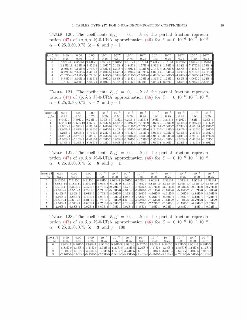
6. TABLES TYPE (F) FOR 0-URA-DECOMPOSITION COEFFICIENTS 49
Table 120. The coefficients cj , j = 0, . . . , k of the partial fraction represen-tation (47) of (q, δ, α, k)-0-URA approximation (46) for δ = 0, 10−6, 10−7, 10−8,α = 0.25, 0.50, 0.75, k = 6, and q = 1
k=6 /δ 0.00 0.00 0.00 10−6 10−6 10−6 10−7 10−7 10−7 10−8 10−8 10−8
j /α 0.25 0.50 0.75 0.25 0.50 0.75 0.25 0.50 0.75 0.25 0.50 0.750 5.95E-1 7.65E-1 9.14E-1 6.22E-1 7.76E-1 9.16E-1 6.13E-1 7.70E-1 9.15E-1 6.07E-1 7.67E-1 9.15E-11 -2.85E-11 -4.34E-9 -1.45E-8 -1.09E-7 -5.22E-8 -2.84E-8 -1.77E-8 -1.51E-8 -1.74E-8 -3.38E-9 -7.27E-9 -1.51E-82 -2.60E-8 -1.12E-6 -2.70E-6 -3.52E-6 -4.29E-6 -3.80E-6 -1.03E-6 -2.13E-6 -2.96E-6 -3.58E-7 -1.45E-6 -2.75E-63 -3.72E-6 -7.18E-5 -1.46E-4 -7.48E-5 -1.57E-4 -1.79E-4 -3.37E-5 -1.04E-4 -1.54E-4 -1.74E-5 -8.31E-5 -1.48E-44 -2.02E-4 -2.18E-3 -4.71E-3 -1.14E-3 -3.37E-3 -5.31E-3 -7.10E-4 -2.66E-3 -4.86E-3 -4.81E-4 -2.36E-3 -4.75E-35 -5.74E-3 -3.90E-2 -1.21E-1 -1.39E-2 -4.83E-2 -1.28E-1 -1.08E-2 -4.31E-2 -1.23E-1 -8.82E-3 -4.06E-2 -1.21E-16 -1.51E-1 -5.61E-1 -8.66E-1 -2.40E-1 -6.13E-1 -8.71E-1 -2.08E-1 -5.84E-1 -8.67E-1 -1.87E-1 -5.70E-1 -8.66E-1
Table 121. The coefficients cj , j = 0, . . . , k of the partial fraction represen-tation (47) of (q, δ, α, k)-0-URA approximation (46) for δ = 0, 10−6, 10−7, 10−8,α = 0.25, 0.50, 0.75, k = 7, and q = 1
k=7 /δ 0.00 0.00 0.00 10−6 10−6 10−6 10−7 10−7 10−7 10−8 10−8 10−8
j /α 0.25 0.50 0.75 0.25 0.50 0.75 0.25 0.50 0.75 0.25 0.50 0.750 6.04E-1 7.79E-1 9.24E-1 6.36E-1 7.93E-1 9.26E-1 6.27E-1 7.86E-1 9.24E-1 6.20E-1 7.82E-1 9.24E-11 -1.45E-12 -3.42E-10 -1.27E-9 -5.35E-8 -1.54E-8 -4.69E-9 -7.37E-9 -3.02E-9 -1.96E-9 -1.14E-9 -9.69E-10 -1.41E-92 -1.36E-9 -8.94E-8 -2.35E-7 -1.14E-6 -8.30E-7 -4.81E-7 -2.67E-7 -2.99E-7 -2.96E-7 -7.21E-8 -1.55E-7 -2.49E-73 -2.05E-7 -5.87E-6 -1.26E-5 -1.80E-5 -2.40E-5 -1.95E-5 -6.42E-6 -1.24E-5 -1.45E-5 -2.60E-6 -8.23E-6 -1.30E-54 -1.24E-5 -1.90E-4 -3.70E-4 -2.23E-4 -4.59E-4 -4.91E-4 -1.11E-4 -3.01E-4 -4.05E-4 -6.14E-5 -2.33E-4 -3.78E-45 -3.96E-4 -3.75E-3 -8.35E-3 -2.25E-3 -6.30E-3 -1.00E-2 -1.46E-3 -4.91E-3 -8.84E-3 -1.01E-3 -4.23E-3 -8.47E-36 -7.99E-3 -5.10E-2 -1.61E-1 -2.03E-2 -6.65E-2 -1.76E-1 -1.59E-2 -5.85E-2 -1.65E-1 -1.30E-2 -5.42E-2 -1.62E-17 -1.77E-1 -6.27E-1 -8.88E-1 -3.02E-1 -7.04E-1 -8.94E-1 -2.59E-1 -6.65E-1 -8.90E-1 -2.31E-1 -6.43E-1 -8.89E-1
Table 122. The coefficients cj , j = 0, . . . , k of the partial fraction represen-tation (47) of (q, δ, α, k)-0-URA approximation (46) for δ = 0, 10−6, 10−7, 10−8,α = 0.25, 0.50, 0.75, k = 8, and q = 1
k=8 /δ 0.00 0.00 0.00 10−6 10−6 10−6 10−7 10−7 10−7 10−8 10−8 10−8
j /α 0.25 0.50 0.75 0.25 0.50 0.75 0.25 0.50 0.75 0.25 0.50 0.750 6.12E-1 7.91E-1 9.31E-1 6.48E-1 8.08E-1 9.35E-1 6.39E-1 8.00E-1 9.32E-1 6.31E-1 7.95E-1 9.31E-11 -8.88E-14 -3.18E-11 -1.30E-10 -3.05E-8 -6.04E-9 -1.14E-9 -3.76E-9 -8.82E-10 -3.11E-10 -4.99E-10 -1.94E-10 -1.68E-102 -8.45E-11 -8.35E-9 -2.42E-8 -4.73E-7 -2.22E-7 -8.52E-8 -9.23E-8 -5.97E-8 -3.91E-8 -2.03E-8 -2.31E-8 -2.77E-83 -1.32E-8 -5.55E-7 -1.29E-6 -5.71E-6 -5.03E-6 -2.91E-6 -1.66E-6 -2.01E-6 -1.75E-6 -5.45E-7 -1.07E-6 -1.40E-64 -8.45E-7 -1.85E-5 -3.68E-5 -5.79E-5 -8.20E-5 -6.37E-5 -2.36E-5 -4.36E-5 -4.51E-5 -1.06E-5 -2.84E-5 -3.90E-55 -2.97E-5 -3.88E-4 -7.43E-4 -4.99E-4 -1.03E-3 -1.08E-3 -2.68E-4 -6.76E-4 -8.52E-4 -1.56E-4 -5.12E-4 -7.72E-46 -6.59E-4 -5.69E-3 -1.31E-2 -3.74E-3 -1.03E-2 -1.68E-2 -2.52E-3 -7.95E-3 -1.44E-2 -1.80E-3 -6.72E-3 -1.35E-27 -1.04E-2 -6.31E-2 -2.00E-1 -2.75E-2 -8.63E-2 -2.24E-1 -2.17E-2 -7.52E-2 -2.08E-1 -1.79E-2 -6.88E-2 -2.02E-18 -2.03E-1 -6.88E-1 -9.02E-1 -3.69E-1 -7.95E-1 -9.07E-1 -3.15E-1 -7.45E-1 -9.04E-1 -2.78E-1 -7.15E-1 -9.02E-1
Table 123. The coefficients cj , j = 0, . . . , k of the partial fraction represen-tation (47) of (q, δ, α, k)-0-URA approximation (46) for δ = 0, 10−6, 10−7, 10−8,α = 0.25, 0.50, 0.75, k = 3, and q = 100
k=3 /δ 0.00 0.00 0.00 10−6 10−6 10−6 10−7 10−7 10−7 10−8 10−8 10−8
j /α 0.25 0.50 0.75 0.25 0.50 0.75 0.25 0.50 0.75 0.25 0.50 0.750 9.92E-3 9.96E-3 9.98E-3 9.92E-3 9.96E-3 9.98E-3 9.92E-3 9.96E-3 9.98E-3 9.92E-3 9.96E-3 9.98E-31 -8.88E-9 -1.13E-6 -1.17E-5 -3.94E-8 -1.27E-6 -1.18E-5 -2.26E-8 -1.17E-6 -1.17E-5 -1.55E-8 -1.14E-6 -1.17E-52 -7.98E-7 -1.10E-5 -3.24E-5 -1.36E-6 -1.12E-5 -3.23E-5 -1.10E-6 -1.10E-5 -3.24E-5 -9.62E-7 -1.10E-5 -3.24E-53 -2.16E-5 -5.53E-5 -5.19E-5 -2.59E-5 -5.58E-5 -5.19E-5 -2.40E-5 -5.55E-5 -5.19E-5 -2.29E-5 -5.54E-5 -5.19E-5
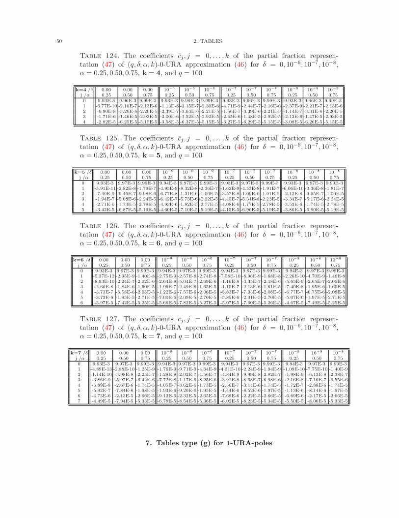
50 2. TABLES
Table 124. The coefficients cj , j = 0, . . . , k of the partial fraction represen-tation (47) of (q, δ, α, k)-0-URA approximation (46) for δ = 0, 10−6, 10−7, 10−8,α = 0.25, 0.50, 0.75, k = 4, and q = 100
k=4 /δ 0.00 0.00 0.00 10−6 10−6 10−6 10−7 10−7 10−7 10−8 10−8 10−8
j /α 0.25 0.50 0.75 0.25 0.50 0.75 0.25 0.50 0.75 0.25 0.50 0.750 9.93E-3 9.96E-3 9.99E-3 9.93E-3 9.96E-3 9.99E-3 9.93E-3 9.96E-3 9.99E-3 9.93E-3 9.96E-3 9.99E-31 -6.77E-10 -2.10E-7 -2.13E-6 -1.13E-8 -3.15E-7 -2.30E-6 -4.71E-9 -2.44E-7 -2.16E-6 -2.37E-9 -2.21E-7 -2.13E-62 -6.90E-8 -3.26E-6 -2.20E-5 -2.39E-7 -3.63E-6 -2.21E-5 -1.56E-7 -3.39E-6 -2.21E-5 -1.14E-7 -3.31E-6 -2.20E-53 -1.71E-6 -1.46E-5 -2.93E-5 -3.00E-6 -1.52E-5 -2.92E-5 -2.45E-6 -1.48E-5 -2.92E-5 -2.13E-6 -1.47E-5 -2.93E-54 -2.82E-5 -6.25E-5 -5.15E-5 -3.58E-5 -6.37E-5 -5.15E-5 -3.27E-5 -6.29E-5 -5.15E-5 -3.08E-5 -6.26E-5 -5.15E-5
Table 125. The coefficients cj , j = 0, . . . , k of the partial fraction represen-tation (47) of (q, δ, α, k)-0-URA approximation (46) for δ = 0, 10−6, 10−7, 10−8,α = 0.25, 0.50, 0.75, k = 5, and q = 100
k=5 /δ 0.00 0.00 0.00 10−6 10−6 10−6 10−7 10−7 10−7 10−8 10−8 10−8
j /α 0.25 0.50 0.75 0.25 0.50 0.75 0.25 0.50 0.75 0.25 0.50 0.750 9.93E-3 9.97E-3 9.99E-3 9.94E-3 9.97E-3 9.99E-3 9.93E-3 9.97E-3 9.99E-3 9.93E-3 9.97E-3 9.99E-31 -5.91E-11 -2.82E-8 -1.79E-7 -4.95E-9 -8.32E-8 -2.36E-7 -1.62E-9 -4.53E-8 -1.91E-7 -6.06E-10 -3.36E-8 -1.81E-72 -7.40E-9 -9.46E-7 -9.98E-6 -6.77E-8 -1.31E-6 -1.06E-5 -3.57E-8 -1.09E-6 -1.01E-5 -2.12E-8 -9.95E-7 -1.00E-53 -1.94E-7 -5.08E-6 -2.24E-5 -6.42E-7 -5.73E-6 -2.22E-5 -4.45E-7 -5.34E-6 -2.23E-5 -3.34E-7 -5.17E-6 -2.24E-54 -2.71E-6 -1.73E-5 -2.78E-5 -4.93E-6 -1.82E-5 -2.77E-5 -4.08E-6 -1.77E-5 -2.78E-5 -3.53E-6 -1.74E-5 -2.78E-55 -3.42E-5 -6.87E-5 -5.19E-5 -4.60E-5 -7.10E-5 -5.19E-5 -4.15E-5 -6.96E-5 -5.19E-5 -3.86E-5 -6.90E-5 -5.19E-5
Table 126. The coefficients cj , j = 0, . . . , k of the partial fraction represen-tation (47) of (q, δ, α, k)-0-URA approximation (46) for δ = 0, 10−6, 10−7, 10−8,α = 0.25, 0.50, 0.75, k = 6, and q = 100
k=6 /δ 0.00 0.00 0.00 10−6 10−6 10−6 10−7 10−7 10−7 10−8 10−8 10−8
j /α 0.25 0.50 0.75 0.25 0.50 0.75 0.25 0.50 0.75 0.25 0.50 0.750 9.93E-3 9.97E-3 9.99E-3 9.94E-3 9.97E-3 9.99E-3 9.94E-3 9.97E-3 9.99E-3 9.94E-3 9.97E-3 9.99E-31 -5.37E-12 -2.95E-9 -1.40E-8 -2.75E-9 -2.57E-8 -2.74E-8 -7.58E-10 -8.96E-9 -1.68E-8 -2.26E-10 -4.70E-9 -1.46E-82 -8.93E-10 -2.24E-7 -2.02E-6 -2.64E-8 -5.04E-7 -2.69E-6 -1.16E-8 -3.35E-7 -2.18E-6 -5.65E-9 -2.65E-7 -2.05E-63 -2.60E-8 -1.84E-6 -1.60E-5 -1.96E-7 -2.49E-6 -1.65E-5 -1.15E-7 -2.13E-6 -1.61E-5 -7.40E-8 -1.95E-6 -1.60E-54 -3.73E-7 -6.58E-6 -2.08E-5 -1.22E-6 -7.57E-6 -2.06E-5 -8.83E-7 -7.03E-6 -2.08E-5 -6.77E-7 -6.75E-6 -2.08E-55 -3.73E-6 -1.95E-5 -2.71E-5 -7.00E-6 -2.09E-5 -2.70E-5 -5.85E-6 -2.01E-5 -2.70E-5 -5.07E-6 -1.97E-5 -2.71E-56 -3.97E-5 -7.42E-5 -5.25E-5 -5.66E-5 -7.82E-5 -5.27E-5 -5.07E-5 -7.60E-5 -5.26E-5 -4.67E-5 -7.49E-5 -5.25E-5
Table 127. The coefficients cj , j = 0, . . . , k of the partial fraction represen-tation (47) of (q, δ, α, k)-0-URA approximation (46) for δ = 0, 10−6, 10−7, 10−8,α = 0.25, 0.50, 0.75, k = 7, and q = 100
k=7 /δ 0.00 0.00 0.00 10−6 10−6 10−6 10−7 10−7 10−7 10−8 10−8 10−8
j /α 0.25 0.50 0.75 0.25 0.50 0.75 0.25 0.50 0.75 0.25 0.50 0.750 9.93E-3 9.97E-3 9.99E-3 9.94E-3 9.97E-3 9.99E-3 9.94E-3 9.97E-3 9.99E-3 9.94E-3 9.97E-3 9.99E-31 -4.89E-13 -2.88E-10 -1.25E-9 -1.76E-9 -9.71E-9 -4.64E-9 -4.31E-10 -2.24E-9 -1.94E-9 -1.09E-10 -7.75E-10 -1.40E-92 -1.14E-10 -3.98E-8 -2.25E-7 -1.28E-8 -2.02E-7 -4.56E-7 -4.84E-9 -9.99E-8 -2.82E-7 -1.98E-9 -6.13E-8 -2.38E-73 -3.86E-9 -5.97E-7 -6.42E-6 -7.72E-8 -1.17E-6 -8.25E-6 -3.92E-8 -8.68E-7 -6.98E-6 -2.16E-8 -7.10E-7 -6.55E-64 -5.89E-8 -2.67E-6 -1.74E-5 -4.05E-7 -3.62E-6 -1.73E-5 -2.56E-7 -3.14E-6 -1.74E-5 -1.72E-7 -2.88E-6 -1.74E-55 -5.92E-7 -7.84E-6 -1.98E-5 -1.93E-6 -9.20E-6 -1.95E-5 -1.44E-6 -8.52E-6 -1.97E-5 -1.13E-6 -8.14E-6 -1.97E-56 -4.73E-6 -2.13E-5 -2.66E-5 -9.12E-6 -2.32E-5 -2.65E-5 -7.69E-6 -2.22E-5 -2.66E-5 -6.69E-6 -2.17E-5 -2.66E-57 -4.49E-5 -7.94E-5 -5.33E-5 -6.78E-5 -8.54E-5 -5.36E-5 -6.02E-5 -8.23E-5 -5.34E-5 -5.50E-5 -8.06E-5 -5.33E-5
7. Tables type (g) for 1-URA-poles
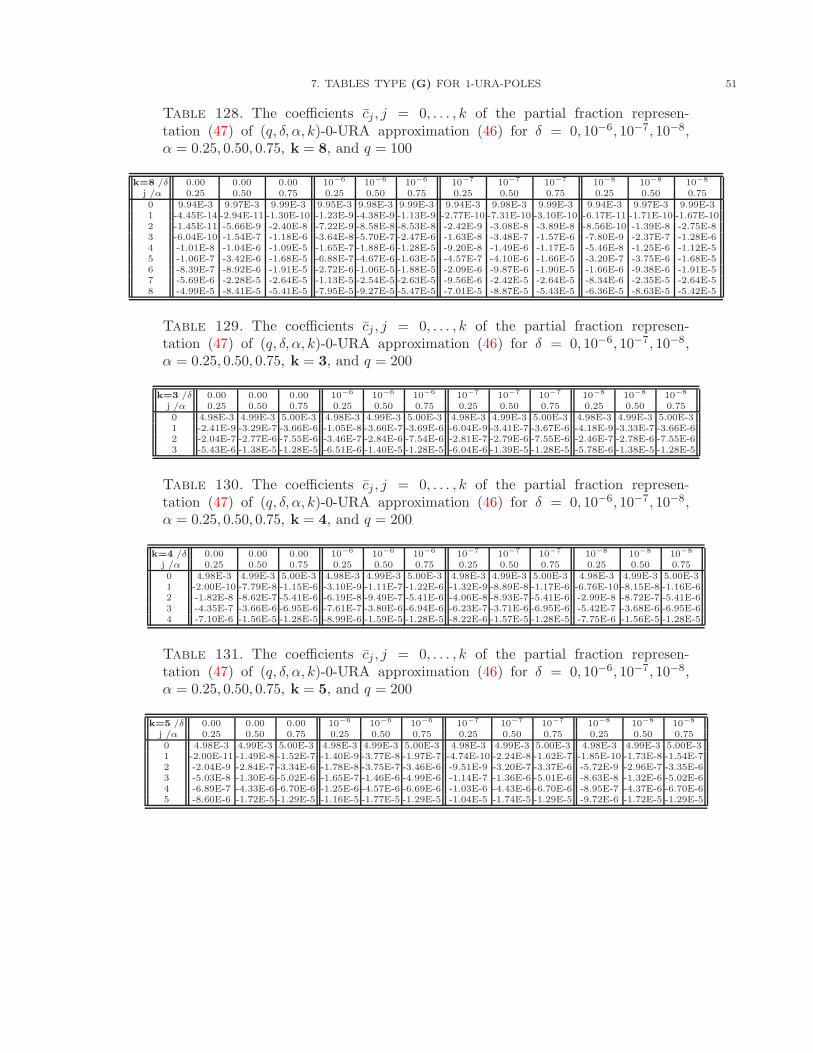
7. TABLES TYPE (G) FOR 1-URA-POLES 51
Table 128. The coefficients cj , j = 0, . . . , k of the partial fraction represen-tation (47) of (q, δ, α, k)-0-URA approximation (46) for δ = 0, 10−6, 10−7, 10−8,α = 0.25, 0.50, 0.75, k = 8, and q = 100
k=8 /δ 0.00 0.00 0.00 10−6 10−6 10−6 10−7 10−7 10−7 10−8 10−8 10−8
j /α 0.25 0.50 0.75 0.25 0.50 0.75 0.25 0.50 0.75 0.25 0.50 0.750 9.94E-3 9.97E-3 9.99E-3 9.95E-3 9.98E-3 9.99E-3 9.94E-3 9.98E-3 9.99E-3 9.94E-3 9.97E-3 9.99E-31 -4.45E-14 -2.94E-11 -1.30E-10 -1.23E-9 -4.38E-9 -1.13E-9 -2.77E-10 -7.31E-10 -3.10E-10 -6.17E-11 -1.71E-10 -1.67E-102 -1.45E-11 -5.66E-9 -2.40E-8 -7.22E-9 -8.58E-8 -8.53E-8 -2.42E-9 -3.08E-8 -3.89E-8 -8.56E-10 -1.39E-8 -2.75E-83 -6.04E-10 -1.54E-7 -1.18E-6 -3.64E-8 -5.70E-7 -2.47E-6 -1.63E-8 -3.48E-7 -1.57E-6 -7.80E-9 -2.37E-7 -1.28E-64 -1.01E-8 -1.04E-6 -1.09E-5 -1.65E-7 -1.88E-6 -1.28E-5 -9.20E-8 -1.49E-6 -1.17E-5 -5.46E-8 -1.25E-6 -1.12E-55 -1.06E-7 -3.42E-6 -1.68E-5 -6.88E-7 -4.67E-6 -1.63E-5 -4.57E-7 -4.10E-6 -1.66E-5 -3.20E-7 -3.75E-6 -1.68E-56 -8.39E-7 -8.92E-6 -1.91E-5 -2.72E-6 -1.06E-5 -1.88E-5 -2.09E-6 -9.87E-6 -1.90E-5 -1.66E-6 -9.38E-6 -1.91E-57 -5.69E-6 -2.28E-5 -2.64E-5 -1.13E-5 -2.54E-5 -2.63E-5 -9.56E-6 -2.42E-5 -2.64E-5 -8.34E-6 -2.35E-5 -2.64E-58 -4.99E-5 -8.41E-5 -5.41E-5 -7.95E-5 -9.27E-5 -5.47E-5 -7.01E-5 -8.87E-5 -5.43E-5 -6.36E-5 -8.63E-5 -5.42E-5
Table 129. The coefficients cj , j = 0, . . . , k of the partial fraction represen-tation (47) of (q, δ, α, k)-0-URA approximation (46) for δ = 0, 10−6, 10−7, 10−8,α = 0.25, 0.50, 0.75, k = 3, and q = 200
k=3 /δ 0.00 0.00 0.00 10−6 10−6 10−6 10−7 10−7 10−7 10−8 10−8 10−8
j /α 0.25 0.50 0.75 0.25 0.50 0.75 0.25 0.50 0.75 0.25 0.50 0.750 4.98E-3 4.99E-3 5.00E-3 4.98E-3 4.99E-3 5.00E-3 4.98E-3 4.99E-3 5.00E-3 4.98E-3 4.99E-3 5.00E-31 -2.41E-9 -3.29E-7 -3.66E-6 -1.05E-8 -3.66E-7 -3.69E-6 -6.04E-9 -3.41E-7 -3.67E-6 -4.18E-9 -3.33E-7 -3.66E-62 -2.04E-7 -2.77E-6 -7.55E-6 -3.46E-7 -2.84E-6 -7.54E-6 -2.81E-7 -2.79E-6 -7.55E-6 -2.46E-7 -2.78E-6 -7.55E-63 -5.43E-6 -1.38E-5 -1.28E-5 -6.51E-6 -1.40E-5 -1.28E-5 -6.04E-6 -1.39E-5 -1.28E-5 -5.78E-6 -1.38E-5 -1.28E-5
Table 130. The coefficients cj , j = 0, . . . , k of the partial fraction represen-tation (47) of (q, δ, α, k)-0-URA approximation (46) for δ = 0, 10−6, 10−7, 10−8,α = 0.25, 0.50, 0.75, k = 4, and q = 200
k=4 /δ 0.00 0.00 0.00 10−6 10−6 10−6 10−7 10−7 10−7 10−8 10−8 10−8
j /α 0.25 0.50 0.75 0.25 0.50 0.75 0.25 0.50 0.75 0.25 0.50 0.750 4.98E-3 4.99E-3 5.00E-3 4.98E-3 4.99E-3 5.00E-3 4.98E-3 4.99E-3 5.00E-3 4.98E-3 4.99E-3 5.00E-31 -2.00E-10 -7.79E-8 -1.15E-6 -3.10E-9 -1.11E-7 -1.22E-6 -1.32E-9 -8.89E-8 -1.17E-6 -6.76E-10 -8.15E-8 -1.16E-62 -1.82E-8 -8.62E-7 -5.41E-6 -6.19E-8 -9.49E-7 -5.41E-6 -4.06E-8 -8.93E-7 -5.41E-6 -2.99E-8 -8.72E-7 -5.41E-63 -4.35E-7 -3.66E-6 -6.95E-6 -7.61E-7 -3.80E-6 -6.94E-6 -6.23E-7 -3.71E-6 -6.95E-6 -5.42E-7 -3.68E-6 -6.95E-64 -7.10E-6 -1.56E-5 -1.28E-5 -8.99E-6 -1.59E-5 -1.28E-5 -8.22E-6 -1.57E-5 -1.28E-5 -7.75E-6 -1.56E-5 -1.28E-5
Table 131. The coefficients cj , j = 0, . . . , k of the partial fraction represen-tation (47) of (q, δ, α, k)-0-URA approximation (46) for δ = 0, 10−6, 10−7, 10−8,α = 0.25, 0.50, 0.75, k = 5, and q = 200
k=5 /δ 0.00 0.00 0.00 10−6 10−6 10−6 10−7 10−7 10−7 10−8 10−8 10−8
j /α 0.25 0.50 0.75 0.25 0.50 0.75 0.25 0.50 0.75 0.25 0.50 0.750 4.98E-3 4.99E-3 5.00E-3 4.98E-3 4.99E-3 5.00E-3 4.98E-3 4.99E-3 5.00E-3 4.98E-3 4.99E-3 5.00E-31 -2.00E-11 -1.49E-8 -1.52E-7 -1.40E-9 -3.77E-8 -1.97E-7 -4.74E-10 -2.24E-8 -1.62E-7 -1.85E-10 -1.73E-8 -1.54E-72 -2.04E-9 -2.84E-7 -3.34E-6 -1.78E-8 -3.75E-7 -3.46E-6 -9.51E-9 -3.20E-7 -3.37E-6 -5.72E-9 -2.96E-7 -3.35E-63 -5.03E-8 -1.30E-6 -5.02E-6 -1.65E-7 -1.46E-6 -4.99E-6 -1.14E-7 -1.36E-6 -5.01E-6 -8.63E-8 -1.32E-6 -5.02E-64 -6.89E-7 -4.33E-6 -6.70E-6 -1.25E-6 -4.57E-6 -6.69E-6 -1.03E-6 -4.43E-6 -6.70E-6 -8.95E-7 -4.37E-6 -6.70E-65 -8.60E-6 -1.72E-5 -1.29E-5 -1.16E-5 -1.77E-5 -1.29E-5 -1.04E-5 -1.74E-5 -1.29E-5 -9.72E-6 -1.72E-5 -1.29E-5
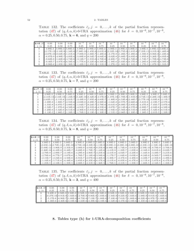
52 2. TABLES
Table 132. The coefficients cj , j = 0, . . . , k of the partial fraction represen-tation (47) of (q, δ, α, k)-0-URA approximation (46) for δ = 0, 10−6, 10−7, 10−8,α = 0.25, 0.50, 0.75, k = 6, and q = 200
k=6 /δ 0.00 0.00 0.00 10−6 10−6 10−6 10−7 10−7 10−7 10−8 10−8 10−8
j /α 0.25 0.50 0.75 0.25 0.50 0.75 0.25 0.50 0.75 0.25 0.50 0.750 4.98E-3 4.99E-3 5.00E-3 4.98E-3 4.99E-3 5.00E-3 4.98E-3 4.99E-3 5.00E-3 4.98E-3 4.99E-3 5.00E-31 -2.17E-12 -2.10E-9 -1.34E-8 -7.98E-10 -1.45E-8 -2.61E-8 -2.32E-10 -5.75E-9 -1.61E-8 -7.35E-11 -3.21E-9 -1.40E-82 -2.67E-10 -8.62E-8 -1.21E-6 -7.08E-9 -1.66E-7 -1.48E-6 -3.17E-9 -1.20E-7 -1.28E-6 -1.58E-9 -9.86E-8 -1.22E-63 -6.97E-9 -4.99E-7 -4.05E-6 -5.09E-8 -6.54E-7 -4.04E-6 -3.02E-8 -5.68E-7 -4.05E-6 -1.95E-8 -5.26E-7 -4.05E-64 -9.62E-8 -1.66E-6 -4.73E-6 -3.12E-7 -1.91E-6 -4.70E-6 -2.26E-7 -1.77E-6 -4.72E-6 -1.74E-7 -1.70E-6 -4.73E-65 -9.46E-7 -4.87E-6 -6.58E-6 -1.77E-6 -5.22E-6 -6.56E-6 -1.48E-6 -5.03E-6 -6.57E-6 -1.28E-6 -4.93E-6 -6.58E-66 -9.98E-6 -1.85E-5 -1.30E-5 -1.42E-5 -1.95E-5 -1.31E-5 -1.27E-5 -1.90E-5 -1.31E-5 -1.17E-5 -1.87E-5 -1.31E-5
Table 133. The coefficients cj , j = 0, . . . , k of the partial fraction represen-tation (47) of (q, δ, α, k)-0-URA approximation (46) for δ = 0, 10−6, 10−7, 10−8,α = 0.25, 0.50, 0.75, k = 7, and q = 200
k=7 /δ 0.00 0.00 0.00 10−6 10−6 10−6 10−7 10−7 10−7 10−8 10−8 10−8
j /α 0.25 0.50 0.75 0.25 0.50 0.75 0.25 0.50 0.75 0.25 0.50 0.750 4.98E-3 4.99E-3 5.00E-3 4.99E-3 4.99E-3 5.00E-3 4.99E-3 4.99E-3 5.00E-3 4.98E-3 4.99E-3 5.00E-31 -2.41E-13 -2.44E-10 -1.24E-9 -5.22E-10 -6.42E-9 -4.57E-9 -1.37E-10 -1.70E-9 -1.91E-9 -3.74E-11 -6.28E-10 -1.38E-92 -3.82E-11 -2.11E-8 -2.01E-7 -3.49E-9 -7.95E-8 -3.83E-7 -1.36E-9 -4.53E-8 -2.48E-7 -5.77E-10 -3.03E-8 -2.11E-73 -1.09E-9 -1.90E-7 -2.55E-6 -2.03E-8 -3.29E-7 -2.88E-6 -1.04E-8 -2.57E-7 -2.66E-6 -5.81E-9 -2.19E-7 -2.57E-64 -1.55E-8 -6.97E-7 -3.88E-6 -1.04E-7 -9.24E-7 -3.79E-6 -6.61E-8 -8.09E-7 -3.85E-6 -4.47E-8 -7.45E-7 -3.87E-65 -1.52E-7 -1.97E-6 -4.58E-6 -4.91E-7 -2.31E-6 -4.55E-6 -3.67E-7 -2.14E-6 -4.57E-6 -2.88E-7 -2.04E-6 -4.58E-66 -1.20E-6 -5.32E-6 -6.51E-6 -2.30E-6 -5.81E-6 -6.50E-6 -1.94E-6 -5.56E-6 -6.51E-6 -1.69E-6 -5.42E-6 -6.51E-67 -1.13E-5 -1.98E-5 -1.33E-5 -1.70E-5 -2.13E-5 -1.33E-5 -1.51E-5 -2.06E-5 -1.33E-5 -1.38E-5 -2.01E-5 -1.33E-5
Table 134. The coefficients cj , j = 0, . . . , k of the partial fraction represen-tation (47) of (q, δ, α, k)-0-URA approximation (46) for δ = 0, 10−6, 10−7, 10−8,α = 0.25, 0.50, 0.75, k = 8, and q = 200
k=8 /δ 0.00 0.00 0.00 10−6 10−6 10−6 10−7 10−7 10−7 10−8 10−8 10−8
j /α 0.25 0.50 0.75 0.25 0.50 0.75 0.25 0.50 0.75 0.25 0.50 0.750 4.98E-3 4.99E-3 5.00E-3 4.99E-3 4.99E-3 5.00E-3 4.99E-3 4.99E-3 5.00E-3 4.99E-3 4.99E-3 5.00E-31 -2.65E-14 -2.72E-11 -1.29E-10 -3.73E-10 -3.22E-9 -1.13E-9 -9.09E-11 -6.08E-10 -3.08E-10 -2.23E-11 -1.52E-10 -1.66E-102 -5.69E-12 -3.96E-9 -2.35E-8 -2.00E-9 -4.04E-8 -8.25E-8 -6.98E-10 -1.74E-8 -3.81E-8 -2.59E-10 -8.79E-9 -2.70E-83 -1.86E-10 -6.42E-8 -8.48E-7 -9.69E-9 -1.79E-7 -1.44E-6 -4.41E-9 -1.22E-7 -1.05E-6 -2.16E-9 -9.01E-8 -9.02E-74 -2.79E-9 -2.99E-7 -3.19E-6 -4.29E-8 -4.96E-7 -3.25E-6 -2.41E-8 -4.04E-7 -3.23E-6 -1.44E-8 -3.49E-7 -3.21E-65 -2.78E-8 -8.77E-7 -3.67E-6 -1.76E-7 -1.18E-6 -3.58E-6 -1.17E-7 -1.04E-6 -3.63E-6 -8.24E-8 -9.56E-7 -3.66E-66 -2.15E-7 -2.24E-6 -4.50E-6 -6.91E-7 -2.67E-6 -4.46E-6 -5.30E-7 -2.47E-6 -4.48E-6 -4.22E-7 -2.35E-6 -4.49E-67 -1.44E-6 -5.71E-6 -6.48E-6 -2.85E-6 -6.35E-6 -6.47E-6 -2.41E-6 -6.05E-6 -6.47E-6 -2.11E-6 -5.87E-6 -6.47E-68 -1.25E-5 -2.10E-5 -1.35E-5 -2.00E-5 -2.31E-5 -1.36E-5 -1.76E-5 -2.21E-5 -1.35E-5 -1.60E-5 -2.16E-5 -1.35E-5
Table 135. The coefficients cj , j = 0, . . . , k of the partial fraction represen-tation (47) of (q, δ, α, k)-0-URA approximation (46) for δ = 0, 10−6, 10−7, 10−8,α = 0.25, 0.50, 0.75, k = 3, and q = 400
k=3 /δ 0.00 0.00 0.00 10−6 10−6 10−6 10−7 10−7 10−7 10−8 10−8 10−8
j /α 0.25 0.50 0.75 0.25 0.50 0.75 0.25 0.50 0.75 0.25 0.50 0.750 2.49E-3 2.50E-3 2.50E-3 2.50E-3 2.50E-3 2.50E-3 2.50E-3 2.50E-3 2.50E-3 2.50E-3 2.50E-3 2.50E-31 -6.27E-10 -8.91E-8 -1.02E-6 -2.70E-9 -9.86E-8 -1.03E-6 -1.56E-9 -9.22E-8 -1.02E-6 -1.08E-9 -9.01E-8 -1.02E-62 -5.17E-8 -6.96E-7 -1.80E-6 -8.75E-8 -7.13E-7 -1.80E-6 -7.10E-8 -7.01E-7 -1.80E-6 -6.22E-8 -6.97E-7 -1.80E-63 -1.36E-6 -3.46E-6 -3.18E-6 -1.63E-6 -3.49E-6 -3.18E-6 -1.52E-6 -3.47E-6 -3.18E-6 -1.45E-6 -3.46E-6 -3.18E-6
8. Tables type (h) for 1-URA-decomposition coefficients

8. TABLES TYPE (H) FOR 1-URA-DECOMPOSITION COEFFICIENTS 53
Table 136. The coefficients cj , j = 0, . . . , k of the partial fraction represen-tation (47) of (q, δ, α, k)-0-URA approximation (46) for δ = 0, 10−6, 10−7, 10−8,α = 0.25, 0.50, 0.75, k = 4, and q = 400
k=4 /δ 0.00 0.00 0.00 10−6 10−6 10−6 10−7 10−7 10−7 10−8 10−8 10−8
j /α 0.25 0.50 0.75 0.25 0.50 0.75 0.25 0.50 0.75 0.25 0.50 0.750 2.50E-3 2.50E-3 2.50E-3 2.50E-3 2.50E-3 2.50E-3 2.50E-3 2.50E-3 2.50E-3 2.50E-3 2.50E-3 2.50E-31 -5.46E-11 -2.44E-8 -4.53E-7 -8.14E-10 -3.35E-8 -4.72E-7 -3.50E-10 -2.75E-8 -4.57E-7 -1.81E-10 -2.54E-8 -4.54E-72 -4.66E-9 -2.20E-7 -1.25E-6 -1.58E-8 -2.41E-7 -1.25E-6 -1.04E-8 -2.28E-7 -1.25E-6 -7.64E-9 -2.23E-7 -1.25E-63 -1.10E-7 -9.18E-7 -1.69E-6 -1.92E-7 -9.52E-7 -1.69E-6 -1.57E-7 -9.30E-7 -1.69E-6 -1.37E-7 -9.22E-7 -1.69E-64 -1.78E-6 -3.90E-6 -3.17E-6 -2.26E-6 -3.98E-6 -3.17E-6 -2.06E-6 -3.93E-6 -3.17E-6 -1.94E-6 -3.91E-6 -3.17E-6
Table 137. The coefficients cj , j = 0, . . . , k of the partial fraction represen-tation (47) of (q, δ, α, k)-0-URA approximation (46) for δ = 0, 10−6, 10−7, 10−8,α = 0.25, 0.50, 0.75, k = 5, and q = 400
k=5 /δ 0.00 0.00 0.00 10−6 10−6 10−6 10−7 10−7 10−7 10−8 10−8 10−8
j /α 0.25 0.50 0.75 0.25 0.50 0.75 0.25 0.50 0.75 0.25 0.50 0.750 2.50E-3 2.50E-3 2.50E-3 2.50E-3 2.50E-3 2.50E-3 2.50E-3 2.50E-3 2.50E-3 2.50E-3 2.50E-3 2.50E-31 -5.91E-12 -6.10E-9 -1.06E-7 -3.73E-10 -1.36E-8 -1.31E-7 -1.29E-10 -8.68E-9 -1.11E-7 -5.13E-11 -6.95E-9 -1.07E-72 -5.38E-10 -7.71E-8 -9.12E-7 -4.58E-9 -9.89E-8 -9.23E-7 -2.46E-9 -8.56E-8 -9.15E-7 -1.49E-9 -8.01E-8 -9.12E-73 -1.28E-8 -3.27E-7 -1.16E-6 -4.17E-8 -3.66E-7 -1.15E-6 -2.90E-8 -3.42E-7 -1.16E-6 -2.19E-8 -3.32E-7 -1.16E-64 -1.74E-7 -1.08E-6 -1.64E-6 -3.14E-7 -1.14E-6 -1.64E-6 -2.60E-7 -1.11E-6 -1.64E-6 -2.25E-7 -1.09E-6 -1.64E-65 -2.16E-6 -4.29E-6 -3.21E-6 -2.90E-6 -4.43E-6 -3.21E-6 -2.62E-6 -4.34E-6 -3.21E-6 -2.44E-6 -4.31E-6 -3.21E-6
Table 138. The coefficients cj , j = 0, . . . , k of the partial fraction represen-tation (47) of (q, δ, α, k)-0-URA approximation (46) for δ = 0, 10−6, 10−7, 10−8,α = 0.25, 0.50, 0.75, k = 6, and q = 400
k=6 /δ 0.00 0.00 0.00 10−6 10−6 10−6 10−7 10−7 10−7 10−8 10−8 10−8
j /α 0.25 0.50 0.75 0.25 0.50 0.75 0.25 0.50 0.75 0.25 0.50 0.750 2.50E-3 2.50E-3 2.50E-3 2.50E-3 2.50E-3 2.50E-3 2.50E-3 2.50E-3 2.50E-3 2.50E-3 2.50E-3 2.50E-31 -7.26E-13 -1.20E-9 -1.22E-8 -2.16E-10 -6.32E-9 -2.31E-8 -6.47E-11 -2.88E-9 -1.46E-8 -2.12E-11 -1.74E-9 -1.27E-82 -7.36E-11 -2.71E-8 -4.91E-7 -1.84E-9 -4.70E-8 -5.56E-7 -8.31E-10 -3.57E-8 -5.09E-7 -4.19E-10 -3.04E-8 -4.95E-73 -1.81E-9 -1.29E-7 -9.15E-7 -1.30E-8 -1.66E-7 -9.04E-7 -7.71E-9 -1.45E-7 -9.12E-7 -5.00E-9 -1.35E-7 -9.15E-74 -2.44E-8 -4.17E-7 -1.12E-6 -7.87E-8 -4.78E-7 -1.12E-6 -5.71E-8 -4.44E-7 -1.12E-6 -4.39E-8 -4.28E-7 -1.12E-65 -2.38E-7 -1.22E-6 -1.62E-6 -4.45E-7 -1.31E-6 -1.62E-6 -3.72E-7 -1.26E-6 -1.62E-6 -3.23E-7 -1.23E-6 -1.62E-66 -2.50E-6 -4.63E-6 -3.25E-6 -3.57E-6 -4.88E-6 -3.26E-6 -3.19E-6 -4.74E-6 -3.25E-6 -2.94E-6 -4.68E-6 -3.25E-6
Table 139. The coefficients cj , j = 0, . . . , k of the partial fraction represen-tation (47) of (q, δ, α, k)-0-URA approximation (46) for δ = 0, 10−6, 10−7, 10−8,α = 0.25, 0.50, 0.75, k = 7, and q = 400
k=7 /δ 0.00 0.00 0.00 10−6 10−6 10−6 10−7 10−7 10−7 10−8 10−8 10−8
j /α 0.25 0.50 0.75 0.25 0.50 0.75 0.25 0.50 0.75 0.25 0.50 0.750 2.50E-3 2.50E-3 2.50E-3 2.50E-3 2.50E-3 2.50E-3 2.50E-3 2.50E-3 2.50E-3 2.50E-3 2.50E-3 2.50E-31 -9.46E-14 -1.81E-10 -1.20E-9 -1.43E-10 -3.30E-9 -4.40E-9 -3.90E-11 -1.05E-9 -1.86E-9 -1.12E-11 -4.31E-10 -1.34E-92 -1.13E-11 -8.55E-9 -1.44E-7 -9.13E-10 -2.50E-8 -2.36E-7 -3.62E-10 -1.59E-8 -1.70E-7 -1.56E-10 -1.15E-8 -1.50E-73 -2.91E-10 -5.28E-8 -7.25E-7 -5.20E-9 -8.57E-8 -7.45E-7 -2.69E-9 -6.87E-8 -7.34E-7 -1.51E-9 -5.96E-8 -7.28E-74 -4.00E-9 -1.77E-7 -8.63E-7 -2.64E-8 -2.33E-7 -8.51E-7 -1.68E-8 -2.04E-7 -8.59E-7 -1.14E-8 -1.89E-7 -8.62E-75 -3.85E-8 -4.94E-7 -1.10E-6 -1.24E-7 -5.78E-7 -1.10E-6 -9.27E-8 -5.36E-7 -1.10E-6 -7.26E-8 -5.12E-7 -1.10E-66 -3.01E-7 -1.33E-6 -1.61E-6 -5.79E-7 -1.45E-6 -1.61E-6 -4.88E-7 -1.39E-6 -1.61E-6 -4.25E-7 -1.36E-6 -1.61E-67 -2.83E-6 -4.95E-6 -3.30E-6 -4.27E-6 -5.33E-6 -3.32E-6 -3.79E-6 -5.14E-6 -3.31E-6 -3.46E-6 -5.03E-6 -3.30E-6
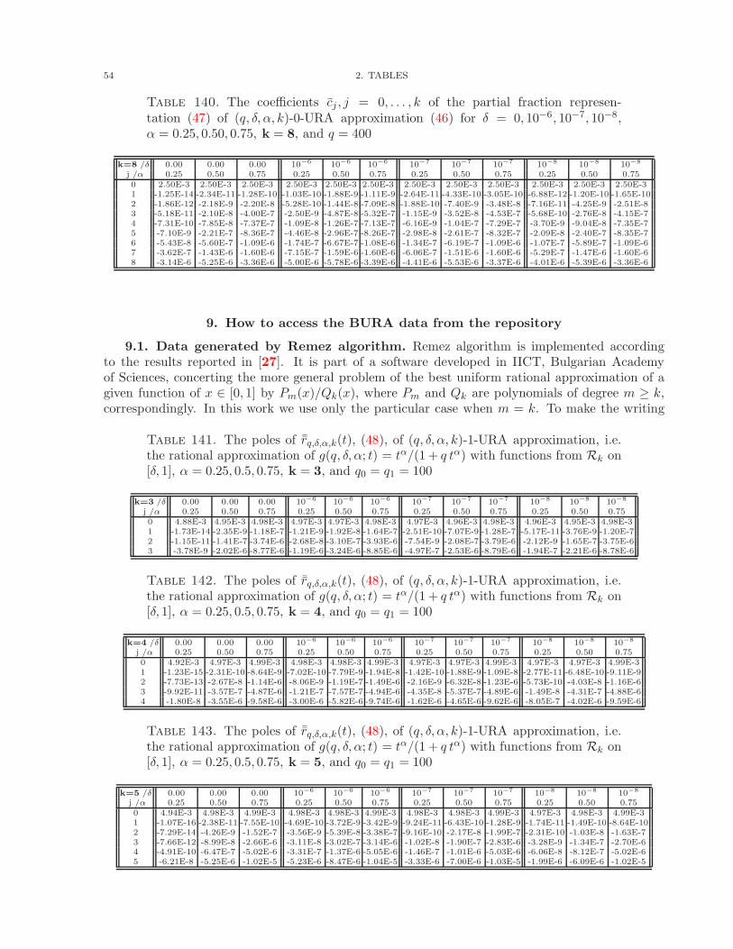
54 2. TABLES
Table 140. The coefficients cj , j = 0, . . . , k of the partial fraction represen-tation (47) of (q, δ, α, k)-0-URA approximation (46) for δ = 0, 10−6, 10−7, 10−8,α = 0.25, 0.50, 0.75, k = 8, and q = 400
k=8 /δ 0.00 0.00 0.00 10−6 10−6 10−6 10−7 10−7 10−7 10−8 10−8 10−8
j /α 0.25 0.50 0.75 0.25 0.50 0.75 0.25 0.50 0.75 0.25 0.50 0.750 2.50E-3 2.50E-3 2.50E-3 2.50E-3 2.50E-3 2.50E-3 2.50E-3 2.50E-3 2.50E-3 2.50E-3 2.50E-3 2.50E-31 -1.25E-14 -2.34E-11 -1.28E-10 -1.03E-10 -1.88E-9 -1.11E-9 -2.64E-11 -4.33E-10 -3.05E-10 -6.88E-12 -1.20E-10 -1.65E-102 -1.86E-12 -2.18E-9 -2.20E-8 -5.28E-10 -1.44E-8 -7.09E-8 -1.88E-10 -7.40E-9 -3.48E-8 -7.16E-11 -4.25E-9 -2.51E-83 -5.18E-11 -2.10E-8 -4.00E-7 -2.50E-9 -4.87E-8 -5.32E-7 -1.15E-9 -3.52E-8 -4.53E-7 -5.68E-10 -2.76E-8 -4.15E-74 -7.31E-10 -7.85E-8 -7.37E-7 -1.09E-8 -1.26E-7 -7.13E-7 -6.16E-9 -1.04E-7 -7.29E-7 -3.70E-9 -9.04E-8 -7.35E-75 -7.10E-9 -2.21E-7 -8.36E-7 -4.46E-8 -2.96E-7 -8.26E-7 -2.98E-8 -2.61E-7 -8.32E-7 -2.09E-8 -2.40E-7 -8.35E-76 -5.43E-8 -5.60E-7 -1.09E-6 -1.74E-7 -6.67E-7 -1.08E-6 -1.34E-7 -6.19E-7 -1.09E-6 -1.07E-7 -5.89E-7 -1.09E-67 -3.62E-7 -1.43E-6 -1.60E-6 -7.15E-7 -1.59E-6 -1.60E-6 -6.06E-7 -1.51E-6 -1.60E-6 -5.29E-7 -1.47E-6 -1.60E-68 -3.14E-6 -5.25E-6 -3.36E-6 -5.00E-6 -5.78E-6 -3.39E-6 -4.41E-6 -5.53E-6 -3.37E-6 -4.01E-6 -5.39E-6 -3.36E-6
9. How to access the BURA data from the repository
9.1. Data generated by Remez algorithm. Remez algorithm is implemented accordingto the results reported in [27]. It is part of a software developed in IICT, Bulgarian Academyof Sciences, concerting the more general problem of the best uniform rational approximation of agiven function of x ∈ [0, 1] by Pm(x)/Qk(x), where Pm and Qk are polynomials of degree m ≥ k,correspondingly. In this work we use only the particular case when m = k. To make the writing
Table 141. The poles of ¯rq,δ,α,k(t), (48), of (q, δ, α, k)-1-URA approximation, i.e.the rational approximation of g(q, δ, α; t) = tα/(1 + q tα) with functions from Rk on[δ, 1], α = 0.25, 0.5, 0.75, k = 3, and q0 = q1 = 100
k=3 /δ 0.00 0.00 0.00 10−6 10−6 10−6 10−7 10−7 10−7 10−8 10−8 10−8
j /α 0.25 0.50 0.75 0.25 0.50 0.75 0.25 0.50 0.75 0.25 0.50 0.750 4.88E-3 4.95E-3 4.98E-3 4.97E-3 4.97E-3 4.98E-3 4.97E-3 4.96E-3 4.98E-3 4.96E-3 4.95E-3 4.98E-31 -1.73E-14 -2.35E-9 -1.18E-7 -1.21E-9 -1.92E-8 -1.64E-7 -2.51E-10 -7.07E-9 -1.28E-7 -5.17E-11 -3.76E-9 -1.20E-72 -1.15E-11 -1.41E-7 -3.74E-6 -2.68E-8 -3.10E-7 -3.93E-6 -7.54E-9 -2.08E-7 -3.79E-6 -2.12E-9 -1.65E-7 -3.75E-63 -3.78E-9 -2.02E-6 -8.77E-6 -1.19E-6 -3.24E-6 -8.85E-6 -4.97E-7 -2.53E-6 -8.79E-6 -1.94E-7 -2.21E-6 -8.78E-6
Table 142. The poles of ¯rq,δ,α,k(t), (48), of (q, δ, α, k)-1-URA approximation, i.e.the rational approximation of g(q, δ, α; t) = tα/(1 + q tα) with functions from Rk on[δ, 1], α = 0.25, 0.5, 0.75, k = 4, and q0 = q1 = 100
k=4 /δ 0.00 0.00 0.00 10−6 10−6 10−6 10−7 10−7 10−7 10−8 10−8 10−8
j /α 0.25 0.50 0.75 0.25 0.50 0.75 0.25 0.50 0.75 0.25 0.50 0.750 4.92E-3 4.97E-3 4.99E-3 4.98E-3 4.98E-3 4.99E-3 4.97E-3 4.97E-3 4.99E-3 4.97E-3 4.97E-3 4.99E-31 -1.23E-15 -2.31E-10 -8.64E-9 -7.02E-10 -7.79E-9 -1.94E-8 -1.42E-10 -1.88E-9 -1.09E-8 -2.77E-11 -6.48E-10 -9.11E-92 -7.73E-13 -2.67E-8 -1.14E-6 -8.06E-9 -1.19E-7 -1.49E-6 -2.16E-9 -6.32E-8 -1.23E-6 -5.73E-10 -4.03E-8 -1.16E-63 -9.92E-11 -3.57E-7 -4.87E-6 -1.21E-7 -7.57E-7 -4.94E-6 -4.35E-8 -5.37E-7 -4.89E-6 -1.49E-8 -4.31E-7 -4.88E-64 -1.80E-8 -3.55E-6 -9.58E-6 -3.00E-6 -5.82E-6 -9.74E-6 -1.62E-6 -4.65E-6 -9.62E-6 -8.05E-7 -4.02E-6 -9.59E-6
Table 143. The poles of ¯rq,δ,α,k(t), (48), of (q, δ, α, k)-1-URA approximation, i.e.the rational approximation of g(q, δ, α; t) = tα/(1 + q tα) with functions from Rk on[δ, 1], α = 0.25, 0.5, 0.75, k = 5, and q0 = q1 = 100
k=5 /δ 0.00 0.00 0.00 10−6 10−6 10−6 10−7 10−7 10−7 10−8 10−8 10−8
j /α 0.25 0.50 0.75 0.25 0.50 0.75 0.25 0.50 0.75 0.25 0.50 0.750 4.94E-3 4.98E-3 4.99E-3 4.98E-3 4.98E-3 4.99E-3 4.98E-3 4.98E-3 4.99E-3 4.97E-3 4.98E-3 4.99E-31 -1.07E-16 -2.38E-11 -7.55E-10 -4.69E-10 -3.72E-9 -3.42E-9 -9.24E-11 -6.43E-10 -1.28E-9 -1.74E-11 -1.49E-10 -8.64E-102 -7.29E-14 -4.26E-9 -1.52E-7 -3.56E-9 -5.39E-8 -3.38E-7 -9.16E-10 -2.17E-8 -1.99E-7 -2.31E-10 -1.03E-8 -1.63E-73 -7.66E-12 -8.99E-8 -2.66E-6 -3.11E-8 -3.02E-7 -3.14E-6 -1.02E-8 -1.90E-7 -2.83E-6 -3.28E-9 -1.34E-7 -2.70E-64 -4.91E-10 -6.47E-7 -5.02E-6 -3.31E-7 -1.37E-6 -5.05E-6 -1.46E-7 -1.01E-6 -5.03E-6 -6.06E-8 -8.12E-7 -5.02E-65 -6.21E-8 -5.25E-6 -1.02E-5 -5.23E-6 -8.47E-6 -1.04E-5 -3.33E-6 -7.00E-6 -1.03E-5 -1.99E-6 -6.09E-6 -1.02E-5
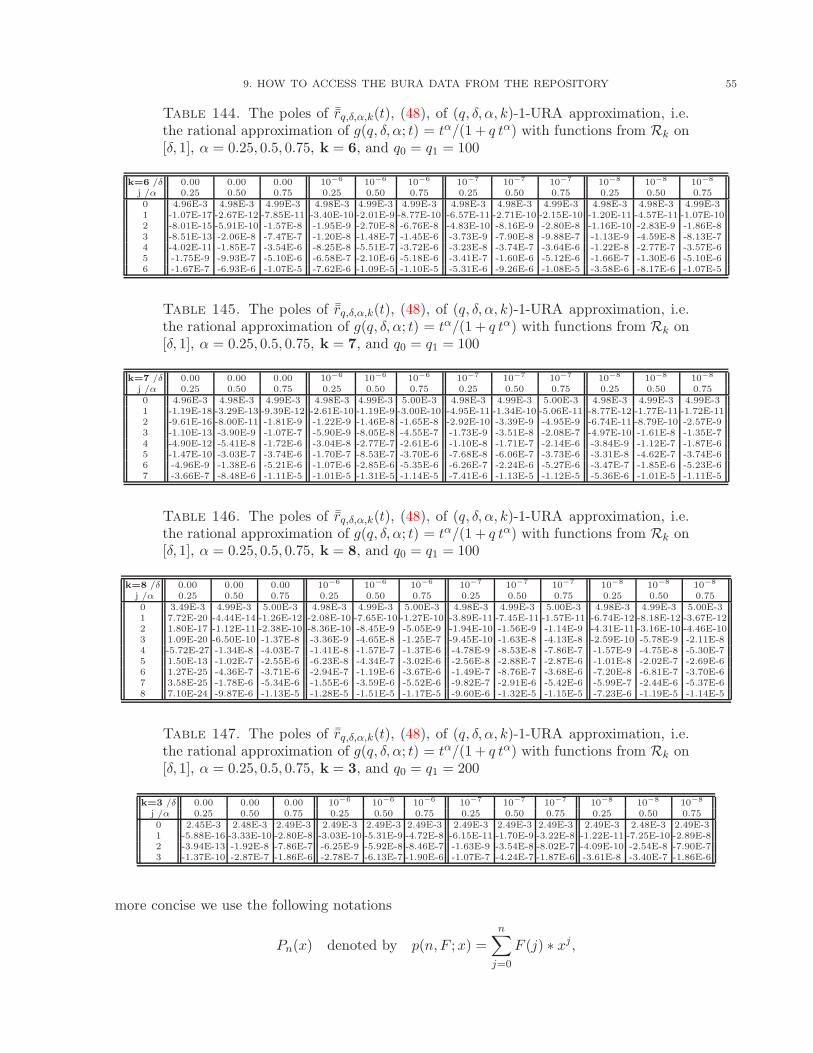
9. HOW TO ACCESS THE BURA DATA FROM THE REPOSITORY 55
Table 144. The poles of ¯rq,δ,α,k(t), (48), of (q, δ, α, k)-1-URA approximation, i.e.the rational approximation of g(q, δ, α; t) = tα/(1 + q tα) with functions from Rk on[δ, 1], α = 0.25, 0.5, 0.75, k = 6, and q0 = q1 = 100
k=6 /δ 0.00 0.00 0.00 10−6 10−6 10−6 10−7 10−7 10−7 10−8 10−8 10−8
j /α 0.25 0.50 0.75 0.25 0.50 0.75 0.25 0.50 0.75 0.25 0.50 0.750 4.96E-3 4.98E-3 4.99E-3 4.98E-3 4.99E-3 4.99E-3 4.98E-3 4.98E-3 4.99E-3 4.98E-3 4.98E-3 4.99E-31 -1.07E-17 -2.67E-12 -7.85E-11 -3.40E-10 -2.01E-9 -8.77E-10 -6.57E-11 -2.71E-10 -2.15E-10 -1.20E-11 -4.57E-11 -1.07E-102 -8.01E-15 -5.91E-10 -1.57E-8 -1.95E-9 -2.70E-8 -6.76E-8 -4.83E-10 -8.16E-9 -2.80E-8 -1.16E-10 -2.83E-9 -1.86E-83 -8.51E-13 -2.06E-8 -7.47E-7 -1.20E-8 -1.48E-7 -1.45E-6 -3.73E-9 -7.90E-8 -9.88E-7 -1.13E-9 -4.59E-8 -8.13E-74 -4.02E-11 -1.85E-7 -3.54E-6 -8.25E-8 -5.51E-7 -3.72E-6 -3.23E-8 -3.74E-7 -3.64E-6 -1.22E-8 -2.77E-7 -3.57E-65 -1.75E-9 -9.93E-7 -5.10E-6 -6.58E-7 -2.10E-6 -5.18E-6 -3.41E-7 -1.60E-6 -5.12E-6 -1.66E-7 -1.30E-6 -5.10E-66 -1.67E-7 -6.93E-6 -1.07E-5 -7.62E-6 -1.09E-5 -1.10E-5 -5.31E-6 -9.26E-6 -1.08E-5 -3.58E-6 -8.17E-6 -1.07E-5
Table 145. The poles of ¯rq,δ,α,k(t), (48), of (q, δ, α, k)-1-URA approximation, i.e.the rational approximation of g(q, δ, α; t) = tα/(1 + q tα) with functions from Rk on[δ, 1], α = 0.25, 0.5, 0.75, k = 7, and q0 = q1 = 100
k=7 /δ 0.00 0.00 0.00 10−6 10−6 10−6 10−7 10−7 10−7 10−8 10−8 10−8
j /α 0.25 0.50 0.75 0.25 0.50 0.75 0.25 0.50 0.75 0.25 0.50 0.750 4.96E-3 4.98E-3 4.99E-3 4.98E-3 4.99E-3 5.00E-3 4.98E-3 4.99E-3 5.00E-3 4.98E-3 4.99E-3 4.99E-31 -1.19E-18 -3.29E-13 -9.39E-12 -2.61E-10 -1.19E-9 -3.00E-10 -4.95E-11 -1.34E-10 -5.06E-11 -8.77E-12 -1.77E-11 -1.72E-112 -9.61E-16 -8.00E-11 -1.81E-9 -1.22E-9 -1.46E-8 -1.65E-8 -2.92E-10 -3.39E-9 -4.95E-9 -6.74E-11 -8.79E-10 -2.57E-93 -1.10E-13 -3.90E-9 -1.07E-7 -5.90E-9 -8.05E-8 -4.55E-7 -1.73E-9 -3.51E-8 -2.08E-7 -4.97E-10 -1.61E-8 -1.35E-74 -4.90E-12 -5.41E-8 -1.72E-6 -3.04E-8 -2.77E-7 -2.61E-6 -1.10E-8 -1.71E-7 -2.14E-6 -3.84E-9 -1.12E-7 -1.87E-65 -1.47E-10 -3.03E-7 -3.74E-6 -1.70E-7 -8.53E-7 -3.70E-6 -7.68E-8 -6.06E-7 -3.73E-6 -3.31E-8 -4.62E-7 -3.74E-66 -4.96E-9 -1.38E-6 -5.21E-6 -1.07E-6 -2.85E-6 -5.35E-6 -6.26E-7 -2.24E-6 -5.27E-6 -3.47E-7 -1.85E-6 -5.23E-67 -3.66E-7 -8.48E-6 -1.11E-5 -1.01E-5 -1.31E-5 -1.14E-5 -7.41E-6 -1.13E-5 -1.12E-5 -5.36E-6 -1.01E-5 -1.11E-5
Table 146. The poles of ¯rq,δ,α,k(t), (48), of (q, δ, α, k)-1-URA approximation, i.e.the rational approximation of g(q, δ, α; t) = tα/(1 + q tα) with functions from Rk on[δ, 1], α = 0.25, 0.5, 0.75, k = 8, and q0 = q1 = 100
k=8 /δ 0.00 0.00 0.00 10−6 10−6 10−6 10−7 10−7 10−7 10−8 10−8 10−8
j /α 0.25 0.50 0.75 0.25 0.50 0.75 0.25 0.50 0.75 0.25 0.50 0.750 3.49E-3 4.99E-3 5.00E-3 4.98E-3 4.99E-3 5.00E-3 4.98E-3 4.99E-3 5.00E-3 4.98E-3 4.99E-3 5.00E-31 7.72E-20 -4.44E-14 -1.26E-12 -2.08E-10 -7.65E-10 -1.27E-10 -3.89E-11 -7.45E-11 -1.57E-11 -6.74E-12 -8.18E-12 -3.67E-122 1.80E-17 -1.12E-11 -2.38E-10 -8.36E-10 -8.45E-9 -5.05E-9 -1.94E-10 -1.56E-9 -1.14E-9 -4.31E-11 -3.16E-10 -4.46E-103 1.09E-20 -6.50E-10 -1.37E-8 -3.36E-9 -4.65E-8 -1.25E-7 -9.45E-10 -1.63E-8 -4.13E-8 -2.59E-10 -5.78E-9 -2.11E-84 -5.72E-27 -1.34E-8 -4.03E-7 -1.41E-8 -1.57E-7 -1.37E-6 -4.78E-9 -8.53E-8 -7.86E-7 -1.57E-9 -4.75E-8 -5.30E-75 1.50E-13 -1.02E-7 -2.55E-6 -6.23E-8 -4.34E-7 -3.02E-6 -2.56E-8 -2.88E-7 -2.87E-6 -1.01E-8 -2.02E-7 -2.69E-66 1.27E-25 -4.36E-7 -3.71E-6 -2.94E-7 -1.19E-6 -3.67E-6 -1.49E-7 -8.76E-7 -3.68E-6 -7.20E-8 -6.81E-7 -3.70E-67 3.58E-25 -1.78E-6 -5.34E-6 -1.55E-6 -3.59E-6 -5.52E-6 -9.82E-7 -2.91E-6 -5.42E-6 -5.99E-7 -2.44E-6 -5.37E-68 7.10E-24 -9.87E-6 -1.13E-5 -1.28E-5 -1.51E-5 -1.17E-5 -9.60E-6 -1.32E-5 -1.15E-5 -7.23E-6 -1.19E-5 -1.14E-5
Table 147. The poles of ¯rq,δ,α,k(t), (48), of (q, δ, α, k)-1-URA approximation, i.e.the rational approximation of g(q, δ, α; t) = tα/(1 + q tα) with functions from Rk on[δ, 1], α = 0.25, 0.5, 0.75, k = 3, and q0 = q1 = 200
k=3 /δ 0.00 0.00 0.00 10−6 10−6 10−6 10−7 10−7 10−7 10−8 10−8 10−8
j /α 0.25 0.50 0.75 0.25 0.50 0.75 0.25 0.50 0.75 0.25 0.50 0.750 2.45E-3 2.48E-3 2.49E-3 2.49E-3 2.49E-3 2.49E-3 2.49E-3 2.49E-3 2.49E-3 2.49E-3 2.48E-3 2.49E-31 -5.88E-16 -3.33E-10 -2.80E-8 -3.03E-10 -5.31E-9 -4.72E-8 -6.15E-11 -1.70E-9 -3.22E-8 -1.22E-11 -7.25E-10 -2.89E-82 -3.94E-13 -1.92E-8 -7.86E-7 -6.25E-9 -5.92E-8 -8.46E-7 -1.63E-9 -3.54E-8 -8.02E-7 -4.09E-10 -2.54E-8 -7.90E-73 -1.37E-10 -2.87E-7 -1.86E-6 -2.78E-7 -6.13E-7 -1.90E-6 -1.07E-7 -4.24E-7 -1.87E-6 -3.61E-8 -3.40E-7 -1.86E-6
more concise we use the following notations
Pn(x) denoted by p(n, F ;x) =
n∑
j=0
F (j) ∗ xj,
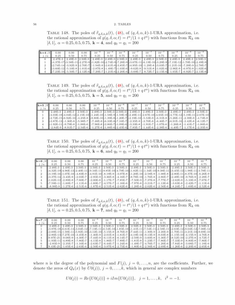
56 2. TABLES
Table 148. The poles of ¯rq,δ,α,k(t), (48), of (q, δ, α, k)-1-URA approximation, i.e.the rational approximation of g(q, δ, α; t) = tα/(1 + q tα) with functions from Rk on[δ, 1], α = 0.25, 0.5, 0.75, k = 4, and q0 = q1 = 200
k=4 /δ 0.00 0.00 0.00 10−6 10−6 10−6 10−7 10−7 10−7 10−8 10−8 10−8
j /α 0.25 0.50 0.75 0.25 0.50 0.75 0.25 0.50 0.75 0.25 0.50 0.750 2.47E-3 2.49E-3 2.50E-3 2.49E-3 2.49E-3 2.50E-3 2.49E-3 2.49E-3 2.50E-3 2.49E-3 2.49E-3 2.50E-31 -4.37E-17 -3.58E-11 -2.27E-9 -1.82E-10 -2.74E-9 -7.28E-9 -3.67E-11 -6.13E-10 -3.29E-9 -7.15E-12 -1.70E-10 -2.49E-92 -2.74E-14 -3.92E-9 -2.70E-7 -1.94E-9 -2.61E-8 -3.85E-7 -4.95E-10 -1.29E-8 -3.03E-7 -1.21E-10 -7.39E-9 -2.78E-73 -3.60E-12 -5.10E-8 -1.01E-6 -2.87E-8 -1.49E-7 -1.03E-6 -9.62E-9 -9.51E-8 -1.02E-6 -2.96E-9 -6.97E-8 -1.02E-64 -7.23E-10 -5.50E-7 -2.12E-6 -7.20E-7 -1.21E-6 -2.20E-6 -3.69E-7 -8.72E-7 -2.15E-6 -1.65E-7 -6.92E-7 -2.13E-6
Table 149. The poles of ¯rq,δ,α,k(t), (48), of (q, δ, α, k)-1-URA approximation, i.e.the rational approximation of g(q, δ, α; t) = tα/(1 + q tα) with functions from Rk on[δ, 1], α = 0.25, 0.5, 0.75, k = 5, and q0 = q1 = 200
k=5 /δ 0.00 0.00 0.00 10−6 10−6 10−6 10−7 10−7 10−7 10−8 10−8 10−8
j /α 0.25 0.50 0.75 0.25 0.50 0.75 0.25 0.50 0.75 0.25 0.50 0.750 2.48E-3 2.49E-3 2.50E-3 2.49E-3 2.50E-3 2.50E-3 2.49E-3 2.49E-3 2.50E-3 2.49E-3 2.49E-3 2.50E-31 -4.03E-18 -4.04E-12 -2.15E-10 -1.24E-10 -1.58E-9 -1.59E-9 -2.49E-11 -2.67E-10 -4.65E-10 -4.77E-12 -5.19E-11 -2.67E-102 -2.72E-15 -6.92E-10 -4.25E-8 -8.80E-10 -1.39E-8 -1.20E-7 -2.19E-10 -5.53E-9 -6.31E-8 -5.26E-11 -2.39E-9 -4.74E-83 -2.87E-13 -1.36E-8 -5.98E-7 -7.48E-9 -6.33E-8 -7.16E-7 -2.35E-9 -3.70E-8 -6.46E-7 -6.91E-10 -2.42E-8 -6.12E-74 -1.92E-11 -9.79E-8 -1.06E-6 -7.96E-8 -2.86E-7 -1.09E-6 -3.33E-8 -1.91E-7 -1.07E-6 -1.26E-8 -1.41E-7 -1.06E-65 -2.84E-9 -8.91E-7 -2.34E-6 -1.27E-6 -1.88E-6 -2.45E-6 -7.85E-7 -1.44E-6 -2.38E-6 -4.40E-7 -1.17E-6 -2.35E-6
Table 150. The poles of ¯rq,δ,α,k(t), (48), of (q, δ, α, k)-1-URA approximation, i.e.the rational approximation of g(q, δ, α; t) = tα/(1 + q tα) with functions from Rk on[δ, 1], α = 0.25, 0.5, 0.75, k = 6, and q0 = q1 = 200
k=6 /δ 0.00 0.00 0.00 10−6 10−6 10−6 10−7 10−7 10−7 10−8 10−8 10−8
j /α 0.25 0.50 0.75 0.25 0.50 0.75 0.25 0.50 0.75 0.25 0.50 0.750 2.48E-3 2.49E-3 2.50E-3 2.50E-3 2.50E-3 2.50E-3 2.49E-3 2.50E-3 2.50E-3 2.49E-3 2.50E-3 2.50E-31 -4.32E-19 -4.96E-13 -2.40E-11 -9.16E-11 -9.85E-10 -4.79E-10 -1.82E-11 -1.34E-10 -9.38E-11 -3.45E-12 -1.98E-11 -3.78E-112 -3.19E-16 -1.07E-10 -4.83E-9 -4.91E-10 -8.19E-9 -3.07E-8 -1.20E-10 -2.58E-9 -1.08E-8 -2.80E-11 -8.37E-10 -6.26E-93 -3.37E-14 -3.43E-9 -2.03E-7 -2.95E-9 -3.36E-8 -4.16E-7 -8.78E-10 -1.76E-8 -2.86E-7 -2.49E-10 -9.76E-9 -2.28E-74 -1.62E-12 -2.89E-8 -7.60E-7 -2.00E-8 -1.17E-7 -7.85E-7 -7.50E-9 -7.37E-8 -7.77E-7 -2.62E-9 -5.10E-8 -7.67E-75 -7.59E-11 -1.60E-7 -1.11E-6 -1.60E-7 -4.57E-7 -1.16E-6 -7.97E-8 -3.21E-7 -1.13E-6 -3.63E-8 -2.42E-7 -1.11E-66 -8.98E-9 -1.27E-6 -2.51E-6 -1.87E-6 -2.51E-6 -2.62E-6 -1.28E-6 -2.02E-6 -2.56E-6 -8.24E-7 -1.69E-6 -2.52E-6
Table 151. The poles of ¯rq,δ,α,k(t), (48), of (q, δ, α, k)-1-URA approximation, i.e.the rational approximation of g(q, δ, α; t) = tα/(1 + q tα) with functions from Rk on[δ, 1], α = 0.25, 0.5, 0.75, k = 7, and q0 = q1 = 200
k=7 /δ 0.00 0.00 0.00 10−6 10−6 10−6 10−7 10−7 10−7 10−8 10−8 10−8
j /α 0.25 0.50 0.75 0.25 0.50 0.75 0.25 0.50 0.75 0.25 0.50 0.750 2.48E-3 2.49E-3 2.50E-3 2.50E-3 2.50E-3 2.50E-3 2.50E-3 2.50E-3 2.50E-3 2.49E-3 2.50E-3 2.50E-31 -3.97E-18 -6.61E-14 -3.04E-12 -7.13E-11 -6.54E-10 -1.85E-10 -1.41E-11 -7.54E-11 -2.58E-11 -2.63E-12 -9.04E-12 -7.08E-122 -2.69E-15 -1.58E-11 -5.92E-10 -3.12E-10 -5.15E-9 -8.76E-9 -7.44E-11 -1.30E-9 -2.20E-9 -1.70E-11 -3.21E-10 -9.69E-103 -2.86E-13 -7.27E-10 -3.45E-8 -1.46E-9 -2.01E-8 -1.81E-7 -4.19E-10 -9.13E-9 -8.03E-8 -1.15E-10 -4.15E-9 -4.76E-84 9.97E-25 -9.08E-9 -4.30E-7 -7.44E-9 -6.11E-8 -6.14E-7 -2.59E-9 -3.60E-8 -5.36E-7 -8.52E-10 -2.27E-8 -4.72E-75 -1.93E-11 -4.89E-8 -7.86E-7 -4.15E-8 -1.86E-7 -7.89E-7 -1.81E-8 -1.23E-7 -7.86E-7 -7.33E-9 -8.80E-8 -7.86E-76 -2.85E-9 -2.35E-7 -1.16E-6 -2.63E-7 -6.44E-7 -1.24E-6 -1.49E-7 -4.76E-7 -1.20E-6 -7.84E-8 -3.68E-7 -1.18E-67 9.43E-25 -1.65E-6 -2.63E-6 -2.50E-6 -3.07E-6 -2.75E-6 -1.80E-6 -2.56E-6 -2.69E-6 -1.26E-6 -2.20E-6 -2.65E-6
where n is the degree of the polynomial and F (j), j = 0, . . . , n, are the coefficients. Further, wedenote the zeros of Qk(x) by U0(j)), j = 0, . . . , k, which in general are complex numbers
U0(j)) = ReU0(j)) + iImU0(j)), j = 1, . . . , k, i2 = −1.
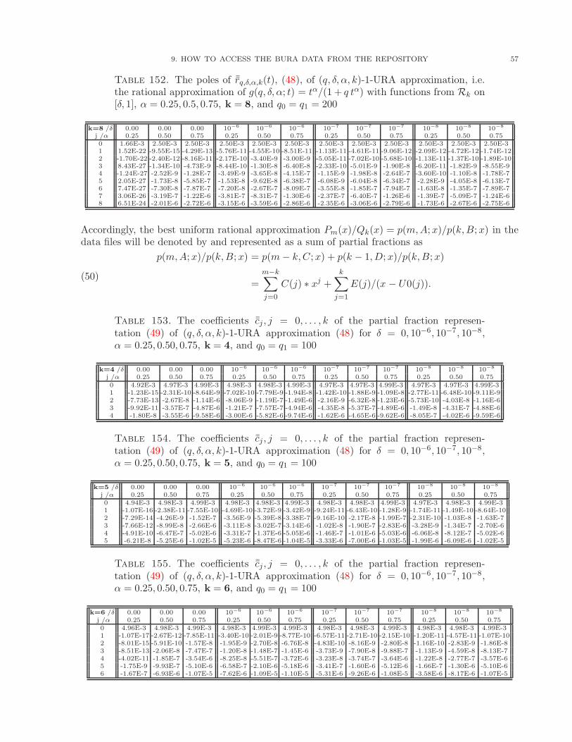
9. HOW TO ACCESS THE BURA DATA FROM THE REPOSITORY 57
Table 152. The poles of ¯rq,δ,α,k(t), (48), of (q, δ, α, k)-1-URA approximation, i.e.the rational approximation of g(q, δ, α; t) = tα/(1 + q tα) with functions from Rk on[δ, 1], α = 0.25, 0.5, 0.75, k = 8, and q0 = q1 = 200
k=8 /δ 0.00 0.00 0.00 10−6 10−6 10−6 10−7 10−7 10−7 10−8 10−8 10−8
j /α 0.25 0.50 0.75 0.25 0.50 0.75 0.25 0.50 0.75 0.25 0.50 0.750 1.66E-3 2.50E-3 2.50E-3 2.50E-3 2.50E-3 2.50E-3 2.50E-3 2.50E-3 2.50E-3 2.50E-3 2.50E-3 2.50E-31 1.52E-22 -9.55E-15 -4.29E-13 -5.76E-11 -4.55E-10 -8.51E-11 -1.13E-11 -4.61E-11 -9.06E-12 -2.09E-12 -4.72E-12 -1.74E-122 -1.70E-22 -2.40E-12 -8.16E-11 -2.17E-10 -3.40E-9 -3.00E-9 -5.05E-11 -7.02E-10 -5.68E-10 -1.13E-11 -1.37E-10 -1.89E-103 8.43E-27 -1.34E-10 -4.73E-9 -8.44E-10 -1.30E-8 -6.40E-8 -2.33E-10 -5.01E-9 -1.90E-8 -6.20E-11 -1.82E-9 -8.55E-94 -1.24E-27 -2.52E-9 -1.28E-7 -3.49E-9 -3.65E-8 -4.15E-7 -1.15E-9 -1.98E-8 -2.64E-7 -3.60E-10 -1.10E-8 -1.78E-75 2.05E-27 -1.73E-8 -5.85E-7 -1.53E-8 -9.62E-8 -6.38E-7 -6.08E-9 -6.04E-8 -6.34E-7 -2.28E-9 -4.05E-8 -6.13E-76 7.47E-27 -7.30E-8 -7.87E-7 -7.20E-8 -2.67E-7 -8.09E-7 -3.55E-8 -1.85E-7 -7.94E-7 -1.63E-8 -1.35E-7 -7.89E-77 3.06E-26 -3.19E-7 -1.22E-6 -3.81E-7 -8.31E-7 -1.30E-6 -2.37E-7 -6.40E-7 -1.26E-6 -1.39E-7 -5.09E-7 -1.24E-68 6.51E-24 -2.01E-6 -2.72E-6 -3.15E-6 -3.59E-6 -2.86E-6 -2.35E-6 -3.06E-6 -2.79E-6 -1.73E-6 -2.67E-6 -2.75E-6
Accordingly, the best uniform rational approximation Pm(x)/Qk(x) = p(m,A;x)/p(k,B;x) in thedata files will be denoted by and represented as a sum of partial fractions as
(50)
p(m,A;x)/p(k,B;x) = p(m− k,C;x) + p(k − 1,D;x)/p(k,B;x)
=m−k∑
j=0
C(j) ∗ xj +k∑
j=1
E(j)/(x − U0(j)).
Table 153. The coefficients ¯cj , j = 0, . . . , k of the partial fraction represen-tation (49) of (q, δ, α, k)-1-URA approximation (48) for δ = 0, 10−6, 10−7, 10−8,α = 0.25, 0.50, 0.75, k = 4, and q0 = q1 = 100
k=4 /δ 0.00 0.00 0.00 10−6 10−6 10−6 10−7 10−7 10−7 10−8 10−8 10−8
j /α 0.25 0.50 0.75 0.25 0.50 0.75 0.25 0.50 0.75 0.25 0.50 0.750 4.92E-3 4.97E-3 4.99E-3 4.98E-3 4.98E-3 4.99E-3 4.97E-3 4.97E-3 4.99E-3 4.97E-3 4.97E-3 4.99E-31 -1.23E-15 -2.31E-10 -8.64E-9 -7.02E-10 -7.79E-9 -1.94E-8 -1.42E-10 -1.88E-9 -1.09E-8 -2.77E-11 -6.48E-10 -9.11E-92 -7.73E-13 -2.67E-8 -1.14E-6 -8.06E-9 -1.19E-7 -1.49E-6 -2.16E-9 -6.32E-8 -1.23E-6 -5.73E-10 -4.03E-8 -1.16E-63 -9.92E-11 -3.57E-7 -4.87E-6 -1.21E-7 -7.57E-7 -4.94E-6 -4.35E-8 -5.37E-7 -4.89E-6 -1.49E-8 -4.31E-7 -4.88E-64 -1.80E-8 -3.55E-6 -9.58E-6 -3.00E-6 -5.82E-6 -9.74E-6 -1.62E-6 -4.65E-6 -9.62E-6 -8.05E-7 -4.02E-6 -9.59E-6
Table 154. The coefficients ¯cj , j = 0, . . . , k of the partial fraction represen-tation (49) of (q, δ, α, k)-1-URA approximation (48) for δ = 0, 10−6, 10−7, 10−8,α = 0.25, 0.50, 0.75, k = 5, and q0 = q1 = 100
k=5 /δ 0.00 0.00 0.00 10−6 10−6 10−6 10−7 10−7 10−7 10−8 10−8 10−8
j /α 0.25 0.50 0.75 0.25 0.50 0.75 0.25 0.50 0.75 0.25 0.50 0.750 4.94E-3 4.98E-3 4.99E-3 4.98E-3 4.98E-3 4.99E-3 4.98E-3 4.98E-3 4.99E-3 4.97E-3 4.98E-3 4.99E-31 -1.07E-16 -2.38E-11 -7.55E-10 -4.69E-10 -3.72E-9 -3.42E-9 -9.24E-11 -6.43E-10 -1.28E-9 -1.74E-11 -1.49E-10 -8.64E-102 -7.29E-14 -4.26E-9 -1.52E-7 -3.56E-9 -5.39E-8 -3.38E-7 -9.16E-10 -2.17E-8 -1.99E-7 -2.31E-10 -1.03E-8 -1.63E-73 -7.66E-12 -8.99E-8 -2.66E-6 -3.11E-8 -3.02E-7 -3.14E-6 -1.02E-8 -1.90E-7 -2.83E-6 -3.28E-9 -1.34E-7 -2.70E-64 -4.91E-10 -6.47E-7 -5.02E-6 -3.31E-7 -1.37E-6 -5.05E-6 -1.46E-7 -1.01E-6 -5.03E-6 -6.06E-8 -8.12E-7 -5.02E-65 -6.21E-8 -5.25E-6 -1.02E-5 -5.23E-6 -8.47E-6 -1.04E-5 -3.33E-6 -7.00E-6 -1.03E-5 -1.99E-6 -6.09E-6 -1.02E-5
Table 155. The coefficients ¯cj , j = 0, . . . , k of the partial fraction represen-tation (49) of (q, δ, α, k)-1-URA approximation (48) for δ = 0, 10−6, 10−7, 10−8,α = 0.25, 0.50, 0.75, k = 6, and q0 = q1 = 100
k=6 /δ 0.00 0.00 0.00 10−6 10−6 10−6 10−7 10−7 10−7 10−8 10−8 10−8
j /α 0.25 0.50 0.75 0.25 0.50 0.75 0.25 0.50 0.75 0.25 0.50 0.750 4.96E-3 4.98E-3 4.99E-3 4.98E-3 4.99E-3 4.99E-3 4.98E-3 4.98E-3 4.99E-3 4.98E-3 4.98E-3 4.99E-31 -1.07E-17 -2.67E-12 -7.85E-11 -3.40E-10 -2.01E-9 -8.77E-10 -6.57E-11 -2.71E-10 -2.15E-10 -1.20E-11 -4.57E-11 -1.07E-102 -8.01E-15 -5.91E-10 -1.57E-8 -1.95E-9 -2.70E-8 -6.76E-8 -4.83E-10 -8.16E-9 -2.80E-8 -1.16E-10 -2.83E-9 -1.86E-83 -8.51E-13 -2.06E-8 -7.47E-7 -1.20E-8 -1.48E-7 -1.45E-6 -3.73E-9 -7.90E-8 -9.88E-7 -1.13E-9 -4.59E-8 -8.13E-74 -4.02E-11 -1.85E-7 -3.54E-6 -8.25E-8 -5.51E-7 -3.72E-6 -3.23E-8 -3.74E-7 -3.64E-6 -1.22E-8 -2.77E-7 -3.57E-65 -1.75E-9 -9.93E-7 -5.10E-6 -6.58E-7 -2.10E-6 -5.18E-6 -3.41E-7 -1.60E-6 -5.12E-6 -1.66E-7 -1.30E-6 -5.10E-66 -1.67E-7 -6.93E-6 -1.07E-5 -7.62E-6 -1.09E-5 -1.10E-5 -5.31E-6 -9.26E-6 -1.08E-5 -3.58E-6 -8.17E-6 -1.07E-5
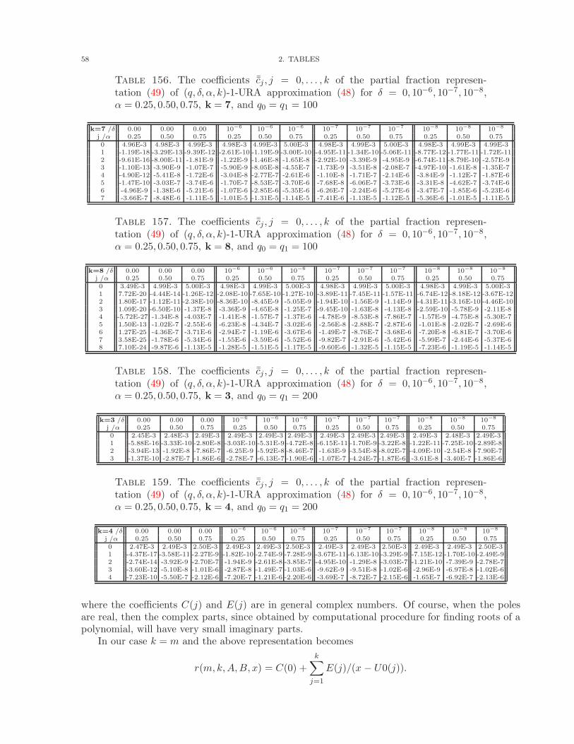
58 2. TABLES
Table 156. The coefficients ¯cj , j = 0, . . . , k of the partial fraction represen-tation (49) of (q, δ, α, k)-1-URA approximation (48) for δ = 0, 10−6, 10−7, 10−8,α = 0.25, 0.50, 0.75, k = 7, and q0 = q1 = 100
k=7 /δ 0.00 0.00 0.00 10−6 10−6 10−6 10−7 10−7 10−7 10−8 10−8 10−8
j /α 0.25 0.50 0.75 0.25 0.50 0.75 0.25 0.50 0.75 0.25 0.50 0.750 4.96E-3 4.98E-3 4.99E-3 4.98E-3 4.99E-3 5.00E-3 4.98E-3 4.99E-3 5.00E-3 4.98E-3 4.99E-3 4.99E-31 -1.19E-18 -3.29E-13 -9.39E-12 -2.61E-10 -1.19E-9 -3.00E-10 -4.95E-11 -1.34E-10 -5.06E-11 -8.77E-12 -1.77E-11 -1.72E-112 -9.61E-16 -8.00E-11 -1.81E-9 -1.22E-9 -1.46E-8 -1.65E-8 -2.92E-10 -3.39E-9 -4.95E-9 -6.74E-11 -8.79E-10 -2.57E-93 -1.10E-13 -3.90E-9 -1.07E-7 -5.90E-9 -8.05E-8 -4.55E-7 -1.73E-9 -3.51E-8 -2.08E-7 -4.97E-10 -1.61E-8 -1.35E-74 -4.90E-12 -5.41E-8 -1.72E-6 -3.04E-8 -2.77E-7 -2.61E-6 -1.10E-8 -1.71E-7 -2.14E-6 -3.84E-9 -1.12E-7 -1.87E-65 -1.47E-10 -3.03E-7 -3.74E-6 -1.70E-7 -8.53E-7 -3.70E-6 -7.68E-8 -6.06E-7 -3.73E-6 -3.31E-8 -4.62E-7 -3.74E-66 -4.96E-9 -1.38E-6 -5.21E-6 -1.07E-6 -2.85E-6 -5.35E-6 -6.26E-7 -2.24E-6 -5.27E-6 -3.47E-7 -1.85E-6 -5.23E-67 -3.66E-7 -8.48E-6 -1.11E-5 -1.01E-5 -1.31E-5 -1.14E-5 -7.41E-6 -1.13E-5 -1.12E-5 -5.36E-6 -1.01E-5 -1.11E-5
Table 157. The coefficients ¯cj , j = 0, . . . , k of the partial fraction represen-tation (49) of (q, δ, α, k)-1-URA approximation (48) for δ = 0, 10−6, 10−7, 10−8,α = 0.25, 0.50, 0.75, k = 8, and q0 = q1 = 100
k=8 /δ 0.00 0.00 0.00 10−6 10−6 10−6 10−7 10−7 10−7 10−8 10−8 10−8
j /α 0.25 0.50 0.75 0.25 0.50 0.75 0.25 0.50 0.75 0.25 0.50 0.750 3.49E-3 4.99E-3 5.00E-3 4.98E-3 4.99E-3 5.00E-3 4.98E-3 4.99E-3 5.00E-3 4.98E-3 4.99E-3 5.00E-31 7.72E-20 -4.44E-14 -1.26E-12 -2.08E-10 -7.65E-10 -1.27E-10 -3.89E-11 -7.45E-11 -1.57E-11 -6.74E-12 -8.18E-12 -3.67E-122 1.80E-17 -1.12E-11 -2.38E-10 -8.36E-10 -8.45E-9 -5.05E-9 -1.94E-10 -1.56E-9 -1.14E-9 -4.31E-11 -3.16E-10 -4.46E-103 1.09E-20 -6.50E-10 -1.37E-8 -3.36E-9 -4.65E-8 -1.25E-7 -9.45E-10 -1.63E-8 -4.13E-8 -2.59E-10 -5.78E-9 -2.11E-84 -5.72E-27 -1.34E-8 -4.03E-7 -1.41E-8 -1.57E-7 -1.37E-6 -4.78E-9 -8.53E-8 -7.86E-7 -1.57E-9 -4.75E-8 -5.30E-75 1.50E-13 -1.02E-7 -2.55E-6 -6.23E-8 -4.34E-7 -3.02E-6 -2.56E-8 -2.88E-7 -2.87E-6 -1.01E-8 -2.02E-7 -2.69E-66 1.27E-25 -4.36E-7 -3.71E-6 -2.94E-7 -1.19E-6 -3.67E-6 -1.49E-7 -8.76E-7 -3.68E-6 -7.20E-8 -6.81E-7 -3.70E-67 3.58E-25 -1.78E-6 -5.34E-6 -1.55E-6 -3.59E-6 -5.52E-6 -9.82E-7 -2.91E-6 -5.42E-6 -5.99E-7 -2.44E-6 -5.37E-68 7.10E-24 -9.87E-6 -1.13E-5 -1.28E-5 -1.51E-5 -1.17E-5 -9.60E-6 -1.32E-5 -1.15E-5 -7.23E-6 -1.19E-5 -1.14E-5
Table 158. The coefficients ¯cj , j = 0, . . . , k of the partial fraction represen-tation (49) of (q, δ, α, k)-1-URA approximation (48) for δ = 0, 10−6, 10−7, 10−8,α = 0.25, 0.50, 0.75, k = 3, and q0 = q1 = 200
k=3 /δ 0.00 0.00 0.00 10−6 10−6 10−6 10−7 10−7 10−7 10−8 10−8 10−8
j /α 0.25 0.50 0.75 0.25 0.50 0.75 0.25 0.50 0.75 0.25 0.50 0.750 2.45E-3 2.48E-3 2.49E-3 2.49E-3 2.49E-3 2.49E-3 2.49E-3 2.49E-3 2.49E-3 2.49E-3 2.48E-3 2.49E-31 -5.88E-16 -3.33E-10 -2.80E-8 -3.03E-10 -5.31E-9 -4.72E-8 -6.15E-11 -1.70E-9 -3.22E-8 -1.22E-11 -7.25E-10 -2.89E-82 -3.94E-13 -1.92E-8 -7.86E-7 -6.25E-9 -5.92E-8 -8.46E-7 -1.63E-9 -3.54E-8 -8.02E-7 -4.09E-10 -2.54E-8 -7.90E-73 -1.37E-10 -2.87E-7 -1.86E-6 -2.78E-7 -6.13E-7 -1.90E-6 -1.07E-7 -4.24E-7 -1.87E-6 -3.61E-8 -3.40E-7 -1.86E-6
Table 159. The coefficients ¯cj , j = 0, . . . , k of the partial fraction represen-tation (49) of (q, δ, α, k)-1-URA approximation (48) for δ = 0, 10−6, 10−7, 10−8,α = 0.25, 0.50, 0.75, k = 4, and q0 = q1 = 200
k=4 /δ 0.00 0.00 0.00 10−6 10−6 10−6 10−7 10−7 10−7 10−8 10−8 10−8
j /α 0.25 0.50 0.75 0.25 0.50 0.75 0.25 0.50 0.75 0.25 0.50 0.750 2.47E-3 2.49E-3 2.50E-3 2.49E-3 2.49E-3 2.50E-3 2.49E-3 2.49E-3 2.50E-3 2.49E-3 2.49E-3 2.50E-31 -4.37E-17 -3.58E-11 -2.27E-9 -1.82E-10 -2.74E-9 -7.28E-9 -3.67E-11 -6.13E-10 -3.29E-9 -7.15E-12 -1.70E-10 -2.49E-92 -2.74E-14 -3.92E-9 -2.70E-7 -1.94E-9 -2.61E-8 -3.85E-7 -4.95E-10 -1.29E-8 -3.03E-7 -1.21E-10 -7.39E-9 -2.78E-73 -3.60E-12 -5.10E-8 -1.01E-6 -2.87E-8 -1.49E-7 -1.03E-6 -9.62E-9 -9.51E-8 -1.02E-6 -2.96E-9 -6.97E-8 -1.02E-64 -7.23E-10 -5.50E-7 -2.12E-6 -7.20E-7 -1.21E-6 -2.20E-6 -3.69E-7 -8.72E-7 -2.15E-6 -1.65E-7 -6.92E-7 -2.13E-6
where the coefficients C(j) and E(j) are in general complex numbers. Of course, when the polesare real, then the complex parts, since obtained by computational procedure for finding roots of apolynomial, will have very small imaginary parts.
In our case k = m and the above representation becomes
r(m,k,A,B, x) = C(0) +
k∑
j=1
E(j)/(x − U0(j)).
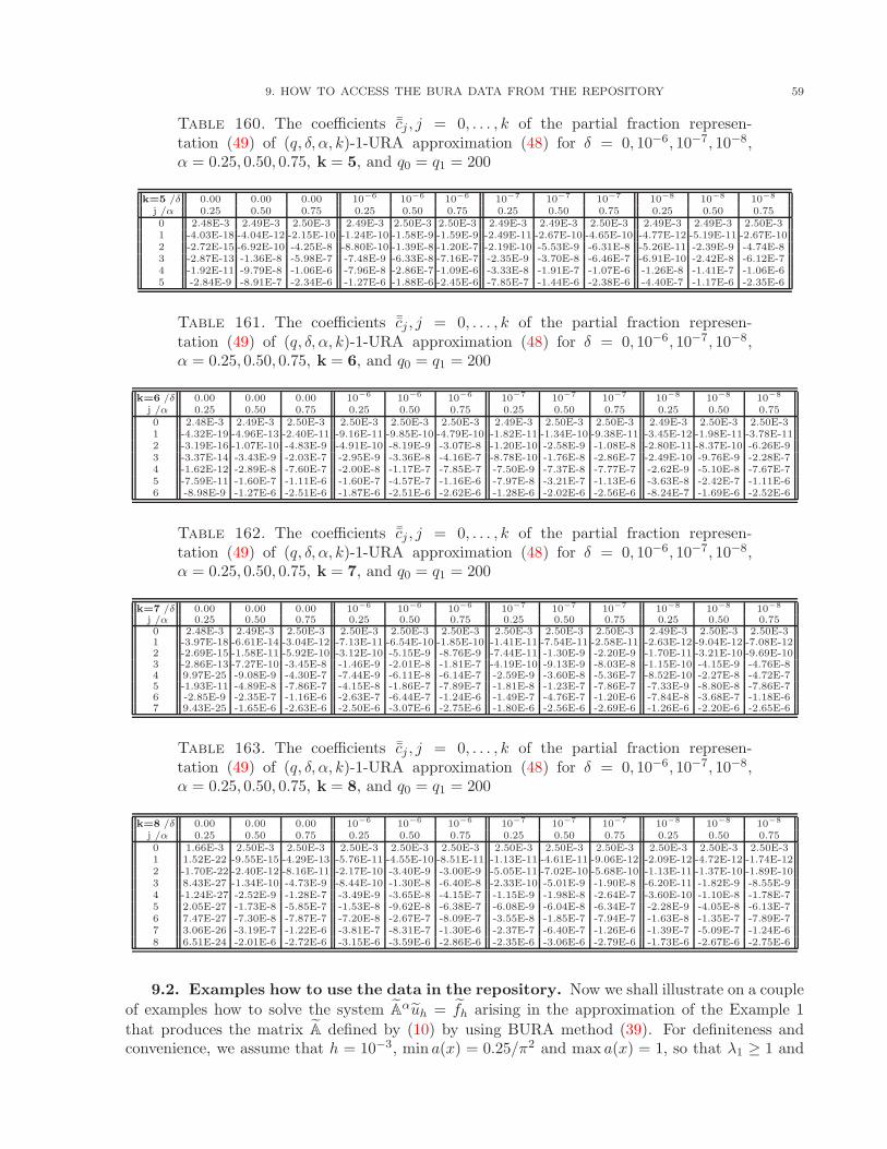
9. HOW TO ACCESS THE BURA DATA FROM THE REPOSITORY 59
Table 160. The coefficients ¯cj , j = 0, . . . , k of the partial fraction represen-tation (49) of (q, δ, α, k)-1-URA approximation (48) for δ = 0, 10−6, 10−7, 10−8,α = 0.25, 0.50, 0.75, k = 5, and q0 = q1 = 200
k=5 /δ 0.00 0.00 0.00 10−6 10−6 10−6 10−7 10−7 10−7 10−8 10−8 10−8
j /α 0.25 0.50 0.75 0.25 0.50 0.75 0.25 0.50 0.75 0.25 0.50 0.750 2.48E-3 2.49E-3 2.50E-3 2.49E-3 2.50E-3 2.50E-3 2.49E-3 2.49E-3 2.50E-3 2.49E-3 2.49E-3 2.50E-31 -4.03E-18 -4.04E-12 -2.15E-10 -1.24E-10 -1.58E-9 -1.59E-9 -2.49E-11 -2.67E-10 -4.65E-10 -4.77E-12 -5.19E-11 -2.67E-102 -2.72E-15 -6.92E-10 -4.25E-8 -8.80E-10 -1.39E-8 -1.20E-7 -2.19E-10 -5.53E-9 -6.31E-8 -5.26E-11 -2.39E-9 -4.74E-83 -2.87E-13 -1.36E-8 -5.98E-7 -7.48E-9 -6.33E-8 -7.16E-7 -2.35E-9 -3.70E-8 -6.46E-7 -6.91E-10 -2.42E-8 -6.12E-74 -1.92E-11 -9.79E-8 -1.06E-6 -7.96E-8 -2.86E-7 -1.09E-6 -3.33E-8 -1.91E-7 -1.07E-6 -1.26E-8 -1.41E-7 -1.06E-65 -2.84E-9 -8.91E-7 -2.34E-6 -1.27E-6 -1.88E-6 -2.45E-6 -7.85E-7 -1.44E-6 -2.38E-6 -4.40E-7 -1.17E-6 -2.35E-6
Table 161. The coefficients ¯cj , j = 0, . . . , k of the partial fraction represen-tation (49) of (q, δ, α, k)-1-URA approximation (48) for δ = 0, 10−6, 10−7, 10−8,α = 0.25, 0.50, 0.75, k = 6, and q0 = q1 = 200
k=6 /δ 0.00 0.00 0.00 10−6 10−6 10−6 10−7 10−7 10−7 10−8 10−8 10−8
j /α 0.25 0.50 0.75 0.25 0.50 0.75 0.25 0.50 0.75 0.25 0.50 0.750 2.48E-3 2.49E-3 2.50E-3 2.50E-3 2.50E-3 2.50E-3 2.49E-3 2.50E-3 2.50E-3 2.49E-3 2.50E-3 2.50E-31 -4.32E-19 -4.96E-13 -2.40E-11 -9.16E-11 -9.85E-10 -4.79E-10 -1.82E-11 -1.34E-10 -9.38E-11 -3.45E-12 -1.98E-11 -3.78E-112 -3.19E-16 -1.07E-10 -4.83E-9 -4.91E-10 -8.19E-9 -3.07E-8 -1.20E-10 -2.58E-9 -1.08E-8 -2.80E-11 -8.37E-10 -6.26E-93 -3.37E-14 -3.43E-9 -2.03E-7 -2.95E-9 -3.36E-8 -4.16E-7 -8.78E-10 -1.76E-8 -2.86E-7 -2.49E-10 -9.76E-9 -2.28E-74 -1.62E-12 -2.89E-8 -7.60E-7 -2.00E-8 -1.17E-7 -7.85E-7 -7.50E-9 -7.37E-8 -7.77E-7 -2.62E-9 -5.10E-8 -7.67E-75 -7.59E-11 -1.60E-7 -1.11E-6 -1.60E-7 -4.57E-7 -1.16E-6 -7.97E-8 -3.21E-7 -1.13E-6 -3.63E-8 -2.42E-7 -1.11E-66 -8.98E-9 -1.27E-6 -2.51E-6 -1.87E-6 -2.51E-6 -2.62E-6 -1.28E-6 -2.02E-6 -2.56E-6 -8.24E-7 -1.69E-6 -2.52E-6
Table 162. The coefficients ¯cj , j = 0, . . . , k of the partial fraction represen-tation (49) of (q, δ, α, k)-1-URA approximation (48) for δ = 0, 10−6, 10−7, 10−8,α = 0.25, 0.50, 0.75, k = 7, and q0 = q1 = 200
k=7 /δ 0.00 0.00 0.00 10−6 10−6 10−6 10−7 10−7 10−7 10−8 10−8 10−8
j /α 0.25 0.50 0.75 0.25 0.50 0.75 0.25 0.50 0.75 0.25 0.50 0.750 2.48E-3 2.49E-3 2.50E-3 2.50E-3 2.50E-3 2.50E-3 2.50E-3 2.50E-3 2.50E-3 2.49E-3 2.50E-3 2.50E-31 -3.97E-18 -6.61E-14 -3.04E-12 -7.13E-11 -6.54E-10 -1.85E-10 -1.41E-11 -7.54E-11 -2.58E-11 -2.63E-12 -9.04E-12 -7.08E-122 -2.69E-15 -1.58E-11 -5.92E-10 -3.12E-10 -5.15E-9 -8.76E-9 -7.44E-11 -1.30E-9 -2.20E-9 -1.70E-11 -3.21E-10 -9.69E-103 -2.86E-13 -7.27E-10 -3.45E-8 -1.46E-9 -2.01E-8 -1.81E-7 -4.19E-10 -9.13E-9 -8.03E-8 -1.15E-10 -4.15E-9 -4.76E-84 9.97E-25 -9.08E-9 -4.30E-7 -7.44E-9 -6.11E-8 -6.14E-7 -2.59E-9 -3.60E-8 -5.36E-7 -8.52E-10 -2.27E-8 -4.72E-75 -1.93E-11 -4.89E-8 -7.86E-7 -4.15E-8 -1.86E-7 -7.89E-7 -1.81E-8 -1.23E-7 -7.86E-7 -7.33E-9 -8.80E-8 -7.86E-76 -2.85E-9 -2.35E-7 -1.16E-6 -2.63E-7 -6.44E-7 -1.24E-6 -1.49E-7 -4.76E-7 -1.20E-6 -7.84E-8 -3.68E-7 -1.18E-67 9.43E-25 -1.65E-6 -2.63E-6 -2.50E-6 -3.07E-6 -2.75E-6 -1.80E-6 -2.56E-6 -2.69E-6 -1.26E-6 -2.20E-6 -2.65E-6
Table 163. The coefficients ¯cj , j = 0, . . . , k of the partial fraction represen-tation (49) of (q, δ, α, k)-1-URA approximation (48) for δ = 0, 10−6, 10−7, 10−8,α = 0.25, 0.50, 0.75, k = 8, and q0 = q1 = 200
k=8 /δ 0.00 0.00 0.00 10−6 10−6 10−6 10−7 10−7 10−7 10−8 10−8 10−8
j /α 0.25 0.50 0.75 0.25 0.50 0.75 0.25 0.50 0.75 0.25 0.50 0.750 1.66E-3 2.50E-3 2.50E-3 2.50E-3 2.50E-3 2.50E-3 2.50E-3 2.50E-3 2.50E-3 2.50E-3 2.50E-3 2.50E-31 1.52E-22 -9.55E-15 -4.29E-13 -5.76E-11 -4.55E-10 -8.51E-11 -1.13E-11 -4.61E-11 -9.06E-12 -2.09E-12 -4.72E-12 -1.74E-122 -1.70E-22 -2.40E-12 -8.16E-11 -2.17E-10 -3.40E-9 -3.00E-9 -5.05E-11 -7.02E-10 -5.68E-10 -1.13E-11 -1.37E-10 -1.89E-103 8.43E-27 -1.34E-10 -4.73E-9 -8.44E-10 -1.30E-8 -6.40E-8 -2.33E-10 -5.01E-9 -1.90E-8 -6.20E-11 -1.82E-9 -8.55E-94 -1.24E-27 -2.52E-9 -1.28E-7 -3.49E-9 -3.65E-8 -4.15E-7 -1.15E-9 -1.98E-8 -2.64E-7 -3.60E-10 -1.10E-8 -1.78E-75 2.05E-27 -1.73E-8 -5.85E-7 -1.53E-8 -9.62E-8 -6.38E-7 -6.08E-9 -6.04E-8 -6.34E-7 -2.28E-9 -4.05E-8 -6.13E-76 7.47E-27 -7.30E-8 -7.87E-7 -7.20E-8 -2.67E-7 -8.09E-7 -3.55E-8 -1.85E-7 -7.94E-7 -1.63E-8 -1.35E-7 -7.89E-77 3.06E-26 -3.19E-7 -1.22E-6 -3.81E-7 -8.31E-7 -1.30E-6 -2.37E-7 -6.40E-7 -1.26E-6 -1.39E-7 -5.09E-7 -1.24E-68 6.51E-24 -2.01E-6 -2.72E-6 -3.15E-6 -3.59E-6 -2.86E-6 -2.35E-6 -3.06E-6 -2.79E-6 -1.73E-6 -2.67E-6 -2.75E-6
9.2. Examples how to use the data in the repository. Now we shall illustrate on a couple
of examples how to solve the system Aαuh = fh arising in the approximation of the Example 1
that produces the matrix A defined by (10) by using BURA method (39). For definiteness andconvenience, we assume that h = 10−3, min a(x) = 0.25/π2 and max a(x) = 1, so that λ1 ≥ 1 and
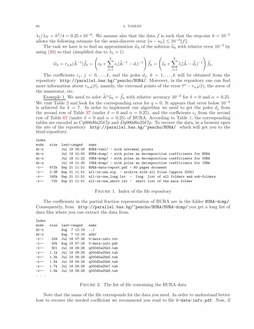
60 2. TABLES
λ1/λN = h2/4 = 0.25 ∗ 10−6. We assume also that the data f is such that the step-size h = 10−3
allows the following estimate for the semi-discrete error ‖u− uh‖ ≤ 10−3‖f‖.The task we have is to find an approximation wh of the solution uh with relative error 10−3 by
using (39) so that (simplified due to λ1 = 1)
wh = rα,k(A−1)fh =
(c0 +
k∑
i=1
ci(A−1 − di)
−1
)fh =
(c0 +
k∑
i=1
ci(A− di)−1
)fh.
The coefficients cj , j = 0, . . . , k, and the poles dj , k = 1, . . . , k will be obtained from therepository http://parallel.bas.bg/~pencho/BURA/. Moreover, in the repository one can findmore information about rα,k(t), namely, the extremal points of the error tα − rα,k(t), the zeros ofthe numerator, etc.
Example 1. We need to solve Aαuh = fh with relative accuracy 10−3 for δ = 0 and α = 0.25.
We visit Table 2 and look for the corresponding error for q = 0. It appears that error below 10−3
is achieved for k = 7. In order to implement our algorithm we need to get the poles dj fromthe second row of Table 37 (under δ = 0 and α = 0.25), and the coefficients cj from the secondrow of Table 67 (under δ = 0 and α = 0.25) of BURA. According to Table 1, the correspondingtables are encoded as Cq000d0a25k7p and Dq000d0a25k7p. To recover the data, in a browser openthe site of the repository http://parallel.bas.bg/~pencho/BURA/ which will get you to thehtml-repository.
Index
mode size last-canged name
dr-x Jul 18 09:26 BURA-tabl/ - with extremal points
dr-x Jul 18 10:50 BURA-dcmp/ - with poles an decomposition coefficients for BURA
dr-x Jul 18 11:22 0URA-dcmp/ - with poles an decomposition coefficients for 0URA
dr-x Jul 18 11:35 1URA-dcmp/ - with poles an decomposition coefficients for 1URA
-r-- 672k Sep 21 11:51 BURA-data-report.pdf - 60 pages document
-r-- 3.2M Sep 21 11:51 all-in-one.zip - archive with all files (approx 2000)
-r-- 165k Sep 21 11:51 all-in-one_long.lst - long list of all folders and sub-folders
-r-- 720 Sep 21 11:51 all-in-one_short.lst - short list of the main folder
Figure 1. Index of the file repository
The coefficients in the partial fraction representation of BURA are in the folder BURA-dcmp/.Consequently, from http://parallel.bas.bg/~pencho/BURA/BURA-dcmp/ you get a long list ofdata files where you can extract the data from.
Index
mode size last-canged name
dr-x Aug 7 12:19 ../
dr-x Aug 7 13:16 add/
-r-- 229 Jul 18 07:26 0-data-info.txt
-r-- 20k Aug 18 07:26 0-data-info.pdf
-r-- 901 Jul 18 09:28 q000d0a25k3.tab
-r-- 1.1k Jul 18 09:28 q000d0a25k4.tab
-r-- 1.3k Jul 18 09:28 q000d0a25k5.tab
-r-- 1.5k Jul 18 09:28 q000d0a25k6.tab
-r-- 1.7k Jul 18 09:28 q000d0a25k7.tab
-r-- 1.9k Jul 18 09:28 q000d0a25k8.tab
. . .
Figure 2. The list of file containing the BURA data
Note that the name of the file corresponds for the data you need. In order to understand betterhow to recover the needed coefficient we recommend you read to file 0-data-info.pdf. Now, if
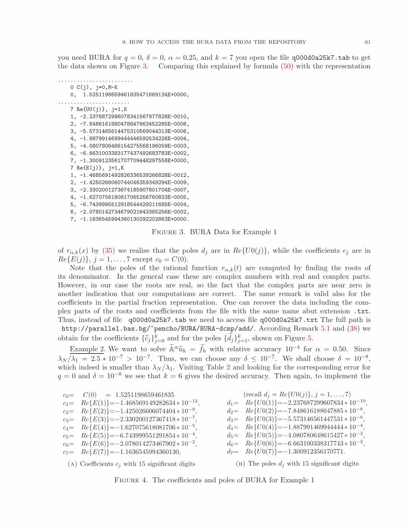
9. HOW TO ACCESS THE BURA DATA FROM THE REPOSITORY 61
you need BURA for q = 0, δ = 0, α = 0.25, and k = 7 you open the file q000d0a25k7.tab to getthe data shown on Figure 3. Comparing this explained by formula (50) with the representation
........................
0 C(j), j=0,M-K
0, 1.5251198659461835471669134E+0000,
.......................
7 ReU0(j), j=1,K
1, -2.2376872996078341567977828E-0010,
2, -7.8486161880478847863452285E-0008,
3, -5.5731465614475310569044313E-0006,
4, -1.8879914699444446592534226E-0004,
5, -4.0807806486154275568196059E-0003,
6, -6.6631003383177437492683783E-0002,
7, -1.3009123561707709448297558E+0000,
7 ReE(j), j=1,K
1, -1.4685691492826336539266828E-0012,
2, -1.4250266060744046359349294E-0009,
3, -2.3302001273674185907801704E-0007,
4, -1.6270756180817065256760833E-0005,
5, -6.7439995512918544429211685E-0004,
6, -2.0780142734679021643365256E-0002,
7, -1.1636545994360130292202863E+0000.
Figure 3. BURA Data for Example 1
of rα,k(x) by (35) we realize that the poles dj are in ReU0(j), while the coefficients cj are inReE(j), j = 1, . . . , 7 except c0 = C(0).
Note that the poles of the rational function rα,k(t) are computed by finding the roots ofits denominator. In the general case these are complex numbers with real and complex parts.However, in our case the roots are real, so the fact that the complex parts are near zero isanother indication that our computations are correct. The same remark is valid also for thecoefficients in the partial fraction representation. One can recover the data including the com-plex parts of the roots and coefficients from the file with the same name abut extension .txt.Thus, instead of file q000d0a25k7.tab we need to access file q000d0a25k7.txt The full path ishttp://parallel.bas.bg/~pencho/BURA/BURA-dcmp/add/. According Remark 5.1 and (38) we
obtain for the coefficients cjkj=0 and for the poles djkj=1, shown on Figure 5.
Example 2. We want to solve Aαuh = fh with relative accuracy 10−4 for α = 0.50. Since
λN/λ1 = 2.5 ∗ 10−7 > 10−7. Thus, we can choose any δ ≤ 10−7. We shall choose δ = 10−8,which indeed is smaller than λN/λ1. Visiting Table 2 and looking for the corresponding error forq = 0 and δ = 10−8 we see that k = 6 gives the desired accuracy. Then again, to implement the
c0= C(0) = 1.5251198659461835c1= ReE(1)=−1.468569149282634 ∗ 10−12,c2= ReE(2)=−1.425026606074404 ∗ 10−9,c3= ReE(3)=−2.330200127367418 ∗ 10−7,c4= ReE(4)=−1.627075618081706 ∗ 10−5,c5= ReE(5)=−6.743999551291854 ∗ 10−4,c6= ReE(6)=−2.078014273467902 ∗ 10−2,c7= ReE(7)=−1.1636545994360130,
(a) Coefficients cj with 15 significant digits
(recall dj = ReU0(j), j = 1, . . . , 7)
d1= ReU0(1)=−2.237687299607834 ∗ 10−10,d2= ReU0(2)=−7.848616188047885 ∗ 10−8,d3= ReU0(3)=−5.573146561447531 ∗ 10−6,d4= ReU0(4)=−1.887991469944444 ∗ 10−4,d5= ReU0(5)=−4.080780648615427 ∗ 10−3,d6= ReU0(6)=−6.663100338317743 ∗ 10−2,d7= ReU0(7)=−1.300912356170771.
(b) The poles dj with 15 significant digits
Figure 4. The coefficients and poles of BURA for Example 1
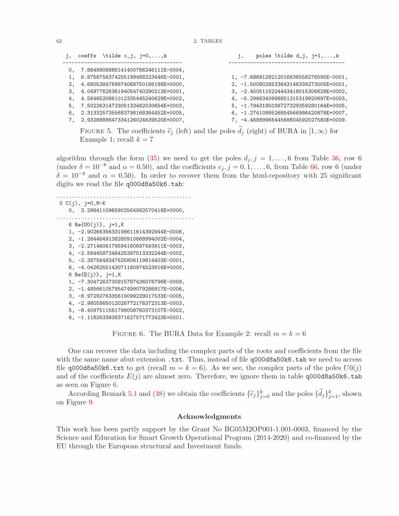
62 2. TABLES
j, coeffs \tilde c_j, j=0,...,k j, poles \tilde d_j, j=1,...,k
--------------------------------------- --------------------------------------
0, 7.8649908986141400766246111E-0004,
1, 6.8758756374255199468223446E-0001, 1, -7.6869129212016636558276595E-0001,
2, 4.6805384769874068750186188E+0000, 2, -1.5008028533643146339273005E+0001,
3, 4.0497762636194054740290213E+0001, 3, -2.4505115224443418015306629E+0002,
4, 4.5646520861012335445240629E+0002, 4, -5.2966340998851315319920697E+0003,
5, 7.5022631473305133482030654E+0003, 5, -1.7943185038727329359280164E+0005,
6, 2.3133257355683798168384452E+0005, 6, -1.2741099526854566986420878E+0007,
7, 2.9328888647334126024639520E+0007, 7, -4.4688996544568804592027580E+0009.
Figure 5. The coefficients cj (left) and the poles dj (right) of BURA in [1,∞) forExample 1; recall k = 7
algorithm through the form (35) we need to get the poles dj , j = 1, . . . , 6 from Table 36, row 6(under δ = 10−8 and α = 0.50), and the coefficients cj, j = 0, 1, . . . , 6, from Table 66, row 6 (underδ = 10−8 and α = 0.50). In order to recover them from the html-repository with 25 significantdigits we read the file q000d8a50k6.tab:
............................................
0 C(j), j=0,M-K
0, 3.2884110965902564982570418E+0000,
.............................................
6 ReU0(j), j=1,K
1, -2.9026635633198611614392944E-0006,
2, -1.2844649138280910668994002E-0004,
3, -2.2714606179594160697493911E-0003,
4, -2.5644587248425397513332244E-0002,
5, -2.3875648347625806119814403E-0001,
6, -4.0426255143071180974523916E+0000,
6 ReE(j), j=1,K
1, -7.3047263730915787436076796E-0009,
2, -1.4856610579547499079286817E-0006,
3, -8.9729276335619099229017533E-0005,
4, -2.9805865012026772176372313E-0003,
5, -8.4097511581798008760373107E-0002,
6, -1.1182633938371627571773423E+0001.
Figure 6. The BURA Data for Example 2: recall m = k = 6
One can recover the data including the complex parts of the roots and coefficients from the filewith the same name abut extension .txt. Thus, instead of file q000d8a50k6.tab we need to accessfile q000d8a50k6.txt to get (recall m = k = 6). As we see, the complex parts of the poles U0(j)and of the coefficients E(j) are almost zero. Therefore, we ignore them in table q000d8a50k6.tabas seen on Figure 6.
According Remark 5.1 and (38) we obtain the coefficients cjkj=0 and the poles djkj=1, shownon Figure 9.
Acknowledgments
This work has been partly support by the Grant No BG05M2OP001-1.001-0003, financed by theScience and Education for Smart Growth Operational Program (2014-2020) and co-financed by theEU through the European structural and Investment funds.

ACKNOWLEDGMENTS 63
c0= C(0) = 3.288411096590256c1= ReE(1)=−7.304726373091578 ∗ 10−9
c2= ReE(2)=−1.485661057954749 ∗ 10−6
c3= ReE(3)=−8.972927633561909 ∗ 10−5
c4= ReE(4)=−2.980586501202677 ∗ 10−3
c5= ReE(5)=−8.409751158179800 ∗ 10−2
c6= ReE(6)=−1.118263393837162 ∗ 10(a) Coefficients cj with 15 significant digits
(recall dj = ReU0(j), j = 1, . . . , 7)
d1= ReU0(1)=−2.902663563319861 ∗ 10−6
d2= ReU0(2)=−1.284464913828091 ∗ 10−4
d3= ReU0(3)=−2.271460617959416 ∗ 10−3
d4= ReU0(4)=−2.564458724842539 ∗ 10−2
d5= ReU0(5)=−2.387564834762580 ∗ 10−1
d6= ReU0(6)=−4.042625514307118 ∗ 10(b) The poles dj with 15 significant digits
Figure 7. The coefficients and the poles for Example 2
........................
0 C(j), j=0,M-K
0, 3.2884110965902564982570418E+0000,
................................
6 U0(j), j=1,K
1, -2.9026635633198611614392944E-0006, -1.7520806294041483876573147E-0037
2, -1.2844649138280910668994002E-0004, 1.8242239649606423471743024E-0037
3, -2.2714606179594160697493911E-0003, -7.2143334828724323886476075E-0039
4, -2.5644587248425397513332244E-0002, -7.2776229715659618428404602E-0047
5, -2.3875648347625806119814403E-0001, -7.3384739154186567125843208E-0052
6, -4.0426255143071180974523916E+0000, -8.8654988085625587825735093E-0067
6 E(j), j=1,K
1, -7.3047263730915787436076796E-0009, 5.7573111695991243362896879E-0037
2, -1.4856610579547499079286817E-0006, -5.9992385756159082541115791E-0037
3, -8.9729276335619099229017533E-0005, 2.4155906802799248832468797E-0038
4, -2.9805865012026772176372313E-0003, 2.2938808341026098990357342E-0041
5, -8.4097511581798008760373107E-0002, 9.4285923737400470688723456E-0042
6, -1.1182633938371627571773423E+0001, 4.4663981643768036611005825E-0042
Figure 8. The BURA Data for Example 2 in complex numbers; recall m = k = 6
j, coeffs \tilde c_j, j=0,...,k j,
---------------------------------------
0, 1.8619525184162842197896828E-0004,
1, 6.8425358785323701384064700E-0001,
2, 1.4752743712419678037242149E+0000,
3, 4.5322129077686442621147161E+0000,
4, 1.7390967446300787239267527E+0001,
5, 9.0048244054276093870632027E+0001,
6, 8.6698293594856505069077514E+0002.
(a) The coefficients cj
j, poles \tilde d_j, j=1,...,k
---------------------------------------
1, -2.4736399561644631729004006E-0001,
2, -4.1883679364017772326828007E+0000,
3, -3.8994583547504784590380748E+0001,
4, -4.4024536110969760472793286E+0002,
5, -7.7853430579096145080903339E+0003,
6, -3.4451116300101647683572511E+0005,
(b) The poles dj
Figure 9. Coefficients cj and poles dj of BURA in [1,∞) for Example 2, k = 6.

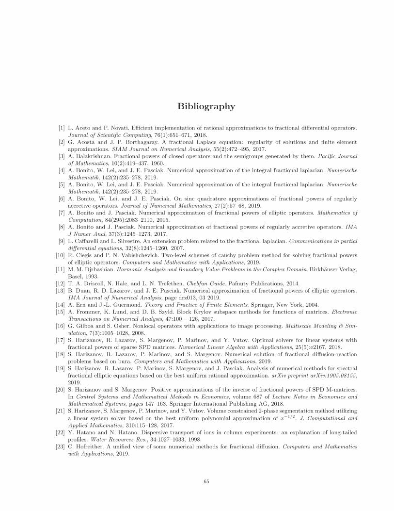
Bibliography
[1] L. Aceto and P. Novati. Efficient implementation of rational approximations to fractional differential operators.Journal of Scientific Computing, 76(1):651–671, 2018.
[2] G. Acosta and J. P. Borthagaray. A fractional Laplace equation: regularity of solutions and finite elementapproximations. SIAM Journal on Numerical Analysis, 55(2):472–495, 2017.
[3] A. Balakrishnan. Fractional powers of closed operators and the semigroups generated by them. Pacific Journal
of Mathematics, 10(2):419–437, 1960.[4] A. Bonito, W. Lei, and J. E. Pasciak. Numerical approximation of the integral fractional laplacian. Numerische
Mathematik, 142(2):235–278, 2019.[5] A. Bonito, W. Lei, and J. E. Pasciak. Numerical approximation of the integral fractional laplacian. Numerische
Mathematik, 142(2):235–278, 2019.[6] A. Bonito, W. Lei, and J. E. Pasciak. On sinc quadrature approximations of fractional powers of regularly
accretive operators. Journal of Numerical Mathematics, 27(2):57–68, 2019.[7] A. Bonito and J. Pasciak. Numerical approximation of fractional powers of elliptic operators. Mathematics of
Computation, 84(295):2083–2110, 2015.[8] A. Bonito and J. Pasciak. Numerical approximation of fractional powers of regularly accretive operators. IMA
J Numer Anal, 37(3):1245–1273, 2017.[9] L. Caffarelli and L. Silvestre. An extension problem related to the fractional laplacian. Communications in partial
differential equations, 32(8):1245–1260, 2007.[10] R. Ciegis and P. N. Vabishchevich. Two-level schemes of cauchy problem method for solving fractional powers
of elliptic operators. Computers and Mathematics with Applications, 2019.[11] M. M. Djrbashian. Harmonic Analysis and Boundary Value Problems in the Complex Domain. Birkhauser Verlag,
Basel, 1993.[12] T. A. Driscoll, N. Hale, and L. N. Trefethen. Chebfun Guide. Pafnuty Publications, 2014.[13] B. Duan, R. D. Lazarov, and J. E. Pasciak. Numerical approximation of fractional powers of elliptic operators.
IMA Journal of Numerical Analysis, page drz013, 03 2019.[14] A. Ern and J.-L. Guermond. Theory and Practice of Finite Elements. Springer, New York, 2004.[15] A. Frommer, K. Lund, and D. B. Szyld. Block Krylov subspace methods for functions of matrices. Electronic
Transactions on Numerical Analysis, 47:100 – 126, 2017.[16] G. Gilboa and S. Osher. Nonlocal operators with applications to image processing. Multiscale Modeling & Sim-
ulation, 7(3):1005–1028, 2008.[17] S. Harizanov, R. Lazarov, S. Margenov, P. Marinov, and Y. Vutov. Optimal solvers for linear systems with
fractional powers of sparse SPD matrices. Numerical Linear Algebra with Applications, 25(5):e2167, 2018.[18] S. Harizanov, R. Lazarov, P. Marinov, and S. Margenov. Numerical solution of fractional diffusion-reaction
problems based on bura. Computers and Mathematics with Applications, 2019.[19] S. Harizanov, R. Lazarov, P. Marinov, S. Margenov, and J. Pasciak. Analysis of numerical methods for spectral
fractional elliptic equations based on the best uniform rational approximation. arXiv preprint arXiv:1905.08155,2019.
[20] S. Harizanov and S. Margenov. Positive approximations of the inverse of fractional powers of SPD M-matrices.In Control Systems and Mathematical Methods in Economics, volume 687 of Lecture Notes in Economics and
Mathematical Systems, pages 147–163. Springer International Publishing AG, 2018.[21] S. Harizanov, S. Margenov, P. Marinov, and Y. Vutov. Volume constrained 2-phase segmentation method utilizing
a linear system solver based on the best uniform polynomial approximation of x−1/2. J. Computational and
Applied Mathematics, 310:115–128, 2017.[22] Y. Hatano and N. Hatano. Dispersive transport of ions in column experiments: an explanation of long-tailed
profiles. Water Resources Res., 34:1027–1033, 1998.[23] C. Hofreither. A unified view of some numerical methods for fractional diffusion. Computers and Mathematics
with Applications, 2019.
65
66 BIBLIOGRAPHY
[24] T. Kato. Fractional powers of dissipative operators. Journal of the Mathematical Society of Japan, 13(3):246–274,1961.
[25] A. Kilbas, H. Srivastava, and J. Trujillo. Theory and Applications of Fractional Differential Equations. Elsevier,Amsterdam, 2006.
[26] A. Lischke, G. Pang, M. Gulian, F. Song, C. Glusa, X. Zheng, Z. Mao, W. Cai, M. M. Meerschaert, M. Ainsworth,and G. Karniadakis. What is the fractional laplacian? arXiv preprint arXiv:1801.09767, 2018.
[27] P. G. Marinov and A. S. Andreev. A modified Remez algorithm for approximate determination of the rationalfunction of the best approximation in Hausdorff metric. Comptes rendus de l’Academie bulgare des Sciences,40(3):13–16, 1987.
[28] R. Metzler and J. Klafter. The restaurant at the end of the random walk: recent developments in the descriptionof anomalous transport by fractional dynamics. J. Phys. A: Math. Gen., 37(31):R161–R208, 2004.
[29] R. H. Nochetto, E. Otarola, and A. J. Salgado. A pde approach to fractional diffusion in general domains: apriori error analysis. Foundations of Computational Mathematics, 15(3):733–791, 2015.
[30] R. H. Nochetto, E. Otarola, and A. J. Salgado. A pde approach to space-time fractional parabolic problems.SIAM Journal on Numerical Analysis, 54(2):848–873, 2016.
[31] I. Podlubny. Fractional Differential Equations. Academic Press, Inc., San Diego, CA, 1999.[32] E. Saff and H. Stahl. Asymptotic distribution of poles and zeros of best rational approximants to xα on [0, 1].
Sta, 299(4), 1992.[33] A. A. Samarskii. The theory of difference schemes, volume 240 of Pure and Applied Mathematics. Marcel Dekker,
Inc., New York, 2001.[34] H. Stahl. Best uniform rational approximation of xα on [0, 1]. Bulletin of the American Mathematical Society,
28(1):116–122, 1993.[35] H. R. Stahl. Best uniform rational approximation of xα on [0, 1]. Acta Mathematica, 190(2):241–306, 2003.[36] V. E. Tarasov. Fractional dynamics: applications of fractional calculus to dynamics of particles, fields and media.
Springer Science & Business Media, 2011.[37] V. Thomee. Galerkin finite element methods for parabolic problems, volume 25 of Springer Series in Computa-
tional Mathematics. Springer-Verlag, Berlin, second edition, 2006.[38] P. J. Torvik and R. L. Bagley. On the appearance of the fractional derivative in the behavior of real materials.
Journal of applied mechanics, 51(2):294–298, 1984.[39] P. N. Vabishchevich. Numerically solving an equation for fractional powers of elliptic operators. Journal of
Computational Physics, 282:289–302, 2015.[40] P. N. Vabishchevich. Numerical solution of time-dependent problems with fractional power elliptic operator.
Computational Methods in Applied Mathematics, 18(1):111–128, 2018.[41] R. S. Varga and A. J. Carpenter. Some numerical results on best uniform rational approximation of xα on [0,
1]. Numerical Algorithms, 2(2):171–185, 1992.