PRACTICAL TUNING METHOD FOR FRACTIONAL ORDER

PROPORTIONAL AND INTEGRAL CONTROLLERS

by

Tripti Bhaskaran

A thesis submitted in partial fulfillmentof the requirements for the degree

of

MASTER OF SCIENCE

in

Electrical Engineering

Approved:

Dr. YangQuan Chen Dr. Hui Fang DouMajor Professor Committee Member

Dr. Jacob Gunther Dr. Byron R. BurnhamCommittee Member Dean of Graduate Studies

UTAH STATE UNIVERSITYLogan, Utah

2007

ii

Copyright c© Tripti Bhaskaran 2007

All Rights Reserved

iii

Abstract

PRACTICAL TUNING METHOD FOR FRACTIONAL ORDER PROPORTIONAL

AND INTEGRAL CONTROLLERS

by

Tripti Bhaskaran, Master of Science

Utah State University, 2007

Major Professor: Dr. YangQuan ChenDepartment: Electrical and Computer Engineering

This thesis presents a new practical tuning method for fractional order proportional and

integral controllers (FO-PI/PIα) for the first order plus delay time (FOPDT) class of sys-

tems. The tuning is optimal in the sense that the load disturbance rejection is optimized

yet with a constraint on the maximum sensitivity. A generalized MIGO(Ms constrained

Integral Gain Optimization), called the F-MIGO (Fractional-MIGO), has been developed

for the FO-PI controllers. The F-MIGO method is then used to develop tuning rules for the

FOPDT class of dynamic systems. The final developed tuning rules apply only the relative

dead-time, τ , of the FOPDT model to determine the best fractional order (α) and at the

same time to determine the best FO-PI gains (K, Ki). Experimental results in two lab

platforms: Heat Flow Experiment and Rotary Flexible Joint are reported using the tuning

rules developed in this thesis. A true analog fractional controller - Fractroller which has

been designed using a new kind of circuit element called the Fractor has also been tested. It

has been demonstrated in this thesis that the tuning rule development procedure for FO-PI

is not only valid for FOPDT systems but also applicable for other general class of plants.

(103 pages)

iv

To all the people whom I hold very dear to my heart and without whose support I wouldnot have been here. I stand proud today because of their support and faith in my

capabilities.

v

Acknowledgments

I would like to express sincere gratitude to my major professor, Dr. YangQuan Chen,

for his excellent guidance at every step in my thesis. His enthusiasm, hard work and kindness

have been my major motivation to continue doing research. As a student and researcher in

CSOIS I have matured into a professional and have honed my technical and personal skills.

I would also like to thank my committee members, Dr. Huifang Dou, Dr. Jacob Gunther

for their patience and support.

I would like to take this opportunity to thank the other members of CSOIS with whom

I have interacted on several occasions and each has added favorably to my experience.

Finally I would like to thank all my dear family and friends who have believed in me and

helped in many tough times to achieve all my goals.

I would like to thank Dr.Gary Bohannan and Montana State University for giving me

the opportunity to work on the SBIR project on ”True Analog Fractional Order Controller”.

This research has been supported in part by Utah State University TCO Technology

Bridge Grant, an NSF Small Business Innovation Research Grant (OII-0538866) and SDL

Skunk Works Research Initiative Grant at Utah State University entitled “Temperature

Uniformity Control Using Spatial Sensors and Actuators”.

vi

Contents

Page

Abstract . . . . . . . . . . . . . . . . . . . . . . . . . . . . . . . . . . . . . . . . . . . . . . . . . . . . . . . iii

Acknowledgments . . . . . . . . . . . . . . . . . . . . . . . . . . . . . . . . . . . . . . . . . . . . . . . v

List of Tables . . . . . . . . . . . . . . . . . . . . . . . . . . . . . . . . . . . . . . . . . . . . . . . . . . . viii

List of Figures . . . . . . . . . . . . . . . . . . . . . . . . . . . . . . . . . . . . . . . . . . . . . . . . . . ix

1 Introduction . . . . . . . . . . . . . . . . . . . . . . . . . . . . . . . . . . . . . . . . . . . . . . . . . 11.1 Motivation . . . . . . . . . . . . . . . . . . . . . . . . . . . . . . . . . . . . 11.2 Contribution . . . . . . . . . . . . . . . . . . . . . . . . . . . . . . . . . . . 21.3 Outline of Thesis . . . . . . . . . . . . . . . . . . . . . . . . . . . . . . . . . 3

2 The F-MIGO Algorithm . . . . . . . . . . . . . . . . . . . . . . . . . . . . . . . . . . . . . . . . 42.1 Background . . . . . . . . . . . . . . . . . . . . . . . . . . . . . . . . . . . . 42.2 Description of the Design Problem . . . . . . . . . . . . . . . . . . . . . . . 5

2.2.1 The Process . . . . . . . . . . . . . . . . . . . . . . . . . . . . . . . . 52.2.2 The Controller . . . . . . . . . . . . . . . . . . . . . . . . . . . . . . 52.2.3 The Design Goal . . . . . . . . . . . . . . . . . . . . . . . . . . . . . 62.2.4 The Sensitivity Functions . . . . . . . . . . . . . . . . . . . . . . . . 62.2.5 The Design Parameters . . . . . . . . . . . . . . . . . . . . . . . . . 9

2.3 The Optimization Problem . . . . . . . . . . . . . . . . . . . . . . . . . . . 102.3.1 Geometric Interpretation of the Sensitivity Constraint . . . . . . . . 122.3.2 Stability Regions of the Sensitivity Constraint . . . . . . . . . . . . 12

2.4 Numerical Solution of the Optimization Problem . . . . . . . . . . . . . . . 142.4.1 The Optimization Problem . . . . . . . . . . . . . . . . . . . . . . . 142.4.2 Simplification of the Optimization Problem . . . . . . . . . . . . . . 15

2.5 The F-MIGO Algorithm . . . . . . . . . . . . . . . . . . . . . . . . . . . . . 192.6 Validation of the F-MIGO Algorithm . . . . . . . . . . . . . . . . . . . . . . 192.7 The Selection Process for An Arbitrary α . . . . . . . . . . . . . . . . . . . 21

3 Practical Tuning Rules for FO-PI Controllers . . . . . . . . . . . . . . . . . . . . . . 253.1 Introduction . . . . . . . . . . . . . . . . . . . . . . . . . . . . . . . . . . . . 253.2 FOPDT Model . . . . . . . . . . . . . . . . . . . . . . . . . . . . . . . . . . 253.3 The Test Batch . . . . . . . . . . . . . . . . . . . . . . . . . . . . . . . . . . 273.4 Selection of the Best Fractional Controller . . . . . . . . . . . . . . . . . . . 273.5 Tuning Rules . . . . . . . . . . . . . . . . . . . . . . . . . . . . . . . . . . . 30

3.5.1 α∗ versus τ . . . . . . . . . . . . . . . . . . . . . . . . . . . . . . . . 303.5.2 Normalized Controller Gains Versus τ . . . . . . . . . . . . . . . . . 303.5.3 Summary of Tuning Rules . . . . . . . . . . . . . . . . . . . . . . . . 32

vii

3.6 Simulation Verification . . . . . . . . . . . . . . . . . . . . . . . . . . . . . . 323.6.1 Tuning Methods for Integer Order PI Controllers . . . . . . . . . . . 323.6.2 Test Batch . . . . . . . . . . . . . . . . . . . . . . . . . . . . . . . . 353.6.3 Results . . . . . . . . . . . . . . . . . . . . . . . . . . . . . . . . . . 353.6.4 Special Systems . . . . . . . . . . . . . . . . . . . . . . . . . . . . . . 37

3.7 Conclusions . . . . . . . . . . . . . . . . . . . . . . . . . . . . . . . . . . . . 42

4 Experimental Verification of Practical FO-PI Tuning Rules . . . . . . . . . . 454.1 Introduction . . . . . . . . . . . . . . . . . . . . . . . . . . . . . . . . . . . . 454.2 Quanser Real-Time Control Components . . . . . . . . . . . . . . . . . . . . 454.3 Heat Flow Experiment . . . . . . . . . . . . . . . . . . . . . . . . . . . . . . 46

4.3.1 HFE Apparatus . . . . . . . . . . . . . . . . . . . . . . . . . . . . . 474.3.2 Open Loop Response and Analysis . . . . . . . . . . . . . . . . . . . 484.3.3 Control Schemes in HFE . . . . . . . . . . . . . . . . . . . . . . . . . 494.3.4 Tuning of FO-PI Controller for HFE . . . . . . . . . . . . . . . . . . 514.3.5 Implementation of the Tuned Controller . . . . . . . . . . . . . . . . 514.3.6 Results . . . . . . . . . . . . . . . . . . . . . . . . . . . . . . . . . . 534.3.7 Conclusion . . . . . . . . . . . . . . . . . . . . . . . . . . . . . . . . 57

4.4 Rotary Flexible Joint . . . . . . . . . . . . . . . . . . . . . . . . . . . . . . . 574.4.1 RFJ Platform . . . . . . . . . . . . . . . . . . . . . . . . . . . . . . . 574.4.2 F-MIGO Applied to RFJ . . . . . . . . . . . . . . . . . . . . . . . . 604.4.3 Simulation and Lab Results . . . . . . . . . . . . . . . . . . . . . . . 62

4.5 Fractroller: True Analog Fractional Controller . . . . . . . . . . . . . . . . . 634.5.1 Introduction . . . . . . . . . . . . . . . . . . . . . . . . . . . . . . . 644.5.2 Fractor . . . . . . . . . . . . . . . . . . . . . . . . . . . . . . . . . . 654.5.3 Extension to State Space Representation . . . . . . . . . . . . . . . . 684.5.4 Fractional Order Control . . . . . . . . . . . . . . . . . . . . . . . . 704.5.5 Results and Findings . . . . . . . . . . . . . . . . . . . . . . . . . . . 71

4.6 Conclusion . . . . . . . . . . . . . . . . . . . . . . . . . . . . . . . . . . . . 72

5 Conclusion . . . . . . . . . . . . . . . . . . . . . . . . . . . . . . . . . . . . . . . . . . . . . . . . . . . 745.1 Summary . . . . . . . . . . . . . . . . . . . . . . . . . . . . . . . . . . . . . 745.2 Future Work . . . . . . . . . . . . . . . . . . . . . . . . . . . . . . . . . . . 75

References . . . . . . . . . . . . . . . . . . . . . . . . . . . . . . . . . . . . . . . . . . . . . . . . . . . . . . 77

Appendices . . . . . . . . . . . . . . . . . . . . . . . . . . . . . . . . . . . . . . . . . . . . . . . . . . . . . 80Appendix A Mathematical Definition of the Fractional Operator . . . . . . . . 81Appendix B Oustaloup’s Recursive Approximation of Fractional Order . . . . 83Appendix C General Equation of An Ellipse . . . . . . . . . . . . . . . . . . . 84Appendix D Newton Raphson Technique . . . . . . . . . . . . . . . . . . . . . 85Appendix E Matlab Code to Generate FOPDT Model. . . . . . . . . . . . . . 86Appendix F F-MIGO algorithm : MATLAB Code . . . . . . . . . . . . . . . . 87

viii

List of Tables

Table Page

2.1 Validation of the F-MIGO method for G1-G6. . . . . . . . . . . . . . . . . . 22

3.1 FOPDT parameters for systems G1(s)−G6(s). . . . . . . . . . . . . . . . . 36

3.2 Controller parameters for systems G1(s)−G6(s). . . . . . . . . . . . . . . . 37

3.3 Scan of fractional order controllers for pure delay system. . . . . . . . . . . 41

3.4 Scan of fractional order controllers for pure integrator with time delay. . . . 42

3.5 Controller parameters for system G(s). . . . . . . . . . . . . . . . . . . . . . 42

4.1 Step response data from open-loop experiment. . . . . . . . . . . . . . . . . 50

4.2 FO-PI gains at various combinations VQ/VF. . . . . . . . . . . . . . . . . . 51

4.3 PI controller gains at different combinations of VQ/VF. . . . . . . . . . . . 52

4.4 Deciding on the design parameters. . . . . . . . . . . . . . . . . . . . . . . . 62

4.5 Analysis of RFJ closed-loop response at different values of the fractional order. 62

ix

List of Figures

Figure Page

2.1 Block diagram of a closed-loop system. . . . . . . . . . . . . . . . . . . . . . 7

2.2 Bode plot of sensitivity functions for a typical system. (Blue line: S(s);Green Line: T (s)). . . . . . . . . . . . . . . . . . . . . . . . . . . . . . . . . 8

2.3 Sensitivity circles for a typical system. (Solid line: Ms circle; Dashed line:Mp circle; Dotted line: Unit circle). . . . . . . . . . . . . . . . . . . . . . . . 9

2.4 Geometric illustration of the envelopes generated by the ellipses, at differentvalues of α, for a typical system. . . . . . . . . . . . . . . . . . . . . . . . . 13

2.5 The F-MIGO algorithm (T: true , F: false). . . . . . . . . . . . . . . . . . . 20

2.6 Solution of G(s) at α = 1. The best solution corresponds to the largest valueof ki which has been marked with green color. . . . . . . . . . . . . . . . . . 23

2.7 Solution at other values of fractional order for G(s). . . . . . . . . . . . . . 24

3.1 Illustration of the procedure for determining the FOPDT model from thestep-response curve. . . . . . . . . . . . . . . . . . . . . . . . . . . . . . . . 26

3.2 Procedure for choosing the best FO-PI controller for a given system. . . . . 29

3.3 Best fractional order (α∗) versus relative dead-time (τ). . . . . . . . . . . . 30

3.4 Normalized FO-PI gains (K∗,K∗i ) versus the relative dead time (τ). . . . . 31

3.5 Step response and load disturbance response for delay dominated systemsG1(s) and G2(s). (Thick solid line: Practical tuning method; Thin line: ZNmethod; Dotted line: Modified ZN; Dash-dotted line: AMIGO method). . . 38

3.6 Step response and load disturbance response for balanced lag and delay sys-tems G3(s) and G4(s).(Thick solid line: Practical tuning method; Thin line:ZN method; Dotted line: Modified ZN; Dash-dotted line: AMIGO method). 39

3.7 Step response and load disturbance response for lag dominated systems G5(s)and G6(s).(Thick solid line: Practical tuning method; Thin line: ZN method;Dotted line: Modified ZN; Dash-dotted line: AMIGO method). . . . . . . . 40

x

3.8 Pure time delay controlled with FO-PI controllers. Best FO-PI controller atα = 1.1 (dashed line) and corresponding gains: K = 0.292 and Ki = 0.73. . 41

3.9 Pure integrator with time delay controlled with FO-PI controller. (Dashedline: Closed loop response without controller; Solid line: Best fractional orderat α = 0.7 and corresponding gains K = 0.324 and Ki = 0.103 (solid line);Dotted dashed line: Integer order controller with K = 0.365 and Ki = 0.042). 43

3.10 Step responses of process with distributed parameter. (Dashed line: Re-sponse without controller; Thick solid line: Practical tuning method; Thinline: ZN method; Dotted line: Modified ZN; Dash-dotted line: AMIGOmethod). . . . . . . . . . . . . . . . . . . . . . . . . . . . . . . . . . . . . . . 44

4.1 Schematic of the real-time digital control of the hardware-in-loop setup. . . 46

4.2 Heat flow apparatus. . . . . . . . . . . . . . . . . . . . . . . . . . . . . . . . 47

4.3 HFE experimental setup. . . . . . . . . . . . . . . . . . . . . . . . . . . . . 48

4.4 Open-loop step responses at the three sensors for VQ = [3, 4, 5] and fixedfan voltage of 4 V. (Blue: T0n; Green: T1n; Red: T2n, where n =[3,4,5] toimply at which VQ input the readings are taken.) . . . . . . . . . . . . . . . 49

4.5 Simulink model used in the HFE experiments. . . . . . . . . . . . . . . . . . 53

4.6 Response comparison of FO-PI and PI controllers for Type1 schemes. . . . 53

4.7 Response comparison of FO-PI and PI controllers for Type2 schemes. . . . 54

4.8 Response comparison of FO-PI and PI controllers for Type3 schemes. . . . 54

4.9 FO-PI control of Type4 and Type5 schemes. . . . . . . . . . . . . . . . . . . 55

4.10 FO-PI control of Type6 and Type7 schemes. . . . . . . . . . . . . . . . . . . 56

4.11 Rotary flexible joint module. . . . . . . . . . . . . . . . . . . . . . . . . . . 58

4.12 RFJ experimental setup in the Mechatronics Lab in Utah State University. 59

4.13 Closed-loop simulation results of the tip angle (θ + φ) RFJ model and con-trollers from table 4.5. . . . . . . . . . . . . . . . . . . . . . . . . . . . . . . 63

4.14 Positioning the tip at 45◦ and load disturbance responses using FO-PI con-troller of (a) α = 0.2; (b) α = 0.3. The graphs show the variation of armdeflection (φ), hub angle (θ), setpoint and output (θ + φ). . . . . . . . . . . 64

xi

4.15 Positioning the tip at 45◦. FO-PI of α = 0.4 versus PI controller. The graphsshow the variation of arm deflection (φ), hub angle (θ), setpoint and output(θ + φ). . . . . . . . . . . . . . . . . . . . . . . . . . . . . . . . . . . . . . . 65

4.16 Prototype Fractance device, the Fractor prepared by Montana State University. 66

4.17 Impedance spectrum of a Fractor with a fractance order ≈ 0.3. . . . . . . . 67

4.18 A fractional order integrator circuit using the Fractor circuit element. . . . 68

4.19 Feedback structure for the RFJ arm. . . . . . . . . . . . . . . . . . . . . . . 69

4.20 Schematic of the Fractroller setup and top view of the Fractroller in thecontrol loop. . . . . . . . . . . . . . . . . . . . . . . . . . . . . . . . . . . . . 69

4.21 System responses with the proportional only control. Observe that the set-point is never reached in this case. . . . . . . . . . . . . . . . . . . . . . . . 70

4.22 System responses with integer order PI control. Increasing the integral gaintended to cause the system to overshoot and stick further from the setpointand then drift back across the set point value in a slow oscillation. . . . . . 71

4.23 System responses with FO-PI controller. Observe that there is no overshootand also the response time is faster compared to the other configurations. . 72

1

Chapter 1

Introduction

1.1 Motivation

The birth of Fractional Calculus is dated back to the year 1695 [1], when Leibniz raised

the following question in a letter to L‘Hospital,“Can the meaning of derivatives with integer

order be generalized to derivatives with non-integer orders?”. L‘Hospital raised a question

in reply: “What if the order will be 1/2?”. Leibniz’s historic reply was, “It will lead to a

paradox, from which one day useful consequences will be drawn.”.

The past decade has seen an increase in research efforts related to fractional calculus

[1, 2] and its applications to control theory [3–8]. Clearly, for closed-loop control systems,

there are four situations: 1) IO (integer order) plant with IO controller; 2) IO plant with

FO (fractional order) controller; 3) FO plant with IO controller and 4) FO plant with FO

controller. In control practice, the fractional-order controller is more common, because

the plant model may have already been obtained as an integer order model in the classical

sense. From an engineering point of view, improving or optimizing performance is the major

concern [6]. Hence, our objective is to apply the fractional-order control (FOC) to enhance

the (integer order) dynamic system control performance [3, 6, 9, 10]. Pioneering works in

applying fractional calculus in dynamic systems and controls and the recent developments

can be found in [3, 11–17].

The general structure of the PID controller namely - PIαDγ was proposed in [18] and

it is an extension of the classical PID structure with an added advantage of considering

the integrator and differentiator of any non-integer order. It is expected that fractional

PID will perform better over an integer order PID due to an extra controller parameter to

be tuned [5]. A lot of research has gone into developing tuning methods for PIα/PIαDγ

2

controllers [5, 19–21].

The motivation for this thesis is to develop simple tuning methods for the fractional

order FO-PI controllers similar to the historic work by Ziegler-Nichols [22,23]. The method

applied in this thesis is an extension of the MIGO (Ms constrained Integral Gain Optimiza-

tion) design method developed in [24,25]. The idea was to improve upon the Ziegler-Nichols

tuning rules which had two major drawbacks 1) Very little process information was taken

into account as the rules were based on the two parameter characterization of the system

dynamics based on step response data, 2) The quarter amplitude damping design method

exhibited very poor robustness. The F-MIGO algorithm has been developed to design a

controller at a given fractional order. The development of the tuning tables which correlate

the controller parameters and system parameter is based on the approach adopted in [26],

where the MIGO method is applied to test batch of monotonic systems which can be ap-

proximated with a suitable FOPDT model. This method has been adapted to find tuning

rules for FO-PI controllers based on the value of τ , the relative dead-time of the system.

1.2 Contribution

This thesis presents a generalized MIGO method called the Fractional Ms Constrained

Integral Gain Optimization (F-MIGO) method. F-MIGO method aims at obtaining the

gains of the FO-PI at any given fractional order α. As in [24, 25], the design is for maxi-

mization of the integral gain ki with a constraint on maximum sensitivity Ms. To develop

tuning rules, a test batch of FOPDT systems is chosen and F-MIGO is applied to scan

them for different values of fractional order in the range [0.1:0.1:1.9]. The best fractional

order controller is then picked for each system based on the ISE (Integrated Squared Er-

ror) criterion. The new tuning rules are then obtained by correlating process dynamics

[Kp, T, L, τ ] and controller parameters [K, Ki and α]. The final tuning rules only apply

the relative dead-time, τ , of the FOPDT model to determine the best fractional order and

the best FO-PI gains. Extensive simulation results are included to illustrate the simple

yet practical nature of the developed new tuning rules. The thesis also develops two lab

experiments: (1) Heat Flow Experiment (HFE) and (2) Rotary Flexible Joint (RFJ) for

3

the Mechatronics Lab, in the Department of Electrical and Computer Engineering at Utah

State University. These labs will help students in designing FO-PI controllers based on the

tuning method developed in this thesis. The thesis also introduces a true analog fractional

order controller, Fractroller, built specially for the control of the RFJ module.

1.3 Outline of Thesis

Chapter 2 introduces the F-MIGO method, a generalization of the MIGO method

developed in [24, 25].The chapter explains in detail the assumptions and derivations neces-

sary to arrive at the F-MIGO algorithm and a validation of the generality of the F-MIGO

method are given. Chapter 3 introduces the concepts of tuning and explains how the F-

MIGO can be applied to a suitable test batch to obtain tuning rules which not only give

the best fractional order but also the gains depending only on the value of relative dead

time of the system. This chapter ends with simulation results comparing the FO-PI and

PI controllers and comments on the advantages and disadvantages of using the fractional

controllers. Chapter 4 introduces two lab experiments, HFE and RFJ, in detail with sys-

tem description and controller design and experimental results. Chapter 5 summarizes the

results of each section and gives ideas for future work.

4

Chapter 2

The F-MIGO Algorithm

2.1 Background

The most imminent and historically important work in the history of PID controller

tuning was done by Ziegler and Nichols [22, 27]. The rules were simple, did not require

the process transfer function, and were based only on the step response data. The rules

were effective and gave the designer a good start. A lot of research henceforth has gone

into obtaining tuning rules for PID controllers based on different criteria like loop-shaping,

robustness to load disturbances and robustness to parameter variations [27, 28]. Among

these tuning rules, worth mentioning is the MIGO design method and the tuning rules

developed by K.J. Astrom and H. Panagopoulos and T. Hagglund [24–26]. Their work was

based on improving the Ziegler-Nichols method which had two major drawbacks [29]:

• The controller parameters were designed with just the S-shaped step response and

for complicated systems this information was not adequate enough to design a good

controller.

• The controllers obtained from this method showed very poor robustness and damping

properties.

The main idea was to come up with simple rules like the Ziegler-Nichols method but also

satisfying robustness requirement to load disturbance. These rules are of the optimization

type which attempt to find the controller parameters with the objective of optimizing the

load disturbance with a constraint on the maximum load disturbance-to-output sensitivity

Ms [24, 25].

Section 2.2 defines the design requirements, controller structure and optimization spec-

ifications. Section 2.3 defines the optimization problem, its geometric interpretation and

5

conditions of stability. In sec. 2.4, the numerical solution of the optimization problem is

provided. The complete algorithm for any system is then defined in sec. 2.5. The final

section in this chapter gives a comparison of the results of the developed algorithm with

the results in [24, 25] which prove that the developed algorithm is indeed a generalization

of the MIGO method.

2.2 Description of the Design Problem

This section gives a description of the process requirements, the structure of the con-

troller and performance specifications of the controlled system. In general it is expected

that a good design method should cover a large range of systems and also the specification

must fulfill relevant performance requirements.

2.2.1 The Process

The most important assumption of this method is that the transfer function of the

system has already been given. The system should be linear, and the system transfer

function must be analytical with finite poles and exhibit an essential singularity at infinity

[24].

2.2.2 The Controller

The FO-PI controller can be described in time domain as:

u(t) = k(sp(t)− y(t)) + kiD−αt (sp(t)− y(t)) (2.1)

where u(t) is the control signal, sp(t) the set point signal and y(t) the process output. The

controller parameters are the proportional gain k, the integral gain ki and non-integer order

α. Dxt is the fractional operator defined in Appendix A. The frequency domain description

of the FO-PI controller is given by:

C(s) =U(s)E(s)

= k +ki

sα. (2.2)

6

The implementation of the fractional operator for numerical simulation has been explained

in detail in Appendix B.

2.2.3 The Design Goal

The primary design aim of this method is the load disturbance rejection. Load dis-

turbances are typically low frequency signals and their attenuation is a very important

characteristic of a controller.

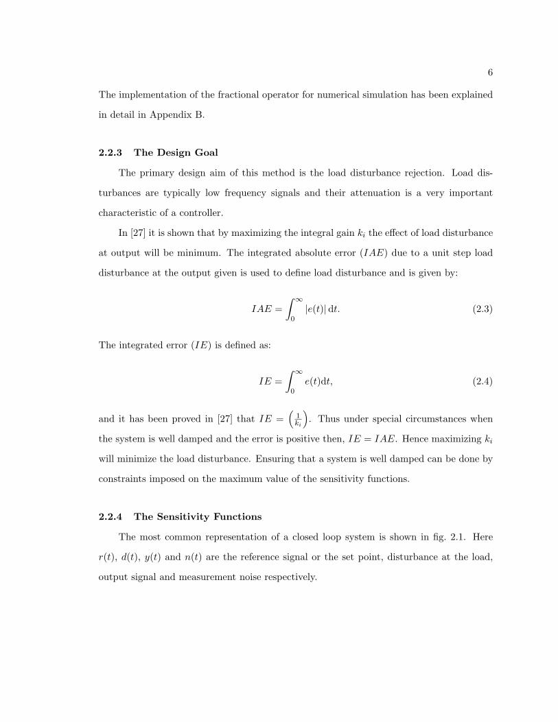
In [27] it is shown that by maximizing the integral gain ki the effect of load disturbance

at output will be minimum. The integrated absolute error (IAE) due to a unit step load

disturbance at the output given is used to define load disturbance and is given by:

IAE =∫ ∞

0|e(t)|dt. (2.3)

The integrated error (IE) is defined as:

IE =∫ ∞

0e(t)dt, (2.4)

and it has been proved in [27] that IE =(

1ki

). Thus under special circumstances when

the system is well damped and the error is positive then, IE = IAE. Hence maximizing ki

will minimize the load disturbance. Ensuring that a system is well damped can be done by

constraints imposed on the maximum value of the sensitivity functions.

2.2.4 The Sensitivity Functions

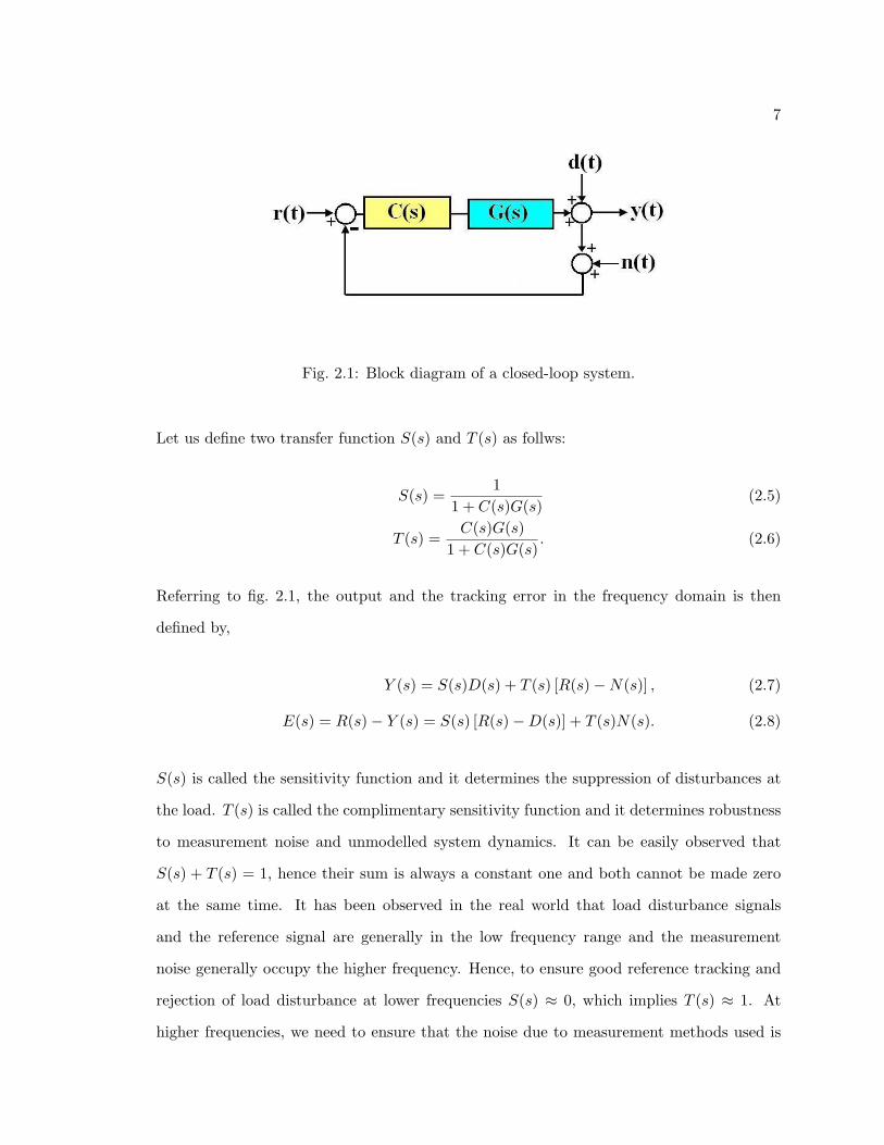
The most common representation of a closed loop system is shown in fig. 2.1. Here

r(t), d(t), y(t) and n(t) are the reference signal or the set point, disturbance at the load,

output signal and measurement noise respectively.

7

Fig. 2.1: Block diagram of a closed-loop system.

Let us define two transfer function S(s) and T (s) as follws:

S(s) =1

1 + C(s)G(s)(2.5)

T (s) =C(s)G(s)

1 + C(s)G(s). (2.6)

Referring to fig. 2.1, the output and the tracking error in the frequency domain is then

defined by,

Y (s) = S(s)D(s) + T (s) [R(s)−N(s)] , (2.7)

E(s) = R(s)− Y (s) = S(s) [R(s)−D(s)] + T (s)N(s). (2.8)

S(s) is called the sensitivity function and it determines the suppression of disturbances at

the load. T (s) is called the complimentary sensitivity function and it determines robustness

to measurement noise and unmodelled system dynamics. It can be easily observed that

S(s) + T (s) = 1, hence their sum is always a constant one and both cannot be made zero

at the same time. It has been observed in the real world that load disturbance signals

and the reference signal are generally in the low frequency range and the measurement

noise generally occupy the higher frequency. Hence, to ensure good reference tracking and

rejection of load disturbance at lower frequencies S(s) ≈ 0, which implies T (s) ≈ 1. At

higher frequencies, we need to ensure that the noise due to measurement methods used is

8

Fig. 2.2: Bode plot of sensitivity functions for a typical system. (Blue line: S(s); GreenLine: T (s)).

rejected. Hence, T (s) ≈ 0, which implies S(s) ≈ 1. Clearly there is a design trade off

between the S(s) and T (s) in frequency domain. The typical Bode plots of the sensitivity

and complimentary sensitivity functions are shown in fig. 2.2.

The maximum value’s of the sensitivity functions S(s) and T (s) are denoted by Ms

and Mp respectively and given by,

Ms = max0<ω<∞

|S(iω| , (2.9)

Mp = max0<ω<∞

|T (iω| . (2.10)

Note that Ms is also the inverse of the shortest distance of the Nyquist curve of the loop

transfer function, L(s) = C(s)G(s), from the critical point (−1, j0) in the complex plane.

A circle drawn with center at (−1, j0) with radius 1/Ms is called the “Ms circle”. Hence,

by imposing a constraint on the value of Ms, we must ensure that the Nyquist curve of the

loop transfer function, L(s), lies outside the Ms circle. The typical values that Ms takes

lies in the range of 1.3 to 2.0. The quantity Mp is the value of the resonance peak of the

9

Fig. 2.3: Sensitivity circles for a typical system. (Solid line: Ms circle; Dashed line: Mp

circle; Dotted line: Unit circle).

closed-loop system and typically lies in the range 1.0 to 1.5. The “Mp circle” is drawn with

center at (−M2p /(M2

p − 1), j0) with radius Mp/(M2p − 1). If we impose a constraint on the

value of Mp then we must ensure that the Nyquist curve of the loop transfer function, L(s),

lies outside the Mp circle. The fig. 2.3 explains the concept of Ms and Mp circles.

2.2.5 The Design Parameters

It has been shown in [24, 25] that choosing Ms as the design parameter is useful as

decreasing or increasing its value causes significant changes in the step response of the

system. However, it is important that the value of Mp is also not very large. This problem

is overcome by choosing the design parameter to be a circle such that this circle encloses

both the Ms and Mp circles. This circle has its center at (−C, j0) with radius R given by:

C =Ms −MsMp − 2MsM

2p + M2

p − 12Ms

(M2

p − 1) , (2.11)

R =Ms + Mp − 12Ms

(M2

p − 1) . (2.12)

10

2.3 The Optimization Problem

The previous section gives a detailed description of the sensitivity constraint. The

mathematical requirement can be stated as,

“Maximize ki to obtain the controller parameters such that the closed-loop system is stable

and the Nyquist curve of the loop transfer function lies outside the circle with center at

s = −C and radius R” [24].

Now, define a function f(k, ki, ω) as:

f(k, ki, ω, α) = |C + C(iω)G(iω)|2 . (2.13)

The sensitivity constraint can be expressed mathematically as:

f(k, ki, ω, α) ≥ R2. (2.14)

Therefore the optimization problem amounts to the maximizing ki subjected to the sensi-

tivity constraint (eq. 2.14).

Some important substitutions have to be made (eq. 2.14) before we go any further with

the analysis of the optimization problem.

• The PIα controller transfer function is defined as:

C(iω) = k +ki

(iω)α. (2.15)

• Here we make another important substitution for 1/(iω)α,

1/(iω)α = (i−α)(ω)−α = e(−iπα2 )ω−α = cos(γ)ω−α − sin(γ)ω−α, (2.16)

where

γ =πα

2.

11

• The system transfer function can be expressed as in complex number in the frequency

domain as:

G(iω) = a(ω) + ib(ω) = r(ω)eiφ(ω), (2.17)

where

a(ω) = r(ω) cos φ(ω),

b(ω) = r(ω) sinφ(ω),

r2(ω) = a2(ω) + b2(ω).

We substitute (2.15), (2.16) and (2.17) in the sensitivity constraint (2.14) to obtain a sim-

plified optimization problem. In the subsequent derivations, ω in all the functions of ω will

be dropped for simplicity.

f =∣∣∣∣C +

[k +

ki

ωα(cos (γ)− i sin (γ))

] [a + ib

]∣∣∣∣2 ≥ R2. (2.18)

Now, we will consider only the left hand side (LHS) of the above equation.

f =∣∣∣∣[C + ak +

aki cos (γ)ωα

+bki sin (γ)

ωα

]+ i

[bk +

bki cos (γ)ωα

− aki sin (γ)ωα

]∣∣∣∣2 .

Using the identity |x + iy|2 = x2 + y2 in the previous equation, we get,

f =[C + ak +

aki cos (γ)ωα

+bki sin (γ)

ωα

]2

+[bk +

bki cos (γ)ωα

− aki sin (γ)ωα

]2

.

Expanding and canceling all the common terms, we finally arrive at the simplified optimiza-

tion problem,

f = C2 + r2k2 + 2Cak +k2

i r2

ω2α+

2r2kki cos (γ)ωα

+2Cki (a cos (γ) + b sin (γ))

ωα≥ R2. (2.19)

12

In the next section, a geometric interpretation of the sensitivity constraint (2.19) will be

discussed.

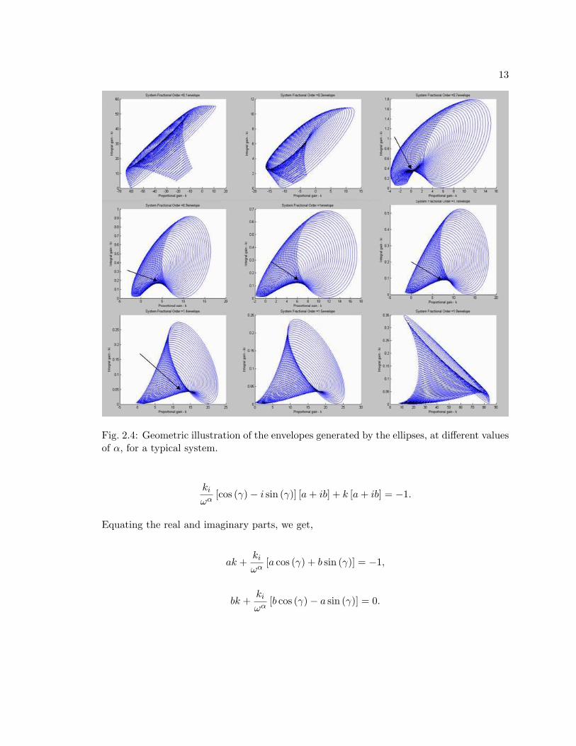
2.3.1 Geometric Interpretation of the Sensitivity Constraint

Equation. 2.19 represents the general equation of an ellipse. Hence, at a given value

of ω, the sensitivity constraint represents the exterior of an ellipse. In [24], it has been

assumed that positive values of ki and k will ensure a stable closed loop system. However,

the difference here is that we have to plot the ellipses at varying values of α also. In fig. 2.4,

we observe how the axis of the ellipse rotates with different values of α. In [24], it has been

mentioned that the ellipses generate an envelope. A detailed description of the general

equation of an ellipse and the conditions for existence is described in Appendix C. We can

plot the ellipses at different ω using any of the standard tools available in MATLAB.

The envelopes have two branches and only the lower branch corresponds to the stable

solution [24]. Hence the maximum value of ki occurring at the lower branch of the envelope

will be the optimal point. This is indicated by the graphs with an arrow marking the

position of the maximum value of ki in fig. 2.4. Another observation is that a solution

cannot be found at all fractional orders. We observe that it is not easy to find a region of

optimization in all graphs, concluding that a solution satisfying the optimization constraint

may not exist at these fractional orders. The geometric illustration of the optimization

problem is easy to understand, however it is time consuming to find the envelopes at each

order as different systems may show different characteristics. Therefore, a reliable numerical

approach is needed which will be discussed in the next section.

2.3.2 Stability Regions of the Sensitivity Constraint

The stability region can be found by checking for the boundary conditions which are

defined at the critical point or the point where C = 1 and R = 0. Substituting these values

in eq. 2.18, we get, ∣∣∣∣1 +ki

ωα[cos (γ)− i sin (γ)] [a + ib]

∣∣∣∣2 = 0,

13

Fig. 2.4: Geometric illustration of the envelopes generated by the ellipses, at different valuesof α, for a typical system.

ki

ωα[cos (γ)− i sin (γ)] [a + ib] + k [a + ib] = −1.

Equating the real and imaginary parts, we get,

ak +ki

ωα[a cos (γ) + b sin (γ)] = −1,

bk +ki

ωα[b cos (γ)− a sin (γ)] = 0.

14

Solving the above equations we obtain the parametric description of the stability region

boundary.

ki = − bωα

r2 sin (γ), (2.20)

k =b cos (γ)r2 sin (γ)

− a sin (γ)r2 sin (γ)

. (2.21)

2.4 Numerical Solution of the Optimization Problem

2.4.1 The Optimization Problem

The figures shown in the previous section represent the solution space, and the op-

timization condition implies that we find the value of ω which gives the maximum ki.

However, it is not easy to generate the envelopes for each system hence efficient numerical

methods have to be derived. The envelopes show the following characteristics:

• Some envelopes will have a continuous derivative at the maximum.

• Some maxima can occur at the corners.

We will consider only the first case in this thesis i.e. envelopes with continous derivative at

the maximum. It is important to observe here that we will consider the fractional order to

be a constant in the subsequent derivations.

The envelope can be described mathematically by the following equations

f(k, ki, ω, α) = R2

∂f

∂ω(k, ki, ω, α) = 0.

(2.22)

The optimization condition as explained before implies finding the maximum ki on the

envelope defined by the eq. 2.22. Considering the case where the maxima occurs at the

point where the envelope has a continuous derivative we can observe that,

df =∂f

∂kdk +

∂f

∂kidki +

∂f

∂ωdω = 0. (2.23)

15

Again, it is important to emphasize the fact that the fractional order α is treated as a

constant in the algorithm. In eq. 2.23, we observe the following:

• From eq. 2.22 we have ∂f∂ω = 0,

• For the local maximum condition dki = 0,

• We impose, that for random variations of dk, ∂f∂k = 0.

Hence, with the above mentioned conditions, the mathematical definition of the optimiza-

tion problem for the simplest scenario of maximum occurring at the point of continuous

derivative is given by:

f(k, ki, ω, α) = R2,

∂f

∂ω(k, ki, ω, α) = 0,

∂f

∂k(k, ki, ω, α) = 0.

(2.24)

The scenario for corner case has not been investigated in this thesis as the first scenario is

the most commonly encountered, but it is assumed that it will follow the same methodology

adopted in [24, 25]. Hence, we have reduced the optimization problem to solving a set of

algebraic equations. Some simplification methods will now be applied to eq. 2.24 and the

simplified optimization problem will be solved using the Newton-Raphson technique as in

[24]. A detailed description of the Newton-Raphson technique can be found in Appendix D

[30].

2.4.2 Simplification of the Optimization Problem

As observed in the previous section the optimization problem was shown to be the

solution of a set of algebraic equations. However, this is a non-linear equation of three

variables and some simple substitutions will give rise to a simple and efficient algorithm as

will be shown in this section.

16

From sec. 2.3, we insert the eq. 2.19 into the eq. 2.23 and solve it to get the following

set of equations,

C2 + r2k2 + 2Cak +k2

i r2

ω2α+

2r2kki cos (γ)ωα

+2Cki (a cos (γ) + b sin (γ))

ωα= R2, (2.25)

∂f

∂ω= 2k2rr′ + 2Cka′ + k2

i

(r2

ω2α

)′+ 2kki cos (γ)

(r2

ωα

)′+ 2Cki cos (γ)

( a

ωα

)′+ 2Cki sin (γ)

(b

ωα

)′= 0, (2.26)

∂f

∂k= 2kr2 + 2Ca +

2r2ki cos (γ)ωα

= 0. (2.27)

In the above equations, the prime implies differentiation with respect to ω and,

(r2

ω2α

)′=

2rr′

ω2α− 2αr2

ω2α+1,(

r2

ωα

)′=

2rr′

ωα− αr2

ωα+1,( a

ωα

)′=

a′

ωα− aα

ωα+1,(

b

ωα

)′=

b′

ωα− bα

ωα+1.

(2.28)

Solving eq. 2.27, derive an expression for k in terms of ki and ω as shown below,

2kr2 + 2Ca +2r2ki cos (γ)

ωα= 0,

k = −ki cos (γ)ωα

− Ca

r2. (2.29)

17

Now substitute eq. 2.29 into eq. 2.25 to solve for k and ki as shown in the subsequent steps

below,

C2 +r2k2

i cos2 (γ)ω2α

+C2a2

r2+

2Caki cos (γ)ωα

− 2Caki cos (γ)ωα

− 2C2a2

r2+

k2i r

2

ω2α+

2r2ki cos (γ)ωα

[−ki cos (γ)

ωα− Ca

r2

]+

2Cki

ωα[a cos (γ) + b sin (γ)]−R2 = 0.

Simplifying and canceling all the common terms,

C2 +k2

i r2

ω2α− C2a2

r2+

2Cbki sin (γ)ωα

− r2k2i cos2 (γ)ω2α

−R2 = 0,

k2i r

2 sin2 (γ)ω2α

+2Cbki sin (γ)

ωα+ C2 − C2a2

r2−R2 = 0.

Now, to complete the squares we add and subtract the term −C2b2 to the previous equation

and proceed,

(kir

2 sin (γ)ωα

+ Cb

)2

+ Cb = −Rr.

Hence, we obtain the equation for ki in terms of ω, R, C and α.

ki = − Rωα

r sin (γ)− Cbωα

r2 sin (γ). (2.30)

Now substitute eq. 2.30 into eq. 2.29 to obtain the expression for k in terms of ω, R, C and

α:

k = Rcos (γ)sin (γ)

+Cb

r2

cos (γ)sin (γ)

− Ca

r2. (2.31)

Equation. 2.30 and eq. 2.31 represent the solution for finding the gains of the controller.

However, they are dependent on the value of ω. Thus, we need to solve for ω which gives

the maximum value of ki. Now, substitute the expressions for k and ki and eq. 2.28 into

18

eq. 2.26 for the final simplification of the optimization problem.

The next set of derivations is very complicated and will be handled in parts, the eq. 2.26

has six individual terms and each will be solved separately and then common terms will be

combined for the final simplification.

The first term,

2k2rr′ =2R2 cos2 (γ)

r sin2 (γ)r′ +

2C2b2 cos2 (γ)r3 sin2 (γ)

r′ +2C2a2

r3r′

− 4RCa cos (γ)r2 sin (γ)

r′ +4RCb cos2 (γ)

r2 sin2 (γ)r′ − 4C2ab cos (γ)

r3 sin (γ)r′.

The second term,

2Cka′ =2RC cos (γ)

r sin (γ)a′ − 2C2b cos (γ)

r2 sin (γ)a′ − 2C2a

r2a′.

The third term,

k2i

(r2

ω2α

)′=

2R2

r sin2 (γ)r′ +

2C2b2

r3 sin2 (γ)r′ +

4RCb

r2 sin2 (γ)r′

− 2R2α

ω sin2 (γ)− 2C2b2α

r2ω sin2 (γ)− 4RCbα

rω sin2 (γ).

The fourth term,

2kki cos (γ)(

r2

ωα

)′= −4R2 cos2 (γ)

r sin2 (γ)r′ − 4RCb cos2 (γ)

r2 sin2 (γ)r′ +

4RCa cos (γ)r2 sin (γ)

r′

− 4RCb cos2 (γ)r2 sin2 (γ)

r′ − 2C2b2 cos2 (γ)r3 sin2 (γ)

r′ +4C2ab cos (γ)

r3 sin2 (γ)r′

+2αR2 cos2 (γ)

ω sin2 (γ)+

2αRCb cos2 (γ)rω sin2 (γ)

− 2αRCa cos (γ)rω sin (γ)

+2αRCb cos2 (γ)

rω sin2 (γ)+

2αC2b2 cos2 (γ)r2ω sin2 (γ)

− 2αC2ab cos2 (γ)r2ω sin2 (γ)

.

19

The fifth term,

2Cki cos (γ)( a

ωα

)′= −2RC cos (γ)

r sin (γ)a′ − 2C2b cos (γ)

r2ω sin (γ)a′

+2αRCa cos (γ)

rω sin (γ)+

2αC2ba cos (γ)r2ω sin (γ)

.

The sixth term,

2Cki sin (γ)(

b

ωα

)′= −2RC

rb′ − 2C2b

r2b′ +

2αRCb

rω+

2αC2b2

r2ω.

Combining all the r′, a′ and b′ terms and simplifying we get the following equation,

∂f

∂ω=

2R2

rr′ +

4RCb

r2r′ − 2αR2

ω− 2αRCb

rω− 2RC

rb′.

This can be further simplified as in [24] to get a simple algebraic equation as shown below,

h(ω) =∂f

∂ω= 2R

([C

b

r+ R

] [r′

r− α

ω

]− C

(b

r

)′). (2.32)

Hence, the optimization problem reduces to the eq. 2.32. Solving this equation will give the

frequency ωo at which ki is maximized and we can compute k and ki given by eq. 2.31 and

eq. 2.30, respectively.

2.5 The F-MIGO Algorithm

The flowchart of the F-MIGO algorithm is presented in fig. 2.5. The next section takes

a typical example and explains the process of selection for the controller parameters. The

code for the implementation has been listed in Appendix F.

2.6 Validation of the F-MIGO Algorithm

This chapter presents a generalized MIGO design algorithm to find the gains of the

FO-PI controller, based on the principle adopted in [24] for PI controller, given a fixed α.

The generalization here implies that we can find controller parameters at any given value of

20

Choose any system

If the reader is unaware or unable to find a suitable starting value it is

suggested to find solutions at all these starting values.

Example: Range =[.01,.03,.05,.08,.1,.3,.5,.8,1,1.5,2,2.5,3,3.5,4,5,6]

Choose Ms and Mp

values. Calculate C and R

Choose the fractional order 0< α <2

Ex: α = .5

Begin the Newton Raphson

technique to find solution of h (w)

Choose an initial value of ω from Range.

Compute the function h (w).

Compute the next iteration until h (w) reaches

zero. Final solution = wo where h (wo) = 0.

Evaluate k and ki at w0 . Are

they both positive ?

Change the initial value

Solution may not exist, change order.

Have all the initial values been checked ?

Check!•Loop transfer function sensitivities ? Ms should be near 1.4 and Mp should lie in the range 1.0-1.4.•Is Closed Loop Stable ?•If Multiple solution exist then choose the one with the largest value of ki

Good Solution!Store all data in excel sheet.

Change Ms and/ or Mp

T

T

T

F

F

F

Fig. 2.5: The F-MIGO algorithm (T: true , F: false).

fractional order of the integrator such that the optimization constraint is satisfied. Hence,

the validation of the generalized method has to be made at α = 1, i.e., the integer order.

We will consider a set of six systems which are normally encountered in control systems

and have also been considered in [24]. These systems satisfy the monotonicity condition

which implies that these systems have a unique solution and also the largest value of ki

occurs at a continuous derivative. The six systems are listed below, G1(s) and G2(s) are

easy to control, G3(s) has a large relative dead time, G4(s) is an integrating system, G5(s)

and G6(s) are not commonly encountered. However, these systems give an example of the

21

wide applicability of the algorithm [24].

G1(s) =1

(s + 1)2,

G2(s) =1

(s + 1)(0.2s + 1)(0.04s + 1)(0.008s + 1),

G3(s) =e−15s

(s + 1)3,

G4(s) =1

s(s + 1)2,

G5(s) =1− 2s

(s + 1)3,

G6(s) =9

(s + 1)(s2 + 2s + 9).

Table 2.1 gives the results of the controller parameters designed using the F-MIGO method

while setting α = 1. Comparing this with the results in [24], we observe that the results

are very close. These results validate the generalization of the F-MIGO method and now it

can be used to find the controller parameters at other values of α. In the next section, the

procedure of using the algorithm to find the solution at an arbitrary α for a typical system

will be discussed.

2.7 The Selection Process for An Arbitrary α

Consider a typical system G(s) given by eq. 2.33. We will apply the F-MIGO algorithm

to this system for α in the range (0.1− 1.9) and try to find a solution.

G(s) =e−s

(s + 1). (2.33)

The first step towards finding the solution is to solve for α = 1, i.e., find the optimal PI

controller, using the initial range shown in fig. 2.5. Since this system is monotonic, the

solution will be unique. The algorithm has been written to check for all values of initial

solutions supplied by the user and the final result is written into an excel sheet. A flag value

is set to zero if all the conditions of a good solution are satisfied. In fig. 2.6, observe that

the flag column is set to the value 0, when k, ki are positive and Ms and Mp values are also

22

Table 2.1: Validation of the F-MIGO method for G1-G6.

Process α Ms k ki Mp ωo

G1(s) 1.0 1.4 0.633 1.945 1.00 0.7371.6 0.861 1.868 1.04 0.7871.8 1.053 1.816 1.24 0.8272.0 1.218 1.779 1.45 0.860

G2(s) 1.0 1.4 1.930 0.744 1.10 3.3781.6 2.741 0.671 1.27 3.8201.8 3.469 0.622 1.46 4.1802.0 4.112 0.587 1.66 4.470

G3(s) 1.0 1.4 0.156 5.862 1.00 0.0961.6 0.201 5.667 1.00 0.0981.8 0.233 5.480 1.02 0.1002.0 0.258 5.352 1.17 0.102

G4(s) 1.0 1.4 0.167 13.64 1.40 0.2931.6 0.231 10.43 1.50 0.3431.8 0.285 8.967 1.62 0.3772.0 0.332 7.960 1.77 0.407

G5(s) 1.0 1.4 0.177 1.758 1.00 0.3851.6 0.223 1.685 1.00 0.3971.8 0.264 1.627 1.04 0.4072.0 0.292 1.583 1.20 0.415

G6(s) 1.0 1.4 0.313 0.373 1.04 1.9851.6 0.386 0.343 1.15 2.0381.8 0.440 0.325 1.26 2.0782.0 0.482 0.312 1.37 2.108

in the acceptable range. We observe that the solutions starting from different initial values

are very close in value. We choose among them the largest value of ki as the final solution

thus we have a solution at wo = 1.026 colored green in fig. 2.6.

Figure 2.7 describes how the solution is obtained for different values of fractional order.

It has been observed that not all fractional order can lead to a solution and hence they have

been omitted from the list. Observe the occurrence of close solution points and also the fact

that the wo for each α lies very close to the one obtained for the integer order controllers,

i.e., α = 1. This section concludes the introduction of the F-MIGO algorithm. We now have

an understanding of the design method and how it can be applied to different systems. The

algorithm has also been validated at α = 1, thus proving that it is indeed a generalization.

23

Fig. 2.6: Solution of G(s) at α = 1. The best solution corresponds to the largest value ofki which has been marked with green color.

We have also studied the selection process by which we can select the correct solution for

any system at a given value of fractional order. The next chapter uses the F-MIGO method

to obtain tuning rules for systems which can be approximated with a good FOPDT model.

24

Fig. 2.7: Solution at other values of fractional order for G(s).

25

Chapter 3

Practical Tuning Rules for FO-PI Controllers

The discussion in this chapter is an extension the work shown in the paper [31].

3.1 Introduction

Chapter 2 gives us an algorithm for designing a FO-PI controller given that the system

transfer function and fractional order are known. By scanning for different values of the

fractional order, a solution range can be found. However, like the Ziegler-Nichols method,

there is a need to eliminate this entire procedure. The need for simple rules which depend

on the process dynamics is important for faster design of the controller. The method of

finding such tuning rules is in fact quite simple. We pick a known reliable design method

with some desired characteristics and apply to a large test batch of systems which may have

some common characteristic or behavior and then try to establish a relationship between

the controller parameters and the process dynamics. In [26], the MIGO design method

has been applied to a set of monotonic systems and Ziegler-Nichols type tuning rules,

called Approximate Ms constrained Integral Optimization (AMIGO), have been derived.

The method followed in this chapter is on similar lines. Find simple tuning rules like the

AMIGO method to design fractional order controllers for those systems which can be easily

approximated by an FOPDT model. We will now proceed with the development of the

tuning methods.

3.2 FOPDT Model

The introduction of test batch is incomplete without a brief description of the FOPDT

model. The First Order Plus Delay Time (FOPDT) model is also known as the KLT model

and is given by eq. 3.1. Figure 3.1 illustrates the FOPDT parameters given the S-shaped

26

step response of a FOPDT class system. Kp is defined as the steady state gain. L is

called the apparent delay determined at the point where the largest slope intersects the

time axis and T, apparent time constant, is determined from the time where the largest

slope intersects the steady state level. FOPDT system’s are characterized by an important

parameter called the relative time delay τ defined in eq. 3.2. This parameter lies in the

range of 0 to 1.0, and is comparable to the controllability ratio L/T , considered in classical

control systems. Systems with τ > 0.6, are called delay dominated systems and systems

with τ < 0.1 are called lag dominated systems. See Appendix E for matlab code to generate

the FOPDT models for a monotonic system from its transfer function [32].

G(s) = Kpe−Ls

(Ts + 1). (3.1)

τ =L

L + T. (3.2)

0 2 4 6 8 10

-0.2

0

0.2

0.4

0.6

0.8

1

1.2

Step Response

Time (sec)

Amplitude

TL

Kp

Fig. 3.1: Illustration of the procedure for determining the FOPDT model from the step-response curve.

27

3.3 The Test Batch

The first test batch to be used in this thesis was the set of systems considered in

equation(2) of [26]. However, since all these systems can be approximated with a FOPDT

model it was decided that a set of FOPDT systems would be a good choice for developing

the tuning rules. Since we are trying to establish a relationship between the controller

parameters and the relative dead-time, it was essential that the systems considered would

span the entire range of τ . The cases of τ = 0 and τ = 1, are special systems and will

be considered later in this chapter. Hence, to build a test batch for the system, we first

considered a set of values for the relative dead time as shown in eq. 3.3. The next parameter

to be considered is a set of delays as shown in eq. 3.4. It has been assumed that all these

processes have been normalized to have unit steady state gain. Therefore, Kp = 1 for all

the systems in the test batch.

Tau = .99, .9, .8, .7, .6, .5, .4, .3, .2, .1, .05, .01, .009. (3.3)

Lset = 20, 10, 1. (3.4)

Using the relationship in eq. 3.2, we can derive the values of the time constant T .

Hence, the test batch consists of 39 systems. A nomenclature will be followed to address

each of these systems. Sys(xy) of Type(x) is used to denote any system such that x takes

the value 1, 2, 3 and y takes the values in 1:1:13. Hence, a system which is designated as

Sys12 implies that it is a FOPDT model with L = 20 and τ = 0.9 and belongs to the Type1

class of systems.

3.4 Selection of the Best Fractional Controller

There are three controller parameters in the case of a FO-PI controller, namely, the

fractional order α, the proportional gain k and the integral gain ki which have to be cor-

related with the process dynamics. The F-MIGO can give the controller at a given value

of fractional order, α, but we need to find the optimal one. This problem is tackled by

28

Algorithm 3.1 Selection of best fractional controller for Sys(xy).Input:

Tau,Lset,Value of x,Value of y.

Output:Best Fractional Controller (α∗, K∗, K∗

i ) for Sys(xy).Begin

Select range of intial solutions,Select the value of Ms and Mp,Apply F-MIGO for α = 1,Narrow down the range near the solution wo for α = 1,Begin

Repeat F-MIGO design procedure for the remaining values of fractional order.EndCreate a table for the solutions.Begin

Run closed loop simulation at each solution.Find the ISE value during each simulation.

EndCompare the ISE values at all solutions.Choose the solution with the minimum ISE value.Label this solution with a (*)

End

scanning each system for fractional order controllers in the range (0.1− 1.9) making a total

of 741 simulations for the 39 systems considered. Now, the question is to arrive at the

best controller among the solutions found. To solve this problem, a number of closed-loop

performance parameters like Gain margin (GM), Phase margin (PM), Integrated squared

error (ISE), Overshoot , Settling time and Rise time were compared and among these ISE

was chosen to be the deciding factor as the other parameters did not show any significant

pattern with change in α. This procedure is explained clearly in algorithm 3.1.

Figure 3.2 shows the selection process for the Type1 class of systems. This type has a

total of 13 systems which have been labeled Sys11-Sys113. During simulations, the following

properties were observed:

29

Fig. 3.2: Procedure for choosing the best FO-PI controller for a given system.

• As the value of τ decreases from 1 to 0, the range of feasible fractional controller

increases. This can be observed in fig. 3.2 which shows the selection process for

systems of Type1. For Sys11 we have feasible FO-PI controllers in the range (0.8−1.4)

and in Sys113 the range spans (0.6− 1.5).

• The ISE Criterion table in fig. 3.2 gives ISE values of the closed loop response of

each feasible controller obtained for each of the Type1 systems. The minimum ISE

value has been marked in yellow and this corresponds to the best fractional controller

for that system.

• The last table lists out the best controller obtained for each system of class Type1. It

is important to note the trend of best fractional order with the decreasing value of τ .

The above procedure is now repeated for Type2 and Type3 systems and the best fractional

controller (α∗,K∗,K∗i ) is found for each system. The next section explains how the tuning

rules are obtained.

30

Fig. 3.3: Best fractional order (α∗) versus relative dead-time (τ).

3.5 Tuning Rules

3.5.1 α∗ versus τ

Figure 3.3 gives the relationship between the best fractional order and τ and reveals

some interesting properties. The best fractional order, α∗, depends on the value of τ

and is almost invariant to the value of L. The ambiguous τ region between 0.4 and 0.6

implies that the best fractional order is close to unity indicating that an integer order is

predicted for these systems. Delay dominated systems need a little more than an integer

order and lag dominated systems can be controlled efficiently with a lower order controller.

This relationship can be mathematically explained in eq. 3.5. The border cases can be

approximated to the lower fractional order.

α =

1.1 if τ ≥ 0.6

1.0 if 0.4 ≤ τ < 0.6

0.9 if 0.1 ≤ τ < 0.4

0.7 if τ < 0.1 .

(3.5)

3.5.2 Normalized Controller Gains Versus τ

31

(a)

(b)

Fig. 3.4: Normalized FO-PI gains (K∗,K∗i ) versus the relative dead time (τ).

The controller parameters are normalized, the proportional gains K∗ are multiplied by

their respective process gain Kp which in this case is unity and the integral gains T ∗i =

K∗/K∗i are divided by their respective process time constant T , and plotted versus τ as

seen in figures 3.4(a) and 3.4(b). The Curve Fitting Toolbox of Matlab has been used to

find the tuning rules in figures 3.4(a) and 3.4(b). It should be noted that the process of data

fitting may not reproduce the exact results of the analytical tuning and hence a region of

±5% or less about the tuning values should be considered. These rules are mathematically

32

described in eq. 3.6 and 3.7 as follows:

K∗ =1

Kp

(.2978

τ + .000307

); (3.6)

T ∗i = T

(.8578

τ2 − 3.402τ + 2.405

). (3.7)

3.5.3 Summary of Tuning Rules

Given a system transfer function or the step response, the tuning rules can be summa-

rized as follows:

1. Find the FOPDT model of the system and define the values Kp, L, T .

2. Find the relative dead time of the system τ .

3. From the value of τ , calculate the fractional order α from eq. 3.5.

4. Find the controller gains from eq. 3.6 and 3.7.

3.6 Simulation Verification

This section explores the advantages of applying the tuning rules shown in eq. 3.5,

3.6 and 3.7 on systems which can be approximated by a good FOPDT model. The tuned

FO-PI controller response is then compared with three existing popular integer order tuning

methods, namely, the Ziegler-Nichols (ZN), Modified ZN and the Approximate MIGO design

methods [33]. First, a brief description of the integer order tuning methods is given and

then the test batch is introduced. The results are summarized based on the value of τ . Some

special systems have also been analyzed using the new FO-PI controllers tuned using the

developed tuning rules. The code to find the PI controllers using the ZN or MZN method

can be found in Appendix F.

3.6.1 Tuning Methods for Integer Order PI Controllers

33

Ziegler Nichols Tuning Method

Ziegler and Nichols proposed a useful formula for evaluating the PI controller gains if

the FOPDT model of a system is known [22]. The rules are given below:

K =0.9T

KpL, (3.8)

Ki =K

3L. (3.9)

Modified Ziegler Nichols Tuning Method

This design method is based on Nyquist loop shaping method [34]. The controller, if

designed properly, can be used to move a point A on the Nyquist curve of the uncontrolled

point to an arbitrary position B on the Nyquist plot of the controlled plant. Suppose that

we have a define a point A on the complex plane defined by GA(jω0) = raej(π+φa) and we

want to move this point to B defined by GB(jω0) = rbej(π+φb). If the controller is defined

at ω0 as Gc(jω0) = rcejφc , we have,

rbej(π+φb) = rarce

j(π+φa+φc). (3.10)

Therefore, rc = rb/ra and φc = φb − φa. Based on this relationship, the PI controller gains

are given by:

K =rbcos(φb − φa)

ra, (3.11)

Ki =K

ω0tan(φa − φb). (3.12)

As a special case, when ra = 1/Kc and φa = 0 we obtain the Modified Ziegler Nichols tuning

method. Here, Kc is defined as the critical gain at the cross over frequency ωc. To ensure

Ti is positive, cos(φb) < 0. If rb and φb are chosen properly we can have a good control over

the overshoot and rise time of the controlled system, giving a definite advantage over the

ZN method.

34

Approximate MIGO Tuning Method

These tuning rules, called AMIGO (approximate MIGO), were developed by applying

MIGO to a large batch of monotonic systems and correlating the resulting PID parameters

to simple features of the process dynamics [26]. The practical tuning rules developed in

this thesis are a direct extension of the AMIGO tuning rules for a FO-PI case. The rules

for FOPDT systems is given by:

K =0.14Kp

+0.28T

KpL, (3.13)

Ki = K

[0.33L +

6.8LT

10L + T

]−1

. (3.14)

The three integer order PI design methods presented above are the most commonly

used methods. These have been picked to compare with the FO-PI controller presented

in this thesis. Some relevant performance characteristics that can be compared are the

step change and load disturbance response. The ISE value is another good performance

characteristic that should be compared. The reason that above PI controllers have been

chosen can be validated as follows:

1. The ZN method was among the first tuning methods to be developed for the PI

controllers. They are simple and give a good starting point for the designers. It is fair

to compare them with similar new methods for tuning FO-PI controllers and examine

if they have any advantage compared to the PI case.

2. The MZN method is an improvement upon the ZN method giving the designer a

greater control over the performance of the controlled loop. It is considered among

the better PI controller design methods and hence comparing a good PI and the newly

tuned FO-PI controller for the same plant helps us in understanding if a fractional

order is really necessary.

3. The practical tuning method is an extension of the AMIGO method for the FO-PI

case for FOPDT systems. Therefore, it is obvious that these two methods should be

35

compared to justify our use of the FO-PI controller.

3.6.2 Test Batch

Six processes have been considered for comparing the FO-PI controllers with the exist-

ing PI controllers. The processes are listed below in eq. 3.15. Table 3.1 lists the parameters

after approximating them with the FOPDT model using the code in the Appendix E. These

six systems have been considered such that we have two delay dominated systems (L >> T ),

two balanced lag and delay systems (L ≈ T ) and two lag dominated systems (L << T ).

Each of these systems are good representatives of the type of systems encountered in pro-

cess industry. The results has been discussed separately for the three different types of the

system.

G1(s) =1

.05s + 1e−s,

G2(s) =1

(s + 1)3e−15s,

G3(s) =1

(s + 1)4, (3.15)

G4(s) =9

(s + 1)(s2 + 2s + 9),

G5(s) =1

(s + 1)(1 + .2s)(1 + .04s)(1 + .008s),

G6(s) =1

(s + 1)(.2s + 1).

3.6.3 Results

Delay Dominated Systems

Table 3.2 summarizes the results obtained for lag dominated systems for the different

tuning strategies. Figures 3.5(a) and 3.5(b) show the step responses and load disturbance

36

Table 3.1: FOPDT parameters for systems G1(s)−G6(s).

System Kp L T τ TypeG1(s) 1 1 0.09 0.92 Delay dominatedG2(s) 1 16.23 1.76 0.9 Delay dominatedG3(s) 1 1.42 2.90 0.33 BalancedG4(s) 1 0.59 0.745 0.44 BalancedG5(s) 1 0.1436 2.65 0.051 Lag dominatedG6(s) 1 0.105 1.11 0.09 Lag dominated

responses for the two lag dominated systems. It is observed here that the FO-PI controlled

systems show a fairly better response compared to the sluggish integer order counterparts,

implying that systems with large dead time need a little more than just an integer order

integrator to improve their closed-loop control performance.

Balanced Lag and Delay Systems

Table 3.2 summarizes the results obtained for the balanced lag and delay systems for

different tuning strategies. Figures 3.6(a) and 3.6(b) show the step responses and load

disturbance responses for the two balanced lag and delay dominated systems. Systems

whose relative dead time falls in the range (0.3 < τ < 0.6) can be considered as lag balanced

systems. It has been observed that for these systems, the fractional order tends to be close

to 1. It also observed from the responses that the best controller cannot be clearly decided

for these systems. This leads us to believe that a fractional order may be unnecessary for

these systems.

Lag Dominated Systems

Table 3.2 summarizes the results obtained for lag dominated systems for the different

tuning strategies. Figures 3.7(a) and 3.7(b) show the step responses and load disturbance

responses for the two lag dominated systems. From the responses, it is very clear that

the F-MIGO controlled systems closed-loop performance is very good compared to the

integer order counterparts which show overshoot and oscillatory responses. Even though

37

Table 3.2: Controller parameters for systems G1(s)−G6(s).

G1(s) G2(s)Method α K Ki Ms ISE K Ki Ms ISE

F-MIGO 1.1 0.32 0.53 1.4 1.32 0.33 0.032 1.4 20.8ZN 1.0 0.41 0.24 1.7 2.00 0.42 0.014 1.7 32.3

MZN 1.0 0.44 0.46 1.9 1.33 0.44 0.028 1.9 21.7AMIGO 1.0 0.16 0.42 1.4 1.63 0.17 0.026 1.4 26.5

G3(s) G4(s)Method α K Ki Ms ISE K Ki Ms ISE

F-MIGO .9 .90 0.51 1.4 2.44 0.67 1.16 1.4 0.96ZN 1.0 1.55 0.40 2.0 2.10 1.06 0.70 1.9 0.89

MZN 1.0 1.71 0.39 2.1 2.08 1.18 0.70 2.0 0.88AMIGO 1.0 0.71 0.34 1.5 2.75 0.50 0.77 1.5 1.09

G5(s) G6(s)Method α K Ki Ms ISE K Ki Ms ISE

F-MIGO 0.7 5.76 5.66 1.40 0.29 3.43 7.64 1.41 .20ZN 1.0 11.85 26.3 2.41 0.31 6.90 21.3 2.32 .21

MZN 1.0 13.28 12.99 2.18 0.24 7.73 10.5 2.14 .17AMIGO 1.0 5.31 7.80 1.42 0.35 3.1 7.72 1.43 .25

the AMIGO method is comparable it shows a slightly larger overshoot compared to the

F-MIGO controller. This leads us to believe that systems with very small dead time may

not need a full integrator to give a good closed-loop response.

3.6.4 Special Systems

This section deals with those systems which show complex dynamics [24]. These sys-

tems cannot be typically approximated with a simple FOPDT model and hence the F-MIGO

algorithm has been directly applied to these systems and scanned for the fractional order in

the range of 0.1 : 0.1 : 1.9. The best controller is then selected based on the ISE criterion.

Pure time delay systems

Pure time delay system is given by the transfer function shown in eq. 3.16. This can

be considered an extreme case of the systems with large values of relative dead time, i.e.,

τ = 1.0. Table 3.3 shows the values obtained via the F-MIGO method for the values of

38

(a) G1(s)

(b) G2(s)

Fig. 3.5: Step response and load disturbance response for delay dominated systems G1(s)and G2(s). (Thick solid line: Practical tuning method; Thin line: ZN method; Dotted line:Modified ZN; Dash-dotted line: AMIGO method).

α considered. Systems with τ close to 1 seem to have a good solution only for α in the

range, 0.8 < α < 1.4 as shown in Table 3.3. Choosing the lowest value of ISE corresponds

to the value of α = 1.1 which again reinforces what has already been discussed for delay

dominated systems. Figure 3.8 shows the response for the obtained solutions.

G(s) = e−s. (3.16)

Pure integrator with time delay system

G(s) =e−s

s. (3.17)

39

(a) G3(s)

(b) G4(s)

Fig. 3.6: Step response and load disturbance response for balanced lag and delay systemsG3(s) and G4(s).(Thick solid line: Practical tuning method; Thin line: ZN method; Dottedline: Modified ZN; Dash-dotted line: AMIGO method).

Pure integrator with time delays is given by eq. 3.17. Following a similar approach,

we scan the system at different values of α and pick the best FO-PI controller based on

the minimum ISE value. Table 3.4 and fig. 3.9 give the summary of the run. The feasible

solutions was obtained for α in the range 0.4 < α < 1.5. However, the best fractional order

in this case is 0.7. Figure 3.9 shows the comparison of the FO-PI and PI controllers.

Observe that without a controller the system is oscillatory. However, with a controller the

oscillations are removed but the FO-PI also increases the rise time and decreases the settling

time compared to the PI controller.

Process with distributed lags

This is another type of special system encountered in control systems. Equation 3.18

40

(a) G5(s)

(b) G6(s)

Fig. 3.7: Step response and load disturbance response for lag dominated systems G5(s)and G6(s).(Thick solid line: Practical tuning method; Thin line: ZN method; Dotted line:Modified ZN; Dash-dotted line: AMIGO method).

represents the heat conduction in a rod [26]. The first step towards analysis of this process is

to find the FOPDT model. The “invfreqs” command in MATLAB finds a continuous-time

transfer function that fits a given complex frequency response of G(s).

G(s) =1

cosh√

s. (3.18)

G(s) =0.5757s2 − 56.86s + 2219

s3 + 64.58s2 + 1052s + 2219. (3.19)

G(s) ≈ e−0.083

0.583s + 1. (3.20)

The transfer function obtained from using the “invfreqs” command is given by (3.19). The

code listed in Appendix E helps in approximating the transfer function to an FOPDT model

41

Fig. 3.8: Pure time delay controlled with FO-PI controllers. Best FO-PI controller atα = 1.1 (dashed line) and corresponding gains: K = 0.292 and Ki = 0.73.

as shown in eq. 3.20. Equation 3.20 reveals that the relative dead time of the system is given

by τ = 0.13. Applying the tuning rules in section 3.5 we observe that a FO-PI controller

of α = 0.9 is required to control this system. Table 3.5 gives the controller parameters

and closed-loop performance characteristics for the four controllers. Figure 3.10 gives a

comparison of step responses of G(s) with FO-PI controller and the popular PI controllers.

This section presents yet another aspect of the practical tuning rule. Given a FOPDT

model we were able to obtain FO-PI controllers for the system, G(s). A number of closed

loop characteristics have been compared in table 3.5 giving us an idea of what each type of

controller can do the best. In this case, the F-MIGO tuning method and AMIGO give very

Table 3.3: Scan of fractional order controllers for pure delay system.

α K Ki wo Ms Mp ISE

0.8 0.075 1.104 1.81 1.40 1.0 1.3740.9 0.204 1.074 1.83 1.40 1.0 1.2781.0 0.157 0.472 1.73 1.40 1.0 1.4851.1 0.292 0.729 1.79 1.41 1.0 1.2091.2 0.291 0.606 1.77 1.41 1.0 1.3301.3 0.291 0.540 1.75 1.41 1.1 1.5131.4 0.288 0.500 1.73 1.41 1.2 1.8143

42

Table 3.4: Scan of fractional order controllers for pure integrator with time delay.

α K Ki wo Ms Mp ISE

0.4 0.141 0.173 0.564 1.40 1.2 2.4480.5 0.209 0.147 0.587 1.40 1.2 2.3790.6 0.262 0.123 0.599 1.40 1.2 2.3590.7 0.324 0.103 0.606 1.41 1.1 2.3480.8 0.351 0.087 0.606 1.40 1.1 2.3750.9 0.282 0.078 0.612 1.40 1.1 2.4071.0 0.365 0.042 0.544 1.40 1.1 2.7931.1 0.368 0.057 0.599 1.40 1.1 2.6451.2 0.375 0.051 0.593 1.40 1.2 2.8741.3 0.373 0.048 0.588 1.40 1.2 3.2451.4 0.377 0.044 0.578 1.40 1.2 4.0271.5 0.157 0.043 0.567 1.40 1.3 5.863

good responses. The FO-PI has a lower rise time but higher overshoot percentage. Thus,

the new tuning rules can be used to build simple FO-PI controllers which can be compared

to existing controllers.

3.7 Conclusions

This chapter uses the F-MIGO method to scan a set of FOPDT systems for the best

fractional order based on the ISE criterion. From the best FO-PI controllers, a relationship

was established between the controller parameters and the relative dead time τ of the

FOPDT systems. Tuning rules were then obtained from these relationships for the FOPDT

systems. Hence, given the step response of a system if the FOPDT model can be found, then

a fractional controller can be suggested for controlling the system. A comparison was then

Table 3.5: Controller parameters for system G(s).

Method α K Ki Ms Mp ISE OS TR TSF-MIGO 0.9 2.37 09.43 1.37 1.0 0.17 24.1 0.17 1.32

ZN 1.0 4.64 18.27 2.24 1.66 0.15 44.4 0.09 0.73MZN 1.0 5.20 09.05 2.11 1.36 0.13 25.1 0.09 0.61

AMIGO 1.0 2.09 08.00 1.45 1.26 0.19 20.2 0.22 1.20

43

Fig. 3.9: Pure integrator with time delay controlled with FO-PI controller. (Dashed line:Closed loop response without controller; Solid line: Best fractional order at α = 0.7 andcorresponding gains K = 0.324 and Ki = 0.103 (solid line); Dotted dashed line: Integerorder controller with K = 0.365 and Ki = 0.042).

made with the existing popular tuning methods for integer order PI controllers. From these

comparisons, the following conclusions can be drawn. Given the FOPDT model of a system,

if the relative dead-time is very small, it has been observed that a fractional PI controller

of order α ≈ 0.7 is found to outperform the integer order counterparts. For systems with

a balanced lag and delay values, an advantage of using a fractional controller cannot be

established. For systems with relative dead-time close to unity, it has been observed that

the fractional order α ≈ 1.1 speeds up the response compared to the sluggish integer order

counterparts. However with the disadvantage of having slightly higher overshoot.

Some special systems were also analyzed using the F-MIGO method directly as they

did not fall in the FOPDT class of systems. The results in these special cases again proved

that the FO-PI controller improves upon the PI controllers performance indicating that

certain systems require a fractional order control to achieve a better control performance.

The final special system considered was the process with distributed lags. A method

of obtaining the FOPDT model from the frequency response was discussed. A comparison

of FO-PI and PI controllers revealed certain advantages and disadvantages in the using the

FO-PI controllers.

The method presented in this chapter helps in synthesis of fractional controllers either

44

Fig. 3.10: Step responses of process with distributed parameter. (Dashed line: Responsewithout controller; Thick solid line: Practical tuning method; Thin line: ZN method; Dottedline: Modified ZN; Dash-dotted line: AMIGO method).

by directly applying the F-MIGO method or depending on the system FOPDT model.

The FO-PI controlled systems can then be compared with existing integer order systems to

observe any advantages of fractional order control. This concludes the simulation validation.

We will now apply the F-MIGO or the tuning rules to experimental platforms and validate

the usefulness of fractional order control by actual experiments.

45

Chapter 4

Experimental Verification of Practical FO-PI Tuning Rules

The discussion in this chapter is an extension of the work shown in the paper [35].

4.1 Introduction

The practical tuning method for fractional order proportional and integral controller

FO-PI was introduced in the previous chapter. The tuning rules require only the relative

dead time, τ , of the FOPDT model to determine the best fractional order α and also

determine the best FO-PI gains. This chapter attempts to apply these method to some

of the practical lab experiments encountered in Mechatronics [36], a senior and graduate

level course offered at the Department of Electrical and Computer Engineering of USU. The

course introduces digital control schemes, hardware-in-loop components, rapid prototyping

platforms and real-time operations. The two platforms are the Heat Flow Experiment

(HFE) and Rotary Flexible Joint (RFJ). The chapter is divided into four main sections:

Section 4.2 introduces the concepts of real-time control and hardware-in-loop. Sections 4.3

and 4.4 will give detailed description of each platform, system analysis, and design of a FO-

PI controller based on practical tuning approach. Section 4.5 introduces a special analog

instrument called the Fractroller which is designed specially for the control of the RFJ and

implements an analog FO-PI controller with a new class of electronic element called the

Fractor. Section 4.6 gives a conclusions and ideas for future work.

4.2 Quanser Real-Time Control Components

A typical feedback control system will have the following components: the Plant, Sen-

sors, Actuators and a Controller. In a digital real-time control application, the analog

controller is replaced by the digital computer (PC). They give the flexibility of changing

46

Fig. 4.1: Schematic of the real-time digital control of the hardware-in-loop setup.

the program according to the change in design requirements or dynamics of the system.

The digital controller needs feedback from the plant in the appropriate format which is

ensured by the DACB (Data Acquisition and Control Boards) provided by Quanser [37]. A

typical DACB board provided by Quanser is the MultiQ3 terminal board which has eight

single ended analog outputs and inputs, sixteen bits of digital inputs and outputs, three pro-

grammable timers and up to eight encoder inputs. These boards accept the sensor signals

from the plant and convert them to digital signals which is then sent back to the computer.

The code which emulates the controller computes on this data and decides the next set of

control signals and sends digital data to the DACB which converts it to an analog signal,

sent to the actuator via power amplifiers. All these operations are performed in real-time

and this is achieved by the real-time Windows2000/XP application WinCon which runs

the C code generated for the control law implemented in Simulink/MATLAB Real Time

Workshop. WinCon has two distinct parts: 1) WinCon Client - it is the real component

of the software and runs at a sampling period specified by the user, 2) WinCon Server -

it interfaces with the DACB unit and provides a graphical user interface for the user to

record the signals returned from the sensors. Schematic of the real-time, hardware-in-loop

configuration provided by Quanser is shown in fig. 4.1 [37].

4.3 Heat Flow Experiment

The HFE apparatus provided by Quanser helps in studying the conduction of heat

in a duct and control of temperature at particular locations along the duct. The experi-

47

Fig. 4.2: Heat flow apparatus.

ment helps students understand concepts of delay, first order system modeling and design

of controllers. Simple PI controllers can be designed for control as shown in the Quanser

manual [37]. However, in our study, we have gone a step further and found the FOPDT

models [27, 28] and used the tuning rules developed in chapter 3 to design an FO-PI con-

troller.

4.3.1 HFE Apparatus

The HFE apparatus shown in the fig. 4.2 consists of a long TUBE equipped with a

HEATER and FAN at one end, three temperature sensors (SENSOR1, SENSOR2, SEN-

SOR3) placed along the tube, and sealed with a VENT at the other end to allow air flow.

It has an in-built power module, analog inputs for controlling the fan and heater (VQ,

VF), three fast settling platinum temperature transducers that are used to measure the

temperature (T0, T1, T2). The fan speed is measured using a tachometer (SENSOR4).

Experimental setup

Figure 4.3 shows the experimental setup of the HFE experiment. The hardware com-

ponents as seen in the figure are the HFE and the DACB unit - MULTI PCI/Q3 Terminal

Board. The WinCon software runs the experiment in real-time. The senor signals on the

HFE are sent to the controller via the DACB unit. The analog inputs and the sensor outputs

are limited in the range (0-5 Volts). The temperature sensors are calibrated as 20◦C/V.

48

Fig. 4.3: HFE experimental setup.

The tachometer is calibrated as 1063 RPM/V.

4.3.2 Open Loop Response and Analysis

In the open-loop experiment, the fan (VF) and heater (VQ) voltages are applied in the

range of 0-5 Volts and the three temperature sensors sampled. It has been observed that

the heating operation takes effect only when VQ > 3 V. Figure 4.4 gives the responses at

VF = 4V and VQ = 3, 4 & 5V. The open loop response shows an initial delay, indicating

that it takes finite time for the sensors to detect the change in the temperature. In Quanser

documentation, a simple first order model has been derived at different settings of the fan

and heater voltages. However, from the open-loop response it is obvious that this modeling

is inadequate. A FOPDT model at a desired sensor is given by:

Tn

Vq= Kp

e−Ls

Ts + 1, (4.1)

where,

Min: Temperature in (◦C) inside the tube before the experiment begins.

Max: Maximum temperature in (◦C) reached after a run of sixty seconds. This is, strictly

speaking, not the steady state value as the temperature is still increasing. However the rate

49

Fig. 4.4: Open-loop step responses at the three sensors for VQ = [3, 4, 5] and fixed fanvoltage of 4 V. (Blue: T0n; Green: T1n; Red: T2n, where n =[3,4,5] to imply at which VQinput the readings are taken.)

of increase considerably slows down after 20 seconds.

Kp: The open loop gain is then given by (Max-Min)/VQ in (◦C/V).

L : The delay in the response in seconds.

T : The time constant is given by the time it takes to reach 63% of the change in temperature

or the time it takes for the response to reach Min + 0.63*(Max-Min).

τ : The relative dead time of the response given by L/(L + T ).

Table 4.1 summarizes the open-loop step response data at the different combinations

of VQ and VF. Some interesting trends in the open-loop behavior are observed. At a given

sensor and VQ, as VF increases, the open-loop gain decreases and relative dead time τ

increases. At a given sensor and VF, as VQ increases, the open-loop gain increases and

τ decreases. At a given VQ and VF, we observe that the open-loop gain decreases and

τ increases with the distance of the sensor from the heater. Table 4.1 indicates that the

system dynamics are dependent on the value of applied inputs.

4.3.3 Control Schemes in HFE

Different control schemes can be tested in the HFE apparatus, some are listed be-

low. The results will be presented according to the nomenclature presented below. All

50

Table 4.1: Step response data from open-loop experiment.

T0Kp (◦C/V ) L (seconds) T (seconds) τ

VQ|VF 3 4 5 3 4 5 3 4 5 3 4 53 4.7 4.3 4.0 0.35 0.36 0.36 13.22 12.00 09.95 0.026 0.028 0.0344 8.5 8.3 8.0 0.28 0.28 0.30 11.40 11.48 10.95 0.023 0.024 0.0265 8.4 8.0 7.8 0.21 0.21 0.22 11.32 11.90 09.94 0.018 0.019 0.021

T1Kp (◦C/V ) L (seconds) T (seconds) τ

VQ|VF 3 4 5 3 4 5 3 4 5 3 4 53 4.0 3.7 3.3 0.60 0.61 0.62 10.77 10.76 08.68 0.053 0.053 0.0644 7.3 7.0 6.7 0.50 0.50 0.53 10.67 10.40 09.47 0.045 0.046 0.0505 7.2 6.8 6.6 0.41 0.42 0.43 10.59 09.96 09.16 0.034 0.038 0.041

T2Kp (◦C/V ) L (seconds) T (seconds) τ

VQ|VF 3 4 5 3 4 5 3 4 5 3 4 53 3.6 3.3 3.3 0.78 0.78 0.80 12.37 12.72 10.72 0.057 0.060 0.0684 6.7 6.5 6.3 0.74 0.74 0.75 12.53 11.90 11.16 0.056 0.059 0.0625 6.6 6.2 6.0 0.69 0.70 0.71 12.20 11.60 10.87 0.054 0.056 0.060

experiments have been performed at the fixed fan voltage VF = 4V. Similar results can be

obtained at other values of the fan voltage.

• Type1: Control of temperature at T0 with feedback from T0.

• Type2: Control of temperature at T1 with feedback from T1.

• Type3: Control of temperature at T2 with feedback from T2.

• Type4: Control of temperature at T1 with feedback from T0.

• Type5: Control of temperature at T2 with feedback from T0.

• Type6: Control of temperature at T0 with feedback from T1.

• Type7: Control of temperature at T0 with feedback from T2.

51

Table 4.2: FO-PI gains at various combinations VQ/VF.

T0K Ki

VQ|VF 3 4 5 3 4 53 2.46 2.42 2.18 0.51 0.54 0.594 1.51 1.50 1.40 0.34 0.35 0.345 1.93 2.12 1.83 0.46 0.49 0.50

T1VQ|VF 3 4 5 3 4 5

3 1.41 1.54 1.39 0.34 0.37 0.414 0.92 0.93 0.88 0.23 0.23 0.245 1.13 1.13 1.08 0.28 0.30 0.31

T2VQ|VF 3 4 5 3 4 5

3 1.37 1.55 1.32 0.28 0.31 0.314 0.80 0.78 0.77 0.16 0.17 0.175 0.28 0.86 0.83 0.18 0.19 0.20

4.3.4 Tuning of FO-PI Controller for HFE

The FOPDT model describing the heating behavior is given by eq. 4.1. Table 4.1 lists

the model values, namely, Kp, L and T . However, we are interested in the value of τ given

in the last column. We observe that at any combination of VQ/VF, the system τ < 0.1,

indicating that the heating model requires a FO-PI controller of order = 0.7. Table 4.2

summarizes the controller gains obtained at each VQ/VF combination from the equations

presented in chapter 3. To make a worthwhile comparison, the counterpart integer order

PI controllers have also been designed to make a comparison with the FO-PI controllers.

Table 4.3 summarize the controller gains of the PI controller designed based on loop shaping

as shown in Quanser manual [37].

4.3.5 Implementation of the Tuned Controller

Table 4.1 indicates that the system dynamics change with different combinations VQ/VF.

Hence, it is important to have a dynamic controller whose gain values change depending on

the system closed-loop dynamics. This can explained as follows: When we begin heating

52

Table 4.3: PI controller gains at different combinations of VQ/VF.

T0K Ki

VQ|VF 3 4 5 3 4 53 3.46 3.36 2.30 1.47 1.44 1.304 1.62 1.68 1.65 0.67 0.72 0.715 1.63 1.80 1.30 0.70 0.77 0.66

T1VQ|VF 3 4 5 3 4 5

3 3.23 3.53 3.08 1.40 1.52 1.354 1.77 1.78 1.67 0.76 0.77 0.735 1.77 1.75 1.65 0.76 0.76 0.72

T2VQ|VF 3 4 5 3 4 5

3 4.10 4.65 3.87 1.75 1.98 1.674 2.236 2.22 2.16 0.96 0.95 0.925 2.42 2.27 2.18 0.96 0.97 0.94

a point along the duct from room temperature to a setpoint 30◦C above room temper-

ature we would first require VQ to be maximum. Once the setpoint has been achieved,

however, VQ should match the VF setting to maintain the temperature. This implies that

the system dynamics is changing as shown in table 4.1. Hence the controller has to be

dynamic too. This can be implemented in Simulink using switch logic with appropriate

decision signals. The fractional order integrator has been implemented using Oustaloup’s

recursive approximation [38]. The next section will present the results obtained for the HFE

experiment.

Figure 4.5 shows a sample of the Simulink model used in the HFE experiments. The

controller part of the model can be replaced by any controller structure designed by the user.

The “Heat Command” and “Fan Command” correspond to the analog output channels of

the Multi PCI/Q3 board. The sensor readings are obtained from the analog input channels

and converted to temperature readings. The “Select” line can be used to change the sensor

which is used as feedback signal. The next section will summarize the results for all the

control schemes implemented in the experiment.

53

Fig. 4.5: Simulink model used in the HFE experiments.

4.3.6 Results

Type1, Type2 and Type3

In this scheme, the controller aims to maintain the temperature at a particular sensor

with feedback from the same sensor. Figure 4.6 shows the control of T0 about the setpoint,

the FO-PI controller shows a much lesser overshoot and faster settling time compared to

its PI counterpart.

The control of T2 is satisfactory. However, the oscillations are not removed completely

0 10 20 30 40 50 60 70 80 90

30

35

40

45

Time in seconds

Temperature in degree Centigrade

Control of T0 about setpoint

T0 FO-PI

SETPOINT

T0 PI

Fig. 4.6: Response comparison of FO-PI and PI controllers for Type1 schemes.

54

0 10 20 30 40 50 60 70 80 9025

30

35

40

45

Time in seconds

Temperature in degree Centigrade

Control of T1 about setpoint

T1 - FO-PI

SETPOINT

T1 - PI

Fig. 4.7: Response comparison of FO-PI and PI controllers for Type2 schemes.

as seen in fig. 4.7. Figure 4.8 shows the response at T3. Even though the FO-PI performs

better than the PI controller, the overall performance of both controllers is not satisfactory.

This may be expected because T3 is farthest from the heater and also closest to the air vent.

The other key feature to observe is the response during cooling, the FOPDT models explain

only the heating dynamics and this makes them inadequate while cooling even though they

perfrom better than the PI controllers.

Type4 and Type5

These are special schemes in the HFE experiment in which we observe the robustness

of the controllers to feedback variations. One of most important advantages is to find out if

0 20 40 60 80 10026

28

30

32

34

36

38

40

42

44

Time in seconds

Temperature in degree Centigrade

Control of T2 about setpoint

T2 FO-PI

SETPOINT

T2 PI

Fig. 4.8: Response comparison of FO-PI and PI controllers for Type3 schemes.

55

0 10 20 30 40 50 60 70 80 9025

30

35

40

45

Time in seconds

Temperature in degree Centigrade

Control of T1 with feedback from T0

T0

T1

SETPOINT

(a) Type4

0 20 40 60 80 10025

30

35

40

45

50

Time in seconds

Temperature in degree Centigrade

Control of T2 with feedback from T0

T0

T2

SETPOINT

(b) Type5

Fig. 4.9: FO-PI control of Type4 and Type5 schemes.

a system can be controlled if one or more sensors have been damaged. In this experiment it

is attempted to control T1 or T2 with feedback from T0. Figures 4.9(a) and 4.9(b) reveal

that even though the control is possible, it is not satisfactory. Since T0 is at a much higher

temperature compared to T1 or T2, it becomes very difficult for the controller to maintain

a constant temperature since T0 is closest to the heater and the fan and its temperature

changes rapidly with slight change in the control variables. A similar response will be

expected when T2 is controlled with a feedback from T1.

56

0 20 40 60 80 10025

30

35

40

45

Time in seconds

Temperature in degree Centigrade

Control of T0 with feedback from T1

T0

T1

SETPOINT

(a) Type6

0 20 40 60 8025

30

35

40

45

Time in seconds

Temperature in degree centigrade

Control of T0 with feedback from T2

T0

T2

SETPOINT

(b) Type7

Fig. 4.10: FO-PI control of Type6 and Type7 schemes.

Type6 and Type7

These are also special cases in the HFE experiment to observe the effects of a delayed

input. Since T1 and T2 are farther away from the heater and the fan, they take more time

to heat up. When used as feedback to control T0, the results are very good. This shows

that the controller is robust to delayed changes in the feedback. Similar results will be

obtained when T1 is controlled with feedback from T2. These results are summarized in

fig. 4.10(a) and fig. 4.10(b).

57

4.3.7 Conclusion

The practical tuning rules have been successfully applied to perform the control schemes

in the HFE experiment. The tuned FO-PI controllers gave a better performance compared

to the PI controllers suggested in the Quanser manual. The heating operation can be

approximated with a simple FOPDT model and gives robust controllers. This proves that

systems with complicated dynamics can also be controlled with FO-PI controllers and in

this case, they give better performance over the PI controllers.

4.4 Rotary Flexible Joint

The Rotary Flexible Joint (RFJ) is a module provided by Quanser which emulates

the flexible joints seen in robotic manipulators. They can also be considered to simulate

the flexibility of tendons and muscles. They are used to study vibration analysis and

resonance. The system description is split into two parts, the first section gives the hardware

components of the RFJ and the second gives the hardware and software components of a

typical RFJ experimental setup [37].

4.4.1 RFJ Platform

The RFJ module shown in fig. 4.11 consists of two separate parts. The first part is a

free beam or LONG ARM which is attached to a spring at one end and the other end can

be extended with the SHORT ARM and SCREWS. The end with the SPRING is used to

clamp the beam onto a base or ALUMINIUM CHASIS with screws at the BODY ANCHOR

POINT on the base and the ARM ANCHOR POINT on the arm. In this way, the beam

is made flexible about the center of the base and the flexibility depends on the stiffness of

the spring. The base is then mounted on a SRV02 SERVOMOTOR in the HIGH GEAR

configuration provided by Quanser. Hence, any rotation by the gears cause the base to rotate

and in turn the beam oscillates while rotating due to the joint flexibility introduced by the

springs. The RFJ is the actuator unit while the sensors on the platform give feedback of the

current state of the system. The sensors can be split into three types as seen in fig. 4.11. (a)

The tachometer generates an analog voltage proportional to the speed of the motor. The

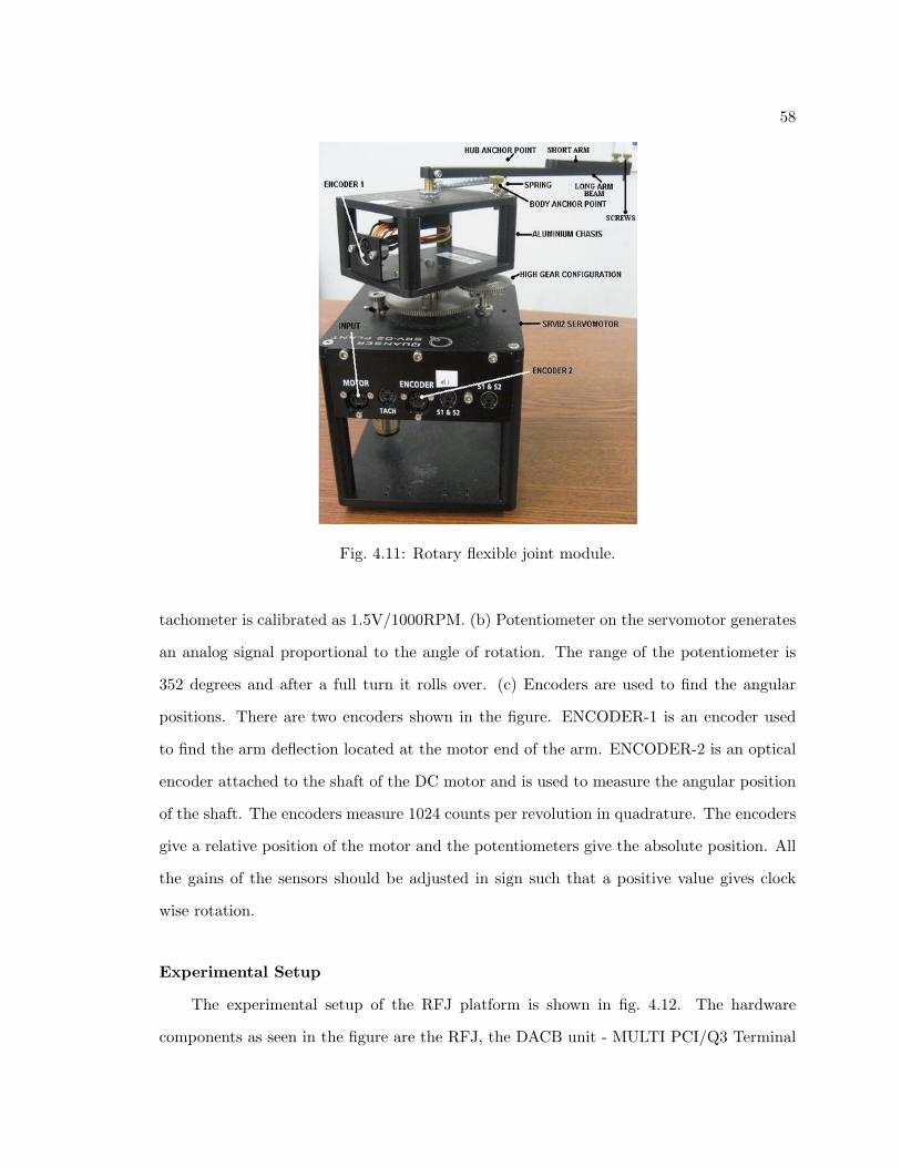
58

Fig. 4.11: Rotary flexible joint module.

tachometer is calibrated as 1.5V/1000RPM. (b) Potentiometer on the servomotor generates

an analog signal proportional to the angle of rotation. The range of the potentiometer is

352 degrees and after a full turn it rolls over. (c) Encoders are used to find the angular

positions. There are two encoders shown in the figure. ENCODER-1 is an encoder used

to find the arm deflection located at the motor end of the arm. ENCODER-2 is an optical

encoder attached to the shaft of the DC motor and is used to measure the angular position

of the shaft. The encoders measure 1024 counts per revolution in quadrature. The encoders

give a relative position of the motor and the potentiometers give the absolute position. All

the gains of the sensors should be adjusted in sign such that a positive value gives clock

wise rotation.

Experimental Setup

The experimental setup of the RFJ platform is shown in fig. 4.12. The hardware

components as seen in the figure are the RFJ, the DACB unit - MULTI PCI/Q3 Terminal

59

Fig. 4.12: RFJ experimental setup in the Mechatronics Lab in Utah State University.

Board, UPM (Universal Power Module). The UPM is used to amplify the voltage supplied

to the servomotor. As seen in the figure, the two encoder signals from the RFJ module are

directly connected to the DACB unit. They are scaled by a factor ±2π/4096 to convert the

encoder reading to radians. The speed information can also be obtained by passing their

input through a derivative filter. The software component of the setup is Simulink and

WinCon. Simulink is used to define the control law and WinCon runs the C code in real

time.

Mathematical Model

The mathematical model as given in Quanser documentation ignores the non-linearities

in the model and derives a linear state space model. The flexible joint is modeled as a fourth

order system. The detailed derivation of the state space model can be found in the Quanser

documentation provided with the RFJ platform [37]. The state variables chosen to define

the combined model of servo motor and RFJ module are given by:

x(t) = [θ φ ω υ]T , (4.2)

i.e. where θ and φ are the servo gear angular displacement and arm angular deflection,

60

respectively. The servo angular velocity is given by ω = θ and the arm angular velocity is

given by υ = φ. The state space model is given by:

θ

φ

ω

υ

=

0 0 1 0

0 0 0 1

0 KsJeq

− ηK2mK2

g+BeqRa

JeqRa0

0 − Ks(Jeq+Jarm)JeqJarm

ηK2mK2

g+BeqRa

JeqRa0

θ

φ

ω

υ

+

0

0ηKmKg

JeqRa

−ηKmKg

JeqRa

u, (4.3)

i.e. where,Ks - Linear estimate of spring stiffness, Km - Motor voltage constant V-s/rad,

Kg - High gear ratio, η - Total efficiency, Jeq - Total inertia Kg m2, Jarm - Arm’s moment

of inertia, Beq - Equivalent viscous friction Nm/(rad/s), Rs - Armature resistance (ohm),

u - Input Signal. The values of these parameters can be obtained from the Quanser docu-

mentation. Ks depends on the position of the spring on the base to the anchor point. Jarm

varies with position of short arm on long arm. The control objective is to position the tip

to a desired setpoint with minimal arm vibration. Hence, the output is defined by the state

space equation as:

y(t) = [1 1 0 0] [θ φ ω υ]T . (4.4)

4.4.2 F-MIGO Applied to RFJ

The control objective is to position the tip of the arm at the desired set-point. In

the Quanser documentation, a state feedback controller has been implemented to achieve

the desired control objective. Here we attempt to achieve the same results with a FO-PI

controller. The transfer function of order 4 is of the integrating type hence it cannot be

approximated with a FOPDT model. The system is then analyzed with the F-MIGO design

method introduced in chapter 2. Choosing appropriate values for the design parameters

Ms and Mp, we scan the systems for fractional order in the range (0.1 - 1.9). The best

controller is then picked based on the minimum Integrated Squared Error (ISE)/Integrated

Time Absolute Error (ITAE) criterion [6].

61

Choosing the Best Design Parameters

In chapter 3, we have seen that the tuning rules were developed with the design param-

eters Ms = 1.4 and Mp = 1.0. However, here, we need to first decide the value of the design

parameters based on the closed loop performance. The idea is to first find a solution at α

= 1, for different values of the design parameters. Table 4.4 summarizes the result of this

procedure. The integer order controllers obtained for the various design constraint show

some interesting trends. For a given value of Ms, any change in Mp affects only the Ki val-

ues. As Ms value increases, the ISE values decrease and K values increase. A closed-loop

simulation of these controllers however showed that for large proportional gains there was

undesired overshoot which caused oscillation in the arm, taking more time to settle down.

A good design parameters was then chosen to be Type 3 systems as they had about enough

gain to avoid overshoot and also their response time was faster compared to the lower types

which gave very slow closed loop responses.

Scanning for the best fractional order

Once the design parameters have been decided the F-MIGO is applied at all other

values of fractional order. Table. 4.5 summarizes the results obtained for different values of

the fractional order. Even though solutions were obtained at α > 1, they gave closed-loop

systems with large overshoot and faster response resulting in oscillations. Hence, they have

been omitted from the final analysis. Table. 4.5 shows that as the fractional order reduces

the ISE and ITAE values start falling. If ISE is chosen the best order is 0.4 and if ITAE

is chosen the best order is 0.2, however we observe very little variations in the controller

proportional gain between the orders - (0.4 - 0.2) indicating that a good solution can be

obtained anywhere within this region of fractional control without a major difference in

control performance. Let us apply the F-MIGO method at α = 1 for different values of the

design constraints Ms and Mp. If a solution is obtained, study the closed-loop performance

and choose the one which gives the best trade off between the performance requirements

and ISE/ITAE values. Now, scan the system again for different values of fractional order

at the desired value of design constraints. Conduct a closed-loop simulation and observe the

62

Table 4.4: Deciding on the design parameters.

Type (Ms,Mp)) K Ki ISE ITAE

1 (1.1,1.1) 0.76 0.092 5.0 124.02 (1.1,1.2) 0.76 0.167 5.1 111.23 (1.2,1.1) 1.39 0.307 3.0 64.784 (1.2,1.2) 1.38 0.558 3.1 58.045 (1.3,1.1) 1.92 0.875 2.4 42.306 (1.3,1.2) 1.92 1.062 2.4 41.757 (1.4,1.1) 2.38 0.898 2.0 36.768 (1.4,1.2) 2.37 1.614 2.0 34.11

Table 4.5: Analysis of RFJ closed-loop response at different values of the fractional order.

α K Ki ω0 ISE ITAE Ms Mp

1.0 1.389 0.307 2.56 3.01 120.6 1.91 1.10.9 1.394 0.309 2.58 2.94 120.0 1.91 1.10.8 1.389 0.316 2.60 2.89 117.7 1.91 1.10.7 1.375 0.332 2.61 2.86 113.2 1.91 1.10.6 1.361 0.366 2.64 2.81 106.1 1.91 1.10.5 1.332 0.421 2.67 2.77 98.25 1.91 1.10.4 1.328 0.556 2.76 2.65 86.83 1.91 1.10.3 1.106 0.690 2.76 2.66 82.20 1.91 1.10.2 0.850 1.014 2.76 2.67 76.70 1.91 1.1

performance. Build a comparison table and decide on the best controller for the system.

4.4.3 Simulation and Lab Results

The simulation results obtained for the closed loop response of RFJ and controllers in

table 4.5 are shown in fig. 4.13. The simulation results show that the orders [0.4,0.3,0.2]

give very close responses. The simulation also predicts an overshoot of about 2◦ above the

setpoint. From the simulation results, it is obvious that the lower fractional order controllers

are better for the control of the tip position of the RFJ module. Figure 4.13 summarizes

the closed-loop and load disturbance responses obtained with the actual RFJ module setup

as shown in fig. 4.12.

The fractional controller was digitally implemented using the Oustaloup’s recursive

63

approximation in the bandwidth of interest. The lab results surprisingly show no overshoot

at the best fractional orders [0.4,0.3,0.2]. The rise time is near 1 second and the settling

time is less than 2 seconds in all the three cases. Figure 4.14 shows the experimental results

for α = 0.2 and α = 0.3. The tip has to be positioned to 45◦. The small glitch is when

the arm is disturbed. Observe that the controller quickly brings it back to the setpoint.

Figure 4.15 shows the comparison of the FO-PI controller of α = 0.4 and PI controller. It

can be observed that the PI controller leads to overshoot and takes 4 seconds to reach the

setpoint.

The results obtained with F-MIGO design method applied to the model provided by

Quanser give good results. However, it is observed that the simulation results and the lab

results differ in some respects. Hence, it is concluded that the linear model is not adequate

enough to model the system behavior. However, it gives a starting solution which can be

used in other complicated models of the RFJ module.

4.5 Fractroller: True Analog Fractional Controller

This section of the chapter was a joint venture of Montana State University, Wavelength

Electronics and Utah State University for submission of patent on “True Analog Fractional

Order Control” [39]. This project was partially funded by National Science Foundation

Small Business Innovation Research grant OII-0538866.

Fig. 4.13: Closed-loop simulation results of the tip angle (θ +φ) RFJ model and controllersfrom table 4.5.

64

(a)

(b)

Fig. 4.14: Positioning the tip at 45◦ and load disturbance responses using FO-PI controllerof (a) α = 0.2; (b) α = 0.3. The graphs show the variation of arm deflection (φ), hub angle(θ), setpoint and output (θ + φ).

4.5.1 Introduction

Fractroller can be described as a Fractor enabled wide bandwidth fractional controller

in a mixed analog/digital environment. Here the “Fractor” is new a kind circuit element

which exhibits fractional order impedance properties. The Fractroller is used to control

the RFJ module based on the results obtained in the previous section. This section will

give a brief description of the Fractor, Fractroller setup, the extension of the state space

model of RFJ to include non-linearities and results obtained with this true analog fractional

controller.

65

(a)

(b)

Fig. 4.15: Positioning the tip at 45◦. FO-PI of α = 0.4 versus PI controller. The graphsshow the variation of arm deflection (φ), hub angle (θ), setpoint and output (θ + φ).

4.5.2 Fractor

Fractional order operators represent memory functions over the history of some physical

signal. For example, a first order integral of a state variable represents a sum over the

history of the state with all points in history being weighted equally, regardless of how

far in the past. A fractional order integral is also a weighted sum, but with the weights

decreasing further back in time. Because the fractional order operators are defined for

all orders (positive and negative), it is possible to use a single fractional order derivative

operator symbol 0Dαt , to indicate an αth order derivative operation over the history from

time 0 to t. A negative value of α would indicate a fractional order integral operation, that

is 0Iαt = 0D

−αt [40]. The most critical aspect of working with fractional order differential

66

Fig. 4.16: Prototype Fractance device, the Fractor prepared by Montana State University.

equations is to arrange the equations in proper cause and effect time ordering. That is,

making sure that the memory function of past time is affecting the future evolution of the

system dynamics and not trying to say that the future evolution creates the past history.

This seems obvious but standard treatment of integer order differential equations can easily

blur this distinction.

For physically realizable systems, the dynamics are invariably described as an integral

over some activity. For example, the voltage across a fractance device is best described as

the fractional order integral of the the current through the device.

vf (t) = Kz 0Dαt i(t), (4.5)

where α is −1 < α < 0 and Kz is an impedance scaling constant.

This is consistent with a capacitor being described as the limiting case when α → −1. In

integer order electronic systems the product of resistance and capacitance values determines

system time constants. In fractional order systems, the time scaling used in describing

the fractance is the determining property. Known digital approximation techniques for

implementing fractional order operators have an effective bandwidth of three decades or less

of frequency response. Many nonlinear phenomena exhibit very broad time scales, often four

decades or more. To deal with these situations an analog approach was investigated. This

67

Fig. 4.17: Impedance spectrum of a Fractor with a fractance order ≈ 0.3.

involved using the Fractor which provides highly accurate implementation of a fractional

order operator in over more than five decades in frequency domain.

The Fractor (patent pending) circuit element is a two-lead electronic component in the

category of resistor, capacitor, or inductor. Currently made by hand, the typical unit is 3.5

cm on a side and about 1.0 cm thick, as shown in fig. 4.16. These devices exhibit fractional

order impedance, or “fractance”, given by

ZF (ω) =K

(jτω)α, (4.6)

where K in the impedance magnitude at a calibration frequency ω0 = 1/τ , j =√−1 the

imaginary radix, and α is a non-integer value 0 < α < 1. The impedance phase shift, φ,

is related to α by φ = −90◦ × α. A typical impedance spectrum for a Fractor is shown in

fig. 4.17.

Figure 4.18 shows how the Fractor can be used to create a fractional order integrator.

This allows for otherwise complex control circuitry by simply replacing conventional capac-

itors with Fractors. The “fractance” circuit symbol was designed to give the impression

of a mixture of resistive and capacitive attributes with the underlying impression of the

generalized Warburg impedance.

68

4.5.3 Extension to State Space Representation

The state space representation was extended to include the weighted history of the

states as required by the fractional calculus. This was done symbolically by a slight change

to the coupling matrices. From eq. 4.3 in the state coupling matrix A, each element is

represented as a pair {aij, αij}, where aij is the normal multiplier and αij represents the

order in the operator 0Dαij

t . When describing a dynamical system in state space, the

history of one or more states drives the evolution of the states. In integer order terms, the

change in the state vector x is the result of the state coupling matrix A operating on the

current state values x plus the input coupling matrix operating B on the input vector u.

The component values of x are updated by x× dt. The output vector y is then computed

from the output coupling matrix C operating on the state variables x. For integer order

operations, this is equivalent to saying

xi(t) =∑

j

∫ t

0aijxj(t′)dt′ +

∑k

∫ t

0bikuk(t′)dt′. (4.7)

For fractional order systems

xi =∑

j

aij 0Dαij

t xj +∑

k

bik 0Dβikt uk, (4.8)

or

xi(t) =∑

j

aij 0I1−αij

t xj +∑

k

bik 0I1−βikt uk, (4.9)

Fig. 4.18: A fractional order integrator circuit using the Fractor circuit element.

69

Fig. 4.19: Feedback structure for the RFJ arm.

where the operations are now over the entire history of x and u and αij and βik are in the

range [0, 1]. This range guarantees the stability of the numerical operation.

The computation for carrying out simulations is straightforward and compatible with

predictor-corrector or other numerical methods. It is also straightforward to extend the

representation to include nonlinear effects as additional functional forms operating on the

state variables. Using combinations of these representations it is possible to simulate non-

linear effects in the A and B matrices and non-integer order operations in the feedback K

matrices. A generalized feedback control scheme for the Quanser robotic arm is shown in

fig. 4.19. The fractional order PID controller (FOC) PIαDµ is the focus of these tuning

methods discussed here. The state variable feedback operation K1 is optional and will be

the subject of future correspondence.

If the robot arm were described perfectly by the linear model, there would be no

Fig. 4.20: Schematic of the Fractroller setup and top view of the Fractroller in the controlloop.

70

Fig. 4.21: System responses with the proportional only control. Observe that the setpointis never reached in this case.

need for any integral term of any order in the controller. However, the arm suffers from a

nonlinear dead band effect that the manufacturer refers to as a “sticky friction”. The motor

will not turn if the voltage (or current) falls below some value. An objective for tuning was

to obtain parameters that allow for variation in the size of the dead band. Starting with a

linear approximation, methods such as F-MIGO discussed above can give a good starting

point.

Given the dead band, proportional control alone tends to result in an undershoot

situation with the arm “sticking” short of the desired set point. Adding an integer order

integral term to the controller tends to cause the arm to overshoot and get stuck past the

set point. These effects are seen in fig. 4.21 and fig. 4.22. Note that attempts to increase

the speed of response cause an unacceptable overextension of the coupling springs between

the hub and arm.

4.5.4 Fractional Order Control

Due to the broad time scaling of the nonlinear effect which could be more than four

decades of frequency, the tests were carried out with an analog controller implementing

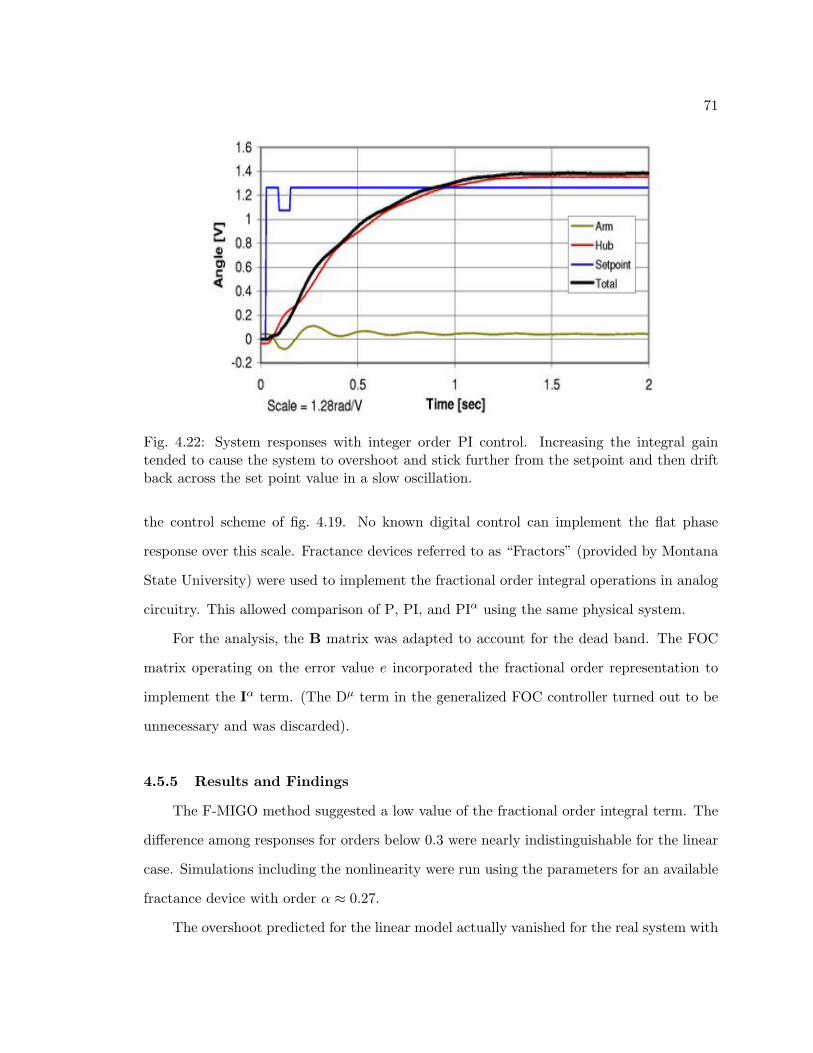
71

Fig. 4.22: System responses with integer order PI control. Increasing the integral gaintended to cause the system to overshoot and stick further from the setpoint and then driftback across the set point value in a slow oscillation.

the control scheme of fig. 4.19. No known digital control can implement the flat phase

response over this scale. Fractance devices referred to as “Fractors” (provided by Montana

State University) were used to implement the fractional order integral operations in analog

circuitry. This allowed comparison of P, PI, and PIα using the same physical system.

For the analysis, the B matrix was adapted to account for the dead band. The FOC

matrix operating on the error value e incorporated the fractional order representation to

implement the Iα term. (The Dµ term in the generalized FOC controller turned out to be

unnecessary and was discarded).

4.5.5 Results and Findings

The F-MIGO method suggested a low value of the fractional order integral term. The

difference among responses for orders below 0.3 were nearly indistinguishable for the linear

case. Simulations including the nonlinearity were run using the parameters for an available

fractance device with order α ≈ 0.27.

The overshoot predicted for the linear model actually vanished for the real system with

72

Fig. 4.23: System responses with FO-PI controller. Observe that there is no overshoot andalso the response time is faster compared to the other configurations.

the dead band. The simulations were confirmed in recording of the actual system response

using the PIα controller with a gain magnitude for the Iα of 1.8 and exponent α ≈ 0.27, as

shown in fig. 4.23.

By starting with an acceptable response using the F-MIGO criteria above, the system

became quite robust to the inclusion of nonlinear effects, with the performance actually

improving with the increasing size of the nonlinear effect. A fractional order integral term

with a low exponent value tends to provide enough memory of the error values to maintain

the control voltage across the motor to allow settling without overshoot. The fading memory

inherent in the fractional order integral allows the control value to decay without the need

for the system to overshoot to produce a change in the sign of the error value to “unwind”

the integrator as would be required in an integer order system.

4.6 Conclusion

This chapter gives an experimental verification of the simplicity of applying the prac-

tical tuning rules or F-MIGO design method to lab experiments. In the HFE module we

were able to apply the practical tuning methods based on the FOPDT model of the system

73

and obtain satisfactory results. The performance of FO-PI was compared to the integer

order PI controller and it was observed that since the HFE systems have very small relative

dead-time, they do not need a full integrator for control. The performance of the FO-PI

controller was observed to be better than the PI controllers used for the orginal lab exper-

iment. However, non-linear behavior during cooling could not be controlled based on the

FOPDT model.

The RFJ module proved to be slightly different. Since the linear model was of in-

tegrating type, we could not directly apply the tuning rules using FOPDT models. The

F-MIGO was then applied to analyze the system at different fractional orders. It was seen

that PI controller caused large overshoot and the system needed only a small fractional

order to meet the design requirements. The simulation and actual lab results showed some

mis-match indicating that the linear model was unable to model the system’s nonlinearities.

The analog fractional controller is an example of practical implementation of the “frac-

tional operator”. The F-MOGO analysis on the linear model provided a good start for

tuning the Fractroller. This project helps in understanding FOC concepts and proves that

if properly implemented, FO-PI controllers can easily replace the existing PI controllers

with additional fractional advantage.

74

Chapter 5

Conclusion

5.1 Summary

The contributions and results presented in this thesis can be summarized as follows.

• Theoretical Results

1. A generalized MIGO design method, called F-MIGO, which gives FO-PI gains

at any arbitrary value of fractional order has been derived in this thesis. The

method gives a natural way of finding a range of orders between which a FO-

PI controller can be found for the system. This gives the user an advantage of

finding a FO-PI controller gains accurately if the order is already known.

2. Simple tuning rules based only on the relative dead time, τ , from the FOPDT

model of the system were derived. The great advantage of the system is that

it does not need a system transfer function. Most systems in industries can be

approximated with a simple FOPDT model. The tuning rules not only give the

user the optimal value of the fractional order, α, but also the corresponding

optimal gains.

3. Certain characteristics were observed in the application of the tuning rules to

the FOPDT systems. Based on the minimum ISE criterion, it was seen that lag

dominated systems did not need a complete integrator to perform better than

their integer counterparts. In fact, it was observed that for such systems the best

fractional order is usually near the value of 0.7. However, delay dominated sys-

tems showed different characteristics. They need a little more than an integrator

to perform better. Balanced lag and delay systems did not show any significant

variation in performance with the use of a fractional order. In fact, the tuning

75

rules developed in this thesis predicted an order close to 1.0. Hence, these rules

define boundaries where a fractional control should be the obvious choice over

their integer order counterpart.

4. Certain special systems were also analyzed using the F-MIGO method directly

and again the advantage of FO-PI controllers was seen in these cases.

• Experimental Results

1. The most important verification was in the easy applicability of the practical

tuning rules to a complicated system such as the HFE. Based on the open-

loop data, we were able to generate FOPDT structures and FO-PI controllers

were designed which gave very good performance compared to the integer order

counterparts.

2. The RFJ experimental platform is far more complicated and cannot be approxi-

mated with a simple FOPDT model. Hence, the F-MIGO was applied directly to

first find a solution range. The interesting thing is that based on the minimum

ISE and ITAE criteria, a low fractional order was predicted for the control of

the tip. Experimental results confirmed this analysis.

3. The final contribution was that the analysis of the RFJ module gave a starting

step for the design of a analog fractional order PI controller. The experimental

results again confirmed the F-MIGO analysis. Also, the Fractroller presents a

new method of implementation of a fractional order integrator.

5.2 Future Work

The design of fractional controllers is a topic without boundaries. The scope of this

thesis covers only a few aspects of finding simple FO-PI controllers focusing on the FOPDT

model. Further research can be extended in areas like:

1. Extension of the F-MIGO design method to FO-PID (fractional order proportional

integral and derivative) controller adding the advantage of the derivative action.

76

2. The ellipse curves generated in the F-MIGO algorithm are an interesting area of

research. Characterizing the curves based on system dynamics can be another method

of studying the controllers.

3. The tuning rules help in designing a FO-PI controller, extension to include a fractional

derivative term is another area of research.

4. Practical solutions for implementation of the fractional operator are necessary to

justify any proposed FOC control techniques.

5. Systems with τ = 0.0 and τ = 1.0 are special cases and need to be treated separately

and can be considered as a separate area of future research.

77

References

[1] L. Debnath, “A Brief Historical Introduction to Fractional Calculus,” Int. J. Math.Educ. Sci. Technol., vol. 35, no. 4, pp. 487–501, 2004.

[2] R. L. Magin, “Fractional Calculus in Bioengineering,” Critical ReviewsTM in Biomed-ical Engineering, vol. 32, no. 1-4, 2004.

[3] B. M. Vinagre and Y. Chen, “Lecture Notes on Fractional Calculus Applica-tions in Automatic Control and Robotics,” in The 41st IEEE CDC2002 Tuto-rial Workshop # 2, B. M. Vinagre and Y. Chen, Eds., pp. 1–310. [Online]http://mechatronics.ece.usu.edu /foc/cdc02 tw2 ln.pdf, Las Vegas, Nevada,USA, 2002.

[4] D. Xue and Y. Chen, “A Comparative Introduction of Four Fractional Order Con-trollers,” in Proc. of The 4th IEEE World Congress on Intelligent Control and Au-tomation (WCICA02), pp. 3228–3235. Shanghai, China: IEEE, June 2002.

[5] Y. Chen, “Ubiquitous Fractional Order Controls ?” in Proc. of The Second IFAC Sym-posium on Fractional Derivatives and Applications (IFAC FDA06, Plenary Paper.), pp.19–21, Porto, Portugal, 2006.

[6] D. Xue, C. N. Zhao, and Y. Q. Chen, “Fractional Order PID Control of a DC-motorwith an Elastic Shaft: A Case Study,” in Proceedings of American Control Conference,pp. 3182–3187, Minneapolis, Minnesota, USA, 2006.

[7] I. Petras, “The Fractional Order Controllers: Methods for Their Synthesis and Appli-cation,” Journal of Electrical Engineering, vol. 50, no. 9-10, pp. 284–288, July.

[8] J. Leu, S. Tsay, and C. Hwang, “Design of Optimal Fractional-order PID Controllers,”Journal of Chinese Institute of Chemical Engineers, vol. 33, no. 2, pp. 193–202.

[9] C. Monje, V. Blas, Y. Chen, V. Feliu, P. Lanusse, and J. Sabatier, “Proposals forFractional PIλDµ Tuning,” in The First IFAC Symposium on Fractional Differentiationand its Applications,Bordeaux, France, July 2004.

[10] R. Caponetto, L. Fortuna, and D. Porto, “Parameter Tuning of a Non Integer OrderPID Controller,” in In Fifteenth International Symposium on Mathematical Theory ofNetworks and Systems.

[11] S. Manabe, “The generalized “saturation function method” for analyzing nonlinearcontrol systems,” JIEE of Japan, vol. 80, no. 863, pp. 1094–1103 (English summaryand Japanese text), 1960.

[12] S. Manabe, “The Non-integer Integral and its Application to Control Systems,” ETJof Japan, vol. 6, no. 3/4, pp. 83–87, 1961.

78

[13] S. Manabe, “The System Design by the Use of a Model Consisting of a Saturation andNon-integer Integrals,” ETJ of Japan, vol. 8, no. 3/4, pp. 147–150, 1963.

[14] A. Oustaloup, “Linear Feedback Control Systems of Fractional Order Between 1 and2,” in Proc. of the IEEE Symposium on Circuit and Systems, Chicago, USA, 4 1981.

[15] M. Axtell and E. M. Bise, “Fractional Calculus Applications in Control Systems,” inProc. of the IEEE 1990 Nat. Aerospace and Electronics Conf., pp. 563–566, New York,USA, 1990.

[16] J. T. Machado, “Special Issue on Fractional Calculus and Applications,” NonlinearDynamics, vol. 29, pp. 1–385, March 2002.

[17] M. D. Ortigueira and J. T. Machado, “Special Issue on Fractional Signal Processingand Applications,” Signal Processing, vol. 83, no. 11, pp. 2285–2480, Nov. 2003.

[18] I. Podlubny, Fractional Differential Equations. San Deigo, LA: Academic Press, 1999.

[19] Concepcion Alicia Monje Micharet, Design Methods of Fractional Order Controllers forIndustrial Applications. Ph.D. dissertation, University of Extremadura, Spain, 2006.

[20] Concepcion Alicia Monje Micharet, “Auto-tuning of Fractional PID Controllers,” inIEEE Control System Society San Diego Chapter Meeting. In Trex Enterprises,, p.Slides available at http://mechatronics.ece.usu.edu/foc/, San Diego, California,USA, Sept. 29 2005.

[21] C. Zhao, Research on Analysis and Design Methods of Fractional Order System. Ph.D.dissertation, Northeastern University, China, 2006.

[22] J. Zeigler and N. Nichols, “Optimum Settings for Automatic Controllers,” Transactionsof ASME, vol. 64, pp. 759–768, 1942.

[23] S. Yamamoto and I. Hasimoto, “Present Status and Future Needs: The View fromJapanese Industry,” in Proceedings. 4th International Conference on Chemical ProcessControl, I. Arkun and Ray, Eds.

[24] K. Astrom, H. Panagopoulos, and T. Hagglund, “Design of PI Controllers Based onNon-Convex Optimization,” Automatica, vol. 34, pp. 585–601, 1998.

[25] K. Astrom, H. Panagopoulos, and T. Hagglund, “Design of PID Controllers based onConstarined Optimization,” in Proceedings of the American Control Conference, pp.858–861, 1999.

[26] K. Johan, Astrom, and T. Hagglund, “Revisiting the Ziegler-Nichols Tuning Rules forPI Control,” Asian Journal of Control, vol. 4, no. 4, pp. 364–380, December 2002.

[27] K. Astrom and T. Hagglund, PID Controller: Theory, Design and Tuning. ResearchTriangle Park, NC: Instrument Society of America, 1995.

[28] K. Astrom and T. Hagglund, Automatic Tuning of PID controllers. Instrumentationsociety, 1998.

79

[29] K. Astrom and T. Hagglund, “Dominant Pole Design – A Unified View of PID Con-troller Tuning,” in 4th IFAC Symposium on Adaptive Systems in Control and SignalProcessing, pp. 127–132, Grenoble, France, 1992.

[30] Newton’s Method, http://mathworld.wolfram.com/NewtonsMethod.html.

[31] T. Bhaskaran, Y. Q. Chen, and D. Xue, “Practical Tuning of Fractional Order Pro-portional and Integral Controller (i): Tuning Rule Development,” September 2007,submitted to: The Third Symposium on Fractional Derivatives and their applica-tions (ASME FDTA2007) at the 6TH ASME International Conference on MultibodySystems, Nonlinear Dynamics and Control at the ASME 2007 International DesignEngineering Techical Conferences,Las Vegas, NE, USA.

[32] D. Xue and Y. Chen, Solving Control Related Mathematic Problems in Matlab. Beijing,China: Tsinghua University Press (to appear, in Chinese), 2007.

[33] G. Silva, A. Datta, and S. Bhattacharyya, PID Controllers for Time Delay Systems.Cambridge, MA: Birkhauser, 2003.

[34] D. Xue and Y. Q. C. anf Derek P Atherton, Linear Feedback Con-trol Systems: Analysis and Design with MATLAB. SIAM Press, 2007,http://mechatronics.ece.usu.edu/siambook/.

[35] T. Bhaskaran, Y. Q. Chen, and G. Bohannan, “Practical Tuning of Fractional OrderProportional and Integral Controller (ii): Experiments,” September 2007, submittedto: The Third Symposium on Fractional Derivatives and their applications (ASMEFDTA2007) at the 6TH ASME International Conference on Multibody Systems, Non-linear Dynamics and Control at the ASME 2007 International Design EngineeringTechical Conferences,Las Vegas, NE, USA.

[36] Y. Chen, “ECE5320 Mechatronics,” http://mechatronics.ece.usu.edu/ece5320/.

[37] Quanser Academic Control Challenges, http://www.quanser.com.

[38] A. Oustaloup, P. Melchoir, P. Lanusse, C. Cois, and F. Dancla., “The CRONE toolboxfor Matlab,” in Proceedings of the 11th IEEE International Symposium on ComputerAided Control System Design - CACSD, Anchorage, USA, 2000.

[39] G. Bohannan, S. K. Hurst, and L. Spangler, “Electrical Component with FractionalOrder Impedance,” Patent Application: US 20060267595 (Filing Date: 03/10/2006).

[40] I. Podlubny, “The Laplace Transform Method for the Linear Differential Equationsof the Fractional Order,” The Academy of Sciences Institute of Experimental Physics,1994.

[41] D. Xue, Computer aided design of control systems - MATLAB language and its appli-cations. Beijing (in Chinese): Tsinghua University Press, 1995.

80

Appendices

81

Appendix A

Mathematical Definition of the Fractional Operator

Fractional calculus is the generalization of the ordinary integer order calculus. The

concept of a fractional operator was to not restrict the order to an integer value and also

to unify the definition of the diffrentiator and integrator. The fractional operator aDαt can

be introduced by:

aDαt =

dα

dtα <(α) > 0,

1 <(α) = 0,∫ ta dτ−α <(α) < 0.

(A.1)

In the above equation α is the fractional order, a is related to the initial conditions. The

two most commonly used definitions for fractional diffrentiation and integration are:

1. Grunwald-Letnikov definition

aDαt f(t) = lim

h→0

1hα

[(t−a)/(h)]∑j=0

(−1)α

(α

j

), (A.2)

where [x] is the flooring operator.

2. Riemann-Liouville definition:

aDαt f(t) =

1Γ(n− α)

dn

dtn

∫ t

a

f(τ)(t− τ)α−n+1

dτ. (A.3)

where (n− 1 < α n) and Γ(x) is the Euler Gamma function.

The fractional order derivative commutes with the integer-order derivation and also the

fractional operator is a linear operator. The Laplace transform of the fractional operator

for the Riemann-Liouville definition is given in eqn. A. Hence, if zero intial condition are

82

assumed, systems with a dynamic behaviour described by differential equations of fractional

order can be decribed by transfer functions of fractional power of s as follows:

L [aDαt f(t)] = sαF (s),

where α can take positive or negative values.

83

Appendix B

Oustaloup’s Recursive Approximation of Fractional Order

Simulation and hardware implementation of the fractional transfer function is done

by approximating them with integer order trasfer functions which shows similar behaviour

approximately. It has been shown that the fractional order systems can be approximated

with integer order transfer functions of infinite order. However, with assumptions, a finite

order transfer function can be obtained. One of the best known approximations is the

one given by Oustoloup, which gives an approximation of the fractional order in a given

frequency range [ωl : ωh] as:

sα =(

ωu

ωh

)α k=N∏k=−N

1 + s/ω′k

1 + s/ωk, (B.1)

i.e. where,

ωu =√

ωlωh, (B.2)

ω′k = ωl

(ωh

ωl

)(k+N+.5−.5∗α)/(2N+1)

, (B.3)

ω′k = ωl

(ωh

ωl

)(k+N+.5+.5∗α)/(2N+1)

. (B.4)

Hence the order of approximation is (2N + 1). The above function can be converted to a

discrete form using any of the usual methods available in Matlab.

84

Appendix C

General Equation of An Ellipse

The general equation of an ellipse in the (x, y) co-ordinate system is given by the

following equation:

ax2 + 2bxy + cy2 + 2dx + 2fy + g = 0. (C.1)

Now we define the matrices

A =

a b d

b c f

d f g

, (C.2)

B =

a b

b c

. (C.3)

Hence the condition for the existance of an ellipse can be summarized in

|A| 6= 0,

|B| > 0,

|A|a + c

< 0.

(C.4)

If all the above conditions are true, we can define the given equation as an ellipse.

85

Appendix D

Newton Raphson Technique

The Newton Raphson method is a numerical method of finding the roots of the function

of the form f(x) = 0 [30]. It uses the first term in the Taylor series expansion of the function

in the vicinity of the solution. Consider the polynomial f(x) = 0. Then the taylor series

about the point x = xo + ε is given by:

f(xo + ε) = f(xo) + f′(xo)ε +

12f

′′(xo)ε2 + . . . , (D.1)

where the ′ represents derivative with respect to x. Now assuming that the point xo is very

close to the solution and ε is a very small quantity, we can approximate the above equation

to a linear equation as,

f(xo + ε) ≈ f(xo) + f′(xo)ε. (D.2)

Now, if we say that xo is very close to the solution , f(xo + ε) ≈ 0, we can obtain the

expression for the amount of estimate, ε0, needed to move closer to the solution from an

initial estimate.

ε0 = − f(xo)f ′(xo)

. (D.3)

Let x1 = x0 + ε0, we can calculate ε1. This process can be repeated till we converge to the

root, i.e.,

εn = − f(xn)f ′(xn)

≈ 0. (D.4)

The general formula for calculating the root is then given by:

xn+1 = xn −f(xn)f ′(xn)

. (D.5)

The solution to f(x) = 0 is reached when εn = εn−1 ≈ 0.

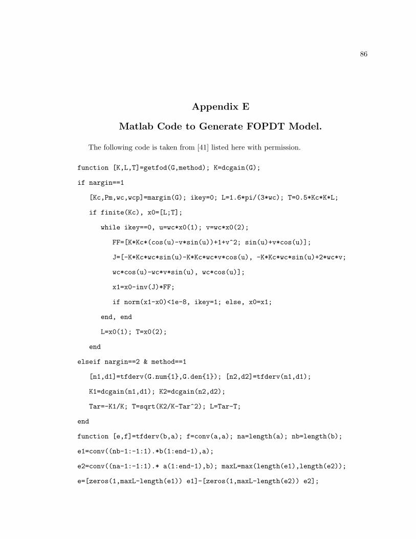
86

Appendix E

Matlab Code to Generate FOPDT Model.

The following code is taken from [41] listed here with permission.

function [K,L,T]=getfod(G,method); K=dcgain(G);

if nargin==1

[Kc,Pm,wc,wcp]=margin(G); ikey=0; L=1.6*pi/(3*wc); T=0.5*Kc*K*L;

if finite(Kc), x0=[L;T];

while ikey==0, u=wc*x0(1); v=wc*x0(2);

FF=[K*Kc*(cos(u)-v*sin(u))+1+v^2; sin(u)+v*cos(u)];

J=[-K*Kc*wc*sin(u)-K*Kc*wc*v*cos(u), -K*Kc*wc*sin(u)+2*wc*v;

wc*cos(u)-wc*v*sin(u), wc*cos(u)];

x1=x0-inv(J)*FF;

if norm(x1-x0)<1e-8, ikey=1; else, x0=x1;

end, end

L=x0(1); T=x0(2);

end

elseif nargin==2 & method==1

[n1,d1]=tfderv(G.num{1},G.den{1}); [n2,d2]=tfderv(n1,d1);

K1=dcgain(n1,d1); K2=dcgain(n2,d2);

Tar=-K1/K; T=sqrt(K2/K-Tar^2); L=Tar-T;

end

function [e,f]=tfderv(b,a); f=conv(a,a); na=length(a); nb=length(b);

e1=conv((nb-1:-1:1).*b(1:end-1),a);

e2=conv((na-1:-1:1).* a(1:end-1),b); maxL=max(length(e1),length(e2));

e=[zeros(1,maxL-length(e1)) e1]-[zeros(1,maxL-length(e2)) e2];

87

Appendix F

F-MIGO algorithm : MATLAB Code

The code which implements the algorithm shown in Section 2.5 is listed below. The

F-MIGO algorithm has one main function which calls five functions.

% Begin the F-MIGO Algorithm. Define the system in get_system.m

option = 1;

% Define the set of intial values in the Range vector.

Range =[.01,.05,.09,.1,.3,.7,1,1.2,1.5,2,2.4,2.8,3,3.1,3.2];

[mx,nx] = size(Range);

% Define the values of design constraint.

Ms = 1.4;

Mp =1.6;

% Compute the values of C and R

C = (-[(Ms - (Ms*Mp) - (2*Ms*(Mp^2)) + (Mp^2) -1) ]/ (2*Ms*((Mp^2)-1)));

R = ((Ms + Mp -1 )/(2*Ms*(Mp-1)));

% Define the value of fractional order , alpha.

ford = 0.7;

% Begin the Newton-Raphson technique.

for range = 1:1:nx

initial_value_w = Range(range);

w = initial_value_w;

for i = 1:50

[r1,be1,r1d,be1d] = get_values(w,option);

[h1] = calc_h(r1,be1,r1d,be1d,w,Ms,Mp,ford);

[r2,be2,r2d,be2d] = get_values(w - .001,option);

88

[h2] = calc_h(r2,be2,r2d,be2d,w - .001,Ms,Mp,ford);

[r3,be3,r3d,be3d] = get_values(w + .001,option);

[h3] = calc_h(r3,be3,r3d,be3d,w+.001,Ms,Mp,ford);

hd1 = (h1 - h2)/.0001;

hd2 = (h3 - h1)/.0001;

hd = (hd1 + hd2) / 2;

w = w - (h1/hd);

end

% Assign the solution to w0.

w0 = w;

% Get the system values at w0

[r,b,a] = eval_r(w0,option);

% Get the values of k and ki at wo

gamma = ford*pi/2;

k = (-C*a/(r^2)) +(R*cos(gamma)/(r*sin(gamma))) ...

+ (C*b*cos(gamma)/((r^2)*sin(gamma))) ;

ki = -((w0^ford)*b*C/((r^2)*sin(gamma)))- ((w0^ford)*R/(r*sin(gamma)));

Ti = k/ki;

% Calculate the maximum value of sensitivity functions

[Ms_max,Mp_max] = sensitivity(k,ki,option,ford);

% Evaluate if the solution is good.

flag = 0;

if ( w0 < 0)

flag = 1; % w0 is a positive value.

end

if ( ki < 0)

flag = 1; % Integral gain is positive value.

end

89

if ( k < 0)

flag = 1; % Proportional gain is a positive value.

end

if ( Mp_max > 2.0)

flag = 1; % The value of Mp does not exceed 2.0

end

if ( Ms_max < 1.35 )

flag = 1; % The value of Ms will not be less than 1.35

end

if ( Ms_max > 2 )

flag = 1; % The value of Ms does not exceed 2.0

end

Final(range,1:11) = [ford k Ti ki w0 Ms_max Mp_max flag ];

position = [’C’ int2str(offset)];

xlswrite(’C:\Desktop\Result’,Final,H,position)

end

%%%%%%%%%%%%%%%%%%%%%%%%%%%%%%%%%%%%%%%%%%%%%%%%%%%%%%%%%%%%%%%%%%%%%%%%%%%

% Returns the transfer function in the complex frequency domain.

function [y] = get_system(option,Ts)

syms s w

s = i*w; Tdly = option;

[np,dp]=pade(Tdly,4);

num = np(1)*s^4 + np(2)*s^3 + np(3)*s^2 + np(4)*s + np(5);

den = dp(1)*s^4 + dp(2)*s^3 + dp(3)*s^2 + dp(4)*s + dp(5);

G = 1/((Ts*s +1));

y = [num/den]*G;

%%%%%%%%%%%%%%%%%%%%%%%%%%%%%%%%%%%%%%%%%%%%%%%%%%%%%%%%%%%%%%%%%%%%%%%%%%%

% Evaluates the values of the real and imaginary part of the system

90

% transfer function at a given frequency.

function [r_val, beta_val,alpha,phi] = eval_r(value,option,Ts)

y = get_system(option,Ts);

al = real(y); be = imag(y); r = abs(y);

w = value; r_val = eval(r);

beta_val = eval(be); alpha =eval(al);

%%%%%%%%%%%%%%%%%%%%%%%%%%%%%%%%%%%%%%%%%%%%%%%%%%%%%%%%%%%%%%%%%%%%%%%%%%%

% Returns the real and imaginary parts of transfer function from the

% eval_r. function.

function [r, beta, diff_r, diff_beta_r] = get_values(value,option,Ts)

[r, beta] = eval_r(value,option,Ts);

[r1, beta1] = eval_r(value + 0.001,option,Ts);

diff_r = (r1 - r) / 0.001;

diff_beta_r = ((beta1/r1) - (beta/r)) / 0.001;

%%%%%%%%%%%%%%%%%%%%%%%%%%%%%%%%%%%%%%%%%%%%%%%%%%%%%%%%%%%%%%%%%%%%%%%%%%%

% Computes the maximum value of the sensitivity functions.

function [Ms,Mp] = sensitivity(k,ki,ford,Kp,L,T)

G = fopdt(Kp,L,T);

if ford == 1

C = k + ki*tf([1],[1 0]);

else

Ci = ora_foc(-ford,4,.0001,1000);

C = k + ki*(Ci);

end

loops = loopsens(G,C);

Ms = norm(loops.Si,inf);

Mp = norm(loops.Ti,inf);

91

%%%%%%%%%%%%%%%%%%%%%%%%%%%%%%%%%%%%%%%%%%%%%%%%%%%%%%%%%%%%%%%%%%%%%%%%%%%

% Approximates the fractional order with a integer order transfer function.

function [sys_foc]=ora_foc(r,N,w_L,w_H)

w_L=w_L*0.1;w_H=w_H*10; % enlarge the freq. range of interest for goodness

mu=w_H/w_L; %

w_u=sqrt(w_H*w_L);

alpha=(mu)^(r/(2*N+1));

eta=(mu)^((1-r)/(2*N+1));

k=-N:N;

w_kp=(mu).^( (k+N+0.5-0.5*r)/(2*N+1) )*w_L;

w_k=(mu).^( (k+N+0.5+0.5*r)/(2*N+1) )*w_L;

D_N_K=(w_u/w_H)^r * prod(w_k) / prod(w_kp);

D_N_P=-w_k;D_N_Z=-w_kp;

[num,den]=zp2tf(D_N_Z’,D_N_P’,D_N_K);

sys_foc=tf(num,den);

%%%%%%%%%%%%%%%%%%%%%%%%%%%%%%%%%%%%%%%%%%%%%%%%%%%%%%%%%%%%%%%%%%%%%%%%%%%

% This function evaluates the parameters of the PI controller via the ZN

% method and the Modified ZN method.

% key = 1,2,3

% vars = Kc, Tc, N or K,L,T,N or Kc,Tc,rb,rc,N

function [Gc,Kp,Ti,Td,H]=ziegler(key,vars)

Ti=[]; Td=[];

if length(vars)==4,

K=vars(1); L=vars(2);

T=vars(3); N=vars(4); a=K*L/T;

if key==1, Kp=1/a;

elseif key==2, Kp=0.9/a; Ti=3.33*L;

elseif key==3 | key==4

92

Kp=1.2/a; Ti=2*L; Td=L/2;

end

elseif length(vars)==3,

K=vars(1); Tc=vars(2); N=vars(3);

if key==1,

Kp=0.5*K;

elseif key==2,

Kp=0.4*K; Ti=0.8*Tc;

elseif key==3 | key==4

Kp=0.6*K; Ti=0.5*Tc; Td=0.12*Tc;

end

elseif length(vars)==5,

K=vars(1); Tc=vars(2);

rb=vars(3); N=vars(5);

pb=pi*vars(4)/180; Kp=K*rb*cos(pb);

if key==2,

Ti=-Tc/(2*pi*tan(pb));

elseif key==3 | key==4

Ti=Tc*(1+sin(pb))/(pi*cos(pb));

Td=Ti/4;

end

end

[Gc,H]=writepid(Kp,Ti,Td,N,key);