arX

iv:h

ep-p

h/94

0941

9v2

2 O

ct 1

995

February 1, 2008 MIT-CTP-2350hep-ph/9409419

Measures of Fine Tuning 1

Greg W. Anderson 2 and Diego J. Castano 3

Center for Theoretical Physics

Laboratory for Nuclear Science

Massachusetts Inst. of Technology

Cambridge, MA 02139.

To appear in: Physics Letters B347, 300-308 (1995)

Abstract

Fine-tuning criteria are frequently used to place upper limits onthe masses of superpartners in supersymmetric extensions of the stan-dard model. However, commonly used prescriptions for quantifyingnaturalness have some important shortcomings. Motivated by this,we propose new criteria for quantifying fine tuning that can be usedto place upper limits on superpartner masses with greater fidelity. Inaddition, our analysis attempts to make explicit the assumptions im-plicit in quantifications of naturalness. We apply our criteria to theminimal supersymmetric extension of the standard model, and we findthat the scale of supersymmetry breaking can be larger than previousmethods indicate.

1This work was supported in part by funds provided by the U.S. Department of Energy(DOE) under cooperative agreement DE-FC02-94ER40818 and by the Texas NationalResearch Laboratory Commission under grant RGFY932786.

2email address: anderson@fnth03.fnal.gov3email address: castano@fshewj.hep.fsu.edu

1 Introduction

One of the principle motivations for weak scale supersymmetry is that itprovides a framework that stabilizes the hierarchy between the weak scaleand the Planck scale, or some other unification scale. In non-supersymmetricmodels, the mass renormalization of fundamental scalars is quadraticallydivergent. This divergence must be cancelled, or the fundamental scalar willhave a renormalized mass on the order of the cutoff. In the standard model,if the Higgs boson remains a fundamental degree of freedom all the way upto some very heavy scale, we must fine tune a precise cancellation order byorder in perturbation theory to maintain the lightness of the weak scale.

Supersymmetry solves this problem because the renormalization effectsof superpartners eliminate the quadratic divergences. But supersymmetryis at best a broken symmetry. There are no superpartners degenerate inmass with the particles that have been observed so far. These superpartnerscan have gauge invariant mass terms if supersymmetry is softly broken, andthese masses can be made arbitrarily large provided we increase the scale ofsupersymmetry breaking. There is a price for this. As the scale of supersym-metry breaking increases the weak scale can only remain light by virtue ofan increasingly delicate cancellation. Eventually a point is reached when themodel no longer appears to provide a complete explanation of why a lightweak scale is stable.

Attempts to pinpoint where and when our understanding of weak scalestability is lost, or becomes incomplete, must of necessity quantify some in-tuitive notion of naturalness. Such a prescription for quantifying naturalnessexists and is widely used in the literature. If we demand that supersymmetricextensions of the standard model should be “complete” in their explanationsof this stability, we can place an upper limit on the scale of supersymme-try breaking. This can be translated into an upper limit on the masses ofsuperpartners.

In this paper, we examine the prescription that is currently used to placeupper bounds on superpartner masses. 4 First, we wish to determine if thesecriteria accurately measure fine tuning. Second, we want to make explicit the

4Heavy superpartner masses can also be bounded, or at least restricted, by the require-ment that the relic density of LSP’s does not over close the universe. These constraintsprovide interesting limits, but they don’t provide an absolute upper limit on sparticlemasses, and they involve model dependent assumptions concerning conserved R-parity.

1

assumptions implicit in any attempt to quantify naturalness. Upper limits onsparticle masses obtained from naturalness criteria influence expectations ofwhen and where sparticles will be discovered if supersymmetry is responsiblefor the stability of the weak scale.

In section two we make a critical examination of fine tuning, and weanalyze the prescription now used to quantify naturalness. We critique thistraditional method by examining a well known hierarchy. We find that thisprescription is not completely satisfactory. The trouble is that the traditionalprescription does not distinguish between instances of global sensitivity andreal instances of fine tuning. We argue that a reliable measure of fine tuningrequires global information about the dependence of certain quantities ontheir arguments, and we show how the existing prescription can be augmentedwith this information to yield reliable measures of fine tuning.

In section three we systematically construct a family of prescriptions thatcoincide with the augmented prescriptions formulated in section two. Ourconstruction clarifies the proper normalization of naturalness measures andmakes explicit the extent of theoretical prejudice present in any such measure.

In section four we apply our prescription to the minimal supersymmetricstandard model (MSSM). We briefly discuss the level of fine tuning the MSSMrequires in light of current experimental constraints, and we show how thecurrent situation is much less fine tuned than it previously appeared. Amore detailed and extensive application of our criteria to supersymmetricextensions of the standard model is in progress[7].

2 Traditional Measures of Fine Tuning

When parameters conspire by cancelling or adding in an unusually pre-cise fashion, we think of an atypical quantity that results as fine tuned. Insuch instances, the quantity, for example MZ , will exhibit a very strong de-pendence on its arguments[2]. In supersymmetric extensions of the standardmodel, the weak scale depends on the soft supersymmetry breaking parame-ters and other couplings through the renormalization group[3]. In a seminalpaper, Barbieri and Giudice used these features to place upper bounds onsuperpartner masses, and they popularized a prescription to quantify finetuning that is now widely used. They looked for sensitivity in the Z massto variations in the values of supersymmetry breaking parameters and other

2

couplings. They measured the sensitivity on a general parameter a by:

c(M2Z ; a) = |

a

M2Z

∂M2Z

∂a| . (2.1)

Note that rescaling the derivative by a/M2Z removes the dependence on the

overall scale of a and MZ . Barbieri and Giudice argued that, if supersymme-try is responsible for stabilizing the weak scale, then c(M2

Z ; a) must be lessthan some upper limit ∆, which they took to be 10. They used this criterionto place upper limits on supersymmetry breaking parameters. This programhas been subsequently adopted by many researchers.

The application of Eq. (2.1) in obtaining upper bounds on superpartnermasses raises several questions. Do we know the normalization of Eq. (2.1)well enough to say that natural solutions should exhibit c(M2

Z , a)’s below 10or any other particular value? Should we expect that a simple applicationof this formula will always give a reliable measure of fine tuning, and ifnot, can we construct alternative definitions that provide better measures ofnaturalness? We can apply Eq. (2.1) to a famous hierarchy in order to shedsome light on these questions.

The lightness of the proton in comparison to either the Planck scale orthe grand unified scale is beautifully explained by the logarithmic runningof the QCD coupling, α3. At one loop, the scale dependence of the strongcoupling constant can be expressed as

α3(µ) =alpha3(MP l)

1 − b32π

α3(MP l) ln(MP l/µ). (2.2)

For simplicity we take Mprot = Λ, where α3(Λ) = 1. A straight forwardapplication of Eq. (2.1) to the proton mass yields

c(Mprot; gs(MP l)) =(

4π

b3

)

1

α3(MP l)>∼ 100. (2.3)

The large value of c(Mprot, g3(MP l)) occurs because the proton mass is avery sensitive function of g3(MP l). The lightness of the proton is, of course,not the result of a fine tuning. The proton mass would have exhibited thisstrong sensitivity no matter what its value was, so it makes no sense to saythat a value near 1 GeV is fine tuned. This example illustrates our central

3

point. Equation (2.1) is really a measure of sensitivity, and sensitivity doesnot automatically translate into fine tuning. For example, the overestimateof fine tuning would have been even worse had we used Eq. (2.1) to study thenaturalness of the technicolour scale with respect to variations in the valueof the technicolour gauge coupling at the extended technicolour scale. 5

A reliable measure of fine tuning should give a large value when a quantityis fine tuned and at the same time reduce to something close to unity whenit encounters typical sensitivity. This suggests that we divide Eq. (2.1) bysome measure of average sensitivity. The resulting ratio will still be largefor solutions that are unusually sensitive, but in cases where solutions havea “typical” sensitivity the resulting ratio will be of order one. So a morereliable measure of fine tuning would be

γ(a) = c(X; a)/c, (2.4)

where c is some average value of c(X; a). For example,

c =

∫

c(a)da∫

da, (2.5)

or

1/c =

∫

c−1(a)da∫

da. (2.6)

If we apply this new criterion to the lightness of the proton, we find that γis of order one. It is a simple matter to check that the ratio γ gives a largevalue in legitimate cases of fine tuning. If we apply Eq. (2.4) to the weakscale hierarchy in a non-supersymmetric model, we get a number of orderΛ/Mweak, where Λ is the scale of the cutoff. As we show in the followingsection, a ratio in a form of Eq. (2.4) can be deduced from very generalconsiderations.

5In these examples there are no cancellations that we can precisely adjust to create alarge fine tuning. However, even in instances of real fine tuning, the largeness of c(X ; a)can be, in part, due to global sensitivity. As we will show in section four, c(M2

Z; a) over

estimates the amount of fine tuning needed to maintain a light Z mass in supersymmetricextensions of the standard model.

4

3 Measuring Fine Tuning

In this section we construct a family of quantitative measures of fine tun-ing that encompass Eq. (2.4), the augmented prescription we motivated inthe previous section. Our purpose is twofold. First, we wish to systemati-cally clarify what measures of fine tuning best quantify our intuitive notionof naturalness and how these measures should be normalized. Second, wewish to make explicit the inherent, discretionary assumptions present in anystandard that quantifies naturalness. Any measure of fine tuning that quan-tifies naturalness can be translated into an assumption about how likely agiven set of Lagrangian parameters is. In the absence of a theoretical reasoncompelling us to choose a certain value, we can consider some sensible dis-tribution of the parameter to study what are the natural predictions of themodel. The “theoretical license” at one’s discretion when making this choicenecessarily introduces an element of arbitrariness to the construction.

Before we proceed to “derive” a quantitative measure of fine tuning somecomments are in order. We are motivated to quantify naturalness for tan-gible theoretical reasons. A model that explains a phenomenon has morepredictive power than a model that merely accommodates it. In addition,we understand why the proton can be naturally many orders of magnitudelighter than the Planck scale but, the stability of a light scale in a theoryof fundamental scalars is mysterious. We would like to understand how theweak scale remains light. Of course, at the level of low energy effective theo-ries, dismissing “unnatural” theories in the quest for a “natural” explanationof weak scale stability could be misguided. We certainly cannot prove thatan explanation of the light weak scale was not butchered by the process inwhich we constructed our effective theory. For example, one loop correctionsto the cosmological constant from an effective theory with soft supersym-metry breaking generate contributions that are many orders of magnitudegreater than the experimental limit. Yet we often entertain the idea that thesolution to this problem is not associated with our choice of a low energyLagrangian. While we cannot elevate the prejudice of searching for naturaltheories above the level of an axiom, we can hope that its application willlead us to a more complete model that explains the stability of the weakscale. Such models will have testable predictions.

In light of this, we proceed to deduce a measure of fine tuning from gen-eral principles. Provided we parameterize our assumptions about the likely

5

distribution for Lagrangian parameters, we should be able to derive a quan-titative measure of naturalness. Assume the probability that a Lagrangianparameter lies between a and a + da is

dP (a) =f(a)da∫

f(a)da. (3.1)

Consider a set of these Lagrangian parameters ai specified at a renormal-ization scale that is the high energy boundary of our effective theory (e.g.,µ = MGUT ). A measurable parameter X (e.g., M2

Z) will depend on the ai

through the renormalization group equations and possibly on a set of min-imization conditions. We can recast Eq. (3.1) as a probability per unit X.Given a probability density f(a), the probability density per unit X is

dP = ρ(X) dX, (3.2)

where

ρ(X) ≃1

X c(X; a)

af(a)∫

f(a)da. (3.3)

In studies of naturalness, we may ask: If the fundamental Lagrangianparameters at our high energy boundary condition are distributed like f(a),how likely is a low energy observable, X(a), to be contained in an intervalu(X) dX about X? A quantity X is relatively unlikely to be in an intervalproportional to u(X)dX if

< uρ >

u(X)ρ(X)>> 1, (3.4)

where < uρ >=∫

da u(X)ρ(X)/∫

da.If we are interested in studying the naturalness of a hierarchy like Mweak/MGUT ,

Mprot/MP lanck, or M2Z/M2

SUSY , the interval that corresponds to the conven-tional sense of naturalness is u(X) = X. 6

6Consider the hierarchy problem in an effective theory with a fundamental scalar de-fined below some scale Λ1: m2

S= g2Λ2

1− Λ2

2. The scalar mass can only remain light in

comparison to the cutoff scale Λ1 if we cancel the quadratic divergence against the bareterm Λ2

2. Note that the cancellation we need to place the scalar mass in a 1 GeV window

at 1016 GeV must be made with the same precision as the cancellation we need to placethe scalar mass in a 1 GeV window at a 100 GeV. A small value of the scalar mass isunnatural in the sense that a small change in g leads to a large fractional change in m2

S

so that it is relatively unlikely to be found in an interval ∝ m2

Sdm2

Saround m2

S.

6

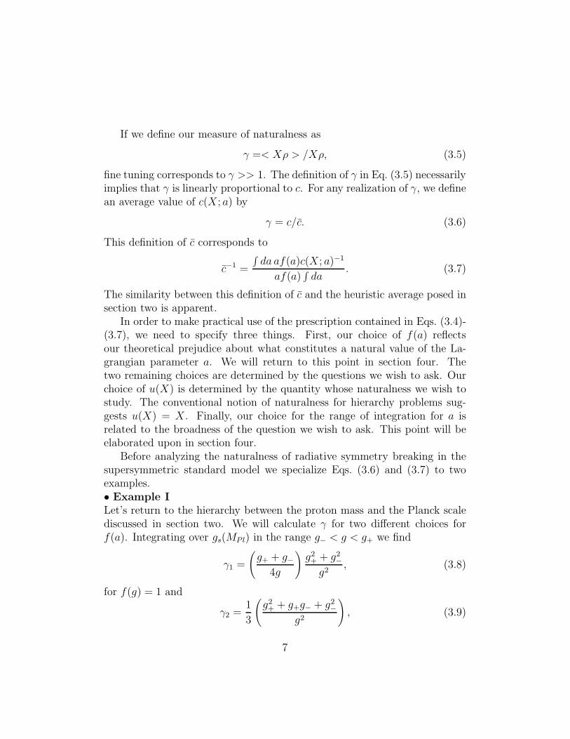
If we define our measure of naturalness as

γ =< Xρ > /Xρ, (3.5)

fine tuning corresponds to γ >> 1. The definition of γ in Eq. (3.5) necessarilyimplies that γ is linearly proportional to c. For any realization of γ, we definean average value of c(X; a) by

γ = c/c. (3.6)

This definition of c corresponds to

c−1 =

∫

da af(a)c(X; a)−1

af(a)∫

da. (3.7)

The similarity between this definition of c and the heuristic average posed insection two is apparent.

In order to make practical use of the prescription contained in Eqs. (3.4)-(3.7), we need to specify three things. First, our choice of f(a) reflectsour theoretical prejudice about what constitutes a natural value of the La-grangian parameter a. We will return to this point in section four. Thetwo remaining choices are determined by the questions we wish to ask. Ourchoice of u(X) is determined by the quantity whose naturalness we wish tostudy. The conventional notion of naturalness for hierarchy problems sug-gests u(X) = X. Finally, our choice for the range of integration for a isrelated to the broadness of the question we wish to ask. This point will beelaborated upon in section four.

Before analyzing the naturalness of radiative symmetry breaking in thesupersymmetric standard model we specialize Eqs. (3.6) and (3.7) to twoexamples.• Example I

Let’s return to the hierarchy between the proton mass and the Planck scalediscussed in section two. We will calculate γ for two different choices forf(a). Integrating over gs(MP l) in the range g

−< g < g+ we find

γ1 =

(

g+ + g−

4g

)

g2+ + g2

−

g2, (3.8)

for f(g) = 1 and

γ2 =1

3

(

g2+ + g+g

−+ g2

−

g2

)

, (3.9)

7

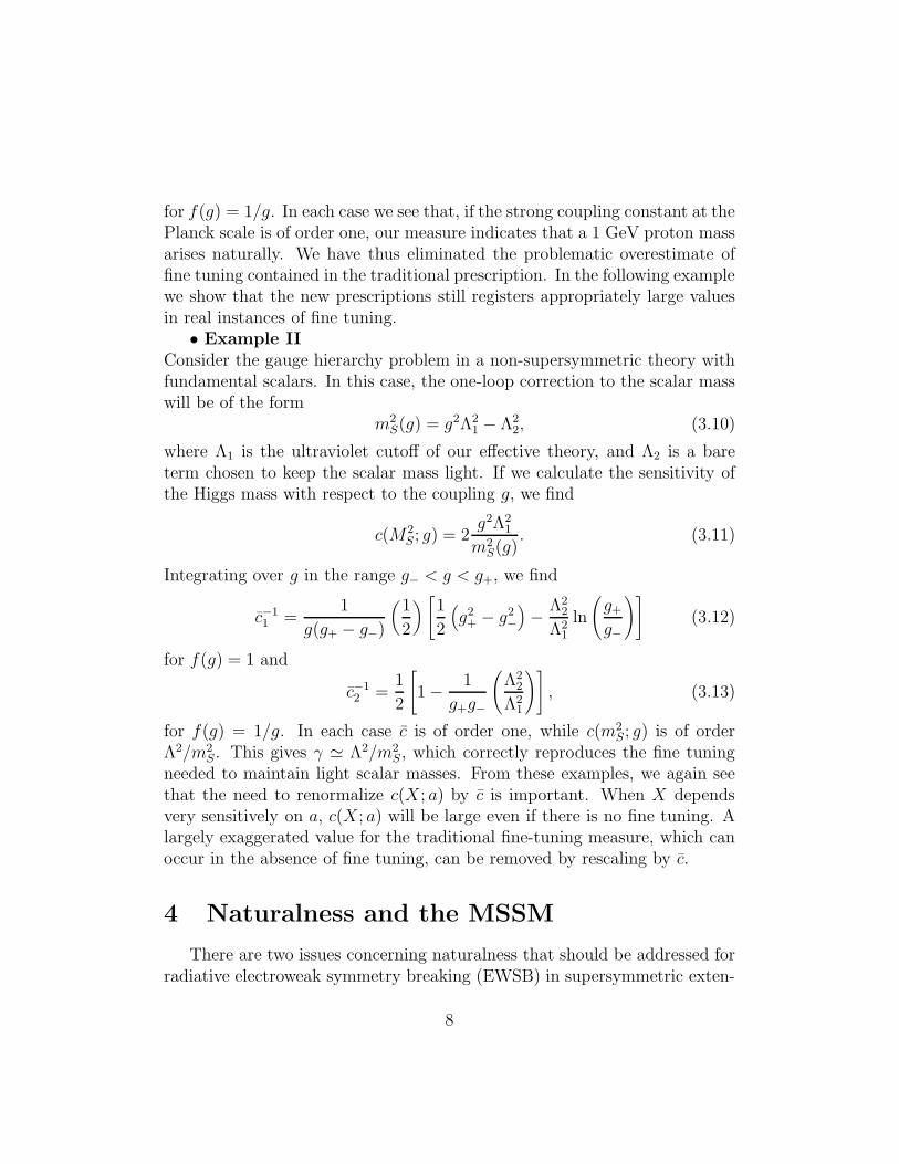
for f(g) = 1/g. In each case we see that, if the strong coupling constant at thePlanck scale is of order one, our measure indicates that a 1 GeV proton massarises naturally. We have thus eliminated the problematic overestimate offine tuning contained in the traditional prescription. In the following examplewe show that the new prescriptions still registers appropriately large valuesin real instances of fine tuning.

• Example II

Consider the gauge hierarchy problem in a non-supersymmetric theory withfundamental scalars. In this case, the one-loop correction to the scalar masswill be of the form

m2S(g) = g2Λ2

1 − Λ22, (3.10)

where Λ1 is the ultraviolet cutoff of our effective theory, and Λ2 is a bareterm chosen to keep the scalar mass light. If we calculate the sensitivity ofthe Higgs mass with respect to the coupling g, we find

c(M2S; g) = 2

g2Λ21

m2S(g)

. (3.11)

Integrating over g in the range g−

< g < g+, we find

c−11 =

1

g(g+ − g−)

(

1

2

)

[

1

2

(

g2+ − g2

−

)

−Λ2

2

Λ21

ln

(

g+

g−

)]

(3.12)

for f(g) = 1 and

c−12 =

1

2

[

1 −1

g+g−

(

Λ22

Λ21

)]

, (3.13)

for f(g) = 1/g. In each case c is of order one, while c(m2S; g) is of order

Λ2/m2S. This gives γ ≃ Λ2/m2

S, which correctly reproduces the fine tuningneeded to maintain light scalar masses. From these examples, we again seethat the need to renormalize c(X; a) by c is important. When X dependsvery sensitively on a, c(X; a) will be large even if there is no fine tuning. Alargely exaggerated value for the traditional fine-tuning measure, which canoccur in the absence of fine tuning, can be removed by rescaling by c.

4 Naturalness and the MSSM

There are two issues concerning naturalness that should be addressed forradiative electroweak symmetry breaking (EWSB) in supersymmetric exten-

8

sions of the standard model. The first concerns the natural value of theelectroweak scale if electroweak symmetry breaks. The second concerns thenaturalness of the EWSB process itself. We will make no attempt to tacklethe second problem in this paper, since this would require either knowledgeof, or additional assumptions about, a more complete theory.

As already noted, supersymmetry must be broken to reconcile the MSSMwith the lack of experimental evidence for superparticles. Since no adequatemodel of spontaneously broken global SUSY exists, supersymmetry is cus-tomarily broken through the introduction of explicit soft terms that do notreintroduce quadratic divergences into the theory. Low energy supergravityprovides the motivation for the introduction of these soft breaking terms.The most general form of the soft SUSY breaking potential, including gaug-ino mass terms, is

Vsoft = m2Φu|Φu|

2 + m2Φd|Φd|

2 + Bµ(ΦuΦd + h.c.)

+ m2

Q|Qi|

2 + m2

L|Li|

2 + m2u|u|

2 + m2˜d|d|2 + m2

e|e|2

+ AuYuuΦuQ + AdYddΦdQ + AeYeeΦdL +1

2Mlλlλl + h.c. .(4.1)

A generic feature of these SUGRA inspired models is universality in the softterms. Therefore, one customarily assumes the following boundary conditionsfor the masses and trilinears at the gauge coupling unification scale

mi = m0 , Au = Ad = Ae = A0 . (4.2)

Some universality is important in avoiding unwanted flavor changing neutralcurrent effects. Given the unification of gauge couplings, it is natural to takethe gaugino masses equal as well

M1 = M2 = M3 = m1/2 . (4.3)

There are therefore five soft breaking parameters, m0, A0, m1/2, B0, andµ0 in the simplest version of the MSSM. For simplicity and definiteness,we will concentrate on this restricted version of the minimal supersymmetricstandard model in this paper, however, our naturalness criteria apply equallywell to other scenarios.

In the MSSM, electroweak symmetry breaking proceeds through radiativeeffects[3, 4, 5, 6]. The 1-loop effective Higgs potential may be expressed as

9

followsV1−loop(Q) = V0(Q) + ∆V1(Q) , (4.4)

where V0 is the tree level potential, and ∆V1 represents the 1-loop correc-tion. 7 Using the renormalization group, the parameters are evolved to lowenergies where the potential attains validity. This renormalization group im-provement uncovers electroweak symmetry breaking. The exact low energyscale at which to minimize is unimportant as long as the 1-loop effectivepotential is used and the scale is in the expected electroweak range. If wearbitrarily take the minimization scale to be MZ , then the two minimizationconditions may be expressed as follows

µ2(MZ) =m2

Φd− m2

Φutan2 β

tan2 β − 1−

1

2M2

Z , (4.5)

B(MZ) =(m2

Φu+ m2

Φd+ 2µ2) sin 2β

2µ(MZ), (4.6)

where m2Φu,d

= m2Φu,d

+ ∂∆V1/∂v2u,d and tanβ is the ratio of the vacuum

expectation values of the Higgs fields, vu/vd. Demanding correct electroweaksymmetry breaking puts constraints on the parameters of the MSSM. Forexample, the top quark Yukawa coupling is one parameter that has to belarge enough in order to achieve the desired radiative breaking. RewritingEq. (4.5) yields an equation for MZ as a function of the parameters of theMSSM

1

2M2

Z =m2

Φd− m2

Φutan2 β

tan2 β − 1− µ2 . (4.7)

In the MSSM, the problem of fine tuning has been commonly treatedusing the prescription of Ref. [1], although the original bound of ∆ = 10 hasoften been increased to as high as ∆ = 100. However, as already discussed,it is difficult to ascertain what constitutes a reasonable bound in the absenceof some comparative norm (normalization). A glaring example of this can befound in c(M2

Z ; a = g3). When applying the criterion of Ref. [1], one typicallytakes the a-parameter to be a soft breaking mass, such as m0, m1/2, µ0, etc.,or the top Yukawa. However, the strong coupling is also a parameter of thetheory, and one can consider c(M2

Z ; g3). We find that over all the parameter

7The effect of including one-loop corrections to the effective potential on the numericalvalue of the Barbieri-Giudice parameter c(M2

Z, yt) was studied in Ref. [9].

10

space of the MSSM that we have so far explored, c(M2Z ; a) is the largest for

a = g3. Since all the parameters are ostensibly on equal footing, imposingc(M2

Z ; g3) < ∆ = 10 − 100 may be overly restrictive.We now apply the realization of γ given in Eqs. (3.5)-(3.7) to the MSSM.

To use this prescription we must specify the range of the parameter a. Wecould simply choose this range by fiat (e.g., 0 < m1/2 < 10 TeV), but thisseems rather ad hoc. Instead we prefer that the choice of range be dictated byelectroweak symmetry breaking. Other choices are possible. We will ask hownatural the value MZ = 91.2 GeV is, given that the gauge symmetry breakingoccurs correctly. For this choice, the range of a should correspond to valuesfor which SU(3)×SU(2)×U(1) is broken to SU(3)×U(1)em. There are thenfinite limits to the range of a that come from two conditions on the value ofMZ . The minimum value of MZ cannot be less than 0, and its maximumvalue cannot exceed some upper bound, often set by the requirement thatsneutrino squared masses be positive.

We display γ(a)’s computed for two different choices of f(a). γ1 corre-sponding to the choice f(a) = 1, and γ2 corresponding to f(a) = 1/a. Ifwe adopt ’t Hooft’s notion of naturalness that Lagrangian parameters shouldnot be small unless setting them to zero increases a symmetry, and we believethat the magnitude of supersymmetry breaking terms should be universal,we should choose f(a) = 1. However, we also consider f(a) = 1/a to studythe sensitivity of our criteria to the choice of f(a) and to allow for non-universality in the magnitude of soft supersymmetry breaking terms (see forexample Ref. [8]). Figures 1-3 show that, in the MSSM, the γ’s are veryinsensitive to which choice of f(a) is made.

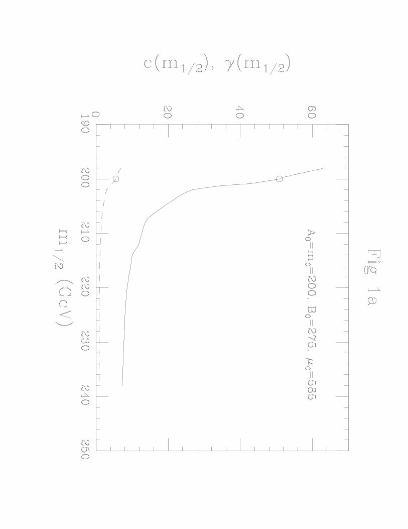
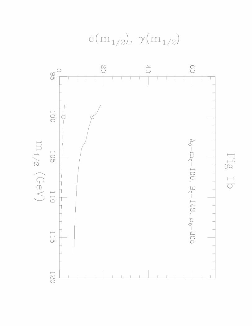
In Figs. 1a and 1b, we plot γ(m1/2) vs. m1/2 for two choices of the softsupersymmetry breaking parameters A0, B0, m0, and µ0. On this scale, γ1

and γ2 are virtually indistinguishable so we only show γ1. On the same plotswe show, for comparison, the traditional prescription c(m1/2) as well. Therange of m1/2 corresponds to the values of the common gaugino mass forwhich SU(3) × SU(2) × U(1) is broken to SU(3) × U(1)em. Note that theasymptotic, “natural” value of c(m1/2) for large m1/2 is order ten and notorder one. This is another demonstration why it is necessary to rescale thec’s to achieve a sensible measure of fine tuning.

Figures 2a and 2b show the effect of increasing the overall scale of softsymmetry breaking on fine tuning. In Fig. 2a the fine-tuning parameterγ(g3) is plotted as a function of g3(MU), where MU is the unification scale.

11

We include three choices of A0, B0, m0, and µ0 with different overall scalesof soft symmetry breaking. The square, circle, and diamond in each figurecorrespond to the point with the correct value of the Z-boson mass for thecases (i) A0 = m0 = m1/2 = 400 GeV, B0 = 523 GeV, µ0 = 1125 GeV,(ii) A0 = m0 = m1/2 = 200 GeV, B0 = 275 GeV, µ0 = 585 GeV, and (iii)A0 = m0 = m1/2 = 50 GeV, B0 = 90 GeV, µ0 = 154 GeV, respectively.The light case has a chargino with a mass less than MZ/2 and therefore isexcluded experimentally. Figure 2b is similar to 2a but displays γ(yt) vs.yt(MU).

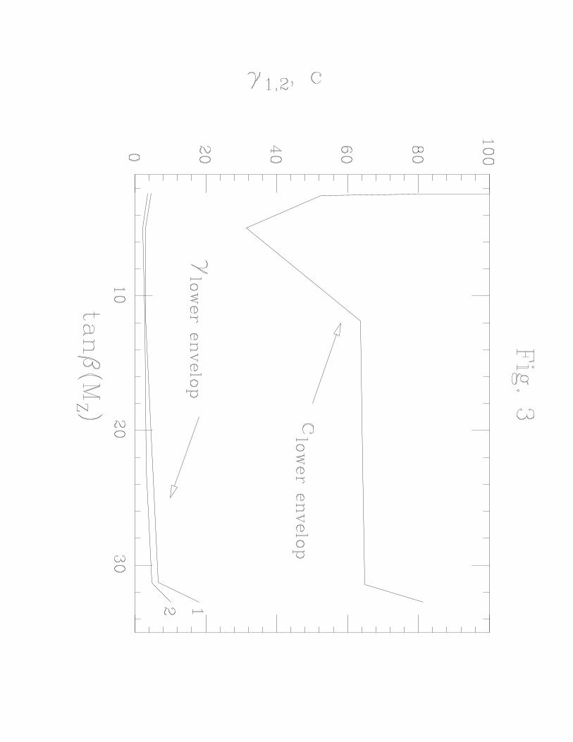
Fig. 3 displays how much fine tuning the MSSM currently requires inlight of some general experimental constraints. We consider a region of ourinput parameter space defined by the ranges |A0| ≤ 400 GeV, m0 ≤ 400GeV, and |m1/2| ≤ 400 GeV. For values of the soft supersymmetry break-ing parameters consistent with a neutral lightest SUSY particle (LSP), withthe current LEP measurement of the Z width, with a Higgs mass heavierthat 60 GeV, and with chargino masses heavier than MZ/2, we plot c =max{c(m1/2), c(m0), c(yt), c(g3)}, γ1 = max{γ1(m1/2), γ1(m0), γ1(yt), γ1(g3)},and γ2 = max{γ2(m1/2), γ2(m0), γ2(yt), γ2(g3)} vs. tanβ(MZ). In the figure,we display curves representing the lower envelopes of the resulting regions.Notice that the original Barbieri and Giudice bound of c(a) < 10 has alreadybeen exceeded, while the new criteria show that weak scale stability can stillarise naturally.

Finally, in Table 1 we display the BG sensitivity parameters c(a) andthe fine tuning parameters γ(a) for various a in a representative case withA0 = m0 = m1/2 = 200 GeV, B0 = 275 GeV, and µ0 = 585 GeV. Note thatthe relative normalization of the sensitivity parameters, c(a), can be quitedifferent. This means that we can not adopt a universal measure of fine tun-ing by appealing only to the c(a)’s (e.g., c < 100). A relative normalizationfor each c(a) must be computed in the manner described in section three.

Table 1

12

a c(a) c1 c2 γ1 γ2

m1/2 50.8 9.29 10.3 5.47 4.92

m0 21.8 3.21 4.66 6.79 4.68

g3 209. 42.3 43.2 4.94 4.84

yt 32.5 4.92 5.77 6.61 5.63

5 Conclusions

Naturalness criteria are frequently used to place upper bounds on superpart-ner masses in supersymmetric extensions standard model. We have analyzedthe prescription popularly used to measure fine tuning. This prescriptionis an operational implementation of Susskind’s statement of Wilson’s senseof naturalness, “Observable properties of a system should be stable againstminute variations of the fundamental parameters.” Because this prescriptionis only a measure of sensitivity, we found that it is not a reliable measure ofnaturalness. We then constructed a family of prescriptions which measurefine tuning more reliably. Our measure is an operational implementation ofa modified version of Wilson’s naturalness criterion: Observable propertiesof a system should not be unusually unstable against minute variations ofthe fundamental parameters. Our derivation determines the normalizationof naturalness measures and makes clear to what extent theoretical prejudiceinfluences these measures. The new prescriptions we construct allow upperbounds on superpartner masses to be placed with greater confidence. Byapplying our prescriptions to the minimal supersymmetric standard model,we find that the theory provides a much more natural explanation of weakscale stability than previous methods indicate. More importantly, we findthat the scale of supersymmetry breaking can be significantly higher thanprevious naturalness criteria indicate.

Acknowledgments

GA would like to thank the Institute for Theoretical Physics in Santa Barbaraand the Aspen Center for Physics for their hospitality.

13

References

[1] R. Barbieri and G. F. Giudice, Nucl. Phys, B306, 63 (1988); J. Ellis,K. Enqvist, D.V. Nanopoulos, and F. Zwirner, Mod. Phys. Lett. A1, 57(1986).

[2] K. Wilson, as quoted by L. Susskind, Phys. Rev. D20, 2619 (1979); G.’tHooft, in Recent developments in gauge theories, ed by G. ’t Hooft et al.(Plenum Press, New York, 1980)p. 135

[3] L. Ibanez and G.G. Ross, Phys. Lett 110B, 215 (1982)

[4] K. Inoue, A. Kakuto, H. Komatsu, and S. Takeshita, Prog. Theor. Phys.68, 927 (1982).

[5] L. Alvarez-Gaume, M. Claudson, and M. B. Wise, Nuc. Phys. B207, 96(1982); L. Alvarez-Gaume, J. Polchinski, and M. B. Wise, Nuc. Phys.B221, 495 (1983).

[6] J. Ellis, J. S. Hagelin, D. V. Nanopoulos, and K. Tamvakis, Phys. Lett.125B, 275 (1983).

[7] G. W. Anderson and , D. J. Castano, Phys. Rev. D52, 1693-1700 (1995)hep-ph/9412322 ; MIT-CTP-2464, hep-ph/9509212.

[8] V.S. Kaplunovsky and J. Louis, Phys. Lett. B306, 269 (1993).

[9] B. de Carlos and J.A. Casas, Phys. Lett B309, 320 (1993).

14

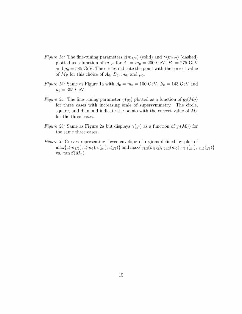
Figure 1a: The fine-tuning parameters c(m1/2) (solid) and γ(m1/2) (dashed)plotted as a function of m1/2 for A0 = m0 = 200 GeV, B0 = 275 GeVand µ0 = 585 GeV. The circles indicate the point with the correct valueof MZ for this choice of A0, B0, m0, and µ0.

Figure 1b: Same as Figure 1a with A0 = m0 = 100 GeV, B0 = 143 GeV andµ0 = 305 GeV.

Figure 2a: The fine-tuning parameter γ(g3) plotted as a function of g3(MU)for three cases with increasing scale of supersymmetry. The circle,square, and diamond indicate the points with the correct value of MZ

for the three cases.

Figure 2b: Same as Figure 2a but displays γ(yt) as a function of yt(MU ) forthe same three cases.

Figure 3: Curves representing lower envelope of regions defined by plot ofmax{c(m1/2), c(m0), c(yt), c(g3)} and max{γ1,2(m1/2), γ1,2(m0), γ1,2(yt), γ1,2(g3)}vs. tan β(MZ).

15

This figure "fig1-1.png" is available in "png" format from:

http://arXiv.org/ps/hep-ph/9409419v2

This figure "fig1-2.png" is available in "png" format from:

http://arXiv.org/ps/hep-ph/9409419v2

This figure "fig1-3.png" is available in "png" format from:

http://arXiv.org/ps/hep-ph/9409419v2

This figure "fig1-4.png" is available in "png" format from:

http://arXiv.org/ps/hep-ph/9409419v2

This figure "fig1-5.png" is available in "png" format from:

http://arXiv.org/ps/hep-ph/9409419v2