1

Fine-tuning Regression Forests Votes forObject Alignment in the Wild

Heng Yang, Student Member, IEEE, Ioannis Patras, Senior Member, IEEE

Abstract—In this paper we propose a object alignment methodthat detects the landmarks of an object in 2D images. Inthe Regression Forests (RF) framework, observations (patches)that are extracted at several image locations cast votes for thelocalization of several landmarks. We propose to refine the votesbefore accumulating them into the Hough space, by sieving and/oraggregating. In order to filter out false positive votes, we passthem through several sieves, each associated with a discrete orcontinuous latent variable. The sieves filter out votes that are notconsistent with the latent variable in question, something thatimplicitly enforces global constraints. In order to aggregate thevotes when necessary, we adjusts on-the-fly a proximity thresholdby applying a classifier on middle-level features extracted fromvoting maps for the object landmark in question. Moreover, ourmethod is able to predict the unreliability of an individual objectlandmark. This information can be useful for subsequent objectanalysis like object recognition. Our contributions are validatedfor two object alignment tasks, face alignment and car alignment,on datasets with challenging images collected in the wild, i.e. theLabeled Face in the Wild, the Annotated Facial Landmarks inthe Wild and the street scene car dataset. We show that withthe proposed approach, and without explicitly introducing shapemodels, we obtain performance superior or close to the state ofthe art for both tasks.

Index Terms—Regression Forests, facial feature, object align-ment.

I. INTRODUCTION

DEFORMABLE object alignment in an image is oneof the most important and well studied problems in

computer vision, where the shape of the object, such asface or car, is typically described by a set of landmarksS = {h1, ..., hj , ..., hJ}, with hj the coordinates of the jthlandmark in the shape space. This alignment step is verycrucial for a variety of applications like facial expressionrecognition [1], object reconstruction and tracking. In the pastdecades, it has been studied extensively and many alignmentmodels have been proposed, particularly for the face align-ment, for instance the Active Appearance Model (AAM) [2].Recent approaches on object alignment attempt to make atransition from images recorded in controlled conditions toimages “in the wild”, for instance [3], [4], [5], [6], [7] for facealignment and [8] for car alignment. However, they still havedifficulties with low quality face images, object pose variationsand partial occlusions, especially when high accuracy and real-time detection are needed.

Copyright (c) 2013 IEEE. Personal use of this material is permitted.However, permission to use this material for any other purposes must beobtained from the IEEE by sending a request to pubs-permissions@ieee.org.

H. Yang and I. Patras are with the School of Electrical Engineering andComputer Science, Queen Mary University of London, London, UK, E1 4NS.e-mail: {heng.yang,i.patras}@qmul.ac.uk.

In this paper, we address the problem using random decisionforests, given their good performance in various challengingcomputer vision tasks like action recognition [9], humanpose estimation [10], head pose estimation [11] and facialfeature detection [4]. We use random Regression Forest inthis work, which is also regarded as an important instance ofthe Generalized Hough Transform [9], [12]. In this framework,image patches that are densely extracted from the image andare propagated through each tree of the forest until they arriveat leaf nodes, where, they cast votes in the Hough space ofthe parameters to be estimated. In general, the number ofvotes is very large since the patches are densely extractedfrom the whole image or region of interest. Taking all thevoting elements into account can lead to a bias towardsthe mean shape, i.e. the average shape of a large numberof samples. Therefore, it is common practice in RegressionForests set a threshold that does not allow elements withlarge offsets to vote, e.g., [4], [10]. This threshold controlsthe maximum allowed offsets of votes. We in this papertransform the Euclidean distance d into a proximity metric bya function f(d) = e−d. Therefore longer distance correspondsto lower proximity. We then equivalently set a threshold onthe proximity on the lower bound. If a large threshold isset on proximity, only votes with small offsets are allowed.Those are expected to have high localization accuracy, unlessthey are contaminated due to conditions like noise, shadowsand occlusions. On the contrary, with a small threshold onproximity, votes are allowed from observations that are farand in this way introduce shape constraints and robustness toocclusions. The extreme case of the latter situation is using allvoting elements from the region of interest. Typically, such athreshold is optimized at training stage and kept fixed duringtesting.

There are two issues with the Regression Forest mechanismdescribed above. First, different landmarks are voted in acompletely independent way, i.e. there is no mechanism thatencourages consistent predictions. Therefore we might seeimplausible detection results that violates the shape consis-tency. Second, keeping the proximity threshold fixed createsproblems on challenging images, for example when somelandmarks are partially occluded. In extreme cases, the sizeof the occluded area is big but very high proximity thresholdis set. In such cases, very few ’good’ votes can be obtained,which in turn results in localization failures. To address thesetwo problems, we propose a method that refines the votes, bysieving and/or aggregating them, before they are accumulatedinto the Hough space, as described below.

Votes Sieving introduces a bank of sieves, each one as-

2

sociated with one of a few latent variables such as the headpose discrete label, or the location of some anchor points forinstance the object center. Essentially, each sieve operates as afilter that rejects votes that are not consistent with hypothesesof the latent variable in question. This introduces globalconsistency and effectively eliminates the false positive votes.

Votes Aggregating learns a model that for each test image,decides whether or not to reduce the proximity threshold foran individual object landmark. This is opposed to using afixed proximity threshold and controls the extend of spatialconstraints. For example, with a low proximity threshold forthe localisation of the left-eyebrow corner, one would alsouse the votes of test-patches that arrive at leaf nodes to whichtraining patches that were extracted close to other facial areasas well (e.g. left eye, or even nose), mostly arrive. Since testpatches that vote for the location of more that one landmarkintroduce shape constraints between the location of thoselandmarks, the proximity threshold can be seen as controllingthe spatial extend of the (implicit) shape model that we use.The decision is made based on a classifier that is built onmiddle-level features which are extracted from the currentvotes for the location of the landmark in question.

Another contribution is that our approach predicts the unre-liability of each individual landmark. The unreliability tellsthe probability of the landmark is with occlusion or otherclutter and provides useful information for subsequent high-level object analysis for instance face recognition.

The experimental results show that without using typicalshape constraints, the approach achieves results superior orcomparable to state-of-the-art on two challenging face land-marks datasets, namely, the Labelled Faces in the Wild, theAnnotated Facial Landmarks in the Wild. In addition, since nospecific model is assumed, the same approach can be appliedwithout modification to other domains. This is illustrated byapplying the approach for car alignment and we obtain thestate-of-the-art results. We also show that the benefits of usingsieves and determining an image-dependent and landmark-dependent threshold are higher for the ’difficult’ images inboth datasets.

The rest of the paper is organised as follows. Relatedwork on random forests and object alignment are given inSection 2. In Section 3 we introduce the proposed method.Experimental results and comparisons with the current state-of-the-art methods are given in Section 4 and in Section 5 wedraw some conclusions.

II. RELATED WORK

In this section we first present an overview of related workon object landmarks detection, and then present a brief reviewof the random forests literature that is relevant to this work.

A. Object Alignment

Object alignment is a well-studied problem in computervision, especially for the face. Two different sources of in-formation are typically exploited for this task: appearance andspatial shape. Based on how those two types of informationare utilized, we categorize the methods into three groups:

discriminative local landmark detection, part-based deformablemodels and explicit shape regression.

Discriminative Local Detection approaches only exploitthe discriminative appearance features of different landmarks.A regressor or a classifier is learned independently for eachlandmark. For instance, in [13], GentleBoost classifier basedon Gabor features is proposed to detect 20 facial points sep-arately. The Support Vector Machine (SVM) classifier is usedas facial point detector in [14] and [3] . Regression Forests(RF) are introduced as a local detector for facial landmarks[4], [15]. In [16], Boddeti et al. introduced Correlation Filtersto learn a local appearance model. Methods in this categorycan be regarded as an extension of general object detection.Since no shape constraints are imposed, this type of methodshave good generality but suffer heavily from partial occlusions.

Part-based Deformable Models focus on using shape priorto regularize the local part detections. Thus the two tasks attraining time are first learning the part models and secondlearning the shape prior. The part model is often learnedfollowing the discriminative local detection methodology de-scribed above. Typical shape models like the ConstrainedLocal Models (CLMs) [17] first align the images using thelandmarks annotation by Procrustes analysis, then learn theshape prior by using Principal Component Analysis (PCA).Other shape models include the probabilistic MRF modelin [18] and tree structured shape models proposed by Zhuand Ramanan [6]. The latter has shown good results bothin capturing global elastic deformation and in finding theglobal optimal solutions by linear programming. Amberg etal. [19] proposed to find an optimal set of local detectionsusing a Branch & Bound method. Recently, several methodsproposed non-parametric shape constraints, for example, theRANSAC-based methods in [3] and [8]; the regularized mean-shift model in [20]; the graph-matching method in [21] andshape constraints within the regression forests in [22].

Explicit Shape Regression approaches jointly model theshape and appearance, and learn directly a mapping from im-age features to the shape space (the location of the landmarks).A typical method is this category is the Active AppearanceModel (AAM) proposed by Cootes et al. [2]. The AAM isfit by learning a linear regression between the appearancedifferences and the increment of alignment parameters. Sincea very simple linear regression method is applied, the originalfitting method suffers from occlusion and is very difficultto deal with unseen images. Tresadern et al. [23] showedthat using boosted regression for AAM discriminative fittingsignificantly improved the original linear formulation. In theboosting/cascade framework, recent methods [24], [7] learn aset of weak regressors (random ferns) to model the relationbetween the image feature and the update of the parameters.They introduce a cascade in which they re-sample featuresbased on the current shape state and use them in the nextregressor. Xiong and De la Torre [25] proposed a similarcascaded method and used more advanced image features(HoG [26] and SIFT [27]) that improves the performance.

3

voting

elements

0

change the threshold k>0

k>0change the threshold

proximity

threshold

control

di erent

sieves

Aggregating

steps

0

Aggregating

steps

Input

OutputForest

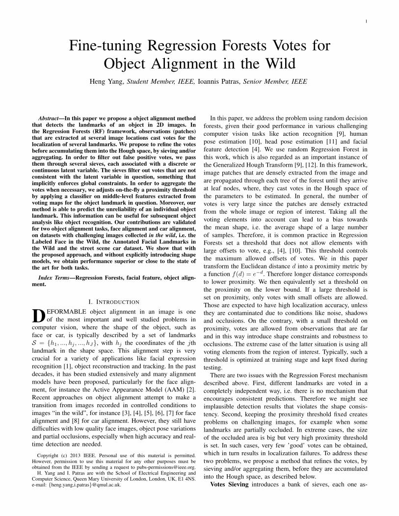
Fig. 1: Framework of the method.

B. Random Forests

Random forests have emerged as a powerful and versatilemethod that has been successful in real-time human poseestimation, semantic segmentation, object detection and actionrecognition [9], [11], [28]. A comprehensive introduction ofdecision forests and their applications in computer vision isgiven in [29]. We in this paper build the random RegressionForest that is similar to the framework used for facial featuredetection [4], [30], [31], 3D head pose estimation [32] andHuman Pose Estimation (body joints prediction) [28].

A regression forest is an ensemble of decision trees thatpredicts continuous outputs. Each binary tree consists ofinternal nodes and leaf nodes. The internal nodes contain testfunctions that evaluate the input features to decide whetherto go to the left or to the right child nodes. The terminalnodes contain continuous prediction models, as opposed to thecategorical prediction in classification forests. At the trainingtime, a set of image patches are randomly extracted from thetraining images. Each of them contain the offset information,e.g. the patch center to each of the facial landmarks. Ateach internal node, a pool of candidate functions is randomlygenerated. The one that maximizes the information gain isselected as the split function at that nodes. This process isrecursively applied until a certain stopping criterion is met,such as that the maximum depth of the tree is reached or thenumber of patches is less than a threshold. During testing time,image patches are densely extracted from the image and fedto each tree. When one patch arrives at a leaf node, there is aregression model, usually a relative offset vector (i.e. vote) toeach of the landmarks of interest (potentially to all landmarks),along with a weight. In this way, a regression forest transformsthe image observation to a set of votes.

Some recent Regression Forests introduce latent variablesand use the additional information at the training phase. Sunet al. [10] propose a conditional regression forest model forhuman pose estimation. During training, at each leaf node,the vote is decomposed into the distribution of 3D bodyjoint locations for each codeword at the leaf node and thecodeword mapping probability. In their model, they use thelatent variables like the body height and body orientation. Theypropose a method to jointly estimate the body joint locationsand the latent variable. Dantone et al. [4] also introduceda regression forests model conditioned on latent variable ofhead pose for face alignment. In their method, they divide thetraining set into subsets according to head pose yaw angles

(left profile, left, front, right, right profile). An individualregression forest is trained on each subset. During testing aset of regression trees is selected according to the estimatedprobability of the head pose yaw angle. The later is given byan additional forest trained to perform head pose estimation.

Our approach is also closely related to those methods thatanalyse votes returned from regression forests. For instance,[33] modelled the joint distribution over all the votes and thehypotheses in a probabilistic way, rather than simply accu-mulating the votes. [12] studied the geometric compatibilitiesof the voting elements in a pairwise fashion within a game-theoretic setting. These methods are developed for persondetection and focus on intra-class geometrical agreement,while the consistency in our problem is inter-class, since weconsider the localization of multiple landmarks on an object.In terms of rejecting irrelevant observations for regression, ourwork is related to [34] that applies classifiers for observationselection for robust object tracking.

III. METHOD

In this section, we describe the proposed method as an-swering the problem of face alignment/facial feature detec-tion. We first introduce the latent space and the votes fromregression forests associated with the latent variable. Then wedescribe the votes sieving strategy based on the latent variableagreement and finally we describe the votes aggregating andlandmark unreliability detection.

A. RF Votes with Latent Variable

For tree construction, we follow the procedure proposed in[4]. We use the information gain (IG) as the criterion to selectthe split function. A entropy-like class uncertainty H(I) on aset of image patches I is defined as:

H(I) = −∑hj∈H

∑Ii∈I p(hj |Ii)|I|

log

(∑Ii∈I p(hj |Ii)|I|

),

(1)

p(hj |Ii) ∝ f(|dIihj|) = exp

(−|dIihj|

α

), (2)

where p(hj |Ii) indicates the probability that the patch Iibelongs to the the j-th landmark [4], j ∈ 1, ..., J . We usehj denote the location of the landmark. f(·) is a functionthat transforms the Euclidean distance dIihj

into a proximitymetric. This proximity metric is used throughout this paper.

4

The constant α controls the steepness of this function Notethat the distance measure d is normalized by the object size.

Once the regression forest is trained, the observations, i.e.image patches Ii ∈ I are extracted from the testing imagelocation yi and fed to it. When they arrive at leaf nodes theycast weighted votes v(h|Ii) for the location of one or morelandmarks. For a given hypothesis h ∈ H , the score of h isdetermined by the sum of votes that support the hypothesis:S(h) =

∑i v(h|Ii). In practice each patch Ii will be sent to

each tree t ∈ T in the forest, i.e. S(h) =∑i

∑t v(h|Iit). We

will drop the t in the subsequent discussion for clarity andconsistency with other methods.

With the procedure described above, there are some votesare inconsistent with some latent variables, for instance, inhead pose and face center. These votes are unlikely to votecorrectly. Some previous work [35] proposes to augment thehypothesis space by a latent space Z to enforce consistencyof the votes in some latent properties z ∈ Z. That methodcan only deal with discrete latent variables and has highmemory requirements and computational complexity, whenlarge training data is used since all training patches need tobe stored. By contrast, the latent space in our work can beeither discrete or continuous. The score of a hypothesis in theaugmented space is then given by:

S(h) =∑

i,z∈φ(z)

v(h, z|Ii) (3)

where φ(z) is an affiliation term defined as follows. When thelatent space is discrete, φ(z) = {z}, with z a discrete label. Itmeans votes with the same latent variable as z are used. Whenthe latent space is continuous, φ(z) = {z : ||z − z|| ≤ r},where r is the radius of a region around z. The details aredescribed in Section III-B.

B. RF Votes Sieving

1) Sieving via Discrete Latent Variable: Our method ofsieving votes using discrete latent variable is similar to theconditional regression forest Partial Model proposed in [10]that was used for human pose estimation. During training,each patch extracted from the training samples is annotatedwith a discrete latent label. We use the tree constructionprocedure proposed in III-A. When the training patches arrivethe leaf node l, we learn one model for each state of thelatent variable. More specifically, we first partition the trainingpatches according to their latent variable labels and then learna model in each partition with latent label z for the hypothesish. The model vector is (∆z

l , ωzl , p

zl ). where ∆z

l is the relativeoffset vector, obtained by taking the center of the largest modefound by mean-shift clustering method [36] in the partitionwith latent label z, similar to [10]. ωzl is weight, given by therelative size of the largest cluster. For the latent variable z,pzl is the probability of the latent variable at leaf node l, thatis calculated as the proportion of the training samples whoselabel is z, that is,

pzl =nzl∑z∈Z n

zl

(4)

where nzl is the number of training patches with the latent labelz. When a patch Ii extracted from the location yi arrives thisleaf node l, the vote is represented as:

v(h, z|l) = ωzl δ(∆zl + yi − h). (5)

Since the probability of the latent variable is independent ofthe hypothesis, its scoring function is:

S(z) =∑i

v(z|Ii) =∑i

∑h∈H

v(h, z|Ii) =∑l

pzl . (6)

The latent variable is estimated as z = arg maxz∈ZS(z). Giventhe estimation, the hypothesis scoring function is formed byusing the votes with the corresponding latent state, i.e.,

S(h) =∑

i,z∈φ(z)

v(h, z|Ii) (7)

(a) (b) (c) (d)

(e) (f) (g) (h)

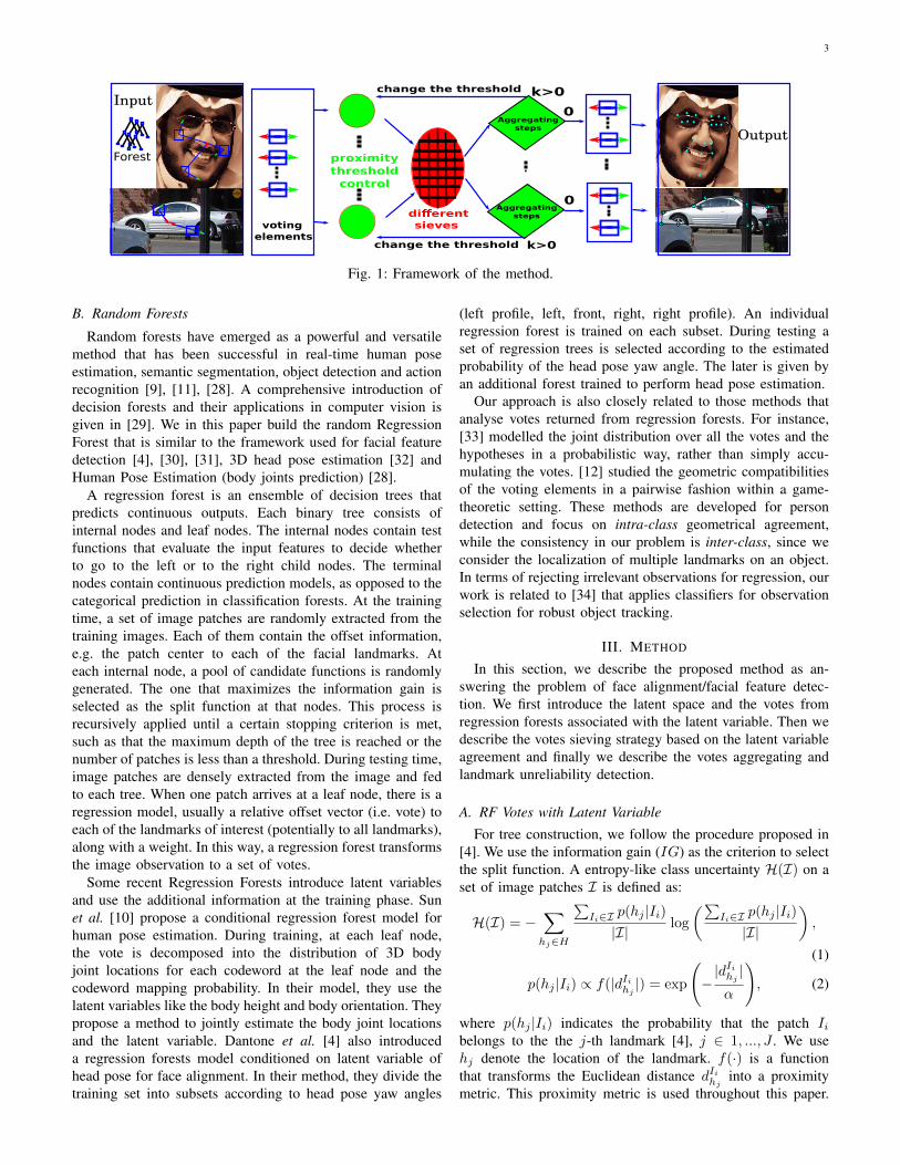
Fig. 2: Illustration of sieving via continuous latent variable(face center). (a) A voting element consists of two offsetvectors, one to the target point (green arrow) and the otherto face center (red arrow). (b) Original set of votes for the leftbrow center. (c) The absolute face center votes, those in greenare regarded as consistent to the face center. (d) The remainingvoting elements filtered by the face center sieve. (e) All votingelements are used to localize the face center (red dot). (f) and(h) are the Hough maps generated from votes of (b) and (d)respectively. (g) shows the corresponding detection results.

2) Sieving via Continuous Latent Variable: The tree con-struction process of the sieving via continuous latent variableis similar. Each training patch is associated with a continuouslatent variable label, for instance the displacement to the objectcenter. This latent information is not used until the patchesarrive the leaf node. We use the face center as an exampleto show how continuous latent variable is modelled. The leafmodel vector is (∆z

l , ωzl ,∆

czl , ω

czl ). In addition to ∆z

l and ωzl ,we have two similar terms, ∆cz

l and ωczl , that are the offsetsto the face center and the corresponding weight respectively,learned in a similar way of learning ∆z

l and ωzl .During testing, we will first estimate the state of the latent

variable z, i.e. the location of the face center. Similar tocalculating the actual voting of the hypothesis, the absolutevoting to the face center in return is yi + ∆zc

l , which is theactual form that is accumulated into the Hough space. Thevoting function is calculated like in Eq. 5. Thus the scorefunction is:

S(z) =∑i

v(z|Ii) =∑i

∑h∈H

v(h, z|Ii) (8)

5

0

0.5

1

0

0.5

1

0

0.5

1

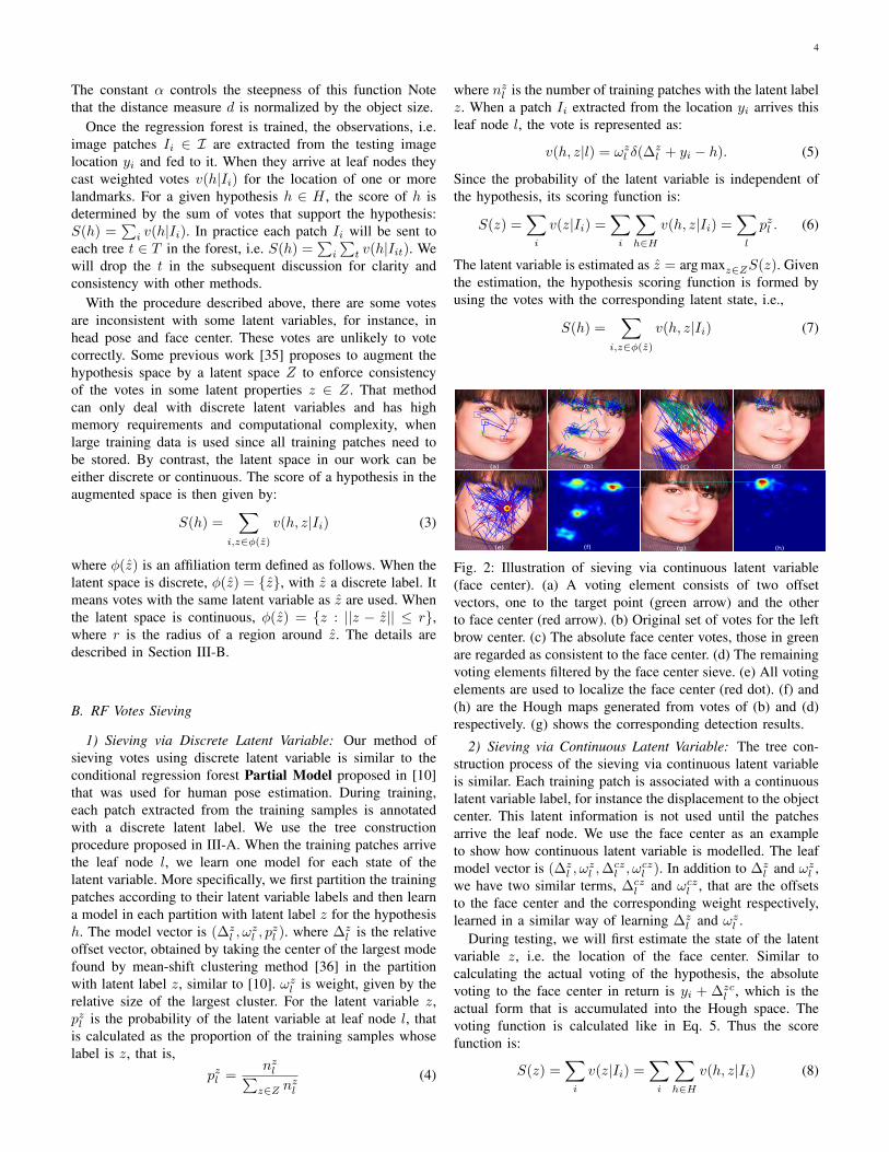
Fig. 3: Illustration of aggregating the votes by updating thethreshold. From left to right, the first row shows the originalface image, all votes for the point (λ = 0.35), votes passedface center sieve and the aggregated votes from updatedthreshold (λ = 0.22) passed face center sieve. The colorrepresents the weight of each vote and the dark terminal isthe voting destination. The second row shows the detectionresults, normalized Hough map for original voting, after facecenter sieving and re-voting.

Then a mean-shift [36] algorithm is employed on the Houghmap to find the mode. This is used as an estimate of the latentvariable, z. We then define a region around z as

φ(z) = {z : ||z − z|| ≤ r} (9)

The radius r is learned at training time. The sieve filters out thepatches which cast votes out of this region, i.e., retains onlythe votes that are consistent with the estimate of the latentvariable. The voting model for the hypothesis is the same asdescribed in Eq. 5. The score function of hypothesis h afterthe latent continuous sieve can be written as:

S(h) =∑

i,z∈φ(z)

v(h, z|Ii) (10)

It shares the same form of Eq. 7 but with different φ(z)property since z here is in continuous space.

As shown in Fig. 2d, after filtering by the sieve, votingelements that violate the face center consistency and vote forother face center hypotheses, are removed from the votes set.The ones that satisfy the face center consistency are kept.

C. RF Votes Aggregating

Taking all the voting elements into account for each hy-pothesis can lead to bias towards the mean shape and also itis very time consuming. Thus in practice, when collecting thevotes for an individual feature point, a threshold is applied,similar to [4], [12], [10]. This works as a filter that prohibitsvotes with large offsets. This threshold is typically optimizedduring training and kept fixed during testing. Only the votesthat satisfy threshold are allowed to vote for the hypothesis,i.e., f(∆) > λ, where f(·) is the proximity function definedin Eq. (2).

This mechanism works well in most cases but fails, forexample when a feature point is heavily occluded. As shownin Fig. 3, in the presence of a heavy occlusion, only fewvalid voting elements remain after the face center sieve isapplied. This is expected since in the case of heavy occlusion,

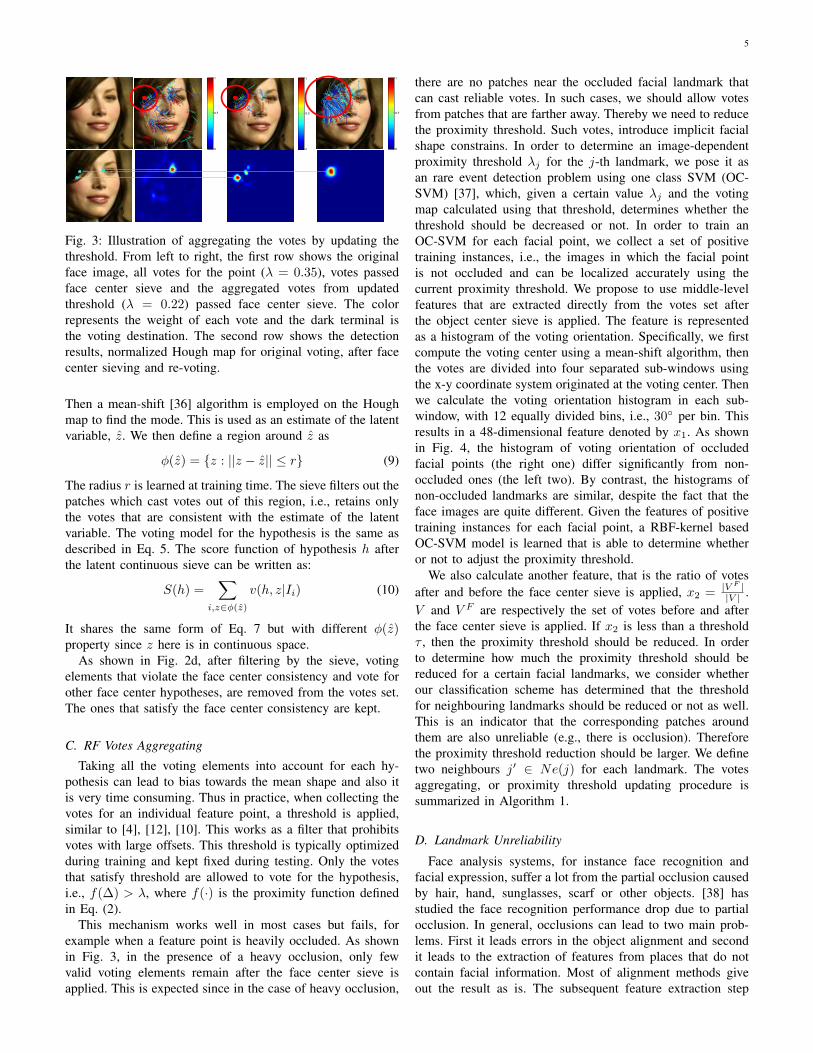
there are no patches near the occluded facial landmark thatcan cast reliable votes. In such cases, we should allow votesfrom patches that are farther away. Thereby we need to reducethe proximity threshold. Such votes, introduce implicit facialshape constrains. In order to determine an image-dependentproximity threshold λj for the j-th landmark, we pose it asan rare event detection problem using one class SVM (OC-SVM) [37], which, given a certain value λj and the votingmap calculated using that threshold, determines whether thethreshold should be decreased or not. In order to train anOC-SVM for each facial point, we collect a set of positivetraining instances, i.e., the images in which the facial pointis not occluded and can be localized accurately using thecurrent proximity threshold. We propose to use middle-levelfeatures that are extracted directly from the votes set afterthe object center sieve is applied. The feature is representedas a histogram of the voting orientation. Specifically, we firstcompute the voting center using a mean-shift algorithm, thenthe votes are divided into four separated sub-windows usingthe x-y coordinate system originated at the voting center. Thenwe calculate the voting orientation histogram in each sub-window, with 12 equally divided bins, i.e., 30◦ per bin. Thisresults in a 48-dimensional feature denoted by x1. As shownin Fig. 4, the histogram of voting orientation of occludedfacial points (the right one) differ significantly from non-occluded ones (the left two). By contrast, the histograms ofnon-occluded landmarks are similar, despite the fact that theface images are quite different. Given the features of positivetraining instances for each facial point, a RBF-kernel basedOC-SVM model is learned that is able to determine whetheror not to adjust the proximity threshold.

We also calculate another feature, that is the ratio of votesafter and before the face center sieve is applied, x2 = |V F |

|V | .V and V F are respectively the set of votes before and afterthe face center sieve is applied. If x2 is less than a thresholdτ , then the proximity threshold should be reduced. In orderto determine how much the proximity threshold should bereduced for a certain facial landmarks, we consider whetherour classification scheme has determined that the thresholdfor neighbouring landmarks should be reduced or not as well.This is an indicator that the corresponding patches aroundthem are also unreliable (e.g., there is occlusion). Thereforethe proximity threshold reduction should be larger. We definetwo neighbours j′ ∈ Ne(j) for each landmark. The votesaggregating, or proximity threshold updating procedure issummarized in Algorithm 1.

D. Landmark Unreliability

Face analysis systems, for instance face recognition andfacial expression, suffer a lot from the partial occlusion causedby hair, hand, sunglasses, scarf or other objects. [38] hasstudied the face recognition performance drop due to partialocclusion. In general, occlusions can lead to two main prob-lems. First it leads errors in the object alignment and secondit leads to the extraction of features from places that do notcontain facial information. Most of alignment methods giveout the result as is. The subsequent feature extraction step

6

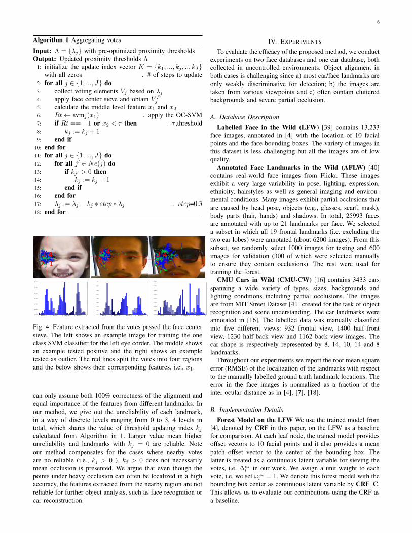
Algorithm 1 Aggregating votes

Input: Λ = {λj} with pre-optimized proximity thresholdsOutput: Updated proximity thresholds Λ

1: initialize the update index vector K = {k1, ..., kj , .., kJ}with all zeros . # of steps to update

2: for all j ∈ {1, ..., J} do3: collect voting elements Vj based on λj4: apply face center sieve and obtain V Fj5: calculate the middle level feature x1 and x26: Rt← svmj(x1) . apply the OC-SVM7: if Rt == −1 or x2 < τ then . τ ,threshold8: kj := kj + 19: end if

10: end for11: for all j ∈ {1, ..., J} do12: for all j′ ∈ Ne(j) do13: if kj′ > 0 then14: kj := kj + 115: end if16: end for17: λj := λj − kj ∗ step ∗ λj . step=0.318: end for

123 4

123 4

123 4

| Region 1 | Region 2 | Region 3 | Region 4 |0.00

0.05

0.10

0.15

0.20

0.25

0.30

| Region 1 | Region 2 | Region 3 | Region 4 |0.00

0.05

0.10

0.15

0.20

0.25

0.30

0.35

0.40

| Region 1 | Region 2 | Region 3 | Region 4 |0.00

0.05

0.10

0.15

0.20

0.25

0.30

0.35

0.40

Fig. 4: Feature extracted from the votes passed the face centersieve. The left shows an example image for training the oneclass SVM classifier for the left eye corder. The middle showsan example tested positive and the right shows an exampletested as outlier. The red lines split the votes into four regionsand the below shows their corresponding features, i.e., x1.

can only assume both 100% correctness of the alignment andequal importance of the features from different landmarks. Inour method, we give out the unreliability of each landmark,in a way of discrete levels ranging from 0 to 3, 4 levels intotal, which shares the value of threshold updating index kjcalculated from Algorithm in 1. Larger value mean higherunreliability and landmarks with kj = 0 are reliable. Noteour method compensates for the cases where nearby votesare no reliable (i.e., kj > 0 ). kj > 0 does not necessarilymean occlusion is presented. We argue that even though thepoints under heavy occlusion can often be localized in a highaccuracy, the features extracted from the nearby region are notreliable for further object analysis, such as face recognition orcar reconstruction.

IV. EXPERIMENTS

To evaluate the efficacy of the proposed method, we conductexperiments on two face databases and one car database, bothcollected in uncontrolled environments. Object alignment inboth cases is challenging since a) most car/face landmarks areonly weakly discriminative for detection; b) the images aretaken from various viewpoints and c) often contain clutteredbackgrounds and severe partial occlusion.

A. Database Description

Labelled Face in the Wild (LFW) [39] contains 13,233face images, annotated in [4] with the location of 10 facialpoints and the face bounding boxes. The variety of images inthis dataset is less challenging but all the images are of lowquality.

Annotated Face Landmarks in the Wild (AFLW) [40]contains real-world face images from Flickr. These imagesexhibit a very large variability in pose, lighting, expression,ethnicity, hairstyles as well as general imaging and environ-mental conditions. Many images exhibit partial occlusions thatare caused by head pose, objects (e.g., glasses, scarf, mask),body parts (hair, hands) and shadows. In total, 25993 facesare annotated with up to 21 landmarks per face. We selecteda subset in which all 19 frontal landmarks (i.e. excluding thetwo ear lobes) were annotated (about 6200 images). From thissubset, we randomly select 1000 images for testing and 600images for validation (300 of which were selected manuallyto ensure they contain occlusions). The rest were used fortraining the forest.

CMU Cars in Wild (CMU-CW) [16] contains 3433 carsspanning a wide variety of types, sizes, backgrounds andlighting conditions including partial occlusions. The imagesare from MIT Street Dataset [41] created for the task of objectrecognition and scene understanding. The car landmarks wereannotated in [16]. The labelled data was manually classifiedinto five different views: 932 frontal view, 1400 half-frontview, 1230 half-back view and 1162 back view images. Thecar shape is respectively represented by 8, 14, 10, 14 and 8landmarks.

Throughout our experiments we report the root mean squareerror (RMSE) of the localization of the landmarks with respectto the manually labelled ground truth landmark locations. Theerror in the face images is normalized as a fraction of theinter-ocular distance as in [4], [7], [18].

B. Implementation Details

Forest Model on the LFW We use the trained model from[4], denoted by CRF in this paper, on the LFW as a baselinefor comparison. At each leaf node, the trained model providesoffset vectors to 10 facial points and it also provides a meanpatch offset vector to the center of the bounding box. Thelatter is treated as a continuous latent variable for sieving thevotes, i.e. ∆cz

l in our work. We assign a unit weight to eachvote, i.e. we set ωczl = 1. We denote this forest model with thebounding box center as continuous latent variable by CRF C.This allows us to evaluate our contributions using the CRF asa baseline.

7

Forest Model on the AFLW We show the contribution ofeach component of our method on AFLW by training modelsthat are listed in Table I. The trees in the forests F1, as in[4] are trained without using any additional information. Inorder to train forests with sieves using latent discrete variable,i.e. F2-F5, we quantize the head yaw angles of the trainingsamples into 3 labels like [4]. We train a forest using theadditional discrete information to learn multiple voting modelsat leaf nodes as described in Section III-B1. A similar ideais proposed by Sun et al. [10] for human pose estimation.We denote their method by CRF-S. In forests F3, F4 and F5,each vote at leaf node contains voting information to the facecenter as described in Section III-B2. In the forest model ofF4, we set the proximity threshold of individual facial pointto 0, i.e. allow all the votes from the face to vote for the facialpoint. The tree model of F5 is the same as F4 but performsthreshold adjustment as described in Section III-C. We use the

TABLE I: Description of forest models trained on the AFLW

Forest ID Sieves AggregationDiscrete ContinuousF1 No No No

F2 (CRF-S) Yes No NoF3 Yes Yes NoF4 Yes Yes Max. aggregatingF5 Yes Yes Yes

same macro settings of the forests of [4] such as the imagefeatures, maximum tree depth (20), number of tests at theinternal nodes (2500), forest size (10 trees in total) and thebandwidth of the mean-shift algorithm. Also we use the samerandom subset of the training samples for the same index oftree in each forest in order to avoid a bias caused by randomsampling of the training data.

Forest Model on the CMU-CW We train one forest foreach of the 5 views using the training set-up used in [16]. Werandomly select 400 images for each view for training and usethe rest for testing. We sample 30 patches sized 30×30 froma non-occluded landmark region for training. We use the carcenter, calculated as the mean value of all the landmarks, asa continuous latent variable in this model. A tree in the forestis trained on 300 randomly sampled car images and 4 trees intotal are trained for each view.

Parameters for votes sieving The key parameter associatedwith the continuous variable sieve, that is the radius r is setto 0.3 through a grid search on the AFLW validation set. Weuse the same sieving parameters for LFW and CMU-CW.

Parameters for votes aggregating For each facial land-mark, we select the most accurate 500 detections (localizationerror less than 0.1) from the AFLW validation dataset aspositive training samples to train the OC-SVM model. Whenthere are not enough training samples we select some from thetraining samples. The OC-SVM models of the CMU-CW isdirectly trained on the training samples. We use the LibSVM[42] to train the OC-SVM model.

0 0.02 0.04 0.06 0.08 0.1 0.12 0.14 0.16 0.18 0.20

0.1

0.2

0.3

0.4

0.5

0.6

0.7

0.8

0.9

1

Fiducial Error as a Fraction of Inter−Ocular Distance

Fra

ctio

n o

f F

iduci

al P

oin

ts

F5

F4

F3

F2

F1

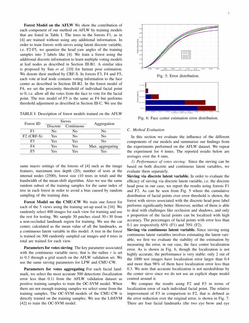
Fig. 5: Error distribution.

0 0.05 0.1 0.15 0.2 0.25 0.3 0.35 0.4 0.45 0.5

[0,0.1]

(0.1,0.2]

(0.2,0.3]

(0.3,0.4]

(0.4,Inf)

Proportion of the Face Images

Face

Cen

ter Lo

caliza

tion E

rror

Fig. 6: Face center estimation error distribution.

C. Method Evaluation

In this section we evaluate the influence of the differentcomponents of our models and summarize our findings fromthe experiments performed on the AFLW dataset. We repeatthe experiment for 4 times. The reported results below areaverages over the 4 runs.

1) Performance of votes sieving: Since the sieving can bebased on both discrete and continuous latent variables, weevaluate them separately.Sieving via discrete latent variable. In order to evaluate theefficacy of sieving via discrete latent variable, i.e. the discretehead pose in our case, we report the results using forests F1and F2. As can be seen from Fig. 5 where the cumulativedistribution of facial points over error threshold is shown, theforest with sieves associated with the discrete head pose labelperforms significantly better. However, neither of them is ableto deal with challenges like occlusion and shadows, and onlya proportion of the facial points can be localized with highaccuracy. The percentages of facial points with error less than0.1 are respectively 65% (F1) and 70% (F2).Sieving via continuous latent variable. Since sieving usingcontinuous latent variables involves estimating the latent vari-able, we first we evaluate the stability of the estimation bymeasuring the error, in our case, the face center localizationerror. As is shown in Fig. 6, though the localization is nothighly accurate, the performance is very stable: only 2 out ofthe 1000 test images have localization error larger than 0.4and more than 98% of them have localization error less than0.3. We note that accurate localization is not needed/done bythe center sieve since we do not use an explicit shape modelcentred around it.

We compare the results using F2 and F3 in terms oflocalization error of each individual facial point. The relativeimprovement of F3 in comparison to F2, that is defined asthe error reduction over the original error, is shown in Fig. 7.There are four facial landmarks (the two eye brow and eye

8

0

0.02

0.04

0.06

0.08

0.1

0.12

left brow left corner

left brow center

left brow right corner

right brow left corner

right brow center

right brow right corner

left eye left corner

left eye center

left eye right corner

right eye left corner

right eye center

right eye right cornernose left

nose center

nose right

mouth left corner

mouth center

mouth right corner

chin center

Mea

n Er

ror

F2

F3

(a)

0

0.05

0.1

0.15

0.2

0.25

0.3

0.35

left brow left corner

left brow center

left brow right corner

right brow left corner

right brow center

right brow right corner

left eye left corner

left eye center

left eye right corner

right eye left corner

right eye center

right eye right cornernose left

nose center

nose right

mouth left corner

mouth center

mouth right corner

chin center

Mea

n Er

ror

F2

F3

(b)

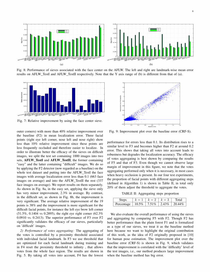
Fig. 8: Performance of sieves associated with the face center on the AFLW. The left and right are landmark-wise mean errorresults on AFLW TestI and AFLW TestII respectively. Note that the Y axis range of (b) is different from that of (a).

0%

10%

20%

30%

40%

50%

left brow left corner

left brow center

left brow right corner

right brow left corner

right brow center

right brow right corner

left eye left corner

left eye center

left eye right corner

right eye left corner

right eye center

right eye right cornernose left

nose center

nose right

mouth left corner

mouth center

mouth right corner

chin center

Relat

ive Im

prov

emen

t

Fig. 7: Relative improvement by using the face center sieve.

outer corners) with more than 40% relative improvement overthe baseline (F2) in mean localization error. Three facialpoints (right eye left corner, nose left and nose right) showless than 10% relative improvement since these points areless frequently occluded and therefore easier to localize. Inorder to illustrate better the efficacy of the sieves on difficultimages, we split the test set containing 1000 images into twosets, AFLW TestI and AFLW TestII, the former containing”easy” and the latter containing ”difficult” images. We do soby applying the F2 detector (now regarded as a baseline) on thewhole test dataset and putting into the AFLW TestI the faceimages with average localization error less than 0.1 (663 faceimages on average) and into the AFLW TestII the rest (337face images on average). We report results on them separately.As shown in Fig. 8a, in the easy set, applying the sieve onlyhas very minor improvement, 2.3% in average. By contrast,in the difficult set, as shown in Fig. 8b, the improvement isvery significant. The average relative improvement of the 19points is 38% and the improvement is more significant for thedifficult facial points, for instance the left eye brow left corner(51.5%, 0.1404 vs 0.2895), the right eye right corner (62.3%0.0910 vs. 0.2413). The superior performance of F3 over F2significantly validates the efficacy of our sieves, particularlyon ’difficult’ images.

2) Performance of votes aggregating: The aggregating ofthe votes is controlled by a proximity threshold associatedwith individual facial landmark. In F3 we use threshold thatare optimized for each facial landmark during training andin F4 reset the proximity threshold to infinity , that allowsvotes from the whole face region. The results are shown inFig. 5. By taking all votes into account, F4 has the lowest

0 0.2 0.4 0.6 0.8 1 1.2 1.4 1.6−0.2

0

0.2

0.4

0.6

0.8

1

1.2

1.4

1.6

Baseline error

Imp

rove

me

nt

ove

r th

e b

ase

line

Fig. 9: Improvement plot over the baseline error (CRF-S).

performance for errors less than 0.1. Its distribution rises to asimilar level to F3 and becomes higher than F2 at around 0.2error. This shows that taking all votes into account leads torobustness but degrades the localization accuracy. The efficacyof votes aggregating is best shown by comparing the resultsof F5 and that of F3. Even though we cannot observe largemargin of improvement in this figure, we note that the votesaggregating performed only when it is necessary, in most caseswhen heavy occlusion is present. In our four test experiments,the proportion of facial points with different aggregating steps(defined in Algorithm 1) is shown in Table II, in total only20% of them adjust the threshold to aggregate the votes.

TABLE II: Aggregating steps proportion

Steps k = 1 k = 2 k = 3 TotalPercentage 10.5% 7.51% 2.43% 20.44%

We also evaluate the overall performance of using the sievesand aggregating by comparing F5 with F2. Though F2 hasbetter performance than the plain forest F1 and is formalizedas a type of our sieves, we treat it as the baseline methodhere because we want to highlight the original contributionof this work, as the idea of F2 originally proposed in [10]for human pose estimation. The improvement plot over thebaseline error (CRF-S) is shown in Fig. 9, which validatesthat the improvement is correlated with the ’difficulty’ level ofthe test images, i.e., our method produces large improvementwhen the baseline method has big error.

9

11 2

2 2

1

1

1

2 31

1 1232

1

1

2

32

1

1

2 2

1

1

Fig. 10: Example results from the AFLW dataset before (top row) and after (bottom row) the votes aggregating. The valuebeside the red dot in the top row indicates the unreliability/ step length of aggregating. For clarity, the reliable point where noaggregating is needed, i.e. 0 is not shown in the figure.

3) Landmark unreliability: We qualitatively show someexamples of facial landmarks unreliability detection in Fig. 10,where the number associated with each point location, that isalso the aggregating step, intuitively reflect the unreliabilitylevel of the point. Since the unreliability of a region can becaused by several reasons, it is very difficult to determine itusing low-level image feature. Our method model exploresthe information from middle level features, extracted fromthe voting map. We also note that some unreliable facialpoints, like the eye corners under sunglasses in the last twocolumns, are not well identified. This is because during whentraining time of the OC-SVM, such images are used as positivetraining samples since the localization accuracy is high. Thusfurther validates our sieving step is very robust to such kindof occlusion.

D. Face Alignment Comparison

In this section we compare the performance of our proposedmethod with the existing face alignment approaches, namelythe closely related random forests-based methods and otherstate-of-the-art methods. We do so on several widely useddatasets.

Comparison with [4] on LFW A work that is closelyrelated to our method is the CRF proposed in [4]. It reportsthe best performance on the LFW dataset. We evaluate thecontribution of our sieve associated with latent continuousvariable by comparing with its publicly available trainedmodel. We randomly select 1000 images from the dataset fortesting and split them into two sets, namely LFW TestI andLFW TestII according to the average localization error ofthe CRF detector. In this way we create an ’easy’ partition,namely the LFW TestI, where the average point localizationerror of the CRF is less than 0.1, and a ’difficult’ partition,namely the LFW TestII, where the average point localizationerror of the CRF is larger than 0.1. We repeated this 4 timesand on average 118 out of 1000 face images ended up intoLFW TestII. This small number is due to the fact that theface images in the LFW dataset are relatively easy. Only afew of them contain occlusions caused by head pose, hairand sunglasses. The absolute improvement of mean error andaccuracy (using the definition of [4]) on the LFW TestI andLFW TestII are shown in Fig. 12 and Fig. 13. On LFW TestI,

there are some points our method even performs slightlyworse, but the difference is negligible. To give the reader anidea, the maximum difference in the average point error isaround 0.05 pixels. The maximum difference in the accuracyis also very small, namely around 0.5%. This is expected sinceour method is designed to maintain the performance of thebaseline regression forests on ”easy” images. On the contrary,the improvement on LFW TestII is noticeable. The absolutereduction in the mean error for the left eye left point in averageis around 0.4 pixels and that of the right eye right point isaround 0.3 pixels. The differences on other points are not sonoticeable. There are three points (left eye left, left eye rightand right eye right) with more than 6% increase in detectionaccuracy.

As can be seen from the example images shown in Fig. 11,since the CRF detector [4] localizes each individual landmarkin a completely independent way, there are some points that arelocalized incorrectly due to occlusion or shadows caused bypose, hair or glasses. On the contrary, after applying our sievesassociated with the face box center, based on the same trainedmodel, our method is able to deal with the partial occlusionin an efficient way.

−0.0015

−0.0010

−0.0005

0.0000

0.0005

0.0010

0.0015

Decre

ase in M

ean E

rror

left eye left

left eye rig

ht

mouth left

mouth right

outer lower lip

outer upper lip

right eye left

right eye right

nose left

nose right

−0.0020

−0.0010

0.0000

0.0010

0.0020

0.0030

0.0040

0.0050

0.0060

Incre

ase in A

ccura

cy

left eye left

left eye rig

ht

mouth left

mouth right

outer lower lip

outer upper lip

right eye left

right eye right

nose left

nose right

Fig. 12: Results on the LFW, compared to [4]. The left andright are respectively the mean error decrease and accuracyincrease on the LFW TestI.

Comparison on AFLW We compare the overall per-formance of our proposed method with methods fromthe academic community as well as commercial systems,namely (1) the structured-output regression forests (SO-RF)in [22], (2) the regression forests based CLM (RF-CLM)[43], (3) the mixture-of-trees (Mix.Tree) [6], (4) Xiongand De la Torre’s Supervised Descent Method (SDM) [25]

10

Fig. 11: Detection results of example images from LFW. The upper shows the results by CRF detector [4] and the lower showsthe results of our method.

0

0.01

0.02

0.03

0.04

0.05

0.06

0.07

0.08

0.09

0.1

Decre

ase in M

ean E

rror

left eye left

left eye rig

ht

mouth left

mouth right

outer lower lip

outer upper lip

right eye left

right eye right

nose left

nose right

0

0.02

0.04

0.06

0.08

0.1

0.12

0.14

Incre

ase in A

ccura

cy

left eye left

left eye rig

ht

mouth left

mouth right

outer lower lip

outer upper lip

right eye left

right eye right

nose left

nose right

Fig. 13: Results on the LFW, compared to [4].The left andright are respectively the mean error decrease and accuracyincrease on LFW TestII Note that the range of the Y axis isdifferent from that of Fig. 12.

and (5) betaface.com’s face detection module [44]. Sincebetaface.com, Mix.Tree models and SDM detector embed facedetection with landmarks detection, for fair comparison webuild our algorithm on top of a Viola-Jones face detectorfrom the Matlab computer vision toolbox. We manually dis-card missed or incorrect detections (e.g. sometimes Mix.Treedetected a half face) by any method when calculating theerror. Among 1000 images, there are 74 missed face detectionsfor betaface.com, 113 for Mix.Tree, 127 for SDM, and 89for Matlab Viola-Jones detector. Though SDM also uses theViola-Jones face detector [45] in OpenCV, the result is slightlyworse than that provided Matlab toolbox, probably becausedifferent trained models are applied. Mix.Tree failed to detectsmall faces because they were trained on large faces where alllandmarks are clearly visible. The test set then contains 776images (555 in AFLW TestI and 221 in AFLW TestII). Wecompare results of 11 common points to CRF-S, betaface.com,SDM and Mix.Tree as shown in Fig. 14a and Fig. 14b. On theAFLW TestI we see that both CRF-S and our method performbetter than Mix.Tree and betaface.com, and slightly worse thanSDM. On AFLW TestII, CRF-S performs significantly worsewhile the other existing methods and our method have morestable performance. Our method performs better than Mix.Treeand betaface.com, and on par with SDM.

In Fig. 15 we compare the average localization error of allthe 17 internal points on a face (the chin center and mouthcenter are excluded) of our method with the random forests-based method, i.e., CRF-S, SO-RF and RF-CLM. We train SO-RF model on AFLW using the code provided by the authors

0 0.02 0.04 0.06 0.08 0.1 0.12 0.14 0.16 0.18 0.20

0.1

0.2

0.3

0.4

0.5

0.6

0.7

0.8

0.9

1

Normalized facewise localization error (17 points)

Frac

tion

of th

e #

of te

stin

g fa

ces

Our method (89.6%)

CRF−S (75.1%)

RF−CLM (87.1%)

SORF (83.1%)

Fig. 15: Results of our method on the AFLW, compared torandom forests-based methods [22], [43]. The numbers inlegend of (c) are the percentage of test faces that have averageerror below 10%.

using the same experimental setting as that of CRF-S andcompare the reported result of RF-CLM. The markup of RF-CLM is slightly different since their results are for 17 pointsbut two are annotated by the authors, that are not publiclyavailable. As can be seen in Fig. 15, where the error cumulativedistribution of the random forests-related methods is shown,our method performs on par with RF-CLM and significantlybetter than SORF and the CRF-S, though both RF-CLM andSORF are based on shape model fitting. An example imageis shown in Fig. 16 where our method performs better thannot only the local detection method, like CR-S, but also theones using shape models such as [6], [22]. In addition, wehave found that in terms of computational complexity andin terms of how well it deals with low quality images, ourmethod performs considerably better than the Mix.Tree model.However, as shown in Fig. 17, unlike the Mix.Tree, our methodfails on side view faces since we have not used such imagesin training.

E. Car Alignment Comparison

We evaluate our method on car alignment using the sameexperimental set-up presented in [16]. More specifically, foreach view, the landmark-wise average RMSE over four dif-ferent subsets is reported. More precisely, 1) the averageover all images, 2) the average over images with occludedlandmarks, 3) the average over the unoccluded landmarks

11

0

0.02

0.04

0.06

0.08

0.1

0.12

0.14

Mean

Erro

r

left brow left corner

left brow right corner

right brow left corner

right brow right corner

left eye left corner

left eye right corner

right eye left corner

right eye right corner

nose center

mouth left corner

mouth right corner

Our method

CRF−S

betaface.com

Mix.Tree

SDM

0

0.05

0.1

0.15

0.2

0.25

Mean

Erro

r

left brow left corner

left brow right corner

right brow left corner

right brow right corner

left eye left corner

left eye right corner

right eye left corner

right eye right corner

nose center

mouth left corner

mouth right corner

Our method

CRF−S

betaface.com

Mix.Tree

SDM

Fig. 14: Results of our method on the on AFLW TestI (Left) and AFLW TestII (Right), compared to [10], [25], [6] andbetaface.com [44].

2345678

RMSE-1

View 2 Our method

RFs by Li et al.

VCF by Boddeti et al.

2345678

RMSE-2

2345678

RMSE-3

2 4 6 8 10 12 14Landmark Index

2468101214

RMSE-4

24681012

RMSE-1

View 3 Our method

RFs by Li et al.

VCF by Boddeti et al.

024681012

RMSE-2

24681012

RMSE-3

1 2 3 4 5 6 7 8 9 10Landmark Index

051015202530

RMSE-4

2345678910

RMSE-1

View 4 Our method

RFs by Li et al.

VCF by Boddeti et al.

2345678910

RMSE-2

234567891011

RMSE-3

2 4 6 8 10 12 14Landmark Index

46810121416

RMSE-4

Fig. 18: Landmark wise RMSE error for each view, from top to bottom: 1) all image, 2) images with no occlusions, 3)unoccluded landmarks of partially occluded image, 4) occluded landmarks of partially occluded image.

Fig. 16: Left to right: Results for Mix.Tree, betaface.com,CRF-S, SO-RF and our method on an image from AFLW.The blue dots are the 12 common points.

Fig. 17: An example image from AFW [6] with results fromMix.Tree (Left) and our method (Right)

in partially occluded images and 4) the average over theoccluded landmarks in partially occluded images. The resultsare shown Fig. 18. From top to bottom are the results of thefour different subsets respectively and from left to right arethe results for views from 2 to 4. The front and back viewimages are less challenging and their results are not shownhere. We compare the baseline regression forests and two other

methods, the Random Forests (RFs) based method proposedby Li et al. [8] and the Vector Correlation Filter (VCF) methodby Boddeti et al. [16]. We compare with their best reportedresults [16], i.e. the results from RFs with RANSAC BPSIshape model and VCF with Greedy BPSI shape model (see[16] better for details). We observe that our method is ableto align most of the landmarks in lower RMSE for differentsubsets of view2 and view3. For view4, our method performsbetter than the RFs-based method and on par with the VCFmethod. To further investigate the error distribution we alsocompare the individually sorted errors for each view in Fig. 19.We observe that in view2 and view3, our method performssignificantly better, i.e., for a given error tolerance our methodaligns more images compared to state-of-the-art methods whilethe baseline regression forests-based method performs worse.In view4, our method performs better than RFs and similarto VCFs. The superior performance over the baseline plainregression forests validate the efficacy of our proposed votessieving and automatic aggregating. Example results from allthe five views are shown in Fig 20. The top row shows theresults from the plain regression forests, that is unable tohandle occlusions. The bottom row shows the results of ourmethod.

12

200 400 600 800 1000Image Index

5

10

15

20

25RM

SEView2

Our methodRFs by Li et al.VCF by Boddeti et al.Regression Forests

50 100 150 200 250 300 350 400Image Index

5

10

15

20

25

RMSE

View3

Our methodRFs by Li et al.VCF by Boddeti et al.Regression Forests

100 200 300 400 500 600 700 800Image Index

5

10

15

20

25

RMSE

View4

Our methodRFs by Li et al.VCF by Boddeti et al.Regression Forests

Fig. 19: Comparison of the sorted RMSE for each view to the VCF model in [16], random forests model in [8] and the baselineRegression Forests in our work. .

100 150 200 250 300 350 400

12

34

56

78

12

34

56

78

− 50 0 50 100 150 200 250 300 350 400

150

200

250

300

350

400

12

3456

78 910

11

12

13

14

0

50

100

150

200

250

12

3456

78 9

1011

12

1314

150

200

250

300

350

400

1

23

4 56 7

89 10

0

50

100

150

200

250

1

2 3

4 5

6 7

89 10

− 50 0 50 100 150 200 250 30

100

150

200

250

300

350

400

1 2

3 45 6

78

− 50

0

50

100

150

200

250

1 2

3 45 6

7 8

− 50

0

50

100

150

200

250

1

23

4 5 6

7 89 10

11 1213

14

− 50 0 50 100 150 200 250 300 350 400

100

150

200

250

300

350

400

12

3

45 6

7 89

10

111213

14

View1 View2 View3 View4 View5

Fig. 20: Detection results of example images of different views from CMU-CW. The upper shows the results by plain regressionforests and the lower shows the results of our method.

V. CONCLUSION

This paper presents a regression forests votes refiningmethod for object alignment problem. Before accumulatingthe votes to a Hough map for detection, it filters out thefalse positives votes by using sieves which impose agreementon latent discrete or continuous variables. In addition, itproposes a votes aggregating strategy which automaticallyseeks additional votes when necessary. Our proposed methodis validated on two challenging tasks: facial feature detectionand car alignment. It yields performance superior or closeto the state-of-the-art on the most challenging datasets withimages collected in the wild. Our results raise some interestingquestions. Other than the face center consistency, can wedevelop more latent variable sieves to filter out irrelevant votesbefore accumulating them into the Hough map? Can we extractmore useful middle-level features from the votes for high-levelvision tasks such as to measure the object similarity or torecognize the facial expression? Also, the proposed strategycan be naturally applied to other applications such as bodyjoint localization. We plan to investigate these questions inour future work.

ACKNOWLEDGMENT

This work is partially supported by EU funded IP projectREVERIE (FP-287723). Heng Yang is supported by aCSC/QMUL joint PhD student scholarship.

REFERENCES

[1] S. Koelstra, M. Pantic, and I. Patras, “A dynamic texture-based approachto recognition of facial actions and their temporal models,” IEEE Trans.Pattern Analysis and Machine Intelligence, vol. 32, no. 11, pp. 1940–1954, 2010.

[2] T. F. Cootes, G. J. Edwards, and C. J. Taylor, “Active appearance mod-els,” IEEE Trans. Pattern Analysis and Machine Intelligence, vol. 23,no. 6, pp. 681–685, 2001.

[3] P. N. Belhumeur, D. W. Jacobs, D. J. Kriegman, and N. Kumar,“Localizing parts of faces using a consensus of exemplars,” in Proc.IEEE Conf. Computer Vision and Pattern Recognition, 2011.

[4] M. Dantone, J. Gall, G. Fanelli, and L. Van Gool, “Real-time facialfeature detection using conditional regression forests,” in Proc. IEEEConf. Computer Vision and Pattern Recognition, 2012.

[5] B. Efraty, C. Huang, S. K. Shah, and I. A. Kakadiaris, “Facial landmarkdetection in uncontrolled conditions,” in Proc. Int’l Joint Conference onBiometrics, 2011.

[6] X. Zhu and D. Ramanan, “Face detection, pose estimation and landmarklocalization in the wild,” in Proc. IEEE Conf. Computer Vision andPattern Recognition, 2012.

[7] X. Cao, Y. Wei, F. Wen, and J. Sun, “Face alignment by explicitshape regression,” in Proc. IEEE Conf. Computer Vision and PatternRecognition, 2012.

[8] Y. Li, L. Gu, and T. Kanade, “Robustly aligning a shape model andits application to car alignment of unknown pose,” IEEE Trans. PatternAnalysis and Machine Intelligence, vol. 33, no. 9, pp. 1860–1876, 2011.

[9] J. Gall, A. Yao, N. Razavi, L. Van Gool, and V. Lempitsky, “Houghforests for object detection, tracking, and action recognition,” IEEETrans. Pattern Analysis and Machine Intelligence, vol. 33, no. 11, pp.2188–2202, 2011.

[10] M. Sun, P. Kohli, and J. Shotton, “Conditional regression forests forhuman pose estimation,” in Proc. IEEE Conf. Computer Vision andPattern Recognition, 2012.

[11] G. Fanelli, J. Gall, and L. Van Gool, “Real time head pose estimationwith random regression forests,” in Proc. IEEE Conf. Computer Visionand Pattern Recognition, 2011.

13

[12] P. Kontschieder, S. R. Bulo, M. Donoser, M. Pelillo, and H. Bischof,“Evolutionary hough games for coherent object detection,” ComputerVision and Image Understanding, 2012.

[13] D. Vukadinovic and M. Pantic, “Fully automatic facial feature pointdetection using Gabor feature based boosted classifiers,” in Proc. IEEEInt’l Conf. Systems, Man and Cybernetics, 2005.

[14] C. T. Liao, Y. K. Wu, and S. H. Lai, “Locating facial feature pointsusing support vector machines,” in International Workshop on CellularNeural Networks and Their Applications, 2005.

[15] H. Yang and I. Patras, “Sieving regression forests votes for facial featuredetection in the wild,” in Proc. Int’l Conf. Computer Vision, 2013.

[16] V. N. Boddeti, T. Kanade, and B. V. Kumar, “Correlation filters forobject alignment,” in Proc. IEEE Conf. Computer Vision and PatternRecognition, 2013.

[17] D. Cristinacce and T. Cootes, “Feature detection and tracking withconstrained local models,” in Proc. British Machine Vision Conference,2006.

[18] B. Martinez, M. Valstar, X. Binefa, and M. Pantic, “Local EvidenceAggregation for Regression Based Facial Point Detection,” IEEE Trans.Pattern Analysis and Machine Intelligence, 2012.

[19] B. Amberg and T. Vetter, “Optimal landmark detection using shapemodels and branch and bound,” in Proc. IEEE Int’l Conf. ComputerVision, 2011.

[20] J. M. Saragih, S. Lucey, and J. F. Cohn, “Face alignment throughsubspace constrained mean-shifts,” in Proc. IEEE Int’l Conf. ComputerVision, 2009.

[21] F. Zhou, J. Brandt, and Z. Lin, “Exemplar-based graph matching forrobust facial landmark localization,” in Proc. IEEE Int’l Conf. ComputerVision, 2013.

[22] H. Yang and I. Patras, “Face parts localization using structured-outputregression forests,” in Proc. Asian Conf. Computer Vision, 2012.

[23] P. A. Tresadern, P. Sauer, and T. F. Cootes, “Additive update predictors inactive appearance models.” in Proc. British Machine Vision Conference,2010.

[24] P. Dollar, P. Welinder, and P. Perona, “Cascaded pose regression,” inProc. IEEE Conf. Computer Vision and Pattern Recognition, 2010.

[25] X. Xiong and F. De la Torre, “Supervised descent method and itsapplications to face alignment,” in Proc. IEEE Conf. Computer Visionand Pattern Recognition, 2013.

[26] N. Dalal and B. Triggs, “Histograms of oriented gradients for human de-tection,” in Proc. IEEE Conf. Computer Vision and Pattern Recognition,2005.

[27] D. G. Lowe, “Distinctive image features from scale-invariant keypoints,”International journal of computer vision, vol. 60, no. 2, pp. 91–110,2004.

[28] R. Girshick, J. Shotton, P. Kohli, A. Criminisi, and A. Fitzgibbon, “Ef-ficient regression of general-activity human poses from depth images,”in Proc. IEEE Int’l Conf. Computer Vision, 2011.

[29] A. Criminisi, “Decision forests: A unified framework for classification,regression, density estimation, manifold learning and semi-supervisedlearning,” Foundations and Trends in Computer Graphics and Vision,vol. 7, no. 2-3, pp. 81–227, 2011.

[30] H. Yang and I. Patras, “Privileged information-based conditional regres-sion forests for facial feature detection,” in Proc. IEEE Int’l Conf. onAutomatic Face and Gesture Recognition, 2013.

[31] X. Jia, H. Yang, A. Lin, K.-P. Chan, and I. Patras, “Structured semi-supervised forest for facial landmarks localization with face maskreasoning,” 2014.

[32] G. Fanelli, M. Dantone, J. Gall, A. Fossati, and L. Van Gool, “Randomforests for real time 3d face analysis,” Int’l J. of Computer Vision, vol.101, no. 3, pp. 437–458, 2013.

[33] O. Barinova, V. S. Lempitsky, and P. Kohli, “On detection of multipleobject instances using hough transforms,” IEEE Trans. Pattern Analysisand Machine Intelligence, vol. 34, no. 9, pp. 1773–1784, 2012.

[34] I. Patras and E. Hancock, “Coupled prediction classification for robustvisual tracking,” IEEE Trans. Pattern Analysis and Machine Intelligence,vol. 32, no. 9, pp. 1553–1567, 2010.

[35] N. Razavi, J. Gall, P. Kohli, and L. Van Gool, “Latent hough trans-form for object detection,” in Proc. European Conf. Computer Vision.Springer, 2012.

[36] D. Comaniciu and P. Meer, “Mean shift: A robust approach towardfeature space analysis,” IEEE Trans. Pattern Analysis and MachineIntelligence, vol. 24, no. 5, pp. 603–619, 2002.

[37] Y. Chen, X. S. Zhou, and T. S. Huang, “One-class svm for learning inimage retrieval,” in Proc. Int’l Conf. on Image Processing, 2001.

[38] H. Ekenel and R. Stiefelhagen, “Why is facial occlusion a challengingproblem?” Advances in Biometrics, pp. 299–308, 2009.

[39] G. B. Huang, M. Ramesh, T. Berg, and E. Learned-Miller, “LabeledFaces in the Wild: A Database for Studying Face Recognition inUnconstrained Environments,” University of Massachusetts, Amherst,Tech. Rep. 07-49, Oct. 2007.

[40] M. Kostinger, P. Wohlhart, P. M. Roth, and H. Bischof, “Annotated FacialLandmarks in the Wild: A Large-scale, Real-world Database for FacialLandmark Localization,” in Proc. IEEE Int’l Conf. Computer VisionWorkshops, 2011, pp. 2144–2151.

[41] http://cbcl.mit.edu/software-datasets/streetscenes/.[42] C.-C. Chang and C.-J. Lin, “Libsvm: A library for support vector

machines,” ACM Transactions on Intelligent Systems and Technology,vol. 2, pp. 27:1–27:27, 2011.

[43] T. F. Cootes, M. C. Ionita, and S. P., “Robust and Accurate Shape ModelFitting using Random Forest Regression Voting,” in Proc. EuropeanConf. Computer Vision, 2012.

[44] http://www.betaface.com/.[45] P. Viola and M. Jones, “Rapid object detection using a boosted cascade

of simple features,” in Proc. IEEE Conf. Computer Vision and PatternRecognition, 2001.

Heng Yang (S’11) received the B.E. degree in Simu-lation Engineering and the M.Sc. degree in ArtificialIntelligence and Pattern Recognition from NationalUniversity of Defense Technology (NUDT), China,in 2009 and 2011 respectively. He is currently pur-suing the Ph.D. degree in the School of ElectronicEngineering and Computer Science, Queen MaryUniversity of London, UK since fall 2011. His re-search interests include computer vision and appliedmachine learning.

Ioannis (Yiannis) Patras (SM’11) received theB.Sc. and M.Sc. degrees in computer science fromthe Computer Science Department, University ofCrete, Heraklion, Greece, in 1994 and 1997, re-spectively, and the Ph.D. degree from the Depart-ment of Electrical Engineering, Delft Universityof Technology, Delft (TU Delft), The Netherlands,in 2001. He is a Senior Lecturer at the Schoolof Electronic Engineering and Computer Science,Queen Mary University of London, U.K. His currentresearch interests are in computer vision and pattern

recognition, with emphasis on the analysis of human motion, including thedetection, tracking, and understanding of facial and body gestures and theirapplications in multimedia data management, multimodal human computerinteraction, and visual communication. He is an Associate Editor of the Imageand Vision Computing Journal.