Lecture-15 RAILWAY ALIGNMENT

* Under revision

INTRODUCTION

Lecture-15

RAILWAY ALIGNMENT

Geometric design of a railway track discusses all those parameters which affect the geometry of

the track. These parameters are as follows:

1. Gradients in the track, including grade compensation, rising gradient, and falling gradient

2. Curvature of the track, including horizontal and vertical curves, transition curves, sharpness of

the curve in terms of radius or degree of the curve, cant or superelevation on curves, etc.

3. Alignment of the track, including straight as well as curved alignment

It is very important for tracks to have proper geometric design in order to ensure the safe and

smooth running of trains at maximum permissible speeds, carrying the heaviest axle loads. The

speed and axle load of the train are very important and sometimes are also included as

parameters to be considered while arriving at the geometric design of the track.

NECESSITY FOR GEOMETRIC DESIGN

The need for proper geometric design of a track arises because of the following considerations:

(a) To ensure the smooth and safe running of trains

(b) To achieve maximum speeds

(c) To carry heavy axle loads

(d) To avoid accidents and derailments due to a defective permanent way

(e) To ensure that the track requires least maintenance

(f) For good aesthetics

DETAILS OF GEOMETRIC DESIGN OF TRACK

The geometric design of the track deals with alignment of railway track and Curves Details

regarding curves and their various aspects.

GRADIENTS

Gradients are provided to negotiate the rise or fall in the level of the railway track. A rising

gradient is one in which the track rises in the direction of movement of traffic and in a down or

falling gradient the track loses elevation the direction of movement of traffic.

* Under revision

A gradient is normally represented by the distance travelled for a rise or fall of one unit.

Sometimes the gradient is indicated as per cent rise or fall. For example, if there is a rise of 1 m

in 400 m, the gradient is 1 in 400 or 0.25 per cent.

Gradients are provided to meet the following objectives:

(a) To reach various stations at different elevations

(b) To follow the natural contours of the ground to the extent possible

(c) To reduce the cost of earthwork

The following types of gradients are used on the railways:

(a) Ruling gradient

(b) Pusher or helper gradient

(c) Momentum gradient

(d) Gradients in station yards

Ruling Gradient

The ruling gradient is the steepest gradient that exists in a section. It determines the maximum

load that can be hauled by a locomotive on that section. While deciding the ruling gradient of a

section, it is not only the severity of the gradient, but also its length as well as its position with

respect to the gradients on both sides that have to be taken into consideration. The power of the

locomotive to be put into service on the track also plays an important role in taking this decision,

as the locomotive should have adequate power to haul the entire load over the ruling gradient at

the maximum permissible speed.

In plain terrain: 1 in 150 to 1 in 250

In hilly terrain: 1 in 100 to 1 in 150

Once a ruling gradient has been specified for a section, all other gradients provided in that

section should be flatter than the ruling gradient after making due compensation for curvature.

Pusher or Helper Gradient

In hilly areas, the rate of rise of the terrain becomes very important when trying to reduce the

length of the railway line and, therefore, sometimes, gradients steeper than the ruling gradient are

provided to reduce the overall cost. In such situations, one locomotive is not adequate to pull the

entire load, and an extra locomotive is required.

* Under revision

When the gradient of the ensuing section is so steep as to necessitate the use of an extra engine

for pushing the train, it is known as a pusher or helper gradient. Examples of pusher gradients are

the Budni-Barkhera section of Central Railway and the Darjeeling Himalayan Railway section.

Momentum Gradient

The momentum gradient is also steeper than the ruling gradient and can be overcome by a train

because of the momentum it gathers while running on the section. In valleys, a falling gradient is

sometimes followed by a rising gradient. In such a situation, a train coming down a falling

gradient acquires good speed and momentum, which gives additional kinetic energy to the train

and allows it to negotiate gradients steeper than the ruling gradient. In sections with momentum

gradients there are no obstacles provided in the form of signals, etc., which may bring the train to

a critical juncture.

Gradients in Station Yards

The gradients in station yards are quite flat due to the following reasons:

(a) It prevents standing vehicles from rolling and moving away from the yard due to the

combined effect of gravity and strong winds.

(b) It reduces the additional resistive forces required to start a locomotive to the extent possible.

It may be mentioned here that generally, yards are not levelled completely and certain flat

gradients are provided in order to ensure good drainage. The maximum gradient prescribed in

station yards on Indian Railways is 1 in 400, while the recommended gradient is 1 in 1000.

GRADE COMPENSATION ON CURVES

Curves provide extra resistance to the movement of trains. As a result, gradients are compensated

to the following extent on curves:

(a) On BG tracks, 0.04 per cent per degree of the curve or 70/R, whichever is minimum

(b) On MG tracks, 0.03 per cent per degree of curve or 52.5/R, whichever is minimum

(c) On NG tracks, 0.02 per cent per degree of curve or 35/R, whichever is minimum

where R is the radius of the curve in metres. The gradient of a curved portion of the section

should be flatter than the ruling gradient because of the extra resistance offered by the curve.

* Under revision

Introduction

Lecture-16

HORIZONTAL CURVES

Curves are introduced on a railway track to bypass obstacles, to provide longer and easily

traversed gradients, and to pass a railway line through obligatory or desirable locations.

Horizontal curves are provided when a change in the direction of the track is required and

vertical curves are provided at points where two gradients meet or where a gradient meets level

ground. To provide comfortable ride on a horizontal curve, the level of the outer rail is raised

above the level of the inner rail. This is known as super elevation.

CIRCULAR CURVES

This section describes the defining parameters, elements, and methods of setting out circular

curves.

= 1 750/R (approximately R is in meter)

In cases where the radius is very large, the arc of a circle is almost equal to the chord connecting

the two ends of the arc. The degree of the curve is thus given by the following formulae:

D = 1750/R (when R is in metres)

D = 5730/ R (when R is in feet) A 2° curve, therefore, has a radius of 1750/2 = 875 m.

Relationship between radius and versine of a curve

Versine is the perpendicular distance of the midpoint of a chord from the arc of a circle. The

relationship between the radius and versine of a curve can be established as shown in Fig. Below.

Let R be the radius of the curve, C be the length of the chord, and V be the versine of a chord of

length C.

Radius or degree of a curve

A curve is denned either by its radius or by its degree. The degree of a curve (D) is the angle

subtended at its centre by a 30.5 m or 100 ft arc.

The value of the degree of the curve can be determined as indicated below.

Circumference of a circle = 2πR

Angle subtended at the centre by a circle with this circumference = 360°

Angle subtended at the centre by a 30.5 m arc, or degree of curve = 360°/2πR x30.5

AC and DE being two chords meeting perpendicularly at a common point B, simple geometry

can prove that

Fig. Relation between radius and versine of a curve

The maximum permissible degree of a curve on a track depends on various factors such as

gauge, wheel base of the vehicle, maximum permissible superelevation, and other such allied

factors. The maximum degree or the minimum radius of the curve permitted on Indian Ra

for various gauges is given in Table below.

Table

Gauge On plain track

AB x BC = DB x BE or V(2R-V)

V being very small, V2can be neglected.

2RV = C2/4 or V = C2

/8R

In above Eqn V, C, and R are in the same unit, say, metres or centimetres. This general equation

can be used to determine versines if the chord and the radius of a curve are known.

Maximum degree of a curve

g two chords meeting perpendicularly at a common point B, simple geometry

Relation between radius and versine of a curve

um permissible degree of a curve on a track depends on various factors such as


factors. The maximum degree or the minimum radius of the curve permitted on Indian Ra

for various gauges is given in Table below.

Maximum permissible degree of curves

On plain track On turnouts

V) =(C/2) x (C/2) or 2RV- V2 = C

2/4

can be neglected. Therefore,

are in the same unit, say, metres or centimetres. This general equation


* Under revision

g two chords meeting perpendicularly at a common point B, simple geometry

um permissible degree of a curve on a track depends on various factors such as


factors. The maximum degree or the minimum radius of the curve permitted on Indian Railways

are in the same unit, say, metres or centimetres. This general equation


Max. degree

BG 10

MG 16

NG 40

Elements of a circular curve

In Fig. below, AO and BO are two tangents of a circular curve which meet or intersect at a point

O, called the point of inter section

tangents, called tangent points (TP). OT

equal in the case of a simple curve. T

Fig.

AOB formed between the tangents AO and OB is called the

angle BOO1, is the angle of deflection

between these elements:

∟1 + ∟ ϕ =1800

Tangent OT1 = OT2 = R tan (ϕ/2)

T1T2 = length of long cord = 2R sin (

Length of the curve = 2πR/360 x

Max. degree Min. radius (m) Max. degree Min. radius (m)

175 8 218

109 15 116

44 17 103


the point of inter section or apex. T1 and T2 are the points where the curve touches the

(TP). OT1 and OT2 are the tangent lengths of the curve and are

equal in the case of a simple curve. T1T2 is the chord and EF is the versine of the same. The

Fig. Elements of a circular curve

AOB formed between the tangents AO and OB is called the angle of intersection

angle of deflection (∟ ϕ). The following are some of the important relations

ϕ/2)

R sin (ϕ/2)

e curve = 2πR/360 x ϕ = πR ϕ / 180

* Under revision

Min. radius (m)


are the points where the curve touches the

are the tangent lengths of the curve and are

is the chord and EF is the versine of the same. The angle

angle of intersection (∟1) and the

ϕ). The following are some of the important relations

The following terms are frequently used in the design of horizontal curves.

Superelevation or cant (Ca) It is the difference in height between the outer and the inner rail on

a curve. It is provided by gradually raising the outer rail above the level of the inner rail. The

inner rail, also known as the gradient rail, is taken as the reference rail and is normal

maintained at its original level. The main functions of superelevation are the

(a) To ensure a better distribution of load on both

(b) To reduce the wear and tear of the rails and rolling

(c) To neutralize the effect of lateral

Cant deficiency (Cd) It occurs when a train travels around a curve at a speed higher than the

equilibrium speed. It is the difference between the theoretical cant required for such high speeds

and the actual cant provided.

Cant excess (Ce) It occurs when a train travels around a curve at a speed lower than the

equilibrium speed. It is the difference between the actual cant provided and the theoretical cant

required for such a low speed.

Cant gradient and cant deficiency gradient

or the deficiency of cant in a given length of transition. A gradient of 1 in 1000 means that a cant

or a deficiency of cant of 1 mm is attained or lost in every 1000 mm of transition length.

Rate of change of cant or cant deficiency

while passing over the transition curve, e.g., a rate of 35 mm per second means that a vehicle will

(d) To provide comfort to passengers

Equilibrium speed When the speed of a vehicle negotiating a curved track is such that the

resultant force of the weight of the vehicle and of radial acceleration is perpendicular to the plane

of the rails, the vehicle is not subjected to any unbalanced radial acceleration and is said to be in

equilibrium. This particular speed is called the equilibrium speed.

Maximum permissible speed This is the highest speed permitted to a train on a curve taking

into consideration the radius of curvature, actual cant, cant deficiency, cant excess, and the

length of transition. On curves where the maximum permissible speed is less than the maximum

sectional speed of the section of the line, permanent speed restriction becomes

Lecture-17

SUPERELEVATION

The following terms are frequently used in the design of horizontal curves.

is the difference in height between the outer and the inner rail on


inner rail, also known as the gradient rail, is taken as the reference rail and is normal

maintained at its original level. The main functions of superelevation are the following:

To ensure a better distribution of load on both rails

To reduce the wear and tear of the rails and rolling stock

To neutralize the effect of lateral forces

) It occurs when a train travels around a curve at a speed higher than the


occurs when a train travels around a curve at a speed lower than the


Cant gradient and cant deficiency gradient These indicate the increase or decrease in the cant



ant deficiency This is the rate at which cant deficiency increases


(d) To provide comfort to passengers

When the speed of a vehicle negotiating a curved track is such that the


cle is not subjected to any unbalanced radial acceleration and is said to be in

equilibrium. This particular speed is called the equilibrium speed.

This is the highest speed permitted to a train on a curve taking

n the radius of curvature, actual cant, cant deficiency, cant excess, and the


sectional speed of the section of the line, permanent speed restriction becomes neces

* Under revision

is the difference in height between the outer and the inner rail on


inner rail, also known as the gradient rail, is taken as the reference rail and is normally

following:

) It occurs when a train travels around a curve at a speed higher than the


occurs when a train travels around a curve at a speed lower than the


the increase or decrease in the cant



This is the rate at which cant deficiency increases


When the speed of a vehicle negotiating a curved track is such that the


cle is not subjected to any unbalanced radial acceleration and is said to be in

This is the highest speed permitted to a train on a curve taking

n the radius of curvature, actual cant, cant deficiency, cant excess, and the


necessary.

* Under revision

experience a change in cant or a cant deficiency of 35 mm in each second of travel over the

transition when travelling at the maximum permissible speed.

CENTRIFUGAL FORCE ON A CURVED TRACK

A vehicle has a tendency to travel in a straight direction, which is tangential to the curve, even

when it moves on a circular curve. As a result, the vehicle is subjected to a constant radial

acceleration. Radial acceleration = a = V2/R

where V is the velocity (metres per second) and R is the radius of curve (metres). This radial

acceleration produces a centrifugal force which acts in a radial direction away from the centre.

The value of the centrifugal force is given by the formula:

Force = mass * acceleration, F = m x (V2/R) = (W/g)x (V

2/R)

where F is the centrifugal force (Kilo newton), W is the weight of the vehicle (tonnes), V is the

speed (m/s), g is the acceleration due to gravity (m/s2), and R is the radius of the curve in metres.

To counteract the effect of the centrifugal force, the outer rail of the curve is elevated with

respect to the inner rail by an amount equal to the superelevation. A state of equilibrium is

reached when both the wheels exert equal pressure on the rails and the superelevation is enough

to bring the resultant of the centrifugal force and the force exerted by the weight of the vehicle at

right angles to the plane of the top surface of the rails. In this state of equilibrium, the difference

in the heights of the outer and inner rails of the curve is known as equilibrium superelevation.

Fig. Equilibrium superelevation

Equilibrium Superelevation

In Fig. above, if θ is the angle that the inclined plane makes with the horizontal line, then

superelevation

* Under revision

tan θ = Superelevation / Gauge = e/ G

tan θ = Centrifugal force/weight = F/W

From these equations

e/ G = F/W

e = f x G/W

e = W/g x V2/R x G/R = GV

2 / gR

Here, e is the equilibrium superelevation, G is the gauge, Vis the velocity, g is the acceleration

due to gravity, and R is the radius of the curve. In the metric system equilibrium superelevation

is given by the formula:

e = GV2 / 127R

where e is the superelevation in millimetres, V is the speed in km per hour, R is the radius of the

curve in metres, and G is the dynamic gauge in millimetres, which is equal to the sum of the

gauge and the width of the rail head in millimetres. This is ermal to 1750 mm for BG tracks and

1058 mm for MG tracks.

Table Maximum value of superelvation

Gauge Group Limiting value of cant (mm)

Under normal conditions With special permission of CE

BG A 165 185

BG B and C 165 -

BG D and E 140 -

MG All routes 90 100

NG 65 75

MAXIMUM VALUE OF SUPERELEVATION

The maximum value of superelevation has been laid down based on experiments carried out in

Europe on a standard gauge for the overturning velocity, taking into consideration the track

maintenance standards. The maximum value of superelevation generally adopted on on many

railways around the world is one-tenth to one-twelfth of the gauge. The values of maximum

superelevation prescribed on Indian Railways are given in Table below.

* Under revision

Lecture-18

CANT DEFICIENCY AND NEGATIVE SUPERELEVATION

Introduction

Cant deficiency is the difference between the equilibrium cant that is necessary for the maximum

permissible speed on a curve and the actual cant provided. Cant deficiency is limited due to two

considerations:

1. Higher cant deficiency causes greater discomfort to passengers

2. Higher cant deficiency leads to greater unbalanced centrifugal force, which in turn leads to the

requirement of stronger tracks and fastenings to withstand the resultant greater lateral forces. The

maximum values of cant deficiency prescribed on Indian Railways are given in Table below.

Table Allowable cant deficiency

Gauge Group Normal cant

deficiency (mm)

Remarks

BG AandB 75 For BG group

BG C, D, and

E

75 For A and B routes; 1 00 mm cant deficiency permitted

only for nominated rolling stock and routes with the

approval of the CE

MG All routs 50

NG - 40

The limiting values of cant excess have also been prescribed. Cant excess should not be more

than 75 mm on BG and 65 mm on MG for all types of rolling stock. Cant excess should be

worked out taking into consideration the booked speed of the trains running on a particular

section. In the case of a section that carries predominantly goods traffic, cant excess should be

kept low to minimize wear on the inner rail. Table below lists the limiting values of the various

parameters that concern a curve.

NEGATIVE SUPERELEVATION

When the main line lies on a curve and has a turnout of contrary flexure leading to a branch line,

the superelevation necessary for the average speed of trains running over the main line curve

cannot be provided. In Fig. below, AB, which is the outer rail of the main line curve, must he

higher than CD. For the branch line, however CF should be higher than AE or point C should be

higher than point A. These two contradictory conditions cannot be met within one layout. In such

cases, the branch line curve has a negative superelevation and, therefore, speeds on both tracks

must be restricted, particularly on the branch line.

negative. The branch line thus has a negative superelevation of x.

(iii) The maximum permissible speed on the main line, which has a

calculated by adding the allowable cant deficiency

the smaller of the two values is taken as the maximum permissible speed on the main line curve.

SAFE SPEED ON CURVES

For all practical purposes safe speed refers to a speed which protects a carriage from the danger

of overturning and derailment and provides a certain margin of safety. Earlier it was calculated

empirically by applying Martin's formula:

For BG and MG Transitioned cur

V = 3.65(R -6)1/2

where V is the speed in km per hour and

The provision of negative superelevation for the branch line and the reduction in speed over the

main line can be calculated as follows:

(i) The equilibrium superelevation for the branch line curve is first calculated using the

e = GV2 / 127R

(ii) The equilibrium superelevation

resultant superelevation to be provided

x = e - Cd

where x is the superelevation, e is the equilibrium superelevation, and C

50 mm for MG. The value of Cd

than point A. These two contradictory conditions cannot be met within one layout. In such


must be restricted, particularly on the branch line.

Fig: Negative superelevation

negative. The branch line thus has a negative superelevation of x.

(iii) The maximum permissible speed on the main line, which has a superelevation of

calculated by adding the allowable cant deficiency (x + Cd). The safe speed is also calculated and


ctical purposes safe speed refers to a speed which protects a carriage from the danger


empirically by applying Martin's formula:

Transitioned curves

where V is the speed in km per hour and R is the radius in metres.


main line can be calculated as follows:

The equilibrium superelevation for the branch line curve is first calculated using the

The equilibrium superelevation e is reduced by the permissible cant deficiency C

resultant superelevation to be provided is

is the equilibrium superelevation, and Cd is 75 mm for BG and

d is generally higher than that of e, and, therefore,

* Under revision

than point A. These two contradictory conditions cannot be met within one layout. In such


superelevation of x, is then

). The safe speed is also calculated and


ctical purposes safe speed refers to a speed which protects a carriage from the danger



The equilibrium superelevation for the branch line curve is first calculated using the formula

is reduced by the permissible cant deficiency Cd and the

is 75 mm for BG and

therefore, x is normally

* Under revision

Non-transitioned curves

Safe speed = four-fifths of the speed calculated using Eqn. above

For NG Transitioned curves

V = 3.65(R – 6)1/2 (subject to a maximum of 50 kmph).

Non-transitioned curves

V = 2.92(R – 6)1/2 (subject to a maximum of 40 kmph).

Indian Railways no longer follows this concept of safe speed on curves or the stipulations given

here.

New Formula for Determining Maximum Permissible Speed on Transitioned Curves

Earlier, Martin's formula was used to work out the maximum permissible speed or safe speed on

curves. This empirical formula has been changed by applying a formula based on theoretical

formulae given below:

For MG

V = 0.347((Ca + Cd) x R)1/2

This is based on the assumption that the centre-to-centre (c/c) distance between the rail heads of

an MG track is 1058 mm.

For NG (762 mm.)

V = 3.65(R – 6 )1/2

(subject to a maximum of 50 kmph)

(i) Maximum sanctioned speed of the section This is the maximum permissible speed

authorized by the commissioner of railway safety. This is determined after an analysis of the

condition of the track, the standard of interlocking, the type of locomotive and rolling stock used,

and other such factors.

considerations as per the recommendations of the committee of directors, chief engineers, and

the ACRS. The maximum speed for transitioned curves is now determined as per the revised

ForBG

V = ((Ca + Cd) x R/ 13.76)1/2

= 0.27((Ca + Cd) x R)1/2

where V is the maximum speed in km per hour, Ca is the actual cant in millimetres, Cd is the

permitted cant deficiency in millimetres, and R is the radius in millimetres. This equation is

derived from Eqn for equilibrium superelevation and is based on the assumption that G = 1 750

mm, which is the centre-to-centre distance between the rail heads of a BG track with 52 g rails.

* Under revision

(ii) Maximum speed of the section based on cant deficiency This is the speed calculated using

the formula given in Table above. First, the equilibrium speed is decided after taking various

factors into consideration and the equilibrium superelevation (Ca) calculated. The cant deficiency

(Cd) is then added to the equilibrium superelevation and the maximum speed is calculated as per

this increased superelevation (Ca + Cd).

(iii) Maximum speed taking into consideration speed of goods train and cant

excess Cant (Ca) is calculated based on the speed of slow moving traffic, i.e., goods train. This

speed is decided for each section after taking various factors into account, but generally its value

is 65 km per hour for BG and 50 km per hour for MG.

The maximum value of cant excess (Ce) is added to this cant and it should be ensured that the

cant for the maximum speed does not exceed the value of the sum of the actual cant + and the

calculated after considering the various lengths of transition curves given by the formulae listed

Example 2: Calculate the superelevation, maximum permissible speed, and transition length for

a 3° curve on a high-speed BG section with a maximum sanctioned speed of 110 kmph. Assume

the equilibrium speed to be 80 kmph and the booked speed of the goods train to be 50 kmph.

cant excess (Ca + Ce).

(iv) Speed corresponding to the length of the transition curves This is the least value of speed

in Table below.

Example 1: Calculate the superelevation and maximum permissible speed for a 2° BG

transitioned curve on a high-speed route with a maximum sanctioned speed of 110 kmph. The

speed for calculating the equilibrium superelevation as decided by the chief engineer is 80 kmph

and the booked speed of goods trains is 50 kmph.

LENGTH OF TRANSITION CURVES

Introduction

As soon as a train commences motion on a circular curve from a straight line track, it is

subjected to a sudden centrifugal force, which not only causes discomfort to the passengers, but

also distorts the track alignment and affects the stability of the ro

smoothen the shift from the straight line to the curve, transition curves are provided on either

side of the circular curve so that the centrifugal force is built up gradually as the superelevation

slowly runs out at a uniform rate

uncomfortable ride, in which the

circular curve. The following are the objectives of a transition curve.

(a) To decrease the radius of the curvature gradually in a planned way from infinity at the

straight line to the specified value of the radius of a circular curve in order to help the vehicle

negotiate the curve smoothly.

(b) To provide a gradual increase of the superelevation

the desired superelevation at the circular

(c) To ensure a gradual increase or decrease of centrifugal forces so as to enable the vehicles to

negotiate a curve smoothly.

Requirements of an Ideal Transition Cur

The transition curve should satisfy the following conditions.

uniform throughout its length, starting from zero at the tangent point to the specified value at the

Lecture-19

LENGTH OF TRANSITION CURVES



also distorts the track alignment and affects the stability of the rolling stock. In order to



slowly runs out at a uniform rate (Fig. below). A transition curve is, therefore, the cure for an

the degree of the curvature and the gain of superelevation

circular curve. The following are the objectives of a transition curve.

the curvature gradually in a planned way from infinity at the


To provide a gradual increase of the superelevation starting from zero at the straight line

the desired superelevation at the circular curve.

To ensure a gradual increase or decrease of centrifugal forces so as to enable the vehicles to

Requirements of an Ideal Transition Curve

The transition curve should satisfy the following conditions.

throughout its length, starting from zero at the tangent point to the specified value at the

* Under revision



lling stock. In order to



(Fig. below). A transition curve is, therefore, the cure for an

superelevation are

the curvature gradually in a planned way from infinity at the


starting from zero at the straight line to

To ensure a gradual increase or decrease of centrifugal forces so as to enable the vehicles to

throughout its length, starting from zero at the tangent point to the specified value at the

* Under revision

(a) It should be tangential to the straight line of the track, i.e., it should start from the straight part

of the track with a zero curvature.

(b) It should join the circular curve tangentially, i.e., it should finally have the same curvature as

that of the circular curve.

(c) Its curvature should increase at the same rate as the superelevation.

(d) The length of the transition curve should be adequate to attain the final superelevation, which

increases gradually at a specified rate.

Types of Transition Curves

The types of transition curves that can be theoretically provided are described here. The shapes

of these curves are illustrated in Fig. below.

Euler's spiral This is an ideal transition curve, but is not preferred due to mathematical

complications. The equation for Euler's spiral is:

� = �2

2��

Cubical spiral This is also a good transition curve, but quite difficult to set on the field.

�2

� =

6��

Bernoulli's lemniscate In this curve, the radius decreases as the length increases and this

causes the radial acceleration to keep on falling. The fall is, however, not uniform beyond a 30°

deflection angle. This curve is not used on railways.

* Under revision

Cubic parabola Indian Railways mostly uses the cubic parabola for transition curves. The

equation of the cubic parabola is: � = 3

6��

In this curve, both the curvature and the cant increase at a linear rate. The can: of the transition

curve from the straight to the curved track is so arranged that the inner rail continues to be at the

same level while the outer rail is raised in the linear form throughout the length of the curve. A

straight line ramp is provided for such transition curves.

The notations used in above Eqs are as follows: � is the angle between the straight line track and

the tangent to the transition curve, l is the distance of any point on the transition curve from the

take-off point, L is the length of the transition curve, x is the horizontal coordinate on the

transition curve, y is the vertical coordinate on the transition curve, and R is the radius of the

circular curve.

The Railway Board has decided that on Indian Railways, transition curves will normally be laid

in the shape of a cubic parabola.

LENGTH OF TRANSITION CURVE

The length of the transition curve is length along the centre line of the track from its meeting

point with the straight to that of the circular curve. This length is inserted at the junction half in

the straight and half in the curve. Let, L = Length of transition curve in metres e = Actual cant or

superelevation in cm. D = Cant deficiency for maximum speed in cm and V = Maximum speed

in kmph.

Indian Railways specify that greatest of the following lengths should be taken as the length of

the transition curve.

S-shaped transition curve In an S-shaped transition curve, the curvature and superelevation

assume the shape of two quadratic parabolas. Instead of a straight line ramp, an S-type parabola

ramp is provided with this transition curve. The special feature of this curve is that the shift

required ('shift' is explained in the following section) in this case is only half of the normal shift

provided for a straight line ramp. The value of shift is:

S = L2/48R

Further, the gradient is at the centre and is twice steeper than in the case of a straight line ramp.

This curve is desirable in special conditions—when the shift is restricted due to site conditions.

* Under revision

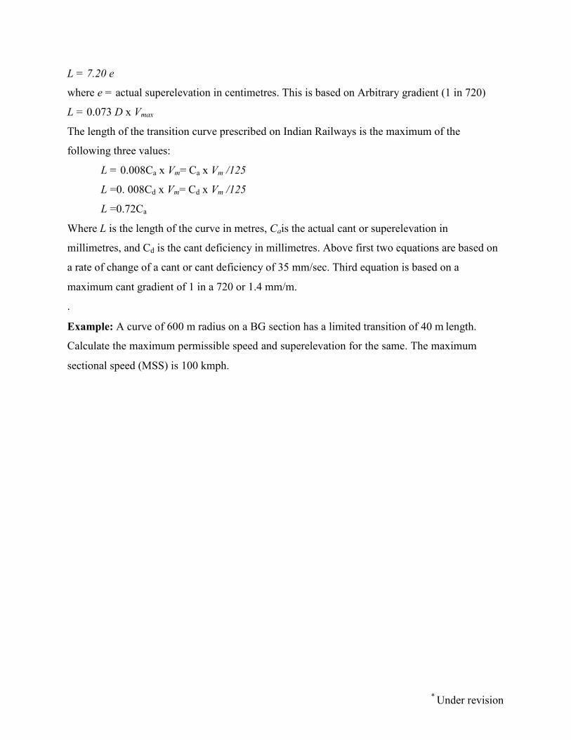
L = 7.20 e

where e = actual superelevation in centimetres. This is based on Arbitrary gradient (1 in 720)

L = 0.073 D x Vmax

The length of the transition curve prescribed on Indian Railways is the maximum of the

following three values:

L = 0.008Ca x Vm= Ca x Vm /125

L =0. 008Cd x Vm= Cd x Vm /125

L =0.72Ca

Where L is the length of the curve in metres, Cais the actual cant or superelevation in

millimetres, and Cd is the cant deficiency in millimetres. Above first two equations are based on

a rate of change of a cant or cant deficiency of 35 mm/sec. Third equation is based on a

.

maximum cant gradient of 1 in a 720 or 1.4 mm/m.

Example: A curve of 600 m radius on a BG section has a limited transition of 40 m length.

Calculate the maximum permissible speed and superelevation for the same. The maximum

sectional speed (MSS) is 100 kmph.

* Under revision

Lecture-20

Introduction

VERTICAL CURVES

Vertical Curves. They are of two types :

(i) Summit curves. (ii) Sag or Valley curves.

Whenever, there is a change in the gradient of the track, an angle is formed at the junction of the

gradients. This vertical kink at the junction is smoothened by the use of curve, so that bad

lurching is not experienced. The effects of change of gradient cause variation in the draw bar pull

of the locomotive.

When a train climbs a certain upgrade at a uniform speed and passes over the summit of the

curve, an acceleration begins to act upon it and makes the trains to move faster and increases the

draw bar pull behind each vehicle, causing a variation in the tension in the couplings.

* Under revision

When a train passes over a sag, the front of the train ascends an up-grade while rear vehicles tend

to compress the couplings and buffers, and when the whole train has passed the sag, the

couplings are again in tension causing a jerk. Due to above reasons, it is essential to introduce a

vertical curve at each sag and at each summit or apex.

A parabolic curve is set out, tangent to the two intersecting grades, with its apex at a level

halfway between the points of intersection of the grade line and the average elevation of the two

tangent points. The length of the vertical curve depends upon the algebraic difference in grade as

shown in figure above and determined by the rate of change gradient of the line.

Lecture-15 RAILWAY ALIGNMENT

Documents

Transcript of Lecture-15 RAILWAY ALIGNMENT