Lecture Notes

Ch1~6, p.31

3. method of probability density function (for continuous r.v.’s and

differentiable, one-to-one transformations, a special case of method 2) :

Theorem 2.6 (univariate continuous case, TBp. 62)

Let X be a continuous random variable with pdf fX(x). Let

Y = g(X), where g is di erentiable, strictly monotone. Then,Y g(X), where g is di erentiable, strictly monotone. Then,

fY (y) = fX(g1(y))

dg 1(y)

dydy

for y s.t. y = g(x) for some x, and fY (y) = 0 otherwise.

Proof Suppose g is strictly increasingProof. Suppose g is strictly increasing.

FY (y) = P (Y y) = P (X g 1(y)) = FX(g1(y))

d d dfY (y) =

d

dyFY (y) =

d

dyFX(g

1(y)) = fX(g1(y))

d

dyg 1(y)

When g is strictly decreasing,

fY (y) = fX(g1(y))

d

dyg 1(y)

Ch1~6, p.32

Question 2.7

Compare Ex. 2.4 and Thm 2.6. What is the role of |dg 1(y)/dy|?How to interpret it?

Example 2.9

X is a random variables with pdf fX(x). Find the distributon( )

of Y = 1/X .

y =1

xg(x) x = g 1(y) =

1

yx y

dg 1

dy=

1

y2and

dg 1

dy=1

y2y y y y

hence

fY (y) = fX(1/y)(1/y2)

NTHU MATH 2820, 2012 Lecture Notes

made by Shao-Wei Cheng (NTHU, Taiwan)

Ch1~6, p.33

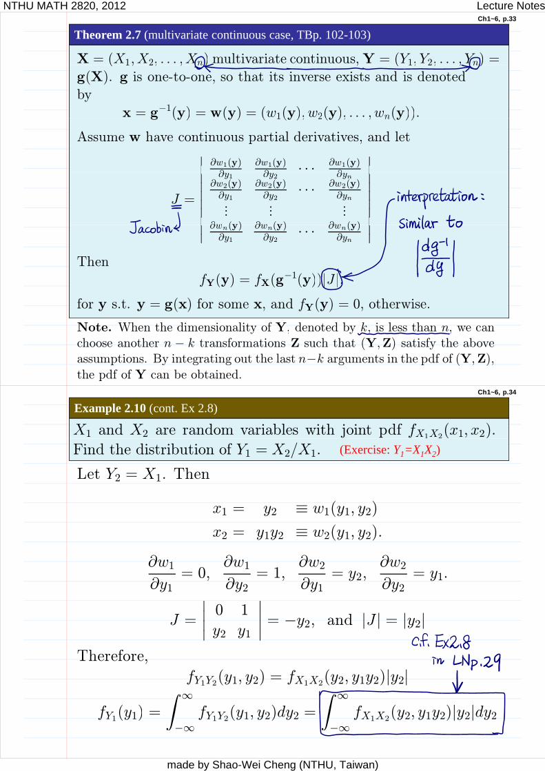
Theorem 2.7 (multivariate continuous case, TBp. 102-103)

X = (X1, X2, . . . , Xn) multivariate continuous,Y = (Y1, Y2, . . . , Yn) =( 1, 2, , n) , ( 1, 2, , n)

g(X). g is one-to-one, so that its inverse exists and is denoted

by

x = g 1(y) = w(y) = (w1(y), w2(y), . . . , wn(y)).g (y) (y) ( 1(y), 2(y), , n(y))

Assume w have continuous partial derivatives, and let

w1(y) w1(y) · · · w1(y)

J =

y1 y2 ynw2(y)

y1

w2(y)

y2· · · w2(y)

yn...

......

w (y) w (y) w (y)wn(y)

y1

wn(y)

y2· · · wn(y)

yn

Then

f (y) f (g 1(y))|J |fY(y) = fX(g (y))|J |.for y s.t. y = g(x) for some x, and fY(y) = 0, otherwise.

Note. When the dimensionality of Y, denoted by k, is less than n, we cany , y , ,choose another n k transformations Z such that (Y,Z) satisfy the aboveassumptions. By integrating out the last n k arguments in the pdf of (Y,Z),the pdf of Y can be obtained.

Ch1~6, p.34

Example 2.10 (cont. Ex 2.8)

X1 and X2 are random variables with joint pdf fX1X2(x1, x2).(Exercise: Y1=X1X2)Find the distribution of Y1 = X2/X1.

Let Y2 = X1. Then

x1 = y2 w1(y1, y2)

x2 = y1y2 w2(y1, y2).

w1y1= 0,

w1y2= 1,

w2y1= y2,

w2y2= y1.

J =0 1

y2 y1= y2, and |J | = |y2|

Th fTherefore,

fY1Y2(y1, y2) = fX1X2(y2, y1y2)|y2|

( ) ( ) ( )| |fY1(y1) = fY1Y2(y1, y2)dy2 = fX1X2(y2, y1y2)|y2|dy2



Ch1~6, p.354. method of moment generating function: based on the uniqueness theorem of moment generating function. To be explained later in Chapter 4explained later in Chapter 4.

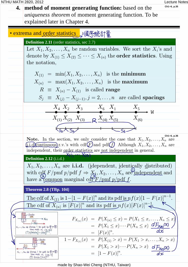
• extrema and order statistics

D fi iti 2 11 ( d i i 3 7)Definition 2.11 (order statistics, sec 3.7)

Let X1, X2, . . . , Xn be random variables. We sort the Xi�s and

denote by X(1) X(2) · · · X(n) the order statistics. Usingthe notation,

X(1) = min(X1, X2, . . . ,Xn) is the minimum

X(n) = max(X1, X2, . . . , Xn) is the maximum

R X(n) X(1) is called range

S X X j 2 ll d i

X1X3X4 X2 X6

Sj X(j) X(j 1), j = 2, . . . , n are called spacings

X5

X(1) X(6)X(5)X(4)X(3)X(2)

Ch1~6, p.36Note. In the section, we only consider the case that X1, X2, . . . , Xn arei.i.d continuous r.v.�s with cdf F and pdf f . Although X1, X2, . . . , Xn areindependent, their order statistics are not independent in general.

Definition 2.12 (i.i.d.)

p , p g

X1, X2, . . . , Xn are i.i.d. (idependent, identically distributed)

/ /

Th 2 8 (TB 104)

with cdf F/pmf p/pdf f X1, X2, . . . , Xn are independent andhave a common marginal cdf F/pmf p/pdf f .

Theorem 2.8 (TBp. 104)

The cdf ofX(1) is 1 [1 F (x)]n and its pdf is nf(x)[1 F (x)]n 1.

The cdf of X(n) is [F (x)]n and its pdf is nf(x)[F (x)]n 1.(n) [ ( )] p f( )[ ( )]

FX(n)(x) = P (X(n) x) = P (X1 x, . . . , Xn x)

= P (X x) P (X x)= P (X1 x) · · ·P (Xn x)

= [F (x)]n.

1 FX(1)(x) = P (X(1) > x) = P (X1 > x, . . . , Xn > x)

= P (X1 > x) · · ·P (Xn > x)

= [1 F (x)]n.



Ch1~6, p.37

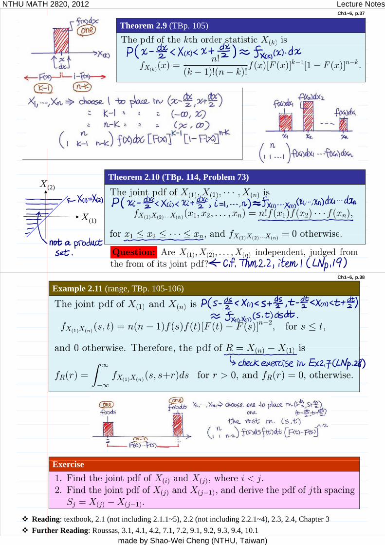
Theorem 2.9 (TBp. 105)

The pdf of the kth order statistic X(k) is( )

fX(k)(x) =n!

(k 1)!(n k)!f(x)[F (x)]k 1[1 F (x)]n k.

Theorem 2.10 (TBp. 114, Problem 73)

The joint pdf of X(1), X(2), · · · ,X(n) isX(2)

j p (1), (2), , (n)

fX(1)X(2)...X(n)(x1, x2, . . . , xn) = n!f(x1)f(x2) · · ·f(xn),for x1 x2 · · · x and fX X X = 0 otherwise

X(1)

for x1 x2 · · · xn, and fX(1)X(2)...X(n) = 0 otherwise.

Question: Are X(1), X(2), . . . , X(n) independent, judged from

the from of its joint pdf?

Ch1~6, p.38

Example 2.11 (range, TBp. 105-106)

The joint pdf of X(1) and X(n) is( ) ( )

fX(1)X(n)(s, t) = n(n 1)f(s)f(t)[F (t) F (s)]n 2, for s t,

and 0 otherwise Therefore the pdf of R = X( ) X( ) isand 0 otherwise. Therefore, the pdf of R = X(n) X(1) is

fR(r) = fX(1)X(n)(s, s+r)ds for r > 0, and fR(r) = 0, otherwise.

Exercise

1. Find the joint pdf of X(i) and X(j), where i < j.2. Find the joint pdf of X(j) and X(j 1), and derive the pdf of jth spacingS X XSj = X(j) X(j 1).

Reading: textbook, 2.1 (not including 2.1.1~5), 2.2 (not including 2.2.1~4), 2.3, 2.4, Chapter 3

Further Reading: Roussas, 3.1, 4.1, 4.2, 7.1, 7.2, 9.1, 9.2, 9.3, 9.4, 10.1



Ch1~6, p.39

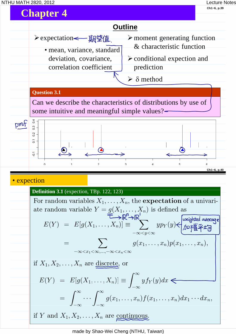
Chapter 4OutlineOutline

expectation

• mean variance standard

moment generating function & characteristic function mean, variance, standard

deviation, covariance, correlation coefficient

conditional expection and prediction

method

Question 3.1

Can we describe the characteristics of distributions by use of some intuitive and meaningful simple values?

0 1 2 3 4 5 6

Ch1~6, p.40

• expection

D fi iti 3 1 ( i TB 122 123)Definition 3.1 (expection, TBp. 122, 123)

For random variables X1, . . . , Xn, the expectation of a univari-

ate random variable Y = g(X1, . . . , Xn) is de ned as( )

E(Y ) = E[g(X1, . . . , Xn)]<y<

ypY (y)

=<x1< ,..., <xn<

g(x1, . . . , xn)p(x1, . . . , xn),

if X1, X2, . . . , Xn are discrete, or

E(Y ) = E[g(X1, . . . , Xn)] yfY (y)dx( ) [g( 1, , n)] yfY (y)dx

= · · · g(x1, . . . , xn)f(x1, . . . , xn)dx1 · · ·dxn,

if Y and X1, X2, . . . , Xn are continuous.



Ch1~6, p.41

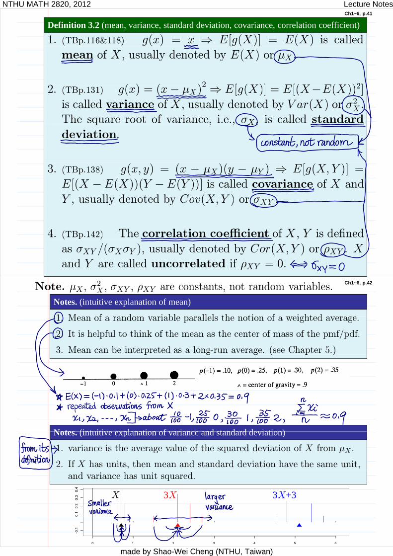
Definition 3.2 (mean, variance, standard deviation, covariance, correlation coefficient)

1. (TBp.116&118) g(x) = x E[g(X)] = E(X) is called

mean of X , usually denoted by E(X) or X .

2 ( ) ( )2 E[ (X)] E[(X E(X))2]2. (TBp.131) g(x) = (x X)2 E[g(X)] = E[(X E(X))2]

is called variance of X , usually denoted by V ar(X) or 2X .

The square root of variance, i.e., X , is called standardq , , X ,

deviation.

3. (TBp.138) g(x, y) = (x X)(y Y ) E[g(X, Y )] =

E[(X E(X))(Y E(Y ))] is called covariance of X and

Y usually denoted by Cov(X Y ) or XYY , usually denoted by Cov(X, Y ) or XY .

4. (TBp.142) The correlation coe cient of X , Y is de ned( ) ,

as XY /( X Y ), usually denoted by Cor(X,Y ) or XY . Xand Y are called uncorrelated if XY = 0.

Ch1~6, p.42

Notes. (intuitive explanation of mean)

Note. X ,2X , XY , XY are constants, not random variables.

1 M f d i bl ll l th ti f i ht d1. Mean of a random variable parallels the notion of a weighted average.

2. It is helpful to think of the mean as the center of mass of the pmf/pdf.

3. Mean can be interpreted as a long-run average. (see Chapter 5.)p g g ( p )

Notes (intuitive explanation of variance and standard deviation)Notes. (intuitive explanation of variance and standard deviation)

1. variance is the average value of the squared deviation of X from X .

2. If X has units, then mean and standard deviation have the same unit,and variance has unit squared.

X 3X 3X+3

0 1 2 3 4 5 6



Ch1~6, p.43

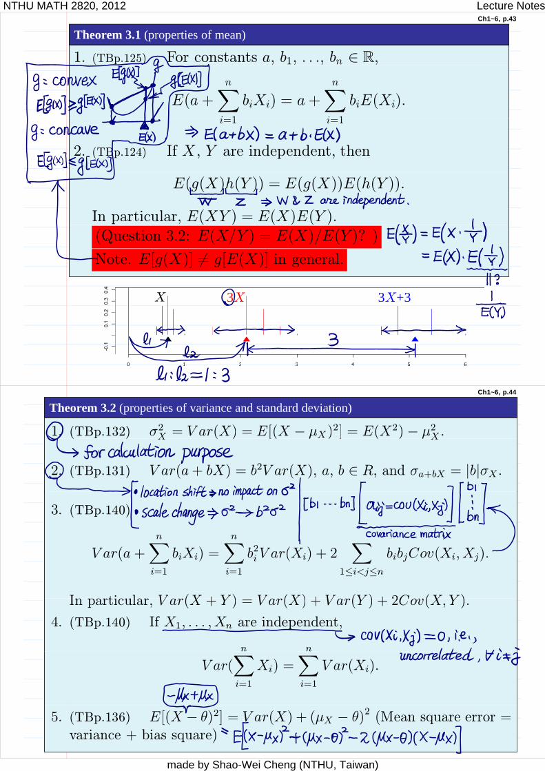
Theorem 3.1 (properties of mean)

1. (TBp.125) For constants a, b1, . . ., bn R,

E(a +

n

i 1

biXi) = a+

n

i 1

biE(Xi).i=1 i=1

2. (TBp.124) If X , Y are independent, then

E(g(X)h(Y )) = E(g(X))E(h(Y )).

In particular, E(XY ) = E(X)E(Y ).(Question 3.2: E(X/Y ) = E(X)/E(Y )? )

Note. E[g(X)] 6= g[E(X)] in general.

X 3X 3X+3

0 1 2 3 4 5 6

Ch1~6, p.44

Theorem 3.2 (properties of variance and standard deviation)

1. (TBp.132) 2X = V ar(X) = E[(X X )

2] = E(X2) 2X .( ) X ( ) [( ) ] ( ) X

2. (TBp.131) V ar(a+ bX) = b2V ar(X), a, b R, and a+bX = |b| X .

3. (TBp.140)

n n

2V ar(a +i=1

biXi) =i=1

b2iV ar(Xi) + 21 i<j n

bibjCov(Xi, Xj).

I a tic la V (X + Y ) V (X) + V (Y ) + 2C (X Y )In particular, V ar(X + Y ) = V ar(X) + V ar(Y ) + 2Cov(X, Y ).

4. (TBp.140) If X1, . . . , Xn are independent,

n n

V ar(i=1

Xi) =i=1

V ar(Xi).

5. (TBp.136) E[(X )2] = V ar(X) + ( X )2 (Mean square error =variance + bias square)



Ch1~6, p.45

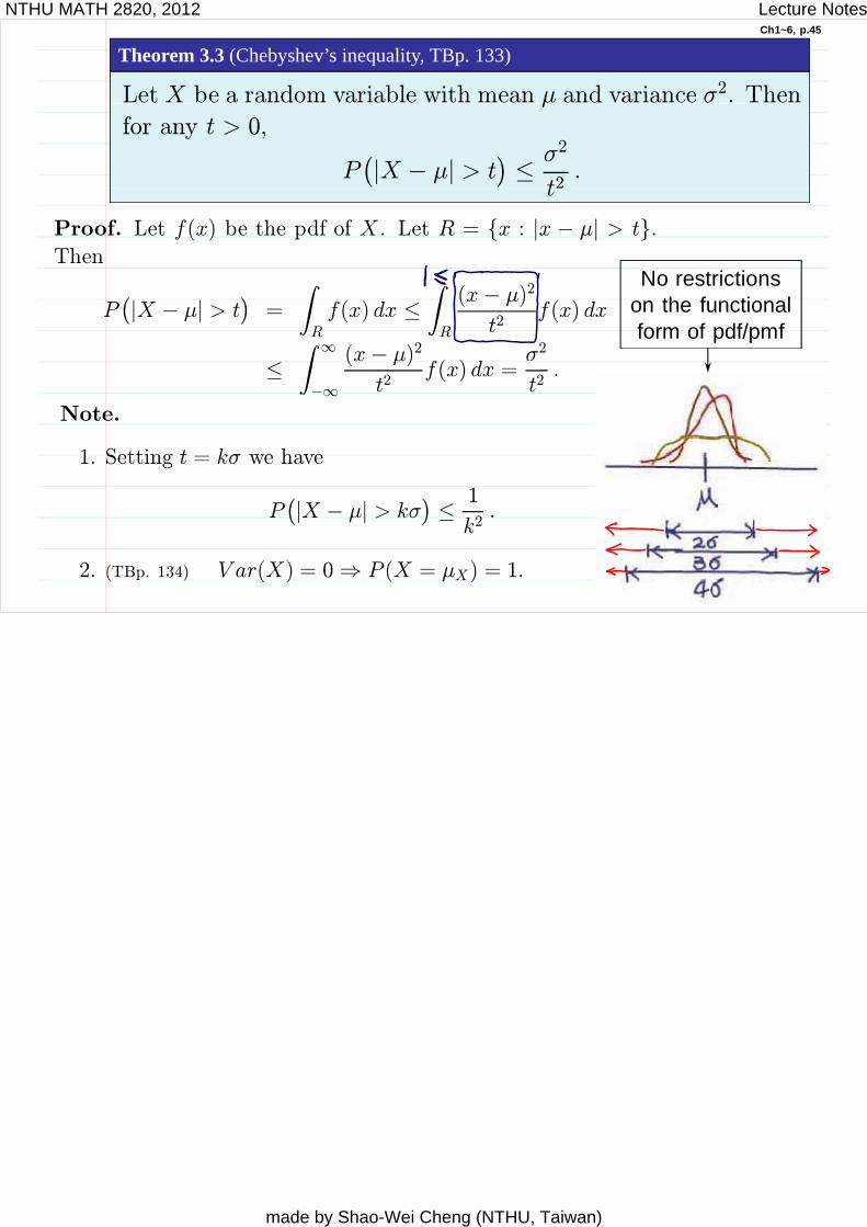
Theorem 3.3 (Chebyshev’s inequality, TBp. 133)

Let X be a random variable with mean and variance 2. Then

for any t > 0,

P |X | > t2

t2.

t

Proof. Let f(x) be the pdf of X . Let R = {x : |x | > t}.Then

N t i ti

P |X | > t =R

f(x) dxR

(x )2

t2f(x) dx

(x )2 2

No restrictionson the functional form of pdf/pmf

(x )

t2f(x) dx =

t2.

Note.

1. Setting t = k we have

P |X | > k 1

k2.

k

2. (TBp. 134) V ar(X) = 0 P (X = X) = 1.



Lecture Notes

Documents

Transcript of Lecture Notes