Lecture notes 9 hypothesys testing

Chapter GoalsAfter completing this chapter, you should be able to:

Formulate null and alternative hypotheses for applications involving a single population mean from a normal distribution a single population proportion (large samples)

Formulate a decision rule for testing a hypothesis

Know how to use the critical value and p-value approaches to test the null hypothesis (for both mean and proportion problems)

Know what Type I and Type II errors are Assess the power of a test

What is a Hypothesis? A hypothesis is a claim (assumption) about a population parameter: population mean

population proportion

Example: The mean monthly cell phone bill of this city is μ = $42

Example: The proportion of adults in this city with cell phones is p = .68

The Null Hypothesis, H0

States the assumption (numerical) to be testedExample: The average number of TV sets in U.S. Homes is equal to three ( )

Is always about a population parameter, not about a sample statistic

3μ:H 0

3μ:H 0 3X:H 0

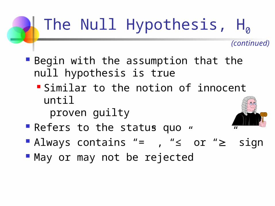
The Null Hypothesis, H0

Begin with the assumption that the null hypothesis is true Similar to the notion of innocent until proven guilty

Refers to the status quo Always contains “=” , “≤” or “” sign May or may not be rejected

(continued)

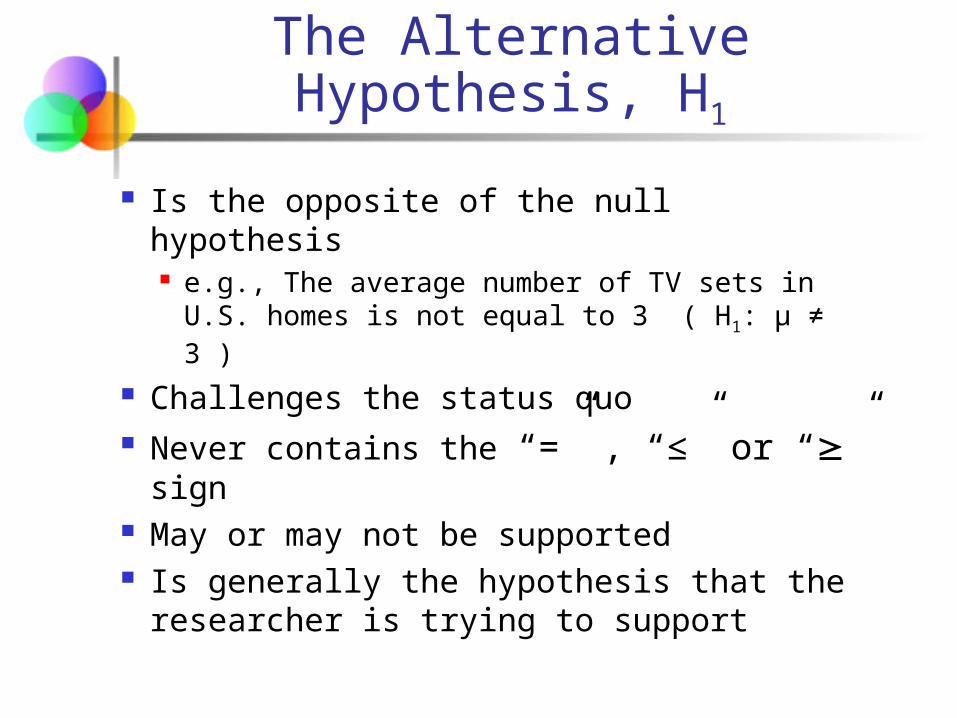
The Alternative Hypothesis, H1

Is the opposite of the null hypothesis e.g., The average number of TV sets in U.S. homes is not equal to 3 ( H1: μ ≠ 3 )

Challenges the status quo Never contains the “=” , “≤” or “” sign

May or may not be supported Is generally the hypothesis that the researcher is trying to support

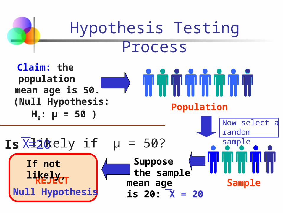
Population

Claim: thepopulationmean age is 50.(Null Hypothesis:

REJECTSupposethe sample

mean age is 20: X = 20

SampleNull Hypothesis

20likely if μ = 50?Is

Hypothesis Testing Process

If not likely,

Now select a random sample

H0: μ = 50 )

X

Sampling Distribution of X

μ = 50If H0 is trueIf it is

unlikely that we would get a sample mean of this value ...

... then we reject the

null hypothesis that μ =

50.

Reason for Rejecting H0

20

... if in fact this were the population mean…

X

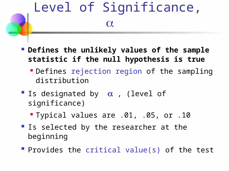
Level of Significance,

Defines the unlikely values of the sample statistic if the null hypothesis is true Defines rejection region of the sampling distribution

Is designated by , (level of significance) Typical values are .01, .05, or .10

Is selected by the researcher at the beginning

Provides the critical value(s) of the test

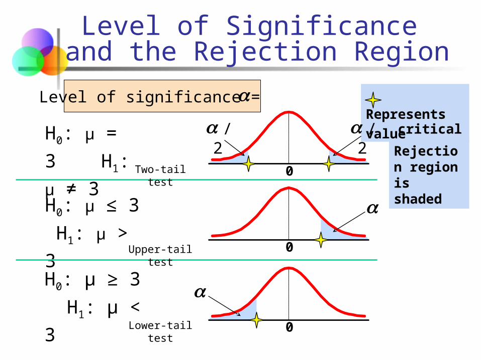
Level of Significance and the Rejection Region

H0: μ ≥ 3 H1: μ < 3 0

H0: μ ≤ 3 H1: μ > 3

Represents critical value

Lower-tail test

Level of significance =

0Upper-tail test

Two-tail test

Rejection region is shaded

/2

0

/2

H0: μ = 3 H1: μ ≠ 3

Errors in Making Decisions

Type I Error Reject a true null hypothesis Considered a serious type of error

The probability of Type I Error is Called level of significance of the test

Set by researcher in advance

Errors in Making Decisions

Type II Error Fail to reject a false null hypothesis

The probability of Type II Error is β

(continued)

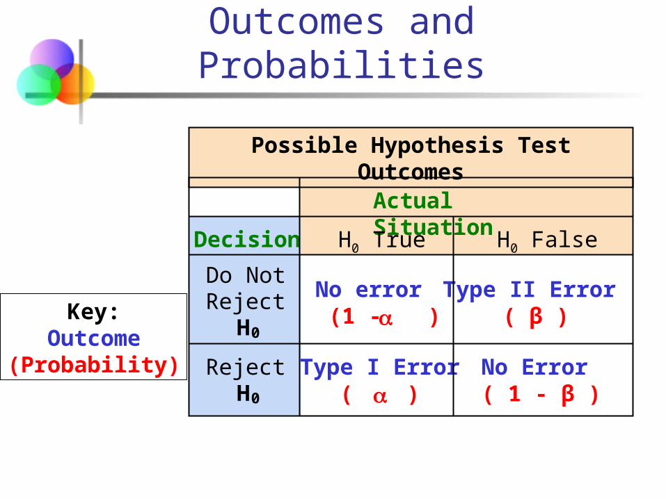
Outcomes and Probabilities

Actual SituationDecision

Do NotReject

H0No error (1 - )

Type II Error ( β )

RejectH0

Type I Error( )

Possible Hypothesis Test Outcomes

H0 False H0 True

Key:Outcome

(Probability) No Error ( 1 - β )

Type I & II Error Relationship

Type I and Type II errors can not happen at the same time

Type I error can only occur if H0 is true Type II error can only occur if H0 is false

If Type I error probability ( ) , then Type II error probability ( β )

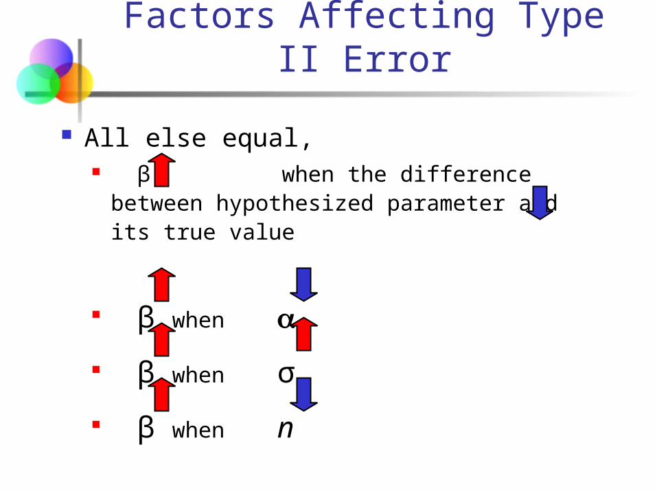
Factors Affecting Type II Error

All else equal, β when the difference between hypothesized parameter and its true value

β when β when σ β when n

Power of the Test

The power of a test is the probability of rejecting a null hypothesis that is false

i.e., Power = P(Reject H0 | H1 is true)

Power of the test increases as the sample size increases

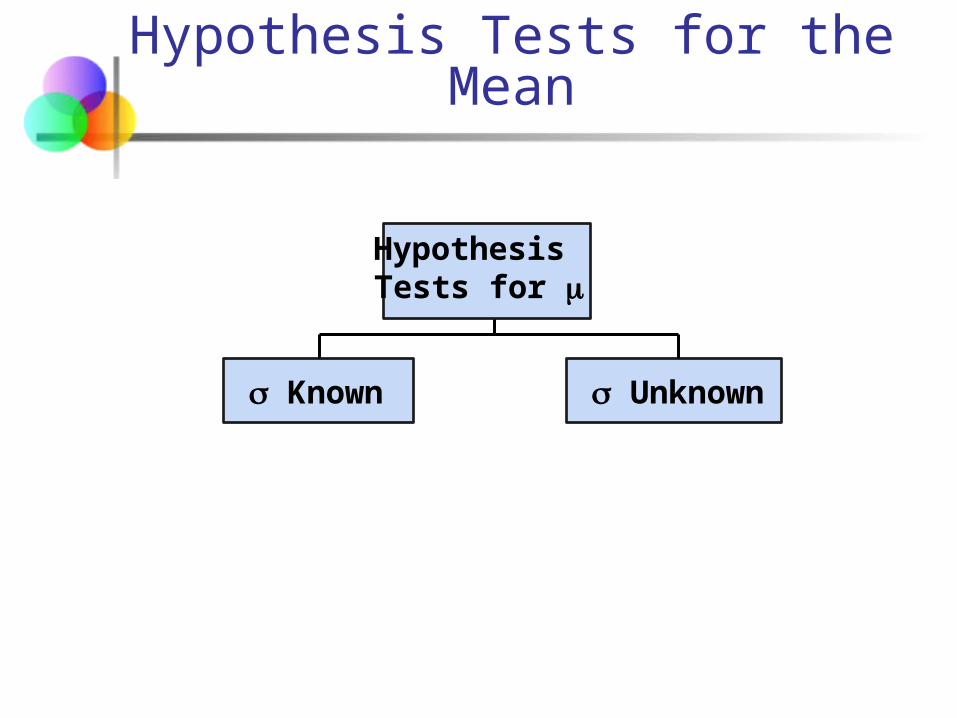
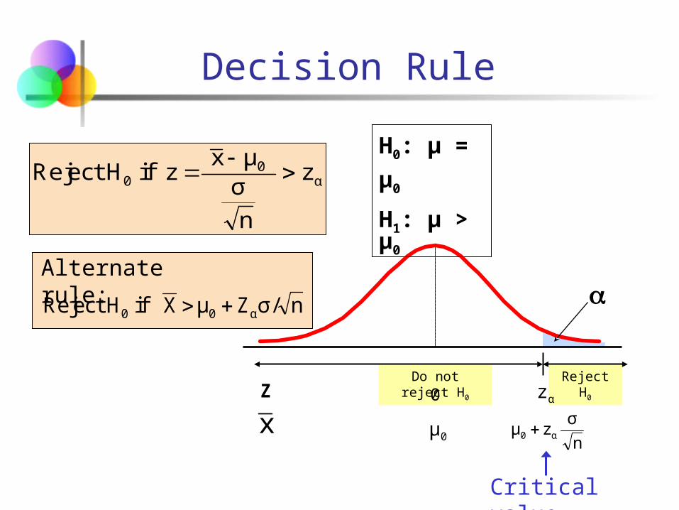
Hypothesis Tests for the Mean

Known Unknown

Hypothesis Tests for

Test of Hypothesisfor the Mean (σ Known)

Convert sample result ( ) to a z value

The decision rule is:

α0

0 z

nσμxz if H Reject

σ Known σ Unknown


Consider the test

00 μμ:H

01 μμ:H

(Assume the population is normal)

x

Reject H0

Do not reject H0

Decision Rule

zα0

μ0

H0: μ = μ0 H1: μ > μ0

Critical value

Z

α0

0 z

nσμxz if H Reject

nσ/ZμX if H Reject α00

nσzμ α0

Alternate rule:

x

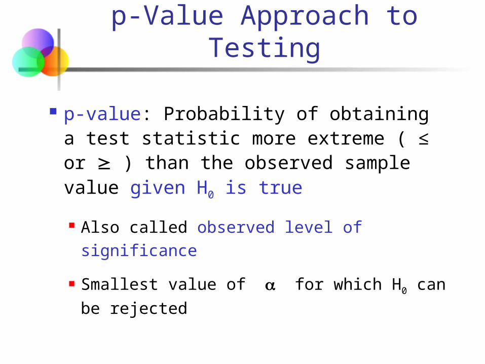
p-Value Approach to Testing

p-value: Probability of obtaining a test statistic more extreme ( ≤ or ) than the observed sample value given H0 is true Also called observed level of significance

Smallest value of for which H0 can be rejected

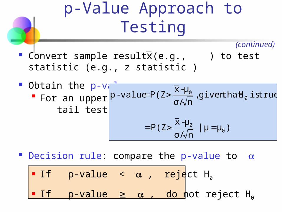
p-Value Approach to Testing

Convert sample result (e.g., ) to test statistic (e.g., z statistic )

Obtain the p-value For an upper tail test:

Decision rule: compare the p-value to If p-value < , reject H0

If p-value , do not reject H0

(continued)x

)μμ | nσ/μ-x P(Z

true) is H that given , nσ/μ-x P(Z value-p

00

00

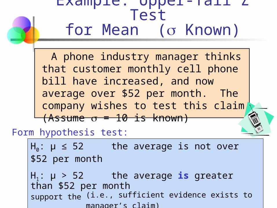
Example: Upper-Tail Z Test

for Mean ( Known) A phone industry manager thinks that customer monthly cell phone bill have increased, and now average over $52 per month. The company wishes to test this claim. (Assume = 10 is known)

H0: μ ≤ 52 the average is not over $52 per monthH1: μ > 52 the average is greater than $52 per month

(i.e., sufficient evidence exists to support the manager’s claim)

Form hypothesis test:

Reject H0

Do not reject H0

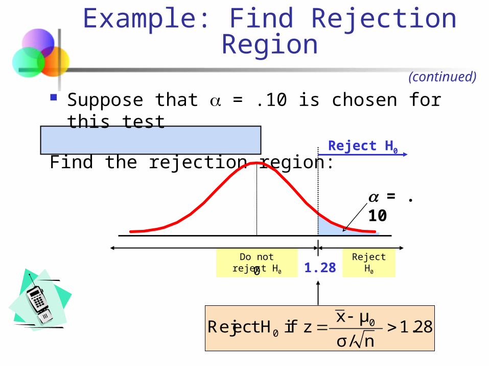
Suppose that = .10 is chosen for this test

Find the rejection region:= .10

1.280

Reject H0

Example: Find Rejection Region

(continued)

1.28nσ/μxz if H Reject 0

0

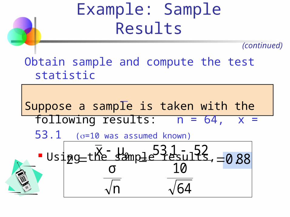
Obtain sample and compute the test statistic

Suppose a sample is taken with the following results: n = 64, x = 53.1 (=10 was assumed known) Using the sample results, 0.88

6410

5253.1

nσμxz 0

Example: Sample Results

(continued)

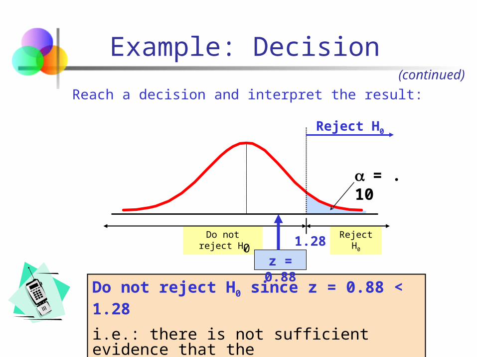
Reject H0

Do not reject H0

Example: Decision

= .10

1.280

Reject H0

Do not reject H0 since z = 0.88 < 1.28i.e.: there is not sufficient evidence that the mean bill is over $52

z = 0.88

Reach a decision and interpret the result:(continued)

Reject H0

= .10

Do not reject H0

1.280

Reject H0

Z = .88

Calculate the p-value and compare to (assuming that μ = 52.0)

(continued)

.1894

.810610.88)P(z

6410/52.053.1zP

52.0) μ | 53.1xP(

p-value = .1894

Example: p-Value Solution

Do not reject H0 since p-value = .1894 > = .10

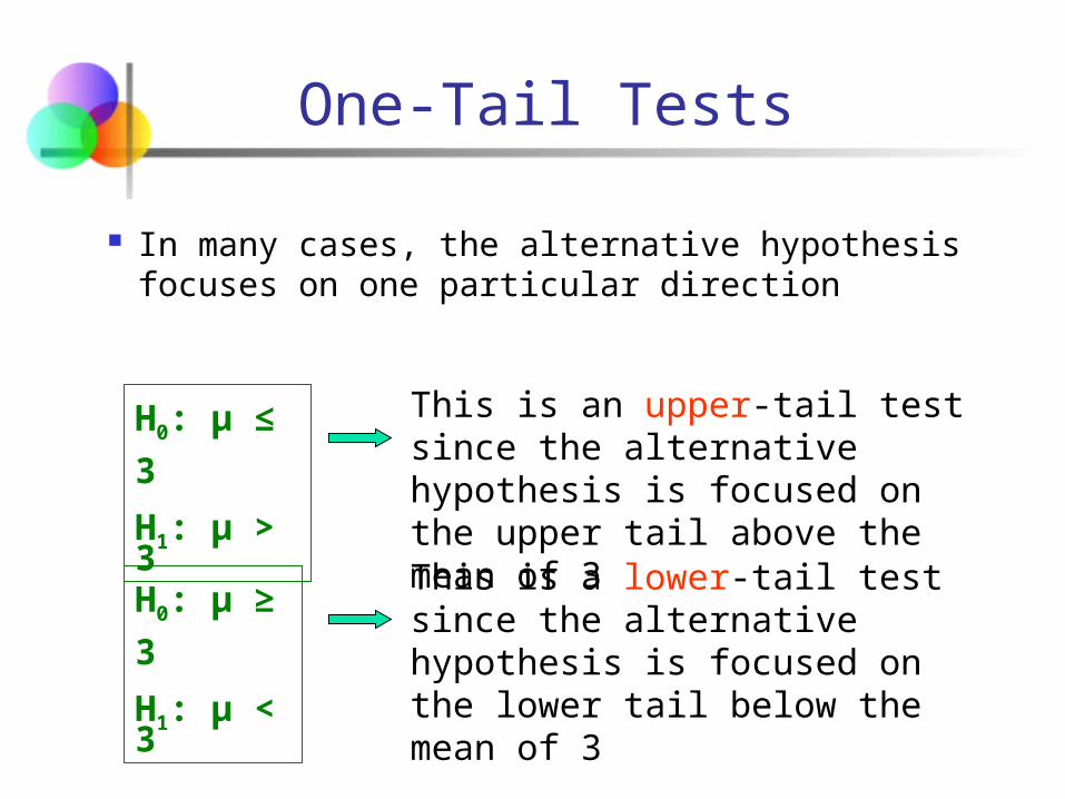
One-Tail Tests

In many cases, the alternative hypothesis focuses on one particular direction

H0: μ ≥ 3 H1: μ < 3

H0: μ ≤ 3 H1: μ > 3 This is a lower-tail test

since the alternative hypothesis is focused on the lower tail below the mean of 3

This is an upper-tail test since the alternative hypothesis is focused on the upper tail above the mean of 3

Reject H0

Do not reject H0

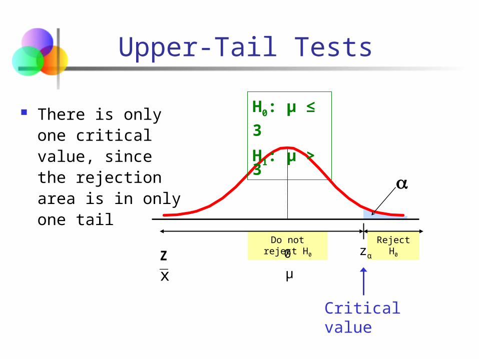
Upper-Tail Tests

zα0μ

H0: μ ≤ 3 H1: μ > 3

There is only one critical value, since the rejection area is in only one tail

Critical value

Zx

Reject H0

Do not reject H0

There is only one critical value, since the rejection area is in only one tail

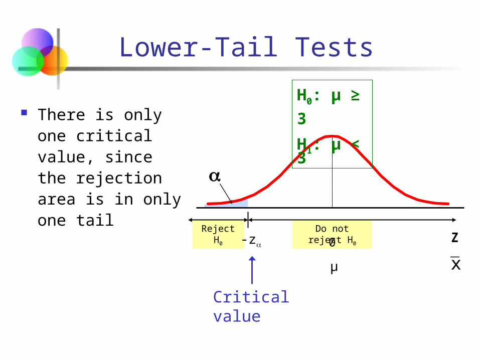
Lower-Tail Tests

-z 0

μ

H0: μ ≥ 3 H1: μ < 3

Z

Critical value

x

Do not reject H0

Reject H0

Reject H0

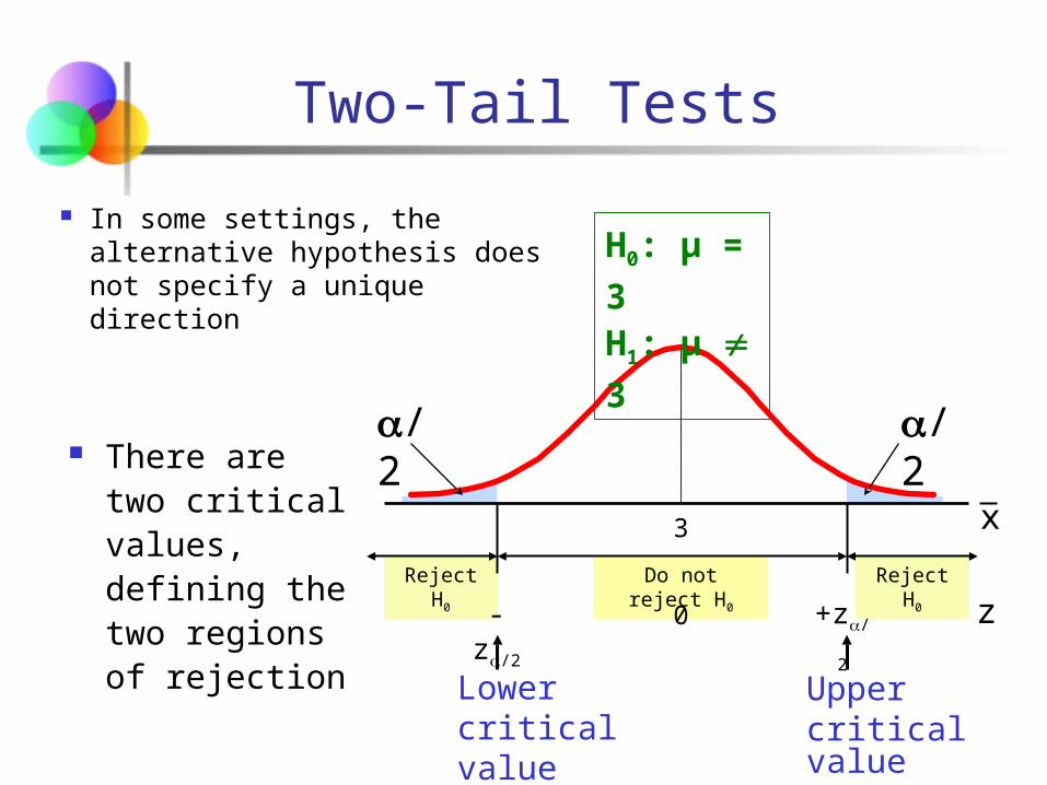
There are two critical values, defining the two regions of rejection

Two-Tail Tests

/2

0

H0: μ = 3 H1: μ 3

/2

Lower critical value

Uppercritical value

3

z

x

-z/2

+z/

2

In some settings, the alternative hypothesis does not specify a unique direction

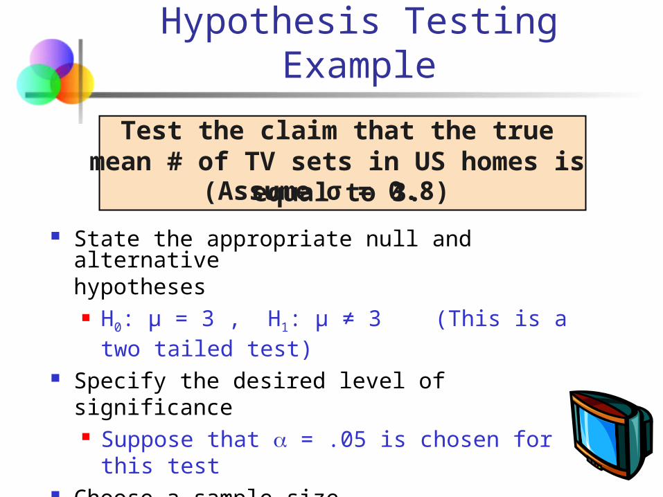
Hypothesis Testing Example

Test the claim that the true mean # of TV sets in US homes is

equal to 3.(Assume σ = 0.8) State the appropriate null and alternativehypotheses H0: μ = 3 , H1: μ ≠ 3 (This is a two tailed test)

Specify the desired level of significance Suppose that = .05 is chosen for this test

Choose a sample size Suppose a sample of size n = 100 is selected

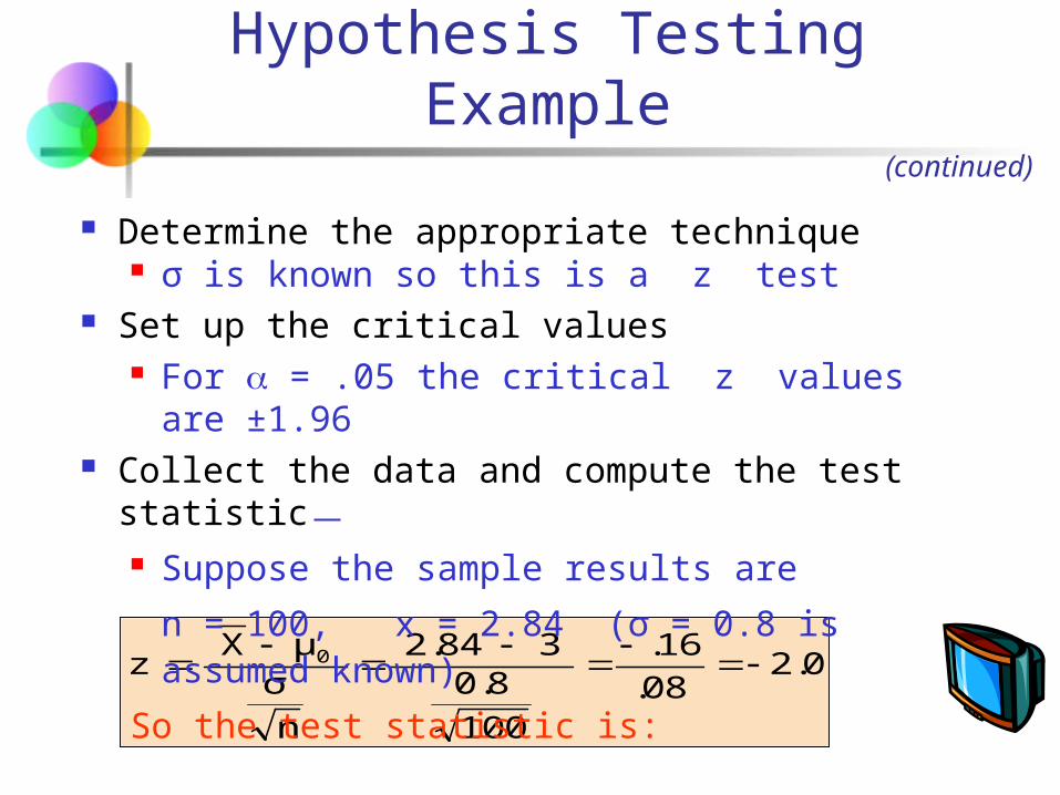
2.0.08.16

1000.8

32.84

nσμXz 0


Determine the appropriate technique σ is known so this is a z test

Set up the critical values For = .05 the critical z values are ±1.96

Collect the data and compute the test statistic Suppose the sample results are n = 100, x = 2.84 (σ = 0.8 is assumed known)

So the test statistic is:

(continued)

Reject H0

Do not reject H0

Is the test statistic in the rejection region?

= .05/2

-z = -1.96

0

Reject H0 if z < -1.96 or z > 1.96; otherwise do not reject H0


(continued)

= .05/2

Reject H0+z =

+1.96

Here, z = -2.0 < -1.96, so the test statistic is in the rejection region

Reach a decision and interpret the result

-2.0Since z = -2.0 < -1.96, we reject the

null hypothesis and conclude that there is sufficient evidence that the mean number of TVs in US homes is not equal to 3


(continued)

Reject H0

Do not reject H0

= .05/2

-z = -1.96

0

= .05/2

Reject H0+z =

+1.96

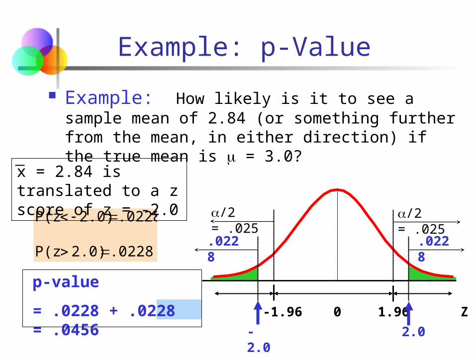
.0228

/2 = .025

Example: p-Value Example: How likely is it to see a sample mean of 2.84 (or something further from the mean, in either direction) if the true mean is = 3.0?

-1.96 0-2.0

.02282.0)P(z

.02282.0)P(z

Z1.962.0

x = 2.84 is translated to a z score of z = -2.0

p-value = .0228 + .0228 = .0456

.0228

/2 = .025

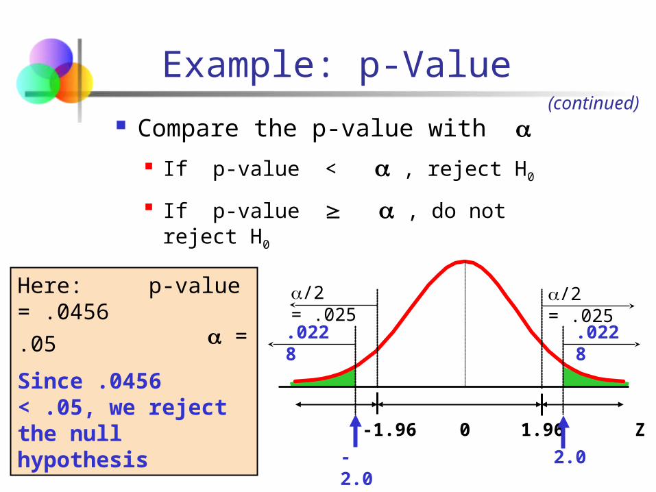
Compare the p-value with If p-value < , reject H0

If p-value , do not reject H0

Here: p-value = .0456

= .05Since .0456 < .05, we reject the null hypothesis

(continued)Example: p-Value

.0228

/2 = .025

-1.96 0-2.0

Z1.962.0

.0228

/2 = .025

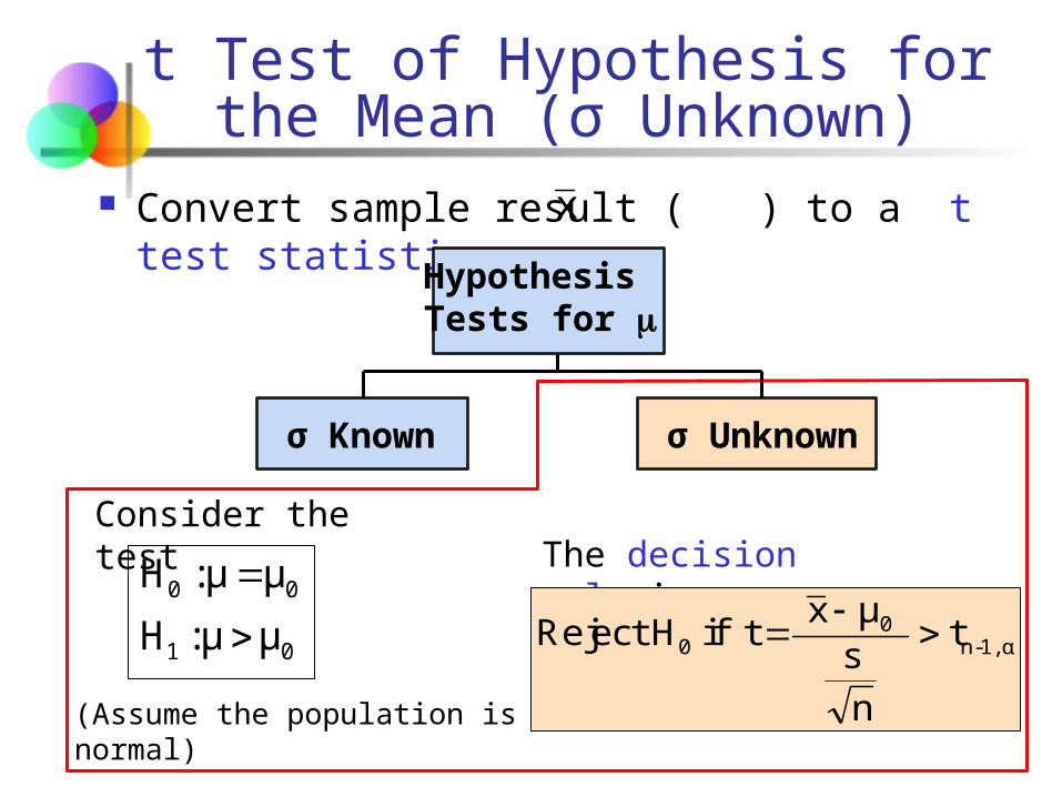
t Test of Hypothesis for the Mean (σ Unknown)

Convert sample result ( ) to a t test statistic

σ Known σ Unknown


x


α , 1-n0

0 t

nsμxt if H Reject

Consider the test

00 μμ:H

01 μμ:H

(Assume the population is normal)

t Test of Hypothesis for the Mean (σ Unknown)

For a two-tailed test:


α/2 , 1-n0

α/2 , 1-n0

0 t

nsμxt if or t

nsμxt if H Reject

Consider the test

00 μμ:H

01 μμ:H

(Assume the population is normal, and the population variance is unknown)

(continued)

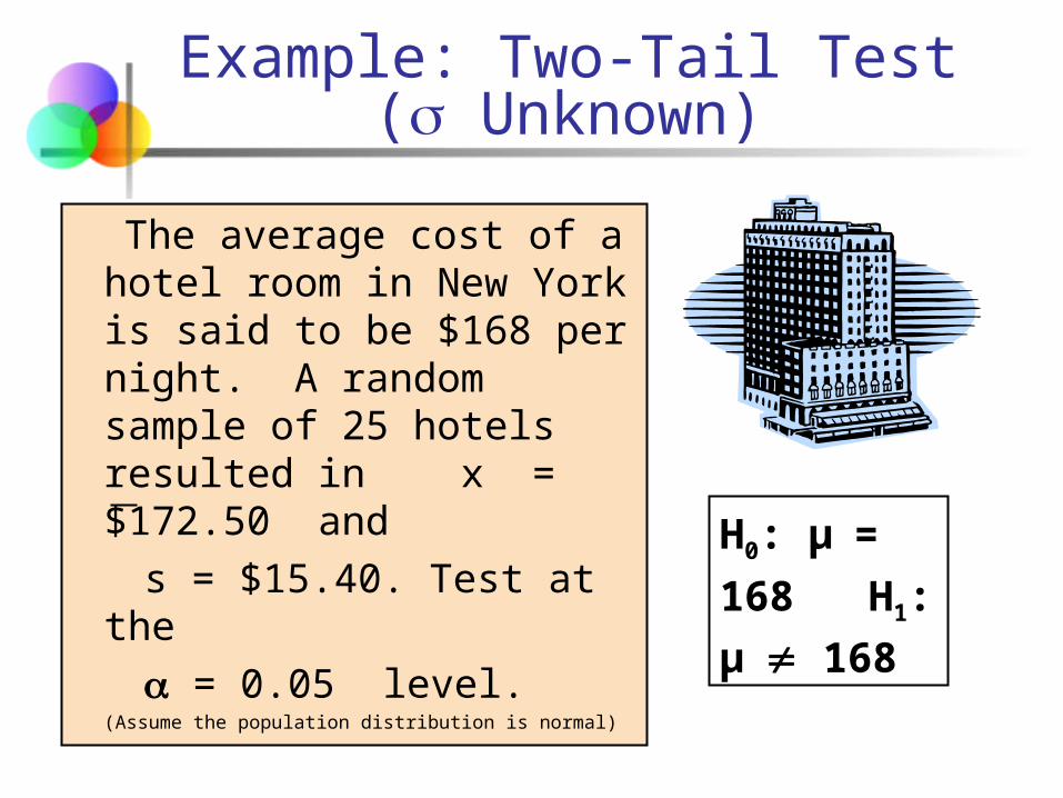
Example: Two-Tail Test( Unknown)

The average cost of a hotel room in New York is said to be $168 per night. A random sample of 25 hotels resulted in x = $172.50 and

s = $15.40. Test at the

= 0.05 level.(Assume the population distribution is normal)

H0: μ= 168 H1: μ 168

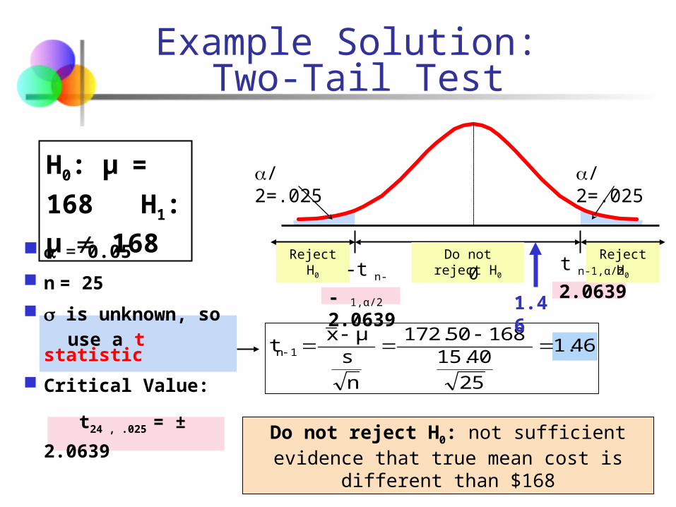
= 0.05 n = 25 is unknown, so use a t statistic

Critical Value: t24 , .025 = ± 2.0639

Example Solution: Two-Tail Test

Do not reject H0: not sufficient evidence that true mean cost is

different than $168

Reject H0

Reject H0

/2=.025

-t n-

1,α/2

Do not reject H00

/2=.025

-2.0639

2.0639

1.46

2515.40

168172.50

nsμxt 1n

1.46

H0: μ= 168 H1: μ 168

t n-1,α/2

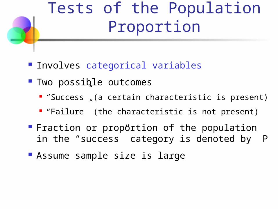
Tests of the Population Proportion

Involves categorical variables Two possible outcomes

“Success” (a certain characteristic is present) “Failure” (the characteristic is not present)

Fraction or proportion of the population in the “success” category is denoted by P

Assume sample size is large

Proportions Sample proportion in the success category is denoted by

When nP(1 – P) > 9, can be approximated by a normal distribution with mean and standard deviation

sizesamplesampleinsuccessesofnumber

nxp ˆ

Pμ p̂nP)P(1σ

p̂

(continued)

p̂

p̂

The sampling distribution of is approximately normal, so the test statistic is a z value:

Hypothesis Tests for Proportions

n)P(1P

Ppz00

0

ˆ

nP(1 – P) > 9

Hypothesis Tests for P

Not discussed in this chapter

p̂

nP(1 – P) < 9

Example: Z Test for Proportion

A marketing company claims that it receives 8% responses from its mailing. To test this claim, a random sample of 500 were surveyed with 25 responses. Test at the = .05 significance level.

Check: Our approximation for P is = 25/500 = .05

nP(1 - P) = (500)(.05)(.95) = 23.75 > 9

p̂

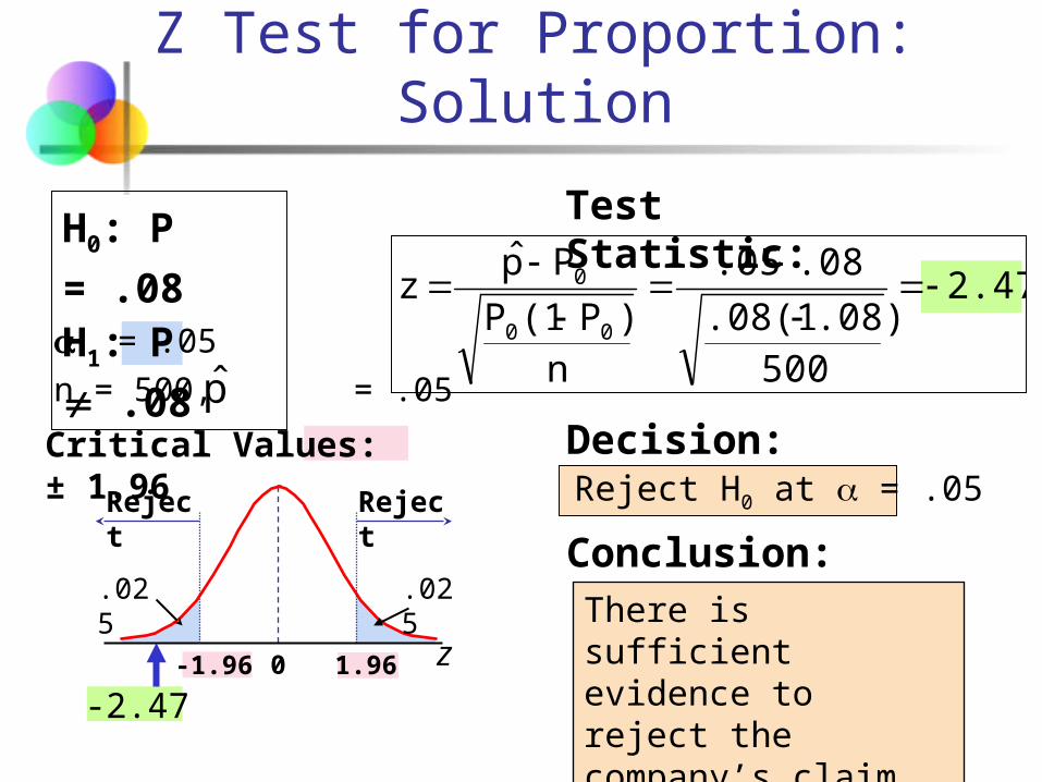
Z Test for Proportion: Solution

= .05 n = 500, = .05

Reject H0 at = .05

H0: P = .08 H1: P .08Critical Values: ± 1.96

Test Statistic:

Decision:

Conclusion:

z0

Reject

Reject

.025

.025

1.96-2.47

There is sufficient evidence to reject the company’s claim of 8% response rate.

2.47

500.08).08(1.08.05

n)P(1P

Ppz00

0

ˆ

-1.96

p̂

Do not reject H0 Reject H0Reject

H0 /2 = .025

1.960

Z = -2.47

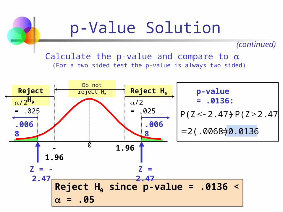
Calculate the p-value and compare to (For a two sided test the p-value is always two sided)

(continued)

0.01362(.0068)2.47)P(Z2.47)P(Z

p-value = .0136:

p-Value Solution

Reject H0 since p-value = .0136 < = .05

Z = 2.47

-1.96

/2 = .025

.0068

.0068

Recall the possible hypothesis test outcomes: Actual

SituationDecisionDo Not Reject H0

No error (1 - )

Type II Error ( β )

Reject H0Type I Error

( )

H0 False H0 TrueKey:Outcome

(Probability)No Error ( 1 - β )

β denotes the probability of Type II Error

1 – β is defined as the power of the testPower = 1 – β = the probability that a false null

hypothesis is rejected

Power of the Test

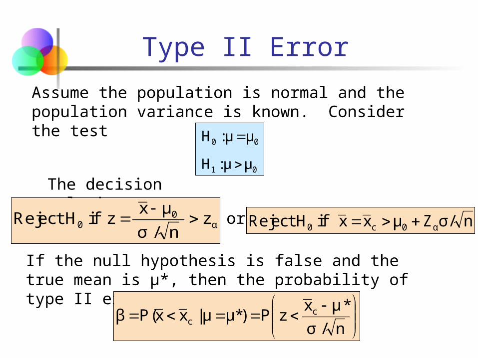
Type II Error

or


α0

0 zn/σμxz if H Reject

00 μμ:H

01 μμ:H

Assume the population is normal and the population variance is known. Consider the test

nσ/Zμxx if H Reject α0c0

If the null hypothesis is false and the true mean is μ*, then the probability of type II error is

n/σ*μxzPμ*)μ|xxP(β c

c

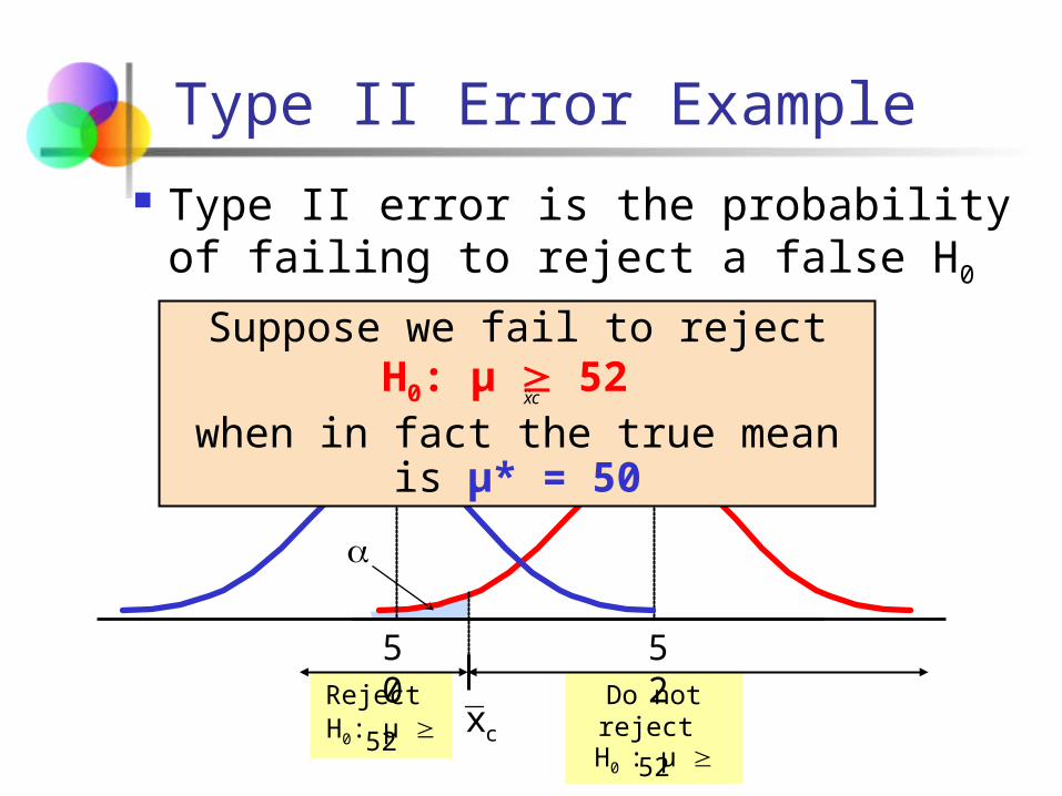
Reject H0: μ 52

Do not reject H0 : μ 52

Type II Error Example Type II error is the probability of failing to reject a false H0

52

50

Suppose we fail to reject H0: μ 52

when in fact the true mean is μ* = 50

cx

cx

Reject H0: μ 52

Do not reject

H0 : μ 52

Type II Error Example

Suppose we do not reject H0: μ 52 when in fact the true mean is μ* = 50

5250

This is the true distribution of x if μ = 50

This is the range of x where H0 is not rejected

(continued)

cx

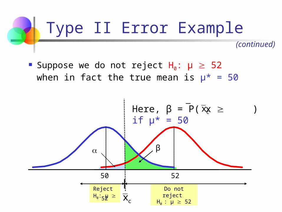
Reject H0: μ 52

Do not reject

H0 : μ 52

Type II Error Example

Suppose we do not reject H0: μ 52 when in fact the true mean is μ* = 50

5250

β

Here, β = P( x ) if μ* = 50

(continued)

cx

cx

Reject H0: μ 52

Do not reject

H0 : μ 52

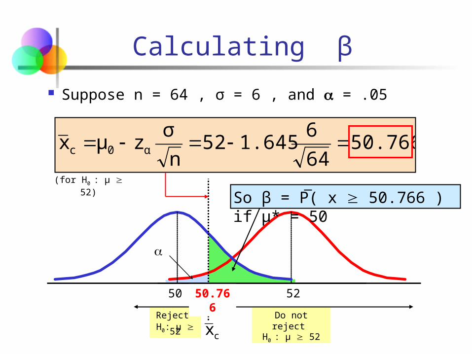
Suppose n = 64 , σ = 6 , and = .05

5250

So β = P( x 50.766 ) if μ* = 50

Calculating β

50.7666461.64552

nσzμx α0c

(for H0 : μ 52)

50.766

cx

Reject H0: μ 52

Do not reject

H0 : μ 52

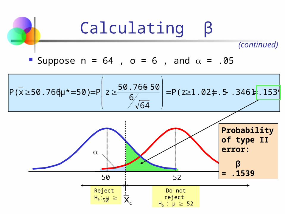
.1539.3461.51.02)P(z64

65050.766zP50)μ*|50.766xP(

Suppose n = 64 , σ = 6 , and = .05

5250

Calculating β(continued)

Probability of type II error: β = .1539

cx

If the true mean is μ* = 50, The probability of Type II Error = β = 0.1539

The power of the test = 1 – β = 1 – 0.1539 = 0.8461

Power of the Test Example

Actual SituationDecision

Do Not Reject H0

No error1 - = 0.95

Type II Error β = 0.1539

Reject H0Type I Error

= 0.05

H0 False H0 TrueKey:Outcome

(Probability)No Error

1 - β = 0.8461

(The value of β and the power will be different for each μ*)

Chapter Summary Addressed hypothesis testing methodology Performed Z Test for the mean (σ known) Discussed critical value and p-value approaches to hypothesis testing

Performed one-tail and two-tail tests Performed t test for the mean (σ unknown) Performed Z test for the proportion Discussed type II error and power of the test

Lecture notes 9 hypothesys testing

Documents

Transcript of Lecture notes 9 hypothesys testing