Lecture Notes in Computer Science 6129
373
Lecture Notes in Computer Science 6129 Commenced Publication in 1973 Founding and Former Series Editors: Gerhard Goos, Juris Hartmanis, and Jan van Leeuwen Editorial Board David Hutchison Lancaster University, UK Takeo Kanade Carnegie Mellon University, Pittsburgh, PA, USA Josef Kittler University of Surrey, Guildford, UK Jon M. Kleinberg Cornell University, Ithaca, NY, USA Alfred Kobsa University of California, Irvine, CA, USA Friedemann Mattern ETH Zurich, Switzerland John C. Mitchell Stanford University, CA, USA Moni Naor Weizmann Institute of Science, Rehovot, Israel Oscar Nierstrasz University of Bern, Switzerland C. Pandu Rangan Indian Institute of Technology, Madras, India Bernhard Steffen TU Dortmund University, Germany Madhu Sudan Microsoft Research, Cambridge, MA, USA Demetri Terzopoulos University of California, Los Angeles, CA, USA Doug Tygar University of California, Berkeley, CA, USA Gerhard Weikum Max-Planck Institute of Computer Science, Saarbruecken, Germany
-
Upload
khangminh22 -
Category
Documents
-
view
1 -
download
0
Transcript of Lecture Notes in Computer Science 6129

Lecture Notes in Computer Science 6129Commenced Publication in 1973Founding and Former Series Editors:Gerhard Goos, Juris Hartmanis, and Jan van Leeuwen
Editorial Board
David HutchisonLancaster University, UK
Takeo KanadeCarnegie Mellon University, Pittsburgh, PA, USA
Josef KittlerUniversity of Surrey, Guildford, UK
Jon M. KleinbergCornell University, Ithaca, NY, USA
Alfred KobsaUniversity of California, Irvine, CA, USA
Friedemann MatternETH Zurich, Switzerland
John C. MitchellStanford University, CA, USA
Moni NaorWeizmann Institute of Science, Rehovot, Israel
Oscar NierstraszUniversity of Bern, Switzerland
C. Pandu RanganIndian Institute of Technology, Madras, India
Bernhard SteffenTU Dortmund University, Germany
Madhu SudanMicrosoft Research, Cambridge, MA, USA
Demetri TerzopoulosUniversity of California, Los Angeles, CA, USA
Doug TygarUniversity of California, Berkeley, CA, USA
Gerhard WeikumMax-Planck Institute of Computer Science, Saarbruecken, Germany
Amihood Amir Laxmi Parida (Eds.)
CombinatorialPattern Matching
21st Annual Symposium, CPM 2010New York, NY, USA, June 21-23, 2010Proceedings
13

Volume Editors
Amihood AmirJohns Hopkins UniversityBaltimore, MD, USAandBar-Ilan UniversityDepartment of Computer Science52900 Ramat-Gan, IsraelE-mail: [email protected]
Laxmi ParidaIBM T.J. Watson Research CenterYorktown Heights, NY, USAE-mail: [email protected]
Library of Congress Control Number: 2010927801
CR Subject Classification (1998): F.2, I.5, H.3.3, J.3, I.4.2, E.4, G.2.1, E.1
LNCS Sublibrary: SL 1 – Theoretical Computer Science and General Issues
ISSN 0302-9743ISBN-10 3-642-13508-0 Springer Berlin Heidelberg New YorkISBN-13 978-3-642-13508-8 Springer Berlin Heidelberg New York
This work is subject to copyright. All rights are reserved, whether the whole or part of the material isconcerned, specifically the rights of translation, reprinting, re-use of illustrations, recitation, broadcasting,reproduction on microfilms or in any other way, and storage in data banks. Duplication of this publicationor parts thereof is permitted only under the provisions of the German Copyright Law of September 9, 1965,in its current version, and permission for use must always be obtained from Springer. Violations are liableto prosecution under the German Copyright Law.
springer.com
© Springer-Verlag Berlin Heidelberg 2010Printed in Germany
Typesetting: Camera-ready by author, data conversion by Scientific Publishing Services, Chennai, IndiaPrinted on acid-free paper 06/3180

Preface
The papers contained in this volume were presented at the 21st Annual Sym-posium on Combinatorial Pattern Matching (CPM 2010) held at NYU-Poly,Brooklyn, New York during June 21–23, 2010.
All the papers presented at the conference are original research contributions.We received 53 submissions from 21 countries. Each paper was reviewed by atleast three reviewers. The committee decided to accept 28 papers. The programalso includes three invited talks by Zvi Galil from Tel Aviv University, Israel,Richard M. Karp from University of California at Berkeley, USA, and Jeffrey S.Vitter from Texas A&M University, USA.
The objective of the annual CPM meetings is to provide an internationalforum for research in combinatorial pattern matching and related applications.It addresses issues of searching and matching strings and more complicated pat-terns such as trees, regular expressions, graphs, point sets, and arrays. The goalis to derive non-trivial combinatorial properties of such structures and to exploitthese properties in order to either achieve superior performance for the corre-sponding computational problems or pinpoint conditions under which searchescannot be performed efficiently. The meeting also deals with problems in com-putational biology, data compression and data mining, coding, information re-trieval, natural language processing and pattern recognition.
The Annual Symposium on Combinatorial Pattern Matching started in 1990,and has since taken place every year. Previous CPM meetings were held in Paris,London, Tucson, Padova, Asilomar, Helsinki, Laguna Beach, Aarhus, Piscat-away, Warwick, Montreal, Jerusalem, Fukuoka, Morelia, Istanbul, Jeju Island,Barcelona, London, Ontario, Pisa, and Lille.
Starting from the third meeting, proceedings of all meetings have been pub-lished in the LNCS series, volumes 644, 684, 807, 937, 1075, 1264, 1448, 1645,1848, 2089, 2373, 2676, 3109, 3537, 4009, 4580, 5029, 5577, and 6129.
Selected papers from the first meeting appeared in volume 92 of TheoreticalComputer Science, from the 11th meeting in volume 2 of Journal of DiscreteAlgorithms, from the 12th meeting in volume 146 of Discrete Applied Mathe-matics, from the 14th meeting in volume 3 of Journal of Discrete Algorithms,from the 15th meeting in volume 368 of Theoretical Computer Science, from the16th meeting in volume 5 of Journal of Discrete Algorithms, and from the 19thmeeting in volume 410 of Theoretical Computer Science.
The whole submission and review process was carried out with the help ofthe EasyChair conference system. The conference was sponsored by the NYU-Poly, Brooklyn, and by IBM Research. Special thanks are due to the members ofthe Program Committee who worked very hard to ensure the timely review of all

VI Preface
the submitted manuscripts, and participated in stimulating discussions that ledto the selection of the papers for the conference.
April 2010 Amihood AmirLaxmi Parida

Organization
Program Committee
Amihood Amir Johns Hopkins University, USA, and Bar-IlanUniversity, Israel (Co-chair)
Rolf Backofen Albert-Ludwigs-Universität Freiburg, GermanyAyelet Butman Holon Academic Institute of Technology, Holon,
IsraelMatteo Comin University of Padova, ItalyMiklós Csurös Université de Montréal, CanadaPetros Drineas Rensselaer Polytechnic Institute, USALeszek Gasieniec University of Liverpool, UKSteffen Heber North Carolina State University, USAJohn Iacono Polytechnic Institute of New York University,
USAShunsuke Inenaga Kyushu University, JapanRao Kosaraju Johns Hopkins University, USAGregory Kucherov Laboratoire d’Informatique Fondamentale de
Lille, FranceGad Landau NYU-Poly, USA, and University of Haifa, IsraelThierry Lecroq University of Rouen, FranceAvivit Levy Shenkar College and CRI, University of Haifa,
IsraelIon Mandoiu University of Connecticut, USAAvi Ma’ayan Mount Sinai, USAGonzalo Navarro University of Chile, ChileLaxmi Parida IBM T.J. Watson Research Center, USA
(Co-chair)Heejin Park Hanyang University, KoreaNadia Pisanti University of Pisa, ItalyEly Porat Bar-Ilan University, IsraelNaren Ramakrishnan Virginia Tech, USAMarie-France Sagot INRIA, FranceRahul Shah Louisiana State University, USADennis Shasha New York University, USADina Sokol City University of New York, USATorsten Suel Polytechnic Institute of NYU, USAJens Stoye Universität Bielefeld, GermanyOren Weimann Weizmann Institute of Science, Israel
VIII Organization
Yufeng Wu University of Connecticut, USADekel Tsur Ben Gurion University of the Negev, IsraelMichal Ziv-Ukelson Ben Gurion University of the Negev, Israel
Organizing Committee
Gad Landau NYU-Poly, USA, and University of Haifa, IsraelLaxmi Parida IBM T.J. Watson Research Center, USA
Steering Committee
Alberto Apostolico University of Padova, Italy, and GeorgiaInstitute of Technology, USA
Maxime Crochemore Université Paris-Est, France, and King’sCollege London, UK
Zvi Galil Columbia University, USA, and Tel AvivUniversity, Israel
Web and Publications Committee
Asif Javed IBM T.J. Watson Research Center, USA
External Referees
Hideo BannaiMichaël CadilhacSabrina ChandrasekaranFrancisco ClaudeMaxime CrochemoreDanny HermelinWing Kai HonBrian HowardPeter HusemannAsif JavedErez KatzenelsonTakuya KidaSung-Ryul KimTsvi KopelowitzAlexander LachmannTaehyung LeeArnaud LefebvreZsuzsanna LiptakNimrod Milo
Mathias MöhlJoong Chae NaShoshana NeuburgerMarius NicolaeGe NongPierre PeterlongoTamar PinhasYoan PinzonBoris PismennyIgor PotapovSven RahmannPaolo RibecaLuis M.S. RussoJeong Seop SimTatiana StarikovskayaSharma ThankachanAlex TiskinCharalampos TsourakakisFabio Vandin

Organization IX
Rossano VenturiniDavide VerzottoIsana Vexler-Lublinsky
Sebastian WillPrudence W.H. WongShay Zakov
Sponsoring Institutions
IBM ResearchNYU-Poly, Brooklyn

Table of Contents
Algorithms for Forest Pattern Matching . . . . . . . . . . . . . . . . . . . . . . . . . . . . 1Kaizhong Zhang and Yunkun Zhu
Affine Image Matching Is Uniform TC0-Complete . . . . . . . . . . . . . . . . . . . . 13Christian Hundt
Old and New in Stringology . . . . . . . . . . . . . . . . . . . . . . . . . . . . . . . . . . . . . . . 26Zvi Galil
Small-Space 2D Compressed Dictionary Matching . . . . . . . . . . . . . . . . . . . . 27Shoshana Neuburger and Dina Sokol
Bidirectional Search in a String with Wavelet Trees . . . . . . . . . . . . . . . . . . 40Thomas Schnattinger, Enno Ohlebusch, and Simon Gog
A Minimal Periods Algorithm with Applications . . . . . . . . . . . . . . . . . . . . . 51Zhi Xu
The Property Suffix Tree with Dynamic Properties . . . . . . . . . . . . . . . . . . . 63Tsvi Kopelowitz
Approximate All-Pairs Suffix/Prefix Overlaps . . . . . . . . . . . . . . . . . . . . . . . . 76Niko Valimaki, Susana Ladra, and Veli Makinen
Succinct Dictionary Matching with No Slowdown . . . . . . . . . . . . . . . . . . . . 88Djamal Belazzougui
Pseudo-realtime Pattern Matching: Closing the Gap . . . . . . . . . . . . . . . . . . 101Raphael Clifford and Benjamin Sach
Breakpoint Distance and PQ-Trees . . . . . . . . . . . . . . . . . . . . . . . . . . . . . . . . . 112Haitao Jiang, Cedric Chauve, and Binhai Zhu
On the Parameterized Complexity of Some Optimization ProblemsRelated to Multiple-Interval Graphs . . . . . . . . . . . . . . . . . . . . . . . . . . . . . . . . 125
Minghui Jiang
Succinct Representations of Separable Graphs . . . . . . . . . . . . . . . . . . . . . . . 138Guy E. Blelloch and Arash Farzan
Implicit Hitting Set Problems and Multi-genome Alignment . . . . . . . . . . . 151Richard M. Karp
Bounds on the Minimum Mosaic of Population Sequences underRecombination . . . . . . . . . . . . . . . . . . . . . . . . . . . . . . . . . . . . . . . . . . . . . . . . . . 152
Yufeng Wu

XII Table of Contents
The Highest Expected Reward Decoding for HMMs with Applicationto Recombination Detection . . . . . . . . . . . . . . . . . . . . . . . . . . . . . . . . . . . . . . . 164
Michal Nanasi, Tomas Vinar, and Brona Brejova
Phylogeny- and Parsimony-Based Haplotype Inference withConstraints . . . . . . . . . . . . . . . . . . . . . . . . . . . . . . . . . . . . . . . . . . . . . . . . . . . . . 177
Michael Elberfeld and Till Tantau
Faster Computation of the Robinson-Foulds Distance betweenPhylogenetic Networks . . . . . . . . . . . . . . . . . . . . . . . . . . . . . . . . . . . . . . . . . . . . 190
Tetsuo Asano, Jesper Jansson, Kunihiko Sadakane,Ryuhei Uehara, and Gabriel Valiente
Mod/Resc Parsimony Inference . . . . . . . . . . . . . . . . . . . . . . . . . . . . . . . . . . . . 202Igor Nor, Danny Hermelin, Sylvain Charlat, Jan Engelstadter,Max Reuter, Olivier Duron, and Marie-France Sagot
Extended Islands of Tractability for Parsimony Haplotyping . . . . . . . . . . . 214Rudolf Fleischer, Jiong Guo, Rolf Niedermeier, Johannes Uhlmann,Yihui Wang, Mathias Weller, and Xi Wu
Sampled Longest Common Prefix Array . . . . . . . . . . . . . . . . . . . . . . . . . . . . 227Jouni Siren
Verifying a Parameterized Border Array in O(n1.5) Time . . . . . . . . . . . . . . 238Tomohiro I, Shunsuke Inenaga, Hideo Bannai, and Masayuki Takeda
Cover Array String Reconstruction . . . . . . . . . . . . . . . . . . . . . . . . . . . . . . . . . 251Maxime Crochemore, Costas S. Iliopoulos, Solon P. Pissis, andGerman Tischler
Compression, Indexing, and Retrieval for Massive String Data . . . . . . . . 260Wing-Kai Hon, Rahul Shah, and Jeffrey Scott Vitter
Building the Minimal Automaton of A∗X in Linear Time, When X Isof Bounded Cardinality . . . . . . . . . . . . . . . . . . . . . . . . . . . . . . . . . . . . . . . . . . . 275
Omar AitMous, Frederique Bassino, and Cyril Nicaud
A Compact Representation of Nondeterministic (Suffix) Automata forthe Bit-Parallel Approach . . . . . . . . . . . . . . . . . . . . . . . . . . . . . . . . . . . . . . . . . 288
Domenico Cantone, Simone Faro, and Emanuele Giaquinta
Algorithms for Three Versions of the Shortest Common SuperstringProblem . . . . . . . . . . . . . . . . . . . . . . . . . . . . . . . . . . . . . . . . . . . . . . . . . . . . . . . . 299
Maxime Crochemore, Marek Cygan, Costas S. Iliopoulos,Marcin Kubica, Jakub Radoszewski, Wojciech Rytter, andTomasz Walen

Table of Contents XIII
Finding Optimal Alignment and Consensus of Circular Strings . . . . . . . . . 310Taehyung Lee, Joong Chae Na, Heejin Park, Kunsoo Park, andJeong Seop Sim
Optimizing Restriction Site Placement for Synthetic Genomes . . . . . . . . . 323Pablo Montes, Heraldo Memelli, Charles Ward, Joondong Kim,Joseph S.B. Mitchell, and Steven Skiena
Extension and Faster Implementation of the GRP Transform forLossless Compression . . . . . . . . . . . . . . . . . . . . . . . . . . . . . . . . . . . . . . . . . . . . . 338
Hidetoshi Yokoo
Parallel and Distributed Compressed Indexes . . . . . . . . . . . . . . . . . . . . . . . . 348Luıs M.S. Russo, Gonzalo Navarro, and Arlindo L. Oliveira
Author Index . . . . . . . . . . . . . . . . . . . . . . . . . . . . . . . . . . . . . . . . . . . . . . . . . . 361

Algorithms for Forest Pattern Matching
Kaizhong Zhang and Yunkun Zhu
Dept. of Computer Science, University of Western Ontario,London, Ontario N6A 5B7, Canada
[email protected], [email protected]
Abstract. Ordered labelled trees are trees where the left-to-right orderamong siblings is significant. An ordered labelled forest is a sequence ofordered labelled trees. Given an ordered labelled forest F (“the targetforest”) and an ordered labelled forest G (“the pattern forest”), the for-est pattern matching problem is to find a sub-forest F ′ of F such thatF ′ and G are the most similar over all possible F ′. In this paper, wepresent efficient algorithms for the forest pattern matching problem fortwo types of sub-forests: closed subforests and closed substructures. AsRNA molecules’ secondary structures could be represented as orderedlabelled forests, our algorithms can be used to locate the structural orfunctional regions in RNA secondary structures.
1 Introduction
An ordered labelled tree is a tree where the left-to-right order among siblingsis significant and each node is labelled by a symbol from a given alphabet. Anordered labelled forest is a sequence of ordered labelled trees. Ordered labelledtrees and forests are very useful data structures for hierarchical data representa-tion. In this paper, we refer to ordered labelled trees and ordered labelled forestsas trees and forests, respectively.
Among numerous applications where trees and forests are useful representa-tions of objects, the need for comparing trees and forests frequently arises. As atypical example, consider the secondary structure comparison problem for RNA.Since RNA is a single strand of nucleotides, it folds back onto itself into a shapethat is topologically a forest [14,3,6,10], which we call its secondary structure.Figure 1 which is adapted from [5] shows an example of the RNA GI:2347024structure, where (a) is a segment of the RNA sequence, (b) is its secondarystructure and (c) is the forest representation. Algorithms for the edit distancebetween forests (tree) [15,2] could be used to measure the global similarity be-tween forests (trees). Motivated mainly by the problem of locating structural orfunctional regions in RNA secondary structures, the forest (tree) pattern match-ing (FPM) problem became interesting and attracted some attention [3,4,5,6].
In this paper, the forest pattern matching (FPM) problem is defined as thefollowing: Given a target forest F and a pattern forest G, find a sub-forest F ′ of
A. Amir and L. Parida (Eds.): CPM 2010, LNCS 6129, pp. 1–12, 2010.c© Springer-Verlag Berlin Heidelberg 2010

2 K. Zhang and Y. Zhu
Fig. 1. (a) A segment of the RNA GI: 2347024 primary structure [8], (b) its secondarystructure, (c) its forest representation
F which is the most similar to G over all possible F ′. There are various ways todefine the term “sub-forest”. For the definition of “sub-forest” as substructures orsimple substructures [5], algorithms have been developed [15,5]. We consider twoalternative definitions of “sub-forest”: closed subforests and closed substructures.
For the closed subforests definition, we present an efficient algorithm whichimproved the complexity results given in [5] of CPM 2006. For the new closedsubstructures definition, we present an efficient algorithm.
2 Preliminaries
Throughout this paper, we use the following definitions and notations.Let F be any given forest, we use a left-to-right postorder numbering of the
nodes in F . |F | denotes the number of nodes in F . In the postorder numbering,F [i..j] will generally be an ordered subforest of F induced by the nodes numberedfrom i to j inclusive. Let f [i] be the ith node in F and F [i] be the subtree rootedat f [i]. A subforest of F is an ordered sequence of subtrees of F . A substructureof F is any connected sub-graph of F . l(i) denotes the postorder number of theleftmost leaf descendant of f [i]. We say f [i1] and f [i2] (or just i1 and i2) aresiblings if they have the same parent. DF and LF denote the depth and thenumber of leaves of F respectively. To simplify the presentation, we assume thatthe forest F has an imaginary parent node, denoted by p(F ). Finally we definethe key roots of F as the set K(F ) = {p(F )}∪{i | i ∈ F and i has a left sibling}and from [15] we have |K(F )| ≤ LF .

Algorithms for Forest Pattern Matching 3
2.1 Forest Edit Distance
Our algorithms are based on forest edit distance. For forest edit distance, thereare three edit operations on a forest F . (1) Change: to change one node labelto another in F . (2) Delete: to delete a node i from F (making the children ofi become the children of the parent of i and then removing i). (3) Insert: toinsert a node i into F (the complement of delete). An edit operation can berepresented as (a, b) where a and b are labels of forest nodes or a null symbolindicating insertion or deletion. Let γ be a cost function that assigns to eachedit operation (a, b) a nonnegative real number γ(a, b). We constrain γ to be adistance metric.
Let S be a sequence s1, · · · , sk of edit operations. An S-derivation from A to Bis a sequence of forests A0, · · · , Ak such that A = A0, B = Ak, and Ai−1 → Ai viasi for 1 ≤ i ≤ k. We extend γ to the sequence S by letting γ(S) =
∑i=|S|i=1 γ(si).
Formally the distance between F and G is defined as follows:
δ(F, G) = min{γ(S) | S is an edit operation sequence taking F to G}.
The definition of γ makes δ a distance metric also. Equivalently forest editdistance can also be defined using the minimum cost mapping between twoforests [11,15].
Tai [11] gave the first algorithm for computing the tree edit distance betweentwo given trees F and G (one can easily extend this algorithm to the forestedit distance problem). Zhang and Shasha [15] gave a more efficient algorithmfor this problem running in O(|F | · |G| · min{DF , LF } · min{DG, LG}) time andO(|F | · |G|) space. More recently, Klein [7], Touzet [12], and Demaine et al. [2]developed faster algorithms which have better time complexity in the worst case.The algorithm of Demaine et al. [2] runs in O(|F | · |G|2 · (1 + log |F |
|G|), |G| < |F |,time and O(|F | · |G|) space.
2.2 Sub-forest Definitions
Let F be a forest. In this paper, we consider two types of sub-forests of F : (1) aclosed subforest : a sequence of subtrees of F such that their roots are consecutivesiblings. (2) a closed substructure: a sequence of substructures of F such thattheir roots are consecutive siblings. Figure 2 shows these two types of sub-forestsof the forest F in Figure 1(c). Here, F1 is a substructure of F , F2 is a closedsubforest of F , and F3 is a closed substructure of F .
Therefore, we can now define the forest pattern matching (FPM) problemmore formally: given a target forest F and a pattern forest G, find a sub-forest(using any one of the above definitions for “sub-forest”) F ′ of F which minimizesthe forest edit distance to G over all possible F ′.
Forest pattern matching problem for substructures have been studied in [15,5].Forest pattern matching problem for closed subforests has been studied in [5].We propose the forest pattern matching problem for closed substructures. Themotivation is from the forest representation of RNA secondary structures. In

4 K. Zhang and Y. Zhu
Fig. 2. Examples of variant sub-forest of the forest F in Figure 1(c)
this representation, see Figure 1, sibling nodes are in fact connected through thebackbone of RNA primary structure. Therefore, it is natural to assume that,in addition to the parent child connection, a node is also connected to its leftand right siblings. Hence a closed substructure we defined is just a connectedsub-graph in this representation. A closed substructure can be used to repre-sent a pattern local to a multiple loop, although it does not imply a physicallyconnected RNA fragment in a tree representatation of RNA [1].
2.3 Previous Work and Our Results
The problem of finding a most similar “closed subforest” was discussed byJansson and Peng in their CPM 2006 paper [5] and their algorithm runs inO(|F | · |G| ·LF ·min{DG, LG}) time and O(|F | · |G|+LF ·DF · |G|+ |F | ·LG ·DG)space.
In this paper, we show how to solve the forest pattern matching (FPM) prob-lem efficiently based on [15,2] for two types of sub-forests, “closed subforest” and“closed substructure”. The time complexity of our algorithms are summarizedin Table 1 and the space complexity of our algorithm is O(|F | · |G|).
Table 1. Our results
FPM Time complexity Section
Closed subforestO(|F | · |G| · min{DF , LF } · min{DG, LG})
O(|F | · |G| · (|G| · (1 + log |F ||G| ) + min{DF , LF })) 3.1
Closed substructureO(|F | · |G| · min{DF , LF } · min{DG, LG})
O(|F | · |G| · (|G| · (1 + log |F ||G| ) + min{DF , LF })) 3.2
Compared with the algorithm of Jansson and Peng [5], our first algorithmsolving the same problem is faster and uses less space. Our second algorithmsolves the problem of finding a most similar closed substructure which could beused to search an RNA structural pattern local to a multiple loop.

Algorithms for Forest Pattern Matching 5
3 Algorithms for the Forest Pattern Matching Problem
In this section, we present efficient algorithms for forest pattern matchingproblem for two types of sub-forests, closed subforest and closed substructure,respectively. We also refer the forest pattern matching problem as the problemof finding a most similar sub-forest.
3.1 An Algorithm for Finding a Most Similar Closed Subforest
Given a target forest F and a pattern forest G, our goal is to compute
min{δ(F [l(i1)..i2], G) | i1 and i2 are siblings}.
Jansson and Peng [5] gave an algorithm for this problem in O(|F | · |G| · LF ·min{DG, LG}) time and O(|F | · |G| + LF · DF · |G| + |F | · LG · DG) space.We present an algorithm which is more efficient in both time and space. Ouralgorithm combines the idea of [15] and the method of approximate patternmatching for sequences [9,13].
We first examine sequence pattern matching method and then give a naturalextension from sequence pattern matching to forest pattern matching for closedsubforest.
Given a pattern sequence P [1..m] and a text sequence T [1..n], the problemis to find a segment T [k..l] in the text which yields a minimum edit distanceto P [1..m]. The idea is that in calculating the score for T [1..i] and P [1..j], anyprefix of T [1..i] could be deleted without any penalty. In other words, the scoreis min{δ(T [i1..i], P [1..j]) | 1 ≤ i1 ≤ i + 1}.
Now consider a node i in a forest F and let the degree of node i be di and itschildren be i1, i2, . . . , idi. Given a pattern forest G, we would like to find u andv such that F [l(iu)..iv] yields the minimum distance to G. Let k ∈ F [is] where1 ≤ s ≤ di, how could we define a score Δ(F [l(i1)..k], G[1..j]) for F [l(i1)..k] andG[1..j] in order to extend the definition from sequences to forests?
If k ∈ {i1, i2, . . . , idi}, then F [l(i1)..k] is a sequence of siblingtrees, i.e. T [i1], . . . , T [is]. Δ(F [l(i1)..k], G[1..j]) is therefore defined asmin{δ(F [l(it)..is], G[1..j]) | 1 ≤ t ≤ s + 1} where δ(, ) is the forest edit distance.In particular, if s = 1, then the score is min{δ(F [l(i1)..i1], G[1..j]), δ(∅, G[1..j])}which can be obtained directly using the forest edit distance algorithm.
If k /∈ {i1, i2, . . . , idi}, then Δ(F [l(i1)..k], G[1..j]) is defined asmin{δ(F [l(it)..k], G[1..j]) | 1 ≤ t ≤ s} since F [l(is)..k] is a proper part of F [is]that can not be deleted without penalty.
With this definition, min{Δ(F [l(i1) ..it], G[1..|G|]) | 1 ≤ t ≤ di} is what wewant to compute for node i. We have the following two lemmas for the thecalculation of Δ(F [l(i1)..k], G[1..j]).

6 K. Zhang and Y. Zhu
Lemma 1. Let i, F and G be defined as the above, i1 ≤ k ≤ idi and 1 ≤ j ≤ |G|,then
Δ(∅, ∅) = 0;
Δ(F [l(i1)..k], ∅) ={
0 if k ∈ {i1, . . . , idi}Δ(F [l(i1)..k − 1], ∅) + γ(f [k],−); otherwise
Δ(F [l(i1)..i1], G[1..j]) = min{
δ(F [l(i1)..i1], G[1..j])δ(∅, G[1..j]).
Proof. This is directly from the above definition. �
Lemma 2. Let i, F and G be defined as the above, i1 < k ≤ idi and 1 ≤ j ≤ |G|,then
Δ(F [l(i1)..k], G[1..j])
= min
⎧⎨
⎩
Δ(F [l(i1)..k − 1], G[1..j]) + γ(f [k],−),Δ(F [l(i1)..k], G[1..j − 1]) + γ(−, g[j]),Δ(F [l(i1)..l(k) − 1], G[1..l(j) − 1]) + δ(F [l(k)..k], G[l(j)..j]).
Proof. We prove this lemma inductively. The base case is k = i1 + 1where we need the fact that Δ(F [l(i1)..i1], G[1..j])= min{δ(F [l(i1)..i1], G[1..j]),δ(∅, G[1..j])}.
For k > i1 and k ∈ {i2, i3, . . . , idi},
min
⎧⎨
⎩
Δ(F [l(i1)..k − 1], G[1..j]) + γ(f [k],−)Δ(F [l(i1)..k], G[1..j − 1]) + γ(−, g[j])Δ(F [l(i1)..l(k) − 1], G[1..l(j) − 1]) + δ(F [l(k)..k], G[l(j)..j])
= min
⎧⎪⎪⎨
⎪⎪⎩
min{δ(F [l(it)..k − 1], G[1..j]) | 1 ≤ t ≤ s} + γ(f [k],−)min{δ(F [l(it)..k], G[1..j − 1]) | 1 ≤ t ≤ s + 1} + γ(−, g[j])min{δ(F [l(it)..l(k) − 1], G[1..l(j) − 1]) | 1 ≤ t ≤ s}
+ δ(F [l(k)..k], G[l(j)..j])
= min{
min{δ(F [l(it)..k], G[1..j]) | 1 ≤ t ≤ s}δ(∅, G[1..j]).
= min{δ(F [l(it)..k], G[1..j]) | 1 ≤ t ≤ s + 1}= Δ(F [l(i1)..k], G[1..j]).
For k > i1 and k /∈ {i2, i3, . . . , idi},
min
⎧⎨
⎩
Δ(F [l(i1)..k − 1], G[1..j]) + γ(f [k],−)Δ(F [l(i1)..k], G[1..j − 1]) + γ(−, g[j])Δ(F [l(i1)..l(k) − 1], G[1..l(j)− 1]) + δ(F [l(k)..k], G[l(j)..j])
= min
⎧⎪⎪⎨
⎪⎪⎩
min{δ(F [l(it)..k − 1], G[1..j]) | 1 ≤ t ≤ s} + γ(f [k],−)min{δ(F [l(it)..k], G[1..j − 1]) | 1 ≤ t ≤ s} + γ(−, g[j])min{δ(F [l(it)..l(k) − 1], G[1..l(j) − 1]) | 1 ≤ t ≤ s}
+ δ(F [l(k)..k], G[l(j)..j])= min{δ(F [l(it)..k], G[1..j]) | 1 ≤ t ≤ s}= Δ(F [l(i1)..k], G[1..j]). �

Algorithms for Forest Pattern Matching 7
Fig. 3. The bold line is the leftmost path of F [i]. The black nodes (a,c) belong to lp(i)and the black and gray nodes (a,b,c,d) belong to layer(i).
With these two lemmas, we can calculate min{Δ(F [l(i1) · · · it], G[1..|G|) | 1 ≤t ≤ di} using dynamic programming. However, we have to do this for every nodei of F . Because for each child subtree of F [i] the calculation starts at i1 insteadof l(i1) and δ(F [l(i1)..i1], G[1..j]) is needed in the calculation, the best way isto do the calculations for all the nodes on the path from a leaf to its nearestancestor key root together. In this way, we do the computation layer by layer,see Figure 3. Lemma 3 and 4 extend Lemma 1 and 2 from a node to the leftmostpath of a key root. Due to the page limitation, we omit the proofs.
We will need the following definitions: lp(i): a set which contains the nodeson the leftmost path of F [i] except the root i; layer(i): a set which contains allof the sibling nodes of nodes in lp(i) including lp(i). In Figure 3, lp(i) = {a, c}and layer(i) = {a, b, c, d}. With these definitions, we have the following twolemmas. In Lemma 4, for convenience, forestdist(F [l(i)..i1], G[1..j1]) representsδ(F [l(i)..i1], G[1..j1]) and treedist(i1, j1) represents δ(F [l(i1)..i1], G[l(j1)..j1]).
Lemma 3. Let i be a key root of F , l(i) ≤ i1 < i and 1 ≤ j1 ≤ |G|, then
Δ(∅, ∅) = 0;
Δ(F [l(i)..i1], ∅) ={
0 if i1 ∈ layer(i)Δ(F [l(i)..i1 − 1], ∅) + γ(f [i1],−); if i1 /∈ layer(i)
Δ(F [l(i)..i1], G[1..j1]) = min{
forestdist(F [l(i)..i1], G[1..j1])δ(∅, G[1..j1]).
if i1 ∈ lp(i)
Lemma 4. Let i be a key root of F , l(i) ≤ i1 < i, i1 /∈ lp(i), and 1 ≤ j1 ≤ |G|,then
Δ(F [l(i)..i1], G[1..j1])
= min
⎧⎨
⎩
Δ(F [l(i)..i1 − 1], G[1..j1]) + γ(f [i1],−),Δ(F [l(i)..i1], G[1..j1 − 1]) + γ(−, g[j1]),Δ(F [l(i)..l(i1) − 1], G[1..l(j1) − 1]) + treedist(i1, j1).

8 K. Zhang and Y. Zhu
Our algorithm is a dynamic programming algorithm. In the first stage of ouralgorithm, we call forest edit distance algorithm [15,2] for F and G to gettreedist(i, j) needed in Lemma 4. In the second stage, the key roots of F aresorted in an increasing order and put in an array KF . And for any key root kof F , we first call forest edit distance algorithm of [15] for F [k] and G to getforestdist(, ) needed in Lemma 3 and then call the procedure for Δ(, ) compu-tation for F [k] and G. We are now ready to give our algorithm for finding a mostsimilar closed subforest of F to G:
Theorem 1. Our algorithm correctly computes the cost of an optimal solution.
Proof. Because of step 1 in Algorithm 1, all the treedist(, ) used in step 7in Procedure Delta(F [i], G) are available. Because of step 4 in Algorithm 1,all the forestdist(, ) used in step 7 in Procedure Delta(F [i], G) are available.
�
Input: A target forest F and a pattern forest G.Output: min{Δ(F [l(x1)..x2], G) | x1 is x2’s leftmost sibling}.Algorithm:Call TreeDistance(F,G) according to [15] or [2];1
for i′ := 1 to |KF | do2
i := KF [i′];3
Call ForestDistance(F [i], G) according to [15];4
Call Procedure Delta(F [i], G);5
end6
Algorithm 1. Finding a most similar closed subforest of F to G
Procedure Delta(F [i], G):Δ(∅, ∅) = 0;1
for i1 := l(i) to i − 1 do2
Compute Δ(F [l(i)..i1], ∅) according to Lemma 3.3
end4
for i1 := l(i) to i − 1 do5
for j1 := 1 to |G| do6
Compute Δ(F [l(i)..i1], G[1..j1 ]) according to Lemma 3 and Lemma 4.7
end8
end9
Theorem 2. Our algorithm can be implemented to run in O(|F | · |G| ·min{DF , LF } · min{DG, LG}) time and O(|F | · |G|) space.
Proof. The time and space complexity of the computation for the edit distanceof all subtree pairs of F and G is O(|F | · |G| · min{DF , LF} · min{DG, LG})and O(|F | · |G|) due to [15]. For one key root i, the time and space for

Algorithms for Forest Pattern Matching 9
ForestDistance(F [i], G) and Delta(F [i], G) are the same: O(|F [i]| · |G|). There-fore the total time and space for all key roots are O(|G||F | ·min{DF , LF }) andO(|G||F |) due to Lamma 7 in [15]. Hence the time and space complexity ofour algorithm are O(|F | · |G| · min{DF , LF } · min{DG, LG}) and O(|F | · |G|)respectively.
If we use the algorithm [2] to compute the edit distance, the time complexityis O(|F | · |G|2 · (1 + log(|F |/|G|))) and the total time complexity is O(|F | · |G| ·(|G| · (1+ log |F |
|G|)+min{DF , LF })). �
3.2 An Algorithm for Finding a Most Similar Closed Substructure
In this section we consider the problem of finding a most similar closed sub-structure. Recall that, for a given forest F , a subtree of F is one of F [i]where 1 ≤ i ≤ |F | and a subforest of F is an ordered sequence of subtreesof F .
Giving a target forest F and a pattern forest G, the forest removing distancefrom F to G, δr(F, G), is defined as the following where subf(F ) is the set ofsubforests of F and F \ f represents the forest resulting from the deletion ofsubforest f from F .
δr(F, G) = minf∈subf(F )
{δ(F \ f, G)}
Zhang and Shasha’s algorithm [15] for approximate tree pattern matching withremoving solves this problem. This can also be solved using the technique ofDemaine et al. [2].
We again consider a node i in forest F and let the degree of node i be di and itschildren be i1, i2, . . . , idi . Let k ∈ F [is] where 1 ≤ s ≤ di, we now define anotherremoving distance δR(F [l(i1)..k], G[1..j]) as follows where subf(F, node set) isthe set of subforests of F such that nodes in node set are not in any of thesubforests.
δR(F [l(i1)..k], G[1..j]) = minf∈subf(F [l(i1)..k],{i1,...idi
})δ(F [l(i1)..k] \ f, G[1..j])
From this definition and the algorithm in [15], we have the following formula forδR(F [l(it)..k], G[1..j]), where 1 ≤ t ≤ s.
δR(F [l(it)..k], G[1..j]) =
min
⎧⎪⎪⎪⎪⎨
⎪⎪⎪⎪⎩
δR(F [l(it)..l(k) − 1], G[1..j]), if k /∈ {i1, i2, . . . , idi}δR(F [l(it)..k − 1], G[1..j]) + γ(f [k],−),δR(F [l(it)..k], G[1..j − 1]) + γ(−, g[j]),δR(F [l(it)..l(k) − 1], G[1..l(j) − 1]) + γ(f [k], g[j])
+ δr(F [l(k)..k − 1], G[l(j)..j − 1]).

10 K. Zhang and Y. Zhu
We can now define Ψ(F [l(i1)..k], G[1..j]) for F [l(i1)..k] and G[1..j] usingδR(, ) for closed substructures. This is exactly the same way as we defineΔ(F [l(i1)..k], G[1..j]) using δ(, ) for closed subforests.
If k ∈ {i1, i2, . . . , idi}, then Ψ(F [l(i1)..k], G[1..j]) is defined asmin{δR(F [l(it)..is], G[1..j]) | 1 ≤ t ≤ s + 1}.
In particular, if s = 1, Ψ(F [l(i1)..i1], G[1..j]) is min{δR(∅, G[1..j]),δR(F [l(i1)..i1], G[1..j])} = δr(F [l(i1)..i1], G[1..j]) which can be obtained directlyusing the forest removing distance algorithm.
If k /∈ {i1, i2, . . . , idi}, then Ψ(F [l(i1)..k], G[1..j]) is defined asmin{δR(F [l(it)..k], G[1..j]) | 1 ≤ t ≤ s}.
For the calculation of Ψ(F [l(i1)..k], G[1..j]), we have the following two lemmas.The proofs are similar to Lemma 1 and Lemma 2.
Lemma 5. Let i, F and G be defined as the above, i1 ≤ k ≤ idi and 1 ≤ j ≤ |G|,then
Ψ(∅, ∅) = 0;Ψ(F [l(i1)..k], ∅) = 0;Ψ(F [l(i1)..i1], G[1..j]) = δr(F [l(i1)..i1], G[1..j]).
Lemma 6. Let i, F and G be defined as the above, i1 < k ≤ idi and 1 ≤ j ≤ |G|,then
Ψ(F [l(i1)..k], G[1..j])
= min
⎧⎪⎪⎪⎪⎨
⎪⎪⎪⎪⎩
Ψ(F [l(i1)..l(k) − 1], G[1..j]), if k /∈ {i2, . . . , idi}Ψ(F [l(i1)..k − 1], G[1..j]) + γ(f [k],−),Ψ(F [l(i1)..k], G[1..j − 1]) + γ(−, g[j]),Ψ(F [l(i1)..l(k) − 1], G[1..l(j) − 1]) + γ(f [k], g[j])
+ δr(F [l(k)..k − 1], G[l(j)..j − 1]).
Lemma 7 and 8 extend Lemma 5 and 6 from a node to the leftmost path of akey root. Due to the page limitation, we omit the proofs.
Lemma 7. Let i be a key root of F , l(i) ≤ i1 < i and 1 ≤ j1 ≤ |G|, then
Ψ(∅, ∅) = 0;Ψ(F [l(i)..i1], ∅) = 0;Ψ(F [l(i)..i1], G[1..j1]) = δr(F [l(i)..i1], G[1..j1]). if i1 ∈ lp(i)
Lemma 8. Let i be a key root of F , l(i) < i1 < i, i1 /∈ lp(i), and 1 ≤ j1 ≤ |G|,then
Ψ(F [l(i)..i1], G[1..j1]) =
min
⎧⎪⎪⎪⎪⎨
⎪⎪⎪⎪⎩
Ψ(F [l(i)..l(i1) − 1], G[1..j1]), if i1 /∈ layer(i)Ψ(F [l(i)..i1 − 1], G[1..j1]) + γ(f [i1],−),Ψ(F [l(i)..i1], G[1..j1 − 1]) + γ(−, g[j1]),Ψ(F [l(i)..l(i1) − 1], G[1..l(j1) − 1]) + γ(f [i1], g[j1])
+ δr(F [l(i1)..i1 − 1], G[l(j1)..j1 − 1]).
We can now show our algorithm for closed substructures.

Algorithms for Forest Pattern Matching 11
Input: A target forest F and a pattern forest G.Output: min{Ψ(F [l(x1)..x2], G) | x1 is x2’s leftmost sibling}.Algorithm:Call Tree RemoveDistance(F,G) according to [15];1
for i′:=1 to |K(F )| do2
i := K(F )[i′];3
Call Forest RemoveDistance(F [i], |G|) according to [15];4
Call Procedure Psi(F [i], G);5
end6
Algorithm 2. Finding most similar closed substructure of F to G
Procedure Psi(F [i], G):Ψ(∅, ∅) = 0;1
for i1 := l(i) to i − 1 do2
Ψ(F [l(i)..i1], ∅) = 0;3
end4
for i1 := l(i) to i − 1 do5
for j1 := 1 to |G| do6
Compute Ψ(F [l(i)..i1], G[1..j1]) according to Lemma 7 and Lemma 8.7
end8
end9
4 Conclusion
We have presented two algorithms for the forest pattern matching problem fortwo types of sub-forest. Our first algorithm for finding a most similar closedsubforest is better than that of [5]. Our second algorithm for finding a mostsimilar closed substructure can be used to search for local forest patterns.
When the input are two sequences represented as forests, both our algorithmsreduce to the sequence approximate pattern matching algorithm [9]. When theinput are two sequences represented as linear trees, our second algorithm reducesto the sequence approximate pattern matching algorithm [9].
References
1. Backofen, R., Will, S.: Local Sequence-structure Motifs in RNA. Journal of Bioin-formatics and Computational Biology 2(4), 681–698 (2004)
2. Demaine, E.D., Mozes, S., Rossman, B., Weimann, O.: An optimal decompositionalgorithm for tree edit distance. In: Arge, L., Cachin, C., Jurdzinski, T., Tarlecki,A. (eds.) ICALP 2007. LNCS, vol. 4596, pp. 146–157. Springer, Heidelberg (2007)
3. Hochsmann, M., Toller, T., Giegerich, R., Kurtz, S.: Local similarity in RNA sec-ondary structures. In: Proceedings of the IEEE Computational Systems Bioinfor-matics Conference, pp. 159–168 (2003)
4. Jansson, J., Hieu, N.T., Sung, W.-K.: Local gapped subforest alignment and itsapplication in finding RNA structural motifs. In: Fleischer, R., Trippen, G. (eds.)ISAAC 2004. LNCS, vol. 3341, pp. 569–580. Springer, Heidelberg (2004)

12 K. Zhang and Y. Zhu
5. Jansson, J., Peng, Z.: Algorithms for Finding a Most Similar Subforest. In: Lewen-stein, M., Valiente, G. (eds.) CPM 2006. LNCS, vol. 4009, pp. 377–388. Springer,Heidelberg (2006)
6. Jiang, T., Wang, L., Zhang, K.: Alignment of trees - an alternative to tree edit.Theoretical Computer Science 143, 137–148 (1995)
7. Klein, P.N.: Computing the edit-distance between unrooted ordered trees. In: Bi-lardi, G., Pietracaprina, A., Italiano, G.F., Pucci, G. (eds.) ESA 1998. LNCS,vol. 1461, pp. 91–102. Springer, Heidelberg (1998)
8. Motifs database, http://subviral.med.uottawa.ca/cgi-bin/motifs.cgi9. Sellers, P.H.: The theory and computation of evolutionary distances: pattern recog-
nition. Journal of Algorithms 1(4), 359–373 (1980)10. Shapiro, B.A., Zhang, K.: Comparing multiple RNA secondary structures using
tree comparisons. Computer Applications in the Biosciences 6(4), 309–318 (1990)11. Tai, K.-C.: The tree-to-tree correction problem. Journal of the Association for
Computing Machinery (JACM) 26(3), 422–433 (1979)12. Touzet, H.: A linear time edit distance algorithm for similar ordered trees. In:
Apostolico, A., Crochemore, M., Park, K. (eds.) CPM 2005. LNCS, vol. 3537,pp. 334–345. Springer, Heidelberg (2005)
13. Ukkonen, E.: Algorithms for approximate string matching. Information and Con-trol 64(1–3), 100–118 (1985)
14. Zhang, K.: Computing similarity between RNA secondary structures. In: Proceed-ings of IEEE International Joint Symposia on Intelligence and Systems, Rockville,Maryland, May 1998, pp. 126–132 (1998)
15. Zhang, K., Shasha, D.: Simple fast algorithms for the editing distance betweentrees and related problems. SIAM Journal on Computing 18(6), 1245–1262 (1989)
Affine Image Matching Is Uniform
TC0-Complete
Christian Hundt
Institut fur Informatik, Universitat Rostock, [email protected]
Abstract. Affine image matching is a computational problem to deter-mine for two given images A and B how much an affine transformated Acan resemble B. The research in combinatorial pattern matching led to apolynomial time algorithm which solves this problem by a sophisticatedsearch in the set D(A) of all affine transformations of A. This paper showsthat polynomial time is not the lowest complexity class containing thisproblem by providing its TC0-completeness. This result means not onlythat there are extremely efficient parallel solutions but also reveals furtherinsight into the structural properties of image matching. The completenessin TC0 relates affine image matching to a number of most basic problemsin computer science, like integer multiplication and division.
Keywords: digital image matching, combinatorial pattern matching,design and analysis of parallel algorithms.
1 Introduction
The affine image matching problem (AIMP, for short) is to determine for twogiven images A and B how much an affine transformation of A can resembleB. Affine image matching (AIM) has a wide range of applications in variousimage processing settings, e.g., in computer vision [16], medical imaging [5,18,19],pattern recognition, digital watermarking [7], etc.
Recently, discretization techniques developed in the combinatorial patternmatching research (CPM, for short) have been used successfully for AIM. Apartfrom algorithmic achievements, this led to improved techniques for the analysis ofthe problem. Essentially, all algorithms developed in CPM for computing a bestmatch f(A) with B share the same plane idea, to perform exhaustive search ofthe entire set D(A), which contains all affine transformations of A. Surprisingly,the fastest known methods which determine the provably best affine image matchcome from this simple approach. In fact, the main challenge of computing D(A),is to find a discretization of the set F of all affine transformations. A convenientstarting point for the research in this direction is given by the discretizationtechniques developed in CPM, although the problem in the focus of CPM consistsin locating an exact match of an affine transformation of A in B, rather than oncomputing the best one like in AIM. See e.g. [17,11,10,1,4,3,2].
In [13,14] affine transformations are characterized by six real parameters and,based on this, a new generic discretization of F is developed which is basically
A. Amir and L. Parida (Eds.): CPM 2010, LNCS 6129, pp. 13–25, 2010.c© Springer-Verlag Berlin Heidelberg 2010

14 C. Hundt
a partition of the parameter space R6 into subspaces ϕ1, . . . , ϕτ(n), where τ(n)
depends on the size n×n of image A. Every subspace ϕi represents one possibletransformation of A and consequently the cardinality of D(A) is shown to bein O(n18) by estimating an upper bound on the number τ(n) of subspaces. Thediscretization motivates an algorithm that first constructs a data structure Inrepresenting the partition and then, to solve the AIMP, it searches all images inD(A) by traversing In. Its running time is linear in τ(n) and thus, in O(n18) forimages A and B of size n× n.
However, the exact time complexity remains unknown. It is also an openquestion whether the decision version of the AIMP is included in a complexityclass that is “easier” than P – the class of problems decidable in polynomialtime. Particularly, it is open whether the problem belongs to low complexityclasses of the hierarchy inside P:
AC0 ⊂ TC0 ⊆ NC1 ⊆ L ⊆ P.
Every class in the hierarchy implies a structural computational advantage againstthe hardness in P. This paper continues the research on AIM in the combinatorialsetting using the algebraic approach introduced in [13] and refined in [14] togive a new, surprisingly low complexity for AIM by showing that the affineimage matching problem is TC0-complete. TC0 is a very natural complexityclass because it exactly expresses the complexity of a variety of basic problems incomputation, such as integer addition, multiplication, comparison and division.
The containment of the AIMP in TC0 ⊆ NC1 means first that AIM can besolved in logarithmic parallel time on multi-processor systems which have boundedfan-in architecture. However, theoretically it can even be solved in constant timeif the processors are assumed to have unbounded fan-in. Secondly, since TC0 ⊆ LAIM can also be solved on deterministic sequential machines using only a loga-rithmic amount of memory. Finally, the completeness of the AIMP in TC0 meansthat there is no polynomially sized, uniformly shaped family of Boolean formulasexpressing AIM since this captures the computational power of AC0 �= TC0.
Anyway, the new results have no immediate impact on practical settings ofAIM. In fact, they have to be seen more as an ambition to uncover the structuralproperties of AIM and related problems. Particularly, the novel TC0 approach toAIM is based on a characterization of the parameter space partition ϕ1, . . . , ϕτ(n)
for affine transformations. Every subspace ϕi is shown to exhibit a positive vol-ume such that an algorithm can simply sample a certain subregion of R
6 to hitevery element of the partition. Thus D(A) can be computed without the datastructure In that implicitely represents the space partition. Interestingly, thisis not an hereditary property. The parameter space partition of linear trans-formations, i.e., the subset of F without translations, contains subspaces withzero volume [14]. This means that, although linear image matching is weakerthan AIM, the low-complexity approach of this paper cannot be applied to thisproblem in a straight forward manner. The author leaves the estimation of thisproblem’s complexity as an open challenge.
This paper presents results which heavily build on previous work [13,14].After a short presentation of technical preliminaries Section 3 briefly provides

Affine Image Matching Is Uniform TC0-Complete 15
the basics of the AIM approach introduced in [13,14] which are necessary tounderstand the new results of this paper. Then Section 4 provides the new TC0
approach to AIM and next Section 5 proves that the AIMP belongs to the hardestproblems of TC0. Finally, the paper concludes by drawing a wider picture of thefinding’s impact. All proofs are removed due to space limitations.
2 Technical Preliminaries
Digital Images and their Affine Transformations. Through the wholepaper, an image is a two-dimensional array of pixels, i.e., of unit squares parti-tioning a certain square area of the real plane R
2. The pixels of an image A areindexed over a set N = {(i, j) | − n ≤ i, j ≤ n}, where n is called the size of A.The geometric center point of the pixel with index (i, j) can be found at coordi-nates (i, j). Each pixel (i, j) has a color A〈i, j〉 that is an element from a finiteset Σ = {0, 1, . . . , σ} of color values. To simplify the dealing with A’s borders letA〈i, j〉 = 0 if (i, j)�∈ N . The distortion between two given images A and B of sizen is measured by Δ(A, B) =
∑(i,j)∈N δ(A〈i, j〉, B〈i, j〉) where δ : Σ ×Σ → N is
a function charging color mismatches, for example, δ(c1, c2) = |c1 − c2|.The set F of affine transformations contains exactly all injective functions
f : R2 → R
2 which can be described by
f(x, y) = ( a1 a2a4 a5 ) · ( x
y ) + ( a3a6 ) (1)
for some constants a1, . . . , a6 ∈ R, with the additional property of a1a5 �= a2a4.Applying an affine transformation f to A gives a transformed image f(A) of
size n. To define a color value for any pixel (i, j) in f(A), let f−1 be the inversefunction of f . Notice that f−1 is always an affine transformation, too. Then definethe color value f(A)〈i, j〉 as the color A〈I, J〉 of the pixel (I, J) = [f−1(i, j)],where [(x, y)] := ([x], [y]) denotes rounding both components of a vector (x, y) ∈R
2. Hence, determining f(A)〈i, j〉 means to choose the pixel (I, J) of A whichgeometrically contains the point f−1(i, j) in its square area. This setting modelsnearest-neighbor interpolation, commonly used in image processing. Now, anyimage A defines the set D(A) = {f(A) | f ∈ F} that contains all possible affinetransformations of A.
Based on this, the following defines the affine image matching problem:
For given images A and B of size n find the minimal distortion Δ(f(A), B) overall transformations f ∈ F .
For the analysis of complexity aspects consider the decision variant of this prob-lem which asks if there is a transformation f ∈ F which yields Δ(f(A), B) ≤ tfor some given threshold t ∈ N.
Circuit Complexity. This paper discusses the complexity of certain functionsf : {0, 1}∗ → {0, 1}∗ mapping binary strings to binary strings. Let |s| be thelength of a binary string s ∈ {0, 1}∗ and for all i ∈ {0 . . . , |s| − 1} let s〈i〉 denotethe ith character of s. Moreover, let 1n be the string of n sequent characters 1and for all strings s and s′ let s|s′ be their concatenation.

16 C. Hundt
Circuits C can be imagined as directed acyclic graphs were vertices, alsocalled gates, compute Boolean functions. Gates gain input truth values frompredecessor gates and distribute computation results to all their successor gates.If C has n sources and m sinks, then it computes a function f : {0, 1}n → {0, 1}m,i.e., C computes for every input string of length n an output string of lengthm. This makes circuits weaker than other computational models, which cancompute functions f : {0, 1}∗ → {0, 1}∗. Consequently one considers families C ={C1, C2, . . .} of circuits to compute f for every input length n with an individualcircuit Cn. On the other hand, such families can be surprisingly powerful becausethey may not necessarily be finitely describable in the traditional sense. A usualworkaround is a uniformity constraint which demands that every circuit Cn
of C can be described by a Turing machine MC with resource bounds relatedto n. Usually MC is chosen much weaker than the computational power of C toavoid the obscuration of C’s complexity. This paper considers only DLOGTIME-uniform families C where MC has to verify in O(log n) time whether Cn fulfills agiven structural property like, e.g., “Gate i computes the ∧-function” or “Gatei is a predecessor of gate j”.
The class DLOGTIME-uniform FAC0 contains all functions f : {0, 1}∗ →{0, 1}∗ which can be computed by constant-depth, polynomial-size families Cof DLOGTIME-uniform circuits, i.e., where (a) every gate computes a function“∧”, “∨” or “¬”, (b) all circuits Cn can be verified by a Turing machine MC thatruns in O(log n)-time (c) the number of gates in Cn grows only polynomially in nand (d) regardless of n, the length of any path in Cn from input to output is notlonger than a constant. For convenience denote this class also by UD-FAC0. Aprominent member of UD-FAC0 is the addition function of two integer numbers.
If the gates can also compute threshold-functions Tk, a generalization of “∧”and “∨” which is true if at least k inputs are true, then the generated functionclass is called DLOGTIME-uniform FTC0 (UD-FTC0), a class that contains abig variety of integer arithmetic functions.
A decision problem is a set Π ⊆ {0, 1}∗, i.e., a set of strings. By UD-AC0
denote the class of all decision problems which can be decided by a functionf ∈ UD-FAC0, i.e., f : {0, 1}∗ → {0, 1} is a function with f(s) = 1 ⇔ s ∈ Π .Accordingly, UD-TC0 is the class of decision problems decidable by a functionin UD-FTC0.
This paper uses special decision problems Πf for any function f : {0, 1}∗ →{0, 1}∗. The set Πf contains all binary strings s which encode pairs (i, s′) ∈N × {0, 1}∗ using a unary encoding for integer i and a binary encoding for s′
such that (i, s′) ∈ Πf if and only if f(s′)〈i〉 = 1, i.e., if the ith character of f(s′)is a 1. Clearly, f is in UD-FAC0 if the output length of f is bounded polynomiallyin the input length and Πf is in UD-AC0. A circuit family C deciding Πf canbe used to compute also f simply by spending one circuit of C for every outputbit. The same holds for functions in UD-FTC0.
By definition, UD-(F)AC0 is a subset of UD-(F)TC0 and thus, UD-FAC0-reductions are suited well to define completeness in the class UD-TC0. A problemΠ is UD-TC0-complete if Π belongs to UD-TC0 and if for all Π ′ ∈ UD-TC0 there
Affine Image Matching Is Uniform TC0-Complete 17
is a function rΠ in UD-FAC0 such that for all s ∈ {0, 1}∗ it is true s ∈ Π ′ ⇔rΠ(s) ∈ Π . Clearly, since UD-FAC0-reductions are transitive, it is also sufficientfor UD-TC0-completeness to find one other UD-TC0-complete problem Π ′ andthen provide a function r in UD-FAC0 such that for all s ∈ {0, 1}∗ it is trues ∈ Π ′ ⇔ r(s) ∈ Π . A canonical UD-TC0-complete set is MAJ, containingstrings over {0, 1}∗ with a majority of 1-characters [6].
For convenience the uniformity statement UD is mostly omitted in the restof the paper since all considered circuit families apply DLOGTIME-uniformity.Due to space limitations this section cannot go into further details of this richtheory and the author refers the reader to the text book [21].
First Order Logic. First order formulas are an important concept from logic. Acomprehensive introduction to first order logic and in particular the connectionto circuit families is given in [21].
In this paper a first order formula F is build recursively over a unary pred-icate s(·) and two binary predicates bit(·, ·) and <(·, ·) by the standard useof “∧”, “∨”, “¬”, “∀” and “∃”. Without loss of generality F is of the formF = Q1v1 . . . QmvmF ′ where Q1, . . . , Qm are quantifiers, “∀” or “∃”, for thevariables v1, . . . , vm and F ′ is a quantifier free formula. The variables v1, . . . , vm
are called bounded and every other variable in F ′ is free. If there are no freevariables then F is called a sentence.
The assertion of a formula F is either true or false, which is defined over therecursive construction of F and relative to (1) a universe, that is a finite subset{0, . . . , n − 1} of N, (2) a specification of s(·) and (3) an assignment of valuesfor free variables. The meaning of the binary predicates is fixed, thus, bit(a, i) istrue if and only if the ith bit in the n-bit binary representation of a is one, and<(a, b) is true if and only if a < b.
This paper applies first order logic to describe sets of strings Π ⊆ {0, 1}∗,i.e., decision problems. Particularly, any string s ∈ {0, 1}∗ defines a universe{0, . . . , |s| − 1} and a specification of s(·) by giving for all i ∈ {0, . . . , |s| − 1}that the predicate s(i) is true if and only if s〈i〉 = 1. Consequently, a string salone determines the truth value of a sentence F because it has no free variables.Then a string s is said to model F , which is denoted by s |= F , if s satisfies F .Thereby a sentence F describes a set ΠF = {s ∈ {0, 1}∗ | s |= F}. For exampleF = ∃v s(v) gives the set of strings which contain at least one character 1.
If F has free variables v1, . . . , vm, then a string s alone is not enough to deter-mine the truth value. However, in this case the formula F [v1 ← i1, . . . , vm ← im],where the free variables are assigned certain values i1, . . . , im from the universe,defines a proper truth value. This paper applies the concept of free variablesin terms of a modular design principle. The variables v1, . . . , vm can be under-stood as parameters of F which influence the formula’s assertion. This meansthat F can be applied as a subformula in a sentence F ′ which uses v1, . . . , vm topass auxiliary arguments i1, . . . , im to F . Such “subformula-calls” are denotedby F [i1, . . . , im].

18 C. Hundt
The set of all problems Π which can be expressed by a first order sentenceF , i.e., for which Π = ΠF , is denoted by FO. It turns out that FO = UD-AC0.Consequently integer addition is first-order-expressible and therefore this paperutilizes the subformula ADD[x1, x2, y] which is satisfied if and only if x1, x2 andy are assigned values satisfying x1 + x2 = y.
TC0 being a generalization of AC0 implies that a characterization of TC0 interms of first order logic needs a language extension. Therefore consider beside“∀” and “∃” the additional majority quantifier “M”, which is defined as follows:The sentence F = Mv F ′ is true for given strings s if and only if the formulasF ′[v ← i] are true for a majority of assignments of i ∈ {0, . . . , |s| − 1} to thefree variable v. Then UD-TC0 = FO[M ], the set of problems expressible by firstorder sentences with additional quantifier “M”.
In some cases it is difficult to express certain relations in FO or FO[M ]-sentences just because the values of variables are restricted to {0, . . . , |s| − 1}.However, one can simply assume that there are long variables v which are ableto take values in the range {−|s|k−1, . . . , |s|k−1} for some arbitrary constant k.The value of v can simply be represented in k+1 ordinary variables v0, . . . , vk−1
and sgn by v = (−1)sgn ·∑k−1i=0 |s|i · vi. A sentence F using a long variable
v realizes the quantification and the predicates <(·, ·) and bit(·, ·) over v byreducing them to their ordinary counterparts.
Beside long variables first order logic can be extended also with a ≤(·, ·)predicate because it easily reduces to <(·, ·). This paper applies these predicatesin infix notation.
3 Previous Results
Previous work [13,14] presented a new algorithmic approach to solve affine imagematching in linear time with respect to the cardinality |D(A)|. Moreover, itprovided an upper bound of O(n18) for this cardinality which means that AIMcan be solved in polynomial time. This section briefly discusses some basics ofthis approach which are used in this paper.
By equation (1) in the previous section, all transformations in F can be char-acterized by the six parameters a1 to a6. Hence, each affine transformation fcan be described by a point (a1, . . . , a6)T in the six-dimensional parameter spaceR
6. Reversely, every such point in R6 which fulfills a1a5 �= a2a4 characterizes
an affine transformation. Now, a discrete characterization of F can be obtainedby a subdivision of the parameter space R
6 into a finite number of subspacesϕ1, . . . , ϕτ(n) with the following property: Any pair of transformations f, f ′ ∈ Fgives the same transformation f(A) = f ′(A) of an image A of size n if their in-verses f−1 and f ′−1 are represented by points (a1, . . . , a6)T , resp. (a′
1, . . . , a′6)
T ,contained in the same subspace ϕi for some i ∈ {1, . . . , τ(n)}. This means thateach of the τ(n) subspaces represents one transformed image in D(A).
The principle of the polynomial time algorithm is searching the whole setD(A)which is a common practice in the CPM. Using the discrete characterizationof F the algorithm traverses all the subspaces ϕ1 to ϕτ(n) of the parameter

Affine Image Matching Is Uniform TC0-Complete 19
space. With each subspace it finds one of the possible transformed images A′ inD(A). Subsequently, the distortion between such images A′ and B is evaluatedto eventually find the best match.
For images of size n the subdivision of the parameter space into the spacesϕ1 to ϕτ(n) is determined by the following set Hn of functions R
6 → R:
Hn = {Iijk(a1, . . . , a6) = ia1 + ja2 + a3 − (k − 0.5) | (i, j) ∈ N , k ∈ {−n, . . . , n + 1}}∪ {Jijk(a1, . . . , a6) = ia4 + ja5 + a6 − (k − 0.5) | (i, j) ∈ N , k ∈ {−n, . . . , n + 1}}
Hence, Hn = {1, . . . , r(n)} is a set of r(n) = (2n +1)2(2n + 2) linear functionswhere every w, either w = Iijk or w = Jijk for some (i, j) ∈ N and k ∈{−n, . . . , n + 1}, describes the following two subspaces of R
6:
h+(w) = {(a1, . . . , a6)T ∈ R6 | w(a1, . . . , a6) ≥ 0},
h−(w) = {(a1, . . . , a6)T ∈ R6 | w(a1, . . . , a6) < 0}.
The meaning of the sets h+(w) and h−(w) can be understood as follows:All the points (a1, . . . , a6)T in h+(Iijk) describe inverse affine transformationsf−1(x, y) = ( a1 a2
a4 a5 ) · ( xy ) + ( a3
a6 ) which have one thing in common: It is alwaystrue that [f−1(i, j)] = (I, J) with I ≥ k. Accordingly, all points (a1, . . . , a6)T inh−(Iijk) give transformations f−1 which uniquely fulfill [f−1(i, j)] = (I, J) withI < k. Finally, a similar property is true for the J-coordinate of [f−1(i, j)] =(I, J) depending on the situation of the point describing f−1 with respect toh+(Jijk) and h−(Jijk).
Now, the partition of the parameter space into the pieces ϕ1 to ϕτ(n) is definedby the intersection of the subspaces h+() and h−() given by the lines in Hn.Particularly, for Hn = {1, . . . , r(n)} define
A(Hn) =
{
ϕ ⊆ R6
∣∣∣∣∣ϕ =
r(n)⋂
w=1
hsw(w) for some s1, . . . , sr(n) ∈ {+,−}, ϕ�= ∅}
.
In literature the set A(Hn) is called the (hyperplane) arrangement given by Hn.For detailed information on such arrangements see [8]. In this paper the elementsof A(Hn) are called faces.
The relation between A(Hn) and D(A) is the most important property for-mulated in [14]:
Theorem 1 ([14]). For all n and every image A of size n there exists a sur-jective mapping
Γn : A(Hn)→ D(A).
Thus, Theorem 1 reduces the enumeration of D(A), a set with no obvious struc-ture, to the enumeration of A(Hn). In turn, the efficient enumeration of all facesin A(Hn) can be realized easily. The algorithm conveniently constructs a graphIn, which contains a node v(ϕ) for each face ϕ ∈ A(Hn) and which encodesthe incidence of faces by edges, i.e., two nodes v(ϕ) and v(ϕ′) are connected byan edge if the faces ϕ and ϕ′ are neighbors in R
6. For a detailed description of
20 C. Hundt
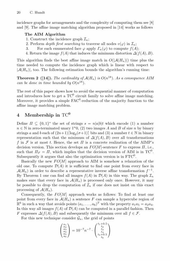
incidence graphs for arrangements and the complexity of computing them see [8]and [9]. The affine image matching algorithm proposed in [14] works as follows
The AIM Algorithm1. Construct the incidence graph In;2. Perform depth first searching to traverse all nodes v(ϕ) in In;3. For each enumerated face ϕ apply Γn(ϕ) to compute f(A);4. Return the image f(A) that induces the minimum distortion Δ(f(A), B).
This algorithm finds the best affine image match in O(|A(Hn)|) time plus thetime needed to compute the incidence graph which is linear with respect to|A(Hn)|, too. The following estimation bounds the algorithm’s running time:
Theorem 2 ([14]). The cardinality of A(Hn) is O(n18). As a consequence AIMcan be done in time bounded by O(n18).
The rest of this paper shows how to avoid the sequential manner of computationand introduces how to get a TC0 circuit family to solve affine image matching.Moreover, it provides a simple FAC0-reduction of the majority function to theaffine image matching problem.
4 Membership in TC0
Define Π ⊆ {0, 1}∗ the set of strings s = n|a|b|t which encode (1) a numbern ∈ N in zero-terminated unary 1n0, (2) two images A and B of size n by binarystrings a and b each of (2n+1)�log2(σ+1)� bits and (3) a number t ∈ N in binaryrepresentation such that the minimum of Δ(f(A), B) over all transformationsf in F is at most t. Hence, the set Π is a concrete realization of the AIMP’sdecision version. This section develops an FO[M ]-sentence F to express Π , i.e.,such that ΠF = Π , which implies that the decision version of AIM is in TC0.Subsequently it argues that also the optimization version is in FTC0.
Basically the new FO[M ] approach to AIM is somehow a relaxation of theold one. To compute D(A) it is sufficient to find one point from every face inA(Hn) in order to describe a representative inverse affine transformation f−1.By Theorem 1 one can find all images f(A) in D(A) in this way. The graph In
makes sure that every face in A(Hn) is processed only once. However, it maybe possible to drop the computation of In if one does not insist on this exactprocessing of A(Hn).
Consequently, the FO[M ] approach works as follows: To find at least onepoint from every face in A(Hn) a sentence F can sample a hypercube region ofR
6 in such a way that avoids points (a1, . . . , a6)T with the property a1a5 = a2a4.In this way all images f(A) of D(A) can be computed in a parallel fashion. ThenF expresses Δ(f(A), B) and subsequently the minimum over all f ∈ F .
For this new technique consider Gn, the grid of points⎛
⎝
a1a2a3a4a5a6
⎞
⎠ = 10−7n−7 ·⎛
⎝
t1+0.5t2t3t4
t5+0.5t6
⎞
⎠

Affine Image Matching Is Uniform TC0-Complete 21
where t1, . . . , t6 are integers in the set {−1012n13, . . . , 1012n13}. The central prop-erty of Gn applied in F is given in the following theorem:
Theorem 3. 1. |Gn| ∈ O(n78).2. Every point p = (a1, . . . , a6)T ∈ Gn fulfills a1a5 �= a2a4.3. For all faces ϕ in A(Hn) there is a point p in the grid Gn such that p ∈ ϕ.
The proof of the theorem is somewhat technical. However, it first shows thatthere is a hypercube that intersects all faces ofA(Hn). Then it establishes a lowerbound on the volume of all faces. Consequently, if the hypercube is sampled withpoints of adequately small distance, every face of A(Hn) gets a hit. Because allpoints (a1, . . . , a6)T avoid the condition a1a5 = a2a4 it is satisfactory to processthe grid Gn to find all elements of D(A) for any given image A of size n.
The advantage of Gn against In is the simple structure which can be easilygenerated on the fly. The disadvantage is the enormous growth of size, which,nevertheless, remains polynomial in n.
The following develops a rough idea of the sentence F that expresses Π .Particularly,
F = ∃t1 . . .∃t6 DELTA[t1, . . . , t6] ∧ (−1012n13 ≤ t1) ∧ (t1 ≤ 1012n13) ∧ . . .
∧ (−1012n13 ≤ t6) ∧ (t6 ≤ 1012n13)
is build by a subformula DELTA[t1, . . . , t6] which is true for given parameterst1, . . . , t6 if the string s encodes numbers and images that fulfill Δ(f(A), B) ≤ twhere f−1 is the transformation given by the grid point (t1, . . . , t6)T . In thisfashion the sentence samples all points of the grid Gn and accepts if and only ifat least one of them represents a transformation of A which resembles B enoughin terms of t. Theorem 3 guarantees the correctness of this approach. Obviouslyt1 to t6 are variables representing long integers such that they can hold valuespolynomially in n.
The formula DELTA can be expressed in first order logic with majorityquantifiers as follows: Basically, DELTA[t1, . . . , t6] has to (1) find the trans-formation f−1 represented by (t1, . . . , t6)T , (2) compute the sum Δ(f(A), B) =∑
(i,j)∈N δ(A〈f−1(i, j)〉, B〈i, j〉) and (3) compare this to t. The computation off−1 by the grid point (t1, . . . , t6)T means to determine
I =[
(2t1+1)i+2t2j+2t32·107n7
]and J =
[2t4i+(2t5+1)j+2t6
2·107n7
].
for all (i, j) ∈ N . This is easily first-order-expressible with majority because itinvolves only a constant number of integer additions, multiplications, divisionsand roundings, all functions in TC0 [6,12]. Now since iterated addition is also inTC0 [6] DELTA can easily compute the sum of δ(A(I, J), B(i, j)) over all (i, j) ∈N . Consequently, the descriptiveness of F in first order logic with majoritydepends on the function δ : Σ×Σ → N. However, since Σ is finite it follows thatδ is even first order-expressible. The expression equivalence between FO[M ] andTC0 implies:
Lemma 1. The decision version of Affine Image Matching is in UD-TC0.

22 C. Hundt
Consequently there exists a uniform family C of constant-depth, polynomial-sizethreshold circuits which decide Π . The optimization version of the AIMP can becomputed by similar means using C. Basically this can be done by constructinganother family Cf of threshold circuits which try all possible values of Δ(f(A), B)in separate parallel copies of C’s circuits. Since Δ(f(A), B) ≤ m ·(2n+1)2, wherem = max{δ(c1, c2) | c1, c2 ∈ Σ) is a constant, it follows that this approachinduces at most a polynomial growth in size. Then, since the minimum of allsatisfying distortion trials can be computed in UD-AC0 [6], the depth remainsconstant, too.
Theorem 4. Affine Image Matching is in UD-FTC0.
5 Completeness in TC0
This section shows the decision version of the AIMP to be TC0-complete. Con-sider the TC0-complete majority problem, i.e., the set MAJ ⊆ {0, 1}∗ of stringswhich contain at least �0.5|s|� characters 1. This section gives an FAC0-reductionr of MAJ to Π , the set of strings s encoding A, B and t such that the minimumΔ(f(A), B) over all affine transformations f is at most t. Hence, r is a functionwhich maps strings s ∈ {0, 1}∗ to a binary encoding of images A and B and aninteger t such that s ∈MAJ if and only if Δ(A, B) ≤ t. Remember, a function ris in FAC0 if the set Πr is in AC0. Consequently, this section argues the existenceof a first order sentence F which expresses Πr, i.e., such that ΠF = Πr.
The basic idea for the reduction is in fact very simple: Consider any strings ∈ {0, 1}∗. Then imagine images As and Bs of size n = 4|s| where As〈i, j〉 =Bs〈i, j〉 = 0 for all pixels (i, j) ∈ N with j �= 0. Additionally set
As〈i, 0〉 ={
s〈i〉, if 0 ≤ i < |s|1, otherwise and Bs〈i, 0〉 = 1
for all i ∈ {−n, . . . , n} and let ts = �0.5|s|�. Obviously, As contains a copy ofs and Bs a row of 1-characters. Moreover ts describes the maximum numberof 0-characters in s to be in MAJ. Then the majority of characters in s is 1if and only if Δ(As, Bs) ≤ ts for the distortion measure δ(c1, c2) = |c1 − c2|.Hence, if transformations were not allowed on As this approach would alreadybe successful.
However, the AIMP allows any affine transformation on As and thus, theabove relation is not enough. To use a similar approach As and Bs are extendedin such a way that the transformations that lead to the optimal match are closeto identity and thus, still count the number of zeros in s. For this end leave mostof As and Bs as before but for all k ∈ {−n, . . . , n} let
As〈k,−n + 2〉 = As〈k, n− 2〉 = As〈−n + 2, k〉 = As〈n− 2, k〉 =Bs〈k,−n〉 = Bs〈k, n〉 = Bs〈−n, k〉 = Bs〈n, k〉 = 2
i.e., draw a frame in As and a little bigger frame in Bs. Now consider the followinglemma:

Affine Image Matching Is Uniform TC0-Complete 23
Lemma 2. Let s ∈ {0, 1}∗ and As, Bs and ts as defined above. Moreover, con-sider the transformation
fopt(x, y) = ( a 00 a ) · ( x
y ) + ( 00 )
where a = 16|s|16|s|−7
. Then s contains a majority of characters 1 if and only ifΔ(fopt(As), Bs) ≤ ts for δ(c1, c2) = |c1 − c2|.The transformation fopt guarantees that (1) the string s remains unaltered and(2) the rest of fopt(As) looks like Bs. This means Δ(fopt(As), Bs) equals thenumber of 0 in s and thus, is at most ts if and only if the majority of charactersin s is 1. However, that is not enough. It remains to show that there is notransformation f ′ ∈ F that performs a better match of f ′(A) to B becauseotherwise the solution of the AIMP would rather go with f ′ and not fopt:
Lemma 3. For all s ∈ {0, 1}∗ it is true that Δ(fopt(As), Bs) under δ(c1, c2) =|c1 − c2| is minimum over all affine transformations in F .
The basic idea behind the lemma’s proof is that the frames in f(As) and Bs
have to be aligned. Together with the alignment of the row j = 0 this leavesall in all only one true transformation f(As). Moreover, the small frame in Aguarantees that f(As) has to be scaled up to match B’s frame. This results inthe effect that every pixel (I, J) in the center of A is represented by a pixel (i, j)in f(As), i.e., (I, J) = [f−1(i, j)]. Consequently no s-character 0 represented inA is forgotten in f(As). Thus, every transformation f(As) has to count at leastall characters 0 in the string s.
The rest is to argue that the computation r(s) = (As, Bs, ts) of the imagesAs and Bs as well as the threshold ts from the string s can be accomplishedby a first order sentence expressing Πr. However, a big deal of that is simplycopying and filling in constants. In particular, both As and Bs can be computedby these simple operations, namely, inserting the string s in As and preparingthe frames in both images. The most complex work is the computation of tsbecause it contains a division. But whereas general division is TC0-complete thedivision by the constant two can be established using only addition by
DIV2[x, y] = ∃z ADD[y, y, x] ∨ (ADD[y, y, z] ∧ADD[z, 1, x]),
i.e., there is a first order subformula DIV2[x, y] that expresses �0.5x� = y. Thefollowing theorem states the completeness result:
Theorem 5. The decision version of the AIMP is UD-TC0-complete underUD-FAC0-reductions.
6 Conclusions
This paper analyzes the complexity of affine image matching. It argues the ex-istence of a first order sentence using the majority quantifier that expresses thisproblem, thus, showing that affine image matching is contained in UD-FTC0.

24 C. Hundt
Moreover, it gives a UD-FAC0-reduction from majority to affine image matchingand therefore provides that the problem is even complete in UD-TC0.
This work concentrates on affine image matching and neglects the superset ofprojective transformations and the subset of linear transformations consideredin [14]. It is a natural conjecture that linear image matching can also be solvedin TC0 and that projective image matching is at least hard in TC0.
In particular the whole approach of this paper can be easily transfered tothe case of projective transformations, i.e., even projective image matching isUD-TC0-complete under UD-FAC0-reductions. This paper sticks to affine imagematching only for convenience because some results become more technical forprojective transformations. Beside the pure complication of introducing previouswork, especially the formulation of an analogue of Theorem 3 requires handlinga multiplicity of cases which makes the basic ideas less perspicuous.
For linear transformations the case is more complicated. Although a propersubclass, the structure of linear transformations is geometrically harder than inthe affine case. This results basically from the fact that the arrangement A(Hn)under linear transformations contains faces which have no volume. Consequently,it is likely that they are missed during a sampling process as described in thispaper. The same holds for several of the small subclasses of affine transforma-tions like scaling and rotation which were analyzed in [15]. Although the authorbelieves that image matching under each of these classes can be done in TC0,it remains open whether this is true. At least the problem’s hardness for TC0 isevident even for scalings because the reduction builds mainly on Δ and benefitsfrom a restriction on the class of transformations.
Regarding the practicability of this paper’s results notice that problems inTC0 can be solved very efficiently in time. However, whereas TC0 restricts sizeonly polynomially, it is practically impossible to create circuits of n78 proces-sors even for small n. But the containment in TC0 has to be seen more in astructural context that gains insight into the problem’s properties. Particularly,the immense growth in size is partially caused by the weak uniformity con-straint, which is a natural choice for complexity analysis. But more powerfulmodels of construction produce much smaller circuits. Consider e.g. P-uniformTC0 families, i.e., where circuits Cn must be constructible by a Turing machinein polynomial time. This is a very natural model for practical settings becauseit allows resources consumption during the planning of Cn but saves them whenCn comes into operation. Under this setting the graph In can be generated andthen used to construct Cn, thus, to reduce the size consumption of the circuit.
According to the above note, this paper is another step towards image match-ing in real applications. The author hopes that it helps to initiate future workon the practical aspects of image matching like for example the first impressionsthat were revealed from [20].
Acknowledgment
The author thanks Maciej Liskiewicz and Ragnar Nevries for helpful ideas andproof reading as well as the anonymous reviewers for improvement suggestions.

Affine Image Matching Is Uniform TC0-Complete 25
References
1. Amir, A., Butman, A., Crochemore, M., Landau, G., Schaps, M.: Two-dimensionalpattern matching with rotations. Theor. Comput. Sci. 314(1-2), 173–187 (2004)
2. Amir, A., Butman, A., Lewenstein, M., Porat, E.: Real two dimensional scaledmatching. Algorithmica 53(3), 314–336 (2009)
3. Amir, A., Chencinski, E.: Faster two-dimensional scaled matching. In: Lewen-stein, M., Valiente, G. (eds.) CPM 2006. LNCS, vol. 4009, pp. 200–210. Springer,Heidelberg (2006)
4. Amir, A., Kapah, O., Tsur, D.: Faster two-dimensional pattern matching withrotations. In: Sahinalp, S.C., Muthukrishnan, S.M., Dogrusoz, U. (eds.) CPM 2004.LNCS, vol. 3109, pp. 409–419. Springer, Heidelberg (2004)
5. Brown, L.G.: A survey of image registration techniques. ACM Computing Sur-veys 24(4), 325–376 (1992)
6. Chandra, A.K., Stockmeyer, L., Vishkin, U.: Constant depth reducibility. SIAM J.Comput. 13(2), 423–439 (1984)
7. Cox, I.J., Bloom, J.A., Miller, M.L.: Digital Watermarking, Principles and Practice.Morgan Kaufmann, San Francisco (2001)
8. Edelsbrunner, H.: Algorithms in Combinatorial Geometry. Springer, Berlin (1987)9. Edelsbrunner, H., O’Rourke, J., Seidel, R.: Constructing arrangements of lines and
hyperplanes with applications. SIAM J. Comput. 15, 341–363 (1986)10. Fredriksson, K., Navarro, G., Ukkonen, E.: Optimal exact and fast approximate
two-dimensional pattern matching allowing rotations. In: Apostolico, A., Takeda,M. (eds.) CPM 2002. LNCS, vol. 2373, pp. 235–248. Springer, Heidelberg (2002)
11. Fredriksson, K., Ukkonen, E.: A rotation invariant filter for two-dimensional stringmatching. In: Farach-Colton, M. (ed.) CPM 1998. LNCS, vol. 1448, pp. 118–125.Springer, Heidelberg (1998)
12. Hesse, W.: Division is in uniform TC0. In: Orejas, F., Spirakis, P.G., van Leeuwen,J. (eds.) ICALP 2001. LNCS, vol. 2076, pp. 104–114. Springer, Heidelberg (2001)
13. Hundt, C., Liskiewicz, M.: On the complexity of affine image matching. In:Thomas, W., Weil, P. (eds.) STACS 2007. LNCS, vol. 4393, pp. 284–295. Springer,Heidelberg (2007)
14. Hundt, C., Liskiewicz, M.: Combinatorial bounds and algorithmic aspects of imagematching under projective transformations. In: Ochmanski, E., Tyszkiewicz, J.(eds.) MFCS 2008. LNCS, vol. 5162, pp. 395–406. Springer, Heidelberg (2008)
15. Hundt, C., Liskiewicz, M., Nevries, R.: A combinatorial geometric approach to two-dimensional robustly pattern matching with scaling and rotation. Theor. Comput.Sci. 51(410), 5317–5333 (2009)
16. Kasturi, R., Jain, R.C.: Computer Vision: Principles. IEEE Computer SocietyPress, Los Alamitos (1991)
17. Landau, G.M., Vishkin, U.: Pattern matching in a digitized image. Algorith-mica 12(3/4), 375–408 (1994)
18. Maintz, J.B.A., Viergever, M.A.: A survey of medical image registration. MedicalImage Analysis 2(1), 1–36 (1998)
19. Modersitzki, J.: Numerical Methods for Image Registration. Oxford UniversityPress, Oxford (2004)
20. Nevries, R.: Entwicklung und Analyse eines beschleunigten Image Matching-Algorithmus fur naturliche Bilder, Diplomarbeit, Universitat Rostock (2008)
21. Vollmer, H.: Introduction to circuit complexity. Springer, Berlin (1999)

Old and New in Stringology
Zvi Galil
Blavatnik School of Computer ScienceTel Aviv University
Twenty five years ago in a paper titled ”Open Problems in Stringology” I listedthirteen open problems in a field I called Stringology. The first part of the talkwill revisit the list. Some problems were solved, others were partially solved andsome resisted any progress.
The second part of the talk will review some recent results in Stringology,namely algorithms in the streaming model. In this model, the algorithms cannotstore the entire input string(s) and can use only very limited space. Surprisingly,efficient algorithms were discovered for a number of string problems.
The talk will conclude with new open problems that are raised by these newresults.
A. Amir and L. Parida (Eds.): CPM 2010, LNCS 6129, p. 26, 2010.c© Springer-Verlag Berlin Heidelberg 2010

Small-Space 2D Compressed Dictionary
Matching
Shoshana Neuburger1,� and Dina Sokol2,��
1 Department of Computer Science, The Graduate Center of the City University ofNew York, New York, NY, [email protected]
2 Department of Computer and Information Science, Brooklyn College of the CityUniversity of New York, Brooklyn, NY, 11210
Abstract. The dictionary matching problem seeks all locations in a textthat match any of the patterns in a dictionary. In the compressed dictio-nary matching problem, the input is in compressed form. In this paperwe introduce the 2-dimensional compressed dictionary matching problemin Lempel-Ziv compressed images, and present an efficient solution forpatterns whose rows are all periodic. Given k patterns, each of (uncom-pressed) size m×m, and a text of (uncompressed) size n×n, all in 2D-LZcompressed form, our algorithm finds all occurrences of the patterns in thetext. The algorithm is strongly inplace, i.e., the extra space it uses is pro-portional to the optimal compression of the dictionary, which is O(km).The preprocessing time of the algorithm is O(km2), linear in the uncom-pressed dictionary size, and the time for performing the search is linear inthe uncompressed text size, independent of the dictionary size. Our algo-rithm is general in the sense that it can be used for any 2D compressionscheme which can be sequentially decompressed in small space.
1 Introduction
The compressed matching problem is the problem of finding all occurrences of apattern in a compressed text. Various algorithms have been devised to solve the2D compressed matching problem, e.g., [6, 3, 4]. The dictionary matching problemis that of locating all occurrences of a set of patterns in a given text. In this paperwe introduce the compressed dictionary matching problem in 2-dimensions. Com-pressed dictionary matching can be trivially solved using any compressed patternmatching algorithm and searching for each pattern separately. Preferably, an al-gorithm should scan the text once so that its search time depends only on the sizeof the text and not on the size of the dictionary of patterns. Aho and Corasickachieved this goal for uncompressed patterns and text.� This work has been supported in part by the National Science Foundation Grant
DB&I 0542751.�� This work has been supported in part by the National Science Foundation Grant
DB&I 0542751 and the PSC-CU Research Award 62280-0040.
A. Amir and L. Parida (Eds.): CPM 2010, LNCS 6129, pp. 27–39, 2010.c© Springer-Verlag Berlin Heidelberg 2010

28 S. Neuburger and D. Sokol
We address 2D compressed dictionary matching when the patterns and textare in LZ78 compressed form. Space is an important concern of a compressedpattern matching algorithm. An algorithm is strongly inplace if the amount ofextra space it uses is proportional to the optimal compression of the data. Thealgorithm we present is both linear time and strongly inplace. The problem weare addressing is of practical significance. Many images are stored in Lempel-Zivcompressed form. Facial recognition is a direct application of 2D compresseddictionary matching. The goal of such software is to identify individuals in alarger image based on a dictionary of previously identified faces. An efficientalgorithm does not depend on the size of the database of known images.
Pattern matching cannot be performed directly on compressed data since com-pression is context-sensitive. The same uncompressed string can be compresseddifferently in different files, depending on the data that precedes the matchingcontent. The key property of LZ78 is the ability to perform decompression usingconstant space in time linear in the uncompressed string. We follow the assump-tion of Amir et. al. [3] and consider the row-by-row linearization of 2D data.
Existing algorithms for 2D dictionary matching are not sequential. Thus, theyare not easily adapted to form strongly-inplace algorithms. Amir and Farachcontributed a 2D dictionary matching algorithm that can be used for squarepatterns [2]. Its time complexity is linear in the size of the text with prepro-cessing time linear in the size of the dictionary. Their algorithm linearizes thepatterns by considering subrow/subcolumn pairs around the diagonal, which isnot conducive to row-by-row decompression. Idury and Schaffer discuss multiplepattern matching in two dimensions for rectangular patterns [9]. Although theiralgorithm is efficient, the data structures require more space than we allow.
We do not know of a small-space dictionary matching algorithm for evenone-dimensional data. Multiple pattern matching in LZW compressed text isaddressed by Kida et. al. [10]. They present an algorithm that simulates theAho-Corasick search mechanism for compressed, one-dimensional texts and anuncompressed dictionary of patterns. Their approach uses space proportionalto both the compressed text and uncompressed dictionary sizes, which is morespace than we allow.
In this paper we present an algorithm that solves the 2D LZ-CompressedDictionary Matching Problem where all pattern rows are periodic and the periodsare no greater than m/4. Given a dictionary of 2D LZ-compressed patterns,P1, P2, . . . , Pk, each of uncompressed size m × m, and a compressed text ofuncompressed size n × n, we find all occurrences of patterns in the text. Ouralgorithm is strongly inplace since it uses O(km) space. The best compressionthat LZ78 can achieve on the dictionary is O(km) [14]. The time complexityof our algorithm is O(km2 + n2 log σ), where σ = min(km, |Σ|) and Σ is thealphabet. After preprocessing the dictionary, the time complexity is independentof the dictionary size.
Amir et. al. present an algorithm for strongly-inplace single pattern matchingin 2D LZ78-compressed data [3]. Their algorithm requires O(m3) time to pre-process the pattern of uncompressed size m × m and search time proportional

Small-Space 2D Compressed Dictionary Matching 29
to the uncompressed text size. Our preprocessing scheme can be used to reducethe preprocessing time of their algorithm to O(m2), linear in the size of theuncompressed pattern, resulting in an overall time complexity of O(m2 + n2).
2 Overview
We overcome the space requirement of traditional 2D dictionary matching al-gorithms with an innovative preprocessing scheme that converts 2D patternsto a linear representation. The pattern rows are initially classified into groups,with each group having a single representative. We store a witness, or positionof mismatch, between the group representatives. A 2D pattern is named by thegroup representative for each of its rows. This is a generalization of the namingtechnique used by Bird [7] and Baker [5] to linearize 2D data. The preprocessingis performed in a single pass over the patterns with no need to decompress morethan two pattern rows at a time. O(1) information is stored per pattern row,resulting in a total of O(km) information. Details of the preprocessing stage canbe found in Section 3.
In the text scanning phase, we name the rows of the text to form a 1D repre-sentation of the 2D text. Then, we use an Aho-Corasick (AC) automaton [1] tomark candidates of possible pattern occurrences in the 1D text in O(n2 log σ)time. Since similar pattern rows were grouped together, we need a verificationstage to determine if the candidates are actual pattern occurrences. With addi-tional preprocessing of the 1D pattern representations, a single pass suffices toverify potential pattern occurrences in the text. The details of the text scanningstage are described in Section 4.
The algorithm of Amir et. al. [3] is divided into two cases. A pattern can (i)have only periodic rows with all periods ≤ m/4 or (ii) have at least one aperiodicrow or a row with a period > m/4. We focus on the more difficult case, (i). Insuch an instance, the number of pattern occurrences is potentially larger than theamount of working space we allow. Our algorithm performs linear-time strongly-inplace 2D LZ-compressed dictionary matching of patterns in which all rows areperiodic with periods ≤ m/4.
A known technique for minimizing space is to work with small overlapping textblocks of uncompressed size 3m/2×3m/2. The potential starts all lie in the upper-left m/2×m/2 square. If O(km2) space were allowed, then the 2D-LZ dictionarymatching problem would easily be solved by decompressing small text blocks andusing any known 2D dictionary matching algorithm within each text block. How-ever, a strongly-inplace algorithm, such as ours, uses only O(km) extra space.
We follow the framework of [3] to sequentially decompress small blocks of 2D-LZ data in time linear in the uncompressed text and in constant space. O(m)pointers are used to keep track of the current location in the compressed text.
3 Pattern Preprocessing
Definition 1. A string p is primitive if it cannot be expressed in the form p =uk, for k > 1 and a prefix u of p.

30 S. Neuburger and D. Sokol
Definition 2. A string p is periodic in u if p = u′uk where u′ is a suffix of u,u is primitive, and k ≥ 2.
A periodic string p can be expressed as u′uk for one unique primitive u. We referto u as “the period” of p. Depending on the context, u can refer to either thestring u or the period size |u|.Definition 3. [8] A 2D m × m pattern is h-periodic, or horizontally periodic,if two copies of the pattern can be aligned in the top row so that there is nomismatch in the region of overlap and the length of overlap in each row is ≥ m/2.
Observation 1. A 2D pattern is h-periodic iff each of its rows is periodic.
A dictionary of h-periodic patterns can occur Ω(km) times in a text block. It is dif-ficult to search for periodic patterns in small space since the output can be largerthan the amount of extra space we allow. We take advantage of the periodicity ofpattern rows to succinctly represent pattern occurrences. The distance betweenany two overlapping occurrences of Pi in the same row is the Least Common Mul-tiple (LCM) of the periods of all rows of Pi. We precompute the LCM of eachpattern so that O(1) space suffices to store all occurrences of a pattern in a row,and O(km) space suffices to store all occurrences of h-periodic patterns.
We introduce two new data structures that allow our algorithm to achieve asmall space yet linear time complexity. They are the witness tree and the offsettree. The witness tree facilitates the linear-time preprocessing of pattern rows.The offset tree allows the text scanning stage to achieve linear time complexity,independent of the number of patterns in the dictionary.
3.1 Lyndon Word Naming
Definition 4. Two words x, y are conjugate if x = uv, y = vu for some wordsu, v [12].
Definition 5. A Lyndon word is a primitive string which is lexicographicallysmaller than any of its conjugates [12].
We partition the pattern rows into disjoint groups. Each group is given a differentname and a representative is chosen for each group. Pattern rows whose periodsare conjugates of each other are grouped together. Conjugacy is an equivalencerelation. Every primitive word has a conjugate which is a Lyndon word; namely,its least conjugate. Computing the smallest conjugate of a word is a practical wayof obtaining a standard representation of a word’s conjugacy class. This processis called canonization and can be done in linear time and space [12]. We will usethe same 1D name to represent all patterns whose periods are conjugates of eachother. This enables us to linearize the 2D patterns in a meaningful manner.
We decompress and name the pattern rows, one at a time. After decompressinga row, its period is found and canonized. If a new Lyndon word or a new periodsize is encountered, the row is given a new name. Otherwise, the row adopts thename already given to another member of its conjugacy class. A 2D pattern is

Small-Space 2D Compressed Dictionary Matching 31
��������
� � � � � � � �
� � � � � � � �
�
�� � � � � � � �
� � � � � � � �
� � � � � � � �
� � � � � � � �
� � � � � � � �
� � � � � � � �
� � � � � � � �
�
�
�
�
�
�
�
� � � � � � � �
� � � � � � � �
�
�
��������
� � � � � � � �
� � � � � � � �
� � � � � � � �
� � � � � � � �
� � � � � � � �
� � � � � � � �
� � � � � � � �
�
�
�
�
�
�
�
� � � � � � � �
� � � � � � � �
�
�
��������
� � � � � � � �
� � � � � � � �
� � � � � � � �
� � � � � � � �
� � � � � � � �
� � � � � � � �
� � � � � � � �
�
�
�
�
�
�
Fig. 1. Three 2D patterns with their 1D representations. Patterns 1 and 2 are not thesame, yet their 1D representations are the same.
transformed to a 1D representation by naming its rows. Thus, an m×m patterncan be represented in O(m) space and a 2D dictionary can be represented inO(km) space.
Three 2D patterns and their 1D representations are shown in Figure 1. Tounderstand the naming process we will look at Pattern 1. The period of thefirst row is aabb, which is four characters long. It is given the name 1. Whenthe second row is examined, its period is found to be aabc, which is also fourcharacters long. aabb and aabc are both Lyndon words of size four, but theyare different, so the second row is named 2. The period of the third row is abca,which is represented by the Lyndon word aabc. Thus, the second and third rowsare given the same name even though they are not identical.
Pattern preprocessing is performed on one row at a time to conserve space. Wedecompress one row at a time and gather the necessary information. An LZ78compressed string can be decompressed in time and space linear to the size of theuncompressed string [3]. After decompressing a pattern row, its period is identifiedusing known techniques in linear time and space, i.e., using a KMP automaton [11]of the string. Then, we compute and store O(1) information per row1: period size,name, and position of the first Lyndon word occurrence in the row (LYpos).
We use the witness tree to name the pattern rows. Since we know whichLyndon word represents a row, the same name is given to pattern rows whoseperiods are conjugates of each other. Rows that have already been named arestored in a witness tree. We only compare a new string to previously namedstrings of the same size. The witness tree keeps track of failures in Lyndon wordcharacter comparisons. With the witness tree, we compare at most one namedrow to the new row.
3.2 Witness Tree
Components of witness tree:
– Internal node: position of a character mismatch. The position is an integer∈ [1, m].
1 This is under the assumption that the word size is large enough to store log m bitsin one word.

32 S. Neuburger and D. Sokol
�
��
�
� � �
�
�
����������
�
��
�� �
���
�
��� �
��
���� ������� � �������
� � ����
� � ����
� � ���
� � ��
� � ����� � ����
� � ����
� � ����
Fig. 2. A witness tree for the Lyndon words of length 4
– Edge: labeled with a character in Σ. Two edges emanating from a node musthave different labels.
– Leaf: an equivalence class representing one or more pattern rows.
When a new row is examined, we need to determine if the Lyndon word of itsperiod has already been named. An Aho-Corasick [1] automaton completes thistask in O(km2) time and space, but we allow only O(km) space. The witnesstree allows us to identify the only named string of the same size that has norecorded position of mismatch with the new string, if there is one. A witnesstree for Lyndon words of length four is depicted in Figure 2.
The witness tree is used as it is constructed in the pattern preprocessingstage. As strings of the same size are compared, points of distinction betweenthe representatives of 1D names are identified and stored in a tree structure.When a mismatch is found between strings that have no recorded distinction,comparison halts, and the point of failure is added to the tree. Characters ofa new string are examined in the order dictated by traversal of the witnesstree, possibly out of sequence. If traversal halts at an internal node, the stringreceives a new name. Otherwise, traversal halts at a leaf, and the new stringis sequentially compared to the string represented by the leaf. Depending onwhether comparison completes successfully, the new string receives either thename of the leaf or a new name.
As an example, we explain how the name 7 becomes a leaf in the witnesstree of Figure 2. We seek to classify the Lyndon word acbc, using the witnesstree for Lyndon words of size four. Since the root represents position 4, thefirst comparison finds that c, the fourth character in acbc, matches the edgeconnecting the root to its right child. This brings us to the right child of theroot, which tells us to look at position 3. Since there is a b at the third positionof acbc, we reach the leaf labeled 2. Thus, we compare the Lyndon words acbcand aabc. They differ at the second position, so we create an internal node forposition 2, with leaves labeled 2 and 7 as its children, and their edges labeled aand c, respectively.

Small-Space 2D Compressed Dictionary Matching 33
Lemma 1. Of the named strings that are the same size as a new string, i, thereis at most one equivalence class, j, that has no recorded mismatch against i.
Proof. The proof is by contradiction. Suppose we have two such classes, l and j.Both l and j have the same size as i and neither has a recorded mismatch withi. By transitivity of the equivalence relation, we have not recorded a mismatchbetween l and j. This means that l and j should have received the same name.This contradicts the assumption that l and j are different classes. ��Lemma 2. The witness trees for the rows of k patterns, each of size m×m, isO(km) in size.
Proof. The proof is by induction. The first time a string of size u is encountered,initialize the tree for strings of size u to a single leaf. Subsequent examination ofa string of size u contributes either zero or one new node (with an accompanyingedge) to the tree. Either the string is given a name that has already been usedor it is given a new name. If the string is given a name already used, the treeremains unchanged. If the string is given a new name, it mismatched anotherstring of the same size. There are two possibilities to consider.
(i) A leaf is replaced with an internal node to represent the position of mis-match. The new internal node has two leaves as its children. One leaf representsthe new name, and the other represents the string to which it was compared.The new edges are labeled with the characters that mismatched.
(ii) A new leaf is created by adding an edge to an existing internal node. Thenew edge represents the character that mismatched and the new leaf representsthe new name. ��Corollary 1. The witness tree for Lyndon words of length u has depth ≤ u.
Lemma 3. A pattern row of size O(m) is named in O(m) time using the ap-propriate witness tree.
Proof. By Lemma 1, a new string is compared to at most one other string, j.A witness tree is traversed from the root to identify j. Traversal of a witnesstree ceases either at an internal node or at a leaf. The time spent traversing atree is bounded by its depth. By Corollary 1, the tree-depth is O(m), so the treeis traversed in O(m) comparisons. Thus, a new string is classified with O(m)comparisons. ��The patterns are named in O(km2) time using only O(km) extra space. Thistime complexity is optimal since each pattern row must be decompressed andexamined at least once. Since we require only O(1) rows to be decompressed ata time, naming is done within O(m) extra space.
3.3 Preprocessing the 1D Patterns
Once the pattern rows are named, an Aho-Corasick (AC) automaton is con-structed for the 1D patterns of names. (See Figure 1 for the 1D names of three

34 S. Neuburger and D. Sokol
patterns.) Several different patterns have the same 1D name if their rows belongto the same equivalence classes. This is easily detected in the AC automatonsince the patterns occur at the same terminal state.
The next preprocessing step computes the Least Common Multiple (LCM)of each distinct 1D pattern. This can be done incrementally, one row at a time,in time proportional to the number of pattern rows. The LCM of an h-periodicpattern reveals the horizontal distance between its candidates in a text block.This conserves space as there are fewer candidates to maintain. In effect, thiswill also conserve verification time.
If several patterns share a 1D name, an offset tree is constructed of the Lyndonword positions in these patterns. We defer the description of the offset tree toSection 4.1 where it is used in the verification phase.
In summary, pattern preprocessing in O(km2) time and O(m) space:
1. For each pattern row, (i) decompress (ii) compute period and canonize (iii)store period size, name, first Lyndon word occurrence (LYpos).
2. Construct AC automaton of 1D patterns.3. Find LCM of each 1D pattern.4. For multiple patterns of same 1D name, build offset tree.
4 Text Scanning
Our algorithm processes the text once and searches for all patterns simultane-ously. The text is broken into overlapping blocks of uncompressed size 3m/2 ×3m/2. Each text row is decompressed O(1) times with 1 or 2 pointers to markthe end of each row in the block of text. One pointer indicates the position inthe compressed text. When the endpoint of a row in the text block occurs inmiddle of a compressed character, a second pointer indicates its position withinthe compressed character. In total, O(m) pointers are used to keep track of thecurrent location in the compressed text.
The text scanning stage has three steps:
1. Name rows of text.2. Identify candidates with a 1D dictionary matching algorithm, e.g., AC.3. Verify candidates separately for each text row using the offset tree of the 1D
pattern.
Step 1. Name Text RowsWe search a 2D text for a 1D dictionary patterns using a 1D Aho-Corasick (AC)automaton. A 1D pattern can begin at any of the first m/2 positions of a textblock row. The AC automaton can branch to one of several characters; we can’tafford the time or space to search for each of them in the text row. Thus, wename the rows of a text block before searching for patterns. The divide-and-conquer algorithm of Main and Lorentz [13] finds all maximal repetitions thatcross a given point in linear time. Repetitions of length ≥ m that cross themidpoint and have a period size ≤ m/4 are the only ones that are of interest toour algorithm.

Small-Space 2D Compressed Dictionary Matching 35
Lemma 4. At most one maximal periodic substring of length ≥ m with period≤ m/4 can occur in a text block row of size 3m/2.
Proof. The proof is by contradiction. Suppose that two maximal periodic sub-strings of length m, with period ≤ m/4 occur in a row. Call the periods of thesestrings u and v. Since we are looking at periodic substrings that begin within anm/2×m/2 square, the two substrings overlap by at least m/2 characters. Since uand v are no larger than m/4, at least two adjacent copies of both u and v occurin the overlap. This contradicts the fact that both u and v are primitive. ��After finding the only maximal periodic substring of length ≥ m with period≤ m/4, the text rows are named in much the same way as the pattern rowsare named. The period of the maximal run is found and canonized. Then, theappropriate witness tree is used to name the text row. We use the witness treeconstructed during pattern preprocessing since we are only interested in identi-fying text rows that correspond to Lyndon words found in the pattern rows. Atmost one pattern row will be decompressed to classify the conjugacy class of atext row. In addition to the name, period size, and LYpos, we maintain a leftand right pointer for each row of a text block. left and right mark the endpointsof the periodic substring in the text. The LYpos (position of first Lyndon wordoccurrence) is computed relative to the left pointer of the row. This process isrepeated for each row, and O(m) information is obtained for the text block.
Complexity of Step 1: The largest periodic substring of a row of width 3m/2,if it exists, can be found in O(m) time and space [13]. Its period can be foundand canonized in linear time and space [12]. The row is named in O(m) timeand space using the appropriate witness tree (Lemma 3). Overall, O(m2) timeand O(m) space is needed to name the rows of a text block.
Step 2. Identify CandidatesAfter Step 1 completes, a 1D text remains, each row labeled with a name, periodsize, LYpos, and left/right boundaries. A 1D dictionary matching algorithm, suchas AC, is used to mark occurrences of the 1D patterns of names. The occurrenceof a 1D pattern indicates the potential occurrence of 2D pattern(s) since several2D dictionary patterns can have the same 1D name. All candidates, or possiblepattern starts, are in rows marked with occurrences of the 1D pattern. Theoccurrence of a 1D pattern is not sufficient evidence that a 2D pattern actuallyoccurs. Thus, a separate verification step is necessary. The left pointer with theLYpos identify the first occurrence of a pattern row. Since the patterns are h-periodic, pattern occurrences are at multiples of the first row’s period size thatleave enough space for the pattern width before right.
Complexity of Step 2: 1D dictionary matching in a string of size m can bedone in O(m log σ) time and O(mk) space using an AC automaton [1].
Step 3. Verify CandidatesThe verification process considers each row of text that contains candidatesseparately. Recall that a text row contains candidates iff a 1D pattern begins

36 S. Neuburger and D. Sokol
� � � � � � � �
� � � � � � � �
� � � � � � � �
� � � � � � � �
� � � � � � � �
� �
� �
� �
� �
� �
���
� � � � � � � �
� � � � � � � �
� � � � � � � �
� �
� �
� �
� � � �
� � � �
� � � �
� � �
� �
� � � �
� � � �
� � � �
� � � �
� � �
� �
� � � �
��� ���
� � � �
� � � �
� �
� � � �
� � � �
� �
Fig. 3. (a) Two consistent patterns are shown. Each pattern is a horizontal cyclicshift of the other. (b) The first Lyndon word occurrence on each row of the pattern isrepresented by a sequence of Xs. (c) The representative of this consistency class. Theclass representative is the shift in which the Lyndon word of the first row begins at thefirst position.
there. Several patterns can share a 1D representation. We need to verify theoverall width of the 1D names, as well as the alignment of the periods amongrows.
After identifying a text row as containing candidates for a pattern occurrence,we need to ensure that the labeled periodic string extends over at least m columnsin each of the next m rows. We are interested in the minimum of all right pointers,minRight, as well as the maximum of all left pointers, maxLeft, as this is therange of positions in which the pattern(s) can occur. If the pattern will not fitbetween minRight and maxLeft, i.e., minRight−maxLeft < m, candidates in therow are eliminated.
The verification stage must also ascertain that the Lyndon word positions inthe text align with the Lyndon word positions in the pattern rows. Naively, thiscan be done in O(m3) time. We verify a candidate row in O(m) time using theoffset tree of a 1D pattern.
Several different patterns that have the same 1D representation can occurat overlapping positions on the same text row. We call such a set of patternsconsistent. Consistent patterns can be obtained from one another by performinga horizontal cyclic permutation of the characters, i.e., by moving several columnsto the opposite end of the matrix. Figure 3 depicts a pair of consistent patterns.Pattern consistency is an equivalence relation. We can form equivalence classesof patterns with the same 1D name and then classify the text as belonging toat most one group. We choose a representative for each equivalence class. Theclass representative is the shift in which the Lyndon word of the first row beginsat the first position.
Each row of the 2D array is represented by its 1D arrays of names and LYpos.To convert a pattern to one that is consistent with it, its rows are shifted bythe same constant, but the LYpos of its rows may not be. However, the shiftis the same across the rows, relative to the period size of each row. Figure 3shows an example of consistent patterns and the relative shifts of their rows.Notice that (b) can be obtained from (c) by shifting two columns towards theleft. The first occurrence of the Lyndon word of the first row is at position 3 in

Small-Space 2D Compressed Dictionary Matching 37
(b) and at position 1 in (c). This shift seems to reverse in the third row, since theLyndon word first occurs at position 1 in (b) and at position 3 in (c). However,the relative shift remains the same, since the shift is cyclic. We summarize thisrelationship in the following lemma.
Lemma 5. Two patterns are consistent iff the LYpos of all their rows are shiftedby C mod period size of the row, where C is a constant.
The proof is omitted due to lack of space and will be included in the journalversion.
4.1 Offset Tree
We construct an offset tree to align the shifted LYpos arrays of patterns withthe same 1D name so that the text can be classified, and ultimately verified, inO(m) time. This allows the text scanning stage to complete in time proportionalto the text size, independent of the dictionary size. An offset tree is shown inFigure 4.
Components of offset tree:
– Root: represents the first row of a pattern.– Internal node: represents a row from 1 to m, strictly larger than its parent.– Edge: labeled by shifted LYpos entries. Two edges that leave a node must
have different labels.– Leaf: represents a consistency class of dictionary patterns.
We construct an offset tree for each 1D pattern of names. One pattern at a time,we traverse the tree and compare the shifted LYpos arrays in sequential orderuntil a mismatch is found or we reach a leaf. If a mismatch occurs at an edgeleading to a leaf, a new internal node and a leaf are created, to represent theposition of mismatch and the new consistency class, respectively. If a mismatchoccurs at an edge leading to an internal node, a new branch is created (andpossibly a new internal node) with a new leaf to represent the new consistencyclass.
����������
�
�
��
�
�
�
�
�� �� ���
� �
�������
�����
��������
�����
� � � �
� � � �
� � � �
� � � ���
��
��
��
�
�
�
�
�
�
��
���������������� ��
� � � �
� � � �
� � � �
� � � �
� � � �
Fig. 4. Offset tree for patterns 1 and 2 which have the same 1D name. The LYposentries are not shifted for the first pattern since its first entry is 1, while the LYposentries of the second pattern are shifted by 2 mod period size of row.

38 S. Neuburger and D. Sokol
Lemma 6. The consistency class of a string of length m is found in O(m) time.
The proof is omitted due to lack of space and will be included in the journalversion.
Observation 2. The offset trees for k 1D patterns, each of size m, is of sizeO(km).
We modify the LYpos array of the text to reflect the first Lyndon word occurrencein each text row after maxLeft. Each modified LYpos entry is ≥ maxLeft andcan be computed in O(1) time with basic arithmetic.
We shift the text’s LYpos values so that the Lyndon word of the first rowoccurs at the first position. We traverse the offset tree to determine which pat-tern(s), if any, are consistent with the text. If traversal ceases at a leaf, then itspattern(s) can occur in the text, provided the text is sufficiently wide.
At this point, we know which patterns are consistent with the window of mrows beginning in a given text row. The last step is to locate the actual positionsat which a pattern begins, within the given text row. We need to reverse the shiftof the consistent patterns by looking up the first LYpos of each pattern that isconsistent with the text block. Then we verify that the periodic substrings of thetext are sufficiently wide. That is, we announce position i as a pattern occurrenceiff minRight − i ≥ m. Subsequent pattern occurrences in the same row are atLCM multiples of the pattern.
Complexity of Step 3: There can be O(m) rows in a text block that containcandidates. maxLeft and minRight are computed in O(m) time for the m rowsthat a pattern can span. The LYpos array is modified and shifted in O(m) time.Then, the offset tree is traversed with O(m log σ) comparisons. Determining theactual occurrences of a pattern requires O(m) time, proportional to the widthof a pattern row.
Verification of a candidate row is done in O(m log σ) time. Overall, verificationof a text block is done in time proportional to the uncompressed text block size,O(m2 log σ). The verification process requires O(m) space in addition to theO(km) preprocessing space.
Complexity of Text Scanning Stage: Each block of text is processed sepa-rately in O(m) space and in O(m2 log σ) time. Since the text blocks are O(m2)in size, there are O(n2)/(m2) blocks of text. Overall, O(n2 log σ) time and O(m)space are required to process text of uncompressed size n × n.
5 Conclusion
We have developed the first strongly-inplace dictionary matching algorithm for2D LZ78-compressed data. Our algorithm is for h-periodic patterns in which theperiod of each row is ≤ m/4. The preprocessing time-complexity of our algorithmis optimal, as it is proportional to the uncompressed dictionary size. The textscanning stage searches for multiple patterns simultaneously, allowing the text

Small-Space 2D Compressed Dictionary Matching 39
block to be decompressed and processed one row at a time. After informationis gathered about the rows of a text block, potential pattern occurrences areidentified and then verified in a single pass. Overall, our algorithm requires onlyO(km) working space.
We would like to extend the algorithm to patterns with an aperiodic row orwith a row whose period period > m/4. With such a row, many pattern rowswith different 1D names can overlap in a text block row. Pattern preprocessingcan focus on the first such row of each pattern and form an AC automaton ofthose rows. However, verification of the candidates requires a small-space 1Ddictionary matching algorithm, which seems to be an open problem.
References
[1] Aho, A.V., Corasick, M.J.: Efficient string matching: an aid to bibliographicsearch. Commun. ACM 18(6), 333–340 (1975)
[2] Amir, A., Farach, M.: Two-dimensional dictionary matching. Inf. Process.Lett. 44(5), 233–239 (1992)
[3] Amir, A., Landau, G.M., Sokol, D.: Inplace 2d matching in compressed images. J.Algorithms 49(2), 240–261 (2003)
[4] Amir, A., Landau, G.M., Sokol, D.: Inplace run-length 2d compressed search.Theor. Comput. Sci. 290(3), 1361–1383 (2003)
[5] Baker, T.J.: A technique for extending rapid exact-match string matching to arraysof more than one dimension. SIAM J. Comp. (7), 533–541 (1978)
[6] Berman, P., Karpinski, M., Larmore, L.L., Plandowski, W., Rytter, W.: On thecomplexity of pattern matching for highly compressed two-dimensional texts. J.Comput. Syst. Sci. 65(2), 332–350 (2002)
[7] Bird, R.S.: Two dimensional pattern matching. Information Processing Let-ters 6(5), 168–170 (1977)
[8] Crochemore, M., Gasieniec, L., Hariharan, R., Muthukrishnan, S., Rytter, W.: Aconstant time optimal parallel algorithm for two-dimensional pattern matching.SIAM J. Comput. 27(3), 668–681 (1998)
[9] Idury, R.M., Schaffer, A.A.: Multiple matching of rectangular patterns. In:STOC 1993: Proceedings of the twenty-fifth annual ACM symposium on Theoryof computing, pp. 81–90. ACM, New York (1993)
[10] Kida, T., Takeda, M., Shinohara, A., Miyazaki, M., Arikawa, S.: Multiple patternmatching in lzw compressed text. In: DCC 1998: Proceedings of the Conferenceon Data Compression, Washington, DC, USA, p. 103. IEEE Computer Society,Los Alamitos (1998)
[11] Knuth, D.E., Morris, J.H., Pratt, V.R.: Fast pattern matching in strings. SIAMJ. Comput. 6(2), 323–350 (1977)
[12] Lothaire, M.: Applied Combinatorics on Words (Encyclopedia of Mathematics andits Applications). Cambridge University Press, New York (2005)
[13] Main, M.G., Lorentz, R.J.: An O(n log n) algorithm for finding all repetitions ina string. ALGORITHMS: Journal of Algorithms 5 (1984)
[14] Ziv, J., Lempel, A.: Compression of individual sequences via variable-rate coding.IEEE Transactions on Information Theory IT-24, 530–536 (1978)

Bidirectional Search in a String with WaveletTrees
Thomas Schnattinger, Enno Ohlebusch, and Simon Gog
Institute of Theoretical Computer Science, University of Ulm, D-89069 Ulm{Thomas.Schnattinger,Enno.Ohlebusch,Simon.Gog}@uni-ulm.de
Abstract. Searching for genes encoding microRNAs (miRNAs) is animportant task in genome analysis. Because the secondary structure ofmiRNA (but not the sequence) is highly conserved, the genes encodingit can be determined by finding regions in a genomic DNA sequence thatmatch the structure. It is known that algorithms using a bidirectionalsearch on the DNA sequence for this task outperform algorithms basedon unidirectional search. The data structures supporting a bidirectionalsearch (affix trees and affix arrays), however, are rather complex andsuffer from their large space consumption. Here, we present a new datastructure called bidirectional wavelet index that supports bidirectionalsearch with much less space. With this data structure, it is possibleto search for RNA secondary structural patterns in large genomes, forexample the human genome.
1 Introduction
It is now known that microRNAs (miRNAs) regulate the expression of manyprotein-coding genes and that the proper functioning of certain miRNAs is im-portant for preventing cancer and other diseases. microRNAs are RNA moleculesthat are encoded by genes from whose DNA they are transcribed, but they arenot translated into protein. Instead each primary transcript is processed into asecondary structure (consisting of approximately 70 nucleotides) called a pre-miRNA and finally into a functional miRNA. This so-called mature miRNA is21-24 nucleotides long, so a gene encoding a miRNA is much longer than the pro-cessed mature miRNA molecule itself. Mature miRNA molecules are either fullyor partially complementary to one or more messenger RNA (mRNA) molecules,and their main function is to down-regulate gene expression. The first miRNAwas described by Lee et al. [1], but the term miRNA was only introduced in 2001when the abundance of these tiny regulatory RNAs was discovered; see [2] for anoverview. miRNAs are highly conserved during evolution, not on the sequencelevel, but as secondary structures. Thus, the task of finding the genes coding fora certain miRNA in a genome is to find all regions in the genomic DNA sequencethat match its structural pattern. Because the structural pattern often consistsof a hairpin loop and a stem (which may also have bulges), the most efficientalgorithms first search for candidate regions matching the loop and then try toextend both ends by searching for complementary base pairs A–U, G–C, or G–U
A. Amir and L. Parida (Eds.): CPM 2010, LNCS 6129, pp. 40–50, 2010.c© Springer-Verlag Berlin Heidelberg 2010

Bidirectional Search in a String with Wavelet Trees 41
that form the stem. Because T (thymine) is replaced with U (uracil) in the tran-scription from DNA to RNA, one must search for the pairs A–T, G–C, or G–Tin the DNA sequence. For example, if the loop is the sequence GGAC, then it isextended by one of the four nucleotides to the left or to the right, say by G tothe right, and all regions in the DNA sequence matching GGACG are searchedfor (by forward search). Out of these candidate regions only those survive thatcan be extended by C or T to the left because only C and T (U, respectively)form a base pair with G, and the stem is formed by complementary base pairs.In other words, in the next step one searches for all regions in the DNA sequencematching either CGGACG or TGGACG (by backward search). Such a searchstrategy can be pursued only if bidirectional search is possible. Mauri and Pavesi[3] used affix trees for this purpose, while Strothmann [4] employed affix arrays.
Research on data structures supporting bidirectional search in a string startedin 1995 with Stoye’s diploma thesis on affix trees (the English translation ap-peared in [5]), and Maaß [6] showed that affix trees can be constructed on-linein linear time. Basically, the affix tree of a string S comprises both the suffixtree of S (supporting forward search) and the suffix tree of the reverse stringSrev (supporting backward search). It requires approximately 45n bytes, wheren is the length of S. Strothmann [4] showed that affix arrays have the samefunctionality as affix trees, but they require only 18n–20n bytes (depending onthe implementation). An affix array combines the suffix arrays of S and Srev,but it is a complex data structure because the interplay between the two suffixarrays is rather difficult to implement. In this paper, we present a new datastructure called bidirectional wavelet index that consists of the wavelet tree ofthe Burrows-Wheeler transformed string of S (supporting backward search) andthe wavelet tree of the Burrows-Wheeler transformed string of Srev (supportingforward search). In contrast to affix arrays, however, the interplay between thetwo is easy to implement. Our experiments show that the bidirectional waveletindex decreases the space requirement by a factor of 21 (compared to affix ar-rays), making it possible to search bidirectionally in very large strings.
2 Preliminaries
Let Σ be an ordered alphabet whose smallest element is the so-called sentinelcharacter $. If Σ consists of σ characters and is fixed, then we may view Σ asan array of size σ such that the characters appear in ascending order in the arrayΣ[1..σ], i.e., Σ[1] = $ < Σ[2] < . . . < Σ[σ]. In the following, S is a string oflength n over Σ having the sentinel character at the end (and nowhere else). For1 ≤ i ≤ n, S[i] denotes the character at position i in S. For i ≤ j, S[i..j] denotesthe substring of S starting with the character at position i and ending with thecharacter at position j. Furthermore, Si denotes the ith suffix S[i..n] of S. Thesuffix array SA of the string S is an array of integers in the range 1 to n specify-ing the lexicographic ordering of the n suffixes of the string S, that is, it satisfiesSSA[1] < SSA[2] < . . . < SSA[n]; see Fig. 1 for an example. In the following, SA−1
denotes the inverse of the permutation SA. The suffix array was introduced by

42 T. Schnattinger, E. Ohlebusch, and S. Gog
i SA BWT SSA[i]
getBounds([6..11], [1..7], )
getBounds([4..8], [5..7], )
getBounds([3..7], [5..6], )
Fig. 1. Left: Suffix array and Burrows-Wheeler-transformed string BWT of string S =el_anele_lepanelen$. Right: Conceptual illustration of the wavelet tree of the stringBWT = nle_pl$nnlleee_eaae. Only the bit vectors are stored; the correspondingstrings are shown for clarity. The shaded regions and the function getBounds will beexplained later.
Manber and Myers [7]. In 2003, it was shown independently and contemporane-ously by three research groups that a direct linear time construction of the suffixarray is possible. To date, over 20 different suffix array construction algorithms areknown; see [8] for details. Forward search on a suffix array can be done in O(log n)time per character by binary search; see [7].
Given the suffix array SA of a string S, the Burrows and Wheeler transforma-tion BWT[1..n] of S is defined by BWT[i] = S[SA[i] − 1] for all i with SA[i] �= 1and BWT[i] = $ otherwise; see Fig. 1. In virtually all cases, the Burrows-Wheelertransformed string compresses much better than the original string; see [9]. Thepermutation LF , defined by LF (i) = SA−1[SA[i] − 1] for all i with SA[i] �= 1and LF (i) = 1 otherwise, is called LF -mapping. Its inverse permutation is usu-ally called ψ-function. Both LF and ψ can be represented more compactly thanthe suffix array. A compressed full-text index based on a compressed form ofthe LF -mapping is commonly referred to as FM-index [10]. If it is based on acompressed ψ-function it is usually called compressed suffix array [11]. The LF -mapping can be implemented by LF (i) = C[c] + Occ(c, i) where c = BWT[i],C[c] is the overall number (of occurrences) of characters in S which are strictlysmaller than c, and Occ(c, i) is the number of occurrences of the character c inBWT[1..i]. Details about the Burrows and Wheeler transform and related topicscan for instance be found in [12].

Bidirectional Search in a String with Wavelet Trees 43
Algorithm 1. Given c ∈ Σ and an ω-interval [i..j], backwardSearch(c, [i..j])returns the cω-interval if it exists, and ⊥ otherwise.backwardSearch(c, [i..j])
i← C[c] + Occ(c, i− 1) + 1j ← C[c] + Occ(c, j)if i ≤ j then return [i..j]else return ⊥
Ferragina and Manzini [10] showed that it is possible to search a patterncharacter-by-character backwards in the suffix array SA of string S, withoutstoring SA. Backward search can be implemented such that each step takesonly constant time, albeit a more space-efficient implementation takes O(log σ)time; see below. In the following, the ω-interval in SA of a substring ω of Sis the interval [i..j] such that ω is a prefix of SSA[k] for all i ≤ k ≤ j, butω is not a prefix of any other suffix of S. For example, the le-interval in thesuffix array of Fig. 1 is the interval [13..15]. Searching backwards in the stringS = el_anele_lepanelen$ for the pattern le works as follows. By definition,backward search for the last character of the pattern starts with the ε-interval[1..n], where ε denotes the empty string. Algorithm 1 shows the pseudo-code ofone backward search step. In our example, backwardSearch(e, [1..19]) returnsthe e-interval [6..11] because C[e] + Occ(e, 1 − 1) + 1 = 5 + 0 + 1 = 6 andC[e] + Occ(e, 19) = 5 + 6 = 11. In the next step, backwardSearch(l, [6..11])delivers the le-interval [13..15] because C[l]+Occ(l, 6−1)+1 = 11+1+1 = 13and C[l] +Occ(l, 11) = 11 + 4 = 15.
With the space-efficient wavelet tree introduced by Grossi et al. [13], eachstep of the backward search in string S takes O(log σ) time, as we shall seenext. We say that an interval [l..r] is an alphabet interval, if it is a subintervalof [1..σ], where σ = |Σ|. For an alphabet interval [l..r], the string BWT[l..r] isobtained from the Burrows-Wheeler transformed string BWT of S by deleting allcharacters in BWT that do not belong to the subalphabet Σ[l..r] of Σ[1..σ]. Asan example, consider the string BWT = nle_pl$nnlleee_eaae and the alphabetinterval [1..4]. The string BWT[1..4] is obtained from nle_pl$nnlleee_eaae bydeleting the characters l, n, and p. Thus, BWT[1..4] = e_$eee_eaae.
The wavelet tree of the string BWT over the alphabet Σ[1..σ] is a balancedbinary search tree defined as follows. Each node v of the tree corresponds to astring BWT[l..r], where [l..r] is an alphabet interval. The root of the tree cor-responds to the string BWT = BWT[1..σ]. If l = r, then v has no children.Otherwise, v has two children: its left child corresponds to the string BWT[l..m]
and its right child corresponds to the string BWT[m+1..r], where m = � l+r2 �. In
this case, v stores a bit vector B[l..r] of size r − l + 1 whose i-th entry is 0 ifthe i-th character in BWT[l..r] belongs to the subalphabet Σ[l..m] and 1 if itbelongs to the subalphabet Σ[m+1..r]. To put it differently, an entry in the bitvector is 0 if the corresponding character belongs to the left subtree and 1 if it

44 T. Schnattinger, E. Ohlebusch, and S. Gog
Algorithm 2. For a character c, an index i, and an alphabet interval [l..r],the function Occ′(c, i, [l..r]) returns the number of occurrences of c in the stringBWT[l..r][1..i], unless l = r (in this case, it returns i).Occ′(c, i, [l..r])
if l = r then return ielse
m = � l+r2�
if c ≤ Σ[m] thenreturn Occ′(c, rank0(B
[l..r], i), [l..m])else
return Occ′(c, rank1(B[l..r], i), [m + 1..r])
belongs to the right subtree; see Fig. 1. Moreover, each bit vector B in the tree ispreprocessed such that the queries rank0(B, i) and rank1(B, i) can be answeredin constant time [14], where rankb(B, i) is the number of occurrences of bit bin B[1..i]. Obviously, the wavelet tree has height O(log σ). Because in an actualimplementation it suffices to store only the bit vectors, the wavelet tree requiresonly n log σ bits of space plus o(n log σ) bits for the data structures that supportrank-queries in constant time.
The query Occ(c, i) can be answered by a top-down traversal of the wavelettree in O(log σ) time. As an example, we compute Occ(e, 16) on the wavelet treeof the string BWT = nle_pl$nnlleee_eaae from Fig. 1. Because e belongs tothe first half Σ[1..4] of the ordered alphabet Σ, the occurrences of e correspondto zeros in the bit vector at the root, and they go to the left child, say node v1,of the root. Now the number of e’s in BWT[1..7] = nle_pl$nnlleee_eaae up toposition 16 equals the number of e’s in the string BWT[1..4] = e_$eee_eaae upto position rank0(B[1..7], 16). So we compute rank0(B[1..7], 16) = 8. Because ebelongs to the second quarter Σ[3..4] of Σ, the occurrences of e correspond toones in the bit vector at node v1, and they go to the right child, say node v2, ofv1. The number of e’s in BWT[1..4] = e_$eee_eaae up to position 8 is equal tothe number of e’s in BWT[3..4] = eeeeeaae up to position rank1(B[1..4], 8) = 5.In the third step, we must go to the right child of v2, and the number of e’s inBWT[3..4] = eeeeeaae up to position 5 equals the number of e’s in BWT[4..4] =eeeeee up to position rank1(B[3..4], 5) = 5. Since BWT[4..4] consists solely of e’s(by the way, that is the reason why it does not appear in the wavelet tree) thenumber of e’s in BWT[4..4] up to position 5 is 5. Pseudo-code for the computationof Occ(c, i) = Occ′(c, i, [1..σ]) can be found in Algorithm 2.
3 Bidirectional Search
The bidirectional wavelet index of a string S consists of
– the backward index, supporting backward search based on the wavelet treeof the Burrows-Wheeler transformed string BWT of S, and

Bidirectional Search in a String with Wavelet Trees 45
i SSA[i] i SrevSArev [i]
Fig. 2. Bidirectional wavelet index of S = el_anele_lepanelen$
– the forward index, supporting backward search on the reverse string Srev ofS (hence forward search on S) based on the wavelet tree of the Burrows-Wheeler transformed string BWTrev of Srev.
The difficult part is to synchronize the search on both indexes. To see this,suppose we know the ω-interval [i..j] in the backward index as well as the ωrev-interval [irev..jrev] in the forward index, where ω is some substring of S. Given[i..j] and a character c, backwardSearch(c, [i..j]) returns the cω-interval in thebackward index (cf. Algorithm 1), but it is unclear how the corresponding in-terval, the interval of the string (cω)rev = ωrevc, can be found in the forwardindex. Vice versa, given [irev..jrev] and a character c, backward search returnsthe cωrev-interval in the forward index, but it is unclear how the correspondingωc-interval can be found in the backward index. Because both cases are symmet-ric, we will only deal with the first case. So given the ωrev-interval, we have tofind the ωrevc-interval in the forward index. As an example, consider the bidirec-tional wavelet index of the string S = el_anele_lepanelen$ in Fig. 2, and thesubstring ω = e = ωrev. The e-interval in both indexes is [6..11]. The le-intervalin the backward index is determined by backwardSearch(l, [6..11]) = [13..15]and the task is to identify the el-interval in the forward index.
All we know is that the suffixes of Srev are lexicographically ordered in the for-ward index. In other words, the ωrevc-interval [p..q] is a subinterval of [irev..jrev]such that (note that |ωrev| = |ω|)

46 T. Schnattinger, E. Ohlebusch, and S. Gog
– Srev[SArev[k] + |ω|] < c for all k with irev ≤ k < p,– Srev[SArev[k] + |ω|] = c for all k with p ≤ k ≤ q,– Srev[SArev[k] + |ω|] > c for all k with q < k ≤ jrev.
In the example of Fig. 2,
– Srev[SArev[k] + 1] = $ < l for k = 6,– Srev[SArev[k] + 1] = l for all k with 7 ≤ k ≤ 9,– Srev[SArev[k] + 1] = n > l for all k with 9 < k ≤ 11.
Unfortunately, we do not know these characters, but if we would know the num-ber smaller of all occurrences of characters at these positions that precede c inthe alphabet and the number greater of all occurrences of characters at thesepositions that follow c in the alphabet, then we could identify the unknownωrevc-interval [p..q] by p = irev + smaller and q = jrev − greater. In our exam-ple, the knowledge of smaller = 1 and greater = 2 would yield the el-interval[6 + 1..11 − 2] = [7..9]. The key observation is that the multiset of characters
{Srev[SArev[k] + |ω|] : irev ≤ k ≤ jrev}coincides with the multiset {BWT[k] : i ≤ k ≤ j}. In the example of Fig. 2,
{Srev[SArev[k] + 1] : 6 ≤ k ≤ 11} = { $, l, l, l, n, n} = {BWT[k] : 6 ≤ k ≤ 11}In other words, it suffices to determine the numbers smaller and greater ofall occurrences of characters in the string BWT[i..j] that precede and followcharacter c in the alphabet Σ. And this task can be accomplished by a top-down traversal of the wavelet tree of BWT. The procedure is similar to theimplementation of Occ(c, i) as explained above. As an example, we compute thevalues of smaller and greater for the interval [6..11] and the character l. Thisexample is illustrated in Fig. 1. Because l belongs to the second half Σ[5..7]of the ordered alphabet Σ, the occurrences of l correspond to ones in the bitvector at the root, and they go to the right child, say node v1, of the root.In order to compute the number of occurrences of characters in the interval[6..11] that belong to Σ[1..4] and hence are in the left child of the root, wecompute
(a0, b0) = (rank0(B[1..7], 6 − 1), rank0(B[1..7], 11)) = (2, 3)
and the number we are searching for is b0 − a0 = 3 − 2 = 1. Then we descendto the right child v1 and have to compute the boundaries of the search intervalin the bit vector B[5..7] that corresponds to the search interval [6..11] in the bitvector B[1..7]. These boundaries are a1 + 1 and b1, where
(a1, b1) = (rank1(B[1..7], 6 − 1), rank1(B[1..7], 11)) = (3, 8)
Proceeding recursively, we find that l belongs to the third quarter Σ[5..6] of Σ,so the occurrences of l correspond to zeros in the bit vector at v1, and they goto the left child, say node v2, of v1. Again, we compute

Bidirectional Search in a String with Wavelet Trees 47
Algorithm 3. Given a BWT-interval [i..j], an alphabet-interval [l..r], and c ∈Σ, getBounds([i..j], [l..r], c) returns the pair (smaller, greater), where smaller(greater) is the number of all occurrences of characters from the subalphabetΣ[l..r] in BWT[i..j] that are smaller (greater) than c.getBounds([i..j], [l..r], c)
if l = r then return (0, 0)else
(a0, b0)← (rank0(B[l..r], i− 1), rank0(B
[l..r], j))(a1, b1)← (i− 1− a0, j − b0)
/* (a1, b1) = (rank1(B[l..r], i− 1), rank1(B
[l..r], j)) */m = � l+r
2�
if c ≤ Σ[m] then(smaller, greater)← getBounds([a0 + 1..b0], [l..m], c)return (smaller, greater + b1 − a1)
else(smaller, greater)← getBounds([a1 + 1..b1], [m + 1..r], c)return (smaller + b0 − a0, greater)
(a′0, b′0) = (rank0(B[5..7], 4 − 1), rank0(B[5..7], 8)) = (2, 7)
(a′1, b′1) = (rank1(B[5..7], 4 − 1), rank1(B[5..7], 8)) = (1, 1)
The number of occurrences of characters in the string BWT[3..8] that belong toΣ[7] = p is b′1 − a′1 = 1 − 1 = 0 and the new search interval in the bit vectorB[5..6] is [a′0 + 1..b′0] = [3..7]. In the third step, we compute
(a′′0 , b′′0) = (rank0(B[5..6], 3 − 1), rank0(B[5..6], 7)) = (1, 4)
(a′′1 , b′′1) = (rank1(B[5..6], 3 − 1), rank1(B[5..6], 7)) = (1, 3)
and find that there are b′′1−a′′1 = 2 occurrences of the character n and b′′0−a′′0 = 3occurrences of the character l. In summary, during the top-down traversal,we found that in the string BWT[6..11] there is one character smaller thanl (so smaller = 1), there are two characters greater than l (so greater =2), and three characters coincide with l. Pseudo-code for the computation of(smaller, greater) = getBounds([i..j], [1..σ], c) can be found in Algorithm 3.
4 Experimental Results
An implementation of the bidirectional wavelet index is available under the GNUGeneralPublicLicense athttp://www.uni-ulm.de/in/theo/research/seqana.To assess the performance of our new data structure, we used it to search for RNAsecondary structures in large DNA sequences. We adopted the depth-first searchmethod described in [4]; for space reasons, it is not repeated here. The followingRNA secondary structures are also taken from [4]:

48 T. Schnattinger, E. Ohlebusch, and S. Gog
Table 1. Comparison of the running times (in seconds) of the searches for the six RNAstructural patterns in the human DNA sequence (about one billion nucleotides). Thenumbers in parentheses below the pattern names are the numbers of matches found.Index 1© is our new bidirectional wavelet index, Index 2© consists of the suffix arraySA of S (supporting binary search in the forward direction), and the wavelet tree ofthe Burrows-Wheeler transformed string of S (supporting backward search). Index 3©is similar to Index 2©, but SA is replaced with a compressed suffix array.
Index MB hairpin1 hairpin2 hairpin4 hloop(5) acloop(5) acloop(10)(2343) (286) (3098) (14870) (294) (224)
1© 799 11.053 0.079 0.792 28.373 0.958 0.420
2© 4408 8.855 0.041 0.365 22.208 0.781 0.336
3© 1053 137.371 0.651 5.642 345.860 12.174 6.381
1. hairpin1 = (stem:=N{20,50}) (loop:=NNN) ^stem2. hairpin2 = (stem:=N{10,50}) (loop:=GGAC) ^stem3. hairpin4 = (stem:=N{10,15}) (loop:=GGAC[1]) ^stem4. hloop(length) = (stem:=N{15,20}) (loop:=N{length}) ^stem5. acloop(length) = (stem:=N{15,20}) (loop:=(A|C){length}) ^stem
The symbol N is used as a wildcard matching any nucleotide. The first patterndescribes a hairpin structure with an apical loop consisting of three nucleotides.On the left and right hand sides of the loop are two reverse complementary se-quences, each consisting of 20 - 50 nucleotides. The second pattern describes asimilar structure, where the loop must be the sequence GGAC. The [1] in thethird pattern means that one nucleotide can be inserted at any position, i.e., theloop is one of the sequences GGAC, NGGAC, GNGAC, GGNAC, GGANC or GGACN. In thelast two patterns length denotes the length of the loop sequence. For example,in the pattern acloop(5) the loop consists of five nucleotides, each of which musteither be A or C. In the experiments reported in Table 1, we searched for six pat-terns in the first five chromosomes of the human genome.1 The concatenation ofthe DNA sequences of these five chromosomes is called “human DNA sequence”in the following; it constitutes about one third of the whole genome (one billionnucleotides). All experiments were conducted on a PC with a Dual-Core AMDOpteron 8218 processor (2,6 GHz) and 8 GB main memory. Unfortunately, theimplementations of affix trees/arrays [3,4] are currently not available.2 For thisreason, one cannot compare the running times. (We conjecture, however, thatour method outperforms the affix array method.) Nevertheless, we can say some-thing about the space consumption. According to Strothmann [4], an affix arrayrequires 18 bytes per nucleotide, so approximately 16.8 GB for the human DNAsequence. The bidirectional wavelet index (index 1©) takes only 799 MB; seeTable 1. Hence it decreases the space requirement by a factor of 21.1 http://hgdownload.cse.ucsc.edu/goldenPath/hg19/bigZips/chromFa.tar.gz2 However, a reimplementation of the affix array method is under way.

Bidirectional Search in a String with Wavelet Trees 49
Due to the lack of affix tree/array implementations, we compared our methodwith the following two approaches to support bidirectional search. First, we com-bined the two well-known data structures supporting forward search (the suffixarray SA of string S) and backward search (the wavelet tree of the Burrows-Wheeler transformed string BWT of S), and obtained an index (index 2©) whichalso supports bidirectional search. Because both data structures deliver intervalsof the suffix array, the two searches can directly be combined without synchro-nization. Interestingly enough, in the technical literature this natural approachhas not been considered yet, i.e., it is new as well. Table 1 shows that index 2©takes 4.4 GB for the human DNA sequence. Second, to reduce the space con-sumption even more, we replaced the suffix array in index 2© by a compressedsuffix array (CSA) which also supports binary search in the forward direction,yielding index 3©. This reduces the memory consumption by another factor of 4,but slows down the running time by a factor of 15.5 (compared with index 2©);see Table 1. This is because the CSA must frequently recover SA-values fromits sampled SA-values (in our implementation every twelveth value is stored;more samples would decrease the running time, but increase the memory re-quirements). By contrast, the time-space trade-off of our bidirectional waveletindex 1© is much better: it reduces the space consumption by a factor of 5.5, butit is only 1.2 - 2.2 time slower than index 2©. This can be attributed to the factthat SA-values are solely needed to output the positions of the matching regionsin the string S (in our implementation a hundredth of all SA-values is stored).
References
1. Lee, R., Feinbaum, R., Ambros, V.: The C. elegans heterochronic gene lin-4 encodessmall RNAs with antisense complementarity to lin-14. Cell 75(5), 843–854 (1993)
2. Kim, N., Nam, J.W.: Genomics of microRNA. TRENDS in Genetics 22(3), 165–173(2006)
3. Mauri, G., Pavesi, G.: Pattern discovery in RNA secondary structure using affixtrees. In: Baeza-Yates, R., Chávez, E., Crochemore, M. (eds.) CPM 2003. LNCS,vol. 2676, pp. 278–294. Springer, Heidelberg (2003)
4. Strothmann, D.: The affix array data structure and its applications to RNA sec-ondary structure analysis. Theoretical Computer Science 389, 278–294 (2007)
5. Stoye, J.: Affix trees. Technical report 2000-04, University of Bielefeld (2000)6. Maaß, M.: Linear bidirectional on-line construction of affix trees. Algorithmica 37,
43–74 (2003)7. Manber, U., Myers, E.: Suffix arrays: A new method for on-line string searches.
SIAM Journal on Computing 22(5), 935–948 (1993)8. Puglisi, S., Smyth, W., Turpin, A.: A taxonomy of suffix array construction algo-
rithms. ACM Computing Surveys 39(2), 1–31 (2007)9. Burrows, M., Wheeler, D.: A block-sorting lossless data compression algorithm.
Research Report 124, Digital Systems Research Center (1994)10. Ferragina, P., Manzini, G.: Opportunistic data structures with applications. In:
Proc. IEEE Symposium on Foundations of Computer Science, pp. 390–398 (2000)11. Grossi, R., Vitter, J.: Compressed suffix arrays and suffix trees with applications
to text indexing and string matching. In: Proc. ACM Symposium on the Theoryof Computing, pp. 397–406. ACM Press, New York (2000)

50 T. Schnattinger, E. Ohlebusch, and S. Gog
12. Manzini, G.: The Burrows-Wheeler Transform: Theory and practice. In: Ku-tyłowski, M., Wierzbicki, T., Pacholski, L. (eds.) MFCS 1999. LNCS, vol. 1672,pp. 34–47. Springer, Heidelberg (1999)
13. Grossi, R., Gupta, A., Vitter, J.: High-order entropy-compressed text indexes. In:Proc. 14th ACM-SIAM Symposium on Discrete Algorithms, pp. 841–850 (2003)
14. Jacobson, G.: Space-efficient static trees and graphs. In: Proc. 30th Annual Sym-posium on Foundations of Computer Science, pp. 549–554. IEEE, Los Alamitos(1989)
A Minimal Periods Algorithm with Applications
Zhi Xu
The University of Western Ontario, Department of Computer Science,Middlesex College, London, Ontario, Canada N6A 5B7
Abstract. Kosaraju in “Computation of squares in a string” brieflydescribed a linear-time algorithm for computing the minimal squaresstarting at each position in a word. Using the same construction of suffixtrees, we generalize his result and describe in detail how to compute theminimal α power, with a period of length longer than s, starting at eachposition in a word w for arbitrary exponent α > 1 and integer s ≥ 0. Thealgorithm runs in O(α|w |)-time for s = 0 and in O(|w |2)-time other-wise. We provide a complete proof of the correctness and computationalcomplexity of the algorithm. The algorithm can be used to detect cer-tain types of pseudo-patterns in words, which was our original goal instudying this generalization.
1 Introduction
A word of the form ww is a square, which is the simplest type of repetition. Studyon repetitions in words occurred as early as Thue’s work [23] in the early 1900’s.There are many works in the literature on finding repetitions (periodicities), animportant topic in combinatorics on words. In 1983, Slisenko [21] described alinear-time algorithm for finding all syntactically distinct maximal repetitions ina word. Crochemore [5], Main and Lorentz [17] described linear-time algorithmsfor testing whether a word contains any square and thus for testing whether aword contains any repetition. Since a word of length n may have Ω(n2)-manysquare factors (such as word 0n), only primitively-rooted or maximal repetitionsare ordinarily considered. Crochemore [4] described an O(n log n)-time algorithmfor finding all maximal primitively-rooted integer repetitions, where maximalmeans that some kth power cannot be extended in either direction to obtain the(k + 1)th power. The O(n log n)-time is optimal since a word of length n mayhave Ω(n log n)-many primitively-rooted repetitions (such as Fibonacci words).Apostolico and Preparata [1] described an O(n log n)-time algorithm for findingall right-maximal repetitions. Main and Lorentz [16] described an O(n log n)-time algorithm for finding all maximal repetitions. Gusfield and Stoye [22,10]described several algorithms for finding repetitions. Both the number of dis-tinct squares [8,12] and the number of maximal repetitions (runs) [14] in a wordare in O(n). This fact suggests the existence of linear-time algorithms on dis-tinct (or maximal) repetitions. Main [18] described a linear-time algorithm forfinding all left-most occurrences of distinct maximal repetitions. Kolpakov and
A. Amir and L. Parida (Eds.): CPM 2010, LNCS 6129, pp. 51–62, 2010.c© Springer-Verlag Berlin Heidelberg 2010

52 Z. Xu
Kucherov [14] described a linear-time algorithm for finding all occurrences ofmaximal repetitions. See the paper [6] for the most recent survey of the topic.
Rather than considering repetitions from a global point of view, there areworks considering repetitions from a local point of view. In a five-pages extendedabstract, Kosaraju [15] briefly described a linear-time algorithm for finding theminimal square when starting at each position in a word. In the same vein, Duval,Kolpakov, Kucherov, Lecroq, and Lefebvre [7] described a linear-time algorithmfor finding the local periods (of squares) centered at each position in a word.Since there may be Ω(log n) primarily-rooted maximal repetitions starting atthe same position (for example, consider the left-most position in a Fibonacciword), the local approach cannot achieve the same efficiency by directly applyinglinear-time algorithms on finding maximal repetitions.
In this paper, we generalize Kosaraju’s algorithm [15] for computing mini-mal squares. Instead of squares, we discuss arbitrary (fractional) powers. Basedon a proper modification of Kosaraju’s algorithm, we use the same techniquesof Weiner’s algorithm for suffix-tree construction and lowest-common-ancestorquery algorithms, and describe in detail an algorithm: the algorithm takes anarbitrary rational number α > 1 and integer s ≥ 0, starts at each position in aword w, and finds the minimal α power with a period of length longer than s.This algorithm runs in O(α|w |)-time for s = 0 and in O(|w |2)-time for arbitrarys. In this paper, we provide a complete proof of the correctness and computa-tional complexity of the modified algorithm. In concluding, we show how thisalgorithm can be used to detect certain types of pseudo-patterns in words, whichwas our original goal in studying this algorithm.
2 Preliminary
We assume the alphabet Σ is fixed throughout this paper. Let w = a1a2 · · · an bea word. The length |w | of w is n. A factor w[p .. q] of w is the word apap+1 · · ·aq
if 1 ≤ p ≤ q ≤ n; otherwise w[p .. q] is the empty word ε. In particular, w[1 .. q]and w[p .. n] are called a prefix and a suffix, respectively. The reverse of w is theword wR = an · · · a2a1. Word w is called an α power for rational number α > 1if w = xky for some words x, y and integer k such that x �= ε, y is a prefix of x,and α = k + | y |
| x | , where α is called the exponent and x is called the period ; wealso write w = xα in this case. The 2nd power and the 3rd power are called thesquare and the cube, respectively.
The prefix period (resp., strict prefix period) of a word w with respect toexponent α and integer s is the shortest word x of length |x | > s, such that xβ
is a prefix of w for some exponent β ≥ α (resp., β = α). We denote the lengthof the prefix period by ppα
s (w), if there is one, or otherwise ppαs (w) = +∞. For
example, if word w = 0100101001, then pp20(w) = 3, pp3
0(w) = +∞, pp23(w) = 5,
pp3/20 (w) = pp
5/40 (w) = 2, and the length of the strict prefix period of w with
respect to exponent 5/4 and integer 0 is 8. By definition, ppp1s1
(w) ≤ ppp2s2
(w) fors1 ≤ s2, p1 ≤ p2. Furthermore, the following lemma holds naturally.

A Minimal Periods Algorithm with Applications 53
Lemma 1. Let α > 1 be a rational number, s ≥ 0 be an integer, and word u be aprefix of word v. (1) If ppα
s (u) �= +∞, then ppαs (v) = ppα
s (u). (2) If ppαs (v) �= +∞
and |u | ≥ α · ppαs (v), then ppα
s (u) = ppαs (v); otherwise, ppα
s (u) = +∞. Thelemma also holds when the length of the prefix period ppα
s is replaced by thelength of the strict prefix period.
The right minimal period array of a word w is defined with respect to the ex-ponent α and the integer s as rmpα
s (w)[i] = ppαs (w[i .. n]), and the left minimal
period array is defined as lmpαs (w)[i] = ppα
s (w[1 .. i]R), for 1 ≤ i ≤ n. For ex-ample, if word w = 0100101001, then rmp2
0(w) = [ 3, +∞, 1, 2, 2, +∞, +∞,1, +∞, +∞ ] and rmp
3/21 (w) = [ 2, 3, 5, 2, 2, 2, +∞, +∞, +∞, +∞ ] (in the
non-strict sense).A suffix tree Tw for a word w = w[1 .. n] is a rooted tree with each edge labeled
with a non-empty word that satisfies the following conditions.
1. All internal nodes excluding the root have at least two children;2. labels on edges from the same node begin with different letters;3. there are exactly n leaves, denoted by leafi, and τ(leafi) = w[i .. n]$,
where function τ maps each node v to the word obtained by concatenating thelabels along the path from the root to v, and $ is a special letter not in thealphabet of w. By definition, a suffix tree for a word is unique up to renamingnodes and reordering among children. For more details on suffix tree, see thebook [9, Chap. 5–9].
root
leaf2 leaf3 leaf1
0$ $0
100$
Fig. 1. The suffix tree for 100
We denote by p(v), or more specifically by pTw(v), the father of node v in thetree Tw. The concepts ancestor and descendent are defined as usual. If node xis a common ancestor of nodes y and z in Tw, by the definition of a suffix tree,τ(x) is a common prefix of τ(y) and τ(z). We define function δ as δ(v) = | τ(v) |.
We denote by lca(u, v) the lowest common ancestor of nodes u and v in a treesuch that any other common ancestor of u and v is an ancestor of lca(u, v). Aftera linear-time preprocessing on the tree, the lowest common ancestor of any pairof nodes can be found in constant-time [11,20].
Lemma 2. Let leafi, leafj, i > j, be leaves in Tw. The word on the edge fromp(leafi) to leafi is not longer than the word on the edge from p(leafj) to leafj.
A suffix tree for a word can be constructed in linear-time [25,19,24]. BothKosaraju’s algorithm [15] for computing rmp2
0(w) and our generalization forcomputing rmpα
s (w) for arbitrary α > 1 and s ≥ 0 are based on Weiner’s al-gorithm [25]. Consequently, we briefly describe it here (see Fig. 2). Weiner’s

54 Z. Xu
algorithm constructs suffix tree Tw by adding leafn, . . . , leaf2, leaf1 into a suf-fix tree incrementally. After each extension by leafi, the new tree is preciselythe suffix tree Tw[i .. n]. By using indicator vectors and inter-node links, the totaltime to locate positions y at Lines 7–8 is in O(n). We omit the details of themethod for locating y because it is not quite relevant.
Input: a word w = w[1 .. n].Output: the suffix tree Tw.begin function make_suffix_tree(w)1
construct Tn = Tw[n .. n] ;2
for i from n− 1 to 1 do Ti ←−extend(Ti+1, w[i .. n]) ; // Ti = Tw[i .. n]3
return T1 ;4
end5
begin function extend(tree, word[i .. n]) // we assume tree = Tword[i+1 .. n]6
find the proper position y in tree to insert the new node leafi ;7
if needed, split an edge x→ z to x→ y, y → z by adding a new node y ;8
create and label the edge y → leafi by word[i + | τ (y) | .. n]$ ;9
end10
Fig. 2. Framework of Weiner’s algorithm for constructing suffix tree
3 The Algorithm for Computing rmpαs (w) and lmpα
s (w)
First, we show how to compute both non-strict and strict prefix periods fromthe suffix tree Tw in O
(| w |
min{s,ppα0 (w)}
)-time. Although in the worst case the time
can be in Θ(|w |), when both s and ppα0 (w) are in Ω(|w |), the time does not
depend on |w |, which is one of the essential reasons that the time of computingrmpα
0 (w) and lmpα0 (w) is linear in |w |.
Lemma 3. Let α > 1 be a rational number, s ≥ 0 be an integer, and Tw be thesuffix tree for a word w. Then ppα
s (w) can be computed in O(
|w |min{s,ppα
0 (w)}
)-
time, even for the strict prefix period case.
Proof. There is an O(
|w |min{s,ppα
0 (w)}
)-time algorithm (see Fig. 3) to compute
ppαs (w). First, along the path from leaf1 to the root, we find the highest ancestor
h of leaf1 such that δ(h) ≥ (α − 1)(s + 1). Second, we find the lowest commonancestor of leaf1 and every leafi, i > s + 1, that is a descendent of h and checkwhether the inequality
δ(lca(leaf1, leafi)) ≥ (α − 1)(i − 1) (1)
holds. If no such leafi satisfies (1), then ppαs (w) = +∞; otherwise, ppα
s (w)= i − 1, where i is the smallest i such that leafi satisfies (1).
To prove correctness, we observe that w = xβy for some non-empty word x andβ ≥ α if, and only if, the common prefix of w[1 .. n] and w[|x | + 1 .. n] is of length

A Minimal Periods Algorithm with Applications 55
Input: a suffix tree tree = Tw[1 .. n] and two integers s ≥ 0, α > 1.Output: the length of the prefix period ppα
s (w).begin function compute_pp(tree, s, α)1
if α(s + 1) > n then return +∞ ; else h←− leaf1 ;2
while δ(p(h)) ≥ (α− 1)(s + 1) do h←− p(h) ;3
pp←− +∞ ;4
preprocessing the tree rooted at h for constant-time lca operation ;5
foreach leafi being a descendent of h other than leaf1 do6
if δ(lca(leaf1, leafi)) ≥ (α− 1)(i− 1) and i− 1 > s then7
if pp > i− 1 then pp←− i− 1 ; // w[1 .. i− 1] is a period8
return pp ;9
end10
Fig. 3. Algorithm for computing ppαs (w), using the suffix tree Tw
at least �(α − 1)|x |�, which means leaf|x |+1 satisfies (1). Furthermore, such xsatisfies |x | > s only if leaf|x |+1 satisfies δ(lca(leaf1, leaf|x |+1)) ≥ (α−1)(s+1),which means leaf|x |+1 is a descendent of h. The minimal length of such a period,if any, is returned and correctness is ensured.
Let us turn to the computational complexity. Let Th be the sub-tree rooted ath and let l be the number of leaves in Th. By the definition of a suffix tree, eachinternal node has at least two children, and thus the number of internal nodes inTh is less than l. Therefore, the time cost of the algorithm is linear in l. Now weprove l ≤ 1 + n
min{s+1,ppα0 (w)} by contradiction. Suppose l > 1 + n
min{s+1,ppα0 (w)}
and leafi1 , leafi2, . . . , leafilare leaves of Th. Then, there are l-many factors of
length t = (α − 1)(s + 1) such that w[i1 .. i1 + t − 1] = w[i2 .. i2 + t − 1] = · · · =w[il .. il + t − 1]. Since 1 ≤ ij ≤ n for 1 ≤ j ≤ l, the pigeon hole principleguarantees two indices, say i1 and i2, such that 0 ≤ i2 − i1 ≤ n
l−1 < min{s +1, ppα
0 (w)}. Then the common prefix of w[i1 .. n] and w[i2 .. n] is of length atleast t = (α − 1)(s + 1) > (α − 1)(i2 − i1), which means there is a prefixof w[i1 .. i1 + t − 1] = w[i2 .. i2 + t − 1] = w[1 .. t − 1] that is an α power withperiod of length i2 − i1, which contradicts i2 − i1 < ppα
0 (w). Therefore, thenumber of leaves in Th is l ≤ n
min{s+1,ppα0 (w)} + 1 and the algorithm runs in
O(
nmin{s,ppα
0 (w)}
)-time.
For the strict prefix period, we add an extra condition “i−1 mod den = 0” tothe if -statement in Line 7 to check whether the length of a candidate period isa multiple of den for α = num/den, gcd(num, den) = 1. This condition ensuresthat the period for the exponent α is strict. �
For a word w = w[1 .. n], the left minimal period array and the right minimalperiod array satisfy lmpα
s (w)[i] = rmpαs (wR)[n + 1 − i] for 1 ≤ i ≤ n. In what
follows, we solely discuss the algorithm for computing rmpαs (w).
A suffix tree with prefix periods T παs
w for a word w is a suffix tree Tw integratedwith a labeling function πα
s (v) = ppαs (τ(v)). When s and α are clear from the

56 Z. Xu
context, we simply write T πw . The suffix tree with prefix periods satisfies the
following property.
Lemma 4. Let α > 1 be a rational number, s ≥ 0 be an integer, and w be aword. For any node v in the tree T π
w such that παs (p(v)) = +∞, either πα
s (v) is+∞ or πα
s (v) satisfies δ(p(v))/α < παs (v) ≤ p(v)/(α − 1).
Proof. Let v be a node in T πw with πα
s (p(v)) = +∞. Suppose παs (v) �= +∞. Since
τ(p(v)) is a prefix of τ(v) and παs (p(v)) = +∞, the inequality δ(p(v)) < απα
s (v) fol-lows by Lemma 1. The common prefix of τ(v)[1 .. δ(v)] and τ(v)[πα
s (v) + 1 .. δ(v)]is of length at least (α− 1)πα
s (v). Since p(v) is the lowest ancestor of v in T πw , the
inequality (α − 1)παs (v) ≤ δ(p(v)) holds. This completes the proof. �
Now we will show how to construct the T παs
w for a word w with arbitrary s ≥ 0and α > 1. Then rmpα
s (w) can be obtained directly from T πw by rmpα
s (w) =[πα
s (leaf1), . . . , παs (leafn)]. This result generalizes Kosaraju’s result [15] for the
case s = 0, α = 2.The algorithm is outlined in Fig. 4. The main idea is to use Weiner’s algorithm
to construct the underlying suffix tree Tw[i .. n] for i = n, . . . , 1 (Lines 2,5) anda series of auxiliary trees (Lines 3,8,11,15,17) to help compute the π (Line 18).By Weiner’s algorithm (see Fig. 2), at each step, either one or two nodes arecreated in the underlying suffix tree and we assign the π values on those newnodes (Lines 7,10,18). The father y of leafi is a new node when there is a spliton the edge from x to z. Since πα
s (z) is already computed, we update παs (y)
directly. leafi is the second new node. When παs (p(leafi)) �= +∞, we update
παs (leafi) directly. Otherwise, we compute πα
s (leafi) by constructing auxiliarysuffix trees. The naıve method constructs Tw[i .. n] and then computes πα
s (leafi) =ppα
s (w[i .. n]), both of which run in O(|w[i .. n] |)-time. We instead constructa series of trees A = Tw[i .. j] for some j in such a way that ppα
s (w[i .. n]) =ppα
s (w[i .. j]). Additionally, the total time of constructing the trees A is in O(n);the time of computing πα
s (leafi) = ppαs (w[i .. j]) in each A is in O(α) for s = 0
and in O(n) for arbitrary s.
Theorem 1. Let α > 1 be a rational number and s ≥ 0 be an integer. Functioncompute_rmp in Fig. 4 correctly computes rmpα
s (w) for w.
Proof. The correctness of the algorithm relies on the claim Ti = T πw[i .. n]. By
Weiner’s algorithm, the underlying suffix tree of Ti is indeed Tw[i .. n]. So it re-mains to show the assignment of πα
s (v) on each node v is correct.At the beginning, Tw[n .. n] contains two nodes and we have πα
s (root) = ppαs (ε) =
+∞, παs (leafn) = ppα
s (w[n .. n]) = +∞. Thus, the assignments on Line 2 arecorrect. Node y is the father of z (when splitting happens) and the father of leafi.Thus, by Lemma 1, the assignments on Lines 7,10 are correct. The only remainingcase is the assignment of πα
s (leafi) when παs (y) = +∞. Since y = p(leafi), by
Lemma 4, ppαs (τ(leafi)) > δ(y)/α, and thus the arguments for calling compute_pp
on Line 18 is valid. The only thing that remains is to prove that ppαs (w[i .. n]) =
ppαs (w[i .. j]).

A Minimal Periods Algorithm with Applications 57
Input: a word w = w[1 .. n] and two integers s ≥ 0, α > 1.Output: the right minimal period array rmpα
s (w).begin function compute_rmp(w, s, α)1
construct Tn by constructing Tw[n .. n] with π(root), π(leafn)←− +∞ ;2
A←− empty, j ←− n, and d←− 0 ;3
for i from n− 1 to 1 do4
Ti ←−extend(Ti+1, w[i .. n]) ; // Ti = Tw[i .. n]5
if splitting then // y, z are obtained from extend()6
if δ(y) ≥ απ(z) then π(y)←− π(z) ; else π(y)←− +∞ ;7
if j − i + 1 > 2αd/(α− 1) or δ(y) < d/2 then A←− empty ;8
if π(y) �= +∞ then9
π(leafi)←− π(y) ;10
if A �= empty then A←−extend(A, w[i .. j]) ;11
else12
if A = empty then13
d←− δ(y) and j ←− i + (α + 1)d/(α− 1)− 1 ;14
A←−make_suffix_tree(w[i .. j]) ;15
else16
A←−extend(A, w[i .. j]) ;17
π(leafi)←−compute_pp(A, max{s, δ(y)/α}, α) ;18
rmp[i]←− π(leafi) ; // Ti = T πw[i .. n] is made19
rmp[n]←− +∞ and return rmp ;20
end21
Fig. 4. Algorithm for computing rmpαs (w)
First, we claim that δ(pTi(leafi)) ≤ δ(pTi+1(leafi+1))+1, where the subscriptof p specifies in which tree the father is discussed. If pTi(leafi+1)pTi+1(leafi+1),then there is splitting on the edge from pTi+1(leafi+1) to leafi+1, and thusleafi, leafi+1 have the same father in Ti. So τ(leafi) begins with a repetition of asingle letter. Thus, we have δ(pTi(leafi)) = δ(pTi(leafi+1)) = δ(pTi+1(leafi+1))+1. If pTi(leafi+1) = pTi+1(leafi+1), then since δ(leafi) = δ(leafi+1) + 1, byLemma 2, we have δ(pTi(leafi)) ≤ δ(pTi(leafi+1)) + 1 = δ(pTi+1(leafi+1)) + 1.
We claim δ(y) ≤ j − i + 1 − 2α−1d holds immediately before Line 18, where
y = p(leafi). Consider the suffix tree A. If A is newly created, then δ(y) = d,i = j +1− α+1
α−1d. Thus, δ(y) = j− i+1− 2α−1d. If A is extended from a previous
suffix tree, then the index i decreases by 1, and the depth δ(y) increases at mostby 1. So δ(y) ≤ j − i + 1 − 2
α−1d still holds.
Now we prove ppαs (w[i .. n]) = ppα
s (w[i .. j]). If ppαs (w[i .. n]) = +∞, by
Lemma 1, ppαs (w[i .. j]) = +∞ = ppα
s (w[i .. n]). Assume ppαs (w[i .. n]) �= +∞.
By Lemma 4, ppαs (w[i .. n]) = ppα
s (τ(leafi)) ≤ δ(y)α−1
. In addition, j− i+1 ≤ 2αα−1
dalways holds immediately before Line 18 whenever A �= empty. Therefore,α · ppα
s (w[i .. n]) ≤ αα−1
(j − i + 1 − 2
α−1d)≤ |w[i .. j] |, and thus, by Lemma 1,
it follows ppαs (w[i .. j]) = ppα
s (w[i .. n]). This completes the proof of the correct-ness of the algorithm. �

58 Z. Xu
Theorem 2. The algorithm in Fig. 4 computes rmpαs (w) in O(α|w |)-time for
s = 0 and in O(|w |2)-time for arbitrary s.
Proof. Let n = |w |. Constructing the underlying suffix tree Tw is in O(n)-time. Every remaining statement except those on Lines 11,15,17,18 can each bedone on constant-time in a unit-cost model, where we assume the operations onintegers with O(log n)-bits can be done in constant-time.
Now we consider the computation of Line 18. We already showed in the proofof Theorem 1 that ppα
s (w[i .. j]) = ppαs (w[i .. n]). By Lemma 4, ppα
s (w[i .. n]) >δ(y)α . In addition, j − i +1 ≤ 2α
α−1d and δ(y) ≥ 12d always hold when A �= empty.
By Lemma 3, since A = Tw[i .. j], the running time of each calling to compute_ppin Fig. 3 is linear in
|w[i .. j] |min{max{s, δ(y)/α}, ppα
0 (w[i .. j])} ≤ 2αd/(α − 1)min{d/2α, ppα
0 (w[i .. j])} ,
which is in O(α) for s = 0 and is in O(n) otherwise.Now we consider the computation of Lines 11,15,17. Those statements con-
struct a series of suffix trees A = Tw[i .. j] by calling make_suffix_tree andextend in Fig. 2. Each suffix tree is initialized at Line 15, extended at Lines 11,17,and destroyed at Line 8. Suppose there are, in total, l such suffix trees, andsuppose, for 1 ≤ m ≤ l, they are initialized by A = Tw[im .. jm] with dm =δ(pTim
(leafim)) and destroyed when A = Tw[i′m .. jm] such that either jm − (i′m −1) + 1 > 2α
α−1dm or δ(pTi′m−1(leafi′m−1)) < 1
2dm. In addition, when A �= empty,the inequality jm − i + 1 ≤ 2α
α−1dm always holds for im ≤ i ≤ i′m. Since a suf-
fix tree is constructed in linear-time in the tree size, the total running time onLines 11,15,17 is linear in
l∑m=1
|w[i′m .. jm] | =l∑
m=1
(jm − i′m + 1) ≤l∑
m=1
2α
α − 1dm.
First, we consider those cases jm − (i′m − 1) + 1 > 2αα−1
dm. Then jm − i′m + 1 =2α
α−1dm, jm = im + α+1α−1dm − 1 hold, and thus im − i′m =
(jm − α+1
α−1dm + 1)−(
jm + 1 − 2αα−1dm
)= dm. Hence,
∑case 1
2αα−1dm = 2α
α−1
∑case 1(im − i′m) ≤
2αα−1 ((n − 1) − 1) = O(n). Second, we consider those cases δ(pTi′m−1
(leafi′m−1))< 1
2dm. It follows δ(pTi′m−1(leafi′m−1)) − δ(pTim
(leafim)) < − 12dm.
In the proof of Theorem 1, we already showed δ(pTi(leafi)) −δ(pTi+1(leafi+1)) ≤ 1. Hence, we have
∑case 2
2αα−1
dm <
2αα−1
∑case 2 2
(δ(pTim
(leafim)) − δ(pTi′m−1(leafi′m−1))
)≤ 4α
α−1(n − 1) = O(n).
The only remaining case is that the suffix tree A is not destroyed even after theconstruction of T1. This situation can be avoided by virtually adding a letter £not in the alphabet of w at the beginning of w. Thus, the total running time onLines 11,15,17 is in O(n).
Therefore, the total running time of the algorithm is in O(αn) for s = 0 andin O(n2) for arbitrary s. �

A Minimal Periods Algorithm with Applications 59
The discussion in this section is also valid for the strict prefix period. The strictversion of the algorithm in Fig. 3 slightly differs from the non-strict version asdescribed in the proof of Lemma 3, and the algorithm in Fig. 4 is the same.
4 Applications — Detecting Special Pseudo-Powers
In this section, we will show how the algorithm for computing rmpαs (w) and
lmpαs (w) can be applied to test whether a word w contains any factor of a
particular type of repetition: the pseudo-powers.Let Σ be the alphabet. A function θ : Σ∗ → Σ∗ is called an involution if
θ(θ(w)) = w for all w ∈ Σ∗ and called an antimorphism if θ(uv) = θ(v)θ(u)for all u, v ∈ Σ∗. We call θ an antimorphic involution if θ is both an involutionand an antimorphism. For example, the classic Watson-Crick complementarity inbiology is an antimorphic involution over four letters {A, T, C, G} such that A �→ T,T �→ A, C �→ G, G �→ C. For integer k and antimorphism θ, we call word w a pseudokth power (with respect to θ) if w can be written as w = x1x2 · · ·xk such thateither xi = xj or xi = θ(xj) for 1 ≤ i, j ≤ k. In particular, we call a pseudo 2nd(3rd) power a pseudo square (cube). For example, over the four letters {A, T, C, G},the word ACGCGT = ACGθ(ACG) is a pseudo square and ACGTAC = ACθ(AC)AC isa pseudo cube with respect to the Watson-Crick complementarity. Pseudo kthpowers are of particular interest in bio-computing [3]. A variation on the pseudokth power has also appeared in tiling problems [2].
Chiniforooshan, Kari, and Xu [3] discussed the problem of testing whether aword w contains any pseudo kth power as a factor. There is a linear-time al-gorithm and a quadratic-time algorithm for testing pseudo squares and pseudocubes, respectively. For testing arbitrary pseudo kth powers, the known algo-rithm is in O(|w |2 log |w |)-time.
We will show these particular types of pseudo kth powers, θ(x)xk−1 , xk−1θ(x),and (xθ(x))
k2 (where (xθ(x))
k2 = (xθ(x))�
k2 �x for odd k) can be tested faster.
First, we need the following concept. The centralized maximal pseudo-palindromearray cmpθ
w of word w with respect to an antimorphic involution θ is de-fined by cmpθ
w[i] = max{m : 0 ≤ m ≤ min{i, |w | − i}, θ(w[i − m + 1 .. i]) =
w[i + 1 .. i + m]}
for 0 ≤ i ≤ |w |. For example, cmpθ0100101001 = [ 0, 0, 0, 3, 0, 0,
0, 0, 2, 0, 0 ].
Lemma 5. Let θ be an antimorphic involution. The array cmpθw can be com-
puted in O(|w |)-time.
Proof. Constructing suffix tree Tw£θ(w), where letter £ is not in w, cmpθw can be
computed via Tw£θ(w) by cmpθw[i] = δ(lca(leafi+1, leaf2n−i+2)) for 1 ≤ i ≤ n−1
and cmpθw[0] = cmpθ
w[n] = 0. �
Theorem 3. Let k ≥ 2 and s ≥ 0 be integers, and θ be an antimorphic in-volution. Whether a word w contains any factor of the form xk−1θ(x) (resp.,θ(x)xk−1) with |x | > s can be tested in O(|w |2)-time and in O(k|w |)-time fors = 0.

60 Z. Xu
Proof. Computing lmpk−1s (w) (resp., rmpk−1
s (w)) and cmpθw, there is a factor
xk−1θ(x) (resp., θ(x)xk−1) with |x | > s if and only if lmpk−1s (w)[i] ≤ cmpθ
w[i](resp., rmpk−1
s (w)[i] ≤ cmpθw[i − 1]) for some 1 ≤ i ≤ n. �
Theorem 4. Let k ≥ 2 and s ≥ 0 be integers and θ be an antimorphic involu-tion. Whether a word w contains any factor of the form (xθ(x))
k2 with |x | > s
can be tested in O(|w |2/k)-time.
Proof. Computing cmpθw and enumerating all possible indices and periods, there
is a factor (xθ(x))k2 with |x | > s if, and only if, there are k − 1 consecutive
terms greater than s in cmpθw with indices being an arithmetic progression with
difference greater than s. �
5 Conclusion
We generalized Kosaraju’s O(|w |)-time algorithm of computing minimal squaresstarting at each position in a word w, which by our definition is presented byrmp2
0(w). We showed a modified algorithm that can compute, for an arbitraryrational number α > 1 and integer s ≥ 0, the minimal α powers to the rightand to the left, with (either non-strict or strict) period larger than s, starting ateach position in a word, which are presented as the right minimal period arrayrmpα
s (w) and the left minimal period array lmpαs (w), respectively.
The algorithm is based on the frame of Weiner’s suffix-tree construction. Al-though there are other linear-time algorithms for suffix-tree construction, such asMcCreight’s algorithm and Ukkonen’s algorithm, none of the two can be alteredto compute minimal period arrays with the same efficiency, due to the specialrequirement that the suffixes of the given word are added into the tree in theorder of shortest to longest and πα
s (v) is only updated when node v is created.The naıve approach to compute rmpα
s (w) is to compare factors, for eachposition and for each possible choice of period, to test whether that periodsatisfies the definition of the prefix period. This procedure leads to an algorithmusing O(1) extra space and running in O(|w |3/α)-time. By building a failuretable as used in the Knuth-Morris-Pratt pattern matching algorithm [13], thereis an algorithm using O(n)-space and running in O(n2)-time for the case of non-strict prefix period with s = 0. The algorithm in the paper uses O(n)-space, runsin O(α|w |)-time for s = 0, and runs in O(|w |2)-time for arbitrary s. Here weassume the alphabet is fixed. An online interactive demonstration of all threealgorithms can be found at the author’s web-page [26].
We showed the algorithm for computing minimal period arrays can be usedto test whether a word w contains any factor of the form xkθ(x) (resp., θ(x)xk)with |x | > s, which runs in O(k|w |)-time for s = 0 and runs in O(|w |2)-time for arbitrary s. We also discussed an O(|w |2/k)-time algorithm for testingwhether a word w contains any factor of the form (xθ(x))
k2 with |x | > s. All
of the words xx · · ·xθ(x), θ(x)x · · · xx, xθ(x)xθ(x) · · · are pseudo-powers. Thereare possibilities that some particular types of pseudo-powers other than those

A Minimal Periods Algorithm with Applications 61
discussed here may be detected faster than the known O(|w |2 log |w |)-timealgorithm.
Acknowledgements
The author would like to thank Prof. Lila Kari for discussion on pseudo-powers,Prof. Lucian Ilie for discussion on the computing of cmpθ
w, and the anonymousreferees for their valuable comments.
References
1. Apostolico, A., Preparata, F.P.: Optimal off-line detection of repetitions in a string.Theoret. Comput. Sci. 22, 297–315 (1983)
2. Beauquier, D., Nivat, M.: On translating one polyomino to tile the plane. DiscreteComput. Geom. 6(1), 575–592 (1991)
3. Chiniforooshan, E., Kari, L., Xu, Z.: Pseudo-power avoidance. CoRR abs/0911.2233 (2009), http://arxiv.org/abs/0911.2233
4. Crochemore, M.: Optimal algorithm for computing the repetitions in a word. Info.Proc. Lett. 12(5), 244–250 (1981)
5. Crochemore, M.: Recherche lineaire d’un carre dans un mot. Comptes RendusAcad. Sci. Paris Ser. I 296, 781–784 (1983)
6. Crochemore, M., Ilie, L., Rytter, W.: Repetitions in strings: Algorithms and com-binatorics. Theoret. Comput. Sci. 410(50), 5227–5235 (2009)
7. Duval, J., Kolpakov, R., Kucherov, G., Lecroq, T., Lefebvre, A.: Linear-time com-putation of local periods. Theoret. Comput. Sci. 326, 229–240 (2004)
8. Fraenkel, A.S., Simpson, J.: How many squares can a string contain? J. Combin.Theory Ser. A 82(1), 112–120 (1998)
9. Gusfield, D.: Algorithms on strings, trees, and sequences: computer science andcomputational biology. Cambridge University Press, Cambridge (1997)
10. Gusfield, D., Stoye, J.: Linear time algorithms for finding and representing all thetandem repeats in a string. J. Comput. Syst. Sci. 69(4), 525–546 (2004)
11. Harel, D., Tarjan, R.E.: Fast algorithms for finding nearest common ancestors.SIAM J. Comput. 13(2), 338–355 (1984)
12. Ilie, L.: A note on the number of squares in a word. Theoret. Comput. Sci. 380(3),373–376 (2007)
13. Knuth, D., Morris, J., Pratt, V.: Fast pattern matching in strings. SIAM J. Com-put. 6(2), 323–350 (1977)
14. Kolpakov, R., Kucherov, G.: Finding maximal repetitions in a word in linear time.In: Proc. 40th Ann. Symp. Found. Comput. Sci (FOCS 1999), pp. 596–604. IEEEComputer Society Press, Los Alamitos (1999)
15. Kosaraju, S.R.: Computation of squares in a string. In: Crochemore, M., Gusfield,D. (eds.) Proc. 5th Combinat. Patt. Matching, pp. 146–150. Springer, Heidelberg(1994)
16. Main, M., Lorentz, R.: An O(n log n) algorithm for finding all repetitions in astring. J. Algorithms 5(3), 422–432 (1984)
17. Main, M., Lorentz, R.: Linear time recognition of square free strings. In: Apostolico,A., Galil, Z. (eds.) Combinat. Algor. on Words, pp. 272–278. Springer, Heidelberg(1985)
62 Z. Xu
18. Main, M.G.: Detecting leftmost maximal periodicities. Discrete Appl. Math. 25(1–2), 145–153 (1989)
19. McCreight, E.M.: A space-economical suffix tree construction algorithm. J. Assoc.Comput. Mach. 23(2), 262–272 (1976)
20. Schieber, B., Vishkin, U.: On finding lowest common ancestors: Simplification andparallelization. SIAM J. Comput. 17(6), 1253–1262 (1988)
21. Slisenko, A.O.: Detection of periodicities and string-matching in real time. J. Math.Sci (N. Y.) 22(3), 1316–1387 (1983)
22. Stoye, J., Gusfield, D.: Simple and flexible detection of contiguous repeats usinga suffix tree preliminary version. In: Farach-Colton, M. (ed.) Proc. 9th Combinat.Patt. Matching, pp. 140–152. Springer, Heidelberg (1998)
23. Thue, A.: Uber unendliche Zeichenreihen. Norske Vid. Selsk. Skr. I. Mat.-Nat.Kl (7), 1–22 (1906)
24. Ukkonen, E.: Constructing suffix trees on-line in linear time. In: Leeuwen, J.V.(ed.) Proc. Infor. Proces. 92, IFIP Trans. A-12., Vol. 1. pp. 484–492. Elsevier,Amsterdam (1992)
25. Weiner, P.: Linear pattern matching algorithms. In: Proc. 14th IEEE Ann. Symp.on Switching and Automata Theory (SWAT), pp. 1–11 (1973)
26. Xu, Z.: http://www.csd.uwo.ca/~zhi_xu/demons/cpm2010xu.html (2010)

The Property Suffix Tree with Dynamic
Properties
Tsvi Kopelowitz
Department of Computer Science, Bar-Ilan University, Ramat-Gan 52900, Israel
Abstract. Recently there has been much interest in the Property In-dexing Problem ([1],[7],[8]), where one is interested to preprocess a textT of size n over alphabet Σ (which we assume is of constant size), and aset of intervals π over the text positions, such that give a query patternP of size m we can report all of the occurrences of P in T which arecompletely contained within some interval from π. This type of match-ing is extremely helpful in scenarios in molecular biology where it haslong been a practice to consider special areas in the genome by theirstructure.
The work done so far has focused on the static version of this problemwhere the intervals are given a-priori and never changed. This paper isthe first to focus on several dynamic settings of π including an incremen-tal version where new intervals are inserted into π, decremental versionwhere intervals are deleted from π, fully dynamic version where intervalsmay be inserted or deleted to or from π, or batched insertions where a setof intervals is inserted into π. In particular, the batched version providesus with a new (optimal) algorithm for the static case.
1 Introduction
In many pattern matching applications the text has some properties attached tovarious locations in it. A property for a string is the set of intervals correspondingto the parts of the string satisfying the conceptual property we are looking for.Property Matching, involves a string matching between the pattern and the text,and the requirement that the text part is contained within one of the intervals.
Some examples come from molecular biology, where it has long been a practiceto consider special areas of the genome by their structure. Examples are repet-itive genomic structures [10] such as tandem repeats, LINEs (Long InterspersedNuclear Sequences) and SINEs (Short Interspersed Nuclear Sequences) [9]. Manyproblems in biology can be expressed as property matching problems, for exam-ple, finding all occurrences of a given pattern in a genome, provided it appearsin a SINE, or LINE.
Clearly, there is no great challenge in sequential pattern matching with prop-erties since the intersection of the properties and matching can be done in lineartime. However, the problem becomes more complex when it is required to indexa text with properties. The classical pattern matching problem [2],[13] is that offinding all occurrences of pattern P = p1p2 · · · pm in text T = t1t2 · · · tn, where
A. Amir and L. Parida (Eds.): CPM 2010, LNCS 6129, pp. 63–75, 2010.c© Springer-Verlag Berlin Heidelberg 2010

64 T. Kopelowitz
T and P are strings over alphabet Σ. In the indexing problem we are given alarge text that we want to preprocess in a manner that allows fast solution ofthe following queries: ”Given a (relatively short) pattern P find all occurrencesof P in T in time proportional to |P | and the number of occurrences”.
The indexing problem and its many variants have been central in patternmatching (e.g. [18],[6],[5],[15],[3]). However, when it comes to indexing a textwith properties, we are now presented with a dilemma. If we use the conventionalindexing techniques and then do the intersection with the properties, our worstcase time may be very large in case the pattern appears many times, and theremay not be any final matches in case all the indexed matches do not satisfy theproperty.
Thus, a few recent results papers have tackled this problem by building theProperty Suffix Tree (or PST for short), which is essentially a suffix tree, whereeach suffix is truncated so we only consider the smallest prefix of it which satisfiesour property. In [1], where the PST was defined, it was shown how one canconstruct the PST in O(|π| + n log log n) time using weighted ancestor queries([4],[12]). Later on, in [7] the authors there showed how one can construct thePST in O(|π| + n) time using range minimum queries. However, there was anunfortunate error in their result, which was corrected by [8].
In this paper, we consider the dynamic version of the problem, where intervalsare inserted or removed to or from the property. We present algorithms for afew versions of this problem, namely incremental updates, decremental updates,fully dynamic updates, and batched updates. While one could use the previousresults, and use the dynamic versions of the inner data structures in there (likedynamic range minimum queries), the overhead of such a change is too expensive.Thus, we present a new approach for confronting the PST, resulting in a newoptimal construction algorithm for the static case as well. The approach is basedon clever use of suffix links.
The paper is organized as follows. In section 2 we give some definitions andpreliminaries. In section 3 we confront the incremental version of the dynamicproblem, which includes the introduction of the basic procedure implementingour new approach for this problem, using suffix links. In section 4 we show howto solve the decremental version. In sections 5 and 6, we show how to solve thefully dynamic and batched versions, respectively, and the batched version leadsus to a new optimal static construction.
2 Preliminaries and Definitions
For a string T = t1 · · · tn, we denote by Ti···j the substring ti · · · tj . The suffixTi···n is denoted by T i, and the suffix tree of T is denoted by ST (T ). The leafcorresponding to T i in ST (T ) is denoted by leaf(T i). The label of an edge ein ST (T ) is denoted by label(e). The concatenation of all of the labels of edgesfrom the root of the suffix tree to a node u is denoted by label(u). For a node uin the suffix tree of a string T , we denote by STu the subtree of the suffix treerooted by u.
We are now ready to define a property for a string.

The Property Suffix Tree with Dynamic Properties 65
Definition 1. A property π of a string T = t1...tn is a set of intervals π ={(s1, f1), ..., (st, ft)} where for each 1 ≤ i ≤ t it holds that: (1) si, fi ∈ {1, ..., n},and (2) si ≤ fi. The size of property π, denoted by |π|, is the number of intervalsin the property (or in other words - t).
The following definition is a slight simplification of a similar definition in [1].
Definition 2. Given a text T = t1...tn with property π and pattern P = p1...pm,we say that P matches Ti···j under property π if P = Ti···j, and there exists(sk, fk) ∈ π such that sk ≤ i and j ≤ fk.
If P = Ti···j we want to be able to quickly check if there exists an interval(s, f) ∈ π for which s ≤ i ≤ j ≤ f . To simplify such a test we introduce thenotion of extents and the maximal extent.
Definition 3. Given a text T = t1...tn with property π for every text location1 ≤ i ≤ n and interval (s, f) ∈ π such that s ≤ i ≤ f we say that f is an extentof i. The maximal extent of i is the extent of i of largest value, or in other words,the finish of the interval containing i which is the most distant from i. We denotethe maximal extent of i by end(i). If for some location i there is no interval inπ containing it, we define end(i) = NIL.
The following lemma shows us the connection between the maximal extentsdefined by a property π, and being able to quickly test if a pattern matches alocation in the text under π.
Lemma 1. Given a text T = t1...tn with property π and pattern P = p1...pm,P matches Ti···j under property π if and only if P = Ti···j and j ≤ end(i).
Proof. We need to show that j ≤ end(i) if and only if there exists (sk, fk) ∈ πsuch that sk ≤ i and j ≤ fk. The first direction is true, as by definition ofmaximal extents, if j ≤ end(i) we have that there exists an interval (s, f) ∈ πsuch that s ≤ i ≤ j ≤ f = end(i). The reverse direction is true as well, as ifthere exists an interval (sk, fk) ∈ π such that sk ≤ i and j ≤ fk, we have thati ∈ [sk, j] ⊆ [sk, fk] and so fk is an extent of i implying that j ≤ fk ≤ end(i). ��Being that the size of π can be O(n2), it would be helpful if we could reduce πto another property π′ where we are guaranteed that the size of π′ is at most n.In fact, it will be even more helpful to reduce our property to one of minimalsize. This can be accomplished with the following.
Definition 4. Two properties π and π′ for text T = t1...tn are said to be con-gruent if for any pattern P , P matches a substring Ti,j under π if and only if itmatches the same substring under π′.
The congruent relation between properties defines equivalence classes for allpossible properties of a text of size n. Every two properties in a given equivalenceclass will produce the same output when querying a text T with pattern P underthose properties. This naturally leads us to the following definition:

66 T. Kopelowitz
Definition 5. A property π for a string of length n is said to be minimal iffor any property π′ congruent to π we have that |π| ≤ |π′|. Also, the process ofconverting π′ into π is called minimizing π′.
Lemma 2. A property π for a string of length n can be minimized using thefollowing process. For any two intervals (s, f), (s′, f ′) ∈ π we remove (s′, f ′) ifone of the following conditions holds: (a)s < s′ ≤ f ′ < f , (b)s < s′ ≤ f ′ = f , or(c) s′ = s ≤ f ≤ f ′. Furthermore, the minimized form of π is of size O(n).
Proof. Due to space limitations, this easy proof is omitted. ��
Definition 6. A property π for a string of length n is said to be in standardform if (a) π is minimal, and (b) s1 < s2 < · · · < s|π|.
For some of the dynamic settings (incremental, and batch inserts) we will want tomaintain π in its minimized form. For other settings, we will need to maintain πcompletely (meaning not minimized), as deletions of intervals can strongly affectthe resulting properties’ equivalence classes due to deletions from two differentproperties in the same equivalence class.
2.1 The Property Suffix Tree
The PST in essence shortens the root to leaf path of each suffix (leaf) in thesuffix tree, to its maximal extent. A simple (naive) method for constructing thePST would be for every leaf in the suffix tree, traverse the path from the root toit, and stop at the character corresponding to the maximal extent of the suffix.If this location is an edge, we break that edge into two, and insert a new nodefor the suffix. If this location is a node, we just add the suffix to a list of suffixesin each node. When removing the leaf corresponding to the suffix in the originalsuffix tree, and the edge connecting it to its parent, we might need to removethe parent from the tree as well. In fact, we won’t want to remove nodes fromthe tree, but rather create a shortcut edge skipping the internal node that needsto be removed. So, we can envision the PST to be the complete suffix tree withthe addition of some shortened suffix nodes, and shortcut edges, so that whenwe traverse the PST (through the suffix tree) with a pattern query, we take ashortcut edge whenever possible.
When answering a query, we traverse down the PST with our pattern, andonce we find the edge or node corresponding to the pattern, we traverse thatnode’s or edge’s subtree to output all of the (shortened) suffixes in it. It should benoted that although not all of the nodes in the subtree have at least two children(as some inner nodes correspond to shortened suffixes), we can still perform thistraversal in time linear in the size of the output as the non branching nodes arethose which correspond to part of the output.
The construction takes quadratic time, and is therefore inefficient. However,we show in section 6.1 how the PST can be constructed in linear time.

The Property Suffix Tree with Dynamic Properties 67
3 The Incremental Version
In this section it is shown how to solve the following problem:
Problem 1. Given a PST for text T = t1...tn and a property π of T we wish tomaintain the PST under the following updates efficiently:
– Insert(s, f) - Insert a new interval (s, f) into π.
We assume that π is maintained in standard form. So π consists of at most nintervals, each with a different starting index.
There are several types of updates that can happen to the PST due to anInsert(s, f) update. These different types of updates are provided by the differentinteractions between the newly inserted interval (s, f) and the intervals alreadyin π prior to the insertion. For simplicity we assume that there is only one interval(s′, f ′) ∈ π, such that [s, f ] ∩ [s′, f ′] �= ∅. This interval can be easily located inO(f − s) time by maintaining each interval in its starting and end location (dueto the minimized form, there is at most one starting and one ending interval ateach location). Then we can scan the length of the interval, locating (s′, f ′) (ifit exists). In a situation where there are no starting or finishing locations in theinterval, we check end(s) so that if it is not NIL, it must be that end(s) > f andso the new interval is completely contained within an already existing intervalin π (a situation which we briefly discuss next).
The possible interactions are as follows
1. The first type of interaction is when s′ ≤ s ≤ f ≤ f ′. In such a case the newinterval does not affect the maximum extent of any of the text locations dueto this interaction and so the PST and π remain unchanged as we want tomaintain π in standard form.
2. The second type of interaction is when s ≤ s′ ≤ f ′ ≤ f . In such a casethe new interval completely contains (s′, f ′) so for any text location i wheres ≤ i ≤ f , the new interval will change end(i) to be f , and the PST mustbe updated to support this. Furthermore, the insertion of the new intervalwill force (s′, f ′) out of π to be replaced by (s, f).
3. The third type of interaction is when s ≤ s′ ≤ f ≤ f ′. In such a case weonly need to update the maximal extent for text location i where s ≤ i < s′
as for any location s′ ≤ i ≤ f ′ we have that f ′ provides a longer propertyextent. The PST must be updated to support this, and the new interval isadded to π.
4. The fourth type of interaction is when s′ ≤ s ≤ f ′ ≤ f . In such a case weonly need to update the maximal extent for text location i where s ≤ i ≤ f ′
as for any text location s ≤ i ≤ f ′ we have that f provides a longer propertyextent (as opposed to the one provided by (s′, f ′)), and for the remainingf ′ < i ≤ f we have that end(i) = f as it is the only extent available. ThePST must be updated to support this, and the new interval is added to π.
For the last three (out of four) types of interactions, we need to updatethe maximum extent for some text locations, and update the PST accordingly.

68 T. Kopelowitz
The locations for which we will have changes made in the PST can be foundin O(f − s) time by scanning the interval in the text, and marking the appro-priate locations (according to the interaction). If we are given the old locationof a shortened suffix in the PST prior to the insertion, together with its newlocation in the PST after the insertion, the additional work will take constanttime. Thus, we are left with the job of locating the new position of each locationin the interval which imposes a change in the PST, as the old locations can beeasily maintained per location. This is explained next.
3.1 The PST Update Traversal
We begin by noting that in any interaction that imposes changes to the suffixtree, the location s (the start of the interval) will always cause a change. Wetraverse the PST with the substring Ts,f , till we reach a node u for which label(u)is a prefix of Ts,f and is of maximum length. We can denote label(u) = Ts,x forsome s ≤ x ≤ f . If x = f then the shortened suffix of s needs to be inserted atu in the PST (as f is the maximal extent of s). Otherwise, let w be the child ofu in the PST for which the first character on the edge (u, w) is tx+1. The pathin the PST corresponding to Ts,f ends on this edge, and so, the shortened suffixof s needs to be inserted at a new node v breaking the edge (u, w) into two.We note briefly that the time to traverse any edge in the traversal can be donein constant time, as we know that Ts,f is in the text. However, when insertingthe new edge v, we want to insert it into the original suffix tree as well (as edge(u, w) might be a shortcut). To do this, we traverse down the suffix tree from utill we reach a node (u) for which label(u) is a prefix of Ts,f and is of maximumlength. We can denote label(u) = Ts,x for some s ≤ x ≤ f . If x = f then theshortened suffix of s needs to be inserted at u in the suffix tree. Otherwise, let wbe the child of u in the suffix tree for which the first character on the edge (u, w)is tx+1. We then insert node v into edge (u, w), updating shortcuts as needed.
We now wish to find the new location in the PST for s + 1. We could re-scan the PST with Ts+1,f , however that would take too long. Instead, we usethe suffix link of u to find a node u′ for which label(u) = ts label(u′). Thus,label(u′) = Ts+1,x. From u′ we continue to traverse down the suffix tree withthe substring Tx+1,f , till we reach a node u1 for which label(u1) is a prefix ofTs+1,f and is of maximum length. We can denote label(u1) = Ts,x1 for somes + 1 ≤ x1 ≤ f . If x1 = f then the shortened suffix of s + 1 needs to be insertedat the node corresponding to u1 in the PST. Otherwise, let w1 be the child ofu1 for which the first character on the edge (u1, w1) is tx1+1. The path in thePST corresponding to Ts+1,f ends on this edge, and so, the shortened suffix ofs + 1 needs to be inserted at a new node v1 breaking the edge (u1, w1) into two.As before, when inserting the new node v1, we want to insert it into the originalsuffix tree as well. To do this, we take the suffix link from u, and continue totraverse down the suffix tree from the node at the other side of the suffix linku1 for which label(u1) is a prefix of Ts+1,f and is of maximum length. We candenote label(u1) = Ts+1,x1 for some s + 1 ≤ x1 ≤ f . The rest of the work for

The Property Suffix Tree with Dynamic Properties 69
this case is the same as in the first phase, however we might also need to updatesuffix links for the newly inserted node.
We continue this process, where at the i′th iteration we use the suffix link of ui−1
to find a node u′i−1 for which label(ui−1) = ts label(u′
i−1). Thus, label(u′i−1) =
Ts+i,x. From u′i−1 we continue to traverse down the suffix tree with the substring
Txi,f , till we reach a node ui for which label(ui) is a prefix of Ts+i,f and is of max-imum length. We can denote label(ui) = Ts,xi for some s + i ≤ x1 ≤ f . If xi = fthen the shortened suffix of s + i needs to be inserted at the node correspondingto ui in the PST. Otherwise, let wi be the child of ui for which the first characteron the edge (ui, wi) is txi+1. The path in the PST corresponding to Ts+i,f endson this edge, and so, the shortened suffix of s + i needs to be inserted at a newnode breaking the edge (ui, wi) into two. As before, when inserting the new nodevi, we want to insert it into the original suffix tree as well. To do this, we take thesuffix link from ui, and continue to traverse down the suffix tree from the node atthe other side of the suffix link ui for which label(ui) is a prefix of Ts+i,f and is ofmaximum length. We can denote label(ui) = Ts+i,x1 for some s+ i ≤ xi ≤ f . Therest of the work for this case is the same as in the first phase, however we mightalso need to update suffix links for the newly inserted node.
The process ends after f − s iterations. In each iteration we updated thelocation of at most one shortened suffix. The running time is as follows. All ofthe updates done to a suffix once its new location is found take constant time.The total traversal in order to find all of the new locations in the PST take atotal of (f − s) time, as in each iteration i we will traverse from xi−1 to xi, andfrom xi−1 to xi.
3.2 Multiple Interactions
If our new interval (s, f) interacts with more than one interval already in πwe need to be able to determine which different interactions occur, and decideaccordingly which locations require a change. In order to do this, we note thatthe two types of interactions that might cause the maximum extent for a givenlocation not to change are the first and third. It is enough to detect one interval(s′, f ′) ∈ π whose interaction with (s, f) is of the first type. This can be done bychecking the end location of s. So assume this is not the case, and focus on dealingwith many interactions of the third type. we can locate all such interactions inO(f − s) time by scanning the interval, and checking end locations for eachlocation encountered. for a location i if end(i) > f then we know that for anylocation j such that ≤ j ≤ f , end(j) will not change. So, once we reach thefirst s ≤ i ≤ f we know that the only locations that need to change are in therange [s, i−1]. Once these locations have been determined, we perform the PSTupdate traversal in order to complete the process.
Theorem 7. Given a PST for text T = t1...tn and a property π of T it ispossible to maintain the PST under Insert(s, f) operations in O(f − s) time.

70 T. Kopelowitz
4 The Decremental Version
In this section it is shown how to solve the following problem:
Problem 2. Given a PST for text T = t1...tn and a property π of T we wish tomaintain the PST under the following updates efficiently:
– Delete(s, f) - Delete the interval (s, f) from π.
As intervals are being deleted from π, maintaining π in standard form isdangerous, as once an interval is deleted, we might require another interval whichwas not in the standard form. Therefore we can no longer assume that the sizeof π is linear in the size of the text. We begin with a preprocessing phase inwhich for every text location i we build two lists. The first list, denoted by ϕi, isthe list of all intervals in π for which the starting time is i, sorted by decreasingfinishing time. The second list, denoted by γi is the list of all intervals in π forwhich the finishing time is i, sorted by increasing starting time. We can easilyconstruct both lists in O(n + |π|) time. In addition, we use a hash function suchthat given an interval (s, f) we can locate in constant time if (s, f) ∈ π, and ifso it will return two pointers to nodes, one to the node in the list ϕs and one tothe node in the list γf which refer to that interval in those lists.
Like in the incremental version, there are several types of updates that canhappen to the PST due to a Delete(s, f) update. These different types of updatesare provided by the different interactions between the deleted interval (s, f) andthe other intervals currently in π. For simplicity we assume that there is onlyone interval (s′, f ′) ∈ π \ {(s, f)}, such that [s, f ]∩ [s′, f ′] �= φ. This interval canbe easily found in O(f − s) time as mentioned before in the incremental version,however we need to use the first nodes in the lists ϕi and γi for each s ≤ i ≤ f .
1. The first type of interaction is when s′ ≤ s ≤ f ≤ f ′. In such a casethe deleted interval does not affect the maximum extent of any of the textlocations.
2. The second type of interaction is when s ≤ s′ ≤ f ′ ≤ f . In such a case thedeleted interval completely contains (s′, f ′) and so for any text location iwhere s′ ≤ i ≤ f ′, the deletion will change end(i) to be f ′, while for theother locations in [s, f ] we need to set their end location to NIL.
3. The third type of interaction is when s ≤ s′ ≤ f ≤ f ′. In such a case weonly need to update the end location for text location i where s ≤ i < s′ tobe NIL.
4. The fourth type of interaction is when s′ ≤ s ≤ f ′ ≤ f . In such a case weonly need to update the end location for text location i where s ≤ i ≤ f asfor any location s ≤ i ≤ f ′ we have that f ′ provided the longer propertyextent (as opposed to the one provided by (s, f)), and for the remainingf ′ < i ≤ f we have that end(i) = NIL as there is no extent available.
For the last three (out of four) types of interactions, we need to update themaximum extent for some text locations, and update the PST accordingly.

The Property Suffix Tree with Dynamic Properties 71
The locations for which we will have changes made in the PST can be foundin O(f − s) time by scanning the interval in the text, and marking the appropri-ate locations (according to the interaction). If we are given the old location of ashortened suffix in the PST prior to the insertion, together with its new locationin the PST after the insertion or an indication that no such extent exists, theadditional work will take constant time. Thus, we are left with the job of locatingthe new position of each location in the interval which imposes a change in thePST, as the old locations can be easily maintained per location.
In order to do this, we want to use the PST update traversal. However inorder for the traversal to be correct, we must prove the following lemma.
Lemma 3. Any change to a maximal extent made due to a Delete(s, f) updatewill result in a NIL, or an extend k such that s ≤ k ≤ f .
Proof. Assume by contradiction that there exists a text location i such that dueto a Delete(s, f) update, end(i) changes to be k such that k < s or k > f . if k < sthen we also must have i < s, and as such the interval which provides i with itsmaximal extent does not interact with (s, f), contradicting our assumption thatend(i) was changed. If k > f , then there exists an interval (s′, k) ∈ π such thats′ ≤ i ≤ f < k. However, this interval existed prior to the deletion of (s, f) andso the maximal extent of i should not have changed due to the deletion. ��Now aided by the lemma, we note that the PST traversal will traverse throughall of the new locations that the shortened suffixes need to be updated at dueto the deletions. Also, we must remove (s, f) from ϕs and gammaf , however asthese values are hashed, this takes constant time. The running time is the sameas that of the insert operation - O(f − s).
4.1 Multiple Interactions
If our deleted interval (s, f) interacts with more than one interval in π \ {(s, f)}we need to be able to determine which different interactions occur, and decideaccordingly which locations require a change. This is done in a similar methodto that of the insertions, and is thus omitted.
Theorem 8. Given a PST for text T = t1...tn and a property π of T it ispossible to maintain the PST under Delete(s, f) operations in O(f − s) time.
5 The Fully Dynamic Version
Problem 3. Given a PST for text T = t1...tn and a property π of T we wish tomaintain the PST under the following updates efficiently:
– Insert(s, f) - Insert a new interval (s, f) into π.– Delete(s, f) - Delete the interval (s, f) from π.

72 T. Kopelowitz
As intervals are being deleted from π, maintaining π in standard form is stilldangerous, as once an interval is deleted, we might require another interval whichwas not in the standard form. We begin with a preprocessing phase in which forevery text location i we build ϕi and γi, both maintained as dynamic priorityqueues. In addition, we use a hash function such that given an interval (s, f) wecan locate in constant time if (s, f) ∈ π, and if so it will return two pointersto nodes, one to the node in ϕs and one to the node in γf which refer to thatinterval in those lists.
The procedures for processing an insertion or deletion are the same as thatof the incremental and decremental ones, with the following changes. All of theinteractions that are made with ϕi and γi for some location i are done throughthe appropriate priority queue. Thus each update performs two lookups (onefor a minimum value, and one for a maximum value), each insertion performstwo priority queue insertions, and each deletion performs two priority queuedeletions. We can use the data structure by van Emde Boas [17] so that eachpriority queue operation requires O(log log n) time. Thus we have the following.
Theorem 9. Given a PST for text T = t1...tn and a property π of T it ispossible to maintain the PST under Delete(s, f) and Insert(s, f) operations inO(f − s + log log n) time per operation.
6 The Batched Insert Version and the Static Case
In this section we solve the following problem.
Problem 4. Given a PST for text T = t1...tn and a property π of T we wish tomaintain the PST under the following updates efficiently:
– Insert(I) - Insert the set of intervals I = {(s1, f1), (s2, f2), ..., (s�, f�)}into π.
We could perform an insert operation per interval in I, and that would takeO(
∑(s,f)∈I f − s) time. However, we do better by presenting an algorithm that
runs in O(cover-size(I)) where
cover-size(I) = |{1 ≤ i ≤ n : ∃(s, f) ∈ Is.t.i ∈ [s, f ]}|.To do this, we begin by processing the intervals in I as follows. We start withan array A of size n. We do not need to spend the time to initialize A - insteadwe can use standard techniques which know for a given location in A if it hasbeen set or not. Next we create an undirected graph G = (V, E), where for eachinterval (sk, fk) ∈ I we have a corresponding vertex vk ∈ V , and we initiate Eto be empty. Now for each 1 ≤ i ≤ � we scan A[s], A[s + 1], ..., A[f ] and do thefollowing. For each location in A, if it was never initialized, we insert i. Otherwise,it has some value j in it, and so we insert (vi, vj) into E, and stop the scan for thisinterval. The total running time for all of the scans will be O(cover-size(I)+|I|) =O(cover-size(I)). Next, we find the connected components in G in O(|I|) time.For each connected component C, we define IC to be the subset of intervals inI which corresponds to the vertices in C.

The Property Suffix Tree with Dynamic Properties 73
Lemma 4. Let C and C′ be two different connected components of G. Thencover-size(IC) + cover-size(IC′) = cover-size(IC ∪ IC′).
Proof. If cover-size(IC)+ cover-size(IC′) > cover-size(IC ∪ IC′) (as the oppositeis clearly not true) then this implies that there exists an interval with a vertexin C, and an interval with a vertex in C′, such that the intersection of thosetwo intervals is not empty. However, from the way we chose the edges in G,this implies that there is an edge between those two vertices, contradicting theassumption that C and C′ are different connected components. ��For each connected component C we can convert IC to be in standard form intime O(cover-size(IC)). So we will assume IC is in standard form. We also as-sume with out loss of generality, that for every interval in IC , its interactionswith π prior to the batch insertion cause some changes (as this can be checkedin O(cover-size(IC)) as well). Denote IC = {(si1 , fi1), (si2 , fi2), ..., (si|C| , fi|C|)},where for every i1 ≤ j ≤ i|C| − 1 we have ij < ij+1. For each i1 ≤ j ≤ i|C| we doInsert(sj , fj) with the following changes. When we run the PST update traversal,we only run till we reach the suffix at sj+1. Once this point is met, we know thatthe maximal extent from this point onwards is at least fj+1 which is larger thanfj. Being that at that point we are considering the shortened suffix Tsj+1,fj we cancontinue traversing down the tree in order to obtain the location of Tsj+1,fj+1 , andthen start the work needed for interval (sj+1, fj+1). Thus, the total time spent oninterval j is sj+1 − sj , and the total time spent on all intervals is
f|C| − s|C| +j=i|C|−1∑
j=i1
sj+1 − sj = O(cover-size(IC)).
For each connected component C we can convert IC to be in standard form intime O(cover-size(IC)). So we will assume IC is in standard form. We also assumethat for every interval in IC , its interactions with π prior to the batch insertioncause some changes (as this can be checked in O(cover-size(IC)) as well). DenoteIC = {(si1 , fi1), (si2 , fi2), ..., (si|C| , fi|C|)}, where for every i1 ≤ j ≤ i|C| − 1 wehave ij < ij+1. For each i1 ≤ j ≤ i|C| we do Insert(sij , fij ) with the followingchanges. When we run the PST update traversal, we only run till we reach thesuffix at sij+1 . Once this point is met, we know that the maximal extent fromthis point onwards is at least fij+1 which is larger than fij . Being that at thatpoint we are considering the shortened suffix Tsij+1 ,fij
we can continue traversingdown the tree in order to obtain the location of Tsij+1 ,fij+1
, and then start thework needed for interval (sij+1 , fij+1). Thus, the total time spent on interval ijis sij+1 − sij , and the total time spent on all intervals is
f|C| − s|C| +j=i|C|−1∑
j=i1
sij+1 − sij = O(cover-size(IC)).
Problem 5. Given a PST for text T = t1...tn and a property π of T can maintainthe PST under the following updates:

74 T. Kopelowitz
– Insert(I) - Insert the set of intervals I = {(s1, f1), (s2, f2), ..., (s�, f�)}into π,
where each update takes O(cover-size(I) time.
6.1 The (New) Static Version
The static version is a special case of batched update, where we have only oneupdate whose intervals are all the intervals in π. This reproves the following.
Theorem 10. Given a property π over T = t1...tn it is possible to construct thePST O(|π| + m) time.
References
1. Amir, A., Chencinski, E., Iliopoulos, C.S., Kopelowitz, T., Zhang, H.: Propertymatching and weighted matching. Theor. Comput. Sci. 395, 298–310 (2008)
2. Boyer, R.S., Moore, J.S.: A fast string searching algorithm. Comm. ACM 20,762–772 (1977)
3. Cole, R., Gottlieb, L., Lewenstein, M.: Dictionary matching and indexing witherrors and don’t cares. In: Proc. 36th annual ACM Symposium on the Theory ofComputing (STOC), pp. 91–100. ACM Press, New York (2004)
4. Farach, M., Muthukrishnan, S.: Perfect Hashing for Strings: Formalizationand Algorithms. In: Proc. 7th Combinatorial Pattern Matching Conference,pp. 130–140 (1996)
5. Ferragina, P., Grossi, R.: Fast incremental text editing. In: Proc. 7th ACM-SIAMSymposium on Discrete Algorithms, pp. 531–540 (1995)
6. Gu, M., Farach, M., Beigel, R.: An efficient algorithm for dynamic text indexing.In: Proc. 5th Annual ACM-SIAM Symposium on Discrete Algorithms, pp. 697–704(1994)
7. Iliopoulos, C.S., Rahman, M.S.: Faster index for property matching. Inf. Process.Lett. 105(6), 218–223 (2008)
8. Juan, M.T., Liu, J.J., Wang, Y.L.: Errata for “Faster index for property matching“.Inf. Process. Lett. 109(18), 1027–1029 (2009)
9. Jurka, J.: Origin and Evolution of Alu Repetitive Elements. In: The Impact ofShort Interspersed Elements (SINEs) on the Host Genome, pp. 25–41 (1995)
10. Jurka, J.: Human Repetitive Elements. In: Molecular Biology and Biotechnology,pp. 438–441 (1995)
11. Karkkainen, J., Sanders, P.: Simple linear work suffix array construction. In:Baeten, J.C.M., Lenstra, J.K., Parrow, J., Woeginger, G.J. (eds.) ICALP 2003.LNCS, vol. 2719, pp. 943–955. Springer, Heidelberg (2003)
12. Kopelwoitz, T., Lewenstein, M.: Dynamic Weighted Ancestors. In: Proc. 18th An-nual ACM-SIAM Symposium on Discrete Algorithms(SODA), pp. 565–574 (2003)
13. Knuth, D.E., Morris, J.H., Pratt, V.R.: Fast pattern matching in strings. SIAM J.Comp. 6, 323–350 (1977)
14. McCreight, E.M.: A space-economical suffix tree construction algorithm. J. of theACM 23, 262–272 (1976)

The Property Suffix Tree with Dynamic Properties 75
15. Sahinalp, S.C., Vishkin, U.: Efficient approximate and dynamic matching of pat-terns using a labeling paradigm. In: Proc. 37th FOCS, pp. 320–328 (1996)
16. Ukkonen, E.: On-line construction of suffix trees. Algorithmica 14, 249–260 (1995)17. van Emde Boas, P.: Preserving Order in a Forest in Less Than Logarithmic Time
and Linear Space. Inf. Process. Letters 6(3), 80–82 (1977)18. Weiner, P.: Linear pattern matching algorithm. In: Proc. 14th IEEE Symposium
on Switching and Automata Theory, pp. 1–11 (1973)

Approximate All-Pairs Suffix/Prefix Overlaps
Niko Valimaki1,�, Susana Ladra2,��, and Veli Makinen1,� � �
1 Department of Computer Science, University of Helsinki, Finland{nvalimak,vmakinen}@cs.helsinki.fi
2 Department of Computer Science, University of A Coruna, [email protected]
Abstract. Finding approximate overlaps is the first phase of many se-quence assembly methods. Given a set of r strings of total length n and anerror-rate ε, the goal is to find, for all-pairs of strings, their suffix/prefixmatches (overlaps) that are within edit distance k = �ε��, where � is thelength of the overlap. We propose new solutions for this problem basedon backward backtracking (Lam et al. 2008) and suffix filters (Karkkainenand Na, 2008). Techniques use nHk + o(n log σ) + r log r bits of space,where Hk is the k-th order entropy and σ the alphabet size. In practice,methods are easy to parallelize and scale up to millions of DNA reads.
1 Introduction
High-throughput short read sequencing is revolutionizing the way molecular bi-ology is researched. For example, the routine task of measuring gene expressionby microarrays is now being replaced by a technology called RNA-seq [4,27];the transcriptome is shotgun sequenced so that one is left with a set of shortreads (typically e.g. of length 36 basepairs) whose sequence is known but it isnot known from which parts of the genome they were transcribed. The processis hence reversed by mapping the short reads back to the genome, assuming thatthe reference genome sequence is known. Otherwise, one must resort to sequenceassembly methods [24].
The short read mapping problem is essentially identical to an indexed multipleapproximate stringmatching problem [21] when using a proper distance/similaritymeasure capturing the different error types (SNPs, measurement errors, etc.). Re-cently, many new techniques for short read mapping have come out building onthe Burrows-Wheeler transform (BWT) [1] and on the FM-index [7] concept. TheFM-index provides a way to index a sequence within space of compressed sequenceexploiting BWT. This index provides so-called backward search principle thatenables very fast exact string matching on the indexed sequence. Lam et al. [13]extended backward search to simulate backtracking on suffix tree [28], i.e., to sim-ulate dynamic programming on all relevant paths of suffix tree; their tool BWT-SW
� Funded by the Helsinki Graduate School in Computer Science and Engineering.�� Funded by MICINN grant TIN2009-14560-C03-02.
� � � Funded by the Academy of Finland under grant 119815.
A. Amir and L. Parida (Eds.): CPM 2010, LNCS 6129, pp. 76–87, 2010.c© Springer-Verlag Berlin Heidelberg 2010

Approximate All-Pairs Suffix/Prefix Overlaps 77
provides an efficient way to do local alignment without the heuristics used in manycommon bioinformatics tools. The same idea of backward backtracking coupledwith search space pruning heuristics is exploited in the tools tailored for shortread mapping: bowtie [14], bwa [16], SOAP2 [5]. In a recent study [17], an exper-imental comparison confirmed that the search space pruning heuristics used inshort read mapping software are competitive with the fastest index-based filters— suffix filters [11] by Karkkainen and Na — proposed in the string processingliterature.
In this paper, we go one step further in the use of backward backtrackingin short read sequencing. Namely, we show that the technique can also be usedwhen the reference genome is not known, i.e., as part of overlap-layout-consensussequence assembly pipeline [12]. The overlap-phase of the pipeline is to detectall pairs of sequences (short reads) that have significant approximate overlap.We show how to combine suffix filters and backward backtracking to obtain apractical overlap computation method that scales up to millions of DNA reads.
2 Background
A string S = S1,n = s1s2 · · · sn is a sequence of symbols (a.k.a. characters orletters). Each symbol is an element of an alphabet Σ = {1, 2, . . . , σ}. A substringof S is written Si,j = sisi+1 . . . sj . A prefix of S is a substring of the form S1,j ,and a suffix is a substring of the form Si,n. If i > j then Si,j = ε, the empty stringof length |ε| = 0. A text string T = T1,n is a string terminated by the specialsymbol tn = $ �∈ Σ, smaller than any other symbol in Σ. The lexicographicalorder “<” among strings is defined in the obvious way. Edit distance ed(T, T ′)is defined as the minimum number of insertions, deletions and replacements ofsymbols to transform string T into T ′ [15]. Hamming distance h(T, T ′) is thenumber of mismatching symbols between strings T and T ′.
The methods to be studied are derivatives of the Burrows-Wheeler transform(BWT) [1]. The transform produces a permutation of T , denoted by T bwt, asfollows: (i) Build the suffix array [19] SA[1, n] of T , that is an array of pointersto all the suffixes of T in the lexicographic order; (ii) The transformed text isT bwt = L, where L[i] = T [SA[i]− 1], taking T [0] = T [n]. The BWT is reversible,that is, given T bwt = L we can obtain T as follows [1]: (a) Compute the arrayC[1, σ] storing in C[c] the number of occurrences of characters {$, 1, . . . , c−1} inthe text T ; (b) Define the LF mapping as follows: LF (i) = C[L[i]]+rankL[i](L, i),where rankc(L, i) is the number of occurrences of character c in the prefix L[1, i];(c) Reconstruct T backwards as follows: set s = 1, for each n − 1, . . . , 1 doti ← L[s] and s← LF [s]. Finally put the end marker tn ← $.
The FM-index [7] is a self-index based on the BWT. It is able to locate theinterval SA[sp, ep] that contains the occurrences of any given pattern P withouthaving SA stored. The FM-index uses an array C and function rankc(L, i) inthe so-called backward search algorithm, calling the rankc(L, i) function O(|P |)times. Its pseudocode is given below.

78 N. Valimaki, S. Ladra, and V. Makinen
Algorithm. Count(P [1 . . . m],L[1 . . . n])(1) i← m;(2) sp← 1; ep← n;(3) while (sp ≤ ep) and (i ≥ 1) do(4) s← P [i];(5) sp← C[s] + ranks(L, sp− 1)+1;(6) ep← C[s] + ranks(L, ep);(7) i← i− 1;(8) if (ep < sp) return “not found”
else return “found (ep− sp + 1) occurrences”.
The correctness of the algorithm is easy to see by induction: At each phase i,the range [sp, ep] gives the maximal interval of SA pointing to suffixes prefixedby P [i . . .m].
To report the occurrence positions SA[i] for sp ≤ i ≤ ep a common approachis to sample SA values and then use the LF -mapping to derive the unsampledvalues from the sampled ones.
Many variants of the FM-index have been derived that differ mainly in theway the rankc(L, i)-queries are solved [22]. For example, on small alphabets, it ispossible to achieve nHk + o(n log σ) bits of space, for moderate k, with constanttime support for rankc(L, i) [8]. Here Hk is the standard k-th order entropy, i.e.,the minimum number of bits to code a symbol once its k-symbol context is seen.There holds Hk ≤ log σ.
Let us denote by tLF and tSA the time complexities of LF -mapping (i.e.rankc(L, i) computation) and SA[i] computation, respectively.
3 All-Pairs Suffix/Prefix Matching
Given a set T of r strings T 1, T 2, . . . , T r, of total length n, the exact all-pairssuffix/prefix matching problem is to find, for each ordered pair T i, T j ∈ T , allnonzero length suffix/prefix matches (dubbed overlaps). The problem can besolved in optimal time by building a generalized suffix tree for the input strings:
Theorem 1 ([9, Sect. 7.10]). Given a set T of r strings of total length n, letr∗ be the number of exact suffix/prefix overlaps longer than a given threshold.All such overlaps can be found in O(n+ r∗) time and in Θ(n log n) bits of space.
In the sequel, we concentrate on approximate overlaps and more space-efficientdata structures. Instead of generalized suffix trees, the following techniques use aFM-index built on the concatenated sequence of strings in T . Since all strings T i
contain the $-terminator as their last symbol, the resulting BWT T bwt containsall r terminators in some permuted order. This permutation is represented withan array D that maps from positions of $s in T bwt to strings in T . Thus, thestring T i corresponding to a terminator T bwt[j] = $ is i = D[rank$(T bwt, j)].The array requires d log d bits.
Next subsection introduces a basic backtracking algorithm that can find ap-proximate overlaps within a fixed distance k. The second subsection describes afiltering method that is able to find approximate overlaps when the maximumnumber of errors depends on length of the overlap.

Approximate All-Pairs Suffix/Prefix Overlaps 79
3.1 Backward Backtracking
The backward search can be extended to backtracking to allow the search forapproximate occurrences of the pattern [13]. To get an idea of this general ap-proach, let us first concentrate on the k-mismatches problem: The pattern P1,m
approximately matches a substring X1,m of some string T i ∈ T , if there are atmost k indices i such that P [i] �= X [i] (i.e. Hamming distance h(P, X) ≤ k).The following pseudocode finds the k-mismatch occurrences, and is analogousto the schemes used in [14,16]. The first call to the recursive procedure iskmismatches(P, T bwt, k, m, 1, n).
Algorithm. kmismatches(P, L, k, j, sp, ep)(1) if (sp > ep) return ;(2) if (j = 0)(3) Report SA[sp], . . . , SA[ep]; return ;(4) for each s ∈ Σ do(5) sp′ ← C[s] + ranks(L, sp− 1)+1;(6) ep′ ← C[s] + ranks(L, ep);(7) if (P [j] �= s) k′ ← k − 1; else k′ ← k;(8) if (k′ ≥ 0) kmismatches(P, L, k′, j − 1, sp′, ep′);
The difference between the kmismatches algorithm and exact searching isthat the recursion considers incrementally, from right to left, all different waysthe pattern can be altered with at most k substitutions. Simultaneously, therecursion maintains the suffix array interval SA[sp . . . ep] where suffixes matchthe current modified suffix of the pattern.
To find approximate overlaps of T i having at most k mismatches, we callkmismatches(T i, T bwt, k, |T i|, 1, n) and modify the algorithm’s output as fol-lows. Notice that, at each step, the range T bwt[sp . . . ep] contains $-terminatorsof all strings prefixed (with at most k mismatches) by the suffix T i
j,m wherem = |T i|. Thus, each of the terminators correspond to one valid overlap oflength j. Terminators and their respective strings T i′ can be enumerated fromthe array D in constant time per identifier; the identifiers i′ to output are in therange D[rank$(T bwt, sp) . . . rank$(T bwt, ep)].
The worst case complexity of backward backtracking is O(|Σ|kmk+1tLF).There are several recent proposals to prune the search space [14,16] but none ofthem can be directly adapted to this suffix/prefix matching problem.
To find all-pairs approximate overlaps, the k-mismatch algorithm is called foreach string T i ∈ T separately. Thus, we obtain the following result:
Theorem 2. Given a set T of r strings of total length n, and a distance k,let r∗ be the number of approximate suffix/prefix overlaps longer than a giventhreshold and within Hamming distance k. All such approximate overlaps can befound in O(σk
∑T∈T |T |k+1tLF + r∗) time and in nHk + o(n log σ) + r log r bits
of space.
From the above theorem, it is straightforward to achieve a space-efficient andeasily parallelizable solution for the exact all-pairs suffix/prefix matching prob-lem (cf. Theorem 1):

80 N. Valimaki, S. Ladra, and V. Makinen
Corollary 1. Given a set T of r strings of total length n, let r∗ be the numberof exact suffix/prefix overlaps longer than a given threshold. All such overlapscan be found in O(ntLF +r∗) time and in nHk +o(n log σ)+r log r bits of space.1
When k-errors searching (edit distance in place of Hamming distance) is usedinstead of k-mismatches, one can apply dynamic programming by building onecolumn of the standard dynamic programming table [26] on each recursive step.Search space can be pruned by detecting the situation when the minimum valuein the current column exceeds k. To optimize running time, one can use Myers’bit-parallel algorithm [20] with the bit-parallel witnesses technique [10] thatenables the same pruning condition as the standard computation. We omit thedetails for brevity.
3.2 Suffix Filters
We build on suffix filters [11] and show two different ways to modify the originalidea to be able to search for approximate overlaps. Let us first describe a sim-plified version of the original idea using an example of approximate matching ofstring P with edit distance k.
Suffix filter splits the string to be searched, here P of length m, into k + 1pieces. More concretely, let string P be partitioned into pieces P = α1α2 · · ·αk+1.Because the FM-index is searched backwards, it is more convenient to talk aboutprefix filters in this context. Now the set of filters to be considered is S ={α1α2 · · ·αk+1, α1α2 · · ·αk, . . . , α1} as visualized in Fig. 1. To find candidateoccurrences of P within edit distance k, each filter S ∈ S is matched against Tas follows. We use backward backtracking (Sect. 3.1) and match pieces of thefilter S starting from the last one with distance k′ = 0. When the backtrackingadvances from one piece to next one (i.e. the preceding piece), the number ofallowed errors k′ is increased by one. Figure 1 gives a concrete example on howk′ increases. If there is an occurrence of P within distance k, at least one of thefilters will output it as an candidate [11]. In the end, all candidate occurrencesmust be validated since the filters may find matches having edit distance largerthan k. However, suffix filters have been shown to be one of the strongest filtersproducing quite low number of wrong candidates [11].
Approximate suffix/prefix matches of T i ∈ T can be found as follows. Insteadof a fixed distance k, we are given two parameters: an error-rate ε ≤ 1 and aminimum overlap threshold t ≥ 1. Now an overlap of length � is called valid ifit is within edit distance �ε� and � ≥ t. Again, the string T i is partitioned into
1 Notice that a stronger version of the algorithm in [9, Sect. 7.10] (the one usingdoubly-linked stacks) can be modified to find r′ < r2 pairs of strings with maximumsuffix/prefix overlap longer than a given threshold. We can simulate that algorithmspace-efficiently replacing doubly-linked stacks with dynamic compressed bit-vectors[18] so that time complexity becomes O(n(tSA + log n) + r′) and space complexitybecomes nHk + o(n log σ)+ r log r +n(1+ o(1)). We omit the details, as we focus onthe approximate overlaps. A stronger variant for approximate overlaps is an openproblem.

Approximate All-Pairs Suffix/Prefix Overlaps 81
Fig. 1. Prefix filters for a string P thathas been partitioned into even lengthpieces. Numbers correspond to maximumnumber of errors allowed during backwardsearch.
Fig. 2. String T i has an overlap of length� = 3p with T j . One of the first threefilters is bound to find the overlap duringbackward search.
pieces, denoted αi, but now the number of pieces is determined by the thresholdt and error-rate ε. Let k = �εt be the maximum number of errors allowed forthe shortest overlap possible, and for simplicity, let us assume that all pieces areof even length p (to be defined later). Now the number of pieces is h = �|T i|/p.
Candidate overlaps are found by searching each prefix filter Si = α1α2 · · ·αi
for 1 ≤ i ≤ h separately: start the backward search from the end of the lastpiece αi and match it exactly. Each time a boundary of two pieces is crossed,the number of allowed errors is increased by one. Now assume that pieces from ito jth piece have been processed, that is, the current range [sp . . . ep] correspondsto pieces αjαj+1 · · ·αi. Before the backward search crosses the boundary fromthe piece αj to αj−1, we check the range T bwt[sp . . . ep] and output those $-terminators as candidate overlaps. These candidates are prefixes of strings in Tthat may be valid approximate overlaps of length p · (h− j + 1). Only overlapswhose lengths are multiples of the piece length p can be obtained.
We give two different strategies to find all approximate overlaps, not just thosewith length p, 2p, 3p, . . . But first, let us prove that the final set of candidatesproduced by the above method contains all valid overlaps of length pj for anyj ≥ �t/p (recall that valid overlaps must be longer than t).
Assume that there is a valid overlap of length � = pj between T i and someT j, as displayed in Fig. 2. Prefix filters of T i will locate this occurrence if wecan guarantee that the suffix T i
m−�,m has been partitioned into �ε�+ 1 pieces,where �ε� gives the maximum edit distance for an overlap of length �. Recallthat in our partition the suffix T i
m−�,m was split into pieces of length p. We can
define p as min|T i|�=t � �
�ε��+1. This guarantees that we have chosen short enoughpieces for our partition, as at least one of the filters Sh, Sh−1, . . . , Sh−j+1 willoutput the string T j as a candidate overlap. Figure 2 illustrates this idea. In the

82 N. Valimaki, S. Ladra, and V. Makinen
Fig. 3. Strategy I produces p differentpartitions of T i
Fig. 4. Strategy II produces two differentpartitions of T i
end, all candidate overlaps must be validated since some of the candidates maynot represent a valid approximate overlap.
Strategy I produces p different partitions for T i so that the boundaries (startposition of pieces) cover all indices of T i. For simplicity, assume that m = |T i|is a multiple of p. The jth partition, 1 ≤ j ≤ p, has boundaries {j, p + j, 2p +j, . . . , m}. As a result, the very last piece “shrinks” as seen in Fig. 3. Eachpartition forms its own set of filters, which are then searched as described above.It is straightforward to see that filters of the jth partition find all overlaps oflengths � ∈ {p− j + 1, 2p− j + 1, 3p− j + 1, . . . , m − j + 1}. Thus, all overlaplengths � ≥ t are covered by searching through all p partitions. Advantage ofthis strategy is that during the backward search, we can always match p symbols(with 0-errors) before we check for candidate matches. The “shrinking” last pieceαh can be shorter than p but it never produces candidates since p ≤ t. Downsideis that the number of different filter sets Si to search for grows to p.
Strategy II produces only two partitions for T i. Again, assume that m = |T i|is a multiple of p. Now the two partitions have the boundaries {1, p + 1, 2p +1, . . . , m} and {�p/2, p + �p/2, 2p + �p/2, . . . , m}, as visualized in Fig. 4. Toacquire candidates for all overlap lengths � ≥ t, we modify the backtrackingsearch as follows: instead of outputting candidates only at the boundaries, westart to output candidates after �p/2 symbols of each piece has been matched.More precisely, assume we are matching symbol at position i′ in some αi. Ifi′ ≤ p−�p/2,we output all $-terminators from range T bwt[sp . . . ep] as candidateoverlaps. Then the first partition outputs candidates for overlap lengths � ∈[�p/2, p]
⋃[p + �p/2, 2p]
⋃· · · and the second partition for lengths � ∈ [p +
1, p + �p/2]⋃
[2p + 1, 2p + �p/2]⋃· · · Since �p/2 ≤ t, these filters together
cover all overlap lengths � ≥ t. Obvious advantage of this strategy is that only twosets of filters must be searched. However, the number of candidates produced isgenerally higher than in strategy I. If p is really small, the number of candidatesfound after �p/2 symbols grows substantially.
Unfortunately, prefix filters cannot guarantee any worst-case time complexi-ties. We conclude with the following theorem:

Approximate All-Pairs Suffix/Prefix Overlaps 83
Table 1. Experiments with k-mismatches. Time is reported as average time (s) perread. Strategy II produces exactly the same overlaps as strategy I.
Method t k ε Time (s) Max. � Avg. � Std.dev. �
Backtracking 20 2 – 0.005 506 33.9 24.020 4 – 0.277 506 27.4 16.420 6 – ≈ 8 full result not computed
Strategy I 20 – 5% 0.365 524 42.1 34.520 – 10% 0.753 1040 46.5 38.140 – 2.5% 0.212 506 74.8 45.640 – 5% 0.213 524 76.7 45.740 – 10% 0.553 1040 78.8 46.4
Strategy II 20 – 5% 0.140 524 42.1 34.520 – 10% 0.990 1040 46.5 38.140 – 2.5% 0.029 506 74.8 45.640 – 5% 0.053 524 76.7 45.740 – 10% 0.341 1040 78.8 46.4
Table 2. Experiments with k-errors. Time is reported as average time (s) per read.Strategy II produces exactly the same overlaps as strategy I.
Method t k ε Time (s) Max. � Avg. � Std.dev. �
Backtracking 40 2 – 0.031 535 77.2 49.440 4 – ≈ 6 full result not computed
Strategy I 40 – 2.5% 1.196 561 116.1 80.940 – 5% 1.960 1010 121.4 82.240 – 10% ≈ 6 1040 123.9 80.5
Strategy II 40 – 2.5% 0.072 561 116.1 80.940 – 5% 0.179 1010 121.4 82.240 – 10% 1.730 1040 123.9 80.5
Theorem 3. Given a set T of r strings of total length n, a minimum overlapthreshold t ≥ 1 and an error-rate ε, all approximate overlaps within edit distance�ε�, where � is the length of the overlap, can be found using prefix filters and innHk + o(n log σ) + r log r bits of space.
4 Experiments
We implemented the different techniques described in Sect. 3 on top of succinctdata structures from the libcds library2. The implementation supports both thek-mismatches and k-errors (i.e. edit distance) models. Edit distance computationis done using bit-parallel dynamic programming [20]. Overlaps can be searchedby using either the backtracking algorithm (for fixed k) or suffix filters (for error-rate ε). The experiments were run on Intel Xeon E5440 and 32 GB of memory.
2 http://code.google.com/p/libcds/

84 N. Valimaki, S. Ladra, and V. Makinen
0
0.05
0.1
0.15
0.2
0.25
0.3
0.35
0.4
1 2 3 4 5
Tim
e pe
r re
ad (
s)
Number of sequences (in millions)
5% - edit distance - strategy II5% - mismatch - strategy II2 - mismatch - backtracking
Fig. 5. Average time per read when the number of sequences increases from 1 to 5million. The average times for ε = 5% (both edit distance and mismatches) weremeasured using strategy II with minimum overlap length t = 40. All averages weremeasured by matching 10 000 reads against each set.
The algorithms were tested on sets of DNA sequences produced by a 454 Se-quencing System [2]. All of the DNA was sequenced from one individual Melitaeacinxia (a butterfly). Since the 454 system is known to produce sequencing errorsin long homopolymers (runs of single nucleotide) [6], all homopolymers longerthan 5 were truncated. The full set contained 5 million reads of total length1.7 GB. The average read length was 355.1 with a standard deviation of 144.2.Smaller sets of 4, 3, 2, and 1 million reads were produced by cutting down thefull set. Majority of these experiments were run using the smallest set of onemillion reads to allow extensive coverage of different parameters in feasible time.
Our implementation of the suffix filters uses extra n log σ + O(d log ud ) bits
(plain sequences plus a delta-encoded bit-vector in main memory) to be able tocheck candidate matches more efficiently. In practice, the total size of the indexfor the sets of 5 and 1 million reads was 2.8 GB and 445 MB, respectively. Aminimum overlap length t ∈ {20, 40} was used to limit the output size. Further-more, results were post-processed to contain only the longest overlaps for eachordered string pair.
Table 1 summarizes our results on k-mismatch overlaps for the set of onemillion reads. As expected, backtracking slows down exponentially and does notscale up to high values of k. The parameter k = 4 corresponds approximatelyto 0.7% ≤ ε ≤ 20%. Strategy I is faster than strategy II when the piece lengthgets small (ε = 10% and t = 20). On all other parameters, however, it is moreefficient to check the candidates produced by the two filters in strategy II, thanto search through all partitions in strategy I. Notice that strategy II (ε = 5% andt = 40) is only about 10 times slower than k = 2 but produces a significantlybigger quantity of long overlaps (cf. Fig. 6). Against k = 4, strategy II is on

Approximate All-Pairs Suffix/Prefix Overlaps 85
1
10
100
1000
10000
100000
1e+06
1e+07
0 100 200 300 400 500
Num
ber
of o
verla
ps
Overlap length
10% - edit distance5% - edit distance
10% - mismatch4 - mismatch2 - mismatch
Fig. 6. Graph of overlap lengths for different error-rates ε and k-mismatches over aset of one million reads. The mismatch curves ε = 10% and k = 4 cross each other atoverlap lengths � where k = �ε��. The y-axis is logarithmic.
par regarding time (when t = 40) and produces longer overlaps. Table 2 givesnumbers for similar tests in the k-errors model.
In our third experiment, we measured the average time as a function of thenumber of sequences. Figure 5 gives the average times per read for backtrackingwith 2-mismatch and suffix filters with ε = 5% and t = 40. The suffix filters,for both edit distance and mismatch, slow down by a factor of ≈ 3.5 betweenthe smallest and largest set. The backtracking algorithm slows down only by afactor of ≈ 1.5.
The graph in Fig. 6 displays the frequencies of overlap lengths computed withthe different k and ε parameters. Notice that increasing k from 2 to 4 mismatchesmainly increases the number of short overlaps.Overlaps computed using error-rategive a much gentle distribution of overlaps, since they naturally allow less errorsfor shorter overlaps. Furthermore, at overlap lengths 100–400, the 10%-mismatchsearch finds about 5 times more overlaps than methods with fixed k. When search-ing with 10%-edit distance, there are more than a hundred times more overlaps oflength 300 compared to the 2-mismatch search. This suggests that insertions anddeletions (especially at homopolymers) are frequent in the dataset.
5 Discussion
Currently, many state-of-the-art sequence assemblers for short read sequences(e.g. [23,29,3]) use de Bruijn graph alike structures that are based on the q-grams

86 N. Valimaki, S. Ladra, and V. Makinen
shared by the reads. It will be interesting to see whether starting instead from theoverlap graph (resulting from the approximate overlaps studied in this paper), andapplying the novel techniques used in the de Bruijn appoaches, yields a competi-tive assembly result. Such pipeline is currently under implementation [25].
Acknowledgments
We wish to thank Richard Durbin, Jared T. Simpson, Esko Ukkonen and LeenaSalmela for insightful discussions, and Jouni Siren for implementing the bit-parallel techniques.
DNA sequences were provided by The Metapopulation Research Group/TheGlanville Fritillary Butterfly Genome and Population Genomics Project: RainerLehtonen3, Petri Auvinen4, Liisa Holm5, Mikko Frilander6, Ilkka Hanski3,funded by ERC (232826) and the Academy of Finland (133132).
References
1. Burrows, M., Wheeler, D.: A block sorting lossless data compression algorithm.Technical Report 124, Digital Equipment Corporation (1994)
2. Roche Company. 454 life sciences, http://www.454.com/3. Simpson, J.T., et al.: Abyss: A parallel assembler for short read sequence data.
Genome Res. 19, 1117–1123 (2009)4. Morin, R.D., et al.: Profiling the hela s3 transcriptome using randomly primed cdna
and massively parallel short-read sequencing. BioTechniques 45(1), 81–94 (2008)5. Li, R., et al.: Soap2. Bioinformatics 25(15), 1966–1967 (2009)6. Wicker, T., et al.: 454 sequencing put to the test using the complex genome of
barley. BMC Genomics 7(1), 275 (2006)7. Ferragina, P., Manzini, G.: Indexing compressed texts. Journal of the ACM 52(4),
552–581 (2005)8. Ferragina, P., Manzini, G., Makinen, V., Navarro, G.: Compressed representations
of sequences and full-text indexes. ACM Transactions on Algorithms (TALG) 3(2),article 20 (2007)
9. Gusfield, D.: Algorithms on Strings, Trees and Sequences: Computer Science andComputational Biology. Cambridge University Press, Cambridge (1997)
10. Hyyro, H., Navarro, G.: Bit-parallel witnesses and their applications to approxi-mate string matching. Algorithmica 41(3), 203–231 (2005)
11. Karkkainen, J., Na, J.C.: Faster filters for approximate string matching. In: Proc.ALENEX 2007, pp. 84–90. SIAM, Philadelphia (2007)
3 Metapopulation Research Group, Department of Biological and Environmental Sci-ences, University of Helsinki.
4 DNA Sequencing and Genomics Laboratory, Institute of Biotechnology, Universityof Helsinki.
5 Institute of Biotechnology and Department of Biological and Environmental Sci-ences, University of Helsinki.
6 Institute of Biotechnology and Metapopulation Research Group, University ofHelsinki.

Approximate All-Pairs Suffix/Prefix Overlaps 87
12. Kececioglu, J.D., Myers, E.W.: Combinatorial algorithms for dna sequence assem-bly. Algorithmica 13, 7–51 (1995)
13. Lam, T.W., Sung, W.K., Tam, S.L., Wong, C.K., Yiu, S.M.: Compressed indexingand local alignment of dna. Bioinformatics 24(6), 791–797 (2008)
14. Langmead, B., Trapnell, C., Pop, M., Salzberg, S.L.: Ultrafast and memory-efficientalignment of short dna sequences to the human genome. Genome Biology 10(3),R25 (2009)
15. Levenshtein, V.I.: Binary codes capable of correcting deletions, insertions and re-versals. Soviet Physics Doklady 10(8), 707–710 (1966)
16. Li, H., Durbin, R.: Fast and accurate short read alignment with burrows-wheelertransform. Bioinformatics (2009), Advance access
17. Makinen, V., Valimaki, N., Laaksonen, A., Katainen, R.: Unifying view of back-ward backtracking in short read mapping. In: Elomaa, T., Mannila, H., Orponen,P. (eds.) LNCS Festschrifts. Springer, Heidelberg (to appear 2010)
18. Makinen, V., Navarro, G.: Dynamic entropy-compressed sequences and full-textindexes. ACM Transactions on Algorithms 4(3) (2008)
19. Manber, U., Myers, G.: Suffix arrays: a new method for on-line string searches.SIAM Journal on Computing 22(5), 935–948 (1993)
20. Myers, G.: A fast bit-vector algorithm for approximate string matching based ondynamic programming. J. ACM 46(3), 395–415 (1999)
21. Navarro, G.: A guided tour to approximate string matching. ACM Comput. Sur-veys 33(1), 31–88 (2001)
22. Navarro, G., Makinen, V.: Compressed full-text indexes. ACM Computing Sur-veys 39(1), article 2 (2007)
23. Pevzner, P., Tang, H., Waterman, M.: An eulerian path approach to dna fragmentassembly. Proc. Natl. Acad. Sci. 98(17), 9748–9753 (2001)
24. Pop, M., Salzberg, S.L.: Bioinformatics challenges of new sequencing technology.Trends Genet. 24, 142–149 (2008)
25. Salmela, L.: Personal communication (2010)26. Sellers, P.: The theory and computation of evolutionary distances: Pattern recog-
nition. Journal of Algorithms 1(4), 359–373 (1980)27. Wang, Z., Gerstein, M., Snyder, M.: Rna-seq: a revolutionary tool for transcrip-
tomics. Nature Reviews Genetics 10(1), 57–63 (2009)28. Weiner, P.: Linear pattern matching algorithm. In: Proc. 14th Annual IEEE Sym-
posium on Switching and Automata Theory, pp. 1–11 (1973)29. Zerbino, D.R., Birney, E.: Velvet: algorithms for de novo short read assembly using
de bruijn graphs. Genome Research 18(5), 821–829 (2008)

Succinct Dictionary Matching with NoSlowdown
Djamal Belazzougui
LIAFA, Univ. Paris Diderot - Paris 7, 75205 Paris Cedex 13, [email protected]
Abstract. The problem of dictionary matching is a classical problem instring matching: given a set S of d strings of total length n characters overan (not necessarily constant) alphabet of size σ, build a data structure sothat we can match in a any text T all occurrences of strings belonging toS. The classical solution for this problem is the Aho-Corasick automatonwhich finds all occ occurrences in a text T in time O(|T | + occ) using arepresentation that occupies O(m log m) bits of space where m ≤ n + 1is the number of states in the automaton. In this paper we show that theAho-Corasick automaton can be represented in just m(log σ + O(1)) +O(d log(n/d)) bits of space while still maintaining the ability to answer toqueries in O(|T |+ occ) time. To the best of our knowledge, the currentlyfastest succinct data structure for the dictionary matching problem usesO(n log σ) bits of space while answering queries in O(|T | log log n + occ)time. In the paper we also show how the space occupancy can be reducedto m(H0+O(1))+O(d log(n/d)) where H0 is the empirical entropy of thecharacters appearing in the trie representation of the set S, provided thatσ < mε for any constant 0 < ε < 1. The query time remains unchanged.
1 Introduction
A recent trend in text pattern matching algorithms has been to succinctly encodedata structures so that they occupy no more space than the data they are builton, without a too significant sacrifice in their query time. The most prominentexample being the data structures used for indexing texts for substring matchingqueries [15, 8, 9].
In this paper we are interested in the succinct encoding of data structuresfor the dictionary matching problem, which consists in the construction of adata structure on a set S of d strings (a dictionary) of total length n over analphabet of size σ (wlog we assume that σ ≤ n) so that we can answer to queriesof the kind: find in a text T all occurrences of strings belonging to S if any.The dictionary matching problem has numerous applications including computersecurity (virus detection software, intrusion detection systems), genetics andothers. The classical solution to this problem is the Aho-Corasick automaton[1], which uses space O(m log m) bits (where m is the number of states in theautomaton which in the worst case equals n + 1) and answers queries in timeO(|T | + occ) (where occ is number of occurrences) if hashing techniques are
A. Amir and L. Parida (Eds.): CPM 2010, LNCS 6129, pp. 88–100, 2010.© Springer-Verlag Berlin Heidelberg 2010

Succinct Dictionary Matching with No Slowdown 89
used, or O(|T | log σ + occ) if only binary search is permitted. The main resultof our paper is that the Aho-corasick automaton can be represented in justm(log σ+3.443+o(1))+d(3 log(n/d)+O(1)) bits of space while still maintainingthe same O(|T | + occ) query time. As a corollary of the main result, we alsoshow a compressed representation suitable for alphabets of size σ < mε forany constant 0 < ε < 1. This compressed representation uses m(H0 + 3.443 +o(1)) + O(d log(n/d)) bits of space where H0 is the empirical entropy of thecharacters appearing in the trie representation of the set S. The query time ofthe compressed representation is also O(|T | + occ).
The problem of succinct encoding for dictionary matching has already beenexplored in [2, 10, 16, 11]. The results in [2] and [11] deal with the dynamic casewhich is not treated in this paper. The best results for the static case we havefound in the literature are the two results from [10] and the result from [16]. Acomparison of the results from [10, 16] with our main result is summarized intable 1 (the two dynamic results of [2, 11] are not shown as in the static casethey are dominated by the static results in [10, 16]). In this table, the two resultsfrom [10] are denoted by HLSTV1 and HLSTV2 and the result of [16] is denotedby TWLY. For comparison purpose, we have replaced m with n in the space andtime bounds of our data structure.
Table 1. Comparison of dictionary matching succinct indexes
Algorithm Space usage (in bits) Query timeHLSTV1 O(n log σ) O(|T | log log(n) + occ)HLSTV2 n log σ(1 + o(1)) + O(d log(n)) O(|T |(logε(n) + log(d)) + occ)TWLY n log σ(2 + o(1)) + O(d log(n)) O(|T |(log(d) + log σ) + occ)Ours n(log σ + 3.443 + o(1)) + O(d log(n/d)) O(|T | + occ)
Our results assume a word RAM model, in which usual operations includingmultiplications, divisions and shifts are all supported in constant time. We as-sume that the computer word is of size Ω(log n), where n is the total size ofthe string dictionary on which we build our data structures. Without loss ofgenerality we assume that n is a power of two. All logarithms are intended asbase 2 logarithms. We assume that the strings are drawn from an alphabet ofsize σ, where σ is not necessarily constant. That is, σ could be as large as n.
The paper is organized as follows: in section 2, we present the main toolsthat will be used in our construction. In section 3 we present our main result.In section 4, we give a compressed variant of the data structure. Finally someconcluding remarks are given in section 5.
2 Basic Components
In this paper, we only need to use three basic data structures from the literatureof succinct data structures.

90 D. Belazzougui
2.1 Compressed Integer Arrays
We will use the following result about compression of integer arrays:
Lemma 1. Given an array A of n integers such that∑
0≤i<n A[i] = U . We canproduce a compressed representation that uses n(�log(U/n)� + 2 + o(1)) bits ofspace such that any element of the array A can be reproduced in constant time.
This result was first described in [9] based on Elias-Fano coding by Elias [5]and Fano [6] combined with succinct bitvectors [3] which support constant timequeries.
2.2 Succinctly Encoded Ordinal Trees
In the result of [13] a tree of n nodes of arbitrary degrees where the nodes areordered in depth first order can be represented in n(2 + o(1)) bits of space sothat basic navigation on the tree can be done in constant time. In this work wewill only need a single primitive: given a node x of preorder i (the preorder ofa node is the number attributed to the node in a DFS lexicographic traversal ofthe tree), return the preorder j of the parent of x.
The following lemma summarizes the result which will be used later in ourconstruction:
Lemma 2. A tree with n nodes of arbitrary degrees can be represented in n(2+o(1)), so that the preorder of the parent of a node of given preorder can becomputed in constant time.
In this paper we also use the compressed tree representation presented in [12]which permits to use much less space than 2n + o(n) bits in the case where treenodes degrees distribution is skewed (e.g. the tree has much more leaves thaninternal nodes).
Lemma 3. A tree with n nodes of arbitrary degrees can be represented in n(H∗+o(1)), where H∗ is the entropy of the degree distribution of the tree, so that thepreorder of the parent of a node of given preorder can be computed in constanttime.
2.3 Succinct Indexable Dictionary
In the paper by Raman, Raman and Rao [14] the following result is proved :
Lemma 4. a dictionary on a set Γ of m integer keys from a universe of sizeU can be built in time O(m) and uses B(m, U) + o(m) bits of space, whereB(m, U) = log
(Um
), so that the following two operations can be supported in
constant time:
– select(i): return the key of rank i in lexicographic order (natural order ofintegers).
– rank(k): return the rank of key k in lexicographic order if k ∈ Γ . Otherwisereturn −1.

Succinct Dictionary Matching with No Slowdown 91
The term B(m, U) = log(
Um
)is the information theoretic lower bound on the
number of bits needed to encode all possible subsets of size n of a universe of sizeU(we have
(Um
)different subsets and so we need log
(Um
)to encode them). The
term B(m, U) can be upper bounded in the worst case by m(log(e)+log(U/m)).The space usage of the dictionary can then be simplified as B(m, U) + o(m) ≤m(log(e) + log(U/m) + o(1)) ≤ m(log(U/m) + 1.443 + o(1)).
3 The Data Structure
Before describing our new representation, we briefly recall the original Aho-Corasick automaton. The variant described here may slightly differ from otherones for the reason that this variant is simpler to adapt to our case. In partic-ular the strings of S are implicitly represented by the automaton and are neverrepresented explicitly.
Given a set of strings S, our Aho-Corasick automaton has m = |P | stateswhere P is the set of all prefixes of strings in S including the empty string andall the strings of S. Each state of the automaton uniquely corresponds to oneof the elements of P . We thus have |P | = m ≤ n + 1 states in the automaton.The states that correspond to strings in S are called terminal states. Our Aho-Corasick representation has three kinds of transitions: next,failure and report:
– For each state vp corresponding to a prefix p, we have a transition next(vp, c)labeled with character c from the state vp to a state vpv corresponding to aprefix pc for each prefix pc ∈ P . Hence we may have up to σ next transitionsper state.
– For each state vp we have a failure transition which connects vp to the statevq corresponding to the longest suffix q of p such that q ∈ P and p �= q.
– Additionally , for each state vp, we may have a report transition from thestate vp to the state corresponding to the longest suffix q of p such that q ∈ Sand p �= q if such q exists (a report transition always points to a terminalstate). If for a given state vp no such string exists, then we do not have areport transition from the state vp.
Our new data structure is very simple. We essentially use two succinctly encodeddictionaries, two succinctly encoded ordinal trees and one Elias-Fano encodedarray. The representation we use is implicit in the sense that the strings of thedictionary are not stored at all. A query will output the occurences as tripletsof the form (occ start pos, occ end pos, string id) where string id is the identi-fier of a matched string from S and occ start pos (occ end pos) is the starting(ending) position of the occurrence in the text.
The central idea is to represent each state corresponding to a prefix p ∈P , by a unique number rankP (p) ∈ [0, m − 1] which represents the rank ofp in P in suffix-lexicographic order (the suffix-lexicographic order is similar tolexicographic order except that the strings are compared in right-to-left orderinstead of left-to-right order). Then it is easy to see that the failure transitionsform a tree rooted at state 0 (which we call a failure tree) and a DFS traversal of

92 D. Belazzougui
A
C
B
A
CB
C
Fail
Report
Next
0 3
5
6
2
4 71
Fig. 1. The Aho-Corasick automaton for the set {"ABC","B","BC","CA"}
the tree will enumerate the states in increasing order. Similarly, the set of reporttransitions represent a forest of trees, which can be transformed into a tree rootedat state 0 (which we call a report tree) by attaching all the roots of the forestas children of state 0. Then similarly a DFS traversal of the report tree willalso enumerate the states of the automaton in order. Then computing a failure(report) transition for a given state amounts to finding the parent of the statein the failure (report) tree. It turns out that the succinct tree representations(lemma 2 and lemma 3) do support parent queries on DFS numbered trees inconstant time.
3.1 State Representation
We now describe the state representation and the correspondence between statesand strings. The states of our Aho-Corasick automaton representation are de-fined in the following way:
Definition 1. Let P be the set of all prefixes of the strings in S, and let m = |P |.We define the function state as a function from P into the interval [0, m − 1]where state(p) = rankP (p) is the rank of the string p in P according to the suffix-lexicographic order (we count the number of elements of P which are smaller thanp in the suffix lexicographic order).
The suffix-lexicographic order is defined in the same way as standard lexico-graphic order except that the characters of the strings are compared in right-to-left order instead of left-to-right order. That is the strings of P are first sortedaccording to their last character and then ties are broken according to their next-to-last character, etc. . . . In order to distinguish final states from the other states,we simply note that we have exactly d terminal states corresponding to the delements of S. As stated in the definition, each of the m states is uniquely iden-tified by a number in range [0, m−1]. Therefore in order to distinguish terminalfrom non-terminal states, we use a succinct indexable dictionary, in which westore the d numbers corresponding to the d terminal states. As those d numbers
Succinct Dictionary Matching with No Slowdown 93
all belong to the range [0, m − 1], the total space occupation of our dictionaryis (at most) d(log(m/d) + 1.443 + o(1)) bits. In the following, we denote thisdictionary as the state dictionary.
3.2 Representation of Next Transitions
We now describe how next transitions are represented. First, we note that atransition goes always from a state corresponding to a prefix p where p ∈ Pto a state corresponding to a prefix pc for some character c such that pc ∈ P .Therefore in order to encode the transition labeled with character c and whichgoes from the state corresponding to the string p (if such transition exists), weneed to encode two informations: whether there exists a state corresponding tothe prefix pc and the number corresponding to that state if it exists. In otherwords, given state(p) and a character c, we need to know whether there existsa state corresponding to pc in which case, we would wish to get the numberstate(pc).
The transition from state(p) to state(pc) can be done in a very simple wayusing a succinct indexable dictionary (lemma 4) which we call the transitiondictionary. For that, we notice that state(p) ∈ [0, m − 1]. For each non emptystring pi = p′ici where pi ∈ P , we store in the transition dictionary, the pairpair(pi) = (ci, state(p′i)) as the concatenation of the bit representation of ci
followed by the bit representation of state(p′i). That is we store a total of m − 1pairs which correspond to the m − 1 non empty strings in P . Notice that thepairs are from a universe of size σm. Notice also that the pairs are first orderedaccording to the characters ci and then by state(p′i) (in the C language notationa pair is an integer computed as pair(pi) = (ci << log m) + state(p′i). Now thefollowing facts are easy to observe:
1. Space occupation of the transition dictionary is m(log((σ · m)/m) + 1.443 +o(1)) = m(log σ + 1.443 + o(1)).
2. The rank of the pairs stored in the succinct dictionary reflects the rank ofthe elements of P in suffix-lexicographic order. This is easy to see as we aresorting pairs corresponding to non empty strings, first by their last charactersbefore sorting them by the rank of their prefix excluding their last character.Therefore we have rank(pair(pi)) = state(pi) + 1, where rank function isapplied on the transition dictionary.
3. A pair (ci, state(p′i)) exists in the transition dictionary if and only if we havea transition from the state corresponding to p′i to the state corresponding top′ici labeled with the ci.
From the last two observations we can see that a transition from a statestate(p) for a character c can be executed in the following way: first computethe pair (c, state(p)). Then query the transition dictionary using the functionrank((c, state(p))). If that function returns −1, we can deduce that there isno transition from state(p) labeled with character c. Otherwise we will havestate(pc) = rank((c, state(p))) + 1. In conclusion we have the following lemma:

94 D. Belazzougui
Lemma 5. The next transitions of an Aho-corasick automaton whose states aredefined according to definition 1 can be represented in (at most) m(log σ+1.443+o(1)) bits of space such that the existence and destination state of a transitioncan be computed in constant time.
3.3 Representation of Failure Transitions
We now describe how failure transitions are encoded. Recall that a failure tran-sition connects a state representing a prefix p to the state representing a prefix qwhere q is the longest suffix of p such that q ∈ P and q �= p. The set of failuretransitions can be represented with a tree called the failure tree. Each node in thefailure tree represents an element of P and each element of P has a correspondingnode in the tree. The failure tree is simply defined in the following way:
– The node representing a string p is a descendant of a node representing thestring q if and only if q �= p and q is suffix of p.
– The children of any node are ordered according to the suffix-lexicographicorder of the strings they represent.
Now an important observation on the tree we have just described is that adepth first traversal of the tree will enumerate all the elements of P in suffix-lexicographic order. That is the preorder of the nodes in the tree correspondsto the suffix lexicographic order of the strings of P . It is clear from the abovedescription that finding the failure transition that connects a state state(p) toa state state(q) (where q is the longest element in P such that q is a suffixof p and q �= p) corresponds to finding the parent in the failure tree of thenode representing the element q. Using a succinct encoding (lemma 2), the treecan be represented using space 2m + o(m) bits such that the parent primitiveis supported in constant time. That is the node of the tree corresponding toa state p will have preorder state(p), and the preorder of the parent of thatnode is state(q). A failure transition is computed in constant time by state(q) =parent(state(p)).
Lemma 6. The failure transitions of the Aho-corasick automaton whose statesare defined according to definition 1 can be represented in m(2 + o(1)) bits ofspace such that a failure transition can be computed in constant time.
3.4 Representation of Report Transitions
The encoding of the report transitions is similar to that of failure transitions. Theonly difference with the failure tree is that except for the root, every internal nodeis required to represent an element of S. We remark that the report transitionsform a forest of trees, which can be transformed into a tree by connecting all theroots of the forest (nodes which do not have a report transition) as children ofstate 0 (which hence becomes the root of the tree). In other words a report treeis the unique tree built on the elements of P which satisfies :

Succinct Dictionary Matching with No Slowdown 95
– All the nodes are descendants of the root (representing state 0) which rep-resents the empty string.
– The node representing a string p is a descendant of a node representing anon empty string s if and only if s ∈ S, s �= p and s is a suffix of p.
– All children of a given node are ordered according to the suffix-lexicographicorder of the strings they represent.
We could encode the report tree in the same way as the failure tree (using lemma2) to occupy m(2+o(1)) bits of space. However we can obtain better space usageif we encode the report tree using the compressed tree representation (lemma3). More specifically, the report tree contains at most d internal nodes as onlystrings of S can represent internal nodes. This means that the tree contains atleast m − d leaves. The entropy of the degree distribution of the report tree isd(log(m/d) + O(1)) bits and the encoding of lemma 3 will use that much space(this can easily be seen by analogy to suffix tree representation in [12] whichuses d(log((d + t)/d) + O(1)) bits of space for a suffix tree with d internal nodesand t leaves). Report transitions are supported similarly to failure transitionsin constant time using the parent primitive which is also supported in constanttime by the compressed tree representation (lemma 3).
Lemma 7. The report transitions of the Aho-corasick automaton whose statesare defined according to definition 1 can be represented in d(log(m/d) + O(1))bits of space such that a report transition can be computed in constant time.
3.5 Occurence Representation
Our Aho-corasick automaton will match strings from S which are suffixes ofprefixes of the text T . This means that the Aho-corasick automaton will outputthe end positions of occurrences. However the user might need to also havethe start position of occurrences. For that we have chosen to report occur-rences as triplets (occ start pos, occ end pos, string id), where string ∈ S andocc start pos (occ end pos) is the start (end) position of the occurrence in thetext. For that we need to know the length of the matched strings. But this infor-mation is not available as we do not store the original strings of the dictionaryin any explicit form. We note that our algorithm outputs string identifiers asnumbers from interval [0, d − 1] where the identifier of each string correspondsto the rank of the string in the suffix lexicographic order of all strings. Hencein order to store the string lengths, we succinctly store an array of d elementsusing the Elias-Fano encoding. In that array a cell i will store the length of thepattern number i. We call the resulting compressed array as the pattern lengthstore. As the total length of the strings of the dictionary is n, the total spaceusage of the pattern length store will be d(�log(n/d)� + 2).
If the user has to associate specific action to be applied when a given stringis matched, then he may use a table action of size d, where a cell number istores the value representing the action associated with the pattern number i.The table could be sorted during the building of the state dictionary.

96 D. Belazzougui
3.6 Putting Things Together
Summarizing the space usage of the data structures which are used for repre-sentation of the Aho-Corasick automaton:
1. The state dictionary which indicates the final states occupies at mostd(log(m/d) + 1.443 + o(1)) ≤ d(log(n/d) + 1.443 + o(1)) bits of space.
2. The next transitions representation occupies B(m, mσ)+o(m) ≤ m(log(σ)+1.443 + o(1)) bits of space.
3. The failure transitions representation occupies m(2 + o(1)) bits of space.4. The report transitions representation occupies d(log(m/d) + O(1)) ≤
d(log(n/d) + O(1)) bits of space.5. The pattern length store occupies d(�log(n/d)� + O(1)) bits of space.
The following lemma summarizes the space usage of our representation:
Lemma 8. The Aho-corasick automaton can be represented in m(log σ+3.443+o(1)) + d(3 log(n/d) + O(1)) bits of space.
Implicit representation of the dictionary strings. We note that the statedictionary and the transition dictionary can be used in combination as an implicitrepresentation of the elements of S.
Lemma 9. For any integer i ∈ [0, d−1], we can retrieve the string x ∈ S of ranki (in suffix-lexicographic order) in time O(|x|) by using the transition dictionaryand state dictionary.
The proof of the lemma is left to the full version.
3.7 Queries
Our query procedure essentially simulates the Aho-Corasick automaton opera-tions, taking a constant time for each simulated operation. In particular perform-ing each of the three kinds of transitions takes constant time. Thus our querytime is within a constant factor of the query time of the original Aho-Corasick.
Lemma 10. The query time of the succinct Aho-Corasick automaton on a textT is O(|T | + occ), where occ is the number of reported occurrences.
3.8 Construction
We now describe the construction algorithm which takes O(n) time . The algo-rithm is very similar to the one described in [4]. We first write each string si ofS in reverse order and append a special character # at the end of each stringgiving a set R. The character # is considered as smaller than all characters oforiginal alphabet σ. Then, we build a (generalized) suffix-tree on the set R. Thiscan be done in time O(n) using the algorithm in [7] for example. Each leaf inthe suffix tree will store a list of suffixes where a suffix s of a string x ∈ Ris represented by the pair (string pointer, suf pos), where string pointer is apointer to x and suf pos is the starting position of s in x. Then we can buildthe following elements:

Succinct Dictionary Matching with No Slowdown 97
1. The transition dictionary can be directly built as the suffix tree will giveus the (suffix-lexicographic) order of all elements of P by a DFS traversal(top-down lexicographic traversal).
2. The failure tree is built by a simple DFS traversal of the suffix tree.3. The report tree is built by doing a DFS traversal of the failure tree.4. The state dictionary can be built by a traversal of the report tree.5. The pattern length store can be built by a simple traversal of the set S.
Details of the construction are left to the full version.
Lemma 11. The succinct Aho-corasick automaton representation can be con-structed in time O(n).
The results about succinct Aho-Corasick representation are summarized by thefollowing theorem:
Theorem 1. The Aho-corasick automaton for a dictionary of d strings of totallength n characters over an alphabet of size σ can be represented in m(log σ +3.443+o(1))+d(3 log(n/d)+O(1)) bits where m ≤ n+1 is the number of states inthe automaton. A dictionary matching query on a text T using the Aho-corasickrepresentation can be answered in O(|T | + occ) time, where occ is the numberof reported strings. The representation can be constructed in O(n) randomizedexpected time.
4 Compressed Representation
The space occupancy of theorem 1 can be further reduced to m(H0 + 3.443 +o(1))+d(3 log(n/d)+O(1)), where H0 is the entropy of the characters appearingas labels in the next transitions of the Aho-Corasick automaton:
Theorem 2. The Aho-corasick automaton for a set S of d strings of total lengthn characters over an alphabet of size σ can be represented in m(H0 + 3.443 +o(1)) + d(3 log(n/d) + O(1)) bits where m ≤ n + 1 is the number of states inthe automaton and H0 is the entropy of the characters appearing in the trierepresentation of the set S. The theorem holds provided that σ < mε for anyconstant 0 < ε < 1. A dictionary matching query for a text T can be answeredin O(|T | + occ) time.
Proof. Compared to theorem 1 we only modify the representation of the nexttransition which dominates the total space usage. That is, we reduce the spaceused to represent the next transitions from m(log σ + 1.443 + o(1)) to m(H0 +1.443 + o(1)) and thus reduce the total space usage to m(H0 + 3.443 + o(1)) +d(3 log(n/d) + O(1)) bits of space. We will use σ indexable dictionaries insteadof a single one to represent the next transitions. Each dictionary corresponds toone of the characters of the alphabet. That is a pair (c, state) will be stored inthe dictionary corresponding to character c (we note that dictionary by I[c]).Additionally we store a table T [0..σ − 1]. For each character c we set T [c] to therank of character c (in suffix-lexicographic order) relatively to the set P (that

98 D. Belazzougui
is the number of strings in the set P which are smaller than the string ′′c′′ inthe suffix lexicographic order). Let Y be the set of pairs to be stored in thetransition dictionary. The indexable dictionary I[c] will store all values statei
such that (c, statei) ∈ Y . Thus the number of elements stored in I[c] is equal tothe number of next transitions labeled with character c.
Now the target state for a transition pair (c, state) is obtained by T [c] +rankI[c](state), where rankI[c](state) is the rank operation applied on the dic-tionary I[c] for the value state. Let’s now analyze the total space used bythe table T and by the indexable dictionaries. The space usage of table T isσ log m ≤ mε log m = o(m). An indexable dictionary I[c] will use at mosttc(log(m/tc) + 1.443 + o(1)) bits , where tc is the number of transitions la-beled with character c. Thus the total space used by all indexable dictionaries is∑
0≤c<σ tc(log(m/tc)+1.443+o(1)) = m(H0+1.443+o(1)) and the total summedspace used by the table T and the indexable dictionaries is m(H0+1.443+o(1)).�
5 Concluding Remarks
Our work gives rise to two open problems: the first one is whether the term3.443m in the space usage of our method which is particularly significant forsmall alphabets (DNA alphabet for example) can be removed without incurringany slowdown. The second one is whether the query time can be improved toO(|T | log σ/w + occ) (which is the best query time one could hope for).
Acknowledgements
The author is grateful to Mathieu Raffinot for proofreading the paper and for use-ful comments and suggestions. The author wishes to thank Kunihiko Sadakaneand Rajeev Raman for confirming that the construction time of their respectivedata structures in [12] and [14] is linear.
References
[1] Aho, A.V., Corasick, M.J.: Efficient string matching: An aid to bibliographicsearch. Commun. ACM 18(6), 333–340 (1975)
[2] Chan, H.-L., Hon, W.-K., Lam, T.W., Sadakane, K.: Dynamic dictionary matchingand compressed suffix trees. In: SODA, pp. 13–22 (2005)
[3] Clark, D.R., Munro, J.I.: Efficient suffix trees on secondary storage (extendedabstract). In: SODA, pp. 383–391 (1996)
[4] Dori, S., Landau, G.M.: Construction of aho corasick automaton in linear time forinteger alphabets. In: Apostolico, A., Crochemore, M., Park, K. (eds.) CPM 2005.LNCS, vol. 3537, pp. 168–177. Springer, Heidelberg (2005)
[5] Elias, P.: Efficient storage and retrieval by content and address of static files. J.ACM 21(2), 246–260 (1974)
[6] Fano, R.M.: On the number of bits required to implement an associative memory,Memorandum 61, Computer Structures Group, Project MAC. MIT, Cambridge(1971)

Succinct Dictionary Matching with No Slowdown 99
[7] Farach, M.: Optimal suffix tree construction with large alphabets. In: FOCS,pp. 137–143 (1997)
[8] Ferragina, P., Manzini, G.: Opportunistic data structures with applications. In:FOCS, pp. 390–398 (2000)
[9] Grossi, R., Vitter, J.S.: Compressed suffix arrays and suffix trees with applicationsto text indexing and string matching (extended abstract). In: STOC, pp. 397–406(2000)
[10] Hon, W.-K., Lam, T.W., Shah, R., Tam, S.-L., Vitter, J.S.: Compressed index fordictionary matching. In: DCC, pp. 23–32 (2008)
[11] Hon, W.-K., Lam, T.W., Shah, R., Tam, S.-L., Vitter, J.S.: Succinct index for dy-namic dictionary matching. In: Dong, Y., Du, D.-Z., Ibarra, O. (eds.) ISAAC 2009.LNCS, vol. 5878. Springer, Heidelberg (2009)
[12] Jansson, J., Sadakane, K., Sung, W.-K.: Ultra-succinct representation of orderedtrees. In: SODA, pp. 575–584 (2007)
[13] Munro, J.I., Raman, V.: Succinct representation of balanced parentheses and statictrees. SIAM J. Comput. 31(3), 762–776 (2001)
[14] Raman, R., Raman, V., Rao, S.S.: Succinct indexable dictionaries with applica-tions to encoding k-ary trees and multisets. In: SODA, pp. 233–242 (2002)
[15] Sadakane, K.: Compressed text databases with efficient query algorithms based onthe compressed suffix array. In: Lee, D.T., Teng, S.-H. (eds.) ISAAC 2000. LNCS,vol. 1969, pp. 410–421. Springer, Heidelberg (2000)
[16] Tam, A., Wu, E., Lam, T.W., Yiu, S.-M.: Succinct text indexing with wildcards.In: SPIRE, pp. 39–50 (2009)
A A Full Example
Let’s now take as example the set S = {′′ABC′′,′′ B′′,′′ BC′′,′′ CA′′}.The example is illustrated in figures 1 and 2. The set P of pre-fixes of S sorted in suffix-lexicographic order gives the sequence:′′ ′′, ′′A′′, ′′CA′′, ′′B′′, ′′AB′′, ′′C′′, ′′BC′′, ′′ABC′′. The first prefix
13
0
5
6 4 2
7
(B)
(BC)
(C)
(ABC)
(AB) (CA)
(A)
3
0
4
5 2 16
7
Fig. 2. Failure and report trees for the set {"ABC","B","BC","CA"}

100 D. Belazzougui
(the empty string) in the sequence corresponds to state 0 and the last onecorresponds to state 7. For this example, we store the following elements:
– The transition dictionary stores the following pairs:(A, 0), (A, 5), (B, 0), (B, 1), (C, 0), (C, 3), (C, 4).
– The state dictionary stores the states 2, 3, 6, 7 which correspond to the finalstates of the automaton (states corresponding to the strings of S).
– The report and failure trees are depicted in figure 2.– The pattern length store, stores the sequence 2, 1, 2, 3 which correspond
to the lengths of the strings of S sorted in suffix lexicographic order(′′CA′′,′′ B′′,′′ BC′′,′′ ABC′′).

Pseudo-realtime Pattern Matching:
Closing the Gap
Raphael Clifford and Benjamin Sach
Department of Computer Science, University of Bristol, UK{clifford,sach}@cs.bris.ac.uk
Abstract. We consider the k-difference and k-mismatch problems inthe pseudo-realtime model where the text arrives online and the timecomplexity measure is per arriving character and unamortised. The well-known k-difference/k-mismatch problems are those of finding all align-ments of a pattern of length m with a text of length n where theedit/Hamming distance is at most k. Offline, the literature gives efficientsolutions in O(nk) and O(n
√k log k) time, respectively. More recently,
a pseudo-realtime solution was given for the former in O(k log m) timeand the latter in O(
√k log k log m) time per arriving text character. Our
work improves these complexities to O(k) time for the k-difference prob-lem and O(
√k log k + log m) for the k-mismatch problem. In the process
of developing the main results, we also give a simple solution with opti-mal time complexity for performing longest common extension queries inthe same pseudo-realtime setting which may be of independent interest.
1 Introduction
We revisit the problem of pattern matching in streaming data. Many well knownand successful techniques have been developed since the 1970s for pattern match-ing under a variety of norms. However, almost without exception, it has beenassumed that the entirety of the text is available to the algorithm during thelength of its operation. In two recent papers [3,4] the pseudo-realtime (PsR)model was introduced. Here it is assumed that we are given a pattern P inadvance and the text T to which it is to be matched arrives one character ata time. The overall task is to report matches between the pattern and text assoon as they occur and to bound the worst case time per text input character.The terminology extends the idea of realtime computing for situations whereachieving constant time per character is not feasible. Crucially, the running timeof the resulting algorithms is not amortised.
We focus on the well-known k-difference and k-mismatch problems inthe pseudo-realtime model. Previously, deterministic algorithms which run inO(k log m) and O(
√k log k log m) time per text character respectively were
shown [3,4]. Our contribution is to narrow the gap between the best knownresult in the offline setting and that which is achievable deterministically inpseudo-realtime. We first consider the k-difference problem and show how tosolve it in O(k) time per text character in the PsR setting, thus matching the
A. Amir and L. Parida (Eds.): CPM 2010, LNCS 6129, pp. 101–111, 2010.c© Springer-Verlag Berlin Heidelberg 2010

102 R. Clifford and B. Sach
best known O(nk) time offline result of [8]. In order to achieve this complexitywe require a realtime longest common extension (LCE) data structure whichcan be updated in constant time as new text characters arrive and which stillpermits constant time queries. Our solution achieves both aims and is, in theauthors’ view, remarkably straightforward and of independent interest. We thenshow how to develop an O(
√k log k+log m) time per character PsR solution for
the k-mismatch problem, improving on the previous PsR result and enabling usto close in on the O(n
√k log k) time offline solution of [2]. Our solution requires
two main technical innovations. First, a new filtering result given in Theorem 10limits the number of k-mismatches that can occur in a length k contiguous regionof the text. Second, we present a new trick that combines the PsR partitioningscheme presented in [3] with a fast algorithm for small values of k.
Our motivation goes further than the interesting theoretical question ofwhether offline and online approximate pattern matching algorithms need neces-sarily have different time complexities. The removal of the multiplicative log mfactor, which is not there in the original offline versions, is also particularly sig-nificant as these bounded versions of the Hamming and edit distance problemsare relevant to situations where the value of k is small.
Prior to the work on PsR approximate pattern matching, the problem of exactmatching in constant time per new text character has been considered in [5] forexample. Very recently, randomised algorithms both for the exact matching andk-mismatch problems in the streaming model, where the amount of workingmemory is smaller than the pattern size, have also been given [10].
2 Pseudo-realtime k-Differences
The k-difference problem is defined in relation to the edit distance. The edit dis-tance between the pattern, P and some text substring, T [i′ . . . i], is the minimumnumber of insert, delete and mismatch operations required to transform P intoT [i′ . . . i]. These operations insert a single character, delete a single character orsubstitute one character for another (mismatch). We consider a formulation ofthe problem where the goal is to output the locations of all substrings of thetext to which the pattern can be transformed in at most k operations. For eachsuch location we also output the edit distance. In the pseudo-realtime model wewill require that each such location, T [i′ . . . i] is outputted as T [i] arrives.
In a recent paper, the present authors demonstrated an algorithm forpseudo-realtime k-differences requiring O(k log m) time per character and O(m)space [4]. As each T [i] arrives, their algorithm outputs the minimal edit distanceover all substrings of the form T [i′ . . . i] with distance at most k. Prior to thiswork, Landau, Myers and Schmidt presented a different k-differences algorithmin a related incremental model [7]. They allow text characters to arrive at eitherend of the text and output all locations as required in O(k) time per arrivingcharacter. However, their work is not immediately applicable in the PsR modelas it requires the entire text to be preprocessed in advance for constant timeLCE queries.

Pseudo-realtime Pattern Matching: Closing the Gap 103
In order to adapt the previous O(k) time k-differences algorithm to the sit-uation where the text cannot be inspected in advance, we develop a realtimeversion of the LCE data structure in Section 2. The LCE is traditionally com-puted via lowest common ancestor (LCA) queries on a generalised suffix treeof the pattern and text. However we completely avoid the complications thatwould arise from performing dynamic LCA queries on an unamortised version ofa suffix tree, giving a conceptually simple solution which may be of independentinterest. We are then able to use this result to derive the final PsR k-differencesresult in Theorem 5.
A Simple Realtime Scheme for Constant Time LCE Queries
We give a dynamic text indexing structure that supports longest common ex-tension (LCE) queries in constant time. The pattern is processed in advancein linear time. An important feature of our approach is that it supports thetext arriving online one character at time and all operations, including updat-ing the data structures used, can be performed in constant time without anyamortisation assumptions.
Throughout we let i be the index of the most recently received text character,T [i]. For a given pattern and text, the longest common extension, LCE(i′, j),is the length of the longest prefix of P [j, . . . m] and T [i′, i] which is common toboth. In addition we will also consider pattern/pattern longest common exten-sion queries, denoted by LCEP (j, j′). The value of LCEP (j, j′) is the length ofthe longest common prefix of P [j . . . m] and P [j′ . . .m]. Observe that we canpreprocess P in linear time to answer LCEP queries in constant time before anytext has arrived using for example [9].
In the following, we will assume that all symbols in T occur at least once inP . If this is not the case, we add a new character, δ into the alphabet whichis different from all pattern and text characters. We then modify P so thatP [m] = δ and modify T as each character arrives online to replace any characternot in P with a δ in constant time per character. The LCE returned may be atmost one symbol too long or too short. This can be corrected with knowledgeof the original P [m] in constant time per query. The details are simple but areomitted for brevity.
Our algorithm splits the text into contiguous substrings which are encodedas triples, (i′, j′, �), each representing a text substring T [i′, i′ + � − 1] whichequals a pattern substring P [j′, j′ + � − 1]. We refer to such triple as a p-regionand a disjoint ordered sequence of triples which encodes the entire text as ap-representation. The length of a p-representation is the number of triples itcontains. Trivially, a representation of at most length n always exists as each T [i′]occurs somewhere in P . To motivate the use of these representations, considerthat to answer an LCE query between the pattern and text we could use ap-representation instead to identify a sequence of LCEP queries to perform. Wenow show in Lemma 1 that if our p-representation is of minimal length, we neednever perform more than three LCEP queries. It will then remain only to showhow to build such a minimal representation efficiently in realtime.

104 R. Clifford and B. Sach
Lemma 1. In a minimal length p-representation of T , for any query LCE(i′, j′)at most three of the p-regions overlap T [i′, i′ + LCE(i′, j′) − 1].
Proof. For a contradiction, assume that at least four p-regions overlap T [i′, i +LCE(i′, j′) − 1]. There must be two contiguous p-regions which correspond totext substrings which are themselves substrings of T [i′, i + LCE(i′, j′) − 1]. Let(a, b, �) and (a+�, b+�, �′) be two such p-regions. Observe that T [a, a+�+�′−1]and P [b, b + � + �′ − 1] are substrings of T [i′, i′ + LCE(i′, j′) − 1] and P [j′, j′ +LCE(i′, j′)−1] respectively. By the definition of the LCE we have that T [i′, i′+LCE(i′, j′)− 1] matches P [j′, j′ + LCE(i′, j′)− 1], therefore T [a, a + � + �′ − 1]matches P [b, b + � + �′ − 1] and (a, b, � + �′) is a p-region. Further we can obtaina shorter p-representation of T by replacing the two original p-regions with thisnew p-region, a contradiction. ��For any p-representation φ(T ), we can obtain a representation of T [1, i], de-noted φi(T ) by shortening the region containing T [i] to end at text positioni and removing all regions to its right. For our realtime algorithm we desirea p-representation, φ(T ), with the property that φi(T ) is minimal for all i.Observe that such a representation is suited to greedy construction. For mo-tivation consider the pattern P = bab and text, T = aba. There is a minimalp-representation given by φ(T ) = (1, 2, 1), (2, 1, 2). However, the representationφ2(T ) = (1, 2, 1), (2, 1, 1) is not of minimal length. On the other hand, it is easilyverified that there is another minimal p-representation, φ′(T ) = (1, 2, 2), (3, 2, 1)for which φ′
1(T ) and φ′2(T ) are both minimal. Lemma 2 shows that for any
pattern and text such a representation exists.
Lemma 2. For any pattern and text, there exists a minimal length p-representation, φ(T ), such that for all i, φi(T ) is a p-representation of T [1, i]with minimal length.
Proof. We begin by letting r(T ) be an arbitrary minimal p-representation ofT . Consider the largest i such that ri(T ) is not minimal. If no such i exists,then there is no work to be done. Otherwise we will modify r(T ) to make ri′(T )minimal for all i ≤ i′ ≤ n. Consider the p-region which contains T [i] in r(T ). Ifthe region extends to the right of T [i], split it in two so that there is a breakimmediately after T [i]. This split increases |r(T )| by one. However, we can nowreplace all the regions to the left of this break with the regions in any minimalp-representation of T [1, i]. As ri(T ) was not minimal pre-modification this stepdecreases the length of |r(T )| by at least one. Therefore our modified r(T ) is nolonger than the original and in fact must be of the same length. Further, observethat ri(T ) is now minimal and ri′(T ) is still minimal for all i < i′ ≤ n. We canrepeat this process until an r(T ) is obtained for which ri(T ) is minimal for all1 ≤ i ≤ n as required. Let φ(T ) = r(T ). ��Our algorithm incrementally constructs a greedy p-representation of the textseen so far, T [1, i], which we denote gi(T ). We show below in Lemma 3 this is aminimal length p-representation of T [1, i]. As a preprocessing step, we construct

Pseudo-realtime Pattern Matching: Closing the Gap 105
a suffix tree of the pattern in linear time. When T [i] arrives we compute gi(T )from gi−1(T ) as follows. Consider the rightmost p-region in gi−1(T ) which hasthe form (i − �, b, �) for some b, �. We determine whether this region can beextended into a p-region (i − �, b, � + 1). To perform this check efficiently wemaintain a pointer into the position in the suffix tree representing the rightmostp-region. Observe that the region can be extended iff it is possible to step downfrom the current position in the suffix tree using the character T [i]. If the p-region cannot be extended, we insert a new p-region, (i, b′, 1) where b′ is somelocation such that P [b′] = T [i] and update the suffix tree pointer.
Lemma 3. For all i, the greedy p-representation, gi(T ), which represents T [1, i]is of minimal length.
Proof. Let φ(T ) be a minimal length p-representation with the property thatφi(T ) is minimal for all i. Such a φ(T ) exists by Lemma 2. We prove that|gi(T )| = |φi(T )| by induction on i. Observe that for the base case i = 1, wehave that |g1(T )| = |φ1(T )| = 1. Therefore by the inductive hypothesis, we as-sume that |gi′(T )| = |φi′(T )| for all 1 ≤ i′ < i. By the algorithm description,|gi(T )| either equals |gi−1(T )| or |gi−1(T )| + 1. In the former, by the mono-tonicity of φi(T ), we have that |φi(T )| = |gi(T )|. Therefore we assume that|gi(T )| = |gi−1(T )| + 1. Let (a, b, �) and (a′, b′, �′) be the triples correspondingto the rightmost p-regions in gi−1(T ) and respectively φi−1(T ). First supposethat a < a′ and observe that φa(T ) contains less than |φi−1(T )| regions. How-ever, ga(T ) contains |gi−1(T )| = |φi−1(T )| regions, which is a contradiction as|ga(T )| = |φa(T )| by the inductive hypothesis (a < a′ ≤ i). Therefore we havethat a ≥ a′. Further, by the construction of gi(T ), we have that T [a, i] does notmatch any substring of P and therefore T [a′, i] does not match any substring ofP . Therefore |φi(T )| = |φi−1(T )| + 1 as required. ��Theorem 4. There exists a dynamic data structure which can answer LCEqueries between the pattern and T [1, i] in O(1) time. When a new text char-acter, T [i + 1] arrives, the structure can be updated in O(1) time. The structurerequires O(i) space and O(m) pattern preprocessing time.
Proof. The algorithm described maintains a p-representation of the text seen sofar which is minimal by Lemma 3. When a text character arrives, the checksrequired can be performed in constant time1. By Lemma 1 we require at mostthree LCEP queries to perform an LCE query. These LCEP queries can beidentified and then performed in constant time. ��
The k-Differences Algorithm
Careful inspection of the k-difference algorithm of Landau, Myers andSchmidt [7] shows that by using the pseudo-realtime LCE processing that we1 Strictly speaking traversing a suffix tree also incurs an O(log |Σ|) penalty at the
nodes. However we omit this from our results to be consistent with the large bodyof previous work.

106 R. Clifford and B. Sach
have presented their algorithm can be translated fully to the pseudo-realtimemodel. The details are left for the full version of the paper but the result issummarised in Theorem 5.
Theorem 5. The k-differences problem can be solved in the PsR model in O(k)time per character and O(m) space.
3 Pseudo-realtime k-Mismatches
The k-mismatch problem is defined in relation to the hamming distance which isthe number mismatches (single character differences) between two strings. Thegoal is to find all alignments where the hamming distance is at most k. Foreach such location we also output the hamming distance. In the pseudo-realtimemodel we will require that each such location, T [i − m + 1 . . . i] is outputted asT [i] arrives.
We now present our pseudo-realtime k-mismatch algorithm which follows theoverall structure of the offline solution of Amir et al. [2]. Their structure is inturn based on a general frequent/infrequent splitting trick which is originallydue to Abrahamson and Kosaraju [1,6]. Our algorithm is parameterised by twovariables f and b which will feature in the time complexity. These will then beset to minimise the time complexity per character in terms of k and m. Whenminimising, we will ensure that bf ≥ 3k which will be required below. We terma character to be frequent if it occurs at least 6f times in the pattern. We nowseparate the algorithm into two cases determined by the number of frequentcharacters in the pattern:
Case 1: There Are Fewer Than 6b Frequent Characters in thePattern
For this case we are able to modify the solution of Amir et al. [2] to make thesolution PsR. Their original method counts matches rather than mismatches andconsiders frequent and infrequent characters separately. They observe that eachtext position which matches an infrequent character matches at fewer than,in our case 6f , positions in the pattern. Therefore all matches involving aninfrequent character can be found in O(nf) time by directly counting the numberof matches at each alignment. This process can be made PsR straightforwardlyas the work is performed independently for each new text character that arrives.However we may require O(log |Σ|) time to classify the arriving text character.This process is therefore upper-bounded by O(f +log m) time per text characterif the text is arriving online.
To handle a single frequent character, Amir et al. transform the pattern andtext into binary representations. These representations have a 1 at locationswhere the frequent character occurs and 0 otherwise. They observe that the num-ber of matches at each alignment can then be found using cross-correlations inO(n log m) time. However, if the text arrives online, we cannot use the standard

Pseudo-realtime Pattern Matching: Closing the Gap 107
FFT-based cross-correlation method. Instead we replace this with the pseudo-realtime cross-correlation method of [3,4]. This method now requires O(log2 m)time per arriving text character. As there are fewer than 6b frequent charac-ters, the original process requires a total of O(nb log m) time and our modifiedpseudo-realtime process requires O(b log2 m) time per character. The result issummarised in Lemma 6.
Lemma 6. Assume that the pattern contains fewer than 6b frequent characters,each of which occurs at least 6f times. The k-mismatch problem can solved inpseudo-realtime in O(f + b log2 m) time per character and O(m) space.
Case 2: There Are at Least 6b Frequent Characters in the Pattern
As in Amir et al.’s offline algorithm we perform two main stages. First, we fil-ter the locations where a potential match could occur and second we verify thefiltered locations which indeed contain at most k mismatches. It is essential forthe translation to the pseudo-realtime setting that unlike the original, our filter-ing results restrict not just the number but also the distribution of potentiallymatching locations. Intuitively this is because otherwise we may encounter along stretch of potentially matching locations each requiring Θ(k) time to verify.To perform the verification in pseudo-realtime, we will require the use of our re-altime LCE results which were presented in Section 2 and also careful schedulingto ensure that the time complexity of the resulting algorithm is unamortised.
We begin by trimming the pattern to remove its rightmost 3k characters,as there are at least 6b frequent characters in P we have that m > 3k. Themismatches between these 3k positions and the text will be handled separately.For motivation we consider the advantage of this trimming. Consider some pat-tern/text alignment where the rightmost character of the trimmed pattern isaligned with the most recently arrived text character, T [i]. At this alignment,the rightmost position of the full pattern is aligned with text character T [i+3k].Therefore there are 3k text character arrivals between the first point at which wehave the seen the text aligned with the trimmed pattern and the point at whichwe must output the result. We will use this delay to give us sufficient schedulingflexibility to output in pseudo-realtime.
The algorithm begins by preprocessing the pattern to identify a set of 2bpattern substrings which can be used to filter the text locations where a k-mismatch could occur. Formally, we say that R[j . . . j′] is an f -balanced substringof some string R for symbol s ∈ Σ if the substring R[j . . . j′−k] contains exactly2f occurrences of s, and R[j′ − k + 1 . . . j′] contains at most f occurrences of s.
To find enough f -balanced substrings in the trimmed pattern to perform ourfiltering we need to show that the trimmed pattern still contains many characterswhich are almost frequent (but not too frequent). As bf ≥ 3k there cannot bemore than b symbols which occur at least f times in the rightmost 3k positions inthe pattern. Further observe that as the trimmed pattern is of length (m−3k) itcontains at most b symbols which occur at least (m−3k)/b times. Therefore thetrimmed pattern contains at least 4b symbols which occur at least 5f and less

108 R. Clifford and B. Sach
than (m− 3k)/b times and hence by Lemma 7 we have that either the trimmedpattern or its reverse contains an f -balanced substring for each of at least 2bdistinct symbols in Σ. We concentrate our explanation on the former case. Inthe latter case, simple modifications are needed and are left for the full version.It is straightforward to find f -balanced substrings in the trimmed pattern for2b distinct symbols in O(sort(m)) time. Here sort(m) is the time taken to sortthe pattern by character which is upper bounded by O(m log |Σ|). We denotethe f -balanced substring found for some symbol s by Wp(s). Further for eachWp(s) := P [j . . . j′] we construct a linked list, Lp(s) of the 2f occurrences of sin P [j . . . j′ − k] in O(m) total time and space.
Lemma 7. Consider an arbitrary string R. Let s ∈ Σ be a symbol which occursat least 5f and less than |R|/b times in R with bf ≥ 3k. There is an f -balancedsubstring in either R or the reverse of R.
Proof. Assume that R has no k-length substring which contains at most f occur-rences of s. Therefore we have that all disjoint k length substrings of R containmore than f occurrences of s, so R contains more than f |R|/k ≥ |R|/b occur-rences of s, a contradiction. Consider the first k-length R substring to containat most f occurrences of s. As s occurs at least 5f times there are at least 2foccurrences of s either to the left or to the right of this substring. The resultfollows from the definition of an f -balanced substring above. ��As the text arrives we will monitor the text substrings which align with thef -balanced substrings found during preprocessing. For each of the 2b f -balancedsubstrings we define the corresponding text window, Wt(s, i), to be the substringof T of length |Wp(s)| which is aligned with Wp(s) when the rightmost positionin the trimmed pattern is aligned with T [i] (the most recently arrived character).For each text window, we maintain a list Lt(s, i) of up to 4f + 1 of the latest(rightmost) occurrences of s in Wt(s, i). As there are 2b such windows these listscan be updated when a new character arrives in O(b) total time per character(and use O(m) total space). Lemma 8 gives the first filtering result for these textwindows.
Lemma 8. If at least b of the text windows, Wt(s, i), contain more than 4foccurrences of s then T [i + 3k − m + 1 . . . i] has more than k mismatches withthe trimmed pattern.
Proof. We have for a single such s that Wt(s, i) contains more than 4f oc-currences of s while Wp(s) contains at most 3f so we have found more than fmismatches where the text character is s. Across all such symbols we have foundmore than bf ≥ 3k mismatches which gives the desired result. ��As there are 2b text windows, by Lemma, 8, we only need to consider locationswhere at least b of the text windows contain at most 4f occurrences of theircorresponding symbol. Using the lists described above we can determine whetherthe current T [i] has this property in constant time. Having found a suitable T [i],we will show how to efficiently find all alignments in the the next k positions

Pseudo-realtime Pattern Matching: Closing the Gap 109
which have at most k mismatches with the trimmed pattern. Recall that thealignment of the rightmost position in the trimmed pattern with T [i] correspondsto the alignment of the full pattern with T [i + 3k]. Hence we still have 3k textarrivals remaining before we need to output our first result. After finding allthese positions, the algorithm begins again with the first suitable position afterT [i+k−1]. Note that computations discussed may overlap but it is easily verifiedthat this only increases the time complexity by a small multiplicative constant.
Let i′ be a suitable text position as identified above, which is fixed in the re-mainder. Consider the at least b f -balanced substrings which correspond to textwindows, Wt(s, i) containing at most 4f occurrences of s. We have that thesef -balanced substrings contain a total of at least b ·2f ≥ 6k distinct pattern posi-tions. Pick 2k of these pattern positions. For each alignment in the next k, countthe matches involving one of those picked pattern positions. Each pattern posi-tion is in some list, Lp(s) and by the construction of the f -balanced substrings,during the next k alignments it only matches with text positions in Lt(s, i′).As each |Lt(s, i′)| ≤ 4f , we perform at total of at most 8fk comparisons in thisstep. We distribute these comparisons over the next k arriving characters so thatO(f) comparisons are made per alignment. Discard any alignment which has lessthan k matches. By Lemma 9 we have that at most 8f alignments remain andthat all discarded alignments had more than k mismatches. Note that there arestill 2k text arrivals before we must make our first output.
Lemma 9. If at least b of the text windows, Wt(s, i), contain at most 4f oc-currences of s then there are at most 8f alignments where there are at mostk-mismatches with the trimmed pattern in the next k text arrivals. The algo-rithm above correctly identifies these positions.
Proof. Consider the 2k positions picked in the algorithm description. Recall thateach picked pattern position is in some Ls and matches at most |Lt(s, i′)| ≤ 4ftimes in the next k alignments. Summing over all 2k pattern positions this givesa total of at most 8kf matches. However, any alignment with less than k matchesmust have more than k mismatches as there are 2k positions. Therefore thereare at most 8f positions where a k-mismatch could occur. ��Theorem 10 summarises the main filtering result that we have shown which canbe seen as a tightening of the central filtering result of Amir et al. [2]. It followsdirectly from Lemma 8, Lemma 9 and the algorithm description.
Theorem 10. Assume there are at least 5b symbols, each of which occurs atleast 5f times in the pattern where bf ≥ 3k. In k consecutive alignments of thepattern with the text, there are at most 8f positions where a k-mismatch occurs.
Having found the at most 8f potential matching alignments in the next k align-ments, it only remains to verify them. To find mismatches with the trimmed pat-tern we use the online LCE query algorithm presented in section 2. We can processthe text to answer text/pattern LCE queries in constant time per arriving charac-ter. Further we can perform the LCE queries in constant time. We can find up to

110 R. Clifford and B. Sach
k + 1 mismatches at a potential location using k + 1 constant time LCE queries.We distribute the at most 8f(k + 1) queries evenly over the next k text arrivalsrequiring O(f) time per character. Again note that there are still k text arrivalsbefore we must make the first output and 2k before the final output (for these kalignments).
We now consider mismatches in the final 3k positions in the pattern. Weonly need to consider the at most 8f known potential k-mismatching alignmentsidentified by the filtering as if the trimmed pattern does not k-mismatch thenthe full pattern certainly does not. Therefore we must make Θ(fk) comparisonsto determine the remaining mismatches. We distribute these comparisons evenlyover the next 2k text arrivals. The comparisons are performed ordered left toright by corresponding alignment. Careful inspection shows that we will haveeach result by the time it is needed on the arrival of a new text character. Theresult is summarised in Lemma 11.
Lemma 11. Assume that the pattern contains at least 6b frequent characters,each of which occurs at least 6b times and that bf ≥ 3k. The k-mismatch problemcan solved in pseudo-realtime in O(f + b log2 m) time per character and O(m)space.
We are now able to give the first new result for the k-mismatch problem inpseudo-realtime setting. Theorem 12 combines the algorithms for the two casesdetailed above.
Theorem 12. The k-mismatch problem can be solved in pseudo-realtime inO(
√k log m + log2 m) time per character and O(m) space.
Proof. By combining Lemma 6 and Lemma 11 we obtain a general algorithmfor the k-mismatch algorithm in pseudo-realtime which is upper bounded byO(f + b log2 m) time per character (and O(m) space). To give the desired result,let f = 2�√k log m and b = 2�√k/ log m. Observe that we have that bf ≥ 3kas required. By substituting and simplifying we obtain the result as stated. ��
An Improved k-Mismatch Algorithm
The result in Theorem 12 depends on both k and m. We now show how toreduce the complexity so that the dependence on log m is only additive ratherthan multiplicative. First consider the case that k5 ≥ m/2. In this case thealgorithm presented above requires O(
√k log k) time per character as desired.
Therefore we only consider the case that k5 < m/2:Following the black box methodology of Clifford et al. [3], we divide the pat-
tern into consecutive substrings of halving length P1, P2 . . . Ps. However, we sets so that the final section is of length k5/2 ≤ |Ps| < k5. Note that all sectionsexcept section s have |Pi| > k5. Also note that 2 ≤ s ≤ �log m. Using thetechniques of the previous work we can compute matches of P1, P2 . . . Ps−1 beforethey are needed. However this time we use the small k algorithm of Amir et al [2](Cor 6.1) for each section. Their algorithm requires O(n + nk4 log k/m) time.

Pseudo-realtime Pattern Matching: Closing the Gap 111
Therefore for subpattern Pi with i < s, the time per arriving text character isupper bounded by O
(1 + k4 log k/|Pi|
) ∈ O(1) as |Pi| > k5. We achieve this com-plexity by distributing the work over arriving characters as described by the blackbox methodology. To compute mismatches with the final section, we use the resultof Theorem 12. As |Ps| < k5, this requires O(
√k log k) time per character. The
results can be summed in O(log m) time per character giving a total complexityas summarised by Theorem 13.
Theorem 13. The k-mismatch problem can be solved in pseudo-realtime inO(
√k log k + log m) time per character and O(m) space.
References
1. Abrahamson, K.R.: Generalized string matching. SIAM J. Comput. 16(6),1039–1051 (1987)
2. Amir, A., Lewenstein, M., Porat, E.: Faster algorithms for string matching with kmismatches. In: SODA 2000, pp. 794–803 (2000)
3. Clifford, R., Efremenko, K., Porat, B., Porat, E.: A black box for online approxi-mate pattern matching. In: Ferragina, P., Landau, G.M. (eds.) CPM 2008. LNCS,vol. 5029, pp. 143–151. Springer, Heidelberg (2008)
4. Clifford, R., Sach, B.: Online approximate matching with non-local distances.In: Kucherov, G., Ukkonen, E. (eds.) CPM 2009. LNCS, vol. 5577, pp. 142–153.Springer, Heidelberg (2009)
5. Galil, Z.: String matching in real time. Journal of the ACM 28(1), 134–149 (1981)6. Kosaraju, S.R.: Efficient string matching (1987) (manuscript)7. Landau, G.M., Myers, E.W., Schmidt, J.P.: Incremental string comparison. SIAM
J. Comput. 27(2), 557–582 (1998)8. Landau, G.M., Vishkin, U.: Fast string matching with k differences. J. Comput.
Syst. Sci. 37(1), 63–78 (1988)9. Manber, U., Myers, G.: Suffix arrays: a new method for on-line string searches. In:
SODA 1990, pp. 319–327 (1990)10. Porat, E., Porat, B.: Exact and approximate pattern matching in the streaming
model. In: FOCS 2009, pp. 315–323 (2009)

Breakpoint Distance and PQ-Trees
Haitao Jiang1,2, Cedric Chauve3, and Binhai Zhu1
1 Department of Computer Science, Montana State University,Bozeman, MT 59717, USA
[email protected] School of Computer Science and Technology, Shandong University, China
[email protected] Department of Mathematics, Simon Fraser University, 8888 University Drive,
Burnaby, BC V5A 1S6, [email protected]
Abstract. The PQ-tree is a fundamental data structure that can en-code large sets of permutations. It has recently been used in compara-tive genomics to model ancestral genomes with some uncertainty: givena phylogeny for some species, extant genomes are represented by per-mutations on the leaves of the tree, and each internal node in the phy-logenetic tree represents an extinct ancestral genome, represented by aPQ-tree. An open problem related to this approach is then to quantifythe evolution between genomes represented by PQ-trees. In this paperwe present results for two problems of PQ-tree comparison motivated bythis application. First, we show that the problem of comparing two PQ-trees by computing the minimum breakpoint distance among all pairsof permutations generated respectively by the two considered PQ-treesis NP-complete for unsigned permutations. Next, we consider a gener-alization of the classical Breakpoint Median problem, where an ances-tral genome is represented by a PQ-tree and p permutations are given,with p ≥ 1, and we want to compute a permutation generated by thePQ-tree that minimizes the sum of the breakpoint distances to the ppermutations. We show that this problem is Fixed-Parameter Tractablewith respect to the breakpoint distance value. This last result appliesboth on signed and unsigned permutations, and to uni-chromosomal andmulti-chromosomal permutations.
1 Introduction
PQ-tree is a fundamental data structure in computer science. First inventedby Booth and Lueker as a tool to verify whether a matrix has the consecutiveones property [4], it has numerous applications: for example, recognizing intervalgraphs, testing whether a graph is planar, and creating a contig map from DNAsegments [4,1,14]. In short, a PQ-tree on the set Σ = {1, . . . , n} is a plane rootedtree with three kinds of nodes: P-nodes, Q-nodes and leaves, with n leaves labeledon Σ (no two leaves can have the same label). A fundamental feature of PQ-treesis that a given PQ-tree encode in linear space a possibly exponential number ofpermutations.
A. Amir and L. Parida (Eds.): CPM 2010, LNCS 6129, pp. 112–124, 2010.c© Springer-Verlag Berlin Heidelberg 2010

Breakpoint Distance and PQ-Trees 113
Recently, PQ-trees have been used to represent extinct ancestral genomes froma set of extant genomes represented by permutations on the same set of markers(see [6] and references there). The PQ-tree representing an extinct ancestralgenome generates possible marker orders that accounts for some uncertaintyregarding the order of some markers along the ancestral chromosomes. Notethat some other ways to account for uncertainty or contradictory informationhave been defined, such as partial orders [18], but not in the context of ancestralgenomes.
Once the internal nodes of a phylogenetic tree are each labeled with a PQ-tree representing the corresponding extinct genome, a natural question is to usethis information to infer quantitative properties on the evolution that gener-ated the observed extant genomes. For branches linking two internal nodes inthe tree, this amounts to quantify the similarity between these two PQ-trees.We consider here the breakpoint distance. Following previous works on com-paring structures generating several permutations, we consider the Minimum-Breakpoint-Permutation from PQ-Trees (MBP-PQ): given two PQ-trees T1 andT2, find a permutation s1 generated by T1 and a permutation s2 generated byT2 such that the breakpoint distance between s1 and s2 is minimum. We showthat, as for partial orders [10,3], this problem is NP-complete. Next, we considerthe restricted problem where T2 generates a single permutation, that we callthe One-Sided MBP-PQ, and we show that this problem is Fixed-ParameterTractable (FPT), with parameter being the optimal breakpoint distance. Weshow that the same result holds for the more general median problem that con-siders p permutations {s1, . . . , sp} and a PQ-tree T and asks for a permutation sgenerated by T that minimizes the sum of the p breakpoint distances between sand each permutation in {s1, . . . , sp}, that we call the p-Minimum-Breakpoint-Median from PQ-Tree (p-MBM-PQ). This problem generalizes naturally theclassical Breakpoint-Median Problem, by imposing constraints on the possiblemedians, at least for permutations that represent uni-chromosomal genomes. Asfar as we know, our FPT algorithm is only the second occurrence of an FPTresult for hard median problems, after [11].
2 Preliminaries
Permutations, breakpoints and medians. Genomes with unique gene content areencoded using permutations on an alphabet of genome markers. Let Σ be such analphabet of n markers. A uni-chromosomal permutation is a permutation on Σ.Given a permutation s, an adjacency a, b is composed of two markers that forma substring in s, either as ab or ba. A linear permutation of n markers containsthen n− 1 adjacencies. From now on, we omit the term linear and consider thatby default every permutation is linear. The two extremities of a permutationare called telomeres. A multi-chromosomal permutation having k chromosomesis a set of k permutations on k disjoint subsets of Σ. It then contains n − kadjacencies and 2k telomeres.

114 H. Jiang, C. Chauve, and B. Zhu
Given two permutations s1 and s2, over the same set of alphabet Σ, we sayab forms a common adjacency if ab or ba is a substring in both s1 and s2.Otherwise, if ab appears in s1 and neither ab nor ba appears in s2, then wesay ab forms a breakpoint. A marker a is a common telomere to s1 and s2 ifit is a telomere in both permutations. We denote by a(s1, s2) (resp. t(s1, s2))the number of common adjacencies (resp. telomeres) between s1 and s2. Thebreakpoint distance between s1 and s2 is defined, as in [17], by the followingformula: db(s1, s2) = n − a(s1, s2) − t(s1, s2)/2. Note that when s1 and s2 areuni-chromosomal permutations, it is common to frame them by two new markers,that become telomeres, and the distance formula, that we will use in this case,is db(s1, s2) = n− a(s1, s2), which is the number of breakpoints between s1 ands2. In both cases, the breakpoint distance can obviously be computed in lineartime.
Given p permutations {s1, . . . , sp}, the Breakpoint-Median Problem asks fora permutation s that minimizes
∑pi=1 db(si, s).
To handle signed markers in permutations, we use the same idea as in [12]:we double the number of markers and for marker i, we represent it with thetwo consecutive markers (2i − 1) (2i), and for marker −i we represent it with(2i) (2i− 1). Common adjacencies and telomeres can then be described as com-mon adjacencies for the corresponding unsigned permutations.
PQ-trees. Formally, a PQ-tree for unsigned permutations is a plane tree withinternal nodes that can be either P-nodes or Q-nodes (P-nodes and Q-nodeshave at least 2 children). (Note that when a P-node has 2 children, it is reallya Q-node.) Reading the leaves of a PQ-tree in a post-order traversal gives apermutation called the signature of this PQ-trees. The operations of reorderingthe children of a P-node in an arbitrary way and reversing the children of a Q-node (and mirroring the corresponding subtrees) are called allowed operations.These operations define an equivalence relation between PQ-trees: two PQ-treesare equivalent if and only if we can transform one into the other by a sequenceof allowed operations. The set of uni-chromosomal permutations generated by agiven PQ-tree is the set of the signatures of all the PQ-trees of its equivalenceclass. See Figure 1 for an illustration of PQ-trees and generated uni-chromosomalpermutations. When dealing with multi-chromosomal permutations, we assumethe root of the considered PQ-tree T is a P-node. The set of multi-chromosomal
P
Q P
Q
8 7 65
2 1 4 3
2 1 4 3
5 8 7 6
(A) (B)
Fig. 1. (A) A PQ-tree T . 〈2, 1, 4, 3, 7, 6, 8, 5〉 and 〈3, 4, 1, 2, 5, 6, 7, 8〉 are permutationsgenerated by this PQ-tree, but not 〈1, 2, 3, 4, 5, 6, 7, 8〉 as 1 has to be adjacent to 4because they are adjacent siblings in a Q-node. (B) A graph representation G of T .

Breakpoint Distance and PQ-Trees 115
permutations from a PQ-tree, is defined as follows: a multi-chromosomal permu-tation s with k chromosomes is generated by a PQ-tree T if and only if thereexists a uni-chromosomal permutation s′ generated by T such that, discardingk−1 adjacencies in s′ formed of markers that belong to subtrees rooted at differ-ent children of the root of T results in s. We denote the number of permutationsgenerated by a PQ-tree T by P (T ), assuming the context makes it clear if theyare uni-chromosomal or multi-chromosomal.
PQ-trees for signed permutations have the additional constraint that, for everyi, the leaves 2i and 2i − 1 are consecutive siblings of a Q-node.
Problem statements. We now formally state the problems we will investigatein this paper. Each has four different versions, depending on whether the con-sidered permutations are uni-chromosomal or multi-chromosomal, and signed orunsigned.
Minimum Breakpoint Permutations from PQ-trees (MBP-PQ):Input: PQ-trees T1 and T2 over the same set of n markers, integer K.Question: Can T1 and T2 generate permutations s1 and s2 respectively suchthat db(s1, s2) ≤ K?
The One-Sided MBP-PQ is the special case where T2 generates a singlepermutation called s2. It is a special case of a more general problem, that gen-eralizes the classical Breakpoint Median Problem.
p-Minimum Breakpoint Median from PQ-tree (p-MBM-PQ):Input: PQ-trees T and p permutations s1, . . . , sp over the same set of n markers,integer K.Question: Can T generate a permutation s such that
∑pi=1 db(s, si) ≤ K?
FPT algorithms. An FPT (Fixed-Parameter Tractable) algorithm for an opti-mization problem Π with parameter value p is an algorithm which solves theproblem in O(f(p)nc) time, where f is any function only on p, n is the inputsize and c is some fixed constant not related to p. For convenience we also saythat Π is in FPT. More details on FPT algorithms can be found in [8].
Existing results. If T is a PQ-tree generating all possible permutations, the p-MBM-PQ Problem is equivalent to the classical Breakpoint-Median Problemdescribed above, that is NP-hard, for signed or unsigned, uni-chromosomal ormulti-chromosomal permutations [5,16,17]. In the uni-chromosomal case, even inthe case where the median is constrained to have only adjacencies that appearin at least one of the genomes si, the problem is NP-hard [5]. This impliesimmediately that the p-MBM-PQ Problem is NP-hard, for p ≥ 3, in all cases.
The MBP-PQ Problem, which we prove to be NP-complete in next section forunsigned permutations, can be solved by an FPT algorithm whose parameter ist = P (T1) × P (T2), as it is easy to list all permutations generated by T1 andT2 in polynomial time and examine each pair of permutations to compute thebreakpoint distance. However P (T ) can be superexponential for a PQ-tree T

116 H. Jiang, C. Chauve, and B. Zhu
with a P-node of large degree, and it is at least exponential in the number ofQ-nodes, as each Q-node can be reversed to generate a new signature.
The same argument applies to the p-MBM-PQ Problem, and, even in thecase where T has only Q-nodes (say q Q-nodes), the time complexity of thealgorithm is O(2qn). In datasets where ancestral genomes are well defined andP (T ) is small, this approach is the most efficient, especially as it allows to con-sider more precise distances than the breakpoint distance. However, we considerin Section 5 some real data where P (T ) is too large for this approach, whichmotivates our investigation of an FPT with respect to an alternative param-eter. In Section 4, we describe an FPT algorithm parameterized by the valueof the searched optimal solution, that is the breakpoint distance of the medianpermutation to the input permutations.
3 MBP-PQ Is NP-Complete
In this section, we prove that MBP-PQ is NP-complete for uni-chromosomaland multi-chromosomal permutations, on unsigned markers. We first consideruni-chromosomal case. We reduce X3C (Exact Cover by 3-Sets) to MBP-PQ.Recall that the input for X3C is a set of 3-sets S = {S1, S2, ..., Sm}. Each set Si
contains exactly 3 elements from a base set V = {v1, v2, ..., vn}, where n = 3q forsome integer q. The problem is to decide whether there are q 3-sets in S whichcover each element in V exactly once.
MBP-PQ is obviously in NP and we now show that X3C can be reduced toMBP-PQ in polynomial time.
We first outline the difficulty in the proof and how to handle them one byone. In terms of generating permutations, P-nodes give the maximum amountof freedom while Q-nodes give the minimum amount of freedom. So we needto somehow balance the use of P-nodes with Q-nodes. (1) In a solution forX3C, each element belongs to exactly one selected 3-set. We enforce this byconstructing a sub-tree in T1 for each element, using both P- and Q-nodes, suchthat the element will appear exactly once in the final solution. (2) The seconddifficulty is to make sure that we must construct a subtree in T2 such that thenumber of possible adjacencies (non-breaking point) it could generate has a fixedpattern. We construct such a sub-tree, using no P-nodes, for each 3-set. Oncethese difficulties are resolved, we still need to have a match between the possibleadjacencies in T1 and T2; moreover, these matches imply a solution for X3C.Next we present the details.
We first construct T1 as follows. The root of T1, r(T1), is a Q-node. Each of thechildren Fi of the root corresponds to an element vi in V and is of 4 levels (withsome leaves possibly compressed in level-3, see Figure 2 (A)), and these childrenare further separated by peg markers (which are leaf nodes directly under the rootr(T1)). Note that peg markers are only used to separate Tf ’s. Let vi appear inSp1 , Sp2 , ..., Spt . For each vi, we construct a subtree Fi as follows. The left child ofr(Fi) is a P-node which contains t Q-nodes as children, and the contents of theseQ-nodes are: vi,p1s
′i,p2
, vi,p2s′i,p3
, ..., vi,pts′i,p1
. The right child of r(Fi) is a P-node

Breakpoint Distance and PQ-Trees 117
ip iq iq ir ir ip s s sip iq irv s’ v s’ v s’
vip sip
(B)(A)
Fig. 2. The subtree Fi. In (A) and (B) the dotted arcs indicate the correspondingadjacencies. (A) shows the construction that vi appears three times in S. (B) showsthe case when vi appears only once in S.
with t leaves: si,p1 , si,p2 , ..., si,pt . Intuitively, vi,pwsi,pw forms an adjacency iff Spw
is selected (to cover vi) in the final X3C solution. In Figure 2 (A), note that t = 3.When vi appears in S exactly once (say, in Sp), Fi would be a Q-node with
two leaves: vi,p, si,p (Figure 2 (B)). We would have to use some peg markers tocompose new leaf nodes to bound s′i,p so that it will never be adjacent to vi,p.We will cover this special case at the end of the whole proof. At this point, weassume that each vi appears in the 3-sets in S at least twice. We summarize theconstruction of Fi’s with the following lemma.
Lemma 1. Fi can generate at most one adjacency vi,pwsi,pw for some 1 ≤ w ≤ t.
We now construct T2. The root of T2 is also a Q-node. Each of the children ofr(T2) is a subtree Hp with a root being a Q-node. Hp corresponds to a 3-setSp = {vi, vj , vk}. An illustration of Hp is shown in Figure 3. Notice that Hp hasfive levels. We have the following lemmas.
Lemma 2. Hp can generate exactly two sets of adjacencies in the form of{vi,psi,p, vj,psj,p, vk,psk,p} or {vi,ps
′i,p, vj,ps
′j,p, vk,ps
′k,p}.
Lemma 3. T1 and T2 each can generate at most 3m adjacencies in the form ofvi,psi,p or vi,ps
′i,p.
Proof. Following Lemma 2, T2 can generate at most 3m adjacencies in the formof vi,psi,p or vj,ps
′j,p.
vip
v
v
s’ s ip jp jp
kp
jp
ips s’ kpskp s’
ipv vjp
kpv
s’ip kps jps sip s’kp s’jp
(A) (B)
Fig. 3. The subtree Hp corresponding to Sp = {vi, vj , vk}. (A) and (B) show the twodifferent kinds of adjacencies (marked by dotted arcs).

118 H. Jiang, C. Chauve, and B. Zhu
Following Lemma 1, T1 can generate exactly n adjacencies in the form ofvi,pwsi,pw for some 1 ≤ w ≤ t. The remaining 3m − n adjacencies can obviouslybe generated in the form of vi,ps
′i,p. ��
Lemma 4. The input X3C instance has a valid solution if and only if T1 andT2 can generate 3m adjacencies.
Proof. The “only if” part is easy to prove. Assume that the instance (S, V ) hasa solution, let Sp = {vi, vj , vk} be in the solution. We permute the P-nodesin Fi and the Q-nodes in Hp such that vi,psi,p forms an adjacency. FollowingLemma 3, we can obtain 3m adjacencies in T1 and T2.
We now prove the “if” part. Assume that T1 and T2 generate exactly 3madjacencies, we first show that there must be n adjacencies in the form of vi,psi,p.If it is not the case, say in T2 some vi,p is never forming an adjacency with si,p,then the adjacencies in T1, T2 will not reach 3m. Symmetrically, if in T1 one ofthe subtrees Fi cannot generate t adjacencies, then there is no way T1, T2 cangenerate 3m adjacencies.
Now assume that among the 3m adjacencies in T1, T2 there are n adjacencies inthe form of vi,psi,p, we argue that they exactly present a corresponding solutionfor X3C. By the way we construct T1, if vi,p forms an adjacency with si,p thenit implies that Sp is selected as part of the solution for the X3C instance. As wehave exactly n adjacencies in the form of vi,psi,p, each of the element appears inthe X3C solution exactly once and we have a valid solution for the X3C instance(S, V ). ��Theorem 1. MBP-PQ is NP-complete for uni-chromosomal unsigned permu-tations.
Proof. Now it is necessary to cover the special case when vi appears in S exactlyonce. In this case we use some peg markers as leaves to bound s′i,p such that itwill never be adjacent to vi,p. The peg markers will be directly under the roots ofT1 and T2 so we can order them in increasing and decreasing order respectivelyso that the peg markers will not form adjacencies in T1 and T2. It is easy to seethat we will not use more than O(n) peg markers.
Let N be the number of peg markers used in the construction. FollowingLemma 4, there are 9m markers in T1 and T2. Therefore, the input X3C instancehas a valid solution if and only if T1 and T2 can generate two permutations withN + 6m − 1 breakpoints.
It is clear that the whole transformation takes linear time. Hence, MBP-PQis NP-complete. ��We can extend the proof to the multi-chromosomal case. Given an instance(T1, T2) of the uni-chromosomal case, create an instance (T ′
1, T′2) by adding to
T1 (resp. T2) a P-node root and two children Q-nodes with each 4 leaves n +1, n + 2, n + 3, n + 4 (resp. n + 2, n + 4, n + 1, n + 3), in this order in both cases,and n + 5, n + 6, n + 7, n + 8 (resp. n + 6, n + 8, n + 5, n + 7), again in this orderin both cases. There are no common telomeres in T1 and T2. Therefore, (T1, T2)

Breakpoint Distance and PQ-Trees 119
has breakpoint distance K if and only if (T ′1, T
′2) has breakpoint distance K + 8
because we add 8 markers that do not form any adjacency, neither commontelomere.
Corollary 1. MBP-PQ is NP-complete for multi-chromosomal unsignedpermutations.
It is open whether one can design efficient FPT and/or approximation algorithmsfor the optimization version of MBP-PQ.
4 An FPT Algorithm for One-Sided MBP-PQ andp-MBM-PQ
In this section, we solve both One-Sided MBP-PQ and p-MBM-PQ with an FPTalgorithm, whose parameter is the value of the optimal breakpoint distance.We first describe our algorithm for the uni-chromosomal case, then discuss itsgeneralization to the multi-chromosomal case.
A graphical representation of PQ-trees. We first introduce a graph-like repre-sentation of a PQ-tree, that encodes the adjacency constraints between markers,and was used in [6] to represent ancestral genomes in a linear-like way. The graphG associated to a PQ-tree T has vertices for all nodes (internal and leaves) of Texcept the root, if it is a P-node. We call the vertices that correspond to leavesmarkers. And the vertices corresponding to P-nodes (resp. Q-nodes) are calledsuper P-nodes (resp. Q-nodes). Edges of G are defined only between pairs ofmarkers (or, of course, two super-nodes which must be adjacent): two markersx and y define an edge (x, y) if and only if they are consecutive children of aQ-node. Edges of G are called black edges. See Figure 1.
We also add an additional structure on G by embedding the vertices followingthe recursive structure of T : the vertices of G corresponding to the children ofa node are embedded into the vertex representing this node (see Figure 1 (B)).A vertex (leaf or super-node) X is contained in another vertex Z if X �= Z andthe node corresponding to X is a descendant of the one corresponding to Z inT (hence Z is a super-node); as a consequence, all the strings generated by Xare substrings of those generated by Z.
We now describe how to augment the graph representation G1 of a PQ-treeT1 using another permutation s2. It turns out that this will be the basis for us tohandle the ancestral genome analysis when a phylogeny is given. We start withG1, and then add an edge, called a blue edge, (x, y) in G1 for every adjacencyxy in s2. We denote this new graph G′
1 (note that G′1 conserves the embedding
structure we defined on G1: only blue edges are added). The degree of a super-node X in G′
1 is the number of edges that connects a marker inside X to amarker outside X . See Figure 1 and Figure 4.
At this point, it is easy to see that the One-Sided MBP-PQ Problem is closelyrelated to the classical Minimum Path Cover Problem.
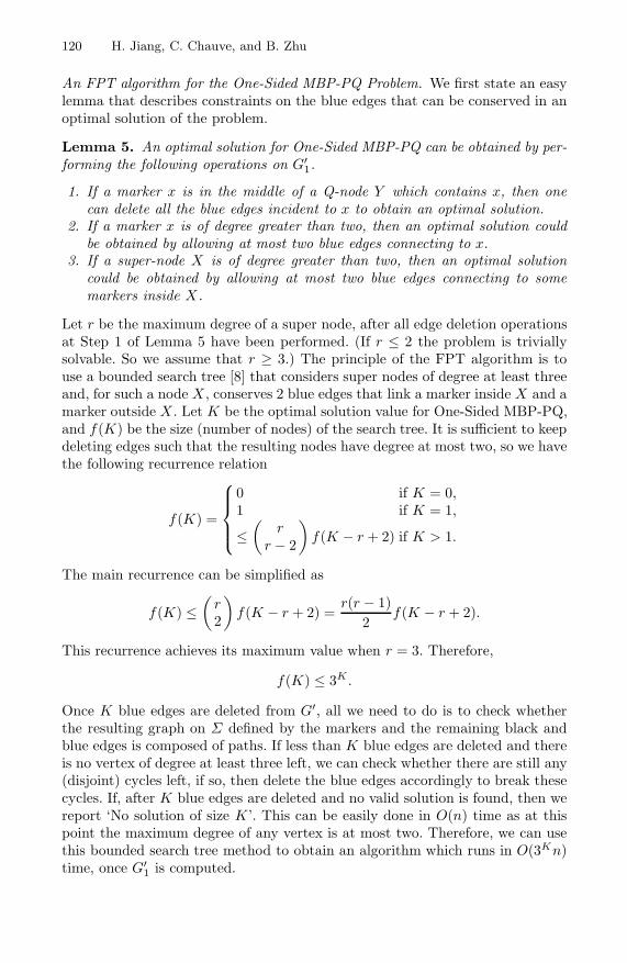
120 H. Jiang, C. Chauve, and B. Zhu
An FPT algorithm for the One-Sided MBP-PQ Problem. We first state an easylemma that describes constraints on the blue edges that can be conserved in anoptimal solution of the problem.
Lemma 5. An optimal solution for One-Sided MBP-PQ can be obtained by per-forming the following operations on G′
1.
1. If a marker x is in the middle of a Q-node Y which contains x, then onecan delete all the blue edges incident to x to obtain an optimal solution.
2. If a marker x is of degree greater than two, then an optimal solution couldbe obtained by allowing at most two blue edges connecting to x.
3. If a super-node X is of degree greater than two, then an optimal solutioncould be obtained by allowing at most two blue edges connecting to somemarkers inside X.
Let r be the maximum degree of a super node, after all edge deletion operationsat Step 1 of Lemma 5 have been performed. (If r ≤ 2 the problem is triviallysolvable. So we assume that r ≥ 3.) The principle of the FPT algorithm is touse a bounded search tree [8] that considers super nodes of degree at least threeand, for such a node X , conserves 2 blue edges that link a marker inside X and amarker outside X . Let K be the optimal solution value for One-Sided MBP-PQ,and f(K) be the size (number of nodes) of the search tree. It is sufficient to keepdeleting edges such that the resulting nodes have degree at most two, so we havethe following recurrence relation
f(K) =
⎧⎪⎪⎨
⎪⎪⎩
0 if K = 0,1 if K = 1,
≤(
rr − 2
)
f(K − r + 2) if K > 1.
The main recurrence can be simplified as
f(K) ≤(
r2
)
f(K − r + 2) =r(r − 1)
2f(K − r + 2).
This recurrence achieves its maximum value when r = 3. Therefore,
f(K) ≤ 3K .
Once K blue edges are deleted from G′, all we need to do is to check whetherthe resulting graph on Σ defined by the markers and the remaining black andblue edges is composed of paths. If less than K blue edges are deleted and thereis no vertex of degree at least three left, we can check whether there are still any(disjoint) cycles left, if so, then delete the blue edges accordingly to break thesecycles. If, after K blue edges are deleted and no valid solution is found, then wereport ‘No solution of size K’. This can be easily done in O(n) time as at thispoint the maximum degree of any vertex is at most two. Therefore, we can usethis bounded search tree method to obtain an algorithm which runs in O(3Kn)time, once G′
1 is computed.

Breakpoint Distance and PQ-Trees 121
abc defxy
T1
a − b − c x − y d − e − fG’
(A)
(B)
s 2 = xyfabcde
1
Fig. 4. An example for the FPT algorithm for One-Sided MBP-PQ
In Figure 4, we show a simple example for the algorithm. An example of T1 ands2 is illustrated in Figure 4 (A). The augmented graph G′
1 is shown in Figure 4 (B).The optimal solution value is K = 1. According to the algorithm, we will have todelete one blue (or dashed) edge in G′
1. The algorithm has the choice of deletingeither (a, f), (y, f), or (c, d). Clearly, deleting (a, f) gives us the optimal solutionwith s1 = abcdefyx and exactly one breakpoint between s1 and s2 = xyfabcde.Deleting (y, f) or (c, d) alone both leads to infeasible solutions.
Theorem 2. One-Sided MBP-PQ can be solved in O(3Kn) time foruni-chromosomal signed and unsigned permutations, where n is the number ofmarkers and K is the number of breakpoints in the optimal solution.
Solving the p-MBM-PQ Problem. It is easy to see that p-MBM-PQ can be solvedin O(3Kn) time as well. The idea is to compute the graph G for the input PQ-tree T and then add blue edges from adjacencies in si, for i = 1, . . . , p. Now ablue edge (x, y) is weighted, with the weight corresponding to the total numberof adjacencies xy or yx in si, for i = 1, . . . , p. So such a weight can be an integerin [1,p]. Let this augmented (weighted) graph be G′′. Then the problem is clearlyequivalent to deleting blue edges with a total weights of K ′ ≤ K from G′′ suchthat the resulting graph is composed of paths. If there are K ′′ such paths, thenadjacencies need to be added to transform them into a single path, and arbitraryadjacencies can be used, each contributing p to the breakpoint distance, that isthen K ′ + p(K ′′ − 1). This leads to the following result.
Corollary 2. p-MBM-PQ can be solved in O(3Kn) time for uni-chromosomalsigned and unsigned permutations.
Note that the actual running time of the FPT algorithm we described is in generalmuch faster than O(3Kn) as any adjacency in one of the genomes si that is dis-carded following Lemma 5.(1) increases the breakpoint distance by 1 but is notconsidered in the computation. More formally, if d is the number of edges dis-carded due to Lemma 5.(1), the running time is in fact O(3K−dn). This has beenconfirmed in our initial computational results. We can also immediately apply ouralgorithm to the variant where the median is constrained to contain only adja-cencies that appear in at least one permutation si, which is also NP-hard for theclassical Breakpoint-Median Problem [5]. Indeed, it suffices to forbid deleting blueedges that disconnects the augmented graph, which is obviously connected at first.

122 H. Jiang, C. Chauve, and B. Zhu
Handling multi-chromosomal permutations. We need here to account for twothings: the set of generated permutations is different (larger in fact) and thebreakpoint distance requires to consider common telomeres. To deal with bothof these issues, we add in the augmented graph a vertex W , that representstelomeres, and a blue edge (W, a) for every telomere a in the si’s. Then, a setof blue edges defining a valid permutation implies that, once edges (W, a) arediscarded, the resulting edges comprise of a set of paths. Finally, as commontelomeres contribute to half the weight of common adjacencies in the break-point distance formula, when the bounded search discards a blue edge (W, a), itincreases the distance by 1/2 instead of 1. This proves the following result.
Corollary 3. p-MBM-PQ can be solved in O(32Kn) time for multi-chromosomalsigned and unsigned permutations.
5 Application to Real Datasets
We present here preliminary computational results on some mammalian and yeastgenomes to illustrate the ability of our FPT algorithm to handle real datasets,using a regular Lenovo laptop and C++. Precise data and results are availableat the URL http://www.cs.montana.edu/bhz/PQ-TREE.html. In both cases, wechange a multi-choromosomal genome into a uni-chromosomal signed permuta-tion; as a consequence, we do not compute exactly the breakpoint distance asdefined in [17], as we might create conserved adjacencies and we ignore commontelomeres in the computation of the distance. But these results are presented to il-lustrate the ability of our algorithm to handle datasets with PQ-trees generatinga large number of permutations. The running times are still high (varying fromtwo days to about a week), but they are already better than what the theoreticalresults imply (for the three cases, we have K = 69, 108, and 348).
The mammalian dataset we use is from the following simple phylogenetictree of five species, (((Human,Macaca)I,(Mouse,Rat)II)III,Dog), given in Newickformat, and we are interested in the ancestors of Human and Macaca (node I)and Mouse and Rat (node II). Permutations and PQ-trees at nodes I and II weregenerated using methods as described as in [15]. In this case, n = 689. In thecompanion webpage, we show in detail the dataset and the sequences generatedusing the FPT algorithm for 2-MBM-PQ, for node I and node II. For node I, wefound that the optimal breakpoint distance is 69, and for node II, the optimaldistance is larger, at 108. Notice that these solutions are not unique (in fact inboth cases there are about 10! permutations which minimizes db(s, s1)+db(s, s2),due to that the roots of the trees are both P-nodes). So an exhaustive searchwould not work to generate an optimal permutation for node III.
The yeast data is from [13], the PQ-tree has a root which is a Q-node with 34children (which are all Q-nodes or leaves). Among these 34 children, 8 of themare leaves. We found an optimal distance of 348. If we wanted to enumerate allgenerated permutations, we would have to try 226 different permutations.

Breakpoint Distance and PQ-Trees 123
6 Conclusion
In this paper, we make the first step in comparing the similarity of PQ-trees, withapplication to comparative genomics. While the general problem is NP-complete(not a surprise!), we show that several interesting cases, that are relevant froman applied point of view, are in FPT, parameterized by the optimal breakpointdistance. We also present some preliminary computational results.
Our first open question is how to construct a general graph or hypergraphincorporating all the information regarding two PQ-trees T1 and T2. Withoutsuch a (hyper?) graph, it seems difficult to design approximation and FPT algo-rithms for the optimization version of MBP-PQ (and possibly some other waysto compare the similarity of T1 and T2). A related question would be to find anFPT algorithm for MBP-PQ whose parameter is the breakpoint distance. Whenthis distance is zero, the problem is in fact easy to solve: it is easy to decide ifT1 and T2 can generate the same permutation [4,2].
How to improve the efficiency of the FPT algorithms for One-Sided MBP-PQand p-MBM-PQ also makes interesting questions. The only other FPT algorithmfor a breakpoint median problem, described in [11], has complexity O(2.15Kn),and it remains to see how the ideas used in that algorithm can be translated tothe case where the median is constrained to be generated by a given PQ-tree.
Regarding p-MBM-PQ, it is recently proved in [17] that the Breakpoint Me-dian Problem for signed multi-chromosomal genomes is tractable if the medianis allowed to have circular chromosomes; it can indeed be solved by a simplemaximum weight matching algorithm. In the case of the p-MBM-PQ, the cor-responding problem would allow that, in the median, the leaves of one or moresubtree rooted at children of the root form a circular chromosome. The com-plexity of this problem is open.
Finally, what if we consider the problems under other distances such as theDCJ (Double-Cut-and-Join) distance? Intuitively, we can expect that such prob-lems are hard too. For example, comparing two PQ-trees of height 2 (every pathbetween a leaf and the root contains at most two edges) whose internal nodesare all P-nodes is equivalent to computing the syntenic distance [9] between twogenomes represented by the gene content of their chromosomes and with no geneorder information, which is NP-hard [7].
Acknowledgments
This research is partially supported by NSF grant DMS-0918034, by NSF ofChina under grant 60928006, and by NSERC Discovery Grant 249834-2006.
References
1. Alizadeh, F., Karp, R., Weisser, D., Zweig, G.: Physical mapping of chromosomesusing unique probes. J. Comp. Biol. 2, 159–184 (1995)
2. Bergeron, A., Blanchette, M., Chateau, A., Chauve, C.: Reconstructing ancestralgene orders using conserved intervals. In: Jonassen, I., Kim, J. (eds.) WABI 2004.LNCS (LNBI), vol. 3240, pp. 14–25. Springer, Heidelberg (2004)

124 H. Jiang, C. Chauve, and B. Zhu
3. Blin, G., Blais, E., Guillon, P., Blanchette, M., ElMabrouk, N.: Inferring Gene Or-ders from Gene Maps Using the Breakpoint Distance. In: Bourque, G., El-Mabrouk,N. (eds.) RECOMB-CG 2006. LNCS (LNBI), vol. 4205, pp. 99–102. Springer,Heidelberg (2006)
4. Booth, K., Lueker, G.: Testing for the consecutive ones property, interval graphs,and graph planarity using PQ-tree algorithms. J. Computer and System Sci-ences 13, 335–379 (1976)
5. Bryant, D.: The complexity of the breakpoint median problem. Technical Re-port CRM-2579. Centre de Recherches en Mathematiques, Universite de Montreal(1998)
6. Chauve, C., Tannier, E.: A methodological framework for the reconstruction ofcontiguous regions of ancestral genomes and its application to mammalian genome.PLoS Comput. 4:e1000234 (2008)
7. DasGupta, B., Jiang, T., Kannan, S., Li, M., Sweedyk, E.: On the Complexity andApproximation of Syntenic Distance. Discrete Appl. Math. 88(1–3), 59–82 (1998)
8. Downey, R., Fellows, M.: Parameterized Complexity. Springer, Heidelberg (1999)9. Feretti, V., Nadeau, J.H., Sankoff, D.: Original synteny. In: Hirschberg, D.S.,
Meyers, G. (eds.) CPM 1996. LNCS, vol. 1075, pp. 159–167. Springer, Heidelberg(1996)
10. Fu, Z., Jiang, T.: Computing the breaking distance between partially orderedgenomes. In: APBC 2007, pp. 237–246 (2007)
11. Gramm, J., Niedermeier, R.: Breakpoint medians and breakpoint phylogenies: Afixed-parameter approach. Bioinformatics 18(Suppl. 2), S128–S139 (2002)
12. Hannenhalli, S., Pevzner, P.: Transforming cabbage into turnip: polynomial algo-rithm for sorting signed permutations by reversals. J. ACM 46(1), 1–27 (1999)
13. Jean, G., Sherman, D.M., Nikolski, M.: Mining the semantic of genome super-blocksto infer ancestral architectures. J. Comp. Biol. 16(9), 1267–1284 (2009)
14. Landau, G., Parida, L., Weimann, O.: Gene proximity analysis across wholegenomes via PQ-trees. J. Comp. Biol. 12, 1289–1306 (2005)
15. Ouangraoua, A., McPherson, A., Tannier, E., Chauve, C.: Insight into the struc-tural evolution of amniote genomes. In: Preliminary version in Cold Spring HarborLaboratory Genome Informatics Meeting 2009, poster 137 (2009)
16. Pe’er, I., Shamir, R.: The median problems for breakpoints are NP-complete. Elec.Colloq. Comput. Complexity, TR-98-071 (1998)
17. Tannier, E., Zheng, C., Sankoff, D.: Multichromosomal median and halving prob-lems under different genomic distances. BMC Bioinformatics 10, 120 (2009)
18. Zheng, C., Lennert, A., Sankoff, D.: Reversal distance for partially orderedgenomes. Bioinformatics 21(Suppl. 1), i502–i508 (2005)

On the Parameterized Complexity of Some OptimizationProblems Related to Multiple-Interval Graphs�
Minghui Jiang
Department of Computer Science, Utah State University, Logan, UT 84322, [email protected]
Abstract. We show that for any constant t ≥ 2, k-INDEPENDENT SET andk-DOMINATING SET in t-track interval graphs are W[1]-hard. This settles anopen question recently raised by Fellows, Hermelin, Rosamond, and Vialette. Wealso give an FPT algorithm for k-CLIQUE in t-interval graphs, parameterizedby both k and t, with running time max{tO(k), 2O(k log k)} · poly(n), where nis the number of vertices in the graph. This slightly improves the previous FPTalgorithm by Fellows, Hermelin, Rosamond, and Vialette. Finally, we use theW[1]-hardness of k-INDEPENDENT SET in t-track interval graphs to obtain thefirst parameterized intractability result for a recent bioinformatics problem calledMAXIMAL STRIP RECOVERY (MSR). We show that MSR-d is W[1]-hard forany constant d ≥ 4 when the parameter is either the total length of the strips, orthe total number of adjacencies in the strips, or the number of strips in the optimalsolution.
1 Introduction
The intersection graph Ω(F) of a family of sets F = {S1, . . . , Sn} is the graph withF as the vertex set and with two different vertices Si and Sj adjacent if and only ifSi ∩ Sj �= ∅. The family F is called a representation of the graph Ω(F).
Let t be an integer at least two. A t-interval is the union of t disjoint intervals inthe real line. A t-track interval is the union of t disjoint intervals in t disjoint parallellines called tracks, one interval on each track. A t-interval graph is the intersectiongraph of a family of t-intervals. A t-track interval graph is the intersection graph of afamily of t-track intervals. If all intervals in the representation of a t-interval graph haveunit lengths, then the graph is called a unit t-interval graph. Similarly for unit t-trackinterval graphs.
As generalizations of the ubiquitous interval graphs, multiple-interval graphs suchas t-interval graphs and t-track interval graphs have wide applications, tradition-ally to scheduling and resource allocation [3,5], and more recently to bioinformat-ics [17,2,19,7,14,1]. In particular, 2-interval graphs and 2-track interval graphs arenatural models for the similar regions of DNA sequences [17,2,1] and for the helices ofRNA secondary structures [19,7,14].
Fellows, Hermelin, Rosamond, and Vialette [9] recently initiated the study of theparameterized complexity of multiple-interval graph problems. In general graphs, the
� Supported in part by NSF grant DBI-0743670.
A. Amir and L. Parida (Eds.): CPM 2010, LNCS 6129, pp. 125–137, 2010.c© Springer-Verlag Berlin Heidelberg 2010

126 M. Jiang
three classical optimization problem k-VERTEX COVER, k-INDEPENDENT SET, and k-DOMINATING SET, parameterized by the optimal solution size k, are exemplary prob-lems in parameterized complexity theory [8]: it is well-known that k-VERTEX COVER
is in FPT, k-INDEPENDENT SET is W[1]-hard, and k-DOMINATING SET is W[2]-hard.Since t-interval graphs are a special class of graphs, all FPT algorithms for k-VERTEX
COVER in general graphs immediately carry over to t-interval graphs. On the otherhand, the parameterized complexity of k-INDEPENDENT SET in t-interval graphs isnot at all obvious. Indeed, in general graphs, k-INDEPENDENT SET and k-CLIQUE areessentially the same problem, but in t-interval graphs, they manifest different parame-terized complexities. Fellows et al. [9] showed that k-INDEPENDENT SET in t-intervalgraphs is W[1]-hard for any constant t ≥ 2, then, in sharp contrast, gave an FPT algo-rithm for k-CLIQUE in t-interval graphs parameterized by both k and t. Similarly, theparameterized complexity of k-DOMINATING SET in t-interval graphs is not obviouseither. Fellows et al. [9] showed that k-DOMINATING SET in t-interval graphs is alsoW[1]-hard for any constant t ≥ 2.
At the end of their paper, Fellows et al. [9] raised three open questions. First,are k-INDEPENDENT SET and k-DOMINATING SET in 2-track interval graphs W[1]-hard? Second, is k-DOMINATING SET in t-interval graphs W[2]-hard? Third, can theparametric time-bound of their FPT algorithm for k-CLIQUE in t-interval graphs beimproved?
The t disjoint tracks for a t-track interval graph can be viewed as t disjoint “host”intervals in the real line for a t-interval graph. Thus the class of t-track interval graphsis contained in the class of t-interval graphs. The containment is proper because thecomplete bipartite graph Kt2+t−1,t+1 is a t-interval graph but not a t-track intervalgraph [21]. It is also known that for any t ≥ 1, t-interval graphs are a proper subclassof (t + 1)-interval graphs, and unit t-interval (resp. unit t-track interval) graphs are aproper subclass of t-interval (resp. t-track interval) graphs; see [18,12,13,10]. Fellowset al. [9] proved that k-INDEPENDENT SET and k-DOMINATING SET in unit 2-intervalgraphs are both W[1]-hard, hence k-INDEPENDENT SET and k-DOMINATING SET int-interval graphs are both W[1]-hard for all t ≥ 2. The main result of this paper isthe following theorem that answers the first open question of Fellows et al. [9] andstrengthens their W[1]-hardness results to encompass even the most basic subclass ofmultiple-interval graphs:
Theorem 1. k-INDEPENDENT SET and k-DOMINATING SET in unit 2-track intervalgraphs are W[1]-hard.
Given a graph G and a vertex-coloring κ : V (G) → {1, 2, . . . , k}, the problemk-MULTICOLORED CLIQUE is that of deciding whether G has a clique of k ver-tices containing exactly one vertex of each color. Fellows et al. [9] proved that k-MULTICOLORED CLIQUE is W[1]-complete, then proved that both k-INDEPENDENT
SET and k-DOMINATING SET in unit 2-interval graphs are W[1]-hard by FPT reduc-tions from k-MULTICOLORED CLIQUE. Our proof of Theorem 1 follows the samestrategy. We note that this k-MULTICOLORED CLIQUE technique [9] is quickly be-coming a standard tool for FPT reductions. We are unable to answer the second openquestion of Fellows et al. [9] on the possible W[2]-hardness of k-DOMINATING SET in

Parameterized Complexity of Problems Related to Multiple-Interval Graphs 127
t-interval graphs, but believe that any new techniques developed for this problem wouldalso have far-reaching influence in parameterized complexity theory.
Let’s move on to the third open question. Fellows et al. [9] presented an FPT algo-rithm for k-CLIQUE in t-interval graphs parameterized by both k and t. They estimatedthat the running time of their algorithm is tO(k log k) · poly(n), where n is the numberof vertices in the graph, and asked whether the parametric time-bound of tO(k log k) canbe improved. Our next theorem makes some small progress on this open question:
Theorem 2. For any constant c ≥ 3, there is an algorithm for k-CLIQUE in t-intervalgraphs with running time O(tck) · O(nc) if k ≤ 1
4 · n1−1/c, where n is the numberof vertices in the graph. In particular, there is an FPT algorithm for k-CLIQUE in t-interval graphs with running time max{tO(k), 2O(k log k)} · poly(n).
Finally, we extend the W[1]-hardness results in Theorem 1 to a bioinformaticsproblem. In comparative genomic, the first step of sequence analysis is usually to de-compose two or more genomes into syntenic blocks that are segments of homologouschromosomes. For the reliable recovery of syntenic blocks, noise and ambiguities in thegenomic maps need to be removed first. A genomic map is a sequence of gene mark-ers. A gene marker appears in a genomic map in either positive or negative orientation.Given d genomic maps as signed sequences of gene markers, MAXIMAL STRIP RE-COVERY (MSR-d) [22,6] is the problem of finding d subsequences, one subsequenceof each genomic map, such that the total length � of the strips in these subsequences ismaximized. Here a strip is a maximal string of at least two markers such that either thestring itself or its signed reversal appears contiguously as a substring in each of the dsubsequences in the solution. Without loss of generality, we can assume that all markersappear in positive orientation in the first genomic map, as in [22,15]. For example, thetwo genomic maps (the markers in negative orientation are underlined)
1 2 3 4 5 6 7 8 9 10 11 128 5 7 6 4 1 3 2 12 11 10 9
have two subsequences
1 3 6 7 8 10 11 128 7 6 1 3 12 11 10
of the maximum total strip length 8. The strip 〈1, 3〉 is positive and forward in bothsubsequences; the other two strips 〈6, 7, 8〉 and 〈10, 11, 12〉 are positive and forward inthe first subsequence, but are negative and backward in the second subsequence. Thefour markers 2, 4, 5, 9 are deleted. Intuitively, the strips are syntenic blocks, and thedeleted markers are noise and ambiguities in the genomic maps.
A strip of length l ≥ 2 has exactly l−1 adjacencies between consecutive markers. Ingeneral, m strips of total length l have l−m adjacencies. Besides the total strip length,the total number of adjacencies in the strips is also a natural objective function of MSR-d. For both objective functions, it is known that MSR-d is APX-hard for any d ≥ 2 [15],and moreover is NP-hard to approximate within Ω(d/ log d) [16]. On the other hand,for any constant d ≥ 2, MSR-d admits a polynomial-time 2d-approximation [6]. Seealso [20,4] for some related results. Our following theorem gives the first parameterizedintractability result for MSR-d:

128 M. Jiang
Theorem 3. MSR-d for any constant d ≥ 4 is W[1]-hard when the parameter is eitherthe total length of the strips, or the total number of adjacencies in the strips, or thenumber of strips in the optimal solution. This holds even if all gene markers are distinctand appear in positive orientation in each genomic map.
2 k-Independent Set
In this section we show that k-INDEPENDENT SET in unit 2-track interval graphsis W[1]-hard. We first review the previous FPT reduction from k-MULTICOLORED
CLIQUE in general graphs to k-INDEPENDENT SET in unit 2-interval graphs [9], thenshow how to modify it into an FPT reduction from k-MULTICOLORED CLIQUE in gen-eral graphs to k-INDEPENDENT SET in unit 2-track interval graphs.
Previous Reduction. Let (G, κ, k) be an instance of k-MULTICOLORED CLIQUE. Theconstruction consists of k+
(k2
)groups of unit intervals occupying disjoint regions of the
real line. Among the k+(k2
)groups, k groups are vertex gadgets, one for each color, and(
k2
)groups are edge gadgets, one for each pair of distinct colors. The vertex gadgets and
the edge gadgets are then linked together, according to the incidence relation betweenthe vertices and the edges, by the validation gadget. Each vertex gadget selects a vertexof a particular color. Each edge gadget selects an edge of a particular pair of colors. Thevalidation gadget ensures the consistency of the selections.
Vertex selection: For each color i, 1 ≤ i ≤ k, let Vi be the set of vertices with color i.The vertex gadget for the color i consists of a group of intervals that can viewed as atable1 with |Vi| rows and k +1 columns. Each row of the table corresponds to a distinctvertex u ∈ Vi: the first interval and the last interval together form a vertex 2-intervalui; the other intervals, each associated with a distinct color j ∈ {1, . . . , k} \ {c} anddenoted by ui∗j , and are used for validation. The intervals in the table are arranged in aparallelogram formation with slanted columns: the intervals in each row are disjoint; theintervals in each column intersect at a common point; the intervals in lower rows havelarger horizontal offsets such that each interval also intersects all intervals in higherrows in the next column.
Edge selection: For each pair of distinct colors i and j, 1 ≤ i < j ≤ k, let Eij bethe set of edges uv such that u has color i and v has color j. The edge gadget for thepair of colors ij consists of a group of intervals that can viewed as a table with |Eij |rows and 4 columns. Each row of the table corresponds to a distinct edge uv ∈ Eij : thefirst interval and the fourth interval together form an edge 2-interval uivj ; the secondand the third intervals, denoted by uivj and vjui, respectively, are used for validation.Again the intervals in the table are arranged in a parallelogram formation.
Validation: For each edge uv such that u has color i and v has color j, the validationgadget includes two validation 2-intervals←−−uivj and−−→uivj : the 2-interval←−−uivj consists ofthe interval uivj and the interval ui∗j; the 2-interval −−→uivj consists of the interval vjui
1 The table is of course only a visualization device; in reality the intervals in all rows of the tableare in the same line.

Parameterized Complexity of Problems Related to Multiple-Interval Graphs 129
. . .
. . .
. . .
. . .
. . .
. . .
. . .
. . .. . . . . . . . .
. . .. . . . . . . . .
. . .
. . .
. . .
. . .
. . .
ui
uivj
←−−uivj
Fig. 1. Construction for k-INDEPENDENT SET. On the left is a vertex gadget. On the right is anedge gadget. The vertex 2-interval ui selects the vertex u for the color i. The edge 2-interval uivj
selects the edge uv for the pair of colors ij. The validation 2-interval validates the selections.
and the interval vj∗i. Note that each validation 2-interval consists of an interval froman edge gadget and an interval from a vertex gadget.
In summary, the following family F of 2-intervals are constructed:
F ={ui | u ∈ Vi, 1 ≤ i ≤ k
} ∪ {uivj ,
←−−uivj ,−−→uivj | uv ∈ Eij , 1 ≤ i < j ≤ k
}.
Refer to Figure 1 for an example. Now set the parameter k′ = k + 3(k2
). It remains to
show that G has a k-multicolored clique if and only if F has a k′-independent set.For the direct implication, it is easy to verify that if K ⊆ V (G) is a k-multicolored
clique, then the following subset of 2-intervals is a k′-independent set in F :{ui | u ∈ K, i = κ(u)
} ∪ {uivj ,
←−−uivj ,−−→uivj | u, v ∈ K, i = κ(u), j = κ(v)
}.
For the reverse implication, suppose that I is a k′-independent set in F . By construc-tion, I can include at most one vertex 2-interval for each color, and at most one edge2-interval plus at most two validation 2-intervals for each pair of distinct colors. Sincek′ = k + 3
(k2
), I must include exactly one vertex 2-interval for each color, and exactly
one edge 2-interval plus two validation 2-intervals for each pair of distinct colors. It fol-lows that the 2
(k2
)= (k − 1)k validation 2-intervals in I have exactly two intervals in
each edge gadget, and exactly k − 1 intervals in each vertex gadget. Moreover, in eachvertex gadget, the intervals of the vertex 2-interval and the k − 1 validation 2-intervalsin I must be in the same row. Similarly, in each edge gadget, the intervals of the edge2-interval and the two validation 2-intervals in I must be in the same row. Since allintervals in the same row of a vertex gadget are associated with the same vertex, andall intervals in the same row of an edge gadget are associated with the same edge, thevertex selection and the edge selection must be consistent. Thus the k vertex 2-intervalsin I corresponds to a k-multicolored clique in G.
This completes the review of the previous reduction. Before we present the newreduction, let’s pause for a moment and ponder why this reduction works. You mayhave noticed that the central idea behind the construction is essentially a geometricpacking argument. Consider each vertex 2-interval as a container of capacity k − 1,each edge 2-interval as a container of capacity 2, and the validation 2-intervals as itemsto be packed. Then, in order to pack each container to its full capacity, the items in eachcontainer must be arranged in a regular pattern, that is, all intervals in each vertex oredge gadget must be in the same row.

130 M. Jiang
New Reduction. We now modify the previous construction to transform each 2-intervalinto a 2-track interval. Move all vertex gadgets to track 1, and move all edge gadgets totrack 2. Then all validation 2-intervals are immediately transformed into 2-track intervals.It remains to fix the vertex 2-intervals on track 1 and the edge 2-intervals on track 2.
We first fix the vertex 2-intervals on track 1. Consider the vertex gadget for the ver-tices Vi with color i. To fix the vertex 2-intervals in this gadget, we replace each 2-interval ui by two 2-track intervals ui left and ui right as follows:
– On track 1, let the intervals of ui left and ui right be the left and the right intervals,respectively, of ui.
– On track 2, put the intervals of ui left and ui right for all u ∈ Vi in a separate region,and arrange them in a parallelogram formation with |Vi| rows and 2 columns: ui left
in the right column, ui right in the left column. As usual, the intervals are disjoint ineach row and are pairwise intersecting in each column, moreover the columns areslanted such that each interval in the left column intersects all intervals in higherrows in the right column.
Refer to Figure 2 for an illustration of the vertex 2-track intervals on the two tracks.In a similar way (with the roles of track 1 and track 2 reversed), we replace each edge2-interval uivj by two 2-track intervals uivj left and uivj right. Then all 2-interval aretransformed into 2-track intervals. The following family F of 2-track intervals are con-structed:
F ={ui left, ui right | u ∈ Vi, 1 ≤ i ≤ k
}
∪ {uivj left, uivj right,
←−−uivj ,−−→uivj | uv ∈ Eij , 1 ≤ i < j ≤ k
}.
Now set the parameter k′ = 2k + 4(k2
). It remains to show that G has a k-multicolored
clique if and only if F has a k′-independent set.For the direct implication, it is easy to verify that if K ⊆ V (G) is a k-multicolored
clique, then the following subset of 2-track intervals is a k′-independent set in F :
{ui left, ui right | u ∈ K, i = κ(u)
}
∪ {uivj left, uivj right,
←−−uivj ,−−→uivj | u, v ∈ K, i = κ(u), j = κ(v)
}.
track 1 track 2
. . .. . .
. . .. . .. . . . . .
. . .. . . . . .
. . .
. . .
. . .
. . .
. . .
ui leftui left ui rightui right
vi left vi leftvi right vi right
Fig. 2. Transforming vertex 2-intervals into 2-track intervals for k-INDEPENDENT SET

Parameterized Complexity of Problems Related to Multiple-Interval Graphs 131
For the reverse implication, suppose I is a k′-independent set in F . The same argu-ment as before shows that I must include exactly two vertex 2-track intervals for eachcolor, and exactly two edge 2-track intervals plus two validation 2-track intervals foreach pair of distinct colors. Refer back to Figure 2. Let ui left and vi right be the twovertex 2-track intervals in I for some color i. The intersection pattern of the vertex 2-track intervals for Vi on track 2 ensures that the row of u must not be higher than therow of v. Without loss of generality, we can assume that they are in the same row, i.e.,u = v, so that the set of validation intervals in the middle columns on track 1 that aredominated by ui left vi right is minimal (or, in terms of geometric packing, this gives thecontainer ui left vi right the largest capacity on track 1). Thus we can assume that the twovertex 2-track intervals for each color i form a pair ui left ui right for the same vertex u.Similarly, we can assume that the two edge 2-track intervals for each pair of colors ijform a pair uivj left uivj right for the same edge uv. Then the same argument as beforeshows that the k pairs of vertex 2-track intervals in I corresponds to a k-multicoloredclique in G.
3 k-Dominating Set
In this section we show that k-DOMINATING SET in unit 2-track interval graphsis W[1]-hard. We first review the previous FPT reduction from k-MULTICOLORED
CLIQUE in general graphs to k-DOMINATING SET in unit 2-interval graphs [9], thenshow how to modify it into an FPT reduction from k-MULTICOLORED CLIQUE in gen-eral graphs to k-DOMINATING SET in unit 2-track interval graphs.
Previous Reduction. Let (G, κ, k) be an instance of k-MULTICOLORED CLIQUE. Thereduction again constructs k vertex gadgets, one for each color, and
(k2
)edge gadgets,
one for each pair of distinct colors. The vertex gadgets and the edge gadgets are thenlinked together by the validation gadget.
Vertex selection: For each color i, 1 ≤ i ≤ k, let Vi be the set of vertices with colori. The vertex gadget for the color i includes one interval ∗i for the color i and oneinterval ui for each vertex u ∈ Vi. The interval ∗i is combined with each interval ui toform a vertex 2-interval ui. The vertex gadget for Vi also includes two disjoint dummy2-intervals that contain the left and the right endpoints, respectively, of the interval ∗i.Edge selection: For each pair of distinct colors i and j, 1 ≤ i < j ≤ k, let Eij bethe set of edges uv such that u has color i and v has color j. The edge gadget for thepair of colors ij includes a group of intervals that can viewed as a table with |Eij | rowsand 3 columns. Each row of the table corresponds to a distinct edge uv ∈ Eij : the leftinterval and the right interval together form an edge 2-interval uivj ; the middle interval,denoted by uivj , is used for validation. Again the intervals in the table are arranged ina parallelogram formation. The edge gadget for Eij also includes two disjoint dummy2-intervals that intersect the left intervals and the right intervals, respectively, of all edge2-intervals uivj .
Validation: For each edge uv such that u has color i and v has color j, the validationgadget includes two validation 2-intervals←−−uivj and −−→uivj : the 2-interval←−−uivj consists

132 M. Jiang
. . . . . .. . .
. . .
. . .
. . .
. . .
. . .ui uivj
←−−uivj
dummy dummy
dummydummy
Fig. 3. Construction for k-DOMINATING SET. On the left is a vertex gadget. On the right is anedge gadget. The vertex 2-interval ui selects the vertex u for the color i. The edge 2-interval uivj
selects the edge uv for the pair of colors ij. The validation 2-interval validates the selections.
of the interval uivj and the interval ui; the 2-interval −−→uivj consists of the interval uivj
and the interval vj .In summary, the following family F of 2-intervals are constructed:
F ={ui | u ∈ Vi, 1 ≤ i ≤ k
}
∪ {uivj ,
←−−uivj ,−−→uivj | uv ∈ Eij , 1 ≤ i < j ≤ k
} ∪ DUMMIES,
where DUMMIES is the set of 2k+2(k2
)dummy 2-intervals, two in each vertex or edge
gadget. Refer to Figure 3 for an example. Now set the parameter k′ = k+(k2
). It remains
to show that G has a k-multicolored clique if and only if F has a k′-dominating set.For the direct implication, it is easy to verify that if K ⊆ V (G) is a k-multicolored
clique, then the following subset of 2-intervals is a k′-dominating set in F :
{ui | u ∈ K, i = κ(u)
} ∪ {uivj | u, v ∈ K, i = κ(u), j = κ(v)
}.
For the reverse implication, suppose that I is a k′-dominating set in F . Because ev-ery dummy 2-interval can be replaced by an adjacent vertex or edge 2-interval in adominating set, we can assume without loss of generality that I does not include anydummy 2-intervals. Then, to dominate the dummy 2-intervals2, I must include at leastone vertex 2-interval for each color, and at least one edge 2-interval for each pair ofdistinct colors. Since k′ = k +
(k2
), I must include exactly one vertex 2-interval for
each color, and exactly one edge 2-interval for each pair of distinct colors. It followsthat for each pair of distinct colors ij, the two validation 2-intervals←−−uivj and−−→uivj mustbe dominated by the two vertex 2-intervals ui and vj , respectively. Therefore the ver-tex selection and the edge selection are consistent, and the k vertex 2-intervals in Icorresponds to a k-multicolored clique in G.
New Reduction. We now modify the previous construction to transform each 2-intervalinto a 2-track interval. To transform the vertex 2-intervals into 2-track intervals, movethe intervals ui to track 1, and move the intervals ∗i to track 2. Then, to transform
2 We remark that the construction can be simplified by including only one dummy 2-interval foreach vertex or edge gadget. Nevertheless we keep two dummy 2-intervals for each gadget inthis presentation, partly for truthfulness to the original reduction, and partly for conveniencein our new reduction (when we split each edge 2-interval into two 2-track intervals later, wedon’t have to add new dummies).

Parameterized Complexity of Problems Related to Multiple-Interval Graphs 133
the validation 2-intervals into 2-track intervals, move all edge gadgets to track 2. Thedummy 2-intervals can be fixed accordingly. It remains to fix the edge 2-intervals nowon track 2.
Consider the edge gadget for the edges Eij with colors ij. To fix the edge 2-intervalsin this gadget, we replace each 2-interval uivj by two 2-track intervals uivj left anduivj right as follows:
– On track 2, let the intervals of uivj left and uivj right be the left and the right inter-vals, respectively, of uivj .
– On track 1, put the intervals of uivj left and uivj right for all uv ∈ Eij in a sepa-rate region, then arrange them, together with |Eij | additional dummy intervals, in aparallelogram formation with |Eij | rows and 3 columns: ui left in the right column,ui right in the left column, and dummies in the middle column. As usual, the inter-vals are pairwise intersecting in each column, and the columns are slanted. But ineach row the three intervals are not all disjoint: the left interval and the middle inter-val slightly overlap, and are both disjoint from the right interval. Now each intervalin the right column intersects all intervals in lower rows in the middle column, andeach interval in the left column intersects all intervals in the same or higher rowsin the middle column. Finally, each of the |Eij | dummy intervals in the middlecolumn is combined with an isolated dummy interval on track 2 to form a dummy2-track interval.
Refer to Figure 4 for an illustration of the edge 2-track intervals on the two tracks. Thefollowing family F of 2-track intervals are constructed:
F ={ui | u ∈ Vi, 1 ≤ i ≤ k
}
∪ {uivj left, uivj right,
←−−uivj ,−−→uivj | uv ∈ Eij , 1 ≤ i < j ≤ k
} ∪ DUMMIES,
where DUMMIES is the set of 2k+2(k2
)+ |E(G)| dummy 2-track intervals, two in each
vertex or edge gadget as before, and one more for each edge (recall the middle columnof each edge gadget on track 1). Now set the parameter k′ = k + 2
(k2
). It remains to
show that G has a k-multicolored clique if and only if F has a k′-dominating set.
track 1track 2
. . .
. . .. . .
. . .. . .
. . .
. . .
. . .. . . . . .
. . .. . .
duivj left duivj leftduivj right duivj right
dxiyj leftdxiyj left dxiyj rightdxiyj right
Fig. 4. Transforming edge 2-intervals into 2-track intervals for k-DOMINATING SET

134 M. Jiang
For the direct implication, it is easy to verify that if K ⊆ V (G) is a k-multicoloredclique, then the following subset of 2-track intervals is a k′-dominating set in F :
{ui | u ∈ K, i = κ(u)
} ∪ {uivj left, uivj right | u, v ∈ K, i = κ(u), j = κ(v)
}.
For the reverse implication, suppose that I is a k′-dominating set in F . Note that anyone of the (original) two dummy 2-track intervals in each vertex or edge gadget canbe replaced by an adjacent vertex or edge 2-interval in a dominating set. Thus we canassume without loss of generality that I includes none of these 2k + 2
(k2
)dummies.
Then, to dominate these dummies, I must include at least one vertex 2-track intervalfor each color, and at least two edge 2-track intervals for each pair of distinct colors.Since k′ = k + 2
(k2
), I must include exactly one vertex 2-track interval for each color,
and exactly two edge 2-track intervals for each pair of distinct colors. Refer back toFigure 4. Let uivj left and xiyj right be the two edge 2-track intervals in I for some pairof colors ij. The intersection pattern of the edge 2-track intervals for Eij on track 1ensures that, in order to dominate all the (new) dummies in the middle column, the rowof xy must not be higher than the row of uv. Without loss of generality, we can assumethat they are in the same row, i.e., uv = xy, so that the set of validation intervals in themiddle column on track 2 that are dominated by uivj left xiyj right is maximal. Thus thetwo edge 2-track intervals for each pair of colors ij form a pair uivj left uivj right forthe same edge uv. Then the same argument as before shows that the k vertex 2-trackintervals in I corresponds to a k-multicolored clique in G.
4 k-Clique
In this section we prove Theorem 2. Fellows et al. [9] presented the following algorithmCLIQUE(G, k) that decides whether a given t-interval graph G has a k-clique:
CLIQUE(G, k):
1. If |V (G)| < k, then return NO.2. Let v be a vertex of minimum degree in G.3. If deg(v) ≥ 2tk, then return YES.4. If v is in a k-clique of G, then return YES.5. Return CLIQUE(G− v, k).
The crucial step of this algorithm, step 3, is justified by a structural lemma [9,Lemma 2]: “if G is a t-interval graph with no k-cliques then G has a vertex of de-gree less than 2tk.” Step 4 can be implemented in O(k2 · (2tk
k
)) time by brute force;
all other steps have running time polynomial in n. Since the total number of recur-sive calls, in step 5, is at most n, the overall time complexity of the algorithm isO(k2 · (2tk
k
)) · poly(n). Fellows et al. [9] estimated that
O(k2 ·(
2tk
k
)) = tO(k log k), (1)
and asked whether this parametric time-bound can be improved.

Parameterized Complexity of Problems Related to Multiple-Interval Graphs 135
Fellows et al. [9] suggested that “a possible good place to start is to consider theproblem for constant values of t, and to attempt to obtain a parametric time-boundof 2O(k).” This suggestion is little misleading because for constant values of t, thealgorithm CLIQUE(G, k) already attains a parametric time-bound of 2O(k). Note that(2tkk
) ≤ 22tk. Thus if t = O(1) then O(k2 · (2tkk
)) = O(22 log k · 22tk) = 2O(k).
Anyway, can we improve the parametric time-bound of tO(k log k)? We next describesuch an FPT algorithm. Our FPT algorithm has two components. The first componentis the following algorithm CLIQUE*(G, k) slightly modified from CLIQUE(G, k):
CLIQUE*(G, k):
1. If |V (G)| < k, then return NO.2. Let v be a vertex of minimum degree in G.3. If deg(v) ≥ 2tk, then return YES.4. If CLIQUE*(neighbors(v), k − 1) returns YES, then return YES.5. Return CLIQUE*(G− v, k).
Note that CLIQUE*(G, k) is identical to CLIQUE(G, k) except step 4. The follow-ing recurrence on the time bound f(k) · g(n) captures the recursive behavior ofCLIQUE*(G, k):
f(k) · g(n) ≤ f(k − 1) · g(2tk) + f(k) · g(n− 1) + O(n2).
Lemma 1. For any constant c ≥ 3, if k ≤ 14 · n1−1/c, then the running time of
CLIQUE*(G, k) is O(tck) ·O(nc).
The second component of our FPT algorithm is the obvious brute-force algorithm thatenumerates and checks all k-subsets of vertices for k-cliques.
Lemma 2. For any constant c ≥ 3, if k > 14 · n1−1/c, then the running time of the
brute-force algorithm is 2O(k log k).
Finally, for any constant c ≥ 3, by choosing the algorithm CLIQUE*(G, k) when k ≤14 · n1−1/c, and choosing the brute-force algorithm when k > 1
4 · n1−1/c, we obtain anFPT algorithm with a parametric time-bound of
max{tO(k), 2O(k log k)}. (2)
Compare our bound (2) with the previous bound (1). It appears that we have obtainedan improvement3, but asymptotically this improvement is negligible. Check that theestimate in (1) is not tight:
O(k2 ·(
2tk
k
)) = O(k2(2tk)k) = tO(k)2O(k log k)
= max{(tO(k))2, (2O(k log k))2} = max{tO(k), 2O(k log k)}.In light of this delicate distinction, perhaps the open question on k-CLIQUE in t-intervalgraphs [9] could be stated more precisely as follows:
3 Under the condition that k ≤ 14· n1−1/c for some constant c ≥ 3, CLIQUE*(G,k)
clearly improves CLIQUE(G,k): in particular, for t = Θ(log k), the parametric bound ofCLIQUE*(G,k) is 2O(k log log k), and the parametric bound of CLIQUE(G,k) is 2O(k log k).

136 M. Jiang
Question 1. Is there an FPT algorithm for k-CLIQUE in t-interval graphs with a para-metric time-bound of tO(k)?
Note that a parametric time-bound of 2O(k log k) alone is beyond reach. This is becauseevery graph of n vertices is a t-interval graph for t ≥ n/4 [11]. If the parameter tdoes not appear in the bound, then we would have an FPT algorithm for the W[1]-hardproblem of k-CLIQUE in general graphs.
5 Maximal Strip Recovery
In this section we prove Theorem 3. Let �-MSR-d be the problem MSR-d parameterizedby the total length � of the strips in the optimal solution. We first prove that �-MSR-4 isW[1]-hard by an FPT-reduction from k-INDEPENDENT SET in 2-track interval graphs.
Let (F , k) be an instance of k-INDEPENDENT SET in 2-track interval graphs, whereF = {I1, . . . , In} is a set of n 2-track intervals. We construct four genomic maps
G→, G←, G1, G2, where each map is a permutation of 2n distinct markersi⊂ and
i⊃,1 ≤ i ≤ n, all in positive orientation. G→ and G← are concatenations of the n pairs ofmarkers with ascending and descending indices, respectively:
G→ :1⊂ 1⊃ · · · n⊂ n⊃
G← :n⊂ n⊃ · · · 1⊂ 1⊃
To construct G1 and G2, we first modify the representation of the 2-track interval graphfor F until the 2n endpoints of the n intervals on each track are all distinct. This canbe done in polynomial time by a standard procedure for interval graphs. Then, on eachtrack, mark the left and the right endpoints of the interval for Ii by the left and the right
markersi⊂ and
i⊃, respectively. Thus we obtain two sequences of markers for the twogenomic maps G1 and G2. This completes the construction.
Now set the parameter � = 2k. By the following two observations, it is easy to checkthat F has a k-independent set if and only G→, G←, G1, G2 have four subsequences oftotal strip length �:
1. G→ and G← ensure that each strip must be a pair of markers.2. G1 and G2 encode the intersection pattern of the 2-track intervals.
Therefore �-MSR-d is W[1]-hard.Since the length of each strip is exactly 2 in our construction, the total number of
adjacencies in the strips and the number of strips are both equal to half the total striplength. Therefore MSR-d remains W[1]-hard when the parameter is changed to eitherthe total number of adjacencies in the strips or the number of strips. For any two con-stants d and d′ such that d′ > d ≥ 2, the problem MSR-d is a special case of theproblem MSR-d′ with d′ − d redundant genomic maps. Thus the W[1]-hardness ofMSR-4 implies the W[1]-hardness of MSR-d for all constants d ≥ 4.

Parameterized Complexity of Problems Related to Multiple-Interval Graphs 137
References
1. Alcon, L., Cerioli, M.R., de Figueiredo, C.M.H., Gutierrez, M., Meidanis, J.: Tree loopgraphs. Discrete Applied Mathematics 155, 686–694 (2007)
2. Bafna, V., Narayanan, B., Ravi, R.: Nonoverlapping local alignments (weighted independentsets of axis-parallel rectangles). Discrete Applied Mathematics 71, 41–53 (1996)
3. Bar-Yehuda, R., Halldorsson, M.M., Naor, J(S.), Shachnai, H., Shapira, I.: Scheduling splitintervals. SIAM Journal on Computing 36, 1–15 (2006)
4. Bulteau, L., Fertin, G., Rusu, I.: Maximal strip recovery problem with gaps: hardness andapproximation algorithms. In: Dong, Y., Du, D.-Z., Ibarra, O. (eds.) ISAAC 2009. LNCS,vol. 5878, pp. 710–719. Springer, Heidelberg (2009)
5. Butman, A., Hermelin, D., Lewenstein, M., Rawitz, D.: Optimization problems in multiple-interval graphs. In: Proceedings of the 18th Annual ACM-SIAM Symposium on DiscreteAlgorithms (SODA 2007), pp. 268–277 (2007)
6. Chen, Z., Fu, B., Jiang, M., Zhu, B.: On recovering syntenic blocks from comparative maps.Journal of Combinatorial Optimization 18, 307–318 (2009)
7. Crochemore, M., Hermelin, D., Landau, G.M., Rawitz, D., Vialette, S.: Approximating the2-interval pattern problem. Theoretical Computer Science 395, 283–297 (2008)
8. Downey, R.G., Fellows, M.R.: Parameterized Complexity. Springer, Heidelberg (1998)9. Fellows, M.R., Hermelin, D., Rosamond, F., Vialette, S.: On the parameterized complexity
of multiple-interval graph problems. Theoretical Computer Science 410, 53–61 (2009)10. Gambette, P., Vialette, S.: On restrictions of balanced 2-interval graphs. In: Brandstadt, A.,
Kratsch, D., Muller, H. (eds.) WG 2007. LNCS, vol. 4769, pp. 55–65. Springer, Heidelberg(2007)
11. Griggs, J.R.: Extremal values of the interval number of a graph, II. Discrete Mathematics 28,37–47 (1979)
12. Griggs, J.R., West, D.B.: Extremal values of the interval number of a graph. SIAM Journalon Algebraic and Discrete Methods 1, 1–7 (1980)
13. Gyarfas, A., West, D.B.: Multitrack interval graphs. Congressus Numerantium 109, 109–116(1995)
14. Jiang, M.: Approximation algorithms for predicting RNA secondary structures with arbi-trary pseudoknots. IEEE/ACM Transactions on Computational Biology and Bioinformatics,doi:10.1109/TCBB.2008.109 (to appear)
15. Jiang, M.: Inapproximability of maximal strip recovery. In: Dong, Y., Du, D.-Z., Ibarra, O.(eds.) ISAAC 2009. LNCS, vol. 5878, pp. 616–625. Springer, Heidelberg (2009)
16. Jiang, M.: Inapproximability of maximal strip recovery: II (Submitted)17. Joseph, D., Meidanis, J., Tiwari, P.: Determining DNA sequence similarity using maximum
independent set algorithms for interval graphs. In: Nurmi, O., Ukkonen, E. (eds.) SWAT1992. LNCS, vol. 621, pp. 326–337. Springer, Heidelberg (1992)
18. Trotter Jr., W.T., Harary, F.: On double and multiple interval graphs. Journal of Graph The-ory 3, 205–211 (1979)
19. Vialette, S.: On the computational complexity of 2-interval pattern matching problems. The-oretical Computer Science 312, 223–249 (2004)
20. Wang, L., Zhu, B.: On the tractability of maximal strip recovery. In: Proceedings of the 6thAnnual Conference on Theory and Applications of Models of Computation (TAMC 2009),pp. 400–409 (2009)
21. West, D.B., Shmoys, D.B.: Recognizing graphs with fixed interval number is NP-complete.Discrete Applied Mathematics 8, 295–305 (1984)
22. Zheng, C., Zhu, Q., Sankoff, D.: Removing noise and ambiguities from comparative maps inrearrangement analysis. IEEE/ACM Transactions on Computational Biology and Bioinfor-matics 4, 515–522 (2007)

Succinct Representations of Separable Graphs
Guy E. Blelloch1 and Arash Farzan2
1 Computer Science Department, Carnegie Mellon University2 Max-Planck-Institut fur Informatik, 66123 Saarbrucken, Germany
[email protected], [email protected]
Abstract. We consider the problem of highly space-efficient represen-tation of separable graphs while supporting queries in constant time inthe RAM with logarithmic word size. In particular, we show constant-time support for adjacency, degree and neighborhood queries. For anymonotone class of separable graphs, the storage requirement of the rep-resentation is optimal to within lower order terms.
Separable graphs are those that admit a O(nc)-separator theoremwhere c < 1. Many graphs that arise in practice are indeed separable.For instance, graphs with a bounded genus are separable. In particular,planar graphs (genus 0) are separable and our scheme gives the firstsuccinct representation of planar graphs with a storage requirement thatmatches the information-theory minimum to within lower order termswith constant time support for the queries.
We, furthers, show that we can also modify the scheme to succinctlyrepresent the combinatorial planar embedding of planar graphs (andhence encode planar maps).
1 Introduction
Many applications use graphs to model connectivity information and relationshipbetween different objects. As the size of these graphs grow, the space efficiencybecomes increasingly important. The structural connectivity of the Web modeledas the Web graph is an example which presently contains billions of vertices andthe number is growing [1]. As a result, compact representation of such graphsfor use in various algorithms has been in interest [2,3,4,5]. Planar (and almostplanar) graphs which capture various structural artifacts such as road networks,form another example of graphs whose space-efficient representation is crucialdue to their massive size. For all these applications, it is desirable to represent thegraph compactly and be able to answer dynamic queries on the graph quickly.
A succinct representation of a combinatorial object is a compact representa-tion of that object such that its storage requirement matches the information-theoretic space lower bound to within lower order terms, and it supports areasonable set of queries in constant time. Succinct data structures performunder the uniform-cost word RAM-model with Θ (lg n) word size [6]1. Hence,the main distinction between succinct and compact representations of an object1 lg n denotes log2 n.
A. Amir and L. Parida (Eds.): CPM 2010, LNCS 6129, pp. 138–150, 2010.c© Springer-Verlag Berlin Heidelberg 2010

Succinct Representations of Separable Graphs 139
is that unlike compact representations, the storage requirement of a succinct rep-resentation cannot be a constant factor away from the optimal and moreover,queries must perform in constant time.
Unstructured graphs are highly incompressible (see section 1.1). Fortunatelyhowever, most types of graph that arise in practice have some structural prop-erties. A most common structural property that graphs in practice have is thatthey have small separators. A graph has small separators if its induced subgraphscan be partitioned into two parts of roughly the same size by removing a smallnumber of vertices (to be defined precisely in section 2). Planar graphs (suchas 2-dimensional meshes), almost planar graphs (such as road networks, distri-bution networks) [7,8], and most 3-dimensional meshes [9] have indeed smallseparators.
In this paper, we study the problem of succinct representations of separa-ble undirected and unlabeled graphs (as defined precisely in definition 1). Wepresent a succinct representation with a storage requirement which achievesthe information-theoretic bound to within lower order terms and show constanttime support for the following set of queries: adjacency queries, neighborhoodqueries, and degree queries. Adjacency queries on a pair of vertices x, y de-termines whether (x, y) is an edge. Neighborhood queries iterate through theneighbors of a given vertex x. Finally, the degree query outputs the number ofincident edges to a given vertex x. A representation that supports these queriesin constant time has the functionality of both an adjacency list and an adjacencymatrix at the same time.
Analogous to Fredrickson’s partitioning scheme for planar graphs [8], our suc-cinct representation is based on recursive decomposition of graphs into smallergraphs. We repeatedly separate the given graph into smaller graphs to obtainsmall graphs of poly-logarithmic size which we refer to as by mini-graphs. Thesemini-graphs are further separated into yet smaller graphs of sub-logarithmic sizewhich we refer to as by micro-graphs. Micro-graphs have small enough sizesto be catalogued and listed in a look-up table. Micro-graphs are encoded bya reference to within the look-up table. At each step that a graph is repeat-edly split into two smaller subgraphs, the vertices in the separator are copiedinto both subgraphs. Therefore there are duplicate vertices in mini-graphs andmicro-graphs. The main difficulty is to be able to represent the correspondencebetween duplicate vertices and the original graph vertices.
The time to construct the representation is dominated by the time neededto recursively decompose the graph into mini-graphs and micro-graphs and alsoby the time needed to assemble the look-up table for micro-graphs. The timefor finding the separators and decomposing the graph recursively varies signif-icantly from a family of graphs to another. For instance, there are linear timealgorithms for finding separators in planar graphs and well-shaped meshes in ar-bitrary dimensions [7,9]. For our purposes a poly-logarithmic approximation ofthe separator size suffices and therefore we use Leighton-Rao’s polynomial timeconstruction [10]. The time required to assemble the look-up table depends onthe maximum size of micro-trees, since we need to exhaustively list all separable

140 G.E. Blelloch and A. Farzan
graphs modulo their isomorphism up to that size. We have a large degree offreedom on the choice of maximum size of a micro-graph, choice of
√lg n
lg lg nas
the maximum micro-graph size ensures a sub-linear look-up table constructiontime. Albeit, for simplicity of presentation of this paper, we will use lg n
lg lg n as themaximum micro-graph size.
1.1 Related Work
As mentioned previously, unstructured graphs are highly incompressible. A sim-ple counting argument shows that a random graph with n vertices and m edgesrequires
⌈lg
((n2)m
)⌉bits. Blandford et al. [11] achieves this bound within a con-
stant multiplicative factor for sparse graphs. Raman et al. [12] give a repre-sentation with a storage requirement which is roughly twice the informationtheory minimum and supports adjacency and neighborhood queries in constanttime. Farzan and Munro [13] prove the infeasibility of achieving the information-theoretic space lower bound to within lower order terms and constant-time querysupport. and give a representation with a storage requirement that is a factor of1 + ε away from the minimum (for any constant ε > 0).
Hence, space efficient representations of graphs with a certain combinato-rial structure has been of interest: e.g. bounded-genus graphs [14], graphs withlimited arboricity, and c-decomposable graphs [15]. A strong line of researchhas been on compressing planar graphs. Given a planar graph with n vertices,Turan [16] gives a O(n)-bit representation. Keeler and Westbrook [17] improvethe space by a constant factor. He et al. [18] improve the first order term ofspace to the information-theory minimum. However, none of these consider fastsupport for queries.
Jacobson [19] gives a linear-space representation for planar graphs which sup-ports adjacency queries in logarithmic time. Munro and Raman [20] gives alinear-space encoding for planar graphs in which supports queries in constanttime. Chuang et al. [21] and subsequently Chiang et al. [22] improve the con-stant on the high order term for space. There is a vast literature on encodingsubfamilies of planar graphs. Two important subfamilies are tri-connected planargraphs and triangulated planar graphs for which in a culminating work CastelliAleardi et al. [23] show a succinct representation. This representation, used forgeneral planar graphs, has a storage requirement which is a constant factor awayfrom the optimal (and therefore is not succinct).
One important aspect in representing planar graphs has been to also representthe associated planar embedding together with the graph (i.e. to represent planarmaps). We demonstrate our scheme yields a succinct representation for bothgeneral planar graphs and planar maps.
Blandford et al. [11] study space-efficient representations of separable graphswith constant time support for adjacency, degree, and neighborhood queries.However their representation is not succinct and can have a storage which is amultiplicative factor away from the optimal. We present a succinct representationfor separable graphs that supports the same set of queries in constant time.

Succinct Representations of Separable Graphs 141
2 Preliminaries
A separator S in a graph G = (V, E) with n vertices is a set of vertices thatdivides V into non-empty parts A ⊂ V and B ⊂ V such that {A, S, B} is apartition of V , and no edge in G joins a vertex in A to a vertex in B.
Definition 1. A family of graphs G that is closed under taking the vertex-induced subgraphs satisfies the f(.)-separator theorem [7] if there are constantsα < 1 and β > 0 such that each member graph G ∈ G with n vertices has aseparator S of size |S| < βf(n) which divides the vertices into parts A, B eachof which contains at most αn vertices (|A| ≤ αn, |B| ≤ αn). We define a familyof graphs as separable if it satisfies the nc-separator theorem for some constantc < 1. A graph is separable if it belongs to a separable family of graphs.
Lipton, Rose, and Tarjan [24] prove that a in family of graphs satisfying a(n/(log n)1+ε
)-separator theorem for some ε > 0, the number of edges of a graph
is linear in the number of vertices. Since separable graphs satisfy a stronger sep-arator theorem, a separable graph has linear number of edges.
We use the dictionary data structures heavily in this work. The first datastructure we need in our tool set is an indexable dictionary (ID) to represent asubset of a universe supporting membership, rank, and select queries on memberelements in constant time. A membership query on a given element X determineswhether x is present in the subset. A rank query on an element x reports thenumber of present elements less than x in the subset. Finally, a select query(which are reverse to rank queries) for a given number i reports element at ranki in the increasing order in the subset.
Lemma 1 ([12]). Given a set S of size s which is a subset of a universe U ={1, . . . , u}, there is an indexable dictionary (ID) on S that requires lg
(us
)+
o (s) + O (log log u) bits and supports rank/select on elements of S in constanttime (rank/select on non-members is not supported).
Unlike IDs, fully indexable dictionaries (FID) support membership, rank, andselect queries on both members and non-members. These are very powerful struc-tures, as they can support predecessor queries in constant time. As a result, theyare not as space-efficient as IDs.
Lemma 2 ([12]). Given a subset S of a universe U , there is a fully indexabledictionary (FID) structure which requires lg
(|U||S|
)+ O (|U | log log |U | / log |U |)
bits and supports rank and select queries both on members and nonmembers ofS in constant time.
3 Succinct Representation
Analogous to the compact representation of separable graphs [11], we find andremove separators recursively to decompose the graph. Given a graph G withn vertices, we find a small separator S (|S| < βnc) whose removal divides G

142 G.E. Blelloch and A. Farzan
A B
A B
S
G
S S
G1G2
Fig. 1. Decomposition of a separablegraph G into G1, G2
The Original Graph
Mini graph Mini graph Mini graph Mini graph
Micro graphs
Fig. 2. A schematic view of the decompo-sition of a separable graph to mini-graphsand then to micro-graphs
into two parts A, B with at most αn vertices each. We obtain two inducedsubgraphs G1 = A∪ S and G2 = B ∪S. We remove internal edges of S from G1
(and retain them in G2). Therefore, we obtain two subgraphs G1, G2 from G.Figure 1 illustrates the decomposition of an example graph G into G1 and G2.
We decompose G1 and G2 to obtain smaller subgraphs. Smaller subgraphsare in turn decomposed similarly into yet smaller subgraphs. We define a con-stant δ = 2/(1 − c) where there are nc-separators (definition 1). We repeat theseparator-based decomposition till the subgraphs have at most (lg n)δ verticeswhere n is the number of vertices in the initial graph. We refer to these subgraphswith at most (lg n)δ vertices as mini-graphs.
Mini-graphs are further decomposed in the same fashion. Each mini-graphis decomposed repeatedly until the number of vertices in subgraphs is at mostlg n/ lg lg n. We refer to these subgraphs with at most lg n/ lg lg n vertices asmicro-graphs. Figure 2 illustrates the decomposition into mini and micro graphs.
The graph representation consists of the representations of mini-graphs whichin turn consist of the representations of micro-graphs. Micro-graphs are smallenough to be catalogued by a look-up table. Vertices in separators are dupli-cated by each iteration of the decomposition and therefore there can be manyoccurrences of a single vertex of the original graph across different mini-graphsand/or micro-graphs.
Each occurrence of a vertex receives three labels: a label within the containingmicro-graph which we refer to as by micro-graph label, a label within the con-taining mini-graph which we refer to as by mini-graph label, and finally a labelin the entire graph which we refer to as by graph label and is visible from out-side our abstract data type for the graph. Queries indicate vertices using theirgraph labels. Dictionary structures of lemmas 1 and 2 are used to maintain therelationship between duplicates of a single vertex.

Succinct Representations of Separable Graphs 143
Combining representations of mini-graphs. We assume mini-graphs are encoded(using a scheme to be discussed shortly), we explain here how these encodingscan be combined to represent the entire graph. We start by bounding the numberof vertices of an individual mini-graph and their accumulative size (proof omitteddue to space constrainsts):
Lemma 3. The number of mini-graphs is Θ(n/(log n)δ
). The total number of
duplicates among mini-graphs ( i.e. sum of multiplicities greater than one) isO
(n/ log2 n
). The sum of the number of vertices of mini-graphs together is n +
O(n/ log2 n
). ��
As discussed previously the given graph is unlabeled and we pick (graph) labelsfor vertices. Labels of vertices with no duplicates precede labels of vertices withduplicates. Mini-graphs are scanned in order and non-duplicate vertices are as-signed graph labels consecutively. Duplicate vertices in the original graph areassigned graph labels arbitrarily using the remaining labels.
To translate graph labels to/from mini-graph labels, we build a bit vectorTranslate with length equal to the sum of the number of vertices in mini-graphs. This vector spans across all mini-graphs in order containing an entry foreach vertex of a mini-graph. The entry is set to zero if the corresponding vertexhas no duplicates and is set to one if it has a duplicate. The fully indexabledictionary (FID) of lemma 2 is used to represent one entries over the universeof all entries in Translate. Support for rank and select on both zeros and onesallows us to translate between locations in Translate and graph labels. Thespace of this structure by lemmas 2,3 is o (n). Figure 3 depicts an overview ofthese structures.
Boundaries is another bit vector which is encoded also using a FID. It marksthe boundaries of mini-graphs in Translate. Translate and Boundaries to-gether enable us to translate labels of non-duplicate vertices. Given the graphlabel of such a vertex, we find the corresponding location in Translate by aselect query and then perform rank on Boundary to obtain the mini-graph num-ber and the offset from the predecessor one which is the mini-graph label ofthat vertex. Conversely, given the mini-graph label of a non-duplicate vertex,we perform select on boundaries to find the start location of the mini-graph inTranslate and add to it the mini-graph label to find the corresponding locationin there. Now a rank over non-duplicates gives us the graph label.
For translating labels of duplicate vertices, we maintain other structures.Duplicates has a list for each duplicate vertex which contains all duplicatesof the vertex as positions in Translate. Duplicates empowers us to iteratethrough duplicates of a vertex. Real-names is an array with length equal to thesum of multiplicities of duplicates vertices. Its entries contain in order the graphlabel of each occurrence of a duplicate vertex in Translate. Real-names allowsus to determine the graph label of an occurrence of a duplicate vertex. Usingthese structures we can translate between graph labels and mini-graph labelsof duplicate vertices. To account for the space of these structures, we note thatΘ (log n) bits are used for any occurrence of duplicate vertices of which there areΘ
(n/ log2 n
)by lemma 3, and therefore the space is Θ (n/ logn) bits.

144 G.E. Blelloch and A. Farzan
4321gfedcba
Non-duplicates Duplicates
Graphlabels:
1
16
1gb3 32 ca f1 4 e 21 4d
0
2 15
1
14
1
13
010 0 11 011 1 0 0
12111098765431
Translate:
00 00000 0 10 001 1 0 0Boundaries:
161111:
156
123
144
2:
3:
4:
Duplicates:
123 31 4241Real-name:
1a
b1
3
4
2
c d
ef
3
g 4
2
Mini-graphs:
Fig. 3. Indexing structures used to translate between graph labels and mini-graphlabels
Combining representations of micro-graphs. The representation of a mini-graphis composed of those of micro-graphs in the same manner as the representationof the entire graph is composed out of mini-graphs. The same set of structuresare built and stored. The technical lemma in this construction is analogous tolemma 3. The details of this construction and the proof of lemma is omitted dueto space constraints.
Lemma 4. Within a particular mini-graph of m vertices, the number of micro-graphs is Θ ((m log log n)/ log n). The total number of duplicates ( i.e. sum ofmultiplicities) is O
((m log log1−c n)/ log1−c n
). Sum of the number of vertices
of micro-graphs together is m + O((m log log1−c n)/ log1−c n
). ��
Representations of micro-graphs. Micro-graphs have Θ (log n/ log log n) verticesand are encoded by an Index to a look-up table. The look-up table lists allpossible micro-graphs with Θ (log n/ log log n) vertices ordered according to theirnumbers of vertices. The table also stores pre-computed answers to all queriesof interest.
Index fields account for the dominant space term. Since we enumerate micro-graphs to list them in the look-up table, the length of the Index field matches theentropy bound for each micro-tree. Since a family of separable graphs has a linearentropy (H() = O (n)) [11], the sum of the lengths of Index fields over all micro-graphs is H(Σ) + o(n) where Σ is the sum of the number of vertices of micro-graphs (o(n) comes from the round-up for individual indices). Lemmas 3 and 4

Succinct Representations of Separable Graphs 145
show that Σ = n + o (n) and thus the length of the encoding is H(n) + o (n).Since all indexes built to combine micro-graphs into mini-graphs and combinemini-graphs into an entire graph is o (n) as shown, and the storage requirementof the look-up table is o(n), the entire representation requires H(n) + o (n) bits.
We now turn to showing support for queries in constant time. The two mainqueries of interest are neighborhood and adjacency queries and support for degreequeries is straightforward.
3.1 Neighborhood Queries
We now explain how neighbors of a vertex can be reported in constant time perneighbor. Given a vertex v by its graph label, we first determine if it has dupli-cates by a simple comparison. If there is no duplicates then the correspondingmini-graph and the mini-graph label are determined. If there are duplicates, weuse Duplicates array to look-up each occurrence of the vertex one by one. Eachoccurrence leads us to a particular vertex in a mini-graph.
Once confined to a mini-graph and a particular vertex u therein, we determineanalogously if u has duplicates across micro-graphs. If no duplicate exists, thenwe find the micro-graph and the micro-graph label therein and the query is an-swered using the pre-computed neighbors in the look-up table. In case duplicatesexist, array Duplicates is used and each occurrence is handled analogously.
Each neighbor vertex name is a micro-graph label and should be translatedto a graph label which is performed by a conversion to mini-graph label andsubsequently to a graph label using Translate, Boundaries structures.
3.2 Adjacency Queries
We use the same approach as in [11] and direct the edges such that in theresulting graph each vertex has a bounded out-degree:
Lemma 5 ([11]). The edges of a separable graph can be directed in linear timesuch that each vertex has out-degree at most b for some constant b > 0.
In order to answer the adjacency query q(u, v), it suffices to show how outgoingedges of a vertex can be looked-up in constant time as the (possible) edge betweenu, v is either directed from u to v or vice versa.
We cannot store the directed graph as the space requirement would exceedour desirable bound. We only store the direction of a sub-linear number of edges.The look-up table remains undirected and intact, and thus it does not reflectthe direction of any edge.
We add the following structures to enable constant time look-up for out-goingedges. In a mini-graph, for each vertex v with duplicates, we store b vertices thatare endpoints of edges going out of v (Θ (log log n) bits each). Similarly, in theentire graph, for each vertex u with duplicates we explicitly store b endpoints ofedges going out of u (Θ (log n) bits each).
More importantly, for each vertex with duplicates across different mini-graphs,we store, in Structure Duplicate-components, the mini-graph numbers in which

146 G.E. Blelloch and A. Farzan
it has a duplicate . We cannot simply list mini-graphs in Duplicate-componentsas we must support membership queries. We use the indexable dictionary struc-ture (lemma 1) over the universe of mini-graphs. Internal to each mini-graph, webuild the same structure as Duplicate components which captures the micro-graph numbers of duplicates of the same vertex across different micro-graphs.The extra space added by using these structures can be proved to be o (n).
Given a query q(u, v) on two vertices u, v. We state the procedure for vertexu, however the same procedure must be repeated for vertex v afterwards. Wefirst determine if u has duplicates in different mini-graphs or micro-graphs. Ifit does so, then endpoints of its outgoing edges are explicitly listed which wecompare against v by translating mini-graph and/or micro-graph labels of thelisted vertices. In case u has duplicates neither across micro-graphs within themini-graph nor across different mini-graphs, u appears in only one mini-graphand one micro-graph therein. For v to have and edge to u, it must appear inthe same micro and mini-graph. We use structure Duplicate-components todetermine if v has a duplicate in the same micro-graph as u. As otherwise, therecannot be an edge uv. We now use a rank query in Duplicate-components toindex to Duplicates and retrieve the micro-graph label of the proper duplicateof v. Within a micro-graph, we use the look-up table, to determine if they areadjacent in constant time.
Theorem 1. Any family of separable graphs (definition 1) with entropy H(n)where n is the number of vertices, can be succinctly encoded in H(n) + o(n) bitssuch that adjacency, neighborhood, and degree queries are supported in constanttime. ��
4 Representing Planar Maps: Encoding theCombinatorial Embedding
A planar drawing of a planar graph is a drawing of the graph in IR2 with no edgecrossings. There is infinitely many planar drawings for any fixed planar graphsG. Two such planar drawings are equivalent if for all vertices the clockwise cyclicordering of neighbors is the same in both graphs. An equivalency class of planardrawings specifies a clockwise cyclic order of neighbors for all vertices which isknown as the combinatorial planar embedding. A planar map is a planar graphtogether with a fixed combinatorial planar embedding.
In this section, we address the issue of representing (unlabeled) planar maps.The underlying planar graphs of a planar map is separable and therefore therepresentation of section 3 can encode them succinctly to support adjacency,degree, and neighborhood queries in constant time. In planar maps representa-tions, we not only need to encode the planar graph, but also we need to store thecombinatorial planar embedding. Hence, we enhance the definition of neighbor-hood queries to report neighbors of a fixed vertex according to the combinatorialplanar embedding: i.e. neighbors should be reported in the clockwise cyclic orderin constant time per neighbor.

Succinct Representations of Separable Graphs 147
Fig. 4. A planar map (left) and the resulting graph where edges are subdivided andconnected according to the combinatorial planar embedding (right)
We first note that we can easily achieve a planar map encoding by increas-ing the storage requirement by a constant factor. Given a planar map G, wesubdivide all edges by introducing a dummy vertex of degree two on each edgeand connect these dummy vertices circularly around each vertex (as depicted infigure 4. Since the number of edges of a planar graph is linear, the number ofvertices is increased by a constant factor. It is easy to verify that the resultinggraph is planar and therefore separable. We can encode this graph using any ofthe compact planar graph representations referred to in section 1.1 using O(n)bits. Using the dummy vertices, we can produce neighbors of a vertex in the cir-cular order according to the combinatorial embedding. Moreover, we explicitlystore a bit for each dummy node which distinguishes the immediate clockwiseand counter-clockwise neighbor (e.g. we set the bit to zero if the neighbor with ahigher label is the clockwise one). Using these bits we can produce the neighborsin the actual clockwise circular order for any fixed node. This encoding provesthat the entropy Hp(n) of planar maps is linear in the number of vertices n.
Although the simple encoding scheme achieves the entropy to within a con-stant factor, a succinct representation that achieves the entropy tightly to withinlower order terms is desired and we will give such representation in this section.
Theorem 2. A planar map G with n vertices can be encoded succinctly inHp(n)+ o(n) bits where n is the number of vertices of G. The encoding supportsqueries adjacency queries, degree queries, and neighborhood queries (accordingto combinatorial planar embedding of G) in constant time.
We subdivide edges of G by introducing dummy vertices of degree two on eachedge as described before to obtain graph G′. Since G′ is planar and separable, weuse the succinct separable graph representation of section 3 to represent it. Thisrepresentation in its current form requires a space which is a constant factoraway from entropy Hp(n). We will make modifications to lessen the space toHp(n) + o(n). We will also show constant-time support for queries.
The succinct separable representation of section 3 divides G into mini-graphsand micro-graphs and creates duplicate vertices which are repeated in more thanone mini/micro-graphs. Among dummy vertices, we retain all that are duplicatesand discard all that are not. A non-duplicate dummy vertex d is discarded bya contraction which deletes the vertex and connects the endpoints of the edged stood for. We refer to by the resulting graph as G. By lemmas 3, and, 4 the

148 G.E. Blelloch and A. Farzan
total number of dummy vertices that are retained is o(n) and therefore the totalnumber of vertices in the graph is n + o(n). Using a bit vector which is storedas in lemma 2, we explicitly store whether a vertex is a dummy vertex.
Micro-graphs are stored by references into a look-up table as before. Themicro-graph is a subgraph of G′ and therefore is planar. Furthermore, the com-binatorial planar embedding of G′ induces a combinatorial planar embedding formicro-graphs. The table stores the combinatorial planar embedding of micro-graphs together with the structure of the graphs. Theorem 1 implies that thestorage requirement of the representation is Hp(n) + o(n) bits.
It only remains to show constant-time support for queries. As the degrees oforiginal vertices in G remain unchanged supporting degree queries is trivial. Sup-port for adjacency queries is more complicated since we have introduced dummyvertices on edges of G. Nevertheless, the adjacency queries in G are handled inthe same manner as adjacency queries in the representation (section 3.2). Toshow support for adjacency queries in section 3.2, we first oriented the edges ofthe graph such that each vertex has a bounded out-degree (lemma 5). To orientG′, we orient the underlying graph G according to lemma 5 and if edge uv inG has a dummy vertex d in G′, we orient edges of G′ as u → d and d → v. Weorient edges between dummy vertices according to the clockwise cyclic order. Itis easy to verify that all vertices have a constant out-degree in G, and thereforewe can repeat the same procedure as in section 3.2. However, the procedureguarantees that we can discover edges between immediate neighbors and in Gthere could be a dummy vertex on an edge. We first note that this is not anissue within a micro-graph as using the look-up table we can easily test if twovertices are connected through a degree-two vertex (which we must also verifyto be a dummy vertex). For vertices that have a duplicate across mini/micro-graphs, we explicitly listed out-neighbors in section 3.2; here we list explicitlyout-neighbors through dummy vertices as well (i.e. if node u is a duplicate andthere are edges u → d → v where d is a dummy vertex, we explicitly store v inthe list). Response to adjacency queries can be computed as in section 3.2.
u
v w
d d'
Fig. 5. Supporting neigh-borhood queries on vertexu: vertex w is reported aftervertex v regardless of exis-tence of d or d′
We now demonstrate how neighborhood queriesare supported. Given an edge uv between two ver-tices u and v of graph G, the neighborhood queryis to report the next neighbor of v in the circularorder according to the combinatorial planar embed-ding. Let us denote by d the dummy vertex in G′
that resides on edge uv of G. Also we denote by wthe next neighbor of u in the circular order in G,and d′ the dummy vertex that resides on edge uw inG′. Either of dummy vertices d, d′ in G′ may or maynot be present in G. Refer to figure 5.
We distinguish two cases according to whether theedge dd′ is present or absent in G. If dd′ ∈ G′ (bothd and d′ are present in G), then clearly we can discover the next neighbor ofu by taking the edge dd′ and arriving at vertex d′ which leads us to vertex w.

Succinct Representations of Separable Graphs 149
Therefore, the more interesting case is where edge dd′ is absent. In this case,neither of d or d′ could be a duplicate vertex (as otherwise, since we retainduplicate dummy vertices and their immediate neighbors, they both would bepresent and therefore edge dd′ would exist). Since d and d′ do not have duplicatesand they are immediately connected (by edge dd′), they belong to the samemicro-graph of G′. Moreover, since u, v, w are immediate neighbors of verticesd, d′, these vertices or a duplicate of them must also belong to the same micro-graph. Since edges of G are not repeated in more than one micro-graph, themicro-graph is the one containing the (possibly subdivided) edge uv in G. Hence,the edge uw can be read from the look-up table as the next neighbor of uv inthe circular order. ��
5 Conclusion and Discussion
We studied the problem of succinctly encoding separable graphs while supportingdegree, adjacency, and neighborhood queries in constant time. For each family ofseparable graphs (e.g. planar graphs). The storage is the information-theoreticminimum to within lower order terms. We achieve the entropy bound for anymonotone family of separable graphs with no knowledge of the actual entropy forthat family of graphs since we use look-up tables for tiny graphs. Namely, whenused for planar graphs, our representation requires a space which is the entropyof the planar graphs to within lower order terms while supporting queries inconstant time. This is when the actual entropy (or equivalently the number ofunlabeled planar graphs) is still unknown [25]. This is an improvement in theheavily-studied compact encoding of planar graphs. Moreover, we showed thatour approach yields a succinct representation for planar maps (i.e. planar graphstogether with a given embedding).
One interesting direction for future work is to extend the idea of this paper torepresent dynamic separable graphs. These are graphs under updates in form ofinsertion and deletion of vertices and edges while the graphs remains separable.
References
1. Gulli, A., Signorini, A.: The indexable web is more than 11.5 billion pages. In:WWW 2005: Special interest tracks and posters of the 14th international conferenceon World Wide Web, pp. 902–903. ACM, New York (2005)
2. Claude, F., Navarro, G.: A fast and compact web graph representation. In: Ziviani,N., Baeza-Yates, R. (eds.) SPIRE 2007. LNCS, vol. 4726, pp. 118–129. Springer,Heidelberg (2007)
3. Broder, A., Kumar, R., Maghoul, F., Raghavan, P., Rajagopalan, S., Stata, R.,Tomkins, A., Wiener, J.: Graph structure in the web. Comput. Netw. 33(1-6),309–320 (2000)
4. Adler, M., Mitzenmacher, M.: Towards compressing web graphs. In: DCC 2001:Proceedings of the Data Compression Conference, Washington, DC, USA, p. 203.IEEE Computer Society, Los Alamitos (2001)
5. Suel, T., Yuan, J.: Compressing the graph structure of the web. In: DCC 2001:Data Compression Conference, p. 213. IEEE, Los Alamitos (2001)
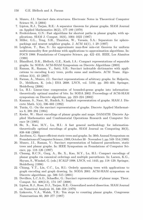
150 G.E. Blelloch and A. Farzan
6. Munro, J.I.: Succinct data structures. Electronic Notes in Theoretical ComputerScience 91, 3 (2004)
7. Lipton, R.J., Tarjan, R.E.: A separator theorem for planar graphs. SIAM Journalon Applied Mathematics 36(2), 177–189 (1979)
8. Frederickson, G.N.: Fast algorithms for shortest paths in planar graphs, with ap-plications. SIAM J. Comput. 16(6), 1004–1022 (1987)
9. Miller, G.L., Teng, S.H., Thurston, W., Vavasis, S.A.: Separators for sphere-packings and nearest neighbor graphs. J. ACM 44(1), 1–29 (1997)
10. Leighton, T., Rao, S.: An approximate max-flow min-cut theorem for uniformmulticommodity flow problems with applications to approximation algorithms. In:FOCS 1988: Foundations of Computer Science, pp. 422–431. IEEE, Los Alamitos(1988)
11. Blandford, D.K., Blelloch, G.E., Kash, I.A.: Compact representations of separablegraphs. In: SODA: ACM-SIAM Symposium on Discrete Algorithms (2003)
12. Raman, R., Raman, V., Satti, S.R.: Succinct indexable dictionaries with appli-cations to encoding k-ary trees, prefix sums and multisets. ACM Trans. Algo-rithms 3(4), 43 (2007)
13. Farzan, A., Munro, J.I.: Succinct representations of arbitrary graphs. In: Halperin,D., Mehlhorn, K. (eds.) ESA 2008. LNCS, vol. 5193, pp. 393–404. Springer,Heidelberg (2008)
14. Lu, H.I.: Linear-time compression of bounded-genus graphs into information-theoretically optimal number of bits. In: SODA 2002: Proceedings of ACM-SIAMsymposium on Discrete algorithms, pp. 223–224 (2002)
15. Kannan, S., Naor, M., Rudich, S.: Implicit representation of graphs. SIAM J. Dis-crete Math. 5(4), 596–603 (1992)
16. Turan, G.: On the succinct representation of graphs. Discrete Applied Mathemat-ics 8, 289–294 (1984)
17. Keeler, W.: Short encodings of planar graphs and maps. DAMATH: Discrete Ap-plied Mathematics and Combinatorial Operations Research and Computer Sci-ence 58 (1995)
18. He, X., Kao, M.Y., Lu, H.I.: A fast general methodology for information-theoretically optimal encodings of graphs. SIAM Journal on Computing 30(3),838–846 (2000)
19. Jacobson, G.: Space-efficient static trees and graphs. In: 30th Annual Symposium onFoundationsofComputerScience,1989,October30–November1,pp.549–554(1989)
20. Munro, J.I., Raman, V.: Succinct representation of balanced parentheses, statictrees and planar graphs. In: IEEE Symposium on Foundations of Computer Sci-ence, pp. 118–126 (1997)
21. Chuang, R.C.N., Garg, A., He, X., Kao, M.Y., Lu, H.I.: Compact encodings ofplanar graphs via canonical orderings and multiple parentheses. In: Larsen, K.G.,Skyum, S., Winskel, G. (eds.) ICALP 1998. LNCS, vol. 1443, pp. 118–129. Springer,Heidelberg (1998)
22. Chiang, Y.T., Lin, C.C., Lu, H.I.: Orderly spanning trees with applications tograph encoding and graph drawing. In: SODA 2001: ACM-SIAM symposium onDiscrete algorithms, pp. 506–515 (2001)
23. Devillers, L.C.A.O., Schaeffer, G.: Succinct representations of planar maps. Theor.Comput. Sci. 408(2-3), 174–187 (2008)
24. Lipton, R.J., Rose, D.J., Tarjan, R.E.: Generalized nested dissection. SIAM Journalon Numerical Analysis 16, 346–358 (1979)
25. Liskovets, V.A., Walsh, T.R.: Ten steps to counting planar graphs. CongressusNumerantium 60, 269–277 (1987)

Implicit Hitting Set Problems
and Multi-genome Alignment
Richard M. Karp
University of California at Berkeley andInternational Computer Science Institute
Let U be a finite set and S a family of subsets of U. Define a hitting set as a subsetof U that intersects every element of S. The optimal hitting set problem is: given apositive weight for each element of U, find a hitting set of minimum total weight.This problem is equivalent to the classic weighted set cover problem.We considerthe optimal hitting set problem in the case where the set system S is not explicitlygiven, but there is an oracle that will supply members of S satisfying certainconditions; for example, we might ask the oracle for a minimum-cardinality setin S that is disjoint from a given set Q. The problems of finding a minimumfeedback arc set or minimum feedback vertex set in a digraph are examples ofimplicit hitting set problems. Our interest is in the number of oracle queriesrequired to find an optimal hitting set. After presenting some generic algorithmsfor this problem we focus on our computational experience with an implicithitting set problem related to multi-genome alignment in genomics. This is jointwork with Erick Moreno Centeno.
A. Amir and L. Parida (Eds.): CPM 2010, LNCS 6129, p. 151, 2010.c© Springer-Verlag Berlin Heidelberg 2010

Bounds on the Minimum Mosaic of Population
Sequences under Recombination
Yufeng Wu
Department of Computer Science and EngineeringUniversity of ConnecticutStorrs, CT 06269, [email protected]
Abstract. We study the minimum mosaic problem, an optimizationproblem originated in population genomics. We develop a new lowerbound, called the C bound. The C bound is provably higher and sig-nificantly more accurate in practice than an existing bound. We showhow to compute the exact C bound using integer linear programming.We also show that a weaker version of the C bound is also more accu-rate than the existing bound, and can be computed in polynomial time.Simulation shows that the new bounds often match the exact optimumat least for the range of data we tested. Moreover, we give an analyticalupper bound for the minimum mosaic problem.
1 Introduction
Recombination is a key genetic process that creates mosaic population sequencesduring meiosis. Throughout this paper, we assume population sequences are bi-nary. This is justified by the current interests in single nucleotide polymorphisms(SNPs). A SNP is a single nucleotide site where exactly two (of four) differentnucleotides occur in a large percentage of the population, and thus can be rep-resented as a binary number. The input data is a binary matrix M with n rows(sequences) and m columns (SNPs). Recombination plays an important role inthe evolutionary history of these sequences. Conceptually, recombination takestwo equal length sequences and generates a new sequence of same length byconcatenating a prefix of one sequence and a suffix of the other sequence. Theposition between the prefix and the suffix is called a breakpoint. Studying recom-bination in populations needs genealogical models. In this paper, we focus on amodel called the mosaic model. The mosaic model [10] assumes that currentpopulation sequences are descendants of a small number of founder sequences.Due to recombination, an extant sequence consists of multiple segments fromthe founders, where breakpoints separate the segments. We ignore point muta-tions in this paper. That is, extant sequences contain exact copies of foundersegments. See Figure 1 for an illustration of the mosaic structure.
The mosaic model is a recurring formulation in population genomics withapplications including study of recombinant inbred mouses [13], hidden Markovmodels (HMMs) in inferring haplotypes from genotypes [2,5,8] and genotype
A. Amir and L. Parida (Eds.): CPM 2010, LNCS 6129, pp. 152–163, 2010.c© Springer-Verlag Berlin Heidelberg 2010

Bounds on the Minimum Mosaic 153
Fig. 1. A minimum mosaic found by program RecBlock containing 55 breakpoints forthe given twenty sequences of length forty. Note that only the sequences are given asinput: we do not know the founders nor the positions of the breakpoints. The top foursequences are founders inferred by program RecBlock, each with a distinct color. Adifferent mosaic for these sequences with 56 breakpoints was shown in [6].
imputation methods (e.g. [3]). A main technical challenge is that even whensequences of M are formed as a mosaic, the breakpoints are invisible. Thusinference needs to be performed to reconstruct the mosaic pattern (and thefounder sequences) from the given sequences. In [10], Ukkonen formulated anoptimization problem for the mosaic model based on parsimony.
The Minimum Mosaic Problem. For a binary matrix M with n rows (sequences)and m columns as well as an integer Kf , find Kf founder sequences that minimizethe total number of breakpoints needed to be put in the input sequences, whichbreak the input sequences into segments from the founder sequences at matchingpositions. Such a mosaic is called the minimum mosaic for M and the number ofbreakpoints needed in the minimum mosaic is denoted as Bmin(M). Note thatno shifting is allowed: segments of founders in the input sequences must retaintheir original positions in the founders.
The minimum mosaic problem can be viewed as a sequence coloring problemas shown in Figure 1. We need to assign colors (one per each founder) to thegiven sequences (i.e. sequences are colored by founders). The total number ofcolor changes (i.e. breakpoints) in the minimum mosaic is the smallest amongall possible coloring. Note at a column, if two sequences are assigned the samecolor, then they must have identical values at this column. Also, Kf is usuallymuch smaller than n.
The minimum mosaic problem has a simple polynomial time algorithm forbinary data [10,12] or even for the so-called genotype data (a mixed descrip-tion of two binary sequences) [12] when Kf = 2. There are two exact methodsfor the general minimum mosaic problem, which are implemented in programHaplovisual [10] and program RecBlock [12]. None of these exact methods runs in

154 Y. Wu
polynomial-time. Our experience suggests that program RecBlock outperformsprogram Haplovisual for many datasets. The basic idea of program RecBlock isto scan from left to right, and enumerate all possible founders at each column.For example, suppose Kf = 3. Then there are 6 configurations for founder set-tings at column 1: 001, 010, 100, 011, 101 and 110 (000 and 111 are excludedbecause we can preprocess the input sequences to remove any columns with only0s or only 1s, and such preprocessing does not change the solution). Now forcolumn 2, we need to enumerate all 6 founder configurations for each of theconfigurations at column 1. Full enumeration quickly becomes infeasible. To ob-tain a practical method, program RecBlock uses several techniques to prune thesearch space. Empirical study shows that program RecBlock seems to work wellfor small number of founders (say three to five) when the data is of mediumsize (say 50 by 50). However, its performance degrades as Kf and/or the size ofmatrix increase.
Since there exists no known polynomial-time algorithm for the minimum mo-saic problem, heuristic methods for handling larger datasets are also developed[12,7]. For example, program RecBlock can run in a non-optimal mode to findrelatively good solutions for larger datasets when exact solutions are difficult toobtain. Although these methods are fast, a major problem is the lack of knowl-edge on the optimality of their solutions. Moreover, little is known on theoreticalquantification of the mosaic structure in general.
This motivates computing lower bounds for the minimum mosaic problem. Alower bound gives an estimate on the necessary breakpoints. Lower bounds canbe useful in the following two ways.
1. A lower bound quantifies the range of the solution, together with the up-per bounds found by heuristic methods. In the ideal case, the lower boundmatches the upper bound, and thus certifies the optimality of the heuristicsolution. Even when the lower bound is smaller than the upper bound, therange of solution given by the bounds can still be useful.
2. A good lower bound can speed up the branch and bound search for theoptimal solution.
A known lower bound. There is an existing lower bound (called the CHbound) in [12] for the minimum mosaic problem, which is inspired by [4]. TheCH bound considers each segment [i, j] of M (i.e. the sub-matrix Mi,j withcolumns between i and j inclusive, where i < j). We let set Si,j contain thedistinct rows of Mi,j, and we denote the multiplicity of a sequence sk
i,j ∈ Si,j
in Mi,j as nki,j . Each sk
i,j represents a “cluster” of nki,j identical sequence within
the interval. For example, in Figure 2, there are four clusters between the firstand the third columns: 001, 100, 010 and 000 (which are numbered from 1to 4 in this order). For the cluster s1
1,3 = 001, n11,3 = 2, while nk
1,3 = 1 fork = 2, 3, 4. We order sequences sk
i,j so that the list of nki,j is non-increasing.
Now if |Si,j | ≤ Kf , then the lower bound on Bmin(Mi,j) is simply 0. Otherwise,Bi,j =
∑|Si,j |k=Kf +1 nk
i,j is a lower bound on Bmin(Mi,j). For the data in Figure 2,when Kf = 3, B1,3 = 1. We say a cluster is cut if each identical sequence of the

Bounds on the Minimum Mosaic 155
cluster contains breakpoints. Otherwise, the cluster is un-cut if some sequenceof the cluster contains no breakpoints. The correctness of Bi,j as a lower boundon Bmin(Mi,j) is due to the fact that there are only Kf colors and Lemma 1.
Lemma 1. Within an interval, two distinct sequences containing no breakpointscan not be colored by the same founder.
Bi,j for each [i, j] is often much smaller than Bmin(M). But Myers and Griffiths[4] introduced a general method to combine Bi,j from all intervals to get a muchhigher overall bound. Intuitively, we consider a straight horizontal line. We needto place the minimum number of breakpoints along the horizontal line, so that foreach interval [i, j], there is at least Bi,j breakpoints that are properly containedinside [i, j]. The CH bound is equal to the minimum number of breakpointsneeded. A breakpoint located at position x within [i, j] contributes to the intervalif i < x < j. Note that breakpoints are not placed at integer points. The CHbound is simple and efficiently computable using a greedy approach [4]. However,practical experience shows that the CH bound often significantly underestimatesBmin(M) (see Section 4), which greatly limits its use.
Contributions. In this paper, we present a new lower bound (called the Cbound) for the minimum mosaic problem. We show that the C bound is prov-ably higher than (or equal to) the CH bound, and often significantly higherin practice. For a large portion of datasets we simulate, the C bound matchesBmin(M). Thus, the C bound can be useful in quantifying the tighter range ofoptimal solution. In terms of efficiency, the C bound can be computed exactlyfor many datasets, and a variation of the C bound (which leads to only a littleloss of accuracy) can be computed in polynomial time. We also evaluate the per-formance of the lower bounds in branch and bound search through simulation,where we do observe, albeit modest, speedup. On the theoretical side, we givean analytical upper bound on Bmin(M).
2 The C Bound: A New Lower Bound
We now present a new lower bound, called the clique bound (or simply C bound)for the minimum mosaic problem. Clique here refers to segments of input se-quences used in the definition of the C bound that are pairwise incompatible(see blow). If we create a graph of sequence segments where there is an edgebetween two segments if they are incompatible, the C bound corresponds tocliques with some special property in this graph.
2.1 Breakpoint Placement
The breakpoint placement by the CH bound is a two-stage approach: first es-timate the number of needed breakpoints inside each interval, and then placebreakpoints along a horizontal line. A breakpoint placed this way is not as-sociated with any particular sequence. Our first idea is to adopt a one-stage

156 Y. Wu
approach: place necessary breakpoints directly in M . That is, each breakpointbelongs to a particular sequence in M . Formally,
Placement of necessary breakpoints. Place the smallest number (denotedas nb) of breakpoints in M (i.e. a breakpoint is placed inside some sequence ofM) such that for each interval [i, j], no more than Kf clusters remain un-cut.Our first version of the C bound is equal to nb, which is a lower bound onBmin(M). This is due to Lemma 2, which is implied by Lemma 1.
Lemma 2. nb ≤ Bmin(M).
We say a lower bound x beats a lower bound y if x is always higher than or equalto y. First note that the C bound always beats the CH bound. This is becausewe can place breakpoints created by the C bound along a horizontal line byprojecting these breakpoints onto the line. These are at least Bi,j breakpoints for[i, j] on the horizontal line. In practice, the C bound is usually higher (sometimesignificantly higher) than the CH bound.
We do not know a polynomial-time algorithm to compute the exact C bound.To compute the C bound in practice, we use the following integer linear pro-gramming (ILP) formulation. We define a binary variable Cr,c for each row rand column c, where Cr,c = 1 if there is a breakpoint in row r between columnsc and c + 1. For each interval [i, j] with |Si,j | clusters within [i, j], we create abinary variable Ui,j,k for the k-th cluster within [i, j], where Ui,j,k = 1 if thiscluster is un-cut within [i, j], and 0 otherwise.
Objective: minimize∑
1≤r≤n,1≤k<m Cr,k.Subject to
1 Ui,j,k +∑
i≤i′<j Cr,i′ ≥ 1, for each 1 ≤ i < j ≤ m and each row r incluster k within [i, j].
2∑|Si,j|
k=1 Ui,j,k ≤ Kf , for each 1 ≤ i < j ≤ m.For each 1 ≤ k < m and 1 ≤ r ≤ n, there is a binary variable Cr,k.For each 1 ≤ i < j ≤ m, and 1 ≤ k ≤ |Si,j |, there is a binary variable Ui,j,k.
Briefly, constraint (1) says that cluster k is un-cut if any sequence in the clustercontains no breakpoints. Constraint (2) says within each interval [i, j], there isno more than Kf un-cut clusters. This ILP formulation can be solved relativelyefficiently in practice for many datasets.
A polynomial-time computable bound. The C bound beats the CH boundboth in theory and in practice. Still, we do not have a polynomial-time algorithmfor computing it. This may limit its use for larger datasets. We now show aweaker version of the C bound (denoted as the Cw bound) that is polynomial-time computable and provably beats the CH bound. This provides more evidenceon the strength of the exact C bound. The Cw bound is computed by solving thelinear programing (LP) relaxation of the ILP formulation of the C bound. Briefly,linear programming relaxation treats each variable in the ILP formulation to bea general real variable (between 0 and 1 for a binary variable). The Cw boundis a legal lower bound on Bmin(M) because the objective of the LP relaxation

Bounds on the Minimum Mosaic 157
can not be higher than that of the original C bound. The number of variablesand constraints in the ILP formulation for the C bound is O(nm2). Thus, theCw bound can be computed in polynomial-time.
We now show that the Cw bound beats the CH bound.
Proposition 1. Cw ≥ CH .
Proof. Conceptually, the CH bound can be computed by the following ILP for-mulation (called the CH formulation).
Objective: minimize∑
1≤k<m Ck.* Subject to:
∑j−1x=i Cx ≥ Bi,j , for each 1 ≤ i < j ≤ m.
For each 1 ≤ k < m, there is a general integer variable Ck.
Ci refers to the number of breakpoints between columns i and i+1. We will firstshow that Cw beats the objective of the LP relaxation of the CH formulation.Then we will show the LP relaxation of the CH formulation has an integeroptimal solution. By combining these two observations, we have Cw ≥ CH .
First, we let Cr,k be an optimal solution for Cw (where Cr,k is a real valuebetween 0 and 1). We now let Ck =
∑1≤r≤n Cr,k. We claim Ck is a legal solution
for the relaxed CH formulation (with the identical objective value as the Cw
formulation). To show this, we only need to show Ck satisfies∑
i≤x<j Cx ≥ Bi,j
for each interval [i, j] when Bi,j > 0. Since∑
i≤x<j Cx =∑
i≤x<j,1≤r≤n Cr,x,and from constraint [1] in the C bound formulation,
∑
i≤x<j
Cx ≥ n−|Si,j |∑
k=1
nki,jUi,j,k
Since 0 ≤ Ui,j,k ≤ 1, and∑|Si,j |
k=1 Ui,j,k ≤ Kf and note that nki,j is ordered
non-decreasingly, we have:∑
i≤x<j Ci′ ≥ n−∑Kf
k=1 nki,j = Bi,j . We achieve the
minimum value by making each Ui,j,k = 1 for k ≤ Kf .We now show the LP relaxation of the CH formulation has an integer optimal
solution. For contradiction, we assume no integer solutions exists for the CHrelaxed formulation. We consider an optimal solution to the LP relaxation of theCH formulation so that its first Ci with non-integer value occurs at a column pwhere p < m is the largest among all such solutions. That is, Cp is not an integer,while Ck is an integer when k < p, and there is no optimal solutions with integervalues for C1 . . . Cp. Let Cp = v + f , where v is an integer and 0 < f < 1. Thenwe create a new solution C′
k by letting C′k = Ck when k �= p and p + 1. Then
C′p = v and C′
p+1 = Cp+1 +f . We need to show the changed solution is legal (i.e.satisfying constraint “*”). Note that only intervals [i, j] overlapping breakpointp need to be checked. This contains two cases: (a) intervals [i, p+1]; (b) intervals[i, j], where i ≤ p and p + 1 < j. The type (a) intervals’ bounds are satisfiedbecause the bounds are integers and thus discarding f still satisfies the boundssince all previous C′
k are integer. The type (b) intervals are satisfied since thesummation of C′
k values is the same as summation of Ci values. This contradicts

158 Y. Wu
our previous assumption that there is no optimal solutions with integer valuesfor C1 . . . Cp. Therefore, there exists an integer solution to the LP relaxation ofthe CH bound. ��
2.2 Improving the C Bound
Simulation shows that the C bound (and the Cw bound) is usually higher thanthe CH bound. For the datasets we simulate, the gap between the C and the CHbounds is usually 10-20%, but the C bound can still be significantly lower thanBmin(M). We now describe techniques that significantly improve the C bound.
We start by strengthening Lemma 1. A moment’s thought suggests Lemma 1can be extended to overlapping segments of different intervals (instead of withina single interval). We say segment [a1, b1] of row r1 (denoted as r1[a1, b1]) andsegment [a2, b2] of row r2 (i.e. r2[a2, b2]) are incompatible if [a1, b1] and [a2, b2]overlap (i.e. with non-empty intersection) and r1[a1, b1] and r2[a2, b2] are notidentical within the overlapping region. Here, [a1, b1] and [b1, c1] are consideredto overlap at [b1, b1]. For example, in Figure 2, r1[1, 2] and r2[2, 3] are compatiblewhile r1[3, 4] and r2[2, 3] are incompatible. Then we have:
Lemma 3. Two incompatible segments can not be colored by the same founder.
c1 c2 c3 c4
r1 0 0 1 1r2 1 |0 0 1r3 0 0 1 0r4 0 1 0 |1r5 0 0 0 1
Fig. 2. An example dataset
Note that Lemma 1 is a special case of Lemma 3,and Lemma 3 can give a higher bound than theoriginal C bound. This motivates an improved Cbound as follows. For each interval [i, j], we searchfor pairwise incompatible segments [ik, jk], each forone of the |Si,j | clusters. Here, i ≤ ik < jk ≤ j. Itis desired that the total length of the segments issmall. The shorter the incompatible segments are,the more restrictive the placement of breakpointsis: fewer breakpoints can contribute to shorter seg-ments and so more breakpoints may be needed. Then, we require no more thanKf incompatible segments remain un-cut:
∑|Si,j|k=1 Uik,jk,ci,j,k(ik,jk) ≤ Kf . Here,
ci,j,k(ik, jk) is the cluster index of the [ik, jk] part within the k-th cluster of [i, j](since [ik, jk] may have a different set of distinct rows from [i, j]). From Lemma4, the new C bound beats the original C bound.
Lemma 4. Using incompatible segments gives a higher C bound.
Proof. For [i, j], if Ui,j,k = 1, then there is no breakpoint between columns iand j. Since [ik, jk] is contained inside [i, j], this implies Uik,jk,k′ = 1 (wherek′ = ci,j,k(ik, jk)). Thus, Ui,j,k ≤ Uik,jk,k′ . Since the C bound prefers smallerUi,j,k values (by constraint 2 of the C bound formulation), using incompatiblesegments leads to a higher bound. ��As an example, we consider the dataset in Figure 2, where we assume Kf = 3.We first consider the ILP constraints of each interval from the original C bound.

Bounds on the Minimum Mosaic 159
For example, for interval [1, 4], we have U1,4,1 +U1,4,2 +U1,4,3 +U1,4,4 +U1,4,5 ≤3, and for r1 = 0011 we have U1,4,1 + C1,1 + C1,2 + C1,3 ≥ 1. Suppose asshown in Figure 2, we place a breakpoint between c1 and c2 in r2 (i.e. C2,1
= 1), and a breakpoint between c3 and c4 for r4 (i.e. C4,3 = 1). This wouldsatisfy constraints of all intervals. But these two breakpoints will not be enoughwhen we consider the following five pairwise incompatible segments: r1[3, 4],r2[1, 3], r3[3, 4], r4[2, 3] and r5[1, 3]. These segments impose an ILP constraint:U3,4,1 + U1,3,2 + U3,4,3 + U2,3,3 + U1,3,5 ≤ 3. Clearly, setting C2,1 and C4,3 to be1 will not satisfy this constraint since C4,3 does not contribute to r4[2, 3] (recallC4,3 refers to the breakpoint between columns 3 and 4, and r4[2, 3] is the 3rdcluster within [2, 3]). So only U1,3,2 = 0 and the other four terms are equal to 1.
Finding incompatible segments. Ideally, we would like to find incompatiblesegments whose total length is minimized (called the shortest incompatible seg-ments or SISs). It is not known whether there is a polynomial-time algorithmfor finding the SISs. We also want to find more than one set of SISs to obtainhigher lower bounds. Thus, we use the following heuristic algorithm for findingapproximate SISs that works reasonably well in practice. This heuristic greedilyfinds incompatible segments for each cluster. To find multiple SISs, we choosedifferent initial positions in the first cluster.
1 Order the clusters (e.g. in the order of their appearance in the dataset).2 Set pos1 ← 1.3 while pos1 < m
3a Initialize the first segment for row 1 as r1[pos1, pos1 + 1].3b For each remaining cluster row ri, let its segment be the shortest segment
such that the segment is incompatible with all previous segments.3c Set pos1 ← pos1 + 1.
Now with ILP constraints imposed on incompatible segments, higher C boundscan be obtained. Moreover, the C bound can also be computed faster thanthe original C bound by ILP. Simulation results show that the CPLEX ILPsolver usually takes only a few seconds for fairly large datasets (say with 100rows and 100 columns with Kf = 10), which is much faster than computingthe original C bound. The speedup is likely due to the reduction of the size ofthe ILP formulation: same segments are often chosen for different overlappingintervals, which reduces the number of needed variables. Thus, the number ofneeded Ui,j,k is often much smaller than that in the original formulation. Ourexperience shows that the new C formulation with overlapping segments can useonly 10% (or fewer) variables as in the original formulation for larger datasets.
Other improvements. The C bound can be further improved by the followingobservations. (a) We can find different SISs by picking a small number of differentcluster orders. (b) We can avoid enumeration of all
(m2
)intervals for a matrix
with m columns in searching for incompatible segments. Suppose for an interval[a, b] the found incompatible segments within [a, b] are all between [a1, b1]. Thenwe can skip all intervals [x, y] where a ≤ x ≤ a1 and b1 ≤ y ≤ b.

160 Y. Wu
2.3 Application in Finding the Exact Minimum Mosaic UsingBranch and Bound
The C bound can speedup program RecBlock in finding the exact minimummosaic with the branch and bound scheme. We have experimented with thefollowing straightforward approach. Briefly, we use the approximate C boundto determine whether a current search path can lead to a better solution. Wefirst compute the C bounds for the segment of input data between column i andm, for each 1 ≤ i ≤ m − 1. For the purpose of efficiency, we only compute theCw bound by solving linear programming relaxation. Program RecBlock buildsa partial mosaic from column 1 to i during its search for the minimum mosaic.If the lower bound on the minimum number of breakpoints for the sub-matrix(from the current site to the right end of the input matrix) plus the currentlyneeded breakpoints in the partial solution is no smaller than the known upperbound, then this search path will not lead to a better solution and can thus bedropped.
Other more advanced strategies are also possible. For example, we can makethe lower bounds more effective by switching to heuristic mode with promisingsearch paths at each column. This may help because it may find the optimalsolution earlier whose optimality may be certified by the lower bound.
3 An Analytical Upper Bound
A natural question is how many breakpoints we may need in a minimum mosaicfor an arbitrary (i.e. unknown) n by m matrix. An answer to this question givesan upper bound and also an estimate on the range of Bmin(M). It was stated in[6] that there can be as many as (m− 1)n/2 breakpoints needed in a minimummosaic when Kf = 2. We now extend to the general case.
Proposition 2. Bmin ≤ (1− 1Kf
)( m�log2(Kf )� − 1)n, for any Kf .
Proof. First note that when Kf = 2, this reduces to the (m− 1)n/2 bound. Ourapproach is similar to [11]. We divide M into m/log2(Kf) non-overlappingintervals, each with log2(Kf ) columns. There are at most Kf distinct binarysequences within each interval. We then pick each of these unique sequences asfounders within the interval. Thus, no breakpoints is needed inside intervals.Since there are m/log2(Kf ) intervals for each of the n rows, we need no morethan (m/log2(Kf ) − 1)n breakpoints between intervals.
We can further improve this bound by carefully picking the colors for neigh-boring intervals and removing some breakpoints between the intervals in a waysimilar to [10,9]. More specifically, we construct a weighted bipartite graph fortwo neighboring intervals IV and IV ′. A vertex Fi corresponds to a founder andalso a sequence cluster colored with this particular founder. There is an edge ofweight ni,j between vertices Fi within IV and Fj within IV ′ if there are ni,j
input sequences as concatenation of founder Fi within IV and founder Fj withinIV ′. We add a weight 0 edge between two founders if there is no such combina-tion in the input sequences. When choosing the coloring for IV and IV ′, we use

Bounds on the Minimum Mosaic 161
the maximum weighted matching of the graph: if Fi is matched with Fj , Fi andFj are colored by the same founder. We avoid ni,j breakpoints between IV andIV ′ since there is no color change within these ni,j rows.
Since the input matrix M is unknown, we can not explicitly construct thebipartite graph and compute the maximum weighted matching. Nonetheless, wecan still rely on the matching to improve the upper bound as follows. First, thetotal weight of the bipartite graph is n. Also, there exists a maximum weightedmatching which is also a perfect matching since the bipartite graph is complete.We claim that there exists a perfect matching in the bipartite graph with atleast n/Kf weight. To see this, note that there are Kf ! perfect matchings fora bipartite graph with Kf nodes on one side, and each edge appears in exactly(Kf − 1)! of these perfect matchings. Thus, the sum of the weights of all perfectmatchings is (Kf−1)!n. The maximum weighted matching has weight of at least(Kf−1)!n/Kf ! = n/Kf . Therefore, we can remove at least n/Kf breakpoints ateach interval boundary by properly selecting how founders are matched for thetwo neighboring intervals. So we need no more than (1−1/Kf)(m/log2(Kf )−1)n breakpoints for any input dataset with Kf founders. ��
4 Simulation Results
We have implemented the lower bound method in program RecBlock with ei-ther CPLEX (a commercial ILP solver) or GNU GLPK ILP solver (mainly ademo of the functionalities for users without a CPLEX license). The CPLEXversion is often much faster. The simulation results in this section are for theCPLEX version. We test our method for simulated data on a 3192 MHz IntelXeon workstation. We use Hudson’s program ms [1] to generate binary popula-tion sequences. We fix the scaled population mutation rate to 10, and the scaledrecombination rate to 10, and generate 100 datasets for 20, 30, 40 and 50 se-quences. We then remove from datasets any columns that have more than 95%or less than 5% 1s. This helps to remove more recent mutations and focus onthe underlying mosaic structures.
Performance of lower bounds. To demonstrate the usefulness of the new Cbound, we compare the performance of the CH bound and the C bound. We useprogram RecBlock to compute the exact Bmin(M). We also evaluate the approx-imate C bound (i.e. the Cw bound) obtained by solving LP relaxation. This isuseful since the Cw bound can be more scalable when data size grows. The per-formance of the lower bounds is shown in Table 1. We use three statistics: (a)percent of datasets where the lower bound matches Bmin(M); (b) average gapbetween the lower bound and Bmin(M) (normalized by Bmin(M)); (c) averagerunning time. From Table 1, we can see that the C bound is very accurate for therange of data we test: for a large percentage of datasets, the C bound matchesBmin(M), and the average gap between the C bound and Bmin(M) is very small(within 2%). Moreover, the C bound remains accurate for larger Kf . In terms ofefficiency, computing the C bound scales well with large Kf : the larger Kf is, thefaster computation is. This is likely because the size of integer programs decreases

162 Y. Wu
when Kf increases since fewer intervals contain more than Kf clusters when Kf
increases. This is very useful to obtain an estimate of Bmin(M): programRecBlockgets increasingly slower when Kf increases. We also note that the Cw bound isvery accurate, and slightly faster to compute than the original C bound. On theother hand, the CH bound performs poorly in all the cases with much larger gaps,although the CH bound is often much faster to compute.
Also, it appears that the GLPK version can be slow in computing the exact Cbound, while it performs relatively well in computing the approximate C bound.For example, the GLPK version takes on average 208 seconds in computingthe exact C bound (excluding one dataset where GLPK runs for more thanone day but does not find the optimal solution), and 61 seconds for computingthe approximate C bounds with the datasets with n = 30 and Kf = 5. Asa comparison, the CPLEX version takes on average 24 seconds and 18 secondsrespectively for computing the exact and the approximate C bounds for the samedatasets. Thus, when using the GLPK version, computing the approximate Cbounds may be more practical for some more difficult datasets.
Application in finding the exact minimum mosaic using branch andbound. We also evaluate how the C bound performs in speeding up programRecBlock with the branch and bound scheme. Simulation results are shown inTable 1. When Kf becomes larger, branch and bound are more likely to beeffective. Although reduction of running time is modest in these simulations,greater speed-up could be achieved if better heuristics are used for finding upperbounds since the C bound is often close to the optimal solution. Moreover, sincebranch and bound needs to compute the C bounds for many segments, using amore powerful integer programming solver (e.g. CPLEX) may have a significantimpact on the running time.
Table 1. Performance of lower bounds. Exact: compute Bmin(M) by programRecBlock. Exact (C): the branch and bound mode of program RecBlock using the Cw
bound. %Opt: percentage of datasets where the lower bound matches Bmin(M). Gap:percentage of difference between Bmin(M) and the lower bound (divided by Bmin(M)).T: time (in seconds). n: number of sequences. Kf : number of founders.
n 20 30 40 50Kf 5 6 7 8 5 6 7 8 5 6 7 8 5 6 7 8
Exact T 1 7 39 255 8 95 848 3620 8 61 418 - 13 123 2024 -
Exact (C) T 3 7 38 196 14 48 304 2152 13 46 361 - 21 73 1671 -
CH %Opt 6 21 43 67 1 2 10 27 1 7 10 - 0 1 5 -
Gap 34 27 18 9 42 37 31 24 38 32 27 - 43 39 33 -
T <1 <1 <1 <1 <1 <1 <1 <1 <1 <1 <1 <1 <1 <1 <1 <1
C %Opt 85 94 98 100 81 82 85 90 72 73 77 - 63 69 68 -
Gap 1 1 <1 0 1 2 1 1 2 2 2 - 2 2 2 -
T 3 3 2 2 24 19 19 14 18 18 15 12 40 37 29 21
Cw %Opt 83 94 98 100 77 81 83 90 71 70 77 - 59 67 66 -
Gap 1 1 <1 0 1 2 1 1 2 2 2 - 2 2 2 -
T 3 3 2 2 18 18 15 13 17 15 14 12 26 24 23 21

Bounds on the Minimum Mosaic 163
Acknowledgment. This work is supported by National Science Foundation[IIS-0803440]. I am also supported by the Research Foundation of University ofConnecticut.
References
1. Hudson, R.: Generating Samples under the Wright-Fisher neutral model of geneticvariation. Bioinformatics 18(2), 337–338 (2002)
2. Kimmel, G., Shamir, R.: A block-free hidden markov model for genotypes and itsapplication to disease association. J. of Comp. Bio. 12, 1243–1260 (2005)
3. Marchini, J., Howie, B., Myers, S., McVean, G., Donnelly, P.: A new multipointmethod for genome-wide associationstudies by imputation of genotypes. NatureGenetics 39, 906–913 (2007)
4. Myers, S.R., Griffiths, R.C.: Bounds on the minimum number of recombinationevents in a sample history. Genetics 163, 375–394 (2003)
5. Rastas, P., Koivisto, M., Mannila, H., Ukkonen, E.: A Hidden Markov Techniquefor Haplotype Reconstruction. In: Casadio, R., Myers, G. (eds.) WABI 2005. LNCS(LNBI), vol. 3692, pp. 140–151. Springer, Heidelberg (2005)
6. Rastas, P., Ukkonen, E.: Haplotype Inference Via Hierarchical Genotype Parsing.In: Giancarlo, R., Hannenhalli, S. (eds.) WABI 2007. LNCS (LNBI), vol. 4645, pp.85–97. Springer, Heidelberg (2007)
7. Roli, A., Blum, C.: Tabu Search for the Founder Sequence Reconstruction Prob-lem: A Preliminary Study. In: Proceedings of Distributed Computing, Artifi-cial Intelligence, Bioinformatics, Soft Computing, and Ambient Assisted Living(IWANN 2009), pp. 1035–1042 (2009)
8. Scheet, P., Stephens, M.: A fast and flexible statistical model for large-scale pop-ulation genotype data: applications to inferring missing genotypes and haplotypicphase. Am. J. Human Genetics 78, 629–644 (2006)
9. Schwartz, R., Clark, A., Istrail, S.: Methods for Inferring Block-Wise AncestralHistory from Haploid Sequences. In: Guigo, R., Gusfield, D. (eds.) WABI 2002.LNCS, vol. 2452, pp. 44–59. Springer, Heidelberg (2002)
10. Ukkonen, E.: Finding Founder Sequences from a Set of Recombinants. In: Guigo,R., Gusfield, D. (eds.) WABI 2002. LNCS, vol. 2452, pp. 277–286. Springer,Heidelberg (2002)
11. Wu, Y.: Analytical Upper Bound on the Minimum Number of Recombinations inthe History of SNP Sequences in Populations, Info. Proc. Letters 109, 427–431(2009)
12. Wu, Y., Gusfield, D.: Improved Algorithms for Inferring the Minimum Mosaic ofa Set of Recombinants. In: Ma, B., Zhang, K. (eds.) CPM 2007. LNCS, vol. 4580,pp. 150–161. Springer, Heidelberg (2007)
13. Zhang, Q., Wang, W., McMillan, L., Prins, J., de Villena, F.P., Threadgill, D.:Genotype Sequence Segmentation: Handling Constraints and Noise. In: Crandall,K.A., Lagergren, J. (eds.) WABI 2008. LNCS (LNBI), vol. 5251, pp. 271–283.Springer, Heidelberg (2008)

The Highest Expected Reward Decoding
for HMMs with Application toRecombination Detection
Michal Nanasi, Tomas Vinar, and Brona Brejova
Faculty of Mathematics, Physics, and Informatics, Comenius University,Mlynska Dolina, 842 48 Bratislava, Slovakia
Abstract. Hidden Markov models are traditionally decoded by the Vi-terbi algorithm which finds the highest probability state path in themodel. In recent years, several limitations of the Viterbi decoding havebeen demonstrated, and new algorithms have been developed to ad-dress them (Kall et al., 2005; Brejova et al., 2007; Gross et al., 2007;Brown and Truszkowski, 2010). In this paper, we propose a new effi-cient highest expected reward decoding algorithm (HERD) that allowsfor uncertainty in boundaries of individual sequence features. We demon-strate usefulness of our approach on jumping HMMs for recombinationdetection in viral genomes.
Keywords: hidden Markov models, decoding algorithms, recombinationdetection, jumping HMMs.
1 Introduction
Hidden Markov models (HMMs) are an important tool for modeling and anno-tation of biological sequences and other data, such as natural language texts.The goal of sequence annotation is to label each symbol of the input sequenceaccording to its meaning or a function. For example, in gene finding, we seekto distinguish regions of DNA that encode proteins from non-coding sequence.An HMM defines a probability distribution Pr(A|X) over all annotations A ofsequence X . Typically, one uses the well-known Viterbi algorithm (Forney Jr.,1973) or its variants for more complex models (Brejova et al., 2007) to find theannotation with the highest overall probability argmaxA Pr(A|X). In this pa-per, we design an efficient HMM decoding algorithm that finds the optimal an-notation for a different optimization criterion that is more appropriate in manyapplications.
In recent years, several annotation strategies were shown to achieve betterperformance than the Viterbi decoding in particular applications (Kall et al.,2005; Gross et al., 2007; Brown and Truszkowski, 2010). Generally, they can beexpressed in the terminology of gain functions introduced in the context ofstochastic context-free grammars (Hamada et al., 2009). In particular, we choosea gain function G(A, A′) which characterizes similarity between a proposed an-notation A and the (unknown) correct annotation A′. The goal is then to find the
A. Amir and L. Parida (Eds.): CPM 2010, LNCS 6129, pp. 164–176, 2010.c© Springer-Verlag Berlin Heidelberg 2010

The Highest Expected Reward Decoding for HMMs 165
annotation A with the highest expected value of G(A, A′) over the distributionof A′ defined by the HMM, conditioning on sequence X . That is, we maximizeEA′|X [G(A, A′)] =
∑A′ G(A, A′)P (A′|X).
Intuitively, the gain function should characterize the measure of prediction ac-curacy appropriate for a particular application domain. If the sequences and thetrue annotations are generated from the HMM, the decoding algorithm optimiz-ing the expected gain will on average reach higher prediction accuracy, measuredby G(A, A′), than any other decoding.
In this framework, the Viterbi decoding optimizes the identity gain functionG(A, A′) = [A = A′], that is the gain is 1 if we predict the whole annotationexactly correctly, and 0 otherwise. There may be many high-probability anno-tations besides the optimal one, and they are disregarded by this gain function,even though their consensus may suggest a different answer that is perhaps moreaccurate locally. On the other hand, the posterior decoding (Durbin et al., 1998)predicts at each position a label that has the highest posterior probability at thatposition, marginalizing over all annotations. Therefore, it optimizes the expectedgain under the gain function that counts the number of correctly predicted labelsin A with respect to A′.
These two gain functions are extremes: the Viterbi decoding assigns a positivegain to the annotation only if it is completely correct, while the posterior decod-ing gain function rewards every correct label. It is often appropriate to considergain functions in between these two extremes. For example, in the context ofgene finding, Gross et al. (2007) use a gain function that assigns a score +1for each correctly predicted coding region boundary and score −γ for predictedboundary that is a false positive. Indeed, one of the main objectives of genefinding is to find exact positions of these boundaries, since even a small errormay change the predicted protein significantly. Parameter γ in the gain functioncontrols the trade-off between sensitivity and specificity.
While the coding region boundaries are well defined in gene finding, and it isdesirable to locate them precisely, in other applications, such as transmembraneprotein topology prediction, we only wish to infer the approximate locations offeature boundaries. The main reason is that the underlying HMMs do not containenough information to locate the boundaries exactly, and there are typicallymany annotations of similar probability with slightly different boundaries. Thisissue was recently examined by Brown and Truszkowski (2010) in a Viterbi-likesetting, where we assign gain to an annotation, if all feature boundaries in Aare within some distance W from the corresponding boundary in the correctannotation A′. Unfortunately, the problem has to be addressed by heuristics,since it is NP-hard even for W = 0.
In this paper, we propose a new gain function in which each feature boundaryin A gets score +1 if it is within distance W from the corresponding boundary inA′, and score −γ otherwise. Our definition allows to consider nearby boundarypositions as equivalent, as in Brown and Truszkowski (2010), yet it avoids therequirement that the whole annotation needs to be essentially correct to receive

166 M. Nanasi, T. Vinar, and B. Brejova
any gain at all. Another benefit is that our gain function can be efficientlyoptimized in time linear in the length of the input sequence.
We apply our algorithm to the problem of detecting recombination in thegenome of the human immunodeficiency virus (HIV) with jumping HMMs(Schultz et al., 2006). A jumping HMM consists of a profile HMM (Durbin et al.,1998) for each known subtype of HIV. Recombination events are represented bya special jump transitions between different profile HMMs. The goal is to deter-mine for a new HIV genome whether it comes from one of the known subtypesor whether it is a recombination of several subtypes. However, the exact positionof a breakpoint can be difficult to determine, particularly if the two recombin-ing strains were very similar near the recombination point. Our gain functioncorresponds to this problem very naturally: it scores individual predicted recom-bination points, but allows some tolerance in their exact placement.
2 HERD: The Highest Expected Reward Decoding
In this section, we propose a new gain function and describe an algorithm for find-ing the annotation with the highest expected gain. Our algorithm is a non-trivialextension of the maximum expected boundary accuracy decoding (Gross et al.,2007).
Hidden Markov models and notation. A hidden Markov model (HMM) is a gener-ative probabilistic model with a finite set of states V and transitions E. There isa single designated start state s and a final state t. The generative process startsin the start state, and in each round it emits a single symbol xi from the emissionprobability distribution evi,xi of the current state vi, and then changes the stateto vi+1 according to the transition probability distribution avi,vi+1 . The genera-tive process continues until the final state is reached. Thus, the joint probabilityof generating a sequence X = x1, . . . , xn by a state path π = s, v1, . . . , vn, tis Pr(π, X) = as,v1 ·
∏ni=1 evi,xi · avi,vi+1 , where vn+1 = t. In other words, the
HMM defines a probability distribution Pr(π, X) over all possible sequences Xand state paths π, or perhaps more appropriately, for a given sequence X , theHMM defines a conditional distribution over all state paths Pr(π |X).
Our aim is to produce an annotation of an input sequence X , i.e. to labeleach symbol of X by a color corresponding to its function (e.g., coding or non-coding in the case of gene finding, or a virus subtype in case of recombinationdetection). Position i in the annotation A = a1 . . . an is a boundary, if ai and ai+1
are different colors. For convenience, we consider positions 0 and n as boundaries.A feature is a region between two consecutive boundaries.
To use HMMs for sequence annotation, we color each state v by a colorc(v). Every state path π = s, v1, . . . , vn, t thus implies an annotation c(π) =c(v1) . . . c(vn). In general, multiple states can have the same color, and severalstate paths may produce the same annotation. Thus, HMMs also define a prob-ability distribution over annotations A, where Pr(A |X) =
∑π:c(π)=A Pr(π |X).

The Highest Expected Reward Decoding for HMMs 167
A
A′
Fig. 1. Example of buddy pairs in two annotations over three colors (white, gray, black)for W = 3. Boundaries are shown by arrows, buddy pairs are connected by lines. Thesecond boundary in A does not have a buddy pair due to condition (ii), whereas thefourth and fifth boundary due to condition (iii). In this example, G(A, A′) = 3 − 4γ.
The highest expected reward decoding problem. To formally define our problem,we first define a gain function G(A, A′) characterizing similarity between anytwo annotations A and A′ of the same sequence. We assign a positive score to aboundary in A if A′ contains a corresponding boundary sufficiently close so thatthey can be considered equivalent. This notion of closeness is formalized in thefollowing definition (see also Figure 1).
Definition 1. Let A and A′ be two annotations of the same sequence. Bound-aries i in A and j in A′ are called buddies if (i) both of them separate the samepair of colors c1 and c2, (ii) |i− j| < W , and (iii) there is no other boundary atpositions min{i, j}, . . . , max{i, j} in either A or A′.
The intuition behind condition (iii) is that the buddies should correspond toboundaries that are only slightly shifted from their correct position, but stillseparate essentially the same pair of features. In the extreme case, such as theboundaries between gray and black features in Figure 1, even a slight shift inthe boundary causes the flanking black features to become non-overlapping.Condition (iii) in fact enforces that pairs of such non-overlapping features arenot considered as corresponding to each other. Moreover, condition (iii) alsoenforces that each boundary in A′ is a buddy to at most one boundary in A andvice versa.
Definition 2 (Highest expected reward decoding problem). Let gainfunction G(A, A′) assign score +1 to each boundary in A if it has a buddy inA′ and score −γ to boundaries in A without a buddy. In the highest expectedreward decoding (HERD), we seek the annotation A maximizing the expectedgain EA′|X [G(A, A′)] =
∑A′ G(A, A′) Pr(A′ |X), where the conditional probabil-
ity Pr(A′ |X) is defined by the HMM as∑
π:c(π)=A′ Pr(π, X)/ Pr(X).
Note that our objective EA′|X [G(A, A′)] can be further decomposed. In partic-ular, from linearity of expectation, EA′|X [G(A, A′)] =
∑i∈B(A) Rγ(pA,i), where
B(A) is the set of all boundaries in A, pA,i is the posterior probability in theHMM that the boundary i in A has a buddy, and Rγ(p) = p − γ · (1 − p) is theexpected score (reward) for a boundary with posterior probability p.
The HERD algorithm computes posterior probabilities and expected rewardsfor all possible boundaries and then uses dynamic programming to choose anannotation with the highest possible sum of expected rewards in its boundaries.The details of the algorithm are described below.

168 M. Nanasi, T. Vinar, and B. Brejova
iA • ◦ ◦ ◦ ◦ • • ◦ p(i, ◦, •, 3, 2)
◦ • • • = Pr(ai−2...i+1 = ◦ •3 |X)◦ • • + Pr(ai−1...i+1 = ◦ •2 |X)◦ • + Pr(ai...i+1 = ◦ • |X)◦ ◦ • + Pr(ai...i+2 = ◦2 • |X)
Fig. 2. Illustration of annotations contributing probability to p(i, c1, c2, wL, wR) forW = 3
Expected reward of a boundary. To compute the posterior probability pA,i thata boundary i in A has a buddy in A′ sampled from the HMM, it is sufficient toexamine only a local neighborhood of boundary i in A. In particular, let c1 andc2 be the two colors separated by this boundary and nL and nR be the lengthsof the two adjacent features. If nL ≤ W , the leftmost possible position of thebuddy in A′ is i−nL + 1, otherwise it is i−W + 1; a symmetric condition holdsfor the rightmost position. Therefore, if A has a buddy in A′, it must be in theinterval [i−wL+1, i+wR−1], where wL = min{W, nL}, and wR = min{W, nR}.If we denote by p(i, c1, c2, wL, wR) the sum of probabilities of all annotations A′
that have a buddy for boundary i in the interval [i − wL + 1, i + wR − 1] (seeFigure 2), the expected reward of boundary i will be Rγ(p(i, c1, c2, wL, wR)).
Probability p(i, c1, c2, wL, wR) can be expressed as a sum of simpler terms,one for each possible position j of the buddy in A′:
p(i, c1, c2, wL, wR) =i∑
j=i−wL+1
Pr(aj...i+1 = c1c2i−j−1 | X)
+i+wR−1∑
j=i+1
Pr(ai...j+1 = c1j−i−1c2 | X).
Note that if the buddy is at position j ≤ i, this position needs to have color c1
and all successive positions up to i + 1 need to have color c2, otherwise therewould be a different boundary between i and j in A′. However, positions outsideof interval [j, i+1] can be colored arbitrarily. Similarly for the buddy at positionj > i, all positions from i up to j need to have color c1 and position j + 1 colorc2. Also note that all terms in the sum represent disjoint sets of annotations,and therefore we are justified to compute the probability of the union of thesesets by a sum. All terms of this sum can be computed efficiently, as described atthe end of this section.
Finding the annotation with the highest expected reward. Once the expectedrewards Rγ(p(i, c1, c2, wL, wR)) are known for all possible boundaries, we cancompute the annotation A with the highest expected gain by dynamic pro-gramming. We can view the algorithm as the computation of the highest-weight

The Highest Expected Reward Decoding for HMMs 169
directed path between two vertices in a directed acyclic graph, where each pathcorresponds to one annotation and its weight to the expected gain.
In particular, the graph has a vertex (i, c, w) for each position i, color c, andwindow length w ≤ W . This vertex represents a boundary at position i betweenan unspecified color on the left and the color c on the right, where the adjacentfeature of color c has length exactly w if w < W , or at least W otherwise. Ifw < W , we will connect vertex (i, c, w) with vertices (i + w, c′, w′) for all colorsc′ and lengths w′ ≤ W . Each such edge will have weight Rγ(p(i+w, c, c′, w, w′)),representing the expected reward of boundary at position i + w. If w = W , weconnect vertex (i, c, w) with vertices (i + w′′, c, c′, w′) for all w′′ ≥ W , w′ ≤ Wand color c′ by long-distance edges. The weight of such edges will be Rγ(p(i +w′′, c, c′, W, w′)).
To finish the construction, we will assume that positions 0 and n + 1 arelabeled by special colors cs and cf and that these two features have correspondingnodes in the graph. We also add a starting vertex (−1, cs, 1) and connect it tovertices (0, c, w) according to normal rules. The annotation with the highestreward corresponds to the highest-weight path from vertex (−1, cs, 1) to vertex(n, cf , 1).
In this graph, the number of long-distance edges is quadratic in the lengthof sequence X , leading to an inefficient algorithm. Fortunately, the cost of along-distance edge from (i, c, w) to (i + w′′, c, c′, w′) does not depend on index i,only on i + w′′. Therefore, every long-distance edge can be replaced by a paththrough a series of special collector vertices of the form (i, c) for a position iand color c. There is an edge of weight 0 from (i, c, W ) to (i + W, c) for enteringthe collector path at an appropriate minimum distance from i, edge of weight0 from (i, c) to (i + 1, c) for continuing in the collector path, and an edge ofweight Rγ(p(i, c, c′, W, w′)) for leaving the collector path from vertex (i, c) tovertex (i, c′, w′). This modified graph has O(nWC) vertices and O(nW 2C2)edges, where n is the length of the sequence, W is the size of the window, andC is the number of different colors in the HMM.
Implementation details and running time. The only remaining detail is the com-putation of the posterior probabilities of the form Pr(ai...i+w = c1c2
w | X) andPr(ai...i+w = cw
1 c2 | X) needed to compute p(i, c, c′, w, w′). We will show how tocompute the first of these two quantities, the second is analogous.
First, we use the standard forward algorithm (Durbin et al., 1998) to com-pute F [i, v], the sum of the probabilities of all state paths ending in state v af-ter generating the first i symbols from X . We use a modified backward algorithm(Durbin et al., 1998) to compute B[i, v, w], the sum of the probabilities of all statepaths generating symbols xi . . . xn that start in state v and generate the first wsymbols in the states of color c(v). Values B[i, v, 1] are computed by the standardbackward algorithm, and B[i, v, w] for 1 < w ≤ W is computed as follows:
B[i, v, w] =∑
v → v′
c(v) = c(v′)
B[i + 1, v, w − 1] · ev,xi · av,v′ .

170 M. Nanasi, T. Vinar, and B. Brejova
Finally, the desired posterior probability is obtained by combining forward andbackward probabilities over all transitions passing from color c1 to color c2 atposition i:
Pr(ai...i+w = c1c2w | X) =
∑
v → v′
c(v) = c1
c(v′) = c2
F [i, v] · av,v′ · B[i + 1, v′, w]/ Pr(x).
The standard forward algorithm works in O(n|E|) time, our extended backwardalgorithm takes O(nW |E|) time. Posterior probabilities are summarized fromthese quantities also in O(nW |E|) time. Finally, we construct and search thegraph in O(nW 2C2) time. Thus the overall running time is O(nW |E|+nW 2C2).Note that the time is linear in the sequence length, which is very important forapplications in genomics, where we analyze very long genomic sequences.
3 Application to Viral Recombination Detection
Most HIV infections are caused by HIV-1 group M viruses. These viruses canbe classified by a phylogenetic analysis into several subtypes and sub-subtypes.However, some HIV genomes are a mosaic of sequences from different subtypesresulting from recombination between different strains (Robertson et al., 2000).Our goal is to classify whether a newly sequenced HIV genome comes entirelyfrom one of the known subtypes or whether it is a recombination of differentsubtypes, which is important for monitoring the HIV epidemics.
Schultz et al. (2006) propose to detect recombination by jumping HMMs. Inthis framework, multiple sequence alignment of known HIV genomes is dividedinto parts corresponding to individual subtypes or sub-subtypes, and a profileHMM is built for each. A profile HMM (Durbin et al., 1998) represents onecolumn of alignment by a match state, insert state and delete state. Emissionprobabilities of the match state correspond to the frequencies of symbols in thatalignment column. The insert state represents sequences inserted immediatelyafter the column, and the delete state is a silent state allowing to bypass thematch state without emitting any symbols, thus corresponding to a deletion. Ajumping HMM also contains low probability jump transitions between profileHMMs corresponding to individual subtypes, as shown in Figure 3.
To use a jumping HMM for recombination detection, we color each state byits subtype. Then, boundaries in the annotation correspond to recombinationbreakpoints. Schultz et al. (2006) use the Viterbi algorithm and report the an-notation corresponding to the most probable state path. However, the sameannotation can be obtained by many different state paths corresponding to dif-ferent alignments of the input sequence to the profile HMMs. Even though in thelatest version of their software (Schultz et al., 2009) they augment the output bydisplaing the posterior probabilities, they still output only a single annotationobtained by the Viterbi algorithm. Since we are not interested in the alignment,

The Highest Expected Reward Decoding for HMMs 171
DM
D
IM
D
IM
DM
D
IM
D
IM
s I tI
Fig. 3. A small example of a jumping HMM with two profile HMMs. For readability,jumping transitions between match states (M) and insert (I) or delete (D) states arenot shown.
only in the annotation, it is more appropriate to use the most probable anno-tation instead of the most probable path. However, the problem of finding themost probable annotation is NP-hard for many HMMs (Brejova et al., 2007),and jumping HMMs, due to their complicated structure with many transitionsbetween states of different color, are likely to belong to this class.
The HERD bypasses this computational difficulty by maximizing a differentgain function that scores individual breakpoints rather than the whole annota-tion. Compared to the Viterbi algorithm, our algorithm considers all possiblestate paths (alignments) contributing to the resulting annotation. In addition,our algorithm considers nearby potential recombination points as equivalent,since in practice it is difficult to determine the exact recombination point, par-ticularly in strongly conserved regions or between related subtypes.
The use of jumping HMMs on HIV genomes is relatively time consuming, as atypical HIV genome has the length of almost 10,000 bases, and the jumping HMMhas 7,356,740 transitions. Schultz et al. (2006) use the beam search heuristic tospeed up the Viterbi algorithm. Unfortunately, this heuristic is not applicable inour case, and our algorithm is also asymptotically slower than the Viterbi algo-rithm by a factor of W . To reduce the running time, we use a simple anchoringstrategy, similar to the heuristics frequently used in the global sequence alignment(Kurtz et al., 2004). We have selected 19 well-conserved portions of the HIV mul-tiple alignment as anchors, and align the consensus sequence of each anchor to thequery sequence. In the forward and backward algorithm, we constrain the align-ment of the query to the profile HMMs so that the position of the anchor in thequery aligns to its known position in the profile HMM. We also extend the algo-rithm described above to handle silent states by modifying the preprocessing stage.
4 Experiments
A toy sequence annotation HMM. We have first tested our algorithm on datagenerated from a toy HMM in Figure 4. This HMM has multiple state pathsfor a given annotation, and we have previously demonstrated that the mostprobable annotation is more accurate than the annotation corresponding to themost probable state path found by the Viterbi algorithm (Brejova et al., 2007).

172 M. Nanasi, T. Vinar, and B. Brejova
s
t
0.5 1 1 p1 p2 1 1
0.95 0.95 0.90.1
Fig. 4. A toy HMM emitting symbols over the binary alphabet, where the numbersinside states represent the emission probability of the symbol 1. States s and t aresilent. The HMM outputs alternating white regions of mean length 20 and gray regionsof mean length 34. The distribution of symbols is constant in the white regions, whilein the gray regions it changes towards the end. The gray regions are flanked by a two-symbol signal 11 on both sides. The HMM was inspired by models of CT-rich introntails in gene finding (Brejova et al., 2007).
Table 1 shows different measures of accuracy for several decoding algorithmson 5000 randomly generated sequences of mean length about 500. We report re-sults for two sets of parameter values of the model, however, the trends observedin the table generally hold also for the other combinations of p1 and p2. As wehave shown earlier, the extended Viterbi algorithm (EVA) (Brejova et al., 2007)for finding the most probable annotation generally outperforms the Viterbi al-gorithm. The HERD with parameters W = 5 and γ = 1 is more accurate whenthe performance is measured by its own gain function, which is not surprising,since the data and baseline predictions are generated from the same model as isused for annotation. On the other hand, the HERD colors fewer bases correctlyand tends to place boundaries on average further away from the correct onesthan the EVA. This is also not unexpected, as the HERD explicitly disregardssmall differences in the boundary position. We have also measured sensitivityand specificity in predicting individual features. Here the HERD works betterthan the EVA for some parameter settings (e.g. p1 = p2 = 0.9 in the table),but not for others. We have also run the HERD with W = 1, which is equiv-alent to maximum expected boundary accuracy decoding (Gross et al., 2007).The accuracy of this decoding is very poor for γ = 1, but markedly improves forlower penalty γ = 0.1. The reason is that for W = 1, we sum over fewer statepaths and therefore the posterior probability of a boundary rarely reaches thethreshold 1/2 necessary to achieve positive expected reward at γ = 1.
HIV recombination detection. Table 2 shows the accuracy of the HERD on pre-dicting recombination in HIV genomes. In all tests, we have used the sequencedata and the jumping of Schultz et al. (2006), though in most tests we haveincreased the jump probability Pj from 10−9 to 10−5. With the original value,the HERD rarely predicts any recombination, since the posterior probabilityof a breakpoint has to be at least 1/2 for γ = 1 to receive a positive score,and with the lower jumping probability, we usually do not reach such a level ofconfidence. We have conducted the tests on a 1696 column region of the wholegenomic alignment, starting at position 6925. This restriction allowed us to testhigher number of sequences than Schultz et al. (2006) reasonably fast.

The Highest Expected Reward Decoding for HMMs 173
Table 1. The accuracy on synthetic data generated from the HMM in Figure 4. (i)Fraction of the bases colored by the same color by the algorithm and the correctannotation (baseline). (ii) Gain G(A, A′) of the prediction compared to the baseline.For evaluation, the parameters of the gain function were set to W = 5 and γ = 1,even though in some tests we have used different parameters in the algorithm. (iii) Afeature is predicted correctly if there is a corresponding feature of the same color in thebaseline with both boundaries within the distance of less than 5. Specificity (sp.) is thefraction of all predicted features that are correct, and sensitivity (sn.) is the fraction ofbaseline features that are correctly predicted. (iv) Mean distance between the baselineand predicted boundary for all correctly predicted features.
Algorithm % bases Gain Feature Feature Avg.
correct(i) (ii) sp.(iii) sn.(iii) dist.
HMM parameters p1 = 0.9, p2 = 0.9HERD W = 5, γ = 1 88.7% 12.7 75.9% 66.9% 1.8HERD W = 1, γ = 1 47.5% 3.0 55.1% 17.8% 0.0HERD W = 1, γ = 0.1 90.4% 2.4 51.8% 66.0% 0.9Viterbi 89.4% 8.9 66.3% 47.3% 0.7Extended Viterbi 91.2% 10.3 69.9% 56.2% 0.8
HMM parameters p1 = 0.7, p2 = 0.8HERD W = 5, γ = 1 77.6% 5.9 54.8% 39.3% 1.37HERD W = 1, γ = 1 47.5% 3.0 55.0% 17.7% 0.0HERD W = 1, γ = 0.1 79.6% -2.7 38.2% 43.9% 0.9Viterbi 75.0% 3.6 51.2% 25.7% 0.4Extended Viterbi 79.7% 4.1 49.0% 31.3% 0.6
The first set of tests was done on 62 real HIV sequences without knownrecombination. These sequences were selected from the subtypes A1, B, C, D,F1 (10 sequences from each subtype) and G, A2, F2 (5, 3, and 4 sequencesrespectively) and omitted from the training set (except for the subtypes A2,F1 and F2 which have very few samples). As we can see in Table 2, the Viterbialgorithm always predicts the correct result. Our algorithm on the jumping HMMwith the original low jumping probability Pj = 10−9 also produces correct answerevery time. However, the value of Pj = 10−5 leads to spurious recombinationspredicted in 11.3% of sequences, thus lowering the accuracy.
The second set of sequences contains artificial recombinants. Each of themwas created as a combination of two sequences from two different subtypes byalternating regions of length 300. The set contains recombinants between sub-type pairs A-B, A-C, A-G, B-C, B-G and C-G, 50 sequences from each pair.Our algorithm performs slightly better with respect to the total number of cor-rectly labeled bases and average distance to the correct boundary, and also itfinds individual features (recombinant regions) with much greater sensitivity andspecificity if we allow some tolerance in the boundary placement. For W = 1, theHERD has a very low accuracy even for lowered penalty γ = 0.1. This suggeststhat our generalization of the maximum expected boundary accuracy decodingto the case W > 1 is crucial in this setting.

174 M. Nanasi, T. Vinar, and B. Brejova
Table 2. The accuracy on the HIV recombination data. The meaning of the columnsis the same as in Table 1, except that we use W = 10 and γ = 1 in the definition ofthe gain function and correctly predicted features.
Algorithm % bases Gain Feature Feature Avg.
correct(i) (ii) sp.(iii) sn.(iii) dist.
Sequences without recombinationHERD, W = 10, γ = 1, Pj = 10−9 100.0% 2.0 100.0% 100.0% 0.0HERD, W = 10, γ = 1, Pj = 10−5 93.7% 1.5 83.9% 83.9% 0.0Viterbi 100.0% 2.0 100.0% 100.0% 0.0Sequences with artificial inter-subtype recombinationHERD W = 10, γ = 1, Pj = 10−5 95.7% 2.61 63.1% 58.9% 2.4HERD W = 1, γ = 0.1, Pj = 10−5 81.6% 1.17 37.7% 30.2% 1.4Viterbi 95.4% 2.1 53.4% 47.9% 1.8Sequences with artificial intra-subtype recombinationHERD W = 10, γ = 1, Pj = 10−5 91.6% 1.7 46.5% 41.9% 2.7Viterbi 88.0% 1.3 32.8% 26.1% 2.7
In the third test, we have used the same procedure to create 170 artificialrecombinants between sequences of two sub-subtypes of the same subtype (A1and A2, F1 and F2), and from the two subtypes (B and D) at a small phylogeneticdistance that is more typical for sub-subtypes. The overall accuracy is lower inthis test, because it is more difficult to distinguish recombination among moreclosely related sequences. The HERD is still much more accurate at the featurelevel and also more accurate than the Viterbi algorithm on the base level.
One issue with our tests is that we have used a lower jump probabilityPj = 10−9 for sequences without recombination and a higher value Pj = 10−5
for sequences with recombination. This distinction is justified by the fact thatalthough recombinant sequences are generally rare, suggesting a low jumpingprobability, they usually have several recombination points, whose detectionthen requires a higher value of Pj . In practice, when faced with a sequenceof unknown origin we propose to first test whether the sequence is likely to be arecombinant, perhaps by a likelihood ratio test with nested models (Felsenstein,2004) in which Pj is optimized for the input sequence in one model and set to0 for the null model. If the sequence appears to contain recombination, we canthen apply the HERD with the higher value of Pj to determine the breakpoints.
We have also run our algorithm on 12 naturally occurring recombinants, usingW = 10, γ = 1.5, and Pj = 10−5. Here, we have used the whole length ofthe sequence. Due to the small number of sequences and uncertain annotation,we do not report the accuracy statistics. Nonetheless, on six sequences, theHERD found the correct set of recombining subtypes (on annotated regions).Two of them the HERD annotated better than Viterbi (CRF08, CRF12). Onthe remaining six, the HERD predicted at least one erroneous subtype and oftenmisplaced breakpoints or jumped frequently, but the Viterbi algorithm also madenumerous mistakes on the two of these sequences.

The Highest Expected Reward Decoding for HMMs 175
5 Conclusion
In this paper, we have introduced a novel decoding algorithm for hidden Markovmodels seeking an annotation of the sequence in which boundaries of individ-ual sequence features are at least approximately correct. This decoding is par-ticularly appropriate in situations where the exact boundaries are difficult todetermine, and perhaps their knowledge is not even necessary.
We apply our algorithm to the problem of recombination detection in HIVgenomes. Here, the Viterbi decoding considers for a given annotation only asingle alignment of the query to the profile HMMs and only one placementof breakpoints. In contrast, we marginalize the probabilities over all possiblealignments and over nearby placements of recombination boundaries. As a result,we are able to predict individual recombinant regions with greater sensitivity andspecificity.
Our experiments also suggest venues for future improvement. First of all, theaccuracy results vary with the choice of parameters Pj , W , and γ. It remains anopen question how to choose these parameters in a principled way. We have alsoobserved that our algorithm does not perform as well as the Viterbi algorithm infinding the exact boundaries. Perhaps this could be solved by a gain function inwhich a boundary with a more distant buddy gets a smaller score. Similarly, ouralgorithm performs in some tests slightly worse in terms of base-level accuracy,and this shortcoming perhaps could be addressed by adding a positive score forevery correctly colored nucleotide to the gain function. In general, the frameworkof maximum expected gain decoding is very promising, because it allows to tailordecoding algorithm to a specific application domain.
Acknowledgements. We would like to thank Dan Brown and JakubTruszkowski for helpful discussion on related problems. Research of TV and BBis funded by European Community FP7 grants IRG-224885 and IRG-231025.
References
Brejova, B., Brown, D.G., Vinar, T.: The most probable annotation problem inHMMs and its application to bioinformatics. Journal of Computer and System Sci-ences 73(7), 1060–1077 (2007)
Brown, D.G., Truszkowski, J.: New decoding algorithms for hidden Markov modelsusing distance measures on labellings. BMC Bioinformatics 11(S1), S40 (2010)
Durbin, R., Eddy, S., Krogh, A., Mitchison, G.: Biological sequence analysis: Proba-bilistic models of proteins and nucleic acids. Cambridge University Press, Cambridge(1998)
Felsenstein, J.: Inferring phylogenies. Sinauer Associates (2004)Forney Jr., G.D.: The Viterbi algorithm. Proceedings of the IEEE 61(3), 268–278 (1973)Gross, S.S., Do, C.B., Sirota, M., Batzoglou, S.: CONTRAST: a discriminative,
phylogeny-free approach to multiple informant de novo gene prediction. GenomeBiology 8(12), R269 (2007)
Hamada, M., Kiryu, H., Sato, K., Mituyama, T., Asai, K.: Prediction of RNA secondarystructure using generalized centroid estimators. Bioinformatics 25(4), 465–473 (2009)

176 M. Nanasi, T. Vinar, and B. Brejova
Kall, L., Krogh, A., Sonnhammer, E.L.L.: An HMM posterior decoder for sequencefeature prediction that includes homology information. Bioinformatics 21(S1), i251–i257 (2005)
Kurtz, S., Phillippy, A., Delcher, A.L., Smoot, M., Shumway, M., Antonescu, C.,Salzberg, S.L.: Versatile and open software for comparing large genomes. GenomeBiology 5(2), R12 (2004)
Robertson, D.L., et al.: HIV-1 nomenclature proposal. Science 288(5463), 55–56 (2000)Schultz, A.-K., Zhang, M., Bulla, I., Leitner, T., Korber, B., Morgenstern, B., Stanke,
M.: jpHMM: improving the reliability of recombination prediction in HIV-1. NucleicAcids Research 37(W), W647–W651 (2009)
Schultz, A.-K., Zhang, M., Leitner, T., Kuiken, C., Korber, B., Morgenstern, B., Stanke,M.: A jumping profile Hidden Markov Model and applications to recombination sitesin HIV and HCV genomes. BMC Bioinformatics 7, 265 (2006)

Phylogeny- and Parsimony-Based
Haplotype Inference with Constraints
Michael Elberfeld and Till Tantau
Institut fur Theoretische InformatikUniversitat zu Lubeck, 23538 Lubeck, Germany{elberfeld,tantau}@tcs.uni-luebeck.de
Abstract. Haplotyping, also known as haplotype phase prediction, isthe problem of predicting likely haplotypes based on genotype data.One fast computational haplotyping method is based on an evolution-ary model where a perfect phylogenetic tree is sought that explains theobserved data. In their cpm 2009 paper, Fellows et al. studied an ex-tension of this approach that incorporates prior knowledge in the formof a set of candidate haplotypes from which the right haplotypes mustbe chosen. While this approach may help to increase the accuracy ofhaplotyping methods, it was conjectured that the resulting formal prob-lem constrained perfect phylogeny haplotyping might be NP-complete. Inthe present paper we present a polynomial-time algorithm for it. Ouralgorithmic ideas also yield new fixed-parameter algorithms for relatedhaplotyping problems based on the maximum parsimony assumption.
1 Introduction
In large-scale studies of the relation between genomic variation and phenotypictraits, low-cost sequencing methods are used to read out the dna sequences ofmany individuals. For each individual the bases present on the two chromosomesat a large number of snp (single nucleotide polymorphism) sites are determined,yielding the individual’s genotype for the different sites. In order to study pheno-typic traits that are related to the bases present on multiple loci on a single dnastrand, it is important to determine haplotypes rather than genotypes. Theydescribe how bases are assigned to chromosomes (this assignment of bases tohaplotypes is also known as phasing), but are expensive to determine directly.Haplotype inference or just haplotyping methods aim at predicting haplotypesfrom genotypes computationally by using biological insights into the haplotypedistribution in a population. They either use statistics, pioneered in [11], or com-binatorics, the two most common approaches being the perfect phylogeny method(haplotype evolution is assumed to take place with unique point mutation andwithout recombination) and the maximum parsimony method (haplotype evolu-tion is assumed to produce only few haplotypes).
Most combinatorial algorithms ignore prior knowledge that we might have onwhich haplotypes may be permissible to explain a given genotype. In some sit-uations a pool of haplotypes from prior studies is already known and we should
A. Amir and L. Parida (Eds.): CPM 2010, LNCS 6129, pp. 177–189, 2010.c© Springer-Verlag Berlin Heidelberg 2010

178 M. Elberfeld and T. Tantau
only pick haplotypes out of this pool. We may even have more specific informa-tion about the permissible haplotypes for the genotypes of the individuals: theethnicity of individuals may be known, allowing us to narrow the pool of per-missible haplotypes for each individual. On the other hand, for some individualsno prior knowledge may be available.
In the present paper we study combinatorial haplotyping methods that takesuch pool constraints into account. For some or all genotypes we are given apool of haplotypes that are allowed for this particular genotype. The task is topredict haplotypes for the genotypes such that all constraints are satisfied andthe haplotypes form a perfect phylogeny or their number is minimal or both.
The above ideas lead to three mathematical problems, whose complexity westudy in the present paper: cpoolspph is the constrained perfect phylogeny hap-lotyping problem, cpoolsmh is the constrained maximum parsimony haplotypingproblem, and cpoolsmpph is the combined problem (see Section 2 for formal defi-nitions). The two problems cpoolspph and cpoolsmh are generalizations of the twoproblems cone pool for allpph and cone pool for allmh recently studied by Fellows etal. [12]; the difference is that Fellows et al. require a single pool of haplotypesto be used for all genotypes while we allow pools to be specified individuallyfor each genotype. We remark that, since we also allow that no constraints areimposed at all, the standard problems pph, mh, and mpph (without any con-straints) are special cases of their constrained counterparts and the algorithmswe present also work for them.
Our Results. Our first main result is a polynomial-time algorithm for cpoolspph.It is based on an initial partition of the genotypes into independent subinstancesand a subsequent recursive decomposition of the pool constraints. Since thisalgorithm also solves the simpler problem cone pool for allpph, we settle the mainopen problem of Fellow et al. [12]: cone pool for allpph is polynomial-time solvable.
Our second set of results concerns maximum parsimony haplotyping. Bothmh and cone pool for allmh are known to be NP-complete, but fixed-parametertractable with respect to the number of distinct haplotypes in the solution [20,12].We show that, in contrast, cpoolsmh is hard for the class W[2] for the same pa-rameter and, therefore, unlikely to have a fixed-parameter algorithm. We provethis by showing that cpools for allmh, where some pool must be specified for eachgenotype, is W[2]-complete. On the positive side we present a fixed-parameteralgorithm for cpoolsmh where the parameter is the number of distinct haplotypesin the solution plus the number of times duplicated genotypes have incomparablepool constraints.
Our third main result is that the NP-complete problem cpoolsmpph is fixed-parameter tractable with respect to the number of distinct haplotypes in thesolution. So, cpoolsmpph has the same complexity as cone pool for allmh. As corol-laries we obtain that mpph and cone pool for allmpph are both fixed-parametertractable, which was not known before. Our algorithm is a combination of thealgorithmic ideas for cpoolspph and cpoolsmh.
We have implemented our polynomial-time algorithm for cpoolspph. The im-plementation shows that the algorithm works very fast in practice. We have
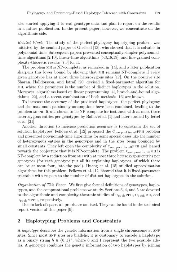
Phylogeny- and Parsimony-Based Haplotype Inference with Constraints 179
also started applying it to real genotype data and plan to report on the resultsin a future publication. In the present paper, however, we concentrate on thealgorithmic side.
Related Work. The study of the perfect-phylogeny haplotyping problem wasinitiated by the seminal paper of Gusfield [13], who showed that it is solvable inpolynomial time. Subsequent papers presented conceptually simpler polynomial-time algorithms [2,10], linear-time algorithms [5,3,18,19], and fine-grained com-plexity-theoretic results [7,8] for it.
The problem mh is NP-complete, as remarked in [14], and a later publicationsharpens this lower bound by showing that mh remains NP-complete if everygiven genotype has at most three heterozygous sites [17]. On the positive siteSharan, Halldorsson, and Istrail [20] devised a fixed-parameter algorithm formh, where the parameter is the number of distinct haplotypes in the solution.Moreover, algorithms based on linear programming [4], branch-and-bound algo-rithms [22], and a recent combination of both methods [16] are known.
To increase the accuracy of the predicted haplotypes, the perfect phylogenyand the maximum parsimony assumptions have been combined, leading to theproblem mpph. It was shown to be NP-complete for instances with at most threeheterozygous entries per genotypes by Bafna et al. [1] and later studied by Ierselet al. [21].
Another direction to increase prediction accuracy is to constrain the set ofsolution haplotypes: Fellows et al. [12] proposed the cone pool for allpph problemand presented polynomial-time algorithms for some special cases like the numberof heterozygous entries in the genotypes and in the sites being bounded bysmall constants. They left open the complexity of cone pool for allpph and leanedtowards the conjecture that it is NP-complete. The problem cone pool for allmh isNP-complete by a reduction from mh with at most three heterozygous entries pergenotypes (for each genotype put all its explaining haplotypes, of which therecan be at most four, into the pool). Huang et al. [15] studied approximationalgorithms for this problem, Fellows et al. [12] showed that it is fixed-parametertractable with respect to the number of distinct haplotypes in the solution.
Organization of This Paper. We first give formal definitions of genotypes, haplo-types, and the computational problems we study. Sections 3, 4, and 5 are devotedto the algorithmic and complexity-theoretic studies of cpoolspph, cpoolsmh, andcpoolsmpph, respectively.
Due to lack of space, all proofs are omitted. They can be found in the technicalreport version of this paper [9].
2 Haplotyping Problems and Constraints
A haplotype describes the genetic information from a single chromosome at snpsites. Since most snp sites are biallelic, it is customary to encode a haplotypeas a binary string h ∈ {0, 1}n, where 0 and 1 represent the two possible alle-les. A genotype combines the genetic information of two haplotypes by joining

180 M. Elberfeld and T. Tantau
their entries to a sequence of sets. Following common conventions, instead ofsets we write a 0 or a 1 when both underlying haplotypes have this value (theseentries are called homozygous) and use the value 2 when the underlying hap-lotypes have different entries (these entries are called heterozygous). A pair ofhaplotypes {h, h′} ⊆ {0, 1}n explains a genotype g ∈ {0, 1, 2}n if for every sites ∈ {1, . . . , n} we have g[s] = h[s] = h′[s] whenever g[s] ∈ {0, 1} and h[s] �= h′[s]whenever g[s] = 2. In a genotype matrix A each row is a genotype. If the matrixis clear from the context, we refer to the genotype in row i by gi. Similar, wearrange haplotypes in a haplotype matrix B and refer to the haplotype in row iby hi. A 2n × m haplotype matrix B explains an n × m genotype matrix A ifevery genotype gi is explained by the haplotype pair {h2i−1, h2i}. We use theterm site to refer to a position in genotypes and haplotypes and to a column ofgenotype and haplotype matrices.
For a pair s and t of sites the induced set ind(B, s, t) contains all strings from{00, 01, 10, 11} that appear in the sites s and t in the haplotype matrix B. We saythat these strings are induced by s and t. The notion of induces can be extendedto genotype matrices A: for two sites s and t the set ind(A, s, t) contains a stringxy ∈ {00, 01, 10, 11} if A has a genotype g with either g[s] = x ∧ g[t] = y org[s] = x ∧ g[t] = 2 or g[s] = 2 ∧ g[t] = y. This implies ind(A, s, t) ⊆ ind(B, s, t)for every haplotype matrix B explaining A.
A haplotype matrix B admits a perfect phylogeny if there exists a tree T (anundirected acyclic graph), such that: (a) Each haplotype from B labels exactlyone vertex of T ; (b) each site s ∈ {1, . . . , m} labels exactly one edge of T andeach edge is labeled by at least one site; and (c) for every two haplotypes hi
and hj from B and every site s ∈ {1, . . . , m}, we have hi[s] �= hj[s] if, and onlyif, s lies on the path from hi to hj in T . It is well-known that B admits a perfectphylogeny if, and only if, it satisfies the following four gamete property: for everypair of sites s and t we have {00, 01, 10, 11}�= ind(B, s, t).
For the three problems pph, mh, and mpph the input is always a genotypematrix plus, for the last two problems, a number k. The questions are whetherthere exists a haplotype matrix B that explains A and admits a perfect phylogeny(pph), has at most k different haplotypes (mh), or admits a perfect phylogenyand has at most k different haplotypes (mpph).
Constrained Haplotyping Problems. For constrained haplotyping problems dif-ferent kinds of constraints are specified along with the input genotype matrix.The first kind of constraints that we study are pool constraints. Let A be an n×mgenotype matrix. A pool constraint specifies that, in the output haplotype ma-trix, the two explaining haplotypes for some particular genotype gi should bothbe drawn from a pool Hi ⊆ {0, 1}n of allowed haplotypes. We write such aconstraint as pool(i, Hi). Clearly, it suffices to allow only one such constraintper genotype. Two pool constraints are incomparable if none of their pools is asubset of the other.
The second kind of constraints are restrictions on the phase of sites. For agenotype g with 2-entries in two sites s and t, the explaining haplotypes addeither {00, 11} or {01, 10} to the induced set. If there is another genotype g′

Phylogeny- and Parsimony-Based Haplotype Inference with Constraints 181
with 2-entries in the sites s and t, then, in order to satisfy the four gamete prop-erty, it must choose the same pair for its explaining haplotypes. In the first casewe say that s and t are phased equally, otherwise phased unequally. The con-straints “equal-phase(s, t)” and “unequal-phase(s, t)” specify that a particularphasing must be chosen for the two sites s and t in a solution matrix. Formally,a haplotype matrix B satisfies equal-phase(s, t) if {01, 10} �⊆ ind(B, s, t); andunequal-phase(s, t) if {00, 11} �⊆ ind(B, s, t).
We indicate constrained haplotyping problems by prefixing the haplotypingproblems mh, pph, and mpph with a c whose index indicates which constraintsare allowed to be specified as part of the input. The index “pools” means thatarbitrary pool constraints are allowed; “pools for all” indicates that (possiblydifferent) pools must be specified for all genotypes (and not only for some); and“one pool for all” indicates that, additionally, the same pool must be specifiedfor all genotypes. The index “phase” indicates that phase constraints are permis-sible. For example, cpools,phasempph is the mpph problem where both haplotypeand phase constraints are allowed as part of the input.
Haplotyping with phase constraints has not been defined formally in the lit-erature, but many known algorithms implicitly handle phase constraints:
Fact 2.1 ([2,10]). There exists an algorithm that, given an n × m genotypematrix with phase constraints, solves the problem cphasepph in time O(nm2).
3 Constrained Perfect Phylogeny Haplotyping
In this section we prove the following theorem, which answers the main questionof Fellows et al. [12] affirmatively: There is a polynomial-time algorithm forcone pool for allpph.
Theorem 3.1. There exists an algorithm that solves cpools,phasepph in timeO(p(n + p)m2), where the input genotype matrix has size n × m and p is thesum of the sizes of all pool constraints.
The outline of the algorithm for cpools,phasepph, which we detail in the rest ofthis section, is as follows: Given an n × m genotype matrix A and a set Kof pool and phase constraints, our algorithm uses procedure solve-cpph fromFigure 1 to preprocesses the input and to partition the genotypes into at most mmatrices As that can be solved independently. Each matrix As has the propertythat there is a site s, called the 2-site of As, that has 2-entries in all genotypesfrom As. Each As along with its corresponding constraints is then solved by theprocedure solve-cpph-2-site from Figure 1 via a recursive branch-and-reduceapproach: For each of the two possible phasings between the 2-site and anothersite, it branches recursively, derives new phase constraints, and splits the poolconstraints.
In the following we describe the four procedures that make up our algo-rithm: the two main procedures solve-cpph and solve-cpph-2-site, whosepseudo-code is depicted in Figure 1, and the simpler procedures sanitize-pool-constraints and deduce-phase-constraints for which no pseudo-code is

182 M. Elberfeld and T. Tantau
given. In the following, we say that a computational step has the correctnessproperty if the following holds: There exists a haplotype matrix that explains thegenotype matrix and satisfies the four gamete property and the constraints beforethe step if, and only, if this holds for the instance after the step. Furthermore,whenever the step outputs “no”, no solution exist for the current instance.
Procedure solve-cpph(A, K).Input: An n×m genotype matrix A and a set of constraints KOutput: An explaining haplotype matrix B for A that satisfies the four gameteproperty and the constraints K, if it exists; or “no”, otherwisePreprocessing:1 ensure that column pairs with different entries induce 002 sort columns decreasingly by leaf count3 update phase constraints with induces4 call deduce-phase-constraints5 call sanitize-pool-constraintsSolve independent subinstances:6 for each site s ∈ {1, . . . , m} do7 Bs ← call solve-cpph-2-site(As, Ks, s)8 if Bs is “no” then return “no”9 return combination of matrices Bs and genotypes without 2-entries
Procedure solve-cpph-2-site(A,K, s2).Input: An n×m genotype matrix A with 2-site s2 and a set of constraints KOutput: An explaining haplotype matrix B for A that satisfies the four gameteproperty and the constraints K, if it exists; or “no”, otherwiseRecursion break:1 if for every pool(i, Hi) ∈ K we have |Hi| = 2 then2 replace all pool constraints by corresponding phase constraints3 return solution for the resulting cphasepph instanceRecursive branch-and-reduce:4 else for each component G′ of Gcover with corresponding instance A′, K′ do5 s← some site from G′
6 B′e ← call try-phase-cpph(A′, K′ ∪ {equal-phase(s2, s)}, s2)
7 B′u ← call try-phase-cpph(A′, K′ ∪ {unequal-phase(s2, s)}, s2)
8 if B′e = B′
u = “no” then return “no” else add B′e or B′
u to solution9 return solution
Sub-Procedure try-phase-cpph(A,K, s2).1 call deduce-phase-constraints and sanitize-pool-constraints for A, K2 if pool(i, ∅) /∈ K for all i then return solve-cpph-2-site(A, K, s2)3 else return “no”
Fig. 1. The polynomial-time algorithm for cpools,phasepph
Procedure sanitize-pool-constraints. This procedure removes superfluoushaplotypes from pool constraints. Let K be a set of constraints. First, for aconstraint pool(i, Hi) ∈ K and a genotype gi, it removes all h from Hi for whichthere exists a site s such that h[s] �= gi[s] ∈ {0, 1}. Second, it deletes every

Phylogeny- and Parsimony-Based Haplotype Inference with Constraints 183
haplotype h from Hi for which there exists no other haplotype h′ ∈ Hi such that{h, h′} explains gi. Third, it deletes haplotypes contradicting phase constraints:For two sites s and t with gi[s] = gi[t] = 2, it deletes h from Hi wheneverh[s] = h[t] ∧ unequal-phase(s, t) ∈ K or h[s] �= h[t] ∧ equal-phase(s, t) ∈ K.Finally, if a pool constraint becomes empty, it outputs “no.” Clearly, this stephas the correctness property.
Procedure deduce-phase-constraints. Let A be a genotype matrix and K aset of constraints. The procedure repeats the following rule as long as possible:Let s, t and u be three sites such that there is a genotype gi with gi[s] =gi[t] = gi[u] = 2 and there is no phase constraint for the pair t and u, butphase constraints for both pairs s and t, and s and u. If these phase constraintshave the same type, we insert equal-phase(t, u) into K and, if their type isdifferent, we insert unequal-phase(t, u) into K. Using graph representations forphase constraints and their dependencies, the result of this procedure can becomputed in time O(nm2) [2,10].
Lemma 3.2. deduce-phase-constraints has the correctness property.
Procedure solve-cpph. The pseudo-code of this procedure is shown in Figure 1.We go over this method line by line.
The first five lines preprocess the input. Line 1 extends an idea from Eskin,Halperin and Karp [10] to constraints. For every site s we iterate downwardsthrough the genotypes and if a 1-entry appears before a 0-entry, we substituteall 1-entries by 0-entries and vice versa and adjust the constraints accordingly.As shown in [10], this step ensures that any two sites with at least one differententry induce 00. In line 2 the procedure first calculates the leaf count [13] of eachcolumn, which is the number of 2-entries of a column plus twice the number ofits 1-entries. Then it sorts the columns decreasingly from left to right by thisvalue. After this sorting we have 10 ∈ ind(A, s, t) for every two sites s and t withdifferent entries and s < t. This holds since otherwise there is no genotype withg[s] = 1 ∧ g[t] ∈ {0, 2} or g[s] = 2 ∧ g[t] = 0, but at least one genotype withg[s] ∈ {0, 2} ∧ g[t] = 1 or g[s] = 0 ∧ g[t] = 2. This would imply that the leafcount of site t should be greater than the leaf count of site s, a contradiction.In line 3 the algorithm considers all pairs of sites s and t and updates theirphase constraints as follows: If {00, 11} ⊆ ind(A, s, t), it inserts equal-phase(s, t)into K; and if {01, 01} ⊆ ind(A, s, t), it inserts unequal-phase(s, t). This stephas the correctness property since the new phase constraints reflect only inducesthat are already in the matrix. Finally, lines 4 and 5 deduce phase constraintsand sanitize the pool constraints. In the following, we call a matrix that hasundergone the preprocessing from lines 1 to 5 a preprocessed genotype matrix.
In lines 6 to 8 the genotype matrix A is partitioned genotype-wise into msubmatrices A1, . . . , Am, one matrix for each site. A genotype g belongs to thematrix As if g[s] = 2 and for every site t < s we have g[t] �= 2. Each As is passedalong with the corresponding pool constraint and all phase constraints, storedin the set Ks, to a call of the procedure solve-cpph-2-site. The construction

184 M. Elberfeld and T. Tantau
of As ensures that site s has 2-entries in all genotypes from As. The effect of thepartition is stated by the following lemma:
Lemma 3.3. Let A be a preprocessed n×m genotype matrix with constraints K.Then there exists an explaining haplotype matrix B for A that satisfies thefour gamete property and the constraints K if, and only if, for every site s ∈{1, . . . , m} there exists an explaining haplotype matrix Bs for As that satisfiesthe four gamete property and the constraints Ks.
Putting it altogether, solve-cpph correctly solves cpools,phasepph, provided thatthe procedure solve-cpph-2-site is correct, which we prove next.
Procedure solve-cpph-2-site. This procedure recursively solves the instancesthat are produced by solve-cpph, each consisting of a genotype matrix A witha 2-site s2 and constraints K. The recursion stops when all pool constraintscontain only two haplotypes (they must contain at least two haplotypes be-cause a 2-entry is present in the genotype). In such a case the phasing of thegenotype is completely known. We remove the pool constraints and, instead,add phase constraints that describe this particular phasing: For each constraintpool(i, {h, h′}) and sites s and t add the phase constraint equal-phase(s, t) ifh[s] = h[t] �= h′[s] = h′[t] and unequal-phase(s, t) if h[s] = h′[t] �= h[t] = h′[s].The resulting instance of cphasepph can be solved in polynomial time by Fact 2.1.
To describe the recursive step, we need some terminology. Let geno2(s) bethe set of A’s genotypes that have a 2-entry at site s. Let Sfree be the set ofsites s of A where s �= s2 and there is no phase constraint for s and s2 in K.Let Scover be the set of sites s ∈ Sfree for which there is no site s′ ∈ Sfree withgeno2(s) ⊆ geno2(s′); in the case that sites from Sfree have the same set of 2-entries, we choose exactly one of them to be contained in Scover. Note that whena genotype from A has a 2-entry in a site from Sfree, then it also has a 2-entrya site from Scover. Let Gcover be the graph that has Scover as its vertex set andan edge between sites s and s′ if geno2(s)∩ geno2(s
′) �= ∅. Whenever there is anedge between sites in Gcover, then there exists a phase constraint for them.
In the recursive step the algorithm iterates over the components G′ of Gcover
and considers the submatrix A′ of A made up by all genotypes with 2-entries insites of G′ along with a constraints set K ′, consisting of the pool constraints forthe genotypes from A′ and all phase constraints. It chooses a site s from G′ andadds once the constraint equal-phase(s2, s) and once unequal-phase(s2, s) to theset of constraints. In each case, it checks which additional phase constraints arenow triggered using the sub-procedure try-phase-cpph. This sub-procedurecalls deduce-phase-constraints followed by sanitize-pool-constraintsand tries to solve the resulting instance recursively by calling solve-cpph-2-site. If for all components a recursive call returns a solution, the procedurecombines them along with haplotypes for genotypes that are not in any matrix A′
to a solution for the whole instance. The following lemma states the correctnessof solve-cpph-2-site:
Lemma 3.4. Let A be a preprocessed n × m genotype matrix with 2-site s2
and constraints K. Then solve-cpph-2-site returns a haplotype matrix B that

Phylogeny- and Parsimony-Based Haplotype Inference with Constraints 185
explains A and satisfies the four gamete property and the constraints K, if itexists, or “no”, otherwise.
Runtime. The input to the algorithm consists of a genotype matrix of dimensionn×m, phase constraints and pool constraints. Let p equal the sum of the sizes ofall pool constraints. We show that the runtime is O(p(n + p)m2), as claimed inTheorem 3.1. All individual operations of the algorithm take time at most O((n+p)m2). Thus, it suffice to show that the tree of recursive calls of procedure solve-cpph-2-site has at most p leafs: The procedure partitions its input matrix intosubmatrices with constraints. For every submatrix A′ with constraints K ′ it maybranch into two possible phasings for the sites s2 and s. The call of deduce-phase-constraints ensures that there are phase constraints between s2 andall sites from G′: when two sites are connected via an edge in Gcover, we knowthat there is a phase constraint for them and a genotype that contains 2-entriesin these sites and s2. Note that the phases between s2 and the sites from G′
for the case equal-phase(s2, s) are exactly opposite to the phases for the caseunequal-phase(s2, s). This implies that, since all genotypes in A′ have a 2-entryin s2 and a site from G′, every haplotype from the pool constraints is passed toat most one recursive call. This yields a partition of sets of haplotypes from thepool constraints among all recursive calls. Since the procedure stops when thesizes of the pools drop to two (or zero), the number of leafs of the recursive treeof procedure solve-cpph-2-site is bounded by p + 1.
We remark that we have implemented the algorithm in Java and applied itto laboratory data. Our prototypical implementation handles typical real-datainputs in a matter of seconds on a standard machine.
4 Constrained Maximum Parsimony Haplotyping
In this section, we present two results on the fixed-parameter tractability (see [6]for background in parametrized complexity theory) of the constrained maximumparsimony haplotyping problem. First, we prove that cpools for allmh is W[2]-complete when parametrized by the minimum number of distinct haplotypesin an explaining haplotype matrix. In sharp contrast, mh and cone pool for allmhare fixed-parameter tractable for this parameter, as shown in [20] and [12], re-spectively. This means that the possibility to specify pool constraints on a per-genotype basis vastly increases the complexity of the problem. Second, we showthat a fixed-parameter algorithm is possible even for cpoolsmh when we extendthe parameter to the number of distinct haplotypes plus the number of dupli-cated genotypes that have incomparable pools.
The algorithms for mh and cone pool for allmh from the literature use datastructures that describe how haplotypes are shared among genotypes. Given ann×m genotype matrix A, we define a haplotype sharing plan P for A of size k asa multigraph G = (V, E) (a graph with multiple edges between the same vertices)with |V | = k and |E| = n where (a) edges are labeled bijectively by genotypesfrom A, (b) some vertices are labeled by haplotypes, and (c) every genotype that

186 M. Elberfeld and T. Tantau
has two labeled incident vertices is explained by the haplotype labels. We calla plan complete if all vertices are labeled and empty if no vertex is labeled. Aplan P extends a plan P ′ if P arises from P ′ by labeling previously unlabeledvertices. A haplotype sharing plan P satisfies a pool constraint pool(i, Hi) if theincident haplotypes of gi lie in Hi. With this definition, constructing haplotypematrices with at most k distinct haplotypes is equivalent to constructing plansof at most size k.
Given a budget k for the number of distinct haplotypes in the solution, theknown fixed-parameter algorithms for mh and cone pool for allmh consider all pos-sible empty haplotype sharing plans of size k and check whether they can be ex-tended to complete ones in polynomial time, using GF[2] equations for mh [20]and dynamic-programming for cone pool for allmh [12]. To bound the number ofedges of the plan they use a preprocessing step that deletes duplicated genotypesand retains only one of them. Since k haplotypes can explain at most k(k−1)/2different genotypes, these algorithms consider at most O(k2n) ≤ O(k2k2
) differ-ent empty plans.
These ideas cannot be extended to a fixed-parameter algorithm when geno-type-specific pool constraints are given since we cannot delete duplicated geno-types in a preprocessing step. This is due to the fact that genotypes mighthave the same entries, but incomparable pools, which we cannot merge directly.Strong evidence that no slightly variation of the standard approaches will workis given by Theorem 4.1.
Theorem 4.1. cpools for allmh, parametrized by the number of distinct haplo-types in the solution, is W[2]-complete. Consequently, cpoolsmh is W[2]-hard forthe same parametrization.
The instances constructed in the W[2]-hardness proof of cpools for allmh containonly identical genotypes, namely completely heterozygous genotypes, while poolsmight be highly incomparable. Since such a worst case instance is unlikely to bepresent in practice, we propose to additionally parametrize the problem by themaximum number l of duplicated genotypes with pairwise incomparable poolconstraints. When parametrized by the number k of distinct haplotypes and atthe same time by l, cpoolsmh becomes fixed-parameter tractable.
Theorem 4.2. cpoolsmh is fixed-parameter tractable with respect to the num-ber of distinct haplotypes that are used in an explaining haplotype matrix plusthe maximum number of duplicated genotypes with pairwise incomparable poolconstraints.
The algorithm (Figure 2 shows pseudo-code) first preprocesses the instance, suchthat at most l genotypes have the same entries. Then it iterates over at mostO(k2n) ≤ O(klk2
) empty plans. After an initial check of whether a plan can beextended to a complete one without constraints, the algorithm considers everycomponent of the plan independently. If a component contains genotypes havingpool constraints, it picks one of these genotypes and an incident vertex andtries all assignments of permissible pool haplotypes to the vertex. A haplotype

Phylogeny- and Parsimony-Based Haplotype Inference with Constraints 187
Procedure solve-cmh(A,K, k).Input: An n×m genotype matrix A, pool constraints K and a budget k.Output: An explaining haplotype matrix B for A with at most k distinct haplotypesthat satisfies the constraints K, if it exists; or “no”, otherwise.Preprocessing :1 call sanitize-pool-constraints2 for each gi and gj with gi = gj do3 if there is no pool constraint for gj ,
or pool(i, Hi) ∈ K, pool(j, Hj) ∈ K, Hi ⊆ Hj then4 delete gj
5 if there are more than lk(k − 1)/2 genotypes then output “no”Try to extend empty haplotype sharing plans:6 for each empty haplotype sharing plan P of size k do7 if P cannot be extended to a complete plan then skip P8 for each component P ′ of P do9 if there is a genotype gi in P ′ with pool(i, Hi) ∈ K then10 v ← some vertex incident to gi
11 for each haplotype h ∈ Hi that is permissible for v in P do12 P ′′ ← P ′; label v with h in P ′′ and calculate haplotypes for all vertices13 if P ′′ is a haplotype sharing plan satisfying its pool constraints then14 store P ′′ as a solution for P ′ and continue with next P ′
15 skip P16 else choose a permissible haplotype for one vertex from P ′,
calculate haplotypes for all other vertices, and store the solution P ′′
17 combine all P ′′ to a plan for A and K and return combined plan18 output “no”
Fig. 2. The fixed-parameter algorithm for cpoolsmh
is permissible for a vertex in a plan if there exists an extending complete planwith the vertex labeled by this haplotype. Conversely, its assignment directlydetermines haplotypes for all other vertices in the component and it remains tocheck that these haplotypes satisfy the other pool constraints. For componentswithout constraints, an assignment of haplotypes is always possible, due to line 7.Since the inner part of the main loop needs only polynomial time, this gives thedesired fixed-parameter runtime.
5 Constrained Maximum ParsimonyPerfect Phylogeny Haplotyping
We show that cpools,phasempph and, therefore, mpph and cone pool for allmpph,are fixed-parameter tractable with respect to the number of distinct haplotypesin the solution.
Theorem 5.1. cpools,phasempph is fixed-parameter tractable with respect to thenumber of distinct haplotypes in the solution.
We prove the theorem by combining the recursive branch-and-reduce techniquefrom Section 3 with haplotype sharing plans, which control the size of solutions.

188 M. Elberfeld and T. Tantau
The algorithm first ensures that the input contains no duplicate genotypes. Thenit iterates over at most O(k2n) ≤ O(k2k2
) empty plans. In every iteration itcomputes the partition from solve-cpph and solves the matrices independently.For this, it also decomposes the current plan such that a subplan is made upby the edges from the genotypes of its corresponding submatrix. To ensure thatdifferent instances are not related through vertices in the plan, the algorithmlabels all vertices that are incident to genotypes from different submatrices withhaplotypes. In the second main part, a recursive branch-and-reduce procedure,instances are partitioned such that the different parts are neither related throughthe matrix nor through the plan. For each part, similar to procedure solve-cpph-2-site, the algorithm branches into different phases between two columns.After labeling some vertices in the plan and sanitizing pool constraints, thealgorithm solves completely independent matrices recursively. The iteration overat most O(k2k2
) plans and the polynomial-time recursion give the desired fixed-parameter runtime.
6 Conclusion
We studied phylogeny- and parsimony-based haplotype inference in the pres-ence of pool and phase constraints. Our main result is that cpools,phasepph ispolynomial-time solvable by a new recursive decomposition technique for geno-types and pools. This solves the question from [12] whether cone pool for allpph ispolynomial-time solvable. Our Java implementation of this algorithm shows thatit works fast in practice. We showed that cpoolsmh is W[2]-hard by proving thatcpools for allmh is W[2]-complete when parametrized by the number of distincthaplotypes in the solution. Both problems are fixed-parameter tractable whenwe also use the comparability of the pools as a parameter. For cpools,phasempphwe presented an algorithm that extends the recursive decomposition of geno-types and pools by a decomposition of haplotype sharing plans, yielding a fixed-parameter algorithm for cpools,phasempph with respect to the number of distincthaplotypes in the solution.
For future work one research direction would be to incorporate more generalconstraints, like, for example, ∗-constraints where some entries in the haplotypescan be chosen freely. We may also try to allow a few additional rare haplotypesto be used that are not in any pool. A second direction would be to adjust theideas to algorithms that work on incomplete data.
References
1. Bafna, V., Gusfield, D., Hannenhalli, S., Yooseph, S.: A note on efficient computa-tion of haplotypes via perfect phylogeny. J. Comput. Biol. 11(5), 858–866 (2004)
2. Bafna, V., Gusfield, D., Lancia, G., Yooseph, S.: Haplotyping as perfect phylogeny:A direct approach. J. of Comput. Biol. 10(3–4), 323–340 (2003)
3. Bonizzoni, P.: A linear-time algorithm for the perfect phylogeny haplotype problem.Algorithmica 48(3), 267–285 (2007)

Phylogeny- and Parsimony-Based Haplotype Inference with Constraints 189
4. Brown, D.G., Harrower, I.M.: Integer programming approaches to haplotype infer-ence by pure parsimony. IEEE/ACM T. on Comput. Biol. and Bioinf. 3(2), 141–154(2006)
5. Ding, Z., Filkov, V., Gusfield, D.: A linear-time algorithm for the perfect phylogenyhaplotyping (PPH) problem. J. Comput. Biol. 13(2), 522–553 (2006)
6. Downey, R.G., Fellows, M.R.: Parameterized Complexity. Springer, New York(1999)
7. Elberfeld, M.: Perfect phylogeny haplotyping is complete for logspace. ComputingResearch Repository (CoRR), abs/0905.0602 (2009)
8. Elberfeld, M., Tantau, T.: Computational complexity of perfect-phylogeny-relatedhaplotyping problems. In: Ochmanski, E., Tyszkiewicz, J. (eds.) MFCS 2008.LNCS, vol. 5162, pp. 299–310. Springer, Heidelberg (2008)
9. Elberfeld, M., Tantau, T.: Phylogeny- and parsimony-based haplotype infer-ence with constraints. Technical Report SIIM-TR-A-10-01, Universitat zu Lubeck(2010)
10. Eskin, E., Halperin, E., Karp, R.M.: Efficient reconstruction of haplotype structurevia perfect phylogeny. J. Bioinf. and Comput. Biol. 1(1), 1–20 (2003)
11. Excoffier, L., Slatkin, M.: Maximum-likelihood estimation of molecular haplotypefrequencies in a diploid population. Mol. Biol. and Evol. 12(5), 921–927 (1995)
12. Fellows, M.R., Hartman, T., Hermelin, D., Landau, G.M., Rosamond, F.A.,Rozenberg, L.: Haplotype inference constrained by plausible haplotype data. In:Kucherov, G., Ukkonen, E. (eds.) CPM 2009. LNCS, vol. 5577, pp. 339–352.Springer, Heidelberg (2009)
13. Gusfield, D.: Haplotyping as perfect phylogeny: Conceptual framework and efficientsolutions. In: Proc. of RECOMB 2002, pp. 166–175. ACM Press, New York (2002)
14. Gusfield, D.: Haplotype inference by pure parsimony. In: Baeza-Yates, R., Chavez,E., Crochemore, M. (eds.) CPM 2003. LNCS, vol. 2676, pp. 144–155. Springer,Heidelberg (2003)
15. Huang, Y.-T., Chao, K.-M., Chen, T.: An approximation algorithm for haplotypeinference by maximum parsimony. J. Comput. Biol. 12(10), 1261–1274 (2005)
16. Jager, G., Climer, S., Zhang, W.: Complete parsimony haplotype inference prob-lem and algorithms. In: Fiat, A., Sanders, P. (eds.) ESA 2009. LNCS, vol. 5757,pp. 337–348. Springer, Heidelberg (2009)
17. Lancia, G., Pinotti, M.C., Rizzi, R.: Haplotyping populations by pure parsi-mony: Complexity of exact and approximation algorithms. INFORMS J. on Com-put. 16(4), 348–359 (2004)
18. Liu, Y., Zhang, C.-Q.: A linear solution for haplotype perfect phylogeny prob-lem. In: Proc. Int. Conf. Adv. in Bioinf. and Appl., pp. 173–184. World Scientific,Singapore (2005)
19. Satya, R.V., Mukherjee, A.: An optimal algorithm for perfect phylogeny haplotyp-ing. J. Comput. Biol. 13(4), 897–928 (2006)
20. Sharan, R., Halldorsson, B.V., Istrail, S.: Islands of tractability for parsimony hap-lotyping. IEEE/ACM T. Comput. Biol. and Bioinf. 3(3), 303–311 (2006)
21. van Iersel, L., Keijsper, J., Kelk, S., Stougie, L.: Shorelines of islands of tractability:Algorithms for parsimony and minimum perfect phylogeny haplotyping problems.IEEE/ACM T. Comput. Biol. and Bioinf. 5(2), 301–312 (2008)
22. Wang, L., Xu, Y.: Haplotype inference by maximum parsimony. Bioinformat-ics 19(14), 1773–1780 (2003)

Faster Computation of the Robinson-Foulds
Distance between Phylogenetic Networks
Tetsuo Asano1, Jesper Jansson2, Kunihiko Sadakane3,Ryuhei Uehara1, and Gabriel Valiente4
1 School of Information Science, Japan Advanced Institute of Science andTechnology, Ishikawa 923-1292, Japan
{t-asano,uehara}@jaist.ac.jp2 Ochanomizu University, 2-1-1 Otsuka, Bunkyo-ku, Tokyo 112-8610, Japan
[email protected] National Institute of Informatics, Hitotsubashi 2-1-2, Chiyoda-ku, Tokyo 101-8430,
4 Algorithms, Bioinformatics, Complexity and Formal Methods Research Group,Technical University of Catalonia, E-08034 Barcelona, Spain
Abstract. The Robinson-Foulds distance, which is the most widely usedmetric for comparing phylogenetic trees, has recently been generalizedto phylogenetic networks. Given two networks N1, N2 with n leaves, mnodes, and e edges, the Robinson-Foulds distance measures the numberof clusters of descendant leaves that are not shared by N1 and N2. Thefastest known algorithm for computing the Robinson-Foulds distancebetween those networks runs in O(m(m + e)) time. In this paper, weimprove the time complexity to O(n(m + e)/ log n) for general networksand O(n m/ log n) for general networks with bounded degree, and tooptimal O(m + e) time for planar phylogenetic networks and bounded-level phylogenetic networks. We also introduce the natural concept of theminimum spread of a phylogenetic network and show how the runningtime of our new algorithm depends on this parameter. As an example,we prove that the minimum spread of a level-k phylogenetic network isat most k + 1, which implies that for two level-k phylogenetic networks,our algorithm runs in O((k + 1)(m + e)) time.
1 Introduction
The Robinson-Foulds distance, introduced in [17], has been the most widelyused metric over almost three decades for comparing phylogenetic trees. How-ever, it is now known that the evolutionary history of life cannot be properlyrepresented as a phylogenetic tree [7], and phylogenetic networks have emergedas the representation of choice for incorporating reticulate evolutionary events,like recombination, hybridization, or lateral gene transfer, in an evolutionaryhistory [16].
A. Amir and L. Parida (Eds.): CPM 2010, LNCS 6129, pp. 190–201, 2010.c© Springer-Verlag Berlin Heidelberg 2010

Faster Computation of the Robinson-Foulds Distance 191
Phylogenetic networks are directed acyclic graphs with tree nodes (those withat most one parent) corresponding to point mutation events and hybrid nodes(with more than one parent) corresponding to hybrid speciation events. As inthe case of phylogenetic trees, the leaves are distinctly labeled by a set of ex-tant species. Additional conditions are usually imposed on these directed acyclicgraphs to narrow down the output space of reconstruction algorithms [13,14] orto provide a realistic model of recombination [19,20].
Two such additional conditions are especially relevant to the Robinson-Fouldsdistance. A phylogenetic network is time consistent when it has a temporalrepresentation [1], that is, an assignment of discrete time stamps to the nodesthat increases from parents to tree children and remains the same from parentsto hybrid children, meaning that the parents of each hybrid node coexist intime and thus, the corresponding reticulate evolutionary event can take place.A phylogenetic network is tree-child when every internal node has at least onetree child [4], meaning that every non-extant species has some extant descendantthrough mutation alone.
The Robinson-Foulds distance between two phylogenetic networks is definedas the cardinality of the symmetric difference between their two sets of all in-duced clusters (where the cluster induced by a node v in a phylogenetic networkis the set of all descendant leaves of v in the network) divided by two, and thusit measures the number of clusters not shared by the networks. It is a metric onthe space of all tree-child time-consistent phylogenetic networks [4, Cor. 1], andit generalizes the Robinson-Foulds distance between rooted phylogenetic trees.Clearly, the Robinson-Foulds distance requires computing the cluster represen-tation of the networks, that is, the set of descendant leaves for each node inthe networks. While there are improved algorithms for computing the clusterrepresentation of a phylogenetic tree [6,15,21,22], the only known algorithm forcomputing the cluster representation of a phylogenetic network [3] is based onbreadth-first searching descendant leaves from each of the nodes in turn, andtakes O(m(m + e)) time using O(n m) space on phylogenetic networks with nleaves, m nodes, and e edges.
In this paper, we present a faster algorithm for computing the Robinson-Foulds distance between two input phylogenetic networks. For general phyloge-netic networks, we first improve the time complexity by following an approachsimilar in spirit to the algorithm proposed in [4] for computing the path multiplic-ity representation of a phylogenetic network; by using a compressed representa-tion of the characteristic vectors, we obtain a simple algorithm for computing theRobinson-Foulds distance between phylogenetic networks in O(n(m + e)/ log n)time using O(n m/ log n) space, assuming a word size of ω = �log n� bits; see [12].For phylogenetic networks of bounded degree, this becomes O(n m/ log n) timeand space.
In the case of level-k phylogenetic networks [5], we further improve the timecomplexity by using a more succinct representation of a cluster of descendantleaves as an interval of consecutive integers, which allows us to compute the Robin-son-Foulds distance in O((k+1)(m+e)) time. For this purpose, we introduce what

192 T. Asano et al.
we call the minimum spread of a phylogenetic network, and prove that every level-k network has minimum spread at most k + 1. For special cases of bounded-levelphylogenetic networks such as planar phylogenetic networks, in particular outer-labeled planar split networks [2,8] and galled-trees [10,11], we show that the min-imum spread is 1, which means that our algorithm can be implemented to run inoptimal O(m + e) time.
The paper is organized as follows. Section 2 introduces some notation andexplains the naive representation of clusters. Section 3 describes more efficientways to represent the clusters both for general networks and for planar andlevel-k networks, and defines the minimum spread of a phylogenetic network. Abottom-up algorithm for computing the Robinson-Foulds distance is presentedin Section 4 that takes advantage of the cluster representation. Finally, someconclusions are drawn in Section 5.
2 Preliminaries
Let N = (V, E) be a given phylogenetic network with n leaves, m nodes, ande edges. For any nodes u, v ∈ V , we say that v is a descendant of u if v isreachable from u in N . (Here, any node is considered to be a descendant ofitself.) For every v ∈ V , define C[v] as the set of all leaves which are descendantsof v. The set C[v] is called the cluster of v, and the collection {C[v] | v ∈ V } iscalled the naive cluster representation of N .
The naive cluster representation of N can be computed in O(m(m + e)) timeand O(n m) space by breadth-first searching descendant leaves from each ofthe nodes of N in turn [3]. A significant improvement in time complexity canbe achieved by replacing the m top-down searches by n bottom-up searches,because m can be arbitrarily large for a phylogenetic network with n leaves and,even in the particular case of a tree-child time-consistent phylogenetic network,m � (n + 4)(n− 1)/2, and this bound is tight [3, Prop. 1]. The following lemmais the basis of such an improvement.
Lemma 1. Let v ∈ V be a node of a phylogenetic network N = (V, E). Then,C[v] = {v} if v is a leaf, and C[v] = C[v1] ∪ · · · ∪ C[vk] if v is an internal nodewith children {v1, . . . , vk}.Proof. The only (trivial) descendant of a leaf in a phylogenetic network is the leafitself. The paths from an internal node to the leaves of a phylogenetic networkare the paths from the children of the internal node to the leaves. ��Lemma 1 suggests a simple bottom-up algorithm (Algorithm 1) for computingthe naive cluster representation of N in polynomial time. In the following de-scription, the cluster C[v] of each node v in N is computed during a bottom-uptraversal of N , with the help of an (initially empty) queue Q of nodes. The clus-ter C[v] of each child v of an internal node u is joined in turn to the (initiallyempty) cluster C[u] of the parent node u.

Faster Computation of the Robinson-Foulds Distance 193
Algorithm 1. Compute the naive cluster representation C of a phylogenetic network N
procedure naive cluster representation(N,C)for each node v of N do
if v is a leaf thenC[v] ← {label(v)}enqueue(Q, v)
elseC[v] ← ∅
while Q is not empty dov ← dequeue(Q)mark node v as visitedfor each parent u of node v do
C[u] ← C[u] ∪ C[v]if all children of u are visited then
enqueue(Q, u)
Lemma 2. Let N be a phylogenetic network with n leaves, m nodes, and e edges.The naive cluster representation of N can be computed in O(n(m+e)) time usingO(n m) space.
Proof. Each node is enqueued and dequeued only once, and each parent of eachdequeued node v is visited only once from v. The union of two subsets of an nelement set, which takes O(n) time, is computed O(m + e) times. ��
3 More Efficient Cluster Representation
3.1 Characteristic Vector Representation
A leaf numbering function is a bijection from the set of leaves in N to theset {1, 2, . . . , n}. For any leaf numbering function f and node v ∈ V , the char-acteristic vector for v under f , denoted by Cf [v], is a bit vector of length nsuch that for any i ∈ {1, 2, . . . , n}, the ith bit equals 1 if and only if f−1(i) is adescendant of v in N . Note that Cf [r] = 111 . . .1 for the root r of N , and thatCf [�] contains exactly one 1 for any leaf � of N .
Example 1. Consider the phylogenetic network in Figure 1. Number the leavesaccording to the circular ordering v2, v20, v27, v28, v34, v45, v42, v43, v46, v47, v10,v22, v23, v36, v37, v33, v12, v18, v25, v26, v14 along the outer face. This correspondsto a depth-first search of the directed spanning tree obtained by removing oneincoming edge (shown in red in Figure 1) for each node of in-degree 2 in thenetwork, and it yields the characteristic vectors listed in Table 1. ��

194 T. Asano et al.
v1
v2 v3
v4 v5
v6 v7 v8
v9 v10 v11 v12 v13 v14
v15 v16 v17 v18 v19
v20 v21 v22 v23 v24 v25 v26
v27 v28 v29 v30
v31 v32 v33
v34 v35 v36 v37
v38
v39 v40
v41 v42 v43 v44
v45 v46 v47
Fig. 1. An example of a phylogenetic network based on real data, adapted from [23].This is the smallest level-2 phylogenetic network consistent with 1,330 rooted tripletsof sequences from different isolates of the yeast Cryptococcus gattii.
Obviously, the characteristic vector representation of all clusters in N can bestored explicitly using a total of m n bits and can be constructed in O(n(m+e))time by an algorithm analogous to Algorithm 1. Our next goal is to find suitableleaf numbering functions for different types of phylogenetic networks which leadto more compact ways of storing the characteristic vectors as well as fasterways of computing them. We first consider arbitrary leaf numbering functions,and then study leaf numbering functions for some important special classes ofphylogenetic networks.
3.2 Compressed Characteristic Vector Representation
Fix any arbitrary leaf numbering function f for the given phylogenetic net-work N . The time complexity of Algorithm 1 can be improved by employing acharacteristic vector of size n to encode each cluster, packing the characteristicvector of a subset of the n leaves into O(n/ log n) integers (assuming a word

Faster Computation of the Robinson-Foulds Distance 195
Table 1. Characteristic vector representation of the clusters for the phylogenetic net-work in Figure 1
node characteristic vector of the clusterv2 v20 v27 v28 v34 v45 v42 v43 v46 v47 v10 v22 v23 v36 v37 v33 v12 v18 v25 v26 v14
v21 0 0 1 1 0 0 0 0 0 0 0 0 0 0 0 0 0 0 0 0 0v15 0 1 1 1 0 0 0 0 0 0 0 0 0 0 0 0 0 0 0 0 0v41 0 0 0 0 0 1 0 0 0 0 0 0 0 0 0 0 0 0 0 0 0v39 0 0 0 0 0 1 1 0 0 0 0 0 0 0 0 0 0 0 0 0 0v44 0 0 0 0 0 0 0 0 1 1 0 0 0 0 0 0 0 0 0 0 0v40 0 0 0 0 0 0 0 1 1 1 0 0 0 0 0 0 0 0 0 0 0v38 0 0 0 0 0 1 1 1 1 1 0 0 0 0 0 0 0 0 0 0 0v35 0 0 0 0 0 1 1 1 1 1 0 0 0 0 0 0 0 0 0 0 0v31 0 0 0 0 1 1 1 1 1 1 0 0 0 0 0 0 0 0 0 0 0v29 0 0 0 0 1 1 1 1 1 1 0 0 0 0 0 0 0 0 0 0 0v9 0 1 1 1 1 1 1 1 1 1 0 0 0 0 0 0 0 0 0 0 0v6 0 1 1 1 1 1 1 1 1 1 1 0 0 0 0 0 0 0 0 0 0v16 0 0 0 0 0 0 0 0 0 0 0 1 1 0 0 0 0 0 0 0 0v32 0 0 0 0 0 0 0 0 0 0 0 0 0 1 1 0 0 0 0 0 0v30 0 0 0 0 0 0 0 0 0 0 0 0 0 1 1 1 0 0 0 0 0v24 0 0 0 0 1 1 1 1 1 1 0 0 0 1 1 1 0 0 0 0 0v17 0 0 0 0 1 1 1 1 1 1 0 0 0 1 1 1 0 0 0 0 0v11 0 0 0 0 1 1 1 1 1 1 0 1 1 1 1 1 0 0 0 0 0v7 0 0 0 0 1 1 1 1 1 1 0 1 1 1 1 1 1 0 0 0 0v4 0 1 1 1 1 1 1 1 1 1 1 1 1 1 1 1 1 0 0 0 0v19 0 0 0 0 0 0 0 0 0 0 0 0 0 0 0 0 0 0 1 1 0v13 0 0 0 0 0 0 0 0 0 0 0 0 0 0 0 0 0 1 1 1 0v8 0 0 0 0 0 0 0 0 0 0 0 0 0 0 0 0 0 1 1 1 1v5 0 0 0 0 1 1 1 1 1 1 0 0 0 1 1 1 0 1 1 1 1v3 0 1 1 1 1 1 1 1 1 1 1 1 1 1 1 1 1 1 1 1 1v1 1 1 1 1 1 1 1 1 1 1 1 1 1 1 1 1 1 1 1 1 1
size of ω = �log n� bits), and computing the bitwise-OR of vectors instead ofperforming the set union operation. See [12] for further details about bit-levelparallelism.
The pseudocode for the improved version of Algorithm 1 is given in Algo-rithm 2, where x � t denotes the bitwise shift of an integer x to the left by t,and x | y denotes the bitwise OR of two integers x and y.
The improvement in time complexity of Algorithm 2 comes from bit-levelparallelism of the set union operations.
Lemma 3. Let N be a phylogenetic network with n leaves, m nodes, and eedges. The cluster representation of N can be computed in O(n(m + e)/ log n)time using O(n2 + n m/ logn) words.
Proof. There are 2log n = n bit vectors, and the bitwise-OR of all these ω-bitvectors takes O(n2) time. After this prepreprocessing, each node is enqueued anddequeued only once, and each parent of each dequeued node v is visited only oncefrom v. The union of two subsets of an n element set, which takes O(n/ log n)time as the bitwise-OR of �n/ω� ω-bit vectors, is computed O(m + e) times.
The bitwise-OR of all the ω-bit vectors is stored in O(n2) words, and thecluster representation is stored as a compact boolean table, with m rows andn/ logn columns. ��

196 T. Asano et al.
Algorithm 2. Compute the compressed cluster representation C of a phylogeneticnetwork N
procedure compressed cluster representation(N,C)n ← number of leaves of Nk ← �n/ω�for x ← 0, . . . , n − 1 do
for y ← 0, . . . , n − 1 doOR[x, y] ← x | y
for each node v of N doC1[v], . . . , Ck[v] ← 0if v is a leaf then
i ← �(f(v) − 1)/ω� + 1Ci[v] ← 1 ω · i − f(v)enqueue(Q, v)
while Q is not empty dov ← dequeue(Q)mark node v as visitedfor each parent u of node v do
for i ← 1, . . . , k doCi[u] ← OR[Ci[u], Ci[v]]
if all children of u are visited thenenqueue(Q, u)
3.3 Interval List Representation
A maximal consecutive sequence of 1’s in a bit vector is called an interval. For agiven leaf numbering function f and node v ∈ V , let If (v) denote the number ofintervals in Cf [v] and let the spread of f be If = maxv∈V If (v). The minimumspread of N is the minimum value of If , taken over all possible leaf numberingfunctions f .
Below, we first bound the minimum spread of certain types of phylogeneticnetworks, and then show more generally how the characteristic vectors of phylo-genetic networks having small minimum spread can be stored compactly. Fromhere on, we only consider phylogenetic networks in which each node has eitherat most one parent (tree node) or exactly two parents (hybrid node).
A phylogenetic network is planar if the underlying undirected graph is outer-labeled planar, that is, if it admits a non-crossing layout on the plane with all theleaves lying on the outer face. Planar phylogenetic networks arise for instancewhen representing conflicting phylogenetic signals, leading to the so-called outer-labeled planar split networks; see [2,9].

Faster Computation of the Robinson-Foulds Distance 197
Lemma 4. If N is a planar phylogenetic network then a leaf numbering func-tion f with If = 1 can be computed in O(m + e) time.
Proof. Fix any planar embedding of N and let f be the leaf numbering functionthat assigns the numbers 1, 2, . . . , n to the leaves in consecutive order along theouter face from the leftmost to the rightmost leaf. We claim that for every v ∈ V ,Cf [v] has a single interval. Since every leaf has a singleton cluster and the unionof two overlapping or neighboring intervals is a single interval, we need to showthat the children of any internal node have overlapping or neighboring clustersof descendant leaves.
Let v ∈ V be an internal node with children u, w ∈ V and assume C[u] ={h, . . . , i} and C[w] = {�, . . . , m} are intervals of descendant leaves with h �i < j � k < � � m but j, . . . , k /∈ C[v]. Then, any path from the root ofN to any of the leaves j, . . . , k will cross some edge along either a path fromv to i or a path from v to �, contradicting the assumption that N is planar.Therefore, j, . . . , k ∈ C[v] and the set {h, . . . , i, j, . . . , k, �, . . . , m} of descendantleaves forms one interval. ��Next, let U(N) denote the undirected graph obtained by replacing every directededge in N by an undirected edge. A biconnected component of an undirectedgraph is a connected subgraph that remains connected after removing any nodeand all edges incident to it; see [18]. Recall the following definition from [5].
Definition 1. A network N is called level-k phylogenetic network if, for everybiconnected component B in U(N), the subgraph of N induced by the set of nodesin B contains at most k nodes with indegree 2.
Corollary 1. If N is a level-1 phylogenetic network (that is, a galled-tree [10,11]),then a leaf numbering function f with If = 1 can be computed in O(m + e) time.
Proof. Since each biconnected component of N forms a cycle and all the cyclesin N are disjoint, the outside of an embedding of a cycle into a plane lies on theouter-plane. Then, it is obvious that If = 1. ��Lemma 5. If N is a level-k phylogenetic network then a leaf numbering func-tion f with If = k + 1 can be computed in O(m + e) time.
Proof. Fix any (directed) spanning tree T of N , and let f be the leaf numberingfunction obtained by doing a depth-first search of T starting at the root andassigning the numbers 1, 2, . . . , n to the leaves in the order that they are firstvisited. Clearly, this takes O(m + e) time.
We now prove that f has spread k +1. For any node v in V , define L(T [v]) asthe set of all leaves in the subtree of T rooted at v. The key observation is thatthe leaves in L(T [v]) must be visited consecutively by any depth-first search of T ,and thus form a single interval in Cf [v]. Next, let u be any node in V and let Hbe the set of hybrid nodes in N that belong to the same biconnected componentas u and which are descendants of u (in case u is not on any merge path thenH is the empty set). Then, the set of leaves that are descendants of u in N can

198 T. Asano et al.
Table 2. Interval list representation of the clusters for the phylogenetic network inFigure 1
node interval list
v21 (v27, v28)v15 (v20, v28)v41 (v45, v45)v39 (v45, v42)v44 (v46, v47)v40 (v43, v47)v38 (v45, v47)v35 (v45, v47)v31 (v34, v47)v29 (v34, v47)
node interval list
v9 (v20, v47)v6 (v20, v10)v16 (v22, v23)v32 (v36, v37)v16 (v22, v23)v32 (v36, v37)v30 (v36, v33)v24 (v34, v47), (v36, v33)v17 (v34, v47), (v36, v33)v11 (v34, v47), (v22, v33)
node interval list of the cluster
v7 (v34, v47), (v22, v12)v4 (v20, v12)v19 (v25, v26)v13 (v18, v26)v8 (v18, v14)v5 (v34, v47), (v36, v33), (v18, v14)v3 (v20, v14)v1 (v2, v14)
be written as L(T [u]) ∪ ⋃h∈H L(T [h]). N is a level-k phylogenetic network, so
|H | � k, which together with the key observation above implies that Cf [u] is theunion of at most k+1 intervals. It follows that If (u) � k+1 for every u ∈ V . ��
Example 2. Consider again the phylogenetic network in Figure 1. The leaf num-bering in Example 1 yields the interval lists listed in Table 2. The network islevel-2 and its spread corresponds to the 3 disjoint intervals (v34, v47), (v36, v33),(v18, v14) of node v5. ��Now, we consider how to store characteristic vectors under leaf numbering func-tions having small spread. An efficient approach is to store the starting andending positions of all intervals in sorted order. We call this representation theinterval list representation of the clusters. We immediately obtain the followingresult.
Lemma 6. Given any leaf numbering function f , the total space needed tostore all characteristic vectors under f using the interval list representation isO(If m log n) bits.
Proof. For each of the m nodes in N , the starting and ending positions of eachof its at most If intervals are stored in �2 log n� bits. ��Lemma 7. Given any leaf numbering function f , all descendant leaf bit vectorsunder f using the interval list representation can be computed in O(If (m + e))time.
Proof. Use Algorithm 1 but replace the union operation as follows. Let v be aninternal node with children u, w. Assuming that Cf [u] and Cf [w] are known,Cf [v] can be computed in O(If ) time by a straightforward algorithm which scansthe two sorted position lists for Cf [u] and Cf [w] and merges any intervals whichoverlap or are neighbors. ��
4 An Algorithm for Computing the Robinson-FouldsDistance
We now present an algorithm for computing the Robinson-Foulds distance be-tween two input phylogenetic networks N1, N2 (Algorithm 3).

Faster Computation of the Robinson-Foulds Distance 199
The algorithm first computes the clusters of N1 and N2 using any of thecluster representations described in the previous sections of this paper. Then,the cardinality of the symmetric difference of the two cluster representationsis obtained by radix sorting and simultaneous traversal techniques. Finally, thealgorithm outputs the Robinson-Foulds distance between N1 and N2.
Algorithm 3. Compute the Robinson-Foulds distance between two phylogenetic net-works N1, N2
function robinson foulds distance(N1, N2)cluster representation(N1, C1); radix sort C1
cluster representation(N2, C2); radix sort C2
m1,m2 ← number of nodes of N1, N2
i1 ← 1i2 ← 1c ← 0while i1 � m1 and i2 � m2 do
if C1[i1] < C2[i2] theni1 ← i1 + 1
else if C1[i1] > C2[i2] theni2 ← i2 + 1
elsei1 ← i1 + 1i2 ← i2 + 1c ← c + 1
return m1 + m2 − 2 · c
Theorem 1. Let N1, N2 be two phylogenetic networks with n leaves, m nodes,and e edges. The Robinson-Foulds distance between N1, N2 can be computed in:
– O(n(m + e)/ log n) time and O(n2 + n m/ logn) words for general networks,– O(n m/ log n) time and O(n2 + n m/ logn) words for general networks with
bounded degree,– O(m + e) time and O(m log n) bits for planar phylogenetic networks,– O((k+1)(m+e)) time and O(k m log n) bits for level-k phylogenetic networks.
Proof. Implement Algorithm 3 by applying Lemmas 3–7 to obtain the respectivecluster representations. The radix sort step and remaining operations can beperformed in O(m x) time, where x denotes the amount of space needed torepresent one cluster. ��

200 T. Asano et al.
5 Conclusion
We have presented a new and simple algorithm for computing the Robinson-Foulds distance between two phylogenetic networks. While the fastest knownalgorithm for computing the Robinson-Foulds distance between two phylogeneticnetworks with n leaves, m nodes, and e edges runs in O(m(m+e)) time, the newalgorithm takes advantage of bit-level parallelism and runs in O(n(m+e)/ log n)time on general networks, assuming a word size of ω = �log n� bits. In the case oflevel-k phylogenetic networks, we take advantage of the succinct representationof clusters as intervals of consecutive integers, and the new algorithm runs inO((k + 1)(m + e)) time.
We have also introduced a new parameter, the minimum spread of a phylo-genetic network, and proved that every level-k network has minimum spread atmost k + 1. For the particular case of bounded-level phylogenetic networks suchas planar phylogenetic networks, which include outer-labeled planar split net-works and galled-trees, we have shown that the minimum spread is 1, meaningthat the new algorithm can be implemented to run in optimal O(m + e) time.
Acknowledgment
JJ was supported by the Special Coordination Funds for Promoting Science andTechnology. TA, RU, GV were supported by the Spanish government and theEU FEDER program under project PCI2006-A7-0603.
References
1. Baroni, M., Semple, C., Steel, M.: Hybrids in real time. Syst. Biol. 55(1), 46–56(2006)
2. Bryant, D., Moulton, V.: Neighbor-Net: An agglomerative method for the con-struction of phylogenetic networks. Mol. Biol. Evol. 21(2), 255–265 (2004)
3. Cardona, G., Llabres, M., Rossello, F., Valiente, G.: Metrics for phylogenetic net-works I: Generalizations of the Robinson-Foulds metric. IEEE ACM T. Comput.Biol. 6(1), 1–16 (2009)
4. Cardona, G., Rossello, F., Valiente, G.: Comparison of tree-child phylogenetic net-works. IEEE ACM T. Comput. Biol. (2009)
5. Choy, C., Jansson, J., Sadakane, K., Sung, W.K.: Computing the maximum agree-ment of phylogenetic networks. Theor. Comput. Sci. 335(1), 93–107 (2005)
6. Day, W.H.E.: Optimal algorithms for comparing trees with labeled leaves. J. Clas-sif. 2(1), 7–28 (1985)
7. Doolittle, W.F.: Phylogenetic classification and the universal tree. Sci-ence 284(5423), 2124–2128 (1999)
8. Grunewald, S., Forslund, K., Dress, A., Moulton, V.: QNet: An agglomerativemethod for the construction of phylogenetic networks from weighted quartets. Mol.Biol. Evol. 24(2), 532–538 (2007)
9. Grunewald, S., Moulton, V., Spillner, A.: Consistency of the QNet algorithmfor generating planar split networks from weighted quartets. Discr. Appl.Math. 157(10), 2325–2334 (2009)

Faster Computation of the Robinson-Foulds Distance 201
10. Gusfield, D., Eddhu, S., Langley, C.: Efficient reconstruction of phylogenetic net-works with constrained recombination. In: Proc. 2nd IEEE Computer SocietyBioinformatics Conf., pp. 363–374 (2003)
11. Gusfield, D., Eddhu, S., Langley, C.H.: The fine structure of galls in phylogeneticnetworks. INFORMS J. Comput. 16(4), 459–469 (2004)
12. Hagerup, T.: Sorting and searching on the word RAM. In: Meinel, C., Morvan, M.(eds.) STACS 1998. LNCS, vol. 1373, pp. 366–398. Springer, Heidelberg (1998)
13. Jin, G., Nakhleh, L., Snir, S., Tuller, T.: Maximum likelihood of phylogenetic net-works. Bioinformatics 22(21), 2604–2611 (2006)
14. Jin, G., Nakhleh, L., Snir, S., Tuller, T.: Efficient parsimony-based methods forphylogenetic network reconstruction. Bioinformatics 23(2), 123–128 (2007)
15. Pattengale, N.D., Gottlieb, E.J., Moret, B.M.: Efficiently computing the Robinson-Foulds metric. J. Comput. Biol. 14(6), 724–735 (2007)
16. Posada, D., Crandall, K.A.: Intraspecific gene genealogies: Trees grafting into net-works. Trends Ecol. Evol. 16(1), 37–45 (2001)
17. Robinson, D.F., Foulds, L.R.: Comparison of phylogenetic trees. Math.Biosci. 53(1/2), 131–147 (1981)
18. Rossello, F., Valiente, G.: All that glisters is not galled. Math. Biosci. 221(1), 54–59(2009)
19. Strimmer, K., Moulton, V.: Likelihood analysis of phylogenetic networks usingdirected graphical models. Mol. Biol. Evol. 17(6), 875–881 (2000)
20. Strimmer, K., Wiuf, C., Moulton, V.: Recombination analysis using directed graph-ical models. Mol. Biol. Evol. 18(1), 97–99 (2001)
21. Sul, S.-J., Brammer, G., Williams, T.L.: Efficiently computing arbitrarily-sizedRobinson-Foulds distance matrices. In: Crandall, K.A., Lagergren, J. (eds.)WABI 2008. LNCS (LNBI), vol. 5251, pp. 123–134. Springer, Heidelberg (2008)
22. Sul, S.-J., Williams, T.L.: An experimental analysis of Robinson-Foulds distancematrix algorithms. In: Halperin, D., Mehlhorn, K. (eds.) Esa 2008. LNCS, vol. 5193,pp. 793–804. Springer, Heidelberg (2008)
23. van Iersel, L., Keijsper, J., Kelk, S., Stougie, L., Hagen, F., Boekhout, T.: Con-structing level-2 phylogenetic networks from triplets. IEEE ACM T. Comput.Biol. 6(4), 667–681 (2009)

Mod/Resc Parsimony Inference
Igor Nor1,2,�, Danny Hermelin3, Sylvain Charlat1, Jan Engelstadter4,Max Reuter5, Olivier Duron6, and Marie-France Sagot1,2,∗
1 Universite de Lyon, F-69000, Lyon, Universite Lyon 1, CNRS, UMR55582 Bamboo Team, INRIA Grenoble Rhone-Alpes, France
3 Max Planck Institute for Informatics, Saarbrucken - Germany4 Institute of Integrative Biology, ETH Zurich, Switzerland
5 University College London, UK6 Institute of Evolutionary Sciences, CNRS - University of Montpellier II, France
[email protected], [email protected]
Abstract. We address in this paper a new computational biology prob-lem that aims at understanding a mechanism that could potentially beused to genetically manipulate natural insect populations infected by in-herited, intra-cellular parasitic bacteria. In this problem, that we denoteby Mod/Resc Parsimony Inference, we are given a boolean matrixand the goal is to find two other boolean matrices with a minimum num-ber of columns such that an appropriately defined operation on thesematrices gives back the input. We show that this is formally equiva-lent to the Bipartite Biclique Edge Cover problem and derive somecomplexity results for our problem using this equivalence. We provide anew, fixed-parameter tractability approach for solving both that slightlyimproves upon a previously published algorithm for the Bipartite Bi-clique Edge Cover. Finally, we present experimental results where weapplied some of our techniques to a real-life data set.
Keywords: Computational biology, biclique edge covering, bipartitegraph, boolean matrix, NP-completeness, graph theory, fixed-parametertractability, kernelization.
1 Introduction
Wolbachia is a genus of inherited, intra-cellular bacteria that infect many arthro-pod species, including a significant proportion of insects. The bacterium was firstidentified in 1924 by M. Hertig and S. B. Wolbach in Culex pipiens, a species ofmosquito. Wolbachia spreads by altering the reproductive capabilities of its hosts[6]. One of these alterations consists in inducing so-called cytoplasmic incompat-ibility [7]. This phenomenon, in its simplest expression, results in the death ofembryos produced in crosses between males carrying the infection and uninfectedfemales. A more complex pattern is the death of embryos seen in crosses betweenmales and females carrying different Wolbachia strains. The study of Wolbachia
� Corresponding authors.
A. Amir and L. Parida (Eds.): CPM 2010, LNCS 6129, pp. 202–213, 2010.c© Springer-Verlag Berlin Heidelberg 2010

Mod/Resc Parsimony Inference 203
and cytoplasmic incompatibility is of interest due to the high incidence of suchinfections, amongst others in human disease vectors such as mosquitoes, wherecytoplasmic incompatibility could potentially be used as a driver mechanism forthe genetic manipulation of natural populations.
The molecular mechanisms underlying cytoplasmic incompatibility are cur-rently unknown, but the observations are consistent with a “toxin / antitoxin”model [16]. According to this model, the bacteria present in males modify thesperm (the so-called modification, or mod factor) by depositing a “toxin” duringits maturation. Bacteria present in females, on the other hand, deposit an anti-toxin (rescue, or resc factor) in the eggs, so that offsprings of infected females candevelop normally. The simple compatibility patterns seen in several insect hostsspecies [1,2,3] has led to the general view that cytoplasmic incompatibility relieson a single pair of mod / resc genes. However, more complex patterns, such asthose seen in Figure 1 of the mosquito Culex pipiens [5], suggest that this conclu-sion cannot be generalized. The aim of this paper is to provide a first model andalgorithm to determine the minimum number of mod and resc genes required toexplain a compatibility dataset for a given insect host. Such an algorithm willhave an important impact on the understanding of the genetic architecture ofcytoplasmic incompatibility. Beyond Wolbachia, the method proposed here canbe applied to any parasitic bacteria inducing cytoplasmic incompatibility.
Fig. 1. The Culex pipiens dataset. Rows represent females and columns males.
Let us now propose a formal description of this problem. Let the compatibilitymatrix C be an n-by-n matrix describing the observed cytoplasmic compatibilityrelationships among n strains, with females in rows and males in columns. For theCulex pipiens dataset, the content of the C matrix is directly given by Figure 1.For each entry Ci,j of this matrix, a value of 1 indicates that the cross betweenthe i’th female and j’th male is incompatible, while a value of 0 indicates it

204 I. Nor et al.
is compatible. No intermediate levels of incompatibility are observed in Culexpipiens, so that such a discrete code (0 or 1) is sufficient to describe the data.Let the mod matrix M be an n-by-k matrix, with n strains and k mod genes.For each Mi,j entry, a 0 indicates that strain i does not carry gene j, and a 1indicates that it does carry this gene. Similarly, the rescue matrix R is an n-by-kmatrix, with n strains and k resc genes, where each Ri,j entry indicates whetherstrain i carries gene j. A cross between female i and male j is compatible onlyif strain i carries at least all the rescue genes matching the mod genes presentin strain j. Using this rule, one can assess whether an (M, R) pair is a solutionto the C matrix, that is, to the observed data.
We can easily find non-parsimonious solutions to this problem, that is, largeM and R matrices that are solutions to C, as will be proven in the next sec-tion. However, solutions may also exist with fewer mod and resc genes. We areinterested in the minimum number of genes for which solutions to C exist, andthe set of solutions for this minimum number. This problem can be summarizedas follows: Let C (compatibility) be a boolean n-by-n matrix. A pair of n-by-kboolean matrices M (mod) and R (resc) is called a solution to C if, for anyrow j in R and row i in M , Ci,j = 0 if and only if Rj,� ≥ Mi,� holds for all �,1 ≤ � ≤ k. This appropriately models the fact stated above that, for any crossto be compatible, the female must carry at least all the rescue genes matchingthe mod genes present in the male. For a given matrix C, we are interested inthe minimum value of k for which solutions to C exist, and the set of solutionsfor this minimum k. We refer to this problem as the Mod/Resc ParsimonyInference problem (see also Section 2). Since in some cases, data (on femalesor males) may be missing, the compatibility matrix C has dimension n-by-mfor n not necessarily equal to m. We will consider this more general situation inwhat follows.
In this paper, we present the Mod/Resc Parsimony Inference problemand prove it is equivalent to a well-studied graph-theoretical problem knownin the literature by the name of Bipartite Biclique Edge Cover. In thisproblem, we are given a bipartite graph, and we want to cover its edges witha minimum number of complete bipartite subgraphs (bicliques). This problemis known to be NP-complete, and thus Mod/Resc Parsimony Inferenceturns out to be NP-complete as well. In Section 4, we investigate a previousfixed-parameter tractability approach [8] for solving the Bipartite BicliqueEdge Cover problem and improve its algorithm. In addition, we show a re-duction between this problem and the Clique Edge Cover problem. Finally,in Section 5, we present experimental results where we applied some of thesetechniques to the Culex pipiens data set presented in Figure 1. This provided asurprising finding from a biological point of view.
2 Problem Definition and Notation
In this section, we briefly review some notation and terminology that will beused throughout the paper. We also give a precise mathematical definition of

Mod/Resc Parsimony Inference 205
the Mod/Resc Parsimony Inference problem we study. For this, we firstneed to define a basic operation between two boolean vectors:
Definition 1. The ⊗ vectors multiplication is an operation between two booleanvectors U, V ∈ {0, 1}k such that :
U ⊗ V :={
1 : U [i] > V [i] for some i ∈ {1, . . . , k}0 : otherwise
In other words, the result of the ⊗ multiplication is 0 if, for all correspondinglocations, the value in the second vector is not less than in the first.
The reader should note that this operation is not symmetric. For example, ifU := (0, 1, 1, 0) and V := (1, 1, 1, 0), then U ⊗ V = 0, while V ⊗U = 1. We nextgeneralize the ⊗ multiplication to boolean matrices. This follows easily from theobservation that the boolean vectors U, V ∈ {0, 1}k may be seen as matricesof dimension 1-by-k. We thus use the same symbol ⊗ to denote the operationapplied to matrices.
Definition 2. The ⊗ row-by-row matrix multiplication is a function {0, 1}n×k×{0, 1}m×k → {0, 1}n×m such that C = M ⊗ R iff Ci,j = Mi ⊗ Rj for all i ∈{1, . . . , n} and j ∈ {1, . . .m}. (Here Mi and Rj respectively denote the i’th andj’th row of M and R.)
Definition 3. In the Mod/Resc Parsimony Inference problem, the inputis a boolean matrix C ∈ {0, 1}n×m, and the goal is to find two boolean matricesM ∈ {0, 1}n×k and R ∈ {0, 1}m×k such that C = M ⊗ R and with k minimal.
We first need to prove there is always a correct solution to the Mod/RescInference Problem. Here we show that there is always a solution for as manymod and resc genes as the minimum between the number of male and femalestrains in the dataset.
Lemma 1. The Mod/Resc Parsimony Inference problem always has asolution.
Proof. A satisfying output for the Mod/Resc Parsimony Inference problemalways exists for any possible C of size n-by-m. For instance, let M be of sizen-by-n and equal to the identity matrix, and let R be of size m-by-n and suchthat R = C
T. This solution is correct since the only 1-value in an arbitrary row
ri of the matrix M is at location Mii. Thus, the only situation where Cij = 1 iswhen Rji = 0, which is the case by construction. ��We will be using some standard graph-theoretic terminology and notation. Weuse G, G′, and so forth to denote graphs in general, where V (G) denotes thevertex set of a graph G, and E(G) its edge-set. By a subgraph of G, we meana graph G′ with V (G′) ⊆ V (G) and E(G′) ⊆ E(G). For a bipartite graph G,i.e. a graph whose vertex-set can be partitioned into two classes with no edgesoccurring between vertices of the same class, we use V1(G) and V2(G) to denotethe two vertex classes of G. A complete bipartite graph (biclique) is a bipartitegraph G with E(G) := {{u, v} : u ∈ V1(G), v ∈ V2(G)}. We will sometimes useB, B1, and so forth to denote bicliques.

206 I. Nor et al.
3 Equivalence to Bipartite Biclique Edge Cover
In this section, we show that the Mod/Resc Parsimony Inference problemis equivalent to a classical and well-studied graph theoretical problem known inthe literature as the Bipartite Graph Biclique Edge Cover problem. Usingthis equivalence, we first derive the complexity status of Mod/Resc ParsimonyInference, and later devise FPT algorithms for this problem. We begin witha formal definition of the Bipartite Graph Biclique Edge Cover problem.
Definition 4. In the Bipartite Biclique Edge Cover Problem problem,the input is a bipartite graph G, and the goal is to find the minimum number ofbiclique subgraphs B1, . . . , Bk of G such that E(G) :=
⋃� E(B�).
Given a bipartite graph G with V1(G) := {u1, . . . , un} and V2(G) := {u1, . . . ,um}, the bi-adjacency matrix of G is a boolean matrix A(G) ∈ {0, 1}n×m definedby A(G)i,j := 1 ⇐⇒ {ui, vj} ∈ E(G). In this way, every boolean matrix Ccorresponds to a bipartite graph, and vice versa.
Theorem 1. Let C be a boolean matrix of size n × m. Then there are twomatrices M ∈ {0, 1}n×k and R ∈ {0, 1}m×k with C = M ⊗ R iff the bipartitegraph G with A(G) := C has a biclique edge cover with k bicliques.
Proof. (⇐=) Let G be the bipartite graph with the bi-adjacency matrix C, andsuppose G has biclique edge cover B1, B2, . . . , Bk. We construct two boolean ma-trices M and R as follows. Let V1(G) := {u1, . . . , un} and V2(G) := {v1, . . . , vm}.We define:
1. Mi,� = 1 ⇐⇒ ui ∈ V1(B�).2. Rj,� = 0 ⇐⇒ vj ∈ V2(B�).
An illustration of this construction is given in Figure 2.We argue that C = M ⊗ R. Consider an arbitrary location Ci,j = 1. By
definition we have {ui, vj} ∈ E(G). Since the bicliques B1, . . . , Bk cover alledges of G, we know that there is some �, � ∈ {1, . . . , k}, with ui ∈ V1(B�)and vj ∈ V2(B�). By construction we know that Mi,� = 1 and Rj,� = 0, andso Mi ⊗ Rj = 1, which means that the entry at row i and column j in M ⊗ Cis equal to 1. On the other hand, if Cij = 0, then {ui, vj} /∈ E(G), and thusthere is no biclique B� with ui ∈ V1(B�) and vj ∈ V2(B�). As a result, for all� ∈ {1, . . . , k}, if Mi,� = 1 then Ri,� = 1 as well, which means that the result ofthe ⊗ multiplication between the i’th row in M and the j’th row in R will beequal to 0.
(=⇒) Assume there are two matrices M ∈ {0, 1}n×k and R ∈ {0, 1}m×k withC = M ⊗ R. Construct k subgraphs B1, . . . , Bk of G, where the �’th subgraphis defined as follows:
1. ui ∈ V1(B�) ⇐⇒ Mi,� = 1.2. vj ∈ V2(B�) ⇐⇒ Rj,� = 0.3. {ui, vj} ∈ E(B�) ⇐⇒ {ui, vj} ∈ E(G).

Mod/Resc Parsimony Inference 207
Fig. 2. Reduction illustrated
We first argue that each of the subgraphs B1, . . . , Bk is a biclique. Consideran arbitrary subgraph B�, and an arbitrary pair of vertices ui ∈ V1(B�) andvj ∈ V2(B�). By construction, it follows that Mi,� = 1 and Ri,� = 0. As aresult, it must be that Ci,j = 1, which means that {ui, vj} ∈ E(G). Next, weargue that
⋃� E(B�) = E(G). Consider an arbitrary edge {ui, vj} ∈ E(G). Since
C = A(G), we have Ci,j = 1. Furthermore, since M⊗R = C, there must be some� ∈ {1, . . . , k} with Mi,� > Rj,�. However, this is exactly the condition for havingui and vj in the biclique subgraph B�. It follows that indeed
⋃� E(B�) = E(G),
and thus the theorem is proved. ��
Due to the equivalence between Mod/Resc Parsimony Inference and Bipar-tite Biclique Edge Cover, we can infer from known complexity results re-garding Bipartite Biclique Edge Cover the complexity of our problem. First,since Bipartite Biclique Edge Cover is well-known to be NP-complete [15],it follows that Mod/Resc Parsimony Inference is NP-complete as well. Fur-thermore, Gruber and Holzer [11] recently showed that the Bipartite BicliqueEdge Cover problem cannot be approximated within a factor of n1/3−ε unlessP = NP where n is the total number of vertices. Since the reduction given inTheorem 1 is clearly an approximate preserving reduction, we can deduce thefollowing:
Theorem 2. Mod/Resc Parsimony Inference is NP-complete, and fur-thermore, for all ε > 0, the problem cannot be approximated within a factor of(n + m)1/3−ε unless P = NP.

208 I. Nor et al.
4 Fixed-Parameter Tractability
In this section, we explore a parameterized complexity approach [4,9,14] for theMod/Resc Parsimony Inference problem. Due to the equivalence shown inthe previous section, we focus for convenience reasons on Bipartite BicliqueEdge Cover. In parameterized complexity, problem instances are appendedwith an additional parameter, usually denoted by k, and the goal is to find analgorithm for the given problem which runs in time f(k) · nO(1), where f is anarbitrary computable function. In our context, our goal is to determine whethera given input bipartite graph G with n vertices has a biclique edge cover of sizek in time f(k) · nO(1).
4.1 The Kernelization
Fleischner et al. [8] studied the Bipartite Biclique Edge Cover problemin the context of parameterized complexity. The main result in their paper isto provide a kernel for the problem based on the techniques given by Grammet al. [10] for the similar Clique Edge Cover problem. Kernelization is acentral technique in parameterized complexity which is best described as apolynomial-time transformation that converts instances of arbitrary size to in-stances of a size bounded by the problem parameter (usually of the same prob-lem), while mapping “yes”-instances to “yes”-instances, and “no”-instances to“no”-instances. More precisely, a kernelization algorithm A for a parameterizedproblem (language) Π is a polynomial-time algorithm such that there existssome computable function f that, given an instance (I, k) of Π , A produces aninstance (I ′, k′) of Π with:
– |I ′| + k′ ≤ f(k), and– (I, k) ∈ Π ⇐⇒ (I ′, k′) ∈ Π .
We refer the reader to e.g. [12,14] for more information on kernelization.A typical kernelization algorithm works with reduction rules, which transform
a given instance to a slightly smaller equivalent instance in polynomial time. Thetypical argument used when working with reduction rules is that once none ofthese can be applied, the resultant instance has size bounded by a function ofthe parameter. For the Bipartite Biclique Edge Cover, two kernelizationrules have been applied by Fleischner et al. [8]:
RULE 1: If G has a vertex with no neighbors, remove this vertex without changingthe parameter.
RULE 2: If G has two vertices with identical neighbors, remove one of thesevertices without changing the parameter.
Lemma 2 ([8]). Applying rules 1 and 2 above exhaustively gives a kernelizationalgorithm for Bipartite Biclique Edge Cover that runs in O(max(n, m)3)time, and transforms an instance (G, k) to an equivalent instance (G′, k) with|V (G′)| ≤ 2k and |E(G′)| ≤ 22k.

Mod/Resc Parsimony Inference 209
We add two additional rules, which will be necessary for further interestingproperties.
RULE 3: If there is a vertex v with exactly one neighbor u in G, then removeboth v and u, and decrease the parameter by one.
Lemma 3. Rule 3 is correct.
Proof. Assume a biclique cover of size k of the graph, and assume that vertexv is a member of some of the bicliques in this cover. By definition, at least oneof the bicliques covers the edge {u, v}. Since this is the only edge adjacent tov, the bicliques that cover {u, v} include only vertex u among the vertices inits bipartite vertex class. Thus, a biclique that covers {u, v} can be extended tocover all other edges of u while keeping the property of being a biclique. ��
RULE 4: Assume Rule 3 does not apply. If there is a vertex v in G which isadjacent to all vertices in the opposite bipartition class of G, then remove vwithout decreasing the parameter.
Lemma 4. Rule 4 is correct.
Proof. After applying Rule 3 above, each remaining vertex in the graph has atleast two neighbors. Assume a biclique cover of size k of all the edges exceptthose adjacent to vertex v. Assume w.l.o.g. that v ∈ V1(G). Since each vertexu ∈ V2(G) has degree at least 2, it is adjacent to an edge which is covered bythe biclique cover. It therefore belongs to some biclique in this cover. For eachbiclique in the cover, add now vertex v to its set of vertices. Since v is adjacentto all the vertices of V2(G), each changed component is a correct biclique andthe new solution covers all the edges, including those of vertex v, and is of samesize. ��
Let us now consider the time complexity for checking the new rules introduced.Let us assume we have a counter for each vertex, which has the size of its setof neighbors. Once a vertex has been found to which the rule should be applied,applying each rule takes O(max(n, m)) time, including updating the counters ofthe neighbors of the deleted vertex. Linearly running through the vertices andchecking each rule condition also requires O(max(n, m)) time using the counters.Since one can apply the reduction rules at most O(max(n, m)) times, the totaltime required for the extended kernelization remains O(max(n, m)3). We observethat although the new rules do not change the kernelization size, which remains2k vertices in a solution of size k, they can be useful in the following section.
4.2 Bipartite Biclique Edge Cover and Clique Edge Cover
In this section, we show the connection between the Bipartite Biclique EdgeCover and the Clique Edge Cover problems. We show that in the context offixed-parameter tractability, we can easily translate our problem to the classical

210 I. Nor et al.
clique covering problem and then use it for a solution to our problem. For in-stance, it gives another way for the kernelization of the problem and can provideinteresting heuristics, mentioned in [10].
Given a kernelized bipartite graph G′ as an instance to the Bipartite Bi-clique Edge Cover problem, we transform G′ into a (non-bipartite) graphG′′ defined by V (G′′) := V (G′) ∪ {v′} ∪ {u′} and E(G′′) := E(G′) ∪ {{u, v} :u, v ∈ V1(G′)∪{v′} and u, v ∈ V2(G′)∪{u′}} where v′ and u′ are two new nodesnot in V (G′).
Theorem 3. The edges of G′ can be covered with k cliques iff the edges of G′′
can be covered with k + 2 cliques.
Proof. Suppose B1, . . . , Bk is a biclique edge cover of G′. Then each V (Bi),i ∈ {1, . . . , k}, induces a clique in G′′. Furthermore, the only remaining edgeswhich are not covered in G′′ are the ones between vertices in V1(G′) ∪ {v′} andvertices in V2(G′) ∪ {u′}, which can be covered by the two cliques induced bythese vertex sets in G′′. Altogether this gives us k+2 cliques that cover all edgesin G′′. Conversely, take a clique edge cover K1, . . . , Kc of G′′. By construction, v′
cannot share a same clique with any node in V2(G′)∪{u′} and likewise u′ cannotshare a same clique with any node in V1(G′)∪{v′}. It follows that there must beat least two cliques in {K1, . . . , Kc}, say K1 and K2, with V (K1) ⊆ V1(G′)∪{v′}and V (K2) ⊆ V2(G′)∪{u′}. Thus, there is a subset of the cliques in {K3, . . . , Kc}which have vertices in both partition classes of G′, and which cover all the edgesin G′. Taking the corresponding bicliques in G′, and adding duplicated bicliquesif necessary, gives us k bicliques that cover all edges in G′. ��
4.3 Algorithms
After the kernelization algorithm is applied, the next step is usually to solve theproblem using brute-force. This is what is done in [8]. However, the time com-plexity given there is inaccurate, and the parametric-dependent time bound oftheir algorithm is O(k4k
23k) = O(222k lg k+3k) instead of the O(22k2+3k) boundstated in their paper. Furthermore, the algorithm they describe is initially givenfor the related Bipartite Biclique Edge Partition problem (where eachedge is allowed to appear exactly once in a biclique), and the adaptation of suchalgorithm to the Bipartite Biclique Edge Cover problem is left vague andimprecise. Here, we suggest two possible brute-force procedures for the Bipar-tite Biclique Edge Cover problem, each of which outperforms the algorithmof [8] in the worst-case. We assume throughout that we are working with a ker-nelized instance obtained by applying the algorithm described in Section 4.1,i.e. a pair (G′, k) where G′ is a bipartite graph with at most 2k vertices (andconsequently at most 4k edges).
The first brute-force algorithm: For each k′ ≤ k, try all possible partitions of theedge-set E(G′) of G′ into k′ subsets. For each such partition Π = {E1, . . . , Ek′},check whether each of the subgraphs G′[E1], . . . , G′[Ek′ ] is a biclique, where

Mod/Resc Parsimony Inference 211
G′[Ei] is the subgraph of G induced by Ei. If yes, report G′[E1], . . . , G′[Ek′ ] as asolution. If some G′[Ei] is not a biclique, check whether edges in E(G′) \ E(G′
i)can be added to E[G′
i] in order to make the graph a biclique. Continue with thenext partition if some graph in G′[E1], . . . , G′[Ek′ ] cannot be appended in thisway in order to get a biclique, and otherwise report the solution found. Finally,if the above procedure fails for all partitions of E(G′) into k′ ≤ k subsets, reportthat G′ does not have a biclique edge cover of size k.
Lemma 5. The above algorithm correctly determines whether G′ has a bipartite
biclique edge cover of size k in time 222k lg k+2k+lg k
k! .
Proof. Correctness of the above algorithm is immediate in case a solution isfound. To see that the algorithm is also correct when it reports that no solutioncan be found, observe that for any biclique edge cover B1, . . . , Bk of G, theset {E1, . . . , Ek} with Ei := E(G′
i) \⋃
j<i E(G′j) defines a partition of E(G′)
(with some of the Ei’s possibly empty), and given this partition, the algorithmabove would find the biclique edge cover of G′. Correctness of the algorithm thusfollows.
Regarding the time complexity, the time needed for appending edges to eachsubgraph is at most O(|(V (G′))2|) = O(22k), and thus a total of O(22kk) =O(22k+lg k) time is required for the entire partition. The number of possiblepartitions of E(G′) into k disjoint set is the Stirling number of the second kind
S(22k, k), which has been shown in [13] to be asymptotically equal to O(k4k
k! =222k lg k
k! ). Thus, the total complexity of the algorithm is O(222k lg k+2k+lg k
k! ). ��The second brute-force algorithm: We generate the set K(G′) of all possibleinclusion-wise maximal bicliques in G′, and try all possible k-subsets of K(G′)to see whether one covers all edges in G′. Correctness of the algorithm is imme-diate since one can always restrict oneself to using only inclusion-wise maximalbicliques in a biclique edge cover. To generate all maximal bicliques, we firsttransform G′ into the graph G′′ given in Theorem 3. Thus, every inclusion-wisemaximal biclique in G′ is an inclusion-wise maximal clique in G′′. We then usethe algorithm of [18] on the complement graph G′′ of G′′, i.e. the graph definedby V (G′′) := V (G′′) and E(G′′) := {{u, v} : u, v ∈ V (G′′), u = v, and {u, v} /∈E(G′′)}.Theorem 4. The Bipartite Biclique Edge Cover problem can be solvedin O(f(k) + max(n, m)3) time, where f(k) := 2k2k−1+3k.
Proof. Given a bipartite graph G as an instance to Bipartite Biclique EdgeCover, we first apply the kernelization algorithm to obtain an equivalentgraph G′ with 2k vertices, and then apply the brute-force algorithm describedabove to determine whether G′ has a biclique edge cover of size k. Correct-ness of this algorithm follows directly from Section 4.1 and the correctnessof the brute-force procedure. To analyze the time complexity of this algo-rithm, we first note that Prisner showed that any bipartite graph on n ver-tices has at most 2n/2 inclusion-wise maximal bicliques [18]. This implies that

212 I. Nor et al.
|K(G′)| ≤ 22k−1. The algorithm of [17] runs in O(|V (G′)||E(G′)||K(G′)|) time,
which is O(2k22k22k−1) = O(22k−1+3k). Finally, the total number of k-subsets
of K(G′) is O(2k2k−1), and checking whether each of these subsets covers the
edges of G′ requires O(|V (G′)||E(G′)|) = O(23k) time. Thus, the total timecomplexity of the entire algorithm is O(22k−1+3k + 2k2k−1+3k + max(n, m)3) =O(2k2k−1+3k + max(n, m)3). ��It is worthwhile mentioning that some particular bipartite graphs have a numberof inclusion-wise maximal bicliques which is polynomial in the number of theirvertices. For these types of bipartite graphs, we could improve on the worst-case analysis given in the theorem above. For instance, a bipartite chordal graphG has at most |E(G)| inclusion-wise maximal bicliques [18]. A bipartite graphwith n + m vertices and no induced cocktail-party graph of order � has at mostmax(n, m)2(�−1) inclusion-wise maximal bicliques [17]. The cocktail party graphof order � is the graph with nodes consisting of two rows of paired nodes inwhich all nodes but the paired ones are connected with a graph edge (for afull definition, see [17]). Observing that the algorithm in Section 4.1 preserveschordality and does not introduce any new cocktail-party induced subgraphs, weobtain the following corollary:
Corollary 1. The Bipartite Biclique Edge Cover problem can be solvedin O(22k2+3k+max(n, m)3) time when restricted to chordal bipartite graphs, andin O(22k2(�−1)+3k + max(n, m)3) time when restricted to bipartite graphs withno induced cocktail-party graphs of order �.
5 Experimental Results
We performed experiments of the parameterized algorithms on the Culex pip-iens dataset, given in Figure 1. We implemented the algorithms in the C++programming language, with source code of approximately 2500 lines.
The main difficulty in practice is to find the minimal size k. Different ap-proaches could be used. One would proceed by first checking if there is no solu-tion of small sizes since this is easy to check using the FPT approach, and thenincreasing the size until reaching a smallest size k for which one solution exists.Another would proceed by using different fast and efficient heuristics to discovera solution of a given size k′ that in general will be greater than the optimal size ksought. Then applying dichotomy (the optimal solution is between 1 and k′−1),the minimal size could be found using the FPT approach for the middle valuebetween 1 and k′ − 1, and so on. The source code and the results can be viewedon the webpage http://lbbe.univ-lyon1.fr/-Nor-Igor-.html.
The result obtained on the Culex pipiens dataset indicates that 8 pairs ofmod/resc genes are required to explain the dataset. This appears to be in sharpcontrast to simpler patterns seen in other host species [2,3,1] that had led to thegeneral belief that cytoplasmic incompatibility can be explained with a singlepair of mod / resc genes. In biological terms, this result means that contrary to

Mod/Resc Parsimony Inference 213
earlier beliefs, the number of genetic determinants of cytoplasmic incompatibilitypresent in a single Wolbachia strain can be large, consistent with the view that itmight involve repeated genetic elements such as transposable elements or phages.
References
1. Bordenstein, S.R., Werren, J.H.: Bidirectional incompatibility among divergentwolbachia and incompatibility level differences among closely related wolbachia innasonia. Heredity 99(3), 278–287 (2007)
2. Mercot, H., Charlat, S.: Wolbachia infections in drosophila melanogaster andd. simulans: polymorphism and levels of cytoplasmic incompatibility. Genetica120(1-3), 51–59 (2004)
3. Dobson, S.L., Marsland, E.J., Rattanadechakul, W.: Wolbachia-induced cytoplas-mic incompatibility in single- and superinfected aedes albopictus (diptera: Culici-dae). J Med Entomol. 38(3), 382–387 (2001)
4. Downey, R.G., Fellows, M.R.: Parameterized Complexity. Springer, Heidelberg(1999)
5. Duron, O., Bernard, C., Unal, S., Berthomieu, A., Berticat, C., Weill, M.: Trackingfactors modulating cytoplasmic incompatibilities in the mosquito culex pipiens. MolEcol. 15(10), 3061–3071 (2006)
6. Engelstadter, J., Hurst, G.D.D.: The ecology and evolution of microbes that ma-nipulate host reproduction. Annual Review of Ecology, Evolution and Systemat-ics (40), 127–149 (2009)
7. Engelstadter, J., Telschow, A.: Cytoplasmic incompatibility and host populationstructure. Heredity (103), 196–207 (2009)
8. Fleischner, H., Mujuni, E., Paulusma, D., Szeider, S.: Covering graphs withfew complete bipartite subgraphs. Theoretical Computer Science 410(21-23),2045–2053 (2009)
9. Flum, J., Grohe, M.: Parameterized Complexity Theory. Springer, Heidelberg (2006)10. Gramm, J., Guo, J., Huffner, F., Niedermeier, R.: Data reduction, exact, and
heuristic algorithms for clique cover. In: Proceedings of the 8th ACM/SIAM work-shop on ALgorithm ENgineering and EXperiments (ALENEX), pp. 86–94 (2006)
11. Gruber, H., Holzer, M.: Inapproximability of nondeterministic state and transitioncomplexity assuming P�=NP. In: Harju, T., Karhumaki, J., Lepisto, A. (eds.) DLT2007. LNCS, vol. 4588, pp. 205–216. Springer, Heidelberg (2007)
12. Guo, J., Niedermeier, R.: Invitation to data reduction and problem kernelization.SIGACT News 38(1), 31–45 (2007)
13. Korshunov, A.D.: Asymptotic behaviour of stirling numbers of the second kind.Diskret. Anal. 39(1), 24–41 (1983)
14. Niedermeier, R.: Invitation to Fixed-Parameter Algorithms. Oxford UniversityPress, Oxford (2006)
15. Orlin, J.: Contentment in graph theory: covering graphs with cliques. IndagationesMathematicae 80(5), 406–424 (1977)
16. Poinsot, D., Charlat, S., Mercot, H.: On the mechanism of wolbachia-induced cy-toplasmic incompatibility: confronting the models with the facts. Bioessays 25(1),259–265 (2003)
17. Prisner, E.: Bicliques in graphs I: Bounds on their number. Combinatorica 20(1),109–117 (2000)
18. Tsukiyama, S., Ide, M., Ariyoshi, H., Shirakawa, I.: A new algorithm for generatingall the maximal independent sets. SIAM Journal on Computing 6(3), 505–517(1977)

Extended Islands of Tractability forParsimony Haplotyping�
Rudolf Fleischer1, Jiong Guo2, Rolf Niedermeier3, Johannes Uhlmann3, Yihui Wang1,Mathias Weller3, and Xi Wu1
1 School of Computer Science, IIPL, Fudan University, Shanghai, China{rudolf,yihuiwang,wuxi}@fudan.edu.cn
2 Universitat des Saarlandes,Campus E 1.4, D-66123 Saarbrucken, Germany
[email protected] Institut fur Informatik, Friedrich-Schiller-Universitat Jena,
Ernst-Abbe-Platz 2, D-07743 Jena, Germany{rolf.niedermeier,johannes.uhlmann,mathias.weller}@uni-jena.de
Abstract. Parsimony haplotyping is the problem of finding a smallest size set ofhaplotypes that can explain a given set of genotypes. The problem is NP-hard, andmany heuristic and approximation algorithms as well as polynomial-time solv-able special cases have been discovered. We propose improved fixed-parametertractability results with respect to the parameter “size of the target haplotypeset” k by presenting an O∗(k4k)-time algorithm. This also applies to the practi-cally important constrained case, where we can only use haplotypes from a givenset. Furthermore, we show that the problem becomes polynomial-time solvable ifthe given set of genotypes is complete, i.e., contains all possible genotypes thatcan be explained by the set of haplotypes.
1 Introduction
Over the last few years, haplotype inference has become one of the central problems inalgorithmic bioinformatics [10,2]. Its applications include drug design, pharmacogenet-ics, mapping of disease genes, and inference of population histories. One of the majorapproaches to haplotype inference is parsimony haplotyping: Given a set of genotypes,the task is to find a minimum-cardinality set of haplotypes that explains the input set ofgenotypes. The task to select as few haplotypes as possible (parsimony criterion) is mo-tivated by the observation that in natural populations the number of haplotypes is muchsmaller than the number of genotypes [2]. Referring for the background in molecularbiology to the rich literature (see, e.g., the surveys by Catanzaro and Labbe [2] andGusfield and Orzack [10]), we focus on the underlying combinatorial problem. In anabstract way, a genotype can be seen as a length-m string over the alphabet {0, 1, 2},
� Supported by the DFG, research projects PABI, NI 369/7, and DARE, GU 1023/1, NI 369/11,NSF China (No. 60973026), Shanghai Leading Academic Discipline Project (project num-ber B114), Shanghai Committee of Science and Technology of China (nos. 08DZ2271800and 09DZ2272800), the Excellence Cluster on Multimodal Computing and Interaction(MMCI), and Robert Bosch Foundation (Science Bridge China 32.5.8003.0040.0).
A. Amir and L. Parida (Eds.): CPM 2010, LNCS 6129, pp. 214–226, 2010.c© Springer-Verlag Berlin Heidelberg 2010

Extended Islands of Tractability for Parsimony Haplotyping 215
while a haplotype can be seen as a length-m string over the alphabet {0, 1}. A set H ofhaplotypes explains, or resolves, a set G of genotypes if for every g ∈ G there is eitheran h ∈ H with g = h (trivial case), or there are two haplotypes h1 and h2 in H suchthat, for all i ∈ {1, . . . , m},
− if g has letter 0 or 1 at position i, then both h1 and h2 have this letterat position i, and
− if g has letter 2 at position i, then one of h1 or h2 has letter 0 at position iwhile the other one has letter 1.
For example, H = {00100, 01110, 10110} resolves G = {02120, 20120, 22110}. Par-simony haplotyping is NP-hard, and numerous algorithmic approaches based on heuris-tics and integer linear programming methods are applied in practice [2]. There is alsoa growing list of combinatorial approaches (with provable performance guarantees) in-cluding the identification of polynomial-time solvable special cases, approximation al-gorithms, and fixed-parameter algorithms [5,13,14,16,11].
In this work, we contribute new combinatorial algorithms for parsimony haplotyp-ing, based on new insights into the combinatorial structure of a haplotype solution.Lancia and Rizzi [14] showed that parsimony haplotyping can be solved in polyno-mial time if every genotype string contains at most two letters 2, while the problembecomes NP-hard if genotypes may contain three letters 2 [13]. Sharan et al. [16]proved that parsimony haplotyping is APX-hard in even very restricted cases and iden-tified instances with a specific structure that allow for polynomial-time exact solutionsor constant-factor approximations. Moreover, they showed that the problem is fixed-parameter tractable with respect to the parameter k =“number of haplotypes in thesolution set”. The corresponding exact algorithm has running time O(kk2+km). Theseresults were further extended by van Iersel et al. [11] to cases where the genotype ma-trix (the rows are the genotypes and the columns are the m positions in the genotypestrings) has restrictions on the number of 2’s in the rows and/or columns. They identi-fied various special cases of haplotyping with polynomial-time exact or approximationalgorithms with approximation factors depending on the numbers of 2’s per columnand/or row, leaving open the complexity of the case with at most two 2’s per column(and an unbounded number of 2’s per row). Further results in this direction have beenrecently provided by Cicalese and Milanic [3]. Finally, Fellows et al. [5] introducedthe constrained parsimony haplotyping problem where the set of haplotypes may notbe chosen arbitrarily from {0, 1}m but only from a pool H of plausible haplotypes.Using an intricate dynamic programming algorithm, they extended the fixed-parametertractability result of Sharan et al. [16] to the constrained case, proving a running timeof kO(k2) · poly(m, |H |). Jager et al. [12] recently presented an experimental study ofalgorithms for computing all possible haplotype solutions for a given set of genotypes,where the integer linear programming and branch-and-bound algorithms were sped upusing some insights into the combinatorial structure of the haplotype solution, as forexample eliminating equal columns from the genotype matrix and recursively decom-posing a large problem into smaller ones.
Our contributions are as follows. We simplify and improve the fixed-parametertractability results of Sharan et al. [16] and Fellows et al. [5] by proposing

216 R. Fleischer et al.
fixed-parameter algorithms for the constrained and unconstrained versions of parsi-mony haplotyping that run in k4k ·poly(m, |H |) time, which is a significant exponentialspeed-up over previous algorithms. Moreover, we develop polynomial-time data reduc-tion rules that yield a problem kernel of size at most 2kk2 for the unconstrained case. Acombinatorially demanding part is to show that the problems become polynomial-timesolvable if we require that the given set of genotypes is complete in the sense that itcontains all genotypes that can be resolved by some pair of haplotypes in the solutionset H . We call this special case induced parsimony haplotyping, and we distinguishbetween the case that the genotypes are given as a multiset (note that different pairs ofhaplotypes may resolve the same genotype), or just as a set without multiplicities. Weshow that, while there may be an exponential number of optimal solutions in the generalcase, there can be at most two optimal solutions in the induced case. For both inducedcases, unconstrained and constrained, we propose algorithms running in O(k · m · |G|)and O(k ·m · (|G|+ |H|)) time, respectively. Note that these polynomial-time solvablecases stand in sharp contrast to previous polynomial-time solvable cases [3,14,16,11],all of which require a bound on the number of 2’s in the genotype matrix.
2 Preliminaries and Definitions
Throughout this paper, we consider genotypes as strings of length m over the alpha-bet {0, 1, 2}, while haplotypes are considered as strings of length m over the alpha-bet {0, 1}. If s is a string, then s[i] denotes the letter of s at position i. This applies toboth haplotypes and genotypes. Two haplotypes h1 and h2 resolve a genotype g, de-noted by res (h1, h2) = g, if, for all positions i, either h1[i] = h2[i] = g[i], or g[i] = 2and h1[i] �= h2[i].
For a given set H of haplotypes, let res (H) := {res (h1, h2) | h1, h2 ∈ H} de-note the set of genotypes resolved by H and mres (H) the multiset of genotypes re-solved by H (the multiplicity of a genotype g in mres (H) corresponds to the numberof pairs of haplotypes in H resolving g). We also write res (h, H) (mres (h, H)) forthe (multi)set of genotypes resolved by h with all haplotypes in H . We say a set Hof haplotypes resolves a given set G of genotypes if G ⊆ res (H), and H induces Gif res (H) = G. If G is a multiset, we similarly require G ⊆ mres (H) and mres (H) =G, respectively. A haplotype h is consistent with a genotype g if h[i] = g[i] for all po-sitions i with g[i] �= 2.
We refer to the monographs [4,6,15] for any details concerning parameterized algo-rithmics and the survey [9] for an overview on problem kernelization.
We consider the following haplotype inference problems parameterized with the sizeof the haplotype set H to be computed:
HAPLOTYPE INFERENCE BY PARSIMONY (HIP):
Input: A set G of length-m genotypes and an integer k ≥ 0.Question: Is there a set H of length-m haplotypes such that |H | ≤ k and G ⊆res (H)?
In CONSTRAINED HAPLOTYPE INFERENCE BY PARSIMONY (CHIP) the input ad-ditionally contains a set H of length-m haplotypes and the task is to find a set of at

Extended Islands of Tractability for Parsimony Haplotyping 217
most k haplotypes from H resolving G. Note that with k haplotypes one can resolve atmost
(k2
)+ k genotypes. Hence, throughout this paper, we assume that |G| is bounded
by(k2
)+ k.
In this paper, we introduce the “induced case” of constrained and unconstrained par-simony haplotyping. To simplify the presentation of the results for the induced case, inSection 3 we assume that each genotype contains at least one letter 2. Then, we needtwo different haplotypes to resolve a genotype. Hence, in the induced case, we assumethat res (H) does not contain an element of H . We claim without proof that our algo-rithms in Section 3 can be adapted to instances without these restrictions.
Formally, INDUCED (CONSTRAINED) HAPLOTYPE INFERENCE BY PARSIMONY,(C)IHIP for short, is defined as follows. Given a set G of length-m genotypes (and aset H of length-m haplotypes), the task is to find a set H(⊆ H) of length-m haplotypessuch that G = res (H)?
Due to the lack of space, some proofs are deferred to a full version of this paper.
3 Induced Haplotype Inference by Parsimony
The main result of this section is that one can solve INDUCED HAPLOTYPE INFERENCE
BY PARSIMONY (IHIP) and INDUCED CONSTRAINED HAPLOTYPE INFERENCE BY
PARSIMONY (ICHIP) in O(k ·m · |G|) and O(k ·m · |G| · |H |) time, respectively. In thefirst paragraph, we consider the following special case of IHIP: given a multiset of
(k2
)
length-m genotypes (which are not necessarily distinct), is there a multiset of k length-m haplotypes inducing them? By allowing genotype multisets, we enforce that the inputcontains information about how often each genotype is resolved by the haplotypes. Thisallows us to observe a special structure in the input, which makes it easier to presentour results. In the second paragraph, we extend our findings to the case that the inputgenotypes are given as a set, that is, without multiplicities. In this case, we might havesome genotypes that are resolved multiple times. However, we do not know in advancewhich of the input genotypes would be resolved more than once. This makes the setcase more delicate than the multiset case. In fact, the set case can be interpreted as ageneralization of the multiset case. However, being easier to present, we focus on themultiset case first. Recall that, for the ease of presentation, throughout this section weassume that every genotype contains at least one letter 2 and that res (H) and mres (H)do not intersect H .
The Multiset Case. In this paragraph, we show that one can solve INDUCED HAPLO-TYPE INFERENCE BY PARSIMONY (IHIP) in O(k · m · |G|) time in the multiset case.This easily generalizes to the constrained case.
We need the following notation. Let #x(i) denote the number of genotypes in Gwhich have letter x at position i, for x ∈ {0, 1, 2}. We start with a simple structuralobservation that must be fulfilled by yes-instances. If G is a yes-instance for IHIP, thenthe set of genotypes restricted to their first positions (i.e., single-letter genotypes) is alsoa yes-instance. By a simple column-exchange argument, this extends to all positions,implying the following observation (see Fig. 1 for an example).

218 R. Fleischer et al.
011
110
000
101100
Fig. 1. An example illustrating the Number Condition with k0 = 2 and k1 = 3. Vertices arelabeled with haplotypes. Solid edges are genotypes starting with 0 or 1 while dashed edges aregenotypes starting with 2.
Observation 1 (“Number Condition”) If a multiset of genotypes is a yes-instance forIHIP, then, for each position i ∈ {1, . . . , m}, there exist two integers k0 ≥ 0 and k1 ≥ 0such that k = k0 + k1, #0(i) =
(k02
), #1(i) =
(k12
), and #2(i) = k0 · k1.
The next lemma is the basis for recursively solving IHIP. For the ease of presentation,we define the operation ⊕. It can be applied to a haplotype h and a genotype g if,for all i ∈ {1, . . . , m}, either h[i] = g[i] or g[i] = 2. It produces the unique length-m haplotype h′ := h ⊕ g such that res (h, h′) = g. We further define i� as the firstposition for which there are genotypes g, g′ ∈ G with g[i�] �= g′[i�]. Furthermore, forall x ∈ {0, 1, 2}, we denote the set of all genotypes g ∈ G with g[i�] = x as Gx.Clearly, any solution for G can be partitioned into a solution for G0 and a solutionfor G1, as formalized by Lemma 1.
Lemma 1. Let G be a multiset of genotypes such that not all genotypes in G are iden-tical. Let H be a set of haplotypes inducing G. For x ∈ {0, 1}, let Hx denote thehaplotypes in H with x at position i�. Then, H0 induces G0, H1 induces G1, and G2 isexactly the multiset of genotypes resolved by taking each time one haplotype from H0
and one haplotype from H1. Moreover, H0 ∩ H1 = ∅.
The function solve(G) (see Alg. 1) recursively computes a solution for G, with thebase cases provided by the next two lemmas. Lemma 2 identifies two cases for whichthere exists a unique solution for G, which in each case can be computed in polynomialtime.
Lemma 2. Assume that |G| ≥ 2. If all genotypes in G are identical or if Gx = ∅ forsome x ∈ {0, 1}, then there exists at most one solution for G. Moreover, in O(|G| · m)time, one can compute a solution or report that G is a no-instance.
Proof. First we consider the case that all genotypes are identical. Since every genotypehas letter 2, Lemma 1 implies that G is a no-instance.
Now, assume that not all genotypes are identical and Gx = ∅ for some x ∈ {0, 1}.Without loss of generality, G0 = ∅ and G1 �= ∅. By definition of i�, G2 �= ∅. Notethat in a solution for G there can be at most one haplotype having letter 0 at position i�
(otherwise, we have a contradiction to the fact that G0 = ∅). Moreover, there must existat least one haplotype with 0 at position i� (otherwise one cannot resolve the haplotypes
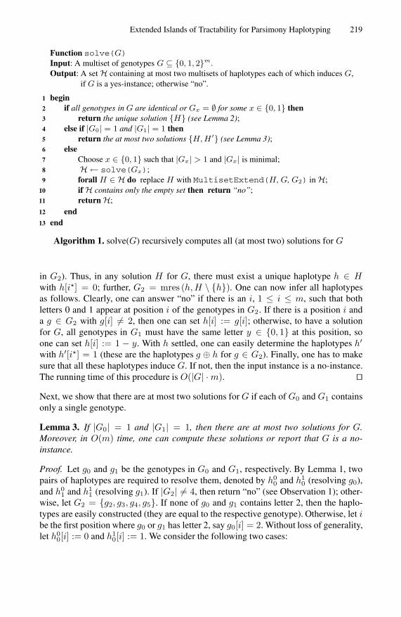
Extended Islands of Tractability for Parsimony Haplotyping 219
Function solve(G)Input: A multiset of genotypes G ⊆ {0, 1, 2}m.Output: A setH containing at most two multisets of haplotypes each of which induces G,
if G is a yes-instance; otherwise “no”.
begin1
if all genotypes in G are identical or Gx = ∅ for some x ∈ {0, 1} then2
return the unique solution {H} (see Lemma 2);3
else if |G0| = 1 and |G1| = 1 then4
return the at most two solutions {H, H ′} (see Lemma 3);5
else6
Choose x ∈ {0, 1} such that |Gx| > 1 and |Gx| is minimal;7
H ← solve(Gx);8
forall H ∈ H do replace H with MultisetExtend(H , G, G2) inH;9
ifH contains only the empty set then return “no”;10
returnH;11
end12
end13
Algorithm 1. solve(G) recursively computes all (at most two) solutions for G
in G2). Thus, in any solution H for G, there must exist a unique haplotype h ∈ Hwith h[i�] = 0; further, G2 = mres (h, H \ {h}). One can now infer all haplotypesas follows. Clearly, one can answer “no” if there is an i, 1 ≤ i ≤ m, such that bothletters 0 and 1 appear at position i of the genotypes in G2. If there is a position i anda g ∈ G2 with g[i] �= 2, then one can set h[i] := g[i]; otherwise, to have a solutionfor G, all genotypes in G1 must have the same letter y ∈ {0, 1} at this position, soone can set h[i] := 1 − y. With h settled, one can easily determine the haplotypes h′
with h′[i�] = 1 (these are the haplotypes g ⊕ h for g ∈ G2). Finally, one has to makesure that all these haplotypes induce G. If not, then the input instance is a no-instance.The running time of this procedure is O(|G| · m). �Next, we show that there are at most two solutions for G if each of G0 and G1 containsonly a single genotype.
Lemma 3. If |G0| = 1 and |G1| = 1, then there are at most two solutions for G.Moreover, in O(m) time, one can compute these solutions or report that G is a no-instance.
Proof. Let g0 and g1 be the genotypes in G0 and G1, respectively. By Lemma 1, twopairs of haplotypes are required to resolve them, denoted by h0
0 and h10 (resolving g0),
and h01 and h1
1 (resolving g1). If |G2| �= 4, then return “no” (see Observation 1); other-wise, let G2 = {g2, g3, g4, g5}. If none of g0 and g1 contains letter 2, then the haplo-types are easily constructed (they are equal to the respective genotype). Otherwise, let ibe the first position where g0 or g1 has letter 2, say g0[i] = 2. Without loss of generality,let h0
0[i] := 0 and h10[i] := 1. We consider the following two cases:

220 R. Fleischer et al.
Case 1: g1[i] �= 2.Without loss of generality, let g1[i] = 0. Then, two of the genotypes in G2 must have 0at position i and the other two must have 2 at position i; otherwise, return “no”. Withoutloss of generality, let g2[i] = g3[i] = 0 and g4[i] = g5[i] = 2. Since g2 and g3 mustbe resolved by h0
0, one can uniquely determine h00 as follows. Consider any position j.
If g2[j] �= 2 and g3[j] �= 2, then they must both be equal (if not, then return “no”). Inthis case, let h0
0[j] = g2[j]. If exactly one of g2[j] and g3[j] is equal to 2, say g3[j] = 2,then let h0
0[j] = g2[j]. If g2[j] = g3[j] = 2, then we know that g1[j] �= 2 (otherwise,return “no”) and thus h0
0[j] := 1 − g1[j]. Finally, let h10 := h0
0 ⊕ g0, h01 := h0
0 ⊕ g2,and h1
1 := h00 ⊕ g3. If these haplotypes also correctly resolve g1, g4, and g5, then we
have a unique solution for G, otherwise return “no”.
Case 2: g0[i] = g1[i] = 2.There is a genotype in G2 having 0 at position i and another having 1 at position i(otherwise, return “no”). Without loss of generality, let g2[i] = 0, g3[i] = 1, h0
1[i] := 0,and h1
1[i] := 1. Then, g4[i] = g5[i] = 2 and g2 = res (h00, h
01) and g3 = res (h1
0, h11).
Now there are two possibilities to resolve g4 and g5. Either g4 = res (h10, h
01) and g5 =
res (h00, h
11), or g4 = res (h0
0, h11) and g5 = res (h1
0, h01). By choosing one of these two
possibilities, all four haplotypes are fixed. Thus, there are at most two solutions for G.Note that there are only six genotypes. Thus, for every position the computations are
clearly doable in constant time. Hence, the whole procedure runs in O(m) time. �The next two lemmas show that one can solve an IHIP instance recursively if neitherLemma 2 nor Lemma 3 applies. That is, we now assume that not all genotypes areidentical and we have |Gx| > 1 for some x ∈ {0, 1}. We show that, given a solutionfor Gx, one can uniquely extend this solution to a solution for G, or decide that G is ano-instance, leading to function MultisetExtend (see Alg. 2)
Lemma 4. Let |Gx| > 1 for some x ∈ {0, 1}, let Hx be a multiset of haplotypesinducing Gx, and let g be a genotype in G2 with the smallest number of 2’s. If G isinduced by H with Hx ⊆ H , then all haplotypes in Hx consistent with g must beidentical.
Proof. Without loss of generality, we assume that |G0| > 1. Suppose that there is an Hwith Hx ⊆ H inducing G. Since g[i�] = 2, there must be a haplotype h1 ∈ Hx anda haplotype h2 ∈ H \ Hx resolving g. Clearly, h1 and h2 are consistent with g. Weshow that there is no other haplotype h ∈ Hx such that h �= h1 and h is consistentwith g. For the sake of contradiction, assume that there is such a haplotype h. First,note that h, h1, and h2 are consistent with g and hence identical at positions where gdoes not have letter 2. Since h �= h1, h differs from h1 in at least one of the positionswhere g has letter 2. Thus, h2 (which together with h1 resolves g and hence is thecomplement of h1 at the positions where g has letter 2) must have the same letter as hat some position where h1 and h2 differ. This implies that res (h, h2) ∈ G2 has fewer2’s than g, contradicting the choice of g. �
Lemma 5. Let |Gx| > 1 for some x ∈ {0, 1}, and let Hx be a multiset of haplotypesinducing Gx. If G is induced by H with Hx ⊆ H , then H is uniquely determined andfunction MultisetExtend (see Alg. 2) computes H in O(|Hx| · |G2| · m) time.

Extended Islands of Tractability for Parsimony Haplotyping 221
Function MultisetExtend(Hx, G, G2)Input: A haplotype multiset Hx inducing Gx for some x ∈ {0, 1}, and a multiset G2 of
genotypes.Output: A haplotype multiset H inducing G with Hx ⊆ H , if one exists; otherwise an
empty set.
begin1
H := Hx;2
while G2 �= ∅ do3
Choose a g ∈ G2 with smallest number of 2’s;4
Choose an h ∈ Hx consistent with g;5
h′ := h⊕ g;6
H := H ∪ {h′};7
G′ := {g′ | ∃h′′ ∈ Hx : g′ = res (h′, h′′)};8
if G′ � G2 then return ∅;9
G2 := G2 \G′;10
end11
if mres (H) = G then return H ;12
else return ∅;13
end14
Algorithm 2. An algorithm to extend a solution for Gx to G in the multiset case
Proof. The correctness of lines 4–7 of MultisetExtend (see Alg. 2) follows fromLemma 4. Since including h′ := h ⊕ g in H is the only choice, the genotypes resolvedby h′ and other haplotypes in Hx should also be in G2; otherwise, no solution exists.Thus, lines 8 and 9 of MultisetExtend are correct. Line 10 of MultisetExtendsafely removes the genotypes resolved by h′ from G2. The next while-iteration pro-ceeds to find the next pair consisting of a haplotype h and a genotype g ∈ G2 satis-fying Lemma 4. If there is a solution for G comprising Hx, then we must end up withan empty G2. Moreover, H \ Hx should resolve all genotypes in G1−x and, togetherwith Hx, the genotypes in G2; this is examined in line 12 of MultisetExtend. Thus,the functionMultisetExtend is correct. By Lemma 4, the solution H with Hx ⊆ His unique.
Concerning the running time, note that the most time-consuming part of the functionis to find the consistent haplotypes in Hx for a given genotype in G2. This can be donein O(|Hx| · |G2| ·m) time by iterating over all haplotypes in Hx and for each haplotypeover all genotypes in G2. �Putting all together, we obtain the main theorem of this paragraph.
Theorem 1. In case of a multiset G of length-m genotypes, INDUCED HAPLOTYPE
INFERENCE BY PARSIMONY and CONSTRAINED INDUCED HAPLOTYPE INFERENCE
BY PARSIMONY can be solved in O(k · m · |G|) and O(k · m · (|G| + |H |)) time,respectively.
Proof. (Sketch) We show that the algorithm solve(G) (see Alg. 1) is correct. If allgenotypes are identical or Gx = ∅, for some x ∈ {0, 1}, then the correctness follows

222 R. Fleischer et al.
from Lemma 2. Hence, in the following, assume that not all genotypes are identi-cal, G0 �= ∅, and G1 �= ∅. Distinguish the cases that |G0| = |G1| = 1 and |Gx| > 1,for some x ∈ {0, 1}. In the case that |G0| = |G1| = 1, one can compute the solu-tions (at most two) for G using Lemma 3. In the other case, for some x ∈ {0, 1}, itholds that |Gx| > 1 and |G1−x| > 0. Without loss of generality, assume |G0| > 1. ByLemma 1, a solution for G consists of a solution H0 for G0 and a solution H1 for G1,and H0 ∩ H1 = ∅. Since one tries to extend every solution for G0 and these extensionsare unique by Lemma 5, one will find every possible solution for G. Since the basecases have at most two solutions and extensions are uniquely determined by Lemma 5,there exist at most two solutions for G. In the constrained case, one only needs to checkwhether one of the computed solutions is in the given set of haplotypes. The claimedrunning time follows from Lemmas 2, 3, and 5. �
The Set Case. If the input is not a multiset, but a set G of genotypes, that is, all geno-types in G are pairwise distinct, then the Number Condition (Observation 1) does notnecessarily hold. Consider the haplotype set H = {000, 001, 110, 111} which inducesthe set res (H) = {002, 112, 221, 220, 222}, but also induces the multiset mres (H) ={002, 112, 221, 220, 222, 222} (observe that res (000, 111) = res (001, 110) = 222).The problem is that we cannot directly infer from G which genotypes should be re-solved more than once. However, many properties of the multiset case (as for exampleLemmas 1,2, and 3) carry over to the set case, so we only need a moderate modificationof the multiset algorithm to solve the set case. More specifically, the key to solve theset case is to adapt function MultisetExtend (all details are deferred to the longversion of this paper).
Theorem 2. In case of a set G of length-m genotypes, INDUCED HAPLOTYPE INFER-ENCE BY PARSIMONY and CONSTRAINED INDUCED HAPLOTYPE INFERENCE BY
PARSIMONY can be solved in O(k ·m · |G|) and O(k ·m ·(|G|+ |H |)) time, respectively.
4 General Haplotype Inference by Parsimony
This section contains an algorithm to solve the general parsimony haplotyping problemfor the unconstrained and the constrained versions in O(k4k+1 ·m) and O(k4k+1 ·m ·|H |) time, respectively, improving and partially simplifying previous fixed-parametertractability results [16,5]. In addition, we provide a simple kernelization.
We start with some preliminary considerations. Given a set of haplotypes resolvinga given set of genotypes, the relation between the haplotypes and the genotypes canbe depicted by an undirected graph, the solution graph, in which the edges are labeledby the genotypes and every vertex v is labeled by a haplotype hv . If an edge {u, v} islabeled by genotype g, we require that g = res (hu, hv). We call such a vertex/edgelabeling consistent. If only the edges are labeled, the graph is an inference graph (be-cause it allows us to infer all the haplotypes). Solution graphs and inference graphs maycontain loops.
In what follows, assume that the input is a yes-instance, i.e., a solution graph exists.Intuitively, our algorithm “guesses” an inference graph for G (by enumerating all pos-sible such graphs) and then infers the haplotypes from the genotype labels on the edges.

Extended Islands of Tractability for Parsimony Haplotyping 223
Input: A set of genotypes G ⊆ {0, 1, 2}m and an integer k ≥ 0.Output: Either a set of haplotypes H with |H | ≤ k and G ⊆ res (H), or “no” if there is no
solution of size at most k.
forall size-k subsets G′ ⊆ G do1
forall inference graphs Γ for G′ on k vertices and k edges do2
forall non-bipartite connected components of Γ do3
if possible, compute the labels of all vertices of the component (Lemma 7),4
otherwise try the next inference graph (goto line 2);end5
forall bipartite connected components of Γ do6
if possible, compute a consistent vertex labeling for the component7
(Lemma 8), otherwise try the next inference graph (goto line 2);end8
Let H denote the inferred haplotypes (vertex labels);9
if G ⊆ res (H) then return H ;10
end11
end12
return “no”;13
Algorithm 3. An algorithm solving HIP in O(k4k+1 · m) time
To this end, it guesses for every connected component of the solution graph a spanningsubgraph with edges labeled by some of the genotypes in G in such a way that we haveenough information at hand to infer the haplotypes. Then, one has to solve the followingsubproblem: Given an inference graph for a subset of genotypes of G, does there exista consistent vertex labeling? The next three lemmas show how to solve this subproblemby separately considering the connected components of the inference graphs.
Lemma 6. Let G be a set of genotypes and let Γ = (V, E) be a connected inferencegraph for G. For each position i, 1 ≤ i ≤ m, if there is a genotype g ∈ G with g[i] �=2, then one can, in O(|V | + |E|) time, uniquely infer the letters of all haplotypes atposition i or report that there is no consistent vertex labeling.
Lemma 7. Let Γ = (V, E) be a connected inference graph for a set G of genotypesthat contains an odd-length cycle. Then, there exists at most one consistent vertex la-beling. Furthermore, one can compute in O(m · (|V | + |E|)) time a consistent vertexlabeling or report that no consistent vertex labeling exists.
Lemma 8. Let Γ = (Va, Vb, E) be a connected bipartite inference graph for a set Gof length-m genotypes. Let u ∈ Va and w ∈ Vb be arbitrarily chosen. Then,
1. one can compute in O(m · (|Va|+ |Vb|+ |E|)) time a consistent vertex labeling orreport that no consistent vertex labeling exists, and
2. the genotypes resolved by hu and hw are identical for every consistent vertex la-beling.
Next, we describe the algorithm for the unconstrained version (HIP), see Alg. 3. Tosolve HIP, we could enumerate all inference graphs for G and then find the vertex

224 R. Fleischer et al.
labeling using Lemmas 7 and 8. However, to be more efficient, we first select a size-k subset of genotypes (line 1 of Alg. 3), and then we enumerate all inference graphson k vertices containing exactly k edges labeled by the k chosen genotypes (line 2 ofAlg. 3). Assume that there exists a solution graph for G. Of all inference graphs onk vertices and k edges consider one with the following properties:
− it contains a spanning subgraph of every connected component of thesolution graph, and
− the spanning subgraph of any non-bipartite connected component containsan odd cycle (thus, the bipartite components of the inference graph areexactly the bipartite components of the solution graph).
Obviously, this inference graph exists and is considered by Alg. 3. By Lemma 7, wecan uniquely infer the vertex labels for all connected components of the inference graphcontaining an odd cycle. For every bipartite component, we can get a consistent vertexlabeling from Lemma 8. In such a bipartite component, for any two vertices u ∈ Va
and v ∈ Vb, the genotypes resolved by hu and hv are identical for every consistentvertex labeling. Thus, the haplotypes resolve all genotypes contained in the respective(bipartite) component of the solution graph. In summary, if the given instance is a yes-instance, then our algorithm will find a set of at most k haplotypes resolving the givengenotypes.
Theorem 3. HAPLOTYPE INFERENCE BY PARSIMONY and CONSTRAINED HAPLO-TYPE INFERENCE BY PARSIMONY can be solved in O(k4k+1 · m) and O(k4k+1 · m ·|H |) time, respectively.
Proof. (Sketch) We first consider the unconstrained case. By the discussion above,Alg. 3 correctly solves HIP. It remains to analyze its running time. First, there areO(
(|G|k
)) size-k subsets G′ of G. Second, there are O(k2k) inference graphs on k ver-
tices containing exactly k edges labeled by the genotypes in G′ because for every geno-type g ∈ G′ we have k2 choices for the endpoints (loops are allowed) of the edgelabeled by g. For each of those inference graphs, applying Lemma 7 and Lemma 8 toits connected components takes O(k·m) time. Hence, the overall running time of Alg. 3sums up to O(
(|G|k
) · k2k · m · k). Since |G| ≤ k2, the running time can be boundedby O(k4k+1 · m).
One can easily adapt Alg. 3 to solve CHIP as follows. As before, one enumerates allsize-k subsets G′ ⊆ G and all inference graphs for G′. Since, by Lemma 7, the vertexlabels for the connected components containing an odd cycle are uniquely determined,one only has to check whether the inferred haplotypes are contained in the given hap-lotype pool H (otherwise, try the next inference graph). Basically, the only differenceis how to proceed with the bipartite components of the inference graph. Let (W, F ) bea connected bipartite component of the current inference graph. Instead of choosing anarbitrary consistent vertex labeling as done in Lemma 8, proceed as follows. Choose anarbitrary vertex v ∈ W and check for every haplotype h ∈ H whether there exists aconsistent vertex labeling for this component where v is labeled by h. Note that fixingthe vertex label for v implies the existence of at most one consistent vertex labelingof (W, F ). If it exists, this labeling can be computed by a depth-first traversal startingat v. If for a haplotype h there exists a consistent vertex labeling of (W, F ) such that
Extended Islands of Tractability for Parsimony Haplotyping 225
all labels are contained in H , then proceed with the next bipartite component. Other-wise, one can conclude that for the current inference graph there is no consistent vertexlabeling using only the given haplotypes, and, hence, one can proceed with the next in-ference graph. The correctness and the claimed running time follow by almost the samearguments as in the unconstrained case. �
Problem Kernelization. In this paragraph, we show that HIP admits an exponential-sizeproblem kernel. To this end, we assume the input G to be in the matrix representationthat is mentioned in the introduction; that is, each row represents a genotype whileeach column represents a position. Since it is obvious that we can upper-bound thenumber n of genotypes in the input by k2, it remains to bound the number m of columns(positions) in the input. The idea behind the following data reduction rule is that we cansafely delete a column if there is another column that is identical. By applying this ruleexhaustively, we can bound the number of columns by 2k.
Reduction Rule. Let (G, k) be an instance of HIP. If two columns of G are equal,then delete one of them.
The correctness of the reduction rule follows by the observation that, given at most khaplotypes resolving the genotypes in the reduced instance, we can easily find a solutionfor the original instance by copying the respective haplotype positions. Next, we boundthe number of columns.
Lemma 9. Let (G, k) be a yes-instance of HIP that is reduced with respect to thereduction rule. Then, G has at most 2k columns.
Proof. Let H denote a matrix of k haplotypes resolving G. It is obvious that if twocolumns i and j of H are equal, then columns i and j of G are equal. Now, since G doesnot contain a pair of equal columns, neither does H . Since there are only 2k differentstrings in {0, 1}k, it is clear that H cannot contain more than 2k columns and thus,neither can G. �Since the number n of genotypes can be bounded by k2 and the number m of columnscan be bounded by 2k (Lemma 9), one directly obtains Proposition 1.
Proposition 1. HAPLOTYPE INFERENCE BY PARSIMONY admits a problem kernel ofsize at most 2k · k2 that can be constructed in O(n · m · log m) time.
Plugging Proposition 1 into Theorem 3, we achieve the following.
Corollary 1. HIP can be solved in O(k4k+1 · 2k + n · m · log m) time.
5 Conclusion
We contributed new combinatorial algorithms for parsimony haplotyping with the po-tential to make the problem more feasible in practice without giving up the demand foroptimal solutions. Our results also lead to several new questions for future research. Forinstance, our kernelization result yields a problem kernel of exponential size. It would

226 R. Fleischer et al.
be interesting to know whether a polynomial-size problem kernel exists, which mayalso be seen in the light of recent breakthrough results on methods to prove the non-existence of polynomial-size kernels [1,7]. A second line of research is to make use ofthe polynomial-time solvable induced cases to pursue a “distance from triviality” ap-proach [8]. The idea here is to identify and exploit parameters that measure the distanceof general instances of parsimony haplotyping to the “trivial” (that is, polynomial-timesolvable) induced cases. Research in this direction is underway. A more speculative re-search direction could be to investigate whether our results on the induced case (withat most two optimal solutions) may be useful in the context of recent research [12]on finding all optimal solutions in the general case. Clearly, it remains an interestingopen problem to find a fixed-parameter algorithm for parsimony haplotyping with anexponential factor of the form ck for some constant c.
References
1. Bodlaender, H.L., Downey, R.G., Fellows, M.R., Hermelin, D.: On problems without poly-nomial kernels. J. Comput. System Sci. 75(8), 423–434 (2009)
2. Catanzaro, D., Labbe, M.: The pure parsimony haplotyping problem: Overview and compu-tational advances. International Transactions in Operational Research 16(5), 561–584 (2009)
3. Cicalese, F., Milanic, M.: On parsimony haplotyping. Technical Report 2008-04, UniversitatBielefeld (2008)
4. Downey, R.G., Fellows, M.R.: Parameterized Complexity. Springer, Heidelberg (1999)5. Fellows, M.R., Hartman, T., Hermelin, D., Landau, G.M., Rosamond, F.A., Rozenberg, L.:
Haplotype inference constrained by plausible haplotype data. In: Kucherov, G., Ukkonen, E.(eds.) CPM 2009. LNCS, vol. 5577, pp. 339–352. Springer, Heidelberg (2009)
6. Flum, J., Grohe, M.: Parameterized Complexity Theory. Springer, Heidelberg (2006)7. Fortnow, L., Santhanam, R.: Infeasibility of instance compression and succinct PCPs for NP.
In: Proc. 40th STOC, pp. 133–142. ACM Press, New York (2008)8. Guo, J., Huffner, F., Niedermeier, R.: A structural view on parameterizing problems: Distance
from triviality. In: Downey, R.G., Fellows, M.R., Dehne, F. (eds.) IWPEC 2004. LNCS,vol. 3162, pp. 162–173. Springer, Heidelberg (2004)
9. Guo, J., Niedermeier, R.: Invitation to data reduction and problem kernelization. ACMSIGACT News 38(1), 31–45 (2007)
10. Gusfield, D., Orzack, S.H.: Haplotype inference. CRC Handbook on Bioinformatics, ch. 1,pp. 1–25. CRC Press, Boca Raton (2005)
11. van Iersel, L., Keijsper, J., Kelk, S., Stougie, L.: Shorelines of islands of tractability: Algo-rithms for parsimony and minimum perfect phylogeny haplotyping problems. IEEE/ACMTrans. Comput. Biology Bioinform. 5(2), 301–312 (2008)
12. Jager, G., Climer, S., Zhang, W.: Complete parsimony haplotype inference problem and al-gorithms. In: Fiat, A., Sanders, P. (eds.) ESA 2009. LNCS, vol. 5757, pp. 337–348. Springer,Heidelberg (2009)
13. Lancia, G., Pinotti, M.C., Rizzi, R.: Haplotyping populations by pure parsimony: Complexityof exact and approximation algorithms. INFORMS Journal on Computing 16(4), 348–359(2004)
14. Lancia, G., Rizzi, R.: A polynomial case of the parsimony haplotyping problem. OperationsResearch Letters 34, 289–295 (2006)
15. Niedermeier, R.: Invitation to Fixed-Parameter Algorithms. Oxford University Press, Oxford(2006)
16. Sharan, R., Halldorsson, B.V., Istrail, S.: Islands of tractability for parsimony haplotyping.IEEE/ACM Trans. Comput. Biology Bioinform. 3(3), 303–311 (2006)

Sampled Longest Common Prefix Array
Jouni Siren�
Department of Computer Science, University of Helsinki, [email protected]
Abstract. When augmented with the longest common prefix (LCP)array and some other structures, the suffix array can solve many stringprocessing problems in optimal time and space. A compressed represen-tation of the LCP array is also one of the main building blocks in manycompressed suffix tree proposals. In this paper, we describe a new com-pressed LCP representation: the sampled LCP array. We show that whenused with a compressed suffix array (CSA), the sampled LCP array oftenoffers better time/space trade-offs than the existing alternatives. We alsoshow how to construct the compressed representations of the LCP arraydirectly from a CSA.
1 Introduction
The suffix tree is one of the most important data structures in string processingand bioinformatics. While it solves many problems efficiently, its usefulness islimited by its size: typically 10–20 times the size of the text [17]. Much work hasbeen put on reducing the size, resulting in data structures such as the enhancedsuffix array [1] and several variants of the compressed suffix tree [22,21,11,18].
Most of the proposed solutions are based on three structures: 1) the suffix ar-ray, listing the suffixes of the text in lexicographic order; 2) the longest commonprefix (LCP) array, listing the lengths of the longest common prefixes of lexi-cographically adjacent suffixes; and 3) a representation of suffix tree topology.While there exists an extensive literature on compressed suffix arrays (CSA)1
[19], less has been done on compressing the other structures.Existing proposals to compress the LCP information are based on the per-
muted LCP (PLCP) array that arranges the entries in text order. While thePLCP array can be compressed, one requires expensive CSA operations to ac-cess LCP values through it. In this paper, we describe the sampled LCP array asan alternative to the PLCP-based approaches. Similar to the suffix array samplesused in CSAs, the sampled LCP array often offers better time/space trade-offsthan the PLCP-based alternatives.
We also modify a recent PLCP construction algorithm [14] to work directlywith a compressed suffix array. Using it, we can construct any PLCP repre-sentation with negligible working space in addition to the CSA and the PLCP.� Funded by the Academy of Finland under grant 119815.1 In this paper, we use the term compressed suffix array to refer to any compressed
self-index based on the Burrows-Wheeler transform.
A. Amir and L. Parida (Eds.): CPM 2010, LNCS 6129, pp. 227–237, 2010.c© Springer-Verlag Berlin Heidelberg 2010

228 J. Siren
A variant of the algorithm can also be used to construct the sampled LCP array,but requires more working space. While our algorithm is much slower than thealternatives, it is the first LCP construction algorithm that does not require ac-cess to the text and the suffix array. This is especially important for large texts,as the suffix array may not be available or the text might not fit into memory.
We begin with basic definitions and background information in Sect. 2. Sec-tion 3 is a summary of previous compressed LCP representations. In Sect. 4,we show how to build the PLCP array directly from a CSA. We describe oursampled LCP array in Sect. 5. Section 6 contains experimental evaluation of ourproposals. We finish with conclusions and discussion on future work in Sect. 7.
2 Background
A string S = S[1, n] is a sequence of characters from alphabet Σ = {1, 2, . . . , σ}.A substring of S is written as S[i, j]. A substring of type S[1, j] is called a prefix,while a substring of type S[i, n] is called a suffix. A text string T = T [1, n] is astring terminated by T [n] = $ �∈ Σ with lexicographic value 0. The lexicographicorder ”<” among strings is defined in the usual way.
The suffix array (SA) of text T [1, n] is an array of pointers SA[1, n] to thesuffixes of T in lexicographic order. As an abstract data type, a suffix array isany data structure with similar functionality as the concrete suffix array. Thiscan be defined by an efficient support for the following operations: (a) count thenumber of occurrences of a pattern in the text; (b) locate these occurrences (ormore generally, retrieve a suffix array value); and (c) display any substring of T .
Compressed suffix arrays (CSA) [12,8] support these operations. Their com-pression is based on the Burrows-Wheeler transform (BWT) [3], a permutationof the text related to the SA. The BWT of text T is a sequence L[1, n] such thatL[i] = T [SA[i] − 1], if SA[i] > 1, and L[i] = T [n] = $ otherwise.
The Burrows-Wheeler transform is reversible. The reverse transform is basedon a permutation called LF -mapping [3,8]. Let C[1, σ] be an array such thatC[c] is the number of characters in {$, 1, 2, . . . , c − 1} occurring in the text. Forconvenience, we also define C[0] = 0 and C[σ + 1] = n. By using this array andthe sequence L, we define LF -mapping as LF (i) = C[L[i]]+rankL[i](L, i), whererankc(L, i) is the number of occurrences of character c in prefix L[1, i].
The inverse of LF -mapping is Ψ(i) = selectc(L, i−C[c]), where c is the highestvalue with C[c] < i, and selectc(L, j) is the position of the jth occurrence ofcharacter c in L [12]. By its definition, function Ψ is strictly increasing in therange Ψc = [C[c] + 1, C[c + 1]] for every c ∈ Σ. Additionally, T [SA[i]] = c andL[Ψ(i)] = c for every i ∈ Ψc.
These functions form the backbone of CSAs. As SA[LF (i)] = SA[i] − 1 [8]and hence SA[Ψ(i)] = SA[i] + 1, we can use these functions to move the suffixarray position backward and forward in the sequence. Both of the functions canbe efficiently implemented by adding some extra information to a compressedrepresentation of the BWT. Standard techniques [19] to support suffix arrayoperations include backward searching [8] for count, and adding a sample ofsuffix array values for locate and display.

Sampled Longest Common Prefix Array 229
Let lcp(A, B) be the length of the longest common prefix of sequences A andB. The longest common prefix (LCP) array of text T [1, n] is the array LCP[1, n]such that LCP[1] = 0 and LCP[i] = lcp(T [SA[i− 1], n], T [SA[i], n]) for i > 1. Thearray requires n logn bits of space, and can be constructed in O(n) time [15,14].
3 Previous Compressed LCP Representations
We can exploit the redundancy in LCP values by reordering them in text order.This results in the permuted LCP (PLCP) array, where PLCP[SA[i]] = LCP[i].The following lemma describes a key property of the PLCP array.
Lemma 1 ([15,14]). For every i ∈ {2, . . . , n}, PLCP[i] ≥ PLCP[i − 1] − 1.
As the values PLCP[i] + 2i form a strictly increasing sequence, we can store thearray in a bit vector of length 2n [22]. Various schemes exist to represent thisbit vector in a succinct or compressed form [22,11,18].
Space-efficiency can also be achieved by sampling every qth PLCP value, andderiving the missing values when needed [16]. Assume we have sampled PLCP[aq]and PLCP[(a + 1)q], and we want to determine PLCP[aq + b] for some b < q.Lemma 1 states that PLCP[aq] − b ≤ PLCP[aq + b] ≤ PLCP[(a + 1)q] + q − b,so at most q + PLCP[(a + 1)q] − PLCP[aq] character comparisons are requiredto determine the missing value. The average number of comparisons over allentries is O(q) [14]. By carefully selecting the sampled positions, we can storethe samples in o(n) bits, while requiring only O(logδ n) comparisons in the worstcase for any 0 < δ ≤ 1 [10].
Unfortunately these compressed representations are not very suitable for usewith CSAs. The reason is that the LCP values are accessed through suffix arrayvalues, and locate is an expensive operation in CSAs. In addition to that, sampledPLCP arrays require access to the text, using the similarly expensive display.
Assume that a CSA has SA sample rate d, and that it computes Ψ(·) in timetΨ . To retrieve SA[i], we compute i, Ψ(i), Ψ2(i), . . . , until we find a sampled suffixarray value. If the sampled value was SA[Ψk(i)] = j, then SA[i] = j−k. We find asample in at most d steps, so the time complexity for locate is O(d·tΨ ). Similarly,to retrieve a substring T [i, i + l], we use the samples to get SA−1[d · � id�]. Thenwe iterate the function Ψ until we reach text position i + l. This takes at mostd + l iterations, making the time complexity for display O((d + l) · tΨ ). Fromthese bounds, we get the PLCP access times shown in Table 1.2
Depending on the type of index used, tψ varies from O(1) to O(log n) in theworst case [19], and is close to 1 microsecond for the fastest indexes in practice[7,18]. This is significant enough that it makes sense to keep tΨ in Table 1.
The only (P)LCP representation so far that is especially designed for usewith CSAs is Fischer’s Wee LCP [10] that is basically the select structure fromSadakane’s bit vector representation [22]. When the bit vector itself would berequired to answer a query, some characters of two lexicographically adjacent
2 Some CSAs use LF -mapping instead of Ψ , but similar results apply to them as well.

230 J. Siren
Table 1. Time/space trade-offs for (P)LCP representations. R is the number of equalletter runs in BWT, q is the PLCP sample rate, and 0 < δ ≤ 1 is a parameter. Thenumbers for CSA assume Ψ access time tΨ and SA sample rate d.
Access timesRepresentation Space (bits) Using SA Using CSA
LCP n log n O(1) O(1)PLCP [22] 2n + o(n) O(1) O(d · tΨ )PLCP [11] 2R log n
R+ O(R) + o(n) O(1) O(d · tΨ )
PLCP [18] 2R log nR
+ O(R log log nR
) O(log log n) O(d · tΨ + log log n)
Sampled PLCP [10] o(n) O(logδ n) O((d + logδ n) · tΨ )Sampled PLCP [16] n
qlog n O(q) O((d + q) · tΨ )
suffixes are compared to determine the LCP value. This increases the time com-plexity, while reducing the size significantly. In this paper, we take the otherdirection by reducing the access time, while achieving similar compression as inthe run-length encoded PLCP variants [11,18].
4 Building the PLCP Array from a CSA
In this section, we adapt the irreducible LCP algorithm [14] to compute thePLCP array directly from a CSA.
Definition 1. For i > 1, the left match of suffix T [SA[i], n] is T [SA[i − 1], n].
Definition 2. Let T [j, n] be the left match of T [i, n]. PLCP[i] is reducible, ifi, j > 1 and T [i−1] = T [j−1]. If PLCP[i] is not reducible, then it is irreducible.
The following lemma shows why reducible LCP values are called reducible.
Lemma 2 ([14]). If PLCP[i] is reducible, then PLCP[i] = PLCP[i − 1] − 1.
The irreducible LCP algorithm works as follows: 1) find the irreducible PLCPvalues; 2) compute them naively; and 3) fill in the reducible values by usingLemma 2. As the sum of the irreducible values is at most 2n logn, the algorithmworks in O(n log n) time [14].
The original algorithm uses the text and its suffix array that are expensive toaccess in a CSA. In the following lemma, we show how to find the irreduciblevalues by using the function Ψ instead.
Lemma 3. Let T [j, n] be the left match of T [i, n]. The value PLCP[i + 1] isreducible if and only if T [i] = T [j] and Ψ(SA−1[j]) = Ψ(SA−1[i]) − 1.
Proof. Let x = SA−1[i]. Then x − 1 = SA−1[j].”If.” Assume that T [i] = T [j] and Ψ(x − 1) = Ψ(x) − 1. Then the left match
of T [SA[Ψ(x)], n] = T [i + 1, n] is T [SA[Ψ(x − 1)], n] = T [j + 1, n]. As i + 1 > 1and j + 1 > 1, it follows that PLCP[i + 1] is reducible.

Sampled Longest Common Prefix Array 231
— Compute the PLCP array1 PLCP[1]← 02 (i, x)← (1, SA−1[1])3 while i < n4 Ψc ← rangeContaining(x)5 if x− 1 �∈ Ψc or Ψ(x− 1) �= Ψ(x)− 16 PLCP[i + 1]← lcp(Ψ(x))7 else PLCP[i + 1]← PLCP[i]− 18 (i, x)← (i + 1, Ψ(x))
— Compute an LCP value9 def lcp(b)10 (a, k)← (b− 1, 0)11 Ψc ← rangeContaining(b)12 while a ∈ Ψc
13 (a, b, k)← (Ψ(a), Ψ(b), k + 1)14 Ψc ← rangeContaining(b)15 return k
Fig. 1. The irreducible LCP algorithm for using a CSA to compute the PLCP array.Function rangeContaining(x) returns Ψc = [C[c] + 1, C[c + 1]] where x ∈ Ψc.
”Only if.” Assume that PLCP[i + 1] is reducible, and let T [k, n] be the leftmatch of T [i + 1, n]. Then k > 1 and T [k − 1] = T [i]. As T [k − 1, n] and T [i, n]begin with the same character, and T [k, n] is the left match of T [i + 1, n], therecannot be any suffix S such that T [k − 1, n] < S < T [i, n]. But now j = k − 1,and hence T [i] = T [j]. Additionally,
Ψ(SA−1[j]) = Ψ(SA−1[k − 1]) = SA−1[k] = SA−1[i + 1] − 1 = Ψ(SA−1[i]) − 1.
The lemma follows. �
The algorithm is given in Fig. 1. We maintain invariant x = SA−1[i], and scanthrough the CSA in text order. If the conditions of Lemma 3 do not hold forT [i, n], then PLCP[i + 1] is irreducible, and we have to compute it. Otherwisewe reduce PLCP[i + 1] to PLCP[i]. To compute an irreducible value, we iterate(Ψk(b − 1), Ψk(b)) for k = 0, 1, 2, . . . , until T [Ψk(b − 1)] �= T [Ψk(b)]. When thishappens, we return k as the requested LCP value. As we compute Ψ(·) for atotal of O(n log n) times, we get the following theorem.
Theorem 1. Given a compressed suffix array for a text of length n, the irre-ducible LCP algorithm computes the PLCP array in O(n log n · tΨ ) time, wheretΨ is the time required for accessing Ψ . The algorithm requires O(log n) bits ofworking space in addition to the CSA and the PLCP array.
We can use the algorithm to build any PLCP representation from Table 1 di-rectly. The time bound is asymptotically tight, as shown in the following lemma.
Lemma 4 (Direct extension of Lemma 5 in [14]). For an order-k de Bruijnsequence on an alphabet of size σ, the sum of all irreducible PLCP values isn(1 − 1/σ) logσ n − O(n).
The sum of irreducible PLCP values of a random sequence should also be closeto n(1 − 1/σ) logσ n. The probability that the characters preceding a suffix andits left match differ, making the PLCP value irreducible, is (1 − 1/σ). On theother hand, the average irreducible value should be close to logσ n [6]. For a text

232 J. Siren
generated by an order-k Markov source with H bits of entropy, the estimatebecomes n(1− 1/σ′)(log n)/H . Here σ′ is the effective alphabet size, defined bythe probability 1/σ′ that two characters sharing an order-k context are identical.
The following proposition shows that large-scale repetitiveness reduces thesum of the irreducible values, and hence improves the algorithm performance.
Proposition 1. For a concatenation of r copies of text T [1, n], the sum of irre-ducible PLCP values is s + (r− 1)n, where s is the sum of the irreducible PLCPvalues of T .
Proof. Let T = T1T2 · · ·Tr be the concatenation, Ta,i the suffix starting at Ta[i],and PLCPa[i] the corresponding PLCP value. Assume that Tr[n] is lexicograph-ically greater than the other end markers, but otherwise identical to them.
For every i, the suffix array of T contains a range with values T1,i, T2,i, . . . , Tr,i[18]. Hence for any a > 1 and any i, the left match of Ta,i is Ta−1,i, making thePLCP values reducible for almost all of the suffixes of T2 to Tr. The exception isthat T2,1 is irreducible, as its left match is T1,1, and hence PLCP2[1] = (r − 1)n.
Let T [j, n] be the left match of T [i, n] in the suffix array of T . Then the leftmatch of T1,i is Tr,j , and PLCP1[i] = PLCP[i]. Hence the sum of the irreduciblevalues corresponding to the suffixes of T1 is s. �
5 Sampled LCP Array
By Lemmas 1 and 2, the local maxima in the PLCP array are among the irre-ducible values, and the local minima are immediately before them.
Definition 3. The value PLCP[i] is maximal, if it is irreducible, and minimal,if either i = n or PLCP[i + 1] is maximal.
Lemma 5. If PLCP[i] is non-minimal, then PLCP[i] = PLCP[i + 1] + 1.
Proof. If PLCP[i] is non-minimal, then PLCP[i+1] is reducible. The result followsfrom Lemma 2. �
In the following, R is the number of equal letter runs in BWT.
Lemma 6. The number of minimal PLCP values is R.
Proof. Lemma 3 essentially states that PLCP[i + 1] is reducible, if and only ifL[Ψ(SA−1[i])] = T [i] = T [j] = L[Ψ(SA−1[j])] = L[Ψ(SA−1[i]) − 1], where T [j, n]is the left match of T [i, n]. As this is true for n−R positions i, there are exactlyR irreducible values. As every maximal PLCP value can be reduced to the nextminimal value, and vice versa, the lemma follows. �
Lemma 7. The sum of minimal PLCP values is S − (n − R), where S is thesum of maximal values.
Proof. From Lemmas 5 and 6. �

Sampled Longest Common Prefix Array 233
If we store the minimal PLCP values in SA order, and mark their positionsin a bit vector, we can use them in a similar way as the SA samples. If weneed LCP[i], and LCP[Ψk(i)] is a sampled position for the smallest k ≥ 0, thenLCP[i] = LCP[Ψk(i)] + k. As k can be Θ(n) in the worst case, the time bound isO(n · tΨ ).
To improve the performance, we sample one out of d′ = n/R1−ε consecutivenon-minimal values for some ε > 0. Then there are R minimal samples andat most R1−ε extra samples. We mark the sampled positions in a bit vector ofRaman et al. [20], taking at most (1+o(1)) ·R log n
R +O(R)+o(n) bits of space.Checking whether an LCP entry has been sampled takes O(1) time.
We use δ codes [5] to encode the actual samples. As the sum of the minimalvalues is at most 2n log n, these samples take at most
R log2n log n
R+ O
(R log log
n
R
)≤ R log
n
R+ O(R log log n)
bits of space. The extra samples require at most logn + O(log log n) bits each.To provide fast access to the samples, we can use dense sampling [9] or directlyaddressable codes [2]. This increases the size by a factor of 1 + o(1), making thetotal for samples (1 + o(1)) · R log n
R + O(R log log n) + o(R log n) bits of space.We find a sampled position in at most n/R1−ε steps. By combining the size
bounds, we get the following theorem.
Theorem 2. Given a text of length n and a parameter 0 < ε < 1, the sampledLCP array requires at most (2+o(1))·R log n
R+O(R log log n)+o(R log n)+o(n)bits of space, where R is the number of equal letter runs in the BWT of the text.When used with a compressed suffix array, retrieving an LCP value takes at mostO((n/R1−ε) · tΨ ) time, where tΨ is the time required for accessing Ψ .
By using the BSD representation [13] for the bit vector, we can remove the o(n)term from the size bound with a slight loss of performance.
When the space is limited, we can afford to sample the LCP array denser thanthe SA, as SA samples are larger than LCP samples. In addition to the mark inthe bit vector, an SA sample requires 2 log n
dbits of space, while an LCP sample
takes just log v + O(log log v) bits, where v is the sampled value.The LCP array can be sampled by a two-pass version of the irreducible LCP
algorithm. On the first pass, we scan the CSA in suffix array order to find theminimal samples. Position x is minimal, if x is the smallest value in the corre-sponding Ψc, or if Ψ(x−1) �= Ψ(x)−1. As we compress the samples immediately,we only need O(log n) bits of working space. On the second pass, we scan theCSA in text order, and store the extra samples in an array. Then we sort thearray to SA order, and merge it with the minimal samples. As the number ofextra samples is o(R), we need o(R log n) bits of working space.
Theorem 3. Given a compressed suffix array for a text of length n, the modifiedirreducible LCP algorithm computes the sampled LCP array in O(n log n · tΨ )time, where tΨ is the time required for accessing Ψ . The algorithm requireso(R log n) bits of working space in addition to the CSA and the samples, whereR is the number of equal letter runs in the BWT of the text.

234 J. Siren
6 Implementation and Experiments
We have implemented the sampled LCP array, a run-length encoded PLCP array,and their construction algorithms as a part of the RLCSA [23].3 For PLCP, weused the same run-length encoded bit vector as in the RLCSA. For the sampledLCP, we used a gap encoded bit vector to mark the sampled positions, and astripped-down version of the same vector for storing the samples.
To avoid redundant work, we compute minimal instead of maximal PLCPvalues, and interleave their computation with the main loop. To save space, weonly use strictly minimal PLCP values with PLCP[i] < PLCP[i + 1] + 1 as theminimal samples. When sampling the LCP array, we make both of the passes intext order, and store all the samples in an array before compressing them.
For testing, we used a 2.66 GHz Intel Core 2 Duo E6750 system with 4 GBof memory (3.2 GB visible to OS) running a Fedora-based Linux with kernel2.6.27. The implementation was written in C++, and compiled on g++ version4.1.2. We used four data sets: human DNA sequences (dna) and English languagetexts (english) from the Pizza & Chili Corpus [7], the Finnish language Wikipediawith version history (fiwiki) [23], and the genomes of 36 strains of Saccharomycesparadoxus (yeast) [18].4 When the data set was much larger than 400 megabytes,a 400 MB prefix was used instead. Further information on the data sets can befound in Table 2.
Only on the dna data set, the sum of the minimal values was close to theentropy-based estimate. On the highly repetitive fiwiki and yeast data sets, thedifference between the estimate and the measurement was very large, as pre-dicted by Proposition 1. Even regular English language texts contained enoughlarge-scale repetitiveness that the sum of the minimal values could not be ad-equately explained by the entropy of the texts. This suggests that, for manyreal-world texts, the number of runs in BWT is a better compressibility measurethan the empirical entropy.
The sum of minimal PLCP values was a good estimate for PLCP constructiontime. LCP sampling was somewhat slower because of the second pass. Bothalgorithms performed reasonably well on the highly repetitive data sets, butwere much slower on the regular ones. The overall performance was roughly anorder of magnitude worse than for the algorithms using plain text and SA [14].
We measured the performance of the sampled LCP array and the run-lengthencoded PLCP array on each of the data sets. We also measured the locateperformance of the RLCSA to get a lower bound for the time and space of anyPLCP-based approach. The results can be seen in Fig. 2.
The sampled LCP array outperformed PLCP on english and dna, where mostof the queries were resolved through minimal samples. On fiwiki and yeast, thesituation was reversed. As many extra samples were required to get reasonable
3 The implementation is available at http://www.cs.helsinki.fi/group/suds/
rlcsa/4 The yeast genomes were obtained from the Durbin Research Group at the Sanger
Institute, http://www.sanger.ac.uk/Teams/Team71/durbin/sgrp/

Sampled Longest Common Prefix Array 235
Table 2. Properties of the data sets. H5 is the order-5 empirical entropy, σ′ the corre-sponding effective alphabet size, # the number of (strictly) minimal values, and S thesum of those values. S′ = n(1 − 1/σ′)(log n)/H5 − n/σ′ is an entropy-based estimatefor the sum of the minimal values. The construction times are in seconds.
Estimates Minimal values Strictly minimalName MB H5 σ′ S′/106 #/106 S/106 S/n #/106 S/106 S/n
english 400 1.86 2.09 3167 156.35 1736 4.14 99.26 1052 2.51fiwiki 400 1.09 1.52 3490 1.79 273 0.65 1.17 117 0.28dna 385 1.90 3.55 4252 243.49 3469 8.59 158.55 2215 5.48yeast 409 1.87 3.34 4493 15.64 520 1.21 10.05 299 0.70
Sample rates PLCP Sampled LCPName SA LCP Time MB/s Time MB/s
english 8, 16, 32, 64 8, 16 1688 0.24 2104 0.19fiwiki 64, 128, 256, 512 32, 64, 128 327 1.22 533 0.75dna 8, 16, 32, 64 8, 16 3475 0.11 3947 0.10yeast 32, 64, 128, 256 16, 32, 64 576 0.71 890 0.46
0 200 400 600 800
010
2030
4050
60
Size (MB)
Tim
e (µ
s)
english
PLCPSampledLocate
0 200 400 600 800
010
2030
4050
60
Size (MB)
Tim
e (µ
s)
dna
PLCPSampledLocate
0 20 40 60 80 100
050
100
200
Size (MB)
Tim
e (µ
s)
fiwiki
PLCPSampledLocate
0 50 100 150 200 250
050
100
150
Size (MB)
Tim
e (µ
s)
yeast
PLCPSampledLocate
Fig. 2. Time/space trade-offs for retrieving an LCP or SA value. The times are averagesover 106 random queries. Sampled LCP results are grouped by SA sample rate.

236 J. Siren
performance, increasing the size significantly, the sampled LCP array had worsetime/space trade-offs than the PLCP array.
While we used RLCSA in the experiments, the results generalize to other typesof CSA as well. The reason for this is that, in both PLCP and sampled LCP,the time required for retrieving an LCP value depends mostly on the number ofiterations of Ψ required to find a sampled position.
7 Discussion
We have described the sampled LCP array, and shown that it offers bettertime/space trade-offs than the PLCP-based alternatives, when the number ofextra samples required for dense sampling is small. Based on the experiments,it seems that one should use the sampled LCP array for regular texts, and aPLCP-based representation for highly repetitive texts.
In a recent proposal [4], the entire LCP array was compressed by using directlyaddressable codes (DAC) [2]. The resulting structure is much faster but usuallyalso much larger than the other compressed LCP representations. See the fullpaper [24] for a comparison between the sampled LCP array and the DAC-basedapproach.
We have also shown that it is feasible to construct the (P)LCP array directlyfrom a CSA. While the earlier algorithms are much faster, it is now possible toconstruct the (P)LCP array for larger texts than before, and the performance isstill comparable to that of direct CSA construction [23]. On a multi-core system,it is also easy to get extra speed by parallelizing the construction.
It is possible to maintain the (P)LCP array when merging two CSAs. Theimportant observation is that an LCP value can only change, if the left matchchanges in the merge. An open question is, how much faster the merging is, bothin the worst case and in practice, than rebuilding the (P)LCP array.
While the suffix array and the LCP array can be compressed to a spacerelative to the number of of equal letter runs in BWT, no such representation isknown for suffix tree topology. This is the main remaining obstacle in the wayto compressed suffix trees optimized for highly repetitive texts.
References
1. Abouelhoda, M.I., Kurtz, S., Ohlebusch, E.: Replacing suffix trees with enhancedsuffix arrays. Journal on Discrete Algorithms 2(1), 53–86 (2004)
2. Brisaboa, N.R., Ladra, S., Navarro, G.: Directly addressable variable-lengthcodes. In: Hyyro, H. (ed.) SPIRE 2009. LNCS, vol. 5721, pp. 122–130. Springer,Heidelberg (2009)
3. Burrows, M., Wheeler, D.: A block sorting lossless data compression algorithm.Technical Report 124, Digital Equipment Corporation (1994)
4. Canovas, R., Navarro, G.: Practical compressed suffix trees. In: Festa, P. (ed.) SEA2010. LNCS, vol. 6049, pp. 94–105. Springer, Heidelberg (2010)
5. Elias, P.: Universal codeword sets and representations of the integers. IEEE Trans-actions on Information Theory 21(2), 194–203 (1975)

Sampled Longest Common Prefix Array 237
6. Fayolle, J., Ward, M.D.: Analysis of the average depth in a suffix tree under aMarkov model. In: Proc. 2005 International Conference on Analysis of Algorithms,DMTCS Proceedings, vol. AD, pp. 95–104. DMTCS (2005)
7. Ferragina, P., Gonzalez, R., Navarro, G., Venturini, R.: Compressed text indexes:From theory to practice. Journal of Experimental Algorithms 13, 1.12 (2009)
8. Ferragina, P., Manzini, G.: Indexing compressed text. Journal of the ACM 52(4),552–581 (2005)
9. Ferragina, P., Venturini, R.: A simple storage scheme for strings achieving entropybounds. In: SODA 2007, pp. 690–696. SIAM, Philadelphia (2007)
10. Fischer, J.: Wee LCP. arXiv:0910.3123v1 [cs.DS] (2009)11. Fischer, J., Makinen, V., Navarro, G.: Faster entropy-bounded compressed suffix
trees. Theoretical Computer Science 410(51), 5354–5364 (2009)12. Grossi, R., Vitter, J.S.: Compressed suffix arrays and suffix trees with applications
to text indexing and string matching. SIAM Journal on Computing 35(2), 378–407(2005)
13. Gupta, A., Hon, W.-K., Shah, R., Vitter, J.S.: Compressed data structures: dic-tionaries and data-aware measures. Theoretical Computer Science 387(3), 313–331(2007)
14. Karkkainen, J., Manzini, G., Puglisi, S.: Permuted longest-common-prefix array.In: Kucherov, G., Ukkonen, E. (eds.) CPM 2009. LNCS, vol. 5577, pp. 181–192.Springer, Heidelberg (2009)
15. Kasai, T., Lee, G., Arimura, H., Arikawa, S., Park, K.: Linear-time longest-common-prefix computation in suffix arrays and its applications. In: Amir,A., Landau, G.M. (eds.) CPM 2001. LNCS, vol. 2089, pp. 181–192. Springer,Heidelberg (2001)
16. Khmelev, D.: Program lcp version 0.1.9 (2004),http://www.math.toronto.edu/dkhmelev/PROGS/misc/lcp-eng.html
17. Kurtz, S.: Reducing the space requirement of suffix trees. Software: Practice andExperience 29(13), 1149–1171 (1999)
18. Makinen, V., Navarro, G., Siren, J., Valimaki, N.: Storage and retrieval of individ-ual genomes. In: Batzoglou, S. (ed.) RECOMB 2009. LNCS, vol. 5541, pp. 121–137.Springer, Heidelberg (2009)
19. Navarro, G., Makinen, V.: Compressed full-text indexes. ACM Computing Sur-veys 39(1), 2 (2007)
20. Raman, R., Raman, V., Rao, S.S.: Succinct indexable dictionaries with applica-tions to encoding k-ary trees and multisets. In: SODA 2002, pp. 233–242. SIAM,Philadelphia (2002)
21. Russo, L., Navarro, G., Oliveira, A.: Fully-compressed suffix trees. In: Laber, E.S.,Bornstein, C., Nogueira, L.T., Faria, L. (eds.) LATIN 2008. LNCS, vol. 4957, pp.362–373. Springer, Heidelberg (2008)
22. Sadakane, K.: Compressed suffix trees with full functionality. Theory of ComputingSystems 41(4), 589–607 (2007)
23. Siren, J.: Compressed suffix arrays for massive data. In: Hyyro, H. (ed.)SPIRE 2009. LNCS, vol. 5721, pp. 63–74. Springer, Heidelberg (2009)
24. Siren, J.: Sampled longest common prefix array. arXiv:1001.2101v2 [cs.DS] (2010)

Verifying a Parameterized Border Array
in O(n1.5) Time
Tomohiro I1, Shunsuke Inenaga2, Hideo Bannai1, and Masayuki Takeda1
1 Department of Informatics, Kyushu University2 Graduate School of Information Science and Electrical Engineering,
Kyushu University744 Motooka, Nishiku, Fukuoka, 819–0395 Japan
[email protected],[email protected],
{bannai,takeda}@inf.kyushu-u.ac.jp
Abstract. The parameterized pattern matching problem is to check ifthere exists a renaming bijection on the alphabet with which a givenpattern can be transformed into a substring of a given text. A param-eterized border array (p-border array) is a parameterized version of astandard border array, and we can efficiently solve the parameterized pat-tern matching problem using p-border arrays. In this paper we presentan O(n1.5)-time O(n)-space algorithm to verify if a given integer arrayof length n is a valid p-border array for an unbounded alphabet. Thebest previously known solution takes time proportional to the n-th Bellnumber 1
e
∑∞k=0
kn
k!, and hence our algorithm is quite efficient.
1 Introduction
The parameterized matching (p-matching) problem [1] is a kind of string match-ing problem, where a pattern is considered to occur in a text when there exists arenaming bijection on the alphabet with which the pattern can be transformedinto a substring of the text. Parameterized matching has applications in e.g.software maintenance, plagiarism detection, and RNA structural matching, thusit has extensively been studied (e.g., see [2,3,4,5,6]).
In this paper we focus on parameterized border arrays (p-border arrays) [7],which are a parameterized version of border arrays [8]. Let Π be the alpha-bet. The p-border array of a given pattern p of length m can be computed inO(m log |Π |) time, and the p-matching problem can be solved in O(n log |Π |)time for any text p-string of length n, using the p-border array [7].
This paper deals with the reverse engineering problem on p-border arrays,namely, the problem of verifying if a given integer array of length n is a p-borderarray of some string. We propose an O(n1.5)-time O(n)-space algorithm to solvethis problem for an unbounded alphabet. We emphasize that the best previouslyknown solution to this problem takes time proportional to the n-th Bell number1e
∑∞k=0
kn
k! , and hence our algorithm is quite efficient.
A. Amir and L. Parida (Eds.): CPM 2010, LNCS 6129, pp. 238–250, 2010.c© Springer-Verlag Berlin Heidelberg 2010

Verifying a Parameterized Border Array in O(n1.5) Time 239
Related Work. There exists a linear time algorithm to solve the reverse prob-lem on p-border arrays for a binary alphabet [9]. An O(pn)-time algorithm toenumerate all p-border arrays of length up to n on a binary alphabet was alsopresented in [9], where pn denotes the number of p-border arrays of length atmost n for a binary alphabet.
In [10], a linear time algorithm to verify if a given integer array is the (stan-dard) border array [8] of some string was presented. Their algorithm works forboth bounded and unbounded alphabets. A simpler linear-time solution for thesame problem for a bounded alphabet was shown in [11]. An algorithm to enu-merate all border arrays of length at most n in O(bn)-time was given in [10],where bn is the number of border arrays of length at most n.
The reverse engineering problems, as well as the enumeration problems forother string data structures (suffix arrays, DAWG, etc.) have been extensivelystudied [12,13,14,15,16,17,18], whose solutions give us further insight concerningthe data structures.
2 Preliminaries
Let Σ and Π be two disjoint finite alphabets. An element of (Σ ∪ Π)∗ is calleda p-string. The length of any p-string s is the total number of constant andparameter symbols in s and is denoted by |s|. The string of length 0 is called theempty string and is denoted by ε. For any p-string s of length n, the i-th symbolis denoted by s[i] for each 1 ≤ i ≤ n, and the substring starting at position iand ending at position j is denoted by s[i : j] for 1 ≤ i ≤ j ≤ n.
Any two p-strings s, t ∈ (Σ ∪ Π)∗ of length m are said to parameterizedmatch (p-match) if s can be transformed into t by a renaming function f fromthe symbols of s to the symbols of t, where f is the identify on Σ. The p-matchingproblem on Σ∪Π is reducible in linear time to the p-matching problem on Π [2].Thus we will only consider p-strings over Π .
Let N be the set of non-negative integers. Let pv : Π∗ → N ∗ be the functions.t. for any p-string s of length n > 0, pv (s) = u where, for 1 ≤ i ≤ n, u[i] = 0if s[i] �= s[j] for any 1 ≤ j < i, and u[i] = i − k if k = max{j | s[i] = s[j], 1 ≤j < i}. Let pv (ε) = ε. Two p-strings s and t of the same length m p-match iffpv(s) = pv(t). For any p ∈ N ∗, let zeros(p) denotes the number of 0’s in p, thatis, zeros(p) = |{i | p[i] = 0, 1 ≤ i ≤ |p|}|. For any s ∈ Π , zeros(pv (s)) equals thenumber of different characters in s. For example, aabb and bbaa p-match sincepv(aabb) = pv (bbaa) = 0 1 0 1. Note zeros(pv (aabb)) = zeros(pv(bbaa)) = 2.
A parameterized border (p-border) of a p-string s of length n is any inte-ger j s.t. 0 ≤ j < n and pv (s[1 : j]) = pv (s[n − j + 1 : n]). For example,the set of p-borders of p-string aabb is {2, 1, 0} since pv (aa) = pv(bb) = 0 1,pv(a) = pv (b) = 0, and pv(ε) = pv (ε) = ε. We also say that b is a p-borderof p ∈ N ∗ if b is a p-border of some p-string s ∈ Π∗ and p = pv (s). Theparameterized border array (p-border array) βs of a p-string s of length n isan array of length n such that βs[i] = j, where j is the longest p-border ofs[1 : i]. For example, for p-string s = aabbaa, βs = [0, 1, 1, 2, 3, 4]. When it is

240 Tomohiro I et al.
clear from the context, we abbreviate βs as β. Let P = {pv(s) | s ∈ Π∗} andPβ = {p ∈ P | β[i] is the longest p-border of p[1 : i], 1 ≤ i ≤ |β|}.
For any i, j ∈ N , let cut(i, j) = 0 if i ≥ j, and cut(i, j) = i otherwise. Forany p ∈ P and 1 ≤ j ≤ |p|, let suf (p, j) = cut(p[|p| − j + 1], 1)cut(p[|p| − j +2], 2) · · · cut(p[|p|], j). Let suf (p, 0) = ε. For example, if p[1 : 10] =0 0 2 0 3 1 3 2 6 3,
suf (p, 5) = cut(p[6], 1)cut(p[7], 2)cut(p[8], 3)cut(p[9], 4)cut(p[10], 5)= cut(1, 1)cut(3, 2)cut(2, 3)cut(6, 4)cut(3, 5) = 0 0 2 0 3.
Then, for any p-string s ∈ Π∗ and 1 ≤ j ≤ |s|, suf (pv (s), j) = pv(s[|s| − j + 1 :|s|]). Hence, j is a p-border of pv(s) iff suf (pv (s), j) = pv (s)[1 : j] for some1 ≤ j < |s|.
This paper deals with the following problem.
Problem 1 (Verifying a valid p-border array). Given an integer array y of lengthn, determine if there exists a p-string s such that βs = y.
To solve Problem 1, we can use the algorithm of Moore et al. [19] to generate allstrings in Pn = {p | p ∈ P, |p| = n} in O(|Pn|) time, and then we check if p ∈ Py
for each generated p ∈ Pn. Still, it is known that |Pn| is equal to the n-th Bellnumber 1
e
∑∞k=0
kn
k!.
As a much more efficient solution, we present our O(n1.5)-time algorithm inthe sequel.
3 Properties on Parameterized Border Arrays
Here we introduce important properties of p-border arrays that are useful tosolve Problem 1.
For any integer array �, let |�| denote the length of the integer array �. Let�[i : j] denote a subarray of � for any 1 ≤ i ≤ j ≤ |�|. Let Γ = {γ | γ[1] = 0, 1 ≤γ[i] ≤ γ[i − 1] + 1, 1 < i ≤ |γ|}. For any γ ∈ Γ and any i ≥ 1, let γk[i] = γ[i]if k = 1, and γ[γk−1[i]] if k > 1 and γk−1[i] ≥ 1. By the definition of Γ , thesequence i, γ1[i], γ2[i], . . . is monotonically decreasing and terminates with 1, 0.Let A = {α | α ∈ Γ, α[i] ∈ {α1[i − 1] + 1, α2[i − 1] + 1, . . . , 1}, 1 < i ≤ |α|}. It isclear that A ⊂ Γ . Let B denote the set of all p-border arrays.
Lemma 1. B ⊆ Γ .
Proof. By definition, it is clear that β[1] = 0 and 1 ≤ β[i] for any 1 < i ≤ |β|. Forany p ∈ Pβ and i, since suf (p[1 : i], β[i]) = p[1 : β[i]], suf (p[1 : i − 1], β[i] − 1) =p[1 : β[i] − 1]. Thus β[i − 1] ≥ β[i] − 1, and therefore β[i] ≤ β[i − 1] + 1. �Lemma 2. For any β ∈ B, p ∈ Pβ, and 1 ≤ i ≤ |p|, {β1[i], β2[i], . . . , 0} is theset of p-borders of p[1 : i].
Lemma 3. For any β ∈ B, p ∈ Pβ, and 1 ≤ i ≤ |p|, if p[i] = 0, then p[b] = 0for any b ∈ {β1[i], β2[i], . . . , 1}.

Verifying a Parameterized Border Array in O(n1.5) Time 241
Lemma 4. B ⊆ A.
Proof. For any β ∈ B, p ∈ Pβ and 1 < i ≤ |p|, since suf (p[1 : i], β[i]) =p[1 : β[i]], suf (p[1 : i − 1], β[i] − 1) = p[1 : β[i] − 1]. Since β[i] − 1 is a p-border of p[1 : i − 1], β[i] − 1 ∈ {β1[i − 1], β2[i − 1], . . . , 0} by Lemma 2. Hence,β[i] ∈ {β1[i − 1] + 1, β2[i − 1] + 1, . . . , 1}. �Definition 1 (Conflict Points). Let α ∈ A. For any c′, c (1 < c′ < c ≤ |α|),if α[c′] = α[c] and c′ − 1 = αk[c− 1] with some k, then c′ and c are said to be inconflict with each other. Such points are called conflict points.
Let Cα be the set of conflict points in α and Cα(c) be the set of points thatconflict with c (1 ≤ c ≤ |α|). For any i ≤ j ∈ N , let [i, j] = {i, i+1, . . . , j} ⊂ N .We denote C
[i,j]α = Cα∩ [i, j] and C
[i,j]α (c) = Cα(c)∩ [i, j] to restrict the elements
of the sets within the range [i, j].
( 2 ) ( 5 )
( )
( 3 ) ( 8 )
( 10 )
( 7 )
Fig. 1. The conflict tree of α =[0, 1, 1, 2, 3, 4, 3, 1, 2, 1]
By Definition 1, C[1,c]α (c) = {c′}∪C
[1,c′]α (c′)
where c′ = maxC[1,c]α (c). Consider a tree
such that Cα ∪ {⊥} is the set of nodeswhere ⊥ is the root, and {(c′, c) | c ∈Cα, c′ = maxC
[1,c]α (c)} ∪ {(⊥, c) | c ∈
Cα, C[1,c]α (c) = ∅} the set of edges. This tree
is called the conflict tree of α and it repre-sents the relations of conflict points of α. LetCTα(c) denote the set of children of nodec and CT
[i,j]α (c) = CTα(c) ∩ [i, j]. We de-
fine orderα(c) to be the depth of node c andmaxcα(c) = max{orderα(c′) | c′ ∈ {c} ∪Cα(c)}.
Fig. 1 illustrates the conflict tree forα = [0, 1, 1, 2, 3, 4, 3, 1, 2, 1]. Here Cα ={2, 3, 5, 7, 8, 10}, Cα(3) = {2, 10}, CTα(2) = {3, 8}, orderα(2) = orderα(5) = 1,orderα(3) = orderα(7) = orderα(8) = 2, orderα(10) = 3, maxcα(5) =maxcα(7) = maxcα(8) = 2, maxcα(2) = maxcα(3) = maxcα(10) = 3, andso on.
Lemma 5 will be used to show the O(n1.5) time complexity of our algorithmof Section 4.
Lemma 5. For any α[1 : n] ∈ A, n ≥ 1 +∑
c∈Cα�2orderα(c)−2�.
Proof. Let ct ∈ Cα with t ≥ 2, C[1:ct]α (ct) = {c1, c2, . . . , ct−1} with c1 < c2 <
· · · < ct. Let m = α[c1] = α[c2] = · · · = α[ct]. By the definition of Γ , for any 1 <i ≤ n, α[i] ≤ α[i−1]+1. Then, it follows from (ct−1)−ct−1 ≥ α[ct−1]−α[ct−1]that m + (ct − 1)− ct−1 ≥ α[ct − 1]. Consequently, by Definition 1, we have ct ≥2ct−1−m from α[ct−1] ≥ ct−1−1. Hence, ct ≥ 2ct−1−m ≥ 22ct−2−m(1+2) ≥· · · ≥ 2t−1c1−m
∑t−2i=0 2i = 2t−1c1−m(2t−1−1) = 2t−1(c1−m)+m ≥ 2t−1+m.
It leads to α[ct] − (α[ct − 1] + 1) ≤ m − ct−1 ≤ −2t−2. Since α[i] = 0 and

242 Tomohiro I et al.
β
p
c’ cmm
Fig. 2. Let c, c′ ∈ Cβ and β[c′] = β[c] = m. Then, c′ ∈ Cβ(c), p[1 : m] = suf (p[1 :c′], m) = suf (p[1 : c], m), and p[1 : c′ − 1] = suf (p[1 : c− 1], c′ − 1).
1 ≤ α[i] ≤ α[i− 1] + 1 for any 1 < i ≤ n, n− 1 should be greater than the valuesubtracted over all conflict points. Therefore, the statement holds. �The relation between conflict points of β ∈ B and p ∈ Pβ is illustrated in Fig. 2.
Lemma 6 shows a necessary-and-sufficient condition for β[1 : i]m to be a validp-border array of some p[1 : i + 1] ∈ N ∗, when β[1 : i] is a valid p-border array.
Lemma 6. Let β[1 : i] ∈ B, m ∈ N , and p[1 : i + 1] ∈ N ∗. Then, β[1 : i]m ∈ Band p[1 : i + 1] ∈ Pβ[1:i]m if and only if
p[1 : i + 1] ∈ P ∧ p[1 : i] ∈ Pβ[1:i] ∧ ∃k, βk[i] = m − 1 ∧ cut(p[i + 1], m) = p[m]
∧ (Cβ[1:i]m(i + 1) �= ∅ ⇒ (
p[m] = 0 ∧ ∀c ∈ Cβ[1:i]m(i + 1), p[i + 1] �= p[c]
∧(∃c′ ∈ Cβ[1:i]m(i + 1), p[c′] = 0 ⇒ m ≤ p[i + 1] < c′)))
.
Lemma 7 shows a yet stronger result, a necessary-and-sufficient condition forβ[1 : i]m to be a valid p-border array of length i + 1, when β[1 : i] is a validp-border array of length i.
Lemma 7. Let β[1 : i] ∈ B and m ∈ N . Then, β[1 : i]m ∈ B if and only if
∃k, βk[i] = m − 1∧ (
Cβ[1:i]m(i + 1) �= ∅ ⇒ (∃p[1 : i] ∈ Pβ[1:i] s.t. p[m] = 0
∧(∃c′ ∈ Cβ[1:i]m(i + 1), p[c′] = 0 ⇒ zeros(p[m : c′ − 1]) ≥ |Cβ[1:i]m(i + 1)|))).Proofs of Lemmas 6 and 7 will be shown in a full version of this paper.
In the next section we design our algorithm to solve Problem 1 based onLemmas 6 and 7.
4 Algorithm
This section presents our O(n1.5)-time O(n)-space algorithm to verify if a giveninteger array of length n is a valid p-border array for an unbounded alphabet.
4.1 Z-Pattern Representation
Lemma 7 implies that, in order to check if β[1 : i]m ∈ B, it suffices for us toknow if p[i] is zero or non-zero for each i. Let be a special symbol s.t. �= 0.

Verifying a Parameterized Border Array in O(n1.5) Time 243
For any p ∈ P and 1 ≤ i ≤ |p|, let ptoz (p)[i] = 0 if p[i] = 0, and ptoz (p)[i] = otherwise. The sequence ptoz (p) ∈ {0, }∗ is called the z-pattern of p. For anyβ ∈ B, let Zβ = {ptoz (p) | p ∈ Pβ}.
The next lemma follows from Lemmas 3, 6, and 7.
Lemma 8. Let β ∈ B and z ∈ {0, }∗. Then, z ∈ Zβ if and only if all of thefollowing conditions hold for any 1 ≤ i ≤ |z|:1. i = 1 ⇒ z[i] = 0.2. z[β[i]] = ⇒ z[i] = .3. ∃c ∈ Cβ , ∃k, i = βk[c] ⇒ z[i] = 0.4. ∃c ∈ Cβ(i), z[c] = 0 ⇒ z[i] = .5. i ∈ Cβ ∧ zeros(z[β[i] : i − 1]) < maxcβ(i) − 1 ⇒ z[i] = .6. i ∈ Cβ ∧ zeros(z[β[i] : i − 1]) = orderβ(i) − 1 ⇒ z[i] = 0.
Let Eβ = {i | ∃c ∈ Cβ , ∃k, i = βk[c]}. For any z ∈ Zβ and i ∈ Eβ , z[i] is always 0.We check if a given integer array y[1 : n] is a valid p-border array in two steps.
Step 1: While scanning y[1 : n] from left to right, check whether y[1 : n] ∈ Aand whether each position i (1 ≤ i ≤ n) of y satisfies Conditions 3 and 4of Lemma 8. Also, we compute Ey , and ordery(i) and maxcy(i) for eachi ∈ Cy.
Step 2: For each i = 1, 2, . . . , n, we determine the value of z[i] so that theconditions of Lemma 8 hold.
If we can determine z[i] for all i = 1, 2, . . . , n in Step 2, then the input array yis a p-border array of some p ∈ P such that ptoz (p) = z.
4.2 Pruning Techniques
Given an integer array y of length n, we inherently have to search {0, }n for a z-pattern z ∈ Zy. To achieve an efficient solution, we utilize the following pruninglemmas.
For any β ∈ B and 1 ≤ i ≤ |β|, we write as u[1 : i] ∈ Ziβ if and only if
u[1 : i] ∈ {0, }∗ satisfies all the conditions of Lemma 8 for any j (1 ≤ j ≤ i).For any h > i, let z[h] = 0 if h ∈ Eβ , and leave it undefined otherwise. Clearly,for any z ∈ Zβ and 1 ≤ i ≤ |β|, z[1 : i] ∈ Zi
β.We can use the contraposition of the next lemma for pruning the search tree
at each non-conflict point of y.
Lemma 9. Let β ∈ B and i /∈ Cβ (2 ≤ i ≤ |β|). For any u[1 : i − 1] ∈ Zi−1β , if
u[β[i]] = 0 and there exists z ∈ Zβ s.t. z[1 : i] = u[1 : i − 1], then there existsz′ ∈ Zβ s.t. z′[1 : i] = u[1 : i − 1]0.
Proof. For any 1 ≤ j ≤ |β|, let v[j] = 0 if j = i, and v[j] = z[j] otherwise. Nowwe show v ∈ Zβ . v[i] clearly holds all the conditions of Lemma 8. Since v[j] = z[j]at any other points, v[j] satisfies Conditions 1, 2, 3 and 4. Furthermore, for anyc ∈ Cβ , v[c] holds Conditions 5 and 6, since zeros(v[β[c] : c− 1]) ≥ zeros(z[β[c] :c − 1]) and z[c] holds those conditions. �
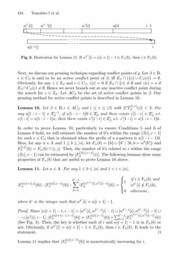
244 Tomohiro I et al.
α[i +1]
i –1
i
α[i]α [i]2α [i]k’–1α [i]k’
Fig. 3. Illustration for Lemma 11. If αk′[i] = α[i + 1]− 1 ∈ Fα(b), then i ∈ Fα(b).
Next, we discuss our pruning technique regarding conflict points of y. Let β ∈ B.c ∈ Cβ is said to be an active conflict point of β, iff Eβ ∩ ({c} ∪ Cβ(c)) = ∅.Obviously, for any z ∈ Zβ and c ∈ Cβ , z[c] = 0 if Eβ ∩ {c} �= ∅ and z[c] = ifEβ ∩Cβ(c) �= ∅. Hence we never branch out at any inactive conflict point duringthe search for z ∈ Zβ. Let ACβ be the set of active conflict points in β. Ourpruning method for active conflict points is described in Lemma 10.
Lemma 10. Let β ∈ B, i ∈ ACβ and i ≤ r ≤ |β| with |CT[1,r]β (i)| < 2. For
any u[1 : i − 1] ∈ Zi−1β , if u[1 : i − 1]0 ∈ Zi
β and there exists z[1 : r] ∈ Zrβ s.t.
z[1 : i] = u[1 : i − 1], then there exists z′[1 : r] ∈ Zrβ s.t. z′[1 : i] = u[1 : i − 1]0.
In order to prove Lemma 10, particularly to ensure Conditions 5 and 6 ofLemma 8 hold, we will estimate the number of 0’s within the range [β[c], c − 1]for each c ∈ Cβ that is obtained when the prefix of a z-pattern is u[1 : i − 1]0.Here, for any α ∈ A and 1 ≤ b ≤ |α|, let Fα(b) = {b} ∪ {b′ | ∃k, b = αk[b′]} andF
[i,j]α (b) = Fα(b) ∩ [i, j]. Then, the number of 0’s related to i within the range
[β[c], c−1] can be estimated by |F [β[c],c−1]β (i)|. The following lemmas show some
properties of Fα(b) that are useful to prove Lemma 10 above.
Lemma 11. Let α ∈ A. For any 1 ≤ b ≤ |α| and 1 < i < |α|,
|F [α[i+1],i]α (b)|−|F [α[i],i−1]
α (b)|−k′−1∑
k=1
|F [αk+1[i],αk[i]−1]α (b)| =
⎧⎪⎨
⎪⎩
1if i ∈ Fα(b) andαk′
[i] /∈ Fα(b),0 otherwise,
where k′ is the integer such that αk′[i] = α[i + 1] − 1.
Proof. Since [α[i + 1]− 1, i − 1] = [αk′[i], αk′−1[i]− 1] ∪ [αk′−1[i], αk′−2[i]− 1] ∪
· · ·∪[α1[i], i−1], |F [α[i+1]−1,i−1]α (b)| = |F [α[i],i−1]
α (b)|+∑k′−1k=1 |F [αk+1[i],αk[i]−1]
α (b)|(See Fig. 3). Then, the key is whether each of i and α[i + 1] − 1 is in Fα(b) ornot. Obviously, if αk′
[i] = α[i + 1] − 1 ∈ Fα(b), then i ∈ Fα(b). It leads to thestatement. �
Lemma 11 implies that |F [α[i],i−1]α (b)| is monotonically increasing for i.

Verifying a Parameterized Border Array in O(n1.5) Time 245
Lemma 12. Let α ∈ A and c′, c ∈ Cα with c′ ∈ C[1,c]α (c). For any 1 ≤ b < c′,
|F [m,c−1]α (b)| ≥ |F [α[c−1],c−2]
α (b)| +k′−1∑
k=1
|F [αk+1[c−1],αk[c−1]−1]α (b)| + 1,
where m = α[c′] = α[c] and k′ is the integer such that αk′[c − 1] = c′ − 1.
Proof. In a similar way to the proof of Lemma 11, we have |F [m,c−2]α (b)| =
|F [α[c−1],c−2]α (b)|+ ∑k′−1
k=1 |F [αk+1[c−1],αk[c−1]−1]α (b)|+ |F [m,c′−2]
α (b)|. Since c− 1 /∈Fα(b) ⇒ αk′
[c − 1] = c′ − 1 /∈ Fα(b),
|F [m,c−1]α (b)| ≥ |F [α[c−1],c−2]
α (b)| +k′−1∑
k=1
|F [αk+1[c−1],αk[c−1]−1]α (b)| + |F [m,c′−1]
α (b)|.
Also, |F [m,c′−1]α (b)| ≥ 1 follows from Lemma 11. Hence, the lemma holds. �
Lemma 13. For any α ∈ A, 1 ≤ b < b′ ≤ |α| and 1 ≤ i < |α|, |F [α[i+1],i]α (b)| ≥
|F [α[i+1],i]α (b′)|.
Proof. We will prove the lemma by induction on i. First, for any 1 ≤ i < b, itis clear that |F [α[i+1],i]
α (b)| = |F [α[i+1],i]α (b′)| = 0. Second, for any b ≤ i < b′, it
follows from Lemma 11 that |F [α[i+1],i]α (b)| ≥ 1. Then, |F [α[i+1],i]
α (b)| ≥ 1 > 0 =|F [α[i+1],i]
α (b′)|. Finally, when b′ ≤ i < |α|, let k′ be the integer such that αk′[i] =
α[i +1]− 1. (I) When i /∈ Fα(b′) or αk′[i] = α[i + 1]− 1 ∈ Fα(b′). It follows from
Lemma 11 that |F [α[i+1],i]α (b)| ≥ |F [α[i],i−1]
α (b)| + ∑k′−1k=1 |F [αk+1[i],αk[i]−1]
α (b)| and
|F [α[i+1],i]α (b′)| = |F [α[i],i−1]
α (b′)| + ∑k′−1k=1 |F [αk+1[i],αk[i]−1]
α (b′)|. By the induction
hypothesis, we have |F [α[i],i−1]α (b)| ≥ |F [α[i],i−1]
α (b′)| and |F [αk+1[i],αk[i]−1]α (b)| ≥
|F [αk+1[i],αk[i]−1]α (b′)| for any 1 ≤ k ≤ k′ − 1. Hence, |F [α[i+1],i]
α (b)| ≥|F [α[i+1],i]
α (b′)|. (II) When i ∈ Fα(b′) and αk′[i] = α[i + 1] − 1 /∈ Fα(b′).
There always exists b′ ∈ {i, α1[i], . . . , αk′−1[i]}, and therefore |F [α[b′],b′−1]α (b)| ≥
1 > 0 = |F [α[b′],b′−1]α (b′)|. Then, |F [α[i+1],i]
α (b)| ≥ |F [α[i],i−1]α (b)| +
∑k′−1k=1 |F [αk+1[i],αk[i]−1]
α (b)| ≥ 1 + |F [α[i],i−1]α (b′)| + ∑k′−1
k=1 |F [αk+1[i],αk[i]−1]α (b′)| =
|F [α[i+1],i]α (b′)|. Hence, |F [α[i+1],i]
α (b)| ≥ |F [α[i+1],i]α (b′)|. �
In a similar way, we have the next lemma.
Lemma 14. Let α ∈ A and c ∈ Cα with CTα(c) = {c′}. For any 1 ≤ i < |α|,|F [α[i+1],i]
α (c)| ≥ ∑g∈G|F [α[i+1],i]
α (g)|, where G = (C [c,|α|]α (c) − c′).
Now, we are ready to prove Lemma 10. We will use Lemmas 13 and 14.
Proof. Let G = {g | g ∈ C[i,r]β (i), z[g] = 0}. Let v be the sequence s.t. for each
1 ≤ j ≤ r, v[j] = 0 if j ∈ Fβ(i), v[j] = if there is g ∈ G s.t. j ∈ Fβ(g), andv[j] = z[j] otherwise.
Now we show v ∈ Zβ . By the definition of v and u[1 : i − 1]0 ∈ Ziβ , it is
clear that v[j] holds Conditions 1, 2, 3 and 4 of Lemma 8 for any 1 ≤ j ≤ r.

246 Tomohiro I et al.
Furthermore, u[1 : i− 1] ∈ Ziβ means that zeros(v[β[i] : i− 1]) ≥ maxcβ(i)− 1.
Hence, v[c] satisfies Conditions 5 and 6 for any c ∈ C[1,r]β (i) since zeros(v[β[c] :
c−1]) ≥ zeros(v[β[i] : i−1]) and maxcβ(i)−1 ≥ maxcβ(c)−1. Then, as the proofof Lemma 9, we have only to show zeros(v[β[c] : c−1]) ≥ zeros(z[β[c] : c−1]) forany c ∈ Cβ . This can be proven by showing |F [β[c],c−1]
β (i)| ≥ ∑g∈G|F [β[c],c−1]
β (g)|.Since it is clear in case where G = ∅, we consider the case where G �= ∅. Letc′ = CTβ(i). Note that |CTβ(i)| = 1 by the assumption. (I) When z[c′] = 0. Sincez[1 : r] satisfies Condition 4 of Lemma 8, G = {c′}. It follows from Lemma 13that |F [β[c],c−1]
β (i)| ≥ |F [β[c],c−1]β (c′)| for any c ∈ C
[1,r]β . (II) When z[c′] �= 0.
It follows from Lemma 14 that |F [β[c],c−1]β (i)| ≥ ∑
g∈G|F [β[c],c−1]β (g)| for any
c ∈ C[1,r]β . Therefore, the lemma holds. �
4.3 Complexity Analysis
Algorithm 1 shows our algorithm that solves Problem 1.
Theorem 1. Algorithm 1 solves Problem 1 in O(n1.5) time and O(n) space foran unbounded alphabet.
Proof. The correctness should be clear from the discussions in the previous sub-sections.
Let us estimate the time complexity of Algorithm 1 until the CheckPBA func-tion is called at Line 1. As in the failure function construction algorithm, thewhile loop of Line 6 is executed at most n times. Moreover, for any 1 ≤ i ≤ n,the values of z[i], prevc[i], and order [i] are updated at most once. When i isa conflict point, Line 20 is executed at most ordery(i) − 1 times. Hence, itfollows from Lemma 5 that the total number of times Line 20 is executed is∑
c∈Cy(ordery(c) − 1) ≤ 1 +
∑c∈Cy
�2ordery(c)−2� ≤ n.Next, we show the CheckPBA function takes in O(n1.5) time for any input
α ∈ A. Let 2 ≤ r1 < r2 < · · · < rx ≤ n be the positions for which we executeLine 6 or 10 when we first visit these positions. If such positions do not exist,CheckPBA returns “valid” in O(n) time. Let us consider x ≥ 1. For any 1 ≤ t ≤ x,let zt[1 : rt − 1] denote the z-pattern when we first visit rt and let lt = min{c |c ∈ AC
[1,rt−1]α , zt[c] = 0}. If x = 1 and such l1 does not exist, then CheckPBA
returns “invalid” in O(n) time. If x > 1, then there exists l1 as we reach rx.Furthermore, there exists lt s.t. lt < r1 since otherwise we cannot get across r1.Henceforth, we may assume l1 ≤ l2 ≤ · · · ≤ lx exist. Note that by the definitionof active conflict points, all elements of Fα(lt)−{lt} are not conflict points, andtherefore for any b ∈ Fα(lt), zt[b] = 0.
Here, let L1 = {c | c ∈ C[l1+1,r1]α , l1 < max C
[1,c]α (c)} and Lt = {c | c ∈
C[rt−1+1,rt]α , lt < maxC
[1,c]α (c)} for any 1 < t ≤ x. Since L1, L2, . . . , Lx are
pairwise disjoint, |L| =∑x
t=1|Lt|, where L =⋃x
t=1 Lt. It follows from Lemma 12that |F [α[rt],rt−1]
α (lt)| − |F [α[rt−1],rt−1−1]α (lt)| ≥ |Lt|. In addition, for any 1 ≤
t ≤ x, let Eint = Eα ∩ ([α[rt], rt − 1] − [α[rt−1], rt−1 − 1]}) and Eout
t = Eα ∩

Verifying a Parameterized Border Array in O(n1.5) Time 247
Algorithm 1. Algorithm to verify p-border arrayInput: an integer array y[1 :n]Output: whether y is a valid p-border array or not/* zeros [1 :n] : zeros [i] = zeros(z[1 : i]). zeros [0] = 0 for convenience. */
/* sign[1 :n] : sign[i] = 1 if i ∈ Ey, sign[i] = −1 if (C[i,n]y (i)∩Ey) �= ∅. */
/* prevc[1 :n] : prevc[i] = max C[1,i]y (i), prevc[i] = 0 otherwise. */
if y[1 :2] �= [0, 1] then return invalid;1
sign[1 :n]← [1, 0, .., 0]; prevc[1 :n]← [0, .., 0]; order [1 :n]← [0, .., 0];2
maxc[1 :n]← [0, .., 0];for i = 3 to n do3
if y[i] = y[i− 1] + 1 then continue;4
b′ ← y[i− 1]; b← y[b′];5
while b > 0 & y[i] �= y[b′ + 1] & y[i] �= b + 1 do6
b′ ← b; b← y[b′];7
if y[i] = y[b′ + 1] then /* i conflicts with b′ + 1 */8
j ← y[i];9
while sign[j] = 0 & order [j] = 0 do /* z[y1[i]], z[y2[i]], . . . , z[0] must10
be 0 */
sign[j]← 1; j ← y[j];11
if sign[j] = −1 then return invalid;12
if sign[j] �= 1 then13
sign[j]← 1; j ← prevc[j];14
while j > 0 do /* ∀j ∈ C[1,i]y (i), z[j] must be � */15
if sign[j] = 1 then return invalid;16
sign[j]← −1; j ← prevc[j];17
if order [b′ + 1] = 0 then order [b′ + 1]← 1;18
prevc[i]← b′ + 1; order [i]← order [b′ + 1] + 1;19
maxc[i]← order [b′ + 1] + 1; j ← b′ + 1;while j > 0 & maxc[j] < order [b′ + 1] + 1 do20
maxc[j]← order [b′ + 1] + 1; j ← prevc[j];21
else if y[i] �= b + 1 then return invalid;22
cnt[1 :n]← [−1, ..,−1]; zeros [1]← 1;23
return CheckPBA(2, n, y[1 :n], zeros [1 :n], sign[1 :n], cnt[1 :n],24
prevc[1 :n], order [1 :n], maxc[1 :n]);
([α[rt−1], rt−1 − 1] − [α[rt], rt − 1]}), where [α[r0], r0 − 1] = ∅. Since for any1 < t ≤ x, zeros(zt[α[rt−1] : rt−1 − 1]) ≥ zeros(zt−1[α[rt−1] : rt−1 − 1]) + 1,
zeros(zt[α[rt] : rt − 1])≥ zeros(zt[α[rt−1] : rt−1 − 1]) + |Ein
t | − |Eoutt |
+|F [α[rt],rt−1]α (lt)| − |F [α[rt−1],rt−1−1]
α (lt)|≥ zeros(zt−1[α[rt−1] : rt−1 − 1]) + 1 + |Ein
t | − |Eoutt | + |Lt|.

248 Tomohiro I et al.
Function. CheckPBA(i, n, y[1 : n], zeros [1 : n], sign[1 : n], cnt[1 : n], prevc[1 :n], order [1 :n], maxc[1 :n])
Result: whether y is a valid p-border array or notif i = n then return valid;1
if order [i] = 0 then /* i is not a conflict point */2
zeros [i]← zeros [i− 1] + zeros [y[i]]− zeros [y[i]− 1];3
return CheckPBA(i + 1, n, y[1 :n], . . . , maxc[1 :n]);4
if sign[i] = 1 then /* z[i] must be 0 */5
if zeros [i− 1]− zeros [y[i]− 1] < maxc[i]− 1 then return invalid;6
zeros [i]← zeros [i− 1] + 1;7
return CheckPBA(i + 1, n, y[1 :n], . . . , maxc[1 :n]);8
if sign[i] = −1 ‖ zeros [i− 1]− zeros [y[i]− 1] < maxc[i]− 1 then /* z[i] must9
be � */
if zeros [i− 1]− zeros [y[i]− 1] < order [i] then return invalid;10
zeros [i]← zeros [i− 1];11
return CheckPBA(i + 1, n, y[1 :n], . . . , maxc[1 :n]);12
/* from here sign[i] = 0 and zeros [i− 1]− zeros [y[i]− 1] ≥ maxc[i]− 1 */
if cnt[i] = −1 then /* first time arriving at i */13
cnt[i] + +; cnt[prevc[i]] + +14
if prevc[i] > 0 & sign[prevc[i]] = 1 then /* ∃c ∈ C[1,i]y (i), z[c] = 0 */15
sign[i]← 1; zeros [i]← zeros [i− 1];16
ret← CheckPBA(i + 1, n, y[1 :n], . . . , maxc[1 :n]); sign[i]← 0;17
return ret;18
sign[i]← 1; zeros [i]← zeros [i− 1] + 1;19
ret← CheckPBA(i + 1, n, y[1 :n], . . . , maxc[1 :n]); sign[i]← 0;20
if ret = valid ‖ cnt[i] < 2 then return ret;21
zeros [i]← zeros [i− 1];22
return CheckPBA(i + 1, n, y[1 :n], . . . , maxc[1 :n]);23
By recursive procedures, we have orderα(rx) ≥ 1 + zeros(zx[α[rx] : rx − 1]) ≥zeros(z1[α[r1] : r1 − 1]) + x +
∑xt=2|Ein
t | − ∑xt=2|Eout
t | +∑x
t=2|Lt|. Sincezeros(z1[α[r1] : r1−1]) ≥ 1+ |Ein
1 |+ |L1| and∑x
t=1|Eint |−∑x
t=2|Eoutt | ≥ 1, then
orderα(rx) ≥ 2 + x + |L|.Now, we evaluate the number of z-patterns we search for during the calls of
CheckPBA. Let C2(t) = {c | c ∈ C[lt,rt]α , |CT
[lt,rt]α (c)| ≥ 2} for any 1 ≤ t ≤ x
and T ′ = {1} ∪ {t | 1 < t ≤ x, lt−1 < lt, |CT[lt,rt−1]α (lt)| = 0}. Let us assume
T ′ = {t′1, t′2, . . . , t′x′} with 1 = t′1 < t′2 < · · · < t′x′ ≤ x. By Lemmas 9 and 10,the number of z-patterns searched for between lt′j and rt′j+1−1 is at most 2|C
′2(t
′j)|
for any 1 ≤ j ≤ x′, where t′x′+1 − 1 = x and C′2(t
′j) =
⋃t′j+1−1
t=t′jC2(t). Then,
the total number of z-patterns is at most∑x′
j=1 2|C′2(t
′j)|. By Lemma 10, for any
1 ≤ j < x′, lt′j must be in C′2(t′j) and by the definition of T ′, lt′j is only in
C′2(t
′j). Hence, if C2 =
⋃xt=1 C2(t), then |C′
2(t′j)| ≤ |C2| − (x′ − 2), and therefore
∑x′
j=1 2|C′2(t
′j)| ≤ 4x′2|C2|−x′
.

Verifying a Parameterized Border Array in O(n1.5) Time 249
1r1lt’ = 11
2r2l
3r3l
4r4l
5r5l
t’ = 32
t’ = 53
Fig. 4. Relation between L and C2. A pair of a big circle and a small circle connectedby an arc represents a parent-child relation in the conflict tree. © is a position in C.• or ◦ is a position in L. � is a position not in L.
Finally, we consider the relation between L and C2 (See Fig. 4). By the defi-nition of L and C2, for any c ∈ (C2 − {l1, l2, . . . , lx}), |CTα(c)∩L| ≥ 2. In addi-tion, by the definition of T ′, for any c ∈ (C2 ∩{l1, l2, . . . , lx}−{lt′1, lt′2 , . . . , lt′x′}),|CTα(c) ∩ L| ≥ 1. Here, let x′′ = |{l1, l2, . . . , lx} − {lt′1 , lt′2 , . . . , lt′x′}|. Clearly,x′+x′′ ≤ x. For these reasons, orderα(rx) ≥ 2+x+|L| ≥ 2+x+2|C2|−2(x′+x′′)+x′′ ≥ 2+2|C2|−x′. It follows from Lemma 5 that n ≥ 1+
∑c∈Cα
�2orderα(c)−2� >
1 +∑2+2|C2|−x′
i=2 2i−2 = 22|C2|−x′+1 and√
n > 21+x′
2 2|C2|−x′> x′2|C2|−x′
. Hence,the total time complexity is proportional to n
∑x′
j=1 2|C′2(t
′j)| ≤ 4nx′2|C2|−x′
<
4n√
n.The space complexity is O(n) as we use only a constant number of arrays of
length n. �
5 Conclusions and Open Problems
We presented an O(n1.5)-time O(n)-space algorithm to verify if a given integerarray y of length n is a valid p-border array for an unbounded alphabet. In casey is a valid p-border array, the proposed algorithm also computes a z-patternz ∈ {0, }∗ s.t. z ∈ Zy, and we remark that some sequence p ∈ Py s.t. ptoz (p) = zis then computable in linear time from z.
Open problems of interest are: (1) Can we solve the p-border array reverseproblem for an unbounded alphabet in o(n1.5) time? (2) Can we efficiently solvethe p-border array reverse problem for a bounded alphabet? (3) Can we effi-ciently count p-border arrays of length n?

250 Tomohiro I et al.
References
1. Baker, B.S.: Parameterized pattern matching: Algorithms and applications. Jour-nal of Computer and System Sciences 52(1), 28–42 (1996)
2. Amir, A., Farach, M., Muthukrishnan, S.: Alphabet dependence in parameterizedmatching. Information Processing Letters 49(3), 111–115 (1994)
3. Kosaraju, S.: Faster algorithms for the construction of parameterized suffix trees.In: Proc. FOCS 1995, pp. 631–637 (1995)
4. Hazay, C., Lewenstein, M., Sokol, D.: Approximate parameterized matching. ACMTransactions on Algorithms 3(3), Article No. 29 (2007)
5. Apostolico, A., Erdos, P.L., Lewenstein, M.: Parameterized matching with mis-matches. Journal of Discrete Algorithms 5(1), 135–140 (2007)
6. I, T., Deguchi, S., Bannai, H., Inenaga, S., Takeda, M.: Lightweight parameterizedsuffix array construction. In: Proc. IWOCA, pp. 312–323 (2009)
7. Idury, R.M., Schaffer, A.A.: Multiple matching of parameterized patterns. Theo-retical Computer Science 154(2), 203–224 (1996)
8. Morris, J.H., Pratt, V.R.: A linear pattern-matching algorithm. Technical Re-port 40, University of California, Berkeley (1970)
9. I, T., Inenaga, S., Bannai, H., Takeda, M.: Counting parameterized border arraysfor a binary alphabet. In: Dediu, A.H., Ionescu, A.M., Martın-Vide, C. (eds.) LATA2009. LNCS, vol. 5457, pp. 422–433. Springer, Heidelberg (2009)
10. Franek, F., Gao, S., Lu, W., Ryan, P.J., Smyth, W.F., Sun, Y., Yang, L.: Verifyinga border array in linear time. J. Comb. Math. and Comb. Comp. 42, 223–236 (2002)
11. Duval, J.P., Lecroq, T., Lefevre, A.: Border array on bounded alphabet. Journalof Automata, Languages and Combinatorics 10(1), 51–60 (2005)
12. Duval, J.P., Lefebvre, A.: Words over an ordered alphabet and suffix permutations.Theoretical Informatics and Applications 36, 249–259 (2002)
13. Bannai, H., Inenaga, S., Shinohara, A., Takeda, M.: Inferring strings from graphsand arrays. In: Rovan, B., Vojtas, P. (eds.) MFCS 2003. LNCS, vol. 2747,pp. 208–217. Springer, Heidelberg (2003)
14. Schurmann, K.B., Stoye, J.: Counting suffix arrays and strings. Theoretical Com-puter Science 395(2-1), 220–234 (2008)
15. Clement, J., Crochemore, M., Rindone, G.: Reverse engineering prefix tables. In:Proc. STACS 2009, pp. 289–300 (2009)
16. Duval, J.P., Lecroq, T., Lefebvre, A.: Efficient validation and construction of borderarrays and validation of string matching automata. RAIRO - Theoretical Informat-ics and Applications 43(2), 281–297 (2009)
17. Gawrychowski, P., Jez, A., Jez, L.: Validating the Knuth-Morris-Pratt failure func-tion, fast and online. In: Proc. CSR 2010 (to appear 2010)
18. Crochemore, M., Iliopoulos, C., Pissis, S., Tischler, G.: Cover array string recon-struction. In: Proc. CPM 2010 (to appear 2010)
19. Moore, D., Smyth, W., Miller, D.: Counting distinct strings. Algorithmica 23(1),1–13 (1999)

Cover Array String Reconstruction
Maxime Crochemore1,2, Costas S. Iliopoulos1,3,Solon P. Pissis1, and German Tischler1,4
1 Dept. of Computer Science, King’s College London, London WC2R 2LS, UK{mac,csi,pississo,tischler}@dcs.kcl.ac.uk
2 Universite Paris-Est, France3 Digital Ecosystems & Business Intelligence Institute, Curtin University
GPO Box U1987 Perth WA 6845, Australia4 Newton Fellow
Abstract. A proper factor u of a string y is a cover of y if every letterof y is within some occurrence of u in y. The concept generalises thenotion of periods of a string. An integer array C is the minimal-cover(resp. maximal-cover) array of y if C [i] is the minimal (resp. maximal)length of covers of y[0 . . i], or zero if no cover exists.
In this paper, we present a constructive algorithm checking the va-lidity of an array as a minimal-cover or maximal-cover array of somestring. When the array is valid, the algorithm produces a string over anunbounded alphabet whose cover array is the input array. All algorithmsrun in linear time due to an interesting combinatorial property of coverarrays: the sum of important values in a cover array is bounded by twicethe length of the string.
1 Introduction
The notion of periodicity in strings is well studied in many fields like combina-torics on words, pattern matching, data compression and automata theory (see[11,12]), because it is of paramount importance in several applications, not totalk about its theoretical aspects.
The concept of quasiperiodicity is a generalisation of the notion of periodicity,and was defined by Apostolico and Ehrenfeucht in [2]. In a periodic repetitionthe occurrences of the single periods do not overlap. In contrast, the quasiperiodsof a quasiperiodic string may overlap. We call a proper factor u of a nonemptystring y a cover of y, if every letter of y is within some occurrence of u in y.In this paper, we consider the so-called aligned covers, where the cover u of yneeds to be a border (i.e. a prefix and a suffix) of y. The array C is called theminimal-cover (resp. maximal-cover) array of the string y of length n, if for eachi, 0 ≤ i < n, C [i] stores either the length of the shortest (resp. longest) coverof y[0 . . i], when such a cover exists, or zero otherwise. In particular, we do notconsider a string to be a cover of itself.
Apostolico and Breslauer [1,4] gave an online linear runtime algorithm com-puting the minimal-cover array of a string. In their definition, a string is a cover
A. Amir and L. Parida (Eds.): CPM 2010, LNCS 6129, pp. 251–259, 2010.c© Springer-Verlag Berlin Heidelberg 2010

252 M. Crochemore et al.
of itself, but it is straightforward to modify their algorithm to accommodate ourdefinition. Li and Smyth [10] provided an online linear runtime algorithm forcomputing the maximal-cover array.
In this paper, we present a constructive algorithm checking if an integer arrayis the minimal-cover or maximal-cover array of some string. When the arrayis valid, the algorithm produces a string over an unbounded alphabet whosecover array is the input array. For our validity checking algorithm, we use theaforementioned algorithms that compute cover arrays.
All algorithms run in linear time. This is essentially due to a combinatorialproperty of cover arrays: the sum of important values in a cover array is boundedby twice the length of the string.
The result of the paper completes the series of algorithmic characterisations ofdata structures that store fundamental features of strings. They concern Borderarrays [6,7], Parameterized Border arrays [9] and Prefix arrays [5] that storesperiods of all the prefixes of a string, as well as the element of Suffix arrays [3,8]that memorises the list of positions of lexicographically sorted suffixes of thestring. The question is not applicable to complete Suffix trees or Suffix automatasince the relevant string is part of these data structures. The algorithms may beregarded as reverse engineering processes and, beyond their obvious theoreticalinterest, they are useful to test the validity of some constructions. Their linearruntime is an important part of their quality.
The rest of the paper is structured as follows. Section 2 presents the basic def-initions used throughout the paper and the problem. In Section 3, we prove someproperties of minimal-cover arrays used later for the design or the analysis ofalgorithms. In Section 4, we describe our constructive cover array validity check-ing algorithms. Section 5 provides some combinatorially interesting numericaldata on minimal-cover arrays.
2 Definitions and Problems
Throughout this paper we consider a string y of length |y| = n on an unboundedalphabet. It is represented as y[0 . . n− 1]. A string w is a factor of y if y = uwvfor two strings u and v. It is a prefix of y if u is empty and a suffix of y ifv is empty. A string u is a period of y if y is a prefix of uk for some positiveinteger k, or equivalently if y is a prefix of uy. The period of y is the shortestperiod of y. A string x of length m is a cover of y if both m < n and thereexists a set of positions P ⊆ {0, . . . , n −m} satisfying y[i . . i + m − 1] = x forall i ∈ P and
⋃i∈P{i, . . . , i + m − 1} = {0, . . . , n − 1}. Note that this requires
x to be a prefix as well as a suffix of y. The minimal-cover array C of y is thearray of integers C [0 . . n − 1] for which C [i], 0 ≤ i < n, stores the length ofthe shortest cover of the prefix y[0 . . i], if such a cover exists, or zero otherwise.The maximal-cover array CM stores longest cover at each position instead. Thefollowing table provides the minimal-cover array C and the maximal-cover arrayCM of the string y = abaababaababaabaababaaba.

Cover Array String Reconstruction 253
i 0 1 2 3 4 5 6 7 8 9 10 11 12 13 14 15 16 17 18 19 20 21 22 23
y[i] a b a a b a b a a b a b a a b a a b a b a a b a
C [i] 0 0 0 0 0 3 0 3 0 5 3 7 3 9 5 3 0 5 3 0 3 9 5 3
CM[i] 0 0 0 0 0 3 0 3 0 5 6 7 8 9 10 11 0 5 6 0 8 9 10 11
We consider the following problems for an integer array A:
Problem 1 (Minimal Validity Problem). Decide if A is the minimal-cover arrayof some string.
Problem 2 (Maximal Validity Problem). Decide if A is the maximal-cover arrayof some string.
Problem 3 (Minimal Construction Problem). When A is a valid minimal-coverarray, exhibit a string over an unbounded alphabet whose minimal-cover arrayis A.
Problem 4 (Maximal Construction Problem). When A is a valid maximal-coverarray, exhibit a string over an unbounded alphabet whose maximal-cover arrayis A.
3 Properties of the Minimal-Cover Array
In this section, we assume that C is the minimal-cover array of y. Its first elementis 0, as we do not consider a string to be a cover of itself. Next elements are 1only for prefixes of the form ak for some letter a. We will use the following factin our argumentation.
Fact 1 (Transitivity). If u and v cover y and |u| < |v|, then u covers v.
For the rest of the section we assume that n > 1 and prove several less obviousproperties of the minimal-cover array.
Lemma 1. If 0 ≤ i < n and C [i] �= 0, then C [C [i]− 1] = 0.
Proof. Immediate from Fact 1. ��
Lemma 2. Let i and j be positions such that j < i, j−C [j] ≥ i−C [i], C [i] �= 0and C [j] �= 0. Furthermore let r = j − (i−C [i] + 1). If i−C [i] = j −C [j] thenC [r] = 0, otherwise if i− C [i] < j − C [j], then C [r] = C [j].
Proof. First assume that i − C [i] = j − C [j]. Then C [j − (i − C [i] + 1)] =C [j − (j − C [j] + 1)] = C [C [j] − 1] = 0 according to Lemma 1. Now assumethat i − C [i] < j − C [j]. This situation is depicted in Figure 1. The stringu = y[j −C [j] + 1 . . j] of length C [j] covers the string y[0 . . j]. By precondition(j < i, j−C [j] > i−C [i]) u also covers y[0 . . r], as there exists an occurrence of uat position r−C [j]+1. Thus we have C [r] ≤ C [j]. The assumption C [r] < C [j]leads to a contradiction to the minimality of C . Thus we have C [r] = C [j]. ��

254 M. Crochemore et al.
u u
ijj'i'
u u
r+1r+1
r
Fig. 1. Case j − C [j] > i − C [i] of Lemma 2 (i′ = i − C[i] + 1, j′ = j − C[j] + 1)
Lemma 3. Let i and j be positions such that j < i and j − C [j] < i − C [i].Then (i− C [i])− (j − C [j]) > C [j]/2.
Proof. For ease of notation let p = C [i], q = C [j] and r = (i − p) − (j − q).Assume the statement does not hold, i.e. r ≤ q
2 . Let u = y[0 . . r − 1]. Thendue to the overlap of y[i − p + 1 . . i] and y[j − q + 1 . . j] both y[0 . . p − 1] andy[0 . . q − 1] are powers of u. Let y[0 . . q − 1] = ue for some exponent e. Observethat e = q/r ≥ q/(q/2) = 2. However y[0 . . q−1] is also covered by v = u1+e−�e�.As |v| < q we obtain a contradiction. ��Definition 1. A position j �= 0 of C is called totally covered, if there is aposition i > j for which C [i] �= 0 and i− C [i] + 1 ≤ j − C [j] + 1 < j.
Let Cp be obtained from C by setting C [i] = 0 for all totally covered indices ion C . We call Cp the pruned minimal-cover array of y. The next table showsthe pruned minimal-cover array of the example string above.
i 0 1 2 3 4 5 6 7 8 9 10 11 12 13 14 15 16 17 18 19 20 21 22 23y[i] a b a a b a b a a b a b a a b a a b a b a a b aC [i] 0 0 0 0 0 3 0 3 0 5 3 7 3 9 5 3 0 5 3 0 3 9 5 3
Cp[i] 0 0 0 0 0 3 0 0 0 0 0 0 0 9 5 0 0 0 0 0 0 9 5 3
Lemma 4. The sum of the elements of Cp does not exceed 2n.
Proof. Let Ii = {i−C [i]+1, i−C [i]+2, . . . i} for i = 0, . . . , n−1 if C [i] �= 0 andIi = ∅ otherwise. Let I ′i denote the lower half of Ii (if C [i] is uneven, the middleelement is included). According to Lemma 3, i �= j implies I ′i ∩ I ′j = ∅. Thus therelation
∑n−1i=0 |I ′i| ≤ n holds, which in turn implies
∑n−1i=0 |Ii| ≤
∑n−1i=0 2|I ′i| ≤ 2n.
��The bound of Lemma 4 is asymptotically tight. For an integer k > 1, let xk =(akbak+1b)n/(2k+3). For k = 2 and n = 23 we get:
i 0 1 2 3 4 5 6 7 8 9 10 11 12 13 14 15 16 17 18 19 20 21 22y[i] a a b a a a b a a b a a a b a a b a a a b a a
Cp[i] 0 0 0 0 0 0 0 0 5 0 0 0 0 7 0 5 0 0 0 0 7 0 5
It is straightforward to see that all segments of length 2k + 3 of Cp contain thevalues 2k + 1 and 2k + 3, except at the beginning of the string. Therefore thesum of elements in Cp is (4k + 4)( n
2k+3− 1), which tends to 2n when k (and n)
goes to infinity.

Cover Array String Reconstruction 255
4 Reverse Engineering a Cover Array
We solve the stated problems in three steps: array transformation, string infer-ence and validity checking.
Transforming Maximal to Minimal-Cover Arrays. We first show how to trans-form a maximal-cover array into a minimal-cover array in linear time. The fol-lowing algorithm Maxtomin converts the maximal-cover array C of y to itsminimal-cover array in linear time.
Maxtomin(C , n)1 for i← 0 to n− 1 do2 if C [i] �= 0 and C [C [i]− 1] �= 0 then3 C [i]← C [C [i]− 1]
The algorithm works in the following way. Assume the for loop is executing forsome i > 0. At this time the prefix C [0 . . i−1] of the array has been converted toa minimal-cover array and we want to determine the value of C [i]. If C [i] is zerothen there is no cover and we leave the value as it is. If C [i] is not zero, then weknow from Fact 1 that if there is a shorter cover, then it covers y[0 . .C [i]− 1].Thus we look up C [C [i]− 1] to see if there is a shorter cover we can substitutefor C [i]. As the segment before index i is already the minimal-cover array up tothis point, we know that such a value is minimal.
String Inference. In this step, we assume that the integer array C of length n isthe minimal- or maximal-cover array of at least one string. From what we wroteabove, we can assume without loss of generality that C is a minimal-cover array.
The nonzero values in C induce an equivalence relation on the positions ofevery string that has the minimal-cover array C . More precisely, if we find thevalue � �= 0 in position i of C , then this imposes the constraints
y[k] = y[i− � + 1 + k]
for k = 0, . . . , �−1. We say that the positions k and i−�+1+k are bidirectionallylinked. Let the undirected graph G(V, E) be defined by V = {0, . . . , n− 1} and
E =⋃
i=0,...,n−1
⋃
j=0,...C [i]−1
({(j, i− C [i] + 1 + j)}) .
Then the nonzero values in C state that the letters at positions i and j of anyword y such that C is the minimal-cover array of y need to be equal, if i and jare connected in G. According to Lemma 2, we do not lose connectivity betweenvertices of G, if we remove totally covered indices from C , i.e. the graph inducedby C has the same connected components as the one induced by its prunedversion Cp. The number of edges in the graph induced by Cp is bounded by 2naccording to Lemma 4.
The pruned minimal-cover array Cp can be obtained from the minimal-coverarray C using the following algorithm Prune in linear time.

256 M. Crochemore et al.
Prune(C , n)1 �← 02 for i← n− 1 downto 0 do3 if � ≥ C [i] then4 C [i]← 05 �← max(0, max(�,C [i])− 1)6 return C
A non-zero value at index i in C defines an interval [i−C [i]+1, i]. The algorithmscans C from large to small indices, where the value � stores the minimal lowerbound of all the intervals encountered so far. If an interval starting at a smallerupper bound has a greater lower bound than �, we erase the corresponding valuein C by setting it to zero. Thus we remove all totally covered indices from Cand obtain the pruned array Cp.
So far we know how to extract information from the non-zero values of C bycomputing connected components in a graph which has no more than 2n edges.The vertices in each connected component designate positions in any producedstring which need to have equal letters. By assigning a different letter to each ofthese components, we make sure not to violate any constraints set by the zerovalues in C . The following algorithm MinArrayToString produces a string yfrom an array A assumed to be a pruned minimal-cover array.
MinArrayToString(A, n)1 � Produce edges2 for i← 0 to n− 1 do3 E[i]← empty list4 for i← 0 to n− 1 do5 for j ← 0 to A[i]− 1 do6 E[i−A[i] + 1 + j].add(j), E[j].add(i −A[i] + 1 + j)7 � Compute connected components by Depth First Search8 � and assign letters to output string9 (S, �)← (empty stack,−1)
10 for i← 0 to n− 1 do11 if y[i] is undefined then12 S.push(i)13 �← � + 114 while not S.empty() do15 p← S.pop()16 y[p]← �17 for each element j of E[p] do18 if y[j] is undefined then19 S.push(j)20 return y
The first two for loops produce the edges E in the graph G induced by A, wherewe implement the transition relation by assigning a linear list of outgoing edges

Cover Array String Reconstruction 257
to each vertex. The third for loop computes the connected components in thegraph by using depth first search and assigns the letters to the output string.Each connected component is assigned a different letter. The runtime of thealgorithm is linear in the number of edges of the graph, which is bounded by 2n.
Theorem 1. The problems Minimal Construction Problem and MaximalConstruction Problem are solved in linear time by the algorithm MinAr-rayToString and the sequence of algorithms MaxToMin and MinArray-ToString respectively.
Validity Checking. In the third step we use the MinArrayToString algorithmas a building block for our validity checking algorithm. Thus we have to ensuresome basic constraints so that the algorithm does not firstly access any unde-fined positions in the input and secondly runs in linear time. As a first step, wehave to make sure that the algorithm will not try to define edges for which atleast one vertex number is not valid. This check is performed by the followingalgorithm Precheck, which runs in linear time.
Precheck(A, n)1 for i← 0 to n− 1 do2 if i−A[i] + 1 < 0 then3 return false4 return true
If Precheck returns true, then MinArrayToString will only generate edgesfrom valid to valid vertices. If we are checking for validity of a maximal-cover ar-ray, we then pass the array through the algorithm MaxToMin as a next step. Inboth cases (minimal and maximal) the next step is to prune the array using thealgorithm Prune. After this, we can call the algorithm MinArrayToStringwith the so-modified array, but it may not run in linear time, as the constraintsimposed by Lemma 3 may not hold if the original input array is invalid. Weavoid this situation with the following algorithm Postcheck.
Postcheck(A, n)1 j ← −12 for i← 0 to n− 1 do3 if A[i] �= 0 then
4 if j �= −1 and (i−A[i])− (j −A[j]) ≤⌊
A[j]2
⌋then
5 return false6 j ← i7 return true
If Postcheck returns false, then the input array was invalid. Otherwise wecan call MinArrayToString and be sure that it will run in linear time. Atthis point we have obtained a string from the input array in linear time. Weknow that if the input array is valid, the minimal- or maximal- (depending onwhat kind of input we are given) cover array of this string matches the input.

258 M. Crochemore et al.
If the input array is not valid, we cannot obtain it by computing the minimal-or maximal-cover array from the obtained string. Thus we can check whether anarray A is a valid maximal-cover array using the following algorithm Check-Maximal.CheckMaximal(A, n)
1 if Precheck(A, n) = false then2 return false3 A←MaxToMin(A, n)4 A← Prune(A, n)5 if Postcheck(A, n) = false then6 return false7 y ←MinArrayToString(A, n)8 if the maximal-cover array of y equals A then9 return true
10 else return false
The algorithm CheckMinimal for checking whether an array A is a validminimal-cover array is obtained from CheckMaximal by removing the callto the function MaxToMin in line 3 and checking whether the minimal insteadof the maximal-cover array of the string y equals A in line 8.
Theorem 2. The problems Minimal Validity Problem and Maximal ValidityProblem are solved by the algorithms CheckMinimal and CheckMaximalrespectively in linear time.
5 Experiments and Numerical Results
Figure 2 shows the maximal ratio of sums of elements of pruned minimal-coverarray, for all words over a two-letter alphabet, using even word lengths 8 to 30.These ratios are known to be smaller than 2 by Lemma 4. However, values closeto this bound are not observed for small word length.
1
1.1
1.2
1.3
1.4
1.5
10 15 20 25 30
ratio
n
Fig. 2. Maximal ratio of sum over pruned minimal-cover array and word length forwords over the binary alphabet of even length 8 to 30

Cover Array String Reconstruction 259
We were able to verify the linear runtime of our algorithm in experiments.The implementation for the CheckMinimal function is available at the Websitehttp://www.dcs.kcl.ac.uk/staff/tischler/src/recovering-0.0.0.tar.bz2,which is set up for maintaining the source code and the documentation.
6 Conclusion
In this paper, we have provided linear runtime algorithms for checking the va-lidity of minimal- and maximal-cover arrays and algorithms to infer strings fromvalid minimal- and maximal-cover arrays. The linear time inference of stringsusing the least possible alphabet size from cover arrays remains an open problem.
References
1. Apostolico, A., Breslauer, D.: Of periods, quasiperiods, repetitions and covers. In:Mycielski, J., Rozenberg, G., Salomaa, A. (eds.) Structures in Logic and ComputerScience. LNCS, vol. 1261, pp. 236–248. Springer, Heidelberg (1997)
2. Apostolico, A., Ehrenfeucht, A.: Efficient detection of quasiperiodicities in strings.Theoretical Computer Science 119(2), 247–265 (1993)
3. Bannai, H., Inenaga, S., Shinohara, A., Take, M.: Inferring strings from graphs andarrays. In: Rovan, B., Vojtas, P. (eds.) MFCS 2003. LNCS, vol. 2747, pp. 208–217.Springer, Heidelberg (2003)
4. Breslauer, D.: An on-line string superprimitivity test. Information Processing Let-ters 44(6), 345–347 (1992)
5. Clement, J., Crochemore, M., Rindone, G.: Reverse engineering prefix tables.In: Albers, S., Marion, J.-Y. (eds.) 26th International Symposium on Theo-retical Aspects of Computer Science (STACS 2009), Dagstuhl, Germany, pp.289–300. Schloss Dagstuhl - Leibniz-Zentrum fuer Informatik, Germany (2009),http://drops.dagstuhl.de/opus/volltexte/2009/1825
6. Duval, J.-P., Lecroq, T., Lefebvre, A.: Border array on bounded alphabet. Journalof Automata, Languages and Combinatorics 10(1), 51–60 (2005)
7. Franek, F., Gao, S., Lu, W., Ryan, P.J., Smyth, W.F., Sun, Y., Yang, L.: Veri-fying a Border array in linear time. Journal on Combinatorial Mathematics andCombinatorial Computing 42, 223–236 (2002)
8. Franek, F., Smyth, W.F.: Reconstructing a Suffix Array. International Journal ofFoundations of Computer Science 17(6), 1281–1295 (2006)
9. Tomohiro, I., Inenaga, S., Bannai, H., Takeda, M.: Counting parameterized borderarrays for a binary alphabet. In: Dediu, A.H., Ionescu, A.M., Martın-Vide, C. (eds.)LATA 2009. LNCS, vol. 5457, pp. 422–433. Springer, Heidelberg (2009)
10. Li, Y., Smyth, W.F.: Computing the cover array in linear time. Algorithmica 32(1),95–106 (2002)
11. Lothaire, M. (ed.): Algebraic Combinatorics on Words. Cambridge UniversityPress, Cambridge (2001)
12. Lothaire, M. (ed.): Applied Combinatorics on Words. Cambridge University Press,Cambridge (2005)

Compression, Indexing, and Retrieval
for Massive String Data�
Wing-Kai Hon1, Rahul Shah2, and Jeffrey Scott Vitter3
1 National Tsing Hua University, [email protected]
2 Louisiana State University, [email protected]
3 Texas A&M University, [email protected]
Abstract. The field of compressed data structures seeks to achieve fastsearch time, but using a compressed representation, ideally requiring lessspace than that occupied by the original input data. The challenge is toconstruct a compressed representation that provides the same function-ality and speed as traditional data structures. In this invited presenta-tion, we discuss some breakthroughs in compressed data structures overthe course of the last decade that have significantly reduced the spacerequirements for fast text and document indexing. One interesting con-sequence is that, for the first time, we can construct data structures fortext indexing that are competitive in time and space with the well-knowntechnique of inverted indexes, but that provide more general search ca-pabilities. Several challenges remain, and we focus in this presentationon two in particular: building I/O-efficient search structures when theinput data are so massive that external memory must be used, and in-corporating notions of relevance in the reporting of query answers.
1 Introduction
The world is drowning in data! Massive data sets are being produced at un-precedented rates from sources like the World-Wide Web, genome sequencing,scientific experiments, business records, image processing, and satellite imagery.The proliferation of data at massive scales poses serious challenges in terms ofstoring, managing, retrieving, and mining information from the data.
Pattern matching — in which a pattern is matched against a massively sizedtext or sequence of data — is a traditional field of computer science that formsthe basis for biological databases and search engines. Previous work has con-centrated for the most part on the internal memory RAM model. However, weare increasingly having to deal with massive data sets that do not easily fit intointernal memory and thus must be stored on secondary storage, such as diskdrives, or in a distributed fashion in a network.� Supported in part by Taiwan NSC grant 96–2221–E–007–082–MY3 (W. Hon) and
USA National Science Foundation grant CCF–0621457 (R. Shah and J. S. Vitter).
A. Amir and L. Parida (Eds.): CPM 2010, LNCS 6129, pp. 260–274, 2010.c© Springer-Verlag Berlin Heidelberg 2010

Compression, Indexing, and Retrieval for Massive String Data 261
Suffix trees and suffix arrays, which are the traditional data structures usedfor pattern matching and a variety of other string processing tasks, are often“bloated” in that they require much more space than that occupied by the un-compressed input data. Moreover, the input data are typically highly compress-ible, often by a factor of 5–10. When compared with the size of the input datain compressed form, the size of suffix trees and suffix arrays can be prohibitivelylarge, often 20–150 times larger than the compressed data size. This extra spaceblowup results in increased memory resources and energy usage, slower data ac-cess (because the bloated data must reside in the slower levels of the memoryhierarchy), and reduced bandwidth.
1.1 Key Themes in This Presentation
In this presentation we focus on some emerging themes in the area of pat-tern matching for massive data. One theme deals with the exciting new fieldcalled compressed data structures, which addresses the bloat exhibited by suffixtrees and suffix arrays. There are two simultaneous goals: space-efficient com-pression and fast indexing. The last decade has seen much progress, both intheory and in practice. A practical consequence is that, for the first time, wehave space-efficient indexing methods for pattern matching and other tasksthat can compete in terms of space and time with the well-known techniqueof inverted indexes [73,52,74] used in search engines, while offering more gen-eral search capabilities. Some compressed data structures are in addition self-indexing [61,19,20,28], and thus the original data can be discarded, making themespecially space-efficient. The two main techniques we discuss — compressed suf-fix array (CSA) and FM-index — are self-indexing techniques that require spaceroughly equal to the space occupied by the input data in compressed format.
A second theme deals with external memory access in massive data applica-tions [1,71,70], in which we measure performance in terms of number of I/Os.A key disadvantage of CSAs and the FM-index is that they do not exhibit lo-cality of reference and thus do not perform well in terms of number of I/Os. Ifthe input data are so massive that the CSA and FM-index do not fit in internalmemory, their performance is slowed significantly. There is much interesting workon compressed data structures in external memory (e.g., [2,4,27,17,16,38,48,55]),but major challenges remain.
The technique of sparsification allows us to reduce space usage but at thesame time exploit locality for good I/O performance and multicore utilization.We discuss sparsification in two settings: One involves a new transform calledthe geometric Burrows-Wheeler transform (GBWT) [9,34] that provides a linkbetween text indexing and the field of range searching, which has been studiedextensively in the external memory setting. In this case, a sparse subset of suffixarray pointers are used to reduce space, and multiple offsets in the pattern mustbe searched, which can be done especially fast on multicore processors. The othersetting introduces the notion of relevance in queries so that only the most relevant(or top-k) matches [53,6,64,69,36] are reported. The technique of sparsificationprovides approximate answers quickly in a small amount of space [36].

262 W.-K. Hon, R. Shah, and J.S. Vitter
Besides the external memory scenario, other related models of interest worthexploring include the cache-oblivious model [25], data streams model [54], andpractical programming paradigms such as multicore [65] and MapReduce [11].
2 Background
2.1 Text Indexing for Pattern Matching
We use T [1 . . n] to denote an input string or text of n characters, where thecharacters are drawn from an alphabet Σ of size σ. The fundamental task of textindexing is to build an index for T so that, for any query pattern P (consisting ofp characters), we can efficiently determine if P occurs in T . Depending upon theapplication, we may want to report all the occ locations of where P occurs in T ,or perhaps we may merely want to report the number occ of such occurrences.
The string T has n suffixes, starting at each of the n locations in the text.The ith suffix, which starts at position i, is denoted by T [i . . n]. The suffixarray [26,49] SA[1 . . n] of T is an array of n integers that gives the sorted orderof the suffixes of T . That is, SA[i] = j if T [j . . n] is the ith smallest suffix of T inlexicographical order. Similarly, the inverse suffix array is defined by SA−1[j] = i.The suffix tree ST is a compact trie on all the suffixes of the text [51,72,68].Suffix trees are often augmented with suffix links. The suffix tree can list all occoccurrences of P in O(p + occ) time in the RAM model. Suffix arrays can alsobe used for pattern matching. If P appears in T , there exist indices � and r suchthat SA[�],SA[�+1], . . . ,SA[r] store all the starting positions in text T where Poccurs. We can use the longest common prefix array to improve the query timefrom O(p log n + occ) to O(p + log n + occ) time.
Suffix trees and suffix arrays use O(n) words of storage, which translatesto O(n log n) bits. This size can be much larger than that of the text, whichis n log σ bits, and substantially larger than the size of the text in compressedformat, which we approximate by nHk(T ), where Hk(T ) represents the kth-orderempirical entropy of the text T .
2.2 String B-Trees
Ferragina and Grossi introduced the string B-tree (SBT) [16], an elegant andefficient index in the external memory model. The string B-tree acts conceptuallyas a B-tree over the suffix array; each internal node does B-way branching. Eachinternal node is represented as a “blind trie” with B leaves; each leaf is a pointerto one of the B child nodes. The blind trie is formed as the compact trie on the Bleaves, except that all but the first character on each edge label is removed. Whensearching within a node in order to determine the proper leaf (and therefore childnode) to go to next, the search may go awry since only the first character on eachedge is available for comparison. The search will always end up at the right placewhen the pattern correctly matches one of the leaves, but in the case where thereis no match and the search goes awry, a simple scanning of the original text candiscover the mistake and find the corrected position where the pattern belongs.

Compression, Indexing, and Retrieval for Massive String Data 263
Each block of the text is never scanned more than once and thus the stringB-tree supports predecessor and range queries in O(p/B + logB n+ occ/B) I/Osusing O(n) words (or O(n/B) blocks) of storage.
3 Compressed Data Structures
In the field of compressed data structures, the goal is to build data structureswhose space usage is provably close to the entropy-compressed size of the text.A simultaneous goal is to maintain fast query performance.
3.1 Wavelet Trees
The wavelet tree, introduced by Grossi et al. [28,24], has become a key tool inmodern text indexing. It supports rank and select queries on arrays of charactersfrom Σ. (A rank query rank(c, i) counts how many times character c occurs inthe first i positions of the array. A select query select(c, j) returns the locationof the jth occurrence of c.) In a sense, the wavelet tree generalizes the rank andselect operations from a bit array [59,57] to an arbitrary multicharacter textarray T , and it uses nH0(T ) + t + O(n/ logσ n) bits of storage, where n is thelength of the array T , and t is the number of distinct characters in T .
The wavelet tree is conceptually a binary tree (often a balanced tree) of logicalbit arrays. A value of 0 (resp., 1) indicates that the corresponding entry is storedin one of the leaves of the left (resp., right) child. The collective size of thebit arrays at any given level of the tree is bounded by n, and they can bestored in compressed format, giving the 0th-order entropy space bound. Whenσ = O( polylog n), the height and traversal time of the wavelet tree can bemade O(1) by making the branching factor proportional to σε for some ε > 0 [21].
Binary wavelet trees have also been used to index an integer array A[1 . . n] inlinear space so as to efficiently support position-restricted queries [35,45]: givenany index range [�, r] and values x and y, we want to report all entries in A[� . . r]with values between x and y. We can traverse each level of the wavelet tree inconstant time, so that the above query can be reported in O(occ log t) time,where occ denotes the number of the desired entries.
Wavelet tree also work in the external memory setting [35]. Instead of usinga binary wavelet tree, we can increase the branching factor and obtain a B-ary(or
√B-ary) wavelet tree so that each query is answered in O(occ logB t) I/Os.
3.2 Compressed Text Indexes
Karkkainen [37] exploited Lempel-Ziv compression to develop a text index that,in addition to the text, used extra space proportional to the size of the text (laterimproved to O(nHk(T )) + o(n log σ) bits). Query time was quadratic in p plusthe time for p 2D range searches. Subsequent work focused on achieving fasterquery times of the form O((p + occ) polylog n), more in line with that providedby suffix trees and suffix arrays. In this section we focus on two parallel efforts— compressed suffix arrays and the FM-index — that achieve the desired goal.

264 W.-K. Hon, R. Shah, and J.S. Vitter
Compressed Suffix Array (CSA). Grossi and Vitter [30,31] introduced thecompressed suffix array (CSA), which settled the open problem of whether itwas possible to simultaneously achieve fast query performance and break the(n log n)-space barrier. In addition to the text, it used space proportional to thetext size, specifically, 2n logσ+O(n) bits, and answered queries in O(p/ logσ n+occ logσ n) time. The key idea was to store a sparse representation of the fullsuffix array, namely, the values that are multiples of 2j for certain j. The neighborfunction Φ(i) = SA−1[SA[i] + 1] allows suffix array values to be computed ondemand from the sparse representation in O(logσ n) time.
Sadakane [61,62] showed how to make the CSA self-indexing by adding auxil-iary data structures so that the Φ function was entire and defined for all i, whichallowed the text values to be computed without need for storing the text T .Queries took O((p + occ) log n) time. Sadakane also introduced an entropy anal-ysis, showing that its space was bounded by nH0(T ) + O(n log log σ) bits.1
Grossi et al. [28] gave the first self-index that provably achieved asymptoticspace optimality (i.e., with constant factor of 1 in the leading term). It usednHk(T )+o(n) bits and achieved O(p log σ+occ(log4 n)/((log2 log n) log σ)) querytime.2 For 0 ≤ ε ≤ 1/3, there are various tradeoffs, such as 1
ε nHk(T ) + o(n)bits of space and O(p/ logσ n + occ(log2ε/(1−ε) n) log1−ε σ) query time. The Φfunction is encoded by representing a character in terms of the contexts of itsfollowing k characters. For each character c in the text, the suffix array indicesfor the contexts following c form an increasing sequence. The CSA achieveshigh-order compression by encoding these increasing sequences in a context-by-context manner, using 0th-order statistics for each context. A wavelet tree isused to reduce redundancy in the sequence encodings.
FM-index. In parallel with the development of the CSA, Ferragina and Manziniintroduced the elegant FM-index [19,20], based upon the Burrows-Wheeler trans-form (BWT) [7,50] data compressor. The FM-index was the first self-indexshown to have both fast performance and space usage within a constant factorof the desired entropy bound for constant-sized alphabets. It used 5nHk(T ) +O(nεσσ+1 +nσ/ logn)+ o(n) bits and handled queries in O(p+ occ logε n) time.The BWT of T is a permutation of T denoted by Tbwt, where Tbwt[i] is thecharacter in the text immediately preceding the ith lexicographically smallestsuffix of T . That is, Tbwt[i] = T [SA[i]−1]. Intuitively, the sequence Tbwt[i] is easyto compress because adjacent entries often share the same higher-order context.The “last to first” function LF is used to walk backwards through the text;LF (i) = j if the ith lexicographically smallest suffix, when prepended with itspreceding character, becomes the jth lexicographically smallest suffix.
The FM-index and the CSA are closely related: The LF function and theCSA neighbor function Φ are inverses. That is, SA[LF (i)] = SA[i] − 1; equiv-alently LF (i) = SA−1[SA[i] − 1] = Φ−1(i). A partition-based implementation
1 We assume for convenience in this presentation that the alphabet size satisfies σ =O( polylog n) so that the auxiliary data structures are negligible in size.
2 We assume that k ≤ α logσ n − 1 for any constant 0 ≤ α ≤ 1, so that the kth-ordermodel complexity is relatively small.

Compression, Indexing, and Retrieval for Massive String Data 265
and analysis of the FM-index, similar to the context-based CSA space anal-ysis described above [28], reduced the constant factor in the FM-index spacebound to 1, achieving nHk(T ) + o(n) bits and various query times, such asO(p + occ log1+ε n) [21,29]. Intuitively, the BWT Tbwt (and the CSA lists) canbe partitioned into contiguous segments, where in each segment the context ofsubsequent text characters is the same. The context length may be fixed (say, k)or variable. We can code each segment of Tbwt (or CSA lists) using the statisticsof character occurrences for that particular context. A particularly useful toolfor encoding each segment is the wavelet tree, which reduces the coding problemfrom encoding vectors of characters to encoding bit vectors. Since each individ-ual partition (context) is encoded by a separate wavelet tree using 0th-ordercompression, the net result is higher-order compression. This idea is behind thenotion of “compression boosting” of Ferragina et al. [14].
Simpler implementations for the FM-index and CSA achieve higher-ordercompression without explicit partitioning into separate contexts. In fact, theoriginal BWT was typically implemented by encoding Tbwt using the move-to-front heuristic [19,20]. Grossi et al. [24] proposed using a single wavelet treeto encode the entire Tbwt and CSA lists rather than a separate wavelet treefor each partition or context. Each wavelet tree node is encoded using run-length encoding, such as Elias’s γ or δ codes [12]. (The γ code represents i > 0with 2�log i� + 1 bits, and the δ code uses �log i� + 2�log(log i + 1)� + 1 bits.)Most analyses of this simpler approach showed higher-order compression up to aconstant factor [50,24,44,13]. The intuition is that encoding a run of length iby O(log i) bits automatically tunes itself to the statistics of the particularcontext.
Makinen and Navarro [46] showed how to use a single wavelet tree and achievea space bound with a constant factor of 1, namely, nHk(T ) + o(n) bits. Theyused a compressed block-based bit representation [59,57] to encode each bitarray within the single wavelet tree. A similar bound can be derived if we insteadencode each bit array using δ coding, enhanced with rank and select capabilities,as done by Sadakane [61,62]; however, the resulting space bound contains anadditional additive term of O(n log Hk(T )) = O(n log log σ) bits, which arisesfrom the 2 log log i term in δ encoding. This additive term increases the constantfactor in the linear space term nHk(T ) when the entropy or alphabet size isbounded by a constant, and under our assumptions on σ and k, it is bigger thanthe secondary o(n) term. Makinen and Navarro [46] also apply their boostingtechnique to achieve high-order compression for dynamic text indexes [8,47].
Extensions. In recent years, compressed data structures has been a thrivingfield of research. The CSA and FM-index can be extended to support morecomplex queries, including dictionary matching [8], approximate matching [40],genome processing [22,41], XML subpath queries [18], multilabeled trees [3],and general suffix trees [63,60,23]. Puglisi et al. [58] showed that compressedtext indexes provide faster searching than inverted indexes. However, they alsoshowed that if the number of occurrences (matching locations) are too many,then inverted indexes perform better in terms of document retrieval. The survey

266 W.-K. Hon, R. Shah, and J.S. Vitter
by Navarro and Makinen [55] also discusses index construction time and otherdevelopments, and Ferragina et al. [15] report experimental comparisons.
4 Geometric Burrows-Wheeler Transform (GBWT)
Range search is a useful tool in text indexing (see references in [9]).Chien et al. [9] propose two transformations that convert a set S of points(x1, y1), (x2, y2), . . . , (xn, yn) into text T , and vice-versa. These transformationsshow a two-way connectivity between problems in text indexing and orthogonalrange search, the latter being a well-studied problem in the external memorysetting and in terms of lower bounds. Let 〈x〉 be the binary encoding of x seenas a string, and let 〈x〉R be its reverse string. For each point (xi, yi) in S, the firsttransform constructs a string 〈xi〉R#〈yi〉$. The desired text T is formed by con-catenating the above string for each point, so that T = 〈x1〉R#〈y1〉$〈x2〉R#〈y2〉$. . . 〈xn〉R#〈yn〉$. An orthogonal range query on S translates into O(log2 n) pat-tern matching queries on T . This transformation provides a framework for trans-lating (pointer machine as well as external memory) lower bounds known forrange searching to the problem of compressed text indexing. An extended ver-sion of this transform, which maps 3D points into text, can be used to derivelower bounds for the position-restricted pattern matching problem.
For upper bounds, Chien et al. introduced the geometric Burrows-Wheelertransform (GBWT) to convert pattern matching problems into range queries.Given a text T and blocking factor d, let T ′[1 . . n/d] be the text formed byblocking every consecutive d characters of T to form a single metacharacter, asshown in Figure 1. Let SA′[1 . . n/d] be the sparse suffix array of T ′. The GBWTof T consists of the 2D points (i, ci), for 1 ≤ i ≤ n/d, where ci is the reverse ofthe metacharacter that precedes T ′[SA′[i]]. The parameter d is set to 1
2 logσ n sothat the data structures require only O(n log σ) bits.
To perform a pattern matching query for pattern P , we find, for each possibleoffset k between 0 and d−1, all occurrences of P that start k characters from the
pos sorted suffix
1 acg tac gtg cgt
4 cgt
3 gtg cgt
2 tac gtg cgt
T’ = acg tac gtg cgt
i SA[i] ci
1 1
4
3
2
---
2 gtg
3 cat
4 gca
sorted suffix of T’ GBWT of T’
(a) (b) (c)
---catgcagtg
1 2 3 4
2D representationof GBWT
Fig. 1. Example of the GBWT for text T = acgtacgtgcgt. The text of metacharactersis T ′ = acg tac gtg cgt. (a) The suffixes of T ′ sorted into lexicographical order.(b) The suffix array SA′ and the reverse preceding metacharacters ci; the GBWT isthe set of tuples (i, ci), for all i. (c) The 2D representation of GBWT.

Compression, Indexing, and Retrieval for Massive String Data 267
0
5
10
15
20
25
30
0 5 10 15 20
Num
ber
of D
isk
Acc
ess
Size of Index (MB)
No occ chart
STST+SA
FSBTFSBT+SA
SSBT+KDtreeSSBT+Rtree
SSBT+Wavelet
0
20
40
60
80
100
120
140
160
0 5 10 15 20 25
Size of Index (MB)
3000 occ chart
STST+SA
FSBTFSBT+SA
SSBT+KDtreeSSBT+Rtree
SSBT+Wavelet
Fig. 2. I/Os per query. On the left, there is no output (i.e., the searches are unsuccess-ful). On the right, there are 3,000 occurrences on average per query.
beginning of a metacharacter. For k �= 0, this process partitions P into 〈 P , ˜P 〉,where ˜P matches a prefix of a suffix of T ′, and P has length k and matchesa suffix of the preceding metacharacter. By reversing P , both subcomponentsmust match prefixes, which corresponds to a 2D range query on the set S of 2Dpoints defined above. The range of indices in the sparse suffix array SA′ can befound by a string B-tree, and the 2D search can be done using a wavelet tree orusing alternative indexes, such as kd-trees or R-trees.
If the pattern is small and fits entirely within a metacharacter, table lookuptechniques (akin to inverted indexes) provide the desired answer using a negli-gible amount of space. The resulting space bound for GBWT is O(n log σ) bits,and the I/O query bound is the same as for four-sided 2D range search, namely,O(p/B + (logσ n) logB n + occ logB n) or O(p/B +
√
n/B logσ n + occ/B) [34].Faster performance can often be achieved in practice using kd-trees or R-trees [10].
Hon et al. [34] introduce a variable-length sparsification so that each metachar-acter corresponds to roughly d bits in compressed form. Assuming k = o(logσ n),this compression further reduces the space usage from linear to O(nHk(T )+n)+o(n log σ) bits of blocked storage. The query time for reporting pattern matchesis O(p/(B logσ n) + (log4 n)/ log log n + occ logB n) I/Os.
4.1 Experimental Results for GBWT
In Figure 2, we compare the pattern matching performance of several indexes:
1. ST: Suffix tree (with naive blocking) and a parenthesis encoding of subtrees.2. ST + SA: Suffix tree (with naive blocking strategy) and the suffix array.

268 W.-K. Hon, R. Shah, and J.S. Vitter
Fig. 3. Finding all exact matches of 1 million short read patterns P with the humangenome. The left graph uses short read patterns sampled from the target genome; theright graph uses short read patterns obtained from the SRR001115 experiment [56].
3. FSBT: Full version of string B-tree containing all suffixes. The structure ofeach blind trie uses parentheses encoding, saving ≈ 1.75 bytes per trie node.
4. FSBT + SA: Full version of string B-tree and the suffix array.5. SSBT(d) + Rtree: Sparse version of the string B-tree with the R-tree 2D
range search data structure. Metacharacter sizes are d = 2, 4, 8.6. SSBT(d) + kd-tree: Sparse version of the string B-tree with the kd-tree
range search data structure. Metacharacter sizes are d = 2, 4, 8.7. SSBT(d) + Wavelet: Sparse version of the string B-tree with the wavelet
tree used for 2D queries. Metacharacter sizes are d = 2, 4, 8.
The first four indexes are not compressed data structures and exhibit significantspace bloat; however, they achieve relatively good I/O performance. The latterthree use sparsification, which slows query performance but requires less space.
4.2 Parallel Sparse Index for Genome Read Alignments
In this section, we consider the special case in the internal memory setting inwhich P is a “short read” that we seek to align with a genome sequence, such asthe human genome. The human genome consists of about 3 billion bases (A, T,C, or G) and occupies roughly 800MB of raw space. In some applications, theread sequence P may be on the order of 30 bases, while with newer equipment,the length of P may be more than 100. We can simplify our GBWT approachby explicitly checking, for each match of ˜P , whether P also matches. We usesome auxiliary data structures to quickly search the sparse suffix array SA′ andemploy a backtracking mechanism to find approximate matches. The reliabilityof each base in P typically degrades toward the end of P , and so our algorithmprioritizes mismatches toward the end of the sequence.
Figure 3 gives timings of short read aligners for a typical instance of the prob-lem, in which all exact matches between each P and the genome are reported:

Compression, Indexing, and Retrieval for Massive String Data 269
1. SOAP2 [42]: Index size is 6.1 GB, based on 2way-BWT, run with parameters-r 1 -M 0 -v 0 (exact search).
2. BOWTIE [41]: Index size 2.9 GB, based upon BWT, run with -a option.3. ZOOM [43]: No index, based on a multiple-spaced seed filtering technique, run
with -mm 0 (exact search).4. Ψ-RA(4): Index size 3.4 GB, uses sparse suffix array with sparsification factor
of d = 4 bases, finds all occurrences of the input patterns.5. Ψ-RA(8): Index size 2.0 GB, uses sparse suffix array with sparsification factor
of d = 8 bases, finds all occurrences of the input patterns.6. Ψ-RA(12): Index size 1.6 GB, uses sparse suffix array with sparsification
factor of d = 12 bases, finds all occurrences of the input patterns.
The size listed for each index includes the space for the original sequence data.Our simplified parallel sparse index read aligner (a.k.a. Ψ-RA) [39] achieves rel-atively high throughput compared with other methods. The experiments wereperformed on an Intel i7 with eight cores and 8GB memory. The Ψ-RA methodcan take advantage of multicore processors, since each of the d offset searchescan be trivially parallelized. However, for fairness in comparisons, the timingsused a single-threaded implementation and did not utilize multiple cores.
5 Top-k Queries for Relevance
Inverted indexes have several advantages over compressed data structures thatneed to be considered: (1) Inverted indexes are highly space-efficient, and theynaturally provide the demarcation between RAM storage (dictionary of words)and disk storage (document lists for the words). (2) They are easy to con-struct in external memory. (3) They can be dynamically updated and also allowdistributed operations [74]. (4) They can be easily tuned (by using frequency-ordered or PageRank-ordered lists) to retrieve top-k most relevant answers tothe query, which is often required in search engines like Google.
Top-k query processing is an emerging field in databases [53,6,64,69,36]. Whenthere are too many query results, certain notions of relevance may make someanswers preferable to others. Database users typically want to see those answersfirst. In the problem of top-k document retrieval, the input data consist of Ddocuments {d1, d2, . . . , dD} of total length n. Given a query pattern P , thegoal is to list which documents contain P ; there is no need to report wherein a document the matches occur. If a relevance measure is supplied (such asfrequency of matches, proximity of matches, or PageRank), the goal is to out-put only the most relevant matching documents. The problem could specify anabsolute threshold K on the relevance, in which case all matching documentsare reported whose relevance value is ≥ K; alternatively, given parameter k, thetop-k most relevant documents are reported.
Early approaches to the problem did not consider relevance and instead re-ported all matches [53,64,69]. They used a generalized suffix tree, and for eachleaf, they record which document it belongs to. On top of this basic data struc-ture, early approaches employed either a chaining method to link together entries

270 W.-K. Hon, R. Shah, and J.S. Vitter
from the same document or else a wavelet tree built over the document array. Asa result, these data structures exhibit significant bloat in terms of space usage.
Hon et al. [36] employ a more space-conscious approach. They use a suffixtree, and every node of the suffix tree is augmented with additional arrays.A relevance queries can be seen as a (2, 1, 1)-query in 3D, where the two x-constraints come from specifying the subtree that matches the pattern P , theone-sided y-constraint is for preventing redundant output of the same document,and the one-sided z-constraint is to get the highest relevance scores. This (2, 1, 1)-query in 3D can be converted to at most p (2, 1)-queries in 2D, which in turncan be answered quickly using range-maximum query structures, thus achievingspace-time optimal results. The result was the first O(n)-word index that takesO(p + k log k) time to answer top-k queries.
Preliminary experimental results show that for 2MB of input data, the in-dex size is 30MB and can answer top-k queries in about 4 × 10⁻⁴ seconds (fork = 10). This implementation represents a major improvement because previoussolutions, such as an adaptation of [53], take about 500MB of index size and arenot as query-efficient. Further improvements are being explored.
Many challenging problems remain. One is to make the data structures com-pressed. The space usage is Ω(n) nodes, and thus Ω(n log n) bits, which is largerthan the input data. To reduce the space usage to that of a compressed rep-resentation, Hon et al. [36] employ sparsification to selectively augment onlyO(n/ log2 n) carefully chosen nodes of the suffix tree with additional informa-tion, achieving high-order compression, at the expense of slower search times.Other challenges include improved bounds and allowing approximate matchingand approximate relevance. Thankachan et al. [67] develop top-k data structuresfor searching two patterns using O(n) words of space with times related to 2Drange search; the approach can be generalized for multipattern queries.
6 Conclusions
We discussed recent trends in compressed data structures for text and documentindexing, with the goal of achieving the time and space efficiency of invertedindexes, but with greater functionality. We focused on two important challengingissues: I/O efficiency in external memory settings and building relevance into thequery mechanism. Sparsification can help address both questions, and it can alsobe applied to the dual problem of dictionary matching, where the set of patternsis given and the query is the text [32,33,66,5]. Much work remains to be done,including addressing issues of parallel multicore optimization, dynamic updates,online data streaming, and approximate matching.
References
1. Aggarwal, A., Vitter, J.S.: The Input/Output complexity of sorting and relatedproblems. Communications of the ACM 31(9), 1116–1127 (1988)
2. Arroyuelo, D., Navarro, G.: A Lempel-Ziv text index on secondary storage. In: Ma,B., Zhang, K. (eds.) CPM 2007. LNCS, vol. 4580, pp. 83–94. Springer, Heidelberg(2007)

Compression, Indexing, and Retrieval for Massive String Data 271
3. Barbay, J., He, M., Munro, J.I., Rao, S.S.: Succinct indexes for strings, binary rela-tions and multi-labeled trees. In: Proc. ACM-SIAM Symp. on Discrete Algorithms,pp. 680–689 (2007)
4. Bayer, R., Unterauer, K.: Prefix B-trees. ACM Transactions on Database Sys-tems 2(1), 11–26 (1977)
5. Belazzougui, D.: Succinct dictionary matching with no slowdown. In: Proc. Symp.on Combinatorial Pattern Matching (June 2010)
6. Bialynicka-Birula, I., Grossi, R.: Rank-sensitive data structures. In: Consens, M.P.,Navarro, G. (eds.) SPIRE 2005. LNCS, vol. 3772, pp. 79–90. Springer, Heidelberg(2005)
7. Burrows, M., Wheeler, D.: A block sorting data compression algorithm. Technicalreport, Digital Systems Research Center (1994)
8. Chan, H.L., Hon, W.K., Lam, T.W., Sadakane, K.: Compressed indexes for dy-namic text collections. ACM Transactions on Algorithms 3(2) (2007)
9. Chien, Y.-F., Hon, W.-K., Shah, R., Vitter, J.S.: Geometric Burrows-Wheelertransform: Linking range searching and text indexing. In: Proc. IEEE Data Com-pression Conf., pp. 252–261 (2008)
10. Chiu, S.-Y., Hon, W.-K., Shah, R., Vitter, J.S.: I/O-efficient compressed text in-dexes: From theory to practice. In: Proc. IEEE Data Compression Conf., pp. 426–434 (2010)
11. Dean, J., Ghemawat, S.: MapReduce: Simplified data processing on large clusters.In: Proc. Symp. on Operating Systems Design and Implementation. December2004, pp. 137–150, USENIX (2004)
12. Elias, P.: Universal codeword sets and representations of the integers. IEEE Trans-actions on Information Theory IT-21, 194–203 (1975)
13. Ferragina, P., Giancarlo, R., Manzini, G.: The myriad virtues of wavelet trees.Information and Computation 207(8), 849–866 (2009)
14. Ferragina, P., Giancarlo, R., Manzini, G., Sciortino, M.: Boosting textual compres-sion in optimal linear time. Journal of the ACM 52(4), 688–713 (2005)
15. Ferragina, P., Gonzalez, R., Navarro, G., Venturini, R.: Compressed text indexes:From theory to practice. ACM Journal of Experimental Algorithmics 12, arti-cle 1.12 (2008)
16. Ferragina, P., Grossi, R.: The String B-tree: A new data structure for string searchin external memory and its applications. Journal of the ACM 46(2), 236–280 (1999)
17. Ferragina, P., Grossi, R., Gupta, A., Shah, R., Vitter, J.S.: On searching com-pressed string collections cache-obliviously. In: Proc. ACM Conf. on Principles ofDatabase Systems, Vancouver, June 2008, pp. 181–190 (2008)
18. Ferragina, P., Luccio, F., Manzini, G., Muthukrishnan, S.: Structuring labeled treesfor optimal succinctness, and beyond. In: Proc. IEEE Symp. on Foundations ofComputer Science, pp. 184–196 (2005)
19. Ferragina, P., Manzini, G.: Opportunistic data structures with applications. In:Proc. IEEE Symp. on Foundations of Computer Science, November 2000, vol. 41,pp. 390–398 (2000)
20. Ferragina, P., Manzini, G.: Indexing compressed texts. Journal of the ACM 52(4),552–581 (2005)
21. Ferragina, P., Manzini, G., Makinen, V., Navarro, G.: Compressed representationsof sequences and full-text indexes. ACM Transactions on Algorithms 3(2) (May2007) Conference version in SPIRE 2004
22. Ferragina, P., Venturini, R.: Compressed permuterm index. In: Proc. ACM SIGIRConf. on Res. and Dev. in Information Retrieval, pp. 535–542 (2007)

272 W.-K. Hon, R. Shah, and J.S. Vitter
23. Fischer, J., Makinen, V., Navarro, G.: Faster entropy-bounded compressed suffixtrees. Theoretical Computer Science 410(51), 5354–5364 (2009)
24. Foschini, L., Grossi, R., Gupta, A., Vitter, J.S.: When indexing equals compression:Experiments on suffix arrays and trees. ACM Transactions on Algorithms 2(4),611–639 (2004); Conference versions in SODA 2004 and DCC 2004
25. Frigo, M., Leiserson, C.E., Prokop, H., Ramachandran, S.: Cache-oblivious al-gorithms. In: Proc. IEEE Symp. on Foundations of Computer Science, vol. 40,pp. 285–298 (1999)
26. Gonnet, G.H., Baeza-Yates, R.A., Snider, T.: New indices for text: PAT trees andPAT arrays. In: Information Retrieval: Data Structures And Algorithms, ch. 5,pp. 66–82. Prentice-Hall, Englewood Cliffs (1992)
27. Gonzalez, R., Navarro, G.: A compressed text index on secondary memory. In: Proc.Intl. Work. Combinatorial Algorithms, Newcastle, Australia, pp. 80–91. CollegePublications (2007)
28. Grossi, R., Gupta, A., Vitter, J.S.: High-order entropy-compressed text indexes.In: Proc. ACM-SIAM Symp. on Discrete Algorithms (January 2003)
29. Grossi, R., Gupta, A., Vitter, J.S.: Nearly tight bounds on the encoding length ofthe Burrows-Wheeler transform. In: Proc. Work. on Analytical Algorithmics andCombinatorics (January 2008)
30. Grossi, R., Vitter, J.S.: Compressed suffix arrays and suffix trees with applica-tions to text indexing and string matching. In: Proc. ACM Symp. on Theory ofComputing, May 2000, vol. 32, pp. 397–406 (2000)
31. Grossi, R., Vitter, J.S.: Compressed suffix arrays and suffix trees with applicationsto text indexing and string matching. SIAM Journal on Computing 35(32), 378–407(2005)
32. Hon, W.-K., Lam, T.-W., Shah, R., Tam, S.-L., Vitter, J.S.: Compressed index fordictionary matching. In: Proc. IEEE Data Compression Conf., pp. 23–32 (2008)
33. Hon, W.-K., Lam, T.-W., Shah, R., Tam, S.-L., Vitter, J.S.: Succinct index for dy-namic dictionary matching. In: Dong, Y., Du, D.-Z., Ibarra, O. (eds.) ISAAC 2009.LNCS, vol. 5878. Springer, Heidelberg (2009)
34. Hon, W.-K., Shah, R., Thankachan, S.V., Vitter, J.S.: On entropy-compressed textindexing in external memory. In: Hyyro, H. (ed.) SPIRE 2009. LNCS, vol. 5721,pp. 75–89. Springer, Heidelberg (2009)
35. Hon, W.-K., Shah, R., Vitter, J.S.: Ordered pattern matching: Towards full-textretrieval. In: Purdue University Tech. Rept. (2006)
36. Hon, W.-K., Shah, R., Vitter, J.S.: Space-efficient framework for top-k string re-trieval problems. In: Proc. IEEE Symp. on Foundations of Computer Science,Atlanta (October 2009)
37. Karkkainen, J.: Repetition-Based Text Indexes. Ph.d., University of Helsinki (1999)
38. Karkkainen, J., Rao, S.S.: Full-text indexes in external memory. In: Meyer,U., Sanders, P., Sibeyn, J. (eds.) Algorithms for Memory Hierarchies, ch. 7,pp. 149–170. Springer, Berlin (2003)
39. Kulekci, M.O., Hon, W.-K., Shah, R., Vitter, J.S., Xu, B.: A parallel sparse indexfor read alignment on genomes (2010)
40. Lam, T.-W., Sung, W.-K., Wong, S.-S.: Improved approximate string matchingusing compressed suffix data structures. Algorithmica 51(3), 298–314 (2008)
41. Langmead, B., Trapnell, C., Pop, M., Salzberg, S.: Ultrafast and memory-efficientalignment of short DNA sequences to the human genome. Genome Biology 10(3),article R25 (2009)

Compression, Indexing, and Retrieval for Massive String Data 273
42. Li, R., Yu, C., Li, Y., Lam, T.-W., Yiu, S.-M., Kristiansen, K., Wang, J.: SOAP2:An improved ultrafast tool for short read alignment. Bioinformatics 25(15),1966–1967 (2009)
43. Lin, H., Zhang, Z., Zhang, M.Q., Ma, B., Li, M.: ZOOM: Zillions of oligos mapped.Bioinformatics 24(21), 2431–2437 (2008)
44. Makinen, V., Navarro, G.: Succinct suffix arrays based on run-length encoding.Nordic Journal of Computing 12(1), 40–66 (2005)
45. Makinen, V., Navarro, G.: Position-restricted substring searching. In: Proc. LatinAmerican Theoretical Informatics Symp., pp. 703–714 (2006)
46. Makinen, V., Navarro, G.: Implicit compression boosting with applications to self-indexing. In: Ziviani, N., Baeza-Yates, R. (eds.) SPIRE 2007. LNCS, vol. 4726,pp. 229–241. Springer, Heidelberg (2007)
47. Makinen, V., Navarro, G.: Dynamic entropy-compressed sequences and full-textindexes. ACM Transactions on Algorithms 4(3), article 12 (June 2008)
48. Makinen, V., Navarro, G., Sadakane, K.: Advantages of backward searching—efficient secondary memory and distributed implementation of compressed suf-fix arrays. In: Fleischer, R., Trippen, G. (eds.) ISAAC 2004. LNCS, vol. 3341,pp. 681–692. Springer, Heidelberg (2004)
49. Manber, U., Myers, G.: Suffix arrays: A new method for on-line string searches.SIAM Journal on Computing 22(5), 935–948 (1993)
50. Manzini, G.: An analysis of the Burrows-Wheeler transform. Journal of theACM 48(3) (2001); Conference version in SODA 1999
51. McCreight, E.M.: A space-economical suffix tree construction algorithm. Journalof the ACM 23(2), 262–272 (1976)
52. Moffat, A., Zobel, J.: Self-indexing inverted files for fast text retrieval. ACM Trans-actions on Information Systems 14(4), 349–379 (1996)
53. Muthukrishnan, S.: Efficient Algorithms for Document Retrieval Problems. In:Proc. ACM-SIAM Symp. on Discrete Algorithms, pp. 657–666 (2002)
54. Muthukrishnan, S.: Data Streams: Algorithms and Applications. Foundations andTrends in Theoretical Computer Science. now Publishers, Hanover (2005)
55. Navarro, G., Makinen, V.: Compressed full-text indexes. ACM Computing Sur-veys 39(1), article 2 (2007)
56. NCBI short read archive SRR001115, http://www.ncbi.nlm.nih.gov/57. Patrascu, M.: Succincter. In: Proc. IEEE Symp. on Foundations of Computer Sci-
ence, pp. 305–313 (2008)58. Puglisi, S.J., Smyth, W.F., Turpin, A.: Inverted files versus suffix arrays for locating
patterns in primary memory. In: Crestani, F., Ferragina, P., Sanderson, M. (eds.)SPIRE 2006. LNCS, vol. 4209, pp. 122–133. Springer, Heidelberg (2006)
59. Raman, R., Raman, V., Rao, S.S.: Succinct indexable dictionaries with applica-tions to encoding k-ary trees, prefix sums and multisets. ACM Transactions onAlgorithms 3(4), article 43 (2007)
60. Russo, L., Navarro, G., Oliveira, A.: Fully-compressed suffix trees. In: Laber, E.S.,Bornstein, C., Nogueira, L.T., Faria, L. (eds.) LATIN 2008. LNCS, vol. 4957,pp. 362–373. Springer, Heidelberg (2008)
61. Sadakane, K.: Compressed text databases with efficient query algorithms based onthe compressed suffix array. In: Lee, D.T., Teng, S.-H. (eds.) ISAAC 2000, LNCS,vol. 1969, pp. 410–421. Springer, Heidelberg (December 2000)
62. Sadakane, K.: New text indexing functiionalities of the compressed suffix arrays.Journal of Algorithms 48(2), 294–313 (2003)
63. Sadakane, K.: Compressed suffix trees with full functionality. Theory of ComputingSystems 41(4), 589–607 (2007)

274 W.-K. Hon, R. Shah, and J.S. Vitter
64. Sadakane, K.: Succinct Data Structures for Flexible Text Retrieval Systems. Jour-nal of Discrete Algorithms 5(1), 12–22 (2007)
65. Sodan, A.C., Machina, J., Deshmeh, A., Macnaughton, K., Esbaugh, B.: Paral-lelism via multithreaded and multicore CPUs. IEEE Computer 43(3), 24–32 (2010)
66. Tam, A., Wu, E., Lam, T.W., Yiu, S.-M.: Succinct text indexing with wildcards.In: Proc. Intl. Symp. on String Processing Information Retrieval, August 2009, pp.39–50 (2009)
67. Thankachan, S.V., Hon, W.-K., Shah, R., Vitter, J.S.: String retrieval for multi-pattern queries (2010)
68. Ukkonen, E.: On-line construction of suffix trees. Algorithmica 14(3), 249–260(1995)
69. Valimaki, N., Makinen, V.: Space-Efficient Algorithms for Document Retrieval.In: Ma, B., Zhang, K. (eds.) CPM 2007. LNCS, vol. 4580, pp. 205–215. Springer,Heidelberg (2007)
70. Vitter, J.S.: Algorithms and Data Structures for External Memory. Foundationsand Trends in Theoretical Computer Science. now Publishers, Hanover (2008)
71. Vitter, J.S., Shriver, E.A.M.: Algorithms for parallel memory I: Two-level memo-ries. Algorithmica 12(2–3), 110–147 (1994)
72. Weiner, P.: Linear pattern matching algorithm. In: Proc. IEEE Symp. on Switchingand Automata Theory, Washington, DC, vol. 14, pp. 1–11 (1973)
73. Witten, I.H., Moffat, A., Bell, T.C.: Managing Gigabytes: Compressing and Index-ing Documents and Images, 2nd edn. Morgan Kaufmann, Los Altos (1999)
74. Zobel, J., Moffat, A.: Inverted files for text search engines. ACM Computing Sur-veys 38(2) (2006)
Building the Minimal Automaton of A∗X in
Linear Time, When X Is of Bounded Cardinality
Omar AitMous1, Frederique Bassino1, and Cyril Nicaud2
1 LIPN UMR 7030, Universite Paris 13 - CNRS, 93430 Villetaneuse, France2 LIGM, UMR CNRS 8049, Universite Paris-Est, 77454 Marne-la-Vallee, France
{aitmous,bassino}@lipn.univ-paris13.fr, [email protected]
Abstract. We present an algorithm for constructing the minimal au-tomaton recognizing A∗X, where the pattern X is a set of m (that is afixed integer) non-empty words over a finite alphabet A whose sum oflengths is n. This algorithm, inspired by Brzozowski’s minimization algo-rithm, uses sparse lists to achieve a linear time complexity with respectto n.
1 Introduction
This paper addresses the following issue: given a pattern X , that is to say a non-empty language which does not contain the empty word ε, and a text T ∈ A+,assumed to be very long, how to efficiently find occurrences of words of X in thetext T ?
A usual approach is to precompute a deterministic automaton recognizing thelanguage A∗X and use it to sequentially treat the text T . To find the occurrencesof words of X , we simply read the text and move through the automaton. Anoccurrence of the pattern is found every time a final state is reached. Once built,this automaton can of course be used for other texts.
The pattern X can be of different natures, and we can reasonably considerthree main categories: a single word, a finite set of words and a regular lan-guage. Depending on the nature of the pattern, the usual algorithms [6] build adeterministic automaton that is not necessary minimal.
For a single word u, very efficient algorithms such as the ones of Knuth, Morrisand Pratt [10,6] or Boyer and Moore [4,6] are used. Knuth-Morris-Pratt algo-rithm simulates the minimal automaton recognizing A∗u. Aho-Corasickalgorithm [1] treats finite sets of words by constructing a deterministic yet non-minimal automaton. And Mohri in [11] proposed an algorithm for regular lan-guages given by a deterministic automaton.
In this article, we consider the case of a set of m non-empty words whosesum of lengths is n, where m is fixed and n tends toward infinity. Aho-Corasickalgorithm [1] builds a deterministic automaton that recognizes A∗X with lineartime and space complexities. Experimentally we remark, by generating uniformlyat random patterns of m words whose sum of lengths is n, that the probabilityfor Aho-Corasick automaton to be minimal is very small for large n. One can
A. Amir and L. Parida (Eds.): CPM 2010, LNCS 6129, pp. 275–287, 2010.c© Springer-Verlag Berlin Heidelberg 2010

276 O. AitMous, F. Bassino, and C. Nicaud
apply a minimization algorithm such as Hopcroft’s algorithm [8] to Aho-Corasickautomaton, but this operation costs an extra O(n log n) time.
We propose another approach to directly build the minimal automaton ofA∗X . It is based on Brzozowski’s minimization algorithm described in [5]. Thisalgorithm considers a non-deterministic automaton A recognizing a language L,and computes the minimal automaton in two steps. First the automaton A isreversed and determinized. Second the resulting automaton is reversed and de-terminized too. Though the complexity of Brzozowski’s algorithm is exponentialin the worst case, our adaptation is linear in time and quadratic in space, usingboth automata constructions and an efficient implementation of sparse lists. Thefact that the space complexity is greater than the time complexity is typical forthat kind of sparse list implementation (see [3] for another such example, usedto minimize local automata in linear time).
Outline of the paper: Our algorithm consists in replacing the first step ofBrzozowski’s algorithm by a direct construction of a co-deterministic automatonrecognizing A∗X , and in changing the basic determinization algorithm into an adhoc one using the specificity of the problem in the second step. With appropriatedata structures, the overall time complexity is linear.
In Section 2 basic definitions and algorithms for words and automata arerecalled. A construction of a co-deterministic automaton recognizing A∗X isdescribed in Section 3. The specific determinization algorithm that achievesthe construction of the minimal automaton is presented in Section 4. Section 5present the way of using sparse lists and the analysis the global complexity ofthe construction.
2 Preliminary
In this section, the basic definitions and constructions used throughout thisarticle are recalled. For more details, the reader is referred to [9] for automataand to [6,7] for algorithms on strings.
Automata. A finite automaton A over a finite alphabet A is a quintuple A =(A, Q, I, F, δ), where Q is a finite set of states, I ⊂ Q is the set of initial states,F ⊂ Q is the set of final states and δ is a transition function from Q × A toP(Q), where P(Q) is the power set of Q. The automaton A is deterministic if ithas only one initial state and if for any (p, a) ∈ Q×A, |δ(q, a)| ≤ 1. It is completeif for any (p, a) ∈ Q × A, |δ(q, a)| ≥ 1. A deterministic finite automaton A isaccessible when for each state q ∈ Q, there exists a path from the initial state toq. The size of an automaton A is its number of states. The minimal automaton ofa regular language is the unique smallest accessible and deterministic automatonrecognizing this language.
The transition function δ is first extended to P(Q) × A by δ(P, a) =∪p∈P δ(p, a), then inductively to P(Q) × A∗ by δ(P, ε) = P and δ(P, w · a) =δ(δ(P, w), a). A word u is recognized by A if there exists an initial state i ∈ Isuch that δ(i, u)∩F �= ∅. The set of words recognized by A is the language L(A).

Building the Minimal Automaton of A∗X in Linear Time 277
The reverse of an automaton A = (A, Q, I, F, δ) is the automaton tA =(A, Q, F, I, tδ). For every (p, q, a) ∈ Q×Q×A, p ∈ tδ(q, a) if and only if q ∈ δ(p, a).We denote by w the mirror word of w. The automaton tA recognizes the lan-guage ˜L(A) = {w | w ∈ L(A)}. An automaton A is co-deterministic if its reverseautomaton is deterministic.
Any finite automaton A = (A, Q, I, F, δ) can be transformed by the subsetconstruction into a deterministic automaton B = (A,P(Q), {I}, FB, δB) recog-nizing the same language and in which FB = {P ∈ P(Q) | P ∩ F �= ∅} andδB is a function from P(Q) × A to P(Q) defined by δB(P, a) = {q ∈ Q | ∃p ∈P such that q ∈ δ(p, a)}. In the following we consider that the determinizationof A only produces the accessible and complete part of B.
Two complete deterministic finite automata A = (A, Q, i0, F, δ) and A′ =(A, Q′, i′0, F
′, δ′) on the same alphabet are isomorphic when there exists a bijec-tion φ from Q to Q′ such that φ(i0) = i′0, φ(F ) = F ′ and for all (q, a) ∈ Q × A,φ(δ(q, a)) = δ′(φ(q), a). Two isomorphic automata only differ by the labels oftheir states.
Combinatorics on words. A word y is a factor of a word x if there exist twowords u and v such that x = u·y ·v. The word y is a prefix of x if u = ε; it is asuffix of x if v = ε. We say that y is a proper prefix (resp. suffix) of x if y is aprefix (resp. suffix) such that y �= ε and y �= x.
A word y is called a border of x if y �= x and y is both a prefix and a suffixof x. The border of a non-empty word x denoted by Border(x) is the longest ofits borders. Note that any other border of x is a border of Border(x). The setof all borders of x is {Border(x), Border(Border(x)), . . .}.
In the following we note x[i] the i-th letter of x, starting from position 0; thefactor of x from position i to j is denoted by x[i··j]. If i > j, x[i··j] = ε.
To compute all borders of a word x of length �, we construct the border array ofx defined from {1, . . . , �} to {0, 1, . . . , �−1} by border[i] = | Border(x[0··i−1]) |.An efficient algorithm that constructs the border array is given in [6,7]. Its timeand space complexities are Θ(|x|). It is based on the following formula that holdsfor any x ∈ A+ and any a ∈ A
Border(x ·a) =
{
Border(x) · a if Border(x) · a is a prefix of x,
Border(Border(x) · a) otherwise.(1)
3 A Co-deterministic Automaton Recognizing A∗X
In this section we give a direct construction of a co-deterministic automatonrecognizing A∗X that can be interpreted as the first step of a Brzozowski-likealgorithm.
Remark that if there exist two words u, v ∈ X such that u is a suffix of v, onecan remove the word v without changing the language, since A∗v ⊂ A∗u andthus A∗X = A∗(X \ {v}). Hence, in the following we only consider finite suffixsets X , i.e. there are not two distinct words u, v ∈ X such that u is a suffix of v.
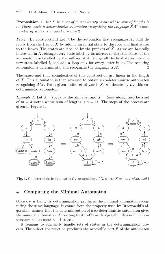
278 O. AitMous, F. Bassino, and C. Nicaud
Proposition 1. Let X be a set of m non-empty words whose sum of lengths isn. There exists a deterministic automaton recognizing the language ˜XA∗ whosenumber of states is at most n − m + 2.
Proof. (By construction) Let A be the automaton that recognizes ˜X , built di-rectly from the tree of ˜X by adding an initial state to the root and final statesto the leaves. The states are labelled by the prefixes of ˜X. As we are basicallyinterested in X , change every state label by its mirror, so that the states of theautomaton are labelled by the suffixes of X . Merge all the final states into onenew state labelled i, and add a loop on i for every letter in A. The resultingautomaton is deterministic and recognizes the language ˜XA∗. ��The space and time complexities of this construction are linear in the lengthof X . This automaton is then reversed to obtain a co-deterministic automatonrecognizing A∗X . For a given finite set of words X , we denote by CX this co-deterministic automaton.
Example 1. Let A = {a, b} be the alphabet and X = {aaa, abaa, abab} be a setof m = 3 words whose sum of lengths is n = 11. The steps of the process aregiven in Figure 1.
ε
a b
aa ba
aaa aab bab
aaba baba
a b
a a
a b b
a a
ε
a b
aa ab
baa bab
i
a b
a a
b b
a a
a
a, b
ε
a b
aa ab
baa bab
i
aa
b b
aa
ba
a
a, b
=⇒ =⇒
Fig. 1. Co-deterministic automaton CX recognizing A∗X, where X = {aaa, abaa, abab}
4 Computing the Minimal Automaton
Once CX is built, its determinization produces the minimal automaton recog-nizing the same language. It comes from the property used by Brzozowski’s al-gorithm, namely that the determinization of a co-deterministic automaton givesthe minimal automaton. According to Aho-Corasick algorithm this minimal au-tomaton has at most n + 1 states.
It remains to efficiently handle sets of states in the determinization pro-cess. The subset construction produces the accessible part B of the automaton

Building the Minimal Automaton of A∗X in Linear Time 279
{i}
{i, aa, baa, bab}
{i, aa, baa, bab, a} {i, aa, ab}
{i, aa, baa, bab, a, ε} {i, baa, bab, aa, a, b}
{i, aa, ab, ε}
ab
ab
a
b
a
b a
b
a
ba
b
Fig. 2. Minimal automaton recognizing A∗X, with 7 states (by subset construction)
ε
a
aaab
aaa aba
abab
abaa
ab
ab
ab
a
b a
b
a
b
a
b
a
b
Fig. 3. Aho Corasick automaton recognizing A∗X, with 8 states
(A,P(Q), {I}, FB, δB) from an automaton A = (A, Q, I, F, δ). The states of Bare labelled by subsets of Q.
Applied to the automaton of Figure 1 the subset construction leads to theminimal automaton depicted in Figure 2. Figure 3 shows Aho-Corasick automa-ton recognizing the same language A∗X where X = {aaa, abaa, abab}. The statesare labelled by prefixes of words of X. This automaton is not minimal since thestates aaa and abaa are equivalent.
4.1 Cost of the Naive Subset Construction
When computing the subset construction, one has to handle sets of states: start-ing from the set of initial states, all the accessible states are built from the fly,using a depth-first traversal (for instance) of the result. At each step, given a set

280 O. AitMous, F. Bassino, and C. Nicaud
of states P and a letter a, one has to compute the set δB(P, a) and then checkwhether this state has already been built.
In the co-deterministic automaton CX , only the initial state i has non-determi-nistic transitions, and for every letter a, the image of i by a is of size at mostm + 1, m being the number of words in X and one corresponding to the loopon the initial state i. Hence δB(P, a) is of cardinality at most m + 1 + |P | andis computed in time Θ(|P |), assuming that it is done using a loop through theelements of P . So even without taking into account the cost of checking whetherδB(P, a) has already been built, the time complexity of the determinization isΩ(
∑
P |P |), where the sum ranges over all P in the accessible part of the subsetconstruction.
For the pattern X = {an−1, b}, the states of the result are {i}, {i, an−2},{i, an−2, an−3}, . . ., {i, an−2, an−3, . . . , a}, {i, an−2, an−3, . . . , a, ε} and {i, ε}, sothat
∑
P |P | = Ω(n2). Therefore the time complexity of the naive subset con-struction is at least quadratic.
In the sequel, we present an alternative way to compute the determinizationof CX whose time complexity is linear.
4.2 Outline of the Construction
We make use of the following observations on CX . In the last automaton ofFigure 1, when the state labelled b is reached, a word u = v · aba has been read,and the state bab has also been reached. This information can be obtained fromthe word b and the borders of prefixes of words in X : aba is a prefix of the wordx = abab ∈ X , and Border(aba) = a. Our algorithm is based on limiting thelength of the state labels of the minimal automaton by storing only one stateper word of X , and one element to mark the state as final or not (ε or ε/). Henceif aba is read, only b is stored for the word x = abab.
When, for a letter c ∈ A, δ(b, c) is undefined, we jump to the state correspond-ing to the longest border of aba (the state bab in our example). We continueuntil either a transition we are looking for is found, or the unique initial state iis reached. More formally define the failure function f from X×Q\{i, ε}×A toQ \ {ε} in the following way: f(x, p, a) is the smallest suffix q of x, with q �= x,satisfying:
– x = up = vq, v being a border of u– δ(q, a) is defined.
If no such q exists, f(x, p, a) = i.
4.3 Precomputation of the Failure Function
Our failure function is similar to Aho-Corasick one in [1]. The difference is thatours is not based on suffixes but on borders of words. The value of Border(v·a)for every proper prefix v of a word u ∈ X and every letter a ∈ A is needed forthe computation.

Building the Minimal Automaton of A∗X in Linear Time 281
Table 1. Extended border array for u = abab, given A = {a, b}
Prefix w of uwith w �= u
Letter ε a ab aba
a 0 1 1 1b / 0 0 2
Extended border array. Let u be a word of length �. We define an extendedborder array from {0, 1, . . . , �−1}×A to {0, 1, . . . , �−1} by border ext[0][u[0]] = 0and border ext[i][a] = |Border(u[0 · ·i − 1] ·a)| for all i ∈ {1, . . . , � − 1}. Recallthat u[0 · ·i] is the prefix of u of length i + 1. Remark that |Border(u[0 · ·i])| =|Border(u[0··i − 1]·u[i])| = border ext[i − 1][u[i]].
Table 1 depicts the extended border array of the word abab. Values computedby a usual border array algorithm are represented in bold.
Algorithm 1 (see Figure 4) computes the extended border array for a word uof length �, considering the given alphabet A.
Standard propositions concerning the border array algorithm given in [7] areextended to Algorithm 1.
Proposition 2. Extended Borders algorithm above computes the extendedborder array of a given word u of length � considering the alphabet A. Its spaceand time complexities are linear in the length of the word u.
Proof. The routine Extended Borders computes sequentially |Border(v · a)|for every proper prefix v of u and every letter a ∈ A. As the size of the alphabet
Algorithm 1. Extended Borders
Inputs: u ∈ X, � = |u|, alphabet A1 border ext[0][u[0]] ← 02 for j ← 1 to �− 1 do3 for a ∈ A do4 i← border ext[j − 1][u[j − 1]]5 while i ≥ 0 and a �= u[i] do6 if i = 0 then7 i← −18 else9 i← border ext[i−1][u[i−1]]
10 end if11 end while12 i← i + 113 border ext[j][a] ← i14 end for15 end for16 return border ext
For every word u ∈ X we compute itsextended border array using the routineExtended Borders. It contains forevery proper prefix x of u and every lettera ∈ A, |Border(x·a)|.
To compute border ext[j][a] =|Border(u[0··j−1])·a|, we need the lengthof Border(u[0··j − 1]) = Border(u[0··j −2]·u[j − 1]). Thus |Border(u[0··j − 1])| =border ext[j − 1][u[j − 1]].
According to Equation (1), if Border(u[0··i − 1]) ·a is not a prefix of u[0 · ·i − 1] ·a,we need to find the longest border of theprefix of u of length i.Since Border(u[0··i−1]) = Border(u[0··i−2]·u[i−1]), we have |Border(u[0··i−1])| =border ext[i− 1][u[i − 1]]).
Fig. 4. Extended border array construction algorithm

282 O. AitMous, F. Bassino, and C. Nicaud
A is considered to be constant, the space complexity of the construction is linearin �.
A comparison between two letters a and b is said to be positive if a = band negative if a �= b. The time complexity of the algorithm is linear in thenumber of letter comparisons. The algorithm computes, for j = 1, . . . , �− 1 anda ∈ A, border ext[j][a] = |Border(u[0 · ·j − 1] · a)|. For a given letter a ∈ A,border ext[j][a] is obtained from |Border(u[0 · ·j−1])| that is already computed.The quantity 2j − i increases by at least one after each letter comparison: bothi and j are incremented by one after a positive comparison; in the case of anegative comparison j is unchanged while i is decreased by at least one.
When � = |u| ≥ 2, 2j− i is equal to 2 at the first comparison and 2�−2 at thelast one. Thus the number of comparisons for a given letter a is at most 2�− 3.The total time complexity is linear in the length of u. ��The extended border array can be represented by an automaton. Given a wordu ∈ A+, we construct the minimal automaton recognizing u. The states arelabelled by prefixes of u. We then define a border link for all prefixes p of u andall letters a ∈ A by:
BorderLink(p, a) = Border(p · a)
that can be computed using Equation (1). This extended border array shows astrong similarity with the classical String Matching Automata (SMA) [6,7]. Anadaptation of the SMA construction could be used as an alternativealgorithm.
Example 2. Figure 5 shows this construction for the word u = abab ∈ X .
Failure function. The value f (u, p, a) of the failure function is precomputedfor every word u ∈ X , every proper suffix p of u and every letter a ∈ A usingAlgorithm 2. The total time and space complexities of this operation are linearin the length of X . Remark that if f (u, p, a) �= i then |δ(f (u, p, a), a)| = 1.
4.4 Determinization Algorithm
Let X = {u1, . . . , um} be a set of m non-empty words whose sum of lengthsis n and let CX = (A, Q, {i}, {ε}, δ) be the co-deterministic automaton recog-nizing the language A∗X obtained in Section 3. We denote by BX the accessi-ble part of the automaton (A, IB , QB, FB, δB), where QB = (Q\{ε})m × {ε, ε/},
ε a ab aba ababa b a b
a, b a
b
a
b
a
b
Fig. 5. Automaton u = abab with border links

Building the Minimal Automaton of A∗X in Linear Time 283
Algorithm 2. Failure Function
Inputs: u∈X, p proper suffix of u, a∈A1 if p[0] = a and |p| > 1 then2 return p3 end if4 j ← border ext[|u| − |p|][a]5 if j ≤ 1 then6 return i7 end if8 return u[j − 1··|u| − 1]
Let v be the prefix of u such that u = v ·p.If δ(p, a) is defined and different than ε thenf (u, p, a) = p.If |Border(v · a)| = 0 then f (u, p, a) = i,where i is the unique initial state of the co-deterministic automaton A recognizing A∗X(see Section 3).If |Border(v·a)| ≥ 1 then Border(v·a) = w·a,with w ∈ A∗. If w = ε then f (u, p, a) = i.Otherwise, f (u, p, a) = q, with Border(v·a) =w1 ·a and u = w1 ·q.
Fig. 6. Failure function
IB = {(i, . . . , i, ε/)} and for all P ∈ FB, P = (v1, v2, . . . , vm, ε), where vr ∈ Q\{ε}for all r ∈ {1, . . . , m}. Given a state P ∈ QB and a letter a ∈ A we use Algo-rithm 3 (see Figure 7) to compute δB(P, a). Note that the automaton BX iscomplete.
Theorem 1. BX is the minimal automaton recognizing A∗X.
Proof. (Sketch) The idea of the proof is to show that BX and the automatonproduced by the classical subset construction are isomorphic.
Denote by M = (A, QM, IM, FM, δM) the minimal automaton built by thesubset construction. Given a state P ∈ QB (resp. P ∈ QM) and the smallestword v (the shortest one, and if there are several words of minimal length, weuse the lexicographical order) such that δB(IB, v) = P (resp. δM(IM, v) = P ) weconstruct the unique corresponding state R inM (resp. in BX) using the sameidea as in Section 4.2. Notice that i is in every state of M. A word s ∈ A+ isin R if there exist two words x ∈ X and u ∈ A+ such that x = u · s and eitheru = v or u is a non-empty border of v. The state R is final and contains ε if andonly if P is final. In the example of Figure 8 the word v = aa is the smallestword such that δB(IB, v) = P = (a, baa, bab, ε/), and the corresponding state inM (see Figure 2) is R = {i, a, aa, baa, bab}. The minimality of the automaton isguaranteed by Brzozowski’s construction [5]. ��Example 3. Algorithm 3 produces the automaton depicted in Figure 8 that isthe minimal automaton recognizing A∗X , where X = {aaa, abaa, abab}.
5 Sparse Lists
In this section we present data structures and analyze the complexity of theconstruction of the minimal automaton. The co-deterministic automaton CX ofsize at most n − m + 2 recognizing A∗X is built in time O(n), where X is a set

284 O. AitMous, F. Bassino, and C. Nicaud
of m words whose sum of lengths is n. As stated before, the analysis is done fora fixed m, when n tends toward infinity. Minimizing CX produces an automatonBX whose number of states is linear in n and our determinization process createsonly states labelled with sequences of m + 1 elements. Sparse lists are used toencode these states.
Let g : {0, . . . , � − 1} → F be a partial function and denote by Dom(g) thedomain of g. A sparse list (see [2][Exercise 2.12 p.71] or [6][Exercise 1.15 p.55])is a data structure that one can use to implement g and perform the followingoperations in constant time: initializing g with Dom(g) = ∅; setting a value g(x)for a given x ∈ {0, . . . , �− 1}; testing whether g(x) is defined or not; finding thevalue for g(x) if it is defined; removing x from Dom(g). The space complexityof a sparse list is O(�).
As we are interested in storing the states during the determinization, weillustrate here how to initialize, insert and test the existence of a value g(x).To represent g, we use two arrays and a list (also represented as an array). Theinitialization consists in allocating these three arrays of size � without initializingthem. The number of elements in the list will be stored in an extra variable size.The values of the image by g are stored in the first array. The second array andthe list are used to discriminate these values due to the random ones comingfrom the lack of initialization.
Algorithm 3. Transition Function
Inputs: P =(v1, v2, . . . vm, j) ∈QB, a ∈ A1 j′ ← ε/2 for r ∈ {1, . . . m} do3 v′
r ← i4 if δ(vr, a) = ε then5 j′ ← ε6 end if7 end for8 for � = 1 to m do9 v� ← f (u�, v�, a)
10 if v� �= i then11 if v′
� = i or |δ(v�, a)| < |v′�| then
12 v′� ← δ(v�, a)
13 end if14 else15 for r = 1 to s such that xr �= ε do16 if v′
t = i or |xr| < |v′t| then
17 v′t ← xr
18 end if19 end for20 end if21 end for22 return R = (v′
1, v′2, . . ., v′
m, j′)
We initialize the first m elements of Rto the unique initial state i in A. Thevalue of the last term of R is calculated(marking the state as final or non-final).
For each member v� we check the valueof the failure function f(u�, v�, a).If f(u�, v�, a) �= i then|δ(f(u�, v�, a), a)| = 1 and we havefound a potential value for v′
� that is asuffix of ul ∈ X. It remains to compareit to the already existing one and storethe smallest in length different than i.
When the initial state i is reached, weare at the beginning of all the words inX. We define variables used in lines 15-17 as follows. From the definition of theautomaton A, δ(i, a) = {x1, x2, . . . , xs}where 0 ≤ s ≤ m and a · x1 ∈ X, . . . , a ·xs ∈ X. For every couple of integers(r1, r2) ∈ {1, . . . , s}2 such that r1 �= r2,a · xr1 �= a · xr2 . For all r ∈ {1, . . . , s}there exists a unique t ∈ {1, . . . , m} suchthat a · xr = ut ∈ X.
Fig. 7. Transition function

Building the Minimal Automaton of A∗X in Linear Time 285
(i, i, i, ε/)
(aa, baa, bab, ε/)
(a, baa, bab, ε/) (i, aa, ab, ε/)
(a, baa, bab, ε) (aa, a, b, ε/)
(i, aa, ab, ε)
ab
ab
a
b
a
b a
b
a
ba
b
Fig. 8. Minimal automaton recognizing A∗X (by our construction), where X ={aaa, abaa, abab}
Figure 9 illustrates the sparse list initialization. Inserting an element g(x) = yrequires the following steps: g[x] = y; index[x] = size; list[size] = x and size =size + 1. The result is shown in Figure 10. A value g(x) is defined if and only ifindex[x] < size and list[index[x]] = x.
Since the states we build are labelled by sequences of size m + 1, and eachof the m first elements is either the initial state i of the automaton CX or aproper suffix of the corresponding word in the pattern, we use a tree of sparselists to store our states. Let X = {u1, . . . , um} be the pattern and denote bySuff(ur) the set of all proper suffixes of ur for 1 ≤ r ≤ m. We define a partialfunction g on {0, . . . , |u1| − 1} whose values are partial functions g(|v1|) forv1 ∈ Suff(u1) ∪ {i}. We consider that |i| = 0. These functions g(v1) are definedon {0, . . . , |u2 − 1|} and their values are again partial functions, denoted byg(|v1|, |v2|) for v1 ∈ Suff(u1) ∪ {i} and v2 ∈ Suff(u2) ∪ {i}. By extension we
0 �− 1
· · ·g
0 �− 1
· · ·index
0 �− 1
· · ·list
size = 0
Fig. 9. Sparse list initialization
y
0 x �− 1
g
size
0 x �− 1
index
x
size
· · ·list
size = size + 1
Fig. 10. Sparse list insertion of g(x) = y

286 O. AitMous, F. Bassino, and C. Nicaud
0 1 2
0 1 2 3
0 1 2 3
P0
ε/ ε
Fig. 11. Tree of sparse lists after inserting P0 = {i, i, i, ε/}
0 1 2
0 1 2 3
0 1 2 3
P0
ε/ ε
0 1 2 3
0 1 2 3
P1
ε/ ε
0 1 2 3
P2
ε/ ε
Fig. 12. Tree of sparse lists
build functions g(|v1|, |v2|, . . . , |vm|) : {0, . . . , |u1| − 1}× {0, . . . , |u2| − 1}× . . .×{0, . . . , |um| − 1} × {ε, ε/} → QB where v1 ∈ Suff(u1) ∪ {i}, v2 ∈ Suff(u2) ∪ {i},. . ., vm ∈ Suff(um)∪ {i} and QB is the set of states in the automaton BX . Thenfor a given state P = (v1, v2, . . . , vm, j) ∈ QB, g(|v1|, |v2|, . . . , |vm|, j) = P .
When inserting a state P = (v1, v2, . . . , vm, j) into our data structure, theexistence of g(|v1|) is tested and, if it does not exist, a sparse list representingthis partial function is created. Then the existence of g(|v1|, |v2|) is checked.The same process is repeated until a function g(|v1|, |v2|, . . . , |vm|) is found.Finally we test whether g(|v1|, |v2|, . . . , |vm|, j) is defined, and if not the valuefor g(|v1|, |v2|, . . . , |vm|, j) is set to P . If g(|v1|, |v2|, . . . , |vm|, j) is already defined,then the state P already exists in the tree.
Figure 11 shows the insertion of the initial state P0 = (i, i, i, ε/) for X ={aaa, abaa, abab} and Figure 12 depicts the tree of sparse lists after insertingP0 = {i, i, i, ε/}, P1 = {aa, baa, bab, ε/} and P2 = {i, aa, ab, ε/}.

Building the Minimal Automaton of A∗X in Linear Time 287
Testing the existence of a state works in the same way, but if a partial functionis not found then the state is not in the data structure.
Theorem 2. Using sparse lists, the construction of the minimal automaton rec-ognizing A∗X runs in time O(n) and requires O(n2) space where n is the lengthof the pattern X.
Proof. From Aho-Corasick’s result the minimal automaton is of size at mostn+1. As each state requires m+1 sparse lists of size |u1|, |u2|, . . . |um|, 2, the totalspace complexity is quadratic in n. The time complexity of the determinizationis linear in n since searching and inserting a state take O(1) time. ��Remark 1. In practice a hash table can be used to store these states. Under thehypothesis of a simple uniform hashing the average time and space complexitiesof the determinization are linear.
The natural continuation of this work is to investigate constructions based onBrzozowski’s algorithm when m is not fixed anymore.
References
1. Aho, A.V., Corasick, M.J.: Efficient string matching: an aid to bibliographic search.Communications of the ACM 18(6), 333–340 (1975)
2. Aho, A.V., Hopcroft, J.E., Ullman, J.D.: The Design and Analysis of ComputerAlgorithms. Addison-Wesley, Reading (1974)
3. Beal, M.P., Crochemore, M.: Minimizing local automata. In: Caire, G., Fossorier,M. (eds.) IEEE International Symposium on Information Theory (ISIT 2007),07CH37924C, pp. 1376–1380. IEEE Catalog (2007)
4. Boyer, R.S., Moore, J.S.: A fast string searching algorithm. Communications of theACM 20(10), 62–72 (1977)
5. Brzozowski, J.A.: Canonical regular expressions and minimal state graphs for def-inite events. In: Mathematical theory of Automata. MRI Symposia Series, vol. 12,pp. 529–561. Polytechnic Press, Polytechnic Institute of Brooklyn, N.Y (1962)
6. Crochemore, M., Hancart, C., Lecroq, T.: Algorithms on Strings, 392 pages. Cam-bridge University Press, Cambridge (2007)
7. Crochemore, M., Rytter, W.: Jewels of Stringology. World Scientific PublishingCompany, Singapore (2002)
8. Hopcroft, J.E.: An n log n algorithm for minimizing states in a finite automaton.In: Theory of Machines and computations, pp. 189–196. Academic Press, London(1971)
9. Hopcroft, J.E., Ullman, J.D.: Introduction To Automata Theory, Languages, AndComputation. Addison-Wesley Longman Publishing Co., Inc., Boston (1990)
10. Knuth, D.E., Morris, J.H., Pratt, V.R.: Fast pattern matching in strings. SIAMJournal of Computing 6(2), 323–350 (1977)
11. Mohri, M.: String-matching with automata. Nordic Journal of Computing 4(2),217–231 (Summer 1997)

A Compact Representation of Nondeterministic
(Suffix) Automata for the Bit-Parallel Approach
Domenico Cantone, Simone Faro, and Emanuele Giaquinta
Universita di Catania, Dipartimento di Matematica e InformaticaViale Andrea Doria 6, I-95125 Catania, Italy{cantone,faro,giaquinta}@dmi.unict.it
Abstract. We present a novel technique, suitable for bit-parallelism,for representing both the nondeterministic automaton and the nonde-terministic suffix automaton of a given string in a more compact way.Our approach is based on a particular factorization of strings which onthe average allows to pack in a machine word of w bits automata stateconfigurations for strings of length greater than w. We adapted the Shift-And and BNDM algorithms using our encoding and compared them withthe original algorithms. Experimental results show that the new variantsare generally faster for long patterns.
1 Introduction
The string matching problem consists in finding all the occurrences of a pattern Pof length m in a text T of length n, both defined over an alphabet Σ of size σ. TheKnuth-Morris-Pratt (KMP) algorithm was the first linear-time solution (cf. [5]),whereas the Boyer-Moore (BM) algorithm provided the first sublinear solutionon average [3]. Subsequently, the BDM algorithm reached the O(n logσ(m)/m)lower bound time complexity on the average (cf. [4]). Both the KMP and theBDM algorithms are based on finite automata; in particular, they respectivelysimulate a deterministic automaton for the language Σ∗P and a deterministicsuffix automaton for the language of the suffixes of P .
The bit-parallelism technique, introduced in [2], has been used to simulateefficiently the nondeterministic version of the KMP automaton. The resultingalgorithm, named Shift-Or, runs in O(n�m/w�), where w is the number of bitsin a computer word. Later, a variant of the Shift-Or algorithm, called Shift-And,and a very fast BDM-like algorithm (BNDM), based on the bit-parallel simulationof the nondeterministic suffix automaton, were presented in [6].
Bit-parallelism encoding requires one bit per pattern symbol, for a total of�m/w� computer words. Thus, as long as a pattern fits in a computer word, bit-parallel algorithms are extremely fast, otherwise their performances degradesconsiderably as �m/w� grows. Though there are a few techniques to maintaingood performance in the case of long patterns, such limitation is intrinsic.
In this paper we present an alternative technique, still suitable for bit-parallelism, to encode both the nondeterministic automaton and the nondeter-ministic suffix automaton of a given string in a more compact way. Our encoding
A. Amir and L. Parida (Eds.): CPM 2010, LNCS 6129, pp. 288–298, 2010.c© Springer-Verlag Berlin Heidelberg 2010

A Compact Representation of Nondeterministic (Suffix) Automata 289
is based on factorizations of strings in which no character occurs more than oncein any factor. This is the key towards separating the nondeterministic part fromthe determinstic one of the corresponding automata. It turns out that the nonde-terministic part can be encoded with k bits, where k is the size of the factorization.Though in the worst case k = m, on the average k is much smaller than m, makingit possible to encode large automata in a single or few computer words. As a con-sequence, bit-parallel algorithms based on such approach tend to be faster in thecase of sufficiently long patterns. We will illustrate this point by comparing exper-imentally different implementations of the Shift-And and the BNDM algorithms.
2 Basic Notions and Definitions
Given a finite alphabet Σ, we denote by Σm, with m ≥ 0, the collection of stringsof length m over Σ and put Σ∗ =
⋃m∈N
Σm. We represent a string P ∈ Σm,also called an m-gram, as an array P [0 .. m − 1] of characters of Σ and write|P | = m (in particular, for m = 0 we obtain the empty string ε). Thus, P [i] isthe (i + 1)-st character of P , for 0 � i < m, and P [i .. j] is the substring of Pcontained between its (i + 1)-st and the (j + 1)-st characters, for 0 � i � j < m.Also, we put first(P ) = P [0] and last(P ) = P [|P | − 1]. For any two strings Pand P ′, we say that P ′ is a suffix of P if P ′ = P [i .. m− 1], for some 0 � i < m,and write Suff (P ) for the set of all suffixes of P . Similarly, P ′ is a prefix of Pif P ′ = P [0 .. i], for some 0 � i < m. In addition, we write P.P ′, or more simplyPP ′, for the concatenation of P and P ′, and P r for the reverse of the string P ,i.e. P r = P [m− 1]P [m− 2] . . . P [0].
Given a string P ∈ Σm, we indicate with A(P ) = (Q, Σ, δ, q0, F ) the nonde-terministic automaton for the language Σ∗P of all words in Σ∗ ending with anoccurrence of P , where:
– Q = {q0, q1, . . . , qm} (q0 is the initial state)– the transition function δ : Q×Σ −→P(Q) is defined by:
δ(qi, c) =Def
⎧⎪⎪⎪⎨
⎪⎪⎪⎩
{q0, q1} if i = 0 and c = P [0]{q0} if i = 0 and c�= P [0]{qi+1} if 1 � i < m and c = P [i]∅ otherwise
– F = {qm} (F is the set of final states).
Likewise, for a string P ∈ Σm, we denote by S(P ) = (Q, Σ, δ, I, F ) the nonde-terministic suffix automaton with ε-transitions for the language Suff (P ) of thesuffixes of P , where:
– Q = {I, q0, q1, . . . , qm} (I is the initial state)– the transition function δ : Q× (Σ ∪ {ε}) −→P(Q) is defined by:
δ(q, c) =Def
⎧⎪⎨
⎪⎩
{qi+1} if q = qi and c = P [i] (0 � i < m){q0, q1, . . . , qm} if q = I and c = ε
∅ otherwise

290 D. Cantone, S. Faro, and E. Giaquinta
– F = {qm} (F is the set of final states).
The valid configurations δ∗(q0, S) reachable by the automata A(P ) on inputS ∈ Σ∗ are defined recursively as follows:
δ∗(q0, S) =Def
{{q} if S = ε,⋃
q′∈δ(q0,S′) δ∗(q′, c) if S = S′c, for some c ∈ Σ and S′ ∈ Σ∗.
Much the same definition of reachable configurations holds for the automataS(P ), but in this case one has to use δ(I, ε) = {q0, q1, . . . , qm} for the base case.
Finally, we recall the notation of some bitwise infix operators on computerwords, namely the bitwise and “&”, the bitwise or “|”, the left shift “”operator (which shifts to the left its first argument by a number of bits equal toits second argument), and the unary bitwise not operator “∼”.
3 The Bit-Parallelism Technique
Bit-parallelism is a technique introduced by Baeza-Yates and Gonnet in [2] thattakes advantage of the intrinsic parallelism of the bit operations inside a com-puter word, allowing to cut down the number of operations that an algorithmperforms by a factor up to w, where w is the number of bits in the computer word.Bit-parallelism is particularly suitable for the efficient simulation of nondeter-ministic (suffix) automata; the first algorithms based on it are the well-knownShift-And [2] and BNDM [6]. The Shift-And algorithm simulates the nondeter-ministic automaton (NFA, for short) that recognizes the language Σ∗P , for agiven string P of length m. Its bit-parallel representation uses an array B of |Σ|bit-vectors, each of size m, where the i-th bit of B[c] is set iff δ(qi, c) = qi+1
or equivalently iff P [i] = c, for c ∈ Σ, 0 � i < m. Automaton configurationsδ∗(q0, S) on input S ∈ Σ∗ are then encoded as a bit-vector D of m bits (the initialstate does not need to be represented, as it is always active), where the i-th bitof D is set iff state qi+1 is active, i.e. qi+1 ∈ δ∗(q0, S), for i = 0, . . . , m− 1. For aconfiguration D of the NFA, a transition on character c can then be implementedby the bitwise operations
D ← ((D 1) | 1) & B[c] .
The bitwise or with 1 (represented as 0m−11) is performed to take into accountthe self-loop labeled with all the characters in Σ on the initial state. When asearch starts, the initial configuration D is initialized to 0m. Then, while thetext is read from left to right, the automaton configuration is updated for eachtext character, as described before.
The nondeterministic suffix automaton for a given string P is an NFA withε-transitions that recognizes the language Suff (P ). The BNDM algorithm sim-ulates the suffix automaton for P r with the bit-parallelism technique, using anencoding similar to the one described before for the Shift-And algorithm. The i-th bit of D is set iff state qi+1 is active, for i = 0, 1, . . . , m−1, and D is initialized

A Compact Representation of Nondeterministic (Suffix) Automata 291
to 1m, since after the ε-closure of the initial state I all states qi represented in Dare active. The first transition on character c is implemented as D ← (D & B[c]),while any subsequent transition on character c can be implemented as
D ← ((D 1) & B[c]) .
The BNDM algorithm works by shifting a window of length m over the text.Specifically, for each window alignment, it searches the pattern by scanning thecurrent window backwards and updating the automaton configuration accord-ingly. Each time a suffix of P r (i.e., a prefix of P ) is found, namely when priorto the left shift the m-th bit of D&B[c] is set, the window position is recorded.A search ends when either D becomes zero (i.e., when no further prefixes of Pcan be found) or the algorithm has performed m iterations (i.e., when a matchhas been found). The window is then shifted to the start position of the longestrecognized proper prefix.
When the pattern size m is larger than w, the configuration bit-vector and allauxiliary bit-vectors need to be splitted over �m/w� multiple words. For this rea-son the performance of the Shift-And and BNDM algorithms, and of bit-parallelalgorithms more in general, degrades considerably as �m/w� grows. A commonapproach to overcome this problem consists in constructing an automaton for asubstring of the pattern fitting in a single computer word, to filter possible can-didate occurrences of the pattern. When an occurrence of the selected substringis found, a subsequent naive verification phase allows to establish whether thisbelongs to an occurrence of the whole pattern. However, besides the costs of theadditional verification phase, a drawback of this approach is that, in the caseof the BNDM algorithm, the maximum possible shift length cannot exceed w,which could be much smaller than m.
In the next section we illustrate an alternative encoding for automata config-urations, which in general requires less than one bit per pattern character andstill is suitable for bit-parallelism.
4 Tighter Packing for Bit-Parallelism
We present a new encoding of the configurations of the nondeterministic (suffix)automaton for a given pattern P of length m, which on the average requiresless than m bits and is still suitable to be used within the bit-parallel frame-work. The effect is that bit-parallel string matching algorithms based on suchencoding scale much better as m grows, at the price of a larger space complexity.We will illustrate such point experimentally with the Shift-And and the BNDMalgorithms, but our proposed encoding can also be applied to other variants ofthe BNDM algorithm as well.
Our encoding will have the form (D, a), where D is a k-bit vector, with k � m(on the average k is much smaller than m), and a is an alphabet symbol (thelast text character read) which will be used as a parameter in the bit-parallelsimulation with the vector D.

292 D. Cantone, S. Faro, and E. Giaquinta
The encoding (D, a) is obtained by suitably factorizing the simple bit-vectorencoding for NFA configurations presented in the previous section. More specif-ically, it is based on the following pattern factorization.
Definition (1-factorization). Let P ∈ Σm. A 1-factorization of size k of P is asequence 〈u1, u2, . . . , uk〉 of nonempty substrings of P such that:
(a) P = u1u2 . . . uk ;(b) each factor uj contains at most one occurrence for any of the characters in
the alphabet Σ, for j = 1, . . . , k .
A 1-factorization of P is minimal if such is its size.
Remark. It can easily be checked that a 1-factorization 〈u1, u2, . . . , uk〉 of P isminimal if first(ui+1) occurs in ui, for i = 1, . . . , k − 1.
Observe, also, that �mσ � � k � m holds, for any 1-factorization of size k of a
string P ∈ Σm, where σ = |Σ|. The worst case occurs when P = am, in whichcase P has only the 1-factorization of size m whose factors are all equal to thesingle character string a.
A 1-factorization 〈u1, u2, . . . , uk〉 of a given pattern P ∈ Σ∗ induces naturallya partition {Q1, . . . , Qk} of the set Q\{q0} of nonstarting states of the canonicalautomaton A(P ) = (Q, Σ, δ, q0, F ) for the language Σ∗P , where
Qi =Def
{q∑ i−1
j=1 |uj |+1, . . . , q∑
ij=1 |uj |
}, for i = 1, . . . , k .
Notice that the labels of the arrows entering the states
q∑ i−1j=1 |uj |+1, . . . , q
∑ ij=1 |uj | ,
in that order, form exactly the factor ui, for i = 1, . . . , k. Hence, if for anyalphabet symbol a we denote by Qi,a the collection of states in Qi with anincoming arrow labeled a, it follows that |Qi,a| � 1, since by condition (b) ofthe above definition of 1-factorization no two states in Qi can have an incomingtransition labeled by a same character. When Qi,a is nonempty, we write qi,a
to indicate the unique state q of A(P ) for which q ∈ Qi,a, otherwise qi,a isundefined. On using qi,a in any expression, we will also implicitly assert that qi,a
is defined.For any valid configuration δ∗(q0, Sa) of the automatonA(P ) on some input of
the form Sa ∈ Σ∗, we have that q ∈ δ∗(q0, Sa) only if the state q has an incomingtransition labeled a. Therefore, Qi ∩ δ∗(q0, Sa) ⊆ Qi,a and, consequently, |Qi ∩δ∗(q0, Sa)| � 1, for each i = 1, . . . , k. The configuration δ∗(q0, Sa) can then beencoded by the pair (D, a), where D is the bit-vector of size k such that D[i] isset iff Qi contains an active state, i.e., Qi ∩ δ∗(q0, Sa)�= ∅, iff qi,a ∈ δ∗(q0, Sa).Indeed, if i1, i2, . . . , il are all the indices i for which D[i] is set, we have thatδ∗(q0, Sa) = {qi1,a, qi2,a, . . . , qil,a} holds, showing that the above encoding (D, a)can be inverted.
To show how to compute D′ in a transition (D, a) A−→ (D′, c) on character cusing bit-parallelism, it is convenient to give some further definitions.

A Compact Representation of Nondeterministic (Suffix) Automata 293
F-PREPROCESS (P, m)
for c ∈ Σ do S[c]← L[c]← 0for c, c′ ∈ Σ do B[c][c′]← 0b← 0, e← 0, k← 0while e < m do
while e < m and S[P [e]] = 0 doS[P [e]]← 1, e← e + 1
for i← b to e− 1 do S[P [i]]← 0for i← b + 1 to e− 1 do
B[P [i− 1]][P [i]]← B[P [i− 1]][P [i]] | (1� k)L[P [e− 1]]← L[P [e− 1]] | (1� k)if e < m then
B[P [e− 1]][P [e]]← B[P [e− 1]][P [e]] | (1� k)b← ek← k + 1
M ← (1� (k − 1))return (B, L, M, k)
Fig. 1. Preprocessing procedure for the construction of the arrays B and L relative toa minimal 1-factorization of the pattern
For i = 1, . . . , k− 1, we put ui = ui.first(ui+1). We also put uk = uk and calleach set ui the closure of ui.
Plainly, any 2-gram can occur at most once in the closure ui of any factor ofour 1-factorization 〈u1, u2, . . . , uk〉 of P . We can therefore encode the 2-gramspresent in the closure of the factors ui by a |Σ| × |Σ| matrix B of k-bit vectors,where the i-th bit of B[c1][c2] is set iff the 2-gram c1c2 is present in ui or,equivalently, iff
(last(ui)�= c1 ∧ qi,c2 ∈ δ(qi,c1 , c2))∨(i < k ∧ last(ui) = c1 ∧ qi+1,c2 ∈ δ(qi,c1 , c2)) ,
(1)
for every 2-gram c1c2 ∈ Σ2 and i = 1, . . . , k.To properly take care of transitions from the last state in Qi to the first state
in Qi+1, it is also useful to have an array L, of size |Σ|, of k-bit vectors encodingfor each character c ∈ Σ the collection of factors ending with c. More precisely,the i-th bit of L[c] is set iff last(ui) = c, for i = 1, . . . , k.
We show next that the matrix B and the array L, which in total require(|Σ|2 + |Σ|)k bits, are all is needed to compute the transition (D, a) A−→ (D′, c)on character c. To this purpose, we first state the following basic property, whichcan easily be proved by induction.
Transition Lemma. Let (D, a) A−→ (D′, c), where (D, a) is the encoding of theconfiguration δ∗(q0, Sa) for some string S ∈ Σ∗, so that (D′, c) is the encodingof the configuration δ∗(q0, Sac).
Then, for each i = 1, . . . , k, qi,c ∈ δ∗(q0, Sac) if and only if either
(i) last(ui)�= a, qi,a ∈ δ∗(q0, Sa), and qi,c ∈ δ(qi,a, c), or(ii) i � 1, last(ui−1) = a, qi−1,a ∈ δ∗(q0, Sa), and qi,c ∈ δ(qi−1,a, c). �

294 D. Cantone, S. Faro, and E. Giaquinta
Now observe that, by definition, the i-th bit of D′ is set iff qi,c ∈ δ∗(q0, Sac) or,equivalently by the Transition Lemma and (1), iff (for i = 1, . . . , k)
(D[i] = 1 ∧B[a][c][i] = 1 ∧ ∼L[a][i] = 1)∨(i � 1 ∧D[i− 1] = 1 ∧B[a][c][i− 1] = 1 ∧ L[a][i− 1] = 1) iff
((D & B[a][c] & ∼L[a])[i] = 1 ∨ (i � 1 ∧ (D & B[a][c] & L[a])[i− 1] = 1)) iff
((D & B[a][c] & ∼L[a])[i] = 1 ∨ ((D & B[a][c] & L[a]) 1)[i] = 1) iff
((D & B[a][c] & ∼L[a]) | ((D & B[a][c] & L[a]) 1))[i] = 1 .
Hence D′ = (D & B[a][c] & ∼L[a]) | ((D & B[a][c] & L[a]) 1) , so that D′
can be computed by the following bitwise operations:
D ← D & B[a][c]H ← D & L[a]D ← (D & ∼H)|(H 1) .
To check whether the final state qm belongs to a configuration encoded as (D, a),we have only to verify that qk,a = qm. This test can be broken into two steps:first, one checks if any of the states in Qk is active, i.e. D[k] = 1; then, one verifiesthat the last character read is the last character of uk, i.e. L[a][k] = 1. The wholetest can then be implemented with the bitwise test D & M & L[a]�= 0k , whereM = (1 (k − 1)).
The same considerations also hold for the suffix automaton S(P ). The onlydifference is in the handling of the initial state. In the case of the automatonA(P ), state q0 is always active, so we have to activate state q1 when the currenttext symbol is equal to P [0]. To do so it is enough to perform a bitwise or of
F-Shift-And (P, m, T, n)
(B, L, M, k)← F-PREPROCESS(P, m)
D ← 0k
a← T [0]for j ← 1 to n− 1
if a = P [0] then D ← D | 0k−11
if (D & M & L[a]) �= 0k
then Output(j − 1)D ← D & B[a][T [j]]H ← D & L[a]D ← (D & ∼H) | (H � 1)a← T [j]
F-BNDM (P, m, T, n)
(B, L, M, k)← F-PREPROCESS(P r, m)j ← m− 1while j < n do
k← 1, l ← 0
D ← ∼ 0k, a← T [j]
while D �= 0k do
if (D & M & L[a]) �= 0k thenif k < m then
l← kelse Output(j)
D ← D & B[a][T [j − k]]H ← D & L[a]D ← (D & ∼H) | (H � 1)a← T [j − k]k ← k + 1
j ← j + m− l
(a) (b)
Fig. 2. Variants of Shift-And and BNDM based on the 1-factorization encoding
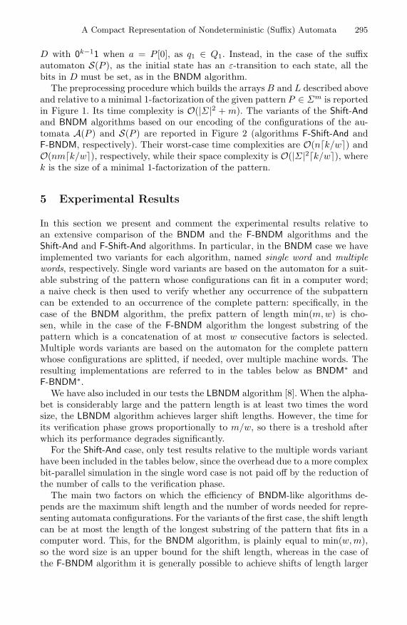
A Compact Representation of Nondeterministic (Suffix) Automata 295
D with 0k−11 when a = P [0], as q1 ∈ Q1. Instead, in the case of the suffixautomaton S(P ), as the initial state has an ε-transition to each state, all thebits in D must be set, as in the BNDM algorithm.
The preprocessing procedure which builds the arrays B and L described aboveand relative to a minimal 1-factorization of the given pattern P ∈ Σm is reportedin Figure 1. Its time complexity is O(|Σ|2 + m). The variants of the Shift-Andand BNDM algorithms based on our encoding of the configurations of the au-tomata A(P ) and S(P ) are reported in Figure 2 (algorithms F-Shift-And andF-BNDM, respectively). Their worst-case time complexities are O(n�k/w�) andO(nm�k/w�), respectively, while their space complexity is O(|Σ|2�k/w�), wherek is the size of a minimal 1-factorization of the pattern.
5 Experimental Results
In this section we present and comment the experimental results relative toan extensive comparison of the BNDM and the F-BNDM algorithms and theShift-And and F-Shift-And algorithms. In particular, in the BNDM case we haveimplemented two variants for each algorithm, named single word and multiplewords, respectively. Single word variants are based on the automaton for a suit-able substring of the pattern whose configurations can fit in a computer word;a naive check is then used to verify whether any occurrence of the subpatterncan be extended to an occurrence of the complete pattern: specifically, in thecase of the BNDM algorithm, the prefix pattern of length min(m, w) is cho-sen, while in the case of the F-BNDM algorithm the longest substring of thepattern which is a concatenation of at most w consecutive factors is selected.Multiple words variants are based on the automaton for the complete patternwhose configurations are splitted, if needed, over multiple machine words. Theresulting implementations are referred to in the tables below as BNDM∗ andF-BNDM∗.
We have also included in our tests the LBNDM algorithm [8]. When the alpha-bet is considerably large and the pattern length is at least two times the wordsize, the LBNDM algorithm achieves larger shift lengths. However, the time forits verification phase grows proportionally to m/w, so there is a treshold afterwhich its performance degrades significantly.
For the Shift-And case, only test results relative to the multiple words varianthave been included in the tables below, since the overhead due to a more complexbit-parallel simulation in the single word case is not paid off by the reduction ofthe number of calls to the verification phase.
The main two factors on which the efficiency of BNDM-like algorithms de-pends are the maximum shift length and the number of words needed for repre-senting automata configurations. For the variants of the first case, the shift lengthcan be at most the length of the longest substring of the pattern that fits in acomputer word. This, for the BNDM algorithm, is plainly equal to min(w, m),so the word size is an upper bound for the shift length, whereas in the case ofthe F-BNDM algorithm it is generally possible to achieve shifts of length larger

296 D. Cantone, S. Faro, and E. Giaquinta
than w, as our encoding allows to pack more state configurations per bit on theaverage as shown in a table below. In the multi-word variants, the shift lengthsfor both algorithms, denoted BNDM∗ and F-BNDM∗, are always the same, asthey use the very same automaton; however, the 1-factorization based encodinginvolves a smaller number of words on the average, especially for long patterns,thus providing a considerable speedup.
All algorithms have been implemented in the C programming language andhave been compiled with the GNU C Compiler, using the optimization options-O2 -fno-guess-branch-probability. All tests have been performed on a 2GHz Intel Core 2 Duo and running times have been measured with a hardwarecycle counter, available on modern CPUs. We used the following input files: (i)the English King James version of the “Bible” (with σ = 63); (ii) a proteinsequence from the Saccharomyces cerevisiae genome (with σ = 20); and (iii) agenome sequence of 4, 638, 690 base pairs of Escherichia coli (with σ = 4).
Files (i) and (iii) are from the Canterbury Corpus [1], while file (ii) is from theProtein Corpus [7]. For each input file, we have generated sets of 200 patterns offixed length m randomly extracted from the text, for m ranging over the values32, 64, 128, 256, 512, 1024, 1536, 2048, 4096. For each set of patterns we reportedthe mean over the running times of the 200 runs.
m Shift-And∗ F-Shift-And∗ LBNDM BNDM BNDM∗ F-BNDM F-BNDM∗
32 8.85 22.20 2.95 2.81 2.92 2.92 2.9964 51.45 22.20 1.83 2.82 3.31 2.00 1.97
128 98.42 22.21 1.82 2.83 3.58 2.35 2.23256 142.27 92.58 1.38 2.82 2.79 1.91 2.14512 264.21 147.79 1.09 2.84 2.47 1.81 1.75
1024 508.71 213.70 1.04 2.84 2.67 1.77 1.721536 753.02 283.57 1.40 2.84 2.95 1.77 1.732048 997.19 354.32 2.24 2.84 3.45 1.75 1.904096 1976.09 662.06 10.53 2.83 6.27 1.72 2.92
Experimental results on the King James version of the Bible (σ = 63)
m Shift-And∗ F-Shift-And∗ LBNDM BNDM BNDM∗ F-BNDM F-BNDM∗
32 6.33 15.72 1.50 1.58 1.64 1.43 1.5664 38.41 15.70 0.99 1.57 1.70 0.89 0.96
128 70.59 40.75 0.70 1.57 1.42 0.64 1.01256 104.42 73.59 0.52 1.57 1.39 0.59 1.01512 189.16 108.33 0.41 1.57 1.29 0.56 0.88
1024 362.83 170.52 0.54 1.58 1.46 0.55 0.911536 540.25 227.98 2.09 1.57 1.73 0.56 1.042048 713.87 290.24 7.45 1.58 2.12 0.56 1.204096 1413.76 541.53 32.56 1.58 4.87 0.59 2.33
Experimental results on a protein sequence from the Saccharomyces cerevisiae genome (σ = 20)
m Shift-And∗ F-Shift-And∗ LBNDM BNDM BNDM∗ F-BNDM F-BNDM∗
32 10.19 25.04 4.60 3.66 3.82 5.18 4.8864 59.00 42.93 3.42 3.64 5.39 2.94 3.69
128 93.97 114.22 3.43 3.65 5.79 2.66 5.37256 162.79 167.11 11.68 3.64 4.79 2.59 4.11512 301.55 281.37 82.94 3.66 4.16 2.53 3.54
1024 579.92 460.37 96.13 3.64 4.21 2.50 3.421536 860.84 649.88 91.45 3.64 4.54 2.49 3.662048 1131.50 839.32 89.45 3.64 4.98 2.48 3.984096 2256.37 1728.71 85.87 3.64 7.81 2.48 6.22
Experimental results on a genome sequence of Escherichia coli (σ = 4)
A Compact Representation of Nondeterministic (Suffix) Automata 297
(A) ecoli protein bible32 32 32 3264 63 64 64
128 72 122 128256 74 148 163512 77 160 169
1024 79 168 1731536 80 173 1762048 80 174 1784096 82 179 182
(B) ecoli protein bible32 15 8 664 29 14 12
128 59 31 26256 119 60 50512 236 116 102
1024 472 236 2041536 705 355 3042048 944 473 4074096 1882 951 813
(C) ecoli protein bible32 2.13 4.00 5.3364 2.20 4.57 5.33
128 2.16 4.12 4.92256 2.15 4.26 5.12512 2.16 4.41 5.01
1024 2.16 4.33 5.011536 2.17 4.32 5.052048 2.16 4.32 5.034096 2.17 4.30 5.03
(A) The length of the longest substring of the pattern fitting in w bits.(B) The size of the minimal 1-factorization of the pattern.(C) The ratio between m and the size of the minimal 1-factorization of the pattern.
Concerning the BNDM-like algorithms, the experimental results show that inthe case of long patterns both variants based on the 1-factorization encodingare considerably faster than their corresponding variants BNDM and BNDM∗.In the first test suite, with σ = 63, the LBNDM algorithm turns out to be thefastest one, except for very long patterns, as the treshold on large alphabets isquite high. In the second test suite, with σ = 20, LBNDM is still competitivebut, in the cases in which it beats the BNDM∗ algorithm, the difference is thin.
Likewise, the F-Shift-And variant is faster than the classical Shift-And algo-rithm in all cases, for m � 64.
6 Conclusions
We have presented an alternative technique, suitable for bit-parallelism, to repre-sent the nondeterministic automaton and the nondeterministic suffix automatonof a given string. On the average, the new encoding allows to pack in a single ma-chine word of w bits state configurations of (suffix) automata relative to stringsof more than w characters long. When applied to the BNDM algorithm, and forlong enough patterns, our encoding allows larger shifts in the case of the singleword variant and a more compact encoding in the case of the multiple wordsvariant, resulting in faster implementations.
Further compactness could be achieved with 2-factorizations (with the obviousmeaning), or with hybrid forms of factorizations. Clearly, more involved factor-izations will also result into more complex bit-parallel simulations and largerspace complexity, thus requiring a careful tuning to identify the best degree ofcompactness for the application at hand.
References
1. Arnold, R., Bell, T.: A corpus for the evaluation of lossless compression algo-rithms. In: DCC 1997: Proceedings of the Conference on Data Compression,Washington, DC, USA, p. 201. IEEE Computer Society, Los Alamitos (1997),http://corpus.canterbury.ac.nz/
2. Baeza-Yates, R., Gonnet, G.H.: A new approach to text searching. Commun.ACM 35(10), 74–82 (1992)

298 D. Cantone, S. Faro, and E. Giaquinta
3. Boyer, R.S., Moore, J.S.: A fast string searching algorithm. Communications of theACM 20(10), 762–772 (1977)
4. Crochemore, M., Rytter, W.: Text algorithms. Oxford University Press, Oxford(1994)
5. Knuth, D.E., Morris Jr., J.H., Pratt, V.R.: Fast pattern matching in strings. SIAMJournal on Computing 6(1), 323–350 (1977)
6. Navarro, G., Raffinot, M.: A bit-parallel approach to suffix automata: Fast extendedstring matching. In: Farach-Colton, M. (ed.) CPM 1998. LNCS, vol. 1448, pp. 14–33.Springer, Heidelberg (1998)
7. Nevill-Manning, C.G., Witten, I.H.: Protein is incompressible. In: DCC 1999: Pro-ceedings of the Conference on Data Compression, Washington, DC, USA, p. 257.IEEE Computer Society, Los Alamitos (1999),http://data-compression.info/Corpora/ProteinCorpus/
8. Peltola, H., Tarhio, J.: Alternative algorithms for bit-parallel string matching.In: Nascimento, M.A., de Moura, E.S., Oliveira, A.L. (eds.) SPIRE 2003. LNCS,vol. 2857, pp. 80–94. Springer, Heidelberg (2003)

Algorithms for Three Versions
of the Shortest Common Superstring Problem
Maxime Crochemore1,3, Marek Cygan2, Costas Iliopoulos1,4,Marcin Kubica2, Jakub Radoszewski2, Wojciech Rytter2,5, and Tomasz Walen2
1 King’s College London, London WC2R 2LS, [email protected], [email protected]
2 Dept. of Mathematics, Computer Science and Mechanics,University of Warsaw, Warsaw, Poland
{cygan,kubica,jrad,rytter,walen}@mimuw.edu.pl3 Universite Paris-Est, France
4 Digital Ecosystems & Business Intelligence Institute,Curtin University of Technology, Perth WA 6845, Australia
5 Dept. of Math. and Informatics,Copernicus University, Torun, Poland
Abstract. The input to the Shortest Common Superstring (SCS) prob-lem is a set S of k words of total length n. In the classical version theoutput is an explicit word SCS(S) in which each s ∈ S occurs at leastonce. In our paper we consider two versions with multiple occurrences,in which the input includes additional numbers (multiplicities), given inbinary. Our output is the word SCS(S) given implicitly in a compactform, since its real size could be exponential. We also consider a casewhen all input words are of length two, where our main algorithmic toolis a compact representation of Eulerian cycles in multigraphs. Due toexponential multiplicities of edges such cycles can be exponential andthe compact representation is needed. Other tools used in our paper area polynomial case of integer linear programming and a min-plus productof matrices.
1 Introduction
The algorithmic aspects of the SCS problem are thoroughly studied in theoreticalas well as in practical computer science. In this paper we consider two variationsof the SCS problem related to the number of occurrences of input words: UniformMultiple Occurrences SCS (SUM-SCS) and Multiple Occurrences SCS Problem(MULTI-SCS). Our algorithms use several interesting combinatorial tools: Eule-rian cycles in multigraphs, shortest paths via matrix multiplication and integerlinear programming with a constant number of variables.
The SCS problem and its variations are studied in their own and also fromthe point of view of computational biologists. Recent advances, based either onsequencing by synthesis or on hybridisation and ligation, are producing millionsof short reads overnight. An important problem with these technologies is how
A. Amir and L. Parida (Eds.): CPM 2010, LNCS 6129, pp. 299–309, 2010.c© Springer-Verlag Berlin Heidelberg 2010

300 M. Crochemore et al.
to efficiently and accurately map these short reads to a reference genome [12]that serves as a framework. The Genome Assembly Problem is as follows: givena large number of short DNA sequences (often called “fragments”) generated bya sequencing machine like the ones mentioned above, put them back togetherto create a representation of the chromosome that sequences were taken from(usually a single organism). There are several software tools for this (calledassemblers), to name a few: Celera Assembler [13] (mostly long reads), SSAKE[16], SHARCGS [5], SHRAP [14], Velvet [17]. When the problem of genomeassembly arisen, computer scientists came up with the above abstraction of theSCS Problem, which they showed to be NP-hard [8], and developed severalefficient approximation algorithms for it (see for example [1,2,3,7,15]). However,the SCS problem actually does not address the following issue of the biologicalGenome Assembly Problem — multiple occurrences of the fragments in theassembly. The shortest common superstring algorithms result in a shortest wordbut ignore repeated occurrences. In our paper we consider some variations ofthe problem in which we deal with multiple occurrences. First we consider aspecial case of SCS in which all fragments are of length 2. It happens thateven this simple version is nontrivial in presence of multiplicities. Then a specialcase of constant number of words in S is considered. It is also nontrivial: weuse sophisticated polynomial time algorithms for integer linear programs withconstant number of variables.
Definitions of problemsLet S = {s1, s2, . . . , sk} be the set of input words, si ∈ Σ∗. In all the problemsdefined below, we assume that S is a factor-free set, i.e. none of the words si isa factor of any other word from S. Let n denote the total length of all words inS. Let #occ(u, v) be the number of occurrences (as a factor) of the word u inthe word v. We consider three problems:
SUM-SCS(k):Given a positive integer m, find a shortest word u such that
∑ki=1 #occ(si, u) ≥ m .
MULTI-SCS(k):Given a sequence of non-negative integers m1, m2, . . . , mk, find a shortestword u such that: #occ(si, u) ≥ mi for each i = 1, 2, . . . , k.
MULTI-SCS2(k):A special case of the MULTI-SCS(k) problem where all input words si areof length 2.
We assume, for simplicity, that the binary representation of each of the numbersin the input consists of O(n) bits, i.e. m = O(2n) in SUM-SCS(k) and mi =O(2n) in MULTI-SCS(k). Moreover, we assume that such numbers fit in asingle memory cell in the RAM model, and thus operations on such numberscan be performed in constant time (if this is not the case, one would need tomultiply the time complexities of the algorithms presented here by a polynomial

Three Versions of the Shortest Common Superstring Problem 301
of the length of binary representation of numbers). Also, the total size of inputdata in each of the problems is O(n).
By finding the SCS in each of the problems we mean computing its lengthand its compressed representation which is of size polynomial in n, that can beused to reconstruct the actual word in a straightforward manner in O(�) time,where � is the length of the word (this could be a context-free grammar, a regularexpression etc).
2 Preliminaries
Let the overlap ov(s, t) of two non-empty words, s and t, be the longest word y,such that s = xy and t = yz for some words x �= ε and z. We define ov(s, t) = εif s = ε or t = ε. Also, let the prefix pr(s, t) of s, w.r.t. t, be the prefix of sof length |s| − |ov(s, t)| — therefore s = pr(s, t)ov(s, t). For a given set S ={s1, s2, . . . , sk} of words, the prefix graph of S is a directed graph with labeledand weighted edges defined as follows. The set of vertices is {0, 1, 2, . . . , k, k +1}; vertices 1, 2, . . . , k represent the words s1, s2, . . . , sk and 0, k + 1 are twoadditional vertices called source and destination, each of which corresponds toan empty word s0 = sk+1 = ε. The edges are labeled with words, and theirlengths (weights) are just the lengths of the labels. For all 0 ≤ i, j ≤ k + 1,i �= k + 1, j �= 0, there is an edge (si, sj) labeled with pr(si, sj). Note that, fora factor-free set S, the concatenation of labels of all edges in a path of the form0 = v1, v2, v3, . . . , vp−1, vp = k + 1, i.e.
pr(sv1 , sv2)pr(sv2 , sv3) . . . pr(svp−1 , svp) ,
represents a shortest word containing words sv2 , sv3 , . . . , svp−1 in that order. Theprefix graph can easily be constructed in O(k · ∑k
i=1 |si|) time, using the prefixfunction from the Morris-Pratt algorithm [4]. However, this can also be done inthe optimal time complexity O(
∑ki=1 |si| + k2) — see [9].
Let A and B be matrices of size (k + 2) × (k + 2) containing non-negativenumbers. The min-plus product A ⊕ B of these matrices is defined as:
(A ⊕ B)[i, j] = min{A[i, q] + B[q, j] : q = 0, 1, . . . , k + 1} .
We assume that the reader is familiar with a basic theory of formal languagesand automata, see [10].
3 MULTI-SCS2(k) Problem
First, let us investigate a variant of the MULTI-SCS(k) problem in which allinput words si are of length 2. Note that in such a case n = 2k. It is a folkloreknowledge that MULTI-SCS2(k) can be solved in polynomial time when allmultiplicities mi are equal to one. We prove a generalization of this result forthe MULTI-SCS2(k) problem:

302 M. Crochemore et al.
Theorem 1. The MULTI-SCS2(k) problem can be solved in O(n2) time. Thelength of the shortest common superstring can be computed in O(n) time, andits compact representation of size O(n2) can be computed in O(n2) time. (Thereal size of the output could be exponential.)
Proof. Let us construct a multigraph G = (V, E), such that each vertex corre-sponds to a letter of the alphabet Σ, and each edge corresponds to some wordsi — (u, v) ∈ E if the word uv is an element of S. Each word si has a givenmultiplicity mi, therefore we equip each edge e ∈ E corresponding to si withits multiplicity c(e) = mi. Using this representation the graph G has size O(k)(|E| = k, and |V | = O(k) if we remove isolated vertices). We refer to such anencoding as to a compact multigraph representation.
Any solution for the MULTI-SCS2(k) problem can be viewed as a path insome supergraph G′ = (V, E ∪ E′) of G, passing through each edge e ∈ E atleast c(e) times. We are interested in finding the shortest solution, consequentlywe can reduce the problem to finding the smallest cardinality multiset of edgesE′ such that the multigraph (V, E ∪ E′) has an Eulerian path. To simplify thedescription, we find the smallest multiset E′ for which the graph (V, E ∪E′) hasan Eulerian cycle, and then reduce the cycle to a path (if E′ �= ∅).
MULTI-SCS2(k) can be solved using the following algorithm:
1: construct the multigraph G = (V, E)2: find the smallest cardinality multiset of edges E′ such that G′ =
(V, E ∪ E′) has an Eulerian cycle3: find an Eulerian cycle C in G′
4: if E′ �= ∅ then5: return path P obtained from C by removing one edge from E′
6: else7: return C
As a consequence of the following Lemma 1, the smallest cardinality multisetE′ can be computed in O(|V | + |E|) time. The compact representation of anEulerian cycle can be computed, by Lemma 2, in O(|V | · |E|) time. This gives usan O(|V | · |E|) = O(n2) time algorithm for the MULTI-SCS2(k) problem. Lemma 1. For a given compact representation of a directed multigraph G =(V, E), there exists an O(|V | + |E|) time algorithm for computing the smallestcardinality multiset of edges E′, such that the multigraph G′ = (V, E ∪ E′) hasan Eulerian cycle.
Proof. In the trivial case, when G already has an Eulerian cycle, we returnE′ = ∅. Let C1, C2, . . . , Cq (Ci ⊆ V ) be connected components in the undirectedversion of the multigraph G. For each component we compute its demand Di
defined as follows:
Di =∑
v∈Ci
max(indeg(v) − outdeg(v), 0)
where indeg(v) (resp. outdeg(v)) is the in (resp. out) degree of a vertex v. Letthe demand of the vertex v be defined as d(v) = |indeg(v) − outdeg(v)|. Let

Three Versions of the Shortest Common Superstring Problem 303
V +(Ci) (resp. V −(Ci)) be the set of vertices v ∈ V (Ci), such that indeg(v) >outdeg(v) (resp. indeg(v) < outdeg(v)). We describe an algorithm that computesthe smallest cardinality multiset E′ of the size:
|E′| =q∑
i=1
max(1, Di) .
First, let us observe that an edge e = (u, v) ∈ E′ can have one of the followingcontributions:
– if u, v ∈ Ci then e can decrease the demand Di by at most 1,– if u ∈ Ci and v ∈ Cj (i �= j, with Di > 0 and Dj > 0) then e merges Ci, Cj
into a single component with demand at least Di + Dj − 1,– if u ∈ Ci and v ∈ Cj (i �= j, with Di = 0 or Dj = 0) then e merges Ci, Cj
into a single component with demand at least Di + Dj .
To construct the optimal set E′, we use the following algorithm (see Fig. 1):
1: E′ = ∅2: first we connect all components:3: while number of components > 1 do4: let Ci, Cj be two different components5: if Di �= 0 then let u be a vertex from the set V +(Ci), otherwise from V (Ci)6: if Dj �= 0 then let v be a vertex from the set V −(Cj), otherwise from V (Cj)7: add to E′ a single edge (u, v) (with c((u, v)) = 1)8: from now on we have only one component C in G, we reduce its demand to 0:9: while V +(C) �= ∅ do
10: let v+ ∈ V +(C), v− ∈ V −(C)11: add to E′ an edge (v+, v−) with multiplicity min(d(v+), d(v−))12: return E′
Observe that if a component Ci admits Di > 0 it means that both sets V −(Ci)and V +(Ci) are nonempty. In the first phase we add exactly q − 1 edges to E′.In the second phase we reduce the total demand to 0, each iteration of thewhile loop reduces the demand of at least one vertex to 0. Hence we add atmost O(|V |) different edges in the second phase. If we store E′ using a compactrepresentation, its size is O(|V | + |E|) and the above algorithm computes it insuch time complexity. Lemma 2. For a given compact representation of a directed Eulerian multi-graph G = (V, E), there exists an O(|V | · |E|) time algorithm for computing therepresentation of an Eulerian cycle in G.
Proof. The Eulerian cycle can be of exponential size, therefore we construct itscompressed representation. Such a representation is an expression of the form
π = wp11 wp2
2 . . . wp�
� ,

304 M. Crochemore et al.
b
a c
d
5 110
17 10
3
20
3
(a)
b
a c
d
5 510
20 10
5
20
3
(b)
Fig. 1. (a) Multigraph G = (V, E) for a set of words S = {ad, ac, ba, bb, bc, ca, db, dc}with a sequence of multiplicities (mi)
8i=1 = (17, 3, 5, 3, 1, 20, 10, 10). It consists of a
single component C with V +(C) = {a, b} and V −(C) = {c, d}. (b) Eulerian multigraphG′ = (V, E ∪ E′) obtained from G by adding the following minimal multiset of edges:E′ = {(a, d) · 3, (a, c) · 2, (b, c) · 4}.
where wi is a path in G, and pi is a non-negative integer. We say that an occurrenceof v ∈ wi is free if pi = 1. The algorithm is a slight modification of the standardalgorithm for computing Eulerian cycles in graphs, see Fig. 2 and 3.
Function EulerianCycle(G) {assume G is an Eulerian multigraph}1: find any simple cycle C in G2: let cmin = min{c(e) : e ∈ C}3: let π = C1 Ccmin−1 { so that each v ∈ V (C) has a free occurrence }4: for all e ∈ C do5: decrease c(e) by cmin, if c(e) = 0 remove e from E(G)6: for all strongly connected components Wi of G do7: let vi be any common vertex of V (C) and V (Wi)8: let πi = EulerianCycle(Wi)9: insert cycle πi to π after some free occurrence of vertex vi
10: return π
We can find a simple cycle in the Eulerian graph G in O(|V |) time by goingforward until we get to an already visited vertex. Each cycle removes at leastone edge from E, so the algorithm investigates at most |E| cycles. A simpleimplementation of lines 6-9 yields O(|V | · |E|) time complexity per recursivestep, however, with a careful approach (G not decomposed to Wi explicitly, πimplemented as a doubly-linked list) one can obtain O(|V |) time complexity ofthese lines. Thus the time complexity and the total size of the representation πis O(|V | · |E|).

Three Versions of the Shortest Common Superstring Problem 305
C
viπi
Fig. 2. Construction of an Eulerian cycle by algorithm EulerianCycle(G)
b
a c
d
5 510
20 10
5
20
3
Fig. 3. Eulerian multigraph obtained for a set of words S = {ad, ac, ba, bb, bc, ca, db, dc}with a sequence of multiplicities (mi)
8i=1 = (20, 5, 5, 3, 5, 20, 10, 10). The
compressed representation of an Eulerian cycle can have the followingform:(a→d→b)(b→b)3(b→a)(a→d→b→a)4(a→c→a)5(a→d→b→c→a)5(a→d→c→a)10,which corresponds to a word adb(b)3a(dba)4(ca)5(dbca)5(dca)10
4 MULTI-SCS(k) Problem for k = O(1)
Let us consider a prefix graph G of S = {s1, s2, . . . , sk}. In order to solve thegeneral MULTI-SCS(k) problem, it suffices to find the shortest path π from 0to k + 1 in G that passes through each vertex i ∈ V (G), for 1 ≤ i ≤ k, at leastmi times. We assume that k = O(1).
Let us treat G as a (deterministic) finite automaton A: 0 is its start state,k + 1 is its accept state, and an edge from i to j in G is identified by a triple(i, j, |pr(si, sj)|) which represents its starting and ending vertex and its length.Let Γ ⊆ {0, . . . , k+1}×{0, . . . , k+1}×(Z+∪{0}) be the set of triples identifyingall edges of G. Each path from 0 to k + 1 corresponds to a word (from Γ ∗) inthe language accepted by A.
Let α(A) be a regular expression corresponding to the language accepted byA — its size is O(1) and it can be computed in O(1) time [10] (recall thatk = O(1)).
Definition 1. We call two words u, v ∈ Γ ∗ commutatively equivalent (notation:u ≈ v) if for any a ∈ Γ , #occ(a, u) = #occ(a, v). We call two regular languages

306 M. Crochemore et al.
L1, L2 commutatively equivalent (notation: L1 ≈ L2) if for each word u ∈ L1
(u ∈ L2) there exists a word v ∈ L2 (v ∈ L1) such that u ≈ v.
Lemma 3. The regular expression α(A) can be transformed in O(1) time intoa regular expression β(A) such that:
L(β(A)) ⊆ L(α(A)) and L(β(A)) ≈ L(α(A)) (1)
and β(A) is in the following normal form:
β(A) = B1 + B2 + . . . + Bk
where Bi = Ci,1Ci,2 . . . Ci,li and each Ci,j is:
– either a ∈ Γ ,– or (a1a2 . . . ap)∗, where ar ∈ Γ .
Proof. The proof contains an algorithm for computing β(A) in O(1) time.In the first step we repetively use the following transformations in every pos-
sible part of α(A) until all Kleene’s stars contain only concatenation of lettersfrom Γ (all letters in the transformations denote regular expressions):
(γ(δ + σ)ρ
)∗ → (γδρ)∗(γσρ)∗ (2)
(γδ∗σ)∗ → (γδ∗σ(γσ)∗
)+ ε . (3)
Since then, it suffices to repetively use the following transformation to obtainthe required normal form:
γ(δ + σ)ρ → (γδρ) + (γσρ) . (4)
It is easy to check that each of the transformations (2)–(4) changes the regularexpression into another regular expression such that the language defined by thelatter is a commutatively equivalent sublanguage of the language defined by theformer. Let us notice that, due to the conditions (1), from our point of view β(A) mayserve instead of α(A) — for each path generated by the expression α(A) thereexists a path generated by β(A) such that the multisets of edges visited in bothpaths are exactly the same (thus the paths are of the same length).
To compute the result for β(A), we process each Bi (see Lemma 3) separatelyand return the minimum of values computed. When computing the result (theshortest path generated by it that visits each vertex an appropriate number oftimes) for a given Bi, the only choices we might have are in those Ci,j ’s that arebuilt using Kleene’s star. For each of them we introduce a single integer variablexj that is used to denote the number of times we take the given fragment of theexpression in the path we are to construct. For a given set of values of variablesxj , it is easy to compute, for each vertex y of the graph, how many times it isvisited in the word, representing a path, generated by Bi:
#(y, Bi) =li∑
j=1
#(y, Ci,j)
and what is the total length of the word:

Three Versions of the Shortest Common Superstring Problem 307
len(Bi) =li∑
j=1
len(Ci,j) .
If Ci,j = a, for a = (v, w, �) ∈ Γ , then
#(y, Ci,j) = δwy len(Ci,j) = �
and if Ci,j = (a1a2 . . . ap)∗, where ar ∈ Γ for 1 ≤ r ≤ p, then
#(y, Ci,j) = xj ·p∑
r=1
#(y, ar) len(Ci,j) = xj ·p∑
r=1
len(ar) .
Here δxy denotes the Kronecker delta: δx,x = 1, and δx,y = 0 for x �= y.If values of the variables are not fixed, we can treat #(y, Bi) and len(Bi) as
(linear) expressions over those variables. Our goal is, therefore, to minimize thevalue of len(Bi) under the following constraints on variables xj ∈ Z:
xj ≥ 0#(y, Bi) ≥ my for y = 1, 2, . . . , k .
But this is exactly an integer linear programming problem (see Example 1). Fora fixed number of variables and constraints it can be solved in polynomial time inthe length of the input, see Lenstra’s paper [11], and even in linear time in termsof the maximum encoding length of a coefficient, see Eisenbrand’s paper [6].
Example 1. Assume that S = {s1, s2}, m1 = 2010, m2 = 30. Note that theset of symbols in the regular expressions α(A) and β(A) is Γ ⊆ {0, . . . , 3} ×{0, . . . , 3} × (Z+ ∪ {0}). Let
Bi = (0, 1, 0)(1, 1, 7)∗(1, 2, 3)((2, 1, 2)(1, 1, 7)(1, 2, 3)
)∗(2, 3, 5)
be a part of the expression β(A) for which we are to compute the shortest pathsatisfying the occurrence conditions.
Observe that we can interpret our task as a graph problem. We are givena directed graph having a form of a directed path (a backbone) with disjointcycles attached, in which vertices are labeled with indices from the set {0, . . . , 3}and edges are labeled with lengths, as in Fig. 3. In this graph we need to findthe length of the shortest path from the vertex labeled 0 to the vertex labeledk + 1 = 3 visiting at least m1 = 2010 1-labeled vertices and at least m2 = 302-labeled vertices.
In the integer program we introduce two variables x1, x2 that uniquely deter-mine a word generated by Bi:
(0, 1, 0)(1, 1, 7)x1(1, 2, 3)((2, 1, 2)(1, 1, 7)(1, 2, 3)
)x2(2, 3, 5) .
The integer program for this example looks as follows:
x1, x2 ≥ 01 + x1 + 2x2 = #(1, Bi) ≥ m1 = 2010
1 + x2 = #(2, Bi) ≥ m2 = 30

308 M. Crochemore et al.
0 1 2 3
1 1
0 3 5
7 7
23
Fig. 4. Labeled graph corresponding to Bi from Example 1. The variables x1 and x2
from the integer program correspond to the number of times the loop (1 → 1) and thecycle (2 → 1 → 1 → 2) are traversed in the shortest path.
and we are minimizing the expression
len(Bi) = 0 + 7x1 + 3 + 12x2 + 5 .
To recompute the actual SCS, we choose the one Bi that attains the globallysmallest value of len(Bi). Note that solving the integer program gives us thevalues of variables xj , from which we can restore the corresponding word vgenerated by the regular expression Bi simply by inserting the values of xj
instead of Kleene’s stars, resulting in a polynomial representation of the shortestcommon superstring.
Theorem 2. MULTI-SCS(k) can be solved in O(poly(n)) time for k = O(1).
5 SUM-SCS(k) Problem
Let G be the prefix graph of S = {s1, s2, . . . , sk}. We are looking for the shortestword containing m occurrences of words from S. Recall that such a word corre-sponds to the shortest path in G from the source to the destination, traversingm + 1 edges. Let M be the adjacency matrix of G. The length of the shortestpath from the vertex 0 to the vertex k + 1 passing through m + 1 edges equalsMm+1[0, k + 1], where Mm+1 is the (m + 1)th power of M w.r.t. the min-plusproduct. Mm+1 can be computed in O(k3 log m) time by repeated squaring, i.e.using identities:
M2p = (Mp)2 M2p+1 = M ⊕ M2p .
Having computed the described matrices, we can also construct a representa-tion of SCS of size O(poly(n)) by a context-free grammar. The set of terminalsis Σ. For each of the matrices Mp that we compute, we create an auxiliary ma-trix Kp containing distinct non-terminals of the grammar. If Mp (for p > 1) iscomputed in the above algorithm using Ma and M b then we add the followingproduction from Kp[i, j]:
Kp[i, j] ⇒ Ka[i, q]Kb[q, j] where Mp[i, j] = Ma[i, q] + M b[q, j] .

Three Versions of the Shortest Common Superstring Problem 309
The production from K1[i, j] is defined as:
K1[i, j] ⇒ pr(si, sj) .
The starting symbol of the grammar is Km+1[0, k + 1].Clearly, this representation uses O(k2 log m) memory and the only word gen-
erated by this grammar is the requested SCS. Hence, we obtain the followingtheorem:Theorem 3. The SUM-SCS(k) problem can be solved in O(n+k3 log m) timeand O(n + k2 log m) memory.
References
1. Armen, C., Stein, C.: A 2 2/3-approximation algorithm for the shortest super-string problem. In: Hirschberg, D.S., Myers, G. (eds.) CPM 1996. LNCS, vol. 1075,pp. 87–101. Springer, Heidelberg (1996)
2. Blum, A., Jiang, T., Li, M., Tromp, J., Yannakakis, M.: Linear approximation ofshortest superstrings. J. ACM 41(4), 630–647 (1994)
3. Breslauer, D., Jiang, T., Jiang, Z.: Rotations of periodic strings and short super-strings. Journal of Algorithms 24(2), 340–353 (1997)
4. Crochemore, M., Rytter, W.: Jewels of Stringology. World Scientific PublishingCompany, Singapore (2002)
5. Dohm, J.C., Lottaz, C., Borodina, T., Himmelbauer, H.: SHARCGS, a fast andhighly accurate short-read assembly algorithm for de novo genomic sequencing.Genome research 17(11), 1697–1706 (2007)
6. Eisenbrand, F.: Fast integer programming in fixed dimension. In: Di Battista, G.,Zwick, U. (eds.) ESA 2003. LNCS, vol. 2832, pp. 196–207. Springer, Heidelberg(2003)
7. Gallant, J., Maier, D., Storer, J.A.: On finding minimal length superstrings. J.Comput. Syst. Sci. 20(1), 50–58 (1980)
8. Garey, M.R., Johnson, D.S.: Computers and Intractability: A Guide to the Theoryof NP-Completeness. W. H. Freeman & Co., New York (1979)
9. Gusfield, D., Landau, G.M., Schieber, B.: An efficient algorithm for the all pairssuffix-prefix problem. Inf. Process. Lett. 41(4), 181–185 (1992)
10. Hopcroft, J.E., Ullman, J.D.: Introduction to Automata Theory, Languages andComputation. Addison-Wesley, Reading (1979)
11. Lenstra Jr., H.W.: Integer programming with a fixed number of variables. Mathe-matics of Operations Research 8(4), 538–548 (1983)
12. Li, H., Ruan, J., Durbin, R.: Mapping short DNA sequencing reads and callingvariants using mapping quality scores. Genome Research 18(11), 1851–1858 (2008)
13. Myers, E.W., et al.: A whole-genome assembly of drosophila. Science 287(5461),2196–2204 (2000)
14. Sundquist, A., Ronaghi, M., Tang, H., Pevzner, P., Batzoglou, S.: Whole-genomesequencing and assembly with high-throughput, short-read technologies. PLoSONE 2(5), e484 (2007)
15. Tarhio, J., Ukkonen, E.: A greedy approximation algorithm for constructing short-est common superstrings. Theor. Comput. Sci. 57(1), 131–145 (1988)
16. Warren, R.L., Sutton, G.G., Jones, S.J., Holt, R.A.: Assembling millions of shortDNA sequences using SSAKE. Bioinformatics 23(4), 500–501 (2007)
17. Zerbino, D.R., Birney, E.: Velvet: algorithms for de novo short read assembly usingde Bruijn graphs. Genome research 18(5), 821–829 (2008)

Finding Optimal Alignment and Consensus of
Circular Strings
Taehyung Lee1,�, Joong Chae Na2,��,Heejin Park3,� � �,†, Kunsoo Park1,�, and Jeong Seop Sim4,‡
1 Seoul National University, Seoul 151-742, South Korea2 Sejong University, Seoul 143-747, South Korea
3 Hanyang University, Seoul 133-791, South Korea4 Inha University, Incheon 402-751, South Korea
Abstract. We consider the problem of finding the optimal alignmentand consensus (string) of circular strings. Circular strings are differentfrom linear strings in that the first (leftmost) symbol of a circular stringis wrapped around next to the last (rightmost) symbol. In nature, for ex-ample, bacterial and mitochondrial DNAs typically form circular strings.The consensus string problem is finding a representative string (consen-sus) of a given set of strings, and it has been studied on linear stringsextensively. However, only a few efforts have been made for the consensusproblem for circular strings, even though circular strings are biologicallyimportant. In this paper, we introduce the consensus problem for circu-lar strings and present novel algorithms to find the optimal alignmentand consensus of circular strings under the Hamming distance metric.They are O(n2 log n)-time algorithms for three circular strings and anO(n3 log n)-time algorithm for four circular strings. Our algorithms areO(n/ log n) times faster than the naıve algorithm directly using the solu-tions for the linear consensus problems, which takes O(n3) time for threecircular strings and O(n4) time for four circular strings. We achieved thisspeedup by adopting a convolution and a system of linear equations intoour algorithms to reflect the characteristics of circular strings that wefound.
� This work was supported by NAP of Korea Research Council of FundamentalScience & Technology. The ICT at Seoul National University provides researchfacilities for this study.
�� This work was supported by the Korea Research Foundation(KRF) grant fundedby the Korea government(MEST) (No. 2009-0069977).
� � � This work was supported by 21C Frontier Functional Proteomics Project fromKorean Ministry of Education, Science and Technology (FPR08-A1-020).
† Corresponding author, E-mail: [email protected]‡ This research was supported by Basic Science Research Program through the Na-
tional Research Foundation of Korea (NRF) funded by the Ministry of Education,Science and Technology (2009-0090441).
A. Amir and L. Parida (Eds.): CPM 2010, LNCS 6129, pp. 310–322, 2010.c© Springer-Verlag Berlin Heidelberg 2010

Finding Optimal Alignment and Consensus of Circular Strings 311
1 Introduction
A circular (or cyclic) string is the string that is constructed by linking the begin-ning and end of a (linear) string together, which can be often found in nature.Gusfield emphasized “Bacterial and mitochondrial DNA is typically circular,both in its genomic DNA and in plasmids, even some true eukaryotes containplasmid DNA. Consequently, tools for handling circular strings may someday beof use in those organisms.” (see [1], page 12)
Finding a representative string of a given set S = {S1, . . . , Sm} of m stringsof equal length, called a consensus string (or closest string or center string), isa fundamental problem in multiple sequence alignment, which is closely relatedto the motif recognition problem. Among the conditions that a string shouldsatisfy to be accepted as a consensus, the two most important conditions are
1. to minimize the sum of (Hamming) distances from the strings in S to theconsensus, and
2. to minimize the longest distance (or radius) from the strings in S to theconsensus.
In this paper we consider four different types of consensus problems, CS,CR, CSR, and BSR: Problem CS is finding the optimal consensus minimizingthe distance sum, Problem CR is finding the optimal consensus minimizing theradius, Problem CSR is finding the optimal consensus minimizing both distancesum and radius if one exists, and finally Problem BSR is finding a consensuswhose distance sum and radius are smaller than given thresholds.
There has been substantial research to solve the problems for linear strings.Problem CS is easy to solve. We can find a string that minimizes the distancesum by selecting the symbol occurring most often in each position of the stringsin S. However, Problem CR is hard in general. Given a parameter r, the problemof asking the existence of a string X such that max1≤i≤m d(X, Si) ≤ r is NP-complete for general m, even when the symbols of the strings are drawn from abinary alphabet [2]. Thus, attention has been restricted to approximation solu-tions [3,4,5,6,7,8] and fixed-parameter solutions [8,9,10,11]. Furthermore, therehave been some algorithms for a small constant m. Gramm et al. [9] proposed adirect combinatorial algorithm for Problem CR for three strings. Sze et al. [12]showed a condition for the existence of a string whose radius is less than or equalto r. Boucher et al. [13] proposed an algorithm for finding a string X such thatmax1≤i≤4 d(X, Si) ≤ r for four binary strings. Problems CSR and BSR wereconsidered by Amir et al [14]. They considered the problems for three strings.However, there have been only a few results on multiple alignment of circularstrings, even though circular strings are biologically important. Our algorithmsdiffer from the existing multiple alignment algorithms for circular strings [15,16],which use the sum-of-pairs score and some general purpose multiple sequencealignment techniques, such as clustalW [17].
In this paper, we introduce the consensus problem for circular strings andpresent novel algorithms to find the optimal alignment and consensus of circularstrings. The consensus problem for circular strings is different from the consensus

312 T. Lee et al.
problem for linear strings because every alignment of the circular strings shouldbe considered to find the optimal alignment and a consensus string, which is notnecessary in the case of linear strings. Our contributions are as follows:
– We present an algorithm to solve Problem CS for three circular strings inO(n2 log n) time. This algorithm uses convolution to compute the minimumdistance sum for each alignment and selects the mininum among them.
– Problems CR, CSR, and BSR for three circular strings can be solved inO(n2 log n) time. The crux of our algorithms is computing the minimumradius, which requires both convolution and solving a system of linear equa-tions. Since those algorithms are similar and due to the page limit, we onlypresent the algorithm for Problem CSR.
– We present an algorithm to solve Problem CS for four circular strings inO(n3 log n) time. For four circular strings, it requires both convolution andsolving a system of linear equations to compute the minimum distance sum.
Our algorithms are O(n/ log n) times faster than the naıve algorithm directlyusing the solutions for the linear consensus problems, which takes O(n3) timefor three circular strings and O(n4) time for four circular strings.
2 Preliminaries
In this section, we introduce formal definition of consensus problems for circu-lar strings. We also give a brief overview of a preliminary result on consensusproblems for linear strings, and introduce a discrete convolution, which will beextensively used to solve the problems for circular strings.
2.1 Problem Definition
A (linear) string s of length n is a sequence of n symbols from a constant-sized alphabet Σ. Generally, s is represented by s[0]s[1] · · · s[n − 1], where eachs[i], 0 ≤ i < n, denotes the ith symbol of s. A circular string S of lengthn is similar to a linear string of length n except that the first symbol S[0] iswrapped around next to the last symbol S[n − 1]. From a circular string S oflength n, n instances of linear strings can be derived where each instance S(r)is a linear string S[r]S[(r + 1) mod n] · · ·S[(r + n − 1) mod n]. We call r theindex of the instance. For instance, if S = ababc, S(0) = ababc, S(1) = babca,S(2) = abcab, and so forth. For two strings x and y, we denote the concatenationof x and y by xy and a tandem repeat xx by x2.
Let S = {S1, S2, . . . , Sm} be a set of m circular strings of equal length n.We define an alignment of S as a juxtaposition of their instances. For m integerindices 0 ≤ ρ1, ρ2, . . . , ρm < n, the alignment ρ = (ρ1, ρ2, . . . , ρm) is a juxta-position of instances S1(ρ1), S2(ρ2), . . . , Sm(ρm). Because we only consider theHamming distance, all alignments (ρ1 + k mod n, ρ2 + k mod n, . . . , ρm + kmod n) for 0 ≤ k < n are essentially the same. This implies that we can natu-rally fix one of the indices of instances, and hence we assume that S1 is fixed,i.e., ρ1 = 0. Therefore, there exist nm−1 distinct alignments instead of nm.

Finding Optimal Alignment and Consensus of Circular Strings 313
For two linear strings x and y, let d(x, y) denote the Hamming distance be-tween x and y, which is the number of positions i where x[i] �= y[i]. Given analignment ρ = (ρ1, ρ2, . . . , ρm) of S = {S1, S2, . . . , Sm} and a string X , the dis-tance sum of X for ρ, denoted by E(ρ, X), is defined as
∑1≤i≤m d(X, Si(ρi)). We
also define the radius of X for ρ, denoted by R(ρ, X), as max1≤i≤m d(X, Si(ρi)).For each alignment ρ, we define Emin(ρ) as the smallest distance sum of anystring X ′ for ρ, i.e., Emin(ρ) = minX′ E(ρ, X ′). Similarly, let Rmin(ρ) be thesmallest radius of any string X ′ for ρ, i.e., Rmin(ρ) = minX′ R(ρ, X ′). ForEmin(ρ) and Rmin(ρ), we will omit the alignment notation ρ if no confusionarises. For any alignment ρ′ and strings X ′, we define Eopt = minρ′,X′ E(ρ′, X ′)and Ropt = minρ′,X′ R(ρ′, X ′).
Now we formally define optimal consensus problem and bounded consensusproblem on circular strings as follows.
Problem 1. Optimal consensusGiven a set S = {S1, . . . , Sm} of m circular strings of length n, find an optimalalignment ρ and a string X (if any) that satisfy:
Problem CS E(ρ, X) = Eopt.Problem CR R(ρ, X) = Ropt.Problem CSR E(ρ, X) = Eopt and R(ρ, X) = Ropt.
If such an optimal alignment and consensus string exist, the string can be ac-cepted as an optimal consensus string of S. However, sometimes such ρ and Xdo not exist, and then, an alignment and a string satisfying weaker conditionsmay be sought for as follows.
Problem 2. Bounded consensusGiven a set S = {S1, . . . , Sm} of m circular strings of length n and two integerss > 0 and r > 0, find an alignment ρ and a string X (if any) that satisfy:
Problem BS E(ρ, X) ≤ s.Problem BR R(ρ, X) ≤ r.Problem BSR E(ρ, X) ≤ s and R(ρ, X) ≤ r.
2.2 Problem CSR for Three Linear Strings
For three linear strings s1, s2 and s3 of equal length n, a consensus string s min-imizing both (Hamming) distance sum and radius can be found efficiently [14].First, each aligned position i is classified into five types as follows:
Type 0 s1[i] = s2[i] = s3[i] (all matches)Type 1 s1[i] �= s2[i] = s3[i] (s1[i] is the minority)Type 2 s2[i] �= s1[i] = s3[i] (s2[i] is the minority)Type 3 s3[i] �= s1[i] = s2[i] (s3[i] is the minority)Type 4 s1[i] �= s2[i], s1[i] �= s3[i], s2[i] �= s3[i] (all mismatches)

314 T. Lee et al.
Then, we count the number of positions that belong to type i as ci, foreach i = 0, . . . , 4. The crux of [14] is that those counters are used to de-termine the minimum possible distance sum Emin and radius Rmin. The au-thors showed that Emin = c1 + c2 + c3 + 2c4 and Rmin = max(L1, L2) whereL1 = �maxi�=j d(si, sj)/2� and L2 = �Emin/3�.
Once the number of each type has been counted, the algorithm in [14] findsa consensus string s with Emin and Rmin if it exists. Since it scans the wholestrings once and computes the above counters, the algorithm runs in O(n) time.
Lemma 1 (Amir et al. [14]). For three linear strings of length n, if we aregiven counters c1 to c4 defined as above,
1. Emin and Rmin are computed in O(1) time.2. The existence of a consensus minimizing both Emin and Rmin are determined
in O(1) time.3. We can construct such a consensus in O(n) time.
2.3 Convolution Method for Counting Matches/Mismatches
A discrete convolution is defined as follows.
Definition 1. Let t and p be arrays of integers, whose lengths are n and m,respectively. The discrete convolution of t and p, denoted by t ⊗ p, is defined asthe array of all inner products of p and a sub-array of t, where:
(t ⊗ p)[i] =m−1∑
j=0
t[i + j]p[j] for i = 0, . . . , n − m .
It is obvious that n elements in the array of t ⊗ p can be computed in O(nm)time. However, the convolution can be computed in O(n log m) time by usingthe fast Fourier transform (FFT). The reader may refer, for example, to [18].
The discrete convolution has been widely used in various string matchingproblems, where we match a pattern and a text at every text position [19,20,21].In this paper, we use convolutions to count the number of matches or mismatchesbetween every pair of instances of two circular strings. For this purpose, we needsome definitions first. Given a string x of length n, we define a bit mask Bx,σ
and an inverse bit mask Bx,σ for each symbol σ ∈ Σ and i = 0, . . . , n − 1,
Bx,σ[i] =
{1, if x[i] = σ
0, if x[i] �= σand Bx,σ[i] =
{1, if x[i] �= σ
0, if x[i] = σ.
For two strings x and y of equal length n and σ ∈ Σ, the inner product of Bx,σ andBy,σ,
∑n−1i=0 Bx,σ[i]By,σ[i], equals the number of positions i where x[i] = y[i] = σ.
Thus, the sum of all the inner products over all σ,∑
σ
∑n−1i=0 Bx,σ[i]By,σ[i] gives
the number of matches between x and y. Likewise, we can compute the number of

Finding Optimal Alignment and Consensus of Circular Strings 315
mismatches between x and y, i.e., Hamming distance d(x, y), by summing up allthe inner products of Bx,σ and By,σ over all σ.
We can further generalize this method to compute distance between twostrings with don’t care (or wildcard) symbols. Assume that a don’t care symbol$ �∈ Σ matches any symbol σ ∈ Σ∪{$}. Then, we can compute d(x, y) by simplysetting Bx,σ[i] = 0 if x[i] = $ and By,σ[i] = 0 if y[i] = $, for i = 0, . . . , n − 1.
We now consider convolution of such bit masks. For two circular strings X andY , convolution BX(0)2,σ ⊗BY (0),σ is an array where the number in each positioni = 0, . . . , n − 1 is the inner product of BX(i),σ and BY (0),σ (or equivalently,BX(0),σ and BY (n−i),σ). Thus, if we compute such convolutions for each σ ∈ Σand add the results, we get the total number of matches for every alignment oftwo circular strings. Since discrete convolution BX2(0),σ ⊗ BY (0),σ can be com-puted in O(n log n) time by using FFT, the total time for counting all matchesis O(|Σ|n log n).
Lemma 2. Given two circular strings X and Y of equal length n over a constant-sized alphabet, the numbers of matches or mismatches in all n alignments can becomputed in O(n log n) time, even with the presence of don’t care symbols.
3 Algorithms
In this section, we first describe an O(n2 log n)-time algorithm to solve ProblemCS for three circular strings. Also, we present an O(n2 log n)-time algorithmthat solves Problem CSR for three circular strings. Then, we show how to solveProblem CS for four circular strings in O(n3 log n) time.
3.1 Problem CS for Three Circular Strings
Assume that we are given a set S = {S1, S2, S3} of three circular strings oflength n. One obvious way to find a consensus minimizing the distance sum ofS is to compute Emin separately for each of n2 alignments of S, and to constructa consensus from an alignment with the smallest Emin among all n2 values.Clearly, this naıve approach takes O(n3) time, since it requires O(n) time foreach alignment.
In contrast, our algorithm solves Problem CS for S in overall O(n2 log n) time.The crux of the algorithm lies in the use of FFT, which enables us to computen values of Emin’s for every n alignments together in O(n log n) time, and henceto achieve a speedup factor of O(n/ log n) over the naıve approach.
Let δ and γ be integer indices ranging from 0 to n−1. Our algorithm consistsof two stages: (a) We first superpose two instances of S1 and S2 into one stringwith displacement of δ, and compute convolutions to overlay an instance of S3 atevery position γ of the superposed string. By doing this, we equivalently evaluateEmin for all alignments of S. (b) Among all n2 alignments, we find the bestalignment with the smallest Emin, and construct a consensus of the alignmentby simply selecting the majority symbol at each aligned position. By definition,the corresponding circular string becomes the consensus circular string of S.

316 T. Lee et al.
We now describe the algorithm in detail. Consider an n-by-n table E, wherewe store the value of Emin(ρ) for each alignment ρ = (0, δ, γ) in entry E[δ, γ].To compute a row of n entries E[δ, 0 : n − 1] altogether, we define the δthsuperposition Zδ of S1 and S2 as follows:
Definition 2 (The δth superposition). For i = 0, . . . , n− 1, we define Zδ ∈(Σ × Σ)∗ as Zδ[i] = (σ1, σ2), where σ1 = S1(0)[i] and σ2 = S2(δ)[i].
We also define a bit mask of Z2δ , the concatenation of two Zδ’s as follows: For
each σ ∈ Σ and i = 0, . . . , 2n− 1,
BZ2δ ,σ[i] =
{1, if Zδ[i mod n] = (σ, ∗) or (∗, σ),0, otherwise.
The following lemma shows correctness of computation of a single row of E[δ, 0 :n − 1] derived from convolutions.
Lemma 3. Given Zδ and S3, the following equation holds for γ = 0, . . . , n−1:
E[δ, γ] =∑
σ∈Σ
(BZ2δ ,σ ⊗ BS3(0),σ)[n − γ] . (1)
Proof. By definition of discrete convolution, the right-hand side of (1) is
∑
σ∈Σ
(BZ2δ ,σ ⊗ BS3(0),σ)[n − γ] =
∑
σ∈Σ
n−1∑
j=0
BZ2δ ,σ[n − γ + j]BS3(0),σ[j] . (2)
Using the relations S3(0)[j] = S3(γ)[(j − γ) mod n] and BZ2δ[n + j] = BZ2
δ[j]
gives
∑
σ∈Σ
n−1∑
j=0
BZ2δ
,σ[n − γ + j]BS3(0),σ[j] =∑
σ∈Σ
n−1∑
j=0
BZ2δ
,σ[n − γ + j]BS3(γ),σ[(j − γ) mod n]
(3)
=∑
σ∈Σ
n−1∑
j=0
BZ2δ
,σ[n + j]BS3(γ),σ[j mod n] (4)
=∑
σ∈Σ
n−1∑
j=0
BZ2δ
,σ[j]BS3(γ),σ [j] . (5)
It remains to show that the summation of all the inner products over all σ in (5)yields E[δ, γ]. First, we have
∑
σ∈Σ
n−1∑
j=0
BZ2δ ,σ[j]BS3(γ),σ[j] =
n−1∑
j=0
∑
σ∈Σ
BZ2δ ,σ[j]BS3(γ),σ[j] . (6)

Finding Optimal Alignment and Consensus of Circular Strings 317
Algorithm 1. Algorithm for Problem CS for three circular strings1: for δ = 0 to n − 1 do2: Compute superposition Zδ and bit mask BZ2
δ,σ for all σ ∈ Σ. // O(n) time
3: Compute BZ2δ
,σ⊗BS3(0),σ for all σ ∈ Σ and add element by element the resulting
arrays. // O(n log n) time4: Take a reverse of the resulting array to compute E[δ, 0 : n − 1]. // O(n) time5: end for6: Find δ∗ and γ∗ where E[δ∗, γ∗] is the minimum. // O(n2) time7: Compute a consensus string of S1(0), S2(δ
∗), and S3(γ∗) // O(n) time
Let s1 = S1(0), s2 = S2(δ), and s3 = S3(γ). For each aligned position j andσ ∈ Σ, it is straightforward to show that
BZ2δ ,σ[j]BS3(γ),σ[j] =
{1, if (s1[j] = σ or s2[j] = σ) and s3[j] �= σ,
0, otherwise.
Then, it follows that the sum∑
σ∈Σ BZ2δ ,σ[j]BS3(γ),σ[j] becomes zero for each
position of type 0, one for each position of types 1 to 3, and two for each positionof type 4. Therefore, adding up these sums over all j’s gives c1 + c2 + c3 + 2c4,which equals Emin of three strings s1, s2,and s3, that is in turn E[δ, γ]. �Algorithm 1 shows how we solve Problem CS for three circular strings. Sinceit requires at most O(n log n) time per iteration (see line 3), Algorithm 1 takesO(n2 log n) time in total. In terms of space complexity, instead of maintainingentire table E, we only keep the best alignment (0, δ∗, γ∗) with the smallestEmin seen so far to accommodate in O(n) space. Therefore, we get the followingtheorem.
Theorem 1. Problem CS for three circular strings can be solved in O(n2 log n)time and O(n) space.
Remark. If the size of alphabet Σ is not constant, the running time in Theorem 1is multiplied by |Σ|, which is also applied to Theorems 2 and 3.
3.2 Problem CSR for Three Circular Strings
We now proceed to Problem CSR for three circular strings. Recall that Lemma 1implies that we can determine the existence of an optimal consensus in O(1)time if we know all counters c1 to c4. Algorithm 1 directly computes Emin foreach alignment, but it does not compute any of counters, c1 to c4, which arerequired for applying Lemma 1 to our problem. In this subsection, we proposean algorithm that explicitly computes all counters for each alignment, which inturn enables us to solve Problem CSR for three circular strings. The key ideais that we can count ci’s for every alignment efficiently using the convolutionand the system of linear equations. Then, we can find an optimal alignment byapplying the algorithm in [14] to each alignment.

318 T. Lee et al.
Lemma 4. For three linear strings s1, s2, and s3, given c0 and d(si, sj)’s forall i �= j ∈ {1, 2, 3}, the following system of linear equations holds for c1, c2, c3,and c4.
c1 + c2 + c3 + c4 = n − c0,
c1 + c2 + c4 = d(s1, s2), c1 + c3 + c4 = d(s1, s3), c2 + c3 + c4 = d(s2, s3) .
Proof. Since each position belongs to exactly one of five types, c0 +c1 +c2 +c3 +c4 = n. By definition, d(s1, s2) is the number of positions i where s1[i] �= s2[i],which occurs in one of the three distinct cases: (i) s1[i] is the minority (Type 1),(ii) s2[i] is the minority (Type 2), or (iii) all three aligned symbols are distinct(Type 4). It implies that c1 + c2 + c4 = d(s1, s2), and similar arguments can beapplied to the other cases for d(s1, s3) and d(s2, s3). �The solution of the system of linear equations in Lemma 4 leads to the followingcorollary.
Corollary 1. Once c0 and the pairwise Hamming distances d(si, sj) for all i <j ∈ {1, 2, 3} have been computed, we can compute c1 to c4 as follows:
c1 = n − d(s2, s3) − c0, c2 = n − d(s1, s3) − c0, c3 = n − d(s1, s2) − c0,
c4 = d(s1, s2) + d(s1, s3) + d(s2, s3) − 2c0 − 2n .
The above corollary can be easily extended to the case of three circular stringsas follows: We store each counter ci for all i = 0, . . . , 4 into an n-by-n tableCi[0 : n − 1, 0 : n − 1], in which each entry Ci[δ, γ] contains counter ci for analignment (0, δ, γ). Suppose that we have computed table C0 and three arrays ofsize n, D12, D23, and D13, which contains pairwise Hamming distances D12[δ] =d(S1(0), S2(δ)), D23[δ] = d(S2(0), S3(δ)), and D13[δ] = d(S1(0), S3(δ)) for δ =0, . . . , n − 1. Then, we have the following lemma.
Lemma 5. For 0 ≤ δ < n and 0 ≤ γ < n,
C1[δ, γ] = n − D23[(γ − δ) mod n] − C0[δ, γ],C2[δ, γ] = n − D13[γ] − C0[δ, γ],C3[δ, γ] = n − D12[δ] − C0[δ, γ],C4[δ, γ] = D12[δ] + D23[(γ − δ) mod n] + D13[γ] − 2C0[δ, γ]− 2n .
The basic idea of our algorithm is to compute C0 and Dij ’s for all n2 possiblealignments efficiently. By Lemma 2, all values of Dij ’s can be computed in timeO(n log n) by using FFT. Thus, if we compute C0[δ, γ] for all 0 ≤ δ, γ < n, wecan get C1[δ, γ] to C4[δ, γ] simultaneously by following the above lemma. Forthis purpose, we define the δth intersection Iδ of S1 and S2 as follows: Given aninteger index 0 ≤ δ ≤ n − 1,
Definition 3 (The δth intersection). For i = 0, . . . , n − 1, we define Iδ ∈(Σ ∪ {#})∗ as
Iδ[i] =
{S1(0)[i], if S1(0)[i] = S2(δ)[i],#, if S1(0)[i] �= S2(δ)[i],

Finding Optimal Alignment and Consensus of Circular Strings 319
Algorithm 2. Algorithm for Problem CSR for three circular strings1: Compute D12[0 : n− 1], D23[0 : n− 1], D13[0 : n− 1] using FFT // O(n log n) time2: for δ = 0 to n − 1 do3: Compute intersection Iδ of S1(0) and S2(δ) // O(n) time4: Compute the number of matches between Iδ and S3(γ) for all 0 ≤ γ < n using
FFT // O(n log n) time5: Take a reverse of the resulting array to compute C0[δ, 0 : n − 1] // O(n) time6: end for7: for all (δ, γ) do8: Compute all Ci[δ, γ]’s by using Lemma 5, and determine Emin and Rmin for
alignment (0, δ, γ).9: end for
10: Find the optimal alignment (0, δ, γ) minimizing Emin and Rmin of S1(0), S2(δ), andS3(γ)
where # �∈ Σ denotes a mismatch symbol, which does not match any symbol inΣ.
Then, the number of matches between Iδ and S3(γ) equals C0[δ, γ]. The firstloop in Algorithm 2 computes C0[δ, γ] for all 0 ≤ γ < n together in O(n log n)time for given δ by counting the number of matches between Iδ and S3(γ). Thisis done by computing convolutions between BI2
δ ,σ and BS3(0),σ for σ ∈ Σ. Hence,we get the following theorem.
Theorem 2. Problem CSR for three circular strings can be solved in O(n2 log n)time and O(n) space.
3.3 Problem CS for Four Circular Strings
We now describe how to compute a consensus minimizing distance sum of S ={S1, S2, S3, S4}.
Basically, we take an approach similar to that for three circular strings, how-ever we need to account for a more number of types of aligned positions inthe case of four strings. Given four linear strings s1, s2, s3, and s4, we classifyeach aligned position i into five types. (We assume that j1, j2, j3, and j4 is apermutation of {1, 2, 3, 4}.)
Type A s1[i] = s2[i] = s3[i] = s4[i] (All matches)Type B sj1 [i] = sj2 [i] = sj3 [i] �= sj4 [i] (One of symbols is the minority, while
the others are the same)Type C sj1 [i] = sj2 [i], sj3 [i] = sj4 [i], sj1 [i] �= sj3 [i] (Two distinct pairs of the
same symbols)Type D sj1 [i] = sj2 [i], sj1 [i] �= sj3 [i], sj1 [i] �= sj4 [i], sj3 [i] �= sj4 [i] (Two of sym-
bols are the same, while the others are distinct)Type E sj[i] �= sj′ [i] for all j �= j′ ∈ {1, 2, 3, 4} (All mismatches)

320 T. Lee et al.
Table 1. Types and counters for aligned positions of four strings
Type A Type B Type C Type D Type E
s1 ♣ ♣ ♦ ♦ ♦ ♣ ♦ ♦ ♣ ♣ ♣ ♦ ♦ ♦ ♣s2 ♣ ♦ ♣ ♦ ♦ ♦ ♣ ♦ ♣ ♦ ♦ ♣ ♣ ♥ ♦s3 ♣ ♦ ♦ ♣ ♦ ♦ ♦ ♣ ♦ ♣ ♥ ♣ ♥ ♣ ♥s4 ♣ ♦ ♦ ♦ ♣ ♣ ♣ ♣ ♥ ♥ ♣ ♥ ♣ ♣ ♠
Counter a b1 b2 b3 b4 c1 c2 c3 d1 d2 d3 d4 d5 d6 e
Table 1 depicts types and counters we consider. Four symbols ♣, ♦, ♥, and ♠represent distinct symbols in each aligned position, and the same symbols in asingle column represents matches among corresponding strings in that position.We count each type of position in all n positions as in Table 1. Note that we divideTypes B, C, and D further with respect to combinations of distinct symbols.
For linear strings, we can construct a consensus string with the minimumdistance sum Emin =
∑i bi + 2(
∑i ci +
∑i di) + 3e. This is easily done in O(n)
time by choosing the majority symbol in each aligned position, while we scanthe whole strings. For circular strings, a naıve algorithm takes O(n4) time sincethere are n3 possible alignments of four circular strings. However, we can dobetter in O(n3 log n) time as in the case of three circular strings.
We basically compute all fifteen counters by setting and solving a system oflinear equations for them. It is quite straightforward to derive twelve equationsfrom the numbers of pairwise, triple-wise, or quadruple-wise matches among fourstrings. Still, we require three more equations to have the solution for fifteencounters and those equations are derived from distance between two pairs ofstrings defined as follows.
For 1 ≤ i < j ≤ 4, we define a string sij from a pair of strings si and sj , inwhich, for k = 0, . . . , n − 1, sij [k] = si[k] if si[k] = sj [k]; otherwise, sij [k] = $,where $ is a don’t care symbol. Then, it is easily shown that Hamming distanced(s12, s34) equals c3. Likewise, c1 = d(s14, s23) and c2 = d(s13, s24). Now wefinally have the following system of linear equations for all fifteen counters.
Lemma 6. The following system of linear equations holds for the counters offour strings.
a + b3 + b4 + c3 + d1 = M12, a + b2 + b4 + c2 + d2 = M13,
a + b2 + b3 + c1 + d3 = M14, a + b1 + b4 + c1 + d4 = M23,
a + b1 + b3 + c2 + d5 = M24, a + b1 + b2 + c3 + d6 = M34,
a + b4 = M123, a + b3 = M124, a + b2 = M134, a + b1 = M234,
a = M1234,
c3 = d(s12, s34), c2 = d(s13, s24), c1 = d(s14, s23),a + b1 + b2 + b3 + b4 + c1 + c2 + c3 + d1 + d2 + d3 + d4 + d5 + d6 + e = n,
where Mij, Mijk, and Mijkl denote the numbers of pairwise, triple-wise, andquadruple-wise matches, respectively, among Si, Sj, Sk and Sl.

Finding Optimal Alignment and Consensus of Circular Strings 321
All six Mij ’s and four Mijk’s for every alignment can be computed in O(n2)and O(n3) time, respectively. All M1234’s for every alignment can be computedin O(n3 log n) time by using the intersection and the convolution in the similarway as explained in Sect. 3.2. To compute d(sij , skl)’s for each alignment, weconstruct sij for each alignment of Si(0) and Sj(δ), and we also compute allHamming distances between n possible sij ’s and n possible skl’s in O(n3 log n)time by using FFTs. Then, using the solutions of the equations in Lemma 6, wecompute all counters and Emin in O(1) time for each of n3 alignments. Finally,we can find an optimal alignment and consensus in O(n) time.
Theorem 3. Problem CS for four circular strings can be solved in O(n3 log n)time and O(n) space.
References
1. Gusfield, D.: Algorithms on Strings, Tree, and Sequences. Cambridge UniversityPress, Cambridge (1997)
2. Frances, M., Litman, A.: On covering problems of codes. Theory of ComputingSystems 30(2), 113–119 (1997)
3. Ben-Dor, A., Lancia, G., Perone, J., Ravi, R.: Banishing bias from consen-sus sequences. In: Hein, J., Apostolico, A. (eds.) CPM 1997. LNCS, vol. 1264,pp.247–261. Springer, Heidelberg (1997)
4. Gasieniec, L., Jansson, J., Lingas, A.: Approximation algorithms for Hammingclustering problems. Journal of Discrete Algorithms 2(2), 289–301 (2004)
5. Lanctot, K., Li, M., Ma, B., Wang, S., Zhang, L.: Distinguishing string selectionproblems. In: Proceedings of the 10th ACM-SIAM Symposium on Discrete Algo-rithms, pp. 633–642 (1999)
6. Li, M., Ma, B., Wang, L.: Finding similar regions in many strings. In: Proceedingsof the 31st Annual ACM Symposium on Theory of Computing, pp. 473–482 (1999)
7. Li, M., Ma, B., Wang, L.: On the closest string and substring problems. Journalof the ACM 49(2), 157–171 (2002)
8. Ma, B., Sun, X.: More efficient algorithms for closest string and substring prob-lems. In: Vingron, M., Wong, L. (eds.) RECOMB 2008. LNCS (LNBI), vol. 4955,pp. 396–409. Springer, Heidelberg (2008)
9. Gramm, J., Niedermeier, R., Rossmanith, P.: Exact solutions for closest string andrelated problems. In: Eades, P., Takaoka, T. (eds.) ISAAC 2001. LNCS, vol. 2223,pp. 441–453. Springer, Heidelberg (2001)
10. Gramm, J., Niedermeier, R., Rossmanith, P.: Fixed-parameter algorithms for clos-est string and related problems. Algorithmica 37(1), 25–42 (2003)
11. Stojanovic, N., Berman, P., Gumucio, D., Hardison, R., Miller, W.: A linear-timealgorithm for the 1-mismatch problem. In: Rau-Chaplin, A., Dehne, F., Sack, J.-R., Tamassia, R. (eds.) WADS 1997. LNCS, vol. 1272, pp. 126–135. Springer,Heidelberg (1997)
12. Sze, S., Lu, S., Chen, J.: Integrating sample-driven and pattern-driven approachesin motif finding. In: Jonassen, I., Kim, J. (eds.) WABI 2004. LNCS (LNBI),vol. 3240, pp. 438–449. Springer, Heidelberg (2004)
13. Boucher, C., Brown, D., Durocher, S.: On the structure of small motif recognitioninstances. In: Amir, A., Turpin, A., Moffat, A. (eds.) SPIRE 2008. LNCS, vol. 5280,pp. 269–281. Springer, Heidelberg (2008)

322 T. Lee et al.
14. Amir, A., Landau, G.M., Na, J.C., Park, H., Park, K., Sim, J.S.: Consensus opti-mizing both distance sum and radius. In: Karlgren, J., Tarhio, J., Hyyro, H. (eds.)SPIRE 2009. LNCS, vol. 5721, pp. 234–242. Springer, Heidelberg (2009)
15. Mosig, A., Hofacker, I., Stadler, P.: Comparative analysis of cyclic sequences:Viroids and other small circular RNAs. Lecture Notes in Informatics, vol. P-83,pp. 93–102 (2006)
16. Fernandes, F., Pereira, L., Freitas, A.: CSA: An efficient algorithm to improvecircular DNA multiple alignment. BMC Bioinformatics 10(1), 230 (2009)
17. Thompson, J., Higgins, D., Gibson, T.: CLUSTAL W: improving the sensitivityof progressive multiple sequence alignment through sequence weighting, position-specific gap penalties and weight matrix choice. Nucleic Acids Research 22,4673–4680 (1994)
18. Cormen, T.H., Leiserson, C.E., Rivest, R.L., Stein, C.: Introduction to Algorithms,2nd edn. The MIT Press, Cambridge (2001)
19. Fischer, M.J., Paterson, M.S.: String matching and other products. In: Karp, R.M.(ed.) Complexity of Computation. SIAM-AMS Proceedings, pp. 113–125 (1974)
20. Abrahamson, K.: Generalized string matching. SIAM J. Comput. 16(6), 1039–1051(1987)
21. Amir, A., Lewenstein, M., Porat, E.: Faster algorithms for string matching withk mismatches. In: SODA 2000: Proceedings of the eleventh annual ACM-SIAMsymposium on Discrete algorithms, Philadelphia, PA, USA, pp. 794–803. Societyfor Industrial and Applied Mathematics (2000)

Optimizing Restriction Site Placement for
Synthetic Genomes
Pablo Montes1,�, Heraldo Memelli1, Charles Ward1,��, Joondong Kim2,� � �,Joseph S.B. Mitchell2,���, and Steven Skiena1,��
1 Department of Computer ScienceStony Brook UniversityStony Brook, NY 11794
{pmontes,hmemelli,charles,skiena}@cs.sunysb.edu2 Department of Applied Mathematics and Statistics
Stony Brook UniversityStony Brook, NY 11794
{jdkim,jsbm}@ams.sunysb.edu
Abstract. Restriction enzymes are the workhorses of molecular biology.We introduce a new problem that arises in the course of our project todesign virus variants to serve as potential vaccines: we wish to modifyvirus-length genomes to introduce large numbers of unique restrictionenzyme recognition sites while preserving wild-type function by substi-tution of synonymous codons. We show that the resulting problem isNP-Complete, give an exponential-time algorithm, and propose effec-tive heuristics, which we show give excellent results for five sample viralgenomes. Our resulting modified genomes have several times more uniquerestriction sites and reduce the maximum gap between adjacent sites bythree to nine-fold.
Keywords: Synthetic biology, restriction enyzme placement, genomerefactoring.
1 Introduction
An exciting new field of synthetic biology is emerging with the goal of designingnovel living organisms at the genetic level. DNA sequencing technology can bethought of as reading DNA molecules, so as to describe them as strings on{ACGT } for computational analysis. DNA synthesis is the inverse operation,where one can take any such string and construct DNA molecules to specificationwith exactly the given sequence. Indeed, commercial vendors such as GeneArt
� On leave from and supported in part by Politecnico Grancolombiano, Bogota,Colombia.
�� Supported in part by NIH Grant 5R01AI07521903, NSF Grant DBI-0444815, andIC Postdoctoral Fellowship HM1582-07-BAA-0005.
� � � Partially supported by grants from the National Science Foundation (CCF-0729019), Metron Aviation, and NASA Ames.
A. Amir and L. Parida (Eds.): CPM 2010, LNCS 6129, pp. 323–337, 2010.c© Springer-Verlag Berlin Heidelberg 2010

324 P. Montes et al.
(http://www.geneart.com) and Blue Heron (http://www.blueheronbio.com)today charge under 60 cents per base to synthesize virus-length sequences, andprices are rapidly dropping [1,2]. The advent of cheap synthesis will have manyexciting new applications throughout the life sciences: the need to design newsequences to specification leads to a variety of new algorithmic problems onsequences.
In this paper, we introduce a new problem that arises in the course of ourproject to design virus variants to serve as potential vaccines [3,4]. In particular,restriction enzymes are laboratory reagents that cut DNA at specific patterns.For example, the enzyme EcoRI cuts at the pattern GAATTC. Each enzymecuts at a particular pattern, and over 3000 restriction enzymes have been studiedin detail, with more than 600 of these being available commercially [5].
Each occurrence of a pattern within a given DNA target sequence is calleda restriction enzyme recognition site or restriction site. Unique restriction siteswithin a given target are particularly prized, as they cut the sequence unambigu-ously in exactly one place. Many techniques for manipulating DNA make use ofunique restriction sites [6,7]. In particular, subcloning is an important methodof inserting a new sequence between two different unique restriction sites.
Thus a genomic sequence which contains unique restriction sites at regularintervals will be easy to manipulate in the laboratory. Traditionally, DNA se-quences manipulated in laboratories were from living organisms, so the exper-imenter had no choice but to work with what they were given. But low-cost,large-scale DNA synthesis changes this equation.
Refactoring [8] is a software engineering term for redesigning a program toimprove its internal structure for better ease of maintenance while leaving itsexternal behavior unchanged. Genome synthesis technology enables us to refac-tor biological organisms: we seek to restructure the genome of an organism intoa sequence which is functionally equivalent (meaning behaves the same in itsnatural environment) while being easier to manipulate.
The redundancy of the genetic code (64 three-base codons coding for 20 dis-tinct amino acids) gives us the freedom to insert new restriction sites at certainplaces and remove them from others without changing the protein coded for bya given gene. Identifying the locations of both current and potential sites can bedone using conventional pattern matching algorithms. Much more challenging isthe problem of finding well-spaced unique placements for many different enzymesto facilitate laboratory manipulation of synthesized sequences. Our contributionsin this paper are:
– Problem Definition – We abstract a new optimization problem on sequencesto model this sequence design task: the Unique Restriction Site PlacementProblem (URSPP). We show this problem is NP-Complete and give approx-imability results.
– Algorithm Design – We present a series of algorithms and heuristics forthe Unique Restriction Site Placement Problem. In particular we give anO(n22r)-time dynamic programming algorithm for URSPP, which is prac-tical for designs with small number of enzymes. We also give an efficient

Optimizing Restriction Site Placement for Synthetic Genomes 325
Polio Virus (Initial) Equine Arteritis Virus (Initial)
Polio Virus (Min Max Gap Algorithm) Equine Arteritis Virus (Min Max Gap Algorithm)
Fig. 1. Visualization of restriction enzymes for Polio Virus and Equine Arteritis Virus.Images were created using Serial Cloner 2.0 [9].
greedy heuristic for site placement, and a heuristic based on weighted bipar-tite matching which is polynomial in both n and r, both of which constructgood designs in practice.
– Sequence Design Tool – Our design algorithms have been integrated withthe Aho-Corasick pattern matching algorithm to yield a sequence designtool we anticipate will be popular within the synthetic biology community.In particular, we have developed this tool as part of a project underway todesign a candidate vaccine for a particular agricultural pathogen.
– Experimental Results for Synthetic Viruses – The URSPP problem abstrac-tion to some extent obscures the practical aspects of sequence design. Thecritical issue is how regularly unique restriction sites can be inserted intothe genomes of representative viruses. We perform a series of experiments todemonstrate that impressive numbers of regularly-spaced, unique restrictionsites can be engineered into viral genomes.
Indeed, our system produces genomes with three to four-fold more uniquerestriction enzymes than a baseline algorithm (details given in the resultssection) and reduces the maximum gap size between restriction sites threeto nine-fold. Figure 1 shows example results for Polio Virus and EquineArteritis Virus.

326 P. Montes et al.
This paper is organized as follows. In Section 2 we briefly review related workon genome refactoring and sequence design. In Section 3 we discuss our algorith-mic approach to the problem. Finally, in Section 4 we give the results for ourrefactored viral genomes.
2 Related Work
Synthetic biology is an exciting new field of growing importance. The synthesisof virus-length DNA sequences, a difficult task just a decade ago [10], is now arelatively inexpensive commercialized service. This enables a tremendous numberof applications, notably the manipulation of viral genomes to produce attenuatedviruses for vaccine production [3,4]. This work is in support of genome refactoringefforts related to this project.
Broadly, the field of genome refactoring seeks to expand our understandingof genetics through the construction of an engineering toolkit to easily mod-ify genomes. Chan et al. [11], for example, refactored the bacteriophage T7 so“that is easier to study, understand, and extend.” A number of different tools forgenome refactoring exist: GeneJAX [12] is a JavaScript web application CADtool for genome refactoring. SiteFind is a tool which seeks to introduce a restric-tion enzyme as part of a point mutation using site-directed mutagenesis [13].However, SiteFind considers the much more restricted problem of introducing asingle restriction site into a short (< 400b) sequence specifically to serve as amarker for successful mutagenesis, in contrast with our efforts to place hundredsof sites in several kilobase genomes.
GeneDesign is a tool which aids the automation of design of synthetic genes [14].One of its functionalities is the silent insertion of restriction sites. The user canmanually choose the enzymes and the sites from the possible places where theycan be inserted, or the program can automatically do the insertion. The latter issimilar to our tool in trying to automate the creation of restriction sites in thesequence, but the process is done quite differently. GeneDesign only attempts toinsert restriction sites of enzymes that do not appear anywhere in the sequence.It follows a simple heuristic to try to space the introduced consecutive sites at an
Fig. 2. Introduction of a restriction site by silent mutation

Optimizing Restriction Site Placement for Synthetic Genomes 327
interval specified by the user, without any attempt or guarantee to optimize theprocess.
Other relevant work includes Skiena [15], which gives an algorithm for opti-mally removing restriction sites from a given coding sequence. The problem herediffers substantially, in that (1) we seek to remove all but one restriction sitesper cutter, and (2) we seek to introduce cut sites of unrepresented enzymes inthe most advantageous manner.
3 Methodology
3.1 Problem Statement
The primary goal of our system is to take a viral plasmid sequence and, throughminimal sequence editing, produce a new plasmid which contains a large numberof evenly spaced unique restriction sites. In order to accomplish this, of course,we create and remove restriction sites in the sequence. The primary restrictionson our freedom to edit the sequence are:
– The amino–acid sequence of all genes must be preserved. Each amino–acidin a gene is encoded by a triplet of nucleotides called a codon; as thereare more triplets than amino–acids, there are between one and six codonswhich encode each amino–acid. Codons which encode the same amino–acidare termed synonymous. Thus, in gene-encoding regions we may only makenucleotide changes which change a codon into a synonymous codon.
Figure 2 shows an example of this concept. Here a single nucleotidechange introduces the EcoRI restriction site, without modifying the amino–acid sequence (GAG and GAA both code for the amino–acid glutamic acid).
– Certain regions of the sequence may not be editable at all. Examples ofsuch regions include known or suspected functional RNA secondary struc-tures. We also lock overlapping regions of multiple open reading frames; veryfew such regions admit useful synonymous codon changes to multiple ORFssimultaneously.
The problem of finding the optimal placement of the restriction sites is interestingand difficult at the same time. Its difficulty arises from the fact that there aremany aspects that the program must keep track off at the same time, and manycombinatorial possibilities that have to deal with: the order of considering theenzymes, the decision on which occurrence of a site to keep, the position ofinserting enzymes. All these should be done while maintaining the amino–acidsequence and trying to minimize the gaps between consecutive sites.
We define the decision problem version of the Unique Restriction Site Place-ment Problem (URSPP) as follows:
– Input: a set of m subsets Si of integers, each in the range [1, . . . , n], aninteger K.
– Output: Does there exist a single element si in all Si such that the maximumgap between adjacent elements of {0, n + 1, s1, . . . , sm} is at most K?

328 P. Montes et al.
Here, each subset consists of the existing or potential recognition sites for a spe-cific restriction enzyme. The decision problem corresponds to choosing a singlesite for each restriction enzyme in such a way that guarantees that adjacentunique restriction sites are no more than K bases apart. The optimization vari-ant of the problem simply seeks to minimize K, the largest gap between adjacentrestriction enzymes.
In the following sections, we show that this problem is NP-Complete, andwe give an exponential time and space dynamic programming algorithm forthis problem. Due to the impracticality of running this algorithm, we also givesuboptimal heuristics which do not give optimal results but still give good resultswhich should prove very useful for our biological purpose.
3.2 NP-Completeness and Approximability
Theorem 1. The decision version of URSPP is NP-complete. Further, the op-timization version of URSPP cannot be approximated within factor 3/2 unlessP=NP.
Proof. The decision problem is clearly in NP, as one can readily verify if aspecified selection of si’s has gap at most k.
In order to prove NP-hardness, we use a reduction from Set Cover. Ourreduction is illustrated in Figure 3.
Fig. 3. Illustration of the reduction from Set Cover to URSPP. The shaded baracross the top represents the interval [0, n = 2k(3M + N)]. The vertical dashed linescorrespond to the singleton sets of values at positions 2k, 4k, 6k, . . . . The rows belowthe shaded bar show the values in the sets Si associated with X1, X2, X3, . . . , in theorder P1, Q1, A1, B1, C1, D1, P2, Q2, A2, . . . . The bottom set of rows correspond to theK copies of the sets {k, 7k, 13k, . . . , (M −1)6k+k}. (Not shown are rows correspondingto the singleton sets at positions 2k, 4k, 6k, . . . .)

Optimizing Restriction Site Placement for Synthetic Genomes 329
Consider an instance of Set Cover, with universe set U = {x1, x2, . . . , xN}and a collection C = {X1, X2, . . . , XM} of subsets Xi ⊆ U . Also given in theinstance is an integer K, with 1 ≤ K ≤ M . The problem is to decide if thereexists a subset C′ ⊆ C, with |C′| ≤ K, such that C′ forms a cover of U :
⋃X∈C′ X =
U . We can assume that each Xi ∈ C has four elements (|Xi| = 4); this specialversion of Set Cover is also known to be NP-complete [16,17].
Given an instance of Set Cover, we construct an instance of URSPP asfollows. First let k be an even positive integer, and we let n = 2k(3M + N).
We specify singleton sets S1 = {2k}, S2 = {4k}, . . ., S3M+N−1 = {2k(3M +N − 1)}. Since each of these sets Si are singletons, the single points si ∈ Si willbe selected in any solution of URSPP. The resulting set of si’s, together with theelements 0 and n = 2k(3M +N), specify a set of 3M +N intervals each of length2k: 0, 2k, 4k, 6k, . . . , 2k(3M + N − 1), 2k(3M + N). We refer to the first 3M in-tervals as set-intervals (they will be associated with the sets Xi) and the last Nintervals as element-intervals (they will be associated with the elements xi ∈ U).
Next, for each of the M sets Xi of the Set Cover instance, we specify 6 setsSi, with each set having some of its elements at values within 3 of the first 3M set-intervals, and some values within the last N element-intervals. We use the firstthree set-intervals for X1, the next three set-intervals for X2, etc. Specifically,X1 = {xa, xb, xc, xd} corresponds to the sets P1 = {k/2, 3k}, Q1 = {3k/2, 5k},A1 = {5k/2, �a}, B1 = {7k/2, �b}, C1 = {9k/2, �c}, D1 = {11k/2, �d}, where�i = 3M · 2k + (i − 1)2k + k is the number (integer) at the midpoint of theith element-interval. These sets are set up to allow “propagation” of a choiceto include set X1 in the set cover: If we select an element si = k (using the“selection-sets” described next), thereby splitting the first set-interval into twointervals of size k, then we are free to select the right element, 3k, in set P1, whichsplits the second set-interval into two intervals of size k, and the right element,5k, in set Q1; these choices result in the second and third set-intervals being splitinto two intervals of size k, freeing up the selections in sets A1, B1, C1, and D1
to be the right elements, �a, �b, �c, �d, each of which splits the element-intervalscorresponding to xa, xb, xc, xd, effectively “covering” these elements. If we donot select an element si = k, then in order to have gaps of length at most k, wemust select the left choices (k/2 and 3k/2) in sets P1 and Q1, which then impliesthat we must also make the left choices in sets A1, B1, C1, D1, implying that wedo not select splitting values in element-intervals corresponding to xa, xb, xc, xd,thereby not “covering” these elements.
Finally, we specify K sets, each exactly equal to the same set {k, 7k, 13k, . . . ,(M − 1)6k + k}. We call these the selection-sets. They each have one elementin the middle of the first (of the 3) set-intervals associated with each set Xi.Selecting element (i − 1)6k + k from one of these selection-sets corresponds todeciding to use set Xi in the collection C′ of sets that should cover U . Since thereare K selection-sets, we are allowed to use up to K sets Xi.
In total, then, our instance of URSPP has m = (3M + N − 1) + 6M + Ksets Si.

330 P. Montes et al.
Claim. The Set Cover instance has a solution if and only if the URSPP in-stance has a solution. In other words, there exists a set cover of size K if andonly if there exists a selection of si’s for URSPP with maximum gap k.
Proof. Assume the Set Cover instance has a solution, C′, with |C′| = K. Then,for the K selection-sets, we select one si corresponding to each X ∈ C′. For eachof these K selected sets, Xi, the corresponding sets Pi and Qi are free to usethe right choices, thereby freeing up sets Ai, Bi, Ci, Di also to use right choices,effectively “covering” the 4 element-intervals corresponding to the elements ofXi. Since C′ is a covering, we know that all N element-intervals are covered,resulting in all element-intervals being split into subintervals of size k. For setsXi not in C′, the corresponding sets Pi and Qi use the left choices (in orderthat the first set-interval for Xi not have a gap larger than k), and the setsAi, Bi, Ci, Di also use the left choices (in order that the second and third set-intervals for Xi not have a gap larger than k). All gaps are therefore at most k,so the instance of URSPP has a solution.
Now assume that the instance of URSPP has a solution, with maximum gapk. Then, every element-interval must be split, by making right choices in severalsets (Ai, Bi, Ci, Di) associated with some of the sets Xi. If such a choice is madefor even one set associated with Xi, then, in order to avoid a gap greater than k(of size at least 3k/2) in either the second or third set-interval associated withXi, at least one of the sets Pi or Qi must also be a right choice. This then impliesthat there must be a selection-set that chooses to use the element that splits thefirst set-interval associated with Xi; otherwise that interval will have a gap ofsize at least 3k/2. Thus, in order that URSPP has a solution, there must be away to make selections in the selection-sets in order that the selected sets Xi
form a cover of U . Thus, the instance of Set Cover has a solution.
In fact, our argument above shows that there exists a set cover of size K if andonly if there exists a selection of si’s for URSPP with maximum gap less than3k/2, since, in any suboptimal solution of the URSPP instance, the gap size isat least 3k/2. This shows the claimed hardness of approximation.
On the positive side, we are able to give an approximation algorithm for theURSPP optimization problem:
Theorem 2. The URSPP optimization problem has a polynomial-time2-approximation.
Proof. We show that in polynomial time we can run an algorithm, for a givenpositive integer k, that will report “success” or “failure”. If it reports “success”, itwill provide a set of selections si ∈ Si, one point per Si, such that the maximumgap is at most 2k−1. If it reports “failure”, then we guarantee that it is impossibleto make selections si ∈ Si such that all gaps are of size at most k. By running thisalgorithm for each choice of k, we obtain the claimed approximation algorithm.
The algorithm is simply a bipartite matching algorithm (see [18]). We considerthe bipartite graph whose “red” nodes are the sets Si and whose “blue” nodes

Optimizing Restriction Site Placement for Synthetic Genomes 331
are the k-element integer sets {jk + 1, jk + 2, . . . , jk + k}, for j = 1, 2, . . . .There is an edge in the bipartite graph from red node Si to blue node {jk +1, jk + 2, . . . , jk + k} if and only if Si contains an integer element in the set{jk + 1, jk + 2, . . . , jk + k}. If there exists a matching for which every set {jk +1, jk + 2, . . . , jk + k} is matched to a red node, then we report “success”; thecorresponding elements from the Si’s have the property that no two consecutiveselections si are separated by more than 2k +1, since each interval {jk +1, jk +2, . . . , jk+k} has an si. On the other hand, if no matching exists for which everyblue node is matched, then it is impossible to select one element si per set Si
with each set {jk + 1, jk + 2, . . . , jk + k} having an element si in it; this impliesthat one cannot achieve a selection with all gaps of size at most k.
We note that it is an interesting open problem to close the gap between theupper and lower bounds on the approximation factor (2 versus 3/2).
3.3 Dynamic Programming Algorithm
Consider a list of events, where each event can be one of (1) a location wherea restriction enzyme is currently cutting or (2) a place where an unused re-striction enzyme can be inserted, sorted according to their position along theDNA sequence. Let i be the number of events, S be a set of unused restrictionenzymes, and j be the index of the last event placed in the sequence. Simi-larly, Position(i) returns the position in the sequence where the event i occurs,Enzyme(i) returns the actual enzyme that can be inserted at the position givenby event i, and isCurrent(i) returns True if event i is a location where arestriction enzyme is currently cutting and False otherwise.
Then the length of the minimum maximum gap possible can be found by thefollowing recurrence relation
C[i, S, j] =
⎧⎪⎪⎪⎨
⎪⎪⎪⎩
Position(j) i < 0
max{C[i − 1, S, i], Position(j) − Position(i)} isCurrent(i)
min{max{C[i − 1, S \ {Enzyme(i)}, i],
Position(j) − Position(i)}, C[i − 1, S, j]} otherwise
Intuitively, current restriction sites should be kept and they have to be takeninto consideration to find the length of the maximum gap. Now, for each placewhere an unused enzyme can be inserted we have two options: either we placethe enzyme in that position or we do not. For each of these options we find thebest placement among the remaining enzymes and the remaining events.
This algorithm runs in time O(n22r) where r is the number of unused enzymesand n is the total number of events. Given the exponential dependence on thenumber of unused enzymes, the algorithm not only takes an exponential amountof time, but also requires an exponential amount of memory.
Our approach to overcoming this problem was to run the dynamic program-ming algorithm in blocks. First we run the algorithm to find the optimal place-ment of a feasibly small set of X enzymes first, then for the following X , and

332 P. Montes et al.
so on until we have covered all enzymes. Moreover, as discussed below, we onlyinsert enzymes with no initial recognition site, and before this, we apply a heuris-tic for deleting multiple restriction sites. This approach, thus, will not alwaysgive the exact optimal solution, but we will end with a good approximation. InSection 4 we give results for this approach using two orderings of enzymes: mostpossible insertion points first and fewest possible insertion points first. Fromour results, it was not clear that either ordering performed consistently better,however.
3.4 Practical Considerations
Restriction Map Construction. In our particular problem, we have a fixedset of patterns, known in advance (the restriction sites), and variable texts (theDNA sequence being analyzed). This fact justifies preprocessing the set of pat-terns so as to speed search. Particularly, we want to efficiently search for alloccurrences of all of the restriction sites within a given DNA sequence in orderto build the restriction map. Furthermore, whenever we make a base change wewant to efficiently check that we have not created an occurrence for anotherrestriction enzyme.
In order to accomplish these two objectives, we use the Aho-Corasick algo-rithm [19]. This is a dictionary-matching algorithm to efficiently find all occur-rences of a finite set of patterns P in a given text, which works by constructinga deterministic finite automaton using a trie of the patterns in P .
Using this algorithm, we compute the main data structure used in the system,the restriction map (as commonly used in restriction enzyme manipulation tools;for in example in [20]). This data structure keeps track of the list of restrictionenzymes, each with its name and its recognition site. Additionally, for everyrestriction enzyme we store a list of occurrences (start/end locations) in theDNA sequence that we are processing.
Deleting Recognition Sites. When deleting a restriction site, we do so bychanging a single base whenever possible. If that base is within a gene (which istrue most of the time for the sequences we are interested in), then the programmakes a change that maintains the amino–acid sequence of the gene. We havesome degree of flexibility in choosing the base change, even inside genes; however,we currently pick a synonymous codon arbitrarily.
It is worth noting that a sufficiently large number of synonymous base changescould substantially disrupt the codon bias of a gene. The codon bias of a genomeis the statistical over-representation of certain codons over other synonymouscodons. Genes which have codon bias significantly different from those of the hostsystem (for example, poliovirus replicating in human cells) are known to expresspoorly. Thus, altering the codon bias of a viral genome could significantly affectthe phenotype of the virus [21]. Although we do not believe that the number ofcodon changes we make is large enough to significantly alter the codon bias fora relatively large genome, such an issue could, in principle, be dealt with by asomewhat more clever policy to handle restriction site deletion.

Optimizing Restriction Site Placement for Synthetic Genomes 333
Inserting Recognition Sites. When adding restriction sites, we again seek tochange a minimal number of bases. However, we cannot just modify the bases ofthe sequence to create a restriction site for a given enzyme anywhere we want:we cannot modify locked regions, we have to make sure that we are maintainingthe amino–acid sequence of genes, and we need to ensure that by creating arecognition site for a given enzyme we are not accidentally creating a recognitionsite for another enzyme, etc. A simple O(nm) algorithm was implemented to findall the possible places where a given restriction enzyme can be inserted, wheren is the length of the sequence and m is the length of the recognition site.
3.5 Program
Our heuristic approach for this problem is:
– First, eliminate all but one restriction site for each enzyme which appear inthe genome initially.
– Second, insert new restriction sites for enzymes which do not appear in thegenome initially.
Recognition Site Deletion Phase. The first phase following preprocessingseeks to create unique restriction sites from those sites which already appear inthe genome. We are trying to have as many unique enzymes as possible in thesequence while trying to minimize the amount of work (in terms of total basechanges), and we attempt to do this with a randomized greedy approach. Wesort the enzymes by number of existing restriction sites, and we immediatelylock the enzymes that have only one occurrence (since they are already uniqueand thus can be used without any base changes).
Then, for those enzymes that have 2 occurrences, we delete one of them,and keep the other. In increasing order of n, for enzymes with n occurrences wedelete n−1, and we randomly keep only one. Although it is possible to constructpathological cases, in practice the randomization of which occurrence to keepmakes the final distribution of sites quite uniform throughout the sequence.This part of the algorithm also discards enzymes that cannot be used becausethey have 2 or more occurrences within locked regions.
Insertion of Unused Enzymes. After modifying our sequence in order todelete restriction sites so that a subset of restriction enzymes have unique oc-currences, we are left with gaps : sequences of contiguous bases between theseunique occurrences in which there are no restriction sites. Our objective is to usethe restriction enzymes that do not currently appear in the genome by creatingrecognition sites for them in order to reduce the size of these gaps. We do this byfinding the ideal places for insertions (in order to minimize the maximum gap)and the actual possible places where the enzymes can be inserted. From this,we consider three approaches to insert the enzymes as close as possible to theoptimal insertion points:

334 P. Montes et al.
– using our exponential time dynamic programming algorithm in X enzymephases, as discussed in Section 3.3;
– a greedy heuristic;– and a maximal bipartite matching method.
Determining the Ideal Insertion Points. Consider the following problem.We are given a set of n gaps G = {g1, g2, . . . , gn}, where a gap gi has length�i, and a set of m separators S = {s1, s2, . . . , sm}. A separator can be placedanywhere within a gap in order to split it in two. If a separator is placed atposition p within a gap of length �, the resulting two gaps will have size p and� − p.
Our task is to place the separators within the gaps so that the maximum lengthof the resulting gaps is minimized. The overall effect is that all the resulting gapsat the end of the process will be of approximately the same length (and restrictionsites will be evenly distributed among the entire sequence).
Our algorithm to compute these ideal insertion points works as follows. Wesay each gap, gi, is composed of ki segments. Initially ki = 1 for 1 ≤ i ≤ n.Every time we insert a separator sj within a gap gi we increment ki by one.Note that at this point we are not making a commitment in terms of the exactposition in which sj should be placed, we are just saying that sj should be placedsomewhere within gi.
As long as there are unused separators, the next available separator should beplaced in the gap gi whose ratio between its length and the number of segmentsit is composed of (li/ki) is highest.
FindPreferredInsertLocations(G,m)1 Without lost of generality, assume �1/k1 > �2/k2 > · · · > �n/kn
2 while there are separators available3 do Place the current separator in the first gap of the list4 Move the first gap of the list to its new position so that the list remains sorted in
decreasing order of the ratio between its length and the number of segments it iscomposed of
The exact location where separators should be placed within a given gap canbe found by evenly dividing the length of the gap by the number of segmentscomposing the gap. Specifically, if a given gap gi begins at position si of thesequence, ki−1 separators should be placed at positions si+1×�i/ki, si+2×�i/ki,. . . , si + (ki − 1) × �i/ki.
The above procedure is used to compute the ideal place where unused enzymesshould be inserted in order to minimize the gaps, where G is a set of n gaps andm is the total number of unused enzymes whose recognition site can be createdin at least one possible location. G is computed based on the current state of therestriction map after we have modified the sequence in order to create uniqueoccurrences for a subset of restriction enzymes.
A Greedy Approach to Insertion. We implemented a simple greedy algo-rithm to try to insert the unused restriction enzymes on or close to the ideal

Optimizing Restriction Site Placement for Synthetic Genomes 335
locations. At each step the algorithm tries to insert the restriction enzyme withthe least number of potential insertion points, as close to a ideal insertion lo-cation as possible. Both the selected enzyme and the selected insert locationare removed from their corresponding lists and the algorithm iterates until allrestriction enzymes are inserted.
Weighted Bipartite Matching. An alternate approach to this problem isthat after we have found both the list of ideal places where enzymes shouldbe inserted and the list of places where each unused enzyme can actually beinserted, we formulate the problem of deciding which enzyme should be insertedin which location as a weighted bipartite matching problem.
Let G = (X ∪ Y, E) be a weighted bipartite graph where X is a set of unusedrestriction enzymes and Y is a list of ideal places where enzymes should beinserted. For each x ∈ X we have an edge e ∈ E from x to every y ∈ Y , wherethe weight of e is given by the squared distance in the sequence between y andthe location where x can be inserted that is closest to y. We then computethe minimum weight perfect matching by using the Hungarian Algorithm [22].This gives us, for each unused enzyme the location where we should create therecognition site for it.
4 Results
We tested our program on several viral sequences acquired fromthe Website of the National Center for Biotechnology Information(http://www.ncbi.nlm.nih.gov): Equine Arteritis Virus, Polio Virus,Enterobacteria Phage λ, Measles Virus, and Rubella Virus. For these results
Table 1. Results for varying viruses under different insertion heuristics, including thebaseline algorithm, and the result of only removing duplicate sites, with no site insertion(“After Removal”)
Virus Metric Initial Baseline After Greedy Weighted Min Max Gap Min Max GapRemoval Bipartite (Fewest First) (Most First)
Equine # of base changes N/A 90 158 188 196 186 190Arteritis # of unique enzymes 24 29 80 90 91 88 92
Virus Max. gap length 3575 1866 949 671 714 498 413
# of base changes N/A 149 371 383 384 384 384λ Phage # of unique enzymes 18 28 77 82 82 82 82
Max. gap length 10085 6288 3091 2954 2954 2954 2954
Measles # of base changes N/A 247 358 397 399 395 395Virus # of unique enzymes 15 42 83 90 89 89 88
Max. gap length 4317 1087 1921 1118 1118 804 977
Polio # of base changes N/A 141 120 207 216 194 189Virus # of unique enzymes 35 40 81 104 105 104 110
Max. gap length 982 537 685 459 240 269 269
Rubella # of base changes N/A 197 174 219 218 204 215Virus # of unique enzymes 32 40 84 99 99 94 97
Max. gap length 990 772 658 351 351 314 314

336 P. Montes et al.
We use a set of 162 restriction enzymes from the REBase restriction enzymedatabase [5] with recognition sites at least 6 bases in length (as shorterrecognition sites appear very frequently).
In the tables below we give the number of nucleotides changed, total numberof unique restriction sites, and maximum gap length for each of our insertionmethods, as well as for the removal alone.
We give as a baseline for comparison one final heuristic. In this heuristic,we first compute a gap-length g which would generate evenly spaced positionsthroughout the genome, based on the total number of restriction enzymes whicheither appear or can be created in the genome. We then attempt to introducea unique restriction site (either by insertion or by deletion) as close to positiong as possible, say at position p. The heuristic then moves to position p + g andrepeats. This algorithm is similar to that used by GeneDesign [14].
5 Conclusion
We consider the problem of manipulating virus-length genomes to insert largenumbers of unique restriction sites, while preserving wild-type phenotype. Wegive an abstraction of this problem, show that it is NP-Complete, give a2−approximation algorithm, and give a dynamic programming algorithm whichsolves it in exponential time and space. We also give several practical heuristics,which create genomes with several times more unique restriction sites, reducingthe largest gap between adjacent sites by three to nine-fold.
Acknowledgments
We would like to thank Estie Arkin, George Hart, and other members of theStony Brook Algorithms Reading Group for their contributions to this paper.
References
1. Bugl, H., Danner, J.P., Molinari, R.J., Mulligan, J.T., Park, H.O., Reichert, B.,Roth, D.A., Wagner, R., Budowle, B., Scripp, R.M., Smith, J.A.L., Steele, S.J.,Church, G., Endy, D.: Dna synthesis and biological security. Nature Biotechnol-ogy 25, 627–629 (2007)
2. Czar, M.J., Anderson, J.C., Bader, J.S., Peccoud, J.: Gene synthesis demystified.Trends in Biotechnology 27(2), 63–72 (2009)
3. Coleman, J.R., Papamichail, D., Skiena, S., Futcher, B., Wimmer, E., Mueller, S.:Virus attenuation by genome-scale changes in codon pair bias. Science 320(5884),1784–1787 (2008)
4. Wimmer, E., Mueller, S., Tumpey, T., Taubenberger, J.: Synthetic viruses: anew opportunity to understand and prevent viral disease. Nature Biotech. 27(12),1163–1172 (2009)
5. Roberts, R., Vincze, T., Posfai, J., Macelis, D.: Rebase–a database for dna re-striction and modification: enzymes, genes and genomes. Nucl. Acids Res. 38,D234–D236 (2010)

Optimizing Restriction Site Placement for Synthetic Genomes 337
6. Gonzalez-Ballester, D., de Montaigu, A., Galvan, A., Fernandez, E.: Restrictionenzyme site-directed amplification PCR: a tool to identify regions flanking a markerDNA. Anal. Biochem. 340(2), 330–335
7. Roberts, R.: How restriction enzymes became the workhorses of molecular biology.Proc. Natl. Acad. Sci. 102, 5905–5908 (2005)
8. Mens, T., Tourwe, T.: A survey of software refactoring. IEEE Transactions onSoftware Engineering 30(2), 126–139 (2004)
9. Serial Cloner, http://serialbasics.free.fr/Serial_Cloner.html10. Cello, J., Paul, A., Wimmer, E.: Chemical synthesis of poliovirus cdna: generation
of infectious virus in the absence of natural template. Science 297(5583), 1016–1018(2002)
11. Chan, L., Kosuri, S., Endy, D.: Refactoring bacteriophage t7. Mol. Syst. Biol. 1(2005)
12. Anand, I., Kosuri, S., Endy, D.: Genejax: A prototype cad tool in support of genomerefactoring (2006)
13. Evans, P., Liu, C.: Sitefind: A software tool for introducing a restriction site as amarker for successful site-directed mutagenesis. BMC Mol. Biol. 6(22)
14. Richardson, S.M., Wheelan, S.J., Yarrington, R.M., Boeke, J.D.: Genedesign:Rapid, automated design of multikilobase synthetic genes. Genome Res. 16(4),550–556 (2006)
15. Skiena, S.: Designing better phages. Bioinformatics 17, S253–S261 (2001)16. Papadimitriou, C., Yannakakis, M.: Optimization, approximation, and complexity
classes. In: STOC 1988: Proceedings of the twentieth annual ACM symposium onTheory of computing, pp. 229–234. ACM, New York (1988)
17. Duh, R.C., Frer, M.: Approximation of k-set cover by semi-local optimization. In:Proc. 29th STOC, pp. 256–264. ACM, New York (1997)
18. Hopcroft, J.E., Karp, R.M.: An n5/2 algorithm for maximum matchings in bipartitegraphs. SIAM Journal on Computing 2(4), 225–231 (1973)
19. Aho, A.V., Corasick, M.J.: Efficient string matching: An aid to bibliographic search.Communications of the ACM 18(6), 333–340 (1975)
20. Vincze, T., Posfai, J., Roberts, R.J.: NEBcutter: a program to cleave DNA withrestriction enzymes. Nucl. Acids Res. 31(13), 3688–3691 (2003)
21. Ermolaeva, M.: Synonymous codon usage in bacteria. Curr. Issues Mol. Biol. 3(4),91–97 (2001)
22. Kuhn, H.W.: The hungarian method for the assignment problem. Naval ResearchLogistics Quarterly 2, 83–97 (1955)

Extension and Faster Implementation of the
GRP Transform for Lossless Compression
Hidetoshi Yokoo
Department of Computer Science, Gunma UniversityKiryu 376-8515, Japan
Abstract. The GRP transform, or the generalized radix permutationtransform was proposed as a parametric generalization of the BWT ofthe block-sorting data compression algorithm. This paper develops itsextension that can be applied with any combination of parameters. Byusing the technique developed for linear time/space implementation ofthe sort transform, we propose an efficient implementation for the inversetransformation of the GRP transform. It works for arbitrary parametervalues, and can convert the transformed string to the original string intime linear in the string length.
1 Introduction
The GRP transform, or the generalized radix permutation transform, was pro-posed by Inagaki, Tomizawa, and the present author in [3] as a parametric gen-eralization of the BWT of the block-sorting data compression algorithm [1],[2].The BWT and its variations [6],[7],[8] can be derived from the GRP transform asits special cases. The GRP transform has two parameters: the block length � andthe context order d, to which we can assign appropriate values so that we canalso realize new transforms. In this sense, the GRP transform is a proper exten-sion of those existing transforms. Preliminary experiments [4] show that somefiles are more efficiently compressed by an appropriate combination of parametervalues with a tuned second-step encoder than by the original BWT.
In spite of its generality, the GRP transform is given concrete proceduresonly in the case where its parameters satisfy n = b� and 0 ≤ d ≤ � for thelength n of the string to be compressed and for an integer b. It is conceptuallypossible to remove these restrictions and to allow n, � and d to be any naturalnumbers. However, it is not obvious whether we can run such a general versionin an efficient way. In our previous paper [3], we have shown that the GRPtransform can be performed in O(n+ bd) = O(n+nd/�) time. This implies thatthe transform runs in time linear in the string length, as long as the parameterd stays in the range of 0 ≤ d ≤ �. However, it may require quadratic time whenwe wish to increase d beyond the range.
In the GRP transform, the inverse transformation is more complicated thanthe forward transformation. We observe a quite similar situation [5], [6] in the
A. Amir and L. Parida (Eds.): CPM 2010, LNCS 6129, pp. 338–347, 2010.c© Springer-Verlag Berlin Heidelberg 2010

Extension and Faster Implementation of the GRP Transform 339
Sort Transform (ST) [7], which has been proposed as a finite-order variant ofthe BWT. The ST, which is also a special case of the GRP transform, wasoriginally developed to speed up the BWT. This aim was achieved in its forwardtransformation with a trade-off of a more demanding and complicated inversetransformation. Nong and Zhang [5] have addressed the problem of developingan efficient inverse ST transform, and gave a linear time/space algorithm withChan in their recent paper [6].
In this paper, we show that the method developed by Nong, Zhang, andChan [6] can be applied to the GRP transform so that its inverse transformationcan be performed in linear time for any combination of the parameters. In orderto show this and make clear the relation between the GRP transform and theBWT, we adopt a completely different description on the GRP transform thanthat given in our previous paper [3]. For example, in [3], the original data stringto be compressed is arranged as a column vector of a matrix. In the presentpaper, on the other hand, we adopt the convention of the BWT, in which theoriginal string is arranged as a row vector of a matrix. The BWT gathers thosesymbols that occur in the same or similar contexts in a source string, wherethe contexts are backward ones in the sense that the string is traversed fromright to left. In this respect, too, we follow the BWT. The introduction of theconventions of the BWT and the ST to the description here makes it easy tounderstand that its inverse transformation runs in linear time.
The rest of the paper is organized as follows: Section 2 gives an extendedversion of the GRP transform. We extend the transform to allow arbitrary pa-rameters. Our main emphasis is on the development of an efficient inverse trans-formation. For this, we apply the technique by Nong, Zhang, and Chan [5], [6] toour transform. Its details and other remarks on complexity issues will be givenseparately in Section 3.
2 GRP Transform with Arbitrary Parameters
2.1 Preliminaries
We consider lossless compression of strings over an ordered alphabet A of a finitesize |A|. Elements of the alphabet are called symbols. The alphabetically largestsymbol in the alphabet, denoted by $, is a sentinel, which appears exactly onceat the end of a data string. We represent a string of length n by
x[1..n] = x1x2 · · ·xn−1$, (1)
where the ith symbol is denoted by x[i], i.e., x[i] = xi for 1 ≤ i ≤ n − 1 andx[n] = $. Similarly, a two-dimensional m × n matrix M of symbols is denotedby M [1..m][1..n]. The purpose of introducing sentinels is twofold. While the firstone is the same as that adopted in the explanation of the BWT, the second oneis specific to the present paper. We append some extra sentinels to the inputstring during the transformation in order to make its length an integer multipleof a parameter.

340 H. Yokoo
The GRP transform, which is an extension of our previous one [3], convertsan input string (1) into another string y[1..n] ∈ An. The transform has twoparameters: the block length � and the (context) order d, where � is an integerin 1 ≤ � ≤ n and d is an integer in 0 ≤ d ≤ n. The values of these parametersand the string length n are shared by the forward and inverse transformationsso that the original string (1) can be uniquely recovered from the transformedstring y[1..n].
In the forward transformation, the input string (1) is divided into blocks ofthe same length �. We call an integer b = �n/�� the number of blocks of thestring. We first consider a string
x′[1..b�] = x1x2 · · ·xn−1$ · · · $, (2)
which is a concatenation of x[1..n] and extra b� − n sentinels. Let x′[0] = $.Then, the forward transformation begins with a b×b� matrix M = M [1..b][1..b�]whose (i, j) element is initialized as
M [i][j] = x′[(i − 1)� + j mod b�], 1 ≤ i ≤ b, 1 ≤ j ≤ b�. (3)
The leftmost d columns and the rightmost � columns of M are called the referencepart and the output part, respectively.Example: For n = 11, d = 4, � = 3, consider the string:
x[1..11] = bacacabaca$. (4)
Then, b = �11/3� = 4, b� = 12, and x′[1..12] = bacacabaca$$. The initialconfiguration of M is given below. Note that the string x′[1..b�] appears as thefirst row, and each row is followed by its �-symbol left cyclic shift. Thus, theconcatenation of the rows of the left � symbols forms the string x′[1..b�]. If weconcatenate the rows of any consecutive � columns in an appropriate order, wecan recover x′[1..b�].
M = M [1..4][1..12] =
⎡⎢⎢⎣b a c a c a b a c a $ $a c a b a c a $ $ b a cb a c a $ $ b a c a c aa $ $ b a c a c a b a c
⎤⎥⎥⎦ .
︸ ︷︷ ︸reference part
︸ ︷︷ ︸output part
(d columns) (� columns)
The forward and inverse transformations can be described in terms of operationson the matrix M . The most basic operation is the sorting of the row vectors.Sorting is performed in a stable manner by using the entire row or its part as asorting key.
In our previous paper [3], we defined the GRP transform on a matrix consistingonly of the reference and output parts because other elements have nothing todo with the transform. In fact, the matrix representation is not essential to thetransform. We simply adopt the above representation so that we can intuitivelyunderstand the relation of the transform with the BWT and the ST.

Extension and Faster Implementation of the GRP Transform 341
2.2 Forward Transformation
The forward transformation comprises sorting of the row vectors of M and out-put of its column vectors.
1. /∗ Initialization ∗/Convert the input string into a matrix M = M [1..b][1..b�] using (3);
2. Use the symbols of the reference part (first d columns) of M as a sort key,and sort the rows of M lexicographically and stably;/∗ The matrix M is said to be in state “A” immediately after Step 2. ∗/
3. for j := b� downto b� − � + 1 do(a) Output the symbols of the jth column of the current M according to:
y′[(b� − j)b + i] := M [i][j] for 1 ≤ i ≤ b;
(b) if j = b� − � + 1 then break;(c) Sort the row vectors of M in a stable manner by the symbols of the jth
column;end for
When there are more than one sentinels in x′[1..b�], the second and other suc-ceeding sentinels are outputted from the last row. Therefore, we do not haveto include these sentinels except for the first one in the transformed string. Inthis case, the number of symbols outputted from the forward transformationis equal to n. We represent the output of the corresponding transformation byy[1..n] = y1y2 . . . yn. The output drawn directly from the above procedure hasbeen denoted by y′[1..b�]. Both y[1..n] and y′[1..b�] are easily converted to oneanother by sharing the parameters d, �, and n.
Example: For the string in (4) and d = 4, � = 3, we have
y′[1..12] = cc$acaa$bbaa, (5)y[1..11] = cc$acaabbaa. (6)
2.3 Relation with Existing Transforms
Before proceeding to a description of the inverse transformation, we reveal closerelations between the GRP transform and other established transforms.
First, consider the case of � = 1 and d = n. In this case, it is easy to seethat y[1..n] (= y′[1..b�]) is exactly the same as one obtained when we apply theBWT to x[1..n]. In this sense, the GRP transform can be regarded as a properextension of the BWT. Similarly, we can consider the case where we limit theorder d to an integer k < n with � = 1. This is known as the k-order variant ofthe BWT, or sometimes called the Sort Transform (ST) [5],[6],[7].
Now, consider an application of the ST to a string over A�. For example,suppose that we have a string CACB over A3, where A = aca, B = a$$, and

342 H. Yokoo
C = bac. The ST with any k ≥ 1 transforms this string into CCBA. If we applythe GRP transform with d = 1 and � = 1 to the same string CACB, we have
M =
⎡⎢⎢⎣C A C BA C B CC B C AB C A C
⎤⎥⎥⎦ −→ MA =
⎡⎢⎢⎣A C B CB C A CC A C BC B C A
⎤⎥⎥⎦ =
⎡⎢⎢⎣a c a b a c a $ $ b a ca $ $ b a c a c a b a cb a c a c a b a c a $ $b a c a $ $ b a c a c a
⎤⎥⎥⎦,
where MA represents the matrix M in state A. With a simple observation, wecan see that, in the case of d = kl, the application of the k-order ST to an|A�|-ary string is essentially equivalent to obtaining the matrix M in state Ain the GRP transform with parameters � and d for the corresponding |A|-arystring. The main difference between the k-order ST for an |A�|-ary string andthe GRP transform for the equivalent |A|-ary string lies in Step 3 of the forwardtransformation of the GRP transform, in which |A|-ary symbols are outputtedsymbolwise and sorted repeatedly according to their right neighbor columns.
In the sequel, we represent a matrix M in state A by MA, which plays asimilar role to a sorted matrix in the BWT and the ST.
2.4 Inverse Transformation
The inverse transformation of the GRP transform consists mainly of two parts:reconstruction of the output part of MA and restoring the original string.
Let L�[1..b][1..�] denote the output part of MA. That is, L�[i][j] = MA[i][(b−1)�+j] for 1 ≤ i ≤ b and 1 ≤ j ≤ �. It can be reconstructed from the transformedstring y′[1..b�] in the following way.
/∗ Reconstruction of the output part of MA ∗/1. Allocate a b × � matrix L�[1..b][1..�] of symbols, and set
L�[i][1] := y′[i + (� − 1)b] for 1 ≤ i ≤ b;
2. for j := 2 to � do(a) Sort the symbols in y′[1 + (� − j)b..b + (� − j)b] alphabetically, and put
the result into L�[1..b][j];(b) Rearrange the rows of L�[1..b][1..j] in a stable manner so that its jth
column corresponds to y′[1 + (� − j)b..b + (� − j)b];end for
The validity of the above procedure was given in [3] as Lemma 1. The outputpart L�[1..b][1..�] plays a similar role to the last column of the sorted matrixof BWT. In BWT, the symbols in the last column are then sorted in order toobtain the first column of the same matrix.
In the GRP transform, on the other hand, we can use L�[1..b][1..�] to obtainthe first d or � columns of MA, depending on the value of d. Actually, however,we do not recover explicitly the left columns of MA. Instead, we keep only twomappings between the left and right ends of MA. To do so, we perform stable sort

Extension and Faster Implementation of the GRP Transform 343
on the set of row vectors of L�[1..b][1..�] in lexicographic order of their prefixes oflength min{d, �}. As a result of sorting, if L�[i][1..�] is the jth one of the sortedlist of the row vectors, then define two column vectors: P [1..b] and Q[1..b] by
P [i] = j and Q[j] = i.
When d = 0, they are defined by P [i] = n for i = 1 and P [i] = i − 1 otherwise,and Q[j] = 1 for j = n and Q[j] = j + 1 otherwise.
In order to continue our description of the inverse transform, we borrow somenotions from [6], in which Nong, Zhang, and Chan developed a linear time imple-mentation of the inverse ST. We first introduce a binary vector D[1..b] ∈ {0, 1}b
such that
D[i] ={
0 for i ≥ 2 and MA[i][1..d] = MA[i − 1][1..d],1 for i = 1 or MA[i][1..d] = MA[i − 1][1..d]. (7)
Further, we introduce a counter vector Cd[1..b] and an index vector Td[1..b].If D[i] = 0, then Cd[i] is also defined to be zero. Otherwise, Cd[i] stores thenumber of the same prefixes of the row vectors in MA as MA[i][1..d]. The indexvector Td[1..b] along with Cd[1..b] is computed in the following way, providedthat D[1..b] is given. The computation of D[1..b] will be deferred to the nextsection.
/∗ Computation of Td and Cd ∗/1. Set Cd[1..b] to be a zero vector;2. for i := 1 to b do
(a) if D[i] = 1 then set j := i;(b) Set Td[Q[i]] := j;(c) Set Cd[j] := Cd[j] + 1;end for
We are now ready to summarize the inverse transformation. We can restore theoriginal string x′[1..b�] using the following procedure.
/∗ Restoring the original string ∗/1. Set j := (b − 1)� + 1;2. Set i := such an index that L�[i][1..�] includes the sentinel $;3. while j > 0 do
(a) Set x′[j..j + � − 1] := L�[i][1..�];(b) Set i := Td[i];(c) Set Cd[i] := Cd[i] − 1;(d) Set i := i + Cd[i];(e) Set j := j − �;end while
Example: First, the transformed string in (6) is converted to its equivalent form(5) by using n = 11 and � = 3. Then, L�[1..b][1..�] and other auxiliary quantities

344 H. Yokoo
are obtained as shown in the left table. Finally, the original string x′[1..12] isrestored as shown right below.
i L3[i][1..3] Q[i] D[i] T4[i] C4[i]1 bac 4 1 3 12 bac 3 1 3 13 a$$ 1 1 2 24 aca 2 0 1 0
j L3[i][1..3], i = 310 x′[10..12] = a$$, i = 27 x′[7..9] = bac, i = 44 x′[4..6] = aca, i = 11 x′[1..3] = bac
3 Details of the Inverse Transformation
3.1 Computation of Vector D
The inverse transformation above is based on the framework of Nong andZhang [5]. A key issue in the framework lies in the computation of D, whichthey called the context switch vector. The same authors gave a more efficientsolution to the issue in their recent paper [6]. We here generalize their recenttechnique in order to apply it to the computation of the vector D[1..b] in ourcase.
As shown in (7), the vector D[1..b] is defined on the matrix in state A, whichis not available when we are about to compute D[1..b]. However, the left dcolumns of MA[1..d][1..b�] can be retrieved only by L�[1..b][1..�] and Q[1..b] inthe following way.
/∗ Reconstruction of the ith row of the reference part of MA ∗/1. Set j := 1 and k := Q[i];2. while j ≤ d do
(a) Set MA[i][j..j + � − 1] := L�[k][1..�]; /∗ valid only up to d columns ∗/(b) Set k := Q[k]; j := j + �;end while
When we wish to have a single value D[i] for a specific i, we may perform theabove procedure for i − 1 and i, and compare the results symbol by symbol.However, in order to obtain the set D[1..b] of those values more efficiently, werather use a new quantity height and the notion of cycles. Thus, the abovereconstruction procedure is no longer used in actual transformation, but shouldbe remarked as a procedural representation of Property 6 in [6] with beinggeneralized to our transform. Property 6 in [6] says that a limited (constant)order context of the ST can be retrieved by the combination of mapping Q andsymbols in the last column.
The vector height [1..b] represents the lengths of the longest common prefixes(LCPs) between adjacent rows in MA. Let height [i] denote the length of the LCPbetween MA[i− 1][1..b�] and MA[i][1..b�]. Obviously, {D[i] = 0} is equivalent to{height [i] ≥ d} for 2 ≤ i ≤ b. The following theorem is a generalization ofTheorem 1 in [6] to the GRP transform with parameters d and �. The originaltheorem in [6] corresponds to the case of � = 1.

Extension and Faster Implementation of the GRP Transform 345
Theorem 1. height [Q[i]] ≥ height [i] − � for 2 ≤ i ≤ b.
Both in the above procedure and in the theorem, the indexes to the row vectorsare retrieved one after another by the use of mapping Q. Starting from an arbi-trary integer i in [1, b], we eventually return to the same integer after successiveapplications of Q. Thus, it is natural to define a set of indexes
α(i) = {i, Q[i], Q2[i], . . . , Qb−1[i]}, (8)
where Qk[i] represents Q[i] for k = 1 and Q[Qk−1[i]] for k ≥ 2. We call α(i) acycle, which we may regard as either a set or a linear list of indexes (integers)depending on the context. Obviously, any two cycles are disjoint. Although ourdefinition of cycles is slightly different from that in [6], where a cycle is defined asa list of symbols, we can apply almost the same discussions as those in [6] to thecomputation of D in the inverse GRP transformation. The most characteristicdifference arises when we apply Theorem 1 to the computation of heights alonga cycle. A specific procedure follows.
/∗ Computation of the heights for the indexes in a cycle α(i) ∗/1. Set j := i and h := 0;2. do
(a) while h < d doif j = 1 or Diff (j, h) then break else h++;
end while(b) Set height [j] := h;(c) Set h := max{h − �, 0};(d) Set j := Q[j];while j = i
In the above procedure, Diff (j, h) is a boolean predicate that indicates whetherthe hth symbols (1 ≤ h ≤ d) of the j − 1th and jth row vectors of MA aredifferent. If we can perform this comparison in O(1) time, the time complexityof the above procedure becomes O(d+ � · |α(i)|) for the cardinality |α(i)| of cycleα(i). This comes from the fact that the total number of times we increment hin Step 2 (a) never exceeds the sum of d and the total number of decrements ofh in Step 2 (c). Since the sum of the cardinalities |α(i)| of all the cycles is equalto b = �n/��, the essential issues to be addressed when we wish to compute thevector D in linear time are the development of O(1)-implementation of Diff (j, h)and the exclusion of d from the complexity of the above procedure for all cycles.Actually, these two issues are the main focus of Nong, Zhang, and Chan [6].
We can apply their method [6] almost as it is in order to compute D[1..b] intime linear in the string length. First, to implement Diff (j, h), note that the hthsymbol of the jth row of MA is given by
MA[j][h] = L�[Q�h/��[j]][(h − 1) mod � + 1] for 1 ≤ j ≤ b, 1 ≤ h ≤ d. (9)
This can be validated by the reconstruction procedure of the reference part ofMA, which was given in the beginning of this subsection. In (9), Q�h/��[j] can be
346 H. Yokoo
computed in a constant time by the use of a suitable data structure [6]. Thus,we can compute Diff (j, h) in O(1)-time from L�[1..b][1..�].
As for the exclusion of d from the complexity∑
cycles O(d + � |α(i)|), we cancompletely follow the technique in [6]. As a result, we can compute the vectorD[1..b] in O(�b) = O(n) time without depending on the value of d.
3.2 Summary of Complexity Issues
We summarize the complexity of the inverse transformation.The inverse transformation begins with the reconstruction of the output part
L�[1..b][1..�] of MA. Assuming that sorting of symbols can be performed in lineartime using bucket sorting, we can reconstruct the output part in time linear in thestring length n. Then, we proceed to the computation of the mappings P [1..b] andQ[1..b]. These mappings are obtained by the sorting of the set of row vectors ofL�[1..b][1..�]. Since the number of the row vectors is b and the length of the key isat most � symbols, the mappings are produced by radix sort in O(b�) = O(n) time.
The computation of vectors Td[1..b] and Cd[1..b] can be done obviously intime linear in b when we already have the vector D, which we can obtain inO(n) time, as mentioned above. The last operation for restoring the originalstring is to simply copy the set of row vectors of L�[1..b][1..�] in a designatedorder. Thus, we can now have the following theorem.
Theorem 2. The inverse transformation of the proposed GRP transform canrestore the original string of length n in O(n) time.
Although we have not discussed the space complexity so far, it is obviousthat the space requirement for the inverse transformation is also O(n) becauseL�[1..b][1..�] requires O(n) space while other auxiliary vectors P , Q, D, Td, andCd require only O(b) space.
To conclude this subsection, we must give a brief comment on the complexityof the forward transformation. Its time complexity is obviously O(b(d + �)) =O(bd + n) when we implement it by using simple radix sort. Although it isdesirable to exclude the order d as in the case with the inverse transformation,O(bd + n) is not so demanding in practice. If we use the same radix sort toimplement the k-order ST, the time complexity of the k-order ST will be O(kn).By choosing appropriate parameters in the GRP transform, we can make its timecomplexity of O(bd+n) significantly smaller than O(kn) of the k-order ST. Whenthe GRP transform corresponds to the BWT, we can use various techniquesdeveloped for faster construction of a suffix array [1]. However, it does not seemplausible to be able to generalize those techniques to the GRP transform. Onthe other hand, the space requirement of the forward transformation is simplyO(n). An array for the input string with a permutation vector representing therow order of M will suffice to implement the matrix. We can access its elementsvia the relation (3).

Extension and Faster Implementation of the GRP Transform 347
4 Conclusion
We have proposed an extension of the GRP transform and its efficient imple-mentation for the inverse transformation. The GRP transform is a proper gen-eralization of the BWT and their typical variations. We can also say that, in analgorithmic viewpoint, the proposed inverse transformation is a generalizationof the Nong–Zhang–Chan implementation of the inverse ST [6]. The generalityof the GRP transform will result also in the generality of second-step encoders,which are used after the transform for actual compression. We can extend theMove-to-Front heuristics, an example of the second-step encoders incorporatedinto the block-sorting compression algorithm, so that it accommodates the char-acteristics of the output of the GRP transform. We will present its details withcompression experiments on another occasion.
Acknowledgement
We thank Kazumasa Inagaki and Yoshihiro Tomizawa for their contribution toour previous work.
References
1. Adjeroh, D., Bell, T., Mukherjee, A.: The Burrows-Wheeler Transform: Data Com-pression, Suffix Arrays, and Pattern Matching. Springer, Heidelberg (2008)
2. Burrows, M., Wheeler, D.J.: A block-sorting lossless data compression algorithm.SRC Research Report 124, Digital Systems Research Center, Palo Alto (1994)
3. Inagaki, K., Tomizawa, Y., Yokoo, H.: Novel and generalized sort-based transformfor lossless data compression. In: Karlgren, J., Tarhio, J., Hyyro, H. (eds.) SPIRE2009. LNCS, vol. 5721, pp. 102–113. Springer, Heidelberg (2009)
4. Inagaki, K., Tomizawa, Y., Yokoo, H.: Data compression experiment with the GRPtransform (in Japanese). In: 32nd Sympo. on Inform. Theory and its Applications,SITA 2009, Yamaguchi, Japan, pp. 330–335 (2009)
5. Nong, G., Zhang, S.: Efficient algorithms for the inverse sort transform. IEEE Trans.Computers 56(11), 1564–1574 (2007)
6. Nong, G., Zhang, S., Chan, W.H.: Computing inverse ST in linear complexity.In: Ferragina, P., Landau, G.M. (eds.) CPM 2008. LNCS, vol. 5029, pp. 178–190.Springer, Heidelberg (2008)
7. Schindler, M.: A fast block-sorting algorithm for lossless data compression. In: DCC1997, Proc. Data Compression Conf, Snowbird, UT, p. 469 (1997)
8. Vo, B.D., Manku, G.S.: RadixZip: Linear time compression of token streams. In:Very Large Data Bases: Proc. 33rd Intern. Conf. on Very Large Data Bases, Vienna,pp. 1162–1172 (2007)

Parallel and Distributed Compressed Indexes�
Luıs M.S. Russo1, Gonzalo Navarro2, and Arlindo L. Oliveira3
1 CITI, Departamento de Informatica, Faculdade de Ciencias e Tecnologia, FCT,Universidade Nova de Lisboa, 2829-516 Caparica, Portugal
[email protected] Dept. of Computer Science, University of Chile
[email protected] INESC-ID, R. Alves Redol 9, 1000 Lisboa, Portugal
Abstract. We study parallel and distributed compressed indexes. Com-pressed indexes are a new and functional way to index text strings. Theyexploit the compressibility of the text, so that their size is a function ofthe compressed text size. Moreover, they support a considerable amountof functions, more than many classical indexes. We make use of thisextended functionality to obtain, in a shared-memory parallel machine,near-optimal speedups for solving several stringology problems. We alsoshow how to distribute compressed indexes across several machines.
1 Introduction and Related Work
Suffix trees are extremely important for a large number of string processing prob-lems, in particular in bioinformatics, where large DNA and protein sequences areanalyzed. This partnership has produced several important results, but it hasalso exposed the main shortcoming of suffix trees. Their large space requirements,plus their need to operate in main memory to be useful in practice, renders theminapplicable in the cases where they would be most useful, that is, on large texts.
The space problem is so important that it has originated a plethora of re-search, ranging from space-engineered suffix tree implementations [1] to noveldata structures to simulate them, most notably suffix arrays [2]. Some of thosespace-reduced variants give away some functionality. For example suffix arraysmiss the important suffix link navigational operation. Yet, all these classical ap-proaches require O(n logn) bits, while the indexed string requires only n logσbits1, being n the size of the string and σ the size of the alphabet. For example thehuman genome can be represented in 700 Megabytes, while even a space-efficientsuffix tree on it requires at least 40 Gigabytes [3], and the reduced-functionalitysuffix array requires more than 10 Gigabytes. This problem is particularly evi-dent in DNA because logσ = 2 is much smaller than logn.� Funded in part by Millennium Institute for Cell Dynamics and Biotechnology
(ICDB), Grant ICM P05-001-F, Mideplan, and Fondecyt grant 1-080019, Chile (sec-ond author).
1 In this paper log stands for log2.
A. Amir and L. Parida (Eds.): CPM 2010, LNCS 6129, pp. 348–360, 2010.c© Springer-Verlag Berlin Heidelberg 2010

Parallel and Distributed Compressed Indexes 349
These representations are also much larger than the size of the compressedstring. Recent approaches [4] combining data compression and succinct datastructures have achieved spectacular results on what we will call genericallycompressed suffix arrays (CSAs). These require space close to that of the com-pressed string and support efficient indexed searches. For example the mostcompact member of the so-called FM-Index family [5], which we will simply callFMI, is a CSA that requires nHk + o(n log σ) bits of space and counts the num-ber of occurrences of a pattern of length m in time O(m(1+ log σ
log log n )). Here nHk
denotes the k-th order empirical entropy of the string [6], a lower bound on thespace achieved by any compressor using k-th order modeling. Within that spacethe FMI represents the text as well, which can thus be dropped.
It turns out that it is possible to add a few extra structures to CSAs andsupport all the operations provided by suffix trees. Sadakane was the first topresent such a compressed suffix tree (CST) [3], adding 6n bits to the size ofthe CSA. This Θ(n) extra-bits space barrier was recently broken by the so-called fully-compressed suffix tree (FCST) [7] and by another entropy-boundedCST [8]. The former is particularly interesting as it achieves nHk + o(n log σ)bits of space, asymptotically the same as the FMI, its underlying CSA.
Distributing CSAs have been studied, yet focusing only on pattern matching.For example, Makinen et al. [9] achieved optimal speedup in the amortized sense,that is, when many queries arrive in batch.
In this paper we study parallel and distributed algorithms for several stringologyproblems (with well-known applications to bioinformatics) based on compressedsuffix arrays and trees. This is not just applying known parallel algorithms to com-pressed representations, as the latter have usually richer functionality than clas-sical ones, and thus offer unique opportunities for parallelization and distributedrepresentations. InSection4wepresentparallel shared-memoryalgorithms to solveproblems like pattern matching, computing matching statistics, longest commonsubstrings, and maximal repeats. We obtain near-optimal speedups, by using so-phisticated operations supported by these compressed indexes, such as generalizedbranching. Optimal speedups for some of those problems (and for others, like all-pairs suffix-prefixmatching) have been obtained on classical suffix trees aswell [10].Here we show that one can obtain similar results on those problems and others, overa compressed representation that handles much larger texts in main memory. InSection 5 we further mitigate the space problem by introducing distributed com-pressed indexes. We show how CSAs and CSTs can be split across q machines, atsome price in extra space and reasonable slowdown. The practical effect is that amuch largermain memory is available, and compressionhelps reducing the numberof machines across which the index needs to be distributed.
2 Basic Concepts
Fig. 1 illustrates the concepts in this section. We denote by T a string; by Σ thealphabet of size σ; by T [i] the symbol at position (i mod n) (so the first symbolof T is T [0]); by T.T ′ the concatenation; by T = T [..i − 1].T [i..j].T [j + 1..]respectively a prefix, a subtring, and a suffix of T .

350 L.M.S. Russo, G. Navarro, and A.L. Oliveira
The path-label of a node v, in a tree with edges labeled with strings overΣ, is the concatenation of the edge-labels from the root down to v. We referindifferently to nodes and to their path-labels, also denoted by v. A point in Tcorresponds to any substring of T ; this can be a node in T or a position withinan edge label. The i-th letter of the path-label is denoted as Letter(v, i) = v[i].The string-depth of a node v, denoted SDep(v), is the length of its path-label,whereas the tree depth in number of edges is denoted TDep(v). SLAQ(v, d) isthe highest ancestor of node v with SDep ≥ d, and TLAQ(v, d) is its ancestorof tree depth d. Parent(v) is the parent node of v, whereas Child(v,X) isthe node that results of descending from v by the edge whose label starts withsymbol X , if it exists. FChild(v) is the first child of v, and NSib(v) the nextchild of the same parent. Ancestor(v, v′) tells whether v is an ancestor of v′,and LCA(v, v′) is the lowest common ancestor of v and v′.
The suffix tree of T is the deterministic compact labeled tree for which thepath-labels of the leaves are the suffixes of T $, where $ is a terminator symbolnot belonging to Σ. We will assume n is the length of T $. The generalizedsuffix tree of T and T ′ is the suffix tree of T $T ′# where # is a new termina-tor symbol. For a detailed explanation see Gusfield’s book [11]. The suffix-linkof a node v �= Root of a suffix tree, denoted SLink(v), is a pointer to nodev[1..]. Note that SDep(v) of a leaf v identifies the suffix of T $ starting at posi-tion n − SDep(v) = Locate(v). For example T [Locate(ab$)..] = T [7 − 3..] =T [4..] = ab$. The suffix array A[0, n−1] stores the Locate values of the leavesin lexicographical order. The suffix tree nodes can be identified with suffix arrayintervals: each node corresponds to the range of leaves that descend from v.The node b corresponds to the interval [3, 6]. Hence the node v will be repre-sented by the interval [vl, vr]. Leaves are also represented by their left-to-rightindex (starting at 0). For example by vl − 1 we refer to the leaf immediatelybefore vl, i.e. [vl−1, vl−1]. With this representation we can Count in constanttime the number of leaves that descend from v. The number of leaves below bis 4 = 6 − 3 + 1. This is precisely the number of times that the string b oc-curs in the indexed string T . We can also compute Ancestor in O(1) time:Ancestor(v, v′) ⇔ vl ≤ v′l ≤ v′r ≤ vr. Operation Ranka(T, i) over a stringT counts the number of times that the letter a occurs in T up to position i.Likewise, Selecta(T, i) gives the position of the i-th occurence of a in T .
2.1 Parallel Computation Models
The parallel algorithms in this paper are studied under the Parallel RandomAccess Model (PRAM), which considers a set of independent sequential RAMprocessors, which have a private (or local) memory and a global shared memory.We assume that the RAMs can execute arithmetic and bitwise operations inconstant time. We use the CREW model, where several processors can read thesame shared memory cell simultaneously, but not write it. We call p the numberof processors, and study the time used by the slowest processor.
For uniformity, distributed processing is studied by dividing the processorsinto q sites, which have a (fast) local memory and communicate using a (slow)

Parallel and Distributed Compressed Indexes 351
4
0 23546 1
bab
b baa
bab
b
b
b
ab
$ $ $$ $5 6
$1 3
$2
A:
b
ab
b
b
b
b
$ba
#b
$ # $ba
# $ba
$$ # $ba
b## 0
0 2 3 4 5 61 187 9 01 11 2
Fig. 1. Suffix tree T of string abbbab (right), with the leaves numbered. The arrow showsthe SLink between node ab and b. Below it we show the suffix array. The portion ofthe tree corresponding to node b and respective leaves interval is highlighted with adashed rectangle. The sampled nodes have bold outlines. We also show the generalizedsuffix tree for abbbab and abbbb (left), using the $ and # terminators respectively.
((0)(1)((2)((3)(4)))((5)(6)(7)((8)(9)(10)(11)(12))))
( 0 1 ( 2 ( 3 (4))) (5)(6)(7)( 8 9 10 11 12 ) )
B : 1 0 0 1 0 1 0 10111 1011011011 0 0 0 0 0 1 1
B0: 1 0 1 0 1 0 1 111 1011 11011 0 0 1 1
B1: 1 0 1 1 10111 1 11011 11 0 0 0 1 1
Fig. 2. A parentheses representation of the generalized suffix tree in Fig. 1 (left),followed by the parentheses representation of the respective sampled tree SC. We alsoshow B bitmap for the LSA operation of the sequential FCST and the Bi bitmaps forthe LSAi operations of the distributed FCST.
shared memory. The number of accesses to this slower memory are accountedfor separately, and they can be identified with the amount of communicationcarried out on shared-nothing distributed models. We measure the local andtotal memory space required by the algorithms.
3 Overview of Sequential Fully-Compressed Suffix Trees
In this section we briefly explain the local FCST [7]. It consists of a compressedsuffix array, a sampled tree S, and mappings between these structures.
Compressed suffix arrays (CSAs) are compact and functional represen-tations of suffix arrays [4]. Apart from the basic functionality of retrievingA[i] = Locate(i) (within a time complexity that we will call Φ), state-of-the-artCSAs support operation SLink(v) for leaves v. This is called ψ(v) in the litera-ture: A[ψ(v)] = A[v]+1, and thus SLink(v) = ψ(v), let its time complexity be Ψ .The iterated version of ψ, denoted ψi, can usually be computed faster than O(iΨ)with CSAs, since ψi(v) = A−1[A[v]+ i]. We assume the CSA also computes A−1
within O(Φ) time. CSAs might also support operation WeinerLink(v,X) [12],

352 L.M.S. Russo, G. Navarro, and A.L. Oliveira
which for a node v gives the suffix tree node with path-label X.v[0..]. This iscalled the LF mapping in CSAs, and is a kind of inverse of ψ. Let its time com-plexity be O(τ). We extend LF to strings, LF(X.Y, v) = LF(X,LF(Y, v)). Forexample, consider the interval [3, 6] that represents the leaves whose path-labelsstart by b. In this case we have that LF(a, [3, 6]) = [1, 2], i.e. by using the LFmapping with a we obtain the interval of leaves whose path-labels start by ab.
CSAs also implement Letter(v, i) for leaves v. Letter(v, 0) = T [A[v]] isv[0], the first letter of the path-label of leaf v. CSAs implement v[0] in O(1)time, and Letter(v, i) = Letter(SLinki(v), 0) in O(Φ) time. CSAs are usuallyself-indexes, meaning that they replace the text: they can extract any substringT [i..i+−1] in time O(Φ+Ψ) time, since T [i..i+−1] = Letter(A−1[i], 0..−1).
We will use a CSA called the FMI [5], which requires nHk + o(n log σ) bits,for any k ≤ α logσ n and constant 0 < α < 1. It achieves Ψ = τ = O(1+ log σ
log log n )and Φ = O(log n log logn).2 The instantiation in Table 1 refers to the FMI.
The δ-sampled tree exploits the property that suffix trees are self-similar,SLink(LCA(v, v′)) = LCA(SLink(v),SLink(v′)). A δ-sampled tree S, from asuffix tree T of Θ(n) nodes, chooses O(n/δ) nodes such that, for each node v,node SLinki(v) is sampled for some i < δ. Such a sampling can be obtainedby choosing nodes with SDep(v) = 0 (mod δ/2) such that there is anothernode v′ for which v = SLinkδ/2(v′). Then the following equation holds, whereLCSA(v, v′) is the lowest common sampled ancestor of v and v′:
SDep(LCA(v, v′)) = max0≤i<δ
{i+ SDep(LCSA(SLinki(v),SLinki(v′)))} (1)
From this relation the kernel operations are computed as follows. The i in LCAis the one that maximizes the computation in Eq. (1).
•SDep(v) = SDep(LCA(v, v)) = max0≤i<d{i+ SDep(LCSA(ψi(vl), ψi(vr)))},•LCA(v, v′) = LF(v[0..i− 1],LCSA(ψi(min{vl, v
′l}), ψi(max{vr, v
′r}))),
•SLink(v) = LCA(ψ(vl), ψ(vr)).
These operations plus Parent(v), which is easily computed on top of LCA,take time O((Ψ + t)δ). The exception is SDep, which takes O(Ψδ).
Note that we have to solve LCSA. This requires mapping nodes to their lowestsampled ancestors in S, an operation called LSA we explain next. In addition,each sampled node v must store its [vl, vr] interval, its ParentS and TDepT ,and also compute LCAS queries in constant time. All this takes O((n/δ) log n)bits. The rest is handled by the CSA.
Computing lowest sampled ancestors. Given a CSA interval [vl, vr] rep-resenting node v of T , the lowest sampled ancestor LSA(v) gives the lowestsampled tree node containing v. With LSA we can compute LCSA(v, v′) =LCAS(LSA(v),LSA(v′)).2 ψ(i) can be computed as selectT [A[i]](T
bwt, T [A[i]]) using the wavelet tree [13]. Thecost for Φ assumes a sampling step of log n log log n, which adds o(n) extra bits.

Parallel and Distributed Compressed Indexes 353
Table 1. Comparing local and distributed FCST representations. The operations aredefined in Section 2. Time complexities, but not space, are big-O expressions. Thedominant terms in the distributed times count slow-memory accesses. We give thegeneralized performance and an instantiation using δ = log n log logn, assuming σ =O(polylog(n)), and using the FMI [5] as the CSA.
Local Distributed
Space in bits |CSA| +O((n/δ) log n)= nHk + o(n log σ)
|CSA|+O((n/δ) log n+n log(1+q/δ))= nHk + o(n log σ) +O(n log q)
SDep Ψδ = log n log log n (log q + Ψ + τ )δ= log q log n log log n
Count 1 = 1 log q = log q
Ancestor 1 = 1 1 = 1
Parent/ FChild/NSib/ SLink/ LCA
(Ψ + τ )δ = log n log log n (log q + Ψ + τ )δ= log q log n log log n
SLinki Φ+ (Ψ + τ )δ= log n log log n
Φ+ (log q + Ψ + τ )δ= log q log n log log n
Letter(v, i) Φ = log n log log n Φ = log n log log n
Child Φ log δ+(Ψ+τ )δ+log(n/δ)= log n(log log n)2
Φ log δ + (Ψ + τ )δ + log(n/δ)= log n(log log n)2
TDep (Ψ + τ )δ2
= (log n log log n)2(log q + Ψ + τ )δ2
= log q (log n log log n)2
TLAQ log n+ (Ψ + τ )δ2
= (log n log log n)2log n+ (log q + Ψ + τ )δ2
= log q (log n log log n)2
SLAQ log n+ (Ψ + τ )δ= log n log log n
log n+ (log q + Ψ + τ )δ= log q log n log log n
WeinerLink τ = 1 τ = 1
The key component for these operations is a bitmap B that is obtained bywriting a 1 whenever we find a ’(’ or a ’)’ in the parentheses representation of thesampled tree S and 0 whenever we find a leaf of T , see Fig. 2. Then the LSA iscomputed via Rank/Select on B. As B contains m = O(n/δ) ones and n zeros,it can be stored in m log(n/m)+O(m+n log logn/ logn) = O((n/δ) log δ)+o(n)bits [14]. We now present a summary of the FCST representation.
Theorem 1. Using a compressed suffix array (CSA) that supports ψ, ψi, T [A[v]]and LF in times O(Ψ), O(Φ), O(1), and O(τ), respectively, it is possible to repre-sent a suffix tree with the properties given in Table 1 (column “local”).
4 Parallel Compressed Indexes
In this section we study the situation where the index resides in main memoryand we want to speed up its main search operations. We start by studying exactmatching, matching statistics and longest common substrings over CSAs andFCSTs, and finish with maximal repeats (only over FCSTs).

354 L.M.S. Russo, G. Navarro, and A.L. Oliveira
The CSA’s basic operations, such as ψ, LF , A[i] and A−1[i], seem to be intrin-sically sequential. However using generalized branching we can speed up severalalgorithms. The generalized branching Child(v1, v2), for suffix tree points v1 andv2, is the point with path label v1.v2 if it exists. This operation was first consid-ered by Huynh et al. [15], who achieved O(Φ log n) time over a CSA. Russo etal. [16] achieved O((Ψ + τ)δ+Φ log δ+ log(n/δ)) time on the FCST. The proce-dure binary searches the interval of v1 for the subinterval where ψSDep(v1) ∈ v2.With the information stored at sampled nodes, only an interval of size δ is binarysearched this way; the other O(log(n/δ)) steps require constant-time accesses.
These binary searches can be accelerated using p processors. Instead of divid-ing the interval into two pieces we divide it into p and assign each comparison to adifferent processor. The time complexity becomes Π(p) = O((Ψ+τ)δ+Φ logp δ+logp(n/δ)). The CSA-based algorithm also improves to Π(p) = O(Φ logp n).
Pattern matching. Assume we want to search for a pattern P of size m. Wedivide P into p parts and assign one to each processor. Each piece is searchedfor, like in the FMI, with the LF operation. This requires O(mτ/p) time. Wethen join the respective intervals with a binary tree of generalized Child oper-ations. Assume for simplicity that m/p is a power of 2. We show a flow-graphof this procedure in Fig. 3. We first concatenate the p/2 pairs of leaves, us-ing 2 processors for the generalized branching operation, using time Π(2). Wethen concatenate the p/4 pairs of nodes of height 1, using 4 processors for thegeneralized branching, using time Π(4). We continue until merging the twohalves of P using p processors. The overall time of the hierarchical concate-nation process is O((Ψ + τ)δ log p + (Φ log δ + log(n/δ)) log log p) on the FCSTand O(Φ log n log log p) on the bare FMI. Using the same instantiation as inTable 1 this result becomes O(m/p + logn log logn(log p + log logn log log p))time on the FCST and O(m/p + log2 n log logn log log p) on the FMI, both innHk + o(n log σ) bits of index space. The speedup is linear in p, except for thepolylogarithmic additive term. On the other hand, there is no point in usingmore than m processors; the optimum is achieved using less than m.
Matching statistics. The matching statistics m(i) indicate the size of thelongest prefix of P [i..] that is a substring of T . Consider for example the stringP = abbbbabb, using the running example suffix tree T , right of Fig. 1. Thecorresponding matching statistics are 4, 3, 5, 4, 3, 3, 2, 1. To compute these valueswe will again resort to the generalized Child operation. As before the idea isto first compute a generalized branch tree, which is the tree in the flow-graphof Fig. 3. This tree contains the intervals over CSA that correspond to stringsP [2jk..2j(k+1)−1], where j will indicate the level in the tree and k the positionin the level. The levels and the positions start at 0. Notice that constructing thistree can be done exactly as for pattern matching, except that we do not stop thetree at pieces of length m/p but continue up to length 1. Since the subtrees forpieces of size m/p must be handled sequentially by one processor, they requireadditional time O(mτ/p + (m/p)Π(2)). Note each node of this branching treestores the suffix tree point (or suffix array interval plus length) that correspondsto its substring, if it exists, and Null otherwise.
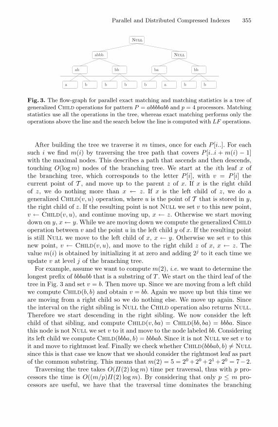
Parallel and Distributed Compressed Indexes 355
a b b b
bbab
abbb
b b ba
ba bb
Null
Null
Fig. 3. The flow-graph for parallel exact matching and matching statistics is a tree ofgeneralized Child operations for pattern P = abbbbabb and p = 4 processors. Matchingstatistics use all the operations in the tree, whereas exact matching performs only theoperations above the line and the search below the line is computed with LF operations.
After building the tree we traverse it m times, once for each P [i..]. For eachsuch i we find m(i) by traversing the tree path that covers P [i..i + m(i) − 1]with the maximal nodes. This describes a path that ascends and then descends,touching O(logm) nodes of the branching tree. We start at the ith leaf x ofthe branching tree, which corresponds to the letter P [i], with v = P [i] thecurrent point of T , and move up to the parent z of x. If x is the right childof z, we do nothing more than x ← z. If x is the left child of z, we do ageneralized Child(v, u) operation, where u is the point of T that is stored in y,the right child of z. If the resulting point is not Null we set v to this new point,v ← Child(v, u), and continue moving up, x ← z. Otherwise we start movingdown on y, x← y. While we are moving down we compute the generalized Childoperation between v and the point u in the left child y of x. If the resulting pointis still Null we move to the left child of x, x ← y. Otherwise we set v to thisnew point, v ← Child(v, u), and move to the right child z of x, x ← z. Thevalue m(i) is obtained by initializing it at zero and adding 2j to it each time weupdate v at level j of the branching tree.
For example, assume we want to compute m(2), i.e. we want to determine thelongest prefix of bbbabb that is a substring of T . We start on the third leaf of thetree in Fig. 3 and set v = b. Then move up. Since we are moving from a left childwe compute Child(b, b) and obtain v = bb. Again we move up but this time weare moving from a right child so we do nothing else. We move up again. Sincethe interval on the right sibling is Null the Child operation also returns Null.Therefore we start descending in the right sibling. We now consider the leftchild of that sibling, and compute Child(v, ba) = Child(bb, ba) = bbba. Sincethis node is not Null we set v to it and move to the node labeled bb. Consideringits left child we compute Child(bbba, b) = bbbab. Since it is not Null we set v toit and move to rightmost leaf. Finally we check whether Child(bbbab, b) �= Nullsince this is that case we know that we should consider the rightmost leaf as partof the common substring. This means that m(2) = 5 = 20 +20 +21 +20 = 7−2.
Traversing the tree takes O(Π(2) logm) time per traversal, thus with p pro-cessors the time is O((m/p)Π(2) logm). By considering that only p ≤ m pro-cessors are useful, we have that the traversal time dominates the branching

356 L.M.S. Russo, G. Navarro, and A.L. Oliveira
tree construction time. Using the instantiation in Table 1 this result becomesO((m/p) logm logn(log log n)2) on the FCST and O((m/p) logm log2 n log logn)on the FMI. The total space is O(m logm) + nHk + o(n log σ) bits. This timethe linear speedup is multiplied by a polylogarithmic factor, since the sequentialalgorithm can be made O(m) time.
Longest common substring. We can compute the longest common substringbetween P and T by taking the maximum matching statistic m(i) in additionalnegligible O(m/p+ log p) time.
Maximal repeats. For this problem we need a FCST, and cannot simulate itwith a CSA as before. A maximal repeat in T is a substring S, of size , thatoccurs in at least two positions i and i′, i.e. S = T [i..i+ − 1] = T [i′..i′ + − 1],and cannot be extended either way, i.e. T [i−1] �= T [i′−1] and T [i+] �= T [i′+].The solution for this problem consists in identifying the deepest internal nodes vof T that are left-diverse, i.e. the nodes for which there exist letters X �= Y suchthat X.v and Y.v are substrings of T [11]. Assume v = [vl, vr]. Then FMIs allowone to access Letter(vl,−1) = T [vl − 1] in O(τ) time3. Hence node v is left-diverse iff Count(LF(Letter(vl,−1), v)) �= Count(v). This can be verified inO(τ) time, moreover this verification can be performed independently for everyinternal node of T . At each step the algorithm chooses p nodes from T andperforms this verification. A simple way to choose all internal nodes (albeit withrepetitions, which does not affect the asymptotic time of this algorithm) is tocompute LCA([i, i], [i + 1, i + 1]) for all 0 ≤ i < n − 1. Hence this procedurerequires O((n/p)(Ψ + τ)δ) time, plus negligible O(n/p + log p) time to find thelongest candidates. Using the same instantiation as in Table 1 the result becomesO((n/p) logn log logn) time within optimal nHk + o(n logσ) overall bits. This isan optimal speedup, if we consider the polylogarithmic penalty of using a FCST.
The speedups in this section are similar to the results obtained for “classical”uncompressed suffix trees by Clifford [10], which do not speed up exact matchingbecause they do not use a generalized Child operation. Clifford speeds up thelongest common substring problem and the maximal repeats, among others.
5 Distributed Compressed Indexes
In this section we study distributed CSAs and FCSTs, mainly to obtain supportfor large string databases. In this case we assume we have a collection C of q textsof total length n, distributed across q machines. Hence distributed FCSTs arealways generalized suffix trees, and likewise for CSAs. In fact, the local text ofeach machine could also be a collection of smaller texts, and the whole databasecould be a single string arbitrarily partitioned into q segments: CSAs and CSTstreat both cases similarly. The only difference is whether the SLink of the lastsymbol of a text sends one to the next text or it stays within that text, but eithervariant can be handled with minimal changes. We choose the latter option.3 This is an access to the Burrows-Wheeler transform.

Parallel and Distributed Compressed Indexes 357
Various data layouts have been considered for distributing classical suffix treesand arrays [17,9,10]. One can distribute the texts and leave each machine indexits own text, or distribute a single global index into lexicographical intervals, oropt for other combinations. In this paper we consider reducing the time of a singlequery, in contrast to previous work [17] where the focus is on speeding up batchesof queries by distributing them across machines. Our approach is essentially thatof indexing each text piece in its own machine, yet we end up distributing someglobal information across machines, similarly to the idea storing local indexeswith global identifiers [17].
First we study the case where the local CSAs are used to simulate a globalCSA, which can then be used directly in the FCST representation. This solutionturns out to require extra space due to the need of storing some redundantinformation. Then we introduce a new technique to combine FCSTs that removessome of those redundant storage requirements.
Distributed Compressed Suffix Arrays. Assume we have a collection C ={Tj}q−1
0 , and the respective local CSAs. We denote their operations with asubscript j, i.e. as Aj , A−1
j , ψj and LFj . The generalized CSA that resultsfrom this collection is denoted AC . Assume we store the accumulated text sizes,AccT [i] =
∑i−1j=0 |Tj |, which need just O(q logn) bits.
We define the sequence IdC of suffix indexes of C, where IdC [i] = j if thesuffix in AC [i] belongs to text Tj. Consider T as T0 and T ′ as T1 in our runningexample. The respective generalized suffix tree is shown in the left of Fig. 1. TheId sequence for this example is obtained by reading the leaves, and replacing $by 0 and # by 1. The resulting sequence is Id = 0100101010101.
If we process Id for Rank and Select queries we can obtain the oper-ations of AC from the operations of the Aj ’s. To compute Locate we usethe equation AC [v] = AId[v][RankId[v](v − 1)] + AccT [Id[v]]. For example forAC [4] we have that A1[Rank1(4 − 1)] + AccT [1] = A1[1] + 7 = 7. To com-pute A−1
C we use a similar relation, A−1C [i] = Selectj(A−1
j [i − AccT [j]] + 1),where j is such that AccT [j] ≤ i < AccT [j + 1]. Likewise ψC is computed asψC [v] = SelectId[v](ψId[v][RankId[v](v − 1)] + 1). Computing LFC(X, [vl, vr])is more complicated: we compute LF in all the CSAs, i.e. LFj(X, [Rankj(vl −1),Rankj(vr)−1]) for every 0 ≤ j < q. If [xvj,l, xvj,r] are the resulting intervalsthen LFC(X, [vl, vr]) = [minq−1
j=0{Selectj(xvj,l + 1)},maxq−1j=0{Selectj(xvj,r +
1)}]. Consider for example, how to compute LFC(a, [5, 12]). We computeLF0(a, [3, 6]) = [1, 2] and LF1(a, [2, 5]) = [1, 1] and use the results to obtainthat LFC(a, [5, 12]) = [min{Select0(1+1),Select1(1+1)},max{Select0(2+1),Select1(1 + 1)}] = [min{2, 4},max{3, 4}] = [2, 4]. This requires O(log q) ac-cesses to slow memory to compute minima and maxima in parallel.
A problem with this approach is the space necessary to store sequence Idand support Rank and Select. An efficient approach is to unfold Id into qbitmaps, BIdj [i] = 1 iff Id[i] = j, and process each one for constant-time binaryRank and Select queries while storing them in compressed form [14]. Thensince BIdj contains about n/q 1s, it requires (n/q) log q+O(n/q) + o(n) bits ofspace. We store each BIdj in the local memory of processor j, which requires

358 L.M.S. Russo, G. Navarro, and A.L. Oliveira
space |CSAj | + (n/q) log q + O(n/q) + o(n) local bits. The total space usage is|CSAC | + n log q + O(n) + o(qn) bits (if the partitions are not equal it is evenless; n log q bits is the worst case). This essentially lets each machine map itsown local CSA positions to the global suffix array, as done in previous work forclassical suffix arrays (where the global identifiers can be directly stored) [17].
In this setup, most of the accesses are to local memory. One model is thatqueries are sent to all processors and the one able of handling it takes the lead.For AC [v], each processor j looks if BIdj [v] = 1, in which case j = Id[v] andthis is the processor solving the query locally, in O(Φ) accesses to fast memory(processor j also stores values AccT [j] and AccT [j+1] locally). For A−1
C [i], eachprocessor j checks if AccT [j] ≤ i < AccT [j+1] and the one answering positivelytakes the lead, answering again in O(Φ) local accesses. ψC proceeds similarly toAC , in O(Ψ) local accesses. LFC is more complex since all the processors must beinvolved, each spending O(τ) local accesses, and then computing global minimaand maxima in O(log q) accesses to slow memory. Compare to the alternative ofstoring CSAC explicitly and splitting it lexicographically: all the local accessesin the time complexities become global.
The o(qn) extra memory scales badly with q (as more processors are avail-able, each needs more local memory). A way to get rid of it is to use bitmaprepresentations that require n log q+ o(n log q) +O(n log log q) = O(n log q) bitsand solve Rank and Select queries within o((log logn)2) time [18]. We willnow present a new technique that directly represents global FCSTs using tuplesof ranges instead of a single suffix array range.
Distributed Fully-Compressed Suffix Trees. Consider the generalized suf-fix tree TC of a collection of texts C = {Tj}q−1
0 and the respective individ-ual suffix trees Ti. Assume, also, that we are storing the Ti trees with theFCST representation and want to obtain a representation for TC . A node ofTC can be represented all the time as a q-tuple of intervals 〈v0, . . . , vq−1〉 =〈[v0,l, v0,r], . . . , [vq−1,l, vq−1,r]〉 over the corresponding CSAs. For example thenode abbb can be represented as 〈[2, 2], [1, 1]〉. In fact we have just explained,in the distributed LF operation, how to obtain from these intervals the [vl, vr]representation of node v of TC (via Select on IdC and distributed minima andmaxima). Thus these intervals are enough to represent v.
To avoid storing the Id sequence we map every interval [vi,l, vi,r ] directly tothe sampled tree of FCSTC , instead of mapping it to an interval v over CSACand then reducing it to the sampled tree of FCSTC with LSAC(v). We usethe same bitmap-based technique for LSAC , but store q local bitmaps insteadof just a global one. The bitmaps Bj are obtained from the bitmap B of theFCSTC by removing the zeros that do not correspond to leaves of Tj , see Fig 2.This means that, in Bj , we are representing the O(n/δ) nodes of the globalsampled tree and the n/q leaves of Tj . As each Bj has n/q 0s and O(n/δ) 1s,the compressed representation [14] supporting constant-time Rank and Selectrequires (n/q) log(1 + q/δ) +O(n/q) + o(n/δ + n/q) bits. This is slightly betterthan the extra space of CSAs, totalling O(n log(1 + q/δ)) + o(nq/δ) bits. Asbefore, the o(. . .) term can be removed by using the representation by Gupta et

Parallel and Distributed Compressed Indexes 359
al. [18] at the price of o((log logn)2) accesses to fast local memory. Now the samecomputation for LSA carried out on Bj gives a global interval.
We then compute LSAC(v) = LCASC(LSA0(v0), . . . ,LSAq−1(vq−1)), whereLCASC is the LCA operation over the sampled tree of TC and LSAj(vj) is theglobal LSA value obtained by processor j. This operation is computed in parallelin O(log q) accesses to slow memory (which replaces the global minima/maximaof the CSA). The sampled tree S and its extra data (e.g., to compute LCA inconstant time) is stored in the shared memory. Hence accesses to S are alwaysslow, which does not change the stated complexities. This mechanism supportsthe usual representation of the global FCST.
Consider, for example, that we want to compute the SDep of node abbb. Notethat the SDep of [2, 2] in T0 is 7 and that the SDep of [1, 1] in T1 is 6. Howeverthe SDep of abbb in TC is 4. In this example we do not have to use ψ to obtainthe result, altough in general it is necessary. By reducing the [2, 2] and [1, 1]intervals to the sampled tree of FCSTC we obtain the node abbb and the leafabbbb#, see Fig. 1. The node we want is the LCA of these nodes, i.e. abbb.
Theorem 2. Given a collection of q texts C = {Tj}q−10 represented by com-
pressed suffix arrays (CSAj) that support ψ, ψi, T [A[v]] and LF in times O(Ψ),O(Φ), O(1), and O(τ), respectively, it is possible to represent a distributed suffixtree with the properties given in Table 1 (column “distributed”).
Moreover this technique has the added benefit that we can simulate the general-ized suffix tree from any subcollection of the q texts, by using only the intervalsof the texts Tj that we want to consider. However in this case we lose the TDep,TLAQ and SLAQ operations.
6 Conclusions and Future Work
Compressed indexes are a new and functional way to index text strings usinglittle space, and their parallelization has not been studied yet. We have focusedon parallel (shared RAM) and distributed suffix trees and arrays, which are themost pervasive compressed text indexes. We obtained almost linear speedups forthe basic pattern search problem, and also for more complex ones such as com-puting matching statistics, longest common substrings, and maximal matches.The sequential algorithms for these problems are linear-time and easy to carryover compressed indexes, but hard to parallelize. Thanks to the stronger func-tionality of compressed indexes, namely the support of generalized branching,we achieve parallel versions for all of these. Some of our solutions can do witha compressed suffix array; others require a compressed suffix tree. We plan toapply this idea to other problems with applications in bioinformatics [11], suchas all-pairs prefix-suffix queries.
Distributing the index across q machines further alleviates the space problem,allowing it to run on a larger virtual memory. Our distributed suffix arraysrequire O(n log q) + o(n) extra bits, whereas our suffix trees require o(nq/δ)extra bits. Both simulate a global index with O(log q) slowdown (measured incommunication cost), so they achieve O(q/ log q) speedup on each query.

360 L.M.S. Russo, G. Navarro, and A.L. Oliveira
A challenge for future work is to reduce this extra space, as O(n log q) canbe larger than the compressed suffix array itself. We also plan to consider othermodels models such as BSP and batched queries [17]. An exciting direction is toconvert the distributed index into an efficient external-memory representationfor compressed text indexes, which suffer from poor locality of reference.
References
1. Giegerich, R., Kurtz, S., Stoye, J.: Efficient implementation of lazy suffix trees.Softw., Pract. Exper. 33(11), 1035–1049 (2003)
2. Manber, U., Myers, E.: Suffix arrays: A new method for on-line string searches.SIAM J. Comput. 22(5), 935–948 (1993)
3. Sadakane, K.: Compressed suffix trees with full functionality. Theory Comput.Syst. 41(4), 589–607 (2007)
4. Navarro, G., Makinen, V.: Compressed full-text indexes. ACM Comp. Surv. 39(1),article 2 (2007)
5. Ferragina, P., Manzini, G., Makinen, V., Navarro, G.: Compressed representationsof sequences and full-text indexes. ACM Trans. Algor. 3(2), article 20 (2007)
6. Manzini, G.: An analysis of the Burrows-Wheeler transform. J. ACM 48(3),407–430 (2001)
7. Russo, L., Navarro, G., Oliveira, A.: Fully-Compressed Suffix Trees. In: Laber,E.S., Bornstein, C., Nogueira, L.T., Faria, L. (eds.) LATIN 2008. LNCS, vol. 4957,pp. 362–373. Springer, Heidelberg (2008)
8. Fischer, J., Makinen, V., Navarro, G.: Faster entropy-bounded compressed suffixtrees. Theor. Comp. Sci. 410(51), 5354–5364 (2009)
9. Makinen, V., Navarro, G., Sadakane, K.: Advantages of backward searching —efficient secondary memory and distributed implementation of compressed suf-fix arrays. In: Fleischer, R., Trippen, G. (eds.) ISAAC 2004. LNCS, vol. 3341,pp. 681–692. Springer, Heidelberg (2004)
10. Clifford, R.: Distributed suffix trees. J. Discrete Algorithms 3(2-4), 176–197 (2005)11. Gusfield, D.: Algorithms on Strings, Trees and Sequences. Cambridge University
Press, Cambridge (1997)12. Weiner, P.: Linear pattern matching algorithms. In: IEEE Symp. on Switching and
Automata Theory, pp. 1–11 (1973)13. Lee, S., Park, K.: Dynamic rank-select structures with applications to run-length
encoded texts. In: Ma, B., Zhang, K. (eds.) CPM 2007. LNCS, vol. 4580, pp. 95–106.Springer, Heidelberg (2007)
14. Raman, R., Raman, V., Rao, S.S.: Succinct indexable dictionaries with applicationsto encoding k-ary trees and multisets. In: Proc 13th SODA, pp. 233–242 (2002)
15. Huynh, T.N.D., Hon, W.K., Lam, T.W., Sung, W.K.: Approximate string matchingusing compressed suffix arrays. Theor. Comput. Sci. 352(1-3), 240–249 (2006)
16. Russo, L., Navarro, G., Oliveira, A.: Dynamic Fully-Compressed Suffix Trees. In:Ferragina, P., Landau, G.M. (eds.) CPM 2008. LNCS, vol. 5029, pp. 191–203.Springer, Heidelberg (2008)
17. Marın, M., Navarro, G.: Distributed query processing using suffix arrays. In: Nasci-mento, M.A., de Moura, E.S., Oliveira, A.L. (eds.) SPIRE 2003. LNCS, vol. 2857,pp. 311–325. Springer, Heidelberg (2003)
18. Gupta, A., Hon, W.K., Shah, R., Vitter, J.: Compressed data structures: dictionar-ies and data-aware measures. In: Alvarez, C., Serna, M. (eds.) WEA 2006. LNCS,vol. 4007, pp. 158–169. Springer, Heidelberg (2006)

Author Index
AitMous, Omar 275Asano, Tetsuo 190
Bannai, Hideo 238Bassino, Frederique 275Belazzougui, Djamal 88Blelloch, Guy E. 138Brejova, Brona 164
Cantone, Domenico 288Charlat, Sylvain 202Chauve, Cedric 112Clifford, Raphael 101Crochemore, Maxime 251, 299Cygan, Marek 299
Duron, Olivier 202
Elberfeld, Michael 177Engelstadter, Jan 202
Faro, Simone 288Farzan, Arash 138Fleischer, Rudolf 214
Galil, Zvi 26Giaquinta, Emanuele 288Gog, Simon 40Guo, Jiong 214
Hermelin, Danny 202Hon, Wing-Kai 260Hundt, Christian 13
Iliopoulos, Costas S. 251, 299Inenaga, Shunsuke 238I, Tomohiro 238
Jansson, Jesper 190Jiang, Haitao 112Jiang, Minghui 125
Karp, Richard M. 151Kim, Joondong 323Kopelowitz, Tsvi 63Kubica, Marcin 299
Ladra, Susana 76Lee, Taehyung 310
Makinen, Veli 76Memelli, Heraldo 323Mitchell, Joseph S.B. 323Montes, Pablo 323
Na, Joong Chae 310Nanasi, Michal 164Navarro, Gonzalo 348Neuburger, Shoshana 27Nicaud, Cyril 275Niedermeier, Rolf 214Nor, Igor 202
Ohlebusch, Enno 40Oliveira, Arlindo L. 348
Park, Heejin 310Park, Kunsoo 310Pissis, Solon P. 251
Radoszewski, Jakub 299Reuter, Max 202Russo, Luıs M.S. 348Rytter, Wojciech 299
Sach, Benjamin 101Sadakane, Kunihiko 190Sagot, Marie-France 202Schnattinger, Thomas 40Shah, Rahul 260Sim, Jeong Seop 310Siren, Jouni 227Skiena, Steven 323Sokol, Dina 27
Takeda, Masayuki 238Tantau, Till 177Tischler, German 251
Uehara, Ryuhei 190Uhlmann, Johannes 214

362 Author Index
Valiente, Gabriel 190Valimaki, Niko 76Vinar, Tomas 164Vitter, Jeffrey Scott 260
Walen, Tomasz 299Wang, Yihui 214Ward, Charles 323Weller, Mathias 214
Wu, Xi 214Wu, Yufeng 152
Xu, Zhi 51
Yokoo, Hidetoshi 338
Zhang, Kaizhong 1Zhu, Binhai 112Zhu, Yunkun 1