Computer Graphics Lecture NotesPart 2

Kamil Niedziałomski

Contents

1 History of computer graphics. Vector and raster graphics 2

2 Raster algorithms: line and circle drawing 3

3 Raster algorithms: filling areas 8

4 Modeling curves and surfaces 11

5 Color in computer graphics 15

6 Hidden surface removal 17

1

1 History of computer graphics. Vector and raster graphics

In computer graphics we distinguish two types of displaying an image: vector graphicsand raster graphics.

1. Raster graphics An image on a monitor or on a sheet of paper in copywriter consistsof finite rectangular elements called pixels. Each pixel can be of a different color.We often call a displayed image in raster graphics a bitmap. Raster monitors, whichare now widely used, ’remember’ displayed primitives, that is simple geometric ob-jects as lines, circles etc. made of pixels. A bitmap is thus a set of horizontal andvertical lines of pixels, which retains in the memory as a table of pixels of a screen.The advantage of raster graphics is that each image takes the same amount of mem-ory (use of memory depends only on resolution of a monitor, that is the number ofpixels) and can be easily displayed.

2. Vector graphics In vector graphics objects are made of arbitrary small lines (points),which may be placed everywhere. Therefore, while scaling and rotating objects wedon’t loose the quality of the displayed objects. In vector monitors the stream of elec-trons goes only to the place where the object is displayed, whereas in raster moni-tors, as we said before, the stream of electrones runs through the whole screen. Oneof the drawbacks of vector graphics is that it is hard to transfer vector object to rasterones.

Figure 1.1: Letter A as a raster and vector image.

The need to use different software led to creation of graphics standards. The first stan-dard 3D Core was developed by ACM SIGGRAPH and was used till 90’s. Nowadays, themost popular standard is OpenGL made by Silikon Graphics (SGI) and Direct3D suggestedby Microsoft. DirectX is accepted standart for Graphics Cards.

As for graphics file formats we can distinguish four:

1. Image file formats related to raster graphics. The most common image formats in-clude GIF, JPEG, PNG, TIFF and BMP.

2

2. Vector graphics file format Examples of vector formats are DXF used by AutodeskCompany in its applications (AutoCad) and SVG made for WWW.

3. Metafile formats Can include both raster and vector information. Examples areWMF and EMF used in MS Windows.

4. Page description language refers to formats used to describe the layout of a printedpage containing text, objects and images. Examples are PostScript and PDF createdby Adobe.

2 Raster algorithms: line and circle drawing

In raster graphics even drawing a line or a circle is not easy, because it is impossible to drawa straight line or round circle with finitely many points (pixels). Thus we need algorithmsto draw these geometric objects (primitives).

2.1 Drawing a line. DDA and Bresenham algorithms.

We want to draw a line as straight and as close to given one as it is possible. Let P0 =(x0, y0) and Pp = (xp , yp ) denote the begining and the end of a line l , and assume that thecoordinates of the point P0 are integer valued. As a first pixel we take P0. The next one canbe chosen from the 8 pixels that are nearby.

Figure 2.1: 8 nearby pixels.

We choose the one closest to the line and continue the process. The easiest strategyto do it is as follows. It is called DDA algorithm. Firsty, we may assume for simplicity, thatx0 < xp and that the slope m of the line satisfies |m| ≤ 1. Put

∆x = xp −x0, ∆y = yp − y0.

Then m = ∆y∆x and the line l is described by an equation

y = ∆y

∆x(x −x0)+ y0.

As we said before we start from the pixel P0 = (x0, y0). We increase the value of x0 by 1,x1 = x0 +1. Then the point Q1 = (x1, y0 +m) lies on l . We choose P1 as the pixel closest toQ1. Hence P1 = (x1,Round(y0 +m)), where Round is the function which rounds the value.In general, if Pi = (xi , yi ) is given, then Pi+1 = (xi +1,Round(yi +m)).

3

Figure 2.2: DDA algorithm.

The above algorithm is not perfect. Parameters yi and m are real numbers and thefunction Round requires time consuming computations. In 1963, Bresenham proposedan algorithm based on the same observation as above, which uses only integer values.

The begininig is the same, however for simplicity we assume 0 < m ≤ 1. We start fromthe pixel P0 = (x0, y0). Assume we have picked the point Pi = (xi , yi ) and we want to findthe next one Pi+1 = (xi+1, yi+1. Since the slope of the line satisfies 0 < m ≤ 1, there are twopossibilities of choosing the point Pi+1: Si+1 = (xi +1, yi ) or Ti+1 = (xi +1, yi +1).

Figure 2.3: Finding Pi+1. Here Pi+1 = Ti+1.

Let A be the intersection of l and the segment Ti+1Si+1. Then the x–coordinate of A isxA = xi +1. Hence the y–coordinate is y A = ∆y

∆x (xi +1− x0)+ y0. Therefore, the length t of

the segment Ti+1 A and the length s of the segment ASi+1 are respectively

t = yi +1− y A = yi +1− y0 − ∆y

∆x(xi +1−x0),

s = y A − yi = ∆y

∆x(xi +1−x0)− (yi − y0).

Hence

(2.1) di =∆x(s − t ) =−2∆x(yi − y0)+2∆y(xi −x0)+2∆y −∆x.

If di ≥ 0 (t ≤ s), then Pi+1 = Ti+1. If di < 0 (t > s), then Pi+1 = Si+1. To improve the re-curence, let us make few observations. Writing (2.1) for di+1 we have

(2.2) di+1 = 2∆x(yi+1 − y0)+2∆y(xi+1 −x0)+2∆y −∆x.

Thus, since xi+1 −xi = 1

di+1 −di =−2∆x(yi+1 − yi )+2∆y(xi+1 −xi ) =−2∆x(yi+1 − yi )+2∆y.

4

Finallydi+1 = di −2∆x(yi+1 − yi )+2∆y.

Going back to choosing between Ti+1 and Si+1, we have

1. di ≥ 0. Then Pi+1 = Ti+1, so yi+1 = yi and di+i = di −2∆x +2∆y .

2. di < 0. Then Pi+1 = Si+1, so yi+1 = yi and di+1 = di +2∆y .

We can now write the pseudocode for this algorithm, we write d x and d y instead of ∆xand ∆y .

constants: P[0]=(x[0],y[0]), dx=x[p]-x[0], dy=y[p]-y[0]d0=2*dy-dx

algorithm: for (i=0) to (x[p]-x[0]-1) do{x[i+1]=x[i]if (d[i] >= 0) then

{d[i+1]=d[i]-2*dx+2*dyy[i+1]=y[i]+1}

else{d[i+1]=d[i]+2*dyy[i+1]=y[i]}

P[i+1]=(x[i+1],y[i+1])}

Using above algorithm we encounter some problems. Firstly, algorithm should be in-dependant of the choice of the end points P0 and Pp . The only situation in which theremay be a confusion is when the line goes througt the middle point A, that is when di = 0.The question is which point to choose, Ti+1 or Si+1. If we decide to choose Ti+1, if thestarting point is P0, as we have done, we must choose Si+1 if the starting point is Pp . Thenext problem is the lenght of the line and number of pixels used to draw it.

Figure 2.4: Two lines of different length with the same number of pixels.

5

In the Figure 2.4, the diagonal line isp

2 times longer than the horizontal one, but theyboth consist of 8 pixels. Thus the diagonal seems to be brighter than the horizontal. Inthat case we should use brighter shade of gray color to draw the horizontal line.

2.2 Drawing a circle

When we want to draw a circle, there is another one aspect which doesn’t play the rolein line drawing. Namely, we need to take into account the shape of a pixels. If the pixelsare rectalngles but not squares, we can obtain an ellipse instead of a circle. Therefore,we define the aspect of a graphics device as a ratio of the lenght and the height of a pixel.Assume the aspect is a rational number a = p/q . We should distinguish between Cartesiancoordinate system (XY) and coordinate system of pixels (xy). If we move up y and right x inPixel coordinate system, then we move up Y = y and right X = ax in Cartesian coordinatesystem.

Figure 2.5: Transfering from Cartesian to Pixel coordinate system.

Assume we want to draw a circle C of radius R centered at (0,0). Then C is given byX 2 +Y 2 −R2 = 0 or equivalently (ax)2 + y2 −R2 = 0. Since a = p/q the circle C is given byan implicit equation

(2.3) f (x, y) = p2x2 +q2 y2 −q2R2 = 0.

Then the area inside the circle is given by f (x, y) < 0 and the area outside the circle byf (x, y) > 0.

Due to the symmetry we consider only the part of a circle f (x, y) = 0, where x, y > 0.Let the starting point be P0 = (0,R). Assume we have found the pixel Pi = (xi , yi ) andwe seek for Pi+1 = (xi+1, yi+1). It is easy to see that the choice restricts to three pointsSi+1 = (xi +1, yi −1), Ti+1 = (xi +1, yi ), Ui+1 = (xi , yi −1).

The tangent vector v(x, y) to a circle at a point (x, y) is by implicit function theorem

v(x, y) = (1,f ′

x

f ′y

(x, y)) = (1,−p2x

q2 y).

Thus if the slope of v(x, y) is <−1, which means p2x > q2 y , we choose between Ti+1 andSi+1, whereas if the slope of v(x, y) is > −1, which means p2x < q2 y , we choose betweenUi+1 and Si+1. We now concentrate on the part of a circle p2x > q2 y leaving the second

6

Figure 2.6: Possibilities of choosing Pi+1.

case to the reader. We proceed in the similar way as in the case of a line. Let A be themiddle of a segment Ti+1Si+1. If A is outside the circle, we choose Si+1. If A is inside thecircle, we choose Ti+1. If A is on a circle, we can take any of these two points (for ourpurposes we choose Ti+1). We have A = (xi +1, yi − 1

2 ). Then

f ai = f (A) = p2(xi +1)2 +q2(yi − 1

2)2 −q2R2.

To improve the recurence let us compute

f ai+1 − f ai = p2(xi+1 −xi )(xi+1 +xi +2)+q2(yi+1 − yi )(yi+1 + yi −1).

For the starting point P0 = (0,R) we have

f a0 = p2 −q2R + R2

4.

To avoid division, we multiply f ai by a factor 4. Concluding we have

1. If f ai ≥ 0, then Pi+1 = Si+1, so xi+1 = xi + 1, yi+1 = yi − 1. Hence f ai+1 = f ai +4p2(2xi+1 +1)−8q2 yi+1.

2. If f ai < 0, then Pi+1 = Ti+1, so xi+1 = xi+1, yi+1 = yi . Hence f ai+1 = f ai+4p2(2xi+1+1).

We can now write a pseudocode for this algorithm

constants: x=0, y=R, fa=4*p*p-4*q*q*R+R*Ralgoryihm: while (p*p*x<q*q*y) do

{P=(x,y)x=x+1

if (fa>=0) then{y=y-1fa=fa+4*p*p*(2*x+1)

7

}else

{fa=fa+4*p*p*(2*x+1)-8*q*q*y}}

In the end we remark that using this algorithm for f (x, y) = p2 A2x2+q2B 2 y2−q2R2 = 0we are able to draw ellipses.

3 Raster algorithms: filling areas

Consider the following problem: Given the boundary of some area, fill this area in. To startdealing with this task we need some theoretical background.

Let A be the set of pixels. We say that A is connected if any two pixels from A can bejoined by neighbouring pixels from A. If the neighbouring pixels are the only these whichlie one above another or one on the left (right) of another we speak about 4-connectedness,whereas if the neighbouring pixels are these which can also lie diagonal to each other wespeak about 8–connectedness.

3.1 Flood Fill algorithm

Assume the boundary of area is 8–connected and that the interior is 4–connented. Let theboundary consist of black pixels and we fill the interior with gray pixels. Assume we havechoosen an interior pixel. Then we check if any of four neighbouring pixels is black. If notwe color it gray and continue the process for this pixel.

Figure 3.1: Flood Fill algorithm.

The function F loodF i l l is thus of the form

FloodFill(x,y){

if (color(x,y)<>black and color(x,y)<>gray) then{

setcolor(x,y,gray)FloodFill(x,y-1)FloodFill(x,y+1)

8

FloodFill(x-1,y)FloodFill(x+1,y)

}}

Flood Fill algorithm is short and simple, however its realization causes problems, mainlybecause of the recurence, which consumes a lot of momory. Moreover, the color of a pixelis often checked few times.

3.2 Filling polygons

We now concentrate on filling polygons. We do not require the polygon to be convex. Thealgorithm of filling the polygon can be described as follows:

For each horizontal line l

1. find all points x1, . . . , xp of intersection of l with the polygon. p is in general an evennumber p = 2k.

2. sort these points x1 < . . . < xp .

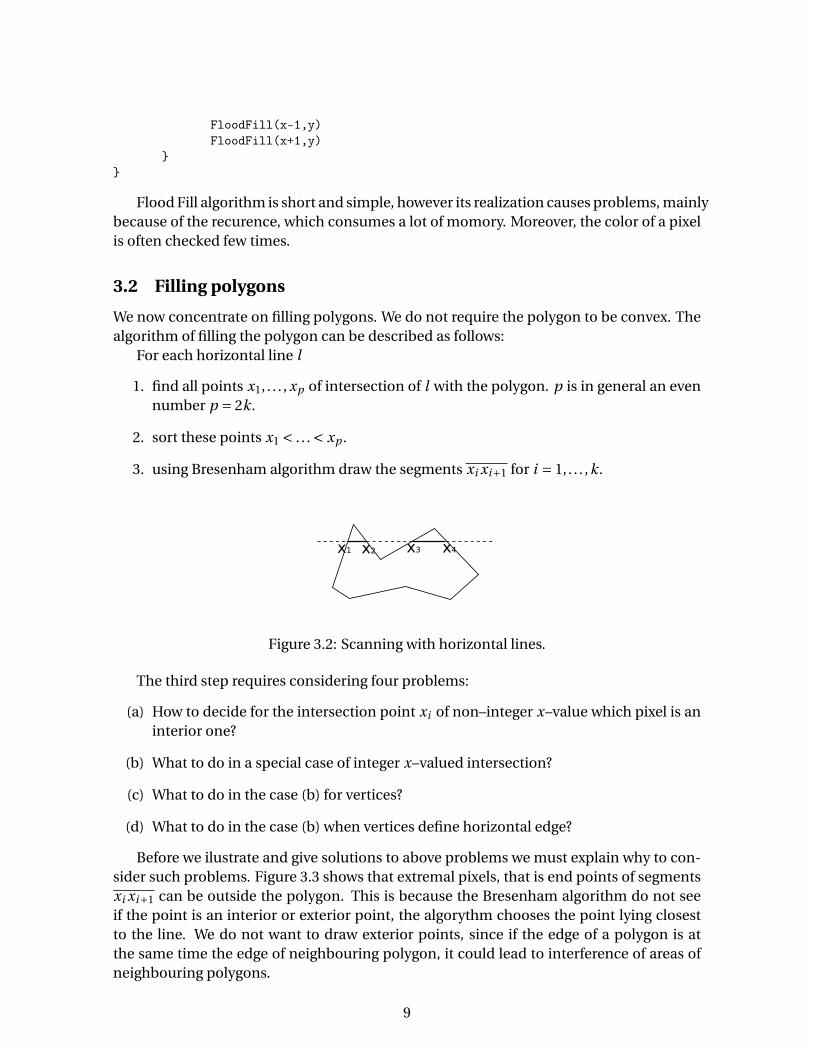
3. using Bresenham algorithm draw the segments xi xi+1 for i = 1, . . . ,k.

Figure 3.2: Scanning with horizontal lines.

The third step requires considering four problems:

(a) How to decide for the intersection point xi of non–integer x–value which pixel is aninterior one?

(b) What to do in a special case of integer x–valued intersection?

(c) What to do in the case (b) for vertices?

(d) What to do in the case (b) when vertices define horizontal edge?

Before we ilustrate and give solutions to above problems we must explain why to con-sider such problems. Figure 3.3 shows that extremal pixels, that is end points of segmentsxi xi+1 can be outside the polygon. This is because the Bresenham algorithm do not seeif the point is an interior or exterior point, the algorythm chooses the point lying closestto the line. We do not want to draw exterior points, since if the edge of a polygon is atthe same time the edge of neighbouring polygon, it could lead to interference of areas ofneighbouring polygons.

9

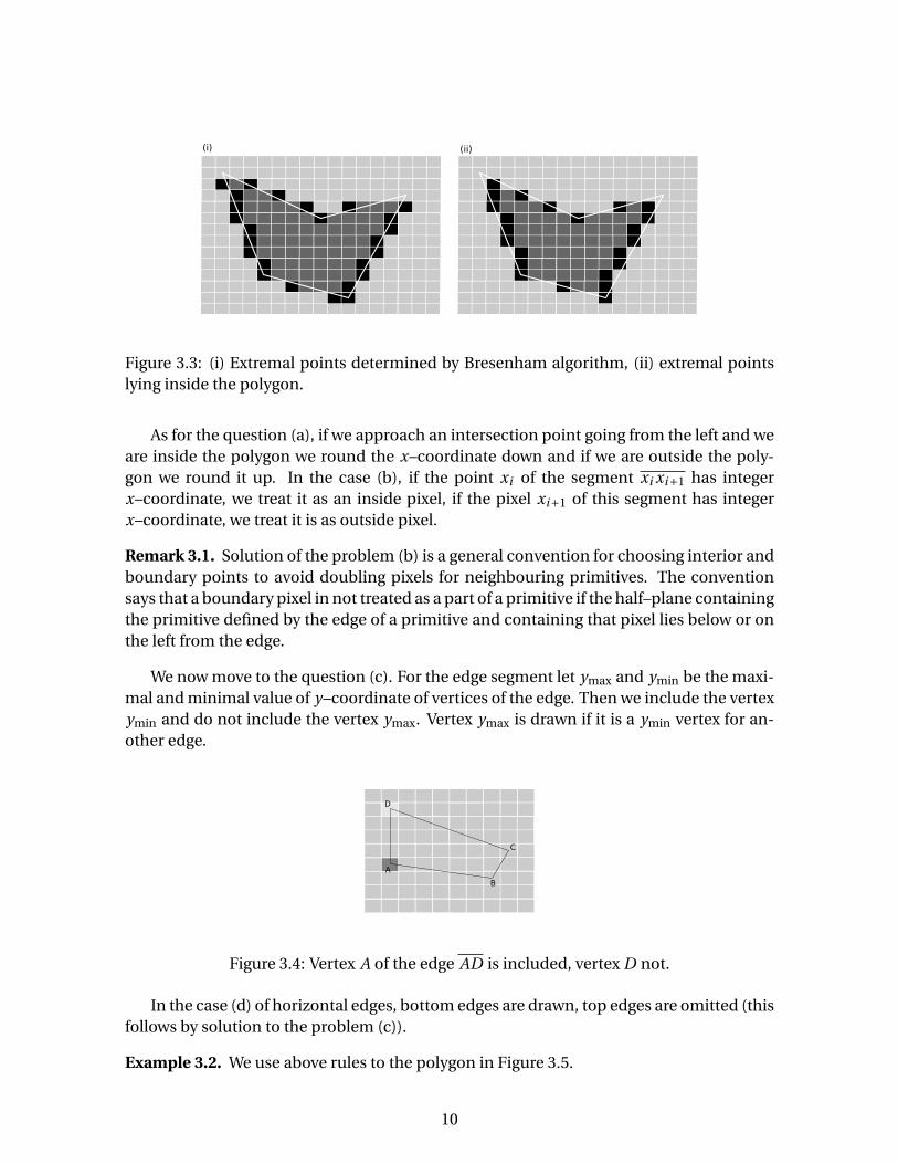
Figure 3.3: (i) Extremal points determined by Bresenham algorithm, (ii) extremal pointslying inside the polygon.

As for the question (a), if we approach an intersection point going from the left and weare inside the polygon we round the x–coordinate down and if we are outside the poly-gon we round it up. In the case (b), if the point xi of the segment xi xi+1 has integerx–coordinate, we treat it as an inside pixel, if the pixel xi+1 of this segment has integerx–coordinate, we treat it is as outside pixel.

Remark 3.1. Solution of the problem (b) is a general convention for choosing interior andboundary points to avoid doubling pixels for neighbouring primitives. The conventionsays that a boundary pixel in not treated as a part of a primitive if the half–plane containingthe primitive defined by the edge of a primitive and containing that pixel lies below or onthe left from the edge.

We now move to the question (c). For the edge segment let ymax and ymin be the maxi-mal and minimal value of y–coordinate of vertices of the edge. Then we include the vertexymin and do not include the vertex ymax. Vertex ymax is drawn if it is a ymin vertex for an-other edge.

Figure 3.4: Vertex A of the edge AD is included, vertex D not.

In the case (d) of horizontal edges, bottom edges are drawn, top edges are omitted (thisfollows by solution to the problem (c)).

Example 3.2. We use above rules to the polygon in Figure 3.5.

10

Figure 3.5: Finding interior pixels.

First we find interior pixels on the horizontal line on the level 6. The intersection pointswith the polygon have x–coordinates 1; 3,5; 7,5; 12. Hence the interior pixels are thesewith x–coordinate 1; 2; 3 and 8; 9; 10; 11. We consider now horizontal edge AB and EF .Since A is the ymin vertex of AH , we draw the segment AB as we said in the case (d). More-over, since the vertex E is ymax for EF we do not draw the edge DE . Vertex H is omited,whereas vertex G is drawn, as we concluded in the case (c). We treat remaining verticessimiliarly.

4 Modeling curves and surfaces

This lecture is devoted to description of Bézier curves and surfaces and surfaces.Let B n

i denote Bernstein polynomials defined on the interval ⟨0,1⟩,

B ni (t ) =

(n

i

)(1− t )n−i t i , t ∈ ⟨0,1⟩.

Bernstein polynomials have the following properties, which are immediate consequencesof the definition

1.∑n

i=0 B ni (t ) = 1,

2. B ni (t ) ≥ 0,

3. B ni (t ) = (1− t )B n−1

i (t )+ tB n−1i−1 (t ).

In the property 3. if i = 0 or i = n we put B n−1 = B n−1

n = 0.

4.1 Bézier curves

Fix n + 1 points P0, . . . ,Pn on a plane or 3–dimensional space. By a Bézier curve c(t ) (ofdegree n) we mean

c(t ) =n∑

i=0B n

i (t )Pi , t ∈ ⟨0,1⟩.

11

The most common case is n = 3. Then

c(t ) = (1− t )3P0 +3(1− t )2tP1 +3(1− t )t 2P2 + t 3P3.

In this case we have

c(0) = P0, c ′(0) = 3(P1 −P0),

c(1) = P3, c ′(1) = 3(P3 −P2).

Hence tangent vectors to c(0) and c(1) are 3(P1 −P0) and 3(P3 −P2) respectively.

Figure 4.1: Examples of Bézier curves of degree 3.

In the general case we have similiarly

c(0) = P0, c ′(0) = 3(P1 −P0),

c(1) = Pn , c ′(1) = 3(Pn −Pn−1).

We will now give an algorithm due to de Casteljau of finding the points on Bézier curve.

Theorem 4.1 (de Casteljau algorithm). Let c(t ) be a Bézier curve determined by the pointsP0, . . . ,Pn . Fix t ∈ ⟨0,1⟩. Put Pi ,0 = Pi and

(4.1) Pi , j = (1− t )Pi−1, j−1 + tPi , j−1.

Then

(4.2) Pn,n = c(t ).

Proof. Fix t ∈ ⟨0,1⟩. Induction on degree n. For n = 1 a Bézier curve is of the form

c(t ) = (1− t )P0 + tP1.

HenceP1,1 = (1− t )P0,0 + tP1,0 = (1− t )P0 + tP1 = c(t ).

Assume (4.7) holds for Bézier curves of degree n −1. Let c(t ) be a Bézier curve of degreen determined by the points P0, . . . ,Pn . Put Qi = Pi+1,1 for i = 0,1, . . . ,n −1 and let γ(t ) be

12

a Bézier curve of degree n −1 determined by Q0, . . . ,Qn−1. Then by induction assumptionγ(t ) =Qn−1,n−1. It sufficies to show

Qn−1,n−1 = Pn,n(4.3)

c(t ) = γ(t ).(4.4)

To prove (4.4) we will show that

(4.5) Qi , j = Pi+1, j+1.

Indeed, Qi ,0 =Qi = Pi+1,1. Assuming (4.5) we have

Qi , j+1 = (1− t )Qi−1, j + tQi , j

= (1− t )Pi , j+1 + tPi+1, j+1

= Pi+1, j+2.

hence by induction (4.5) holds. Therefore, Qn−1,n−1 = Pn,n so (4.3) holds. Moreover, usingproperty 3. of Bernstein polynomials we have

γ(t ) =n−1∑i=0

B n−1i (t )Qi

=n−1∑i=0

(t )Pi+1,1

=n−1∑i=0

B n−1i (t )((1− t )Pi + tPi+1)

=n−1∑i=0

(1− t )B n−1i (t )Pi +

n∑i=1

tB n−1i−1 (t )Pi

=n∑

i=0((1− t )B n−1

i + tB n−1i−1 (t ))Pi

=n∑

i=0B n

i (t )Pi

= c(t ),

which proves (4.4) and the whole theorem.

4.2 Bézier surfaces

To obtain a Bézier surfaces of degree (n,m) we need to fix (n + 1)(m + 1) points Pi , j , i =0, . . . ,n, j = 0, . . . ,m. Then a Bézier surface is given parametricaly

S(s, t ) = S̃(u0 + s(u1 −u0), v0 + t (v1 − v0)) =n∑

i=0

m∑j=0

B ni (s)B m

j (t )Pi , j , s, t ∈ ⟨0,1⟩,

13

where B ni and B m

j are Bernstein polynomials of degree n and m respectively, and the sur-

face is defined over the set ⟨u0,u1⟩×⟨v0, v1⟩. Denoting γi (t ) =∑j B m

j Pi , j , we see that γi isa Bézier curve and

S(t , s) =∑i

B ni (s)γi (t )

is also a Bézier curve with respect to parameter s. Thus we get a Bézier surface as a familyof Bézier curves obtained from other Bézier curves.

Figure 4.2: Bézier surface.

Instead of building Bézier surfaces over rectangles ⟨u0,u1⟩× ⟨v0, v1⟩ we can considerBézier surfaces over triangles. Each point P inside a triangle ∆ABC is of the form

P = r A+ sB + tC , r + s + t = 1, r, s, t ≥ 0.

Then by a Bézier surface over ∆ABC we mean the surface S given by equation

S(r, s, t ) = ∑i+ j+k=n

B ni , j ,k (r, s, t )Pi , j ,k ,

where Pi , j ,k are fixed points, B ni , j ,k are Bernstein polynomials of degree n,

B ni , j ,k (r, s, t ) = n!

i ! j !k !r i s j t k .

The surface S is defined by 12 (n +1(n +2) points Pi , j ,k . As in the case of Bézier curves we

have de Casteljau algorithm for finding points on Bézier surfaces.

Theorem 4.2 (de Casteljau algorithm). Let S(r, s, t ) be a Bézier surface determined by thepoints Pi , j ,k . Fix r, s, t ≥ 0 such that r + s + t = 1. Put P 0

i , j ,k = Pi , j ,k for i + j +k = n and

(4.6) P li , j ,k = r P l−1

i+1, j ,k + sP l−1i , j+1,k + tP l−1

i , j ,k+1

for i + j +k = n − l , l = 1,2, . . . ,n. Then

(4.7) P n0,0,0 = S(r, s, t ).

14

5 Color in computer graphics

Light is an electromagnetic radiation, which is visible for a human eye. It is a radiation ofwavelength around 400–700 nm (nanometres). The wavelength 400 nm responds to violetcolor, whereas wavelength 700 nm to red color. Decent man can distinguish about 150colors. There are three attributes that affect human color impression: hue, lightness (orbrightness) and saturation (or colorfulness). Hue is described by the wavelength. Light-ness is the difference between a color against gray and saturation is the difference of acolor against its own brightness. The most saturated colors are green, red, blue and yel-low. Considering lightness and saturation we can distinguish between 400000 colors.

By above short characteristic, we see that color modeling is not easy and the sameimage on a screen can be interpreted differently depending on the light in the room wherethe monitor is situated.

Figure 5.1: Chromaticity diagram.

Now we concentrate on the color in computer graphics. Our main source of ligth -the Sun - radiates electromagnetic radiation of all possible visible wavelength, which giveswhite color. We can obtain white color by mixing other colors in appropriate proportion(for example mixing red, green and blue colors in proportion 26:66:8). Mixing few colors,we can obtain a vast scale of different colors. These main colors, whoch together givewhite color, are called primary. There is no perfect choice of primary colors, since, asit will be soon remarked, any finite number of primary colors can’t give all spectrum ofcolors. However, in 1931 International Commission on Illumination defined, so called,CIA XYZ color space, i.e. the standard for primary colors. According to this standard wedistinguish three primary colors. Denoting by A, B , C the amount of each of primary colorin resulting color, we define chromatic coordinates of this color by

x = A

A+B +C, y = B

A+B +C, z = C

A+B +C.

15

Sincex + y + z = 1,

any of two values of x, y, z define remaining one (x, y imply z = 1 − x − y). To a givencolor we define a complementary color, that is the color, which with given one gives pri-mary colors. For example, complementary color to red is green and blue color, whereascomplementary to yellow is blue color. Using chromaticity diagram (Figure 9.1) we canmeasure saturation of a color, find the wavelength of the color, complementary colors etc.

Any color C made of primary colors C1,C2,C3 is described by equality C = xC1 + yC2 +zC3 in chromaticity diagram, hence C lies inside the triangle ∆C1C2C3. In general, anycolor C made of primary colors C1, . . . ,Cn lies inside the convex hull of primary colors.Therefore, we see that we can’t derive all colors using finite number of primary colors. Wewill now describe three color models (spaces) which are widely used in computer graphics.

1. RGB model In this model as a primary colors we choose red (R), green (G) and blue(B) and each color corresponds to a point in the unit cube.

Figure 5.2: RGB model.

Origin (0,0,0) corresponds to white color, (1,0,0) to red, (0,1,0) to green, (0,0,1) toblue. The main diagonal consists of gray colors, from white to black. Given two col-ors (r1, g1,b1) and (r1, g2,b2) in RGB model we can add these colors to obtain (r, g ,b)by the rule

r = min(r1 + r2,1), g = min(g1 + g2,1), b = min(b1 +b2,1).

Since (1,1,1) is a representation of a white color, to get the color complementary to(r, g ,b) we compute (1− r,1− g ,1−b). RGB is an additive model, that is addition ofcolor defined above, agrees with reality.

2. CMY model This model is similar to RGB model but uses dfferent primary colors:cyan (C), magenta (M) and yellow (Y), the complementary colors to red, green andblue. Thus to obtain a color in CMY model it is sufficient to take this color in RGBmodel (r, g ,b) and compute

(c,m, y) = (1,1,1)− (r, g ,b).

Therefore, in contrary to RGB model, CMY is a substractive model.

16

Figure 5.3: CMY model.

3. HSV model This model was introduced by Smith in 1979. Name HSV comes fromthree attributes of color, described above, hue (H), saturation (S) and value (V). HSVmodel is based on regular pyramid based on hexagon.

Figure 5.4: HSV model.

Color is measured by the angle H around V axis, saturation S which measures thedistance from V axis and differs from 0 to 1 and the value V which measures thelightness (distance from the white color, V differs from 0 to 1). H = 0o correspondsto red color, H = 120o to green, H = 240o to blue.

6 Hidden surface removal

Hidden surface removal concerns detecting which elements of objects are invisible forthe observer (the camera). From the point of view of the camera, objects lying furtherare obscured by objects lying closer. However, this simple observation doesn’t transleteto simple algorithm. It is hard to measure precisely the distance from the camera to theobject. We may imagine two objects obscuring each other.

17

Figure 6.1: Two objects obscuring each other.

Above considerations led to creation of many algorithms of removal of hidden sur-faces, but there are two fundamental algorithms or we should say two types of algorithms:algorithm with image precision and algorithm with object precision.

In the first case, we check which of n objects is visible in each pixel of the image. Thepseudocode for this algorithm is the following

for (each pixel of the image){

1. find the closest object to the camera, which lies on the linejoining the camera and given pixel;

2. draw this pixel with the right color, the color of the object;}

For each pixel we need to check all n objects and find the closest one. Thus for p pixelsthe complexivity of this algorithm is pn.

In the second case, we compare all objects with themselves (that is we do n2 compar-isons) and choose these or parts of these objects, which are visible. We can describe it inthe following way

for (each object){

1. find parts of the object, which are not obscured by other objects;2. draw these parts;

}

Alhtough it seems that the second solution is better for n < p, however its implemen-tation is not easy.

Now we describe roughly some hidden surface removal algorithms.

6.1 Backface removal

Backface removal can be considered as a preprocessing step to speed up hidden surfaceremoval. Backface removal checks every face of the object by finding the normal outwardvector N to the surface. If the vector N point away from the viewer it means that thissurface is invisible and can be removed. This algorithm can be described as follows: takeany two edges k and l of the face, which are counterclockwise oriented. Then N is a vector

18

product of k and l , N = k × l . Let v denotes the vector joining any point of the face withthe viewer. If the angle between N and v is grater or equal to 90o , then the face is invisible.In other words, using inner product, if ⟨N , v⟩ ≤ 0.

Figure 6.2: Backface removal.

There is one question: how to decide that the edges k and l are counterclockwise ori-ented? To avoid such problem it is convenient to make a representation of each object (seelecture 8), which contains such information. This information can be contained in the listof faces (3’). Each face is represented by a sequence of vertices. We put vertices in such or-der that first three vertices of the sequence (X1, X2, X3, . . .) determine edges k = X1X2 andl = X2X3.

6.2 Depth sort

This algorithm was proposed by Newell, Newell and Sancha in 1972 and can be describedas follows: Paint each polygon in the scene in order, from the most distant to the nearest.However there are many exeptions to consider, see for example Figure 8.1. We will try toexplain more precisely this algorithm.

For a object T let x–restriction be the smallest interval ⟨xmin, xmax⟩ such that x–coordinatesof all points of T are in this interval. We define analogously y and z–restriction. The stepsof depth sort are

1. Sort all faces of all objects in order from the furthest to the nearest with respect tozmax of each face.

2. Denote the furthest face by S. If z–restriction of S and remaining faces are disjoint,then S doesn’t obscure remaining faces. Hence we draw S and delete it from the listof faces. Otherwise we must check which of the remaining faces T1, . . . ,Tk that havenonempty z–restrictions with S obscures S. For each i = 1, . . . ,k we check if

(a) x–restriction of Ti is disjoint with x–restriction of S

(b) y–restriction of Ti is disjoint with y–restriction of S

19

(c) face S lies on the side of the plane containing Ti which is further from theviewer

(d) face Ti lies on the side of the plane containing S which is closer to the viewer

(e) projections of S and Ti on x y–plane are disjoint.

3. If any of the conditions (a)–(e) holds then S doesn’t obscure remaining faces and wedraw S and delete it from the list of faces. If some face Ti doesn’t satisfy any of theseconditions, we switch Ti and S in the list of faces and repeat all steps for this newlist.

Above strategy is not flawless. It is not effective for two or more faces which obscure them-selves (Figure 8.1). In this situation we divide faces to smaller ones.

6.3 Scan line

This is a generalization of algorithm of filling polygons, which was described in the lecture3. This is an algorithm with image precision.

First, we make a list of edges (LE) of all polygons but we do not consider horizon-tal edges. Therefore for each edge l the end points (x0, y0) and (x1, y1) have differenty–coordinetes. Assume y0 < y1. Then we sort edges with respect to y0 from lowest togratest value of y0. In a group of edges with the same value of y0 we sort edges with re-spect to x0 from the greatest to lowest. Each edge in the list is represented by a sequence(x0, y1,c, f1, . . . , fk ), where c = x1−x0

y1−y0and fi are numbers representing faces containing this

edge.We also need the list of faces (LF), which beside the number reresenting the face, con-

tains the following information:

1. coefficients of the plane π containing the face, i.e. numbers A,B,C,D, where π is ofthe form Ax +B y +C z +D = 0.

2. color of the face.

3. logical datatype in-out, which is primarly set to false.

We fill all pixels with background color. We scan projected image with horizontal linesfrom bottom to top and from left to right. Durign scaning we make the list of active edges(LAE). We will describe this algorithm on an example (Figure 8.3).

Consider three cases

y = a Here LAE = {AB , AC }. When we cross AB , the in-out data is true (we are inside∆ABC ) and we fill the line y = a from AB to AC with the color of the triangle ∆ABC .Then in-out is set to false since we are outside triangles. The edge AC is the last onein LAE, so we finish scaning this line.

y = b Here LAE = {AB , AC ,F D,F E }. When we cross AB the in-out is true and we fill theline from AB to AC with the color of the triangle ∆ABC . Then in-out is set to falsebecause we are outside triangles. The next edge intersecting the line is F D . Thenthe value of in-out is true and we fill the line from F D to F E with the color of thetriangle ∆DEF . Since F E is the last edge in L AE we finish scaning this line.

20

Figure 6.3: Scan line algorithm.

y = c Here LAE = {AB ,DE ,BC ,EF }. When we cross AB , in-out takes the value true andwe fill the line from AB to DE with the color of the triangle ∆ABC . Then, sincewe are inside the next triangle ∆DEF , in-out is still set to true. Now, since in-outhasn’t changed, we need to check which of triangles ∆ABC and ∆DEF is closer. Wecompare z–coordinates of the planes containing these triangles, where y = c and xis the x–coordinate of the intersection of the line y = c with DE . In our example,∆DEF is closer. Hence we fill the line y = c from DE to BC with the color of thetriangle ∆DEF . Then in-out of ∆ABC is false and in-out for ∆DEF is true, so we fillthe line from BC to EF with the color of the triangle ∆DEF . The edge EF is the lastone in LAE. Thus we end scaning the line y = c.

For more information on scan line algorithm see [2] or [3].

6.4 Z–buffer

Z–buffer is hidden surface removal algorithm simplest in implementation. It works withimage precision. It uses the buffer, called z–buffer, with the number of elements the sameas the number of pixels. Each element of the buffer remembers the color of the closestface.

Let us describe more precisely the algorithm for z–buffer. For simplicity, we assumethat a projection (orthographic or perspective) is along z–axis, see lecture 5. First, we fillthe buffer with the background color. Then, increasing z coordinate, for each face F andeach pixel (i , j ) in the image (with respect to projection on the screen) of the face, we findthe z–coordinate of the point (x, y, z) of the face which projects on (i , j ). We fill the bufferwith the color of a point (x, y, z). We continue the procedure until we check the closestface.

Let buff(i , j , Z ,C ) be the z–buffer. C is a color of a point (x, y, Z ), which is projected on(i , j ). Let ReadZ(i , j ) and WriteZ(i , j , Z ) be the functions, which read and write Z –valueto/from z–buffer, and the function WriteC(x, y, z), which writes the color to z–buffer. Thesourcecode is following

for (all pixels (i,j)) WriteZ(i,j,color of the backgrund);

21

Figure 6.4: Idea of z–buffer.

for (all faces F)for (all pixels (i,j) in the image of F)

{Z=z value of a point (x,y,z) in the face F projected on (i,j);if (Z>=ReadZ(i,j))

{WriteZ(i,j,Z);WriteC(x,y,Z);}

}

References

[1] R. C. Alperin, The Matrix of a Rotation, The College Mathematical Journal, Vol 20, no.3, May 1989.

[2] J. D. Foley, A. van Dam, S. K. Feiner, J. F. Hughes, R. L. Phillips, Introduction to Com-puter Graphics, Addison-Wesley, 1993

[3] W. Jankowski, Elementy grafiki komputerowej, WNT, 2006 (in Polish)

[4] A. LaMothe, Triki najlepszych programistow gier 3D, Helion 2004 (in Polish)

[5] H–O. Peitgen, H. Jürgens, D. Saupe, Chaos and Fractals. New Frontiers of Science,Springer 2004

[6] P. Shirley el at., Fundamentals of computer graphics, A K Peters, Ltd. 2005

[7] , D. Shreiner, M. Woo, J. Neider, T. Davis, The OpenGL Programming Guide - The Red-book, http://www.glprogramming.com/red/

22