Introduction to Probability and Statistics for Engineers and ...
Upload
khangminh22Category
view
0download
0
Malla Reddy College Engineering
(Autonomous)
Maisammaguda, Dhulapally (Post Via. Hakimpet), Secunderabad, Telangana-500100 www.mrec.ac.in
Department of Information Technology
II B. TECH I SEM (A.Y.2018-19)
Lecture Notes
On
80B09- PROBABILITY AND STATISTICS
Malla Reddy College Engineering
(Autonomous)
Maisammaguda, Dhulapally (Post Via. Hakimpet), Secunderabad, Telangana-500100 www.mrec.ac.in
Department of Information Technology
III B. TECH I SEM (A.Y.2018-19)
Lecture Notes
On
80512 - Database Management Systems

2018-19
Onwards
(MR-18)
MALLA REDDY ENGINEERING COLLEGE
(Autonomous)
B.Tech.
III Semester
Code: 80B09 PROBABILITY AND STATISTICS
(Common for ME, CSE, IT and Min.E)
L T P
Credits: 3 3 - -
Prerequisites: Basic Probability
Course Objectives:
This course is meant to provide a grounding in Statistics and foundational concepts that can be
applied in modeling processes, decision making and would come in handy for the prospective
engineers in most branches.
Module - I: Probability [09 Periods]
Introduction to Probability, events, sample space, mutually exclusive events, Exhaustive events,
Addition theorem for 2& n events and their related problems. Dependent and Independent events,
conditional probability, multiplication theorem , Baye’s Theorem, Statement of Weak law of
large numbers
Module - II: Random Variables and Probability Distributions [10 Periods]
Random variables – Discrete Probability distributions. Bernoulli, Binomial, poisson, mean,
variance, moment generating function–related problems. Geometric distributions. Continuous
probability distribution, Normal distribution, Exponential Distribution, mean, variance, moment
generating function–related problems. Gamma distributions (Only mean and Variance) Central
Limit Theorem
Module - III: Sampling Distributions & Testing of Hypothesis [11 Periods]
A: Sampling Distributions: Definitions of population-sampling-statistic, parameter. Types of
sampling, Expected values of Sample mean and variance, sampling distribution, Standard error,
Sampling distribution of means and sampling distribution of variance. Parameter estimations –
likelihood estimate, point estimation and interval estimation.

B: Testing of hypothesis: Null hypothesis, Alternate hypothesis, type I, & type II errors
– critical region, confidence interval, and Level of significance. One tailed test, two tailed test.
Large sample tests:
1. Testing of significance for single proportion.
2. Testing of significance for difference of proportion.
3. Testing of significance for single mean.
4. Testing of significance for difference of means.
Module IV: Small sample tests [09 Periods]
Student t-distribution, its properties; Test of significance difference between sample mean and
population mean; difference between means of two small samples, Paired t- test, Snedecor’s F-
distribution and it’s properties. Test of equality of two population variances, Chi-square
distribution, its properties, Chi-square test of goodness of fit and independence of attributes.
Module V: Correlation, Regression: [09 Periods]
Correlation & Regression: Correlation, Coefficient of correlation, the rank correlation.
Regression, Regression Coefficient, The lines of regression: simple regression.
TEXT BOOKS:
1. Walpole, Probability & Statistics, for Engineers & Scientists, 8th Edition, Pearson
Education.
2. Paul A Maeyer Introductory Probability and Statistical Applications, John Wiley
Publicaitons.
3. Monte Gomery, “Applied Statistics and Probability for Engineers”, 6th Edition, Wiley
Publications.
REFERENCES:
1. Sheldon M Ross, Introduction to Probability & Statistics, for Engineers & Scientists,
5th Edition, Academic Press.
2. Miller & Freund’s , Probability & Statistics, for Engineers & Scientists, 6th Edition,
Pearson Education.
3. Murray R Spiegel, Probability & Statistics, Schaum’s Outlines, 2nd Edition, Tata Mc.
Graw Hill Publications.
4. S Palaniammal, Probability & Queuing Theory, 1st Edition, Printice Hall.
E RESOURCES:
1. http://www.csie.ntu.edu.tw/~sdlin/download/Probability%20&%20Statistics.pdf
(Probability & Statistics for Engineers & Scientists text book)
2. http://www.stat.pitt.edu/stoffer/tsa4/intro_prob.pdf (Random variables and its
distributions)
3. http://users.wfu.edu/cottrell/ecn215/sampling.pdf (Notes on Sampling and hypothesis
testing)
4. http://nptel.ac.in/courses/117105085/ (Introduction to theory of probability)
5. http://nptel.ac.in/courses/117105085/9 (Mean and variance of random variables)
6. http://nptel.ac.in/courses/111105041/33 (Testing of hypothesis)
7. http://nptel.ac.in/courses/110106064/5 (Measures of Dispersion)
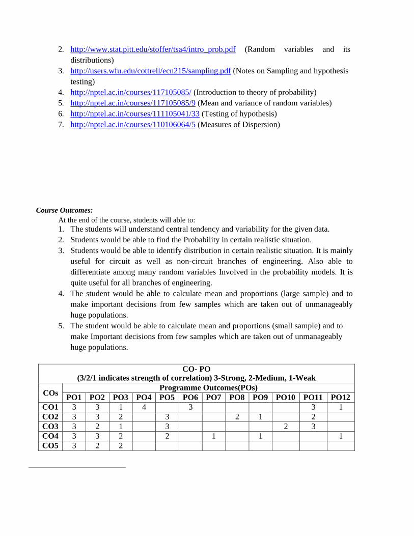
Course Outcomes:
At the end of the course, students will able to:
1. The students will understand central tendency and variability for the given data.
2. Students would be able to find the Probability in certain realistic situation.
3. Students would be able to identify distribution in certain realistic situation. It is mainly
useful for circuit as well as non-circuit branches of engineering. Also able to
differentiate among many random variables Involved in the probability models. It is
quite useful for all branches of engineering.
4. The student would be able to calculate mean and proportions (large sample) and to
make important decisions from few samples which are taken out of unmanageably
huge populations.
5. The student would be able to calculate mean and proportions (small sample) and to
make Important decisions from few samples which are taken out of unmanageably
huge populations.
CO- PO
(3/2/1 indicates strength of correlation) 3-Strong, 2-Medium, 1-Weak
COs Programme Outcomes(POs)
PO1 PO2 PO3 PO4 PO5 PO6 PO7 PO8 PO9 PO10 PO11 PO12
CO1 3 3 1 4 3 3 1
CO2 3 3 2 3 2 1 2
CO3 3 2 1 3 2 3
CO4 3 3 2 2 1 1 1
CO5 3 2 2
PROBABILITY
INTRODUCTION:
Probability theory was originated from gambling theory. A large number of problems exist even
today which are based on the game of chance, such as coin tossing, dice throwing and playing cards.
The probability is defined in two different ways,
➢ Mathematical (or a priori) definition
➢ Statistical (or empirical) definition
SOME IMPORTANT TERMS &CONCEPTS:
• RANDOM EXPERIMENTS:
Experiments of any type where the outcome cannot be predicted are called random
experiments.
• SAMPLE SPACE:
A set of all possible outcomes from an experiment is called a sample space.
Eg: Consider a random experiment E of throwing 2 coins at a time. The possible outcomes are
HH, TT, HT, TH. These 4 outcomes constitute a sample space denoted by, S ={ HH, TT, HT, TH}.
• TRAIL & EVENT:
Consider an experiment of throwing a coin. When tossing a coin, we may get a head(H) or
tail(T). Here tossing of a coin is a trail and getting a hand or tail is an event.
In otherwords, “Every non-empty subset of A of the sample space S is called an event”.
• NULL EVENT:
An event having no sample point is called a null event and is denoted by ∅.
• EXHAUSTIVE EVENTS:
The total number of possible outcomes in any trail is known as exhaustive
events.
Eg: In throwing a die the possible outcomes are getting 1 or 2 or 3 or 4 or 5 or 6. Hence we have
6 exhaustive events in throwing a die.
• MUTUALLY EXCLUSIVE EVENTS:
Two events are said to be mutually exclusive when the occurrence of one affects the
occurrence of the other. In otherwords, if A & B are mutually exclusive events and if A happens
then B will not happen and viceversa.
Eg: In tossing a coin the events head or tail are mutually exclusive, since both tail & head cannot
appear in the same time.

• EQUALLY LIKELY EVENTS:
Two events are said to be equally likely if one of them cannot be expected in the preference to
the other.
Eg: In throwing a coin, the events head & tail have equal chances of occurrence.
• INDEPENDENT & DEPENDENT EVENTS:
Two events are said to be independent when the actual happening of one doesnot
influence in any way the happening of the other. Events which are not independent are called
dependent events.
Eg: If we draw a card in a pack of well shuffled cards and again draw a card from the rest of pack
of cards (containing 51 cards), then the second draw is dependent on the first. But if on the other
hand, we draw a second card from the pack by replacing the first card drawn, the second draw is
known as independent of the first.
• FAVOURABLE EVENTS:
Mathematical or classical or a priori definition of probability,
Probability (of happening an event E) = 𝑁𝑢𝑚𝑏𝑒𝑟 𝑜𝑓 𝑓𝑎𝑣𝑜𝑢𝑟𝑎𝑏𝑙𝑒 𝑐𝑎𝑠𝑒𝑠
𝑇𝑜𝑡𝑎𝑙 𝑛𝑢𝑚𝑏𝑒𝑟 𝑜𝑓 𝑒𝑥ℎ𝑎𝑢𝑠𝑡𝑖𝑣𝑒 𝑐𝑎𝑠𝑒𝑠
= 𝑚
𝑛 Where m = Number of favourable cases
n = Total number of exhaustive cases.
PROBLEMS:
1. In tossing a coin, what is the prob. of getting a head. Sol: Total no. of events = {H, T}= 2
Favourable event = {H}= 1
Probability = 𝑁𝑢𝑚𝑏𝑒𝑟 𝑜𝑓 𝑓𝑎𝑣𝑜𝑢𝑟𝑎𝑏𝑙𝑒 𝑐𝑎𝑠𝑒𝑠
𝑇𝑜𝑡𝑎𝑙 𝑛𝑢𝑚𝑏𝑒𝑟 𝑜𝑓 𝑒𝑥ℎ𝑎𝑢𝑠𝑡𝑖𝑣𝑒 𝑐𝑎𝑠𝑒𝑠
= 1
2
2. In throwing a die, the prob. of getting 2.
Sol: Total no. of events = {1,2,3,4,5,6}= 6 Favourable
event = {2}= 1
Probability = 𝑁𝑢𝑚𝑏𝑒𝑟 𝑜𝑓 𝑓𝑎𝑣𝑜𝑢𝑟𝑎𝑏𝑙𝑒 𝑐𝑎𝑠𝑒𝑠
𝑇𝑜𝑡𝑎𝑙 𝑛𝑢𝑚𝑏𝑒𝑟 𝑜𝑓 𝑒𝑥ℎ𝑎𝑢𝑠𝑡𝑖𝑣𝑒 𝑐𝑎𝑠𝑒𝑠
= 1
6
3. Find the prob. of throwing 7 with two dice.
Sol: Total no. of possible ways of throwing a dice twice = 36 ways
Number of ways of getting 7 is, (1,6), (2,5), (3,4), (4,3), (5,2), (6,1) = 6

Probability = 𝑁𝑢𝑚𝑏𝑒𝑟 𝑜𝑓 𝑓𝑎𝑣𝑜𝑢𝑟𝑎𝑏𝑙𝑒 𝑐𝑎𝑠𝑒𝑠
𝑇𝑜𝑡𝑎𝑙 𝑛𝑢𝑚𝑏𝑒𝑟 𝑜𝑓 𝑒𝑥ℎ𝑎𝑢𝑠𝑡𝑖𝑣𝑒 𝑐𝑎𝑠𝑒𝑠
= 6
36
= 1
6
4. A bag contains 6 red & 7 black balls. Find the prob. of drawing a red ball. Sol: Total no. of possible ways of getting 1 ball = 6 + 7
Number of ways of getting 1 red ball = 6
Probability = 𝑁𝑢𝑚𝑏𝑒𝑟 𝑜𝑓 𝑓𝑎𝑣𝑜𝑢𝑟𝑎𝑏𝑙𝑒 𝑐𝑎𝑠𝑒𝑠
𝑇𝑜𝑡𝑎𝑙 𝑛𝑢𝑚𝑏𝑒𝑟 𝑜𝑓 𝑒𝑥ℎ𝑎𝑢𝑠𝑡𝑖𝑣𝑒 𝑐𝑎𝑠𝑒𝑠
= 6
13
5. Find the prob. of a card drawn at random from an ordinary pack, is a diamond. Sol: Total no. of possible ways of getting 1 card = 52
Number of ways of getting 1 diamond card is 6
Probability = 𝑁𝑢𝑚𝑏𝑒𝑟 𝑜𝑓 𝑓𝑎𝑣𝑜𝑢𝑟𝑎𝑏𝑙𝑒 𝑐𝑎𝑠𝑒𝑠
𝑇𝑜𝑡𝑎𝑙 𝑛𝑢𝑚𝑏𝑒𝑟 𝑜𝑓 𝑒𝑥ℎ𝑎𝑢𝑠𝑡𝑖𝑣𝑒 𝑐𝑎𝑠𝑒𝑠
= 13
52
= 1
4
6. From a pack of 52 cards, 1 card is drawn at random. Find the prob. of getting a queen. Sol: A queen may be chosen in 4 ways.
Total no. of ways of selecting 1 card = 52
Probability = 𝑁𝑢𝑚𝑏𝑒𝑟 𝑜𝑓 𝑓𝑎𝑣𝑜𝑢𝑟𝑎𝑏𝑙𝑒 𝑐𝑎𝑠𝑒𝑠
𝑇𝑜𝑡𝑎𝑙 𝑛𝑢𝑚𝑏𝑒𝑟 𝑜𝑓 𝑒𝑥ℎ𝑎𝑢𝑠𝑡𝑖𝑣𝑒 𝑐𝑎𝑠𝑒𝑠
= 4
= 1
52 13
7. Find the prob. of throwing: (a) 4, (b) an odd number, (c) an even number with anordinary die (six
faced). Sol: a) When throwing a die there is only one way of getting 4.
Probability = 𝑁𝑢𝑚𝑏𝑒𝑟 𝑜𝑓 𝑓𝑎𝑣𝑜𝑢𝑟𝑎𝑏𝑙𝑒 𝑐𝑎𝑠𝑒𝑠
𝑇𝑜𝑡𝑎𝑙 𝑛𝑢𝑚𝑏𝑒𝑟 𝑜𝑓 𝑒𝑥ℎ𝑎𝑢𝑠𝑡𝑖𝑣𝑒 𝑐𝑎𝑠𝑒𝑠
= 1
6
b) Number of ways of falling an odd number is 1, 3, 5 = 3
Probability = 𝑁𝑢𝑚𝑏𝑒𝑟 𝑜𝑓 𝑓𝑎𝑣𝑜𝑢𝑟𝑎𝑏𝑙𝑒 𝑐𝑎𝑠𝑒𝑠
= 3
= 1
𝑇𝑜𝑡𝑎𝑙 𝑛𝑢𝑚𝑏𝑒𝑟 𝑜𝑓 𝑒𝑥ℎ𝑎𝑢𝑠𝑡𝑖𝑣𝑒 𝑐𝑎𝑠𝑒𝑠 6 2

c) Number of ways of falling an even number is 2, 4, 6 = 3
Probability = 𝑁𝑢𝑚𝑏𝑒𝑟 𝑜𝑓 𝑓𝑎𝑣𝑜𝑢𝑟𝑎𝑏𝑙𝑒 𝑐𝑎𝑠𝑒𝑠
= 3
= 1
𝑇𝑜𝑡𝑎𝑙 𝑛𝑢𝑚𝑏𝑒𝑟 𝑜𝑓 𝑒𝑥ℎ𝑎𝑢𝑠𝑡𝑖𝑣𝑒 𝑐𝑎𝑠𝑒𝑠 6 2
8. From a group of 3 Indians, 4 Pakistanis, and 5 Americans, a sub-committee of four people is selected by lots. Find the probability that the sub-committee will consist of
i) 2 Indians and 2 Pakistanis.
ii) 1 Indians, 1 Pakistanis and 2 Americans.
iii) 4 Americans.
Sol: Total no. of people = 3 + 4 + 5 = 12
∴ 4 people can be chosen from 12 people = 12𝐶4 ways
= 12 ×11 ×10 ×9
= 495 ways
1 ×2 ×3×4
i) 2 Indians can be chosen from 3 Indians = 3𝐶2 ways 2 Pakistanis can be chosen from 4 Pakistanis = 4𝐶2 ways
∴ No. of favourable cases = 3𝐶2 × 4𝐶2
∴ Prob. = 3𝐶2× 4𝐶2
= 2
495 55
ii) 1 Indian can be chosen from 3 Indians = 3𝐶1 ways
1 Pakistani can be chosen from 4 Pakistanis = 4𝐶1 ways
2 Americans can be chosen from 5 Americans = 5𝐶2 ways
Favourable events = 3𝐶1 × 4𝐶1 × 5𝐶2
∴ Prob. = 3𝐶1× 4𝐶2× 5𝐶2
= 8
495 33
iii) 4 Americans can be chosen from 5 Americans = 5𝐶4 ways
∴ Prob. = 5𝐶4 = 1
495 99
9. A bag contains 7 white, 6 red & 5 black balls. Two balls are drawn at random. Find the prob. that they both will be white.
Sol: Total no. of balls = 7 + 6 + 5
= 18

From there 18 balls, 2 balls can be drawn in 18𝐶2 ways
i.e) 18 × 17
= 153 1 ×2
2 white balls can be drawn from 7 white balls = 7𝐶2 ways
= 21
∴ Favourable cases = 21
P(drawing 2 white balls) = 21 = 7
153 51
10. A bag contains 10 white, 6 red, 4 black & 7 blue balls. 5 balls are drawn at random. What is the prob. that 2 of them are red and one is black?
Sol: Total no. of balls = 10 + 6 + 4 + 7 =27
5 balls can be drawn from these 27 balls = 27𝐶5 ways
= 27 × 26 ×25 × 24 ×23
1 ×2 ×3×4 ×5
= 80730 ways Total
no. of exhaustive events = 80730
2 red balls can be drawn from 6 red balls = 6𝐶2 ways
= 6 × 5 = 15 ways
1 ×2
1 black balls can be drawn from 4 black balls = 4𝐶1 ways
= 4
∴ No. of favourable cases = 15 × 4 = 60
Probability = 𝑁𝑢𝑚𝑏𝑒𝑟 𝑜𝑓
𝑓𝑎𝑣𝑜𝑢𝑟𝑎𝑏𝑙𝑒 𝑐𝑎𝑠𝑒𝑠
𝑇𝑜𝑡𝑎𝑙 𝑛𝑢𝑚𝑏𝑒𝑟 𝑜𝑓 𝑒𝑥ℎ𝑎𝑢𝑠𝑡𝑖𝑣𝑒 𝑐𝑎𝑠𝑒𝑠
= 60
80730
= 6
8073
11. What is the prob. of having a king and a queen, when 2 cards are drawn from a pack of 52 cards?
Sol: 2 cards can be drawn from a pack of 52 cards = 52𝐶2 ways
= 52 × 51
= 1326 ways
1 ×2
1 queen card can be drawn from 4 queen cards = 4𝐶1 ways 1
king card can be drawn from 4 king cards = 4𝐶1 ways Favourable cases = 4 × 4 = 16 ways
P(drawing 1 queen & 1 king card ) = 𝑁𝑢𝑚𝑏𝑒𝑟 𝑜𝑓 𝑓𝑎𝑣𝑜𝑢𝑟𝑎𝑏𝑙𝑒 𝑐𝑎𝑠𝑒𝑠
= 8
663
𝑇𝑜𝑡𝑎𝑙 𝑛𝑢𝑚𝑏𝑒𝑟 𝑜𝑓 𝑒𝑥ℎ𝑎𝑢𝑠𝑡𝑖𝑣𝑒 𝑐𝑎𝑠𝑒𝑠=
16
1326
12. What is the prob. that out of 6 cards taken from a full pack, 3 will be black and 3 will be red? Sol: A full pack contains 52cards. Out of 52 cards, 26 cards are red & 26 black cards .
6 cards can be chosen from 52 cards = 52𝐶6 ways 3 black cards can be chosen from 26 black cards = 26𝐶3 ways 3 red
cards can be chosen from 26 red cards = 26𝐶3 ways Favourable cases = 26𝐶3 × 26𝐶3
Probability = 𝑁𝑢𝑚𝑏𝑒𝑟 𝑜𝑓 𝑓𝑎𝑣𝑜𝑢𝑟𝑎𝑏𝑙𝑒 𝑐𝑎𝑠𝑒𝑠
𝑇𝑜𝑡𝑎𝑙 𝑛𝑢𝑚𝑏𝑒𝑟 𝑜𝑓 𝑒𝑥ℎ𝑎𝑢𝑠𝑡𝑖𝑣𝑒 𝑐𝑎𝑠𝑒𝑠
= 26𝐶3× 26𝐶3
52𝐶6
13. Find the prob. that a hand at bridge will consist of 3 spades, 5 hearts, 2 diamonds & 3 clubs? Sol: Total no. of balls = 3 + 5 + 2 + 3 = 13
From 52 cards, 13 cards are chosen in 52𝐶13 ways
In a pack of 52 cards, there are 13 cards of each type. 3
spades can be chosen from 13 spades = 13𝐶3 ways 5
hearts can be chosen from 13 hearts = 13𝐶5 ways
2 diamonds can be chosen from 13 diamonds = 13𝐶2 ways 3
clubs can be chosen from 13 clubs = 13𝐶3 ways Hence the total no. of favourable cases are = 13𝐶3 × 13𝐶5 × 13𝐶2 × 13𝐶3
Probability = 𝑁𝑢𝑚𝑏𝑒𝑟 𝑜𝑓 𝑓𝑎𝑣𝑜𝑢𝑟𝑎𝑏𝑙𝑒 𝑐𝑎𝑠𝑒𝑠
𝑇𝑜𝑡𝑎𝑙 𝑛𝑢𝑚𝑏𝑒𝑟 𝑜𝑓 𝑒𝑥ℎ𝑎𝑢𝑠𝑡𝑖𝑣𝑒 𝑐𝑎𝑠𝑒𝑠
= 13𝐶3×13𝐶5 × 13𝐶2 ×
13𝐶3 52𝐶13
OPERATIONS ON SETS:
If A & B are any two sets, then
i) UNION OF TWO SETS
𝐴 ∪ 𝐵 = {𝑥: 𝑥 ∈ 𝐴 (𝑜𝑟) 𝑥 ∈ 𝐵}
In general, 𝐴1 ∪ 𝐴2 ∪ … . .∪ 𝐴𝑛 = {𝑥: 𝑥 ∈ 𝐴1 𝑜𝑟 𝑥 ∈ 𝐴2 𝑜𝑟 ........ 𝑜𝑟 𝑥 ∈ 𝐴𝑛}
i.e) ⋃𝑛 𝐴𝑖 = {𝑥: 𝑥 ∈ 𝐴𝑖, for atleast onei} 𝑖=1
ii) INTERSECTION OF TWO SETS
𝐴 ∩ 𝐵 = { 𝑥: 𝑥 ∈ 𝐴 & 𝑥 ∈ 𝐵}
In general, 𝐴1 ∩ 𝐴2 ∩ … . .∩ 𝐴𝑛 = {𝑥: 𝑥 ∈ 𝐴1 𝑎𝑛𝑑 𝑥 ∈ 𝐴2 𝑎𝑛𝑑 ........ 𝑎𝑛𝑑 𝑥 ∈ 𝐴𝑛}
i.e) ⋂𝑛 𝐴𝑖 = {𝑥: 𝑥 ∈ 𝐴𝑖, for all i = 1,2,3… n} 𝑖=1
iii) COMPLEMENT OF A SET
𝐴′ 𝑜𝑟 �� = {𝑥: 𝑥 ∉ 𝐴}
iv) DIFFERENCE OF TWO SETS A –
B = {𝑥: 𝑥 ∈ 𝐴 𝑏𝑢𝑡 𝑥 ∉ 𝐵} COMMUTATIVE LAW:
𝐴 ∪ 𝐵 = 𝐵 ∪ 𝐴 & 𝐴 ∩ 𝐵 = 𝐵 ∩ 𝐴
ASSOCIATIVE LAW:
(𝐴 ∪ 𝐵) ∪ 𝐶 = 𝐴 ∪ (𝐵 ∪ 𝐶) & (𝐴 ∩ 𝐵) ∩ 𝐶 = 𝐴 ∩ (𝐵
∩ 𝐶) DISTRIBUTIVE LAW:
𝐴 ∪ (𝐵 ∩ 𝐶) = (𝐴 ∪ 𝐵) ∩ (𝐴 ∪ 𝐶)
𝐴 ∩ (𝐵 ∪ 𝐶) = (𝐴 ∩ 𝐵) ∪ (𝐴 ∩ 𝐶)
COMPLEMENTARY LAW:
𝐴 ∪ 𝐴′ = 𝑆 & 𝐴 ∩ 𝐴′ = ∅
AXIOMATIC APPROACH TO PROBABILITY:
It is a rule which associates to each event a real number P (A) which satisfies the following
three axioms.
AXIOM I : For any event A, P (A) ≥ 0. AXIOM
II : P (S) =1
AXIOM III: If A1, A2,….., An are finite number of disjoint event of S, then
P(A1, A2,….., An) = P(A1) + P(A2) + …..+ P(An)
= ∑ P (Ai)
THEOREMS ON PROBABILITY:
THEOREM 1: Probability of an impossible event is zero. i.e) P (∅) = 0
THEOREM 2: Probability of the complementary event �� of A is given by, P (��) =1 – P(A).
THEOREM 3: For any two events A & B, P (�� ∩ 𝐵) = P (B) – P(A∩ 𝐵).
THEOREM 4: If A and B are two events such that A ⊂ B, then P (B ∩ ��) = P (B) – P
(A).THEOREM 5: If B ⊂ A, then P (A) ≥ P (B).
THEOREM 6: If A ∩ B = ∅, then P (A) ≤ P (��). LAW OF ADDITION OF PROBABILITIES:
P (𝐴 ∪ 𝐵) = P (A) + P (B) – P (𝐴 ∩ 𝐵), where A & B are any two events and are not disjoint. PROBLEMS:
1. If from a pack of cards a single card is drawn. What is the prob. that it is eithera spade or a
king?
Sol: P (A) = P (a spade card) = 13
52

P (B) = P (a king card) = 4
52
P (either a spade or a king card) = P (A or B)
= P (A ∪ 𝐵)
= P (A) + P (B) – P (A ∩ 𝐵)
13 4 13 4
= + - [ × ] 52
5
2
= 4
13
52 52
2. A person is known to hit the target in 3 out of 4 shots, whereas another person is known to hit the
target in 2 out of 3 shots. Find the probability of the targets being hit at all when they both person
try.
Sol: The prob. that the first person hit the target = P (A) = 3
4
The prob. that the second person hit the target = P (B) = 2
3
The two events are not mutually exclusive, since both persons hit the same target.
P (A or B) = P (A ∪ 𝐵)
= P (A) + P (B) – P (A ∩ 𝐵)
= 3
+ 2
- [ 3
× 2]

4 3 4 3
= 11
12
MULTIPLICATION LAW OF PROBABILITY (INDEPENDENT EVENTS):
If A & B are two independent events, then
P (A ∩ 𝐵) = P (Both A & B will happen)
= P (A) × P (B)
PROBLEMS:
1. If P (A) = 0.35, P (B) = 0.73, P (A ∩ 𝐵) = 0.14. Find P (�� ∪ ��) Sol: Using Demargon’s Law,
�� ∪ �� = ��∪
P (�� ∪ ��) = P (𝐴∪ 𝐵) P
(�� ∪ ��) = 1 – P (A ∩ 𝐵) = 1 – 0.14 = 0.86
2. A bag contains 8 white and 10 black balls. Two balls are drawn in succession. What is the prob.
that first is white and second is black.
Sol: Total no. of balls = 8 + 10 = 18
P (drawing one white ball from 8 balls) = 8
18
P (drawing one black ball from 10 balls) = 10
18
P (drawing first white & second black) = 8
× 10
1
8 18
= 20
8
1
1
3. Two persons A & B appear in an interview for 2 vacancies for the same post. The probability of
A’s selection is 1 and that of B’s selection is 1 . What is the probability that, i) both of them will 7 5
be selected, ii) none of them will be selected.
Sol: P (A selected) = 1
7
P (B selected) = 1
5
P (A will not be selected) = 1 - 1 = 6
7 7
P (B will not be selected) = 1 - 1 = 4
5 5
i) P (Both of them will be selected) = P (A) × P (B)
= 1
× 1
7 5
= 1
35
ii) P (none of them will be selected) = P (A) × P (B)
= 6
× 4
7 5
= 24
35
4. A problem in mathematics is given to 3 students A, B, C whose chances of solving it are
1 1, , respectively. What is the prob. that the problem will be solved?
2 3 4
Sol: P (A will not solve the problem) = 1- 1 = 1
2 2
P (B will not solve the problem) = 1- 1 = 2 3 3
P (C will not solve the problem) = 1- 1 = 3 4 4
P (all three will not solve the problem) = 1
2 ×
2 ×
3
3 4
= 1
4

∴ P (all the three will solve the problem) = 1- 1 = 3
4 4
5. What is the chance of getting two sixes in two rolling of a single die?
Sol: P (getting a six in first rolling) = 1
6
P (getting a six in second rolling) = 1
6
Since two rolling are independent.
∴ P (getting two sixes in 2 rolls) = 1 × 1
6 6
= 1
36
6. An article manufactured by a company consists of two parts A & B. In the process of
manufacture of part A, 9 out of 100 are likely to be defective. Similarly, 5 0ut of 100 are likely
to be defective in the manufacture of part B. Calculate the prob. that theassembled article will
not be (assuming that the events of finding the part A non-defective and that of B are
independent).
Sol: Prob. that part A will be defective = 9
100
∴ P (A will not be defective) = 1- 9 100
= 100 − 9
100
= 91
100
Prob. that part B will be defective = 5
100
∴ P (A will not be defective) = 1- 5
100
= 100 − 5
100
= 95
100
∴ P (the assembled article will not be defective) = P (A will not be defective) ×
P (B will not be defective)

= 91
100 ×
95
100
= 0.86
7. From a bag containing 4 white and 6 black balls, two balls are drawn at random. If the balls are drawn one after the other without replacement, find the probability that
i) both balls are white.
ii) both balls are black.
iii) the first ball is white and the second ball is black.
iv) one ball is white and the other is black.
Sol: Total no. of balls = 4 + 6 = 10
i) P (first ball is white) = 4
10
P (second ball is white) = 3
9
∴ P (both balls are white) = 4 × 3
10 9
= 2
15
ii) P (first ball is black) = 6
10
P (second ball is black) = 5
9
∴ P (both balls are black) = 6 × 5
10 9
= 1
3

×
iii) P (first ball is white) = 4
10
P (second ball is black) = 6
9
∴ P (first ball is white & second ball is black) = 4 6
10 9
= 4
15
iv) a) P (first ball is white & second ball is black) = 4
×
6
10 9
= 24
90
b) P (first ball is black & second ball is white) = 6 × 4
10 9
= 24
90
Hence both events (a) & (b) are mutually exclusive.
∴ P (one ball is white & the other is black) = 24
9
+ 24
90
0
= 8
1
5

×
8. Find the probability in each of the below four cases, if the balls are drawn one after the other with replacement. A bag containing 4 white & 6 black balls, 2 balls are drawn at random.
i) both balls are white.
ii) both balls are black.
iii) the first ball is white and the second ball is black.
iv) one ball is white and the other is black.
Sol: Total no. of balls = 4 + 6 = 10
i) P (first ball is white) = 4
10
P (second ball is white) = 4
10
∴ P (both balls are white) = 4 × 4
10 10
= 4
25
ii) P (first ball is black) = 6
10 P (second ball is black) = 6
10
∴ P (both balls are black) = 6 × 6
10 10
= 9
25
iii) P (first ball is white) = 4
10
P (second ball is black) = 6
10
∴ P (first ball is white & second ball is black) = 4 6
10 10
= 6
25
iv) P (first ball is white & second ball is black) = 4 × 6
10 10
= 6
25
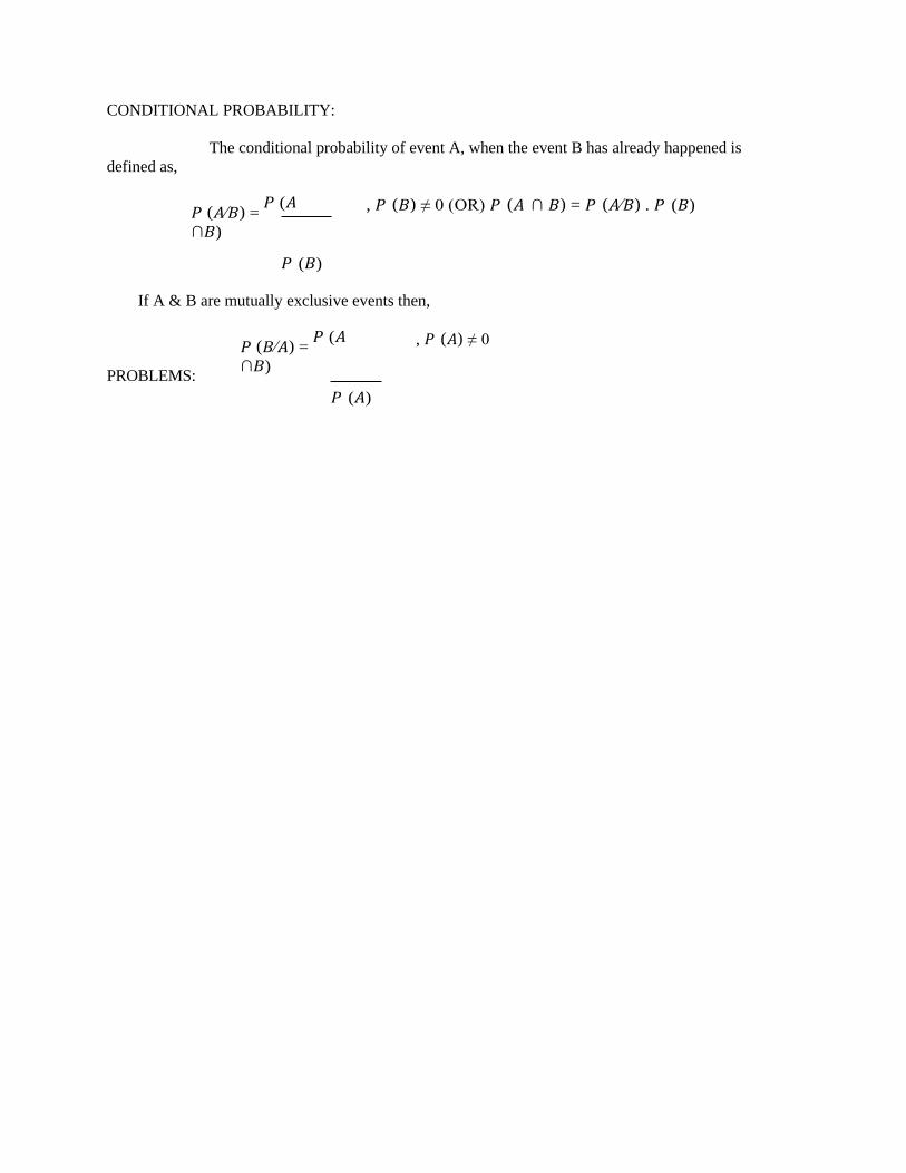
CONDITIONAL PROBABILITY:
The conditional probability of event A, when the event B has already happened is
defined as,
𝑃 (𝐴⁄𝐵) = 𝑃 (𝐴
∩𝐵)
𝑃 (𝐵)
, 𝑃 (𝐵) ≠ 0 (OR) 𝑃 (𝐴 ∩ 𝐵) = 𝑃 (𝐴⁄𝐵) . 𝑃 (𝐵)
If A & B are mutually exclusive events then,
PROBLEMS:
𝑃 (𝐵⁄𝐴) = 𝑃 (𝐴
∩𝐵)
𝑃 (𝐴)
, 𝑃 (𝐴) ≠ 0

1. A bag contains 3 red & 4 white balls. Two draws are made without replacement. What is the prob. that both the balls are red.
Sol: P (drawing a red ball in the first draw) = 3
7
i.e) P (A) = 3
7
P (drawing a red ball in the first draw given that first ball drawn is red) = 2
6
i.e) 𝑃 (𝐵⁄𝐴) = 2 6
∴ 𝑃 (𝐴 ∩ 𝐵) = 𝑃 (𝐵⁄𝐴) × 𝑃 (𝐴)
= 2
× 3
6 7
= 1
7
2. Find the prob. of drawing a queen and a king from a pack of cards in two consecutive draws, the cards drawn not being replaced.
Sol: P (drawing a queen card) = 4 52
i.e) P (A) = 4
52
P (drawing a king after a queen has been drawn) = 4
51
i.e) 𝑃 (𝐵⁄𝐴) = 4
51
∴ 𝑃 (𝐴 ∩ 𝐵) = 𝑃 (𝐵⁄𝐴) × 𝑃 (𝐴)
= 4
× 4
51 52
= 4
663
3. In a box there are 100 resistors having resistance and tolerance as shown in the following table. Let
a resistor be selected from the box and assume each resistor has the same likelihood of being
chosen. Define three events A as draw a 47𝛺 resistor, B as draw a resistor with 5% tolerance and
C as draw a 100Ω resistor. Find
𝑃 (𝐴⁄𝐵), 𝑃 (𝐴⁄𝐶), 𝑃 (𝐵⁄𝐶).
Resistance Ω 5% 10% Total

22 10 14 24
47 28 16 44
100 24 8 32
Total 62 38 100
Sol: P (A) = P (47Ω) = 44
10
0
P (B) = P (5%) = 62
100

P (C) = P (100Ω) = 32 100
The joint probabilities are,
P (A ∩ 𝐵) = P (47Ω ∩ 5%)
= 28
100
P (A ∩ 𝐶) = P (47Ω ∩ 100𝛺)
= 0
P (B ∩ 𝐶) = P (5% ∩ 100𝛺)
= 24
100
∴ 𝑃 (𝐴⁄𝐵) = 𝑃 (𝐴
∩𝐵)
𝑃 (𝐵)
= 28
62
= 28⁄100
62⁄100
𝑃 (𝐴⁄𝐶) = 𝑃 (𝐴 ∩𝐶)
= 0
𝑃 (𝐶) 32⁄100
= 0
𝑃 (𝐵⁄𝐶) = 𝑃 (𝐵 ∩𝐶)
= 24⁄100
𝑃
= 24 (𝐶)
32
32⁄100
4. The Hindu newspaper publishes three columns entitled politics (A), books(B), cinema(C).
Reading habits of a randomly selected reader with respect to three columns are,
Read
Regularly
A B C A ∩ B A ∩ C B ∩ C A ∩ B ∩ C
Probability 0.14 0.23 0.37 0.08 0.09 0.13 0.05
Find P (A/B), P (A/B∪C), P (A/reads atleast one), P (A∪B /C).
Sol: 𝑃 (𝐴⁄𝐵) = 𝑃 (𝐴 ∩𝐵)
𝑃 (𝐵)
= 0.08
0.23
= 0.348

P (𝐴⁄𝐵 ∪ 𝐶) = 𝑃 [𝐴 ∩(𝐵 ∪𝐶)]
𝑃 (𝐵 ∪𝐶)
= 0.04+0.05+0.03
0.47
= 0.255
P (A / reads atleast one) = P [A / (A∪ 𝐵 ∪ 𝐶)]
= 𝑃 [𝐴∩(𝐴∪𝐵∪𝐶)]
𝑃 (𝐴∪𝐵∪𝐶)
= 𝑃 (𝐴)
𝑃 (𝐴∪𝐵∪𝐶)
= 0.14
0.49
= 0.286
P (A ∪ 𝐵 / C) = 𝑃 [(𝐴∪𝐵)∩𝐶]
𝑃 (𝐶)
= 0.04+0.05+0.08
0.37
= 0.459

34
RandomVariablesand Probability Distributions
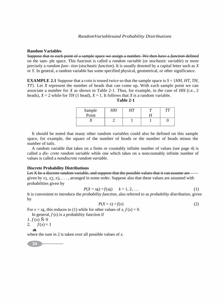
Random Variables
Suppose that to each point of a sample space we assign a number. We then have a function defined
on the sam- ple space. This function is called a random variable (or stochastic variable) or more
precisely a random func- tion (stochastic function). It is usually denoted by a capital letter such as X
or Y. In general, a random variable has some specified physical, geometrical, or other significance.
EXAMPLE 2.1 Suppose that a coin is tossed twice so that the sample space is S = {HH, HT, TH,
TT}. Let X represent the number of heads that can come up. With each sample point we can
associate a number for X as shown in Table 2-1. Thus, for example, in the case of HH (i.e., 2
heads), X = 2 while for TH (1 head), X = 1. It follows that X is a random variable. Table 2-1
Sample
Point
HH HT T
H
TT
X 2 1 1 0
It should be noted that many other random variables could also be defined on this sample
space, for example, the square of the number of heads or the number of heads minus the
number of tails.
A random variable that takes on a finite or countably infinite number of values (see page 4) is
called a dis- crete random variable while one which takes on a noncountably infinite number of
values is called a nondiscrete random variable.
Discrete Probability Distributions
Let X be a discrete random variable, and suppose that the possible values that it can assume are
given by x1, x2, x3, . . . , arranged in some order. Suppose also that these values are assumed with
probabilities given by
P(X = xk) = f (xk) k = 1, 2, . . . (1)
It is convenient to introduce the probability function, also referred to as probability distribution, given
by
P(X = x) = f (x) (2)
For x = xk, this reduces to (1) while for other values of x, f (x) = 0.
In general, f (x) is a probability function if
1. f (x) Š 0
2. f (x) = 1
ax where the sum in 2 is taken over all possible values of x.


35 CHAPTER 2 Random Variables and Probability Distributions
EXAMPLE 2.2 Find the probability function corresponding to the random variable X of
Example 2.1. Assuming that the coin is fair, we have
P(HH ) = P(HT ) = P(TH ) = P(T T ) = 1
The
n
1 4
1 4 1
4 4
P(X = 0) = P(TT) = 1
4
P(X = 1) = P(HT < TH ) = P(HT ) + P(TH ) = 1
+
1
= 1
4 4 2 P(X = 2) = P(HH) =
1 4
The probability function is thus given by
Table 2-2. Table 2-2
x 0
>
1
>
2
>
f (x)
1 4
1 2
1 4
Distribution Functions for Random Variables
The cumulative distribution function, or briefly the distribution function, for a random variable X is
defined by
F(x) = P(X Š x) (3)
where x is any real number, i.e., —` < x < `.
The distribution function F(x) has the following properties:
1. F(x) is nondecreasing [i.e., F(x) Š F(y) if x Š y].
2. lim F(x) = 0; lim F(x) = 1.
xS—` xS`
3. F(x) is continuous from the right [i.e., lim F(x + h) = F(x) for all x].
hS0+
Distribution Functions for Discrete Random Variables
The distribution function for a discrete random variable X can be obtained from its probability function
by noting that, for all x in (—`, ),
F(x) = P(X Š x) = f (u)
uaŠ x
where the sum is taken over all values u taken on by X for which u Š x.
If X takes on only a finite number of values x1, x2, . . . , xn, then the distribution function is
given by
(4)
0 —` < x < x1
f (x1) x1 Š x < x2
F(x) = e f (x1) + f (x2) x2 Š x < x3
( (
f (x1) + c+ f (xn) xn Š x < `
(5)
EXAMPLE 2.3 (a) Find the distribution function for the random variable X of Example 2.2. (b)
Obtain its graph. function is
(a) The distribution
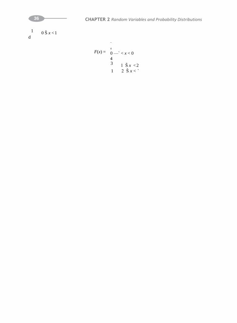
36 CHAPTER 2 Random Variables and Probability Distributions
1
0 Š x < 1 d
4
F(x) = 0 —` < x < 0
4 3
1 Š x < 2
1 2 Š x < `
37 CHAPTER 2 Random Variables and Probability Distributions
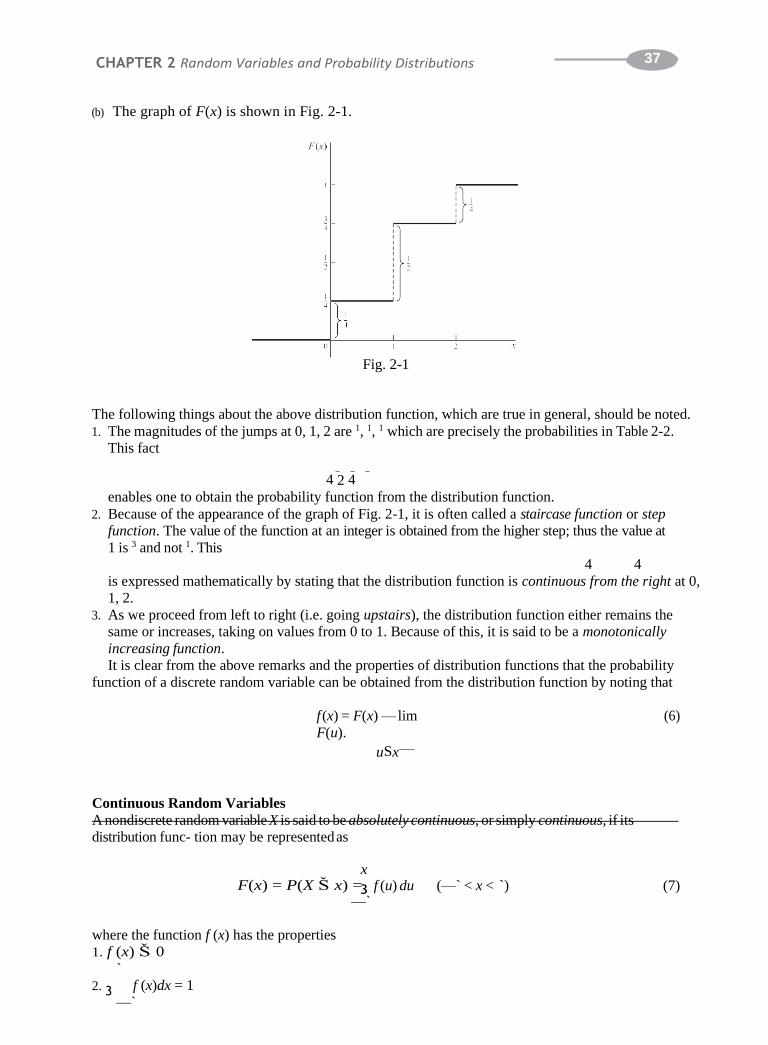
(b) The graph of F(x) is shown in Fig. 2-1.
Fig. 2-1
The following things about the above distribution function, which are true in general, should be noted.
1. The magnitudes of the jumps at 0, 1, 2 are 1, 1, 1 which are precisely the probabilities in Table 2-2.
This fact
4 2 4 enables one to obtain the probability function from the distribution function.
2. Because of the appearance of the graph of Fig. 2-1, it is often called a staircase function or step
function. The value of the function at an integer is obtained from the higher step; thus the value at
1 is 3 and not 1. This 4 4
is expressed mathematically by stating that the distribution function is continuous from the right at 0,
1, 2.
3. As we proceed from left to right (i.e. going upstairs), the distribution function either remains the
same or increases, taking on values from 0 to 1. Because of this, it is said to be a monotonically
increasing function.
It is clear from the above remarks and the properties of distribution functions that the probability
function of a discrete random variable can be obtained from the distribution function by noting that
f (x) = F(x) — lim
F(u).
(6)
uSx—
Continuous Random Variables
A nondiscrete random variable X is said to be absolutely continuous, or simply continuous, if its
distribution func- tion may be represented as
x F(x) = P(X Š x) =3
f (u) du (—` < x < `) (7)
—`
where the function f (x) has the properties
1. f (x) Š 0
`
2. 3 f (x)dx = 1
—`

38 CHAPTER 2 Random Variables and Probability Distributions
It follows from the above that if X is a continuous random variable, then the probability that X
takes on any one particular value is zero, whereas the interval probability that X lies between two
different values, say, a and b, is given by
P(a < X < b) =
b
3f (x) dx a
(8)

39 CHAPTER 2 Random Variables and Probability Distributions
x
3 3
9
EXAMPLE 2.4 If an individual is selected at random from a large group of adult males, the
probability that his height X is precisely 68 inches (i.e., 68.000 . . . inches) would be zero.
However, there is a probability greater than zero than X is between 67.000 . . . inches and 68.500
. . . inches, for example.
A function f (x) that satisfies the above requirements is called a probability function or probability
distribu- tion for a continuous random variable, but it is more often called a probability density
function or simply den- sity function. Any function f (x) satisfying Properties 1 and 2 above will
automatically be a density function, and required probabilities can then be obtained from (8).
f (x) = cx2 0 < x < 3
EXAMPLE 2.5 (a) Find the constant c such thabt the function 0 otherwise
cx3 2
3
is a density function, and (b) compute P(1 < X < 2).
` 3
2
(a) Since f (x) satisfies Property 1 if c Š 0, it must satisfy Property 2 in order to be a density
function. Now
3 f (.x)dx = 3 cx dx = 38 = 9c
(b) —` 21 2
9 x3 2 0
1 7
and since this must equal 1, we have c = 1>9
1 1
In case f (x) is continuous, which we shall assume unless otherwise stated, the probability that X is
P(1 < X < 2) = 3 dx = 2 = — = equal
to any particular value is zero. In such case we can re2p7lace ei2th7er o2r7both27of the signs < in (8) by Š.
Thus, in
Example 2.5,
P(1 Š X Š 2) = P(1 Š X < 2) = P(1 < X Š 2) = P(1 < X < 2) = 7
27
EXAMPLE 2.6 (a) Find the distribution function for the random variable of Example 2.5. (b) Use
the result of (a) to
find P(1 < x Š 2).
(a) We have
F(x) = P(X Š x) =
3
x f (u) du
—` If x < 0, then F(x) = 0. If 0 Š x < 3, then
F(x) = x
f (u) du = x
1 u2 du =
x3
If x Š 3,
then 0 0 9 27
F(x) = 3 x 3 1 x f (u) du + f (u) du = u2 du + 0 du = 1 3 3 3 3
0 3 0 3
Thus the required distribution function is
F(x) =
0 x < 0
• > x1
3 27 0 Š x <x 3Š 3
Note that F(x) increases monotonically from 0 to 1 as is required for a distribution function. It
0

40 CHAPTER 2 Random Variables and Probability Distributions
should also be noted
that F(x) in this case is continuous.

41 CHAPTER 2 Random Variables and Probability Distributions
3 (12)
(b) We have
as in Example
2.5.
P(1 < X Š 2) 5 P(X Š 2) — P(X Š 1)
5 F(2) — F(1)
5 23
— 13
= 7
27 27 27
The probability that X is between x and x + Ax is given by x +Ax
P(x Š X Š x + Ax) =
3x so that if Ax is small, we have approximately
f (u) du (9)
P(x Š X Š x + Ax) = f (x)Ax
We also see from (7) on differentiating both sides that dF(x)
dx = f (x)
(10)
(11)
at all points where f (x) is continuous; i.e., the derivative of the distribution function is the density
function.
It should be pointed out that random variables exist that are neither discrete nor continuous. It can
be shown that the random variable X with the following distribution function is an example. 0 x <1
μ 2 1 Š x < 2
F(x) = x
1 x Š 2
In order to obtain (11), we used the basic property
d x
f (u) du = f (x)
dx a
which is one version of the Fundamental Theorem of Calculus.
Graphical Interpretations
If f (x) is the density function for a random variable X, then we can represent y = f (x) graphically by a
curve as in Fig. 2-2. Since f (x) Š 0, the curve cannot fall below the x axis. The entire area bounded
by the curve and the x axis must be 1 because of Property 2 on page 36. Geometrically the
probability that X is between a and b, i.e., P(a < X < b), is then represented by the area shown
shaded, in Fig. 2-2.
The distribution function F(x) = P(X Š x) is a monotonically increasing function which increases
from 0 to 1 and is represented by a curve as in Fig. 2-3.

42 CHAPTER 2 Random Variables and Probability Distributions
Fig. 2-2 Fig. 2-3
43 CHAPTER 2 Random Variables and Probability Distributions
Joint Distributions
The above ideas are easily generalized to two or more random variables. We consider the typical case
of two ran- dom variables that are either both discrete or both continuous. In cases where one variable
is discrete and the other continuous, appropriate modifications are easily made. Generalizations to
more than two variables can also be made.
1. DISCRETE CASE. If X and Y are two discrete random variables, we define the joint
probability func- tion of X and Y by
P(X = x, Y = y) = f (x, y) (13) where 1. f (x, y) Š 0
2. f (x, y) = 1
ax ay i.e., the sum over all values of x and y is 1.
Suppose that X can assume any one of m values x1, x2, . . . , xm and Y can assume any one of n values
y1, y2, . . . , yn.
Then the probability of the event that X = xj and Y = yk is given by
P(X = xj, Y = yk) = f (xj, yk) (14)
A joint probability function for X and Y can be represented by a joint probability table as in
Table 2-3. The probability that X = xj is obtained by adding all entries in the row corresponding to
xi and is given by
n f (x , y (15)
P(X = x ) = f (x ) = a )
j 1 j j k
k=1
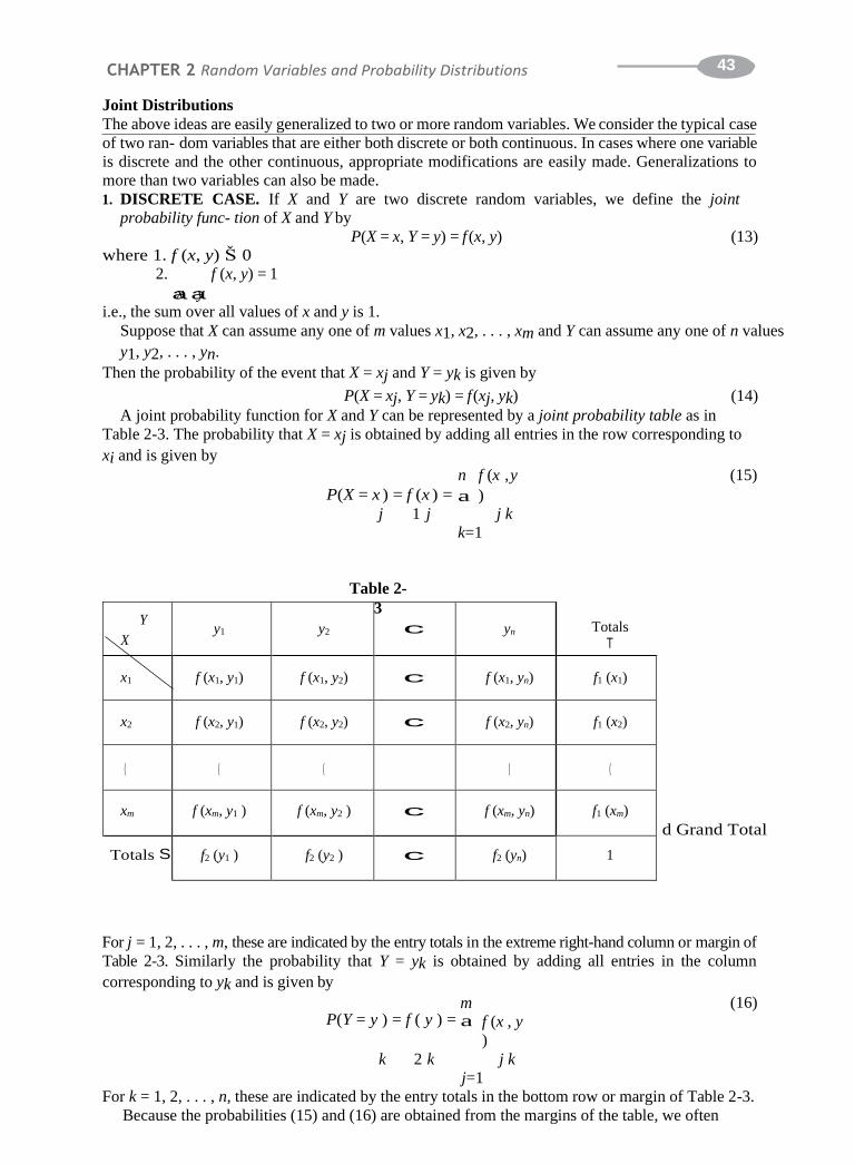
Table 2-
d Grand Total
For j = 1, 2, . . . , m, these are indicated by the entry totals in the extreme right-hand column or margin of
Table 2-3. Similarly the probability that Y = yk is obtained by adding all entries in the column
corresponding to yk and is given by
m P(Y = y ) = f ( y ) = a
f (x , y
)
(16)
k 2 k j k
j=1
For k = 1, 2, . . . , n, these are indicated by the entry totals in the bottom row or margin of Table 2-3.
Because the probabilities (15) and (16) are obtained from the margins of the table, we often
Y
X
y1
y2
3
c
yn
Totals T
x1 f (x1, y1) f (x1, y2) c f (x1, yn) f1 (x1)
x2 f (x2, y1) f (x2, y2) c f (x2, yn) f1 (x2)
(
(
(
(
(
xm f (xm, y1 ) f (xm, y2 ) c f (xm, yn) f1 (xm)
Totals S f2 (y1 ) f2 (y2 ) c f2 (yn) 1

44 CHAPTER 2 Random Variables and Probability Distributions
refer to
f1(xj) and f2(yk) [or simply f1(x) and f2(y)] as the marginal probability functions of X and Y,
respectively.
45 CHAPTER 2 Random Variables and Probability Distributions
It should also be noted m n
that a f (x ) = 1 a f (y ) = 1 (17)
which can be
written
1 j
j=1
m n
2 k
k=1
a a f (x , y ) =
1
(18)
j k
j=1 k=1
This is simply the statement that the total probability of all entries is 1. The grand total of 1 is
indicated in the lower right-hand corner of the table.
The joint distribution function of X and Y is defined by F(x, y) = P(X Š x, Y Šy) =
a a f (u,
v) (19)
uŠ x vŠ y
In Table 2-3, F(x, y) is the sum of all entries for which xj Š x and yk Š y.
2. CONTINUOUS CASE. The case where both variables are continuous is obtained easily by
analogy with the discrete case on replacing sums by integrals. Thus the joint probability function
for the random vari- ables X and Y (or, as it is more commonly called, the joint density function of
X and Y ) is defined by
1. f (x, y) Š 0 `
2. 3 3
f (x, y) dx dy = 1
—` —`
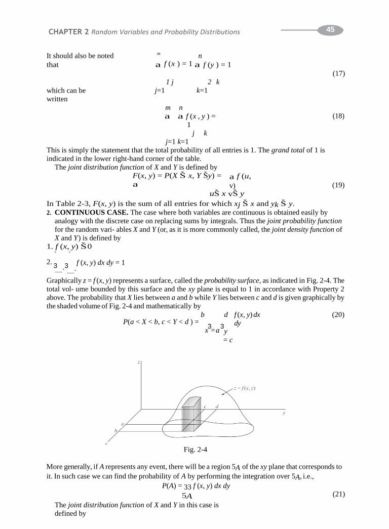
Graphically z = f (x, y) represents a surface, called the probability surface, as indicated in Fig. 2-4. The
total vol- ume bounded by this surface and the xy plane is equal to 1 in accordance with Property 2
above. The probability that X lies between a and b while Y lies between c and d is given graphically by
the shaded volume of Fig. 2-4 and mathematically by
P(a < X < b, c < Y < d ) = b d
x3= a
3y
= c
f (x, y) dx
dy
(20)
Fig. 2-4
More generally, if A represents any event, there will be a region 5A of the xy plane that corresponds to
it. In such case we can find the probability of A by performing the integration over 5A, i.e.,
P(A) = 33 f (x, y) dx dy
5A
The joint distribution function of X and Y in this case is
defined by
(21)

46 CHAPTER 2 Random Variables and Probability Distributions
x y F(x, y) = P(X Š x, Y Š y)3=
3
f (u, v) du
(22)
u =—` v= dv
—`

47 CHAPTER 2 Random Variables and Probability Distributions
It follows in analogy with (11), page 38,
that '2F
'x 'y
= f (x, y)
(23)
i.e., the density function is obtained by differentiating the distribution function with respect to x and y.
From (22) we obtain
P(X Š x) = F1(x) =3
x `
3 u v= =—` —
f (u, v) du
dv f (u, v)
dudv
(24)
3 3 ` y
P(Y Š y) = F2( y) =
(25)
u v= =—` —`
We call (24) and (25) the marginal distribution functions, or simply the distribution functions, of X and
Y, respec-
tively. The derivatives of (24) and (25) with respect to x and y are then called the marginal density
functions, or simply the density functions, of X and Y and are given by
` f1(x) = 3
` f (x, v) dv f2( y) = 3
f (u, y)
(26)
v=—` u =—` du
Independent Random Variables
Suppose that X and Y are discrete random variables. If the events X = x and Y = y are independent
events for all x and y, then we say that X and Y are independent random variables. In such case,
P(X = x, Y = y) = P(X = x)P(Y = y) (27)
or
equivalently
f (x, y) = f1(x) f2(y) (28)
Conversely, if for all x and y the joint probability function f (x, y) can be expressed as the product of
a function of x alone and a function of y alone (which are then the marginal probability functions of
X and Y), X and Y are independent. If, however, f (x, y) cannot be so expressed, then X and Y are
dependent.
If X and Y are continuous random variables, we say that they are independent random variables if
the events X Š x and Y Š y are independent events for all x and y. In such case we can write
P(X Š x, Y Š y) = P(X Š x)P(Y Š y) (29)
or
equivalently F(x, y) = F1(x)F2( y) (30)
where F1(z) and F2(y) are the (marginal) distribution functions of X and Y, respectively. Conversely,
X and Y are independent random variables if for all x and y, their joint distribution function F(x, y) can
be expressed as a prod- uct of a function of x alone and a function of y alone (which are the marginal
distributions of X and Y, respec- tively). If, however, F(x, y) cannot be so expressed, then X and Y
are dependent.
For continuous independent random variables, it is also true that the joint density function f (x, y) is
the prod- uct of a function of x alone, f1(x), and a function of y alone, f2( y), and these are the

48 CHAPTER 2 Random Variables and Probability Distributions
(marginal) density functions of X and Y, respectively.
Change of Variables
Given the probability distributions of one or more random variables, we are often interested in
finding distribu- tions of other random variables that depend on them in some specified manner.
Procedures for obtaining these distributions are presented in the following theorems for the case of
discrete and continuous variables.

49 CHAPTER 2 Random Variables and Probability Distributions
)|du dv|
1. DISCRETE VARIABLES
Theorem 2-1 Let X be a discrete random variable whose probability function is f (x). Suppose that a
discrete random variable U is defined in terms of X by U = Ø(X), where to each value
of X there corre- sponds one and only one value of U and conversely, so that X = $(U). Then the probability func- tion for U is given by
g(u) = f [$(u)] (31)
Theorem 2-2 Let X and Y be discrete random variables having joint probability function f (x, y).
Suppose that two discrete random variables U and V are defined in terms of X and Y
by U = Ø1(X, Y), V = Ø2 (X, Y), where to each pair of values of X and Y there
corresponds one and only one pair of val- ues of U and V and conversely, so that X =
$1(U, V ), Y = $2(U, V). Then the joint probability function of U and V is given by
g(u, v) = f[$1(u, v), $2(u, v)] (32)
2. CONTINUOUS VARIABLES
Theorem 2-3 Let X be a continuous random variable with probability density f (x). Let us define U
= Ø(X) where X = $(U ) as in Theorem 2-1. Then the probability density of U is given
by g(u) where
dx
g(u)2 | du2 | = f (x)| dx | (33) or g(u) = f (x)
du = f [c (u)]Z cr(u)Z (34)
Theorem 2-4 Let X and Y be continuous random variables having joint density function f (x, y). Let
us define
U = Ø1(X, Y ), V = Ø2(X, Y ) where X = $1(U, V ), Y = $2(U, V ) as in Theorem 2-2. Then the
joint density function of U and V is given by g(u, v) where
or g(u, v) = fg(x(u, ,yv) 2 '(x, y)
=2 =f (fx[,cy)(| dux, vd)y,| c (u, v)]ZJ Z (35)
In (36) the Jacobian determinant, or briefly Jacobian, is given by
'(u, v) 1 2
J = '(x, y)
= ∞ 'u 'v
∞
(36)
'(u, v) 'x 'x
'y 'y
'u 'v
(37)
Probability Distributions of Functions of Random Variables
Theorems 2-2 and 2-4 specifically involve joint probability functions of two random variables. In
practice one often needs to find the probability distribution of some specified function of several
random variables. Either of the following theorems is often useful for this purpose.
Theorem 2-5 Let X and Y be continuous random variables and let U = Ø1(X, Y ), V = X (the second
choice is arbitrary). Then the density function for U is the marginal density obtained
from the joint den- sity of U and V as found in Theorem 2-4. A similar result holds for
probability functions of dis- crete variables.
Theorem 2-6 Let f (x, y) be the joint density function of X and Y. Then the density function g(u) of
the random variable U = Ø1(X, Y ) is found by differentiating with respect to u the
distribution
50 CHAPTER 2 Random Variables and Probability Distributions
function given
by
G(u) = P[f1 (X, Y ) Š u] = 6 f (x, y) dx
dy
5 (38)
Where 5 is the region for which Ø1(x, y) Š u.
Convolutions
As a particular consequence of the above theorems, we can show (see Problem 2.23) that the density
function of the sum of two continuous random variables X and Y, i.e., of U = X + Y, having joint
density function f (x, y) is given by `
g(u) = 3
f (x, u — x)
(39)
—` dx
In the special case where X and Y are independent, f (x, y) = f1 (x) f2 (y), and (39) reduces to `
g(u) =3 f1(x) f2 (u — (40)
—` x) dx
which is called the convolution of f1 and f2, abbreviated, f1 * f2.
The following are some important properties of the convolution:
1. f1 * f2 = f2 * f1
2. f1 *( f2 * f3) = ( f1 * f2) * f3
3. f1 *( f2 + f3) = f1 * f2 + f1 * f3
These results show that f1, f2, f3 obey the commutative, associative, and distributive laws of algebra
with respect to the operation of convolution.
Conditional Distributions
We already know that if P(A) >
P(B A) P(A ¨ B)
0, u = P(A)
(41)
If X and Y are discrete random variables and we have the events (A: X = x), (B: Y = y), then (41)
becomes
f (x, y)
P(Y = y u X = x) = f1(x
)
(42)
where f (x, y) = P(X = x, Y = y) is the joint probability function and f1 (x) is the marginal probability
function for X. We define
f ( y u x) ;
f (x,
y)
f1(x)
(43)
and call it the conditional probability function of Y given X. Similarly, the conditional probability
function of X given Y is
f (x u y) ;
f (x,
y)
f2(
y)
(44)
We shall sometimes denote f (x u y) and f ( y u x) by f1 (x u y) and f2 ( y u x), respectively.
These ideas are easily extended to the case where X, Y are continuous random variables. For
example, the con-
ditional density function of Y given X is f (x,
f ( y u x) ; y) f1(x)

51 CHAPTER 2 Random Variables and Probability Distributions
(45)

52 CHAPTER 2 Random Variables and Probability Distributions
where f (x, y) is the joint density function of X and Y, and f1 (x) is the marginal density function of X.
Using (45) we can, for example, find that the probability of Y being between c and d given that x < X < x + dx is
P(c < Y < d u x < X < x + dx) =
d f3( y u x) dy
c
(46)
Generalizations of these results are also available.
Applications to Geometric Probability
Various problems in probability arise from geometric considerations or have geometric
interpretations. For ex- ample, suppose that we have a target in the form of a plane region of area K
and a portion of it with area K1, as in Fig. 2-5. Then it is reasonable to suppose that the probability
of hitting the region of area K1 is proportional to K1. We thus define
Fig. 2-5
P(hitting region of area K ) =
K1 (47)
1 K
where it is assumed that the probability of hitting the target is 1. Other assumptions can of course be
made. For example, there could be less probability of hitting outer areas. The type of assumption
used defines the proba- bility distribution function.
SOLVED PROBLEMS
Discrete random variables and probability distributions
2.1. Suppose that a pair of fair dice are to be tossed, and let the random variable X denote the sum of the points.
Obtain the probability distribution
for X.
>36.
The sample points for tosses of a pair of dice are given in Fig. 1-9, page 14. The random
variable X is the sum of >
the coordinates for each point. Thus for (3, 2) we have X = 5. Using the fact that all 36 sample
points are equally
probable, so that each sample point has probability 1 36, we obtain Table 2-4. For example,
corresponding to X = 5, we have the sample points (1, 4), (2, 3), (3, 2), (4, 1), so that the associated probability is 4
Tab e 2-4
x 2 3 4 5 6 l 7 8 9 10 11 12

53 CHAPTER 2 Random Variables and Probability Distributions
( (
1
Q
Find the probability distribution of boys and girls in families with 3 children, assuming equal
probabilities for boys and girls.
Problem 1.37 treated the case of n mutually independent trials, where each trial had just two
possible outcomes,
A and A', with respective probabilities p and q = 1 — p. It was found that the probability of
getting exactly x A’s
in the n trials is nCx px qn—x. This result applies to the present problem, under the assumption that successive births
(the “trials”) are independent as far as the sex of the child is concerned. Thus, with A being the event “a boy,” n = 3,
and p = q = 1, we have
2 Q R Q R Q R P(exactly x P(X x) = 3
x 1
x 1 3—=x 3 x 3
boys) = = C 2 C
2 2
where the random variable X represents the number of boys in the family. (Note that X is defined on the
sample space of 3 trials.) The probability function for X,
f (x) 1 3
R
C
is displayed in Table
2-5.
= 3 x 2
x 0 1
>
2
>
3
>
8 3 8 3 8 1 8
Discrete distribution functions
(a) Find the distribution function F(x) for the random variable X of Problem 2.1, and (b) graph
this distri- bution function.
(a) We have F(x) = P(X Š x) = guŠx f (u). Then from the results of Problem 2.1, we find
36 2 Š x < 3
03 — 3 <Š xx<<24
(b) See Fig. 2-6.
F(x) = 6 36 4 Š x < 5 1>
>36
g3>5 36 11 Š x < 12
1 12 Š x < `
>
Fig. 2-6

54 CHAPTER 2 Random Variables and Probability Distributions
(a) Find the distribution function F(x) for the random variable X of Problem 2.2, and (b) graph
this distri- bution function.
55 CHAPTER 2 Random Variables and Probability Distributions
4 =
p
[tan x — tan (—u`)+] =1
—`
6
+
(a) Using Table 2-5 from Problem 2.2, we
obtain
3 Š x < `
e 1>
1>
F(x) = 0 —` < x < 0
8 0 Š x < 1
1 2 1 Š x < 2
7 8 2 Š x < 3 (b) The graph of the distribution function of (a) is shown in Fig. 2-7.
Fig. 2-7
Continuous random variables and probability distributions
(x + 1), where —` < x < `. (a) Find the value of
the constant c. (b) Find the probability that X2 lies betwe3eannd1 1.
`
(a) Wsoe mthuastt hca=ve13
3 —`
f (x) dx =31, i.e., 3
P B ¢ ≤R 3
` dxc dx 1 1 dx ` 2 1 p dx p
1 — 3
—
x2 + 1
= c tan—1 x = c 2 — —
2 = 1
p x2 + 1 + p 3 x2 + 1
= p x2 + 1 ¢ 2
≤R
> G.
>
! 3 !3>3
(b) If 1
Š X2 Š 1, then either 23
Š X Š 1 or —1 Š X Š — 23
. Thus the required probability is
2.5. A random variable X has the density functionBf (x) = c> 2
3 !3> —1
3 3 = 2p¢
p >— p
≤ 1
F(x)== 13 f (—u1
) du = p3—1 2 =1 p B6 tan—1
u —p
R 3
2.6. Find the distribution function corresponding to the density funcBtio
tnan
of Pxro
+blem
R23.5.
p 2 p—1 —12
= p tan (1) — tan x
1 x
—` —`
du
1 —1 Z
1 1 tan —1 x
2
x
=
`
56 CHAPTER 2 Random Variables and Probability Distributions
0
The distribution function for a random variable X is
F(x) = 1e— e—2x x Š 0
0 x < 0
Find (a) the density function, (b) the probability that X > 2, and (c) the probability that —3 < X
Š 4.
(a) f (x) = d
F(x) = e 2e x > 0
—2x
dx 0 x < 0
(b)
Another
method
P(X > 2) =
3` P`
2e—2u du = —e—2u 2 = e—4
2
By definition, P(X Š 2) = F(2) = 1 — e—4. Hence,
P(X > 2) = 1 — (1 — e—4) = e—4
0 4
(c)
Another method
4 3 3 3 P(—3 < X Š 4) =
f (u) du = 0 du + 2e—2u du
—3 —3 0
= —e—2u Z 4 = 1 — e—8
P(—3 < X Š 4) = P(X Š 4) — P(X Š —3)
= F(4) — F(—3)
= (1 — e—8) — (0) = 1 — e—8
Joint distributions and independent variables
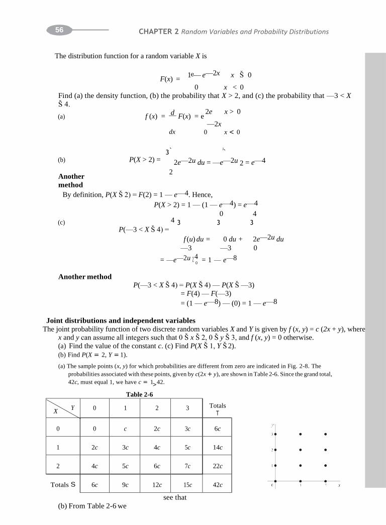
The joint probability function of two discrete random variables X and Y is given by f (x, y) = c (2x + y), where x and y can assume all integers such that 0 Š x Š 2, 0 Š y Š 3, and f (x, y) = 0 otherwise.
(a) Find the value of the constant c. (c) Find P(X Š 1, Y Š 2).
(b) Find P(X = 2, Y = 1).
(a) The sample points (x, y) for which probabilities are different from zero are indicated in Fig. 2-8. The
probabilities associated with these points, given by c(2x + y), are shown in Table 2-6. Since the grand total,
42c, must equal 1, we have c = 1> 42.
Table 2-6
see that
(b) From Table 2-6 we
X Y 0 1 2 3 Totals
T
0 0 c 2c 3c 6c
1
2c
3c
4c
5c
14c
2
4c
5c
6c
7c
22c
Totals S 6c 9c 12c 15c 42c

57 CHAPTER 2 Random Variables and Probability Distributions
P(X = 2, Y = 1) = 5c + 5
42
Fig. 2-
8

58 CHAPTER 2 Random Variables and Probability Distributions
(c) From Table 2-6 we see that
P(X Š 1, Y Š 2) = a a f (x, y)
xŠ1 yŠ2 = (2c + 3c + 4c)(4c + 5c + 6c)
= 24c = 24
= 4
42 7
as indicated by the entries shown shaded in the table.
2.9. Find the marginal probability functions (a) of X and (b) of Y for the random variables of Problem 2.8.
(a) The marginal probability function for X is given by P(X = x) = f>1(x) and can be obtained from the margin
totals•in the right>-hand column of Table 2-6. From these we see that
Chec
k:
1 + 1
7 3
+ 11
2 1
P(X = x) = f1 (x) =
= 1
164cc == 11 73 xx == 10
22c = 11
>21 x = 2
(b) The marginal probability function for Y is given by P(Y = y) = f2(y) and can be obtained from the margin
totals in the last row of Table 2-6. From these we see that
μ 12c = 2>7 y = 2
Chec
1 + 3 + 2 + 5
P(Y = y) = f2( y) =
= 1
6c = 1 7 y = 0 9c = 3 14 y = 1
15c = 5> 14 y = 3
k:
7 14 7 14
Show that the random variables X and Y of Problem 2.8 are dependent.
If the random variables X and Y are independent, then we must have, for all x and y,
P(X = x, Y = y) = P(X = x)P(Y = y)
But, as seen from Problems 2.8(b) and 2.9,
P(X = 2, Y = 1) = 5
P(X = 2) = 11
P(Y = 1) = 3
42 21 14
so that P(X = 2, Y = 1) 2 P(X = 2)P(Y = 1)
The result also follows from the fact that the joint probability function (2x + y)> 42 cannot be expressed as
function of x alone times a function of y alone. a
The joint density function of two continuous random variables X and Y is
f (x, y) = cxy 0 < x < 4, 1 < y < 5
e 0 otherwise
(a) Find the value of the constant c. (c) Find P(X Š 3, Y Š
2). (b) Find P(1 < X < 2, 2 < Y < 3). (a) We must have the total probability equal to 1, i.e.,
` `
3 3 f (x, y) dx dy = 1 —` —`

59 CHAPTER 2 Random Variables and Probability Distributions
2
3
3
5
R
xy dy dx
Using the definition of f(x, y), the integral has the value
4 5 4
3 3 3 B 3 x =
4
x = 0
25x x
0 y = 1 x = 0
cxy dxdy = c 4
= c 34
= c
z = 0
2 dx = c 3 ¢ 2
— 2
≤ dx xy2 5
x = 0
3
y=1
12x dx = c(6x2)2
4
x=0
= 96c
(b) Using the value of c found in (a), we have
Then 96c = 1 and c >96. B3 R 1 xy2 2
3 = 1
P(1 < X <
2, 2 < Y <
3) =
=2 1 2
3
3 3 xy
3
2
dx dy3
96 xy dy dx = 96 5
1 x = 1 y = 2 x = 1 = y = 2 x2
2 dx
x 4= 12 956x 5 a 2 y=2
P(X Š 3, Y Š 2) = 936 3 2 dx = 192 2 1
x = x = 1 xy
dx dyb 2 = 128
(c)
1 4 396
2
3y = 1926
1 4
x = 3 3 xy dy dx = 96 3x = 3 x2y2 2
dx
= 1 4
y = 1 R B
2y=1
3 3x dx = 7
96 x=3 2 128
Find the marginal distribution functions (a) of X and (b) of Y for Problem 2.11.
(a) The marginal distribution function for X if 0 Š x < 4 is
x `
F1(x) = P(X Š x) =3 3 f (u, v) dudv
5
= 3x 3
u =—` v=
—`
uv dudv
x2 3
1 x 5
= 3 B R
u = 0 v= 1 96
96 u = 0 v= uv dv du = 16
1
For x Š 4, F1(x) = 1; for x < 0, F1(x) =
0. Thus
•
0 x < 0
2>
=

60 CHAPTER 2 Random Variables and Probability Distributions
F1(x) = x 16 0 Š x <4
1 x Š 4
As F1 (x) is continuous at x = 0 and x =y =41, we could replace < by Š in the above
expression.
61 CHAPTER 2 Random Variables and Probability Distributions
= =
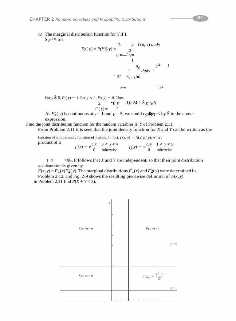
(b) The marginal distribution function for Y if 1
Š y ™ 5 is
F2( y) = P(Y Š y) = `3 y
3 u =—` v=
1
f (u, v) dudv
u y2 — 1 y
v dudv =
= 34 3v= 1 96
u = 0 24
For y Š 5, F2( y) = 1. For y < 1, F2( y) = 0. Thus
2 •(0 y — 1)>24 1 Š yy <<51
F ( y) = 2
As F2( y) is continuous at y = 1 and 1y = 5, we could reyplŠac5e < by Š in the above
expression. Find the joint distribution function for the random variables X, Y of Problem 2.11.
From Problem 2.11 it is seen that the joint density function for X and Y can be written as the
function of x alone and a function of y alone. In fact, f (x, y) = f1(x) f2( y), where
product of a f (x) e
c1x 0 < x < 4 f ( y) e
c2 y 1 < y < 5 1 0 otherwise 2 0 otherwise
1 2 >96. It follows that X and Y are independent, so that their joint distribution and cfcun=ctcio=n 1is given by
F(x, y) = F1(x)F2( y). The marginal distributions F1(x) and F2( y) were determined in
Problem 2.12, and Fig. 2-9 shows the resulting piecewise definition of F(x, y).
In Problem 2.11 find P(X + Y < 3).

62 CHAPTER 2 Random Variables and Probability Distributions
Fig. 2-9
In Fig. 2-10 we have indicated the square region 0 < x < 4, 1 < y < 5 within which the
joint density function of X and Y is different from zero. The required probability is given
by
P(X + Y < 3) = 65 f (x, y) dx dy

3
CHAPTER2 Random Variables and Probability Distributions 51 where
5 is the part of the square over which x + y < 3, shown shaded in Fig. 2-10. Since f (x, y) = xy
over 5, this probability is given by >96
2
3x = 3 0
3 — x xy
y= 1 96 dxdy
1 2 3 — x
B 3 x = 0 y = 1
xydy R dx x)2 — x] = 1
48
1 2 xy2 3—x 1 2
= x=0 2
2 y=1
dx = 3 x = 0
[x(3 —
Change of variables
Prove Theorem 2-1, page 42.
The probability function for U is given by
g(u) = P(U = u) = P[f(X) = u] = P[X = c(u)] = f [c(u)]
In a similar manner Theorem 2-2, page 42, can be proved.
Prove Theorem 2-3, page 42.
Consider first the case where u = Ø(x) or x = $(u) is an increasing function, i.e., u
increases as x increases (Fig. 2-11). There, as is clear from the figure, we have
(1) P(u1 < U < u2) = P(x1 < X < x2)
or u2 x2
(2) 3 g(u) du = 3 f (x) dx
u1 x1
Fig. 2-11
Fig. 2-10
= 3
96 192
96

52 CHAPTER 2 Random Variables and Probability Distributions
e
Letting x = $(u) in the integral on the right, (2) can be written
u2 u2
3 g(u) du = 3 f [c (u)] cr(u) du
u1 u1
This can hold for all u1 and u2 only if the integrands are
identical, i.e.,
g(u) = f [c(u)]cr(u)
This is a special case of (34), page 42, where cr(u) > 0 (i.e., the slope is positive). For
the case where cr(u) Š 0, i.e., u is a decreasing function of x, we can also show that (34)
holds (see Problem 2.67). The theorem can also be proved if cr(u) Š 0 or cr(u) < 0. Prove Theorem 2-4, page 42.
We suppose first that as x and y increase, u and v also increase. As in Problem 2.16 we
can then show that
P(u1 < U < u2, v1 < V < v2) = P(x1 < X < x2, y1 < Y < y2)
u2 v2 x2 y2
or 3 3 g(u, v) du dv = 3 3 f (x, y) dx dy
v1 v1 x1 y1
Letting x = $1 (u, v), y = $2(u, v) in the integral on the right, we have, by a theorem of
advanced calculus, u2 v2 u2 v2
3 3 g(u, v) du dv = 3 3 f [c1 (u, v), c2(u, v)]J du dv
where
is the Jacobian.
Thus
v1 u1 v1 v1
'(x, y)
J = '(u, v)
g(u, v) = f [c1(u, v), c2(u, v)]J
which is (36), page 42, in the case where J > 0. Similarly, we can prove (36) for the case
where J < 0.
The probability function of a random variable X is
f(x) = 2—x x = 1, 2, 3, c
0 otherwise
Find the probability function for the random variable U = X4 + 1.
Since U = X4 + 1, the relationship between the values u and x of the random variables U and
X is given by
u = x4 + 1 or x = u4 — 1, where u = 2, 17, 82, . . . and the real positive root is taken. Then
the required
probability function for U is
given by
—24
2 u—1 u = 2, 17, 82, . . . 0 otherwise
using Theorem 2-1, page 42, or Problem 2.15.
g(u) = e

53 CHAPTER 2 Random Variables and Probability Distributions
f (x) x2> —3 < x < 6
The probability function of a random variable X is given by
= e 81
0 otherwise
Find the probability density for the random variable 3U = 1 (12 — X ).

CHAPTER2 Random Variables and Probability Distributions 54
2u
2
2
We have u = 1 (12 — x) or x = 12 — 3u. Thus to each value of x there is one and only one value of u and
> 3
conversely. The values of u corresponding to x = —3 and x = 6 are u = 5 and u = 2, respectively. Since
cr(u) = dx du = —3, it follows by Theorem 2-3, page 42, or Problem 2.16 that the density function for U is
>
g(u) = e (12 — 3u)2 27 2 < u < 5
0 otherwise
5 (12 — 3u)2 (12 — 3u)3 5
3 Check:
2 27 du = —
243 = 1
2.20. Find the probability density of the random variable U = X2 where X is the random variable of Problem
2.19.
We have u = x2 or x = ±! . Thus to each value of x there corresponds one and only one
value of u, but to u
each value of u 2 0 there correspond two values of x. The values of x for which —3 < x ™
6 correspond to values of u for which 0 Š u ™ 36 as shown in Fig. 2-12.
As seen in this figure, the interval —3 < x Š 3 corresponds to 0 Š u Š 9 while 3 < x
™ 6 corresponds to 9 < u ™ 36. In this case we cannot use Theorem 2-3 directly but
can proceed as follows. The distribution function for U is
G(u) = P(U Šu)
Now if 0 Š u Š 9,
we have
G(u) = P( U Š u) = P(X2 Š u) = P(— u Š X Š u)
! !
1
u f (x) dx = 3 1
— u
Fig. 2-12

53 CHAPTER 2 Random Variables and Probability Distributions
But if 9 < u ™ 36, we have
G(u) = P(U Š u) = P(—3 < X < !u) = 3—3 f (x) dx

CHAPTER2 Random Variables and Probability Distributions 54
u
Since the density function g(u) is the derivative of G(u), we have, using (12),
f (!u) +2f!(—u !u)
g(u) = e u!) f (
!u
0
2
Using the given definition of f (x), this b!eco
>mes
0 Š u Š 9
9 < u < 36
otherwise
g(u) = • !u> 81 0 Š u Š 9
9 36
3 3 0
162 2u93><2u < u336>2 2 36
2 9otherwise
Chec !u !u
du +
+ 243
9 = 1
k: 0 81
162 du = 243 0
If the random variables X and Y have joint9 density function
f (x, y) = xy 96 0 < x < 4, 1 < y < 5
e 0 > otherwise (see Problem 2.11), find the density function of U = X + 2Y. Method 1
Let u = x + 2y, v = x, the second relation being chosen arbitrarily. Then simultaneous so2lution yields x = v, y = 1 (u — v). Thus the region 0 < x < 4, 1 < y < 5 corresponds to the region 0 < v ™ 4, 2 < u — v < 10 shown shaded in Fig. 2-13.
The Jacobian is
given by
Fig. 2-13
'x 'x
J = 4 'u 'v 4
'y 'y
'u 'v
0 1 = 1 1
2 —
2
1
= —2

CHAPTER 2 Random Variables and Probability Distributions
1
4
Then by Theorem 2-4 the joint density function of U and V is
g(u, v) = e v(u — v)>384 2 < u — v < 10, 0 < v < 4
0 otherwise
The marginal density function of U is given by
g3 u — 2 v(u — v)
3v= 0 384 dv 2 < u < 6
v(u — v)
g1(u) =
v= 0 384 dv 6 < u < 10 4
3 v= u —10
v(u —
v)
384
dv 10 < u < 14
0 otherwise
as seen by referring to the shaded regions I, II, III of Fig. 2-13. Carrying out the integrations, we find (u — 2)2(u + 4)>
d >
(348u — u3 — 212283)0>42304 210<<uu<<614
g (u) = (3u — 8) 144 6 < u < 10
0 otherwise
A check can be achieved by showing that the integral of g1 (u) is equal to 1.
Method 2
The distribution function of the random variable X + 2Y is given by
P(X + 2Y Š u) = 6 f (x, y) dxdy = 6
xy
96 dxdy
x + 2y Š u x0 <+x <24y Šu (u — u — 2 x(u
1 < y < 5 x R
For 2 < u < 6, we see by referring tox)F>igx. y2-14, that the last inteBgral equals
— x)2
u — 2 3 3
y = 1
2
96 dx dy = 3 x = 0
768
— 192
>2304. In a similar manner we can obtain
dx
x = 0
The derivative of this with respect to u is found to be (u — 2)2(u + 4)
the result of Method 1 for 6 < u < 10, etc.

Fig. 2-14 Fig. 2-15
—1> >
CH56APTER 2 CHAPTER2 Random Variables and Probability Distributions Random Variables and Probability Distributions
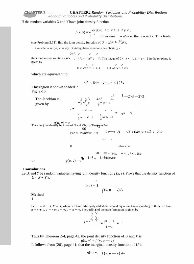
If the random variables X and Y have joint density function
f (x, y) = e xy 96 0 < x < 4, 1 < y < 5
0 >
otherwise = u>v so that y = ux>v. This leads
(see Problem 2.11), find the joint density function of U = XY 2, V =toX2Y.
Consider u = xy2, v = x2y. Dividing these equations, we obtain>y x
2>3 > > > the simultaneous solution x = v given by
which are equivalent to
u —1 3, y = u23 v —1 3. The image of 0 < x < 4, 1 < y < 5 in the uv-plane is
> > > > 0 < v2 3u—1 3 < 4 1 < u2 3v—1 3 < 5
v2 < 64u v < u2 < 125v
This region is shown shaded in
Fig. 2-15.
The Jacobian is
1 2
>
4 3 —4>3 2
1 —2>3 —2>3
given by —3 v u 3 v 3u—1 3
4 J =
—1>3 —1>
2
> >
1 = —3 u v
g(u, v) = c
3 u v 3 —3
u2 3v—4 3
Thus the joint density function of U and V is, by Theo(r3em 2-4,
96 (v2> 3u—1>3u)(u2>3v—1>3)
1
3 v—2 3) v2 < 64u, v < u2 < 125v
—2> >
0 otherwise
288 v2 < 64u, v < u 2 < 125v
or g(u, v) = e0u—1>3 v—1>3o>therwise
Convolutions
Let X and Y be random variables having joint density function f (x, y). Prove that the density function of
U = X + Y is
Method
1
g(u) = ` 3
f (v, u — v)dv
—`
Let U = X + Y, V = X, where we have arbitrarily added the second equation. Corresponding to these we have
u = x + y, v = x or x = v, y = u — v. The Jac'oxbia
'nx
of the transformation is given by
'u 'y
J = 4 'u
'v
'y 'v
4= 2 0 1 2 = —1
1 —1
Thus by Theorem 2-4, page 42, the joint density function of U and V is
g(u, v) = f (v, u — v)
It follows from (26), page 41, that the marginal density function of U is `
g(u) =3
—` f (v, u — v) dv


3
e dv = 6e (e — e
CHAPTER 2 Random Variables and Probability Distributions
Method 2
The distribution function of U = X + Y is equal to the double integral of f (x, y) taken over
the region defined by x + y Š u, i.e.,
G(u) = 6 f (x, y) dx dy
x +y Š u
Since the region is below the line x + y = u, as indicated by the shading in Fig. 2-16, we see that
` u — x
G(u) = 3 B 3 f (x, y) dyRdx x =—` y =—`
Fig. 2-16
The density function of U is the derivative of G (u) with respect to u and is given by `
g(u) =3
—` f (x, u — x) dx
using (12) first on the x integral and then on the y integral.
Work Problem 2.23 if X and Y are independent random variables having density functions f1(x),
f2( y), respectively.
In this case the joint density function is f (x, y) = f 1(x) f2( y), so that by Problem 2.23
the density function of U = X + Y is
which is the convolution of
f1 and f2.
` g(u) = 3
—`
f1(v) f2(u — v)dv = f1 * f2
If X and Y are independent random variables having density functions
f (x) = e 2e—2xx Š 0
1 0 x < 0
find the density function of their sum, U = X + Y.
f
(2y)
e 3e—3yy Š 0
= 0 y < 0
By Problem 2.24 the required density function is the convolution of f1 and f2 and is given by `
g(u) = f1 * f2 =
—` f1(v) f2(u — v) dv
In the integrand f1 vanishes when v < 0 and f2 vanishes when v > u. Hence
g(u) = u
(2e—2v)(3e—3(u—v)) dv 3 0
= 6e—3u u
v3 —3u u —2u 3u
57
— 1) = 6(e )

58 CHAPTER 2 Random Variables and Probability Distributions
0

4
CHAifPuTER 2 Random Variables and Probability Distributions Š 0 and g(u) = 0 if u <
` 0.
` 1 1
3 3 ¢ ≤
= 1
g(—u) du = 6 (e—0 2u — e—3u) du =26 3—
Chec
k:
2.26. Prove that f1 * f2 = f2 * f1 (Property 1, page 43). We have
` f1 * f2 =3
v=—`
f1(v) f2(u — v) dv
Letting w = u — v so that v = u — w, dv = —dw, we obtain —` f1(u — w) f2(w)(—dw) =
f1 * f2 =
w3
=`
3
w =—`
f2(w)f1(u — w) dw = f2 * f1
Conditional
distributions
f (y u x) =
f (x, y)
f (x) =
> (2x + y) 42
f (x)
Find (a) f ( y u 2), (b) P(Y = 1 u X = 2) for the distribution of Problem 2.8.
(a) Using the results in Problems 2.8 and 2.9, we have
f ( y u 2) = (4 + y) >42
= 4 + y
111 21 1 22 252
(b) so that with x = 2 P(Y = 1 u X = 2) = f (1 u 2) = If X and Y have the joint density function
3 + xy 0 < x < 1, 0 < y < 1 e >
f (x, y) = 0 otherwise
find (a) f ( y u x), (b) P(Y > 1 u 1 < X < 1 + dx).
2 2
(a) For 0 < x < 1,
and
2 f1(x) = 3
¢ ≤
0
4 4 2
3 + 4xy
• 3 + 2x f1(x)
0 other y
1 3 3 x
+ xy dy = +
f (x, y) 0 < y < 1
f ( y u x) = =
(b) For other values of x, f ( y u x) is not defined.
P(Y > 2 u 2 < X < 2 + dx) = 31 f ( y u 2) dy =
3
4 dy = 16
1 1 1 `>
e 1
1> 3 + 2y 9
2 1 2
The joint density function of the random variables X and Y is given by
f (x, y) = 8xy 0 Š x Š 1, 0 Š y Š x
0 otherwise
Find (a) the marginal density of X, (b) the marginal density of Y, (c) the conditional density of
59

60 CHAPTER 2 Random Variables and Probability Distributions
X, (d) the conditional density of Y.
The region over which f (x, y) is different from zero is shown shaded in Fig. 2-17.

61 CHAPTER 2 Random Variables and Probability Distributions
3 3
3 3 3 3
Fig. 2-17
(a) To obtain the marginal density of X, we fix x and integrate with respect to y from 0 to x
as indicated by the vertical strip in Fig. 2-17. The result is
x f1(x) =3
8xy dy = 4x 3
y = 0
for 0 < x < 1. For all other values of x, f1
(x) = 0.
(b) Similarly, the marginal density of Y is obtained by fixing y and integrating with respect to x
from x = y to x = 1, as indicated by the horizontal strip in Fig. 2-17. The result is, for 0
< y ™ 1,
For all other values of y, f2 (
y) = 0.
f2 ( y) =3
1
x = y
8xy dx = 4y(1 — y2)
>
(c) The conditional density function of X is, for 0 < y <1, f (x u y) = f (x, y)= e 2x (1 — y2) y Š x Š 1 1 f2(y) 0 other x
The conditional density function is not defined when f2( y) = 0.
(d) The conditional density function of Y is, for 0 < x ™ 1,
f ( y u x) = f (x, y)
= e 2y>x 2 0 Š y Š x
2 f1(x) 0 other y
The conditional density function is not defined when f1(x) = 0.
Chec
k:
1 f1(x) dx =
1 4x 3 dx = 1,
1 f2( y) dy =
1 4y(1 — y2) dy = 1
0 0 0 0
1 f1(x u y) dx =
1 2x dx = 1
y y 1 — y2
x x 2y
3 f2( y u x) dy = 3 dy = 1
0 0 x2

62 CHAPTER 2 Random Variables and Probability Distributions
Determine whether the random variables of Problem 2.29 are independent.
In the shaded region of Fig. 2-17, f (x, y) = 8xy, f1(x) = 4x3, f2( y) = 4y (1 —
y2). Hence f (x, y) 2
and thus X and Y are dependent.
f1(x) f2( y),
It should be noted that it does not follow from f (x, y) = 8xy that f (x, y) can be expressed
as a function of x alone times a function of y alone. This is because the restriction 0 Š y
Š x occurs. If this were replaced by some restriction on y not depending on x (as in
Problem 2.21), such a conclusion would be valid.

63 CHAPTER 2 Random Variables and Probability Distributions
r
¢ r
≤ 2
R
Applications to geometric probability
P(r Š R Š r + dr)
= c
A person playing darts finds that the probability of the dart sBtriking between r and r + dr is 1 — a dr
Here, R is the distance of the hit from the center of the target, c is a constant, and a is the radius
of the tar- get (see Fig. 2-18). Find the probability of hitting the bull’s-eye, which is assumed
to have radius b. As-
sume that the target is always
hit.
The density function is given
by
Since the target is always hit, we have
f (r) = c 2
B ¢ ≤ R
1 — a
a r
2
c 3 B1 — ¢ a ≤ R dr = 1 0
Fig. 2-18¢
r ≤
from which c = 3>2a. Then the probability of hitting the b2ull’s-eye is R
b 3 b
3 f (r) dr =2a 3 B
0 0 1 — a
dr =
b (3a2 — b2)
2a3
Twopoints are selected at random in the interval 0 Š x Š 1. Determine the probability that the
sum of their squares is less than 1.
Let X and Y denote the random variables associated with the given points. Since equal
intervals are assumed to have equal probabilities, the density functions of X and Y are
given, respectively, by
(1) f (x) = e
1 0 Š x
Š 1
f ( y) = e 1 0 Š y Š 1
1 0 otherwise 2 0 otherwise
Then since X and Y are independent, the joint density function is given by
(2) f (x, y) = f (x) f (y) = e 1 0 Š x Š 1, 0 Š y Š 1
1 2 0 otherwise It follows that the required probability is given by
(3) P(X2 + Y2 Š1) = 6 dx dy
r

64 CHAPTER 2 Random Variables and Probability Distributions
whereristheregiondefinedby x2 + y2 Š 1, x Š 0, y Š 0, which isaquarterofacircleofradius 1 (Fig. 2-19).
Now since (3) represents the area of r, we see that the required probability is p >4.
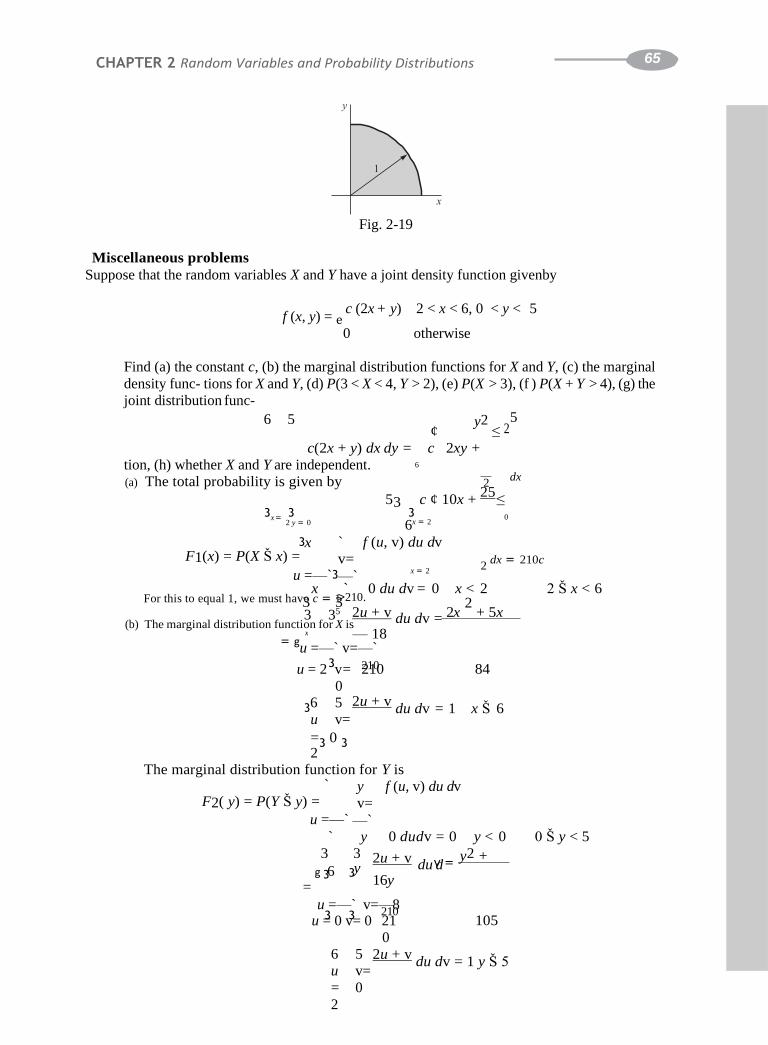
65 CHAPTER 2 Random Variables and Probability Distributions
Fig. 2-19
Miscellaneous problems
Suppose that the random variables X and Y have a joint density function givenby
f (x, y) = e c (2x + y) 2 < x < 6, 0 < y < 5
0 otherwise
Find (a) the constant c, (b) the marginal distribution functions for X and Y, (c) the marginal
density func- tions for X and Y, (d) P(3 < X < 4, Y > 2), (e) P(X > 3), (f ) P(X + Y > 4), (g) the
joint distribution func-
6 5 ¢
y2 ≤ 2
5
c(2x + y) dx dy = c 2xy +
tion, (h) whether X and Y are independent. 6
(a) The total probability is given by 2 dx
53 c ¢ 10x + 25
≤ 3 3 3 x = 0
2 y = 0
3x F1(x) = P(X Š x) =
6x = 2
` f (u, v) du dv
v=
2
dx = 210c
u =—`3—` x = 2
x ` 0 du dv = 0 x < 2 2 Š x < 6 For this to equal 1, we must hav3e c = 13>210. 2
3 35 2u + v du dv = 2x + 5x (b) The marginal distribution function for X is
— 18 = g
u =—` v=—`
u = 23v= 221100 84
0
36 5
u v=
2u + v du dv = 1 x Š 6
=3 0 3
2 The marginal distribution function for Y is
` F2( y) = P(Y Š y) =
y f (u, v) du dv
v= u =—` —`
` y 0 dudv = 0 y < 0 0 Š y < 5
3
g 36 =
3 2u + v duvd=
y2 + 3y
16y
u =—` v=—21
80
u =3 0 v3= 0 21
0
105
6 5
u v=
= 0
2
2u + v du dv = 1 y Š 5
x

CHAPTER2 Random Variables and Probability Distributions 62
(d) 3
3
(c) The marginal density function for X is, from part (b),
f (x) = d F (x) = (4x + 5) 84 2 < x < 6
1 dx 1 0
The marginal density function for Y is, from part (eb), > otherwise
f ( y) = d F (y) = e (2y + 16) >105 0 < y < 5
2 dy 2 0 otherwise
P(3 < X < 4, Y > 2) = 1 4
35
(2x + y) dx dy =
3
210 x
5= 3
y = 2 20
(e) P(X > 3) = 1 6
3 (2x + y) dx dy = 23
210 x
=
3
y = 0 28
(f ) P(X + Y > 4) = 6 f (x, y) dxdy
r
where r is the shaded region of Fig. 2-20. Although this can be found, it is easier to
use the fact that
P(X + Y > 4) = 1 — P(X + Y Š 4) = 1
— 6
where rr is the cross-hatched region ofiFg. 2-20. We have
f (x, y) dx dy
r
1 4
P(X + Y Š 4) = 3 4
— x (2x + y) dx dy =
2
Thus P(X + Y > 4) = 33>35. 210 x = 2 y = 0 35
Fig. 2-20 Fig. 2-21
(g) The joint distribution function is 3
x F(x, y) = P(X Š x, Y Š y) =
v=—`
u3=—` y
3

67 CHAPTER 2 Random Variables and Probability Distributions
f (u, v) du dv
In the uv plane (Fig. 2-21) the region of integration is the intersection of the quarter
plane u Š x, v Š y and the rectangle 2 < u < 6, 0 ™ v < 5 [over which f (u, v) is nonzero].
For (x, y) located as in the figure, we have 6 y
F(x, y) = 3 3
u = 2 v=
0
2u + v duvd=
21
0
16y + y2
105


63 CHAPTER 2 Random Variables and Probability Distributions
3 3
When (x, y) lies inside the rectangle, we obtain another expression, etc. The complete
results are shown in Fig. 2-22.
(h) The random variables are dependent since
f (x, y) 2 f1(x) f2( y)
or equivalently, F(x, y) 2
F1(x)F2(y).
Let X have the density function
f (x) = e 6x (1 — x) 0 < x < 1
0 otherwise
Find a function Y = h(X) which has the density function
g( y) = 12y3(1 — y2) 0 < y < 1
e 0 otherwise
Fig. 2-22
We assume that the unknown function h is such that the intervals X Š x and Y Š y +
h(x) correspond in a one-one, continuous fashion. Then P(X Š x) = P(Y Š y), i.e., the
distribution functions of X and Y must be equal. Thus, for 0 < x, y < 1,
x6u(1 — u) du =
y12v3 (1 — v2) dv
0 0
or 3x2 — 2x3 = 3y4 — 2y6
!x is a solution, and this solution has the desired properties. Thus
By inspection, x = y2 or y = h(x) = + Y = +!
X.
2.35. Find the density function of U = XY if the joint density function of X and Y is f (x, y). >
Method
1 4 'u 'v
4 2 0 1 2
Let U = XY and V = X, corresponding to which u = xy, v = x or x = v, y = u v. Then the
Jacobian is given by

'x 'x
J = 'y 'y
'u
'v
= v—1 —
uv—2
= —v—1
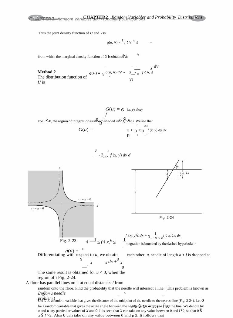
x u 1
f
CH64APTER 2 Random VariaCbHlesAaPnTdEPRro2baRbialintydoDmistVriabruitaibolness and Probability Distribut6i5ons
Thus the joint density function of U and V is
g(u, v) = 1
f ¢ v, u
≤
from which the marginal density function of U is obtaineudvau s
`
v
` 1
vu dv
Method 2
The distribution function of
U is
g(u) = 3 g(u, v) dv =
—`
3—` u
vu
f ¢ v, ≤
G(u) = 6
f
(x, y) dxdy
For u Š 0, the region of integration is sh0owB
n shaded inxFyigŠ. 2u-23. We see that
` u>x
G(u) = x + 3 B 3 f (x, y) dyR dx
R 0 —`
3 x
—` 3u> f (x, y) dy d
Fig. 2-24
`
f ¢x, x ≤ dx = 3—` u x u
¢ x, u
≤ dx
Fig. 2-23
g(u) =
¢ —1
≤ f ¢ x, u
≤ 1
ntegration is bounded by the dashed hyperbola in
0 `
Differentiating with respect to u, we obtain each other. A needle of length a < l is dropped at 3
x x dx +3
x
—` 0
The same result is obtained for u < 0, when the
region of i Fig. 2-24.
A floor has parallel lines on it at equal distances l from
random onto the floor. Find the probability that the needle will intersect a line. (This problem is known as
Buffon’s needle >
pLreot Xbl
beema.r)andom variable that gives the distance of the midpoint of the needle to the nearest line (Fig. 2-24). Let 0
be a random variable that gives the acute angle between the nePed(ule Š(or0its +extdeuns)io=n)2adnud the line. We denote by
x and u any particular values of X and 0. It is seen that X can take on any value between 0 and l >2, so that 0 Š
x Š l >2. Also 0 can take on any value between 0 and p 2. It follows that

P(x < X Š x + dx) = 2
dx p
i.e., the density functions of X and 0 are given by f1(x) = 2>l, f2(u) = 2>p. As a check, we note that
l> 2
30 l 0 p
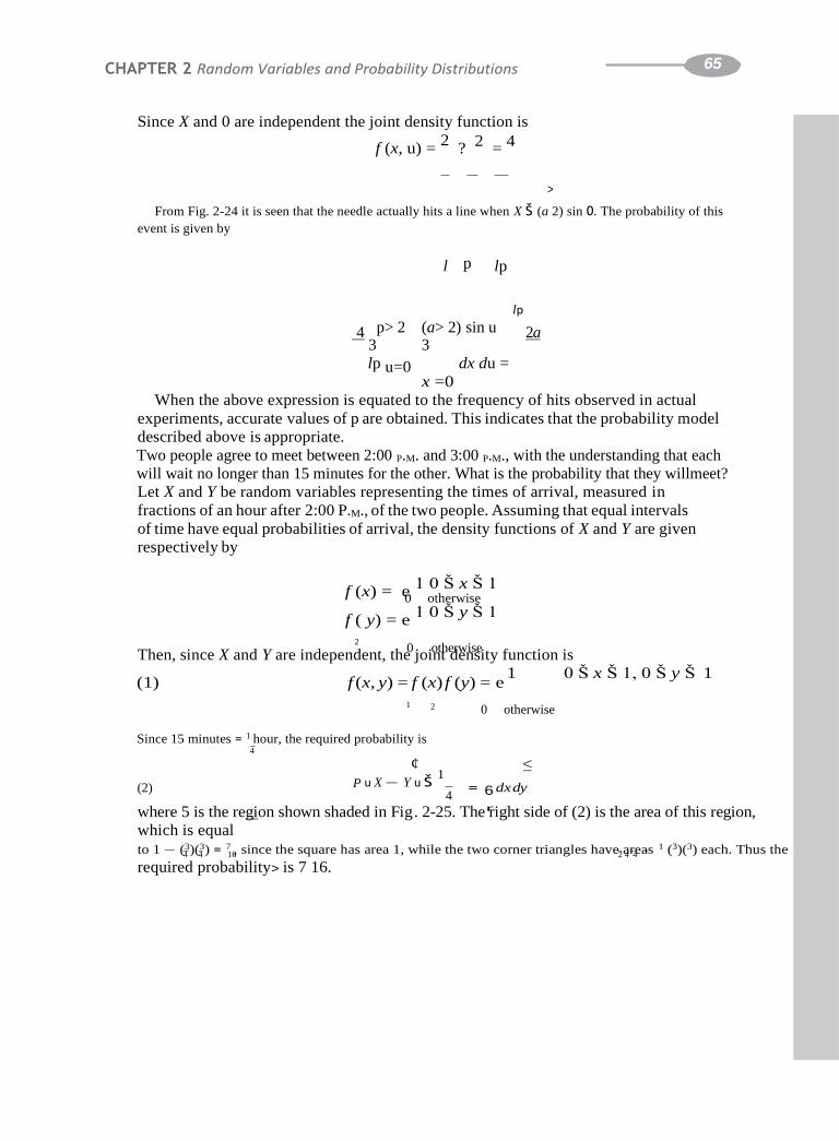
65 CHAPTER 2 Random Variables and Probability Distributions
1
0 otherwise
4 4 16 2 4 4
Since X and 0 are independent the joint density function is
f (x, u) = 2
? 2
= 4
>
From Fig. 2-24 it is seen that the needle actually hits a line when X Š (a 2) sin 0. The probability of this
event is given by
l p lp
lp
4 p> 2 (a> 2) sin u 2a 3 3
lp u=0 dx du =
x =0
When the above expression is equated to the frequency of hits observed in actual
experiments, accurate values of p are obtained. This indicates that the probability model
described above is appropriate.
Two people agree to meet between 2:00 P.M. and 3:00 P.M., with the understanding that each
will wait no longer than 15 minutes for the other. What is the probability that they willmeet?
Let X and Y be random variables representing the times of arrival, measured in
fractions of an hour after 2:00 P.M., of the two people. Assuming that equal intervals
of time have equal probabilities of arrival, the density functions of X and Y are given
respectively by
f (x) = e 1 0 Š x Š 1
0 otherwise
f ( y) = e 1 0 Š y Š 1
2
Then, since X and Y are independent, the joint density function is
(1) f (x, y) = f (x) f (y) = e 1 0 Š x Š 1, 0 Š y Š 1
1
Since 15 minutes = 1 hour, the required probability is
4
2 0 otherwise
(2)
¢
P u X — Y u Š 1
4
≤
= 6 dx dy
where 5 is the region shown shaded in Fig. 2-25. Therright side of (2) is the area of this region,
which is equal
to 1 — (3)(3) = 7 , since the square has area 1, while the two corner triangles have areas 1 (3)(3) each. Thus the
required probability> is 7 16.
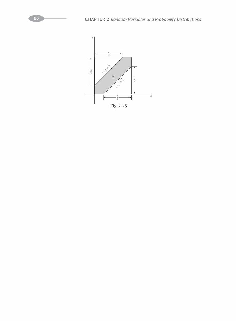
66 CHAPTER 2 Random Variables and Probability Distributions
Fig. 2-25

67 CHAPTER 2 Random Variables and Probability Distributions
x 1 2 3
2 1 3 1 6
x 1 2 3 4
F(x) 1 8 3 8 3 4 1
SUPPLEMENTARY PROBLEMS
Discrete random variables and probability distributions
A coin is tossed three times. If X is a random variable giving the number of heads that
arise, construct a table showing the probability distribution of X.
An urn holds 5 white and 3 black marbles. If 2 marbles are to be drawn at random without
replacement and X
denotes the number of white marbles, find the probability distribution for X.
Work Problem 2.39 if the marbles are to be drawn with replacement.
Let Z be a random variable giving the number of heads minus the number of tails in 2 tosses
of a fair coin. Find the probability distribution of Z. Compare with the results of Examples
2.1 and 2.2.
Let X be a random variable giving the number of aces in a random draw of 4 cards from an
ordinary deck of 52 cards. Construct a table showing the probability distribution of X.
Discrete distribution functions
The probability function of a random variable X is shown in Table 2-7. Construct a table
giving the distribution function of X.
Obtain the distribution function for (a) Problem 2.38, (b) Problem 2.39, (c) Problem 2.40.
Obtain the distribution function for (a) Problem 2.41, (b) Problem 2.42.
Table 2-8 shows the distribution function of a random variable X. Determine (a) the probability
function, (b) P(1 Š X Š 3), (c) P(X Š 2), (d) P(X < 3), (e) P(X > 1.4).
Continuous random variables and probability distributions
A random variable X has density function
f (x) = ce—3x x > 0
e 0 x Š 0
Find (a) the constant c, (b) P(l < X < 2), (c) P(X Š 3), (d) P(X < 1).
Find the distribution function for the random variable of Problem 2.47. Graph the
density and distribution functions, describing the relationship between them.
A random variable X has density
function
f (x) =
> cx 2 1 Š x Š 2
• cx 2 < x < 3 0 otherwise
Find (a) the constant c, (b) P(X > 2), (c) P(1 2 < X < 3 2). >

68 CHAPTER 2 Random Variables and Probability Distributions
Find the distribution function for the random variable X of Problem 2.49.
The distribution function of a random variable X is given by
cx3 0 Š x < 3
F(x) = • 1 x Š 3 0 x < 0
If P(X = 3) = 0, find (a) the constant c, (b) the density function, (c) P(X > 1), (d) P(1 < X < 2).
Can the function
be a distribution function?
Explain.
F(x) = e c(1 — x2) 0 Š x Š 1
0 otherwise
Let X be a random variable having density function
f (x) = cx 0 Š x Š 2
e 0 otherwise
Find (a) the value of the constant c, (b) P(1 < X < 3), (c) P(X > 1), (d) the distribution
function.
2 2
Joint distributions and independent variables
The joint probability function of two discrete random variables X and Y is given by f(x, y) =
cxy for x = 1, 2, 3 and y = 1, 2, 3, and equals zero otherwise. Find (a) the constant c, (b) P(X
= 2, Y = 3), (c) P(l Š X Š 2, Y Š 2), (d) P(X Š 2), (e) P(Y < 2), (f ) P(X = 1), (g) P(Y = 3).
Find the marginal probability functions of (a) X and (b) Y for the random variables of Problem
2.54.
(c) Determine whether X and Y are independent.
Let X and Y be continuous random variables having joint density function
f (x, y) = c(x 2 + y2)0 Š x Š 1, 0 Š y Š 1
e 0 otherwise
Determine (a) the constant c, (b) P(X < 1, Y > 1), (c) P (1 < X < 3), (d) P(Y < 1), (e) whether X
and Y are
independe
nt.
2 2 4 4 2
Find the marginal distribution functions (a) of X and (b) of Y for the density function of Problem
2.56.
Conditional distributions and density functions
Find the conditional probability function (a) of X given Y, (b) of Y given X, for the distribution of
Problem 2.54.
e x + y 0 Š x Š 1, 0 Š y Š 1
Let f (x, y) =
0 otherwise
Find the conditional density function of (a) X given Y, (b) Y given X.
Find the conditional density of (a) X given Y, (b) Y given X, for the distribution of Problem 2.56.

69 CHAPTER 2 Random Variables and Probability Distributions
Let
f (x, y) = e—(x+y) x Š 0, y Š 0
0 otherwise
be the joint density function of X and Y. Find the conditional density function of (a) X given
Y, (b) Y given X.
70 CHAPTER 2 Random Variables and Probability Distributions
e
Change of variables
Let X have density function
f (x) =
e—xx > 0
0 x Š 0
Find the density function of
Y = X2.
(a) If the density function of X is f (x) find the density function of X3. (b) Illustrate the
result in part (a) by choosing
2.64. If X has density function f (x) = 2(p—) 1>
and check the
answer.
f (x) =e 2e—2x x Š 0
0 x < 0
22> 2
2e—x , —` < x < `, find the density function of Y = X .
2.65. Verify that the integral of g1(u) in Method 1 of Problem 2.21 is equal to 1.
If the density of X is f (x) = 1> 2 1
Complete the work neededpto(xfi+nd1)g, —1(u)<inx M< et,hfoindd2thoefdPenrsoibtyleomf Y2=.2ta1nandX.check your answer.
Let the density of X be
Find the density of (a) 3X — 2,
(b) X3 + 1.
f (x) =
e
1>2 —1 < x < 1
0 otherwise
Check by direct integration the joint density function found in Problem 2.22.
Let X and Y have joint density
function f (x, y) =e
e—(x+y) x Š 0, y Š 0
0 otherwise
If U = X>Y
, V = X + Y, find the joint density function of U and V.
Use Problem 2.22 to find the density function of (a) U = XY 2, (b) V = X 2Y.
Let X and Y be random variables having joint density function f (x, y) = (2p)—1 e—(x2+y2), —` <
x < `,
—` < y < `. If R and 0 are new random variables such that X = R cos 0, Y = R sin 0, show
that the density
function of
R is
g(r) = e —
re r2 0 > r < 0
2 r Š 0

71 CHAPTER 2 Random Variables and Probability Distributions
Let
f (x, y) =e 1 0 Š x Š 1, 0 Š y Š 1
0 otherwise
be the joint density function of X and Y. Find the density function of Z = XY.
Convolutions
Let X and Y be identically distributed independent random variables with density function
f (t) = 1 0 Š t Š 1
e 0 otherwise
Find the density function of X + Y and check your answer.
Let X and Y be identically distributed independent random variables with density function
f (t) = e—t t Š 0
e 0 otherwise
Find the density function of X + Y and check your answer.
Work Problem 2.21 by first making the transformation 2Y = Z and then using convolutions
to find the density function of U = X + Z.
If the independent random variables X1 and X2 are identically distributed with density function
f (t) = te—t t Š 0
e 0 t < 0
find the density function of X1 + X2.
Applications to geometric probability
Two points are to be chosen at random on a line segment whose length is a > 0. Find the
probability that the three line segments thus formed will be the sides of a triangle.
It is known that a bus will arrive at random at a certain location sometime between 3:00
P.M. and 3:30 P.M. A man decides that he will go at random to this location between
these two times and will wait at most 5 minutes for the bus. If he misses it, he will take the
subway. What is the probability that he will take the subway?
Two line segments, AB and CD, have lengths 8 and 6 units, respectively. Two points P and Q
are to be chosen at random on AB and CD, respectively. Show that the probability that the
area of a triangle will have height AP and that the base CQ will>be greater than 12 square units is equal to (1 — ln 2) 2.
3 , x = 1, 2, c, is the probability function for a random variable X. (a) >Determine c.
Miscellaneous problems
Suppose that f (x) = c x
(b) Find the distribution function. (c) Graph the probability function and the distribution
function. (d) Find
P(2 Š X < 5). (e) Find P(X Š 3).
Suppose that
f (x) = e cxe—2x x Š 0
0 otherwise
is the density function for a random variable X. (a) Determine c. (b) Find the distribution
function. (c) Graph the density function and the distribution function. (d) Find P(X Š 1). (e) Find P(2 Š X < 3).

72 CHAPTER 2 Random Variables and Probability Distributions
The probability function of a random variable X is given by
2p x = 1
f (x) = μ p x = 2
4p x = 3 0
otherwi
se where p is a constant. Find (a) P(0 Š X < 3), (b) P(X
> 1).
(a) Prove that for a suitable
constant c, F(x) =
0 x Š 0
e c(1 — e—x)2 x > 0
is the distribution function for a random variable X, and find this c. (b) Determine P(l < X <
2).
A random variable X has density function 3(1 — x2) 0 Š x Š 1
f (x) = e 2
0 otherwise
Find the density function of the random variable Y = X2 and check your answer.
Two independent random variables, X and Y, have respective density functions
f (x) = c1e—2x x
g( y) = c2 ye—3y y > 0
> 0 e e 0 y Š 0
0 x Š 0
Find (a) c1 and c2, (b) P(X + Y > 1), (c) P(l < X < 2, Y Š 1), (d) P(1 < X < 2), (e) P(Y Š l).
In Problem 2.86 what is the relationship between the answers to (c), (d), and (e)? Justify your
answer.
Let X and Y be random variables having joint density function
f (x, y) = c(2x + y) 0 < x < 1, 0 < y < 2
e 0 otherwise
Find (a) the constant c, (b) P(X > 1, Y < 3), (c) the (marginal) density function of X, (d) the
(marginal) density
2 2
function of Y.
2.89. In Problem 2.88 is P(X > 1, Y < 3) = P(X > 1)P(Y < 3)? Why?
2 2 2 2
In Problem 2.86 find the density function (a) of X2, (b) of X + Y.
f (x, y) = e y 0 < x < y, 0 < y < 1
Let X and Y have joint density function 10>
otherwise

73 CHAPTER 2 Random Variables and Probability Distributions
(a) Determine whether X and Y are independent, (b) Find P(X > 1). (c) Find P(X < 1, Y > 1).
(d) Find
P(X + Y > 1).
2
2 2 3
Generalize (a) Problem 2.74 and (b) Problem 2.75 to three or more variables.
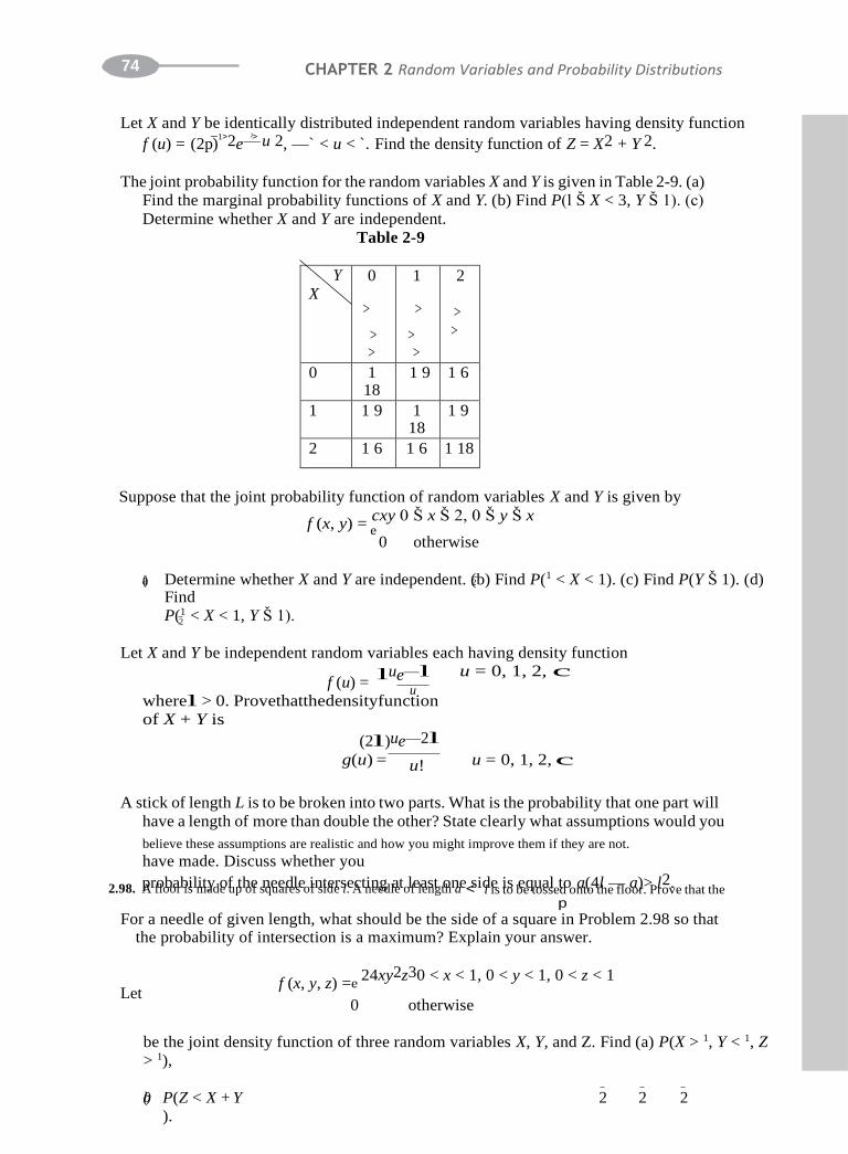
74 CHAPTER 2 Random Variables and Probability Distributions
e
2
u
l is to be tossed onto the floor. Prove that the
Let X and Y be identically distributed independent random variables having density function
f (u) = (2p—)
1>2e—2> u 2, —` < u < `. Find the density function of Z = X2 + Y 2.
The joint probability function for the random variables X and Y is given in Table 2-9. (a)
Find the marginal probability functions of X and Y. (b) Find P(l Š X < 3, Y Š 1). (c)
Determine whether X and Y are independent.
Table 2-9
Y
X 0
>
> >
1
>
> >
2
>
>
0 1 18
1 9 1 6
1 1 9 1 18
1 9
2 1 6 1 6 1 18
Suppose that the joint probability function of random variables X and Y is given by
f (x, y) = cxy 0 Š x Š 2, 0 Š y Š x
0 otherwise
(a) Determine whether X and Y are independent. (2b) Find P(1 < X < 1). (c) Find P(Y Š 1). (d)
Find
P(1 < X < 1, Y Š 1).
Let X and Y be independent random variables each having density function
f (u) = lue—l
wherel > 0. Provethatthedensityfunction
of X + Y is
u = 0, 1, 2, c
(2l)ue—2l
g(u) = u! u = 0, 1, 2, c
A stick of length L is to be broken into two parts. What is the probability that one part will
have a length of more than double the other? State clearly what assumptions would you
believe these assumptions are realistic and how you might improve them if they are not.
have made. Discuss whether you
2.98. Aprfoloboarbisilmitaydoe fupthoef snqeueardelseoifnstideersl.eActnineegdlaetolfelaesntgtohnae<side is equal to a(4l — a)> l2.
p
For a needle of given length, what should be the side of a square in Problem 2.98 so that the probability of intersection is a maximum? Explain your answer.
f (x, y, z) =e 24xy2z30 < x < 1, 0 < y < 1, 0 < z < 1
Let 0 otherwise
be the joint density function of three random variables X, Y, and Z. Find (a) P(X > 1, Y < 1, Z
> 1),
(b) P(Z < X + Y
).
2 2 2

75 CHAPTER 2 Random Variables and Probability Distributions
2.101. A cylindrical stream of particles, of radius a, is directed toward a hemispherical target ABC with center at O as
indicated in Fig. 2-26. Assume that the distribution of particles is given by
1> f (r) = e
a 0 < r < a
0 otherwise

CHAPTER2 Random Variables and Probability Distributions 72
>
where r is the distance from the axis OB. Show that the distribution of particles along the
target is given by
g(u) = cos u 0 < u < p 2
> e 0 otherwise
where u is the angle that line OP (from O to any point P on the target) makes with the axis.
Fig. 2-26
In Problem 2.101 find the probability that a particle will hit the target between u = 0 and u = p
4.
Suppose that random variables X, Y, and Z have joint density function
f (x, y, z) = 1 — cos px cos py cos pz 0 < x < 1, 0 < y < 1, 0 < z < 1
e 0 otherwise
Show that although any two of these random variables are independent, i.e., their marginal
density function factors, all three are not independent.
ANSWERS TO SUPPLEMENTARY PROBLEMS
2.38
.
2.40
.
2.42
.
2.43
.
2.46. (a)
2.39.
(b) 3>4 (c) 7 8
>(d) 3 8 (e)
>7 8
>
x 0 1 2
f (x) 3 28 15 28 5 14
x 0 1 2 3
f (x) 1 8
x 0 1 2
f (x) 9 64 15 32 25 64
x 0 1 2 3 4
f (x) 194,580
270,725
69,184
270,725
6768
270,725
192
270,725 1
270,725
x 0 1 2 3
f (x) x 1 2 3 4
f (x) 1 8 1 4 3 8 1 4

73 CHAPTER 2 Random Variables and Probability Distributions
6
2.47. (a) 3 (b) e—3 — e—6 (c)
e—9
(d) 1 —
e—3
2.48. F (x) = e 1 — e—3x x Š 0
> > > 0 x Š 0
0 x Š 1
2.49. (a) 6 29 (b) 15 29 (c) 19 116
2.50. F
= μ27 (d) 7 27>
(x)
0 otherwise
(3x 2 +>2) 29 2 Š x Š 3
2.51. (a) 1/27 (b) f (x) = e x 2/9 0 Š
x < 3
(c) 26 1 x Š 3
2.53. (a) 1>2 (b) 1>2 (c) 3>4 (d) F(x) 0= • 2>4 x 0Š Š0 x Š 2
> > > > >x > >
> 1 > x Š 2 0 other x 0 other y
2.54. (a) 1 36 (b) 1 6 (c) 1 4 (d) 5 6 (e) 1 6 (f ) 1 6 (g) 1 2
2.55. (a) f (x) = e x 6 x = 1, 2,
(b) f ( y) = e y 6 y = 1, 2, 3
3 1 2
2.57. (a) F (x) = • 1 (x 3 + x) (b) F ( y) = • y3 + y) 0 Š y Š 1
2.56. (a) 3>12 (b) 1>4 (c) 29>64 (d)05>Š16x Š 1 2
1 0 x Š 0
(a) f (x u y) = f21(x) for y = 1, 2, 3 (see Problem
0 y Š 0
2 (
1 x Š 1 2.55) 1 y Š 1
(b) f ( y u x) = f2( y) for x = 1, 2, 3 (see Problem 2.55)
(x + y)>( y + 1
) 0 Š x Š 1, 0 Š y Š 1
(a) f (x u y) = e 0 2 other x, 0 Š y Š 1
(b) f ( y u x) = e
(a) f (x u y) = e (x +
y)
>(x + 2 ) 0 Š x Š 1, 0 Š y Š 1
>( y 1
+ 3 ) 0 Š x Š 1, 0 Š y Š 1 0
(b) f ( y ux) = (x 2 + >
2
0 Š x Š 1, other y
1 e y2) (x + 3 ) 0 Š x Š 1, 0 Š y Š 1
0e—x x Š 0, y Š 0 other x, 0 Š y Š 1 2.61. (a) f (x u y) = e 2
2 2 1 (b) f (y ux) = e e—y x Š 0, y Š 0
0(x +x <y 0), y Š 0 0 x Š 0, y < 0
0 0 Š x Š 1, other y
e— 1 y>2 !y for y > 0; 0 otherwise 2.64. (2p)—1> 2y—1> 2 e—y> 2 for y > 0; 0 otherwise
e —5 < y <
2.66. 1>p for —p>12 < y < p>2; 0 otherwise •
6 >
2.70. ve—v (1 +1 u)2 for u Š 0, v Š 0; 0 othe1r(w1 i—sey)—2>3 0 < y < 1
2.68. (a) g(
>
y) = 6
0 otherwise (b) g( y) = 1 ( —2 3y — 1)1 < y
0 otherwise

74 CHAPTER 2 Random Variables and Probability Distributions
2.73. g(z) = —ln z 0 < z < 1
e0 otherwise
u 0 Š u Š
1 • 0 u < 0
2.77. g(x) =e x 3e—x/6 x Š 0
0 x < 0
>72 >
2.74. g(u) = 2 — u 1 Š u Š 2 2.78. 1 4
u0e—u u oŠth0 erwise 2.75. g(u) = e 1 — 30—y2.79yx.Š<61x1< y + 1; y = 1, 2, 3, c (d) 26>81 (e) 1>9 2.81. (a) 2 (b) F(x) = e
1 — e—2x (2x + 1) x Š 0 2.832.. ((aa)) 34>7 (b()bF)(x>5) =7 e 2.84. (a) c = 1x(b+) e1
—4 — 3e—(2d+) 32e—e 21
(e) 5e—4 — 7e—6
0 e x < 0
> > 0 < x < 1 1 ( y + 1) 0 < y < 2
2.86. (a) c1 =
!2, c2 = 9 (b) 9e—(b)2 e—
18e—2
(u
c) 4u
e>—05 —
(d) e—2 —
0 otherwise
(e) 4e—3
14e—3 4e—7 e—4
2.88. (a) 1 4 (b) 27 64 (c) f1(x) = 2 (d) f2( y) = e 4
2.90. (a) e e—2y/ y y > 0
2.91. 1
— ln 2) (c) 1
+ 1
0
e 1 ln 2
otherwis 2.95. (b) 15
>256 (c) 9>16 (d) 0
0 (b) (1
2 se
2
> othe6rwi
(d) 2
2.100. (a) 45
512 (b) 1>14
2.94. (b) 7
01
e—z 2 zz Š<00
18 2.102. ! >2 2
ln 2

MathematicalExpectation
Definition of Mathematical Expectation
A very important concept in probability and statistics is that of the mathematical expectation, expected
value, or briefly the expectation, of a random variable. For a discrete random variable X having the
possible values x1, c, xn, the expectation of X is defined as
E(X) = x P(X = x ) + c+ x P(X = x ) =
n x P(X = x (1)
a )
1 1 n n j j
j=1
or equivalently, if P(X = xj) = f (xj),
E(X) = x f (x ) + c + x f (x ) = a x f (x ) = ax f
1 1 n
n
n (x) (2)
j j
j=1
where the last summation is taken over all appropriate values of x. As a special case of (2), where
the probabil- ities are all equal, we have
E(X) = x1 + x2 + c+
xn n (3)
which is called the arithmetic mean, or simply the mean, of x1, x2,
c, xn. x f (x ) provided that the infinite se- g
If X takes on an infinite number of values x , x , c, then E(X)
= `
1 2
ries converges
absolutely.
j=1 j j
For a continuous random variable X having density function f (x), the expectation of X is defined as
` E(X) =3
xf (x)
(4)
—`dx
provided that the integral converges absolutely.
The expectation of X is very often called the mean of X and is denoted by mX, or simply m, when
the partic- ular random variable is understood.
The mean, or expectation, of X gives a single value that acts as a representative or average of the
values of X, and for this reason it is often called a measure of central tendency. Other measures are
considered on page 83.
EXAMPLE 3.1 Suppose that a game is to be played with a single die assumed fair. In this
game a player wins $20 if a 2 turns up, $40 if a 4 turns up; loses $30 if a 6 turns up; while the
player neither wins nor loses if any other face turns up. Find the expected sum of money to be
won. hen the die The prob-
CHAPTER 3

74 CHAPTER 2 Random Variables and Probability Distributions
6 =
Let X betherandomvariablegivingtheamount of moneywon on anytoss. Thepossibleamountswonw
turns up 1, 2, c, 6 are x1, x2, c, x6, respectively, while the probabilities of these are f (x1), f (x2), . . . , f (x6).
ability function for X is displayed in Table 3-1. Therefore, the expected value or expectation is
¢ ≤ ¢ ≤ ¢ ≤ ¢ ≤ ¢ ≤ ¢
E(X) (0) 1 6
(20) 1
6 (0)
1
6 (40)
1
6 (0)
1
6 + (—30)
1 = 5 + + + +

0
CHAPTER 3 Mathematical Expectation
Table 3-1
xj 0
>
+ 2
> 0
0
>
+ 4
>
0
0
>
—
30
>
f
(xj)
1 6 1 6 1 6 1 6 1 6 1 6
It follows that the player can expect to win $5. In a fair game, therefore, the player should be
expected to pay $5 in order to play the game.
EXAMPLE 3.2 The density function of a random variable X is given by
e12 x 0 < x < 2
f (x) = 0 otherwise
The expected value of X is then
2x ¢
1 x3
2 2 4
E(X) = `
3
—`
Functions of Random Variables
≤ 3
0
xf (x) dx
=
2 x 2 x2
dx = 3 2 dx = 6 = 3
0
Let X be a discrete random variable with probability function f (x). Then Y = g(X) is also a discrete
random vari-
able, and the probability function of
Y is
xZg(x)
=y6 5xZg(x)=y6
If X takes on the values x1, x2, c, xn, and Y the values y1, y2, c, ym (m Š n), then y1h(y1) + y2h(y2)
+ c+
y h( y ) = g(x )f (x ) + g(x ) f (x ) + c+ g(x ) f (x ). Therefore,
m m 1 1 2 2 n n
E[g(X)] = g(x1) f (x1) + g(x2) f (x2) + c+ g(xn)f (xn)
g(x )f(x ) = a g(x)f
(x) n
= a
j j
(5)
j=1
Similarly, if X is a continuous random variable having probability density f (x), then it can be shown
that `
E[g(X)] =3
g(x) f (x) dx
(6)
—`
Note that (5) and (6) do not involve, respectively, the probability function and the probability
density function of Y = g(X). Generalizations are easily made to functions of two or more random variables. For example, if X and
Y are two
continuous random variables having joint density function f (x, y), then the expectation of g(X, Y) is
given by `
E[g(X, Y)] = 3 3
—`
` g(x, y) f (x, y) dx dy —`
76
(3x — 2x) f (x) dx = 3 ¢ ≤
EXAMPLE 3.3
2 1 10
If X is the random variable of Example 3.2,
(7)
2
(3x2 — 2x)2 x dx =
3
—`
Some Theorems on Expectation
Theorem 3-1 If c is any constant, then
E(cX) = cE(X) (8)
0

CHAPTER 3 Mathematical Expectation
Theorem 3-2 If X and Y are any random variables, then
E(X + Y) = E(X) + E(Y) (9)
Theorem 3-3 If X and Y are independent random variables, then
E(XY) = E(X )E(Y ) (10)
Generalizations of these theorems are easily made.
The Variance and Standard Deviation
We have already noted on page 75 that the expectation of a random variable X is often called the
mean and is denoted by m. Another quantity of great importance in probability and statistics is
called the variance and is defined by
Var(X) = E[(X — m)2] (11)
The variance is a nonnegative number. The positive square root of the variance is called the standard deviation
and is given by
sX = 2Var (X) = 2E[(X — m)2] (12)
Where no confusion can result, the standard deviation is often denoted by s instead of sX, and the
variance in such case is s2. If X is a discrete random variable taking the values x1, x2, . . . , xn and having probability
function f (x), then the variance is given by
s2 = E[(X — m)2] = — m)2f (x ) = a(x —
nX
a (x
j=1
j m)2 j
f (x) (13)
In the special case of (13) where the probabilities are all equal, we have >
s2 = [(x1 — m)2 + (x2 — m)2 + c + (xn — m)2] n
which is the variance for a set of n numbers x1, . . . , xn.
(14)
If X takes on an infinite number of values x , x , . . . , then sg2
= (x — m)2f (x ), provided that the
series
converge
s. 1 2 j=1 j j
X
If X is a continuous random variable having density function f (x), then the variance is given by
`
s2X= E[(X — m)2]
3=
(x — m)2 f
(x) dx
(15)
—`
provided that the integral converges.
The variance (or the standard deviation) is a measure of the dispersion, or scatter, of the values
of the ran- dom variable about the mean m. If the values tend to be concentrated near the mean, the
variance is small; while if the values tend to be distributed far from the mean, the variance is large.
The situation is indicated graphically in Fig. 3-1 for the case of two continuous distributions having
the same mean m.
77

Fig. 3-1

CHAPTER 3 Mathe
s = E B¢ ≤ R ¢ ≤ ¢ ≤ ¢ ≤
x —
3
78 matical Expectation
CHAPTER 3 Mathematical Expectation 79
2 4 4 4 1 2 ance and standard deviation of the random variableof Example 3.2. As found in Example 3.2,
EXAMPLE 3.4 Find the vari Then the v2ariance is given by2 2 2
the mean is m = E(X) = 4>3.
X — 3 = 3 —` 3
f (x) dx = 3 0
x — 3 2 x dx = 9
and so the standard deviation is s =
9 2
= 2
Note that if X has certain dimensions or units, such as centimeters (cm), then the variance of X has
units cm2 while the standard deviation has the same unit as X, i.e., cm. It is for this reason that the
standard deviation is often used.
Some Theorems on Variance
Theorem 3-4 s2 = E[(X — m)2] = E(X2) — m2 = E(X2) — [E(X)]2 (16)
where m = E(X).
Theorem 3-5 If c is any constant,
Var (cX) = c2 Var(X) (17)
Theorem 3-6 The quantity E[(X — a)2] is a minimum when a = m = E(X).
Theorem 3-7 If X and Y are independent random variables,
(18)
Var (X — Y) = Var (X) + Var (Y) or s2—Y = s2 + s2 (19)
X X Y
Generalizations of Theorem 3-7 to more than two independent variables are easily made. In
words, the vari- ance of a sum of independent variables equals the sum of their variances.
Standardized Random Variables
Let X be a random variable with mean m and standard deviation s(s > 0). Then we can define an
associated stan- dardized random variable given by
X* = X —
ms (20)
An important property of X* is that it has a mean of zero and a variance of 1, which accounts for the
name stan- dardized, i.e., E(X*) = 0, Var (X*) = 1 (21)
The values of a standardized variable are sometimes called standard scores, and X is then said to be
expressed in standard units (i.e., s is taken as the unit in measuring X – m).
Standardized variables are useful for comparing different distributions.
Moments
The rth moment of a random variable X about the mean m, also called the rth central moment, is
defined as
mr = E[(X — m)r] (22)
A
Var (X + Y) = Var (X) + Var (Y) or s2+Y = s2 + s2
X X Y


79 CHAPTER 3 Mathematical Expectation
where r = 0, 1, 2,...... It follows that m0 = 1, m1 = 0, and m2 = s2, i.e., the second central moment or
second
moment about the mean is the variance. We have, assuming absolute convergence,
mr = a(x — m)r f (x) (discrete
variable) (23)
`
mr =3 (x — m)r f(x) dx (continuous (24) —`variable)
The rth moment of X about the origin, also called the rth raw moment, is
defined as
mrr = E(Xr)
(25)
where r = r c j r j c+ m = 0. 0, 1, 2, . . m. , a=ndminr —this cas¢e th≤emrer aremfo+rmula+s a(n—alogo1u)s t¢o (2≤3m) randm(24+) in which
The relationship between these moments is g(iv—en b1y)rmr mr
r r
1 r—1 j r—j 0
As special cases we have, using m1r = m and mr0 = 1,
m2 = m2r — m2
m3 = mr3 — 3mr2 m + 2m3
m4 = mr4 — 4m3r m + 6m2r m2
— 3m4
(26)
(27)
Moment Generating Functions
The moment generating function of X is defined by
MX (t) = E(etX) (28)
that is, assuming convergence, MX(t) = aetx f (x) (discrete
variable) (29)
` MX(t) =3
etx f (x) dx (continuous
(30)
—`variable)
We can show that the Taylor series expansion is [Problem 3.15(a)]
M (t) = 1 + mt + mr t2
+ c+ mr tr
+
c
(31)
X 2 2!
2
r r!
X
Since the coefficients in this expansion enable us to find the moments, the reason for the name moment
gener- ating function is apparent. From the expansion we can show that [Problem 3.15(b)]
mr = dr
M (t) (32)
r dtr X t=0
i.e., mrr is the rth derivative of MX (t) evaluated at t = 0. Where no confusion can result, we often write
M(t) in-

80 CHAPTER 3 Mathematical Expectation
stead of M (t). Some Theorems on Moment Generating Functions
stants, then the moment generating function of (X + a) is
M > (t) = eat>bM ¢ t ≤
(X+a) b X b (33)

81 CHAPTER 3 Mathematical Expectation
2! r
r
Theorem 3-9 If X and Y are independent random variables having moment generating functions MX(t)
and
MY(t), respectively, then
MX + Y (t) = MX (t) MY (t) (34)
Generalizations of Theorem 3-9 to more than two independent random variables are easily made. In
words, the moment generating function of a sum of independent random variables is equal to the
product of their moment generating functions.
Theorem 3-10 (Uniqueness Theorem) Suppose that X and Y are random variables having moment
generat- ing functions MX (t) and MY (t), respectively. Then X and Y have the same
probability distribu- tion if and only if MX (t) = MY (t) identically.
Characteristic Functions
If we let t = iv, where i is the imaginary unit, in the moment generating function we obtain an
important func- tion called the characteristic function. We denote this by
fX(v) = MX(iv) = E(eivX)
(35)
It follows
that
fX(v) = aeivx f (x) (discrete
variable)
(36)
fX(v) =
` 3 eivx f (x) dx (continuous
(37)
—`variable)
Since u eivx u = 1, the series and the integral always converge absolutely.
The corresponding results (31) and (32) become
fX(v) = 1 + imv — mr2 v2
+ c + irmr vr
+ c r!
mr = (—1)rir d f
(38)
wher
e (v) 2
r dvr X v=0
(39)
When no confusion can result, we often write f(v) instead of fX(v). Theorems for characteristic functions corresponding to Theorems 3-8, 3-9, and 3-10 are as follows.
Theorem 3-11 If fX(v) is the characteristic function of the random variable X and a and b (b 2 0) are con-
stants, then the characteristic function of (X +> a) b is
f(X a)>b(v) = eaiv>bfX ¢ v
≤
+ b
(40)
Theorem 3-12 If X and Y are independent random variables having characteristic functions fX (v) and fY (v),
respectively, then
fX+Y (v) = fX (v)
fY (v)
(41)
More generally, the characteristic function of a sum of independent random variables is equal to
the product of their characteristic functions.
Theorem 3-13 (Uniqueness Theorem) Suppose that X and Y are random variables having

82 CHAPTER 3 Mathematical Expectation
characteristic func- tions fX (v) and fY (v), respectively. Then X and Y have the
same probability distribution if and only if fX (v) = fY (v) identically.

83 CHAPTER 3 Mathematical Expectation
3
An important reason for introducing the characteristic function is that (37) represents the Fourier
transform of the density function f (x). From the theory of Fourier transforms, we can easily determine
the density function from the characteristic function. In fact,
1 `
3 e—ivx
fX (v) dv
2p —`
(42)
which is often called an inversion formula, or inverse Fourier transform. In a similar manner we can
show in the discrete case that the probability function f (x) can be obtained from (36) by use of
Fourier series, which is the analog of the Fourier integral for the discrete case. See Problem 3.39.
Another reason for using the characteristic function is that it always exists whereas the moment
generating function may not exist.
Variance for Joint Distributions. Covariance
The results given above for one variable can be extended to two or more variables. For example, if X
and Y are two continuous random variables having joint density function f (x, y), the means, or
expectations, of X and Y are `
mX = E(X) = 3 3
—`
` xf (x, y) dx dy, mY = E(Y) =3
—`
`
3 yf (x, y) dx dy
(43)
and the variances are
—` —`
` `
X X X
s2 = E[(X — m )2]3= 3
dx dy (x — m )2 f(x, y) (44)
—` —` ` `
Y Y 3 3 Y
s2 = E[(Y — m )2] = ( y — m )2 f (x, y) dxdy
—` —`
Note that the marginal density functions of X and Y are not directly involved in (43)
and (44). Another quantity that arises in the case of two variables X and Y is the covariance
defined by
sXY = Cov (X, Y ) = E[(X — mX)(Y — mY)]
In terms of the joint density function f (x, y), we have `
(45)
sXY = `
—`3 (x — mX)(y — mY) f
(x, y) dx dy
(46)
—`
Similar remarks can be made for two discrete random variables. In such cases (43) and (46) are
replaced by
mX = a a xf (x, y) mY = a ayf (x,
y) (47)
x y x y
sXY = a a( x — mX)( y —
mY) f (x, y) (48)
x y
where the sums are taken over all the discrete values of X and Y.
f (x) =

84 CHAPTER 3 Mathematical Expectation
The following are some important theorems on covariance. Theorem 3-
14 sXY = E(XY) — E(X)E(Y ) = E(XY)
— mXmY
(49)
Theorem 3-15 If X and Y are independent random variables,
then
Theorem 3-16
or
Theorem 3-
17
sXY = Cov (X, Y ) =
0
Var (X ± Y ) = Var (X) + Var (Y ) ± 2 Cov (X,
Y )
s2±Y = s2 + s2 ± 2sXY X X Y
ZsXY Z Š
sX sY
(50)
(51)
(52)
(53)
85 CHAPTER 3 Mathematical Expectation
The converse of Theorem 3-15 is not necessarily true. If X and Y are independent, Theorem 3-16
reduces to Theorem 3-7.
Correlation Coefficient
If X and Y are independent, then Cov (X, Y) = sXY = 0. On the other hand, if X and Y are completely
dependent, for example, when X = Y, then Cov (X, Y) = sXY = sX sY. From this we are led to a
measure of the dependence of the variables X and Y given by
sX
Y r = sX
sY
(54)
We call r the correlation coefficient, or coefficient of correlation. From Theorem 3-17 we see that
—1 Š r Š 1. In the case where r = 0 (i.e., the covariance is zero), we call the variables X and Y
uncorrelated. In such cases, however, the variables may or may not be independent. Further
discussion of correlation cases will be given in Chapter 8.
Conditional Expectation, Variance, and Moments If X and Y have joint density function f (x, y), then as we have seen in Chapter 2, the conditional density
function >
of Y given X is f ( y u x) = f (x, y) f1 (x) where f1 (x) is the marginal density function of X. We can
define the con- ditional expectation, or conditional mean, of Y given X by
E(Y u X = x) =3 `
—`
yf ( y u x)
dy
(55)
where “X = x” is to be interpreted as x < X Š x + dx in the continuous case. Theorems 3-1 and 3-2
also hold for conditional expectation. We note the following properties:
1. E(Y u X = x) = E(Y ) when X and Y are independent.
2. E(Y) = `
3—`
E(Y u X = x) f1(x) dx.
It is often convenient to calculate expectations by use of Property 2, rather than directly.
EXAMPLE 3.5 The average travel time to a distant city is c hours by car or b hours by bus. A
woman cannot decide whether to drive or take the bus, so she tosses a coin. What is her
expected travel time?
Here we are dealing with the joint distribution of the outcome of the toss, X, and the travel time,
Y, where Y = Ycar if
X = 0 and Y = Ybus if X = 1. Presumably, both Ycar and Ybus are independent of X, so that by
Property 1 above
E(Y u X = 0) = E(Ycar u X = 0) = E(Ycar) = c
and E(Y u X = l) = E(Ybus u X = 1) = E(Ybus) = b
Then Property 2 (with the integral replaced by a sum) gives, for a fair coin,
E(Y) = E(Y u X = 0)P(X = 0) + E(Y u X = 1)P(X = 1) = c + b
2
In a similar manner we can define the conditional variance of Y given X as
E[(Y — m )2 u X = x] = `
2 3 (y — m2)2 f(y u (56) —`
x) dy
86 CHAPTER 3 Mathematical Expectation
where m2 = E(Y u X = x). Also we can define the rth conditional moment of Y about any value a given
X as
E[(Y — a)r u X = x] =3`
—`
( y — a)r f ( y u x)
dy (57)
The usual theorems for variance and moments extend to conditional variance and moments.

87 CHAPTER 3 Mathematical Expectation
n
2 n
S
Chebyshev’s Inequality
An important theorem in probability and statistics that reveals a general property of discrete or
continuous ran- dom variables having finite mean and variance is known under the name of
Chebyshev’s inequality.
Theorem 3-18 (Chebyshev’s Inequality) Suppose that X is a random variable (discrete or
continuous) having mean m and variance s2, which are finite. Then if P is any
positive number,
or, with P =
ks,
P( uX — m u Š P) ŠP2
s2
P(uX — mu Š ks) Š
1
k2
(58)
(59)
EXAMPLE 3.6 Letting k = 2 in Chebyshev’s inequality (59), we see that
P (u X — m u Š 2s) Š 0.25 or P(u X — m u < 2s) Š 0.75
In words, the probability of X differing from its mean by more than 2 standard deviations is less
than or equal to 0.25; equivalently, the probability that X will lie within 2 standard deviations of
its mean is greater than or equal to 0.75. This is quite remarkable in view of the fact that we have
not even specified the probability distribution of X.
Law of Large Numbers
The following theorem, called the law of large numbers, is an interesting consequence of Chebyshev’s
inequality.
Theorem 3-19 (Law of Large Numbers): Let X1, X¢ ,2 . . . , X
2 be m≤utually independent random variables (dis-
crete or continuous), each having finite mean m and variance s2. Then if Sn = X1 + X2 + c+
Xn(n = 1, 2, c),
nS lim P
Sn
n — m Š P = 0 (60)
meSainncSenSnn >ndiisfftehreinagritfhrmometiictsmeexapneocfteXd1, v. a. l.u,eXmn, tbhyis mthoeoreretmhasntaPtesapthpartotahcehpersobzaebriolitaysonf Sthe .aArithsmtroetnicger result, >
which we might expect to be true, is that limn >nS= m, but this is actually false. However, we can prove that
> `
lnim Sn n = m with probability one. This result is often called the strong law of large numbers, and, by
contrast, S`
that of Theorem 3-19 is called the weak law of large numbers. When the “law of large numbers” is
referred to without qualification, the weak law is implied.
Other Measures of Central Tendency
As we have already seen, the mean, or expectation, of a random variable X provides a measure of
central ten- dency for the values of a distribution. Although the mean is used most, two other
measures of central tendency are also employed. These are the mode and the median.
1. MODE. The mode of a discrete random variable is that value which occurs most often or, in
other words, has the greatest probability of occurring. Sometimes we have two, three, or more
values that have relatively large probabilities of occurrence. In such cases, we say that the
distribution is bimodal, trimodal, or multi- modal, respectively. The mode of a continuous
random variable X is the value (or values) of X where the probability density function has a
relative maximum.

88 CHAPTER 3 Mathematical Expectation
2. MEDIAN. The median is that value x for which P(X < x) Š 1 and P(X > x) Š 1. In the case of acon-
tinuous distribution we have P(X < x) = 1 = P(X > x 2 2
2 ), and the median separates the density curve into
two parts having equal areas of 1 2 each. In the case of a discrete distribution a unique
median may not exist (see Problem 3.34).
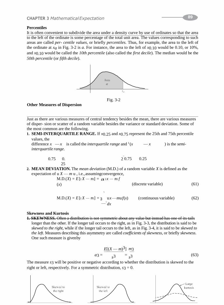
89 CHAPTER 3 Mathematical Expectation
Percentiles
It is often convenient to subdivide the area under a density curve by use of ordinates so that the area
to the left of the ordinate is some percentage of the total unit area. The values corresponding to such
areas are called per- centile values, or briefly percentiles. Thus, for example, the area to the left of
the ordinate at xa in Fig. 3-2 is a. For instance, the area to the left of x0.10 would be 0.10, or 10%,
and x0.10 would be called the 10th percentile (also called the first decile). The median would be the
50th percentile (or fifth decile).
Fig. 3-2
Other Measures of Dispersion
Just as there are various measures of central tendency besides the mean, there are various measures of disper- sion or scatter of a random variable besides the variance or standard deviation. Some of
the most common are the following.
1. SEMI-INTERQUARTILE RANGE. If x0.25 and x0.75 represent the 25th and 75th percentile
values, the
difference x — x is called the interquartile range and 1 (x — x ) is the semi-
interquartile range.
0.75 0.
25
2 0.75 0.25
2. MEAN DEVIATION. The mean deviation (M.D.) of a random variable X is defined as the
expectation of u X — m u , i.e., assumingconvergence,
M.D.(X) = E [u X — m u] = a u x — mu f
(x) (discrete variable) (61)
` M.D.(X) = E [u X — mu] = 3
u x — mu f (x)
(continuous variable) (62)
—`dx
Skewness and Kurtosis
1. SKEWNESS. Often a distribution is not symmetric about any value but instead has one of its tails
longer than the other. If the longer tail occurs to the right, as in Fig. 3-3, the distribution is said to be
skewed to the right, while if the longer tail occurs to the left, as in Fig. 3-4, it is said to be skewed to
the left. Measures describing this asymmetry are called coefficients of skewness, or briefly skewness.
One such measure is given by
E[(X — m)3] m3
a3 = s3 =
s3 (63)
The measure s3 will be positive or negative according to whether the distribution is skewed to the
right or left, respectively. For a symmetric distribution, s3 = 0.

90 CHAPTER 3 Mathematical Expectation
Fig. 3-3 Fig. 3-4 Fig. 3-5
2. KURTOSIS. In some cases a distribution may have its values concentrated near the mean so that
the dis- tribution has a large peak as indicated by the solid curve of Fig. 3-5. In other cases the
distribution may be

91 CHAPTER 3 Mathematical Expectation
=
a
d
relatively flat as in the dashed curve of Fig. 3-5. Measures of the degree of peakedness of a
distribution are called coefficients of kurtosis, or briefly kurtosis. A measure often used is given
by
E[(X — m)4] m4
a4 = s4 =
s4 (64)
This is usually compared with the normal curve (see Chapter 4), which has a coefficient of kurtosis
equal to 3. See also Problem 3.41.
SOLVED PROBLEMS
Expectation of random variables
In a lottery there are 200 prizes of $5, 20 prizes of $25, and 5 prizes of $100. Assuming that
10,000 tickets are to be issued and sold, what is a fair price to pay for a ticket?
Let X be a random variable denoting the amount of money to be won on a ticket. The various
values of X together with their probabilities are shown in Table 3-2. For example, the
probability of getting one of the 20 tickets giving a $25 prize is 20 10,000 = 0.002. The >expectation of X in ollars is thus
E(X) = (5)(0.02) + (25)(0.002) + (100)(0.0005) + (0)(0.9775) = 0.2
or 20 cents. Thus the fair price to pay for a ticket is 20 cents. However, since a lottery is
usually designed to raise money, the price per ticket would be higher.
Table 3-2
x (dollars)
5 25 100 0
P(X = x) 0.0 2
0.00 2
0.000 5
0.977 5
Find the expectation of the sum of points in tossing a pair of fair dice.
Let X and Y be the points showing on the two dice. We have
E(X) = E(Y) = 1 ¢1 ≤ + 2¢1 ≤ c ¢1≤ 7 + + 6 =
Then, by Theorem
3-2,
f (x) 16 6 6 2 2
¢ 1
≤
E(X +2 Y) = E4(X) + E(Y) = 7 + 3
3.3. Find the expectation of a discrete random variable X whose proba4bility function is given by
x
We have
+ 8
2 ¢ ≤
4
` ¢
1 ≤
x
1
(x =
1, 2, 3, c)
E(X) = x

92 = 2 + 2 CHAPTER 3 Mathematical Expectation 2 x=1
¢ 1
≤ c
8 1+6
To find this sum, let S = 1
+ 2 ¢ 1
≤ 3 ¢ 1
≤ + 4 ¢ 1
≤ + c The 1
S =
8 16 1 + 2 ¢
1 ≤ + 3 ¢
1 ≤ + c
nSubtracting,
1 S =
1 +
1 +
1 +
1
+ c= 1
Therefore, S =2.
2 2 4 8 16

93 CHAPTER 3 Mathematical Expectation
4
= =
—
)
3.4. A continuous random variable X has probability density given by
Find (a) E(X), (b)
f (x) =
= 2 e—
2e—2x x > 0 e
0 x Š 0 e—2x 0
E(X2). B ` ¢
` ¢
`
E(X) = 3 xf2(xx) dx = 3 x(2e—2x)dx = 2=3 2xe—2xdx
(a)
—` ≤ ≤R 2 0
3 (x) 2
1 3
= 2 B(x2)¢
e—2x ≤
0
— (1)
¢ e—
2x ≤
¢ e—2x
≤R 2 ` 1
(b E(X2) =
` x2f (x) dx = 2
—` 0 —2
`x2e —2x dx
3.5. The joint density function of two random var—ia
(b2lxe)s X a4nd Y+is(g2i)ven—b8y =
2 xy>96 0 < x < 4, 1 < y < 5
0
f (x, y) = e 0 otherwise x ¢
xy ≤
8
F(aind (a) E(X ), (b) E(Y ), (c) E(XY ), (d) E(2X + 3Y).
)
5
96 dx dy = 3
(b) E(X) =
` ` 3 34
3 3
x 0 y 1
xf (x, y) dx dy =
96 dx dy =
9
3` 3` 3 35 xy 31 —` 4—` ¢ ≤
E(Y) = yf (x, y) dxdy = y —` —` x = 0 y 5= 1 xy
¢
xy ≤248
`
(c) E(XY) =
` 4
(xy) f (x, y) dxdy = (xy)
4 y = 1
5 96
dx dy = 27
47
3 3 3 3
(d E(2X + 3Y)
) = 3
—` —` x = 03
` ` (2x + 3y) f (x, y) dx
3 dy =
3
(2x + 3y) 96
y =¢1 ≤
dx dy = 3
Another method
—` —` x
=
0
E(XY) = E(X)E(Y) = ¢ ≤¢ ≤
8 31 248
= (c) Since X and Y are independent, we have, using parts=(a) and (b),
3 839 27931 3 47
E(2X + 3Y) = 2E(X) + 3E(Y) = 2 ¢ ≤ + 3 ¢ ≤ 3.6. P(Ldre)otvBfey(TTxhh,eeyoo)rreebmmes3t3h--2e1, japonadigne3t-72p7,r.poabgaesb7il6i–ty77f,utongcettihoenr woifthX(aa) nanddY(b,)a, ssumed discrete. Then
E(X + Y) =a a(x + y) f (x, y)
x y
= a axf (x, y) + a ayf (x, y)
x y x y = E(X) + E(Y)
If either variable is continuous, the proof goes through as before, with the appropriate
summations replaced by
integrations. Note that the theorem is true whether or not X and Y are independent.

94 CHAPTER 3 Mathematical Expectation
¢ ≤
3
Prove Theorem 3-3, page 77.
Let f (x, y) be the joint probability function of X and Y, assumed discrete. If the variables X and
Y are independent,
we have f (x, y) = f1 (x) f2 ( y). Therefore,
B R
a
E(XY) = a a xyf (x, y) = a a xyf1(x) f2 ( y)
x y x y
= a xf1(x)ayf2( y)
x y
= [(xf1(x)E( y)]
x
= E(X)E(Y)
If either variable is continuous, the proof goes through as before, with the appropriate
summations replaced by
integrations. Note that the validity of this theorem hinges on whether f (x, y) can be expressed
as a function of x
multiplied by a function of y, for all x and y, i.e., on whether X and Y are independent. For
dependent variables it is not true in general.
6 >
Variance and standard deviation
3.8. (Fai)nd
RT(heaef)net,hrbrey
invTaghrei
taoonrec
Pmer,o3(bb-4)l,eth
me s
3t.a2n,dward
e dheavviaetiEon
(Xo)f t
=he
Es(uYm)
o=bt1ained in tossing a pair of fair dice.
¢ ≤ ¢ ¢ ≤
Var (X) = Var (Y) = 2. Moreover,
6 2
E(X2) = E(Y2) = 12 1
+ 22 1
+ c+=6122 1
= 91
691 7 2 35
6 6
≤ and, since X and Y are independent, Theorem 3-7 gives
Var (X + Y) = Var (X) +—Var (Y) = 35
6
(b) s X+Y = 2Var (X + Y) 35 = A 6
Find (a) the variance, (b) the standard deviation for the random variable of Problem 3.4.
` ¢ 1
≤ 2
(a) As in Problem 3.4, the mean of X is m = E(X) = 1. Then the variance is
2
Var (X) = E[(X — m)2] = E B¢
X — 1
≤ 2
R
= 2 —
x — 2 f (x) dx
` 1 2
¢ x — ≤ —2x 1
Another
method
By Theorem
= 3 0
3-4,
2 (2e ) dx = 4

95 CHAPTER 3 Mathematical Expectation
Var(X) = E[(X —
m)2] = E(X2) —
[E(X)]2 = 1
— ¢ 1
≤ 2
1
(b) s = 2 Var (X) = A4 = 2
1 1
2 2 =
4

96 CHAPTER 3 Mathematical Expectation
E [ X — m ) + (Y — m )
1)
Prove Theorem 3-4, page 78.
We have
E[(X — m)2] = E(X2 — 2mX + m2) = E(X2) — 2mE(X ) + m2
= E(X2) — 2m2 + m2 = E(X2) — m2
= E(X2) — [E(X)]2
2 Prove Theorem 3-6, page 78.
E [(X — a)2] = E [ 5(X — m) + (m 6— a) ]
= E [(X — m)2 + 2(X — m)(m — a) + (m — a)2]
= E [(X — m)2] + 2(m — a)E(X — m) + (m — a)2
= E [(X — m)2] + (m — a)2
since E(X — m) = E(X ) — m = 0. From this we see that the minimum value of E[(X —
a) 2] occurs when
(m — a)2 = 0> , i.e.,
when a = m.
¢ s ≤ = s [E(X — m)] = s [E(X) — m] = 0
If X* = (X — m) s is a standardized random variable, prove that (a) E(X*) = 0, (b) Var(X*) =
1. (a) E(X*) =
E X — m 1 1
(b) since E(X) =
m. Var (X*) = Var ¢
X — m ≤ =
1 E[(X — m)2] = 1
s s2
3.13. ProvuesiTnhgeoTrehmeo3r-7e,mpa3g-e57,8p. age 78, and the fact that E[(X — m)2] = s2.
(X + Y ) — (mX + mY) ]
Var (X + Y ) = E [5( X Y
2 2] 26 2
= E [5(X — mX) + 2(6X — mX)(Y — mY) + (Y — mY) ]
using the fact
that
= E [(X — mX)2] + 2E[(X — mX)(Y — mY)] + E[(Y —
mY)2]
= Var (X ) + Var(Y )
E[(X — mX)(Y — mY)] = E(X — mX)E(Y — mY) = 0
since X and Y, and therefore X — mX and Y — mY, are independent. The proof of
(19), page 78, follows on
replacing Y by —Y and using Theorem 3-5.
Moments and moment generating functions
Prove the result (26), page 79. ¢
= E r
r ≤ X r—1m + c+ (—1) j ¢
r ≤ X r—j m j
mr = E[(X — m)r] ≤ Xmr—1 + (—1)rmrR
X+ c+ (—
—r—1 1 r j
B ¢
r — 1
n
+ + +
= E(Xr) — r
r—1 c j ¢ r
89
≤ r—jj
¢ ≤ E(X
1
)m
+ (—1) j E(X
CHAPTER 3 Mathematical Expectation )m +
+ c+ (—1)rr—1 ¢ r
≤ E(X )mr—1 + (—1)rmr 1
+ c+ (—1)rr—— 1
j 1rmr + (—1)—rmr
= mr — ¢ r
≤ mr 1m + + (—1) j ¢ r ≤ mr j m j r—
c r—
r—1 r where the last two terms can be combined to give (—l) (r — 1)m .
Prove (a) result (31), (b) result (32), page 79.
(a) Using the power series expansion for eu (3., Appendix A), we have
M (t) = E(etX) = E 1 + tX + t2X2
+ t3X3
+ c
¢ ≤
X 2! 3!
= 1 + tE(X ) + t2
E(X2) + t3
E(X3) + c
2! 3!
= 1 + mt + mr t2
+ mr t3
+ c
2 2! 3 3!
(b) This follows immediately from the fact known from calculus that if the Taylor series of f (t)
about t = a is `
f (t) = a c (t — a)n
n=0 n
2
then
3.16. Prove Theorem 3-9, page 80.
cn =n1! ddt
n
f (t) t=a
Since X and Y are independent, any function of X and any function of Y are independent.
Hence,
MX+Y (t) = E[et(X+Y )] = E(etXetY ) = E(etX )E(etY ) =
MX(t)MY (t) 3.17. The random variable X can assume the values 1 and —1 with probability 1 each. Find (a) the moment gen-
erating function, (b) the first four moments about the origin. 2
(a) E(etX) = et(1)
1 1
2 + et(—1) 2
¢ ≤
= 1
(et + e—t)
¢ ≤
(b) We have
et = 1 + t
t t2
t t
2
t3 t4 c
e—t = 1 — t + 2! 2
2!
—
3! 4!
3 4 — c
3! +
4!
+

98 CHAPTER 3 Mathematical Expectation
Then
(1) 1
(et + e—t) = 1 + t2
+ t4
+ c
2 2! 4!
But
(2) M (t) = 1 + mt + mr t2
+ mr t3
+
mr
t4 + c
X
Then, comparing (1) and (2),
we have
2 3
2! 3!
4 4!
m = 0, m2r = 1, m3r = 0, m4r = 1, c
The odd moments are all zero, and the even moments are all one.


90 CHAPTER 3 Mathematical Expectation
(a) 3
3 ) dx = 2 e3
2 3
2
A random variable X has density function given by
f (x) =
e 2e—2xx Š 0
0 x < 0
Find (a) the moment generating function, (b) the first four moments about the origin.
M(t) = E(etX ) = `
etx f (x) dx 2
t — 2 0
—`
2 — t
= `etx(2e—2x
` (t—2)x dx
= 0 = , 0assuming t < 2
2e(t—2)x ` 2
(b) If |t | < 2 we have 2 = 1
> = 1 +
t +
t2 +
t3 +
t4 + c
But M2 —
(t)t = 11+—mt 2t + mr
t22+ m
4r
t3 8+ mr
16t4 + c
2 2! 3 3! 4 4!
Therefore, on comparing terms, m = 1, mr = 1, mr = 3, mr = 3.
f (x) = e 81 0 Š x Š 3
24x(29 —2x2)>3 4 4 2
Find the first four moments (a) about the origin, (b) about the mean, for a random variable X having den-
sity function
0 otherwise
(a) m1r = E(X) = 4
3 x2(9 — x2) dx =
8 = m
3
81 0 5
mr = E(X2) = 4 3
x3(9 — x2) dx = 3
81 0
mr = E(X3) = 4
3
x4(9 — x2) dx = 216
(b) Using the result (27), pag3e 79, wehave
m = 0
3
81 0 35 1
4 3 27
mr4 = E(X4) = 3 x5(9 — x2) dx =
81 0 2
m2 = 3 — ¢58
≤= 1215 = s2
m = 216
— 3(3) ¢ 8
≤ ¢ 8
≤ 32
3 35 5 + 2
5 3 = —
875
= 27
— 4 ¢ 216
≤¢ 8
≤ + 6(3) ¢ 8
≤ 2
3693
m4 2 35 5
— 3 ¢ 8
≤ 4
5 5 =
8750
Characteristic E(eivX ) = eiv(1) ¢ 1 ≤ iv(—1) ¢ 1 ≤ 1 iv iv f3u.2n0c. tFiionndsthe characteristic function of the random variable X of Problem 3.17.
The characteristic function is given by
2 + e
2 = 2 (e + e ) = cos v

91 CHAPTER 3 Mathematical Expectation
3
3
0
`
0
using Euler’s formulas,
eiu = cos u + i si
nu e—iu = cos u — i sin u
>
with u = v. The result can also be obtained from Problem 3.17(a) on putting t = iv.
Find the characteristic function of the random variable X having density function given by
f (x) = e1 2a Z x Z < a
0 otherwise The characteristic function is given by
Find the characteristic function of the random variable X having density function f (x) = ce–a|x|,
E(eivX) = `
eivx dx 3
= iv
2 = a =
eivx f (x) dx = 1
—` 2a —a
1 eivx a eiav —
e—iav
2a —a 2iav
using Euler’s formulas (see Problem 3.20) with u = av.
—` < x < `, where a > 0, and c is a suitable constant.
Since f (x) is a density function, we must have
`
sin
av
av
3 f (x) dx = 1
so
that
—` 0
c —`
e—aZxZ dx —
`
—a(x)
= c a(— dx + 3 e dx `
E(e 3
B —`
ex) R
) = 3 e f (x) edaxx 0 e—ax ` 2c
B= c a 2 + c —a
2 = —` 0
a = 1R
Then c = a >2. The characteristic function is therefore given by
ivX = 2 iv3x e dx + 3
—` e
dx R
= a 0 2 + a ` 2 =2
2a +3 iveivxe—a(—x—) dx(a+—3eivixve—) a(x) dx
Covariance and correlation coefficient —` 0
`
Prove Theorem 3-14, page 81. a (a+iv)x `
—(a—iv)x0
By definition the covariance of X an—d Y is 0 a a2
sXY = Cova e
((Xa+, ivY)x )0 =+E[(X — m=X)(aY2 —v
m2 Y)] e—(a—iv)x +
= E[XYa — mXY — mYX + mXmY] = 2(a + iv)
—` 2(a — iv)
= E(XY ) — mXE(Y ) — mYE(X ) + E(mXmY)
= E(XY ) — mXmY — mYmX + mXmY
= E(XY ) — mXmY
= E(XY ) — E(X )E(Y )

92 CHAPTER 3 Mathematical Expectation
x y y x
XY 2 2 2 = =
63
= —0.2103 approx.
Prove Theorem 3-15, page 81.
If X and Y are independent, then E(XY) = E(X )E(Y ). Therefore, by Problem 3.23,
sXY = Cov (X, Y ) = E(XY ) — E(X )E(Y ) = 0
3.25. Find (a) E(X), (b) E(Y), (c) E(XY), (d) E(X2), (e) E(Y2), (f) Var (X), (g) Var (Y), (h) Cov (X, Y), (i) r, if the
random variables X and Y are defined as in Problem 2.8, pages 47–48.
(a) E(X ) = a axf (x, y) = ax Bf a (x, y)R
x y x y 58 29 = (0)(6c) + (1)(14c) + (2)(22c) = 58c =
E(Y ) = a a yf (x, y) = a y a f
=
42 21
(b) (x, y) B R
x y y x
= (0)(6c) + (1)(9c) + (2)(12c) + (3)(15c) = 78c = 78
= 13
42 7
(c) E(XY ) = a a
xyf (x, y)
x y = (0)(0)(0) + (0)(1)(c) + (0)(2)(2c) + (0)(3)(3c)
+ (1)(0)(2c) + (1)(1)(3c) + (1)(2)(4c) + (1)(3)(5c)
+ (2)(0)(4c) + (2)(1)(5c) + (2)(2)(6c) + (2)(3)(7c)
= 102c = 102
= 17
= (0)2(6c) + (1)2(14c) + (2)2(22c) = 102c = 102
= 17
42 7
(d) E(X2) =x ay a x2 f(x, y)x = B ay
a x2
f (x, Ry)
42 7
(e) E(Y2) = a a y2 f (x, y) = ay2 Ba f (x, y)R
(g) s2 = Var (Y ) = E(Y2) — [E(Y )]2 = 32
— ¢ 13
≤ 55
2 = (0)2(6c) + (1)2(9c) + (2)2(12c) + (3)2(15c) = 192c = 192
= 32
(h) (f) s = Var(X) = E(X ) — [E(X)] =
177
— ¢
2291≤
42 7
2 7 230= —147
r = XXY
= >147 —270 21441
s = Cov(X, Y ) = E(XY ) — E(X )E(Y ) = 17
— ¢ 29
≤¢ 13
≤
Y 7 7 =
49
20
2 > 255 >49 2230 255
3.26. Work Problem 3.25 if the random variables X and Y are defined as in Problem 2.33, pages 61–63.
(Ui)sing c = 1 s E(X ) = —206 5
(x)(2x + y) dx dy = 268
(a) sXs1Y 230 4341 3
x y
(b)
>210, wehave:
210
E(Y ) = 1
6 3
= 5=
2 0
3 (y)(2x + y) dx dy = 170
210 x
=
2
y = 0 63

93 CHAPTER 3 Mathematical Expectation
3 3
(c) E(XY ) = 1 6 5
(xy)(2x + y) dx dy = 80
210 x = 2 y = 0 7

94 CHAPTER 3 Mathematical Expectation
x = 2
X Y
2
3
(d)
E(X2) = 1
6
3
3 (x2)(2x + y) dx dy = 1220
5
210 x = 2 y = 0 63
(f ) 6 5
(e) E(Y2) = 1
3 3 1175 2 y = 0(y )(2x + y) dx dy =
210 s2 = Var(X ) = E(X 2) — [E(X )]2 =
126 5036
(g) 1220
2
— ¢ 268 ≤
= 3969
X 63 63 = 7938
Y 126 63
—200>3969 = 2
= —2020
= —160,.02321529 approx.
s = Var(Y) = E(Y ) — [E(Y )] =
1175 — ¢ 170 ≤
2
(h) s = Cov(X, Y ) = E(XY ) — E(X )E(Y) =
80 —
200
s¢X2sY 68 ≤¢ 170 ≤ 7 63
= —3969
sXY 25036>3969216,225>7938 22518216,225
Cond(iit)ional e
rx=pectation, variance, and moments
3.27. Find the conditional expectation of Y given X = 2 in Problem 2.8, pages 47–48.
As in Problem 2.27, page 58, the conditional probability function of Y given X = 2 is
4 + y
f ( y u2) =
Then the conditional expectation of Y given X = 2
is
E(Y u X = 2) =
22
y¢4 + y ≤
a 22
y
where the sum isE(tYaku Xen=o2v)e=r a(l0l) ¢y co≤rr+es1p¢ond≤ing to¢ X =≤ 2. T¢his ≤is given by
¢ ≤
3.28. F(ai)nd the conditional expectation of (a) Y given X, (b) X given Y in Pdryo=blem 2.29, pages 58–59.
` ` x 2y 2x
(b) E(Y u X = x) 3 yf2(y u x) dy = y 2
—` 0 x ≤ 1 2x
E(X uY = y) = 3 xf1(x u y) dx = 3 x —` y
1 — y2 dx
32((11——y3) y22)(13(+1 y++yy2)) = =
3.29. Find the conditional variance of Y given X for Problem 2.29, pages 58–59.
The required variance (second moment about the mean) is given by
` x 2 2y u ¢ ≤ ¢ ≤
2 2 3 2 2 32 3 2
dy = 18 2x x2 E[(Y — m ) u X = x] = —` (y — m ) 0f (y x) dy =x y —
where we have used the fact that m = E(Y u X = x) = 2x >3 from Problem 3.28(a).
63
3
¢
4 5 6 7 19
22 22 + 2 22 + 3
22 =
11

95 CHAPTER 3 Mathematical Expectation
2
Chebyshev’s inequality
Prove Chebyshev’s inequality.
We shall present the proof for continuous random variables. A proof for discrete variables
is similar if integrals are replaced by sums. If f (x) is the density function of X, then
s2 = E[(X — m)2] (x — m)2f (x) dx
` 3
= —`

96 CHAPTER 3 Mathematical Expectation
S
Since the integrand is nonnegative, the value of the integral can only decrease when the
range of integration is diminished. Therefore,
s2 Š3
ux — mu ŠP
(x — m)2f (x) d3x Š
ux — mu ŠP
P2f (x) dx =
P2 3
ux —
mu ŠP
f (x) dx
But the last integral is equal to P( u X — mu Š P). Hence,
P( uX — m u Š P) Š s2
For the random variable of Problem 3.18, (a) find P( uPX2
— mu > 1). (b) Use Chebyshev’s
inequality to ob- tain an upper bound on P( u X — mu > 1) and compare with the result in (a).
(a) From Problem 3.18, m = 1 2. Then
P( uX >— m u < 1) = P X — 1
< 1 = P 1 3
2 —
2<
2
Therefo
re
¢ 2 2 ≤ ¢ X < ≤
3>22e—2x dx = 1 — e—3
= 3 0
P ¢ 2 X — 1 2 Š 1 =≤ 1 — (1 — e —)3= e —3= 0.04979
2
(b) From Problem 3.18, s2 = m2r — m2 = 1 4. Chebyshev’s inequality with P = 1 then gives
P( u X — mu Š 1) Š s 2 = 0.25
Comparing with (a), we see that the bound furnished by Chebyshev’s inequality is here
quite crude. In practice, Chebyshev’s inequality is used to provide estimates when it is
inconvenient or impossible to obtain exact values.
Law of large numbers
Prove the law of large numbers stated in Theorem 3-19, page 83.
We
have E(X1) = E(X2) = c = E(Xn) = m
Var (X1) = Var (X2) = c = Var (Xn) = s2
S X + c + X 1 1
Then E ¢ n
n ≤ = E 1 n n = n [E(X1 ) +c¢
≤
+ E(Xn )] = n(nm) = m
Var (Sn) = Var (X1 + c + Xn) = Var (X1) + c + Var (Xn) = ns2
Var ¢ ≤ Var ( ) n 1 s
so that n = n2
> Sn = n
where we have used Theorem 3-5 and an extension of Theorem 3-7.
Therefore, by Chebyshev’s inequality with X = Snn, we have
P ¢ 2 — m 2 Š P ≤ Šn
Sn2nP
s2
Taking the limit as n S `, this lbimecPo¢m2
n S`
ens, as 2requ≤ired, S — m Š P = 0
n
Other measures of central
tendency
2

97 CHAPTER 3 Mathematical Expectation
= e
3.33. The density function of a continuous random variable X is 4x — x2)> 81 0 Š x Š 3
f (x) (9
0 otherwise
(a) Find the mode. (b) Find the median. (c) Compare mode, median, and mean.

98 CHAPTER 3 Mathematical Expectation
81
d B
4x(9 —
(a) The mode is oxb2ta)ined by finding where the density f (x) has a relative maximum. The relative maxima of
f (x) occur where Rthe derivative is zero, i.e.,
= 36 — 12x=2 0
dx 81
Then x = !3 = 1.73 approx., which is the required mode. Note that this does give the maximum since
the second derivative, —24x>81, is negative for x = !3>.2
(b) The median is that value a for which P(X Š a) = 1 . Now, for 0 < a < 3,
4 a 4 ¢
9a2 a4 ≤
P(X Š a) =
81 3 x(9 — x2) dx = 81 2
— 4
Setting this equal to 1>2, we find that 2a4 — 36a2 + 81 = 0
from which
a2 =
36 ±
2
(36)2— 4(2)(81) =
36 ± 2648 = 9 ±
9 22
2(2) 4 2
Therefore, the required median, which must lie betwe2en 0 and 3, is given by
a2 = 9 — 9
2
2
from which a = 1.62 3
2 2 4 3 x5 2 3
(c) approx.
E(X ) = 4
x (9 — x ) dx = ¢ 3x — ≤
0
81 3 81
5
= 1.60
0
which is practically equal to the median. The mode, median, and mean are shown in Fig.
3-6.
Fig. 3-6
3.34. A discrete random>variable has probability function f (x) = 1 >2x where x = 1, 2, ......... Find (a) the mode,
(b) the median, and (c) compare them with the mean.
>
2 could represent the median. For convenience, we choose the midpoint of the interval, (a) The mode is the value x having largest associated probability. In this case it is x = 1, for which the
0

99 CHAPTER 3 Mathematical Expectation
i.e., 3 2.
(c) As found in Problem 3.3, m = 2. Therefore, the ordering of the three measures is just
the reverse of that in Problem 3.33.

8
>
4x
Det1er0mine the (a) 10th, (b) 25th, (c) 75th percentile values foCr tHheAdPisTtrEibRut3ion oMf aPtrohbelmema3t.i3c3a.l Expectation
From Problem 3.33(b) we have
P(X Š a) = 4
¢ 9a2
— a4
≤ = 18a2 — a4
Percentiles
81 2 4 81
(a) The10thpercentileisthevalueofaforwhichP(X Š a)=0.10,i.e.,thesolutionof(18a2 —a4)>81=0.10.
Using the method of Problem 3.33, we find a = 0.68 approx.
(b) The 25th percentile is the value of a such that (>1881 a20—.25, aand4w) e find a = 1.098 a=pprox.
(c) The 75th percentile is the value of a such that>8(118=a02.75—, andaw4e)find a = 2.121 approx.
Other measures of dispersion
Determine, (a) the semi-interquartile range, (b) the mean deviation for the distribution of Problem 3.33.
(a) By Problem 3.35 the 25th and 75th percentile values are 1.098 and 2.121, respectively.
Therefore,
Semi-interquartile range2=.121 — 1.09=80.51 approx.
2 >5. Then
(b) From Problem 3.33 the mean is m = 1.60 = 8
`
Mean deviation = M.D.5E(uX — m u ) = 3 —
u x — mu f(x)dx
= 3 2 x —3 5 2 B
841x (9 — x ) R dx
2
0 3
= 8>5 8
8 4x
3 ¢5 — x ≤B 81 (9 — x2) R dx + 3 ¢ x — 5 ≤B 81 (9 — x 2) R dx
0 8 5
= 0.555 approx.
Skewness and kurtosis
Find the coefficient of (a) skewness, (b) kurtosis for the distribution of Problem 3.19.
From Problem 3.19(b) we have
(a) Coefficient of
2 11
s = 25
= m3
32
m3 = —
875
3693 m4
=8750
skewness
(b) Coefficient of
kurtosis
a3 = s3 = —0.1253
= m4
a4 = s4 = 2.172
It follows that there is a moderate skewness to the left, as is indicated in Fig. 3-6. Also
the distribution is somewhat less peaked than the normal distribution, which has a
kurtosis of 3.
Miscellaneous problems
If M(t) is the moment generating function for a random variable X, prove that the mean is m = Mr(0)
and the variance is s2 = Ms(0) — [Mr(0)]2. From (32), page 79, we have on letting r = 1 and r = 2,
m1r = Mr(0) m2r = Ms(0)
Then from
(27)
m =
Mr(0)
m2 = s2 = Ms(0) — [Mr(0)]2

10 CHAPTER 3 Mathematical Expectation
3
2 2
=
Let X be a random variable that takes on the values xk = k with probabilities pk where k = ±1, . . . , ± n.
(a) Find the characteristic function f(v) of X, (b) obtain pk in terms of f(v).
(a) The characteristic function is
f(v) = E(eivX)
n eivx = n pkeikv
= a k pk a
k=—n k=—n
(b) Multiply both sides of the expression in (a) by e—ijv and integrate with respect to v from
0 to 2p. Then 3
2p
e—ijvf(v) dv =
n
k=—n
2p
v= 0
v= 0
2p
pk 3
2 • ei(k—j)v
ei(k—j)v dv = 2ppj
since 3 ei(k—j)v dv =
v= 0
pj = 1
2i(pk — j) 2p
0 = 0 k 2 j
k = j
Therefor
e, 2p e—ijvf(v) dv
3 2p v= 0
or, replacing j
by k, pk =
1
2p 3
e—ikvf(v) dv
2p v= 0
We often call gnp eikv (where n can theoretically be infinite) the Fourier series of f(v) and
p the
k=—n k k
Fourier coefficients. For a continuous random variable, the Fourier series is replaced by
the Fourier integral (see page 81).
Use Problem 3.39 to obtain the probability distribution of a random variable X whose characteristic
func- tion is f(v) = cos v.
From Problem 3.39
pk = 1
2p e—ikv cos v
dv e—ikv eiv
= 1
3
2p
v= 0
2p
v= 0
+ e—iv
B R
2 dv
= 1 2p ei(1—k)v dv +
3 1 2p e—i(1+k)v dv
3 4p v= 0 4p v= 0
If k = 1, we find p1 = 1; if k = —1, we find p—1 = 1. For all other values of k, we have p k = 0. Therefore, the
random variable is given by X e
1 probability 1 2
>
2p

10 CHAPTER 3 Mathematical Expectation
—1 probability 12
As a check, see Problem 3.20.
3.41. Find the coefficient of (a) skewness, (b) kurtosis of the distribution defined by the normal curve, having
density
1 —x2>2
f (x) = 22p
e —` < x <
(a) The distribution has the appearance of Fig. 3-7. By symmetry, m1r = m = 0 and mr3 =
0. Therefore the coefficient of skewness is zero.

10 CHAPTER 3 Mathematical Expectation
Y
2 2
`
(b) We
have
Fig. 3-7
2 —x2 2 2
—` 2p 0
x2e—x 2 dx x e
1 ` m = E(X2) = 33 >
>2 dx = 3 >
2
r2 2 ≤ ¢ ≤
2p 2
= 2 v 2e—v dv
1
p 0
= 2 T 3 = 2
? 1
T 1
= 1 ¢
2p p 2
where we have made the
transformation x2 >
2 = v and used prop2er2tieps of the gamma function given in (2) and
x e 2 dx = x4e—x 2 dx
2p (5) of Appendix A. Similarly we obtain 1 4
0
` 2>
r 4 2
m4 = E(X ) = p
v3 2e—v dv 2 ` —`
= 4
3
0
2
¢ 2
>
— 2
x2>
≤
¢ ≤ 3 1
T
= 4
T 5
= 4 ? ?
1 = 3
Now
p 2 p 2 2 2
s2 = E[(X — m) 2] = E(X )2 = mr2 = 1
m4 = E[(X — m)4] = E(X4) = m4r = 3
Thus the coefficient of kurtosis is
3.42. Prove that —1 Š r Š 1 (see page
82).
m4
s4 = 3
For any real constant c, we have
Now the left side can be
written
E[{Y — mY — c(X —
m)}2] Š 0
Y
X ¢ c
— s2 ≤
s
E[(Y — mY)2] + c2E[(X — mX)2] — 2cE[(X — mX)(Y — m ¢)] = s2 + c2s2 — 2csXY
Y X c — s2 ≤
3 3
`

10 CHAPTER 3 Mathematical Expectation
X — s2
= s2 + s2 2 2csXY X
c — = s2 + s2 2 sXY 2 =
s2s2 s—2 s2 X2 XY
X X ssX2 Y 2
X Y XY + s2
X X

10 CHAPTER 3 Mathematical Expectation
0 otherwise
e >
e 5
e
In order for this last quantity to be greater than or equal to zero for every value of c, we must
have
s2 Y
s2s2 — s2 Š 0 or X Š 1
X Y XY s2 s2
X Y
which is equivalent to r2 Š 1 or —1 Š r Š 1.
SUPPLEMENTARY PROBLEMS
Expectation of random variables
—2 prob. 1 3
3.43. Arandomvariable X isdefinedby X = • 3 prob. 1>2. Find (a) E(X ), (b) E(2X + 5), (c) E(X2).
Let X be a random variable defined by1the
pdroebn.s1i>t6y function f (x) = e
3x2 0 Š x Š 1
Find (a) E(X ), (b) E(3X — 2), (c) E(X2). 0
The density function of a random variable X is f (x) = e e—x x Š 0
.
Find (a) E(X ), (b) E(X2), (c) E[(X — 1)2].
What is the expected number of points that will come up in 3 successive tosses of a fair die?
Does your answer seem reasonable? Explain.
A random variable X has the density function f (x) = e—x x Š 0
. Find E(e2X 3).
0 x < 0
Let X and Y be independent random variables each having density function
f (u) = 2e—2u u Š 0
e 0 otherwise
Find (a) E(X + Y ), (b) E(X2 + Y2), (c) E(XY ).
Does (a) E(X + Y ) = E(X ) + E(Y ), (b) E(XY ) = E(X )E(Y ), in Problem 3.48? Explain.
Let X and Y be random variables having joint density function 3 x(x + y) 0 Š x Š 1, 0 Š y Š 2
f (x, y) =
0 otherwise
Find (a) E(X ), (b) E(Y ), (c) E(X + Y ), (d) E(XY ).
Does (a) E(X + Y ) = E(X ) + E(Y ), (b) E(XY ) = E(X )E(Y ), in Problem 3.50? Explain.
Let X and Y be random variables having joint density
f(x, y) = 4xy 0 Š x Š 1, 0 Š y Š 1
0 otherwise

10 CHAPTER 3 Mathematical Expectation
Find (a) E(X ), (b) E(Y ), (c) E(X + Y ), (d) E(XY ).

10 CHAPTER 3 Mathematical Expectation
Does (a) E(X + Y ) = E(X ) + E(Y ), (b) E(XY ) = E(X ) E(Y ), in Problem 3.52? Explain.
1 (2x + y)0 Š x Š 1, 0
Let f (x, y) =
4
Š y Š 2
0 otherwise
. Find (a) E(X ), (b) E(Y ), (c) E(X2), (d) E(Y2),
(e) E(X + Y ), (f ) E(XY ).
Y = e 2 prob. 3>4
1 prob.—
13>2
prob. 1>4
Find (a) E(3X + 2Y), (b) E(2X2 — Y2), (c) E(XY), (d) E(X2Y). Let X and Y be independent random variables
such that 1 prob. 1> 3.56. Let X1, X2, . . . , Xn be n random variablees which are id3entically distributed such that
X = 0 prob. 2>
3
Xk = • prob. 1 3 >
6
Find (a) E(X 2
+ X —1 prob. 1
+ c+ X ), (b) E(X2 + X2 + c+ X2).
l 2 n 1 2 n
Variance and standard deviation
Find (a) the variance, (b) the standard deviation of the number of points that will come up on a
single toss of a
fair die.
Let X be a random variable having density function
1>
Find (a) Var(X ),
(b) sX.
f (x) =
e
4 —2 Š x Š 2
0 otherwise
Let X be a random variable having density function
f (x) = e—x x Š 0
e
0 otherwise
Find (a) Var (X ), (b) sX.
Find the variance and standard deviation for the random variable X of (a) Problem 3.43, (b)
Problem 3.44.
A random variable X has E(X ) = 2, E(X2) = 8. Find (a) Var(X ), (b) sX.
If a random variable X is such that E[(X — 1)2] = 10, E[(X — 2)2] = 6 find (a) E(X ), (b)
Var(X ), (c) sX.
Moments and moment generating functions
X = e
> >
1
2 prob. 1>2
e

10 CHAPTER 3 Mathematical Expectation
and (b) the first four moments about
the origin.
2 prob. 1 2
—1

CHAPTER 3 Mathematical Expectation
(a) Find the moment generating function of a random variable X having density function
f (x)= e 2x> 0 Š x Š 2
0 otherwise
(b) Use the generating function of (a) to find the first four moments about the origin.
Find the first four moments about the mean in (a) Problem 3.43, (b) Problem 3.44.
(a) Find the moment generating function of a random variable having density function
f (x) = e—x x Š 0
e
0 otherwise
and (b) determine the first four moments about the origin.
In Problem 3.66 find the first four moments about the
mean.
Let X have density function f (x)1>
= e (b —
a) a Š x Š b
kth moment about (a) the origin,
(b) the
mean.
0
otherwi
se
. Find the
If M(t) is the moment generating function of the random variable X, prove that the 3rd and
4th moments about the mean are given by
m3 = M-(0) — 3Ms(0)Mr(0) + 2[Mr(0)]3
m4 = M(iv)(0) — 4M-(0)Mr(0) + 6Ms(0)[Mr(0)]2 — 3[Mr(0)]4
Characteristic functions
Find the characteristic function of the random variable X = a prob. p
. e b prob. q = 1 — p
3.71. Find the characteristic function of a random variable X that has density function
1 2a u x>u Š a f (x) = e
0 otherwise
3.72. Find the characteristic function of a random variable with density function
1 prob.
1>
2
f (x) = e>x 2 0 Š x Š 2
0 otherwise
function of the random variable 2
X1 + X2 + c + Xn
3.73. Let Xk = e —1 prob. 1> be independent random variables (k = 1, 2, . . . , n). Prove that the characteristic
n
>!
is [cos (v n)]n.
Prove that as n S ` the characteristic function of Problem 3.73 approa> ches e—v2 2. (Hint:
Take the logarithm of the characteristic function and use L’Hospital’s rule.)

102 CHAPTER 3 Mathematical Expectation
Covariance and correlation coefficient
Let X and Y be random variables having joint density function
f (x, y) = x + y 0 Š x Š 1, 0 Š y Š 1
e 0 otherwise
Find (a) Var (X ), (b) Var (Y ), (c) sX, (d) sY, (e) sXY, (f ) r.
Work Problem 3.75 if the joint density function is f (x, y) = e—(x+y) x Š 0, y Š 0
. e
0 otherwise
Find (a) Var(X), (b) Var(Y ), (c) sX, (d) sY, (e) sXY, (f ) r, for the random variables of Problem
2.56.
Work Problem 3.77 for the random variables of Problem 2.94.
Find (a) the covariance, (b) the correlation coefficient of two random variables X and Y if E(X ) =
2, E(Y ) = 3,
E(XY) = 10, E(X2) = 9, E(Y2) = 16.
The correlation coefficient of two random variables X and Y is —1 while their variances are 3 and
5. Find the 4
covariance.
Conditional expectation, variance, and moments
Let X and Y have joint density function
f (x, y) = x + y 0 Š x Š 1, 0 Š y Š 1
e 0 otherwise
Find the conditional expectation of (a) Y given X, (b) X given Y.
Work Problem 3.81 if f (x, y) = 2e—(x+2y) x Š 0, y Š 0
e
0 otherwise
Let X and Y have the joint probability function given in Table 2-9, page 71. Find the conditional
expectation of
(a) Y given X, (b) X given Y.
Find the conditional variance of (a) Y given X, (b) X given Y for the distribution of Problem 3.81.
Work Problem 3.84 for the distribution of Problem 3.82.
Work Problem 3.84 for the distribution of Problem 2.94.
Chebyshev’s inequality
A random variable X has mean 3 and variance 2. Use Chebyshev’s inequality to obtain an upper
bound for
(a) P( u X —3 u Š 2), (b) P( u X — 3 u Š 1).
Prove Chebyshev’s inequality for a discrete variable X. (Hint: See Problem 3.30.)
A random variable X has the density function f (x) = 1 e—|x|, —` < x < `. (a) Find P( u X — mu
> 2). (b) Use 2
Chebyshev’s inequality to obtain an upper bound on P(u X — m u > 2) and compare with the

CHAPTER 3 Mathematical Expectation
result in (a).

103 CHAPTER 3 Mathematical Expectation
Law of large
numbers
lim P ¢ 2 Sn 2 ≤
3.90. Show that the (weak) law of large numbers can be stated as
nS` n — m < P = 1
and interpret.
3.91. Let Xk (k = 1, . . . , n) be n independent random variables such that
X = e 1 prob. p
k 0 prob. q = 1 — p
¢ 2 2 ≤
Sn = X1 + c + X ?
(a) If we interpret Xk to be the number of heads on the kth toss of a coin, what interpretation can be given to
n
(b) Show that the law of large numbers in this case reduces to
and interpret this result.
Other measures of central
tendency
lim P nS`
Sn
n — p Š P = 0
Find (a) the mode, (b) the median of a random variable X having density function
f (x) = e—xx Š 0
e
0 otherwise
and (c) compare with the mean.
Work Problem 3.100 if the density function is
f (x) = 4x(1 — x2) 0 Š x Š 1
e 0 otherwise
Find (a) the median, (b) the mode for a random variable X definedby
X = 2 prob. 1 3
e >
and (c) compare with the mean. —1 prob. 2> 3
Find (a) the median, (b) the mode of the set of numbers 1, 3, 2, 1, 5, 6, 3, 3, and (c) compare with
the mean.
Percentiles
Find the (a) 25th, (b) 75th percentile values for the random variable having density function
f (x) = 2(1 — x) 0 Š x Š 1
e 0 otherwise
Find the (a) 10th, (b) 25th, (c) 75th, (d) 90th percentile values for the random variable having
density function
f (x) = ec(x — x3) 0 < x < 1
0 otherwise
where c is an appropriate constant.
Other measures of dispersion

104 CHAPTER 3 Mathematical Expectation
Find (a) the semi-interquartile range, (b) the mean deviation for the random variable of Problem
3.96.
Work Problem 3.98 for the random variable of Problem 3.97.

105 CHAPTER 3 Mathematical Expectation
u
Find the mean deviation of the random variable X in each of the following cases.
(a) f (x) = e e—x x Š 0
0
otherwis
(b) f
(x)
= 1 ,
p(1 + x2) —` < x < .
e
Obtain the probability that the random variable X differs from its mean by more than the
semi-interquartile range in the case of (a) Problem 3.96, (b) Problem 3.100(a).
Skewness and kurtosis
Find the coefficient of (a) skewness, (b) kurtosis for the distribution of Problem 3.100(a). f (x) =
c Q1 — u x
•
If R
a u x u Š a
0 u x u > a
where c is an appropriate constant, is the density function of X, find the coefficient of (a)
skewness,
(b) kurtosis.
Find the coefficient of (a) skewness, (b) kurtosis, for the distribution with density function
f (x) = le— lx x Š 0
e 0 x < 0
> > Miscellaneous problems
>2. Find (a) the mean, (b) the variance, (c) the moment generating function, (d) the characteristic function, Let X be a random variable that can take on the values 2, 1, and 3 with respective
probabilities 1 3, 1 6, and 1
(e) the third moment about the mean.
Work Problem 3.105 if X has density function
f (x) = c(1 — x) 0 < x < 1
e 0 otherwise
where c is an appropriate constant.
Three dice, assumed fair, are tossed successively. Find (a) the mean, (b) the variance of the sum.
Let X be a random variable having density function
f (x) = cx 0 Š x Š 2
e 0 otherwise
where c is an appropriate constant. Find (a) the mean, (b) the variance, (c) the moment
generating function,
(d) the characteristic function, (e) the coefficient of skewness, (f ) the coefficient of kurtosis.
Let X and Y have joint density function
f (x, y) = cxy 0 < x < 1, 0 < y < 1
e0 otherwise
Find (a) E(X2 + Y2), (!b) E( X2 + Y2).
> >

106 CHAPTER 3 Mathematical Expectation
Work Problem 3.109 if X and Y are independent identically distributed random variables
having density function f (u) = (2p)—1 2e—u2 2, —` < u < .

107 CHAPTER 3 Mathematical Expectation
3.61. (a) 4 (b) 2 3.62. (a) 7 2 (b) 15 4 (c)
Let X be a random variable having density
function e1
—1 < x < 1
f (x) = 2
0 otherwise
and let Y = X2. Find (a) E(X), (b) E(Y), (c) E(XY).
ANSWERS TO SUPPLEMENTARY PROBLEMS
33..4435. . (a()a1) 1(b)(7b) (2c) 6(c) 13.44. (a) 3 >4 3(b.)416>.4 10(.c5) 3 >5 3.47. 3
3.48. (a) 1
(b) 1 (c
>
) 1 4
> > > > 3.50. (a) 7 10 (b) 6 5 (c) 19 10 (d) 5 6
3.52. (a) 2
> >
3 (b) 2 3
> >
>
(c) 4 3
>
>
(d) 4 9
> > >
3.54. (a) 7 12 (b) 7 6
> >
(c) 5 12
>
(d) 5 3
>
(e) 7 4 (f ) 2 3
3.55. (a) 5 2 (b) –55 12 (c) 1 4 (d) 1 4
3.56. (a) n (b) 2n 3.57. (a) 35 12 (b) 12
>
> ! >
4
!35>
3.60. (a) Var (X) = 5, sX = !5 (b) Var (X) = 3>80, sX = 215>20
3.58. (a) 4 3 (b) 3 3.59. (a) 1 (b) 1
> > !
3.63. (a) 1(et>2 + e—t>2) = cosh(t>2) (b) m = 01,5m>2r = 1, mr = 0, mr = 1
3.65. (a) m1 = 0, m2 = 5, m3 = —5, m4 = 35 (b) m1 = 0, m2 = 3>80, m3 = —121>160, m4 = 2307>89260 2 3 4
3.66. (a) 1 (1 — t), | t | < 1 (b) m = 1, mr2 = 2, m3r = 6, m4r = 24 3.64. (a) (1 + 2te2t – e2t)>2t2 (b) m = 4>3, mr2 = 2, m3r = 16>5, m4r = 16>3
3.67. m1 = 0, m2 = 1, m3 = 2, m4 = 33
3.68. (a) (bk+1 – ak+1) ( + 1)(b — a) (b) [1 + (—1)k](b — a)k 2k + 1(k + 1)
3.70. pei>va + qeivb 3.71. ( sin av) v 3.72. (e2iv — 2ive2iv — 1)>
> k
>
>
a
2v2

) 1 2 (b)
0
2 (>usel
1
es>s)
2
>
Y 0 1 2
Var (X u Y) 3.89.
5 9 (a)
29 36 e–2 (
7 12 b) 0.5
106 CHAPTER 3 Mathematical Expectation
3.75. (a) 11>144 (b) 11>144 (c) !11>12 (d) ! > > >
(d) !11 12 (e)
(–e1) –
1414>
(6f4)
(–f1)
1–115>73
>960
3.76. (a) 1 (b) 1 (c) 1 (d) 1
(e) 0 (f ) 0
3.77. (a) 73>960 (b) 7>3 960
960
!(c) >
73
3.78. (a) 233>324 (b) 233>324 (c)
!233>18
73
233 (d) !18 >
(e) –91>324 (f ) –91>233
3.79. (a) 4 (b) 4>!35 3.80. —!15>4 3.81. (a) (3x + 2)>(6x + 3) for 0 Š x Š 1 (b) (3y + 2)>(6y + 3) for 0 Š y Š 1
3.82. (a) 1 2 for x Š 0 (b) 1 for y Š 0
3.83. (a) (b)
3.84. (a)
6x2 + 6x + 1
for 0 Š x Š 1 (b) 18(2x + 1)2
6y2 + 6y +1
18(2y + 1)2 for 0 Š y Š 1
9 (b) 1
3.94. (a) does not exist (b) –1 (c) 0 3.95. (a) 3 (b) 3 (c) 3
3.96. (a) 1 — 1 ! >2
2 3 (b) 1
1
3.97. (a) # — (3> !10) (b) #1 — ( 23>2) (c) !1>2 (d) #1 — (1>!10) 3.98. (a) 1 (b) (! 3 — 1)>
4
3.101. (a) (5 — 2 !
>
(c) 16>—81 1 ! >
3) 3
3) 3
3.99. (a) 1 (b) 0.17 (b(c) )(30.—025e1 3.100. (a) 1 — 2e–1 (b) does not exist
3.102. (a) 2 (b) 9 3.103. (a) 0 (b) 24>5a 3.104. (a) 2 (b) 9
Y 0 1 2
E(X u Y) 4 3 7 6 1 2
X 0
1 2
>E(Y u X) 4 3 1 5 7
3.85. (a) 1>
3.86. (a)
(b)
3.87. (a
3.92. (a) + 0
8 15
(b) ln 2 (c) 1
3.93.
(a) 1>!3 (b)
1 — (1 2) (c)

107 CHAPTER 3 Mathematical Expectation
3.105. (a) 7>3 (b) 5>9 (c) (et + 2e2t + 3e3t)>6 (d) (eiv + 2e2iv + 3e3iv)>6 (e) —7>2
3.106. (a) 1>3 (b) 1>18 (c) 2(et — 1 — t)>t2 (d) —2(eiv — 1 — iv)>v2 (e) 1>
7
135
3.107. (a) 21 2 (b) 35 4 (e) —2 !18>15 (f ) 12>5
> >
3.108. (a) 4>3 (b) 2>9 (c) (1 + 2te2t — e2t)>2t2 (d) —(1 + 2ive2iv — e2iv)>2v2
3.109. (a) 1 (b) 8(2 !2 — 1)>15
3.111. (a) 0 (b) 1>3 (c) 0
3.110. (a) 2 (b) !2p>2
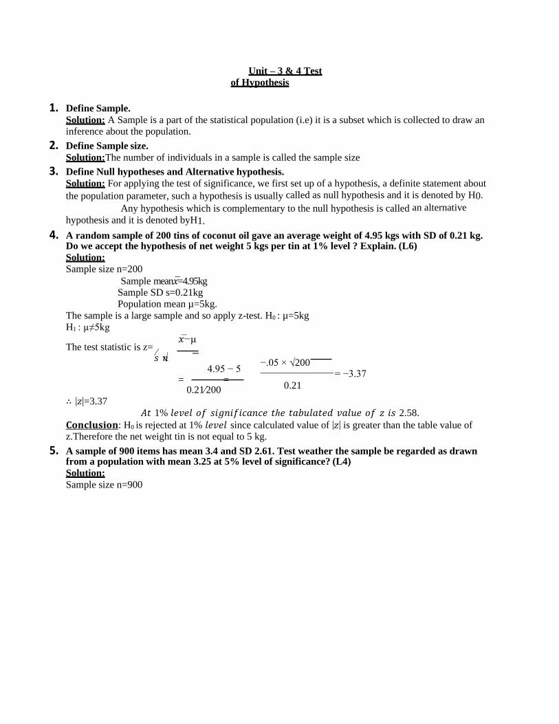
Unit – 3 & 4 Test
of Hypothesis
1. Define Sample.
Solution: A Sample is a part of the statistical population (i.e) it is a subset which is collected to draw an inference about the population.
2. Define Sample size.
Solution:The number of individuals in a sample is called the sample size
3. Define Null hypotheses and Alternative hypothesis.
Solution: For applying the test of significance, we first set up of a hypothesis, a definite statement about
the population parameter, such a hypothesis is usually called as null hypothesis and it is denoted by H0.
Any hypothesis which is complementary to the null hypothesis is called an alternative
hypothesis and it is denoted byH1.
4. A random sample of 200 tins of coconut oil gave an average weight of 4.95 kgs with SD of 0.21 kg. Do we accept the hypothesis of net weight 5 kgs per tin at 1% level ? Explain. (L6)
Solution:
Sample size n=200
Sample mean��=4.95kg Sample SD s=0.21kg Population mean µ=5kg.
The sample is a large sample and so apply z-test. H0 : µ=5kg
H1 : µ≠5kg
The test statistic is z= ⁄
��−µ
∴ |𝑧|=3.37
𝑠 √𝑛 = =
0.21⁄200
−.05 × √200
= −3.37
0.21
𝐴𝑡 1% 𝑙𝑒𝑣𝑒𝑙 𝑜𝑓 𝑠𝑖𝑔𝑛𝑖𝑓𝑖𝑐𝑎𝑛𝑐𝑒 𝑡ℎ𝑒 𝑡𝑎𝑏𝑢𝑙𝑎𝑡𝑒𝑑 𝑣𝑎𝑙𝑢𝑒 𝑜𝑓 𝑧 𝑖𝑠 2.58.
𝐂𝐨𝐧𝐜𝐥𝐮𝐬𝐢𝐨𝐧: H0 is rejected at 1% 𝑙𝑒𝑣𝑒𝑙 since calculated value of |𝑧| is greater than the table value of z.Therefore the net weight tin is not equal to 5 kg.
5. A sample of 900 items has mean 3.4 and SD 2.61. Test weather the sample be regarded as drawn from a population with mean 3.25 at 5% level of significance? (L4)
Solution:
Sample size n=900
4.95 − 5

⁄
Sample mean��=3.4 Sample
SD s=2.61 Population mean µ=3.25
The sample is a large sample and so apply z-test. H0 : µ=3.25
H1 : µ≠3.25 ��−µ
The test statistic is z= 3.4 − 3.25 0.15 𝑠 √𝑛
= = = 1.72
∴ |𝑧|=1.72 2.61⁄√900 2.61⁄30
𝐴𝑡 1% 𝑙𝑒𝑣𝑒𝑙 𝑜𝑓 𝑠𝑖𝑔𝑛𝑖𝑓𝑖𝑐𝑎𝑛𝑐𝑒 𝑡ℎ𝑒 𝑡𝑎𝑏𝑢𝑙𝑎𝑡𝑒𝑑 𝑣𝑎𝑙𝑢𝑒 𝑜𝑓 𝑧 𝑖𝑠 2.58.
𝐂𝐨𝐧𝐜𝐥𝐮𝐬𝐢𝐨𝐧: H0 is accepted at 1% 𝑙𝑒𝑣𝑒𝑙 since calculated value of |𝑧| is less than the table value of z.Therefore H0 is accepted.
6. A Sample of 400 male students is found to have a mean height of 171.38 cms. Can it be reasonable regarded as a sample from a large population with mean height 171.17 cms and standard deviation
3.30 cms? Justify? (L6)
Solution:
Sample size n=400
Sample mean��=171.38cm Population
SD𝜎=3.30cm Population mean µ=171.17cm
The sample is a large sample and so apply z-test. H0 :
µ=171.17cm H1 : µ≠171.17cm
The test statistic is z= ⁄
𝑥 −µ
0.21 × 20
∴ |𝑧|=1.72
𝑠 √𝑛
=
171.38 − 171.17
=
3.30⁄√400
3.30
= 1.27
𝐴𝑡 5% 𝑙𝑒𝑣𝑒𝑙 𝑜𝑓 𝑠𝑖𝑔𝑛𝑖𝑓𝑖𝑐𝑎𝑛𝑐𝑒 𝑡ℎ𝑒 𝑡𝑎𝑏𝑢𝑙𝑎𝑡𝑒𝑑 𝑣𝑎𝑙𝑢𝑒 𝑜𝑓 𝑧 𝑖𝑠 1.96.
𝑪𝒐𝒏𝒄𝒍𝒖𝒔𝒊𝒐𝒏: H0 is accepted at 5% 𝑙𝑒𝑣𝑒𝑙 since calculated value of |𝑧| is less than the table value of z.Therefore H0 is accepted andµ=171.17cm.
7. The mean of two samples of 1000 and 2000 numbers are respectively 67.5 and 68 inches. Can they be regarded as draws from the same population with SD 2.5 inches? Justify? (L6)
Solution:
𝑥 1=67.5, ��2=68

𝑛1=1000, 𝑛2=2000
Population SD𝜎=2.5
The two given samples are large samples. H0 : µ1=µ2
H1 :µ1 ≠ µ2
The test statistic is z= ��1−��2
67.5−68 =−6.25
𝜎⁄√ 1
+ 1
2.5⁄√ 1
+ 1
∴ |𝑧|=6.25 𝑛1 𝑛 2
100
0
2000
𝐴𝑡 1% 𝑙𝑒𝑣𝑒𝑙 𝑜𝑓 𝑠𝑖𝑔𝑛𝑖𝑓𝑖𝑐𝑎𝑛𝑐𝑒 𝑡ℎ𝑒 𝑡𝑎𝑏𝑢𝑙𝑎𝑡𝑒𝑑 𝑣𝑎𝑙𝑢𝑒 𝑜𝑓 𝑧 𝑖𝑠 2.58. 𝑪𝒐𝒏𝒄𝒍𝒖𝒔𝒊𝒐𝒏: H0 is rejected at 1% 𝑙𝑒𝑣𝑒𝑙 since calculated value of |𝑧| is greater than the table value of z.
∴H0 is rejected at 1% 𝑙𝑒𝑣𝑒𝑙 of significance and so the two samples cannot be regarded as belonging to the
same population.
8. The random samples of sizes 400 and 500 have mean 10.9 and 11.5 respectively. Can the samples be regarded as drawn from the same population with variance 25? Justify? (L6) Solution:
𝑥 1=10.9, ��2=11.5
𝑛1=400, 𝑛2=500
𝜎2=25
The two given samples are large samples. H0 : µ1=µ2
H1 :µ1 ≠ µ2
The test statistic is z= ��1−��2
10.9−11.5 =−2.38
𝜎⁄√ 1
+ 1
5⁄√ 1
+ 1
∴ |𝑧|=2.38 𝑛1 𝑛 2
40 500
0
𝐴𝑡 1% 𝑙𝑒𝑣𝑒𝑙 𝑜𝑓 𝑠𝑖𝑔𝑛𝑖𝑓𝑖𝑐𝑎𝑛𝑐𝑒 𝑡ℎ𝑒 𝑡𝑎𝑏𝑢𝑙𝑎𝑡𝑒𝑑 𝑣𝑎𝑙𝑢𝑒 𝑜𝑓 𝑧 𝑖𝑠 2.58.
𝐂𝐨𝐧𝐜𝐥𝐮𝐬𝐢𝐨𝐧: H0 is accepted at 1% 𝑙𝑒𝑣𝑒𝑙 since calculated value of |𝑧| is less than the table value of z. Therefore the samples come from the population with variance 25.
9. A sample of 26 bulbs given a mean life of 990 hours with a SD of 20 hours. The manufactures claims that the mean life of bulbs is 1000 hours. Is the sample not upto the standard? Justify? (L6) Solution: Sample size n=26< 30(𝑠𝑚𝑎𝑙𝑙 𝑠𝑎𝑚𝑝𝑙𝑒)
Sample mean��=990 Sample SD s=20
=
=

2 ∑
2 ∑
𝑆
Population mean µ=1000 Degrees of
freedom=n-1=26-1=25
Here we know ��,µ,SD and n.Therefore, we use student’s ‘t’ test. H0 : The sample is upto the standard. H1 : The sample is not upto the standard.
��−µ
The test statistic is t=𝑠⁄√𝑛−1
∴ |𝑡|=2.5 (i.e) Calculated t=2.5
990 − 1000 = −2.5
=
20⁄√25
𝐴𝑡 5% 𝑙𝑒𝑣𝑒𝑙 𝑜𝑓 𝑠𝑖𝑔𝑛𝑖𝑓𝑖𝑐𝑎𝑛𝑐𝑒 𝑡ℎ𝑒 𝑡𝑎𝑏𝑢𝑙𝑎𝑡𝑒𝑑 𝑣𝑎𝑙𝑢𝑒 𝑜𝑓 𝑧 𝑎𝑡 25𝑑. 𝑓 𝑖𝑠 2.06
𝐂𝐨𝐧𝐜𝐥𝐮𝐬𝐢𝐨𝐧:H0is rejected as calculated value is greater than the tabulated value. ∴The sample is not
upto the standard.
10. In one sample of 8 observations the sum of the squares of deviations of the sample values from the sample mean was 84.4 and it the other sample of 10 observations it was 102.6. Test whether this difference is significant at 5% level? (L4) Solution:
𝑛1=8, 𝑛2=10
(𝑥−��)2 84.4 𝑆 = =
1 𝑛1−1 =12.057
7
(𝑦−��)2 102.6 𝑆 = = =11.4
2 𝑛2−1 9
H0 :𝑆2 = 𝑆2
1
𝑆2
2 12.057
Now F= 1
=2
2
11.
4
= 1.057
(i.e) calculated F=1.057
Tabulated value of F for(7,9) degrees of freedom is 3.29. Calculated value
F<Tabulated value F
∴We accept the null hypothesis.
11.A sample of size 13 gave an estimates population variance of 3.0, while another sample of size 15
gave an estimate of 2.5. Could both samples be from populations with the same variance. Justify?
(L6)
Solution:
𝑛1=13, 𝑛2=15
𝑆2 = ∑ (𝑥 − ��)2 1 𝑆2 = ∑
2 𝑛1 − 1 (𝑦
− ��)2
𝑛2 − 1
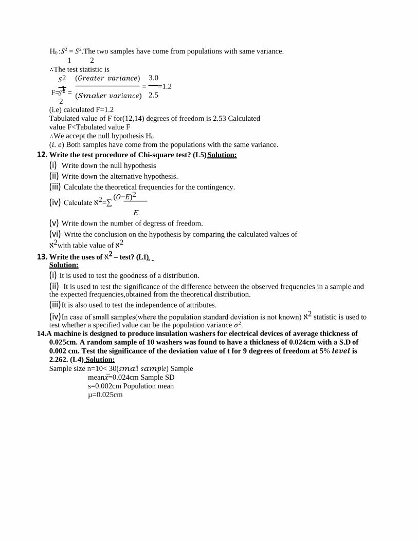
𝑆
H0 :𝑆2 = 𝑆2.The two samples have come from populations with same variance. 1 2
∴The test statistic is
𝑆2
F= 12 =
2
(𝐺𝑟𝑒𝑎𝑡𝑒𝑟 𝑣𝑎𝑟𝑖𝑎𝑛𝑐𝑒)
=
(𝑆𝑚𝑎𝑙𝑙𝑒𝑟 𝑣𝑎𝑟𝑖𝑎𝑛𝑐𝑒)
3.0 =1.2
2.5
(i.e) calculated F=1.2
Tabulated value of F for(12,14) degrees of freedom is 2.53 Calculated
value F<Tabulated value F
∴We accept the null hypothesis H0
(𝑖. 𝑒) Both samples have come from the populations with the same variance.
12. Write the test procedure of Chi-square test? (L5) Solution:
(i) Write down the null hypothesis
(ii) Write down the alternative hypothesis.
(iii) Calculate the theoretical frequencies for the contingency.
(iv) Calculate ℵ2=∑ (𝑂−𝐸)2
𝐸
(v) Write down the number of degress of freedom.
(vi) Write the conclusion on the hypothesis by comparing the calculated values of
ℵ2with table value of ℵ2
13. Write the uses of ℵ2 – test? (L1) Solution:
(i) It is used to test the goodness of a distribution.
(ii) It is used to test the significance of the difference between the observed frequencies in a sample and the expected frequencies,obtained from the theoretical distribution.
(iii) It is also used to test the independence of attributes.
(iv) In case of small samples(where the population standard deviation is not known) ℵ2 statistic is used to test whether a specified value can be the population variance 𝜎2.
14.A machine is designed to produce insulation washers for electrical devices of average thickness of
0.025cm. A random sample of 10 washers was found to have a thickness of 0.024cm with a S.D of
0.002 cm. Test the significance of the deviation value of t for 9 degrees of freedom at 5% 𝒍𝒆𝒗𝒆𝒍 is
2.262. (L4) Solution:
Sample size n=10< 30(𝑠𝑚𝑎𝑙𝑙 𝑠𝑎𝑚𝑝𝑙𝑒) Sample
mean��=0.024cm Sample SD
s=0.002cm Population mean
µ=0.025cm

Degrees of freedom=n-1=10-1=9
Here we know ��,µ,SD and n.Therefore, we use student’s ‘t’ test. H0 : The difference
between �� and µ is not significant
𝑥 −µ
The test statistic is t=𝑠⁄√𝑛−1
= −1.5
∴ |𝑡|=1.5 (i.e) Calculated t=1.5
𝐴𝑡 5% 𝑙𝑒𝑣𝑒𝑙 𝑜𝑓 𝑠𝑖𝑔𝑛𝑖𝑓𝑖𝑐𝑎𝑛𝑐𝑒 𝑡ℎ𝑒 𝑡𝑎𝑏𝑢𝑙𝑎𝑡𝑒𝑑 𝑣𝑎𝑙𝑢𝑒 𝑜𝑓 𝑧 𝑎𝑡 9𝑑. 𝑓 𝑖𝑠 2.06
𝐂𝐨𝐧𝐜𝐥𝐮𝐬𝐢𝐨𝐧:H0 is accepted as calculated value is less than the tabulated value.
PART-B
1. Find student’s t, for the following variate value in a sample of eight -4, -2,- 2,0,2,2,3,3 taking
the mean of the universe to be zero.(L1)
Solution:
∴n=8
∴ µ=0
Number of samples=8
Mean of universe is zero
��=average value of X
(−4)+(−2)+(−2)+0+2+2+3+3
=
8
=0.25
To calculate S,we have the formula
S =√∑(𝑋−��)2
𝑛−1
Hypothesis: There is no significant difference between sample mean and population mean
𝑋 𝑋 − 𝑋 (𝑋 − ��)2
−4 −4.25 18.06
−2 −2.25 5.06
−2 −2.25 5.06
0 −0.25 0.06
2 1.75 3.06
2 1.75 3.06
3 2.75 7.56
3 2.75 7.56

⁄
∑(𝑋 − ��)2 = 49.98
∑(𝑋−��)2 49,48 S =√ = √ =√5.497 =2.658
��−µ t= =
𝑛−1 0.25−0
8−1
𝑆⁄√𝑛
−1 ⁄ =0.248
2.658 √7
Table value=2.26
∴calculated value <tabulated value
∴ Hypothesis is accepted and so there is no significant difference between sample mean and population mean.
2. Ten students are selected at random in a university and their heights are measured in inches as
64,65,65,67,67,69,69,70,72 and 72.Using these data, Discuss the suggestion that the mean height of
the students in the universityis 66.(At 5% level of significance the value of t for 9 d.f is 2.262).(L2)
Solution:
��−µ t= 𝑆 √𝑛
S =√∑(𝑋−��)2
𝑛−1
��=average value of X 64+65+65+67+67+69+69+70+72+72
=68
=
10
Hypothesis: There is no significant difference between sample height and
population height.
𝑋 𝑋 − 𝑋 (𝑋 − ��)2
64 −4 16
65 −3 9
65 −3 9
67 −1 1
67 −1 1
69 1 1
69 1 1
70 2 4
72 4 16
72 4 16
∑(𝑋 − ��)2 = 74

S=√ =2.867
74 74 =√
10−1 9
Here ��=68, µ = 66, n = 10 68−66 =2.205
𝑡 =
2.867⁄√10
Table value=2.26
∴calculated value <tabulated value,therefore Hypothesis is accepted and the height of population group can be taken as 66.
3. A fertilizer mixing machine is set to give 12kg of nitrate for every quintal bag of fertilizer.Ten
100kg bags are examined.The percentages of nitrate are as follows 11,14,13,12,13,12,13,14,11,12.Is
there reason to belive that the machines is defective? (value of t for 9 d.f is 2.262). Justify? (L6)
Solution:
Hypothesis: There is no significant difference between sample percentage and population percentage.
Here n=10
𝑋=average value of X µ = 12 11+14+13+12+13+12+13+14+11+12
=
10
=12.5
𝑋 𝑋 − 𝑋 (𝑋 − ��)2
11 −1.5 2.25
14 1.5 2.25
13 0.5 0.25
12 −0.5 0.25
13 0.5 0.25
12 −0.5 0.25
13 0.5 0.25
14 1.5 2.25
11 −1.5 2.25
12 −0.5 0.25
To calculate S,we have the formula
S =√∑(𝑋−��)2
=√ 10.5
∑(𝑋 − ��)2 = 10.5
S=1.08 𝑛−1 10−1

2
1
2
��−µ t= =
𝑆⁄√
𝑛
t=1.389
Table value=2.26
12.5−12 × 3
1.08
∴calculated value <tabulated value
∴ Hypothesis is accepted and the machine cannot be believed to be defective.
4. Two random samples drawn from two normal populations aregiven below.Test whether the two
populations have the same variances (L4)
Samples I 20 16 26 27 23 22 18 24 25 19
Samples II 17 23 32 25 22 24 28 6 31 20 33 27
Solution:
Hypothesis: There is no significant difference between variances of the two samples.
By Formula
𝑆2
F= 1
if 𝑆2 > 𝑆2
𝑆2 1 2
𝑆2
= 2
if 𝑆2 > 𝑆2
𝑆2 2 1
𝑤ℎ𝑒𝑟𝑒 𝑆2 =∑
(𝑋1 − ��1)2
Here 𝑛1 = 10, 𝑛2=12
1
𝑛1 − 1
𝑆2 = ∑ (𝑋2 − 𝑋2)2
𝑛2 − 1
Calculating the averages of two samples we get,
��1 = 22, 𝑋2 = 24
𝑋1 𝑋1 − �� 1 (𝑋1 − ��1)2 𝑋2 𝑋2 − ��2 (𝑋2 − 𝑋2)
2
20 −2 4 17 −7 49
16 −6 36 23 −1 1
26 4 16 32 8 64
27 5 25 25 1 1
23 1 1 22 −2 4
22 0 0 24 0 0
18 −4 16 28 4 16
24 2 4 6 −18 324
25 3 9 31 7 49
19 −3 9 33 9 81
20 −4 16

𝑆
27 3 9
∑(𝑋1 − ��1)2 = 120 ∑(𝑋2 − ��2)
2 =614
𝑆2 = ∑
1
(𝑋1 − ��1)
2
𝑛1 − 1
120
=
9
= 13.33
𝑆2 = ∑ (𝑋2 − 𝑋2)2 614 = 55.81 ⇒ 𝑆2 > 𝑆2
=
𝑆2
∴F= 22=
1
2
55.8
1
13.3
3
=4.18
𝑛2 − 1 11 2 2
Degrees of freedom 𝛾1 = 12 − 1 = 11, 𝛾2 = 10 −1 = 9
Table value=3.10
Calculated value > Table value
∴ Hypothesis is rejected.
∴ There is significant difference between the variance.
5. In two groups of ten children each increases in weight due to two different
diets in the same period were in pounds.
8 5 7 8 3 2 7 6 5 7
3 7 5 6 5 4 4 5 3 6
Find whether the variance are significantly different . (L1) Solution :
Ho : there is no significant Diffenence between the variance of the two samples
𝑆 21
F =
If 𝑆2 > 𝑆2= 𝑆 2
𝑖𝑓 𝑆2 > 𝑆2
𝑆22
1 2 22 2 1 1
Where 𝑆2 ∑(𝑋1−��1)
2
Here 𝑛 =10 𝑛 = 10
1 𝑛1−1 1 2
2 ∑(𝑋2−��2)2
𝑆 = 𝑋 =5.8𝑋 =4.8
𝑋1 𝑋1- ��12 (𝑋 − 𝑋 )
𝑛2−1 1 1 1 1 𝑋2 𝑋2- 𝑋2 (𝑋 − 𝑋
) 2 2
𝑆
=
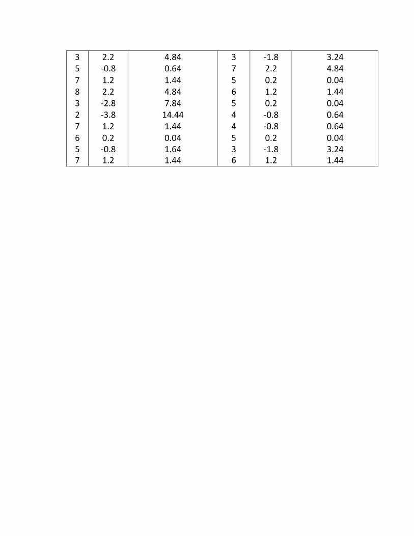
3 5 7 8 3 2 7 6 5 7
2.2 -0.8 1.2 2.2 -2.8 -3.8 1.2 0.2 -0.8 1.2
4.84 0.64 1.44 4.84 7.84
14.44 1.44 0.04 1.64 1.44
3 7 5 6 5 4 4 5 3 6
-1.8 2.2 0.2 1.2 0.2 -0.8 -0.8 0.2 -1.8 1.2
3.24 4.84 0.04 1.44 0.04 0.64 0.64 0.04 3.24 1.44
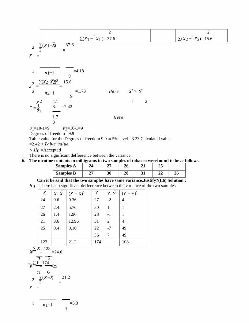
2
2
F = 2
=
2
2
∑(𝑋1 − 𝑋1 ) =37.6
2
∑(𝑋2 − 𝑋2) =15.6
∑(𝑋1−��1)2
𝑆 =
37.6
=
1 𝑛1−1 =4.18
9
∑(𝑋2−��2)2 15.6 𝑆 = =
2 𝑛2−1 =1.73
9 𝐻𝑒𝑟𝑒 𝑆2 > 𝑆2
𝑆 2 1
𝑆2
4.1
8
=
1.7
3
=2.42
1 2
𝐻𝑒𝑟𝑒
𝑣1=10-1=9 𝑣2=10-1=9
Degrees of freedom =9.9
Table value for the Degrees of freedom 9.9 at 5% level =3.23 Calculated value
=2.42 < 𝑇𝑎𝑏𝑙𝑒 𝑣𝑎𝑙𝑢𝑒
∴ 𝐻0 =Accepted
There is no significant deffeerence between the variance .
6. The nicotine contents in milligrams in two samples of tobacco werefound to be as follows.
Samples A 24 27 26 21 25
Samples B 27 30 28 31 22 36
Can it be said that the two samples have same variance.Justify?(L6) Solution :
𝐻0 = There is no significant deffeerence between the variance of the two samples
𝑋 𝑋- �� (𝑋 − X)2 𝑌 𝑌- �� (𝑌 − Y)2
24 0.6 0.36 27 -2 4
27 2.4 5.76 30 1 1
26 1.4 1.96 28 -1 1
21 3.6 12.96 31 2 4
25 0.4 0.16 22 -7 49
36 7 49
123 21.2 174 108
��=∑ 𝑋 123
=24.6
𝑛 5
𝑌=∑ 𝑌
=174
=29
𝑛 6
∑(𝑋−��)2
𝑆 =
21.2
=
1 𝑛1−1 =5.3
4

𝑆2
=∑(𝑌−��)2
= 108
=21.6

2 𝑛2−1 5

𝑆
2 2
𝑆 2 21.6 =4.07 2
F= 2 1
5.3
Calculated value =4.07
Table value of F for (5,4 ) d,f at 5% level is 6.26
∴ calculated value calculated value < Table value.
∴ We accept 𝐻0 𝑖e ; The variance are equal .
7. Two random samples were drawn from two normal populations andtheir values are
A 66 67 75 76 82 84 88 90 92
B 64 66 74 78 82 85 87 92 93 95 97
Test whether the two populations have the same variance at 5% level of Significance.
(L4)
Solution :
There is no significant difference between the variance of the sample .
𝑋 𝑋- �� (𝑋 − X )2 𝑌 𝑌- �� (𝑌 − Y )2
66
67
75
76
82
84
88
90
92
-14
-13
-5
-4
2
4
8
10
12
196
169
25
16
4
16
64
100
144
64
66
74
78
82
85
87
92
93
95
97
-19
-17
-9
-5
-1
2
4
9
10
12
14
361
289
81
25
1
4
16
81
100
144
196
720 0 734 913 0 1298
∑(𝑋−��)2 734 ∑(𝑌−��)2 1298
𝑆 = = =91. 𝑆 = = 1 𝑛1−1 8 2 𝑛2−1
𝑆2 > 𝑆2
=129.8
10
2
𝑆2
1
129.8
F= 2 𝑆=2
1 91.75
=1.41
Degree of freedom is (10,8)
Table value of F =3.34 AT 5% LEVEL
∴ calculated value < Table value.
∴ WE Accepted 𝐻0.
There is no significant difference between the variance of the two population .
=

8. Do the following data give evidence of the effectiveness of
inoculation?Justify?(L6)
Attacked Not attacked
Inoculated 20 300
Not inoculated 80 600
Solution :
𝐻0 : There is no effect inoculation .
Table of observed frequencies is formed from the given data .
TOTAL
20
80
300
600
320
680
TOTAL 100 900 1000
Table of expected frequencies
Total
100×320 900×320 320
=32 =288
1000 1000
100×6800 900×680 680 =68 =612
1000 1000
Total 100 900 1000
𝑐ℎ𝑖 𝑠𝑞𝑢𝑎𝑟𝑒 𝑇𝑎𝑏𝑙𝑒.
O E O-E (𝑂 − 𝐸)2 (𝑂 −
𝐸)2
𝐸 20 32 -12 144 4.5
300 288 12 144 0.50
80 68 12 144 2.12
600 612 -12 144 0.24
(𝑂 − 𝐸)2
∑ 𝐸
= 7.36
Degrees of freedom =(𝑟 − 1)(𝑐 − 1) =(2 − 1)(2 − 1) =1 Table value of ℵ2 for 1 d.f at 5% Level Is 3.841 c.v= 7.36 T.V =3.841 C.V>T.V
∴ Hypothesis is rejected ..There is effect ofinoculation.
9. The following data are collected on two characters
Smokers Non smokers
Literates 83 57

Illiterates 45 68
Based on this ,can you say there is no relation between smoking and literacy. Justify? (L6)
Solution :
𝐻0 : There is no relation between smoking and literacy . Table of
observed frequencies
Total
83
45
57
68
140
113
Total 128 125 253
Table of expected frequencies
Total
128×140 125×140 140
=70.83 =69.17
253 253
100×6800 900×680 113
=57.17 =55.83
1000 1000
Total 128 125 253
𝑐ℎ𝑖 𝑠𝑞𝑢𝑎𝑟𝑒 𝑇𝑎𝑏𝑙𝑒.
O E O-E (𝑂 − 𝐸)2 (𝑂 −
𝐸)2
𝐸 83 70.83 12.17 148.11 2.09
57 69.17 -12.17 148.11 2.14
45 57.17 -12.17 148.11 2.59
68 55.83 12.17 148.11 2.65
(𝑂 −
𝐸)2
∑ 𝐸
= 9. .47
Degrees of freedom =(𝑟 − 1)(𝑐 − 1) =(2 − 1)(2 − 1) =1 Table value of ℵ2 for 1 d.f at 5% Level Is 3.841
c.v= 7.36 T.V =3.841 C.V>T.V
∴ Hypothesis is rejected ..There is a relation between smoking and literacy.
10. The following table gives the number of good and bad parts producedby each of three
shifts in a factory.
Shifts Good Bad
Day 900 130

Evening 700 170
Night 400 200
Test if there is any association between shifts and quality. (L4) Solution :
𝐻0 : There is no sognificant association between shifts and literacy quality. Table of observed
frequencies
Total
900
700
400
130
170
200
1030
870
600
Total 2000 500 2500
Table of expected frequencies.
Total
2000×1030 500×1030 1030
=824 =206
2500 2500
2000×870 500×870 870
=696 =174
2500 2500
2000×600 500×600 600
=480 =120
2500 2500
Total 2000 500 2500
𝑐ℎ𝑖 𝑠𝑞𝑢𝑎𝑟𝑒 𝑇𝑎𝑏𝑙𝑒.
O E O-E (𝑂 − 𝐸)2 (𝑂 − 𝐸)2
𝐸
900 824 76 5776 7.01
130 206 -76 5776 28.04
700 696 4 16 0.02
170 174 -4 16 0.09
400 480 -80 6400 13.33
200 120 -80 6400 53.33
(𝑂 −
𝐸)2
∑ 𝐸
= 9. .47
Degrees of freedom =(𝑟 − 1)(𝑐 − 1) =(3 − 1)(2 − 1) =2 Table value of ℵ2 for 2 d.f at 5% Level Is 5.99
c.v= 101.83 T.V =5.99 C.V>T.V
∴ Hypothesis is rejected ..There is a association between shifts and quality.
11. The number of students in each category is given following table.
Ability in Mathematics

Such in Medical school Low Average High
Low 14 8 5
Average 12 51 11
High 7 24 18
On the basis of contingency table,should we conclude that success in medical school is related
to ability in Mathematics? Test at 0.05 level of
significant. (L4)
Solution :
𝐻0 : There is no sognificant relation between success and abilityTable of observed
frequencies
Total
14
12
7
8
51
24
5
11
18
27
74
49
Total 33 83 34 150
Table ofexpected frequencies.
Total
33×27 83×27 =14.9 34×27 =6.12 27
=5.94
150
150
150
33×74 83×74 =40.9 34×74 =16.7 74
=16.2
150
150
150
33×49 83×49 =27.1 34×49 =11.1 49
=10.7
150 150
150
Total 33 83 34 150
𝑐ℎ𝑖 𝑠𝑞𝑢𝑎𝑟𝑒 𝑇𝑎𝑏𝑙𝑒.
O E O-E (𝑂 − 𝐸)2 (𝑂 − 𝐸)2
𝐸
14
8
5
12
51
11
7
24
18
5.94
14.9
6.12
16.2
40.9
16.7
10.7
27.1
11.1
8.06
-6.90
-1.12
-4.20
10.10
-5.7
-3.7
-3.10
6.90
64.96
47.61
1.25
17.64
102.01
32.49
13.69
9.61
47.61.
10.94
3.20
0.20
1.09
2.49
1.95
1.28
0.35
4.29
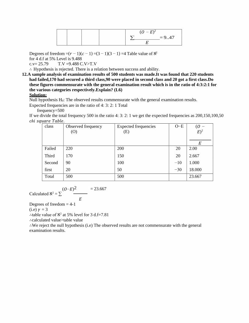
(𝑂 − 𝐸)2
∑ = 9..47 𝐸
Degrees of freedom =(𝑟 − 1)(𝑐 − 1) =(3 − 1)(3 − 1) =4 Table value of ℵ2
for 4 d.f at 5% Level is 9.488 c.v= 25.79 T.V =9.488 C.V>T.V
∴ Hypothesis is rejected. There is a relation between success and ability.
12.A sample analysis of examination results of 500 students was made.It was found that 220 students
had failed,170 had secured a third class,90 were placed in second class and 20 got a first class.Do
these figures commensurate with the general examination result which is in the ratio of 4:3:2:1 for
the various categories respectively.Explain? (L6)
Solution: Null hypothesis H0: The observed results commensurate with the general examination results.
Expected frequencies are in the ratio of 4: 3: 2: 1 Total
frequency=500 If we divide the total frequency 500 in the ratio 4: 3: 2: 1 we get the expected frequencies as 200,150,100,50
𝑐ℎ𝑖 𝑠𝑞𝑢𝑎𝑟𝑒 𝑇𝑎𝑏𝑙𝑒.
class Observed frequency
(O)
Expected frequencies
(E)
O−E (𝑂 −
𝐸)2
𝐸 Failed 220 200 20 2.00
Third 170 150 20 2.667
Second 90 100 −10 1.000
first 20 50 −30 18.000
Total 500 500 23.667
(𝑂−𝐸)2 Calculated ℵ2 = ∑
𝐸 Degrees of freedom = 4-1
(i.e) 𝛾 = 3
= 23.667
∴table value of ℵ2 at 5% level for 3 d.f=7.81
∴calculated value>table value
∴We reject the null hypothesis (i.e) The observed results are not commensurate with the general examination results.

13. On the basis of information given below about the treatment of 200 patients suffering from a disease,state whether the new treatment is comparatively superior to the conventional treatment. (L1)
Favourable Not favourable Total
New 60 30 90
Conventional 40 70 110
Solution:
Null hypothesis H0:No difference between new and conventional treatment (or) New and conventional treatment are independent.
The no. of d.f is (2−1)(2−1)=1
Expected Frequency table:
Total
90×100 90×100 90
=45 =45
100 200
100×110 100×110 110
=55
=55
100 200
Total 100 100 200
𝑐ℎ𝑖 𝑠𝑞𝑢𝑎𝑟𝑒 𝑇𝑎𝑏𝑙𝑒.
Observed frequency
(O)
Expected frequencies
(E)
(𝑂 −
𝐸)2
(𝑂 −
𝐸)2
𝐸 60 45 225 2.00
30 45 225 2.667
40 55 225 1.000
70 55 225 18.000
18.18
(𝑂−𝐸)2 Calculated ℵ2 = ∑
𝐸
= 18.18
∴Table value of ℵ2 at 5% level for 1 d.f=3.841
∴calculated value>table value and so we reject the null hypothesis.
(𝑖. 𝑒)New and conventional treatment are not independent.
14. Give the table for hair colour and eye colour.Find the value of 𝝍𝟐.Is there good association between the two. (L1)
Hair colour
Eye colour Fair Brown Black Total
Blue 15 5 20 40
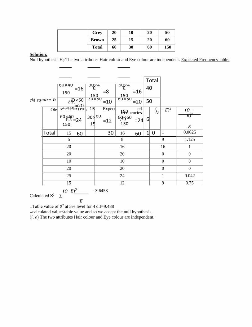
Grey 20 10 20 50
Brown 25 15 20 60
Total 60 30 60 150
Solution:
Null hypothesis H0:The two attributes Hair colour and Eye colour are independent. Expected Frequency table:
𝑐ℎ𝑖 𝑠𝑞
(𝑂−𝐸)2 Calculated ℵ2 = ∑
𝐸
= 3.6458
∴Table value of ℵ2 at 5% level for 4 d.f=9.488
∴calculated value<table value and so we accept the null hypothesis.
(𝑖. 𝑒) The two attributes Hair colour and Eye colour are independent.
Total
𝑢𝑎𝑟𝑒 𝑇𝑎
60×40 =16
150
30×40
=8 150
60×40
=16 150
40
𝑏6𝑙𝑒0.×50
=20
30×50 =10
60×50 =20 50
Obse rv1e5d0frequenc y 150 Expect ed
1fr5e0quencies (
𝑂 − 𝐸)2 (𝑂 −
𝐸)2
𝐸
60×(O6
)0 =24
150
30×
150
60
=12 6(0E×) 60
=24
150 60
Total 15 60 30 16 60 15 0 1 0.0625
5 8 9 1.125
20 16 16 1
20 20 0 0
10 10 0 0
20 20 0 0
25 24 1 0.042
15 12 9 0.75
20 24 16 0.666


172 • CHAPTER 6 STATISTICAL QUALITY CONTROL
000
6
C H A P TER
SSttaattiissttiiccaallQQuuaalliittyyCCoonnttrrooll
Before studying this chapter you should know or, if necessary, review
1. Quality as a competitive priority, Chapter 2, page 00.
2. Total quality management (TQM) concepts, Chapter 5, pages 00 – 00.
LEARNING OBJECTI VES
After studying this chapter you should be able to
Describe categories of statistical quality control (SQC).
Explain the use of descriptive statistics in measuring quality characteristics.
3 Identify and describecauses of variation.
4 Describe the use of controlcharts.
Identify the differences between x-bar, R-, p-, and c-charts.
6 Explain the meaning of process capability and the process capability index.
7 Explain the term Six Sigma.
8 Explain the process of acceptance sampling and describe the use of operating characteristic (OC) curves.
9 Describe the challenges inherent in measuring quality in service organizations.
CHAPTER OUTLINE
What Is Statistical Quality Control? 172
Links to Practice: Intel Corporation 173
Sources of Variation: Common and
Assignable
Causes 174
Descriptive Statistics 174
Statistical Process Control Methods 176
Control Charts for Variables 178
Control Charts for Attributes 184 C-Charts 188
Process Capability 190
Links to Practice: Motorola, Inc. 196
Acceptance Sampling 196
Implications for Managers 203
Statistical Quality Control in Services 204
Links to Practice: The Ritz-Carlton Hotel
Company, L.L.C.; Nordstrom, Inc. 205
Links to Practice: Marriott International, Inc. 205
OM Across the Organization 206 Inside OM 206
Case: Scharadin Hotels 216
Case: Delta Plastics, Inc. (B) 217
171

W e have all had the experience of purchasing a
prod- uct only to discover that it is defective in
some way
or does not function the way it was designed to. This
could be a new backpack with a broken zipper or an
“out of the box” malfunctioning computer printer.
Many of us have struggled to assemble a product the
manufacturer has indicated would need only “minor”
assembly, only to find that a piece of the product is
missing or defective. As consumers, we expect the
products we purchase to func- tion as intended.
However, producers of products know that it is not
always possible to inspect every product and
every aspect of the production process at all times. The challenge is to design
ways to maximize the ability to monitor the quality of products being produced
and eliminate defects. One way to ensure a quality product is to build quality into the process.
Consider Steinway & Sons, the premier maker of pianos used in concert halls all
over the world. Steinway has been making pianos since the 1880s. Since that time
the company’s manufacturing process has not changed significantly. It takes the
company nine months to a year to produce a piano by fashioning some 12,000-
hand crafted parts, carefully measuring and monitoring every part of the process.
While many of Stein- way’s competitors have moved to mass production, where
pianos can be assembled in 20 days, Steinway has maintained a strategy of quality
defined by skill and craftsman- ship. Steinway’s production process is focused on
meticulous process precision and extremely high product consistency. This has
contributed to making its name synony- mous with top quality.
Marketing, Management,
Engineering
€ Statistica1 quality
control (SQC)
The general category of
statistical tools used to
evaluate organizational
quality.
€ Descriptive
statistics Statistics
used to describe
quality characteristics
and relationships.
source, and quality made everyone’s responsibility. However, talking about solving quality problems is not enough. We need specific tools that can help us
make the right quality decisions. These tools come from the area of statistics and
are used to help identify quality problems in the production process as well as in
the product itself. Statistical quality control is the subject of this chapter.
Statistica1 quality control (SQC) is the term used to describe the set of
statistical tools used by quality professionals. Statistical quality control can be
divided into three broad categories:
1. Descriptive statistics are used to describe quality characteristics and
relation- ships. Included are statistics such as the mean, standard deviation,
the range, and a measure of the distribution of data.
WHAT IS STATISTICAL QUALITY CONTROL?
In Chapter 5 we learned that total quality management (TQM) addresses
organiza- tional quality from managerial and philosophical viewpoints. TQM
focuses on customer-driven quality standards, managerial leadership, continuous
improvement, quality built into product and process design, quality identified
problems at the

WHAT IS STATISTICAL QUALITY CONTROL?• 172 • CHAPTER 6 STATISTICAL QUALITY CONTROL
173
2. Statistical process control (SPC) involves inspecting a random sample of
the output from a process and deciding whether the process is producing
products with characteristics that fall within a predetermined range. SPC
answers the question of whether the process is functioning properly or not.
3. Acceptance sampling is the process of randomly inspecting a sample of
goods and deciding whether to accept the entire lot based on the results.
Acceptance sampling determines whether a batch of goods should be
accepted or rejected.
The tools in each of these categories provide different types of information for
use in analyzing quality. Descriptive statistics are used to describe certain quality
characteris- tics, such as the central tendency and variability of observed data.
Although descriptions of certain characteristics are helpful, they are not enough to
help us evaluate whether there is a problem with quality. Acceptance sampling can
help us do this. Acceptance sampling helps us decide whether desirable quality has
been achieved for a batch of products, and whether to accept or reject the items
produced. Although this informa- tion is helpful in making the quality acceptance
decision after the product has been pro- duced, it does not help us identify and
catch a quality problem during the production process. For this we need tools in the
statistical process control (SPC) category.
All three of these statistical quality control categories are helpful in measuring
and evaluating the quality of products or services. However, statistical process
control (SPC) tools are used most frequently because they identify quality
problems during the production process. For this reason, we will devote most of
the chapter to this category of tools. The quality control tools we will be learning
about do not only measure the value of a quality characteristic. They also help us
identify a change or variation in some quality characteristic of the product or
process. We will first see what types of variation we can observe when measuring
quality. Then we will be able to identify specific tools used for measuring this
variation.
Variation in the production
process leads to quality defects
and lack of product consistency.
The Intel Cor- poration, the
world’s largest and most
profitable manufacturer of
microprocessors, understands this.
Therefore, Intel has implemented
a program it calls “copy-exactly”
at all its manufacturing facilities.
The idea is that regardless of
whether the chips are made in
Arizona, New Mexico, Ireland, or
any of its other plants, they are
made in exactly the
same way. This means using the same equipment, the same exact materials, and
workers
performing the same tasks in the exact same order. The level of detail to which the
“copy-exactly” concept goes is meticulous. For example, when a chipmaking
machine was found to be a few feet longer at one facility than another, Intel made
them match. When
water quality was found
to be different at one
facility, Intel instituted a
purifica- tion system to
eliminate any
differences. Even when
a worker was found
polishing equipment in
one direction, he was
asked to do it in the
approved circular
pattern. Why such
attention to exactness of
detail? The reason is to
minimize all variation.
Now let’s look at the
different types of
variation that exist.
LINKS TO PRACTICE
Intel Corporation www.intel.com

€ Statistical process control (SPC)
A statistical tool that involves inspecting a random sample of the output from a
process and deciding whether the process is producing products with
characteristics that fall within a predetermined range.
€ Acceptance sampling The process of randomly inspecting a sampleof goods
and deciding whether to accept the entire lot based on the results.


174 • CHAPTER 6 STATISTICAL QUALITY CONTROL
€ Common
causes of
variation
Random causes that
cannot be identified.
€ Assignable
causes of
variation
Causes that can be
identified and
eliminated.
If you look at bottles of a soft drink in a grocery store, you will notice that no two
bottles are filled to exactly the same level. Some are filled slightly higher and
some slightly lower. Similarly, if you look at blueberry muffins in a bakery, you
will notice that some are slightly larger than others and some have more
blueberries than others. These types of differences are completely normal. No two
products are exactly alike because of slight differences in materials, workers,
machines, tools, and other factors. These are called common, or random, causes
of variation. Common causes of varia- tion are based on random causes that we
cannot identify. These types of variation are unavoidable and are due to slight
differences in processing.
An important task in quality control is to find out the range of natural random
variation in a process. For example, if the average bottle of a soft drink called
Cocoa Fizz contains 16 ounces of liquid, we may determine that the amount of
natural vari- ation is between 15.8 and 16.2 ounces. If this were the case, we
would monitor the production process to make sure that the amount stays within
this range. If produc- tion goes out of this range— bottles are found to contain on
average 15.6 ounces — this would lead us to believe that there is a problem with
the process because the vari- ation is greater than the natural random variation.
The second type of variation that can be observed involves variations where
the causes can be precisely identified and eliminated. These are called assignable
causes of variation. Examples of this type of variation are poor quality in raw
materials, an employee who needs more training, or a machine in need of repair.
In each of these examples the problem can be identified and corrected. Also, if
the problem is allowed to persist, it will continue to create a problem in the
quality of the product. In the ex- ample of the soft drink bottling operation,
bottles filled with 15.6 ounces of liquid would signal a problem. The machine
may need to be readjusted. This would be an assignable cause of variation. We
can assign the variation to a particular cause (ma- chine needs to be readjusted)
and we can correct the problem (readjust the machine).
DESCRIPTIVE STATISTICS Descriptive statistics can be helpful in describing certain characteristics of a
product and a process. The most important descriptive statistics are measures of
central ten- dency such as the mean, measures of variability such as the standard
deviation and range, and measures of the distribution of data. We first review
these descriptive sta- tistics and then see how we can measure their changes.
The Mean
In the soft drink bottling example, we stated that the average bottle is filled
with 16 ounces of liquid. The arithmetic average, or the mean, is a statistic that
measures the central tendency of a set of data. Knowing the central point of a set of
data is highly important. Just think how important that number is when you receive
test scores!
To compute the mean we simply sum all the observations and divide by the
€ Mean (average)
A statistic that
measures the central
tendency of a set of
data.
total number of observations. The equation for computing the mean is
n
\ xi
SOURCES OF VARIATION: COMMON AND ASSIGNABLE CAUSES

172 • CHAPTER 6 STATISTICAL QUALITY CONTROL
x = i=1
n

DESCRIPTIVE STATISTICS• 175
where x = the mean
xi = observation i, i = 1, . . . , n
n = number of observations
The Range and Standard Deviation
In the bottling example we also stated that the amount of natural variation in the
bottling process is between 15.8 and 16.2 ounces. This information provides us
with the amount of variability of the data. It tells us how spread out the data is
around the mean. There are two measures that can be used to determine the
amount of variation in the data. The first measure is the range, which is the
difference between the largest and smallest observations. In our example, the
range for natural variation is 0.4 ounces.
Another measure of variation is the standard deviation. The equation for
comput- ing the standard deviation is
\n(xi — x)2
= i=1
n — 1
€ Range
The difference between
the largest and smallest
observations in a set of
data.
€ Standard deviation
A statistic that measures
the amount of data
dispersion around the
mean.
where o = standard deviation of a sample
x = the mean xi = observation i, i = 1, . . . , n
n = the number of observations in the sample
Small values of the range and standard deviation mean that the observations are
closely clustered around the mean. Large values of the range and standard
deviation mean that the observations are spread out around the mean. Figure 6-1
illustrates the differences between a small and a large standard deviation for our
bottling operation. You can see that the figure shows two distributions, both with
a mean of 16 ounces. However, in the first distribution the standard deviation is
large and the data are spread out far around the mean. In the second distribution
the standard deviation is small and the data are clustered close to the mean.
Normal distributions with
varying standard deviations
Differences between symmetric
and skewed distributions
FIGURE 6-1 FIGURE 6-2

172 • CHAPTER 6 STATISTICAL QUALITY CONTROL
Skewed distribution
Symmetric distribution
15.7 15.8 15.9 16.0 16.1 16.2 16.3
Mean
Small standard deviation Large standard deviation
15.7 15.8 15.9 16.0 16.1 16.2 16.3
Mean
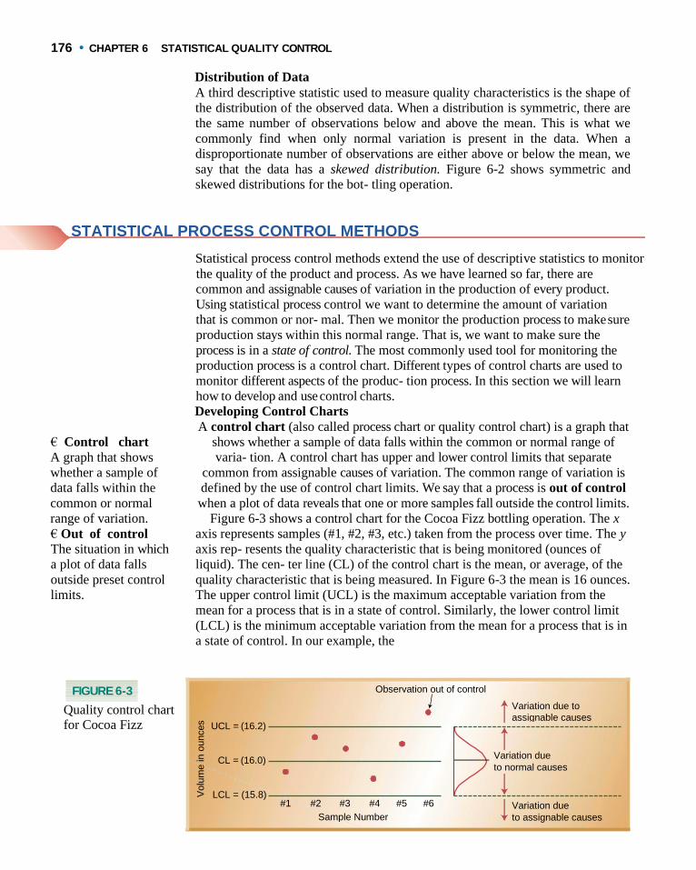
176 • CHAPTER 6 STATISTICAL QUALITY CONTROL
Distribution of Data
A third descriptive statistic used to measure quality characteristics is the shape of
the distribution of the observed data. When a distribution is symmetric, there are
the same number of observations below and above the mean. This is what we
commonly find when only normal variation is present in the data. When a
disproportionate number of observations are either above or below the mean, we
say that the data has a skewed distribution. Figure 6-2 shows symmetric and
skewed distributions for the bot- tling operation.
€ Control chart
A graph that shows
whether a sample of
data falls within the
common or normal
range of variation.
€ Out of control
The situation in which
a plot of data falls
outside preset control
limits.
Statistical process control methods extend the use of descriptive statistics to monitor
the quality of the product and process. As we have learned so far, there are
common and assignable causes of variation in the production of every product.
Using statistical process control we want to determine the amount of variation
that is common or nor- mal. Then we monitor the production process to make sure
production stays within this normal range. That is, we want to make sure the
process is in a state of control. The most commonly used tool for monitoring the
production process is a control chart. Different types of control charts are used to
monitor different aspects of the produc- tion process. In this section we will learn
how to develop and use control charts.
Developing Control Charts
A control chart (also called process chart or quality control chart) is a graph that
shows whether a sample of data falls within the common or normal range of
varia- tion. A control chart has upper and lower control limits that separate
common from assignable causes of variation. The common range of variation is
defined by the use of control chart limits. We say that a process is out of control
when a plot of data reveals that one or more samples fall outside the control limits.
Figure 6-3 shows a control chart for the Cocoa Fizz bottling operation. The x
axis represents samples (#1, #2, #3, etc.) taken from the process over time. The y
axis rep- resents the quality characteristic that is being monitored (ounces of
liquid). The cen- ter line (CL) of the control chart is the mean, or average, of the
quality characteristic that is being measured. In Figure 6-3 the mean is 16 ounces.
The upper control limit (UCL) is the maximum acceptable variation from the
mean for a process that is in a state of control. Similarly, the lower control limit
(LCL) is the minimum acceptable variation from the mean for a process that is in
a state of control. In our example, the
Quality control chart for Cocoa Fizz
FIGURE 6-3
STATISTICAL PROCESS CONTROL METHODS
Observation out of control
Variation due to
assignable causes UCL = (16.2)
CL = (16.0) Variation due
to normal causes
LCL = (15.8) #1 #2 #3 #4 #5 #6
Sample Number
Variation due
to assignable causes
Volu
me
in
ounces
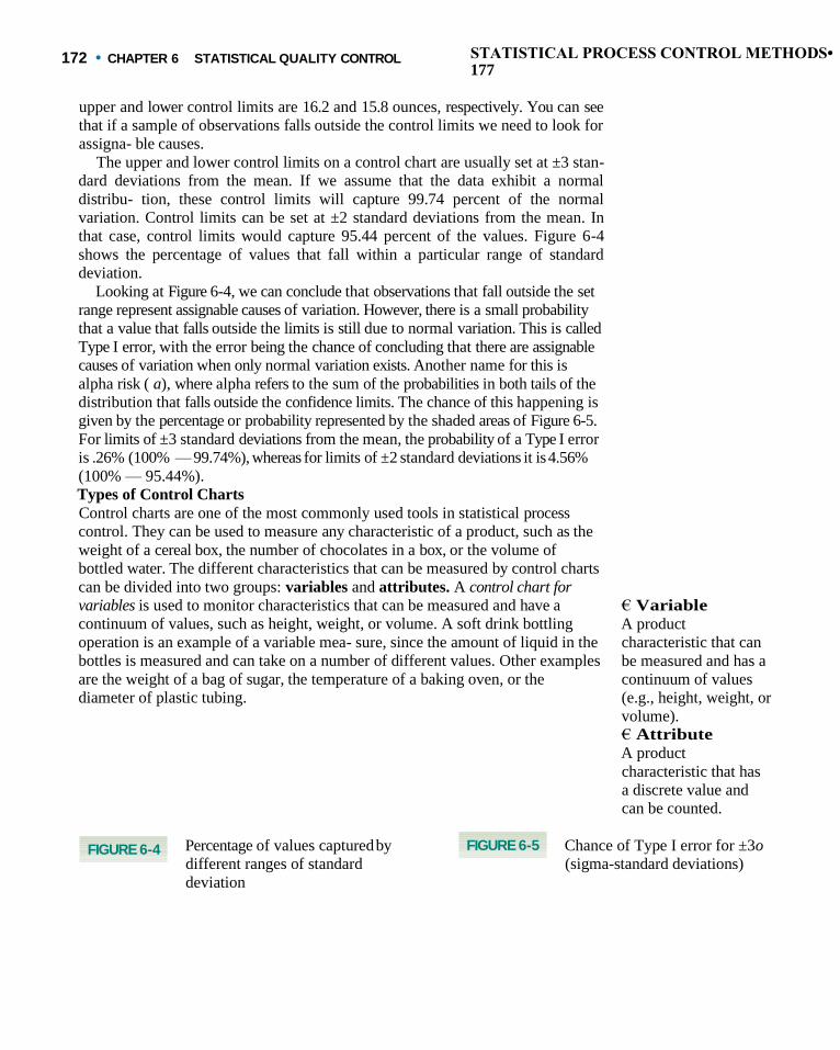
STATISTICAL PROCESS CONTROL METHODS• 172 • CHAPTER 6 STATISTICAL QUALITY CONTROL
177
upper and lower control limits are 16.2 and 15.8 ounces, respectively. You can see
that if a sample of observations falls outside the control limits we need to look for
assigna- ble causes.
The upper and lower control limits on a control chart are usually set at ±3 stan-
dard deviations from the mean. If we assume that the data exhibit a normal
distribu- tion, these control limits will capture 99.74 percent of the normal
variation. Control limits can be set at ±2 standard deviations from the mean. In
that case, control limits would capture 95.44 percent of the values. Figure 6-4
shows the percentage of values that fall within a particular range of standard
deviation.
Looking at Figure 6-4, we can conclude that observations that fall outside the set
range represent assignable causes of variation. However, there is a small probability
that a value that falls outside the limits is still due to normal variation. This is called
Type I error, with the error being the chance of concluding that there are assignable
causes of variation when only normal variation exists. Another name for this is
alpha risk ( a), where alpha refers to the sum of the probabilities in both tails of the
distribution that falls outside the confidence limits. The chance of this happening is
given by the percentage or probability represented by the shaded areas of Figure 6-5.
For limits of ±3 standard deviations from the mean, the probability of a Type I error
is .26% (100% — 99.74%), whereas for limits of ±2 standard deviations it is 4.56%
(100% — 95.44%).
Types of Control Charts
Control charts are one of the most commonly used tools in statistical process
control. They can be used to measure any characteristic of a product, such as the
weight of a cereal box, the number of chocolates in a box, or the volume of
bottled water. The different characteristics that can be measured by control charts
can be divided into two groups: variables and attributes. A control chart for
variables is used to monitor characteristics that can be measured and have a
continuum of values, such as height, weight, or volume. A soft drink bottling
operation is an example of a variable mea- sure, since the amount of liquid in the
bottles is measured and can take on a number of different values. Other examples
are the weight of a bag of sugar, the temperature of a baking oven, or the
diameter of plastic tubing.
€ Variable
A product
characteristic that can
be measured and has a
continuum of values
(e.g., height, weight, or
volume). € Attribute
A product
characteristic that has
a discrete value and
can be counted.
Percentage of values captured by
different ranges of standard
deviation
Chance of Type I error for ±3o
(sigma-standard deviations) FIGURE 6-4 FIGURE 6-5

Type 1 error is .26%
–3 –2 Mean
99.74%
+2 +3 –3 –2 Mean
95.44%
99.74%
+2 +3


178 • CHAPTER 6 STATISTICAL QUALITY CONTROL
A control chart for attributes, on the other hand, is used to monitor
characteristics that have discrete values and can be counted. Often they can be
evaluated with a sim- ple yes or no decision. Examples include color, taste, or
smell. The monitoring of attributes usually takes less time than that of variables
because a variable needs to be measured (e.g., the bottle of soft drink contains
15.9 ounces of liquid). An attribute requires only a single decision, such as yes or
no, good or bad, acceptable or unaccept- able (e.g., the apple is good or rotten, the
meat is good or stale, the shoes have a defect or do not have a defect, the lightbulb
works or it does not work) or counting the number of defects (e.g., the number of
broken cookies in the box, the number of dents in the car, the number of barnacles
on the bottom of a boat).
Statistical process control is used to monitor many different types of variables
and attributes. In the next two sections we look at how to develop control charts
for vari- ables and control charts for attributes.
€ x-bar chart
A control chart used to
monitor changes in the
mean value of a
process.
Control charts for variables monitor characteristics that can be measured and have a
continuous scale, such as height, weight, volume, or width. When an item is
inspected, the variable being monitored is measured and recorded. For example, if we
were produc- ing candles, height might be an important variable. Wecould take
samples of candles and measure their heights. Two of the most commonly used
control charts for variables mon- itor both the central tendency of the data (the
mean) and the variability of the data (ei- ther the standard deviation or the range).
Note that each chart monitors a different type of information. When observed values
go outside the control limits, the process is as- sumed not to be in control.
Production is stopped, and employees attempt to identify the cause of the problem
and correct it. Next we look at how these charts are developed. Mean (x-Bar) Charts
A mean control chart is often referred to as an x-bar chart. It is used to monitor
changes in the mean of a process. To construct a mean chart we first need to
construct the center line of the chart. To do this we take multiple samples and
compute their means. Usually these samples are small, with about four or five
observations. Each sample has its own mean, x. The center line of the chart is then
computed as the mean of all " sample means, where " is the number of samples: x 1 + x 2 + ··· x "
x = "
To construct the upper and lower control limits of the chart, we use the following
formulas: Upper control limit (UCL) = x + z x
Lower control limit (LCL) = x — z x
where x = the average of the sample means
z = standard normal variable (2 for 95.44% confidence, 3 for 99.74%
confidence)
x =standard deviation of the distribution of sample means, /
computed as
o = population (process) standard deviation
n = sample size (number of observations per sample)
Example 6.1 shows the construction of a mean (x-bar) chart.
CONTROL CHARTS FOR VARIABLES
n

CONTROL CHARTS FOR VARIABLES• 179
A quality control inspector at the Cocoa Fizz soft drink company has taken
twenty- five samples with four observations each of the volume of bottles filled.
The data and the computed means are shown in the table. If the standard
deviation of the bottling operation is 0.14 ounces, use this information to develop
control limits of three standard deviations for the bottling operation.
Observations
Sample (bottle volume in ounces) Average Range
22
23
24
25
Total
• Solution
The center line of
the control data is
the average of the
samples:
25
Number 1 2 3 4 x R
1 15.8 5
16.0 2
15.8 3
15.9 3
15.91 0.1 9
2 16.1 2
16.0 0
15.8 5
16.0 1
15.99 0.2 7
3 16.0 0
15.9 1
15.9 4
15.8 3
15.92 0.1 7
4 16.2 0
15.8 5
15.7 4
15.9 3
15.93 0.4 6
5 15.7 4
15.8 6
16.2 1
16.1 0
15.98 0.4 7
6 15.9 4
16.0 1
16.1 4
16.0 3
16.03 0.2 0
7 15.7 5
16.2 1
16.0 1
15.8 6
15.96 0.4 6
8 15.8 2
15.9 4
16.0 2
15.9 4
15.93 0.2 0
9 16.0 4
15.9 8
15.8 3
15.9 8
15.96 0.2 1
10 15.6 4
15.8 6
15.9 4
15.8 9
15.83 0.3 0
11 16.1 1
16.0 0
16.0 1
15.8 2
15.99 0.2 9
12 15.7 2
15.8 5
16.1 2
16.1 5
15.96 0.4 3
13 15.8 5
15.7 6
15.7 4
15.9 8
15.83 0.2 4
14 15.7 3
15.8 4
15.9 6
16.1 0
15.91 0.3 7
15 16.2 0
16.0 1
16.1 0
15.8 9
16.05 0.3 1
16 16.1 2
16.0 8
15.8 3
15.9 4
15.99 0.2 9
17 16.0 1
15.9 3
15.8 1
15.6 8
15.86 0.3 3
18 15.7 8
16.0 4
16.1 1
16.1 2
16.01 0.3 4
19 15.8 4
15.9 2
16.0 5
16.1 2
15.98 0.2 8
20 15.9 2
16.0 9
16.1 2
15.9 3
16.02 0.2 0
21 16.1 16.0 16.0 15.8 16.00 0.2

180 • CHAPTER 6 STATISTICAL QUALITY CONTROL
4
EXAMPLE 6.1
Constructing a Mean (x-Bar) Chart
The control
limits are
UCL = x +
z
LCL = x
— z
x = 15.95 + 3 (.14
)= 16.16
x = 15.95 — 3 (.14
)= 15.74 4

180 • CHAPTER 6 STATISTICAL QUALITY CONTROL
16.20
16.10
16.00
15.90
15.80
15.70
15.60 1 2 3 4 5 6 7 8 9 10 11 12 13 14 15 16 17 18 19 20 21 22 23 24 25
LCL CL UCL Sample Mean
The resulting control chart is:
This can also be computed using a spreadsheet as shown.
A B C D E F G
1
2 X-Bar Chart: Cocoa Fizz
3
F7:
=AVERAGE
(B7:E7)
4
G7:
=MAX(B7:E7)-
MIN(B7:E7)
5 Bottle Volume in
Ounces
6 Sample
Num
7 1
8 2
9 3
1 4
0
1 5
1
1 6
2
1 7
3
1 8
4
1 9
Obs
1
15.85
16.12
16.00
16.20
15.74
15.94
15.75
15.82
16.04
Obs
2
16.02
16.00
15.91
15.85
15.86
16.01
16.21
15.94
15.98
Obs
3
15.83
15.85
15.94
15.74
16.21
16.14
16.01
16.02
15.83
Obs
4
15.9
3
16.0
1
15.8
3
15.9
3
16.1
0
16.0
3
15.8
6
15.9
4
15.9
Averag
e
15.91
16.00
15.92
15.93
15.98
16.03
15.96
15.93
15.96
Range
0.1
9
0.2
7
0.1
7
0.4
6
0.4
7
0.2
0
0.4
6
0.2
0
0.2
Ou
nce
s

CONTROL CHARTS FOR VARIABLES• 181
5 8 1
1 6
1 0
15.64 15.86 15.94 15.8 9
15.83 0.3 0
1 7
1 1
16.11 16.00 16.01 15.8 2
15.99 0.2 9
1 8
1 2
15.72 15.85 16.12 16.1 5
15.96 0.4 3
1 9
1 3
15.85 15.76 15.74 15.9 8
15.83 0.2 4
2 0
1 4
15.73 15.84 15.96 16.1 0
15.91 0.3 7
2 1
1 5
16.20 16.01 16.10 15.8 9
16.05 0.3 1
2 2
1 6
16.12 16.08 15.83 15.9 4
15.99 0.2 9
2 3
1 7
16.01 15.93 15.81 15.6 8
15.86 0.3 3
2 4
1 8
15.78 16.04 16.11 16.1 2
16.01 0.3 4
2 5
1 9
15.84 15.92 16.05 16.1 2
15.98 0.2 8
2 6
2 0
15.92 16.09 16.12 15.9 3
16.02 0.2 0
2 7
2 1
16.11 16.02 16.00 15.8 8
16.00 0.2 3
2 8
2 2
15.98 15.82 15.89 15.8 9
15.90 0.1 6
2 9
2 3
16.05 15.73 15.73 15.9 3
15.86 0.3 2
3 0
2 4
16.01 16.01 15.89 15.8 6
15.94 0.1 5
3 1
2 5
16.08 15.78 15.92 15.9 8
15.94 0.3 0
3 2
15.95 0.2 9
3 3
Number of Samples
2 5
Xbar- bar
R-bar
3 4
Number of Observations per Sample
4
3
5 G32:
=AVERAGE(
G7:G31)
F32:
=AVERAGE(
F7:F31)
3 6

180 • CHAPTER 6 STATISTICAL QUALITY CONTROL
A B C D E F G
39 Computations for X-Bar
Chart
D40: =F32
4 0
Overall Mean (Xbar-
bar) =
15.95
41 Sigma for
Process =
0.14 ounces
D42:
=D41/SQRT(D
34)
4 2
Standard Error of the
Mean =
0.07
4 3
Z-value for control
charts =
3
44
D45:
=D40
45 CL: Center
Line =
15.95
D46: =D40-
D43*D42
4
6 LCL: Lower Control
Limit =
15.74
D47:
=D40+D43*D
42
4 7
UCL: Upper Control
Limit =
16.16
Another way to construct the control limits is to use the sample range as an
estimate of the variability of the process. Remember that the range is simply the
dif- ference between the largest and smallest values in the sample. The spread of
the range can tell us about the variability of the data. In this case control limits
would be constructed as follows:
Upper control limit (UCL) = x + A2 R
Lower control limit (LCL) = x — A2 R where x = average of the samplemeans
R = average range of thesamples A2 = factor obtained from Table 6-1.
Notice that A2 is a factor that includes three standard deviations of ranges and is de- pendent on the sample size being considered.
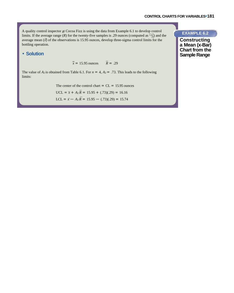
CONTROL CHARTS FOR VARIABLES• 181
25
A quality control inspector at Cocoa Fizz is using the data from Example 6.1 to develop control
limits. If the average range (R) for the twenty-five samples is .29 ounces (computed as 7.17) and the
average mean (x) of the observations is 15.95 ounces, develop three-sigma control limits for the
bottling operation.
• Solution
x = 15.95 ounces R = .29
The value of A2 is obtained from Table 6.1. For n = 4, A2 = .73. This leads to the following
limits:
The center of the control chart = CL = 15.95 ounces
UCL = x + A2 R = 15.95 + (.73)(.29) = 16.16
LCL = x — A2 R = 15.95 — (.73)(.29) = 15.74
EXAMPLE 6.2
Constructing a Mean (x-Bar) Chart from the Sample Range


182 • CHAPTER 6 STATISTICAL QUALITY CONTROL
Factors for three-sigma control limits of x and
R-charts Source: Factors
adapted from the
ASTM Manual on Quality
Control of Materials.
€ Range (R) chart
A control chart that
monitors changes in the
dispersion or variability
of process.
Range (R) Charts
Range (R) charts are another type of control chart for variables. Whereas x-bar
charts measure shift in the central tendency of the process, range charts
monitor the dispersion or variability of the process. The method for developing
and using R-charts is the same as that for x-bar charts. The center line of the
control chart is the average range, and the upper and lower control limits are
computed as fol- lows:
CL = R
UCL = D4 R
LCL = D3 R
TABLE 6-1 Sample Size
n
Factor for x-Chart
A2
Factors for R-Chart
D3 D4
2 1.88 0 3.27
3 1.02 0 2.57
4 0.73 0 2.28
5 0.58 0 2.11
6 0.48 0 2.00
7 0.42 0.08 1.92
8 0.37 0.14 1.86
9 0.34 0.18 1.82
10 0.31 0.22 1.78
11 0.29 0.26 1.74
12 0.27 0.28 1.72
13 0.25 0.31 1.69
14 0.24 0.33 1.67
15 0.22 0.35 1.65
16 0.21 0.36 1.64
17 0.20 0.38 1.62
18 0.19 0.39 1.61
19 0.19 0.40 1.60
20 0.18 0.41 1.59
21 0.17 0.43 1.58
22 0.17 0.43 1.57
23 0.16 0.44 1.56
24 0.16 0.45 1.55
25 0.15 0.46 1.54

CONTROL CHARTS FOR VARIABLES• 183
where values for D4 and D3 are obtained from Table
6-1.

184 • CHAPTER 6 STATISTICAL QUALITY CONTROL
0.60
0.50
0.40
0.30
0.20
0.10
0.00 1 2 3 4 5 6 7 8 9 10 11 12 13 14 15 16 17 18 19 20 21 22 23 24 25
The quality control inspector at Cocoa Fizz would like to develop a range (R)
chart in order to mon- itor volume dispersion in the bottling process. Use the
data from Example 6.1 to develop control limits for thesample range.
• Solution
From the data in Example 6.1 you can see that the average sample range is:
R = 7.17
25
R = 0.29
n = 4
EXAMPLE 6.3
Constructing a Range (R)
Chart
From Table 6-1 for n = 4:
D4 = 2.28 D3 = 0 UCL = D4 R = 2.28 (0.29) = 0.6612 LCL = D3 R = 0 (0.29) = 0
The resulting control chart is:
0.70
LCL CL UCL Sample Mean
Using Mean and Range Charts Together
You can see that mean and range charts are used to monitor different variables.
The mean or x-bar chart measures the central tendency of the process, whereas
the range chart measures the dispersion or variance of the process. Since both
vari- ables are important, it makes sense to monitor a process using both mean
and
Ou
nce
s

CONTROL CHARTS FOR VARIABLES• 183
CONTROL CHARTS FOR ATTRIBUTES
Process shifts captured by x- charts and R-charts
range charts. It is possible to have a shift in the mean of the product but not a
change in the dispersion. For example, at the Cocoa Fizz bottling plant the ma-
chine setting can shift so that the average bottle filled contains not 16.0 ounces,
but
15.9 ounces of liquid. The dispersion could be the same, and this shift would
be detected by an x-bar chart but not by a range chart. This is shown in part (a)
of Figure 6-6. On the other hand, there could be a shift in the dispersion of the
prod- uct without a change in the mean. Cocoa Fizz may still be producing
bottles with an average fill of 16.0 ounces. However, the dispersion of the
product may have in- creased, as shown in part (b) of Figure 6-6. This
condition would be detected by a range chart but not by an x-bar chart.
Because a shift in either the mean or the range means that the process is out of
control, it is important to use both charts to monitor the process.
Control charts for attributes are used to measure quality characteristics that are
counted rather than measured. Attributes are discrete in nature and entail
simple yes-or-no decisions. For example, this could be the number of
nonfunctioning lightbulbs, the proportion of broken eggs in a carton, the
number of rotten ap- ples, the number of scratches on a tile, or the number of
FIGURE 6-6
15.8 15.9 16.0 16.1 16.2 Mean
15.8 15.9 16.0 16.1 16.2 Mean
x–-chart UCL
LCL
UCL R-chart
LCL
(a) Shift in mean detected by x–-chart but not by R-chart
15.8 15.9 16.0 16.1 16.2 Mean
15.8 15.9 16.0 16.1 16.2 Mean
x–-chart UCL
UCL
R-chart
LCL LCL
(b) Shift in dispersion detected by R-chart but not by x–-chart

186 • CHAPTER 6 STATISTICAL QUALITY CONTROL
complaints issued. Two

CONTROL CHARTS FOR ATTRIBUTES• 189
of the most common types of control charts for attributes are p-charts and c-
charts.
P-charts are used to measure the proportion of items in a sample that are
defective. Examples are the proportion of broken cookies in a batch and the pro-
portion of cars produced with a misaligned fender. P-charts are appropriate when
both the number of defectives measured and the size of the total sample can be
counted. A proportion can then be computed and used as the statistic of mea-
surement.
C-charts count the actual number of defects. For example, we can count the
num- ber of complaints from customers in a month, the number of bacteria on a
petri dish, or the number of barnacles on the bottom of a boat. However, we
cannot compute the proportion of complaints from customers, the proportion of
bacteria on a petri dish, or the proportion of barnacles on the bottom of aboat.
Problem-Solving Tip: The primary difference between using a p-chart and a c-
chart is as follows. A p-chart is used when both the total sample size and the
number of defects can be computed. A c-chart is used when we can compute
only the number of defects but cannot compute the propor- tion that is defective.
P-Charts
P-charts are used to measure the proportion that is defective in a sample. The
com- putation of the center line as well as the upper and lower control limits is
similar to the computation for the other kinds of control charts. The center line is
computed as the average proportion defective in the population, p. This is
obtained by taking a
number of samples of observations at random and computing the average value of p
across all samples.
To construct the upper and lower control limits for a p-chart, we use the
following formulas:
UCL = p + z p
LCL = p — z p
where z = standard normal variable
p = the sample proportion defective
p = the standard deviation of the average proportion defective
As with the other charts, z is selected to be either 2 or 3 standard deviations,
depend- ing on the amount of data we wish to capture in our control limits.
Usually, however, they are set at 3.
The sample standard deviation is computed as follows:
€ P-chart
A control chart that
monitors the proportion
of defects in a sample.
where n is the sample size.
p(1 — p)
p = n

186 • CHAPTER 6 STATISTICAL QUALITY CONTROL
EXAMPLE
6.4
Constructinga
p-Chart
A production manager at a tire manufacturing plant has inspected the number of
defective tires in twenty random samples with twenty observations each.
Following are the number of defective tires found in each sample:
Sampl
e
Numbe
r
Number
of
Defective
Tires
Number of
Observatio
ns Sampled
Fractio
n
Defectiv
e
1 3 20 .15
2 2 20 .10
3 1 20 .05
4 2 20 .10
5 1 20 .05
6 3 20 .15
7 3 20 .15
8 2 20 .10
9 1 20 .05
10 2 20 .10
11 3 20 .15
12 2 20 .10
13 2 20 .10
14 1 20 .05
15 1 20 .05
16 2 20 .10
17 4 20 .20
18 3 20 .15
19 1 20 .05 20 1 20 .05
Tota
l
40 400
Construct a three-sigma control chart ( z = 3) with this information.
• Solution
The center line of the chart is
CL = p = total number of defective tires
= 40
= .10
total number of observations400 p(1 — p) (.10)(.90)
p = n = 20
= .067
UCL = p + z
( LCL = p —
z (
p) = .10 + 3(.067) = .301
p) = .10 — 3(.067) = —.101 9: 0

CONTROL CHARTS FOR ATTRIBUTES• 189
In this example the lower control limit is negative, which sometimes occurs
because the computa- tion is an approximation of the binomial distribution.
When this occurs, the LCL is rounded up to zero because we cannot have a
negative control limit.

188 • CHAPTER 6 STATISTICAL QUALITY CONTROL
0.35
0.3
0.25
0.2
0.15
0.1
0.05
0
1 2 3 4 5 6 7 8 9 10 11 12 13 14 15 16 17 18 19 20
Sample Number
LCL CL UCL p
The resulting control chart is as follows:
This can also be computed using a spreadsheet as shown below.
A B C D
1
2 Constructing a p-Chart
3
4 Size of Each
Sample
20
5 Number
Samples
20
6
7
Sample
#
#
Defectiv
e
Tires
Fracti
on
Defecti ve
C8:
=B8/C$
4
8 1 3 0.15
9 2 2 0.10
1 0
3 1 0.05
1 1
4 2 0.10
1 2
5 1 0.05
1 3
6 3 0.15
1 4
7 3 0.15
1 5
8 2 0.10
1 6
9 1 0.05
1 7
1 0
2 0.10
1 1 3 0.15
Fra
ction
De
fective (
p)

CONTROL CHARTS FOR ATTRIBUTES• 189
8 1
1 9
1 2
2 0.10
2 0
1 3
2 0.10
2 1
1 4
1 0.05
2 2
1 5
1 0.05
2 3
1 6
2 0.10
2 4
1 7
4 0.20
2 5
1 8
3 0.15
2 6
1 9
1 0.05
2 7
2 0
1 0.05
A B C D E F
29 Computations for p-Chart
C29:
=SUM(B8:B27)/(C
4*C5)
30 p bar
=
0.100
C30:
=SQRT((C29*(1-
C29))/C4) 31 Sigma_p
=
0.067
32 Z-value for control
charts=
3
33 C33:
=C29
34 CL: Center
Line =
0.100
C34: =MAX(C$29-
C$31*C$30,0) 35 LCL: Lower Control
Limit =
0.000
C35:
=C$29+C$31*C $30
36 UCL: Upper Control
Limit =
0.301

190 • CHAPTER 6 STATISTICAL QUALITY CONTROL
The average n um ber of complaints per week is 44 = 2.2. Therefore, c = 2.2.
art for this example:
7
6
5
4
3
2
LCL CL UCL p
€ C-chart
A control chart
used to monitor
the number of
defects per unit.
C-charts are used to monitor the number of defects per unit. Examples are the
number of returned meals in a restaurant, the number of trucks that exceed their
weight limit in a month, the number of discolorations on a square foot of carpet,
and the number of bacteria in a milliliter of water. Note that the types of units of
measurement we are considering are a period of time, a surface area, or a
volume of liquid.
The average number of defects, c, is the center line of the control chart. The
upper and lower control limits are computed as follows: UCL = c + z
LCL = c — z
Computing a
C-Chart
The number of weekly customer complaints are monitored at a large hotel using a c-chart. Com-
plaints have been recorded over the past twenty weeks. Develop three-sigma control limits using the
following data:
Tota
Week 1 2 3 4 5 6 7 8 9 10 11 12 13 14 15 16 17 18 19
20
No. of
Complain
ts
3 2 3 1 3 3 2 1 3 1 3 4 2 1 1 1 3 2 2
3 44
• Solution 20
UCL = c + z c = 2.2 + 32.2 = 6.65
LCL = c — z c = 2.2 — 32.2 = —2.25 9: 0
As in the previous example, the LCL is negative and should be rounded up to zero. Following is the
control ch
1
0
1 2 3 4 5 6 7 8 9 10 11 12 13 14 15 16 17 18 19 20
Week
C-CHARTS
c
c
EXAMPLE 6.5
Co
mp
lain
ts P
er
Wee
k

C-CHARTS • 189
28 Z-value for control 1.48323 C31: =C26 charts = 29 30
Sigma_c =
97 C32: =MAX(C$26- C$27*C$29,0) C33:
31 2.20 =C$26+C$27*C$29
32 CL: Center 0.00
Line= 6.65
33 LCL: Lower Control
Limit =
34 UCL: Upper Control
Limit =
This can also be computed using a spreadsheet as shown below.
A B
1
2 Computing a C-Chart
3
Number of
4 Wee Complaint
k s
5 1 3
6 2 2
7 3 3
8 4 1
9 5 3
10 6 3
11 7 2
12 8 1
13 9 3
14 10 1
15 11 3
16 12 4
17 13 2
18 14 1
19 15 1
20 16 1
21 17 3
22 18 2
23 19 2
24 20 3
A B C D E F G
26 Computations for a C-
Chart 27 c bar
=
2.2 3
C27: =AVERAGE(B5:B24)
C30:
=SQRT(C27)

190 • CHAPTER 6 STATISTICAL QUALITY CONTROL
Before You Go On
We have discussed several types of statistical quality control (SQC) techniques. One category of SQC techniques
consists of descriptive statistics tools such as the mean, range, and standard deviation. These tools are used to
describe quality characteristics and relationships. Another category of SQC techniques consists of statistical
process control (SPC) methods that are used to monitor changes in the production process. To understand SPC
methods you must understand the differences between common and assignable causes of variation. Common

C-CHARTS • 189
€ Process
capability
The ability of a
production process to
meet or exceed preset
specifications.
€ Product
specifications Preset
ranges of acceptable
quality
characteristics.
So far we have discussed ways of monitoring the production process to ensure that it is
in a state of control and that there are no assignable causes of variation. A critical
aspect of statistical quality control is evaluating the ability of a production process
to meet or exceed preset specifications. This is called process capability. To
understand exactly what this means, let’s look more closely at the term
specification. Product specifica- tions, often called tolerances, are preset ranges of
acceptable quality characteristics, such as product dimensions. For a product to be
considered acceptable, its characteris- tics must fall within this preset range.
Otherwise, the product is not acceptable. Prod- uct specifications, or tolerance
limits, are usually established by design engineers or product design specialists.
For example, the specifications for the width of a machine part may be
specified as 15 inches ±.3. This means that the width of the part should be 15
inches, though it is acceptable if it falls within the limits of 14.7 inches and 15.3
inches. Similarly, for Cocoa Fizz, the average bottle fill may be 16 ounces with
tolerances of ±.2 ounces. Although the bottles should be filled with 16 ounces of
liquid, the amount can be as low as 15.8 or as high as 16.2 ounces.
Specifications for a product are preset on the basis of how the product is going
to be used or what customer expectations are. As we have learned, any
production process has a certain amount of natural variation associated with it. To
be capable of producing an acceptable product, the process variation cannot
exceed the preset spec- ifications. Process capability thus involves evaluating
process variability relative to preset product specifications in order to determine
whether the process is capable of producing an acceptable product. In this section
we will learn how to measure process capability. Measuring Process Capability
Simply setting up control charts to monitor whether a process is in control does
not guarantee process capability. To produce an acceptable product, the process
must be capable and in control before production begins. Let’s look at three
examples of process variation relative to design specifications for the Cocoa Fizz
soft drink company. Let’s say that the specification for the acceptable volume of
liquid is preset at 16 ounces ±.2 ounces, which is 15.8 and 16.2 ounces. In part (a)
of Figure 6-7 the process produces 99.74 percent (three sigma) of the product with
volumes between
and 16.2 ounces. You can see that the process variability closely matches the
pre- set specifications. Almost all the output falls within the preset specification
range.
PROCESS CAPABILITY
causes of variation are based on random causes that cannot be identi fied. A certain amount of common or
normal variation occurs in every process due to differences in materials, workers, machines, and other factors.
Assignable causes of variation, on the other hand, are variations that can be identi fied and eliminated. An im-
portant part of statistical process control (SPC) is monitoring the production process to make sure that the
only variations in the process are those due to common or normal causes. Under these conditions we say that a
production process is in a state ofcontrol. You should also understand the different types of quality control charts that are used to monitor the produc-
tion process: x-bar charts, R-range charts, p-charts, and c-charts.


PROCESS CAPABILITY• 191
Specification Width
LSL USL
15.7 15.8 15.9 16.0 16.1 16.2 16.3
Mean
Process Variability3
Specification Width
LSL USL
15.7 15.8 15.9 16.0 16.1 16.2 16.3
Process Variability 3
FIGURE 6-7
In part (b) of Figure 6-7, however, the process produces 99.74 percent (three
sigma) of the product with volumes between 15.7 and 16.3 ounces. The process
vari- ability is outside the preset specifications. A large percentage of the product
will fall outside the specified limits. This means that the process is not capable of
producing the product within the presetspecifications.
Part (c) of Figure 6-7 shows that the production process produces 99.74
percent (three sigma) of the product with volumes between 15.9 and 16.1 ounces.
In this case the process variability is within specifications and the process
exceeds the minimum capability.
Process capability is measured by the process capability index, Cp, which is
com- puted as the ratio of the specification width to the width of the process
variability:
€ Processcapability
index An index used
to measure process
capability.
specification width
Cp = process width
USL — LSL
= 6
where the specification width is the difference between the upper specification
limit (USL) and the lower specification limit (LSL) of the process. The process
width is
(a) Process variability meets specification width (b) Process variability outside specification width

192 • 15.7 15.8 15.9 16.0 16.1 16.2 16.3
CHAPTER 6 STATISTICMAeLanQUALITY CONTROL
Process Variability
3
(c) Process variability within
specification width
Relationship between process variability and
specification width
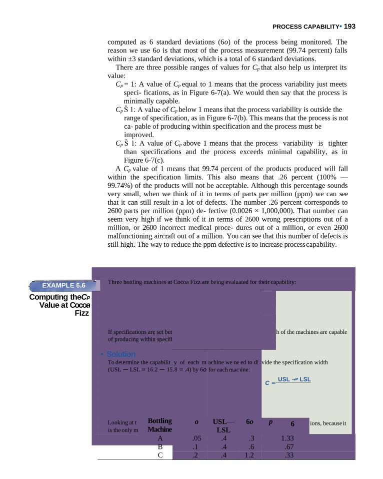
PROCESS CAPABILITY• 193
ween 15.8 and 16.2 ounces, determine whic
cations.
he Cp values, only ma
achine that has a Cp
chine A
value at
is capable of fi
or above 1.
lling bottles within specificat
EXAMPLE 6.6
Computing theCP
Value at Cocoa Fizz
computed as 6 standard deviations (6o) of the process being monitored. The
reason we use 6o is that most of the process measurement (99.74 percent) falls
within ±3 standard deviations, which is a total of 6 standard deviations.
There are three possible ranges of values for Cp that also help us interpret its
value:
Cp = 1: A value of Cp equal to 1 means that the process variability just meets
speci- fications, as in Figure 6-7(a). We would then say that the process is
minimally capable.
Cp Š 1: A value of Cp below 1 means that the process variability is outside the
range of specification, as in Figure 6-7(b). This means that the process is not
ca- pable of producing within specification and the process must be
improved.
Cp Š 1: A value of Cp above 1 means that the process variability is tighter
than specifications and the process exceeds minimal capability, as in
Figure 6-7(c).
A Cp value of 1 means that 99.74 percent of the products produced will fall
within the specification limits. This also means that .26 percent (100% —
99.74%) of the products will not be acceptable. Although this percentage sounds
very small, when we think of it in terms of parts per million (ppm) we can see
that it can still result in a lot of defects. The number .26 percent corresponds to
2600 parts per million (ppm) de- fective (0.0026 × 1,000,000). That number can
seem very high if we think of it in terms of 2600 wrong prescriptions out of a
million, or 2600 incorrect medical proce- dures out of a million, or even 2600
malfunctioning aircraft out of a million. You can see that this number of defects is
still high. The way to reduce the ppm defective is to increase process capability.
Three bottling machines at Cocoa Fizz are being evaluated for their capability:
If specifications are set bet
of producing within specifi
• Solution To determine the capabilit
(USL — LSL = 16.2 — 15
Looking at t Bottling is the only m Machine
Bottling
Machine
A
B
C
y of each m
.8 = .4) by 6o
o
achine we ne
for each mac
USL—
LSL
Standar
Deviatio
.0 5
.1
.2
ed to di
hine:
6o
d
n
h of the machines are capable
vide the specification width
C = USL — LSL
p 6 ions, because it
A .05 .4 .3 1.33 B .1 .4 .6 .67 C .2 .4 1.2 .33

194 • CHAPTER 6 STATISTICAL QUALITY CONTROL
( )
FIGURE 6-8
Cp is valuable in measuring process capability. However, it has one
shortcoming: it assumes that process variability is centered on the speci fication
range. Unfortunately, this is not always the case. Figure 6-8 shows data from the
Cocoa Fizz example. In the figure the specification limits are set between 15.8
and 16.2 ounces, with a mean of 16.0 ounces. However, the process variation is not centered; it has a mean of
15.9 ounces. Because of this, a certain proportion of products will fall outside the
specification range.
The problem illustrated in Figure 6-8 is not uncommon, but it can lead to
mistakes in the computation of the Cp measure. Because of this, another measure for process capability is used more frequently:
Cpk = min USL —
, — LSL
3 3 where µ = the mean of the process
o = the standard deviation of the process
This measure of process capability helps us address a possible lack of centering of
the process over the specification range. To use this measure, the process
capability of each half of the normal distribution is computed and the minimum
of the two is used. Looking at Figure 6-8, we can see that the computed Cp is 1:
Process mean: µ = 15.9
Process standard deviation o = 0.067
LSL = 15.8 USL = 16.2
0.4
Cp = 6(0.067)
= 1
The Cp value of 1.00 leads us to conclude that the process is capable.
However, from the graph you can see that the process is not centered on the
specification range
Process variability not centered
across specification width
Specification Width
LSL USL
15.7 15.8 15.9 16.0 16.1 16.2 16.3
Mean
Process Variability 3

PROCESS CAPABILITY• 195
( )
EXAMPLE 6.7
Computing the Cpk Value
Compute the Cpk measure of process capability for the following machine and interpret the findings.
What value would you have obtained with the Cp measure?
Machine Data: USL = 110
LSL = 50
Process o = 10
Process µ = 70
• Solution To compute the Cpk measure of process capability:
Cpk = min (
(
USL — ,— LSL
3 3
= min 110 — 60 60 — 50
3(10) 3(10) ,
)
) = min (1.67, 0.33)
= 0.33
This means that the process is not capable. The Cp measure of process capability gives us the
following measure,
Cp= 60
= 1 6(10)
leading us to believe that the process is capable. The reason for the difference in the measures is that
the process is not centered on the speci fication range, as shown in Figure 6-9.
and is producing out-of-spec products. Using only the Cp measure would lead to
an incorrect conclusion in this case. Computing Cpk gives us a different answer and leads us to a different conclusion:
Cpk = min USL —
, — LSL
3 3
Cpk = min ( 16.2 — 15.9
, 15.9 — 15.8
)
3(.1) Cpk = min (1.00, 0.33)
.1
Cpk = .3
= .33
3(.1)
The computed Cpk value is less than 1, revealing that the process is not capable.

196 • CHAPTER 6 STATISTICAL QUALITY CONTROL
Six Sigma Quality
The term Six Sigma® was coined by the Motorola Corporation in the 1980s to
describe the high level of quality the company was striving to achieve. Sigma (o)
stands for the number of standard deviations of the process. Recall that ±3 sigma
(o) means that 2600 ppm are defective. The level of defects associated with Six
Sigma is approximately 3.4 ppm. Figure 6-10 shows a process distribution with
quality levels of
±3 sigma (o) and ±6 sigma (o). You can see the difference in the number of
defects produced.
€ Six sigma
quality A high
level of quality
associated with
approximately 3.4
defective parts per
million.
PPM defective for ±3o versus ±6o quality (not to scale)
FIGURE 6-10
LSL USL
Specification Width
30 50 60 75 90 110
Process Variability
Process variability not centered across specification width for
Example 6.7
Process capability of machines
is a critical element of
statistical process control.
FIGURE 6-9
LSL
Number of defects
USL
2600 ppm
3.4 ppm
Mean
3
6

PROCESS CAPABILITY• 197
ACCEPTANCE SAMPLING
To achieve the goal of Six Sigma, Motorola
has instituted a quality focus in every
aspect of its organization. Before a product
is de- signed, marketing ensures that
product char- acteristics are exactly what
customers want. Operations ensures that
exact product char- acteristics can be
achieved through product design, the
manufacturing process, and the materials
used. The Six Sigma concept is an integral
part of other functions as well. It is used in
the finance and accounting depart- ments
to reduce costing errors and the time
required to close the books at the end of the
month. Numerous other companies, such
as General Electric and Texas Instruments,
have followed Motorola’s leadership and
have also instituted the Six Sigma concept.
In fact, the Six Sigma quality standard has
become a benchmark in many industries.
There are two aspects to implementing the Six Sigma concept. The first is the
use of technical tools to identify and eliminate causes of quality problems. These
technical tools include the statistical quality control tools discussed in this
chapter. They also include the problem-solving tools discussed in Chapter 5, such
as cause-and-effect di- agrams, flow charts, and Pareto analysis. In Six Sigma
programs the use of these tech- nical tools is integrated throughout the entire
organizational system.
The second aspect of Six Sigma implementation is people involvement. In Six
Sigma all employees have the training to use technical tools and are responsible
for rooting out quality problems. Employees are given martial arts titles that
reflect their skills in the Six Sigma process. Black belts and master black belts are
individuals who have extensive training in the use of technical tools and are
responsible for carrying out the implementation of Six Sigma. They are
experienced individuals who oversee the measuring, analyzing, process
controlling, and improving. They achieve this by acting as coaches, team leaders,
and facilitators of the process of continuous improve- ment. Green belts are
individuals who have sufficient training in technical tools to serve on teams or on
small individual projects.
Successful Six Sigma implementation requires commitment from top company
leaders. These individuals must promote the process, eliminate barriers to
implemen- tation, and ensure that proper resources are available. A key individual
is a champion of Six Sigma. This is a person who comes from the top ranks of the
organization and is responsible for providing direction and overseeing all aspects
of the process.
Acceptance sampling, the third branch of statistical quality control, refers to the
LINKS TO PRACTICE
Motorola, Inc. www.motorola.com

198 • CHAPTER 6 STATISTICAL QUALITY CONTROL
process of randomly inspecting a certain number of items from a lot or batch in
or- der to decide whether to accept or reject the entire batch. What makes
acceptance

ACCEPTANCE SAMPLING• 197
sampling different from statistical process control is that acceptance sampling is
per- formed either before or after the process, rather than during the process.
Acceptance sampling before the process involves sampling materials received
from a supplier, such as randomly inspecting crates of fruit that will be used in a
restaurant, boxes of glass dishes that will be sold in a department store, or metal
castings that will be used in a machine shop. Sampling after the process involves
sampling finished items that are to be shipped either to a customer or to a
distribution center. Examples in- clude randomly testing a certain number of
computers from a batch to make sure they meet operational requirements, and
randomly inspecting snowboards to make sure that they are not defective.
You may be wondering why we would only inspect some items in the lot and
not the entire lot. Acceptance sampling is used when inspecting every item is not
physi- cally possible or would be overly expensive, or when inspecting a large
number of items would lead to errors due to worker fatigue. This last concern is
especially im- portant when a large number of items are processed in a short
period of time. An- other example of when acceptance sampling would be used is
in destructive testing, such as testing eggs for salmonella or vehicles for crash
testing. Obviously, in these cases it would not be helpful to test every item!
However, 100 percent inspection does make sense if the cost of inspecting an item
is less than the cost of passing on a defec- tive item.
As you will see in this section, the goal of acceptance sampling is to
determine the criteria for acceptance or rejection based on the size of the lot,
the size of the sample, and the level of confidence we wish to attain.
Acceptance sampling can be used for both attribute and variable measures,
though it is most commonly used for attributes. In this section we will look at
the different types of sampling plans and at ways to evaluate how well
sampling plans discriminate between good and bad lots.
Sampling Plans
A sampling plan is a plan for acceptance sampling that precisely specifies the
parame- ters of the sampling process and the acceptance/rejection criteria. The
variables to be specified include the size of the lot ( N), the size of the sample
inspected from the lot (n), the number of defects above which a lot is rejected (c),
and the number of sam- ples that will betaken.
There are different types of sampling plans. Some call for single sampling, in
which a random sample is drawn from every lot. Each item in the sample is
exam- ined and is labeled as either “good” or “bad.” Depending on the number of
defects or “bad” items found, the entire lot is either accepted or rejected. For
example, a lot size of 50 cookies is evaluated for acceptance by randomly
inspecting 10 cookies from the lot. The cookies may be inspected to make sure
they are not broken or burned. If 4 or more of the 10 cookies inspected are bad,
the entire lot is rejected. In this exam- ple, the lot size N = 50, the sample size n =
10, and the maximum number of defects at which a lot is accepted is c = 4. These parameters define the acceptance sampling plan.
Another type of acceptance sampling is called double sampling. This provides an
op- portunity to sample the lot a second time if the results of the first sample are
inconclusive. In double sampling we first sample a lot of goods according to preset
crite- ria for definite acceptance or rejection. However, if the results fall in the
middle range,
Sampling involves randomly
inspecting items from a lot.
€ Sampling plan
A plan for acceptance
sampling that precisely
specifies the
parameters of the
sampling process and
the
acceptance/rejection
criteria.

198 • CHAPTER 6 STATISTICAL QUALITY CONTROL
they are considered inconclusive and a second sample is taken. For example, a
water treatment plant may sample the quality of the water ten times in random
intervals throughout the day. Criteria may be set for acceptable or unacceptable
water quality, such as .05 percent chlorine and .1 percent chlorine. However, a
sample of water con- taining between .05 percent and .1 percent chlorine is
inconclusive and calls for a sec- ond sample of water.
In addition to single and double-sampling plans, there are multiple sampling
plans. Multiple sampling plans are similar to double sampling plans except that
criteria are set for more than two samples. The decision as to which sampling
plan to select has a great deal to do with the cost involved in sampling, the time
consumed by sampling, and the cost of passing on a defective item. In general, if
the cost of collecting a sam- ple is relatively high, single sampling is preferred. An
extreme example is collecting a biopsy from a hospital patient. Because the actual
cost of getting the sample is high, we want to get a large sample and sample only
once. The opposite is true when the cost of collecting the sample is low but the
actual cost of testing is high. This may be the case with a water treatment plant,
where collecting the water is inexpensive but the chemical analysis is costly. In
this section we focus primarily on single sampling plans.
(LTPD)
The upper limit of the percentage of defective items consumers are willing to tolerate.
€ Operating
characteristic (OC)
curve
A graph that shows the
probability or chance
of accepting a lot given
various proportions of
defects in the lot.
€ Acceptablequality
level (AQL)
The small percentage
of defects that
consumers are willing
to accept.
€Lottolerance
percent defective

ACCEPTANCE SAMPLING• 197
Operating Characteristic
(OC) Curves
As we have seen,
different
sampling plans
have different
capabilities for
discriminat- ing
between good
and bad lots. At
one extreme is
100 percent
inspection, which
has perfect
discriminating
power. However,
as the size of the
sample inspected
decreases, so does
the chance of
accepting a
defective lot. We
can show the
discriminating
power of a
sampling plan on
a graph by means
of an operating
characteristic
(OC) curve. This
curve shows the
probability or
chance of
accepting a lot
given various
propor- tions of
defects in the lot.
Figure 6-11
shows a typical
OC curve. The x
axis shows the
percentage of
items that are
defective in a lot.
This is called “lot
quality.” The y
axis shows the
probability or
chance of
accepting a lot.
You can see that if we use 100 percent inspection we are certain of accepting only
lots with zero defects. However, as the proportion of defects in the lot increases,
our chance of accepting the lot decreases. For example, we have a 90 percent
probability of accepting a lot with 5 percent defects and an 80 percent probability
of accepting a lot with 8 percent defects.
Regardless of which sampling plan we have selected, the plan is not perfect.
That is, there is still a chance of accepting lots that are “bad” and rejecting
“good” lots. The steeper the OC curve, the better our sampling plan is for
discriminating be- tween “good” and “bad.” Figure 6-12 shows three different
OC curves, A, B, and C. Curve A is the most discriminating and curve C the
least. You can see that the steeper the slope of the curve, the more discriminating
is the sampling plan. When 100 percent inspection is not possible, there is a
certain amount of risk for con- sumers in accepting defective lots and a certain
amount of risk for producers in re- jecting good lots.
There is a small percentage of defects that consumers are willing to accept.
This is called the acceptable quality level (AQL) and is generally in the order of 1
– 2 percent. However, sometimes the percentage of defects that passes through is
higher than the AQL. Consumers will usually tolerate a few more defects, but at
some point the num- ber of defects reaches a threshold level beyond which
consumers will not tolerate them. This threshold level is called the lot tolerance
percent defective (LTPD). The

200 • CHAPTER 6 STATISTICAL QUALITY CONTROL
Example of an operating characteristic (OC) curve
OC curves with different steepness levels and different levels of discrimination
LTPD is the upper limit of the percentage of defective items consumers are
willing to tolerate.
Consumer’s risk is the chance or probability that a lot will be accepted that
con- tains a greater number of defects than the LTPD limit. This is the probability
of mak- ing a Type II error — that is, accepting a lot that is truly “bad.”
Consumer’s risk or Type II error is generally denoted by beta ( þ). The
relationships among AQL, LTPD, and þ are shown in Figure 6-13. Producer’s
risk is the chance or probability that a lot containing an acceptable quality level
will be rejected. This is the probability of mak- ing a Type I error — that is,
rejecting a lot that is “good.” It is generally denoted by alpha (a). Producer’s risk
is also shown in Figure 6-13.
We can determine from an OC curve what the consumer ’s and producer’s
risks are. However, these values should not be left to chance. Rather, sampling
plans are usually designed to meet specific levels of consumer’s and producer’s
risk. For example, one common combination is to have a consumer’s risk (þ) of
10 percent and a producer’s risk (a) of 5 percent, though many other
combinations are possible.
Developing OC Curves
An OC curve graphically depicts the discriminating power of a sampling plan. To
draw an OC curve, we typically use a cumulative binomial distribution to obtain
€ Consumer’s risk
The chance of
accepting a lot that
contains a greater
number of defects than
the LTPD limit.
€ Producer’s risk
The chance that a lot
containing an
acceptable quality level
will be rejected.
Probability or Chance
of Accepting a Lot
1.00
.90
Curve A: Highest Discrimination
between “Good” and
“Bad” Lots
.80
.70 .60
Curve B: Less Discrimination
between “Good”
and “Bad” Lots
.50
.40
Curve C: Least Discrimination
between “Good”
and “Bad” Lots
.30
.20 .10
.05 .10 .15 .20 .25 .30 .35 Proportion of Defective Items in Lot
(Lot Quality)
Probability or Chance
of Accepting a Lot
1.00
.90
.80 90% probability of accepting a lot with 5% defective items
.70
.60
.50
.40
.30
.20
10% probability of accepting a lot with 24% defective items
.10
.05 .10 .15 .20 .25 .30 .35
Proportion of Defective Items in Lot
(Lot Quality)
FIGURE 6-12 FIGURE 6-11

ACCEPTANCE SAMPLING• 201
TABLE 6-2
Probability or Chance
An OC curve showing producer’s risk (a) aonf dAccepting a Lot
consumer’s risk (þ) 1.00
.90
.80
.70
.60
.50
.40
.30
.20
.10
Probability of rejecting
a “good” lot (producer's risk )
Probability of accepting a
“bad” lot (consumer's risk )
.05
AQL
.10 .15 .20 .25
LTPD
.30 .35
Good
Lots Poor Quality Lot Quality
Tolerated Bad Quality Not Tolerated
probabilities of accepting a lot given varying levels of lot defects.1 The
cumulative binomial table is found in Appendix C. A small part of this table is
reproduced in Table 6-2. The top of the table shows values of p, which
represents the proportion of defective items in a lot (5 percent, 10 percent, 20
percent, etc.). The left-hand column shows values of n, which represent the
sample size being considered, and x represents the cumulative number of
defects found. Let’s use an example to illus- trate how to develop an OC curve
for a specific sampling plan using the informa- tion from Table 6-2.
Partial Cumulative Binomial Probability
Table
1For n Š 20 and p Š .05 a Poisson distribution is generally used.
FIGURE 6-13
Proportion of Items Defective (p)
.05 .10 .15 .20 .25 .30 .35 .40 .45 .50
n x
5 0 .7738 .5905 .4437 .3277 .2373 .1681 .1160 .0778 .0503 .0313
1 .9974 .9185 .8352 .7373 .6328 .5282 .4284 .3370 .2562 .1875
2 .9988 .9914 .9734 .9421 .8965 .8369 .7648 .6826 .5931 .5000

202 • CHAPTER 6 STATISTICAL QUALITY CONTROL
Let’s say that we want to develop an OC curve for a sampling plan in which a
sample of n = 5 items is drawn from lots of N = 1000 items. The accept/reject
criteria are set up in such a way that we accept a lot if no more than one defect (c = 1) is found.
• Solution
Let’s look at the partial binomial distribution in Table 6-2. Since our criteria
require us to sample n = 5, we will go to the row where n equals 5 in the left-hand
column. The “x” column tells us the cumulative number of defects found at which
we reject the lot. Since we are not allowing more than one defect, we look for an x
value that corresponds to 1. The row corresponding to n = 5 and x = 1 tells us our
chance or probability of accepting lots with various proportions of defects using
this sampling plan. For example, with this sampling plan we have a 99.74%
chance of accepting a lot with 5% defects. If we move down the row, we can see
that we have a 91.85% chance of accepting a lot with 10% defects, a 83.52%
chance of accepting a lot with 15% defects, and a 73.73% chance of accepting a
lot with 20% defects. Using these values and those remaining in the row, we can
con- struct an OC chart for n = 5 and c = 1. This is shown in Figure 6-14.
EXAMPLE 6.8
Constructing an OC
Curve
Probability or Chance
of Accepting a Lot
OC curve with n = 5 and c = 1
1.00
.90
.80
.9974 .9185
OC Curve with n = 5, c = 1
.8352
.70
.60
.50
.40
.30
.20
.10
.7373
.6328
.5282
.4284
.3370
.2562
0 .05 .10 .15 .20 .25 .30 .35 .40 .45
Proportion of Defective Items in Lot
(Lot Quality)
Average Outgoing Quality of lots to get a sense of
As we observed with the OC curves, the higher the quality of the lot, the higher is the overall outgoing the chance that it will be accepted. Conversely, the lower the quality of the lot, the quality of the product.
greater is the chance that it will be rejected. Given that some lots are accepted Assuming that all lots and some rejected, it is useful to compute the average outgoing quality (AOQ) have the
FIGURE 6-14

ACCEPTANCE SAMPLING• 203
€ Averageoutgoingquality (AOQ)
The expected proportion of defective items that will be passed to the customer
under the sampling plan.

204 • CHAPTER 6 STATISTICAL QUALITY CONTROL
same proportion of defective items, the average outgoing quality can be
computed as follows:
)p( N — n AOQ = (Pac N ) where Pac = probability of accepting a given lot
p = proportion of defective items in a
lot N = the size of the lot n = the sample size chosen for inspection
Usually we assume the fraction in the previous equation to equal 1 and simplify
the equation to the following form: AOQ = (Pac)p
We can then use the information from Figure 6-14 to construct an AOQ curve for
dif- ferent levels of probabilities of acceptance and different proportions of
defects in a lot. As we will see, an AOQ curve is similar to an OC curve.
EXAMPLE
6.9
Constructing an
AOQCurve
Let’s go back to our initial example, in which we sampled 5 items (n = 5) from a
lot of 1000 ( N = 1000) with an acceptance range of no more than 1(c = 1) defect.
Here we will construct an AOQ curve for this sampling plan and interpret its
meaning.
• Solution
For the parameters N = 1000, n = 5, and c = 1, we can read the probabilities of
Pac from Figure 6-14. Then we can compute the value of AOQ as AOQ = (Pac) p.
p .05 .10 .15 .20 .25 .30 .35 .40 .45 .50
Pac .9974 .9185 .8352 .7373 .6328 .5282 .4284 .3370 .2562 .187 5
AOQ .0499 .0919 .1253 .1475 .1582 .1585 .1499 .1348 .1153 .093 8
Figure 6–15 shows a graphical representation of the AOQ values. The AOQ
varies, depending on the proportion of defective items in the lot. The largest value oFfIGAUORQE ,6-c1a5lled the average o
Au
Otg
Qoing qual- ity limit (AOQL), is around 15.85%.
You can see from Figure 6-15.2t0hat the average outgoingquality
.15
.10
The AOQ for n = 5 and c = 1.05
.10
.20
.30
.40 .50 Proportion of Defective Items (p)
IMPLICATIONS FOR MANAGERS• 203
In this chapter we have learned about a variety of different statistical quality
control (SQC) tools that help managers make decisions about product and
process quality. However, to use these tools properly managers must make a
number of decisions. In this section we discuss some of the most important
decisions that must be made when implementing SPC.
How Much and How Often to Inspect
Consider Product Cost and Product VolumeAs you know, 100 percent inspection is
rarely possible. The question then becomes one of how often to inspect in order to
minimize the chances of passing on defects and still keep inspection costs
manage- able. This decision should be related to the product cost and product
volume of what is being produced. At one extreme are high-volume, low-cost
items, such as paper, pen- cils, nuts and bolts, for which 100 percent inspection
would not be cost justified. Also, with such a large volume 100 percent inspection
would not be possible because worker fatigue sets in and defects are often passed
on. At the other extreme are low- volume, high-cost items, such as parts that will
go into a space shuttle or be used in a medical procedure, that require 100 percent
inspection.
Most items fall somewhere between the two extremes just described. For these
items, frequency of inspection should be designed to consider the trade-off
between the cost of inspection and the cost of passing on a defective item.
Historically, inspec- tions were set up to minimize these two costs. Today, it is
believed that defects of any type should not be tolerated and that eliminating them
helps reduce organizational costs. Still, the inspection process should be set up to
consider issues of product cost and volume. For example, one company will
probably have different frequencies of inspection for different products.
Consider Process Stability Another issue to consider when deciding how much to
inspect is the stability of the process. Stable processes that do not change
frequently do not need to be inspected often. On the other hand, processes that
are unstable and change often should be inspected frequently. For example, if it
has been observed that a particular type of drilling machine in a machine shop
often goes out of tolerance, that machine should be inspected frequently.
Obviously, such decisions cannot be made without historical data on process
stability.
Consider Lot Size The size of the lot or batch being produced is another factor
to consider in determining the amount of inspection. A company that produces a
small number of large lots will have a smaller number of inspections than a
company that produces a large number of small lots. The reason is that every lot
should have some inspection, and when lots are large, there are fewer lots to
will be high for lots that are either very good or very bad. For lots that have close to 30% of defective
items, the AOQ is the highest. Managers can use this information to compute the worst possible
value of their average outgoing quality given the proportion of defective items ( p). Then this infor-
mation can be used to develop a sampling plan with appropriate levels of discrimination.
IMPLICATIONS FOR MANAGERS

204 • CHAPTER 6 STATISTICAL QUALITY CONTROL
inspect.

IMPLICATIONS FOR MANAGERS• 203
STATISTICAL QUALITY CONTROL IN SERVICES
Where to Inspect
Since we cannot inspect every aspect of a process all the time, another important
decision is to decide where to inspect. Some areas are less critical than others.
Follow- ing are some points that are typically considered most important for
inspection.
Inbound Materials Materials that are coming into a facility from a supplier or
distri- bution center should be inspected before they enter the production process.
It is impor- tant to check the quality of materials before labor is added to it. For
example, it would be wasteful for a seafood restaurant not to inspect the quality of
incoming lobsters only to later discover that its lobster bisque is bad. Another
reason for checking inbound ma- terials is to check the quality of sources of supply.
Consistently poor quality in materials from a particular supplier indicates a
problem that needs to be addressed.
Finished Products Products that have been completed and are ready for shipment
to customers should also be inspected. This is the last point at which the product
is in the production facility. The quality of the product represents the company ’s
overall quality. The final quality level is what will be experienced by the
customer, and an in- spection at this point is necessary to ensure high quality in
such aspects as fitness for use, packaging, and presentation.
Prior to Costly Processing During the production process it makes sense to check
quality before performing a costly process on the product. If quality is poor at that
point and the product will ultimately be discarded, adding a costly process will
simply lead to waste. For example, in the production of leather armchairs in a
furniture fac- tory, chair frames should be inspected for cracks before the leather
covering is added. Otherwise, if the frame is defective the cost of the leather
upholstery and workman- ship may be wasted.
Which Tools to Use
In addition to where and how much to inspect, managers must decide which
tools to use in the process of inspection. As we have seen, tools such as control
charts are best used at various points in the production process. Acceptance
sampling is best used for inbound and outbound materials. It is also the easiest
method to use for attribute measures, whereas control charts are easier to use for
variable measures. Surveys of industry practices show that most companies use
control charts, especially x-bar and R-charts, because they require less data
collection than p-charts.
Statistical quality control (SQC) tools have been widely used in manufacturing
organizations for quite some time. Manufacturers such as Motorola, General
Electric, Toyota, and others have shown leadership in SQC for many years.
Unfortunately, ser- vice organizations have lagged behind manufacturing firms in
their use of SQC. The primary reason is that statistical quality control requires
measurement, and it is dif fi- cult to measure the quality of a service. Remember
that services often provide an in- tangible product and that perceptions of quality
are often highly subjective. For example, the quality of a service is often judged

206 • CHAPTER 6 STATISTICAL QUALITY CONTROL
by such factors as friendliness and courtesy of the staff and promptness in resolving complaints.

STATISTICAILMPQLUICAALTIIOTNYS CFOORNTMRANOALGIENRSS•E2R0V7 ICES•
205
A way to measure the quality of services is to devise quantifiable
measurements of the important dimensions of a particular service. For example,
the number of com- plaints received per month, the number of telephone rings
after which a response is received, or customer waiting time can be quantified.
These types of measurements are not subjective or subject to interpretation.
Rather, they can be measured and recorded. As in manufacturing, acceptable
control limits should be developed and the variable in question should be
measured periodically.
Another issue that complicates quality control in service organizations is that
the service is often consumed during the production process. The customer is
often present during service delivery, and there is little time to improve quality.
The work- force that interfaces with customers is part of the service delivery. The
way to manage this issue is to provide a high level of workforce training and to
empower workers to make decisions that will satisfy customers.
One service organization that has
demonstrated quality leadership is
The Ritz-Carlton Hotel Company.
This luxury hotel chain caters to
trav- elers who seek high levels of
customer service. The goal of the
chain is to be recognized for
outstanding service quality. To this
end, computer records are kept of
regular clients’ preferences. To keep
customers happy, employees are
empowered to spend up to $2,000
on the spot to correct any customer complaint. Consequently, The Ritz-Carlton has re-
ceived a number of quality awards including winning the Malcolm Baldrige
National Quality Award twice. It is the only company in the service category to
do so.
Another leader in service quality that uses the strategy of high levels of
employee training and empowerment is Nordstrom Department Stores.
Outstanding customer service is the goal of this department store chain. Its
organizational chart places the customer at the head of the organization. Records
are kept of regular clients’ prefer- ences, and employees are empowered to make
decisions on the spot to satisfy cus- tomer wants. The customer is considered to
always be right.
Service organizations, must also use
statisti- cal tools to measure their
processes and monitor performance. For
example, the Marriott is known for
regularly collecting data in the form of
guest surveys. The com- pany randomly
surveys as many as a million guests each
year. The collected data is stored in a large
database and continually exam- ined for
patterns, such as trends and changes in
customer preferences. Statistical
LINKS TO PRACTICE
The Ritz-Carlton Hotel Company, L.L.C. www.ritzcarlton.com
Nordstrom, Inc. www.nordstrom.com
LINKS TO PRACTICE
Marriott International, Inc. www.marriott.com

techniques are used to analyze the data
and
provide important information, such as identifying areas that have the highest impact
on performance, and those areas that need improvement. This information allows
Marriott to provide a superior level of customer service, anticipate customer de-
mands, and put resources in service features most important to customers.


206 • CHAPTER 6 STATISTICAL QUALITY CONTROL
OM ACROSS THE ORGANIZATION
It is easy to see how operations managers can use the
tools of SQC to monitor product and process quality.
However, you may not readily see how these statistical
techniques affect other functions of the organization. In
fact, SQC tools require input from other functions, in
flu- ence their success, and are actually used by other
organi- zational functions in designing and evaluating
their tasks. Marketing plays a critical role in setting
up prod- uct and service quality standards. It is up to
marketing to provide information on current and
future quality standards required by customers and
those being of- fered by competitors. Operations
managers can incor-
porate this information into product and process de-
sign. Consultation with marketing managers is
essential to ensure that quality standards are being
met. At the same time, meeting quality standards
is essential to the marketing department, since sales
of products are dependent on the standards being
met.
Finance is an integral part of the statistical quality
control process, because it is responsible for placing
fi- nancial values on SQC efforts. For example, the
finance department evaluates the dollar costs of
defects, mea- sures financial improvements that
result from tighten- ing of quality standards, and is
actively involved in ap- proving investments in
quality improvement efforts.
Human resources becomes even more important
with the implementation of TQM and SQC methods,
as the role of workers changes. To understand and
utilize SQC tools, workers need ongoing training and
the ability to work in teams, take pride in their work,
and assume higher levels of responsibility. The human
resources de- partment is responsible for hiring
workers with the right skills and setting proper
compensation levels.
Information systems is a function that makes
much of the information needed for SQC accessible
to all who need it. Information systems managers
need to work closely with other functions during the
imple- mentation of SQC so that they understand
exactly what types of information are needed and in
what form. As we have seen, SQC tools are
dependent on information, and it is up to information
systems managers to make that information
available. As a company develops ways of using
TQM and SQC tools, information systems managers
must be part of this ongoing evolution to en- sure
that the company’s information needs are being met.
All functions need to work closely together in the
implementation of statistical process control.
Everyone benefits from this collaborative
relationship: opera- tions is able to produce the
right product ef fi- ciently; marketing has the exact
product cus- tomers are looking for; and finance
can boast of an
improved financial picture for the organization.
SQC also affects various organizational functions
through its direct application in evaluating quality
per- formance in all areas of the organization. SQC
tools are not used only to monitor the production
process and ensure that the product being produced is
within speci- fications. As we have seen in the
Motorola Six Sigma ex- ample, these tools can be
used to monitor both quality levels and defects in
accounting procedures, financial record keeping,
sales and marketing, office administra- tion, and other
functions. Having high quality stan- dards in
operations does not guarantee high quality in the
organization as a whole. The same stringent stan-
dards and quality evaluation procedures should be
used in setting standards and evaluating the
performance of all organizational functions.

IMPLICATIONS FOR MANAGERS• 207
INSIDE OM The decision to increase the level of quality standard and reduce the number of product
defects requires support from every function within operations management. Two areas
of operations management that are particularly affected are product and process design.
Process design needs to be modified to incorporate customer-defined quality and simpli-
fication of design. Processes need to be continuously monitored and changed to build
quality into the process and reduce variation. Other areas that are affected are job design,

KEY TERMS • 207
Chapter Highlights
Statistical quality control (SQC) refers to
statistical tools that can be used by quality
professionals.
Statistical quality control can be divided into
three broad categories: descriptive statistics,
acceptance sampling, and statistical process
control(SPC).
Descriptive statistics are used to describe
quality characteristics, such as the mean, range,
and vari- ance. Acceptance sampling is the
process of randomly inspecting a sample of
goods and deciding whether to accept or reject
the entire lot. Statistical process control (SPC)
involves inspecting a random sample of output
from a process and deciding whether the
process is producing products with
characteristics that fall within preset
specifications.
There are two causes of variation in the quality of
a product or process: common causes and
assignable causes. Common causes of variation
are random causes that we cannot identify.
Assignable causes of variation are those that can
be identified and eliminated.
A control chart is a graph used in statistical
process control that shows whether a sample of
data falls within the normal range of variation.
A control chart has upper and lower control
limits that separate common from assignable
causes of variation. Con- trol charts for
variables monitor characteristics that can be
measured and have a continuum of values,
such as height, weight, or volume. Control
charts for
attributes are used to monitor characteristics
that have discrete values and can be
counted.
Control charts for variables include x-bar
charts and R-charts. X-bar charts monitor the
mean or average value of a product
characteristic. R-charts monitor the range or
dispersion of the values of a product
characteristic. Control charts for attributes
include p-charts and c-charts. P-charts are used
to monitor the proportion of defects in a
sample. C-charts are used to monitor the actual
number of defects in a sample.
Process capability is the ability of the
production process to meet or exceed preset
specifications. It is measured by the process
capability index, Cp, which is computed as the
ratio of the speci fication width to the width of
the process variability.
The term Six Sigma indicates a level of
quality in which the number of defects is no
more than 3.4 parts per million.
The goal of acceptance sampling is to
determine criteria for acceptance or rejection
based on lot size, sample size, and the desired
level of confidence.
Operating characteristic (OC) curves are graphs
that show the discriminating power of a
sampling plan.
It is more difficult to measure quality in services
than in manufacturing. The key is to devise
quantifiable measurements for important service
dimensions.
Key Terms
statistical quality control
(SQC) 172 descriptive statistics 172
statistical process control
(SPC) 173 acceptance
sampling 173
common causes of
variation 174
assignable causes
of variation 174
mean (average)
174
range 175
standard deviation 175
control chart 176
as we expand the role of employees to become responsible for monitoring quality levels
and to use statistical quality control tools. Supply chain management and inventory con-
trol are also affected as we increase quality standard requirements from our suppliers and
change the materials we use. All areas of operations management are involved when in-
creasing the quality standard of a firm.
4
3
2
1
9
8
7
6
5

IMPLICATIONS FOR MANAGERS• 209
out of control 176 variable 177
attribute 177
x-bar chart 178
R-chart 182
p-chart 185
c-chart 188
process capability 190
product specifications 190 process
capability index 191
S
i
x
S
i
g
m
a
q
u
a
l
i
t
y
1
9
5
s
a
m
p
l
i
n
g
p
l
a
n
1
9
7
operating
characteristic
(OC) curve
198 acceptable
quality level
(AQL) 198
l
olerance percent
defective (LTPD) 198
consumer’s risk 199
producer’s risk 199
average outgoing
quality
(AOQ) 201
o
t
t

210 • CHAPTER 6 STATISTICAL QUALITY CONTROL
n
c
Formula Review
n
5. Control Limits for R-
Charts
UCL = D R
1. Mea
n
\ xi
x = i=1
n
n
6. Control Limits for p-
Charts
4
LCL = D R
3
2. Standard
Deviation \(xi — x)2
= i=1
UCL = p + z ( p)
n — 1
3. Control Limits for x-Bar Charts Upper
control limit
7. Control Limits for c-
Charts
LCL = p — z ( p)
UCL = c + z
(UCL) = x + z x LCL = c + z
Lower control limit
(LCL) = x — z x 8. Measures for Process Capability
specification width
USL — LSL
x = Cp = process
= 6
width
4. Control Limits for x-Bar Charts Using Sample
Range as an
Cpk = min( USL —
, — LSL
)
Estimate of Variability 3 3
Upper control
limit (UCL) = x + A2 R
Lower control
limit (LCL) = x — A2 R
9. Average Outgoing Quality AOQ = (Pac)p
Solved Problems
• Problem 1 A quality control inspector at the Crunchy Potato Chip Com- If the standard deviation of the bagging operation is 0.2
pany has taken 3 samples with 4 observations each of the vol- ounces, use the information in the table to develop control lim-
ume of bags filled. The data and the computed means are its of 3 standard deviations for the bottling operation.
shown in the following table:
Sample of Potato Chip Bag Volume in Ounces
Sample Observations
• Solution The center line of the control data is the average of the samples:
x = 12.4 + 12.5 + 12.5 + 12.6
= 12.5 ounces
4
c

SOLVED PROBLEMS • 209
Numbe r
1 2 3 4
1 12. 5
12. 3
12. 6
12. 7
2 12. 8
12. 4
12. 4
12. 8
3 12. 1
12. 6
12. 5
12. 4
4 12. 2
12. 6
12. 5
12. 3
5 12. 4
12. 5
12. 5
12. 5
6 12. 3
12. 4
12. 6
12. 6
7 12. 6
12. 7
12. 5
12. 8
8 12. 4
12. 3
l2.6 12. 5
9 12. 6
12. 5
l2.3 12. 6
10 12. 1
12. 7
12. 5
12. 8
Mean x 12. 4
12. 5
12. 5
12. 6

210 • CHAPTER 6 STATISTICAL QUALITY CONTROL
12.90 X-Bar Chart (Based on Known Sigma)
12.80
12.70
12.60
12.50
12.40
12.30
12.20
12.10
12.00
1 2 3 4 5 6 7 8 9 10
LCL CL UCL Sample Mean
Following is the associated control chart:
The problem can also be solved using a spreadsheet.
A B C D E F G
1
2 Crunchy Potato Chips Company
3
F7:
=AVERAGE(
B7:E7)
4
5 Bottle Volume in Ounces
6 Sample
Num
Obs
1
Obs
2
Obs
3
Obs
4
Average
7 1 12.50 12.30 12.60 12.70 12.53
8 2 12.80 12.40 12.40 12.80 12.60
9 3 12.10 12.60 12.50 12.40 12.40
1 0
4 12.20 12.60 12.50 12.30 12.40
1 1
5 12.40 12.50 12.50 12.50 12.48
1 2
6 12.30 12.40 12.60 12.60 12.48
1 3
7 12.60 12.70 12.50 12.80 12.65
1 4
8 12.40 12.30 12.60 12.50 12.45
Ounces

SOLVED PROBLEMS • 209
1 5
9 12.60 12.50 12.30 12.60 12.50
1 6
1 0
12.10 12.70 12.50 12.80 12.53
1 7
12.50
1 8
Number of
Samples
10 Xbar-bar
1 9
Number of Observations per Sample
4
2
0 F17:
=AVERAGE(F
7:F16)
2 1
2 2
Computations for X-Bar
Chart
D23:
=F17
23 Overall Mean (Xbar-
bar) =
12.50
2
4 Sigma for
Process =
0.
2
ounces D25:
=D24/SQRT(
D19)
2 5
Standard Error of the Mean =
0.1
2 6
Z-value for control charts =
3
27
D28: =D23
2 8
CL: Center
Line =
12.50 D29: =D23-
D26*
D25
2 9
LCL: Lower Control Limit =
12.20 D30:
=D23+D26*
D25
30 UCL: Upper Control
Limit =
12.80

SOLVED PROBLEMS • 211
al
Construct a three-sig
1
0
• Problem 2
Use of the sample range to estimate variability can
also be ap- plied to the Crunchy Potato Chip
operation. A quality control inspector has taken 4
samples with 5 observations each, mea- suring the
volume of chips per bag. If the average range for
the 4 samples is .2 ounces and the average mean of
the observa-
The value of A2 is obtained from Table 6-1. For n = 5, A2 =
.58. This leads to the following limits:
The center of the control chart is CL = 12.5 ounces
UCL = x + A2 R = 12.5 + (.58)(.2) = 12.62
tions is 12.5 ounces, develop three-sigma control limits for the
bottling
operation.
• Solution x = 12.5
ounces
R = .2
LCL = x — A2 R = 12.5 — (.58)(.2) = 12.38
• Problem 3
Ten samples with 5 observations each have been
taken from the Crunchy Potato Chip Company
plant in order to test for vol- ume dispersion in the
bagging process. The average sample range was
found to be .3 ounces. Develop control limits for
the sample range.
From Table 6-1 for n = 5:
D4 = 2.11 D3 = 0
Therefore,
UCL = D4 R = 2.11(.3) = .633
LCL = D3 R = 0(.3) = 0
• Solution
R = .3 ounces
n = 5
• Problem 4
A production manager at a light bulb plant has
inspected the number of defective light bulbs in 10
random samples with 30 observations each.
• Solution
The center line of the chart is:
CL = p = number
defective
17 = .057
Following are the numbers of defective light bulbs
found: number of
observations
=
300 p(1 — p) (.057)(.943)
of Number
s
Number
Observation
p = n = 30
= .042
Sample Defective in Sample 17 300
1 1 30
2 3 30
3 3 30
4 1 30
5 0 30
6 5 30
7 1 30
8 1 30
9 1 30
ma control chart
( z = 3) with this infor- mation.
1
3 0
T
o
t

210 • CHAPTER 6 STATISTICAL QUALITY CONTROL
UCL = p + z(
LCL = p — z( p) = .057 +
3(.042) = .183
p) = .057 —
3(.042) = —.069
9: 0
UCL = .183
CL = .057
LCL = 0
2
Sample Number 4 6 8 10
Pro
port
ion D
efe
ctive

SOLVED PROBLEMS • 211
0.0422119 9
l limit o s using the fol lowing d ata:
14 0.166
13 0 5 12
11 3 10
3 2 9
1 1 8 # Defective Sample # 7
6 mber Sam Nu 5
4
3 uality Q
b Light Bul p-Chart for 2
8/C$4
1 C B A G F E D
Sample Si ze 30
ples10
s p C8: =B
0.1
6 5 0
This is also solved using a spreadsheet.
0.03333333
0.03333333 16 9 1
0.03333333
17 10 1
0.03333333
18
19 p bar = 0.05666667
20 Sigma_p =
C19:
=SUM(B8:B17)/(C4*
C5) C20:
=SQRT((C19*(1-
C19))/C4)
C23: =C19
C24: =MAX(C$19-
C$21*C$20,0) C25:
=C$19+C$21*C$20
1 8 15 0.03333333
1 7
66667
33333 0.033 1 4 3 0.1
21 Z-value for control charts = 3
22
23 CL: Center Line = 0.05666667
24 LCL: Lower Control Limit = 0
25 UCL: Upper Control Limit = 0.18330263
Week
Number of
Complaints
Week
Number of
Complaints 1 0 11 4
2 3 12 3

210 • CHAPTER 6 STATISTICAL QUALITY CONTROL
The resulting control chart is:

212 • CHAPTER 6 STATISTICAL QUALITY CONTROL
LCL CL UCL p
6
5
4
3
2
1
0
1 2 3
4
5
6 7 8
9 10 11 12 13 14 15 16 17 18 19 20
Week
• Problem 6
Three bagging machines at the Crunchy Potato
Chip Company are being evaluated for their
capability. The following data are recorded:
• Solution
To determine the capability of each machine we
need to divide the specification width (USL — LSL
= 12.65 — 12.35 = .3) by 6o for each machine:
Bagging
Machine Standard Deviation Bagging C =
USL —
LSL
A .2 Machi
ne
o
US L
—
LSL
6o p 6o
B .3 A .2 .3 1.2 0.2 5
C .05 B .3 .3 1.8 0.1 7
C .05 .3 .3 1.0 0
If specifications are set between 12.35 and 12.65
ounces, deter- mine which of the machines are
capable of producing within specification.
Looking at the Cp values, only machine C is
capable of bagging the potato chips within
specifications, because it is the only machine that
has a Cp value at or above 1.
• Problem 7
Compute the Cpk measure of process capability for
the follow- ing machine and interpret the findings.
What value would you
Cpk =
min(
USL — ,
3
— LS
L 3
) have obtained with the Cp
measure? = min(
80 — 60 , 60 — 50
)
Machine Data: USL = 80 P
LSL = 50 r

PROBLEMS • 213
Com
pla
ints
Pe
r W
eek
ess o= 5
Process µ =
60
3(5)
= min(1.33,
0.67)
= 0.67
3(5)
• Solution
To compute the Cpk measure of process
capability:
This means that the process is not capable. The Cp
measure of process capability gives us the following
measure:
C = 30
= 1.0
p 6(5)
which leads us to believe that the process is capable.
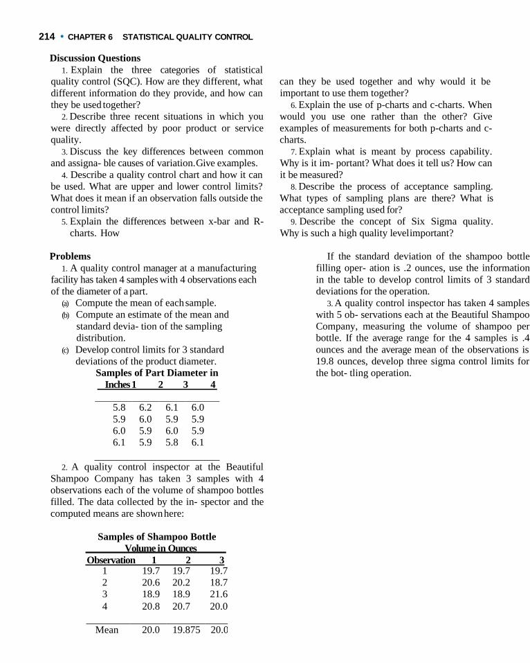
214 • CHAPTER 6 STATISTICAL QUALITY CONTROL
Discussion Questions
1. Explain the three categories of statistical
quality control (SQC). How are they different, what
different information do they provide, and how can
they be used together?
2. Describe three recent situations in which you
were directly affected by poor product or service
quality.
3. Discuss the key differences between common
and assigna- ble causes of variation. Give examples.
4. Describe a quality control chart and how it can
be used. What are upper and lower control limits?
What does it mean if an observation falls outside the
control limits?
5. Explain the differences between x-bar and R-
charts. How
can they be used together and why would it be
important to use them together?
6. Explain the use of p-charts and c-charts. When
would you use one rather than the other? Give
examples of measurements for both p-charts and c-
charts.
7. Explain what is meant by process capability.
Why is it im- portant? What does it tell us? How can
it be measured?
8. Describe the process of acceptance sampling.
What types of sampling plans are there? What is
acceptance sampling used for?
9. Describe the concept of Six Sigma quality.
Why is such a high quality level important?
Problems
1. A quality control manager at a manufacturing
facility has taken 4 samples with 4 observations each
of the diameter of a part. (a) Compute the mean of each sample.
(b) Compute an estimate of the mean and
standard devia- tion of the sampling
distribution.
(c) Develop control limits for 3 standard
deviations of the product diameter. Samples of Part Diameter in
Inches 1 2 3 4
5.8 6.2 6.1 6.0
5.9 6.0 5.9 5.9
6.0 5.9 6.0 5.9
6.1 5.9 5.8 6.1
2. A quality control inspector at the Beautiful
Shampoo Company has taken 3 samples with 4
observations each of the volume of shampoo bottles
filled. The data collected by the in- spector and the
computed means are shown here:
Samples of Shampoo Bottle
Volume in Ounces
Observation 1 2 3
If the standard deviation of the shampoo bottle
filling oper- ation is .2 ounces, use the information
in the table to develop control limits of 3 standard
deviations for the operation.
3. A quality control inspector has taken 4 samples
with 5 ob- servations each at the Beautiful Shampoo
Company, measuring the volume of shampoo per
bottle. If the average range for the 4 samples is .4
ounces and the average mean of the observations is
19.8 ounces, develop three sigma control limits for
the bot- tling operation.
1 19.7 19.7 19.7
2 20.6 20.2 18.7
3 18.9 18.9 21.6
4 20.8 20.7 20.0
Mean 20.0 19.875 20.0

PROBLEMS • 215
4. A production manager at Ultra Clean
Dishwashing company is monitoring the quality of
the company’s production process. There has been
concern relative to the quality of the operation to
accurately fill the 16 ounces of dishwashing liquid.
The product is designed for a fill level of 16.00 ± 0.30.
The company collected the following sample data on
the production process:
Observations
Sampl e
1 2 3 4
1 16.4 0
16.1 1
15.9 0
15.7 8
2 15.9 7
16.1 0
16.2 0
15.8 1
3 15.9 1
16.0 0
16.0 4
15.9 2
4 16.2 0
16.2 1
15.9 3
15.9 5
5 15.8 7
16.2 1
16.3 4
16.4 3
6 15.4 3
15.4 9
15.5 5
15.9 2
7 16.4 3
16.2 1
15.9 9
16.0 0
8 15.5 0
15.9 2
l6.12 16.0 2
9 16.1 3
16.2 1
16.0 5
16.0 1
10 15.68 16.43 16.20 15.97
(a) Are the process mean and range in statistical control?
(b) Do you think this process is capable of
meeting the de- sign standard?
5. Ten samples with 5 observations each have
been taken from the Beautiful Shampoo Company
plant in order to test for volume dispersion in the
shampoo bottle filling process. The av- erage
sample range was found to be .3 ounces. Develop
control limits for thesample range.
6. The Awake Coffee Company produces gourmet
instant cof- fee. The company wants to be sure that
the average fill of coffee containers is 12.0 ounces. To
make sure the process is in control, a worker
periodically selects at random a box containing 6
containers of coffee and measures their weight. When
the process is in control, the range of the weight of
coffee samples averages .6 ounces.
(a) Develop an R-chart and an x-chart for this process. (b) The measurements of weight from the last
five samples taken of the 6 containers are
shown below:
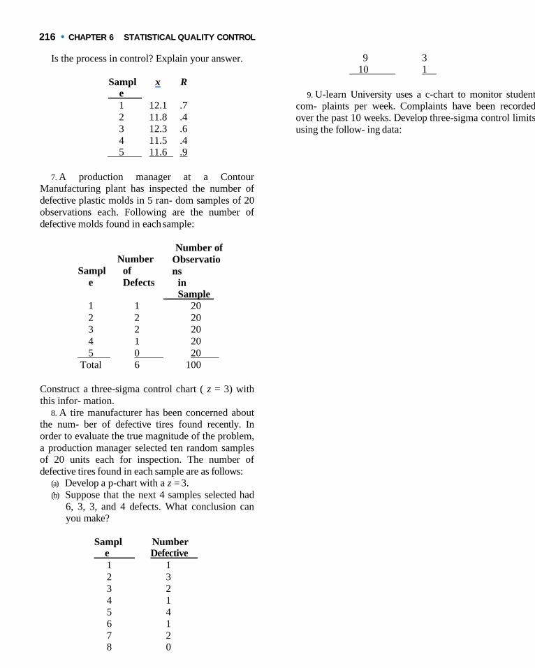
216 • CHAPTER 6 STATISTICAL QUALITY CONTROL
Is the process in control? Explain your answer.
Sampl e
x R
1 12.1 .7
2 11.8 .4
3 12.3 .6
4 11.5 .4 5 11.6 .9
7. A production manager at a Contour
Manufacturing plant has inspected the number of
defective plastic molds in 5 ran- dom samples of 20
observations each. Following are the number of
defective molds found in each sample:
Sampl
e
Number
of
Defects
Number of
Observatio
ns
in Sample
1 1 20
2 2 20
3 2 20
4 1 20
5 0 20
Total 6 100
Construct a three-sigma control chart ( z = 3) with
this infor- mation.
8. A tire manufacturer has been concerned about
the num- ber of defective tires found recently. In
order to evaluate the true magnitude of the problem,
a production manager selected ten random samples
of 20 units each for inspection. The number of
defective tires found in each sample are as follows: (a) Develop a p-chart with a z = 3.
(b) Suppose that the next 4 samples selected had
6, 3, 3, and 4 defects. What conclusion can
you make?
9 3 10 1
9. U-learn University uses a c-chart to monitor student
com- plaints per week. Complaints have been recorded
over the past 10 weeks. Develop three-sigma control limits
using the follow- ing data:
Sampl e
Number Defective
1 1
2 3
3 2
4 1
5 4
6 1
7 2 8 0
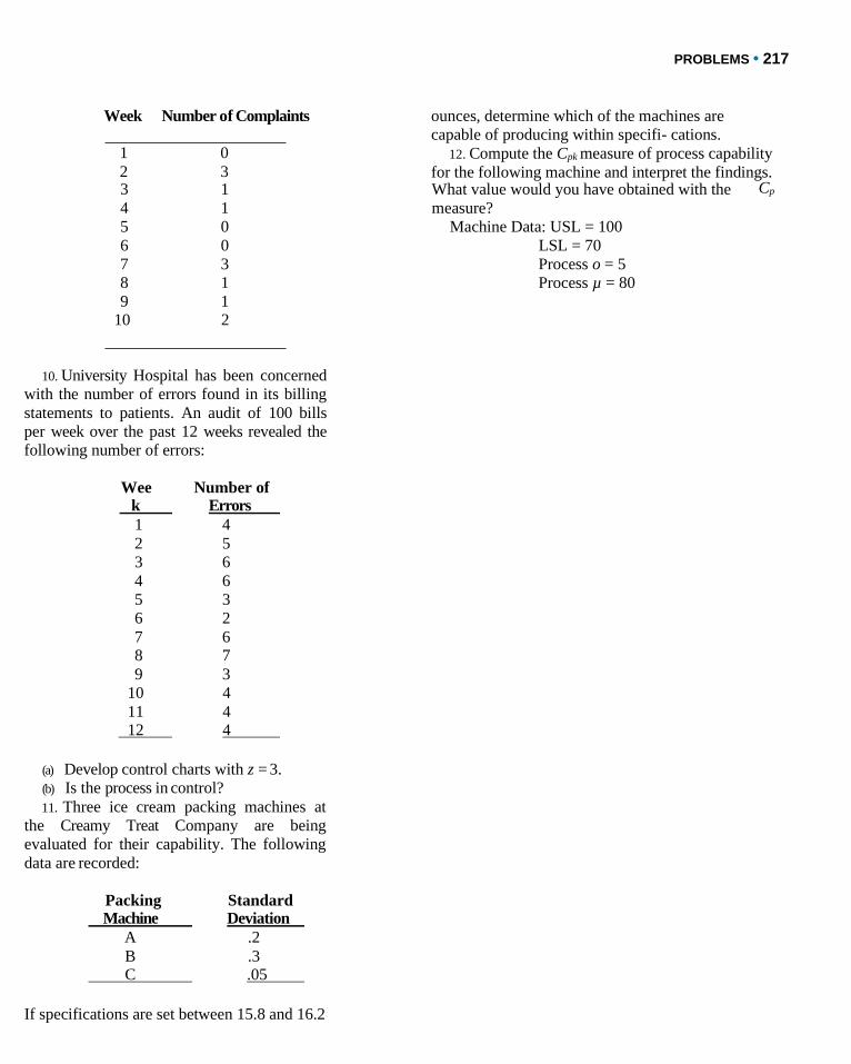
PROBLEMS • 217
Week Number of Complaints
1 0
2 3
ounces, determine which of the machines are
capable of producing within specifi- cations.
12. Compute the Cpk measure of process capability for the following machine and interpret the findings.
3 1 What value would you have obtained with the Cp
4 1 measure?
5 0 Machine Data: USL = 100
6 0 LSL = 70
7 3 Process o = 5
8 1 Process µ = 80
9 1
10 2
10. University Hospital has been concerned
with the number of errors found in its billing
statements to patients. An audit of 100 bills
per week over the past 12 weeks revealed the
following number of errors:
Wee k
Number of Errors
1 4
2 5
3 6
4 6
5 3
6 2
7 6 8 7
9 3
10 4
11 4 12 4
(a) Develop control charts with z = 3.
(b) Is the process in control?
11. Three ice cream packing machines at
the Creamy Treat Company are being
evaluated for their capability. The following
data are recorded:
Packing
Machine Standard Deviation
A .2
B .3 C .05
If specifications are set between 15.8 and 16.2

218 • CHAPTER 6 STATISTICAL QUALITY CONTROL
13. Develop an OC curve for a sampling plan in
which a sample of n = 5 items is drawn from lots of
N = 1000 items. The accept/reject criteria are set up
in such a way that we accept a lot if no more than
one defect (c =1) is found.
14. Quality Style manufactures self-assembling
furniture. To reduce the cost of returned orders, the
acceptance sampling plan for Med-Tech. The
contract with the supplier states that the acceptable
quality level is 1% defective. Also, the lot toler- ance
proportion defective is 4%, the producer’s risk is 5%,
and theconsumer’s risk is 10%.
(a) Develop an acceptance sampling plan for
Joshua that meets the stated criteria.
manager of its quality control department inspects (b) Draw the OC curve for the plan you developed.
the final packages each day using randomly selected
samples. The defects include wrong parts, missing
connection parts, parts with apparent painting prob-
lems, and parts with rough surfaces. The average
defect rate is three per day.
(a) Which type of control chart should be used?
Construct a control chart with three-sigma
controllimits.
(b) Today the manager discovered nine defects.
What does this mean?
15. Develop an OC curve for a sampling plan in
which a sample of n = 10 items is drawn from lots
of N = 1000. The accept/reject criteria is set up in
such a way that we accept a lot if no more than one
defect (c = 1) is found.
16. The Fresh Pie Company purchases apples
from a local farm to be used in preparing the filling
for their apple pies. Sometimes the apples are fresh
and ripe. Other times they can be spoiled or not ripe
enough. The company has decided that they need an
acceptance sampling plan for the purchased ap- ples.
Fresh Pie has decided that the acceptable quality
level is 5 defective apples per 100, and the lot
tolerance proportion de- fective is 5%. Producer’s
risk should be no more than 5% and consumer’s risk
10% orless.
(a) Develop a plan that satisfies the above
requirements.
(b) Determine the AOQL for your plan,
assuming that the lot size is 1000 apples.
17. A computer manufacturer purchases
microchips from a world-class supplier. The buyer
has a lot tolerance proportion defective of 10 parts
in 5000, with a consumer’s risk of 15%. If the
computer manufacturer decides to sample 2000 of
the mi- crochips received in each shipment, what
acceptance number, c, would they want?
18. Joshua Simms has recently been placed in
charge of pur- chasing at the Med-Tech Labs, a
medical testing laboratory. His job is to purchase
testing equipment and supplies. Med-Tech currently
has a contract with a reputable supplier in the indus-
try. Joshua’s job is to design an appropriate
(c) What is the AOQL of your plan, assuming a
lot size of 1000?
19. Breeze Toothpaste Company makes tubes of
toothpaste. The product is produced and then
pumped into tubes and capped. The production
manager is concerned whether the fill-
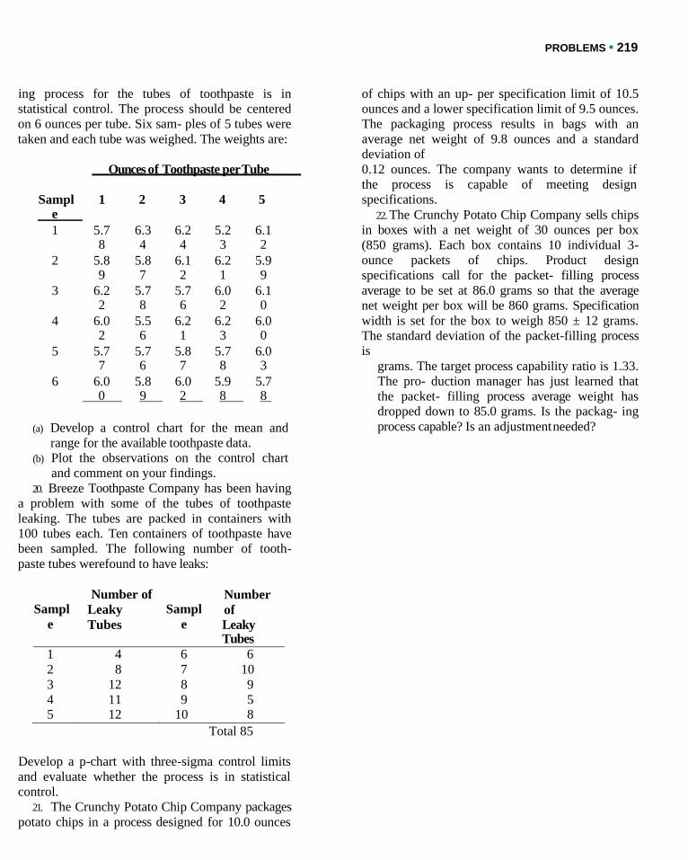
PROBLEMS • 219
ing process for the tubes of toothpaste is in
statistical control. The process should be centered
on 6 ounces per tube. Six sam- ples of 5 tubes were
taken and each tube was weighed. The weights are:
Ounces of Toothpaste per Tube
of chips with an up- per specification limit of 10.5
ounces and a lower specification limit of 9.5 ounces.
The packaging process results in bags with an
average net weight of 9.8 ounces and a standard
deviation of
0.12 ounces. The company wants to determine if
the process is capable of meeting design
specifications.
22. The Crunchy Potato Chip Company sells chips
in boxes with a net weight of 30 ounces per box
(850 grams). Each box contains 10 individual 3-
ounce packets of chips. Product design
specifications call for the packet- filling process
average to be set at 86.0 grams so that the average
net weight per box will be 860 grams. Specification
width is set for the box to weigh 850 ± 12 grams.
The standard deviation of the packet-filling process
is
(a) Develop a control chart for the mean and
range for the available toothpaste data.
(b) Plot the observations on the control chart
and comment on your findings.
20. Breeze Toothpaste Company has been having
a problem with some of the tubes of toothpaste
leaking. The tubes are packed in containers with
100 tubes each. Ten containers of toothpaste have
been sampled. The following number of tooth-
paste tubes werefound to have leaks:
Sampl
e
Number of
Leaky
Tubes
Sampl
e
Number
of
Leaky Tubes
1 4 6 6
2 8 7 10
3 12 8 9
4 11 9 5 5 12 10 8
Total 85
Develop a p-chart with three-sigma control limits
and evaluate whether the process is in statistical
control.
21. The Crunchy Potato Chip Company packages
potato chips in a process designed for 10.0 ounces
grams. The target process capability ratio is 1.33.
The pro- duction manager has just learned that
the packet- filling process average weight has
dropped down to 85.0 grams. Is the packag- ing
process capable? Is an adjustment needed?
Sampl e
1 2 3 4 5
1 5.7 8
6.3 4
6.2 4
5.2 3
6.1 2
2 5.8 9
5.8 7
6.1 2
6.2 1
5.9 9
3 6.2 2
5.7 8
5.7 6
6.0 2
6.1 0
4 6.0 2
5.5 6
6.2 1
6.2 3
6.0 0
5 5.7 7
5.7 6
5.8 7
5.7 8
6.0 3
6 6.0 0
5.8 9
6.0 2
5.9 8
5.7 8

220 • CHAPTER 6 STATISTICAL QUALITY CONTROL
CASE: ScharadinHotels
Scharadin Hotels are a national hotel chain started Coleman, head of MIS, defended the system, stating that
in 1957 by Milo Scharadin. What started as one the system was sound and the problems were exag-
upscale hotel in New York City turned into a highly
reputable national hotel chain. Today Scharadin
Hotels serve over 100 1ocations and are recognized
for their customer service and quality. Scharadin
Hotels are typ- ically located in large metropolitan
areas close to convention centers and centers of
commerce. They cater to both business and
nonbusiness customers and offer a wide array of
services. Maintaining high customer service has
been considered a prior- ity for the hotel chain.
A Problem with Quality
The Scharadin Hotel in San Antonio, Texas, had
recently been experiencing a large number of guest
complaints due to billing errors. The complaints
seem to center around guests disputing charges on
their final hotel bill. Guest complaints ranged from
extra charges, such as meals or services that were
not purchased, to confusion for not being charged at
all. Most hotel guests use express checkout on their
day of departure. With express check- out the hotel
bill is left under the guest’s door in the early morn-
ing hours and, if all is in order, does not require any
additional action on the guest’s part. Express
checkout is a welcome service by busy travelers who
are free to depart the hotel at their conve- nience.
However, the increased number of billing errors
began creating unnecessary delays and frustration
for the guests who unexpectedly needed to settle
their bill with the front desk. The hotel staff often
had to calm frustrated guests who were rushing to
the airport and were aggravated that they were
getting charged for items they had not purchased.
Identifying the Source ofthe Problem
Larraine Scharadin, Milo Scharadin’s niece, had
recently been
appointed to run the San Antonio hotel. A recent
business school graduate, Larraine had grown up in
the hotel business. She was poised and confident,
and understood the importance of high quality for
the hotel. When she became aware of the billing
problem, she immediately called a staff meeting to
un- cover the source of the problem.
During the staff meeting discussion quickly
turned to prob- lems with the new computer system
and software that had been put in place. Tim
gerated. Tim claimed that a few hotel guests made an
issue of a

PROBLEMS • 221
few random problems. Scott Schultz, head of
operations, was not so sure. Scott said that he
noticed that the number of com- plaints seem
to have significantly increased since the new
system was installed. He said that he had asked
his team to perform an audit of 50 random
bills per day over the past 30 days. Scott
showed the following numbers to Larraine,
Tim, and the other staff members.
f
Everyone looked at the data that had been
presented. Then Tim exclaimed: “Notice that
the number of errors increases in the last third
of the month. The computer system had been
in place for the entire month so that can ’t be
the problem. Scott, it is probably the new
employees you have on staff that are not en-
tering the data properly.” Scott quickly
retaliated: “The employ- ees are trained
properly! Everyone knows the problem is the
computer system!”
The argument between Tim and Scott
become heated, and Larraine decided to step
in. She said, “Scott, I think it is best if you
perform some statistical analysis of that data
and send us your findings. You know that we
want a high-quality stan- dard. We can’t be
Motorola with six-sigma quantity, but let’s try
for three-sigma. Would you develop some
control charts with the data and let us know if
you think the process is in control?”
Case Questions
1. Set up three-sigma control limits with the given data.
2. Is the process in control? Why?
3. Based on your analysis do you think the
problem is the new computer system or
something else?
4. What advice would you give to Larraine based
on the information that you have?
Day
Number of
Incorrect
Bills
Day
Number of
Incorrect
Bills
Day
Number o
Incorrect
Bills 1 2 11 1 21 3
2 2 12 2 22 3
3 1 13 3 23 3
4 2 14 3 24 4
5 2 15 2 25 5
6 3 16 3 26 5
7 2 17 2 27 6
8 2 18 2 28 5
9 1 19 1 29 5
10 2 20 3 30 5


INTERACTIVE LEARNING • 217
CASE: Delta Plastics, Inc.(B)
Jose De Costa, Director of Manufacturing at Delta
Plastics, sat at his desk looking at the latest
production quality report, show- ing the number and
type of product defects per week (see the quality
report in Delta Plastics, Inc. Case A, Chapter 5). He
was faced with the task of evaluating production
Jose was opposed to starting production until R&D
had fully completed testing and refining the new
material. However, the CEO of Delta ordered
production despite objections from man- ufacturing
and R&D. Jose carefully looked at the report in
front of him and prepared to analyze the results.
quality for prod- ucts made with two different
materials. One of the materials was new and called
“super plastic” due to its ability to sustain large
temperature changes. The other material was the
standard plastic that had been successfully used by
Delta for many years.
The company had started producing products
with the new “super plastic” material only a month
earlier. Jose suspected that the new material could
result in more defects during the pro- duction
process than the standard material they had been
using.
Case Questions
1. Prepare a three-sigma control chart for both
production processes, using the new and standard
material (use the quality report in Delta Plastics,
Inc. Case A, Chapter 5). Are both processes in
control? What can you conclude?
2. Are both materials equally subject to the defects?
3. Given your findings, what advice would you give Jose?
Interactive Learning
Enhance and test your knowledge of Chapter 6. Use the CD and visit our Web sitew,ww.wiley.com/college/reid, for
additional resources and information.
1. Spreadsheets Solved Problems 1 and 4
2. Company Tours
Rickenbacker International Corporation
Genesis Technologies, Inc.
Canadian Springs Water Company
3. AdditionalWeb Resources
American Society for Quality Control,
www.asqc.org Australian Quality Council,
www.aqc.org.au
4. Internet Challenge Safe-Air
To gain business experience, you have volunteered
to work at Safe-Air, a nonprofit agency that
monitors airline safety records and customer
service. Your first assignment is to compare three
airlines based on their on-time arrivals and
departures. Your manager has asked you to get your
information from the Inter- net. Select any three
airlines. For an entire week check the daily arrival
and departure schedules of the three airlines from
your city or closest airport. Remember that it is
important to com- pare the arrivals and departures
from the same location and during the same time
period to account for factors such as the weather.
Record the data that you collect for each airline.
Then
218 • CHAPTER 6 STATISTICAL QUALITY CONTROL
decide which types of statistical quality control tools
you are going to use to evaluate the airlines’
performances. Based on your findings, draw a
conclusion regarding the on-time arrivals and
departures of each of the airlines. Which is best and
which is worst? Are there large differences in
performance among the airlines? Also describe the
statistical quality control tools you have decided to
use to monitor performance. If you have cho- sen to
use more than one tool, are you finding the tools
equally useful or is one better at capturing
differences in performance? Finally, based on what
you have learned so far, how would you perform
this analysis differently in the future?
Virtual Company: Valley Memorial Hospital
Assignment: Statistical Quality Control This assignment involves controlling nursing
hours at Valley Memorial Hospital. Lee Jordan, director of the hospital’s Medical/Surgical
Nursing Unit, has already told you that VMH employs more than 500 nurses, with an
annual nursing budget of $5,000,000. “We’re trying for a five

INTERACTIVE LEARNING • 219
percent reduction in nursing FTEs — full-time equivalents,” he says. “I’ve been
personally record- ing the nursing hours per patient per day for over three
months in Med/Surg. I would like you to look at the numbers and see if you can
tell me how to meet our goals.
To complete this assignment, go to www.wiley.com/college/reid to get more details on the
fol-
lowing projects:
1. Develop upper and lower limits for FTEs within which the Medical/Surgical Nursing
Unit will be efficient and will maintain quality at least 95 percent of the time.
2. Look at the data and determine whether Jordan is really in control of nursing hours. If he
isn ’t, tell him why.
3. Determine how the Medical/Surgical Nursing Unit can bring nursing hours per patient
day (NHPPD) down to 8.00. Also, provide some advice on how Jordan can get his staff
to buy into the concept of an NHPPD tar- get of 8.00.
4. Jot down your thoughts on the three statistical problems, which are contained in memos
Jordan received from other VMH staff:
• Will Hartmann, in the Business Office has kept track of billing errors for the past 21 weeks. Based on this data, determine control limits for billing errors. Also, is the percentage of defective bills a valid measure for this analysis?
• Analyze trends in patient surveys about the meals served at VMH. Doug Jennings, in Dietary, thinks the
number of OUTSTANDING responses has been declining, but he’s not sure if
that decline is statistically significant.
• Margot Hamilton, in Housekeeping, has been keeping track of defects in room cleaning. Based on her data, develop some recommendations on how she can get better results.
To access the Web site:
• Go to www.wiley.com/college/reid
• Click Student Companion Site
• Click VirtualCompany
• Click Kaizen Consulting, Inc.
• Click Consulting Assignments
• Click Statistical Quality Control
Bibliography
Brue, G. Six Sigma for Managers. NewYork:
McGraw-Hill, 2002. Duncan, A. J. Quality Control
and Industrial Statistics. 5th ed.
Homewood, Ill.: Irwin, 1986.
Evans, James R., and William M. Lindsay. The
Management and Control of Quality. 4th ed.
Cincinnati: South-Western, 1999. Feigenbaum, A. V.
Total Quality Control. New York: McGraw- Hill, 1991.
Grant, E. L., and R. S. Leavenworth. Statistical
Quality Control.
6th ed. New York: McGraw-Hill, 1998.
www.wiley.com/ college/reid

220 • CHAPTER 6 STATISTICAL QUALITY CONTROL
Hoyer, R. W., and C. E. Wayne. “A Graphical
Exploration of SPC, Part 1.” Quality
Progress,29, no. 5 (May 1996), 65-73.
Juran, J. M., and F. M. Gryna. Quality Planning and
Analysis.
2nd ed. New York: McGraw-Hill, 1980.
Wadsworth, H. M., K. S. Stephens, and A. B.
Godfrey. Modern Methods for Quality
Control and Improvement. New York:
Wiley, 1986.

RECTO RUNNING HEAD • 219
Copyright © 2022 FDOKUMEN