Lecture note on Descriptive Statistics (STS 102)

www.crescent-university.edu.ng

LECTURE NOTE

ON

DESCRIPTIVE STATISTICS

(STS 102)

BY

ADEOSUN SAKIRU ABIODUN

E-mail: [email protected]

mailto:[email protected]


2

COURSE CONTENTS

Statistical data: types, sources and methods of collection. Presentation of data: tables,

charts and graphs. Error and Approximations. Frequency and cumulative distributions.

Measures of location, partition, dispersion, Skewness and kurtosis. Rates, Proportion

and index numbers.

READING LISTS

1. Adamu S.O and Johnson Tinuke L (1998): Statistics for Beginners; Book 1.

SAAL Publication. Ibadan. ISBN: 978-34411-3-2

2. Clark G.M and Cooke D (1993): A Basic course in statistics. Third edition.

London: Published by Arnold and Stoughton.

3. Olubosoye O.E, Olaomi J.O and Shittu O.I (2002): Statistics for

Engineering, Physical and Biological sciences. Ibadan: A Divine Touch

Publications.

4. Tmt. V. Varalakshmi et al (2005): Statistics Higher Secondary - First year.

Tamilnadu Textbook Corporation, College Road, Chennai- 600 006


3

INTRODUCTION

In the modern world of information and communication technology, the

importance of statistics is very well recognised by all the disciplines. Statistics has

originated as a science of statehood and found applications slowly and steadily in

Agriculture, Economics, Commerce, Biology, Medicine, Industry, planning, education

and so on. As of today, there is no other human walk of life, where statistics cannot

be applied.

Statistics is concerned with the scientific method of collecting, organizing,

summarizing, presenting and analyzing statistical information (data) as well as

drawing valid conclusion on the basis of such analysis. It could be simply defined as

the “science of data”. Thus, statistics uses facts or numerical data, assembled,

classified and tabulated so as to present significant information about a given

subject. Statistic is a science of understanding data and making decisions in the face

of randomness.

The study of statistics is therefore essential for sound reasoning, precise

judgment and objective decision in the face of up- to- date accurate and reliable

data. Thus many researchers, educationalists, business men and government

agencies at the national, state or local levels rely on data to answer operations and

programs. Statistics is usually divided into two categories, which is not mutually

elution namely: Descriptive statistics and inferential statistics.

DESCRIPTIVE STATISTICS

This is the act of summarizing and given a descriptive account of numerical

information in form of reports, charts and diagrams. The goal of descriptive

statistics is to gain information from collected data. It begins with collection of data

by either counting or measurement in an inquiry. It involves the summary of specific

aspect of the data, such as averages values and measure of dispersion (spread).

Suitable graphs, diagrams and charts are then used to gain understanding and clear


4

interpretation of the phenomenon under investigation keeping firmly in mind

where the data comes from. Normally, a descriptive statistics should:

i. be single – valued

ii. be algebraically tractable

iii. consider every observed value.

INFERENTIAL STATISTICS

This is the act of making deductive statement about a population from the

quantities computed from its representative sample. It is a process of making

inference or generalizing about the population under certain conditions and

assumptions. Statistical inference involves the processes of estimation of

parameters and hypothesis testing. However, this concept is not in the context of

this course.

USES OF STATISTICS

Statistics can be used among others for:

1) Planning and decision making by individuals, states, business organizations,

research institution etc.

2) Forecasting and prediction for the future based on a good model provided

that its basic assumptions are not violated.

3) Project implementation and control. This is especially useful in on-going

projects such as network analysis, construction of roads and bridges and

implementation of government programs and policies.

4) The assessment of the reliability and validity of measurements and general

points significance tests including power and sample size determination.


5

STATISTICAL DATA

Data can be described as a mass of unprocessed information obtained from

measurement of counting of a characteristics or phenomenon. They are raw facts

that have to be processed in numerical form they are called quantitative data. For

instance the collection of ages of students offering STS 102 in a particular session is

an example of this data. But when data are not presented in numerical form, they

are called qualitative data. E.g.: status, sex, religion, etc.

Definition: Statistical data are data obtained through objective measurement or

enumeration of characteristics using the state of the art equipment that is precise

and unbiased. Such data when subjected to statistical analysis produce results with

high precision.

SOURCES OF STATISTICAL DATA

1. Primary data: These are data generated by first hand or data obtained

directly from respondents by personal interview, questionnaire,

measurements or observation. Statistical data can be obtained from:

(i) Census – complete enumeration of all the unit of the population

(ii) Surveys – the study of representative part of a population

(iii) Experimentation – observation from experiment carried out in

laboratories and research center.

(iv) Administrative process e.g. Record of births and deaths.

ADVANTAGES

Comprises of actual data needed

It is more reliable with clarity

Comprises a more detail information


6

DISADVANTAGES

Cost of data collection is high

Time consuming

There may larger range of non response

2. Secondary data: These are data obtained from publication, newspapers, and

annual reports. They are usually summarized data used for purpose other

than the intended one. These could be obtain from the following:

(i) Publication e.g. extract from publications

(ii) Research/Media organization

(iii) Educational institutions

ADVANTAGES

The outcome is timely

The information gathered more quickly

It is less expensive to gather.

DISADVANTAGES

Most time information are suppressed when working with

secondary data

The information may not be reliable

METHODS OF COLLECTION OF DATA

There are various methods we can use to collect data. The method used depends

on the problem and type of data to be collected. Some of these methods include:

1. Direct observation


7

2. Interviewing

3. Questionnaire

4. Abstraction from published statistics.

DIRECT OBSERVATION

Observational methods are used mostly in scientific enquiry where data are

observed directly from controlled experiment. It is used more in the natural

sciences through laboratory works than in social sciences. But this is very useful

studying small communities and institutions.

INTERVIEWING

In this method, the person collecting the data is called the interviewer goes to ask

the person (interviewee) direct questions. The interviewer has to go to the

interviewees personally to collect the information required verbally. This makes it

different from the next method called questionnaire method.

QUESTIONNAIRE

A set of questions or statement is assembled to get information on a variable (or a

set of variable). The entire package of questions or statement is called a

questionnaire. Human beings usually are required to respond to the questions or

statements on the questionnaire. Copies of the questionnaire can be administered

personally by its user or sent to people by post. Both interviewing and

questionnaire methods are used in the social sciences where human population is

mostly involved.


8

ABSTRACTIONS FROM THE PUPLISHED STATISTICS

These are pieces of data (information) found in published materials such as figures

related to population or accident figures. This method of collecting data could be

useful as preliminary to other methods.

Other methods includes: Telephone method, Document/Report method, Mail

or Postal questionnaire, On-line interview method, etc.

PRESENTATION OF DATA

When raw data are collected, they are organized numerically by distributing

them into classes or categories in order to determine the number of individuals

belonging to each class. Most cases, it is necessary to present data in tables, charts

and diagrams in order to have a clear understanding of the data, and to illustrate the

relationship existing between the variables being examined.

FREQUENCY TABLE

This is a tabular arrangement of data into various classes together with their

corresponding frequencies.

Procedure for forming frequency distribution

Given a set of observation , for a single variable.

1. Determine the range (R) = L – S where L = largest observation in the raw

data; and S = smallest observation in the raw data.

2. Determine the appropriate number of classes or groups (K). The choice of K is

arbitrary but as a general rule, it should be a number (integer) between 5 and

20 depending on the size of the data given. There are several suggested guide

lines aimed at helping one decided on how many class intervals to employ.

Two of such methods are:


9

(a) K = 1 +3.322

(b) K = where = number of observations.

3. Determine the width of the class interval. It is determined as

4. Determine the numbers of observations falling into each class interval i.e. find

the class frequencies.

NOTE: With advent of computers, all these steps can be accomplishes easily.

SOME BASIC DEFINITIONS

Variable: This is a characteristic of a population which can take different values.

Basically, we have two types, namely: continuous variable and discrete variable.

A continuous variable is a variable which may take all values within a given range.

Its values are obtained by measurements e.g. height, volume, time, exam score etc.

A discrete variable is one whose value change by steps. Its value may be obtained

by counting. It normally takes integer values e.g. number of cars, number of chairs.

Class interval: This is a sub-division of the total range of values which a

(continuous) variable may take. It is a symbol defining a class E.g. 0-9, 10-19 etc.

there are three types of class interval, namely: Exclusive, inclusive and open-end

classes method.

Exclusive method:

When the class intervals are so fixed that the upper limit of one class is the lower

limit of the next class; it is known as the exclusive method of classification. E.g. Let

some expenditures of some families be as follows:

0 – 1000, 1000 – 2000, etc. It is clear that the exclusive method ensures continuity

of data as much as the upper limit of one class is the lower limit of the next class. In

the above example, there are so families whose expenditure is between 0 and

999.99. A family whose expenditure is 1000 would be included in the class interval

1000-2000.


10

Inclusive method:

In this method, the overlapping of the class intervals is avoided. Both the lower and

upper limits are included in the class interval. This type of classification may be used

for a grouped frequency distribution for discrete variable like members in a family,

number of workers in a factory etc., where the variable may take only integral

values. It cannot be used with fractional values like age, height, weight etc. In case of

continuous variables, the exclusive method should be used. The inclusive method

should be used in case of discrete variable.

Open end classes:

A class limit is missing either at the lower end of the first class interval or at the

upper end of the last class interval or both are not specified. The necessity of open

end classes arises in a number of practical situations, particularly relating to

economic and medical data when there are few very high values or few very low

values which are far apart from the majority of observations.

Class limit: it represents the end points of a class interval. {Lower class limit &

Upper class limit}. A class interval which has neither upper class limit nor lower

class limit indicated is called an open class interval e.g. “less than 25”, ’25 and

above”

Class boundaries: The point of demarcation between a class interval and the next

class interval is called boundary. For example, the class boundary of 10-19 is 9.5 –

19.5

Cumulative frequency: This is the sum of a frequency of the particular class to the

frequencies of the class before it.


11

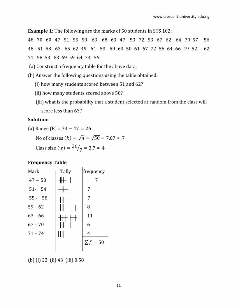
Example 1: The following are the marks of 50 students in STS 102:

48 70 60 47 51 55 59 63 68 63 47 53 72 53 67 62 64 70 57 56

48 51 58 63 65 62 49 64 53 59 63 50 61 67 72 56 64 66 49 52 62

71 58 53 63 69 59 64 73 56.

(a) Construct a frequency table for the above data.

(b) Answer the following questions using the table obtained:

(i) how many students scored between 51 and 62?

(ii) how many students scored above 50?

(iii) what is the probability that a student selected at random from the class will

score less than 63?

Solution:

(a) Range (R) =

No of classes

Class size

Frequency Table

Mark Tally frequency

7

51- 54 7

55 - 58 7

59 – 62 8

63 – 66 11

67 – 70 6

71 – 74 4

(b) (i) 22 (ii) 43 (iii) 0.58


12

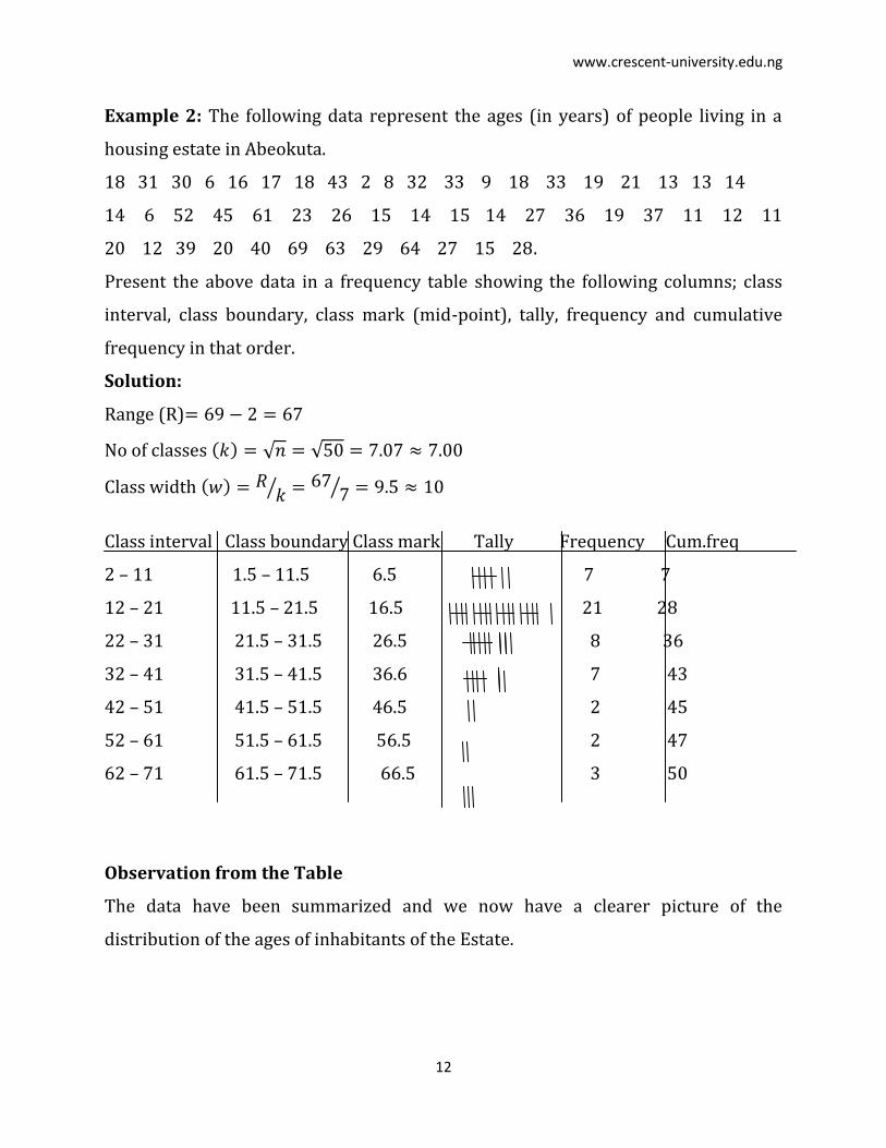
Example 2: The following data represent the ages (in years) of people living in a

housing estate in Abeokuta.

18 31 30 6 16 17 18 43 2 8 32 33 9 18 33 19 21 13 13 14

14 6 52 45 61 23 26 15 14 15 14 27 36 19 37 11 12 11

20 12 39 20 40 69 63 29 64 27 15 28.

Present the above data in a frequency table showing the following columns; class

interval, class boundary, class mark (mid-point), tally, frequency and cumulative

frequency in that order.

Solution:

Range (R)

No of classes

Class width

Class interval Class boundary Class mark Tally Frequency Cum.freq

2 – 11 1.5 – 11.5 6.5 7 7

12 – 21 11.5 – 21.5 16.5 21 28

22 – 31 21.5 – 31.5 26.5 8 36

32 – 41 31.5 – 41.5 36.6 7 43

42 – 51 41.5 – 51.5 46.5 2 45

52 – 61 51.5 – 61.5 56.5 2 47

62 – 71 61.5 – 71.5 66.5 3 50

Observation from the Table

The data have been summarized and we now have a clearer picture of the

distribution of the ages of inhabitants of the Estate.


13

Exercise 1

Below are the data of weights of 40students women randomly selected in Ogun

state. Prepare a table showing the following columns; class interval, frequency, class

boundary, class mark, and cumulative frequency.

96 84 75 80 64 105 87 62 105 101 108 106 110 64 105 117

103 76 93 75 110 88 97 69 94 117 99 114 88 60 98 77

96 96 91 73 82 81 91 84

Use your table to answer the following question

i. How many women weight between 71 and 90?

ii. How many women weight more than 80?

iii. What is the probability that a woman selected at random from Ogun state

would weight more than 90?

GRAPHICAL PRESENTATION OF DATA

It is not enough to represent data in a tabular form. The most attractive way

of representing data is through charts or graphs.

PICTOGRAM

Pictograms or pictographs are representations in form of pictures. They convey

broad meanings and relationships among data. Also they are the simplest way of

presenting information. Pictograms are popularly used in newspapers by journalists

and advertisers.

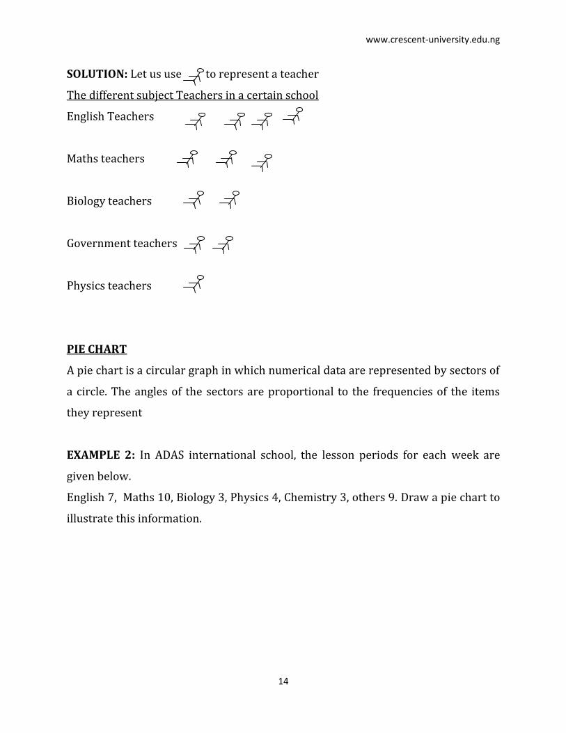
EXAMPLE 1: In a certain secondary school, there are 4 Eng teachers, 3 math

teachers, 2 Biology teachers, 2 government teachers and 1 Physics teacher. Draw a

pictogram to represent this information.


14

SOLUTION: Let us use to represent a teacher

The different subject Teachers in a certain school

English Teachers

Maths teachers

Biology teachers

Government teachers

Physics teachers

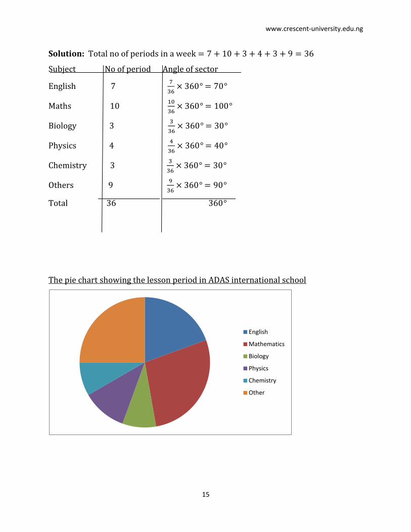
PIE CHART

A pie chart is a circular graph in which numerical data are represented by sectors of

a circle. The angles of the sectors are proportional to the frequencies of the items

they represent

EXAMPLE 2: In ADAS international school, the lesson periods for each week are

given below.

English 7, Maths 10, Biology 3, Physics 4, Chemistry 3, others 9. Draw a pie chart to

illustrate this information.


15

Solution: Total no of periods in a week

Subject No of period Angle of sector

English 7

Maths 10

Biology 3

Physics 4

Chemistry 3

Others 9

Total 36

The pie chart showing the lesson period in ADAS international school

English

Mathematics

Biology

Physics

Chemistry

Other


16

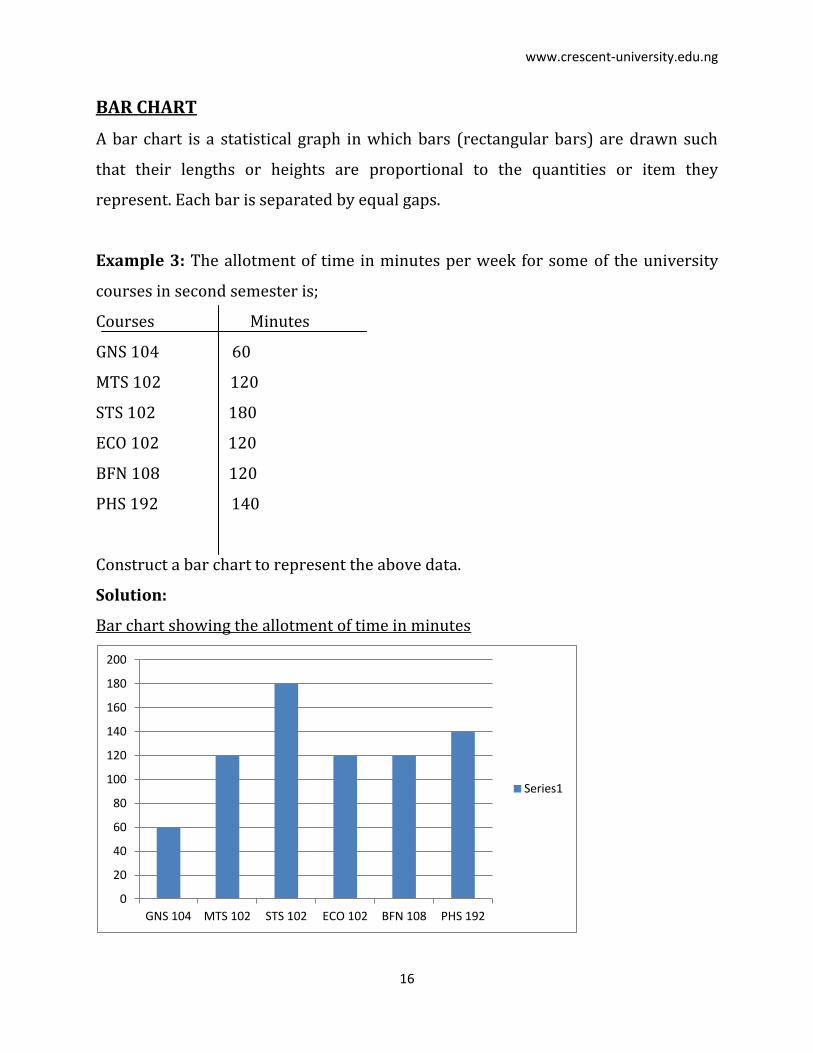
BAR CHART

A bar chart is a statistical graph in which bars (rectangular bars) are drawn such

that their lengths or heights are proportional to the quantities or item they

represent. Each bar is separated by equal gaps.

Example 3: The allotment of time in minutes per week for some of the university

courses in second semester is;

Courses Minutes

GNS 104 60

MTS 102 120

STS 102 180

ECO 102 120

BFN 108 120

PHS 192 140

Construct a bar chart to represent the above data.

Solution:

Bar chart showing the allotment of time in minutes

0

20

40

60

80

100

120

140

160

180

200

GNS 104 MTS 102 STS 102 ECO 102 BFN 108 PHS 192

Series1


17

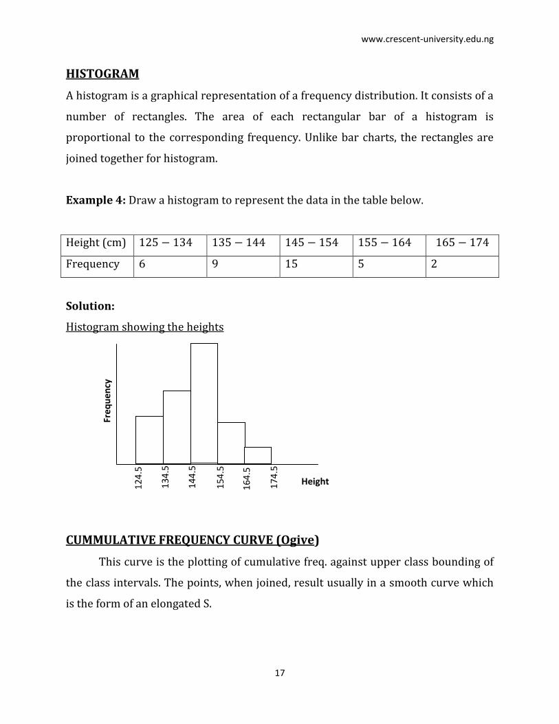
HISTOGRAM

A histogram is a graphical representation of a frequency distribution. It consists of a

number of rectangles. The area of each rectangular bar of a histogram is

proportional to the corresponding frequency. Unlike bar charts, the rectangles are

joined together for histogram.

Example 4: Draw a histogram to represent the data in the table below.

Height (cm)

Frequency 6 9 15 5 2

Solution:

Histogram showing the heights

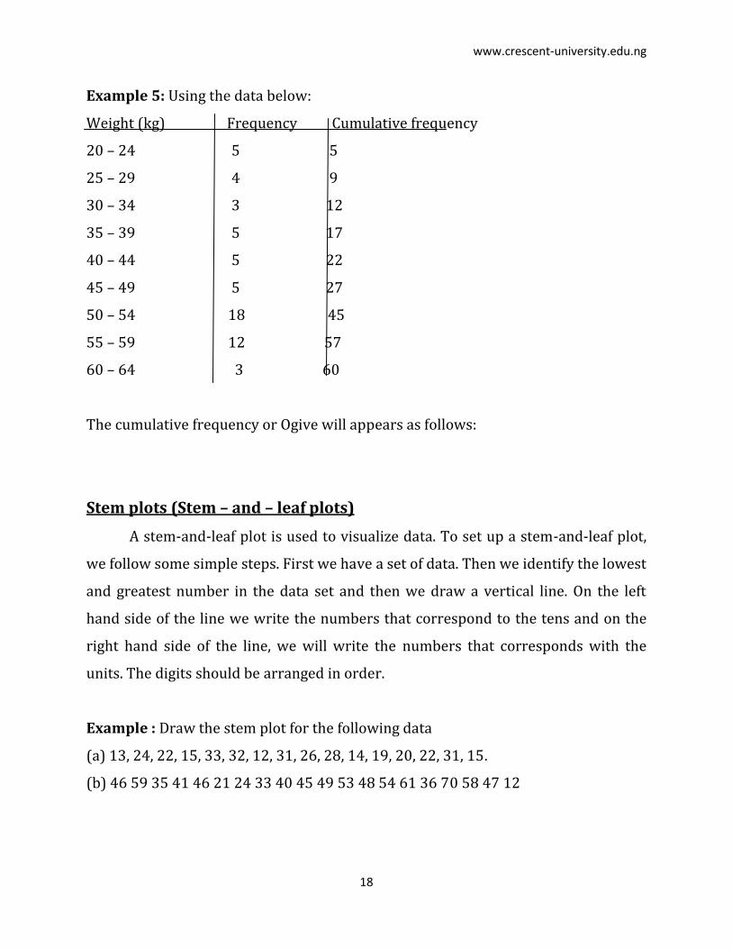
CUMMULATIVE FREQUENCY CURVE (Ogive)

This curve is the plotting of cumulative freq. against upper class bounding of

the class intervals. The points, when joined, result usually in a smooth curve which

is the form of an elongated S.

174

.5

164

.5

154

.5

144

.5

134

.5

124

.5

Fre

qu

en

cy

Height


18

Example 5: Using the data below:

Weight (kg) Frequency Cumulative frequency

20 – 24 5 5

25 – 29 4 9

30 – 34 3 12

35 – 39 5 17

40 – 44 5 22

45 – 49 5 27

50 – 54 18 45

55 – 59 12 57

60 – 64 3 60

The cumulative frequency or Ogive will appears as follows:

Stem plots (Stem – and – leaf plots)

A stem-and-leaf plot is used to visualize data. To set up a stem-and-leaf plot,

we follow some simple steps. First we have a set of data. Then we identify the lowest

and greatest number in the data set and then we draw a vertical line. On the left

hand side of the line we write the numbers that correspond to the tens and on the

right hand side of the line, we will write the numbers that corresponds with the

units. The digits should be arranged in order.

Example : Draw the stem plot for the following data

(a) 13, 24, 22, 15, 33, 32, 12, 31, 26, 28, 14, 19, 20, 22, 31, 15.

(b) 46 59 35 41 46 21 24 33 40 45 49 53 48 54 61 36 70 58 47 12


19

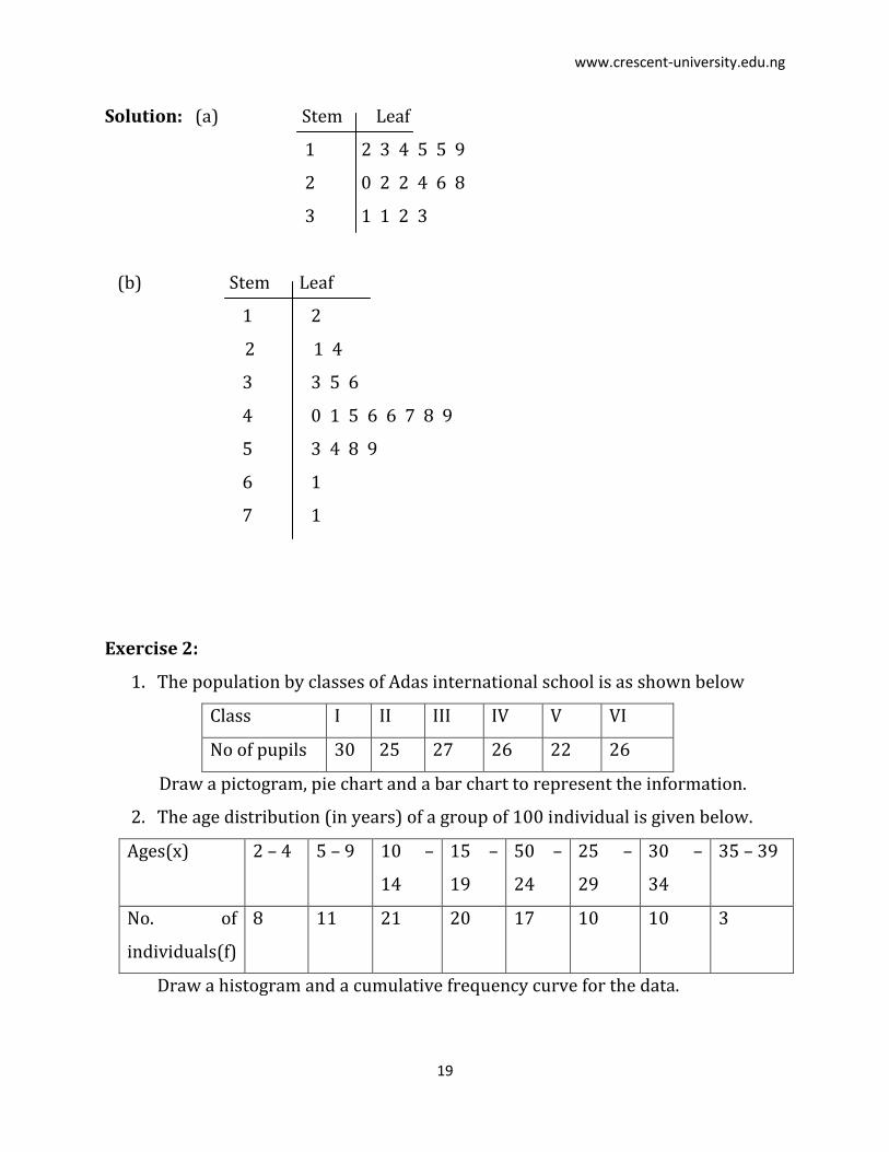
Solution: (a) Stem Leaf

1 2 3 4 5 5 9

2 0 2 2 4 6 8

3 1 1 2 3

(b) Stem Leaf

1 2

2 1 4

3 3 5 6

4 0 1 5 6 6 7 8 9

5 3 4 8 9

6 1

7 1

Exercise 2:

1. The population by classes of Adas international school is as shown below

Class I II III IV V VI

No of pupils 30 25 27 26 22 26

Draw a pictogram, pie chart and a bar chart to represent the information.

2. The age distribution (in years) of a group of 100 individual is given below.

Ages(x) 2 – 4 5 – 9 10 –

14

15 –

19

50 –

24

25 –

29

30 –

34

35 – 39

No. of

individuals(f)

8 11 21 20 17 10 10 3

Draw a histogram and a cumulative frequency curve for the data.


20

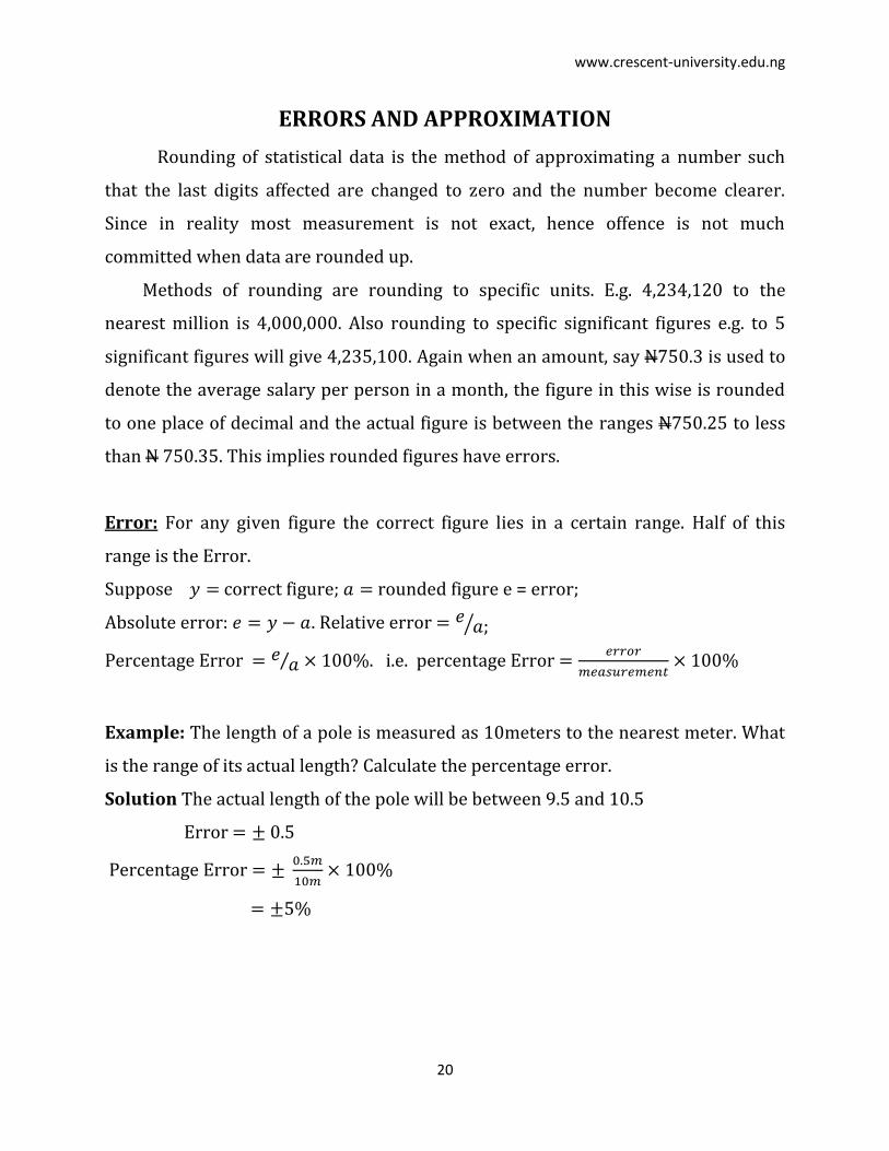
ERRORS AND APPROXIMATION

Rounding of statistical data is the method of approximating a number such

that the last digits affected are changed to zero and the number become clearer.

Since in reality most measurement is not exact, hence offence is not much

committed when data are rounded up.

Methods of rounding are rounding to specific units. E.g. 4,234,120 to the

nearest million is 4,000,000. Also rounding to specific significant figures e.g. to 5

significant figures will give 4,235,100. Again when an amount, say N750.3 is used to

denote the average salary per person in a month, the figure in this wise is rounded

to one place of decimal and the actual figure is between the ranges N750.25 to less

than N 750.35. This implies rounded figures have errors.

Error: For any given figure the correct figure lies in a certain range. Half of this

range is the Error.

Suppose correct figure; rounded figure e = error;

Absolute error: . Relative error

Percentage Error . i.e. percentage Error

Example: The length of a pole is measured as 10meters to the nearest meter. What

is the range of its actual length? Calculate the percentage error.

Solution The actual length of the pole will be between 9.5 and 10.5

Error

Percentage Error


21

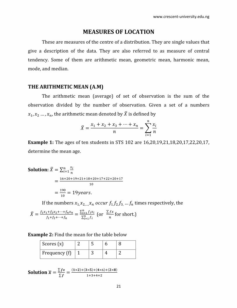
MEASURES OF LOCATION

These are measures of the centre of a distribution. They are single values that

give a description of the data. They are also referred to as measure of central

tendency. Some of them are arithmetic mean, geometric mean, harmonic mean,

mode, and median.

THE ARITHMETIC MEAN (A.M)

The arithmetic mean (average) of set of observation is the sum of the

observation divided by the number of observation. Given a set of a numbers

, the arithmetic mean denoted by is defined by

Example 1: The ages of ten students in STS 102 are

determine the mean age.

Solution:

.

If the numbers times respectively, the

(

for short.)

Example 2: Find the mean for the table below

Scores (x) 2 5 6 8

Frequency (f) 1 3 4 2

Solution


22

.

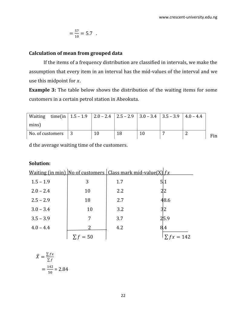
Calculation of mean from grouped data

If the items of a frequency distribution are classified in intervals, we make the

assumption that every item in an interval has the mid-values of the interval and we

use this midpoint for .

Example 3: The table below shows the distribution of the waiting items for some

customers in a certain petrol station in Abeokuta.

Fin

d the average waiting time of the customers.

Solution:

Waiting (in min) No of customers Class mark mid-value(X)

1.5 – 1.9 3 1.7 5.1

2.0 – 2.4 10 2.2 22

2.5 – 2.9 18 2.7 48.6

3.0 – 3.4 10 3.2 32

3.5 – 3.9 7 3.7 25.9

4.0 – 4.4 2 4.2 8.4

= 2.84

Waiting time(in

mins)

1.5 – 1.9 2.0 – 2.4 2.5 – 2.9 3.0 – 3.4 3.5 – 3.9 4.0 – 4.4

No. of customers 3 10 18 10 7 2


23

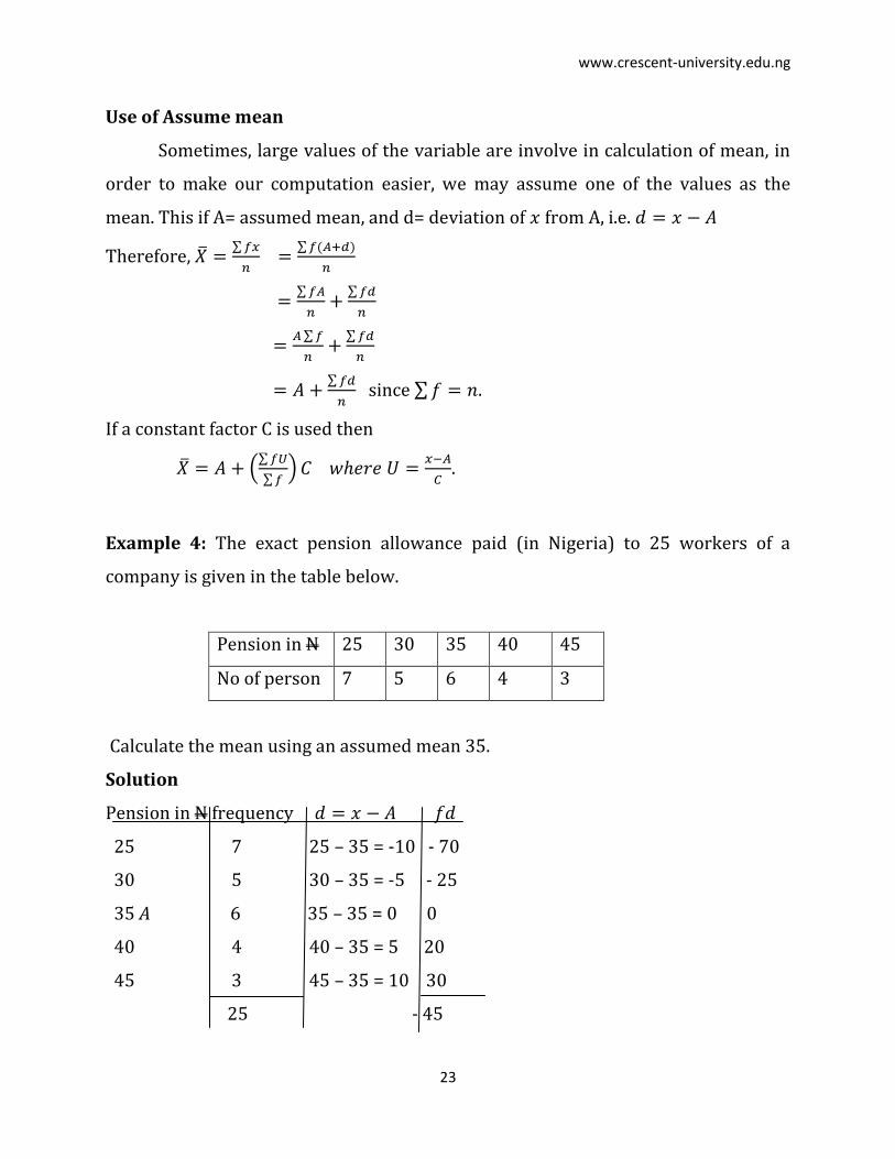
Use of Assume mean

Sometimes, large values of the variable are involve in calculation of mean, in

order to make our computation easier, we may assume one of the values as the

mean. This if A= assumed mean, and d= deviation of from A, i.e.

Therefore,

since .

If a constant factor C is used then

.

Example 4: The exact pension allowance paid (in Nigeria) to 25 workers of a

company is given in the table below.

Pension in N 25 30 35 40 45

No of person 7 5 6 4 3

Calculate the mean using an assumed mean 35.

Solution

Pension in N frequency

25 7 25 – 35 = -10 - 70

30 5 30 – 35 = -5 - 25

35 A 6 35 – 35 = 0 0

40 4 40 – 35 = 5 20

45 3 45 – 35 = 10 30

25 - 45


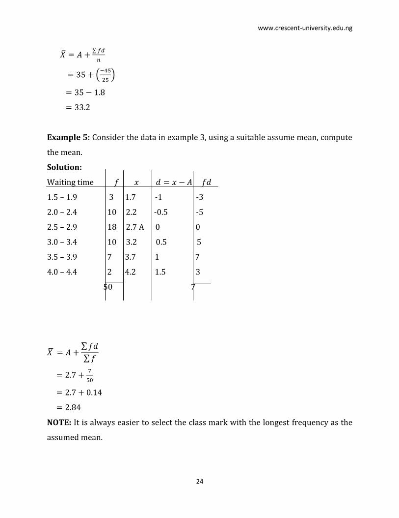
24

Example 5: Consider the data in example 3, using a suitable assume mean, compute

the mean.

Solution:

Waiting time

1.5 – 1.9 3 1.7 -1 -3

2.0 – 2.4 10 2.2 -0.5 -5

2.5 – 2.9 18 2.7 A 0 0

3.0 – 3.4 10 3.2 0.5 5

3.5 – 3.9 7 3.7 1 7

4.0 – 4.4 2 4.2 1.5 3

50 7

NOTE: It is always easier to select the class mark with the longest frequency as the

assumed mean.


25

ADVANTAGE OF MEAN

The mean is an average that considers all the observations in the data set. It is single

and easy to compute and it is the most widely used average.

DISAVANTAGE OF MEAN

Its value is greatly affected by the extremely too large or too small observation.

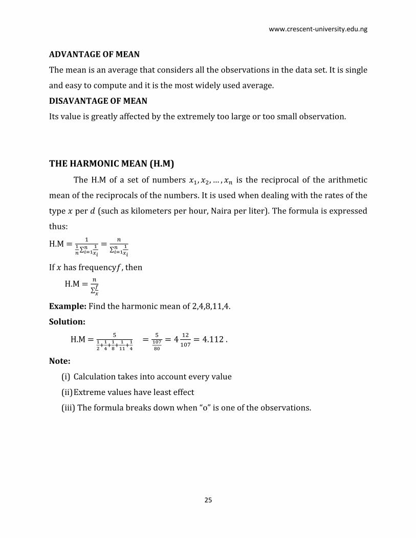
THE HARMONIC MEAN (H.M)

The H.M of a set of numbers is the reciprocal of the arithmetic

mean of the reciprocals of the numbers. It is used when dealing with the rates of the

type per (such as kilometers per hour, Naira per liter). The formula is expressed

thus:

H.M

If has frequency , then

H.M

Example: Find the harmonic mean of .

Solution:

H.M

.

Note:

(i) Calculation takes into account every value

(ii) Extreme values have least effect

(iii) The formula breaks down when “o” is one of the observations.


26

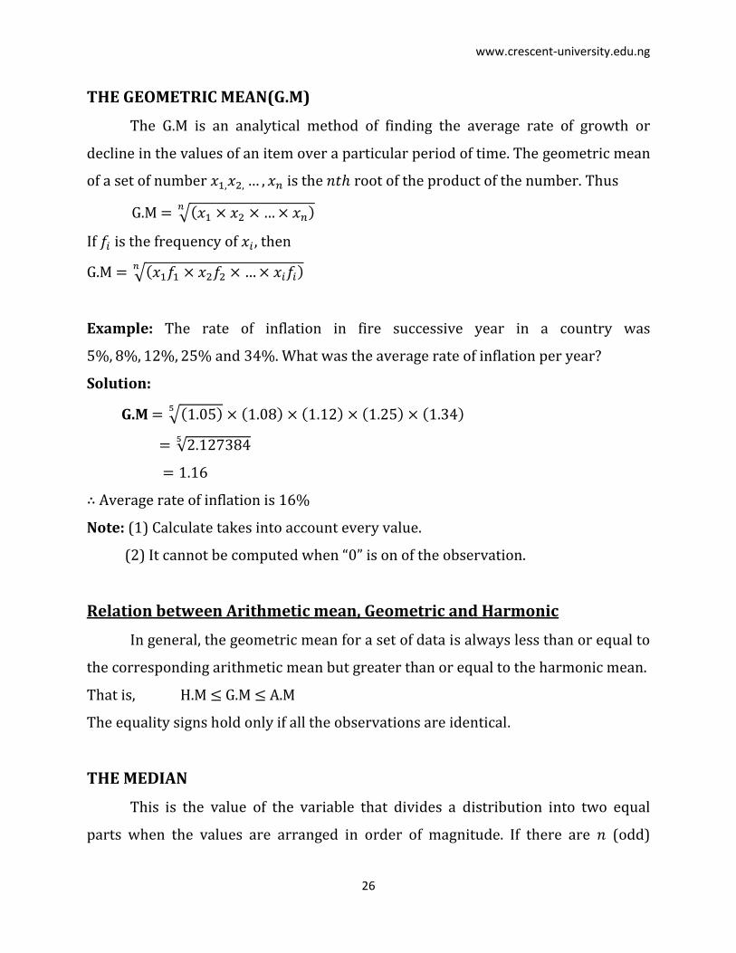
THE GEOMETRIC MEAN(G.M)

The G.M is an analytical method of finding the average rate of growth or

decline in the values of an item over a particular period of time. The geometric mean

of a set of number is the root of the product of the number. Thus

G.M

If is the frequency of , then

G.M

Example: The rate of inflation in fire successive year in a country was

. What was the average rate of inflation per year?

Solution:

G.M

Average rate of inflation is

Note: (1) Calculate takes into account every value.

(2) It cannot be computed when “0” is on of the observation.

Relation between Arithmetic mean, Geometric and Harmonic

In general, the geometric mean for a set of data is always less than or equal to

the corresponding arithmetic mean but greater than or equal to the harmonic mean.

That is, H.M G.M A.M

The equality signs hold only if all the observations are identical.

THE MEDIAN

This is the value of the variable that divides a distribution into two equal

parts when the values are arranged in order of magnitude. If there are (odd)


27

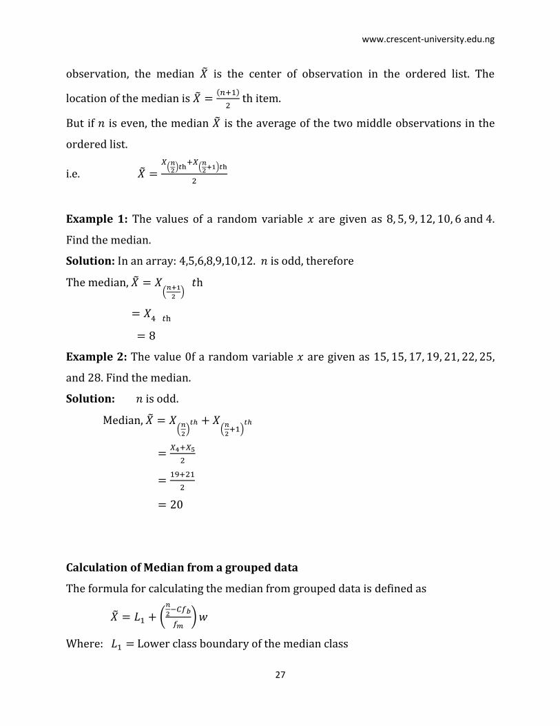
observation, the median is the center of observation in the ordered list. The

location of the median is

th item.

But if is even, the median is the average of the two middle observations in the

ordered list.

i.e.

Example 1: The values of a random variable are given as

Find the median.

Solution: In an array: . is odd, therefore

The median,

Example 2: The value 0f a random variable are given as

and . Find the median.

Solution: is odd.

Median,

Calculation of Median from a grouped data

The formula for calculating the median from grouped data is defined as

Where: Lower class boundary of the median class


28

Total frequency

Cumulative frequency before the median class

Frequency of the median class.

Class size or width.

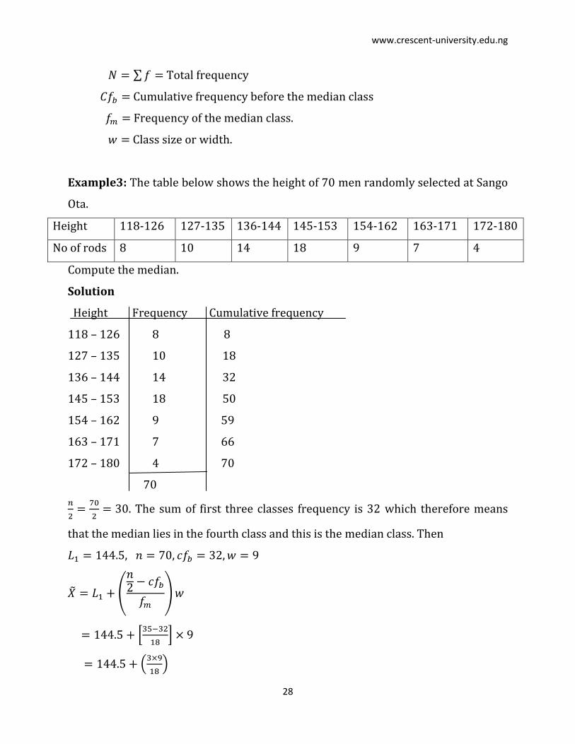
Example3: The table below shows the height of 70 men randomly selected at Sango

Ota.

Height 118-126 127-135 136-144 145-153 154-162 163-171 172-180

No of rods 8 10 14 18 9 7 4

Compute the median.

Solution

Height Frequency Cumulative frequency

118 – 126 8 8

127 – 135 10 18

136 – 144 14 32

145 – 153 18 50

154 – 162 9 59

163 – 171 7 66

172 – 180 4 70

70

. The sum of first three classes frequency is 32 which therefore means

that the median lies in the fourth class and this is the median class. Then


29

.

ADVANTAGE OF THE MEDIAN

(i) Its value is not affected by extreme values; thus it is a resistant measure of

central tendency.

(ii) It is a good measure of location in a skewed distribution

DISAVANTAGE OF THE MEDIAN

1) It does not take into consideration all the value of the variable.

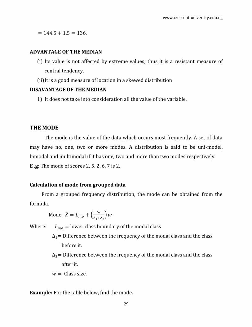
THE MODE

The mode is the value of the data which occurs most frequently. A set of data

may have no, one, two or more modes. A distribution is said to be uni-model,

bimodal and multimodal if it has one, two and more than two modes respectively.

E .g: The mode of scores 2, 5, 2, 6, 7 is 2.

Calculation of mode from grouped data

From a grouped frequency distribution, the mode can be obtained from the

formula.

Mode,

Where: lower class boundary of the modal class

Difference between the frequency of the modal class and the class

before it.

Difference between the frequency of the modal class and the class

after it.

Class size.

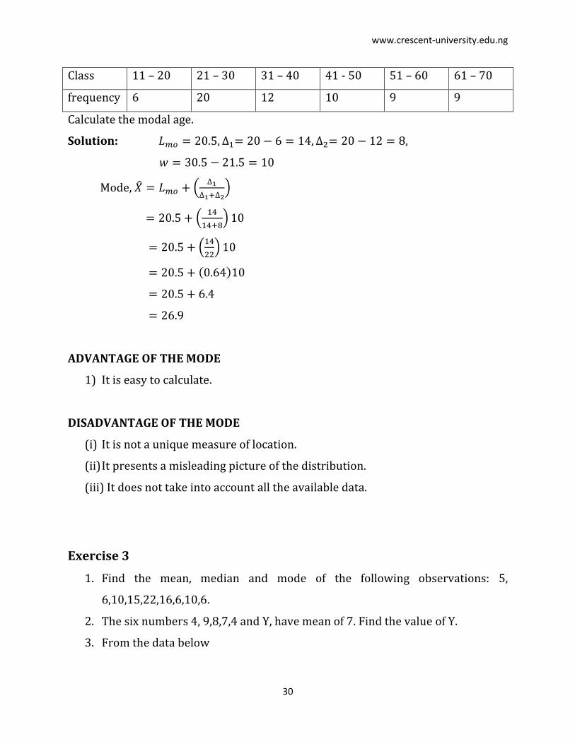
Example: For the table below, find the mode.


30

Class 11 – 20 21 – 30 31 – 40 41 - 50 51 – 60 61 – 70

frequency 6 20 12 10 9 9

Calculate the modal age.

Solution:

Mode,

ADVANTAGE OF THE MODE

1) It is easy to calculate.

DISADVANTAGE OF THE MODE

(i) It is not a unique measure of location.

(ii) It presents a misleading picture of the distribution.

(iii) It does not take into account all the available data.

Exercise 3

1. Find the mean, median and mode of the following observations: 5,

6,10,15,22,16,6,10,6.

2. The six numbers 4, 9,8,7,4 and Y, have mean of 7. Find the value of Y.

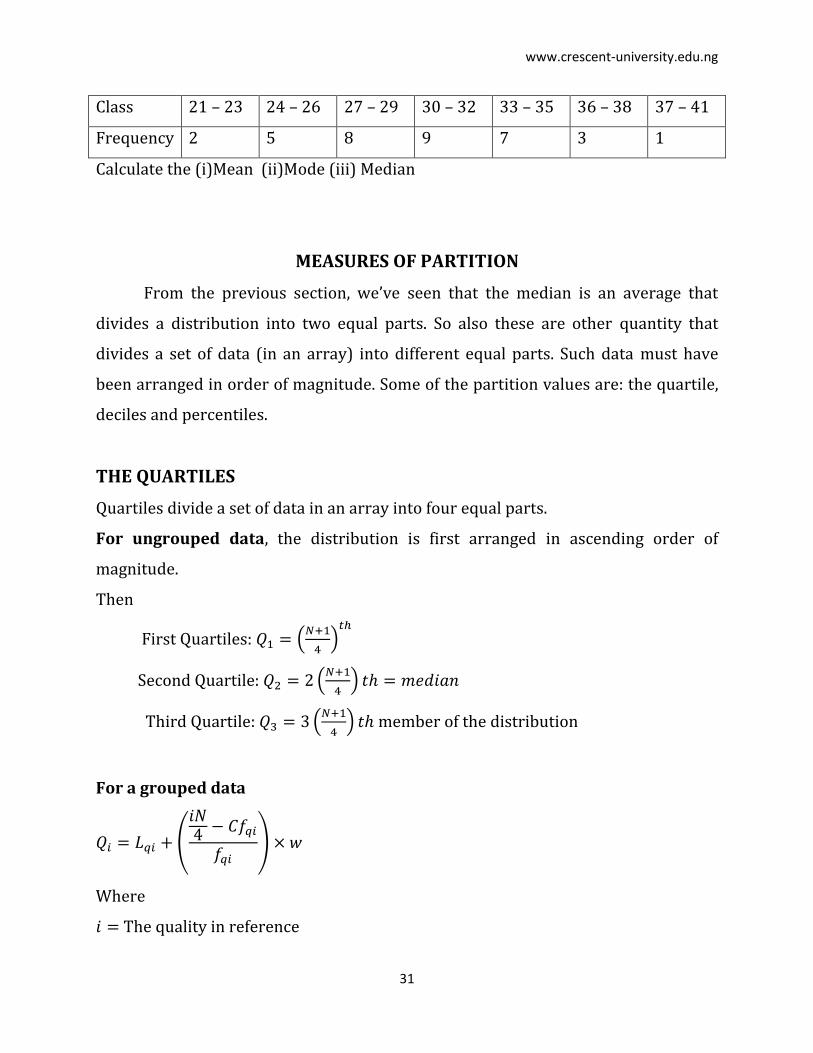
3. From the data below


31

Class 21 – 23 24 – 26 27 – 29 30 – 32 33 – 35 36 – 38 37 – 41

Frequency 2 5 8 9 7 3 1

Calculate the (i)Mean (ii)Mode (iii) Median

MEASURES OF PARTITION

From the previous section, we’ve seen that the median is an average that

divides a distribution into two equal parts. So also these are other quantity that

divides a set of data (in an array) into different equal parts. Such data must have

been arranged in order of magnitude. Some of the partition values are: the quartile,

deciles and percentiles.

THE QUARTILES

Quartiles divide a set of data in an array into four equal parts.

For ungrouped data, the distribution is first arranged in ascending order of

magnitude.

Then

First Quartiles:

Second Quartile:

Third Quartile:

For a grouped data

Where

The quality in reference


32

Lower class boundary of the class counting the quartile

Total frequency

Cumulative frequency before the class

The frequency of the class

Class size of the class.

DECILES

The values of the variable that divide the frequency of the distribution into

ten equal parts are known as deciles and are denoted by the fifth

deciles is the median.


magnitude. Then

For a grouped data

Where


33

PERCENTILE

The values of the variable that divide the frequency of the distribution into

hundred equal parts are known as percentiles and are generally denoted by

The fiftieth percentile is the median.


magnitude. Then

For a grouped data,

Where

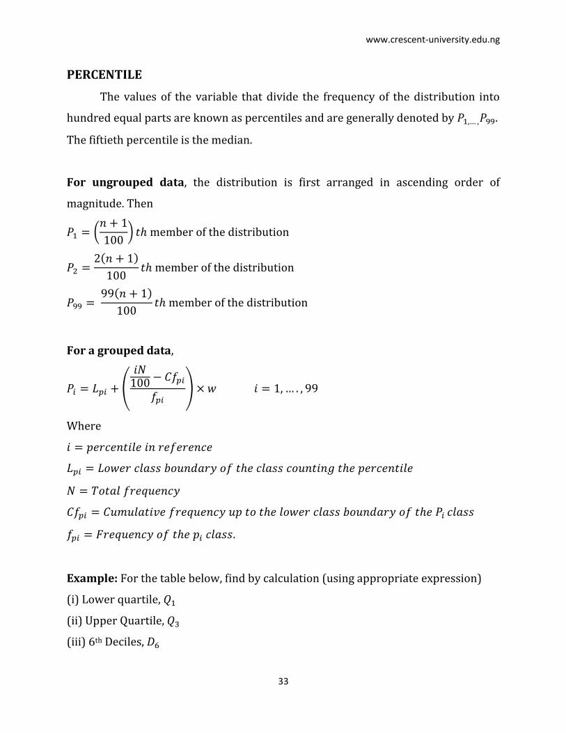
Example: For the table below, find by calculation (using appropriate expression)

(i) Lower quartile,

(ii) Upper Quartile,

(iii) 6th Deciles,


34

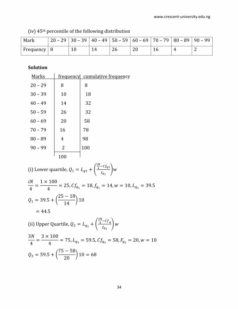
(iv) 45th percentile of the following distribution

Mark 20 – 29 30 – 39 40 – 49 50 – 59 60 – 69 70 – 79 80 – 89 90 – 99

Frequency 8 10 14 26 20 16 4 2

Solution

Marks frequency cumulative frequency

20 – 29 8 8

30 – 39 10 18

40 – 49 14 32

50 – 59 26 32

60 – 69 20 58

70 – 79 16 78

80 – 89 4 98

90 – 99 2 100

100

(i) Lower quartile,

w

(ii) Upper Quartile,


35

(iii)

(iv)

MEASURES OF DISPERSION

Dispersion or variation is degree of scatter or variation of individual value of a

variable about the central value such as the median or the mean. These include

range, mean deviation, semi-interquartile range, variance, standard deviation and

coefficient of variation.

THE RANGE

This is the simplest method of measuring dispersions. It is the difference

between the largest and the smallest value in a set of data. It is commonly used in

statistical quality control. However, the range may fail to discriminate if the

distributions are of different types.

Coefficient of Range


36

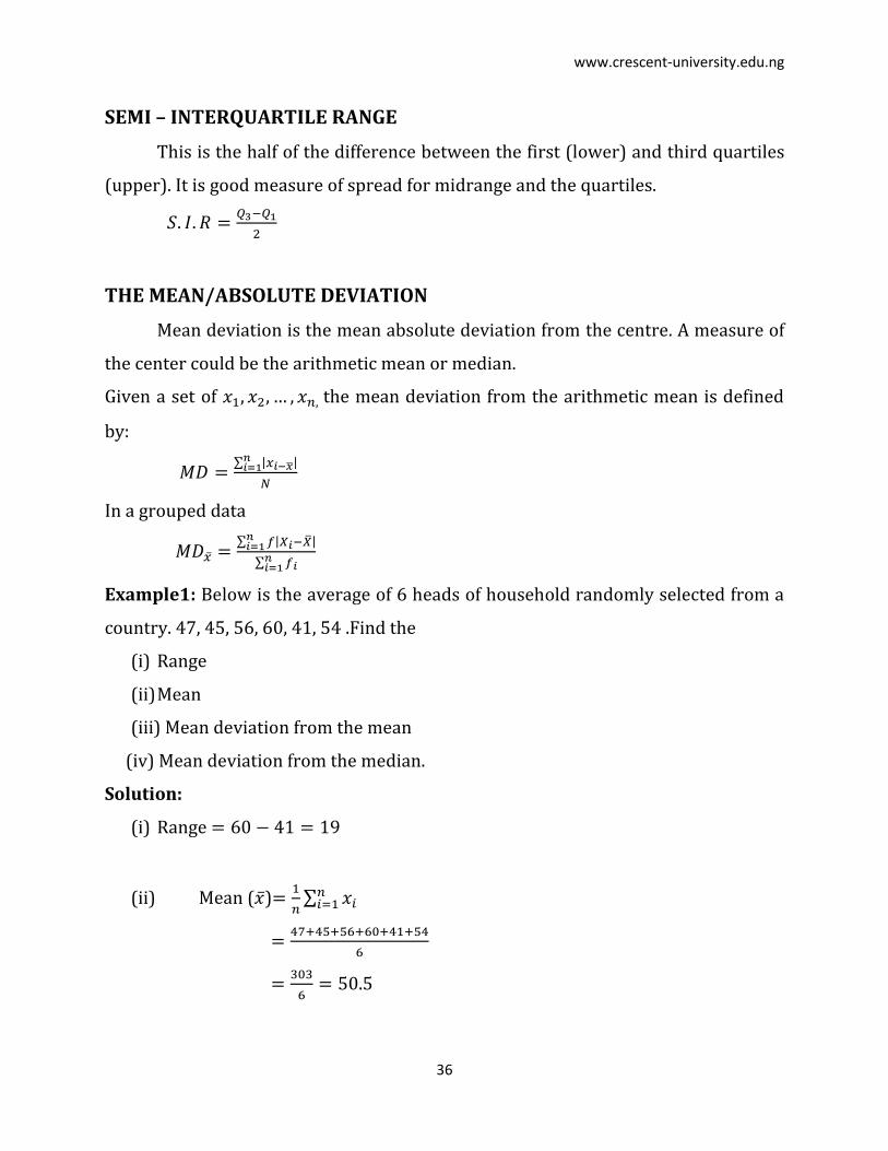
SEMI – INTERQUARTILE RANGE

This is the half of the difference between the first (lower) and third quartiles

(upper). It is good measure of spread for midrange and the quartiles.

THE MEAN/ABSOLUTE DEVIATION

Mean deviation is the mean absolute deviation from the centre. A measure of

the center could be the arithmetic mean or median.

Given a set of the mean deviation from the arithmetic mean is defined

by:

In a grouped data

Example1: Below is the average of 6 heads of household randomly selected from a

country. 47, 45, 56, 60, 41, 54 .Find the

(i) Range

(ii) Mean

(iii) Mean deviation from the mean

(iv) Mean deviation from the median.

Solution:

(i) Range

(ii) Mean ( )


37

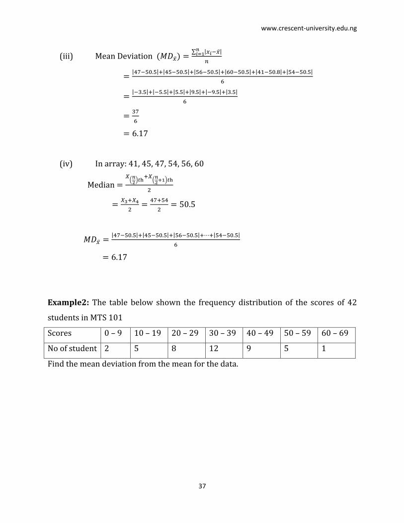
(iii) Mean Deviation

(iv) In array: 41, 45, 47, 54, 56, 60

Median

Example2: The table below shown the frequency distribution of the scores of 42

students in MTS 101

Scores 0 – 9 10 – 19 20 – 29 30 – 39 40 – 49 50 – 59 60 – 69

No of student 2 5 8 12 9 5 1

Find the mean deviation from the mean for the data.


38

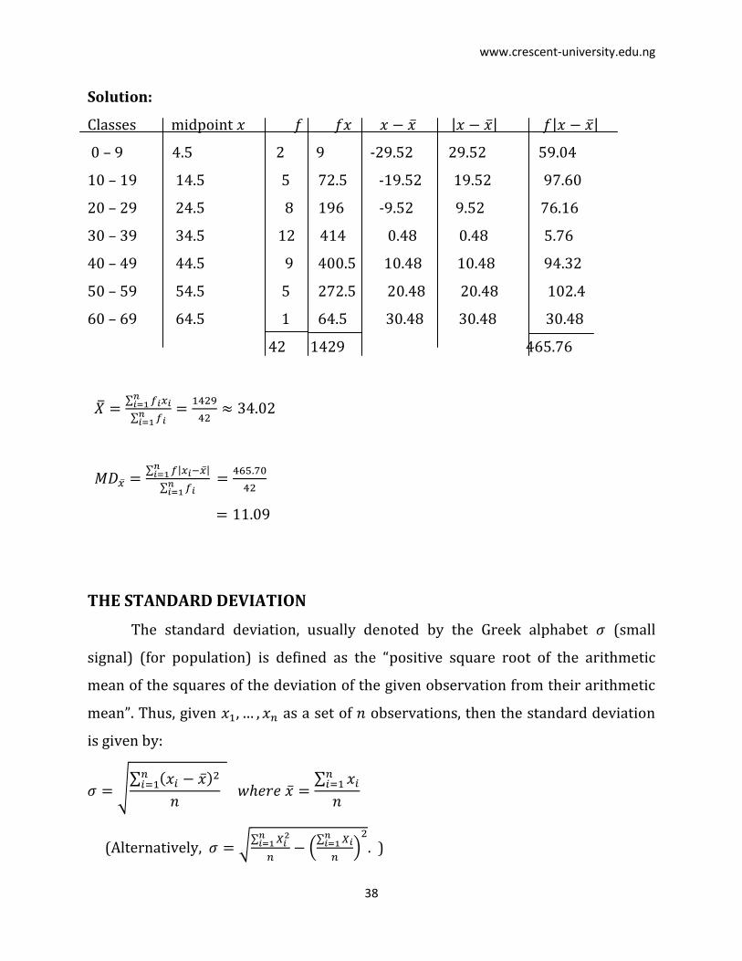
Solution:

Classes midpoint

0 – 9 4.5 2 9 -29.52 29.52 59.04

10 – 19 14.5 5 72.5 -19.52 19.52 97.60

20 – 29 24.5 8 196 -9.52 9.52 76.16

30 – 39 34.5 12 414 0.48 0.48 5.76

40 – 49 44.5 9 400.5 10.48 10.48 94.32

50 – 59 54.5 5 272.5 20.48 20.48 102.4

60 – 69 64.5 1 64.5 30.48 30.48 30.48

42 1429 465.76

THE STANDARD DEVIATION

The standard deviation, usually denoted by the Greek alphabet (small

signal) (for population) is defined as the “positive square root of the arithmetic

mean of the squares of the deviation of the given observation from their arithmetic

mean”. Thus, given as a set of observations, then the standard deviation

is given by:

(Alternatively,

. )


39

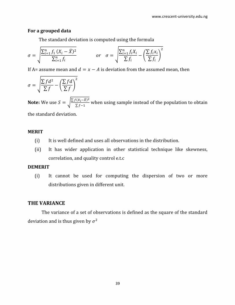
For a grouped data

The standard deviation is computed using the formula

If A= assume mean and is deviation from the assumed mean, then

Note: We use

when using sample instead of the population to obtain

the standard deviation.

MERIT

(i) It is well defined and uses all observations in the distribution.

(ii) It has wider application in other statistical technique like skewness,

correlation, and quality control e.t.c

DEMERIT

(i) It cannot be used for computing the dispersion of two or more

distributions given in different unit.

THE VARIANCE

The variance of a set of observations is defined as the square of the standard

deviation and is thus given by


40

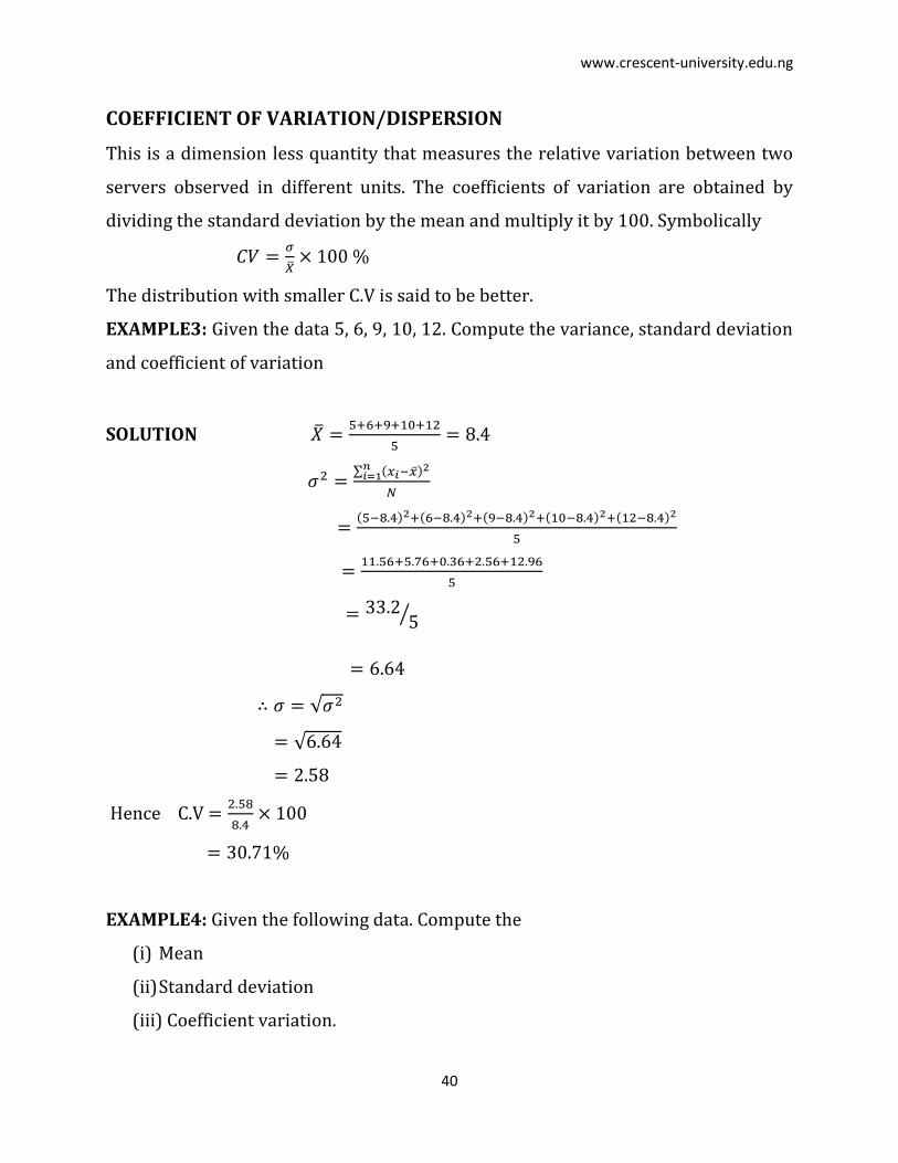
COEFFICIENT OF VARIATION/DISPERSION

This is a dimension less quantity that measures the relative variation between two

servers observed in different units. The coefficients of variation are obtained by

dividing the standard deviation by the mean and multiply it by 100. Symbolically

The distribution with smaller C.V is said to be better.

EXAMPLE3: Given the data 5, 6, 9, 10, 12. Compute the variance, standard deviation

and coefficient of variation

SOLUTION

Hence C.V

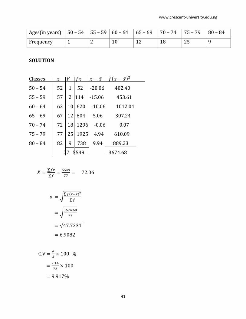
EXAMPLE4: Given the following data. Compute the

(i) Mean

(ii) Standard deviation

(iii) Coefficient variation.


41

Ages(in years) 50 – 54 55 – 59 60 – 64 65 – 69 70 – 74 75 – 79 80 – 84

Frequency 1 2 10 12 18 25 9

SOLUTION

Classes

50 – 54 52 1 52 -20.06 402.40

55 – 59 57 2 114 -15.06 453.61

60 – 64 62 10 620 -10.06 1012.04

65 – 69 67 12 804 -5.06 307.24

70 – 74 72 18 1296 -0.06 0.07

75 – 79 77 25 1925 4.94 610.09

80 – 84 82 9 738 9.94 889.23

77 5549 3674.68

C.V


42

Exercise 4

The data below represents the scores by 150 applicants in an achievement text for

the post of Botanist in a large company:

Scores 10 – 19 20 – 29 30 – 39 40 – 49 50 – 59 60 – 69 70 – 79 80 – 89 90 – 99

Frequency 1 6 9 31 42 32 17 10 2

Estimate

(i) The mean score

(ii) The median score

(iii) The modal score

(iv) Standard deviation

(v) Semi – interquartile range

(vi) D4

(vii) P26

(viii) coefficient of variation

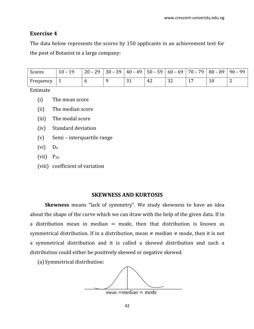
SKEWNESS AND KURTOSIS

Skewness means “lack of symmetry”. We study skewness to have an idea

about the shape of the curve which we can draw with the help of the given data. If in

a distribution mean in median mode, then that distribution is known as

symmetrical distribution. If in a distribution, mean median mode, then it is not

a symmetrical distribution and it is called a skewed distribution and such a

distribution could either be positively skewed or negative skewed.

(a) Symmetrical distribution:

mean median mode


43

Mean, median and mode coincide and the spread of the frequencies is the

same on both sides of the centre point of the curve.

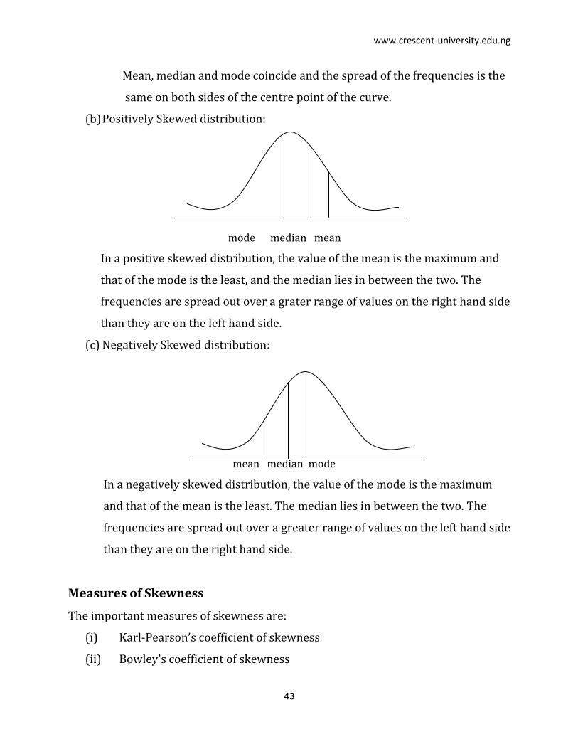
(b) Positively Skewed distribution:

mode median mean

In a positive skewed distribution, the value of the mean is the maximum and

that of the mode is the least, and the median lies in between the two. The

frequencies are spread out over a grater range of values on the right hand side

than they are on the left hand side.

(c) Negatively Skewed distribution:

mean median mode

In a negatively skewed distribution, the value of the mode is the maximum

and that of the mean is the least. The median lies in between the two. The

frequencies are spread out over a greater range of values on the left hand side

than they are on the right hand side.

Measures of Skewness

The important measures of skewness are:

(i) Karl-Pearson’s coefficient of skewness

(ii) Bowley’s coefficient of skewness


44

(iii) Measures of skewness based on moments.

Karl-Pearson’s coefficient of skewness

This is given by:

Karl-Pearson’s Coefficient Skewness

.

In case of mode is ill-defined, the coefficient can be determined by the formula:

Coefficient of Skewness

.

Bowley’s coefficient of skewness

This is given by:

Bowley’s Coefficient of Skewness

.

Measure of skewness based on moment

First, we note the following moments:

1st moment about mean:

;

.

2nd moment about mean:

;

.

3rd moment about mean:

;

.

4th moment about mean:

;

.

Then the measure of skewness based on moments denoted by is given by:

.

KURTOSIS

The expression ‘Kurtosis’ is used to describe the peakedness of a normal

curve. The three measures – central tendency, dispersion and skewness, describe

the characteristics of frequency distributions. But these studies will not give us a


45

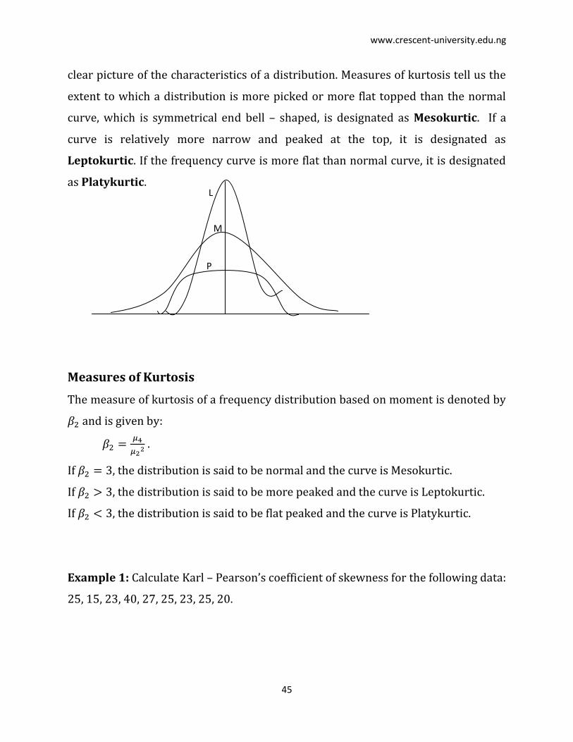
clear picture of the characteristics of a distribution. Measures of kurtosis tell us the

extent to which a distribution is more picked or more flat topped than the normal

curve, which is symmetrical end bell – shaped, is designated as Mesokurtic. If a

curve is relatively more narrow and peaked at the top, it is designated as

Leptokurtic. If the frequency curve is more flat than normal curve, it is designated

as Platykurtic.

Measures of Kurtosis

The measure of kurtosis of a frequency distribution based on moment is denoted by

and is given by:

.

If , the distribution is said to be normal and the curve is Mesokurtic.

If , the distribution is said to be more peaked and the curve is Leptokurtic.

If , the distribution is said to be flat peaked and the curve is Platykurtic.

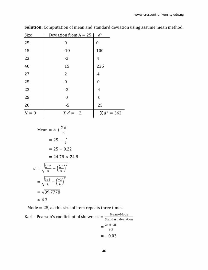
Example 1: Calculate Karl – Pearson’s coefficient of skewness for the following data:

25, 15, 23, 40, 27, 25, 23, 25, 20.

P

M

L


46

Solution: Computation of mean and standard deviation using assume mean method:

Size Deviation from A 25

25 0 0

15 -10 100

23 -2 4

40 15 225

27 2 4

25 0 0

23 -2 4

25 0 0

20 -5 25

Mean

Mode , as this size of item repeats three times.

Karl – Pearson’s coefficient of skewness


47

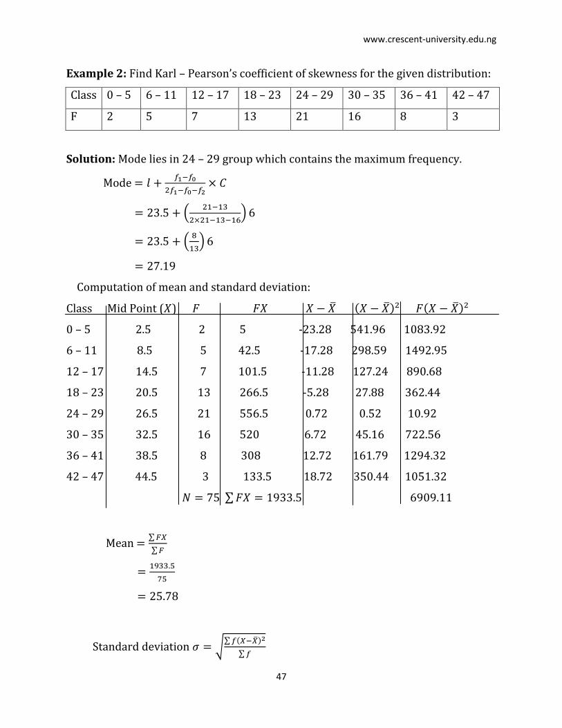
Example 2: Find Karl – Pearson’s coefficient of skewness for the given distribution:

Class 0 – 5 6 – 11 12 – 17 18 – 23 24 – 29 30 – 35 36 – 41 42 – 47

F 2 5 7 13 21 16 8 3

Solution: Mode lies in 24 – 29 group which contains the maximum frequency.

Mode

Computation of mean and standard deviation:

Class Mid Point ( )

0 – 5 2.5 2 5 -23.28 541.96 1083.92

6 – 11 8.5 5 42.5 -17.28 298.59 1492.95

12 – 17 14.5 7 101.5 -11.28 127.24 890.68

18 – 23 20.5 13 266.5 -5.28 27.88 362.44

24 – 29 26.5 21 556.5 0.72 0.52 10.92

30 – 35 32.5 16 520 6.72 45.16 722.56

36 – 41 38.5 8 308 12.72 161.79 1294.32

42 – 47 44.5 3 133.5 18.72 350.44 1051.32

Mean

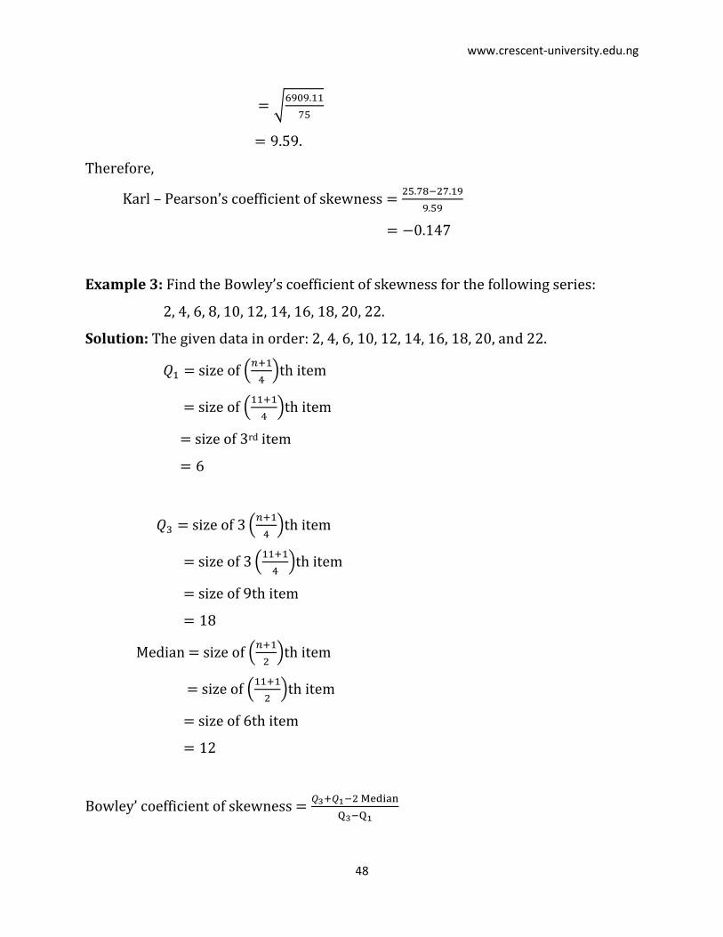
Standard deviation


48

.

Therefore,

Karl – Pearson’s coefficient of skewness

Example 3: Find the Bowley’s coefficient of skewness for the following series:

2, 4, 6, 8, 10, 12, 14, 16, 18, 20, 22.

Solution: The given data in order: 2, 4, 6, 10, 12, 14, 16, 18, 20, and 22.

size of

th item

size of

th item

size of 3rd item

size of

th item

size of

th item

size of 9th item

Median size of

th item

size of

th item

size of 6th item

Bowley’ coefficient of skewness


49

Since skewness , the given series is a symmetrical data.

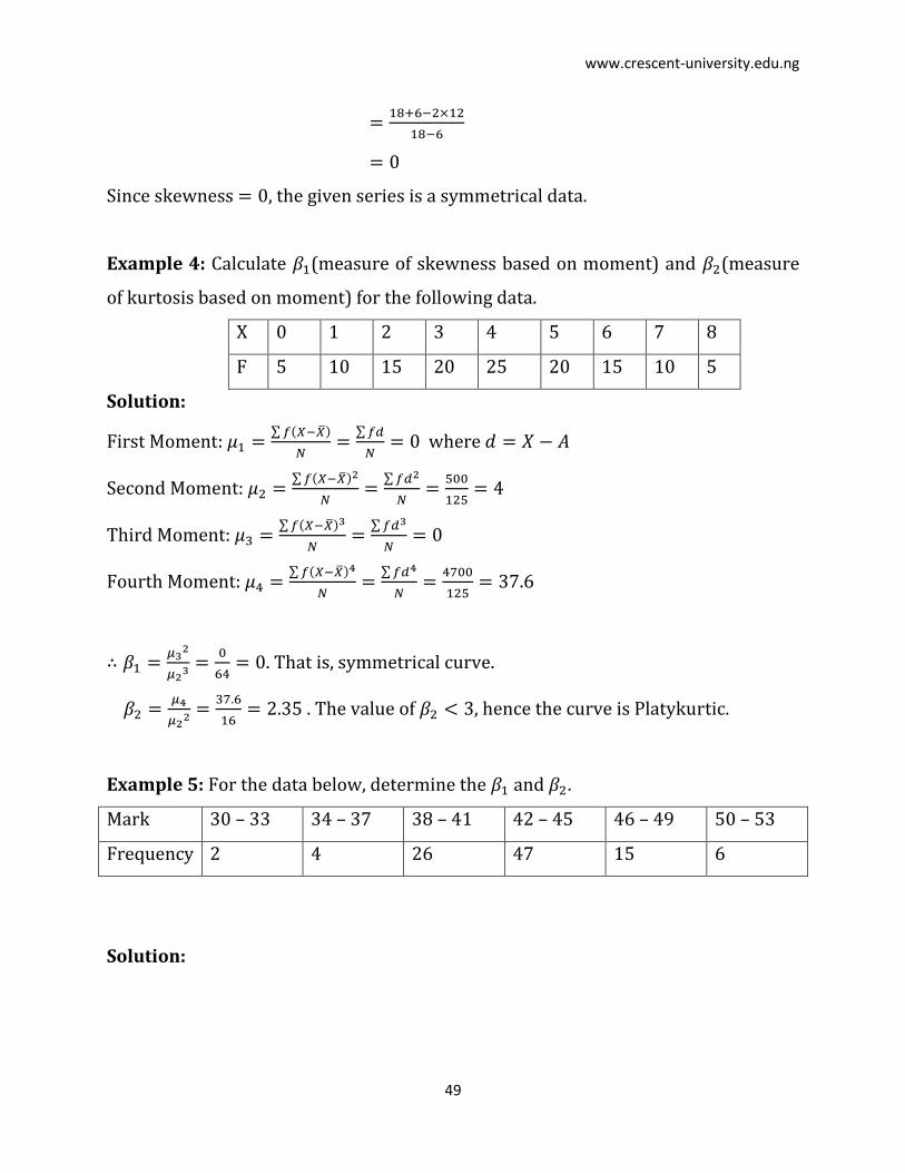
Example 4: Calculate (measure of skewness based on moment) and (measure

of kurtosis based on moment) for the following data.

X 0 1 2 3 4 5 6 7 8

F 5 10 15 20 25 20 15 10 5

Solution:

First Moment:

where

Second Moment:

Third Moment:

Fourth Moment:

. That is, symmetrical curve.

. The value of , hence the curve is Platykurtic.

Example 5: For the data below, determine the and .

Mark 30 – 33 34 – 37 38 – 41 42 – 45 46 – 49 50 – 53

Frequency 2 4 26 47 15 6

Solution:


50

Mark Mid Point ( )

30 – 33 31.5 2 63 -11.48 131.79 263.58

34 – 37 35.5 4 142 -7.48 55.95 223.80

38 – 41 39.5 26 1027 -3.48 12.11 314.87

42 – 45 43.5 47 2044.5 0.52 0.27 12.71

46 – 49 47.5 15 712.5 4.52 20.43 306.46

50 – 53 51.5 6 309 8.52 72.59 435.54

100 4298 1556.96

-1512.95 -3025.91 17368.71 34737.42

-18.51 -1674.04 3130.45 12521.79

-42.14 -1095.64 146.66 3813.16

0.14 6.58 0.07 3.44

92.35 1385.25 417.40 6261.02

618.47 3710.82 5269.37 31616.22

-692.94 88952.90

. Since , the curve is Leptokurtic.


51

Exercise 5

Calculate the and for the data below and interpret your result.

Class 10 – 14 15 – 19 20 – 24 25 – 29 30 – 34 35 – 39 40 – 44 45 – 49

f 1 4 8 19 35 20 7 5

Rates, Proportion and Index Numbers

Proportion

Proportion is the ratio of a number of items with certain characteristics (X)

and the total number of items exposed to such characteristics (N). It is defined as

.

The above expresses the chance of occurrences of such characteristics (i.e.

Probability of event X).

Example: If the voting age population (people 18 years and above) in Ifo ward I

consists of 550 males and 600 females. What is the proportion of males?

Solution: , Total population .

Proportion of males,

.

Rates

When proportion refers to the number of events or cases occurring during

certain period of time, it becomes a rate and is usually expressed as so many per

1000. Thus we refer to birth rate as the number of birth per 1000 population in a

year. So also we have death rate, migration rate, marriage rate etc.


52

INDEX NUMBERS

There are various types of index numbers, but in brief, we shall discuss three

kinds, namely: (a) Price Index (b) Quality Index (c) Value Index.

(a) Price Index

For measuring the value of money, in general, price index is used. It is an

index number which compares the prices for a group of commodities at a certain

time as at a place with prices of a base period. There are two price index numbers

such as whole sale price index numbers and retail price index numbers. The

wholesale price index reveals the changes into general price level of a country, but

the retail price reveals the changes in the retail price of commodities such as

consumption of goods, bank deposit etc.

(b) Quantity Index

This is the changes in the volume of goods produced or consumed. They are

useful and helpful to study the output in an economy.

(c) Value Index

Value index numbers compare the total value of a certain period with total

value in the base period. Here a total vale is equal to the price of commodity

multiplied by the quantity consumed.

NOTATION: For any index number, two time periods are needed for comparison.

These are called the Base period and the Current year. The period of

the year which is used as a basis year and the other is the current year.

The various notations used are as given below:


53

Price of current year Price of base year

Quantity of current year Quantity of base year

Definition (The weight): Different weights are used in different part of the country

for a particular commodity. For instance, “congo” – western part of Nigeria, “mudu”

– northern part etc.

Problems in the construction of Index numbers

No index number is an all purpose index number. Hence, there are many

problems involved in the construction of index numbers, which are to be tackled by

an economist or statistician. They are:

1. Purpose of the index numbers

2. Selection of base period

3. Selection of items

4. Selection of source of data

5. Collection of data

6. Selection of average

7. System of weighting

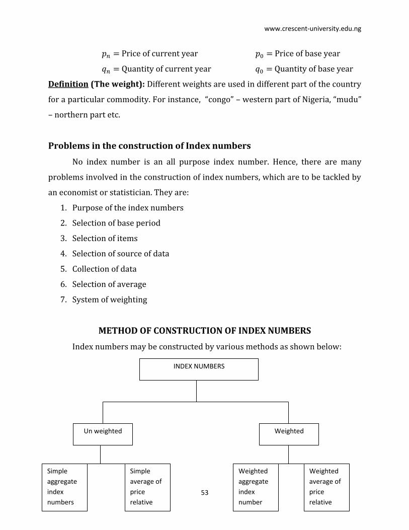
METHOD OF CONSTRUCTION OF INDEX NUMBERS

Index numbers may be constructed by various methods as shown below:

INDEX NUMBERS

Un weighted Weighted

Simple

average of

price

relative

Simple

aggregate

index

numbers

Weighted

aggregate

index

number

Weighted

average of

price

relative


54

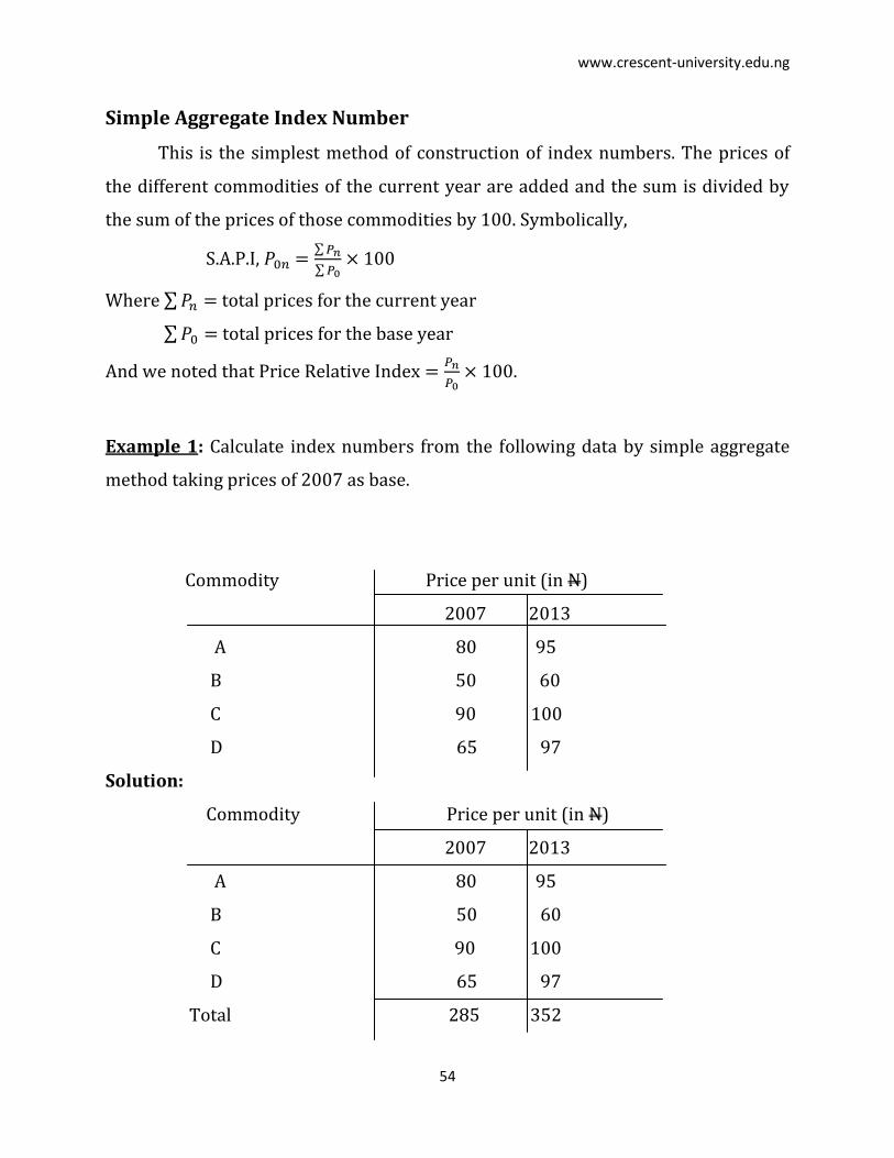
Simple Aggregate Index Number

This is the simplest method of construction of index numbers. The prices of

the different commodities of the current year are added and the sum is divided by

the sum of the prices of those commodities by 100. Symbolically,

S.A.P.I,

Where total prices for the current year

total prices for the base year

And we noted that Price Relative Index

.

Example 1: Calculate index numbers from the following data by simple aggregate

method taking prices of 2007 as base.

Commodity Price per unit (in N)

2007 2013

A 80 95

B 50 60

C 90 100

D 65 97

Solution:

Commodity Price per unit (in N)

2007 2013

A 80 95

B 50 60

C 90 100

D 65 97

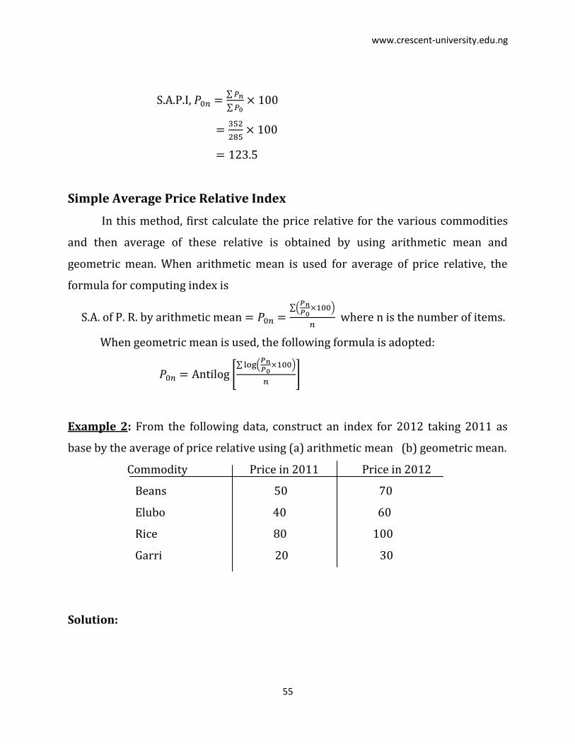
Total 285 352


55

S.A.P.I,

Simple Average Price Relative Index

In this method, first calculate the price relative for the various commodities

and then average of these relative is obtained by using arithmetic mean and

geometric mean. When arithmetic mean is used for average of price relative, the

formula for computing index is

S.A. of P. R. by arithmetic mean

where n is the number of items.

When geometric mean is used, the following formula is adopted:

Example 2: From the following data, construct an index for 2012 taking 2011 as

base by the average of price relative using (a) arithmetic mean (b) geometric mean.

Commodity Price in 2011 Price in 2012

Beans 50 70

Elubo 40 60

Rice 80 100

Garri 20 30

Solution:


56

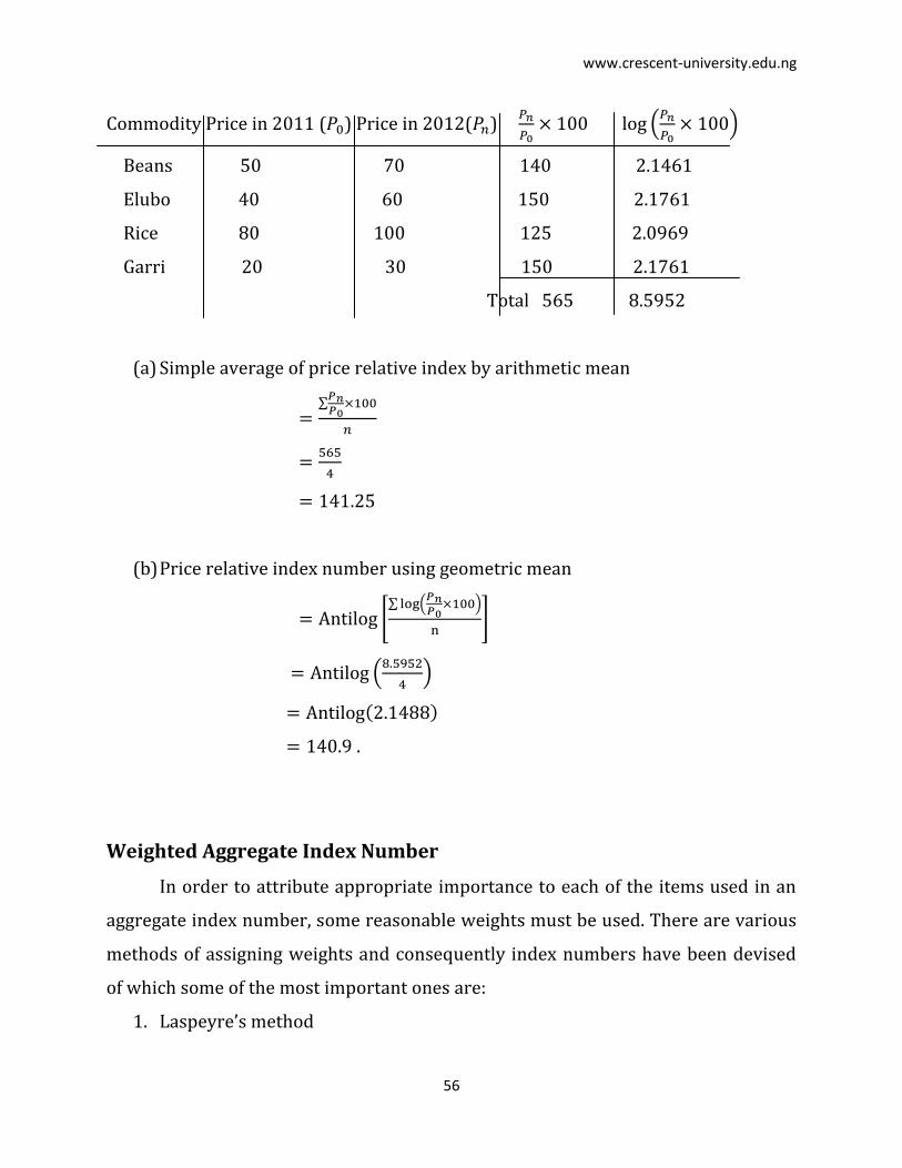
Commodity Price in 2011 ( ) Price in 2012( )

Beans 50 70 140 2.1461

Elubo 40 60 150 2.1761

Rice 80 100 125 2.0969

Garri 20 30 150 2.1761

Total 565 8.5952

(a) Simple average of price relative index by arithmetic mean

(b) Price relative index number using geometric mean

.

Weighted Aggregate Index Number

In order to attribute appropriate importance to each of the items used in an

aggregate index number, some reasonable weights must be used. There are various

methods of assigning weights and consequently index numbers have been devised

of which some of the most important ones are:

1. Laspeyre’s method


57

2. Paasche’s method

3. Fisher’s Ideal method

4. Bowley’s method

5. Marshall – Edgeworth method

6. Kelly’s method

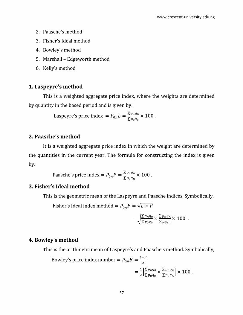
1. Laspeyre’s method

This is a weighted aggregate price index, where the weights are determined

by quantity in the based period and is given by:

Laspeyre’s price index

.

2. Paasche’s method

It is a weighted aggregate price index in which the weight are determined by

the quantities in the current year. The formula for constructing the index is given

by:

Paasche’s price index

.

3. Fisher’s Ideal method

This is the geometric mean of the Laspeyre and Paasche indices. Symbolically,

Fisher’s Ideal index method

.

4. Bowley’s method

This is the arithmetic mean of Laspeyre’s and Paasche’s method. Symbolically,

Bowley’s price index number

.


58

5. Marshall – Edgeworth method

In this method, the current year as well as base year prices and quantities are

considered. The formula in using to get this is given as follows:

Marshall – Edgeworth price index

.

6. Kelly’s method

Kelly has suggested the following formula for constructing the index

number:

Kelly’s price index number

where

. Here the average of the quantities of two years is used as

weights.

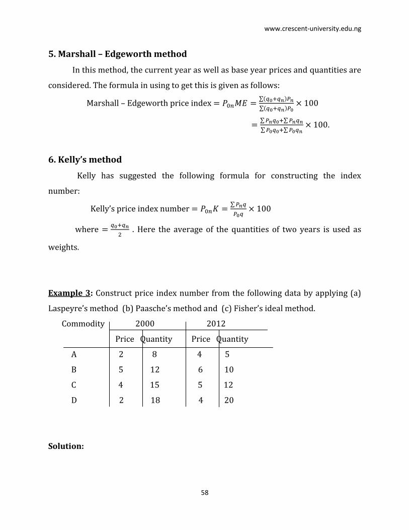
Example 3: Construct price index number from the following data by applying (a)

Laspeyre’s method (b) Paasche’s method and (c) Fisher’s ideal method.

Commodity 2000 2012

Price Quantity Price Quantity

A 2 8 4 5

B 5 12 6 10

C 4 15 5 12

D 2 18 4 20

Solution:


59

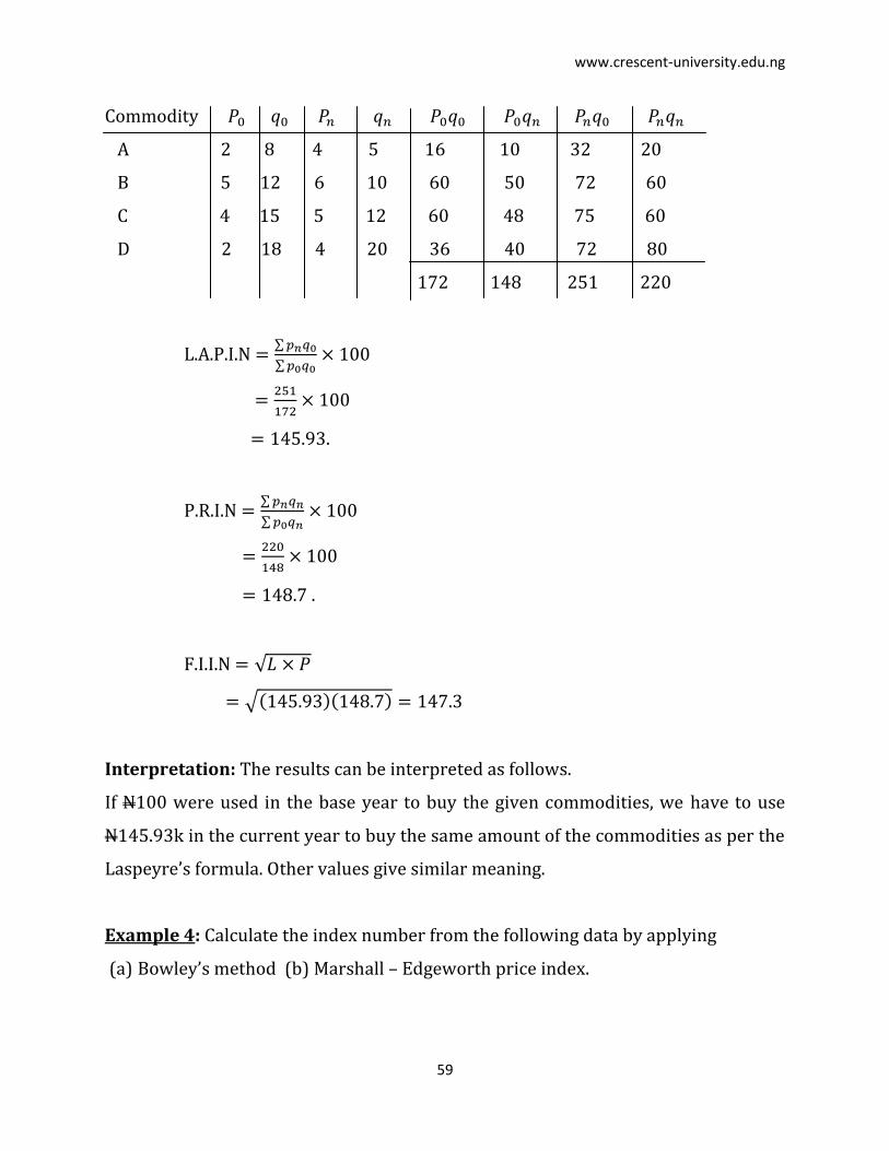
Commodity

A 2 8 4 5 16 10 32 20

B 5 12 6 10 60 50 72 60

C 4 15 5 12 60 48 75 60

D 2 18 4 20 36 40 72 80

172 148 251 220

L.A.P.I.N

.

P.R.I.N

.

F.I.I.N

Interpretation: The results can be interpreted as follows.

If N100 were used in the base year to buy the given commodities, we have to use

N145.93k in the current year to buy the same amount of the commodities as per the

Laspeyre’s formula. Other values give similar meaning.

Example 4: Calculate the index number from the following data by applying

(a) Bowley’s method (b) Marshall – Edgeworth price index.


60

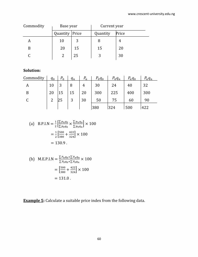
Commodity Base year Current year

Quantity Price Quantity Price

A 10 3 8 4

B 20 15 15 20

C 2 25 3 30

Solution:

Commodity

A 10 3 8 4 30 24 40 32

B 20 15 15 20 300 225 400 300

C 2 25 3 30 50 75 60 90

380 324 500 422

(a) B.P.I.N

.

(b) M.E.P.I.N

.

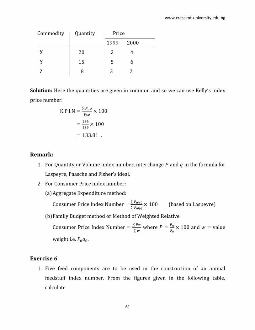
Example 5: Calculate a suitable price index from the following data.


61

Commodity Quantity Price

1999 2000

X 20 2 4

Y 15 5 6

Z 8 3 2

Solution: Here the quantities are given in common and so we can use Kelly’s index

price number.

K.P.I.N

.

Remark:

1. For Quantity or Volume index number, interchange and in the formula for

Laspeyre, Paasche and Fisher’s ideal.

2. For Consumer Price index number:

(a) Aggregate Expenditure method:

Consumer Price Index Number

(based on Laspeyre)

(b) Family Budget method or Method of Weighted Relative

Consumer Price Index Number

where

and value

weight i.e. .

Exercise 6

1. Five feed components are to be used in the construction of an animal

feedstuff index number. From the figures given in the following table,

calculate


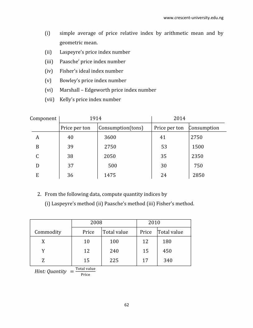
62

(i) simple average of price relative index by arithmetic mean and by

geometric mean.

(ii) Laspeyre’s price index number

(iii) Paasche’ price index number

(iv) Fisher’s ideal index number

(v) Bowley’s price index number

(vi) Marshall – Edgeworth price index number

(vii) Kelly’s price index number

Component 1914 2014

Price per ton Consumption(tons) Price per ton Consumption

A 40 3600 41 2750

B 39 2750 53 1500

C 38 2050 35 2350

D 37 500 30 750

E 36 1475 24 2850

2. From the following data, compute quantity indices by

(i) Laspeyre’s method (ii) Paasche’s method (iii) Fisher’s method.

2008 2010

Commodity Price Total value Price Total value

X 10 100 12 180

Y 12 240 15 450

Z 15 225 17 340

Hint: Quantity


63

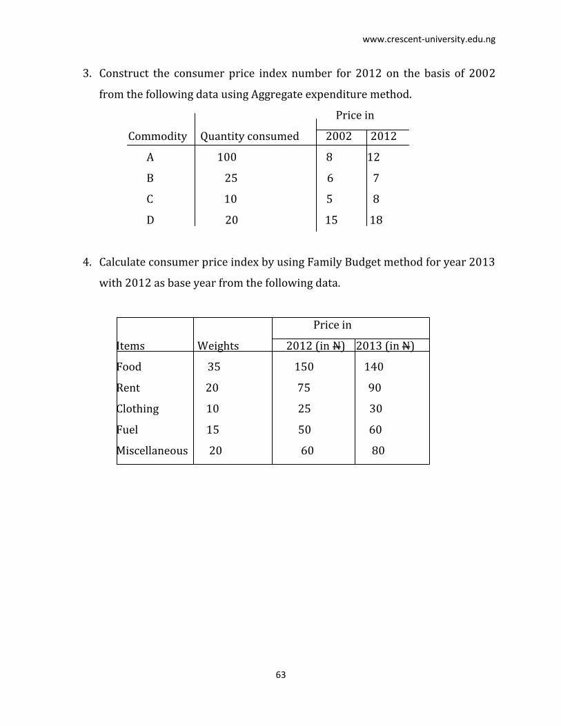
3. Construct the consumer price index number for 2012 on the basis of 2002

from the following data using Aggregate expenditure method.

Price in

Commodity Quantity consumed 2002 2012

A 100 8 12

B 25 6 7

C 10 5 8

D 20 15 18

4. Calculate consumer price index by using Family Budget method for year 2013

with 2012 as base year from the following data.

Price in

Items Weights 2012 (in N) 2013 (in N)

Food 35 150 140

Rent 20 75 90

Clothing 10 25 30

Fuel 15 50 60

Miscellaneous 20 60 80

Lecture note on Descriptive Statistics (STS 102)

Documents

Transcript of Lecture note on Descriptive Statistics (STS 102)