The Partition of Unity Meshfree Method for Solving Transport-Reaction Equations on Complex Domains:...
25
The Partition of Unity Meshfree Method for Solving Transport-Reaction Equations on Complex Domains: Implementation and Applications in the Life Sciences Martin Eigel 1 , Erwin George 2 , and Markus Kirkilionis 3 1 Mathematics Institute, University of Warwick, Coventry, UK [email protected] 2 Mathematics Institute, University of Warwick, Coventry, UK [email protected] 3 Mathematics Institute, University of Warwick, Coventry, UK [email protected] Summary. There is a wide range of highly significant scientific problems which on appropriate physical scales can be formulated as partial differential equations defined on so-called complex domains. Such complex domains often occur when material is transported through an environment of high geometrical complexity, for example porous media, domains with many obstacles, or membrane systems that are folded in a topologically complex configuration. The latter often occurs in cell biology, where the biological membranes inside the cell are strikingly topologically complex. In addition the medium in which, for example, proteins diffuse in the cell nucleus, is a complex porous media type of environment as many macro-molecules and protein-DNA complexes like the chromatin form a highly irregular structure in which many bio-molecular interactions occur. The distribution of biomolecules inside cells and tissues, their over-abundance or absence in metabolism, signalling etc., is the cause of many human diseases, therefore numerical simulations will be essential for future diagnostic abilities. Under appropriate assumptions the resulting molecular transport can be formulated as a PDE (Partial Differential Equation). The first challenge for any numerical discretisation is the generation of a cover for the underlying computational domain. Here, the meshfree Partition of Unity Method (PUM) offers a number of new degrees of freedom, as patches can be shifted, their size increased or diminished, with no need to create a non-overlapping cover at all times as is characteristic for traditional Finite Element and Finite Volume discretisations. Further advances in cover creation algorithms as discussed in this paper will allow the routine simulation of problems on domains with more complex geometries than have been treatable before. Key words: Complex Domains, PUM, Meshfree Discretisation, Cover Con- struction, Cell Biology
-
Upload
independent -
Category
Documents
-
view
2 -
download
0
Transcript of The Partition of Unity Meshfree Method for Solving Transport-Reaction Equations on Complex Domains:...
The Partition of Unity Meshfree Method forSolving Transport-Reaction Equations onComplex Domains: Implementation andApplications in the Life Sciences
Martin Eigel1, Erwin George2, and Markus Kirkilionis3
1 Mathematics Institute, University of Warwick, Coventry, [email protected]
2 Mathematics Institute, University of Warwick, Coventry, [email protected]
3 Mathematics Institute, University of Warwick, Coventry, [email protected]
Summary. There is a wide range of highly significant scientific problems whichon appropriate physical scales can be formulated as partial differential equationsdefined on so-called complex domains. Such complex domains often occur whenmaterial is transported through an environment of high geometrical complexity, forexample porous media, domains with many obstacles, or membrane systems thatare folded in a topologically complex configuration. The latter often occurs in cellbiology, where the biological membranes inside the cell are strikingly topologicallycomplex. In addition the medium in which, for example, proteins diffuse in the cellnucleus, is a complex porous media type of environment as many macro-moleculesand protein-DNA complexes like the chromatin form a highly irregular structurein which many bio-molecular interactions occur. The distribution of biomoleculesinside cells and tissues, their over-abundance or absence in metabolism, signallingetc., is the cause of many human diseases, therefore numerical simulations will beessential for future diagnostic abilities. Under appropriate assumptions the resultingmolecular transport can be formulated as a PDE (Partial Differential Equation).The first challenge for any numerical discretisation is the generation of a coverfor the underlying computational domain. Here, the meshfree Partition of UnityMethod (PUM) offers a number of new degrees of freedom, as patches can be shifted,their size increased or diminished, with no need to create a non-overlapping coverat all times as is characteristic for traditional Finite Element and Finite Volumediscretisations. Further advances in cover creation algorithms as discussed in thispaper will allow the routine simulation of problems on domains with more complexgeometries than have been treatable before.
Key words: Complex Domains, PUM, Meshfree Discretisation, Cover Con-struction, Cell Biology
2 Martin Eigel, Erwin George, and Markus Kirkilionis
1 Introduction
Many and perhaps the most important problems in Cell Biology can be mathe-matically formulated as transport processes, and most of them must be definedon complex domains. The complexity of the domain is due to the immenserichness of cellular sub-structures, like membranes folding in a particular way,or macro-molecular assemblies like the cytoskeleton or the chromatin chang-ing constantly their shapes. Traditionally the focus in Cell Biology has beenon other scales, for example looking at the molecular design (Structural Bi-ology, for a current review see [14]) of proteins, protein complexes or othermacro-molecules. One of the most important general new research questionsin Cell Biology is posed on a more macroscopic scale, but takes these mi-croscopic molecular properties into account: How abundant and with whatkind of distributions are certain types of bio-molecules present in the cell? Onwhat spatial and temporal scales do molecule distributions change in the cell?If these questions could be answered in more detail the most urgent prob-lems in Cell Biology could be understood and solved. Most questions on asystems level about the function and variability of regulatory and metabolicnetworks could be answered as they ultimately depend on the interaction ofbio-molecules, which itself is dependent on the spatial and temporal variationof different molecular species. Even the memory of the system, for exampleencoded in the DNA, is depending on such molecular interaction.
The experimental basis allowing to pose questions on cellular moleculardistributions is relatively new and rapidly evolving. This has been triggeredby new microscopy techniques covering a wide range of spatial scales, thedevelopment of photon emitting molecular markers allowing life cell imagingof dynamical processes (such as the most common GFP, Green FluorescentProtein), and techniques to manipulate photon emission or link the emissionto molecular transport or interaction events. Here we mention as examplesFRET (Fluorescence Resonance Energy Transfer), FLIP (Fluorescence LossIn Photobleaching) or FRAP (Fluorescence Recovery After Photobleaching).Some references where such techniques are explained and used successfullyare for example [10], [11] and [6]. It is tempting to make such microscopytechniques more quantitative. For a recent research paper in this directionsee [13]. Using such methods the complexity of the macro-molecular cellularstructure can sometimes be shown to exhibit anomalous diffusion, see [19].In combination with cloning, antibody production and modern techniques ofimage analysis to post-process the captured images there is a chance to un-derstand how cellular (and tissue) geometry in combination with molecularproperties influence changes in molecular distribution and composition.
As cellular form and function has/is such a highly complex organisa-tion/process there is a need to develop new numerical techniques that are ableto simulate spatial-temporal processes on domains which can be retrieved by
Meshfree PUM Methods Designed For Application in the Life Sciences 3
image analysis tools from microscopy images. This is in no way a simple task.Many even sophisticated grid generating algorithms working in two spatial di-mensions (on which we restrict ourselves in this paper) have severe problemsto generate automatically meshes delivering the necessary computational gridused by general purpose Finite Element (FEM) or Finite Volume Methods(FVM). Here the recent exploration of a discretisation based on a Partition ofUnity Method (PUM) using overlapping patches to create a cover has provento be a very promising alternative ([1, 3, 4, 12, 25, 27]). In this paper we willdiscuss the basic ideas of the method, introduce new cover generation algo-rithms, and demonstrate the feasibility of the whole discretisation with thehelp of different complex test domains. We also show that we can introducesuccessfully cover adaptivity for PUM when considering temporal processes,i.e. solving parabolic problems.
Similar complex domain problems are of interest in other areas of appli-cations. We would like to mention engineering, where certain fine structureshave to be resolved explicitly, for example in designing optimal catalysators.On an appropriate scale also porous media, for example relevant in geologyand hydrology should be mentioned. This holds primarily in cases where thehomogenised equation is not used for all the medium and some geometricalstructures in the soil are resolved explicitly. All these and areas with similarproblems will benefit from the increased flexibility PUM has to offer, espe-cially in the area of cover creation.
This paper will mainly focus on the two-dimensional geometrical aspects oftransport-reaction equations modelling typical problems in Cell Biology, withemphasis on simple transport behaviour, i.e. diffusion processes. We will notgo into detail with discussing the reaction part of this class of equations. Thereaction part essentially is determined from the structure of the metabolic andregulatory networks present in the cell. In most cases such reaction networksincorporating a large number of interacting molecular species are consideredwithout any reference to the geometrical properties of cells. In other wordssuch complex network models covering biochemical interactions rely on thebasic hyptheses that the cell is a homogeneously mixed reactor, perhaps withsome structure when simple cellular compartments are included. As there aretypically many reactions even under such simplifying homogeneity assump-tion the analysis of such reaction networks (for example their qualitative be-haviour) is not simple. Recent advances can be found in [7], a recent review in[8]. It will be an additional future challenge to consider the high-dimensionaltransport-reaction equations that simulate problems modelling spatially ex-plicit reaction networks. The second challenge is surely the consideration ofthree-dimensional physical space in combination with this problem class.
Finally some comments on multi-scale analysis of cellular processes. Theequations used to model transport equations are of continuum type, formu-
4 Martin Eigel, Erwin George, and Markus Kirkilionis
lated as Partial Differential Equations (PDE). This can be justified math-ematically when considering the typical resolution of a confocal microscopeand the abundance of molecules in typical experiments based on fluorescencemarkers. Nevertheless all PDE in this context must be interpreted as limitequations of underlying stochastic processes describing the movement of par-ticles, or/and derived by averaging over geometrical fine structures (finer hereshould mean finer relative to the scale chosen, i.e. the resolution of the mi-croscope). The latter is usually called a homogenisation process inside themathematical literature (see for example [22]). Nevertheless much insight willbe gained by deriving such limit equations from microscopic rules, both aboutrelevant properties of macro-molecules (such as enzymes) and about statisticsof the cellular media in which these macro-molecules are moving. For recentadvances on one part of the problem, a multi-scale analysis of macro-molecules(with the help of describing microscopic properties by Markov chains), see[15], [16] and [17]. As a next step such methods need to be given a spa-tial extension. Such a procedure should deliver meaningful refined models oftransport-reaction processes with high explanatory value that can eventuallybe solved with a PUM as described in this paper.
2 The Partition of Unity Method and its Implementation
2.1 Overview
In the following we develop the version of the PUM that has been taken asthe basis of our PDE discretisation. Let H be an appropriate Hilbert space(H = H1 for 2nd order problems). We can obtain the variational form of thePDE using a continuous bilinear form a : H × H → R and a linear forml ∈ H ′ along with appropriate boundary conditions. The final problem weseek to solve may be summarised as
Find u ∈ H s.t. a(u, v) = l(v) ∀v ∈ H. (1)
The basic method of discretisation in the PUM framework is then given bythe following steps:
• Given a domain Ω on which a linear scalar PDE is defined, open setscalled patches are used to form a cover of the domain. (ΩN := ωiN
i=1,with Ω ⊂
⋃i ωi).
• A partition of unity ϕiNi=1 subordinate to the cover is constructed.
• The local function space on patch ωi, 1 ≤ i ≤ N , is given by Vi :=spanψk
i pi
k=1, with ψki
pi
k=1 being a set of base functions defining the ap-proximation space for each patch. The global approximation space, alsocalled the trial or the PUM space, is defined by VPU := spanϕiψ
ki i,k.
Replacing H by the finite dimensional subspace4 VPU, a global approxi-4 note that VPU is conforming for the Neumann problems we are concerned with
in this article
Meshfree PUM Methods Designed For Application in the Life Sciences 5
mation uh to the unknown solution u of the PDE is defined as a (weighted)sum of local approximation functions on the patches:
uh(x) =N∑
i=1
ϕi(x)
(∑k
ξki ψ
ki (x)
).
• The unknown coefficients ξki are determined by substituting the above
approximation into the PDE and using the method of weighted residualsto derive an algebraic system of equations
Aξ = b. (2)
More detail on the PUM, including a description of its approximationproperties and how to construct the PUM space, may be found in, for example,[3, 23, 9]. We have implemented the PUM in a C++ code called the GenericDiscretisation Framework (GDF ), and in this paper we focus on the aspectsof our implementation of the method which are unique.
An arbitrary cover of patches can lead to a set of local basis functionswhose union is not linearly independent on some patches. While this mightnot be a major problem as long as only a few function spaces exhibit lineardependence, the solution process may become more difficult. A recent inves-tigation of this topic can be found in [18].
By the cover construction algorithm described in Sec. 2.2 we completelyabolish this difficulty by ensuring linear independent function spaces. In [26]Schweitzer defined the so called flat top property which is a sufficient (but notnecessary) condition for this. In a partition of unity exhibiting this propertyall patches ωi have a subset ωi larger than a null-set in the Lebesgue sensewith no other patches overlapping. See [26] for a more formal definition.
2.2 Cover Construction
Introduction
A key first step in the discretisation of a set of partial differential equationsin the mesh-free partition of unity framework, is the formation of a finiteopen cover ΩN = ωiN
i=1 of the domain of interest, Ω ⊂⋃
i ωi. Here Nrepresents the number of patches in the cover, and we typically associate onepoint or node in a patch with that patch leading to N nodes. Recall fromSec. 2 that a global approximation space VPU is created by blending togetherlocal approximation spaces V with i = 1, . . . , N . The support of each Vi is theclosure of a unique cover patch, ωi. The cover greatly influences the efficiencyof the mesh-free method, with, for example, the neighbouring relationshipsNi = ωj ∈ ΩN | ωi∩ωj 6= ∅ determining the sparseness of the linear systemresulting from the discretisation and determining the speed with which theapproximate solution can be evaluated at a given point x. That is why we
6 Martin Eigel, Erwin George, and Markus Kirkilionis
focus on this aspect of the discretisation, making the method very versatilewhen dealing with complex domains.
Core Cover Construction Algorithm
Cover construction in GDF is based on the algorithm described in [12], how-ever our focus on subdomains and extremely complicated domains has leadto several unique extensions to that existing algorithm. These extensions areprimarily encapsulated later in this section as well as in steps 6, 7, and 8 ofour core cover construction algorithm summarised below in Algorithm 1. Thefollowing notation is used throughout this section:
• Ω : the domain of interest (with Ω being its closure).• N0 : the initial number of points to be inserted in Ω to help form the
cover. These points can be either regularly or irregularly distributed.• N : the final number of patches in the cover.• ωi (i = 1 . . . N) : the ith cover patch (with ωi being its closure). These
patches are chosen to be simple d−dimensional boxes (d = 1, 2, 3) in prac-tical computations.
• ΩN : a cover of Ω consisting of N patches (ΩN = ωiNi=1).
• xi : the point (or node) associated with patch ωi. Typically, this point isin the centre of the patch.
• αi : the cover factor of the ith patch = the number by which the length(and width and breadth) of patch i is multiplied in order to extend it sothat patches overlap and form a proper cover of the domain (as opposedto simply partitioning the domain). Often, αi = αj ∀ i, j ∈ 1, . . . , Nand we refer to the cover factor simply as α.
Algorithm 1
1. Form a (minimum) bounding box B ⊇ Ω.2. Insert the first point x1 into the domain and let ω1 = B initially.3. For each new xj , j = 2, . . . , N0,
• insert xj into Ω.• if xj /∈ ωi for i = 1, . . . , j − 1, name the patch into which xj was
inserted ωj
• else if xj ∈ ωi for some i ∈ 1, . . . , j − 1 subdivide ωi into 2 (1d) or4 (2d) or 8 (3d) equally sized patches. Rename ωi as the new smallerpatch containing xi.
• repeat the preceding two sub-steps until xi and xj are in differentpatches.
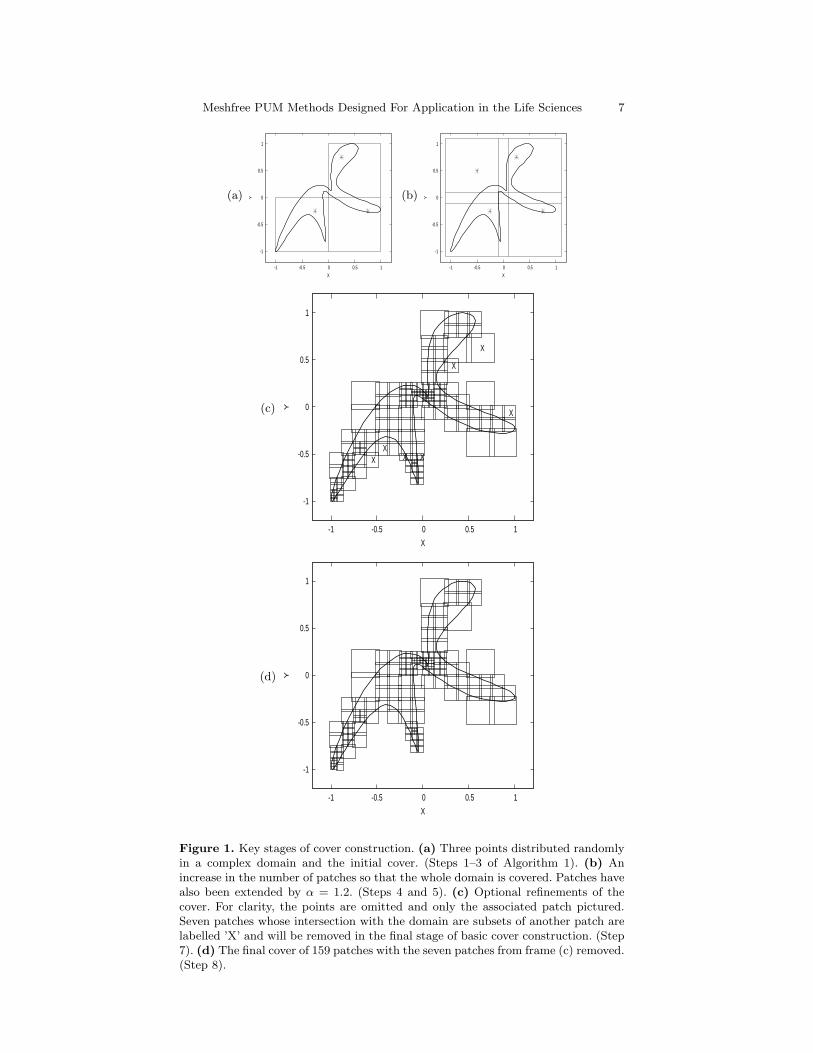
Note that if the spatial dimension is greater than 1, many empty patchesmay be created by the preceding steps. For example, subdividing a 2d boxonly once to isolate two points into separate sub-patches creates two emptypatches. Furthermore, non-empty patches obtained from these first threesteps will likely not cover the entire domain (see Fig. 1 (a) and (b)).
Meshfree PUM Methods Designed For Application in the Life Sciences 7
(a)
-1
-0.5
0
0.5
1
-1 -0.5 0 0.5 1
Y
X
(b)
-1
-0.5
0
0.5
1
-1 -0.5 0 0.5 1
Y
X
(c)
-1
-0.5
0
0.5
1
-1 -0.5 0 0.5 1
Y
X
XX
X
X
X
X X
(d)
-1
-0.5
0
0.5
1
-1 -0.5 0 0.5 1
Y
X
Figure 1. Key stages of cover construction. (a) Three points distributed randomlyin a complex domain and the initial cover. (Steps 1–3 of Algorithm 1). (b) Anincrease in the number of patches so that the whole domain is covered. Patches havealso been extended by α = 1.2. (Steps 4 and 5). (c) Optional refinements of thecover. For clarity, the points are omitted and only the associated patch pictured.Seven patches whose intersection with the domain are subsets of another patch arelabelled ’X’ and will be removed in the final stage of basic cover construction. (Step7). (d) The final cover of 159 patches with the seven patches from frame (c) removed.(Step 8).
8 Martin Eigel, Erwin George, and Markus Kirkilionis
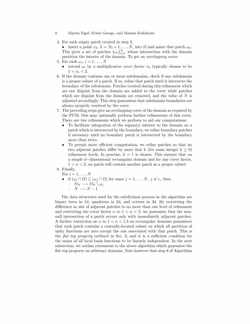
4. For each empty patch created in step 3,• insert a point xk, k = N0 + 1, . . . , N , into Ω and name that patch ωk.This gives a set of patches ωiN
i=1 whose intersection with the domainpartition the interior of the domain. To get an overlapping cover:
5. For each ωi, i = 1, . . . , N• extend ωi by a multiplicative cover factor αi typically chosen to be
1 < αi < 2.6. If the domain contains one or more subdomains, check if any subdomain
is a proper subset of a patch. If so, refine that patch until it intersects theboundary of the subdomain. Patches created during this refinement whichare not disjoint from the domain are added to the cover while patcheswhich are disjoint from the domain are removed, and the value of N isadjusted accordingly. This step guarantees that subdomain boundaries arealways properly resolved by the cover.
7. The preceding steps give an overlapping cover of the domain as required bythe PUM. One may optionally perform further refinements of this cover.There are two refinements which we perform to aid our computations:• To facilitate integration of the region(s) interior to the domain on a
patch which is intersected by the boundary, we refine boundary patchesif necessary until no boundary patch is intersected by the boundarymore than twice.
• To permit more efficient computation, we refine patches so that notwo adjacent patches differ by more that k (for some integer k ≥ 0)refinement levels. In practise, k = 1 is chosen. This ensures that ona simple d−dimensional rectangular domain and for any cover factor,1 < α < 2, no patch will contain another patch as a proper subset.
8. Finally,For i = 1, . . . , N• if (ωi ∩Ω) ⊆ (ωj ∩Ω) for some j = 1, . . . , N, j 6= i,, then
– ΩN −→ ΩN \ ωj
– N −→ N − 1
The data structures used for the subdivision process in the algorithm arebinary trees in 1d, quadtrees in 2d, and octrees in 3d. By restricting thedifference in size of adjacent patches to no more than one level of refinementand restricting the cover factor α to 1 < α < 2, we guarantee that the non-null intersection of a patch occurs only with immediately adjacent patches.A further restriction on α to 1 < α < 1.5 on rectangular domains guaranteesthat each patch contains a centrally-located subset on which all partition ofunity functions are zero except the one associated with that patch. This isthe flat top property outlined in Sec. 2, and it is a sufficient condition forthe union of all local basis functions to be linearly independent. In the nextsubsection, we outline extensions to the above algorithm which guarantee theflat top property on arbitrary domains. Note however that step 8 of Algorithm
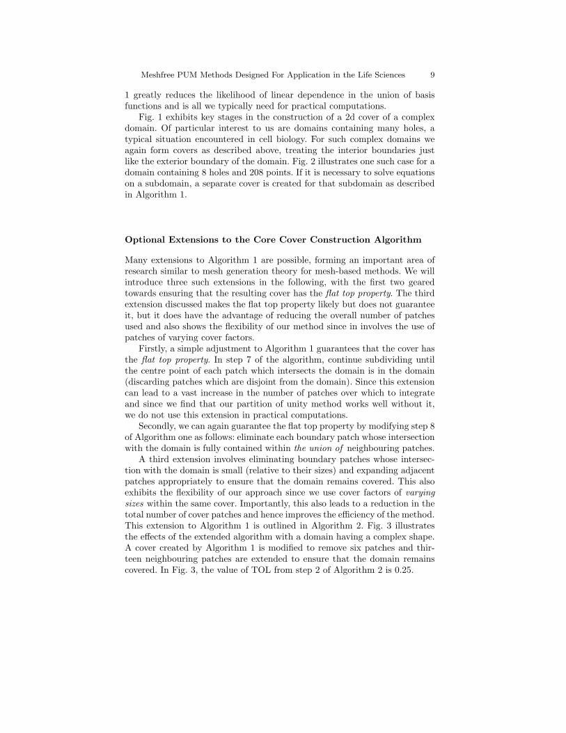
Meshfree PUM Methods Designed For Application in the Life Sciences 9
1 greatly reduces the likelihood of linear dependence in the union of basisfunctions and is all we typically need for practical computations.
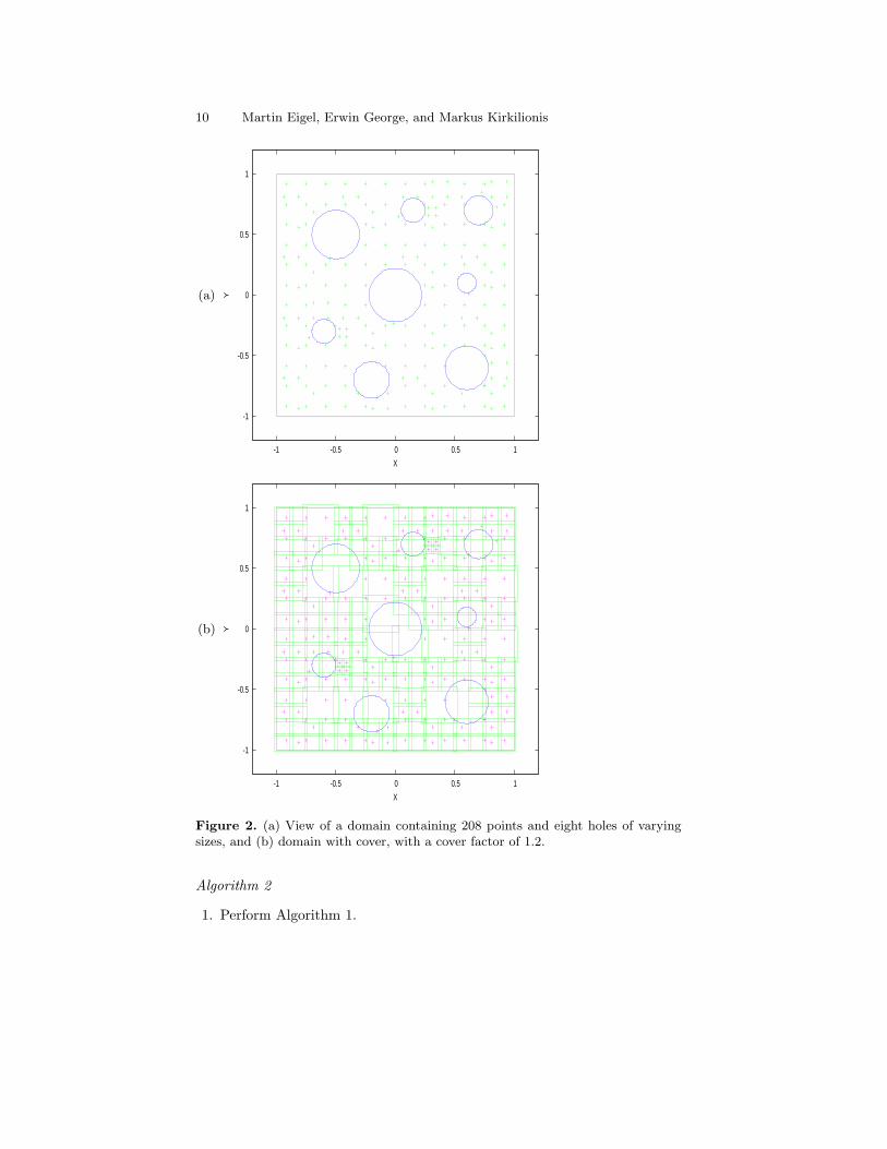
Fig. 1 exhibits key stages in the construction of a 2d cover of a complexdomain. Of particular interest to us are domains containing many holes, atypical situation encountered in cell biology. For such complex domains weagain form covers as described above, treating the interior boundaries justlike the exterior boundary of the domain. Fig. 2 illustrates one such case for adomain containing 8 holes and 208 points. If it is necessary to solve equationson a subdomain, a separate cover is created for that subdomain as describedin Algorithm 1.
Optional Extensions to the Core Cover Construction Algorithm
Many extensions to Algorithm 1 are possible, forming an important area ofresearch similar to mesh generation theory for mesh-based methods. We willintroduce three such extensions in the following, with the first two gearedtowards ensuring that the resulting cover has the flat top property. The thirdextension discussed makes the flat top property likely but does not guaranteeit, but it does have the advantage of reducing the overall number of patchesused and also shows the flexibility of our method since in involves the use ofpatches of varying cover factors.
Firstly, a simple adjustment to Algorithm 1 guarantees that the cover hasthe flat top property. In step 7 of the algorithm, continue subdividing untilthe centre point of each patch which intersects the domain is in the domain(discarding patches which are disjoint from the domain). Since this extensioncan lead to a vast increase in the number of patches over which to integrateand since we find that our partition of unity method works well without it,we do not use this extension in practical computations.
Secondly, we can again guarantee the flat top property by modifying step 8of Algorithm one as follows: eliminate each boundary patch whose intersectionwith the domain is fully contained within the union of neighbouring patches.
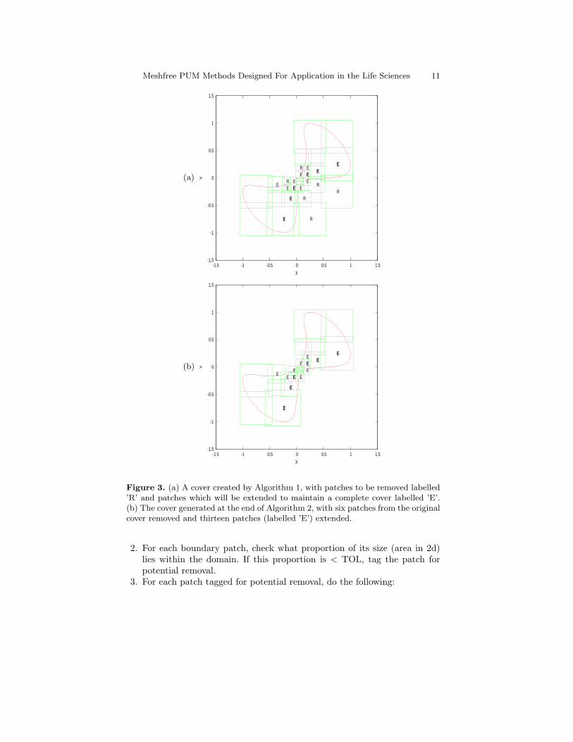
A third extension involves eliminating boundary patches whose intersec-tion with the domain is small (relative to their sizes) and expanding adjacentpatches appropriately to ensure that the domain remains covered. This alsoexhibits the flexibility of our approach since we use cover factors of varyingsizes within the same cover. Importantly, this also leads to a reduction in thetotal number of cover patches and hence improves the efficiency of the method.This extension to Algorithm 1 is outlined in Algorithm 2. Fig. 3 illustratesthe effects of the extended algorithm with a domain having a complex shape.A cover created by Algorithm 1 is modified to remove six patches and thir-teen neighbouring patches are extended to ensure that the domain remainscovered. In Fig. 3, the value of TOL from step 2 of Algorithm 2 is 0.25.
10 Martin Eigel, Erwin George, and Markus Kirkilionis
(a)
-1
-0.5
0
0.5
1
-1 -0.5 0 0.5 1
Y
X
(b)
-1
-0.5
0
0.5
1
-1 -0.5 0 0.5 1
Y
X
Figure 2. (a) View of a domain containing 208 points and eight holes of varyingsizes, and (b) domain with cover, with a cover factor of 1.2.
Algorithm 2
1. Perform Algorithm 1.
Meshfree PUM Methods Designed For Application in the Life Sciences 11
(a)
-1.5
-1
-0.5
0
0.5
1
1.5
-1.5 -1 -0.5 0 0.5 1 1.5
Y
X
E
E
EE
E EE
EE E
E EE
EE
E
E
E E
R
R
R
RR
R
(b)
-1.5
-1
-0.5
0
0.5
1
1.5
-1.5 -1 -0.5 0 0.5 1 1.5
Y
X
E
E
EE
E EE
EE E
E EE
EE
E
E
E E
Figure 3. (a) A cover created by Algorithm 1, with patches to be removed labelled’R’ and patches which will be extended to maintain a complete cover labelled ’E’.(b) The cover generated at the end of Algorithm 2, with six patches from the originalcover removed and thirteen patches (labelled ’E’) extended.
2. For each boundary patch, check what proportion of its size (area in 2d)lies within the domain. If this proportion is < TOL, tag the patch forpotential removal.
3. For each patch tagged for potential removal, do the following:
12 Martin Eigel, Erwin George, and Markus Kirkilionis
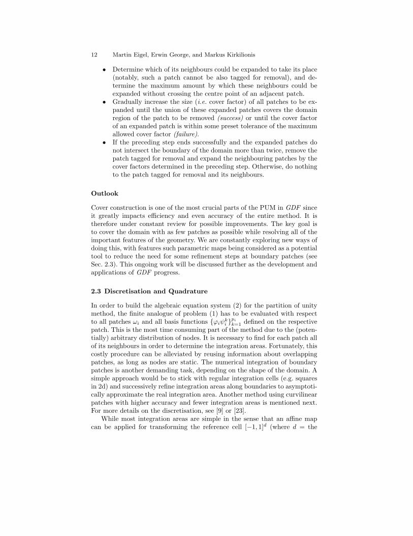
• Determine which of its neighbours could be expanded to take its place(notably, such a patch cannot be also tagged for removal), and de-termine the maximum amount by which these neighbours could beexpanded without crossing the centre point of an adjacent patch.
• Gradually increase the size (i.e. cover factor) of all patches to be ex-panded until the union of these expanded patches covers the domainregion of the patch to be removed (success) or until the cover factorof an expanded patch is within some preset tolerance of the maximumallowed cover factor (failure).
• If the preceding step ends successfully and the expanded patches donot intersect the boundary of the domain more than twice, remove thepatch tagged for removal and expand the neighbouring patches by thecover factors determined in the preceding step. Otherwise, do nothingto the patch tagged for removal and its neighbours.
Outlook
Cover construction is one of the most crucial parts of the PUM in GDF sinceit greatly impacts efficiency and even accuracy of the entire method. It istherefore under constant review for possible improvements. The key goal isto cover the domain with as few patches as possible while resolving all of theimportant features of the geometry. We are constantly exploring new ways ofdoing this, with features such parametric maps being considered as a potentialtool to reduce the need for some refinement steps at boundary patches (seeSec. 2.3). This ongoing work will be discussed further as the development andapplications of GDF progress.
2.3 Discretisation and Quadrature
In order to build the algebraic equation system (2) for the partition of unitymethod, the finite analogue of problem (1) has to be evaluated with respectto all patches ωi and all basis functions ϕiψ
ki
pi
k=1 defined on the respectivepatch. This is the most time consuming part of the method due to the (poten-tially) arbitrary distribution of nodes. It is necessary to find for each patch allof its neighbours in order to determine the integration areas. Fortunately, thiscostly procedure can be alleviated by reusing information about overlappingpatches, as long as nodes are static. The numerical integration of boundarypatches is another demanding task, depending on the shape of the domain. Asimple approach would be to stick with regular integration cells (e.g. squaresin 2d) and successively refine integration areas along boundaries to asymptoti-cally approximate the real integration area. Another method using curvilinearpatches with higher accuracy and fewer integration areas is mentioned next.For more details on the discretisation, see [9] or [23].
While most integration areas are simple in the sense that an affine mapcan be applied for transforming the reference cell [−1, 1]d (where d = the
Meshfree PUM Methods Designed For Application in the Life Sciences 13
-1
-0.5
0
0.5
1
-1 -0.5 0 0.5 1 1.5
Y
X
BoundaryParametric Boundary
Region Magnified
0.05
0.1
0.15
0.2
0.25
0.3
0.35
0.4
0.45
0.55 0.6 0.65 0.7 0.75 0.8 0.85 0.9 0.95 1
Y
X
Parametric BoundaryBoundary
Integration RegionControl Points
(a) (b)
0.05
0.1
0.15
0.2
0.25
0.3
0.35
0.4
0.45
0.55 0.6 0.65 0.7 0.75 0.8 0.85 0.9 0.95 1
Y
X
Parametric BoundaryBoundary
Integration RegionControl Points
0.05
0.1
0.15
0.2
0.25
0.3
0.35
0.4
0.45
0.55 0.6 0.65 0.7 0.75 0.8 0.85 0.9 0.95 1
Y
X
Parametric BoundaryBoundary
Integration RegionControl Points
(c) (d)
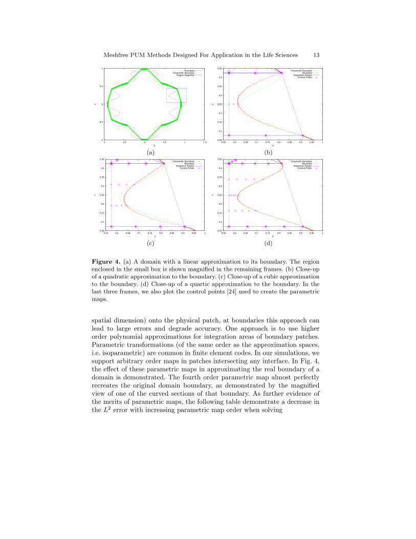
Figure 4. (a) A domain with a linear approximation to its boundary. The regionenclosed in the small box is shown magnified in the remaining frames. (b) Close-upof a quadratic approximation to the boundary. (c) Close-up of a cubic approximationto the boundary. (d) Close-up of a quartic approximation to the boundary. In thelast three frames, we also plot the control points [24] used to create the parametricmaps.
spatial dimension) onto the physical patch, at boundaries this approach canlead to large errors and degrade accuracy. One approach is to use higherorder polynomial approximations for integration areas of boundary patches.Parametric transformations (of the same order as the approximation spaces,i.e. isoparametric) are common in finite element codes. In our simulations, wesupport arbitrary order maps in patches intersecting any interface. In Fig. 4,the effect of these parametric maps in approximating the real boundary of adomain is demonstrated. The fourth order parametric map almost perfectlyrecreates the original domain boundary, as demonstrated by the magnifiedview of one of the curved sections of that boundary. As further evidence ofthe merits of parametric maps, the following table demonstrate a decrease inthe L2 error with increasing parametric map order when solving

14 Martin Eigel, Erwin George, and Markus Kirkilionis
−∆u+ u = f in Ω, (3)∂
∂νu = g on ∂Ω. (4)
on the domain of Fig. 4 using GDF. The f and g are chosen to give a solutionof u(x, y) = x2y and all normal derivatives are computed on the real domainboundary.
Parametric Map Order L2 Error1 (Linear) 0.05153332 (Quadratic) 0.04737683 (Cubic) 0.04532044 (Quartic) 0.0436432
2.4 The Generic Discretisation Framework, GDF
Figure 5. GDF flow chart
Meshfree PUM Methods Designed For Application in the Life Sciences 15
The PUM is implemented by the authors in a C++ code called the GenericDiscretisation Framework (GDF ). Modern paradigms for software design suchas reusability by object orientation and generic programming through tem-plates are incorporated into the design of GDF. Fig. 5 shows the steps requiredfor setting up a problem and solving it in the framework. In the left columnthe events the user manages are detailed while the right column shows theobjects being created during that process.
3 Numerical Examples
Standard h and p convergence tests have been carried out on both simple andcomplex (h−refinement only) domains using GDF. The results indicate thateven on complicated domains such as those containing many holes, optimalconvergence rates are obtained [9].
Here we demonstrate the flexibility of GDF in handling computations oncomplex domains. We perform adaptive parabolic computations and then wesimulate several biologically relevant scenarios.
3.1 Adaptive refinement
Two of the main advantages a cover has when compared to a mesh is theflexibility to resolve geometrical features (demonstrated in the next section)and to easily adapt to local approximation requirements. In this section, we usea simple explicit error indicator in order to steer a time-dependent adaptiverefinement of our cover.
As usual (see e.g. [20, 2]), we define boundary and interior residuals subjectto an approximate solution uh ∈ VPU
r := f +∆uh − uh in Ω (5)
R := g − ∂
∂νuh on ∂Ω. (6)
From the bilinear form a(·, ·) of the weak problem and the Galerkin orthogo-nality a(e, v) = 0 ∀v ∈ VPU for the error e = u− uh, we get
a(e, v) = l(v)− a(uh, v) =∫
Ω
fv +∫
∂Ω
∂νuhv +∫
Ω
(∆uh − u)v
=∫
Ω
rv +∫
∂Ω
Rv =∑
i
∫Ω
ϕir(v − vh) +∑
i
∫∂Ω
ϕiR(v − vh).(7)
In this integration by parts argument we exploited the regularity of the PUMshape functions. In our simulations, we employ a PU of degree 2 (i.e. ϕi ∈C2(ωi)) based on cubic splines. Hence, there are no additional boundary termson the interior patch edges or within the patches that need to be taken into
16 Martin Eigel, Erwin George, and Markus Kirkilionis
t = 0 t = 0.01
-1
-0.5
0
0.5
1
-1 -0.5 0 0.5 1
Y
X
-1
-0.5
0
0.5
1
-1 -0.5 0 0.5 1
Y
X
t = 0.02 t = 0.04
-1
-0.5
0
0.5
1
-1 -0.5 0 0.5 1
Y
X
-1
-0.5
0
0.5
1
-1 -0.5 0 0.5 1
Y
X
t = 0.08 t = 0.19
-1
-0.5
0
0.5
1
-1 -0.5 0 0.5 1
Y
X
-1
-0.5
0
0.5
1
-1 -0.5 0 0.5 1
Y
X
Initial u(x, y, t = 0.01) u(x, y, t = 0.08)
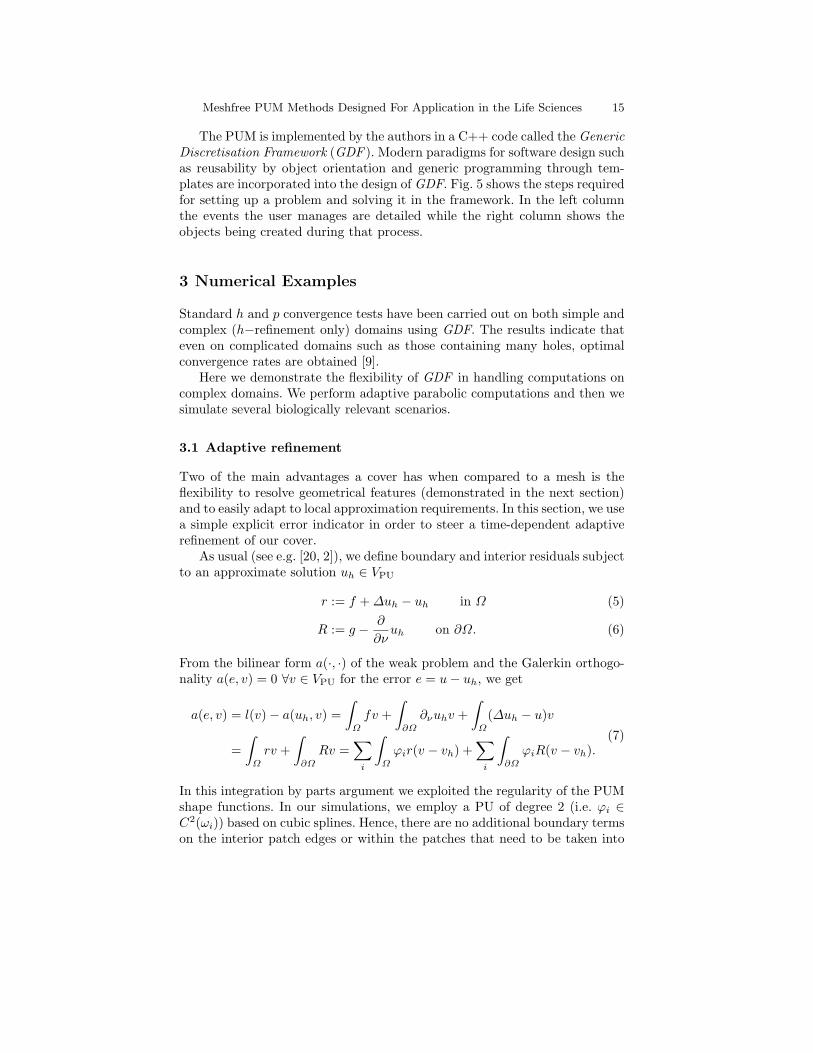
Figure 6. Successive refinement and coarsening of the cover in an adaptive parabolicproblem at selected timesteps (TS). The initial and final (see TS = 19) cover consistsof 16 equally-sized patches. The solution u(x, y, t) after an initial time step and attime step 8 of the simulation are shown in the last two frames.
Meshfree PUM Methods Designed For Application in the Life Sciences 17
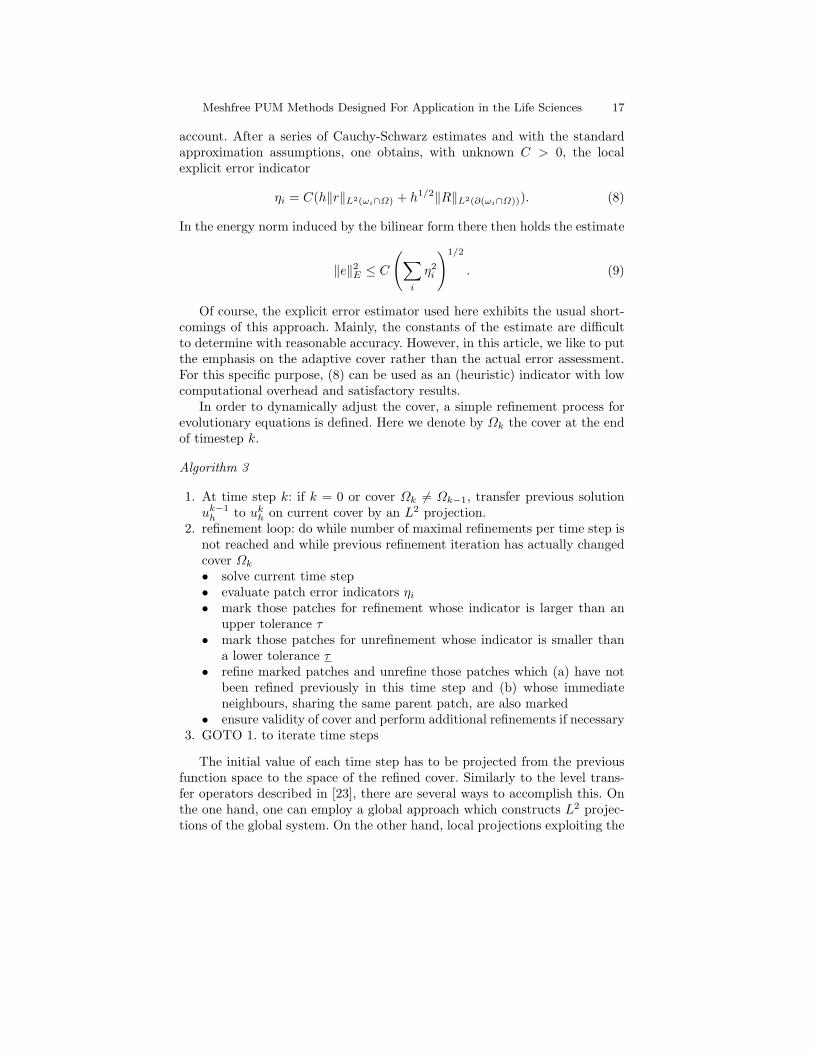
account. After a series of Cauchy-Schwarz estimates and with the standardapproximation assumptions, one obtains, with unknown C > 0, the localexplicit error indicator
ηi = C(h‖r‖L2(ωi∩Ω) + h1/2‖R‖L2(∂(ωi∩Ω))). (8)
In the energy norm induced by the bilinear form there then holds the estimate
‖e‖2E ≤ C
(∑i
η2i
)1/2
. (9)
Of course, the explicit error estimator used here exhibits the usual short-comings of this approach. Mainly, the constants of the estimate are difficultto determine with reasonable accuracy. However, in this article, we like to putthe emphasis on the adaptive cover rather than the actual error assessment.For this specific purpose, (8) can be used as an (heuristic) indicator with lowcomputational overhead and satisfactory results.
In order to dynamically adjust the cover, a simple refinement process forevolutionary equations is defined. Here we denote by Ωk the cover at the endof timestep k.
Algorithm 3
1. At time step k: if k = 0 or cover Ωk 6= Ωk−1, transfer previous solutionuk−1
h to ukh on current cover by an L2 projection.
2. refinement loop: do while number of maximal refinements per time step isnot reached and while previous refinement iteration has actually changedcover Ωk
• solve current time step• evaluate patch error indicators ηi
• mark those patches for refinement whose indicator is larger than anupper tolerance τ
• mark those patches for unrefinement whose indicator is smaller thana lower tolerance τ
• refine marked patches and unrefine those patches which (a) have notbeen refined previously in this time step and (b) whose immediateneighbours, sharing the same parent patch, are also marked
• ensure validity of cover and perform additional refinements if necessary3. GOTO 1. to iterate time steps
The initial value of each time step has to be projected from the previousfunction space to the space of the refined cover. Similarly to the level trans-fer operators described in [23], there are several ways to accomplish this. Onthe one hand, one can employ a global approach which constructs L2 projec-tions of the global system. On the other hand, local projections exploiting the
18 Martin Eigel, Erwin George, and Markus Kirkilionis
knowledge about which patches were refined or coarsened from the cover ofthe previous time step can be much more efficient.
We solve the heat equation for 19 timesteps on Ω = [−1, 1]2 with an initialcondition of u(x, y, t = 0) = e−20(x−1)2(y−1)2 , a function with height concen-trated around the upper right hand corner of the domain. The initial coverconsists of 4 × 4 equally sized patches. An initially large error is indicatedin the corner of the domain where the initial function exhibits large values.In the multi-step refinement procedure described above, patches in the upperright corner are thus successively refined. As the problem we are solving doesnot include additional sources in the domain, the solution quickly becomessmooth and the refinement algorithm identifies regions whose average erroris sufficiently small to unrefine sets of patches again. By the time the simula-tion has ended, the refinements and coarsening of the patches as the solutionu(x, y, t) smoothens, have lead back to the original coarse cover (see Fig. 6).
3.2 Complex domain
-1
-0.5
0
0.5
1
-1 -0.5 0 0.5 1
Y
X
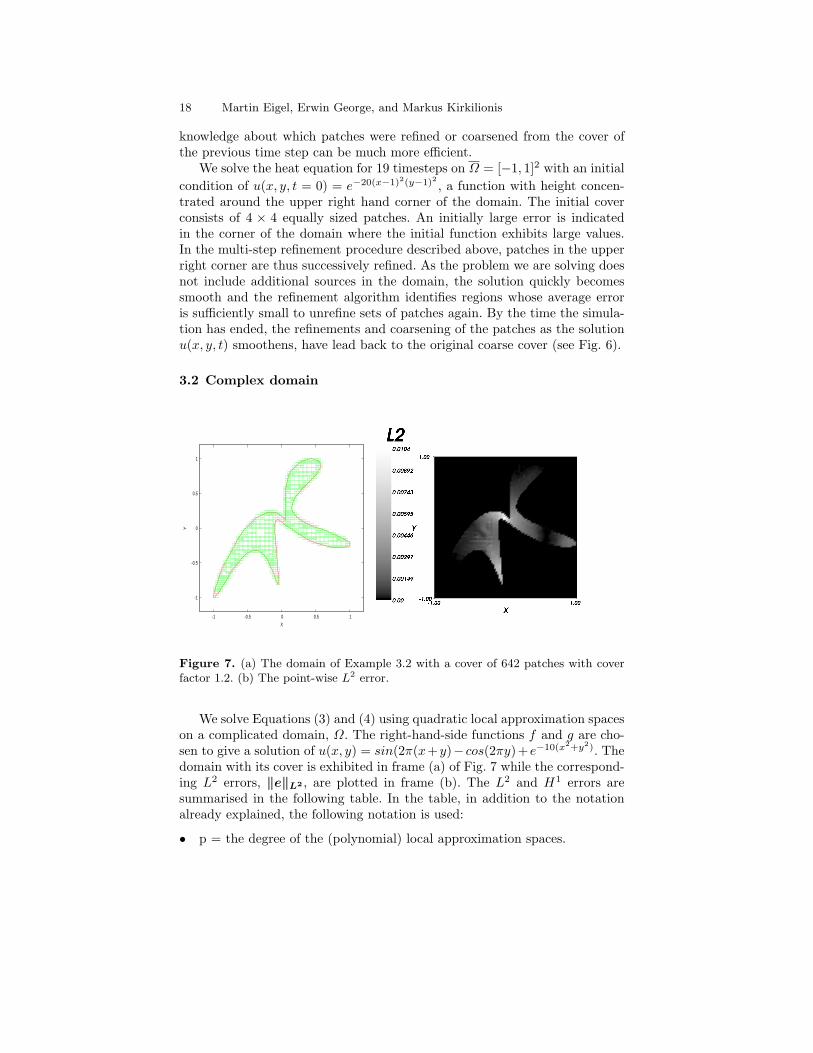
Figure 7. (a) The domain of Example 3.2 with a cover of 642 patches with coverfactor 1.2. (b) The point-wise L2 error.
We solve Equations (3) and (4) using quadratic local approximation spaceson a complicated domain, Ω. The right-hand-side functions f and g are cho-sen to give a solution of u(x, y) = sin(2π(x+y)− cos(2πy)+e−10(x2+y2). Thedomain with its cover is exhibited in frame (a) of Fig. 7 while the correspond-ing L2 errors, ‖e‖L2 , are plotted in frame (b). The L2 and H1 errors aresummarised in the following table. In the table, in addition to the notationalready explained, the following notation is used:
• p = the degree of the (polynomial) local approximation spaces.
Meshfree PUM Methods Designed For Application in the Life Sciences 19
• dof = the degrees of freedom =∑
i dim(Vi).• ‖e‖H1= The H1 norm of the error.
N p dof ‖e‖L2 ‖e‖H1
642 2 3852 0.0315751 0.467831
3.3 Signal transport from the cell membrane into the nucleus - anexample with nested subdomains
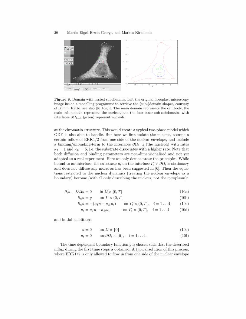
We now illustrate a typical biological process, cellular signalling, that posesnew and challenging problems to numerical mathematics. First the compart-mentalisation of the cell requires that the computational domain can be splitinto nested sub-domains. Each of these sub-domains will have its own coverwhere the different cover constructions discussed earlier will be applied in-dependently. GDF (see section 2.4) has been constructed to allow theoret-ically for an arbitrary hierarchy of such nested sub-domains. Between thesub-domains interface conditions have to be specified. Such interface condi-tons model for example the rate of protein translocation, or the rate withwhich molecules pass the nuclear pore complexes (NPC). Again the biologicalbackground induces a complex mixture of boundary and interface conditionsacting between the nested sub-domains. The overall problem setting with re-spect to sub-domain strucure which we will discuss in the following can beseen in Figure 8. It is related to typical processes which need to be understoodfor cell signalling. The figure shows a typical mammalian fibroblast, a very flatcell type justifying the two-dimensional approach. One important experimentdiscussed in [6] is ERK1/2 shuttling between the cell nucleus and cytoplasm.The extracellular signal-regulated protein kinase ERK1/2 is a crucial effectorlinking extracellular stimuli to cellular responses: upon phosphorylation ERK[also known as mitogen-activated protein kinase P42/P44 (MAPK)] concen-trates in the nucleus where it activates specific programmes of gene expression.Little is known about the time course and regulation of ERK exchange be-tween nucleus and cytoplasm in living cells, and here simulations can addimmensely to our understanding. In [6] the speed of ERK2 shuttling betweennucleus and cytoplasm was measured quantitatively and it was determinedthat shuttling accelerated after ERK activation. Finally it was demonstratedthat ERK2 did not diffuse freely in the nucleus and that diffusion was furtherimpeded after phosphorylation, suggesting the formation of complexes of lowmobility, or the binding to nuclear sub-structures. To understand this andsimilar processes better GDF was especially constructed to allow additionalstate variables on every boundary and interface, i.e. on lower dimensionalmanifolds, for example describing a concentration of bound molecules alongthe surface.
We can test, as one possible hypothesis, that the nucleoli create impenetra-ble obstacles Ω1...4 which act as binding partners for the diffusing substrate udescribing ERK1/2. Another idea would be that ERK1/2 can bind anywhere
20 Martin Eigel, Erwin George, and Markus Kirkilionis
-1.5
-1
-0.5
0
0.5
1
1.5
-2 -1.5 -1 -0.5 0 0.5 1 1.5
Y
X
Figure 8. Domain with nested subdomains. Left the original fibroplast microscopyimage inside a modelling programme to retrieve the (sub-)domain shapes, courtesyof Gimmi Ratto, see also [6]. Right: The main domain represents the cell body, themain sub-domain represents the nucleus, and the four inner sub-subdomains withinterfaces ∂Ω1...4 (green) represent nucleoli.
at the chromatin structure. This would create a typical two-phase model whichGDF is also able to handle. But here we first isolate the nucleus, assume acertain inflow of ERK1/2 from one side of the nuclear envelope, and includea binding/unbinding-term to the interfaces ∂Ω1...4 (the nucleoli) with ratesκI = 1 and κB = 5, i.e. the substrate dissociates with a higher rate. Note thatboth diffusion and binding parameters are non-dimensionalised and not yetadapted to a real experiment. Here we only demonstrate the principles. Whilebound to an interface, the substrate ui on the interface Γi ∈ ∂Ωi is stationaryand does not diffuse any more, as has been suggested in [6]. Then the equa-tions restricted to the nuclear dynamics (treating the nuclear envelope as aboundary) become (with Ω only describing the nucleus, not the cytoplasm):
∂tu−D∆u = 0 in Ω × (0, T ] (10a)∂nu = g on Γ × (0, T ] (10b)∂nu = −(κIu− κBui) on Γi × (0, T ], i = 1 . . . 4 (10c)ui = κIu− κBui on Γi × (0, T ], i = 1 . . . 4 (10d)
and initial conditions
u = 0 on Ω × 0 (10e)ui = 0 on ∂Ωi × 0, i = 1 . . . 4. (10f)
The time dependent boundary function g is chosen such that the describedinflux during the first time steps is obtained. A typical solution of this process,where ERK1/2 is only allowed to flow in from one side of the nuclear envelope

Meshfree PUM Methods Designed For Application in the Life Sciences 21
for a short time, can be seen in Figure 9. Figure 10 shows that the numericalscheme performs quite well with respect to mass conservation, where materialis exchanged from the surfaces with the interior of the domain. Finally Figure11 shows that we can scale up the problem to include the whole fibroblastas the computational domain. In this case the boundary condition for thenuclear envelope (described by Γ := ∂Ω in Eq. 10) had been changed into aninterface condition, where molecules can translocate in and out of the nucleusthrough the NPC, where the translocation rate anywhere along Γ (i.e. theNPCs are assumed to have a ’concentration’ in the nuclear envelope, they arenot modelled as discrete entities) does depend on the concentration gradient.
t = 0.01 t = 0.02 t = 0.05
t = 0.12 t=0.17 t=0.23
Figure 9. Simulation of hindered diffusion process with binding to obstacle inter-faces, shown at different time steps (dt=0.01).
3.4 Current Work
Here we give some general comments on our implementation. Our currentwork focuses on interface problems in biology, in which processes in a maindomain affect and are affected by processes on an interface adjacent to thedomain. In this work (currently in 2d) the codimension 1 boundaries of subdo-mains are discretised using finite element methods and diffusion equations aresolved on that interface. Meanwhile, the surrounding main domain is discre-tised using the partition of unity meshfree method and interchange betweenthe two domains (interior and meshfree) are handled by flux type interface
22 Martin Eigel, Erwin George, and Markus Kirkilionis
0
0.5
1
1.5
2
0 0.2 0.4 0.6 0.8 1 1.2
MA
SS
TIME
INTERIORINTERFACECOMBINED
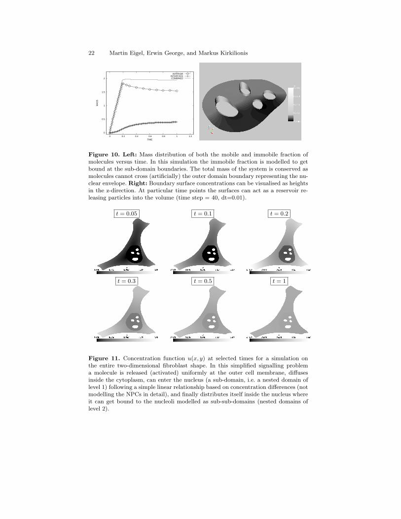
Figure 10. Left: Mass distribution of both the mobile and immobile fraction ofmolecules versus time. In this simulation the immobile fraction is modelled to getbound at the sub-domain boundaries. The total mass of the system is conserved asmolecules cannot cross (artificially) the outer domain boundary representing the nu-clear envelope. Right: Boundary surface concentrations can be visualised as heightsin the z-direction. At particular time points the surfaces can act as a reservoir re-leasing particles into the volume (time step = 40, dt=0.01).
t = 0.05 t = 0.1 t = 0.2
t = 0.3 t = 0.5 t = 1
Figure 11. Concentration function u(x, y) at selected times for a simulation onthe entire two-dimensional fibroblast shape. In this simplified signalling problema molecule is released (activated) uniformly at the outer cell membrane, diffusesinside the cytoplasm, can enter the nucleus (a sub-domain, i.e. a nested domain oflevel 1) following a simple linear relationship based on concentration differences (notmodelling the NPCs in detail), and finally distributes itself inside the nucleus whereit can get bound to the nucleoli modelled as sub-sub-domains (nested domains oflevel 2).

Meshfree PUM Methods Designed For Application in the Life Sciences 23
conditions, which include the possibility of exploring different binding andunbinding rates of a species to and from the interface. This work is exploredin a forthcoming manuscript by the authors.
4 Conclusion and Outlook
It was demonstrated that cellular biology and new microscopy techniqes of-fer many new challenging problems for modelling and numerical analysis. Weshowed that the meshfree PUM can be extended to problems with complexdomains. There is a need to investigate and test new cover creation algo-rithms in order to automise the work flow going from microscopy images tosimulations detecting basic transport modes in cellular signalling or any otherregulatory or metabolic process in the cell. Moreover we showed that the covercan be adaptively refined and coarsened for time-dependent problems.
Future challenging extensions of the methods presented would be au-tomatic cover creation algorithms in three dimensions. Similarly adaptivecover generating algorithms will need to be analysed and tested for higher-dimensional systems of parabolic equations describing the simultaneous trans-port and interaction of different molecular species. Finally, as mentioned inthe introduction, there is a need to derive a better understanding of molecu-lar transport behaviour on the typical scales of the confocal microscope. Thisshould be based generally on a multi-scale analysis of both the medium inwhich the molecules move, as well as on the microscopic properties of themany molecular machines involved in the process. As an important step adetailed multi-scale analysis of the nuclear pore complexes (NPCs) would im-mensely help our understanding of cellular signalling.
References
1. I. Babuska, U. Banerjee, and J. E. Osborn, Meshless and Generalized Finite El-ement Methods: A Survey of Some Major Results, Meshfree Methods for PartialDifferential Equations (M. Griebel and M. A. Schweitzer, eds.), Lecture Notesin Computational Science and Engineering, vol. 26, Springer, 2002, pp. 1–20.
2. Ainsworth, Mark and Oden, J. Tinsley (1993). A unified approach to a posteriorierror estimation using element residual methods. Numerische Mathematik, 65(1)
3. Babuska and J. M. Melenk, The partition of unity method, Internat. J. Numer.Methods Engrg., 40(4) (1997), 727–758.
4. Belytschko, T., Y. Y. Lu, and L. Gu, Element-free Galerkin methods, Int. J.Numer. Meth. Engrg. 37 (1994), 229–256.
5. Bouchekhima, A.-N., Frigerio, L., and Kirkilionis, M. A. (2007). Geomet-ric Quantification of the Plant Endoplasmatic Reticulum. Warwick Preprint11/2007. Submitted to Journal of Microscopy.
24 Martin Eigel, Erwin George, and Markus Kirkilionis
6. Costa, M., Marchi, M., Cardarelli, F., Roy, A, Beltram, F., Maffei, L. and Ratto,G.M., Dynamic regulation of ERK2 nuclear translocation and mobility in livingcells, Journal of Cell Science 119, pp. 4952-4963, 2006.
7. Domijan, M. and Kirkilionis, M. (2007). Bistability and Oscillations in Chem-ical Reaction Networks. Warwick Preprint 04/2007. Submitted to Journal ofMathematical Biology.
8. Domijan, M. and Kirkilionis, M. (2007). Graph Theory and Qualitative Analy-sis of Reaction Networks. Warwick Preprint 13/2007. Accepted: Networks andHeterogeneous Media, 2008.
9. Eigel, M., E. George, and M. Kirkilionis, A Meshfree Partition of Unity Methodfor Diffusion Equations on Complex Domains, Warwick Preprint:10/2007. Sub-mitted to IMA J. Num. Anal.
10. Gerlich, D. and Ellenberg, J., 4D imaging to assay complex dynamics in livespecimens. Nat Cell Biol , Vol. Suppl , pp. S14-S19 , 2003.
11. Goodwin, J. S. and Kenworthy, A. K, Photobleaching approaches to investigatediffusional mobility and trafficking of Ras in living cells.. Methods Cell Biol ,Vol. 37 , pp. 154-164 , 2005.
12. Griebel, M. and Schweitzer, M.A., A Particle-partition of unity method. II. Ef-ficient cover construction and reliable integration, SIAM J. Sci. Comput., 23(5)(2002), 1655–1682 (electronic).
13. McNally, J. G., Quantitative FRAP in analysis of molecular binding dynamicsin vivo. Methods Cell Biol , Vol. 85 , pp. 329-351 , 2008.
14. Robinson, C. V., Sali, A., and Baumeister, W. (2007). The molecular sociologyof the cell. Nature, 450(7172), 973-982.
15. Sbano, L. and Kirkilionis, M. (2007). Molecular Systems with Infinite and Fi-nite Degrees of Freedom. Part I: Continuum Approximation. Warwick Preprint05/2007. Submitted to J. Math. Biol.
16. Sbano, L. and Kirkilionis, M. (2007). Molecular Systems with Infinite and FiniteDegrees of Freedom. Part II: Deterministic Dynamics and Examples. WarwickPreprint 07/2007. Submitted to J. Math. Biol.
17. Sbano, L. and Kirkilionis, M. (2007). Multiscale Analysis of Reaction Networks.Warwick Preprint 12/2007.
18. Tian, R., G. Yagawa, H. Terasaka, Linear dependence problems of partitionof unity-based generalized FEMs, Comput. Methods Appl. Mech. Engrg., 195(2006), 4768–4782.
19. Weiss, M.; Hashimoto, H. and Nilsson, T. Anomalous protein diffusion in livingcells as seen by fluorescence correlation spectroscopy. Biophys J , Vol. 84 , pp.4043-4052 , 2003.
20. Ainsworth, M. and Tinsley, J., A Posteriori Error Estimation in Finite ElementAnalysis, John Wiley & Sons., 2000.
21. Braess, D., Finite elements: Theory, fast solvers, and applications in solid me-chanics, Cambridge University Press, 2001.
22. Cioranescu, D. and Donato, P.. An Introduction to homogenization. OxfordUniversity Press, 1999.
23. Schweitzer, M.A., A parallel multilevel partition of unity method for elliptic par-tial differential equations, Lecture Notes in Computational Science and Engi-neering, vol. 29, Springer, 2003.
24. Strang, G. and Fix, G. J., An Analysis of the Finite Element Method, Prentice-Hall, 1973.
Meshfree PUM Methods Designed For Application in the Life Sciences 25
25. Griebel, M. and Schweitzer, M.A., (eds.), Meshfree Methods for Partial Dif-ferential Equations, Lecture Notes in Computational Science and Engineering,vol. 26, Springer, 2002.
26. Griebel, M. and Schweitzer, M.A., A Particle-Partition of Unity Method PartVII: Adaptivity, Lecture Notes in Computational Science and Engineering,vol. 57, Springer, 2007.
27. Griebel, M. and Schweitzer, M.A., (eds.), Meshfree Methods for Partial Differ-ential Equations II, Lecture Notes in Computational Science and Engineering,vol. 43, Springer, 2005.