Maximum-entropy meshfree method for incompressible media problems

Maximum-entropy meshfree method for incompressible

media problems

A. Ortiz∗,a, M. A. Pusob, N. Sukumara

aDepartment of Civil and Environmental Engineering, University of California, One

Shields Avenue, Davis, CA 95616, U.S.A.bLawrence Livermore National Laboratory, P.O. Box 808, Livermore, CA 94551, U.S.A.

Abstract

A novel maximum-entropy meshfree method that we recently introduced in

Ref. [1] is extended to Stokes flow in two dimensions and to three-dimensional

incompressible linear elasticity. The numerical procedure is aimed to rem-

edy two outstanding issues in meshfree methods: the development of an

optimal and stable formulation for incompressible media, and an accurate

cell-based numerical integration scheme to compute the weak form integrals.

On using the incompressibility constraint of the standard u-p formulation, a

u-based formulation is devised by nodally averaging the hydrostatic pressure

around the nodes. A modified Gauss quadrature scheme is employed, which

results in a correction to the stiffness matrix that alleviates integration er-

rors in meshfree methods, and satisfies the patch test to machine accuracy.

The robustness and versatility of the maximum-entropy meshfree method

is demonstrated in three-dimensional computations using tetrahedral back-

ground meshes for integration. The meshfree formulation delivers optimal

∗Corresponding authorEmail address: [email protected] (A. Ortiz)

Preprint submitted to Elsevier December 25, 2010

rates of convergence in the energy and L2-norms. Inf-sup tests are presented

to demonstrate the stability of the maximum-entropy meshfree formulation

for incompressible media problems.

Key words: elasticity, Stokes problem, volumetric locking, numerical

integration, maximum-entropy principle, meshfree methods

1. Introduction

In the analysis of time-independent incompressible media problems, the

Stokes problem provides a means to study the behavior of both solids and

fluids. In solid mechanics, the Stokes equations arise in the treatment of in-

compressible linear elastic isotropic materials, whereas in fluid mechanics the

Stokes equations emerge in the analysis of slow (typically, high-viscous) time-

independent flows. The weak form for the Stokes boundary-value problem

leads to a saddle-point problem, which is identified with mixed variational for-

mulations [2, 3]. In the saddle-point problem, mathematical relations need to

be fulfilled between the approximations chosen for the displacement (or veloc-

ity) and pressure fields—not all choices for these approximation spaces lead

to stability. The stability of such mixed formulations is characterized by the

celebrated Ladyzhenskaya-Babuska-Brezzi (LBB) inf-sup condition [2, 4, 5].

The analytical proof to establish LBB-stability is either cumbersome [6] or

impossible to accomplish for distorted finite elements [7], which has led to

the development of other approaches that by-pass the inf-sup condition [8, 9].

Alternatively, a numerical test to verify the inf-sup condition has been devel-

oped [7], which can be readily performed over any finite element discretiza-

tion. Finite element spaces for the displacement (or velocity) and pressure

2

that pass the numerical (Chapelle-Bathe) inf-sup test are likely to satisfy its

analytical counterpart [10].

The finite element literature is replete with use of mixed formulations

and their stability analysis for incompressible media problems (for exam-

ple, see Refs. [11, 12]). The performance and comparison among several

stabilization procedures for finite elements is provided in Ref. [13]. How-

ever, less attention has been given to meshfree methods. In solid mechan-

ics, displacement-pressure mixed formulations have been adopted for dif-

ferent meshfree methods in Refs. [14, 15, 16, 17] among others. In fluid

mechanics, Desimone et al. [18] formulated a velocity-pressure mixed formu-

lation using moving least-squares approximation, and a LBB-stable meshfree

procedure that combines boundary integral formulation with moving least-

squares approximation was employed by Li and Zhu [19] and Li [20] in a

Galerkin velocity-pressure mixed formulation. Huerta et al. [21] devised an

element-free Galerkin method using approximations that asymptotically be-

come divergence-free as the discretization is refined. Other approaches where

the LBB condition does not appear as a stability criterion have also been

studied with meshfree methods [22, 23, 24, 25, 26, 27]

The study of stability in meshfree mixed formulations is rendered difficult

due to the rational form of meshfree basis functions and the absence of an

element structure in the construction of the meshfree approximation. For

instance, Dolbow and Belytschko [14] and De and Bathe [15] emphasize the

difficulty in obtaining an analytical proof to the inf-sup condition and in

passing the inf-sup test. A stable meshfree formulation for incompressible

media based on mixed formulations is, in general, an outstanding issue in

3

meshfree methods. A few instances of meshfree methods that violate the

LBB condition have also been developed within the framework of stabilized

methods [28, 29, 30].

Galerkin-based meshfree methods are based on rational (non-polynomial)

basis functions whose supports do not coincide with the union of background

cells that are employed in the numerical integration. Due to the latter, inac-

curacies in the numerical integration of weak form integrals appear. The nu-

merical integration issue was first addressed by Dolbow and Belytschko [31].

To alleviate integration errors, they suggested the use of integration cells

aligned with the support of basis functions. The aforementioned procedure

is computationally expensive; instead, higher-order Gauss quadrature is usu-

ally employed. A theoretical study on the influence of numerical quadrature

errors in meshfree methods was recently put forth by Babuska et al. [32].

In Ref. [32] a recipe to correct the computed stiffness matrix is proposed to

eliminate the inaccuracy in the numerical integration. In Ortiz et al. [1], we

introduced a modified integration scheme which reduced integration errors

in general and suppressed them entirely for the constant strain patch test.

In this paper, we extend the Galerkin-based meshfree method presented

in Ref. [1] to two-dimensional Stokes flow and to three-dimensional analysis

of incompressible elastic solids. In a nutshell, the method consists of de-

veloping a displacement or velocity-based formulation by nodally averaging

the hydrostatic pressure around the nodes in the divergence-free constraint.

Additionally, numerical inf-sup tests are presented to establish the stability

of the formulation, and optimal convergence in energy- and L2-norms is es-

tablished. The remainder of this paper is organized as follows. In Section 2,

4

a short introduction to maximum-entropy basis functions is presented. In

Section 3, the new meshfree formulation for incompressible problems is de-

veloped, and in Section 4, the inf-sup test is described for the maximum-

entropy meshfree method. Numerical examples are presented in Section 5

for benchmark linear problems in both solids and fluids to demonstrate the

effectiveness of the proposed procedure for time-independent incompressible

media problems. We also demonstrate that the meshfree formulation passes

the Chapelle-Bathe inf-sup test [7] on several benchmark problems. Finally,

we conclude with some final remarks in Section 6.

2. Maximum-entropy basis functions

In three dimensions, the constant and linear reproducing conditions, namely,∑n

a=1 φa(x) = 1 and∑n

a=1 φa(x)xa = x do not prescribe unique basis func-

tions for n > 4 (more unknowns than linear equations). On viewing basis

functions as discrete probabilities, it is suitable to apply the principle of

maximum entropy [33] to find the least-biased probability distribution. The

Shannon entropy is used by Sukumar [34] to construct max-ent basis func-

tions on polygons, whereas a modified entropy functional for meshfree meth-

ods is proposed by Arroyo and Ortiz [35]. A generalization of the entropy

functional of Ref. [35] is further developed in Sukumar and Wright [36] on

using the notion of a ‘prior’ within the Shannon-Jaynes entropy functional.

We adopt the latter approach in this paper. Although any meshfree basis

function can be employed in our formulation, the weak Kronecker-delta prop-

erty that max-ent basis functions posses on the boundary [35] makes them

appealing for a meshfree method since it enables the direct imposition of

5

essential boundary conditions as in finite elements1.

Consider a weight function wa(x) associated with node a. On using

the Shannon-Jaynes entropy functional, the set of max-ent basis functions

φa(x) ≥ 0na=1 is obtained via the solution of the following convex optimiza-

tion problem:

maxφ∈R

n

+

−n

∑

a=1

φa(x) ln

(

φa(x)

wa(x)

)

(1a)

subject to the linear reproducing conditions:

n∑

a=1

φa(x) = 1,n

∑

a=1

φa(x)xa = 0 (1b)

where xa = xa − x are shifted nodal coordinates and Rn+ is the non-negative

orthant. If wa(x) = 1 for all a, then the Shannon entropy functional,

−∑

a φa lna, is recovered. In practice, any weight function that is compactly-

supported and at least C0-continuous may be used. Typical weight functions

are smooth Gaussian radial basis functions [35]

wa(x) = exp(−βa‖xa − x‖2) (2a)

and C2 quartic polynomials [40]

wa(q) =

1− 6q2 + 8q3 − 3q4 0 ≤ q ≤ 1

0 q > 1(2b)

1Most available meshfree basis functions would typically not vanish on the boundary

and as such special procedures are needed to enforce essential boundary conditions [37,

38, 39].

6

where βa = γ/h2a; γ is a parameter that controls the support-width of the

basis function at node a; and ha is a characteristic nodal spacing that may be

distinct for each node a. In n dimensions, we set ha as the distance to the n-

nearest neighbor from node a. For the quartic polynomial, q = ‖xa − x‖/ρaand ρa = γha is the radius of the basis function support at node a. In

a recent study on max-ent meshfree methods [41], it has been shown that

substantial improvements in accuracy are realized by letting the support-

width parameters as unknowns and solving for them through the variational

structure (minimizing principle) of the continuum problem.

On using the procedure of Lagrange multipliers, the solution of the vari-

ational statement (1) is [36]:

φa(x) =Za(x;λ

∗)

Z(x;λ∗), Za(x;λ

∗) = wa(x) exp(−λ∗ · xa) (3)

where the partition function Z(x;λ∗) =∑

b Zb(x;λ∗), and in three dimen-

sions xa = [xa ya za]T and λ∗ = [λ∗

1 λ∗

2 λ∗

3]T. In (3), the Lagrange multiplier

vector λ∗ is the minimizer of the dual of the optimization problem posed

in (1)

λ∗ = arg minλ∈R3

lnZ(x;λ) (4)

which gives rise to the following system of nonlinear equations:

f(λ) = ∇λ lnZ(λ) = −n

∑

a

φa(x)xa = 0 (5)

where ∇λ stands for the gradient with respect to λ. Once the converged λ∗

is found, the basis functions are computed from (3) and the gradient of the

basis functions is [40]

∇φa = φa

xa ·[

(H)−1 − (H)−1 ·A]

+∇wa

wa

−n

∑

b=1

φb

∇wb

wb

(6a)

7

where

A =n

∑

b=1

φbxb ⊗∇wb

wb

(6b)

and H is the Hessian matrix defined by

H = ∇λf = ∇λ∇λ lnZ =

n∑

b=1

φbxb ⊗ xb (6c)

In Fig. 1, plots of a max-ent basis function computed with a Gaussian prior

for various support-width parameter γ are illustrated for two dimensions.

For γ = 2, plots of the Gaussian weight function and the corresponding

max-ent basis function along with their derivatives are shown in Fig. 2. For

the Gaussian prior, (6a) reduces to [35]

∇φa = φaH−1 · xa (7)

3. Governing equations and variational formulation

3.1. Strong form

Consider a body defined by an open bounded domain Ω ⊂ Rn (n =

2, 3) with boundary Γ such that Γ = Γu ∪ Γt and Γu ∩ Γt = ∅. A nearly-

incompressible linear isotropic elastic solid or fluid under static loads and no

body force is governed by the following equations [42]:

∇ · σ = 0 in Ω (8a)

∇ · u+p

η= 0 in Ω (8b)

8

(a) (b) (c)

Fig. 1: Plots of a maximum-entropy basis function computed with a Gaussian

prior for three values of γ. Note that the locality of the basis function is

affected but it always vanishes on the boundary. (a) γ = 1; (b) γ = 2; and

(c) γ = 3.

and the following essential (displacement or velocity) and natural (traction)

boundary conditions imposed on Γu and Γt, respectively:

u = u on Γu (8c)

σ · n = t on Γt (8d)

where the Cauchy stress tensor σ is related to the strain tensor ε and the

pressure parameter p by the following isotropic linear elastic constitutive

relation:

σ(u, p) = −pI+ 2µε(u) (8e)

In (8) η and µ are identified with the first and second Lame parameters

of the solid, whereas a penalty parameter and the dynamic viscosity of the

fluid, respectively. The penalty parameter is usually taken as η ∼ 107µ [42].

The kinematic relation between the strain tensor ε and the displacement or

9

(a) (b) (c)

(d) (e) (f)

Fig. 2: Plots of Gaussian prior (γ = 2) and maximum-entropy basis function

and their derivatives for node a. Note that wa(xa) = 1, but φa(xa) 6= 1,

and hence the interior basis function φa does not satisfy the Kronecker-delta

property. The smoothness of the basis function and its derivatives are in-

herited from the Gaussian prior. (a) Gaussian prior, wa; (b) ∂wa/∂x; (c)

∂wa/∂y; (d) φa; (e) ∂φa/∂x; and (f) ∂φa/∂y.

10

velocity vector u is:

ε =1

2[u⊗∇+∇⊗ u] (9)

3.2. Weak form

For Galerkin-based mixed formulations with u,v as the trial and test

displacement (or velocity) functions, and p, q as the trial and test hydrostatic

pressure functions, the weak form of (8) reads [42]:

Find u ∈ U and p ∈ P such that

a(u,v)− b(p,v) = (t,v) ∀v ∈ V (10a)

b(q,u) +1

η(p, q) = 0 ∀q ∈ P (10b)

where U ⊂ H1(Ω), V ≡ H10(Ω) and P ≡ L2

0(Ω) are the usual Sobolev

spaces. The bilinear forms a(·, ·) and b(·, ·) are given by

a(u,v) = 2µ

∫

Ω

ε(u) : ε(v) dΩ (10c)

b(q,v) =

∫

Ω

q∇ · v dΩ (10d)

whereas the linear form (t, ·) is

(t,v) =

∫

Γt

t · v dΓ (10e)

3.3. Discrete weak form

Our objective is to obtain a formulation solely in terms of the primary

variable u. To this end, we write the pressure field in terms of nodal pres-

sure values that are obtained by volume-averaging of the divergence-free con-

straint in a neighborhood of a given node. This procedure has been previously

11

adopted in finite element and meshfree studies [43, 44, 45, 46]. Consider the

following discretizations for the displacement (or velocity) and pressure (trial

and test functions) over a background mesh of triangles or tetrahedra:

uh(x) =

N∑

a=1

φa(x)ua, vh(x) =

N∑

a=1

φa(x)va (11a)

ph(x) =N∑

a=1

Na(x)pa, qh(x) =N∑

a=1

Na(x)qa (11b)

where N = 3, 4, uh ∈ Uh ∈ U and ph ∈ Ph ∈ P; φa are max-ent basis

functions and Na are standard finite element shape functions.2 We point

out that in order to ensure stability of the solution [42], the displacement

(or velocity) approximation is enhanced with an extra node in the interior

of each triangle or tetrahedron (see Fig. 3), which bears resemblance to the

so-called MINI element [47]. However, in the meshfree case the basis function

related to the interior node does not necessarily vanish on the boundary of

the element. On substituting (11) into the weak form (10b) and relying on

the arbitrariness of nodal pressure test functions yields

N∑

b=1

∫

Ω

NamTBbub dΩ+

1

η

N∑

b=1

∫

Ω

NaNbpb dΩ = 0 (12)

and performing row-sum in the pressure term leads to

N∑

b=1

∫

Ω

NamTBb dΩ

ub +

1

η

∫

Ω

Na dΩ

pa = 0 (13)

2Note that since the derivative of the pressure does not appear in the weak form, there is

no need to use meshfree basis functions and hence we adopt finite element shape functions

in the discretization of the pressure.

12

a

Fig. 3: Mesh to compute volume-averaged nodal pressure around a represen-

tative node a. Filled black circles represent displacement or velocity nodes

and open circles are for pressure nodes.

Now, solving for pa in (13), the following volume-averaged nodal pressure is

obtained [1]:

pa = −ηN∑

b=1

∫

ΩNam

TBb dΩ∫

ΩNa dΩ

ub (14)

where mT = [1 1 0] in two dimensions or mT = [1 1 1 0 0 0] in three dimen-

sions.

For the purpose of computation of integrals in (14), Ω is the union of

all the elements attached to node a, i.e., Ω = ∪Ωea. A reference mesh

for our proposed method in two dimensions is illustrated in Fig. 3. In

three dimensions the 3-node triangle is replaced by a 4-node tetrahedron.

A similar approach but with different roots has been recently proposed by

Krysl and Zhu [46] for finite elements within a nodal integration framework.

In (14), Ba(x) is a special form of the standard strain matrix Ba(x) associ-

ated with node a, i.e., the matrix that results from the discretization of (9)

13

using uh(x) =∑N

a=1 φa(x)ua,

Ba(x) =

φa,x 0

0 φa,y

φa,y φa,x

(15)

in two dimensions or

Ba(x) =

φa,x 0 0

0 φa,y 0

0 0 φa,z

φa,y φa,x 0

φa,z 0 φa,x

0 φa,z φa,y

(16)

in three dimensions, and which defines εh =∑N

a=1Ba(x)ua.

In Ref. [1], we have shown that the use of (15) in the numerical integra-

tion of the weak form (10) using standard (STD) Gauss quadrature may lead

to inaccurate results. Similarly, the same applies for (16). The reason for

such inaccuracies is well-documented in Ref. [31] and can be understood due

to the following characteristic of meshfree basis functions. Meshfree basis

functions are rational (non-polynomial) functions and their support do not

coincide with the union of background cells that are employed in the numer-

ical integration. When performing numerical integration of the weak form,

multiplication between Ba’s for two distinct nodes arises. This in turn leads

to multiplication between basis function derivatives (for instance, φa,xφb,y)

whose support is the intersection of the support of φa and φb and as such

can differ appreciably from the union of the cells used in the numerical in-

tegration. As a consequence, significant numerical errors can be expected

14

from the numerical integration using (15) or (16). In an endeavor to alle-

viate integration errors in meshfree methods, we have devised a modified

(MOD) numerical integration scheme in Ref. [1]. The procedure is summa-

rized as follows. Let us consider the following modified strain (resemblance

to assumed strain methods [48]) in a certain 3-node triangular or 4-node

tetrahedral background (integration) cell:

ε = ε− ε+ ¯ε (17)

where ε is the standard small strain tensor, ε is the volume average strain

tensor over the background cell, and ¯ε corresponds to ε written as a surface

integral by means of Green’s theorem. The corresponding equations are

ε =1

2[u⊗∇+∇⊗ u] (18a)

ε =1

V e

∫

Ωe

ε dΩ (18b)

¯ε =1

V e

∫

Γe

1

2[u⊗ n+ n⊗ u] dΓ (18c)

where (18c) is used in nodally-integrated finite element and meshfree meth-

ods [49]. In the numerical examples that are presented in this paper, we

refer to the integral in (18b) as the volume integral and the integral in (18c)

as the surface integral. When linearly complete finite elements are used,

(18b) and (18c) yield the same result with ε = ¯ε, and the standard strain

tensor is recovered. However, for meshfree basis functions ε 6= ¯ε, in gen-

eral. The latter observation allows one to see ε − ¯ε as a correction that is

introduced into the stiffness matrix such that the integration error is reduced

when the same Gauss quadrature rule is employed to integrate ε as well as

ε. On the other hand, the evaluation of (18c) is carried out using Gauss

15

quadrature along the boundary of the cell. The explicit form of Ba(x) is

obtained by discretizing (17) with uh(x) =∑N

a=1 φa(x)ua, which yields

Ba(x) = Ba(x)− Ba +¯Ba (19a)

where in two and three dimensions

Ba =

n∑

p=1

Ba(xp)wp (19b)

whereas in two dimensions

¯Ba =1

Ae

3∑

L=1

m∑

r=1

¯Na(ξr)|J(ξr)|wr

(19c)

¯Na(ξr) =

φanx 0

0 φany

φany φanx

(19d)

or in three dimensions

¯Ba =1

V e

4∑

L=1

m∑

r=1

¯Na(xr)wr

AL (19e)

¯Na(xp) =

φanx 0 0

0 φany 0

0 0 φanz

φany φanx 0

φanz 0 φanx

0 φanz φany

(19f)

In two as well as three dimensions, ¯Na is evaluated along the boundary of

the element. Note that when Ba − ¯Ba = 0, the standard strain matrix Ba is

recovered.

16

Now, substituting (11) along with the nodal pressure expression (14) into

the weak form (10a), and appealing to the arbitrariness of nodal test func-

tions, the following discrete system of equations is obtained:

Kd = f (20a)

where d is the vector of nodal coefficients and

Kab =

∫

Ω

BTa CBb dΩ−

∫

Ω

BTam

3∑

c=1

NcQcb

dΩ (20b)

fa =

∫

Γt

φat dΓ (20c)

with

C =

2µ 0 0

0 2µ 0

0 0 µ

(20d)

for plane strain or

C =

2µ 0 0 0 0 0

0 2µ 0 0 0 0

0 0 2µ 0 0 0

0 0 0 µ 0 0

0 0 0 0 µ 0

0 0 0 0 0 µ

(20e)

in three dimensions and

Qcb = −η

∫

ΩNcm

TBb dΩ∫

ΩNc dΩ

(20f)

17

Note that only unknowns related to u appear in the system given in (20). The

pressure field p can be computed a posteriori from the u field through (14).

The numerical evaluation of the integrals appearing in (20) is performed over

the background mesh of triangles or tetrahedra using the modified numerical

integration scheme that was described earlier.

4. Inf-sup condition and numerical inf-sup test

Consider the bilinear forms appearing in the weak form (10). The opti-

mality and stability of the mixed formulation is guaranteed if the consistency

of the approximation, the ellipticity of a(·, ·) on the null space of b(·, ·) andthe LBB inf-sup condition [2, 4, 5] on b(·, ·) are satisfied [10]. By construc-

tion, max-ent basis functions satisfy the linear consistency required by the

weak form (10). On the other hand, if numerical integration is accurate

enough—which is the case herein (see Section 3.3), the ellipticity condition

is always met by displacement or velocity-pressure mixed formulations [50].

What remains to be established for the stability of the meshfree formulation

is the satisfaction of the inf-sup condition [2, 4, 5]:

infqh∈H

0(Ω)sup

vh∈H10(Ω)

∫

Ω

|qh∇ · vh| dΩ

‖qh‖0‖vh‖1= αh ≥ α > 0 (21)

holds with α a positive constant independent of h. Since in our formulation

the pressure field is eliminated by writing it as a function of the displacement

(or velocity) field, i.e., qh ≡ qh(wh), the following equivalent form of the inf-

sup condition is useful:

infwh∈H

10(Ω)

supvh∈H

10(Ω)

∫

Ω

|qh(wh)∇ · vh| dΩ

‖qh(wh)‖0‖vh‖1= αh ≥ α > 0 (22)

18

The condition in (22) is verified through the numerical inf-sup test [7, 10].

To this end, let us consider the matrix (numerical) form of (22), namely

infWh

supVh

WThG

hVh√

WThG

hWh

√

VThS

hVh

= αh ≥ α > 0 (23)

where Wh and Vh are vectors corresponding to the nodal displacement or

velocity test functions wh and vh with

‖qh(wh)‖20 =∫

Ω

(qh(wh))2 dΩ = WT

hGhWh (24)

and

‖vh‖21 =∫

Ω

2∑

i,j=1

(

∂(vh)i∂xj

)2

dΩ = VThS

hVh (25)

In our meshfree formulation, matrices Gh and Sh in two dimensions are given

by

Ghab =

∫

Ω

BTam

3∑

c=1

Nc

∫

ΩNcm

TBb dΩ∫

ΩNc dΩ

dΩ (26a)

Shab =

∫

Ω

φa,xφb,x + φa,yφb,y 0

0 φa,xφb,x + φa,yφb,y

dΩ (26b)

The numerical evaluation of the inf-sup value αh in (23) is based on the

solution of the following generalized eigenvalue problem, which is computed

on a sequence of refined meshes [7, 10]:

Ghψ = ωShψ (27)

If the eigenvalues are set in increasing order, then the smallest nonzero eigen-

value ωk is used to compute the numerical inf-sup value αh as [7, 10]

αh =√ωk (28)

19

provided that there are no spurious pressure modes. The number of pressure

modes can be anticipated from [10]

kpm = k − (nu − np + 1)

where nu is the number of displacement or velocity degrees of freedom and

np the number of pressure degrees of freedom. A formulation that passes

the inf-sup test must do so with kpm = 0 (no pressure modes) or if kpm > 0

(constant or spurious pressure modes), the pressure modes must be constant

pressure modes as these can be removed by appropriate modification of the

essential boundary conditions [10, 6]. Hence, a formulation that is free of

spurious pressure modes and does not show a decrease towards a vanishing

αh with mesh refinement is said to pass the inf-sup test. In Section 5.5,

we show that the inf-sup test is passed by the maximum-entropy meshfree

method for several benchmark problems.

5. Numerical examples

We now examine the performance of the maximum-entropy meshfree

method (MEM) for three-dimensional analysis of incompressible linear elastic

solids and for Stokes flow in two dimensions. In the numerical experiments,

STD stands for standard Gauss quadrature (i.e., Ba− ¯Ba = 0) and MOD for

the modified integration scheme described in Section 3.3 (i.e., Ba− ¯Ba 6= 0).

Unless stated otherwise, we use MOD with a second-order accurate scheme

for both the volume and surface integrals. Low-order (4-node) tetrahedral

meshes are well-known to behave poorly for the analysis of incompressible

solids, which has spurred research on special finite element formulations to

20

overcome this deficiency [43, 44, 51, 52, 53, 45, 54, 46]. In three dimen-

sions it is possible to obtain poor tessellations (i.e, near slivers), which can

lead to inaccurate results using finite elements. In this instance, the use of

meshfree basis functions appears as a more robust alternative since these

basis functions do not depend on the element topology. We consider two

three-dimensional benchmark problems in incompressible linear elasticity to

illustrate the capability of our proposed meshfree method on unstructured

tetrahedral meshes.

5.1. Three-dimensional cantilever beam

In this example, we study a three-dimensional cantilever beam subjected

to an end load to establish the robustness of the maximum-entropy meshfree

method in bending problems. The geometry, boundary and loading condi-

tions are depicted in Fig. 4(a). The tetrahedral background mesh used in this

example is illustrated in Fig. 4(b). The geometry and loading parameters are

set as follows: L = 21, H = 4, W = 6 and P = 50000. The following ma-

terial parameters are considered: E = 200000 and ν = 0.4999. We focus on

the tip deflection at point A of the beam whose exact solution is −21.11, as

well as on the smoothness of the pressure field. The analysis is conducted for

the MINI element and the MEM method. In the latter case we use the MOD

integration technique. The corresponding numerical solutions are shown in

Figs. 5(a) and 5(b) for the MINI element, whereas Figs. 5(c) and 5(d) depict

the solutions for the MEM method. We note that the maximum-entropy

solution is proximal to the exact one, whereas the MINI element solution be-

haves somewhat ‘stiff’ on the same mesh. Additionally, we observe that the

pressure field is smoother in the maximum-entropy meshfree method than in

21

A

z

y

x

PH

W

L

(a)

(b)

Fig. 4: Three-dimensional cantilever beam. (a) Geometry, boundary and

loading conditions; and (b) background mesh for integration.

the MINI element method.

In order to demonstrate the need for the MOD integration scheme in three

dimensions, we conduct the same analysis using an eight-order Gauss quadra-

ture rule (STD integration scheme) for the MEM method. The numerical and

exact tip deflections at point A are summarized in Table 1. We observe that

the STD scheme can not deliver the correct result, and indeed higher-order

22

(a) (b)

(c) (d)

Fig. 5: Three-dimensional cantilever beam. (a) MINI element solution for

vertical displacement; (b) MINI element solution for hydrostatic pressure

field; (c) MEM solution for vertical displacement; and (d) MEM solution for

hydrostatic pressure field.

Gauss quadrature is needed. The latter is not surprising since due to the

unstructured mesh, the support of basis functions can get significantly large

leading to under-integration if the accuracy of the quadrature rule employed

is not sufficient. However, use of very higher-order Gauss quadrature is un-

appealing in a meshfree method since it imposes a computational burden on

the simulations.

23

Table 1: Tip deflection for the cantilever beam at point A.

Method Numerical Exact

MINI −16.02 −24.11

MEM (MOD) −24.02 −24.11

MEM (STD) −141.99 −24.11

5.2. Three-dimensional rigid flat punch

In this example, we consider a simple model of three-dimensional fric-

tionless indentation to showcase the performance of the MEM method un-

der compressive loads. Similar benchmark problems are typically studied

in two dimensions [55, 56, 57]. The geometry of the problem is depicted

in Fig. 6(a). A severe constraint on allowable deformation states is intro-

duced by fully clamping the bottom surface and the four lateral surfaces. A

frictionless downward displacement of 0.15 is applied on the center of the

top surface within a square area of 2/3 × 2/3. Due to the symmetry of the

problem, only a quarter of the geometry is considered. The material param-

eters are set to E = 3 × 107 and ν = 0.4999. The unstructured tetrahedral

background mesh shown in Fig. 6(b) is used to demonstrate the ability of

the MEM method. The numerical solutions for the MINI element are pre-

sented in Figs. 7(a) and 7(b), whereas the maximum-entropy solutions are

depicted in Figs. 7(c) and 7(d). In light of these results, the MEM method

is clearly superior in the prediction of the displacement field and in realizing

a smoother pressure solution.

24

1

uy = −1.5

2

2/3

2/3

2

(a)

(b)

Fig. 6: Three-dimensional rigid flat punch. (a) Geometry and boundary

conditions; and (b) background mesh for integration.

5.3. Leaky-lid driven cavity flow

The leaky-lid driven cavity flow problem is a standard benchmark to test

the performance of numerical methods in incompressible flow [42, 58, 59, 60].

The geometry, background mesh and prescribed velocity along the boundary

of the domain are depicted in Fig. 8. Max-ent basis functions are used with

a support-width parameter γ = 2.0 for the Gaussian prior.

In Fig. 9, the numerical velocity and hydrostatic pressure fields for the

25

(a) (b)

(c) (d)

Fig. 7: Three-dimensional rigid flat punch. (a) MINI element solution for dis-

placement field; (b) MINI element solution for hydrostatic pressure field; (c)

MEM solution for displacement field; and (d) MEM solution for hydrostatic

pressure field.

MINI element and MEM formulation are compared. We observe that the

velocity field is quite similar for both approximations and that they are in

agreement with the numerical results of Ref. [59]. We also observe in Fig. 10

a good match between the velocity of the MINI and MEM solutions. How-

ever, the MEM method better predicts the hydrostatic pressure field with a

smoother solution throughout the domain. This behavior is also confirmed

26

P

P

x

y

0.5 0.5

0.5

0.5

v = 0,u = 1

Q Q

Fig. 8: Leaky-lid driven cavity flow. Geometry, mesh and boundary condi-

tions.

by the results shown in Fig. 11, where the nodal pressure is plotted for two

background meshes along line Q-Q. The first one, a coarser mesh of 12× 12

divisions and the second one, a finer mesh of 24×24 divisions shown in Fig. 8.

On the finer mesh, the MINI element solution drifts away from the smooth

MEM solution, and the former also has some oscillations. The situation is

still worse for the MINI element in the coarser mesh, whereas the MEM so-

lution on both meshes is similar and they are in agreement with the results

of Ref. [59].

5.4. Colliding flow

We consider a simple model of colliding flow, which is a well-known and

standard benchmark test problem (for example, see Refs. [61, 62]). The ge-

27

(a) (b)

(c) (d)

Fig. 9: Leaky-lid driven cavity flow. (a) MINI element solution for veloc-

ity field, (b) MEM solution for velocity field, (c) MINI element solution for

hydrostatic pressure field; and (d) MEM solution for hydrostatic pressure

field.

ometry, a typical background mesh and boundary conditions are shown in

Fig. 12. We study the convergence of the MEM formulation with successive

nodal refinement and the influence of the numerical integration scheme em-

ployed. To this end, we use the energy norm of the error and the L2-norm of

both the velocity and pressure error, together with the following analytical

28

0 0.2 0.4 0.6 0.8 1−0.3

−0.1

0.1

0.3

0.5

0.7

0.9

y

Hor

izon

tal v

eloc

ity a

long

line

P−

P

MINIMEM

(a)

0 0.2 0.4 0.6 0.8 1−0.3

−0.2

−0.1

0

0.1

0.2

0.3

x

Ver

tical

vel

ocity

alo

ng li

ne Q

−Q

MINIMEM

(b)

Fig. 10: Leaky-lid driven cavity flow. Nodal velocity measured along lines

(a) P -P and (b) Q-Q.

0 0.2 0.4 0.6 0.8 1−0.7

−0.5

−0.3

−0.1

0.1

0.3

0.5

0.7

x

Nod

al p

ress

ure

alon

g lin

e Q

−Q

MINIMEM

(a)

0 0.2 0.4 0.6 0.8 1−0.7

−0.5

−0.3

−0.1

0.1

0.3

0.5

0.7

x

Nod

al p

ress

ure

alon

g lin

e Q

−Q

MINIMEM

(b)

Fig. 11: Leaky-lid driven cavity flow. Nodal pressure measured along line

Q-Q (a) for 12× 12 mesh and (b) for 24× 24 mesh.

29

solution [62]:

u = 20(x− 1)(y − 1)3 (29a)

v = 5(x− 1)4 − 5(y − 1)4 (29b)

p = 60(x− 1)2(y − 1)− 20(y − 1)3 (29c)

Eqs. (29a) and (29b) are used as essential boundary conditions along the

boundary of the domain. Max-ent basis functions are used with a support-

width parameter γ = 1.5 for the quartic prior. The velocity and pressure

fields for the reference mesh of Fig. 12 are depicted in Fig. 13 for the MINI el-

ement and MEM solutions. Firstly, we observe that for both approximations,

a refined mesh is needed to obtain an acceptable solution—the analytical so-

lution is quartic and both approximations are linearly complete. Secondly,

the MINI element and MEM solutions for the velocity field are quite similar.

Thirdly, a smooth pressure field is obtained for the MEM near the corners

of the domain, whereas the MINI element solution has some oscillations.

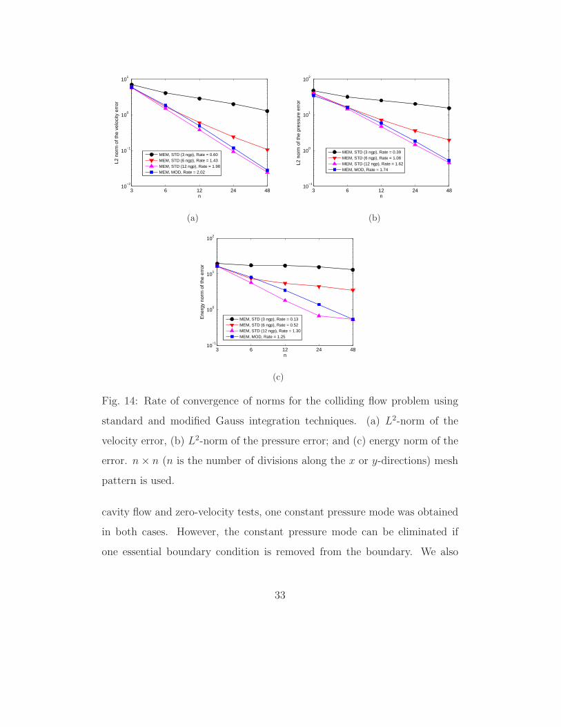
To assess the influence of numerical integration, a study of the MEM

method with STD and MOD schemes is conducted (see Section 3.3). The

numerical results are presented in Fig. 14. As we pointed out in Section 3.3,

due to numerical integration errors in meshfree methods, low-order stan-

dard Gauss quadrature can not deliver accurate numerical solutions with

optimal rates of convergence. Improved accuracy and better rate of conver-

gence in L2-norm are obtained with a 6-point rule, and a 12-point rule is

able to deliver about the same accuracy as the modified integration scheme

(Figs. 14(a) and 14(b)). It is noteworthy to point out that for the energy

norm curves shown in Fig. 14(c), the STD scheme with a 12-point rule results

30

2

x

y

u, v u, v

2

u, v

u, v

Fig. 12: Colliding flow. Geometry, mesh and boundary conditions.

in a sudden change in the slope of the curve with mesh refinement (quadra-

ture error is not sufficiently smaller than the approximation error), whereas

the MOD scheme consistently yields the optimal rate of convergence.

Finally, the accuracy and rate of convergence of the MINI element and

the maximum-entropy meshfree method are compared in Fig. 15. We ob-

serve that the MINI element and MEM solutions have the optimal rate of

convergence in the energy and L2-norms, but that the MEM formulation can

deliver more accurate results.

5.5. Inf-sup tests

The numerical inf-sup test described in Section 4 has been assessed for

meshfree methods [14, 15]. Here, we apply the inf-sup test on three problems:

leaky-lid driven cavity flow, Poiseuille flow, and a square domain (the same

used for the cavity flow) with zero-velocity imposed along the boundary.

When a vanishing velocity is imposed along the boundary of the domain, a

31

(a) (b)

(c) (d)

Fig. 13: Colliding flow. (a) MINI element solution for velocity field, (b) MINI

element solution for hydrostatic pressure field, (c) MEM solution for velocity

field; and (d) MEM solution for hydrostatic pressure field.

zero pressure field must be obtained everywhere. Otherwise, the formulation

would suffer from spurious pressure modes [6]. In order to compute the

numerical inf-sup value, four nodal discretizations are considered in each

problem. The background meshes are shown in Fig. 16. Numerical inf-sup

values are presented in Table 2. From Table 2, we observe that for all the

tests the numerical inf-sup values converge to a value that is bounded away

from zero with successive mesh refinements. Since the whole boundary has

been imposed with essential boundary conditions for the leaky-lid driven

32

3 6 12 24 4810

−2

10−1

100

101

n

L2 n

orm

of t

he v

eloc

ity e

rror

MEM, STD (3 ngp), Rate = 0.60MEM, STD (6 ngp), Rate = 1.43MEM, STD (12 ngp), Rate = 1.98MEM, MOD, Rate = 2.02

(a)

3 6 12 24 4810

−1

100

101

102

n

L2 n

orm

of t

he p

ress

ure

erro

r


(b)

3 6 12 24 4810

−1

100

101

102

n

Ene

rgy

norm

of t

he e

rror


(c)

Fig. 14: Rate of convergence of norms for the colliding flow problem using

standard and modified Gauss integration techniques. (a) L2-norm of the

velocity error, (b) L2-norm of the pressure error; and (c) energy norm of the

error. n× n (n is the number of divisions along the x or y-directions) mesh

pattern is used.

cavity flow and zero-velocity tests, one constant pressure mode was obtained

in both cases. However, the constant pressure mode can be eliminated if

one essential boundary condition is removed from the boundary. We also

33

3 6 12 24 4810

−2

10−1

100

101

n

L2 n

orm

of t

he v

eloc

ity e

rror

MINI, Rate = 2.11MEM, Rate = 2.02

(a)

3 6 12 24 4810

−1

100

101

102

n

L2 n

orm

of t

he p

ress

ure

erro

r


(b)

3 6 12 24 4810

−1

100

101

102

n

Ene

rgy

norm

of t

he e

rror


(c)

Fig. 15: Rate of convergence of norms for the colliding flow problem. (a)

L2-norm of the velocity error, (b) L2-norm of the pressure error; and (c)

energy norm of the error. n× n (n is the number of divisions along the x or

y-directions) mesh pattern is used.

mention that a zero-pressure field was obtained for the zero-velocity test,

which indicates that the MEM formulation is free of spurious pressure modes.

The inf-sup test is therefore passed and the MEM formulation is stable.

34

Table 2: Values of αh in the numerical inf-sup tests.

Problem n = 4 n = 8 n = 12 n = 16

Cavity 0.295 0.308 0.308 0.300

Poiseuille 0.112 0.113 0.113 0.113

Zero-velocity 0.295 0.308 0.308 0.300

(a) (b) (c) (d)

(e) (f)

(g) (h)

Fig. 16: Distorted background meshes employed for the inf-sup test. (a),

(b), (c) and (d) for the leaky-lid driven cavity flow and the zero-boundary

velocity problems; (e), (f), (g) and (h) for the Poiseuille problem. n×n mesh

pattern is used for the leaky-lid driven cavity flow and zero-boundary velocity

problems, while for the Poiseuille flow, n × n/2 mesh pattern is considered.

In both cases n is the number of divisions along the x-direction.

35

6. Concluding Remarks

In this paper, a meshfree method based on maximum-entropy approx-

imants that we recently presented in Ref. [1] was extended to Stokes flow

in two dimensions and to three-dimensional analysis of incompressible linear

elastic solids. The adoption of max-ent basis functions provides flexibility

and eases the implementation since it permits the direct imposition of es-

sential boundary conditions. A standard u-p mixed formulation was used to

compute volume-averaged nodal pressures a posteriori from the displacement

field of surrounding nodes, which led to a single-field (u-based) formulation.

Various benchmark problems in two and three dimensions, which included a

three-dimensional cantilever beam, a three-dimensional rigid flat punch prob-

lem, a leaky-lid driven cavity flow, and a colliding flow over a square domain

were conducted to demonstrate the performance of the maximum-entropy

meshfree method for incompressible media problems. The three-dimensional

problems were tested on unstructured tetrahedral integration meshes and ex-

cellent accuracy was realized by the MEMmethod. For the three-dimensional

cantilever beam problem, we found that accuracy considerations demanded

the need for very high-order Gauss quadrature rule on unstructured meshes,

whereas second-order accuracy sufficed for the numerical integration of both

the volume and surface integrals in our modified integration scheme. On

the benchmark problems, good agreement with analytical and reference so-

lution results was found, and the MEM solution delivered the optimal rate

of convergence in energy- and L2-norms. We studied the stability of our

method by conducting numerical inf-sup test on three benchmark problems.

With nodal refinement, the numerical inf-sup value remained a constant that

36

was bounded away from zero; furthermore, there were no spurious pressure

modes. The accuracy and robustness of the MEM method in two- and three-

dimensional incompressible linear problems suggests its potential in three-

dimensional nonlinear simulations.

ACKNOWLEDGEMENT

The authors (A. Ortiz and N. Sukumar) gratefully acknowledge the re-

search support of the National Science Foundation through contract Grants

CMMI-0626481 and CMMI-0826513 to the University of California at Davis.

A. Ortiz also thanks Professor K. J. Bathe for helpful clarifications on the

inf-sup test. The work of M. A. Puso was performed under the auspices of

the U.S. Department of Energy by Lawrence Livermore National Laboratory

under Contract DE-AC52-07NA27344.

References

[1] A. Ortiz, M. A. Puso, N. Sukumar, Maximum-entropy meshfree method

for compressible and near-incompressible elasticity, Computer Methods

in Applied Mechanics and Engineering 199 (25–28) (2010) 1859–1871.

[2] F. Brezzi, On the existence, uniqueness and approximation of saddle-

point problems arising from Lagrangian multipliers, RAIRO, Analyse

Numerique 8 (1974) 129–151.

[3] D. S. Malkus, T. J. R. Hughes, Mixed finite element methods – reduced

and selective integration techniques: a unification of concepts, Computer

Methods in Applied Mechanics and Engineering 15 (1) (1978) 63–81.

37

[4] O. A. Ladyzhenskaya, The Mathematical Theory of Viscous Incompress-

ible Flows, Gordon and Breach, London, 1969.

[5] I. Babuska, The finite element method with Lagrangian multipliers, Nu-

merische Mathematik 20 (3) (1973) 179–192.

[6] K. J. Bathe, Finite Element Procedures, Prentice Hall, Englewood Cliffs,

NJ, 1996.

[7] D. Chapelle, K. J. Bathe, The inf-sup test, Computers and Structures

47 (4–5) (1993) 537–545.

[8] F. Brezzi, J. Pitkaranta, On the stabilization of finite element approxi-

mations of the Stokes equations, In: W. Hackbusch (Ed.), Efficient so-

lutions of elliptic systems. Notes on numerical fluid mechanics 10 (1984)

11–19.

[9] T. J. R. Hughes, L. P. Franca, M. Balestra, A new finite element formula-

tion for computational fluid dynamics: V. Circumventing the Babuska-

Brezzi condition: a stable Petrov-Galerkin formulation of the Stokes

problem accommodating equal-order interpolations, Computer Methods

in Applied Mechanics and Engineering 59 (1) (1986) 85–99.

[10] K. J. Bathe, The inf-sup condition and its evaluation for mixed finite

element methods, Computers and Structures 79 (9) (2001) 243–252.

[11] F. Brezzi, M. Fortin, Mixed and Hybrid Finite Element Methods,

Springer, NY, 1991.

38

[12] D. Boffi, F. Brezzi, L. F. Demkowicz, R. G. Durn, R. S. Falk, M. Fortin,

Mixed Finite Elements, Compatibility Conditions, and Applications.

Edited by D. Boffi and L. Gastaldi. Lecture Notes in Mathematics, 1939,

Springer-Verlag, Berlin Fondazione C.I.M.E., Florence, 2008.

[13] J. Li, H. Yinnian, Z. Chen, Performance of several stabilized finite ele-

ment methods for the Stokes equations based on the lowest equal-order

pairs, Computing 86 (1) (2009) 37–51.

[14] J. Dolbow, T. Belytschko, Volumetric locking in the element free

Galerkin method, International Journal for Numerical Methods in En-

gineering 46 (6) (1999) 925–942.

[15] S. De, K. J. Bathe, Displacement/pressure mixed interpolation in the

method of finite spheres, International Journal for Numerical Methods

in Engineering 51 (3) (2001) 275–292.

[16] D. Gonzalez, E. Cueto, M. Doblare, Volumetric locking in natural neigh-

bour Galerkin methods, International Journal for Numerical Methods in

Engineering 61 (4) (2004) 611–632.

[17] J. Yvonnet, P. Villon, F. Chinesta, Natural element approximations

involving bubbles for treating mechanical models in incompressible me-

dia, International Journal for Numerical Methods in Engineering 66 (7)

(2006) 1125–1152.

[18] H. Desimone, S. Urquiza, H. Arrieta, E. Pardo, Solution of Stokes equa-

tions by moving least squares, Communications in Numerical Methods

in Engineering 14 (10) (1998) 907–920.

39

[19] X. L. Li, J. L. Zhu, A meshless Galerkin method for Stokes problems

using boundary integral equations, Computer Methods in Applied Me-

chanics and Engineering 198 (34–40) (2009) 2874–2885.

[20] X. L. Li, Meshless analysis of two-dimensional Stokes flows with the

Galerkin boundary node method, Engineering Analysis with Boundary

Elements 34 (1) (2010) 79–91.

[21] A. Huerta, Y. Vidal, P. Villon, Pseudo-divergence-free element free

Galerkin method for incompressible fluid flow, Computer Methods in

Applied Mechanics and Engineering 193 (12–14) (2004) 1119–1136.

[22] D. L. Young, S. C. Jane, C. Y. Lin, C. L. Chiu, K. C. Chen, Solutions

of 2D and 3D Stokes laws using multiquadrics method, Engineering

Analysis with Boundary Elements 28 (10) (2004) 1233–1243.

[23] M. H. Mohammadi, Stabilized meshless local Petrov-Galerkin (MLPG)

method for incompressible viscous fluid flows, CMES: Computer Mod-

eling in Engineering & Sciences 29 (2) (2008) 75–94.

[24] M. Cheng, G. R. Liu, A novel finite point method for flow simulation,

International Journal for Numerical Methods in Fluids 39 (12) (2002)

1161–1178.

[25] M. B. Liu, W. P. Xie, G. R. Liu, Modeling incompressible flows using a

finite particle method, Applied Mathematical Modelling 29 (12) (2005)

1252–1270.

[26] J. Fang, A. Parriaux, A regularized Lagrangian finite point method for

40

the simulation of incompressible viscous flows, Journal of Computational

Physics 227 (20) (2008) 8894–8908.

[27] H. Wendland, Divergence-free kernel methods for approximating the

Stokes problem, SIAM Journal on Numerical Analysis 47 (4) (2009)

3158–3179.

[28] T. P. Fries, H. G. Matthies, A stabilized and coupled mesh-

free/meshbased method for the incompressible Navier-Stokes equations-

Part I: Stabilization, Computer Methods in Applied Mechanics and En-

gineering 195 (44–47) (2006) 6205–6224.

[29] X. Li, Q. Duan, Meshfree iterative stabilized Taylor-Galerkin and

characteristic-based split (CBS) algorithms for incompressible NS equa-

tions, Computer Methods in Applied Mechanics and Engineering

195 (44–47) (2006) 6125–6145.

[30] L. Zhang, J. Ouyang, X. H. Zhang, W. B. Zhang, On a multi-scale

element-free Galerkin method for the Stokes problem, Applied Mathe-

matics and Computation 203 (2) (2008) 745–753.

[31] J. Dolbow, T. Belytschko, Numerical integration of Galerkin weak form

in meshfree methods, Computational Mechanics 23 (3) (1999) 219–230.

[32] I. Babuska, U. Banerjee, J. E. Osborn, Q. L. Li, Quadrature for meshless

methods, International Journal for Numerical Methods in Engineering

76 (9) (2008) 1434–1470.

[33] E. T. Jaynes, Information theory and statistical mechanics, Physical

Review 106 (4) (1957) 620–630.

41

[34] N. Sukumar, Construction of polygonal interpolants: a maximum en-

tropy approach, International Journal for Numerical Methods in Engi-

neering 61 (12) (2004) 2159–2181.

[35] M. Arroyo, M. Ortiz, Local maximum-entropy approximation schemes:

a seamless bridge between finite elements and meshfree methods, Inter-

national Journal for Numerical Methods in Engineering 65 (13) (2006)

2167–2202.

[36] N. Sukumar, R. W. Wright, Overview and construction of meshfree ba-

sis functions: from moving least squares to entropy approximants, In-

ternational Journal for Numerical Methods in Engineering 70 (2) (2007)

181–205.

[37] S. Li, W. K. Liu, Meshfree and particle methods and their applications,

Applied Mechanics Reviews 55 (1) (2002) 1–34.

[38] T. P. Fries, H. G. Matthies, Classification and overview of meshfree

methods, Tech. Rep. Informatikbericht-Nr. 2003-03, Institute of Sci-

entific Computing, Technical University Braunschweig, Braunschweig,

Germany (2004).

[39] S. Fernandez-Mendez, A. Huerta, Imposing essential boundary condi-

tions in mesh-free methods, Computer Methods in Applied Mechanics

and Engineering 193 (12–14) (2004) 1257–1275.

[40] L. L. Yaw, N. Sukumar, S. K. Kunnath, Meshfree co-rotational formula-

tion for two-dimensional continua, International Journal for Numerical

Methods in Engineering 79 (8) (2009) 979–1003.

42

[41] A. M. Rosolen, R. D. Millan, M. Arroyo, On the optimum support size

in meshfree methods: a variational adaptivity approach with maximum

entropy approximants, International Journal for Numerical Methods in

Engineering 82 (7) (2010) 868–895.

[42] T. J. R. Hughes, The Finite Element Method: Linear Static and Dy-

namic Finite Element Analysis, Dover Publications, Inc, Mineola, NY,

2000.

[43] J. Bonet, A. J. Burton, A simple average nodal pressure tetrahedral ele-

ment for incompressible and nearly incompressible dynamic explicit ap-

plications, Communications in Numerical Methods in Engineering 14 (5)

(1998) 437–449.

[44] C. R. Dohrmann, M. W. Heinstein, J. Jung, S. W. Key, W. R.

Witkowski, Node-based uniform strain elements for three-node trian-

gular and four-node tetrahedral meshes, International Journal for Nu-

merical Methods in Engineering 47 (9) (2000) 1549–1568.

[45] M. A. Puso, J. Solberg, A stabilized nodally integrated tetrahedral, In-

ternational Journal for Numerical Methods in Engineering 67 (6) (2006)

841–867.

[46] P. Krysl, B. Zhu, Locking-free continuum displacement finite elements

with nodal integration, International Journal for Numerical Methods in

Engineering 76 (7) (2008) 1020–1043.

[47] D. N. Arnold, F. Brezzi, M. Fortin, A stable finite element for the Stokes

equations, Calcolo 21 (4) (1984) 337–344.

43

[48] J. C. Simo, T. J. R. Hughes, On the variational foundations of assumed

strain methods, Journal of Applied Mechanics 53 (1) (1986) 51–54.

[49] M. A. Puso, J. S. Chen, E. Zywicz, W. Elmer, Meshfree and finite

element nodal integration methods, International Journal for Numerical

Methods in Engineering 74 (3) (2008) 416–446.

[50] F. Brezzi, K. J. Bathe, A discourse on the stability conditions for mixed

finite element formulations, Computer Methods in Applied Mechanics

and Engineering 82 (1–3) (1990) 27–57.

[51] R. L. Taylor, A mixed-enhanced formulation for tetrahedral finite el-

ements, International Journal for Numerical Methods in Engineering

47 (1–3) (2000) 205–227.

[52] J. Bonet, M. Marriot, O. Hassan, An averaged nodal deformation gra-

dient linear tetrahedral element for large strain explicit dynamic appli-

cations, Communications in Numerical Methods in Engineering 17 (8)

(2001) 551–561.

[53] F. M. Andrade Pires, E. A. de Souza Neto, J. L. de la Cuesta Padilla,

An assessment of the average nodal volume formulation for the analysis

of nearly incompressible solids under finite strains, Communications in

Numerical Methods in Engineering 20 (7) (2004) 569–583.

[54] G. Irving, C. Schroeder, R. Fedkiw, Volume conserving finite element

simulations of deformable models, ACM Transactions on Graphics 26 (3)

(2007) 13.1–13.6.

44

[55] E. A. de Souza Neto, F. M. Andrade Pires, D. R. J. Owen, F-bar-based

linear triangles and tetrahedra for finite strain analysis of nearly incom-

pressible solids. Part I: formulation and benchmarking, International

Journal for Numerical Methods in Engineering 62 (3) (2005) 353–383.

[56] P. Hauret, E. Kuhl, M. Ortiz, Diamond elements: a finite

element/discrete-mechanics approximation scheme with guaranteed op-

timal convergence in incompressible elasticity, International Journal for

Numerical Methods in Engineering 72 (3) (2007) 253–294.

[57] N. Kikuchi, Remarks on 4CST-elements for incompressible materials,

Computer Methods in Applied Mechanics and Engineering 37 (1) (1983)

109–123.

[58] O. C. Zienkiewicz, R. L. Taylor, The Finite Element Method, Volume

1: The Basis, 5th Edition, Butterworth-Heinemann, Oxford, UK, 2000.

[59] K. B. Nakshatrala, A. Masud, K. D. Hjelmstad, On finite element for-

mulations for nearly incompressible linear elasticity, Computational Me-

chanics 41 (4) (2008) 547–561.

[60] D. Z. Turner, K. B. Nakshatrala, K. D. Hjelmstad, On the stability

of bubble functions and a stabilized mixed finite element formulation

for the Stokes problem, International Journal for Numerical Methods in

Fluids 60 (12) (2009) 1291–1314.

[61] P. Hansbo, M. G. Larson, Piecewise divergence-free discontinuous

Galerkin methods for Stokes flow, Communications in Numerical Meth-

ods in Engineering 24 (5) (2008) 355–366.

45

[62] H. C. Elman, D. J. Silvester, A. J. Wathen, Finite Elements and Fast

Iterative Solvers: with Applications in Incompressible Fluid Dynamics,

Oxford University Press, Inc, NY, 2006.

46

Maximum-entropy meshfree method for incompressible media problems

Documents

Transcript of Maximum-entropy meshfree method for incompressible media problems