Entropy 2014, 16, 1287-1314; doi:10.3390/e16031287

entropy ISSN 1099-4300

www.mdpi.com/journal/entropy

Article

Entropy: From Thermodynamics to Hydrology

Demetris Koutsoyiannis

Department of Water Resources and Environmental Engineering, School of Civil Engineering,

National Technical University of Athens, 157 80 Zographou, Greece; E-Mail: dk@itia.ntua.gr;

Tel.: +30 210 772 2831; Fax: +30 210 772 2832

Received: 13 January 2014; in revised form: 8 February 2014 / Accepted: 12 February 2014 /

Published: 27 February 2014

Abstract: Some known results from statistical thermophysics as well as from hydrology

are revisited from a different perspective trying: (a) to unify the notion of entropy in

thermodynamic and statistical/stochastic approaches of complex hydrological systems and

(b) to show the power of entropy and the principle of maximum entropy in inference, both

deductive and inductive. The capability for deductive reasoning is illustrated by deriving the

law of phase change transition of water (Clausius-Clapeyron) from scratch by maximizing

entropy in a formal probabilistic frame. However, such deductive reasoning cannot work in

more complex hydrological systems with diverse elements, yet the entropy maximization

framework can help in inductive inference, necessarily based on data. Several examples of

this type are provided in an attempt to link statistical thermophysics with hydrology with a

unifying view of entropy.

Keywords: entropy; principle of maximum entropy; statistical thermophysics;

hydrology; stochastics

PACS Codes: 89.70.Cf; 05.70.-a; 92.40.-t; 02.50.Fz

1. Introduction

Uncertainty is the only certainty there is, and knowing how to live with insecurity is the

only security.

(Paulos [1], quoting his father)

Entropy is etymologized from the ancient Greek ἐντροπία but was introduced as a scientific term by

Rudolf Clausius only in 1865, although the concept appears also in his earlier works (see [2]). The

OPEN ACCESS

Entropy 2014, 16 1288

rationale for introducing the term is explained in his own words [3] (p. 358, which indicates that he

was not aware of the existence of the word ἐντροπία in ancient Greek):

We might call S the transformational content of the body […]. But as I hold it to be better

to borrow terms for important magnitudes from the ancient languages, so that they may be

adopted unchanged in all modern languages, I propose to call the magnitude S the entropy

of the body, from the Greek word τροπή, transformation. I have intentionally formed the

word entropy so as to be as similar as possible to the word energy; for the two magnitudes

to be denoted by these words are so nearly allied their physical meanings, that a certain

similarity in designation appears to be desirable.

In addition to its semantic content, this quotation contains a very important insight: the recognition

that entropy is related to transformation and change and the contrast between entropy and energy,

where the latter is a quantity that is conserved in all changes. This meaning has been more clearly

expressed in Clausius’ famous aphorism [4]:

Die Energie der Welt ist konstant [The energy of the world is constant].

Die Entropie der Welt strebt einem Maximum zu [The entropy of the world strives to a maximum].

In other words, entropy and its ability to increase (as contrasted to energy and other quantities that

are conserved) is the driving force of change. This property of entropy has seldom been acknowledged;

instead in common perception entropy is typically identified with disorganization and deterioration as

if change can only have negative consequences.

Mathematically, the thermodynamic entropy, S, is defined in the same Clausius’ texts through the

equation dS = dQ/T, where Q and T denote heat and temperature. The definition, however, applies to a

reversible process only. The fact that in an irreversible process dS > dQ/T makes the definition imperfect

and affected by circular reasoning, as, in turn, a reversible process is one in which the equality holds.

Two decades later, in 1877, Ludwig Boltzmann [5,6] gave entropy a statistical content as he related

it to probabilities of statistical mechanical system states, thus explaining the Second Law of

thermodynamics as the tendency of the system to run toward more probable states, which have higher

entropy. The statistical concept of entropy was advanced later in the works of Gibbs in

thermodynamics and von Neumann in quantum mechanics. In 1948 Shannon [7] used an essentially

similar, albeit more general, entropy definition to describe the information content, which he also

called entropy at von Neumann’s suggestion [8,9]. According to the latter definition, entropy is a

probabilistic concept, a measure of information or, equivalently, uncertainty (see next section). A

decade later, Jaynes [10] introduced the principle of maximum entropy thus equipping the entropy

concept with a powerful tool for logical inference.

More than half a century later, the meaning of entropy is still debated and a diversity of opinion

among experts is encountered [11]. In particular, despite having the same name, probabilistic (or

information) entropy and thermodynamic entropy are still regarded by many as two distinct notions

having in common only the name. The classical definition of thermodynamic entropy (as above) does

not give any hint about similarity with the probabilistic entropy. The fact that the former is a

dimensionless quantity and the latter has units (J/K) has been regarded as an argument that the two are

dissimilar. Even Jaynes [12], the founder of the maximum entropy principle, states:

Entropy 2014, 16 1289

We must warn at the outset that the major occupational disease of this field is a persistent

failure to distinguish between the information entropy, which is a property of any

probability distribution, and the experimental entropy of thermodynamics, which is instead

a property of a thermodynamic state as defined, for example by such observed quantities

as pressure, volume, temperature, magnetization, of some physical system. They should

never have been called by the same name; the experimental entropy makes no reference

to any probability distribution, and the information entropy makes no reference to

thermodynamics. Many textbooks and research papers are flawed fatally by the author’s

failure to distinguish between these entirely different things, and in consequence proving

nonsense theorems.

Nevertheless, the units of thermodynamic entropy are only an historical accident, related to the

arbitrary introduction of temperature scales [13,14]. In a recent book, Ben-Naim [15] has attempted to

replace altogether the concept of entropy with the concept of information. However, such a

replacement is unnecessary or even meaningless if we accept that the two concepts are identical. As

recently has been shown (Koutsoyiannis [16]) the formal probability theory can produce the

thermodynamic entropy of gases without difficulties and without the need of strange assumptions (e.g.,

the indistinguishability of particles). The logical basis of the latter study includes the following points.

(a) The classical definition of thermodynamic entropy is not necessary; it can be abandoned and

replaced by the probabilistic definition.

(b) The thus defined entropy is the fundamental thermodynamic quantity, which supports the

definition of all other derived ones. For example, the temperature is defined as the inverse of

the partial derivative of entropy with respect to the internal energy (see Equation (26)).

(c) The entropy retains its dimensionless character even in thermodynamics, thus rendering the

unit of kelvin an energy unit, a tiny submultiple of the joule (i.e., 1 K = 0.13806505 yJ =

1.3806505 × 10−23

J).

(d) The entropy retains its probabilistic interpretation as a measure of uncertainty, leaving aside the

traditional but obscure “disorder” interpretation.

(e) The tendency of entropy to reach a maximum is the driving force of natural change. This

tendency is formalized as the principle of maximum entropy [10], which can be regarded

both as a physical (ontological) principle obeyed by natural systems, as well as a logical

(epistemological) principle applicable in making inference about natural systems.

The present study is an extension of the previous one [16] in the field of hydrology.

Thermodynamics is one of the pillars of hydrology and in this respect entropy has been in use, albeit

indirectly and implicitly, in most hydrological studies (as well as in all geosciences, see e.g., [17,18]).

The probabilistic formalization of entropy has not been used in hydrology for long. Only in the 1960s

did the pioneering study by Leopold and Langbein [19], which relies on Boltzmann’s definition of

entropy (see Section 2.3), appear. In the 1970s hydrologists began to use Shannon’s definition of

entropy (see Section 2.1) mainly for parameter estimation of models [20] and probability distributions [21],

while in the early 1980s some doctoral theses on the use of entropy in hydrology were conducted [22,23].

Extensive reviews on the use of entropy in applications in hydrology and water resources have been

Entropy 2014, 16 1290

provided by Singh [24,25]. Additional hydrological studies which rely on entropy will be referred

to later on.

The aim of this paper is not to derive new results. In fact no new results are presented. At the same

time it is not a review paper. It presents some known results from a different perspective trying (a) to

unify the notion of entropy in thermodynamic and statistical/stochastic approaches and (b) to show the

power of entropy and the principle of maximum entropy in inference, both deductive and inductive.

The capability for deductive reasoning is illustrated by deriving the law of phase change transition

of water from scratch by using probabilistic entropy (Section 3). Although the law is very old

(Clausius-Clapeyron), the derivation provided is new and constitutes an ideal example of how by

maximizing entropy, i.e., uncertainty, at the microscopic level we can derive a physical law which

virtually expresses certainty at a macroscopic level. Such deductive reasoning cannot work in more

complex hydrological systems with diverse elements, yet the entropy maximization framework can

help in inductive inference, necessarily based on data. Several examples of this type are provided

(Section 4). Overall, the paper is written as a self-contained study with a pedagogic style in an attempt

to help students of the entropy topic to avoid some confusion which all of us may have experienced.

For this reason, the paper also contains a logical and mathematical foundation of the concepts used

(Section 2) as well as several side derivations necessary to make the presentation complete (Section 3

and Appendix).

2. Logical and Mathematical Foundation

2.1. Entropy = Uncertainty

The definition of entropy relies on probability theory and is very economic as it only needs the concept

of a random variable and its distribution function. Before discussing this definition it is useful to make two

notes about the notation used: (a) for random variables the Dutch convention [26] is followed, according to

which an underlined symbol denotes a random variable, while the same symbol not underlined represents a

value (or realization) of the random variable; (b) entropy is denoted by Φ to avoid confusion with the

classical thermodynamic entropy S (the original symbol used by Clausius), which has some (mostly

logistic) differences (e.g., it is regarded to be a dimensional quantity, while Φ is dimensionless). Some

texts use the symbol H for Shannon entropy; however here the symbol Φ was preferred for several

reasons including historical ones: for long time, entropy used to be denoted by φ [27–29] and this is

still echoed in the term tephigram (T-Φ-gram) used in meteorology.

The entropy definition follows some postulates originally set up by Shannon [7]. Assuming a

discrete random variable z taking values zj with probability mass function Pj ≡ P(zj) = P{z = zj},

j = 1,…,w, the postulates, as reformulated by Jaynes [12] (p. 347), are:

(a) It is possible to set up a numerical measure Φ of the amount of uncertainty which is expressed

as a real number.

(b) Φ is a continuous function of Pj.

(c) If all the Pj are equal (Pj = 1/w) then Φ should be a monotonic increasing function of w.

(d) If there is more than one way of working out the value of Φ, then we should get the same value

for every possible way.

Entropy 2014, 16 1291

Quantification of the latter postulate is given, among others, in [8] (p. 3) and [30] (Theorem 1) and

is related to refinement of partitions to which the probabilities Pj refer. From these general postulates

about uncertainty, a unique (within a multiplicative factor) function Φ is defined. For discrete

variables, for which probabilities satisfy the obvious relationship:

∑ = 1

= 1

(1)

the entropy is defined as:

Φ[z] :=

E[–ln P(z)]

=

–∑ ln

= 1

(2)

where E[ ] denotes expectation. Extension of the above definition for the case of a continuous random

variable z with probability density function f(z), where:

∫ ( )d = 1

(3)

is possible, although not contained in Shannon’s [7] original work. This extension involves some

additional difficulties. Specifically, if we discretize the domain of z into intervals of size δz, then (2)

would give an infinite value for the entropy as δz tends to zero (the quantity –ln p = –ln (f(z) δz)) will

tend to infinity). However, if we involve a (so-called) “background measure” with density h(z) and

take the ratio (f(z) δz)/ (h(z) δz) = f(z)/h(z), then the logarithm of this ratio will generally not diverge.

This allows the definition of entropy for continuous variables as (see e.g. [12], p. 375, and [30]):

Φ[z] := [– ln (z)

h(z)] = – ∫ ln

( )

h( ) ( )d

- (4)

The background measure h(z) can be any probability density, proper (with integral equal to 1, as in

Equation (3)) or improper (meaning that its integral does not converge); typically it is an (improper)

Lebesgue density, i.e., a constant with dimensions [h(z)] = [f(z)] = [z−1

], so that the argument of the

logarithm function be dimensionless. It is easily seen that for both discrete and continuous variables

the entropy Φ[z] is a dimensionless quantity. For discrete variables it can only take positive values,

while for continuous variables it can be either positive or negative, depending on the assumed h(z).

2.2. The Principle of Maximum Entropy: Why Entropy is Important

As already mentioned, from a physical perspective, the tendency of entropy to become maximal

(Second Law of thermodynamics) is the driving force of natural change. The counterpart of the

physical law in logic is the principle of maximum entropy [10], which postulates that the entropy of a

random variable z should be at maximum, under some conditions, formulated as constraints, which

incorporate the information that is given about this variable. The rationale of the principle is very

simple and almost self-evident: If uncertainty is not the maximum possible, then there must be some

more information; but all information is already incorporated in the constraints. Compared to physical

laws expressed in the form of equations (e.g., equality of conserved quantities), the ME principle, as a

variational law, is extremely more powerful: it can determine infinitely many (or even uncountably

many) unknown probabilities.

Entropy 2014, 16 1292

To illustrate the ME principle we start with the simple example of determining the probabilities of

the outcomes of a die throw. The example may look trivial. However, as will be seen later on, with the

same reasoning we can infer more interesting things, such as the saturation vapour pressure in the

atmosphere. The logic in the two cases is the same: we maximize the uncertainty with respect to the

state of a die or a water molecule. For the die the entropy is:

Φ = E[–ln P(z)] = –P1 ln P1 – P2 ln P2 – P3 ln P3 – P4 ln P4– P5 ln P5 – P6 ln P6 (5)

The equality constraint is:

P1 + P2 + P3 + P4 + P5 + P6 = 1 (6)

Inequality constraints about probabilities (0 ≤ Pi ≤ 1) are not necessary to include in optimization

in this case. The solution of the optimization problem (e.g. by the Lagrange method) yields a

single maximum:

P1 = P2 = P3 = P4 = P5 = P6 = 1/6 (7)

The entropy is Φ = –6 (1/6) ln (1/6) = ln 6. In this case, the application of the ME principle (a

variational law) is equivalent to the principle of insufficient reason (Bernoulli-Laplace; an equation

form). It is noted that entropy and information are complementary to each other. When we know

(observe) that the outcome is i (Pi = 1, Pj = 0 for j ≠ i), the entropy is zero.

While in this simple case the principle of insufficient reason works equally well as the ME

principle, in fact the latter is more powerful as it can perform in any type of problems, in which

uniformity is a priori excluded. To see this let us assume that the die is loaded and that we have prior

information that P6 – P1 = 0.2 ≠ 0. What is the probability that the outcome of a die throw will be i in

this case? For the entropy maximization we only need to consider the additional constraint P6 – P1 –

0.2 = 0 (e.g., with an additional Lagrange multiplier). The solution of the optimization problem is a

single maximum depicted in Figure 1. The entropy is Φ = 1.732, smaller than in the case of

equiprobability, where Φ =

ln

6

=

1.792. The decrease of entropy in the loaded die derives from the

additional information incorporated in the constraints.

Figure 1. Probability Pi of the outcome i of a die throw for the cases where the die is fair

or loaded with prior information P6 – P1 = 0.2.

0

0.1

0.2

0.3

0.4

1 2 3 4 5 6

i

p i Fair

Loaded

Entropy 2014, 16 1293

2.3. Maximum Entropy and Uniformity

As in the die case, entropy maximization without constraints, except the obvious Equation (1),

results in equal probabilities for all outcomes. The entropy for w equiprobable outcomes is:

Φ = ln w (8)

This corresponds to the original Boltzmann’s definition of entropy, according to which the entropy

is the logarithm of the number of possible configurations of the phase space (or in probability terms the

number of possible outcomes). However, when compared to Equation (8), Equation (2) provides a

more general definition, applicable also to cases where, due to constraints, equiprobability is not

possible, or where the number of possible outcomes or configurations is infinite. In other words, in the

general case, the entropy equals the expected value of the minus logarithm of probability (rather than

just the minus logarithm of probability).

A similar result is obtained for continuous variables z. Entropy maximization without constraints,

except Equation (3), over a finite interval (or volume, in a vector space) Ω, will result in uniform

probability density i.e. f(z) = 1/Ω, if we also assume a constant background measure density, h(z) = h.

The maximized entropy then becomes:

Φ = ln (Ωh) (9)

Again this corresponds to the original Boltzmann’s definition of entropy, in this case giving the

entropy in terms of the logarithm of the volume of the accessible phase space Ω. Yet Equation (4)

provides a more general definition than Equation (9), applicable in every case, even if the volume of

phase space is infinite.

An important characteristic of the general entropy definitions in Equations (2) and (4) is that they

both are independent of the specific metric that is used to define the random variables which describe a

physical phenomenon. This is obvious in Equation (2), which is an expression of probabilities and does

not involve values of the random variables at all. It is less obvious in Equation (4) and in fact, if we

assume h(z) ≡ 1 as most probability texts do (e.g., [31], p. 565), the entropy value is not unique but

changes if a transformation z → y(z) is applied. However, this problem is resolved if entropy is defined

as in Equation (4) and the transformation is applied also to h(z). Indeed it is easy to show that the

entropy value is invariant under the transformation z → y(z) (i.e., Φ[y] = Φ[z]). The reason is that both

f and h transform in the same way under a change of variables [12] (pp. 375–376). However, as has

been already noted, in continuous variables the entropy value changes if a different background

measure is chosen. Also, in both continuous and discrete random variables the entropy changes in

coarse grained descriptions of the system, in which probabilities refer to elements of partitions of the

basic set, rather than elementary events.

2.4. Expected Values as Constraints: General Solution

In the most typical application of the ME principle, we wish to infer the probability density function

f(z) of a continuous random variable z (scalar or vector) for constant background measure (for

simplicity taken h(z) = 1) with constraints formulated as expectations of functions gj(z). In other words,

Entropy 2014, 16 1294

the given information, which is used in maximizing entropy, is expressed as a set of constraints

formed as:

[ ( )] = ∫

( ) ( )d

- =

, j = 1, …, n (10)

The resulting maximum entropy distribution (by maximizing entropy as defined in Equation (4)

with constraints (10) and the obvious additional constraint (3)) is [31] (p. 571):

( ) = exp(– 0 –∑ ( )

= 1

) (11)

where 0 and j are constants determined such as to satisfy Equations (3) and (10), respectively. The

resulting maximum entropy is:

Φ[z] = 0 ∑ = 1 (12)

Typical results for the most common constraints are provided in Table 1.

Table 1. Typical results of entropy maximization.

Constraints for the continuous variable z Resulting distribution f(z) and entropy Φ (for h(z) = 1)

z bounded in [0, w]; no equality constraint f(z) = 1/w (uniform)

Φ = ln w

z unbounded from both below and above

No constraint or constrained mean μ not defined

Constrained mean μ and variance σ2 f(z)

=

exp(–((z

–

μ)/σ)

2/2)

/ ( 2π σ) (Gaussian)

Φ = ln ( 2πe σ)

Nonnegative z unbounded from above

No equality constraint not defined

Constrained mean μ f(z) = (1/μ) exp(–z/μ) (exponential)

Φ = ln (eμ)

Constrained mean μ and variance σ2 with σ < μ f(z) = A exp(–((z – α)/β)

2/2) (truncated Gaussian tending to

exponential as σ → μ); the constants A, a and β are

determined from the constraints and Φ from (12)

As above but with σ > μ not defined

3. Application to Simple Physical Systems

3.1. ME Applied to the Uncertain Motion of a Particle

In this section we will derive physical laws which are extensively used in hydrology—in particular

the law for the phase transition of water—applying the same method with which we derived the

probabilities of a die outcome in Section 2.2 and the probability distribution functions in Table 1. We

consider a motionless cube with edge a (volume V = a3) containing spherical particles of mass m0 (e.g.,

monoatomic molecules) in fast motion, in which we cannot observe the exact position and velocity. A

particle’s state is described by six variables, three indicating its position xi and three indicating its

velocity ui, with i = 1, 2, 3 (three degrees of freedom); all are represented as random variables, forming

the vector z = (x1, x2, x3, u1, u2, u3).

Entropy 2014, 16 1295

The constraints for position are:

0 ≤ xi ≤ a, i = 1, 2, 3 (13)

While these are inequality constraints, those for velocity are equality constraints given in terms of

integrals over feasible space Ω, i.e., (0, a) for each xi and (– , ) for each ui. Specifically, the

conservation of momentum is E[m0 ui] = m0 ∫Ω ui f(z) dz = 0 (because the cube is not in motion), so that:

E[ui] = 0, i = 1, 2, 3 (14)

Likewise, conservation of energy yields E[m0 ||u||2/2] = (m0 /2)

∫Ω ||u||

2 f(z) dz = ε, here ε is

the kinetic energy of the particle (known as thermal energy) and ||u ||2 = u

1

u

u

; thus, the

constraint is:

E[||u||2] = 2ε/m0 (15)

In general, the expectation E[ui] represents the macroscopic velocity of the motion, while ui – E[ui]

represents velocity fluctuation at a microscopic level. If E[ui] ≠ 0 (if the cube was moving), then the

macroscopic and microscopic kinetic energies should be treated separately, the latter being

ε = Ε[m0 (||u – E[u]||)2/2].

By dimensional considerations we define the background measure in terms of universal constants,

i.e., the Planck constant h = 6.6 6 × 10− 4

J·s and the proton mass mp. It is easily verified that h(z) =

(mp/h)3

(dimensions L–6

T3), thereby giving the entropy as:

Φ[z] := E[–ln((h/mp)3 f(z))]= –∫Ω ln ((h/mp)

3f(z)) f(z) dz (16)

Application of the principle of maximum entropy with constraints as in Equations (3), (13), (14) and

(15) gives the distribution of z (see proof in Appendix 1 and in [16]) as:

f(z) = (1/a)3 (3m0 / 4πε)

3/2 exp(–3m0 ||u||

2/ 4ε), 0 ≤ xi ≤ a (17)

The marginal distribution of each of the location coordinates xi is uniform in [0, a], i.e.:

f(xi) = 1/a, i = 1, 2, 3 (18)

The marginal distribution of each of the velocity coordinates ui is derived as:

f(ui) = (3m0 / 4πε)1/2

exp(–3m0 ui2

/ 4ε), i = 1, 2, 3 (19)

This is Gaussian with mean 0 and variance 2ε / 3m0 (= × energy per unit mass per degree of

freedom). The marginal distribution of the velocity magnitude ||u|| is:

f(||u||) = ( /π)1/2

(3m0 / 2ε)3 ||u||

2 exp(–3m0||u||

2/ 4ε) (20)

This is known as the Maxwell–Boltzmann distribution.

The entropy then results as:

Φ[z] = 3

2 ln

4πe

3

mp2

h2 m0

ε V 2/3

=

3

2 ln

4πe

3

mp2

h2 m0

+

3

2 ln ε + ln V (21)

where e is the base of natural logarithms.

From Equation (17) we readily observe that the joint distribution f(z) is a product of functions of z’s

coordinates x1, x2, x3, u1, u2, u3. This means that all six random variables are jointly independent. The

independence results from entropy maximization. From Equations (17) and (19) we also observe the

Entropy 2014, 16 1296

symmetry with respect to the three velocity coordinates, resulting in uniform distribution of the energy

ε into ε/3 for each direction or degree of freedom. This is known as the equipartition principle and is

again a result of entropy maximization.

3.2. Extension for Many Particles

The coordinates of N identical monoatomic molecules which are in motion in the same cube of

volume V form a vector Z = (z1,…, zN) with 3N location coordinates and 3N velocity coordinates. If E

is the total kinetic energy of the N molecules and ε = E/N is the energy per particle, then following a

similar approach we find [16] the entropy as:

Φ[Z] = 3N

2 ln

4πe

3

mp2

h2 m0

ε V 2/3

=

3N

2 ln

4πe

3

mp2

h2 m0

+

3N

2 ln ε + N ln V (22)

The resulting Equation (22) is fully consistent with the probabilistic character of entropy and also

with the thermodynamic content of entropy [16]. It is noted that the equation found in literature,

known as the Sackur-Tetrode equation (after H. M. Tetrode and O. Sackur, who developed it

independently at about the same time in 1912) differs from Equation (22) in the last term, which is

N ln (V/N) instead of N ln V. To derive the Sackur-Tetrode expression, an assumption is made (inspired

from quantum physics) that particles are indistinguishable. This assumption is problematic and here is

avoided (see details in [16]).

3.3. Extension to Many Degrees of Freedom

The number of microscopic degrees of freedom β that can store energy in a particle depend on the

particle architecture and interactions. Thus, in gases:

A monoatomic molecule has β = 3 translational degrees of freedom, corresponding to the three

components of the velocity vector, as already described.

A diatomic molecule (e.g., of N2 or O2 which are the most typical in the atmosphere) has a linear

structure; thus, in addition to the kinetic energy it has rotational energy at two axes perpendicular

to the line defined by the two atoms; in total it has β = 5 degrees of freedom.

A triatomic, not linear, molecule (e.g., H2O), or a more complex one, has three rotational degrees

of freedom or β = 6 degrees of freedom in total.

In solids and liquids there are degrees of freedom associated to vibrational energy. Generalizing

Equations (21) and (22) for β degrees of freedom we obtain the entropy per molecule as:

φ := Φ[z] = c + β

ln ε + ln V (23)

where c incorporates all related physical and mathematical constants. Likewise, the total entropy of N

molecules is:

Φ = Nφ = Φ[Z] = Νc + βΝ

ln ε + Ν ln V = Νc +

βΝ

ln

N + Ν ln V (24)

Entropy 2014, 16 1297

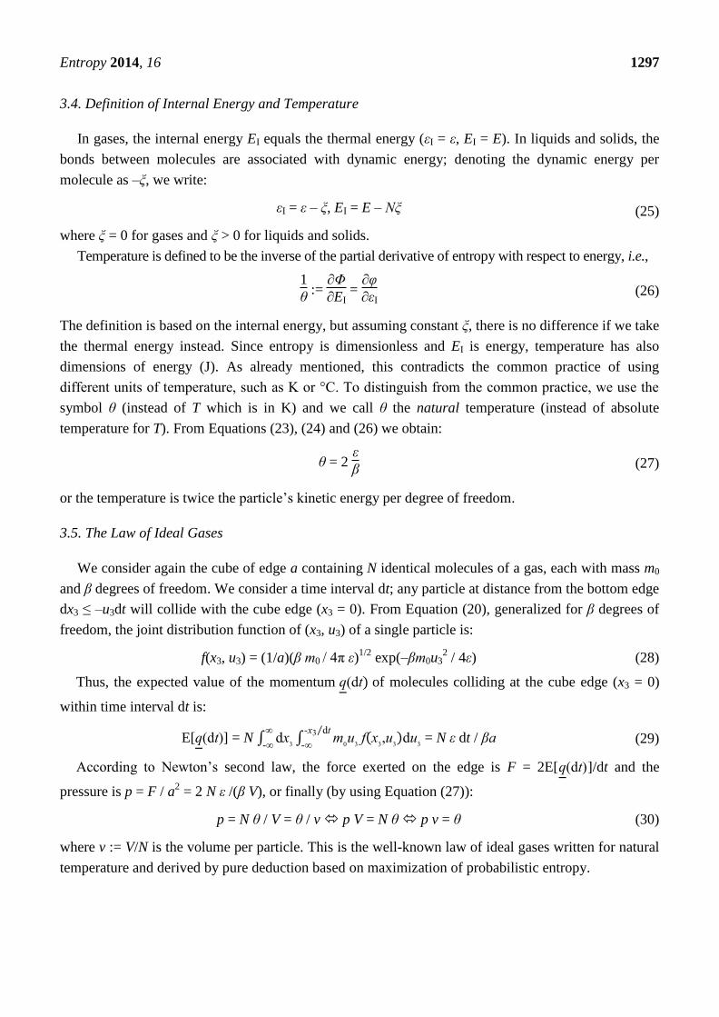
3.4. Definition of Internal Energy and Temperature

In gases, the internal energy EI equals the thermal energy (εI = ε, EI = E). In liquids and solids, the

bonds between molecules are associated with dynamic energy; denoting the dynamic energy per

molecule as –ξ, we write:

εI = ε – ξ, EI = E – Nξ (25)

where ξ = 0 for gases and ξ > 0 for liquids and solids.

Temperature is defined to be the inverse of the partial derivative of entropy with respect to energy, i.e.,

1

θ := ∂Φ

∂EI = ∂φ

∂εI (26)

The definition is based on the internal energy, but assuming constant ξ, there is no difference if we take

the thermal energy instead. Since entropy is dimensionless and EI is energy, temperature has also

dimensions of energy (J). As already mentioned, this contradicts the common practice of using

different units of temperature, such as K or °C. To distinguish from the common practice, we use the

symbol θ (instead of T which is in K) and we call θ the natural temperature (instead of absolute

temperature for T). From Equations (23), (24) and (26) we obtain:

θ = 2 ε

β (27)

or the temperature is twice the particle’s kinetic energy per degree of freedom.

3.5. The Law of Ideal Gases

We consider again the cube of edge a containing N identical molecules of a gas, each with mass m0

and β degrees of freedom. We consider a time interval dt; any particle at distance from the bottom edge

dx3 ≤ –u3dt will collide with the cube edge (x3 = 0). From Equation (20), generalized for β degrees of

freedom, the joint distribution function of (x3, u3) of a single particle is:

f(x3, u3) = (1/a)(β m0 / 4π ε)1/2

exp(–βm0u32 / 4ε) (28)

Thus, the expected value of the momentum (dt) of molecules colliding at the cube edge (x3 = 0)

within time interval dt is:

E[ (dt)] = N ∫ d

- ∫ m

0u (

,u

)du

- dt⁄

- = N ε dt / βa (29)

According to Newton’s second law, the force exerted on the edge is F = 2E[ (dt)]/dt and the

pressure is p = F / a2 = 2 N ε /(β V), or finally (by using Equation (27)):

p = N θ / V = θ / v p V = N θ p v = θ (30)

where v := V/N is the volume per particle. This is the well-known law of ideal gases written for natural

temperature and derived by pure deduction based on maximization of probabilistic entropy.

Entropy 2014, 16 1298

3.6. Phase Change and Saturation Vapour Pressure

We have now almost everything to derive the law determining the equilibrium of liquid and gaseous

phase of water, known as the Clausius-Clapeyron equation, which is very important in hydrology.

Again this law will be derived by maximizing probabilistic entropy, i.e. uncertainty. In particular, the

law is derived by studying a single molecule (see Figure 2) and maximizing the combined uncertainty

of its state related to:

(a) its phase (whether gaseous, denoted as A, or liquid, denoted as B);

(b) its position in space; and

(c) its kinetic state, i.e., its velocity and other coordinates corresponding to its degrees of freedom

and making up its thermal energy.

Furthermore, it is assumed that water vapour behaves as an ideal gas, so that Equation (30) holds.

As its molecule has a 3-dimensional (not linear) structure, the rotational energy is distributed into three

directions, so that the total number of degrees of freedom (translational and rotational) is:

βA = 6 (31)

Figure 2. Explanatory sketch indicating basic quantities involved in the equilibrium of the

water vapour with liquid water, with zoom on a single molecule which “tries to hide itself”

by maximizing the combined uncertainty related to its phase (being either gaseous or liquid

with probabilities πΑ and πB, respectively), position and kinetic state.

Liquid water will be assumed incompressible, so that the volume per particle is:

vB := VB/NB = constant (32)

where VB is the volume occupied by the liquid phase and NB is the number of particles in that phase.

The number of degrees of freedom in the liquid phase is greater than βA because of the “social

Entropy 2014, 16 1299

behaviour” of water molecules. Specifically, in addition to the translational and rotational degrees of

freedom of individual molecules, there are local clusters with low energy vibrational modes that can be

thermally excited. The average number of degrees of freedom per molecule (individual and collective

involving more than one water molecules) is very high (e.g., [32]):

βB = 18 (33)

For a molecule to move from the liquid to gaseous phase, an amount of energy ξ to break its bonds

with other molecules needs to be supplied (phase change energy). The partial entropies of the two

phases, i.e., the entropies conditional on the particle being in the gaseous (A) or liquid (B) phase, are:

φA = cA + (βA/2) ln εA + ln VA, φB = cB + (βB/2) ln εB + ln VB (34)

The total entropy is [16]:

φ = πΑ φA + πΒ φB + φπ, where φπ := –πΑ ln πΑ – πΒ ln πΒ (35)

or:

φ = πΑ (φA – ln πΑ) + πΒ (φΒ – ln πΒ) (36)

The two phases are in open interaction and the constraints are:

πΑ + πΒ = 1 (37)

πΑ εA + πΒ (εΒ – ξ) = ε (38)

The calculations of entropy maximization are shown in Appendix 2. The resulting saturation vapour

pressure is:

p = constant × e−ξ/θ

θ −(βB/2 − βA/2 − 1)

(39)

Assuming that at some temperature θ0, p(θ0) = p0, we write Equation (39) in a more convenient and

dimensionally consistent manner as:

p = p0 e ξ/θ0 (1− θ0/θ)

(θ0/θ) (βB/2 − βA/2 − 1)

(40)

This is the final form of the proposed equation quantifying phase change. Equation (40) can be

anchored at the triple point of water, in which θ0 = 37.714 yJ = 273.16 K, p0 = 6.11657 hPa [33], while

an optimized value of the constant ξ/θ0 based on accurate measurements is ξ/θ0 = 24.861.

The Newton-Raphson method applied to Equation (40) gives the approximation:

p = p0 e (ξ/θ0 − βB/2 + βA/2 + 1) (1− θ0/θ)

(41)

The latter is the standard solution of the Clausius-Clapeyron equation appearing in books, which however

is an inconsistent approximate description of the phenomenon [34]. Figure 3 (upper) compares the

proposed Equation (40) with the standard Equation (41); they seem indistinguishable. However, the lower

panel of the figure, which compares relative differences from measurements, clearly indicates the

superiority of Equation (40) derived here. A slightly more accurate version, based on experimental

values of specific heats, instead of using integral degrees of freedom, can be found in [34] (the slight

differences are in the numerical values of the constants, i.e., (βB/2 – βA/2 – 1) = 5.06 and

ξ/θ0 = 24.921).

Entropy 2014, 16 1300

Figure 3. (upper) Comparison of saturation vapour pressure obtained by the proposed

Equation (40) and by the standard but inconsistent Equation (41). (lower) Comparison of

relative differences of the saturation vapour pressure obtained by the proposed Equation (40),

as well as by Equation (41), with accurate measurement data of different origins, as

indicated in the legend (for details on data see [34]).

4. Application to Complex Hydrological Systems

4.1. From Statistical Thermodynamics of Systems with Identical Elements to Hydrological Systems

The law of phase change constitutes an amazing example of how we can derive, based on deductive

reasoning, a virtually deterministic law by maximizing entropy (i.e., uncertainty). The key that made

this possible is the huge number of identical elements involved in the phenomenon. This does not

happen in higher levels of macroscopization, which are associated with higher complexity and diverse

elements, each of them being a macroscopic entity per se and all of them being not so many as in

typical thermodynamic systems (Figure 4).

Due to higher complexity, the probabilistic description is even more imperative in hydrological

systems. Maximization of entropy (i.e., uncertainty) should provide the way to deal with the complex

macroscopic hydrological systems. This contrasts the recent research trend in hydrology (and other

disciplines), which invested hopes to the power of computers that would enable faithful and detailed

0.1

1

10

100

1000

-40 -30 -20 -10 0 10 20 30 40 50

Satu

rati

on

vap

ou

r p

ress

ure

(h

Pa)

Temperature (°C)

Proposed

Standard solution of Clausius-Clapeyron

-1

0

1

2

3

4

5

6

7

8

-40 -30 -20 -10 0 10 20 30 40 50

Rela

tive d

iffe

rence (

%)

Temperature (°C)

Proposed vs. IAPWS Standard vs. IAPWS

Proposed vs. ASHRAE Standard vs. ASHRAE

Proposed vs. Smiths. Standard vs. Smiths.

Proposed vs. WMO Standard vs. WMO

Entropy 2014, 16 1301

representation of the diverse system elements. This research trend was based on the idea that the

hydrological processes could be modelled using merely “first principles”, thus resulting in

(deterministic) “physically-based” models which would tend to approach in complexity the real world

systems. The aspiration of detailed and exact deterministic modelling traces a research direction that is

wrong and opposite to the parsimonious way that Nature works.

Figure 4. Schematic of macroscopization levels and their associated complexities: (left)

schematic of the interior of a rain drop, which is a typical thermodynamic system with

identical elements (water molecules); (middle) a higher macroscopization level indicating

that rain drops are not identical to each other and their motion is affected by turbulence

(photo by author from monsoon rainfall in India); (right) an even higher macroscopization

level, where the diversity of elements becomes more prominent (photo by author of

confluent rivers in Greece with the different colours of water in the two branches).

In high-level macroscopic hydrological systems we expect to encounter more difficulties in comparison

to simple thermodynamic systems. The constraints in entropy extremization do not necessarily coincide

with those in classical statistical thermophysics. In particular, the mean μ and variance σ2 are important

indices of the statistical behaviour (see [35]) with an intuitive conceptual meaning, but they are not

constrained by physical laws as in the kinetic theory of gases—rather they are estimated from data. In

addition, independence among different elements and across time (as assumed in the derivations of the

previous section) is most often invalidated in high-level macroscopic systems. This, combined with the

diversity of elements, entails that all laws should remain probabilistic. High-level macroscopic

quantities in hydrological systems will never approach the near certainty of low-level macroscopic

quantities in typical thermodynamic systems—regardless of progress in computers and algorithms.

Inevitably, physically-based hydrological models are stochastic models (cf. [36]).

4.2. Towards Adaptation of the ME Framework for Nonnegative Random Variables

Typically for continuous random variables ranging in (– , ) the Lebesgue measure is used in the

entropy function, so that h(z) = constant = 1/[z] where [z] denotes the physical unit in which the

quantity z is expressed. The background measure h(z) determines the way of measuring distances d

between values of z; the Lebesgue measure corresponds to the Euclidean distance, d(z, z΄) = |z΄ – z|.

However, most hydrometeorological variables are non-negative physical quantities unbounded from

above (e.g., precipitation, streamflow, temperature—natural or absolute). In positive physical

Entropy 2014, 16 1302

quantities (e.g., rainfall depth) often the Euclidean distance is not a proper metric; sometimes we use a

logarithmic distance d(z, z΄) = |ln(z΄/ z)|, as shown in the example of Table 2.

Table 2.Illustration of the Euclidean and logarithmic difference: which of the second and

third couples is equidistant to the first one?

Euclidean Distance Logarithmic Distance

z = 0.1 mm, z΄ = 0. mm 0.1 mm ln 2

z = 100 mm, z΄ = 100.1 mm 0.1 mm ln 1.001

z = 100 mm, z΄ = 00 mm 100 mm ln 2

In an attempt to merge/unify the Euclidean and logarithmic distance, we heuristically introduce the

generalized background measure for nonnegative variables:

h( )=1

(42)

where p is a characteristic scale parameter, which also serves as a physical unit for z; for p → , h(x) tends

to the Lebesgue measure. According to this generalized measure, the distance of any point z from 0 is:

( ) =∫ h( )d

0

= ln(1 ⁄ ) (43)

An example plot for H(z) is given in Figure 5. Hence, the distance between any two points z and z΄ is:

( , ΄) = | ( ΄) – ( )| = |ln(1 ΄ ⁄

1 ⁄)| (44)

For small z values, i.e., z < z΄ << p, the distance is d(z, z΄) = p ln (1 + (z΄ – z)/(p + z)) ≈ z΄ – z

(Euclidean distance). For large values, p << z < z΄, d(z, z΄) ≈ p ln (z΄/z) (logarithmic distance). We

notice that both H(z) and d(z, z΄) have the same units as z (physical consistency).

Figure 5. Illustration of the distance function H(z); the example plot of y = H(z) is for p =

10 and shows that for small z (<p/10) H(z) is virtually identical to z, while for large z

(>10p) H(z) is a linear function of ln z.

0.0001

0.001

0.01

0.1

1

10

100

1000

10000

0.0001 0.001 0.01 0.1 1 10 100 1000 10000

y

z

y = p ln(z/p)

y = z

y = H(z)

Entropy 2014, 16 1303

4.3. ME Distribution with a Single Constraint

For the background measure defined in (42) the entropy is:

Φp[z] =E[–ln(f(z) (p + z)] = –∫ ln ( ( )( )) ( )d

0 (45)

It is reasonable to replace constraints of raw moments with those of generalized moments introduced

in [37]. The simplest constraint is the preservation of a “generalized mean”, i.e.:

E[H(z)] = E[p ln(1 + z/p)] = mp (46)

The entropy maximizing distribution (derived by the general methodology in [31], p. 571) is:

f(z) = A exp ((1 − 1p) ln(1 + z/p)) = Α (1 + z/p)1─ 1p

(47)

where 1 is a Lagrange multiplier and A is such that (3) holds. By renaming parameters

(p = /κ, 1 = (1 + 2κ)/ ) we obtain the typical expression of the two-parameter Pareto distribution:

f(z) = (1/ ) (1 + κ z/ )─1 ─ 1/κ

(48)

with mean μ = /(1 – κ), standard deviation σ = /((1 – κ) √1 κ), generalized mean mp = and

entropy Φp[z] = E[–ln(f(z) ( /κ + z)] = ln(eκ).

By setting κ = 0 and applying L’Hôpital’s rule we recover the exponential distribution f(z) = (1/ )

exp(–z/ ), whose basic statistics are μ = σ = . For a specified p the generalized mean of the

exponential distribution is mp = p exp( / ) Γ / (0) and the entropy Φp[z] = ln(e /p) – mp/p (as can be

found after algebraic manipulations in (45)); clearly Φp[z] is smaller than ln(e /p) which corresponds

to the Pareto distribution.

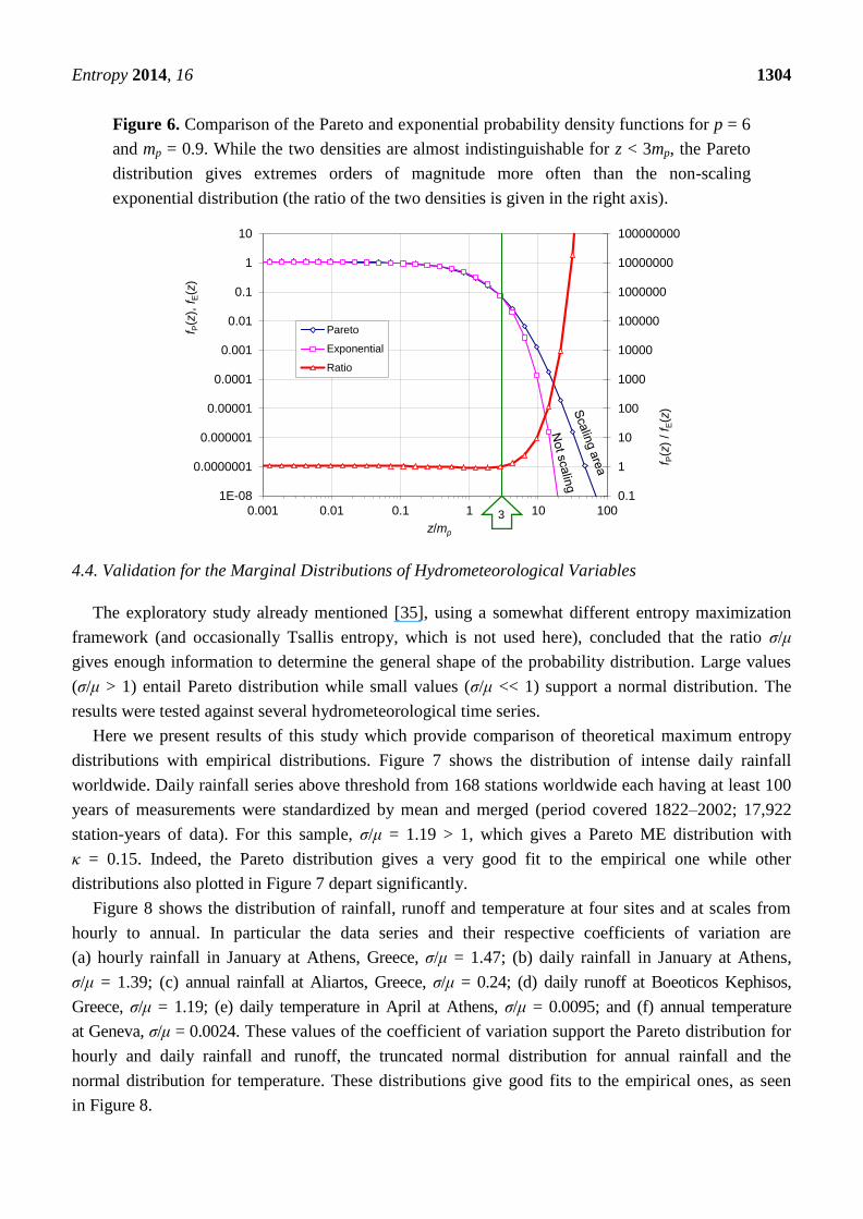
Figure 6 provides a comparison of the two density functions, Pareto, fP(z), with κ = 0.15 and

P = 0.9 and exponential, fE(z), with E = 0.953. The parameters are chosen so that both distributions

have the same mp = 0.9 for p = P/κ = 6. Their raw means are μP = 1.059 > μE = 0.953 and their

entropies are ΦpP = –0.897 > ΦpE = –0.897 – 0.9/6. The enhanced uncertainty resulting from the

proposed framework (Pareto distribution) in comparison to classical statistical mechanics (exponential

distribution) is reflected in the distribution tail, where in the Pareto case it is a scaling law and

produces much more frequent and intense extreme events.

It is recalled (Table 1) that in classical statistical mechanics a constrained mean results in

exponential distribution with σ/μ = 1 while the case σ/μ > 1 is unattainable if the Lebesgue measure is

used as background one. This problem is resolved with the above described framework: In the Pareto

distribution σ/μ = √1 κ > 1. For σ/μ < 1 the above framework does not suffice as neither the

exponential nor the Pareto distribution are compatible with this condition. Obviously, an additional

constraint is needed for the entropy maximization. Koutsoyiannis [35] provided an exploratory

framework using two constraints, mean and variance, while Papalexiou and Koutsoyiannis [37]

provided a detailed modelling framework using generalized constraints.

Entropy 2014, 16 1304

Figure 6. Comparison of the Pareto and exponential probability density functions for p = 6

and mp = 0.9. While the two densities are almost indistinguishable for z < 3mp, the Pareto

distribution gives extremes orders of magnitude more often than the non-scaling

exponential distribution (the ratio of the two densities is given in the right axis).

4.4. Validation for the Marginal Distributions of Hydrometeorological Variables

The exploratory study already mentioned [35], using a somewhat different entropy maximization

framework (and occasionally Tsallis entropy, which is not used here), concluded that the ratio σ/μ

gives enough information to determine the general shape of the probability distribution. Large values

(σ/μ > 1) entail Pareto distribution while small values (σ/μ << 1) support a normal distribution. The

results were tested against several hydrometeorological time series.

Here we present results of this study which provide comparison of theoretical maximum entropy

distributions with empirical distributions. Figure 7 shows the distribution of intense daily rainfall

worldwide. Daily rainfall series above threshold from 168 stations worldwide each having at least 100

years of measurements were standardized by mean and merged (period covered 1822–2002; 17,922

station-years of data). For this sample, σ/μ = 1.19 > 1, which gives a Pareto ME distribution with

κ = 0.15. Indeed, the Pareto distribution gives a very good fit to the empirical one while other

distributions also plotted in Figure 7 depart significantly.

Figure 8 shows the distribution of rainfall, runoff and temperature at four sites and at scales from

hourly to annual. In particular the data series and their respective coefficients of variation are

(a) hourly rainfall in January at Athens, Greece, σ/μ = 1.47; (b) daily rainfall in January at Athens,

σ/μ = 1.39; (c) annual rainfall at Aliartos, Greece, σ/μ = 0.24; (d) daily runoff at Boeoticos Kephisos,

Greece, σ/μ = 1.19; (e) daily temperature in April at Athens, σ/μ = 0.0095; and (f) annual temperature

at Geneva, σ/μ = 0.0024. These values of the coefficient of variation support the Pareto distribution for

hourly and daily rainfall and runoff, the truncated normal distribution for annual rainfall and the

normal distribution for temperature. These distributions give good fits to the empirical ones, as seen

in Figure 8.

0.1

1

10

100

1000

10000

100000

1000000

10000000

100000000

1E-08

0.0000001

0.000001

0.00001

0.0001

0.001

0.01

0.1

1

10

0.001 0.01 0.1 1 10 100

f P(z

) / f E

(z)

f P(z

), f

E(z

)

z/mp

Pareto

Exponential

Ratio

3

Entropy 2014, 16 1305

Figure 7. Plot of daily rainfall depth (x) from a unified standardized (by mean) sample

above threshold, formed from data of 168 stations worldwide, vs. return period (T), in

comparison to Pareto, exponential, normal and truncated normal distributions (adapted

from [35]).

Figure 8. Plots of hydrometeorological data at several stations vs. return period (points) in

comparison with entropy maximizing distributions (lines), which are: Pareto for hourly and

daily rainfall and runoff, truncated normal for annual rainfall and normal for temperature.

The figure merges several ones from Reference [35], which provides the details of each

data series and its statistical characteristics.

4.5. Systems Evolving in Time: Entropy and Clustering

Clustering (e.g., of similar events in time, of stars in space, etc.) is a universal behaviour and it can be

hypothesized that it has some connection with maximum entropy, even though intuitively nonuniformity

0.1

1

10

0.1 1 10 100 1000 10000 100000

T (years)

x

Empirical ParetoExponential Truncated NormalNormal

0.1

1

10

100

1000

10000

0.01 0.1 1 10 100

Return period (years)

Ra

infa

ll, ru

no

ff (

mm

) .

280

284

288

292

296

300

Te

mp

era

ture

(K

)

Hourly rainfall, January, Athens Daily rainfall, January, Athens

Annual rainfall, Aliartos Daily runoff, Boeoticos Kephisos

Daily temperature, April, Athens Annual temperature, Geneva

Entropy 2014, 16 1306

seems to contradict maximum entropy. To investigate this we can explore the entropy of two synthetic

series of “extreme” events, in a period of 1,000 “years”, each having probability of occurrence in each

“year” P =1/10 (Figure 9). The first series (R) is composed of random points in time, without

clustering, while the second (C) was produced so as to have a clustering effect. The entropies of the

two series are equal: ΦC = ΦR = (1/10) ln(10) + (9/10) ln(10/9) = 0.33. However, if we view the series

at a decadal time scale, the entropy of the clustered series is higher: the entropy estimates, considering

the probabilities of all possible numbers of extreme events (from 0 to 10), are ΦC = 1.29 > ΦR = 1.23.

This simple example shows that clustering increases entropy (i.e., uncertainty) at aggregate time scales.

Figure 9. Illustration of the relation of time scale and maximum entropy using two simulated

series of 100 “extreme” events each, in a period of 1,000 “years”, with and without clustering,

plotted at (upper) “yearly” and (lower) “decadal” time scale.

This idea was exploited in modelling rainfall occurrence, which is known to be characterized by

clustering behaviour [38]. It has been shown that the observed behaviour can be explained by

maximizing, for a range of scales, the entropy of the binary-state rainfall process using two constraints

representing the observed occurrence probabilities at two time scales (1 and 2 hours). As shown in

Figure 10, the entropy maximization with only two parameters determined from only two data points

(the minimal information required to evaluate constraints) give impressively good predictions for all

time scales.

0 100 200 300 400 500 600 700 800 900 1000

Year

Random points in time Clustering effect

0

1

2

3

4

5

6

7

8

9

10

0 20 40 60 80 100Decade

Num

ber

of

extr

em

es p

er

decade

Random points in time Clustering effect

8 extreme years in a decade! (normal=1)

15 extreme years in

two consecutive

decades! (normal = 2)

In 25 decades no extreme event at all! (normal = 25)

Entropy 2014, 16 1307

Figure 10. Probability p(k)

that an interval of k hours is dry, as estimated from the Athens

rainfall data set (70 years) and predicted by the model of maximum entropy for the entire

year (full triangles and full line) and the dry season (empty triangles and dashed line); see

details in [38].

4.6. Maximum Entropy Production and Scaling in Time

The dependence structure (expressed in terms of autocorrelogram, periodogram or climacogram, which

are transformations of each other) of continuous-state processes evolving in continuous time can be

determined by entropy extremization. Koutsoyiannis [9] suggested the use of entropy production in

logarithmic time (EPLT) in a continuous time representation of the process of interest. EPLT is defined as:

φ[z(t)] := dΦ[z(t)]/d(ln t) (49)

with z(t) being a cumulative stochastic process (notice the different meaning of the symbol φ here and

in section 3). The specific assumptions are: (a) Lebesgue background measure (assumption good for

σ/μ << 1); (b) constrained mean μ and variance σ2; and (c) constrained lag-one autocorrelation ρ.

Constraints (b) and (c) are formulated for a single observation time scale but the extremization of

entropy production is made at asymptotic time scales, i.e., t → 0 and t → . Constraint (b) results in

Gaussian marginal distribution, hence (see Table 1):

Φ[z(t)] = (1/2) ln[2πe γ(t)] (50)

where γ(t) := Var [z(t)]. Such extremization of entropy production yields two simple solutions:

A (non-scaling) Markov process (the AR(1) process in discrete time, or the Ornstein–Uhlenbeck

process in continuous time).

A (scaling) Hurst-Kolmogorov (HK) process (due to Hurst [39] and Kolmogorov [40]).

In particular, as t → 0, the PLT is maximized by the Markov process, which however minimizes

EPLT as t → . In contrast, as t → , the EPLT is maximized by an HK process. The HK process has

constant EPLT = H, where H is the Hurst coefficient—the half of the exponent of the power law γ(t) =

t2H

γ(1). Actually, this power law can serve as a definition of the HK process. The two EPLT

extremimizing solutions are depicted in Figure 11 in terms of the implied EPLT variation through time.

0.01

0.1

1

1 10 100 1000 10000

k

p (k )

Data points used for model construction

Model

Data points used for model verification

Entropy 2014, 16 1308

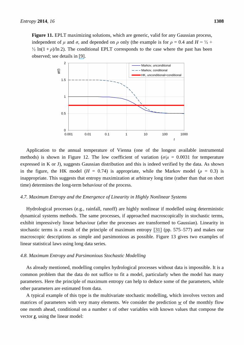
Figure 11. EPLT maximizing solutions, which are generic, valid for any Gaussian process,

independent of μ and σ, and depended on ρ only (the example is for ρ = 0.4 and H = ½

½ ln(1 +

ρ)/ln

2). The conditional EPLT corresponds to the case where the past has been

observed; see details in [9].

Application to the annual temperature of Vienna (one of the longest available instrumental

methods) is shown in Figure 12. The low coefficient of variation (σ/μ = 0.0031 for temperature

expressed in K or J), suggests Gaussian distribution and this is indeed verified by the data. As shown

in the figure, the HK model (H = 0.74) is appropriate, while the Markov model (ρ = 0.3) is

inappropriate. This suggests that entropy maximization at arbitrary long time (rather than that on short

time) determines the long-term behaviour of the process.

4.7. Maximum Entropy and the Emergence of Linearity in Highly Nonlinear Systems

Hydrological processes (e.g., rainfall, runoff) are highly nonlinear if modelled using deterministic

dynamical systems methods. The same processes, if approached macroscopically in stochastic terms,

exhibit impressively linear behaviour (after the processes are transformed to Gaussian). Linearity in

stochastic terms is a result of the principle of maximum entropy [31] (pp. 575–577) and makes our

macroscopic descriptions as simple and parsimonious as possible. Figure 13 gives two examples of

linear statistical laws using long data series.

4.8. Maximum Entropy and Parsimonious Stochastic Modelling

As already mentioned, modelling complex hydrological processes without data is impossible. It is a

common problem that the data do not suffice to fit a model, particularly when the model has many

parameters. Here the principle of maximum entropy can help to deduce some of the parameters, while

other parameters are estimated from data.

A typical example of this type is the multivariate stochastic modelling, which involves vectors and

matrices of parameters with very many elements. We consider the prediction w of the monthly flow

one month ahead, conditional on a number s of other variables with known values that compose the

vector z, using the linear model:

0

0.5

1

1.5

2

0.001 0.01 0.1 1 10 100 1000

φ(t

)

t

Markov, unconditional

Markov, conditional

HK, unconditional+conditional

Entropy 2014, 16 1309

w = aT z + v (51)

where a is a vector of parameters (T denotes transpose) and v is the prediction error, assumed to be

independent of z; for simplicity, all elements of z are assumed normalized and with zero mean and

unit variance.

Figure 12. (upper) Mean annual temperature of Vienna, Austria: 235 years of annual

temperature (1775–2009; the part for 1851–1991, labelled as “adjusted” in figure, is the

one included in the Global Historical Climatology Network—GHCN). (lower) Entropy of

the cumulative temperature process Φ[xΔ] where Δ is of aggregation scale, which is in

one-to-one correspondence (Equation (50)) with the logarithm of variance γ(Δ), thus

allowing empirical estimate through that of variance, g(Δ), and comparison with the

theoretical entropy extremizing models; see details in [9].

6

7

8

9

10

11

12

1770 1790 1810 1830 1850 1870 1890 1910 1930 1950 1970 1990 2010

Θ (ºC)

Original Adjusted 30-year average

Slope = 0.5

Slope = 0.7

4

0

1

2

3

4

5

6

1

1.5

2

2.5

3

3.5

4

4.5

0 0.5 1 1.5 2 2.5 3 3.5 4

ln Δ

Φ [xΔ ]ln γ (Δ ),

ln g (Δ ),

ln E [g (Δ )]

Empirical

White noise

Markov

HK, theoretical

HK, adapted

_

Entropy 2014, 16 1310

Figure 13. Two examples of linear statistical laws between lagged hydrological

observations: (left) rainfall at Iowa measured at temporal resolution of 10 s for lag of 10

times steps (from [41]); (right) monthly Nile flows of consecutive months (data from [42]).

For the model to take account of both short-range and long-range dependence (HK behaviour), a

possible composition of z may include [42]: (a) the flows of a few previous months of the same year,

and (b) all available flow measurements of the same month on previous years. The model parameters

are estimated from:

aT = η

T H

−1, Var[v] = 1 – η

T H

−1 η = 1 – a

T η (52)

where η := Cov[w, z] and H := Cov[z, z] (see [43]).

Altogether, the vector η and the matrix H may contain numerous items, typically of the order of

103–10

4 (e.g., for a dimensionality 100, if we have 100 years of observations: 100 100 × 100 =

10,100 items—albeit reduced due to symmetry of matrix). Traditionally, the items of such covariance

matrices and vectors have been estimated directly from data; this is totally illogical (100 years of data

cannot support the statistical estimation of 1,000–10,000 parameters). An alternative approach is to use

data to estimate a couple of parameters per month and derive all other “unestimated” parameters by

maximizing entropy. Such entropy maximization is in fact very simple; it only needs a generalized

Cholesky decomposition of the matrix H (assuming that H = B BT, where B is a lower triangular

matrix to be calculated by maximizing entropy). Using this approach, Koutsoyiannis et al. [42] were

able to reduce a number of 1,872 model parameters to be estimated to only 26.

5. Conclusions

Entropy is none other than uncertainty quantified and its tendency to become maximal is not a

curse; rather it is blessing. This tendency constitutes the driving force of change and evolution; also, it

offers the basis to understand and describe Nature. By maximizing entropy, i.e., uncertainty, we can

describe the behaviour of physical systems; such description is essentially probabilistic.

However, if a system is composed of numerous identical elements, the uncertainty, despite being

maximal at the microscopic level, in the macroscopic description it becomes as low as to yield a

-4

-3

-2

-1

0

1

2

3

4

-4 -3 -2 -1 0 1 2 3 4

Stan

dar

diz

ed f

low

at

mo

nth

t

Standardized flow at month t - 1

Original

Normalized

Equality line

Entropy 2014, 16 1311

physical law that is in effect deterministic. This is the case in the equilibrium of liquid water and water

vapour (Clausius-Clapeyron equation).

Extremal entropy considerations provide a theoretical basis in modelling hydrological processes.

However, at high macroscopization levels there is no hope to derive deterministic laws. Only stochastic

modelling is feasible. Linking statistical thermophysics to hydrology with a unifying view of entropy as

uncertainty is a promising scientific direction. Uncertainty and entropy are not enemies of science that

should be eliminated. Rather they are important objects to be studied and understood.

Appendix

Appendix 1: Proof of Equations (17–21)

According to Equation (11) and taking into account the equality constraints (3), (14) and (15), the

ME distribution will have density:

f(z) = exp (– 0 – 1u1 – 2u2 – 3u3 – 4(u1 u

u )) (A1)

This proves that the density will be an exponential function of a second order polynomial of (u1, u2, u3)

involving no products of different ui. The f(z) in Equation (17) is of this type, and thus it suffices to

show that it satisfies the constraints. Note that the inequality constraint (13) is not considered at this

phase but only in the integration to evaluate the constraints. That is, the integration domain will be

Ω: = {0 ≤ x1 ≤ a, 0 ≤ x2 ≤ a, 0 ≤ x3 ≤ a, – < u1 < , – < u2 < , – < u3 < }. We denote by ∫Ω dz the

integral over this domain. It is easy then to show (the calculation of integrals is trivial) that:

∫Ω f(z) dz

=

1; ∫Ω u1f(z)

dz = 0; ∫Ω u2f(z) dz = 0; ∫Ω u3f(z)

dz = 0; ∫Ω ((u1

u u

))f(z) dz = 2ε/m0 (A2)

Thus, all constraints are satisfied. To find the marginal distribution of each of the variables we

integrate over the entire domain of the remaining variables; due to independence this is very easy and

the results are given in Equations (18) and (19). To find the marginal distribution of ||u|| (Equation (20)),

we recall that the sum of squares of n independent N(0, 1) random variables has a χ2(n) distribution [44]

(pp. 219, 221); then we use known results for the density of a transformation of a random variable [44]

(p. 118) to obtain the distribution of the square root, thus obtaining Equation (20).

To calculate the entropy, we observe that –ln(f(z)) = (3/2) ln(4πε/3m0)

+

ln

a

3 +

3m0((u1

u u

)) /

4ε and ln h(z) = 3 ln (mp/h). Thus, the entropy is derived as follows:

Φ[z] = ∫Ω (–ln f(z) + ln h(z)) f(z) dz = ( / ) ln ((4πε /3m0 (mp/h)2)) + ln

a

3 + (3m0 / 4ε) (2ε/m0) =

( / ) ln(4πmp2

/3 h2m0) + (3/2) ln ε + ln V + 3/2

(A3)

This can be written as in Equation (21).

Appendix 2: Proof of (39)

Based on the assumption of Equation (32), if V is the total volume, then that of the gaseous phase is:

VA = V – VB = V – πBvBN (A4)

Using Equation (A4), (34) becomes:

φA = cA + (βA/2) ln εA + ln (V – πBvBN), φB = cB + (βB/2) ln εB + ln (πBvBN) (A5)

Entropy 2014, 16 1312

We wish to find the conditions which maximize the entropy φ in Equation (35) under constraints

(37) and (38) with unknowns εA, εB, πA, πB. We form the function ψ incorporating the total entropy φ

as well as the two constraints with Langrage multipliers κ and :

ψ = πΑ (φA – ln πΑ) + πΒ (φΒ – ln πΒ) + κ (πΑ εA + πΒ (εΒ – ξ) – ε) + (πA + πB – 1) (A6)

To maximize ψ, equating to 0 the derivatives with respect to εA and εB, we obtain:

∂ψ

∂εA =

πA βA

2εA + κ πΑ = 0,

∂ψ

∂εB =

πB βB

2εB + κ πΒ = 0 (A7)

By virtue of Equation (27), this obviously results in equal temperature θ in the two phases, i.e.,

κ = –βA

2εA = –

βΒ2εΒ

= –1

θA = –

1

θΒ = –

1

θ (A8)

Equating to 0 the derivatives with respect to πA and πB, we obtain:

∂ψ

∂πA = φA – ln πΑ – 1 + κ εA + = 0,

∂ψ

∂πΒ =

–πAvBN

V – πBvBN + φΒ – ln πΒ – 1 + 1 + κ (εΒ – ξ) + = 0

(A9)

It can be seen that the first term of ∂ψ/∂πΒ equals –vB/vA and is negligible since vB << vA. After

eliminating , substituting κ from Equation (A8), and making algebraic manipulations, we get:

(φA – ln πΑ) – (φΒ – ln πΒ) = ξ/θ – (βB/2 – βA/2 – 1) (A10)

On the other hand, from Equation (34), the entropy difference is:

(φA – ln πΑ) – (φΒ – ln πΒ) = cA + (βA/2) ln εA + ln vA – cB – (βB/2) ln εB – ln vB (A11)

Substituting θ for εA and εB from Equation (A8) and using the ideal gas to express vA in terms of θ

and p we obtain:

(φA – ln πΑ) – (φΒ – ln πΒ) = –(βB/2 – βA/2 – 1) ln θ – ln p + constant (A12)

Combining Equations (A10) and (A12), and eliminating (φA – ln πΑ) – (φΒ – ln πΒ), we find

Equation (39).

Acknowledgments

I thank Pierre Hubert and Levent Kavvas for their invitations to talk about entropy in Melbourne

(IUGG, 2011) and Davis (2013), respectively. Ideas from these talks were reworked to produce this

paper, where reworking was partly funded by the Greek General Secretariat for Research and

Technology through the research project “Combined REnewable Systems for Sustainable ENergy

DevelOpment” (CR SS NDO). Finally, I am grateful to the Entropy Guest Editor Nathaniel A. Brunsell

and Managing Editor Jely He for their invitation to make this paper, as well as to two reviewers for

their encouraging comments.

Conflicts of Interest

The author declares no conflict of interest.

Entropy 2014, 16 1313

References

1. Paulos, J.A. A Mathematician Plays the Stock Market; Basic Books: New York, NY, USA, 2003.

2. Clausius, R. A contribution to the history of the mechanical theory of heat. Phil. Mag. 1872, 43,

106–115.

3. Clausius, R. The Mechanical Theory of Heat: With Its Applications to the Steam-Engine and To

the Physical Properties of Bodies; J. van Voorst: London, UK, 1867. Available online:

http://books.google.gr/books?id=8LIEAAAAYAAJ (accessed on 10 January 2014).

4. Clausius, R. Ueber verschiedene für die Anwendung bequeme Formen der Hauptgleichungen der

mechanischen Wärmetheorie. Annalen der Physik und Chemie 1865, 125, 353–400. (In German)

5. Boltzmann, L. Über die Beziehung zwischen dem zweiten Hauptsatze der mechanischen

Wärmetheorie und der Wahrscheinlichkeitsrechnung respektive den Sätzen über das

Wärmegleichgewicht. Wien. Ber. 1877, 76, 373–435. (In German)

6. Swendsen, R.H. Statistical mechanics of colloids and Boltzmann’s definition of the entropy. Am.

J. Phys. 2006, 74, 187–190.

7. Shannon, C.E. The mathematical theory of communication. Bell Syst. Tech. J. 1948, 27, 379–423.

8. Robertson, H.S. Statistical Thermophysics; Prentice Hall: Englewood Cliffs, NJ, USA, 1993.

9. Koutsoyiannis, D. Hurst-Kolmogorov dynamics as a result of extremal entropy production.

Physica A 2011, 390, 1424–1432.

10. Jaynes, E.T. Information theory and statistical mechanics. Phys. Rev. 1957, 106, 620–630.

11. Swendsen, R.H. How physicists disagree on the meaning of entropy. Am. J. Phys. 2011, 79, 342–348.

12. Jaynes, E.T. Probability Theory: The Logic of Science; Cambridge Univ. Press: Cambridge,

UK, 2003.

13. Atkins, P. Four Laws that Drive the Universe; Oxford Univ. Press: Oxford, UK, 2007.

14. Kalinin, M.; Kononogov, S. Boltzmann’s constant, the energy meaning of temperature, and

thermodynamic irreversibility. Meas. Tech. 2005, 48, 632–636.

15. Ben-Naim, A. A Farewell to Entropy: Statistical Thermodynamics Based on Information; World

Scientific Pub.: Singapore, 2008.

16. Koutsoyiannis, D. Physics of uncertainty, the Gibbs paradox and indistinguishable particles.

Studies in History and Philosophy of Modern Physics 2013, 44, 480–489.

17. Brunsell, N.A.; Schymanski, S.J.; Kleidon, A. Quantifying the thermodynamic entropy budget of

the land surface: is this useful? Earth Syst. Dynam. 2011, 2, 87–103.

18. Ruddell, B.L.; Brunsell, N.A.; Stoy, P. Applying information theory in the geosciences to quantify

process uncertainty, feedback, scale. Eos 2013, 94, 56–56.

19. Leopold, L.B.; Langbein, W.B. The Concept of Entropy in Landscape Evolution; US Government

Printing Office: Washington, DC, USA, 1962.

20. Sonuga, J.O. Principle of maximum entropy in hydrologic frequency analysis. J. Hydrol. 1972,

17, 177–191.

21. Jackson, D.R.; Aron, G. Parameter estimation in hydrology: The state of the art. J. Am. Water

Resour. Assoc. 1971, 7, 457–472.

22. Harmancioglu, N. Measuring the Information Content of Hydrological Processes by the Entropy

Concept (In Turkish). Ph.D. Thesis, Ege University, İzmir, Turkey, 1980.

Entropy 2014, 16 1314

23. Bendjoudi H. Application du concept d’entropie dans les sciences de l’eau (In French). Ph.D.

Thesis, École Nationale Supérieure des Mines de Paris, Paris, France, 1983. Available online:

http://hydrologie.org/THE/BENDJOUDI.pdf (accessed on 7 February 2014).

24. Singh, V.P. The use of entropy in hydrology and water resources. Hydrol. Process. 1997, 11, 587–626.

25. Singh, V. Hydrologic synthesis using entropy theory: Review. J. Hydrol. Eng. 2011, 16, 421–433.

26. Hemelrijk, J. Underlining random variables. Stat. Neerl. 1966, 20, 1–7.

27. Perry, J. The Thermodynamics of Heat Engines. Nature 1903, 67, 602–605.

28. Swinburne, J. Entropy. Nature 1904, 70, 54–55.

29. Ewing, J. LXII. The specific heat of saturated vapour and the entropy-temperature diagrams of

certain fluids. Lond. Edinb. Dubl. Phil. Mag. J. Sci. 1920, 39, 633–646.

30. Uffink, J. Can the maximum entropy principle be explained as a consistency requirement? Studies

in History and Philosophy of Modern Physics 1995, 26, 223–261.

31. Papoulis, A. Probability, Random Variables and Stochastic Processes, 3rd ed.; McGraw-Hill:

New York, NY, USA, 1991.

32. Fraundorf, P. Heat capacity in bits. Am. J. Phys. 2003, 71, 1142–1151.

33. Wagner, W.; Pruss, A. The IAPWS formulation 1995 for the thermodynamic properties of ordinary

water substance for general and scientific use. J. Phys. Chem. Ref. Data 2002, 31, 387–535.

34. Koutsoyiannis, D. Clausius-Clapeyron equation and saturation vapour pressure: simple theory

reconciled with practice. Eur. J. Phys. 2012, 33, 295–305.

35. Koutsoyiannis, D., Uncertainty, entropy, scaling and hydrological stochastics, 1, Marginal

distributional properties of hydrological processes and state scaling. Hydrol. Sci. J. 2005, 50, 381–404.

36. Montanari, A.; Koutsoyiannis, D. A blueprint for process-based modeling of uncertain

hydrological systems. Water Resour. Res. 2012, doi: 10.1029/2011WR011412.

37. Papalexiou, S.M.; Koutsoyiannis, D. Entropy based derivation of probability distributions: A case

study to daily rainfall. Adv. Water Resour. 2012, 45, 51–57.

38. Koutsoyiannis, D. An entropic-stochastic representation of rainfall intermittency: The origin of

clustering and persistence. Water Resour. Res. 2006, doi: 10.1029/2005WR004175.

39. Hurst, H.E. Long term storage capacities of reservoirs. Trans. Am. Soc. Civil Engrs. 1951, 116,

776–808.

40. Kolmogorov, A.N. Wienersche Spiralen und einige andere interessante Kurven in Hilbertschen

Raum. Dokl. Akad. Nauk URSS 1940, 26, 115–118 (In German).

41. Papalexiou, S.M.; Koutsoyiannis, D.; Montanari, A. Can a simple stochastic model generate rich

patterns of rainfall events? J. Hydrol. 2011, 411, 279–289.

42. Koutsoyiannis, D.; Yao, H.; Georgakakos, A. Medium-range flow prediction for the Nile: A

comparison of stochastic and deterministic methods. Hydrol. Sci. J. 2008, 53, 142–164.

43. Koutsoyiannis, D. A generalized mathematical framework for stochastic simulation and forecast

of hydrologic time series. Water Resour. Res. 2000, 36, 1519–1533.

44. Papoulis, A. Probability and Statistics; Prentice-Hall: Englewood Cliffs, NJ, USA, 1990.

© 014 by the authors; licensee MDPI, Basel, Switzerland. This article is an open access article

distributed under the terms and conditions of the Creative Commons Attribution license

(http://creativecommons.org/licenses/by/3.0/).