Snow Hydrology:

Snow Hydrology: Snow Hydrology: Guest LectureGuest Lecture

Kristi R. ArsenaultKristi R. Arsenault

1

CourseCourse: The Hydrosphere (EOS 656): The Hydrosphere (EOS 656)March 16, 2010March 16, 2010

Introduction

SnowSnow – is an important variable and component of the hydrosphere.

All forms of snow and ice on the Earth’s surface, including both land and ocean surfaces, are part of the Earth’s cryospherecryosphere.

These cryospheric components can influence global, regional, and local climate and environmental conditions at different timescales.

In this lecture, we’ll explore some of these components, and how they are observed and modeled.

2

Importance of SnowImportance of Snow

Water Water Resource SupplyResource Supply

Mountain-area snowpack can provide up to 90% of the water supply to growing populations in semi-arid regions (e.g., Western United States)

Agricultural, hydropower, and other human uses

Ecological and environmental needs (e.g., species survival)

Flood PredictionFlood Prediction

Knowledge of antecedent winter snowpack can lead to improved forecasts of flooding and associated effects

Input in to Climate and Numerical Weather Input in to Climate and Numerical Weather Prediction ModelsPrediction Models

Snow’s albedo and thermal insulation on the ground can impact radiation, energy and moisture budgets which play significant role in improving these models predictive capabilities.

3

BASIC SNOW HYDROLOGY BASIC SNOW HYDROLOGY PRINCIPLES AND PHYSICSPRINCIPLES AND PHYSICS

4

Snow Hydrology Lecture

Snow Snow CharacteristicsCharacteristics

5

Snow – Basic Physics and Descriptions

Snow – Properties

Snow – Distribution

Snow – Something

Water Balance for a Single Land Surface Slab, Without Snow(e.g., standard bucket model)

P = E + R + Cw w/ t + miscellaneous

whereP = Precipitation

E = Evaporation

R = Runoff (effectively consisting of surface runoff and baseflow)

Cw = Water holding capacity of surface slab

Dw = Change in the degree of saturation of the surface slab

Dt = time step length

P E

w

Terms on LHS come fromthe climate model.Strongly dependenton cloudiness, watervapor, etc.

Terms on RHS come aredetermined by the land surfacemodel.

R

(From R. Koster; NASA)

6

Water Balance for a Snowpack Slab

Psnow = Esnow + M + wsnow/ t

where

Psnow = Snowfall, freezing rain, etc. (typically when temps: < 273 K)

Esnow = Sublimation from snow surface

M = Snowmelt

Wsnow = change in snow amount (“infinite” capacity possible)

t = time step length

Liquid water amount in snow is also called snow water equivalent (SWE).

P (snowfall) Esnow (sublimation)

wsnow


7

M


(soil layer)T1

Sw Sw Lw Lw H sE

Tsnow m MInternal

energyGS1

where,

lm = latent heat of melting

ls = latent heat of sublimation

M = snowmelt rate

GS1 = heat flux between bottom of pack and soil layer

8

Energy Balance for a Snowpack Slab

Snow Snow CharacteristicsCharacteristics

9

Snow – Basic Physics and Descriptions

Snow – Properties

Snow – Distribution

Snow – Something

Reflected Shortwave Radiation: Albedo

Assume: Sw = Sw direct, band b + Sw diffuse, band b

b=1

# bands # bands

b=1

Compute: Sw = Sw direct, band b a direct, band b

+ Sw diffuse, band b a diffuse, band b

# bands

b=1

# bands

reflectance for

spectral band

Simplest description:

Consider only one band (the whole

spectrum) and do not differentiate

between diffuse and direct components:

Sw = Sw aalbedo

Typical albedoes (from Houghton):

sand .18-.28

grassland .16-.20

green crops .15-.25

forests .14-.20

dense forest .05-.10

fresh snow .75fresh snow .75--.95.95

old snow .40old snow .40--.60.60

urban .14-.18

b=1

(From R. Koster; NASA)10

Critical property of snow: Low thermal conductivity

Strong insulation …

soil

snow

soil

snow

Temperature

profile

250oK

260oK

270oK

272oK

To capture such properties,

the snow can be modeled

as a series of layers, each

with its own temperature.


11

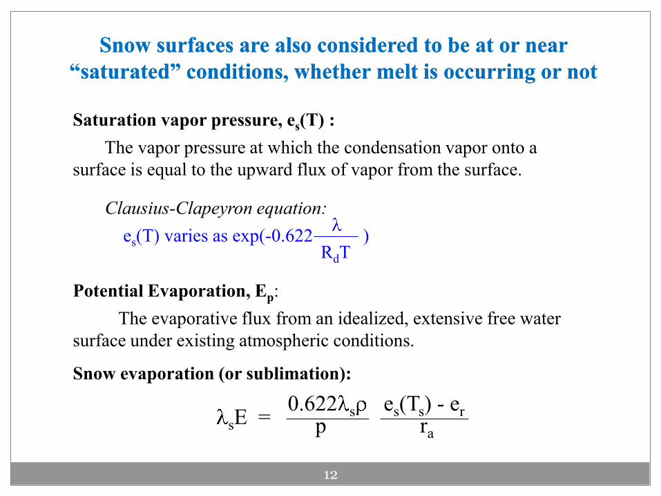
Snow surfaces are also considered to be at or near Snow surfaces are also considered to be at or near

“saturated” conditions, whether melt is occurring or not “saturated” conditions, whether melt is occurring or not

12

Saturation vapor pressure, es(T) :

The vapor pressure at which the condensation vapor onto a

surface is equal to the upward flux of vapor from the surface.

Clausius-Clapeyron equation:

es(T) varies as exp(-0.622 )

Potential Evaporation, Ep:

The evaporative flux from an idealized, extensive free water

surface under existing atmospheric conditions.

RdT

Snow evaporation (or sublimation):

sE =0.622 s es(Ts) - er

p ra

Evaporation from a fully wetted surface (=Ep)

Here’s the famous Penman equation:

EPenman =(Rnet - G) + ( cp/ra) (es(Tr) - er)

d(es)/dT cpp/(0.622 ) G = heat flux into Rnet = net

ground radiation

“equilibrium evaporation for

a saturated air mass passing

over a wet surface”

contribution due to

subsaturated air

Contains terms that are

relatively easy to measure


13

Snow Cover Distribution

Three Major Spatial Scales

Macroscale

Areas up to 106 km2

Characteristic Distances of 10-1000 km Dynamic meteorological effects are important

Mesoscale

Characteristic Distances of 100 m to 10 km Redistribution of snow along relief features due to wind Deposition and accumulation of snow may be related to terrain variables

and to vegetation cover

Microscale

Characteristic Distances of 10 to 100 m Differences in accumulation result from variations in air flow patterns

and transport

14

* (from J* (from J. S. . S. Price, U. of Waterloo)Price, U. of Waterloo)


Effect of Topography:

The depth of seasonal snow cover usually increases with elevation, depending mostly on slope, aspect and elevation height

Though the rate of increase with elevation may vary widely from year-to-year

Other factors include:

Vegetation effects,

Wind characteristics,

Temperature, and

Characteristics of the parent weather systems

E.g., Rainfall can contribute more significantly to snow melt processes than temperature can

15




Open areas exposed to more accumulated snowfall Influences of meso- and micro-scale differences in

vegetation and terrain features may produce wide variations in snow distribution.

Snow Cover:Snow Cover:Northern/eastern Northern/eastern

slopes of slopes of

mountain areasmountain areas

Exposed Exposed Ground:Ground:South slopesSouth slopes

Another effect … Another effect …

Differences in solar Differences in solar

radiation, especially radiation, especially

in mountainous in mountainous

areas …areas …

Another effect … Another effect …

Differences in solar Differences in solar

radiation, especially radiation, especially

in mountainous in mountainous

areas …areas …

17

Vegetation Effects:

Vegetation canopies affect snowfall by:

1) Turbulent air flow involving the canopy

2) Direct interception of snowfall by the

canopy which can lead to sublimation or throughfall to the ground

Vegetation type, density, and the proximity of nearby open areas all play roles in distribution as well


18



19


Forested Environments

o Greatest snow accumulation differences occur between different coniferous and deciduous stands than within species of conifers

Coniferous stands are all relatively efficient snow interceptors

Snow is more susceptible to sublimation losses in the canopy than on the forest floor

o Typically greater snow accumulation in clearings than in the forest

o Interception and subsequent sublimation are the major factors contributing to the difference

Up to 40% of tree-based snow can be lost to sublimation

20-45%Greater SnowAccumulation

Wind Effects on Snow

Snow transported by wind processes undergo:

Redistribution of Snow Water Equivalent

Loss of Water by Sublimation

1. Shear velocity

2. Threshold windspeed

3. Transport mechanism

1. Atmospheric condition: e.g.temperature, humidity, windspeed

2. Transport distance

20


Wind Effects on Snow Characteristics

Mechanical fragmentation and sublimation losses result in small, rounded particles

Windblown snow deposits are inherently more dense

2 mm

Snow crystalcollected during

snowfall undercalm winds

Windblown snowparticle collected during transport

21

Wind Effects on Snow


22 * (from J* (from J. S. . S. Price, U. of Waterloo)Price, U. of Waterloo)

Blowing Snow

Shear Velocity - Wind

The friction velocity u* is usually calculated from wind profiles, but can be estimated from a single 10-m wind speed (u10):

u* =u10 1.18/41.7

u* =u10/26.5

u* =u10 1.30/44.2

Antarctic Ice Sheet

Snow-covered Lake

Snow-coveredFallow Field

uu1010 = 5 m/s= 5 m/s

u* = 0.19

u* = 0.16

u* = 0.18

23 * (from J* (from J. S. . S. Price, U. of Waterloo)Price, U. of Waterloo)

Blowing Snow

Creep

TYPE MOTION HEIGHT WINDSPEED

Saltation

TurbulentDiffusion

Roll

Bounce

Suspended

< 1 cm

1 cm - 10 cm

1 m - 100 m

<< 5 m/s

5 - 10 m/s

> 10 m/s

Three Types of Transport

Threshold Shear Velocity - Snow

u*t is the friction velocity at which snow transport begins(depends on snow characteristics)

0

0.2

0.4

0.6

0.8

1

1.2

1 2 3 4 5 6 7 8 9 10 11 12 13 14 15 16 17 18 19 20 21

10-m Wind Speed

u*

Antarctic Lake Field

Older, wind-hardened,dense or wet-snow:u*t = 0.25 - 1.0 m/s

Fresh, loose, dry snow,and during snowfall:u*t = 0.07 - 0.25 m/s

Blowing Snow

Sublimation Losses

30

25

2522

16

225020

Mean Annual Blowing Snow Sublimation

CANADA, 1970-1976Loss in mm SWE over 1 km

24


25

Frozen Soil Effects

Thermal effects: Enhances the soil heat capacity through diurnal and seasonal freezing-thawing cycles.

Hydrological effects: Affects snowmelt runoff and soil hydrology by reducing soil permeability. In turn, for example, runoff from Arctic river systems affects ocean salinity and the thermohaline circulation.

Ecological effects: Affects ecosystem diversity and productivity and carbon decomposition and release.

* (Z.* (Z.--L. Yang, L. Yang, U.TexasU.Texas –– Austin)Austin)

26 * (Z.* (Z.--L. Yang, L. Yang, U.TexasU.Texas –– Austin)Austin)

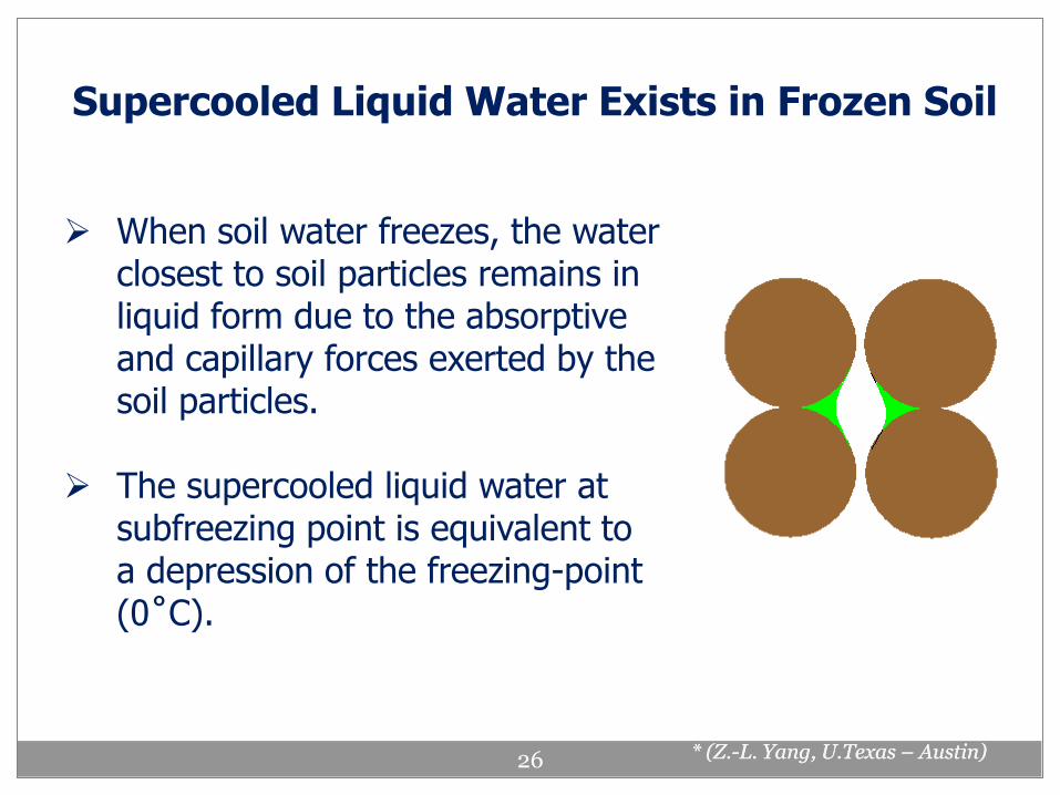
When soil water freezes, the water closest to soil particles remains in liquid form due to the absorptive and capillary forces exerted by the soil particles.

The supercooled liquid water at subfreezing point is equivalent to a depression of the freezing-point (0˚C).

Supercooled Liquid Water Exists in Frozen Soil

27 * (Z.* (Z.--L. Yang, L. Yang, U.TexasU.Texas –– Austin)Austin)

Frozen Soil Is Permeable?

Early Russian literature and recent works showed that frozen soil has very weak or no effects on runoff. For example …

Russian laboratory and field experiments in 1960s and 1970s (Koren, 1980).

Shanley and Chalmers (1999), Lindstrom et al. (2002

Stahli et al. (2004): Dye tracer techniques revealed that water can infiltrate into deep soil through preferential pathways which are air-filled pores at the time of freezing.

28

The Importance of Snow-Atmosphere Interactions

Snow surfaces have the ability not only to alter the land surface and landscape properties, like albedo and roughness, but can also impact the atmosphere from local to global scales.

On a regional to global scale, a large body of research emphasizes the importance of snow to the climate system:

e.g., Robock (1983); Cohen and Rind (1991); Walland and Simmonds (1997); Cohen and Entekhabi (1999); Watanabe and Nitta (1998); Watanabe and Nitta (1999); Gong et al. (2003); Hahn and Shukla (1976); Dickson (1984); Dey and Kumar (1982); Vernekar et al. (1995); Bamzai and Shukla (1996); Douville and Royer (1996); Harzallah and Sadourny(1997); Kripalani and Kulkarni (1999); Ferranti and Molteni (1999); Wu and Qian(2003); Fasullo (2004); Dash et al. (2005); Barnett et al. (1989); Qian and Saunders (2003); Saito et al.(2001); and Shinoda (2001); Yang et al. (2001); Toshi et al. (2003), Hawkins et al. (2002); and Jin and Miller (2007), and many others.

DIFFERENT METHODS OF DIFFERENT METHODS OF OBSERVING SNOWOBSERVING SNOW

29


Snow Observations Overview30

Observing snow, ice and frozen ground characteristics is Observing snow, ice and frozen ground characteristics is

critical to better understanding the hydrological cycle and critical to better understanding the hydrological cycle and

managing water resources.managing water resources.

However, making accurate snow measurements can be However, making accurate snow measurements can be

quite challenging when dealing with different scales, quite challenging when dealing with different scales,

environments and instrument limitations.environments and instrument limitations.

This next section provides an overview of some of the This next section provides an overview of some of the

different snow observation and instrument types different snow observation and instrument types

These includeThese include: Station (or in: Station (or in--situ) ground and remotely situ) ground and remotely

sensed observationssensed observations

Also some of the issues faced with each will be addressed Also some of the issues faced with each will be addressed

31

Some of the Problems with Snow Measurements

Most inMost in--situ snow observation networks tend to be situ snow observation networks tend to be

sparse sparse in mountain in mountain regionsregions

This can make This can make it difficult to obtain it difficult to obtain accurate accurate

representation representation of of highly spatial highly spatial snow variabilitysnow variability

AlsoAlso, remotely sensed products encounter many , remotely sensed products encounter many

issues, like they can either have too coarse of a issues, like they can either have too coarse of a

resolution to map the snow well or clouds obscure the resolution to map the snow well or clouds obscure the detection of snowdetection of snow

Snow Snow ObservationsObservations

32

In-situ Measurements – Station Networks

In-situ Measurements – Field Measurements

Remote Sensing Retrievals

33

Gage Measurement Networks

o Global coverage with various operational, national/regional networks.

o Manual and automatic gauges, measuring water equivalent (amount), not snow particle size.

o Manual gauges can measure snowfall (rate) at 6-hour to daily time intervals, and auto gauges can provide hourly (or sub-hourly) snowfall (rate).

o Snow rulers are also used for snowfall observations at the national/regional networks, providing snow depth info, not SWE.

o Snow pillow/snowboard/snow depth sensor record snow accumulation changes over time - (in)direct info of snowfall.

o Gauge networks/data are long-term and fundamental, defining global snowfall/climate regimes and changes.

34

Precipitation Component: Snow Accumulation

o Input to winter snowpack and spring snowmelt runoff in mountain and polar regions – critical element of basin water cycle and regional water resources

o Influence on large-scale land surface radiation and energy budget particularly during accumulation

o Effect on glacier/ice sheet accumulation/mass balance, lake/river and sea ice, seasonal frozen-ground and permafrost

o Impact to human society and activity, such as air/ground transportation, disaster prevention, agriculture, water resources management, and recreation…

Some national standard gauges (here tested in Barrow, AK)

Canadian Nipher

Hellmann

Russian Tretyakov

US 8”

36

USDA/ NRCS USDA/ NRCS SNOwSNOw TELemetryTELemetry(SNOTEL) Gage Network in (SNOTEL) Gage Network in Mountainous Western U.S.Mountainous Western U.S.

Snow PillowSnow Pillow

SNOTEL sites record and transmit SWE, precipitation, temperature, and soil moisture/temperature for hundreds of sites in 13 western states.

SNOTEL sites typically are found in higher elevation – watershed locations, but the data are used for many different hydrological and water resources applications.

Rain Rain GageGage

From http://www.wcc.nrcs.usda.gov/snotel/SNOTEL-brochure.pdf

37

Rio Grande Headwaters Basin Topography & SNOTEL Sites

Yellow Stars:SNOTEL sites

39

SNOTEL vs. North American Regional Reanalysis (NARR)Accumulated Precipitation Comparison

Cosgrove et al.Cosgrove et al.

Precip-NARRPrecip-SNOTEL

40

o Wind-induced gauge under-catch

o Wetting and evaporation losses

o Underestimate of trace precipitation events

o Blowing snow into gauges at high winds

o Uncertainties in auto gauge systems

Some Biases in Gauge Measurements

Precipitation phase and wind speed are the most important

meteorological parameters for the systematic error

Systematic gauge measuring error

WMO Solid Precipitation Measurement Comparison

Study

The GPCC has

developed a method to

estimate wind speed,

precipitation phase,

air temperature and

humidity from synoptic

data, which are needed

to calculate the bias

corrections on a daily

“on event“ basis.

(Figure: T. Günther in

Goodison et al, 1998)

Note that there are also spatial sampling errors and process errors (virga)


42




43

Snow Course Surveys

*http://www.wcc.nrcs.usda.gov/snowcourse

A snow course is a permanent site where manual measurements of snow depth and snow water equivalent are taken by trained observers.*

o Measurements usually taken near beginning of month during the winter and spring.

o Courses typically ~1,000 feet long and situated in small, wind-protected meadow.

o Snow samples collected with a "snow sampling set" – a series of aluminum tubes, which are weighed along with the snow cores to obtain SWE and snow depth.

44 (From I. Rangwala – Rutgers U.)

From: From: http://www.comet.ucar.edu/class/hydromet/09_Oct13_1999/docs/cline/comet_snowhydro/index.htmhttp://www.comet.ucar.edu/class/hydromet/09_Oct13_1999/docs/cline/comet_snowhydro/index.htm

Photos taken by Photos taken by Jennifer Jennifer HolvoetHolvoet

Layers and Measuring Layers and Measuring TapeTape

A measuring tape is fastened to the wall of the pit after the layers are exposed with the trowel.

Taking A SampleTaking A Sample

Researcher carefully takes a sample of a layer while the other in the background reaches for a plastic bag

http://www.travelblog.org/Antarctica/blog-35022.html

Snow pit measurementsSnow pit measurementstaken in taken in AntarcticaAntarctica..

http://www.travelblog.org/Bloggers/jenHolvoet/

http://www.travelblog.org/Bloggers/jenHolvoet/

Snow depth measurement.Snow depth measurement.

Probes are graduated in centimeters, and

measurements are to be recorded to the nearest

centimeter. This probe has two sections, so the measured

depth here is 165 cm.

http://www.nohrsc.nws.gov/%7Ecline/clp/field_exp/clpx_plan/chapters/CLPX_plan_chap10.htm#10.4.%20SNOW%20PIThttp://www.nohrsc.nws.gov/%7Ecline/clp/field_exp/clpx_plan/chapters/CLPX_plan_chap10.htm#10.4.%20SNOW%20PIT

Shallow pits (1 meter depth or less) do not need to be very large. A pit 1.5-m x 1.5-m square is

adequate to allow room for sampling.

http://www.nohrsc.nws.gov/~cline/clp/field_exp/clpx_plan/figures/CLPX_plan_fig62.htm

Pits deeper than 1-m require excavation of a larger area. Steps need to be excavated to facilitate access to the base of the pit, and for personnel

to stand on in order to reach the top of the pit for sampling.

http://www.nohrsc.nws.gov/~cline/clp/field_exp/clpx_plan/figures/CLPX_plan_fig64.htm

Demonstration of shaving the face of the pit wall to create a clean, flat sampling sample

area. For photo purposes, the unshaded-side of this pit is

being shaved. For data collection, the shaded side of

the pit will be shaved.

Temperature Temperature sampling of a sampling of a snow pack. snow pack. Samples are Samples are taken at 10taken at 10--cm cm intervals on the intervals on the sloped face of sloped face of the snow pit.the snow pit.

50

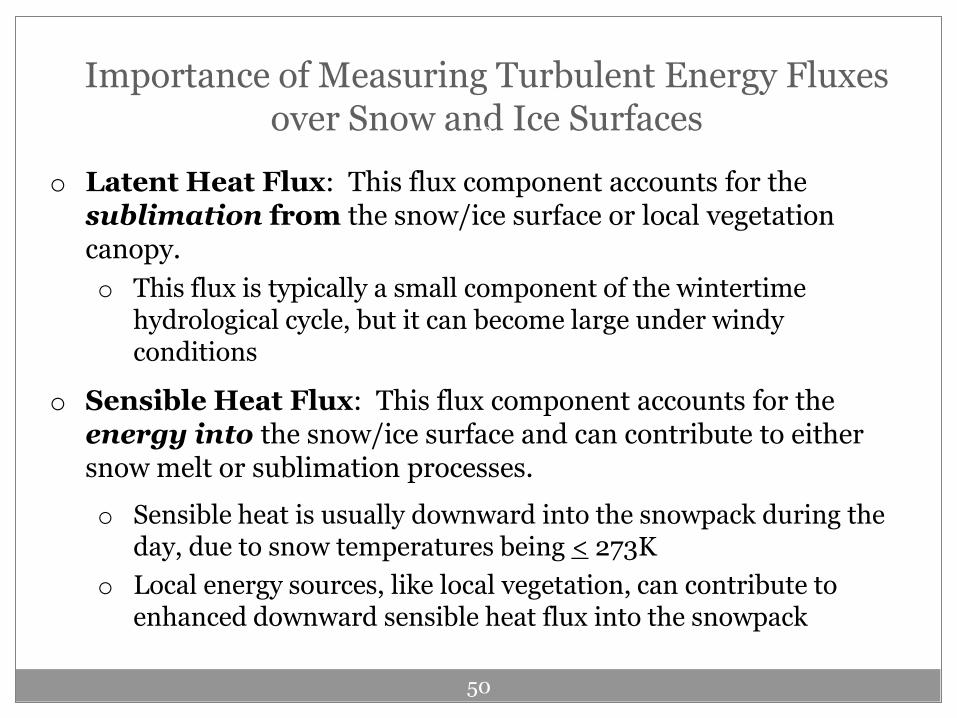
Importance of Measuring Turbulent Energy Fluxes over Snow and Ice Surfaces50

o Latent Heat Flux: This flux component accounts for the sublimation from the snow/ice surface or local vegetation canopy.

o This flux is typically a small component of the wintertime hydrological cycle, but it can become large under windy conditions

o Sensible Heat Flux: This flux component accounts for the energy into the snow/ice surface and can contribute to either snow melt or sublimation processes.

o Sensible heat is usually downward into the snowpack during the day, due to snow temperatures being < 273K

o Local energy sources, like local vegetation, can contribute to enhanced downward sensible heat flux into the snowpack

51

FLOSS II Tower((FLuxesFLuxes Over Snow Surfaces)Over Snow Surfaces)

34-meter FLOSS2 Tower with 8 measurement levels (Humidity at 2-, 10-,20- and 30-m heights)

Radiation components and snow depth measurements on a separate stands

Data obtained from both OSU (Mahrt, Vickers, Sun) and NCAR (Oncley)

NCAR FLOSS2 Report: http://www.eol.ucar.edu/rtf/projects/FLOSSII/

Site: Tower Sage Lake

Obs. Heights

(m)

.5, 1, 2, 5, 10, 15, 20, 25, 30

2 2

Elev. (m) 2476 2475 2474

Soil Type Sandy loam Sandy

Veg. Type Grass Sage Bare

52

Eddy Covariance Flux Measurements over Snow

• Snow can lead to very stable boundary layer conditions in association with temperature inversions and low wind speeds near the surface.

• An example given to the right using the FLOSS2 data.

(Vickers and Mahrt, 2004)

BL heightBL height< 20 m< 20 m

53

Eddy Covariance (EC) Flux Measurements over Snow

o Profile method: (i.e., measurements taken at two different heights) is compared against the eddy covariance method (Figure 7 to the right).

o Bulk method:Measurements are only taken at one height level, and if above the SL, then the fluxes may be underestimated.

53o EC Flux method: More directly estimates sensible heat flux, if the

instruments on the tower are above the surface layer (SL) then this method could generate the wrong results (Arck and Scherer, 2002).


54




Remote Sensing of Snow

Reflected Solar Radiation (0.4 – 3.0 µm)• Visible, near-infrared (0.4 - 1.1 µm): e.g., snow cover, contaminants in snow• Short-wave infrared (1.1 µm- 2.5 µm): e.g., snow vs. clouds, grain size

Emitted Thermal Radiation (3.0 – 14.0 µm)• Mid-wave and thermal infrared (3-5 µm, 8-14 µm):

e.g., Temperature, emissivity• Microwave (1-20 mm):

e.g., Dry vs. wet snow, snow water equivalence (SWE)

RADAR (2-70 cm):• e.g., Topography, roughness, ice velocity

55

MODIS Snow Cover and AlbedoModerate-Resolution Imaging Spectro-radiometer (MODIS)

Visible, near-infrared and thermal infrared.

Snow Cover Map Algorithm: [Hall et al, 2000]

Normalized Difference Snow Index:

NDSI=(*B6-B4)/(B6+B4)

Thermal threshold: 4ºC

NDVI/NSDI to distinguish forested snow

“Validated” Algorithm

*Note: “B” indicates “band”Image courtesy of Jeff Smaltz of MODISLand Rapid Response Team, NASA GSFC

56

MODIS (visible/infrared):

500 m and 1 km resolutions

Two satellites: Terra and Aqua

Giving 2x daylight passes (and 2x nighttime passes)

Sinusoidal Projection

Main limitations – cloud obstruction, and

Difficult to identify cirrus clouds vs. snow

MODIS Snow Cover

57

60

Measure microwave brightness temperatures

from emitted radiation from the snowpack surface, since snow crystals are effective scatterers of microwave radiation.

Deep snowpacks -

More snow crystals to scatter microwave energy away from the sensor,

Since microwave brightness temperatures are

generally lower for deep snowpacks (more scatterers) than they are for shallow snowpacks(fewer scatterers)

Microwave Sensors

SSM/I SWE and Snow Cover(Defense Meteorological Satellite Program; DMSP)

o Passive Microwave Channels (Ghz): 19V, 19H, 22V, 37V, 37H, 85V,85H

o Empirical “NSIDC Algorithm” based on [Chang, 1987]:

SWE (mm) = 4.77 * ((T19H - 6) - (T37H - 1))

-- (T19H and T37H in Kelvins)

o Global dataset from 1987 to present at 25 km resolution

o EASE-Grid Lambertian Equal Area

Main limitations – poor spatial resolution, no thin or wet snow, mountain and vegetation impacts on signal

61

Advanced Microwave Advanced Microwave

Scanning Radiometer Scanning Radiometer ––

Earth Observing Earth Observing

System (AMSRSystem (AMSR--E) E)

instrument aboard instrument aboard

NASA’s Aqua satelliteNASA’s Aqua satellite

Global passive MW snow Global passive MW snow

depth retrievals (coverage: depth retrievals (coverage:

20022002--present)present)

Forest attenuation effects are Forest attenuation effects are

corrected forcorrected for

Snow density is used to derive Snow density is used to derive

SWE from snow depth SWE from snow depth

25 km EASE25 km EASE--grid usedgrid used

Global passive MW snow Global passive MW snow

depth retrievals (coverage: depth retrievals (coverage:

20022002--present)present)

Forest attenuation effects are Forest attenuation effects are

corrected forcorrected for

Snow density is used to derive Snow density is used to derive

SWE from snow depth SWE from snow depth

25 km EASE25 km EASE--grid usedgrid used

Graphic is courtesy of NASA.

63 (From J. Dong (NCEP), C. Peters-Lidard (NASA) et al.)

Some of AMSR-E SWE issues result from:

(1) underestimation of the SWE retrievals when compared with in-situ measurements (e.g., SNOTEL sites),

(2) comparisons made on different spatial scales (e.g., point-to-area)

(3) land surface complexities within AMSR-E footprints

Issues with AMSR-E and Other Passive MW Sensors

AMSRAMSR--EE SWESWE

(Northern CO)

(WY)

~50 km == 2 AMSRE Pixels~50 km == 2 AMSRE Pixels

MODIS SCFMODIS SCF

Issues with MW Satellite-derived Snow Products

Issues also arise from varying terrain, vegetation, soil moisture effects, etc.

Also, due to its coarse spatial scale, a 25 km pixel could become skewed/shifted (e.g., due to reprojection) and values not be fully representive (see below).

Terra’s ASTER Sensor:Terra’s ASTER Sensor:• Visible Snow Cover Retrievals

• Resolution: ~ 100 m

• Only available when clouds are absent

• Similar to Landsat sensor – snow images, but more spectral bands and repeat times

65

MODELING MODELING SNOWPACKSNOWPACKCHARACTERISTICS AND CHARACTERISTICS AND

DYNAMICSDYNAMICS

66



In practice, several energy balance calculations In practice, several energy balance calculations may be combined into a single “model” … e.g.,may be combined into a single “model” … e.g.,

a a Land surface model (LSM) Land surface model (LSM)

Sw Sw Lw Lw H E

Sw Sw Lw Lw H H

Tc

T2

T1

T3

G12

G23

Sw Sw Lw Lw H sE

Tsnow mMGS1

E

The trick is to keep the fluxes between the “control volumes” consistent.

If the energy balance calculation for the snowpack includes a flux GS1

from the bottom of the pack to the ground, then the energy balance for

the top soil layer must include an input flux of GS1.

67

Some Basic Snow Modeling Elements

Energy balance in snowpack

T1

Sw Sw Lw Lw H sE

Tsnow mMInternal

energy GS1

Snowmelt occurs only

when snow temperature

reaches 273.16oK.

Internal energy

a function of

snow amount,

snow temperature,

and liquid water

retention

Albedo is high when

the snow is fresh, but

it decreases as the

snow ages.

Thermal conductivity

within snow pack

varies with snow age.

It increases with snow

density (compaction

over time) and with

liquid water retention.

Solid

fraction

0

1

Temperature 273.16


68

One Simple Snowmelt Model Approach …

1. Solve the energy balance for a layer and determine

the updated temperature.

2. If the new temperature is < 273.16oK, move to next timestep.

3. If the new temperature is > 273.16oK, then recompute the energy

balance, assuming the new temperature is exactly 273.16oK.

The excess energy flux obtained should be used to melt snow:

where m = latent heat of melting

M = snowmelt rate

Excess energy flux = mM


69

70

Importance of Modeling Snowmelt Timing CorrectlyImportance of Modeling Snowmelt Timing Correctly

Land surface models and snow schemes are known to have biases and errors in their physics and physical parameterizations

(e.g., Slater et al., 2001; Sheffield et al., 2003; Pan et al., 2003; Feng et al., 2008).

0

5

10

15

20

25

30

0 30 60 90 120 150 180 210 240 270 300

Day of Water Year 2004

SW

E (

inch

es)

SNOTEL

CLM2 (Tfrz)

CLM2 (Tfrz+Tcrit)

Noah (Tfrz)

Noah (Tfrz+Tcrit)

51 Stations - WAFor example, the Noah LSM tends to melt off its snowpack too early in the spring (e.g., Jin and Miller, 2007; Feng et al., 2008), even when a higher temperature threshold is used to determine snowfall

(in figure to the right).

With the snow melting off too soon, the errors in the land surface would potentially feedback onto an atmospheric model it’s coupled to.

Representations of Snow Cover and Representations of Snow Cover and SWESWE

NatureClimate Modeling Remote Sensing

1. A land grid has multiple vegetation types plus bare ground.

2. Energy and mass balances.

3. For each vegetation-covered area, on the ground, one mean SWE, one SCF. Canopy interception and canopy snow cover.

1. Pixels.

2. Integrated signals from multi-sources (e.g., snow, soil, water, vegetation), depending on many factors (e.g., view angle, aerosols, cloud cover, etc).

3. Each pixel, MODIS provides one SCF. AMSR provides one SWE.

Veg Type

GroundSCF

Interception

SWESWE


72

Snow Cover Fraction and Air TemperatureSnow Cover Fraction and Air Temperature

])/(5.2

tanh[0 newsnog

sno

z

hSCF

NEW – OBS

OLD – OBS

The new scheme reduces the warm bias in winter and spring in NCAR GCM (i.e. CAM2/CLM2).

Smaller Snow Cover Warmer Surface

SnowSnow VegetationVegetation

Liston (2004) JCL


73

Theory of Sub-grid Snow Cover

Liston (2004), “Representing Liston (2004), “Representing SubgridSubgrid Snow Cover Heterogeneities Snow Cover Heterogeneities in Regional and Global Models”. in Regional and Global Models”. Journal Journal of Climateof Climate..

The snow distribution during the accumulation phase can be represented using a lognormal distribution function, with the mean of snow water equivalent and the coefficient of variation as two parameters.

Liston (2004) JCL


The snow distribution during the melting phase can be analyzed by assuming a spatially homogenous melting rate applied to the snow accumulation distribution.

CV – Coefficient of Variation

74

Snow Model Physics – In OperationsMulti-layer Energy- and Mass-Balance Model

75

SNTHERM (SNow THERmal Model): One of the more complicated snow schemes of today ...

SNTHERM numerical scheme divides both soil and snow layers in to finite element increments known as “nodes”. The model can maintain around 23 nodes within the snow pack layer.

Each node is characterized by its own temperature, water content, grain size, and thickness.

For inputs, SNTHERM requires typical meteorological forcing (e.g.):

radiation fluxes,

liquid water precipitation

air temperature

Certain model parameters (e.g.):

Met. station height

basic soil type

snow grain material characteristics.

76

SNTHERM Run SNTHERM Run -- Rabbit Ears: Buffalo PassRabbit Ears: Buffalo Pass (CLPX)(CLPX)RB - SNTHERM vs.CLPX Snow Depth

0

0.2

0.4

0.6

0.8

1

1.2

1.4

1.6

1.8

2

274 279 284 289 294 299 304 309 314 319 324 329 334 339 344 349 354 359 364

DOY

(m)

CLPX SNTHERM - SNOTEL PPT

77

An Evaluation of Snow Model Complexity at An Evaluation of Snow Model Complexity at Three CLPX SitesThree CLPX Sites

Results from the article:

Xia Feng, Alok Sahoo, Kristi Arsenault, Paul Houser, Yan Luo, and Tara Troy, 2008: The Impact of Snow Model Complexity at Three CLPX Sites. Journal of Hydrometeorology.

Overview:

- A comparison between five land surface models of varying complexity in terms of the snowpack physics at three different Cold Land Processes Experiment (CLPX) instrument sites in Colorado

(m)

(WY)

(CO)

CLPX Sites and Domain10 Main ISA stations. Also includes, Fluxes over Snow

Surfaces (FLOSS) and Local Scale Observation Site (LSOS) Towers.

Representing a range of environments which influence snowpack evolution and snow-atmosphere exchanges

North Park (NP) AreaNorth Park (NP) Area

Rabbit Ears Rabbit Ears (RB) Area(RB) Area

Fraser (FR)Fraser (FR)AreaArea

Main SitesLSOS FLOSS2

79

Snow Depth Variability Among ISA Sites

RBRBRBRBRBRB

Upper right picture from: http://www.nohrsc.nws.gov/~cline/clp/field_exp/clpx_02/update_020224.html

80

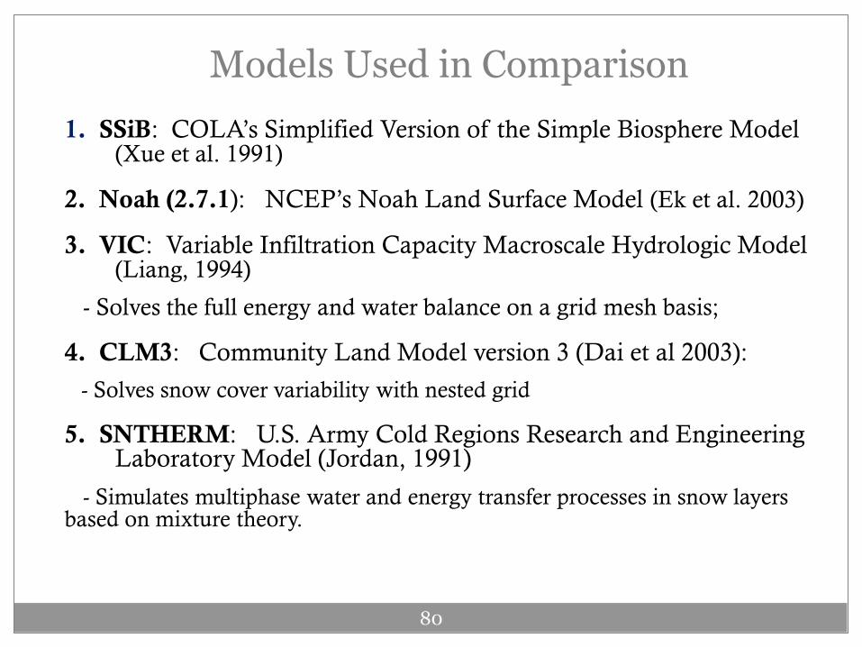
Models Used in Comparison

1. SSiB: COLA’s Simplified Version of the Simple Biosphere Model (Xue et al. 1991)

1) 2. Noah (2.7.1): NCEP’s Noah Land Surface Model (Ek et al. 2003)

2) 3. VIC: Variable Infiltration Capacity Macroscale Hydrologic Model (Liang, 1994)

- Solves the full energy and water balance on a grid mesh basis;

4. CLM3: Community Land Model version 3 (Dai et al 2003):

- Solves snow cover variability with nested grid

5. SNTHERM: U.S. Army Cold Regions Research and Engineering Laboratory Model (Jordan, 1991)

- Simulates multiphase water and energy transfer processes in snow layers based on mixture theory.

81

Cold Land Processes Experiment Sites (Main ISA Sites)

SiteSite Latitude and Latitude and

longitude longitude

(N,W)(N,W)

Soil Temperature Soil Temperature

((ooC) C)

(5cm, 20cm, (5cm, 20cm,

50cm)50cm)

ElevationElevation

(m)(m)

Soil TypeSoil Type Vegetation TypeVegetation Type

RBRB (40.53(40.53 oo ,106.68,106.68 oo )) 7.772, 6.297, 7.772, 6.297,

6.9776.977

32003200 LoamLoam GrasslandGrassland

FAFA ( 39,85( 39,85 oo ,105.86,105.86 oo ) ) 6.807, 6.648, 6.807, 6.648,

3.0143.014

35853585 Sandy Sandy

loamloam

GrasslandGrassland

FHQFHQ (39.9(39.9 oo , 105.88, 105.88 oo )) --0.815, 0.109, 0.815, 0.109,

1.1171.117

27602760 Clay loamClay loam Evergreen Evergreen

forestforest

1) Rabbit Ears MSA – Buffalo Pass Site (RB)2) Frasier MSA – Alpine Site (FA)3) Frasier MSA – Headquarters Site (FHQ)

82

RB: Snow Depth and SWE

Models:

SSiBSSiB = = Blue triangleBlue triangle

NoahNoah = = Brown starBrown star

VICVIC = = Pink circlePink circle

CLM3CLM3 = = Green Green diamonddiamond

SNTHERMSNTHERM = = Black plusBlack plus

Observations:

Snow Depth Obs = Red LineSnow Pit Data – Black Dots

82

83

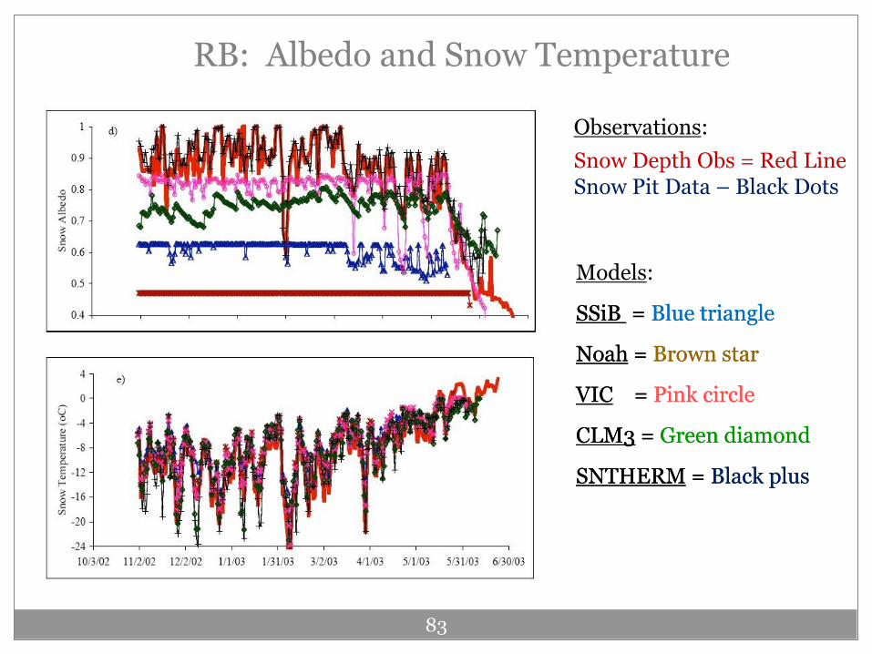
RB: Albedo and Snow Temperature

83

Models:






Observations:


84

CLPX Site: Frasier – Alpine

Picture - ftp://sidads.colorado.edu/pub/DATASETS/CLP/data/ground_data/nsidc0172_met_main/photos/iop3/alpine

The instrument heights for air temperature and relative humidity above the ground surface are 3 m in the Fraser. Wind speed measurement is taken from 10m.

85

FA: Snow Depth and SWE

Models:






Observations:


86

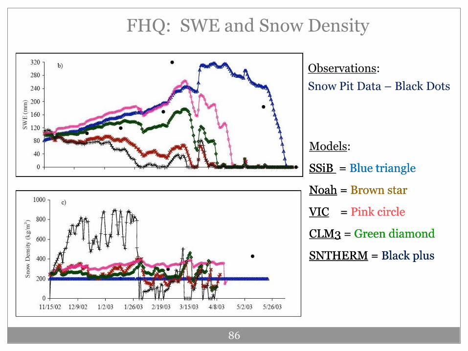
FHQ: SWE and Snow Density

86

Models:






Observations:

Snow Pit Data – Black Dots

87

Noah: Special Albedo Experiments

RB Site:Snow Albedo

0.50.5 = = PurplePurple

0.70.7 = = PinkPink

0.90.9 = = GreenGreen

ObsObs = = RedRed

87

88

Precipitation Comparison and Experiments

RB Site:Precipitation

Daily GageDaily Gage = = RedRed

LDASLDAS = = GreenGreen

PSDPSD = = BlueBlue

89

RB: Snow Depth and SWE (LDAS-Only)

Models:






Observations:


90

LDAS-OBS: Snow Depth and SWE

90

Models:






Observations:


91

Summary of Results

These models simulate the snow accumulation and snowpack ablation with varying skill when forced with the same meteorological observations, initial conditions, similar soil and vegetation parameters.

The simple snow schemes, such as SSiB and Noah capture snow accumulation at RB, however, both of them show inaccuracy in the simulation of SWE amount and the snowmelt timing.

VIC, CLM3 and SNTHERM produce similar snow depth, SWE and the snowmelt timing. However, they show substantial discrepancy in snow ablation through snow sublimation and snow melting due to different internal snow physics treatment.

SNOW DATA ASSIMILATIONSNOW DATA ASSIMILATION

92


93

o Much interest exists in improving hydrological predictions in complex terrain regions and global climate models using snow measurements.

o The assimilation of snow observations in land surface models is a promising approach to enhance runoff timing and discharges, mainly during critical melt periods.

o Also, improving weather and climate forecasts with assimilating observed snow data into coupled land-atmospheric models is another major area of research

Snow Data AssimilationSnow Data Assimilation

94

Modeling Snow at Higher ResolutionsModeling Snow at Higher Resolutions

April 1, 2004 (08Z)April 1, 2004 (08Z)

Snow Water Equivalent (in mm)Snow Water Equivalent (in mm)

April 1, 2005 (08Z)April 1, 2005 (08Z)

(mm)(mm)

April 1, 2006 (08Z)April 1, 2006 (08Z)

(mm)(mm)

(mm)(mm)

“Normal” Year“Normal” Year

“Drought” Year“Drought” Year

“Flood” Year“Flood” Year

Integrating MODIS Integrating MODIS Snow Cover into Snow Cover into thetheCLM CLM 33--Year Year Comparison for the Comparison for the Yakima River BasinYakima River Basin

95

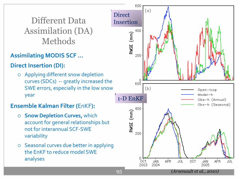
Different Data Assimilation (DA)

Methods

1-D EnKF

Direct Insertion

Assimilating MODIS SCF …

Direct Insertion (DI):

Applying different snow depletion curves (SDCs) -- greatly increased the SWE errors, especially in the low snow year

Ensemble Kalman Filter (EnKF):

Snow Depletion Curves, which account for general relationships but not for interannual SCF-SWE variability

Seasonal curves due better in applying the EnKF to reduce model SWE analyses

(Arsenault et al., 2010)

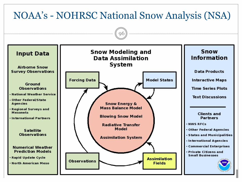
NOAA’s - NOHRSC National Snow Analysis (NSA)

96

Example NSA OutputAutomated Model Discussion:March 2, 2009

Area Covered By Snow: 59.5%

Area Covered Last Month: 7.9%

Snow Depth Average: 1.8 inches (for region)

Snow Water Equivalent Average: 0.3 inches

Snow Depth Map for Snow Depth Map for March 2, 2009March 2, 2009

97

98

SNODAS Basin Average animations 2003-04 vs. 2004-05

CLIMATE CHANGE AND OTHER CLIMATE CHANGE AND OTHER POTENTIAL POTENTIAL ANTHROPOGENICANTHROPOGENIC

EFFECTS ON SNOWEFFECTS ON SNOW

99


Atmospheric Moisture

100

Climate Change and an “Accelerated” Water Cycle ?

Snow & Rain

Soil & Surface Wetting

Evaporation

Runoff

101

Potential Impacts of Climate Change on Snow-Atmosphere Relationships

o In a potentially warming climate, temperature changes could impact snow conditions which could then positively feedback further on the climate system.

o Different general circulation model (GCM) studies have demonstrated the sensitivity of the regional to global climate response to such changes in snow cover and albedo (e.g., Levis et al., 2007; Euskirchen et al., 2007; Vavrus, 2007; and also several mentioned on the previous slide).

o Observational studies (e.g., Stone et al., 2002; Hamlet et al., 2005) have shown that with warmer temperatures in polar regions or mountain areas, earlier onsets of snow melt may be occurring and contributing to shifts in springtime runoff (e.g., Stewart et al., 2004).

o In addition, studies like Feng and Hu (2007) show transitions to more rainfall versus snowfall events in different parts of the world (e.g., North America), which can also impact spring snowmelt.

http://zubov.atmos.uiuc.edu/ACIA/http://zubov.atmos.uiuc.edu/ARCTIC/

Our best climate models project that the Arctic will become warmer. And the Arctic is indeed warming

Permafrost• The discontinuous permafrost region, currently within 1-2 degrees of thawing, will see most dramatic melt

• Where ground ice contents are high, this permafrost degradation will have associated physical impacts.

• Biggest concern are soils with the potential for instability upon thaw (thaw settlement, creep or slope failure).Such instabilities may have implications for the landscape, ecosystems, and infrastructure. (GSC 2002)

Changes since 1978 in permafrost temperatures at 20 m depth (updated from Osterkamp 2003) -- Northern Alaska (ARC 2008).

RUNOFF

GLACIERS

107

Historical retreat of non-polar

glaciers

World Glacier Monitoring Service www.geo.unizh.ch/wgms

NASA satellite data has revealed regional changes in the weight of the Greenland ice sheet between 2003 and 2005. Low coastal regions (blue) lost three times as much ice per year from excess melting and icebergs than thehigh-elevation interior (orange/red) gained from excess snowfall Credit: Scott Luthcke, NASA Goddard

Melt descending into a moulin, a vertical shaftcarrying water to ice sheet base.

Source: Roger Braithwaite, University of Manchester (UK)

Greenland Mass Loss – From Gravity Satellite

109

Snowpack Augmentation (Conceptual Model)

Example Silver Iodide Generators for the Denver Water Program

Colorado Wintertime Cloud Seeding Programs 2004-2005

Central Rockies Program (Denver Water + Arkansas Basin ) Vail/Beaver Creek Ski Resort

Grand Mesa Program Gunnison Basin Program (expanded late

2003)

Telluride/Upper San Miguel Basin San Juan Mountains Program (expanded in

2002)

From http://cwcb.state.co.us/Weather_Modification/Permit_Program.htm

Supercooled Liquid Water (SLW)

SLW is water droplets in a liquid state at temperatures below freezing SLW also causes aircraft icing

SLW is the fuel required for cloud seeding to work - droplets need a nucleus on which to freeze

Cloud seeding provides those nuclei

Result: more large ice particles, which fall to ground as snow

Help! I’ve Help! I’ve fallen and fallen and I can’t get I can’t get

up!up!Questions?

Snow Hydrology:

Documents

Transcript of Snow Hydrology: