Monitoring Snow and Glaciers of Himalayan Region
430
Monitoring Snow and Glaciers of Himalayan Region Space Applications Centre (ISRO) Ahmedabad – 380 015
-
Upload
khangminh22 -
Category
Documents
-
view
0 -
download
0
Transcript of Monitoring Snow and Glaciers of Himalayan Region

Monitoring Snow and Glaciers of
Himalayan Region
Space Applications Centre (ISRO)
Ahmedabad – 380 015

Front Cover shows debris covered ablation zone near snout of Batal glacier in Lahaul and Spiti district,
Himachal Pradesh. Back cover upper panel shows IRS AWiFS FCC and RISAT-1 MRS images over
Moraine dammed lake (buried under snow during winter season) of Samudra Tapu glacier in Chandra
Basin (Himachal Pradesh). Lower panel shows GPR survey over bare ice ablation zone of Chota Shigri
glacier in Chandra basin.

Monitoring Snow and Glaciers of
Himalayan Region
Space Applications Centre, ISRO
Ahmedabad 380 015

Published by: Space Applications Centre, ISRO, Ahmedabad, India www.sac.gov.in
Copyright: © Space Applications Centre, ISRO, 2016
This publication may be produced in whole or in part and in any form for education or non-profit uses, without special permission from the copyright holder, provided acknowledgement of source is made. SAC will appreciate a copy of any publication which uses this publication as a source.
Citation: SAC (2016) Monitoring Snow and Glaciers of Himalayan Region, Space Applications Centre, ISRO, Ahmedabad, India, 413 pages, ISBN: 978 – 93 – 82760 – 24 – 5
ISBN: ISBN: 978 – 93 – 82760 – 24 – 5
Available from: Space Applications Centre, ISRO, Ahmedabad - 380015, India
Publications: SAC carried out the work in collaboration with State Remote Sensing Applications Centers, Academic Institutes and Government Organisations. This project is sponsored by Ministry of Environment, Forest and Climate Change and Department of Space, Government of India.
Printed by: Chandrika Corporation, Ahmedabad

i
Monitoring Snow and Glaciers of Himalayan Region
Space Applications Centre ISRO, Ahmedabad
Preamble
Himalayan Cryosphere plays an important role as a sensitive indicator of climate
change. Melt water from Himalayan snow and glaciers is perennial source for
irrigation, hydropower, domestic water requirements and sustainability of bio-diversity
& environment in particular. Monitoring Himalayan snow and glaciers is important in
view of the associated natural hazards such as, avalanches, bursting of glacial lakes,
floods and landslides.
This volume is the outcome of a national project on “Monitoring Snow and Glaciers of
Himalayan Regions”, providing details of the current status of Himalayan snow and
glaciers based on the analysis of time series multi-sensor data from Indian Earth
Observation satellite supported by field based observations. It covers details about the
types of satellite sensors used, methodology developed and salient findings related to
snow cover, glaciers and Himalayan Glacier Information System. Studies have been
carried out using Ground Penetrating Radar (GPR), hyperspectral data, SAR
Interferometry and Photogrammetry for glacier ice thickness, snow pack
characterization, glacier flow determination and glacier mass balance estimation.
Development of advance technique using INSAT-3D, RISAT-1, Gravity Recovery and
Climate Experiment (GRACE), ICESat/GLAS laser altimetry data for snow cover,
detection of glacial lakes buried under snow, estimation of regional water mass
variations and monitoring ice thickness changes have been well documented in the
document.
I am sure that the information generated in the document will be extremely useful to
the Ministry of Environment, Forest and Climate Change, representing India in various
international forums related to Climate Change, concerned policy makers, planners,
managers and researchers.
I congratulate the team behind this information compilation for their valuable
contributions.
(A. S. Kiran Kumar)
Bangalore September 21, 2016


ii
Monitoring Snow and Glaciers of Himalayan Region
Space Applications Centre ISRO, Ahmedabad
Preface
Himalayas possess one of the largest resources of snow and ice outside the Polar Regions. It is the snow and glacier melt runoff from the Himalayan region which sustains the perennial flow of the Indus, Ganga and Brahmaputra river systems. These river systems receive almost 30-50% of the annual flow from snow and glacier melt runoff. The runoff from the Himalayan rivers support domestic, irrigational and industrial water demand of a very large population residing in the Himalayas and the Indo-Gangetic alluvial plains. Melt water from the Himalayan region is required for generation of hydropower and sustainability of Himalayan bio-diversity and environment.
There are increasing concerns by scientific community that global warming caused by increase in concentration of greenhouse gases in atmosphere can cause significant impact on the snow and glacier melt runoff in the river systems. In view of the importance and significance of snow fields and glaciers for water security of the nation and assessing climatic impact in Indian sub-continent, these cryosphere elements need to be regularly mapped and monitored. Sensitivity of snow and glaciers to variations in temperature makes them a key indicator of climate change.
Himalayan region is difficult to study using conventional field based methods due to rugged topography, high altitude and extreme weather conditions. Satellite data due to its synoptic view, distinct spectral properties of snow and glaciers, high temporal frequency aided by advanced digital image processing and analysis techniques provide accurate and reliable observations.
This document provides details of the salient findings of a national project entitled, “Monitoring Snow and Glaciers of Himalayan region (Phase-II)”, taken up under National Natural Resources Management (NNRMS) Program and jointly sponsored by the Ministry of Environment, Forest and Climate Change (MoEF&CC) and Department of Space (DOS). The project has been successfully completed by Space Applications Centre, Indian Space Research Organisation (ISRO), Ahmedabad as a nodal agency along with eighteen partner institutes. A large geospatial database on changes in the Himalayan Snow and Glaciers based on space based observations has been generated. Field data has been collected through various glacier expeditions and utilised for development of analysis techniques and validation. Recent advanced techniques of satellite data interpretation and future trends are also highlighted.
I am sure that findings of the present work would be extremely useful to various national and International Programs of the Ministry as well to concerned scientific and academic community. I appreciate the efforts made by the national team and recommend that monitoring Himalayan Cryosphere using various current and planned Earth Observation Space Missions should be continued.
New Delhi
September 21, 2016
(Ajay Narayan Jha)


iii
Monitoring Snow and Glaciers of Himalayan Region
Space Applications Centre ISRO, Ahmedabad
Foreword
Monitoring of the Himalayan snow and glaciers is important in view of water security
of the nation, hydroelectric power generation, understanding impact of climate change,
assessing disaster vulnerability and protection of the biodiversity and environment.
Snow and Glacier Studies of the Himalayan region are one of the major thrust area
identified by the Ministry of Environment, Forest & Climate Change, Government of
India. Snow and glaciers of Himalayan region are difficult to study using conventional
field based methods due to rugged topography, high altitude and extreme weather
conditions. Space Applications Centre (SAC) has been developing tools and
techniques of space based observations from various EO Missions for past few
decades.
The present Final Technical Report provides salient results and analysis of the Project
on “Monitoring Snow and Glaciers of Himalayan Region – Phase-II”, jointly funded by
MoEF&CC and DOS. Himalayan snow cover monitoring has been carried out for the
time frame 2008-14 using AWiFS data of Resourcesat-2 satellite from October to June
(Hydrological year) at every five day interval. Around 2018 glaciers for time frame
2000-2010 have been monitored using multi-date satellite data and the analysis
depicted that 87% of the glaciers showed no change, 12% retreated and 1 % glaciers
have advanced. The geospatial database of glacier inventory carried out on 1:50,000
scale using Resourcesat-1 satellite data contains 34919 glaciers covering 75, 779 sq
km area. A Himalayan Glacier Information System (HGIS) has been developed. Some
of the advanced techniques of satellite data analysis for snow and glacier studies are
also demonstrated.
I compliment the entire team of scientists from both ISRO and other organizations for
carrying out this task diligently. I do hope, the findings of the project presented in this
documents shall be extremely useful to the MoEF&CC which represents India in key
International forums of climate change and also to the researchers working in the field
of environment, glaciology, hydrology and climate change.
(Tapan Misra)


iv
Monitoring Snow and Glaciers of Himalayan Region
Space Applications Centre ISRO, Ahmedabad
Acknowledgements
Ministry of Environment, Forest & Climate Change (MoEF&CC), Govt. of India has
identified Himalayan glaciers and snow cover as one of the thrust area under NNRMS
Standing Committee on Bio-resources and Environment (NNRMS SC-B). Based on
the recommendations of NNRMS SC-B, a project on “Monitoring Snow and Glaciers
of Himalayan Region (Phase-II)” was taken up by Space Applications Centre at the
behest of MoEF&CC with joint funding by DOS and MoEF&CC, in continuation of
generating long term space based database created earlier under Phase-I.
We would like to place on record our deep sense of gratitude to Shri A.S. Kiran Kumar,
Secretary DOS and Chairman ISRO and Shri Tapan Misra, Director, SAC for their
encouragement and guidance in carrying out this national project. We are very much
thankful to Shri Lalit Kapur, Advisor, RE, Dr. T. Chandni, former Advisor, RE, Dr. G.V.
Subrahmanyam, former Advisor, RE, Dr. Jag Ram, Director, Dr. Harendra Kharkwal,
Deputy Director and Shri Pankaj Verma, Joint Director, MoEF&CC for their continuous
support in executing this project.
We express our thanks to the Dr. B. S. Gohil, Deputy Director, EPSA, Dr. J. S. Parihar,
and Dr P. K. Pal, former Deputy Directors, Dr. Rajkumar, Group Director, GHCAG and
Dr. M. Chakraborty, former Group Director, GSAG for providing technical guidance
and necessary support in carrying out this project. We are thankful to SAC Committee
on “Space Applications: Projects Monitoring and review, Outsourcing and Inter Agency
Document Review Committee”, in particular Shri R.M. Parmar, Deputy Director &
Committee Chairman and Shri Vivek Pandey, Member Secretary for their comments
and suggestions. We are grateful to Dr. S. Bandyopadhyay, Scientist, EOS, ISRO HQ
for providing necessary support.
We extend our gratitude to Directors/Heads of the Institute/Vice-Chancellors of
eighteen collaborating research organizations/academic institutions of the country for
their support in executing this project.
(Dr. A.S. Rajawat) Project Director


iv
Monitoring Snow and Glaciers of Himalayan Region
Space Applications Centre ISRO, Ahmedabad
National Team
Project Director
Dr. A.S. Rajawat
Dr. Ajai (upto October, 2013)
Deputy Project Directors
Dr. I.M. Bahuguna
Mr. A.K. Sharma
Space Applications Centre, ISRO,
Ahmedabad
Mr. B.P. Rathore
Dr. Sushil Kumar Singh
Ms. Gunjan Rastogi
Mr. Ritesh Agrawal
Dr. Sreejith, K.M.
Mr. Manish Parmar
Mr. J.G. Patel
Mr. Anish Mohan
Ms. Sandhya Rani Pattnaik
Department of Geology, M G Science
Institute, Ahmedabad
Prof. R.D. Shah Dr. Rupal Brahmbhatt
Mr. Mann Chaudhary
Centre for Environment and Planning
Technology (CEPT) University,
Ahmedabad
Prof. Anjana Vyas
Ms. Darshana Rawal
Mr. Purnesh Jani
Mr. Utkarsh Shah
Mr. Kaivalya Pathak
Mr. Anand Paleja
Mr. Ashish Upadhyay
Department of Geography, University of
Jammu, Jammu
Prof. M.N. Koul
Prof. V.S. Manhas
Mr. Devinder Manhas
Mr. Sadiq Ali
H.P. State Centre on Climate Change,
State Council of Science, Technology
and Environment, Himachal Pradesh,
Shimla
Dr. S.S. Randhawa
Ms. Anjana Sharma
Mr. Arvind Bhardwaj
Department of Geology, Government
Post Graduate College, Dharamshala,
Himachal Pradesh
Dr. Sunil Dhar
Mr. Dinesh Kumar
Mr. Vikas Pathania
National Bureau of Plant Genetic
Resources (NBPGR), Regional Station,
Phagli, Shimla
Dr. J.C. Rana
Mr. Rameshwar Singh
Ms. Supriyanka Rana
Uttarakhand Space Application Centre,
Department of Science & Technology,
Dehradun
Dr. M.M. Kimothi
Dr. Asha Thapliyal
Ms. Anju Panwar
Prof. Durgesh Pant

v
Monitoring Snow and Glaciers of Himalayan Region
Space Applications Centre ISRO, Ahmedabad
Remote Sensing Applications Center,
Uttar Pradesh, Lucknow
Dr. A.K. Tangri
Mr. S.K.S. Yadav
Mr. Ramchandra
Mr. Rupendra Singh
Mr. Diwakar Pandey
Mr. Dhanendra Kumar Singh
Department of Earth Sciences,
University of Kashmir, Srinagar
Prof. Shakil Ahmed Romshoo
Mr. Irfan Rashid
Mr. Gowhar Meraj
Ms. Midhat Fayaz
Mr. Obaidullah
Mr. Khalid Omar
Centre for the Study of Regional
Development, (UGC-Centre for Advance
Studies in Geography), Jawaharlal Nehru
University, New Delhi
Dr. Milap Chand Sharma
Mr. Ishwar Singh Mr. Sanjay Deswal Mr. Rakesh Saini Mr. Rakesh Arya Mr. Satya Prakash
CSRE, Indian Institute of Technology-
Bombay, Mumbai
Prof. G. Venkataraman
Prof. Avik Bhattacharya
Ms. Fajana Sikandar Birajdar
Divecha Centre of Climate Change,
Indian Institute of Science, Bangalore
Dr. A.V. Kulkarni
Ms. Enakshi Bhar
G.B. Pant National Institute of Himalayan
Environment & Sustainable
Development (formerly known as G.B.
Pant Institute of Himalayan Environment
& Development), Almora
Er. Kireet Kumar
Mr. Kavindra Upreti
Ms. Joyeeta Poddar
Mr. Jagdish Pande
Mr. Chanchal Singh
Sikkim State Remote Sensing Applications Centre, Department of Science & Technology and Climate Change, Government of Sikkim, Gangtok Mr. D.G. Shrestha
Mr. Narpati Sharma
Mr. Pranay Pradhan
State Remote Sensing Applications Centre, Arunachal Pradesh State Council for Science and Technology, Department of Science and Technology, Government of Arunachal Pradesh, Itanagar Er. T. Ronya Dr. Swapna Acharjee Mr. Jutsam Katang Mr. Saumitra Deb
School of Environmental Science,
Jawaharlal Nehru University, New Delhi
Prof. A.L. Ramanathan
Mr. Mohd. Soheb
Department of Remote Sensing, Birla
Institute of Technology, Mesra, Ranchi
Dr. V.S. Rathore
Dr. M.S. Nathawat
Dr. A.C. Pandey
Department of Geology, University of
Jammu, Jammu
Prof. R.K. Ganjoo Ms. Sunita Chahar
vi
Monitoring Snow and Glaciers of Himalayan Region
Space Applications Centre ISRO, Ahmedabad
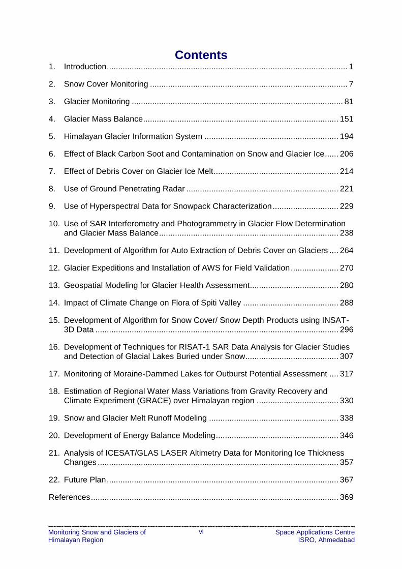
Contents 1. Introduction .......................................................................................................... 1
2. Snow Cover Monitoring ....................................................................................... 7
3. Glacier Monitoring ............................................................................................. 81
4. Glacier Mass Balance ...................................................................................... 151
5. Himalayan Glacier Information System ........................................................... 194
6. Effect of Black Carbon Soot and Contamination on Snow and Glacier Ice ...... 206
7. Effect of Debris Cover on Glacier Ice Melt ....................................................... 214
8. Use of Ground Penetrating Radar ................................................................... 221
9. Use of Hyperspectral Data for Snowpack Characterization ............................. 229
10. Use of SAR Interferometry and Photogrammetry in Glacier Flow Determination and Glacier Mass Balance ............................................................................... 238
11. Development of Algorithm for Auto Extraction of Debris Cover on Glaciers .... 264
12. Glacier Expeditions and Installation of AWS for Field Validation ..................... 270
13. Geospatial Modeling for Glacier Health Assessment ....................................... 280
14. Impact of Climate Change on Flora of Spiti Valley .......................................... 288
15. Development of Algorithm for Snow Cover/ Snow Depth Products using INSAT-3D Data ........................................................................................................... 296
16. Development of Techniques for RISAT-1 SAR Data Analysis for Glacier Studies and Detection of Glacial Lakes Buried under Snow ......................................... 307
17. Monitoring of Moraine-Dammed Lakes for Outburst Potential Assessment .... 317
18. Estimation of Regional Water Mass Variations from Gravity Recovery and Climate Experiment (GRACE) over Himalayan region .................................... 330
19. Snow and Glacier Melt Runoff Modeling ......................................................... 338
20. Development of Energy Balance Modeling ...................................................... 346
21. Analysis of ICESAT/GLAS LASER Altimetry Data for Monitoring Ice Thickness Changes .......................................................................................................... 357
22. Future Plan ...................................................................................................... 367
References ............................................................................................................. 369


1 Monitoring Snow and Glaciers of Himalayan Region
Space Applications Centre ISRO, Ahmedabad
1. Introduction
Himalayas possess one of the largest resources of snow and ice outside the Polar
Regions. Himalayan region due to its geo-climatic setting, arcuate length of approx.
2400 km, high altitude of its mountain ranges, proximity to Indian Ocean and sub-polar
regions undergoes annually a cycle of snow precipitation and melting.
It is the snow and glacier melt runoff from the Himalayan region which sustains the
perennial flow of the Indus, the Ganga and the Brahmaputra river systems. These river
systems receive almost 30-50% of the annual flow from snow and glacier melt runoff.
The runoff from the Himalayan rivers support domestic, irrigational and industrial water
demand of a very large population residing in the Himalayas and the Indo-Gangetic
alluvial plains. Melt water from the Himalayan region is also required for generation of
hydropower and sustainability of Himalayan bio-diversity and environment. Monitoring
of the Himalayan snow and glaciers is important in view of its hydrological significance
and also the associated natural hazards like avalanches, bursting of high altitude lakes
and consequent flooding downstream, mass wasting and debris flow etc. leading to
several disasters in the region.
The importance of snow fields and glaciers of the Himalaya also lies in their interaction
with atmosphere. Albedo from snow is one of the important components of
the Earth's radiation balance. The difference in temperature between the Himalayan
cryosphere and the Indian Ocean pulls SW monsoon towards the Indian landmass
during summer. So collectively, snow fields and glaciers govern the climate system of
the Indian land mass at regional and global scales. Sensitivity of snow and glaciers to
variations in temperature makes them a key indicator of climate change.
There are increasing concerns by scientific community that global warming caused by
increase in concentration of greenhouse gases in atmosphere can cause dramatic
impact on the snow melt runoff in the river systems. In view of the importance and
significance of snow fields and glaciers for water security of the nation and assessing
climatic variations in Indian sub-continent, these cryosphere elements need to be
regularly mapped and monitored.
Himalayan region is difficult to study using conventional field based methods due to
rugged topography, high altitude and extreme weather conditions. Satellite data due
to its synoptic view, distinct spectral properties of snow and glaciers, high temporal
frequency aided by advanced digital image processing and analysis techniques
provide accurate and reliable observations. Therefore, methods based on remote
sensing (RS) coupled with Geographical Information System (GIS) techniques have
become very useful tools to carry out accurate, quick inventory, mapping and
monitoring of the inaccessible Himalayan terrain. Remote sensing methods are
developed in the country since past two and a half decades to monitor the Himalayan

2 Monitoring Snow and Glaciers of Himalayan Region
Space Applications Centre ISRO, Ahmedabad
snow and glaciers by Space Applications Centre (SAC) along with concerned
Central/State government Departments and academic institutions (SAC & MoEF,
2010).
Ministry of Environment, Forest and Climate Change (MoEF&CC) is the nodal Ministry
which represents India in key International forums of climate change. Therefore, in
view of the role and importance of the Himalayan snow and glaciers as sensitive
indicator of climate change and likely impact on fresh water resources of the Indo-
Gangetic plains, the National Natural Resources Management Standing Committee
on Bio-Resources (NNRMS SC-B) Chaired by Secretary, MoEF&CC had identified
“Snow and Glacier Studies”, as one of the thrust area where space based observations
can be effectively utilized.
Accordingly, a project on “Snow and Glacier Studies” was taken up and completed by
Space Applications Centre (SAC) along with 13 concerned Central/State government
Departments and Academic Institutes using remote sensing and GIS techniques. The
project was jointly funded by the MoEF&CC and the Department of Space (DOS),
Govternment of India. The project has been completed during the time frame March
2005 to October 2010. The project aimed at i) Inventory of all Himalayan glaciers on
1,50,000 scale, ii) monitoring of seasonal snow cover (every 5 days) in hydrological
years 2004-2008 for entire Indian Himalayan region, iii) monitoring of retreat/advance
of the glaciers in fourteen glaciated basins representing different climatic zones of
the Indian Himalayas and iv) estimation of mass balance of glaciers based on
monitoring of snow line on glaciers at the end of ablation period in ten glaciated
basins of the Himalaya (SAC, 2010; SAC, 2011a).
This project had generated large amount of geospatial database using primarily
multidate satellite data in GIS environment of glacier inventory, snow cover mapping,
changes in glacier retreat/advance and estimation of glacier mass balance. The
information generated under the project provided accurate and reliable information on
Himalayan snow cover and glaciers based on space based observations. It provided
up-to-date information on the state of the Himalayan cryosphere and could be utilized
in climate change research, snow and glacier melt runoff modeling, hydropower
potential estimation and glacial lakes monitoring (SAC, 2010; SAC, 2011a; SAC,
2011b).
It was recommended by the NNRMS SC-B that snow and glacier resources of the
Himalayan region need to be monitored continuously using satellite data for usage in
climate change and hydrological applications and research.
Accordingly, the project entitled, “Monitoring Snow and Glaciers of Himalayan region
(Phase-II)”, has been taken up by Space Applications Centre, ISRO, Ahmedabad and
is jointly funded by the MoEF&CC and DOS, Government of India. The project has
been completed during the time frame December 2010 to March 2015.

3 Monitoring Snow and Glaciers of Himalayan Region
Space Applications Centre ISRO, Ahmedabad
Monitoring the Himalayan Snow and Glaciers:
There are four major work elements completed in the project for monitoring the
Himalayan Snow and Glaciers using satellite data viz.,
I) Snow Cover Monitoring (2008-2014)
II) Monitoring Glacier Retreat/Advance (2000-2010)
III) Monitoring Glacier Mass Balance (2008-2013)
IV) Development of Himalayan Glacier Information System
R&D Studies:
Apart from the above mentioned work, several R&D studies were carried out. These
studies are as follows:
i. Effect of black carbon soot and contamination on snow and glacier ice
ii. Effect of debris cover on glacier ice-melt
iii. Use of Ground Penetrating Radar (GPR) for determining glacier ice thickness
iv. Use of hyperspectral data in snow pack characterization
v. Use of SAR Interferometry and photogrammetry in glacier flow determination
and glacier mass balance
vi. Development of algorithm for auto extraction of debris cover on glaciers and
moraine dammed lakes
vii. Installation of AWS for field validation of data
viii. Geospatial modeling for glacier health assessment
ix. Impact of climate change on flora of Spiti valley
x. Development of algorithm for snow cover/snow depth products using INSAT-
3D Data
xi. Development of techniques for RISAT SAR data analysis for glacier studies
and detection of glacial lakes buried under snow

4 Monitoring Snow and Glaciers of Himalayan Region
Space Applications Centre ISRO, Ahmedabad
xii. Monitoring of Moraine-Dammed Lakes for Outburst Potential Assessment
xiii. Estimation of regional mass anomalies from Gravity Recovery and Climate
Experiment (GRACE) over Himalayan region
xiv. Snow and glacier melt runoff Modelling
xv. Development of energy balance modeling
xvi. Analysis of ICESat/GLAS laser altimetry data for monitoring ice thickness
changes
The project has been executed by Space Applications Centre, ISRO, Ahmedabad as
a nodal agency along with eighteen partner institutes. Table-1 provides list of
participating organisations and their work responsibility.
Table 1: Participating Organisations and Work Responsibility
Sr.
No.
Participating
Organisations Work Responsibility
1 Department of Geology,
M G Science Institute,
Ahmedabad
Glacier monitoring and mass balance estimation in
Bhut and Warwan sub-basins of Chenab basin
2 Centre for Environment
and Planning Technology
(CEPT) University,
Ahmedabad
Snow cover monitoring (Chandra, Bhaga, Miyar,
Bhut, Warwan & Ravi sub-basins of Chenab basin),
Develop Himalayan Glacier Information System
(HGIS), Glacier Health Assessment
3 Department of
Geography, University of
Jammu, Jammu
Glacier monitoring (Drass sub-basin), mass
balance studies of Machoi glacier based on field
expeditions
4 H.P. State Centre on
Climate Change, State
Council of Science,
Technology and
Environment, Himachal
Pradesh, Shimla
Snow cover monitoring (Spiti, Pin, Baspa, Jiwa,
Parbati & Beas sub-basins of Satluj basin), Glacier
Monitoring and Mass Balance (Spiti sub-basin)
5 Department of Geology,
Government Post
Graduate College,
Dharamshala, Himachal
Pradesh
Glacier monitoring (Chenab sub-basin, Lahaul-Spiti
district, Himachal Pradesh) and field expeditions

5 Monitoring Snow and Glaciers of Himalayan Region
Space Applications Centre ISRO, Ahmedabad
6 National Bureau of Plant
Genetic Resources
(NBPGR), Regional
Station, Phagli, Shimla
Understand impact of snow line on floral distribution
and societal impacts in Spiti valley
7 Uttarakhand Space
Application Centre,
Department of Science &
Technology, Dehradun
Snow cover monitoring (Alaknanda, Bhagirathi and
Yamuna sub-basins), Glacier monitoring
(Alaknanda & Bhagirathi sub-basins)
8 Remote Sensing
Applications Center, Uttar
Pradesh, Lucknow
Snow cover monitoring (Nubra, Shyok, Shigar,
Hanza, Gilgit & Sasgan sub-basins), Glacier
monitoring (Satopanth and Bhagirath Kharak
glaciers in Alaknanda and Bhagirathi sub-basins)
and field expeditions
9 Department of Earth
Sciences, University of
Kashmir, Srinagar
Glacier monitoring in Suru and Jhelum sub-basins,
Field expeditions Kolhoi glacier
10 Centre for the Study of
Regional Development,
(UGC-Centre for
Advance Studies in
Geography), Jawaharlal
Nehru University, New
Delhi
Glacier monitoring in Miyar sub-basin and field
expeditions
11 CSRE, Indian Institute of
Technology-Bombay,
Mumbai
Glacier monitoring and mass balance estimation
(Bhaga sub-basin), Develop SAR Interferometry
apparoaches for mass balance estimation and
snow pack studies using hyperspectral data
12 Divecha Centre of
Climate Change, Indian
Institute of Science,
Bangalore
Glacier mass balance in Chandra sub-basin and
improve existing model for mass balance
estimation
13 G.B. Pant National
Institute of Himalayan
Environment &
Sustainable Development
(formerly known as G.B.
Pant Institute of
Himalayan Environment
& Development), Almora
Glacier monitoring (Dhauliganga, Goriganga &
Kaliganga sub-basins), field expeditions in
Dhauliganga sub-basin
14 Sikkim State Remote
Sensing Applications
Centre, Department of
Snow cover and glacier monitoring (Tista, Ranjit
sub-basins)

6 Monitoring Snow and Glaciers of Himalayan Region
Space Applications Centre ISRO, Ahmedabad
Science & Technology
and Climate Change,
Government of Sikkim,
Gangtok
15 State Remote Sensing
Applications Centre,
Arunachal Pradesh State
Council for Science and
Technology, Department
of Science and
Technology, Government
of Arunachal Pradesh,
Itanagar
Snow cover monitoring (Subansiri, Tawang &
Diwang sub-basins of Brahamaputra basin),
Glacier Monitoring (Tawang sub-basin of
Brahmaputra basin)
16 School of Environmental
Science, Jawaharlal
Nehru University, New
Delhi
Glacier mass balance estimation of Patsio glacier,
and energy balance modelling (Bhaga sub-basin)
17 Department of Remote
Sensing, Birla Institute of
Technology, Mesra,
Ranchi
Snow cover monitoring, Glacier monitoring and
mass balance estimation (Zanskar sub-basins)
18 Department of Geology,
University of Jammu,
Jammu
Glacier monitoring in Nubra sub-basin, Glacier
mass balance Rulung glacier based on field
expeditions
19 Space Applications
Centre, ISRO,
Ahmedabad
Project conceptualization, formulation, overall
coordination, geospatial database design and
organisation, training, quality checking, All activities
defined under R&D Components, analysis of
outcome and report/Atlas preparation.

7 Monitoring Snow and Glaciers of Himalayan Region
Space Applications Centre ISRO, Ahmedabad
2. Snow Cover Monitoring
2.1. Objective
To map, create and analyze geospatial database for snow cover monitoring (every 5
days and 10 days) in hydrological year 2008 to 2014 of Himalayan region covering
Indus, Ganga and Brahmaputra river basins using IRS (Resourcesat-1 and 2) AWiFS
data. List of basins / sub-basins is given in Table 2. Figure 1 shows locations of sub-
basins taken up for snow cover monitoring.
Table 2: Sub-basins taken up for snow cover monitoring
Sr. No. Basin Sub-basin
1 Indus Gilgit
2 Hanza
3 Shigar
4 Shasgan
5 Nubra
6 Shyok
7 Astor
8 Kishanganga
9 Shigo
10 Drass
11 Jhelum
12 Suru
13 Zanskar
14 Chenab Warwan
15 Bhut
16 Miyar
17 Bhaga
18 Chandra
19 Ravi
20 Satluj Beas
21 Parbati
22 Jiwa
23 Baspa
24 Pin
25 Spiti
26 Ganga Bhagirathi
27 Yamuna
28 Alaknanda
29 Tista Tista
30 Rangit
31 Brahmaputra Tawang
32 Subansiri
33 Dibang

8 Monitoring Snow and Glaciers of Himalayan Region
Space Applications Centre ISRO, Ahmedabad
Fig
ure
1: L
oca
tio
n o
f su
b-b
asin
s in
Him
ala
yan
re
gio
n t
ake
n u
p fo
r sn
ow
co
ve
r m
on
ito
rin
g s
ho
wn o
n I
RS
AW
iFS
FC
C

9 Monitoring Snow and Glaciers of Himalayan Region
Space Applications Centre ISRO, Ahmedabad
2.2. Scientific Rationale
Snow is a type of precipitation in the form of crystalline ice, consisting of a multitude
of snowflakes that fall from clouds. Snow is composed of small ice particles. It is a
granular material. The process of this precipitation is called snowfall. The density of
snow when it is fresh is 30-50 kg/m3. When it becomes firn the density becomes about
400-830 kg/m3. Snow becomes glacier ice when density is 830-910 kg/m3. Snow
becomes firn when it survives for minimum one summer and becomes glacier ice in
many years. Density increases due to remelting and recrystallization and reduction in
air spaces within the ice crystals.
The required atmospheric conditions for snow fall are met at higher latitudes and
altitudes of the earth. There are three major classes of snow cover i.e. temporary,
seasonal and permanent. Temporary and seasonal snow-cover occurs in winters while
permanent snow cover is retained for many years. Permanent snow cover occurs
principally in Antarctica, Greenland and above permanent snow line in mountainous
areas. Monitoring accumulation and ablation of seasonal snow cover is an important
requirement for various applications.
In terms of the spatial extent, snow cover is second largest component of the
cryosphere and covers approximately 40–50% of the Earth’s land surface during
Northern Hemisphere winter (Hall et al., 1995; Pepe et al., 2005). Extent of the snow
cover is considered as an important parameter for numerous climatological and
hydrological applications.
Snow keeps Earth’s radiation budget in balance as it reflects a large portion of the
insolation (Foster and Chang, 1993; Klein et al., 2000; Jain et al, 2008; Zhao et al.,
2009). The thermal insulation provided by snow protects plants from low winter
temperatures (Rees, 2006). Several fundamental physical properties of snow
modulate energy exchanges between the snow surface and the atmosphere
(Armstrong and Brun, 2008). The surface reflection of incoming solar radiation is
important for the surface energy balance (Wiscombe and Warren, 1981). The higher
albedo for snow causes rapid shifts in surface reflectivity in autumn and spring in high
latitudes. The high reflectivity of snow generates positive feedback to surface air
temperature. Snow cover exhibits the greatest influence on the Earth radiation balance
in spring (April to May) when incoming solar radiation is greatest over snow cover
areas (Groisman et al., 1994a, 1994b).
The second role which snow precipitation plays is in feeding the glaciers of the world.
Annual precipitation of snow feeds the accumulation zone of the glaciers and is
considered as an important parameter for glacier mass balance studies. The third
major importance of snow lies in its melt runoff. Snowmelt is the source of freshwater

10 Monitoring Snow and Glaciers of Himalayan Region
Space Applications Centre ISRO, Ahmedabad
required for drinking, domestic, agricultural and industrial sectors especially in middle
and high latitudes (Jain et al., 2008; Akyurek and Sorman, 2002).
Himalayas being the loftiest mountains of the world are abode of snow and glaciers.
The mountains are drained by three major rivers, i.e. Indus, Ganga and Brahmaputra
and their tributaries. The higher altitudes of these three major rivers situated in
temperate climate receive heavy snowfall during winters. The snowfall feeds glaciers
of Himalayas and almost 30–50% of annual flow of all the rivers originating from higher
Himalayas comes from its melt run-off (Agarwal et al., 1983; Jain et al., 2010).
Increase in atmospheric temperature can influence snowmelt and stream runoff
pattern which is considered as crucial for determining hydropower potential (Kulkarni
et al, 2002a; Kulkarni et al., 2011; Rathore et al., 2009; Rathore et al., 2011).
Information on snow cover is also needed for strategic application, as arrival of snow
can significantly affect mobility of man and machine.
Mapping and monitoring of seasonal snow cover using conventional methods is a
challenging task especially in harsh climatic conditions and rugged terrain of
Himalayas. The ground measurements are point measurements and need high
density of weather stations. Moreover, weather stations require telemetry of the data
through satellites. In rugged mountainous regions, ground instruments do not survive
for a longer period. Mapping and monitoring of seasonal snow cover can be best done
by remote sensing because a large area is covered, high temporal frequency data are
available and snow has distinct signatures in optical remote sensing data which makes
it easily identifiable (Figure 2 and Figure 3).
Snow cover monitoring using satellite images started from TIROS-1 in April 1960
(Singer and Popham, 1963). Since then, the potential for operational satellite-based
mapping has been enhanced by the development of sensors with higher temporal
frequency and higher spatial resolution. Sensors with better radiometric resolutions,
such as MODIS and AWiFS, have been used for generating the snow products (Hall
et al., 1995; Kulkarni et al., 2006b; SAC, 2011, Singh et al., 2014; Nolin, 2010) and
improvements over vegetation (Klein et al., 1998). Characteristics of the snow cover
in the Hindukush, Karakoram and Himalaya region using satellite data have been
studied (Butt, 2012; Gurung et al., 2011). An analysis of snow cover changes in the
Himalayan region using MODIS snow products and in-situ temperature data has been
made (Maskey et al., 2011).
Snow cover extracted from earlier data and snow products prepared using recent
satellite images by auto extraction approaches have been analysed to know the trends
in the snow cover variability in many other studies. A decrease in snow-covered areas
has been observed globally since the 1960s (Brown, 2000). In some region such as
China, a trend of increasing snow cover has been observed from 1978 to 2006 (Che
et al., 2008) based on utilization of SMMR/SMMI data. Snow cover for the Indian

11 Monitoring Snow and Glaciers of Himalayan Region
Space Applications Centre ISRO, Ahmedabad
Himalaya has been monitored using AWiFS data for the period 2004-2007 and
accumulation and ablation patterns studied (SAC, 2011).
There are difficulties in mapping of snow cover under mountain shadow. This makes
snow cover mapping cumbersome and time consuming. To overcome this problem
normalized difference snow index method has been developed. In optical region snow
reflectance is higher as compared to other land features as grass, rock and water.
However, in SWIR region snow reflectance is lower than rock and vegetation (Figure
4 and Figure 5). Therefore, snow on satellite images appears white in visible and black
in SWIR region. This characteristic has been effectively used to develop Normalized
Difference Snow Index (NDSI) for snow cover mapping. It is a useful technique in the
Himalayan region, as it can be applied under mountain shadow condition (Kulkarni et
al. 2002c; Hall et al. 1995). This is possibly due to reflectance from diffuse radiation in
shadow areas. It also overcomes the problem of cloud and snow under mountain
shadow.
Figure 2: Spectral reflectance of fresh snow, firn, glacier ice and dirty glacier ice. Note
changes in reflectance as fresh snow changes into glacier ice (Source: Hall
and Martinec, 1985)

12 Monitoring Snow and Glaciers of Himalayan Region
Space Applications Centre ISRO, Ahmedabad
Figure 3: The spectral directional hemispherical reflectance of snow as calculated
using the DISORT model. Each curve represents the spectrum for a
different snow grain radius. The dashed line indicates the location of the
1.03-lm absorption feature (Source: Anne W. Nolin and Jeff Dozier, 2000)
Figure 4: Discrimination of snow and cloud using SWIR channel (1.55 – 1.75 μm) of
AWiFS. The band 2 shows snow and cloud in white tone and non-snow in
dark tone whereas the band 5 shows snow in dark tone and cloud in white
tone

13 Monitoring Snow and Glaciers of Himalayan Region
Space Applications Centre ISRO, Ahmedabad
Figure 5: Discrimination of snow and cloud using FCC with SWIR channel (1.55 – 1.75
μm) of AWiFS
As snow reflects strongly in visible region and absorbs in SWIR, an NDSI image is
prepared to delineate snow and non-snow features with the help of difference ratio of
visible and SWIR channel, as given below;
Green Reflectance (B2) - SWIR Reflectance (B5)
NDSI = ---------------------------------------------------------------------
Green Reflectance (B2) + SWIR Reflectance (B5)
Polar orbiting sensors such as MODIS, AWiFS etc. have been routinely used to map
and monitor snow cover at regular interval (Hall et al., 1995; Kulkarni et al., 2006b;
SAC, 2011; Singh et al., 2014; Rathore et al., 2015a). Snow being very dynamic in
nature, high temporal frequency is essential requirement in snow cover monitoring.
The Advanced Wide Field Sensor (AWiFS) camera is one of the three imaging
instruments onboard IRS-P6 satellite also known as Resourcesat-1. AWiFS was also
put on subsequent follow on Resourcesat-2 satellite. AWiFS provides a significant
enhancement of imaging capabilities over WiFS of IRS 1C/D. AWiFS comprises a set
of two identical cameras, each housing four lens assemblies, detectors and associated

14 Monitoring Snow and Glaciers of Himalayan Region
Space Applications Centre ISRO, Ahmedabad
electronics pertaining to the four spectral bands in visible, NIR and SWIR region at 56
m spatial resolution. Two cameras are used to achieve 750 km swath. The imaging
concept is based on the push broom scanning scheme. The data from this sensor is
available since 2004 onboard Resourcesat-1 and Resourcesat-2 satellites at 5 days
interval. The reflected energy is converted into radiance and reflectance images using
sensor calibration coefficients. Various parameters needed for estimating spectral
reflectance are maximum and minimum band pass spectral radiances and mean solar
exo-atmospheric spectral irradiances in the satellite sensor bands, satellite data
acquisition time, solar declination, solar zenith and solar azimuth angles, mean Earth-
Sun distance etc. (Markham and Barker, 1987; Srinivasulu and Kulkarni, 2004). A
threshold value of ≥ 0.4 has been found suitable for AWiFS sensor using sensitivity
analysis. AWiFS data has been used extensively for snow cover mapping in
Himalayas using an algorithm based on NDSI approach.
2.3. Methodology
(i) Georeferencing of data for each sub-basin
The data obtained from NRSC, Hyderabad has undergone the basic geometric and
radiometric corrections. This data (band 2, band 3, band 4, and band 5) is
georeferenced with master images already archived. This is a second order correction
applied to data. The georeferencing with master images is carried out by identifying
a set of ground control points on the maps and images. The ERDAS imagine version
9.1 is used for this work.
(ii) Snow product generation
Snow products are generated at an interval of 5-days and 10-days, depending upon
availability of AWiFS data. In 10-daily product, three scenes are analyzed, if available.
For example, in generating snow cover product of 10th March, AWiFS data of 5, 10
and 15 March were used. If any pixel is identified as snow on any one date, then this
pixel will be classified as snow on final product. This provides snow cover at an interval
of 10 days, an important requirement in hydrological applications. Since this product
is using three scenes, probability becomes high that at least in one scene, pixel may
be cloud-free and this helps in overcoming problem associated with snow under cloud
cover. If three consecutive scenes are not available, then all available scenes in 10
days interval were used in the analysis. To differentiate water and snow, water bodies
were marked in pre-winter season and then masked in the final products during winter.
Flow diagram of the algorithm is given in Figure 6. Few examples of various sub-basin
wise AWiFS images and corresponding 10 daily snow products for the years 2014 and
2013 are shown in Figure 7 to Figure 16.

15 Monitoring Snow and Glaciers of Himalayan Region
Space Applications Centre ISRO, Ahmedabad
Figure 6: Flow chart showing NDSI algorithm (Source: Kulkarni et al., 2006b)

16 Monitoring Snow and Glaciers of Himalayan Region
Space Applications Centre ISRO, Ahmedabad
Figure 7: Snow cover products of Alaknanda sub-basin prepared using IRS AWiFS
data of April, 2014

17 Monitoring Snow and Glaciers of Himalayan Region
Space Applications Centre ISRO, Ahmedabad
Figure 8: 10 Daily Snow cover maps of Alaknanda sub-basin basin prepared using
IRS AWiFS data of April, 2014

18 Monitoring Snow and Glaciers of Himalayan Region
Space Applications Centre ISRO, Ahmedabad
Figure 9: Snow cover products of Ravi sub-basin prepared using IRS AWiFS data of
November, 2013

19 Monitoring Snow and Glaciers of Himalayan Region
Space Applications Centre ISRO, Ahmedabad
Figure 10: 10 Daily Snow cover maps of Ravi sub-basin Ravi sub-basin prepared
using IRS AWiFS data of November, 2013

20 Monitoring Snow and Glaciers of Himalayan Region
Space Applications Centre ISRO, Ahmedabad
Figure 11: Snow cover products of Astor sub-basin prepared using IRS AWiFS data
of March, 2014

21 Monitoring Snow and Glaciers of Himalayan Region
Space Applications Centre ISRO, Ahmedabad
Figure 12: 10 Daily Snow cover maps of Astor sub-basin prepared using IRS AWiFS
data of March, 2014

22 Monitoring Snow and Glaciers of Himalayan Region
Space Applications Centre ISRO, Ahmedabad
Figure 13: Snow cover products of Zanskar sub-basin prepared using IRS AWiFS
data of April, 2014

23 Monitoring Snow and Glaciers of Himalayan Region
Space Applications Centre ISRO, Ahmedabad
Figure 14: 10 Daily Snow cover maps of Zanskar sub-basin prepared using IRS
AWiFS data of April, 2014

24 Monitoring Snow and Glaciers of Himalayan Region
Space Applications Centre ISRO, Ahmedabad
Figure 15: Snow cover products of Tista sub-basin prepared using IRS AWiFS data
of November, 2013

25 Monitoring Snow and Glaciers of Himalayan Region
Space Applications Centre ISRO, Ahmedabad
Figure 16: 10 Daily Snow cover maps of Tista sub-basin prepared using IRS AWiFS
data of November, 2013

26 Monitoring Snow and Glaciers of Himalayan Region
Space Applications Centre ISRO, Ahmedabad
2.4. Results and Discussion
The spatial and temporal pattern of accumulation and ablation of snow cover within
each basin varies from one sub-basin to other. It is governed by several factors such
as temperature, wind velocity, humidity, latitude, aspect, altitude etc. The aim of
presenting the results is to establish a unique pattern for each sub-basin which will
help in snow-melt runoff behavior and any anomalous pattern will lead to understand
the anomaly in weather system. As shown in earlier sections that snow cover has been
mapped for each sub-basin and its variation has been measured as percentage of
snow cover area to total sub-basin area. Absolute quantity of snow cover in each sub-
basin is converted into percentage and plotted against time. The ascending part of
snow cover is said to be accumulation and descending part is called the ablation. Intra-
annual patterns are clubbed to get inter-annual patterns. The significance of these
patterns lies in the snow melt runoff, glacier mass balance and climate change studies.
Snow cover atlases prepared under this project is being provided in Annexure as soft
copy in the form of CD.
i) Indus basin
Indus basin comprises thirteen sub-basins covering 125009 sq. km area. Six sub-
basins i. e Gilgit, Hanza, Shigar, Shasgan, Nubra and Shyok are located in the North
and seven sub-basins i.e. Astor, Kisan Ganga, Shigo, Drass, Jhelum, Suru and
Zanskar are located in the South of Indus river. Although Shasgan sub-basin is
draining towards China but is situated within the Indian territory.
Minimum and maximum snow cover
For each sub-basin of Indus basin, the minimum and maximum snow cover in each
hydrological year from 2004-05 to 2013-14 has been compiled in the Tables 3 to 15.
The snow cover in the tables has been represented in absolute value and in
percentage as well. Mean and Standard Deviations (SD) are also mentioned in the
tables.
It is observed that the mean of minimum snow cover is highest in Nubra sub basin and
lowest in Jhelum sub-basin. The mean of maximum snow cover is high in Shigo, Astor,
Suru, Zanskar and low in Jhelum sub-basins. It is observed that maximum variation
of minimum snow cover is seen in Gilgit Astor and Suru sub-basins and minimum
variation is seen in Jhelum sub-basin among all the sub-basins. The variation in
maximum snow cover is seen more in Jhelum sub-basin. The values of SD of
maximum snow cover suggests less variability in snow cover. Otherwise the SD values
of rest of the sub-basins indicate less variability of maximum snow cover in the period
of ten years.

27 Monitoring Snow and Glaciers of Himalayan Region
Space Applications Centre ISRO, Ahmedabad
The maximum and minimum amount of minimum snow cover also varies in each sub-
basin. For example, the maximum % of minimum snow cover in Gilgit sub-basin is 57
in 2008-09 and 2010-11 and lowest of minimum snow cover is 9 % in 2013-14. But
this figure is different for other sub-basins and in different years. This suggests that
within Indus basin also the different sub-basins experience different amount of
precipitation in different years due to variations in governing factors.
Table 3: Minimum and maximum snow cover in Gilgit sub-basin during 2004-14
Gilgit sub-basin (13615 sq. km)
Year Minimum snow cover Maximum snow cover
Sq. km % Sq. km %
2004-05 3268 24 13070 96
2005-06 4221 31 11845 87
2006-07 2859 21 11573 85
2007-08 2859 21 11981 88
2008-09 7761 57 12662 93
2009-10 5582 41 12117 89
2010-11 2451 18 12934 95
2011-12 7761 57 12254 90
2012-13 4085 30 12526 92
2013-14 1225 9 11437 84
Mean 4207 31 12240 90
SD 2203 16 554 4
Table 4: Minimum and maximum snow cover in Hanza sub-basin during 2004-14
Hanza sub-basin (13711 sq. km)
Year Minimum snow cover Maximum snow cover
Sq. km % Sq. km %
2004-05 6856 50 13025 95
2005-06 5759 42 10969 80
2006-07 4936 36 11243 82
2007-08 4250 31 11106 81
2008-09 6993 51 12888 94
2009-10 7678 56 12340 90
2010-11 4113 30 12203 89
2011-12 7541 55 11791 86
2012-13 5073 37 12888 94
2013-14 6581 48 11654 85
Mean 5978 44 12011 88
SD 1330 10 773 6

28 Monitoring Snow and Glaciers of Himalayan Region
Space Applications Centre ISRO, Ahmedabad
Table 5: Minimum and maximum snow cover in Shigar sub-basin during 2004-14
Shigar sub-basin (4258 sq. km)
Year Minimum snow cover Maximum snow cover
Sq. km % Sq. km %
2004-05 2470 58 4258 100
2005-06 2086 49 3832 90
2006-07 1661 39 3790 89
2007-08 2129 50 3790 89
2008-09 2555 60 3917 92
2009-10 2555 60 3832 90
2010-11 1874 44 4173 98
2011-12 2427 57 4003 94
2012-13 2427 57 4173 98
2013-14 2086 49 4088 96
Mean 2227 52 3986 94
SD 307 7 178 4
Table 6: Minimum and maximum snow cover in Shasgan sub-basin during 2004-14
Shasgan sub-basin (7613 sq. km)
Year Minimum snow cover Maximum snow cover
Sq. km % Sq. km %
2004-05 3730 49 7537 99
2005-06 3654 48 6776 89
2006-07 3121 41 5634 74
2007-08 3121 41 5405 71
2008-09 3426 45 6014 79
2009-10 2817 37 5557 73
2010-11 3045 40 6090 80
2011-12 2208 29 6243 82
2012-13 3121 41 6090 80
2013-14 2893 38 6319 83
Mean 3114 41 6167 81
SD 439 6 628 8

29 Monitoring Snow and Glaciers of Himalayan Region
Space Applications Centre ISRO, Ahmedabad
Table 7: Minimum and maximum snow cover in Nubra sub-basin during 2004-14
Nubra sub-basin (7050 sq. km)
Year Minimum snow cover Maximum snow cover
Sq. km % Sq. km %
2004-05 4724 67 7050 100
2005-06 3455 49 6416 91
2006-07 3666 52 6275 89
2007-08 3455 49 5993 85
2008-09 4089 58 6557 93
2009-10 3314 47 6698 95
2010-11 3948 56 6698 95
2011-12 4019 57 6557 93
2012-13 3878 55 6909 98
2013-14 3737 53 6275 89
Mean 3829 54 6543 93
SD 408 6 317 4
Table 8: Minimum and maximum snow cover in Shyok sub-basin during 2004-14
Shyok sub-basin (27120 sq. km)
Year Minimum snow cover Maximum snow cover
Sq. km % Sq. km %
2004-05 11390 42 26035 96
2005-06 5695 21 22781 84
2006-07 6238 23 18442 68
2007-08 6509 24 17086 63
2008-09 9221 34 25222 93
2009-10 5424 20 24137 89
2010-11 5695 21 23594 87
2011-12 7322 27 23323 86
2012-13 7594 28 24679 91
2013-14 7865 29 20882 77
Mean 7295 27 22618 83
SD 1863 7 2935 11

30 Monitoring Snow and Glaciers of Himalayan Region
Space Applications Centre ISRO, Ahmedabad
Table 9: Minimum and maximum snow cover in Astor sub-basin during 2004-2014
Astor sub-basin (4008 sq. km)
Year Minimum snow cover Maximum snow cover
Sq. km % Sq. km %
2004-05 1723 43 3968 99
2005-06 401 10 3808 95
2006-07 281 7 3928 98
2007-08 401 10 3888 97
2008-09 1002 25 3968 99
2009-10 2044 51 3968 99
2010-11 441 11 3928 98
2011-12 1042 26 3968 99
2012-13 882 22 3928 98
2013-14 200 5 3888 97
Mean 842 21 3924 98
SD 629 16 51 1
Table 10: Minimum and maximum snow cover in Kisanganga sub-basin during 2004-14
Kisanganga sub-basin (7451 sq km)
Year Minimum snow cover Maximum snow cover
Sq. km % Sq. km %
2004-05 1043 14 7451 100
2005-06 224 3 7078 95
2006-07 149 2 6855 92
2007-08 224 3 6929 93
2008-09 745 10 6706 90
2009-10 2161 29 6557 88
2010-11 224 3 7227 97
2011-12 1937 26 7004 94
2012-13 373 5 7004 94
2013-14 75 1 6929 93
Mean 716 10 6974 94
SD 765 10 251 3

31 Monitoring Snow and Glaciers of Himalayan Region
Space Applications Centre ISRO, Ahmedabad
Table 11: Minimum and maximum snow cover in Shigo sub-basin during 2004-14
Shigo sub-basin (5539 sq. km)
Year Minimum snow cover Maximum snow cover
Sq. km % Sq. km %
2004-05 1329 24 5539 100
2005-06 886 16 5484 99
2006-07 111 2 5539 100
2007-08 166 3 5539 100
2008-09 1274 23 5539 100
2009-10 554 10 5539 100
2010-11 222 4 5539 100
2011-12 554 10 5539 100
2012-13 222 4 5539 100
2013-14 55 1 5539 100
Mean 537 10 5534 100
SD 476 9 17 0
Table 12: Minimum and maximum snow cover in Drass sub-basin during 2004-14
Drass sub-basin (1683 sq. km)
Year Minimum snow cover Maximum snow cover
Sq. km % Sq. km %
2004-05 589 35 1683 100
2005-06 168 10 1649 98
2006-07 168 10 1683 100
2007-08 252 15 1649 98
2008-09 555 33 1683 100
2009-10 421 25 1666 99
2010-11 303 18 1666 99
2011-12 404 24 1683 100
2012-13 370 22 1649 98
2013-14 151 9 1683 100
Mean 338 20 1669 99
SD 158 9 16 1

32 Monitoring Snow and Glaciers of Himalayan Region
Space Applications Centre ISRO, Ahmedabad
Table 13: Minimum and maximum snow cover in Jhelum sub-basin during 2004-14
Jhelum sub-basin (14472 sq. km)
Year Minimum snow cover Maximum snow cover
Sq. km % Sq. km %
2004-05 579 4 10275 71
2005-06 289 2 6223 43
2006-07 724 5 11867 82
2007-08 145 1 10420 72
2008-09 434 3 6512 45
2009-10 434 3 11433 79
2010-11 145 1 13748 95
2011-12 1158 8 14038 97
2012-13 289 2 13314 92
2013-14 145 1 9407 65
Mean 434 3 10724 74
SD 320 2 2762 19
Table 14: Minimum and maximum snow cover in Suru sub-basin during 2004-14
Suru sub-basin (3575 sq. km)
Year Minimum snow cover Maximum snow cover
Sq. km % Sq. km %
2004-05 1287 36 3575 100
2005-06 787 22 3504 98
2006-07 644 18 3575 100
2007-08 679 19 3539 99
2008-09 1001 28 3575 100
2009-10 536 15 3539 99
2010-11 751 21 3539 99
2011-12 930 26 3575 100
2012-13 1394 39 3575 100
2013-14 536 15 3575 100
Mean 855 24 3557 100
SD 298 8 25 1

33 Monitoring Snow and Glaciers of Himalayan Region
Space Applications Centre ISRO, Ahmedabad
Table 15: Minimum and maximum snow cover in Zanskar sub-basin during 2004- 14
Zanskar sub-basin (14914 sq km)
Year Minimum snow cover Maximum snow cover
Sq. km % Sq. km %
2004-05 3281 22 14914 100
2005-06 1641 11 14467 97
2006-07 1193 8 14616 98
2007-08 1342 9 14467 97
2008-09 3878 26 14467 97
2009-10 1939 13 14914 100
2010-11 1641 11 14914 100
2011-12 1790 12 14914 100
2012-13 2535 17 14765 99
2013-14 1939 13 14168 95
Mean 2118 14 14661 98
SD 863 6 263 2
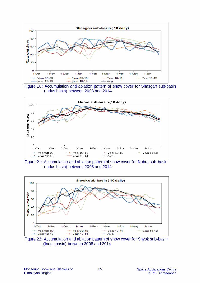
Monthly accumulation and ablation patterns (2008-2014) and Annual changes
(2004-2014) of snow cover
Figures 17 to 28 show the curves of accumulation and ablation of snow plotted against
time for each sub-basin of Indus basin. The curves have been generated from the
snow cover data generated from 2008-09 to 2013-14. It is observed from these curves
that for each sub-basin snow accumulation in each hydrological year differs from one
sub-basin to other. Within each sub-basin also the part of curve is not similar for each
hydrological year. This indicates high variability of snow accumulation in different sub-
basins. The unevenness in accumulation indicate precipitation and subsequent
melting of snow. But broadly it is observed that the sub-basins located at northern side
of Indus river are showing moderate slope of accumulation pattern in comparison to
sub-basins located at southern side. The slope of accumulation indicates rate of
precipitation. The point of initiation of accumulation also varies. The accumulation
pattern of Shasgan sub-basin is distinct as the accumulation starts from about 50 %
snow but does not reach more than 80 %. In all northern sub-basins, the snow cover
does not reach 100 % of the sub-basin area though the point of initiation is higher in
northern sub-basins. In southern sub-basins the point of initiation are much lower but
the maximum snow cover reaches near 100%. There are instances of sharp rise of
accumulation as seen in year 2009-10 and 2012-13. There is close similarity of
ablation pattern of snow cover for each sub-basin in different hydrological years. All
sub-basins behave in a similar manner. The slopes of northern sub-basins are gentler
than southern sub-basins. This indicates a contrast in the temperature regime of
northern and southern sub-basins. The accumulation and ablation of snow in Jhelum
sub-basin is different than of other sub-basins.

34 Monitoring Snow and Glaciers of Himalayan Region
Space Applications Centre ISRO, Ahmedabad
Figure 17: Accumulation and ablation pattern of snow cover for Gilgit sub-basin (Indus
basin) between 2008 and 2014
Figure 18: Accumulation and ablation pattern of snow cover for Hanza sub-basin
(Indus basin) between 2008 and 2014
Figure 19: Accumulation and ablation pattern of snow cover for Shigar sub-basin
(Indus basin) between 2008 and 2014
0
20
40
60
80
100
1-Oct 1-Nov 1-Dec 1-Jan 1-Feb 1-Mar 1-Apr 1-May 1-Jun
% A
real
ext
ent o
f sno
w
Gilgit sub-basin ( 10 daily)
Year 08-09 Year 09-10 Year 10-11 Year 11-12
year 12-13 year 13-14 Avg.
0
20
40
60
80
100
1-Oct 1-Nov 1-Dec 1-Jan 1-Feb 1-Mar 1-Apr 1-May 1-Jun
% A
real
ext
ent o
f sno
w
Hanza sub-basin ( 10 daily)
Year 08-09 Year 09-10 Year 10-11 Year 11-12
year 12-13 year 13-14 Avg.
0
20
40
60
80
100
1-Oct 1-Nov 1-Dec 1-Jan 1-Feb 1-Mar 1-Apr 1-May 1-Jun
% A
real
ext
ent o
f sno
w
Shigar sub-basin ( 10 daily)
Year 08-09 Year 09-10 Year 10-11 Year 11-12
year 12-13 year 13-14 Avg.
35 Monitoring Snow and Glaciers of Himalayan Region
Space Applications Centre ISRO, Ahmedabad
Figure 20: Accumulation and ablation pattern of snow cover for Shasgan sub-basin (Indus basin) between 2008 and 2014
Figure 21: Accumulation and ablation pattern of snow cover for Nubra sub-basin
(Indus basin) between 2008 and 2014
Figure 22: Accumulation and ablation pattern of snow cover for Shyok sub-basin (Indus basin) between 2008 and 2014
0
20
40
60
80
100
1-Oct 1-Nov 1-Dec 1-Jan 1-Feb 1-Mar 1-Apr 1-May 1-Jun
% A
real
ext
ent o
f sno
w
Nubra sub-basin (10 daily)
Year 08-09 Year 09-10 Year 10-11 Year 11-12
year 12-13 year 13-14 Avg.

36 Monitoring Snow and Glaciers of Himalayan Region
Space Applications Centre ISRO, Ahmedabad
Figure 23: Accumulation and ablation pattern of snow cover for Astor sub-basin (Indus basin) between 2008 and 2014
Figure 24: Accumulation and ablation pattern of snow cover for Kisanganga sub-basin
(Indus basin) between 2008 and 2014
Figure 25: Accumulation and ablation pattern of snow cover for Shigo sub-basin (Indus basin) between 2008 and 2014

37 Monitoring Snow and Glaciers of Himalayan Region
Space Applications Centre ISRO, Ahmedabad
Figure 26: Accumulation and ablation pattern of snow cover for Jhelum sub-basin (Indus basin) between 2008 and 2014
Figure 27: Accumulation and ablation pattern of snow cover for Suru sub-basin (Indus basin) between 2008 and 2014
Figure 28: Accumulation and ablation pattern of snow cover for Zanskar sub-bas
(Indus basin) between 2008 and 2014
-20
0
20
40
60
80
100
1-Oct 1-Nov 1-Dec 1-Jan 1-Feb 1-Mar 1-Apr 1-May 1-Jun
% A
real
ext
ent o
f sno
w
Jhelum sub-basin ( 10 daily)
Year 08-09 Year 09-10 Year 10-11 Year 11-12
year 12-13 year 13-14 Avg.
0
20
40
60
80
100
1-Oct 1-Nov 1-Dec 1-Jan 1-Feb 1-Mar 1-Apr 1-May 1-Jun
% A
real
ext
ent o
f sno
w
Suru sub-basin ( 10 daily)
Year 08-09 Year 09-10 Year 10-11 Year 11-12
year 12-13 year 13-14 Avg.
0
20
40
60
80
100
1-Oct 1-Nov 1-Dec 1-Jan 1-Feb 1-Mar 1-Apr 1-May 1-Jun
% A
real
ext
ent o
f sno
w
Zanskar sub-basin ( 10 daily)
Year 08-09 Year 09-10 Year 10-11 Year 11-12
year 12-13 year 13-14 Avg.

38 Monitoring Snow and Glaciers of Himalayan Region
Space Applications Centre ISRO, Ahmedabad
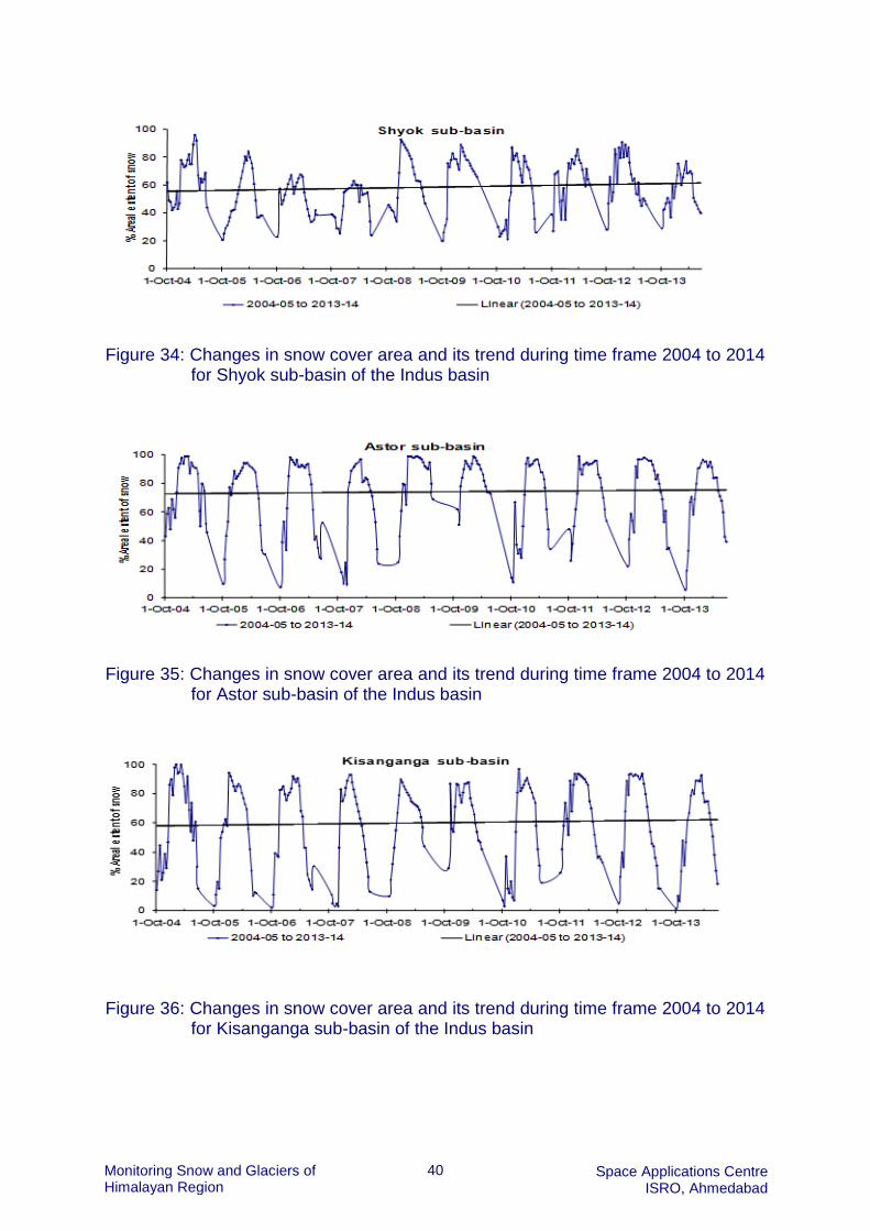
Snow cover variations from 2004 to 2014 for different sub-basins are shown in Figures
29 to 41. These trends also depend on intra-annual variability but represent an overall
trend of increase or decrease of snow cover. In all the 13 sub-basins there is no
increase or decrease of snow cover beyond 5% of Mean. This indicates that snow
precipitation within 10-year period has been almost stable. There is no difference in
the northern or southern basins across Indus river. Though the pattern of accumulation
and ablation in each year is different in different sub-basins but there is not much
change within 10-year period (Figure 4.1.29 to 4.1.41).
Figure 29: Changes in snow cover area and its trend during time frame 2004 to 2014
for Gilgit sub-basin of the Indus basin
Figure 30: Changes in snow cover area and its trend during time frame 2004 to 2014
for Hanza sub-basin of the Indus basin

39 Monitoring Snow and Glaciers of Himalayan Region
Space Applications Centre ISRO, Ahmedabad
Figure 31: Changes in snow cover area and its trend during time frame 2004 to 2014
for Shigar sub-basin of the Indus basin
Figure 32: Changes in snow cover area and its trend during time frame 2004 to 2014 for Shasgan sub-basin of the Indus basin
Figure 33: Changes in snow cover area and its trend during time frame 2004 to 2014
for Nubra sub-basin of the Indus basin
40 Monitoring Snow and Glaciers of Himalayan Region
Space Applications Centre ISRO, Ahmedabad
Figure 34: Changes in snow cover area and its trend during time frame 2004 to 2014
for Shyok sub-basin of the Indus basin
Figure 35: Changes in snow cover area and its trend during time frame 2004 to 2014
for Astor sub-basin of the Indus basin
Figure 36: Changes in snow cover area and its trend during time frame 2004 to 2014
for Kisanganga sub-basin of the Indus basin

41 Monitoring Snow and Glaciers of Himalayan Region
Space Applications Centre ISRO, Ahmedabad
Figure 37: Changes in snow cover area and its trend during time frame 2004 to 2014
Shigo sub-basin of the Indus basin
Figure 38: Changes in snow cover area and its trend during time frame 2004 to 2014
Drass sub-basin of the Indus basin
Figure 39: Changes in snow cover area and its trend during time frame 2004 to 2014
for Jhelum sub-basin of the Indus basin

42 Monitoring Snow and Glaciers of Himalayan Region
Space Applications Centre ISRO, Ahmedabad
Figure 40: Changes in snow cover area and its trend during time frame 2004 to 2014
for Suru sub-basin of the Indus basin
Figure 41: Changes in snow cover area and its trend during time frame 2004 to 2014
for Zanskar sub-basin of the Indus basin
ii) Chenab basin
Chenab basin comprises six sub-basins The sub-basins are Miyar, Bhaga, Chandra
Warwan and Bhut and Ravi. The following paragraphs describe temporal and spatial
variability of snow cover in the sub-basins of Chenab basin.
Minimum and maximum snow cover
For each sub-basin of Chenab basin, the minimum and maximum snow cover in each
hydrological year from 2004-05 to 2013-14 has been compiled in the Tables from 16
to 21. Referring to data compiled in these tables, it is observed that mean of minimum
snow cover is highest in Chandra sub-basin and lowest in Ravi sub-basin. There is a
large variation of minimum snow cover in each hydrological year and in each sub-
basin. The SD values of minimum snow cover indicate a large variation in minimum
snow cover. The mean values of maximum snow cover show 95 to 100 % snow cover
each year except in Ravi sub-basin. The SD values of maximum snow cover show
relatively less variation in maximum snow cover except in Ravi sub-basin.
0
20
40
60
80
100
1-Oct-04 1-Oct-05 1-Oct-06 1-Oct-07 1-Oct-08 1-Oct-09 1-Oct-10 1-Oct-11 1-Oct-12 1-Oct-13
% A
real
ext
ent o
f sno
w
Suru sub-basin
2004-05 to 2013-14 Linear (2004-05 to 2013-14)
0
20
40
60
80
100
1-Oct-04 1-Oct-05 1-Oct-06 1-Oct-07 1-Oct-08 1-Oct-09 1-Oct-10 1-Oct-11 1-Oct-12 1-Oct-13
% A
real
ext
ent o
f sno
w
Zaskar sub-basin
2004-05 to 2013-14 Linear (2004-05 to 2013-14)

43 Monitoring Snow and Glaciers of Himalayan Region
Space Applications Centre ISRO, Ahmedabad
The maximum and minimum amount of minimum snow cover also varies in each sub-
basin. Overall the minimum snow cover was lowest in Chenab basin in the 2013-14
year. The quantity of minimum snow cover varies in each year for different sub-basins
and is not uniformly same. This suggests that within Chenab basin also the different
sub-basins experience different amount of precipitation in different years.
Table 16: Minimum and maximum snow cover in Warwan sub-basin during 2004- 14
Warwan sub-basin ( 4670 sq. km)
Year Minimum snow cover Maximum snow cover
Sq. km % Sq. km %
2004-05 1868 40 4670 100
2005-06 747 16 4110 88
2006-07 1401 30 4203 90
2007-08 887 19 4483 96
2008-09 1074 23 4063 87
2009-10 1354 29 4670 100
2010-11 701 15 4483 96
2011-12 747 16 4623 99
2012-13 1261 27 4530 97
2013-14 607 13 4483 96
Mean 1065 23 4432 95
S D 402 9 226 5
Table 17: Minimum and maximum snow cover in Bhut sub-basin during 2004-14
Bhut sub-basin ( 2218 sq km)
Year Minimum snow cover Maximum snow cover
Sq km % Sq km %
2004-05 976 44 2218 100
2005-06 488 22 1952 88
2006-07 399 18 2018 91
2007-08 555 25 2174 98
2008-09 466 21 1930 87
2009-10 421 19 2218 100
2010-11 444 20 2107 95
2011-12 444 20 2196 99
2012-13 665 30 2151 97
2013-14 421 19 2151 97
Mean 528 24 2112 95
S D 176 8 107 5

44 Monitoring Snow and Glaciers of Himalayan Region
Space Applications Centre ISRO, Ahmedabad
Table 18: Minimum and maximum snow cover in Miyar sub-basin during 2004-14
Miyar sub-basin ( 4449 sq km)
Year Minimum snow cover Maximum snow cover
Sq km % Sq km %
2004-05 1913 43 4449 100
2005-06 845 19 4405 99
2006-07 578 13 4360 98
2007-08 890 20 4449 100
2008-09 1335 30 4360 98
2009-10 756 17 4449 100
2010-11 667 15 4449 100
2011-12 756 17 4449 100
2012-13 1290 29 4449 100
2013-14 534 12 4449 100
Mean 956 22 4427 100
S D 431 10 38 1
Table 19: Minimum and maximum snow cover in Bhaga sub-basin during 2004-14
Bhaga sub-basin ( 1680 sq km)
Year Minimum snow cover Maximum snow cover
Sq km % Sq. km %
2004-05 1159 69 1680 100
2005-06 638 38 1663 99
2006-07 420 25 1680 100
2007-08 504 30 1680 100
2008-09 840 50 1680 100
2009-10 672 40 1680 100
2010-11 622 37 1680 100
2011-12 470 28 1680 100
2012-13 907 54 1680 100
2013-14 353 21 1680 100
Mean 659 39 1678 100
S D 249 15 5 0
45 Monitoring Snow and Glaciers of Himalayan Region
Space Applications Centre ISRO, Ahmedabad
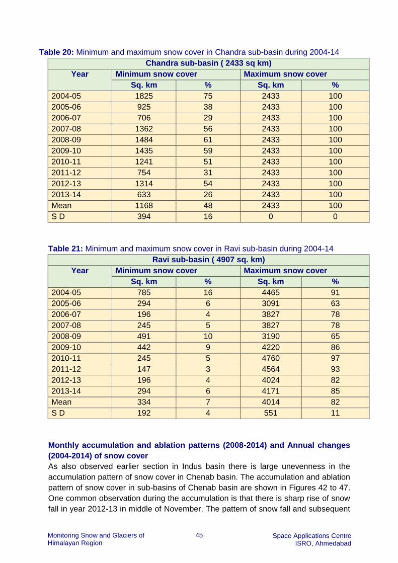
Table 20: Minimum and maximum snow cover in Chandra sub-basin during 2004-14
Chandra sub-basin ( 2433 sq km)
Year Minimum snow cover Maximum snow cover
Sq. km % Sq. km %
2004-05 1825 75 2433 100
2005-06 925 38 2433 100
2006-07 706 29 2433 100
2007-08 1362 56 2433 100
2008-09 1484 61 2433 100
2009-10 1435 59 2433 100
2010-11 1241 51 2433 100
2011-12 754 31 2433 100
2012-13 1314 54 2433 100
2013-14 633 26 2433 100
Mean 1168 48 2433 100
S D 394 16 0 0
Table 21: Minimum and maximum snow cover in Ravi sub-basin during 2004-14
Ravi sub-basin ( 4907 sq. km)
Year Minimum snow cover Maximum snow cover
Sq. km % Sq. km %
2004-05 785 16 4465 91
2005-06 294 6 3091 63
2006-07 196 4 3827 78
2007-08 245 5 3827 78
2008-09 491 10 3190 65
2009-10 442 9 4220 86
2010-11 245 5 4760 97
2011-12 147 3 4564 93
2012-13 196 4 4024 82
2013-14 294 6 4171 85
Mean 334 7 4014 82
S D 192 4 551 11
Monthly accumulation and ablation patterns (2008-2014) and Annual changes
(2004-2014) of snow cover
As also observed earlier section in Indus basin there is large unevenness in the
accumulation pattern of snow cover in Chenab basin. The accumulation and ablation
pattern of snow cover in sub-basins of Chenab basin are shown in Figures 42 to 47.
One common observation during the accumulation is that there is sharp rise of snow
fall in year 2012-13 in middle of November. The pattern of snow fall and subsequent

46 Monitoring Snow and Glaciers of Himalayan Region
Space Applications Centre ISRO, Ahmedabad
melting of snow up to middle of January is common in all the sub-basins. There is
quite similarity in melting of snow cover from early march onwards. The slopes of
ablation are also gentle. This indicates that there is no sudden rise of temperature up
to end of June. In some of the sub-basins the snow cover becomes 100 % but in the
sub-basins located in lower altitude such as Ravi sub-basin the snow cover does not
reach 100 %. The slopes of accumulation and ablation in Ravi sub-basin are sharper
as compared to her sub-basins. In Chandra basin the minimum snow cover before
and after ablation season more or less remains same. Chandra and Bhaga sub-basins
behave more or less in similar way as they are located near to each other. Warwan
and Bhut sub-basins behave in a similar way as they are closer to each other
geographically but quite away from Chandra and Bhaga sub-basins. Miyar sub-basin
is located north of Chandra and Bhaga. Ravi sub-basin mainly drains in Kangra district
and is climatically located much away from Chandra and Bhaga basin and thus
respond differently to snow precipitation and melting.
Figure 42: Accumulation and ablation pattern of snow cover for Warwan sub-basin (Chenab basin) between 2008 and 2014
Figure 43: Accumulation and ablation pattern of snow cover for Bhut sub-basin
(Chenab basin) between 2008 and 2014

47 Monitoring Snow and Glaciers of Himalayan Region
Space Applications Centre ISRO, Ahmedabad
Figure 44: Accumulation and ablation pattern of snow cover for Miyar sub-basin (Chenab basin) between 2008 and 2014
Figure 45: Accumulation and ablation pattern of snow cover for Bhaga sub-basin
(Chenab basin) between 2008 and 2014
Figure 46: Accumulation and ablation pattern of snow cover for Chandra sub-basin (Chenab basin) between 2008 and 2014

48 Monitoring Snow and Glaciers of Himalayan Region
Space Applications Centre ISRO, Ahmedabad
Figure 47: Accumulation and ablation pattern of snow cover for Ravi sub-basin
(Chenab basin) between 2008 and 2014
Changes in snow cover for the duration 2004-2014 in sub-basins of the Chenab basin
are shown in Figure 48 to Figure 53. It is observed that Ravi sub-basin shows minimum
snow cover (5 to 70%), while remaining sub-basins show snow cover changes ranging
20 to 100% annually. All the sub-basins are showing a marginal increasing trend of
snow cover during 2004-2014 time frame.
Figure 48: Changes in snow cover area and its trend during time frame 2004 to 2014
for Warwan sub-basin of the Chenab basin
0
20
40
60
80
100
1-Oct-04 1-Oct-05 1-Oct-06 1-Oct-07 1-Oct-08 1-Oct-09 1-Oct-10 1-Oct-11 1-Oct-12 1-Oct-13
% A
real
exte
nt
of
sn
ow
Warwan sub-basin
2004-05 to 2013-14 Linear (2004-05 to 2013-14)

49 Monitoring Snow and Glaciers of Himalayan Region
Space Applications Centre ISRO, Ahmedabad
Figure 49: Changes in snow cover area and its trend during time frame 2004 to 2014
for Bhut sub-basin of the Chenab basin
Figure 50: Changes in snow cover area and its trend during time frame 2004 to 2014 for Miyar sub-basin of the Chenab basin
Figure 51: Changes in snow cover area and its trend during time frame 2004 to 2014
for Bhaga sub-basin of the Chenab basin

50 Monitoring Snow and Glaciers of Himalayan Region
Space Applications Centre ISRO, Ahmedabad
Figure 52: Changes in snow cover area and its trend during time frame 2004 to 2014
for Chandra sub-basin of the Chenab basin
Figure 53: Changes in snow cover area and its trend during time frame 2004 to 2014
for Ravi sub-basin of the Chenab basin iii) Satluj basin
Satluj basin comprises six sub-basins covering 15583 sq km area. The sub-basins are
Beas, Parbati, Jiwa, Baspa, Pin and Spiti sub-basins. Parbati and Jiwa river are
tributary of Beas river. Beas, Baspa, Pin & Spiti are tributary of Satluj river.
Maximum and minimum snow cover
For each sub-basin of Satluj basin the minimum and maximum snow cover in each
hydrological year from 2004-05 to 2013-14 has been compiled in the Tables 22 to 27.
The snow cover has been represented in absolute value and in percentage. Mean and
standard deviations (SD) of snow cover are also mentioned in the tables.
The mean of minimum snow cover in % varies from 9 to 37 for different sub-basins.
The SD of minimum snow cover varies from 4 to 23. This is a large variation in snow
cover in each year for different sub-basins. The mean of minimum snow cover is high
in Pin, Basapa and Parbati sub-basins and very low in rest of sub-basins. The mean

51 Monitoring Snow and Glaciers of Himalayan Region
Space Applications Centre ISRO, Ahmedabad
of maximum snow cover is high in almost all the sub-basins except in. Jiwa sub-basin.
The variation in maximum snow cover is seen more in Jiwa sub-basin. The maximum
and minimum amount of minimum snow cover also varies in each sub-basin. This
suggests that within Satluj basin also the different sub-basins experience different
amount of precipitation in different years.
Table 22: Minimum and maximum snow cover in Beas sub-basin during 2004-14
Beas sub-basin ( 1132 sq. km)
Year Minimum snow cover Maximum snow cover
Sq. km % Sq. km %
2004-05 204 18 996 88
2005-06 79 7 872 77
2006-07 45 4 928 82
2007-08 102 9 917 81
2008-09 158 14 804 71
2009-10 125 11 1109 98
2010-11 68 6 940 83
2011-12 45 4 1121 99
2012-13 79 7 1109 98
2013-14 102 9 1075 95
Mean 101 9 987 87
S D 50 4 112 10
Table 23: Minimum and maximum snow cover in Parbati sub-basin during 2004-14
Parbati sub-basin ( 1773 sq. km)
Year Minimum snow cover Maximum snow cover
Sq. km % Sq. km %
2004-05 904 51 1613 91
2005-06 479 27 1489 84
2006-07 426 24 1578 89
2007-08 638 36 1578 89
2008-09 851 48 1472 83
2009-10 762 43 1738 98
2010-11 656 37 1578 89
2011-12 426 24 1720 97
2012-13 638 36 1738 98
2013-14 372 21 1720 97
Mean 615 35 1622 92
S D 186 11 101 6

52 Monitoring Snow and Glaciers of Himalayan Region
Space Applications Centre ISRO, Ahmedabad
Table 24: Minimum and maximum snow cover in Jiwa sub-basin during 2004-14
Jiwa sub-basin (1445 sq. km)
Year Minimum snow cover Maximum snow cover
Sq. km % Sq. km %
2004-05 246 17 968 67
2005-06 116 8 751 52
2006-07 87 6 838 58
2007-08 173 12 983 68
2008-09 202 14 665 46
2009-10 173 12 1214 84
2010-11 101 7 910 63
2011-12 87 6 1344 93
2012-13 145 10 1344 93
2013-14 72 5 1199 83
Mean 140 10 1022 71
S D 57 4 242 17
Table 25: Minimum and maximum snow cover in Baspa sub-basin during 2004-14
Baspa sub-basin (1096 sq. km)
Year Minimum snow cover Maximum snow cover
Sq. km % Sq. km %
2004-05 504 46 1096 100
2005-06 274 25 1074 98
2006-07 175 16 1096 100
2007-08 219 20 1096 100
2008-09 406 37 1052 96
2009-10 449 41 1096 100
2010-11 449 41 1052 96
2011-12 197 18 1096 100
2012-13 252 23 1096 100
2013-14 252 23 1096 100
Mean 318 29 1085 99
S D 121 11 19 2

53 Monitoring Snow and Glaciers of Himalayan Region
Space Applications Centre ISRO, Ahmedabad
Table 26: Minimum and maximum snow cover in Pin sub-basin during 2004-14
Pin sub-basin (1266 sq. km)
Year Minimum snow cover Maximum snow cover
Sq. km % Sq. km %
2004-05 696 55 1266 100
2005-06 342 27 1266 100
2006-07 329 26 1266 100
2007-08 506 40 1266 100
2008-09 658 52 1266 100
2009-10 671 53 1266 100
2010-11 481 38 1266 100
2011-12 203 16 1266 100
2012-13 380 30 1266 100
2013-14 203 16 1266 100
Mean 447 35 1266 100
S D 186 15 0 0
Table 27: Minimum and maximum snow cover in Spiti sub-basin during 2004-14
Spiti sub-basin (8871 sq. km)
Year Minimum snow cover Maximum snow cover
Sq. km % Sq. km %
2004-05 2306 26 8782 99
2005-06 1419 16 8427 95
2006-07 444 5 8427 95
2007-08 1508 17 8427 95
2008-09 2306 26 8427 95
2009-10 2218 25 8516 96
2010-11 1952 22 8871 100
2011-12 532 6 8871 100
2012-13 976 11 8871 100
2013-14 710 8 8871 100
Mean 1437 16 8649 98
S D 741 8 218 2
Monthly accumulation and ablation patterns (2008-2014) and Annual changes
(2004-2014) of snow cover
The accumulation or ablation paten of snow cover in sub-basins of Satluj basin are
shown in Figures 54 to 59. The pattern of accumulation in all the sub-basins are closely
matching indicating sharp rise in slopes or precipitation and subsequent melting. The
pattern of snow accumulation is similar in Parbati and Beas sub-basins. It is similar in
Basapa, Pin and Spiti sub-basins. The precipitation in Jiwa sub-basin is different than
in other sub-basins. This likely due to geographical and climatic similarity. Slopes of

54 Monitoring Snow and Glaciers of Himalayan Region
Space Applications Centre ISRO, Ahmedabad
accumulation are steeper than in ablation. This is commonly observed in all sub-basins
of Himalaya except in North-Western region. In the pattern of accumulation there is
an unevenness indicating precipitation followed by melting. The unevenness is more
in Basapa, Pin and Spiti sub-basins than in Beas and Parbati sub-basins. There are
certain anomalies too. Maximum snow cover is attained in middle of January. The
slopes of accumulation and ablation are sharper. Those sub-basins which are at
higher altitude, the maximum snow cover reaches to 100 % and remains there for at
least two months. The lowest part of ablation curves indicates that by end of June the
snow cover does not reach to a low value in certain sub-basins as observed in Parbati
and Pin sub-basins. The slope of ablation of Beas and Spiti sub-basins is steeper
indicating a rapid decline in snow or melting.
Figure 54: Accumulation and ablation pattern of snow cover for Beas sub-basin
(Satluj basin) between 2008 and 2014
Figure 55: Accumulation and ablation pattern of snow cover for Parbati sub-basin
(Satluj basin) between 2008 and 2014

55 Monitoring Snow and Glaciers of Himalayan Region
Space Applications Centre ISRO, Ahmedabad
Figure 56: Accumulation and ablation pattern of snow cover for Jiwa sub-basin
(Satluj basin) between 2008 and 2014
Figure 57: Accumulation and ablation pattern of snow cover for Baspa
sub-basin (Satluj basin) between 2008 and 2014
Figure 58: Accumulation and ablation pattern of snow cover for Pin sub-basin (Satluj
basin) between 2008 and 2014

56 Monitoring Snow and Glaciers of Himalayan Region
Space Applications Centre ISRO, Ahmedabad
Figure 59: Accumulation and ablation pattern of snow cover for Spiti sub-basin
(Satluj basin) between 2008 and 2014
Monthly accumulation and ablation patterns (2008-2014) and Annual changes
(2004-2014) of snow cover
Figures 60 to 65 show trend of snow cover in each sub-basin from 2004 to 2014. There
is slight increase in snow cover of the order of 0 to 10 % in Beas, Parbati and Jiwa
sub-basin. But in Basapa, Pin and Spiti sub-basins, no trend of decrease or increase
of snow cover is observed.
Figure 60: Changes in snow cover area and its trend during time frame 2004 to 2014
for Beas sub-basin of the Satluj basin
0
20
40
60
80
100
1-Oct-04 1-Oct-05 1-Oct-06 1-Oct-07 1-Oct-08 1-Oct-09 1-Oct-10 1-Oct-11 1-Oct-12 1-Oct-13
% A
rea
l e
xte
nt
of
sn
ow
Beas sub-basin
2004-05 to 2013-14 Linear (2004-05 to 2013-14)

57 Monitoring Snow and Glaciers of Himalayan Region
Space Applications Centre ISRO, Ahmedabad
Figure 61: Changes in snow cover area and its trend during time frame 2004 to 2014
for Parbati sub-basin of the Satluj basin
Figure 62: Changes in snow cover area and its trend during time frame 2004 to 2014
for Jiwa sub-basins of the Satluj basin
Figure 63: Changes in snow cover area and its trend during time frame 2004 to 2014 for Baspa sub-basins of the Satluj basin

58 Monitoring Snow and Glaciers of Himalayan Region
Space Applications Centre ISRO, Ahmedabad
Figure 64: Changes in snow cover area and its trend during time frame 2004 to 2014
for Pin sub-basin of the Satluj basin
Figure 65: Changes in snow cover area and its trend during time frame 2004 to 2014
for Spiti sub-basins of the Satluj basin
iv) Ganga basin
Three sub-basins have been monitored in Ganga basin covering 22055 sq. km area
viz., Bhagirathi, Yamuna and Alaknanda sub-basins. Alaknanda sub-basin is in east
of Bhagirathi and Yamuna is in west of it.
Minimum and maximum snow cover
The following Tables 28-30 present the amount of minimum and maximum snow cover
in three sub-basins. There is not much variation in mean of minimum snow cover as
indicated by SD values. However, the variation of maximum snow cover is higher.
The minimum snow cover varies between 9 to 21 %. It is very low in year 2005-06 and

59 Monitoring Snow and Glaciers of Himalayan Region
Space Applications Centre ISRO, Ahmedabad
2006-07. The maximum snow cover in Bhagirathi sub basin varies between 54 to 79
%. In most of the years it is below 70 % except in year 2011-12 and 2013-14. The SD
values suggest low values for all three sub-basins. This suggest less variability of snow
cover in Ganga basin in comparison to other basins.
Table 28: Minimum and maximum snow cover in Bhagirathi sub-basin during 2004-14
Bhagirathi sub-basin (7438 sq. km)
Year Minimum snow cover Maximum snow cover
Sq. km % Sq. km %
2004-05 1562 21 4909 66
2005-06 818 11 3942 53
2006-07 669 9 4165 56
2007-08 1339 18 4165 56
2008-09 1264 17 4017 54
2009-10 1190 16 4983 67
2010-11 1339 18 4017 54
2011-12 893 12 5876 79
2012-13 1041 14 4686 63
2013-14 818 11 5727 77
Mean 1093 15 4649 63
S D 289 4 716 10
Table 29: Minimum and maximum snow cover in Yamuna sub-basin during 2004-14
Yamuna sub-basin (3527 sq. km)
Year Minimum snow cover Maximum snow cover
Sq. km % Sq. km %
2004-05 459 13 2645 75
2005-06 212 6 1622 46
2006-07 141 4 1728 49
2007-08 388 11 2081 59
2008-09 353 10 1622 46
2009-10 353 10 2857 81
2010-11 317 9 1728 49
2011-12 282 8 3068 87
2012-13 353 10 2575 73
2013-14 317 9 3174 90
Mean 318 9 2310 66
S D 90 3 622 18

60 Monitoring Snow and Glaciers of Himalayan Region
Space Applications Centre ISRO, Ahmedabad
Table 30: Minimum and maximum snow cover in Alaknanda sub-basin during 2004-14
Alaknanda sub-basin (11090 sq km)
Year Minimum snow cover Maximum snow cover
Sq. km % Sq. km %
2004-05 2218 20 6765 61
2005-06 1996 18 5656 51
2006-07 1220 11 6321 57
2007-08 2551 23 5989 54
2008-09 1774 16 5545 50
2009-10 2107 19 7319 66
2010-11 2551 23 5878 53
2011-12 998 9 7874 71
2012-13 1553 14 6543 59
2013-14 1774 16 7985 72
Mean 1874 17 6588 59
S D 519 5 886 8
Monthly accumulation and ablation patterns (2008-2014) and Annual changes
(2004-2014) of snow cover
In Bhagirathi sub-basin there is consistency in accumulation pattern except in one
year. The snow cover varies between 20 to 80 % during accumulation period. The
accumulation period is more uneven indicating precipitation and simultaneous melting.
The maximum snow cover is observed in middle of February. Then there is a gradual
decline in snow cover indicating gradual rise in temperature (Figure 66).
In Yamuna sub-basin snow cover varies from about 10 % to maximum 90 %. The
decline in snow cover has higher slopes indicating sharp fall in snow cover. The peak
of maximum snow cover is sharper in Yamuna sub-basin then in Bhagirathi basin
(Figure 67).
In Alaknanda sub-basin the unevenness in accumulation is less than in Bhagirathi or
Yamuna sub-basin. The maximum variation in accumulation is seen to vary between
20% to 70 %. The decline in snow cover is very gentle and similar to Bhagirathi sub-
basin. Snow cover decline is consistent in all the years (Figure 68).

61 Monitoring Snow and Glaciers of Himalayan Region
Space Applications Centre ISRO, Ahmedabad
Figure 66: Accumulation and ablation pattern of snow cover for Bhagirathi sub-basin
(Ganga basin) between 2008 and 2014
Figure 67: Accumulation and ablation pattern of snow cover for Yamuna sub-basin
(Ganga basin) between 2008 and 2014
Figure 68: Accumulation and ablation pattern of snow cover for Alaknanda sub-basin
(Ganga basin) between 2008 and 2014

62 Monitoring Snow and Glaciers of Himalayan Region
Space Applications Centre ISRO, Ahmedabad
Inter-annual variations indicate an increasing trend of snow cover in Bhagirathi sub-
basin (Figure 69) and Yamuna sub-basins (Figure 70). The trend is consistent in
Alaknanda basin (Figure 71).
Figure 69: Changes in snow cover area and its trend during time frame 2004 to 2014 for Bhagirathi sub-basin of the Ganga basin
Figure 70: Changes in snow cover area and its trend during time frame 2004 to 2014 for Yamuna sub-basin of the Ganga basin
Figure 71: Changes in snow cover area and its trend during time frame 2004 to 2014
for Alaknanda sub-basin of the Ganga basin

63 Monitoring Snow and Glaciers of Himalayan Region
Space Applications Centre ISRO, Ahmedabad
v) Tista Basin
Tista basin has two sub-basins namely Tista and Rangit sub-basins covering 7096 sq.
km area in Sikkim state. The spatial and temporal variability of these two sub-basins
are discussed as following;
Minimum and maximum snow cover
The minimum and maximum snow cover in each hydrological year from 2004-05 to
2013-14 has been compiled in the Tables 31 and 32. It is observed from the data that
Tista sub-basin gets more precipitation than Rangit sub-basin. The mean values of
snow cover show that the minimum % of snow cover in Rangit sub-basin is much
lesser than Tista sub-basin. The standard deviation of minimum snow cover suggests
more temporal variability in Tista sub-basin than in Rangit sub-basin. and % of
maximum snow cover is also less in Rangit. The data of maximum snow cover also
shows higher % of snow cover in Tista sub-basin than in Rangit sub-basin. The SD
values suggest close similarity in temporal variability of snow cover.
Table 31: Minimum and maximum snow cover in Tista sub-basin during 2004-14
Tista sub-basin (5466 sq km)
Year Minimum snow cover Maximum snow cover
Sq. km % Sq. km %
2004-05 1039 19 3280 60
2005-06 547 10 3006 55
2006-07 984 18 3662 67
2007-08 765 14 2569 47
2008-09 820 15 3006 55
2009-10 547 10 2733 50
2010-11 437 8 2842 52
2011-12 547 10 3389 62
2012-13 765 14 3772 69
2013-14 547 10 3498 64
Mean 700 13 3176 58
S D 206 4 406 7

64 Monitoring Snow and Glaciers of Himalayan Region
Space Applications Centre ISRO, Ahmedabad
Table 32: Minimum and maximum snow cover in Rangit sub-basin during 2004-14
Rangit sub-basin (1630 sq. km)
Year Minimum snow cover Maximum snow cover
Sq. km % Sq. km %
2004-05 82 5 310 19
2005-06 49 3 310 19
2006-07 65 4 489 30
2007-08 98 6 293 18
2008-09 49 3 310 19
2009-10 49 3 277 17
2010-11 33 2 228 14
2011-12 49 3 261 16
2012-13 33 2 440 27
2013-14 49 3 391 24
Mean 56 3 331 20
S D 21 1 83 5
Monthly accumulation and ablation patterns (2008-2014) and Annual changes
(2004-2014) of snow cover
It is observed that in Tista sub-basin there is more unevenness in precipitation,
however in ablation season there is gradual decline of snow cover. The time of highest
snow cover in Tista sub-basin is late January (Figure 72). The pattern of Rangit sub-
basin is unique among all the sub-basins in terms of accumulation and ablation. In
Rangit sub-basin the accumulation and ablation curves in each year are more or less
similar in pattern (Figure 73). Its near horizontal pattern indicates low precipitation
and low ablation. In Rangit sub-basin the snow cover does not exceed more than 20
%.
Figure 72: Accumulation and ablation pattern of snow cover for Tista sub-basin between 2008 and 2014

65 Monitoring Snow and Glaciers of Himalayan Region
Space Applications Centre ISRO, Ahmedabad
Figure 73: Accumulation and ablation pattern of snow cover for Rangit sub-basin
between 2008 and 2014
In Tista sub-basin there is slight gain of snow cover of the order of 0 to 5 % over a
period of 10 years (Figure 74). In Rangit sub-basin, in contrast, there is consistency of
snow cover during this period (Figure 75). Tista sub-basin covers areas of high altitude
and northern latitudes than the Rangit sub-basin. The trend of snow cover in Rangit
sub-basin remains near horizontal.
Figure 74: Changes in snow cover area and its trend during time frame 2004 to 2014
for Tista sub-basin of the Tista basin

66 Monitoring Snow and Glaciers of Himalayan Region
Space Applications Centre ISRO, Ahmedabad
Figure 75: Changes in snow cover area and its trend during time frame 2004 to 2014 for Rangit sub-basin of the Tista basin
vi) Brahmaputra basin
Tawang, Subansiri and Dibang sub-basins are part of Brahmaputra basin and drain in
Arunachal Pradesh in north-east of India. These sub-basins together cover 41224 sq.
km area.
Minimum and maximum snow cover
The minimum and maximum snow cover in each hydrological year from 2004-05 to
2013-14 has been compiled in the Tables 33 to 35. It is observed that areal extent of
snow in 2008-09, 2009-10, 2010-11 & 2011-12 were higher than the mean of all years
of observations for all the sub-basins. It is observed that there is a not much variation
of minimum snow covers in each hydrological year and in each sub-basin but the
variation in maximum snow cover is relatively higher. The mean of maximum snow
cover varies among three sub-basins. The SD values suggest low temporal variability
in minimum snow cover. However, for all the three sub-basins there is contrast in
minimum and maximum snow cover. This suggests that within Brahmaputra basin,
different sub-basins experience different amount of precipitation in different years. The
mean and standard deviation values suggest that variation is higher in Tawang sub-
basin.

67 Monitoring Snow and Glaciers of Himalayan Region
Space Applications Centre ISRO, Ahmedabad
Table 33: Minimum and maximum snow cover in Tawang sub-basin during 2004-14
Tawang sub-basin (6721 sq. km)
Year Minimum snow cover Maximum snow cover
Sq. km % Sq. km %
2004-05 874 13 4839 72
2005-06 269 4 3764 56
2006-07 605 9 5780 86
2007-08 67 1 4839 72
2008-09 538 8 5175 77
2009-10 336 5 3965 59
2010-11 1075 16 4772 71
2011-12 403 6 6049 90
2012-13 336 5 5578 83
2013-14 538 8 3697 55
Mean 504 8 4846 72
SD 296 4 832 12
Table 34: Minimum and maximum snow cover in Subansiri sub-basin during 2004-14
Subansiri sub-basin (25345 sq. km)
Year Minimum snow cover Maximum snow cover
Sq. km % Sq. km %
2004-05 507 2 5576 22
2005-06 1267 5 5069 20
2006-07 2028 8 8110 32
2007-08 760 3 5576 22
2008-09 2535 10 9124 36
2009-10 1014 4 9124 36
2010-11 1267 5 6083 24
2011-12 760 3 7350 29
2012-13 1267 5 7604 30
2013-14 1267 5 4562 18
Mean 1267 5 6818 27
S D 609 2 1666 7

68 Monitoring Snow and Glaciers of Himalayan Region
Space Applications Centre ISRO, Ahmedabad
Table 35: Minimum and maximum snow cover in Dibang sub-basin during 2004-14
Dibang sub-basin (9158 sq. km)
Year Minimum snow cover Maximum snow cover
Sq. km % Sq. km %
2004-05 549 6 5953 65
2005-06 1832 20 3846 42
2006-07 824 9 5770 63
2007-08 458 5 6227 68
2008-09 1007 11 4762 52
2009-10 2564 28 4762 52
2010-11 458 5 5312 58
2011-12 1007 11 5312 58
2012-13 733 8 5128 56
2013-14 458 5 5220 57
Mean 989 11 5229 57
S D 693 8 682 7
Monthly accumulation and ablation patterns (2008-2014) and Annual changes
(2004-2014) of snow cover
The analysis of accumulation and ablation patterns of snow cover show a distinct
pattern in three sub-basins. In Tawang sub-basin the snow cover remains steady up
to end of January followed by a sharp rise (Figure 76). Then it gradually decreases. In
Subansiri sub-basin there is neither growth nor decay of snow cover. There remains
a permanent snow cover of about less than 20% area of sub-basin (Figure 77). In
Dibang sub-basin there is gentle rise of snow cover and gentle melting down (Figure
78). The pattern almost remains same in each year. These sub-basins are located
adjacent each other, however snow precipitation and melting have a distinct contrast.
Figure 76: Accumulation and ablation pattern of snow cover for Tawang sub-basin (Brahmaputra basin) between 2008 and 2014

69 Monitoring Snow and Glaciers of Himalayan Region
Space Applications Centre ISRO, Ahmedabad
Figure 77: Accumulation and ablation pattern of snow cover for Subansiri sub-basin
(Brahmaputra basin) between 2008 and 2014
Figure 78: Accumulation and ablation pattern of snow cover for Dibang sub-basin (Brahmaputra basin) between 2008 and 2014
In Tawang and Subansiri sub-basins, a decrease in snow cover has been observed
(Figure 79 and Figure 80). It is higher in Tawang i.e. less than 10%. In Subansiri sub-
basin the decrease is much lesser. In Dibang sub basin there is 2-3 % rise in snow
cover (Figure 81). The sub-basins in Arunachal Pradesh are influenced by climate of
Bay of Bengal. The sub-basins are south facing and due to difference in altitude and
geographic location respond differently to climatic variations.

70 Monitoring Snow and Glaciers of Himalayan Region
Space Applications Centre ISRO, Ahmedabad
Figure 79: Changes in snow cover area and its trend during time frame 2004 to 2014
for Tawang sub-basin of the Brahmaputra basin
Figure 80: Changes in snow cover area and its trend during time frame 2004 to 2014 for Subansiri sub-basin of the Brahmaputra basin
Figure 81: Changes in snow cover area and its trend during time frame 2004 to 2014
for Dibang sub-basin of the Brahmaputra basin

71 Monitoring Snow and Glaciers of Himalayan Region
Space Applications Centre ISRO, Ahmedabad
Overall, it is summarized that the analysis of snow cover data of 33 sub-basins for the
period 2004-2014 shows 1-7 % increase in snow cover. It has been observed that
snow line has come down to lower altitudes during the time frame 2010-2014 as
compared to previous years. It is also observed that variation in snow cover changes
are higher during October to February time frame.
Analysis of the mean maximum, mean minimum and mean variability ranges of snow
cover area for 33 sub-basins of the Himalayan region during accumulation and
ablations seasons of 2004-2014 time frame reveals that characteristics of snow cover
extent in western (Indus, Chenab and Satluj), west-central (Ganga) and eastern (Tista
and Brahamaputra) sub-basins are distinctly different i.e., western sub-basins (max.
71—100%, min. 3 – 54% and variability 39-90%), West-Central (max. 59-66%, min.
9-17% and variability 42-57%) and Eastern (max. 20-72%, min. 3-13% and variability
17-64%). The study indicated that the snow cover in the West-Central and Eastern
Himalaya is around 30-40 % less as compared to sub-basins in the Western Himalaya
during accumulation period.
During ablation season minimum snow cover has been observed in Jhelum (Indus),
Rangit (Tista) and Subansiri (Brahamaputra) sub-basins ( < 5%) and maximum snow
cover has been observed in Shigar (Indus) and Nubra (Indus) Sub-basins ( > 50%).
During accumulation season Shigo (Indus), Suru (Indus), Miyar (Chenab), Bhaga
(Chenab), Chandra (Chenab) and Pin (Satluj) sub-basins are observed to have 100%
snow cover, whereas minimum snow cover is observed in the Rangit (Tista) and
Subansiri sub-basins (Brahamaputra) (20-27%). The mean variability of maximum and
minimum snow cover is observed in Shigo (Indus) sub-basin (90%) and minimum in
Rangit sub-basin (Tista) (17%). The mean variability of maximum and minimum snow
cover is observed to be low for sub-basins north of the Indus river i.e., Gilgit, Hanza,
Shigar, Sasgan, Nubra and Shyok (39-59%) and high for sub-basins south of the Indus
river i.e., Astor, Kisanganga, Shigo, Drass, Jhelum, Suru and Zanskar (71-90%). The
temporal fluctuations of snow cover during accumulation season is higher in Jhelum
(Indus), Jiwa (Satluj) and Yamuna sub-basins (Ganga) (17-19 %).
Analysis of the annual accumulation and ablation pattern of snow cover in 33 sub-
basins during 2008-2014 time frame has shown that variability of snow cover changes
is higher during accumulation period than in ablation period. This is probably due to
the fact that during the accumulation period snow reaches to its lower altitudes where
fluctuations are rapid due to variations in temperature.
72 Monitoring Snow and Glaciers of Himalayan Region
Space Applications Centre ISRO, Ahmedabad
vii) Detailed comparative analysis of spatial and temporal variability of snow
cover in Alaknanda, Bhagirathi and Yamuna sub-basins of Ganga basin
A detailed comparative analysis of snow cover data of Alaknanda, Bhagirathi and
Yamuna sub-basins of Ganga basin was carried out (Rathore et al., 2015a). Monthly
average snow cover reached to its maximum in the month of January 2012 for all three
sub-basins, corresponding to 71, 79 and 87 % (7874, 5876 and 3068 sq. km) of the
total area for Alaknanda, Bhagirathi and Yamuna sub-basins respectively. The
minimum was observed during October 2012 which corresponds to 9, 9 and 4 % (998,
669 and 141 sq. km) of the total area respectively. Monthly average snow cover for
the period 2004-12 along with ±1σ was analyzed (Figure 82). Most of the variations
were observed during accumulation period especially in Yamuna sub-basin which is
located at lower altitude ranging from 1000 to 6100 m. Alaknanda sub-basin has
shown relatively low variation in standard deviation for monthly averaged snow cover
for the period 2004-12 in comparison to other two sub-basins. However, Bhagirathi
shows more snow cover area which could be due to coverage of more sub-basin area
under high altitude region as shown in the hypsographic curve of all sub-basins (Figure
83).
If total snow cover over a year is considered in Ganga basin, then it is seen that areal
extent of snow for the year 2004-05, 2007-08 and 2011-12 was higher than the mean
of total snow cover over eight years (Figure 84). Snow cover area has shown slight
increasing trend for all sub-basins from 2004 to 2014, however, it was found to be
statistically insignificant using Mann-Kendall test. Minimum snow cover has not shown
any variation which corresponds to negligible change in maximum snow line altitude,
whereas maximum snow cover has shown an increasing pattern which corresponds
to lowering of snow line altitude during the observed period that means snow fall
reaches to lower region.
The pattern of accumulation and ablation also differs from one basin to other in Ganga
basin. Annual accumulation and ablation pattern of snow cover of each sub-basins
from 2004-2012 is shown in Figure 84. Frequent fluctuations of snow cover are
observed during accumulation period. These fluctuations are being attributed to
frequent snowfalls and continuous melting in the lower altitude regions. But this
phenomenon is not true for ablation period. As the snow line progressively moves up
during ablation months (April to June), fluctuations in snow cover on higher altitudes
are not observed. Yamuna sub-basin has shown accumulation and ablation
throughout the year in comparison to other two sub-basins as 77 % of the area falls
below 4000-meter altitude. The gradient of ablation curves for all the years are similar
indicating comparable time and rates of melting. Area-altitude distribution indicating
the area covered in some definite altitude zones area was estimated for each sub-
basin. The distribution is shown by hypsographic curves. Hypsographic curves of
Yamuna sub-basin show gentle slope among all the three sub-basins which indicates

73 Monitoring Snow and Glaciers of Himalayan Region
Space Applications Centre ISRO, Ahmedabad
Yamuna sub-basin to be located in lower altitude zones than Bhagirathi or Alaknanda
sub-basins.
Figure 82: Monthly average snow cover for the period for 2004 to 2012 along with ±1σ
(Source: Rathore et al., 2015a)
Figure 83: Hypsographic curve giving percentage cumulative area for Alaknanda,
Bhagirathi and Yamuna sub-basins (Source: Rathore et al., 2015a)
0
2000
4000
6000
0 20 40 60 80 100
Alaknanda sub-basin Bhagirathi sub-basin Yamuna sub-basin
Alt
itu
de
(m)
Cumulative area (%)
0
20
40
60
80
Oct
De
c
Feb
Ap
r
Jun
e
Yamuna sub-basin
0
20
40
60
80
Oct
De
c
Feb
Ap
r
Jun
e
Bhagirathi sub-basin
0
20
40
60
80
Oct
De
c
Feb
Ap
r
Jun
% s
no
w c
ove
r Alaknanda sub-basin

74 Monitoring Snow and Glaciers of Himalayan Region
Space Applications Centre ISRO, Ahmedabad
Figure 84: Snow accumulation and ablation pattern for Alaknanda, Bhagirathi and
Yamuna sub-basins between 2004 and 2012 (Source: Rathore et al.,
2015a)
However, it was observed that 60 % of the area of Bhagirathi sub-basin falls in higher
altitudes in comparison to Alaknanda sub-basin. Mean monthly minimum and
maximum snow cover was computed as 2329, 1488, 423 and 5434, 3793, 1658 sq.
km for Alaknanda, Bhagirathi and Yamuna sub-basins respectively. Minimum and
maximum snow line altitudes were determined as 3311, 3482, 2922 and 4924, 5232,
4362 m respectively (Table 36). This shows a variation of 3105, 2305 and 1235 sq.
km in snow cover corresponding to 1613, 1770 and 1440 meter fluctuation in snow
line altitudes. It has been observed that maximum variation takes place in 3000-4000
0
20
40
60
80
100
1-Oct 1-Nov 1-Dec 1-Jan 1-Feb 1-Mar 1-Apr 1-May 1-Jun
% A
rea
l ex
ten
t o
f s
no
w
Days
Alaknanda sub-basin ( 10 daily)
year 04-05 year05-06 year 06-07 year 07-08 Year 08-09
Year 09-10 Year 10-11 Year 11-12 Avg.
0
20
40
60
80
100
1-Oct 1-Nov 1-Dec 1-Jan 1-Feb 1-Mar 1-Apr 1-May 1-Jun
% A
real
ext
ent
of
sno
w
Days
Bhagirathi sub-basin (10 daily)
year 04-05 year 05-06 year 06-07 year 07-08 Year 08-09
Year 09-10 Year 10-11 Year 11-12 Avg.
0
20
40
60
80
100
1-Oct 1-Nov 1-Dec 1-Jan 1-Feb 1-Mar 1-Apr 1-May 1-Jun
% A
real
ext
ent
of
sno
w
Days
Yamuna sub-basin (10 daily)
year 04-05 year 05-06 year 06-07 year 07-08 Year 08-09
Year 09-10 Year 10-11 Year 11-12 Avg.

75 Monitoring Snow and Glaciers of Himalayan Region
Space Applications Centre ISRO, Ahmedabad
m altitude zone in all the three sub-basins corresponding to 0 to 95, 0 to 100 and 0 to
95 % change in snow cover respectively (Figure 85). It is probably due to high
atmospheric temperature and heat conduction from ground in this altitude range. In
4000-5000 m zone, the snow cover varied from 4 to 100, 11 to 100 and 9 to 100 % for
three sub-basins as this zone is characterized by occurrence of glacier ice, inducing
low geothermal heat and moderately low air temperature. Snow cover does not vary
much above 5000m amsl altitude. This zone remains mostly above permanent snow
line throughout the year. Air temperature data of Dehradun (TuTiempo.net) is depicted
in Figure 86 from year 2004 to 2012 which shows subtle increasing trend for both
minimum and maximum 10 daily average temperatures. Rise in temperature and
reduced snow cover was observed in the month of May and June 2012 which also
gets reflected in high snow line for year 2012. Percent change in areal extent of snow
in Alaknanda sub-basin had inverse correlation with temperature data (Figure 87). It
is showing right angle pattern because of maximum variation during accumulation and
minimum during ablation period.
Table 36: Mean monthly areal extent of snow and snow-line altitude from year 2004
to 2012 (Source: Rathore et al., 2015a)
Sub-
basin
Alaknanda sub-
basin
Bhagirathi sub-
basin Yamuna sub-basin
Month
Area
(sq. km)
Altitude
(meter)
Area
(sq. km)
Altitude
(meter)
Area
(sq. km)
Altitude
(meter)
October 2773 4812 1934 4946 494 4262
November 2994 4740 1934 4946 564 4189
December 3216 4654 2231 4738 882 3958
January 4880 3683 3793 3482 1517 3174
February 5434 3311 3793 3482 1658 2922
March 5434 3311 3719 3548 1376 3408
April 4325 4053 3198 3995 1023 3846
May 3216 4654 2380 4634 741 4052
June 2329 4924 1488 5232 423 4362

76 Monitoring Snow and Glaciers of Himalayan Region
Space Applications Centre ISRO, Ahmedabad
Figure 85: Snow cover variation for various altitude zones at 1000 m interval
(Source: Rathore et al., 2015a)
0
20
40
60
80
100
3000-4000 4000-5000 5000-6000 6000-7000
Alaknanda sub-basin%
Are
al e
xte
nt o
f sn
ow
0
20
40
60
80
100
3000-4000 4000-5000 5000-6000 6000-7000
Bhagirathi sub-basin
% A
real
ext
en
t of s
no
w

77 Monitoring Snow and Glaciers of Himalayan Region
Space Applications Centre ISRO, Ahmedabad
Figure 86: Air temperature (10 daily average) at Dehradun (Source: Rathore et al.,
2015a)
Figure 87 Scatter plot showing snow cover with air temperature for Alaknanda sub-
basin (Source: Rathore et al., 2015a)
0
5
10
15
20
25
30
35
40
45
Max. Temp. Min Temp.
Linear (Max. Temp.) Linear (Min Temp.)
Tem
pe
ratu
re (o
C)
0
10
20
30
40
50
60
70
80
0 10 20 30 40
Max. Temp. Min Temp.
% S
no
wco
ver
Temperature (o C)

78 Monitoring Snow and Glaciers of Himalayan Region
Space Applications Centre ISRO, Ahmedabad
viii) Regional snow cover analysis for Indus, Ganga and Brahmaputra basins
using MODIS data
Moderate Resolution Spectroradiometer (MODIS) is an imaging radiometer that
acquires imagery of the Earth surface in 36 discrete spectral bands. MODIS
(Terra/Aqua) provided regional to global information on land, ocean and atmosphere
at spatial resolution of 250m, 500m and 1000m between 0.4 to 14.0 µm. In this
investigation, monthly snow cover product of MODIS for time frame 2000-2011 were
downloaded from http://reverb.echo.nasa.gov. and analysed to understand the
changes in the extent of snow cover for the three major river basins of the Himalayas,
namely the Indus, the Ganga and the Brahmaputra basins.
The analysis of MODIS snow cover products for the period 2000 to 2011 revealed that the maximum snow cover for the three basins altogether is 85.54 % of the total geographic area which reduces to 9.94 % during ablation (Table 37).
Table 37: Percentage snow cover area for Indus, Ganga and Brahmaputra Basins (Singh et al., 2014)
Basins Maximum snow cover
area % Minimum snow cover
area %
Indus 92.08 10.41
Ganga 77.30 11.32
Brahmaputra 84.23 8.10
Total 85.54 9.94
The analysed results are shown in Figure 88. Accumulation and ablation patterns of
snow cover for all the three basins are very clearly depicted. Indus basin has the
highest snow cover in comparision to Brahmaputra and Ganga basins. All the three
basins have shown similar pattern of snow accumulation and ablation, but with
different magnitudes. Accumulation period (October-June) has shown highest snow
cover for Indus and lowest for Ganga whereas ablation period has shown lowest snow
cover for Ganga basin. It is very clearly observed from Figure 88 that the ablation
period for Ganga basin is prolonged upto the month of December. Indus basin shows
minimum ablation period following high snow cover area whereas Brahmaputra basin
behaves moderately. This makes snow and glacier system of the Ganga basin less
nourished and non-replenishing in nature.
Overall, there is an increasing trend of snow cover in Indus Basin, whereas Ganga
and Brahmaputra basins have shown subtle decreasing trend (Figure 89) during the
same period. Indus basin has the highest snow cover in comparison to Brahmaputra
and Ganga basins. A jump in peak during winter months was observed in all the three
basins which shows initiation of snowfall. A smaller peak was also

79 Monitoring Snow and Glaciers of Himalayan Region
Space Applications Centre ISRO, Ahmedabad
Figure 88: Monthly averaged accumulation and ablation snow cover of Indus, Ganga
and Brahmaputra basins for the period 2000-2011 along with 1 bar (Source: Singh et al., 2014)
Figure 89: Monthly snow cover variability using MODIS product for Indus, Ganga and
Brahmaputra basins (2000-2011). Indus snow cover shows an increasing
trend; Ganga shows almost no change and Brahmaputra shows a
decreasing trend (Source: Singh et al., 2014)
Jan Apl Aug Dec
Snow
cover
are
a (
km
2)
0
50000
100000
150000
200000
Dec-99 Apr-01 Sep-02 Jan-04 May-05 Oct-06 Feb-08 Jul-09 Nov-10 Apr-12
indus Brahmaputra Ganga
sn
ow
co
ve
r a
rea
(km
2)

80 Monitoring Snow and Glaciers of Himalayan Region
Space Applications Centre ISRO, Ahmedabad
observed during October-November months followed by reduction in snow cover area
due to melting. Indus basin has shown least ablation period whereas Ganga has
shown prolonged ablation period. The present study shows that all the three major
river basins may respond differently to changing climate (Singh et al., 2014).
The analysis of AWiFS derived snow cover products discussed in earlier sections also
reveal that the snow accumulation and ablation in sub-basins of Western, West
Central and Eastern Himalaya are observed to have distinct patterns. Mean value for
minimum and maximum snow cover during the time frame 2004-05 to 2013-14 in
Western Himalaya comprising of 13 sub-basins of Indus, 6 sub-basins of Chenab, 6
sub-basins of Satluj; West Central Himalaya comprising of 3 sub-basins of Ganga and
Eastern Himalaya comprising of 5 sub-basins ranges from 3-100 %, 7-100 %, 9-100
%, 9-63 % and 3-72 % respectively. These observations show that the snow cover in
the Ganga and Eastern Himalaya is around 30-40 % less as compared to basins in
the Western Himalaya during accumulation period.
The findings indicated that the glaciers in the Indus basin are more stable than the
other two basins and Ganga basin has the least snow cover area.
.

81 Monitoring Snow and Glaciers of Himalayan Region
Space Applications Centre ISRO, Ahmedabad
3. Glacier Monitoring
3.1. Objective
To monitor the changes (advance/retreat) in extent of glaciers in selected sub- basins
representing different climatic zones of Himalayan region using satellite data and carry
out change analysis in GIS environment for time frame 2000-2011 in particular using
moderate to high resolution satellite images available from Indian satellites.
List of Basins and sub-basins selected for monitoring changes in glacier extent
(retreat/advance) is given in the Table 4.2.1.
Table 38: Basins and Sub-basins selected for monitoring changes in glacier extent
Serial no. Basin Sub-basins
1 Indus Nubra
2 Indus Zanskar
3 Indus Shasgan
4 Indus Shigar
5 Indus Shyok
6 Indus Dras
7 Indus Suru
8 Satluj Spiti
9 Satluj Parbati
10 Chenab Chandra
11 Chenab Bhaga
12 Chenab Warwan
13 Chenab Bhut
14 Chenab Miyar
15 Chenab Ravi
16 Ganga Alaknanda
17 Ganga Bhagirathi
18 Ganga Dhauliganga
19 Ganga Gauriganga
20 Ganga Kosi
21 Brahmaputra Tista

82 Monitoring Snow and Glaciers of Himalayan Region
Space Applications Centre ISRO, Ahmedabad
3.2. Scientific rationale
Glaciers are mass of snow, ice, water and rock debris slowly moving down a gradient
under the influence of gravity. Glaciers are formed due to recrystallization and
metamorphism of naturally fallen snow on land surface. It is permanent snow cover
which gives rise to formation of glaciers. Glaciers are formed on the earth when rate
of accumulation of snow is higher than rate of ablation and falling snow gets enough
time and space to get metamorphosed to form ice. Nonetheless the glacier ice must
move down under the influence of gravity to be called as glacier. Out of these ice is
an essential component. Presently, glaciers are distributed either in Polar Regions of
earth or in high mountainous regions. Two major zones of glaciers are normally
identified i.e., accumulation and ablation zones separated by an equilibrium line. In the
accumulation zone, the total accumulation from winter snowfall remains more than the
summer ablation. Therefore, area above equilibrium line contains snow on the surface.
In ablation zone, the total summer melting remains more than the winter snow
accumulation. Therefore, the ablation zone contains the bare ice. Some part of
ablation zone is also found to have partial or full debris cover. The part of ablation
zone of the glacier from where river or stream appears on the surface is its terminus
or snout. It is the part of the glacier which at its lowest altitude. Many Himalayan
glaciers do not have clean surfaces and remain covered with varying amounts of
moraine cover, consisting of dust, silts sands, gravel, cobbles and boulders. Moraine
cover is one of the most important components of a glacier system in view of the
control it exercises on rate of glacier melting. Its areal cover and thickness should be
known in order to estimate effect of climate on retreat of glaciers.
The distribution of glaciers as what we see today is the result of last glaciation.
Glaciation and deglaciation are the alternate cycles of cold and warm climate of earth.
During Pleistocene, the earth's surface had experienced repeated glaciations over a
large land mass. The most recent glaciations reached its maximum advance about
20,000 years ago due to fall of temperatures by 5º to 8º C. A Little ice age has been
recognized during 1650-1850 AD. During peak of glaciations approximately 47 million
km2 area was covered by glaciers, three times more than the present ice cover of the
earth. Based upon morphological characteristics of glaciers, the glaciers can be
grouped into classes such as ice sheet, ice cap, and glacier constrained by
topography. Ice sheet and ice cap are formed when underlying topography is fully
submerged by ice and glacier flow is not influenced by topography. On the other hand,
when glaciers are constrained by the surrounding topography and the shape of valley
influences their flow, then such glaciers are classified as valley glaciers, cirque glaciers
and ice fields. Mountain glaciers as in Himalayas, Alps, Andes are basically
constrained by topography and are predominantly of valley type. In Himalayas glaciers
are distributed from West in Kashmir to East in Arunachal Pradesh covering entire
stretch of Himachal Pradesh, Uttarakhand, Nepal and Sikkim Bhutan. The distribution
and intensity of glaciation is governed by latitude and altitude of the mountains.
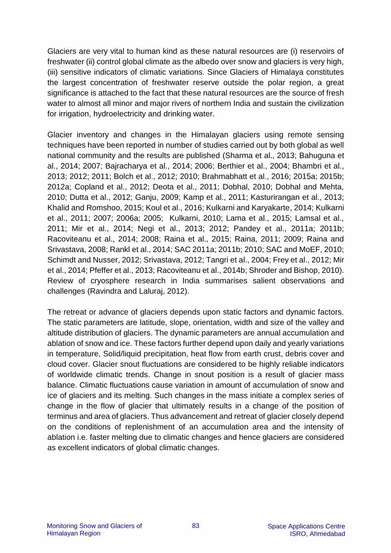
83 Monitoring Snow and Glaciers of Himalayan Region
Space Applications Centre ISRO, Ahmedabad
Glaciers are very vital to human kind as these natural resources are (i) reservoirs of
freshwater (ii) control global climate as the albedo over snow and glaciers is very high,
(iii) sensitive indicators of climatic variations. Since Glaciers of Himalaya constitutes
the largest concentration of freshwater reserve outside the polar region, a great
significance is attached to the fact that these natural resources are the source of fresh
water to almost all minor and major rivers of northern India and sustain the civilization
for irrigation, hydroelectricity and drinking water.
Glacier inventory and changes in the Himalayan glaciers using remote sensing
techniques have been reported in number of studies carried out by both global as well
national community and the results are published (Sharma et al., 2013; Bahuguna et
al., 2014; 2007; Bajracharya et al., 2014; 2006; Berthier et al., 2004; Bhambri et al.,
2013; 2012; 2011; Bolch et al., 2012; 2010; Brahmabhatt et al., 2016; 2015a; 2015b;
2012a; Copland et al., 2012; Deota et al., 2011; Dobhal, 2010; Dobhal and Mehta,
2010; Dutta et al., 2012; Ganju, 2009; Kamp et al., 2011; Kasturirangan et al., 2013;
Khalid and Romshoo, 2015; Koul et al., 2016; Kulkarni and Karyakarte, 2014; Kulkarni
et al., 2011; 2007; 2006a; 2005; Kulkarni, 2010; Lama et al., 2015; Lamsal et al.,
2011; Mir et al., 2014; Negi et al., 2013; 2012; Pandey et al., 2011a; 2011b;
Racoviteanu et al., 2014; 2008; Raina et al., 2015; Raina, 2011; 2009; Raina and
Srivastava, 2008; Rankl et al., 2014; SAC 2011a; 2011b; 2010; SAC and MoEF, 2010;
Schimdt and Nusser, 2012; Srivastava, 2012; Tangri et al., 2004; Frey et al., 2012; Mir
et al., 2014; Pfeffer et al., 2013; Racoviteanu et al., 2014b; Shroder and Bishop, 2010).
Review of cryosphere research in India summarises salient observations and
challenges (Ravindra and Laluraj, 2012).
The retreat or advance of glaciers depends upon static factors and dynamic factors.
The static parameters are latitude, slope, orientation, width and size of the valley and
altitude distribution of glaciers. The dynamic parameters are annual accumulation and
ablation of snow and ice. These factors further depend upon daily and yearly variations
in temperature, Solid/liquid precipitation, heat flow from earth crust, debris cover and
cloud cover. Glacier snout fluctuations are considered to be highly reliable indicators
of worldwide climatic trends. Change in snout position is a result of glacier mass
balance. Climatic fluctuations cause variation in amount of accumulation of snow and
ice of glaciers and its melting. Such changes in the mass initiate a complex series of
change in the flow of glacier that ultimately results in a change of the position of
terminus and area of glaciers. Thus advancement and retreat of glacier closely depend
on the conditions of replenishment of an accumulation area and the intensity of
ablation i.e. faster melting due to climatic changes and hence glaciers are considered
as excellent indicators of global climatic changes.

84 Monitoring Snow and Glaciers of Himalayan Region
Space Applications Centre ISRO, Ahmedabad
3.3. Methodology
(i) Georeferencing of satellite images
The data obtained from NRSC has undergone the basic geometric and radiometric
corrections. This data is (band 2, band 3, band 4, and band 5) georeferenced with
master images already archived. This is a second order correction applied to data.
The georeferencing with master images is carried out by identifying a set of ground
control points on the maps and images. The ERDAS imagine version 9.1 is used for
this work.
(ii) Delineation of glacial boundaries
A period of the year i.e. from July to end of September, when seasonal snow cover is
at its minimum and permanent snow cover and glaciers are fully exposed, is selected
for the glacier mapping using remote sensing data. Multi-temporal geocoded FCC’s of
standard band combination such as 2 (0.52-0.59 μm), 3 (0.62-0.68 μm) and 4 (0.77-
0.86 μm) of IRS LISS III sensors at 1: 50,000 scale are used for interpretation. Most
of the work carried out in phase I was done using survey of India topographical maps
of 1962, IRS LISS III data of 2001 and in many cases of 2006/2007 and Landsat TM
data of 1989. Spatial resolution of the Landsat and LISS III sensor is 30 m and 23.5 m
respectively.
To extract glacial boundary from satellite image false color composite (FCCs) are
viewed in different combination of band 1 to band 4. The SWIR band is used to
discriminate cloud and snow because it might happen that clouds are observed on the
upper boundary of the glaciers. The distinction of non-glaciated and glaciated region
is sharper in SWIR band. The unique reflectance of snow-ice, shape of the valley
occupied by the glacier, the flow lines of ice movement of glaciers, the rough texture
of the debris on the ablation zone of the glaciers, the shadow of the steep mountain
peaks and presence of vegetated parts of the mountains help in clear identification of
a glacier on the satellite image. The understanding of reflectance curve of various
glacier features helps to vectorize the glacial boundary on satellite data.
The snout of the glacier is a vital element of interpretation of glacial extents. The
terminus is identified using multiple criterions for example:
Sometimes the river originates from the snout and river can be easily identified on
the image.
The peri-glacier area downstream of the snout has distinct geomorphological set
up then the glacier surface.
In many instances the frontal portion of the glaciers which are retreating has
convex shape therefore it helps identification of the terminus.
When interpretation becomes more complex sometimes DEM is used in the
background to confirm the snout as there is a chance of change in the slope of

85 Monitoring Snow and Glaciers of Himalayan Region
Space Applications Centre ISRO, Ahmedabad
glacier profile near the snout and 3d view help to identify the lateral and terminal
boundary of glacial extent.
Extreme care is taken while delineating glacier boundary that boundaries are
marked in the inner side of the lateral moraines.
Snouts of a few selected glaciers for which Corona photographs (spatial resolution
4m) of 1965 were available were also compared with snouts seen on LISS III data of
the corresponding year.
(iii) Estimating loss in area
To estimate change in glacial area the two sources of glacier extent are overlaid on
each other. While matching of the boundary, it is seen that the scale of the map and
image is kept at 1: 50,000 because the mapping depends on the scale. A map
prepared at 1:50,000 scale and map prepared at larger scale might not match for their
features. Increase or decrease in the evacuated area from glaciers can be measured.
Mapping of glacial boundaries has been carried out using Landsat and LISS-III
images. Images of July-September are normally used because during this period snow
cover is at its minimum and glaciers are fully exposed.
(iv) Field verification
Field verification of location of snout using GPS observations has been conducted for
a few glaciers. Normally ground verifications are carried out for those glaciers which
are not easily interpreted.
3.4. Results and Discussion
(a) Himalayan region
In Himalayan region, 2018 glaciers were monitored. These glaciers represent six
major climatic zones of Himalayan region; Kashmir Himalayas, Punjab Himalayas
(Satluj Basin), Himachal Himalayas (Chenab Basin), Uttarakhand Himalayas, Nepal
Himalayas and Sikkim Himalayas. Glaciers were monitored using IRS LISS III images
of 2001 and 20111/12 (Bahuguna et al 2014). Table 39 summarises the findings of
change in glaciers in 17 sub-basins of Himalaya. Figure 90 shows the location of
glaciers monitored in different climatic zones of Himalayas. This number also includes
a few glaciers of Nubra valley (Karakoram region). Area–frequency distribution of the
monitored glaciers in the six regions is given in Table 40. Glaciers having area less
than 1 sq. km constitutes 45% of the number monitored. Ninety-seven glaciers occupy
area larger than 20 sq km.

86 Monitoring Snow and Glaciers of Himalayan Region
Space Applications Centre ISRO, Ahmedabad
Table 39: Changes in glacier extent studied for selected glaciers in 17 sub-basins of
Himalayan region during 2000-2011 time frame
Serial no.
No. of
glaciers
Stable
Retreat
Advance
Glaciated Area (sq Km)
Area Change (Sq Km)
Sub-basins
Year
2000/2001 2010/11
1 Nubra 149 111 20 18 1686.22 1681.87 -4.35
2 Zanskar 188 180 8 0 102.49 102.21 -0.28
3 Suru 110 75 35 0 156.61 152.93 -3.68
4 Spiti 431 415 16 0 36.34 35.79 -0.55
5 Parbati 12 9 3 0 38.39 38.18 -0.21
6 Chandra 140 121 19 0 173.83 172.89 -0.94
7 Bhaga 69 53 16 0 100.58 97.35 -3.23
8 Warwan 77 56 21 0 170.68 167.4 -3.28
9 Bhut 167 158 9 0 64.5 63.54 -0.96
10 Miyar 59 52 7 0 111.77 111.61 -0.16
11 Ravi 36 33 3 0 11.61 11.47 -0.14
12 Alaknanda 20 13 7 0 132.29 131.43 -0.86
13 Bhagirathi 202 165 37 0 183.24 181.5 -1.74
14 Dhauliganga 68 64 4 0 7.66 7.42 -0.24
15 Gauriganga 63 57 6 0 130.08 129.8 -0.28
16 Kosi 195 168 27 0 326.4 322.5 -3.9
17 Tista 32 22 10 0 59.73 57.55 -2.18
Total 2018 1730 238 18 3432.69 3407.89 -24.8
Figure 90: Locations of basins undertaken for glacier monitoring (Source: Bahuguna
et al., 2014)

87 Monitoring Snow and Glaciers of Himalayan Region
Space Applications Centre ISRO, Ahmedabad
Table 40: The size-frequency distribution of glaciers in the six region (Source:
Bahuguna et al., 2014)
Area
(sq km)
Karakoram Zanskar Himachal Uttarakhand Nepal Sikkim Total
<1 8 436 261 184 21 4 914
1 to 3 46 197 139 90 59 8 539
3 to 5 30 43 54 23 32 7 189
5 to 10 17 31 51 26 37 8 170
10 to 20 21 9 33 18 25 3 109
>20 27 13 22 12 21 2 97
Total 149 729 560 353 195 32 2018
Monitoring of 2018 glacier snouts from the satellite data of 2000/01/02 shows that
1752 glaciers (86.8%) have been observed to be stable (no change in the snout
position), 248 glaciers (12.3%) have exhibited retreat and 18 of them (0.9%) have
experienced advancement (Figure 91).
Figure 91: Number of glaciers showing No Change, retreat and advance (Source:
Bahuguna et al., 2014)
Region-wise mean shift in snout position for the retreating glaciers is shown in Figure
92. It varies from 145 to 313 m for the 2000/01/02 period with a positional uncertainty
of 11.5 m. Average movement of 300 m of snout was observed for advancing glaciers
(18 glaciers) of Karakoram. Maximum retreat was observed in Sikkim region followed
by Karakoram and Himachal region. The mean retreat of snout for 248 retreating
glaciers was found to be 170 m (17 m annually approx.). However, by considering all
the 2018 glaciers monitored, the mean retreat was found to be 21 m (2.1 m annually).
No detachment of glaciers in the ablation zones in the study area was observed during
the period of monitoring.
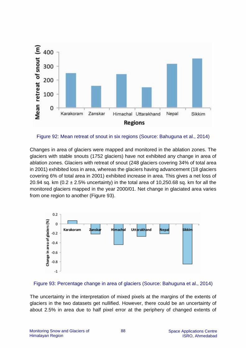
88 Monitoring Snow and Glaciers of Himalayan Region
Space Applications Centre ISRO, Ahmedabad
Figure 92: Mean retreat of snout in six regions (Source: Bahuguna et al., 2014)
Changes in area of glaciers were mapped and monitored in the ablation zones. The
glaciers with stable snouts (1752 glaciers) have not exhibited any change in area of
ablation zones. Glaciers with retreat of snout (248 glaciers covering 34% of total area
in 2001) exhibited loss in area, whereas the glaciers having advancement (18 glaciers
covering 6% of total area in 2001) exhibited increase in area. This gives a net loss of
20.94 sq. km (0.2 ± 2.5% uncertainty) in the total area of 10,250.68 sq. km for all the
monitored glaciers mapped in the year 2000/01. Net change in glaciated area varies
from one region to another (Figure 93).
Figure 93: Percentage change in area of glaciers (Source: Bahuguna et al., 2014)
The uncertainty in the interpretation of mixed pixels at the margins of the extents of
glaciers in the two datasets get nullified. However, there could be an uncertainty of
about 2.5% in area due to half pixel error at the periphery of changed extents of
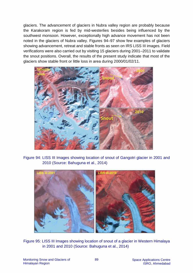
89 Monitoring Snow and Glaciers of Himalayan Region
Space Applications Centre ISRO, Ahmedabad
glaciers. The advancement of glaciers in Nubra valley region are probably because
the Karakoram region is fed by mid-westerlies besides being influenced by the
southwest monsoon. However, exceptionally high advance movement has not been
noted in the glaciers of Nubra valley. Figures 94–97 show few examples of glaciers
showing advancement, retreat and stable fronts as seen on IRS LISS III images. Field
verifications were also carried out by visiting 15 glaciers during 2001–2011 to validate
the snout positions. Overall, the results of the present study indicate that most of the
glaciers show stable front or little loss in area during 2000/01/02/11.
Figure 94: LISS III Images showing location of snout of Gangotri glacier in 2001 and
2010 (Source: Bahuguna et al., 2014)
Figure 95: LISS III Images showing location of snout of a glacier in Western Himalaya
in 2001 and 2010 (Source: Bahuguna et al., 2014)

90 Monitoring Snow and Glaciers of Himalayan Region
Space Applications Centre ISRO, Ahmedabad
Figure 96: LISS III Images showing location of snout of Siachen glacier in 2001 and
2010 (Source: Bahuguna et al., 2014)
Figure 97: LISS III Images showing retreat of a glacier from 2001 to 2010 and increase
in surface area of moraine-dammed lake (Source: Bahuguna et al., 2014)
In the Himalayan region, mean loss of 16% in area of glaciers was reported using
topographical maps of 1962 and satellite images of 2001 (Kulkarni et al., 2007).
However, present study show that the number and rate of glacier retreat have come
down in the last decade compared to period prior to 2001. Most of the glaciers show
no change during last decade. This period of monitoring almost corresponds to hiatus
in global warming in the last decade. It is worthwile to note that an interval of one
decade could be smaller than the response time of glaciers to be reflected in terms of
any significant change with 23.5 m spatial resolution of data. Therefore, further studies
using high-resolution multitemporal satellite data are required. Few examples of IRS
LISS III images and corresponding maps interpreted are shown in Figures 98 to 111.

91 Monitoring Snow and Glaciers of Himalayan Region
Space Applications Centre ISRO, Ahmedabad
Figure 98: IRS P6 LISS III image of 2010, showing the glaciers of part of the Warwan
sub-basin (Reference: Map No 43O/13)
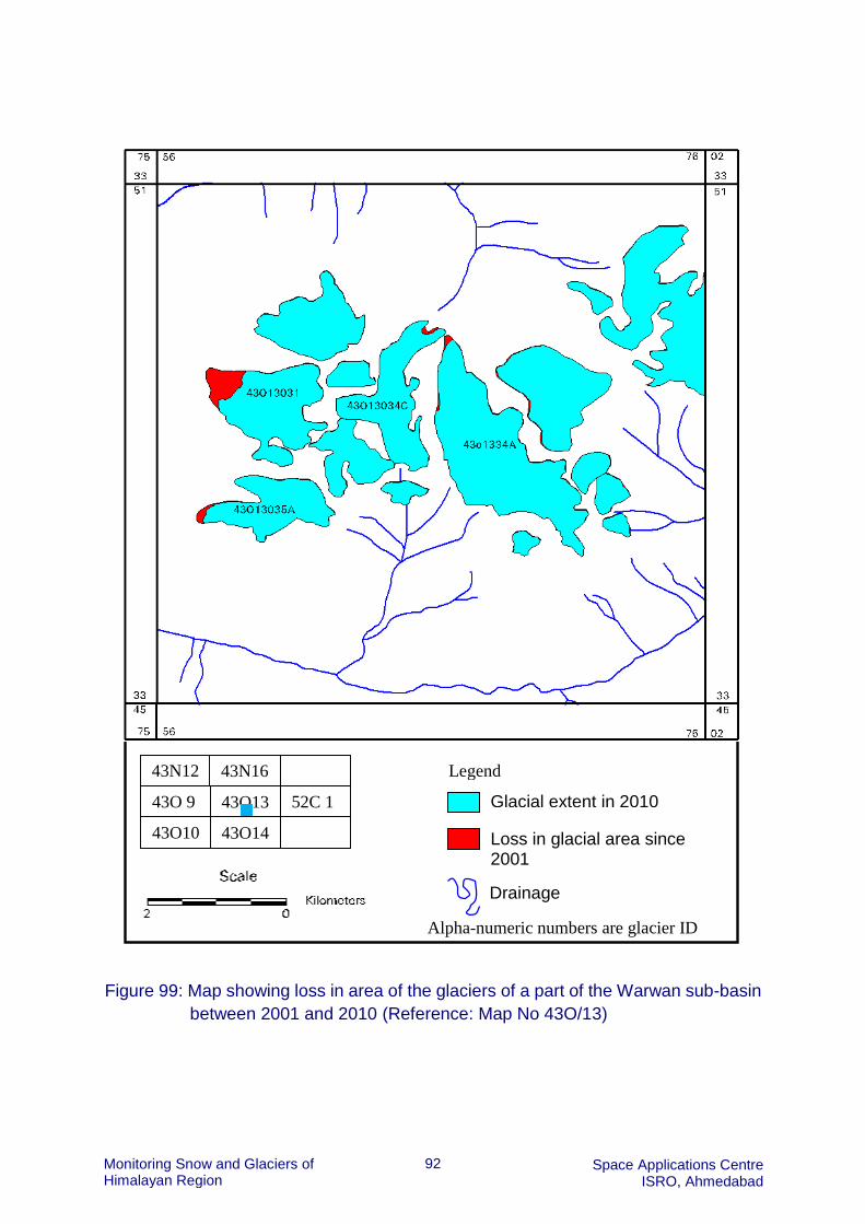
92 Monitoring Snow and Glaciers of Himalayan Region
Space Applications Centre ISRO, Ahmedabad
Figure 99: Map showing loss in area of the glaciers of a part of the Warwan sub-basin
between 2001 and 2010 (Reference: Map No 43O/13)
43N12 43N16
43O 9 43O13 52C 1
43O10 43O14
Glacial extent in 2010
Loss in glacial area since 2001
Legend
Drainage
Alpha-numeric numbers are glacier ID

93 Monitoring Snow and Glaciers of Himalayan Region
Space Applications Centre ISRO, Ahmedabad
Figure 100: IRS P6 LISS III image of 2010, showing the glaciers of part of the Warwan
sub-basin (Reference Map 43 O/14)

94 Monitoring Snow and Glaciers of Himalayan Region
Space Applications Centre ISRO, Ahmedabad
Figure 101: Map showing loss in area of the glaciers of a part of the Warwan sub-
basin between 2001 and 2010 (Reference: Map No 43O/14)
43O 9 43O13 52C 1
43O10 43O14 52C 2
43O11 43O15 52C 3
Legend
Glacial extent in 2010
Loss in glacial area since 2001
Drainage
Alpha-numeric numbers are glacier ID

95 Monitoring Snow and Glaciers of Himalayan Region
Space Applications Centre ISRO, Ahmedabad
Figure 102: IRS P6 LISS III image of 2010, showing the glaciers of part of the Warwan
sub-basin (Reference: Map No 52C / 02)

96 Monitoring Snow and Glaciers of Himalayan Region
Space Applications Centre ISRO, Ahmedabad
Figure 103: Map showing loss in area of the glaciers of a part of the Warwan sub-
basin between 2001 and 2010 (Reference: Map No 52C / 02)
43O13 52C 1 52C 5
43O14 52C 2 52C 6
52C 2 43O15 52C 3
Glacial extent in 2010
Loss in glacial area since 2001
Legend
Drainage
Alpha-numeric numbers are glacier ID

97 Monitoring Snow and Glaciers of Himalayan Region
Space Applications Centre ISRO, Ahmedabad
Figure 104: IRS P6 LISS III image of 2008, showing the glaciers of part of the Bhut
sub-basin (Reference: Map No. 52C/3)

98 Monitoring Snow and Glaciers of Himalayan Region
Space Applications Centre ISRO, Ahmedabad
Figure 105: Map showing loss in area of the glaciers of a part of the Bhut sub-basin
between 2002 and 2011 (Reference: Map No. 52C/3)
43O14 52C 2 52C 6
43O15 52C 3 52C 7
43O16 52C 4 52C 8
Legend
Glacial extent in 2008
Loss in glacial area since 2002
Drainage
Alpha-numeric numbers are glacier ID

99 Monitoring Snow and Glaciers of Himalayan Region
Space Applications Centre ISRO, Ahmedabad
Figure 106: IRS 1C LISS III image of October, 2011 showing the Glaciers of part of
the Bhaga sub-basin (Reference: Map No. 52H/1)

100 Monitoring Snow and Glaciers of Himalayan Region
Space Applications Centre ISRO, Ahmedabad
Figure 107: Map showing loss in area of the glaciers of a part of the Bhaga sub-
basin between 2001 and 2011 (Reference map no.52H/1)
Legend
Glacial extent in 2011
Loss in glacial area since 2001
Drainage
Alpha-numeric numbers are glacier ID
52D13 52H 1 52H 5
52D14 52H 2 52H 6
52D15 52H 3 52H 7

101 Monitoring Snow and Glaciers of Himalayan Region
Space Applications Centre ISRO, Ahmedabad
Figure 108: Landsat TM, image of October, 9 1989 showing the Glaciers of part of the
Bhut sub-basin (Reference: Map No. 52H/7)

102 Monitoring Snow and Glaciers of Himalayan Region
Space Applications Centre ISRO, Ahmedabad
Figure 109: Map showing loss in area of the glaciers of a part of the Bhut sub-basin
between 1989-2001-2011 (Reference map no.52H/7)
52C 6 52C1
0
52C5
4 52C 7 52C2
1
52C6
5 52C 8 52C3 52C7
6
Legend
Glacial extent in 2001
Loss in glacial area since 1962
Drainage
Alpha-numeric numbers are glacier ID
Glacial extent in 1989

103 Monitoring Snow and Glaciers of Himalayan Region
Space Applications Centre ISRO, Ahmedabad
Figure 110: IRS P6 LISS III image of 2008, showing the glaciers of part of the Bhut
sub-basin (Reference: Map No. 52C/7)

104 Monitoring Snow and Glaciers of Himalayan Region
Space Applications Centre ISRO, Ahmedabad
Figure 111: Map showing loss in area of the glaciers of a part of the Bhut sub-basin
between 2002 and 2008 (Reference: Map No. 52C/7)
52C 2 52C 6 52C1
0 52C 3 52C 7 52C1
1 52C 4 52C 8 52C1
2
Legend
Glacial extent in 2008
Loss in glacial area since 2002
Drainage
Alpha-numeric numbers are glacier ID

105 Monitoring Snow and Glaciers of Himalayan Region
Space Applications Centre ISRO, Ahmedabad
(b) Karakoram region
A detailed study has been carried out for 607 glaciers in the Shasgan, Shigar, Nubra
and Shyok sub-basins of the Karakoram region. These glaciers were monitored for the
period 1977 to 2013 using Landsat and IRS data (Brahmbhatt et al., 2015a; 2015b).
This study show a complete analysis of changes observed in the 607 glaciers during
the time intervals 1977-1990, 1990-2000, 2000-2010 and 2010-2013. The location of
glaciers in Karakoram region are shown in Figure 112.
Figure 112: Locations of glaciers monitored in Karakoram region shown in satellite
data (AWiFS image of year 2014 showing FCC of SWIR-NIR-Red)
(Source: Brahmbhatt et al., 2015a)
The dynamics of glaciers in terms of stability, retreat or advance during 1977 to 2013
has been shown in the Figure 113 resembling like a tree. The glacier dynamics is
discussed below:
1977-1990: Status of sub-basin wise changes in glaciers during 1977-1990 time frame
is summarized in Table 41. It has been observed that out of 607 glaciers, 505 glaciers
show no change, 79 glaciers show retreat and 23 glaciers show advance. Glaciers in
all the four sub-basins viz., Shasgan, Shigar, Nubra and Shyok show loss in glaciated
area. The total glaciated area of 607 glaciers in Karakoram region of 7894.95 sq. km.
in 1977 has reduced to 7885.01 sq km in 1990. It is observed that net loss of glaciated
area during 1977-1990 time frame is 9.94 sq km., indicating insignificant changes.

106 Monitoring Snow and Glaciers of Himalayan Region
Space Applications Centre ISRO, Ahmedabad
Figure 113: Glacier dynamics (S=Stable; R=Retreating; A=Advancing) of 607 glaciers
of Karakoram during 1977-1990, 1990-2000, 2000-2010 and 2010-2013
time frames (Source: Brahmbhatt et al., 2015a)

107 Monitoring Snow and Glaciers of Himalayan Region
Space Applications Centre ISRO, Ahmedabad
Table 41: Status of sub-basin wise changes in glaciers of Karakoram region during
1977 – 1990 time frame
Sub-
basin
Glaciers
studied
(number)
Glaciers
Stable
(number)
Glaciers
Retreating
(number)
Glaciers
Advancing
(number)
Glaciated
area in
1977
(km2)
Glaciated
area in
1990
(km2)
Change
in
glaciated
area
(km2)
Shasgan 291 263 21 7 2167.01 2165.35 -1.66 Shigar 139 123 12 4 2452.05 2449.15 -2.9 Nubra 135 86 41 8 1767.02 1764.68 -2.34 Shyok 42 33 5 4 1508.87 1505.83 -3.04 Total 607 505 79 23 7894.95 7885.01 -9.94
1990-2000: Status of sub-basin wise changes in glaciers during 1990-2000 time frame
is summarized in Table 42. It is observed that out of 607 glaciers, 401 glaciers show
no change, 123 glaciers show retreat and 83 glaciers show advance. Glaciers in
Shigar and Shyok sub-basins show gain in area, whereas those in Shasgan and Nubra
sub-basins show loss in glaciated area. However, the net glaciated area in Karakoram
region of 7885.01 sq km in 1990 has reduced to 7882.18 sq km. It is observed that net
loss of glaciated area during this time frame is 2.83 sq km., indicating insignificant
changes.
Table 42: Status of sub-basin wise changes in glaciers of Karakoram region during
1990 – 2000 time frame
Sub-
basin
Glaciers
studied
(number)
Glaciers
Stable
(number)
Glaciers
Retreating
(number)
Glaciers
Advancing
(number)
Glaciated
area in
1990
(km2)
Glaciated
area in
2000
(km2)
Change
in
glaciated
area
(km2)
Shasgan 291 203 71 17 2165.35 2155.52 -9.83 Shigar 139 112 10 17 2449.15 2453.78 4.63 Nubra 135 84 31 20 1764.68 1762.34 -2.34 Shyok 42 2 11 29 1505.83 1510.54 4.71 Total 607 401 123 83 7885.01 7882.18 -2.83
Considering all the sub-basins together, Figure 113 show that 505 glaciers classified
as stable during 1977-1990 time frame are observed to fall into three classes during
1990-2000 time frame viz., Stable - 371, Retreating - 92 and Advancing – 42. Glaciers
observed to be retreating i.e., 79 glaciers during 1977-1990 time frame fall into three
classes viz., Stable - 22, Retreating - 25 and Advancing - 32. Similarly, 23 glaciers
classified as Advancing during 1977-1990 time frame show Stable – 8, Retreating – 6
and Advancing - 9 during 1990-2000 time frame. These observations indicate that
behavior of glacier in one time frame may or may not be same during the subsequent
time frames.

108 Monitoring Snow and Glaciers of Himalayan Region
Space Applications Centre ISRO, Ahmedabad
2000-2010: Status of sub-basin wise changes in glaciers during 2000-2010 time
frame is summarized in Table 43. It is observed that out of 607 glaciers, 504 glaciers
show no change, 62 glaciers show retreat and 41 glaciers show advance. Glaciers in
Shyok sub-basin show gain in area, whereas those in Shasgan and Nubra have
remained stable, while those in Shigar sub-basin have shown insignificant loss in area.
However, the net glaciated area in Karakoram region of 7882.18 sq km in 2000 has
increased to 7885.78 sq km. It is observed that net gain of glaciated area during this
time frame is 3.6 sq km. Among advancing glaciers, 7 glaciers were observed to have
sudden increase in their area. These glaciers are indicative of surging behavior.
Table 43: Status of sub-basin wise changes in glaciers of Karakoram region during
2000 – 2010 time frame
Sub-
basin
Glaciers
studied
(number)
Glaciers
Stable
(number)
Glaciers
Retreating
(number)
Glaciers
Advancing
(number)
Glaciated
area in
2000
(km2)
Glaciated
area in
2010
(km2)
Change
in
glaciated
area
(km2)
Shasgan 291 290 1 0 2155.52 2155.22 -0.3 Shigar 139 100 29 10 2453.78 2451.52 -2.26 Nubra 135 105 19 11 1762.34 1762.12 -0.22 Shyok 42 9 13 20 1510.54 1516.92 6.38 Total 607 504 62 41 7882.18 7885.78 3.6
Considering all the sub-basins together, Figure 113 show status of number of glaciers
initially classed as Stable – 505, Retreating – 79, Advancing - 23 during 1977-1990
time frame in subsequent 1990-2000 and 2000-2010 time frames.
2010-2013: Status of sub-basin wise changes in glaciers during 2010-2013 time frame
is summarized in Table 44. It is observed that out of 607 glaciers, 583 glaciers show
no change, 9 glaciers show retreat and 15 glaciers show advance. Glaciers in
Shasgan and Shyok sub-basin show gain in area, whereas those in Shigar and Nubra
have remained stable. However, the net glaciated area in Karakoram region of
7885.78 sq km in 2010 has increased to 7888.63 sq km. It is observed that net gain of
glaciated area during this time frame is 2.85 sq km.
Considering the overall changes in 607 glaciers of Karakoram region and also
assessing the overall mapping accuracy, the salient findings are summarized in Table
45 and Figure 114, Figure 115, Figure 116 and Figure 117.

109 Monitoring Snow and Glaciers of Himalayan Region
Space Applications Centre ISRO, Ahmedabad
Table 44: Status of sub-basin wise changes in glaciers of Karakoram region during
2010 – 2013 time frame
Sub-
basin
Glaciers
studied
(number)
Glaciers
Stable
(number)
Glaciers
Retreating
(number)
Glaciers
Advancing
(number)
Glaciated
area in
2001
(km2)
Glaciated
area in
2010
(km2)
Change
in
glaciated
area
(km2)
Shasgan 291 275 4 12 2155.22 2157.75 2.53 Shigar 139 138 1 0 2451.52 2451.45 -0.07 Nubra 135 134 1 0 1762.12 1761.72 -0.4 Shyok 42 36 3 3 1516.92 1517.71 0.79 Total 607 583 9 15 7885.78 7888.63 2.85
Net glaciated area of advancing glaciers show increasing trend, retreating glaciers
show a dip during 1977-1990 and since 1990 show increasing trend and stable
glaciers remain stable during 1977-1990 and then a dip during 2000 and since 2000
show increasing trend. Some examples of advancing glaciers are shown in Figure
118, Figure 119 and Figure 120.
Table 45: Changes in glaciated area of 607 glaciers in Karakoram for time frame 1977-
2013 (Source: Brahmbhatt et al., 2015a)
Year Total
Glacier
Area (km2)
Period Change in
total glacier
area (km2)
Change of
area
Advancing
glacier (km2)
Change of area of
retreating glaciers
(km2)
1977 7895 (+8%) - - - -
1990 7885 (+3%) 1977-
1990
(-)10 (+8%) 3.62 (+10%) 13.6(+6%)
2000 7882 (+3%) 1990-
2000
(-)3
(+1.7%)
20.2 (+1.8%) 23 (+1.5%)
2010 7885.8
(+3%)
2000-
2010
(+)4
(+2.5%)
10.6 (+2.1) 7.04 (+2.8 %)
2013 7888.6
(+3%)
2010-
2013
(+)3
(+3.8%)
5.5 (+3.6) 2.7 (+4%)

110 Monitoring Snow and Glaciers of Himalayan Region
Space Applications Centre ISRO, Ahmedabad
Figure 114: Total glaciated area of 607 glaciers in Karakoram during different time
periods monitored using satellite data
Figure 115: Total glaciated area of 23 advancing glaciers (as per changes observed
during 1977-1990) in Karakoram during different time periods monitored
using satellite data (Source: Brahmbhatt et al., 2015a)
7865
7870
7875
7880
7885
7890
7895
1977 1990 2001 2010 2013Period of Monitoring
Tota
l Gla
cier
are
a (s
q k
m)

111 Monitoring Snow and Glaciers of Himalayan Region
Space Applications Centre ISRO, Ahmedabad
Figure 116: Total glaciated area of 79 retreating glaciers (as per changes observed
during 1977-1990) in Karakoram during different time periods monitored
using satellite data (Source: Brahmbhatt et al., 2015a)
Figure 117: Total glaciated area of 505 stable glaciers (as per changes observed
during 1977-1990) in Karakoram during different time periods monitored
using satellite data (Source: Brahmbhatt et al., 2015a)

112 Monitoring Snow and Glaciers of Himalayan Region
Space Applications Centre ISRO, Ahmedabad
Spatial distribution of change in area of glaciers of Karakoram since 1977 is provided
in Figure 118. Glaciers located at north-western and southeastern parts of the study
area show tremendous variation in the advance and retreat for three time frames.
Glaciers behaved very differently in each time frame, thus, no significant generalized
trend was identified in changes of glaciers. In a few cases, glaciers have experienced
advancement and overrode on other glacier and then gradually merged to main trunk
glacier (Figure 119). In other cases, glaciers were advancing slowly and then stabilized
(Figure 120). In a few cases, the tributary glaciers advanced and merged into main
trunk glaciers, whereas the snout of main trunk glacier didn't show any considerable
change (Figure 121).
Figure 118: Spatial distribution of change in area of glaciers of Karakoram since 1977.
Note: R = Retreat, A= Advance and S = Stable E.g.: R-A-S = Retreat
(in 1977-1990) – Advance (in 1990-2000) – Stable (in 2000-2013)
(Source: Brahmbhatt et al., 2015a)
Glaciers of the Karakoram have shown inconsistency in advance, retreat and no
change during this period, and some examples of glacier surging have been observed.
341 glaciers exhibited no measured change throughout the 36 years of the study.
Among other glaciers, no significant and sustained pattern of retreat or advance was
observed. The overall changes in glacier area in the whole region are of small
magnitudes (positive and negative values) in the various measured intervals.
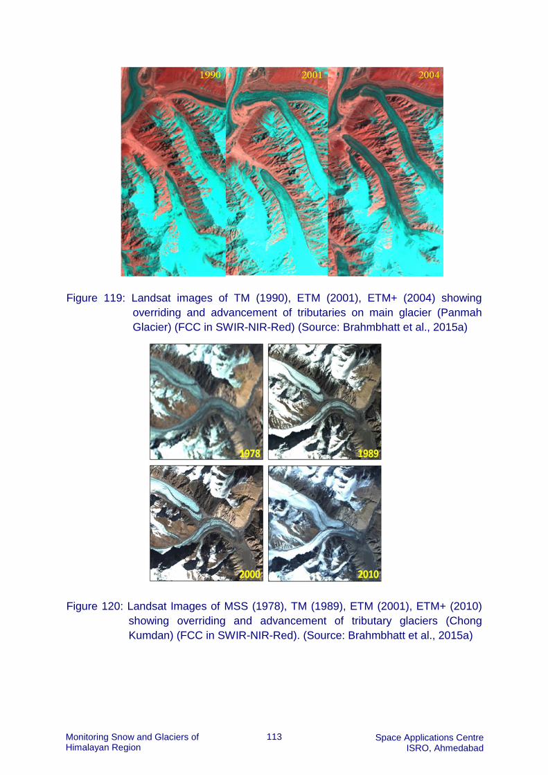
113 Monitoring Snow and Glaciers of Himalayan Region
Space Applications Centre ISRO, Ahmedabad
Figure 119: Landsat images of TM (1990), ETM (2001), ETM+ (2004) showing
overriding and advancement of tributaries on main glacier (Panmah
Glacier) (FCC in SWIR-NIR-Red) (Source: Brahmbhatt et al., 2015a)
Figure 120: Landsat Images of MSS (1978), TM (1989), ETM (2001), ETM+ (2010)
showing overriding and advancement of tributary glaciers (Chong
Kumdan) (FCC in SWIR-NIR-Red). (Source: Brahmbhatt et al., 2015a)

114 Monitoring Snow and Glaciers of Himalayan Region
Space Applications Centre ISRO, Ahmedabad
Figure 121: Images showing advancing of tributary glaciers up to bank of main trunk
(Baltoro) glaciers. (Source: Brahmbhatt et al., 2015a)
Moreover, it is mostly disconnected glaciers in tributary valleys which have advanced,
whereas the main former trunk glaciers have primarily not changed. The dynamical
differences between disconnected former tributaries and trunks may be related to
response time differences, with the smaller, perhaps steeper tributaries responding
more rapidly than trunks to brief climatic fluctuations.
Precipitation system of Karakoram –Pamir region is different from other parts of
Himalaya. Himalayas are influenced by SW and SE monsoon whereas Karakoram is
nourished by western winds carrying moisture. The latitudinal differences account for
difference in onset and longevity of winters and consequent impact on glacier
dynamics of the Karakoram region, which is different than other parts of the
Himalayas.

115 Monitoring Snow and Glaciers of Himalayan Region
Space Applications Centre ISRO, Ahmedabad
(c) Detail study of Kolahoi glacier in Kashmir valley, Himalayas
Four glaciations are evident in the Kolahoi valley on the basis of the detailed galcio-
geomorphological features mapped in the field during the study. The oldest glaciation
i.e., Pahalgam stage is represented by subglacial moraines which at present are
overlain by bedded soil layers and vegetation identified and mapped during the field
survey. The second glaciation (Aru Stage) is well represented by a 6 km long end
moraine. The third glaciation (Lidderwat stage) is represented by well preserved end
and lateral moraines. The fourth glaciation (Satlanjen stage), about 2.5 km
downstream from the present snout position is represented by partially eroded end
moraine and well preserved lateral moraines. Based on the presence of the moraines
throughout the main valley, the present study proposes four glaciations witnessed in
the region in the recent past. However, the number and timing of the major glacial
advances in the region can be determined only by dating the moraines preserved in
the valley.
Kolahoi glacier is the largest glacier (6 km long) in the Kashmir valley located in the
Greater Himalayan range. A time series of satellite and other historical survey data
was used for detecting recent changes in the snout, area and volume of Kolahoi glacier
from 1857-2013. The analysis of the archived and remote sensing data revealed that
the glacier has retreated 2.5 km from 1857 to 2013. On an average, the rate of retreat
is 21.53 m/year during the period of observation. From 1887 till 1992 enhanced rate
of snout retreat is observed. The glacier continued to melt at the average rate of 16.75
m/yr till 1992. The rate of retreat declined during 1992-2000 and was estimated as
5.55 m/year during the period (Figure 122 and 123). Though, low retreat of glacier
tongue along its length is observed during 1992-2000, however, the glacier
experienced relatively more recession across the width of its tongue during the period.
The rate of retreat increased to its maximum between 2006 and 2014 receeding at a
rate of 56 m/yr during the period. This enhanced rate is partly attributed to the calving
of the snout flowing over the steep bedrock. Though, the snout retreat is consistent
with a number of glaciers studied across Himalayas including Milam in central
Himalaya, Samandurtapu in western Himalaya and Gongotri in central Himalaya,
however, a number of studies carried out in the neighboring Zanskar, Ladakh and
Karakoram suggest that the snout retreat of Kolahoi glacier is quite high. The higher
rate of retreat observed for the Kolahoi could be attributed to high temperatures
observed in the region during the last century and comparatively low elevation of
Kolahoi glacier snout

116 Monitoring Snow and Glaciers of Himalayan Region
Space Applications Centre ISRO, Ahmedabad
Figure 122: Deglaciation of Kolhoi valley (from field evidences)
Figure 123: Position of Snout of Kolahoi at different points in time from 1857-2013

117 Monitoring Snow and Glaciers of Himalayan Region
Space Applications Centre ISRO, Ahmedabad
(d) Detailed study of glaciers of Miyar sub-basin
A detailed analysis of glaciers in the Miyar Basin, Lahaul & Spiti District of Himachal
Pradesh (1963-2013) was carried out (Figure 124). Satellite iamges of post monsoon
season i.e. September-October were selected for monitoring the glaciers, because
this is the end of melting season. Since the basin is quite large in area and has a large
number of glaciers, the satellite data of a particular year is not covering all glaciers
and therefore every glacier has been monitored separately as per the availability of
data. Corona images and Landsat images are freely downloadable from USGS earth
explorer while the IRS PAN, IRS LISS III and IRS LISS IV images have been procured
from NRSC, Hyderabad (Table 46).
Figure 124: Location map of Miyar sub-basin
Corona images of Miyar basin are available for the years of 1965, 1971 and 1980.
However, all glaciers of the basin could not be mapped using Corona because of the
huge cloud cover. Therefore, Corona images have been used for a few glaciers only.
Along with the remote sensing methods, field measurements have also been carried
out for snout monitoring of the selected glaciers (Miyar, Pimu, Menthosa, Tharang and
Uldhampu) with GPS in October 2006, June 2008, October 2010 (available archives),
June 2011, June 2012 and June 2013.
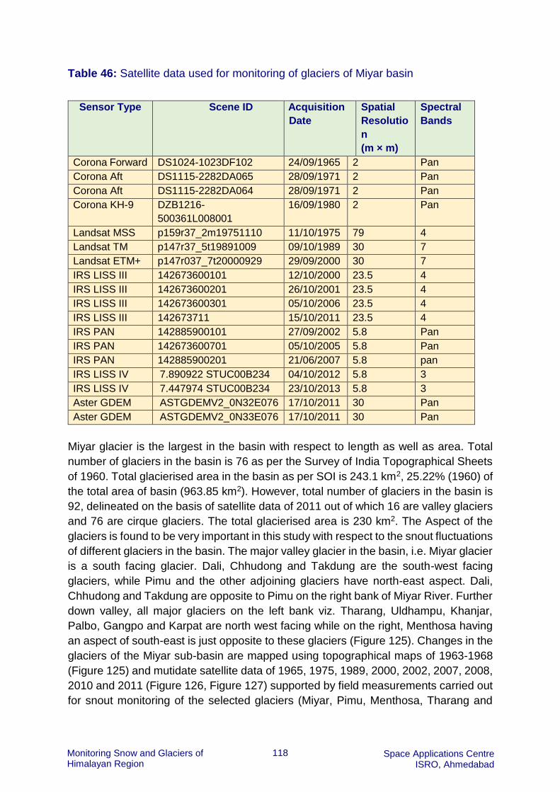
118 Monitoring Snow and Glaciers of Himalayan Region
Space Applications Centre ISRO, Ahmedabad
Table 46: Satellite data used for monitoring of glaciers of Miyar basin
Miyar glacier is the largest in the basin with respect to length as well as area. Total
number of glaciers in the basin is 76 as per the Survey of India Topographical Sheets
of 1960. Total glacierised area in the basin as per SOI is 243.1 km2, 25.22% (1960) of
the total area of basin (963.85 km2). However, total number of glaciers in the basin is
92, delineated on the basis of satellite data of 2011 out of which 16 are valley glaciers
and 76 are cirque glaciers. The total glacierised area is 230 km2. The Aspect of the
glaciers is found to be very important in this study with respect to the snout fluctuations
of different glaciers in the basin. The major valley glacier in the basin, i.e. Miyar glacier
is a south facing glacier. Dali, Chhudong and Takdung are the south-west facing
glaciers, while Pimu and the other adjoining glaciers have north-east aspect. Dali,
Chhudong and Takdung are opposite to Pimu on the right bank of Miyar River. Further
down valley, all major glaciers on the left bank viz. Tharang, Uldhampu, Khanjar,
Palbo, Gangpo and Karpat are north west facing while on the right, Menthosa having
an aspect of south-east is just opposite to these glaciers (Figure 125). Changes in the
glaciers of the Miyar sub-basin are mapped using topographical maps of 1963-1968
(Figure 125) and mutidate satellite data of 1965, 1975, 1989, 2000, 2002, 2007, 2008,
2010 and 2011 (Figure 126, Figure 127) supported by field measurements carried out
for snout monitoring of the selected glaciers (Miyar, Pimu, Menthosa, Tharang and
Sensor Type Scene ID Acquisition
Date
Spatial
Resolutio
n
(m × m)
Spectral
Bands
Corona Forward DS1024-1023DF102 24/09/1965 2 Pan
Corona Aft DS1115-2282DA065 28/09/1971 2 Pan
Corona Aft DS1115-2282DA064 28/09/1971 2 Pan
Corona KH-9 DZB1216-
500361L008001
16/09/1980 2 Pan
Landsat MSS p159r37_2m19751110 11/10/1975 79 4
Landsat TM p147r37_5t19891009 09/10/1989 30 7
Landsat ETM+ p147r037_7t20000929 29/09/2000 30 7
IRS LISS III 142673600101 12/10/2000 23.5 4
IRS LISS III 142673600201 26/10/2001 23.5 4
IRS LISS III 142673600301 05/10/2006 23.5 4
IRS LISS III 142673711 15/10/2011 23.5 4
IRS PAN 142885900101 27/09/2002 5.8 Pan
IRS PAN 142673600701 05/10/2005 5.8 Pan
IRS PAN 142885900201 21/06/2007 5.8 pan
IRS LISS IV 7.890922 STUC00B234 04/10/2012 5.8 3
IRS LISS IV 7.447974 STUC00B234 23/10/2013 5.8 3
Aster GDEM ASTGDEMV2_0N32E076 17/10/2011 30 Pan
Aster GDEM ASTGDEMV2_0N33E076 17/10/2011 30 Pan

119 Monitoring Snow and Glaciers of Himalayan Region
Space Applications Centre ISRO, Ahmedabad
Uldhampu) with GPS in June 2011, 2012 and 2013. Glaciological field evidences for
changes in glacial extent were also studied.
Figure 125: Glaciers in Miyar sub-basin as per topographical maps of 1963-1968

120 Monitoring Snow and Glaciers of Himalayan Region
Space Applications Centre ISRO, Ahmedabad
Figure 126: Changes in glaciers of Miyar sub-basin during 1965-2007
0
0
0
0
0
77°5'0"E
77°5'0"E
77°0'0"E
77°0'0"E
76°55'0"E
76°55'0"E
76°50'0"E
76°50'0"E
76°45'0"E
76°45'0"E
76°40'0"E
76°40'0"E
33°1
5'0
"N
33°1
5'0
"N
33°1
0'0
"N
33°1
0'0
"N
33°5
'0"N
33°5
'0"N
33°0
'0"N
33°0
'0"N
32°5
5'0
"N
32°5
5'0
"N
32°5
0'0
"N
32°5
0'0
"N
32°4
5'0
"N
32°4
5'0
"N
0 6 123 Kilometers
Background Imagery: IRS LISS-IV, Dated: 27 August 2007
±GLACIERS IN MIYAR(Between 1965 - 2007)
Legend
0 GPS Points
Glaciers 2007
Glaciers 2002
Glaciers 2000
Glaciers 1989
Glaciers 1975
Glaciers 1965

121 Monitoring Snow and Glaciers of Himalayan Region
Space Applications Centre ISRO, Ahmedabad
Figure 127: Extent of glaciers of Miyar sub-basin in 2011
It has been observed that the total glaciated area in the Miyar basin in 2007 has
reduced to 169.60 km2 from 243.12 km2 in 1965, indicating a loss of 73.52 km2 area
during 42 years (Table 47). Total retreat and the rate of retreat of different glaciers
viz., Miyar, Pimu, Menthosa, Hulat, Karpat, Gangpu, Palbo, Khanjar, Uldhampu,
Tharang, Tarsalamu, Nakori, Gumba and Dali galciers (Total 14 glaciers) in Miyar sub-
basin are given in Tables 48 to 61. Various data sets are used for various glaciers
depending upon the availability of best scenes. A pattern of glacier recession can be
observed from the Tables 48 to 61.

122 Monitoring Snow and Glaciers of Himalayan Region
Space Applications Centre ISRO, Ahmedabad
Table 47: Total and percent glacerised area in Miyar sub-basin
Year Total glacerised
area (km2)
% glacerised
area
1965 243.12 25.22
1975 170.87 17.72
1989 170.70 17.71
2000 170.13 17.65
2002 169.75 17.61
2007 169.60 17.59
Table 48: Monitoring of Miyar glacier
Miyar
Glacier
SoI
topos
heet
1963
16 Sept.
1980
(Corona)
9
Oct.1989
(Landsat
TM)
27 Sept.
2002
(IRS
PAN)
5 Oct.
2005
(IRS
PAN)
23 Oct.
2013
(IRS
LISS IV)
Total
Change
Linear
retreat
(meter)
Base
year
1963-
1980
1980-
1989
1989-
2002
2002-
2005
2005-
2013
1980-
2013
627 58 128 33 121 340
Per year
rate of
retreat
(meter)
____
___
36.8 6.4 9.8 11 15.1 10
Table 49: Monitoring of Pimu glacier
Pimu
Glacier
SoI
toposheet
1963
28 Sept.
1971
(Corona)
16 Sept.
1980
(Corona)
9 Oct.
1989
(Landsat
TM)
26 Oct.
2001
(IRS
LISS
III)
23 Oct.
2013
(IRS
LISS
IV)
Total
Change
Linear
retreat
(meter)
Base
year
1963-
1971
1971-
1980
1980-
1989
1989-
2001
2001-
2013
1971-
2013
1788 No
Change
147 149 92 388
Per year
rate of
retreat
(meter)
_______ 223 ------------
-
16 12 7 9.2

123 Monitoring Snow and Glaciers of Himalayan Region
Space Applications Centre ISRO, Ahmedabad
Table 50: Monitoring of Menthosa glacier
Menthosa
Glacier
SoI
topos
heet
1963
24 Sept.
1965
(Corona)
9 Oct. 1989
(Landsat
TM)
26 Oct.
2001 (IRS
LISS III)
23 Oct.
2013
(IRS
LISS IV)
Total Change
Linear
retreat
(meter)
Base
year
1963-
1965
1965-
1989
1989-2001 2001-
2013
1965-2013
Advance
of 1260
meter
124 48 46 218
Per year
rate of
retreat
(meter)
_____
___
630 5 4 3.8 4.5
Table 51: Monitoring of Hulat glacier
Hulat
Glacier
28 Sept.
1971
(Corona)
9 Oct. 1989
(Landsat TM)
23 Oct. 2013
(IRS LISS IV)
Total Change
Linear
retreat
(meter)
Base year 1971-1989 1989-2013 1971-2013
125 551 676
Per year
rate of
retreat
(meter)
_________ 6.9 22.9 16
Table 52: Monitoring of Karpat glacier
Karpat
Glacier
SoI
toposheet
1963
9 Oct.
1989
(Landsat
TM)
12 Oct.
2000
(IRS
LISS III)
27 Sept.
2002
(IRS
PAN)
5 Oct.
2005
(IRS
PAN)
23 Oct.
2013
(IRS
LISS IV)
Total
Change
Linear
retreat
(meter)
Base
year
1963-
1989
1989-
2000
2000-
2002
2002-
2005
2005-
2013
1989-
2013
300 No
Change
No
Change
No
Change
No
Change
No
Change
Per
year
rate of
retreat
(meter)
11.5 ------ ------ ------ ------- ---------
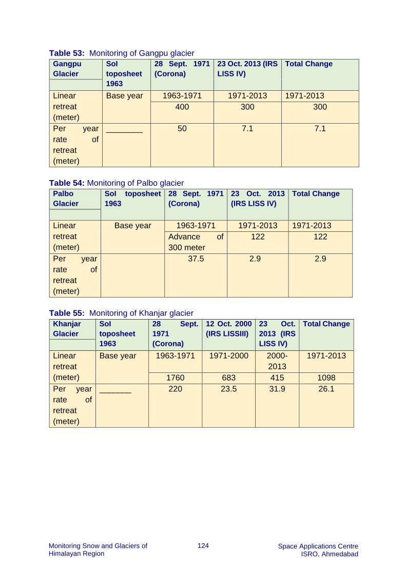
124 Monitoring Snow and Glaciers of Himalayan Region
Space Applications Centre ISRO, Ahmedabad
Table 53: Monitoring of Gangpu glacier
Gangpu
Glacier
SoI
toposheet
1963
28 Sept. 1971
(Corona)
23 Oct. 2013 (IRS
LISS IV)
Total Change
Linear
retreat
(meter)
Base year 1963-1971 1971-2013 1971-2013
400 300 300
Per year
rate of
retreat
(meter)
________ 50 7.1 7.1
Table 54: Monitoring of Palbo glacier
Palbo
Glacier
SoI toposheet
1963
28 Sept. 1971
(Corona)
23 Oct. 2013
(IRS LISS IV)
Total Change
Linear
retreat
(meter)
Base year 1963-1971 1971-2013 1971-2013
Advance of
300 meter
122 122
Per year
rate of
retreat
(meter)
37.5 2.9 2.9
Table 55: Monitoring of Khanjar glacier
Khanjar
Glacier
SoI
toposheet
1963
28 Sept.
1971
(Corona)
12 Oct. 2000
(IRS LISSIII)
23 Oct.
2013 (IRS
LISS IV)
Total Change
Linear
retreat
(meter)
Base year 1963-1971 1971-2000 2000-
2013
1971-2013
1760 683 415 1098
Per year
rate of
retreat
(meter)
_______ 220 23.5 31.9 26.1

125 Monitoring Snow and Glaciers of Himalayan Region
Space Applications Centre ISRO, Ahmedabad
Table 56: Monitoring of Uldhampu glacier
Uldhampu
Glacier
SoI
toposheet
1963
28 Sept.
1971
(Corona)
9 Oct.
1989
(Landsat
TM)
12 Oct.
2000
(IRS
LISS
III)
5 Oct.
2006
(IRS
LISS
III)
23 Oct.
2013
(IRS
LISS
IV)
Total
Change
Linear
retreat
(meter)
Base
year
1963-
1971
1971-
1989
1989-
2000
2000-
2006
2006-
2013
1971-
2013
908 30 50 234 65 379
Per year
rate of
retreat
(meter)
_______ 113.5 1.6 4.5 39 9.2 9
Table 57: Monitoring of Tharang glacier
Tharang
Glacier
SoI
toposhe
et 1963
28 Sept.
1971
(Corona)
9 Oct.
1989
(Lands
at TM)
12 Oct.
2000
(IRS
LISS III)
5 Oct.
2006
(IRS
LISS
III)
23
Oct.
2013
(IRS
LISS
IV)
Total
Change
Linear retreat
(meter)
Base
year
1963-
1971
1971-
1989
1989-
2000
2000-
2006
2006-
2013
1971-
2013
880 128 No
Change
110 310 548
Per year rate of
retreat (meter)
______
__
110 7.1 -----------
--
18.3 44.2 13
Table 58: Monitoring of Tarsalamu glacier
Tarsalamu
Glacier
SoI
toposheet
1963
28 Sept.
1971
(Corona)
9 Oct.
1989
(Landsat
TM)
12 Oct.
2000
(IRS
LISS III)
23 Oct.
2013
(IRS
LISS IV)
Total
Change
Linear retreat
(meter)
Base year 1963-
1971
1971-
1989
1989-
2000
2000-
2013
1971-
2013
Advance
of 1610
meter
239 142 336 717
Per year rate
of retreat
(meter)
________ 201.2 13.2 12.9 25 17

126 Monitoring Snow and Glaciers of Himalayan Region
Space Applications Centre ISRO, Ahmedabad
Table 59: Monitoring of Nakori glacier
Nakori
Glacier
SoI
toposheet
1963
28 Sept.
1971
(Corona)
9 Oct. 1989
(Landsat
TM)
12 Oct.
2000
(IRS
LISS III)
23 Oct.
2013 (IRS
LISS IV)
Total
Change
Linear
retreat
(meter)
Base year 1963-
1971
1971-1989 1989-
2000
2000-2013 1971-
2013
Advance
of 750
meter
105 102 101 308
Per year
rate of
retreat
(meter)
________ 93.7 5.8 9.2 7.7 7.3
Table 60: Monitoring of Gumba glacier
Gumba
Glacier
SoI
toposheet
1963
28 Sept.
1971
(Corona)
9 Oct.
1989
(Landsat
TM)
26 Oct.
2001
(IRS
LISS III)
23 Oct.
2013
(IRS
LISS IV)
Total
Change
Linear
retreat
(meter)
Base year 1963-
1971
1971-
1989
1989-
2001
2001-
2013
1971-
2013
146 136 81 96 313
Per
year
rate of
retreat
(meter)
__________ 18.5 7.5 6.7 8 7.4
Table 61: Monitoring of Dali glacier
Dali
Glacier
SoI toposheet
1963
9 Oct. 1989
(Landsat TM)
23 Oct. 2013
(IRS LISS IV)
Total Change
Linear
retreat
(meter)
Base year 1963-1989 1989-2013 1989-2013
1680 No Change No Change
Per year
rate of
retreat
(meter)
_________ 64.6 ________ ________

127 Monitoring Snow and Glaciers of Himalayan Region
Space Applications Centre ISRO, Ahmedabad
Miyar glacier has retreated by 340 meters between 1980 and 2013 at a rate of about
10 meters per year. The rate of retreat is 15 meter/year since 2005, however, GPS
positions and field photographs (Figure 128) of Miyar snout shows the similar position
in 2012 and 2013.
Figure 128: Field photographs showing changes in snout position of Miyar glacier
during 2008-2013
Pimu glacier on the other hand, shows a rate of retreat of 7 meter/year between 2001
and 2013 and a total rate of 9.1 meter/year, therefore indicating a diminishing rate.
Changes in the Minthosa glacier using multidate satellite data has been studied in detail. Figure 129 shows glacial extent on satellite data of 1971, 1980, 1989, 2000, 2005, 2013. Menthosa glacier has been studied extensively in the field in 2006, 2008, 2010, 2011, 2012 and 2013. As is the case of Pimu glacier, Menthosa glacier also shows a diminishing rate of retreat but interestingly it never had a rate of retreat more than 5 meter per year during last 48 years. Figures 130 and 131 are showing the field photographs of 2008 and 2013 and 3D views of Menthosa snout of 1965 and 2013 respectively. Figure 132 show field photographs for region around snout of Tharang glacier. One very important observation from the recession behaviour of glaciers is that the adjoining glaciers behave more or less similarly. Tarsalamu, Tharang, Uldhampu, Khanjar, Palbo, Gangpu and Karpat are situated in the parallel valleys with an aspect of North-West.

128 Monitoring Snow and Glaciers of Himalayan Region
Space Applications Centre ISRO, Ahmedabad
Figure 129: Changes in extent of Menthosa glacier as seen on satellite data of different
time periods.
These glaciers can be grouped into two categories. While Karpat, Gangpu and Palbo
have changed very little since earliest available images i.e. Corona of 1971 (Landsat
TM 1989 in case of Karpat), other four glaciers (Khanjar, Uldhampu, Tharang and
Tarsalamu) exhibit a recession behaviour which can be labelled as very fast since the
turn of century. Exceptionally high rate of retreat (39 meter/year) in Uldhampu glacier
between 2000 and 2006 can be attributed to the occurrence of a pro-glacial lake in
this period, but the similar behaviour of Khanjar, Tharang and Tarsalamu glaciers can
only be interpreted in terms of their micro-climate. In the similar fashion Dali,
Chhudong and Takdung are in parallel valleys with an aspect towards south in upper
parts and towards west in the lower zones. All these three glaciers have also exhibit a
very little change since the 1980; however, change is not measurable because of
intense shadow on the snout in all of the satellite images. Overall the study show that
recessional pattern of glaciers in Miyar sub-basin is highly variable, where it is
observed that some glaciers changed very little in last 40-50 years, and at the same
time some glaciers have retreated rapidly during some time periods. The major glacier
in the basin i.e., Miyar retreated by 340 meters since 1980 at the rate of 10 m/year. 10
glaciers out of 16 showed a retreat rate below 10 m/year

129 Monitoring Snow and Glaciers of Himalayan Region
Space Applications Centre ISRO, Ahmedabad
Figure 130: Field photograph of Menthosa glacier.

130
Monitoring Snow and Glaciers of Himalayan Region
Space Applications Centre ISRO, Ahmedabad
Figure 131: 3-D view of Menthosa glacier as seen in Corona (1965) and IRS LISS-IV
(2013)
Figure 132: Field photographs showing region around snout of Tharang glacier

131
Monitoring Snow and Glaciers of Himalayan Region
Space Applications Centre ISRO, Ahmedabad
Equilibrium Line Altitude (ELA) estimation is very important aspect of glaciology
because ELA is the altitude of the line of balance between accumulation and ablation
of a glacier. A glacier is in equilibrium only if annual discharge through the equilibrium
line cross section is equal to the net annual accumulation up-glacier and the net annual
ablation down-glacier. Otherwise, it will grow or shrink. Rising ELAs indicate negative
mass balance, while lowering ELA is a result of positive mass balance.
ELA in the Miyar sub-basin has been estimated using four different methods and the
mean ELA has been worked out. These methods are Area Weighted Mean (A-WM),
Area Accumulation Ratio (AAR), Toe to Headwall Ratio (THAR) and Maximum
Elevation of Lateral Moraine (MELM)”. ELA based on different methods and average
ELA for selected glaciers in the Miyar basin are given in Table 62. Change in ELAs
from Local Glacial Maximum (LGM) to the Present are provided in Table 63. The
altitude of the LGM terminus has been taken as 3040 m (near Karpat village) on the
basis of the geomorphic evidence of truncated spurs and trimlines. The position of the
Holocene snouts of all the glaciers is well preserved by the end moraines. There are
variations in the ELA values obtained from different methods, therefore average ELAs
computed on the basis of ELAs obtained from all the four methods may help in
reducing the error margin (Table 64).
Glacier retreat pattern in Miyar sub-basin during Last Glacial Maxima (LGM), Holocene and Recent (2011) is shown in Figure 133 and extent of Equilibrium Line Altitude (ELA) during Last Glacial Maxima (LGM), Holocene and Recent is shown in Figure 134. It shows that glaciers in the Miyar sub-basin are retreating since LGM, however impact of climate change may get reflected in accelerated retreat during past few decades.

132
Monitoring Snow and Glaciers of Himalayan Region
Space Applications Centre ISRO, Ahmedabad
Ta
ble
62
: E
qu
ilibrium
Lin
e A
ltitu
de
ba
sed
on
diffe
rent m
eth
od
s a
nd
ma
jor
cha
racte
ristics o
f se
lecte
d g
lacie
rs in
the
Miy
ar
ba
sin
(b
ase
d o
n th
e S
OI to
po
gra
ph
ical m
ap
s s
urv
eye
d b
etw
ee
n 1
963
-19
68
)
Na
me
of th
e g
lacie
rA
sp
ect
Le
ng
th
(km
)
Siz
e
(sq
km
)
He
ad
wa
ll
alti
tud
e
(m)
Sno
ut
po
sitio
n
(ele
vatio
n
in m
)
EL
A
ba
se
d o
n
A-W
M
(m a
msl)
EL
A
ba
se
d o
n
AA
R
(0.4
4)
(m a
msl)
EL
A
ba
se
d o
n
AA
R
(0.4
8)
(m a
msl)
EL
A
ba
se
d o
n
TH
AR
(m a
msl)
Me
an
EL
A
(m a
msl)
Tha
rang
NW
5.4
86
55
60
40
00
50
27
51
40
51
00
47
80
50
12
Gum
ba
S7
6.8
56
80
44
20
49
26
49
40
49
00
50
50
49
54
Ta
kd
ung
SW
12
.55
15
58
40
42
00
50
65
52
40
51
60
50
20
51
21
Miy
ar
S2
7.4
38
5.6
60
00
39
80
50
78
52
40
52
00
49
90
51
27
Chhud
ong
SW
11
.26
10
.75
76
04
50
05
14
25
20
05
16
05
13
05
15
8
Pim
uN
E6
.45
7.4
54
80
43
00
48
71
49
60
49
20
48
90
49
10
Uld
ha
mp
uN
W8
.17
.55
60
04
34
04
86
44
96
04
92
04
87
04
92
8
Kha
nja
rN
W5
.88
4.9
52
00
42
00
48
45
49
40
49
20
47
00
48
51
Me
nth
osa
SE
3.8
63
.35
68
04
48
04
90
64
72
04
70
05
08
04
82
6
Ka
rpa
tN
W4
.54
4.9
57
20
42
00
49
90
50
40
50
00
49
60
49
97
Hula
tS
W7
.86
5.4
58
00
39
40
48
44
48
80
48
40
48
70
48
58
Oth
er
ice
bo
die
s8
5.6
To
tal G
lace
rise
d A
rea
24
3.1
To
tal a
rea
of th
e b
asin
96
3.8
5

133
Monitoring Snow and Glaciers of Himalayan Region
Space Applications Centre ISRO, Ahmedabad
T
ab
le 6
2:
Equ
ilibrium
Lin
e A
ltitu
de
ba
sed
on
diffe
rent m
eth
od
s a
nd
ma
jor
cha
racte
ristics o
f se
lecte
d g
lacie
rs in
the
Miy
ar
ba
sin
(b
ase
d o
n th
e S
OI to
po
gra
ph
ical m
ap
s s
urv
eye
d b
etw
ee
n 1
963
-19
68
)
Na
me
of
the
gla
cie
r
He
ad
wa
ll
LG
M
Te
rmin
i
Ho
loce
n
e
Te
rmin
i
Pre
se
nt
Te
rmin
i
Lo
ca
l
Gla
cia
l
Ma
xim
um
EL
A
Ho
loce
ne
EL
A
Pre
se
nt
EL
A
(TH
AR
0.5
)
EL
A R
ise
fro
m L
GM
to
Ho
loce
ne
EL
A R
ise
fro
m
Ho
loce
ne
to P
rese
nt
To
tal R
ise
in E
LA
fro
m
LG
M to
pre
se
nt
Tha
rang
55
60
30
40
36
00
40
09
43
00
45
80
47
85
28
02
05
48
5
Gum
ba
54
50
30
40
39
00
45
00
42
45
46
75
49
75
43
03
00
73
0
Ta
kd
ung
55
70
30
40
39
50
43
80
43
05
47
60
49
75
45
52
15
67
0
Miy
ar
60
00
30
40
39
70
40
43
45
20
49
85
50
21
46
53
65
01
Chhud
ong
55
00
30
40
39
50
45
58
42
70
47
25
50
29
45
53
04
75
9
Pim
u5
48
03
04
03
95
04
60
44
26
04
71
55
04
24
55
32
77
82
Uld
ha
mp
u5
45
03
04
03
45
04
34
64
24
54
45
04
89
82
05
44
86
53
Kha
nja
r5
38
03
04
03
45
04
64
44
21
04
41
55
01
22
05
59
78
02
Me
nth
osa
56
80
30
40
33
00
43
80
43
60
44
90
50
30
13
05
40
67
0
Miy
ar
Ba
sin
55
63
30
40
37
24
43
85
43
02
46
44
49
74
34
23
30
67
2

134
Monitoring Snow and Glaciers of Himalayan Region
Space Applications Centre ISRO, Ahmedabad
Table 64: ELA by Maximum Elevation of Lateral Moraine (MELM) Method for selected glaciers of Miyar sub-basin
Name of the glacier ELA based on MELM 2010 Average ELAs
Tharang 5085 5012
Gumba 4821 4954
Takdung 5000 5121
Miyar 4957 5157
Chhudong 5000 5158
Pimu 4933 4910
Uldhampu 4866 4928
Khanjar 4906 4851
Menthosa 4732 4826
Karpat 4750 4997
Hulat 5020 4858

135
Monitoring Snow and Glaciers of Himalayan Region
Space Applications Centre ISRO, Ahmedabad
Figure 133: Glacier retreat pattern in Miyar sub-basin during Last Glacial Maxima (LGM), Holocene and Recent (2011) in Miyar sub-basin

136
Monitoring Snow and Glaciers of Himalayan Region
Space Applications Centre ISRO, Ahmedabad
Figure 134: Extent of Equilibrium Line Altitude (ELA) during Last Glacial Maxima (LGM), Holocene and Recent in Miyar sub-basin

137
Monitoring Snow and Glaciers of Himalayan Region
Space Applications Centre ISRO, Ahmedabad
(e) Glaciers of Chandra Sub-basin
Chandra sub-basin is located between 32º10’ to 32º85’ North and 77 º 00’ to 77º 75’
East in Lahaul and Spiti district of Himachal Pradesh. The Chandra river originates
from the Great Himalayas and joins river Bhaga at Tandi in Lahaul and Spiti district.
Changes in the glaciers of the Chandra basin were studied for the time frame 1980,
2001, 2007 and 2011 using multidate satellite data. (Figure 135). The salient results
are summarized in Table 65.
Figure 135: Location of glaciers studied in Chandra basin, Himachal Pradesh
Table 65: Changes in glaciers of the Chandra basin, Himachal Pradesh as per size
frequency distribution during 1980-2011
Glacier Area (sq km)
1980 2001 2007 2011
No. of glaciers
Glaciated Area (sq km)
No. of glaciers
Glaciated Area (sq km)
No. of glaciers
Glaciated Area (sq km)
No. of glaciers
Glaciated Area (sq km)
0-1 16 11.95 20 12.83 20 10.44 20 9.78
1-3 17 35.10 20 39.03 23 45.28 24 44.72
3-5 09 34.17 07 25.63 03 11.98 04 16.45
5-10 08 61.45 10 72.49 09 63.33 10 68.13
>10 10 225.83 08 189.39 07 169.83 07 163.33
Total 60 368.50 65 339.71 62 300.67 65 302.09

138
Monitoring Snow and Glaciers of Himalayan Region
Space Applications Centre ISRO, Ahmedabad
It is observed that 10 larger glaciers i.e., with more than 10 sq km glaciated area in 1980 reduced to 7 in 2011 and smaller glaciers i.e. with glaciated area in category of 0-1 and 1-3 sq km have increased from 16 to 20 and 17 to 24 respectively in 2011. It indicates that glaciers have retreated as well fragmented into smaller glaciers.
Table 66 summarizes net change in glaciated area of glaciers in the Chandra basin,
as per size frequency distribution during 2001-2011. It is observed that overall there
has been net loss of 37.62 sq km glaciated area of the Chandra sub-basin during the
time frame 2001-2011 for the 65 glaciers, which constitutes 11% net loss.
Fragmentation of one glacier with >10 sq km glaciated area is also indicated by
increase of 4 glaciers in the category of glaciers with 1-3 sq km area and 5.69 sq km
gain in glaciated area, which is 14.6% net gain. Reduction in glaciated area of 3
glaciers in the category of glaciers with 3-5 sq km area.is also indicated. It is also
observed that glaciers upto 5 sq km area (upto 35.8%) have shown higher loss in
glaciated area than glaciers greater than 5 sq km area (upto 13.7%). It may be due to
their debris free nature as well steeper slope.
Table 66: Net change in glaciated area of glaciers in the Chandra basin, Himachal
Pradesh as per size frequency distribution during 2001-2011
Glacier Area (sq km)
2001 2011 Net Change in glaciated area (sq km)
% change in glacial area
No. of glaciers
Glaciated Area (sq km)
No. of glaciers
Glaciated Area (sq km)
0-1 20 12.83 20 9.78 - 3.05 - 23.8
1-3 20 39.03 24 44.72 + 5.69 +14.6
3-5 07 25.63 04 16.45 -9.18 -35.8
5-10 10 72.49 10 68.13 -4.36 -6
>10 08 189.39 07 163.33 -26.06 -13.7
Total 65 339.71 65 302.09 -37.62 -11
Changes in Samudra Tapu, Geepang Gath and Batal glaciers, Chandra basin
Samudra Tapu, Geepang Gath and Batal glaciers (Figure 136) have been studied in
detail by interpreting multidate satellite data as well collecting field based glaciological
observations. The salient characteristics of these glaciers are given in Table 67.
Samudra Tapu glacier is second largest glacier in Chandra sub-basin. It is east facing
glacier with snout at 4160 m amsl (Figure 137). Geepang Gath glacier is NW facing
glacier with largest moraine dammed lake in H.P. at its snout at 4088 m amsl. Batal
glacier is a NE facing glacier with its snout at 4217 m amsl. Changes in glaciated area
and retreat of Samudra Tapu, Geepang Gath and Batal glaciers are summarized in
Table 68 and Table 69 respectively. It is observed that Samudra Tapu, Geepang Gath
and Batal glaciers have retreated by 717 m, 507 m and 232.39 m during 31 years
(1980-2011), with an average retreat of 23 m/year, 16 m/year and 7.50 m/year
respectively. It is observed that loss in glaciated area of Samudra Tapu, Geepang
Gath and Batal glaciers is 9.64 sq km, 2.86 sq km and 2.15 sq km during 31 years
(1980-2011) respectively. However, % loss in glaciated area is highest for Batal
(30.8%), followed by Geepang Gath (20.7%) and Samudra Tapu (11.5%) glaciers

139
Monitoring Snow and Glaciers of Himalayan Region
Space Applications Centre ISRO, Ahmedabad
respectively. Field photographs showing snout and adjoining parts of the Samudra
Tapu, Geepang Gath and Batal glaciers are given in Figures 138 to Figure 145. It may
be seen that there are distinct geomorphological evidences showing retreat of these
glaciers and enlargement of the moraine dammed lakes of the Samudra Tapu as well
Geepang Gath lakes.
Figure 136: Geepang Gath, Samudra Tapu and Batal glaciers in the Chandra basin in
Lahaul and Spiti district, Himachal Pradesh Table 67: Salient Characteristics of Samudra Tapu, Geepang Gath and Batal glaciers
Parameters Samundra
Tapu
Glacier
Gepang Gath
Glacier
Batal Glacier
Length (km) 16 .2 5.5 6.3
Catchment Area ( sq.km) 87.58 13.57 7.40
Snout Altitude (a.s.l) 4160 m
(2001)
4088 m (2001) 4217 m (2001)
Orientation E facing NW facing NE facing
Equilibrium Line Altitude
(ELA)
5386 m
(2001)
4860 m (2001) 5520 m (2001)

140
Monitoring Snow and Glaciers of Himalayan Region
Space Applications Centre ISRO, Ahmedabad
Table 68: Snout retreat of Samudra Tapu, Geepang Gath and Batal glaciers
Glacier Name
Snout retreat (m) 1980-1989
Snout retreat (m) 1989-1999
Snout retreat (m) 1999-2007
Snout retreat (m) 2007-2011
Snout retreat (m) 1980-2011
Average snout retreat m/yr 1980-2011
Samudra Tapu glacier
215 98
241 163 717 23
Geepang gath glacier
48 42 300 --- 507 16
Batal Glacier
135 (1980-2001)
--- 84 (2001-2007)
13.39 232.39 7.50
Table 69: Loss in glaciated area of Samudra Tapu, Geepang Gath and Batal glaciers
Glacier Name
Glaciated area in 1980 (sq km)
Glaciated area in 2001 (sq km)
Glaciated area in 2007 (sq km)
Glaciated area in 2011 (sq km)
Loss in glaciated area 1980-2011
% loss in glaciated area 1980-2011
Samudra Tapu glacier
84.06 80.41 77.28 74.42 9.64 11.5
Geepang gath glacier
13.80 12.23 11.63 10.94 2.86 20.7
Batal Glacier
6.97 5.28 5.25 4.82 2.15 30.8

141
Monitoring Snow and Glaciers of Himalayan Region
Space Applications Centre ISRO, Ahmedabad
Figure 137: Panaromic view of Samudra Tapu glacier, Chandra basin, Lahaul and
Spiti district, Himachal Pradesh
Figure 138: Field photograph showing glacial area evacuated by Samudra Tapu Glacier between eight years (2004 and 2012). Red line shows extent of glacier area vacated in 2012

142
Monitoring Snow and Glaciers of Himalayan Region
Space Applications Centre ISRO, Ahmedabad
Figure 139: Field photograph showing snout of Samudra Tapu glacier in 2004 (Upper)
and the snout location submerged in lake (Lower) in subsequent years since 2007

143
Monitoring Snow and Glaciers of Himalayan Region
Space Applications Centre ISRO, Ahmedabad
Figure 140: Field photograph showing enlargement of moraine dammed lake of
Samudra Tapu glacier in different years. Red line indicates vacated area of the glacier
Figure 141: Field photograph showing Subterraneous tunnels at snout of Samudra
Tapu glacier

144
Monitoring Snow and Glaciers of Himalayan Region
Space Applications Centre ISRO, Ahmedabad
Figure 142: Field photograph showing snout of Geepang Gath glacier and moraine
dammed lake
Figure 143: Field photograph showing accumulation area of Geepang Gath glacier

145
Monitoring Snow and Glaciers of Himalayan Region
Space Applications Centre ISRO, Ahmedabad
Figure 144: Field photograph showing retreating snout of Batal glacier
Figure 145: Field photograph showing moraine deposits exposed due to the retreat of
Batal glacier

146
Monitoring Snow and Glaciers of Himalayan Region
Space Applications Centre ISRO, Ahmedabad
(f) Detailed Study of Satopanth and Bhagirath-Kharak glaciers, Alaknanda sub-
basin, Uttarakhand
Changes in the Satopanth and Bhagirath-Kharak glaciers located at the head of
Alaknanda river valley in Chamoli district, Uttarakhand were studied using old archived
data, Corona satellite data of 1968 and Landsat as well IRS data of 1988, 2004, 2010
and 2013. Changes in the frontal parts of Bhagirath-Kharak and Satopanth glaciers as
mapped using satellite data are shown in Figure 146 and Figure 147. The field
photographs showing the frontal parts and snout are shown in Figure 148 and Figure
149. Table 70 summarises the retreat, rate of retreat/year and loss in glaciated area
during 1968-1988, 1988-2004, 2004-2010 and 2010-2013 time frames for the
Bhagirath-Kharak and Satopanth glaciers.
The earliest records have mentioned single glacier front for both these glaciers,
however Corona photographs of 1968 show separate snouts. It is observed that for
the entire time period between 1968 and 2013, Satopanth glacier shows an annual
average retreat of 9.86 meters per year, whereas Bhagirath-Kharak glacier shows an
average annual retreat of 8.13 meters per year. As a result of the retreat of the frontal
parts of these glaciers, the area vacated by the Satopanth glacier between 1968 and
2013 is 0.39 sq km, while during the same period, the Bhagirath Kharak glacier has
vacated an area of 0.24 sq km.
Figure 146: Changes in the frontal parts of Bhagirath-Kharak and Satopanth glaciers
in Uttarakhand

147
Monitoring Snow and Glaciers of Himalayan Region
Space Applications Centre ISRO, Ahmedabad
Figure 147: Changes in the frontal parts of Bhagirath-Kharak and Satopanth glaciers
during 1968-2013
Figure 148: Field photograph of the frontal parts of the Satopanth glacier

148
Monitoring Snow and Glaciers of Himalayan Region
Space Applications Centre ISRO, Ahmedabad
Figure 149: Field photograph of the frontal parts of the Bhagirath Kharak glacier
Table 70: Changes in the frontal parts of Bhagirath-Kharak and Satopanth glaciers at
the head of Alaknanda river, Chamoli district, Uttarakhand
YEAR/ PERIOD
BHAGIRATH-KHARAK GLACIER SATOPANTH GLACIER
Total retreat in mts.
Average retreat In mts/year
Loss in area
(sq km)
Total retreat in mts.
Average retreat In mts/year
Loss in area
(sq km)
1968-1988 40.83 2.04 0.0565 37.51 1.87 0.1323
1988-2004 148.00 9.25 0.1143 294.00 18.37 0.1622
2004-2010 134.00 22.33 0.0618 070.00 11.66 0.0875
2010-2013 43.10 14.36 0.0080 42.50 14.16 0.0140
1968-2013 365.93 8.131 0.2426 444.01 9.86 0.3960

149
Monitoring Snow and Glaciers of Himalayan Region
Space Applications Centre ISRO, Ahmedabad
(g) Glaciers in Drass sub-basin
Drass is the sub-basin of Indus river. Drass river joins Indus near Kargil in Jammu and
Kashmir. Drass sub basin is the Vth order basin of IVth order Indus and it extends
between the Gumri (close to Zoji-La) in the west to Kargil in the east. Satellite data
analysis revealed that there are 150 glaciers in Drass glacier sub-basin, whereas as
per topographical maps of 1965, the basin occupied 115 glaciers and that the
increased number in glaciers (115 to 150) is due to fragmentation (Koul et al., 2016).
150 glaciers cover an area of 152.68 km2 with ice volume of 62.02 km3. Monitoring of
150 glaciers using satellite data for time frame 2001 to 2013 indicate that 120 glaciers
show no change, 28 glaciers show loss and 2 glaciers show gain in glaciated area.
The study show that larger glaciers above 5 km2 has vacated a small area (0.64% to
2.64% of glacier area) in comparison to small glacier ranging in area 2 km2 to 5 km2
(1.68% to 9% of glacier) during 12 years period. There by indicating that glaciers of
Drass valley in general retreat at slow pace. Two glaciers shows gain in area by 30%
and 40% (Figure 150).
Eighty-one glaciers of Drass valley were selected for long-term monitoring for the
period 1965-2001 and 2001-2013. It is observed that ten glaciers experienced gain in
area, 13 glaciers a loss more than 50% of its area, 18 glaciers lost 25% - 50% of
glacier area and the remaining glaciers lost marginal area during last 50 years period
(Figure 151).
Out of the ten glaciers showing gain in area, four glaciers show gain in area during
1965 to 2001 but loss in area from 2001 to 2013 and remaining six glaciers of the
category show gain in area from 1965 to 2001, and no change in their area between
2001 and 2013.
Figure 150: Glaciers in Drass valley showing changes in area 2001-2013 (Source: Koul et al., 2016)

150
Monitoring Snow and Glaciers of Himalayan Region
Space Applications Centre ISRO, Ahmedabad
Figure 151: Glaciers in Drass valley showing change in area (1965-2013) (Source: Koul et al., 2016)
(h) Other glaciated areas
Detailed study of Bairpal Nai and Dharlang glaciers in the Chenab basin, Jammu &
Kashmir region show that the tributary glaciers are getting detached from the main
trunk glacier causing fragmentation and interestingly, rate of retreat of main trunk
glacier is higher than that of the tributary glacier (Brahmbhatt et al., 2015b). The
causes of fragmentation and changes in rate of retreat are attributed to Accumulation
Area Ratio (AAR), slope and altitude.
Changes in the glaciated area of the Warwan and Bhut basins of western Himalaya
during the period 1962 and 2001/02 time frame have shown 19% and 9% loss
respectively, which may be due to i) smaller size of glaciers of the Warwan basin (e.g.,
164 glaciers having < 1 sq km area in comparision to 101 glaciers in Bhut basin), ii)
lower percentage of debris cover in Warwan (18%) than in the Bhut basin (30%) and
iii) higher percentage of glaciated area lying below 5100 m i.e,, 80% in Warwan
whereas 70% in the Bhut basin (Brahmbhatt et al., 2012a; Brahmbhatt, 2014;
Brahmbhatt et al., 2016). Changes in debris free 13 glaciers in Warwan and Bhut sub-
basins during time frame 2001 to 2007 studied using IRS LISS-III data show rate of
retreat of the order 2 to 16 percent (Brahmbhatt et al., 2014).
Changes in glaciers in the Bhaga basin for the time frame 2001 and 2011 based on
IRS LISS-III data show that the glacerised area of the 231 glaciers covering an area
of 391.56 ±3.76 km2 in 2001 has been reduced to 385.17 ±3.71 km2 in 2011; a loss of
1.63 ±1.0% in glacierized area within a period of 10 years (Birajdar et al., 2014).

151
Monitoring Snow and Glaciers of Himalayan Region
Space Applications Centre ISRO, Ahmedabad
4. Glacier Mass Balance
4.1. Objective
To determine the annual specific mass balance of glaciers of using AAR approach for
four consecutive years (2010-2013) and analyze the variations in mass balance
glaciers of identified sub-basins (Table 71) of Indus, Ganga and Brahmaputra river
basins of Himalayan region based on their geographical and climatic diversity.
Table 71: Basins and sub-basins for glacial mass balance studies taken up under the
project
Sr. No.
Basin Sub-basins ↓
1 Indus Nubra
2 Indus Zanskar
3 Chenab Warwan
4 Chenab Bhut
5 Chenab Chandra
6 Chenab Bhaga
7 Chenab Miyar
8 Beas Parbati
9 Satluj Basapa
10 Ganga Alaknanda
11 Ganga Bhagirathi
12 Ganga Dhauliganga
13 Ganga Goriganga
4.2. Scientific Rationale
The mass balance of the glacier is usually referred to as the total loss or gain in mass
at the end of the hydrological year. It is estimated by measuring the total accumulation
of seasonal snow and ablation of snow and ice. Mass balance has two components,
accumulation and ablation. The accumulation (input) includes all forms of deposition,
mainly precipitation, and ablation (output) means loss of snow and ice in the form of
melting, evaporation and calving etc. from the glacier. The boundary at the end of
ablation season between accumulation and ablation is known as Equilibrium line. The
difference between net accumulation and net ablation for the whole glacier over a
period of one year is Net balance. The net balance for each glacier is different in
amount and depends upon the size/shape of the glacier and climatic condition of the
area. The net balance per unit area of glacier is specific mass balance or SMB,
expressed in cm of water equivalent. There is wide variation in mass changes from
time to time and place to place on the glacier due to the various factors. The process
of mass balance of the glaciers over an entire region is complex, as it is irregular in
152
Monitoring Snow and Glaciers of Himalayan Region
Space Applications Centre ISRO, Ahmedabad
amount, rate and time of occurrence. Therefore, the ultimate aim to monitor mass
balance is to match it with the changes in various parameters of the glaciers. This
change directly affects the flow of the glacier and its terminus position. i.e.
advancement and recession of the frontal position of the glaciers. Generally mass
balance studies are carried out using methods (Ben and Evans, 2010; Cuffley and
Paterson, 2010; Gardelle et al., 2013) such as geodetic, glaciological, hydrological
and AAR based.
Mass balance of a glacier determined annually is the most important parameter to
assess the health of glaciers to understand the effect of climatic variations on the
locked fresh water resource within a glacier. Trends of mass balances are direct
indicator of climatic variations, however mass balance estimations require a large
amounts of efforts in terms of resources, logistics and accuracy in any glaciated
environment. Mountain glaciers in the Himalayan region are largely influenced by their
climatic conditions and topographic undulations. This restricts field measurements
using glaciological methods throughout the year (Wagnon et al., 2007; Dobhal et al.,
2008). It is not feasible to study all the mountain glaciers in the field for every year,
and hence it is important to replace the conventional methods by some cost effective,
fast and reliable techniques so that a quick assessment of mass balance of individual
glaciers could be done over a period of time. Remote sensing based methods have
become an important alternative to conventional methods of mass balance estimation.
These methods include monitoring of snow line at the end of ablation season, DEM
differencing., LIDAR techniques, gravity measurements and GPR etc. Remote
sensing has played a crucial role for mass balance estimation in the Himalayan region
using Digital Elevation Model (DEM) (Bahuguna et al., 2007; Berthier et al., 2007) and
Accumulation Area Ratio (AAR) approach (Kulkarni, 1992; Kulkarni et al., 2004b;
Singh et al., 2013b).
Position of snow line at the end of ablation season is used to compute Accumulation
Area Ratio (AAR). AAR is a ratio between accumulation area to total glacial area.
Accumulation and ablation zone are defined as zones of glacier above and below
snow line at the end of ablation season (melting season). It is a close approximation
to the equilibrium line on glaciers in mountain glaciers. Snowline at the end of ablation
season can be mapped using high temporal images in VNIR region. AAR is further
used to compute specific mass balance based on empirical relationship between AAR
and specific mass balance developed using field mass balance data of Shaune
Garang and Gor Garang glaciers (Figure 152, Kulkarni 1992). The model has shown
AAR representing zero mass balance as 0.48. On the basis of accumulation area ratio
(area of accumulation divided by whole area of glacier) mass balance in terms of gain
or loss can be estimated. This method is commonly used to assess mass balance at
reconnaissance level. The approach based on satellite observations provide a quick
regional assessment. However, to use AAR method, we are required to develop a
relationship between mass balance and AAR for a particular glacier and a particular
period. This relationship can be extended to many other glaciers of the basin.

153
Monitoring Snow and Glaciers of Himalayan Region
Space Applications Centre ISRO, Ahmedabad
4.3. Methodology
Data from AWiFS sensor onboard Resourcesat-1 and 2 satellites is main source of
delineate the snow line at the end of ablation season. However, appropriate AWiFS
data was not observed over few selected sub-basins and was identified cloudy in the
ablation period. Therefore, AAR estimation was extended to six years instead of four
years for those sub-basins for which the data was available. Thus, AAR estimation
has been carried out for the hydrological years 2007-08, 2008-09, 2009-10, 2010-11,
2011-12 and 2012-13 for twelve sub-basins. The steps which are followed to extract
AAR for each glacier under study have been enumerated as below.
1) AWiFS images of period from July to October were georeferenced with master
images.
2) Basin boundaries were digitized and overlaid on the images. Image to map
registration was carried out to match basin boundary.
3) All the glaciers boundaries were digitized on screen using IRS LISS III image to
get area of glaciers. The LISS III scenes are used in order to ascertain the
boundary of glaciers using higher resolution of the data. These boundaries are
further confirmed using SOI maps. To match the boundary of glaciers from maps
and satellite data, part of accumulation zone is matched on the ridges based on
the shadows observed.
4) Glacier boundaries are overlaid on all AWiFS scenes sequentially. Snowline of
the respective date is created for individual glacier.
5) The accumulation area is the area of glacier above equilibrium line or snow line
at end of ablation season. Thus AAR is derived for each glacier based on
location of snow line at the end of ablation season.
6) A table is generated for AAR of each glacier corresponding to each scene. The
least AAR is considered for estimation of mass balance.
7) The mass balance for each glacier is estimated using relationship between AAR
and mass balance.
Figure 152: Relationship of AAR and Specific mass balance (Source: Kulkarni, 1992)
-140
-120
-100
-80
-60
-40
-20
0
20
40
60
0 0.1 0.2 0.3 0.4 0.5 0.6 0.7 0.8
Accumulation area ratio
Ma
ss
ba
lan
ce
(c
m)
R = 0.89

154
Monitoring Snow and Glaciers of Himalayan Region
Space Applications Centre ISRO, Ahmedabad
4.4. Results and Discussion
The mass balance was estimated for mainly valley glaciers and not for small glaciers
/permanent snow fields (<3 sq. km) considering the accuracy in using 56 m spatial
resolution AWiFS data.
Example of variation of snow line at the end of ablation season for an individual glacier
are shown in Figure 153. Snow line fluctuates due to precipitation and melting and is
observed to vary from one year to another as can be seen in the Figure for all
respective years.
Figure 153: Variation of Snow line at the end of ablation season on glaciers for
estimation of AAR.

155
Monitoring Snow and Glaciers of Himalayan Region
Space Applications Centre ISRO, Ahmedabad
(a) Sub-basin wise Glacier Mass Balance
The salient results of glacier mass balance for 13 sub-basins are summarized in Table
72 and Table 73. This data has been further analysed and salient results are discussed
subsequently.
Table 72: Number of glaciers experiencing positive and negative specific mass
balance using AAR approach during 2008 to 2013 in each sub-basin. C is
cloudy data.
Basin Sub-basin ↓ Years → 2008 2009 2010 2011 2012 2013
Indus Nubra Negative 42 3 3 6 10 20
Positive 41 83 83 70 75 66
Indus Zanskar Negative c c 6 10 12 31
Positive c c 46 68 24 62
Chenab Warwan Negative 37 2 14 11 7 13
Positive 8 32 30 28 37 30
Chenab Bhut Negative 14 2 12 14 14 5
Positive 15 12 32 32 32 33
Chenab Chandra Negative 40 16 1 0 16 14
Positive 64 73 104 98 84 29
Chenab Bhaga Negative 7 3 20 5 64 0
Positive 55 70 41 44 13 50
Chenab Miyar Negative 153 98 33 32 97 53
Positive 47 50 177 203 63 19
Beas Parbati Negative 17 1 3 3 9 6
Positive 14 17 35 25 16 22
Satluj Basapa Negative 13 11 4 8 9 c
Positive 3 8 10 11 2 c
Ganga Alaknanda Negative 60 78 10 26 55 88
Positive 24 21 48 94 66 12
Ganga Bhagirathi Negative 67 73 4 27 50 52
Positive 11 16 10 114 54 21
Ganga Dhauliganga Negative 62 28 26 35 37 c
Positive 40 11 21 45 6 c
Ganga Goriganga Negative 6 17 7 4 10 c
Positive 23 6 3 23 14 c
Total Negative 518 332 143 181 390 282
Positive 345 399 640 855
486
344
Grand Total 863 731 783 1036 876 626

156
Monitoring Snow and Glaciers of Himalayan Region
Space Applications Centre ISRO, Ahmedabad
Table 73: Average Accumulation Area Ratio (AAR) and Specific Mass Balance (SMB)
in cm for selected glaciers studied in 13 sub-basins of Himalayan region
during 2008 to 2013
C-cloudy data
Basin Sub-basin 2008 2009 2010 2011 2012 2013
Indus Nubra AAR 0.5 0.85 0.77 0.78 0.67 0.62
SMB 1.57 87.33 66.76 68.88 42.98 23.32
Indus Zanskar AAR - - 0.72 0.63 0.55 0.55
SMB - - 54.59 32.61 13.57 13.05
Chenab Warwan AAR 0.36 0.77 0.55 0.6 0.74 0.61
SMB -32.3 66.51 14.21 25.61 58.93 28.55
Chenab Bhut AAR 0.48 0.65 0.56 0.54 0.56 0.67
SMB -2.43 37.12 16.22 10.84 14.9 41.77
Chenab Chandra AAR 0.53 0.68 0.83 0.94 0.68 0.61
SMB 7.14 45.23 81.8 107.67 45.38 26.87
Chenab Bhaga AAR 0.7 0.84 0.58 0.83 0.71 0.81
SMB 49.61 84.01 19.84 81.22 50.86 74.87
Chenab Miyar AAR 0.37 0.43 0.71 0.62 0.58 0.38
SMB -31.88 -17.25 51.44 30.03 20.01 -29.37
Beas Parbati AAR 0.5 0.7 0.73 0.73 0.53 0.73
SMB 0.56 50.89 52.84 57.43 9.02 56.35
Satluj Basapa AAR 0.28 0.45 0.69 0.59 0.35 c
SMB -51.26 -11.3 48.12 5.49 -36.54 c
Ganga Alaknanda AAR 0.4 0.34 0.68 0.69 0.56 0.25
SMB -24.35 -38.83 44.95 46.88 15.13 -60.45
Ganga Bhagirathi AAR 0.31 0.33 0.9 0.71 0.55 0.38
SMB -45.18 -41.01 99.17 52.27 12.64 -28.34
Ganga Dhauliganga AAR 0.47 0.36 0.54 0.54 0.29 c
SMB -5.53 -33.84 9.95 1.44 -51.73 c
Ganga Gauriganga AAR 0.55 0.4 0.65 0.67 0.53 c
SMB 12.85 -23.45 36.6 42.5 7.48 c
i) Indus Basin (Nubra and Zanskar Sub-basins)
Glacier mass balance has been estimated based on the shift of snow line to highest
elevation during the abalation season as interpreted from IRS AWiFS data and AAR
approach. Figure 154 shows the snow line fluctuation during ablation period in the
Nubra sub-basin. This image shows gradual shift of snow line upwards reaching to
highest elevation on August 30, 2010 and then downward shift of snowline due to fresh
snowfall in the valley.

157
Monitoring Snow and Glaciers of Himalayan Region
Space Applications Centre ISRO, Ahmedabad
Figure 154: IRS AWiFS images showing fluctuation of snow line in a glacier of Nubra
sub-basin during 2010
It is observed that number of glaciers having negative & positive mass balance in
Nubra sub-basin are almost equal in year 2008, however in subsequent year 2009,
the number of glacier with positive mass balance has doubled and remains same
during 2010 and marginal reduction is observed during 2010-2013 (Figure 155). It is
also observed that there is a continuous rise in number of glaciers having negative
mass balance during 2009-2013 time frame. Speciifc Mass Balance has been
observed to be close to zero in 2008 and maximum positive for year 2009 (Figure
156). This status is maintained during subsequent years with marginal reduction
during year 2010 and 2011. There is further decreasing trend of SMB during 2011-
2013. Glaciers in the Zanskar sub-basin show rise in number of glaciers showing
negative mass balance during 2010-2013 (Figure 157), which is also reflected in
decreasing trend of SMB (Figure 158). It may be noted that overall glaciers in Nubra
and Zanskar sub-basins show positive mass balance for the entire period of
observation i.e. 2008-2013, however the decreasing trend of SMB is also observed.

158
Monitoring Snow and Glaciers of Himalayan Region
Space Applications Centre ISRO, Ahmedabad
Figure 155: Number of glaciers experiencing negative or positive SMB in Nubra sub-
basin based on location of snow line at the end of ablation season
Figure 156: Mean Specific MB (in water equivalent or cm) for Nubra sub-basin based
on Snow line at the end of ablation season
0.0
20.0
40.0
60.0
80.0
100.0
2008 2009 2010 2011 2012 2013
Nu
mb
er
of
gla
cie
rs (
%)
Year of Observations
Nubra Sub-Basin Negative (%)
Positive (%)
-100
-50
0
50
100
150
2008 2010 2012 2014
Ma
ss B
ala
nce
(cm
)
Year of Observations
Nubra

159
Monitoring Snow and Glaciers of Himalayan Region
Space Applications Centre ISRO, Ahmedabad
Figure 157: Number of glaciers experiencing negative or positive SMB in Zaskar sub-
basin based on location of snow line at the end of ablation season
Figure 158: Mean Specific MB (in water equivalent or cm) for Zanskar sub-basin
based on Snow line at the end of ablation season
0.0
20.0
40.0
60.0
80.0
100.0
2010 2011 2012 2013
Nu
mb
er
of
gla
cie
rs (
%)
Year of Observations
Zanskar Sub-Basin Negative (%)
Positive (%)
-100
-50
0
50
100
150
2008 2010 2012 2014
Ma
ss B
ala
nce
(cm
)
Year of Observations
Zaskar

160
Monitoring Snow and Glaciers of Himalayan Region
Space Applications Centre ISRO, Ahmedabad
ii) Chenab Basin (Warwan, Bhut, Chandra, Bhaga and Miyar Sub-basins)
Figure 159 shows the delineation of snow line of 28 July and 10 September 2013 for
Warwan sub-basin. This depicts the upward movement of snow line in the month of
September 2013 representing it as a suitable dataset for determining AAR and SMB
respectively.
Figure 159: IRS AWiFS images showing fluctuation of snow line in a glacier of Warwan
sub-basin during 2013
In Warwan sub-basin, number of glaciers having negative mass balance is high for
year 2008 i.e., > 80%, whereas number of glaciers showing positive mass balance is
> 68% in subsequent 2009-2013 time frame (Figure 160). SMB trend also clearly show
negative mass balance during 2008 and positive mass balance subsequently (Figure
161). It is observed that ~ 30 % glaciers show negative mass balance during 2010,
2011 and 2013. However, fluctuations in SMB are observed indicating dynamic
changes in glaciated region.
Bhut sub-basin has also shown similar pattern as Warwan sub-basin. Number of
glaciers with positive mass balance i.e., > 69 % during 2009-2013 time frame are
observed (Figure 162). Speciifc Mass Balance has been observed to be close to zero
in 2008 (Figure 163). Overall, SMB in Bhut sub-basin is positive during the entire time
frame 2009-2013, however, ~ 13-30 % glaciers show negative mass balance.

161
Monitoring Snow and Glaciers of Himalayan Region
Space Applications Centre ISRO, Ahmedabad
Figure 160: Number of glaciers experiencing negative or positive SMB in Warwan sub-
basin based on location of snow line at the end of ablation season
Figure 161: Mean Specific MB (in water equivalent or cm) for Warwan sub-basin
based on Snow line at the end of ablation season
0.0
20.0
40.0
60.0
80.0
100.0
2008 2009 2010 2011 2012 2013
Nu
mb
er
of
gla
cie
rs (
%)
Year of Observations
Warwan Sub-Basin Negative (%)
Positive (%)
-100
-50
0
50
100
150
2008 2010 2012 2014
Ma
ss B
ala
nce
(cm
)
Year of Observations
Warwan
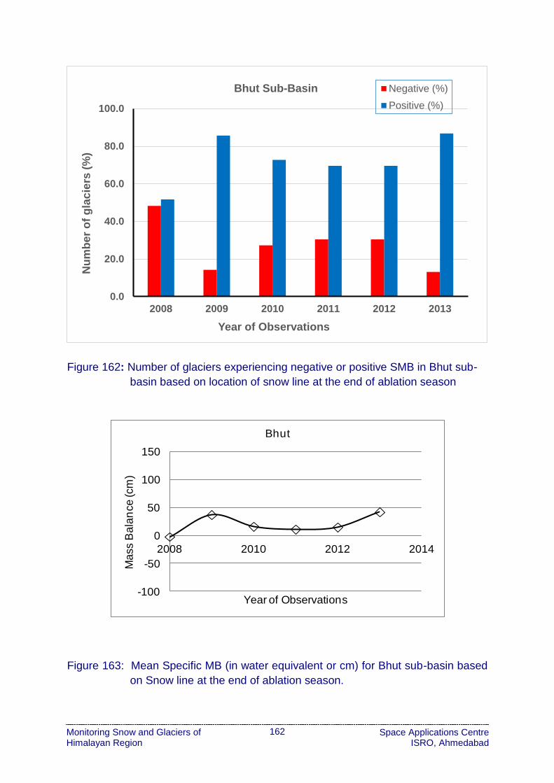
162
Monitoring Snow and Glaciers of Himalayan Region
Space Applications Centre ISRO, Ahmedabad
Figure 162: Number of glaciers experiencing negative or positive SMB in Bhut sub-
basin based on location of snow line at the end of ablation season
Figure 163: Mean Specific MB (in water equivalent or cm) for Bhut sub-basin based
on Snow line at the end of ablation season.
0.0
20.0
40.0
60.0
80.0
100.0
2008 2009 2010 2011 2012 2013
Nu
mb
er
of
gla
cie
rs (
%)
Year of Observations
Bhut Sub-Basin Negative (%)
Positive (%)
-100
-50
0
50
100
150
2008 2010 2012 2014
Ma
ss B
ala
nce
(cm
)
Year of Observations
Bhut

163
Monitoring Snow and Glaciers of Himalayan Region
Space Applications Centre ISRO, Ahmedabad
Figure 164 shows the variability in snow line during ablation month from July to
September 2012 in few glaciers of the Chandra sub-basin. It may be seen that the
snow line recedes from July and reaches maximum elevation during September 10,
2012. The number of glaciers showing positive mass balance in Chandra sub-basin
ranges between 61.5 to 100 % during 2008 to 2013 (Figure 165). Number of glaciers
during 2008, 2009, 2012 and 2013 showing negative mass balance are 38.5%, 18%,
16% and 32.6%. During 2011 all the glaciers in Chandra sub-basin show positive mass
balance. Overall glaciers in Chandra sub-basin show positive mass balance during
2008-2013 with increasing trend during 2008-2011 and decreasing trend during 2011-
2013 (Fig. 166).
Figure 164: IRS AWiFS images showing fluctuation of snow line in few glaciers of
Chandra sub-basin during 2012.
Bhaga sub-basin have shown similar pattern of positive mass balance except number
of glaciers having negative mass balance were high in year 2012 (Figure 167 & Figure
168).

164
Monitoring Snow and Glaciers of Himalayan Region
Space Applications Centre ISRO, Ahmedabad
Figure 165: Number of glaciers experiencing negative or positive SMB in Chandra
sub-basin based on location of snow line at the end of ablation season
Figure 166: Mean Specific MB (in water equivalent or cm) for Chandra sub-basin
based on Snow line at the end of ablation season
0.0
20.0
40.0
60.0
80.0
100.0
2008 2009 2010 2011 2012 2013
Nu
mb
er
of
gla
cie
rs (
%)
Year of Observations
Chandra Sub-Basin Negative (%)
Positive (%)
-100
-50
0
50
100
150
2008 2010 2012 2014
Ma
ss B
ala
nce
(cm
)
Year of Observations
Chandra

165
Monitoring Snow and Glaciers of Himalayan Region
Space Applications Centre ISRO, Ahmedabad
Figure 167: Number of glaciers experiencing negative or positive SMB in Bhaga sub-
basin based on location of snow line at the end of ablation season
Figure 168: Mean Specific MB (in water equivalent or cm) for Bhaga sub-basin based
on Snow line at the end of ablation season
0.0
20.0
40.0
60.0
80.0
100.0
2008 2009 2010 2011 2012 2013
Nu
mb
er
of
gla
cie
rs (
%)
Year of Observations
Bhaga Sub-Basin Negative (%)
Positive (%)
-100
-50
0
50
100
150
2008 2010 2012 2014
Ma
ss B
ala
nce
(cm
)
Year of Observations
Bhaga

166
Monitoring Snow and Glaciers of Himalayan Region
Space Applications Centre ISRO, Ahmedabad
Figure 169 shows the variability in snow line during ablation month from July to
September 2011 in Miyar sub-basin. Snow line was observed to be minimum on 26
August 2011. It may be seen that the snow line recedes from July and reaches
maximum elevation during August 26, 2011. AWiFS data has shown the presence of
cloud during the observed period which sometimes severely affects the availability of
suitable dataset for delineation of snow line and AAR derived mass balance.
Figure 169: IRS AWiFS images showing fluctuation of snow line in few glaciers of
Miyar sub-basin during 2011
In the Miyar sub-basin, number of glaciers having negative mass balance is observed
to be higher than positive mass balance throughout the observed period except year
2010 and 2011 (Figure 170) which is also reflected in the trend of SMB (Figure 171).
Maximum positive mass balance is observed in the year 2010, which reduces
subsequently and reaches to negative mass balance in year 2013.
iii) Beas Basin (Parbati Sub-basin)
Glaciers in the Parbati sub-basin show zero mass balance during the year 2008 and
subsequently positive mass balance during 2009 to 2013 (Figure 172 and Figure 173).
SMB is positive from 2009 to 2013 consistently except a drop in year 2012.

167
Monitoring Snow and Glaciers of Himalayan Region
Space Applications Centre ISRO, Ahmedabad
Figure 170: Number of glaciers experiencing negative or positive SMB in Miyar sub-
basin based on location of snow line at the end of ablation season
Figure 171: Mean Specific MB (in water equivalent or cm) for Miyar sub-basin based
on Snow line at the end of ablation season
0.0
20.0
40.0
60.0
80.0
100.0
2008 2009 2010 2011 2012 2013Nu
mb
er
of
gla
cie
rs (
%)
Year of Observations
Miyar Sub-Basin Negative (%)
Positive (%)
-100
-50
0
50
100
150
2008 2010 2012 2014
Ma
ss B
ala
nce
(cm
)
Year of Observations
Miyar

168
Monitoring Snow and Glaciers of Himalayan Region
Space Applications Centre ISRO, Ahmedabad
Figure 172: Number of glaciers experiencing negative or positive SMB in Parbati sub-
basin based on location of snow line at the end of ablation season
Figure 173: Mean Specific MB (in water equivalent or cm) for Parbati sub-basin based
on Snow line at the end of ablation season
0.0
20.0
40.0
60.0
80.0
100.0
2008 2009 2010 2011 2012 2013
Nu
mb
er
of
gla
cie
rs (
%)
Year of Observations
Parbati Sub-Basin Negative (%)
Positive (%)
-100
-50
0
50
100
150
2008 2010 2012 2014
Ma
ss B
ala
nce
(cm
)
Year of Observations
Parbati

169
Monitoring Snow and Glaciers of Himalayan Region
Space Applications Centre ISRO, Ahmedabad
iv) Satluj Basin (Baspa Sub-basin)
Number of glaciers showed negative mass balance for all years of observations except
year 2010 and 2011 and SMB was found to be negative throughout except year 2010
(Figure 174 & 175).
v) Ganga Basin (Bhagirathi, Alaknanda, Dhauliganga and Gauriganga sub-
basins)
Bhagirathi sub-basin has shown number of glaciers having negative mass balance
were high for observation period except 2010 & 2011 (Figure 176). SMB was observed
to be negative for year 2008 & 2009 whereas it was observed to be positive for year
2010 & 2011 (Figure 177).
Alaknanda sub-basin has shown number of glaciers having negative mass balance
were high for year 2010, 2011 & 2012 (Figure 178). SMB was observed to be negative
for year 2008, 2009 & 2012 whereas it was observed to be positive for year 2010,
2011 & 2012 (Figure 179).
Gauriganga sub-basin has shown number of glaciers having negative mass balance
were high for year 2008, 2011 & 2012 (Figure 180). SMB was observed to be negative
only for year 2009 whereas it was observed to be slightly more positive for 2010 &
2011 (Figure 181). No suitable data was found for year 2013 due to cloudy conditions.
Dhauliganga sub-basin has shown number of glaciers having negative mass balance
throughout the observed period except year 2011 where more number of glaciers
having positive mass balance were observed (Figure 182). Overall mass balance was
negative or close to zero for year 2010 & 2011 (Figure 183). No suitable data was
found for year 2013 due to cloudy conditions.
Overall, it is summarized that the total number of glaciers studied during time frame
2008 – 2013 for 13 sub-basins and % of glaciers showing negative and positive mass
balance year-wise are viz., 2008: 863 (-60%,+40%); 2009: 731 (-45%,+55%); 2010:
783 (-18%,+82%); 2011: 1036 (-17.5%,+82.5%); 2012: 876 (-44.5%,+55.5%); 2013:
626 (-45%,+55%). Only selected valley glaciers in each sub-basin were studied. The
number of glaciers studied varied each year due to cloud cover in satellite data during
ablation season. In addition, due to cloud cover problem, same glacier may not have
been studied consecutively in few cases during the time frame 2008-2013.
Mean specific mass balance is observed to be negative for Alaknanda sub-basin
(minimum – 60.45 cm in 2013), Bhagirathi, Dhauliganga, Basapa and Miyar sub-basin
three times and Warwan, Bhut and Gauriganga sub-basins once during 2008-2013
time frame.

170
Monitoring Snow and Glaciers of Himalayan Region
Space Applications Centre ISRO, Ahmedabad
Figure 174: Number of glaciers experiencing negative or positive SMB in Baspa sub-
basin based on location of snow line at the end of ablation season
Figure 175: Mean Specific MB (in water equivalent or cm) for Baspa sub-basin based
on Snow line at the end of ablation season
0.0
20.0
40.0
60.0
80.0
100.0
2008 2009 2010 2011 2012
Nu
mb
er
of
gla
cie
rs (
%)
Year of Observations
Baspa Sub-Basin Negative (%)
Positive (%)
-100
-50
0
50
100
150
2008 2010 2012 2014
Ma
ss B
ala
nce
(cm
)
Year of Observations
Baspa
Not suitable data

171
Monitoring Snow and Glaciers of Himalayan Region
Space Applications Centre ISRO, Ahmedabad
Figure 176: Number of glaciers experiencing negative or positive SMB in Bhagirathi
sub-basin based on location of snow line at the end of ablation season
Figure 177: Mean Specific MB (in water equivalent or cm) for Bhagirathi sub-basin
based on Snow line at the end of ablation season
0.0
20.0
40.0
60.0
80.0
100.0
2008 2009 2010 2011 2012 2013
Nu
mb
er
of
gla
cie
rs (
%)
Year of Observations
Bhagirathi Sub-Basin Negative (%)
Positive (%)
-100
-50
0
50
100
150
2008 2010 2012 2014
Ma
ss B
ala
nce
(cm
)
Year of Observations
Bhagirathi

172
Monitoring Snow and Glaciers of Himalayan Region
Space Applications Centre ISRO, Ahmedabad
Figure 178: Number of glaciers experiencing negative or positive SMB in Alaknanda
sub-basin based on location of snow line at the end of ablation season
Figure 179: Mean Specific MB (in water equivalent or cm) for Alaknanda sub-basin
based on Snow line at the end of ablation season
0.0
20.0
40.0
60.0
80.0
100.0
2008 2009 2010 2011 2012 2013
Nu
mb
er
of
gla
cie
rs (
%)
Year of Observations
Alaknanda Sub-Basin Negative (%)
Positive (%)
-100
-50
0
50
100
150
2008 2010 2012 2014
Ma
ss B
ala
nce
(cm
)
Year of Observations
Alaknanda

173
Monitoring Snow and Glaciers of Himalayan Region
Space Applications Centre ISRO, Ahmedabad
Figure 180: Number of glaciers experiencing negative or positive SMB in Gauriganga
sub-basin based on location of snow line at the end of ablation season
Figure 181: Mean Specific MB (in water equivalent or cm) for Gauriganga sub-basin
based on Snow line at the end of ablation season
0.0
20.0
40.0
60.0
80.0
100.0
2008 2009 2010 2011 2012
Nu
mb
er
of
gla
cie
rs (
%)
Year of Observations
Gauriganga Sub-Basin Negative (%)
Positive (%)
-100
-50
0
50
100
150
2008 2010 2012 2014
Ma
ss B
ala
nce
(cm
)
Year of Observations
Gauriganga
Not suitable data

174
Monitoring Snow and Glaciers of Himalayan Region
Space Applications Centre ISRO, Ahmedabad
Figure 182: Number of glaciers experiencing negative or positive SMB in Dhauliganga
sub-basin based on location of snow line at the end of ablation season
Figure 183: Mean Specific MB (in water equivalent or cm) for Dhauliganga sub-basin
based on Snow line at the end of ablation season
0.0
20.0
40.0
60.0
80.0
100.0
2008 2009 2010 2011 2012
Nu
mb
er
of
gla
cie
rs (
%)
Year of Observations
Dhauliganga Sub-Basin Negative (%)
Positive (%)
-100
-50
0
50
100
150
2008 2010 2012 2014
Ma
ss B
ala
nce
(cm
)
Year of Observations
Dhauliganga
Not suitable data

175
Monitoring Snow and Glaciers of Himalayan Region
Space Applications Centre ISRO, Ahmedabad
All other sub-basins show mean specific mass balance positive during 2008-2013
(maximum +107.67 cm for Chandra sub-basin in the year 2011), however it varies and
fluctuates during period of observation. In general, sub-basins of western Himalayan
region show positive mass balance, whereas sub-basins of west-central Himalaya
show negative mass balance.
The salient findings for glacier mass balance studied for 700 glaciers in 10 sub-basins
for the year 2010 show that positive mass balance is indicated for 80% glaciers (Singh
et al., 2013b). Specific mass balance for 43 glaciers of Warwan and 38 glaciers of
Bhut sub-basins of Western Himalaya show negative mass balance for the year 2005
to 2007 and a loss of 4.3 and 0.83 km3 area of glaciated region respectively
(Brahmbhatt et al., 2012b).
The purpose of monitoring snow line is to create a database of long term so that a
pattern of snowline fluctuations could be understood. It is also desired that the
database can be updated with a LISS III data and RISAT-1 SAR data for a better
accuracy of snow line altitude. When this type of data is generated for entire Himalaya,
it could give improved insight to draw conclusions on the nature of precipitation and
melting across Himalayan region during ablation period. One of the limitations of this
method is that it is based on the equation of 1992. If the size of the glaciers has
reduced since then, the AAR of zero SMB might change. So there is a need to improve
the relationship using more datasets for different climatic regions of Himalaya.
(b) Field based glacier mass balance studies for Machoi glacier, Drass sub-
basin, Jammu & Kashmir
Machhoi glacier was selected as benchmark glacier in Drass sub-basin for detailed
glacier mass balance studies. Machoi glacier is a transverse valley glacier situated 11
km east of Zoji La. The glacier basin is confined between the 340 15’30 ̋ N to 340 17ˊ
40˝ N latitudes and 750 31ˊ to 750 33ʹ 30”E longitudes and is located in Drass Tehsil
of Kargil District of Jammu and Kashmir State.
Systematic monitoring for mass balance of Machoi glacier was carried out during
2011-2012, 2012-2013 and 2013-2014. During this period the net annual
accumulation and ablation measurement were carried out on the basis of winter and
summer balance through pit study method (Figure 184). Snow densities were
measured for estimating water equivalent mass.
Surface Ablation
The surface ablation measurement of Machoi glacier were carried out by monitoring
42 ablation stakes (graduated bamboo sticks with pointed metallic base) spread over
glacier body from snout to 3650m to 4700m asl. The surface melting of the glacier
result due to the high air temperature of summer season. Melt water plays an important
role in lubricating the bed of the glacier. The surface ablation values of Machoi glacier

176
Monitoring Snow and Glaciers of Himalayan Region
Space Applications Centre ISRO, Ahmedabad
were measured during the month of August and September 2011 (1.53 cm/day); June,
July, August and September, and October 2012 (1.71 cm/day), July, August,
September and October 2013 (1.56 cm/day), July, August-September 2014
(1.43cm/day) field seasons by the stake measurements method. The surface ablation
measurement of 38 stakes (graduated bamboo stick with pointed metallic base) of 3
meters length were fixed in the body of glacier with help of motor-operated drill spread
over glacier body from snout (3652 m) to accumulation zone (4700m) at equal
altitudinal interval of 100 meters, in three rows, one along the central part and two on
the either sides (east and west) of the glacier. Hot water was poured around the stakes
and snow and ice were packed around them so that they would freeze and remain in
place during the field season of 2011 and 2012 (Figure 185).

177
Monitoring Snow and Glaciers of Himalayan Region
Space Applications Centre ISRO, Ahmedabad
Figure 184: Location of ablation stakes and snow pits for estimating glacier mass
balance of the Machoi glacier

178
Monitoring Snow and Glaciers of Himalayan Region
Space Applications Centre ISRO, Ahmedabad
Figure 185: Fixing of ablation stacks and measurements on Machoi glacier

179
Monitoring Snow and Glaciers of Himalayan Region
Space Applications Centre ISRO, Ahmedabad
Nearly 20 stakes were lost due to intense melting as well by high speed catabatic
winds as observed in July 2013. Later 15 new mass balance stakes were installed
deep up to 5 meters by newly acquired Heuck ice drill for the next year measurement.
These stakes were planted in a linear form in ablation zone and as far as possible to
the accumulation zone of the glacier. The stakes established for measuring the
summer ablation were monitored in July, August, and, September months. The glacier
melt during year 2012 was considerable as the stakes No. 23, 25 and 28 in altitude
zone 4400m reported 2.22m of glacier ice loss in comparison 2013 and 2014.
The ablation data four years (2011, 2012, 2013, and 2014) show that average degree-
day melting of three years is 1.54 cm/day during the peak melting season (July and
August). The ablation rate varies, both way i.e. with respect to altitude and onset of
summer. The gradual decrease in the melting of the glacier starts from the month of
September (0.6 cm/day) till in October it reaches to zero. The degree-day melting of
the Machoi glacier reaches maximum (1.24 to 5.1 cm/day) between the altitudes 4080
to 4480 meters asl during the summers of the years 2011 and 2012. Machoi glacier
has a large ablation area lying between the snout and equilibrium line (3652-4620
meters). The ablation zone is sub-divided into lower zone with low melting (3652-
3760), middle lower zone with moderate melting (3800-4080 meters), middle higher
zone with high melting (4080-4400 meters) and upper zone with low melting (4400-
4580 meters) according to their degree-day melting. The analysis of the ablation
records of the glacier during the years 2011 to 2014 reveals that the melting of the
glacier follows ablation pattern as per the altitude of the glacier. In the lower glacier
zone the mean ablation measurements during the year 2011 is 1.5 cm/day with a
standard deviation of 0.53; during 2012 (June, July, August, and September) it varies
between 0.8 cm/day, 1.1 cm/day, 1.8 and 0.9 cm/day respectively with standard
deviation. 0.95. In the year 2013 (June, July, August, and September), the mean
melting range in lower glacier zone varies between 0.7 cm/day, 1.5 cm/day and 1.7
cm/day with standard deviation 0.78. In 2014 (July, August, September), it varies
between 0.6 cm/day and 1.4 cm/day with standard deviation 0.56cm (Figure 186).
In the middle lower zone (3800 to 4080 m) the mean ablation measurements during
the year 2011 is 1.9 cm/day with standard deviation of 0.35; during 2012 (June, July,
August, September), it varies between 1.3 cm/day, 1.9 cm/day, 2.8/day and 2.1
cm/day with standard deviation. 0.79; during 2013 (July, August, September) it varies
between 1.1 cm/day, 2.0 cm/day and 1.5 cm/day with standard deviation of 0.7. In the

180
Monitoring Snow and Glaciers of Himalayan Region
Space Applications Centre ISRO, Ahmedabad
Figure 186: Mean monthly ablation pattern with respect to elevation changes of
Machoi glacier during hydrological year 2011-2014

181
Monitoring Snow and Glaciers of Himalayan Region
Space Applications Centre ISRO, Ahmedabad
year 2014 (June, July, August, September), the mean melting range in middle zone
ranges between 0.5cm/day to 1.8 cm/day with standard deviation of 0.49 (Figure 186).
In the middle upper zone (4080 to 4400 m) the mean ablation measurements during
2011 in August, September and October the melting rate varied 3.9cm/day,2.8cm/day
and 0.45cm/day respectively, In the year 2012 June, July, August, September,
October the mean melting rate range between 2.7cm/day, 3.2cm/day, 3.8cm/day,
1.6cm/day and 0.46cm/day. During the year 2013 the melting rate varied between 1.8
cm/day, 2.9cm, 2.8cm/day, 1.9cm/day, and 0.34cm/day (Figure 186). In the year 2014
July, August, September the mean melting range varied 1.9cm/day,2.9cm/day and
1.5cm/day respectively.
In the year 2011 July, August, September the mean melting in the upper zone ranges
between 0.5 cm/day, 0.2 cm/day and 0.01 cm/day with a std.dev. of 0.36; during the
2012 June, July, August, September it varies between 0.5 cm/day and 0.01 cm/day
with a std.dev. of 0.19 and during the year 2013 (July, August, September) it ranges
between 0.3 cm/day, 0.4cm/day and 0.01 cm/day with a std.dev. 0.39. In the year 2014
June, July, August the mean melting rate ranged 0.2cm/day, 0.3cm/day, 0.01cm/day
with a st.dev of 0.27.
The overall analysis reveals that the degree-day melting was higher in the middle
lower zone as well middle upper zone (3880 to 4400 m) during the years 2011, and
2012 as compared to 2013 and 2014. This clear reflects that years 2011, and 2012
has a warmer dry summer season as compared to the years 2013 and 2014, the cool
and moist summer year being 2014 (Figure 186).
The melting of glacier in the lower zone is higher near front part of the snout area
during the summer as it has a thin layer of debris on its body but along its margins
(east and west) it has thick debris cover. The melting of glacier at its margins is very
less due to which the height of the margins of the glacier and their extent is larger than
the central part or clean part of the glacier. High rate of ablation in summer is due to
high maximum temperature (17.23 ̊ C). Further the high rate of melting is observed in
the east part of the glacier as it has a very thin layer of dark colour debris (few
centimeters) that absorbs and reflects more heat, and transfer heat to glacier body.
The western part of the glacier is covered with somewhat thick debris, big boulders
and angular rock fragments that prevent incoming of solar radiation from affecting the
glacial surface and results in negligible melting. Further this side of glacier is confined
in shadow zone hence the duration of incoming of the solar radiation is less as
compared to the western and central part of the glacier. The presence of transverse
as well as longitudinal crevasses in the snout further adds to variable rate of melting
along the margin in comparison to the central part that leads to a tongue like outline
of the snout. The variable rate of melting at different altitude levels of the glacier during
the period 2011-2014 show that melting rate of glacier is comparatively maximum
at<4080m asl to 4400m asl and minimum in the vicinity of equilibrium line (4509m asl

182
Monitoring Snow and Glaciers of Himalayan Region
Space Applications Centre ISRO, Ahmedabad
to 4540m asl) and nearly zero at equilibrium line altitude (4509masl, 4520m asl and
4540 masl) as seen in Figure 186. Mean monthly Maximum temperature and mean
monthly ablation of Machoi glacier from 2011-2014 are summarized in Table 74.
Table 74: Mean monthly Maximum temperature and mean monthly ablation of Machoi
glacier from 2011-2014
Month
2011 2012 2013 2014
Max.
temp
Melting Max.tem Melting Max.tem Melting Max.tem Melting
Cͦͦͦͦͦͦͦͦͦͦͦͦͦͦͦͦ
cm/day ͦͦͦͦC cm/day ͦͦͦͦC cm/day ͦͦͦͦC cm/day
June 12.1 1.8 9.2 1.1 8.8 0.9
July 15.7 2.1 13.5 1.8 11.7 1.6
August 18.4 1.7 18.6 2.8 16.4 2 14.9 1.9
September 14.2 1.1 15.3 1.3 11.8 1 11.3 1.4
Accumulation Patterns
Snow accumulation responds to precipitation and temperature variation and forms an
interesting climate index. These parameters integrate to influence during the entire
late summer to spring period-September to July. Machoi glacier is cold glacier, where
accumulation occurs both during winter as well in summer too in higher parts (4400m
asl), and ablation during summer (June to September). While bulk of accumulation
indeed occurs in winter which extends to June/July, often concentrated in short heavy
snow fall events associated with western disturbances. Apart from its positive
contribution to mass balance, the summer snow fall increases albedo. The effect of
summer accumulation is especially remarkable around equilibrium line as low
temperature reduces the melting rate appreciably and further helps to insulate snow
and ice near equilibrium line and shifts it tens of meters. Change in timing of snow fall
and periods of accumulation season from year to year in Machoi glacier has affected
the position of equilibrium line. The annual measurement of net accumulation of snow
is carried out at the end of each ablation season (September) of residual snow
accumulated by opening pits in the vicinity of equilibrium line (4500m to 4600m). This
altitudinal zone acts as transition between accumulation and ablation zone (Figure
187).
The thickness of winter snow pack was conducted during June 2012 on the
accumulation stakes established at different elevations of the glacier and snow pack
density was carried in snow pit. Snow pack density ranged from 0.39gm/cc to
0.49gm/cc and the specific winter mass balance of the glacier in 2012 is estimated to
be 412mm w.e.v. The results closely corroborated with net accumulation snow carried
out in September of residual snow. The residual snow measurements were carried
during the field trips from 2011 to 2014 and it ranged between 1.5 to 2.5 meters. The
average snow density in the

183
Monitoring Snow and Glaciers of Himalayan Region
Space Applications Centre ISRO, Ahmedabad
Figure 187: Accumulation zone of the Machoi glacier and associated field features

184
Monitoring Snow and Glaciers of Himalayan Region
Space Applications Centre ISRO, Ahmedabad
accumulation zone was 0.49 gm3 in late summers. The accumulation zone
encompasses nearly 65% of the total area out of which two altitudinal zones ranging
between 4500 to 4800 meters, and 4800 to 5000 meters amounted for nearly 79% of
the net accumulated area of the glacier. These accumulation zones are mainly cirque
floors separated by stairs that encompasses near the 74% of the accumulation area.
The snow pits dug at different altitudinal levels between 4500m and 4700m in
accumulation zone at the end of each melting season, September (2011-2012, 2012-
2013, 2013-2014), displays somewhat little variations with maximum extent of
accumulated residual snow (2.2m and 2m) during 2011-2012 and 2012-2013 and least
(2 m-1.9m) during 2013-2014. These variations in snowfall effect the position of the
firn line (equilibrium line). In course of a single year, the firn line oscillates tens of
meters around a definite mean position (Figure 187).
Accumulation Area Ratio (AAR)
The Accumulation Area Ratio (AAR) is a ratio between snow accumulated area of the
glacier and total area of the glacier. It is useful parameter in determining the general
mass balance of the glacier and in defining the equilibrium line. In Machoi glacier the
AAR value ranges between 0.65 and 0.615. It is highest (0.65) during the year 2013-
2014, and shows descending trend from 2012-2013 to 2011-2012 (0.637, 0.615)
respectively (Figure 188). The marginal increasing trends in AAR values indicate the
increase of accumulation area and decrease of ablation area. This is supported by
successive positive mass balance during 2011-2014. The analysis also suggests that
AAR value is directly proportional to ELA. The ELA (Line of residual snow, separating
accumulation zone from ablation zone) is observed to have descended from its
position at 4540m asl during 2011-2012 to 4520m asl in 2012-2013 and to 4509m
during 2013-2014 (Figure 188). During the balance years of 2011-2012, 2012-2013,
and 2013-2014 the glacier had a positive net balance (+0.9603×10⁶×m³,
+0.7196×10⁶×m³, and +1.002×10⁶×m³) (Figure 189). The marginal variation in net
mass balance is attributed to low summer temperature leading low glacier melt.
Net Mass Balance
The estimates of net balance apparently reflect the trend of fluctuation in surface
melting of ice in water equivalent. Machoi glacier being a cold dry type has a lesser
ablation rate than those of accumulation rates. The glacier has net positive balance of
+ 0.960392×10⁶×m³ in the year 2011-2012, +0.719603×10⁶×m³ in the year 2012-2013
and +1.002060×10⁶×m³ in the year 2013-2014 (Table 75). The increase in net positive
balance during the year 2013-2014 than year 2012-2013, is due to cool and moist
summer. In comparison, during 2011 -2012 the accumulation as well ablation is more
(Table 75 and Figure 190). There is consistency in low temperature from June to
September leading to less summer melting than the earlier reporting years.
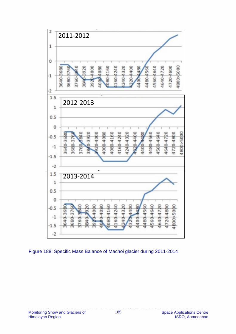
185
Monitoring Snow and Glaciers of Himalayan Region
Space Applications Centre ISRO, Ahmedabad
Figure 188: Specific Mass Balance of Machoi glacier during 2011-2014
2011-2012
2012-2013
2013-2014

186
Monitoring Snow and Glaciers of Himalayan Region
Space Applications Centre ISRO, Ahmedabad
Figure 189: Specific Mass Balance of Machoi glacier during 2011-2014
Figure 190: Net Mass Balance of Machoi glacier during 2011-2014

187
Monitoring Snow and Glaciers of Himalayan Region
Space Applications Centre ISRO, Ahmedabad
The fluctuation in net balance values is also attributed to variability in meteorological
parameters particularly with respect to pattern of snowfall, amount of solar radiation
and duration of sunshine hours during summer.
Table 75: Summary of Net Mass Balance estimates of Machoi glacier (2011-2014)
(Source: modified after Koul et al., 2016)
Year Abl. area Accu. Area Net Abl. Net Accu. Net Bal. AAR ELA
(Km²) (Km²) (Km³) (Km³) (Km³) (m)
2011-2012 2.219 3.54 -2.748 3.709 0.960 0.615 4540
2012-2013 2.100 3.62 -2.585 3.261 0.675 0.636 4520
2013-2014 1.933 3.83 -2.263 3. 265 1.002 0.65 4509
The study shows positive net mass balance with cumulative specific balance of 0.16
m w.e./km/yr, resulting into shifting of Equilibrium Line Altitude (ELA) from 4540 m asl
in the year 2011-2012 to 4509 m asl in 2013-14 for the Machoi glacier (Koul et al.,
2016). The positive balance mass indicates about the stability phase of the glaciers.
(c) Field based glacier mass balance studies for Patsio glacier, Bhaga sub-
basin, Himachal Pradesh
Patsio glacier is a valley type glacier, in the Bhaga river basin (Chandra-Bhaga River),
located in the Lahaul valley, ~60 km from Keylong, headquarter of Lahaul & Spiti
district, Himachal Pradesh (Figure 191). This glacier falls in the Great Himalayan range
(western Himalaya). Patsio glacier is a compound glacier fed by two tributaries in the
upper zone. Total area of the glacier is 2.25 km2, with catchment area 7.82 km2 , mean
orientation North-east, length approximately 2.7 km, maximum elevation 5741 m amsl,
mean elevation 5298 m amsl and snout position at 4886 m amsl.
Figure 191: Glacier boundary of the Patsio glacier, H.P.

188
Monitoring Snow and Glaciers of Himalayan Region
Space Applications Centre ISRO, Ahmedabad
Glaciological observations and measurements were taken during various glacier
expeditions organised during 2010-11, 2011-12, 2012-13 and 2013-14. Specific net
mass (annual/summer and winter) balance of Patsio glacier was estimated. Winter
mass balance has been calculated based on in-stu measured data on snow depth,
snow core and snow pits. Summer ablation has been calculated based on ablation
stakes, while accumulation was calculated by subtracting winter accumulation from
annual accumulation. Twenty stakes have been put at various locations on the Patsio
glacier. Location of various field measurement sites on Patsio glacier, H.P. are shown
in Figure 192. Some of the field photographs during expeditions are shown in Figure
193. Specific net mass balance of Patsio glacier for 2011/12 and 2012/13 are
presented in Figure 194. Maximum ablation was found in the lowermost part of the
ablation zone in 2011/12 but in 2012/13 ablations were quite similar below the ELA at
various altitudes. Annual mass balance Measurements were taken at end of the
ablation season e.g. end of September. Specific net mass (annual/summer and winter)
balance of Patsio glacier for 2012/13 is presented in Figure 195.
Figure 192: Locations of various field measurement sites on Patsio glacier, H.P.

189
Monitoring Snow and Glaciers of Himalayan Region
Space Applications Centre ISRO, Ahmedabad
Figure 193: Field photographs of Patsio glacier, H.P. during 2012-2013

190
Monitoring Snow and Glaciers of Himalayan Region
Space Applications Centre ISRO, Ahmedabad
Figure 194: Annual Specific mass balance of the Patsio glacier during 2011-12 and
2012-13
Figure 195: Specific net mass (annual/summer and winter) balance of Patsio glacier
for 2012/13. Dark blue line represents the winter mass balance,
calculated based on snow depth, snow core and pit. Light blue line
represents the summer mass balance. Summer ablation was calculated
based on ablation stakes, while accumulation was calculated by
subtracting winter accumulation from annual accumulation. Green colour
represents the annual mass balance measured from stakes and snow
core

191
Monitoring Snow and Glaciers of Himalayan Region
Space Applications Centre ISRO, Ahmedabad
During the period 2012- 2013 the glacier wide annual mass balance of Patsio glacier
was slightly negative at -0.04 ± 0.40 m w.e. The Equilibrium Line Altitude (ELA) was
around 5350 m a.s.l. (based interpolation between ablation stake and the snow core
measurement on the eastern flank) the Accumulation Area Ratio was found to be 47%.
Changes in annual Specific Mass Balance of Patsio glacier during 2010-2011, 2011-
12, 2012-13 and ablation at different elevations are shown in Figure 196.
Figure 196: Changes in annual Specific Mass Balance of Patsio glacier during 2010-
2011, 2011-12, 2012-13 and ablation at different elevations
In June 2014, a field expedition was carried out to monitor the winter mass balance of
the Patsio glacier. Snow depths were measured at different elevations on the glacier,
by using a snow probe between 4913 m and 5125 m a. s. l. (Figure 197). At higher
elevations a snow pit and two snow cores were used to measure winter accumulation.
One snow pit was made at 5158 m a. s. l., while two snow cores were extracted at
5235 m and 5375 m a. s. l. Table 76 is showing the detailed information of snow core
take at 5375 m a.s.l. in 9th June 2014 for winter balance estimation. Salient results of
the specific net ablation at various elevations of Patsio glacier for the balance year
2013-2014 (measured in end of September 2014) are shown in Figure 198.

192
Monitoring Snow and Glaciers of Himalayan Region
Space Applications Centre ISRO, Ahmedabad
Figure 197: Snow depths at various elevations of Patsio glacier in June 2014
Table 76: Details of the core taken at 5375 amsl on 9th June 2014
Core
Length
(cm)
Mass (g) Comments Volume
(cm3)
Density
(g/cm3)
15-25 447 -- 1004.8 0.444865
37-50 405 -- 653.12 0.6201
60-78 364 -- 904.32 0.402512
93-103 295 -- 502.4 0.587182
130-150 602 Firn 1004.8 0.599124
170-180 330 Hard Firn 502.4 0.656847
188-210 306 Firn 602.88 0.507564
236-250 380 -- 703.36 0.540264
263-270 257 ~ 5 cm hard
ice
351.68 0.730778
290-300 336 Dirt Layer 502.4 0.6687

193
Monitoring Snow and Glaciers of Himalayan Region
Space Applications Centre ISRO, Ahmedabad
Figure 198: Specific net ablation at various elevations of Patsio glacier for the balance
year 2013-2014 (measured in end of September 2014)
Overall mass balance for the study period was slight negative, which shows Patsio
glacier is somewhat in equilibrium state.

194
Monitoring Snow and Glaciers of Himalayan Region
Space Applications Centre ISRO, Ahmedabad
5. Himalayan Glacier Information System
5.1. Objective
To develop a Web based Himalayan Glacier Information System (HGIS) using Open
Source GIS tools.
5.2. Scientific Rationale
The web based information systems for snow and glaciers available in public domain
(with certain restrictions) are from the World glacier inventory (WGI), the National
Snow Data Centre, Global Land Ice Measurements from Space (GLIMS), and the
International Centre for Integrated Mountain Development (ICIMOD). The GLIMS is
used for glacier data preparation as per the GLIMS standards and imbibing into the
GLIMS system.
A geospatial database has been created for the glacier inventory carried out in Phase-
I (SAC, 2011a). The database contains inventory of all the glaciers in the Indus, Ganga
and the Brahmaputra basins encompassing the Himalayas, Trans-Himalaya and
Karakoram regions carried out on 1: 50,000 scale using Resourcesat-1 satellite data
of 2004–2007 periods during Phase-I. The results show that there are 32, 392 glaciers
covering 71,182 km2 area in the Indus, Ganga and Brahmaputra basins draining into
the Indian territory (Sharma et al., 2013). During Phase-II, the work was extended to
map glaciers of West Indus basin which are draining into neighboring countries. Thus
the total glacier inventory data for all the three Indus, Ganga and Brahmaputra basins
show that there are 34919 glaciers covering 75, 779 sq. km area.
Such large repository of geospatial database of glacier inventory available at SAC has
significant usage in Himalayan cryosphere studies and can be made available to
researchers through a web-based geo-portal named as Himalayan Glacier Information
System (HGIS). HGIS provides a platform for utilizing the glacier inventory data in
various applications/studies related to climate change, water resource planning,
hydropower site selection and assessment of glacial lake outburst flood (GLOF)
hazards. A well designed, user friendly and robust Himalayan Glacier Information
System (HGIS) would be helpful to researchers and encourage them to use the
available information effectively.
5.3. Study area and Data Used
The study area (Figure 199) comprised of the glaciated parts of Indus, Ganga and
Brahmaputra Basins over Himalayan, Trans Himalayan Karakoram region spread
across India, Nepal, Bhutan, Tibet/China, Pakistan and Afghanistan.

195
Monitoring Snow and Glaciers of Himalayan Region
Space Applications Centre ISRO, Ahmedabad
Figure 199: Study area – Indus, Ganga and Brahmaputra basins (Source: Sharma et
al., 2013)
5.4. Methodology
Efforts were made to standardize and organize the available spatial and aspatial data
in usable format in GIS. The HGIS information content comprises of 1) glacier
inventory maps and 2) inventory data sheets. The map displays the glacier
morphology features like accumulation zone and ablation (ice exposed and debris
covered) zones, snout location, de-glaciated valleys, moraines and glacier lakes. The
basin, sub-basin and administrative boundaries form the background. The inventory
data sheet attributes for each glacier provides information on glacier Location,
Identification, Dimension, Orientation, Elevation, Classification, etc.
The HGIS software design and development is carried out after making
comprehensive review of existing information Systems / Decision Support System
(DSS) like Glacier Land Ice Measurements from Space (GLIMS), International Centre
for Integrated Mountain Development (ICIMOD) & Water Resources Information
System (WRIS).
The spatial map and datasheet are linked by unique glacier identification number
(glac_id) which is a key field present in all corresponding glacier related point, polygon

196
Monitoring Snow and Glaciers of Himalayan Region
Space Applications Centre ISRO, Ahmedabad
or line layers. All the glacier attribute is made amenable to query and analysis by users.
The HGIS architecture is based on Open Geospatial Consortium (OGC) standards
and utilizes OpenGeo Suite bundled software comprising of Postgresql (PostGIS),
Geoserver, GeoWebCache and GeoExplorer each having a different function. The
spatial and aspatial glacier data sets were stored in a pre-defined format and imbibed
into spatially enabled database (PostGIS), having sophisticated functions for spatial
data analysis and query.
HGIS development involved various components viz., i) Glacier Inventory, ii) HGIS
software design and development, iii) Preparation of data for HGIS, base preparation
and iv) Populating data in HGIS, installation and testing. The details are discussed
below:
i) Glacier Inventory
Glacier inventory of the Himalayan region has been completed using IRS Satellite data
on 1:50, 000 scale in Phase-I of the project (SAC, 2011a, Sharma et al., 2013). During
the current project, all glaciers located in western parts of the Indus Basin (Pakistan-
Afghanistan region) within the Kabul, Kunar, Swat and Indus sub-basins were mapped
using Resourcesat-1&2 satellite data of 2007-2011 period following the methodology
used in Phase-1 (SAC, 2011a, Sharma et al., 2013). Geocoded AWiFS data at the
end of ablation season (July to September) were used to map the glaciological
features using FCC with standard band combination 2 (0.52-0.59 m), 3 (0.62-0.68
m) and 4 (0.77-0.86 m) and additional SWIR band 5 (1.55-1.70 m). The SRTM
DEM product, globally available at 90 m spatial resolution and vertical root mean
square error of 16 m, has been used for generating the altitude information. The
significant glaciological features extracted using satellite data comprised accumulation
area, ablation area (both ice exposed and debris covered), glacieret & snow field,
snout, ice divide, transient snow line, highest and lowest elevation points, deglaciated
valley (DGV), glacial lakes, etc. Details required for generating the glacier data sheet
such as glacier dimensions, orientations, elevation etc. were obtained and stored
using GIS procedures. Inventory datasheets for all glaciers were prepared as per
global standards. Thus the final glacier inventory data base for Indus, Ganga and
Brahmaputra basins of the Himalayan-Karakoram region comprises of 34,919 glaciers
covering 71,182 km2 glaciated area.
ii) HGIS Software Design and Development
The HGIS software design and development comprised of review of existing
information Systems / Decision Support System (DSS) like Glacier Land Ice
Measurements from Space (GLIMS), International Centre for Integrated Mountain
Development (ICIMOD) & Water Resources Information System (WRIS). The HGIS
architecture was designed to use open source software and tools as broadly
represented in Figure 200.

197
Monitoring Snow and Glaciers of Himalayan Region
Space Applications Centre ISRO, Ahmedabad
Figure 200: Basic HGIS Architecture
The HGIS Architecture comprises of OpenGeo Suite (Bundle) with PostgreSQL
(PostGIS), Geoserver, Geocache and GeoExplorer.
• The Open-source software PostgreSQL is Database management system. The
PostGIS extension enables PostgrSQL with Spatial capability
• The Geoserver is useful as web mapping server and enables user with
functionalities like map sharing and web development.
• OpenLayers is a javascript library to enable web mapping support to the client
over any modern browser.
Based on the above architecture and with a focus on available data sets and
anticipated user requirements the HGIS was developed to meet the functional
requirements a) Display and primary theme creation; b) multi-criteria based selective
query and display through custom filters and c) Output generation (Outputs like map
compositions, tables and graphs as per custom filters selection).
Elements for multi-parameter query are given in Table 77.
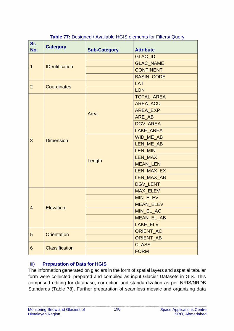
198
Monitoring Snow and Glaciers of Himalayan Region
Space Applications Centre ISRO, Ahmedabad
Table 77: Designed / Available HGIS elements for Filters/ Query
Sr.
No. Category
Sub-Category Attribute
1 IDentification
GLAC_ID
GLAC_NAME
CONTINENT
BASIN_CODE
2 Coordinates LAT
LON
3 Dimension
Area
TOTAL_AREA
AREA_ACU
AREA_EXP
ARE_AB
DGV_AREA
LAKE_AREA
Length
WID_ME_AB
LEN_ME_AB
LEN_MIN
LEN_MAX
MEAN_LEN
LEN_MAX_EX
LEN_MAX_AB
DGV_LENT
4 Elevation
MAX_ELEV
MIN_ELEV
MEAN_ELEV
MIN_EL_AC
MEAN_EL_AB
LAKE_ELV
5 Orientation ORIENT_AC
ORIENT_AB
6 Classification CLASS
FORM
iii) Preparation of Data for HGIS
The information generated on glaciers in the form of spatial layers and aspatial tabular
form were collected, prepared and compiled as input Glacier Datasets in GIS. This
comprised editing for database, correction and standardization as per NRIS/NRDB
Standards (Table 78). Further preparation of seamless mosaic and organizing data

199
Monitoring Snow and Glaciers of Himalayan Region
Space Applications Centre ISRO, Ahmedabad
sets at Sub-basin and Basin level in GIS was done. The database was made
compatible for accessing through the Open Source Web Based HGIS software.
Table 78: Database Design Specifications (Based on NRIS/NRDB Standards)
Sr. No. Element Specification
A] Input Specifications
1 Location reference Latitude-longitude
2 Scale 1:50,000
3 Projection/Map standard WGS84
4 Thematic Accuracy
Minimum Survey Unit 0.02 sq. km. or 2.0 ha
Mapping Accuracy 90/90 (unverified)
B] Database Specifications
1 Spatial framework
Registration scheme Lat.-Long. Graticule 15’ x 15’
Projection / Coordinate system WGS84 / UTM
Coordinate units Meters
2 Accuracy/Error limits
Registration accuracy (rms) 6.25 m
Area 0.3%
Weed tolerance 6.25
iv) Populating data in HGIS, installation and testing
The standardized spatial and aspatial data sets are populated into the HGIS. The
HGIS is installed onto a server and tested and evaluated for its various designed
functions. In case, there were errors in operating the HGIS, these were rectified. The
HGIS is then demonstrated to users for its operational usage. The specifications for
system requirements at server end (and client end) are given in Table 79.

200
Monitoring Snow and Glaciers of Himalayan Region
Space Applications Centre ISRO, Ahmedabad
Table 79: System Requirement (Server end)
Sr
no
Item Requirement/specification
1 Operating System
Vista, 7, 8, Server 2003 or newer, XP (client and
dev tools only)
2 Memory 1GB minimum (2GB recommended)
3 Disk space 600MB minimum (plus extra space for data)
4 Browser (client end) Any modern web browser is supported
5 Permissions Administrative rights
6 Software .NET Framework 4 (for windows, free
downloadable)
5.5. Results and Discussion
Figure 201 shows the view of HGIS home page. The various installed capabilities of
HGIS are discussed below:
The HGIS displays the major Indus, Ganga and Brahmaputra Basin boundaries
with international boundaries in the back ground (international boundaries are
not authenticated) and allows one to choose any one major basin for display,
query, graph generation (Figure 202).
Figure 201: View of HGIS Home Page

201
Monitoring Snow and Glaciers of Himalayan Region
Space Applications Centre ISRO, Ahmedabad
Figure 202: Display of three major basins of Himalayan Region (Indus, Ganga and
Brahmaputra basins)
For any one selected basin (say Ganga Basin) HGIS can display sub-basins
with glaciers as a) glacier outlines b) glacier morphology with legend. (Figure
203, Figure 204 and Figure 205).
Figure 203: Display of the Ganga basin and its sub-basins

202
Monitoring Snow and Glaciers of Himalayan Region
Space Applications Centre ISRO, Ahmedabad
Figure 204: Display of glacier outlines in selected sub-basins
Figure 205: Glacier morphology within a sub-basin with Legend (Zoom view)

203
Monitoring Snow and Glaciers of Himalayan Region
Space Applications Centre ISRO, Ahmedabad
The glacier morphology features like accumulation area, ablation area-ice
exposed, ablation area debris covered, de-glaciated valley, supra glacier lakes
and moraine dam / periglacial lakes can be displayed. An option for display
glacier snout as point location and Centre line of glacier is also provided.
On selecting any individual glacier by using the onscreen cursor, the five
characteristic information about that specific glacier viz., glacier identification
number, glacier total area, minimum elevation, maximum elevation and mean
elevation are displayed on left display panel along the side of that glacier
(Figure 205).
The left panel also has a Layer display menu (ink blue, Figure 205)) which aids
in switching on and off selective layers such as major basins with sub-basin
boundary, glaciers outlines displayed in single colour, glacier morphology
displayed in multi-colour colour as per legend.
The detailed inventory information table for any one specific glacier can be
assessed by selecting that glacier (Figure 206 and Figure 207).
Figure 206: Glacier characteristics are displayed (Five major characteristics within the
display screen in left) and detailed forty characteristics (Right scrollable
panel)

204
Monitoring Snow and Glaciers of Himalayan Region
Space Applications Centre ISRO, Ahmedabad
Figure 207: Multi-parameter query available as fifteen filters in HGIS
205
Monitoring Snow and Glaciers of Himalayan Region
Space Applications Centre ISRO, Ahmedabad
Thus a robust, user friendly Web based Himalayan Glacier Information System
(HGIS), a first of its kind in the country is developed which facilitates any user to
selectively display, query, analyze, compose maps and graphs and print, spatial and
aspatial information on glaciers relevant to his interests (Sharma et al., 2015; Rajawat
and Sharma, 2015). HGIS represents a significant step towards mapping and
compiling individual glacier level inventory data in spatial form to fill the void in data
and information on the status of Glaciers in the Himalaya and Trans-Himalayan
Karakoram region. HGIS provides a basis for assessing the glacier inventory data
which has applications in studies related to climate change, water resource planning,
hydropower site selection and mitigation of glacial lake outburst flood (GLOF) hazards.
Space Applications Centre, ISRO, Ahmedabad has developed a Web Portal
http://www.vedas.gov.in for providing access to all thematic maps prepared for land
applications under its recent efforts named as “Visualisation of Earth Data and Archival
System (VEDAS)”. All the Himalayan glacier inventory maps have been ported into
VEDAS for easy access by research community and it is planned to provide services
of HGIS through SAC Web Portal VEDAS to user/research community.

206
Monitoring Snow and Glaciers of Himalayan Region
Space Applications Centre ISRO, Ahmedabad
6. Effect of Black Carbon Soot and
Contamination on Snow and Glacier Ice
6.1. Objective
To measure the black carbon soot mass concentration on snow and glacier ice in
representative glaciated regions of Himalayas using portable Aethalometer.
6.2. Scientific Rationale
Absorbing aerosols such as black carbon (BC) or dust over high-altitude Himalayan
regions have potential implications on the regional climate and hydrological cycle. The
black carbon also commonly referred to as “soot” comprises of microscopic particles
of about 70 microns size that are released, but not broken down entirely, when burning
fossil fuels. Soot consists primarily of elemental carbon that mostly comes from the
consumption of fossil fuels particularly coal, diesel fuel, jet fuel, natural gas, kerosene
and the burning of wood, animal dung, vegetable oil and other biomass fuels. In recent
years scientists have begun to recognize soot as having the potential to cause
changes in climate. Soot absorbs sunlight and, therefore, heats the surrounding air,
also reducing the amount of sunlight that reaches the ground, resulting in a cooler
surface. The heated air can create an unstable atmosphere resulting in rising air,
forming clouds and bringing rainfall to areas heavily concentrated with soot. The rising
air is often balanced by an increase in sinking air in neighboring regions, which tends
to prevent cloud formation and rainfall. Black carbon soot is considered to be the
second largest contributor to global warming next to the greenhouse gas carbon
dioxide. Scientists propagate that a worldwide reduction in soot emissions and
controlling biomass burning could quell the alarming pace of global warming and also
reduce our reliance on soot-producing fuels. The International Global Panel on Climate
Change (IGPCC) agreed that black carbon soot is a major contributor to global
warming. It concluded that black carbon soot has a dire atmospheric warming
effect. This was significant because soot had previously been unaddressed as a major
contributor to global warming. Nor had the amplification of black carbon’s warming
effect previously been taken into account when mixed with other aerosols, creating
additional secondary fine particulates.
Soot also has been found to cause climate forcing in areas of higher latitude where
ice and snow are more common. Typically, ice and snow reflect sunlight rather than
absorb it due to having a white background, also known as an albedo effect. When
snow and ice are covered in soot, the soot absorbs the sunlight warming the ice and
snow and causing a faster than normal melt. As more melting occurs, the warming
effect increases as the soot becomes more concentrated on the snow surface and the
land surface is exposed. Monitoring of BC over fragile High altitude snow and glacier
regions of Himalaya is thus very significant.

207
Monitoring Snow and Glaciers of Himalayan Region
Space Applications Centre ISRO, Ahmedabad
The reported work on BC monitoring for the Himalayan region is very limited. The
Nepal Climate Observatory - PYRAMID established in 1990 at altitude of 5050 amsl
in Mount Everest region in the north facing Nepal Himalayas in is the only permanent
station monitoring BC in high altitude mountainous region of Himalaya. The NCO-
PYRAMID is joint experiment by scientific agencies from Nepal and Italy and over the
years has participation from more than 180 other national and international scientific
institutes from various parts of the world.
Absorbing aerosols such as black carbon (BC) or dust over high-altitude Himalayan
regions have potential implications on the regional climate and hydrological cycle over
South Asia. Deposition of black carbon (BC) soot on highly reflecting surfaces like
snow or ice could reduce the surface albedo and result in a positive radiative forcing
(warming) at the top of the atmosphere. A mean radiative forcing of +0.1 ± 0.1 W m-2
for BC induced changes in snow albedo has been estimated (IPCC, 2007). Figure 208
shows the radiative forcing and efficacies of direct, semi-direct, and snow albedo effect
of BC estimated based on the model simulations. It is seen that there exist large
uncertainties in the estimates of all BC forcing. Also, snow albedo modification via BC
has a very high efficacy compared to other BC forcing and most of the other climate
forcing agents (Hansen et al., 2005, IPCC, 2013, Flanner et al., 2012, Flanner et al.,
2011). For the range of 10-200 mg kg-1 of BC in snow, the diurnally averaged forcing
due to snow darkening has been found to vary from 0.87 to 10.2W m-2 for fresh snow
and from 2.6 to 28.1W m-2 for the aged snow, which is significantly higher than the
estimated direct radiative forcing of 1.67 W m_2 (Nair et al 2013). Potentials of remote
sensing for detecting black carbon in snow has been investigated (Warren, 2013).
Thus BC over Himalaya in general and glacier in particular has been a topic of prime
scientific interest and several investigators have studied the BC over Himalayan region
(Kulkarni et al., 2013, Das et al., 2010, Prasad et al., 2011, Lau et al., 2010) and few
case studies based on the measurements from the northern (Nepal and Chinese
regions) or Western (Pakistan) Himalaya (Yasunari et al., 2010, Ming et al., 2009).
Aerosol Optical Depth (AOD) data of 2001-2008 from MODIS was studied to
understand its impact on the Dokriani Glacier, Bhagirathi Valley, Garhwal Himalaya.
An increase in AOD was observed after 2005, which is observed to be correlated with
accelerated recession of the Dokriani glacier (Das et al., 2010). It is speculated that
increased AOD has resulted in the enhanced aerosol induced heating and consequent
accelerated recession of the Dokriani glacier. Modeling studies also predicted increase
in Himalayan glacier melt and retreat due to the BC induced snow surface darkening.
In view of the above, investigation of snow, BC and albedo changes over Himalayan
region has been taken up as a topic of research. Aerosol measurement of BC over
Himalayan region was carried out in campaign mode using portable Aethalometer
during expeditions to several valley glaciers spread in different climatic zones. The
observations were carried out during ablation period of 2011 to 2014.

208
Monitoring Snow and Glaciers of Himalayan Region
Space Applications Centre ISRO, Ahmedabad
Figure 208: Radiative forcings and efficacies of direct effect, semi-direct effect and
snow albedo effect of black carbon aerosols estimated based on global
climate model simulations (Source: IPCC, 2007; Lohmann & Feichter,
2001)
6.3. Study Area
The study area comprised several valley glaciers occurring in different climatic zones
of Himalayas in India. The glaciers are located in the states of Jammu & Kashmir,
Himachal Pradesh, Uttrakhand and Sikkim. The location of glaciers is shown in Figure
209 and also given in Table 80.
6.4. Principle of Aethalometer
Multi-spectral portable Aethalometer (AE-42, Magee Scientific, USA) working on the
principle of optical attenuation technique (Hansen et al., 1984) has been used for this
study. The Aethalometer aspirate the ambient air at known flow rate (5 LPM for
Himalayan conditions) and deposit on a quartz fiber filter tape to measure the change
in optical attenuation due to aerosols deposited on the filter tape. The Aethalometer
measures the black carbon soot at 370 nm (Ultra Violet) and 880 nm (Infra-Red)
regions of the Electromagnetic spectrum. The quantity of black carbon measured is
recorded in nano gram per cubic meter of air. The uncertainties associated with
Aethalometer caused by the loading of aerosols on the filter tape and multiple
scattering are well documented (Arnott et al., 2005; Nair et al., 2007).

209
Monitoring Snow and Glaciers of Himalayan Region
Space Applications Centre ISRO, Ahmedabad
Figure 209: Locations of selected glaciers in different climatic zones of Himalayas
taken up for monitoring of Black Carbon. (1. Thajwas, 2. Hoksar, 3.
Machoi 4. Pensilumpa 5. Chhota Shigri 6. Satopanth 7. Changme
Khanku)
Table 80: Details of Glacier locations selected for Black Carbon Soot studies in
Himalayas
Sr.
no.
Name of glacier Sub-basin/
Glacier valley
State Measurements
at Elevation
(m amsl)
1 Thajwas Jhelum
(Sind Nala)
Jammu & Kashmir 2850-2950
2 Hoksar Jhelum
(W. Liddar)
Jammu & Kashmir 3390-3660
3 Machoi Drass Jammu & Kashmir 3700-3750
4 Pensilumpa Zanskar Jammu & Kashmir 4100-4950
5 Chhota Shigri Chandra Himachal Pradesh 3750-4200
6 Satopanth Alaknanda Uttrakhand 3200-4400
7 Changme Khanku Tista Sikkim 4600

210
Monitoring Snow and Glaciers of Himalayan Region
Space Applications Centre ISRO, Ahmedabad
6.5. Methodology
The Aethalometer is operated at various altitudes within glacier valley and on the
glacier surface.
Preferably the instrument is operated to obtain profile of BC mass variations along
the track leading to glacier and on the glacier surface.
The sites comprised the approachable regions like the de-glaciated valley, glacier
snout, parts of ablation zone and accumulation zone of glacier sometimes in
regions of fresh snowfall in vicinity of the glacier.
The coordinates of the geographic location of BC observation site are recorded
using hand held GPS instrument.
The site is also identified on Resourcesat-1 satellite data. Some BC measurements
were made at nearby settlement locations for understanding the altitude
distribution of BC.
The aerosol optical depth (AOD) at the site is measured by using a hand held Sun
Photometer.
The AOD information is related to the amount of solar radiation reaching the site
and affecting the glacier melt.
Aethalometer measurements during 1100-1500 hours when the dispersion of
suspended particulate matter is maximum are recorded along the expedition track
for a systematic profile of BC variations at different altitudes.
Diurnal variations of BC are recorded by continuous Aethalometer recording at or
near the camping sites.
The local BC contributions can be observed during such long term diurnal
recordings.
On average, 5 to 10 measurements were made at each location.
6.6. Results and Discussion
BC measurements using portable Aethalometer are made at glacier locations in
various climatic zones spread across Himalayas. The main focus was to obtain BC
mass concentration data to fill the gaps in information content and understand the BC
mass variation over snow and glacier region over India Himalayan region. The
variation in BC mass distribution over Himalayan glaciers are analyzed. Following are
major findings:
Aerosol BC measurements depicts large spatio-temporal variations due to the
heterogeneities in source and sink characteristics. In general the BC mass
concentration and dispersion is affected by remoteness from human settlements &
infrastructure, rapidly varying sky conditions, humidity, precipitation (rainfall or
snowfall), wind direction and wind velocity.

211
Monitoring Snow and Glaciers of Himalayan Region
Space Applications Centre ISRO, Ahmedabad
Diurnal variation showing increased BC concentration during peak human activity
noon and evening time and fall in concentration during night time is observed
(Figure 210).
There is distinct latitudinal variation of BC mass concentration as seen through
measurements across the Himalayas.
High BC values observed at the lower altitudes decrease drastically as we move
to higher altitudes. Steady BC concentration of about 200 ng m-3 is recorded in
Himalayas above 4000 m amsl. Sample graph along with the observation locations
marked on satellite data showing the altitudinal variation for Satopanth glacier in
Uttrakhand are given in Figure 211. Results of altitudinal BC variations from several
glacier located in J& K region are given in Figure 212. There exists a large temporal
variability at the lower altitudes due to the proximity to the source regions and
diurnal evolution of the boundary layer.
The Zonal BC measurements from west to east in the Himalaya made at Jammu
& Kashmir, Himachal Pradesh, Uttrakhand and Sikkim distinctly show that while
the Leh-Ladhak & Drass region has relatively low BC mass concentration, the
Kashmir valley glacier regions have relatively higher concentration of BC. The
Sikkim region at 4600 m amsl has low BC as seen in Figure 213.
The mean values of BC measurements of 200 ng m-3 recorded during the study at
higher altitudes correspond well to the reported climatological mean of atmospheric
BC over Hanle (Western Himalayas, 4500 m amsl) and Nepal Climate
Observatory-Pyramid (Central Himalayas, 5000 m amsl) having BC values of
106±27 ng m-3 and 190±95 ng m-3 respectively.
The direct and surface albedo radiative forcing due to BC (Nair et al., 2013) could
contribute in warming effect over snow and glacier regions of the Himalayas.
Figure 210: Diurnal variation of BC mass concentration above 3 km and below 3 km
altitude regions over the Indus basin

212
Monitoring Snow and Glaciers of Himalayan Region
Space Applications Centre ISRO, Ahmedabad
Figure 211: Vertical distribution of BC mass concentration inferred from the
measurements at different altitudes for Satopanth glacier
Uttrakhand.The BC measurement locations are marked on
Resourcesat-1 satellite data
Figure 212: Vertical distribution of BC mass concentration inferred from the
measurements at different altitudes for glaciers in Indus Basin (Jammu
& Kashmir and Himachal Pradesh Himalayas). Legend: 1-Haskar, 2-
Thajawas, 3-Machoi, 4-Pensilumpa and 5- Chhota Shigri

213
Monitoring Snow and Glaciers of Himalayan Region
Space Applications Centre ISRO, Ahmedabad
Figure 213: Variation in BC mass concentration across Himalayan region
214
Monitoring Snow and Glaciers of Himalayan Region
Space Applications Centre ISRO, Ahmedabad
7. Effect of Debris Cover on Glacier Ice Melt
7.1. Objective
To carry out studies to understand the effect of debris cover on glacier retreat.
7.2. Scientific Rationale
Most of the large glaciers in Himalayan region are covered with debris in their ablation
areas. These glaciers are classified as debris covered glaciers. Debris is mainly
confined to lower parts of ablation zones. The thickness, which may run sub-meters
to meters, gradually increases down glaciers, and becomes maximum at the snout.
The source of rock fragments is the surrounding high relief mountains which get
shattered/broken due to frost action owing to high temperature extremities and gets
deposited. The surface of a glacier is generally lower than the crest of the lateral side
moraines. This difference gradually increases as one moves downward due to high
probability of sliding of debris from the surroundings to the glacier surface. It is well
established that the melting of glacier is influenced largely by the presence of dust or
debris on the glacier body, because radiation balance is affected, which, in turn,
influences the melt rate (Basnett et al 2013). An assessment of ablation rate under a
dust or debris cover is needed for the studies of glacier mass balance, glacier
dynamics, and artificial ablation control engineering and hydrological purpose. The
ablation rate under the debris cover is governed by the radiation, air temperature and
physical characteristics such as thickness, albedo, and thermal conductivity of the
debris layer. There are two difficulties in estimating the mean value of ablation under
a debris layer extending over a wide area (i) direct determination of thermal resistance
of the layer in the field which is one of the essential parameter for estimation of ablation
and (ii) detail information on meteorological variables necessary for estimation.
Understandings the effect of debris cover on the ablation of glacier ice for predicting
the water supply from mountain glacier is essential (Ben and Evans, 2010). Usually,
the effect of debris cover on the melting of glacier is not included in the modeling of
glacier melt runoff.
Debris thickness mapping of Bara Shigri glacier using remote sensing techniques has
been attempted (Schauwecker et al., 2015). Use of optical, thermal and microwave
imagery for debris characterization in Bara-Shigri Glacier, Himalayas has been found
to be extremely useful (Tiwari et al., 2012). The influence of debris cover and glacial
lakes on the recession of glaciers in Sikkim Himalaya has been studied (Smriti Basnett
et al., 2013). Spatially variable response of Himalayan glaciers to climate change
affected by debris cover has been observed (Scherler et al., 2011). Temporal changes
in elevation of the debris-covered ablation area of Khumbu Glacier in the Nepal
Himalaya since 1978 have been studied (Nuimura et al., 2011). Geochemical
characterization of supraglacial debris via in situ and optical remote sensing methods

215
Monitoring Snow and Glaciers of Himalayan Region
Space Applications Centre ISRO, Ahmedabad
has been demonstrated through a case study in Khumbu Himalaya, Nepal (Casey et
al., 2012). Decision tree and texture analysis for mapping debris-covered glaciers in
the Kangchenjunga area, Eastern Himalaya has been attempted (Racoviteanu and
William, 2012).
It is observed that a thin layer of debris cover accelerates melting, but thick layer
retards it (Singh et al., 2000). Dusting of snow and ice surfaces by dark materials is
known to increase in absorption rate of solar radiation. There is a significant difference
in mean seasonal ablation rate between site varying thickness of debris and also in
ablation rates at same site over a time. The debris thickness at maximum ablation
occurs is known as “effective debris thickness”. There is a “critical thickness”, which is
defined as the thickness of the debris layer at which the ablation rate of a debris
covered glacier is same as for a debris free glacier. It is observed that an increase in
the thick ness of the debris cover on a clean ice surface initially increased the rate of
ablation, but it led to decrease after the critical thickness was reached. At sites with
thinner debris thickness than effective thickness, the reflectivity of surface is high, thus
less incoming energy is used for increasing the temperature of debris materials and
ice melting. The critical thickness and effective thickness varied from day to day
depending up on the total energy available for the melting. During night, a constant
ablation was observed for all thickness of the debris.
7.3. Case Study I: Warwan-Bhut sub-basins, Chenab basin
The study area covers glaciers of the Warwan and Bhut sub-basins belonging to the
Chenab Basin, Western Himalaya. The sub-basins are located in Jammu and Kashmir
between 33°30′–34°21′N lat. and 75°39′–76°28′E long. and 33°15′–33°64′N lat. and
75°72′–76°78′E long. with an area of 4,828.4 sq. km and 2,285.4 sq. km respectively.
In the Warwan Basin, the largest glacier covers 51.8 sq. km, (lat./long. 33°45′
52.43″N/76°07′02.15″E) followed by one with an area of 48.7 sq. km (lat./long.
33°32′14.16″N/76°06′07.25″E). In case of the Bhut Basin, the largest glacier has an
area of 49.9 sq. km (lat./long. 33°12′10.21″N/76°43′05.08″E). Most of the glaciers in
the two sub-basins have slope in the range 10°–20°. Both the basins lie between
altitude 1,100 and 6,500 m. Most of the larger-sized glaciers are covered by rock
fragments in the ablation zones, whereas smaller glaciers are debris-free. Majority of
the glaciers in the Bhut Basin are moraine-covered than those of the Warwan Basin.
The host rocks for the glaciers to rest are gneisses and schist of the Central Crystalline
Zone. One major difference between the glaciers of the two basins is that glaciers of
the Bhut Basin are mainly south-facing whereas those of the Warwan Basin are north
to northwest-facing.
Glacier extent was first adopted from topographical maps and then monitored using
satellite images. Mapping from images requires use of elements of visual
interpretation, such as unique reflectance of snow and ice, shape of the valley

216
Monitoring Snow and Glaciers of Himalayan Region
Space Applications Centre ISRO, Ahmedabad
occupied by the glaciers, the flow lines of ice movement, rough texture of the debris
on the ablation zone, and the shadow of the steep mountain peaks and presence of
vegetation on the mountains. The SWIR band was used to discriminate cloud and
snow as in many cases the glaciers are covered by clouds at the ridges. The snout of
a glacier is the most important feature for monitoring, because the movement of the
snout helps in recognizing the advance or retreat of the glaciers. Sometimes snouts
of many glaciers were not distinct on the images due to debris cover. In such cases
various other indicators such as location of origin of streams from the glaciers,
presence of distinct geomorphic features in the form of braided streams, lakes, glacio–
fluvial sands, etc. helped in the identification of snouts. Additionally, changes of slope
or elevation near the snouts observed through DEM from SRTM, also helped in the
identification of snouts. The moraine cover was estimated using NDSI technique. The
NDSI utilizes the spectral characteristics of snow (Hall et. al., 1995).
NDSI algorithm is applied within the glacier boundary which discriminate snow-ice
cover and non snow-ice cover. The threshold value 0.4 has been used to separate
snow/ice from debris cover ice (Kulkarni, et al., 2006b; Shukla et al., 2010a; Shukla et
al., 2010b). The non snow-ice part of the glaciers corresponds to moraine cover area.
Then extracted moraine cover area has been verified using visual interpretation
technique. This technique includes the usage of band combination as B2 (0.52-0.59
m), B4 (0.77-0.86 m) and B5 (1.55-1.75 µm). Reflectance of rock in band B5 is higher
than ice; therefore, debris cover on glacier gives a red tone (Kulkarni, et. al., 2005).
The moraine cover for each glacier was estimated using semi-automatic approach
with the help of manual correction for study area.
It has been observed that the larger sized glaciers are covered by high percentage of
debris cover as they have gentle slopes. Further monitoring of glaciers in Warwan and
Bhut sub-basins using satellite images of 2001 to 2011 was carried out. The study
indicate that the smaller glaciers (upto 10 sq km) show variation in debris cover upto
10%, whereas larger glaciers ( 30-40 sq km) show variation in debris cover upto 23%.
Loss in glacial area is observed to be ~ 3.4 % for debris free smaller glaciers, whereas
it is 1.2-1.5 % for debris-covered smaller glaciers. Larger debris free glaciers show
loss in glacial area ~ 0.5 %, whereas large debris covered (12 – 25 % debris cover)
glaciers show negligible retreat (Figure 214) for period of 2001 - /2011. More retreat
was observed in debris free than in debris cover glaciers.

217
Monitoring Snow and Glaciers of Himalayan Region
Space Applications Centre ISRO, Ahmedabad
Figure 214: Influence of debris cover on glacier on Loss in glaciers area during the
monitoring period 2001/2002 – 2010/2011
7.4. Case Study II: Alaknanda and Bhagirathi sub-basins
The various glacier features are distinctly identifiable on Resourcesat-1 optical data
using different band combinations and proper contrast. Outer limits of glacier boundary
are conspicuously seen by using FCC with band combination of B2, B3 & B4/B5.
Glaciological features comprising accumulation area, ablation area (both ice exposed
and debris covered), glacieret & snow field, snout, ice divide, transient snow line,
highest and lowest elevation points, de-glaciated valley, glacial lakes, etc. were
mapped based on various interpretation keys (Sharma et al 2013). Moraine/debris
cover can be identified using visual interpretation key like tone, texture with elongated
pattern and association with glaciated region. By using the glacier inventory map
layers in GIS environment, systematic observations and measurements are made on
the glacial feature and recorded in tabular form in the inventory data sheets created
as per modified UNESCO/TTS guidelines with few additional parameters. By
measurement in GIS of various stored line features, information for length and width
is obtained. Altitude information is extracted from SRTM-DEM using GIS.
Debris cover area with respect to altitude information has been extracted for individual
sub-basins. Scatterplot was prepared to understand the variation of debris cover with
respect to change in altitude for Ganga basin. AAR (Accumulation area/Total area)
and DAR (Debris cover ablation area/Total area) was estimated while ignoring the
glacier with negligible debris cover less than 0.1 sq km. Glaciers without ablation and
accumulation zone was not considered for the analysis. This exercise was carried out
0
0.5
1
1.5
2
2.5
3
3.5
4
<5 5 to 10 10 to 20 20 to 30 30 to 40 >40
Loss
in g
laci
al a
rea
sin
ce 2
00
1 (
%)
Glacier Area (sq km)
0% debris 0 to 10 % debris 10 to 20 % debris >20 % debris

218
Monitoring Snow and Glaciers of Himalayan Region
Space Applications Centre ISRO, Ahmedabad
at sub-basin level. Glacier area, debris and snout altitude was categorized with respect
to change in their area. Averaged ablation area (with or without debris) and number of
glacier were also categorized in altitude zone to understand the variation of debris with
respect to elevation. Alaknanda and Bhagirathi basin are two adjoining basins which
have been reported to shown different retreat in Ganga basin in Indian Himalayas
(Bahuguna et al., 2014). These basins were selected to understand the possible
linkage of debris cover with respective retreat. Change in debris cover area was
studied with respect to the elevation of snout of respective glacier. Average debris
cover area (sq km) was being categorized into different altitude zone.
Ganga basin has shown mean high accumulation and ablation area with significant
area occupied by mean moraine dam lakes and supra glacier lake. Ganga has shown
highest debris covered ablation zone with less number of small glacier in comparison
to Indus and Brahmaputra basin. Accumulation, Ablation and Debris Cover area
cumulatively affect the retreating pattern of a particular basin. This information was
further sub-divided into sub-basin scale which showed varying trend for different sub-
basins. Alaknanda, Bhagirathi and Karnali was found to be in high negative correlation
in comparison to remaining basins. Figure 215 shows that for smaller glaciers the
percentage of debris cover is significantly high along with high altitude of snout. The
relationship depicts vice-versa pattern for large glaciers. This analysis was further
carried out for considering only ablation area as shown in Figure 216. This shows that
the glaciers are few in the altitude range of 3000-3500 m but average debris cover
area is highest. This also holds true for altitude range of 3500-4000 and lowest towards
higher altitude range. The occurrence of maximum debris cover area coincides with
the lower to middle altitude range which is prone to maximum melting during the
ablation period.
Alaknanda and Bhagirathi sub-basins have been taken further to understand the effect
of retreating pattern. Figure 217 shows that Bhagirathi shows a high percentage of
debris covered area of glaciers than Alaknanda in the altitude range of 3500-4000 m
of snout whereas no class was observed for 3000-3500 m. This indicates that more
protection was provided to Bhagirathi sub-basin than Alaknanda sub-basin. A
scatterplot of debris cover area for both basins with respect to their snout altitude
position shows a relatively higher negative trend for Alaknanda sub-basin (Figure 218).
This can lead to an understanding of more retreat of glaciers in Alaknanda sub-basin
than Bhagirathi sub-basin. This observation also matches with more retreat for
Alaknanda showing 14% than Bhagirathi basin showing 11% retreat based on SOI
maps, and 10 % and 1.8% based on satellite images respectively (SAC, 2011a).

219
Monitoring Snow and Glaciers of Himalayan Region
Space Applications Centre ISRO, Ahmedabad
Figure 216: Bar diagram of debris cover and debris free ablation zone of Ganga
Figure 215: Altitude-wise distribution of total and debris cover area of Ganga
basin
0
500
1000
1500
2000
2500
0.0
0.5
1.0
1.5
2.0Exp Abl area(sq km)
Debris cover Abl area (sq km)
No. of glacier
25
00
-30
00
30
00
-35
00
35
00
-40
00
40
00
-45
00
45
00
-50
00
50
00
-55
00
55
00
-60
00
60
00
-65
00
No
. of G
laci
er
Ave
rage
Are
a (s
q k
m)
4000
4200
4400
4600
4800
5000
0
20
40
60
80
100
Avg total area (sq km) % Debris Avg snout altitude (m)
Gla
cie
r are
a(s
q k
m) / %
Atli
tude
snout
(m)
0-1 1-2 2-5 5-10 10-20 20-50 >50

220
Monitoring Snow and Glaciers of Himalayan Region
Space Applications Centre ISRO, Ahmedabad
Figure 217: A comparative bar diagram of debris cover glaciated area for Alaknanda
and Bhagirathi sub-basin
Figure 218: Scatterplot of altitude of snout and debris cover area for both sub-basins
3000
3500
4000
4500
5000
5500
6000
0 20 40 60 80
Alaknanda
Bhagirathi
Debris cover area (sq km)
Sno
ut a
ltit
ud
e(m
)
0
5
10
15Alaknanda Debris cover (sq km)
Bhairathi Debris cover (sq km)
25
00
-30
00
30
00
-35
00
35
00
-40
00
40
00
-45
00
45
00
-50
00
50
00
-55
00
55
00
-60
00
60
00
-65
00
Ave
rag
e D
eb
ris c
ove
r (s
q k
m)
Altitudeclasses (m)

221
Monitoring Snow and Glaciers of Himalayan Region
Space Applications Centre ISRO, Ahmedabad
8. Use of Ground Penetrating Radar
8.1. Objective
Estimation of glacier ice thickness using Ground Penetrating Radar in the Himalayan
region.
8.2. Scientific Rationale
One of the key issues in Himalayan glaciology is the estimation of glacier ice thickness.
Glacier ice thickness is an important parameter to assess the frozen water reservoirs
which depends on glacier geomorphology and its areal extent. The ice thickness of a
glacier may vary from few meters for small glaciers to few hundred meters for large
glaciers and ice sheets. Change in glacier ice thickness can provide an important input
to understand the effect of global warming on glaciers. Numerous approaches like
seismic method, gravitational method, electrical resistivity method and magnetic
method has been used to estimate the depth of glacier in different part of world
(Kennett, 1966; Stern, 1978; Merlanti and Pavan, 1998; Shean et al. 2007). Besides
these techniques, Ground Penetrating Radar has emerged as a recent technique to
estimate the subsurface ice thickness in addition to its role in other sub-surface
geological studies. Radio wave penetrate deeper through glacier due to low dielectric
constant of ice and gets reflected from bedrock. GPR is a non-destructive technique
which provides fast and accurate method and widely used in numerous other
applications other than glaciological studies. GPR is used to map geologic conditions
that include depth to bedrock, depth to the water table (Wright et al., 1984; Irvin-Flnn,
et al., 2006), depth and thickness of soil and sediment strata on land and under fresh
water bodies (Beres and Haeni, 1991; Smith and Jol, 1997), and the location of
subsurface cavities and fractures in bedrock (Imse and Levine, 1985). It has also
shown promising applications in the location of buried objects like pipes, drums, tanks,
cables, and boulders, mapping landfill and trench boundaries (Benson et al., 1983),
mapping contaminants (Cosgrave et al., 1987; Brewster and Annan, 1994; Daniels et
al., 1995; Guy et al., 2000), and conducting archeological investigations (Conyers and
Goodman, 1997). Polar ice shelves may contain layers of basal sea ice a few to a
hundred of meters of thick (Blindow, 1994), while temperature terrestrial glaciers may
contain stratified, debris-rich basal ice tens of meters thick (Arcone et al, 1995; Lawson
et al. 1998). Chaohai and Sharma (1988) developed a relationship to estimate ice
thickness of glaciers with respect to its areal extent. Ice thickness measurements of
Dokriani bamak (glacier) in Himalayan region were carried out with a ground
penetrating radar (GPR) pulse EKKO IV Sensor Software, Canada using 12.5 MHz
(Gergan et al, 1999). Singh et al, 2010 reported the estimation of snout and moraine
thickness of glaciers in Chandra Bhaga basin, however failed to estimate snout
thickness (35-40 m) at Samudra tapu glacier using 50 MHz frequency. Airborne survey
has been carried out over Antarctica to estimate the ice thickness (Tabacco et al,

222
Monitoring Snow and Glaciers of Himalayan Region
Space Applications Centre ISRO, Ahmedabad
2002) whereas it has been used to snow depth and buried objects under snow in
Himalayan region (Negi et al, 2008). The current study presents the results of GPR
survey for estimating glacier ice thickness of bare ice ablation zone and subsurface
features using 16 MHz frequency in the Himalayan region.
8.3. Study Area and Instrument used
Chhota Shigri is a valley glacier and a part of Chandra sub-basin in Chenab basin
located in Lahaul-Spiti valley of Himachal Pradesh. The Lahaul and Spiti valley is
considered to be a cold desert and does not possess any permanent vegetation due
to snow and glacier covered region. Chhota Shigri glacier lies within the crystalline of
the Pir-Panjal range. This crystalline axis is comprised mostly of meso- to ketazonal
metamorphites, migmatites and gneisses. Figure 219 shows the location of Chhota
Shigri glacier (approximately 77.480-77.530 N and 32.190-32.280 E). GPR operation is
marked with red line on ablation zone along with the field photograph of snout. This
glacier is oriented roughly NE-SW in its ablation area, and has variety of orientation in
accumulation area. Satellite data of AWiFS sensor for year 2007 (10 July, 20 July, 30
July, 04 Aug, 18 Aug, 27 Aug, 01 Sep, 11 Sep, 15 Sep and 05 Oct) along with LISS
IV (16 September 2006 and LISS III (27 August 2001) were used to identify different
glacier features and glacier boundary. The temperature variation between the
maximum and the minimum at equilibrium line (4600 m) were found to be 10.5 0C to -
5.2 0C, whereas near the snout a maximum temperature of 16 0C and a minimum of 4 0C have been recorded. Field expedition was organized during August 26-September
07, 2010 using Geophysical Survey System Inc. (GSSI) with SIR-3000 control unit and
Multiple Low Frequency (MLF) antenna. A 16 MHz frequency was used for the GPR
survey on September 02-03, 2010 during this field investigation. The SIR-3000 is a
lightweight, portable, single-channel ground penetrating radar system. GSSI’s SIR
3000 runs on intuitive and user friendly DAQ GUI, and radar parameters were set up
in the field using control unit of GPR.
8.4. Methodology
Ground penetrating radar of low frequency antenna of GSSI was used to estimate the
ice thickness of glacier. 16 MHz frequency antenna was used in point mode. A field
photograph and schematic diagram of GPR layout has been shown in Figure 220.
This antenna extends an arm of 6 m of rod of transmitter and receiver, and connected
with the control unit. The GPR survey parameters (like dielectric constant, scan,
frequency, scan/unit etc.) were set in the field using SIR 3000. A signal was triggered
through transmitter; data collection was confirmed through a beep at control unit. A 50
cm step wise movement of antenna was carried out and same process was repeated
throughout the survey. The data was collected along the bare ice ablation zone during
0900-1600 hours in the month of September as glacier is completely free from
seasonal snow. Total four profiles were measured with a length of approximately 400
m excluding profile 2. Profile 2 was discarded during the operation due to poor signal.
Figure 221 shows the operation of GPR survey using MLF frequency.

223
Monitoring Snow and Glaciers of Himalayan Region
Space Applications Centre ISRO, Ahmedabad
Figure 219: Study area and location of GPR operation (marked with blue line on
ablation zone) along with field photograph of snout at Chhota Shigri
glacier (Satellite data: LISS IV FCC – 16 September 2006) (Source:
Singh et al., 2012)
Figure 222 (a) shows the raw field data and trace window (O scope) at Chhota Shigri
glacier. The field data was collected along with 3 transects line along the glacier. The
weather gone bad during the fourth profiling exercise and data could not be collected
further. RADAN 6.5 software was used to open and process the GPR data. This
software is developed by GSSI to display, edit, process and output generation along
with advanced processing of dataset. Figure 222 (b) shows the processing steps of
GPR data. Correct position was done to rectify the signal received due to direct arrival
at receiver through air/ground. This is done while adjusting time-zero in ground
coupled bistatic antenna so that the depth scale starts at the ground surface, not
several nano second (ns) before. Spatial filtering generates a two-dimensional matrix
of phase and amplitude of various spatial waves and allows the user to develop a two
dimensional filter to attenuate the noise. Performing the inverse Fourier transformation
of the product matrix from the transformed data and the filter yields a data with reduced
noise. The advantage of F-K filtering over successive vertical and horizontal one-
dimensional frequency filtering is that it enables a better distinction to be made
between the signal and the noise. Deconvolution is the filtering method used to remove
multiples or "ringing" effect when the radar signal bounces back and forth between an

224
Monitoring Snow and Glaciers of Himalayan Region
Space Applications Centre ISRO, Ahmedabad
object and the antenna, causing repetitive reflection patterns throughout the data and
obscuring information at lower depths. RADAN uses a method called Predictive
Deconvolution. The Hilbert Transform is used to display subtle properties of the earth.
The phase information is sometimes more sensitive to important subsurface
(dielectric) changes than the amplitude or geometric information. Hilbert Transform will
decompose a radar signal represented as a time series into its magnitude (via
envelope detection), instantaneous phase, or instantaneous frequency components
derivative of phase).
Figure 220: GPR set up on the ablation zone of Chhota Shigri glacier (Source: Singh
et al., 2012)

225
Monitoring Snow and Glaciers of Himalayan Region
Space Applications Centre ISRO, Ahmedabad
Figure 221: Operation of MLF antenna on ablation zone of Chhota Shigri glacier
(Source: Singh et al., 2012)
Figure 222: (a) Field data collected through GPR and trace window (Line scan and
Wiggle (b) Processing step of collected GPR data (Source: Singh et al.,
2012)

226
Monitoring Snow and Glaciers of Himalayan Region
Space Applications Centre ISRO, Ahmedabad
Figure 223 shows the output after incorporating the processing steps as mentioned in
Figure 222 (b). In addition, continuous monitoring of AWiFS sensor in ablation season
of year 2007 was carried out to determine minimum snow cover data to identify
accumulation and ablation zone. However, glacier boundary was delineated using
LISS IV data (2006) to calculate accumulation and ablation area in conjunction with
LISS III of 2001. Average thickness of glacier was also estimated using empirical
relationship developed for the Himalayan region for Chhota Shigri glacier. Figure 224
shows the field survey and output of GPR survey using MLF antenna on Machoi glacier
in Dras sector, J&K.
Figure 223: GPR processed data over Chhota Shigri glacier (Source: Singh et al.,
2012)
8.5. Results and Discussion
GPR survey depends on many technical/logistics reasons restricting its utilization in
Himalayan region. At the same time, it has a constraint of rough terrain, harsh climate
and limited time window span (preferably ablation period) to conduct the experiment.
Frequency of antenna, dielectric constant of medium (like snow, ice, debris), range to
achieve required depth, distance between transmitter/antenna for point mode
antenna, sampling of observations are crucial for these investigations.

227
Monitoring Snow and Glaciers of Himalayan Region
Space Applications Centre ISRO, Ahmedabad
Figure 224: GPR survey using MLF antenna on Machoi glacier in Dras sector, J&K
The MLF frequency of GPR was able to penetrate through ice to interact with bed and
retrieve the depth information. Total profiling of GPR survey was approximately 400 m
along the glacier. Figure 222 (a) shows the O-scope (raw data) of the survey at Chhota
shigri. The processing steps (Figure 222 (b) were used to remove the noise and
improve the data information to estimate the thickness of ice thickness. Figure 223
and Figure 224 show the processed data depicting different glacier sub-surface
features at Chhota Shigri and Machoi glacier respectively. Any change in dielectric
constant within subsurface medium shows a change in reflection as shown in O-scope
of Figure 223. This continuous change in reflection along the bed, which is due to the
change in dielectric constant of ice and rock, shows a small dipping bed signature.
This change in reflectivity was used to derive the ice thickness information. Vertical
resolution at 16 MHz was estimated approximately 2.5 m using pulse width of signal
at 16 MHz and velocity of EM waves in glacier ice. GPR profiles have shown the ice
thickness varies from 110 m to 150 m at Chota Shigri glacier. An average depth of 130
m using GPR showed the volume of ice approximately 0.0572 km3 (water equivalent
0.049 km3) for the surveyed ablation zone section in Chhota Shigri glacier. Non-bed
reflection may occur due to the entrained debris layer along a shear plane. A review
suggested ice density variations, ice crystallographic anisotropy and chemical
variability may also cause internal reflections. Further, a study suggested that during
an ablation season, scattering of EM pulses can result from enhanced melting and/or
refreezing leading to englacial heterogeneities. Hyperbola shape represents the
englacial object signature due to presence of a point source of different dielectric
Machoi Glacier, Dras
MLF antenna 16 MHz

228
Monitoring Snow and Glaciers of Himalayan Region
Space Applications Centre ISRO, Ahmedabad
permittivity like rock. A non-bed reflector was present in profile 3 of survey. There is
one vertical structure (possibly crevasse) and in continuation of that melting/refreezing
leads to englacial heterogeneities and behaving as different dielectric material.
Change in magnitude value (Hilbert transform) clearly shows the presence of
subsurface discontinuity, however, phase and frequency (Hilbert transform) could not
able to pick up any such variability. Area depth relationship was used to estimate the
thickness of glacier (~101 m) using the relationship of Chaohai and Sharma (1988).
Total volume of ice and water equivalent of Chhota Shigri glacier was found to be 1.20
and 1.05 km3 respectively.
GPR profile over the ablation zone of Machoi glacier has shown a disturbed
subsurface which could be due to the layering of different ice layers. The ice thickness
was observed to change from 60 m to 100 m as we move from left to right in upward
direction of glacier. A linear bed reflector was also observed in the right side of profile,
which may refer to the presence of different lithological layer.
GPR is non-destructive technique which showed potential to estimate ice thickness
and identify englacial subsurface features in Chota Shigri and Machoi glacier. A low
frequency antenna (16 MHz) was used in the present study and survey have shown
that the glacier thickness changed from 110 m to 150 m and from 60 to 100 m as we
move upward glacier direction at Chota Shigri and Machoi glaciers. The presence of
point reflector (hyperbola signature) and non-bed reflector (due to englacial
heterogeneities) could be helpful to understand the subsurface glacier phenomenon.
Vertical resolution at 16 MHz was estimated approximately 2.5 m using pulse width of
signal and velocity of EM waves in glacier ice. This study presents the application of
GPR for ice thickness estimation and identification of subsurface features of glaciers
in Himalayan region; however, one has to take care various crucial parameters
required for GPR survey especially in Himalayan region.
8.6. Conclusions
GPR is non-destructive technique which showed potential to ice thickness and
englacial subsurface features in Chota Shigri glacier. A low frequency antenna (16
MHz) was used in the present study and survey have shown that the glacier thickness
changed from 110 m to 150 m across the 400 m profile length as we move towards
equilibrium line. Area-depth relationship has shown thickness of glacier ice
approximately 101 m averaged over total glacier using Chaohai and Sharma (1988).
The presence of point reflector (hyperbola signature) and non-bed reflector (due to
englacial heterogeneities) could be helpful to understand the subsurface glacier
phenomenon. GPR survey using MLF antenna was also carried out over ablation zone
of Machoi glacier in Dras sector, J&K. This study demonstrates and provides an
opportunity to develop area-depth relationship for Himalayan region in conjunction with
remote sensing based information.

229
Monitoring Snow and Glaciers of Himalayan Region
Space Applications Centre ISRO, Ahmedabad
9. Use of Hyperspectral Data for Snowpack
Characterization
9.1. Objective
To explore and demonstrate the potential of hyperspectral data for snow pack
characterization.
9.2. Scientific Rationale
Hyperspectral imaging is simultaneous acquisition of images in many (usually 100 or
more) narrow contiguous spectral bands e.g. Hyperion collects data in 220 channels
in spectral range of 400-2500 nm at 10 nm interval or ASD field based spectrometer
covers spectral range from 350-2500 nm with 3 nm spectral resolution in VIR and 10
nm spectral resolution in SWIR. Such datasets are extremely useful to develop new
algorithms for retrieving various snow and glacier parameters.
Initially, the snow cover mapping process was largely based on the conventional
techniques such as manual delineation of snow cover boundaries, segmentation of
ratio images and hard or crisp classification. Other analysis techniques such as visual,
hybrid (visual and supervised classification) have also been used to estimate the areal
extent of snow cover (Kulkarni et al., 2004; Kulkarni et al., 2006b). However, a major
difficulty in snow cover monitoring using above techniques is mountain shadow and
confusing signature of snow and cloud in the visible and near-infrared region. Because
of the above-mentioned reasons, reflectance ratio/index approaches were introduced
as they can remove the effects of some sensor radiometric errors and random
changes in scene irradiance due to changing effects in the atmosphere and
topographical changes across the scene (Dozier, 1989). The spectral region between
350 and 2500 nm is called the reflective part of the spectrum. In the Visible and Near-
Infra Red (VNIR) region, the bulk optical properties of ice and water are very similar.
This makes reflectance and transmittance of the snowpack depend on the wavelength
variation of the refractive index of ice, the grain size distribution of the snow, the depth
and density of the snowpack, and the size and amount of those impurities whose
refractive indices are substantially different from ice and water (Warren, 1982; Painter
and Dozier, 2004). Snow shows very high reflectance in visible region as compared to
other objects, this makes appearance of snow as a bright white object on the ground
and can be distinctly separated based on its high albedo. However, snow reflectance
decreases towards longer wavelength i.e. in NIR and SWIR region (Warren and
Wiscombe, 1980; Nolin and Dozier, 1993). Local maxima in the reflectance occur at
1.1, 1.3, 1.8 and 2.2 m, corresponding to local minima in the absorption coefficient of
ice. An approach to estimate spectral reflectance for the Himalayan terrain using the
Hyperion data and how it varies by different topography in snow field from Earth

230
Monitoring Snow and Glaciers of Himalayan Region
Space Applications Centre ISRO, Ahmedabad
observing-1(EO-1) satellite has been developed. Effect of varying snow physical
properties on snow reflectance has also been discussed in the Himalayan region
(Singh et al., 2010; 2011, Negi et al., 2006; 2010; 2015; Negi and Kokhanovsky, 2011).
It may be seen that large amount of work has been done for snow spectral reflectance
studies using the Landsat, AWIFS and other multispectral data sets, however, limited
work on use of hyperspectral data for snow pack characterization has been done so
far.
9.3. Study Area and Data Used
The study area consists a part of the tributary basin named “Spiti” from the main basin
“Satluj”. Spiti basin covers total 597 snow fields which cover an areal extent of 368.37
km2 (SAC & MoEF, 2010). Hyperion sensor data onboard NASA’s EO-1 satellite
(http://eo1.usgs.gov), was selected due to its spatial, spectral and radiometric
resolution which is appropriate for Himalayan terrain. Hyperion collects data in 220
unique spectral channels ranging from 357nm to 2576nm with approximately 10 nm
bandwidth and 12 bit quantization (EO-1/Hyperion science data user’s guide). The
instrument has a spatial resolution of 30m for all bands with the standard swath width
7.7 km. The available data was in 16-bit signed integer radiance values and for each
pixel location, 242 spectral channels of 20 data are obtained. Spectral channels from
1–70 are collected from the VNIR and channels 71–242 are collected from the SWIR.
Due to low signal for some channels, and to reduce the VNIR-SWIR overlap region,
some of these spectral channels are not calibrated. The Uncalibrated channels are set
as zero values. The above characteristics of Hyperion sensor provide us to explore
the suitable spectral bands for snow study. We have used only the four identified
bands of Hyperion data for the snow retrievals i.e. wavelengths 548, 599, 650, and
691 nm. These have corresponding band numbers 20, 25, 30 and 34 for VNIR and
wavelengths 1608, 1548, 1648, and 1689 nm have corresponding band numbers 146,
140,150, and 154 for SWIR. One can use the above multi-spectral data easily due to
its smaller file size and faster processing in comparison to all 242 bands of
hyperspectral data for operational monitoring of snow cover properties.
9.4. Methodology
One of the important concepts in the determination of various objects through remote
sensing is that different objects reflect energy differently in various parts of the
electromagnetic spectrum. On a satellite image, this reflected energy is normally
represented as a binary value, known as digital number (DN) and depends on the
calibration parameters and radiometric resolution of the sensor. Whereas the actual
spectral reflectance from an object, which is based on fraction of incoming solar
radiation, depends on various parameters, such as solar elevation, surface slope and
its orientation, surface anisotropy, and atmospheric constituents. Optimum detection
of object requires that data be expressed in physical units, such as radiance or

231
Monitoring Snow and Glaciers of Himalayan Region
Space Applications Centre ISRO, Ahmedabad
reflectance. Therefore, understanding of the spectral characteristics is necessary for
proper interpretation of satellite images. Estimation of reflectance from digital satellite
data involves conversion of digital numbers into the radiance values, known as sensor
calibration, and then estimation of reflectance from this radiance values. Reflectance
also forms an important input in estimating NDSI, which is useful for snow identification
under the conditions of cloud cover and mountain shadow. The ENVI v4.4 software
was used for the pre-processing of satellite data and atmospheric correction was
carried out using Fast Line-of-sight Atmospheric Analysis of Spectral Hypercubes
(FLAASH) module based on the MODTRAN-4 radiative transfer code (Figure 225).
In the Himalayan region, during winter time the classification techniques like
supervised, unsupervised, etc., are difficult to apply due to mountain shadow and
cloud cover (Kulkarni et al., 2002c; 2006b). This problem can be partially solved if the
technique based upon the normalized difference snow index (NDSI) is properly
developed. The NDSI is estimated for Hyperion sensor data using the following
relationship:
NDSI = (Green – SWIR) ÷ (Green + SWIR)
where Green and SWIR are the reflectance of the Green (0.5-0.7 µm) and shortwave
infrared (1.5-1.7 µm) bands respectively. Impurities like soil, coal drastically reduces
snow reflectance in the visible region. Qualitative and quantitative contamination
experiments were planned using these two primary contaminants in the Himalayan
region. Numerous avalanche sites exist on Solang-Dhundi route in the Beas basin and
disturb the track because of triggering of avalanches during winter period. Snow was
qualitatively categorized into clean, low, medium and high contaminated snow under
natural conditions. In quantitative experiments, soil and coal contaminants were used
in varying quantities under two set of experiments. Study area has minimum human
interference to avoid any other environmental effect during the experiments. Position,
strength and shape of a spectral curve can provide the information on smoothly
varying spectral properties. Relative strength, width and asymmetry of the absorption
feature were computed after continuum removal for different wavelength region.
Continuum removal isolates the properties of the absorption features from the overall
reflectance properties. Continuum depth removal was carried out for varying grain
size, contaminated snow (qualitative and quantitative) and metamorphic snow (dry,
moist and wet) with respect to the moisture content. Band shape and width of the
absorption peak was also estimated. The atmospheric corrected reflectance data was
an input to Spectral Hour Glass (SHG) module for the analysis which performs
Minimum Noise Fraction (MNF), Data Dimensionality Analysis, End Member selection
and Spectral Angle Mapper (SAM) functions.

232
Monitoring Snow and Glaciers of Himalayan Region
Space Applications Centre ISRO, Ahmedabad
Figure 225: (a) Hyperion total scene in gray scale (b) Geo corrected study area in
gray scale (c) Subset geo corrected over study area in gray scale
9.5. Results and Discussion
i) Estimation of NDSI
An image of winter month has been selected to perform NDSI analysis. To estimate
the NDSI, 4 wavelength channels (548, 1608), (599, 1548), (650, 1648) and (691,
1689) nm have been taken into consideration. The threshold has been selected based
on manual exercise and AWiFS snow product. The major difficulty in the study was to
confirm/set a threshold value of NDSI, so that the above model can classify correctly
a pixel as snow or non-snow pixel. NDSI could better identify a snow pixel especially
in case of shadow due to diffuse radiation which is otherwise difficult to locate
manually. NDSI threshold (0.25-0.3) is used for mapping of snow cover above which
all pixel will be assigned as a snow pixel. To accurately estimate the threshold value
we have taken a comparative analysis of snow cover area (%) for different band ratios
and the snow covered area by unsupervised classification. For identifying a pixel as a
snow pixel (by NDSI threshold), the range of the percentage snow covered area by
a b c

233
Monitoring Snow and Glaciers of Himalayan Region
Space Applications Centre ISRO, Ahmedabad
the unsupervised classification (threshold by default=0.968) and by different NDSI
thresholds for different wavelengths has been analyzed (Figure 226). It was also
compared with the AWIFS data for the same region. The highlight areas (bold) in Table
81 are the matching with unsupervised classification and with AWIFS data, and a
threshold value of 0.28 was found to classify snow for all combinations.
Table 81: NDSI threshold and snow cover area for different spectral ratios
R1(548,1608 nm) R2(599,1548 nm) R3(650,1648 nm) R4(691,1689 nm)
NDSI
threshold
Area
(sq km)
NDSI
threshold
Area
(sq km)
NDSI
threshold
Area
(sq km)
NDSI
threshold
Area
(sq km)
0.00 251.25 0.00 266.82 0.00 264.54 0.00 267.36
0.05 241.39 0.05 260.19 0.05 257.30 0.05 259.48
0.10 228.24 0.10 252.85 0.10 247.55 0.10 250.09
0.15 210.98 0.15 242.91 0.15 232.70 0.15 236.17
0.20 192.71 0.20 228.59 0.20 212.33 0.20 215.50
0.25 175.66 0.25 210.25 0.25 191.03 0.25 192.56
0.30 159.04 0.30 191.48 0.30 170.99 0.30 170.72
0.35 143.62 0.35 173.54 0.35 152.12 0.35 150.68
0.40 129.54 0.40 156.24 0.40 135.09 0.40 132.95
0.45 115.85 0.45 140.82 0.45 119.33 0.45 116.14
0.50 101.97 0.50 126.12 0.50 103.80 0.50 99.48
0.55 87.96 0.55 111.86 0.55 88.08 0.55 82.32
(0.6 73.30 0.60 97.11 0.60 71.32 0.60 63.33
0.65 56.63 0.65 82.15 0.65 52.54 0.65 41.93
0.70 38.56 0.70 65.89 0.70 31.79 0.70 18.63
0.75 18.71 0.75 47.32 0.75 11.30 0.75 3.22
ii) Snowpack characterization using Hyperspectral data:
Snow reflectance depends on contaminants, grain size and thickness of snow
(Figure 227). Snow was categorized into three types of grain as fine, medium and
coarse based on crystal gauge observations. NIR bands centered at 1025 nm and
1350 nm shows a reduction in reflectance of approximately 28% with an increase in
grain size. SWIR bands show the reduction in reflectance of 8% for finer grain to
coarser grain snow. Clean snow gets qualitatively contaminated; reflectance
substantially drops in visible region i.e. up to 70 % in blue region from light to heavily
contamination. A shift of peak towards longer wavelength (from 575 nm to 735 nm)
has also been observed in visible region as the amount of contamination increases
in snow. It was also observed that as contamination increases, depth of absorption
peak at 1025 nm is influenced.

234
Monitoring Snow and Glaciers of Himalayan Region
Space Applications Centre ISRO, Ahmedabad
Figure 226: a) Hyperion data of study area in gray scale b) Unsupervised
classification of the study area (threshold by default=0.9681)
G=snow, B=non-snow c) Best classified threshold (=0.28) among all
four band ratios (for Ratio 4)
Depth of absorption peak was computed using continuum depth approach. Estimation
of continuum depth brings out all observations at same platform and could able to pick
up the change in depth of absorption peak due to varying snow physical properties
(Figure 227). The relative strength at 1025 nm, after continuum removal, has shown a
decreasing trend for quantitative amount of contamination whereas a reverse pattern
of increasing relative strength was observed for grain size (Figure 228).
a b c

235
Monitoring Snow and Glaciers of Himalayan Region
Space Applications Centre ISRO, Ahmedabad
Figure 227: Influence of a&b) contamination; c) grain size and d) optical dept on
snow reflectance
It has been observed that as the level of contamination increases, the albedo has been
found to be decreasing. Albedo value has been found to be reduced by ~12 % from
fine to medium grain size. Present study shows the influence of snow physical
properties on snow reflectance and demonstrates the potential of hyperspectral data
over multispectral remote sensing to improve our understanding. Reflectance
characteristics (in the form of spectral library), hyperspectral analysis (continuum
depth, asymmetry, first derivative, peak shift, image processing tools and statistical
methods) along with better availability of temporal satellite based hyperspectral data
can address the hydrological and climatic applications (like contamination, grain size
etc.) for better understanding of climate in snow covered areas of the Himalayan
region. This understanding of hyperspectral observations was implemented to classify
the hyperspectral satellite data over Himalayan region. Hyperion scene (21 March
2006) of the Himalayan region was atmospherically corrected using FLAASH
algorithm and Spectral Hour Glass (SHG) was used to classify the snow. Field based
reflectance data was used to select End Members and to classify space based
hyperspectral data using Spectral Angle Mapper (SAM) approach in Himalayan region.
This study shows the utilization of field and satellite based hyperspectral data analysis
in the Himalayan region and demonstrates the possibility of retrieval of snow physical
parameters (Figure 229). Continuum depth of moist snow was observed to be 0.70
which increased to 0.52 for wet snow due to variations in grain size.

236
Monitoring Snow and Glaciers of Himalayan Region
Space Applications Centre ISRO, Ahmedabad
Figure 228: Continuum removal of a) contaminated snow and b) grain size.
Estimation of c) band depth and d) albedo for different contamination
levels (Source: modified after Singh et al., 2011)
Figure 229: a- Hyperion image; b- Classified output using SAM; c- subset of a; d-
Reflectance spectra of objects; e- continuum depth of reflectance
spectra
9.5.1. Conclusions
Present study shows the influence of snow physical properties on snow reflectance
and demonstrates the potential of hyperspectral data over multispectral remote
sensing to improve our understanding. Hyperion data was used for different band
combination to evaluate the NDSI to identify snow pixel. It was observed that in four
identified ratio, a threshold value of 0.28 was found suitable to identify snow pixel
which was also observed to match with unsupervised classification and AWiFS snow
product. However, a saturation problem in visible region was also noticed which could
be due to calibration issue of sensor. Hyperspectral data also play a crucial role in
a b c d
Moist snow
Wet snow
Rock
e
21mar06

237
Monitoring Snow and Glaciers of Himalayan Region
Space Applications Centre ISRO, Ahmedabad
snowpack characterization. A increase in continuum depth from moist snow to wet
snow was found in field data which was also observed in Hyperion scene in the
Himalayan region. Reflectance characteristics (in the form of spectral library),
hyperspectral analysis (continuum depth, asymmetry, first derivative, peak shift, image
processing tools and statistical methods) along with better availability of temporal
satellite based hyperspectral data can address the hydrological and climatic
applications (like contamination, grain size etc.) for better understanding of climate in
snow covered areas of the Himalayan region. With the planned future missions and
improved advanced image processing techniques, space borne hyperspectral data
availability will definitely address many issue of Himalayan Cryosphere to improve our
understanding for hydrologic and climate applications.
238
Monitoring Snow and Glaciers of Himalayan Region
Space Applications Centre ISRO, Ahmedabad
10. Use of SAR Interferometry and
Photogrammetry in Glacier Flow
Determination and Glacier Mass Balance
10.1. Objective
To use SAR interferometry and photogrammetry techniques in glacier mass balance,
glacier velocity and glacier ice thickness estimation.
10.2. Scientific Rationale
Digital Elevation Models (DEMs) can be produced by photogrammetric,
interferometric, GPS and digitization of topographic maps based techniques. DEM are
extremely useful for deriving various useful parameters for glacier studies. Satellite
images combined with DEMs in a GIS provide glacier parameters such as length,
termini elevations, median elevations, Equilibrium Line Altitudes (ELA), hypsometry
maps, time sequential glacier flow patterns, glacier divides or basin boundaries, glacier
outlines etc. DEMs can be used to generate orthoimages particularly for mountainous
region where relief distortion is high and thus facilitating quantitative analysis of
morphology. The accuracy of DEMs are governed by many factors depending upon
the source of DEM. For example, the DEMs derived from optical stereo data depend
on accuracy of GCPs, B/H ratio of stereo pair, DEM interpolation algorithms and Image
matching algorithms. Synthetic Aperture Radar (SAR) data used in repeat pass
interferometric mode, along with its associated signal processing, termed “InSAR”, has
proven to be extremely useful for estimating topography or displacements of the
earth’s surface. By measuring the phase differences between two co-registered SAR
images, taken with a time lapse and/or a slightly different viewing angle of the sensor,
repeat-pass InSAR has been used to generate interferograms and subsequently
Digital Elevation Models (DEMs) of the earth’s surface. Differencing of the time
sequential interferograms known as Differential SAR Interferometry (D-InSAR) is
useful to measure surface deformation to millimeter level accuracy. The accuracy of
DEM derived from SAR interferometric techniques depends on wavelength, look angle
surface roughness and pair of interferometric SAR. Some of the satellite derived DEM
widely used are TanDEM-X, SRTM, SPOT5, ASTER, CORONA, ALOS PRISM,
CARTOSAT etc.
Suitability of the SRTM DEM and ASTER GDEM for the compilation of topographic
parameters in glacier inventories has been assessed (Frey and Paul, 2012). Glacier
surface velocity estimation using SAR interferometry technique applying ascending
and descending passes in Himalayas has been demonstrated (Kumar et al., 2011).
Ice thickness of Gangotri glacier using surface velocities and slope could be estimated

239
Monitoring Snow and Glaciers of Himalayan Region
Space Applications Centre ISRO, Ahmedabad
(Gantayat et al., 2014). Elevation changes of glaciers were studied using
multitemporal digital elevation models (1992-2008) calibrated by GPS survey in the
Khumbu region, Nepal Himalayas (Nuimura et al., 2012). Multi-temporal digital terrain
model of the Mt. Everest area from different optical sensors were generated and
evaluated (Pieczonka et al., 2011). Bias correction of CartoDEM using IcesatGlas data
was done (Rastogi et al., 2015). SAR interferometry and offset tracking approaches
for glacier movement estimation in the Himalaya have been attempted (Vijay Kumar
et al., 2011).
In absence of direct field measurements, mass balance can be estimated using an
indirect method (“geodetic method”) which involves measuring elevation changes over
time from various multi-temporal Digital Elevation Models (DEMs) constructed over
the glacier surface. Elevations from older DEMs are subtracted from recent DEMs
either on a pixel by pixel basis or as average elevation change to obtain elevation
difference maps. If elevation changes are computed pixel-by-pixel basis, the elevation
difference are multiplied by the pixel area to give the volumetric changes per pixel. If
elevation differences are computed over the whole glacier surface, the average
elevation change is multiplied with the glacier area to obtain the overall change in
volume. The volume change is translated into mass balance change by multiplication
with the density of glacier ice. This method yields the changes in the average mass
balance expressed as meters water equivalent over the time period considered
(Racoviteanu et al., 2008). The geodetic approach has been used in several studies
(Surazakov and Aizen, 2006; Surazakov et al., 2007; Narama et al., 2007; Berthier et
al., 2004, 2006, 2007; Kaab et al., 2003; Kaab, 2007; Kaab et al., 2012; Kaab et al.,
2014; Bahuguna et al., 2004, 2007; Racoviteanu et al., 2007; Rivera and Casassa,
1999; Dedieu et al., 2003; Rabatel et al., 2005; 2008; Hagg et al., 2004; Bolch et al.,
2011a; Frey et al., 2013). Bahuguna et. al., (2004) attempted to study variations in the
glacier extent over a period of time using Dgital Elevation Model (DEM) and
orthoimages derived from IRS-IC PAN stereo pairs of 1997-98 and topographical map
surveyed during 1962-63 in the Janapa Garang and Shaune Garang glaciers of the
Baspa basin, India. The Janapa garang and the Shaune garang are observed to have
retreat of 596 m and 923 m respectively. Studies carried out by Berthier et al., 2007
for estimating mass balance changes in glaciers covering parts of the Himachal
Pradesh in Indian Himalaya using DEMs from 2004 SPOT5 and 2000 SRTM showed
significant thinning of the glacier surface of -8 to -10 m at lower elevations including
debris-cover tongues, and less thinning in the upper part of the glacier (-2m). The
mass calculation values were within the range of field-based mass balance
measurements for the same period in the Lahaul-Spiti region (Wagnon et al., 2007).
The remote sensing geodetic method can be utilized to validate other methods of mass
balance estimation, with the advantage of being fast and easy to apply. However, it is
limted to estimation of mass balance at decadal scales. The accuracy of the geodetic-
based mass balance estimation is highly dependent on: i) the interpolation method
used to derive a DEM from digitized contour or GPS measurements; ii) errors

240
Monitoring Snow and Glaciers of Himalayan Region
Space Applications Centre ISRO, Ahmedabad
introduced by any change in spatial resolution (downscaling or upscaling) used to
match various DEMs; iii) biases inherent in the remote sensing-derived DEMs, such
as elevation and slope biases; iv) assumptions about the density of the lost or gained
mass; v) time of imaging e.g., DEM should be generated for ablation season only.
Errors in the source DEMs propogate with each arithmetic operation performed, and
may introduce large errors in the output mass balance estimations, necessitating a
careful evaluation or validation. Due to these large uncertainities, currently the
geodetic method should only be applied for estimating changes in glacier surface and
mass balance at decadal or longer time scale (Racoviteanu et al., 2008).
Two of the major parameters used to characterize glacier dynamics are surface
velocity and ice thickness. Glacier surface ice velocity can be estimated from satellite
data using SAR interferometry, SAR image data intensity tracking or feature tracking
from optical data. Although SAR interferometry is a widely used technique for
deformation and velocity mapping, it has limitations in highly rugged terrains like the
Himalaya and especially for fast-moving glaciers. The visibility of the target glacier is
affected in such rugged terrain conditions due to oblique viewing SAR images. Further,
high incidence angle requires accurate Digital Elevation Models (DEMs) to correctly
orthorectify the measurements. Optical image correlation is another promising
technique used to deduce deformation or displacement of a moving object. The
principle involved in this technique is that two images acquired at different times are
correlated to find out the shift in position of any moving object, which is then treated
as displacement in this time interval. Coregistration of Optically Sensed Images and
Correlation (COSI-Corr) technique permits remote detection of deformation on the
Earth’s surface by comparing pairs of optical satellite images acquired on different
dates. COSI-Corr technique can map the horizontal component of deformation by
sub-pixel correlation of optical images. This technique involves precise image
registration, orthorectification and correlation, allowing for the pair wise coregistration
with a 1/50 pixel accuracy leading to measurement of horizontal offset with an
accuracy on the order of 1/20 of the pixel size. COSI-Corr technique has been utilized
for glacier velocity estimation by various investigators (Berthier et al., 2005; Kaab et
al., 2003; Kaab, 2005; Scambos et al., 1992; Scherler et al., 2008; Leprince et al.,
2008; Tiwari et al., 2014). Tiwari et al., 2014 studied the surface ice velocity of the
Chhota-Shigri glacier, Himachal Pradesh by applying sub-pixel image correlation
technique (COSI-Corr software of ENVI) on the ASTER time series data (2003–2009).
The remote sensing-derived measurements are found to match quite well with the field
measurements. In general, the surface ice velocity varies from ~20 m/yr to ~40 m/yr.
Velocity variations occur in different parts of the glacier and also from year to year. In
all the years considered for this glacier, the mid-ablation zone and the accumulation
zone exhibit higher velocities and zones near the snout and equilibrium line altitude
have relatively lower velocities. Further, the velocities are found to be relatively higher
in the years 2005–2006 and 2007–2008 and lower in the years 2006–2007 and 2008–
2009 (Tiwari et al., 2014).

241
Monitoring Snow and Glaciers of Himalayan Region
Space Applications Centre ISRO, Ahmedabad
Glacier ice thickness is estimated using laminar ice flow model in which the retrieved
surface ice velocity is used as an input. Gantayat et al., 2014 estimated the distribution
of ice thickness for a Himalayan glacier using surface velocities, slope and the ice flow
law. Surface velocities over Gangotri Glacier were estimated using sub-pixel
correlation of Landsat TM and ETM+ imagery. Velocities range from ~ 14–85 m a–1 in
the accumulation region to ~20–30 m a–1 near the snout. Depth profiles were
calculated using the equation of laminar flow. Thickness varies from ~ 540 m in the
upper reaches to ~ 50–60 m near the snout. The volume of the glacier is estimated to
be 23.2 ±4.2 km3.
In the present section few case studies related to geodetic mass balance estimation
using DEM differencing approach, glacier velocity estimation using COSI-Corr
technique and subsequently glacier ice thickness estimation using laminar ice flow
model are described.
10.3. Results and Discussion
i) Estimation of changes in glacier mass balance using SRTM and TanDEM-
X DEM for time frame 2000 - 2011
A procedure of calculating elevation changes on glacier surfaces was demonstrated
by generating TanDEM-X DEM (2011) using the standard InSAR technique for parts
of Bhaga sub-basin in Himachal Pradesh and subtracting from SRTM DEM (2000).
Ten glaciers were studied. A total of about 60.97 km2 glacier area has been evaluated
for elevation, volume and mass change between 2000 and 2011.
Co-registered TanDEM-X pairs were used to generate TanDEM-X DEM with the help
of standard InSAR technique (Figure 230). Evaluation module of SARscape software
is used. The generation of DEM consists of following steps:
Interferogram generation
Phase unwrapping
Phase to height conversion
Geocoding
Figure 231 shows the flow diagram of the various steps followed in finding difference
of elevations using two sources of DEMs.

242
Monitoring Snow and Glaciers of Himalayan Region
Space Applications Centre ISRO, Ahmedabad
Figure 230: DEM generated using TanDEM SAR data
Figure 231: Procedure of calculating elevation changes on glacier surfaces
Change in elevation of 10 glaciers was computed by subtracting TanDEM-X DEM
(2011) from SRTM DEM (2000). The glacier is divided into three parts as Terminus,
Ablation and Accumulation. Depending on the glacier size, more than 2000 points
Phase unwrapped image Coherence image
TanDEM-X DEM 5
2

243
Monitoring Snow and Glaciers of Himalayan Region
Space Applications Centre ISRO, Ahmedabad
were taken from each part for estimation of change. The average elevation changes
for each part then considered as the total elevation change for entire glacier.
Change in surface elevation, volume and mass balance was derived for 10 glaciers
covering 60.97 km2 area. The corrections were applied related to snow cover during
2000. Then slope corrections on SRTM were applied. The elevation profiles show the
difference in elevation of glaciers along the central line. Over the last 11 years the
glaciers of Bhaga basin display significant decrease in surface elevation and thinning.
Figure 232 to 241 show the surface elevation changes observed on the area of
glaciers. The average thinning for the total 60.97 km2 glacier area of the 10 glaciers
studied in the Bhaga basin is 4.37 m in the last decade with a loss of about 0.20 km3
volume of ice. Three glacier zones as Terminus, Ablation zone and accumulation zone
are considered for the observation of the thickness change of glaciers of Bhaga basin.
The average elevation changes for each zone are then considered as the total
elevation change for entire glacier. The thickness change is multiplied with the glacier
area to obtain volume change. It is estimated that the total volume loss in the Bhaga
sub-basin is 0.2060 km3 during the time frame 2000 – 2011. The volume change is
multiplied by the density of ice i.e. 900 kg m3 to estimate the geodetic mass balance.
The estimated mean geodetic mass balance is -0.27 m we/year for the 11 years period
of investigation.

244
Monitoring Snow and Glaciers of Himalayan Region
Space Applications Centre ISRO, Ahmedabad
Figure 232: Map of Patsio glacier showing change in elevation (top) and corresponding
curves showing difference in elevation along the profile of glacier (bottom)

245
Monitoring Snow and Glaciers of Himalayan Region
Space Applications Centre ISRO, Ahmedabad
Figure 233: Map of Panchinala A glacier showing change in elevation (top) and
corresponding curves showing difference in elevation along the profile
of glacier(bottom)

246
Monitoring Snow and Glaciers of Himalayan Region
Space Applications Centre ISRO, Ahmedabad
Figure 234: Map corresponding curves showing difference in elevation along the
profile of glacier(bottom)of Panchinala B glacier showing change in
elevation (top) and

247
Monitoring Snow and Glaciers of Himalayan Region
Space Applications Centre ISRO, Ahmedabad
Figure 235: Map of Mulkila glacier showing change in elevation (top) and
corresponding curves showing difference in elevation along the profile
of glacier(bottom)

248
Monitoring Snow and Glaciers of Himalayan Region
Space Applications Centre ISRO, Ahmedabad
Figure 236: Map of glacier 52H06032 showing change in elevation (top) and
corresponding curves showing difference in elevation along the profile
of glacier(bottom)

249
Monitoring Snow and Glaciers of Himalayan Region
Space Applications Centre ISRO, Ahmedabad
Figure 237: Map of glacier 52H06038 showing change in elevation (top) and
corresponding curves showing difference in elevation along the profile
of glacier(bottom)

250
Monitoring Snow and Glaciers of Himalayan Region
Space Applications Centre ISRO, Ahmedabad
Figure 238: Map of glacier 52H06019 showing change in elevation (top) and
corresponding curves showing difference in elevation along the profile
of glacier(bottom)

251
Monitoring Snow and Glaciers of Himalayan Region
Space Applications Centre ISRO, Ahmedabad
Figure 239: Map of glacier 52H06010 showing change in elevation (top) and
corresponding curves showing difference in elevation along the profile
of glacier(bottom)
52H06010 E
levati
on
(Mete
r)
52H06010
Distance (Meter)

252
Monitoring Snow and Glaciers of Himalayan Region
Space Applications Centre ISRO, Ahmedabad
Figure 240: Map of glacier 52H06030 showing change in elevation (top) and
corresponding curves showing difference in elevation along the profile
of glacier(bottom)
52H06030
Ele
vati
on
(M
ete
r)
Distance (Meter)

253
Monitoring Snow and Glaciers of Himalayan Region
Space Applications Centre ISRO, Ahmedabad
Figure 241: Map of glacier 52H06010 showing change in elevation (top) and
corresponding curves showing difference in elevation along the profile
of glacier(bottom)
52H06029
Ele
vati
on
(Mete
r)
Distance
(Meter)

254
Monitoring Snow and Glaciers of Himalayan Region
Space Applications Centre ISRO, Ahmedabad
ii) Estimation of changes in glacier mass balance using DEM derived from
topographical map and SRTM DEM for time frame 1962 - 2000
Elevation changes and specific mass balance were found for a few Himalayan glaciers
by comparing a 1962 Toposheet (DEM) with the 2000 SRTM (Shuttle Radar
Topographic Mission) DEM data (Figure 242). Before comparing the mass change on
glaciers bodies, two DEMs were analyzed on the stable areas surrounding the glaciers
where no elevation change was expected. To carry out this analysis on the stable
areas adjoining the glacier bodies, the slopes of the adjoining area, like river (gentle
slope) and other non-glaciated regions were calculated to remove the biases. Slope
classes were made in three degree class interval i.e. 0-3, 3-6, 6-9. Data was
generated for about 200 points. For each slope class RMSD between two sources of
elevations were calculated (Figure 243). It was observed that RMSD was high on high
sloping areas and low in gently sloping areas. For example, deviation was observed
less in Class-2 (19.88 m) and deviation was more in class-9 (52.17 m).
Figure 242: Location map of study area
Then difference in the elevations on the glaciers were found. For each glacier, slope
was generated. And finally the RMSD of difference of non-glaciated regions were
applied for correction of elevations on glacier surfaces according to slope of each
glacier. Figure 244 shows variation of elevation differences observed glacier surfaces
with respect to latitudes. It is observed that lowering of surfaces has been observed
more on low latitude glaciers than on high latitude glaciers.

255
Monitoring Snow and Glaciers of Himalayan Region
Space Applications Centre ISRO, Ahmedabad
Figure 243: Variation of mean elevation difference on slope categories
Figure 244: Variation of mean elevation change on glaciers with respect latitude
Glaciers have been identified using topographical maps and satellite images and
glaciers numbering have been given according to SOI defined method. Glacier
boundaries are then delineated manually. It has been found that all the glaciers in the
study area are retreating. Linear and areal changes of glaciers have been calculated
from 1962-2000.

256
Monitoring Snow and Glaciers of Himalayan Region
Space Applications Centre ISRO, Ahmedabad
Overall, the it is concluded that the changes in elevation were computed using DEM
derived from topographical maps of 1962 and SRTM DEM of 2000 and results show
that average mass balance change for eighteen glaciers in part of Chenab basin is
estimated as -70 cm/a water equivalent (w.e.) in 38 years. It is observed that glaciers
which lie at lower altitude regions are retreating more than the higher altitude regions.
Highest negative mass change has been estimated in low latitude regions (-154.93
cm) and lowest negative mass change has been estimated in high latitude regions (-
24.48 cm).
iii) Glacier velocity and ice thickness estimation using COSI-Corr technique
An attempt has been made to estimate glacier surface velocity using optical remote
sensing data utilizing newly introduced Coregistration of Optically Sensed Images and
Correlation (COSI-Corr) technique. COSI-Corr is a technique that permits remote
detection of deformation on the Earth’s surface by comparing pairs of optical satellite
images acquired on different dates.
COSI-Corr technique can map the horizontal component of deformation by sub-pixel
correlation of optical images. This technique involves precise image registration,
orthorectification and correlation. In Cosi-Corr, image registration and correlation is
achieved with an iterative unbiased processor that estimates the phase plane in the
Fourier domain for sub-pixel shift detection. Remote sensing images acquired using
pushbroom satellite systems are most suitable for this technique. In pushbroom
imaging systems, all optical parts remain fixed during the acquisition, and the scanning
is accomplished by the forward motion of the spacecraft. Each line in the image
depends on the varying attitudes of the platform. In this case, COSI-Corr corrects the
viewing parameters by linearly correcting the camera look directions to compensate
for attitude drifts and sensor orientation uncertainties during image acquisition.
Viewing geometry of each pixel has to be physically modeled to account for
topography and attitude variations. Raw images are wrapped onto the topography
within the DEM resolution, and pair wise coregistered with a 1/50 pixel accuracy,
allowing for the measurement of horizontal fault offset with an accuracy on the order
of 1/20 of the pixel size.
COSI-Corr technique was used to study glacier surface displacement and velocity in
part of the Chandra sub-basin (Figure 245 and Figure 246) using ASTER data for the
period of 2007-2009 (Table 82 and Table 83) and methodology shown in Figure 247.
Glacier velocity was further utilized to compute the glacier ice thickness distribution
using laminar ice flow equation.

257
Monitoring Snow and Glaciers of Himalayan Region
Space Applications Centre ISRO, Ahmedabad
Figure 245: Study area showing major glaciers in Chandra sub-basin, Himachal
Pradesh
Figure 246: ASTER DEM of the Chandra sub-basin, Himachal Pradesh

258
Monitoring Snow and Glaciers of Himalayan Region
Space Applications Centre ISRO, Ahmedabad
Table 82: Charactreistics of ASTER Satellite data used
Table 83: Master- Slave and correlation image pair details
S
No.
Master Image Slave Image Pair
Number
Temporal
Variation (in year)
1 Hill Shaded Image Image 1
2 Image 1 Image 2 Pair-I 0.9611
3 Image 1 Image 3 Pair-II 1.75
4 Image 1 Image 4 Pair- III 1.79
Figure 247 shows processing chain utilized for generation of relative displacement
between two images using COSI-Corr. COSI-Corr contains different component for
automatic and precise ortho rectification of the image. The processing chain is
composed of four fundamental processes: The first process projects each pixel from
the satellite focal plane onto a ground reference system. This operation utilizes
knowledge from both the imaging system and the ground topography. The second
process performs the resampling of the acquired image according to the projection
mapping previously calculated. This yields ground-projected images, called
orthorectified images. Cumulative uncertainties on both the imaging system and the
topography lead to distortions and miss-registrations between the pairs of
orthorectified images to be compared. The processing chain is therefore augmented
with a third process, optimizing the satellite viewing parameters with respect to some
reference frame. This reference frame will be either a shaded version of the
topography model or another image previously orthorectified. Miss- registrations to be
corrected are measured from the fourth process.
Image
No
Granule ID Acquisition
Date
Incidence
angle
Sun
elevation
Sun
Azimuth
1 ASTL1A
0712150535230807180227
15.12.2007
-8.569
32.02364
161.54698
2 ASTL1A
0812010535530812040284
01.12.2008
-8.580
34.06769
162.70681
3 ASTL1A
0909150535330909180130
15.09.2009
-8.589
56.73344
147.21543
4 ASTL1A
0910010535250910040121
01.10.2009
-8.586
51.44754
154.05516

259
Monitoring Snow and Glaciers of Himalayan Region
Space Applications Centre ISRO, Ahmedabad
Figure 247: Processing chain for generation of relative displacement between two
images using COSI-Corr
Correlation Image gives the displacement in East/ West and North/South direction.
Using Post processed Correlation image we can calculate the velocity of Glacier.
Velocity in term of Displacement is the total displacement per unit time.

260
Monitoring Snow and Glaciers of Himalayan Region
Space Applications Centre ISRO, Ahmedabad
Total Displacement using displacement image in two different directions can be
calculated in Band Math using following Formula;
Total displacement= √𝐵12 + 𝐵2
2)………………………………………...…………(i)
𝐵1 =East/West displacement
𝐵2 =North/South displacement
Velocity = 𝐷𝑖𝑠𝑝𝑙𝑎𝑐𝑒𝑚𝑒𝑛𝑡
𝑡𝑖𝑚𝑒…………………………………………………………………..(ii)
Time = Difference between two Scene in Year or Second.
Using Glacier Velocity, Glacier ice thickness should be calculated with an equation (iii)
(Cuffey and Paterson, 2010)
𝑈𝑠 = 𝑈𝑏 + (2𝐴
𝑛+1) 𝜏𝑏
𝑛𝐻…………………………………………………………………(iii)
𝑈𝑠 and 𝑈𝑏 are surface and basal velocities
𝑈𝑏= 25% 𝑈𝑠 (Swaroop et al, .2003)
n = Glen’s flow law exponent = 3(assumed) (Gantayat et.al,2014)
H = Ice thickness
A = Creep parameter= 3.24 x(10−24)(𝑃𝑎−3)𝑠−1 (Cuffey and Paterson et al, 2010)
𝜌 = Ice density = 900 kg(m−3) (Farinotti et al, 2009)
f = Scale factor i.e. the ratio between the driving stress and basal stress along a glacier
= 0.8, (Haeberli and Hoelzle et al., 1995)
g = Acceleration due to gravity = 9.8m𝑠−1
The basal stress is modeled by an equation (iv);
𝜏𝑏 = 𝑓 𝜌𝑔𝐻 sinα………………………………………………………………………….(iv)
𝛼 = Slope calculated from DEM
𝜏𝑏= Basal Stress
From above 2 equations we can conclude equation (v) as;
𝐻 = √1.5𝑈𝑠
𝐴𝑓3 (𝜌𝑔𝑠𝑖𝑛𝛼)3
4………………………………………………………………………..(v)
Horizontal Displacement Horizontal displacement in East-West and North-South directions was derived using
sub-pixel correlation techniques with temporal ASTER image pairs. In addition, SNR
images were also generated to evaluate the quality of the correlation for the respective
image pairs. In general, it was observed that horizontal displacement was found to
vary between 20 m and 70 m for both East-West and North-South directions over
glaciated regions (Figure 248). SNR was observed to be less than 0.2 over glacier
surface which indicate the quality of the estimate displacement values. The
displacement for pair - I was observed to vary from ~-64 to -27 m in E-W (Figure 248a)
and from ~ 30 to 64 m in N-S (Figure 248b) directions. The displacement for pair -II
was observed to vary from ~ -64 to –20 m in E-W (Figure 248d) and from ~ 35 to 69

261
Monitoring Snow and Glaciers of Himalayan Region
Space Applications Centre ISRO, Ahmedabad
m in N-S (Figure 248e) directions. The displacement for pair –III was observed to vary
from ~ -69 to –59 m in E-W (Figure 248g) and from ~ 20 to 69 m in N-S (Figure 248h)
directions.
Figure 248: Surface deformation using pair- I (Top), pair-II (Middle) and pair-III
(Bottom). Positive towards East and North direction. Eastward
component (a, d and g); Northward component (b, e and h); Signal to
Noise Ratio (c, f and i)
Flow vectors and streamlines showing general flow pattern is shown in Figure 249 for
pair-1, pair-II and pair-III respectively. Length of the arrow indicates the magnitude of
the vector. If length of the arrow is small in size, it indicates that the flow field of the
displacement is low and if length of the arrow is large in size, it indicates that the flow
field of the displacement is high. It is observed that main trunk of Bara Shigri glacier
moves in NW direction whereas movements of tributaries are clearly indicating the
orientation towards main trunk. Chota Shigri glacier is flowing in NNE direction.
Accumulation zone of the glacier have shown relatively less displacement which
increases to reach its maximum near equilibrium line, and further reduces towards the
end of terminus in the ablation zone.

262
Monitoring Snow and Glaciers of Himalayan Region
Space Applications Centre ISRO, Ahmedabad
Figure 249: Glacier surface displacement of the Bara Shigri and Chhota Shigri glaciers, Chandra sub-basin, H.P. (derived from Pair-I, Left Panel; Pair-II, Central Panel; Pair-III, Left Panel)
Glacier velocity estimation Glacier surface velocity was extracted using displacement vectors. Three velocity
fields were produced for the duration year 2007 to 2009 (pairs I, II, III) presenting the
velocity field over the active glacier area in part of Chandra sub-basin (Figure 250).
Flow velocities was observed to be ~77 to 90 m/yr in the upper part of the ablation
zone for Bara Shigri glacier which decreases to ~32 to 50 m/yr on the lower part of the
ablation zone.
Figure 250: Surface velocity of the Bara Shigri and Chhota Shigri glaciers, Chandra
sub-basin, H.P. (Maximum velocity in the higher reaches varies from ~77
to 90 m/yr (derived from Pair-I, Left Panel); ~45 to 51 m/yr (Central Panel,
Pair-II and Left Panel, Pair-III); whereas minimum velocity near the snout
and glacier boundary varies from ~32 to 50 m/yr (Left Panel); ~22 to 30
m/yr (Central Panel, Pair-II and Left Panel, Pair-III)
Glacier ice thickness estimation An attempt has been made to estimate glacier ice thickness using glacier surface
velocity with the help of equation of laminar flow of ice as described earlier. For glacier
thickness estimation, surface velocity from pair I was utilized as it has maximum
coverage in glaciated region and possess high SNR in comparison with pair II and pair
III. Figure 251 shows the distribution of glacier ice thickness covering Bara Shigri and
Chhota Shigri glaciers in Chandra sub-basin. It was found that ice thickness varies

263
Monitoring Snow and Glaciers of Himalayan Region
Space Applications Centre ISRO, Ahmedabad
from ~70-400 m from accumulation zone to snout. The spatial variability in the ice
thickness can be observed for various zones of the glacier
Glacier ice thickness estimated for the Chhota Shigri glacier was observed to be comparable with GPR measurements in the ablation zone (Singh et al., 2012), however, no ground data was available for Bara Shigri glacier for comparison of results.
Figure 251: Ice-thickness distribution of glaciers in part of Chandra sub-basin including
Bara Shigri. Maximum ice thickness is ~400 m in the central part of the main trunk of Bara Shigri glacier which decreases in the range 200-350 m towards snout
In general, horizontal displacements of two major glaciers in the study area, namely
Bara Shigri and Chhota Shigri, were observed to vary between 20 m and 70 m.
Further, these displacements were converted to glacier surface velocities using
temporal image pairs. It is observed that the upper glacier zones adjoin to the
equilibrium line have shown higher velocities of the order of ~77 to 90 m/yr which has
reduced to ~32 to 50 m/yr towards the lower part of the ablation zone. Glacier ice
thickness was estimated using laminar ice flow model in which the retrieved surface
ice velocity was used as an input. It was found that ice thickness varies from ~70-400
m from the snout to the accumulation zone of Bara Shigri glacier. The glacier ice
thickness for Chhota Shigri glacier was found to vary between ~ 50-250 m from the
snout to the accumulation zone of the Chhota Shigri glacier Sensitivity analysis
suggests that slope of the glacier surface significantly affect the glacier thickness
estimation. Error in slope estimation can significantly influence the accuracy of glacier
ice thickness.

264
Monitoring Snow and Glaciers of Himalayan Region
Space Applications Centre ISRO, Ahmedabad
11. Development of Algorithm for Auto
Extraction of Debris Cover on Glaciers
11.1. Objective
To develop an algorithm for auto extraction of debris cover on glaciers using optical
and thermal data.
11.2. Scientific Rationale
One of the key parameter influencing rates of melting around terminus of glaciers is
debris cover over glaciers. Debris cover varies depending upon geomorphology and
rock type of surrounding terrain. Therefore, debris cover varies from glacier to glacier,
even if these are located in same valley. Supraglacial moraine is a very important
glacier feature because its thickness can either enhance or reduce the rate of melting
of glacier ice e.g., Figure 252 shows a field photo of debris cover over ice). Morainic
materials get deposited in the deglaciated valley as a result of glacier retreats so it is
very difficult to differentiate supra glacial moraines from deposited moraine using VNIR
data. But the temperature of supraglacial moraine remains less than the deposited
moraine. An algorithm based on the thermal infrared data can differentiate both
moraines.
11.3. Methodology
An algorithm has been developed to estimate debris cover on glaciers. This is possible
due to distinct reflectance characteristics of snow, ice and rock. The reflectance of
snow, contaminated snow and ice is higher in visible region of the electromagnetic
spectrum. However, in SWIR region reflectance of soil is higher than snow and ice.
The emission of EMR from debris cover glacier can be observed using thermal
channels. The thermal channels of Landsat TM data have been used to delineate
debris cover over glaciers. Different glaciated features were used to collect the
reflectance and temperature sample over the Samudra Tapu glacier. To improve the
accuracy of extraction, DEM has been used.
11.4. Results and Discussion
Figure 253 shows the image of Samudra tapu glacier of Chandra sub-basin over which
data for reflectance and brightness temperature has been generated for development
of algorithm. Figure 254 shows the temperature thresholds for various categories of
glacier surface. Figure 255 shows the flow chart of the steps followed in generation of
algorithm. Reflectance image is subtracted from Thermal image (Figure 256). There
are many other features (snow along hill, shadows, moist deglaciated valley) also

265
Monitoring Snow and Glaciers of Himalayan Region
Space Applications Centre ISRO, Ahmedabad
having same thermal property of supra glacial debris. In order to eliminate such errors
slope image created using DEM is used because supra-glacier debris occur only on
the ablation area and most of glacier’s ablation area having a slope less than 15o DEM
was included in the algorithm to bring more accuracy of debris cover extent (Figure
257). Algorithm was applied on Gangotri, Samudra Tapu (Figure 258) and Kumbhu
glacier (Figure 259). Based on the debris cover over ice, accurate extents of glacier
ice can be mapped.
Figure 252: Debris covered ice on glacier

266
Monitoring Snow and Glaciers of Himalayan Region
Space Applications Centre ISRO, Ahmedabad
Figure 253: Reflectance and temperature samples of different features collected over
Samudra Tapu glacier Landsat Thermal bands
240
250
260
270
280
290
300
310
320
Ice Snow Moraine De glaciated Exposed Rock Vegetation
Thermal Bands
Thermal 1
Thermal2
Te
mp
era
ture
(K
)
Samples
Figure 254: Temperature thresholds for various categories of glacier surface

267
Monitoring Snow and Glaciers of Himalayan Region
Space Applications Centre ISRO, Ahmedabad
Georeferenc
ing
Reflectance Image
of VNIR and SWIR
Band ratio of Green
and SWIR
Landsat satellite data of 2001
Supra Glacier Moraine
Digital Elevation Model
Slope ImageRatio Image
Image 4
Image 2
(SGM, snow/ice )
Temperature
<280K)
Thermal Band
DN
Image 2 –
Image 1
Calculating the
temperature in Kelvin
Thermal
Image (Kelvin)
Area of interest (if
slope >15 degree)
Image3 –
Image4
Image 3 (SGM with errors due
to shadow dirty snow, and
moisture in deglaciated
valley)
Image 1
(SGM, snow/ice)
Figure 255: Methodology for developing algorithm for extraction of glacier extents
below debris cover
Landsat 7 ETM+ Data
Temperature Image Reflectance Image
TEMP <280O
K
GREEN/SWIR
Subtraction
Figure 256: Automatic method for extracting supra glacier debris cover using thermal

268
Monitoring Snow and Glaciers of Himalayan Region
Space Applications Centre ISRO, Ahmedabad
data
Figure 257: Use of DEM in generation of algorithm for extraction of debris cover
Figure 258: Extraction of debris cover for a) Samudra Tapu and b) Gangotri glaciers

269
Monitoring Snow and Glaciers of Himalayan Region
Space Applications Centre ISRO, Ahmedabad
Figure 259: Debris cover over Khumbu glacier, Nepal

270
Monitoring Snow and Glaciers of Himalayan Region
Space Applications Centre ISRO, Ahmedabad
12. Glacier Expeditions and Installation of AWS
for Field Validation 12.1. Objectives
To collect in-situ data from representative glaciers located in different Himalayan
regions, establish high altitude laboratory near selected glacier and installing AWS for
catering to the needs of field validation and developing advanced techniques for
cryospheric studies.
12.2. Glacier Expeditions
Expeditions were organized in 22 representative glaciers located in different
Himalayan regions for collecting ground truth or in-situ data and checking the accuracy
of glacier features interpreted using satellite data or validating the satellite data
interpretation (Table 84).
Table 84: List of Glacier Expeditions
Sr.
no. Name of glacier
Sub-
basin/Basin
Glacier valley
State Year
1 Machoi Drass Jammu & Kashmir 2011, 2012,
2013, 2014
2 Hoksar Jhelum Jammu & Kashmir 2013, 2014
3 Thajewas Jhelum Jammu & Kashmir 2013, 2014
4 Pensilgumpa Zanskar Jammu & Kashmir 2013
5 Kolahoi Liddar Jammu & Kashmir 2013, 2014
6 Shishram Liddar Jammu & Kashmir 2013, 2014
7 Chhota Shigri Chandra Himachal Pradesh 2011, 2012,
2013, 2014
8 Batal Chandra Himachal Pradesh 2013
9 Patsio Bhaga Himachal Pradesh 2013, 2014
10 Miyar Miyar Himachal Pradesh 2012, 2013
11 Menthosa Miyar Himachal Pradesh 2011, 2012,
2013
12 Gepang-gath Bhaga Himachal Pradesh 2012
13 Satopanth Alaknanda Uttarakhand 2011, 2012,
2014
14 Bhagirath Kharak Alaknanda Uttarakhand 2011, 2012,
2014

271
Monitoring Snow and Glaciers of Himalayan Region
Space Applications Centre ISRO, Ahmedabad
15 Chipa near Baling
village Dhauliganga Uttarakhand 2014
16 Meola Dhauliganga Uttarakhand 2012
17 Lapang Dhauliganga Uttarakhand 2012
18 Milam Goriganga Uttarakhand 2012
19 Jyoling Dhauliganga Uttarakhand 2012
20 Naglaphu Dhauliganga Uttarakhand 2012
21 Lapa Dhauliganga Uttarakhand 2012
22 Changme Khanku Tista Sikkim 2012, 2013
Teams from SAC and partner Institutes visited selected glaciers during the time frame
2011-2014. The major tasks during the expeditions was making observations about
the geographic location of snout position, observations about glacial landforms,
installing stakes on glacier surface for monitoring changes in snow/ice and their
positions for glacier mass balance and velocity estimation, black carbon soot
measurements, glacier ice/debris thickness estimation, glacier surface roughness
estimation, surface/ambient temperature measurements, wind direction and velocity
measurements, aerosol optical depth measurements, albedo measurements,
snow/ice radiometric measurements etc. However, it may be noted that each
expedition had certain specific objectives and accordingly in-situ data were collected.
Instruments used are listed in Table 85.
Table 85: Instruments utilized during in-situ data collection and purpose
Instrument Purpose
GPS (Differential) & GPS Snout position, Surface elevation
profile over glacier ablation zone
Aethalometer Aerosol (Black Carbon soot)
Sun photometer Aerosol Optical Depth
Surface profilometer Surface roughness (Debris zone and
exposed ice zone)
Temperature/RH sensor Near surface air & glacial surface
temperature and relative humidity
Digital Camera Field photographs of glacier features
Instrument controller/Data
Logger/Laptop
Data storage/data transfer from
various instruments/field
observations
Ground Penetrating
Radar (GPR) Snow/Ice Depth
Spectroradiometer Spectral measurements over
snow/ice/debris

272
Monitoring Snow and Glaciers of Himalayan Region
Space Applications Centre ISRO, Ahmedabad
Observations made during various glacier expeditions are discussed in respective
sections of this report. Figure 260 to Figure 263 show some of the field photographs
during glacier expeditions to Chhota Shigri glacier in Chandra sub-basin, Himachal
Pradesh during September 08-22, 2014 and Chipa glacier in Dhauliganga sub-basin,
Uttarakhand during September 10-22, 2014. Observations for Black Carbon and AOD
using Aethalometer and Sun Photometer, measurements of elevation of glacier
surface using DGPS, measurement of surface roughness and temperature were
carried out. DGPS points were established at Chhota Darra village near Chhota Shigri
glacier for monitoring of snout and velocity of glacier ice. Observations using Ground
Penetrating Radar (15-80 MHz) for ice thickness estimation, observation of
geographical position of snout using GPS, measurements of surface roughness and
ground validation of nature of debris cover over the glacier were carried out at Machoi
and Chipa glacier near Baling village.
Figure 260: DGPS measurements over the ablation zone of the Chhota Shigri glacier
in Himachal Pradesh
Figure 261: Aethalometer measurements over the ablation zone of the Chhota Shigri
glacier in Himachal Pradesh

273
Monitoring Snow and Glaciers of Himalayan Region
Space Applications Centre ISRO, Ahmedabad
Figure 262: Field observations on Chipa glacier including GPR measurements,
Dhauliganga basin, Uttar Pradesh
Figure 263: Establishment of DGPS Base stations and rover near the snout of Chhota
Shigri glacier in Himachal Pradesh

274
Monitoring Snow and Glaciers of Himalayan Region
Space Applications Centre ISRO, Ahmedabad
12.3. Establishing Glacier Lab and AWS at Chhota Shigri glacier
The in-situ data collection carried out in campaign mode over a glacier is for a very
limited duration of 5-15 days. In order to measure various in-situ parameters which are
essential for carrying out scientific studies on long term basis, there was a need to
establish and setup laboratory in identified high altitude glaciated region for obtaining
data on continuous basis. The laboratory setups on a glacier site will be a reference
for future development activities. The laboratory at Chhota Shigri has been set up with
capability to provide in-situ data for various studies as given below:
Mass balance using energy balance approach
Effect of carbon soot on melting of glaciers
Effect of debris cover on glacier ice-melt
Determination of Glacier depth
Snow pack characterization
Snow and glacier melt run off modeling
Chhota Shigri glacier, located at 32°19'N, 77°3I'E at an altitude of ~4000 amsl, is a
valley-type glacier that lies on the northern ridge of the Pir-panjal range in the Lahul &
Spiti valley of Himachal Pradesh, Indian Himalaya. This glacier lies on left bank of
Chandra river. It is located on Manali- Kaza road which passes through Rohtang Pass.
The glacier is approx. 70 km from Manali town and 35 km from Koksar village on main
Manali-Leh highway. Due to its proximity to road the glacier is ideal for observation
and requires approx 3 hrs of trekking to reach the glacier snout from base camp after
crossing Chandra river and about 3-4 hours to reach ablation zone. As it is a medium
sized glacier (approx. 10 km length), it is more suitable as entire glacier can be
approached and studied. Also results from earlier mass balance studies by
glaciological methods are available for validation, comparison and continuity of data
(Ramanathan, 2011; Azam et al., 2011). The glacier is having narrow stream channel
which is ideal for discharge measurements. Published Mass balance measurement
data is available for the last 10 years for comparison purpose. Figure 264 shows the
location map and AWiFS image showing Chhota Shigri (encircled) and nearby
Glaciers.

275
Monitoring Snow and Glaciers of Himalayan Region
Space Applications Centre ISRO, Ahmedabad
Figure 264: Location map and AWiFS image of Chhota Shigri glacier
Design of the modular laboratory
The modular laboratory was found ideal for installing AWS and Aetholometer at
Chhota Darra PWD guest house campus located at the base of Chhota Shigri glacier
at altitude of 3851 m for continuous data collection. The modular laboratory of size 10
ft. x 25 ft. dimension has inbuilt residential section with adequate facility for staying
two operators. The laboratory is created for data collection and for transmitting data
through INSAT. Currently power is provided through portable generator carried to the
site. However, 10 KVA power through solar rechargeable batteries is planned. Figure
265 shows a sketch of the pre-fabricated-readymade laboratory installed at Chhota
Darra. Figure 266 – 269 are field photos showing outside view, panoramic view, inside
view of installed High Altitude Field Laboratory
Figure 265: Drawing of Modular Laboratory

276
Monitoring Snow and Glaciers of Himalayan Region
Space Applications Centre ISRO, Ahmedabad
Figure 266: Laboratory established at PWD Guest house, Chhota Darra
Figure 267: Panoramic view of Laboratory and PWD Guest house at Chhota Darra

277
Monitoring Snow and Glaciers of Himalayan Region
Space Applications Centre ISRO, Ahmedabad
Figure 268: Inside view of Laboratory at Chhota Darra
Figure 269: Inside view of Laboratory at Chhota Darra

278
Monitoring Snow and Glaciers of Himalayan Region
Space Applications Centre ISRO, Ahmedabad
Parameters for in-situ measurement
To carry out the identified studies, various parameters and frequency of
measurements are given below:
Energy balance study: Hourly measurements of Net Radiations, Albedo,
Air Temperature, Relative Humidity, Wind Speed and direction, Atmospheric
Pressure, Snow Depth and Snow/Ice surface temperature will be carried out
using appropriate instruments.
Velocity of glacier: Four measurements per season using differential GPS
at identified marker locations
Retreat: One measurement each for location of snout at the beginning and
end of ablation season using differential GPS
Snow cover: One measurement fortnightly for the reflectance of snow and
ice using radiometer
Moraine cover: One measurement per season on debris cover part of
glacier for surface reflectance
Black Carbon Soot: Daily at 5-minute interval using Aethalometer
Runoff: Four measurements of stream discharge per day
Description of Instruments
Aethalometer for black carbon soot monitoring. The available Portable unit is
being carried out by the operator to glacier site periodically to obtain information
about the concentration of black carbon in the atmosphere. The portable 7
channel instrument having sensitivity of 0.1 µg/m3 @ 1-minute resolution can
operate continuously for up to 4-5 hours on a single battery charge. Multiple
batteries with chargers are being used to extend the monitoring period.
Pack of handheld sensors. These are battery operated sensors attached with
individual data logger that are carried by the operator to different locations on the
glacier to take measurements at regular intervals. The instruments /sensors
comprise of Net Radiation Sensor, Albedo Sensor, Air temperature sensor
(ventilated), Relative humidity sensor, Wind Speed sensor (ultrasonic), Wind
Direction Sensor (ultrasonic).
DGPS permanent stations: These are permanent marker points established as
steel sections cemented into the ground at known location the coordinates for
which are obtained through long term (24-48 hrs) continuous reading using DGPS.
Two such stations are established in the field one near to AWS at Chhota Darra
and second station near to snout of Chhota Shigri (Base Camp) including rover as
seen in Figure 260 and Figure 263.

279
Monitoring Snow and Glaciers of Himalayan Region
Space Applications Centre ISRO, Ahmedabad
All instruments are maintained & calibrated through annual maintenance contract
(AMC) through the suppliers of instruments. Maintenance and calibration is
preferably done before the winter season. SAC has provided hands-on-training to
scientists / operating staff for data collection using portable instruments.
Establishing Automatic Weather Station
AWS built by M/s ASTRA Systems has been installed at the base of glacier near the
field laboratory in PWD Guest house campus (Figure 270). The sensors on AWS are
Wind Speed and Wind Direction Sensor, Ambient Temperature and Relative Humidity
Sensor, Atmospheric pressure sensor, Albedometer, Net radiation sensor, Ultrasonic
Snow Depth Sensor, Soil Temperature sensor, High capacity snow precipitation
gauge. Stored data is being transmitted through INSAT series satellite in S-band once
in a day and the data is received at SAC and made available through MOSDAC web
site.
Figure 270: AWS installed at Chhota Darra near Chhota Shigri glacier, H.P.

280
Monitoring Snow and Glaciers of Himalayan Region
Space Applications Centre ISRO, Ahmedabad
13. Geospatial Modeling for Glacier Health
Assessment
13.1. Objective
To carry out multi-parameter weighted index analysis for assessing relative health of
glaciers and sub-basins.
13.2. Scientific Rationale
The conventional approach to assess the changes in glacier health over time comprise
of i) annual mass balance changes, ii) advance / retreat of glacier measured at snout
and iii) glacier area changes. Integrated geospatial modeling using various
weather/climatic and glaciological parameters can be carried out in a GIS
environment. Some of the parameters are e.g., insolation, temperature, precipitation,
wind, humidity, glacier dimension, glacier morphology, debris cover, slope, altitude,
orientation, hypsometry, glacier-valley morphology, valley geology, valley land use,
valley vegetation, etc. Each of these parameters has distinct effect on the health of the
glacier. Glacier health indices for each glacier at the end of an annual hydrological
cycle can be computed. A comparative analysis of glaciers in a basin over a period of
time may bring out relatively fragile glaciers that need more attention and detailed
observations.
In this study relative health assessment of glaciers is carried out with the help of multi-
sensor, multi-temporal satellite data. Analysis of IRS-P6 AWiFS data of 2004-07
period, SRTM DEM of 2002 and MODIS LST data of 2010-13, using image processing
and GIS tools has provided significant information on glacier dimensions, orientation,
elevation, morphology related physical and climatic parameters. Synergistic approach
is used for the relative health assessment of glaciers and sub-basins. Data synergy
involves the combination of independent datasets to extract new or to obtain more
accurate information about a parameter being measured (Bingham and Rees, 1997).
Many researchers have assessed the health of glaciers using single satellite data
sources, but in this research by combining different satellite data sets relative, health
of glaciers are identified. An attempt is made to use the multi-parameter weighted
index analysis method for assessing relative health of glaciers and sub-basins. Saaty’s
analytical hierarchy process and weighted analysis method is adopted to analyze the
identified glacier parameters and to derive the Composite Glacier Health Index (CGHI)
for glaciers (Jyotsna et al., 2014; Swati Tak et al., 2014).

281
Monitoring Snow and Glaciers of Himalayan Region
Space Applications Centre ISRO, Ahmedabad
13.3. Study Area
The study area (Figure 271) is the glaciated part of the Ganga Basin in the Himalayas
spread across India, Nepal and China (Tibet). In Ganga Basin, there are 6237
numbers of glaciers encompassing 18393 km2 of glaciated area (SAC, 2011a; Sharma
et.al, 2013).
Figure 271: Study area Ganga basin and sub-basins (Source: Jyotsna et al., 2014)
The study area is located between 27 6’ to 31 21’ N latitude and 78 2’ to 88 5’ E
longitude (approx.) of Ganga Basin in Himalayas. The total study area sub-set
selected to cover the glaciated parts in Ganga Basin is 148588 km2. The Ganga basin
study area is divided into seven glaciated sub-basins namely Yamuna, Bhagirathi,
Alaknanda, Ghaghara, Karnali, Narayani and Kosi as per their relative location from
west to east.
Ganga basin is taken as study area because this basin is mostly affected by the
anthropogenic activities. Also, for this basin the accumulation–ablation area ratios
were low and most of the glaciated areas had varying amounts of debris cover. The
thick debris cover plays an important role by stopping the heat from sun rays in
reducing the melting of glacier ice. However, the status of these glacier features
depends on its altitude and latitudinal distribution. Mass balance is a key parameter
for assessing the health of a glacier.

282
Monitoring Snow and Glaciers of Himalayan Region
Space Applications Centre ISRO, Ahmedabad
13.4. Methodology
In the current study morphological parameter for glaciers are considered for relative
glacier health assessment. Many factors like area–altitude distribution, mass balance,
slope and debris cover contribute to variation in rates of retreat (Kulkarni and
Karyakarte, 2014; Deota et al., 2011; Singh et al., 2010). Remote sensing-derived
outlines combined with DEMs in a GIS provide glacier parameters such as length,
termini elevations, median elevations, hypsometry maps and glacier flow patterns at
different time steps (Racoviteanu et al., 2008). The details of glacier primary
parameters like area, length, orientation, elevation, latitude and derived parameters
like percent slope, percent debris cover, percent ice exposed which are responsible
for glacier health and used in the present study are discussed below.
i) Length of glacier- The definitions used are: Mean length: The average of the
lengths of each tributary along its longest flow lines to the glacier snout. Maximum
length: The longest flow line of the whole glacier (Paul et al., 2009). In this study
maximum length of glacier is used as one of the physical parameter associated with
glaciers morphology. Length is calculated by manually drawing the line from highest
point to the lowest point (snout) of the glacier along the major tributary. In glacier
inventory datasheets length of glacier is classified into different length classes such as
maximum length and Mean length.
ii) Mean Elevation- Glacier advancement and recession are the most significant
evidences of change in glacier geometry. In this study mean elevation is taken as one
of the important parameter and has higher priority. In general, the most vulnerable
glaciers are at relatively low elevations, whereas glaciers at high altitudes are more
robust (UNEP, 2010). Elevation information for glacier snout, snowline, and highest
glacier elevation is derived from combination of glacier information obtained from
Resourcrsat-1 AWIFS and elevation obtained from SRTM (DEM).
iii) Total area of glacier- The surface area of a glacier is a very sensitive parameter
as it is used in a wide range of applications including global scaling up of glacier area
(ICIMOD, 2011) and glacier properties (Paul et al., 2009). In this study total area is
one of the important morphological parameter for assessing the relative health of
glaciers. In glacier inventory datasheet total area of glacier consist of accumulation
area and ablation area. The ablation area is further divided into debris cover area and
ablation area exposed. Accumulation includes all processes by which material is
added to glacier.
iv) Orientation of glacier- The aspect or orientation of a glacier is a useful parameter
for all kinds of modeling (Evans, 2006). Aspect is a circular (directional) parameter and
means aspect values must be derived by decomposition into the respective sine and
cosine values (Manley, 2008). The calculated orientation values are transformed into
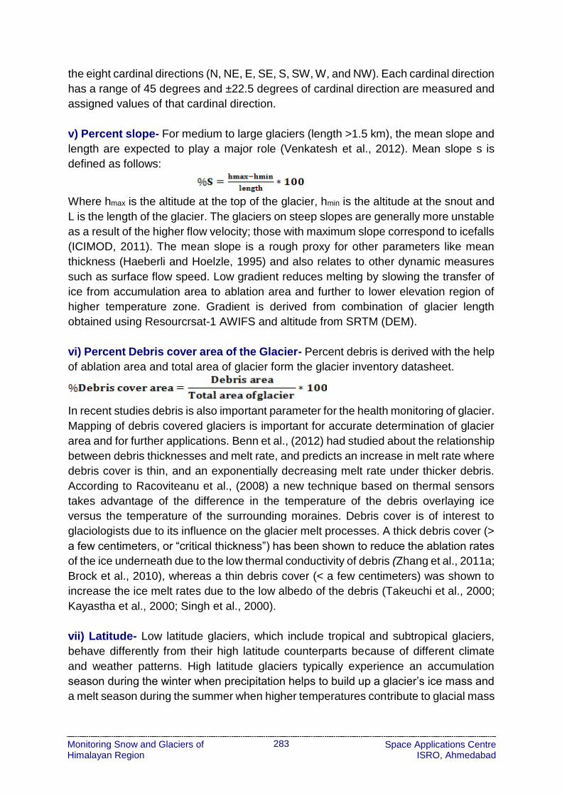
283
Monitoring Snow and Glaciers of Himalayan Region
Space Applications Centre ISRO, Ahmedabad
the eight cardinal directions (N, NE, E, SE, S, SW, W, and NW). Each cardinal direction
has a range of 45 degrees and ±22.5 degrees of cardinal direction are measured and
assigned values of that cardinal direction.
v) Percent slope- For medium to large glaciers (length >1.5 km), the mean slope and
length are expected to play a major role (Venkatesh et al., 2012). Mean slope s is
defined as follows:
Where hmax is the altitude at the top of the glacier, hmin is the altitude at the snout and
L is the length of the glacier. The glaciers on steep slopes are generally more unstable
as a result of the higher flow velocity; those with maximum slope correspond to icefalls
(ICIMOD, 2011). The mean slope is a rough proxy for other parameters like mean
thickness (Haeberli and Hoelzle, 1995) and also relates to other dynamic measures
such as surface flow speed. Low gradient reduces melting by slowing the transfer of
ice from accumulation area to ablation area and further to lower elevation region of
higher temperature zone. Gradient is derived from combination of glacier length
obtained using Resourcrsat-1 AWIFS and altitude from SRTM (DEM).
vi) Percent Debris cover area of the Glacier- Percent debris is derived with the help
of ablation area and total area of glacier form the glacier inventory datasheet.
In recent studies debris is also important parameter for the health monitoring of glacier.
Mapping of debris covered glaciers is important for accurate determination of glacier
area and for further applications. Benn et al., (2012) had studied about the relationship
between debris thicknesses and melt rate, and predicts an increase in melt rate where
debris cover is thin, and an exponentially decreasing melt rate under thicker debris.
According to Racoviteanu et al., (2008) a new technique based on thermal sensors
takes advantage of the difference in the temperature of the debris overlaying ice
versus the temperature of the surrounding moraines. Debris cover is of interest to
glaciologists due to its influence on the glacier melt processes. A thick debris cover (>
a few centimeters, or “critical thickness”) has been shown to reduce the ablation rates
of the ice underneath due to the low thermal conductivity of debris (Zhang et al., 2011a;
Brock et al., 2010), whereas a thin debris cover (< a few centimeters) was shown to
increase the ice melt rates due to the low albedo of the debris (Takeuchi et al., 2000;
Kayastha et al., 2000; Singh et al., 2000).
vii) Latitude- Low latitude glaciers, which include tropical and subtropical glaciers,
behave differently from their high latitude counterparts because of different climate
and weather patterns. High latitude glaciers typically experience an accumulation
season during the winter when precipitation helps to build up a glacier’s ice mass and
a melt season during the summer when higher temperatures contribute to glacial mass

284
Monitoring Snow and Glaciers of Himalayan Region
Space Applications Centre ISRO, Ahmedabad
loss. Low latitude glaciers are more sensitive to increases in temperature than mid
and high latitude glaciers (Rachel, 2012).
viii) Percent Ice Exposed Area of the Glacier- Percent ice exposed area is the bare
ice area of the glacier. This is derived by total area and ice exposed area of the glacier.
The formula used for the derivation is as follows:
The glacier inventory maps and inventory datasheets prepared based on Indian
Remote Sensing Satellite (IRS-P6) AWiFS data of 2004-07 periods, Shuttle Radar
Terrain Mapping SRTM-DEM, MODIS land surface temperature and other ancillary
data are the main data sets used in deriving the required physical and climatic
parameters for the study. Primary physical parameters are taken from the inventory
datasheet and with these parameters secondary parameters are derived and land
surface temperature is derived from MODIS product. Morphological parameters such
as Total area of glacier, Length, Elevation, Orientation, Latitude and Ice exposed area
are the primary parameters. Percent debris covers, Percent slope, Temperature are
the derived parameters. Each parameter is further grouped into 5 classes based on its
range of available values and is assigned with a rank as per its significance for the
glacier health. The comparisons of parameters are made using a scale of absolute
judgments that represents how much more; one element dominates another with
respect to a given attribute. The broad study approach is given in flow diagram Figure
272.
The parameters are compared and assigned importance as per Saaty’s (Saaty, 2008)
method and comparison matrix is prepared. The matrix is solved by Eigen vector
method for deriving the consistency index, Eigen weights and consistency ratio. The
consistency ratio less than or equal to 0.1 is acceptable (Saaty, 2008). Larger values
require the decision maker to reduce the inconsistencies by revising judgments.
Weighted ranks are obtained by multiplying the Eigen weights (Table 86) and rank
assigned to each parameter. The composite weights are then obtained by summation
of all weighted ranks for a given glacier. These composite values obtained for each
glacier are the Composite Glacier Health Index (CGHI) values and are categorized
from low to high into five health status classes to identify the relative fragile and healthy
glaciers in the Ganga basins.
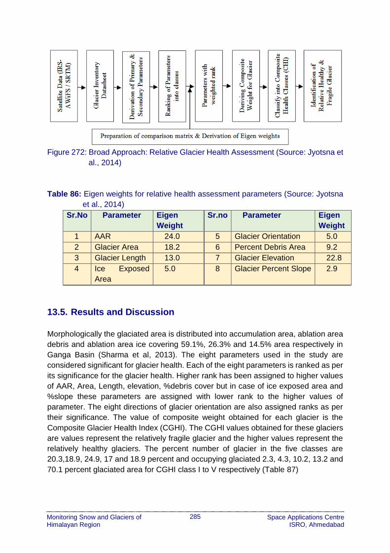
285
Monitoring Snow and Glaciers of Himalayan Region
Space Applications Centre ISRO, Ahmedabad
Figure 272: Broad Approach: Relative Glacier Health Assessment (Source: Jyotsna et
al., 2014)
Table 86: Eigen weights for relative health assessment parameters (Source: Jyotsna
et al., 2014)
Sr.No Parameter Eigen
Weight
Sr.no Parameter Eigen
Weight
1 AAR 24.0 5 Glacier Orientation 5.0
2 Glacier Area 18.2 6 Percent Debris Area 9.2
3 Glacier Length 13.0 7 Glacier Elevation 22.8
4 Ice Exposed
Area
5.0 8 Glacier Percent Slope 2.9
13.5. Results and Discussion
Morphologically the glaciated area is distributed into accumulation area, ablation area
debris and ablation area ice covering 59.1%, 26.3% and 14.5% area respectively in
Ganga Basin (Sharma et al, 2013). The eight parameters used in the study are
considered significant for glacier health. Each of the eight parameters is ranked as per
its significance for the glacier health. Higher rank has been assigned to higher values
of AAR, Area, Length, elevation, %debris cover but in case of ice exposed area and
%slope these parameters are assigned with lower rank to the higher values of
parameter. The eight directions of glacier orientation are also assigned ranks as per
their significance. The value of composite weight obtained for each glacier is the
Composite Glacier Health Index (CGHI). The CGHI values obtained for these glaciers
are values represent the relatively fragile glacier and the higher values represent the
relatively healthy glaciers. The percent number of glacier in the five classes are
20.3,18.9, 24.9, 17 and 18.9 percent and occupying glaciated 2.3, 4.3, 10.2, 13.2 and
70.1 percent glaciated area for CGHI class I to V respectively (Table 87)
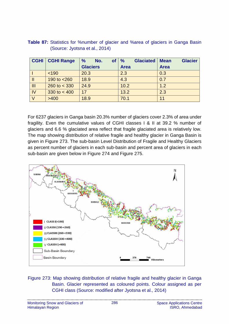
286
Monitoring Snow and Glaciers of Himalayan Region
Space Applications Centre ISRO, Ahmedabad
Table 87: Statistics for %number of glacier and %area of glaciers in Ganga Basin
(Source: Jyotsna et al., 2014)
CGHI CGHI Range % No. of
Glaciers
% Glaciated
Area
Mean Glacier
Area
I <190 20.3 2.3 0.3
II 190 to <260 18.9 4.3 0.7
III 260 to < 330 24.9 10.2 1.2
IV 330 to < 400 17 13.2 2.3
V >400 18.9 70.1 11
For 6237 glaciers in Ganga basin 20.3% number of glaciers cover 2.3% of area under
fragility. Even the cumulative values of CGHI classes I & II at 39.2 % number of
glaciers and 6.6 % glaciated area reflect that fragile glaciated area is relatively low.
The map showing distribution of relative fragile and healthy glacier in Ganga Basin is
given in Figure 273. The sub-basin Level Distribution of Fragile and Healthy Glaciers
as percent number of glaciers in each sub-basin and percent area of glaciers in each
sub-basin are given below in Figure 274 and Figure 275.
Figure 273: Map showing distribution of relative fragile and healthy glacier in Ganga
Basin. Glacier represented as coloured points. Colour assigned as per
CGHI class (Source: modified after Jyotsna et al., 2014)

287
Monitoring Snow and Glaciers of Himalayan Region
Space Applications Centre ISRO, Ahmedabad
Figure 274: Sub-basin Level Distribution of Fragile and Healthy Glaciers: Percent
number of glaciers in each sub-basin Alaknanda (ALAK), Bhagirathi
(BHAG), Ghagra (GHARA), Karnali (KAR), Kosi (KOSI), Narayani (Nar),
Yamuna (YAM)
Figure 275: Sub-basin Level Distribution of Fragile and Healthy Glaciers: Percent area
of glaciers in each sub-basin Alaknanda (ALAK), Bhagirathi (BHAG),
Ghagra (GHARA), Karnali (KAR), Kosi (KOSI), Narayani (Nar), Yamuna
(YAM)
The spatial distribution of relatively fragile glaciers is obtained based on the multi-
parameter weighted index method by using eight key glacier physical parameters.
About 20.3% number of glaciers covers 2.3% area. Apparently the smaller glaciers
with mean size of 0.3 km2 area in Ganga Basin are relatively fragile.
Remote sensing and GIS based multi-parameter weighted index method is useful to
identify spatial distribution of fragile glaciers. The flexibility inherent to this model
permits addition of more parameters and thereby has scope for increasing the
accuracy of assessment. The climatic parameter not used in this model can be added

288
Monitoring Snow and Glaciers of Himalayan Region
Space Applications Centre ISRO, Ahmedabad
to further improve the accuracy. Efforts for systematic validation of results are also
required.
14. Impact of Climate Change on Flora of Spiti
Valley
14.1. Objective
To understand the impact of snow line on the floral distribution in the valley and its
societal impact in Spiti valley, Himachal Pradesh.
14.2. Scientific Rationale
Impact of climate change on the the flora and habitats in regions adjacent to glaciated
terrain needs to be studied. Retreating glaciers and dwindling water resources have
significant impact on the biodiversity and species richness of the flora. In this context
a pilot study to understand the impact of retreating glaciers on the flora of the Spiti
valley as well local inhabitants has been taken up. Flora of Spiti valley are extremely
important to be conserved not only because of large biodiversity and species richness
but also because inhabitants of the area have dependence on these plant resources
required for food, health, shelter, fodder, fuel wood and other cultural purposes.
Glacier retreat as well as agro-diversity changes are occurring at an alarming rate
since last one decade in the Spiti valley. Water availability is apparently one of the
gravest /serious impacts of climatic change in Spiti valley which is mainly dependent
on glacier melt water for irrigation and domestic purposes. Natural water resources
have decreased up to 27.81% in all the Spiti Villages. Most of the natural springs have
dried up and there is insufficient water for irrigation.
Populations of endangered and vulnerable species are gradually diminishing due to
great demand for medicinal purposes. Over exploitation, Land scalping, over-grazing
and developmental activities are other factors for depletion of this natural wealth.
Economically important species of the valley are significantly shifting toward higher
altitudinal regimes and making them highly vulnerable. The species of high altitudinal
region are under great threats as they have limited opportunity to migrate farther
upwards in elevation to find cooler habitat conditions. The climate sensitive species
are required to be regularly monitored, protected and modeled by suitable latest
modeling tools for their distribution pattern and phenological attributes so that the base
line data can be utilized for understanding impact of future climate changes in the area.
There is a need for regular monitoring the habitats and communities to understand the
dynamics of the habitats and communities and accordingly plan for their management.

289
Monitoring Snow and Glaciers of Himalayan Region
Space Applications Centre ISRO, Ahmedabad
14.3. Methodology
Field studies were conducted in the Spiti valley of Lahual and Spiti District in Himachal
Pradesh (Figure 276). and analysis of floristic diversity. Plots of 20×20 m were
selected in different aspects and habitat. 20 quadrats of 5X5 m for shrubs and 20
quadrats of 1×1 m for herbs were randomly laid within the plot. Communities were
identified based on their importance, value-index and calculated as the sum of relative-
frequency, relative density and relative abundance. For the collection and analysis of
data from these quadrats standard ecological methods (Simpson, 1949; Shannon &
Weaver, 1963; Curtis and Intosh, 1950; Grieg-Smith, 1957; Chacko, 1965; Kersaw,
1973; Muller-Dombois and Ellenberge, 1974; Dhar et al., 1997; Samant and Joshi
2004) were followed. During qualitative assessment, surveys and samplings between
3180-4560 m were done in each season and identified with the help of floras and
literature available in this field (Polunin and Stainton, 1984; Aswal and Mehrotra, 1994;
Chowdhery and Wadhwa, 1984; Dhaliwal and Sharma, 1999; Samant, 1999; Samant
and Pangtey, 1993;Samant et al., 2000; Samant and Joshi, 2004; Singh and Rawat,
2000 and Murti, 2001).Socio-economic survey on the impact of retreading glacier,
changing weather and cropping pattern was done through interview using formal and
informal set of questions.
Figure 276 Map showing the study area in Lahul and Spiti district, Himachal Pradesh
290
Monitoring Snow and Glaciers of Himalayan Region
Space Applications Centre ISRO, Ahmedabad
14.4. Results and Discussion
The present study was conducted for phyto-diversity assessment in Spiti valley of
Himachal Pradesh, India in 84 sites which were distributed between 3000-4560 m
above mean sea level. Sites were selected based on different topographical features
such as habitat type, altitude, aspect, slope, and different vegetation types. Geo-
references for each site/habitat were taken with the help of Global Positioning System
(GPS). The number of herbs, shrubs and trees are 369, 24 and 9 respectively. Six
species are under shrubs; 3 species are either herbs or shrubs. Betula utilis is either
a shrub or a tree. The top 9 families of the flora of Spiti are Asteraceae (58 species),
Papilionaceae (40 species), Poaceae (30), Brassicaceae (25), Rosaceae (24),
Ranunculaceae (23 species), Apiaceae (20 species), Scrophulariaceae (18 species),
and Polygonaceae (15 species).
Qualitative analysis of vegetation was carried out between 3180–4560 m. 412 species
belonging to 216 genera and 55 families have been collected, identified and
photographed. Out of these 362 species belonging to 184 genera and 45 families are
dicots, 47 species belonging to 30 genera and 8 families are monocots. The top 10
families of the flora of Spiti are Asteraceae (58 species), Papilionaceae (40 species),
Poaceae (30), Brassicaceae (25), Rosaceae (24), Ranunculaceae (23), Apiaceae
(20), Scrophulariaceae (18), Polygonaceae (15) and Caryophyllaceae (12). We
delineated 41 alpine communities (33 shrub and 8 herb communities) based on
relative density for the shrub and herb communities. Amongst these, Caragana
brevifolia community represented by maximum sites (15 sites); followed by Hippophae
rhamnoides & Ephedra gerardiana (7 each); Hippophae tibetina and Potentilla
arbuscula (4) Myricaria elegans, Lonicera spinosa, Astragalus strobiliferus, Myricaria
germanica and Astragalus webbianus (3 each); Ephedra intermedia (2 each) and rest
of the communities represented by one site only.
Present study depicts 167 native and 245 non-natives, 37 as endemic, 42 near
endemic species in the valley. Increasing number of non-native species is a major
concern and hence showing the significance of conservation prioritization in the valley.
People in Spiti valley believe in indigenous medicines known as Amchi system of
medicine which is based on Tibetan System of Medicine. The widely used medicinal
plants from high altitude regions are Aconitum heterophyllum, Dactylorhiza hatagirea,
Ephedra gerardiana, Hippophae rhamnoides, Inula racemosa, Podophyllum
hexandrum, Rheum webbianum, etc.
Altitudinal Shift of the plant species

291
Monitoring Snow and Glaciers of Himalayan Region
Space Applications Centre ISRO, Ahmedabad
The present study when compare to the earlier studies revealed that the economically
important species of the valley are significantly shifting toward higher altitudinal
regimes and making them highly vulnerable (Figure 277)
Figure 277: Important species of the valley shifting toward higher altitude
Various ecological parameters studied along altitudinal gradient
In 3000-3500m altitudinal range
Among shrubs the relative density of Ephedra intermedia (23.83%) are maximum
followed by Ephedra gerardiana &Hippophae rhamnoides (17.83 & 8.96 %)
respectively. Whereas the IVI of Ephedra intermedia (65.47) are maximum followed
by Ephedra gerardiana & Lectuca orientalis (35.87 & 29.77). The distribution of
species (a/f ratio) in this altitudinal showed that 64.70% species were random and
35.29 % species were contiguous. Among herbs the relative density and IVI are
maximum of Carex melanantha (3.23% & 6.97) followed by Koberasia napalensis &
Carum carvi (2.90 & 2.65 % and 6.48 & 6.00) respectively. The distribution of species
(a/f ratio) in this altitudinal showed that 100% species were of contiguous in nature.
In 3500-4000m altitudinal range
Among shrubs the relative density and IVI are maximum of Myricaria elegans (16.66%
&34.57) followed by Ephedra gerardiana & Myricaria saquamosa (9.57 & 6.72 % and
22.95 & 18.01) respectively. The distribution of species (a/f ratio) in this altitudinal
showed that 4.16% species were regular,58.33% random and 37.5% species were
contiguous in nature. Among herbs the relative density and IVI are maximum of Carex
melanantha (2.88% and 5.74) followed by Carex borii & Euphorbia officinalis (2.66 &

292
Monitoring Snow and Glaciers of Himalayan Region
Space Applications Centre ISRO, Ahmedabad
2.13 % and 5.39 & 4.58) respectively. The distribution of species (a/f ratio) in this
altitudinal showed that 100% species were contiguous in nature.
In 4000-4500m altitudinal range
Among shrubs the relative density and IVI are maximum of Hippophae tibetana (8.56%
& 20.99) followed by Hippophae rhamnoides & Potentilla salesoviana (8.41 & 7.69 %
and 20.78 & 19.65) respectively. The distribution of species (a/f ratio) in this altitudinal
showed that 4.16% species were regular,75% random and 20.83 % species were
contiguous. Among herbs the relative density and IVI are maximum of Carex
melanantha (2.89% and 5.87) followed by Carum carvi & Carex orbicularis (2.42 &
2.41 % and 5.38 & 5.36) respectively. The distribution of species (a/f ratio) in this
altitudinal showed that 100% species were contiguous in nature. Abundance
frequency ratio of the Species along altitudinal gradient of shrubs and herbs was
observed in different altitudes in Spiti valley. It was reported that the distribution was
contiguous in 3000-3500 m range but was regular in 3500-4000 and 4000-4500m
Spiti valley is rich in wild plant resources. The inhabitants of the area have close
relationship with surrounding plant resources with reference, to some extent, of their
dependence on plant resources for their food, health, shelter, fodder, fuel wood and
other cultural purposes. Total 42 villages were surveyed and 316 people of age group
25-88wereinterviewed for dependence on local plant resources. In Spiti valley
stakeholders use different plant parts in the preparation of indigenous medicines.
Study revealed that leaves (49 spp.) are being used most of the times followed by
aerial parts (36 spp.), roots & whole plants (29 spp.) and flower (27 spp.) The economic
species can be categorized into medicinal (169 species), edible (50 species), fodder
(65 species), fuel yielding (21), dye yielding (16 species), oil yielding (11 species),
Tannin yielding (8), Wood yielding (7 species), Spices and condiments (7 species),
sacred value (7 species), ornamental value (5 species), Soil binder (5), narcotic (2
species) and fiber yielding (2 species).
A comprehensive base line data which has been generated through present study will
further enhance the knowledge of the flora, microbial diversity and other ecological
aspects of the valley. The study on the niche modeling of the selected ecological an
economically important species for keeping the track of the population and their
possible distribution in the times to come is urgently required as the anthropogenic
activities and habitat destruction and fragmentation and climate change etc. are
contributing to the vulnerability of the flora from the region. Maximum species richness
& density are distributed below 4000 m and diversity is 3000-3500 m. Some species
have wider range of distribution which is present in both altitude range e,g. Astragallus
himalayanus Carex melanantha Causina thomsonii, Gentiana, argentea, Gentiana
moorcroftiana, Lomatogonium carinthiacum, Nepeta podostachys etc. The species
which are above 4000 m are Aconitum violacium, Rhodila hetrodonta, Saxifragra
flagellaris, Walthemia tomentosa, W. glabra, Rheum moorcroftiana etc. shows high
rate of acclimatization for the arid environments (Figure 278). The species of high

293
Monitoring Snow and Glaciers of Himalayan Region
Space Applications Centre ISRO, Ahmedabad
altitudinal region are under great threats as they have limited opportunity to migrate
farther upwards in elevation to find cooler habitat conditions. Species density and
diversity index of herbs is decreasing as we go in the higher elevation because of
harsh and arid conditions which make survival of the herbs difficult. Whereas species
richness is maximum at 3500-4000 m which may be is due to its diverse habitats and
suitable bitats. Altitudinal range 3500-4000 m is occupying the maximum number of
species.
Figure 278: Acclimatization of the herb and shrub to the arid environments
Agriculture/Horticulture and Cropping patternsof Spiti valleys
The data recorded on old crops grown in Spiti valley namely Field Pea, Wheat, Barley,
Potato and Mustard shows decrease in their cropping area. Area under these crops 2
decade ago has maximum under barley (55.2%) and minimum under mustard
(0.96%). However, in present area under barley reduced 37.72%. Newly introduced
crop includes Garden pea (42.66%) and Apple (6.93%) is emerging as major cash
value crop therefore other crops agricultural area is shrinking as compare to past.
Villages under apple cultivation are Kaza, Lidang, Lara, Shichiling, Poh, Tabo, Hurling,
Lari and Dhankar. Maximum apple growing village is Tabo (53.75%) and minimum
Lari (35.23%). Garden pea and apple covers 49.59% area out of total cultivated land.
(Figure 279).
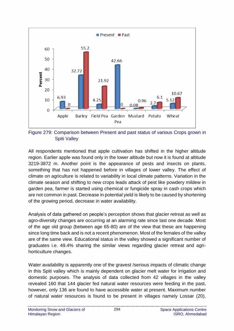
294
Monitoring Snow and Glaciers of Himalayan Region
Space Applications Centre ISRO, Ahmedabad
Figure 279: Comparison between Present and past status of various Crops grown in
Spiti Valley
All respondents mentioned that apple cultivation has shifted in the higher altitude
region. Earlier apple was found only in the lower altitude but now it is found at altitude
3219-3872 m. Another point is the appearance of pests and insects on plants,
something that has not happened before in villages of lower valley. The effect of
climate on agriculture is related to variability in local climate patterns. Variation in the
climate season and shifting to new crops leads attack of pest like powdery mildew in
garden pea, farmer is started using chemical or fungicide spray in cash crops which
are not common in past. Decrease in potential yield is likely to be caused by shortening
of the growing period, decrease in water availability.
Analysis of data gathered on people’s perception shows that glacier retreat as well as
agro-diversity changes are occurring at an alarming rate since last one decade. Most
of the age old group (between age 65-80) are of the view that these are happening
since long time back and is not a recent phenomenon. Most of the females of the valley
are of the same view. Educational status in the valley showed a significant number of
graduates i.e. 49.4% sharing the similar views regarding glacier retreat and agri-
horticulture changes.
Water availability is apparently one of the gravest /serious impacts of climatic change
in this Spiti valley which is mainly dependent on glacier melt water for irrigation and
domestic purposes. The analysis of data collected from 42 villages in the valley
revealed 160 that 144 glacier fed natural water resources were feeding in the past,
however, only 136 are found to have accessible water at present. Maximum number
of natural water resources is found to be present in villages namely Lossar (20),

295
Monitoring Snow and Glaciers of Himalayan Region
Space Applications Centre ISRO, Ahmedabad
Dhankar (16), Kibber (15). Followed by Mudh (12) and Burr (10). But there is no
significant fall in the number of kuhls in Spiti basin which were used to be 103 in past
but left 101 presently. Natural water resources are decreased up to 27.81% all the
Spiti Villages. The maximum natural water source (Kulh) is reduced in the village
Hansa and Kaza up to 40% also minimum reduced in village Jomle (15%).
Regular monitoring using random sampling by quadrat method is suggested in the
habitats and communities to understand the dynamics of the habitats and communities
and accordingly plan for their management. The climate sensitive species are required
to be regularly monitored or modeled by suitable latest modeling tools for their
distribution pattern and phenological attributes so that the base line data can be
generated for future changes in the area. The information generated on these lines
will provide a better insight about the present status of floristic diversity and help in
developing adequate strategies and action plan for the management of such
biodiversity rich areas. Further, for in-situ conservation of the economically and
ecologically important species, regular monitoring of the sites and complete protection
of the habitats is suggested. In addition, seed germination protocols developed may
be used for mass multiplication of the species and seedlings should be transplanted
in comparable habitats so that viable population of the species can be maintained.
Furthermore, the effect of retreating glaciers on the biodiversity of the region may be
monitored from time to time by suitable modeling tools. The findings would help policy
planners, conservationists and local people to devise suitable strategies to protect the
economic flora in the valley.

296
Monitoring Snow and Glaciers of Himalayan Region
Space Applications Centre ISRO, Ahmedabad
15. Development of Algorithm for Snow Cover/
Snow Depth Products using INSAT-3D Data
15.1. Objective
To develop algorithm for generating snow cover/snow depth product from INSAT 3D
Imager data (geostationary platform) and operationalize generation of daily digital
snow cover map products.
15.2. Scientific Rationale
Water is one for the most important component on the Earth surface and plays an
important role in collection, distribution, analysis and management for hydrological and
climatological applications at regional and global scale (Dozier, 1992). About 10% of
the earth’s surface, 15 × 106 km2, is covered by polar ice caps and glaciers (the
Cryosphere). The glaciers and mountain ice caps cover an area of about 550,000 km2
on Earth (excluding Antarctica and Greenland) and nearly all of its lies in the North
America and Eurasia. Snow covers almost 40 per cent of the Earth's land surface
during Northern Hemisphere winter. This makes snow albedo and area an important
component of the Earth's radiation balance (Foster and Chang, 1993). The
geographical extent of snow cover over the Northern Hemisphere varies from a
maximum of ~46 × 106 km2 in January and February to a minimum of ~4.6 × 10⁶ km2
in August. About 60 to 65 % of winter snow cover is found in Eurasia and most mid-
summer snow cover is found in Greenland (Frei and Robinson, 1999). However, the
spatial density of in-situ measurement network is too low to provide an adequate
characterization of its distribution (Mognard et al., 2003). The remoteness and hostile
environment of snow and glaciated region means investigations by remote sensing
methods, preferably from space platform is desirable (Massom 1991). Cryosphere is
being monitored from space since the mid-1960s (Foster and Chang, 1993). Large
areas in the Himalayas are also covered by snow during wintertime. Area of snow can
change significantly during winter and spring. This can affect stream flow during spring
and summer of the rivers originating in the Higher Himalayas. The maximum snow
cover for the three major river basins, namely the Indus, the Ganga and the
Brahmaputra, altogether is approximately 85% of the total geographic area which
reduces to approximately 10% during ablation (Singh et al., 2014). In addition, snow
pack ablation is highly sensitive to climatic variation. Increase in atmospheric
temperature can influence snowmelt and stream runoff pattern (Kulkarni, et al. 2002b).
Therefore, mapping of areal extent and reflectance of snow is an important parameter
for various climatological and hydrological applications. In addition, extent of snow
cover can also be used as an input for avalanche investigation.

297
Monitoring Snow and Glaciers of Himalayan Region
Space Applications Centre ISRO, Ahmedabad
Snow was first observed by satellite in eastern Canada from the TIROS-1 satellite in
April 1960. Since then, the potential for operational satellite-based mapping has been
enhanced by the development of higher temporal-frequency and satellite sensors with
higher spatial resolution. Remote sensing technique has been extensively used for
snow cover monitoring in the Himalayan region with the help of numerous satellite
sensors (Hall et al., 2001; Romanov et al., 2000, 2003; Kulkarni and Rathore. 2003).
The discrimination between snow and cloud can be done by using various techniques
such as textural analysis, association with shadow and by using multi temporal
analysis. Discrimination between cloud and snow is not feasible due to similar high
reflectance in VNIR region, however it is possible due to contrasting behavior of them
in SWIR region. To overcome the problem of cloud and snow, Normalized Difference
Snow Index (NDSI) method was developed (Hall et al., 1995; Kulkarni et al., 2006b).
Satellite sensors with better radiometric resolutions, such as MODIS and AWiFS have
been used successfully for snow mapping (Hall et al. 2002; Kulkarni et al., 2010; Singh
et al., 2014). Information generated from satellite observations has been extensively
used for snowmelt runoff modeling (Kulkarni et al. 2002a).
15.3. Study Area and Data Used
INSAT 3D Imager covers the India and neighboring countries from geostationary
platform. The entire Hindukush-Karakoram-Himalaya (HKH) region is covered for
generating snow cover product. AWiFS derived snow cover product have been used
to validate and derive fractional snow cover product over the study area. Auxiliary data
such as DEM has been used along with INSAT 3D derived reflectance and thermal
data.
15.4. Algorithm Development
Snow strongly reflects in the visible region and absorbs in the SWIR region which
makes snow a distinct object on the Earth surface. Figure 280 shows the spectral
characterization of snow and other objects. It can be clearly observed that snow is
very bright object in visible region due to its high albedo. Snow behaves as a dark
object as it moves towards longer wavelength. AWiFS channel collects the radiance
in Green (B2), Red (B3), NIR (B4) and SWIR (B5) region and Figure 281 shows the
TOA reflectance over the Himalayan terrain. Snow appears quite bright in B2, B3 and
B4 whereas it becomes dark in B5. Non-snow area is showing low reflectance in B2,
3 & 4 whereas return comparatively high reflectance in B5. Cloud has persistently
shown high reflectance in all bands, however, can be identified based on textural
information. The high reflectance in visible region and low reflectance in SWIR region
forms a base to estimate Normalized Difference Snow Index (NDSI).

298
Monitoring Snow and Glaciers of Himalayan Region
Space Applications Centre ISRO, Ahmedabad
Figure 280: Spectral behaviour of snow and other objects in parts of the Himalayas
Figure 281: TOA reflectance of AWiFS data over Himalayan region
0.0
0.2
0.4
0.6
0.8
1.0
350 850 1350 1850 2350
Re
fle
cta
nce
Wavelength (nm)
water vegetation soil snow (3days old)
Band 2 (0.52-0.59 µm)
Band 4 (0.77-0.86 µm) Band 5 (1.55 – 1.70 µm)
snow
cloud
Non-snow
Band 3 (0.62-0.68 µm)
snow
cloud
Non-snow

299
Monitoring Snow and Glaciers of Himalayan Region
Space Applications Centre ISRO, Ahmedabad
Normalized Difference Snow Index (NDSI)
The NDSI is useful for the identification of the snow, and for separating snow and most
of the clouds. The NDSI is a measure of the relative magnitude of the characteristic
reflectance difference of snow between the visible and short-wave IR reflectance. The
NDSI is insensitive to a wide range of illumination conditions (Kulkarni et al., 2006b).
The NDSI is analogous to the Normalized Difference Vegetation Index (NDVI) (Tucker,
1979 and 1986; Townshend and Tucker, 1984). NDSI can be calculated using
normalized difference ratio of visible and SWIR channels for INSAT 3D imager, as
given below;
𝑁𝐷𝑆𝐼 =𝑣𝑖𝑠𝑖𝑏𝑙𝑒𝐼𝑁𝑆𝐴𝑇 3𝐷 𝐵1 − 𝑆𝑊𝐼𝑅𝐼𝑁𝑆𝐴𝑇 3𝐷 𝐵2
𝑣𝑖𝑠𝑖𝑏𝑙𝑒𝐼𝑁𝑆𝐴𝑇 3𝐷 𝐵1 + 𝑆𝑊𝐼𝑅𝐼𝑁𝑆𝐴𝑇 3𝐷 𝐵2
Pixels that are approximately 75 % or greater covered by snow have been found to
have NDSI values 0.4 in our field investigation at Dhundi test site in Himachal
Pradesh (Negi et. al., 2006, 2010). These NDSI thresholds have been verified from
detailed analysis of numerous AWiFS scenes, comparisons with supervised-
classification techniques and NDSI technique (Kulkarni et. al. 2004). Pure snow has
a high NDSI but NDSI decreases as other features are mixed in a pixel. Snow in mixed
pixels has an NDSI that is less than that for pure snow. Pure snow can be distinguished
by its high NDSI value (Negi et. al., 2006, 2010). NDSI threshold value was
established using visual interpretation and field based spectral data of different targets.
Utilization of INSAT 3A CCD data
INSAT 3A CCD data was also used for the characterization of different land cover
classes and cloud. However, a need to recalibrate the INSAT 3A data was felt due to
degradation of sensor and AWiFS sensor was used for the same. AWiFS sensor has
been routinely calibrated over Chharodi site at Sanand in Gujarat (India) maintaining
flat uniform area, stability of surface reflectance, identified area in satellite image and
easy accessibility for conducting experiment. The calibration analysis was carried out
and the recent calibration data showed less than 2 % degradation for LISS IV and
LISS III sensor and 3 % degradation for AWiFS sensor over a period of 3 years
(Manjunath and Muralikrishnan, 2008). Three individual scenes from January,
February and March months for each sensor were used. Concurrent clear sky satellite
overpasses (at 0500 GMT) over India on 23 January 2007, 16 February 2007 and 26
March 2007 for INSAT 3A CCD and AWiFS data were selected. The AWiFS and
INSAT 3A CCD have similar spectral channels in visible, NIR and SWIR region but at
different spatial resolution of 56 m and 1 km respectively. The study area
encompasses spatial extent (22-370 N, 69-940 E) which includes different land cover
classes over Northern India such as: snow, agriculture, bare soil, forest, cloud and
water bodies. The time for INSAT 3A CCD data was chosen at 10.30 a.m. and the
satellite equatorial crossing time for AWiFS was 10.30 a.m. ± 5 min. In addition, INSAT
3A CCD data on 05 March 2007 was also used in the study to compare the effect of
pre-launch and post-launch calibration coefficients. The at-sensor apparent
reflectance (TOA reflectance) was computed assuming a lambertian surface and

300
Monitoring Snow and Glaciers of Himalayan Region
Space Applications Centre ISRO, Ahmedabad
RSR-weighted exo-atmospheric bandpass irradiances (E0()). The INSAT 3A CCD
NDSI and NDVI were computed from TOA reflectance before and after cross-
calibration.
The average at-sensor radiances for each class were computed for each channel
(Visible, NIR and SWIR). Average radiance values of common homogeneous subset
of collocated targets were calculated for all INSAT pixels to all respective AWiFS pixels
of one object. This accounts for the spatial heterogeneity introduced due to the
difference in spatial resolutions of both the sensors. The radiances from both AWiFS
and INSAT 3A CCD were subsequently plotted for all the three channels. The linear
regression was performed for individual channels between calibrated AWiFS and
INSAT 3A CCD at-sensor radiances with pre-launch calibration (Figure 282). The
regression analysis between corresponding AWiFS and INSAT 3A CCD channels
showed linear relations with high R2 of 0.96 for visible channel (0.63-0.69 µm) and of
0.92 for NIR (0.77-0.89 µm) channels with 16 datasets. The INSAT 3A CCD SWIR
channel showed severe sensor degradation with low R2 of 0.60. The slope values after
cross calibration for Visible, NIR and SWIR channels were found to be 1.839, 1.589
and 2.232, and intercepts as -5.803, -4.950 and -0.481, respectively. The linear
relations were further used to compute CCD at-sensor radiances, TOA apparent
reflectances, NDVI and NDSI with independent INSAT 3A CCD dataset of 5 march
2007. It was observed that central wavelength difference varies from 5-9 nm for INSAT
3A and AWiFS and is not significant. It rules out any effect of shift in central wavelength
on differences in at-sensor radiances between two sensors.
An improvement on dynamic range of reflectance with old calibration (15-75 %) and
new calibration coefficient (10-110 %) were found in the visible channel. High reflecting
objects such as snow and cloud have shown a significant improvement from old TOA
reflectance to new TOA reflectance computation. In agriculture and forest land cover
classes, visible channel TOA reflectance has shown a reduction whereas SWIR
channel has shown an increase. SWIR channel was also found to be increased for
desert and rock land cover classes. This established that the new coefficients of
INSAT 3A CCD data for Visible, NIR and SWIR channels can be used to recalibrate
and improve the radiometric quantity for routine applications. The Figure 283a showed
the INSAT 3A CCD data of 05 March 2007 and Figure 283b showed the scatterplots
of TOA apparent reflectance of visible channel and NDSI using old and new calibration
coefficients.

301
Monitoring Snow and Glaciers of Himalayan Region
Space Applications Centre ISRO, Ahmedabad
Figure 282: Regression fits between for INSAT 3A CCD and AWiFS at sensor
radiances for a) Visible channel, b) NIR channel and c) SWIR channel
(Source: Singh et al., 2013)
Figure 284 showed the histogram of NDSI and NDVI for pre-launch and post-launch
calibration. The NDSI and NDVI values were computed using both old and new
calibrated coefficients. The NDSI and NDVI dynamic ranges have shown an
improvement from 0.0 - 0.7 to -0.45 – 0.85 and 0.0 – 0.50 to -0.10 - 0.80,
respectively. The NDSI peak has been shifted from 0.1 to -0.25 which showed the
dominant presence of non-snow pixels as can be observed in False Colour
Composite (FCC) image. Another broad peak of 0.66 was shifted to 0.71 which is
(a) INSAT 3A ~ AWiFS (visible channel)
y = 1.8385x - 5.8035
R2 = 0.96
0
10
20
30
40
0 5 10 15 20 25AWiFS radiance (w/m2/sr/microm)
INS
AT
3A
CC
D r
adia
nce
(w/m
2/s
r/m
icro
m)
(c) INSAT 3A ~ AWiFS (SWIR channel)
y = 2.2323x - 0.4808
R2 = 0.600.0
0.5
1.0
1.5
2.0
2.5
0.0 0.5 1.0 1.5AWiFS radiance (w/m2/sr/microm)
INS
AT
3A
CC
D r
ad
ian
ce
(w/m
2/s
r/m
icro
m)
(b) INSAT 3A ~ AWiFS (NIR channel)
y = 1.589x - 4.9496
R2 = 0.920
5
10
15
20
25
0 5 10 15 20AWiFS radiance (w/m2/sr/microm)
INS
AT
3A
CC
D r
adia
nce
(w/m
2/s
r/m
icro
m)
snow
vegetation
forest
x barren land
rock
water
+ cloud
snow
vegetation
forest
x barren land
rock
water
+ cloud

302
Monitoring Snow and Glaciers of Himalayan Region
Space Applications Centre ISRO, Ahmedabad
related to snow covered pixels. NDVI values too have shown a peak shifted towards
negative side close to 0.0. The dynamic range of NDSI and NDVI was found to be
improved in Histograms. This redistribution of NDSI and NDVI values would be
helpful further to identify different classes of snow and vegetation pixels. This
highlights the importance of post calibration to correct the radiometric quantities for
better estimation of various indices for natural resources applications. Thus, these
new calibration coefficients will help to improve the monitoring of snow cover and
vegetation, and will provide important input to model the long term monitoring of
natural resources of Earth environment (Singh et al., 2013a).
Figure 283: Comparison of INSAT 3A CCD data (05 March 2007) with old and
recalibrated coefficients; a. INSAT 3A CCD FCC of 5 March 2000; b.
Scatterplots of NDSI (X-axis) and TOA reflectances of red channel (Y-
axis) of old and new calibration coefficients (Source: Singh et al.,
2013)
INSAT 3A CCD data of 23 January 2007 were also analyzed for different land cover
classes. Figure 285 shows the FCC, scatterplot and threshold of SWIR region to
separate ice cloud and snow from the snow. However, with the availability of INSAT3D
data, seasonal and temporal analysis will be carried out to finalize the suitable
threshold of SWIR channel to separate ice cloud and snow in conjunction with NDSI.
Separation of cloud will be used as an additional criterion and will be verified with
INSAT 3D derived cloud mask product (Figure 285).
a
b

303
Monitoring Snow and Glaciers of Himalayan Region
Space Applications Centre ISRO, Ahmedabad
Figure 284: Histograms for NDSI and NDVI from INSAT 3A CCD (5 March 2007 at
0500 GMT) using old and new calibration coefficients (Source: Singh et
al., 2013)
Figure 285: INSAT 3A CCD image of 23 Jan 2007 and SWIR threshold to separate
ice cloud from snow product
Snow Cover using INSAT 3D
Snow strongly reflects in visible region and absorbs in SWIR. This peculiar
characteristic of snow among various earth objects has been used to develop snow
cover mapping algorithm for optical sensors like AWiFS based on Normalized
Difference Snow Index (NDSI) approach. While the NDSI can separate snow from
NDSI NDVI
Freq
uen
cy
Freq
uen
cy
a) old coefficient c) old coefficient
b) new coefficient d) new coefficient
NDSI NDVI

304
Monitoring Snow and Glaciers of Himalayan Region
Space Applications Centre ISRO, Ahmedabad
most obscuring clouds, it does not identify or discriminate cirrus clouds from snow due
to similar spectral signature. NDSI based algorithm has been developed and validated
for AWiFS sensor of Resourcesat. However, INSAT-3D has a broad bandwidth in
visible channel whereas SWIR channel collects the radiance in similar bandwidth as
in AWiFS. The difference in Visible region of AWiFS and INSAT 3D requires fine tuning
of the threshold value for INSAT-3D Imager data.
Visible and SWIR channels of INSAT 3D Imager was used to develop NDSI based
approach for snow pixel identification. Thermal data (TIR 1) was used to separate ice
cloud and snow based on difference in their temperature. In addition, SWIR
reflectance, DEM and Latitude of the study area was also used to remove wrongly
classify snow pixels.
NDSI = (VisibleINSAT B1 - SWIRINSAT B2) / (VisibleINSAT B1 + SWIRINSAT B2)
Figure 286 shows the operationally generated regional snow cover product, showing
in inset the scatterplot of different objects in Visible and SWIR data.
In validation exercise, the product was validated using 4 different approaches (Figure
287).
1. INSAT 3 D snow cover product was validated using archived field
spectroradiometer data for varying type of snow and various objects. Snow pixels
were well above the NDSI based threshold.
2. AOI of area was selected and accuracy was observed well within 10% except few
locations which was due to the inclusion of cloud and sub-pixel heterogeneity
during manual mapping of snow.
3. 10 INSAT 3D FCC and derived snow cover product were selected in this exercise.
Pure snow subset pixels were selected in FCC which were later verified in the
binary product with 100% accuracy.
4. A comparison of INSAT3D snow cover product was carried out with AWiFS derived
snow cover product. Snow cover product were accurate within 12% except few
dates, caused by the sub-pixel heterogeneity due to coarse resolution of INSAT
3D.
This leads to estimation of fractional snow cover product of INSAT 3D to increase the
accuracy of snow cover area. Synchronous INSAT 3D and AWiFS data was used in
this exercise covering different level of snow cover area distributed along Himalayan
region. Fractional snow cover products of INSAT 3D have been prepared which
becomes an input to snow depth estimation in the Himalayan region. However, at
present snow depth approach for North America region has been adopted and further
improvements and fine tuning for Himalayan region is in progress.

305
Monitoring Snow and Glaciers of Himalayan Region
Space Applications Centre ISRO, Ahmedabad
Figure 286: INSAT-3D snow cover product using Imager data. Scatterplot of different
objects has been shown using Visible and SWIR region in the inset
15.5. Conclusions
This work presents the approach developed to generate snow cover maps using
INSAT 3D Imager data. In present analysis, AWiFS, INSAT 3A CCD, MODIS and ASD
spectroradiometer data was used to understand the applicability and Implementation
of NDSI based approach to estimate snow cover area. Cross-calibration of INSAT 3A
CCD was also carried out in conjunction with AWiFS data which shows improvement
over Red and NIR channels, however, depicts severe calibration issue for SWIR
channel. NDSI based approach on INSATD-3D data was made operationalized at IMD
using Visible, SWIR, Thermal data along with additional input based on DEM and
geography of the region. In future, INSAT-3D derived snow cover product will be
further improved for different categories of land cover, fractional snow cover,
understanding of slope corrected area at coarser resolution, and validation of snow
cover product as continuing activity will be further carried out.
Field based reflectance of different objects
0.0
0.2
0.4
0.6
0.8
1.0
350 500 650 800 950 1100 1250 1400 1550 1700 1850 2000 2150 2300 2450wavelength (nm)
refle
cta
nce
Dry snow
grass
water
soil
dry pavement
0
10
20
30
40
50
60
0 10 20 30 40 50 60
RS
WIR
RVIS
20 Nov 2013 INSAT 3D
desert vegetation snow cirrus cloud warm cloud water

306
Monitoring Snow and Glaciers of Himalayan Region
Space Applications Centre ISRO, Ahmedabad
Figure 287: Snow cover product validation using INSAT-3D imager data using a)
Field Spectroradiometer data; b) visual aoi extraction of snow cover
area; c) pure snow pixels on FCC image; and d) AWiFS snow cover
products.
Field based scatterplot of NDSI of INSAT 3D and AWiFS
-0.6
-0.4
-0.2
0.0
0.2
0.4
0.6
0.8
1.0
-0.6 -0.4 -0.2 0.0 0.2 0.4 0.6 0.8 1.0
AWiFS NDSI
INS
AT
3D
ND
SI
A
B
-50
-40
-30
-20
-10
0
10
% c
ha
ng
e in
sn
ow
co
ve
r
Date
Nepal region Indus region
30
No
v 1
3
11
No
v 1
3
13
No
v 1
3
25
No
v 1
3
15
De
c 1
3
a
b
c
d
0
25
50
75
100
-1 -0.5 0 0.5 1
RV
IS
NDSI
dry snow moist snow wet snow
green grass dry grass green plant
road water soil
snow+vegetation snow+soil+vegetation snow+soil
light contaminated snow medium contaminated snow heavy contaminated snow
ice

307
Monitoring Snow and Glaciers of Himalayan Region
Space Applications Centre ISRO, Ahmedabad
16. Development of Techniques for RISAT-1
SAR Data Analysis for Glacier Studies and
Detection of Glacial Lakes Buried under
Snow
16.1. Objectives
To develop techniques for RISAT-1 SAR data analysis for glacier studies and
detection of glacial lakes buried under snow
16.2. Scientific Rationale
Active microwave sensor based imaging system (Synthetic Aperture Radar-SAR) is
independent of cloud and can be operated in day/night. SAR signal is transmitted
which interacts with surface and return back to the receiver at satellite system. The
received signal is influenced by sensor parameters such as frequency, polarization,
incidence angle and target parameters such as dielectric constant and surface
roughness (Ulaby et al. 1986, Joseph, 2003). These factors make understanding of
radar data more difficult in comparison to optical region.
Surface roughness and dielectric constant are dominant factors in determining the
strength of radar signal. A rough surface scatters the energy in all directions and small
fraction of that is received at antenna. However smooth surface returns large amount
of energy following specular reflections and angle play a important role in collection of
energy at antenna. Surface roughness of snow/ice regions depends on the availability
of liquid water content at the time of data collection which severely influenced by the
atmospheric temperature. Dielectric constant of snow is a function of frequency, snow
wetness, temperature and density. Snow has a dielectric constant between 1.2 and
2.0 for density ranging from 0.1 to 0.5 gm/cc. Dielectric constant of snow significantly
alters the depth of penetration of radar signal into a snowpack. Backscatter received
at SAR antenna is a sum of surface scattering at the air/snow interface, volume
scattering within the snowpack, scattering at the snow/soil interface and volumetric
scattering from the underlying surface (Hall, 1998). Moraine on glacier surface
changes surface roughness which influences the return radar signal. Surface
roughness and dielectric constant provides crucial keys to identify the different
glaciated features. Optimal antenna-look angle for the mountainous terrain was found
between 400 and 600 (MacDonald and Waite, 1971; Rott, 1984). C-band was used to
discriminate wet snow from adjoining areas with accuracies more than 80% but failed
to separate glacier ice from snow and rock (Shi and Dozier, 1993). The microwave
backscattering backscattering properties of most glaciers show significant seasonal
variations. Snow is transparent at microwave wavelengths, and depending on

308
Monitoring Snow and Glaciers of Himalayan Region
Space Applications Centre ISRO, Ahmedabad
frequency radar penetration depth can reach upto tens of meters in dry snow
conditions (Rees 2006; Shi 2008). Backscatter received at SAR antenna is a sum of
surface scattering at the air/snow interface, volume scattering within the snowpack,
scattering at the snow/soil interface and volumetric scattering from the underlying
surface (Hall 1998). SAR data has provided useful information over glaciated terrain
irrespective of being complex in nature; however, not much information is available for
understanding glacier signature in the Himalayan region (Venkataraman and Singh
2011, Singh et al 2013c). ERS-1 data was studied over 5 lakes in Northern Montana
region to understand the different processes of frozen lake and break up date over a
decade-scale time frame (Hall et al 1994). Terra SAR-X and Radarsat-2 SAR data
was successfully used to map and monitor the glacial lake detection during snow- and
ice- free season, emphasizing a need for integrated multi-level approach (Strozzi et al
2012). Lakes at high altitude fluctuate seasonally due to the change in melt rate during
accumulation and ablation period. The accessibility of these lakes is restricted in
optical spectrum due to the cloud cover in ablation period and snow cover in the
accumulation period. Techniques for snow physical parameters extraction including
density retrieval using SAR data, validation and applications in part of North Western
Himalaya are developed (SASE, 2012; Thakur et al., 2013; 2012).
The recently launched satellite, RISAT-1 C band SAR sensor took off on 26 April 2012
by the ISRO which carries multi-mode SAR system at different resolution and swath,
and has enhanced the imaging capacity in microwave region along with other existing
satellite system (Kiran Kumar 2013; Misra et al., 2013). RISAT data has been found
to be extremely useful for snow and glacier studies (Kundu and Chakraborty, 2015;
Chakraborty et al., 2013). This section presents a case study of the use of winter time
RISAT-1 SAR MRS data to detect snow buried glacial lakes using multi-temporal
images covering Samudra Tapu and Gepang-gath MDLs in Chandra sub-basin,
Himachal Pradesh, supported with synchronous AWiFS optical data (Singh et al.,
2015).
16.3. Data Used and Methodology
RISAT-1 MRS data over a complete year from winter period (Jan-Feb) to November
covering ablation period has been considered in to present study and study area has
been shown in Figure 288. The technical specification of the RISAT-1 MRS has are
given in Table 88. The synchronous optical AWiFS data was used to validate the
existing conditions during SAR data acquisition dates. ERDAS Image processing
software has been used to process the RISAT-1 and AWiFS data. Digital number (DN)
of RISAT-1 MRS mode was converted into backscattering coefficient for each pixel
using meta data. Equation 1 was used to estimate the backscattering coefficient (0)
given below;
0 = 20 𝑙𝑜𝑔10(𝐷𝑁𝑝) − 𝐾𝑑𝑏 + 10 𝑙𝑜𝑔10(sin 𝐼𝑝
sin 𝐼𝑐𝑒𝑛𝑡𝑟𝑒)

309
Monitoring Snow and Glaciers of Himalayan Region
Space Applications Centre ISRO, Ahmedabad
where, Ip is the incidence angle at the pth pixel, Icentre is the incidence angle at centre
of scene, Kdb is the absolute calibration constant, DN is average pixel intensity. Area
of interest (AOI) of backscattering coefficients data over various glacier features and
MDL was extracted using the aoi tool. Average 0 was calculated for temporal RISAT-
1 MRS data. Snowfall takes place due to the NW disturbances and region remains
under sub-zero temperature conditions during February month in Chandra basin.
Snow remains dry in nature which is a mixture of air and ice crystal causing volume
scattering losses more prominent during SAR interaction. Depth of penetration of SAR
signal depends on the relative permittivity of dry snow which further depends on snow
density. Snow density for dry snow generally vary over ranges from 0.1-0.5 gm/cc.
The depth of penetration (p) in snow (a loss less medium) was computed using eqn
given below;
𝑝 = √′
2 ′′
where is the wavelength and ’ & ’’ are the real and imaginary components of
dielectric constant of dry snow.
16.4. Results and Discussion
i) Glacier Features and Backscattering Response
Himalayan terrain is covered by either cloud or snowpack and glaciers are
opportunistically visible for their monitoring in optical data in that short window period.
This problem becomes further severe as one move from Central towards Eastern part
of the Himalayas. RISAT-1, being a SAR sensor, demonstrates its capability to
penetrate through cloud/snowpack providing critical information over glaciated terrain
in the Himalayan region throughout the year. It was observed that SAR signal not only
Figure 288: Location map of Chandra and Bhaga sub-basins in the Western
Himalayan region
Chandra basin
H.P.
J & K
I N D I A
BHAGA
BEAS
CHANDRA

310
Monitoring Snow and Glaciers of Himalayan Region
Space Applications Centre ISRO, Ahmedabad
Table 88: Sensor characteristics of RISAT-1 MRS
Sensor specifications RISAT-1 (MRS)
Frequency C (5.350 GHz)
Resolution (m) 25 x 25
Swath (Km) 115
Sensitivity (0 in dB) -17.0
Polarization Dual
travels through cloud and snowpack but also brings out additional information of the
glaciated terrain. Temporal variation in Back Scattering Coefficient (BSC) of different
glaciated features of Samudra Tapu glacier has been shown in Figure 289.
BSC response over accumulation zone in glacier significantly changes during
transition from winter to ablation month. 0 varies from -7.61 to -19.08 dB in
accumulation zone for 24 February and 18 August 2013 respectively and an evident
change of ~11 dB in BSC was observed. This is due to the varying physical properties
of snow and ice due to change in climate conditions which alter the dielectric constant
and surface roughness of the medium. During ablation month (18 August 2013), air
temperature shoots up making snow wet which acts as a smooth surface, returning
low BSC. High BSC in winter months is followed by a slightly low BSC in 29 June 2013
due to increase in wetness and smoothening of snow surface. Snowfall takes place in
the higher ridges of glaciers and air temperature also starts falling concurrently. Onset
of winter refreezes the wet snow layer and SAR signal gets scattered back returning
high BSC, which was observed during 07 October and 01 November 2013 images.
BSC signature over bare ice ablation zone does not vary significantly during winter
and ablation month. 0 varies from (–14.08 to -14.81 dB) dB in bare ice ablation zone
for typical accumulation and ablation months such as 24 February and 18 August 2013
respectively. Two distinct signatures were observed during 4 & 29 June and 7 October
2013. Snow starts melting and becomes wet over the bare ice ablation zone and
glacier ice behaves as a smooth surface returning low signature. On the other hand,
snowfall take place in the beginning of onset of winter months i.e. 07 October 2013
and lowering air temperature refreezes the overlying snow layer returning slightly high
BSC (-8.7 dB) which is very close to BSC (-8.3 dB) in accumulation zone due to similar
phenomenon. In November month, snow starts being much colder, and SAR signal
penetrates and interacts with glacier ice returning further low BSC in bare ice ablation
zone. BSC of debris cover ablation zone and deglaciated valley shows similar
signature. Both features lie down at the lower altitude of the glacier. Rocks returns
high amount of backscatter due to irregular setting of the medium which was observed
in both the features. However, SAR returned slightly low amount of SAR signal
probably due to the loss by volume scattering mechanism by overlying snow in winter
months.

311
Monitoring Snow and Glaciers of Himalayan Region
Space Applications Centre ISRO, Ahmedabad
Figure 289: Temporal backscattering signature of various glaciated features of
Samudra Tapu glacier
Crevasses are large cracks in the glacier developed due to glacier movement over
the uneven terrain and curved topography. These cracks are developed due to the
shear stress which can run for several hundreds of meters and return high
backscattering energy back to the sensor. Figure 290 shows that RISAT-1 MRS
SAR (30 January 2013) data, optical image of LISS III and field photograph of visible
cracks on the surface of glacier in Chandra basin. Glacier features are completely
buried in RISAT-1 image as discussed previously. Optical data (LISS III with alike
spatial resolution as MRS) shows the glacier features at the end of ablation period
and fractures was less intensely visible on the glacier surface in ablation period.
High resolution images could provide better identification with a severe constraint of
cloud and snow free data. SAR signal penetrates through the snowpack, interacts
with buried crack and returns high amount of backscattering energy (encircled in
both RISAT-1 and LISS III image). This demonstrates that how SAR data could see
the large opening on the glacier surface which is otherwise not feasible in optical
region and is crucial for any human movement on the glacier surface, especially in
crucial winter months.
-25
-20
-15
-10
-5
0
01
-Ja
n-1
3
02
-Ma
r-13
01
-Ma
y-1
3
30
-Ju
n-1
3
29
-Au
g-1
3
28
-Oct-1
3
Accumulation
-25
-20
-15
-10
-5
0
01
-Ja
n-1
3
02
-Ma
r-13
01
-Ma
y-1
3
30
-Ju
n-1
3
29
-Au
g-1
3
28
-Oct-1
3
Bare ice ablation
-25
-20
-15
-10
-5
0
01
-Ja
n-1
3
02
-Ma
r-13
01
-Ma
y-1
3
30
-Ju
n-1
3
29
-Au
g-1
3
28
-Oct-1
3
Deglaciated valley-25
-20
-15
-10
-5
0
01
-Ja
n-1
3
02
-Ma
r-13
01
-Ma
y-1
3
30
-Ju
n-1
3
29
-Au
g-1
3
28
-Oct-1
3
Debris cover ablation
-25
-20
-15
-10
-5
0
01
-Ja
n-1
3
02
-Ma
r-13
01
-Ma
y-1
3
30
-Ju
n-1
3
29
-Au
g-1
3
28
-Oct-1
3
MDL
a b
c d
e

312
Monitoring Snow and Glaciers of Himalayan Region
Space Applications Centre ISRO, Ahmedabad
Figure 290: Identification of crevasses under snowpack using RISAT-1 MRS data in
part of Chandra sub-basin. Optical image (LISS III) of ablation period
(Lower Right) and field photo with crevasses (Upper Right)
Delineation of glacier boundaries in the accumulation area has been a tricky expertise
job in optical due to its nadir viewing geometry and snow covered terrain. RISAT-1
SAR data was observed to be useful for identification the delimiting boundaries in
accumulation zone of a glacier. SAR data was exploited due to its side looking facility
which enhanced the topography of the region. Glacier boundaries along with snow line
were delineated over winter image for Samudra tapu and Bara shigri glacier. Snow
line were also taken into consideration using AWiFS data of ablation period i.e. 10 Sep
2012 and 10 Sep 2013. It was difficult to delineate the snow line using ablation period
image where both glaciers have shown close BSC for accumulation and ablation zone.
Snow line can be clearly demarcated based on the contrast in dB between
accumulation and ablation zone in winter data. Winter image is found more suitable to
delineate snow line due to RISAT-1 penetration capability and high amount of
backscattering due to multiple melt-refrozen cycle of previous year underlying snow.
The identification of snowline on RISAT-1 image requires more detailed investigation
to make it operational in the Himalayan region. These observations shows the
potential of RISAT-1 as a complementary information to optical images, however, at
the same time leads for a more detailed investigations for sample glaciers in the
Himalayan region for confirming snowline on RISAT-1 SAR data along with a
extensive validation with AWiFS data.
ii) Detection of Glacial Lakes buried under Snowpack
Moraine Dammed Lakes (MDLs) of Samudra Tapu and Gepang-gath glaciers have
been chosen in the present study which lies in the Chandra sub-basin of the Lahaul
and Spiti region, Himachal Pradesh. Samudra Tapu glacier is the second largest
glacier in Chandra sub-basin after Bara Shigri glacier. The snout of the glacier is

313
Monitoring Snow and Glaciers of Himalayan Region
Space Applications Centre ISRO, Ahmedabad
located at Lat. 32°30’ N and Long. 77°32’ E, at an altitude of 4200 m from MSL and
about 10 km SW of famous Chandra Tal Lake. Gepang-gath glacier is debris covered
glacier with an area of 13.1 sq km, located at Lat. 32°31’ N and Long. 77°14’ E at an
altitude of 4300 m from MSL.
Land cover information was completely opaque in AWiFS data due to cloud cover
which is a common phenomenon in the Himalayan terrain, and is clearly visible in
RISAT-1 SAR data. This region experiences heavy snowfall during winter months and
whole area is buried under thick snowpack. This snow starts melting as one move
towards ablation period and glacier features attain a state of minimum snow cover.
During this period, snow deposited on the lake is completely melted and the lake is
fully exposed. Figure 291 and Figure 292 shows the synchronous capture of RISAT-1
and AWiFS images over Samudra Tapu and Gepang-gath MDLs. It was observed that
the lakes were completely snow covered on 03&05 January, 30 January and 24
February 2013 and not visible in AWiFS. However, the lakes were completely visible
on RISAT-1 images of similar dates which demonstrates the penetration capability of
RISAT-1 C-band through thick snow cover and able to retrieve the buried lake
signature.
Lake starts melting as it approaches towards summer which is visible in 08 June and
30 June 2013. AWiFS image has shown distinct signature of melted water on 07
October 2013. In November month, fresh snowfall again took place covering lake with
snowpack. Another example of presence of Gepang-gath MDL buried under snow has
been shown in Figure 292. These observations show first results of RISAT-1 SAR data
penetration to detect the signature of buried lake and validated using optical datasets.
Samudra Tapu MDL has shown low backscattering coefficient throughout the year (-
15.16 dB). Penetration depth was computed for dry snowpack for varying density (0.1-
0.50 gm/cc) at various microwave frequencies such as X, C, S and L. Figure 293
shows schematic diagram of snow deposited on the lake and modeled penetration
depth for dry snow.

314
Monitoring Snow and Glaciers of Himalayan Region
Space Applications Centre ISRO, Ahmedabad
Fig
ure
29
1: R
ISA
T-1
an
d A
WiF
S d
ata
ove
r S
am
ud
ra T
apu
MD
L d
uring a
ccu
mu
latio
n a
nd
ab
latio
n s
ea
son
s. A
WiF
S d
ata
sh
ow
s
MD
L c
om
ple
tely
co
ve
red
with
sn
ow
du
rin
g a
ccu
mu
lation
(w
inte
r),
wh
ere
as c
orr
esp
on
din
g R
ISA
T-1
SA
R d
ata
sh
ow
s p
rese
nce o
f M
DL
bu
rie
d u
nd
er
sn
ow
(Left
tw
o p
ane
ls).
MD
L i
s s
een
in
bo
th A
WiF
S a
nd R
ISA
T-1
SA
R
da
tase
ts d
urin
g a
bla
tio
n s
ea
so
n (
Rig
ht
two
pa
ne
ls).
Th
e M
DL
ha
s b
een
sho
wn
in
do
tte
d b
lack c
ircle
. (S
ou
rce:
Sin
gh
et a
l.,
20
15
)

315
Monitoring Snow and Glaciers of Himalayan Region
Space Applications Centre ISRO, Ahmedabad
Fig
ure
29
2:
RIS
AT
-1 a
nd A
WiF
S d
ata
ove
r G
ep
an
g-g
ath
MD
L c
om
ple
tely
co
ve
red
with
sn
ow
du
rin
g a
ccum
ula
tio
n s
ea
son
(win
ter)
. R
ISA
T-1
is a
ble
to
pe
ne
tra
te a
nd
de
tect th
e p
rese
nce
of M
DL
(U
pp
er
Pa
ne
ls).
The
MD
L h
as b
een
sh
ow
n
in d
otte
d b
lack c
ircle
. (S
ou
rce: S
ingh
et
al., 20
15
)

316
Monitoring Snow and Glaciers of Himalayan Region
Space Applications Centre ISRO, Ahmedabad
Figure 293: Penetration depth in dry snow for varying dielectric constant (for density range
0.1-0.5 gm/cc) at typical spaceborne SAR sensors frequencies. Schematic
diagram shows the thick snowpack over moraine-dam lake during accumulation
month (Source: Singh et al., 2015)
It shows that the penetration depth over snow increases as one move towards lower
microwave frequencies. This penetration will allow SAR signal to interact with MDL at base
of snow covered surface. Penetration depth was observed to vary from 4 to 22 m for 0.1-
0.5 gm/cc snow density at C band. These observations were further linked with field snow
thickness obtained using Airborne GPR survey data made available by SASE, Chandigarh
in that region. Airborne GPR survey conducted on March 2009 and 2010 over Samudra
Tapu glacier region has shown snow accumulation of 1.47 and 1.68 m, respectively. The
standing snow was further correlated using nearest Patseo observatory data for 30 January
and 25 February 2013 with an estimated snow thickness of 1.20 and 2.01 m, respectively
(Ganju, 2014) which matches with the modeled thickness. The present analysis shows that
RISAT-1 C-band has the capacity to penetrate the thick accumulated snowpack and able
to detect the buried lake signature in the Himalayan region. This study demonstrates the
advantage of RISAT-1 SAR data over optical data which has limited window period due to
presence of snow and cloud for monitoring the expansion of high altitude lakes in the
Himalayan region.
Dry snow
Bed rock
Moraine-dam Lake
(water)
x
d
X C LS
Wavelength (cm)
Pe
ne
tra
tio
n D
ep
th (
m)

317
Monitoring Snow and Glaciers of Himalayan Region
Space Applications Centre ISRO, Ahmedabad
17. Monitoring of Moraine-Dammed Lakes for
Outburst Potential Assessment
17.1. Objective
To carry out monitoring and mapping of Moraine-Dammed Lakes (MDLs) for outburst
potential assessment.
17.2. Scientific Rationale
Himalayan glaciers have been observed to be retreating (SAC, 2011a; Kulkarni, 2010;
Kulkarni and Karyakarte, 2014; Kulkarni et al 2007; 2006a; 2011; Brahmbhatt et al. 2012a).
The pace of retreat is attributed to global warming in the last century. The retreat of glaciers
sometimes has given rise to formation of glacial lakes and their expansion. Glacial lakes
can be classified according to their topographic position and nature of dam (Tweed and
Russel, 1999; Clague and Evans, 2000; Ben and Evans 2010) i.e. sub-glacial lakes, supra
glacial lakes, englacial lakes or proglacial lakes. Among various types of glacial lakes, some
are formed at the terminus of the glacier due to damming by the moraine brought down by
glacier movement across the channel of glacier melt water, if there is a steady rise in the
ablation rates of glaciers (Yamada, 1998; Clague and Evans, 2000; Iturrizage, 2005). Large
proglacial moraine dam lakes can only form where debris supply at the glacier margin is
greater than the capacity of melt stream to transport sediment away and affects glacier
mass balance and hydrology (Benn et al., 2001; Hambrey et al., 2008). Adjoining water
bodies in the form of moraine-dammed lakes (MDL) considerably accelerates the rate of
ablation near the glacier terminus in comparison to ice beneath debris cover (Sakai et al.,
2000; Benn et al., 2001).
Himalaya has one of the largest concentrations of glaciers outside Polar regions. A very
recent update on number of glaciers, glacier area and number of pro-glacial lakes and debris
cover in entire Himalayan region has been given by Sharma et al. (2013) based on glacier
inventory carried out using multi-temporal IRS LISS III data. According to these authors,
24.16% of glaciers region in Himalaya is covered with debris. Therefore, the probability of
formation and expansion of MDL is high in Himalayas. Some glacier lakes have started to
expand at the terminus of glaciers since 1950s and 1960s (Yamda, 1998; Komori, 2008).
Moraine-dammed lakes formed in this way could be disastrous if breaching of dam occurs
due to heavy rainfall or avalanche or excessive melting of glacier ice. This results into GLOF
(Glacial lake outburst flood) caused by MDL which is a common phenomenon in the
glaciated terrains. These floods can cause extensive damage to the natural environment
and human lives as relatively small lake can cause extremely rapid dramatic flood
(Deslognes et al., 1989; Carry, 2008). Many events of outbursts floods are reported in North
America, Europe and in the Himalaya (Clarke and Mathews, 1981; Deslognes et al., 1989;
Gansser, 1983). Friendship bridge of the China- Nepal Highway and Koshi power station in

318
Monitoring Snow and Glaciers of Himalayan Region
Space Applications Centre ISRO, Ahmedabad
Nepal was damaged by GLOF event and caused serious losses during 1981(Bajracharya
et al. 2006). This event may be cyclic and can occur periodically. The first GLOF event was
reported in 1926, flood released by Shyok valley, Jammu & Kashmir, destroyed Abuden
village and the surrounding area which were at a distance of 400 km from the outburst
source (Mason, 1929). On 3rd September 1977, an outburst from a moraine dammed lake
occurred in Mingbo valley, Dudh Koshi region, East Nepal. The flood was reported at 70 km
downstream from the Mingbo valley (Fushimi et al., 1985). Another burst of moraine
dammed lake was reported in Shaune Garang glacier due to sudden release of water from
lake in Himachal Pradesh in 1981 and 1988 based on high discharge measured
downstream (Sangewar et al., 1999). Recently, a biggest calamity has occurred in
Chorabari glacier at Kedarnath, Uttarakhand due to simultaneous bursting of cloud and MDL
(Dobhal et al., 2013). Flood and sediment disasters caused by glacial lake outbursts have
occurred frequently in recent year in Himalayas of Nepal. Tsho Rolpa glacial lake due to
two types of moraine dam failure caused by seepage flow or water overtopping (Shrestha
and Nakagawa, 2014). However, no systematic record of floods is available due to outburst
of moraine dammed lakes in Indian Himalayas.
Therefore, monitoring of such lakes in Himalayan region has been recognized as the priority
area especially from the disaster point of view. Since Glaciers and MDLs are located in very
high altitude, cold weather and rugged terrain conditions, making it tedious, hazardous and
time consuming task to monitor them by conventional methods. Remote sensing with multi-
temporal and multi-sensor capabilities plays a significant role in monitoring of the glacier
moraine-dammed lakes. Remote sensing based monitoring of moraine dam lakes in
Himalayan region has also been reported earlier (Kulkarni, 1996; Kulkarni et al. 2006a;
Randhawa et al. 2005; Dhar et al. 2009; Raj et al. 2013; 2012; Raj, 2010; Basnett et al.
2013; SAC, 2012). A good correlation of glacier retreat with change in pro-glacier lakes for
east-central Himalayan region has been shown by Bahuguna (2013). Identification of the
potentially dangerous glacial lakes and modelling the burst potential using integration of
remote sensing and in-situ data has been attempted in a number of studies (Bolch et al.,
2011; Fujita et al., 2013; 2012; Gardelle et al., 2011; Koike and Takenaka, 2012; Komori et
al, 2012; Sakai, 2012; Sakai and Fujita, 2010; Tadono et al., 2010; Wang et al., 2012; 2011;
Xiaojun et al., 2012; Zhang et al., 2011b).
This study reports occurrence, expansion and outburst probability of two MDLs in western
Himalaya monitored using Landsat and IRS images of the year 1976, 1989, 2001, 2006/07
and 2012. Empirical relationship has been used to estimate volume (Akiko Sakai, 2012) and
peak discharge (Clague and Mathews, 1973). The objective of this section is to present the
evidences of expansion of the lakes which could be taken up for establishing ground based
early warning system (Rathore et al. 2015).

319
Monitoring Snow and Glaciers of Himalayan Region
Space Applications Centre ISRO, Ahmedabad
17.3. Study Area and Data used
The lakes are located at the mouth or snout of Katkar in Zanskar and Gepang-gath glaciers
in Chandra sub-basins (Figure 294). Katkar glacier is shown on an IRS LISS IV data of 5.8m
spatial resolution of date Aug. 26, 2008. Various glacial features of Katkar glacier are seen
on the image distinctly (Figure 295).
Figure 294: Location map of study area for monitoring glacier lakes (Source: Rathore et al.,
2015b)
Figure 295: Glacier features of Katkar glacier (a) Moraine dammed Lake (b) Glacier Snout
(c) Terminal Moraine (d) Glacier Limb (e) Ablation area (f) Accumulation area
(Source: Rathore et al., 2015b)

320
Monitoring Snow and Glaciers of Himalayan Region
Space Applications Centre ISRO, Ahmedabad
Both of the glaciers are situated at opposite side of a ridge line of Indus and Chenab basins.
Katkar glacier is debris free glacier with an area of 24.4 sq km and having a slope less than
3⁰ near snout with reference to SOI of 1962. Gepang-gath glacier is debris covered glacier
with an area of 13.1 sq km and having a slope less than 2⁰ near snout with reference to SOI
of 1962. The oldest information about glacial extent is available on Survey of India
topographic maps, surveyed in 1962, using vertical air photograph and limited field checks.
Toposheets no. 52 C/16 for Katkar glacier and 52 H/2, H/3, H/6 and H/7 for Gepang-gath
glacier were used in this study. Multi-temporal mapping of glaciers extent and lakes was
carried out using Corona data of 1965, Landsat MSS of 1976, Landsat TM of 1989, IRS
LISS III of 2001, 2006, 2007 and IRS LISS IV satellite data of 2008. Landsat of year 2012
& 2014 was used for the latest monitoring of glaciers and MDLs. Altitude information was
obtained from the Global Digital Elevation Model (GDEM) version 2 of the Advanced Space
borne Thermal Emission & Reflectance Radiometer (ASTER). The spatial resolution of the
ASTER GDEM v2 is between 71 & 82 meter with accuracy of 17 m at the 95% confidence
level (Aster GDEM team, 2011).
17.4. Methodology
The study was carried out in three stages:
a) Mapping of glaciers and moraine dammed lakes
Firstly, the IRS LISS III and LISS IV data were georeferenced with the SOI topographical
maps. Sufficient numbers of distributed Ground Control Points (GCPs) were selected on the
satellite data and maps for performing georeferencing. Drainage intersections were given
priority as GCPs. Second order polynomial model was used for registration with nearest
neighbor approach. Georeferencing was performed at pixel level in conjunction with SOI
maps at 1:50000 scale with a positional accuracy of 12.5 meter. Inventory of Himalayan
glaciers carried out by Sangewar & Shukla (2009) using SOI Topographical maps with
limited field checks. Change in areal extent of Katkar & Gepang-gath glaciers is 4% & 3%
respectively with glaciers mapping carried out in this study using SOI maps. The Erdas
imagine image processing software was used in the present analysis. Landsat images were
reprojected with reference to georeferenced IRS LISS III and LISS IV.
The extents of glaciers and MDL were adopted from SOI topographical maps. Then these
extents were digitized and first baseline information corresponding to year 1962 was
prepared. This layer was further used in comparing the extents derived from satellite
images.
Extents of glaciers and MDLs were extracted from satellite images using elements of visual
interpretation as the procedures discussed in various publications (Brahmbhatt et al.
2012a). Standard FCC, combination of bands of multispectral optical data was used for
mapping. Image enhancement techniques were sometimes required to enhance the tone
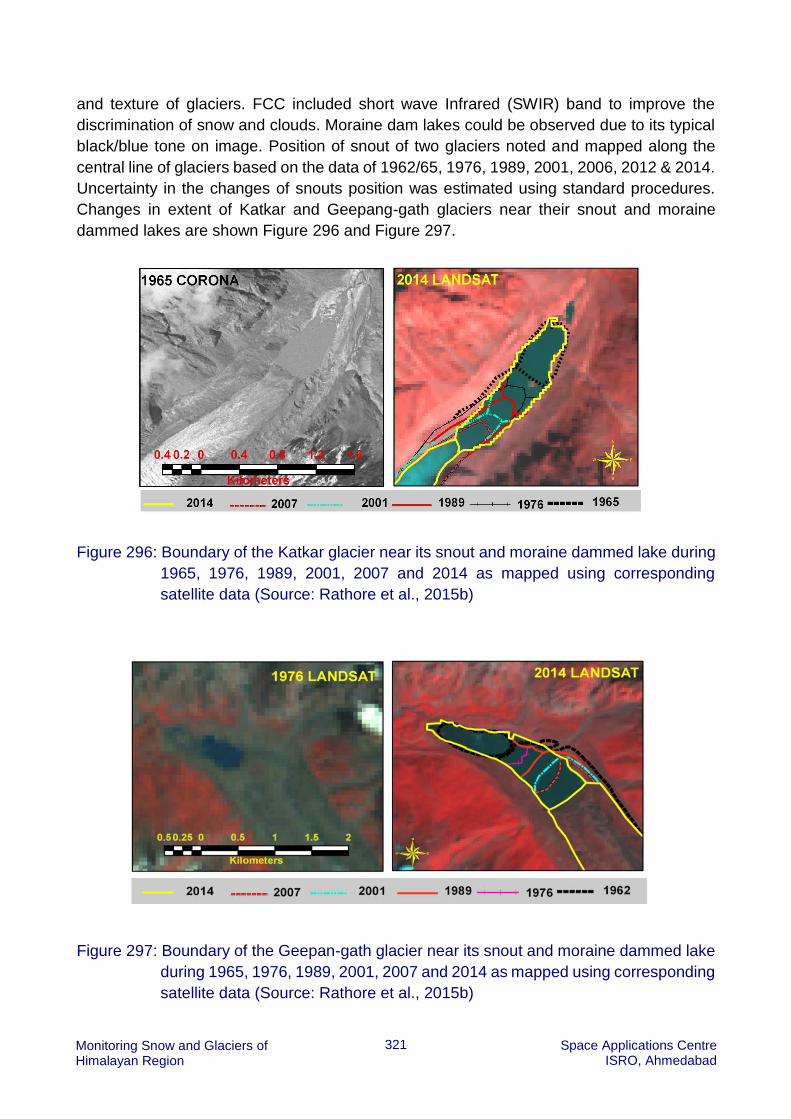
321
Monitoring Snow and Glaciers of Himalayan Region
Space Applications Centre ISRO, Ahmedabad
and texture of glaciers. FCC included short wave Infrared (SWIR) band to improve the
discrimination of snow and clouds. Moraine dam lakes could be observed due to its typical
black/blue tone on image. Position of snout of two glaciers noted and mapped along the
central line of glaciers based on the data of 1962/65, 1976, 1989, 2001, 2006, 2012 & 2014.
Uncertainty in the changes of snouts position was estimated using standard procedures.
Changes in extent of Katkar and Geepang-gath glaciers near their snout and moraine
dammed lakes are shown Figure 296 and Figure 297.
Figure 296: Boundary of the Katkar glacier near its snout and moraine dammed lake during
1965, 1976, 1989, 2001, 2007 and 2014 as mapped using corresponding
satellite data (Source: Rathore et al., 2015b)
Figure 297: Boundary of the Geepan-gath glacier near its snout and moraine dammed lake
during 1965, 1976, 1989, 2001, 2007 and 2014 as mapped using corresponding
satellite data (Source: Rathore et al., 2015b)
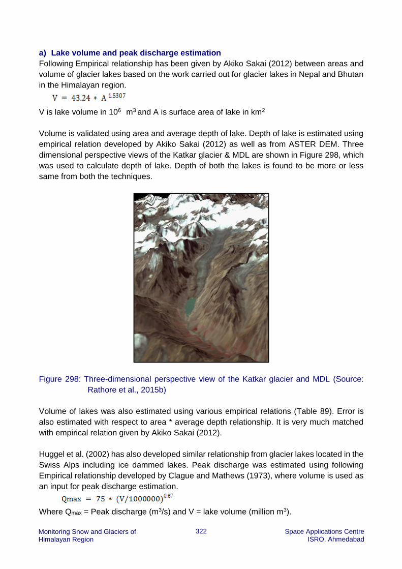
322
Monitoring Snow and Glaciers of Himalayan Region
Space Applications Centre ISRO, Ahmedabad
a) Lake volume and peak discharge estimation
Following Empirical relationship has been given by Akiko Sakai (2012) between areas and
volume of glacier lakes based on the work carried out for glacier lakes in Nepal and Bhutan
in the Himalayan region.
V is lake volume in 106 m3 and A is surface area of lake in km2
Volume is validated using area and average depth of lake. Depth of lake is estimated using
empirical relation developed by Akiko Sakai (2012) as well as from ASTER DEM. Three
dimensional perspective views of the Katkar glacier & MDL are shown in Figure 298, which
was used to calculate depth of lake. Depth of both the lakes is found to be more or less
same from both the techniques.
Figure 298: Three-dimensional perspective view of the Katkar glacier and MDL (Source:
Rathore et al., 2015b)
Volume of lakes was also estimated using various empirical relations (Table 89). Error is
also estimated with respect to area * average depth relationship. It is very much matched
with empirical relation given by Akiko Sakai (2012).
Huggel et al. (2002) has also developed similar relationship from glacier lakes located in the
Swiss Alps including ice dammed lakes. Peak discharge was estimated using following
Empirical relationship developed by Clague and Mathews (1973), where volume is used as
an input for peak discharge estimation.
Where Qmax = Peak discharge (m3/s) and V = lake volume (million m3).

323
Monitoring Snow and Glaciers of Himalayan Region
Space Applications Centre ISRO, Ahmedabad
Table 89: List of models used for estimation of volume of lake (Source: modified after
Rathore et al., 2015b)
For development of above mentioned formula, many physical based models were
developed to estimate the peak discharge. But due to non-availability of other information it
is difficult to develop our own model. Therefore, the relationship developed by Clague &
Mathew (1973) is used to estimate peak discharge. Peak discharge of lake in case of
outburst was also estimated using various empirical relations. It varies from 196-716 and
287-1012 m3/sec for Katkar & Gepang-gath mdl respectively. Average value of peak
discharge lies near to that given by Clague & Mathews (1973).
b) Probability of outburst lake
The extent of a flood caused by the breach of a moraine dam is relevant for further hazard
analyses. The present study used the outburst probability model developed by McKillop and
Clague (2009) for assessing the dangerous nature of the moraine-dammed lake and the
equation proposed by Clague and Mathews for estimating the peak discharge of the lake in
case of an outburst. McKillop and Clague (2009) developed the moraine-dammed lake
outburst probability model by considering the utility of remote sensing in gathering
information and also based on the inventory of 189 moraine-dammed lakes in British
Columbia.
Where α is the intercept, β1, βj, β2 and βk are the regression coefficients for M_hw (moraine
height-to-width ratio), Ice_core (moraine – ice free or ice core), Lk_area (lake area) and
Geology (moraine constituents – sedimentary, metamorphic) respectively. The parameters
such as moraine height-to-width ratio can be derived using digital elevation data by
overlaying the satellite data over the DEM. Presence/absence of an ice-core in the moraine
Sr. No.
References Empirical relation for
volume
Katkar lake Gepang-gath lake
Results Volume 106 m3
Comparison with area-
depth relationship
% error
Results Volume 106 m3
Comparison with
area-depth
relationship
% error
1 Akiko Sakai et al(2012)
43.24*(A)1.530
7 18.29 1.83 9 30.73 1.27 4
2 Mathematical Areal extent * Avg. depth
20.12 0 0 32 0 0
3 O’Connoret et al
3.114*A+.0001685(A)2
56.52 -36.40 181 110.33 -78.33 -245
4 Huggel et. al (2002)
.104*(A)1.42 15.50 4.62 23 25.09 6.91 22
4 Yao, Xiaojun et al.
.493*(A).9304 29.22 -9.10 45 40.06 -8.06 -25

324
Monitoring Snow and Glaciers of Himalayan Region
Space Applications Centre ISRO, Ahmedabad
is established using the following methods proposed by McKillop and Clague (2009); (i) a
moraine with a rounded surface with minor superimposed ridges was assumed to be ice-
cored; (ii) a moraine with a disproportionately large end in front of a small glacier was
suspected to be ice-cored and (iii) a narrow, sharp crested moraine with an angular cross-
section was interpreted to be ice-free. The lake area is estimated from the lake boundary
layer prepared from satellite data and main rock type forming the moraines is derived from
the lithological interpretation of the study area. The regression parameters taken from
McKillop and Clague (2009) and the four predictors taken from satellite data of 2014. The
M_hw value taken from satellite data was used to measure moraine height and width. For
further analysis, height of moraine is taken as ~35 & 40 m, width of moraine is ~25 & 40 m
and average width is 350 & 500 m for Katkar and Gepang-gath MDLs respectively.
17.5. Results and Discussion
Changes in area and length of Katkar and Geepang-gath glaciers
Areal extent of Katkar glacier was estimated as 24.38 sq km in 1962. Areal extent of glacier
continuously decreased from 24.38 to 23.58 sq km during 1962 to 2014. Percent retreat in
areal extent of glaciers wrt 1962 is shown in Figure 299. It has been reported that SOI
topographical maps estimates higher areal extent of glacier (Bhambri and Bolch, 2009). The
length of glacier along central line decreased from 12.56 km to 11.0 km during 1962-2014.
Percent retreat in length of glaciers wrt 1962 is shown in Figure 300 According to a study
carried by Kamp et al., (2011), glaciers of Chenab sub-basin were retreating at an average
rate of less than 20 meter per year (Kulkarni and Karyakarte, these glaciers are not attached
with MDL, so we can say that MDL enhances retreat of glacier. The data suggests that rate
of retreat decreases from 1962-1976 interval up to 2001 but again increases during 2001-
2014. Altitude of glacier snout was 4520 meter in 1962 which was elevated to 4572 meter
in 2014.
Gepang-gath glacier is debris covered glacier and located in Chandra sub-basin.
Approximately 29% area of glacier is covered by debris. Areal extent of glacier was
estimated 13.1 sq km in 1962 which reduced to 12.22 sq km. Areal extent of glacier was
observed to be continuously reducing between 1962 and 2014. Percent retreat in areal
extent of Gepang-gath glacier is higher than Katkar glacier (Figure 299). Length of glacier
along central line was 6.7 km in 1962 which decreased to 5.7 km in 2014. Rate of retreat
were observed to be gradually increasing from 1962 to 2014, reaching 31 meter per year
during 2001-14. Percent retreat in length of both the glaciers was more or less same (Figure
300). According to a study carried by Sangewar (2011), glaciers of Chenab sub-basin were
retreating at an average rate of less than 20 meter per year (Kulkarni and Karyakarte, 2014).
These glaciers are not attached with MDL so we can say that MDL enhances retreat of
glacier. Width of glacier is around 500 meter. Altitude of glacier snout was 4079 meter in
1962 which elevated to 4132 meter in 2014. Beyond this altitude slope of glacier is less than
5° which support a continuous increase in the rate of change of lake area.

325
Monitoring Snow and Glaciers of Himalayan Region
Space Applications Centre ISRO, Ahmedabad
Figure 299: Retreat in areal extent of Katkar and Geepan-gath glaciers w.r.t. 1962 during
different time frames upto 2014 (Source: Rathore et al., 2015b)
Figure 300: Retreat in length of Katkar and Geepan-gath glaciers wrt 1962 during different
time frames upto 2014 (Source: Rathore et al., 2015b)
Changes in the Moraine Dammed Lakes of Katkar and Geepang-gath glaciers
MDL of Katkar glacier was not there during 1962 as per the SOI topographical map. The
lake was observed on the corona image of 1965. This shows that this lake was formed
between 1962 and 1965. However, supra-glacial lakes, smaller than this, are shown on the
0.0
1.0
2.0
3.0
4.0
5.0
6.0
7.0
8.0
1965 1976 1989 2001 2006 2012 2014
Ch
ange
in a
rea
ext
en
t o
f gl
acie
r (%
)
Years
katkar Gepang-gath
0
2
4
6
8
10
12
14
16
1965 1976 1989 2001 2006 2012 2014
Ch
ange
in le
ngt
h o
f gl
acie
r (%
)
Years
katkar Gepang-gath

326
Monitoring Snow and Glaciers of Himalayan Region
Space Applications Centre ISRO, Ahmedabad
map. This confirms that the lake is not a matter of omission. Glacial lakes are formed, where
the inclination of glacier surface is less than 2° (Huggel et. al., 2002). Slope near snout of
this glacier was found to be less than 3 which provide suitable terrain condition for the
formation of MDL. Area of MDL was observed 21 ha in 1965 which increases to 57 ha in
2014. MDL area increased significantly during 2001 to 14 (Figure 301 and Figure 302).
which is also reflected in more retreat over the same period (Figure 299 and Figure 300).
Beyond this altitude slope of glacier becomes 9° which reduces the rate of change of lake
area. Expansion of MDL of Katkar glacier from 1965 to 1989 is higher than 1989 onwards.
It may be due to higher slope toward glacier. 2014 onwards due to higher slope rate of
expansion of lake should reduce.
Figure 301: Increase in areal extent of Gepang-gath & Katkar lakes during 1976 to 2014
w.r.t 1962 (SOI Map) and 1965 (Corona Image) respectively (Source:
Rathore et al., 2015b)
Maximum depth of MDL was estimated by Akaki Sakai, (2012), 50 meter in 1976 and 73
meter in 2012 which results 5.72x10⁶ m3 and 17.25x10⁶ m3 volume of lake respectively.
Depth of lake was found to be 25 m and 35.3 m in 1976 and 2012 respectively using SOI
contour approach which was used to estimate the volume. The difference in both
approaches for estimating volume was found to be 11%. Peak discharge, using empirical
relationship (Clague and Mathews, 1973), was estimated 189 m3/sec in 1965 to 526 m3/sec
in 2014 (Table 90). This storage is quite large in comparison to summer discharge as
reported 10 cumec for Chhota Shigri glacier in Himachal Pradesh (Kulkarni, 1996).
0
50
100
150
200
250
1962 1965 1976 1989 2001 2006 2012 2014
Ch
ange
in a
rea
ext
en
t o
f la
ke (
%)
Years
katkar Gepang-gath

327
Monitoring Snow and Glaciers of Himalayan Region
Space Applications Centre ISRO, Ahmedabad
Figure 302: Change in areal extent of Geepang-gath and Katkar lakes during 1976-
2014 (Source: Rathore et al., 2015b)
Table 90: List of models used for estimation of peak discharge (Source: modified after
Rathore et al., 2015b)
Expansion of MDL of Gepang-gath glacier from 1965 to 1989 was lower than 1989 onwards.
It may be due to lower slope toward glacier. 2014 onwards due to lower slope, areal extent
of lake should expand at higher rate.
Lake area was measured 27 ha in 1962 which gradually increases to 80 ha in 2014. Figure
302 shows variation in areal extent of glacier and moraine dammed lake of Gepang-gath
glacier. Maximum depth was estimated 50 meter in 1962 and 86 meter in 2014 using Akiko
Sakai (2012) approach. Volume of lake was 5.70x10⁶ m3 in 1962 which gradually increased
to 30.73x10⁶ m3 in 2014. Three dimensional perspective views of the Gepang-gath glacier
& lake are shown in Figure 298, which was used to calculate depth of lake. Volume was
estimated using 22 m and 40 m average depth during 1962 and 2014 respectively using
SOI contour. The difference in both approaches for estimating volume was found to be 9 %.
Peak discharge was estimated 241 m3/sec in 1962 to 744 m3/sec in 2014 using imperial
S
No.
References Empirical
relation
Results Peak discharge
m3 /sec
Katkar lake Gepang-gath
lake
1 Costa &
Schuster (1988)
0.0000055
*(PE)0.59
196 287
2 Clague &
Mathews (1973)
75 (V)0.67 526 744
3 Costa (1988) 113(V)0.64 726 1012
0
10
20
30
40
50
60
1976 1989 2001 2006 2012 2014
Gepang-gath Katkar
Incr
ea
se in
Are
al e
xte
nt
of
Lake
(h
a)
Year

328
Monitoring Snow and Glaciers of Himalayan Region
Space Applications Centre ISRO, Ahmedabad
relation developed by Clague and Mathews (1973). Detail information about glacier retreat,
variation in lake area, volume and peak discharge is given in Table 89 and Table 90.
The present analysis shows that increase in lake has accelerated the rate of retreat and the
receded vacated area of glacier was occupied by the MDL. The rate of expansion of
Gepang-gath lake is higher than Katkar lake (Figure 302). It may be because of lower slope
of Gepang-gath glacier as compared to Katkar glacier. Uncertainty in terminus change and
accuracy in areal extent of glacier and lake is estimated using empirical relationship
developed by Hall et al. (2003) and Wang et al. (2009). Overall accuracy was estimated
±107 m for SOI maps and Landsat MSS data (1962-1976), ±113 m for Landsat MSS and
TM data, ±49 m for Landsat TM & IRS LISSIII data, ±45 m for LISS III data and ±45 m for
LISS III and Landsat ETM data. Changes in areal extent of glacier and MDL were measured
with an accuracy of 0.017 km2, 0.006 km2, 0.002 km2, 0.002 km2 and 0.003 km2 between
each pair of datasets i.e. 1962-1976, 1976-1989, 1989- 2001, 2001-2006/07 and 2006/07-
2014 respectively.
By considering the probability model of McKillop and Clague (2009) and incorporating the
predictor parameters, the model yields a very low outburst probability of less than 1% for
the both the lake (<6% very low; 6–12% low; 12–18% medium; 18–24% high; > 24% very
high). The very low outburst probability shows that, if the lake increases its extent in due
course of time, it may not cause a dangerous outburst flood. As all the MDLs of Himalayan
regions are continuously dewatering so water is being releasing slowly by its outlet channel.
So lakes will not outburst by its own but it may outburst due to natural calamity like earth
quake, cloud burst or avalanche. In this situation water stored at higher altitude may cause
large damage to lower region due to higher kinetic energy. Three glaciers which are located
north of Gepang-gath glacier are draining toward lake. These glaciers are having steep
slopes as observed by slope map. Slope map is prepared using Aster DEM. So chances of
avalanche or landslide are there. Due to this reason lake may outburst and cause damage
at Sissu village, which is located 10 km downstream from lake. One glacier which is located
at south east side of Katkar glacier is draining toward Katkar lake. But this glacier is not
having steep slope. So chances are less for avalanche or landslide. So Katkar lake is not
likely to outburst as compared to Gepang-gath due to avalanche or landslide. This is a
preliminary assessment their probability to outburst and more field-based studies are
needed for proving the hazardous potential.
17.6. Conclusions
In present study, satellite images in conjunction with SOI topographical maps were analyzed
for identification and monitoring of crucial MDLs in parts of the Himalayan region over 5
decades. Katkar glacier is a debris free glacier which has shown higher linear retreat in
comparison to debris covered (3%) Gepang-gath glacier. In present scenario, Katkar glacier
is expected to show lesser rate of increase in lake area in comparison to Gepang-gath
glacier as slope of glacier above snout is 9° for Katkar and less than 3° for Gepang-gath. It

329
Monitoring Snow and Glaciers of Himalayan Region
Space Applications Centre ISRO, Ahmedabad
is highly probable that increase in lake area for Gepang-gath glacier may gradually further
increase. Peak discharge for Katkar glacier has increased from 189 to 505 m3/sec between
1965 and 2014 whereas it varied from 241 to 675 m3/sec between 1962 and 2014 for
Gepang-gath glacier. Chances of probability of outburst of both the lakes are very less,
however due to landslide or avalanche Gepang-gath lake may outburst & cause damage to
lower region. Gepang-gath glacier is required to be monitored regularly as compared to
Katkar lake. Similar studies in other parts of the Himalayan terrain are required for
assessment of possible GLOF hazards, so that measures to mitigate flash floods from the
outburst of MDLs may be planned well in advance.

330
Monitoring Snow and Glaciers of Himalayan Region
Space Applications Centre ISRO, Ahmedabad
18. Estimation of Regional Water Mass Variations
from Gravity Recovery and Climate Experiment
(GRACE) over Himalayan region
18.1. Objective
To estimate regional water mass variations over the Indus, the Ganga and the Brahmaputra
basins using Gravity Recovery And Climate Experiment (GRACE) data for the time frame
2003-2012.
18.2. Scientific Rationale
The Earth’s global gravity field can be defined by tracking LEO satellites. When the satellites
are passing over the mass anomalies, disturbances in the LEO satellites occurs due to
attraction of gravity field (Avsar and Ustan, 2012). A joint Mission named as “Gravity
Recovery And Climate Experiment (GRACE)”, between National Aeronautics and Space
Administration and Deutschen Zentrum f¨ur Luft- und Raumfahrt (NASA & DLR) was
launched on March 17, 2002 from the Plesetsk Cosmodrome in Russia under the NASA
Earth System Science Pathfinder Program (ESSP).The satellites were equipped with dual-
frequency, K-band microwave ranging (KBR) separated by ∼200 km to continuously monitor
the variation in distance between the satellites due to varying gravity field of the earth. The
satellites also consist with high precision accelerometers (ACC) for measuring the non-
gravitational accelerations, highly precise Global Positioning System (GPS) receiver for
absolute positioning and star cameras for satellite attitude determination (Tapley et. al,
2005; 2004). The primary goal of GRACE mission was to estimate the time varying gravity
field mapping for earth science studies, especially monitoring of hydrological mass
redistribution through their integrated gravitational effect (Tapley et al., 2004).
The principle of the GRACE satellite system is based on satellite-to-satellite tracking (SST),
both in the high–low mode (SST-hl) and low–low mode (SST-ll) (Liu 2008). In SST-hl mode
the LEO satellites are monitored through the GPS satellites which are at higher altitude. The
LEO satellite orbit is disturbed due to mass anomalies (Figure 303) and the gravity field can
be recovered by the measurements of the non-gravitational acceleration through three-axis
accerolmeter. SST-ll mode not only provides, the static gravity field with higher resolution
but also gives higher temporal resolution with adequate spatial resolutions. In SST-ll mode,
the LEO satellites are tracked with reference to each other. In GRACE mission the two
GRACE satellites are tracked with the help of K-band microwave ranging instruments. Using
the combination of SST-hl and SST-ll mode the accuracy and resolution of the gravity map
is enhanced to produce a detailed map of the earth gravity field (Liu 2008). In other words,
gravity field changes are sensed by the twin GRACE satellites and GPS networks give the

331
Monitoring Snow and Glaciers of Himalayan Region
Space Applications Centre ISRO, Ahmedabad
combined indirect and direct effect of all mass redistributions and mass variability within the
Earth and its fluid envelops (Kusche and Schrama, 2005).
Figure 303: A schematic diagram of GRACE-1 Mission Concept (Source: Agrawal et al.,
2014)
The earth’s gravity field is measured at approximately monthly intervals with a spatial
resolution of a few hundred kilometers (Klees et. al, 2007). These monthly estimates of the
Earth’s gravity field produced by the GRACE give information about the mass variability at
and below the surface of the Earth (Swenson and Wahr, 2006). An estimate of a surface
mass anomaly does not represent as a point measurement but rather a spatial average due
to coarser resolution (Swenson and Wahr, 2002.). Accuracy of better than 1 cm of
equivalent water thickness is expected from such gravity field measurements (Swenson and
Wahr, 2002).
Each monthly solution consists of a set of spherical harmonic coefficients complete to
degree and order 120. The seasonal gravity variation can be measured by the differencing
of the monthly solution by taking one solution as a reference gravity field. The differences
in the seasonal gravity field are caused by post glacial rebound, atmospheric and ocean
mass transport and redistribution of water, snow and ice on land. To understand the gravity
field behavior on the land, GRACE measurements have already been corrected for the
major contribution variation due to ocean and atmosphere. Therefore, differences between
monthly solutions mainly consists of changes in terrestrial water storage (TWS), i.e.
groundwater, soil moisture, rivers, lakes, snow, and ice (Klees et. al, 2007).
GRACE observations has no vertical resolution (Wahr et. al., 2006) and it reflects changes
in vertically integrated stored water, which includes variations from snow pack, glaciated
areas, surface water, soil moisture and ground water at different depths (Longuvergne et
al., 2010). Due to combination of different storage factor, it is not possible to compute

332
Monitoring Snow and Glaciers of Himalayan Region
Space Applications Centre ISRO, Ahmedabad
whether the variation in mass is caused due to change in Land surface, subsurface or
atmospheric component (Wahr et. al., 2006). The extraction of water from any one of the
storage component (e.g., snow packs) requires disaggregating the vertically integrated
water storage observation, either by making assumptions or by using different models to
eliminate other components. Monitoring of the total water storage as surface and subsurface
is essential for understanding of hydrological cycle in climate change environment (Tiwari,
et. al., 2009) to understand seasonal behavior, where climate-driven mass transport of
water plays a major role towards gravity (Davis et.al, 2008). Time-variable ice loss in Asian
high mountains have been estimated from satellite gravimetry (Matsuo and Heki, 2010).
Snow packs and glaciers are a very important component of the Earth’s climate system (Su
et.al, 2010). In the Himalayan region regional mass anomalies show large variations in
terms of snow water equivalent over a season. The accurate estimation of snowpack and
its variation is important for various hydrological applications. In this study, the annual mass
variability including the rate of mass change were estimated for bringing out the water mass
variations in terms of changes in Water Equivalent Heights (WEH) over three major basins
of the Himalayan region viz., the Indus, the Ganga and the Brahamputra basins using
GRACE data for the time frame 2003-2012 (Agrawal et al., 2014).
18.3. Study Area
The study area in general extends in the south-east from latitude 250 39’ N and longitude
970 46’ E (approx.) to north-west up to latitude 370 05’ N and longitude 720 14’ E (approx.)
covering the Himalayas, Trans-Himalaya and Karakoram regions across four countries viz.
India, Nepal, Bhutan and China (Tibet). The study area has been further restricted to the
Indus, Ganga and Brahmaputra basins covering the mountainous and piedmont regions
(Figure 304). These basins represent the three mighty rivers, which originate from the
glaciers of the Himalayan region and are fed by seasonal snow and glacier melt water.
The Indus, Ganga and Brahmaputra basins have a total geographic area of 1.9 ×10⁵ sq km,
0.6 ×10⁵ sq km and 1.2 ×10⁵ sq km respectively, with 0.95 million km2 area mapped under
glacier inventory (Sharma et al., 2013). The geographical classification of region broadly
coincides with the source of precipitation i.e., Southeastern monsoon is more active in
eastern Himalayas (decreases westwards) whereas northwestern monsoon is more active
in the western Himalayas (decreases eastwards).

333
Monitoring Snow and Glaciers of Himalayan Region
Space Applications Centre ISRO, Ahmedabad
Figure 304: Location of study area consisting three major river basins Indus, Ganga and
Brahmaputra in the Himalayas (background image is INSAT 3A-CCD) (Source:
Agrawal et al., 2014)
18.4. Data Used
The GRACE data is collected at GRACE Science Data System, which is shared between
Jet Propulsion Laboratory (JPL), University of Texas Center for Space Research (CSR) and
Deutsches GeoForschungsZentrum (GFZ) (Avsar et.al, 2012). The collected data are
processed to generate Level-1B followed by the Level-2 data in the form of harmonic co-
efficient with a temporal resolution of one month or shorter duration (Longuvergne et al.,
2010), which can be inverted to estimate changes in mass at the surface. These processed
datasets in form of Spherical harmonics produced by different agencies are available online
at official data processing repository http://podaac.jpl.nasa.gov/grace/ (CSR, GFZ, JPL).The
different components contributed in the GRACE measurement are analyzed with the help
of FES 2004 model for taking care of diurnal and semidiurnal tides, IERS 2003 model for
computing solid earth tidal contribution to geo-potential and solid earth pole tide and Ocean
pole tide defined based on satellite altimetry data (Liu, 2008). Similarly, datasets are also
corrected with variable atmospheric conditions by AOD1B products. The remaining gravity
changes are interpreted as monthly vertically integrated stored water of snow packs, ground
water and soil moisture in terms of Water Equivalent Height (WEH).
The data is further enhanced with the help of two filtering techniques to reduce the presence
of the measurement errors. First filter is designed for removal of correlated errors between
spherical harmonic coefficients, which is manifested as stripes oriented towards North-
South in GRACE maps (Swenson and Wahr, 2006). Second filter is a Gaussian averaging
filter with a half width of 300 Km which reduces random errors in higher degree co-efficient
(Wahr et.al, 2006). The data are further translated into global sets of localized surface mass
concentrations termed as “mascons”, which omits the direct use of the spherical harmonics

334
Monitoring Snow and Glaciers of Himalayan Region
Space Applications Centre ISRO, Ahmedabad
coefficient. The mascons datasets are basically a conversion form of the spherical datasets
into a geographical co-ordinate system and such data sets are available with a spatial
resolution of 10X 10 resolution cell. In this study, the monthly mascons data from the CSR
processing agency were downloaded for a period of ten years (2003-2012) and analyzed to
compute water mass variations over Himalayan basins.
18.5. Methodology
A quantitative analysis of secular and seasonal water mass anomaly was carried out. A
weighted least-squares fit was used to estimate the annual cosine (winter-summer)
component, the annual sine (spring-fall) component, and a linear trend over a decade of the
GRACE derived water mass (Equation 1).
Mathematic model:
(1)
Time in month
The model component a1 gives the secular water mass changes (Figure 305).
The sine terms a3 indicates positive showing maximum water mass in summer season and
negative value indicates maximum water mass in winter. The cosine terms a2 indicates
negative value for the maximum mass in summer season and positive value indicates
maximum mass in winter.
The magnitude of the annual mass variability can be computed as (Equation 2).
(2)

335
Monitoring Snow and Glaciers of Himalayan Region
Space Applications Centre ISRO, Ahmedabad
The annual water mass variability shows the variations in a year due to the seasonal
changes in precipitation, snowfall, evaporation, surface/subsurface movement of water and
groundwater extraction.
18.6. Results and Discussion
It is distinctly observed that the northern Indo-Gangetic plains in parts of Punjab, Haryana,
and northern Rajasthan are showing high depletion of water mass during 2003-12 (Figure
4.17.3). These results further support the earlier findings of GRACE data analysis for time
frame 2002-2008 (Tiwari et al. 2009 and Rodell et al. 2009). It is also observed that the
Ganga and the Brahamputra basins show depletion trend of water mass while the Indus
basin shows a mix of negative and positive secular water mass.
Figure 305: Spatial secular water mass changes (WEH) over the Himalayan and adjoining
regions estimated using GRACE data of 2003-12 (Source: Agrawal et al., 2014)
The spatial annual water mass variability over the Himalayan and adjoining regions during
time frame 2003-12 shows very low annual water mass variability in the Western Himalaya
and Tibetan plateau, while the Central and Eastern Himalaya shows low to high annual
water mass variability (Figure 306). The gridded data of Water Equivalent Height (WEH) for
Himalayan region were used for statistical analysis and estimation for the secular trends
over the Indus, Ganga and Brahamputra Basins. The temporal profile of spatial averaged
WEH over Indus, Ganga and Brahamputra basins are shown in Figure 307.

336
Monitoring Snow and Glaciers of Himalayan Region
Space Applications Centre ISRO, Ahmedabad
Figure 306: Spatial annual mass variability over the Himalayan and adjoining regions
estimated using GRACE data of 2003-12. (Source: Agrawal et al., 2014)
a) b)
c)
Figure 307: Temporal profile showing secular trend of spatially averaged WEH (2003-2012)
over a) Indus, b) Ganga and c) Brahmaputra basin (Source: Agrawal et al.,
2014)
- 1.27 cm/Yr
-1.06 cm/Yr

337
Monitoring Snow and Glaciers of Himalayan Region
Space Applications Centre ISRO, Ahmedabad
The trend analysis over Ganga and Brahamputra basins have shown an average annual
change of -1.28 cm and -1.06 cm in terms of WEH whereas Indus basin has shown a slight
annual change of -0.07 cm, which is statistically insignificant at 95% confidence level. It is
inferred that there is no water mass change in the Indus basin and there is depleting trend
in the Ganga and Brahmaputra basins.
The present analysis has not computed the changes in groundwater extraction, soil
moisture and snowpack individually and is presently representing the sum of all these
components. GRACE data are also sensitive towards interior strain variation, surface uplift
and surface subsidence cover over a large area. Therefore, future work has been planned
to quantify these components individually. The next mission GRACE-2 with increased
resolution is expected to provide more information on changes in water masses and shall
be extremely useful to understand the impact of climate change on the Himalayan
Cryosphere and Hydrology.

338
Monitoring Snow and Glaciers of Himalayan Region
Space Applications Centre ISRO, Ahmedabad
19. Snow and Glacier Melt Runoff Modeling
19.1. Objective
To develop a distributed snow & glaciers melt runoff model.
19.2. Scientific Rationale
Himalayan region has high concentration of mountain glaciers. Large extent of this region
is covered by seasonal snow cover during winter. Runoff generated from melting of these
snow & glaciers is one of the important sources of water for the Himalayan Rivers. Only 1%
of the world ‘s water is usable to us. About 97% is salty sea water and 2% is in frozen state
as snow and glaciers. As 1% is insufficient to overcome the causes of water scarcity which
vary from natural causes such as climate change and draught and human causes such as
demand over stripping supply, population growth, water quality and resource allocation. So
studies on mountain glaciers and snow are welcomed. The pious peaks of the Himalayas
are known as the water towers of Asia providing drops of elixir to quench the parched plains
and to satisfy the scorching throats of the living world. They store a significant quantity of
fresh water which is found in the concentrated form of seasonal snow cover and glaciers
outside the polar realm. Indeed, they have the capacity for supplying 86,000,000 cubic
meters of water annually to Asia‘s seven great rivers. Western Himalayan Rivers combine
into the Indus Basin, of which the Indus River is the largest. The Indus begins in Tibet at the
confluence of Sengge and Gar river and flows southwest through India and then through
Pakistan to the Arabian Sea. It is fed by the Jhelum, the Chenab, the Ravi, the Beas and
the Sutlej River, among others. In western Himalayas, the temperature is lesser due to
higher altitude as well as latitude and as a consequence the snowline in the western
Himalaya is at a lower altitude than the eastern Himalaya. As distance from the sea is
greater, both annual and diurnal range of temperature is greater in the western Himalayas.
So it receives lesser precipitation than eastern Himalayas (Bose, 2013). As in western
Himalayas, the snowmelt commences in March, the snow line starts receding upwards and
by the end of June to an altitude of 4,500m (Prasad and Roy, 2005). Changes in climate
have drastic repercussions on the entire earth and have affected more dramatically on the
Himalayan glaciers. These glaciers are more susceptible to climate change due to their
latitudinal and altitudinal position and other interrelated processes. These processes need
detailed multidisciplinary investigations and have opened a new venue for estimating the
runoff with the help of different models. These models require the fundamental variables
which directly affect the melt process. For snowmelt runoff modeling, the two pragmatic
approaches are accessible. They are energy balance approach and degree day method. In
comparison to the energy balance approach, degree day approach is more practicable and
needs minimum parameters for simulating snow & glacier melt runoff. It is widely used due
to its being less complicated. The energy exchange at snowpack surface can be explained
by four major components. They are shortwave radiation exchange and heat exchange,
convective and adventive heat transfer. These radiations exchange and heat transfer can

339
Monitoring Snow and Glaciers of Himalayan Region
Space Applications Centre ISRO, Ahmedabad
be estimated if information on various parameters as cloud covers, albedo, wind, cloud
temperature and dew point temperature are known (Anderson, 1976). Information on these
parameters is normally not available; therefore, degree-day approach is used for operational
forecasting (Quick and Pipes., 1988). Precipitation and temperature are the major factors
for generating runoff in mountainous regions which are covered with snow and glaciers.
Precipitation falls either in the form of liquid (rain) at lower latitude and altitude or in the form
of solid (snow) at higher latitude and altitude. When rainfall occurs, runoff is estimated by
subtracting various types of water losses. In case of snow fall, snow remains static for quite
some time and it requires certain amount of temperature to convert it into liquid and then to
set the process of runoff. Integrated approach for snowmelt runoff estimation using
temperature index model, remote sensing and GIS has been developed (Aggarwal et al.,
2014). Present and future glacier melt-water contribution to runoff in a Central Himalayan
river basin have been estimated (Prasch et al., 2012). Snowmelt contributions to discharge
of the Ganges are also estimated (Siderius et al., 2013). However, missing (in-situ) snow
cover data hampers climate change and runoff studies in the Greater Himalayas (Rohrer et
al., 2013).
19.3. Study Area
Parbati sub-basin of Satluj basin in Himachal Pradesh has been selected as the study area.
It is continuously fed by melting of high altitude snowfields and glaciers. This basin is sub
divided in to various watersheds. Tosh watershed is one of the significant and substantial
watersheds of Parbati sub-basin, representing similar hydrologic processes as that of the
whole Parbati sub-basin and is identified as an intensive study site. Figure 308 shows the
study area and river network of Parbati sub-basin and Tosh watershed. Parbati sub-basin
covers the area of 1773 km2. Elevation range of this catchment is 1110 m to 6597 m. Tosh
watershed covers the area of 329 km2 which is a part of Parbati sub-basin.
Figure 308: Location map of Parbati sub-basin, Himachal Pradesh

340
Monitoring Snow and Glaciers of Himalayan Region
Space Applications Centre ISRO, Ahmedabad
19.4. Data Used
i) Satellite data
The Advanced Wide Field Sensor (AWiFS) data have been used for this study. It provides
a spatial resolution of 56 m and covering a swath of 740 Km. to cover this wide swath, the
AWIFS camera is split into two separate electro optic modules, AWiFS-A and AWiFS-B.
Because of its large swath the repetivity of the AWiFS is 5 days. These data are imported
from NRSC (National Remote Sensing Centre), Hyderabad. Reflectance, NDSI images are
generated using NDSI algorithm (Kulkarni et al., 2006b). Advanced Space born Thermal
emission and Reflection radiometer (ASTER) sensor is one of the five remote sensory
devices on board the Terra satellite launched into the Earth‘s orbit by NASA in 1999. ASTER
GDEM (Global Digital Elevation Model) is the global DEM created using ASTER.
ii) Meteorological data
Surface variables like precipitation and temperature are to be highlighted for estimation of
runoff in snow & glacier covered area. Indeed, precipitation is said to be any product of the
condensation of atmospheric water vapour that falls under gravity while the changes in air
temperature in the atmosphere which take place due to dynamic processes should both be
taken in to account. These significant parameters which have high contribution in snow &
glacier melt runoff have been taken from Bhuntar, Kullu District of Himachal Pradesh for this
present study. For clarity, maximum and minimum air temperatures and precipitation data
from 2004-2005 available in daily format are converted in to 10-daily format specifically for
utilizing and for fulfilling the requirements of the model.
iii) Hydrological data
For the calibration period of the model at Tosh watershed, the discharge data are collected
from the U/s of the confluence of both Tosh Nala and Parbati River. For the validation period
of the model at Parbati sub-basin, the discharge data are collected from the D/s of the
Parbati sub-basin near the dam site. These places are the focal and centric points where
total discharge is collected from both the catchments.
19.5. Methodology
Model is designed to simulate and forecast stream flow in mountain basins where snowmelt
is a major runoff factor. To develop the model different remote sensing and GIS techniques
are used. Catchments are distributed using grid. Model works on NDSI to estimate snow
cover and on reflectance to estimate melt factor. Using ARC GIS 9.3, distribution of the
Tosh watershed (329 Km2) and Parbati sub-basin (1773 km2) is done by fabricating a grid
of the same size and laying it over the catchments. So consequently, the catchments are
distributed into a number of small grid cells. In this way, the Tosh watershed and Parbati
sub-basin are divided respectively in to 90,236 and 78,411 cells. For Tosh watershed, the
area of cells 0.0046 km2 while for the Parbati sub-basin is 0.0228 Km2. So it can be said
that for Tosh watershed area of cell is smaller than the AWiFS resolution and for Parbati

341
Monitoring Snow and Glaciers of Himalayan Region
Space Applications Centre ISRO, Ahmedabad
sub-basin area of cell is equal to 3-pixel resolution of the AWiFS. Figure 309 shows
distribution of Parbati sub-basin.
Figure 309: Fishnet map of Parbati sub-basin
From time to time, runoff generated from snow and glacier melt and also from rainfall is
computed using the following equation (Martinec et al., 1975):
where, Q = Average 10-Daily runoff (m3/s), C1 = Runoff coefficient for glaciated areas, C2
= Runoff coefficient for non-snow and non-glaciated areas, C3 = Runoff coefficient for
seasonal snow covered areas, = Melt-factor (cm °C-1 d-1), T =Average 10-daily degree
days (°C. d), G = Grid cell area of glaciers, permanent and 10-daily snow (km2), S = Grid
cell area of 10-daily snow (km2), P = Average 10-daily rainfall (cm), B = Grid cell area
without snow/glacial cover (km2), Factor 10000/86400 is required for conversion of units
from cmkm2d-1 tom3s-1, K= recession coefficient, Qlast= last average 10-daily discharge,
n= No of cells.

342
Monitoring Snow and Glaciers of Himalayan Region
Space Applications Centre ISRO, Ahmedabad
Model Parameters
i) Temperature
Daily maximum and minimum temperature data are used from 2004-2005. From the
available maximum and minimum daily temperature data, average daily temperature data
are calculated and finally converted in to 10-daily format. Then they are extrapolated to each
cell of the grid by overlaying it on Aster DEM using temperature lapse rate (Martinec et al,
1975).
T = (T max + T min)/2
ii) Snow cover area and Precipitation
Model itself estimates snow cover area using NDSI. Catchments are distributed in to small
cells and each cell has its own NDSI value. Principally, NDSI value varies from -1 to 1. The
value >= 0.4 indicates snow cover area (SCA) while the value < 0.4 indicates snow free
area (SFA)Model has capacity to sense whether the cell area is under snow cover or snow
free area as shown in table. It takes the threshold values of NDSI that means model senses
all the grid cell area which has NDSI value greater than or equal to 0.4, considering as snow
cover area (Kulkarni et al., 2006b). Available precipitation data of Bhuntar meteorological
station are extrapolated to the mean hypsometric altitudes of the respective grid cell. There
are two forms of precipitation: Rain and Snowfall. Critical temperature (Tcrit) determines
whether the measured precipitation is either rain or snow. Model gives an output from each
grid cell whether it is snowmelt-runoff, rainfall-runoff or the mixture of both. This model
output is dependent on critical temperature, occurrence of an event (rain fall/snowfall) and
whether it is SCA or SFA.
iii) Melt factor
Model computes both reflectance based melt factor and field based melt factor (using
degree-days). In this study, the melt factor parameter is calculated by model itself by using
reflectance value of each cell. Reflectance changes with the changes in density of
snow/glacier (Reflectance decreases with increment in density of snow/glacier). The
threshold values of reflectance are adjusted with the density of new snow, damp snow,
settled snow, depth hoar, wind packed snow, very wet snow and firn and glacier ice. Using
below empirical equation (Martinec et al., 1975), melt factor is computed of all cells:
a = 1.1*(density of snow) / (density of water)
iv) Runoff coefficients
Runoff coefficient shows difference between the available water volume (snowmelt +
rainfall) and the outflow from the basin. Runoff coefficient of rain indicates the percentage
of rainfall converted to runoff. It is found 0 to 0.72forTosh watershed and 0 to 0.84for Parbati
sub-basin. Runoff coefficients of snow/glacier indicate the percentage of snowfall converted
to runoff. These coefficients are found 0.21 to 0.78for Tosh watershed and they are 0.13 to
0.69for Parbati sub-basin. These coefficients have been calibrated using observed runoff
on a 10-dailybasis.

343
Monitoring Snow and Glaciers of Himalayan Region
Space Applications Centre ISRO, Ahmedabad
v) Recession coefficient
Recession coefficient indicates the fraction of discharge contribution from last day ‘s
discharge of snowmelt on a current day. In this study, observed daily discharges are plotted
on log-log scale and the slope of the best fit line is determined as the recession coefficient.
It is calibrated on 10-daily basis. It varies from 0.73 to 1 for Tosh watershed and 0.64 to 1
for Parbati sub-basin.
Model is developed at the Tosh watershed and executed at Parbati sub-basin for 2004-
2005. After applying the model at the Tosh watershed, training of the model is done using
the available field data for calibration. The best match simulation is adopted. After this
procedure, model is executed at Parbati sub-basin. Model is developed and validated on
the 10-daily basis using degree day approach.
19.6. Results and Discussion
Snow and glacier melt runoff modeling at Tosh watershed and Parbati sub-basin has been
carried out by integrating space based and in-situ data using degree-day method.
Parameters such as melt factor, runoff coefficients and recession coefficient for the model
are derived from satellite, topographic and hydro meteorological data. For Tosh watershed
and Parbati sub-basin maximum snow cover areas are respectively found 99.82% and
92.53%. Minimum snow cover for both Tosh watershed and Parbati sub-basin are
respectively: 23.16% and 13.56%. Mean annual snow cover for both Tosh watershed and
Parbati sub-basin are: 80.25 % and 63.06 % respectively. Snow cover in the Tosh
watershed and Parbati sub-basin is maximum in winter while it is minimum in monsoon on
the 10-daily basis using AWiFS data (Table 91). Geographically, Tosh watershed is situated
at higher elevation so in winter it is found that this watershed area is almost covered with
snow. As some part of Parbati sub-basin is situated at lower elevation so in winter only this
lower elevated part is found without snow. For both the catchments, the least snow cover is
found in the season of monsoon.
Table 91: Snow cover pattern for year 2004-2005
No. Catchment Minimum SCA(%) Maximum (SCA) Annual mean
SCA (%)
1 Tosh 23 (17 Aug. 04) 100 (21 Dec. 04) 80
2 Parbati 14 (12, Sep. 04) 93 (19 Jan. 05) 63
Temperature and precipitation are observed to be major factors in contributing runoff.
Temperature data suggest that the winter season exists normally and the melt season starts
from March and ends in June. Precipitation occurs normally in July, August, September and
October. However, some isolated precipitation is also observed in other months as this
study area is for mountainous region.

344
Monitoring Snow and Glaciers of Himalayan Region
Space Applications Centre ISRO, Ahmedabad
Runoff due to rain is noted high during monsoon while it is very low in winter. Runoff
generated from snow and glaciers is noted high in summer and monsoon than winter and
autumn. By using grid of smaller size cells, physical processes can be represented easily
and the results are found to be accurate and reliable. Indirect way of estimating the melt
factor using the threshold values of reflectance is found to be very successful and
convenient by using AWiFS satellite data as it calculates melt factor remotely.
Efficiency of the model
Efficiency of model is derived by computing coefficient of determination (R2) and (%) volume
difference (Dv) using below equations Martinec et al., 1975):
where, R2 = Coefficient of determination, Qi = Measured 10-daily discharge, Q'i = Simulated
10-daily discharge, = Average daily discharge for the simulation year or simulation season,
n = Number of 10-daily discharge values, DV= (%) Volume Difference between the total
observed and simulated runoff, VR = Observed 10- daily runoff volume, VR‘= Simulated 10-
daily runoff volume.
Figure 310 shows coefficient of regression and comparison between observed and
simulated discharge for both the catchments. It also shows that except monsoon, best
match is found between observed and simulated discharge.
Table 92 and Figure 311 comprehensively show that for Tosh watershed, co-efficient of
determination (R2) is derived 0.91, Volume difference (Dv) is derived 8.82%, and coefficient
of regression from graph is derived 0.938. For Parbati sub-basin, co-efficient of
determination (R2) is derived 0.92, Volume difference (Dv) is derived 5.44%, and coefficient
of regression from graph is derived 0.93.
Figure 310 Coefficient of regression for Tosh watershed and Parbati sub-basin

345
Monitoring Snow and Glaciers of Himalayan Region
Space Applications Centre ISRO, Ahmedabad
Figure 311: Comparisons of simulated and observed discharge for Tosh watershed and
Parbati sub-basin
Table 92: Accuracy criteria of model
catchment Year Coefficient of
determination
(R2)
Volume
difference (Dv)
Coefficient of
regression
(Graph)
Tosh watershed 2004-05 0.91 8.8 0.94
Parbati sub-
basin
2004-05 0.92 5.4 0.96
19.7. Conclusion
The study has developed and demonstrated a distributed hydrological model based on
inputs from satellite data as well in-situ measured hydrological data for Parbati sub-basin in
Himachal Pradesh. It is observed that simulated discharges are fairly matching with the
observed discharges. The coefficient of determinations, % volume differences and
coefficient of regressions for Tosh watershed and Parbati sub-basin indicate that the model
is efficient and has high potential for application of snow and glacier prediction.

346
Monitoring Snow and Glaciers of Himalayan Region
Space Applications Centre ISRO, Ahmedabad
20. Development of Energy Balance Modeling
20.1. Objective
To carry out energy balance modeling for ablation estimation of Gangotri and Chota Shigri
glaciers.
20.2. Scientific Rationale
Glacier surface melt rate can be calculated by two different approaches: i) empirical models
based on temperature index/ temperature degree day and ii) energy-balance models. Both,
process-based models (derived from a surface energy balance) and empirical models,
which correlate melt with temperature and to some extent the radiation, have been
developed for glacierized regions. Empirical models/approach are normally area specific
and difficult to extend to other regions as they are developed under specific conditions
(geomorphic settings and physical environment). Empirical model based on air temperature
were refined for estimating glacier melt rate (Jones 1997, Hock 2003). These models relate
ice melt with temperature but sometimes additional input variables such as incoming
shortwave radiations are also incorporated through parameterization based on time and
locations. Energy Balance approach are generic in nature offering better accuracy as it
involves computations based on basic principles of Physics. Energy Balance approach is
based on the computation of the relevant energy fluxes and melt rate is calculated as the
sum of the individual fluxes (Pellicciotti et.al., 2005). The energy balance incorporates
radiative fluxe, turbulent fluxe and the energy flux in the subsurface. This approach requires
information on radiation energy, sensible and latent heat flux. These models more properly
describe the physical processes at the glacier surface and provides reliable estimate of
ablation and melt rates. There has been a large number of studies on energy balance
computation on glaciers in different parts of the world, e.g. in the Sierra Nevada (Marks and
Dozier, 1992), in Antarctica (Bintanja et al., 1997), in the Alps (Oerlemans and Klok, 2002;
Klok and Oerlemans, 2002). Studies have been done to compute glacier ablation in outer
tropics using energy balance approach (Wagnon et al. 1999a, 1999b, 2001, 2003). Favier
et. al. (2004) computed the annual cycle of the local surface energy balance on the ablation
zone of Antizana Glacier 15, Ecuadorian Andes (inner tropics). Moolg and Hardy et. al.
(2004) estimated the energy balance of a horizontal glacier surface on Kilimanjaro, tropical
East Africa, for the periods March to September 2000 and March 2001 to February 2002 to
study the impact of climate variations. Sicart et. al. (2005) examined the surface energy
fluxes of the Bolivian Zongo Glacier (South American Andes) for identifying the atmospheric
variables that control melting. A distributed surface energy-balance model was developed
by Hock and Holmgren (2005) for complex topography of Storglaciaren, a valley glacier in
Sweden. Energy and mass balance of Zhadang glacier surface situated in central Tibetan
Plateau has been estimated by Zhang et. al. (2013). Though energy balance studies have
been carried out in Antarctica, Andes, Alps, inner and outer tropical region, however it has
not been used for estimating glacier ablation, mass balance and melt run off in the valley

347
Monitoring Snow and Glaciers of Himalayan Region
Space Applications Centre ISRO, Ahmedabad
glaciers of the Himalayas. The difficulties in taking in-situ measurements, required for
formulation of energy balance equation in the highly undulating and difficult terrains might
have been the main reason for lack of such studies in the Himalaya. The Himalayas have
the highest concentration of glaciers outside the polar region and thus holds one of the most
important natural resources of water in frozen form. It is important from the point of view of
water and energy security of India and many other countries in the region.
To understand the response of Himalayan glaciers to climatic variability, a study was taken
to compare energy balance on two of the Himalayan glaciers, one each from Indus and
Ganga basins, which have different climatic and physiographic conditions. The salient
findings have been reported (Rastogi and Ajai, 2014, 2013a and 2013b).
20.3. Study Area
Gangotri glacier in Uttarakhand and Chhota Shigri glacier in Himachal Pradesh have been
taken up as study areas (Figure 312).
Figure 312: FCC of AWiFS image showing Gangotri glacier, Uttarakhand (Left panel) and
Chhota Shigri glacier, Himachal Pradesh (Right Panel) (Source: Rastogi and
Ajai, 2014)

348
Monitoring Snow and Glaciers of Himalayan Region
Space Applications Centre ISRO, Ahmedabad
The first glacier chosen for this study is Gangotri glacier. Gangotri glacier is one of the
largest glaciers in the central Himalaya. It is located in Uttarkashi District, Uttarakhand,
India. Gangotri glacier originating from Chaukhamba peaks (7138 amsl) and is about 27 km
long with a glacierised area of about 143.58 km2. This is a valley type glacier in Ganga basin
and the source of a major river system Ganga in northern India. This glacier is bounded
between longitude 780 59ˈ30 ̎and 790 17ˈ45̎ E and latitude 300 43ˈ00 ̎and 300 57ˈ15̎ N. The
snout is around 18 km from Gangotri Township. This glacier is having orientation in the
north-west direction and is about 2 to 3 km wide. Most of the people depend on these rivers
for their water and food supply. Indian population is dependent on it for irrigation and
drinking water purposes.
The second glacier chosen for surface energy balance comparison is Chhota Shigri glacier.
The Chhota Shigri glacier of Chandra River basin on the northern poles of the Pir Panjal
range in the Lahaul and Spiti valley of Himachal Pradesh, is located at a distance of about
36 km SE of Rohtang Pass, in the western Himalaya and bounded by latitudes 32.19-32.280
N and longitudes 77.49-77.550 E. Its reported maximum elevation is 6263 amsl, snout
position is nearly at 4050 amsl, and length of glacier is ~ 9 km and width of about 1.5 km in
its widest portion. It is included in the upper basin of the Chandra River, contributing to
Chenab River, one of the tributaries of the Indus river basin. This valley-type glacier is
oriented roughly north-south in its ablation area, but variety of orientations in the
accumulation area. This glacier is well developed and easily accessible glaciers of the
Chandra river basin. As this glacier falls in the monsoon-arid transition zone that is why it is
considered to be a sensitive indicator of northern climate. It lies in high pressure belt that is
controlled by the intense heat of summer and severe cold in winter season. It is covered by
debris because of weathering effects. The climate of this zone is mainly characterized by
extreme winters from October to April.
20.4. Data Used
The input data sources used to compute energy balance components in the present study
are described as under:
Satellite data
Surface reflectance and land surface temperature products (at 500m and 1km resolution
respectively) of MODIS, onboard TERRA satellite are used in this study. MODIS has 36
spectral bands with spatial resolutions as: 250m (band1 – 2), 500m (band3 – 7), 1000m
(band8 – 36) and quantization is 12 bits (Suzanne et. al., 2006).
Meteorological data
Meteorological parameters such as wind speed, air temperature and relative humidity were
obtained through a manned observatory of Snow and Avalanche Study Establishment
(SASE) located at Bhojbasa in Gangotri sub-basin. Meteorological parameters over the

349
Monitoring Snow and Glaciers of Himalayan Region
Space Applications Centre ISRO, Ahmedabad
Chhota Shigri glacier have been taken from an AWS (Automatic Weather Station), installed
there at 3850 m above sea level (Figure 270).
Field data
The surface roughness parameter used to calculate turbulent heat fluxes is obtained
through doing field measurements using surface profilometer. The surface roughness
parameter is estimated by microtopographic method (Figure 313).
Figure 313: Measurement of roughness on glacier with profilometer
20.5. Methodology
The developed methodology is based on following principles of energy balance:
A unit volume of glacier is defined from the surface to a depth where there are no significant
heat fluxes. On this volume, for a unit of time, and assuming a lack of horizontal energy
transfers, the surface energy balance equation is written as follows, where the fluxes toward
the surface are positive (Oke, 1987):
R + H + LE + G +P = ∆Qm + ∆Qs = ∆Q ..1
R is the net all-wave radiation, H is the turbulent sensible heat flux, LE is the turbulent latent
heat flux. The conductive heat flux in the snow/ice G can be disregarded as the glacier is
isothermal. The heat advected by precipitation P is insignificant compared to the other terms
(Wagnon et al., 1999a; 1999b). ∆Qm is the latent heat storage change due to melting and
freezing and ∆Qs is the net convergence or divergence of sensible heat fluxes within the
350
Monitoring Snow and Glaciers of Himalayan Region
Space Applications Centre ISRO, Ahmedabad
volume. The change of the energy ∆Q is stored in the volume or utilized in the melting
process. If the top layers of a glacier have a temperature below 00C, then ∆Q corresponds
to a temperature change within the surface layers. If these layers are at 00C, then ∆Q is
available for the melting process (Favier et. al., 2004).
Net Radiation
Solar radiation is the major energy source and is able to change large quantities of liquid
water into water vapour. The net radiation is the balance of the incident and reflected short-
wave radiation and the incident and emitted long-wave. It can be expressed as-
R = (1 – α)G + (Li – Lo)
According to Stefan’s Boltzmann law above equation can be expressed as (Sellers et. al.,
1997)-
R = (1 – α)G + εaσTa4– εs σTs
4
where α is albedo, G is global radiations, εa and εs are air and surface emissivities
respectively, σ is Stefan’s constant and its value is 5.67×10⁻⁸ W/m2K4 and Ta, Ts are air and
surface temperatures respectively (Singh and Singh, 2001).All these parameters are
detailed below:
Albedo
The conversion formula for the total shortwave broadband albedo for MODIS is given as
under (Liang, 2000) –
αMODIS = 0.160α1 + 0.291α2 + 0.243α3 + 0.116α4 + 0.112α5 + 0.081α7 – 0.0015
where α1, α2, α3, α4, α5 and α7 are spectral narrowband albedos in 1, 2, 3, 4, 5 and 7 bands
respectively.
Global Radiations
For clear sky G can be calculated using the following equation (Samani et. al., 2007):
G = (as + (bs* n/N)) Ra
where n is actual duration of sunshine (hour), N is maximum possible duration of sunshine
or daylight hours (hour), n/N is relative sunshine duration, Ra is extraterrestrial radiation (M
J m-2 day-1), as is regression constant, expressing the fraction of extraterrestrial radiations
reaching the earth on overcast days (n=0), (as + bs) fraction of extraterrestrial radiation
reaching the earth on clear days (n=N). Commonly used values for as and bs are 0.25 and
0.50 respectively (Singh and Singh, 2001). Equation number (4) for the clear sky radiation
reaching the earth on clear sky days (n=N) can be written as:
G = (as + bs) Ra

351
Monitoring Snow and Glaciers of Himalayan Region
Space Applications Centre ISRO, Ahmedabad
By substituting values of different parameters, it can be expressed as:
G = 0.75 * Ra in M J m-2 day-1
Incoming long wave radiations
They are emitted by the atmosphere, primarily by water vapour, CO2 and ozone.
Wavelength range is 4-120 µm. During higher temperature and more cloudy conditions, long
wave radiations are high. It is calculated as (Hock, 2010)-
Li = εaσTa4
where εa is emissivity of air and Ta.
Outgoing long wave radiations
Long wave radiations are emitted by earth’s surface. It is a function of temperature of the
ice/snow surface and it can’t exceed 316W/m2 because ice/snow can’t be warmer than zero
degrees. It is calculated as-
Lo = εsσTs4
where εs is surface emissivity taken from literature as 0.965 (average value) and Ts is land
surface temperature obtained as from Terra-MODIS data.
Sensible and Latent heat fluxes
The transport of heat and moisture in the surface boundary layer of the atmosphere is
dominated by turbulent motions and that is why sensible and latent heat fluxes are called
turbulent heat fluxes. Bulk aerodynamic method was used to calculate turbulent fluxes of
sensible and latent heat. It employs bulk transfer coefficients derived from flux gradient
relationships. The bulk transfer coefficients explicitly account for variable stability, surface
conditions and measurement heights, and are used for melt estimation. Stability of the
surface layer is assessed by calculating the bulk Richardson number, Rb, which relates the
relative effects of buoyancy to mechanical forces (Reid and Brock, 2010):
Rb = (g*(Ta – Ts) * (za – z0m)) / (Tm u2)
where Ta and u are the values of air temperature (in K) and horizontal wind speed (in m/s)
respectively at the level of measurement z; g is the acceleration due to gravity (g = 9.8 m s-
2); Ts is the surface temperature (in K); Tm is the mean absolute air temperature between
the surface and the measurement level z (in K); z0m is the surface roughness length for
momentum transfer. The roughness length is defined as the height above a surface at which
the extrapolated horizontal wind speed profile reaches zero.

352
Monitoring Snow and Glaciers of Himalayan Region
Space Applications Centre ISRO, Ahmedabad
Assuming that local gradients of mean horizontal wind speed u, mean air temperature Ta
and mean vapour pressure are equal to the finite differences between the measurement
level and the surface, it is possible to give analytical expressions for the turbulent fluxes.
(Oke, 1987):
H = {(ρCpk2u (Ta – Ts)) / (ln (za/z0m) * ln (za/z0t))} * (Φm Φh)-1
LE = {(ρLvk2u (qa – qs)) / (ln (za/z0m) * ln (za/z0q))} * (Φm Φν)-1
where qa and qs are specific humidities at the level of measurement z and surface,
respectively. ρ is the air density; Cp is the specific heat capacity for air at constant pressure;
k is the von Karman's constant (k = 0.4) and Lv is the Latent heat of vapourization (Lv =
2.476 * 106 J/kg). The surface roughness lengths for heat z0t and humidity z0q were
considered equal to z0m.
Ground heat flux
The ground heat flux or the conductive heat transfer within a glacier tends to be small when
compared to radiative or turbulent fluxes (Marks and Dozier, 1992). The thermal energy
stored by the ground during the summer period, when there is no snow cover over the
ground, is released during winter and spring which contributes to the melting of the overlying
snowpack. The temperature of the ground surface is reduced due to existing snowpack in
comparison to the lower part of the ground, which results in a temperature gradient. Thus
the heat is supplied by ground in the upward direction. In case the temperature of snow just
above the ground is below 00C, the ground heat flux raises the temperature and makes it
ready for melting. The vertical flux of heat at the snow surface is described as
G = -K * ∂T/∂z
where K is the thermal conductivity of snow/ice (in W m-1 K-1), T is the snow/ice temperature,
and z is the depth.
Surface energy balance of snowpack
The internal energy change of the glacier (∆Qm + ∆Qs) is calculated using equation (1). If
the left hand side of the equation (1) is positive, energy is available to the snow/ice. This
energy is first used to increase the snow/ice temperature until it reaches 00C (∆Qs > 0 and
∆Qm = 0), and as soon as temperature reaches 00C, the melting of snow/ice starts (∆Qm >
0). If the LHS is negative then the reverse situation is observed, it indicates that the melted
water of the glacier refreezes (∆Qm < 0) and then snow/ice temperature decreases (∆Qs <
0). In equation (1), ∆Qs is the rate of gain/loss of heat in a vertical column extending from
the surface to the depth of snowpack. Therefore considering daily means, ∆Qs usually
remains zero because the gain of heat during the day is compensated by the loss of heat
at night. Therefore looking at daily means, the change of the internal energy of glacier is
reduced to the latent heat storage change. Now Q (kJ/m2d) is converted to mass units using
the Latent heat of fusion Lf (Lf = 333.5 kJ/kg).

353
Monitoring Snow and Glaciers of Himalayan Region
Space Applications Centre ISRO, Ahmedabad
M = 0.0031 * Q
where M is the depth of melt water (mm/day). Similarly, the sublimation rate can be
calculated using following relation:
LE = Ls * S
where LE is the Latent Heat Flux calculated by equation (18) and Ls is the Latent heat of
sublimation Ls (Ls = 28.3 * 105 J/kg). The ablation (A) can be calculated as:
A = M + S
20.6. Results and Discussion
For comparison of Energy Balance on Gangotri and Chhota Shigri Glaciers different energy
components (Net radiations, Sensible heat flux and Latent heat flux) have been computed
on daily basis for November and December, 2011. Total energy available for melting of the
glaciers has also been computed by taking the algebric sum of above mentioned energy
fluxes. Different energy fluxes for two glaciers are shown in Figures 314 and Figure 315.
Net Radiations (NR)
The net radiation is the balance of the incident and reflected short-wave radiation and the
incident and emitted long-wave radiation. As shown in Figure 4.19.2(a) the monthly average
value of net radiations during November, 2011 on Gangotri is 87.26 W/m2 while on Chhota
Shigri is 50.04 W/m2. This variation is because incoming shortwave radiation is higher on
Gangotri than Chhota Shigri and outgoing longwave radiation is higher on Chhota Shigri
than Gangotri. Figure 4.19.3 (a) depicts the similar trend in December, 2011. Monthly
average value of net radiations during December, 2011 on Gangotri is 73.25 W/m2 while on
Chhota Shigri is 57.31 W/m2.
Sensible Heat Flux (SH)
This is the heat exchange that takes place because of temperature gradient between
atmospheric boundary layer and glacier surface. As shown in Figure 4.19.2(b) the monthly
average value of Sensible heat flux during November, 2011 on Gangotri is 3.28 W/m2 while
on Chhota Shigri is 14.41 W/m2. Sensible heat flux in Chhota Shigri is higher than Gangotri
glacier because the wind speed and ambient temperature values are higher in Chhota Shigri
than Gangotri glacier. Figure 4.19.3(b) depicts the similar trend in December, 2011. Monthly
average value of Sensible heat flux during December, 2011 on Gangotri is 1.45 W/m2 while
on Chhota Shigri is 17.78 W/m2.

354
Monitoring Snow and Glaciers of Himalayan Region
Space Applications Centre ISRO, Ahmedabad
Figure 314 Variation of heat fluxes on Gangotri and CS glacier during November,
2011(a) Daily variation of net radiations; (b) Daily variation of sensible
heat flux; (c) Daily variation of latent heat flux; (d) Daily variation of total
energy (Source: Rastogi and Ajai, 2014)
Figure 315 Variation of heat fluxes on Gangotri and CS glacier during December,
2011(a) Daily variation of net radiations; (b) Daily variation of sensible heat
flux; (c) Daily variation of latent heat flux; (d) Daily variation of total energy
(Source: Rastogi and Ajai, 2014)

355
Monitoring Snow and Glaciers of Himalayan Region
Space Applications Centre ISRO, Ahmedabad
Latent Heat Flux (LH)
This is the heat exchange that takes place because of moisture gradient between
atmospheric boundary layer and glacier surface. As shown in Figure 314(c) the
monthly average value of Latent heat flux during November, 2011 on Gangotri is -1.85
W/m2 while on Chhota Shigri is -5.48 W/m2. Here negative sign of heat flux represents
heat sink. Negative values of latent heat flux also indicate that snow/ice surface loses
mass by sublimation and also infers that the stratification of the lower atmosphere is
moderately stable. Latent heat flux in Chhota Shigri is lesser than Gangotri glacier
because the atmosphere in Chhota Shigri is dry than Gangotri glacier. Figure 315(c)
depicts the similar trend in December, 2011. Monthly average value of Latent heat flux
during December, 2011 on Gangotri is -1.34 W/m2 while on Chhota Shigri is -1.38
W/m2.
Total Energy (TE)
Total heat flux available for melting of the glaciers has also been computed by taking
the algebric sum of above mentioned energy fluxes. As shown in Figure 314(d) the
monthly average value of total heat flux during November, 2011 on Gangotri is 85.53
W/m2 while on Chhota Shigri is 57.64 W/m2. Figure 315(d) depicts the similar trend in
December, 2011. Monthly average value of Total heat flux during December, 2011 on
Gangotri is 74.30 W/m2 while on Chhota Shigri is 73.35 W/m2. Total heat flux on
Gangotri glacier is higher than Chhota Shigri because net radiation contribution and
latent heat contribution is higher on Gangotri. Thus the melting of ice is higher for
Gangotri as compared to Chhota Shigri glacier during the above two months.
Comparison of energy balance model with temperature index model
Temperature index model is simple and has potential to predict mass balances and
discharges. It is based on the assumption that melt rates are linearly related to air
temperature, which is considered as an integrated index of the total energy available
for melt. The factor of proportionality is called degree day factor, DDF (mm 0C-1 per
time step). The melt rate based on this model is given as under (Pellicciotti et al.,
2005):
M = DDF snow/ice T T > TT
0 T ≤ TT
where M is the melt rate (mm water equivalent per unit of time), T is the mean air
temperature of each time step (0C) and TT is a threshold temperature above which
melt is assumed to occur (e.g. 10C). The degree day factors for the analysis period
were optimized for our study area. The results from energy balance model and
temperature index model were compared for Gangotri glacier. Comparison of daily
average melt rate from energy balance model and temperature index model are shown
in Figure 316. The correlation between the melt rates computed from the above
mentioned two models shown in Figure 316. It is observed from the Figure 316 that
there is a good agreement in daily averaged melt rates as computed from the two
models.

356
Monitoring Snow and Glaciers of Himalayan Region
Space Applications Centre ISRO, Ahmedabad
Figure 316: Comparison of melt rate estimated from Energy Balance Model and
Temperature Index Model (Source: Rastogi and Ajai, 2013)

357
Monitoring Snow and Glaciers of Himalayan Region
Space Applications Centre ISRO, Ahmedabad
21. Analysis of ICESAT/GLAS LASER Altimetry
Data for Monitoring Ice Thickness Changes
21.1. Objective
To demonstrate potentials of laser altimetry data for monitoring ice thickness changes.
21.2. Scientific Rationale
Surface elevation and its variation remains an important parameter for studying the
global environment and climate change. Till date a large number of earth observation
satellites have been launched to retrieve surface elevation data. Satellite radar
altimetry have been used for estimation of surface elevation and its change detection
since late 1970s (Zwally et al., 1989; Wingham et al., 1998; Johannessen et al., 2005).
Due to limitation of large footprint size, the satellite radar altimetry is mainly suitable
to the region of low relief glaciers and ice sheets in cryosphere studies. Estimation of
surface ice thickness change over in high relief glaciers, requires high resolution
altimetry elevation datasets available. In last few years, altimeters like Ice, Cloud and
land Elevation Satellite (ICESat) laser altimeter (Zwally et al., 2002) provides high
resolution and Cryosat-2 radar altimeter (Wingham et al., 2006) also gives high
resolution datasets by implying advanced SAR interferometric altimeter techniques
that are comparable to maps (Sauber et al., 2005; Muskett et al., 2008; Nuth et al.,
2010).
ICESat which was launched by NASA in January 2003 had a prime objective to
estimate ice-elevation changes in Polar Regions. However, the utility of ICESat/GLAS
data covered more aspects other than its main objective. Laser altimeter named
Geoscience Laser Altimeter System (GLAS) on board ICESat with high resolution
footprint of 70m with along-track spacing of 170m provides elevation data with
exceptional accuracy. During 2003 to 2009 a large amount of data was acquired by
three laser sensors of GLAS.
Glaciers are among the best indicators of terrestrial climate change, contribute to
water resources in different parts of world. Varying glacier elevation can provide an
insight to fluctuations in climate over these areas. Himalayan glaciers cover over
71,182 km2 and monitoring changes in their thickness is a key issue as the melting of
glaciers in central Asia may significantly contribute to sea level rise (Sharma et al.,
2013). In addition, runoff generated by the melting of the glaciers in the Himalaya is
an important source of water for domestic, industrial and recreational activities. Given
the size and remoteness of glaciers in Himalayas, in-situ measurements are sparse in
these regions and thus satellite imagery is a viable alternate to obtain a
comprehensive and frequent monitoring (Berthier et al., 2006). The mostly applied

358
Monitoring Snow and Glaciers of Himalayan Region
Space Applications Centre ISRO, Ahmedabad
technique for estimation of changes in elevation over these areas by comparing multi-
temporal DEMs, which is generated from satellite photogrammetry (Gardelle et al.,
2012).
Himalayan glaciers, however, generally have rough surface and steep regional slopes
than the ice sheets for which ICESat was optimized (Sauber et al., 2005). Elevation
changes over glaciers from satellite altimetry is computed directly using elevation
difference at crossover points between ascending and descending satellite passes.
This method gives coarse sampling for computation of elevation changes instead of
accurate method (Brenner et al., 2007). In this paper, an attempt has been made to
explore the potential of repeat track ICESat altimetry with the help of reference DEM
to derive interim glacier elevation changes for four glaciers namely Siachin, Baltoro
and Drenmarg in Indus basin and Gangotri in the Ganga basin of Himalayan region.
21.3. Study Area
Three glaciers from Indus basin, namely, Siachen, Drenmarg and Baltoro and one
glacier from Ganga basin, Gangotri, have been taken in this study. Figure 317 and
Figure 318 shows the location of all four glaciers.
i. Gangotri Glacier, one of the largest glaciers in the central Himalaya, is located
in Uttarkashi District, Uttarakhand state of India.This is a valley type glacier in
Ganga basin and the source of a major river system Ganga in Northern India.
The glacier has an estimated glacier volume of about 27 km3 and it is about 27
km long and 1-2 km wide. The orientation of the glacier is towards North West
(NW).
ii. Siachen Glacier, located in the eastern Karakoram Range in the Himalayan
Mountains, is the longest glacier in the Karakoram and second-longest in the
world's mountain glacier areas. It lies between the Saltoro Ridge immediately
to the west and the main Karakoram Range to the east. Including all tributary
glaciers, the Siachen Glacier system covers about 700 km2 area and 1.3-
3.2 km wide. The orientation of the glacier is towards South East (SE).
iii. Baltoro Glacier, located in the Karakoram Range and is the origin of Shigar
River which is a tributary of the Indus River. The glacier covers an area of 872
km2. It is about 57.6 km long with orientation towards South West (SW) and
1.7-3 km wide. The glacier altitude varies from 3,497 to 6,011 amsl.
iv. Drenmarg Glacier is located in the eastern Karakoram Range in the Himalayan
Mountains. The glacier altitude varies from 5,467 to 3,769 amsl. The glacier
covers an area of 413.5 km2. It is about 25.31 km long with orientation toward
South East (SE) and 0.8-1.5 km wide.
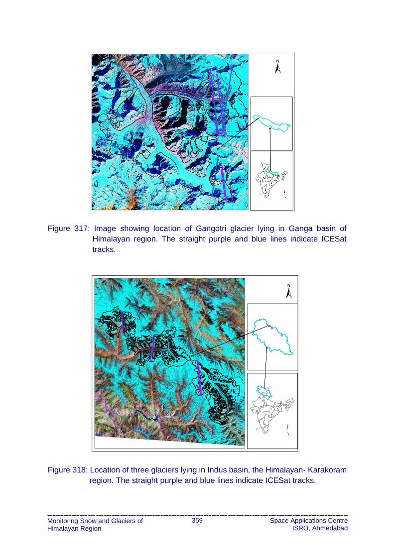
359
Monitoring Snow and Glaciers of Himalayan Region
Space Applications Centre ISRO, Ahmedabad
Figure 317: Image showing location of Gangotri glacier lying in Ganga basin of
Himalayan region. The straight purple and blue lines indicate ICESat
tracks.
Figure 318: Location of three glaciers lying in Indus basin, the Himalayan- Karakoram
region. The straight purple and blue lines indicate ICESat tracks.
360
Monitoring Snow and Glaciers of Himalayan Region
Space Applications Centre ISRO, Ahmedabad
21.4. Data Used
a) ICESat/GLAS
ICESat has an onboard laser altimeter system, to collect surface elevations all over
the globe with high precision. Since 2003 to the end of its operation in 2009, GLAS
has been operating for three annual observation campaigns, each of approximately
35 days. This instrument combines a 3 cm precision 1064-nm laser altimeter with a
laser pointing angle determination system (Sirota et al., 2005) and it is used to
measure the Earth’s surface and it also measure the backscattering profile from thicker
clouds, while those at 532-nm use photon-counting detectors and measure the height
distributions of optically thin clouds and aerosol layers. A GPS receiver on the
spacecraft provides data for determining the spacecraft position, and also the absolute
time reference for the instrument measurements and altimetry clock (Abshire et al.,
2005). It retrieves surface elevations within 70 m diameter footprints and along track
spacing of 170 m. GLAS elevation accuracy is reported to be 15 cm over flat terrain
(Zwally et al., 2002). In this study GLA06 product of ICESat has been used between
2003 and 2009 available from the National Snow and Ice Data Centre (NSIDC) (Zwally
et al., 2008).
b) DEMs
CartoDEM as well as SRTM DEM has been used to project ICESat repeat tracks onto
common locations and to extrapolate elevation changes to unmeasured locations.
Carto DEM
Cartosat-1 Digital Elevation Model (CartoDEM) is a National DEM developed by the
Indian Space Research Organization (ISRO), derived from the Cartosat-1. Cartosat-1
has a pair of Panchromatic cameras having an along track stereoscopic capability to
acquire two images simultaneously, one forward looking (Fore) at +26 degrees and
another rear looking (Aft) -5 degrees with a base-to-height ratio of about 0.63. Its
Absolute planimetric accuracy is 15m and absolute vertical accuracy is 8 m and having
5 m relative vertical accuracy (Muralikrishnan et. al., 2011).
SRTM DEM
The SRTM (Shuttle RADAR Topographic Mission) was the first mission using space-
borne single pass interferometric SAR which was flown in February 2000. The goal of
the mission was to survey the Earth surface and to generate a homogeneous elevation
data set of the world with a grid spacing of 3arcsec. The digital topographic map
products expected to meet the Interferometric Terrain Height Data (ITHD)-2
specifications sampling with 16 m absolute vertical height accuracy, 10 m relative
vertical height accuracy and 20 meter absolute horizontal accuracy (Balmer, 1999).
The horizontal datum is the World Geodetic System 1984. The vertical datum is mean
sea level as defined by the Earth Gravitational Model geoid (EGM-96). Most of the
users commonly ignore the original vertical datum and use SRTM data as referenced
to the WGS84 ellipsoid as geoid models (Markus, 2005).

361
Monitoring Snow and Glaciers of Himalayan Region
Space Applications Centre ISRO, Ahmedabad
21.5. Methodology
Researchers have used mainly three approaches for estimation of the elevation
change using ICESat altimetry (Moholdt et al., 2010). The first approach, which
computes elevation changes at crossover points, has very high accuracy. Elevations
at crossover points are linearly interpolated from the two closest footprints within 200
m in each track (Brenner et al., 2007). The main drawback of this approach is that the
sampling is too coarse. The second approach uses a DEM to correct for the surface
slope between the centre points of overlapping footprints (Slobbe et al., 2008) and
used over the Greenland ice sheet. This approach takes care of the slope-induced
errors; however, it is constrained by the data availability for comparison. It is difficult
to compare repeat track ICESat profiles due to the relatively large cross track
separation between repeat profiles. In view of the limitations of the first two
approaches, the third approach has been used in this study which utilizes near repeat
ICESat tracks having small cross-track separation (Moholdt et. al.,2010) shown in
Figure 319 and Figure 320.
Figure 319: Flowchart showing the near repeat track methodology for elevation
change estimation

362
Monitoring Snow and Glaciers of Himalayan Region
Space Applications Centre ISRO, Ahmedabad
Figure 320: Projection of near repeat tracks on common locations using DEMs. Green
dots represent projected location, Pink dots represent secondary track
and Yellow dots represent reference track (adopted from Moholdt et al.,
2010)
In this approach two near repeat ICESat tracks (Ta and Tb) pertaining to different years
and same season has been taken. For every pair of ICESat repeat tracks one track is
considered as the reference track and other one is secondary track. The track which
is oldest is chosen as the reference track. The second track is projected on the
reference track and topographical change at these two locations can be estimated by
the change in elevation values of these locations using DEM. The elevation
information Ha and Hb has been extracted from the DEM at the ICESat footprints on
track Ta and Tb respectively. The difference (Ha – Hb) of this elevation information
(Ha&Hb) is represented as the unmeasured topography between the near repeat
tracks. Here the utility of DEM implies along-track interpolation to restrict the DEM
slope correction to the cross-track distance between two repeat-tracks (Moholdt et al.,
2010b). Now each footprint on Track Tb is projected perpendicularly on track Ta. The
ICESat elevation on the projected points (Ia) over reference track (Ia) can be computed
as in equation given below
Ia = Ib + Ha – Hb
At the same projected points on the reference track Ta, ICESat elevation (Iint) is
estimated through lineraly interpolating the neighbouring footprints (Ta1 and Ta2) along
the track. The elevation difference at the projected points (dh) is the change in the
elevation between the projected (Ia) and interpolated ICESat elevation (Iint) and it can
be computed as in equation given below:
dh = Ia – Iint
where,
dh= elevation difference of two different periods

363
Monitoring Snow and Glaciers of Himalayan Region
Space Applications Centre ISRO, Ahmedabad
Ia = ICESat elevation at projected location on track Ta
Iint= interpolated ICESat elevation on track Ta
Ib= ICESat elevation on track Tb
Ha= extracted elevation from DEM on track Ta
Hb= extracted elevation from DEM on track Tb
21.6. Results and Discussion
The ICESat altimetry data of near repeat tracks (Ta and Tb) have been used to estimate
the elevation changes in the glaciers (Figure 321). Here track Ta is considered as the
reference track and track Tb as secondary track. The mean elevation changes and
mean offsets are computed from the repeat passes of the ICESat for the four glaciers
are given in Table 93. Different tracks over Gangotri glacier shows the variations in
the thinning/thickening rate in the range of 0.01 to 0.71m/Year by utilizing CartoDEM.
Similar variation (-0.20 to 0.84 m/Year) is obtained while using SRTM DEM. The
reason behind the variation is due to the pass of the track over different region.
Table 93: Mean elevation change along the ICESat tracks of Gangotri, Siachen,
Baltoro and Drenmarg Glacier
S. No Glacier
name
ICESat Tracks Mean
Offset (m)
Elevation change rate
(m/Year)
Track
Ta (Ref.)
Track Tb Carto-DEM SRTM
1. Gangotri
Mar-04 Mar-08 273.77 0.01 ± 2.83 -0.20 ± 2.85
Mar-05 Apr-07 34.67 0.71 ± 3.24 0.84 ± 4.25
Feb-04 Feb-08 15.06 0.02 ± 2.54 0.04 ± 2.39
2.
Siachen Oct-04 Oct-09 5.14 0.23 ± 0.60 0.27 ± 0.56
Oct-03 Oct-05 24.03 -0.19 ± 1.70 -0.38 ± 0.95
3. Baltoro Oct-03 Oct-09 277.95 0.44 ± 1.27 0.66 ± 1.20
4. Drenmarg
Oct-03 Oct-07 182.68 -1.02 ± 2.21 -1.05 ± 2.64
Considering the second near repeat track on Gangotri Glacier taken as April, 2007
and March, 2005, the mean elevation change rate is observed to be positive which
depicts the thickening of glacier surface in a period of two years. The mean separation
between the ICESat near repeat tracks in the Siachen glacier is observed as 14.5m.

364
Monitoring Snow and Glaciers of Himalayan Region
Space Applications Centre ISRO, Ahmedabad
The first near repeat track on Siachen Glacier was October, 2009 and October, 2004,
the mean elevation change rate during this period is observed more or less similar
with CartoDEM (0.23 m/Year) and with SRTM (0.27 m/Year). The positive elevation
change rate depicts the thickening of glacier surface in a period of five years. The
second near repeat track was taken as October, 2005 and October, 2003 and the
mean elevation change rate observed with CartoDEM is -0.19 m/Year and with SRTM
is -0.39 m/Year. Here the negative elevation change rate depicts the thinning of glacier
surface in a period of two years.
The near repeat track on Baltoro Glacier has a temporal separation of six years and
the mean elevation change rate during this period observed with CartoDEM is 0.44
m/Year and with SRTM is 0.66 m/Year. The ICESat near repeat track on Drenmarg
Glacier having temporal separation of 4 years (October, 2003, October, 2007) and the
mean elevation change rate during this period is observed more or less similar with
CartoDEM (-1.02 m/Year) and with SRTM (-1.05 m/Year). Fiure 4.20.5 shows the
average annual 2003-2009 elevation change rates at different locations of different
glacier. There are large local dh/dt variations which may attribute to glacier dynamics,
wind drift and error in the datasets. The datasets error contains instrumental error of
GLAS as well as the relative inaccuracies of DEMs. It has also been observed that the
thinning/thickening rate computed using SRTM and CartoDEM are similar. Most of the
complexities are likely caused by glacier dynamics and wind posting of snow might
also have an impact. The change rates are slightly different in different glaciers which
reflect different local climatic conditions, different hypsometry’s of the glaciers, and
different glacier flow dynamics.

365
Monitoring Snow and Glaciers of Himalayan Region
Space Applications Centre ISRO, Ahmedabad
Figure 321: Elevation change rate along ICESat tracks on Siachen, Gangotri, Baltoro
and Drenmarg glaciers of the Himalayan region.
21.7. Conclusion
In this study four glaciers in the Himalaya region have been taken up for the estimation
of elevation change using ICESat altimetry data and DEMs (CartoDEM and SRTM).
Until now, ICESat has mainly been applied in Antarctica and Greenland ice sheets.
Here, ICESat laser altimetry proved to be a highly valuable dataset for computing
regional scale elevation changes for smaller glaciers with mountainous topography.
Its applicability for smaller glaciers in mountainous regions is limited because of the
insufficient spatial distribution of tracks. In this study the near repeat track approach
has been used to compute elevation changes by estimating unmeasured variation in

366
Monitoring Snow and Glaciers of Himalayan Region
Space Applications Centre ISRO, Ahmedabad
local topography with the consideration of reference DEM. This approach takes care
of the slope induced error but the relative error in the DEM may place an important
role for change detection. To minimize the relative inaccuracies in DEM the near
repeat track separation should have minimum value.
This study shows the similar variation with the CartoDEM and SRTM DEM. The
thinning rate is observed negative in tracks of Gangotri and Baltoro Glaciers while
tracks on Drenmarg glaciers have high thinning rate. Since the observed tracks are
very limited over the glaciers, the observed estimates may be biased towards the
representation for the entire glacier region. To estimate the mean elevation, change in
the glacier region more near repeat tracks distributed spatially are required. However,
this procedure can be used for the better estimates in the Himalaya region with the
processing of future ICESat-2 mission, which will cover densely with close spacing
and dense point coverage using six laser beam configuration. This work can be
extended to other Himalayan regions to assess elevation change of glacier ice and to
better understand its association with provincial climate changes.

367
Monitoring Snow and Glaciers of Himalayan Region
Space Applications Centre ISRO, Ahmedabad
22. Future Plan Monitoring of Himalayan region using space based observations needs to be
continued for improved understanding of Himalayan cryosphere. Ongoing as well
future plans to understand Himalayan Cryosphere include analysis of satellite data
from existing as well planned Earth Observation Missions of ISRO and other
International Missions. Large scale glacier mapping and monitoring shall be carried
out. Techniques shall be developed/improved for estimation of snow depth, snow pack
characterization, glacier mass balance estimation, glacier velocity determination,
snow and glacier melt estimation and early warning of snow and glacier related
hazards.
A new project entitled, “Integrated studies of Himalayan Cryosphere using space
based inputs and impact assessment due to climate change”, has been initiated
from Finanacial Year 2016-17 which is funded by Department of Space. This project
is aimed to do a comprehensive integrated study of Hindu Kush-Karakoram-
Himalayan region using space based observations for societal benefits and
understand impact due to climate change. The major work components currently
undertaken are given below:
i) Glacier characterisation using SAR data which involves understanding of the
freeze-melt cycle of glaciers occurring in different climatic regions of Himalayan
terrain in spatial and temporal domain using RISAT-1 SAR data. Selected large
glaciers from entire Himalaya-Karakoram-Hindukush region have been taken
up. This work is aimed to generate multi-temporal glacier facies maps along
with their spatial and temporal analysis.
ii) Snow Cover Mapping component involves sub-basin wise snow cover product
generation in GIS environment and analysis of geospatial database. Snow
cover products shall be generated at every 5 days and 10 days for hydrological
year 2015 to 2018 covering 35 sub-basins of Indus, Ganga and Brahmaputra
river basins using IRS (Resourcesat-1 and 2) AWiFS data. This database is in
continuation of the earlier phases and thus shall enrich the existing geospatial
database of snow cover for long term analysis.
iii) Development of techniques for estimation of mass balance of glaciers using
Altimeric, Geodetic and AAR methods (Photogrammetry, Interferometry,
GRACE, Laser Altimetry). Work shall be carried out for selected glaciers for
hydrological year 2015-2018.
iv) Estimation and validation of snow and glacier melt run-off for selected sub-
basins in Satluj, Ganga and Chenab basins. The work involves improvement
in accuracy of model and spatial and temporal variability of snow and glacier
melt runoff in the Himalayan region.

368
Monitoring Snow and Glaciers of Himalayan Region
Space Applications Centre ISRO, Ahmedabad
v) Techniques for retrieving velocity of glaciers using optical and microwave data
shall be developed for selected glaciers from sub-basins in western, west-
central, central and eastern Himalayan regions;
vi) Techniques for retrieval of snow depth in the Himalayan region using AWiFS
and RISAT-1 SAR data in winters for Beas basin and Bhaga basin shall be
developed.
In addition, it is planned to carry out glacier mapping and change detection of
selected glaciers on 1:10, 000 scale using high resolution satellite images (~100
glaciers); Mapping and monitoring of glacial and peri-glacial lakes (~ 2,000 - 2, 500
lakes); Development of Himalayan Cryosphere Information System (HKH Region);
Evaluating feasibility of geostationary satellite data for Cryosphere studies
(Estimation of snow depth Snow cover, snow line and melt runoff studies using
INSAT-3D); Retrieval of snow pack characterisation using Hyperspectral data;
Monitoring and impact assessment of Black Carbon soot on glaciers; Study of
spatial and temporal variability of snow Albedo for assessing radiative transfer over
Himalayan snow covered regions; Development of empirical relation for glacier ice
thickness using GPR; Energy Balance modelling on snow and glaciers;
Development of approach for Glacier health Bulletin; Development of alert system
for glacial lakes outbursts; Comparative study of glacier dynamics in Himalayan,
Central Asian mountains, Alps and Svalbard regions

369
Monitoring Snow and Glaciers of Himalayan Region
Space Applications Centre ISRO, Ahmedabad
References
1. Abshire J B, Sun X L, Riris H, Sirota J M, McGarry J F, Palm S, Yi D H, and
Liiva P (2005) Geoscience Laser Altimeter System (GLAS) on the ICESat
mission: On-orbit measurement performance Geophys. Res.Lett. 32 L21S02
doi:10.1029/2005 GL024028
2. Aggarwal S P, Thakur K P, Nikam B R and Garg, V (2014) Integrated approach
for snowmelt runoff estimation using temperature index model, remote sensing
and GIS Current Science 106(3) 397-407
3. Aggarwal K C, Kumar V and Dass T (1983) Snowmelt run-off for a catchment
of Beas basin. In: Proc. First National Symp. on Seasonal Snow Cover, SASE,
Manali 28-30 April, 1983 II 43-63
4. Agrawal Ritesh, Singh S K, Rajawat A S and Ajai (2014) Estimation of regional
mass anomalies from Gravity Recovery and Climate Experiment (GRACE) over
Himalayan region. In: The International Archives of the Photogrammetry,
Remote Sensing and Spatial Information Sciences Volume XL-8 2014 ISPRS
Technical Commission VIII Symposium doi:10.5194/isprsarchives-XL-8-329-
2014, 329-332
5. Akiko Sakai (2012) Glacial lakes in the Himalayas: a review on formation and
expansion processes Global Environ. Res. 16 23–30
6. Akyurek Z and Sorman A U (2002) Monitoring snow-covered areas using
NOAAAVHRR data in the eastern part of Turkey Hydrol. Sci. 47 243–252
7. Anderson E A (1976) National river forecast system-snow accumulation and
ablation model, NOAA Tech. Memo.NWS Hydro-17, US Dept. of Commerce,
Silver Spring, USA
8. Arcone S A, Lawson D E and Delaney A J (1995) Short-pulse radar wavelet
recovery and resolution of dielectric contrasts within englacial and basal ice of
Motanuska glacier, Alaka Journal of Glaciology 41 68-86
9. Armstrong R L and Brun E (2008) Snow Climate, Cambridge University Press,
222; ISBN 978-0-521-85454-2
10. Arnott W P, Hamasha K, Moosmuller H, Shredian P J and Orgen J A (2005)
Towards aerosol light-absorption measurements with a 7-wavelength
aethalometer: Evaluation with a photoacoustic instrument and 3-wavelength
nephelometer Aerosol Sci. Technol., 39 17-29

370
Monitoring Snow and Glaciers of Himalayan Region
Space Applications Centre ISRO, Ahmedabad
11. Aster GDEM team (2011) Aster digital Global Digital Elevation model version 2
– summary of validations result. GDEM2, validation report final,
http://www.ersdac or jp/GDEM/ver2validation/summary
12. Aswal B S and Mehrotra B N (1994) Flora of Lahaul-Spiti (A Cold Desert in
North-West Himalaya). Bishen Singh Mahendra Pal Singh, Dehradun
13. Avsar N B and Ustun A (2012) Analysis of regional time variable gravity using
GRACE’s 10-day solutions FIG Working Week 2012 Knowing to manage the
territory, protect the environment, evaluate the cultural heritage Rome, Italy, 6
10 May 2012
14. Azam M F, Wagnon P, Ramanathan A L, Vincent C, Sharma P, Arnaud Y, Linda
A, Pottakkal J G, Chevallier P, Singh V B and Etienne B (2011) From balance
to imbalance: a shift in the dynamic behaviour of Chhota Shigri Glacier
(Western Himalaya, India) Jour. Glacio. 58(208) 315-324
15. Bahuguna I M, Rathore B P, Brahmabhatt R, Sharma M, Dhar S, Randhawa S
S, Kumar K, Romshoo S, Shah R D, Ganjoo R K and Ajai (2014) Are the
Himalayan glaciers retreating? Current Science 106(7) 1008-1013
16. Bahuguna I M (2013) Geomatics in early assessment of Himalayan lakes
outburst hazards. Newsl. ISG 19(2) 57–64
17. Bahuguna I M, Kulkarni A V, Nayak S, Rathore B P, Negi H S and Mathur P
(2007) Himalayan glacier retreat using IRS 1C PAN stereo data Int. J. Remote
Sensing 28(2) 437–442
18. Bahuguna I M, Kulkarni A V and Nayak S R (2004) DEM from IRS-1C PAN
stereo coverage over Himalayan glaciated region Int. J. Remote Sensing 25(19)
4029–4041
19. Bajracharya S R, Maharjan S B, Shrestha F (2014) The status and decadal
change of glaciers in Bhutan from 1980's to 2010 based on the satellite data
Ann. Glaciol. 55(66) 159-166. doi: 10.3189/2014AoG66A125
20. Bajracharya S R, Mool P K and Shrestha B R (2006) The impact of global
warming on the glaciers of the Himalaya. In Proceedings of the International
Symposium on Geo-disasters, Infrastructure Management and Protection of
World Heritage Sites, Nepal Engineering College, Ehime College and National
Society for Earthquake Technology, Nepal, 25–26 November 2006 231–242

371
Monitoring Snow and Glaciers of Himalayan Region
Space Applications Centre ISRO, Ahmedabad
21. Bamler R (1999) The SRTM Mission – A Worldwide 30 m Resolution DEM from
SAR Interferometry in 11 Days. In: Photogrammetric Week ´99 D (Eds.: Fritsch
D and Spiller R) WichmannVerlag, Heidelberg, Germany 145-154
22. Basnett S, Kulkarni A V and Bolch T (2013) The influence of debris cover and
glacial lakes on the recession of glaciers in Sikkim Himalaya, India J of
Glaciology 59 1035-1046 http://dx.doi.org/10.3189/2013JoG12J184
23. Benn D I, Bolch T, Hands K, Gulley J, Luckman A, Nicholson L I, Quincey D,
Thompson S, Toumi R and Wiseman S (2012) Response of debris-covered
glaciers in the Mount Everest region to recent warming, and implications for
outburst flood hazards Earth-Science Reviews 114 156–174
doi:10.1016/j.earscirev.2012.03.008
24. Benn D I and Evans D J A (2010) Glaciers and Glaciation, Hodder Education,
London, 802; ISBN 978-0-340-90579-1
25. Benn D I, Wisemen S and Hands K (2001) Growth and drainage of supraglacial
lakes on debris-mantled Ngozumpa glacier, Khumbu Himal, Nepal J. Glaciol.
47 625–638
26. Benson R C, Glaccum R A and Noel M R (1983) Geophysical techniques for
sensing buried wastes and waste migration. Environmental Monitoring Systems
Laboratory, US Environmental Protection Agency, Contract ≠ 68-03-3050 Las
Vegas NV 236
27. Beres M and Haeni F P (1991) Application of Ground-Penetrating-Radar
methods in hydrogeologic studies Groundwater 29(3) 375-386
28. Berthier E, Arnaud Y, Kumar R, Ahmad S, Wagnon P and Chevallier P (2007)
Remote sensing estimates of glacier mass balances in the Himachal Pradesh
(Western Himalaya, India) Remote Sensing Environ.108 327–338
29. Berthier E, Arnaud Y, Vincent C and Remy F (2006) Biases of SRTM in high-
mountain areas: Implications for the monitoring of glacier volume changes.
Geophys. Res. Lett., 32(8) L08502. doi:10.1029/2006GL025862
30. Berthier E, Vadon H, Baratoux D, Arnaud Y, Vincent C, Feigl K L, Remy F and
Legresy B (2005) Surface motion of mountain glaciers derived from satellite
optical imagery Rem Sens Environ 95(1)14-28
31. Berthier E, Arnaud Y, Baratoux D, Vincent C and Remy F (2004) Recent rapid
thinning of the "Mer de Glace'' glacier derived from satellite optical images
Geoph Res Lett, 31 (17)

372
Monitoring Snow and Glaciers of Himalayan Region
Space Applications Centre ISRO, Ahmedabad
32. Bhambri R, Bolch T, Kawishwar P, Dobhal D P, Srivastrava D and Pratap B
(2013) Heterogeneity in glacier response in the upper Shyok valley, northeast
Karakoram Cryosphere 7 1385–1398 (doi: 10.5194/tc-7-1385-2013)
33. Bhambri R, Bolch T and Chaujar R (2012) Frontal recession of Gangotri
Glacier, Garhwal Himalayas, from 1965 to 2006, measured through high-
resolution remote sensing data Current Science 102 489-494
34. Bhambri R, Bolch T, Chaujar R K and Kulshreshtha S C (2011) Glacier changes
in the Garhwal Himalaya, India, from 1968 to 2006 based on remote sensing J
Glaciol 57(203) 543–556 (doi: 10.3189/002214311796905604)
35. Bhambri R and Bolch T (2009) Glacier mapping: a review with special reference
to the Indian Himalayas Prog. Phys. Geogr. 33 672–704
36. Bingham A W and Rees W G (1997) Satellite data synergies for monitoring
Arctic ice masses. In: Proc. 3rd ERS Scientific Symp. March 17-21,1997
Florence, Italy (SP-414 Vol. 2) ESA, Frascati Italy 867-870
37. Bintanja R, Jonsson S and Knap W (1997) The annual cycle of the surface
energy balance of Antartic blue ice. J. Geophys. Res. 102(D2) 1867–1881
38. Birajdara F S, Venkataramana G, Bahuguna I M and Samant H P (2014) A
revised glacier inventory of Bhaga basin Himachal Pradesh, India. In: ISPRS
Annals of the Photogrammetry, Remote Sensing and Spatial Information
Sciences, Volume II-8, 2014, ISPRS Technical Commission VIII Symposium,
doi:10.5194/isprsannals-II-8-37-2014, 37-43
39. Blindow N (1994) The central part of the Filchner-Ronne Ice Shelf, Antarctica:
internal structures revealed by 40 MHz mono pulse RES Annals of Glaciology
20 365-371
40. Bolch T, Kulkarni A, Kaab A, Huggel C, Paul F, Cogley J G, Frey H, Kargel J S,
Fujita K, Scheel M, Bajracharya S and Stoffel M (2012) The state and fate of
Himalayan glaciers, Science 336(6079) 310-314
(doi:10.1126/science.1215828)
41. Bolch T, Pieczonka T and Benn D I (2011a) Multi-decadal mass loss of glaciers
in the Everest area (Nepal Himalaya) derived from stereo imagery The
Cryosphere 5 349–358, www.the-cryosphere.net/5/349/2011/ doi: 10.5194/tc-
5-349-2011

373
Monitoring Snow and Glaciers of Himalayan Region
Space Applications Centre ISRO, Ahmedabad
42. Bolch T, Peters J, Pradhan B, Yegorov A B, Buchroithner M F and
Blagoveshchenskiy V P (2011) Identification of potentially dangerous glacial
lakes in the northern Tien Shan Nat. Hazards 59(3) 1691–1714
43. Bolch T et al. (2010) A glacier inventory for the western Nyainqentanglha Range
and the Nam Co Basin, Tibet, and glacier changes 1976–2009 Cryosphere 4
419–433
44. Bose A (2013) Comparison of Eastern and Western Himalayas. Indian
Geography, http://www.importantindia.com/4310/compare-westernand-
eastern-himalayas/
45. Brahmbhatt R M, Bahuguna I M, Rathore B P, Shah R D, Kargel J S and
Rajawat A S (2016) Significance of glacio-morphological factors in the glacier
retreat: A case study of part of Chenab basin, Himalaya, J of Mountain Science
(in Press)
46. Brahmbhatt R M, Bahuguna I M, Rathore B P, Singh S K, Rajawat A S, Shah
R D and Kargel J S (2015a) Satellite monitoring of glaciers in the Karakoram
from 1977 to 2013: an overall almost stable population of dynamic glaciers The
Cryosphere Discussions 9 1555- 1592, doi:10.5194/tcd-9-1555-2015
47. Brahmbhatt R M, Rathore B P, Pattnaik S, Jani P, Bahuguna I M, Shah R D
and Rajawat A S (2015b) Peculiar characteristics of fragmentation of glaciers:
a case study of Western Himalaya, India Int J Geosciences 6 455-463
48. Brahmbhatt, R.M., Nainwal, H.C. and Kulkarni, A.V. (2014) Impact of
Accumulation Area Ratio (AAR) on Glacial Change: A Few Examples of Jammu
& Kashmir J Geomatics 8 61-65
49. Brahmbhatt R M (2014) Study of Glacio-geomorphic Characteristics and its
effect on Glacial Dimensions in parts of Chenab basin using Remote Sensing
and Geographic Information System. Ph. D. Thesis, H. N. B. Garhwal
University (Central University), Garhwal, Srinagar
50. Brahmbhatt R M, Bahuguna I M, Rathore B P, Kulkarni A V, Nainwal H C, Shah
R D and Ajai (2012a) A comparative study of deglaciation in two neighboring
basins (Warwan and Bhut) of Western Himalaya Current Science, 103(3) 298-
304
51. Brahmbhatt R M, Bahuguna I M, Rathore B P, Kulkarni A V, Shah R D, Nainwal
H C and Ajai (2012b) Variation of snowline and mass balance of glaciers of
Warwan and Bhut basin of Western Himalaya using remote sensing technique
J Ind Soc Remote Sensing 40(4) 629-637

374
Monitoring Snow and Glaciers of Himalayan Region
Space Applications Centre ISRO, Ahmedabad
52. Brenner A C, DiMarzio J R and Zwally H J (2007) Precision and accuracy of
satellite radar and laser altimeter data over the continental ice sheets. IEEE T.
Geosci. Remote, 45(2) 321–331 doi:10.1109/TGRS.2006.887172
53. Brewster M I and Annan A P (1994) Ground penetrating radar monitoring of a
controlled DNAPL release: 200 MHz radar Gephysics 59 1211-1221
54. Brock B W, Mihalcea C, Kirkbride M P, Diolaiuti G, Cutler M E J, Smiraglia C
(2010) Meteorology and surface energy fluxes in the 2005–2007 ablation
seasons at the Miage debris-covered glacier, Mont Blanc Massif, Italian Alps.
J. Geophys. Res. 115 D09106
55. Brown R D (2000) Northern Hemisphere snow cover variability and change,
1915–1997 J Climate 13 2339–2355
56. Butt M J (2012) Characteristics of the snow cover in the Hindukush, Karakoram
and Himalaya region using Landsat satellite data Hydrol Process 26(24) 3689-
3698
57. Carey M (2008) Disasters, development and glacial lake control in twentieth-
century Peru. In: Mountains Sources of Water, Sources of Knowledge.
Advances in Global Change Research (Ed: Wiegandt E) Springer the
Netherlands 31 181–196
58. Casey K A, Kaab A and Benn D I (2012) Geochemical characterization of
supraglacial debris via in situ and optical remote sensing methods: a case study
in Khumbu Himalaya, Nepal The Cryosphere 6 85–100
59. Chacko V J (1965) A Manual of Sampling Technique for Forest Surveys.
Manager Publications Delhi 172
60. Chakraborty M, Panigrahy S, Rajawat A S, Kumar R, Murthy T V R, Halder D,
Chakraborty A, Kumar T, Rode S, Kumar H, Mahapatra M and Kundu S (2013)
Initial results using RISAT-1 C band SAR data Current Science 104(4) 490–
501
61. Chaohai L and Sharma C K (1988) Report on First Expedition to Glaciers in the
Pumqu (Arun) and Poiqu (Bhote-Sun Kosi) River Basins, Xizang (Tibet). China,
Science Press, Beijing, China 192
62. Che T, Li X, Jin R, Armstrong R and Zhang T (2008) Snow depth derived from
passive microwave remote sensing data in China Ann. Glaciol. 49 145–154

375
Monitoring Snow and Glaciers of Himalayan Region
Space Applications Centre ISRO, Ahmedabad
63. Chowdhery H J and Wadhwa B M (1984) Flora of Himachal Pradesh 1-3 Bot.
Surv. India, Calcutta
64. Clague J J and Evans S G (2000) A review of catastrophic drainage of moraine
dammed lakes in British Columbia. Quaternary Sci. Rev. 19 1763–1783
65. Clarke G K C and Mathews W H (1981) Estimation of magnitude of glacier
outburst floods from Dojeck, Yukon Territory, Canada Can. J. Earth Sci.18
1452–1463
66. Clague J J and Mathews W H (1973) The magnitude of jokulaphs J. Glaciol. 12
501–504
67. Conyers L B and Goodman D (1997) Ground Penetrating Radar: An
Introduction for Archaeologists, Altamira Press, Walnut Creek, CA 232
68. Copland L, Sylvestre T, Bishop M P, Shroder J F, Seong Y B, Owen L A, Bush
A and Kamp U (2011) Expanded and recently increased glacier surging in the
Karakoram Arct. Antarct. Alp. Res. 43 503–516
69. Cosgrave T M, Greenhouse J P and Barker J F (1987) Shallow stratigraphic
reflections from ground-penetrating-radar. In: First National Outdoor Action
Conference on Aquifer Restoration Ground Water Monitoring and Geophysical
Methods, Las Vegas N V 559-569
70. Cuffey K M and Paterson W S B (2010) The Physics of Glaciers Fourth Edition
Academic Press 704 ISBN 9780123694614
71. Curtis J T and Mc Intosh (1950) The interrelation of certain analytic and
phytosociological characters Ecol. 31 434-455
72. Daniels J J, Roberts R and Vendl M (1995) Ground penetrating radar for the
detection of liquid contaminants J. Appl. Geophys. 33 195–207
73. Das S K, Dobhal D P and Juyal N (2010) Variability of aerosol optical depth and
recent recessional trend in Dokriani Glacier, Bhagirathi Valley, Garhwal
Himalaya Current Science 99(12) 1816–1821
74. Davis J L, Tamisiea M E, Elo´segui P, Mitrovica J X and Hill E M (2008) A
statistical filtering approach for Gravity Recovery and Climate Experiment
(GRACE) gravity data, Journal of Geophysical Research 113 B04410
doi:10.1029/2007JB005043

376
Monitoring Snow and Glaciers of Himalayan Region
Space Applications Centre ISRO, Ahmedabad
75. Dedieu J P, Rabatel A, Vincent C, Valla F, Thibert E and Arnaud Y (2003)
Glacier mass balance determination by remote sensing in the French Alps:
progress and limitation for time series monitoring In: Proceedings of
Geoscience and Remote Sensing Symposium, IGARSS '032003; 4; 2602-2604
vol.4
76. Deota B S, Trivedi Y N, Kulkarni A V, Bahuguna I M and Rathore B P (2011)
RS and GIS in mapping of geomorphic records and understanding the local
controls of glacial retreat from the Baspa Valley, Himachal Pradesh, India,
Current Science 100(10) 1555– 1563
77. Deslognes J R, Jones D P and Kiker K E (1989) Estimation of peak
discharge from drainage of ice dammed Ape lake, British Columbia Can. J.
Glaciol. 35 349–354
78. Dhaliwal D S and Sharma M (1999) Flora of Kullu District. Himachal Pradesh.
Dehra Dun: Bishen Singh Mahendra Pal Singh
79. Dhar S, Kulkarni A V, Rathore B P and Kalia R (2009) Reconstruction of the
moraine dammed lake, based on field evidences and paleohistory, Samudra
Tapu Glacier, Chandra Basin, Himachal Pradesh J. Indian Soc. Remote
Sensing 38(1)133–141
80. Dhar U, Rawal R S and Samant S S (1997) Structural diversity and
representativeness of forest vegetation in a protected area of Kumaun
Himalaya, India Implications for conservation Biod. Cons. 6 1045-1062
81. Dobhal D P, Gupta A K, Mehta M and Khandewal D D (2013) Kedarnath
disaster: facts and plausible causes. Current Science 105(2) 171–174
82. Dobhal D P (2010) Climate Change and Glacier Retreat in the Himalaya, India
– an Overview. In: Climate Change at the Third Pole: The Impact of Climate
Instability on Himalayan Ecosystems and Himalayan Communities (Eds: Shiva
V and Bhatt V K) p. 67-77
83. Dobhal D P and Mehta M (2010) Surface morphology, elevation changes and
Terminus retreat of Dokriani Glacier, Garhwal Himalaya: implication for climate
change Him. Geol. 31(1) 71-78
84. Dobhal D P, Gergan J T, Thayyen R J (2008) Mass balance studies of the
Dokriani glacier from 1992 to 2000, Garhwal Himalaya, India. Bulletin of
Glaciological Research 25 9–17

377
Monitoring Snow and Glaciers of Himalayan Region
Space Applications Centre ISRO, Ahmedabad
85. Dozier J (1992) Opportunities to improve hydrologic data Review of Geophysics
30(4) pp 315-331
86. Dozier J (1989) Spectral signature of Alpine snow cover from the Landsat
Thematic Mapper Remote Sens. Environ. 28 9-12
87. Dutta S, Ramanathan A L and Linda A (2012) Glacier fluctuation using satellite
data in Beas basin, 1972–2006, Himachal Pradesh, India J. Earth Syst. Sci.
121(5) 1105–1112
88. Evans I S (2006) Local aspect asymmetry of mountain glaciations: a global
survey of consistency of favored directions for glacier numbers and altitudes
Geomorphology 73(1–2) 166–184
89. Favier V, Wagnon P, Chazarin J P, Maisincho L and Coudrain A (2004) One-
year measurements of surface heat budget on the ablation zone of Antizana
glacier 15, Ecuadorian Andes J. Geophys. Res. 109 D18105
doi:10.1029/2003JD004359
90. Flanner M G, Liu X, Zhou C, Penner J E and Jiao C (2012) Enhanced solar
energy absorption by internally-mixed black carbon in snow grains Atmos Chem
Phys 12(10):4699–721
91. Flanner M G, Shell K M, Barlage M, Perovich D K and Tschudi M A (2011)
Radiative forcing and albedo feedback from the Northern Hemisphere
cryosphere between 1979 and 2008 Nat Geosci 4(3) 151–155
92. Foster J L and Chang A T C (1993) Snow Cover, In: Atlas of Satellite
Observations related to Global Change (Eds.: Gurney R J, Parkinson C L and
Foster J L), Cambridge University Press, Cambridge 361-370
93. Frey H, Machguth H, Huss M, Huggel C, Bajracharya S, Bolch T, Kulkarni A,
Linsbauer A, Salzmann N, Stoffel M (2013) Ice Volume estimates for the
Himalaya-Karakoram region: evaluating different methods The Cryosphere 7(5)
4813-4854 doi:10.519/tcd-7-4813-2013
94. Frey H, Paul F and Strozzi T (2012) Compilation of a glacier inventory for the
western Himalayas from satellite data: methods, challenges, and results
Remote Sens Environ 124 832–843
95. Frey H and Paul F (2012) On the suitability of the SRTM DEM and ASTER
GDEM for the compilation of topographic parameters in glacier inventories. Int.
J. Appl. Earth Obs. Geoinf. 18 480–490 (doi: 10.1016/j.jag.2011.09.020)
378
Monitoring Snow and Glaciers of Himalayan Region
Space Applications Centre ISRO, Ahmedabad
96. Frei A and Robinson D A (1999) Northern Hemisphere snow extent: regional
variability 1972-1994 International J. of Climatology 19 1535-1560
97. Fujita K, Sakai A, Takenaka S, Nuimura T, Surazakov A B, Sawagaki T and
Yamanokuchi T (2013) Potential flood volume of Himalayan glacial lakes Nat.
Hazards Earth Syst. Sci. 13 1827–1839. www.nat-hazards-earth-syst-
sci.net/13/1827/2013/ doi:10.5194/nhess-13-1827-2013
98. Fujita K, Nishimura K, Komori J, Iwata S, Ukita J, Tadono
T and Koike T (2012) Outline of research project on glacial lake outburst floods
in the Bhutan Himalayas Global Environ. Res. 16 3-12
99. Fushimi H, Ikegani K, Higuchi K and Shankar K (1985) Nepal Case Study:
Catastrophic Floods, Techniques for Prediction of Runoff from Glacierised
Areas, IASH Publ. 149 125–130
100. Ganju R K (2009) Is the Siachen glacier melting? Scientific Correspondence
Current Science 97(3) 309
101. Gansser A (1983) Geology of the Bhutan Himalaya Mem. Soc. Sci. Nat. 149–
154
102. Gantayat P, Kulkarni A V and Srinivasan J (2014) Estimation of ice thickness
using surface velocities and slope: case study of Gangotri glacier, India J
Glaciology 60(220) 277-282
103. Gardelle J, Arnaud Y and Berthier E (2011) Contrasted evolution of glacial lakes
along the Hindu Kush Himalaya mountain range between 1990 and 2009
Global Planet. Change 75(1–2) 47–55 (doi: 10.1016/j.gloplacha.2010.10.003)
104. Gardelle J, Berthier E and Arnaud Y (2012) Slight mass gain of Karakoram
glaciers in the early twenty-first century Nature Geoscience 5(5) 322-325, doi:
10.1038/NGEO1450
105. Gardelle J, Berthier E, Arnaud Y and Kaab A (2013) Region-wide glacier mass
balances over the Pamir-Karakoram-Himalaya during 1999-2011 The
Cryosphere 7 1263-1286 http://dx.doi.org/10.5194/tc-7-1263-2013
106. Gergan J T, Dobhal D P and Kaushik R (1999) Ground penetrating radar ice
thickness measurements of Dokriani bamak (glacier), Garwal Himalaya. Curr.
Sci. 77 169–173
107. Greig-Smith P (1957) Quantitative Plant Ecology. Academic Press, New York

379
Monitoring Snow and Glaciers of Himalayan Region
Space Applications Centre ISRO, Ahmedabad
108. Groisman P Y, Karl T R and Knight R W (1994a) Observed impact of snow
cover on the heat balance and the rise of continental spring temperatures
Science 263 198–200
109. Groisman P Y, Karl T R and Knight R W (1994b) Changes of snow cover,
temperature and relative heat balance over the Northern hemisphere J.
Climatol. 7 1633–1656
110. Gurung D R, Kulkarni A V, Giriraj A, Aung K S, Shrestha B, Srinivasan J (2011)
Changes in seasonal snow cover in Hindu Kush-Himalayan region The
Cryosphere Discuss 5 755–777
111. Guy E D, Daniels J J, Holt J, Radzevicius S J and Vendl M A (2000)
Electromagnetic induction and GPR measurements for creosote contaminant
investigation J Env. Engineering Gephysics 5(2) 11-19
112. Haeberli W and Hoelzle M (1995) Application of inventory data for estimating
characteristics of and regional climate-change effects on mountain glaciers: a
pilot study with the European Alps. Ann. Glaciol. 21 206–212
113. Hagg W, Braun L, Uvarov V N, and Makarevich K G (2004) A Comparison of
three Methods of Mass Balance Determination in the Tuyuksu Glacier Region,
Tien Shan J Glaciol 50(171), 505-510
114. Hall D K et al. (2003) Consideration of the errors inherent in mapping historical
glacier positions in Austria from the ground and space (1893–2001) Remote
Sensing Environ. 86(4) 566–577
115. Hall D K, Salomonson V V, Riggs G A, DiGirolamo N and Bayr K J (2002)
MODIS snow cover products Remote Sensing Environ. 83 181-194
116. Hall D K, Kelly R E J, Riggs G A, Chang A T C and Foster J L (2001)
Assessment of the relative accuracy of hemispheric-scale snow-cover maps
Annals of Glaciology 34 24-30
117. Hall D K (1998) Remote sensing of snow and ice using imaging radar; in
Principles and Applications of Imaging Radars, Third Edition-Vol. 2 (Eds.:
Henderson F M and Lewis L A; Editor-in-Chief Ryerson R A) John Wiley & Sons
Inc. 677-703
118. Hall D K, Riggs G A and Salomonson V V (1995) Development of methods for
mapping global snow cover using moderate resolution image
spectroradiometer data Rem Sens Environ 54 127-140

380
Monitoring Snow and Glaciers of Himalayan Region
Space Applications Centre ISRO, Ahmedabad
119. Hall D K, Fagre D B, Klasner F, Linebaugh G and Liston G E (1994) Analysis
of ERS 1 Synthetic Aperture Radar of frozen lakes in northern Montana and
implications for climate studies Journal of Geophysical Research 99(C11)
22,473-22,482
120. Hall D K and Martinec J (1985) Remote Sensing of Ice and Snow, Chapman
and Hall, New York, 189p
121. Hambrey M J, Quincey D J, Glasser N F, Reynolds J M, Richardson S J and
Clemments S (2008) Sedimentological, geomorphological and dynamic context
of debris mantled glaciers, Mount Everest (Sagarmatha) region, Nepal
Quaternary Sci. Rev. 27 2361–2389
122. Hansen J et al. (2005) Efficacy of climate forcings J. Geophys. Res. 110
D18104, doi:10.1029/2005JD005776
123. Hansen A D A, Rosen H and Novakov T (1984) The Aethalometer, an
instrument for the real-time measurement of optical absorption by aerosol
particles Sci. Total Environ. 36 191–196.
124. Hock R (2010) Glacier meteorology energy balance. Summer school in
glaciology, 1-10
125. Hock R and Holmgren B (2005) A distributed surface energy balance model for
complex topography and its application to Storglaciaren Journal of Glaciology
51 25-36
126. Hock R (2003) Temperature index melt modelling in mountain areas. Journal
of Hydrology 282 104-115
127. Huggel C, Kääb A, Haeberli W, Teysseire P and Paul F (2002) Remote sensing
based assessment of hazards from glacier lake outbursts: a case study in the
Swiss Alps Can. Geotech. J. 39 316–330.
128. ICIMOD (2011) Glacial lakes and glacial lake outburst floods in Nepal, ICIMOD,
Kathmandu, Nepal, 99
129. Imse J P and Levine E N (1985) Conventional and state of art geophysical
techniques for fracture detection. In: Proc. Nat. Water Well Assoc. Annual
Eastern Groundwater Regional Conf. 2d Portland Maine 18-36

381
Monitoring Snow and Glaciers of Himalayan Region
Space Applications Centre ISRO, Ahmedabad
130. IPCC (2013) Summary for Policymakers. In: Climate Change 2013: The
Physical Science Basis. Contribution of Working Group I to the Fifth
Assessment Report of the Intergovernmental Panel on Climate Change (Eds:
Stocker, T. F. et al.) Cambridge University Press Cambridge UK
131. IPCC (2007) Summary for policymakers. In: Climate Change: The Physical
Science Basis. Contribution of Working Group I to the Fourth Assessment
Report of the Intergovernmental Panel on Climate Change (Eds.: Solomon S,
Qin D, Manning M, Chen Z, Marquis M, Averyt K B, Tignor M and Miller H L)
Cambridge University Press, Cambridge, United Kingdom and New York, NY,
USA
132. Irvin-Flnn T D L, Moorman B J, Williams J L M and Walter F S A (2006)
Seasonal changes in ground-penetrating radar signature observed at a
polythermal glacier, Bylot Island, Canada Earth Surf. Process. Land. 31 892–
909
133. Iturrizage L (2005) New observations on present and prehistorical glacier
dammed lakes in the Shimshal valley (Karakoram mountains) J. Asian Earth
Sci. 25 545–555
134. Jain S K, Goswami A and Saraf A K (2010) Snowmelt runoff modeling in a
Himalayan basin with the aid of satellite data Int. J. Remote Sensing 31(24)
6603–6618
135. Jain S K, Goswami A and Saraf A K (2008) Accuracy assessment of MODIS,
NOAA and IRS data in snow cover mapping under Himalayan conditions Int. J.
Remote Sensing 29 5863–5878
136. Johannessen O M, Khvorostovsky K, Miles M W and Bobylev L P (2005)
Recent icesheet growth in the interior of Greenland Science 310(5750)
1013−1016 doi:10.1126/science.1115356
137. Jones J A A (1997) Global Hydrology. Harlow: Pearson
138. Joseph G., 2003, Fundamentals of Remote Sensing, Universities Press (India)
433
139. Jyotsna V, Sharma A K and Sinha V S P (2014) Remote sensing and GIS based
weighted model for assessing health of glaciers in Ganga basin, India Int J of
Applied Engineering Research, ISSN 0973-4562, 9(2) 171 – 176

382
Monitoring Snow and Glaciers of Himalayan Region
Space Applications Centre ISRO, Ahmedabad
140. Kaab A, Nuth C, Treichler D and Berthier E (2014) Brief Communication:
Contending estimates of early 21st century glacier mass balance over the
Pamir-Karakoram-Himalaya The Cryosphere 8 5857-5874.
http://dx.doi.org/10.5194/tcd-8-5857-2014
141. Kaab A, Berthier E, Nuth C, Gardelle J and Arnaud Y (2012) Contrasting
patterns of early twenty-first-century glacier mass change in the Himalayas
Nature 488(7412) 495–498 (doi:10.1038/nature11324)
142. Kääb A (2007) Glacier Volume Changes using ASTER Optical Stereo. A Test
Study in Eastern Svalbard IEEE Trans Geosci Rem Sens
10.1109/IGARSS.2007.4423724 3994 -3996
143. Kääb A (2005) Combination of SRTM3 and repeat ASTER data for deriving
alpine glacier flow velocities in the Bhutan Himalaya Rem Sens Environ 94(4)
463-474
144. Kääb A, Huggel C, Paul F, Wessels R, Raup B, Kieffer H, Kargel J (2003)
Glacier Monitoring from ASTER Imagery: Accuracy and Applications. In:
Proceedings of EARSeLLIS-SIG Workshop, Berne, March 11-13, 2002
145. Kamp U, Byrne M and Bolch T (2011) Glacier fluctuations between 1975 and
2008 in the Greater Himalaya Range of Zanskar, southern Ladakh J. Mt. Sci.
8(3) 374–389 (doi: 10.1007/s11629-011-2007-9)
146. Kasturirangan K, Navalgund R R and Ajai (2013) Observed changes in the
Himalaya-Tibetan glacier. In Working group on Fate of Mountain Glaciers in the
Anthropocene. Vatican City. Pontifical Academy of Sciences, Scripta Varia 118
1-28 www.pas.va/content/dam/accademia/pdf/sv118/sv118-kasturirangan.pdf
147. Kayastha R B, Takeuchi Y, Nakawo M and Ageta Y (2000) Practical prediction
of ice melting beneath various thickness of debris cover on Khumbu Glacier,
Nepal, using a positive degree-day factor. In Debris-Covered Glaciers (Eds.:
Nakawo M, Raymond C F, and Fountain A) IAHS: Wallingford UK, 71–81
148. Kennett P (1966) Reconnaissance gravity and magnetic surveys of part of the
Larsen ice shelf and adjacent mainland. Br. Antarct. Surv. Bull. 8 49–62
149. Kersaw K A (1973) Quantitative and Dynamic Plant Ecology. Second Edition.
Edward Arnold Limited, London
150. Khalid Omar Murtaza and Shakil A Romshoo (2015) Recent Glacier
Changes in the Kashmir Alpine Himalayas, India Geocarto International, DOI:
10.1080/10106049.2015.1132482

383
Monitoring Snow and Glaciers of Himalayan Region
Space Applications Centre ISRO, Ahmedabad
151. Kiran Kumar A S (2013) Significance of RISAT-1 in ISRO’s Earth Observation
Programme, Current Science 104(4) 444-445
152. Klees R, Zapreeva E A, Winsemius H C, and Savenije H H G (2007) The bias
in GRACE estimates of continental water storage variations Hydrol. Earth Syst.
Sci. 11 1227–1241
153. Klein A G, Hall D K and Nolin A W (2000) Development of a prototype snow
albedo algorithm for the NASA MODIS instrument. In: 57th Eastern Snow
Conference, Sysacuse, NY, USA, 17–19 May 2000, 143–158
154. Klein A G, Hall D K and Riggs G A (1998) Improving snow cover mapping in
forests through the use of a canopy reflectance model Hydrol. Proc. 12 1723–
1744
155. Klok E J and Oerlemans J (2002) Model study of the spatial distribution of the
energy and mass balance of Morteratschgletscher, Switzerland, J. Glaciol.
48(163) 505– 518
156. Koike T and Takenaka S (2012) Scenario analysis on risks of glacial lake
outburst floods on the Mangde Chhu River, Bhutan Global Environ. Res. 16
41–49
157. Komori J, Koike T, Yamanokuchi T and Tshering P (2012) Glacial lake outburst
events in the Bhutan Himalayas Global Environ. Res. 16 59–70
158. Komori J (2008) Recent expansions of glacial lakes in the Bhutan Himalayas
Quaternary Int.184 177–186
159. Koul M N, Bahuguna I M, Ajai, Rajawat A S, Sadiq Ali and Sumit Koul (2016)
Glacier area change over past 50 years to stable phase in Drass Valley, Ladakh
Himalaya (India), American Journal of Climate Chang 5 88-102 Published
Online March 2016 in SciRes. http://www.scirp.org/journal/ajcc
http://dx.doi.org/10.4236/ajcc.2016.510
160. Kulkarni A V and Karyakarte Y (2014) Observed changes in Himalayan
glaciers, Current Science, 106(2) 237-244
161. Kulkarni A V, Kumar G Vinay, Negi H S, Srinivasan J and Satheesh S K (2013)
The effect of black carbon on reflectance of snow in the accumulation area of
glaciers in the Baspa basin, Himachal Pradesh, India The Cryosphere
Discussions 7 1359–1382

384
Monitoring Snow and Glaciers of Himalayan Region
Space Applications Centre ISRO, Ahmedabad
162. Kulkarni A V, Rathore B P, Singh S K and Bahuguna I M (2011) Understanding
changes in Himalayan cryosphere using remote sensing technique, Int J
Remote Sensing 32(3) 601-615
163. Kulkarni A V, Rathore B P, Singh S K and Ajai (2010) Distribution of seasonal
snow cover in central and western Himalaya Annals of Glaciology 51(54) 123-
128
164. Kulkarni A V (2010) Monitoring Himalayan Cryosphere using remote sensing
techniques J Ind Inst Sci 90(4) 457-469
165. Kulkarni A V, Bahuguna I M, Rathore B P, Singh S K, Randhawa S S, Sood R
K and Dhar S (2007) Glacial retreat in Himalaya using Indian remote sensing
satellite data Current Science 92(1) 69–74
166. Kulkarni A V, Dhar S, Rathore B P, Govindharaj K and Kalia R (2006a)
Recession of Samudra Tapu glacier, Chandra River basin, Himachal Pradesh
J. ISRS 34(1) 39–46
167. Kulkarni A V, Singh S K, Mathur P and Mishra V.D. (2006b) Algorithm to monitor
snow cover using AWiFS data of Resourcesat for the Himalayan region Int J
Remote Sensing 27(12) 2449-2457
168. Kulkarni A V, Rathore B P, Mahajan S and Mathur P (2005) Alarming retreat of
Parbati glacier, Beas basin, Himachal Pradesh Current Science 88(11) 1844-
1850
169. Kulkarni A V, Mathur P, Singh S K, Rathore B P and Thakur N (2004a) Remote
sensing based techniques for snow cover monitoring for the Himalayan region.
In: Proceedings International symposium on Snow Monitoring and Avalanches
(ISSMA-2004), Manali (12-16 April 2004) 399-405
170. Kulkarni A V, Rathore B P, Alex S (2004b) Monitoring of glacial mass balance
in the Baspa basin using accumulation area ratio method, Current Science,
86(1) 185-190
171. Kulkarni A V and Rathore B P (2003) Snow cover monitoring in Baspa basin
using IRS WiFS data Mausam 54(1) 335-34
172. Kulkarni A V, Randhawa S S, Rathore B P, Bahuguna, I M and Sood R K
(2002a) Snow and glacier melt runoff model to estimate hydropower potential
J ISRS 30(4) 220-228
173. Kulkarni A V, Mathur P, Rathore B P, Alex Suja, Thakur N and Manoj Kumar
(2002b) Effect of global warming on snow ablation pattern in the Himalayas,
Current Science 83(2) 120-123

385
Monitoring Snow and Glaciers of Himalayan Region
Space Applications Centre ISRO, Ahmedabad
174. Kulkarni A V, Srinivasulu J, Manjul S S and Mathur P (2002c) Field based
spectral reflectance to develop NDSI method for snow cover monitoring J ISRS
30 221-228
175. Kulkarni A V (1996) Moraine-dammed glacial lake studies using remote sensing
techniques Himalayan Geology 17 161-164
176. Kulkarni A V (1992) Mass balance of Himalayan glaciers using AAR and ELA
methods Journal of Glaciology 38(128) 101-104
177. Kumar V, Venkataramana G and Hogda K A (2011) Glacier surface velocity
estimation using SAR interferometry technique applying ascending and
descending passes in Himalayas Int J Applied Earth Observation and
Geoinformation 13 545–551
178. Kundu S and Chakraborty M (2015) Delineation of glacial zones of Gangotri
and other glaciers of Central Himalaya using RISAT-1 C-band dual-pol SAR,
Int J Rem Sen 36(6) 1529-1550 DOI: 10.1080/01431161.2015.1014972
179. Kusche J and Schrama E J O (2005) Surface mass redistribution inversion from
global GPS deformation and Gravity
180. Lama L, Kayastha R B, Maharjan S B, Bajracharya S R, Chand M B and Mool
P K (2015) Glacier area and volume changes of Hidden Valley, Mustang, Nepal
from ~1980s to 2010 based on remote sensing. In: Remote Sensing and GIS
for Hydrology and Water Resources (IAHS Publ. 368, 2015) 57-62
doi:10.5194/piahs-368-57-2015
181. Lamsal D, Sawagaki T and Watanabe T (2011) Digital terrain modelling using
Corona and ALOS PRISM data to investigate the distal part of Imja Glacier,
Khumbu Himal, Nepal. Journal of Mountain Science 8 390-402
182. Lau W, Kim M K, Kim K M and Lee W S (2010) Enhanced surface warming and
accelerated snow melt in the Himalayas and Tibetan Plateau induced by
absorbing aerosols Environ Res Lett 5(2) 025204
183. Lawson D E, Strasser J C, Everson E B, Alley R B, Larsen G J and Arcone S
A (1998) Glaciohydraulic supercooling: a mechanism to create stratified debris
rich basal ice, Field evidences and conceptual model Journal of Glaciology 44
547-562
184. Leprince S, Berthier E, Ayoub F, Delacourt C and Avouac J (2008) Monitoring
Earth surface dynamics with optical imagery. EOS Trans. Am. Geophys. Union
89 1–2

386
Monitoring Snow and Glaciers of Himalayan Region
Space Applications Centre ISRO, Ahmedabad
185. Liang S (2000) Narrowband to broadband conversions of land surface albedo I
algorithms Remote Sensing of Environment 76 213-238
186. Liu X (2008) Global gravity field recovery from satellite-to-satellite tracking data
with the acceleration approach, Ph. D. thesis, Netherlands Geodetic
Commission, Publications on Geodesy, 68, Delft, The Netherlands
187. Lohmann U and Feichter J (2001) Can the direct and semi-direct aerosol effect
compete with the indirect effect on a global scale? Geophysical Research
Letters 28(1) 159-161
188. Longuevergne L, Scanlon B R and Wilson C R (2010) GRACE hydrological
estimates for small basins: Evaluating processing approaches on the High
Plains Aquifer, USA Water Resources Research 46 W11517
doi:10.1029/2009WR008564
189. MacDonald H C and Waite W P (1971) Optimum radar depression angles for
geological analysis Modern Geology 2 179-193
190. Manjunath A S and Muralikrishnan S (2008) Geometric and radiometric
evaluation of Resourcesat-1 sensors. Int. J Applied Earth Observation and
Geoinformatics 10 159-164
191. Manley W F (2008) Geospatial inventory and analysis of glaciers: a case study
for the eastern Alaska Range. US Geol. Surv. Prof. Pap. 1386-K, K424–K439
192. Markham B L and Barker J L (1987) Radiometric properties of U.S. processed
Landsat MSS data Rem Sens Environ 22 39-71
193. Marks D and Dozier J (1992) Climate and energy exchange at the snow surface
in the Alpine Region of the Sierra Nevada: 2. Snow cover energy balance.
Water Resour. Res. 28 3043-3054
194. Markus N (2005) SRTM and VMAP0 data in OGR and GRASS GRASS-News
3 2-6
195. Martinec J (1975) Snowmelt runoff model for stream flow forecast Nordic
Hydrology 84 197-219
196. Maskey S, Uhlenbrook S and Ojha S (2011) An analysis of snow cover changes
in the Himalayan region using MODIS snow products and in-situ temperature
data Clim Change 108(1–2) 391–400
197. Mason K (1929) Indus floods and Shyok glaciers Himalayan J 1 10–29

387
Monitoring Snow and Glaciers of Himalayan Region
Space Applications Centre ISRO, Ahmedabad
198. Massom R (1991) Satellite Remote Sensing of Polar Regions. Lewis
publication, Boca Raton, Florida 307
199. Matsuo K and Heki K (2010) Time-variable ice loss in Asian high mountains
from satellite gravimetry Earth Planet. Sc. Lett. 290 30–36
200. McKillop R J and Clauge J (2009) Statitical remote sensing based approach for
estimating the probability of catastishi drainage from moraine dammed lakes in
southwestern British Columbia Global Planet. Change 56 153–171
201. Merlanti F and Pavan M (1998) A geoelectrical survey above an Antarctic ice
shelf Ann. Geofis. 41 271–287
202. Ming J, Xiao C, Cachier H, Qin D, Qin X, Li Z and Pu J (2009) Black Carbon
(BC) in the snow of glaciers in west China and its potential effects on albedos
Atmospheric Research 92 114–123
203. Mir R A, Jain S K, Saraf A K and Goswami A (2014) Glacier changes using
satellite data and effect of climate in Tirungkhad basin located in western
Himalaya Geocarto International 29(3) 293-313
204. Misra T, Rana S S, Desai N M, Dave D B, Rajeevjyoti, Arora R K, Rao C V N,
Bakori B V, Neelakantan R and Vachchani J G (2013) Synthetic Aperture Radar
payload on-board RISAT-1: configuration, technology and performance Current
Science 104(4) 446-461
205. Mognard N M, Kouraev A V and Josberger E G (2003) Global snow cover
evolution from twenty years of satellite passive microwave data. International
Geoscience and Remote Sensing Symposium (IGARSS03), Inst. of Electr. and
Electron. Eng., Toulouse, France, 21 – 25 July, 2003
206. Moholdt G, Hagen J O, Eiken T and Schuler T V (2010) Geometric changes
and mass balance of the Austfonna ice cap, Svalbard The Cryosphere 4(1)
21−34 doi:10.5194/tc-4-21-2010
207. Moolg T and Hardy D R (2004) Ablation and associated energy balance of a
horizontal glacier surface on Kilimanjaro J. Geophys. Res.-Atmos. 109 16104–
16116 doi:10.1029/2003JD004338 98
208. Muller-Dombois D and Ellenberge H (1974) Aims and Methods of Vegetation
Ecology. John Willey and Sons, New York.
209. Muralikrishnan S, Narender B, Reddy S and Pillai A (2011) Evaluation of Indian
National DEM from Cartosat-1 Data. Summary Report (Ver.1)

388
Monitoring Snow and Glaciers of Himalayan Region
Space Applications Centre ISRO, Ahmedabad
210. Murti S K (2001) Flora of Cold Deserts of Western Himalaya. Vol (I)
Monocotyledons. Botanical Survey of India, Kolkata.
211. Muskett R R, Lingle C S, Sauber J A, Rabus, B T and Tangborn W V (2008)
Acceleration of surface lowering on the tidewater glaciers of Icy Bay, Alaska,
USA from InSAR DEMs and ICESat altimetry. Earth Planet.Sci.Lett. 265(3-4)
345−359 doi: 10.1016/j.epse.2007.10.012
212. Nair Vijayakumar S, Suresh Babu S, Krishna Moorthy K, Sharma A K, Marinoni
Angela and Ajai (2013) Black carbon aerosols over the Himalayas: direct and
surface albedo forcing Tellus B 65 19738 Int. Met. Institute Stockholm Sweden.
http://dx.doi.org/10.3402/tellusb.v65i0.19738
213. Nair V S, Moorthy K K, Alappattu D P, Kunhikrishnan P K, George S, Nair P
R, Babu S S, Abish B, Satheesh S K, Tripathi S N, Niranjan K, Madhavan B L,
Srikant V, Dutt C B S, Badarinath K V S and Reddy R R (2007) Wintertime
aerosol characteristics over the Indo-Gangetic plain (IGP): Impacts of local
boundary layer processes and long-range transport J. Geophys. Res. 2
D13205, doi:10.1029/2006JD008099
214. Narama C, Kääb A, Kajiura T, and Abdrakhmatov K (2007) Spatial variability of
recent glacier area and volume changes in Central Asia using Corona, Landsat,
ASTER and ALOS optical satellite data Geophys Res Abstr 9(08178) SRef-ID:
1607-7962/gra/EGU2007-A-08178
215. Negi H S, Chander Shekhar and Singh S K (2015) Snow and glacier
investigations using hyperspectral data in the Himalaya Current Science 108(5)
892-902
216. Negi H S, Saravana, G, Rout R and Snehmani (2013) Monitoring of great
Himalayan glaciers in Patsio region, India using remote sensing and climatic
observations Current Science 105(10) 1383-1392
217. Negi H S, Thakur N K, Ganju A and Snehmani (2012) Monitoring
of Gangotri Glacier using Remote Sensing and Ground Observations J. Earth
Syst. Sci. 121(4), 855–866
218. Negi H S and Kokhanovsky A (2011) Retrieval of snow albedo and grain size
using reflectance measurements in Himalayan basin Cryosphere 5(1) 203-217
219. Negi H S, Singh S K, Kulkarni A V and Semwal B S (2010) Field based spectral
reflectance measurements of seasonal snow cover in the Indian Himalaya Int.
J. Remote Sens. 31 2393–2417

389
Monitoring Snow and Glaciers of Himalayan Region
Space Applications Centre ISRO, Ahmedabad
220. Negi H S, Snehmani, Thakur N K and Sharma J K (2008) Estimation of snow
depth and detection of buried objects using airborne Ground Penetrating Radar
in Indian Himalaya. Current Science 94 865–870
221. Negi H S, Kulkarni A V, Prajapati R P, Singh S K and Sharma J K (2006) Effect
of contamination and mixed objects on snow reflectance using
spectroradiometer, Scientific Report number RSAM/SAC/RESIPA/MWRG-
GLI/SN25/2006, Space Applications Centre, Ahmedabad, India 24
222. Nuimura T, Fujita K, Fukui K, Asahi K, Aryal R and Ageta Y (2011) Temporal
changes in elevation of the debris-covered ablation area of Khumbu Glacier in
the Nepal Himalaya since 1978 Arctic, Antarctic, and Alpine Research 43 246-
255
223. Nolin A W (2010) Recent advances in remote sensing of seasonal snow.
Journal of Glaciology 56(200) 1141–1150
224. Nolin A W and Dozier J (2000) A hyperspectral method of remotely sensing the
grain size of snow Rem Sens Environ 74 207-216
225. Nolin A W and Dozier J (1993) Estimating snow grain size using AVIRIS data
Rem Sens Environ 44 231-238
226. Nuimura T, Fujita K, Yamaguchi S and Sharma RR (2012) Elevation changes
of glaciers revealed by multitemporal digital elevation models calibrated by GPS
survey in the Khumbu region, Nepal Himalayas, 1992–2008 J Glaciol 58(210)
648–656 (doi: 10.3189/2012JoG11J061)
227. Nuth C, Moholdt, G, Kohler, J, Hagen, J O and Kääb A (2010) Svalbard glacier
elevation changes and contribution to sea level rise J. Geophys. Res., 115
F01008 doi:10.1029/2008JF001223.
228. Oerlemans J and Klok E J (2002) Energy balance of a glacier surface: Analysis
of AWS data from the Morteratschglatscher, Switzerland, Arct. Antarct. Alp.
Res. 34(123) 115–123
229. Oke T R (1987) Boundary Layer Climates, 2nd ed., Routledge, New York 435
230. Painter T H and Dozier J (2004) The effect of anisotropic reflectance on imaging
spectroscopy of snow properties Remote Sens. Environ. 89 409-422
231. Pandey A C, Ghosh S and Nathawat M S (2011a) Evaluating patterns of
temporal glacier changes in Greater Himalayan Range, Jammu & Kashmir,
India Geocarto Int. 26, 321–338.

390
Monitoring Snow and Glaciers of Himalayan Region
Space Applications Centre ISRO, Ahmedabad
232. Pandey A C, Ghosh S, Nathawat M S and Tiwari R K (2011b) Area change and
thickness variation over Pensilungpa Glacier (J&K) using remote sensing J.
Indian Soc. Remote Sensing 40(2) 245-255 doi:10.1007/s12524-011-0134-y
233. Paul F, Barry R G, Cogley J G, Frey H, Haeberli W, Ohmura A, Ommanney C
S L, Raup B, Rivera A, Zemp M (2009) Recommendations for the compilation
of glacier inventory data from digital sources Annals of Glaciology 50(53) 119-
126
234. Pellicciotti F, Brock B, Strasser U, Burlando P, Funk M and Corripio J (2005)
An enhanced temperature index glacier melt model including the Shortwave
radiation balance: Development and testing for Haut Glacier d’Arolla,
Switzerland Journal of Glaciology 51 573-587
235. Pfeffer W T, 18 others and Randolph consortium (2013) The Randolph glacier
inventory [v3.0]: a globally complete inventory of glaciers. Colorado, USA
(http://www.glims.org/RGI/randolph.html)
236. Pepe M, Brivio P A, Rampini A, Rota Nodari F and Boschetti M (2005) Snow
cover monitoring in Alpine regions using ENVISAT optical data Int. J. Remote
Sensing 26 4661–4667
237. Pieczonka T, Bolch T, Buchroithner M F (2011) Generation and evaluation of
multi-temporal digital terrain model of the Mt. Everest area from different optical
sensors ISPRS J. Photogramm. Remote Sens. 66 927-940
doi:10.1016/j.isprsiprs. 2011.07.003
238. Polunin O and Stainton A (1984) Flowers of the Himalaya. Oxford University
Press, Delhi
239. Prasad A K, Elaskary Hesham M, Asrar Ghassem R,
Kafatos Menas and Jaswal Ashok (2011) Melting of major glaciers in
Himalayas : Role of desert dust and anthropogenic aerosols. In: Planet Earth
2011 – Global Warming Challenges and Opportunities for Policy and Practice
89-122
240. Prasad V H and Roy P S (2005) Estimation of snowmelt runoff in Beas Basin,
India, Geocarto International 20(2)
241. Quick M C and Pipes A (1988) High mountain snowmelt and application to
runoff forecasting Proc. of Workshop on Snow Hydrology, held at Manali from
Nov. 23-26,1988, ppIV1-32

391
Monitoring Snow and Glaciers of Himalayan Region
Space Applications Centre ISRO, Ahmedabad
242. Prasch M, Mauser W and Weber M (2012) Quantifying present and future
glacier melt-water contribution to runoff in a Central Himalayan river basin
Cryosphere Discuss 6(5) 4557–98
243. Rabatel A, Dedieu J P, Thibert E, Letreguilly A, and Vincent C (2008) Twenty-
five years ofequilibrium-line altitude and mass balance reconstruction on the
Glacier Blanc, French Alps (1981-2005), using remote-sensing method and
meteorological data. J Glaciol 54 307-314
244. Rabatel A, Dedieu J P, and Vincent C (2005) Using remote-sensing data to
determine equilibrium-line altitude and mass-balance time series: validation on
three French glaciers, 1994-2002. J Glaciol 51(175) 539-546
245. Rachel C (2012) Assessing the impact of climate change on high mountain
glacial watersheds in the Andes and Himalayas, Sustainability on UT campus:
A Symposium 1-7
246. Racoviteanu A, Arnaud Y, Williams M, and Manley W F (2014a) Spatial patterns
in glacier area and elevation changes from 1962 to 2006 in the monsoon-
influenced eastern Himalaya The Cryosphere Discuss. 8 3949–3998
doi:10.5194/tcd-8-3949-2014
247. Racoviteanu A, Bolch T, Bhambri R, Bajracharya S, Mool P, Chaujar R K,
Kargel J, Leonard G, Furfaro R, Kaab A, Rauenfelder R, Sossna I, Kamp U,
Byrne M, Kulkarni A V, Baghuna I M, Berthier E, Arnaud Y, Bishop M P and
Shroder J F (2014b) Himalayan glaciers (India, Bhutan, Nepal) Chapter 24. In:
Global Land Ice Measurements from Space (Eds. Kargel J S, Leonard G J,
Bishop M P, Kaab A and Raup B) 20 Springer-Praxis, Heidelberg, 549–582,
ISBN 978-3-540-79817-0, e-ISBN 978-3-540-79818-7, doi:10.1007/978-3-540-
79818-7
248. Racoviteanu A, William M W (2012) Decision tree and texture analysis for
mapping debris-covered glaciers in the Kangchenjunga area, Eastern Himalaya
Remote Sens. 4(10) 3078-3109, doi:10.3390/rs4103078
249. Racoviteanu A E, Williams M W and Barry R G (2008) Optical remote sensing
of glacier characteristics: a review with focus on the Himalayas Sensors 8 3355-
3383 DOI:10.3390/s8053355
250. Racoviteanu A E, Manley W F, Arnaud Y and Williams M (2007) Evaluating
digital elevation models for glaciologic applications: An example from Nevado
Coropuna, Peruvian Andes Global Planet Change 59(1-4) 110-125

392
Monitoring Snow and Glaciers of Himalayan Region
Space Applications Centre ISRO, Ahmedabad
251. Raina V K, Snehmani and Sangewar C V (2015) Glacier Snout Monitoring in
the HIMALAYAS. Geological Society of India, ISBN: 978-93-80998-06-0 377
252. Raina V K (2011) Glacial retreat and global warming – A Review Indian Journal
of Geomorphology 16 19-28
253. Raina V K (2009) Himalayan Glaciers, A State-of-Art Review of Glacial Studies,
Glacial Retreat and Climate Change, MoEF Discussion Paper, Ministry of
Environment and Forests, Government of India 56
254. Raina V K and Srivastava D (2008) Glacier Atlas of India. Geological Society
of India, Bangalore
255. Raj B K G, Kumar V K and Remya S N (2012) Remote sensing-based inventory
of glacial lakes in Sikkim Himalaya: semi-automated approach using satellite
data. Geomat. Natur. Hazards Risk, 4(3) 241–253 (doi: 10.1080
/19475705.2012.707153)
256. Raj K B G, Remya S N and Kumar K V (2013) Remote sensing based hazard
assessment of glacial lakes in Sikkim Himalaya Current Science 104(3), 359–
364
257. Raj K B G (2010) Remote sensing based hazard assessment of glacial lakes:
a case study from Zanskar basin, Jammu & Kashmir Geomatics, Nat. Hazards
Risks 1 339–347
258. Rajawat A S and Sharma A K (2015) Web based Himalayan Glacier Information
System, ISG Newsletter 22(1)11-14
259. Ramanathan A L (2011) Status Report on Chhota Shigri Glacier (Himachal
Pradesh),Department of Science and Technology, Ministry of Science and
Technology, New Delhi Himalayan Glaciology Technical Report 1 88
260. Randhawa S S, Sood R K, Rathore B P and Kulkarni A V (2005)
Moraine dammed lakes study in the Chenab and Satluj river basins
using IRS data J. ISRS 33(2) 285–290
261. Rankl M, Kienholz C and Braun M (2014) Glacier changes in the Karakoram
region mapped by multimission satellite imagery The Cryosphere 8 977–989
doi:10.5194/tc-8-977-2014
262. Rastogi G, Agrawal R and Ajai (2015) Bias correction of CartoDEM using
IcesatGlas data in hilly regions GIScience & Remote Sensing
http://dx.doi.org/10.1080/ 15481603.2015. 1060923

393
Monitoring Snow and Glaciers of Himalayan Region
Space Applications Centre ISRO, Ahmedabad
263. Rastogi G and Ajai (2014) Comparison of energy balance of Gangotri and
Chhota Shigri glaciers. In: The International Archives of the Photogrammetry,
Remote Sensing and Spatial Information Sciences, Volume XL-8, 2014 ISPRS
Technical Commission VIII Symposium, 09 – 12 December 2014, Hyderabad,
India doi:10.5194/isprsarchives -XL-8-537-2014 537-542
264. Rastogi G and Ajai (2013a) Modeling energy and mass balance of Chhota
Shigri glacier. In: Climate Change and Himalayan Informatics (Eds:
Sundaresen J, Gupta P, Santosh K M and Ram Boojh) Scientific Publishers
(India) ISBN: 978-81-7233-846-6 1-18
265. Rastogi G and Ajai (2013b) Energy balance modeling for ablation estimation of
Gangotri glacier, Journal of Geomatics 7(2) 178-185
266. Rathore B P, Singh S K, Bahuguna I M, Brahmbhatt R M, Rajawat A S,
Thapliyal A, Panwar A and Ajai (2015a) Spatio temporal variability of snow
cover in Alaknanda , Bhagirathi and Yamuna sub-basins, Uttarakhand
Himalaya Current Science 108(7) 1375-1380
267. Rathore B P, Singh S K, Brahmbhatt R M, Bahuguna I M, Rajawat A S and Ajai
(2015b) Monitoring of moraine-dammed lakes: a remote sensing based case
study in the Western Himalaya Current Science 109(10) 1843-1849
268. Rathore B P, Kulkarni A.V., Randhawa S S, Bahuguna I M and Ajai (2011)
Operationalization of snow and glacier melt runoff model to compute
hydropower potential of 72 watersheds in Chenab basin, Himachal Pradesh,
India J Geomatics 5(1) 53-59
269. Rathore B P, Kulkarni A V and Sherasia N K (2009) Understanding future
changes in snow and glacier melt runoff due to global warming in Wangar gad
sub-basin, India. Current Science 97(7) 1077–1081
270. Ravindra R and Laluraj C M (2012) Status Report Cryosphere Research: Indian
Perspective Proc. Ind Nat Sci Acad 78(3) 249-257
271. Rees W G (2006) Remote Sensing of Snow and Ice, Cambridge University,
England, CRC Press, Taylor & Francis Group ISBN 9780415298315 312
272. Reid T D and Brock B W (2010) An energy balance model for debris covered
glaciers including heat conduction through the debris layer Journal of
Glaciology 56 903-916
273. Rivera A and Casassa G (1999) Volume changes on Pio XI glacier, Patagonia:
1975-1995. Global Planet Change 22(1-4) 233-244

394
Monitoring Snow and Glaciers of Himalayan Region
Space Applications Centre ISRO, Ahmedabad
274. Rodell M, Velicogna I and Famiglietti J S (2009) Satellite based estimates of
groundwater depletion in India Nature 460 999-1002 doi:10.1038/460789a
275. Rohrer M, Salzmann N, Stoffel M and Kulkarni A V (2013) Missing (in-situ) snow
cover data hampers climate change and runoff studies in the Greater
Himalayas Science of the Total Environment 468-469 560-570
276. Romanov P, Tarpley D, Gutman G and Carroll T (2003) Mapping and
monitoring of snow cover fraction over North America J. of Geophysical
Research 108 D16 8619 14-1 to 14-15
277. Romanov P, Gutman G and Csiszar I (2000) Automated monitoring of snow
cover over North America with multispectral satellite data J. of Applied
Meteorology 39 1866-1880
278. Rott H (1984) Synthetic Aperture Radar capabilities for snow and glacier
monitoring, Advance Space Research 4(11) 241-246
279. Saaty T L (2008) Decision making with the analytic hierarchy process. Int. J.
Services Sciences 1(1) 83-98
280. SAC (2012) National Wetland Atlas: High Altitude Lakes of India (Eds.:
Panigrahy S., Patel, J.G. and Parihar J S), Space Applications Centre, ISRO,
Ahmedabad, India ISBN :978-93-82760-00-9 108
281. SAC (2011a) Snow and Glaciers of the Himalayas (Study carried out under the
joint project of Ministry of Environment and Forests and Department of Space,
Government of India), Space Applications Centre, ISRO, Ahmedabad, India
ISBN 13, 978-81-909978-7-4, 258
282. SAC (2011b) Glimpses of Earth Observations - An Indian Experience, Space
Applications Centre, ISRO, Ahmedabad, India ISBN 978-81-909978-4-3, 180
283. SAC & MoEF (2010) Snow and Glaciers of the Himalayas: Inventory and
Monitoring (Work carried out by Space Applications Centre, ISRO in
collaboration with other Organisations) Discussion Paper II Space Applications
Centre, ISRO, Ahmedabad and Ministry of Environment and Forests, New Delhi
88
284. SAC (2010) Final Technical Report Snow and Glacier Studies (A joint project
of Ministry of Environment and Forests and Department of Space, Government
of India), Space Applications Centre, ISRO, Ahmedabad Technical Report No.
SAC/RESA/MESG/SGP /TR/59/2010 268

395
Monitoring Snow and Glaciers of Himalayan Region
Space Applications Centre ISRO, Ahmedabad
285. Sakai A (2012) Glacial lakes in the Himalayas: a review on formation and
expansion processes Global Environ. Res. 16 23–30
286. Sakai A and Fujita K (2010) Correspondence. Formation conditions of
supraglacial lakes on debris-covered glaciers in the Himalaya J Glaciol 56(195)
177–181 (doi: 10.3189/002214310791190785)
287. Sakai A, Takeuchi N, Fujita K and Nekawo M (2000) Role of supra-glacial
ponds in the ablation process of a debris covered glacier in the Nepal Himalaya
IAHS Publication Washington USA 264 53–61
288. Samani Z, Bawazir A S, Bleiweiss M, Skaggs A S R and Tran V D (2007)
Estimation daily net radiations over vegetation canopy through remote sensing
and climatic data. Journal of Irrigation and drainage engineering 133 291-297
289. Samant S S and Joshi H C (2004) Floristic diversity, community patterns and
changes of vegetation in Nanda Devi National Park. In: Biodiversity Monitoring
Expedition Nanda Devi 2003. Bishen Singh Mahendra Pal Singh, Dehradun
39-54
290. Samant S S, Joshi H C and Arya S C (2000) Diversity, nativity and endemism
of vascular plants in Pindari area of Nanda Devi Biosphere Reserve-II. Himal.
Bios. Reserv., 2(1&2) 1-29
291. Samant S S (1999) Diversity, nativity and endemism of vascular plants in a part
of Nanda Devi Biosphere Reserve in west Himalaya I. Himalayan Biosphere
Reserves (Biannual Bulletin) 1(1&2) 1-28
292. Samant S S and Pangtey Y P S (1993) Rediscovery of some rare and
endangered shrubs and climbers of Kumaun Himalaya J. Econ. Tax. Bot. 17(3)
509-512
293. Sangewar C V (2011) Remote sensing applications to study Indian glaciers
Geocarto International 27(3) 197-206 DOI:10.1080/10106049.2011.617841.
294. Sangewar C V and Shukla S P (2009) Inventory of the Himalayan glaciers – a
contribution to the International Hydrological Programme (an updated edition)
[Spl. Pub., No. 34]. Kolkata: Geological Survey of India 588
295. Sangewar C V, Srivastava D and Singh R K (1999) Reservoir within the Shaune
Garang glacier, district Kinnaur, Himachal Pradesh. In Proceedings of the
Symposium on Snow, Ice and Glaciers: A Himalayan Perspective, Abstr.,
Geological Survey of India 39–40
396
Monitoring Snow and Glaciers of Himalayan Region
Space Applications Centre ISRO, Ahmedabad
296. SASE (2012) Field Survey Report for Project Development of Methodology for
Snow Pack Characterization and Glacial Movement Studies Using Multi-
Frequency SAR Time Series Data, Under Department of Science & Technology
Sponsored Project, Snow and Avalanche Study Establishment, Defence
Research and Development Organization (DRDO), Chandigarh.
http://www.dst.gov.in/about_us/ar10-11/PDF/17-21.pdf
297. Sauber J, Molnia B, Carabajal C, Luthcke S and Muskett R (2005) Ice
elevations and surface change on the Malaspina Glacier, Alaska Geophys.
Res. Lett. 32 L23S01 doi:10.1029/2005GL023943
298. Scambos T A, Dutkiewicz M J, Wilson J C and Bindschadler R A (1992)
Application of image cross-correlation to the measurement of glacier velocity
using satellite image data. Remote Sensing Environ. 42 177–186
299. Schauwecker S, Rohrer M, Huggel C, Kulkarni A, Ramanathan A L, Salzmann
N, Stoffel M, Brock B (2015) Remotely sensed debris thickness mapping of
Bara Shigri Glacier, Indian Himalaya Journal of Glaciology 61(228) 675-688
doi: 10.3189/2015JoG14J102
300. Scherler D, Bookhagen B and Strecker M R (2011) Spatially variable response
of Himalayan glaciers to climate change affected by debris cover, Nature
Geoscience, 4(3) 156-159
301. Scherler D, Leprince S and Strecker M R (2008) Glacier-surface velocities in
alpine terrain from optical satellite imagery – accuracy improvement and quality
assessment Remote Sensing Environ 112 3806–3819
302. Schmidt S and Nusser M (2012) Changes of high altitude glaciers from 1969 to
2010 in the Trans-Himalayan Kang Yatze Massif, Ladakh, Northwest India
Arct., Antarct. Alpine Res. 44 107
303. Shi J (2008) Active microwave remote sensing systems and applications to
snow monitoring. In: Advances in Land Remote Sensing (Editor: Liang S)
Springer Science + Business Media B.V. 19-49
304. Shi J and Dozier J (1993) Measurements of snow- and glacier- covered areas
with single-polarization SAR Annals of Glaciology 17 72-76
305. Shroder J F and Bishop M P (2010) Satellite Image Atlas of Glacier of the World.
In: Asis Professional Paper 1386-F, F201–F257. Washington, DC: US
Geological Survey, US Goverment Printing Office.

397
Monitoring Snow and Glaciers of Himalayan Region
Space Applications Centre ISRO, Ahmedabad
306. Sellers P J, Dickinson R E, Randall D A, Betts A K, Hall F G, Berry J A, Collatz
G J, Denning A S, Mooney H A, Nobre C A, Sato N, Field C and Sellers A H
(1997) Modeling the exchanges of energy, water, and carbon between
continents and the atmosphere Journal of Glaciology 51 25-36
307. Shannon C E and Weaver W (1963) The Mathematical Theory of
Communication. University of Illinois Press, Urbana.
308. Sharma A K, Rawal D, Vyas A and Rajawat A S (2015) Test Plan Specifications,
Himalayan Glacier Information System (HGIS) SAC Technical Report
SAC/EPSA/GSAG/GSD/SN/02/2015
309. Sharma A K, Singh S K, Kulkarni A V and Ajai (2013) Glacier Inventory in Indus,
Ganga and Brahmaputra Basins of the Himalaya National Academy Science
Letters, ISSN 0250-541X, 36(5) 497-505, DOI 10.1007/s40009-013-0167-6
310. Shean D E, Head III J W and Marchant D R (2007) Shallow seismic surveys
and ice thickness estimates of the Mullins valley debris-covered glacier,
McMurdo dry valleys, Antarctica Antarct. Sci.19 485–496
311. Shrestha B B and Nakagawa H (2014) Assessment of potential outburst floods
from the Tsho Rolpa glacial lake in Nepal. Nat. Hazards 71(1) 913–936
312. Shukla A, Arora M K and Gupta R P (2010a) Synergistic approach for mapping
debris-covered glaciers using optical–thermal remote sensing data with inputs
from Geomorphometric parameters Remote Sensing of Environ. 114 (7) 1378-
1387
313. Shukla A, Gupta R.P. and Arora M K (2010b) Delineation of debris covered
glacier boundaries using optical and thermal remote sensing data Remote
Sensing Letters 1(1) 11-17
314. Sicart J E, Wagnon P and Ribstein P (2005) Atmospheric controls of the heat
balance of Zongo Glacier (160S, Bolivia) J. Geophys. Res.-Atmos. 110 12106–
12122, doi:10.1029/2004JD005732 98
315. Siderius C, Biemans H, Wiltshire A, Rao S, Franssen W H P, Kumar P et al
(2013) Snowmelt contributions to discharge of the Ganges Sci Total Environ
468–469(Suppl.) S93–S101
316. Simpson E H (1949) Measurement of diversity Nature 163(688)
317. Singer F S and Popham R W (1963) Non-meteorological observations from
satellites Astronaut. Aerospace Eng. 1(3) 89–92

398
Monitoring Snow and Glaciers of Himalayan Region
Space Applications Centre ISRO, Ahmedabad
318. Singh K K, Kulkarni A V and Mishra V D (2010) Estimation of glacier depth and
moraine cover study using Ground Penetrating Radar in the Himalayan region
J. Indian Soc. Remote Sensing 38(1) 1–9
319. Singh S K, Rajawat A S, Rathore B P, Bahuguna I M and Manab Chakraborty
(2015) Detection of glacier lakes buried under snow by RISAT-1 SAR in the
Himalayan terrain, Current Science, 109(09) 1728-1732
320. Singh S K, Rathore B P, Bahuguna I M and Ajai (2014) Snow cover variability
in the Himalayan-Tibetan region Int. J. Climatol. 34 446–452; doi:
10.1002/joc.3697
321. Singh S K (2013) Applications of Hyperspectral Data for Snowpack
Characterization in the Himalayan Region, Ph. D. Thesis, Kurukshetra
University, Kurukshetra
322. Singh S K, Bhattacharya B K and Kulkarni A V (2013a) Cross Calibration of
INSAT 3A CCD Channel Radiances with IRS P6 AWiFS Sensor, J Earth
System Sciences 122(4) 957-966
323. Singh S K, Bahuguna I M, Rathore B P and Ajai (2013b) Spatial distribution of
glacier mass balance using remote sensing data in the Himalayan region. In:
Climate Change and Himalaya, Natural Hazards and Mountain Resources
(Eds: Sundaresen J, Gupta P, Santosh K M and Ram Boojh) Scientific
Publishers (India), ISBN: 978-81-7233-881-7 1-6.
324. Singh S K, Rathore B P and Bahuguna I M (2013c) Understanding the Effect of
Various Glacier Features on Backscattering Coefficients using SAR Data in the
Himalayan region, SAC Scientific Report, SAC/EPSA/MPSG/GSD/RISAT
/SR/83/2013, 24 p.
325. Singh, S K, Rathore B P, Bahuguna I M, Ramanathan A L and Ajai (2012)
Estimation of glacier ice thickness using Ground Penetrating Radar in the
Himalayan region, Current Science 103(1) 68-73
326. Singh S K, Kulkarni, A V and Chaudhary B S (2011) Spectral characterization
of soil and coal contamination on snow reflectance using hyperspectral
analysis, J. Earth Syst. Sci. 120(2) 321-328
327. Singh S K, Kulkarni A V and Chaudhary, B S (2010) Hyperspectral analysis of
snow reflectance to understand the effects of contamination and grain size
Annals of Glaciology 54(44) 83-88

399
Monitoring Snow and Glaciers of Himalayan Region
Space Applications Centre ISRO, Ahmedabad
328. Singh S K and Rawat G S (2000) Flora of Great Himalayan National Park,
Himachal Pradesh. Bishen Singh Mahendra Pal Singh, Dehradun.
329. Singh P and Singh V P (2001) Snow and Glacier Hydrology. The Netherlands:
Kluwer Academic, (Chapter 6)
330. Singh P K, Naresh R K S and Yatveer S (2000) Influence of a fine debris layer
on the melting of snow and ice on a Himalayan Glacier. In Debris-Covered
Glaciers (Eds. Nakawo M, Raymond C F and Fountain A) IAHS: Wallingford
UK 63–69
331. Sirota J M, Bae S, Millar P, Mostofi D, Webb C, Schutz B and Luthcke S (2005)
The transmitter pointing determination in the Geoscience Laser Altimeter
System Geophys. Res. Lett. 32 L22S11 doi:10.1029/2005GL024005
332. Slobbe D, Lindenbergh R and Ditmar P, (2008) Estimation of volume change
rates of Greenland's ice sheet from ICESat data using overlapping footprints.
Remote Sens Environ, 112(12) 4204−4213
333. Smith D G and Jol H M (1995) Ground penetrating radar: antenna frequencies
and maximum probable depths of penetration in Quaternary sediments J. Appl.
Geophys. 33 93–100
334. Smriti Basnett, Kulkarni A V and Bolch T (2013) The influence of debris cover
and glacial lakes on the recession of glaciers in Sikkim Himalaya, India Journal
of Glaciology 59(218) doi: 10.3189/2013JoG12J184 1035-1046
335. Srinivasulu J and Kulkarni A V (2004) A satellite based spectral reflectance
model for snow and glacier studies in Himalayan terrain. In: Proc. Indian
Academy of Science (Earth and Planetary Science) 113(1) 117-128
336. Srivastava D (2012) Status Report on Gangotri Glacier, Science and
Engineering Research Board, Department of Science and Technology, New
Delhi, Himalayan. Glaciology Technical Report No. 3, 102
337. Stern T A (1978) Gravity Survey of the Taylor Glacier, Victoria Land,
Antarctica, Geology Department, Victoria University of Wellington, New
Zealand 8 1–6
338. Strozzi T, Wiesmann A, Kaab A, Joshi S and Mool P (2012) Glacial lake
mapping with very high resolution satellite SAR data Nat. Hazards Earth Syst.
Sci. 12 2487–2498
400
Monitoring Snow and Glaciers of Himalayan Region
Space Applications Centre ISRO, Ahmedabad
339. Su H, Yang Z L, Dickinson R E, Wilson C R and Niu G Y (2010) Multisensor
snow data assimilation at the continental scale: The value of Gravity Recovery
and Climate Experiment terrestrial water storage information J. Geophys. Res.
115 D10104 doi:10.1029/2009JD013035
340. Surazakov A B, Aizen V B, Aizen E M and Nikitin S A (2007) Glacier changes
in the Siberian Altai mountains, Ob river basin (1952 - 2006) estimated with
high resolution imagery Environ Res Lett 2007, 10.1088/1748-9326/2/4/045017
341. Surazakov A B and Aizen V B (2006) Estimating volume change of mountain
glaciers using SRTM and map-based topographic data IEEE Trans Geosci
Rem Sens 2006 44(10) 2991-2995
342. Suzanne W S, Eva E B, Jun L, Menzel W P and Liam E G (2006) MODIS
atmospheric profile retrieval algorithm theoretical basis document. Cooperative
Institute for Meteorological Satellite Studies, University of Wisconsin-Madison,
Version-6
343. Swati Tak, Sharma A K, Rajawat A S, Ajai and Palria S (2014) Assessment of
glacier health in Alaknanda Sub-basin of Ganga using remote sensing and GIS
techniques Int J of Adv. Remote Sensing and GIS 3(1), 598-605 Article ID Tech-
287 ISSN2320 – 0243
344. Swenson S and Wahr J (2006) Post-processing removal of correlated errors in
GRACE data Geophysical Research Letters 33 L08402,
doi:10.1029/2005GL025285
345. Swenson S and Wahr J (2002) Methods for inferring regional surface-mass
anomalies from Gravity Recovery and Climate Experiment (GRACE)
measurements of time-variable gravity J. Geophys. Res. 107(B9)
doi:10.1029/2001JB000576
346. Tabacco I E, Binachi C, Zirizzotti A, Zuccheretti E, Forieri A and Vedova A D
(2002) Airborne radar survey above Vostok region, east-central Antarctica: ice
thickness and Lake Vostok geometry Journal of Glaciology 48 62-69
347. Tadono T, Takaku J, Kawamoto S, Yamanokuchi T, Fujita K, Nishimura K
(2010) Evaluations for potential of glacial lake outburst floods (GLOFS)
in the Bhutan Himalaya using PRISM and AVNIR-2 onboard ALOS in:
International Archives of the Photogrammetry, Remote Sensing and Spatial
Information Science, Volume XXXVIII, Part 8, Kyoto Japan 52-55

401
Monitoring Snow and Glaciers of Himalayan Region
Space Applications Centre ISRO, Ahmedabad
348. Takeuchi Y, Kayastha R B and Nakawo M (2000) Characteristics of ablation
and heat balance in debris-free and debris-covered areas on Khumbu Glacier,
Nepal Himalayas, in the pre-monsoon season. In Debris-Covered Glaciers
(Eds.: Nakawo M, Raymond C F and Fountain A) IAHS: Wallings ford, UK 53–
61
349. Tangri A K, Ram Chandra and Yadav S K S (2004) Temporal monitoring of the
snout, equilibrium line and ablation zone of Gangotri glacier through remote
sensing and GIS techniques: An attempt at deciphering the climatic variability
Geol. Surv. Ind. Spl. Pub. 80 145-153
350. Tapley B D, Ries J C, Bettadpur S, Chambers D, Cheng M, Condi F, Gunter B,
Kang Z, Nagel P, Pastor R, Pekker T, Poole S and Wang F (2005) GGM02 –
An improved Earth gravity field model from GRACE J Geod 79 467-478 DOI
10.1007/s00190-005-0480-z
351. Tapley B D, Bettadpur S, Ries J C, Thompson P F, Watkins M M (2004) GRACE
measurements of mass variability in the Earth system Science 305 (503–505)
352. Thakur P K, Garg R D, Aggarwal S P, Garg P K, Snehmani and Shi J (2013)
Snow density retrieval using SAR data: algorithm validation and applications in
part of North Western Himalaya The Cryosphere Discuss. 7 1927–1960
www.the-cryosphere-discuss.net/7/1927/2013/ doi:10.5194/tcd-7-1927-2013
353. Thakur P K, Aggarwal S P, Garg P K, Garg R D, Snehmani, Pandit A and Kumar
S (2012) Snow physical parameter estimation using space based SAR
Geocarto International 27 263–288 doi:10.1080/10106049.2012.672477
354. Tiwari R K, Gupta R P and Arora M K (2014) Estimation of surface ice velocity
of Chhota – Shigri glacier using sub-pixel ASTER image correlation Current
Science 106(6) 853-859
355. Tiwari R K, Gupta R P, Gens R and Prakash A (2012) Use of optical, thermal
and microwave imagery for debris characterization in Bara-Shigri Glacier,
Himalayas, India. In: IGARSS 2012. Proceedings of the International
Geoscience and Remote Sensing Symposium 22–27 July 2012, Munich IEEE,
4422–4425 (doi: 10.1109/IGARSS.2012.6350392)
356. Tiwari V M, Wahr J and Swenson S (2009) Dwindling groundwater resources
in northern India from satellite gravity observations, Geophys. Res. Lett. 36
L18401 doi:10.1029/2009GL039401

402
Monitoring Snow and Glaciers of Himalayan Region
Space Applications Centre ISRO, Ahmedabad
357. Townshend J R G and Tucker C J (1984) Objective assessment of Advanced
Very High Resolution Radiometer data for land cover mapping Int J. Remote
Sensing 5 497-504
358. Tucker C J (1986) Maximum normalized difference vegetation index images for
sub-Saharan Africa for 1983-1985 Int J Remote Sensing 7 1383-1384
359. Tucker C J (1979) Red and photographic infrared linear combinations for
monitoring vegetation Remote Sensing of Environment 8 127-150
360. Tweed F S and Russell A J (1999) Controls on the formation and
sudden drainage of glacier-impounded lakes: implications for
jokulhlaup characteristics Prog. Phys. Geogr. 23 79–110
361. Ulaby F T, Moore R K and Fung A K (1986) Microwave remote sensing active
and passive III Addison-Wesley publishing Company Reading MA 2162
362. UNEP (2010) High Mountain Glaciers and Climate Change – Challenges to
Human Livelihood and Adaptation (Eds.: Kaltenborn B P, Nellemann C and
Vistnes I I) Printed by Birkeland Trykkeri A S Norway ISBN: 978-82-7701-087-
8 52
363. Venkataraman G and Singh G (2011) Radar application in snow, ice and
glaciers. In: Encyclopedia of Snow, Ice and Glaciers (Eds. Singh V P, Singh P
and Haritashya U K) doi 10.1007/978-90-481-2642-2 883-903
364. Venkatesh T N, Kulkarni A V and Srinivasan J (2012) Relative effect of slope
and equilibrium line altitude on the retreat of Himalayan glaciers The
Cryosphere 6 301–311 doi:10.5194/tc-6-301-2012
365. Vijay Kumar, Venkataramana G, Yngvar Larsenb and Hogdab K A (2011) SAR
interferometry and offset tracking approaches for glacier movement estimation
in the Himalaya. In: IGARSS-2011, 978-1-4577-1005-6/11/$26.00 ©2011 IEEE,
3175-3178
366. Wagnon P, Kumar R, Arnaud Y, Linda A, Sharma P, Vincent C, Pottakal J,
Berthier E, Ramanathan A, Hassnain S I and Chevalier P (2007) Four years of
mass balance on Chhota Shigri Glacier, Himachal Pradesh, India, a new
benchmark glacier in the western Himalaya J Glaciol 53(183) 603 - 611
367. Wagnon P, Sicart J E, Berthier E and Chazarin J P (2003) Wintertime high-
altitude surface energy balance of a Bolivian glacier, Illimani, 6340 m above
sea level J. Geophys. Res. 108(D6) 4177 doi:10.1029/2002JD002088

403
Monitoring Snow and Glaciers of Himalayan Region
Space Applications Centre ISRO, Ahmedabad
368. Wagnon P, Ribstein P, Francou B and Sicart J E (2001) Anomalous heat and
mass budget of Glaciar Zongo, Bolivia, during the 1997/98 El Nin˜o year J.
Glaciol. 47 21–28
369. Wagon P, Ribstein P, R E, Francou B and Pouyaud B (1999a) Annual cycle of
energy balance of Zongo Glacier, Cordillera Real, Bolivia Journal of
Geophysical Research 104 3907-3923
370. Wagnon P, Ribstein P, Kaser G and Berton P (1999b) Energy balance and
runoff seasonality of a Bolivian glacier, Global Planet. Change 22 49– 58
371. Wahr J, Swenson S, and Velicogna I (2006) Accuracy of GRACE mass
estimates Geophys. Res. Lett. 33 L06401 doi:10.1029/2005GL025305
372. Wang W, Yang X, and Yao T (2012) Evaluation of ASTER GDEM and SRTM
and their suitability in hydraulic modelling of a glacial lake outburst flood in
southeast Tibet Hydrol. Process. 26 213–225. doi:10.1002/hyp.8127
373. Wang W, Yao T, Gao Y, Yang X and Kattel D B (2011) A first order method to
identify potentially dangerous glacial lakes in a region of the southeastern
Tibetan Plateau Mt. Res. Dev. 31 122–130
374. Wang Y, Hou S and Liu Y (2009) Glacier changes in the Karlik Shan, eastern
Tien Shan, during 1971/72–2001/02. Ann. Glaciol. 50(53) 39–45
375. Warren S G (2013) Can black carbon in snow be detected by remote sensing?
J Geophys Res http://dx.doi.org/10.1029/2012JD018476
376. Warren S G (1982) Optical properties of snow Rev. Geophys. Space Phys. 20
67-89
377. Warren S G and Wiscombe W J (1980) A model for the spectral albedo of snow-
II: Snow containing atmospheric aerosols J. Atmos. Sci. 37 2734–2745
378. Wingham D J, Francis C R, Baker S, Bouzanac C, Brockley D, Cullen R, Thierry
P C, Laxon S W, Mallow U, Mavrocordatoy C, Phalippou L, Ratio G, Rey L,
Rostan F, Viau P and Wallis D W (2006) CryoSat: a mission to determine the
fluctuations in Earth's land and marine ice fields. Adv. Space Res. 37(4)
841−871 doi: 10.1016/j.asr.2005.07.027
379. Wingham D J, Ridout A J, Scharroo R, Arthern R J and Shum C K (1998)
Antarctic elevation change from 1992 to 1996 Science, 282(5388) 456−458,
doi:10.1126/science.282.5388 456

404
Monitoring Snow and Glaciers of Himalayan Region
Space Applications Centre ISRO, Ahmedabad
380. Wiscombe N J and Warren G S (1981) A model for spectral albedo
of snow, I, pure snow. J. Atmos. Sci. 37 2712–2733
381. Wright D L, Olhoeft G R and Watts R D (1984) Ground-penetrating radar
studies on Cape Cod. In: NWAA/EPA Conference on surface and borehole
geophysical methods in groundwater investigations (Eds.: Nielson D M and Curl
M) National Water Well Association, Worthington, Ohio 666-680
382. Xiaojun Yao, Shiyin, Liu, Meiping, Sun, Junfenj, Wei, Wanqin, Guo (2012)
Volume calculation and analysis of the changes in morainedammed lakes in
the North Himalaya: a case study of Longbasaba lake. J. Glaciol., 2012,
58(210), 753–760
383. Yamada T (1998) Glacier lake and its outburst flood in the Nepal Himalaya
Monograph no. 1 Data Center for Glacier Research, Japanese Society of Snow
and Ice, Tokyo 96
384. Yasunari T J, Bonasoni P, Laj P, Fujita K, Vuillermoz E, Marinoni A, Cristofanelli
P, Duchi R, Tartari G, Lau K M (2010) Estimated impact of black carbon
deposition during premonsoon season from Nepal Climate Observatory –
Pyramid data and snow albedo changes over Himalayan glaciers Atmos Chem
Phys 10 6603–6615, doi: 10.5194/acp-10-6603.
385. Zhang G. et al. (2013), Energy and mass balance of Zhadang glacier surface,
Central Tibetan Plateau J Glaciol 59(213) 137-148
386. Zhang Y, Fujita K, Liu S, Liu Q, Nuimura T (2011a) Distribution of debris
thickness and its effect on ice melt at Hailuogou glacier, southeastern Tibetan
Plateau, using in situ surveys and ASTER imagery J Glaciol 57 1147–1157
387. Zhang G, Hongjie X, Kang S, Yi D and Stephen F A (2011b) Monitoring lake
level changes on the Tibetan Plateau using ICESat altimetry data (2003-2009)
Remote Sensing of Environment 115 1733-1742
388. Zhao H and Fernandes R (2009) Daily snow cover estimation from advanced
very high resolution radiometer polar pathfinder data over Northern
Hemisphere land surfaces during 1982–2004 J. Geophys. Res. 114, 1–14
389. Zwally H J, Schutz R, Bentley C, Bufton J, Herring T, Minster B, Spinhirne J
and Thomas R (2008) GLAS/ICESat L1B Global Elevation Data V028, 20
February 2003 to 21 March 2008. Boulder. CO: National Snow and Ice Data
Centre Digital media

405
Monitoring Snow and Glaciers of Himalayan Region
Space Applications Centre ISRO, Ahmedabad
390. Zwally H J, Schutz B, Abdalati W, Abshire J, Bentley C, Brenner A, Bufton J,
Dezio J, Hancock D, Harding D, Herring T, Minster B, Quinn K, Palm S,
Spinhirne Jand Thomas R (2002) ICESat's laser measurements of polar ice,
atmosphere, ocean, and land. J. GEODYN. 34(3-4) 405−445,
doi:10.1016/s0264-3707(02)00042-X
391. Zwally H J, Brenner A C, Major J A, Bindschadler R A and Marsh J G (1989)
Growth of the Greenland ice sheet - measurement Science 246(4937)
1587−1589, doi:10.1126/science.246.4937.1587

406
Monitoring Snow and Glaciers of Himalayan Region
Space Applications Centre ISRO, Ahmedabad
Annexure-1: Field Photographs
Snow cover in High altitude in Chenab basin, parts of Himachal Pradesh (H.P.)
Snow cover in Bhaga basin, H.P.
Observation of meteorological & physical properties of snow at Dhundi Observatory, Beas basin, H. P.
Observation of radiometric & physical properties of snow at Beas basin, H. P.
Radiometric measurements in glaciated terrain at Patsio glacier, H. P.
Density measurement of snow at Dhundi Observatory, H. P.

407
Monitoring Snow and Glaciers of Himalayan Region
Space Applications Centre ISRO, Ahmedabad
Panoramic view of Samudra Tapu glacier in Chandra sub-basin, H.P. showing deglaciated valley, moraine dammed lake, ablation zone, accumulation zone and other geomorphological features
Bare ice and fractures in Ablation zone of Machoi glacier, Dras, J&K
Debris covered ablation zone of Chipa glacier in Alaknanda sub-basin, Uttarakhand
Stream originating from the snout of the Machoi, Glacier, Dras, J&K
GPS measurement at snout of glacier in Chandra basin, H.P.

408
Monitoring Snow and Glaciers of Himalayan Region
Space Applications Centre ISRO, Ahmedabad
A cave like view of Miyar glacier snout in Miyar basin, H.P.
Glacier snout and snow bridge at Machoi glacier, Dras, J&K
Satopanth and Bhagirath Kharak glacial valley separated by Balakun ridge, Alaknanda sub-basin Uttarakhand
Snout of Satopanth glacier, Alaknanda sub-basin, Uttarakhand
Trekking of expedition team members over debris covered ablation zone of Batal glacier, H. P.
Water channels flowing over bare ice of ablation zone in Chota Shigri glacier, H. P.
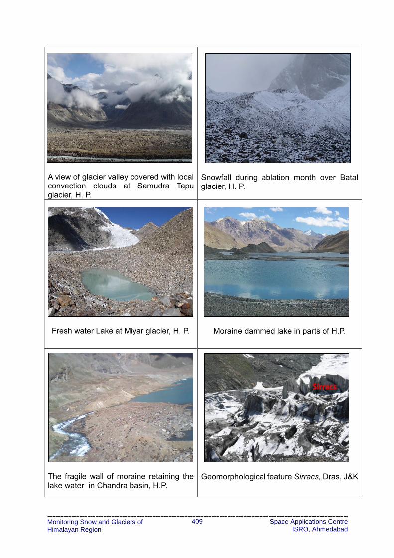
409
Monitoring Snow and Glaciers of Himalayan Region
Space Applications Centre ISRO, Ahmedabad
A view of glacier valley covered with local convection clouds at Samudra Tapu glacier, H. P.
Snowfall during ablation month over Batal glacier, H. P.
Fresh water Lake at Miyar glacier, H. P.
Moraine dammed lake in parts of H.P.
The fragile wall of moraine retaining the lake water in Chandra basin, H.P.
Geomorphological feature Sirracs, Dras, J&K

410
Monitoring Snow and Glaciers of Himalayan Region
Space Applications Centre ISRO, Ahmedabad
Lateral moraine and Debris cover of glacier in Miyar valley, H.P.
Striations in the deglaciated region of the glacier, Chandra basin H.P.
Downside view of deglaciated terminal moraine deposits in Chandra basin, H.P.
Erratic boulder in Chandra basin, H.P.
Ropeway (Local Jhula) to cross the river in Baspa valley, H.P.
Expedition kit & members crossing river as bridge was not usable in Baspa valley, H.P.

411
Monitoring Snow and Glaciers of Himalayan Region
Space Applications Centre ISRO, Ahmedabad
Field Lab at Chhota Dara, H.P.
Inside view of Field Lab at Chhota Dara, H.P.
GPR survey over Debris cover Glacier in Dras, J&K
Automatic Weather Station at Chhota Dara, H.P.
Black Carbon (BC) measurement using Aethalometer over Glacier in Dras, J&K
Observations of Energy balance parameters in glaciated region at Chhota Shigri glacier, H.P.

412
Monitoring Snow and Glaciers of Himalayan Region
Space Applications Centre ISRO, Ahmedabad
Measuring glaciological mass balance using bamboo sticks, Dras, J&K
Ephedra intermedia- Artemesia maritima community, Basapa Valley, H.P.
Cotoneaster bacillaris community, Basapa Valley, H.P.
Rosa webbiana community, Basapa Valley, H.P.
Caragana brevifolia community, Basapa Valley, H.P.
Hyssopus officinalis- Chrysopogon gryllus- Asperula oppositifolia mixed community, Basapa Valley, H.P.

413
Monitoring Snow and Glaciers of Himalayan Region
Space Applications Centre ISRO, Ahmedabad
Snow fall covering tents at Glacier base camp in Chandra basin, H.P.
A view of Kedarnath valley downhill to Chora Bari glacier, Uttarakhand
A view of glacier base camp during glacier expedition of Nardu glacier, Baspa sub-basin, H. P.
Expedition team members at Chhota Shigri glacier, H.P.
Expedition team members at Machoi glacier, Dras, J&K
Expedition team members at Nardu glacier Baspa sub-basin, H. P.

Printed by:
Chandrika Corporation, Ahmedabadwww.sac.gov.in