
PRINCIPLES OF SNOW HYDROLOGY
428
-
Upload
khangminh22 -
Category
Documents
-
view
0 -
download
0
Transcript of PRINCIPLES OF SNOW HYDROLOGY

This page intentionally left blank
PRINCIPLES OF SNOW HYDROLOGY
Snow hydrology is a specialized field of hydrology that is of particular importance for high latitudesand mountainous terrain. In many parts of the world, river and groundwater supplies for domestic, irri-gation, industrial, and ecosystem needs are generated from snowmelt, and an in-depth understandingof snow hydrology is of clear importance. Study of the impacts of global warming has also stimulatedinterest in snow hydrology because increased air temperatures are projected to have major impactson the snow hydrology of cold regions.
Principles of Snow Hydrology describes the factors that control the accumulation, melting, andrunoff of water from seasonal snowpacks over the surface of the earth. The book addresses not onlythe basic principles governing snow in the hydrologic cycle, but also the latest applications of remotesensing, and principles applicable to modelling streamflow from snowmelt across large, mixed land-use river basins. Individual chapters are devoted to climatology and distribution of snow, ground-basedmeasurements and remote sensing of snowpack characteristics, snowpack energy exchange, snowchemistry, modelling snowmelt runoff (including the SRM model developed by Rango and others),and principles of snowpack management on urban, agricultural, forest, and range lands. There arelists of terms, review questions, and problems with solutions for many chapters available online atwww.cambridge.org/9780521823623.
This book is invaluable for all those needing an in-depth knowledge of snow hydrology. It isa reference book for practising water resources managers and a textbook for advanced hydrologyand water resources courses which span fields such as engineering, Earth sciences, meteorology,biogeochemistry, forestry and range management, and water resources planning.
David R. DeWalle is a Professor of Forest Hydrology with the School of Forest Resources atthe Pennsylvania State University, and is also Director of the Pennsylvania Water Resources ResearchCenter. He received his BS and MS degrees in forestry from the University of Missouri, and hisPhD in watershed management from Colorado State University. DeWalle has conducted researchon the impacts of atmospheric deposition, urbanization, forest harvesting, and climate change onthe hydrology and health of watersheds in Pennsylvania. He regularly teaches courses in watershedmanagement, snow hydrology, and forest microclimatology. In addition to holding numerous admin-istrative positions at Penn State, such as Associate Director of the Institutes of the Environment andForest Science Program Chair, DeWalle has been major advisor to over 50 MS and PhD studentssince coming to Penn State in 1969. DeWalle has also been a visiting scientist with the Universityof Canterbury in New Zealand, University of East Anglia in England, and most recently the USDA,Agricultural Research Service in Las Cruces, New Mexico. He has served as President and is a fellowof the American Water Resources Association.
Albert Rango is a Research Hydrologist with the USDA Agricultural Research Service, JornadaExperimental Range, Las Cruces, New Mexico, USA. He received his BS and MS in meteorologyfrom the Pennsylvania State University and his PhD in watershed management from Colorado StateUniversity. Rango has conducted research on snow hydrology, hydrological modelling, effects ofclimate change, rangeland health and remediation, and applications of remote sensing. He has beenPresident of the International Commission on Remote Sensing, the Western Snow Conference, andthe American Water Resources Association. He is a fellow of the Western Snow Conference and theAmerican Water Resources Association. He received the NASA Exceptional Service Medal (1974),the Agricultural Research Service Scientist of the Year Award (1999), and the Presidential RankAward – Meritorious Senior Professional (2005). He has published over 350 professional papers.


PRINCIPLES OF
SNOW HYDROLOGY
DAVID R. DEWALLEPennsylvania State University, USA
ALBERT RANGOUnited States Department of Agriculture

CAMBRIDGE UNIVERSITY PRESS
Cambridge, New York, Melbourne, Madrid, Cape Town, Singapore, São Paulo
Cambridge University PressThe Edinburgh Building, Cambridge CB2 8RU, UK
First published in print format
ISBN-13 978-0-521-82362-3
ISBN-13 978-0-511-41400-8
© D. R. DeWalle and A. Rango 2008
2008
Information on this title: www.cambridge.org/9780521823623
This publication is in copyright. Subject to statutory exception and to the provision of relevant collective licensing agreements, no reproduction of any part may take place without the written permission of Cambridge University Press.
Cambridge University Press has no responsibility for the persistence or accuracy of urls for external or third-party internet websites referred to in this publication, and does not guarantee that any content on such websites is, or will remain, accurate or appropriate.
Published in the United States of America by Cambridge University Press, New York
www.cambridge.org
eBook (EBL)
hardback

Contents
Preface page vii
1 Introduction 1
2 Snow climatology and snow distribution 20
3 Snowpack condition 48
4 Ground-based snowfall and snowpack measurements 76
5 Remote sensing of the snowpack 118
6 Snowpack energy exchange: basic theory 146
7 Snowpack energy exchange: topographic and forest effects 182
8 Snowfall, snowpack, and meltwater chemistry 211
9 Snowmelt-runoff processes 235
10 Modelling snowmelt runoff 266
11 Snowmelt-Runoff Model (SRM) 306
12 Snowpack management and modifications 365
Appendix A: Physical constants 392
Appendix B: Potential solar irradiation theory 394
Index 403
The color plates are situated between pages 234 and 235.
v


Preface
This book is the culmination of several years of effort to create an up-to-date
text book and reference book on snow hydrology. Our interest in snow hydrology
was initiated while we were both taking an early snow hydrology class taught by
Dr. James R. Meiman at Colorado State University. The book is an outgrowth of
our interest in snow hydrology borne out of that class and later experiences while
teaching snow hydrology courses of our own and conducting snow-related research.
The book includes the basics of snow hydrology and updated information about
remote sensing, blowing snow, soil frost, melt prediction, climate change, snow
avalanches, and distributed modelling of snowmelt runoff, especially considering
the effects of topography and forests. A separate chapter is devoted to the SRM
or Snowmelt Runoff Model that Rango helped to develop, which includes the
use of satellite snow-cover data. We have also added a chapter on management
of snowpacks in rangeland, cropland, forest, alpine, and urban settings. Topics
related to glaciology and glacial hydrology were largely avoided. The chapters are
sequenced so that students with a basic understanding of hydrology and physics
can progressively learn the principles of snow hydrology in a semester-long class.
The book can serve as a text in an upper-level undergraduate or graduate-level
class. We have included example computations in some of the chapters to enhance
understanding. A website has been created for students with example problems and
discussion questions related to specific chapters.
The authors are indebted to employers, colleagues, students, and family for mak-
ing this book possible. Work began on the book during spring 2001 while DeWalle
was on sabbatical leave from Penn State at USDA, Agricultural Research Service at
Beltsville, MD. During summer 2001 the USDA ARS kindly provided support for
Dr. DeWalle in Las Cruces, NM to continue this work. Over the intervening years
many colleagues offered advice and comments on the various chapters, notably
John Pomeroy (Chapter 2), Takeshi Ohta (Chapter 7), Martyn Tranter (Chapter 8),
Doug Kane (Chapter 9), George Leavesley and Kevin Dressler (Chapter 10), and
vii

viii Preface
James Meiman (Chapters 2, 3, and 12). Students in several of DeWalle’s snow
hydrology classes at Penn State also provided useful feedback. We appreciate the
many helpful comments we have received, but in the final analysis we are respon-
sible for any errors and mistakes. Penn State students Anthony Buda helped with
literature searches, Brian Younkin helped prepare figures, and Sarah MacDougall
helped with formatting the text. Staff at Penn State Institutes of the Environment,
especially Sandy Beck, Chris Pfeiffer, and Patty Craig also provided valuable help.
We are also very appreciative of the many people who kindly gave permissions to
use figures, data, photos, etc. for the book. Finally, we are grateful to our families,
especially spouses Nancy and Josie, for their support while this book writing project
was underway.
Book Cover
Cover photo courtesy Dr. Randy Julander (United States Department of Agriculture,
Natural Resources Conservation Service) showing Upper Stillwater Dam on Rock
Creek, tributary to the Duchesne River and then Green River, on the south slope of
the Uintah Mountains near Tabiona, Utah.

1
Introduction
1.1 Perceptions of snow
There is a general lack of appreciation by society of the importance of snow to
everyday life. One good example of this is found in the Rio Grande Basin in the
southwestern United States and Mexico. The Rio Grande, the third longest river
in the United States, is sustained by snow accumulation and melt in the mountain
rim regions which provide a major contribution to the total streamflow, despite its
flowing right through the heart of North America’s largest desert (Chihuahuan).
Because the majority of the population in the basin resides in a few large cities in
the Rio Grande Valley, which are all located in the desert (see Figure 1.1), there is
little realization on the part of the urban residents that snowmelt far to the north is an
important factor in their lives. This same situation is true in many arid mountainous
regions around the globe. Where agricultural water use predominates, however,
the importance of snow for the water supply and food production is more widely
known, at least by farmers and ranchers and the rural populace.
The importance of snow during and in the aftermath of a snowstorm is immedi-
ately evident because of its significant effect on transportation (see Figure 1.2). The
effects of snowstorms on wagon trains (in the past), railroads, and motorized trans-
port are widely documented by Mergen (1997). Except for very small countries, the
effect of a snowstorm on transportation is localized and does not affect the entire
country. Such local effects are evident in the United States as in the leeward areas
of the Great Lakes where persistent and heavy annual snowfalls occur, such as over
370 in (940 cm) on the Tughill Plateau area of upstate New York (Macierowski,
1979). Areas just a short distance away, however, have annual averages of only
about 65 in (165 cm) a year. Storm tracks or snowbands are relatively narrow, so
that the majority of the population is seldom impacted but small regions can be
severely impacted (see Figure 1.3). One exception to this in winter in the United
States is when a low-pressure area tracks its way from the Gulf of Mexico all the
1

2 Introduction
Figure 1.1 Location of the Rio Grande Basin in the United States and Mexico withlarge cities identified in relation to mountain snowpack areas and desert areas.

1.1 Perceptions of snow 3
Figure 1.2 The effect of snow on transportation as documented on the frontpage of the Providence, Rhode Island, “The Evening Bulletin,” on Wednesday,February 8, 1978 (from www.quahog.org/include/image.php?id=133).
way up the eastern US coast where the majority of the US population is concen-
trated. Figure 1.4 shows the snow depth map compiled from ground measurements
associated with the “Blizzard of 1996” which was a “Nor’easter.”
If the storm is particularly severe, normal transport can be shut down for
extended periods. Figure 1.5 shows the clearing of mountain highways in the
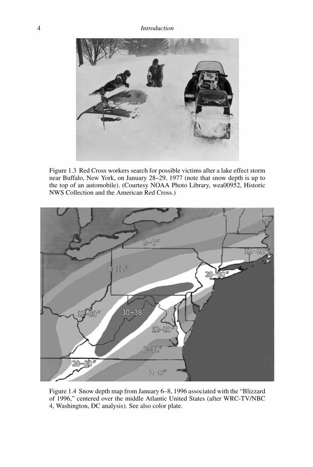
4 Introduction
Figure 1.3 Red Cross workers search for possible victims after a lake effect stormnear Buffalo, New York, on January 28–29, 1977 (note that snow depth is up tothe top of an automobile). (Courtesy NOAA Photo Library, wea00952, HistoricNWS Collection and the American Red Cross.)
Figure 1.4 Snow depth map from January 6–8, 1996 associated with the “Blizzardof 1996,” centered over the middle Atlantic United States (after WRC-TV/NBC4, Washington, DC analysis). See also color plate.

1.1 Perceptions of snow 5
Figure 1.5 Transportation department snow blower at work clearing Highway 143between Cedar Breaks and Panguitch, Utah in 2005. (Courtesy R. Julander.) Seealso color plate.
western United States. Additionally, in these severe snowstorms, communication
is frequently disrupted by downed utility lines. Those affected for that period of
time would certainly support the (in this case, negative) importance of snow.
Because of the disruptions to human activities caused by extreme snowfalls,
Kocin and Uccellini (2004) developed a Northeast Snowfall Impact Scale (NESIS)
to categorize snow storms in the northeast United States. The scale is based upon the
amount of snowfall, the areal distribution of the snowfall and the human population
density in the affected areas. Maximum category 5 “Extreme” events are those like
the January 1996 event (NESIS rating = 11.54) depicted in Figure 1.4 with up to 75-
cm snowfall depths which affected about 82 million people over nearly 0.81 million
square kilometers in the Northeast. At the other extreme, category 1 “Notable”
events were those like the February 2003 event (NESIS rating = 1.18) with up to
25-cm snowfall depths which affected 50 million people over 0.23 million square
kilometers. The NESIS ratings of storms combined with information about wind
speeds controlling drifting during and after snowfall should significantly improve
our appreciation of the severity of impacts of snowfall.
When a fresh snowfall blankets the landscape, most people will agree that snow
is aesthetically pleasing and a positive visual experience. Less widely known and

6 Introduction
more important, however, is that a snow cover radically changes the properties of
the Earth’s surface by increasing albedo and also insulating the surface. Extremely
cold air temperatures may exist right above the surface of the snow, but the insulat-
ing effect can protect the underlying soil and keep it relatively warm and unfrozen.
In General Circulation Models (GCM), it is important to precisely locate the areas
of the Earth’s surface covered by snow because of the great differences in energy
and water fluxes between the atmosphere and snow-covered and snow-free por-
tions of the landscape. Because such differences are important in the reliability of
simulations produced by GCMs, providing correct snow cover inputs to GCMs is
critical.
In many areas of the world like the western United States, snow accumulation and
subsequent melt are the most critical determining factors for producing an adequate
water supply. To quantitatively estimate this water supply, including volume, timing,
and quality, it is important to have a detailed understanding of snow hydrology
processes, the goal of this book. As water demand outstrips the water supply,
which is happening in most of the world today, this knowledge of snow hydrology
becomes increasingly important.
The technology of remote sensing has had a major impact on data collection
for measuring snow accumulation and snow ablation rates. The reasons for the
ready application of remote sensing to snow hydrology are multifaceted. Significant
snowpacks accumulate and deplete in remote, inaccessible areas that are easily
imaged with remote-sensing platforms. These snowpack processes in mountain
regions are active generally during the most inhospitable time of year which makes
considerations of human safety important. The use of remote-sensing approaches
is much safer than employing ground access during these times. In most cases, the
appearance of snow in various types of remote-sensing data products is strikingly
different from snow-free surfaces, allowing snow mapping in different spectral
bands.
A surprising amount of biological activity occurs within and beneath the snow
cover, especially so for deep snowpacks, because of warm soil conditions promoted
by the insulating effect of the snow (see Jones et al., 2001). This insulating effect
protects many types of vegetation from the low air temperatures just above the snow
surface. In many cases, plant survival is dependent upon the occurrence of a regular
winter snowpack. In agriculture, this property is relied upon for the survival of the
winter wheat crop which requires a snowpack of 10 cm or more (Steppuhn, 1981).
For the world’s winter wheat crop, the Food and Agriculture Organization (1978)
has estimated that each centimeter of snow from 5–10 cm in depth would produce
a crop survival benefit of $297 000 000 cm−1 (Steppuhn, 1981).
Small animals survive beneath the snowpack for the same reasons as certain
plants. About 20 cm of snow depth seems to be the breakpoint to allow such activity

1.2 History of snow hydrology 7
(a) (b)
Figure 1.6 (a) Sample of red snow (containing green algae cells, Chlamydomonasnivalis) taken from a snowfield surface near the South Cascade Glacier and imagedwith the Low-Temperature Scanning Electron Microscope (LTSEM) showingenlarged view of two individual cells. (b) LTSEM image of an ice worm (a speciesof oligochaetes) which was collected 1 m below the top of the seasonal snowpacknear South Cascade Glacier. (Courtesy USDA, Agricultural Research Service,Beltsville, MD.)
(Jones et al., 2001). The snow itself is the habitat for various micro-organisms like
snow worms and algae which are shown in Figures 1.6(a) and (b) taken with a Low-
Temperature Scanning Electron Microscope. See Jones, et al. (2001) for further
details on snow ecology.
1.2 History of snow hydrology
Although history suggests that technical understanding of snow hydrology was
a relatively recent phenomenon, some evidence exists that the role of snow was
understood by some very early in our study of the physical world. References to
the philosophy of the ancient Greek, Anaxagoras (500–428 BCE), indicate a rather
surprising early understanding of the relationships between river flows and freezing
and thawing of water, for example (Franks 1898): “The Nile comes from the snow

8 Introduction
in Ethiopia which melts in summer and freezes in winter” (Aet. Plac. iv 1;385);
“And the Nile increases in summer because waters flow down into it from snowsat the north” (Hipp. Phil. 8; Dox. 561). Passages from the Bible also show an
early general understanding of the role of snow in the natural world, most notably
perhaps: “For as the rain and the snow come down from heaven, And do not returnthere without watering the earth, And making it bear and sprout, And furnishingseed to the sower and bread to the eater.” (Isaiah 55:10, New American Standard
Bible®, Copyright C© 1995 by the Lockman Foundation, used by permission). These
early references show that some basic concepts underpinning snow hydrology have
existed for millennia.
Much later, literature from the writings of naturalist/geologist Antonio Vallisnieri
(1661–1730) in Italy showed specific recognition of the role of snow in hydrology.
He correctly theorized that rivers arising from springs in the Italian Alps came from
rain and snowmelt seeping into underground channels (attributed to Lupi, F. W.,
www.killerplants.com/whats-in-a-name/20030725.asp).
In the United States during World War II, the US Army Corps of Engineers and
the US Weather Bureau initiated the Cooperative Snow Investigations in 1944 (US
Army Corps of Engineers, 1956). The snow investigations were organized to address
specific snow hydrology problems that were being encountered by both agencies. In
order to meet snow hydrology objectives of both agencies, it was deemed necessary
to establish fundamental research in the physics of snow. An extensive laboratory
program across the western United States was established and observations were
gathered starting in 1945. Analysis of these data formed the basis for developing
the basic relationships and methods of application derived to develop solutions to
the key snow hydrology problems (US Army Corps of Engineers, 1956).
Three snow laboratories were established: the Central Sierra Snow Laboratory
(CSSL), Soda Springs, CA (see Figure 1.7); the Upper Columbia Snow Laboratory
(UCSL), Marias Pass, MT; and the Willamette Basin Snow Laboratory (WBSL)
Blue River, OR. The drainage areas where the research was concentrated had areas
as follows: CSSL, 10.26 km2; UCSL, 53.61 km2; and WBSL, 29.81 km2. Although
the major report coming from these studies was written in 1956 (US Army Corps
of Engineers, 1956), this book, Snow Hydrology, is still an excellent reference book
for students and forms the basis for much of the information on snow hydrology in
basic hydrology texts.
Both the CSSL and WBSL received snow indicative of maritime-influenced cli-
mate conditions. The UCSL snowfall was influenced by both maritime and conti-
nental climate conditions. A fourth snow laboratory was established for cooperative
snow investigations by the US Bureau of Reclamation and the US Forest Service at
the Fraser Experimental Forest, Fraser, CO. Continuous measurements were made
there starting in 1947. The climate conditions influencing snowfall at Fraser are

1.2 History of snow hydrology 9
Figure 1.7 Instrumentation at the Central Sierra Snow Laboratory in Soda Springs,California. (Courtesy R. Osterhuber.) See also color plate.
more of a true continental origin than the UCSL. The emphasis at Fraser was on
evaluation of various snow and runoff measurements, development of snowmelt-
runoff forecasting techniques, and the effect of forest management on water yield
from snow-fed basins. The final report of the project, Factors Affecting Snowmeltand Streamflow (Garstka et al., 1958), has also been identified as a significant con-
tribution to understanding snow hydrology. Snow hydrology research has continued
to the current day at the CSSL and the Fraser Experimental Forest.
Outside the United States, a number of snow laboratories and research watersheds
were established. The Marmot Creek Basin (9.4 km2), about 80 km west of Calgary,
Alberta, Canada, was instrumented in 1962 to study the water balance in a typical
subalpine spruce-fir forested watershed (Storr, 1967). A network of 40 precipitation
gauges and 20 snow courses cover the basin. The overriding reason for establishing
this research basin was to determine the effects of forest clearing practices on snow
accumulation and streamflow. Treatments were performed in 1974 which involved
clear-cutting five separate blocks ranging from 8–13 ha (Forsythe, 1997).
Work in Russia on snow hydrology began in the 1930s, but, as in the United
States, specific field research sites were set up in the mid- to late 1940s. The primary
field sites were the Valdai Hydrological Research Laboratory and the Dubovskoye

10 Introduction
Hydrological Laboratory. Much Russian work on heat and water balance of snow,
snow cover observations, and snow metamorphism is reported by Kuz′min (1961).
In the same work, the arrangements of permanent snow stakes and instrumentation,
like gamma ray snow water equivalent detection systems, are reported.
In 1959, the Chinese Academy of Sciences established the Tianshan Glaciolog-
ical Station at the source of the Urumqi River in the Tianshan Mountains at 3600 m
above sea level (a.s.l.) to provide comprehensive observations and studies of
snowmelt and glacier hydrology. The station has full research facilities and living
accommodation for both permanent staff and visiting scholars (Liu et al., 1991).
Studies are conducted on the total Urumqi River basin (4684 km2) and also on
the part of the basin only in the mountains (Ying Qiongqia hydrometric station,
924 km2). Recent studies at the Tianshan Glaciological Station have emphasized
effects of global climate change, ice and snow physical processes, energy and
mass balances of glaciers and snow, water balances of the upper mountain snow
zone, and application of advanced observation technology, including remote sens-
ing. Applications of outside investigators to participate in research at the Tianskan
Glaciological Station are encouraged.
Several notable texts on snow hydrology also exist from early and recent lit-
erature. Kuz′min’s (1961) summary book on Melting of Snow, which has been
translated into English, is a rich source of information about early Russian studies.
The Handbook of Snow edited by Gray and Male (1981) dealt with a wide variety
of snow topics, including hydrology. Singh and Singh (2001) have written a book,
Snow and Glacier Hydrology, that covers topics in snow hydrology and glaciology
and some fundamentals of hydrology. Seidel and Martinec (2004) concentrate on
remote-sensing applications in Remote Sensing and Snow Hydrology.
1.3 Snow hydrology research basins
Experimental basins established for snow hydrology research have had two major
functions. First would be for the purpose of collecting all types of snow information
for better understanding the physics of snow hydrology. An example of such a basin
would be the Reynolds Creek Watershed in southwestern Idaho. The second pur-
pose is for evaluating the effectiveness of snow management treatments to manip-
ulate the quantity, quality, and timing of streamflow. The first example of this in
the United States was the Wagon Wheel Gap experiment in the Upper Rio Grande
Basin of Colorado (Bates and Henry, 1922; 1928). Both the data collection and
snow management functions can be satisfied in the same research area. A good
example of this would be at the previously mentioned Fraser Experimental Forest
where long-term snow hydrology data have been collected and a classic, paired-
watershed study was used to evaluate the effects of forest clear-cutting on snowmelt

1.3 Snow hydrology research basins 11
Figure 1.8 Fool Creek clear-cut watershed near the center and the East St. LouisCreek control watershed to the right of center, both in the Fraser ExperimentalForest, Colorado. (US Forest Service Photo, courtesy C. Leaf.)
runoff using the Fool Creek and East St. Louis Creek Basins (Goodell, 1958; 1959)
(Figure 1.8).
Various basins are representative of different snow hydrology regions. Reynolds
Creek (239 km2) (Figure 1.9) is administered by the USDA Agricultural Research
Service (ARS) and is indicative of high relief, semiarid rangelands where seasonal
snow and frozen soil dominate the annual hydrologic cycle (Slaughter and Richard-
son, 2000). Data have been collected for 38 years. Another USDA/ARS original
experimental watershed, the Sleepers River Basin (111 km2) in Vermont, started
operation in 1958 (Figure 1.10). It is indicative of snow hydrology processes in
northeastern United States forested basins. After ARS, this basin was administered
by the National Weather Service and now jointly by the US Geological Survey and
the US Army Cold Regions Research and Engineering Laboratory. The US For-
est Service administers another forested snow research basin in the northeastern
United States – the Hubbard Brook Basin (31.4 km2) near North Woodstock, New
Hampshire. In the central Rocky Mountains, the USGS administers the Loch Vale
Watershed in the Rocky Mountain National Park, Colorado, a small glacierized
basin (6.6 km2). Seasonal snow accumulation and melt are the major drivers of the

12 Introduction
Figure 1.9 Site of the 239 km2 Reynolds Creek Experimental Watershed in theOwyhee Mountains about 80 km southwest of Boise, Idaho, operated by theAgriculture Research Service. (Courtesy USDA, Agriculture Research Service;www.ars.usda.gov/is/graphics/photos/.) See also color plate.
hydrologic cycle in this basin. A similar basin (7.1 km2) in the Green Lakes region
of Colorado is part of the Niwot Ridge LTER project and is run by the University
of Colorado (Bowman and Seastedt, 2001). There are numerous additional basins
across the snow zone of the United States that are administered by US Government
agencies or universities where significant snow research is being conducted. Many
times it is possible to become a collaborating investigator and thereby gain access
to a valuable snow data resource.
Today, given Internet availability of data and services, key sources of information
related to snow hydrology from Federal agencies within the United States can also
be found at:
� USDA, Natural Resources Conservation Service – SNOTEL network of pressure pillows,
snow survey data, forecasts of streamflow from snowmelt.� USDC, NOAA, National Operational Hydrologic Remote-Sensing Center – satellite snow
cover, gamma radiation surveys, maps and interactive products.� USDI, Geological Survey – streamflow and groundwater data.� USDC, NOAA, National Snow and Ice Data Center – polar and cyrospheric research
center, snow cover, sea and ground ice, and more.

1.4 Properties of water, ice, and snow 13
Figure 1.10 Outlet of the W-3 watershed in the Sleepers River Basin in Vermontduring snowmelt. (Courtesy S. Sebestyen.)
� USDC, NOAA, National Climate Data Center – precipitation, snowfall, temperature, and
other data.� US Dept. of the Army, Corps of Engineers, Cold Regions Research and Engineering
Laboratory – basic research on snow, ice, and frozen ground with application to the
military.� US National Atmospheric Deposition Program – precipitation chemistry.
1.4 Properties of water, ice, and snow
Snow hydrology is affected in important ways by the physical and chemical prop-
erties of water. Properties such as the density, specific heat, melting and freezing
point, adhesion and cohesion, viscosity, and solubility of water are all affected by
molecular structure. In this section a brief review is given of the molecular structure
of water and ice and how it affects properties of water in all its phases, in preparation
for more detailed discussions in later chapters. Physical properties of air, water, and
ice useful to snow hydrologists are given in Appendix Tables A1 and A2.
14 Introduction
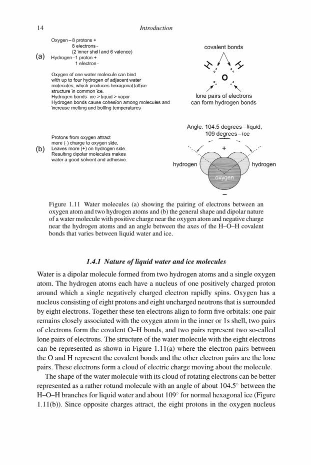
Figure 1.11 Water molecules (a) showing the pairing of electrons between anoxygen atom and two hydrogen atoms and (b) the general shape and dipolar natureof a water molecule with positive charge near the oxygen atom and negative chargenear the hydrogen atoms and an angle between the axes of the H–O–H covalentbonds that varies between liquid water and ice.
1.4.1 Nature of liquid water and ice molecules
Water is a dipolar molecule formed from two hydrogen atoms and a single oxygen
atom. The hydrogen atoms each have a nucleus of one positively charged proton
around which a single negatively charged electron rapidly spins. Oxygen has a
nucleus consisting of eight protons and eight uncharged neutrons that is surrounded
by eight electrons. Together these ten electrons align to form five orbitals: one pair
remains closely associated with the oxygen atom in the inner or 1s shell, two pairs
of electrons form the covalent O–H bonds, and two pairs represent two so-called
lone pairs of electrons. The structure of the water molecule with the eight electrons
can be represented as shown in Figure 1.11(a) where the electron pairs between
the O and H represent the covalent bonds and the other electron pairs are the lone
pairs. These electrons form a cloud of electric charge moving about the molecule.
The shape of the water molecule with its cloud of rotating electrons can be better
represented as a rather rotund molecule with an angle of about 104.5◦ between the
H–O–H branches for liquid water and about 109◦ for normal hexagonal ice (Figure
1.11(b)). Since opposite charges attract, the eight protons in the oxygen nucleus

1.4 Properties of water, ice, and snow 15
Figure 1.12 Hexagonal structure of normal or Ih ice showing the oxygen atoms(dark circles) and hydrogen atoms (gray bars) with four hydrogen bonds betweenoxygen atoms in one molecule and hydrogen atoms in adjacent molecules (withpermission from K. G. Libbrecht, Caltech from the SnowCrystals.com website).
exert a stronger attraction for the electrons than the hydrogen nucleii with one
proton each, leaving the hydrogen side of the molecule with slightly less electron
charge than the oxygen side which has a higher density of negative charge. Thus, as
shown in Figure 1.11(b), the oxygen side represents the negatively charged part and
the hydrogen side represents the positively charged part of the electric field around
the water molecule, giving the molecule its dipolar nature. The dipolar nature of the
water molecule gives water its ability to act as a solvent and its adhesive nature.
Since there are two lone electron pairs in a water molecule, each oxygen can align
with up to four hydrogen atoms from adjacent water molecules forming what are
known as hydrogen bonds. These hydrogen bonds are much weaker than covalent
bonds and in a liquid form near freezing the bonds are continually being formed and
broken. Each oxygen in liquid water is associated with about 3.4 hydrogen atoms,
while in ice the bonds are more permanent with about four hydrogen bonds per
oxygen being formed. Even fewer hydrogen bonds exist for water in a vapor form.
Regardless, hydrogen bonding among molecules of water leads to much higher
intermolecular attractive forces which causes higher melting and boiling points,
higher specific heat, and higher latent heats of fusion and vaporization for water
than most other liquids.
The hydrogen bonds in ice produce a characteristic hexagonal lattice struc-
ture represented in Figure 1.12. Ice can exist in at least 10 other forms, but for
16 Introduction
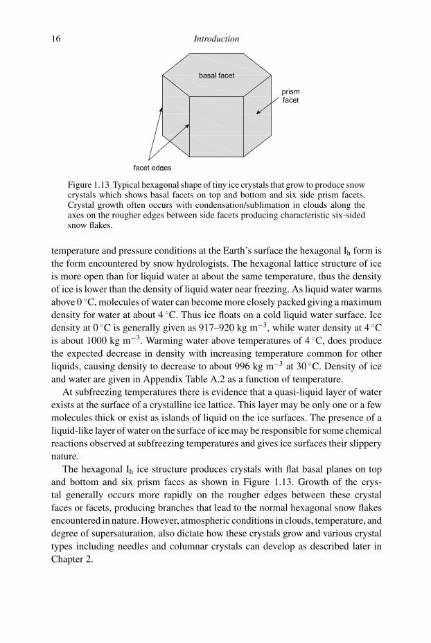
Figure 1.13 Typical hexagonal shape of tiny ice crystals that grow to produce snowcrystals which shows basal facets on top and bottom and six side prism facets.Crystal growth often occurs with condensation/sublimation in clouds along theaxes on the rougher edges between side facets producing characteristic six-sidedsnow flakes.
temperature and pressure conditions at the Earth’s surface the hexagonal Ih form is
the form encountered by snow hydrologists. The hexagonal lattice structure of ice
is more open than for liquid water at about the same temperature, thus the density
of ice is lower than the density of liquid water near freezing. As liquid water warms
above 0 ◦C, molecules of water can become more closely packed giving a maximum
density for water at about 4 ◦C. Thus ice floats on a cold liquid water surface. Ice
density at 0 ◦C is generally given as 917–920 kg m−3, while water density at 4 ◦C
is about 1000 kg m−3. Warming water above temperatures of 4 ◦C, does produce
the expected decrease in density with increasing temperature common for other
liquids, causing density to decrease to about 996 kg m−3 at 30 ◦C. Density of ice
and water are given in Appendix Table A.2 as a function of temperature.
At subfreezing temperatures there is evidence that a quasi-liquid layer of water
exists at the surface of a crystalline ice lattice. This layer may be only one or a few
molecules thick or exist as islands of liquid on the ice surfaces. The presence of a
liquid-like layer of water on the surface of ice may be responsible for some chemical
reactions observed at subfreezing temperatures and gives ice surfaces their slippery
nature.
The hexagonal Ih ice structure produces crystals with flat basal planes on top
and bottom and six prism faces as shown in Figure 1.13. Growth of the crys-
tal generally occurs more rapidly on the rougher edges between these crystal
faces or facets, producing branches that lead to the normal hexagonal snow flakes
encountered in nature. However, atmospheric conditions in clouds, temperature, and
degree of supersaturation, also dictate how these crystals grow and various crystal
types including needles and columnar crystals can develop as described later in
Chapter 2.

1.4 Properties of water, ice, and snow 17
Table 1.1 Description of phase changes of water. (Based upon data in List, 1963.)
PHASECHANGE PROCESS ENERGY EXCHANGEDa
MJ kg−1
@ 0 ◦C
Liquid → Vapor Evaporation Latent heat of vaporization (Lv) −2.501Vapor → Liquid Condensation Latent heat of vaporization (Lv) +2.501Solid → Liquid Melting Latent heat of fusion (Lf) −0.334Liquid → Solid Freezing Latent heat of fusion (Lf) +0.334Solid ↔ Vapor Sublimation, either way Latent heat of sublimation (Ls) ±2.835
a Lv in MJ kg−1 = 3 × 10⁻⁶T 2 − 0.0025T + 2.4999, −50 ◦C ≤ T ≤ 40 ◦CLf in MJ kg−1 = −1 × 10⁻⁵T 2 + 0.0019T + 0.3332, −50 ◦C ≤ T ≤ 0 ◦CLs in MJ kg−1 = Lv + Lf, −50 ◦C ≤ T ≤ 0 ◦C
1.4.2 Phase changes of water
An understanding of phase changes of water in the environment is fundamental
to snow hydrology. Water commonly exists in all three phases – gas, liquid, and
solid – at the same time in cold environments. Changes in phase involve energy
transfer expressed as latent heats in MJ kg−1 (Table 1.1), which vary slightly with
temperature. Latent heats can be adjusted to a specific temperature using equations
given at the bottom of Table 1.1. The latent heat of sublimation at subfreezing
temperatures is the sum of the respective latent heats of vaporization and fusion.
At the freezing point, the latent heat of vaporization is approximately 7.5 times
greater than the latent heat of fusion. Thus, condensation/evaporation of water
involves 7.5 times more energy exchange per kg than melt/freeze conditions.
1.4.3 Snowpack water equivalent
One of the most common properties of snowpacks needed by snow hydrologists
is snowpack water equivalent. The water equivalent of a snowpack represents the
liquid water that would be released upon complete melting of the snowpack. Water
equivalent is measured directly or computed from measurements of depth and
density of the snowpack as:
SWE = d(ρs/ρw) (1.1)
SWE = water equivalent, m
d = snowpack depth, m
ρs = snowpack density, kg m−3
ρw = density of liquid water, approx. 1×10³ kg m−3

18 Introduction
Given measurements of snowpack depth of 0.22 m and snowpack density of
256 kg m−3, the snowpack water equivalent would be:
SWE = (0.22)(256/1000) = 0.0563 m or 5.6 cm
Snowpack water equivalent includes any liquid water that may be stored in the
snowpack along with the ice crystals at the time of measurement. Snowpack water
equivalent is treated as a primary input to the discussion of snow hydrology in the
following chapters.
1.5 References
Bates, C. G. and Henry, A. J. (1928). Forest and streamflow experiment at Wagon WheelGap, CO.: final report on completion of second phase of the experiment. Mon.Weather Rev., 53(3), 79–85.
Bates, C. G. and Henry, A. J. (1922). Streamflow experiment at Wagon Wheel Gap, CO.:preliminary report on termination of first stage of the experiment. Mon. Weather Rev.,(Suppl. 17).
Bowman, W. D. and Seastedt, T. R. (eds.) (2001). Structure and Function of an AlpineEcosystem, Niwot Ridge, CO. Oxford: Oxford University Press.
Food and Agriculture Organization (1978). 1977 Production Yearbook: FAO Statistics,vol. 31, Ser. No. 15. Rome: United Nations Food and Agriculture Organization.
Forsythe, K. W. (1997). Stepwise multiple regression snow models: GIS application in theMarmot Creek Basin (Kananaskis Country, Alberta) Canada and the National ParkBerchtesgaden, (Bayern) Germany. In Proceedings of the 65th Annual Meeting of theWestern Snow Conference, Banff, Alberta, Canada, pp. 238–47.
Franks, A. (1898). (ed., trans.). The First Philosophers of Greece. London: Kegan Paul,Trench, Trubner, and Company.
Garstka, W. U., Love, L. D., Goodell, B. C., and Bertle, F. A. (1958). Factors AffectingSnowmelt and Streamflow; a Report on the 1946–53 Cooperative SnowInvestigations at the Fraser Experimental Forest, Fraser, CO. Denver, CO: USDAForest Service, Rocky Mountain Forest and Range Experiment Station and USDIBureau of Reclamation, Division of Project Investigations.
Goodell, B. C. (1958). A Preliminary Report on the First Year’s Effects of TimberHarvesting on Water Yield from a Colorado Watershed. No. 36. Fort Collins, CO:Rocky Mountain Forest and Range Experiment Station, USDA Forest Service.
Goodell, B. C. (1959). Management of forest stands in western United States to influencethe flow of snow-fed streams. International Association of Scientific Hydrology, 48,49–58.
Gray, D. M. and Male, D. H. (1981). Handbook of Snow, Principles, Processes,Management and Use. Ontario: Pergamon Press.
Jones, H. G., Pomeroy, J. W., Walker, D. A., and Hohem, R. W. (eds.). (2001). SnowEcology. Cambridge: Cambridge University Press.
Kocin, P. J. and Uccellini, L. W. (2004). A snowfall impact scale derived from Northeaststorm snowfall distributions. Bulletin Amer. Meteorol. Soc., 85(Feb), 177–194.
Kuz′min, P. P. (1961). Protsess tayaniya shezhnogo pokrova (Melting of Snow Cover).Glavnoe Upravlenie Gidrometeorologischeskoi Sluzhby Pri Sovete Ministrov SSSRGosudarstvennyi Gidrologischeskii Institut. Main Admin. Hydrometeorol. Service,

1.5 References 19
USSR Council Ministers, State Hydrol. Institute. Translated by Israel Program forScientific Translations. Avail from US Dept. Commerce, National Tech. Inform.Service, 1971, TT 71–50095.
List, R. J. (1963). Smithsonian meteorological tables. In Revised Edited SmithsonianMiscellaneous Collections. Vol. 114, 6th edn. Washington, DC: SmithsonianInstitution.
Liu, C., Zhang, Y., Ren, B., Qui, G., Yang, D., Wang, Z., Huang, M., Kang, E., and Zhang,Z. (1991). Handbook of Tianshan Glaciological Station. Gansu: Science andTechnology Press.
Macierowski, M. J. (1979). Lake Effect Snows East of Lake Ontario. Booneville, NY:Booneville Graphics.
Mergen, B. (1997). Snow in America. Washington, DC: Smithsonian Institution Press.Seidel, K. and Martinec, J. (2004). Remote Sensing in Snow Hydrology: Runoff Modeling,
Effect of Climate Change. Berlin: Springer-Praxis.Singh, P. and Singh, V. P. (2001). Snow and Glacier Hydrology. Water Science and
Technol. Library, vol. 37, Dordrecht: Kluwer Academic Publishers.Slaughter, C. W. and Richardson, C. W. (2000). Long-term watershed research in
USDA-Agricultural Research Service. Water Resources Impact, 2(4), 28–31.Steppuhn, H. (1981). Snow and Agriculture. In The Handbook of Snow, ed. D. M. Gray
and D. H. Male, Willowdale, Ontario: Pergamon Press, pp. 60–125.Storr, D. (1967). Precipitation variations in a small forested watershed. In Proceedings of
the 35th Annual Meeting of the Western Snow Conference, Boise, ID, pp. 11–17.US Army Corps of Engineers. (1956). Snow Hydrology: Summary Report of the Snow
Investigations. Portland, OR: US Army Corps of Engineers, North Pacific Division.

2
Snow climatology and snow distribution
One of the most fundamental aspects of snow hydrology is an understanding of the
processes that lead to snowfall and the eventual distribution of a snowpack on the
landscape. The factors that lead to the formation of snowfall are generally discussed
in the beginning sections of this chapter. Since snowfall once formed, unlike rain, is
quite easily borne by the wind and redistributed across the landscape before finally
coming to rest to form a snowpack, the basic principles controlling blowing snow
are also reviewed. Finally, the interception of snow by vegetation, that can have a
profound effect on the amount and timing of snow that accumulates into a snowpack
beneath a plant canopy, is described in the last section of the chapter.
2.1 Snowfall formation
The occurrence of snowfall in a region is generally dependent upon several geo-
graphic and climatic factors: latitude, altitude, the distance from major water bodies,
and the nature of regional air mass circulation (McKay and Gray, 1981). General
discussions of the climatic factors affecting snowfall formation and precipitation
are given by Sumner (1988) and Ahrens (1988). Latitude and altitude largely control
the temperature regime of a region and dictate where it is cold enough for snowfall
to occur. Virtually no snowfall occurs in low latitudes where the heat balance at
the Earth’s surface causes air temperatures to average well above freezing during
winter. Since air temperature declines with altitude, higher altitudes generally mean
lower air temperatures and greater opportunity for snowfall to occur. Proximity to
major water bodies affects atmospheric moisture supplies needed for snowfall for-
mation. However, atmospheric circulation is needed to transport water vapor and
ultimately controls the nature of interactions between the land surface and various
air masses in a region. Regions typically downwind from oceans or large lakes
receive moist air that can lead to snowfall, providing temperatures are low enough
at the surface. Circulation of moist air over mountain ranges or moist, warm air
20

2.1 Snowfall formation 21
over cold, dry air masses can cause uplifting and cooling leading to snowfall. Given
cold air and an adequate supply of moisture, it is the atmospheric circulation that
ultimately explains the local and regional snowfall climatology. In this section, the
meteorological factors affecting snowfall are described.
All precipitation ultimately depends upon air becoming saturated with water
vapor. A primary mechanism for saturation to occur in the atmosphere is uplifting
which cools the air below the dewpoint temperature. Uplifting of air can occur by
uplifting over mountains and other terrain features, frontal activity, convection, and
convergence in the atmosphere. Saturation can also be achieved by contact of cold
air with relatively warm water surfaces. In either case, saturation levels are reached
in the air mass and ice crystal and snowflake formation may begin.
2.1.1 Ice crystal and snowflake formation in clouds
The creation of snow and ice crystals within cold clouds is a complicated process
that largely involves the interaction of super-cooled water droplets and tiny ice
crystals (Schemenauer et al., 1981; Sumner, 1988). Super-cooled water droplets
form in clouds by condensation of water vapor on condensation nuclei from soil
dust, pollution, forest fires, sea salt spray, and other sources. These droplets can
exist at temperatures below freezing in clouds that are supersaturated with water
vapor. Tiny ice crystals also form in such clouds due to spontaneous freezing of
super-cooled water droplets, sublimation of vapor onto freezing nuclei, and freezing
of droplets onto freezing nuclei. Freezing nuclei are thought to be certain types of
clay minerals carried in the atmosphere that resemble ice crystals.
Whatever the cause, tiny water droplets and ice crystals coexist in cold clouds
at the same temperature. This coexistence is a dynamic one due to the fact that the
saturation vapor pressure over the droplets is slightly greater than that over the ice
crystals. Thus, there is a transfer of water vapor from the droplets to the crystals and
crystals grow at the expense of droplets. This process is referred to as the Bergeron
process and is schematically depicted in Figure 2.1. By this process, crystals can
grow in clouds as long there is a sufficient supply of vapor to the cloud. The type
and shape of ice crystals formed by this process is primarily a function of tem-
perature and secondarily a function of the degree of supersaturation in the clouds
(Figure 2.2). Crystals also grow due to interactions with other crystals and contact
with super-cooled water droplets to create snow flakes and other types of frozen
precipitation. Crystal contact with super-cooled water droplets causes freezing onto
the surface and a gradual rounding of the crystal by a process referred to as riming.
Heavily rimed crystals are referred to as graupel. When crystals accrete to a size and
mass that allows gravitational settling, they fall from the cloud. Some pictures of
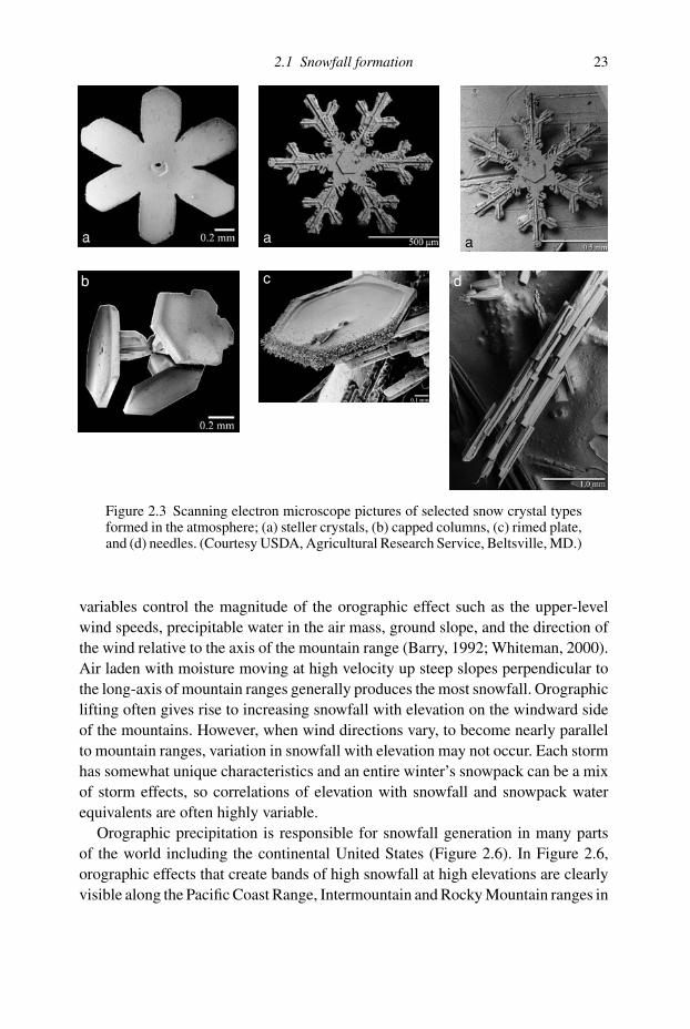
falling snow crystal types taken with a scanning electron microscope are shown in
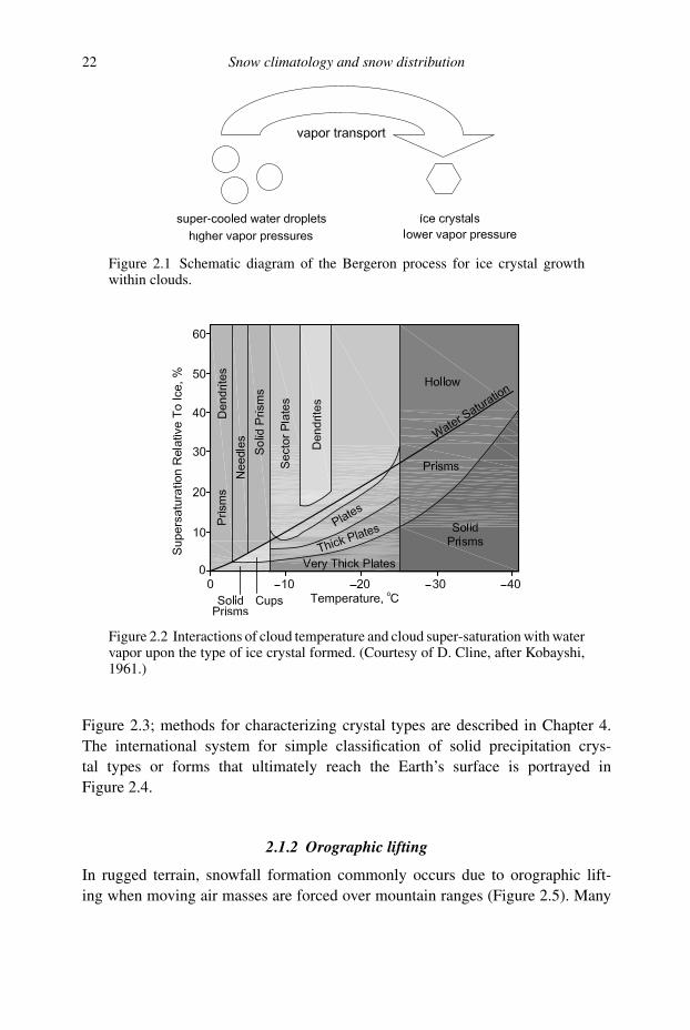
22 Snow climatology and snow distribution
Figure 2.1 Schematic diagram of the Bergeron process for ice crystal growthwithin clouds.
Figure 2.2 Interactions of cloud temperature and cloud super-saturation with watervapor upon the type of ice crystal formed. (Courtesy of D. Cline, after Kobayshi,1961.)
Figure 2.3; methods for characterizing crystal types are described in Chapter 4.
The international system for simple classification of solid precipitation crys-
tal types or forms that ultimately reach the Earth’s surface is portrayed in
Figure 2.4.
2.1.2 Orographic lifting
In rugged terrain, snowfall formation commonly occurs due to orographic lift-
ing when moving air masses are forced over mountain ranges (Figure 2.5). Many
2.1 Snowfall formation 23
a a
b c d
Figure 2.3 Scanning electron microscope pictures of selected snow crystal typesformed in the atmosphere; (a) steller crystals, (b) capped columns, (c) rimed plate,and (d) needles. (Courtesy USDA, Agricultural Research Service, Beltsville, MD.)
variables control the magnitude of the orographic effect such as the upper-level
wind speeds, precipitable water in the air mass, ground slope, and the direction of
the wind relative to the axis of the mountain range (Barry, 1992; Whiteman, 2000).
Air laden with moisture moving at high velocity up steep slopes perpendicular to
the long-axis of mountain ranges generally produces the most snowfall. Orographic
lifting often gives rise to increasing snowfall with elevation on the windward side
of the mountains. However, when wind directions vary, to become nearly parallel
to mountain ranges, variation in snowfall with elevation may not occur. Each storm
has somewhat unique characteristics and an entire winter’s snowpack can be a mix
of storm effects, so correlations of elevation with snowfall and snowpack water
equivalents are often highly variable.
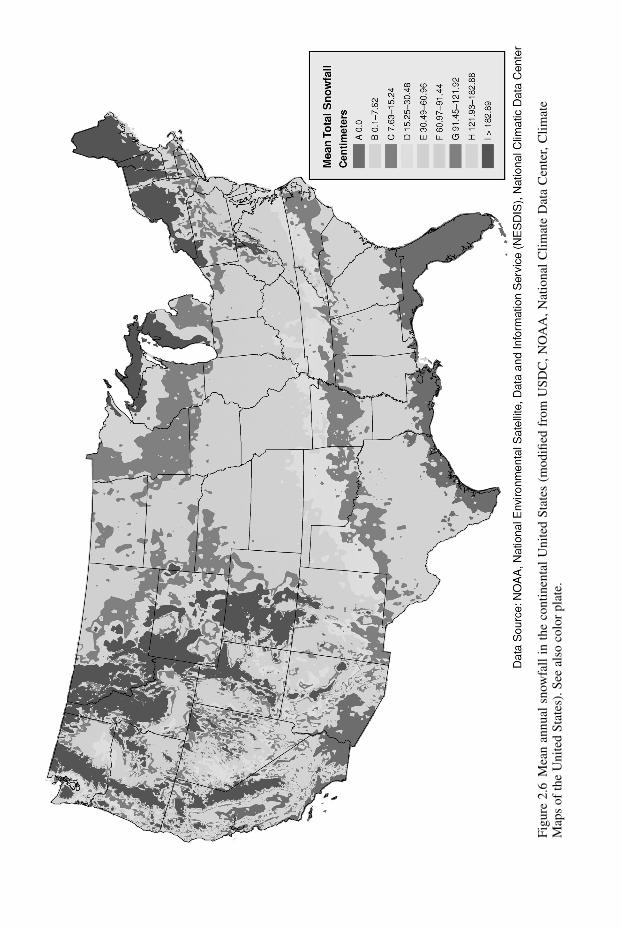
Orographic precipitation is responsible for snowfall generation in many parts
of the world including the continental United States (Figure 2.6). In Figure 2.6,
orographic effects that create bands of high snowfall at high elevations are clearly
visible along the Pacific Coast Range, Intermountain and Rocky Mountain ranges in

24 Snow climatology and snow distribution
CodeGraphicSymbol Typical Forms Terms
Plates
Stellar cyrstals
Columns
Needles
Spatila dendrites
Capped columns
Irregular particles
Graupel (soft hail)
Ice pellets (Am. sleet)
Hail
Typ
e o
f p
arti
cle
(F)
Figure 2.4 Snow crystal forms from the international classification system forsolid precipitation (adapted from Mason, 1971).
the west and Appalachian Mountain range in the east. Bands of gradually increasing
mean annual snowfall with increasing latitude are also visible in the central region
of the country. High snowfall downwind from the Great Lakes due to lake-effect
snow is also evident as discussed in the section on lake-effect snowfall.
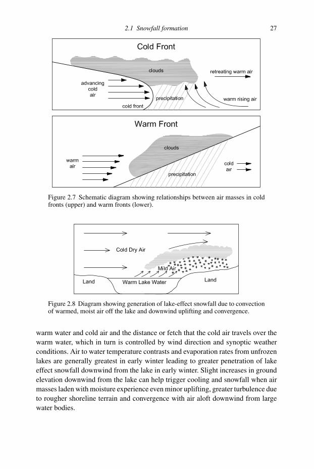
2.1.3 Frontal activity
The uplifting of air masses associated with warm fronts (warm air moving horizon-
tally and being uplifted over cool air) or cold fronts (cool air pushing under warm

2.1 Snowfall formation 25
Figure 2.5 Orographic snowfall generation.
air) also can lead to snowfall (Figure 2.7). The boundary between cool air and warm
air is much steeper with cold fronts than with warm fronts. Thus, cold fronts give
rise to more rapid uplifting and more intense snowfall, but generally over a smaller
geographic area and for a shorter duration at a point than warm fronts. Snowfall
associated with warm fronts is often spread over a broader area, but with lower
intensity.
2.1.4 Convergence
Air converging towards regions of low pressure at the surface can result in uplift
and cooling and widespread snowfall. Convergence at the surface is accompanied
by divergence aloft. When divergence aloft is greater than convergence at the sur-
face the low pressure and uplifting at the surface intensifies. Frontal activity often
accompanies low-level convergence around a surface low-pressure center. Terrain
features can also cause convergence of air flows around isolated mountains or
through narrow valleys and cause localized uplift and snowfall.
2.1.5 Lake-effect snowfalls
Convection due to contact of cold air with warm surfaces such as large unfrozen
water bodies in winter can cause uplifting and localized heavy snowfall in winter
(Figure 2.8). Convection over mountains when exposed rock surfaces are heated
by the Sun can also lead to localized convection and light snowfall/graupel events
even in summer.
Lake-effect snowfalls influence snow accumulation over hundreds of kilometers
downwind from the Great Lakes in North America (Figure 2.9) and can be respon-
sible for some of the highest snowfall intensities recorded. Lake-effect snows can
be attributed to uplifting caused by the addition of moisture and heat to cold, dry
continental air in contact with a warm, unfrozen lake surface. The magnitude of
the lake-effect snowfall effect is controlled by the temperature contrast between the
26 Snow climatology and snow distribution
Fig
ure
2.6
Mea
nan
nu
alsn
owfa
llin
the
con
tin
enta
lU
nit
edS
tate
s(m
od
ified
fro
mU
SD
C,
NO
AA
,N
atio
nal
Cli
mat
eD
ata
Cen
ter,
Cli
mat
eM
aps
of
the
Un
ited
Sta
tes)
.S
eeal
soco
lor
pla
te.
2.1 Snowfall formation 27
Figure 2.7 Schematic diagram showing relationships between air masses in coldfronts (upper) and warm fronts (lower).
Figure 2.8 Diagram showing generation of lake-effect snowfall due to convectionof warmed, moist air off the lake and downwind uplifting and convergence.
warm water and cold air and the distance or fetch that the cold air travels over the
warm water, which in turn is controlled by wind direction and synoptic weather
conditions. Air to water temperature contrasts and evaporation rates from unfrozen
lakes are generally greatest in early winter leading to greater penetration of lake
effect snowfall downwind from the lake in early winter. Slight increases in ground
elevation downwind from the lake can help trigger cooling and snowfall when air
masses laden with moisture experience even minor uplifting, greater turbulence due
to rougher shoreline terrain and convergence with air aloft downwind from large
water bodies.

28 Snow climatology and snow distribution
Figure 2.9 Distribution of annual snowfall around the Great Lakes in NorthAmerica during 1951–80 showing enhanced downwind snowfall due to lake-effect snowfalls (adapted from Norton and Bolsenga, 1993, C© 1993 AmericanMeterological Society).
2.1.6 El Nino/La Nina Southern Oscillation effects
The Southern Oscillation which gives rise to El Nino conditions, or its counterpart
La Nina conditions, is now known to have far-reaching effects on global climate
and snowfall (Clark et al., 2001; Smith and O’Brien, 2001; Kunkel and Angel,
1999). El Nino conditions are represented by warm southern Pacific Ocean surface
temperatures off the west coast of Peru during winter, while La Nina conditions
in contrast are represented by cool sea surface temperatures in that region. The
occurrence of El Nino or La Nina conditions alternate within a period of about
three to seven years, although the El Nino events have been much more frequent in
recent years. The causes and forecasting of these oscillations are the topics for much
research, but their effect on climate and snowfall is rapidly becoming appreciated.
These oscillations between ocean surface warming and cooling cause shifts in
the position of the jet stream over North America that can influence regional and
even global climate. El Nino events cause the jet stream to be deflected northward
towards Alaska and are associated with warmer, dryer winter conditions and lower
snowfall in the western United States. In contrast, La Nina conditions direct the

2.2 Blowing snow 29
0
20
40
60
80
100
120
140
160
180
Seattle WA PortlandOR
SpokaneWA
Boise ID BozemanMT
Salt LakeCity UT
Mea
n s
no
wfa
ll, c
mLa Nina
Neutral
El Nino
Moderate and Strong La Nina and El Nino years only
Figure 2.10 Mean winter snowfall for locations in the Pacific Northwest and west-ern regions of the United States for La Nina, Neutral and El Nino years (adaptedfrom USDC, NOAA, Climate Prediction Center, El Nino/LaNina Snowfall forSelected US Cities).
jet stream toward the Pacific Northwest of the United States where it produces
slightly cooler and relatively moist winters with greater snowfall. Figure 2.10 shows
snowfall totals for November–March for El Nino, La Nina, and Neutral years
at various locations in the Pacific Northwest and western regions of the United
States. Snowfall totals in moderate to strong La Nina years averaged higher than in
moderate to strong El Nino years, while neutral years generally had intermediate
snowfall totals. Several investigators have found that snowpack and streamflow
from snowmelt in the northwest United States can be related to indicies of the
strength of the Southern Oscillation (for example see Beebee and Manga 2004,
McCabe and Dettinger 2002).
2.2 Blowing snow
Snow is often transported by the wind for distances measured in km before it
sublimates or comes to rest to form a snowpack. Blowing snow creates problems
with direct measure of snowfall using standard precipitation gauges as described in
Chapter 4 and also leads to very irregular snowpack distribution. Uneven snowpack
distribution in turn causes serious problems with modelling snowmelt runoff due
to uneven melt water delivery to soils across a watershed. Recent development of
snowpack remote-sensing methods and theoretical models for computing fluxes of

30 Snow climatology and snow distribution
Figure 2.11 Modes of transport for blowing snow.
blowing snow have helped account for blowing-snow effects. Sublimation of blow-
ing snow can also result in losses of as much as 50% of winter precipitation. Losses
of this magnitude in regions with low precipitation and without supplemental irri-
gation can have significant impacts on spring soil moisture levels and agricultural
productivity. Blowing snow also interacts with vegetation, especially trees, to influ-
ence the magnitude of canopy interception losses. Canopy interception losses are
discussed in the following section of this chapter. For many reasons, an enhanced
understanding of blowing-snow processes is important to snow hydrology.
2.2.1 Modes of blowing-snow transport
Three major modes of transport are commonly recognized for transport of blowing
snow: turbulent suspension, saltation, and creep (Figure 2.11). Transport of snow
in full turbulent suspension occurs when the uplift due to turbulent eddies in the
air can completely support the ice grains against settling due to gravity. Turbulent
suspension generally involves transport of smaller ice and snow particles and can
involve an air layer up to several meters thick. Larger particles that are only partially
supported by turbulent eddies are often transported in the saltation mode where the
particles bounce and skip along the ground surface. Saltation occurs in a layer only
a few centimeters thick over the snow surface, but blowing-snow episodes always
begin with saltation and the subsequent breaking and loosening of surface snow
particles. Saltating particles often loosen others upon impact with the surface. Under
some conditions ice particles may also be transported by surface creep where large,
loose particles simply slide or roll along the surface due to the force of the wind.
The dominant mode and magnitude of blowing-snow transport depends upon the
interaction of climate, snow surface conditions, and terrain features, but in general
transport is dominated by suspension and secondarily by saltation.

2.2 Blowing snow 31
2.2.2 Factors influencing blowing snow
Blowing-snow occurrence generally depends upon interactions among climatic,
snow surface, and topographic conditions (Kind, 1981). Blowing snow over a
smooth unobstructed snowpack surface begins whenever the force of the wind or
shear stress on the surface exceeds the snowpack surface shear strength that resists
movement. Shear stress of the wind depends upon the roughness of the surface and
wind speed. Rougher surfaces generate greater turbulence and greater shear stress
for a given wind speed. Wind shear also increases with wind speed and conse-
quently the winter climatology of an area will play an important part in control of
the occurrence of blowing snow. High amounts of snowfall, high wind speeds, and
cold air temperatures that slow metamorphism and melt of the snowpack surface
all contribute to greater masses of blowing snow.
Under neutral stability conditions in the atmosphere, the shear stress of wind
over a uniform snow surface of infinite extent can be related to wind speed (u) and
surface roughness (z0) using the simple logarithmic profile Equation (2.1):
τ = ρk2u2[ln(z/z0)]−2 (2.1)
where:
τ = shear stress, kg m−1 s−2
ρ = air density, kg m−3
k = von Karman’s constant, = 0.4, dimensionless
u = wind speed, m s−1
z0 = roughness length, m
z = height of wind speed measurement, m
Shear stress is also often expressed as a friction velocity (u∗, m s−1) where,
u∗ = (τ/ρ)1/2 = uk[ln(z/z0)]−1 (2.2)
If a wind speed of 2 m s−1 is measured at a height of 2 m above a snow surface
with a roughness length of 0.001 m and the air temperature is −5 ◦C giving an air
density of 1.3 kg m−3, then by Equation (2.1) the shear stress is:
τ = (1.3)(0.4)2(2)2[ln(2/0.001)]−2 = 0.0144 kg m−1 s−2
The corresponding friction velocity by Equation (2.2) would be:
u∗ = (0.0144/1.3)1/2 = 0.105 m s−1
The computed shear stress must be compared to the surface shear strength of
the snow to determine if blowing snow will occur. The condition when the shear
stress increases to the point when snow particles are first set in motion defines the

32 Snow climatology and snow distribution
threshold shear stress, wind speed or friction velocity. Alternatively, the threshold
condition can also be defined as the shear stress, wind speed or friction velocity
when particle motion ceases. Regardless, the threshold shear stress needed to initiate
blowing snow is highly dependent on snow surface metamorphism and bonding of
ice crystals. Fresh, light snow that has not been strongly bonded to surrounding
crystals can exhibit relatively low surface shear strength and be set in motion at
shear stresses of only about 0.01 kg m−1 s−2, while hard, well-bonded or wet snow
surfaces may require shear stresses of 1 kg m−1 s−2 to be scoured by the wind (see
Kind, 1981). Thus in the above example, a wind shear stress of 0.0144 kg m−1 s−2,
corresponding to a 2 m s−1 wind speed, would be sufficient to transport fresh new
snow, but this wind speed would be far too low to erode a hardened compacted
snow surface. In fact, for the same snowpack roughness and air temperature used in
the example, the wind speed would have to be nearly 12 m s−1 to initiate movement
from a hard compacted snow surface. As a rough rule-of-thumb, friction velocities
needed to initiate motion of 0.2 m s−1 can be used for fresh, light snow and 1 m s−1
for hard wind-packed or wet snow. Snowpack metamorphism processes that affect
the shear strength of snowpack surfaces are discussed in Chapter 3 of this book.
Although physical tests of the shear strength of the snow surface can be conducted,
occurrence of blowing snow can be operationally predicted using wind speed, air
temperature, and age of the snowpack surface (Li and Pomeroy, 1997a, 1997b).
During blowing-snow events part of the force of the wind is expended on the
snow surface and part is used to transport blowing snow. Short vegetation like
grasses, forbs, brush, and crop stubble, in areas with sufficient blowing snow, gen-
erally cause drifts to form to the tops of the plants; a process that increases the snow
water stored on the landscape (McFadden et al., 2001). Consequently, changes in
vegetative cover over a watershed can markedly alter the snow storage. When the
tops of plants protrude through the snowpack, part of the force of the wind will
be expended on these objects and less energy will be available to transport snow
from the surface. Intermittent melt events during a winter season allow vegeta-
tion to protrude through the snowpack surface and also increase the bonding of
surface snow crystals, both of which reduce the total amount of blowing snow. Iso-
lated larger objects protruding through the snow, like boulders and tree boles, can
lead to localized scouring and drift formation, while numerous large protrusions
such as groves of trees can completely eliminate the opportunity for blowing snow
by absorbing momentum of the moving air and displacing the entire air stream
upward above the snow surface. However in that case, the force of the wind
can be expended, at least partially, in transport of snow intercepted on the plant
canopy.
Patterns of snowpack accumulation over the landscape are related to regions with
accelerating and decelerating winds due to surface obstructions and topography. The

2.2 Blowing snow 33
mass of blowing snow over flat terrain generally increases in the downwind direction
and reaches a steady state over fetches of 300 m or more. Abrupt transitions such as
fence lines and ridges and more gradual changes in watershed relief, in combination
with prevailing wind directions, can give rise to repeating annual patterns of snow
accumulation and scour. Large drifts often form downwind from obstacles and large
open areas of terrain that represent source areas for blowing snow.
2.2.3 Sublimation of blowing snow
Static snowpack surfaces tend to lose mass by sublimation during winter (see Chap-
ter 9), but sublimation losses are greatly increased when ice particles are transported
by the wind due to the greater amount of exposed surface area and increased con-
vection. Blowing-snow particles will lose mass due to sublimation whenever the
vapor pressure at the ice-particle surface is greater than that in the air (Schmidt,
1972). The vapor pressure at the blowing ice-particle surface is the saturation vapor
pressure with respect to ice and increases as air temperature increases to 0 ◦C. Sub-
limating particles will cool to the ice-bulb temperature and extract sensible heat
from the air by slight cooling (0.5–1 ◦C) of the air layer in contact with the blowing
snow. Solar radiation on clear days can also add energy to the blowing snow par-
ticles and enhance sublimation rates. Air will gradually increase in vapor content
from the sublimating particles and the rise in humidity can limit the rate of subli-
mation downwind, unless the air is exchanged with dryer air from aloft. Despite the
opportunity for humidity increases in the air layer near the ground, very significant
losses of mass from sublimation of blowing snow have been reported.
Table 2.1 shows a wide range in estimates of sublimation losses due to blowing
snow. Most of these results are based upon model calculations, augmented in some
cases by comparisons with field measurements of snow accumulation on the ground
or amounts of blowing snow. Estimated sublimation losses vary from over 40% of
annual snowfall in warm windy climates to only about 10–15% of annual snowfall
in colder and/or calmer sites. Modelling studies by Xiao et al. (2000) and Dery
and Yau (1999) also show that sublimation rates from blowing snow ranging from
about 2 to 3 mm d−1 are possible. In any location, existence of vegetative stubble
protruding through the snow reduces the sublimation loss (Pomeroy and Gray,
1994). In regions with blowing snow and relatively low precipitation, it is obvious
that sublimation can represent a significant loss to the water balance.
2.2.4 Modelling blowing snow
Advances have been made in recent years to improve our ability to model the
impact of blowing snow on the spatial distribution of snowpack water equivalent.
34 Snow climatology and snow distribution
Table 2.1 Estimates of sublimation losses from blowing snow
Reference Location
Sublimation Loss fromBlowing Snow (% ofannual snowfall)
King et al. 2001 Antarctica 12.5%Pomeroy et al. 1998 Arctic 19.5%Pomeroy and Gray 1995 Canadian prairies 15–40%Pomeroy et al. 1997 Western Canadian Arctic 28%Pomeroy and Li 2000 Canadian prairie
Canadian arctic tundra29%22%
Benson 1982 Alaska north slope 32%Pomeroy et al. 1993 Saskatchewan, Canada
Cool, calm site 15–44%Warm, windy site 41–74%
One approach has been to solve the following mass balance for each landscape
segment for months or an entire winter accumulation season (Pomeroy et al.,1997):
Qnet = P − [dQt/dx](x) − Qe (2.3)
where:
Qnet = net snow accumulation flux after sublimation, kg m2 s−1
P = snowfall flux, kg m2 s−1
Qt = total blowing snow transport flux, kg m2 s−1
Qe = blowing snow sublimation flux, kg m2 s−1
Qnet in Equation (2.3) can be either negative (surface is a source of blowing snow) or
positive (surface is a sink for blowing snow) depending upon the balance between
snowfall and the sum of sublimation and wind transport of snow at a specific
point on the landscape. Assuming that P is accurately measured or modelled for a
watershed, then computations of Qe and Qt as a function of downwind position (x)
are needed to compute Qnet.
Tabler et al. (1990) reviewed the functions used to compute the mass flux and
sublimation rates for blowing snow. By computing the transport of blowing snow
and subtracting sublimation, they presented Equation (2.4) to predict the total sea-
sonal transport of blowing snow that provides an “excellent first approximation” of
the snow available for trapping using snow fencing as:
Q′net = 500DP(1 − 0.14F/D) (2.4)

2.2 Blowing snow 35
where:
Q′net = net mass of blowing snow for a winter season, kg m−1
D = distance an average snow particle travels before completely sublimating, m
P = water equivalent of winter snowfall, m
F = fetch or length of upwind source area for blowing snow, m
In Equation (2.4) increases in winter snowfall (P) or fetch (F) that provides more
source area for blowing snow can lead to increased blowing snow flux. The net flux
of blowing snow after sublimation is measured as mass per unit width perpendic-
ular to the prevailing wind direction. Average snow particle size, wind speed, and
humidity conditions in an area are embodied in the D parameter in Equation (2.4),
which for Wyoming conditions was computed as 3000 m. However, greater subli-
mation rates, which would lead to shorter distances for the average snow particle
to sublimate (lower D), would reduce Q′net.
To estimate the mass of blowing snow available downwind from a plain of
1000 m length (F) in a region with 0.3 m of annual snowfall water equivalent and
an average distance that a snow particle travels before sublimating completely of
3500 m (D):
Q′net = (500)(3500)(0.3)(1 − 0.141000/3500) = 225 630 kg m−1
for the winter season.
More recently, Pomeroy et al. (1997) used a set of empirical relationships based
upon theoretical modelling with the Prairie Blowing Snow Model (PBSM) to quan-
tify the Qt and Qe fluxes in Equation (2.3) as a function of fetch distance, snowpack,
and meteorological variables over level watershed surfaces. As shown in Figure 2.12
from their paper, the instantaneous flux of blowing snow (dQt/dx) increases rapidly
and peaks within the first 300 m of fetch and then gradually declines with increas-
ing distance (x). The total flux of blowing snow (Qt) reaches a nearly steady rate
as dQt/dx approaches zero. The total flux of sublimated water gradually increases
with increasing fetch. Many other modelling approaches are being used to quan-
tify the fluxes of blowing and sublimating snow (Xiao et al., 2000; Dery and Yau,
1999) with some explicitly considering effects of varying alpine or mountain terrain
and vegetation (Essery et al., 1999, Gauer, 2001; Liston and Sturm, 1998; Prasad
et al., 2001; Liston et al., 2002). Rapid advances are being made using these models
for more realistic simulations of snowmelt hydrology for watersheds affected by
blowing snow.

36 Snow climatology and snow distribution
Q t
Qe
dQ t/dx
Figure 2.12 Estimated annual blowing-snow flux variations with fetch normalizedto 1000 m values on level terrain; Qt = blowing snow transport flux and Qe =blowing snow sublimation flux (Pomeroy et al. 1997, C© 1997, John Wiley & Sons,reproduced with permission).
2.3 Snow interception by vegetation
Snowfall often interacts with vegetation before it forms a snowpack over the land-
scape. Snow that is lodged within the canopies of plants is referred to as intercepted
snow, while snow that falls or drips to the ground from or through the canopy is
termed throughfall. Throughfall from intercepted snow can be in the form of ice
particles dislodged by the wind that filter through the canopy during cold, windy
conditions or in the form of large masses of intercepted snow that slide from the plant
branches during warm, melting conditions or as branches bend under the weight
of intercepted snow. Meltwater from intercepted snow that reaches the ground by
flowing down the stems of plants is called stemflow. Stemflow is a minor path-
way for intercepted water to reach the ground (Brooks et al., 1997; Johnson, 1990),
especially in winter when melt rates from intercepted snow are often much less than
rainfall rates. Intercepted snow can be sublimated or evaporated from the canopy
before reaching the ground and the mass lost to the atmosphere is referred to as
interception loss. Interception loss can occur while the snow is stored within the
canopy or as the intercepted snow is being redistributed within and over the land-
scape by the wind. Knowledge of the distribution and type of vegetation across a
watershed is essential in successfully modelling effects of interception on snowmelt
runoff.
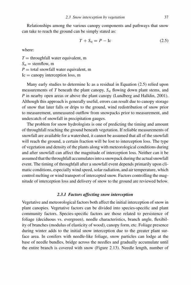
2.3 Snow interception by vegetation 37
Relationships among the various canopy components and pathways that snow
can take to reach the ground can be simply stated as:
T + Sst = P − Ic (2.5)
where:
T = throughfall water equivalent, m
Sst = stemflow, m
P = total snowfall water equivalent, m
Ic = canopy interception loss, m
Many early studies to determine Ic as a residual in Equation (2.5) relied upon
measurements of T beneath the plant canopy, Sst flowing down plant stems, and
P in nearby open areas or above the plant canopy (Lundberg and Halldin, 2001).
Although this approach is generally useful, errors can result due to canopy storage
of snow that later falls or drips to the ground, wind redistribution of snow prior
to measurement, unmeasured outflow from snowpacks prior to measurement, and
undercatch of snowfall in precipitation gauges.
The problem for snow hydrologists is one of predicting the timing and amount
of throughfall reaching the ground beneath vegetation. If reliable measurements of
snowfall are available for a watershed, it cannot be assumed that all of the snowfall
will reach the ground, a certain fraction will be lost to interception loss. The type
of vegetation and density of the plants along with meteorological conditions during
and after snowfall can affect the magnitude of interception loss. Neither can it be
assumed that the throughfall accumulates into a snowpack during the actual snowfall
event. The timing of throughfall after a snowfall event depends primarily upon cli-
matic conditions, especially wind speed, solar radiation, and air temperature, which
control melting or wind transport of intercepted snow. Factors controlling the mag-
nitude of interception loss and delivery of snow to the ground are reviewed below.
2.3.1 Factors affecting snow interception
Vegetative and meteorological factors both affect the initial interception of snow in
plant canopies. Vegetative factors can be divided into species-specific and plant
community factors. Species-specific factors are those related to persistence of
foliage (deciduous vs. evergreen), needle characteristics, branch angle, flexibil-
ity of branches (modulus of elasticity of wood), canopy form, etc. Foliage presence
during winter adds to the initial snow interception due to the greater plant sur-
face area. In conifers with needle-like foliage, snow particles can lodge at the
base of needle bundles, bridge across the needles and gradually accumulate until
the entire branch is covered with snow (Figure 2.13). Needle length, number of

38 Snow climatology and snow distribution
Figure 2.13 Heavy accumulation of intercepted snow on pendulous conifer treebranches showing effects of bridging across needle bundles (top) and interceptedsnow in a mixed hardwood/conifer forest after a wet, cohesive snowfall under calmconditions at 0 ◦C (bottom).

2.3 Snow interception by vegetation 39
needles per bundle, and orientation of needle bundles and branches theoretically
should influence snow catch in conifers, but most studies show minor effects
attributed to species of conifers. Flexibility of branches then determines when
branches bend and unload masses of snow (Schmidt and Gluns, 1991). Schmidt
and Pomeroy (1990) showed that as air temperatures increased from −12 to 0 ◦C
branches became more flexible due to changes in elasticity which helped to explain
the dumping of snow from conifer canopies as air temperatures increased. Scaling
snow interception from individual branches and or an entire tree canopy to full
plant community effects remains a challenge.
Plant community factors relate to the total biomass per unit land area available to
intercept snow that is often indicated as a function of leaf-area index (LAI). Leaf-
area index is defined as projected surface area of leaves and/or needles integrated
from canopy top to ground per unit of ground area. In deciduous plant communities
in winter the plant-area index is used which includes the total surface area of twigs,
branches, and stems (Figure 2.13). Interception increases as leaf- and plant-area
indices increase and species effects are difficult to separate from plant community
effects.
Meteorological factors also affect canopy interception of snow. Conditions dur-
ing snowfall that increase cohesiveness of snow particles, such as air temperatures
approaching 0 ◦C, lead to increased amounts of snow being held within the canopy
(Figure 2.13). Cohesive snow combined with high winds can plaster intercepted
snow deep within tree canopies and onto branches and plant stems. Snow parti-
cles falling at temperatures well below freezing are generally not as cohesive and
either singly or in combination with high wind speeds during snowfall events can
lead to reduced snow interception. Non-cohesive particles can also bounce off of
or dislodge snow already intercepted on branches. Melting of intercepted snow
is also thought to contribute to sliding of snow masses as well as dripping from
canopies. High winds can dislodge intercepted snow long after snowfall events have
occurred. Finally, rainfall occurring on intercepted snow in plant canopies can be
initially stored by the snow, but with sufficient liquid-water inputs, due to added
weight on branches, can eventually lead to liquid throughfall and delivery of large
masses of snow to the ground. It is clear that many interactions between meteoro-
logical conditions and vegetation can occur and regional climates will help dictate
the dominant types of snow interception processes that occur. Excellent reviews of
early literature on snow interception processes were given by Miller (1964, 1966).
2.3.2 Modelling snow interception
Models of interactions between snow and more or less continuous plant canopies
can vary from simple to complex. The simplest approach is to assume a fixed per-
centage of total snowfall is lost due to sublimation in the plant canopy. Many past

40 Snow climatology and snow distribution
mass balance studies show that Ic from snowfall can represent a loss ranging from
about 45% of P for dense evergreens to about 10% of P for leafless deciduous
forests (Lundberg and Halldin, 2001; Essery and Pomeroy, 2001). Storck et al.(2002) showed that in a coastal Douglas-fir forest in Oregon, USA interception
efficiency remained a constant 60% of snowfall both within events and for total
events. Assuming constant percentage interception loss did not account for varia-
tion in canopy density, Pomeroy et al. (2002) modified and validated a method of
estimating snowpack accumulation beneath forest canopies developed by Kuz′min
(1960) for cold climate forests of Canada with an equation in the form:
Sf = Sc{1 − [0.144 ln(LAI′) + 0.223]} (2.6)
and
LAI′ = exp(Cc/0.29 − 1.9) (2.7)
where:
Sf = snowpack accumulation beneath the forest canopy, mm
Sc = snowpack accumulation in a forest opening, mm
LAI′ = effective winter forest leaf- and stem-area index, dimensionless
Cc = winter forest canopy density, dimensionless
These two equations can be used to estimate snow accumulation and indirectly
canopy interception losses in cold regions, where sublimation of intercepted snow
can be significant, using only measurements of snowfall or snowpack in openings
and canopy density.
More complex models involve computation of the amount of initial interception
by the vegetation and the unloading of intercepted snow over time from branches
due to melt, sublimation and dislodgement by gravity or the wind. Hedstrom and
Pomeroy (1998) developed an exponential model that shows interception effi-
ciency starting high for low snowfall amounts and gradually decreasing as snowfall
increases, based upon measurements in boreal forest regions of Canada where sub-
limation losses are significant. This model also accounted for the gradual unloading
of snow from the canopy and is described further below.
According to Hedstrom and Pomeroy (1998) as modified in Pomeroy et al.(1998), an operational model to predict the amount of snow intercepted in the
canopy for each time step could be written as:
I = c(Sm − I0)[1 − exp(−Cc P/Sm)] (2.8)
where:
I = intercepted snow, mm
c = empirical snow canopy unloading coefficient, approx. 0.7 per hour

2.3 Snow interception by vegetation 41
Sm = maximum canopy snow load, mm
I0 = initial canopy snow load, mm
Cc = fractional canopy cover, dimensionless
P = snowfall, mm
They further computed the maximum canopy snow load (S) by scaling maximum
snow storage loads per unit area of branches given by Schmidt and Gluns (1991)
using the LAI for the plant stand as:
Sm = Sb(LAI)(0.27 + 46/ρs) (2.9)
where:
Sm = maximum canopy snow storage, mm
Sb = maximum branch snow storage, 6.6 and 5.9 mm for pine and spruce
forest respectively
LAI = winter leaf- and stem-area index corrected for clumping, dimensionless
ρs = fresh snow density, kg m−3
Using this approach, first the maximum canopy snow storage was computed with
knowledge of the LAI of the forest stand and the fresh snow density in Equation
(2.9). The snow density was computed operationally from air temperatures. Then,
using Equation (2.8), the new intercepted snowfall amount was computed knowing
Sm, any intercepted snow from a previous time period, the canopy cover Cc, and the
snowfall amount for the current time period. Further details are given in Hedstrom
and Pomeroy (1998). If a snowfall of 1 mm with a density of 80 kg m−3 fell
during an hour onto a dry pine forest (Sb = 6.6 mm, I0 = 0) with canopy coverage
of 82% and LAI = 2.2, the canopy interception during that hour would be computed
as:
Equation (2.9): Sm = (6.6)(2.2)(0.27 + 46/80) = 12.3 mm
Equation (2.8): I = (0.7)(12.3 − 0)(1 − exp[(−0.82)(1)/12.3]) = 0.55 mm
or 55% of snowfall would be intercepted at the end of the hour. This storage would
then become the input snow storage (I0) for the next hour’s calculation.
In the above approach, the amount of intercepted snow was predicted over time
and used to estimate sublimation losses using energy balance considerations. The
difference between precipitation amounts and the sum of canopy storage and sub-
limation from the canopy, can be used to approximate throughfall and snowpack
accumulation on the ground. The above relationships were developed for Canadian

42 Snow climatology and snow distribution
Table 2.2 Mean snow interception coefficients for the logistic growth curve modelEquation (2.10) on branches or individual trees
SpeciesSm
mmP0
mmkmm−1 Reference
Douglas-fir(Pseudotsuga menziesii (Mirb.))
2.81 4.88 0.98 Satterlund and Haupt (1967),2 weighed trees
Western white pine(Pinus monticola (Dougl.))
1.84 4.44 1.04 Satterlund and Haupt (1967),2 weighed trees
Englemann spruce(Picea Englemanii (Parry))
5.22 4.14 0.6 Schmidt and Gluns (1991)branch interception
Subalpine fir(Abies lasiocarpa (Hook) Nutt.)
3.94 3.49 0.79 Schmidt and Gluns (1991)branch interception
Lodgepole pine(Pinus contorta Dougl.)
4.35 3.69 0.84 Schmidt and Gluns (1991)branch interception
Conifers 2.58 0.76 0.72 Nakai (1995), trees andbranches
boreal forest conditions without frequent melting and rainfall during the winter, but
do allow for a more complete accounting of the fate of intercepted snow. Gelfan
et al. (2004) recently used this procedure to model accumulation, sublimation, and
melt in conifer forests in Russia. More detailed process studies are needed in the
future to extend such prediction schemes to a broader set of site conditions.
Observations of snow interception on isolated branches and individual trees sug-
gest that cumulative snow interception follows a logistic growth curve. According
to Satterlund and Haupt (1967) snow interception on isolated conifer trees could
be modelled as Equation (2.10):
I = Sm/[1 + e−k(P−P0)] (2.10)
where:
I = water equivalent of intercepted snow storage for an event, mm
Sm = water equivalent of maximum snowfall canopy storage capacity, mm
k = rate of interception storage, mm−1
P0 = water equivalent of snowfall at inflection point on the sigmoid growth
curve, mm
P = water equivalent of snowfall for an event, mm
The values for I, P0, Sm are generally expressed over the projected horizontal area of
the crowns of trees or branches (Table 2.2). The general trend of snow interception
using this type of model is shown in Figure 2.14 using coefficients represent-
ing Douglas-fir trees from Satterlund and Haupt (1967). As snowfall increases the

2.3 Snow interception by vegetation 43
0
0.5
1
1.5
2
2.5
3
0 4 8 12 16 20
Snowfall, mm
Inte
rcep
ted
Sn
ow
, mm
Maximum interception efficiency 35.5%
Figure 2.14 Predicted interception of snow on an isolated conifer canopy withvarying snowfall amounts described using a logistic growth curve. Calculationsare based upon average values for Sm, P0 and k in Equation (2.10) of 2.81 mm, 4.88mm and 0.98 mm−1, respectively, for Douglas-fir (Psuedotsuga menziesii (Mirb.))from Satterlund and Haupt (1967) given in Table 2.2.
interception of snow increases rapidly at a rate indexed by k to the point of inflection
on the logistic growth curve (snowfall around P0) due to cohesion and bridging and
then gradually approaches an asymptote at the canopy or branch maximum canopy
storage (Sm) and as the branches become laden with snow, bend and unload. The
point of inflection of the curve, around a snowfall of 7 mm water equivalent for
specific coefficients chosen in the example, represents a maximum interception
efficiency expressed as a percentage of snowfall of about 35.5% of snowfall inter-
cepted. Not all investigators have found that the logistic growth function applies to
snow interception. Storck et al. (2002) also showed a variety of interception pat-
terns from linear to logistic by studying weight gains of isolated conifer trees during
snowfall.
It is important to realize that initial snow interception in a plant canopy described
by the logistic function does not necessarily represent interception loss due to evap-
oration/sublimation. For example, Satterlund and Haupt (1970) estimated that 80%
of snow initially intercepted on canopies in their isolated conifer tree experiments
eventually fell to the ground as solid or liquid in a relatively humid environment.
Storck et al. (2002) showed that under conditions favoring melting and events

44 Snow climatology and snow distribution
that ended as rain, evaporation or sublimation losses from intercepted snow in a
Douglas-fir canopy in coastal Oregon, USA were essentially zero. Mass release of
intercepted snow falling to the ground accounted for 28% and dripping from the
canopy to the ground represented 72% of snow initially intercepted in the canopy.
For non-melt conditions they found rates of canopy sublimation in excess of 0.5 mm
d−1, but true snow interception losses were only about 5% of winter precipitation
in this humid coastal environment. In contrast, in drier climates where canopies can
retain intercepted snow for days to months after snowfalls, sublimation losses can
be much greater.
2.4 Applications in snow hydrology
Processes controlling snowfall amounts and timing are reasonably well understood,
but snow hydrologists still must rely on precipitation and snowpack measurements
to obtain basic liquid inputs to models. However, as is evident from details in
this chapter, it is becoming possible to predict the distribution of snow across
landscapes due to effects of blowing snow and vegetation interception. Blowing-
snow adjustments are especially needed in cold locations with high wind speeds
where entire slopes may be swept free of snow while others may be deeply drifted.
Basins with a wide variety of land cover types and extensive dense tree and shrub
vegetation will also require adjustment for canopy interception due to differences in
types of vegetation as well as vegetation density. A simple reduction of snowfall for
interception may suffice in some applications, but in others where time and space
scales are expanded, accounting for storage of snow in the canopy and gradual
sublimation losses and intermittent throughfall releases are needed. Much has been
learned, but blowing snow and canopy interception remain two of the most important
challenges for hydrologic simulation in the future.
2.5 References
Ahrens, C. D. (1988). Meteorology Today, 3rd edn. St. Paul, MN: West Publishing Co.Barry, R. G. (1992). Mountain Weather and Climate, 2nd edn. New York: Routledge.Beebee, R. A. and Manga, M. (2004). Variation in the relationship between snowmelt
runoff in Oregon and ENSO and PDO. J. Amer. Water Resour. Assoc., 40, 1011–24.Benson, C. S. (1982). Reassessment of Winter Precipitation on Alaska’s Arctic Slope and
Measurements on the Flux of Windblown Snow, Report UAG R-288. Univ. AlaskaFairbanks: Geophysical Instit.
Brooks, K. N., Ffolliott, P. F., Gregersen, H. M., and DeBano, L. F. (1997). Hydrology andthe Management of Watersheds, 3rd edn. Ames, IA: Iowa State University Press.
Clark, M. P., Serreze, M. C., and McCabe, G. J. (2001). Historical effects of El Nino andLa Nina events on the seasonal evolution of the montane snowpack in the Columbiaand Colorado River Basins. Water Resour. Res., 37(3), 741–57.

2.5 References 45
Dery, S. J. and Yau, M. K. (1999). A bulk blowing snow model. Boundary-LayerMeteorol., 93, 237–51.
Essery, R. and Pomeroy, J. (2001). Sublimation of snow intercepted by coniferous forestcanopies in a climate model. In Proceedings Symposium Soil-Vegetation-AtmosphereTransfer Schemes and Large-Scale Hydrological Models, IAHS Publ. No. 270, SixthIAHS Scientific Assembly, Maastricht, The Netherlands July 2001, pp. 343–7.
Essery, R., Long, L., and Pomeroy, J. (1999). A distributed model of blowing snow overcomplex terrain. Hydrol. Processes, 13, 2423–38.
Gauer, P. (2001). Numerical modelling of blowing and drifting snow in Alpine terrain. J.Glaciol., 47(156), 97–110.
Gelfan, A. N., Pomeroy, J. W., Kuchment, L. S. (2004). Modeling forest cover influenceson snow accumulation, sublimation and melt. J. Hydromet., 5, 785–803.
Hedstrom, N. R. and Pomeroy, J. W. (1998). Measurements and modelling of snowinterception in the boreal forest. Hydrol. Processes, 12, 1611–25.
Johnson, R. C. (1990). The interception, throughfall and stemflow in a forest in HighlandScotland and the comparison with other upland forests in the U.K. J. Hydrol., 118,281–7.
Kind, R. J. (1981). Chap. 8: Snow drifting. In Handbook of Snow, Principles, Processes,Management and Use, ed. D. M. Gray and D. H. Male. Toronto: Pergamon Press,pp. 338–58.
King, J. C., Anderson, P. S., and Mann, G. W. (2001). The seasonal cycle of sublimation atHalley, Antarctica. J. Glaciol., 47(156), 1–8.
Kobayashi, T. (1961). The growth of snow crystals at low supersaturations. PhilosophicalMagazine B, 6, 1363–1370.
Kunkel, K. E. and Angel, J. R. (1999). Relationship of ENSO to snowfall and relatedcyclone activity in the contiguous United States. J. Geophys. Res., 104(D16),19425–34.
Kuz′min, P. P. (1960). Formirovanie Snezhnogo Pokrova i Metody OpredeleniyaSnegozapasov, Gidronmeteoizdat: Leningrad.[Published 1963 as Snow Cover andSnow Reserves. English translation by Israel Program for Scientific Translation,Jerusalem], National Science Foundation, Washington, DC.
Li, L. and Pomeroy, J. W. (1997a). Estimates of threshold wind speeds from snowtransport using meteorological data. J. Appl. Meteorol., 36, 205–13.
Li, L. and Pomeroy, J. W. (1997b). Probability of occurrence of blowing snow. J.Geophys. Res., 102(D18), 21955–64.
Liston, G. E. and Sturm, M. (1998). A snow-transport model for complex terrain. J.Glaciol., 44(148), 498–516.
Liston, G. E., McFadden, J. P., Sturm, M., and Pielke Jr., R. A. (2002). Modelled changesin arctic tundra snow, energy and moisture fluxes due to increased shrubs. GlobalChange Biol., 8(1), 17–32.
Lundberg, A. and Halldin, S. (2001). Snow interception evaporation: review ofmeasurement techniques, processes and models. Theoretical and AppliedClimatology, 70, 117–33.
Mason, B. J. (1971). The Physics of Clouds. Oxford: Clarendon Press.McCabe, G. J., Dettinger, M. J. (2002). Primary modes and predictability of year-to-year
snowpack variations in the western United States from teleconnections with PacificOcean Climate. J. Hydromet., 3, 13–25.
McFadden, J. P., Liston, G. E., Sturm, M., Pielke, R. A. Jr, and Chapin III, F. S. (2001).Interactions of shrubs and snow in arctic tundra measurements and models. InSoil-Vegetation-Atmosphere Transfer Schemes and Large-Scale Hydrological
46 Snow climatology and snow distribution
Models, IAHS Publ. 270, Sixth IAHS Scientific Assembly, Masstricht, TheNetherlands July 2001, pp. 317–25.
McKay, G. A. and Gray, D. M. (1981). Chapter 5: The distribution of snowcover. InHandbook of Snow, Principles, Processes, Management and Use, ed. D. M. Gray andD. H. Male. Toronto: Pergamon Press, pp. 153–90.
Miller, D. H. (1964). Interception Processes during Snowstorms. Res. Paper PSW-18, USForest Service.
Miller, D. H. (1966). Transport of Intercepted Snow from Trees during Snowstorms. Res.Paper PSW-33, US Forest Service.
Nakai, Y. (1995). An observational study on evaporation from intercepted snow on forestcanopies. Unpublished PhD thesis, Kyoto University Japan.
Norton, D. C. and Bolsenga, S. J. (1993). Spatiotemporal trends in lake effect andcontinental snowfall in the Laurentian Great Lakes, 1951–1980. J. Climate, 6,1943–56.
Pomeroy, J. W. and Gray, D. M. (1994). Sensitivity of snow relocation and sublimation toclimate and surface vegetation. In Snow and Ice Covers: Interactions with theAtmosphere and Ecosystems, IAHS Publ. 223, Proceedings of Yokohama SymposiaJ2 and J5, July 1993, pp. 213–25.
Pomeroy, J. W. and Gray, D. M. (1995). Snow Accumulation, Relocation andManagement, NHRI Science Report 7. Saskatoon: Environment Canada.
Pomeroy, J. W. and Li, L. (2000). Prairie and arctic areal snow cover mass balance using ablowing snow model. J. Geophy. Res., 105(D21), 26619–34.
Pomeroy, J. W., Gray, D. M., Hedstrom, N. R., and Janowicz, J. R. (2002). Prediction ofseasonal snow accumulation in cold climate forests. Hydrol. Process., 16, 3543–58.
Pomeroy, J. W., Gray, D. M., and Landine, P. G. (1993). The prairie blowing snow model:characteristics, validation and operation. J. Hydrol., 144, 165–92.
Pomeroy, J. W., Marsh, P., and. Gray, D. M. (1997). Application of a distributed blowingsnow model to the arctic. Hydrol. Processes, 11, 1451–64.
Pomeroy, J. W., Parviainen, J. Hedstrom, N., and Gray, D. M. (1998). Coupled modellingof forest snow interception and sublimation. Hydrol. Processes, 12, 2317–37.
Prasad, R., Tarboton, D. G., Liston, G. E., Luce, C. H., and Seyfried, M. S. (2001). Testinga blowing snow model against distributed snow measurements at Upper Sheep CreekIdaho, USA. Water Resour. Res., 37(5), 1341–50.
Satterlund, D. R. and Haupt, H. F. (1967). Snow catch by conifer crowns. Water Resour.Res., 3(4), 1035–9.
Satterlund, D. R. and Haupt, H. F. (1970). The disposition of snow caught by conifercrowns. Water Resour. Res., 6(2), 649–52.
Schemenauer, R. S., Berry, M. O. and Maxwell J. B. (1981). Chapter 4: Snowfallformation. In Handbook of Snow, Principles, Processes, Management and Use, ed.D. M. Gray and D. H. Male. Toronto: Pergamon Press, pp. 129–52.
Schmidt, R. A., Jr. (1972). Sublimation of Wind-Transported Snow – a Model, ResearchPaper RM-90. Rocky Mtn. For. and Range Exper. Station: USDA Forest Service.
Schmidt, R. A. and Gluns, D. R. (1991). Snowfall interception on branches of threeconifer species. Can. J. For. Res., 21:1262–9.
Schmidt, R. A. and Pomeroy, J. W. (1990). Bending of a conifer branch at subfreezingtemperatures: implications for snow interception. Can. J. For. Res. 20, 1250–53.
Smith, S. R. and O’Brien, J. J. (2001). Regional snowfall distributions associated withENSO: Implications for seasonal forecasting. Bull. Amer. Meteorol. Soc., 82(6),1179–92.

2.5 References 47
Storck, P., Lettenmaier, D. P. and Bolton, S. M. (2002). Measurement of snow interceptionand canopy effects on snow accumulation and melt in a mountainous maritimeclimate, Oregon, U.S. Water Resour. Res., 38(11:1223), 5–1 to 5–16.
Sumner, G. (1988). Precipitation, Processes and Analysis. Chichester: John Wiley andSons.
Tabler, R. D., Pomeroy, J. W., and Santana, B. W. (1990). Drifting snow. In Cold RegionsHydrology and Hydraulics, ed. W. L Ryan and R. D. Crissman. New York: AmericanSociety of Civil Engineers, pp. 95–145.
Whiteman, C. D. (2000). Mountain Meteorology: Fundamentals and Applications. NewYork: Oxford University Press.
Xiao, J., Bintanja, R., Dery, S. J., Mann, G. W., and Taylor, P. A. (2000). Anintercomparison among four models of blowing snow. Boundary-Layer Meteorol.,97, 109–35.

3
Snowpack condition
Once snow has accumulated on the landscape, the individual ice grains can be
rapidly transformed or metamorphosed into a structured snowpack. Metamorphism
ultimately influences the thermal conductivity and liquid permeability of the snow-
pack that in turn influence the snowpack temperature regime and storage and release
of liquid water. Snowpacks vary seasonally from low density, subfreezing snow-
packs capable of refreezing any liquid-water inputs to isothermal, dense snowpacks
that rapidly transmit liquid water to the ground below. In this chapter, important
processes controlling snowpack metamorphism and the conduction of heat and
liquid water in snow are described along with some methods hydrologists use to
describe snowpack condition.
3.1 Snowpack metamorphism
Snow crystals that fall from the atmosphere undergo changes in size and shape
over time as they become part of the snowpack. Owing to their large surface area
to volume ratio, crystals are quite unstable in the snowpack and can transform
to rounded or faceted ice grains. Processes causing metamorphism of ice grains
and snowpacks vary between dry snow and wet snow. Metamorphism within the
snowpack is important to hydrologists because it can ultimately lead to changes in
thermal conductivity and liquid permeability that influences the snowpack energy
budget and release of meltwater. The following discussion of snowpack metamor-
phism is largely based upon writings by Perla and Martinelli (1978) and McClung
and Schaerer (1993). Major snowpack processes for snowpack metamorphism are
summarized in Table 3.1.
3.1.1 Formation of rounded grains in dry snow
Ice crystals with irregular shapes can be transformed into rounded grains by migra-
tion of vapor from convex to concave ice surfaces. Vapor pressure is higher over
48
juras
Zvýraznění
juras
Zvýraznění
juras
Zvýraznění
juras
Zvýraznění
juras
Zvýraznění

Tab
le3.1
Sum
mar
yof
maj
orm
etam
orph
icpr
oces
ses
influ
enci
ngsn
owpa
ckde
nsit
yan
dst
ruct
ure
Maj
or
Met
amorp
hic
Pro
cess
Physi
cal
Pri
nci
ple
Eff
ect
Occ
urr
ence
1.
Vap
or
dif
fusi
on
over
cry
stal
surf
aces
(Eq
ui-
tem
per
atu
reM
etam
orp
his
m)
Vap
or
pre
ssu
reh
igh
erover
conv
exth
anco
nca
ve
ice
surf
aces
Fo
rmat
ion
of
rou
nd
ed,
wel
l-b
on
ded
ice
gra
ins
Beg
ins
soo
naf
ter
snow
fall
2.
Vap
or
dif
fusi
on
amo
ng
gra
ins
(Tem
per
atu
re-g
rad
ien
tM
etam
orp
his
m)
Vap
or
pre
ssu
reh
igh
erin
war
mer
than
coo
ler
snow
pac
klo
cati
on
sF
orm
atio
no
ffa
cete
d,
po
orl
yb
on
ded
,ic
eg
rain
san
dd
epth
ho
ar
Occ
urs
insu
bfr
eezi
ng
snow
pac
ks
du
rin
gw
inte
r3
.M
elt–
free
zecy
cles
Sm
all
ice
gra
ins
hav
elo
wer
mel
tin
gte
mp
erat
ure
sth
anla
rger
gra
ins
As
sub
free
zin
gsn
oww
arm
s,sm
all
gra
ins
mel
tb
efo
rela
rge
gra
ins,
refr
eezi
ng
lead
sto
wel
l-b
on
ded
,la
rge-
gra
ined
snow
pac
k
Occ
urs
late
rin
seas
on
wit
hsu
rfac
em
elti
ng
and
rain
4.
Pre
ssu
reS
low
com
pre
ssio
nca
use
sv
isco
-ela
stic
def
orm
atio
no
fic
eP
ress
ure
of
new
snow
on
top
of
old
snow
lead
sto
form
atio
no
ffi
rnan
dg
laci
alic
e
Occ
urs
mai
nly
inp
eren
nia
lo
lder
snow
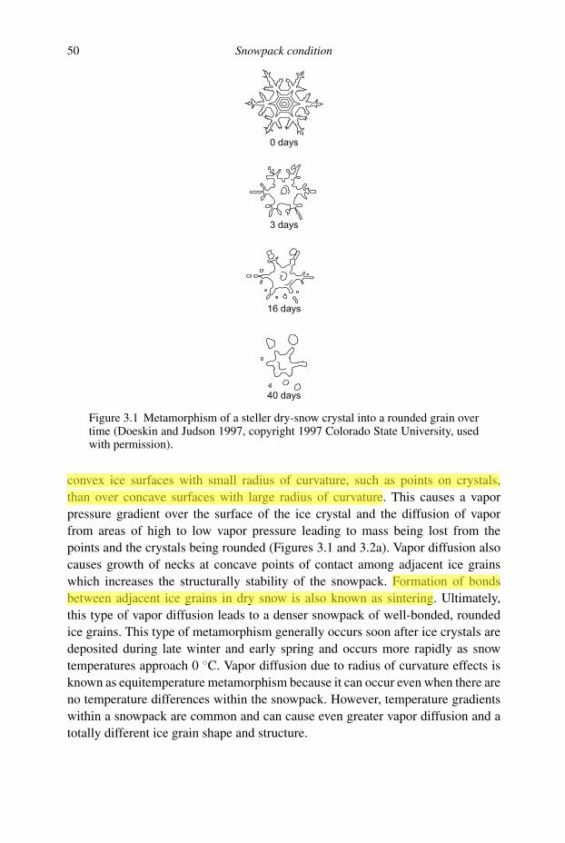
50 Snowpack condition
Figure 3.1 Metamorphism of a steller dry-snow crystal into a rounded grain overtime (Doeskin and Judson 1997, copyright 1997 Colorado State University, usedwith permission).
convex ice surfaces with small radius of curvature, such as points on crystals,
than over concave surfaces with large radius of curvature. This causes a vapor
pressure gradient over the surface of the ice crystal and the diffusion of vapor
from areas of high to low vapor pressure leading to mass being lost from the
points and the crystals being rounded (Figures 3.1 and 3.2a). Vapor diffusion also
causes growth of necks at concave points of contact among adjacent ice grains
which increases the structurally stability of the snowpack. Formation of bonds
between adjacent ice grains in dry snow is also known as sintering. Ultimately,
this type of vapor diffusion leads to a denser snowpack of well-bonded, rounded
ice grains. This type of metamorphism generally occurs soon after ice crystals are
deposited during late winter and early spring and occurs more rapidly as snow
temperatures approach 0 ◦C. Vapor diffusion due to radius of curvature effects is
known as equitemperature metamorphism because it can occur even when there are
no temperature differences within the snowpack. However, temperature gradients
within a snowpack are common and can cause even greater vapor diffusion and a
totally different ice grain shape and structure.
juras
Zvýraznění
juras
Zvýraznění

3.1 Snowpack metamorphism 51
a b
c
c
Figure 3.2 Scanning electron microscope pictures of selected metamorphosedsnow crystal types occurring in the snowpack: (a) dendritic crystals undergo-ing equi-temperature metamorphism, (b) faceted crystals formed by temperature-gradient metamorphism, and (c) bonded snow grains after melt–freeze metamor-phism. (Courtesy USDA, Agricultural Research Service, Beltsville, MD.)
3.1.2 Formation of faceted grains in dry snow
Vapor diffusion due to temperature gradients within the snowpack can lead to
formation of faceted ice grains with multiple plane surfaces. Faceted crystals can
take a variety of shapes and patterns, variously described as anisotropic, striated,
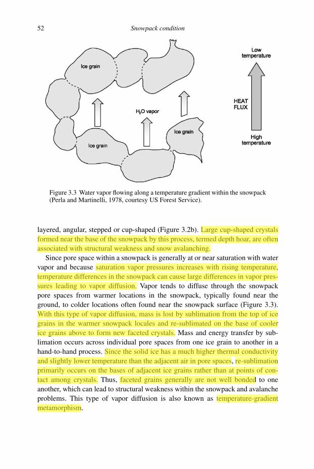
52 Snowpack condition
Figure 3.3 Water vapor flowing along a temperature gradient within the snowpack(Perla and Martinelli, 1978, courtesy US Forest Service).
layered, angular, stepped or cup-shaped (Figure 3.2b). Large cup-shaped crystals
formed near the base of the snowpack by this process, termed depth hoar, are often
associated with structural weakness and snow avalanching.
Since pore space within a snowpack is generally at or near saturation with water
vapor and because saturation vapor pressures increases with rising temperature,
temperature differences in the snowpack can cause large differences in vapor pres-
sures leading to vapor diffusion. Vapor tends to diffuse through the snowpack
pore spaces from warmer locations in the snowpack, typically found near the
ground, to colder locations often found near the snowpack surface (Figure 3.3).
With this type of vapor diffusion, mass is lost by sublimation from the top of ice
grains in the warmer snowpack locales and re-sublimated on the base of cooler
ice grains above to form new faceted crystals. Mass and energy transfer by sub-
limation occurs across individual pore spaces from one ice grain to another in a
hand-to-hand process. Since the solid ice has a much higher thermal conductivity
and slightly lower temperature than the adjacent air in pore spaces, re-sublimation
primarily occurs on the bases of adjacent ice grains rather than at points of con-
tact among crystals. Thus, faceted grains generally are not well bonded to one
another, which can lead to structural weakness within the snowpack and avalanche
problems. This type of vapor diffusion is also known as temperature-gradient
metamorphism.
juras
Zvýraznění
juras
Zvýraznění
juras
Zvýraznění
juras
Zvýraznění
juras
Zvýraznění
juras
Zvýraznění
juras
Zvýraznění

3.1 Snowpack metamorphism 53
The rate of vapor diffusion and the size and amount of faceted grains formed by
this temperature-gradient process increases with the magnitude of the temperature
gradient, porosity of the snowpack and the temperature. Locations with shallow,
porous snowpacks and large temperature differences between the ground and the
snowpack surface will commonly have well-developed faceted ice grain formation.
Continental locations such as the Rocky Mountains in Colorado, USA favor faceted
grain growth. Other locations with deep, dense snowpacks and warmer winter air
temperatures, commonly found in coastal regions of western North America, do
not.
Since saturation vapor pressures are more sensitive to temperature changes than
radius of curvature effects in the snowpack, it is common for temperature-gradient
vapor diffusion processes to dominate during winter and early spring. Once snow-
packs begin to warm and approach 0 ◦C, the importance of vapor diffusion due to
temperature gradients is lessened. At this point melt/freeze and liquid-water effects
begin to dominate snowpack metamorphism. However, brief periods of overnight
cooling and localized vapor diffusion at the snowpack surface can occur at any time
during the melt season.
3.1.3 Wet-snow metamorphism
Occurrence of melting and freezing cycles and rainfall can also affect ice grain
size, shape, and bonding. Metamorphism in wet snow is mainly controlled by the
fact that small ice grains have a slightly lower melting temperature than larger ice
grains. As a subfreezing snowpack warms, the smaller ice grains with lower melting
temperature, melt first. The energy for melting comes from the larger grains, which
cool, and refreeze the liberated water. Thus, the larger ice grains cannibalize the
smaller grains. Liquid water within snowpack pore space replaces air and greatly
increases the rate of energy transfer among ice grains. Large, rounded ice grains
grow more rapidly when liquid water is abundant.
Slight reductions in melting temperature can also occur at points of contact
between ice grains, especially when pressure is exerted from the weight of the
snow above. Preferential melting of bonds among grains can cause weakening of
the snowpack structure, but increases the snowpack density as grains move closer
together. Refreezing of liquid water held by capillary forces between grains and
liquid films over the surfaces of ice grains during melt and rain can greatly increase
snowpack strength (Figure 3.2c). Such melt–freeze metamorphism is usually the
last major process affecting seasonal snowpacks; however, for perennial snowcover
pressure metamorphism may also be significant.
Snowpacks that persist through an entire melt season into another accumulation
season can also be affected by the pressure of overlying snow. Densification of
juras
Zvýraznění
juras
Zvýraznění
juras
Zvýraznění
juras
Zvýraznění
juras
Zvýraznění
juras
Zvýraznění
juras
Zvýraznění
juras
Zvýraznění
juras
Zvýraznění

54 Snowpack condition
snow to firn, the transitional state between snow and ice, can occur due to pressure
metamorphism. Snow under pressure behaves as a visco-elastic material. When
subjected to slow compression it gradually deforms into firn and then ice. Major
differences in the density, thermal conductivity, and shortwave reflectivity exist
among snow, firn, and glacial ice.
3.1.4 Other snowpack transformations
In addition to the metamorphic changes described above, several other transforma-
tions in snowpack density and structure can occur due to effects of wind, refreezing
of liquid water, and sublimation on the snowpack surface. Wind can cause the for-
mation of wind slab, a densified, dry-snow layer at the snowpack surface formed
due to compression of fresh, low-density snow or deposition and packing of broken
crystals of blowing snow. Wind slab often has enough structure to be lifted off
the snowpack surface as an intact layer. Due to its greater density, wind slab has
a higher thermal conductivity and altered surface shortwave reflectivity that can
affect snowpack heat exchange. Water from surface melt or rainfall can refreeze
within the snowpack leading to the formation of ice lenses on or near the surface.
Although ice lenses generally are not completely impermeable and continuous,
they can affect delivery of liquid water from the snowpack to the ground surface.
Finally, sublimation of vapor onto the snowpack surface during cold, clear, calm
nights can lead to development of surface hoar crystals or the solid-phase equiva-
lent of dew formation. Surface hoar has an extremely low density and is structural
very weak and doubtless has an impact on the reflection of shortwave radiation
from the snowpack surface. All of these transformations can have some impacts on
snowpack ripening, melt, and water delivery.
3.1.5 Snowpack density and densification
Snowpack density ultimately controls the pore space available for storage and
transmission of liquid water and gases. A formal definition of snowpack density
that includes the possible effects of liquid water on snowpack mass is:
ρs = ρi(1 − φ) + ρwφSw (3.1)
where:
ρs = density of snowpack, kg snow per m3 of snowpack volume
ρ i = density of ice, 917 kg per m3 of ice
ρw = density of liquid water, 103 kg per m3 of water
φ = porosity of snowpack, m3 of pore space per m3 of snowpack volume
Sw = water saturation, volume of liquid water per volume of pore space, m3 m−3
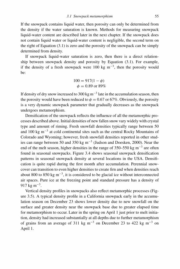
3.1 Snowpack metamorphism 55
If the snowpack contains liquid water, then porosity can only be determined from
the density if the water saturation is known. Methods for measuring snowpack
liquid-water content are described later in the next chapter. If the snowpack does
not contain liquid water or liquid-water content is negligible, the second term on
the right of Equation (3.1) is zero and the porosity of the snowpack can be simply
determined from density.
If snowpack liquid-water saturation is zero, then there is a direct relation-
ship between snowpack density and porosity by Equation (3.1). For example,
if the density of a fresh snowpack were 100 kg m−3, then the porosity would
be:
100 = 917(1 − φ)
φ = 0.89 or 89%
If density of dry snow increased to 300 kg m−3 late in the accumulation season, then
the porosity would have been reduced to φ = 0.67 or 67%. Obviously, the porosity
is a very dynamic snowpack parameter that gradually decreases as the snowpack
undergoes metamorphism.
Densification of the snowpack reflects the influence of all the metamorphic pro-
cesses described above. Initial densities of new fallen snow vary widely with crystal
type and amount of riming. Fresh snowfall densities typically range between 50
and 100 kg m−3 at cold continental sites such as the central Rocky Mountains of
Colorado and Wyoming; however, fresh snowfall densities reported in other stud-
ies can range between 50 and 350 kg m−3 (Judson and Doesken, 2000). Near the
end of the melt season, higher densities in the range of 350–550 kg m−3 are often
found in seasonal snowpacks. Figure 3.4 shows seasonal snowpack densification
patterns in seasonal snowpack density at several locations in the USA. Densifi-
cation is quite rapid during the first month after accumulation. Perennial snow-
cover can transition to even higher densities to create firn and when densities reach
about 800 to 850 kg m−3, it is considered to be glacial ice without interconnected
air spaces. Pure ice at the freezing point and standard pressure has a density of
917 kg m−3.
Vertical density profiles in snowpacks also reflect metamorphic processes (Fig-
ure 3.5). A typical density profile in a California snowpack early in the accumu-
lation season on December 23 shows lower density due to new snowfall on the
surface and greater density near the snowpack base due to greater elapsed time
for metamorphism to occur. Later in the spring on April 1 just prior to melt initia-
tion, density had increased substantially at all depths due to further metamorphism
of grains from an average of 311 kg m−3 on December 23 to 422 kg m−3 on
April 1.

56 Snowpack condition
0
100
200
300
400
500
600
0 20 40 60 80 100 120 140
Age, days
Den
sity
, kg
m−3
Alta, UT
Berthoud Pass, CO
Mt. Olympus, WA
Figure 3.4 Typical seasonal changes in average snowpack density at three locationsin the United States (Doeskin and Judson 1997, copyright 1997 Colorado StateUniversity, used with permission).
0
0.4
0.8
1.2
1.6
2
0 100 200 300 400 500 600
Density, kg m−3
Hei
gh
t ab
ove
gro
un
d, m
December 23
April 1
Figure 3.5 Examples of snowpack density profiles measured early and late in thesnowpack accumulation season at the Central Sierra Snow Lab, CA, 1953 (datafrom US Army Corps of Engineers, 1956).

3.2 Heat conduction in snowpacks 57
3.1.6 International classification system for seasonal snow cover
An international system has been developed to describe seasonal snow on the ground
that has undergone metamorphism (Colbeck et al., 1990; Table 3.2). The system
is used to standardize terminology and help describe snowpack conditions in rela-
tion to metamorphic processes influencing the snowpack. The classification of
precipitation types was previously discussed in Chapter 2. Due to structural differ-
ences, the thermal conductivity, liquid-water holding capacity, and other properties
important to snow hydrology will vary among snow types.
3.2 Heat conduction in snowpacks
Heat transfer along a temperature gradient in the snowpack occurs by three major
processes:
� conduction through the solid portion of the ice matrix� conduction through air in snowpack pores� latent heat exchange due to molecular diffusion of water vapor.
Since the thermal conductivity of ice is nearly 100 times greater than that of air
(e.g. at 0 ◦C k(ice) = 2.24 W m−1 K−1 while k(air) = 0.024 W m−1 K−1), pure heat
conduction in snow is strongly controlled by conduction through the ice matrix.
Bonding of individual ice grains and overall snowpack structure exert major controls
on snowpack thermal conductivity. Conduction through air in the snowpack pore
space plays an insignificant role, but vapor transfer of latent heat of condensation/
sublimation in the pore space can increase heat transferred along a temperature
gradient by up to 50% (Sturm et al., 1997). The thermal conductivity of snow
generally is referred to as an effective thermal conductivity due to the combined
effects of conduction and latent heat transfer.
Latent heat transfer occurs along a temperature gradient in snowpacks when
vapor is sublimated or evaporated from the surface of a warmer ice grain and the
vapor either diffuses out of the snowpack through pore spaces or is condensed or
re-sublimated onto the surface of a slightly cooler ice grain. Latent heat liberated
by condensation/sublimation is conducted through the slightly cooler ice grain and
produces further evaporation/sublimation and mass losses from grain surfaces along
the temperature gradient. Repeated losses and gains of mass from ice grains along a
temperature gradient by this process can transfer significant amounts of latent heat.
Because latent heat transfer increases with snow temperature, the effective thermal
conductivity of snow generally increases with temperature when vapor transfer is
important, even though the thermal conductivity of ice decreases with increasing
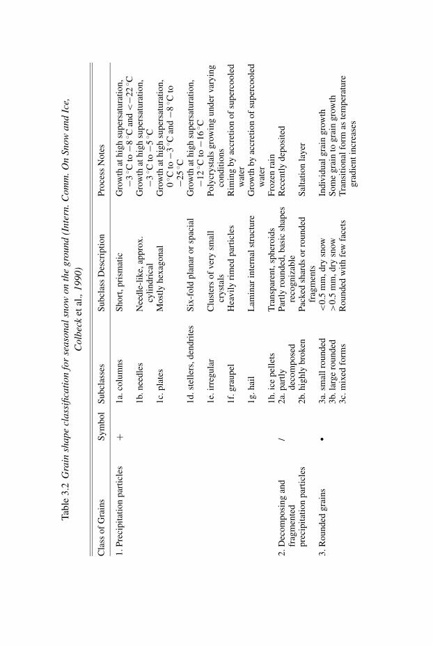
Tab
le3.2
Gra
insh
ape
clas
sific
atio
nfo
rse
ason
alsn
owon
the
grou
nd(I
nter
n.C
omm
.On
Snow
and
Ice,
Col
beck
etal
.,19
90)
Cla
sso
fG
rain
sS
ym
bo
lS
ub
clas
ses
Su
bcl
ass
Des
crip
tio
nP
roce
ssN
ote
s
1.
Pre
cip
itat
ion
par
ticl
es+
1a.
colu
mn
sS
ho
rt,
pri
smat
icG
row
that
hig
hsu
per
satu
rati
on
,−3
◦ Cto
−8◦ C
and
<−2
2◦ C
1b.
nee
dle
sN
eed
le-l
ike,
app
rox
.cy
lin
dri
cal
Gro
wth
ath
igh
sup
ersa
tura
tio
n,
−3◦ C
to−5
◦ C1
c.p
late
sM
ost
lyh
exag
on
alG
row
that
hig
hsu
per
satu
rati
on
,0
◦ Cto
−3◦ C
and
−8◦ C
to−2
5◦ C
1d
.st
elle
rs,
den
dri
tes
Six
-fo
ldp
lan
aro
rsp
acia
lG
row
that
hig
hsu
per
satu
rati
on
,−1
2◦ C
to−1
6◦ C
1e.
irre
gu
lar
Clu
ster
so
fver
ysm
all
cry
stal
sP
oly
cry
stal
sg
row
ing
un
der
vary
ing
con
dit
ion
s1
f.g
rau
pel
Hea
vil
yri
med
par
ticl
esR
imin
gb
yac
cret
ion
of
sup
erco
ole
dw
ater
1g
.h
ail
Lam
inar
inte
rnal
stru
ctu
reG
row
thb
yac
cret
ion
of
sup
erco
ole
dw
ater
1h
.ic
ep
elle
tsT
ran
spar
ent,
sph
ero
ids
Fro
zen
rain
2.
Dec
om
po
sin
gan
dfr
agm
ente
d/
2a.
par
tly
dec
om
po
sed
Par
tly
rou
nd
ed,
bas
icsh
apes
reco
gn
izab
leR
ecen
tly
dep
osi
ted
pre
cip
itat
ion
par
ticl
es2
b.h
igh
lyb
roken
Pac
ked
shar
ds
or
rou
nd
edfr
agm
ents
Sal
tati
on
lay
er
3.
Ro
un
ded
gra
ins
�3
a.sm
all
rou
nd
ed<
0.5
mm
,d
rysn
owIn
div
idu
alg
rain
gro
wth
3b.
larg
ero
un
ded
>0
.5m
m,
dry
snow
So
me
gra
into
gra
ing
row
th3
c.m
ixed
form
sR
ou
nd
edw
ith
few
face
tsT
ran
siti
on
alfo
rmas
tem
per
atu
reg
rad
ien
tin
crea
ses
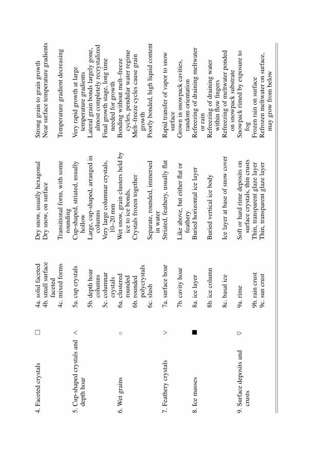
4.
Fac
eted
cry
stal
s�
4a.
soli
dfa
cete
dD
rysn
ow,
usu
ally
hex
ago
nal
Str
on
gg
rain
tog
rain
gro
wth
4b.
smal
lsu
rfac
efa
cete
dD
rysn
ow,
on
surf
ace
Nea
rsu
rfac
ete
mp
erat
ure
gra
die
nts
4c.
mix
edfo
rms
Tra
nsi
tio
nal
form
,w
ith
som
ero
un
din
gT
emp
erat
ure
gra
die
nt
dec
reas
ing
5.
Cu
p-s
hap
edcr
yst
als
and
dep
thh
oar
∧5
a.cu
pcr
yst
als
Cu
p-s
hap
ed,st
riat
ed,
usu
ally
ho
llow
Ver
yra
pid
gro
wth
atla
rge
tem
per
atu
reg
rad
ien
ts5
b.d
epth
ho
arco
lum
ns
Lar
ge,
cup
-sh
aped
,ar
ran
ged
inco
lum
ns
Lat
eral
gra
inb
on
ds
larg
ely
go
ne,
alm
ost
com
ple
tely
recr
yst
aliz
ed5
c.co
lum
nar
cry
stal
sV
ery
larg
eco
lum
nar
cry
stal
s,1
0–
20
mm
Fin
alg
row
thst
age,
lon
gti
me
nee
ded
for
gro
wth
6.
Wet
gra
ins
◦6
a.cl
ust
ered
rou
nd
edW
etsn
ow,
gra
incl
ust
ers
hel
db
yic
eto
ice
bo
nd
s,B
on
din
gw
ith
ou
tm
elt–
free
zecy
cles
,p
end
ula
rw
ater
reg
ime
6b.
rou
nd
edp
oly
cry
stal
sC
ryst
als
fro
zen
tog
eth
erM
elt–
free
zecy
cles
cau
seg
rain
gro
wth
6c.
slu
shS
epar
ate,
rou
nd
ed,
imm
erse
din
wat
erP
oo
rly
bo
nd
ed,
hig
hli
qu
idco
nte
nt
7.
Fea
ther
ycr
yst
als
∨7
a.su
rfac
eh
oar
Str
iate
d,
feat
her
y,u
sual
lyfl
atR
apid
tran
sfer
of
vap
or
tosn
owsu
rfac
e7
b.ca
vit
yh
oar
Lik
eab
ove,
but
eith
erfl
ato
rfe
ath
ery
Gro
wn
insn
owp
ack
cav
itie
s,ra
nd
om
ori
enta
tio
n8
.Ic
em
asse
s�
8a.
ice
lay
erB
uri
edh
ori
zon
tal
ice
lay
erR
efre
ezin
go
fd
rain
ing
mel
twat
ero
rra
in8
b.ic
eco
lum
nB
uri
edver
tica
lic
eb
od
yR
efre
ezin
go
fd
rain
ing
wat
erw
ith
infl
owfi
ng
ers
8c.
bas
alic
eIc
ela
yer
atb
ase
of
snow
cover
Ref
reez
ing
of
mel
twat
erp
on
ded
on
snow
pac
ksu
bst
rate
9.
Su
rfac
ed
epo
sits
and
cru
sts
– ∨9
a.ri
me
So
fto
rh
ard
rim
ed
epo
sits
on
surf
ace
cry
stal
s,th
incr
ust
sS
now
pac
kri
med
by
exp
osu
reto
fog
9b.
rain
cru
stT
hin
,tr
ansp
aren
tg
laze
lay
erF
roze
nra
ino
nsu
rfac
e9
c.su
ncr
ust
Th
in,
tran
spar
ent
gla
zela
yer
Ref
roze
nm
eltw
ater
on
surf
ace,
may
gro
wfr
om
bel
ow

60 Snowpack condition
temperature. Mass loss and gain from the surfaces of ice grains can also create
faceted and poorly bonded ice grains (see discussion in Section 3.1.2).
Two other processes can be responsible for energy transfer in snowpacks: radi-
ation transmission and convection. Radiation transmission in snow is discussed in
Chapter 6 in relation to snowmelt. Convection due to air currents in the snowpack
caused by temperature-induced buoyancy effects can occur in snow, but conditions
under which convection occurs are not well understood (Powers et al., 1985). Con-
vection due to wind pressure forces on the snowpack surface, the so-called pressure
pumping of snowpack air, can also occur that transfers gases within the snowpack
(Massman et al., 1995; Colbeck, 1997).
Heat conduction in snow can be described by the equation:
q = −keffdT/dz (3.2)
where:
q = flux density of heat conducted by snow, W m−2
keff = effective thermal conductivity of snow, W m−1 K−1
dT/dz = temperature gradient, K m−1
The effective thermal conductivity of snow has often been related to density,
although the bonding and structure of ice grains and temperature are the controlling
factors. In an extensive review of past studies and analysis of their own data, Sturm
et al. (1997) give the following general relationships for keff:
keff = 0.138 − 1.01ρ + 3.233ρ2 [0.156 ≤ ρ ≤ 0.6]
keff = 0.023 + 0.234ρ {ρ < 0.156} (3.3)
where ρ is snow density in g cm−3. The experimental data set used to generate this
relationship (n = 488) represented an average snowpack temperature of −14.7 ◦C
and an average density of 317 kg m−3. As can be seen in Figure 3.6, the effective
thermal conductivity of snow for densities up to 0.6 g cm−3 is still well below that
for solid ice (2.24 W m−1 K−1), while for very low snow densities it approaches
the thermal conductivity for air (0.024 W m−1 K−1). Sturm et al. (1997) show
that the density dependence of keff is greatest for well-bonded and wind-compacted
snow and least, or non-existent, for poorly bonded depth hoar. Sturm and John-
son (1992) found that the keff for depth hoar was from one-half to one-fourth of
the values normally reported for other snow types of similar density due to thin
and infrequent ice bonds. Sturm et al. (1997) recommend using simple average
keff values for poorly bonded snow and give average values of keff for various
ICSSG (see Table 3.2) snow types for that purpose. Heat conduction rates under

3.2 Heat conduction in snowpacks 61
Figure 3.6 Effective thermal conductivity of snow as a function of density (mod-ified from Sturm et al. 1997 from Journal of Glaciology with permission of theInternational Glaciological Society).
steady-state conditions in uniform snow can be computed using Equations (3.2)–
(3.3). Given a structurally uniform snowpack that is 0.22 m deep with constant
surface and base temperatures of −7 ◦C (266 K) and 0 ◦C (273 K), respectively,
and a density of 0.35 g cm−3, the rate of heat flow can be computed as:
keff = 0.138 − 1.01(0.35) + 3.233(0.35)2 = 0.18 W m−1 K−1
q = −(0.18 W m−1 K−1)[(266 K − 273 K)/(0.22 m − 0 m)] = 5.73 W m−2
Unfortunately, heat conduction in a subfreezing snowpack is seldom at steady
state and the snowpack is seldom structurally uniform, which cause considerable
difficulty in modelling snowpack temperatures. Several models exist that can be
used to predict the heat conduction, temperature and density distribution within the
snowpack over time (Jordan, 1991).

62 Snowpack condition
0
0.4
0.8
1.2
1.6
2
2.4
Temperature, oC
Hei
gh
t ab
ove
gro
un
d, m
1100 hr Dec 23
1230 hr April 1
Figure 3.7 Temperature profiles in a California snowpack in the early and lateaccumulation season at the Central Sierra Snow Lab, CA (US Army Corps ofEngineers, 1956).
3.3 Snowpack temperatures and cold content
Snowpack temperatures can vary seasonally and daily as a result of the com-
plex processes of energy transfer within the snowpack. Temperatures profiles in a
California snowpack on December 23 and April 1 from the early Corps of Engi-
neers Cooperative Snow Investigations are shown in Figure 3.7 to illustrate typical
seasonal differences. In late morning on December 23, profiles show subfreezing
temperatures near the snowpack surface due to contact with cold air and tempera-
tures near or at 0 ◦C at the snowpack base due to soil heat conduction from below. By
April 1 just prior to snowpack melting, the snowpack has warmed to an isothermal
0 ◦C due to heat conduction from above and below. Note that the temperature pro-
files in Figure 3.7 correspond to the same snowpack represented by density profiles
shown in Figure 3.5. Warming of snowpacks from above is greatly enhanced by
the infiltration of liquid water from surface melting and rainfall, which refreezes in
the colder snow below and releases the latent heat of fusion within the snowpack.
Refreezing of liquid water inputs on successive melt days early in the spring season
can quickly warm even deep snowpacks. Once the snowpack is warmed to 0 ◦C
and liquid-water holding capacities are satisfied, the snowpack is referred to as a
ripe snowpack. See later sections in this chapter for typical liquid-water holding
capacities for snow.

3.3 Snowpack temperatures and cold content 63
Figure 3.8 Typical diurnal snowpack temperature (◦C) variations in a winterColorado snowpack at local standard time (LST) (Bergen 1968, courtesy US ForestService) showing periodic cooling and warming near the surface and a relativelystable temperature regime near the ground.
Daily temperature fluctuations with depth in subfreezing snowpacks can be
considerable. Due to the low thermal conductivity of snow, heat can not be added
quickly by conduction into the snowpack during the daytime or lost quickly by con-
duction from within the snowpack during nocturnal cooling. Consequently, snow-
packs exhibit very large temperature gradients near the surface and large time lags
for propagation of daily temperature waves and rapid damping of diurnal temper-
ature fluctuations in deeper snowpack layers. Secondary temperature maxima can
occur just below the surface in snow during clear daytime periods due to the com-
bined influence of heat conduction and transmission of shortwave radiation (Koh
and Jordan, 1995). Figure 3.8 shows typical diurnal variations in the temperature
of a subfreezing winter snowpack in Colorado (Bergen, 1968). Daily amplitudes in
temperature are large at the snowpack surface but rapidly diminish with increasing
depth. Peak daily temperatures also occur later with increasing depth in the snow.
Temperatures near ground level remain relatively stable and often approach 0 ◦C.
Hydrologists often use snowpack temperature and density profile data to compute
snowpack cold content. Cold content represents the amount of liquid water from
melt or rainfall that must be frozen in a subfreezing snowpack to warm the snowpack
from its current temperature to an isothermal 0 ◦C. Before liquid water can be
released from the snowpack an isothermal condition must generally exist, although
pockets of subfreezing snow can exist adjacent to fingers of ripe snow conducting
water. Cold content can be calculated as:
CC = [ρscid(273.16 − Ts)]/(ρwL f) (3.4)

64 Snowpack condition
where:
CC = snowpack cold content, m of liquid water
ρs = average snowpack density, kg m−3
ci = specific heat of ice, J kg−1 K−1
d = snowpack depth, m
Ts = average snowpack temperature, K
ρw = density of liquid water = 103 kg m−3
Lf = latent heat of fusion, J kg−1
Cold content can also be computed using Equation 3.4 for individual layers in a
snowpack and summed using the respective densities and temperatures. Computed
cold contents can be compared to the daily predicted melt or forecasted rainfall to
help determine when liquid water will be released from snowpacks. Cold contents
for ripe snowpacks that are isothermal at 0 ◦C are zero. Nocturnal cooling can
result in small cold contents even during the melt season that must be satisfied
before meltwater can be released the next day. Computations of runoff time lags
due to cold content are discussed in Chapter 9, Section 9.3.1. A discussion of the
snowpack energy balance with consideration of heat storage and use of degree-days
to model cold content are given in Chapter 6.
An example computation of cold content using Equation (3.4) can be given for the
conditions represented by snowpack conditions for December 23 in Figures 3.5 and
3.7. The depth of snow on that date was 1.524 m, average density was 311 kg m−3,
and average temperature was −3.1 ◦C or 270.1 K. Given the specific heat of ice of
2100 J kg−1 K−1 and latent heat of fusion of 0.334 × 10⁶ J kg−1 at the freezing
point (see Appendix A1), the cold content would be:
CC = [(311)(2100)(1.524)(273.16 − 270.1)]/(103)(0.334 × 106)
= 9.208 × 10⁻³ m
= 9.2 mm of liquid water
A cold content of this magnitude could easily be satisfied by surface melt in one
day since daily melt frequently exceeds 10 mm.
3.4 Liquid water in snow
Liquid water from melting or rain will first satisfy any snowpack cold content and
then the liquid-water holding capacity of the snow. The remaining liquid water
will percolate vertically downward through the snowpack to the soil surface unless
diverted by less permeable layers and crusts. Once water reaches the base of the
snowpack, it can flow downslope through basal layers of the snowpack if the ground
3.4 Liquid water in snow 65
surface is impermeable or infiltrate the soil. In preceding sections, the importance of
liquid water in snowpack metamorphism and ripening was described. In this section,
the storage and movement of liquid water in snow are described. Measurement of
snowpack liquid-water content is discussed in Chapter 4.
3.4.1 Liquid-water content of snow
The liquid-water content of a snowpack represents all liquid water in the snow
including water in transit from rain or melt and water that is stored against gravi-
tational forces. The latter liquid water is called the irreducible liquid saturation or
liquid-water holding capacity of snow. Liquid content of snow is expressed either
on a volumetric basis (θv) as the volume of liquid water per unit volume of snow
or a mass basis (θm) as the mass of liquid water per unit mass of snowpack. The
two measures are related as:
θv = θm(ρs/ρw) (3.5)
where:
θv = volumetric liquid-water content, m3 of liquid water per m3 of snow
θm = liquid-water content on mass basis, kg of liquid water per kg snow
ρs = snowpack density, kg m−3
ρw = liquid-water density, 103 kg m−3
It should be pointed out that the liquid content of snow is computed differently than
the liquid content of soils. In soil, the moisture content by weight is based upon the
dry mass of soil, while the liquid content of snow on a mass basis is based upon
the total mass of the snow including the mass of liquid water.
Liquid-water contents vary over time due to surface melting and rain. In Figure
3.9, liquid-water contents of snow on a mass basis are shown to vary between about
0–2% at night during drainage, up to about 30% during active melt on the third
day. If the snowpack density were 400 kg m−3 during active melt, then by Equation
(3.5) a 30% liquid content on a mass basis would be equal to a liquid content of
12% on a volumetric basis.
Liquid-water contents affect the amount of water released during melt per unit of
energy input. A unit of energy input at times of high liquid-water content will release
more water than at times of low liquid content, due to release of water already held
in the snowpack as well as water created by melt. To account for the effects of
liquid water and cold content when computing melt, hydrologists commonly use a
dimensionless parameter called thermal quality (B). Thermal quality (B) is defined
as the energy required to melt a unit mass of snow divided by the energy required
to melt a unit mass of ice at 0 ◦C. The energy required to melt a unit mass of snow
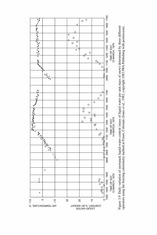
Fig
ure
3.9
Dai
lyva
riat
ion
of
snow
pac
kli
qu
id-w
ater
con
ten
t(m
ass
of
liq
uid
wat
erp
eru
nit
mas
so
fsn
ow)
det
erm
ined
by
thre
ed
iffe
ren
to
per
ato
rsu
sin
gth
efr
eezi
ng
calo
rim
etry
met
ho
dat
Fra
ser,
Co
lora
do
(Jo
nes
etal
.,1
98
3,c
opy
rig
ht
19
83
IWA
Pu
bli
shin
gw
ith
per
mis
sio
n).

3.4 Liquid water in snow 67
is the sum of: (1) energy needed to raise the temperature of the snow to 0◦C when
the snowpack is subfreezing and (2) the energy needed to melt the solid portion of
the snowpack. Thermal quality is computed as:
B = [(1 − θm)L f + ciT ]/L f (3.6)
where:
B = thermal quality, dimensionless
θm = liquid-water content, mass liquid per unit mass snow
Lf = latent heat of fusion, 0.334 × 10⁶ J kg−1 at 0 ◦C
ci = specific heat of ice, 2.1 × 10³ J kg−1 ◦C−1
T = snowpack temperature depression below 0 ◦C
When snow is ripe and contains some liquid water, the numerator is less than Lf and
B is <1. When snow is subfreezing, the numerator is greater than Lf and B is >1.
For ripe snow with liquid water present, the thermal quality is simply the fraction of
snowpack mass that is ice. The computation ignores the minor contribution of air to
snowpack mass. Thermal quality ranges from about 0.8 for ripe snow to about 1.1
for subfreezing snow. The use of thermal quality in melt computations is discussed
in Chapter 6.
An example computation can be used to illustrate the two snowpack thermal quality
regimes.
For unripe snow with zero liquid water and an average snowpack temperature of
−4.5 ◦C, the thermal quality would be:
B = [(1 − 0)(0.334 × 10⁶ J kg−1)
+(2.1 × 10³ J kg−1 ◦C−1)(4.5 ◦C)]/(0.334 × 106 J kg−1)
= 1.028
For ripe snow at 0 ◦C and liquid-water content on a mass basis of 0.15, the thermal
quality would be:
B = [(1 − 0.15)(0.334 × 10⁶ J kg−1)]/(0.334 × 106 J kg−1)
= 1 − 0.15 = 0.85
3.4.2 Theory of water movement in snow
Liquid-water movement in snow can be generally described with classical theory
of flow in porous media using Darcy’s law (Wankiewicz, 1978). Due to the rela-
tively uniform and coarse-grained nature of snow, effects of capillarity on water
movement in snow are generally ignored and gravitational forces are considered
dominant. Figure 3.10 shows relationships between capillary pressure and liquid

68 Snowpack condition
0
0.1
0.2
0.3
0.4
0 2000 4000 6000 8000 10000
Negative pressure, N m−2
Vo
lum
etri
c liq
uid
co
nte
nt
Sandy soil
Snow
Figure 3.10 Comparison of liquid content vs. capillary pressure curves for snowand sandy soils (data from Colbeck, 1974 and Oke, 1987) showing some snowsamples at least have even less capillary attraction for liquid water than sands fora given negative pressure in Newtons (N) m−2.
content for snow in comparison to sandy soil. Over 80% of the snowpack pore
space is drained with a pressure of only −800 N m−2 or a suction force equivalent
to only 8 cm of water, while typical sandy soils would retain more moisture at that
same capillary pressure. Wankiewicz (1978) showed similar data for a snow sample
taken in February, but a response more similar to sandy soil with a snow sample
collected in July. Due to the small effects of capillarity, capillary rise in snow is
limited generally to a few centimeters (Coleou et al. 1999).
With capillary effects ignored, Darcy’s law describing liquid-water movement
in snow can be written as:
uw = ρwkwg/μw = αkw (3.8)
uw = volume flux of liquid water, m3 m−2 s−1 or m s−1
ρw = density of water, 103 kg m−3
kw = intrinsic permeability of water in snow, m2
g = acceleration due gravity, 9.80 m s−2
μw = dynamic viscosity of water, 1.79 × 10⁻² kg m−1 s−1 at 0 ◦C
α = ρw g/μw = 5.47 × 10⁵ m−1 s−1

3.4 Liquid water in snow 69
As in any porous media, the permeability of snow during two-phase or unsaturated
flow is related to the level of liquid saturation described by the effective saturation
(S∗) where:
S∗ = (Sw − Swi)/(1 − Swi) (3.9)
S∗ = effective saturation, dimensionless
Sw = liquid saturation, volume of liquid water per volume of pore space, m3 m−3
Swi = irreducible liquid saturation, irreducible volume of liquid water per unit
volume of pore space, m3 m−3
Effective saturation ranges from zero to one, that is, liquid-water content varies
from 0% to 100% of the pore space available to water flow. Typically, S∗ ranges
between 0.1 and 0.2 during normal melting.
The irreducible volumetric water content is defined by the condition when water
films within the snowpack become discontinuous or flow due to gravity drainage
is negligible. Colbeck (1974) found a value of 0.07 and Jordan (1991) successfully
used a value of 0.04. The commonly used liquid-water holding capacity of snow (θvi)
expressed as the irreducible volume of liquid water per unit volume of snowpack
is related to Swi as:
θvi = Swiφ (3.10)
where φ = porosity of the snowpack (volume of pore space per unit volume of
snow). Thus a liquid-water holding capacity of θ i = 0.03 in a snowpack with
porosity φ = 0.6 is equivalent to Swi = 0.03/0.6 = 0.05.
Liquid permeability in snow is related to effective saturation (S∗) by:
kw = kS∗n(3.11)
where k equals the intrinsic permeability (m2) or the permeability with single phase
flow at liquid saturation. The exponent n is an empirical constant ranging from two
to four, with a typical value being three. According to the form of Equation (3.11),
the permeability of snow will obviously be strongly controlled by the level of liquid
saturation and hence the melt or rainfall rate. The intrinsic permeability of snow
(k) appearing in Equation (3.11) has been related to snowpack grain size (d) and
porosity (φ) by Shimizu (1970) as:
k = 0.077 d2 exp[−7.8(1 − φ)ρi/ρw] (3.12)
where:
k = intrinsic permeability, m2
d = mean grain diameter, m
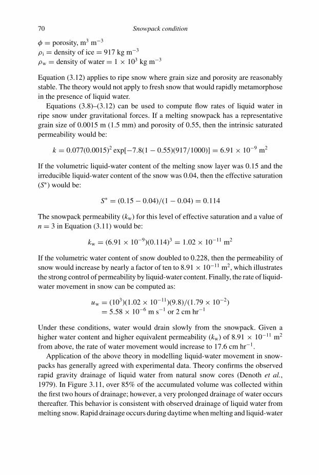
70 Snowpack condition
φ = porosity, m3 m−3
ρ i = density of ice = 917 kg m−3
ρw = density of water = 1 × 10³ kg m−3
Equation (3.12) applies to ripe snow where grain size and porosity are reasonably
stable. The theory would not apply to fresh snow that would rapidly metamorphose
in the presence of liquid water.
Equations (3.8)–(3.12) can be used to compute flow rates of liquid water in
ripe snow under gravitational forces. If a melting snowpack has a representative
grain size of 0.0015 m (1.5 mm) and porosity of 0.55, then the intrinsic saturated
permeability would be:
k = 0.077(0.0015)2 exp[−7.8(1 − 0.55)(917/1000)] = 6.91 × 10⁻⁹ m2
If the volumetric liquid-water content of the melting snow layer was 0.15 and the
irreducible liquid-water content of the snow was 0.04, then the effective saturation
(S∗) would be:
S∗ = (0.15 − 0.04)/(1 − 0.04) = 0.114
The snowpack permeability (kw) for this level of effective saturation and a value of
n = 3 in Equation (3.11) would be:
kw = (6.91 × 10⁻⁹)(0.114)3 = 1.02 × 10⁻¹¹ m2
If the volumetric water content of snow doubled to 0.228, then the permeability of
snow would increase by nearly a factor of ten to 8.91 × 10⁻¹¹ m2, which illustrates
the strong control of permeability by liquid-water content. Finally, the rate of liquid-
water movement in snow can be computed as:
uw = (103)(1.02 × 10⁻¹¹)(9.8)/(1.79 × 10−2)
= 5.58 × 10⁻⁶ m s−1 or 2 cm hr−1
Under these conditions, water would drain slowly from the snowpack. Given a
higher water content and higher equivalent permeability (kw) of 8.91 × 10⁻¹¹ m2
from above, the rate of water movement would increase to 17.6 cm hr−1.
Application of the above theory in modelling liquid-water movement in snow-
packs has generally agreed with experimental data. Theory confirms the observed
rapid gravity drainage of liquid water from natural snow cores (Denoth et al.,1979). In Figure 3.11, over 85% of the accumulated volume was collected within
the first two hours of drainage; however, a very prolonged drainage of water occurs
thereafter. This behavior is consistent with observed drainage of liquid water from
melting snow. Rapid drainage occurs during daytime when melting and liquid-water

3.4 Liquid water in snow 71
Figure 3.11 Accumulated drainage from melting snow core over time modelledwith Darcy’s law with the assumption of negligible capillary effects (Denoth et al.,1979, courtesy US Army, Cold Regions Res. Engin. Lab.) showing rapid initialand very slow later drainage of meltwater. Lines show fitted model with varyingexponents “n” for the snowpack permeability function in Equation (3.11).
contents are highest and a long gradual drainage occurs overnight when liquid inputs
and snowpack water contents are low.
Further extension of this theory in combination with the continuity equation
allows prediction of the rate of water movement in a snowpack for a given value
of water flux as a function of time at various depths in the snow as (Colbeck, 1972,
1977):
dz/dt |u = 3α1/3k1/3[φ(1 − Swi)]−1 u2/3
w (3.13)
Here the speed of the wetting front in a snowpack, dz/dt|u, is directly related to
the flux of water uw2/3 due to melting or rainfall. In Figure 3.12 a plot of predicted
volume flux at various depths in snow for an assumed surface water flux distribution
is shown. The surface volume flux is translated with only slight modification in
shape to a depth of 0.6 m within two hours. At greater depths modification of the
melt wave is seen with a more abrupt leading edge and elongated tail, due to the
fact that faster moving meltwater (from times when surface melt rates are greater)
can overtake slower moving meltwater from other times to create a shock wave
type behavior. Simulations indicate that for shallow seasonal snow covers, runoff

Fig
ure
3.1
2M
od
elle
dm
eltw
ater
wav
esat
the
surf
ace
and
sever
ald
epth
sw
ith
ina
snow
pac
kil
lust
rati
ng
that
rap
idd
rain
age
du
rin
gw
ette
rh
igh
-mel
tp
erio
ds
can
over
take
slow
erd
rain
age
fro
mp
rio
rm
elt
top
rod
uce
a“s
ho
ckw
ave”
typ
eb
ehav
ior
of
the
wet
tin
gfr
on
tw
ith
inth
esn
owp
ack
(Co
lbec
k,
19
72
,w
ith
per
mis
sio
no
fth
eIn
tern
atio
nal
Gla
cio
log
ical
So
ciet
y).

3.4 Liquid water in snow 73
Figure 3.13 Flow fingers for preferential liquid-water movement that formed dur-ing initial day’s melting of a homogeneous 28-cm depth snowpack resulting froma single snowfall in Pennsylvania (photo D. R. DeWalle). Water mixed with foodcoloring was uniformly sprayed over the snowpack surface to trace water move-ment. Also note evidence of meltwater movement downslope to the right in thesurface layer and at the soil–snow interface. See also color plate.
delays due to liquid-water movement in ripe snow will be minimal. In deeper snow
or snow with significant cold content, the delays are much greater. Lag times in
snowmelt runoff due to liquid-water movement in snow are discussed further in
Chapter 9.
Application of theory of flow in porous media to snow is made difficult by
spatial variation in snowpack properties that develop over time and cause erratic
liquid-water behavior. Liquid water in snow often drains along preferred flow fin-
gers (Figure 3.13). How such flow fingers develop is not understood, but surface
depressions in melting snow on flat terrain are thought to be physical manifestations
of such flow channels. Ice columns in snowpacks have also been observed where
liquid water in these flow fingers has refrozen. Preferred flow channels may speed
release of liquid water from a snowpack. Ice layers and layers of snow with varying
density can also delay initial water release from snowpacks and cause horizontal
shunting of water. On slopes, liquid water may also travel through the base of the

74 Snowpack condition
snowpack in pipes. All of these variations in flow paths make modelling of liquid-
water release from the snowpack more difficult. A solution to this problem is to
define a reference volume of snow that behaves according to theory. One suggestion
of such a reference volume is to model a snowpack surface area equal to Z2, where
Z is the snowpack depth (Male and Gray, 1981). If such a snowpack reference area
can be defined, then models can be used to represent average conditions for these
reference volumes, rather than snow at a smaller scale. Marsh (1999) discussed
spatial variations of flow paths within snowpacks and the challenges this presents
to modelling meltwater delivery.
3.5 References
Bergen, J. D. (1968). Some Observations on Temperature Profiles of a Mountain SnowCover, Res. Note RM-110. Rocky Mtn. For. and Range Exp. Sta.: US Forest Service.
Colbeck, S. C. (1972). A theory of water percolation in snow. J. Glaciol., 11(63), 369–85.Colbeck, S. C. (1974). Water flow through snow overlying an impermeable boundary.
Water Resour. Res., 10(1), 119–23.Colbeck, S. C. (1977). Short-term forecasting of water run-off from snow and ice. J.
Glaciol., 19(8), 571–88.Colbeck, S. C. (1997). Model of wind pumping for layered snow. J. Glaciol., 43(143),
60–5.Colbeck, S., Akitaya, E., Armstrong, R., Gruber H., Lafeuille, J., Lied, K., McClung, D.,
and Morris, E. (1990). The International Classification for Seasonal Snow on theGround. Internat. Comm. Snow and Ice, IASH.
Coleou, C., Xu, K., Lesaffre, B., and Brzoska, J.-B. (1999). Capillary rise in snow.Hydrol. Processes, 13, 1721–32.
Denoth, A., Seidenbusch, W., Blumthaler, M., Kirchlechner, P., Ambach, W., andColbeck, S. C. (1979). Study of Water Drainage from Columns of Snow, CRRELReport 79–1. Cold Regions Res. and Engin. Lab: US Army, Corps of Engineers.
Doesken, N. J. and Judson, A. (1997). The Snow Booklet: A Guide to the Science,Climatology, and Measurement of Snow in the United States, 2nd edn. Ft. Collins,CO: Colorado Climate Center, Dept. Atmospheric Sci., Colorado State University.
Jones, E. B., Rango, A., and Howell, S. M. (1983). Snowpack liquid water determinationsusing freezing calorimetry. Nordic Hydrol., 14, 113–126.
Jordan, R. (1991). A one-dimensional temperature model for a snow cover. In TechnicalDocumentation for SNTHERM.89, Special Rpt. 91–16. Cold Regions Res. Engin.Lab: US Army Corps of Engineers.
Judson, A. and Doesken, N. (2000). Density of freshly fallen snow in the central RockyMountains. Bull. Amer. Meteorol. Soc., 81(7), 1577–87.
Koh, G. and Jordan, R. (1995). Sub-surface melting in a seasonal snow cover. J. Glaciol.,41(139), 474–82.
Male, D. H. and Gray, D. M. (1981). Snowcover ablation and runoff. In Handbook ofSnow: Principles, Processes, Management and Use, ed. D. M. Gray and D. H. Male.Toronto: Pergamon, pp. 360–436.
Marsh, P. (1999). Snowcover formation and melt: recent advances and future prospects.Hydrol. Processes, 13, 2117–34.

3.5 References 75
Massman, W. R., Sommerfeld, R., Zeller, K., Hehn, T., Hudnell, L., and Rochelle, S.(1995). CO2 flux through a Wyoming seasonal snowpack: diffusional and pressurepumping effects. In Biogeochemistry of Seasonally Snow-covered Catchments, Publ.No. 228, ed. K. A. Tonnessen, M. W. Williams and M. Tranter. IAHS, pp. 71–80.
McClung, D. and Schaerer, P. (1993). The Avalanche Handbook. Seattle, WA: TheMountaineers Books.
Oke, T. R. (1987). Boundary Layer Climates, 2nd edn., New York: Methuen and Co.Perla, R. I. and Martinelli, Jr., M. (1978). Avalanche Handbook. In Agriculture Handbook
489. Washington, DC: US Printing Office.Powers, D., Colbeck, S. C., and O’Neill, K. (1985). Experiments on thermal convection in
snow. Annals Glaciol., 6, 43–7.Shimizu, H. (1970). Air permeability of deposited snow. Low Temp. Sci., 22(Series A),
1–32.Sturm, M. and Johnson, J. B. (1992). Thermal conductivity measurements of depth hoar.
J. Geophys. Res., 97(B2), 2129–39.Sturm, M., Holmgren, J., Konig, M., and Morris, K. (1997). Thermal conductivity of
seasonal snow. J. Glaciol., 43(143), 26–41.US Army Corps of Engineers (1956). Snow Hydrology – Summary Report of the Snow
Investigations. Portland, OR: US Army, Corps of Engineers, N. Pacific Div.Wankiewicz, A. (1978). A review of water movement in snow. In Proceedings, Modelling
of Snow Cover Runoff, ed. S. C. Colbeck and M. Ray. Cold Regions Res. Engin. Lab:U.S. Army, Corps of Engineers, pp. 222–68.

4
Ground-based snowfall and snowpack measurements
4.1 Measurement of snow at time of fall
4.1.1 Precipitation gauges
Several complications arise when using precipitation gauges to measure snowfall
that are not as much of a problem when measuring rainfall. Gauge catch losses
are more severe for snow than rain, so that precipitation gauge shields are much
more of a necessity. Additionally, subfreezing temperatures during winter, and
usually during a snowfall event, dictate that an antifreeze solution be used to prevent
collected water from freezing (an evaporation suppressant might be necessary to
minimize evaporative losses); and, to insure that bridging of snow over the gauge
orifice does not happen, the gauge is sometimes heated. The positioning of the
snow-precipitation gauge on the landscape must also be considered in order to get
a more representative catch of snowfall.
Nonrecording gauges
There are two classes of nonrecording gauges, those read on a daily or more frequent
basis and storage gauges that are read only after a period of time has elapsed, like
once a month or once a season. A subtype of the daily nonrecording gauge is the
gauge that is only read after a snowfall event has been observed. If a gauge is to
be read on a 6- or 24-hour interval, antifreeze, orifice heating, and evaporation
suppressants are not as critical as for a storage gauge. For those nonrecording
gauges, the funnel and collection tube, used for rainfall events, are removed from
the gauge and snow falls directly into the outside container. When the measurement
is made, the collected snow must be melted and poured into the collection tube and
the depth of precipitated water measured with a calibrated measuring stick.
The storage gauge, which is left unattended for periods up to several months,
needs to have extra precautions such as antifreeze to melt collected snow and an
evaporation suppressant. McCaughey and Farnes (1996) report that storage gauges
76
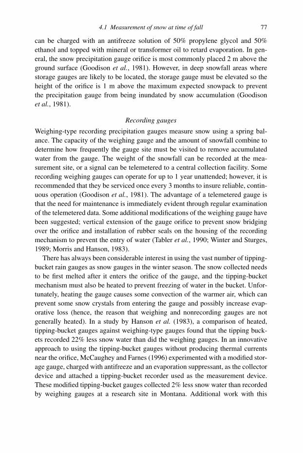
4.1 Measurement of snow at time of fall 77
can be charged with an antifreeze solution of 50% propylene glycol and 50%
ethanol and topped with mineral or transformer oil to retard evaporation. In gen-
eral, the snow precipitation gauge orifice is most commonly placed 2 m above the
ground surface (Goodison et al., 1981). However, in deep snowfall areas where
storage gauges are likely to be located, the storage gauge must be elevated so the
height of the orifice is 1 m above the maximum expected snowpack to prevent
the precipitation gauge from being inundated by snow accumulation (Goodison
et al., 1981).
Recording gauges
Weighing-type recording precipitation gauges measure snow using a spring bal-
ance. The capacity of the weighing gauge and the amount of snowfall combine to
determine how frequently the gauge site must be visited to remove accumulated
water from the gauge. The weight of the snowfall can be recorded at the mea-
surement site, or a signal can be telemetered to a central collection facility. Some
recording weighing gauges can operate for up to 1 year unattended; however, it is
recommended that they be serviced once every 3 months to insure reliable, contin-
uous operation (Goodison et al., 1981). The advantage of a telemetered gauge is
that the need for maintenance is immediately evident through regular examination
of the telemetered data. Some additional modifications of the weighing gauge have
been suggested; vertical extension of the gauge orifice to prevent snow bridging
over the orifice and installation of rubber seals on the housing of the recording
mechanism to prevent the entry of water (Tabler et al., 1990; Winter and Sturges,
1989; Morris and Hanson, 1983).
There has always been considerable interest in using the vast number of tipping-
bucket rain gauges as snow gauges in the winter season. The snow collected needs
to be first melted after it enters the orifice of the gauge, and the tipping-bucket
mechanism must also be heated to prevent freezing of water in the bucket. Unfor-
tunately, heating the gauge causes some convection of the warmer air, which can
prevent some snow crystals from entering the gauge and possibly increase evap-
orative loss (hence, the reason that weighing and nonrecording gauges are not
generally heated). In a study by Hanson et al. (1983), a comparison of heated,
tipping-bucket gauges against weighing-type gauges found that the tipping buck-
ets recorded 22% less snow water than did the weighing gauges. In an innovative
approach to using the tipping-bucket gauges without producing thermal currents
near the orifice, McCaughey and Farnes (1996) experimented with a modified stor-
age gauge, charged with antifreeze and an evaporation suppressant, as the collector
device and attached a tipping-bucket recorder used as the measurement device.
These modified tipping-bucket gauges collected 2% less snow water than recorded
by weighing gauges at a research site in Montana. Additional work with this

78 Ground-based snowfall and snowpack measurements
system in North Dakota indicated that it was a viable way to get reliable data
using a tipping-bucket approach (Carcoana and Enz, 2000).
4.1.2 Measurement errors
Although the measurement of precipitation with gauges seems straightforward,
errors can arise that need to be accounted for, especially with snowfall as opposed
to rainfall. The height of the gauge orifice in relation to the maximum snowpack
height must be considered so the gauge is not covered in high accumulation years.
A snowcap or bridge over the gauge orifice can form, especially in areas prone to
rime ice formation (Tabler et al., 1990). Wind can deflect precipitation particles on
trajectories that cause an undercatch of actual precipitation, which is especially true
for snow particles compared to rain particles and more so as wind speed increases.
Wetting the interior walls of the container or collector and subsequent evaporation
can cause a loss of a greater magnitude than errors arising from splash of raindrops
out of gauge or evaporation of water accumulated in the container (Sevruk, 1986).
Associated with this is the inability of gauges to accurately measure small snowfall
amounts. Also to be considered are errors arising from the effects of surrounding
topography and structures and the collection of snow blowing from the ground or
off nearby vegetation (Tabler et al., 1990).
Minimizing or correcting for errors
Considering that wind can reduce the catch of total snowfall by 50 to 80% (Goodison
et al., 1981; Larson and Peck, 1974; Sevruk, 1986; Goodison, 1978; Tabler et al.,1990), this error would be very important to reduce or at least correct for using the
results of gauge-catch studies. The first solution is to locate the gauge to minimize
the impact of wind, such as in small clearings in the forest snow zone or in brush.
Unfortunately, the snow zone does not often have such barriers to the wind. Also,
where possible, the gauge orifice should not be elevated more than necessary as
the wind speed increases with height and, thus, increases the catch deficit. Because
most gauges have to be exposed to the wind, other means to reduce wind speed
across the gauge orifice must be used.
Studies show that utilization of various types of gauges with wind shields
increases the amount of snowfall caught by the gauge. Many different types of
shields have been used around the world (see Figure 4.1). Some of the more com-
mon shields employed around the world today are shown in Figure 4.2. Tabler
et al. (1990) provides details of the Nipher, Alter, Double-Fence, Wyoming, and
Dual-Gauge shielding systems. There should be very strong consideration given
to shielding all precipitation gauges used to measure winter snowfall due to the
extreme catch deficit that can develop as wind speed increases.

4.1 Measurement of snow at time of fall 79
Figure 4.1 Shielded snow gauge in the northwest United States used to registersnow fall (courtesy National Oceanic and Atmospheric Administration (NOAA),NOAA Central Library, NOAA Photo Library, wea 00901, Historic NWS Col-lection, original photo, US Weather Bureau, 1917 in “Boy with Weather Men,”p. 224)
If a wind shield is not used on a precipitation gauge in snowfall areas, it is
puzzling why coefficients to correct for the catch deficit are not widely utilized. In
fact, very few snowfall records are corrected and published, while there has been
much published on methods to correct such data (Sevruk, 1986; 1989; Goodison
et al., 2002). Studies have been done in a variety of countries to come up with wind
correction factors that vary according to wind speed and can be used to reconstruct
precipitation amounts. For example, Bryazgin and Radionov (2002) provide wind
correction factors for liquid, mixed, and solid precipitation events. They also
provide correction factors for recalculating precipitation amounts affected by
wetting the interior of the precipitation gauge. Such corrections need to be made
in order to generate correct data for climate studies and runoff forecasting if
precipitation gauges are to be used in such analyses. Unfortunately, several other
problems arise of which the user of the data needs to be aware. First, the same
correction methods are not used in Canada and the northern United States. Second,
about half of the US synoptic stations adjust the observed amount collected using a
correction factor, but this correction is not noted in the published records. As a result,
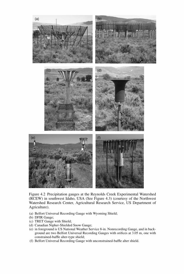
(a)
(c)
(e) (f)
(d)
(b)
Figure 4.2 Precipitation gauges at the Reynolds Creek Experimental Watershed(RCEW) in southwest Idaho, USA (See Figure 4.3) (courtesy of the NorthwestWatershed Research Center, Agricultural Research Service, US Department ofAgriculture).
(a) Belfort Universal Recording Gauge with Wyoming Shield;(b) DFIR Gauge;(c) TRET Gauge with Shield;(d) Canadian Nipher-Shielded Snow Gauge;(e) in foreground is US National Weather Service 8-in. Nonrecording Gauge, and in back-
ground are two Belfort Universal Recording Gauges with orifices at 3.05 m, one withconstrained-baffle alter-type shield;
(f) Belfort Universal Recording Gauge with unconstrained-baffle alter shield.

4.1 Measurement of snow at time of fall 81
historical precipitation data do not have a consistent relation to actual snowfall
(Peck, 1997).
Placement of precipitation gauges in natural openings in a forested area is desir-
able so the wind effect on catch is minimized, but care must be taken not to place
the gauge too close to the forest or the wind might blow snow off the trees and into
the gauge. The recommendation of the SCS (Soil Conservation Service, 1972) is to
place a gauge no closer in horizontal distance than four times the average height of
the trees. Although different agencies make different recommendations (see Tabler
et al., 1990), a similar “rule of thumb” should be employed when locating gauges.
When locating gauges near man-made structures, the same “rule of thumb” should
also be employed.
Case study intercomparison in Idaho
A site was established by the USDA/ARS on the Reynolds Creek Experimental
Watershed in southwestern Idaho (see Figure 4.3) in fall 1987 and operated through
spring 1994 to compare precipitation catch between nine precipitation measuring
systems (some with shields, some unshielded) (Hanson et al., 1999). This site was
established as part of the World Meteorological Organization’s (WMO) program to
compare current national methods of measuring snowfall with precipitation gauges.
A schematic of the location of the precipitation gauges and other instruments on
the WMO comparison site is shown in Figure 4.4.
The following nine gauging systems were used in this study (see Figure 4.2):
(1) The Belfort universal recording gauge (orifice at 2.2 m) with a Wyoming
shield (WYO) (Rechard, 1975); (2) the Russian double-fence intercomparison
reference (DFIR) gauge, consisting of a shielded Tretyakov (TRET) gauge (ori-
fice at 3.0 m) with two concentric wooden outer shields; (3) the Russian TRET
gauge (orifice at 2.0 m) with shield; (4) the Canadian Nipher shielded snow
gauge (CAN) (orifice at 1.6 m) (Canadian Department of Environment, 1985);
(5) the US National Weather Service 8-inch nonrecording gauge (orifice at 0.94 m)
without a shield (NATUNSHLD); (6) the Belfort universal recording gauge (ori-
fice at 1.4 m) with an Alter shield with unconstrained baffles (NATSHLD) (Alter,
1937); (7) the Belfort universal recording gauge (orifice at 3.05 m) without
a shield (BELUNSHLD); (8) the Belfort universal recording gauge (orifice at
3.05 m) with an Alter-type shield with the shield’s baffles individually constrained
at an angle of 30◦ from the vertical (BELSHLD); and, (9) the dual-gauge (DUAL-
GAUGE) (Hamon, 1973; Hanson, 1989) configuration that is discussed in the next
section.
Table 4.1 is a summary of gauge catch for the study period of 1987–94. The
WYO catch amounts were used as the base values in this study because WYO had
the greatest total catch during this study. These results agree with a previous study

82 Ground-based snowfall and snowpack measurements
Figure 4.3 World Meteorological Organization (WMO) precipitation gauge catchsite on at the RCEW in southwest Idaho (adapted from Hanson et al. [1999]).
at this same site by Hanson (1989), which found that the WYO had a slightly greater
total precipitation catch than the DUAL-GAUGE system.
SnowAs shown in Table 4.1, the computed snow catch from the DUAL-GAUGE system
and the CAN catch were greater than the WYO catch by 4 and 1%, respectively.
The greater catch of snow by the DUAL-GAUGE system supports previous findings
by Hanson (1989). The DFIR and NATSHLD catches were only 2 and 4% less,
respectively, than the WYO catch. The TRET and BELSHLD caught approximately

4.1 Measurement of snow at time of fall 83
Figure 4.4 Location of precipitation gauges and other meteorological instrumen-tation on the RCEW test site (adapted from Hanson et al. [1999]).
1% less snow than the WYO. The NATUNSHLD and the BELUNSHLD gauges
caught 12 and 24% less, respectively.
Total precipitationFor all precipitation types and events combined (total in Table 4.1), the WYO caught
more precipitation than any of the other gauges; however, the undercatch was only
3% or less for the DFIR, CAN, NATSHLD, and DUAL-GAUGE. The catch by the
WYO, CAN, and DUAL-GAUGE were not significantly different. These results
indicate that these five gauging systems may be used with little or no correction,
but there may be a small undercatch relative to the WYO. The TRET, NATUN-
SHLD, and BELSHLD caught between 8 and 9% less total precipitation than the
WYO. It should be noted here that the BELSHLD and the NATSHLD gauges are the

Tab
le4.1
Tota
lgau
geca
tch
(mm
)fo
r19
87–1
994
win
ter
peri
ods,
Rey
nold
sC
reek
Exp
erim
enta
lWat
ersh
ed,I
daho
(Han
son
etal
.,19
99)
Gau
ge
Pre
cip
itat
ion
typ
e(1
)W
YO
(2)
DF
IR(3
)T
RE
T(4
)C
AN
(5)
NA
TU
NS
HL
D(6
)N
AT
SH
LD
(7)
BE
LU
NS
HL
D(8
)B
EL
SH
LD
(9)
DU
AL
-G
AU
GE
(10
)
Sn
ow(N
=4
9)
21
1.8
b2
07
.2c
19
1.6
d2
13
.3b
18
7.3
d2
02
.3c
16
0.4
e1
92
.1d
22
0.9
aR
atio
0.9
80
.90
1.0
10
.88
0.9
60
.76
0.9
11
.04
Mix
ed(N
=2
3)
11
8.7
a1
15
.40
a1
10
.50
b1
15
.10
a1
07
.90
b1
15
.20
a9
7.6
0c
10
7.5
0b
11
5.5
0a
Rat
io0
.97
0.9
30
.97
0.9
10
.97
0.8
20
.91
0.9
7R
ain
(N=
37
)1
78
.7a
17
0.0
b1
64
.3cd
16
7.5
bc
16
7.0
bc
17
4.5
b1
60
.6d
16
5.3
c1
68
.7b
cR
atio
0.9
50
.92
0.9
40
.93
0.9
80
.90
0.9
30
.94
To
tal
(N=
10
9)
50
9.2
a4
92
.60
b4
66
.40
c4
95
.90
ab4
62
.20
c4
92
.00
b4
18
.60
d4
64
.90
c5
05
.10
abR
atio
0.9
70
.92
0.9
70
.91
0.9
70
.82
0.9
10
.99
Not
e.T
he
mea
nva
lues
of
row
sw
ith
the
sam
ele
tter
wer
en
ot
sig
nifi
can
tly
dif
fere
nt
atth
e0
.05
pro
bab
ilit
yle
vel
.R
atio
=gau
ge
catc
hva
lues
/WY
Oca
tch
.

4.1 Measurement of snow at time of fall 85
same type of gauge and both were shielded; however, the BELSHLD orifice was
at 3.05 m, which most likely accounted for most of the difference in catch between
these two gauges. The BELUNSHLD, with its orifice at 3.05 m, caught 18% less
precipitation than the WYO gauge, which was significantly less than any of the
other gauging systems.
In general, the results of this case study emphasize that precipitation gauge
shielding and the location of the orifice above the ground are critical to reliable
precipitation measurements. The results also support the concept of correcting
precipitation catch when different gauging systems are used.
4.1.3 Manual snow-depth determinations
Ruler measurements and snowboards
A ruler measurement of snow depth provides a physical depth observation that can
be converted to snow water equivalent if a representative density can be determined
for the area in question. In Canada, a standard ruler measurement is the average
of several snow-depth readings over a representative area (Goodison et al., 1988).
The major factor that must be considered is selection of the representative area so
that the effects of drifting snow are avoided. The determination of the amount of
snowfall deposited in a specific storm can be difficult as the entire snowpack, and
especially the new snow, is continually settling. The use of snowboards is one way to
measure an incremental depth of snow input to the snowpack and avoid measuring
the old snow. A snowboard is a square piece (about 40 cm × 40 cm; Goodison
et al., 1981) of plywood or lightweight metal, painted white in order to minimize
any melting of the snow. After each depth observation (with a ruler), the snowboard
is swept clear of snow and set on top of the snow surface in preparation for the next
measurement. Most accurate measurements are acquired if the snowboard reading
is made after snowfall ceases or several times during a long lasting snowstorm.
To convert a recent snowfall depth to a snow water equivalent value, multiply the
snow depth by 0.1, which is the commonly used average density of new snow.
However, this value can vary widely from region to region and storm to storm, and
errors in calculating the snow water equivalent in this way can be large. The actual
snow water equivalent can be obtained by taking a sample core off the snowboard,
melting the sample, and measuring the melted depth.
Snow stakes and aerial markers
Where snow depth measurements of the entire snowpack are required from some
distance, snow stakes can be used, painted with a bright color and contrasting num-
bers for ease of observation and avoidance by snowmobiles (Trabant and Clagett,
1990) or skiers. Placing the site on level ground helps prevent horizontal pressure

86 Ground-based snowfall and snowpack measurements
Figure 4.5 Oblique aerial photography of simulated aerial snow marker in Buckpasture, Black Forks Basin, Uinta Mountains, Utah at SNOTEL site (courtesyNatural Resources Conservation Service, US Department of Agriculture).
from downslope motion on the stake, and the use of round, as opposed to rectan-
gular, cross section stakes helps minimize drifting or melt out around the stake. By
being able to make a reading from the outside of the snow stake plot, destruction
or disturbance of the accumulated snow cover is avoided. If aerial surveys of snow
depth are required, aerial snow markers that contrast with the snow and are easy to
read from a rapidly moving airplane are necessary. These are the best approaches to
use in remote areas with difficult winter access. The aerial markers are commonly
made of wood and steel with an established horizontal bar interval. Long horizontal
bars are placed every even foot (30.5 cm) (and shorter bars are sometimes placed at
the odd foot [30.5 cm]) with taller markers used in deep snowpack areas, being rein-
forced by diagonal bracing crossing at one-half the measurement interval selected
(Trabant and Clagett, 1990).
When visually observing snow depth from a low-flying aircraft, the observation
of the number of bars visible from the top down is recorded, with subtraction from
the total bars included on a particular marker to be done after the flight. To assure a
record of the aerial snow marker, oblique photography of the marker can be obtained
during the flight for later analysis. Visual readings of the snow-depth marker are
usually accurate to ± 50 mm (Trabant and Clagett, 1990). Photographing the marker
with high speed film in a 35 mm camera with a 500 mm telephoto lens has been used
by Schumann (1975) to determine the snow depth to ±7.5 mm. Figure 4.5 shows
an aerial snow-marker photograph from an aerial snow-survey flight in Utah. Any
4.1 Measurement of snow at time of fall 87
such snow-depth data must be multiplied by representative snow-density values to
obtain the snow water equivalent. The density values, if chosen incorrectly, can
cause large errors in estimating the water volume.
4.1.4 Automatic weather stations
The places in a snow basin at which we would like to acquire measurements are
often remote and/or experience severe weather conditions. Many times, the only
way to acquire the necessary weather data is to make measurements automatically.
Strangeways (1984) has devoted significant time to designing an automatic weather
station (AWS) that can operate unattended for long time periods. He has come up
with an AWS that can operate in cold environments where high winds and icing of
instruments are problems. It needs only an aqualung to de-ice the sensors by shock
induction and flexing (Strangeways, 1984), and the AWS can measure incoming
and reflected solar radiation, temperature, humidity, wind speed and direction, and
precipitation. Still, the measurement of the solid precipitation component remains
a significant problem, and the most recent advances of accurate solid precipitation
component measurement must be incorporated into the AWS concept. More will
be said about remote, automated measurements when snowpack measurements are
discussed later in this chapter.
4.1.5 Other methods for measuring falling snow
Goodison et al. (1988) report on an acoustic ranging instrument developed in
Canada to measure the incremental snow depth over any selected period of time.
The most recent version measures the time elapsed for an acoustic pulse to travel
from a transducer to the target (snow surface) and back again. Air temperature
must be measured to account for the fact that speed of sound in air is temperature
dependent. The potential resolution of the sensor for measuring incremental snow
depth is 1.0 mm. Because the snowpack is dynamic, it is not realistic to expect this
measurement accuracy. Over the course of the winter season, the automated acous-
tic snow sensor measures to ±2.5 cm of the total new snow-depth accumulation
(Goodison et al., 1988; Tanner and Gaza, 1990).
The light attenuation snow-rate sensor is a device that measures the change in
light transmission over a path length as snow falls through the light beam. This
instrument gives a detailed time history of snow rate and will operate for days
unattended. In contrast to a conventional collecting gauge, it has no problems
with snow bridging across the orifice. The major disadvantage is that it gives no
measurement of snow totals directly, but rather a history of instantaneous rates. An
instrument like this is used in the National Weather Service Automated Surface
Observing System (ASOS) (Doesken and Judson, 1997).
88 Ground-based snowfall and snowpack measurements
(a) (b)
Figure 4.6 Hotplate snow gauge operation where both upper (a) and lower(b) plates are heated and maintained at 75 ◦C. The power difference betweenthe top and bottom plates is proportional to the precipitation rate (courtesy R.Rasmussen, National Center for Atmospheric Research).
A “hotplate snow gauge” has been developed to do away with oil, glycol, or an
expensive wind shield, now typically required for current weighing precipitation
gauges. The system has an upper and lower plate heated to constant, identical
temperatures (Rasmussen et al., 2002). The two plates are maintained at constant
temperatures during wind and precipitation conditions by increasing or decrea-
sing the current to the plate heaters (see Figure 4.6). During precipitation condi-
tions, the top plate has an additional cooling effect due to melting and evaporation
of precipitation. The difference between the power required to heat the top plate
compared to the bottom plate is proportional to the precipitation rate (Rasmussen
et al., 2002).
As noted by Singh and Singh (2001), investigators in Norway (Bakkehoi et al.,1985) have developed a vibrating wire-strain gauge that can measure falling pre-
cipitation with a resolution of about 0.1 mm. The weight of solid precipitation on
the wire causes a change in frequency vibration, which corresponds to a certain
snowfall amount. This gauge can be continuously recording or preset to read at
certain specific time intervals (Singh and Singh, 2001).
Ground-based weather radar can be used to estimate areal precipitation in snow-
fall events in a way similar to rainfall events. Because of several factors, the esti-
mation of areal snowfall is more difficult than estimating areal rainfall amounts.
Most weather radars use S-band, but Giguere and Austin (1991) indicate the use
of X-band would improve the measurement of areal snowfall due to an increased
range of observation and more sensitivity to lower intensity snowfalls. In snowfall
situations, it is common to have mixed precipitation, which further confuses the
radar determination due to part of the reflected wave being from snow and part from
rain. In general, ground-based radar determinations of snowfall can be as much as

4.2 Measurement of snow on the ground 89
50% in error. However, when combined with conventional gauge measurements
(and sometimes satellite determinations), the value of the radar lies in its areal
coverage and nearly continuous operation.
4.1.6 Snowfall records and data
In the United States, the greatest snowfall depth in a 24-hour period was 192.5
cm at Silver Lake, CO, on April 14–15, 1921. The greatest snowfall in one storm
occurred at the Mt. Shasta Ski Bowl in California and totaled 480 cm from February
13–19, 1959. The largest total snowfall to occur in one snow season was 2,475 cm at
Thompson Pass in Alaska during 1952–53. The greatest snow depth ever measured
on the ground was 1145.5 cm at Tamarack, CA on March 11, 1911. Measuring
snow on the ground, however, presents an entirely different challenge, as we shall
cover in the next section.
4.2 Measurement of snow on the ground
Measurement of falling snow amounts and recently accumulated snow depth is
complicated enough, but measuring the water equivalent of snow on the ground
may be even more difficult because of the need to find a representative location
and not to disturb the snowpack, making return visit measurements possible. The
most common way to assess the snow water equivalent of snow on the ground in
the western United States, where snow makes up over 50% of the water supply, is
to measure snow water equivalent with a calibrated snow sampler at a number of
points along an established transect called a snow course.
4.2.1 Snow-course surveys
Originally, snow courses were established to assess the snow water equivalent of
a snowfield to come up with an estimate of the amount of resulting runoff when
the snowpack melts in the spring and summer. However, accessibility of represen-
tative snowpack areas is often difficult, especially in winter, when the snow courses
not only extend over a mere fraction of the snow fields but are often not located in
certain key snow accumulation and ablation areas. As a result, snow courses have
usually been used to obtain a consistent index to the quantity of runoff that the
snow will generate during melt. In more singular cases, the snow course can also
be located to represent the accumulation of snow over fairly large, adjacent areas.
The layout of a snow course is usually in one or more lines of about 10 points
(ranging from 5–15 measurement points), similar to that shown by the Natural
Resources Conservation Service (2003d) in Figure 4.7. Most snow courses estab-
lished by the Natural Resources Conservation Service in the United States are about
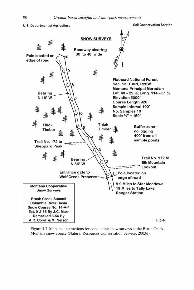
90 Ground-based snowfall and snowpack measurements
Figure 4.7 Map and instructions for conducting snow surveys at the Brush Creek,Montana snow course (Natural Resources Conservation Service, 2003d).

4.2 Measurement of snow on the ground 91
1000 ft (305 m) long and, if possible, protected from the wind by locating them
in small meadows (Julander, 2003). The snow course can be laid out between
two stakes, marked by signs on trees, or described by written directions and
compass headings (Goodison et al., 1981). Notes can be kept so that measure-
ments are not taken in the same location more than once during the season. In
the United States, measurements are taken on the first of every month starting on
January 1 and continuing until May 1 or June 1, depending on the snow condi-
tions. Mid-month surveys are made in Canada, as well as at the beginning of the
month, and, in special situations, in the United States to help evaluate changing
conditions.
The snow sampler equipment is simple in concept. A graduated tube with a
cutter on the lower end, allowing easy insertion into the snowpack, is used to
obtain a snow core. The tube and core are then weighed on a spring balance.
The balance is scaled to read directly in snow-water-equivalent units. Most snow
tubes are made of aluminum, but some are made out of plastic or fiberglass. In the
western part of North America, the aluminum snow tube sections are made so they
can be screwed together, thus, making determination of snow water equivalent in
deep snowpacks possible. In the eastern part of North America where snowpacks
are relatively shallow, the snow tubes used are typically only one section, like
the Adirondack or Canadian MSC snow samplers. Goodison et al. (1981) present
interesting comparison information on the snow samplers used in North America
(Table 4.2).
Before making measurements, the surveyor makes sure the tube is completely
clear of any snow, ice, or soil. The manual snow surveys are conducted with a team
of two or more surveyors for both safety and technical reasons. One surveyor takes
the measurements and a second surveyor serves as the recorder. At the designated
measurement point on the course, the snow sampling tube(s) is inserted into the
snow all the way to the ground surface, the snow depth is recorded from the scale
on the outside of the tube, and a core is extracted with soil plug at the end. The soil
plug verifies the tube reached to the ground surface (Julander, 2003). The soil is
cleared from the tube and the length of the core is verified to roughly correspond to
the outside of the tube depth measurement. The weight of the tube and snow core
measured on the spring balance and the tare weight of the empty tube are subtracted
to give the snow water equivalent of the snowpack. All the snow water equivalent
values are averaged to get one overall value for the snow course.
The average snow-course value is most often used in an empirical regression,
along with other independent variables such as precipitation, antecedent streamflow
and other snow-course average values, to produce a seasonal snowmelt volume
forecast as close as possible to the first of the month, corresponding to when
the snow course measurement was made. All streamflow forecasts generated are for

Tab
le4.2
Snow
sam
pler
prop
erti
es(G
oodi
son
etal
.,19
81)
Sta
nd
ard
a
Fed
eral
Fed
eral
bB
owm
anc
L-S
McC
alld
Can
adia
ne
MS
CA
dir
on
dac
kf
Mat
eria
lA
lum
inu
mA
lum
inu
mP
last
ico
rA
lum
inu
mH
eav
yG
aug
eA
lum
inu
mA
lum
inu
mG
lass
Fib
er
Len
gth
of
tub
eg(c
m)
76
.27
6.2
76
.27
6.2
10
9.2
15
3.7
Th
eore
tica
lID
of
cutt
er(c
m)
3.7
72
3.7
72
3.7
72
3.7
72
7.0
51
6.7
44
Nu
mb
ero
fte
eth
16
81
61
61
6N
on
eh
Dep
tho
fsn
owth
atca
nb
esa
mp
led
(m)
>5
>5
>3
.5>
51
.01
.5R
etai
ns
snow
core
sre
adil
yY
esY
esY
esY
esN
oN
o
aS
tan
dar
dsa
mp
ler
use
din
the
wes
tern
Un
ited
Sta
tes
and
Can
ada.
bId
enti
cal
to“S
tan
dar
dF
eder
al”
but
has
an8
-to
oth
cutt
er.
cC
utt
erh
asal
tern
ate
cutt
eran
dra
ker
teet
han
dm
ayb
em
ou
nte
do
np
last
ico
rst
and
ard
alu
min
um
tub
ing
.It
ism
ore
anex
per
imen
tal
rath
erth
ano
per
atio
nal
sam
ple
r.d
Use
din
den
sesn
owo
ric
e.It
isa
hea
vy
gau
ge
alum
inum
tube
wit
h5-c
mcu
tter
wit
hst
raig
ht
flukes
.It
may
be
dri
ven
into
the
pac
kw
ith
asm
all
slid
ed
rop
ham
mer
pro
du
cin
gan
ice-
pic
kef
fect
.e
Atm
osp
her
icE
nvir
on
men
tS
erv
ice
larg
ed
iam
eter
sam
ple
ru
sed
insh
allo
wsn
owco
ver
.f
Lar
ge
dia
met
erfi
ber
gla
sssa
mp
ler
com
mo
nly
use
din
east
ern
Un
ited
Sta
tes.
gM
ost
snow
sam
ple
rsin
No
rth
Am
eric
au
sein
ches
and
ten
ths
asth
eir
bas
icu
nit
so
fm
easu
rem
ent.
Val
ues
inth
ista
ble
are
corr
esp
on
din
gm
etri
ceq
uiv
alen
ts.
hS
tain
less
stee
lci
rcu
lar
cutt
ered
ge
or
smal
lte
eth
.

4.2 Measurement of snow on the ground 93
streamflow volumes that would occur naturally without any upstream influences.
A set of forecasts is made with the most probable forecast being one that has a
50% chance streamflow volume will exceed the forecast value and a 50% chance
streamflow volume will be less than the forecast value. The most probable forecast
will rarely be correct because of errors resulting from future weather conditions and
from errors in the forecast equation itself (Natural Resources Conservation Service,
2003a).
4.2.2 SNOwpack TELemetry (SNOTEL) system
The SNOTEL system is a logical extension of the manual snow course network.
NRCS installs, operates, and maintains an extensive, automated SNOTEL system
used to collect snowpack and climate data (including related fire-hazard data),
especially in remote regions and in response to an economic need to reduce the
number of costly, manual snow courses. SNOTEL data are collected and relayed
using meteor burst communications technology. Radio signals are reflected off an
ever-present band of ionized meteorite trails existing 50–75 miles above the Earth’s
surface. SNOTEL sites are generally located in remote, high elevation basins with
difficult access. These sites are designed to operate unattended for a year. Solar
power is used to recharge batteries. The approximately 730 SNOTEL sites are
polled daily by three master stations in the western United States, and data are
transmitted to the NRCS National Weather and Climate Center in Portland, OR,
where the data are stored (Natural Resource Conservation Service, 2003b).
Basic SNOTEL sites have a pressure-sensing snow pillow, a sonic snow depth
sensor, storage precipitation gauge, and an air-temperature sensor. The four snow
pillows, shown in Figure 4.8, are envelopes of stainless steel or synthetic rubber,
containing an antifreeze solution, about 4 ft (1.22 m) on a side and arranged to
form a square approximately 8 ft (2.44 m) on a side. As snow accumulates on
the pillows, a pressure is exerted on the antifreeze solution. The snow load on the
pillow is sensed either by a pressure transducer or by the fluid level in a standpipe.
These devices convert the weight of the snow to an electrical reading of the snow
water equivalent. Larger surface area pillows are used in areas where bridging of the
snowpack over the pillows is a possibility. The precipitation gauge measures all pre-
cipitation in any form that falls during the year, while the temperature sensor records
maximum, minimum, and average daily readings (Natural Resources Conservation
Service, 2003c). The SNOTEL system has a great capability to incorporate addi-
tional sensors at particular sites that can be used for other environmental problems.
Additional variables that have been measured include wind speed and direction,
soil temperature, soil moisture, snow depth, barometric pressure, humidity, and
radiation.

94 Ground-based snowfall and snowpack measurements
Figure 4.8 Schematic of a typical SNOTEL site. Pressure pillows are used formeasuring snow water equivalent, a storage gauge provides seasonal precipitationat the site, and a temperature sensor measures the existing air temperature (adaptedfrom Natural Resources Conservation Service, 2003c).
Both snow course and SNOTEL data are available on the Natural Resources
Conservation Service, National Water and Climate Center website, www.wcc.
nrcs.usda.gov/. Figure 4.9 shows the location of the SNOTEL sites in Utah, and
by putting the cursor on a point, the name of the SNOTEL site is displayed. By
clicking on the SNOTEL site, various options for data retrieval are presented.
Table 4.3 shows the data for Wolf Creek Summit SNOTEL in Colorado for several
days.
4.2.3 Other methods of measuring snow water equivalent (SWE)
Cosmic radiation, particularly the gamma portion, passes through the atmosphere
and penetrates the winter snowpack. The greater the snow water equivalent, the
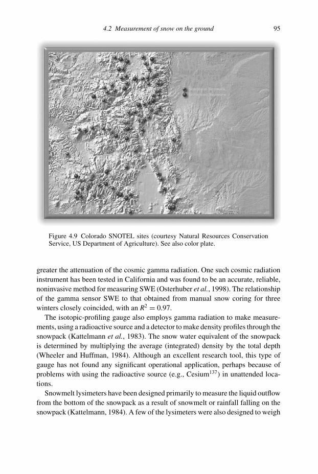
4.2 Measurement of snow on the ground 95
Figure 4.9 Colorado SNOTEL sites (courtesy Natural Resources ConservationService, US Department of Agriculture). See also color plate.
greater the attenuation of the cosmic gamma radiation. One such cosmic radiation
instrument has been tested in California and was found to be an accurate, reliable,
noninvasive method for measuring SWE (Osterhuber et al., 1998). The relationship
of the gamma sensor SWE to that obtained from manual snow coring for three
winters closely coincided, with an R2 = 0.97.
The isotopic-profiling gauge also employs gamma radiation to make measure-
ments, using a radioactive source and a detector to make density profiles through the
snowpack (Kattelmann et al., 1983). The snow water equivalent of the snowpack
is determined by multiplying the average (integrated) density by the total depth
(Wheeler and Huffman, 1984). Although an excellent research tool, this type of
gauge has not found any significant operational application, perhaps because of
problems with using the radioactive source (e.g., Cesium137) in unattended loca-
tions.
Snowmelt lysimeters have been designed primarily to measure the liquid outflow
from the bottom of the snowpack as a result of snowmelt or rainfall falling on the
snowpack (Kattelmann, 1984). A few of the lysimeters were also designed to weigh

Tab
le4.3
Wol
fCre
eka
sum
mit
SNO
TE
Lda
tare
port
–da
ily
read
ings
(Nat
ural
Res
ourc
esC
onse
rvat
ion
Serv
ice,
2004
)b
Sn
oww
ater
Yea
r-to
-dat
eC
urr
ent
Pre
vio
us
day
’ste
mp
(◦ F)
Tim
eeq
uiv
alen
tS
now
dep
thp
reci
pit
atio
nte
mp
Dat
e(P
ST
)(i
nch
es)
(in
ches
)(i
nch
es)
(◦ F)
Max
Min
Av
g
5/2
6/2
00
40
25
39
.63
5.2
35
.24
8.9
32
.53
9.7
5/2
7/2
00
40
24
.53
7.5
35
.23
6.2
52
.12
9.5
40
.25
/28
/20
04
02
3.5
35
.73
5.2
37
.75
8.9
30
.94
3.2
5/2
9/2
00
40
22
.43
33
5.2
41
.45
9.5
36
.54
6.8
5/3
0/2
00
40
22
.13
2.2
35
.22
6.1
45
.72
5.9
35
.65
/31
/20
04
02
1.7
31
.13
5.2
29
47
.42
1.1
33
.36
/1/2
00
40
21
28
.93
5.2
36
.75
6.5
28
.54
1.7
aB
asin
:U
pp
erS
anJu
an(H
UC
14
08
01
01
)E
leva
tio
n:
11
00
0bP
rov
isio
nal
dat
a(A
so
f:T
ue
Jun
01
13
:00
:26
PD
T2
00
4),
sub
ject
tore
vis
ion
c Pre
cip
(YT
D)=
Pre
cip
itat
ion
fro
mO
cto
ber
1to
curr
ent
dat
e.
4.2 Measurement of snow on the ground 97
the snowpack in place (e.g. Cox and Hamon, 1968). For determining the snow water
equivalent, however, devices such as snow pillows have received more emphasis in
the last 20 years than lysimeters.
Some attempts have been made to develop an alternative to the snow pillow.
Moffitt (1995) reported on the development of a 1m2, circular, perforated aluminum
plate mounted on three load cells. The weight on the snow plate is converted to
snow water equivalent. The instrument is accurate and portable. However, it still
has snow bridging problems similar to snow pillows because of its relative small
size. If coupled with an ultrasonic snow-depth sensor, the combination of sensors
can be used to indirectly measure snow density.
4.2.4 Liquid-water measurements
Liquid water in a snowpack, although recognized for some time as a quantifiable
parameter of hydrologic significance, is not a regularly reported snowpack charac-
teristic due to difficulties with its measurement in the field. The amount of liquid
water representing the liquid phase of snowpack is an important parameter in fore-
casting runoff, predicting wet slab avalanche release, and interpreting snowpack
remote sensing data using microwave techniques. Variation in snowpack liquid
water produces changes in the dielectric properties of the snowpack for most of the
microwave region, which in turn will have an effect on any microwave techniques
being used to estimate water equivalent or snow depth.
The liquid-water content of a snowpack, sometimes called free water, snow
water content, or liquid-phase water, includes gravitational water moving downward
through the snowpack and capillary water held by surface tension between the
individual snow grains.
Various techniques have been used or proposed to measure the liquid-water
content of a snowpack. Most of these techniques can be broadly categorized as cen-
trifugal, dielectric, dilution, and calorimetric. Some investigators have tested other
methods, including Shoda (1952) who used a measurement of volume expansion
upon freezing and Bader (1948) who used the concept of dilution of a solution by the
liquid water in the snowpack. Morris (1981) has reported improvement of the solu-
tion method for field use. These and other techniques are summarized in Table 4.4.
Kuroda and Hurukawa (1954) and Carroll (1976) described centrifugal separa-
tion of the liquid water from a snow sample. Langham (1974, 1978) subsequently
improved the method by isolating the amount of melt that occurs during the cen-
trifuging process. The National Bureau of Standards (Jones, 1979) compared the
centrifuge technique with the calorimetric technique. It was concluded that the
centrifuge and freezing calorimeter methods do not measure the same phenomena
and that water may be present in the snowpack in a form which is detectable by

98 Ground-based snowfall and snowpack measurements
Table 4.4 Methods for determination of the liquid-water content of snow
Method Operating principle Reference
Melting calorimetry Energy required to melt massof ice is measured whenwarm water is added tosnow sample
Radok et al., 1961; Fisk,1982, 1983; Ohmura,1980; Kawashima et al.,1998
Freezing calorimetry Energy liberated when theliquid water in snow isfrozen by a freezing agent ismeasured
Leaf, 1966; Fisk, 1982,1983; Boyne and Fisk,1987, 1990; Jones et al.,1983
Alcohol calorimetry Temperature depressionmeasured as snow samplemelts in methanol at 0 ◦C
Fisk, 1983, 1986
Dilution Reduction in electricalconductivity of a solutiondue to dilution by snowpackliquid water is measured
Davis et al., 1985; Boyneand Fisk, 1987, 1990
Dielectric constant Capacitance or TDRmeasurement in snow variesdue to large difference indielectric constants of liquidwater and ice
Boyne and Fisk, 1987,1990; Denoth, 1994;Ambach and Denoth,1974; Schneebeli et al.,1998
Freezing-point depression Freezing-point depression in asalt solution added to a snowsample due to liquid water ismeasured
Bader, 1950; Morris, 1981
Centrifuge Centrifugal force is used toseparate liquid water fromice in a snow sample
Kuroda and Hurukawa,1954; Jones, 1979
the freezing calorimeter method but not by the centrifuge method. Colbeck (1978)
analyzes this in more detail.
The dielectric method for measuring liquid-water content relies on the con-
trast between the dielectric properties of dry and wet snow. Ambach and Denoth
(1974, 1980) have developed capacitance techniques and used them extensively
in the field. These dielectric sensors have generally been calibrated with freezing
calorimetry. Linlor et al. (1974, 1975) and Linlor and Smith (1974) have used
various dielectric techniques, including capacitance and microwave beam atten-
uation, in the laboratory with some field testing. The capacitance method is dis-
cussed for determining free water in glacial snowfields (Østrem and Brugman, 1991)
(Figure 4.10).
The dilution method, as described by Davis et al. (1985), mixes snow with free
water with an aqueous solution (like 0.1N hydrochloric acid) and measures the
change in concentration of the aqueous solution. One advantage of the approach
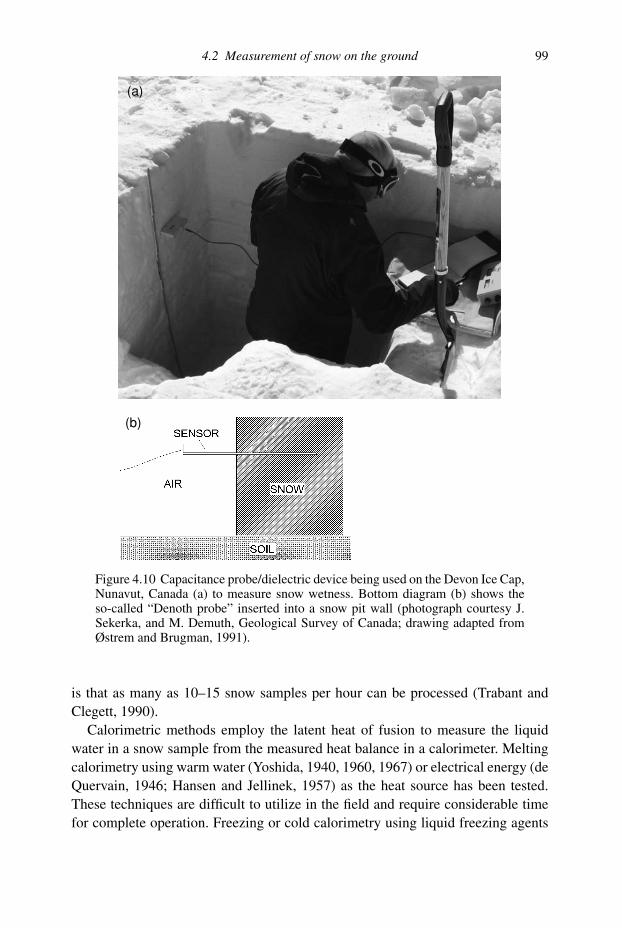
4.2 Measurement of snow on the ground 99
(a)
(b)
Figure 4.10 Capacitance probe/dielectric device being used on the Devon Ice Cap,Nunavut, Canada (a) to measure snow wetness. Bottom diagram (b) shows theso-called “Denoth probe” inserted into a snow pit wall (photograph courtesy J.Sekerka, and M. Demuth, Geological Survey of Canada; drawing adapted fromØstrem and Brugman, 1991).
is that as many as 10–15 snow samples per hour can be processed (Trabant and
Clegett, 1990).
Calorimetric methods employ the latent heat of fusion to measure the liquid
water in a snow sample from the measured heat balance in a calorimeter. Melting
calorimetry using warm water (Yoshida, 1940, 1960, 1967) or electrical energy (de
Quervain, 1946; Hansen and Jellinek, 1957) as the heat source has been tested.
These techniques are difficult to utilize in the field and require considerable time
for complete operation. Freezing or cold calorimetry using liquid freezing agents

100 Ground-based snowfall and snowpack measurements
has been described by Radok et al. (1961) and used in the field by Leaf (1966).
Howell et al. (1976) and Bergman (1978) used the freezing calorimeter with toluene
as the freezing agent. Although toluene is satisfactory for freezing the snow liquid
water, its toxic properties and relatively high flash point make its use somewhat
hazardous. Silicone oil has been used successfully as the freezing agent (Jones
et al., 1983), and it has significantly improved safety features over toluene.
Freezing calorimetry has been used both in operational-type fieldwork and snow
hydrology research. Because freezing calorimetry has gained acceptance as a stan-
dard method for field measurements of liquid-water content and as a method for
calibrating new measurement methods, it is presented in more detail here to illus-
trate an easily duplicated field measurement method.
Calorimetric analysis
The freezing or cold calorimeter technique has been selected by investigators pri-
marily because it is relatively inexpensive, simple to use, and based on known
and documented physical phenomena. In addition, it appears that, because a
small amount of liquid water is frozen in the freezing calorimetric approach as
opposed to a large amount of ice melted in the melting calorimetric method,
the freezing calorimetric method is more sensitive to variations in liquid-water
content.
A calorimetric analysis is based on the concept that heat gained by the system
must equal the heat lost. The calorimeter and the freezing agent gain heat; the snow
sample and the liquid water lose heat. If the heat gained terms are set equal to the
heat lost terms, the following equation results:
(m3 − m2)(T3 − T2)ci + mwL f = [(m2 − m1) + E](T2 − T1)cf (4.1)
where:
mw = mass of the liquid water, kg
Lf = latent heat of fusion, J kg−1
cf = specific heat of freezing agent at (T1 + T2)/2, J kg−1 ◦C−1
ci = specific heat of ice at (T2 + T3)/2, J kg−1 ◦C−1
E = calorimeter constant, kg
m1 = mass of calorimeter, kg
m2 = mass of calorimeter and freezing agent, kg
m3 = mass of calorimeter, freezing agent and snow, kg
T1 = initial temperature of the freezing agent, ◦C
T2 = initial temperature of the snow at sample point, ◦C
T3 = Final temperature of snow and freezing agent, ◦C
If θm is the fraction of liquid water in the sample, then:
mw = θm(m3 − m2) (4.2)

4.2 Measurement of snow on the ground 101
Substituting in Equation (4.1), the expression for the percent of liquid water in the
snow sample is
θm = [(m2 − m1) + E](T2 − T1)cf
L f(m3 − m2)− ci(T3 − T2)
L f
(4.3)
Snow thermal quality, B as defined by Bruce and Clark (1966) is the fraction (by
weight) of water in the solid state or (1 − θm) and can, therefore, be determined by
calorimetric methods (see Section 3.4.1).
The type of container generally used for mixing the freezing agent and the snow
sample in cold calorimetry is a vacuum-insulated bottle with a temperature probe
and a tightly fitted rubber stopper. Experience indicates that a commercial, 1-qt (946
ml), stainless steel, wide-mouth vacuum bottle works well. The temperature probe
is used to monitor changes in temperature that occur in the vacuum bottle during
the mixing process. The heat-balance equation requires accurate measurements
of temperature changes inside the bottle during the mixing process. Because the
vacuum-insulated bottle is not a perfect system and the bottle itself gains some heat,
the heat-balance equation contains a calorimeter constant, E. Each calorimeter bottle
will have its own constant that must be determined independently. For convenience
in using the heat-balance equation, the calorimeter constant is expressed in terms
of equivalent weight of freezing agent. Various methods may be used to determine
this constant (Jones et al., 1983).
Freezing-calorimeter equipment and materials
Certain basic equipment is required for utilizing the freezing-calorimeter method
described in this section. First is the calorimeter which, as previously stated, is a
wide-mouth vacuum bottle made of stainless steel. Scales capable of weighing up to
2000 gm with accuracy to the nearest tenth of a gm are required for determining the
various weights. Finally, 30 cm long, stainless-steel thermocouple probes accurate
to 0.2 ◦C (used with a multi-channel digital readout) are needed for measuring
the temperature changes occurring in the calorimeter. In addition to these basic
requirements, several ancillary equipment items are recommended. They are a cold
chest for storing the freezing agent, thermal containers for transporting the snow
samples, timing devices, and miscellaneous tools, including shovels, trowels, and
spoons. As a result, the system is not easily portable in the field.
Cold calorimetry requires using a freezing agent to freeze the liquid water in the
snow sample. It is recognized that a small portion of the capillary water may not
be frozen, but the resulting error is considered to be very small.
Analysis of error associated with freezing calorimetry by various investigators
has indicated that the approach is accurate to within ±1.0–2.0% by weight. To
minimize errors, special care must be taken during determination of weights and
temperatures.

102 Ground-based snowfall and snowpack measurements
Melt-calorimetry approach
Basic theory and computations involved with the melt-calorimetry method are
reviewed here to illustrate another commonly applied method. In this method, a
snow sample is added to water in a vacuum bottle hot enough to melt all the ice and
the temperature of the resulting mixture is measured. The hot water is cooled in
proportion to the fractional mass of ice relative to liquid water in the snow sample.
An energy balance can be established for the vacuum bottle to compute the mass of
liquid water where the energy lost from the hot water and vacuum bottle (left side
of Equation 4.4) is equal to the energy required to melt all the ice in the sample
and warm the entire sample from 0 ◦C to the final temperature of the mixture (right
side of Equation 4.4) as:
(mhw + E)(Thw − Tf)cw = (ms − mw)L f + ms(Tf − Ts)cw (4.4)
where:
mhw = mass of hot water, kg
mw = mass of liquid water, kg
ms = mass of snow, kg
Thw = initial temperature of hot water, ◦C
Ts = initial temperature of snow, ◦C
Tf = final temperature of snow–hot water mixture, ◦C
cw = specific heat of water, 4.188 × 10³ J kg −1 ◦C−1
Lf = latent heat of fusion, 0.334 × 10⁶ J kg−1
E = calorimeter constant, kg
The calorimeter constant represents heat gained by the vacuum bottle from its
environment during the measurement and must be experimentally determined. E
is expressed in equivalent mass of hot water for simplicity. For reliable results,
this method requires temperature measurements to within 0.1 ◦C and mass within
0.001 kg.
A simple example ignoring the calorimeter constant can be used to illustrate the
use of the melting calorimetry method. If 0.2 kg of snow at 0 ◦C were added to a
vacuum bottle filled with 0.3 kg of hot water at 90 ◦C and the resulting mixture
achieved a final temperature of 25 ◦C, then the mass of liquid water in the snow
could be computed from Equation (4.4) as:
(0.3)(90 − 25)(4.188 × 10³) = (0.2 − mw)0.334
× 106 + (0.2)(25 − 0)(4.188 × 10³)
mw = 0.018 kg
Thus, the liquid water content on a mass basis would be 0.018/0.2 = 0.091 or 9.1%
liquid water.

4.2 Measurement of snow on the ground 103
Intercomparison of techniques
Boyne and Fisk (1987) compared four snow cover liquid-water measurement tech-
niques – alcohol calorimetry, freezing calorimetry, dilution, and capacitance. Each
method has advantages and disadvantages and should be chosen based on the spe-
cific project and resources available. However, Boyne and Fisk (1987) conclude
that all methods should be capable of giving comparable accuracies within 1–2%
on mass basis.
Liquid-water outflow measurements at the base of the snowpackwith snow lysimeters
Several different designs of lysimeters have been used to record the outflow of
liquid water at the base of the snowpack. A snowmelt lysimeter consists of a col-
lector, a flow-measuring device and a connector between the two major components
(Kattelmann, 1984). The most widely used is the ground-based, unenclosed lysime-
ter, but this design allows for collection of lateral flows of melt water as well as
melt generated in the column of snow directly over the lysimeter. In most cases,
it is assumed that lateral flow into the column of snow equals lateral flow out of
the column. Where this is not the case, a rim 10–15 cm high around the collector–
snow column interface is used to provide a more accurate monitoring of snowmelt in
the column of snow (Kattelmann, 1984). Because of problems that can arise by stor-
age of water above the collector and restrictions in proper drainage of the lysimeter,
much care in the design, construction, and installation of snowmelt lysimeters is
necessary to ensure accurate measurements (Kattelmann, 1984).
4.2.5 Snow pits
Digging a snow pit to determine the properties of a snowpack has important appli-
cations for avalanche forecasting, glaciology, remote-sensing data interpretation
and snow hydrology. Snow pits can be shallow (if others have been dug on a reg-
ular basis) or deep (all the way to the ground surface). In addition, snow-pit data
can be compared against many of the measurements previously discussed. Snow-
pit observations typically yield information on the snowpack temperature profile,
density profile, layers, grain type, grain size, layer hardness, free water content,
height, ram number (if a ram penetrometer is used near the snow pit), and snow
water equivalent (both for the total vertical snowpack and by horizontal layers in
the snowpack). Figure 4.11 is an adaptation of a snow-profile schematic of a snow
pit from Perla and Martinelli (1976).
Normally, the snow pit will have a square or rectangular cross section. The
southern (shaded) wall of the snow pit should remain untouched, as this is the side
that will be used for measurements. There should be a confined area around this
shaded wall where no one can step and where no removed snow is thrown. Once

104 Ground-based snowfall and snowpack measurements
Figure 4.11 Snowpack profile plotted from snow-pit field notes (adapted fromPerla and Martinelli, 1976).
the snow pit is excavated, the shaded wall should be freshly cut back several cm
and the temperature, wetness, and density measurements made in a timely manner.
The depth of the snowpack should be established first with zero being the ground
surface. When using a ram penetrometer to measure the hardness of each layer, it
can be left in place when the ground is reached. The snow pit can be dug adjacent
to the ram and it can serve as a measure of height. The shaded pit wall should be
shaved with a shovel and then brushed horizontally with a soft brush to accentuate
the layers (Perla and Martinelli, 1976). The layer thickness should be recorded
before additional work is done. Snow temperature can be measured with a 30-cm-
long, digital thermometer. This can be measured every 10 cm and in every layer as
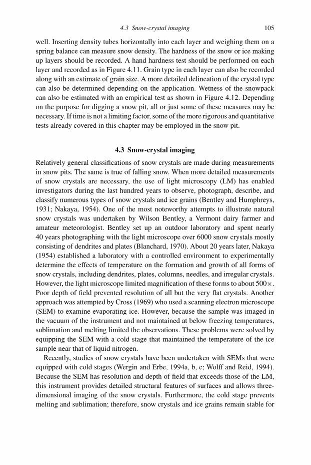
4.3 Snow-crystal imaging 105
well. Inserting density tubes horizontally into each layer and weighing them on a
spring balance can measure snow density. The hardness of the snow or ice making
up layers should be recorded. A hand hardness test should be performed on each
layer and recorded as in Figure 4.11. Grain type in each layer can also be recorded
along with an estimate of grain size. A more detailed delineation of the crystal type
can also be determined depending on the application. Wetness of the snowpack
can also be estimated with an empirical test as shown in Figure 4.12. Depending
on the purpose for digging a snow pit, all or just some of these measures may be
necessary. If time is not a limiting factor, some of the more rigorous and quantitative
tests already covered in this chapter may be employed in the snow pit.
4.3 Snow-crystal imaging
Relatively general classifications of snow crystals are made during measurements
in snow pits. The same is true of falling snow. When more detailed measurements
of snow crystals are necessary, the use of light microscopy (LM) has enabled
investigators during the last hundred years to observe, photograph, describe, and
classify numerous types of snow crystals and ice grains (Bentley and Humphreys,
1931; Nakaya, 1954). One of the most noteworthy attempts to illustrate natural
snow crystals was undertaken by Wilson Bentley, a Vermont dairy farmer and
amateur meteorologist. Bentley set up an outdoor laboratory and spent nearly
40 years photographing with the light microscope over 6000 snow crystals mostly
consisting of dendrites and plates (Blanchard, 1970). About 20 years later, Nakaya
(1954) established a laboratory with a controlled environment to experimentally
determine the effects of temperature on the formation and growth of all forms of
snow crystals, including dendrites, plates, columns, needles, and irregular crystals.
However, the light microscope limited magnification of these forms to about 500×.
Poor depth of field prevented resolution of all but the very flat crystals. Another
approach was attempted by Cross (1969) who used a scanning electron microscope
(SEM) to examine evaporating ice. However, because the sample was imaged in
the vacuum of the instrument and not maintained at below freezing temperatures,
sublimation and melting limited the observations. These problems were solved by
equipping the SEM with a cold stage that maintained the temperature of the ice
sample near that of liquid nitrogen.
Recently, studies of snow crystals have been undertaken with SEMs that were
equipped with cold stages (Wergin and Erbe, 1994a, b, c; Wolff and Reid, 1994).
Because the SEM has resolution and depth of field that exceeds those of the LM,
this instrument provides detailed structural features of surfaces and allows three-
dimensional imaging of the snow crystals. Furthermore, the cold stage prevents
melting and sublimation; therefore, snow crystals and ice grains remain stable for

Snow
at
0 °
C. S
now
flo
oded
wit
h w
ater
and c
onta
inin
g
rela
tivel
y s
mal
l am
ounts
of
air.
Snow
at
0 °
C. W
ater
can
be
pre
ssed
out
by m
oder
ate
squee
zing i
n t
he
han
d. T
her
e is
sti
ll a
n a
ppre
ciab
le
amount
of
air
confi
ned
wit
hin
the
snow
.
Snow
at
0 °
C. W
ater
vis
ible
as
a m
enis
cus
bet
wee
n
gra
ins
but
cannot
be
pre
ssed
out
by m
oder
ate
squee
zing
in t
he
han
d.
Snow
at
0 °
C. N
o w
ater
vis
ible
even
wit
h h
and l
ens.
Snow
mak
es g
ood s
now
bal
l.
Snow
usu
ally
, but
not
nec
essa
rily
, bel
ow
0 °
C. G
rain
s
hav
e li
ttle
ten
den
cy t
o s
tick
toget
her
in a
snow
bal
l w
hen
lightl
y p
ress
ed i
n g
loved
han
d.
Des
crip
tion
Slu
sh
Ver
y w
et
Wet
Mois
t
Dry
Ter
m
Fre
e W
ater
C
onte
nt
Sym
bol
Gra
upel
. O
ccas
ional
ly a
ppre
ciab
le l
ayer
s of
this
form
of
soli
d p
reci
pit
atio
n c
an b
e
iden
tifi
ed i
n t
he
snow
cover
.
Ice
layer
, le
ns,
or
pock
et.
----
Ice
Rounded
gra
ins
form
ed b
y M
F
met
amorp
his
m. G
rain
s usu
ally
lar
ger
than
1
mm
and o
ften
str
ongly
bonded
.
Over
100
Knif
eV
ery h
ard
Angula
r gra
ins
wit
h s
tepped
fac
es;
at l
east
som
e holl
ow
cups.
A
dvan
ced s
tages
of
TG
met
amorp
his
m.
51–100
Pen
cil
Har
dA
ngula
r gra
ins
wit
h f
lat
sides
or
face
s. E
arly
stag
es o
f T
G m
etam
orp
his
m.
16–50
One
finger
Med
ium
har
d
Rounded
, oft
en e
longat
ed, is
om
etri
c gra
ins.
End s
tages
of
ET
met
amorp
his
m. G
rain
s
usu
ally
les
s th
an 2
mm
in d
iam
eter
.
3–
15
Four
finger
s
Soft
Irre
gula
r gra
ins,
most
ly r
ounded
but
oft
en
bra
nch
ed. S
truct
ure
oft
en f
eltl
ike.
E
arly
stag
es o
f E
T m
etam
orp
his
m.
0–2
Fis
tV
ery s
oft
Fre
shly
dep
osi
ted s
now
. I
nit
ial
form
s ca
n b
e
easi
ly r
ecogniz
ed.
Ram
N
umbe
r (k
g)**
Han
d T
est*
Des
crip
tion
Har
dnes
s
Sym
bol
Des
crip
tion
Inte
rnat
iona
l sym
bols
and
mea
sure
men
ts
Gra
in
Typ
e
Sym
bol
Slu
sh
+ +
+
+ +
+
^ ^
^
^ ^
^
^
^ ^
^ ^
*In
the
han
d t
est
the
spec
ifie
d o
bje
ct c
an b
e push
ed i
nto
the
snow
in t
he
pit
wal
l w
ith a
forc
e of
about
5 k
g. I
n h
ard s
now
, fo
r ex
ample
, a
pen
cil
can b
e push
ed i
nto
the
snow
, but
wit
h t
he
sam
e pre
ssure
, a
finger
can
not.
**R
am n
um
ber
is
from
a c
one
pen
etro
met
erw
ith a
60°
apex
and 4
cm
dia
met
er.
Fig
ure
4.1
2In
tern
atio
nal
sym
bo
lsan
dm
easu
rem
ents
for
snow
gra
inty
pes
,sn
owh
ard
nes
sh
and
test
,an
dfr
eew
ater
con
ten
than
dte
st(a
dap
ted
fro
mP
erla
and
Mar
tin
elli
,1
97
6).

4.3 Snow-crystal imaging 107
indefinite periods of time. Using this technique, Wergin and Erbe (1994a, b, c)
captured snow crystals near their laboratory, quickly transferred them to the SEM
and were able to observe numerous forms of intact crystals. Since that time, snow
crystals and ice grains have been collected from numerous remote locations (Rango
et al., 1996a, b, c; 2000) (Wergin et al., 1995; 1996a, b, c; 1998a, b; 2002a, b). The
following provides brief descriptions of the equipment and procedures that were
fabricated and successfully used to collect, ship, store, and image snow and ice with
low temperature SEM (LTSEM).
4.3.1 Materials and methods
The equipment and techniques described below enable collecting, shipping, stor-
ing, and observing snow crystals and ice grains that are maintained at near-liquid
nitrogen temperatures (−196◦C). At this temperature, specimens remain stable dur-
ing observation in the LTSEM where they can be imaged and photographed. Many
of the devices that are described are unique and must be fabricated in the labora-
tory because they are currently unavailable commercially. The devices, which were
originally designed for studies with LTSEM, can also be used for observations with
light microscopy.
The term “cryo-system” is used generically in this study; it refers to an accessory
that is available from several manufacturers and can be retrofitted to most SEMs.
A cryo-system typically consists of: (1) a specimen holder (Figure 4.13a); (2)
a vacuum transfer assembly mechanism, consisting of a rod that attaches to the
specimen holder and is used to move the holder through the various stages or
compartments of the cryo-system; (3) a freezing chamber, where specimens are
typically plunged into liquid nitrogen (LN2) or some other cryogen; (4) a pre-
chamber, where the specimen can be fractured and/or coated with a heavy metal;
and, (5) a cold stage, which is mounted in the microscope and can be maintained
near LN2 temperatures.
Secondary specimen holders (sampling plates)
Close inspection of Figure 4.13, including the caption (Erbe et al., 2003), reveals the
details of the various components that are needed for field sampling and laboratory
processing of snow crystals for LTSEM photography. A commercial cryo-system
normally comes with a single universal specimen holder; replacements or spare
holders of this type frequently cost several hundred dollars each. When collecting
snow or ice at remote sites, several dozen specimens are frequently desired. There-
fore, numerous specimen holders are essential. To solve this problem, a simple,
inexpensive secondary specimen holder or sampling plate was devised. The plate
is used in the field to collect the sample. In the laboratory, a modified commercial
specimen holder that is compatible with the cryo-system accommodates the plate.
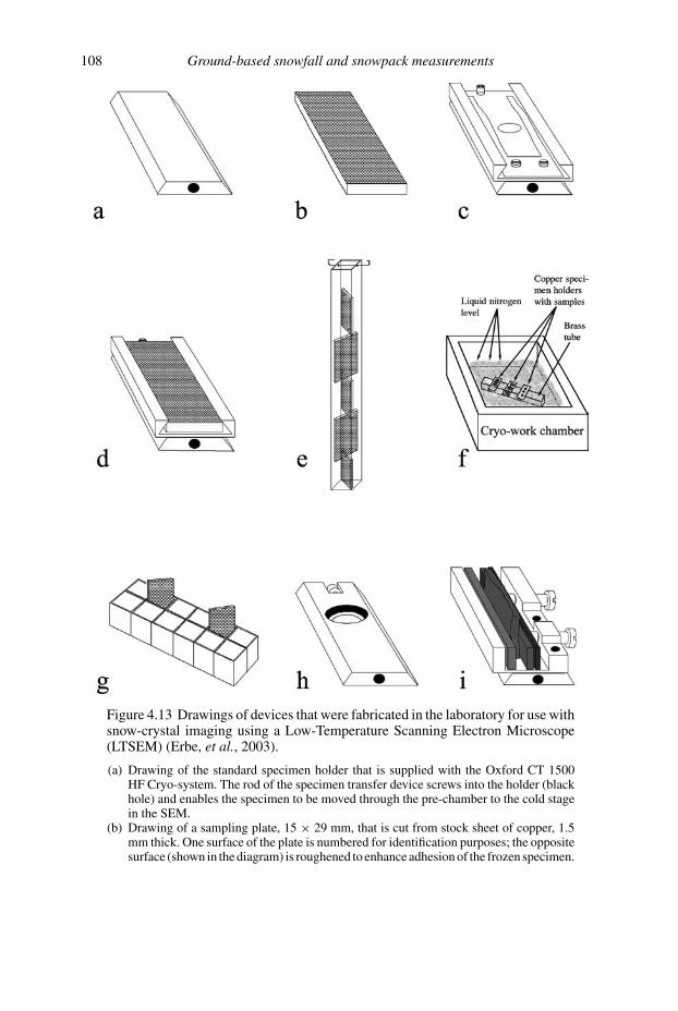
108 Ground-based snowfall and snowpack measurements
Figure 4.13 Drawings of devices that were fabricated in the laboratory for use withsnow-crystal imaging using a Low-Temperature Scanning Electron Microscope(LTSEM) (Erbe, et al., 2003).
(a) Drawing of the standard specimen holder that is supplied with the Oxford CT 1500HF Cryo-system. The rod of the specimen transfer device screws into the holder (blackhole) and enables the specimen to be moved through the pre-chamber to the cold stagein the SEM.
(b) Drawing of a sampling plate, 15 × 29 mm, that is cut from stock sheet of copper, 1.5mm thick. One surface of the plate is numbered for identification purposes; the oppositesurface (shown in the diagram) is roughened to enhance adhesion of the frozen specimen.

4.3 Snow-crystal imaging 109
Shipping sampling plates
At the collection site, tubes containing the sampling plates are lowered into a
lightweight, dry shipping Dewar or Cryopak Shipper (Taylor Wharton, Theodore,
AL 36582) that has previously been cooled with LN2. The Dewar is placed in a
backpack or hand carried from the collection site and then either transported by
van or sent by priority air express to the laboratory. The shipper, which is designed
to maintain LN2 temperatures for a minimum of 21 days when fully pre-cooled,
has been used to transport samples from numerous locations, including remote
regions of the states of Washington, North Dakota and Alaska. Upon reaching the
laboratory, the samples are transferred to a LN2 storage Dewar where they remain
until being further prepared for observation with LTSEM.
Sampling procedures
Preparing sampling platesAll samples of snow and ice are collected on the sampling plates, which are
pre-coated with a thin layer of cryo-adhesive such as Tissue Tek, a methyl cellulose
←−−−−−−−−−−−−−−−−−−−−−−−−−−−−−−−−−−−−−−−−−−−−−−−−−−−−−−−−−Figure 4.13 (cont.)
(c) Drawing of a modified specimen carrier that is fabricated and attached to the standardspecimen holder (lower level) depicted in (a).
(d) Drawing of the modified specimen carrier containing the sampling plate depicted in(b). The entire assembly, which attaches to the transfer rod of the cryo-system, can thenbe moved through the pre-chamber and onto the cold stage in the SEM.
(e) Drawing of the square brass tubing, 13 × 13 mm ID. The bottom end is permanentlycapped; two holes are drilled in the opposing sides of the upper end. Four plates can beinserted diagonally into the tubes; each plate is alternated at 90◦. A paper clip insertedthrough the holes retains the plates in the tube during shipping and storage.
(f) Drawing of a Styrofoam work chamber, 12 × 20 × 4 cm (depth) where samplescollected on the plates are either contact- or plunge-frozen in LN2 and held until theyare transferred to the square brass shipping tubes shown in (e). A Styrofoam cover isused between sample collections to prevent condensation or frost from forming in theLN2.
(g) Drawing of the staging jig that holds up to 10 plates in the Styrofoam box prior toloading in the square brass tubes. This device is fashioned by soldering together twelve1-cm segments of the square brass tubing.
(h) Drawing of a standard cylindrical stub holder, which is used to hold a metal tubecontaining an ice core. The tube is placed in the circular well and held firmly bytightening the setscrew (far end). In the pre-chamber, the core can be fractured toexpose an untouched, pristine surface.
(i) Drawing of an indium vise specimen holder. An ice sample can be clamped into theholder where it is held between two sheets of indium metal. Indium, which is thermallyconductive and pliable at LN2 temperatures, helps prevent shattering of the sample.This device has been used to hold glacial ice, icicles, hail, ice lenses, pond ice, and dryice.

110 Ground-based snowfall and snowpack measurements
solution. The adhesive and the plates must be cooled to temperatures at or slightly
below freezing. However, the adhesive will solidify at temperatures below −3 ◦C;
therefore, it must be protected from freezing in the container, as well as on the
sampling plate prior to sampling. To keep the adhesive near its freezing point
(−3 ◦C), the stock bottle can be placed in a pocket of one’s parka. Similarly, cold
plates, which will also freeze the adhesive prior to sampling, must be maintained at
near freezing temperatures. Immediately after a specimen has been collected, the
plate containing the adhesive and sample are plunged into a vessel of LN2. For this
purpose, a Styrofoam box, 12 × 20 × 4 cm (depth) containing a 1- to 2-cm layer
of LN2 is used. The box is used to plunge-freeze the plates that contain the samples
and to hold them for short-term storage (Figure 4.13f).
In warm or sunny conditions, such as late spring or on glacier surfaces during
summer, the temperature of the plates and cryo-adhesive may be well above freez-
ing. When this occurs, the plates and the adhesive can be pre-cooled by placing them
in the snowpack and then proceeding as described above. In these cases, excellent
preservation of structure has been accomplished if the sampling is done rapidly and
the plate is plunged immediately (less than 1 second) into LN2.
Sampling fresh and falling snowFalling snow is sampled by allowing it to settle on the surface of the plate containing
the cryo-adhesive. Alternatively, a fresh sample can be lightly brushed onto the
plate. In either case, the plate containing the sample is then rapidly plunge-frozen
in the LN2 vessel.
Snow-pit samplesTo collect samples from snow pits, a pre-cooled (LN2) scalpel is used to gently
dislodge snow crystals from a freshly excavated pit wall. The crystals are allowed
to accumulate onto a plate containing the cryo-adhesive and then plunged rapidly
into the LN2. If LN2 cannot be carried to the snow pit, a brass block, pre-cooled
with LN2 is transported to the pit. After the crystals are sampled, the plate is placed
on the brass block and allowed to freeze, then processed as previously described.
Hoar frostPlates can also be placed in an area where rime, surface hoar or frost are expected to
occur and simply allowed to serve as the substrate for the sample that forms. In this
case, the cryo-adhesive is not necessary. When a sufficient sample has sublimed on
the plate, it is plunge-frozen in LN2.
Fractured samplesFracturing of snow clusters or glacial ice is used to reveal the extent of air spaces,
details of sintering and biota, such as ice worms, snow algae (Chlamydomonas
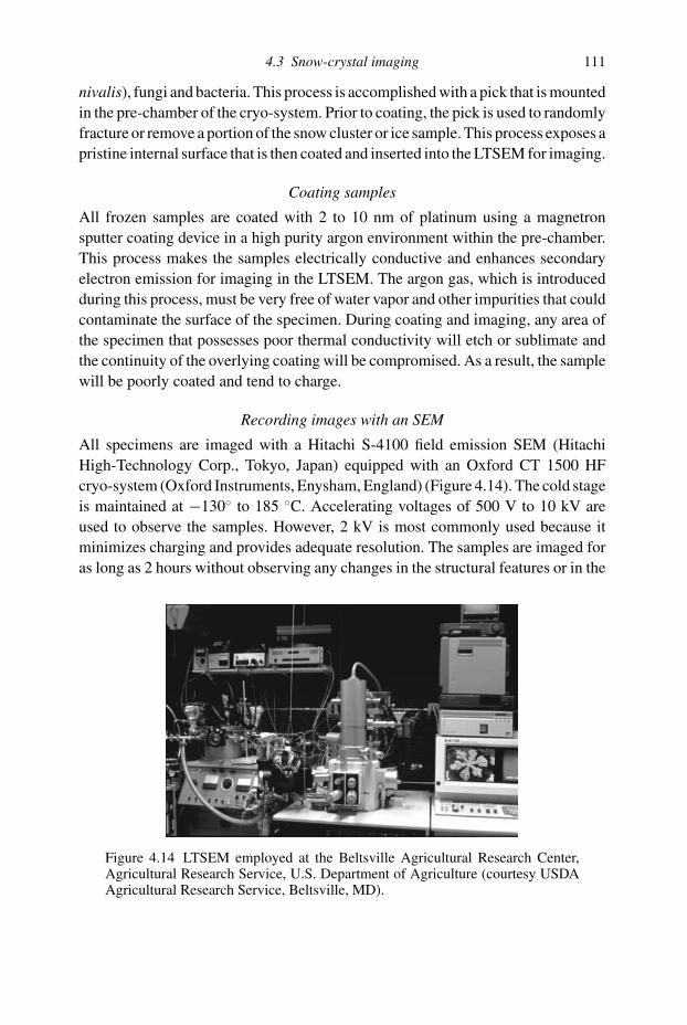
4.3 Snow-crystal imaging 111
nivalis), fungi and bacteria. This process is accomplished with a pick that is mounted
in the pre-chamber of the cryo-system. Prior to coating, the pick is used to randomly
fracture or remove a portion of the snow cluster or ice sample. This process exposes a
pristine internal surface that is then coated and inserted into the LTSEM for imaging.
Coating samples
All frozen samples are coated with 2 to 10 nm of platinum using a magnetron
sputter coating device in a high purity argon environment within the pre-chamber.
This process makes the samples electrically conductive and enhances secondary
electron emission for imaging in the LTSEM. The argon gas, which is introduced
during this process, must be very free of water vapor and other impurities that could
contaminate the surface of the specimen. During coating and imaging, any area of
the specimen that possesses poor thermal conductivity will etch or sublimate and
the continuity of the overlying coating will be compromised. As a result, the sample
will be poorly coated and tend to charge.
Recording images with an SEM
All specimens are imaged with a Hitachi S-4100 field emission SEM (Hitachi
High-Technology Corp., Tokyo, Japan) equipped with an Oxford CT 1500 HF
cryo-system (Oxford Instruments, Enysham, England) (Figure 4.14). The cold stage
is maintained at −130◦ to 185 ◦C. Accelerating voltages of 500 V to 10 kV are
used to observe the samples. However, 2 kV is most commonly used because it
minimizes charging and provides adequate resolution. The samples are imaged for
as long as 2 hours without observing any changes in the structural features or in the
Figure 4.14 LTSEM employed at the Beltsville Agricultural Research Center,Agricultural Research Service, U.S. Department of Agriculture (courtesy USDAAgricultural Research Service, Beltsville, MD).

112 Ground-based snowfall and snowpack measurements
coating integrity of the snow crystals. Selected images are recorded onto Polaroid
Type 55 P/N film (Polaroid, Cambridge, MA, USA).
Stereo pairs are obtained by recording one image, tilting the sample 6◦, re-
centering the subject and then recording the second image. The two images result-
ing from this procedure contain the parallax information necessary for three-
dimensional observation and study.
For much greater detail on the LTSEM field and laboratory sampling methods,
the reader is referred to Erbe et al. (2003).
4.4 References
Alter, J. C. (1937). Shielded storage precipitation gauges. Mon. Weather Rev., 65, 262–5.Ambach, W. and Denoth, A. (1974). On the dielectric constant of wet snow. In
Proceedings of the Grindelwald Symposium: Snow Mechanics. IAHS-AISHPublication 114, pp. 136–42.
Ambach, W. and Denoth, A. (1980). The dielectric behaviour of snow: a study versusliquid water content. In NASA Conference Publication 2153. Fort Collins, CO,pp. 69–92.
Bader, H. (1948). Theory of non-calorimetric methods for the determination of the liquidwater content of wet snow. Schweiz. Mineral. Petrogr. Mitt. 28, 344–61.
Bader, H. (1950). Note on the liquid water content of wet snow. J. Glaciol., 1, 446–7.Bakkehoi, S., Oien, K., and Førland, E. J. (1985). An automatic precipitation gauge based
on vibrating-wire strain gauges. Nordic Hydrol., 16, 193–202.Bentley, W. A. and Humphreys, W. J. (1931). Snow Crystals. New York: McGraw-Hill.Bergman, J. A. (1978). A method for the determination of liquid phase water in a
snowpack using toluene freezing calorimetry. Unpublished MS Forestry Thesis,University of Nevada, Reno, NV.
Blanchard, D. C. (1970). Wilson Bentley, the snowflake man. Weatherwise, 23, 260–9.Boyne, H. S. and Fisk, D. (1987). A comparison of snow cover liquid water measurement
techniques. Water Resour. Res., 23(10), 1833–36.Boyne, H. S. and Fisk, D. J. (1990). A Laboratory Comparison of Field Techniques for
Measurement of the Liquid Water Fraction of Snow, Special Report 90–3. US Army,Corps of Engineers, Cold Regions Research and Engineering Laboratory.
Bruce, J. P. and Clark, R. H. (1966). Introduction to Hydrometeorology. New York:Pergamon Press.
Bryazgin, N. N. and Radionov, V. F. (2002). Empirical method of correction of monthlyprecipitation totals for climatic studies. In Proceedings of the WCRP Workshop onDetermination of Solid Precipitation in Cold Climate Regions. Fairbanks, AK.
Canadian Department of Environment. (1985). Measuring Snowfall Water Equivalentusing the Nipher-Shielded Snow Gauge System, Report No. IB 04-03-01/1. Ottawa,Canada: Atmospheric Environment Service, Canadian Department of Environment.
Carcoana, R. and Enz, J. W. (2000). An enhanced technique for more reliable daily snowmeasurements with an antifreeze-based, tipping-bucket gauge. In Proceedings of the68th Annual Meeting of the Western Snow Conference, Port Angeles, WA,pp. 87–91.
Carroll, T. (1976). Estimation and Prediction of the Liquid Water Distribution in a HighAltitude Spring Snowpack. Avalanche Workshop. University of Calgary, Banff.

4.4 References 113
Colbeck, S. C. (1978). The difficulties of measuring the water saturation and porosity ofsnow. J. Glaciol., 20(28), 189–201.
Cox, L. M. and Hamon, W. R. (1968). A universal surface precipitation gauge. InProceedings of the 36th Annual Meeting of the Western Snow Conference, pp. 6–8.
Cross, J. D. (1969). Scanning electron microscopy of evaporating ice. Science, 164, 174–5.Davis, R. E., Dozier, J., LaChapelle, E. R., and Perla, R. (1985). Field and laboratory
measurements of snow liquid water by dilution. Water Resour. Res., 21, 1415–20.de Quervain, M. (1946). Zur bestimmung des wassergehalts von nass-schnee. Verhl.
Schweiz. Naturf. Ges., 94.Denoth, A. (1994). An electronic device for long-term snow wetness recording. Annals
Glaciol., 19, 104–6.Doesken, N. J. and Judson, A. (1997). The Snow Booklet: A Guide to the Science,
Climatology and Measurement of Snow in the United States. Fort Collins, CO:Colorado Climate Center, Department of Atmospheric Science, Colorado StateUniversity.
Erbe, E. F., Rango, A., Foster, J., Josberger, E. G., Pooley, C., and Wergin, W. P. (2003).Collecting, shipping, storing, and imaging snow crystals and ice grains with lowtemperature scanning electron microscopy. Microsc. Res. Techniq., 62, 19–32.
Fisk, D. (1982). Snow calorimetric measurement at Snow-One. In Proceedings of SnowSymposium, I, US Army, Corps of Engineers, Cold Regions Research EngineeringLab, pp. 133–8.
Fisk, D. J. (1983). Progress in methods of measuring the free water content of snow. InOptical Engineering for Cold Environments, Society of Photo-OpticalInstrumentation Engineers Conference Proceedings. 414, 48–51.
Fisk, D. (1986). Method of measuring liquid water mass fraction of snow by alcoholsolution. J. Glaciol., 32, 538–40.
Giguere, A. and Austin, G. L. (1991). On the significance of radar wavelength in theestimation of snowfall. In Hydrological Applications of Weather Radar, ed. I. D.Cluckie and C. G. Collier. London: Ellis Horwood, pp. 117–30.
Goodison, B. E. (1978). Accuracy of Canadian snow gauge measurements. J. Appl.Meteorol., 17, 1542–8.
Goodison, B. E., Ferguson, H. L., and McKay, G. A. (1981). Measurement and dataanalysis, Chapter 6. In Handbook of Snow, ed. D. M. Gray and D. H. Male. Toronto:Pergamon Press, pp. 191–274.
Goodison, B., Lawford, R., Rudolf, B., and Yang, D. (2002). WCRP Workshop onDetermination of Solid Precipitation in Cold-Climate Regions, ECGC-WCRP 2002,Proceedings CD, Fairbanks, AK.
Goodison, B. E., Metcalfe, J. R., Wilson, R. A., and Jones, K. (1988). The Canadianautomatic snow depth sensor: A performance update. In Proceedings of the 56thAnnual Meeting of the Western Snow Conference, Kalispell, MT, pp. 178–81.
Hamon, W. R. (1973). Computing Actual Precipitation; Distribution of Precipitation inMountainous Areas, vol. 1, WMO Report 362. Geneva: World MeteorologicalOrganization.
Hansen, B. L. and Jellinek, H. H. G. (1957). A Portable Adiabatic Calorimeter. SIPRETechnical Report No. 49.
Hanson, C. L. (1989). Precipitation catch measured by the Wyoming shield and dualgauge system. Water Resour. Bull., 25, 159–64.
Hanson, C. L., Johnson, G. L., and Rango, A. (1999). Comparison of precipitation catchbetween nine measuring systems. J. of Hydrol. Engineering, 4(11), 70–5.
Hanson, C. L., Zuzel, J. F., and Morris, R. P. (1983). Winter precipitation catch by heatedtipping-bucket gauges. T. Am. Soc. Ag. Eng., 26(5), 1479–80.

114 Ground-based snowfall and snowpack measurements
Howell, S., Jones, E. B., and Leaf, C. F. (1976). Snowpack Ground Truth (Radar Test SiteSteamboat Springs, CO, April 8–16). Mission Report (Contract NAS5-22312).Greenbelt, MD: Goddard Space Flight Center.
Jones, E. B., Rango, A., and Howell, S. M. (1983). Snowpack liquid water determinationsusing freezing calorimetry. Nordic Hydrol., 14, 113–26.
Jones, R. N. (1979). A Comparison of Centrifuge and Freezing Calorimeter Methods forMeasuring Free Water in Snow, Report NBSIR 79–1604. Boulder, CO: NationalBureau of Standards.
Julander, R. (2003). Snow Hydrology: Measuring Snow, www.civil.utah.edu/∼cv5450/measuring snow/snow measuring.html.
Kattelmann, R. C. (1984). Snowmelt lysimeters: design and use. In Proceedings of the52nd Annual Meeting of the Western Snow Conference, Sun Valley, ID, pp. 68–79.
Kattelmann, R. C., McGurk, B. J., Berg, N. H., Bergman, J. A., Baldwin, J. A., andHannaford, M. A. (1983). The isotope-profiling snow gauge: twenty years ofexperience. In Proceedings of the 51st Annual Meeting of the Western SnowConference, Vancouver, WA, pp. 1–8.
Kawashima, K., Endo, T., and Takeuchi, Y. (1998). A portable calorimeter for measuringliquid-water content of wet snow. Annals Glaciol., 26, 103–6.
Kuroda, M. and Hurukawa, I. (1954). Measurement of water content of snow. IASHPublication, General Assembly of Rome. 39 (IV), 38–41.
Langham, E. J. (1974). Problems of measuring meltwater in the snowpack. In Proceedingsof the 1974 Annual Meeting of the Eastern Snow Conference, Ottawa, Canada,pp. 60–71.
Langham, E. J. (1978). Measurement of the Liquid Water Content of Snow by RepeatedCentrifugal Extraction, Technical Report. Ottawa, Canada: Glaciology Division,Department of Fisheries and Environment.
Larson, L. W. and Peck, E. L. (1974). Accuracy of precipitation measurements forhydrologic modeling. Water Resour. Res., 10(4), 857–63.
Leaf, C. F. (1966). Free water content of snowpack in subalpine areas. In Proceedings ofthe 34th Western Snow Conference, Seattle, WA, pp. 17–24.
Linlor, W. I. and Smith, J. L. (1974). Electronic measurements of snow sample wetness. InAdvanced Concepts and Techniques in the Study of Snow and Ice Resources.Washington, DC: National Academy of Sciences, pp. 720–8.
Linlor, W. I., Clapp, F. D., Meier, M. F., and Smith, J. L. (1975). Snow wetnessmeasurements for melt forecasting. In NASA Special Publication 391. Washington,DC: NASA, pp. 375–97.
Linlor, W. I., Meier, M. F. and, Smith, J. L. (1974). Microwave profiling of snowpackfree-water content. In Advanced Concepts and Techniques in the Study of Snow andIce Resources. Washington, DC: National Academy of Sciences, pp. 729–39.
McCaughey, W. W. and Farnes, P. E. (1996). Measuring winter precipitation with anantifreeze-based tipping bucket system. In Proceedings of the 64th Annual Meetingof the Western Snow Conference, Bend, OR, pp. 130–6.
Moffitt, J. A. (1995). Snow plates: preliminary tests. In Proceedings of the 63rd AnnualMeeting of the Western Snow Conference, Sparks, NV, pp. 156–9.
Morris, E. M. (1981). Field measurement of the liquid-water content of snow. J. Glaciol.,27(95), 175–8.
Morris, R. P. and Hanson, C. L. (1983). Weighing and recording precipitation gaugemodification. T. Am. Soc. Civ. Eng., 26(1), 167–78.
Nakaya, U. (1954). Snow Crystals: Natural and Artificial. Cambridge, MA: HarvardUniversity Press.
4.4 References 115
Natural Resources Conservation Service (2003a). Interpreting Streamflow Forecasts.www.wcc.nrcs.usda.gov/factpub/interpet.html.
Natural Resources Conservation Service (2003b). SNOTEL Data Collection Network FactSheet. www.wcc.nrcs.usda.gov/factpub/sntlfct1.html.
Natural Resources Conservation Service (2003c). Snow Surveys – SNOTEL. www.wcc.nrcs.usda.gov/factpub/sect 4b.html.
Natural Resources Conservation Service (2003d). Snow Survey Sampling Guide: SnowSampling Procedures – Step 1. www.wcc.nrcs.usda.gov/factpub/ah169/ah169.htm.
Natural Resources Conservation Service (2004). Wolf Creek Summit SNOTEL DataReport. www.wcc.nrcs.usda.gov/nwcc/ sntl-data0000.jsp?site=874&days=7&state=CO
Ohmura, A. (1980). An economical calorimeter for measuring water content of a snowcover. Zeitschrift fur Gletscherkunde und Glazialgeologie, 16(1), 125–30.
Osterhuber, R., Gehrke, F., and Condreva, K. (1998). Snowpack snow water equivalentmeasurement using the attenuation of cosmic gamma radiation. In Proceedings of the66th Annual Meeting of the Western Snow Conference, Snowbird, UT, pp. 19–25.
Østrem, G. and Brugman, M. (1991). Glacier Mass-Balance Measurements. NHRIScience Report No. 4. Saskatoon, Saskatchewan, Canada: National HydrologyResearch Institute.
Peck, E. L. (1997). Improvement in Method to Adjust U.S. Solid Precipitation Records.Phase 1 Interim Report, GCIP/OGP/NOAA. Hydex Corporation.
Perla, R. I. and Martinelli, M. (1976). Avalanche handbook. In Agriculture Handbook489. Washington, DC: US Printing Office.
Radok, U., Stephens, S. K., and Sutherland, K. L. (1961). On the calorimetricdetermination of snow quality. In IAHS Publication 54, International Association ofHydrological Sciences, 132–5.
Rango, A., Wergin, W. P., and Erbe, E. F. (1996a). Snow crystal imaging using scanningelectron microscopy: I. Precipitated snow. Hydrol. Sciences Journal, 41, 219–33.
Rango, A., Wergin, W. P., and Erbe, E. F. (1996b). Snow crystal imaging using scanningelectron microscopy: II. Metamorphosed snow. Hydrol. Sciences Journal, 41,235–50.
Rango, A., Wergin, W. P., and Erbe, E. F. (1996c). 3-D characterization of snow crystalsas an aid to remote sensing of snow water equivalent. In Applications of RemoteSensing in Hydrology, ed. G. W. Kite, A. Pietroniro and T. J. Pultz. Saskatoon,Saskatchewan, Canada: National Hydrology Research Institute, pp. 295–310.
Rango, A., Wergin, W. P., Erbe, E. F., and Josberger, E. G. (2000). Snow crystal imagingusing scanning electron microscopy: III. Glacier ice, snow and biota. Hydrol.Sciences Journal, 45, 357–75.
Rasmussen, R. M., Hallett, J., Purcell, R., Cole, J., and Tryhane, M. (2002). The hotplatesnow gauge. In Proceedings of the WCRP Workshop on Determination of SolidPrecipitation in Cold Climate Regions. Fairbanks, AK.
Rechard, P. A. (1975). Measurement of winter precipitation in wind-swept areas. InProceedings of the Symposium on Snow Management on the Great Plains,Publication 73, Great Plains Agriculture Council. Lincoln, NE, pp. 13–30.
Schneebeli, M., Coleiu, C., Touvier, F. and Lesaffre, B. (1998). Measurement of densityand wetness in snow using time-domain reflectometry. Annals Glaciol., 26,69–72.
Schumann, H. H. (1975). Operational applications of satellite snowcover observations andLandsat data collection systems operations in central Arizona. In Proceedings of aWorkshop on Operational Applications of Satellite Snowcover Observations, NASA

116 Ground-based snowfall and snowpack measurements
SP-391. Washington, DC: National Aeronautics and Space Administration,pp. 13–28.
Sevruk, B. (1986). Correction of precipitation measurements summary report. InCorrection of Precipitation Measurements, ed. B. Sevruk. ETH/IAH/WMOWorkshop on the Correction of Precipitation Measurements, Report ZGS 23.Geographisches Institut, Eidgenossische Technische Hochschule Zurich,pp. 13–23.
Sevruk, B. (ed.). (1989). Precipitation measurement. In Proceedings of theWMO/IAHS/ETH Workshop on Precipitation Measurement. Geographisches Institut,Eidgenossische Technische Hochschule Zurich.
Shoda. M. (1952). Methods of measuring snow water content. Seppyo (Japan), 13, 103–4.Singh, P. and Singh, V. P. (2001). Snow and Glacier Hydrology. Dordrecht: Kluwer
Academic Publishers.Soil Conservation Service (1972). Snow survey and water supply forecasting. In SCS
National Engineering Handbook, sect 22. Washington, DC.Strangeways, I. C. (1984). The development of an automated weather station for cold
regions. In Proceedings of the 52nd Annual Meeting of the Western SnowConference, Sun Valley, ID, pp. 12–23.
Tabler, R. D., Berg, N. H., Trabant, D. C., Santeford, H. S., and Richard, P. A. (1990).Measurement and evaluation of winter precipitation. In Cold Regions Hydrology andHydraulics Monograph, ed. W. L. Ryan and R. D. Crissman. New York: AmericanSociety of Civil Engineers, pp. 9–38.
Tanner, B. D. and Gaza, B. (1990). Automated snow depth and snowpack temperaturemeasurements. In Proceedings of the 58th Annual Meeting of the Western SnowConference, Sacramento, CA, pp. 73–8.
Trabant, D. E. and Clagett, G. P. (1990). Measurement and evaluations of snowpacks. InCold Regions Hydrology and Hydraulics Monograph, ed. W. L. Ryan and R. D.Crissman. New York: American Society of Civil Engineers, pp. 39–93.
Wergin, W. P. and Erbe, E. F. (1994a). Can you image a snowflake with an SEM?Certainly! Proc. Roy. Microsc. Soc., 29, 138–40.
Wergin, W. P. and Erbe, E. F. (1994b). Snow crystals: capturing snowflakes for observationwith the low temperature scanning electron microscope. Scanning, 16, IV88–IV89.
Wergin, W. P. and Erbe, E. F. (1994c). Use of low temperature scanning electronmicroscopy to examine snow crystals. In Proceedings of the 13th InternationalCongress of Electron Microscopy, Publication 3B, pp. 993–4.
Wergin, W. P., Rango, A., and Erbe, E. F. (1995). Observations of snow crystals using lowtemperature scanning electron microscopy. Scanning, 17, 41–9.
Wergin, W. P., Rango, A., and Erbe, E. F. (1996a). The structure and metamorphism ofsnow crystals as revealed by low temperature scanning electron microscopy. InProceedings of the Eastern Snow Conference, Publication 53, pp. 195–204.
Wergin, W. P., Rango, A., Erbe, E. F., and Murphy, C. A. (1996b). Low temperature SEMof precipitated and metamorphosed snow crystals collected and transported fromremote sites. J. of the Microscopy Society of America, 2, 99–112.
Wergin, W. P., Rango, A., and Erbe, E. F. (1996c). Use of low temperature scanningelectron microscopy to observe icicles, ice fabric, rime and frost. In Proceedings ofthe Microscopy Society of America Meeting, Publication 54, pp. 147–8.
Wergin, W. P., Rango, A., and Erbe, E. F. (1998a). Image comparisons of snow and icecrystals photographed by light (video) microscopy and low temperature scanningelectron microscopy. Scanning, 20, 285–296.
4.4 References 117
Wergin, W. P., Rango, A., and Erbe, E. F. (1998b). Use of video (light) microscopy andlow temperature scanning electron microscopy to observe identical frozenspecimens. Electron Microsc., 1998, 325–6.
Wergin, W. P., Rango, A., Foster, J., Erbe, E. F., and Pooley, C. (2002a). Irregular snowcrystals: structural features as revealed by low temperature scanning electronmicroscopy. Scanning, 2, 247–56.
Wergin, W. P., Rango, A., Foster, J., Erbe, E. F., and Pooley, C. (2002b). Low temperaturescanning electron microscopy of “irregular snow crystals”. Microsc. Microanal., 8,722–3CD.
Wheeler, P. A. and Huffman, D. J. (1984). Evaluation of the isotopic snow measurementgauge. In Proceedings of the 52nd Annual Meeting of the Western Snow Conference,Sun Valley, ID, pp. 48–56.
Winter, C. J. and Sturges, D. L. (1989). Improved Procedures for Installing and OperatingPrecipitation Gauges and Alter Shields on Windswept Land, Research Note RM-489.USDA Forest Service.
Wolff, E. W. and Reid, A. P. (1994). Capture and scanning electron microscopy ofindividual snow crystals. J. Glaciol., 40, 195–7.
Yoshida, Z. (1940). A method of determining thaw water content in snow layers. J. ofFaculty of Science, ser. II–III, 4.
Yoshida, Z. (1960). A calorimeter for measuring the free water content of wet snow. J.Glaciol., 3, 574–6.
Yoshida, Z. (1967). Free water content of snow. In Proceedings of the InternationalConference on Low Temperature Science, Sapporo, Japan, pp. 773–84.

5
Remote sensing of the snowpack
5.1 The importance of snow
There is such a vast difference in the physical properties of snow and other natural
surfaces that the occurrence of snow in a drainage basin can cause significant
changes in the energy and water budgets. As an example, the relatively high albedo
of snow reflects a much higher percentage of incoming, solar, shortwave radiation
than snow-free surfaces (80% or more for relatively new snow as opposed to roughly
15% or less for snow-free vegetation). Snow may cover up to 53% of the land surface
in the northern hemisphere (Foster and Rango, 1982) and up to 44% of the world’s
land areas at any one time. On a drainage basin basis, the snow cover can vary
significantly by elevation, time of year, or from year to year. The Rio Grande Basin
near Del Norte, Colorado, is 3419 km2 in area and ranges from 2432 m a.s.l. at
the streamgauge up to 4215 m a.s.l. at the highest point in the basin. Figure 5.1
compares the snow-cover depletion curves obtained from Landsat data in 1977 and
1979 in elevation zones A (780 km2; 2432–2926 m), B (1284 km2; 2926–3353 m),
and C (1355 km2; 3353–4215 m) of the Rio Grande Basin. In a period of only
2 years from April 10, 1977, to April 10, 1979, a great difference in seasonal snow-
cover extent was experienced. Landsat data show that 49.5% or 1693 km2 were
covered by snow on April 10, 1977. Two years later in 1979, 100% or 3419 km2
were snow covered on April 10.
Snow cover and its subsequent melt supplies at least one-third of the water that
is used for irrigation and the growth of crops worldwide (Steppuhn, 1981). In high
mountain snowmelt basins of the Rocky Mountains, USA, as much as 75% of the
total annual precipitation is in the form of snow (Storr, 1967) and 90% of the annual
runoff is from snowmelt (Goodell, 1966). The runoff depth can vary greatly from
year to year for mountain basins because of differences in the seasonal snow-cover
accumulation. In the Rio Grande Basin near Del Norte, Colorado, the seasonal snow
cover in the 2 years cited above, 1977 and 1979, produced vastly different annual
118

5.1 The importance of snow 119
Figure 5.1 Comparison of snow-cover depletion curves for the Rio Grande basinnear Del Norte, Colorado derived from Landsat data for elevation zones A, B, andC for 1977 and 1979. On April 10, the snow cover is 100% in all zones for 1979and 97.5%, 29%, and 0% in zones A, B, and C for 1977.
runoff depths of 7.8 cm and 35.36 cm for 1977 and 1979, respectively (Rango and
Martinec, 1997).
Because the physical properties of snow are so much different than other naturally
occurring surfaces, it has opened up possibilities of exploiting widely different parts
of the electromagnetic spectrum to learn more about the snowpack resource. In
the above cited example, the visible portion (0.4–0.7 μm) of the electromagnetic
spectrum (shown in Figure 5.2) was used to map the percentages of the basin covered
by snow because of the difference in reflectance of snow and snow-free areas. The
near infrared portion (0.7–1.1 μm) can also be used for snow mapping and for the
detection of near surface liquid water because of the near infrared sensitivity to
the liquid water molecule. The thermal infrared portion of the spectrum (8–14 μm)
is also a possible area to exploit, but to date little has been done. The capability
of detecting snowpack surface temperature variability in space and time can be
directly linked to the presence of water in the snowpack and perhaps to snowmelt.
Although in widely disparate portions of the spectrum, the gamma radiation (3 ×10⁻⁶–3 × 10⁻⁵ μm) and the microwave radiation (1 mm–1 m) bands can be used
in similar ways to detect the snowpack water equivalent using the attenuation of
the relevant radiation by the snowpack itself. In the gamma radiation portion, the

120 Remote sensing of the snowpack
Figure 5.2 Electromagnetic spectrum and instrumentation associated with specificelectromagnetic intervals (adapted from Allison et al., 1978; Hall and Martinec,1985.)
snowpack attenuates the gamma ray signal. In the microwave portion, the snowpack
emits and attenuates depending on the size and shape of crystals and the presence
of liquid water. The use of active microwaves as opposed to passive microwaves
adds the additional complication of surface orientation and reflectance.
5.2 General approach
5.2.1 Gamma radiation
Snow-water-equivalent methodology
The use of gamma radiation to measure snow water equivalent (SWE) is based on the
attenuation of natural terrestrial radiation by the mass of water in the overlying snow
cover. Gamma radiation is emitted from potassium (40K), uranium (238U), and
thorium (208Ti) radioisotopes in the soil with the majority of the emission coming
from the top 20 cm. The intensity of gamma radiation is measured using a gamma
radiation spectrometer, which is generally flown on an airplane for snow survey
measurements. Fritzsche (1982) provides a description of the physics behind the
airborne, gamma radiation spectrometer flown by the US National Weather Service
(NWS) (see Table 5.1 at end of chapter for acronyms) and methods of calibration.
Airborne gamma measurements of snow water equivalent in a basin are generally
acquired along an established network of flight lines. A background (no-snow)

5.2 General approach 121
flight is conducted in the fall before snow accumulation and then the same lines
are flown during the winter when snow covered. When an airborne gamma snow
survey is conducted, several flight lines are usually flown within a basin, providing
information on the relative spatial variation in SWE over the basin.
Airborne snow-water-equivalent measurements using gamma radiation are made
using the relationship given in Equation (5.1) (Carroll, 1990):
SWE = 1
A
(ln
C0
C− ln
100 + 1.11M
100 + 1.11M0
)(5.1)
where:
SWE = snow water equivalent, g cm−2
C and C0 = uncollided, terrestrial gamma counts over snow and bare ground,
respectively
M and M0 = percent soil moisture in snow-covered and bare-soil areas, respectively
A = Radiation attenuation coefficient in water, cm2 g−1
The use of airborne gamma measurements for snow-water-equivalent retrieval is
a reliable technique that has been proven effective for operational hydrological
monitoring in many countries. Basin surveys can be completed in a matter of hours,
producing information on the spatial distribution of snow water equivalent and a
representative estimate of the volume of snow contained in the basin. The method is
applicable to all sizes of basins. As demonstrated by the NWS operational airborne
gamma snow-survey program (Carroll, 1990), the derived SWE information can be
made available to user agencies within several hours of the airborne survey, thus
providing timely information for hydrological forecasts. Carroll (1986) presents a
cost–benefit analysis of airborne gamma SWE data acquired in support of snowmelt
flood forecasting for a major flood event that occurred in the USA in February 1985.
Since gamma radiation is attenuated by water in all phases, the radiation mea-
surements will include the effects of water in the soil as well as the snow-cover
mass and, thus, the contribution of soil moisture has to be taken into account.
Inaccurate estimates of soil moisture will yield over- or under-estimations of snow
water equivalent. By conducting a background airborne gamma flight in the fall
before snow accumulation, the soil moisture background is measured, but it will
not be representative if subsequent rainfall adds moisture to the soil or if mois-
ture migrates upward from the soil to the snow during winter. Ground-based soil
moisture measurements conducted along the flight line during the winter over-snow
flight can help contribute to a more accurate snow water equivalent (Carroll et al.,1983). Additionally, atmospheric absorption of gamma radiation limits the area
measured to relatively narrow flight line swaths resulting from low-altitude aircraft
overpasses.

122 Remote sensing of the snowpack
As discussed earlier, the use of airborne gamma surveys for snow-water-
equivalent retrieval in support of hydrological monitoring has been conducted in
several northern countries. One of the largest operational programs is maintained by
the US National Weather Service. Over 1500 flight lines have been established in the
USA and Canada, and each winter from January to April, snow-water-equivalent
measurements are collected continuously over many of these lines (Carroll, 1990).
After each survey, data are transmitted to the NWS National Operational Hydrologic
Remote Sensing Center (NOHRSC) for archiving, processing, and distribution to
forecast offices, other government agencies, and the general public. The NOHRSC
website, www.nohrsc.nws.gov, provides a description of the NWS airborne gamma
survey program, locations of flight lines, and access to data products. Historical
data are also available from the US National Snow and Ice Data Center (NSIDC) in
Boulder, Colorado. Low-flying aircraft are generally the platforms used to acquire
airborne gamma measurements. The NWS airborne gamma survey program uses
Aero Commander and Turbo Commander twin-engine aircraft, which fly at 150 m
above the ground during the gamma surveys (Carroll, 1990), which prevents air-
borne gamma measurement in rugged topographic areas. The maximum snow water
equivalent that can be obtained using airborne gamma surveys is between 30–50
cm (Vershinina, 1985; Carroll and Vose, 1984).
5.2.2 Visible and near infrared imagery
Snow-extent methodology
Snow cover can be detected and monitored with a variety of remote-sensing devices,
but the greatest application has been found in the visible and near infrared region
of the electromagnetic spectrum. The red band (0.6–0.7 μm) of the multispectral
scanner subsystem (MSS) on the Landsat satellite was used extensively for snow-
cover mapping because of its strong contrast with snow-free areas. Originally, snow-
extent mapping was performed manually using photointerpretive devices and MSS
photographs (Bowley et al., 1981). More recently, digital mapping of the snow
cover has been the preferred approach (Baumgartner et al., 1986; 1987; Dozier and
Marks, 1987; Baumgartner and Rango, 1995), and the Landsat TM and ETM+with a red band at 0.63–0.69 μm is used.
The greatest problem hindering Landsat (and SPOT) snow mapping in the past
was a poor observational frequency. Depending on the Landsat satellite being used,
each study area or drainage basin was only revisited every 16–18 days. In areas
with minimal cloud cover during the snowmelt season, like the southwest United
States, this was a sufficient frequency of observation. In other mountain snow areas,
however, this observational frequency is inadequate because cloud cover will often
hide the underlying snow from the satellite sensors.
5.2 General approach 123
As a result of the Landsat (and SPOT) frequency of observation problem, many
users turned to the NOAA polar orbiting satellite with the AVHRR, which has a
resolution of about 1 km in the 0.58–0.68 μm red band. The frequency of coverage
is twice every 24 hours (one daytime pass and one nighttime pass). The major
problem with the NOAA-AVHRR data is that the spatial resolution of 1100 m
may be insufficient for snow mapping on small basins. As the nighttime pass of
NOAA-AVHRR cannot be used for snow mapping in the visible spectrum, only
one-half of the overflights can be used. However, several NOAA satellites may pass
overhead at different times on a given day in specific locations.
Recently, a linear combination of the AVHRR visible (channel 1) and near
infrared (channel 2) bands has provided the percentage of snow cover present
in each pixel (Gomez-Landesa and Rango, 2002). The method is further improved
using the 250 m spatial resolution visible (0.62–0.67 μm) and near infrared (0.841–
0.876 μm) bands on the Terra MODIS sensor (Gomez-Landesa et al., 2004). This
approach has thus provided subpixel information allowing much smaller basins to
be mapped for snow extent. A near infrared, spectral channel (1.55–1.75 μm), cur-
rently available on the TM, ETM+, and AVHRR instruments can be used to assist
in mapping snow cover when clouds partially cover a drainage basin. In this band,
clouds are usually more reflective than snow (Dozier, 1989). As a result, automatic
discrimination between snow and clouds is possible. Although useful, this capa-
bility does not overcome the problem of a complete cloud cover or an inadequate
frequency of observation. A similar but more narrow spectral band (1.628–1.652
μm) is also available on MODIS. Another sensor, the Medium Resolution Imaging
Spectrometer (MERIS), was launched in 2002 on ENVISAT and has pertinence to
snow-cover mapping (Seidel and Martinec, 2004). It has 15 narrow spectral bands
in the visible and near infrared with a spatial resolution of 300 m at nadir.
When a basin is partially snow covered, a method has been developed to estimate
the snow cover in the cloud-obscured parts of the basin (Lichtenegger et al., 1981;
Baumgartner et al., 1986; Erhler et al., 1997). The method uses digital topographic
data and assumes that pixels with equal elevation, aspect and slope have the same
relative snow coverage over the entire basin. With this extrapolation method, infor-
mation from the cloud-free portion of the basin can be used to estimate the snow
cover in the cloud-covered parts of the basin.
Despite the various problems mentioned, visible and near infrared aircraft and
satellite imagery have been found to be very useful for monitoring both the buildup
of snow cover in a drainage basin and, even more importantly, the disappearance
of the snow-covered area in the spring. This disappearance or depletion of the
snow cover is important to monitor for snowmelt-runoff forecasting purposes. It
has been recommended (Rango, 1985) that the optimum frequency of observa-
tion of the snow cover during depletion would be once a week. Depending on the

124 Remote sensing of the snowpack
remote-sensing data used, it could be very difficult to obtain this frequency. Nev-
ertheless, certain snowmelt-runoff applications have been possible with as few as
two to three observations during the entire snowmelt season (Rango, 1985).
According to Seidel and Martinec (2004), depletion curves of snow cover are
usually S-shaped. This results from the frequency distribution of snow depths in
a basin which is bell-shaped with a peak in the middle elevations of the basin;
snowmelt starts in the low parts of the basin, progresses across the middle elevations,
and ends in the high elevations. Because the area–elevation curve in a basin is
usually steep in the low and high parts and flat in the middle elevations, the resulting
depletion curve of snow coverage is steep in the middle portion and fairly flat on
both ends (Seidel and Martinec, 2004).
There are several advantages to using visible and near infrared satellite data
for snow applications. First, the data are relatively easy to interpret, and it is also
relatively easy to distinguish snow from snow-free areas. If necessary, the analysis
of visible satellite data for snow mapping can be accomplished on microcomputer-
based systems (Baumgartner and Rango, 1995). The visible satellite data is available
in a range of resolutions from 0.61 m resolution (QuickBird) to 8 km resolution
(NOAA satellites), which allows applications on small headwater subcatchments
up to applications on continental-size areas. Because these data have progressed to
an operational status in some cases, much snow-extent data are readily available to
many users on the World Wide Web free of charge, except for certain private-sector
satellites like QuickBird and Ikonos.
There are also several disadvantages to using visible satellite data for snow and
ice mapping. Nothing can directly be learned about snow water equivalent from the
visible data. Snow-cover extent is valuable in forecasting of snowmelt runoff, but
clouds can be a significant problem in restricting observations, especially when the
frequency of observation is every 16 days. The recent availability of Terra MODIS
with daily coverage and resolution of 250 m fills a significant gap. It would seem
that the advantages of Landsat and NOAA-AVHRR are combined in MODIS, and
it is the optimum source of snow-cover data.
There is no restriction on acquiring visible or near infrared data for a partic-
ular area; however, you must have financial resources available to purchase the
more expensive, high-resolution data such as QuickBird, Ikonos, Landsat ETM+,
and SPOT. The primary satellites and sensors employed for snow mapping are
Landsat-TM, Landsat ETM+, DMSP, NOAA-AVHRR, GOES, and, very recently,
ASTER and MODIS on the EOS platforms. Airplanes are infrequently, but effec-
tively, used to provide areal snow-cover data. Table 5.2 compares spatial resolution,
swath width, and first year of operation for the sensors that have been primarily
used for satellite snow mapping. Dozier and Painter (2004) provide a comprehen-
sive review of visible and near infrared remote sensing of alpine snow properties,

5.2 General approach 125
Table 5.2 Spaceborne imaging systems most applicable to snow cover monitoringusing visible and near infrared wavelengths
SATELLITE SENSORSPATIALRESOLUTION SWATH WIDTH
YEAR FIRSTLAUNCHED
NOAA AVHRR 1100 m 2400–3000 km 1972Landsat MSS 80 m 185 km 1972
TM 30 m 185 km 1982ETM+ 15 m 185 km 1999
NOAA GOES 1100 m Geostationary 1975DMSP OLS 600 m 3000 km 1982Terra/Aqua MODIS 250, 500, 1000 m 2300 km 1999
ASTER 15, 30 m 60 km 1999
including snow-covered area, albedo, grain size, contaminants, and liquid-water
content.
5.2.3 Thermal infrared
Thermal infrared remote sensing currently only has minor potential for snow map-
ping and snow hydrology. Thermal infrared mapping, like visible mapping, is hin-
dered by cloud cover. In addition, the surface temperature of snow is not always that
much different from the surface temperatures of other surfaces in rugged mountain
terrain where elevation and aspect differences can cause major changes in tempera-
ture. This makes it extremely difficult to distinguish snow cover from other features,
especially during the snowmelt period. When clouds permit, the big advantage of
thermal snow-cover mapping is that the mapping can be done during the nighttime
overpasses.
In hydrological forecasting, monitoring the surface temperature of the snowpack
may have some direct application to delineating the areas of a basin where snowmelt
may be occurring. If the snow surface temperature is always below 0 ◦C, no melt
is occurring. If the snow surface is at 0 ◦C during the daytime and below 0 ◦C at
night, the melt–freeze cycle is occurring but it is uncertain whether melt water is
being released at the bottom of the snowpack. If the snow surface stays at 0 ◦C
both day and night, then it is highly likely that the snowpack is isothermal and that
melt is occurring and being released at the base of the snowpack. Much research
needs to be done to determine whether thermal infrared remote sensing can play a
useful role in assisting in snowmelt-runoff modelling and forecasting. The primary
sensors applicable to this application are AVHRR, MODIS, and ASTER. The best
thermal infrared spatial resolution is from ASTER with 90 m.

126 Remote sensing of the snowpack
5.2.4 Passive and active microwave
In general, there are two types of remote-sensing systems: passive and active sen-
sors. A passive system detects or measures radiation of natural origin, usually
reflected sunlight or energy emitted by an object. In the case of the microwave
spectrum, passive-microwave radiometers are used. Conversely, an active sensor,
providing its own source of electromagnetic radiation, transmits a series of signals
to the target and detects the reflected signal. Examples of active-microwave sensors
are a synthetic aperture radar or a radar altimeter (Kramer, 2002).
Snow water equivalent and associated applications
Snow on the Earth’s surface is, in simple terms, an accumulation of ice crystals or
grains, resulting in a snowpack, which over an area may cover the ground either
completely or partly. The physical characteristics of the snowpack determine its
microwave properties; microwave radiation emitted from the underlying ground is
scattered in many different directions by the snow grains within the snow layer,
resulting in a microwave emission at the top of the snow surface being less than
the ground emission. Properties affecting microwave response from a snowpack
include: depth and water equivalent, liquid-water content, density, grain size and
shape, temperature, and stratification as well as snow state and land cover. The
sensitivity of the microwave radiation to a snow layer on the ground makes it pos-
sible to monitor snow cover using passive-microwave remote-sensing techniques
to derive information on snow extent, snow depth, snow water equivalent and snow
state (wet/dry). Because the number of scatterers within a snowpack is proportional
to the thickness and density, SWE can be related to the brightness temperature (TB)
(the temperature of a black body radiating the same amount of energy per unit area
at the microwave wavelengths under consideration as the observed body) of the
observed scene (Hallikainen and Jolma, 1986); deeper snowpacks generally result
in lower brightness temperatures.
The general approach used to derive SWE and snow depth from passive-
microwave satellite data relates back to those presented by Rango et al. (1979)
and Kunzi et al. (1982) using empirical approaches and Chang et al. (1987a) using
a theoretical basis from radiative transfer calculations to estimate snow depth from
SMMR data. As discussed in Rott (1993), the most generally applied algorithms
for deriving depth or snow water equivalent (SWE) are based on the generalized
relation given in Equation (5.2):
SWE = A + B((TB( f 1) − TB( f 2))/( f 2 − f 1)) in mm, for SWE > 0 (5.2)
where A and B are the offset and slope of the regression of the brightness
temperature difference between a high-scattering channel (f2, commonly 37GHz)
and a low-scattering one (f1, commonly 18 or 19 Ghz) of vertical or horizontal

5.2 General approach 127
polarization. No single, global algorithm will estimate snow depth or water
equivalent under all snowpack- and land-cover conditions. The coefficients are
generally determined for different climate and land-covered regions and for
different snow-cover conditions; algorithms used in regions other than for which
they were developed and tested usually provide inaccurate estimates of snow cover.
Also, accurate retrieval of information on snow extent, depth, and water equivalent
requires dry snow conditions because the presence of liquid water within the
snowpack drastically alters the emissivity of the snow, resulting in brightness
temperatures significantly higher than if that snowpack were dry. Therefore,
an early morning overpass (local time) is preferred for retrieval of snow-cover
information to minimize wet snow conditions. Despite the fact that water in the
snowpack hinders estimation of snow water equivalent, it is also recognized that
knowledge of snowpack state, particularly the presence of melt water, is useful
for hydrological applications. Regular monitoring allows detection of the onset of
melt or wet snow conditions (Goodison and Walker, 1995).
The accuracy of the retrieval algorithms is a function of the quality of both
the satellite data and the snow-cover measurements used in their development.
Empirical methods to develop algorithms involve the correlation of observed TB
with coincident conventional depth measurements (as from meteorological stations)
or ground SWE data (such as from areally representative snow courses). Goodison
et al. (1986) used coincident airborne microwave data and airborne gamma data (see
Section 5.2.1) collected over the Canadian prairie area, supplemented by special
ground surveys, to derive their SWE algorithm, which has now been used for over
10 years in operational hydrological forecast operations. As originally suggested
by Rango et al. (1979), non-forested, open prairie areas have generally shown the
best correlation between areal SWE and brightness temperature (e.g., Kunzi et al.,1982; Goodison et al., 1986; Chang et al., 1987b). Hallikainen and Jolma (1986)
and Hallikainen (1989) report on Finnish studies over various landscapes. Rott
and Nagler (1993) report on European algorithm development which incorporates
information from 19, 37, and 85 GHz channels for snow-cover mapping; the 85
GHz data were of use in mapping very shallow snowcovers (<5 cm depth). They
use a decision tree for snow classification, including the separation of snow/no
snow and the calculation of depth. On a global scale, Grody and Basist (1996) use
a decision tree to produce an objective algorithm to monitor the global distribution
of snow cover, which includes steps to separate snow cover from precipitation, cold
deserts, and frozen ground. With time, algorithms can be expected to become more
sophisticated as they incorporate filters to eliminate or minimize errors or biases.
Several investigators have attempted to use SAR data to map snow-cover area
and to infer the snow water equivalent. In the snow-cover aspects, Nagler and Rott
(1997) indicate that the European Remote Sensing (ERS) satellite SAR (C-band)
cannot distinguish dry snow and snow-free areas. When the snow becomes wet,

128 Remote sensing of the snowpack
the backscattering coefficient is significantly reduced and the wet snow area can
be detected. In order to derive a snow map for mountain regions, both ascending
(northward) and descending (southward) ERS SAR orbit images must be compared
with reference images acquired from the same positions. This technique was used
to successfully derive snow cover for input to the Snowmelt Runoff Model (SRM)
for two drainage basins in the Austrian Alps (Nagler and Rott, 1997). Haefner and
Piesberger (1997) also used ERS SAR data to map wet snow cover in the Swiss Alps.
Shi and Dozier (2000) are developing multiband-multipolarization methods that
have some promise for obtaining snow water equivalent with SAR data; however,
the required satellite sensors are not likely to be available in the near future.
Microwave data are used to derive other cryospheric information. Although the
resolution of passive-microwave satellite data prevents its use in deriving infor-
mation on mountain glaciers and river ice, satellite SAR data has been shown to
be useful for locating the firn or snowline on glaciers and monitoring ice breakup
in rivers (Rott and Nagler, 1993; Leconte and Klassen, 1991; Rott and Matzler,
1987). Glacier snowline mapping is an important input in hydrological models and
in the computation of glacier mass balance. Adam et al. (1997) used ERS-1 C-band,
VV SAR data to map the glacier snowline within 50–75 m of ground-based mea-
surements. The technique could separate wet, melting snow from glacier ice and
bedrock but was not applicable when the snow was dry, since dry snow was trans-
parent to C-band SAR. Some research has been done on freeze–thaw applications
in permafrost areas (England, 1990; Zuerndorfer et al., 1989) but other sensors with
higher resolution (e.g. Landsat) may be more suited to mapping permafrost areas
(Leverington and Duguay, 1997; Duguay and Lewowicz, 1995).
Passive-microwave data provides several advantages not offered by other satellite
sensors. Studies have shown that passive-microwave data offer the potential to
extract meaningful snowcover information, such as SWE, depth, extent, and snow
state. SSM/I is a part of an operational satellite system, providing daily coverage
of most snow areas with multiple passes at high latitudes, hence allowing the study
of diurnal variability. The microwave-based technique generally has all-weather
capability (although affected by precipitation at 85GHz) and can provide data during
the night. The data are available in near-real time, and hence can be used for
hydrological forecasting. SAR has an additional advantage of having resolution of
about 25 m conceptually making it very useful for mountain snowpacks.
There are limitations and challenges in using microwave data for deriving snow-
cover information for hydrology. The coarse resolution of passive microwave satel-
lite sensors such as SMMR and SSM/I (∼25 km) is more suited to regional and large
basin studies, although Rango et al. (1989) did find that reasonable SWE estimates
could be made for basins of less than 10 000 km2. Heterogeneity of the surface
and the snow cover within the microwave footprint results in a mixed signature,

5.2 General approach 129
which is ultimately represented by a single brightness temperature that is an
areally weighted mean of the microwave emission from each surface type within
the footprint. Hence, an understanding of the relationship between snow cover,
surface terrain, and land cover (e.g., Goodison et al., 1981) is important for devel-
oping a better remote-sensing estimate of the snow cover in these mixed-pixel
areas.
Another challenge is to incorporate the effect of changing snowpack conditions
throughout the winter season. Seasonal aging, or metamorphism, results in a change
in the grain size and shape, and this will affect the microwave emission from the
snowpack. In very cold regions, depth hoar, characterized by its large crystal struc-
ture, enhances the scattering effect on the microwave radiation, resulting in lower
surface emission producing an overestimate of SWE or snow depth (Hall, 1987 and
Armstrong et al., 1993). The increase in TB associated with wet snow conditions
currently prevents the quantitative determination of depth or water equivalent since
algorithms will tend to produce zero values under these conditions. The best way
to view the seasonal variability in microwave emission from the snowpack is to
compile a time series of satellite data spanning the entire season, which can then
be related to changes in the pack over the season (Walker et al., 1995).
SAR data has a major disadvantage of not being able to detect the dry snowpack.
Additionally, the SAR data is difficult to process with backscattering from rough
surfaces beneath the snow causing interpretation problems. The optimum bands
for snow, around 1 cm wavelength, are not represented in any existing or planned
SAR instrument.
Passive-microwave data for hydrological and climatological studies are available
from sensors operated onboard NASA’s Nimbus 7 (SMMR) and the US Defense
Meteorological Satellites (DMSP). Kramer (2002) provides comprehensive details
of the individual satellites. Data are archived and available in a variety of formats at
NSIDC; the EASE-Grid brightness temperature product (Armstrong and Brodzik,
1995), a gridded, 25-km resolution, global dataset (12.5 km at 85.5 GHz) is partic-
ularly suited to historical hydrological analyses where the user may wish to run dif-
ferent regional snow-cover algorithms or integrate other geophysical information.
SSM/I data are available in near real-time for operational hydrological applications
from the NOAA National Environmental Satellite Data and Information Services
(NESDIS).
5.2.5 Related applications
Hand-drawn snow maps
It is possible to use a base map, such as a snow-free Landsat image, and map the
location of the snow line in a basin during an aircraft over flight. This approach is
130 Remote sensing of the snowpack
even possible from the ground in a very small basin (say less than several km2 in
area) by climbing to the highest point and visually transferring the area covered by
snow to a base map (Seidel and Martinec, 2004). These techniques are most useful
where access to the basin or aircraft flights is easily arranged.
Photointerpretation
Where labor is inexpensive in certain developing countries, it is still possible to
take the photos from satellite overpasses and manually map the area covered by
snow and save a considerable amount of money. Computer systems have become
so reasonable in price, however, that the photointerpretive approach is no longer
used very much.
Frequency Modulated-Continuous Wave (FM-CW) radar
In recent years FM-CW radars of various types have found applications in snow
and ice. Sturm et al. (1996) used an X-band FM-CW radar mounted on a towed sled
to make dry snow-depth measurements in Alaska. Much care has to be taken in the
data collection with coincident field verification of the snow depths. With frequent
field calibration, the radar-determined snow depths were accurate to about 2 cm.
5.3 Current applications
5.3.1 NOHRSC – snow-cover and snow-water-equivalent products
Because areal snow-cover-extent data have been available since the 1960s, various
investigators have found many useful applications. A team of scientists from a vari-
ety of US government agencies developed plans in the early 1980s for operational
snow mapping by the US National Weather Service (NWS) for hydrological pur-
poses. In 1986, NWS adopted these plans and proceeded to develop operational,
remote-sensing products, mostly for snow hydrology. The most widely distributed
products of the NWS National Operational Hydrologic Remote Sensing Center
(NOHRSC) are periodic river basin snow-cover-extent maps from NOAA-AVHRR
and the Geostationary Operational Environmental Satellite (GOES). Digital maps
for about 4000 basins in North America are produced about once per week and
are used by a large group of users, including the NWS River Forecast Centers and
individual water authorities. On about 10% of these basins, the mapping is done by
elevation zone (Carroll, 1995). Data distribution is possible in real time through a
variety of electronic methods such as the Internet and with the assistance of Geo-
graphic Information Systems. The 1-km resolution of the product makes it useful
on basins or sub-areas greater than 200 km2 in area (Rango et al., 1985), and various
users employ the data to assist in hydrological forecasting using models. NOHRSC

5.3 Current applications 131
products are continually under development, and the latest products and services
can be accessed by visiting their website at www.nohrsc.nws.gov.
In addition to producing operational snow-cover-extent data, NOHRSC also pro-
duces operational, airborne, gamma radiation, snow-water-equivalent data. The dif-
ference between the NOHRSC airborne radiation measurements over bare ground
and snow-covered ground is used to calculate a mean areal snow-water-equivalent
value with a root-mean-square error of less than 1 cm (Carroll, 1995). Immedi-
ately after each airborne snow survey, the snow water equivalent derived for each
flight line is used in a GIS to generate a contoured surface of snow water equiv-
alent for the region of the survey. After each survey, users of the data are able
to operationally obtain a contour map of snow water equivalent in the region and
the mean areal snow water equivalent for each basin in the region by electronic
means.
In recent years, NOHRSC has provided daily comprehensive snow information
across the USA through its National Snow Analyses (NSA). The NSA are based
on modelled snowpack characteristics that are updated every weekday using a
variety of data, including operationally available satellite, airborne, and ground-
based observations of snow cover, depth, and water equivalent. The model is a
multilayer, physically based snowpack model operated at 1 km2 spatial resolution
and up to hourly temporal resolution. Although the products provided are difficult
to validate, the integration of all current technologies provides timely information
otherwise unavailable (NOHRSC, 2004). Recent versions of this procedure, the
SNOw Data Assimilation System (SNODAS) are discussed in Section 5.4.4.
5.3.2 Canadian prairie snow-water-equivalent mapping
In Canada, a federal government program (Climate Research Branch, Atmospheric
Environment Service) has been ongoing since the early 1980s to develop, validate,
and apply passive-microwave satellite data to determine snow extent, snow water
equivalent and snowpack state (wet/dry) in Canadian regions for near real-time
and operational use in hydrological and climatological applications. Goodison and
Walker (1995) provide a summary of the program, its algorithm research and devel-
opment, and future thrusts. For the prairie region a snow-water-equivalent algorithm
was empirically derived using airborne microwave radiometer data (Goodison et al.,1986) and tested and validated using Nimbus-7 SMMR and DMSP SSM/I satellite
data (Goodison, 1989).
With the launch of the first SSM/I on the DMSP F-8 satellite in 1987 came
the ability to access passive-microwave data in near real-time and generate
snow-cover products for users within several hours after data acquisition. Since
1989, the Climate Research Branch prairie SWE algorithm has been applied to

132 Remote sensing of the snowpack
Figure 5.3 Operational snow-water-equivalent map for the Canadian Prairies onJanuary 22, 2006 derived from passive-microwave satellite data. Numbers on themap indicate point measurements of observed snow depth. Maps are distributedby posting on the World Wide Web, www.socc.ca/SWE/snow˙swe.html/. (Repro-duced with the permission of the Minister of Public Works and Government Ser-vices Canada, 2006.) See also color plate.
near-real-time SSM/I data to generate weekly maps depicting current SWE condi-
tions for the provinces of Alberta, Saskatchewan, and Manitoba in western Canada.
Thirkettle et al. (1991) describe the procedures for data acquisition, processing and
mapping of the SWE information. The prairie maps are disseminated (originally
by fax machine, now over the World Wide Web) (see Figure 5.3) to water resource
agencies and meteorological offices throughout the prairie region where they are
used to monitor snow-cover conditions, plan for field surveys, and make forecasts
regarding spring water-supply conditions including potential flooding or drought.
In the winter and spring of 1994, the maps were particularly useful for monitoring
the high SWE conditions in southern Manitoba and North Dakota preceding the
devastating Red River flood (Warkentin, 1997).
After 15 winter seasons in operation, the Canadian prairie SWE mapping
program has successfully demonstrated a useful application of SSM/I-derived

5.3 Current applications 133
snow-cover information for operational hydrological analyses. It is also a coop-
erative program in that user feedback has served to enhance the validation and
the refinement of the SSM/I SWE algorithm (Goodison and Walker, 1995). One
enhancement has been the development of a wet-snow indicator (Walker and
Goodison, 1993), which overcomes a major limitation of the passive-microwave
technique by providing the capability to discriminate wet-snow areas from snow-
free areas and, hence, a more accurate retrieval of snow extent during melting condi-
tions. A more recent development, starting with December 1, 1999, employs a new
SWE algorithm taking into account forest-cover effects on the passive-microwave
satellite data. This new algorithm is employed in the boreal forest regions of Alberta,
Saskatchewan, and Manitoba, and the original algorithm is used in the true prairie
regions (Goita et al., 2003).
The Climate Research Branch prairie SWE algorithm has been applied to
Nimbus-7 SMMR and DMSP SSM/I data to create a 25-year time series of maps
depicting winter SWE conditions over the Canadian prairie region for the purpose
of investigating seasonal and interannual variability in support of the Branch’s
climate-research activities in assessing climate variability and change. Walker
et al. (1995) present the SMMR time series in the form of an atlas.
5.3.3 Snowmelt-runoff-forecast operations
Very few hydrological models have been developed to be compatible with remote-
sensing data. One of the few models that was developed requiring direct remote
sensing input is the Snowmelt-Runoff Model (SRM) (Martinec et al., 1998).
SRM requires remote-sensing measurements of the snow-covered area in a basin.
Although aircraft observations can be used, satellite-derived snow-cover extent is
the most common.
Two versions of SRM are now available. The most commonly used version
employs the degree-day approach to melting the snow cover in a basin (Martinec
et al., 1998). A second version of the model has recently been developed (Brubaker
et al., 1996) that adds a net radiation index to the degree-day index to melt snow
from a basin’s hydrologic response units (based on elevation and aspect). This
version (SRM-Rad) is more physically based and, thus, requires more data than the
original version of SRM. If actual net radiation is not measured, SRM-Rad needs
cloud-cover observations to calculate actual net radiation.
Norway power applications
Norway has been using satellite snow-cover data for planning of hydroelectric
power generation since 1980. This approach is a simple digital ratioing, which
is converted to a percentage of snow cover by pixel in the study basin (Andersen,

134 Remote sensing of the snowpack
1991; 1995). NOAA-AVHRR has again been used as the data source for this system
because of its daily coverage. Snow-cover maps are produced for the various basins,
and snow cover by elevation zone in a basin is also a product. The data are now input
to snowmelt-runoff models for the prediction of streamflow (Andersen, 1995).
Spain power applications
Spain is also using NOAA-AVHRR snow-cover data for the forecasting of
snowmelt-runoff volume during the spring and summer months in the Pyrenees.
Development of subpixel analysis techniques (Gomez-Landesa, 1997) has allowed
snow-cover mapping on basins as small as 10 km2 using the AVHRR data. A pixel-
reflectance value greater than or equal to a certain snow threshold corresponds to
a fully covered snow area. Conversely, pixel-reflectance values less than or equal
to a certain ground threshold corresponds to a completely snow-free area. The
pixel reflectances between the thresholds correspond to different percentages of
snow cover in each NOAA-AVHRR pixel (Gomez-Landesa and Rango, 2002). The
snow-cover data for each basin or zone are input into the Snowmelt-Runoff Model
(SRM) for use in forecasting the seasonal snowmelt-runoff volume in the Pyrenees
to assist in planning hydropower production. More recently MODIS data have been
used to derive the snow cover data for the forecasts (Rango et al., 2003). Figure
5.4 shows a comparison of NOAA-AVHRR and MODIS snow-cover maps for the
Noguera Ribagorzana basin (572.9 km2) in the Central Pyrenees of Spain. The
higher resolution of the MODIS data is very evident and allows mapping on basins
as small as 2–3 km2.
India runoff forecasts
Some good examples of operational application of snow-extent data are found in
India. Initially, Ramamoorthi (1983, 1987) started to use NOAA-AVHRR data in a
simple regression approach for empirical forecasts of seasonal snowmelt runoff in
the Sutlej River Basin (43 230 km2) and the forecasts were extended to other basins.
Ramamoorthi (1987) also decided to use satellite data as input to a snowmelt-runoff
model for shorter-term forecasts. This idea was developed by Kumar et al. (1991),
and satellite data were input to SRM (Martinec et al., 1998) for use in operational
forecasts of daily and weekly snowmelt runoff on the Beas (5144 km2) and Parbati
(1154 km2) Rivers in India. Figure 5.5 shows the SRM results of Kumar et al.(1991) who produced very accurate simulations on the Beas River at Thalot, India,
with very little historical data. Kumar et al. (1991) conclude that short-term runoff
models, such as SRM, can be effectively put to use in hydroelectric schemes already
in operation or can be developed for projects being planned or under construction.
Apparently, because of the isolation of these remote basins, the only way forecasts
can be made in this region is with the use of remote-sensing data.

5.3 Current applications 135
Figure 5.4 Comparison of NOAA-AVHRR and MODIS derived snow coverfor the Noguera Ribagorzana Basin (572.9 km2) in the Central Pyrenees of Spainon April 7, 2000. The different gray levels correspond to different percents ofsnow cover in each pixel. Snow cover in the Basin totals 181 km2 from AVHRRand 184 km2 from MODIS as reported by Rango et al. (2003). See also colorplate.
Figure 5.5 SRM computed versus measured snowmelt runoff on the Beas Riverat Thalot, India for 1987 (Kumar et al., 1991).

136 Remote sensing of the snowpack
United States runoff-forecast applications
NOHRSC has also developed a subpixel snow-mapping algorithm that can be used
in the United States and southern Canada. This is a refinement of the river-basin
snow-cover mapping that has gone on since the early 1990s. Both river-basin snow-
cover maps and fractional snow-cover maps are used by NOAA/NWS River Fore-
cast Centers and other agencies in their forecasting procedures.
5.4 Future directions
5.4.1 Improved resolution in the passive microwave
The most significant problem standing in the way of effective snow-water
equivalent-mapping from space is a poor resolution at present in the passive
microwave. This changed when the Advanced Microwave Scanning Radiometer
(AMSR) on EOS-Aqua satellite was launched in 2002 that improved the resolution
at about 0.8 cm wavelength from 25 km to 8 km. It gives investigators previously
experienced with the 25 km capabilities the chance to determine the improved
resolution advantages over study areas previously used.
5.4.2 Improved algorithms in the passive microwave
It is generally agreed that no single algorithm will produce representative values
on a global basis due to spatial variations in land cover, terrain, and snow-cover
characteristics. Hence, a regional approach to snow-cover algorithm development
has been adopted by several research groups (e.g., Goodison and Walker, 1995;
Solberg et al., 1998).
In 1992, a strategy for future snow-cover algorithm development was outlined by
the passive-microwave research community at an international workshop – “Passive
Microwave Remote Sensing of Land-Atmosphere Interactions.” This strategy is
outlined in Choudhury et al. (1995). The priorities identified at this meeting
included: (i) the need for signature research using ground-based microwave radiom-
etry to understand the influence of vegetation cover and physical variations in snow-
pack structure; (ii) the development of theoretical models to characterize microwave
interactions with snowpack properties; (iii) the incorporation of land-cover infor-
mation (e.g., type and density) into snow-cover retrieval algorithms; (iv) the iden-
tification of target areas with good in-situ snow-cover measurement for algorithm
development and validation; and (v) investigation of “mixed pixels,” characterized
by high spatial variations in snow distributions and/or land use, and the associ-
ated variations in microwave emission that contribute to the brightness temperature
measured for the pixel. Since that meeting, research has focused on these priority

5.4 Future directions 137
areas with a common goal of developing algorithms that will produce consistently
representative information on snow-cover parameters over as much of the globe
as possible. Examples of recent passive-microwave snow-cover research develop-
ments in relation to the above priorities include: Chang et al. (1987b), Matzler
(1994), Woo et al. (1995), Foster et al. (1996), De Seve et al. (1997), Sun et al.(1997), and Kurvonen and Hallikainen, (1997).
5.4.3 Outlook for radar applications
The application of current satellite active-microwave sensors for snow-cover infor-
mation retrieval is generally limited to wet-snow detection and mapping (Rott,
1993), mainly due to the single frequency (typically C-band) and single trans-
mit/receive polarization characteristics of these sensors. Thus, the outlook for
improved snow-cover information retrieval from active-microwave sensors has
focused on multifrequency and multipolarization systems (Rott, 1993).
In 1994, a multifrequency and multipolarization SAR system (SIR-C/X-SAR)
was flown on two NASA Space Shuttle missions, providing research datasets for
investigating the potential of an advanced SAR system for retrieval of snow-cover
information. The SIR-C (Spaceborne Imaging Radar-C) operated at L- and C-
bands and the X-SAR (X-Band Synthetic Aperture Radar) operated at X-band,
thus providing simultaneous data for three radar frequencies (1.25, 5.3 and 9.6
GHz). The SIR-C also operated at four different transmit/receive polarizations to
provide polarimetric data. The results of snow-cover investigations using SIR-C/X-
SAR data demonstrated a potential for using multifrequency polarimetric SAR data
to retrieve information, such as the discrimination of wet-snow areas (Li and Shi,
1996), snow-cover wetness or liquid-water content (Shi and Dozier, 1995; Matzler
et al., 1997), and the water equivalent of dry snow (Shi and Dozier, 1996).
Although the availability of routine SAR data from satellites is currently lim-
ited to single frequency and single polarization, two polarimetric SAR sensors are
planned for launch in the near future. The Advanced Synthetic Aperture Radar
(ASAR), launched on the European Space Agency’s Envisat-1 platform in 2002,
provides C-band images in a number of alternating polarization modes. Radarsat-2,
the Canadian Space Agency’s C-band SAR follow-on to the current Radarsat-1,
was launched in late 2007 and has new advanced capabilities, including dual or
quad polarization options on selected beam modes. Radarsat-2 will offer SAR
imagery at horizontal, vertical, and cross polarizations over a range of resolu-
tions from 3–100 m with swath widths ranging from 20–500 km. The availabil-
ity of polarimetric SAR data from these satellite platforms should enhance the
use of active-microwave sensors for routine snow-cover monitoring in support
of hydrological applications, especially in small alpine basins. The appropriate

138 Remote sensing of the snowpack
frequency and polarization combinations for operational monitoring by a single
space platform, however, will be unlikely in the future.
5.4.4 Integration of various data types
Combinations of two different remote sensors can at certain times increase the infor-
mation available about the snowpack. As an example, a method has been developed
in Finland that combines several different approaches to measure or estimate snow
water equivalent (Kuittinen, 1989). Ground-based point measurements of water
equivalent were made as usual about twice a month. One airborne gamma ray flight
was made at the beginning of the snowmelt season to give line transect values of
snow water equivalent. All available NOAA-AVHRR satellite images in the spring
are used to provide areal snow-water-equivalent estimates based on a relationship
between the percentage of bare spots in the snow cover and snow water equivalent
(Kuittinen, 1989). The point, line, and areal snow-water-equivalent values were
used with a method of correlation functions and weighting factors, as suggested
by Peck et al. (1985), to determine an areal value based on all data. Evaluations
in the Finland study have shown that the error of the estimate of areal snow water
equivalent is less than 3.5 cm (Kuittinen, 1989). Carroll (1995) also developed
a system that combines ground-based snow observations and airborne gamma ray
snow-water-equivalent observations to yield gridded snow-water-equivalent values.
Satellite snow-cover-extent data are used to constrain the snow-water-equivalent
interpolations to regions where snow cover is observed to be present.
Later Carroll et al. (2001) developed SNODAS to integrate remote sensing,
ground based and modelling into a product available on the National Operational
Hydrologic Remote Sensing Center website, www.nohrsc.nws.gov/. The purpose
of SNODAS is to provide a physically consistent framework for displaying and
integrating the wide variety of snow data available at different times. SNODAS
includes (1) data ingest and downscaling procedures, (2) a spatially distributed
energy and mass balance snow model that is run once each day, for the previous 24-
hour period and for a 12-hour forecast period, at high spatial (1 km) and temporal
(1 h) resolutions, and (3) data assimilation and updating procedures (Carroll et al.,2001).
With technological advances in data processing and transmission, data and
derived snow and ice products from many of the current sensors are available to
the hydrological community in near real-time (e.g., within 6–24 hours of satellite
overpass). The development of the Internet and World Wide Web has facilitated the
availability of many remote-sensing-derived snow and ice products to users right
from their computers. As the technology related to data access continues to advance,
the hydrological community can expect to see an expanded variety of satellite-data

5.5 References 139
Table 5.3 Relative sensor band responses to various snowpack properties
SENSOR BAND
SNOW PROPERTY Gamma raysVisible/nearinfra-red
Thermalinfra-red Microwaves
Snow-covered area Low High Medium HighDepth Medium Low Low MediumWater equivalent High Low Low HighStratigraphy No No No HighAlbedo No High No NoLiquid water content No Low Medium HighTemperature No No High MediumSnowmelt No Low Medium MediumSnow-soil interface Low No No High
Additional factorsAll weather capability No No No YesCurrent best spatial resolution
from space platformNot possible 1 m 90 m 8 km passive
10 m active
products available to them for use in hydrological monitoring and modelling. With
both the Terra and Aqua EOS platforms in orbit since 2002, NASA has made a
variety of snow products available to users from MODIS (daily snow cover and
8-day composite, maximum snow cover at 500 m resolution; daily climate mod-
elling grid (CMG) snow cover, and 8-day composite, CMG maximum snow cover
at 1/4◦ × 1/4
◦ resolution) and AMSR (daily global snow-storage index map; pentab
(5-day) composite snow-storage index map). The cost associated with satellite-
derived snow and ice products varies depending on the data policy associated with
the satellite sensor. For commercial satellite platforms, such as Radarsat-1 and 2
SAR or QuickBird, derived products may come with a price tag in the thousands
of dollar range, whereas products from federally funded satellite platforms (e.g.,
NOAA-AVHRR, DMSP, SSM/I, MODIS) are generally available at no cost via the
Internet. The various sensors covering different spectral bands have varying appli-
cations for measuring snowpack properties. The relative sensor band responses to
different snowpack properties are shown in Table 5.3 as updated from Rango (1993).
5.5 References
Adam, S., Pietroniro, A., and Brugman, M. M. (1997). Glacier snowline mapping usingERS-1 SAR imagery. Remote Sens. Environ., 61, 46–54.
Allison, L. J., Wexler, R. Laughlin, C. R., and Bandeen, W. R. (1978). Remote sensing ofthe atmosphere from environmental satellites. In American Society for Testing andMaterials: Special Publications 653m. Philadelphia, PA, pp. 58–155.

140 Remote sensing of the snowpack
Andersen, T. (1991). AVHRR data for snow mapping in Norway. In Proceedings of the5th AVHRR Data Users Meeting. Tromsoe, Norway.
Andersen, T. (1995). SNOWSAT-Operational snow mapping in Norway. In Proceedingsof the First Moderate Resolution Imaging Spectroradiometer (MODIS) Snow and IceWorkshop, NASA Conf. Publ. CP-3318, Greenbelt, MD: NASA/Goddard SpaceFlight Center, pp. 101–2.
Armstrong, R. L. and Brodzik, M. J. (1995). An earth-gridded SSM/I dataset forcryospheric studies and global change monitoring. Adv. Space Res., 16(10), 155–63.
Armstrong, R. L., Chang, A., Rango, A., and Josberger, E. (1993). Snow depths andgrain-size relationships with relevance for passive microwave studies. AnnalsGlaciol., 17, 171–6.
Baumgartner, M. F. and Rango, A. (1995). A microcomputer-based alpine snowcover andanalysis system (ASCAS). Photogramm. Eng. Rem Sens., 61(12), 1475–86.
Baumgartner, M. F., Seidel, K., Haefner, H., Itten, K. I., and Martinec, J. (1986). Snowcover mapping for runoff simulations based on Landsat-MSS data in an alpine basin.In Hydrological Applications of Space Technology Proceedings, IAHS Publ.No. 160, Cocoa Beach Workshop, pp. 191–9.
Baumgartner, M. F., Seidel, K. and Martinec, J. (1987). Toward snowmelt runoff forecastbased on multisensor remote-sensing information. IEEE Trans. Geosci. RemoteSens., 25, 746–50.
Bowley, C. J., Barnes, J. C., and Rango, A. (1981). Satellite Snow Mapping and RunoffPrediction Handbook, NASA Technical Paper 1829. Washington, DC: NationalAeronautics and Space Administration.
Brubaker, K., Rango, A., and Kustas, W. (1996). Incorporating radiation inputs into theSnowmelt Runoff Model. Hydrol. Processes, 10, 1329–43.
Carroll, T. R. (1986). Cost-benefit analysis of airborne gamma radiation snow waterequivalent data used in snowmelt flood forecasting. In Proceedings of the 54thAnnual Meeting of the Western Snow Conference, Phoenix, AZ, pp. 1–11.
Carroll, T. R. (1990). Airborne and satellite data used to map snow cover operationally inthe U.S. and Canada. In Proceedings of the International Symposium on RemoteSensing and Water Resources. Enschede, The Netherlands, pp. 147–55.
Carroll, T. R. (1995). Remote sensing of snow in the cold regions. In Proceedings of theFirst Moderate Resolution Imaging Spectroradiometer (MODIS) Snow and IceWorkshop. NASA Conf. Publ. CP-3318, Greenbelt, MD: NASA/Goddard SpaceFlight Center, pp. 3–14.
Carroll, T. R. and Vose, G. D. (1984). Airborne snow water equivalent measurements overa forested environment using terrestrial gamma radiation. In Proceedings of the 41stAnnual Eastern Snow Conference. New Carrollton, MD.
Carroll, T. R., Glynn, J. E., and Goodison, B. E. (1983). A comparison of U.S. andCanadian airborne gamma radiation snow water equivalent measurements. In:Proceedings of the 51st Annual Western Snow Conference, Vancouver, BC, Canada,pp. 27–37.
Carroll, T., Kline, D., Fall, G., Nilsson, A., Li, L., and Rost, A. (2001). NOHRSCoperations and the simulation of snow cover properties for the coterminous U.S., InProceedings of the 69th Annual Western Snow Conference, Sun Valley, ID, pp. 1–10.
Chang, A. T. C., Foster, J. L., Hall, D. K., Goodison, B. E., Walker, A. E., Metcalfe, J. R.,and Harby, A. (1987a). Snow parameters derived from microwave measurementsduring the BOREAS winter field campaign. J. Geophys. Res., 102(D24), 29 663–71.
Chang, A. T. C., Foster, J. L., and Hall, D. K. (1987b). Nimbus-7 SMMR-derived globalsnow cover parameters. Annals Glaciol., 9, 39–44.

5.5 References 141
Choudhury, B. J., Kerr, Y. H., Njoku, E. G., and Pampaloni, P. (eds.). (1995). Workinggroup A1: Snow. In Passive Microwave Remote Sensing of Land-AtmosphereInteractions, Utrecht: VSP, pp. 651–6.
De Seve, D., Bernier, M., Fortin, J. P., and Walker, A. (1997). Preliminary analysis ofsnow microwave radiometry using the SSM/I passive-microwave data: The case ofLa Grande River watershed (Quebec). Annals Glaciol., 25, 353–61.
Dozier, J. (1989). Spectral signature of alpine snow cover from the Landsat ThematicMapper. Remote Sens. Environ., 28, 9–22
Dozier, J. and Marks, D. (1987). Snow mapping and classification from Landsat ThematicMapper data. Annals Glaciol., 9, 1–7.
Dozier, J. and Painter, T. H. (2004). Multispectral and hyperspectral remote sensing ofalpine snow properties. Annu. Rev. Earth Pl. Sci., 32, 465–94.
Duguay, C. R. and Lewkowicz, A. G. (1995). Assessment of SPOT panchromatic imageryin the detection and identification of permafrost features, Fosheim Peninsula,Ellesmere Island, N.W.T. In Proceedings of the 17th Canadian Symposium onRemote Sensing, Saskatoon, Saskatchewan, pp. 8–14.
England, A. W. (1990). Radiobrightness of diurnally heated, freezing soil. IEEE Trans.Geosci. Remote Sens., 28(4), 464–76.
Erhler, C., Seidel, K., and Martinec, J. (1997). Advanced analysis of snow cover based onsatellite remote sensing for the assessment of water resources. In Remote Sensingand Geographic Information Systems for Design and Operation of Water ResourcesSystems, IAHS Publication 242, pp. 93–101.
Foster, J. L. and Rango, A. (1982). Snow cover conditions in the northern hemisphereduring the winter of 1981. J. Clim., 20, 171–83.
Foster, J., Chang, A., and Hall, D. (1996). Improved passive microwave algorithmsfor North America and Eurasia. In Proceedings of the Third InternationalWorkshop on Applications of Remote Sensing in Hydrology, Greenbelt, MD,pp. 63–70.
Fritzsche, A. E. (1982). The National Weather Service Gamma Snow System Physics andCalibration, Publication NWS-8201. Las Vegas, NV: EG&G, Inc.
Goita, K., Walker, A., and Goodison, B. (2003). Algorithm development for theestimation of snow water equivalent in the boreal forest using passive microwavedata. Int. J. Remote Sens., 24(5), 1097–102.
Gomez-Landesa, E. (1997). Evaluacion de Recursos de Agua en Forma de Nievemediante Teledeteccion usando satelites de la sine NOAA (Evaluation of waterresources in the form of snow by remote sensing using NOAA satellites).Unpublished PhD thesis,Universidad Politenica de Madrid, Madrid, Spain.
Gomez-Landesa, E. and Rango, A. (2002). Operational snowmelt runoff forecasting in theSpanish Pyrenees using the Snowmelt Runoff Model. Hydrol. Processes, 16,1583–1591.
Gomez-Landesa, E., Rango, A., and Bleiweiss, M. (2004). An algorithm to address theMODIS bowtie effect, Can. J. Remote Sens., 30(4), 644–50
Goodell, B. C. (1966). Snowpack management for optimum water benefits. In ASCEWater Resources Engineering Conference Preprint 379. Denver, CO.
Goodison, B. E. (1989). Determination of areal snow water equivalent on the Canadianprairies using passive microwave satellite data. In Proceedings of the InternationalGeoscience and Remote Sensing Symposium, IGARSS. Vancouver, Canada,pp. 1243–6.
Goodison, B. E. and Walker, A. E. (1995). Canadian development and use of snow coverinformation from passive microwave satellite data. In Passive Microwave Remote
142 Remote sensing of the snowpack
Sensing of Land-Atmosphere Interactions, ed. B. J. Choudhury, Y. H. Kerr, E. G.Njoku, and P. Pampaloni. Utrecht: VSP, pp. 245–62.
Goodison, B. E., Ferguson, H. L., and McKay, G. A. (1981). Measurement and DataAnalysis. In Handbook of Snow, ed. D. M. Gray and D. H. Male. Toranto: PergamonPress, pp. 191–274.
Goodison, B. E., Rubinstein, I., Thirkettle, F. W., and Langham, E. J. (1986).Determination of snow water equivalent on the Canadian prairies using microwaveradoimetry. In Modelling Snowmelt Induced Processes, IAHS Publication 155,pp. 163–73.
Grody, N. C. and Basist, A. N. (1996). Global identification of snowcover using SSM/Imeasurements. IEEE Trans. Geosci. Remote Sens., 34(1), 237–49.
Haefner, H. and Piesberger, J. (1997). High alpine snow cover monitoring using ERS-1SAR and Landsat TM data. In Remote Sensing and Geographic Information Systemsfor Design and Operation of Water Resources Systems, Proc. Rabat Symp, IAHSPublication 242, pp. 113–18.
Hall, D. K. (1987). Influence of depth hoar on microwave emission from snow in northernAlaska. Cold Reg. Sci. Technol., 13, 225–231.
Hall, D. K. and Martinec, J. (1985). Remote Sensing of Ice and Snow. New York:Chapman and Hall.
Hallikainen, M. (1989). Microwave radiometry of snow. Adv. Space Res., 9(1), 267–75.Hallikainen, M. and Jolma, P. (1986). Development of algorithms to retrieve the water
equivalent of snow cover from satellite microwave radiometer data. In Proceedingsof the International Geoscience and Remote Sensing Symposium, IGARSS. Zurich,Switzerland, pp. 611–16.
Kramer, H. J. (2002). Observation of Earth and Its Environment: Survey of Missions andSensors. Berlin: Springer-Verlag.
Kuittinen, R. (1989). Determination of snow water equivalents by using NOAA-satelliteimages, gamma ray spectrometry and field measurements. In Remote Sensing andLarge-Scale Global Processes, IAHS Publication No. 186, pp. 151–9.
Kumar, V. S., Haefner, H., and Seidel, K. (1991). Satellite snow cover mapping andsnowmelt-runoff modelling in Beas Basin. In Snow Hydrology and Forests in HighAlpine Areas, Proc. Vienna Symp, IAHS Publ. 205, pp. 101–9.
Kunzi, K. F., Patil, S., and Rott, H. (1982). Snow cover parameters retrieved fromNimbus-7 Scanning Mutlichannel Microwave Radiometers (SMMR) data. IEEETrans. Geosci. Remote Sens., GE-20(4), 452–67.
Kurvonen, L. and Hallikainen, M. (1997). Influence of land-cover category on brightnesstemperature of snow. IEEE Trans. Geosci. Remote Sens., 35(2), 367–77.
Leconte, R. and Klassen, P. D. (1991). Lake and river ice investigations in northernManitoba using airborne SAR imagery. Arctic, 44(Supp.1), 153–63.
Leverington, D. W. and Duguay, C. R. (1997). A neural network method to determine thepresence or absence of permafrost near May, Yukon Territory, Canada. PermafrostPeriglac. 8, 205–15.
Li, Z. and Shi, J. (1996). Snow mapping with SIR-C multipolarization SAR in TienshenMountain. In Proceedings of the International Geoscience and Remote SensingSymposium, IGARSS. Lincoln, NE, pp. 136–8.
Lichtenegger, J., Seidel, K., Keller, M., and Haefner H. (1981). Snow surfacemeasurements from digital Landsat MSS data. Nordic Hydrol., 12, 275–88.
Martinec, J., Rango, A., and Roberts, R. (1998). Snowmelt Runoff Model (SRM) User’sManual. Geographica Bernensia P35, Department of Geography, University of Berne.
Matzler, C. (1994). Passive microwave signatures of landscapes in winter. Meteorol.Atmos. Phys., 54, 241–60.

5.5 References 143
Matzler, C., Strozzi, T., Weise, T., Floricioiu, D. M., and Rott, H. (1997). Microwavesnowpack studies made in the Austrian Alps during the SIR-C/X-SAR experiment.Int. J. Remote Sens., 18(12), 2505–30.
Nagler, T. and Rott, H. (1997). The application of ERS-1 SAR for snowmelt runoffmodelling. In Remote Sensing and Geographic Information Systems for Design andOperation of Water Resources Systems, Proc. Rabat Symp., IAHS Publication 242,pp. 119–26.
NOHRSC (2004). Overview of the Center’s Website and Products. Minneapolis, MN:National Operational Hydrologic Remote Sensing Center, National Weather Service,www.nohrsc.nws.gov.
Peck, E. L., Johnson, E. R., Keefer, T. N., and Rango, A. (1985). Combiningmeasurements of hydrological variables of various sampling geometries andmeasurement accuracies. In Hydrological Applications of Remote Sensing andRemote Data Transmission, Proc. Hamburg Symp., IAHS Publ. 145, pp. 591–9.
Ramamoorthi, A. S. (1983). Snow-melt run-off studies using remote sensing data. Proc.Indian Acad. Sci., 6(3), 279–86.
Ramamoorthi, A. S. (1987). Snow cover area (SCA) is the main factor in forecastingsnowmelt runoff from major basins. In Large-Scale Effects of Seasonal Snow Cover,Proc. Vancouver Symp., IAHS Publ. 166, pp. 279–86.
Rango, A. (1985). The snowmelt-runoff model. In Proceedings of the ARS NaturalResources Modeling Symposium, USDA-ARS-30, Pingree Park, CO, pp. 321–25.
Rango, A. (1993). Snow hydrology processes and remote sensing. Hydrol. Processes, 7,121–38.
Rango, A. and Martinec, J. (1997). Water storage in mountain basins from satellite snowcover monitoring. In Remote Sensing and Geographic Information Systems forDesign and Operation of Water Resources Systems, Proc. Rabat Symp, IAHSPublication 242, pp. 83–91.
Rango, A., Chang, A. T. C., and Foster, J. L. (1979). The utilization of spacebornemicrowave radiometers for monitoring snowpack properties. Nordic Hydrol., 10,25–40.
Rango, A., Gomez-Landesa, E., Bleiweiss, M., Havstad, K., and Tanksley, K. (2003).Improved satellite snow mapping, snowmelt runoff forecasting, and climatechange simulations in the upper Rio Grande Basin. World Resource Review, 15(1),25–41.
Rango, A., Martinec, J., Chang, A. T. C., Foster, J., and van Katwijk, V. (1989). Averageareal water equivalent of snow in a mountain basin using microwave and visiblesatellite data. IEEE Trans. Geosci. Remote Sens., GE-27(6), 740–5.
Rango, A., Martinec, J., Foster, J., and Marks, D. (1985). Resolution in operational remotesensing of snow cover. In Hydrological Applications of Remote Sensing and RemoteData Transmission, Proc. Hamburg Symp., IAHS Publ. 145, pp. 371–82.
Rott, H. (1993). Capabilities of microwave sensors for monitoring areal extent andphysical properties of the snowpack. In Proceedings of the NATO AdvancedResearch Workshop on Global Environmental Change and Land Surface Processesin Hydrology. Tucson, AZ.
Rott, H. and Matzler, C. (1987). Possibilities and limits of synthetic aperture radar forsnow and glacier surveying. Annals Glaciol., 9, 195–9.
Rott, H. and Nagler, T. (1993). Snow and glacier investigations by ERS-1 SAR – Firstresults. In Proceedings, First ERS-1 Symposium: Space at the Service of OurEnvironment. Cannes, France, pp. 577–82.
Seidel, K. and Martinec, J. (2004). Remote Sensing in Snow Hydrology: Runoff Modelling,Effect of Climate Change. Berlin Springer-Praxis.

144 Remote sensing of the snowpack
Shi, J. and Dozier, J. (1996). Estimation of snow water equivalence using SIR-C/X-SAR.In Proceedings of the International Geoscience and Remote Sensing Symposium,IGARSS, Lincoln, NE, pp. 2002–4.
Shi, J. and Dozier, J. (1995). Inferring snow wetness using C-band data from SIR-C’spolarimetric synthetic aperture radar. IEEE Trans. Geosci. Remote Sens., 33(4),905–14.
Shi, J. and Dozier, J. (2000). On estimation of snow water equivalence usingSIR-C/X-SAR. In Proceedings of the Fourth International Workshop on Applicationsof Remote Sensing in Hydrology. NHRI Symposium Report, Santa Fe, NM,pp. 197–208.
Solberg, R., Hiltbrunner, D., Koskinen, J., Guneriussen, T., Rautiainen, K., andHallikainen, M. (1998). SNOWTOOLS: Research and development of methodssupporting new snow products. In Proceedings of the XX Nordic HydrologyConference. Helsinki, Finland.
Steppuhn, H. (1981). Snow and Agriculture. In Handbook of Snow: Principles, Processes,Management and Use, ed. D. M. Gray and D. H. Male. Toronto: Pergamon Press,pp. 60–125.
Storr, D. (1967). Precipitation variations in a small forested watershed. In Proceedings ofthe 35th Annual Western Snow Conference, pp. 11–16.
Sturm, M., Holmgren, J. A., and Yankielun, N. E. (1996). Using FM-CW radar to makeextensive measurements of arctic snow depth: problems, promises, and successes.EOS Trans., AGU, 77(46), F196.
Sun, C., Neale, C. M. U., McDonnell, J. J., and Cheng, H. D. (1997). Monitoringland-surface snow conditions from SSM/I data using an artificial neural networkclassifier. IEEE Trans. Geosci. Remote Sens., 35(4), 801–9.
Thirkettle, F., Walker, A., Goodison, B., and Graham, D. (1991). Canadian prairie snowcover maps from near real-time passive microwave data: from satellite data to userinformation. In Proceedings of the 14th Canadian Symposium on Remote Sensing,Calgary, Canada, pp. 172–7.
Vershinina, L. K. (1985). The use of aerial gamma surveys of snowpack for springsnowmelt runoff forecasts. In Hydrological Applications of Remote Sensing andRemote Data Transmission, Proc. of the Hamburg Symposium, IAH Publication 145,pp. 411–20.
Walker, A. E. and Goodison, B. E. (1993). Discrimination of a wet snow cover usingpassive microwave satellite data. Annals Glaciol., 17, 307–11.
Walker, A., Goodison, B., Davey, M., and Olson, D. (1995). Atlas of Southern CanadianPrairies Winter Snow Cover from Satellite Passive Microwave Data: November 1978to March 1986. Atmospheric Environment Service, Environment Canada.
Warkentin, A. A. (1997). The Red River flood of 1997: an overview of the causes,predictions, characteristics and effects of the flood of the century. CMOS Bulletin,25(5).
Woo, M. K., Walker, A., Yang, D., and Goodison, B. (1995). Pixel-scale ground snowsurvey for passive microwave study of the Arctic snow cover. In Proceedings of the52nd Annual Meeting of the Eastern Snow Conference, Toronto, Ontario, Canada,pp. 51–7.
Zuerndorfer, B., England, A. W., and Wakefield, G. H. (1989). The radiobrightness offreezing terrain. In: Proceedings of the International Geoscience and RemoteSensing Symposium, IGARSS, Vancouver, Canada, pp. 2748–51.

5.5 References 145
Table 5.1 Definitions of satellite, instrument, and program acronyms
ACRONYM DEFINITION
AMSR Advanced Microwave Scanning RadiometerASAR Advanced Synthetic Aperature RadarASTER Advanced Spaceborne and Thermal Emission and Reflection RadiometerAVHRR Advanced Very High Resolution RadiometerDMSP Defense Meteorological Satellite ProgramEASE Equal Area Scalable EarthENVISAT Environmental SatelliteEOS Earth Observation SystemERS European Remote Sensing satelliteESA European Space AgencyETM+ Enhanced Thematic Mapper plusFM-CW Frequency Modulated-Continuous WaveGOES Geosynchronous Operational Environmental SatelliteMERIS Medium Resolution Imaging SpectrometerMODIS Moderation Resolution Imaging SpectroradiometerMSS Multispectral Scanner SubsystemNASA National Aeronautics and Space AdministrationNESDIS National Environmental Satellite Data and Information ServicesNOAA National Oceanic and Atmospheric AdministrationNOHRSC National Operational Hydrologic Remote Sensing CenterNSA National Snow Analyses of NOHRSCNSIDC National Snow and Ice Data CenterNWS National Weather ServiceOLS Operational Linescan SystemRadar Radio Detection and RangingSAR Synthetic Aperature RadarSIR-C Spaceborne Imaging Radar-C bandSMMR Scanning Multichannel Microwave RadiometerSNODAS SNOw Data Analysis System of NOHRSCSPOT Systeme Pour l’Observation de la TerreSSM/I Special Sensor Microwave ImagerTM Thematic Mapper

6
Snowpack energy exchange: basic theory
6.1 Introduction
The exchange of energy between the snowpack and its environment ultimately deter-
mines the rate of snowpack water losses due to melting and evaporation/sublimation.
Energy exchange primarily occurs at the snowpack surface through exchange of
shortwave and longwave radiation and turbulent or convective transfer of latent heat
due to vapor exchange and sensible heat due to differences in temperature between
the air and snow. Relatively small amounts of energy can also be added due to
warm rainfall on the snowpack surface and soil heat conduction to the snowpack
base. Changes in snowpack temperature and meltwater content also constitute a
form of internal energy exchange. Melting usually represents the major pathway
for dissipation of excess energy when the snowpack ripens and becomes isothermal
at 0 ◦C (see Chapter 3).
The energy budget for the snowpack can be written as the algebraic sum of
energy gains and losses as:
Qi = Qns + Qnl + Qh + Qe + Qr + Qg + Qm (6.1)
where:
Qns = net shortwave radiant energy exchange (≥0)
Qnl = net longwave radiant energy exchange (±)
Qh = convective exchange of sensible heat with the atmosphere (±)
Qe = convective exchange of latent heat of vaporization and sublimation with
the atmosphere (±)
Qr = rainfall sensible and latent heat (≥0)
Qg = ground heat conduction (±)
Qm = loss of latent heat of fusion due to meltwater leaving the snowpack (≤0)
Qi = change in snowpack internal sensible and latent heat storage (±)
146

6.2 Shortwave radiation exchange 147
Each of these energy exchange terms is commonly written as an energy flux den-
sity expressed as energy exchange per unit surface area per unit time. Flux density
is generally expressed as J s−1 m−2 or W m−2. In older literature, units of cal
cm−2 min−1 or ly min−1 were used where 1 ly (langley) = 1 cal cm−2. All terms
except for Qns, Qr, and Qm can represent either energy gains or losses to the snow-
pack depending upon the time interval involved, as indicated by the signs given in
Equation (6.1).
Several reviews of the snowpack energy budget have been previously given. Early
comprehensive works on the snowpack energy budget by the US Army Corps of
Engineers (1956) and Kuz′min (1961) were followed by more recent review papers
and book chapters by Male and Granger (1981), Male and Gray (1981), Morris
(1989), Nakawo et al. (1998), and Singh and Singh (2001). Although the processes
of snowpack energy exchange are reasonably well understood, computation of
snowmelt and/or vapor losses are often made difficult by the lack of on-site snow-
pack and meteorological data. The physics behind computations of each energy
budget component with example calculations are given in this chapter for a hori-
zontal snowpack in open conditions. Approximate analysis of snowmelt and cold
content using degree-day or temperature indices is covered in Chapter 10 which
deals with modelling snowmelt runoff. Forest cover and topographic effects are
covered in the next chapter, Chapter 7.
6.2 Shortwave radiation exchange
The net flux density of shortwave radiation generally represents the major source of
energy for snowmelt. Net shortwave radiation (Qns) represents the sum of incoming
and outgoing flux densities of shortwave radiant energy according to:
Qns = K↓ − K↑ (6.2)
where:
K = shortwave radiation (wavelengths (λ) = 0.4–2 μm)
↓↑ = incoming and outgoing radiation flux densities, respectively.
Outgoing or reflected shortwave radiation can be computed simply from K↓ as:
K↑ = αK↓ (6.3)
where α is the albedo or fractional reflectivity of the snowpack averaged across the
entire shortwave region. In the next several sections, the theory and computation
of incoming and outgoing shortwave flux densities for snowpacks are described.

148 Snowpack energy exchange: basic theory
6.2.1 Incoming shortwave radiation
Shortwave radiation from the Sun is transmitted, absorbed, refracted, and reflected
by atmospheric constituents. Scattering is a term used to describe multiple reflec-
tions and refraction in the atmosphere that diffuses shortwave radiation. Conse-
quently, the flux density reaching the Earth’s surface, sometimes referred to as
global radiation, occurs as the sum of a direct-beam portion transmitted by the
atmosphere at a given zenith angle and a diffuse portion emanating unevenly from
the entire hemisphere overhead due to scattering in the atmosphere. The flux density
of incoming solar radiation on a horizontal surface can then be shown as:
K↓ = D + Ib cos Z (6.4)
where:
K↓ = global radiation or incoming shortwave flux density
D = diffuse shortwave radiation flux density
Ib = beam shortwave radiation flux density passing through the atmosphere
measured at normal incidence
Z = zenith angle
Zenith angle is the angle between the solar beam and a perpendicular to the horizon-
tal snowpack surface. Zenith angle varies with time of day and day of the year. Solar
altitude, or the elevation angle of the Sun above the horizon, is the complement
(90 − Z) of the zenith angle.
Cloud cover and zenith angle affect the fraction of incoming shortwave radiation
received as beam and diffuse components. On clear days, about 80% of incoming
shortwave radiation occurs as direct beam (Ib cos Z) and 20% as diffuse shortwave
(D) radiation for solar altitudes >40◦ above the horizon. At lower solar altitudes and
in morning and evening, the diffuse fraction is larger because the solar beam must
pass through a greater path length in the atmosphere and more scattering occurs.
In contrast, on days with thick, complete cloud cover, total incoming shortwave
radiation is reduced and 80% or more occurs as diffuse or scattered radiation.
High-latitude stations that have large zenith angles throughout the accumulation
and melt season will also experience higher fractions of diffuse shortwave radiation
than mid-latitude stations with smaller zenith angles.
Incoming shortwave radiation received on unobstructed, horizontal surfaces is
ideally obtained by direct measurement using radiometers at nearby index stations.
Pyranometers are radiometers used to measured total incoming shortwave radiation.
Shortwave instruments generally respond to wavelengths between 0.4 and about 2
microns, which includes the majority of solar radiant energy received at the Earth’s
surface. Pyranometers can also be shaded using moving occulting discs or fixed
shading bands that eliminate the direct beam radiation to record diffuse or scattered
juras
Zvýraznění
juras
Zvýraznění

6.2 Shortwave radiation exchange 149
(a)
(c) (d)
(b)
Figure 6.1 Radiation instruments at the Penn State, Pennsylvania SURFRADNetwork site: (a) pyranometer used to measure incoming shortwave radiation on ahorizontal surface, (b) a continuously shaded pyranometer (near) and pyrgeometer(far) used to measure incoming diffuse shortwave and incoming longwave radia-tion, respectively, (c) tubular pyrheliometer (see arrow) mounted on a solar trackerto measure direct-beam solar radiation at normal incidence, and (d) inverted pyra-nometer and pyrgeometer on tower to measure reflected shortwave and outgoinglongwave radiation from the ground surface (photographs by D. DeWalle). Seealso color plate.
shortwave from the atmosphere. Pyrheliometers are radiometers that are rotated
to receive the solar beam at normal incidence on the sensing surface that allows
independent measurement of direct-beam shortwave radiation. Inverted pyranome-
ters are generally used to measure the flux density of reflected shortwave radiation.
Examples of some shortwave radiation instruments commonly employed are shown
in Figure 6.1. Networks for radiation measurements exist in many locations that
juras
Zvýraznění

150 Snowpack energy exchange: basic theory
0
5
10
15
20
25
30
35
40
45
50
0 50 100 150 200 250 300 350
Julian Date
MJ
m−2
0
10
20
30
40
50
60
7080Lat. = 90
−
Figure 6.2 Potential solar irradiation of an unobstructed horizontal surface(MJ m−2 d−1) by Julian Date (Jan 1 = 1) for latitudes 0–90◦ North. Datawere generated with equations in Appendix B using 1360 W m−2 or 4.896MJ h−1 m−2 as the solar constant.
allow for extrapolation of data to the application site. For example the SURFRAD
network provides measurements of incoming shortwave total, direct-beam, and
diffuse radiation at a number of sites in the United States, www.srrb.noaa.gov/
surfrad.
If measured incoming shortwave radiation data are lacking, computations can
be based upon potential solar radiation theory (Lee, 1963; Frank and Lee, 1966).
Potential solar radiation theory involves computations to adjust energy received
from the Sun for time of day, time of year, slope, aspect, and latitude for the
watershed or site of interest, without including any atmospheric effects. Figure
6.2 shows the annual variations of total daily potential solar radiation in MJ m−2
received on a horizontal surface for various latitudes computed with equations given
in Appendix B. Seasonal variations in daily potential irradiation are a minimum at
the equator, where day length is constant. Maximum seasonal variations occur at
the poles. Absolute symmetry between summer and winter does not occur between
hemispheres due to slight differences in Earth–Sun distance or radius vector with
time of year. When computations are needed for a single latitude it is possible to
empirically derive polynomial expressions relating potential solar irradiation values
juras
Zvýraznění

6.2 Shortwave radiation exchange 151
to day number for ease of computation (Shutov, 1997). Once daily potential solar
radiation is obtained, corrections for atmospheric effects can be incorporated into
the estimates for snowmelt computation.
6.2.2 Empirical estimation of incoming shortwave radiation
Empirical methods are available for estimation of incoming shortwave radiation
(K↓) when direct measurements are unavailable. All of these models involve poten-
tial solar irradiation calculations (Iq see Figure 6.2 and Appendix B) to account for
astronomical variations, plus use of either the fraction of maximum possible hours
of sunshine during a day (n/N), the fractional coverage of the sky by clouds (C), or
the daily range of air temperature (�T). Using these approaches and some derived
values of empirical coefficients (Linacre, 1992; Bristow and Campbell, 1984), the
daily global radiation can be computed using:
K↓ = Iq(0.25 + 0.5 n/N ) (6.5)
K↓ = Iq(0.85 − 0.47 C) (6.6)
K↓ = Iq{0.7[1 − exp(−0.01�T 2.4)]} (6.7)
Although empirical coefficients are given for these models, parameters are some-
what to very site-specific due to variations in air pollution, clouds, and the range
of solar altitudes encountered. For clear skies, n/N = 1 and C = 0, Equations (6.5)
and (6.6), show that K↓/Iq = 0.75 to 0.85; thus on clear days anywhere from 75 to
85% of potential radiation is received at the surface. Under conditions of complete
cloud cover, e.g. n/N = 0 or C = 1, these equations show that K↓/Iq = 0.25 to
0.38. Using Equation (6.7), a cloudy day with �T = 5 ◦C would give K↓/Iq = 0.26,
while a clear day with �T = 20 ◦C would give K↓/Iq = 0.7. All these models agree
in general; however, errors using any of these relationships to estimate K↓ on indi-
vidual days can be as great as 30% and local measurement of K↓ is recommended
wherever possible.
Ideally, parameters for these models should be determined for conditions where
they are to be applied. According to Linacre (1992), Equation (6.5) is preferred over
Equation (6.6), since hours of sunshine can be measured with less error than cloud
cover can be visually estimated. However, cloud-cover data can be easily observed
in field campaigns and published cloud-cover records are more readily available.
Shutov (1997) employed a cloud-cover function in Russia that made use of total and
low-level cloud-cover amounts. Equation (6.7) was originally proposed by Bristow
and Campbell (1984) and several different methods of deriving coefficients and
defining �T have been developed (Weiss et al., 1993; Thornton and Running,1999;

152 Snowpack energy exchange: basic theory
Donatelli et al., 2003; Bellocchi et al., 2002). The air-temperature approach is par-
ticularly well suited for snow hydrology applications when only air-temperature
data are available, but coefficients vary for high latitudes and snow-covered
ground.
As a simple example of use of these empirical equations and given potential solar
irradiation (Figure 6.2) for a latitude of 55◦ N on February 7 or Julian Day = 38 of
approximately 9.6 MJ m−2 d−1 or 111 W m−2 averaged over a 24-hour period, cloud
cover can be used to estimate total incoming shortwave radiation using Equation
(6.6). If the fraction of cloud cover was C = 0.3, representing relatively clear sky,
the incoming shortwave radiation estimate would be:
K↓ = (111 W m−2)[0.85 − (0.47)(0.3)] = 78.7 W m−2
Equation (6.6) was employed to account for cloud cover here to facilitate later
comparisons with estimated incoming longwave radiation functions that also
involve C.
6.2.3 Transmission of shortwave radiation
Shortwave radiation can be transmitted through snow, especially as snow densi-
fies and approaches solid ice in structure. Reflection of shortwave radiation is not
a simple surface phenomena. Transmission, absorption, and multiple reflections
of shortwave radiation can occur within the snowpack and transmission of some
shortwave radiation to the ground below is possible. Warming of underlying soil
or objects buried in the snow by shortwave radiation transmitted through the snow
can accelerate the melting of shallow snowcover and reduce the effective albedo of
the snowpack. Transmission through snow can be approximated by Beer’s Law for
radiation penetration through a homogeneous media:
K↓z = K↓0[exp(−νz)] (6.8)
where K↓z is the shortwave flux density at depth z in the snowpack, K↓0 is the
shortwave flux density at the surface, and ν is an extinction coefficient aver-
aged across the shortwave wavelength spectrum. Extinction coefficients range
from about ν = 0.4 cm−1 for low-density snow to about ν = 0.1 cm−1 for
high-density snow (Anderson, 1976). Pure ice is a relatively good transmitter
and has a shortwave extinction coefficient of only about 0.01 cm−1. The tran-
sition from low-density fresh snow to older high-density snow is thus accom-
panied by a large increase in the ability of the snowpack to transmit shortwave
radiation.
juras
Zvýraznění

6.2 Shortwave radiation exchange 153
To illustrate the depth to which shortwave radiation can penetrate snow, Equation
(6.8) can be used to compute the depth of high-density snow (ν = 0.1 cm−1) needed
to reduce the incoming shortwave by 90% or to a level equal to 10% of its surface
value as:
K↓z/K↓0 = 0.10 = exp[(−0.1 cm−1)z]
ln(0.10) = −0.1 zz = −2.30/− 0.1 = 23 cm
Thus, the flux density of shortwave radiation transmitted is only 10% of the surface
value at a snowpack depth of 23 cm.
Penetration of shortwave radiation to the ground could affect melt rates for
the last 20–25 cm depth of dense snowpacks. In comparison, only about 6-cm
depth is required to cause a 90% reduction in shortwave radiation penetration
for fresh, low-density snow (ν = 0.4 cm−1). Even though shortwave radiation is
not easily transmitted through low-density snow, shortwave radiation absorption
helps to speed metamorphism in surface layers of fresh snow (Koh and Jordan,
1995).
6.2.4 Outgoing or reflected shortwave radiation
Outgoing or reflected shortwave radiation as given in Equation (6.3) depends upon
the snowpack albedo. Snowpack albedo (α) ranges from above 0.95 for a fresh
snowfall down to below 0.40 for shallow, dirty snow. Albedo of a snowpack is
affected by many factors (Warren, 1982; Marks and Dozier, 1992; Kustas et al.,1994; Winther, 1993) that make precise prediction of snowpack albedo difficult
(see Table 6.1). In the absence of measured reflected shortwave radiation data, some
investigators have estimated snowpack albedo based upon theory with grain size and
zenith angle of the Sun (Marks and Dozier, 1992; Kustas et al., 1994). Due to lack of
data for theoretical approaches, others have stressed development of more empirical
approaches to predict snowpack albedo using accumulated air temperatures or time
since last snowfall as indices (Pluss and Mazzoni, 1994; Winther, 1993). Shutov
(1997) applied a correction to snowpack albedo for particulate pollution. Regardless
of the approach employed to estimate snowpack albedo, net solar energy is one of
the most important energy sources for snowmelt and the choice of α becomes
critical in any melt-prediction scheme.
Early work by the US Army Corps of Engineers (1956) showed snowpack albedo
could be related to accumulated maximum daily air temperatures (Figure 6.3).
A simple polynomial expression fit to these data is given. Winther (1993) used
temperature, solar radiation, and snowpack water equivalent to predict albedo at a
site in Norway. Anderson (1976) developed an expression for α as a function of

154 Snowpack energy exchange: basic theory
Table 6.1 Factors controlling snowpack albedo
Factor Theory Effect
Ice grain size Albedo decreases as grain sizeincreases
Albedo declines after snowfallwith metamorphosis andcrystal growth
Zenith angle Albedo decreases as the zenithangle for direct-beamshortwave radiation decreases(solar altitude increases)
Albedo lower during mid-day andlater in the melt season; effectpronounced on clear days withhigher direct beam radiation
Visible vs.near-infraredradiation
Albedo lower in near-infrared(0.7–2.8 μm) than visible(0.4–0.7 μm) region
Albedo lower on cloudy dayswhen relatively morenear-infrared radiation isreceived
Snowpackcontaminants
Albedo decreased by particulatesand larger organic debrisdeposited or exposed on thesnowpack surface
Albedo lower in forests andregions with aeolian dust orpolluted air
Snowpack depth Albedo affected by transmissionof shortwave radiation within asnowpack layer whosethickness varies with snowdensity
Albedo declines as snowpackbecomes shallow and denseand transmitted shortwaveradiation is absorbed byground below
snow surface density, that was computed with a finite-difference model, for snow at
an open site at the Sleepers River Research Watershed near Danville, VT, USA (see
Figure 6.4). In a related empirical model, Kuchment and Gelfan (1996) estimated
albedo (α) from snow density (ρs, g cm−3) as α = 1.03 − ρs. All of these schemes
suggest that snowpack α will decline over time, but can rapidly increase with fresh
snowfall onto the snowpack.
A simple approach to modelling snowpack albedo given by Rohrer and Braun
(1994) based upon the US Army Corps of Engineers’ (1956) work and tested on
two other data sets is:
α = α0 + K exp(−nr) (6.9)
where:
α = snowpack albedo
α0 = minimum snowpack albedo ∼= 0.4
K = constant ∼= 0.44
n = number of days since last major snowfall
r = recession coefficient
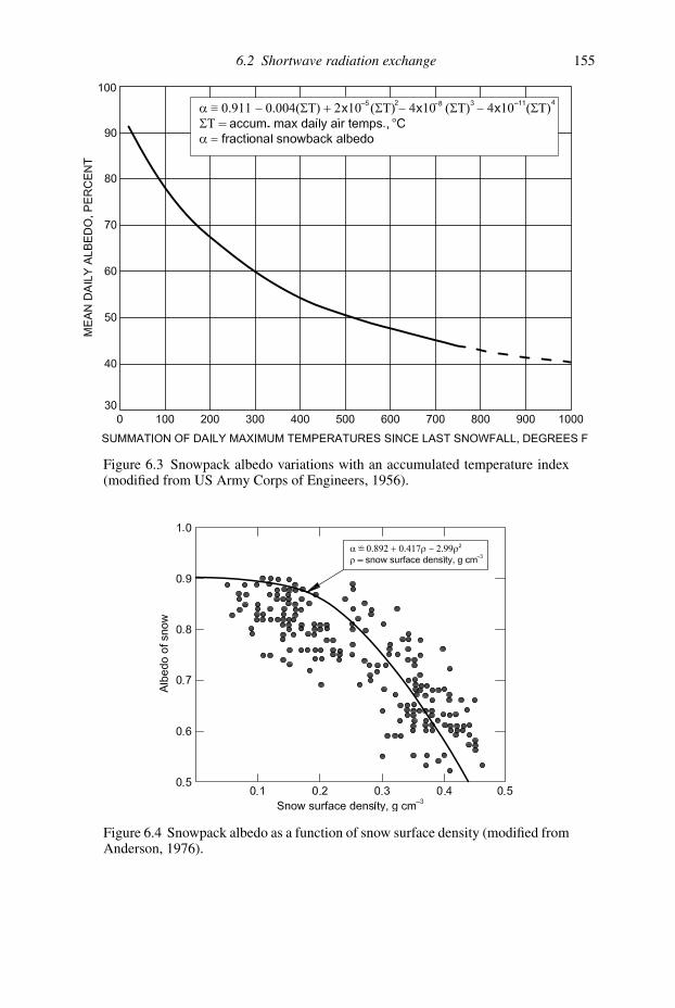
6.2 Shortwave radiation exchange 155
Figure 6.3 Snowpack albedo variations with an accumulated temperature index(modified from US Army Corps of Engineers, 1956).
Figure 6.4 Snowpack albedo as a function of snow surface density (modified fromAnderson, 1976).

156 Snowpack energy exchange: basic theory
The recession coefficient was found to be 0.05 for air temperatures less than 0 ◦C
and 0.12 for temperatures greater than 0 ◦C. The definition of a major snowfall
needed for determining n was a snowfall depth of at least 3 cm over as many days.
The maximum albedo when n = 0 is 0.84 using values of the constants given above.
If n were 3 days and air temperatures had been above freezing, then the computed
albedo would be:
α = 0.4 + (0.44)(2.72)−(3)(0.12) = 0.71 or 71%
The equation worked well as long as snow depths exceeded 10 cm. Pluss and
Mazzoni (1994) found the model underpredicted slightly at low temperatures and
overestimated at temperatures above freezing.
6.2.5 Net shortwave radiation exchange
Once the albedo of the snowpack has been resolved by measurement or computa-
tion, it is a simple matter to compute net shortwave radiation exchange. Given a
representative high mid-winter albedo of 0.8 and the estimated incoming shortwave
radiation flux density for relatively clear sky of 78.7 W m−2, computed previously,
the reflected shortwave flux density would be:
K↑ = αK↓ = 0.8(78.7) = 63.0 W m−2
and net shortwave radiation exchange would be:
Qns = K↓ − K↑ = 78.7 − 63.0 = 15.7 W m−2
As illustrated here, under conditions of mid-winter solar irradiation and high snow-
pack albedo, the absorbed shortwave radiation available for melt can be quite low.
However, small changes in albedo when the albedo is high can disproportionately
affect net shortwave radiation exchange. If the albedo in the above example were
reduced by 25% from 0.8 to 0.6, then net shortwave radiation exchange would
double (31.5 W m−2). As incoming shortwave radiation increases during the spring
melt season and the snowpack albedo declines due to combined effects of increas-
ing grain size, greater solar altitude, snowpack surface contamination, and possi-
bly transmission of radiation to the ground, net shortwave exchange can become
increasingly important as an energy budget component.
6.3 Longwave radiation exchange
All substances above absolute zero in temperature radiate or emit radiant energy
and at terrestrial temperatures materials such as atmospheric gases, clouds, for-
est vegetation, and snowpacks radiate in the longwave region (λ = 2–100 μm).

6.3 Longwave radiation exchange 157
Unlike shortwave radiation exchange that is restricted to daytime, longwave radi-
ation exchange occurs both day and night, which increases the importance of the
longwave component. Measurements of incoming longwave radiation are much
less common than for shortwave radiation, but in recent years radiometers have
been developed that can be used for routine monitoring. Regardless, computations
of longwave exchange are often possible using other available environmental data
as described below.
Net longwave radiation exchange (Qnl) in Equation (6.1) for an unobstructed,
horizontal snowpack surface can be defined as the sum of incoming (L↓) and
outgoing (L↑) longwave radiation flux densities as:
Qnl = L↓ − L↑ (6.10)
Outgoing longwave radiation can be computed using the Stefan–Boltzmann equa-
tion derived to describe emission from a perfect or black-body radiator as:
L↑ = εσ T 4s + (1 − ε)L↓ (6.11)
where:
ε = emissivity of snowpack surface
σ = Stefan–Boltzmann constant = 5.67 × 10⁻⁸ W m−2 K−4
Ts = surface temperature of the snowpack, K, (K = ◦C + 273.16)
Emissivity is the ratio of radiation emitted by a substance to that emitted by a
perfect or black-body radiator at the same temperature. The ratio or emissivity
equals one for a black body and snowpacks come fairly close to being a perfect
radiator with ε = 0.97 − 1.00 (Kondrat’yev, 1965; Anderson, 1976). Since, by
Kirchhoff’s law, emissivity is equal to absorptivity at a given wavelength, the term
(1 − ε) represents the small fraction of incoming longwave radiation that is reflected
from the snow surface. The loss of longwave radiant energy is primarily a function
of snow surface temperature, but does depend slightly on the incoming longwave
radiation flux density from the atmosphere due to reflection.
Since the surface temperature of a snowpack during melt is 0 ◦C, the flux density
of longwave radiation that could be lost from the snowpack for an assumed ε = 1
would be:
L↑ = (1)(5.67 × 10⁻⁸ W m−2 K−4)(273.16 K)4 = 316 W m−2
More precise calculation of outgoing longwave depends upon knowing the snow-
pack emissivity and the concurrent flux of incoming longwave radiation. In addition,
estimating the snowpack surface temperature during non-melting conditions, when
the snowpack is at less than 0 ◦C, becomes problematical for many operational
snowmelt simulations.
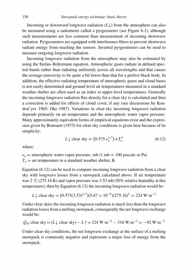
158 Snowpack energy exchange: basic theory
Incoming or downward longwave radiation (L↓) from the atmosphere can also
be measured using a radiometer called a pyrgeometer (see Figure 6.1), although
such measurements are less common than measurement of incoming shortwave
radiation. Pyrgeometers are equipped with interference filters to prevent shortwave
radiant energy from reaching the sensors. Inverted pyrgeometers can be used to
measure outgoing longwave radiation.
Incoming longwave radiation from the atmosphere may also be estimated by
using the Stefan–Boltzmann equation. Atmospheric gases radiate in defined spec-
tral bands rather than radiating uniformly across all wavelengths and that causes
the average emissivity to be quite a bit lower than that for a perfect black body. In
addition, the effective radiating temperature of atmospheric gases and cloud bases
is not easily determined and ground-level air temperatures measured in a standard
weather shelter are often used as an index to upper-level temperatures. Generally
the incoming longwave radiation flux density for a clear sky is calculated and then
a correction is added for effects of cloud cover, if any (see discussions by Kon-
drat’yev 1965; Oke 1987). Variations in clear-sky incoming longwave radiation
depends primarily on air temperature and the atmospheric water vapor pressure.
Many approximately equivalent forms of empirical equations exist and the expres-
sion given by Brutsaert (1975) for clear-sky conditions is given here because of its
simplicity:
L↓ clear sky = (0.575 e1/7
a
)σ T 4
a (6.12)
where:
ea = atmospheric water vapor pressure, mb (1 mb = 100 pascals or Pa)
Ta = air temperature in a standard weather shelter, K
Equation (6.12) can be used to compare incoming longwave radiation from a clear
sky with longwave losses from a snowpack calculated above. If air temperature
was 2 ◦C (275.16 K) and vapor pressure was 3.53 mb (50% relative humidity at this
temperature), then by Equation (6.12) the incoming longwave radiation would be:
L↓ clear sky = [0.575(3.53)1/7](5.67 × 10−8)(275.16)4 = 224 W m−2
Under clear skies the incoming longwave radiation is much less than the longwaveradiation losses from a melting snowpack, consequently the net longwave exchangewould be:
Qnl clear sky = (L↓ clear sky) − L↑ = 224 W m−2 − 316 W m−2 = −92 W m−2
Under clear-sky conditions, the net longwave exchange at the surface of a melting
snowpack is commonly negative and represents a major loss of energy from the
snowpack.

6.4 Sensible heat convection 159
Table 6.2 Cloud-cover factors used to computeincoming longwave radiation with Equation (6.13)
(Kondrat’yev, 1965; Oke, 1987)
Cloud Type ac
Cirrus 0.04Cirrostratus 0.08Altocumulus 0.17Altostratus 0.20Cumulus 0.20Stratocumulus 0.22Stratus 0.24Fog 0.25
Incoming longwave radiation with cloud cover is simply estimated by adjusting
clear-sky estimates using an equation such as:
L↓ cloudy sky = (L↓ clear sky)(1 + acC2) (6.13)
where C is fractional cloud cover and the empirical coefficient ac varies with cloud
type (see Table 6.2).
Given the range of cloud-cover factors in Table 6.2, complete cloud cover or
fog (C2 = 1) can increase incoming longwave by about 24–25% for a given air
temperature and humidity value. If in our example a cumulus cloud cover of 0.3
occurred (ac = 0.2), then by Equation (6.13) we would be increasing incoming
clear longwave radiation computed by a factor of [1 + (0.20)(0.3)2] = 1.018 or
about 2% from L↓ = 224 W m−2 to L↓ = 228 W m−2. Net longwave exchange over
melting snow would therefore be increased from –92 to –88 W m−2 or by about
4%. Complete cumulous cloud cover (C = 1.0, ac = 0.2) would have increased
incoming longwave radiation to 269 W m−2 and net longwave radiation exchange
at the snowpack surface by 50%. Obviously, clouds can significantly add incoming
longwave radiation to the snowpack and significantly reduce net longwave radiation
losses.
6.4 Sensible heat convection
Whenever a temperature difference exists between the atmosphere and the snow-
pack surface, the potential exists for significant convective transfer of sensible heat
to or from the snowpack depending upon the magnitude and sign of the tempera-
ture difference, wind speed, surface roughness, and stability of the air. Late-lying

160 Snowpack energy exchange: basic theory
Figure 6.5 Solar-powered climate stations equipped with data loggers (left) areused to provide data (wind speed, air temperature, humidity) to support computa-tions of snowpack convective exchange. The addition to climate stations of sonicanemometers (top right), fine-wire thermocouples, and high-speed open-path gasanalyzers for CO2 and water vapor (bottom right) allows computation of convec-tive exchange using the eddy covariance method (photographs by D. DeWalle).See also color plate.
melting snowpacks in late spring and early summer can exist when air temperatures
are over 20 ◦C greater than the snow, causing large energy gains to the snowpack.
In contrast, during winter or at night during the melt season, the snowpack can be
warmer than air, causing convective energy losses from the snowpack to air.
In this section an approach to computation of sensible heat flux densities is
presented. The bulk aerodynamic approach for computation of sensible heat and
water vapor flux in the atmosphere will be stressed here because it often becomes
the method of choice due to lack of meteorological data. The bulk aerodynamic
method uses measurements of wind speed, air temperature, and humidity in the air
at a fixed height above the snow surface (Figure 6.5). Marks and Dozier (1992)
applied a bulk aerodynamic method corrected for stability adapted from Brutsaert
(1982) that iteratively solves for friction velocity and the sensible and latent heat
flux densities over snow. Application of bulk aerodynamic theory to computation
of sensible heat exchange involves several simplifying assumptions (Moore, 1983).
Despite these theoretical limitations, bulk theory has been used to approximate
sensible heat exchange to and from snowpacks within acceptable error limits (see
Anderson, 1976; Kustas et al., 1994).
Several other approaches exist to compute atmospheric convective fluxes on
an operational level (Oke, 1987; Arya, 1988). The eddy covariance method, which

6.4 Sensible heat convection 161
requires measurements of the fluctuations of vertical wind speed, air temperature,
and humidity is rapidly becoming feasible for snow hydrology applications with
continuing improvements in sensor technology (Figure 6.5); however, greater costs,
more complex data manipulation and harsh winter weather conditions still present
considerable challenges for snow hydrologists.
According to bulk aerodynamic theory the sensible heat flux density can be
computed as (Kustas et al., 1994):
Qh = ρa cp Ch ua(Ta − Ts) (6.14)
Chn = k2[ln(za/z0)]−2 (6.15)
where:
ρa = density of air, kg m−3
cp = specific heat of air, J kg−1 K−1
Ch = bulk transfer coefficient for sensible heat, dimensionless,
Chn = bulk transfer coefficient for sensible heat for neutral stability
atmosphere, dimensionless,
k = von Karmin’s constant = 0.4
z0 = aerodynamic roughness length for the snow surface, m
ua = wind speed at height za, m s−1
Ta = air temperature at height za, K
Ts = air temperature at the snowpack surface, K
The aerodynamic roughness length indexes the mean height of snowpack surface
obstacles that control the friction between the moving air and snow. Roughness
length is evaluated as the height above the ground where the wind speed (ua)
extrapolates to zero when plotted against ln(height) as defined by the logarithmic
wind profile equation:
uz = u∗/k ln(z/z0) (6.16)
where u∗ is the friction velocity in m s−1 and u∗/k defines the slope of the line at
neutral stability. The friction velocity is related to the shear stress or flux density of
horizontal momentum at the snow surface (τ , kg m−1 s−2) where u∗ = (τ/ρa)1/2.
Detailed evaluations of roughness lengths for surfaces are generally done with at
least four anemometers that are spaced logarithmically with height under neutral
stability atmospheric conditions.
Values for snowpack roughness lengths reported in the literature generally fall
between 0.001 and 0.005 m (1 and 5 mm, respectively) for average seasonal snow-
pack conditions with a very wide range from about 0.0002 m to 0.02 m reported
for very smooth to very rough snowpack and ice conditions (see reviews by Moore,
1983 and Morris, 1989). Given the very wide range of roughness lengths for snow

162 Snowpack energy exchange: basic theory
reported in the literature, and the relative importance of this parameter, an objective
method of selecting the appropriate z0 is needed. A relationship originally devel-
oped by Paeschke (1937) can help somewhat (see discussion by Brutsaert, 1982),
where roughness length (z0) is related to the average height of roughness obstacles
(h0) as:
z0 = 0.136 h0 (6.17)
Using this relationship for commonly observed snowpack roughness lengths of
1 and 5 mm, the average heights of roughness obstacles would be 7.4 and 37
mm, respectively. These mean heights of roughness obstacles are greater than the
typical dimensions of individual ice grains and suggest that measurements of the
larger-scale surface features of the snowpack roughness elements are needed to
estimate h0.
Stability conditions in the air above a surface can greatly affect the amount
of turbulence and rates of sensible heat exchange. Neutral stability conditions
that are assumed by Equations (6.14) and (6.15) refer to an atmosphere with
no buoyancy effects on turbulence. Under neutral stability conditions all turbu-
lence is created by forced convection due to horizontal wind movement over a
rough surface. Free convection refers to turbulence due to rising or sinking air
caused by density differences in the air near the ground. Air in contact with a rel-
atively warm surface will warm, expand, and rise due to reduced density and can
greatly enhance turbulent mixing. This type of atmospheric condition is referred
to as “unstable” and is not common over a cold snow surface. In contrast, air in
contact with a relatively cool surface like snow will cool, become more dense,
sink, and retard turbulent mixing. This atmospheric condition, referred to as “sta-
ble,” commonly occurs over snow (Anderson, 1976; Shutov, 1993). In the atmo-
sphere, turbulence is generally caused by a mixture of forced and free convec-
tion processes. Corrections for the effects of atmospheric stability on turbulence
are made to the bulk transfer coefficient (CHN) using an index to atmospheric
stability.
Atmospheric stability conditions can be indexed using the dimensionless bulk
Richardson number (RiB) that is calculated as:
RiB = [g T −1
m
]za(Ta − Ts)/
(u2
a
)(6.18)
where g is the acceleration due to gravity, 9.8 m s−2, Tm = (Ta + Ts)/2 in K, and all
other parameters have been previously defined. The bulk Richardson number relates
the consumption of energy by buoyancy forces to the generation of energy by shear
stress forces. Positive values of RiB indicate stable conditions and negative values
indicate unstable conditions. Magnitudes of the computed RiB, either positive or

6.4 Sensible heat convection 163
negative, indicate the degree of instability or stability in the air. Values of RiB from
about −0.01 to +0.01 indicate neutral stability. Values of RiB greater than about 0.2
to 0.4 are believed to represent conditions where turbulence is completely damped
and no convection would occur.
Empirical functions to correct Ch for the effects of stability can be based upon
RiB. The functions predict the ratio of the bulk transfer coefficient for the actual
conditions (Ch) to that for neutral stability conditions (Chn) as given by Equation
(6.19). This ratio (Ch/Chn) is then multiplied by Chn given by Equation (6.15) to
correct for stability effects. Equations derived from field data to correct for stability
appearing in the literature vary widely and remain controversial (Morris, 1989;
Male and Gray, 1981; Oke, 1987; Anderson, 1976; Hogstrom, 1988; Brutsaert,
1982; Shutov, 1993; Granger and Male, 1978; Kustas et al., 1994). General sta-
bility correction equations given by Oke (1987) for unstable conditions and stable
conditions are given here:
Unstable: Ch/Chn = (1 − 16RiB)0.75 (6.19a)
Stable: Ch/Chn = (1 − 5RiB)2 (6.19b)
Equation (6.19b) gives Ch/Chn = 0 when RiB equals 0.2 as expected for fully
damped turbulence. Anderson (1976) used Equation (6.19b) for stable conditions
over snow. Equation (6.19a) for unstable conditions gives similar results to a func-
tion derived from data over snow used by Granger and Male (1978) for Ri approach-
ing –0.02. Once the ratio Ch/Chn is obtained with the appropriate function (Equation
6.19a or 6.19b), then Ch is computed as Ch = (Ch/Chn)Chn. Atmospheric stability
conditions over snowcover and effects on convection of sensible heat to and from
the snowpack are summarized in Table 6.3.
Example calculations will help illustrate the use of this theory and support-
ing empirical relationships. Assuming air temperature of 2 ◦C and wind speed of
3.2 m s−1 at 2 m height over melting snow with a small roughness length of 0.0005
m and using cp = 1.005 × 10³ J kg−1 K−1 and ρa = 1.27 kg m−3, the sensible
heat exchange for neutral stability can be computed. Refer to Appendix A1 for
specific heat and air density data. First the bulk transfer coefficient for sensible heat
exchange under neutral stability is computed with Equation (6.15) as:
Chn = (0.4)2 [ln(2 m/0.0005 m)]−2 = 0.00232 dimensionless
If the roughness length were increased in the above computation to z0 = 0.005 m,
Chn would increase to 0.00446 an increase of 92%. Obviously, roughness length is
a major control on the bulk transfer coefficient.

164 Snowpack energy exchange: basic theory
Table 6.3 Summary of atmospheric stability and snowpack convection conditions
AtmosphericStability
MeteorologicalConditions Occurrence
Bulk RichardsonNumber Ch/Chn
Unstable-freeconvection
Ts >> Ta, ua
relatively lowRare over snow <−1 >>1
Unstable-mixedconvection
Ts > Ta, ua
relatively highOccasional; windy, cold
winter accumulationseason, night time
<−0.01 >1
Neutral-forcedconvection
Ts ∼ Ta, ua
relatively highCommon; windy, cool
periods, meltinitiation
−0.01 to +0.01 ∼ 1
Stable-dampedforcedconvection
Ts < Ta, ua
relatively highCommon; windy, warm
melt periods>+0.01 < 1
Stable-fullydamped forcedconvection
Ts << Ta, ua
relatively lowCommon; calm, warm
melting periods;nights with fog andcold air drainage
→critical value∼ +0.2 to +0.4
→ 0
Next, the bulk Richardson number is needed to compute the correction for sta-
bility using Equation (6.18):
RiB = [(9.8 m s−2)/((275.16 + 273.16)/2 K)]
× (2 m)(275.16 − 273.16 K)/(3.2 m s−1)2
= 0.014
This small, positive value of RiB indicates neutrally stable to slightly stable con-
ditions. The ratio Ch/Chn computed from RiB using Equation (6.19b) for stable
conditions becomes:
Ch/Chn = [1 − (5)(0.014)]2 = 0.865
Turbulence is damped by the slightly stable atmospheric conditions. This correction
factor is then multiplied by Chn, previously derived, to obtain the corrected bulk
transfer coefficient as Ch = (Ch/Chn) Chn = (0.865) (0.00232) = 0.00201.
Finally, the sensible heat flux density is computed using Equation (6.14) as:
Qh = (1.27 kg m−3)(1.005 × 10³ J kg−1 K−1)(0.00201)(3.2 m s−1)(2 − 0 ◦C)
= 16.4 J s−1 m−2 = 16.4 W m−2
Since air temperature is greater than snow surface temperature, Qh is positive or an
energy gain in the context of an energy budget.
Note that with a higher roughness length of z0 = 0.005 m and Chn = 0.00446,
Ch becomes 0.00386 after the stability correction and Qh = 31.5 W m−2. In this
6.5 Latent heat convection 165
example, stability conditions, roughness length, wind speed, and the temperature
difference all controlled the computed sensible heat flux density.
Rugged terrain, discontinuous snow cover with adjacent bare ground, and pres-
ence of trees as roughness elements in the airflow increase the errors in apply-
ing one-dimensional vertical exchange theory presented here. In situations where
horizontal gradients of roughness, surface temperature, and/or moisture become
important, advection or lateral exchange of heat and vapor also becomes important.
Advection of heat from bare ground to adjacent snow patches can greatly increase
local sensible heat supplied to the snowpack (Liston, 1995; Neumann and Marsh,
1997, 1998). In forests, warm tree boles and branches and exposed ground can
also enhance local advection of sensible heat. DeWalle and Meiman (1971) found
that sensible heat convection and advection to late-lying snow patches in Colorado
subalpine conifer forest contributed 85 W m−2 to snowmelt during a two-day period
in June with day-time wind speeds in excess of 4 m s−1 and maximum air tempera-
tures in excess of 22 ◦C. Energy exchange due to sensible and latent heat exchange
with patchy snow cover and other conditions causing advection, presents special
challenges to estimating heat exchange.
6.5 Latent heat convection
Water vapor exchange between the snowpack and atmosphere also occurs due to
turbulent mixing in the boundary layer. Transfer of vapor from the snowpack to
the atmosphere constitutes a loss of latent heat of vaporization if the snowpack has
liquid water present and a loss of latent heat of sublimation if subfreezing tempera-
tures prevail. Conversely, sublimation or condensation of vapor onto the snowpack
constitutes an energy gain due to liberation of the latent heat of sublimation or
vaporization, respectively.
Generally, during the cold winter season a snowpack loses water due to evapo-
ration and sublimation. For example, Schmidt et al. (1998) estimated that 20% of
the peak snowpack water equivalent or about 78 mm water equivalent was lost due
to sublimation from the snowpack during a 40-d accumulation period in Colorado
subalpine forest. However, during melting periods, and during periods with rainfall,
the vapor pressure in the atmosphere often exceeds that at the snowpack surface,
since vapor pressure at the snowpack surface cannot exceed the saturation vapor
pressure at 0 ◦C. Condensation/sublimation onto the snowpack occurs under these
conditions (Leydecker and Melack, 1999). The process of latent heat convection
is generally believed to be similar to that for sensible heat exchange and subject
to the same errors, with the difference in vapor pressure between snowpack and
atmosphere, roughness length, wind speed, and stability again playing major roles.
juras
Zvýraznění
juras
Zvýraznění
juras
Zvýraznění
juras
Zvýraznění
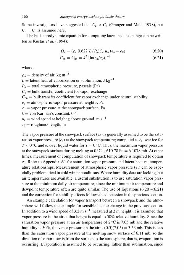
166 Snowpack energy exchange: basic theory
Some investigators have suggested that Ce < Ch (Granger and Male, 1978), but
Ce = Ch is assumed here.
The bulk aerodynamic equation for computing latent heat exchange can be writ-
ten as Kustas et al. (1994):
Qe = (ρa 0.622 L/Pa)Ce ua (ea − e0) (6.20)
Cen = Chn = k2 [ln(za/z0)]−2 (6.21)
where:
ρa = density of air, kg m−3
L = latent heat of vaporization or sublimation, J kg−1
Pa = total atmospheric pressure, pascals (Pa)
Ce = bulk transfer coefficient for vapor exchange
Cen = bulk transfer coefficient for vapor exchange under neutral stability
ea = atmospheric vapor pressure at height z, Pa
e0 = vapor pressure at the snowpack surface, Pa
k = von Karman’s constant, 0.4
ua = wind speed at height z above ground, m s−1
z0 = roughness length, m
The vapor pressure at the snowpack surface (e0) is generally assumed to be the satu-
ration vapor pressure (es) at the snowpack temperature; computed as es over ice for
T < 0 ◦C and es over liquid water for T = 0 ◦C. Thus, the maximum vapor pressure
at the snowpack surface during melting at 0 ◦C is 610.78 Pa = 6.1078 mb. At other
times, measurement or computation of snowpack temperature is required to obtain
e0. Refer to Appendix A1 for saturation vapor pressure and latent heat vs. temper-
ature relationships. Measurement of atmospheric vapor pressure (ea) can be espe-
cially problematical in cold winter conditions. Where humidity data are lacking, but
air temperatures are available, a useful substitution is to use saturation vapor pres-
sure at the minimum daily air temperature, since the minimum air temperature and
dewpoint temperature often are quite similar. The use of Equations (6.20)–(6.21)
and the correction for stability effects follows the discussion in the previous section.
An example calculation for vapor transport between a snowpack and the atmo-
sphere will follow the example for sensible heat exchange in the previous section.
In addition to a wind speed of 3.2 m s−1 measured at 2 m height, it is assumed that
vapor pressure in the air at that height is equal to 50% relative humidity. Since the
saturation vapor pressure at an air temperature of 2 ◦C is 7.05 mb and the relative
humidity is 50%, the vapor pressure in the air is (0.5)(7.05) = 3.53 mb. This is less
than the saturation vapor pressure at the melting snow surface of 6.11 mb, so the
direction of vapor flow is from the surface to the atmosphere, that is, evaporation is
occurring. Evaporation is assumed to be occurring, rather than sublimation, since
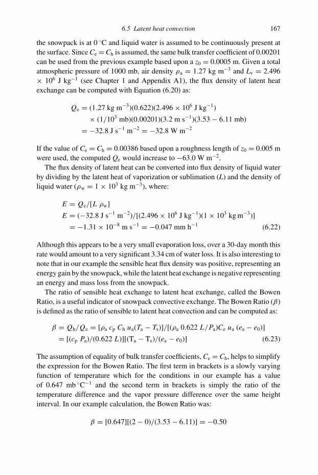
6.5 Latent heat convection 167
the snowpack is at 0 ◦C and liquid water is assumed to be continuously present at
the surface. Since Ce = Ch is assumed, the same bulk transfer coefficient of 0.00201
can be used from the previous example based upon a z0 = 0.0005 m. Given a total
atmospheric pressure of 1000 mb, air density ρa = 1.27 kg m−3 and Lv = 2.496
× 106 J kg−1 (see Chapter 1 and Appendix A1), the flux density of latent heat
exchange can be computed with Equation (6.20) as:
Qe = (1.27 kg m−3)(0.622)(2.496 × 10⁶ J kg−1)
× (1/103 mb)(0.00201)(3.2 m s−1)(3.53 − 6.11 mb)
= −32.8 J s−1 m−2 = −32.8 W m−2
If the value of Ce = Ch = 0.00386 based upon a roughness length of z0 = 0.005 m
were used, the computed Qe would increase to −63.0 W m−2.
The flux density of latent heat can be converted into flux density of liquid water
by dividing by the latent heat of vaporization or sublimation (L) and the density of
liquid water (ρw = 1 × 10³ kg m−3), where:
E = Qe/[L ρw]
E = (−32.8 J s−1 m−2)/[(2.496 × 106 J kg−1)(1 × 10³ kg m−3)]
= −1.31 × 10⁻⁸ m s−1 = −0.047 mm h−1 (6.22)
Although this appears to be a very small evaporation loss, over a 30-day month this
rate would amount to a very significant 3.34 cm of water loss. It is also interesting to
note that in our example the sensible heat flux density was positive, representing an
energy gain by the snowpack, while the latent heat exchange is negative representing
an energy and mass loss from the snowpack.
The ratio of sensible heat exchange to latent heat exchange, called the Bowen
Ratio, is a useful indicator of snowpack convective exchange. The Bowen Ratio (β)
is defined as the ratio of sensible to latent heat convection and can be computed as:
β = Qh/Qe = [ρa cp Ch ua(Ta − Ts)]/[(ρa 0.622 L/Pa)Ce ua (ea − e0)]
= [(cp Pa)/(0.622 L)][(Ta − Ts)/(ea − e0)] (6.23)
The assumption of equality of bulk transfer coefficients, Ce = Ch, helps to simplify
the expression for the Bowen Ratio. The first term in brackets is a slowly varying
function of temperature which for the conditions in our example has a value
of 0.647 mb ◦C−1 and the second term in brackets is simply the ratio of the
temperature difference and the vapor pressure difference over the same height
interval. In our example calculation, the Bowen Ratio was:
β = [0.647][(2 − 0)/(3.53 − 6.11)] = −0.50

168 Snowpack energy exchange: basic theory
Figure 6.6 Regimes of latent heat exchange over melting snow defined by air tem-perature and relative humidity. The line of zero vapor pressure difference betweenthe air and snow surface defines two regimes: one with high humidity and con-densation energy gains on the snowpack surface and another with low humidityand evaporative heat loss from the snowpack surface. Temperature and humidityconditions defining varying Bowen Ratios (β = Qh/Qe) are also shown above(+) and below (−) the zero vapor exchange line. Computations assume a totalatmospheric pressure of 1000 mb.
which indicates the sensible heat flux density was only half as large as that for
latent heat exchange and of opposite sign. In other words, the sensible heat gain
could only be responsible for about 50% of the latent heat loss due to evaporation/
sublimation.
As illustrated in Figure 6.6, Bowen Ratios can be simply predicted by air tempera-
ture and relative humidity conditions over melting snow, where surface temperature
(T = 0 ◦C) and vapor pressure (e0 = 6.11 mb) are fixed. Relative humidity is the
ratio of actual vapor pressure (e) to saturation vapor pressure (es) at that temperature
expressed as a percentage [RH = 100(e/es)]. Temperature and relative humidity
conditions exist where evaporative heat losses exactly offset the sensible heat gains
to the snowpack (Bowen Ratio = −1). Under such conditions, sensible heat and
latent heat exchange offset each other and melt would be primarily dependent upon
radiation exchange. Conditions also exist where both sensible and latent heat gains
are positive and equal (β= +1) and energy supply for snowmelt is derived from
both net radiation and convection. At any given air temperature, as relative humidity
juras
Zvýraznění

6.6 Rainfall energy 169
approaches the zero vapor exchange line in Figure 6.6 from either direction, vapor
exchange approaches zero, sensible heat exchange becomes relatively important
and the Bowen Ratio approaches infinitely large or small values.
When air temperature is less than snow surface temperature, only evaporation
or sublimation of vapor from the snowpack can occur, since it is impossible for
atmospheric vapor pressure to exceed snow surface vapor pressure even at 100%
relative humidity. When air temperature is less than snow temperature, both vapor
exchange and sensible heat exchange represent energy losses from the snowpack
(β > 0); a condition common in winter. The specific meteorological conditions
encountered and the balance between sensible heat and evaporative/sublimation
energy exchange can obviously greatly affect the snowpack energy budget and
rates of snowmelt.
The snowpack surface has been likened to a wet-bulb thermometer where
latent heat losses are balanced by sensible heat gains (Geiger, 1965). A wet-bulb
thermometer when exposed to air with a relative humidity less than 100% will
evaporate/sublimate and cool below the current air temperature (dry-bulb temper-
ature). Since cooling of the wet bulb creates a temperature difference between the
wet-bulb surface and the air, the wet bulb will gain sensible heat from the sur-
rounding air. When the wet bulb cools to a temperature where the latent heat lost
by evaporation/sublimation is matched by the sensible heat gain from the air, an
equilibrium exists and the wet-bulb temperature will have been reached.
The wet-bulb analogy with a snowpack surface is correct as long as there are
no additional sources of energy to drive snowpack evaporation or sublimation. In
the absence of significant radiant energy, such as in winter or at night, a snow-
pack exposed to relatively dry air can cool by sublimation and approach a balance
between latent heat loss and sensible heat gain. Some investigators in areas with
relatively dry air have noted the approximate balance between snowpack evapo-
ration/sublimation energy losses and sensible heat gains which leads to a zero net
turbulent energy exchange (Marks and Dozier, 1992). However, during periods with
significant radiant energy supply, the snowpack surface does not cool below 0 ◦C,
melting will utilize some of the available energy, and the wet-bulb analogy fails.
6.6 Rainfall energy
Rainfall can influence the energy budget of snowpacks in three ways:
� sensible heat additions due to the heat added by a volume of relatively warm rain,� release of the latent heat of fusion if rainfall freezes on a sub-zero snowpack, and� condensation on the snowpack due to high humidity associated with rainy weather.

170 Snowpack energy exchange: basic theory
The first type of energy input that pertains when the snowpack is at 0 ◦C can be
simply computed as:
Qr1 = Pr ρw cw (Tr − Ts) (6.24)
where:
Qr1 = sensible heat exchange due to rainfall on snow, W m−2
Pr = rainfall intensity, m s−1
ρw = density of liquid water, liquid water = 1 × 10³ kg m−3
cw = specific heat of liquid water = 4.1876 × 10³ J kg−1 ◦C−1
Tr = temperature of rain, ◦C, (assumed equal to air temperature during the event)
Ts = temperature of snow, 0 ◦C
The energy exchange shows that sensible heat inputs from rain are generally rel-
atively modest, since this example is for a rather large and very warm rain storm.
However, this computation is a bit misleading since the time base for rainfall is one
day. If all that rain occurred in one hour, then the energy input due to the rain would
be huge (e.g. 291 W m−2) relative to other sources for that hour.An example for a major rainfall event with an intensity of 2.5 cm depth in a day
(Pr = (0.025 m)(24 h × 3600 s h−1)−1 = 2.894 × 10⁻⁷ m s−1) and a temperatureof 10 ◦C can help to show the importance of this energy input:
Qr1 = (2.89 × 10⁻⁷ m s−1)(1 × 10³ kg m−3)(4.1876 × 10³ J kg−1 ◦C−1)(10 − 0 ◦C)= 12.1 J s−1 m−2 = 12.1 W m−2
A second possible source of energy input from rain is the release of latent heat
of fusion when rain freezes on a subfreezing snowpack. The heat flux due to this
component can be computed as:
Qr2 = Pr ρw L f Ts < 0 (6.25)
where:
Qr2 = flux density of latent heat released due to rainfall freezing, W m−2
Lf = latent heat of fusion, J kg−1 (see Chapter 1).
Other terms have been previously defined.
Using the same rainfall intensity as in the above example (Pr = 2.89 × 10⁻⁷ m
s−1) and Lf = 0.3275 × 10⁶ J kg−1 representing snow temperature of about –3 ◦C,
the latent heat flux due to refreezing is:
Qr2 = (2.89 × 10⁻⁷ m s−1)(1 × 10³ kg m−3)(0.3275 × 10⁶ J kg−1)
= 94.5 J s−1 m−2 = 94.5 W m−2

6.7 Ground heat conduction 171
Rainfall onto a subzero snowpack would initially give up its sensible heat. If that
was not sufficient to warm the snow to 0 ◦C, then the rain water would refreeze and
release latent heat of fusion. Thus, the total energy released by a rainfall event for
the given conditions would be 12 W m−2 due to sensible heating and 94.5 W m−2
due to latent heat release for a total of 106.6 W m−2. Computation of this energy
flux depends upon knowing the snowpack and rainfall temperatures which are not
routinely available. Warming of the snowpack due to sensible and latent gains from
rain would be detected in accounting for the heat storage changes in the snowpack
discussed in Section 6.8.
Finally, high humidity associated with rainfall could also cause condensa-
tion/sublimation onto the snowpack which could add considerable energy. Con-
densation/sublimation is predicted with Equations (6.20) and (6.21). Each kilogram
of vapor that sublimated onto the cold snowpack in our example (−3 ◦C) would
release 2.4943 MJ of energy, while each kilogram that refroze would release 0.3275
MJ. Thus, sublimation releases 7.6 more energy per unit mass of water added to
the snowpack than freezing and can be a very important energy source due to rainy
weather.
6.7 Ground heat conduction
Ground heat conduction to the base of the snowpack generally represents a very
minor energy source for melt. Factors contributing to the relatively small contribu-
tions of soil heat conduction are the fact that soil in general is a poor conductor of
heat and that the temperatures in the soil are often quite low due to the lack of solar
warming beneath deep snowpacks. During the winter snow accumulation season,
heat conducted from the soil can contribute to gradual ripening and slow melting
of snowpack basal layers, but this contribution gradually diminishes into spring.
When snowpack depth decreases to levels that allow transmission of shortwave
radiation to the ground in the late spring, 20–25 cm depth based upon Equation
(6.8), ground warming and heat conduction become relatively more important.
The heat conduction flux density to the base of the snowpack can be computed
as:
Qg = kg dTg/dz ∼= kg(Tg − Tsb)/(z2 − z1) (6.26)
where:
Qg = soil heat conduction flux density, W m−2
kg = thermal conductivity of soil, W m−1 ◦C−1
z = soil depth, m
Tg = soil temperature at depth z2, ◦C
Tsb = temperature at base of snowpack at depth z1 = 0 m, ◦C

172 Snowpack energy exchange: basic theory
An example of computation for ground heat conduction using Equation (6.26) will
illustrate the basic units and magnitudes. Assuming a soil temperature of 1 ◦C at
a soil depth of 0.5 m, 0 ◦C temperature at the snowpack base, and a soil thermal
conductivity of 2 W m−1 ◦C−1 gives:
Qg = (2 W m−1 ◦C−1)(1 − 0 ◦C)(0.5 − 0 m)−1 = 4 W m−2
This equation was simplified to the expression on the right-hand side by assuming
thermal conductivity was constant with depth and integrating. The equation was
also written without a negative sign, customarily used to indicate that heat flow is
toward lower temperatures, to avoid confusion about whether Qg is adding energy
to or subtracting energy from the snowpack. Thermal conductivity for soil varies
widely with moisture and organic matter content and ranges from about 0.2 to 2 W
m−1 ◦C−1 (Oke, 1987). Temperature at the base of the snowpack is often around
0 ◦C and soil beneath snow gradually approaches this temperature during the winter-
spring (US Army Corps of Engineers, 1956; Marks et al., 1992).
Obviously soil heat conduction flux density is small compared with other
energy budget components discussed so far. Soil heat conduction to the snowpack
based upon measurements or calculations from field data ranging from about 0 to
10 W m−2 have been reported (Cline, 1997; Marks and Dozier, 1992; Male and
Gray,1981), so the calculation above is within the range of observed data. Granger
and Male (1978) found that for relatively shallow snowpacks on the Canadian
prairie, soil heat conduction varied diurnally and lagged solar radiation when the
snowpack was dry, but heat conduction in the soil was relatively constant beneath
melting snow. Given the small value of Qg some investigators have assumed Qg was
negligible or assumed a small positive constant value for heat flow to the snowpack
base. Others have employed a model to compute soil heat conduction where sup-
porting snow and soil temperature data were available (Marks and Dozier, 1992;
Cline, 1997).
6.8 Internal snowpack energy storage
Changes in the amount of sensible and latent heat stored in the snowpack (Qi)
can at times represent a significant snowpack energy budget component. Sensible
heat changes are represented by changes in snowpack temperature and mass over
time integrated over the depth of the snowpack. Mass increases due to subfreezing
snow falling on the snowpack can also significantly add to snowpack cold content
that must be satisfied before liquid water is yielded at the base of the snowpack.
Warming of deep, dense snowpacks to 0 ◦C can represent a significant energy budget
component in winter when other energy budget components are quite small. Once
the snowpack is isothermal at 0 ◦C and melting begins, the importance of this energy

6.8 Internal snowpack energy storage 173
budget component diminishes drastically. However, even after general snowpack
ripening has occurred in spring, surface layers of the snowpack at exposed sites
can cool and refreeze overnight creating small energy deficits that must be satisfied
before melt can occur on the following day.
Latent heat of fusion storage changes within the snowpack are seldom consid-
ered, but would be represented by depth integrated changes in the amount of liquid
water derived from melt within the snowpack. If surface melting occurs and the
liquid water does not drain completely from the snowpack and does not refreeze,
then changes in liquid-water content would represent a form of latent heat of fusion
storage. If water from melt at the surface refreezes deeper within the snowpack
releasing the latent heat of fusion, then no net energy exchange between the snow-
pack and its environment has taken place. Of course, if liquid water due to melting
drains from the snowpack, that represents a loss of latent heat of fusion energy from
the snowpack. Estimation of latent heat of fusion storage changes would require
detailed evaluations of snowpack liquid-water content. Only sensible heat storage
changes are described quantitatively below.
The general relationship to be used to assess the sensible heat change in snowpack
energy storage is:
�Qi =∫ z=d
z=0
(ρs ci δTs/δt) dz (6.27)
where:
�Qi = change in internal snowpack energy storage, W m−2
ρs = snowpack density, kg m−3
ci = specific heat of ice, J kg−1 ◦C−1
Ts = snowpack temperature, ◦C
t = time, s
z = height above ground, z = 0 at ground, z = d at snowpack surface, m
d = snowpack depth, m
The integration is performed from ground level to the snowpack surface and requires
that measurements or model predictions of snowpack depth, density, and tempera-
ture profiles over time are available.
The computation of Qi for a hypothetical winter day when the snowpack is not
yet ripe is given in Table 6.4 for a snowpack with three layers. It is assumed that
density and depth of the layers are constant between days although precipitation
and sublimation could cause mass changes in a real case. The change in energy
storage for each layer then becomes:
�Qi = (ρs ci)(�Ts/�t)�z

174 Snowpack energy exchange: basic theory
Table 6.4 Computation of daily change in internal snowpack energy storage
Depth Interval(m)
�z(m)
ci
(J kg−1 ◦C−1)ρs
(kg m−3)�Ts
(◦C)�t(s)
�Qi
(W m−2)
1.5–1.2 0.3 2100 120 3.5 86,400 3.061.2–0.5 0.7 2100 150 2 86,400 5.100.5–0.0 0.5 2100 200 1 86,400 2.40
sum 10.56
During longer time intervals, the assumption of constant snowpack density and
depth cannot be made due to gradual snowpack metamorphosis and addition of
new precipitation.
Using the specific heat of ice as ci = 2.1 × 10³ J kg−1 ◦C−1 and a time step of
86 400 s d−1, the change in energy storage for the uppermost layer shown in
Table 6.4 is computed as:
�Qi = −(120 kg m−3)(2.1 × 10³ J kg−1 ◦C−1)(+3.5 ◦C/86 400 s)(0.3 m)
= −3.06 J s−1 m−2 = 3.06 W m−2
The change in energy storage for other layers, computed in similar manner, and
the sum for all layers for the day (10.56 W m−2) is relatively small compared
to radiation and convective energy exchange considered above. Regardless, such
internal energy storage changes could be significant for days when other energy
budget components are small. Note that the middle layer of snowpack in Table
6.4 had the greatest mass and the largest change in energy storage, even though
the temperature change was less than in the surface layer. Obviously the depth,
density, and temperature changes occurring in the snowpack will dictate the relative
importance of this energy exchange component.
6.9 Melt energy
Melt energy (Qm) represents a loss of latent heat of fusion when liquid water drains
from the snowpack. In snowmelt prediction schemes, Qm is generally solved for as
a residual in Equation (6.1). Once the sum of energy available for melt is obtained,
the mass flux density of meltwater (M) can be computed as:
M = Qm(ρw L f B)−1 (6.28)

6.9 Melt energy 175
where:
M = melt rate, m s−1
Qm = flux density of melt energy, J s−1 m−2 or W m−2
ρw = density of liquid water, kg m−3
Lf = latent heat of fusion, J kg−1
B = thermal quality of the snowpack, dimensionless
Thermal quality of snow (B) has been previously described in Chapter 3 and for
ripe snow B represents the fraction of the snowpack mass that is ice rather than
liquid water. For example, a snowpack liquid-water content of 0.03 on a mass basis
is often assumed for melting snow giving a thermal quality of 0.97. In other words,
3% more liquid water will be yielded during melting than expected from the avail-
able melt energy (Qm) due to the fraction of snowpack mass that is already liquid
water.
If the algebraic sum of average flux density energy available for melt for a day
(Qm) was 25.2 W m−2 (= 25.2 J s−1 m−2) with B = 0.97, ρw = 1 × 10³ kg m−3,
and Lf = 0.334 × 10⁶ J kg−1 at 0 ◦C (see Appendix A1), then the melt rate would
be:
M = (25.2 J s−1 m−2)[(1 × 10³ kg m−3)(0.334 × 10⁶ J kg−1)(0.97)]−1
= 7.78 × 10⁻⁸ m s−1(102 cm m−1)(8.64 × 10⁴ s d−1) = 0.67 cm d−1
Melt rate can be considered equivalent to outflow of liquid water from the snow-
pack as long as the transmission time in the snowpack is less than the time step for
the computation. For example, with a daily time step and shallow ripe snow, lag
times for meltwater outflow can generally be ignored. Transmission and storage of
liquid water in snowpacks was also discussed in Chapter 3.
The situation is more complicated for subfreezing snowpacks. In subfreezing
snowpacks energy must first be used to warm the snowpack to an isothermal 0 ◦C
condition and satisfy the liquid-water holding capacity of the snow. A liquid-water
holding capacity for snow of 3% on a mass basis is generally assumed necessary
before liquid water can drain from the snowpack. If the cold content of the snowpack
(see Chapter 3) is greater than the energy supply available, then the snowpack is
only partially ripened and no melt would occur. If the available energy is greater
than the cold content, energy will be first used to warm the snow to 0 ◦C and then to
raise the liquid-water content to 3% on a mass basis. Deep, cold winter snowpacks
may require days to weeks to completely ripen, while shallow fresh snowpacks may
ripen and completely melt in one day or less. Accounting for changes in internal
snowpack energy storage (�Qi) during the ripening process is one of the challenges
to accurate modelling of streamflow from snowmelt.

176 Snowpack energy exchange: basic theory
6.10 Energy budget examples and applications
The energy budget of seasonal snowpacks and glaciers has been studied many
times generally with the objective of computing rates of snowmelt and/or evapo-
ration/sublimation losses. Collectively the results of these studies have verified the
utility of the energy budget approach. A dominant theme of these studies is that net
allwave radiation is the major source of energy transported to the snowpack both
in the open and forest. Male and Granger (1981) compared results of 15 studies
that showed net allwave radiation explained about 59% of total energy exchange
on average. The importance of energy exchange due to convection of sensible heat
and latent heat of evaporation/sublimation is generally less; representing 35% and
–10% of total energy exchange, respectively, in the studies reviewed by Male and
Granger (1981). Obviously, the greatest emphasis should be placed on measuring or
estimating net allwave radiation exchange. However, variations in the significance
of energy budget components occur due to the influence of vegetation, differences
in regional climates, and changing climatic patterns in the transition from winter
accumulation to spring and summer melt seasons.
Marks and Dozier (1992) showed how snowpack energy exchange varied dur-
ing the seasons from winter accumulation to summer melt in a Sierra Nevada
alpine basin (Figure 6.7). Basically, net longwave radiation exchange and latent heat
exchange represented energy losses from the snowpack throughout the November–
July period, while net shortwave radiation exchange and sensible heat convection
represented energy gains. Net shortwave energy gains in winter were low due to
high snowpack albedo, large zenith angles, and short day lengths. In spring and
early summer, day length increased and albedo and zenith angles decreased which
caused much greater net shortwave radiation energy gains. The net longwave bal-
ance was negative in all months due to snowpack exposure to the relatively clear,
dry, and cold alpine atmosphere and the relatively warm snowpack once melting
began. Turbulent exchange of sensible heat represented a small positive energy
supply even in winter and, as the air warmed to average melt-season temperatures
of 10 ◦C, increased to levels equal to or slightly greater than net shortwave radiation
exchange. Turbulent exchange of latent heat due to sublimation and evaporation was
negative from November to July due to relatively low atmospheric vapor pressures
(3.5–4 mb) and high wind speeds at the site (Marks et al., 1992). Thus, the major
positive inputs of energy to the snowpack were net shortwave radiation exchange
and sensible heat convection balanced against losses due to net longwave exchange
and latent heat convection.
Small amounts of energy were added at the snowpack base by soil heat conduc-
tion (not shown), but these represented an average monthly flux density of only
7 W m−2 in November and diminished to 2 W m−2 in July. Precipitation energy
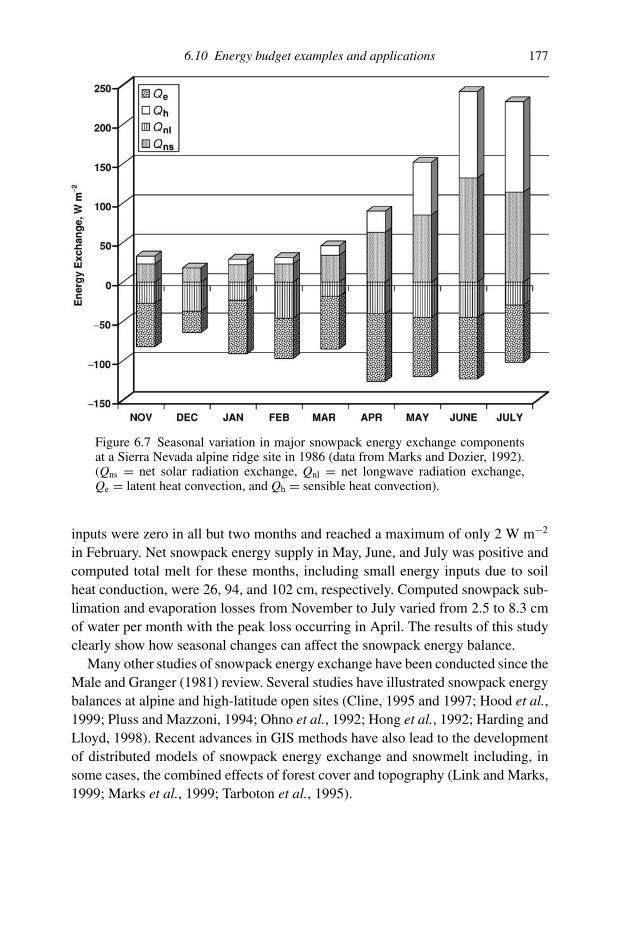
6.10 Energy budget examples and applications 177
Figure 6.7 Seasonal variation in major snowpack energy exchange componentsat a Sierra Nevada alpine ridge site in 1986 (data from Marks and Dozier, 1992).(Qns = net solar radiation exchange, Qnl = net longwave radiation exchange,Qe = latent heat convection, and Qh = sensible heat convection).
inputs were zero in all but two months and reached a maximum of only 2 W m−2
in February. Net snowpack energy supply in May, June, and July was positive and
computed total melt for these months, including small energy inputs due to soil
heat conduction, were 26, 94, and 102 cm, respectively. Computed snowpack sub-
limation and evaporation losses from November to July varied from 2.5 to 8.3 cm
of water per month with the peak loss occurring in April. The results of this study
clearly show how seasonal changes can affect the snowpack energy balance.
Many other studies of snowpack energy exchange have been conducted since the
Male and Granger (1981) review. Several studies have illustrated snowpack energy
balances at alpine and high-latitude open sites (Cline, 1995 and 1997; Hood et al.,1999; Pluss and Mazzoni, 1994; Ohno et al., 1992; Hong et al., 1992; Harding and
Lloyd, 1998). Recent advances in GIS methods have also lead to the development
of distributed models of snowpack energy exchange and snowmelt including, in
some cases, the combined effects of forest cover and topography (Link and Marks,
1999; Marks et al., 1999; Tarboton et al., 1995).

178 Snowpack energy exchange: basic theory
One ultimate goal in snow hydrology is to couple energy-budget models with
hydrologic models to predict streamflow from snowmelt. Although prediction of
streamflow from snowmelt is a subject of a later chapter, mention of a few studies is
made here. Anderson’s (1968, 1973, 1976) classic work that combined an energy-
budget approach to prediction of snowmelt with the US National Weather System
River Forecast System was an early successful attempt at such synergy. Kustas et al.(1994) developed an energy-budget model that was combined with the Snowmelt
Runoff Model (Martinec et al., 1983) and then used to simulate snowmelt runoff
from a lysimeter and watershed. Other models using snowpack energy budgets to
compute streamflow from snowmelt have been developed by Ujihashi et al. (1994),
Kuchment and Gelfan (1996) and Ishii and Fukushima (1994). Data availability
is a chief limitation to employing the full energy-budget approach in a model
representing a complete watershed, but in the final analysis any simplifications must
be based upon knowledge of the physics of melt and evaporation/sublimation. In
the following chapter, specific effects of topography and forest cover on snowpack
energy exchange are given.
6.11 References
Anderson, E. A. (1968). Development and testing of snow pack energy balance equation.Water Resour. Res., 4(1), 19–37.
Anderson, E. A. (1973). National Weather Service River Forecast System – SnowAccumulation and Ablation Model. NOAA Tech. Memo, NWS HYDRO-17. USDept. Commerce, National Oceanic Atmos. Admin.
Anderson, E. A. (1976). A Point Energy and Mass Balance Model of a Snow Cover.NOAA Tech. Rpt., NWS 19. US Dept. Commerce, National Oceanic Atmos. Admin.
Arya, S. P. S. (1988). Introduction to Micrometeorology, vol. 42. Internat. GeophysicsSeries. San Diego, CA: Academic Press.
Bellocchi, G., Acutis, M., Fila, G. and Donatelli, M. (2002). An indicator of solarradiation model performance based on a fuzzy expert system. Agron. J., 94,1222–33.
Bristow, K. L. and Campbell, G. S. (1984). On the relationship between incoming solarradiation and daily maximum and minimum temperature. Agric. and ForestMeteorol., 31, 159–66.
Brutsaert, W. (1975). On a derivable formula for long-wave radiation from clear skies.Water Resour. Res., 11, 742–4.
Brutsaert, W. (1982). Evaporation into the Atmosphere: Theory, History, andApplications. Dordrecht: D. Reidel Publ. Co.
Cline, D. (1995). Snow surface energy exchanges and snowmelt at a continental alpinesite. In Biogeochemistry of Seasonally Snow-Covered Catchments, Publ. No. 228, ed.K. A. Tonnessen, M. W. Williams, and M. Tranter. International Association ofHydrological Sciences, pp. 157–66.
Cline, D. W. (1997). Snow surface energy exchanges and snowmelt at a continental,midlatitude alpine site. Water Resour. Res., 33(4), 689–701.

6.11 References 179
DeWalle, D. R. and Meiman, J. R. (1971). Energy exchange and late seasonsnowmelt in a small opening in Colorado subalpine forest. Water Resour. Res., 7(1),184–8.
Donatelli, M., Bellocchi, G., and Fontana, F. (2003). RadEst 3.00: Software to estimatedaily radiation data from commonly available meteorological variables. Eur. J.Agron., 18, 363–7.
Frank, E. C. and Lee, R. (1966). Potential solar beam irradiation on slopes: tables for 30◦to 50◦ latitude, Res. Paper RM-18. Rocky Mtn. For. Range Exp. Sta.: US Dept.Agric., Forest Service.
Geiger, R. (1965). The Climate Near the Ground, Revised Edition. Cambridge, MA:Harvard University Press.
Granger, R. J. and D. H. Male. (1978). Melting of a prarie snowpack. J. Appl. Meteorol.,17, 1833–42.
Harding, R. J. and Lloyd, C. R. (1998). Fluxes of water and energy from three highlatitude tundra sites in Svalbard. Nordic Hydrol., 29(4/5), 267–84.
Hogstrom, U. (1988). Non-dimensional wind and temperature profiles in the atmosphericsurface layer: a re-evaluation. Boundary-Layer Meteorol., 42, 55–78.
Hong, M., Zongchao, L., and Yifeng, L. (1992). Energy balance of a snow cover andsimulation of snowmelt in the western Tien Shan mountains, China. Annals ofGlaciol., 16, 73–8.
Hood, E., Williams, M., and Cline, D. (1999). Sublimation from a seasonal snowpack at acontinental mid-latitude alpine site. Hydrol. Process., 13, 1781–97.
Ishii, T. and Fukushima, Y. (1994). Effects of forest coverage on snowmelt runoff. InSnow and Ice Covers: Interactions with the Atmosphere and Ecosystems, IAHS Publ.No. 223, ed. H. G. Jones, T. D. Davies, A. Ohmura, and E. M. Morris. InternationalAssociation of Hydrological Sciences, pp. 237–45.
Koh, G. and Jordan, R. (1995). Sub-surface melting in a seasonal snow cover. J. Glaciol.,41(139), 474–82.
Kondrat’yev, K. Y. (1965). Radiative Heat Exchange in the Atmosphere. Oxford:Pergamon Press.
Kuchment, L. S. and Gelfan, A. N. (1996). The determination of the snowmelt rate and themeltwater outflow from a snowpack for modelling river runoff generation. J. Hydrol.,179, 23–36.
Kustas, W. P., Rango, A., and Uijlenhoet, R. (1994). A simple energy budget algorithm forthe snowmelt runoff model. Water Resour. Res., 30(5), 1515–27.
Kuz′min, P. P. (1961). Protsess tayaniya shezhnogo pokrova (Melting of Snow Cover).Glavnoe Upravlenie Gidrometeorologischeskoi Sluzhby Pri Sovete Ministrov SSSRGosudarstvennyi Gidrologischeskii Institut. Main Admin. Hydrometeorol. Service,USSR Council Ministers, State Hydrol. Institute. Translated by Israel Program forScientific Translations. Avail from US Dept. Commerce, National Tech. Inform.Service, 1971, TT 71–50095.
Lee, R. (1963). Evaluation of Solar Beam Irradiation as a Climatic Parameter ofMountain Watersheds, vol. 2. Ft. Collin, CO: Colorado State University.
Leydecker, A. and Melack, J. M. (1999). Evaporation from snow in the Central SierraNevada of California. Nordic Hydrol., 30(2), 81–108.
Linacre, E. (1992). Climate Data and Resources. London: Routledge.Link, T. and Marks, D. (1999). Distributed simulation of snowcover mass- and
energy-balance in the boreal forest. Hydrol. Processes, 13, 2439–2452.Liston, G. E. (1995). Local advection of momentum, heat, and moisture during the melt of
patchy snow covers. J. Appl. Meterol., 34, 1705–15.

180 Snowpack energy exchange: basic theory
Male, D. H. and Granger, R. J. (1981). Snow surface energy exchange. Water Resour.Res., 17(3), 609–27.
Male, D. H. and Gray, D. M. (1981). Chapter 9. Snowcover ablation and runoff. InHandbook of Snow: Principles, Processes, Management and Use, ed. D. M. Grayand D. H. Male. Toronto: Pergamon Press, pp. 360–436.
Marks, D. and Dozier, J. (1992). Climate and energy exchange at the snow surface in thealpine region of the Sierra Nevada, 2. snow cover energy balance. Water Resour. Res.,28(11), 3043–54.
Marks, D., Dozier, J., and Davis, R. E. (1992). Climate and energy exchange at the snowsurface in the alpine region of the Sierra Nevada, 1. metrological measurements andmonitoring. Water Resour. Res., 28(11), 3029–42.
Marks, D., Domingo, J., Susong, D., Link, T., and Garen, D. (1999). A spatiallydistributed energy balance snowmelt model for application in mountain basins.Hydrol. Processes, 13, 1935–59.
Martinec, J., Rango, A., and Major, E. (1983). The Snowmelt-Runoff Model (SRM) User’sModel, NASA Ref. Publ. 1100. US National Aeronautics and Space Administration.
Moore, R. D. (1983). On the use of bulk aerodynamic formulae over melting snow. NordicHydrol., 14(4), 193–206.
Morris, E. M. (1989). Turbulent transfer over snow and ice. J. Hydrol., 105, 205–23.Nakawo, M., Hayakawa, N., and Goodrich, L. E. (eds.) (1998). Chapter 6: Heat budget of
a snow pack. In Snow and Ice Science in Hydrology, Intern. Hydrol. Prog., 7thTraining Course on Snow Hydrology. Nagoya Univ. and UNESCO, pp. 69–87.
Neumann, N. and Marsh, P. (1997). Local advection of sensible heat during snowmelt. InProceedings of the 54th Annual Meeting Western Snow Conference, Banff, Alberta,Canada May 4–8, 1997, pp. 175–85.
Neumann, N. and Marsh, P. (1998). Local advection of sensible heat in the snowmeltlandscape of Arctic tundra. Hydrol. Processes, 12, 1547–60.
Oke, T. R. (1987). Boundary Layer Climates, 2nd edn. London: Methuen, Inc.Ohno, H., Ohata, T., and Higuchi, K. (1992). The influence of humidity on the ablation of
continental-type glaciers. Annals Glaciol., 16, 107–14.Paeschke, W. (1937). Experimentelle untersuchungen zum rauhigkeits- und
stabilitatsproblem in der bodennahen luftschicht. Beitrage z. Phys. d. freien Atmos.,24, 163–89.
Pluss, C. and Mazzoni, R. (1994). The role of turbulent heat fluxes in the energy budget ofhigh alpine snow cover. Nordic Hydrol., 25(1994), 25–38.
Rohrer, M. B. and Braun, L. N. (1994). Long-term records of snow cover water equivalentin the Swiss Alps, 2. Simulation. Nordic Hydrol., 25, 65–78.
Schmidt, R. A., C. A. Troendle, and J. R. Meiman. (1998). Sublimation of snowpacks insubalpine conifer forests. Can. J. For. Res., 28, 501–13.
Shutov, V. A. (1993). Calculation of snowmelt. Russian Meteorol. Hydrol., 4, 14–20.Shutov, V. A. (1997). Radiation factors of snowmelt. Russian Meteorol. Hydrol., 9,
60–7.Singh, P. and Singh, V. P. (2001). Snow and Glacier Hydrology. Dordrecht: Kluwer
Academic Publishers.Tarboton, D. G., Chowdhury, T. G., and Jackson, T. H. (1995). A spatially distributed
energy balance snowmelt model. In Biogeochemistry of Seasonally Snow-CoveredCatchments, IAHS Publ. No. 228, ed. K. A. Tonnessen, M. W. Williams, and M.Tranter. International Association of Hydrological Sciences, Proc. Boulder Symp.,pp. 141–55.

6.11 References 181
Thornton, P. E. and Running, S. W. (1999). An improved algorithm for estimating incidentdaily solar radiation from measurements of temperature, humidity and precipitation.Agric. and Forest Meteorol., 93(4), 211–28.
Ujihashi, Y., Takase, N., Ishida, H. and Hibobe, E. (1994). Distributed snow cover modelfor a mountainous basin. In Snow and Ice Covers: Interactions with the Atmosphereand Ecosystems, IAHS Publ. No. 223, ed. H. G. Jones, T. D. Davies, A. Ohmura, andE. M. Morris. International Association of Hydrological Sciences, pp. 153–62.
US Army Corps of Engineers. (1956). Snow Hydrology, Summary Report of the SnowInvestigations. Portland, OR: US Army, Corps of Engineers, N. Pacific Div.
Warren, S. G. (1982). Optical properties of snow. Rev. Geophys. Space Physics, 20(1),67–89.
Weiss, A., Hays, C. J., Hu, Q. and Easterling, W. E. (1993). Incorporating bias error incalculating solar irradiance. Agron. J., 93, 1321–6.
Winther, J. G. (1993). Short- and long-term variability of snow albedo. Nordic Hydrol.,24, 199–212.

7
Snowpack energy exchange: topographic andforest effects
7.1 Introduction
Recent innovations in computing techniques and the need for modelling snow-
pack energy exchange processes for large diverse basins have lead to consideration
of topographic and forest effects. Both topography and forests can have a major
impact on snowpack radiation energy exchange. Effects on convective exchange
are less well known. Methods for adjusting the basic theory of snowpack energy
exchange for the effects of topography and forests are considered in this chapter.
Topographic effects on precipitation and snow accumulation and forest effects on
snow interception were previously discussed in Chapter 3.
7.2 Topographic influences
Topography controls the elevation, slope and aspect, and exposure of snowpack sur-
faces that can significantly influence energy exchange and melt across a watershed.
Since many watersheds with significant snowpacks are quite mountainous, correc-
tion for the effects of topography becomes important when trying to develop spa-
tially accurate models of snowmelt-runoff processes. Slope inclination and aspect
angles modify the exchange of direct-beam and diffuse shortwave radiation and
longwave radiation. Topographic relief can also lead to shading of surfaces by
adjacent terrain. Precipitation amounts and types, wind speeds, temperatures, and
humidities that are used in computing the energy budget for snowpack surfaces
are also influenced by elevation and slope orientation. Snowpack exposure to pre-
vailing winds and typical storm patterns can be influenced by topography and can
greatly affect snowpack energy exchange. Lapse rates can be used to adjust temper-
ature data for effects of elevation, but corrections for topographic effects on other
meteorological parameters important to energy exchange are more problematical.
Ideally, a network of monitoring sites would be available to provide representative
meteorological data for landscape types within large watersheds.
182

7.2 Topographic influences 183
Figure 7.1 Relationship between zenith angle on horizontal surface (Z) and angleof incidence on sloping surface (Z ′).
7.2.1 Shortwave radiation on slopes
Shortwave radiation received by a snowpack on a slope can be broken into two
components: a direct-beam component and a diffuse component. The direct-beam
component varies from that on the horizontal because beam radiation on the slope is
received at a different angle of incidence than a horizontal surface (see Figure 7.1).
Diffuse shortwave radiation on a slope differs from that on a horizontal surface
because the slope is tilted towards surrounding terrain and the view from the slope
to the atmosphere is restricted. Thus, a slope receives a portion of diffuse shortwave
radiation that is reflected from the surrounding terrain and a portion of diffuse
radiation scattered from the atmosphere overhead.
The incoming flux density of shortwave radiation on a slope can be computed
as:
Ks↓ = Ib cos Z ′ + Ds (7.1)
where:
Ks↓ = incoming shortwave radiation flux density on the slope
Ib = incoming direct-beam shortwave radiation measured at normal incidence
Z ′ = angle between solar beam and a perpendicular to the slope
Ds = incoming diffuse shortwave radiation flux density to slope
Net shortwave (Q′ns) radiation exchange on a slope, following earlier derivations in
Chapter 6, can be computed as:
Q′ns = Ks↓ − αKs↓ = (1 − α)Ks↓ (7.2)
where the snowpack albedo (α) remains the same as for the horizontal case. Deriva-tions of the direct-beam and diffuse shortwave components are given separately
below.
Direct-beam shortwave radiation on slopes
Potential solar irradiation theory can be used to illustrate the patterns of beam
radiation received on slopes with varying slope steepness and aspect (Appendix B).
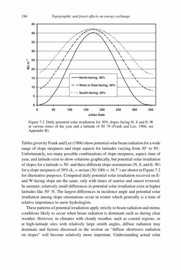
184 Topographic and forest effects on energy exchange
0
5
10
15
20
25
30
35
40
45
0 50 100 150 200 250 300 350
Julian Date
MJ
m−2
North-facing, 30%
West or East-facing, 30%
South-facing, 30%
γφ
Figure 7.2 Daily potential solar irradiation for 30% slopes facing N, S and E–Wat various times of the year and a latitude of 50 ◦N (Frank and Lee, 1966; seeAppendix B).
Tables given by Frank and Lee (1966) show potential solar beam radiation for a wide
range of slope steepness and slope aspects for latitudes varying from 30◦ to 50◦.
Unfortunately, too many possible combinations of slope steepness, aspect, time of
year, and latitude exist to show solutions graphically, but potential solar irradiation
of slopes for a latitude = 50◦ and three different slope orientations (N, S, and E–W)
for a slope steepness of 30% (ks = arctan (30/100) = 16.7◦) are shown in Figure 7.2
for illustrative purposes. Computed daily potential solar irradiation received on E-
and W-facing slope are the same, only with times of sunrise and sunset reversed.
In summer, relatively small differences in potential solar irradiation exist at higher
latitudes like 50◦ N. The largest differences in incidence angle and potential solar
irradiation among slope orientations occur in winter which generally is a time of
relative importance to snow hydrologists.
These patterns of potential irradiation apply strictly to beam radiation and mimic
conditions likely to occur when beam radiation is dominant such as during clear
weather. However, in climates with cloudy weather, such as coastal regions, or
at high-latitude sites with relatively large zenith angles, diffuse radiation may
dominate and factors discussed in the section on “diffuse shortwave radiation
on slopes” will become relatively more important. Understanding actual solar

7.2 Topographic influences 185
radiation received on slopes must begin with an understanding of how atmospheric
conditions affect diffuse and beam radiation fraction.
An empirical relationship given by Linacre (1992) inter-relates the daily diffuse
shortwave flux density on a horizontal surface (D), the total incoming shortwave
flux density on the horizontal (K↓) and the daily potential solar radiation on a
horizontal surface (Iq) as:
D/K↓ = 1 − 1.2(K↓/Iq) + 0.13(K↓/Iq)2 (7.3)
and can be used to compute the fraction of incoming solar radiation that is diffuse.
This relation was derived by Linacre (1992) from several empirical studies over the
range of K↓/Iq from 0.3 to 0.7 and should be used with caution. Other approaches to
obtaining instantaneous diffuse and direct-beam shortwave radiation for clear and
cloudy conditions that involve numerical integration to obtain daily totals have been
employed (Kustas et al., 1994). This relationship suggests that with only 30% of
potential solar radiation reaching the ground (K↓/Iq = 0.30), which is equivalent to
heavy cloud cover, the diffuse fraction of incoming shortwave radiation (D/K↓) is
0.65. Thus, by difference, 35% is direct-beam shortwave radiation. In contrast, for
mostly clear skies when incoming shortwave is 70% of potential (K↓/Iq = 0.70),
Equation (7.3) indicates that about 22% is diffuse radiation and 78% is direct beam.
The direct-beam shortwave radiation received on a slope depends upon the flux
density of beam radiation at normal incidence (Ib) being transmitted through the
atmosphere and the angle of incidence Z ′ of the beam radiation on the slope,
as described in Appendix B (see Equation (7.1)). The angle of incidence can be
computed either for an instant in time or for an entire solar day or part thereof. Beam
radiation can either be measured with radiometers (see Chapter 6 and Figure 6.1) at
a reference station or approximated using empirical relationships and potential solar
irradiation theory. Given the fraction D/K↓ using Equation (7.3) and an independent
measurement of K↓ on a horizontal surface from radiometer measurements or other
computations (see Chapter 6), Ib can be found and used to compute beam radiation
received by a variety of slope orientations.
To illustrate atmospheric effects on diffuse and direct beam radiation and Ib,
we can complete our example calculations given in Chapter 6 for solar radiation
received at a latitude of 55◦ N on Feb 7. For an assumed cloud cover fraction of 0.3,
the estimated global radiation flux density was 78.7 W m−2 for a potential solar
flux density of 111 W m−2 on a horizontal surface (Figure 6.3). By Equation (7.3)
above, the diffuse fraction would be:
D/K↓ = 1 − 1.2(78.7/111) + 0.13(78.7/111)2 = 0.214
Thus, 21.4% of the 78.7 W m−2 of estimated incoming shortwave radiation on this
example day, or 16.8 W m−2, would be diffuse shortwave radiation scattered by the
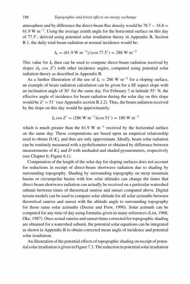
186 Topographic and forest effects on energy exchange
atmosphere and by difference the direct-beam flux density would be 78.7 − 16.8 =61.9 W m−2. Using the average zenith angle for the horizontal surface on this day
of 77.5◦, derived using potential solar irradiation theory in Appendix B, Section
B.1, the daily total beam radiation at normal incidence would be:
Ib = (61.9 W m−2)/(cos 77.5◦) = 286 W m−2
This value for Ib then can be used to compute direct-beam radiation received by
slopes (Ib cos Z ′) with other incidence angles, computed using potential solar
radiation theory as described in Appendix B.
As a further illustration of the use of Ib = 286 W m−2 for a sloping surface,
an example of beam radiation calculation can be given for a SE aspect slope with
an inclination angle of 30◦ for the same day. For February 7 at latitude 55◦ N, the
effective angle of incidence for beam radiation during the solar day on this slope
would be Z ′ = 51◦ (see Appendix section B.2.2). Thus, the beam radiation received
by the slope on this day would be approximately:
Ib cos Z ′ = (286 W m−2)(cos 51◦) = 180 W m−2
which is much greater than the 61.9 W m−2 received by the horizontal surface
on the same day. These computations are based upon an empirical relationship
used to obtain D/K↓ and thus are only approximate. Ideally, beam solar radiation
can be routinely measured with a pyrheliometer or obtained by difference between
measurements of K↓ and D with unshaded and shaded pyranometers, respectively
(see Chapter 6; Figure 6.1).
Computation of the length of the solar day for sloping surfaces does not account
for reductions in receipt of direct-beam shortwave radiation due to shading by
surrounding topography. Shading by surrounding topography on steep mountain
basins or circumpolar basins with low solar altitudes can change the times that
direct-beam shortwave radiation can actually be received on a particular watershed
subunit between times of theoretical sunrise and sunset computed above. Digital
terrain models can be used to compare solar altitude for all solar azimuths between
theoretical sunrise and sunset with the altitude angle to surrounding topography
for those same solar azimuths (Dozier and Frew, 1990). Solar azimuth can be
computed for any time of day using formulas given in many references (List, 1968;
Oke, 1987). Once actual sunrise and sunset times corrected for topographic shading
are obtained for a watershed subunit, the potential solar equations can be integrated
as shown in Appendix B to obtain corrected mean angle of incidence and potential
solar irradiation.
An illustration of the potential effects of topographic shading on receipt of poten-
tial solar irradiation is given in Figure 7.3. The reduction in potential solar irradiation

7.2 Topographic influences 187
0
0.1
0.2
0.3
0.4
0.5
0.6
0.7
0.8
0.9
1
0 5 10 15 20 25 30 35 40 45 50 55
Shade Altitude
Fra
ctio
n o
f P
ote
nti
al S
ola
r
θ = 40
θ = 50
θ = 60
θ = 70
θ = 80
θ = 40
θ = 50
θ = 60
Spring and Fall Equinox
Winter Solstice
Figure 7.3 Reduction in daily potential solar irradiation received by a horizontalsurface due to simulated topographic shading at varying shade altitudes. Curvesare given for several latitudes (θ ) at times of the winter solstice and the spring andfall equinoxes.
that would reach a horizontal surface due to shading by surrounding topography
is given for several latitudes and times of the equinoxes and winter solstice and a
range of shade altitudes. The computations assume symmetry of topographic shad-
ing around the horizon throughout each day. Clearly, potential solar irradiation and
thus beam radiation receipt can be greatly reduced or eliminated by topographic
shading for commonly occurring shade altitudes. On high-latitude watersheds or
on steep mountain basins, some snowpack surfaces may receive only diffuse solar
radiation due to topographic shading.
Diffuse shortwave radiation on slopes
Diffuse shortwave radiation flux density incident on a slope (Ds) is derived from
shortwave radiation scattered from the atmosphere and reflected to the slope from
the surrounding terrain. The flux density can be approximately computed as:
Ds = D(cos2 ks/2) + (1 − cos2 ks/2)αt Kt↓ (7.4)
where:
Ds = flux density of diffuse shortwave radiation on the slope
D = flux density of diffuse shortwave radiation on horizontal surface

188 Topographic and forest effects on energy exchange
Table 7.1 View factors from slope to sky and surrounding terrain
Slope inclinationangle (ks
◦)View factor to sky(cos2 ks/2)
View factor to surrounding terrain(1 − cos2 ks/2)
0 1.000 0.0005 0.998 0.002
10 0.992 0.00815 0.983 0.01720 0.970 0.03030 0.933 0.06745 0.854 0.14690 0.500 0.500
ks = slope inclination angle
αt = albedo of surrounding terrain
Kt↓ = total shortwave flux density on surrounding terrain
The first term in Equation (7.4), called a sky-view factor, corrects for the fraction
of atmospheric diffuse shortwave radiation received by the slope. As shown in
Table 7.1, cos2 ks/2 has a maximum value of unity when ks = 0◦ and a minimum
value of 0.5 when ks = 90◦. That is, as ks gradually increases, less and less sky is
viewed by the slope. In the extreme case, a vertical slope, only one-half of the sky
radiation is received.
The second term in Equation (7.4) represents the shortwave radiation reflected
by the surrounding terrain that is received by the slope. The term (1 − cos2 ks/2)
is the fraction of the view from the slope occupied by the surrounding terrain,
while αt Kt↓ is a rough approximation of shortwave reflected from the facing
terrain. For example, at a slope inclination angle of 30◦, 93.3% of atmospheric
diffuse shortwave radiation and 6.7% of shortwave diffuse reflected from the
facing terrain is received by the slope. Kt↓ is seldom known directly, since this
surface may also be sloping and shaded by topography, and for convenience
the radiation received on the horizontal (K↓) can be substituted as a first
approximation.
Equation (7.4) assumes that the atmosphere is a diffuse radiator, that is, scattered
radiation from the atmosphere varies only with the cosine of the angle from the
zenith, and further assumes that reflection from the surrounding terrain is also non-
directional and diffuse. In reality neither of these assumptions is strictly correct,
especially on clear days, but the relatively small view factors for slope inclinations
up to about 20–30◦, suggests that errors due to these assumptions are generally
acceptable. In specialized applications or for very steep slopes, the distribution of
diffuse shortwave radiation from the atmosphere (see discussion in Robinson, 1966)

7.2 Topographic influences 189
can be accounted for using an approach given by Perez et al. (1990) developed for
solar energy collectors.
An example of the correction for diffuse shortwave radiation on a slope can be
given based upon assumptions in previous examples. Earlier we derived a daily
diffuse shortwave flux density on a horizontal surface of 16.4 W m−2 for February
7 at a latitude of 55◦ N and a fractional cloud cover of 0.3. Combining this estimate
of D for a horizontal surface with a snowpack albedo of 0.6, Kt↓ = 78.7 W m−2
(assumed) and a 30◦ slope inclination, gives the following solution for diffuse solar
radiation on a slope using Equation (7.4):
Ds = (16.4 W m−2)(cos2 30◦/2) + (1 − cos2 30◦/2)(0.6)(78.7 Wm−2)
= 18.5 W m−2
In this case, the diffuse solar on the slope is about 13% greater than on a horizontal
surface, primarily due to the relatively high albedo ofαt =0.6 assumed for landscape
facing the slope. Topographic effects on diffuse shortwave radiation are much less
than for shortwave beam radiation; therefore, conditions where diffuse shortwave
radiation dominates, e.g. cloudy weather and large zenith angles, produce smaller
differences in shortwave radiation received among slopes.
Completing the computation of Ks↓ for the slope by combining the diffuse and
direct beam components in our example gives:
Ks↓ = Ib cos Z ′ + Ds = 180 W m−2 + 18.5 W m−2 = 198 W m−2
where the major increase in total shortwave radiation on the slope compared to
the horizontal is due to increased beam shortwave radiation rather a correction for
diffuse shortwave. Net shortwave radiation exchange on the slope for an albedo of
0.6 would thus be:
Q′ns = (1 − α)Ks↓ = (1 − 0.6)(198 W m−2) = 79.2 W m−2
The comparable net shortwave radiation flux density found previously for the hori-
zontal surface (Qns = 31.5 W m−2) shows that net shortwave exchange is essentially
doubled on the slope. Again, most of this difference is due to the direct-beam com-
ponent.
Effects of surrounding topography on view factors of slopes to the atmosphere
can also be significant on steep mountain basins. On certain shaded subunits of
steep mountain basins, the fraction of the sky viewed can actually be much less
than that computed for the surface slope inclination and azimuth angle as given in
Table 7.1. For example, a sloping snowpack surface in a deeply incised basin may
receive reflected shortwave radiation from the facing valley slopes and slopes on
the opposite side of the valley. View factors for several different basin geometries

190 Topographic and forest effects on energy exchange
have been derived that could be used to approximate shading effects of surrounding
topography on incoming diffuse shortwave radiation (Oke, 1987) following proce-
dures given above. These same view factors can also be used to correct incoming
longwave radiation.
7.2.2 Longwave radiation on slopes
Longwave radiation received by a slope comes partially from the atmosphere and
partially from the terrain facing the slope; assumed here to be snow covered. View
factors previously used for diffuse shortwave are again applied along with the
assumption that longwave radiation from the sky and facing terrain are isotropic
or perfectly diffuse. Outgoing longwave radiation from the slope is the same as for
the horizontal case. Assuming reflected longwave radiation to be negligible, the net
longwave radiation exchange for the slope (Qnl′) can be approximately written as:
Q′nl = εsLs↓ − εs σ T 4
s (7.5)
Ls↓ = L↓(cos2 ks/2) + (1 − cos2 ks/2)εt σ T 4t (7.6)
where:
Ls↓ = incoming longwave radiation flux density to slope
L↓ = incoming longwave radiation flux density from sky to a horizontal surface
εs = snowpack emissivity
σ = Stefan–Boltzmann constant, 5.67 × 10⁻⁸ W m−2 K−4
Ts = snowpack surface temperature
ks = slope inclination angle
εt = emissivity of the facing terrain
Tt = surface temperature of facing terrain, K
In effect, the longwave radiation emitted by the atmosphere that reaches the slope
is reduced by the factor cos2 ks/2 (see Table 7.1) and a fraction (1 − cos2 ks/2) of
the longwave radiation emitted by the facing terrain is added. If the facing terrain
is snow covered, then we are substituting near-black body radiation from snow for
lower effective emissivity radiation from a fraction of the sky. If melting snow with
εs = 0.98 is assumed to be on the surface of the slope and facing terrain (L↑ = 309
W m−2), then net longwave radiation exchange for our 30◦ slope with previously
computed incoming longwave radiation from the atmosphere with 0.3 cumulus
cloud cover on the horizontal surface (L↓ = 228 W m−2) becomes:
Q′nl = (228 W m−2)(cos2 30◦/2) + (1 − cos2 30◦/2)(309 W m−2) − 309 W m−2
= −75 W m−2

7.2 Topographic influences 191
Table 7.2 Comparison of radiation exchange (W m−2) onexposed horizontal and sloping snowpack surfaces computed for
a latitude of 55◦ N on February 7a
Radiation Term Horizontal 30◦ SE Slope
Incoming beam shortwave 62 180Incoming diffuse shortwave 16 18Total incoming shortwave 78 198Outgoing shortwave −47 −119Net shortwave 31 79
Incoming longwave 228 234Outgoing longwave −309 −309Net longwave −81 −75
Net allwave −50 4
aAssumptions: C = 0.3 cumulus clouds, α = αt = 0.6, Ta = 2 ◦C,RH = 50%, Ts = 0 ◦C, εs = εt = 0.98, no longwave reflection, see text.
The net longwave exchange on the slope is thus only about 7% greater than the
−81 W m−2 for a horizontal surface for conditions of relatively clear skies, 50%
relative humidity and air temperature of 2 ◦C that were assumed. The correction
would be even less under cloudy skies for our given assumptions of melting snow
on the facing terrain. Non-isotropic longwave emission from the atmosphere could
modify these results, but as with the correction for diffuse shortwave radiation, the
effects would be generally small given the rather small view factors to facing terrain
typically found in nature.
Differences in the radiation budget calculations for sloping and horizontal snow-
pack surfaces in the example are summarized in Table 7.2. By far the largest differ-
ence due to topography is the direct-beam shortwave radiation and the net shortwave
components resulting from the SE orientation of the sloping surface towards the Sun.
The rather high snowpack albedo tends to minimize this difference in the overall
radiation balance however. Differences in incoming diffuse shortwave and incom-
ing longwave radiation due to the 30◦ slope inclination angle are relatively small.
Regardless, the differences in absorbed direct-beam shortwave radiation produced
a positive net radiation flux density on the slope, while a relatively large negative net
radiation would occur on a horizontal snowpack surface for the same conditions.
The net allwave radiation flux density for snowpacks on an entire watershed can
be approached in various ways. Lee (1963) introduced the “watershed lid” concept
that represents an entire watershed as a single plane fit to the watershed topographic
boundaries. Once the slope and aspect of the plane representing the watershed lid
is found, net allwave radiation can be computed for this plane to represent the net

192 Topographic and forest effects on energy exchange
exchange of radiant energy for the entire watershed. Another approach to computing
net allwave radiation exchange across watersheds is to divide the watershed area
into subareas with fixed slope inclination and aspect characteristics and compute
the net radiant exchange for each subarea. Several models employing this latter
method have been developed with the advent of geographic information system
methods (Ohta, 1994; Matsui and Ohta, 2003). Also see discussion of modelling
in Chapter 10.
7.2.3 Topography and convection
As distributed models of snowpack energy exchange advance, greater attention will
be given to adjusting parameters such as wind speed, air temperature, and humidity
for the effects of topography. It is common practice to adjust air temperature data
in degree-day applications for the effects of elevation using lapse rates. Humidity is
often assumed invariant across a basin and wind-speed adjustments are problemati-
cal and the subject of considerable research. Marks et al. (1992) reported essentially
no difference in vapor pressure but a nearly 50% difference in wind speed between
a ridge top and lake site in the alpine in California. Susong et al. (1999) developed
methods to estimate precipitation, air temperature, vapor pressure, wind speeds,
radiation fluxes, snowpack properties, and soil temperature across complex terrain
for use in distributed models of snowmelt.
Correction of air temperatures for the effect of elevation usually takes the form:
�T = γ (hst − h)/100 (7.7)
where:
�T = change in temperature with elevation, ◦C
γ = temperature lapse rate, ◦C 100 m−1
hst = elevation of temperature index station, m
h = elevation of station to be estimated, m
The temperature lapse rates are best derived from local climatic data. Values used
in snow studies range between the dry adiabatic lapse rate of −0.98 ◦C 100 m−1
up to about −0.2 ◦C 100 m−1. Values of about −0.5 to −0.65 ◦C 100 m−1 are
typically employed (Verdhen and Prasad, 1993; Braun et al., 1993; Kumar et al.,1991; Zhenniang et al., 1991 and 1994; Ujihashi et al., 1994; Martinec et al., 1998).
Lapse rates also vary with time of year (Zhenniang et al., 1994; Martinec et al.,1998). A simple example calculation of the use of a temperature lapse rate follows.
Given a lapse rate of −0.6 ◦C 100 m−1, if the air temperature at a station at 3500
m elevation was needed, the �T needed to correct temperatures at an index station
at 2700 m elevation would be:
�T = (−0.6 ◦C/100 m)(3500 m − 2700 m)/100 = −4.8◦C

7.3 Forest influences 193
The proper elevation (h) of the station that temperature is being estimated for is an
issue within watersheds with many terrain subunits. For subunits delineated strictly
as elevation zones, the hypsometric mean elevation, or elevation above and below
which 50% of the area in that zone occurs, is often used.
Variation of wind speed with topography controls not only the accumulation
and sublimation of snow as described in Chapter 3, but also the convective heat
exchange of the snowpack. Protection from or exposure to winds by the landscape
can vary with wind direction and the need to model wind speed across large areas
will require routine observation of wind direction. Hartman et al. (1999) adapted
a snow transport model developed by Liston and Sturm (1998) to generate a wind-
speed field for an alpine/subalpine basin in Colorado for typical westerly winds.
The model was able to predict increased wind speeds on ridges and windward
slopes and reduced speeds in valleys and lee slopes. Nakayama and Hasegawa
(1994) used a shear flow model to elucidate the effects of topography on wind
speed and snowfall around Ishikari Bay in Japan. In the future, more applications
like these will undoubtedly be used to predict distributed wind-speed maps for
large watersheds that will help simulate convection of energy to and from the
snowpack.
7.3 Forest influences
Forests have a major influence on the energy budget of snowpacks, especially
radiative and convective heat exchange (Figure 7.4). Unfortunately, climatic data
such as radiation, wind speed, air temperature, and humidity are generally not
available for snowpacks in forests and adjustments to data for open conditions
are needed. The one-dimensional equations given previously in this chapter do
not strictly apply to snowpack surfaces in forests, where air flow may be de-
coupled from that above the forest and turbulence is generated by air moving
past tree boles and understory vegetation. Forest effects also vary due to varying
species composition, age, and density of trees and with the nature of understory
vegetation. At the least, broad distinctions need to be made between the effects
of coniferous and leafless deciduous forest. Finally, since plant canopies inter-
cept precipitation, the impact of rainfall on snowpacks in the forest is likely to be
altered.
7.3.1 Shortwave radiation in forests
The flux density of shortwave radiation that reaches the snowpack surface beneath
a forest canopy is the net result of complex multiple reflection, transmission and
absorption occurrences with foliage, woody plant tissue, and the ground surface
(Ross, 1981). Shortwave beam radiation is transmitted through varying path lengths

194 Topographic and forest effects on energy exchange
Figure 7.4 Prediction of snowmelt in forests requires accounting for canopy effectson snowpack energy exchange, especially radiation exchange. Shadow patternssuggest varying patterns of canopy shading between coniferous forests with foliage(top) and deciduous forests without foliage (bottom) in these pictures from mid-latitude Pennsylvania, USA sites. See also color plate.
in the forest during each day due to differences in the solar zenith angle. Larger
path lengths in the forest increase the chances for extinction by vegetation. The
fraction of beam radiation that reaches the snowpack surface will generally decrease
with increasing zenith angles or path lengths. In contrast, a relatively constant
fraction of shortwave diffuse radiation, coming more uniformly from the entire
atmosphere above, is transmitted by the forest to the snowpack. Varying beam and
diffuse shortwave fractions due to variation in cloud cover, zenith angle, and other
factors cause differences in the fraction of shortwave radiation transmitted by the
forest.
The nature and distribution of the vegetation elements in the forest obviously
also play a major role in the degree of interaction with incoming shortwave radia-
tion. The architecture and spectral properties of conifer forests and leafless decid-
uous forest that are common to snow-covered landscapes can have an important
influence on melt rates. A small fraction (10%) of total shortwave radiation is

7.3 Forest influences 195
generally transmitted by dense conifer forest, but even fully stocked, leafless decid-
uous forest only transmits about 50% of total shortwave radiation. Boreal forests
are often quite sparse, but still can significantly influence radiation exchange at
the snowpack surface. The albedo of the snowpack even plays a role, since a por-
tion of shortwave radiation reflected from the snowpack can be re-reflected by
the forest back to the ground. Snow intercepted on the foliage and branches will
likely enhance these multiple reflections between the snowpack and forest. Ulti-
mately a method is needed to correct the flux density of incoming shortwave radi-
ation computed or measured for open conditions for the complex interactions with
forests.
Models of shortwave radiation transmission in forests range widely from simple
fractional transmission based upon field studies (Kittredge, 1948) to more complex
models of atmosphere–forest–ground interactions (Li et al., 1995). In early studies
radiation transmission in relatively closed forests was simply related to crown clo-
sure or stem density (Reifsnyder and Lull, 1965). Beer’s law model, similar to the
model for shortwave radiation transmission in snow, has been used with success to
describe radiation transmission of beam and diffuse shortwave radiation in leafless
deciduous forest canopies by Federer (1971) and Link and Marks (1999). However,
Reifsnyder et al. (1971/72) found that Beer’s law did not represent the transmis-
sion of shortwave beam radiation by deciduous forest in full leaf, but appeared to
fit data for conifer forest. Models developed to describe radiation within closed
crop canopies that consider the distribution of leaf area and leaf angle distribution
within the plant canopy (Ross, 1975) have been applied to forests (Jarvis et al., 1976;
Rauner, 1976). In relatively sparse boreal or subarctic forests, theoretical models
(GORT) that assume the forest to be randomly distributed tree crowns of ellipsoidal
shape have been developed and tested (Li et al., 1995; Ni et al., 1997; Hardy et al.,1997). Woo and Giesbrecht (2000) modelled shortwave radiation transmission in a
low-density subarctic spruce forest by assuming trees were represented by isolated
vertical cylinders. The approach taken to modelling shortwave radiation transmis-
sion should vary with the nature of the forest and the data needs to implement the
model.
A simple semi-empirical exponential model that considers transmission of total
shortwave radiation can be used to approximate forest effects (Monsi and Saeki,
1953). In this model, transmission of total solar radiation through a forest canopy is
related to a measure of vegetation density termed the leaf-area index (LAI) which
is the projected surface area of leaves and/or needles per unit ground area inte-
grated from canopy top to ground level. In leafless deciduous forest the appro-
priate measure becomes the plant-area index or the integrated areas of twigs,
branches, boles as well as leaves when present. Leaf-area index varies with tree
density, age, and species composition. The fraction of shortwave radiation that
196 Topographic and forest effects on energy exchange
penetrates the forest canopy to the snowpack (K↓f/K↓) can be simply written
as:
K↓f/K↓ = exp(−κ LAI) (7.8)
where κ is a dimensionless extinction coefficient for shortwave radiation in forest.
Incoming shortwave radiation above a forest stand is assumed equal to K↓ computed
for a horizontal or sloping snowpack surface in the open. The extinction coefficient
varies between the visible and near-infrared wavelength regions and also with
the zenith angle, the ratio of diffuse to beam shortwave radiation received, and
with depth within the forest canopy (Ross, 1981; Jarvis et al., 1976), but some
approximate values are given in Table 7.3 for use in estimating daily totals of
radiation. These values should be used with caution since most were derived for
conditions without snow on the ground or snow intercepted on the canopy, but they
give reasonable results. However, Pomeroy and Dion (1996) found that intercepted
snow had very little effect on extinction of shortwave radiation in a pine canopy.
If values for pine forest from Table 7.3 are used with LAI = 4 and κ = 0.4,
then the fraction of shortwave radiation transmitted would be:
K↓f/K↓ = exp(−0.4(4)) = 0.20
A correction for leafless deciduous forest with LAI = 0.5 and κ = 1 from Table7.3, gives K↓f/K↓ = 0.61. In either case, conifer or deciduous hardwoods, the
correction for shortwave transmission is not trivial, but determining the leaf-area
index and the appropriate extinction coefficient are still problematical. LAI can
be estimated by a variety of ground-based methods (Chen et al., 1997b) and from
remote-sensing data (Chen and Cihlar, 1996).
Another physically based and relatively simple model for shortwave radiation
transmission in forests is to assume that a Beer’s-law type extinction process applies
to direct-beam shortwave radiation and that a constant transmission fraction can be
used for diffuse shortwave radiation (Federer, 1971; Link and Marks, 1999). With
this model, the radiation penetrating to the snowpack in forests would be:
K↓f = τd D + Ib cos Z exp(−μ ht sec Z ) (7.9)
where:
K↓f = incoming shortwave flux density in forest, W m−2
τ d = transmissivity for diffuse shortwave radiation, dimensionless
D = diffuse shortwave radiation flux density, W m−2
Ib = direct beam shortwave radiation flux density at normal incidence, W m−2
Z = zenith angle of the Sun (or incidence angle (Z′) for sloping surfaces)
μ = extinction coefficient for direct beam shortwave radiation, m−1
ht = average forest height, m

Tab
le7.3
Ext
inct
ion
coef
ficie
nts
for
inco
min
gsh
ortw
ave
radi
atio
nin
fore
sts
for
Equ
atio
n(7
.8).
Lea
f-o
rF
ore
stT
yp
eT
ree
Hei
gh
t(m
)P
lan
t-A
rea
Ind
exκ
So
urc
ea
Pin
e(P
inus
spp
.)m
id-d
ay1
5.5
,2
22
.6–
4.3
0.2
8–
0.5
7(1
)tw
ost
and
sS
pru
ce(P
icea
spp
.)m
id-d
ay1
1.5
,2
7.5
8.4
–9
.80
.28
–0
.58
(1)
two
stan
ds
Oak
(Que
rcus
spp
.)fu
llle
af−
5.5
∗0
.42
(2)
and
(3)
leafl
ess
0.5
∗1
.00
Oak
-Hic
ko
ry(Q
.an
dC
arya
spp
.)1
7–
26
(3)
full
leaf
4.9
0.5
79
leafl
ess
0.5
∗1
.12
Asp
en(P
opul
ustr
emul
oide
s)2
1.5
(4)
full
leaf
2.1
0.6
0le
afles
s0
.2∗
0.7
2B
irch
(Bet
ula
pube
scen
ssp
p.
tort
uosa
)5
–7
der
ived
wit
hd
ata
fro
m(5
)fu
llle
af2
.00
.39
leafl
ess
0.3
6∗
1.0
3
a(1
)Ja
rvis
etal
.,1
97
6,
(2)
Rau
ner
,1
97
6,
(3)
Bal
do
cch
iet
al.,
19
84
,(4
)C
hen
etal
.,1
99
7a,
and
(5)
Ov
hed
and
Ho
lmg
ren
,1
99
5.
∗ pla
nt-
area
ind
exin
clu
des
leav
es,
ifp
rese
nt,
and
wo
od
ym
ater
ial.

198 Topographic and forest effects on energy exchange
Table 7.4 Forest shortwave radiation transmission parameters for Equation (7.9)
Forest Type
Direct beamshortwaveμ, m−1
Diffuse shortwaveτ d Sourcea
Deciduous 0.025 0.44 (1)Mixed conifer/deciduous 0.033 0.30 (1)Medium conifer 0.040 0.20 (1)Dense conifer 0.074 0.16 (1)Mixed deciduous 0.019–0.027 − (2) Canopy space only
a (1) Link and Marks, 1999; (2) Federer, 1971.
Figure 7.5 Solar beam path length in forest in relation to tree height and zenithangle.
The term “ht sec Z” in Equation (7.9) represents the path length for direct beam
radiation in the forest (see Figure 7.5). Extinction coefficients (μ) for beam radi-
ation and average integrated transmissivities for diffuse radiation (τ d) derived
from experimental data are given for several forest types in Table 7.4. Pomeroy
and Dion (1996) applied the same model to total incoming shortwave radia-
tion in a boreal pine forest and found that the extinction coefficient varied from
zero to 0.14 m−1 with solar altitudes from 0 to about 40◦, respectively. It is
important to realize that τ d is linked to a specific value of μ, since τ d rep-
resents, theoretically at least, an average value of the direct-beam transmission
function integrated over zenith angles of 0 to 90◦ to represent diffuse short-
wave transmission from the entire hemisphere. Neither parameter should be varied
independently.Given the values for D = 16.4 W m−2, Ib cos Z = 62.2 W m−2 and mean zenith
angle Z = 77.5◦ from previous calculations, the flux density of incoming shortwave

7.3 Forest influences 199
radiation in a leafless deciduous forest with an average height of 15 m, μ = 0.02m−1 and τ d = 0.4 would be:
K↓f = (0.4)(16.4 W m−2) + (62.2 W m−2) exp[−(0.02 m−1)(15 m)(sec 77.5◦)]
= 6.56 W m−2 + (62.2 W m−2)(0.25) = 22.1 W m−2
Thus only 22.1 W m−2 or 28% of the total 78.7 W m−2 incoming shortwave
radiation above the canopy would reach the snowpack for this forest condition. After
incoming shortwave radiation at the snowpack surface in the forest is estimated, the
reflected shortwave radiation at the snowpack surface in the forest can be simply
estimated as K↑f = α K↓f. Computation of net allwave radiation for snowpacks in
forests also requires consideration of longwave exchange that is described in the
next section.
7.3.2 Longwave radiation in forests
Incoming longwave radiation at the snowpack surface in forests comes from the
atmosphere through the gaps and openings and from the forest canopy overhead.
Since nearly all longwave radiation received by the forest canopy is absorbed, and
little is transmitted or reflected, the computation of longwave exchange beneath the
canopy is simple relative to shortwave radiation exchange. If the view factor from
the snowpack to the overhead canopy is known (Fs−f) then the fraction of the view
open to the atmosphere is 1 − Fs−f. With these simple ideas as a model, the net
longwave radiation beneath the forest canopy can be written as:
Qnlf = L↓(1 − Fs−f) + σ εf T 4c (Fs−f) − σ εs T 4
s (7.10)
where:
Qnlf = net longwave radiation flux density beneath a forest canopy, W m−2
L↓ = incoming longwave radiation flux density in open (horizontal or sloping
surface), W m−2
Fs−f = view factor from snowpack surface to overhead forest, dimensionless
σ = Stefan–Boltzmann constant, 5.67 × 10⁻⁸ W m−2 K−4
εf = emissivity of forest canopy, dimensionless
Tc = temperature of forest canopy, K
εs = emissivity of snowpack surface
Ts = temperature of snowpack surface, K
Emissivity of the forest canopy elements is quite high and ranges from 0.97 to 0.99.
The radiating temperature of the forest canopy overhead is seldom known and is
a deficiency in computing net longwave radiation exchange below the canopy. A
first approximation would be to assume that canopy temperature was equal to the

200 Topographic and forest effects on energy exchange
air temperature within the forest; however, temperatures of sunlit portions of the
canopy and tree boles can be heated well above air temperature during the day
and increase incoming longwave radiation beneath the canopy. View factors from
a plane surface to the overhead canopy are also not easily obtained from forest
characteristics, but canopy closure, the projection of overhead canopy and bole
area onto a horizontal plane (Storck and Lettenmaier, 1999; US Army Corps of
Engineers, 1956) or one minus transmissivity for diffuse shortwave radiation (τ d)
in Table 7.4 can be substituted (Link and Marks, 1999).The effects of longwave radiation from the forest canopy on net longwave
exchange can be computed using Equation (7.10). In previous examples for par-tially cloudy conditions and melting snow, the incoming longwave radiation fromthe atmosphere at 2 ◦C, a C = 0.3 cumulus cloud cover and 50% relative humid-ity was 228 W m−2 (L↓) and the longwave radiation loss from the melting snowwas 309 W m−2 (σ εs Ts
4 without considering reflected longwave radiation). Netlongwave exchange for these conditions was 228–309 W m−2 or a relatively largeenergy loss of −81 W m−2. Assuming a view factor from snow to forest of 0.8,or roughly 80% canopy closure equivalent to a dense conifer canopy, an effectivecanopy radiating temperature of 3 ◦C (1 ◦C above air temperature) and εf = 0.98,the snowpack net longwave exchange would be:
Qnlf = (228 W m−2)(1 − 0.8)
+ (5.67 × 10⁻⁸ W m−2 K−4)(0.98)(276.16 K)4(0.8)
− 309 W m−2 = −4.9 W m−2
The forest canopy can increase the incoming longwave to the snowpack (Hashimoto
et al., 1994) and in this example for a simulated coniferous forest produces a small
negative net longwave exchange at the snowpack surface. Positive net longwave
radiation exchange commonly occurs in forests during the melting season and
development of snowpack cold content overnight is often prevented by the overhead
canopy.
Theoretical analysis of view factors from the snowpack to individual tree trunks
and canopies has been used to help understand forest effects on longwave radiation
exchange. Analysis by Bohren and Thorud (1973) suggests that nearly all longwave
radiation received by a snowpack from the forest comes from tree boles and crowns
within 2–3 times the average crown radius away. Woo and Geisbrecht (2000) pre-
sented a theoretical analysis attributed to J. A. Davies that showed that the view
factor from the snow surface to an individual tree trunk dropped below 0.01 or 1%
of the total view when the point was farther than about one-third the trunk height
away. Both of these studies suggest that most longwave radiation received by the
snowpack from the forest would be received from nearby trees.
The net allwave radiation at the snowpack surface in a forest can be computed
from the sum of net shortwave and net longwave radiation exchange as in above

7.3 Forest influences 201
Table 7.5 Comparison of snowpack radiation exchange (W m−2) for open,leafless deciduous forest, and dense coniferous forest sites computed for a latitude
of 55◦ N on February 7a
Radiation Term OpenLeafless DeciduousForestb
Dense ConiferousForestc
Incoming beam shortwave 62 16 1Incoming diffuse shortwave 16 7 3Incoming total shortwave 78 23 4Outgoing shortwave −47 −14 −2Net shortwave 31 9 2
Incoming longwave 228 285 304Outgoing longwave −309 −309 −309Net longwave −81 −24 −5
Net allwave −50 −15 −3
a ht = 15 m, εf = 0.98, Tc = 3 ◦C, other assumptions same as in Table 6.6b leafless deciduous forest: td = 1 − Fs−f = 0.4, μ = 0.02 m−1
c coniferous forest: td = 1 − Fs−f = 0.2, μ = 0.07 m−1
examples (Table 7.5). In Table 7.5 a complete example for leafless deciduous forest
and coniferous forest is shown using Equations (7.9) and (7.10) and parameters
given in Table 7.4. The large reduction in incoming diffuse shortwave and beam
shortwave radiation, especially in the coniferous forest, is seen to be partially off-
set by the increased incoming longwave radiation from the forest canopy. In this
example the forest canopy was assumed to be 1 ◦C warmer than air temperature
for the entire day. The net allwave radiation under dense conifers would be slightly
negative under these conditions, while a large negative net allwave radiation sum
occurred in the open. The leafless deciduous forest had an intermediate, but nega-
tive, net allwave exchange for the example conditions. This comparison generally
illustrates the differences between deciduous and coniferous forests on snowpack
radiant energy exchange relative to open conditions. Obviously, the choice of dif-
fuse and beam radiation transmission parameters and the assumed temperature of
the forest canopy and the radiation conditions in the open determine the forest
effects using this approach.
Other procedures for estimating snowpack net radiation in forests have been
employed. Price (1987) estimated net allwave radiation at the forest floor using
a regression analysis with incoming shortwave radiation and air temperature as
predictor variables. This procedure could be employed after calibration for the spe-
cific forest conditions of interest. Parrott (1974) showed relationships between
above and below canopy net allwave radiation in leafless deciduous forest in

202 Topographic and forest effects on energy exchange
Pennsylvania during periods with snow cover. Peters (1980) showed that snow-
pack net radiation in deciduous forest was only half that in an adjacent clear-cut
opening on days with complete snow cover. Extinction coefficients for predicting
net allwave radiation in the forest similar to those used for incoming shortwave
radiation (Equation (7.8) and Table 7.3) have also been derived (Jarvis et al., 1976),
but introduce the additional requirement that net radiation above the forest canopy
be estimated.
7.3.3 Forest effects on wind speed and convection
Convective exchange of sensible and latent heat between the snowpack and air in the
forest is poorly understood. Due to the very low wind speeds often observed above
snowpacks in forests, convective sensible and latent heat exchange computed using
Equations (6.14) and (6.20), respectively, would be quite low (Price, 1988; Ohta
et al., 1993; Barry et al., 1990). Sauter and McDonnell (1992) state that during
passage of frontal storms convective exchange in forests could be significant on a
diurnal basis. In addition, equations derived for uniform, open snowpack conditions
do not strictly apply within forests. Jarvis et al. (1976) indicate that for conifer forest,
wind speed near ground level is often controlled by horizontal pressure gradients
that negate simple one-dimensional analysis of heat, mass, and momentum beneath
the canopy. Turbulence within the forest is generated more by air flow around tree
boles and through understory and lower canopy vegetation, rather than by air flow
over the snowpack surface. Not surprisingly then, results of some studies have
suggested that the bulk transfer coefficients (Ch and Ce) necessary to account for
observed convective exchange at ground level in forests would have to be several
to many times greater than those based upon the roughness length at the snowpack
surface for open conditions (Parrott, 1974; Ishii and Fukushima, 1994; Tanaka,
1997; Suzuki and Ohta, 2003). Kuz′min (1961) also suggested use of adjustment
factors for bulk transfer coefficients in forests that ranged up to 2 for conifers and
1.6 for deciduous forests, but indicated these had not been experimentally verified.
Estimation of wind speeds at the snowpack surface in forests from open mea-
surements is also not a straightforward procedure without site-specific data. Ratios
of wind speed in the forest to that in the open without consideration of meteoro-
logical, topographic, and forest characteristics do not appear to produce consistent
results. In addition, wind speeds below the canopy are often quite low (<1 m s−1)
and difficult to measure accurately without sensitive instruments. A wide range of
ratios between wind speed in deciduous forest and that in the open or above the
canopy are given in the literature: 0.4 for mixed oak (Quercus spp.) forest on sloping
ground (Parrott, 1974), 0.9 for maple (Acer mono) in mountainous terrain in Japan
(Ishii and Fukushima, 1994), 0.51 and 0. 77 for two other deciduous stands in Japan
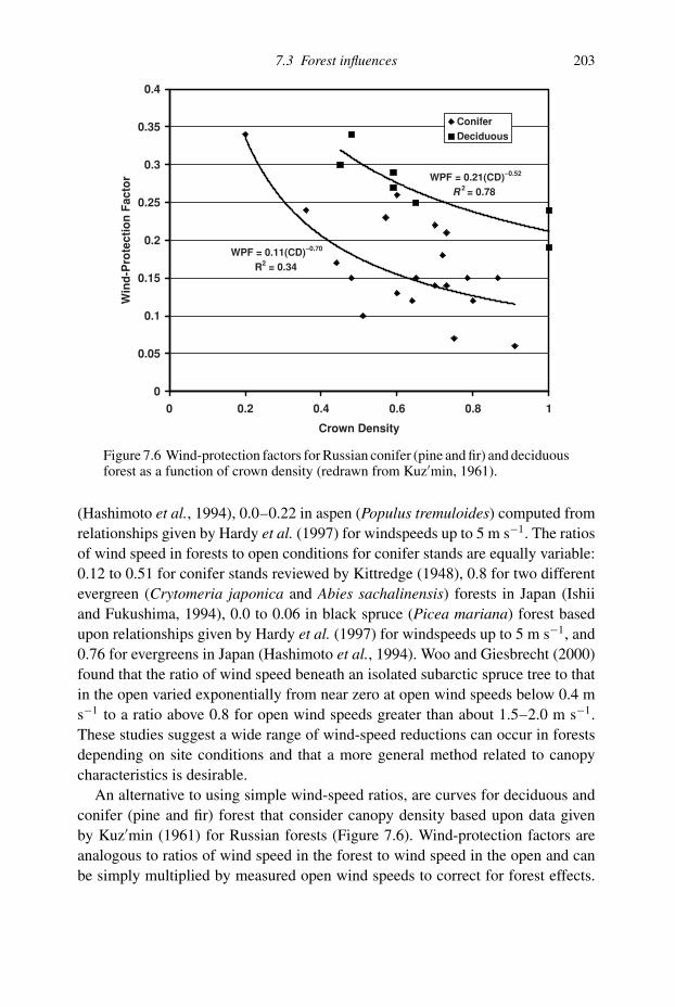
7.3 Forest influences 203
WPF = 0.21(CD)−0.52
R
df
2 = 0.78
WPF = 0.11(CD)−0.70
R2 = 0.34
0
0.05
0.1
0.15
0.2
0.25
0.3
0.35
0.4
0 0.2 0.4 0.6 0.8 1
Crown Density
Win
d-P
rote
ctio
n F
acto
rConifer
Deciduous
−
−
Figure 7.6 Wind-protection factors for Russian conifer (pine and fir) and deciduousforest as a function of crown density (redrawn from Kuz′min, 1961).
(Hashimoto et al., 1994), 0.0–0.22 in aspen (Populus tremuloides) computed from
relationships given by Hardy et al. (1997) for windspeeds up to 5 m s−1. The ratios
of wind speed in forests to open conditions for conifer stands are equally variable:
0.12 to 0.51 for conifer stands reviewed by Kittredge (1948), 0.8 for two different
evergreen (Crytomeria japonica and Abies sachalinensis) forests in Japan (Ishii
and Fukushima, 1994), 0.0 to 0.06 in black spruce (Picea mariana) forest based
upon relationships given by Hardy et al. (1997) for windspeeds up to 5 m s−1, and
0.76 for evergreens in Japan (Hashimoto et al., 1994). Woo and Giesbrecht (2000)
found that the ratio of wind speed beneath an isolated subarctic spruce tree to that
in the open varied exponentially from near zero at open wind speeds below 0.4 m
s−1 to a ratio above 0.8 for open wind speeds greater than about 1.5–2.0 m s−1.
These studies suggest a wide range of wind-speed reductions can occur in forests
depending on site conditions and that a more general method related to canopy
characteristics is desirable.
An alternative to using simple wind-speed ratios, are curves for deciduous and
conifer (pine and fir) forest that consider canopy density based upon data given
by Kuz′min (1961) for Russian forests (Figure 7.6). Wind-protection factors are
analogous to ratios of wind speed in the forest to wind speed in the open and can
be simply multiplied by measured open wind speeds to correct for forest effects.

204 Topographic and forest effects on energy exchange
Although the scatter of data is large, especially for conifer stands, curves fit to these
data show that for a given crown density wind speeds in conifers are reduced more
than in deciduous forest. These curves should obviously not be used outside the
range of data used to derive them. The term crown density used in the Russian
literature is related to canopy closure, but the terms may not be strictly equivalent.
Another quantitative approach is to use plant- or leaf-area index (LAI or PAI )
to estimate wind speed in forests as (Rauner, 1976):
uz/uh = exp (−n PAI) (7.11)
where:
uz = wind speed near ground level in the forest, m s−1
uh = wind speed at the top of the canopy, m s−1
PAI = plant-area index, dimensionless
n = wind-speed extinction coefficient, dimensionless
Rauner (1976) found that the wind-extinction coefficient “n” ranges from 0.25 to
0.35 for several deciduous forests in full leaf for wind speeds of 1–3 m s−1. At higher
wind speeds the value of n decreases, decreasing by 50% at 5 m s−1. Plant-area
index is the area of leaves or needles, twigs, branches, and boles integrated from
the top of the canopy to the ground and expressed per unit ground area. Using this
equation, given a plant-area index for deciduous forest of 2 and n = 0.3, the ratio
of below canopy to above canopy wind speed would be about 0.55. It is not certain
whether this range of extinction coefficients applies to winds in leafless deciduous
and conifer stands at different plant-area index values. To use Equation (7.11) to
estimate wind speed in forests, wind speed measured above the canopy must be
available or assumed equal to that in the open.
Air temperature and humidity above the snowpack surface are also modified
somewhat by forest cover. Generally, maximum daily air temperatures are reduced
due to canopy shading, while minimum daily air temperatures are increased due
to enhanced longwave exchange beneath the canopy relative to an open area. The
net result is generally a significant reduction in the range of daily temperatures
and a decrease in mean daily air temperatures beneath the canopy. Forest effects
on air temperature would be greater in coniferous than leafless deciduous forest.
Reductions in daily mean air temperatures relative to an open site for conifer stands
are about 0.5–1.5 ◦C in winter (Kittredge, 1948), but negligible in leafless deciduous
forest (Parrott, 1974; Peters, 1980). Peters (1980) showed maximum and minimum
daily air temperatures in leafless deciduous forest with snowcover were 0.9 ◦C
lower and 0.6 ◦C higher, respectively, than in an adjacent clear-cut.
Water vapor pressure in the air within the forest can also be slightly elevated
compared to the open, due to reduced convection and evaporation/sublimation at

7.3 Forest influences 205
the snowpack surface and to transpiration by the overhead canopy late in the melt
season. Differences in relative humidity between open and forest areas are quite
large due to temperature differences, but in absolute terms vapor pressure elevations
of <0.5 mb occur in forest relative to open areas during snowmelt. Corrections
for forest effects on air temperature and humidity are often small during snowmelt
(Kuz′min, 1961; Ishii and Fukushima, 1994), but for some applications and
locations they could be important. DeWalle and Meiman (1971) showed that vapor
pressure gradients above late-season melting snowpacks in Colorado conifer forest
varied diurnally leading to evaporation at night and condensation during daytime.
Atmospheric stability conditions over snowpacks may also be affected by forests,
following the computation scheme given previously. Reductions in wind speed and
possible changes in the temperature difference between snowpack surface and air
by forests could affect the magnitude of the bulk Richardson number (RiB) and
stability corrections for convective transport. Since reductions in wind speeds will
probably dominate any changes in temperature within the forest, RiB will likely
increase further into the stable range. Thus, the bulk transfer coefficients Ch and Ce
given by Equation (6.22b) would also likely be less than in the open due to stability
effects.
7.3.4 Forest energy budget examples
Studies of snowpack energy budgets in forest have enhanced our understand-
ing of forest effects on radiative and convective exchange (Ishii and Fukushima,
1994; Hashimoto et al., 1994; Yamazaki and Kondo, 1992; Davis et al., 1997;
Hardy et al., 1997; Fitzgibbon and Dunne, 1983; Metcalfe and Buttle, 1997; Barry
et al., 1990). In a study near Mt. Iwate in Japan, Ohta et al. (1993) evaluated the
snowpack energy budget at an open site and an adjacent leafless, deciduous forest
site both on level terrain (Figure 7.7). Incoming shortwave radiation was reduced
by about 38% and wind speed was reduced by 71% in the forest relative to the open
site, but air temperatures and vapor pressures were similar between sites. Latent
heat convection represented an energy gain to the snowpack at both sites on most
days, due to the generally high vapor pressures in the air in the region. Very high
latent heat convection occurred on March 20 due to high wind speeds (8.6 m s−1)
and very high humidity (9.6 mb) due to the occurrence of a small rainfall event.
Sensible heat convection was also positive on all days at both sites due to warm
daytime air temperatures. Average daily air temperatures of 7.6 ◦C combined with
high wind speeds on March 20 also produced the highest sensible heat convection
to the snowpack. Latent heat and sensible heat convection were much lower in the
forest than in the open due to reduced wind speeds. Net radiation was the dominant
snowpack energy budget component at both the open and forest sites. Net radiation

206 Topographic and forest effects on energy exchange
Open
0
5
10
15
20
3/6 3/20 3/21 3/22 3/23 3/24 3/25 3/26 4/2 4/3
MJ
m−2
Qe
Qh
Qn
Deciduous Forest
0
5
10
15
20
3/6 3/20 3/21 3/22 3/23 3/24 3/25 3/26 4/2 4/3
MJ
m−2
Qe
Qh
Qn
−−
Figure 7.7 Comparison of snowpack energy budgets during melt at open anddeciduous forest sites in Japan (redrawn from Ohta et al., 1993). (Qe = latent heatconvection, Qh = sensible heat convection, and Qn = net allwave radiation).
was reduced by about 20% by the forest relative to the open, based upon regression
analysis of hourly data. Because of overall differences in net radiation and total
energy supply to the snowpack, daily snowmelt rates in the forest were reduced by
15–60% compared to melt at the open site. Results of this study illustrate how forest
cover can reduce the snowpack energy supply and how more humid conditions can
increase the importance of latent heat convection as a source of melt energy.
7.4 References
Baldocchi, D. B., Matt, D. R., Hutchison, B. A., and McMillen, R. T. (1984). Solarradiation within an oak-hickory forest: an evaluation of the extinction coefficients forseveral radiation components during fully-leafed and leafless periods. Agric. For.Meteorol., 32, 307–22.
Barry, R., Prevost, M., Stein, J., and Plamondon, A. P. (1990). Application of a snowcover energy and mass balance model in a balsam fir forest. Water Resour. Res.,26(5), 1079–92.
Bohren, C. F. and Thorud, D. B. (1973). Two theoretical models of radiation heat transferbetween forest trees and snowpacks. Agric. Meteorol., 11(1973), 3–16.
Braun, L. N., Grabs, W., and Rana, B. (1993). Application of a conceptualprecipitation-runoff model in the Langtang Khola Basin, Nepal Himalaya. In Snowand Glacier Hydrology, Publ. 218, ed. G. J. Young. International Association ofHydrological Sciences, pp. 221–37.
7.4 References 207
Chen, J. M. and Cihlar, J. (1996). Retrieving leaf area index of boreal conifer forest usingLANDSAT TM images. Remote Sens. Environ., 55(2), 153–62.
Chen, J. M., Blanken, P. D., Black, T. A., Guilbeault, M., and Chen, S. (1997a). Radiationregime and canopy architecture in a boreal aspen forest. Agric. For. Meteorol., 86(1997), 107–25.
Chen, J. M., Rich, P. M., Gower, S. T., Norman, J. M., and Plummer, S. (1997b). Leaf areaindex of boreal forests: theory, techniques, and measurements. J. Geophys. Res.,102(D24), 29 429–43.
Davis, R. E., Hardy, J. P., Ni, W., Woodcock, C., McKenzie, J. C., Jordan, R., and Li., X.(1997). Variation of snow cover ablation in the boreal forest: a sensitivity study onthe effects of conifer canopy. J. Geophys. Res., 102(D24), 29 389–95.
DeWalle, D. R. and Meiman, S. R. (1971). Energy exchange and late season snowmeltin a small opening in Colorado subalpine forest. Water Resour. Res. 7(1),184–8.
Dozier, J. and Frew, J. (1990). Rapid calculation of terrain parameters for radiationmodelling from digital elevation data. IEEE Trans. Geosci. Remote Sens., 28(5),963–9.
Federer, C. A. (1971). Solar radiation absorption by leafless hardwood forests. Agric.Meteorol., 9(1971/1972), 3–20.
FitzGibbon, J. E. and Dunne, T. (1983). Influence of subarctic vegetation cover onsnowmelt. Phys. Geogr., 4(1), 61–70.
Frank, E. C. and Lee, R. (1966). Potential Solar Beam Irradiation on Slopes: Tables for30◦ to 50◦ Latitude, Res. Paper RM-18, Rocky Mtn. For. Range Exp. Sta.: US Dept.Agric., Forest Service.
Hardy, J. P., Davis, R. E., Jordan, R., Ni, W., and Woodcock, C. (1997). Snow ablationmodelling in conifer and deciduous stands of the boreal forest. In Proceedings of the54th Annual Meeting Western Snow Conference, Banff, Alberta, Canada May 4–8,1997, pp. 114–24.
Hartman, M. D., Baron, J. S., Lammers, R. B., Cline, D. W., Band, L. E., Liston, G. E.,and Tague, C. (1999). Simulations of snow distribution and hydrology in a mountainbasin. Water Resour. Res., 35(5), 1587–603.
Hashimoto, T., Ohta, T., Fukushima, Y., and Ishii, T. (1994). Heat balance analysis offorest effects on surface snowmelt rates. In Snow and Ice Covers: Interactions withthe Atmosphere and Ecosystems, IAHS Publ. No. 223, ed. H. G. Jones, T. D. Davies,A. Ohmura, and E. M. Morris. International Association of Hydrological Sciences,pp. 247–58.
Ishii, T. and Fukushima, Y. (1994). Effects of forest coverage on snowmelt runoff. InSnow and Ice Covers: Interactions with the Atmosphere and Ecosystems, IAHS Publ.No. 223, ed H. G. Jones, T. D. Davies, A. Ohmura, and E. M. Morris. InternationalAssociation of Hydrological Sciences, pp. 237–45.
Jarvis, P. G., James, G. B. and Landsberg, J. J. (1976). Chapter 7: coniferous forest.Vegetation and the Atmosphere Case Studies, vol. 2, ed. J. L. Monteith. London:Academic Press, pp. 171–240.
Kittredge, J. (1948). Forest Influences. New York: McGraw-Hill.Kumar, V. S., Haefner, H., and Seidel, K. (1991). Satellite snow cover mapping and
snowmelt runoff modelling in Beas basin. In Snow Hydrology and Forests in HighAlpine Areas, Publ. No. 205, ed. H. Bergmann, H. Lang, W. Frey, D. Issler and B.Salm. International Association of Hydrological Sciences, pp. 101–9.
Kustas, W. P., Rango, A., and Uijlenhoet, R. (1994). A simple energy budget algorithm forthe snowmelt runoff model. Water Resour. Res., 30(5), 1515–27.

208 Topographic and forest effects on energy exchange
Kuz′min, P. P. (1961). Protsess tayaniya shezhnogo pokrova (Melting of Snow Cover).Glavnoe Upravlenie Gidrometeorologischeskoi Sluzhby Pri Sovete Ministrov SSSRGosudarstvennyi Gidrologischeskii Institut. Main Admin. Hydrometeorol. Service,USSR Council Ministers, State Hydrol. Institute. Translated by Israel Program forScientific Translations. Avail from US Dept. Commerce, National Tech. Inform.Service, 1971, TT 71–50095.
Lee, R. (1963). Evaluation of Solar Beam Irradiation as a Climatic Parameter ofMountain Watersheds, Hydrol. Paper No. 2, Ft. Collin, CO: Colorado StateUniversity.
Li, X., Strahler, A. H., and Woodcock, C. E. (1995). A hybrid geometric optical-radiativetransfer approach for modelling albedo and directional reflectance of discontinuouscanopies. IEEE Trans. Geos. Remote Sens., 33, 466–80.
Linacre, E. (1992). Climate Data and Resources. London: Routledge.Link, T. and Marks, D. (1999). Distributed simulation of snowcover mass- and
energy-balance in the boreal forest. Hydrol. Processes, 13, 2439–52.List, R. J. (1968). Smithsonian Meteorological Tables, 6th edn., vol. 114, Smithsonian
Publ. 4014. Washington, DC: Smithsonian Institution Press.Liston, G. E. and Sturm, M. (1998). A snow-transport model for complex terrain. J.
Glaciol., 44(148), 498–516.Marks, D., Dozier, J., and Davis, R. E. (1992). Climate and energy exchange at the snow
surface in the alpine region of the Sierra Nevada, 1. metrological measurements andmonitoring. Water Resour. Res., 28(11), 3029–42.
Martinec, J., Rango, A. and Roberts, R. (1998). Snowmelt Runoff Model (SRM) user’smanual, updated edn. 1998, ver. 4.0. In Geographica Bernensia, ed. M. F.Baumgartner. Berne: Department of Geography, University of Berne.
Matsui, K. and Ohta, T. (2003). Estimating the snow distribution in a subalpine regionusing a distributed snowmelt model. In Water Resources Systems: Water Availabilityand Global Change, IAHS Publ. 280, ed. S. Franks, G. Bloschl, M. Kumagai, K.Musiake, and D. Rosbjerg. International Association of Hydrological Sciences,pp. 282–91.
Metcalfe, R. A. and Buttle, J. M. (1997). Spatially-distributed snowmelt rates in a borealforest basin. In Proceedings of the 54th Annual Meeting Western Snow Conference,Banff, Alberta, Canada May 4–8, 1997, pp. 163–74.
Monsi, M. and Saeki, T. (1953). Uber den lichtfaktor in den pflanzengesellschaften undseine bedeutung fur die stoffproduktion. Japan. J. Bot., 14, 22–52.
Nakayama, K. and Hasegawa, K. (1994). Analysis of wind fields in winter by usingAMeDAS and considering topography. In Snow and Ice Covers: Interactions with theAtmosphere and Ecosystems, Publ. 223, ed. H. G. Jones, T. D. Davies, A. Ohmura,and E. M. Morris. International Association of Hydrological Science, pp. 177–86.
Ni, W., Xiaowen, L., Woodcock, C. E., Roujean, J. L., and Davis, R. E. (1997).Transmission of solar radiation in boreal conifer forests: measurements and models.J. Geophys. Res., 102(D24), 29 555–66.
Ohta, T. (1994). A distributed snowmelt prediction model in mountain areas based on anenergy balance method. Annals Glaciol. 19, 107–13.
Ohta, T., Hashimoto, T., and Ishibashi, H. (1993). Energy budget comparison of snowmeltrates in a deciduous forest and an open site. Annals Glaciol., 18, 53–9.
Oke, T. R. (1987). Boundary Layer Climates, 2nd edn. London: Methuen, Inc.Ovhed, M. and Holmgren, B. (1995). Spectral quality and absorption of solar radiation in
a mountain birch forest, Abisko, Sweden. Arctic and Alpine Res., 27(4), 380–8.

7.4 References 209
Parrott, H. A. (1974). Radiation exchange and snowmelt characteristics at deciduousforest and clearcut sites in central Pennsylvania. Unpublished MS Thesis, ThePennsylvania State University.
Peters, J. G. (1980). The effects of clearcutting deciduous forest on net radiation exchangeand snowmelt in central Pennsylvania. Unpublished MS Thesis, The PennsylvaniaState University.
Perez, R., Ineichen, P., Seals, R., Michalsky, J. and Stewart, R. (1990). Modelling daylightavailability and irradiance components from direct and global irradiance. Sol.Energy, 44(5), 271–89.
Pomeroy, J. W. and Dion, K. (1996). Winter radiation extinction and reflection in a borealpine canopy: measurements and modelling. Hydrol. Processes, 10, 1591–608.
Price, A. G. (1987). Modelling of snowmelt rates in a deciduous forest. In SeasonalSnowcovers: Physics, Chemistry, Hydrology, NATO ASI Series, Series C:Mathematical and Physical Sciences, vol. 211, ed. H. G. Jones and W. J.Orville-Thomas. Dordrecht: D. Reidel Publishing Company, pp. 151–65.
Price, A. G. (1988). Prediction of snowmelt rates in a deciduous forest. J. Hydrol., 101,145–57.
Rauner, J. L. (1976). Chapter 8: deciduous forests. In Vegetation and the Atmosphere CaseStudies, vol. 2, ed. J. L. Monteith. London: Academic Press, pp. 241–64.
Reifsnyder, W. E. and Lull, H. W. (1965). Radiant Energy in Relation to Forests. Tech.Bull. 1344. US Department of Agriculture.
Reifsnyder, W. E., Furnival, G. M., and Horowitz, J. L. (1971/72). Spatial and temporaldistribution of solar radiation beneath forest canopies. Agric. Meteorol., 9, 21–7.
Robinson, N. (Ed.). (1966). Solar Radiation. Amsterdam: Elsevier.Ross, J. (1975). Chapter 2: radiative transfer in plant communities. In Vegetation and the
Atmosphere Principles, vol. 1, ed. J. L. Monteith. London: Academic Press,pp. 13–55.
Ross, J. (1981). The Radiation Regime and Architecture of Plant Stands. The Hague: DrW. Junk Publishers.
Sauter, K. A. and McDonnell, J. J. (1992). Prediction of snowmelt rates at a forestedalpine site in northern Utah. In Proceedings of the Western Snow Conference,Jackson Hole, WY April 14–16, 1992, pp. 95–102.
Storck, P. and Lettenmaier, D. P. (1999). Predicting the effect of a forest canopy onground snow pack accumulation and ablation in maritime climates. Proceedings ofthe 67th Annual Western Snow Conference, Lake Tahoe, CA April 19–22, 1999,pp. 1–12.
Susong, D., Marks, D., and Garen, D. (1999). Methods for developing time-series climatesurfaces to drive topographically distributed energy- and water-balance models.Hydrol. Processes, 13, 2003–21.
Suzuki, K. and Ohta, T. (2003). Effect of larch forest density on snow surface energybalance. J. Hydrometeorol. 4, 1181–93.
Tanaka, Y. (1997). Evaporation and bulk transfer coefficients on a forest floor during timesof leaf-shedding. J. Agric. Meteorol. (Japan), 53(2), 119–29.
Ujihashi, Y., Takase, N., Ishida, H., and Hibobe, E. (1994). Distributed snow cover modelfor a mountainous basin. In Snow and Ice Covers: Interactions with the Atmosphereand Ecosystems, Publ. 223, ed. H. G. Jones, T. D. Davies, A. Ohmura, and E. M.Morris., International Association of Hydrological Sciences, pp. 153–62.
US Army Corps of Engineers. (1956). Snow Hydrology, Summary Report of the SnowInvestigations. Portland, OR: US Army, Corps of Engineers, N. Pacific Div.

210 Topographic and forest effects on energy exchange
Verdhen, A. and Prasad, T. (1993). Snowmelt runoff simulation models and theirsuitability in Himalayan conditions. In Snow and Glacier Hydrology, Publ. 218, ed.G. J. Young. International Association of Hydrological Sciences, pp. 239–48.
Woo, M. and Giesbrecht, M. A. (2000). Simulation of snowmelt in a subarctic sprucewoodlands: 1. tree model. Water Resour. Res., 36(8), 2275–85.
Yamazaki, T. and Kondo, J. (1992). The snowmelt and heat balance in snow-coveredforested areas. J. Appl. Meteorol., 31, 1322–27.
Zhenniang, Y., Zhihuai, W., and Qiang, W. (1991). Characteristics of hydrologicalprocesses in a small high mountain basin. In Snow Hydrology and Forests in HighAlpine Areas, Publ. 205, ed. H. Bergmann, H. Lang, W. Frey, D. Issler, and B. Salm,International Association of Hydrological Sciences, pp. 229–36.
Zhenniang, Y., L. Fungxian, Y. Zhihuai, W., and Qiang, W. (1994). The effect of water andheat on hydrological processes of a high alpine permafrost area. In Snow and IceCovers: Interactions with the Atmosphere and Ecosystems, Publ. 223, ed. H. G.Jones, T. D. Davies, A.Ohmura, and E. M. Morris. International Association ofHydrological Sciences, pp. 259–68.

8
Snowfall, snowpack, and meltwater chemistry
8.1 Introduction
Biogeochemical cycling of nutrients and pollutants in the environment is signif-
icantly affected by the occurrence of snowfall and snowpacks. Snowpacks can
be viewed as reservoirs of chemicals that, unlike substances dissolved in rainfall,
can be largely stored for significant periods of time during winter until melting
occurs. Snowpacks reflect the chemical nature of the original snowfall events or
wet deposition that accumulated to create them as well as the dry deposition of
chemicals occurring as aerosol droplets, particles, and gases in the atmosphere
deposited on the snowpack surface during non-precipitation periods. Both natu-
rally cycling chemicals and pollutants in the environment end up in the snowpack
in this manner. Snowpack chemistry may also be affected by interactions with plant
canopies during interception and the activity of organisms that find a home in the
snow. Once melting or rain-on-snow events occur, chemicals are redistributed and
released from the snowpack non-uniformly due to fractionation processes leading
to relative enrichment of the initial liquid-water releases. In polluted environments,
early spring fish kills have been attributed to effects of these initial concentrated
acidic snowmelt-runoff events that caused toxic levels of dissolved aluminum to
occur in streams. Studies have also shown that some ions are preferentially eluted or
leached from the snowpack in different ratios than found in the snow itself. Stable
isotope fractionation also occurs in snow during winter and can be used to study
phase changes important in snow hydrology.
8.2 Snowfall and wet deposition
The chemical nature of precipitation occurring as snow is influenced by both nat-
urally occurring and anthropogenically derived gases and aerosol particles and
droplets in the atmosphere. Aerosols here refer to droplets and solid particles that
211

212 Snowfall, snowpack, and meltwater chemistry
Table 8.1 Comparison of rainfall and snowfall chemistry at BrookhavenNational Laboratory at Upton, NY over five winters (Raynor and Hayes, 1983)
Concentrations (ueq L−1)
Precipitation type H+ SO42− NO3
− + NO2− NH4
+ Na+ Cl−
Rain 20 40 16 11 23 31Snow 25 57 46 20 56 62
are small enough to be borne aloft by atmospheric turbulence. Gases that react
with atmospheric water are derived from natural biological processes, volcanoes,
and wild fires. Natural aerosols are derived from sea salt, soil dust, wild fires, and
vegetation. Human-related processes such as combustion of fuels, incineration of
waste, high-temperature industrial processes, and photochemical reactions in the
atmosphere also contribute gases and aerosols. Aerosol particles initially influence
snowfall chemistry by acting as condensation nuclei for initial ice crystal formation.
Once ice crystals are formed in clouds and snowfall begins, the gases and aerosols
can be scavenged by snow falling within the clouds (washout) or by snow falling
below the cloud base to the ground (rainout).
Riming of ice crystals within clouds due to impact with super-cooled water
droplets can significantly affect snowfall chemistry. Super-cooled droplets are often
highly concentrated due to interactions between gases and aerosols within clouds.
Many high-elevation sites are shrouded by clouds during major snowfall events,
thus the depth of the atmosphere for scavenging is limited, but riming of intercepted
snow or the snowpack surface can also occur.
Snowflakes are more efficient at scavenging due to their large surface area to mass
ratio and thus snowfall is generally more highly concentrated than rainfall under
the same atmospheric conditions. Table 8.1 shows the concentrations of substances
in snow relative to rain from a study in New York state (Raynor and Hayes, 1983).
Higher concentrations in snowfall than rain were particularly noticeable for nitrate
plus nitrite. Particulates in the atmosphere during winter snowfalls are thus quite
likely to be scavenged by snowfall and accumulated in the snowpack.
Scavenging of pollutants causes some interesting variations in snowfall chem-
istry in the Cairngorm mountains of Scotland. Higher concentrations of acidic
pollutants in fresh snowfalls are found at lower altitudes in this region (Davies
et al., 1988) due to greater scavenging by snowflakes falling through increased
depths of the atmosphere. It is also in this region where highly acidic “black snow-
fall” events are experienced due to scavenging of carbon aerosols and other pollu-
tants. Back-trajectory analysis of these storm events from Scotland reveals air-mass
origins from eastern Europe and the former USSR (Davies et al., 1984; 1988).

8.2 Snowfall and wet deposition 213
Chemical interactions of snowfall with forest canopies are not as well understood
as that for rainfall. Enrichment of dissolved solids in throughfall and stemflow
during rainfall commonly occurs due to washoff of intercepted dry deposition, leaf
and bark tissue exchange, surficial biological activity and evaporation loss (see
review by Schaefer and Reiners, 1990). Reductions in nitrogen concentrations in
throughfall compared to rainfall in the open have also been commonly observed
due to assimilation by canopy organisms. The extent of enrichment with intercepted
snow at subfreezing temperatures in the forest canopy is not well known. Studies
by Stottlemyer and Troendle (1995) show that a conifer canopy in Colorado caused
reductions in snowfall NH4+ and NO3
− concentrations, likely due to uptake by
lichens in the forest canopy. In contrast, Pomeroy et al. (1999) reported that SO42−
and Cl− concentrations in intercepted snow were 5–6 times greater than snow away
from trees in a boreal forest at Inuvik, Northwest Territories, Canada, apparently
due to enhanced dry deposition on intercepted snow from high levels of atmospheric
aerosols found at that site.
Regional differences in snowfall chemistry are quite pronounced in the United
States and serve to illustrate differences that can occur due to pollution and natural
factors. Regions like the western United States with relatively low levels of atmo-
spheric pollutants give rise to precipitation with relatively low dissolved solids and
a pH around 5.6 due to dissolution of CO2. In contrast, air pollution in regions
such as the northeastern United States greatly increases concentrations of dis-
solved solids and acidity in precipitation with pHs often approaching 4.0. Wet-
deposition data collected as part of the National Atmospheric Deposition Program,
http://nadp.sws.uiuc.edu/ in regions where snowfall dominates in winter precipita-
tion provide a useful comparison of a polluted site in New Hampshire (Hubbard
Brook) and a relatively unpolluted site in California (Yosemite National Park). Wet
deposition data for January, 2000 in Figure 8.1 show a 20 times greater total dis-
solved solids due primarily to sulfate and nitrate ions at the more polluted New
Hampshire site. Average pH of wet deposition was 5.4 at the California site and
4.5 at the New Hampshire site during January 2000. At coastal sites it is customary
for sodium and chloride concentrations to be relatively high in wet deposition, but
this is difficult to see at the Yosemite site due to the very low concentrations of all
constituents.
The rate of transfer of a chemical represented by wet deposition of snow is often
computed for use in biogeochemical cycle studies. Just as for energy exchange the
mass rate of transfer can be expressed as a mass flux (mass transferred per unit
time) or preferably for watershed studies as the mass flux density (mass transferred
per unit watershed area per unit time). The flux density in precipitation (Fp) can be
computed as the product of snowfall intensity expressed as the volumetric water
equivalent of snowfall per unit of ground area and per unit of time (P) and the
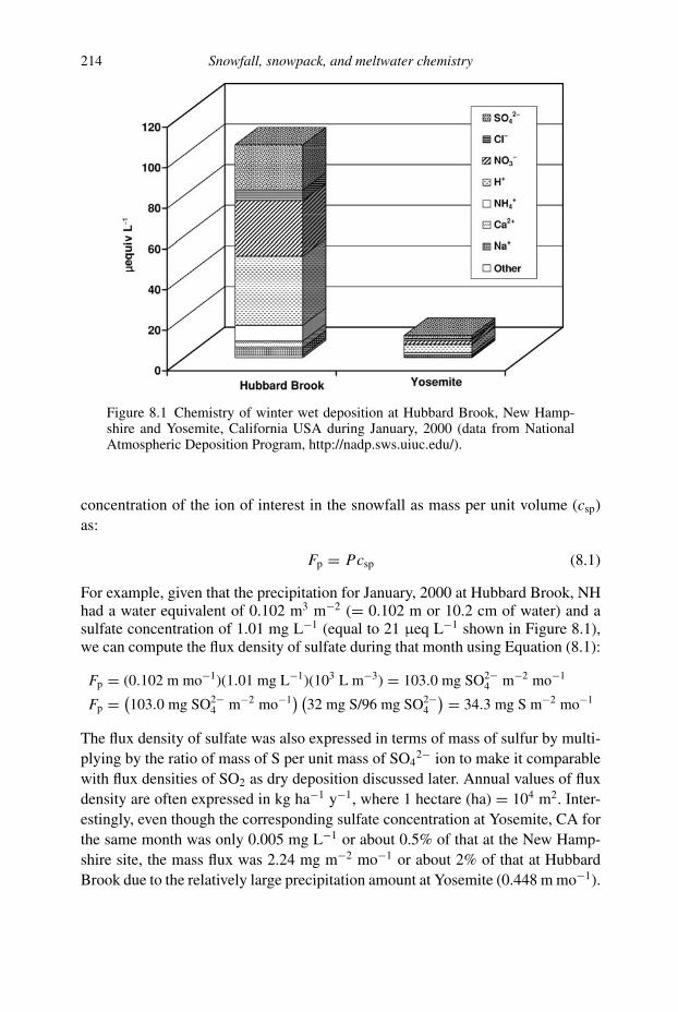
214 Snowfall, snowpack, and meltwater chemistry
Figure 8.1 Chemistry of winter wet deposition at Hubbard Brook, New Hamp-shire and Yosemite, California USA during January, 2000 (data from NationalAtmospheric Deposition Program, http://nadp.sws.uiuc.edu/).
concentration of the ion of interest in the snowfall as mass per unit volume (csp)
as:
Fp = Pcsp (8.1)
For example, given that the precipitation for January, 2000 at Hubbard Brook, NHhad a water equivalent of 0.102 m3 m−2 (= 0.102 m or 10.2 cm of water) and asulfate concentration of 1.01 mg L−1 (equal to 21 μeq L−1 shown in Figure 8.1),we can compute the flux density of sulfate during that month using Equation (8.1):
Fp = (0.102 m mo−1)(1.01 mg L−1)(103 L m−3) = 103.0 mg SO2−4 m−2 mo−1
Fp = (103.0 mg SO2−
4 m−2 mo−1) (
32 mg S/96 mg SO2−4
) = 34.3 mg S m−2 mo−1
The flux density of sulfate was also expressed in terms of mass of sulfur by multi-
plying by the ratio of mass of S per unit mass of SO42− ion to make it comparable
with flux densities of SO2 as dry deposition discussed later. Annual values of flux
density are often expressed in kg ha−1 y−1, where 1 hectare (ha) = 104 m2. Inter-
estingly, even though the corresponding sulfate concentration at Yosemite, CA for
the same month was only 0.005 mg L−1 or about 0.5% of that at the New Hamp-
shire site, the mass flux was 2.24 mg m−2 mo−1 or about 2% of that at Hubbard
Brook due to the relatively large precipitation amount at Yosemite (0.448 m mo−1).

8.3 Dry deposition on snowpacks 215
This comparison shows that concentrations as well as precipitation intensity can be
influential in controlling mass fluxes in precipitation or snowfall at a site.
In order to assess wet-deposition fluxes for a site, it may be possible to find rep-
resentative wet-deposition chemistry data through networks, such as the National
Atmospheric Deposition Program (NADP) Internet site for the United States,
http://nadp.sws.uiuc.edu/. Other monitoring networks and experimental sites exist
that can provide similar data, for example wet deposition data for Canada are avail-
able through the Internet, www.msc-smc.ec.gc.ca/NatChem/.
8.3 Dry deposition on snowpacks
Dry deposition of gases and aerosols on snow surfaces can also significantly affect
chemical inputs to the landscape. Unlike wet deposition that occurs only during
precipitation events, dry deposition occurs continuously. The rate of dry deposition
is controlled by a large number of factors (Davidson and Wu, 1990):
� atmospheric conditions (wind speed, turbulence, stability conditions, etc.)� the nature of the snow surface (roughness, chemistry, terrain features, etc.)� the properties of the depositing gas or aerosol (particle sizes and shapes, aerosol reactivity,
etc.).
Transport of dry deposits to the snow surface occurs in three stages: aerody-
namic transport to the top of the boundary sublayer by turbulent motion, transport
through the quasi-laminar boundary layer by diffusion, impaction, sedimentation
or interception; and finally by direct surface interactions such as dissolution, adhe-
sion, adsorption, or chemical reaction. Dry deposition on porous snowpacks can
also take place below the surface due to natural and forced convection of gases and
aerosols in the snowpack pore space. Any of these three stages can limit or control
the dry deposition rate. To further complicate matters, surface gaseous reactions
are sometimes reversible and/or particulates can rebound and re-suspend in the
turbulent air stream. Blowing surface snow that is sublimated to vapor can also
concentrate substances in the remaining snow or re-suspend gases and aerosols
in the atmosphere. These processes are very complex and readers are referred to
papers by Davidson and Wu (1990), Waddington et al. (1996), Davidson et al.(1996), and Barrie (1985), for more detailed discussions.
Flux density as dry deposition (Fd) can be computed as the product of the con-
centration of the chemical species in the atmosphere (cc) given as mass per unit
volume and the dry-deposition velocity (vd) which has units of length per unit time:
Fd = vdcc (8.2)

216 Snowfall, snowpack, and meltwater chemistry
Table 8.2 Average wintertime atmospheric concentrations and computed drydeposition velocities to the snowpack for several chemical species at a rural
Michigan site (Cadle and Dasch, 1987b)
SpeciesConcentrations(μg m−3)
Dry Deposition Velocity(m s−1 × 10²)
SO2 7.6 0.093 ± 0.093SO4
2− 2.7 0.10a
HNO3 0.69 1.4 ± 1.0NO3
− 1.2 0.10a
NO2 3.8 0.02a
NH4+ 0.78 0.10 ± 0.11
NH3 0.03 1.0a
Ca2+ 0.15 2.1 ± 1.8Mg2+ 0.04 1.5 ± 1.3Na+ 0.10 0.44 ± 0.48K+ 0.08 0.51 ± 0.60
a assumed values, others computed from experimental data
Concentration data are often available from air quality monitoring stations, but
dry-deposition velocities vary for each gaseous or aerosol chemical species and for
the specific atmospheric and surface conditions being considered. Given detailed
site and meteorological data, vd may be computed (Davidson et al., 1996), or
published values for vd tabulated from experimental snow studies can be employed
(see reviews of deposition velocity data by Davidson and Wu, 1990 and DeWalle,
1987).Average wintertime dry-deposition velocities in Table 8.2 from a study in Michi-
gan by Cadle and Dasch (1987b) illustrate typical values for snow surfaces for majorchemical species. Note that the error bars around these vd estimates are quite wide.In general the uncertainty in estimating dry deposition is much larger than for wetdeposition. To illustrate the use of deposition velocities from the study by Cadleand Dasch, using an average atmospheric SO2 concentration of 7.6 μg m−3 and arepresentative deposition velocity from Table 8.2 of about 0.00093 m s−1 gives adry-deposition rate of:
Fd = (7.6 μg SO2 m−3)(0.00093 m s−1)(2.592 × 10⁶ s mo−1)(10−3 mg μg−1)
= 18.3 mg SO2 m−2 mo−1
Fd = (18.3 mg SO2 m−2 mo−1
)(32 mg S/64 mg SO2) = 9.16 mg S m−2 mo−1
Flux density here was converted to units for a 30-day month and also expressed as
mass of S by multiplying by the ratio of mass of S per unit mass of SO2 (32/64) to
be comparable with wet-deposition flux density of S (34.3 mg S m−2 mo−1) in the

8.4 Snowpack chemistry 217
earlier example. Conversions to make flux density of other compounds comparable,
such as the varying forms of N in Table 8.3, are made in similar fashion. Cadle
and Dasch (1987b) estimated that average wintertime dry deposition to snowpacks
at this rural Michigan site supplied as little as 6% of total atmospheric deposition
for H+ to as much as 34% of total atmospheric deposition for Ca2+. However,
contributions of dry deposition at a more polluted urban site were much greater
for some ions (e.g. 80% for Cl−). At remote sites dry deposition will generally be
a minor contributor to snowpack chemistry compared to wet deposition, while in
heavily industrialized and urbanized regions it can be of greater significance.
In the United States there are two networks that provide dry deposition data
for selected sites. The first of these is the Clean Air Status and Trends Network
(CASTNET) with a network of 70 stations operated by the Environmental Protec-
tion Agency. These sites are co-located with NADP wet-deposition sites to assess
the effectiveness of air pollution control efforts on total deposition, www.epa.gov/
castnet/. The other network, known as AIRMoN for Atmospheric Integrated
Monitoring Network, www.arl.noaa.gov/research/projects/airmon dry.html/, is
primarily a research network with 13 stations operated by the National Oceanic
and Atmospheric Administration in cooperation with both CASTNET and NADP.
Both networks provide data in down-loadable files that give measured atmospheric
concentrations, computed vd, and computed dry-deposition fluxes for weekly, sea-
sonal, and annual time periods and several chemical species.
Early studies of atmospheric deposition employed measurement of bulk depo-
sition. Bulk deposition represents the flux of wet deposition and dry deposition in
continuously open buckets or tubs. Dry deposition to an open bucket or tub is not
necessarily equal to that on the surrounding landscape due to bucket aerodynamics
and differences between physical-chemical reactions between plastic bucket and
natural surfaces, but this approach was used to provide a relative index and to
avoid measurement of atmospheric concentrations and meteorological data at a site
needed to more accurately estimate dry deposition. Thus, bulk-deposition measure-
ments are not necessarily directly comparable to the sum of wet plus dry deposition
given by Equations (8.1) and (8.2).
8.4 Snowpack chemistry
Seasonal snowpacks accumulate and lose chemical substances through several
mechanisms summarized in Table 8.3. The major pathways for chemical gains
are new snow and rain events and dry deposition to the snowpack. Chemically dis-
tinct layers or horizons often form in snowpacks from each major wet-deposition
event and these layers often persist with identifiable chemical characteristics until
they come in contact with liquid water from rain or melt. A true loss of chemical
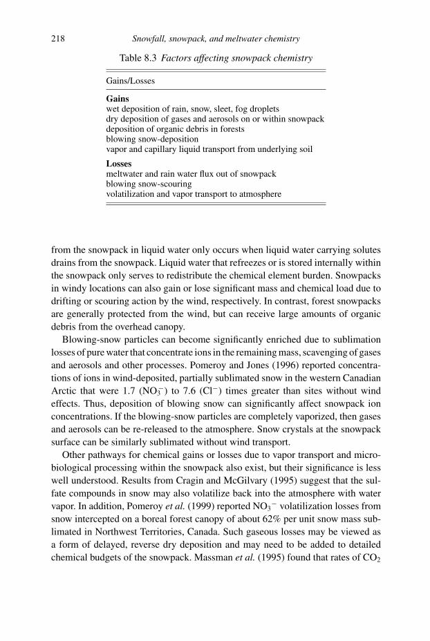
218 Snowfall, snowpack, and meltwater chemistry
Table 8.3 Factors affecting snowpack chemistry
Gains/Losses
Gainswet deposition of rain, snow, sleet, fog dropletsdry deposition of gases and aerosols on or within snowpackdeposition of organic debris in forestsblowing snow-depositionvapor and capillary liquid transport from underlying soil
Lossesmeltwater and rain water flux out of snowpackblowing snow-scouringvolatilization and vapor transport to atmosphere
from the snowpack in liquid water only occurs when liquid water carrying solutes
drains from the snowpack. Liquid water that refreezes or is stored internally within
the snowpack only serves to redistribute the chemical element burden. Snowpacks
in windy locations can also gain or lose significant mass and chemical load due to
drifting or scouring action by the wind, respectively. In contrast, forest snowpacks
are generally protected from the wind, but can receive large amounts of organic
debris from the overhead canopy.
Blowing-snow particles can become significantly enriched due to sublimation
losses of pure water that concentrate ions in the remaining mass, scavenging of gases
and aerosols and other processes. Pomeroy and Jones (1996) reported concentra-
tions of ions in wind-deposited, partially sublimated snow in the western Canadian
Arctic that were 1.7 (NO3−) to 7.6 (Cl−) times greater than sites without wind
effects. Thus, deposition of blowing snow can significantly affect snowpack ion
concentrations. If the blowing-snow particles are completely vaporized, then gases
and aerosols can be re-released to the atmosphere. Snow crystals at the snowpack
surface can be similarly sublimated without wind transport.
Other pathways for chemical gains or losses due to vapor transport and micro-
biological processing within the snowpack also exist, but their significance is less
well understood. Results from Cragin and McGilvary (1995) suggest that the sul-
fate compounds in snow may also volatilize back into the atmosphere with water
vapor. In addition, Pomeroy et al. (1999) reported NO3− volatilization losses from
snow intercepted on a boreal forest canopy of about 62% per unit snow mass sub-
limated in Northwest Territories, Canada. Such gaseous losses may be viewed as
a form of delayed, reverse dry deposition and may need to be added to detailed
chemical budgets of the snowpack. Massman et al. (1995) found that rates of CO2

8.4 Snowpack chemistry 219
Table 8.4 Comparison of snowpack chemistry (μeq L−1) from regions withwidely varying levels of pollution
Ion
Tien Shan Mtns.Northwest China(1)∗
Sierra NevadaMtns., NV and CA,USA(2)
Appalachian Mtns.,PA, USA(3)
Black Snow,Cairngorm Mtns.,Scotland(4)
pH 6.9 5.6 4.3 3.0H+ 0.13 2.5 50 1,000Ca2+ 53 2.5 28 31Mg2+ 5.9 0.8 4 43NH4
+ 13 – 15 17Na+ 9.7 3.9 14 197K+ 1.2 1.0 – 10SO4
2− 16 3.5 42 412NO3
− 5.7 2.1 53 337Cl− 9.9 5.9 9 418
∗Sources: (1) May 1990 survey data, Williams et al., 1992, (2) 4 surveys in 1975, Brownand Skau, 1975, (3) 12 survey averages during 1979–81, DeWalle et al., 1983, (4) February1984 survey, Davies et al., 1984.
movement from soil to atmosphere were augmented, beyond rates of simple molec-
ular diffusion, by “pressure pumping” of snowpack air by the wind. Hogan and
Leggett (1995) showed that vapors from synthetic organic compounds used as trac-
ers in the soil, could be detected in snowpack samples after 3–75 day periods. These
studies of gaseous movement through the snowpack suggest that gases originating
from the soil or within the snowpack could also be transported and affect snowpack
chemistry.
Internal processing of the snowpack chemical load by microbes and animals
can represent either a source (decomposition) or sink (assimilation by organisms)
for dissolved solids (Jones, 1999). Jones (1987) presents evidence that NO3− and
NH4+ are lost from meltwater in forest snowpacks due to assimilation by organisms
such as lichens, algae, bacteria, and fungi associated with organic debris from the
canopy that accumulates in the snowpack. Such losses due to snowpack biota may
be more important for forest snowpacks where a greater supply of organic matter
and associated microflora and fauna is found.
Studies of snowpack chemistry throughout the world illustrate a variety of chem-
ical element concentrations that reflect differences in wet-deposition chemistry due
to atmospheric pollution and other natural factors. Data from studies of two rel-
atively clean and two polluted snowpacks are shown in Table 8.4 to illustrate the
range of conditions that can be encountered. Samples of relatively clean snowpacks
collected in the Tien Shan Mountains in northwest China (Williams et al., 1992)

220 Snowfall, snowpack, and meltwater chemistry
show a basic reaction due to the effects of aeolian dust, suggesting a CaSO4 source
in the soil. Unpolluted snowpacks in the Sierra Nevada Mountains of Nevada and
California show a pH expected due to typical levels of CO2 in the atmosphere
(Brown and Skau, 1975). It is interesting to note that the major cation and anion in
these Sierra samples was Na+ and Cl−, respectively, which suggests an influence
of sea salt. Snowpacks in Pennsylvania (DeWalle et al., 1983) are relatively acidic
(pH = 4.3) with H+ the major cation and SO42− and NO3
− the major anions. The
relatively high Ca2+ concentrations in Pennsylvania snow was attributed to dry
deposition of dust from limestone quarries. Finally, data for a fresh “black snow”
layer in Scotland (Davies et al., 1984) is an extreme example of a polluted snow-
pack with high H+, SO42−, and NO3
−. Both Cl− and Na+ levels are also high in
the black snow likely due to sea salt and industrial sources of chloride, such as coal
combustion.
The load of a chemical compound or ion stored within a snowpack or a snow
layer is often needed to document snowpack chemical conditions at a given time
and place. The load of a specific chemical species (Ws, mass per unit ground area)
is computed as the product of the water equivalent (SWE, depth of liquid water) of
the snow layer and the concentration of the chemical compound or ion in the snow
layer (css, mass per unit volume) as:
Ws = SWE css (8.3)
For example, if the water equivalent of a snowpack or snowpack layer was 0.056
m of liquid water and the nitrate concentration of the snowpack was 3.2 mg L−1,
then the load of nitrate would be:
Ws = (0.056 m)(3.2 mg L−1)(103 L m−3) = 179 mg NO3 m−2
Obviously, computing the load in a snowpack depends upon an accurate mea-
surement of concentration as well as water equivalent. Unfortunately, no routine
nation-wide measurement network for snowpack chemistry exists in the United
States. Snow depth on the ground is measured at selected meteorological stations,
but snow density observations are generally not available. A density of 100 kg
m−3 is often assumed for fresh snow on the ground as a rough approximation, but
the snowpack on the ground will quickly densify due to snowpack metamorphism
thereafter.
One problem with chemical characterizations of snowpacks is that concentra-
tions are measured after the samples have been melted and liquid water has had
some time to interact with particulates and organic debris in the snowpack. Of
course such solids do come into contact with liquid water during melt and rain
for indeterminate lengths of time, but there is no standard way to approximate the
length of contact. Another problem is the extremely high variability of snowpack

8.5 Meltwater chemistry 221
chemistry that causes great difficulty in obtaining representative samples. The best
index to snowpack impacts on chemical cycling in the environment and streamflow
often is to measure the chemistry of the water leaving the snowpack.
8.5 Meltwater chemistry
Meltwater releases from a snowpack also represent a chemical flux density delivered
to the soil surface. The meltwater flux density (Fmw) for a chemical species is
computed (like the wet deposition flux in Equation (8.1)) as:
Fmw = Mcmw (8.4)
where M is the melt water expressed as a liquid volume per unit ground area and per
unit time (m3 m−2 = m) and cmw is the concentration of the species in the meltwater.
Mass fluxes of ions in meltwater can then be compared to mass fluxes in wet
and dry deposition. Concentrations of ions in meltwater, however, are not simply
a reflection of the average snowpack chemistry due to the effects of fractionation
and preferential elution processes to be discussed below. Nakawo et al. (1998) have
also reviewed the effects of these processes on snowpack meltwater chemistry.
8.5.1 Melt fractionation
Impurities in snowpacks are generally located on the surface of ice grains that
allows the early liquid water passing through a snowpack layer to flush out a greater
amount of substances than later liquid water passing through that layer. This process
is referred to as melt fractionation; a term from chemistry that refers to separation
of constituents into parts based upon their different properties, in this case their
solubility and availability on the surface of ice grains. During formation of ice
crystals the bulk of impurities is excluded from the crystal matrix and migrates to
the crystal surface where even at subfreezing temperatures a quasi-liquid layer of
water can be found (Davies et al., 1987). Substances scavenged from the atmosphere
during snowfall also accumulate on the ice crystal surfaces. Once in the snowpack,
metamorphosis of ice grains also tends to cause migration of impurities to the crystal
surface. The end result is that the early flushes of water from a snowpack due to
melt, or rain-on-snow, tends to wash out more of the impurities relative to average
snowpack chemical concentrations than late-season meltwater which is relatively
depleted in impurities. Another type of fractionation, isotope fractionation, also
occurs in the snowpack that is discussed later in Section 8.7.
Johannessen and Hendriksen (1978) were the first to describe the fractionation
process during snowmelt. They showed with both field and controlled laboratory
studies that H+, SO42−, NO3
−, and Pb were present in early meltwater fractions

222 Snowfall, snowpack, and meltwater chemistry
Figure 8.2 Concentration factors for H+, SO42−, and Pb in meltwater illustrat-
ing the effects of fractionation on enrichment of early meltwater releases fromthe snowpack (Johannessen and Henriksen, 1978, C© 1978 American GeophysicalUnion). Concentration factors are given as the ratio of concentration in meltwaterto the average concentration in the initial snowpack.
at concentrations three to six times greater than the overall initial snowpack con-
centration, while late season releases had only a fraction of the concentration of
the initial snowpack. They found that the first 30% of meltwater released from the
snowpack contained 2–2.5 times higher concentrations than the snowpack average
(Figure 8.2). Consequently, streamflow from snowmelt during the initial flush of
acid meltwater can lead to stream acidification and high aluminum concentrations
toxic to fish.
Since this early study, fractionation of snowpack chemicals into the early melt-
water volumes has been studied by many investigators (for example Colbeck, 1981;
Cadle and Dasch, 1987a; Williams and Melack, 1991; Davies et al., 1987; Bales
et al., 1989). Results from Hudson and Golding (1998) show the effects of fraction-
ation on the distribution of snowpack impurities within snowpack layers at a British
Columbia site. Concentrations in the snowpack for several ions were completely
shifted from higher concentrations in the surface layers to higher concentrations in
deeper layers (Figure 8.3) due to fractionation during a relatively brief April 13–15
melt cycle.
Winter climate and the frequency of melt–freeze events helps to control the
magnitude of acidic snowmelt releases. Regions with very cold winters, infrequent
thaws, and deep snowpacks will have fractionation effects isolated in a few large

8.5 Meltwater chemistry 223
0
0.1
0.2
0.3
0.4
0.5
0.6
0 20 40 60 80 100 120
Ion Sum, μeq L−1
Hei
gh
t A
bo
ve G
rou
nd
, m
April 15 Post-melt
April 13 Pre-melt
Figure 8.3 Change in the sum of ion concentrations with height above ground inthe snowpack during a three-day melt sequence in a British Columbia, Canadasnowpack (adapted from Fig 2–3, Hudson and Golding 1998, with permissionof copyright holders, International Water Association Publishing). The sum ofconcentrations represents nitrate, sulfate, chloride, calcium, and sodium concen-trations in the snowpack at the 240 Watershed site.
acidic snowmelt events in spring. Davis et al. (1995) have found that the highest
concentrations in meltwater occur with longer-duration melt events and lower-
melt-rate events that allow more time for washout of impurities and for meltwater
to reach the base of the snowpack. Melt or rain water that gradually refreezes in
deep snowpacks as ripening occurs, will tend to store impurities in ice lenses near
the base of the snowpack until the beginning of melt. In regions with shallower
snowpacks and frequent winter thaws and rainfall, fractionation tends to gradually
reduce snowpack acidity due to frequent liquid-water releases and lessen the severity
of snowmelt events.
The mechanism for water delivery from the snowpack can interact with frac-
tionation effects. Suzuki et al., 1994 showed that meltwater released from the
snowpack during a daily melt cycle came first from meltwater with high NO3−
concentration that was stored in the base of the snowpack from prior days’ melt.
Meltwater release later in the same day came from current melting of surface snow
with a low NO3− concentration. Thus it appeared that the current day’s melt forced
the release of stored water from the snowpack base in a type of translatory flow

224 Snowfall, snowpack, and meltwater chemistry
Figure 8.4 Ionic composition of (a) fresh snow, (b) within-pack snow, and(c) meltwater in the Scottish Highlands showing effects of preferential elution(Tranter et al., 1986, C© 1986 by permission from Elsevier).
process often ascribed to watershed soils and caused the NO3− concentrations in
meltwater to vary diurnally from high to low.
8.5.2 Preferential elution
More recent studies have shown that in addition to fractionation effects, not all
ions are flushed from the snowpack with the same efficiency in the early meltwater
(Davies et al., 1982). The tendency for some ions to be washed out before others is
referred to as preferential elution. Some conflicting results from field and laboratory
experiments occur, but Brimblecombe et al. (1985) suggest the following elution
sequence from high to low mobility in snowpacks:
SO2−4 > NO−
3 > NH+4 > K+ > Ca2+ > Mg2+ > H+ > Na+ > Cl−.
The reasons for preferential elution are not clear, but may be related to the abil-
ity of ions to become incorporated into the ice crystal lattice rather than on the
surfaces of ice grains (Davies et al., 1987). Since the major anions in snow are
generally SO42−, NO3
+, and Cl−, the shifts in snowpack anion chemistry due to
preferential elution can be shown on a triangular diagram as in Figure 8.4 (Tran-
ter et al., 1986). Preferential elution caused fresh snow that had an initial wide
range of anion concentrations (Figure 8.4(a)) to be gradually depleted of SO42−
and NO3− and dominated by Cl− (Figure 8.4(b)). Meltwaters from these snow-
packs were relatively enriched in SO42− and NO3
+ compared to within-pack snow
(Figure 8.4(c)).
The effects of fractionation and preferential elution combined tend to create
more acidic releases of meltwater early in the season. Not only are more impuri-
ties in the snowpack released early in the melt season, but the more acidic anions,
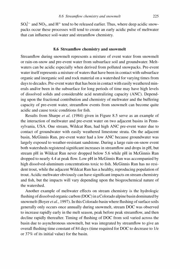
8.6 Streamflow chemistry and snowmelt 225
SO42− and NO3, and H+ tend to be released earlier. Thus, where deep acidic snow-
packs occur these processes will tend to create an early acidic pulse of meltwater
that can influence soil-water and streamflow chemistry.
8.6 Streamflow chemistry and snowmelt
Streamflow during snowmelt represents a mixture of event water from snowmelt
or rain-on-snow and pre-event water from subsurface soil and groundwater. Melt-
waters can be acidic especially when derived from polluted snowpacks. Pre-event
water itself represents a mixture of waters that have been in contact with subsurface
organic and inorganic soil and rock material on a watershed for varying times from
days to decades. Pre-event water that has been in contact with easily weathered min-
erals and/or been in the subsurface for long periods of time may have high levels
of dissolved solids and considerable acid neutralizing capacity (ANC). Depend-
ing upon the fractional contribution and chemistry of meltwater and the buffering
capacity of pre-event water, streamflow events from snowmelt can become quite
acidic and cause toxic conditions for fish.
Results from Sharpe et al. (1984) given in Figure 8.5 serve as an example of
the interaction of meltwater and pre-event water on two adjacent basins in Penn-
sylvania, USA. One stream, Wildcat Run, had high ANC pre-event water due to
contact of groundwater with easily weathered limestone strata. On the adjacent
basin, McGinnis Run, pre-event water had a low ANC because groundwater was
largely exposed to weather-resistant sandstone. During a large rain-on-snow event
both watersheds registered significant increases in streamflow and drops in pH, but
stream pH in Wildcat Run never dropped below 5.6 while pH in McGinnis Run
dropped to nearly 4.4 at peak flow. Low pH in McGinnis Run was accompanied by
high dissolved-aluminum concentrations toxic to fish. McGinnis Run has no resi-
dent trout, while the adjacent Wildcat Run has a healthy, reproducing population of
trout. Acidic meltwater obviously can have significant impacts on stream chemistry
and fish, but the impacts will vary depending upon the biogeochemical nature of
the watershed.
Another example of meltwater effects on stream chemistry is the hydrologic
flushing of dissolved organic carbon (DOC) in a Colorado alpine basin dominated by
snowmelt (Boyer et al., 1997). In this Colorado basin where flushing of surface soils
generally only occurs once annually during snowmelt, stream DOC was observed
to increase rapidly early in the melt season, peak before peak streamflow, and then
decline rapidly thereafter. Timing of flushing of DOC from soil varied across the
basin due to asynchronous snowmelt, but was integrated by streamflow to give an
overall flushing time constant of 84 days (time required for DOC to decrease to 1/e
or 37% of its initial value) for the basin.

226 Snowfall, snowpack, and meltwater chemistry
Figure 8.5 Comparison of stream discharge and pH between two adjacent water-sheds during a major rain-on-snow event in southwestern Pennsylvania during1981 (from Sharpe et al., 1984, C© 1984 by permission from American Societyof Agronomy). Wildcat Run with well-buffered pre-event water showed a muchsmaller pH decline during the event than McGinnis Run with poorly bufferedpre-event water.
The fraction of streamflow due to current melting can be determined using a
simple two-component model and conservative chemical or isotopic tracers:
Qe/Qt = (cstream − cpre-event)/(cevent − cpre-event) (8.5)
where Qe is the streamflow rate due to event water from current melt, Qt is the total
streamflow rate, cstream is the concentration of some tracer in the total streamflow,
cpre-event is the concentration of the tracer in the stream baseflow prior to melt, and
cevent is the concentration in the meltwater or snowpack. An example from work
by Sueker (1995) using Na+ as a tracer in the Rocky Mountains will be used to
illustrate this method. Sueker (1995) found that the Na+ concentration in the bulk
snow on Spruce Creek was about 1.5 μeq L−1 which was used to represent cevent,
while the stream at baseflow was 44.2 μeq L−1 which was used to represent cpre-event.
Spruce Creek at peak streamflow during melt had a Na+ concentration of about 28
μeq L−1, which gave a fraction of event water at peak flow of:
Qe/Qt = (28 − 44.2)/(1.5 − 44.2) = 0.38 or 38%
Stable isotopes 2H and 18O in water preferably should be used as conservative
tracers in computing the fraction of event water during snowmelt (see Rodhe, 1998).
Ideally, meltwater chemistry should be used to index event-water concentrations.
8.7 Snowpack stable isotopes 227
A chemical mass flux density in streamflow can be computed just as for fluxes in
precipitation and meltwater exiting the snowpack. If the streamflow rate (Qt) and
ion concentration (cstream) are known, then the mass flux density in streamflow (Fst)
can be obtained as:
Fst = Qtcstream (8.6)
where Qt is expressed in volume per unit watershed area per unit of time, cstream
is given in mass per unit volume and computations follow previous examples for
Equation (7.1) and (7.4). It is customary to compare the mass flux densities of
ion inputs to watersheds computed with Equation (8.1) and Equation (8.2) with
streamflow export computed with Equation (7.4) and Equation (7.6).
Another major, albeit indirect, impact of snowpacks on the biogeochemistry of
watersheds and streamflow is control of nitrogen processing in the soil (Brooks
and Williams, 1999). The depth and the duration of snowcover can affect soil tem-
peratures and the rates of nitrogen assimilation by soil microbes. Shallow or inter-
mittent snowcover allows surface soils to cool to temperatures below the thresh-
old for soil-heterotrophic microbes that can assimilate nitrogen. Without uptake
by soil heterotrophs, relatively large amounts of nitrogen from decomposition of
organic matter over the winter will be leached and appear in streamflow. In con-
trast, soils protected by deep snow throughout much of the winter season will stay
warm enough to permit heterotroph activity and consequent low nitrogen export to
streamflow. Nitrogen export in streamflow from watersheds in the same region, e.g.
alpine vs. subalpine (Heuer et al., 1999), can vary significantly depending upon
depth and duration of snow cover. In the growing season uptake by plants generally
ties up much of the available nitrogen.
8.7 Snowpack stable isotopes
Isotopes of hydrogen (1H, 2H, 3H) and oxygen (16O, 17O, 18O) in water have played
an increasingly important role as conservative tracers and indicators of snowpack
processes in snow hydrology research in recent years. Tritium (3H) is a radioactive
isotope with a very low abundance which decays with a half-life of 12.26 years.
Other isotopes do not decay or spontaneously disintegrate and are defined as stable
isotopes. Water molecules formed from heavier isotopes of hydrogen and oxygen
(e.g. 1H218O or 2H2
16O) have greater mass than 1H216O molecules that increases the
binding energy and reduces the mobility of the heavier molecules. This can result in
shifts in the relative abundances of heavy and light isotopes, during phase changes
and chemical and biological reactions, referred to as isotope fractionation. A brief
review of stable-isotope geochemistry with applications to snow hydrology is given

228 Snowfall, snowpack, and meltwater chemistry
here. More complete discussions can be found in Kendall and McDonnell (1998,
see especially Chapters 4 and 12), Clark and Fritz (1997), and Stichler (1987).
Abundances of heavier isotopes of hydrogen and oxygen in water molecules
are small but can be measured quite accurately with a mass spectrometer. Natural
hydrogen isotopes in water 1H, 2H (deuterium or D), and 3H (tritium) occur with
relative abundances of about 0.99985, 0.00015, and 10−16 to 10−18, respectively,
while the oxygen isotopes in water 16O, 17O, 18O occur with relative abundances of
about 0.99757, 0.00038, and 0.00205, respectively. Abundance of a heavier stable
isotope relative to a lighter isotope in a water sample (Rx) is generally described
relative to the ratio of the heavier to lighter abundances in a standard (Rs) by:
δ = (Rx/Rs − 1) 1000 (8.7)
where δ or delta is dimensionless and commonly given as per mil or parts per
thousand (‰), Rx is the ratio of numbers of heavier atoms to lighter atoms (e.g.18O/16O) in a sample, and Rs is the same ratio found in a known standard. Vienna
Standard Mean Ocean Water or VSMOW is commonly used as a standard for 2H
or 18O. For example, if a precipitation sample had an abundance ratio of 0.0019650
for 18O/16O based upon analysis with a mass spectrometer and given the VSMOW
reference ratio for 18O/16O was 0.0020052 (Kendall and Caldwell, 1998), then:
δ 18O = [(0.0019650/0.0020052) − 1] 1000 = −20.05 ‰
This indicates that the water sample was depleted in 18O relative to VSMOW by
20.05 ‰ which is equivalent to depletion by 2.005%. Ocean water would have a
relative abundance similar to that of VSMOW and δ 18O≈ 0.
Deuterium δ 2H values in precipitation are related to δ 18O values due to similarity
in fractionation processes for these isotopes as (Craig, 1961):
δ 2H (‰) = 8 δ 18O + 10 (8.8)
This relationship, known as the Global Meteoric Water Line (GMWL), expresses
the average relationship found in freshwaters worldwide and is a useful reference
for comparisons with waters from various climates and geographic locations. In the
above example, the value of δ 2H for the precipitation sample corresponding to the
value of δ 18O given would be −150.4 ‰ according to the GMWL, Equation (8.8).
VSMOW has a deuterium abundance ratio of 0.00015575 (Kendall and Caldwell,
1998).
Due to differences in rates of evaporation–sublimation and melt–freezing among
heavier (1H218O or 2H2
16O) and lighter (1H216O) water molecules, the ratio of
isotopes that appear in liquid, solid, and vapor phases of snowpack water can change

8.7 Snowpack stable isotopes 229
over time and space. Fractionation among the phases of water under equilibrium
conditions gives:
δ 18O ice > δ 18O liquid > δ 18O vapor
and
δ 2H ice > δ 2H liquid > δ 2H vapor.
For example, lighter water molecules 1H216O have a higher surface vapor pres-
sure causing them to evaporate or sublimate (lose mass) more rapidly than heav-
ier 1H218O or 2H2
16O molecules. Consequently, snowpack ice and liquid surfaces
exposed to the atmosphere can become relatively enriched in the heavier 1H218O or
2H216O molecules during vapor loss, while vapor becomes enriched with 1H2
16O
molecules.
Sublimation and vapor migration during crystal metamorphism within and at
the surface of snowpacks can cause isotope fractionation during winter. Cooper
(1998) showed the results of a classic experiment by Sommerfield et al. (1991)
(Figure 8.6) that showed how sublimation under subfreezing conditions could alter
the stable-isotope distribution in a snow column subjected to temperature gradient
metamorphism. Surface as well as deeper snow column layers showed relative
enrichment of heavier 2H (deuterium or D) and 18O isotopes due to fractionation
caused by sublimation and vapor migration after 31 days.
During condensation in the atmosphere, the vapor phase becomes relatively
enriched in 1H216O, while the condensate (precipitation) becomes relatively
enriched in 1H218O or 2H2
16O. Thus atmospheric vapor transported from the oceans
over land becomes gradually depleted in heavier water molecules due to rain and
snowfall occurring along the air-mass trajectory, causing vapor and precipitation
to be progressively lighter or more depleted in 1H218O or 2H2
16O with increas-
ing distance from the ocean. Isotopic fractionation is also more pronounced with
colder temperatures such that this depletion in 1H218O or 2H2
16O in precipitation
is generally more pronounced in winter and at higher elevations and higher lat-
itudes due to temperature. This causes snowfall, snowpack, and meltwater to be
relatively depleted in heavier isotopes compared to summer rainfall, soil water, and
streamflow. Since air masses have varying trajectories over land, varying amounts of
mixing with vapor from terrestrial sources, and differing temperature chronologies,
each precipitation event can therefore be somewhat unique in terms of its stable-
isotope profile. Individual snowfall events can often be detected from their isotope
signatures within the snowpack, but the snowpack isotope profile can also change
and homogenize due to crystal metamorphism, vapor migration, wind drifting and
scour, and rainfall or intermittent melt events.

230 Snowfall, snowpack, and meltwater chemistry
Figure 8.6 Isotopic profiles of δ 2H and δ 18O with depth in a snow column after31 days of temperature gradient metamorphism showing enrichment in surfaceand bottom layers due to fractionation caused by vapor movement and sublima-tion (Cooper, 1998 after Sommerfield et al., 1991, C© 1991 with permission fromElsevier).
Melting also causes fractionation, whereby 1H216O molecules become enriched
in meltwater, while heavier 1H218O molecules become enriched in the residual
snowpack. This fractionation occurs both during melt of surface layers of the snow-
pack and as water percolates downward through the snowpack and contacts deeper
ice layers. Initial meltwater leaving a seasonal snowpack will be relatively depleted
and later melt will be relatively enriched in heavier isotopes. Stable-isotope lev-
els in meltwater leaving the snowpack and travelling through or over the soil to
streams will thus vary during the melt season (Figure 8.7). Taylor et al. (2001)
showed that melt rate can also affect the degree of fractionation, with meltwater
being more depleted in heavier isotopes during periods of lower flow rates from the

8.8 References 231
Figure 8.7 Progressive changes in meltwater δ18O during the melt season at fourUS sites showing depletion in early melt followed by enrichment in later meltrelative to the original snowpack condition (horizontal line) (Taylor et al., 2002,C© 2002 with permission from John Wiley and Sons).
snowpack. Overall the message is clear, when doing hydrograph separations using
stable isotopes (see Equation (8.5)) it is important to sample the meltwater leaving
the snowpack for the period of interest, rather than using an average snowpack
sample to characterize the new water input (Taylor et al., 2002).
8.8 References
Bales, R. C., Davis, R. E., and Stanley, D. A. (1989). Ion elution through shallowhomogeneous snow. Water Resour. Res., 25, 1869–77.
Barrie, L. A. (1985). Atmospheric particles: their physical and chemical characteristics,and deposition processes relevant to the chemical composition of glaciers. AnnalsGlaciol., 7, 100–8.
Boyer, E. W., G. M. Hornberger, K. E. Bencala, and D. M. McKnight. (1997). Responsecharacteristics of DOC flushing in an alpine catchment. Hydrol. Processes, 11,1635–47.
Brimblecombe, P., Tranter, M., Abrahams, P. W., Blackwood, I., Davies, T. D., andVincent, C. E. (1985). Relocation and preferential elution of acidic solute through thesnowpack of a small, remote, high-altitude Scottish catchment. Annals Glaciol., 7,141–47.

232 Snowfall, snowpack, and meltwater chemistry
Brooks, P. D. and Williams, M. W. (1999). Snowpack controls on nitrogen cycling andexport in seasonally snow-covered catchments. Hydrol. Processes, 13(14–15),2177–90.
Brown, J. C. and Skau, C. M. (1975). Chemical composition of snow in the East CentralSierra Nevada. Coop. Rpt. Series, Publ. AG-1, Reno, NV: Renewable NaturalResour. Div., University of Nevada.
Cadle, S. H. and Dasch, J. M. (1987a). Composition of snowmelt and runoff in northernMichigan. Environ. Sci. Technol., 21(3), 295–9.
Cadle, S. H. and Dasch, J. M. (1987b). The contribution of dry deposition to snowpackacidity in Michigan. In Seasonal Snowcovers: Physics, Chemistry, Hydrology, NATOASI Series C: Math. and Phys. Sci., vol. 211, ed. H. G. Jones and W. J.Orville-Thomas, pp. 299–320.
Clark, I. D. and Fritz, P. (1997). Environmental Isotopes in Hydrogeology. Boca Raton,FL: Lewis Publishers.
Colbeck, S. C. (1981). A simulation of the enrichment of atmospheric pollutants in snowcover runoff. Water Resour. Res., 17(5), 1383–8.
Cooper, L. W. (1998). Chapter 4: Isotopic Fractionation in Snow Cover. In Isotope Tracersin Catchment Hydrology, ed. B. V. Kendall and J. J. McDonnell, Amsterdam:Elsevier, pp. 119–36.
Cragin, J. H. and McGilvary, R. (1995). Can inorganic chemical species volatilize fromsnow? In Biogeochemistry of Seasonally Snow-Covered Catchments, IAHS Publ.228, ed. K. A. Tonnessen, M. W. Williams, and M. Tranter. Proc. Boulder Symp.,July 1995, pp. 11–16.
Craig, H. (1961). Isotopic variations in meteoric waters. Science, 133, 1702–3.Davidson, C. I. and Wu, Y. L. (1990). Dry deposition of particles and vapors. In Acidic
Precipitation: Sources, Deposition, and Canopy Interactions, vol. 3, ed. S. E.Lindberg, A. L. Page, and S. A. Norton. New York: Springer-Verlag, pp. 103–216.
Davidson, C. I., Bergin, M. H., and Kuhns, H. D. (1996). The deposition of particles andgases to ice sheets. In Chemical Exchange between the Atmosphere and Polar Snow,NATO ASI Series I, Global Environ. Change, vol. 43, ed. E. W. Wolff and R. C.Bales. Berlin: Springer-Verlag, pp. 275–306.
Davies, T. D., Abrahams, P. W., Tranter, M., Blackwood, I., Brimblecombe, P., andVincent, C. E. (1984). Black acidic snow in the remote Scottish Highlands. Nature,312, 58–61.
Davies, T. D., Brimblecombe, P., Blackwood, I. L., Tranter, M., and Abrahams, P. W.(1988). Chemical composition of snow in the remote Scottish Highlands. In AcidDeposition at High Elevation Sites, NATO ASI Series C, vol. 252, ed. M. H.Unsworth and D. Fowler. Dordrecht: Kluwer Academic, pp. 517–40.
Davies, T. D., Brimblecombe, P., Tranter, M., Tsiouris, S., Vincent, C. E., Abrahams,P. and Blackwood, I. L. (1987). The removal of soluble ions from meltingsnowpacks. In Seasonal Snowcovers: Physics, Chemistry, Hydrology, NATO ASISeries C: Math. and Phys. Sci., vol. 211, ed. H. G. Jones and W. J. Orville-Thomas,pp. 337–92.
Davies, T. D., Vincent, C. E., and Brimblecombe, P. (1982). Preferential elution of strongacids from a Norwegian ice cap. Nature, 300, 161–3.
Davis, R. E., Petersen, C. E., and Bales, R. C. (1995). Ion flux through a shallowsnowpack: effects of initial conditions and melt sequences. In Biogeochemistry ofSeasonally Snow-Covered Catchments., IAHS Publ. 228, ed. K. A. Tonnessen, M. W.Williams, and M. Tranter, pp. 115–28.

8.8 References 233
DeWalle, D. R. (1987). Review of snowpack chemistry studies. In Seasonal Snowcovers:Physics, Chemistry, Hydrology, NATO ASI Series C: Math. and Phys. Sci., vol. 211,ed. H. G. Jones and W. J. Orville-Thomas, pp. 255–68.
DeWalle, D. R., Sharpe, W. E., Izbicki, J. A., and Wirries, D. L. (1983). Acid snowpackchemistry in Pennsylvania, 1979–81. Water Resour. Bull., 19(6), 993–1001.
Heuer, K., Brooks, P. D. and Tonnessen, K. A. (1999). Nitrogen dynamics in two highelevations catchments during spring snowmelt. Hydrol. Processes, 13(14–15),2203–14.
Hogan, A. and Leggett, D. (1995). Soil-to-snow movement of synthetic organiccompounds in natural snowpack. In Biogeochemistry of Seasonally Snow-CoveredCatchments, IAHS Publ. 228, ed. K. A. Tonnessen, M. W. Williams, and M. Tranter,pp. 97–106.
Hudson, R. O. and Golding, D. L. (1998). Snowpack chemistry during snow accumulationand melt in mature subalpine forest and regenerating clear-cut in the southern interiorof B. C. Nordic Hydrol., 29, 221–4.
Johannessen, M. and Henriksen, A. (1978). Chemistry of snow meltwater: changes inconcentration during melting. Water Resour. Res., 14(4), 615–19.
Jones, H. G. (1987). Chemical dynamics of snowcover and snowmelt in a boreal forest. InSeasonal Snowcovers: Physics, Chemistry, Hydrology. NATO ASI Series C: Math.and Phys. Sci., vol. 211, ed. H. G. Jones and W. J. Orville-Thomas, pp. 531–74.
Jones, H. G. (1999). The ecology of snow-covered systems: a brief overview of nutrientcycling and life in the cold. Hydrol. Processes, 13, 2135–47.
Kendall, C. and Caldwell, E. A. (1998). Chapter 2: Fundamentals of IsotopeGeochemistry. In Isotope Tracers in Catchment Hydrology, ed. B. V. Kendall and J. J.McDonnell. Amsterdam: Elsevier, pp. 51–86.
Kendall, C. and McDonnell, J. J. (1998). Isotope Tracers in Catchment Hydrology.Amsterdam: Elsevier.
Massman, W., Sommerfeld, R., Zeller, K., Hehn, T., Hudnell, L., and Rochelle, S. (1995).CO2 flux through a Wyoming seasonal snowpack: diffusional and pressure pumpingeffects. In Biogeochemistry of Seasonally Snow-Covered Catchments, ed. K. A.Tonnessen, M. W. Williams, and M. Tranter. IAHS Publ. 228, pp. 71–80.
Nakawo, M., Hayakawa, N., and Goodrich, L. E. (1998). Chapter 9: Changes in snowpack and melt water chemistry during snowmelt. In Snow and Ice Science inHydrology. International Hydrological Programme, 7th Training Course on SnowHydrology, Nagoya University and UNESCO, pp. 119–32
Pomeroy, J. W. and Jones, H. G. (1996). Wind-blown snow: sublimation, transport andchanges to polar-snow. In Chemical Exchange between the Atmosphere and PolarSnow, NATO ASI Series I, Global Environ. Change, vol. 43, ed. E. W. Wolff andR. C. Bales. Berlin: Springer-Verlag, pp. 453–89.
Pomeroy, J. W., Davies, T. D., Jones, H. G., Marsh, P., Peters, N. E., and Tranter, M.(1999). Transformations of snow chemistry in the boreal forest: accumulation andvolatilization. Hydrol. Processes, 13(14–15), 2257–73.
Raynor, G. S. and Hayes, J. V. (1983). Differential rain and snow scavenging efficiencyimplied by ionic concentration differences in winter precipitation. In PrecipitationScavenging, Dry Deposition, and Resuspension, 4th Intern. Conf Proc. PrecipitationScavenging., vol. 1, US DOE and EPA, Santa Monica, CA, ed. H. R. Pruppacher,R. G. Semonin and W. G. N. Slinn. New York: Elsevier, pp. 249–62.
Rodhe, A. (1998). Chapter 12: Snowmelt-dominated systems. In Isotope Tracers inCatchment Hydrology, ed. Kendall, C. and J. J. McDonnell. Amsterdam: Elsevier,pp. 391–433.

234 Snowfall, snowpack, and meltwater chemistry
Schaefer, D. A. and Reiners, W. A. (1990). Throughfall chemistry and canopy processingmechanisms. In Acidic Precipitation: Sources, Deposition, and Canopy Interactions,vol. 3, ed. S. E. Lindberg, A. L. Page, and S. A. Norton. New York: Springer-Verlag,pp. 241–84.
Sharpe, W. E., DeWalle, D. R., Leibfried, R. T., Dinicola, R. S., Kimmel, W. G., andSherwin, L. S. (1984). Causes of acidification of four streams on Laurel Hill insouthwestern Pennsylvania. J. Environ. Qual., 13(4), 619–31.
Sommerfield, R. A., Judy, C., and Friedman, I. (1991). Isotopic changes during formationof depth hoar in experimental snowpacks. In Stable Isotope Geochemistry: A Tributeto Samuel Epstein, ed. H. P. Taylor, J. R. O’Neil, and I. R. Kaplan. San Antonio, TX:The Geochemical Society, pp. 205–10.
Stichler, W. (1987). Snowcover and snowmelt processes studied by means ofenvironmental isotopes. In Seasonal Snowcovers: Physics, Chemistry, Hydrology.NATO ASI Series C: Math. and Phys. Sci., vol. 211, ed. H. G. Jones and W. J.Orville-Thomas, pp. 673–726.
Stottlemyer, R. and C. A. Troendle. (1995). Surface water chemistry and chemicalbudgets, alpine and subalpine watersheds, Fraser Experimental Forest, Colorado. InBiogeochemistry of Seasonally Snow-Covered Catchments. IAHS Publ. 228, ed.K. A. Tonnessen, M. W. Williams, and M. Tranter, pp. 321–8.
Sueker, J. K. (1995). Chemical hydrograph separation during snowmelt for threeheadwater basins in Rocky Mountain National Park, Colorado. In Biogeochemistry ofSeasonally Snow-Covered Catchments, IAHS Publ. 228, ed. K. A. Tonnessen, M. W.Williams, and M. Tranter, pp. 271–82.
Suzuki, K., Ishii, Y., Kodama, Y., Kobayashi, D., and Jones, H. G. (1994). Chemicaldynamics in a boreal forest snowpack during the snowmelt season. In Snow and IceCovers: Interactions with Atmosphare and Ecosystems, IAHS Publ. 223, ed. H. G.Jones, T. D. Davies, A. Ohmura, and E. M. Morris, pp. 313–22.
Taylor, S., Feng, X., Kirchner, J. W., Osterhuber, R., Klaue, B., and Renshaw, C. E.(2001). Isotopic evolution of a seasonal snowpack and its melt. Water Resour. Res.,37(3), 759–69.
Taylor, S., Feng, X., Williams, M., and McNamara, J. (2002). How isotopic fractionationof snowmelt affects hydrograph separation. Hydrol. Processes, 16, 3683–90.
Tranter, M., Brimblecombe, P., Davies, T. D., Vincent, C. E., Abrahams, P. W., andBlackwood, I. (1986). The composition of snowfall, snowpack and meltwater in theScottish Highlands-evidence for preferential elution. Atmos. Environ., 20(3), 517–25.
Waddington, E. D., Cunningham, J., and Harder, S. (1996). The effects of snowventilation on chemical concentrations. In Chemical Exchange between theAtmosphere and Polar Snow, NATO ASI Series I, Global Environ. Change, vol. 43,ed. E. W. Wolff and R. C. Bales. Berlin: Springer-Verlag, pp. 403–52.
Williams, M. W. and Melack, J. M. (1991). Solute chemistry of snowmelt and runoff in analpine basin, Sierra Nevada. Water Resour. Res., 27(7), 1575–88.
Williams, M. W., Tonnessen, K. A., Melack, J. M., and Daqing, Y. (1992). Sources andspatial variation of the chemical composition of snow in the Tien Shan, China.Annals Glaciol., 16, 25–32.
Figure 1.4 Snow depth map from January 6–8, 1996 associated with the “Blizzardof 1996,” centered over the middle Atlantic United States (after WRC-TV/NBC4, Washington, DC analysis).
Figure 1.5 Transportation department snow blower at work clearing Highway 143between Cedar Breaks and Panguitch, Utah in 2005. (Courtesy R. Julander.)

Figure 1.7 Instrumentation at the Central Sierra Snow Laboratory in Soda Springs,California. (Courtesy R. Osterhuber.)
Figure 1.9 Site of the 239 km2 Reynolds Creek Experimental Watershed in theOwyhee Mountains about 80 km southwest of Boise, Idaho, operated by theAgriculture Research Service. (Courtesy USDA, Agriculture Research Service;www.ars.usda.gov/is/graphics/photos/.)

Mean Total SnowfallCentimeters
A 0.0
B 0.1–7.62
C 7.63–15.24
D 15.25–30.48
E 30.49–60.96
F 60.97–91.44
G 91.45–121.92
H 121.93–182.88
I > 182.89
Data Source: NOAA, National Environmental Satellite, Data and Information Service (NESDIS), National Climatic Data Center
Figure 2.6 Mean annual snowfall in the continental United States (modified fromUSDC, NOAA, National Climate Data Center, Climate Maps of the United States).
Figure 3.13 Flow fingers for preferential liquid-water movement that formed dur-ing initial day’s melting of a homogeneous 28-cm depth snowpack resulting froma single snowfall in Pennsylvania (photo D. R. DeWalle). Water mixed with foodcoloring was uniformly sprayed over the snowpack surface to trace water move-ment. Also note evidence of meltwater movement downslope to the right in thesurface layer and at the soil–snow interface.

Figure 4.9 Colorado SNOTEL sites (courtesy Natural Resources ConservationService, US Department of Agriculture).
Figure 5.3 Operational snow-water-equivalent map for the Canadian Prairies onJanuary 22, 2006 derived from passive-microwave satellite data. Numbers on themap indicate point measurements of observed snow depth. Maps are distributedby posting on the World Wide Web, www.socc.ca/SWE/snow˙swe.html/. (Repro-duced with the permission of the Minister of Public Works and Government Ser-vices Canada, 2006.)
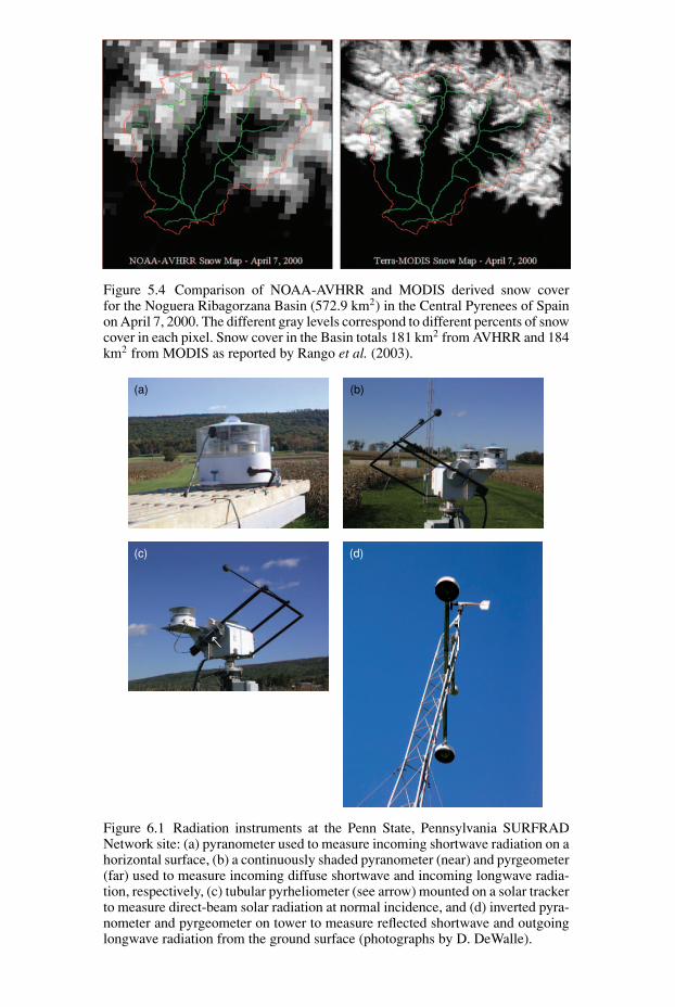
Figure 5.4 Comparison of NOAA-AVHRR and MODIS derived snow coverfor the Noguera Ribagorzana Basin (572.9 km2) in the Central Pyrenees of Spainon April 7, 2000. The different gray levels correspond to different percents of snowcover in each pixel. Snow cover in the Basin totals 181 km2 from AVHRR and 184km2 from MODIS as reported by Rango et al. (2003).
(a)
(c) (d)
(b)
Figure 6.1 Radiation instruments at the Penn State, Pennsylvania SURFRADNetwork site: (a) pyranometer used to measure incoming shortwave radiation on ahorizontal surface, (b) a continuously shaded pyranometer (near) and pyrgeometer(far) used to measure incoming diffuse shortwave and incoming longwave radia-tion, respectively, (c) tubular pyrheliometer (see arrow) mounted on a solar trackerto measure direct-beam solar radiation at normal incidence, and (d) inverted pyra-nometer and pyrgeometer on tower to measure reflected shortwave and outgoinglongwave radiation from the ground surface (photographs by D. DeWalle).

Figure 6.5 Solar-powered climate stations equipped with data loggers (left) areused to provide data (wind speed, air temperature, humidity) to support computa-tions of snowpack convective exchange. The addition to climate stations of sonicanemometers (top right), fine-wire thermocouples, and high-speed open-path gasanalyzers for CO2 and water vapor (bottom right) allows computation of convectiveexchange using the eddy covariance method (photographs by D. DeWalle).
Figure 7.4 Prediction of snowmelt in forests requires accounting for canopy effectson snowpack energy exchange, especially radiation exchange. Shadow patternssuggest varying patterns of canopy shading between coniferous forests with foliage(top) and deciduous forests without foliage (bottom) in these pictures from mid-latitude Pennsylvania, USA sites.

Figure 9.4 Rapid delivery of meltwater as overland flow on frozen ground in apasture swale that has turned the snow into a slush layer.
Figure 12.10 Urban snow requires dedicated areas for snow storage (left) and maylead to accumulation of surface contaminants later in the spring (right) (photos byD. R. DeWalle).

Figure 12.11 Ratnik low-energy modified snow gun (left) and modified fan-typeLenko snow gun (right) being used to augment snowpack for skiing (courtesy ofRatnik Industries, Inc. and Lenko Quality Snow, Inc., respectively).
Figure 12.12 Large slab avalanche in Colorado, USA that began in the alpinestartup zone (photo courtesy of Richard Armstrong, US National Snow and IceData Center, Boulder, CO).

9
Snowmelt-runoff processes
9.1 Introduction
Understanding the generation of streamflow from snowmelt involves integration of
processes that produce meltwater within the snowpack, processes that delay and
store liquid water in the snowpack and processes that direct the flow of meltwater
through watersheds to stream channels. Computations of liquid-water dynamics in
snowpacks and melt rates have been covered in prior chapters. In this chapter these
concepts and computations are synthesized with a discussion of the movement of
meltwater within watersheds and the resulting hydrographs of snowmelt runoff.
Emphasis is given to factors unique to generation of streamflow from snowmelt,
such as frozen-ground effects, rain-on-snow flooding and snow damming.
9.2 Snowpack water balance
The snowpack water balance is fundamental to understanding and modelling
snowmelt runoff generation. The snowpack water balance can be written as:
�SWE = P ± E − O (9.1)
where:
�SWE = (SWEt2 – SWEt1) = change in water equivalent (liquid and solid) of the
snowpack over a time interval t2 – t1P = net precipitation inputs from rainfall, snowfall, and wind redistribution
E = net vapor exchange between the snowpack and environment by sublimation,
evaporation, and condensation
O = outflow of liquid water from the snowpack base
All terms in the Equation (9.1) can be expressed either as a water mass change per
unit area per unit time such as kg m−2 or m depth per unit time. The water-balance
235

236 Snowmelt-runoff processes
model is linked to the snowpack energy-budget model given in Chapter 6 through
the respective outflow (melt), evaporation/sublimation, and precipitation terms.
Outflow of liquid water from a snowpack represents water from melt (M)
and rainfall (Pr) and internal changes in liquid-water holding capacity due to
metamorphosis. During non-rain periods, nearly all outflow is due to melting. Daily
melt rates up to 2 cm d−1 occur frequently and maximum daily rates of 7–8 cm d−1
have been noted (Kuchment, 1997; Cooley and Palmer, 1997). Hourly melt rates
can reach 0.1 to 0.3 cm h−1. Meltwater generated at the surface of the snowpack can
refreeze deeper within unripe snowpacks or be temporally stored as liquid water
within the snowpack by ice layers. Thus the timing of outflow at the snowpack
base can be altered considerably by storage and transmission within the snowpack.
Precipitation inputs to the snowpack in the form of liquid or solid are considered
in the mass balance. Both solid and liquid precipitation may be intercepted in
forest canopies with significant canopy interception losses before being added to
the snowpack (see Chapter 2). Wind transport of snow may also cause scouring or
deposition of snow at a particular site (see Chapter 2). Rain falling on a snowpack
with subfreezing temperatures can be refrozen in transit and through release of latent
heat of fusion can alter the snowpack energy budget (Chapter 6). Rainfall on ripe
snow can move quickly to the soil below and rain-on-snow events are commonly
associated with annual peak flows and flooding for climates where heavy rain can
occur with snowcover.
Net vapor exchange between the snowpack and the atmosphere can repre-
sent a small but significant loss in dry, windy climates. Seasonally, evaporation/
sublimation loss from snowpacks generally represents <10% of maximum snow-
pack water equivalent (Leydecker and Melack, 1999; Cline, 1997), although Aizen
et al. (1995) reported losses of 30% of annual snow accumulation in central Asia.
Sublimation losses from blowing snow can equal 15–45% of winter snowfall in
grassland prairie settings (Marsh, 1999). Schmidt et al. (1998) estimated snowpack
sublimation losses equaled 20% of peak snowpack accumulation or 78 mm over a
40-d period in Colorado subalpine forest. Vapor losses from snowpacks on a daily
basis are generally much smaller than melt, ranging up to about 0.2–0.3 cm d−1
(Leydecker and Melack, 1999). Vapor gains within the snowpack are common when
moist air masses come in contact with cold snowpacks; the process becomes more
important late in the melt season when humidity increases due to evapotranspira-
tion. Vapor is also exchanged between the snowpack and soil when moisture mainly
in the form of vapor, coupled with heat, is forced upward along the temperature
gradient. The importance of this form of vapor exchange has not been completely
assessed but in settings like boreal forests it can be important. Vapor-exchange
computations are described in Chapter 6.
The net change in snowpack water equivalent (SWE) accounts for changes in the
amount of liquid and solid phase water stored in the snowpack over time. Meltwater

9.3 Snowpack storage and time lags 237
or rainfall that freezes within the snowpack, liquid water temporally detained within
the snowpack and snowfall would represent storage gains, while melt and rain water
outflows at the snowpack base and evaporation/sublimation losses at the snowpack
surfaces represent storage losses.
Melt rates for comparisons with energy-budget or degree-day computations are
often computed using a snowpack water balance. By monitoring the changes in
snowpack water equivalent and precipitation over time and assuming no change
in storage of meltwater or rainfall in the snowpack, melt rates can be estimated.
Evaporation/sublimation losses are generally assumed to be negligible for short time
periods with this method. For example, if the water equivalent of a ripe snowpack
changed from 27.9 cm to 26.7 cm over a single 24-h period with no precipitation
inputs and no vapor exchange losses or gains assumed, the outflow and melt rate
for the day would be computed as:
(26.7 − 27.9) cm d−1 = −O
O = M = 1.2 cm d−1
If all of the liquid water due to melting during the period had not drained from the
snowpack or if some of the melt was refrozen due to incomplete snowpack ripeness,
then the final water equivalent would include some refrozen liquid water or liquid
water still in transit. In this case the true melt rate would be underestimated.
The interpretation is more complicated when precipitation occurs during the
time period, because of the added uncertainty in correctly assessing how much
precipitation was rain or snow. Following from the above example, if a precipitation
input of 0.37 cm of rainfall (Pr) and a small vapor loss of 0.04 cm also occurred
during the 24-hour period and all liquid water drained from the snowpack, then the
melt rate would be:
(26.7 − 27.9) cm d−1 = +0.37 − 0.04 − O
O = 1.53 cm d−1 = M + Pr = M + 0.37
M = 1.16 cm d−1
Since measurements of changes in snowpack liquid-water content or the form of
precipitation (rain or snow) are generally lacking, use of the snowpack mass balance
to estimate true melt rates can lead to errors.
9.3 Snowpack storage and time lags
Storage and time lags for liquid water to travel through a snowpack can be due to
refreezing of liquid water in subfreezing snowpacks with a significant cold con-
tent, time required to satisfy snowpack liquid-water holding capacity and, for ripe
snowpacks, the time for transmission of liquid water through the porous matrix

238 Snowmelt-runoff processes
of ice crystals. Each time lag and storage can be simply computed separately and
the times summed to estimate the total delay for liquid water in the snowpack
(US Army Corps of Engineers, 1956). Here we are primarily dealing with vertical
flows in snowpacks, situations where lateral flows commonly occur through snow-
packs such as with snow damming on low-gradient watersheds would require other
analysis and is discussed later in this chapter.
9.3.1 Cold-content lag times
The storage and time lag due to cold content can represent a significant loss of
water and delay to snowpack outflow. As described in Chapter 3, snowpack cold
content (CC) expresses the amount (cm) of liquid water that would have to refreeze
within the snowpack to warm it to 0 ◦C. The units are convenient since the cold
content can be compared directly with the rates of liquid water input from melt
and rain. Liquid water refrozen within the snowpack is lost to current outflow and
represents the first type of snowpack storage. The time lag for melt or rainfall to
satisfy snowpack cold content can be computed as:
tc = CC/(Pr + M) (9.2)
where:
tc = time needed to satisfy snowpack cold content, h
CC = snowpack cold content, cm
Pr = rainfall intensity, cm h−1
M = melt rate, cm h−1
The small amount of sensible heat added by warm rainfall is ignored in the above
calculation (see Chapter 6 for discussion of melting due to rain). Melt rates are
computed using formulas given in Chapter 6. Time lags can be computed for cold
contents that develop over the snow-accumulation season as well as cold contents
that develop overnight.
Given seasonal snowpack cold content of about 0.94 cm of liquid water, repre-
senting a typical mid-winter snowpack with 30 cm water equivalent and average
temperature of −5 ◦C, cold-content lag times can be computed for various liquid-
water input rates. With modest melt rates of about 0.5 cm d−1, the time lag needed
to satisfy this cold content would be:
tc = (0.94 cm)/(0.5 cm/24 h) = 45.1 h = 1.88 d
At a higher melt rate of 2 cm per day, only 11.3 hours would be required to warm
the snowpack. In contrast, modest rainfall plus melt during rainy weather of 1.5 cm
per day would satisfy this cold content in less than four hours. In all cases an actual
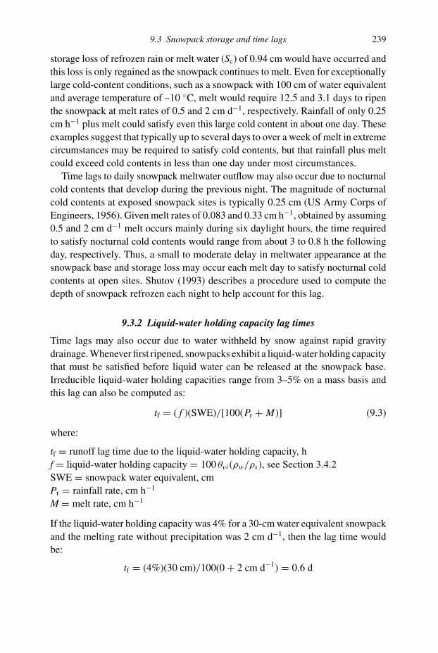
9.3 Snowpack storage and time lags 239
storage loss of refrozen rain or melt water (Sc) of 0.94 cm would have occurred and
this loss is only regained as the snowpack continues to melt. Even for exceptionally
large cold-content conditions, such as a snowpack with 100 cm of water equivalent
and average temperature of –10 ◦C, melt would require 12.5 and 3.1 days to ripen
the snowpack at melt rates of 0.5 and 2 cm d−1, respectively. Rainfall of only 0.25
cm h−1 plus melt could satisfy even this large cold content in about one day. These
examples suggest that typically up to several days to over a week of melt in extreme
circumstances may be required to satisfy cold contents, but that rainfall plus melt
could exceed cold contents in less than one day under most circumstances.
Time lags to daily snowpack meltwater outflow may also occur due to nocturnal
cold contents that develop during the previous night. The magnitude of nocturnal
cold contents at exposed snowpack sites is typically 0.25 cm (US Army Corps of
Engineers, 1956). Given melt rates of 0.083 and 0.33 cm h−1, obtained by assuming
0.5 and 2 cm d−1 melt occurs mainly during six daylight hours, the time required
to satisfy nocturnal cold contents would range from about 3 to 0.8 h the following
day, respectively. Thus, a small to moderate delay in meltwater appearance at the
snowpack base and storage loss may occur each melt day to satisfy nocturnal cold
contents at open sites. Shutov (1993) describes a procedure used to compute the
depth of snowpack refrozen each night to help account for this lag.
9.3.2 Liquid-water holding capacity lag times
Time lags may also occur due to water withheld by snow against rapid gravity
drainage. Whenever first ripened, snowpacks exhibit a liquid-water holding capacity
that must be satisfied before liquid water can be released at the snowpack base.
Irreducible liquid-water holding capacities range from 3–5% on a mass basis and
this lag can also be computed as:
tf = ( f )(SWE)/[100(Pr + M)] (9.3)
where:
tf = runoff lag time due to the liquid-water holding capacity, h
f = liquid-water holding capacity = 100 θvi (ρw/ρs), see Section 3.4.2
SWE = snowpack water equivalent, cm
Pr = rainfall rate, cm h−1
M = melt rate, cm h−1
If the liquid-water holding capacity was 4% for a 30-cm water equivalent snowpack
and the melting rate without precipitation was 2 cm d−1, then the lag time would
be:
tf = (4%)(30 cm)/100(0 + 2 cm d−1) = 0.6 d

240 Snowmelt-runoff processes
Over one-half of the day’s melt would be required to satisfy the liquid-water holding
capacity, before liquid water could be released from the snowpack. The storage loss
in this example would be 4% of 30 cm or 1.2 cm of liquid water (Sl). Water initially
stored is gradually released as the snowpack is melted. Once the water holding
capacity is satisfied, the liquid-water holding capacity only needs to be replenished
if the snowpack is refrozen or if new snowfall is added. Surface snowpack layers
refrozen overnight during formation of nocturnal cold contents or during sudden
extremely cold weather during the melt season exert a new liquid-water holding
capacity. The depth and density of refrozen snowpack layers are needed to compute
additional storage losses, although these losses are likely to be quite small.
9.3.3 Lag times in ripe snow
Once cold content and liquid-water holding capacities are satisfied, the remaining
lag time is the time required for transmission of liquid water from the ripe snowpack
to the ground. The delay for water originating at the surface to exit a ripe snowpack
would simply be:
tt = d/vt (9.4)
where:
tt = time for liquid-water transmission through snowpack, h
d = snowpack depth, cm
vt = transmission rate, cm h−1
The US Army Corps of Engineers (1956) observed transmission rates that varied
from 2 to 60 cm per minute. For a snowpack with a water equivalent of 0.3 m and
a density of 350 kg m−3, the depth would be 0.86 m. If the transmission rate was
10 cm per minute or 6 m per hour, the time lag for water to be transmitted through
the snowpack would be:
tt = (0.86 m)/(6 m h−1) = 0.14 h ∼= 0.01 d
Lag times for transmission in this example are relatively small in comparison to
other time lags, but our ability to predict transmission rates is very uncertain. In many
snowmelt runoff models, time for transmission through ripe snow is not considered.
For example, Zhang et al. (2000) assumed that vertical travel time through snow was
negligible compared to the error in computing the time of lateral downslope in an
Arctic setting. As discussed in Chapter 3, gravity forces generally dominate liquid-
water movement in the snowpack and the permeability of the snowpack changes
over time due to metamorphism. Permeability also increases dramatically with the
snowpack liquid-water content that is controlled by rainfall and melt rates. Thus,
water moves the quickest through the snowpack under the highest liquid-water

9.3 Snowpack storage and time lags 241
contents during active melt and rainfall. At night as the snowpack drains liquid-
water movement is quite slow.
The total time lag due to cold content, liquid-water holding capacity and trans-
mission in the above example calculations is:
tc + tf + tt = 1.88 + 0.60 + 0.01 = 2.49 d (9.5)
The total storage due to cold content and liquid-water holding capacity is 0.94 +1.2 = 2.14 cm, respectively. In this analysis the snowpack is assumed to be homo-
geneous, but occurrence of preferential flow channels that develop in snowpacks
can facilitate rapid drainage of liquid water to the ground before the entire snowpack
is ripened as discussed in Chapter 3.
Anderson (1973) developed an operational scheme to lag and route melt water
through ripe snow in lieu of computations using Equation (9.5). The scheme was
based upon empirical snowmelt lysimeter data and a model with a six-hour compu-
tation interval. Liquid water added to the snowpack during a time interval, in excess
of snowpack liquid-water holding capacity, was initially lagged by an amount that
increased with snowpack water equivalent and decreased with the relative amount
of excess liquid water in the snowpack. Anderson’s (1973) function for lag time is:
LAG = 5.33{1 − exp[(−0.03)(SWE/EXCESS)]} (9.6)
where:
LAG = lag time applied to inputs of liquid water during the current time period, h
SWE = snowpack water equivalent, cm
EXCESS = liquid water in excess of water holding capacity in snowpack, cm/6 h
Lag times for a 30 cm snowpack water equivalent with excess liquid water in
transit of 5 cm (e.g. one good day’s melt) would give the ratio SWE/EXCESS =30/5 = 6 and a lag time of:
LAG = 5.33{1 − exp[(−0.03)(6)]} = 0.88 h
Increasing water equivalent to 100 cm with the same excess liquid content, would
increase the lag time from 0.88 to 2.4 hours. If the water equivalent were 30 cm
and the excess water was 7 cm, then the computed lag would be reduced from 0.88
to 0.64 hours. The maximum lag time for deep snowpacks that could be computed
with Equation (9.6) for conditions of relatively little water in transit would be 5.33
hours.
In Anderson’s (1973) scheme, after the time lag was applied to liquid water
inputs for the current time period, outflow from the snowpack was determined by a

242 Snowmelt-runoff processes
Table 9.1 Example of a lag-and-route procedure used to simulate thetransmission of liquid water in ripe snow. A constant lag time of 1 h and routing
coefficient of 0.6 h−1 was assumed
Time, h. 1 2 3 4 5 6 7 8 9 10 11 12
Input Melt, mm 2 6 12 6 2 0 0 0 0 0 0 0Lagged Input, mm 0 2 6 12 6 2 0 0 0 0 0 0Storage, mm 0 0.8 2.72 5.89 4.76 2.70 1.08 0.43 0.17 0.07 0.03 0.01Outflow, mm 0 1.2 4.08 8.83 7.13 4.05 1.62 0.65 0.26 0.10 0.04 0.02
routing coefficient. The routing coefficient is defined as the fraction of liquid water
in transit (current inflow during the time interval plus liquid left from previous
periods) that leaves the snowpack per unit of time. The routing coefficient can
be computed for a six-hour interval using Anderson’s (1973) function adjusted to
metric units as:
R = {(0.5)[exp(−110)(I/SWE1.3)] + 1}−1 (9.7)
where:
R = routing coefficient, (6 h)−1
I = lagged inflow of liquid water during the current time interval, cm
(6 h)−1
SWE = water equivalent of snowpack, cm
Given a current inflow of 5 cm (6 h)−1 and a water equivalent of 30 cm, following
the above example, the routing coefficient would be:
R = {(0.5)[exp(−110)(5/301.3)] + 1}−1 = {(0.5)[exp(−6.61)] + 1}−1
= 0.999(6 h−1)
For these conditions essentially all of the excess liquid water would drain
from the snowpack during a six-h period. If the current inflow is relatively
small compared to snowpack water equivalent, for example I = 0.05 cm
(6 h)−1 for SWE = 30 cm, then the routing coefficient would reduce to 0.68
(6 h)−1. The minimum value for R using Anderson’s function is 0.667 (6 h)−1.
These computations suggest that routing of liquid water in ripe snow is relatively
rapid and essentially all of a given day’s melt input would drain from a ripe snow-
pack in 24 hours. Simulations for hourly time steps would require greater attention
to meltwater routing.
An example of the lag-and-route procedure for an assumed daily melt wave
in ripe snow is given in Table 9.1. For simplicity, an hourly time step, constant

9.4 Meltwater flow paths 243
Figure 9.1 Diagram showing four major hydrologic flow paths possible for snow-fall and meltwater.
one-hour lag time and a routing coefficient of 0.6 h−1 were assumed. The hourly
surface melt would be computed using an energy budget and the lagged input
mimics this surface input simply delayed by one hour. Zero snowpack water storage
is assumed intially. In the second hour, 0.6 of the hour’s lagged melt of 2 mm
becomes outflow (0.6 × 2 = 1.2 mm) and the remaining fraction (0.4 × 2 = 0.8 mm)
goes into storage as liquid water in transit. In the third hour, outflow equals 0.6 of
the current lagged input of 6 mm plus 0.6 of stored water in transit of 0.8 mm,
giving:
Outflow hour 3 = (0.6)(6) + (0.6)(0.8) = 4.08 mm
Storage in hour three becomes 0.4 of the current lagged input of 6 mm plus the
remaining 0.4 of the prior hour’s storage giving:
Storage hour 3 = (0.4)(6) + (0.4)(0.8) = 2.72 mm
Each successive hour is handled in a similar manner to predict the hydrograph of
outflow from the snowpack. Increases in the routing coefficient reduce the magni-
tude of storage and vice versa.
9.4 Meltwater flow paths
Once snowpack outflows reach the landscape surface, outflows can often be quickly
translated into streamflow due to soil frost, permafrost, or saturated subsurface
depending upon the hydrologic flow paths that are active. Hydrologic flow paths
involved in the generation of streamflow from snowmelt differ from those for
rainfall-generated flows in some respects. Flowpaths can be categorized as: (1)
channel precipitation, (2) overland flow, (3) subsurface stormflow, and (4) ground-
water flow (Figure 9.1) and each will be discussed relative to meltwater delivery.

244 Snowmelt-runoff processes
Channel precipitation is represented by rain and snow that fall directly into the
channel system. Water following this flow path is quickly routed to the basin mouth
and contributes the water in the initial stages of streamflow response to precipi-
tation as long as the stream is not frozen. The volume of water delivered by this
flow pathway is often limited since the fraction of watershed area covered by chan-
nel areas is often quite small (<1% of basin area). However, wetlands associated
with the channel system can also become active during these events and greatly
expand the area available for receiving atmospheric inputs. Since many basins with
hydrology dominated by melt have considerable wetlands, channel precipitation
may be a more important pathway for meltwater than frequently realized. Snow-
fall contributions to flow as channel precipitation are generally separated in time
from basin-wide contributions due to delayed melt. When channels and associated
wetlands are frozen in winter, snowfall is stored on the stream ice until break-up
or melt occurs. In this manner, melt can make significant contributions to flow as
channel precipitation. In windy, low-relief environments, additional redistributed
snow can find its way into the depressions of the drainage network, thus enhancing
early runoff or by causing snow dams delay meltwater delivery downstream.
Overland flow is rain or meltwater delivered to the soil surface at rates in excess
of the soil infiltration rate which subsequently flows over the soil surface to a
channel. Since rates of rainfall commonly exceed snowmelt rates, rainfall poten-
tially can contribute more overland flow than snowmelt. However, snowmelt onto
impermeable, frozen soils can also generate overland flow. Studies by Gibson
et al. (1993) on a wetland basin with permafrost in the Northwest Territories,
Canada and Bengtsson et al. (1992) on an agricultural basin in Finland reported
overland flow of meltwater on frozen soil. The infiltration capacity of undisturbed
soils often exceeds the rates of either rainfall or snowmelt, so that true overland
flow is quite rare on undisturbed basins without soil frost or saturated soils. How-
ever, seasonal frost on watersheds may limit the infiltration capacity if near sur-
face soil pores are ice-rich, thus producing overland flow (Kane and Stein 1983).
On basins with impermeable, paved or compacted surfaces, both rain and melt
can create overland flows (Bengtsson and Westerstrom, 1992; Semadeni-Davies,
1998).
Subsurface stormflow or interflow is defined as water from rainfall or melt that
infiltrates the soil and moves quickly through shallow soil layers to contribute to
streamflow. Infiltrated water can move quickly through shallow soil layers to reach
the channel due to the higher permeability near the soil surface as compared to
deeper subsurface layers (Kendall et al., 1999) and through soil macropores and
natural pipes (Gibson et al., 1993). Bathhurst and Cooley (1996) reported modelling
evidence supporting rapid, near-channel subsurface delivery of meltwater to streams
in Idaho, USA. Infiltrated meltwater can also displace older stored soil water into
the channel through shallow soil layers by a process known as “translatory flow.”

9.4 Meltwater flow paths 245
Figure 9.2 Schematic diagram showing flow paths for melt and shallow subsurfacewater to reach the stream channel during “saturated overland flow” conditions.
Translatory flow is a concept supported by isotope hydrology studies where much
of streamflow during events has isotope levels similar to water stored in the basin
subsurface prior to the event, rather than isotope levels of event water itself. This
suggests that new water infiltrating a basin acted as a piston to force out stored
water or translate older stored water into streamflow.
Older stored water can exfiltrate the soil at seepage faces on the channel banks or
on adjacent lower slopes where the land surface intersects the water table and flows
over the surface to a channel. This type of flow generation is termed “saturated
overland flow” and commonly occurs during snowmelt. Seepage zones represent
saturated soil areas that not only seep water that had already infiltrated the basin,
but also intercept current snowmelt or rainfall and quickly deliver this water as
overland flow to channels. Figure 9.2 illustrates flow conditions during saturated
overland flow where subsurface water and current melt water flow over the surface
in seepage areas to channels. Small rain events or rainfall on relatively dry soils
often do not generate appreciable subsurface stormflow. However, melt usually
occurs for several consecutive days to weeks at a time and produces very wet soils
that lead to larger contributions as subsurface stormflow.
Groundwater flows reach the channel via pressure gradients and gravity through
saturated porous materials intersected by the channel. Infiltrating melt or rain
water recharge the groundwater as evidenced when the elevation of the water table
increases during and after events. Due to reduced permeabilities common in subsur-
face rock and till aquifers, recharged deep groundwater may take months to years
before emerging as streamflow. Prolonged periods of rain or melt cause saturated
conditions and significant groundwater recharge that sustains both the baseflow of
streams and groundwater supplies during summer periods after snowpacks have
entirely melted.
The net effect of flow paths followed by rainfall and meltwater can be deduced
from isotope studies of streamflow events. It is common for melt water or rainfall
(event water) to have a different stable-isotope level than baseflow (pre-event water).

246 Snowmelt-runoff processes
This occurs because isotope levels in each precipitation event vary due to atmo-
spheric temperatures during condensation/evaporation and groundwater flow is a
mixture of many past rain and melt events. Hydrograph separation of streamflow
into event water and pre-event water components can be accomplished using Equa-
tion (8.5) previously introduced in Chapter 8:
Qe/Qt = (cstream − cpre-event)/(cevent − cpre-event)
Using stable isotopes such as 2H and 18O in stream water, the fraction of event water
can be computed for rainfall compared to melt events. Results from a large number
of studies on small relatively undisturbed basins suggest (Buttle, 1994; Rodhe,
1998) that snowmelt events have a greater event water fraction at peakflows than
rainfall events. Such isotope studies indicate the source of the water for streamflow
(event vs. pre-event), not how the water got there but, nevertheless, these studies
allow some speculation about pathways for greater event water contributions for
melt events.
As already implied in the discussion of flow paths, greater event water contri-
butions for melt than rain events would be consistent with a combination of flow
paths such as channel precipitation, overland flow, macropore flow and saturated
overland flow paths. Greater importance of channel precipitation for melt than rain
events could occur early in the melt season on basins with considerable frozen
wetland areas with a stored snowpack on the surface. Snow stored in wetland areas
connected to the main channel could quickly become streamflow during melt. A
greater importance of overland flow for meltwater could also occur because of
frozen soils. Macropore flow leading to direct delivery of meltwater to channels
could be more important due to the very wet soils that accompany prolonged peri-
ods of snowmelt. Finally, greater soil moisture levels during melt may also lead to
greater saturated overland flow. Even though much of the water forced out of the
soil at seepage faces by infiltrating meltwater would likely be stored water from
prior events, the exposed seepage faces create an impermeable surface, like frost,
that causes current melt to become overland flow. The exact causes for greater event
water contributions probably vary in each individual study but, overall, these flow
paths are probably responsible for delivering greater amounts of event meltwater
than rain water to streams during events.
9.5 Frozen ground
Snowpack outflow onto frozen, impermeable ground can result in overland flow,
surface ponding, and storage and in many cases rapid streamflow response. Rapid
delivery of meltwater is a particular problem in arctic basins with permanently
frozen ground or permafrost (Woo, 1986). Prevost et al. (1990) found that the low

9.5 Frozen ground 247
Figure 9.3 Streamflow from snowmelt in 1993 with deep soil frost and 1994 withshallow soil frost on a Vermont agricultural watershed (Shanley and Chalmers,1999 C© 1999 John Wiley & Sons Limited, reproduced with permission).
infiltration capacity of frozen soil caused overland flow and contributed to high
peak streamflows during spring snowmelt at Lac Laflamme in Quebec, Canada.
In an Arctic watershed, McNamara et al. (1997) found from isotope studies that
runoff in spring was primarily (90%) due to event melt water from the snowpack,
but runoff in summer was typically sustained (70%) by older water released from
storage by thawing of the shallow soil layer or active layer above the permafrost.
A soil infiltration index was needed to account for frozen soil effects in models
for accurate peak-streamflow prediction. Prediction of the depth of soil frost and
the infiltration capacity of the frozen ground can be quite important to successful
modelling of streamflow from snowmelt.
One of the more dramatic examples of soil-frost effects on the generation of
streamflow from snowmelt was presented by Shanley and Chalmers (1999) for
a small agricultural watershed (W2) in Vermont, USA (Figure 9.3). In 1993, a
year with deep soil frost, daily streamflow from melt occurred in a series of daily
runoff events each with a very high peak flow rate followed by a return to about
the same relatively low flow rate overnight. At the end of the melt period stream
baseflow rates were about the same as prior to melt. In 1994, a year with shallow
soil frost, each day’s melt event produced smaller peak flows followed by daily

248 Snowmelt-runoff processes
minimum flows that gradually increased during the melt period. By the end of the
melt period in 1994, baseflow levels had increased dramatically and a period of
baseflow recession occurred. These differences suggest that deeper soil frost in
1993 prevented infiltration and caused overland flow that led to rapid streamflow
response to melting during each day, but limited any groundwater recharge that
could sustain stream baseflow during later periods.
The snowpack, by virtue of its excellent insulating properties, plays a dominant
role in the formation and preservation of soil frost despite the many other climatic,
vegetative, topographic, and soil factors of importance to frost formation. Soils
that are unfrozen prior to snowfall, generally will not freeze appreciably during
the winter under snowcover and soils will be maintained in a permeable condition.
Snow depths of about 50 cm are generally considered adequate to protect soils
from freezing as a rule of thumb in the continental United States. In contrast, soils
that are frozen prior to snowfall, either due to seasonal cooling or existence of
permafrost, will generally remain frozen throughout the winter when buried deep
beneath a snowpack. Once melting begins, water at the snowpack base will refreeze
and warm the frost layer to 0 ◦C, much as meltwater refreezes and reduces snowpack
cold contents. Once shallow frost layers are warmed to 0 ◦C by refreezing meltwater,
however, they are protected against further energy gains by the snowpack and can
persist until the snow disappears and thawing begins at the surface. In permafrost
regions, a layer of soil as shallow as 50 cm above the permafrost zone, called the
active layer, thaws and refreezes each year and is primarily responsible for shallow
storage of water that influences hydrology on Arctic basins. Regardless, meltwater
infiltration into frozen soils may be reduced or completely prevented and relatively
rapid flow of liquid water can occur over the soil surface (see Figure 9.4).
Carey and Woo (1998) describe the differences in meltwater delivery between
south slopes with seasonal soil frost and north slopes with a thick surface organic
mat of mosses, sedge, grass, lichens, and peat overlying permafrost in the clayey
till soil. The south slope melted quickly and soil frost did not cause overland flow.
When melt began on the north slope the south slope was free of both snow and frost.
Melting on the north slope resulted in overland flow through the frozen organic layer
and rapid subsurface flow through soil pipes.
Frost depth in watersheds varies with snow depth and many other factors. Snow-
depth variations caused by climatic variations, wind re-distribution of snow, inter-
ception of snow by vegetation (Hardy and Albert, 1995), and soil properties can
all affect the occurrence of soil frost. Climate controls amount of snowfall and the
severity and duration of the freezing period which affect frost formation. Stadler
et al. (1996) also found greater frost penetration and occurrence of overland flow
near tree trunks as opposed to canopy gaps in subalpine spruce forest due to effects
of canopy interception of snow. Apart from snow-depth effects, greater soil freezing
generally also occurs in open terrain where bare mineral soil is exposed, rather than

9.5 Frozen ground 249
Figure 9.4 Rapid delivery of meltwater as overland flow on frozen ground in apasture swale that has turned the snow into a slush layer. See also color plate.
in forests with the protective influence of the overhead canopy (increased longwave
radiation from above and insulating organic matter on the soil), or where a thick
organic mulch or turf exists on the surface. More rapid soil freezing and slower thaw-
ing also occurs on north-facing than south-facing slopes (Zhenniang et al., 1994).
Effects of soil properties on soil freezing are difficult to generalize, sandy soils have
higher thermal conductivity than silt and clay soils for a given soil density and water
content. However, increasing water content of soil, which is also related to texture
and other soil properties, tends to reduce the rate of penetration of soil frost because
the latent heat released when soils freeze must be conducted to the surface before
the freezing front can advance downward into the soil. Overall, all of these factors
make the occurrence and depth of soil frost difficult to understand and predict.
9.5.1 Predicting soil frost depth
Analysis of the effects of frozen ground on snowmelt hydrology must begin with
prediction of the depth of frost penetration at any given time. Heat transfer during
seasonal soil freezing and thawing is very complex and difficult to approximate
using limited climatic data. Basically, heat is lost from the soil to the atmosphere

250 Snowmelt-runoff processes
or overlying snowpack due to the energy balance at the soil surface. Cooling of the
soil surface to freezing temperatures initiates the development of the soil frost layer.
The frost layer grows from the surface downward into the soil as heat is conducted
through the layer of frozen ground to the surface. The thermal conductivity of the
frozen soil layer, which increases with soil density and water content, thus plays
a major role in the rate of frost penetration. Cooling of the soil frost layer is also
dependent upon the volumetric heat capacity of the soil. Soils with greater density
and water content will cool more slowly. The temperature at the base of the growing
soil frost layer is maintained at 0 ◦C as freezing of soil water liberates the latent
heat of fusion. Fusion energy released during freezing must also be conducted to
the surface before the frost layer can grow further.
The situation is complicated further by heat conduction and migration of water
to the base of the frost layer from below due to thermal and pressure gradients.
Liquid water moves upward by pressure gradients and water vapor diffuses upward
along a temperature-induced vapor pressure gradient in the soil pores. Upward
migration of water and freezing at the base of the frost layer often results in a
dry soil layer below and a upper layer enriched with ice that can significantly
impact infiltration and runoff. Also, solute concentrations in soil water also can
cause the migration of water in soil from high to low solute concentrations. Liq-
uid and vapor movement and solute concentrations are generally not considered
in soil frost prediction equations currently available, but Flerchinger and Sax-
ton (1989) developed a physically based numerical model to predict depth of soil
freezing as affected by tillage and crop residues that includes effects of soil water
movement.
One method commonly used for predicting the depth of soil frost is the modified
Berggren equation (Aldrich, 1956, Kersten, 1949). This equation considers heat
conduction in the frozen soil layer and the unfrozen soil layer below, the volumetric
heat capacity of the frozen and unfrozen soil, and the latent heat of the soil per
unit volume. It does not consider the effects of liquid or vapor movement in the
soil. According to the modified Berggren equation, the depth of soil frost can be
computed as:
Zf = λ(48KmN/L)1/2 (9.8)
where:
Zf = frost depth, cm
λ = dimensionless coefficient (see Figure 9.5)
Km = mean thermal conductivity of the frozen and unfrozen soil layers, J m−1
h−1 ◦C−1
N = number of degree days in the freezing or thawing period, ◦C-d
L = latent heat of fusion of water per unit soil volume, J m−3
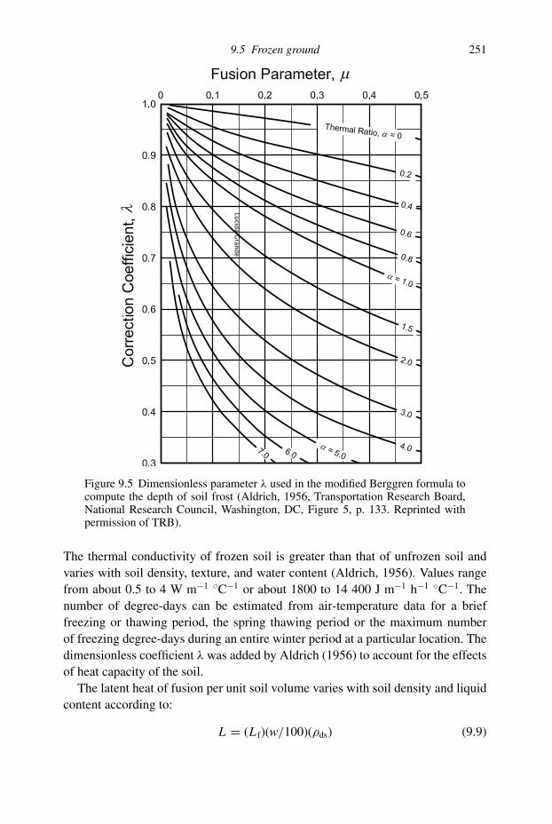
9.5 Frozen ground 251
Lucid
a G
rande
Figure 9.5 Dimensionless parameter λ used in the modified Berggren formula tocompute the depth of soil frost (Aldrich, 1956, Transportation Research Board,National Research Council, Washington, DC, Figure 5, p. 133. Reprinted withpermission of TRB).
The thermal conductivity of frozen soil is greater than that of unfrozen soil and
varies with soil density, texture, and water content (Aldrich, 1956). Values range
from about 0.5 to 4 W m−1 ◦C−1 or about 1800 to 14 400 J m−1 h−1 ◦C−1. The
number of degree-days can be estimated from air-temperature data for a brief
freezing or thawing period, the spring thawing period or the maximum number
of freezing degree-days during an entire winter period at a particular location. The
dimensionless coefficient λ was added by Aldrich (1956) to account for the effects
of heat capacity of the soil.
The latent heat of fusion per unit soil volume varies with soil density and liquid
content according to:
L = (L f)(w/100)(ρds) (9.9)

252 Snowmelt-runoff processes
where:
L = volumetric latent heat of fusion of water in soil, J m−3
Lf = latent heat of fusion of water, 0.334 MJ kg−1 at 0 ◦C, see Appendix A
w = soil water content, % dry wt.
ρds = dry-soil density, kg m−3
The dimensionless coefficient λ can be found in Figure 9.5 as a function of two
other dimensionless parameters (α and μ):
μ = fusion parameter = C(Ts − Tf)/L = C(N/t − Tf)/L (9.10)
where:
C = the mean volumetric heat capacity of the frozen and unfrozen soil layers, J
m−3 K−1
Ts = temperature of frozen soil layer = N/t, ◦C
t = duration of the freezing period, d
Tf = freezing temperature of soil water, 0 ◦C assumed here
The mean soil volumetric heat capacity can be computed as the mean of unfrozen
and frozen soil conditions as:
Cunfrozen = (ρds)(712 + 4188w/100) (9.11)
Cfrozen = (ρds)(712 + 2094w/100) (9.12)
where the constants 712, 4188, and 2094 represent the specific heats for mineral
soil, liquid water, and ice, respectively, in J kg−1 K−1. Since the temperature of
the frozen soil layer (Ts) is generally not known, the number of freezing degree-
days (N) divided by the number of days in the freezing period (t) provides a useful
estimate. Tf could be varied to account for solute effects on the freezing point.
The value of the fusion parameter, μ, is the ratio of the sensible heat loss during
cooling of the frozen soil layer to the latent heat of fusion released during freezing
of soil water. Increasing values of μ reduce the value of λ in Figure 9.5 and thus
reduce the depth of frost penetration, other factors held constant. Conditions where
the soil cooling is relatively great and the heat capacity is relatively large compared
to the latent heat of soil water (e.g. dryer soils) produce such conditions.
A second dimensionless parameter needed to find λ in Figure 9.5 is α where:
α = thermal ratio = (T0 − Tf)/(Ts − Tf)
= for annual periods (Tm − Tf)/(N/t − Tf) (9.13)
where:
T0 = initial temperature of the soil layer, ◦C
Tf = freezing temperature of the soil water, ◦C

9.5 Frozen ground 253
Ts = final temperature of the frozen soil layer, ◦C
Tm = mean annual air temperature, ◦C
As indicated in Figure 9.5, increases in α reduce λ and the predicted depth of frost
penetration. Large values of α occur in climates where cooling of the soil layer from
the annual average temperature and the effects of soil volumetric heat capacity are
relatively large (more temperate climates) compared to the frozen-soil temperature.
An example computation of maximum depth of frost penetration using the mod-
ified Berggren formula (Equation (9.8)) for a region with an average winter N =833 ◦C-days below freezing, a duration of freezing period of t = 130 days, and
a mean annual air temperature Tm = 4.44 ◦C follows. These conditions roughly
correspond to a location in central Maine in the northeastern United States. A ther-
mal conductivity of 4032 J h−1 m−1 ◦C−1 (Km) will be assumed that represents an
average for homogeneous silty soil in the frozen and unfrozen state with a 15%
water content (w) and a dry density of 1500 kg m−3 (ρds) based upon curves given
by Aldrich (1956). The latent heat of fusion for this soil would be:
L = (334000 J kg−1)(15/100)(1500 kg m−3) = 7.52 × 10⁷ J m−3
The volumetric heat capacity for the frozen and unfrozen soil layers would be:
Cunfrozen = (1500 kg m−3)(712 + (4188)(15%)/100) = 2.01 MJ m−3 K−1
Cfrozen = (1, 500 kg m−3)(712 + (2094)(15%)/100) = 1.54 MJ m−3 K−1
giving a mean C of 1.78 MJ m−3 K−1. The freezing temperature of soil water is
assumed to be 0 ◦C. The temperature of the frozen soil layer in degrees below
freezing is approximated as N/t = 6.4 ◦C. The dimensionless parameters needed
to find λ from Figure 9.5 are:
μ = [(1.78 × 10⁶ J m−3 ◦K−1)(6.4 ◦C)/(7.52 × 107 J m−3)] = 0.15
and
α = 4.44/6.4 = 0.69
The value of λ in Figure 9.5 corresponding to these values of α and μ is about 0.85.
The maximum depth of frost penetration would then be:
Zf = (0.85)[48(4, 032 J h−1 m−1 K−1)(833 ◦C-days)/(7.52 × 107 J m−3)]1/2
= 1.24 m = 124 cm
This is the estimated maximum depth of soil frost for a winter season for a bare
mineral soil.
A method is also needed to account for effects of snow cover or surface vegetation
on soil frost penetration. A trial-and-error method given by Aldrich (1956) for
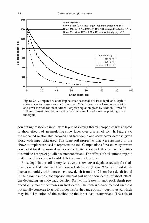
254 Snowmelt-runoff processes
0
20
40
60
80
100
120
140
0 20 40 60 80 100 120 140
Snow depth, cm
So
il fr
ost
dep
th, c
m
Snow w (%) = 2
Snow L (J m−3) = 3.34 x 10⁵ (w/100)(snow density, kg m−3)
Snow C (J m−3K−1) = [712 + 3141(w/100)](snow density, kg m−3 )
Snow Km ( W m−1K −1) = 2.93 x 10⁻⁶ (snow density, kg m−3)2
Snow density 350 kg m−3
250 kg m−3
150 kg m−3
−−
− −
− −
−
−
Figure 9.6 Computed relationship between seasonal soil frost depth and depth ofsnow cover for three snowpack densities. Calculations were based upon a trial-and-error method for the modified Berggren equation given by Aldrich (1956) forsoil and climatic conditions used in the text example and snow properties given inthe figure.
computing frost depth in soil with layers of varying thermal properties was adapted
to show effects of an insulating snow layer over a layer of soil. In Figure 9.6
the modelled relationship between soil frost depth and snow-cover depth is given
along with input data used. The same soil properties that were assumed in the
above example were used to represent the soil. Computations for a snow layer were
conducted for three snow densities and effective snowpack thermal conductivities
to simulate a range of possible winter conditions. The effects of soil surface organic
matter could also be easily added, but are not included here.
Frost depth in the soil is very sensitive to snow-cover depth, especially for shal-
low snowpack depths and low snowpack densities (Figure 9.6). Soil frost depth
decreased rapidly with increasing snow depth from the 124-cm frost depth found
in the above example for exposed mineral soil up to snow depths of about 20–50
cm depending on snowpack density. Further increases in snowpack depth pro-
duced only modest decreases in frost depth. The trial-and-error method used did
not rapidly converge to zero frost depths for the range of snow depths tested which
may be a limitation of the method or the input data assumptions. The rule of

9.5 Frozen ground 255
thumb given previously that 50 cm of snow is needed to avoid soil frost appears
to be approximately correct for low-density snow. DeGaetano et al. (1996) pre-
sented an alternate method for computing depth of frozen ground from readily
available climatic data that also includes effects of varying snow depth. DeGaetano
et al., found that the insulating effect of snow and surface vegetation were impor-
tant parameters controlling frost depth. Whichever method is used to compute the
depth of soil frost, the infiltration capacity of the frozen soil layer must also be
considered.
9.5.2 Infiltration rates and soil frost
Seasonally frozen soils are generally permeable. The infiltration capacity of frozen
soil varies inversely with the pre-melt soil moisture content that controls the ice con-
tent of soil pores upon freezing (Kane and Stein, 1983). Wet soils when frozen gener-
ally have more pore space occupied by ice and less available for infiltration of melt-
water than dry soils. Like the snowpack refreezing of meltwater also occurs in the
soil profile thus producing additional ice and some reduction in the infiltration rate.
Zhao and Gray (1999) proposed the following model for infiltration into frozen
soil based upon numerical simulations and comparisons with field data:
INF = C S2.920 (1 − Sl)
1.64[(273.15 − Tl)/273.15]−0.45 t0.44 (9.14)
where:
INF = cumulative infiltration into frozen soil, mm
C = bulk coefficient
S0 = fractional surface saturation, range 0.7–0.9
Sl = fractional initial soil saturation, range 0.4–0.6
Tl = initial soil temperature, K, range –4 to –8 ◦C
t = elapsed time, h, range 2–24 h
The bulk coefficients varied from C = 1.3 for boreal forest soil and C = 2 for prairie
agricultural soils. In this relationship, cumulative infiltration increases with increas-
ing surface saturation that controls initial capillary pressure gradients into the soil,
increases with decreases in initial soil saturation that controls the amount of poros-
ity occupied by ice, increases with increasing soil temperature that controls the heat
deficit of the frozen soil layer, and increases with increasing time. For example,
the cumulative 24-h amount of infiltration into a boreal forest soil (C = 1.3) at an
initial temperature of –6 ◦C, a surface saturation of 0.9 and initial soil saturation of
0.6 would be:
INF = (1.3)(0.9)2.92(1 − 0.6)1.64[(273.15 − 267.15)/273.15]−0.45(24)0.44
= 4.8 mm = 0.48 cm

256 Snowmelt-runoff processes
This infiltration capacity would not be adequate for daily melts that commonly
exceed 2 cm. Increasing the temperature of the frozen soil layer to −4 ◦C and
reducing the initial soil saturation to 0.4, both of which should increase infiltration
capacity, increases the 24-h total to 1.1 cm which is more than adequate to infiltrate
a day’s melt.
A simplified approach to accounting for soil frost occurrence and permeability
was used by Rekolainen and Posch (1993) in adapting the CREAMS model to
conditions in Finland. A simple degree-day function was used, such that the soil was
considered impermeable due to frost whenever the accumulated freezing degree-
days exceeded 10 ◦C-days in the fall and the soil was considered thawed and
permeable whenever thawing degree-days exceeded 30 ◦C-d in spring. The fall and
spring thresholds were based upon conditions in Finland, but a similar threshold
approach could be adapted to other locales.
9.6 Snow damming
In windy, low-relief basins such as found in the Arctic, snow dams can alter the
timing of meltwater delivery downstream (Woo and Sauriol, 1980; Woo, 1983).
In Arctic basins, streamflow generally will cease completely during winter due
to freezing of the shallow soil active zone above the permafrost. During winter,
redistribution of snow by the wind on these basins will fill topographic depressions
with compacted wind-blown snow with very large cold contents. As melt begins in
the spring these deposits of compacted snow act as dams and can slow downslope
movement of meltwater as they refreeze meltwater from upslope and gradually
ripen. Such deposits of snow often become saturated with meltwater causing slush
flows, tunnels within the snowpack, or surface flow over the saturated snow layers.
In topographic depressions and where large blocks of wind-blown snow fall or
calve into channels, ponding of water by snow dams can also occur. As such dams
fail, streamflow begins in steps and halts. Delays up to several days can occur due
to snow dams and dam failures have been implicated in causing extreme sediment
transfer events (Lewis et al., 2005). Snow damming presents special problems for
modelling the movement of meltwater along slopes through the snow and prediction
of snowmelt runoff in such basins (Hinzman and Kane, 1991).
9.7 Snowmelt hydrographs
Streamflow hydrographs from snowmelt are strongly coupled to the energy supply
for melt. Melting in steep mountain basins generally occurs first at low elevations
and later at high elevations due to differences in air temperature and energy sup-
ply. Elevation may be much less important on low-relief Arctic basins; and some

9.7 Snowmelt hydrographs 257
0
0.05
0.1
0.15
0.2
0.25
0.3
0.35
0.4
10/1/69 11/30/69 1/29/70 3/30/70 5/29/70 7/28/70 9/26/70
1969/1970 water year
Str
eam
flo
w, m
3 s−1
km
−2
Rainfall Dominated
Snowmelt Dominated
−−
Figure 9.7 Contrasting annual streamflow hydrographs for small watersheds withhydrology dominated by rainfall (Waldy Run near Emporium PA, USA) andsnowmelt (Fall Creek near Rustic, CO, USA), http://waterdata.usgs.gov.
Arctic north-flowing river basins begin melting in the headwater regions. Super-
imposed on variations with elevation are melt variations because of varying slope
inclination and aspect. South-facing slopes melt more rapidly than north-facing
slopes. Differences in vegetative cover over basins also affect snowmelt timing.
Many high-elevation mountain basins have snowpacks shaded by forest cover at
low elevations and relatively exposed snowpacks in the alpine at high elevations.
Other basins exhibit forest cover at high elevations and open urbanized and agri-
cultural land at lower elevations. Finally, the duration and depth of snowcover and
existence of permanent snow and ice fields also influence the importance of melt
runoff in overall basin hydrology.
Annual streamflow hydrographs on watersheds where hydrology is dominated by
snowmelt show a distinctive pattern of flow in contrast to basins where hydrology
is dominated by rainfall events. Clear examples at the large watershed scale are
the north-draining Mackenzie River in Canada and the Ob, Yenisey, and Lena
Rivers in Russia where the annual peak is from snowmelt. Basins dominated by
snowmelt such as Fall Creek (9.3 km2) in the Rocky Mountains of Colorado (Figure
9.7) show flow rates that reflect the seasonal availability of energy for melt. Very
low rates of flow occur during the winter snowpack accumulation season, due to

258 Snowmelt-runoff processes
baseflow recession from prior periods of recharge and low rates of melt caused by
ground heat conduction to the snowpack base. In the spring as energy supplies for
melt increase, the flow rates gradually increase and build to a peak annual flow in
late spring or early summer. Seasonal peak flows due to snowmelt occur earlier in
warmer years (Westmacott and Burn, 1997) and higher and later seasonal peaks also
generally occur in years with greater snowfall. Flows decline thereafter with a few
minor perturbations due to occasional rain storms until the following winter at this
Colorado site. Timing and magnitude of annual peaks on a particular watershed tend
to vary from year to year with the sequence of climatic and snowpack conditions.
Watersheds with glaciers in the extreme headwaters also display hydrographs with
extended high flows (Aizen et al., 1995; Moore, 1993) or even double seasonal
peaks due to snowpack melting at lower elevation followed by melt of glacier ice
at higher elevations (Aizen et al., 1996).
On watersheds such as Waldy Run (13.6 km2) in the Appalachian Mountains of
Pennsylvania shown in Figure 9.7, hydrology is dominated by rainfall with some
minor snowmelt and rain-on-snow events possible. Rainfall on this basin is evenly
distributed throughout the year. Flows rise and fall more rapidly during rainfall
events than snowmelt events, with about 12 major events apparent in the year
shown. Peak streamflow rates still commonly occur in early spring due to rainfall
on wet soils and snow, but the peak flows are still primarily due to rainfall. Energy
supply limits the maximum rates of snowmelt compared to rainfall on a given day.
Net energy available for melt of 100 W m−2, which roughly equals average energy
available for open snowpacks in mid-summer in the Sierra Nevadas (see Chapter 6),
would only cause approximately 2.6 cm d−1 of melt. Rainfall can exceed this amount
in an hour for the site in Pennsylvania. On Waldy Run low flows occur during
summer due to high evapotranspiration rates. Annual stream hydrographs shown in
Figure 9.7 were generated by plotting average daily flow rates for each day of the
year; therefore, this approach masks the typical diurnal variation snowmelt runoff.
The timing of daily snowmelt hydrographs also reflects patterns of melt energy
availability with a lag between surface melting and channel flow related to basin
and snowpack conditions. The hydrograph on E. Br. Bear Brook, a small forested
basin with an area about 0.11 km2, shows that streamflow began to rise each morn-
ing before noon and peaked each day in early evening (Figure 9.8). This type of
response is typical of small headwater catchments where streamflow response to
melt energy inputs is relatively rapid. Streamflow response to melt on Kingsbury
Stream and Piscataquis River during the same time period shows the lagged and
damped response to melt due to greater basin size (longer travel distances) and
possibly incomplete snow cover at lower elevations. The peak flows due to melt
on one day actually occur around 0600 hours on the following day on the Pis-
cataquis River. These curves are presented for illustration purposes only, as each

9.7 Snowmelt hydrographs 259
Figure 9.8 Comparison of timing of daily streamflow hydrographs duringsnowmelt on April 21–25, 2001 for three basins with varying area in Maine,http://water.usgs.gov/realtime.html.
watershed has a unique lag time due to varying land use and vegetation cover,
topography, areal extent of snow cover, climatic conditions, etc. However, within
a relatively uniform region, the lag in snowmelt runoff on a given day may be
related to basin area alone. Persson (1976) found that lag times for peak runoff
for basins in the Lapptrasket catchment of Sweden increased with the square root
of basin area. As basin size approaches about 1000 km2 in the United States,
it is common for the daily flow variations due to melt to be masked by human
interventions (discharges, withdrawals, and flow regulation by reservoirs). Caine
(1992) found that daily amplitude of snowmelt runoff decreased and the time of
daily peak flows shifted earlier in the day as the melt season advanced. These
hydrograph changes were related to reduced areal snow cover and snowpack depth
(Caine, 1992). Lundquist et al. (2005) developed a model to predict diurnal cycles
in streamflow due to snowmelt. They found that time lag increased with snow depth,
slope length, and channel length and decreased with channel velocity. The opportu-
nity for more rapid translation of daily melt through permeable, near-surface soils
as the watershed approaches saturation also may be a factor in advancing daily melt
cycles.
Hydrograph separations to determine one day’s contribution to melt have been
conducted to relate melt to causal factors (Figure 9.9; Garstka et al., 1958). Each

260 Snowmelt-runoff processes
Figure 9.9 Graphical hydrograph separation used to determine one day’s meltcontribution (adapted from Garstka et al., 1958, courtesy USDA Forest Service).
day’s contribution can be computed as the sum of two parts: (1) the volume of melt-
water generated during the first 24 hours above the prior day’s baseflow recession
curve, and (2) the volume of meltwater generated due to the difference in flows
between the current day’s and prior day’s baseflow recession integrated to infinity.
Baseflow recession coefficients were fit to prior streamflow data to insure accurate
prediction of recession flows. Negative daily meltwater volumes occurred occa-
sionally. They were due to either re-freezing of meltwater in transit or lack of fit of
the chosen baseflow recession model. Regardless, meltwater volumes determined
in this manner were strongly related to meteorological factors on each day.
A ready source of streamflow data in the United States that shows variations due
to snowmelt is the US Geological Survey water website at http://water.usgs.gov/.
Daily average flow rates for the period of record are available for all gauged streams
in the United States by selecting “Historical Data” and selecting the state of interest.
Updated, “real-time” data for the past week can also be accessed at this site, which
gives flow rate variations generally at 15-minute intervals. Both historical and real-
time data can be acquired on-line in graphical or tabular form. Real-time data are
provisional data that are verified later before becoming part of the historical record.

9.8 Snowmelt and rain-on-snow floods 261
9.8 Snowmelt and rain-on-snow floods
A combination of conditions within watersheds can lead to flooding from snowmelt
or rain-on-snow events. Todhunter (2001) analyzed the 1997 Grand Forks flood
resulting from snowmelt in the Red River of the North which at the time was the
most costly flood on a per capita basis in US history. A combination of wet soils at
the beginning of the winter, concrete frost in the soil, record snowfalls including a
late-season snowfall that delayed melt, a sudden warm period, and channel clogging
by river ice all occurred to produce catastrophic flooding that forced the evacuation
of 75 000 people. The only factor that did not affect flooding during this event was
rainfall, which was thankfully absent.
Peak flows from rain-on-snow (ROS) events can be much greater than peak
flows from snowmelt or rain alone and have also been the cause of severe flooding.
ROS floods are often associated with large sediment and dissolved solids yields,
are sometimes associated with damage to facilities and property and on occasion
cause loss of life. Anderson and Larson (1996) reported on a major ROS event
in northeastern United States in January 1996 that produced the second highest
flow recorded for the Susquehanna River at Wilkes-Barre PA. This ROS flood was
exceeded only by the flood caused by Hurricane Agnes in 1972. ROS peak flows
for the period of record on 17 watersheds in the Sierra Nevada mountains of the
western United States reported by Kattleman et al. (1991) ranged from 0.6 to 3.9 m3
s−1 km−2 and averaged 1.3 m3 s−1 km−2. Although the frequency of occurrence of
severe ROS events in a region is often uncertain, MacDonald and Hoffman (1995)
showed that the majority of peak annual daily flow rates in six basins in northwestern
Montana and northeastern Idado were caused by ROS events. Obviously conditions
leading up to the occurrence of severe ROS events deserve special consideration.
Flooding due to snowmelt and rain-on-snow events appears to be caused by a
combination of circumstances that defy easy prediction. Factors contributing to
these floods are many and not all contribute in all cases, but those identified include
(see Kattleman, 1997):
� relatively widespread, deep snowcover extending to low elevations� heavy rainfall extending to high elevations� warm, windy conditions during rainfall conducive to condensation–convection melt� rainfall occurring in mid-winter� ripening of snowpack or loss of cold content prior to or in early stages of the rain event� wet antecedent soil conditions� occurrence of impermeable soil frost� occurrence of river ice jams that can lead to overbank flooding.
Occurrence of widespread and deep snowcover can lead to prolonged melting
over a large area of the watershed. Any melting that does occur is added to the

262 Snowmelt-runoff processes
rainfall and creates wet soils that lead to increased response from later rainfall
inputs. Since rainy weather is accompanied by cloud cover, melt during rainfall is
primarily driven by convection of latent and sensible heat to the snowpack rather
than radiation. Given the typically high humidity during rainfall, wind speeds and
air temperatures generally determine melting during ROS events. Although sig-
nificant snowpack melting does not always occur along with rainfall, Anderson
and Larson (1996) reported that melt due to warm air, high wind speeds, and high
humidity associated with a near-record ROS event in the Northeast contributed as
much water as the rainfall itself. On mountain basins, where rain events are often
restricted to low elevations where snowcover is uncommon, ROS events that extend
to very high elevations produce the largest ROS events. MacDonald and Hoffman
(1995) found that mid-winter ROS peak flow events produced the greatest peak
flows, but were much less frequent than ROS peak flows during the spring melt
period in the mountains of northeastern Idaho and northwestern Montana. Mid-
winter ROS events were associated with greater rainfall amounts than spring ROS
events and possibly greater areal snow cover. Identification of unique sets of con-
ditions that can lead to major ROS events is essential to forecasting the threat of
ROS flooding.
Forest harvesting has been suggested as a possible cause of increased ROS
flooding. Cutting of trees reduces canopy interception losses for both rain and snow.
Cutting trees also reduces evapotranspiration rates leading to higher soil water levels
and exposes the snowpack to increased wind speeds that can drive convection melt
during rainfall. Available evidence from watershed studies lends support to this
hypothesis (Harr, 1986; Berris and Harr, 1987; Marks et al., 1998). As forests re-
grow, canopy interception losses, evapotranspiration rates, and snowpack protection
from wind all increase. However, at higher elevations and latitudes, re-growth rates
of forests after cutting are low due to shorter, and sometimes climatically severe,
growing seasons. If widespread cutting occurs on a watershed, large areas of the
basin that have not sufficiently re-grown may be predisposed to yield larger peak
flows during ROS events.
9.9 Applications
Hydrologic processes influencing the movement and storage of water through snow-
packs and watersheds to stream channels have been described in this chapter, as
well as the resulting streamflow hydrographs. These concepts and equations form
the basis for modelling streamflow from snowmelt discussed in the next chapter.
The current trend is to model streamflow from snowmelt on a continuous basis on
large heterogeneous watersheds where spatial and temporal variations in control-
ling factors must be considered. Models of the processes and conditions leading

9.10 References 263
up to rain-on-snow floods that cause considerable damage and loss of life are par-
ticularly important. Modelling with these objectives can only be successful with a
good understanding of the behavior of hydrologic systems during melt as discussed
here.
9.10 References
Aizen, V. B., Aizen, E. M., and Melack, J. M. (1995). Climate, snow cover, glaciers, andrunoff in the Tien Shan, Central Asia. Water Resour. Bull., 31(6), 1113–29.
Aizen, V. B., Aizen, E. M., and Melack, J. M. (1996). Precipitation, melt and runoff in thenorthern Tien Shan. J. Hydrol., 186, 229–51.
Aldrich, H. P., Jr. (1956). Frost penetration below highway and airfield pavements.Highway Res. Board, 135, 124–44.
Anderson, E. A. (1973). National Weather Service River Forecast System – SnowAccumulation and Ablation Model. NWS Hydro-17. US Dept. Commerce, NOAA,National Weather Service.
Anderson, E. and Larson, L. (1996). The role of snowmelt in the January 1996 floods inthe Northeastern United States. In Proceedings of the 53rd Annual Meeting, EasternSnow Conf ., pp. 141–9.
Bathurst, J. C. and Cooley, K. R. (1996). Use of SHE hydrological modelling system toinvestigate basin response to snowmelt at Reynolds Creek, Idaho. J. Hydrol., 175,181–211.
Bengtsson, L. and Westerstrom, W. (1992). Urban snowmelt and runoff in northernSweden. Hydrol. Sci., 37, 263–75.
Bengtsson, L., Seuna, P., Lepisto, A., and Saxena, R. K. (1992). Particle movement ofmelt water in a subdrained agricultural basin. J. Hydrol., 135, 383–98.
Berris, S. N. and Harr, R. D. (1987). Comparative snow accumulation and melt duringrainfall in forested and clear-cut plots in the Western Cascades of Oregon. WaterResour. Res., 23(1), 135–42.
Buttle, J. M. (1994). Isotope hydrograph separations and rapid delivery of pre-event waterfrom drainage basins. Prog. Phys. Geog., 18(1), 16–41.
Caine, N. (1992). Modulation of the diurnal streamflow response by the seasonalsnowcover of an alpine basin. J. Hydrol., 137, 245–60.
Carey, S. K. and Woo, M. (1998). Snowmelt hydrology of two subarctic slopes, SouthernYukon, Canada. Nordic Hydrol., 29(4/5), 331–46.
Cline, D. W. (1997). Snow surface energy exchanges and snowmelt at a continental,midlatitude Alpine site. Water Resour. Res., 33(4), 689–701.
Cooley, K. R. and Palmer, P. (1997). Characteristics of snowmelt from NRCS SNOTEL(SNOwTELemetry) sites. Proceedings of the 65th Annual Western Snow Conference,Banff, Alberta, Canada, pp. 1–11.
DeGaetano, A. T., Wilks, D. S., and McKay, M. (1996). A physically based model of soilfreezing in humid climates using air temperature and snow cover data. J. Appl.Meteorol., 35, 1009–27.
Flerchinger, G. N. and Saxton, K. E. (1989). Simultaneous heat and water model of afreezing snow-residue-soil system I. Theory and development. Trans., ASAE, 232(2),565–71.
Garstka, W. U., Love, L. D., Goodell, B. C., and Bertle, F. A. (1958). Factors AffectingSnowmelt and Streamflow: a Report on the 1946–1953 Cooperative Snow

264 Snowmelt-runoff processes
Investigations at the Fraser Experimental Forest, Fraser, Colorado. US Bureau ofReclamation, US Forest Service, US Government Printing Office.
Gibson, J. J., Edwards, T. W. D., and Prowse, T. D. (1993). Runoff generation in a highboreal wetland in northern Canada. Nordic Hydrol., 24, 213–24.
Hardy, J. P. and M. R. Albert. (1995). Snow-induced thermal variations around a singleconifer tree. In Proceedings of the 52nd Eastern Snow Conference, Toronto, Ontario,Canada: June 7–8, 1995, pp. 239–47.
Harr, R. D. (1986). Effects of clearcutting on rain-on-snow runoff in Western Oregon: anew look at old studies. Water Resour. Res., 22(7), 1095–100.
Hinzman, L. D. and D. L. Kane. (1991). Snow hydrology of a headwater Arctic basin 2.Conceptual analysis and computer modeling. Water Resour. Res., 27, 1111–21.
Kane, D. L. and Stein, J. (1983). Water movement into seasonally frozen soils. WaterResour. Res., 19(6), 1547–57.
Kattleman, R. (1997). Flooding from rain-on-snow events in the Sierra Nevada. InDestructive Water: Water-Caused Natural Disasters, their Abatement and Control,Conference Proceedings, IAHS Publ. No. 239, Anaheim, CA, June 1966, pp. 59–65.
Kattleman, R., Berg, N., and McGurk, B. (1991). A history of rain-on-snow floods in theSierra Nevada., In Proceedings of the 59th Western Snow Conference, Juneau, AlaskaApril 13–15, 1991, pp. 138–41.
Kersten, M. (1949). Thermal properties of soils. University of Minnesota, Engin. Exp. Sta.Bulletin, 28.
Kendall, K. A., Shanley, J. B., and McDonnell, J. J. (1999). A hydrometric andgeochemical approach to test the transmissivity feedback hypothesis duringsnowmelt. J. Hydrol., 219, 188–205.
Kuchment, L. S. (1997). Estimating the risk of rainfall and snowmelt disastrous floodsusing physically-based models of river runoff generation. In Destructive Water:Water Caused Natural Disasters, Their Abatement and Control, ConferenceProceedings, IAHS Publ. 239, Anaheim, CA, pp. 95–100.
Leydecker, A. and Melack, J. M. (1999). Evaporation from snow in the Central SierraNevada of California. Nordic Hydrol., 30(2), 81–108.
Lewis, T., C. Braun, D. R. Hardy, P. Francus, and R. S. Bradley. (2005). An extremesediment transfer event in a Candadian high Arctic stream. Arct., Antarct. Alp. Res.,37, 477–82.
Lundquist, J. D., Dettinger, M. D. and Cayan, D. R. (2005). Snow-fed streamflow timingat different basin scales: Case study of the Tuolumne River above Hetch Hetchy,Yosemite, California. Water Resour. Res., 41(W07005), 1–14.
MacDonald, L. H. and Hoffman, J. A. (1995). Causes of peak flows in NorthwesternMontana and Northeastern Idaho. Water Resour. Bull., 31(l), 79–95.
Marks, D., Kimball, J., Tingey, D., and Link, T. (1998). The sensitivity of snowmeltprocesses to climate conditions and forest cover during rain-on-snow: a case study ofthe 1996 Pacific Northwest flood. Hydrol. Processes, 12, 1569–87.
Marsh, P. (1999). Snowcover formation and melt: recent advances and future prospects.Hydrol. Processes, 13, 2117–34.
McNamara, J. P., D. L. Kane and L. D. Hinzman. (1997). Hydrograph separation in anArctic watershed using mixing model and graphical techniques. Water Resour. Res.,33, 1707–19.
Moore, R. D. (1993). Application of a conceptual streamflow model in a glacierizeddrainage basin. J. Hydrol., 150, 151–68.
Persson, M. (1976). Hydrologiska undersokningar i Lapptraskets representativa omrade(In Swedish, English title: Hydrological Studies in the Lapptrasket Representative

9.10 References 265
Catchment), SMHI HB Rapport no. 13, Norrkoping, Sweden: Swedish Meteorol. andHydrol. Instit.
Prevost, M., Barry, R., Stein, J., and Plamondon, A. P. (1990). Snowmelt runoff modellingin a balsam fir forest with a variable source area simulator (VSAS2). Water Resour.Res., 26(5), 1067–77.
Rekolainen, S. and Posch, M. (1993). Adapting the CREAMS model for Finnishconditions. Nordic Hydrol., 24, 309–22.
Rodhe, A. (1998). Chapter 12: Snowmelt dominated systems. In Isotope Tracers inCatchment Hydrology, ed. B. V. C. Kendall and J. J. McDonnell, Amsterdam:Elsevier, pp. 391–433.
Semadeni-Davies, A. (1998). Modelling snowmelt induced waste water inflows. NordicHydrol., 29(4/5), 285–302.
Schmidt, R. A., C. A. Troendle, and J. R. Meiman. (1998). Sublimation of snowpacks insubalpine conifer forests. Can. J. For. Res., 28, 501–13.
Shanley, J. B. and Chalmers, A. (1999). The effect of frozen soil on snowmelt runoff atSleepers River, Vermont. Hydrol. Processes, 13, 1843–57.
Shutov, V. A. (1993). Calculation of snowmelt. Russian Meteorol. and Hydrol., 4, 14–20.Stadler, D., Wunderli, H., Auckenthaler, A., Fluhler, H., and Brundl, M. (1996).
Measurement of frost-induced snowmelt runoff in a forest soil. Hydrol. Process., 10,1293–1304.
Todhunter, P. E. (2001). A hydroclimatological analysis of the Red River of the Northsnowmelt flood catastrophe of 1997. J. Amer. Water Resour. Assoc., 37, 1263–78.
US Army Corps of Engineers (1956). Snow Hydrology: Summary Report of the SnowInvestigations. Portland, OR: North Pacific Div., US Army Corps of Engineers.
Westmacott, J. R. and Burn, D. H. (1997). Climate change effects on the hydrologicregime within the Churchill-Nelson River Basin. J. Hydrol., 202, 263–79.
Woo, M.-K. (1986). Permafrost hydrology in North America. Atmos. Ocean, 24(3),201–234.
Woo, M.-K. (1983). Hydrology of a drainage basin in the Canadian high Arctic. AnnalsAssoc. Amer. Geogr., 73, 577–596.
Woo, M.-K. and J. Sauriol. (1980). Channel development in snow-filled valleys, Resolute,N. W. T., Canada. Geogr. Ann., 62A, 37–56.
Zhang, Z., D. L. Kane, and L. D. Hinzman. (2000). Development and application of aspatially-distributed Arctic hydrological and thermal process model (ARHYTHM).Hydrol. Processes, 14, 1017–44.
Zhao, L. and Gray, D. M. (1999). Estimating snowmelt infiltration into frozen soils.Hydrol. Processes, 13, 1827–42.
Zhenniang, Y., Fungzian, L., Zhihuai, Y., and Qiang, W. (1994). The effect of water andheat on hydrological processes of a high alpine permafrost area. In Snow and IceCovers: Interactions with the Atmosphere and Ecosystems, IAHS Publ. 223, ed. E. G.Jones, T. D. Davies, A. Ohmura, and E. M. Morris, pp. 259–68.

10
Modelling snowmelt runoff
10.1 Introduction
Hydrologic models used to predict streamflow can be generally classified as either
deterministic or stochastic and as either lumped-parameter or distributed (Beven,
2000). Deterministic models predict a single value of streamflow from a given set
of input variables, while stochastic models predict a range of possible outcomes
based upon the statistical distributions of input variables. Nearly all of the snowmelt
models used to continuously predict streamflow from snowmelt are deterministic,
but a type of statistical model has been historically used to great advantage to predict
seasonal totals of streamflow using measured snowpack and precipitation data each
spring. These models are in widespread use in the western United States to forecast
spring runoff.
Deterministic models can be further categorized as either lumped-parameter or
distributed. Lumped-parameter models consider the entire watershed as a homo-
geneous unit, while distributed models break the watershed into subunits or grid
points based upon a variety of criteria. Early snowmelt models were of the lumped-
parameter type, but many distributed-snowmelt modelling studies have been con-
ducted in the past decade. In terms of snowmelt prediction, the lumped-parameter
type of model assumes that the snow cover and melt rates are uniform across the
entire basin. These so called point-snowmelt models are still in use today and are
generally found imbedded in most deterministic, distributed models. Distributed-
snowmelt models generally adapt simple point-snowmelt models for conditions
that vary from point to point across basins. Conditions such as varying topography
(slope, aspect, and elevation), wind redistribution and sublimation of snow, vegeta-
tive cover (forest cover and type), and soil freezing conditions can all be included
in distributed models.
All models also have characteristic temporal and spatial scales that can be used
to classify them (Bengtsson and Singh, 2000). Statistical snowmelt models can be
266

10.2 Statistical snowmelt-runoff models 267
used to predict streamflow totals for entire runoff seasons, while deterministic melt
models considering hydrologic processes may operate on time steps as short as one
hour. Due to data limitations and the nature of the snowmelt-runoff process, daily
time steps are often used for snowmelt models for prediction of spring snowmelt
runoff. Spatial scales can range from treating the entire watershed as a single homo-
geneous unit down to dividing the watershed into a number of separate grid points
or nodes. Vertical spatial scales also become relevant for snowmelt modelling since
the snowpack can be modelled as a set of layers of varying properties that interact
with themselves, the atmosphere above and soil below. Overall, each model will be
developed with a spatial and temporal scale needed to achieve a specific objective,
but ultimately many are constrained by availability of data and our knowledge of
the processes involved.
Deterministic models used to continuously predict streamflow often explicitly
consider the many hydrologic processes that control the generation of streamflow
from precipitation. Although the level of detail considered in each model varies
considerably, the hydrologic processes that can be considered are (DeVries and
Hromadka, 1992): canopy interception, evapotranspiration, snowmelt, interflow,
overland flow channel flow, unsaturated subsurface flow, and saturated subsurface
flow. In this context snowmelt is seen as just one component of complex models
that often involve many uncertain parameters in addition to those related to snow.
Independent estimates of snowmelt parameters from those needed for simulating
the rest of the hydrologic system is obviously a good idea.
This chapter begins with a review of statistical models used to forecast streamflow
totals rather than prediction of continuously varying streamflow. Point-snowmelt
models that predict the release of melt water from the snowpack to the soil are next
described in detail. A general discussion of distributed-snowmelt-runoff modelling
will follow. The chapter concludes with a brief summary of the models currently in
use to predict streamflow from snowmelt. As in the prior chapters, emphasis will be
on aspects of hydrologic modelling unique or important to snow hydrology. Others
sources (Maidment, 1992; US Army Corps of Engineers, 1956; Beven, 2000) can
be consulted for a more complete and general discussion of hydrologic modelling.
10.2 Statistical snowmelt-runoff models
Statistical methods have traditionally been used to estimate or forecast seasonal
runoff volumes from snowmelt. These models rely upon statistical relationships
between measured variables and can not be expected to predict runoff for unusual
conditions not previously experienced. Ability to predict flows under unusual or
extreme conditions is the commonly used justification for deterministic, physically
based process models. As long as all the physical processes are well represented,
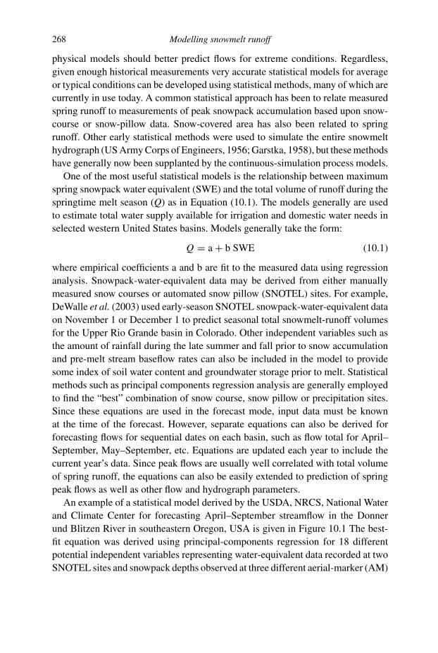
268 Modelling snowmelt runoff
physical models should better predict flows for extreme conditions. Regardless,
given enough historical measurements very accurate statistical models for average
or typical conditions can be developed using statistical methods, many of which are
currently in use today. A common statistical approach has been to relate measured
spring runoff to measurements of peak snowpack accumulation based upon snow-
course or snow-pillow data. Snow-covered area has also been related to spring
runoff. Other early statistical methods were used to simulate the entire snowmelt
hydrograph (US Army Corps of Engineers, 1956; Garstka, 1958), but these methods
have generally now been supplanted by the continuous-simulation process models.
One of the most useful statistical models is the relationship between maximum
spring snowpack water equivalent (SWE) and the total volume of runoff during the
springtime melt season (Q) as in Equation (10.1). The models generally are used
to estimate total water supply available for irrigation and domestic water needs in
selected western United States basins. Models generally take the form:
Q = a + b SWE (10.1)
where empirical coefficients a and b are fit to the measured data using regression
analysis. Snowpack-water-equivalent data may be derived from either manually
measured snow courses or automated snow pillow (SNOTEL) sites. For example,
DeWalle et al. (2003) used early-season SNOTEL snowpack-water-equivalent data
on November 1 or December 1 to predict seasonal total snowmelt-runoff volumes
for the Upper Rio Grande basin in Colorado. Other independent variables such as
the amount of rainfall during the late summer and fall prior to snow accumulation
and pre-melt stream baseflow rates can also be included in the model to provide
some index of soil water content and groundwater storage prior to melt. Statistical
methods such as principal components regression analysis are generally employed
to find the “best” combination of snow course, snow pillow or precipitation sites.
Since these equations are used in the forecast mode, input data must be known
at the time of the forecast. However, separate equations can also be derived for
forecasting flows for sequential dates on each basin, such as flow total for April–
September, May–September, etc. Equations are updated each year to include the
current year’s data. Since peak flows are usually well correlated with total volume
of spring runoff, the equations can also be easily extended to prediction of spring
peak flows as well as other flow and hydrograph parameters.
An example of a statistical model derived by the USDA, NRCS, National Water
and Climate Center for forecasting April–September streamflow in the Donner
und Blitzen River in southeastern Oregon, USA is given in Figure 10.1 The best-
fit equation was derived using principal-components regression for 18 different
potential independent variables representing water-equivalent data recorded at two
SNOTEL sites and snowpack depths observed at three different aerial-marker (AM)
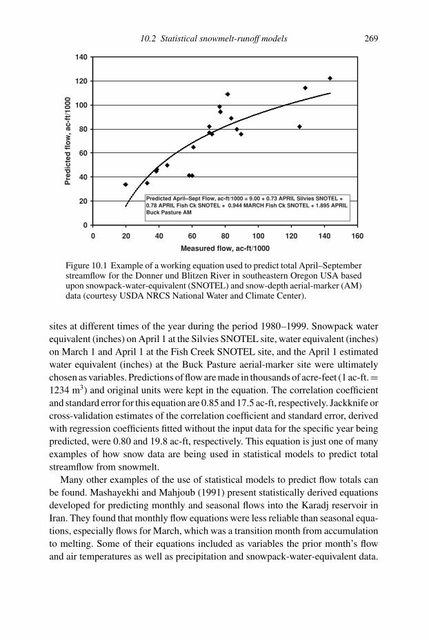
10.2 Statistical snowmelt-runoff models 269
0
20
40
60
80
100
120
140
0 20 40 60 80 100 120 140 160
Measured flow, ac-ft/1000
Pre
dic
ted
flo
w, a
c-ft
/100
0
Predicted April–Sept Flow, ac-ft/1000 = 9.00 + 0.73 APRIL Silvies SNOTEL + 0.78 APRIL Fish Ck SNOTEL + 0.944 MARCH Fish Ck SNOTEL + 1.895 APRIL Buck Pasture AM
Figure 10.1 Example of a working equation used to predict total April–Septemberstreamflow for the Donner und Blitzen River in southeastern Oregon USA basedupon snowpack-water-equivalent (SNOTEL) and snow-depth aerial-marker (AM)data (courtesy USDA NRCS National Water and Climate Center).
sites at different times of the year during the period 1980–1999. Snowpack water
equivalent (inches) on April 1 at the Silvies SNOTEL site, water equivalent (inches)
on March 1 and April 1 at the Fish Creek SNOTEL site, and the April 1 estimated
water equivalent (inches) at the Buck Pasture aerial-marker site were ultimately
chosen as variables. Predictions of flow are made in thousands of acre-feet (1 ac-ft.=1234 m3) and original units were kept in the equation. The correlation coefficient
and standard error for this equation are 0.85 and 17.5 ac-ft, respectively. Jackknife or
cross-validation estimates of the correlation coefficient and standard error, derived
with regression coefficients fitted without the input data for the specific year being
predicted, were 0.80 and 19.8 ac-ft, respectively. This equation is just one of many
examples of how snow data are being used in statistical models to predict total
streamflow from snowmelt.
Many other examples of the use of statistical models to predict flow totals can
be found. Mashayekhi and Mahjoub (1991) present statistically derived equations
developed for predicting monthly and seasonal flows into the Karadj reservoir in
Iran. They found that monthly flow equations were less reliable than seasonal equa-
tions, especially flows for March, which was a transition month from accumulation
to melting. Some of their equations included as variables the prior month’s flow
and air temperatures as well as precipitation and snowpack-water-equivalent data.

270 Modelling snowmelt runoff
0
20
40
60
80
100
0 20 40 60 80 100
Percentage of measured spring runoff
Sn
ow
co
vere
d a
rea,
%
Lexen Ck.
Deadhorse Ck.
E. St. Louis Ck.
Figure 10.2 Relationship between snow-covered area and the percentage of accu-mulated spring runoff on three Rocky Mountain subalpine watersheds in Colorado(see text example, modified after Leaf, 1969, courtesy of the US Western SnowConference).
Seasonal forecasts were made with an error of about 15%. Thapa (1993) used
a regression of March snow-covered area from satellite remote sensing against
streamflow volumes to estimate pre-monsoon streamflow amounts for several basins
in the Himalayas where other forms of data were lacking.
Another statistical approach for snowmelt prediction is the use of standard curves
relating snow-covered area on a watershed to the fraction of total runoff occurring
during the spring melt period. Characteristic curves fit using regression analysis to
snow cover and flow data can be derived on a watershed as illustrated in Figure 10.2
for three basins in the Colorado Rocky Mountains (Leaf, 1969; Leaf and Haeffner,
1971). Such curves are quite consistent from year to year on a given watershed and
each basin has its own characteristic curve. Note the differences in curves between
Deadhorse Creek and the other two basins in Figure 10.2, East St. Louis Creek
and Lexen Creek. Whenever an estimate of snow-covered area is available during
the melt season, these curves can be used to estimate the volume of remaining
snowmelt runoff.
An example taken from Leaf (1969) for E. St. Louis Creek helps to illustrate
the use of these curves (Figure 10.2). The snow-covered area on the watershed in

10.3 Point-snowmelt models 271
mid-June was estimated from photographs as 41% of basin area at a time when the
total spring runoff based upon measured streamflow had been about 738 000 m3 (598
acre-ft). Since this snow-covered area normally occurs when 37% of spring runoff
has occurred according to the curve in Figure 10.2, the expected volume for the
remainder of the melt season would be 738 000/0.37 ∼= 1 995 000 m3 (1616 acre-ft).
This type of relationship provides information about the timing of streamflow in
addition to estimates of remaining flow volumes and provides a means for updating
forecasts during the melt season. As snow-covered-area data from satellite remote
sensing are now available for most basins at regular time intervals (see Chapter 5),
use of this method could easily be increased in the future. When more frequent
estimates of flows are needed, point- or distributed-snowmelt models of continuous
streamflow are the best alternative.
10.3 Point-snowmelt models
Modelling the snowpack water equivalent and release of water from the snowpack
to the soil at a point requires several modelling considerations in addition to those
required for modelling response to rainfall inputs only:
� correction of snowfall amounts for wind-induced precipitation-gauge-catch errors,� determination of precipitation type (rain, snow, or proportions of each),� estimation of melt rates using energy-budget or temperature-index methods,� estimation of snowpack temperature and cold content,� estimation of snowpack liquid-water holding capacity and storage,� routing liquid water through the snowpack to the soil.
Correction of snowfall data for measurement errors from precipitation gages with
or without wind shields was previously discussed in Chapter 4. Even though cor-
rections for gauge-catch errors are needed for both rain and snow, corrections for
snowfall generally are greater. Computation of melt rates and snowpack cold con-
tent using an energy-balance approach was discussed in Chapters 6 and 7. The
use of air-temperature data and the degree-day approach, though less precise, can
also be used to predict melt and that method is described in detail here. Finally,
modelling liquid-water behavior in snow was described in Chapters 3 and 9 and
further applications are given later. All of these factors affect our ability to predict
water releases from snowpacks at a point.
10.3.1 Form of precipitation
Since routine observations of the form of precipitation (rain or snow) are generally
lacking, air temperature is commonly used to decide the form of precipitation in

272 Modelling snowmelt runoff
0
1
2
3
4
5
6
20 30 40 50 60 70 80 90 100
Relative humidity, %
Cri
tica
l tem
per
atu
re, o
C
Rain
Snow
Figure 10.3 Critical temperature for separation of rain/snow events and maximumrelative humidity conditions predicted with the psychrometric equation.
hydrological modelling. A critical temperature is used to determine whether pre-
cipitation fell as rain or snow. Since snow crystals falling in the atmosphere will be
cooled by sublimation into relatively dry air they may survive as solid precipitation
even when air temperatures are somewhat above freezing. Thus, critical tempera-
tures based upon air temperatures are often slightly above freezing. In conditions
where potential flood-causing rainstorms occur in winter with deep snow, the clas-
sification of precipitation events as either rain or snow is particularly important.
The amount of cooling of falling snow crystals due to sublimation, or the frost-
bulb depression, depends in part on the relative humidity of the air near the ground.
Snow-crystal temperature could be maintained at 0 ◦C by sublimation cooling at
air temperatures of approximately 0.5, 1, 2, and 3 ◦C for relative humidities of 91,
83, 68 and 55%, respectively. In other words, snow falling through air at 2 ◦C with
a 68% relative humidity could maintain a temperature of 0 ◦C and remain solid,
while at 2 ◦C and 83% relative humidity the snow would melt and become rainfall.
The relationship between the amount of frost-bulb cooling and relative humidity
needed to maintain precipitation at 0 ◦C is shown in Figure 10.3. The significance of
frost-bulb cooling in determining the form of precipitation will be highly variable
due to humidity variations in the lower atmosphere at the beginning of precipitation
events and variations in humidity during events. Regardless, the magnitude of the
frost-bulb cooling is sufficient to explain observed critical air temperatures needed
to separate snow and rain events.
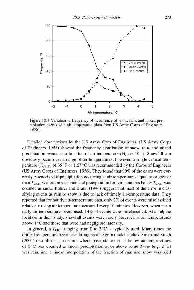
10.3 Point-snowmelt models 273
0
20
40
60
80
100
−2 −1 0 1 2 3 4 5
Air temperature, oC
Fre
qu
ency
, %
Snow eventsMixed events Rain events
Figure 10.4 Variation in frequency of occurrence of snow, rain, and mixed pre-cipitation events with air temperature (data from US Army Corps of Engineers,1956).
Detailed observations by the US Army Corp of Engineers, (US Army Corps
of Engineers, 1956) showed the frequency distribution of snow, rain, and mixed
precipitation events as a function of air temperature (Figure 10.4). Snowfall can
obviously occur over a range of air temperatures; however, a single critical tem-
perature (TCRIT) of 35 ◦F or 1.67 ◦C was recommended by the Corps of Engineers
(US Army Corps of Engineers, 1956). They found that 90% of the cases were cor-
rectly categorized if precipitation occurring at air temperatures equal to or greater
than TCRIT was counted as rain and precipitation for temperatures below TCRIT was
counted as snow. Rohrer and Braun (1994) suggest that most of the error in clas-
sifying events as rain or snow is due to lack of timely air-temperature data. They
reported that for hourly air-temperature data, only 2% of events were misclassified
relative to using air temperature measured every 10 minutes. However, when mean
daily air temperatures were used, 14% of events were misclassified. At an alpine
location in their study, snowfall events were rarely observed at air temperatures
above 1 ◦C and those that were had negligible intensity.
In general, a TCRIT ranging from 0 to 2 ◦C is typically used. Many times the
critical temperature becomes a fitting parameter in model studies. Singh and Singh
(2001) described a procedure where precipitation at or below air temperatures
of 0 ◦C was counted as snow, precipitation at or above some TCRIT (e.g. 2 ◦C)
was rain, and a linear interpolation of the fraction of rain and snow was used
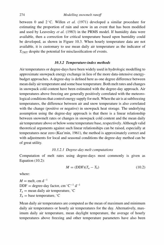
274 Modelling snowmelt runoff
between 0 and 2 ◦C. Willen et al. (1971) developed a similar procedure for
estimating the proportion of rain and snow in an event that has been modified
and used by Leavesley et al. (1983) in the PRMS model. If humidity data were
available, then a correction for critical temperature based upon humidity could
be developed, as shown in Figure 10.3. When hourly temperature data are not
available, it is customary to use mean daily air temperature as the indicator of
TCRIT despite the potential for misclassification of events.
10.3.2 Temperature-index methods
Air temperatures or degree-days have been widely used in hydrologic modelling to
approximate snowpack energy exchange in lieu of the more data-intensive energy-
budget approaches. A degree-day is defined here as one degree difference between
mean daily air temperature and some base temperature. Both melt rates and changes
in snowpack cold content have been estimated with the degree-day approach. Air
temperatures above freezing are generally positively correlated with the meteoro-
logical conditions that control energy supply for melt. When the air is at subfreezing
temperatures, the difference between air and snow temperature is also correlated
with the change (positive or negative) in snowpack heat storage. The underlying
assumption using the degree-day approach is that there is a linear relationship
between snowmelt rates or changes in snowpack cold content and the mean daily
air temperature above or below some temperature base, respectively. Although valid
theoretical arguments against such linear relationships can be raised, especially at
temperatures near zero (Kuz′min, 1961), the method is approximately correct and
with adjustments for local and seasonal conditions the degree-day method can be
of great utility.
10.3.2.1 Degree-day melt computations
Computation of melt rates using degree-days most commonly is given as
Equation (10.2):
M = (DDF)(Ta − Tb) (10.2)
where:
M = melt, cm d−1
DDF = degree-day factor, cm ◦C−1 d−1
Ta = mean daily air temperature, ◦C
Tb = base temperature, ◦C
Mean daily air temperatures are computed as the mean of maximum and minimum
daily air temperatures or hourly air temperatures for the day. Alternatively, max-
imum daily air temperature, mean daylight temperature, the average of hourly
temperatures above freezing and other temperature parameters have also been

10.3 Point-snowmelt models 275
used instead of mean daily temperatures (Martinec, 1976; Kuz′min, 1961; US
Army Corps of Engineers, 1956). Base temperatures (Tb) of 0 ◦C are generally
used for melt computation, but other base temperatures have also been employed
with success for specific sites (US Army Corps of Engineers, 1956). Although
Equation (10.2) is written for a daily time step, similar expressions can be devel-
oped to predict melt over longer time periods by simply accumulating degree-days,
but time periods less than one day are problematical due to variations in the corre-
lation between air temperature and snowpack energy supply between day and night
periods.
Degree-day factors are affected by the air and base temperature parameters
selected for use and a number of variables that are spatially or temporally related
to snowmelt energy supply, as summarized in Table 10.1. Not surprisingly, a wide
range of DDFs are found in the literature with most values falling between 0.1 to
0.8 cm ◦C−1 d−1. In any given application it is highly desirable to obtain represen-
tative and accurate melt and air temperature data to compute local values of DDF
as DDF = M/(Ta – Tb). SNOTEL data in the western United States can be used to
compute local DDFs for specific watersheds (DeWalle et al., 2002). The degree-
day approach is essentially empirical, but DDF can be related to energy exchange
processes. The physical interpretation of the DDF has been derived by Brubaker
et al. (1996) and Bengtsson (1976).
Use of Equation (10.2) is straight forward once the proper DDF is obtained.
Assuming that maximum and minimum air temperature on a given day were 6
and –2 ◦C, respectively, the mean daily air temperature would be 2 ◦C. Hourly
temperature data, that is often lacking, would be required to compute the mean of
positive or daylight air temperatures. If the DDF for this day was 0.4 cm ◦C−1 d−1,
then the computed melt rate would be 0.8 cm d−1. Errors in predicting daily melt can
be quite large and the method works best for prediction of melt over extended time
periods such as weeks to an entire snowmelt season. Application of this approach
on a hourly basis using a constant DDF does not satisfactorily reproduce the diurnal
changes in melt rates (Hock, 1999). Melt on days with rain can be handled using
more detailed energy budget approaches as previously described in this chapter or
with an adjustment to the DDF (Kuusisto, 1980).
Adjustments to DDF for seasonal changes in snowpack and environmental con-
ditions have been developed. Martinec (1960) developed a method to adjust DDF
for seasonal changes based upon snowpack density as Equation (10.3):
DDF = 1.1(ρs/ρw) (10.3)
where:
DDF = degree-day factor, cm ◦C−1 d−1
ρs = snowpack density, kg m−3
ρw = density of liquid water = 103 kg m−3

276 Modelling snowmelt runoff
Table 10.1 Variables affecting snowmelt Degree-Day Factors (DDF).
Variable Cause DDF Response
Time of year Decreasing snowpack coldcontent and albedo andincreasing shortwaveradiation and snow densityas season advances
DDF increases duringaccumulation and meltseason
Forest cover vs. openconditions
Shading and wind protectionby forest
DDF lower and lessvariable in forest than inopen
Topography Variations in incomingshortwave radiation andexposure to wind
DDF higher onsouth-facing slopes andwindy sites
Areal snow cover Varying fraction of watershedcontributing to melt
DDF for basin decreases asareal snow coverdecreases
Snow surfacecontamination
Dust and debris on snowsurface decreases thealbedo
DDF increases
Rainfall High humidity increasescondensation energysupply and rain adds somesensible heat, cloudsreduce solar
DDF generally lower onrainy days, as cloudinessdominates
Ice vs. snow cover Glacier ice has lower albedothan snow
DDF higher on glacialbasins when ice exposed
Other meteorologicalconditions for a given airtemperature
Melt energy greater duringunusually high wind,shortwave radiation, orhumidity conditions at agiven air temperature
DDF higher with greatermelt energy supply for agiven air temperature
Maximum daily airtemperature used for Ta
Causes higher Ta anddegree-day total
DDF lower, approx. half ofDDF for mean daily airtemperature
Mean of positive ordaylight air temperaturesused for Ta
Causes higher Ta anddegree-day total
DDF lower than DDF formean daily airtemperature
Thus, if snowpack density gradually increased from 200 to 400 kg m−3 during the
spring season, DDF would change from 0.22 to 0.44 cm ◦C−1 d−1. It should be noted
that Martinec (1960) defined degree-days based upon the average of positive air
temperatures during a day which gives a lower DDF than when using mean daily air
temperatures. Anderson (1973) also varied DDF seasonally between minimum and
maximum DDF values during the year using a sine-wave function, while Federer

10.3 Point-snowmelt models 277
and Lash (1983) used a linear increase in DDF from January 1 to June 23. DeWalle
et al. (2002), showed that DDF derived from SNOTEL data, linearly increased with
Julian Date during spring by about 0.5% to 1% per day; a rate that exceeded the
rate of increase of potential solar irradiation.
Forest-cover effects on degree-day melt factors have also been quantified. Federer
et al. (1972) reported the following ranges of DDF based upon mean daily air
temperatures for open vs. forest conditions in northeast United States: open 0.45–
0.75, leafless deciduous 0.27–0.45, and conifer 0.14–0.27 cm ◦C−1 d−1. These
ranges were based upon several studies in the northeast giving the DDF ratios
for open:deciduous:conifer conditions of approximately 3:2:1. Kuusisto (1980)
showed that the DDF (cm ◦C−1 d−1) based upon mean daily air temperatures in
Finnish forests could be computed using Equation (10.4):
DDF = 0.292 − 0.164Cc (10.4)
where Cc = fractional canopy cover. Using this model, forest canopy cover of 0.1
and 0.7 (the limits of the forest-cover data) would represent DDFs of 0.28 and 0.18
cm ◦C−1 d−1, respectively. These relationships allow some corrections of DDF for
forest effects.
In order to increase the temporal and spatial resolution of DDF melt estimates,
several hybrid models using temperature and radiation parameters have also been
developed. Cazorzi and Fontana (1996) developed a multiplicative model with a
temperature term and an index to monthly average potential clear-sky shortwave
radiation for various slopes, aspects, and elevations; Hock (1999) used an additive
degree-day temperature term and a term for computed clear-sky potential shortwave
radiation for various slopes and aspects, and in studies by Martinec and deQuervain
(1975), Brubaker et al. (1996), and Hamlin et al. (1998), a component representing
net allwave radiation exchange was added to a degree-day term in melt computa-
tions. In all of these hybrid models, the DDF takes on a new physical meaning since
it is now independent or partially independent of radiation exchange. These models
enhance melt prediction over large areas by consideration of topography along with
degree-days. Models developed by Hock (1999) and Cazorzi and Fontana (1996) do
not require additional data, while models by Martinec and deQuervain (1975) and
Brubaker et al. (1996) require incoming shortwave radiation or cloud-cover data
at the minimum. Hock’s (1999) model was applied hourly and improved ability to
simulate diurnal melt variations.
10.3.2.2 Degree-day cold-content computations
Air temperatures can also be used to track the snowpack cold content and ripeness.
Cold content is expressed as cm of liquid-water equivalent that would have to
refreeze in the snowpack to warm it to 0 ◦C (see Chapter 3). When average daily
278 Modelling snowmelt runoff
air temperatures are below freezing, it is generally assumed that no melt will occur
and that the snowpack can lose or gain energy and cold content as a linear function
of the difference in temperature between the air and snowpack. Applications of
the degree-approach to cold-content computations are less common than for melt.
Leavesley and Striffler (1978) estimated cold-content development for the PRMS
model (see later section) using an approximation of heat conduction in a two-layer
snowpack model that requires predicting snow density. According to Anderson
(1976) the change in cold content of the snowpack can be computed as Equation
(10.5):
�CC = CCF(Ts − Ta) (10.5)
where:
�CC = rate of change in cold content, cm d−1
CCF = cold-content degree-day factor, cm ◦C−1 d−1
Ta = mean daily air temperature, ◦C
Ts = snow surface temperature, ◦C
Optimized CCF values used in melt simulations have ranged from about 0.02 to
0.05 cm ◦C−1 d−1 (Anderson, 1973; Federer and Lash, 1983). The CCF values are
about 1/10 of the values of DDF, indicating that snowpack warming and cooling
due to heat conduction in the snow occurs at a much slower rate than melting does
per degree-day. Since the snowpack gains or loses heat chiefly by conduction when
there is no melt and the conductivity increases with density, a gradual seasonal
increase in CCF is normally applied. Federer and Lash (1983) allowed CCF to
increase linearly from 0.02 cm ◦C−1 d−1 on January 1 to 0.4 cm ◦C−1 d−1 on June
23. Anderson (1973) applied the same sine-wave function for CCF as used to
seasonally adjust degree-day melt factors (DDF).
Application of Equation (10.5) to compute change in snowpack cold content is
relatively direct. Assuming a CCF of 0.03 cm ◦C−1 d−1, a mean daily air temper-
ature of −6 ◦C and a snow surface temperature of –4 ◦C, the change in snowpack
cold content would be an increase of 0.06 cm water equivalent for the day due to
snowpack cooling. In contrast, if air temperature were –2 ◦C, with the same CCF
and snow temperature, a –0.06 cm increment to cold content or snowpack warming
would result. Operationally, changes in cold content are added to the previous day’s
cold content and an accounting scheme is used to determine when the snowpack is
ripe (zero cold content).
An estimate of snow surface temperature is also required to use Equation (10.5).
Although theoretical-based, layered-snowpack temperature models that require
complete energy-budget data have been developed (Jordan, 1991; Anderson, 1976;
10.3 Point-snowmelt models 279
Horne and Kavvas, 1997), Anderson (1973) and Marks et al. (1992) used a simple
temperature-index approach where:
Ts2 = Ts1 + TSF(Ta2 − Ts1) (10.6)
where:
Ts2 = snowpack surface temperature at t2, ◦C
Ts1 = snowpack surface temperature at t1, ◦C
TSF = surface temperature factor, dimensionless
Ta2 = mean daily air temperature at t2, ◦C
The TSF employed by Marks et al. (1992) was 0.1, while Anderson (1973) initially
used 0.5. The snow surface temperature is always limited to a maximum of 0 ◦C.
In addition, surface temperature is set equal to the value of air temperature on
days when snowfall exceeds about 0.5 cm water equivalent, since the new snowfall
becomes the surface layer (Anderson, 1976).
An example of surface temperature computation using Equation (10.6) follows.
Given a surface temperature of –4.0 ◦C on day 1 (Ts1), an air temperature of –2.0 ◦C
on day 2 (Ta2), and TSF = 0.1, the surface temperature on day 2 would become:
Ts2 = −4.0 + 0.1(−2.0 − (−4.0)) = −3.8 ◦C
Larger values of TSF would allow snowpack surface temperature to track current
air temperatures more closely; for example, if TSF = 0.5, then Ts2 would increase
to −3.0 ◦C. Following the example calculations using Equations (10.5) and (10.6),
snowpack surface temperature and cold content can be approximated with only air
temperature and precipitation data. Ideally, snowpack conditions such as tempera-
tures and cold content can be periodically measured at representative locations and
used to update models.
10.3.3 Point-snowmelt model algorithms
Understanding the logic behind computation of snowmelt or snowpack outflow at
a point is important to snow hydrology modelling. The diagram in Figure 10.5
illustrates the components and inter-relationships for a given time interval. Four
types of situations are shown depending upon air temperature (Ta) or energy-budget
melt energy (Qm), critical temperature (Tc), and precipitation amount (P):
� P> 0 and Ta ≥ TCRIT (Rainfall) When precipitation occurs as rainfall (Pr), melting (M )
during the rainfall is computed and rain plus melt become potential snowpack outflow.
Melt can be computed using either the degree-day or energy-budget approach.� P > 0 and Ta < TCRIT (Snowfall) If precipitation occurs as snowfall, the snowpack
water equivalent (SWE) of the snowpack is incremented by the amount P, cold content is

280 Modelling snowmelt runoff
Figure 10.5 Flow diagram illustrating snowmelt-runoff computation during a timeincrement within a point-snowmelt model.
incremented depending upon P and temperature of snowfall relative to the snowpack
temperature, and any melt during the snowfall event (M) is computed. Melt and cold-
content changes are again computed using energy-budget or degree-day approaches.� P = 0, Qm > 0 or Ta > 0 ◦C (Melt Event) If no precipitation occurs and air temperatures
or melt energy is greater than zero, then melting is occurring and computed melt is added
to potential snowpack outflow.� P = 0, Qm < 0 or Ta < 0 ◦C (Non-Event) If no precipitation occurs and air tempera-
tures or melt energy supply are negative, then the snowpack cold content must be either
decreased or increased depending on whether the air temperature is greater or less than
the snowpack temperature.
Melt and/or rain computed from any of the first three types of conditions must
be compared with the snowpack cold content before it becomes outflow. If snow
is at 0 ◦C and cold content is zero, then water is directly available for routing in
the pack. If snow temperature is subfreezing, then liquid water will refreeze. Any

10.3 Point-snowmelt models 281
excess liquid water after the snowpack is warmed to 0 ◦C then becomes available
for routing. Any unfulfilled deficit in liquid-water holding capacity is subtracted
from the excess liquid water. Liquid water in the ripe snowpack is routed to become
outflow. Snowpack water equivalent is reduced by the amount of melt that leaves
the pack in the time interval.
As implied above and in Figure 10.5, three types of storages are needed to
complete the computations for each time step: snowpack-water-equivalent storage,
cold-content storage, and liquid-water holding capacity storage. The snowpack
water equivalent (SWE) is incremented with each new precipitation event (�P)
and by increases in liquid water stored in the snowpack (�WHC, see below), and
is reduced by the melt and rain water (Pr) that becomes outflow in the interval
(�(M + Pr)):
SWE2 = SWE1 + �P + �WHC − �(M + Pr) (10.7)
where the minimum SWE is zero. The snowpack SWE is initially set to zero and
the budget is used to determine the presence or absence of a snowpack at a point.
Cold content (CC) changes with changes in snow temperature and mass changes
over time (�CC) until the snowpack becomes isothermal as:
CC2 = CC1 + �CC (10.8)
where the maximum CC is zero. Changes to cold content can be computed using
an energy-budget or temperature-index approach. Cold-content change due to large
snowfalls at temperatures different than snowpack temperature is generally negligi-
ble and is ignored here. Liquid-water holding capacity (WHC) is incremented with
each new snowfall and reduced with gradual melt or rain liquid up to the maximum
percentage (f ) assumed as:
WHC2 = WHC1 + ( f/100)�P − �(M + Pr) (10.9)
where the minimum WHC is zero. Although generally a small correction, any water
stored is added to the SWE of the snowpack in the interval as indicated above.
Example calculations using the point-snowmelt model concepts just described
are given in Table 10.2. The computations illustrate a brief four-day snow-
accumulation period followed by a day with melt and a day with rain. No routing
was employed since it was assumed that all liquid water drained from the snowpack
each day. Decisions relating to rain vs. snow are straightforward with events at air
temperatures greater than or equal to the TCRIT = 1 ◦C counted as rain. Melt is easily
computed with a DDF = 0.4 cm ◦C−1 d−1 using Equation (10.2). However, on the
last day only 0.776 cm melt occurred even though 0.8 cm was computed, because
only 0.776 cm water equivalent of snow was left on that day.

282 Modelling snowmelt runoff
Table 10.2 Example computations illustrating use of a snowmelt budgetprocedure at a point.a
DayPcm
Ta◦CSnowcm
Raincm
Meltcm
Ts◦CCCcm
WHCcm
SWEcm
Outflowcm
1 0 −2 0 0 0 0 0 0 0 02 0.3 −1 0.3 0 0 −0.5 −0.01 0.009 0.3 03 0.2 −2 0.2 0 0 −1.25 −0.02 0.015 0.5 04 1.2 −3 1.2 0 0 −3.0 −0.025 0.051 1.7 05 0 2.5 0 0 1.0 0 0 0 0.776 0.9246 0.6 2 0 0.6 .776 0 0 0 0 1.376
aEquations (6.38), (6.39), (6.40), (9.6), (9.7), and (9.8) were used with DF = 0.4 cm ◦C−1
d−1, TSF = 0.5, CCF = 0.02 cm ◦C−1 d−1, f = 3%, and TCRIT = 1 ◦C. Assumed all liquidwater drained from snowpack each day. See text for explanation of other terms.
Snow temperatures (Ts) computed with Equation (10.6) and TSF = 0.5 require
more explanation. Snow temperature (Ts) was arbitrarily set to 0 ◦C on day one to
allow computation between day one and two. Snow temperature is also set equal to
air temperature on day four with a large snowfall, since large snowfalls dominate the
snowpack temperature as previously discussed. Finally, snow temperature becomes
0 ◦C whenever cold content is reduced to zero, as it was on day five and six.
Cold content increased during the first three days. From day three to day four no
change in CC occurred, since setting snowpack temperature equal to air temperature
for big snow events reduces the temperature difference to zero. On day five all of the
–0.025 cm of snowpack cold content was eliminated by melt on that day; e.g. 0.025
cm of predicted melt was refrozen in the snowpack and 0.975 cm was available for
outflow. Cold content remained at zero on day six since the air temperature was
above freezing.
Liquid-water holding capacity of the snow was computed using Equation (10.9)
and an assumed f = 3%. Each snowfall added to the water-holding capacity of
the snowpack (WHC) up through day four. However, on day five melt exceeded
WHC and of the 0.975 cm of melt water available after satisfying the cold content,
another 0.051 cm was lost to water holding capacity, reducing liquid water available
to become outflow to 0.924 cm. Water holding capacity remained at zero on day
six since no new snow occurred.
The water equivalent of the snowpack (SWE) was computed using Equation
(10.7). The water equivalent of the snowpack initially increased on three successive
days with snowfall and no melt. On day five, 0.924 cm of meltwater was lost due to
drainage from the pack and 0.071 cm was gained due to 0.025 cm of refrozen water
from the cold content and 0.051 cm of liquid-water storage. Increased liquid-water

10.3 Point-snowmelt models 283
0
10
20
30
40
50
60
0 50 100 150 200 250 300 350
Days, Oct 1 = 0
Wat
er e
qu
ival
ent,
cm
PredictedMeasured
Figure 10.6 Example of prediction of daily snowpack water equivalent at aSNOTEL site using a simple degree-day approach requiring only air-temperatureand precipitation data.
storage due to the refrozen water (3% of 0.025 cm) on day five was negligible
and ignored. Finally, on day six when computed melt exceeded the WE, all of the
remaining water stored in the snowpack was released, both stored liquid and ice.
Predicted snowpack water equivalent reflects the outcome of budget computations
as well as snowpack outflow.
Outflow simply reflects the sum of melt and rain available from routing in the
snowpack. Clearly, from the foregoing discussion, not all melt becomes outflow
because of refreezing and liquid-water storage. If the budget were being conducted
on an hourly basis, rather than daily, then a routing procedure might have been
needed to satisfactorily represent the outflow hydrograph.
An example of point-melt model predictions following the above discussion that
has been adapted to available SNOTEL data is shown in Figure 10.6. SNOTEL data
consist of daily snow pillow snowpack water equivalent, maximum and minimum
daily air temperatures, and daily precipitation measured with a shielded precipita-
tion gage at the site (see SNOTEL data at www.wcc.nrcs.usda.gov/snow/). Since
outflow is not measured directly by the snow pillow, the simulation was performed
to match the measured snowpack water equivalent. A degree-day approach to com-
pute melt and cold content was employed as illustrated in Table 10.2 and given by
Anderson (1973). Model parameters were adjusted by trial and error to achieve a

284 Modelling snowmelt runoff
good fit. It was assumed that liquid water drained rapidly from the pack each day
and no routing was performed.
The overall fit for predicted versus measured snowpack water equivalent for
the year was good (R2 = 0.989) and the average daily difference between pre-
dicted and measured water equivalent was 0.33 cm. The maximum and minimum
melting degree-day factors (DDF in Equation (10.2)) used were 0.4 and 0.15 cm
melt ◦C−1 day−1. A sine-wave variation in degree-day factors was assumed with
the minimum and maximum factors occurring on the winter and summer solstices,
respectively. The maximum and minimum cold-content degree-day factors were
0.09 and 0.034 cm ◦C−1 day−1 (CCF in Equation (10.5)) with a similar sine-wave
variation assumed. The surface temperature factor used to predict snowpack sur-
face temperature was 0.5 (TSF in Equation (10.6)). The critical temperature for
rain vs. snow was 1.67 ◦C and the liquid-water holding capacity of the snowpack
was assumed to be 1%. Although the predicted melt amounts on individual days
are still subject to large errors using this approach, the example shows that with just
air-temperature and precipitation data a reasonable simulation of snowpack water
equivalent over the accumulation and melt season is possible.
10.4 Distributed-snowmelt models
Snowmelt runoff models have gradually evolved into distributed, deterministic
models. This evolution was driven in part by the need to shorten the time interval
for streamflow predictions, to accommodate the shift from simple degree-day to
energy-budget methods of melt prediction, and to enable the prediction of effects of
environmental change, such as that due to climate or land-use change, on large het-
erogeneous basins. The expanding availability of distributed watershed data, such
as snow-cover and digital elevation data, and increased capabilities of computers
and development of geographic information system (GIS) software and methods
have expedited this evolution.
Many approaches have been taken to model the distributed nature of snow pro-
cesses across watersheds and within snowpacks. Watersheds have been represented
as a number of equally spaced grid points or nodes or the sum of processes within
discrete elevation zones, sub-watersheds, or other areas with similar distributed
properties such as vegetative cover, land use, hydrologic response, etc. Mitchell
and DeWalle (1998) used a combination of elevation and vegetation cover to define
zones within a low-relief, Pennsylvania, USA basin for melt simulation using the
SRM model (Martinec et al., 1998). High and low elevation zones each with either
forest or open agricultural land-use gave better streamflow simulation results than
use of elevation zones alone. Harrington et al. (1995) used an iterative clustering
algorithm to cluster pixels according to elevation, snowpack water equivalent and

10.4 Distributed-snowmelt models 285
potential solar radiation. Snowmelt was computed separately for the resulting set
of clustered regions and summed to estimate discharge on the basin. These meth-
ods are used to account for horizontally distributed factors across watersheds, but
vertical snowpack variations due to depth-dependent snowpack properties can also
be considered.
The snowpack has generally been modelled as one homogeneous layer
(Anderson, 1973), but vertical distribution can also be modelled where the snow-
pack is divided into several to many layers to better estimate internal snowpack
processes. In particular, these models are quite helpful in accurately computing
snowpack surface temperature needed for surface energy-balance computations
and accounting for cold-content and liquid-water-storage changes within the snow-
pack. Anderson (1976) used a multiple-layer snowpack model with finite-difference
computations that considered impacts of new snowfall, compaction, metamor-
phic changes, and retention and transmission of liquid water. More recently, Jor-
dan (1991) developed a numerical, one-dimensional, layered snowpack model
(SNTHERM.89) that employed improved methods for predicting liquid-water
movement in the snowpack. The snow module for the PRMS model (Leavesley
and Stannard, 1995) computes the energy balance with a two-layer snowpack.
Without such models, surface temperatures needed for energy-budget computa-
tions have to be estimated from air-temperature data, as previously described by
Equation (10.6).
Distributed-snowmelt models vary greatly in complexity. Fully distributed mod-
els could include mass and energy-budget computations for a number of relatively
homogeneous watershed subunits or regularly spaced grid points with consideration
of effects of factors such as:
� snow-covered area� elevation� slope and aspect� forest cover (interception and melt effects)� frozen ground� wind redistribution of snow� glaciers� topographic shading� avalanches
Snow-covered area needs to be considered in some manner on nearly all but essen-
tially flat basins, while steep mountain catchments often require consideration of
the effects of elevation, slope and aspect, and topographic shading. Issues related
to frozen-ground and blowing-snow effects are more important in open alpine
and trans-arctic settings. Forest-cover effects are widespread in mid-elevation
286 Modelling snowmelt runoff
glaciated and mountainous terrain. Distributed modelling to consider each of these
factors is discussed briefly below.
10.4.1 Snow-covered area
Snow-cover depletion curvesThe simplest semi-distributed models include provisions for computing or includ-
ing measurements of snow-covered area. In simplest form, an equation is used to
represent the changes in snow-covered area over time and melting is assigned only
to the snow-covered portion. Rain inputs occur over the entire watershed, bare or
snow-covered. Because snow accumulation and melt patterns are consistent from
year to year across watersheds, it is possible to model changes in snow-covered area
on a watershed based upon past data. The percentage of watershed area covered
by snow can be related to the fraction of maximum snowpack water equivalent
remaining on the basin (US Army Corp of Engineers, 1956; Anderson, 1973). A
generalized curve used by Anderson (1973) with success on several basins in the
National Weather Service River Forecast System model for the United States is
shown in Figure 10.7 and can approximated as:
S = 5.9 + 194.5(SWE/SWEi) − 139.4(SWE/SWEi)2 + 39.1(SWE/SWEi)
3
(10.10)
where:
S = snow-covered area, %
SWE = snowpack water equivalent, cm
SWEi = minimum snowpack water equivalent at which snow cover always
exceeds 100%, cm
This equation, or one derived for local conditions, can be used to increase snow-
covered area in the accumulation season and decrease snow-covered area during the
melt season. Based upon experience of the US Army Corps of Engineers (1956),
the degree of curvature of such a relationship should increase as a basin becomes
more homogeneous. The SWEi must be set based upon experience or maximum
snowpack accumulation during the current season. Once the proper equation has
been developed, use of the expression is straight forward, except for accounting for
the dynamics of snow-covered-area changes at times of new snowfall during the
melt season.
The effect of new snowfall (S) during the melt season was assumed by Anderson
(1976) to temporarily increase snow-covered area to 100% until 25% of the new

10.4 Distributed-snowmelt models 287
Snow-Covered Area % = 39.1(WE/WEi)3 − 139.4(WE/Wei)2 + 194.5(WE/Wei) + 5.90
0
20
40
60
80
100
0 0.2 0.4 0.6 0.8 1
WE/WEi
Sn
ow
co
ver,
%
Figure 10.7 Generic snow-cover depletion curve used to relate snow-covered areaon a watershed (%) to a snowpack-water-equivalent index (WE/WEi) (based uponAnderson, 1976); WE = snowpack water equivalent and WEi = minimum snow-pack water equivalent where snow-cover area always equals or exceeds 100% ona basin.
snowfall water equivalent had been melted. Snow-covered area then was linearly
interpolated back to the original SCA curve given by Equation (10.10) as:
S2 = S1 + [(0.75 P − MS)/0.75 P](100 − S1) (10.11)
where:
S2 = interpolated new snow-covered area, S1 ≤ S2 ≤ 100%
S1 = original snow-covered area, %
P = new snowfall water equivalent, cm
MS = subsequent melt, ≤0.75 S, cm
Once the original S1 is reached the original non-linear function such as Equa-
tion (10.10) would be used to compute further declines in S. The decision
to use 25% of S as the beginning point for linear interpolation was arbitrary
and could vary among watersheds. This procedure is detailed in the following
example.

288 Modelling snowmelt runoff
If a watershed has complete snow cover whenever snowpack water equiva-
lent exceeds 25 cm (SWE) and the current snowpack water equivalent (SWE) is
15.5 cm, then the snow-covered area by Equation (10.10) would be:
S = 5.90 + 194.5(15.5/25) − 53.59(15.5/25)2 + 39.1(15.5/25)3 = 82.2%
If a major new snowfall with water equivalent of 2.2 cm occurred on the watershed,
then S would increase to 100% and remain at 100% until 25% of 2.2 cm or 0.55
cm had melted. After 0.55 cm of melt occurred, the S would linearly decline as the
remaining 1.65 cm of new snowfall (75% of 2.2 cm) was melted to the original
water equivalent of 15.5 cm. For example, if melt of 1.80 cm were predicted, Swould remain at 100% during 0.55 cm of melt. After the remaining 1.80 – 0.55 =1.25 cm of melt, S would decline from 100% to:
S = 82.2 + [(1.65 − 1.25)/1.65](100 − 82.2) = 86.5%
Once S declined to 82.2% following the new snowfall, the snow-cover depletion
curve (Equation (10.10)) would then be used to account for further declines.
Anderson (1973) applied the snow-cover depletion curves to an entire water-
shed, but it is possible to use snow-cover depletion curves to parts of a basin.
Martinec and Rango (1991) used a similar procedure to estimate snow-covered
area for the Upper Rio Grande Basin in Colorado, USA, except they used a
family of curves, each for a different snow depth corrected for new snow rather
than SWE/SWEi. The Precipitation-Runoff Modelling System (PRMS) developed
by the US Geological Survey also employs user-specified snow-cover depletion
curves following Anderson’s (1973) procedure within hydrologic response units
on a watershed, www.brr.cr.usgs.gov/projects/SW precip runoff/mms/html/ snow-
comp prms.html. In this manner, distinctly different snow-cover depletion patterns
can be simulated in separate regions of the same basin. Snow-covered area can also
be indexed to the observed elevation of the snowline in high mountain ranges like
the Himalayas (Rao et al., 1996).
Snow-cover data Another approach to accounting for snow-cover depletion is to
employ measured snow-covered area from satellite remote sensing, which has been
done in both hydrologic and land-surface models (e.g. Rango, 1996; Turpin et al.,1999; Rodell and Houser, 2004; Dressler et al., 2006; Clark et al., 2006). This
approach obviates use of snow-cover depletion curves and substitutes measured
snow-cover data for more detailed distributed computations of melt across a water-
shed. Further, S has been used to update the distribution of SWE by using direct-
insertion approaches in which model estimates of SWE are adjusted by the satellite
S (Mcguire et al., 2006; Dressler et al., 2006) and by using more robust approaches

10.4 Distributed-snowmelt models 289
such as the Kalman-type assimilation strategy (Clark et al., 2006) that blends satel-
lite information and that from model simulations.
Measured snow-cover data integrates the distributed effects of varying snowpack
accumulation and melt rates due to topography and can index effects of wind redis-
tribution of snow and avalanching later in the melt season. Snow-cover data can be
obtained for watershed subunits frequently enough to permit use in a forecasting
mode, but some method is still needed for extending snow-covered area between
data acquisitions. Although snow-cover data are not commonly used in models to
date, measured snow-cover data could be used as input to verify melt computations
in complex distributed models. A semi-distributed model, SRM (Snowmelt-Runoff
Model) (Martinec et al., 1998), uses satellite snow-cover data to directly determine
snow-cover depletion for up to nine elevation zones on a watershed. In the forecast-
ing mode, snow-cover data are updated as frequently as possible and characteristic
curves based upon past remote-sensing data for each zone are used to extend the
snow-cover curve until the next satellite coverage is available.
Measured snow-covered area can be compared to the computed snowpack water
equivalent in that zone to adjust model parameters. Kirnbauer et al. (1994) found
that comparisons of measured snow cover with model predictions of the presence
or absence of snow cover on various slopes and aspects was much more effective
in selecting model alternatives than comparisons of predicted and measured runoff.
Dressler et al. (2006) reported that greater improvement in melt-runoff predic-
tion from snow-cover data occurs in topographically homogeneous basins relative
to more topographically complex basins in the southwestern United States while
Brandt and Bergstrom (1994) found that greatest improvement occurred in high-
elevation regions of Scandinavia with sparse climatic data resources (the cost of
obtaining snow-cover data was not justified in forested lowland where climate was
more homogeneous and well represented by available data).
10.4.2 Elevation
Elevation differences across watersheds affect air temperatures and other meteo-
rological data. Many snow hydrology applications have accounted for effects of
elevation by dividing watersheds into elevation zones or categorizing grid points
established as equal intervals across basins by elevation (for example, see Mar-
tinec et al., 1998; Bell and Moore, 1999; Williams and Tarboton, 1999). Bell and
Moore (1999) found that performance in runoff prediction greatly improved when
5–25 elevation zones were used, depending upon year, for two upland British catch-
ments. Relatively simple input such as topographic maps are required to characterize
watersheds by elevation zones and digital elevation models can be used to model
the watershed as a set of grid points. Ideally, climatic data are available at sites

290 Modelling snowmelt runoff
representing each elevation zone or a function can be derived to predict variables
according to elevation. When representative sites are not available, then adjustments
are made to available data for the effects of elevation. Typically, the elevation used
to represent zones is the hypsometric mean elevation for that zone that represents
the elevation where 50% of zonal area lies above and 50% lies below that elevation.
When the degree-day approach to melt computation is used, air-temperature
data are generally adjusted to the hypsometric mean elevation of each zone using
average lapse rates discussed in Chapter 7. This extrapolation is critical not only
to computing the melt rates in each elevation zone, but in also deciding on the
form of precipitation, rain or snow, in each zone. When using the energy-budget
approach for melt computation, adjustment of other meteorological data for effects
of elevation, such as humidity or wind speed, is also required. In all models a scheme
is also needed to adjust precipitation data for elevation effects (see Chapter 2).
Correcting meteorological data for elevation is complicated and local statistical
methods commonly have to be relied on to relate elevation to climatic data available
for a region.
Elevation adjustments can vary seasonally as well as daily and minimum tem-
peratures can be lower at low elevation sites due to temperature inversions and
cold-air drainage (Ishikawa et al., 1998). Although elevation adjustment parame-
ters for meteorological data could be fitted in the streamflow modelling process, it is
suggested that adjustments be independent of overall streamflow model parameter
fitting.
10.4.3 Slope and aspect
Slope and aspect exert a major control on the receipt of shortwave and longwave
radiation as described in Chapter 7 and Appendix B. Consideration of the effects
of slope and aspect is generally only needed when radiation exchange is explicitly
considered, such as when the energy budget or a combined radiation–temperature
index method is used to predict melt. Digital elevation models can be used to
categorize grid points within a watershed by slope and aspect. Many models have
now been developed that consider effects of slope and aspect on melt rates (Bloschl
et al., 1991a, b; Braun et al., 1994, Gellens et al., 2000; Harrington et al., 1995;
Hartman et al., 1999; Hock, 1999; Link and Marks, 1999; Marks et al., 1999;
Ujihashi et al., 1994).
Interactions between slope and aspect and other non-radiative factors could also
be considered. Wind speeds that influence the rates of latent and sensible heat
convection and sublimation from snowpacks vary with topography. Terrain can
funnel air flow through valleys and accelerate wind over ridges. Slope and aspect
also interact with the presence and depth of seasonal soil frost due to differences in

10.4 Distributed-snowmelt models 291
depth of snow and the energy budget at the soil surface. Slope/aspect combinations
facing to the north or those with shallow or no snow will have deeper soil frost.
Occurrence of permafrost also varies with aspect. Many of these secondary effects
of slope and aspect have yet to be considered in distributed-snowmelt modelling.
Molotch et al. (2005) successfully used a variable they termed “northness” to
index the complex influence of slope and aspect on snow cover. Northness was
derived from the product of the aspect and the sine of the slope. This variable in
combination with elevation, potential solar radiation, slope, aspect and a variable
describing wind redistribution was used in a binary regression tree model to predict
snow depth in a Californian alpine basin.
In addition to energy-budget models that consider slope and aspect, Hottelet
et al. (1994) developed a degree-day model that considered effects of aspect on
melt rates. Degree-day melt factors within the HBV-ETH model (Bergstrom 1976,
1995) were adjusted for effects of aspect for several watersheds in Switzerland and
Bohemia. Degree-day melt factors for south-facing slopes were multiplied by 1.5
(+50% adjustment) and those for north-facing slopes were divided by 1.5 (−33%
adjustment). No corrections were used for east-facing or west-facing watershed
units.
10.4.4 Forest cover
Forest cover affects both the accumulation of snow due to canopy interception
losses and the melt rates due to the modification of the heat balance at the snow-
pack surface. Canopy interception losses of snow were covered in Chapter 2 and
forest effects on radiation exchange and melt rates were considered in Chapter 7.
Simple characterizations of land-use and land-cover data, such as LULC data
at http://eros.usgs.gov/products/landcover/lulc.html, or other sources, can provide
information on the spatial variations of forest-cover types on large watersheds.
Major differences in the distribution and density of leafless-deciduous forest, conif-
erous forest, and open terrain can be considered easily in distributed models. As
described in Chapter 7, forest density has been considered from two points of view:
boreal forests with scattered, small trees where the effects of individual trees on
energy exchange are considered and more or less closed forests where the forest is
treated as a relatively homogeneous medium with prescribed radiation spectral and
other properties. Models for the distributed effects of forest cover have been devel-
oped by Metcalfe and Buttle (1998), Giesbrecht and Woo (2000), Link and Marks
(1999). Metcalfe and Buttle (1998) were able to link melt rates to a remotely-sensed
index to canopy closure obtained from Landsat TM data and ground-based mea-
surements of canopy gap fractions in their distributed modelling of forest effects in
Manitoba, Canada.

292 Modelling snowmelt runoff
10.4.5 Frozen ground
Frozen, impermeable ground can lead to overland flow and rapid translation of melt
into streamflow. Approaches to prediction of the depth of frost penetration and the
infiltration capacity of frozen ground were reviewed in Chapter 9 and could be
incorporated into streamflow prediction schemes. Most hydrologic models have a
soil infiltration component that can also be adjusted for the effects of soil frost, but
a realistic module including effects of varying air temperature, wind, snow-cover
depth, and soil thermal and moisture conditions will probably be needed. Process
studies of soil frost effects have been completed and distributed models of effects
of soil frost on streamflow including snow-depth effects are obviously the next step
in distributed modelling.
10.4.6 Wind redistribution of snow
The influence of wind on redistribution of snow across the landscape can be one of
the most important distributed modelling parameters in flat to gently rolling, windy
open terrain. Prevailing wind directions will often cause scour of all snow from
some terrain elements facing into the wind and drift of snow into terrain elements
on the lee or downwind side (Kane et al., 1991). If not accounted for, such redis-
tribution of snow often results in modelling difficulties due to occurrence of melt
from deep residual drifts late in the melt season. Wind effects on accumulation of
snow were discussed in Chapter 2 and several blowing-snow models (e.g. Liston
and Sturm 1998 and Pomeroy et al. 1993) have been adapted for use in hydrologic
models. Wind-redistribution effects considered here are separate from adjustments
of wind speed for topographic effects that can affect convective mass and heat
exchange between the snowpack and environment. Bloschl and Kirnbauer (1992)
found that effects of topography like elevation and slope were more important deter-
minants of snow cover early in the melt season and effects of wind redistribution
and avalanching were more influential later in the melt season.
Several distributed-snowmelt modelling attempts have been made to include
wind-redistribution effects. Bloschl et al. (1991a) adjusted snowpack water equiv-
alent based upon slope steepness and slope curvature. All slopes above 60◦ were
assumed to be snow free. All mountain tops with a radius of curvature of 50 m or less
were also assumed to be snow free, while depressions with the same curvature were
assigned 200% of snowpack values for open flat terrain. Snow on all other slopes
was linearly interpolated between level and 60◦ conditions. These adjustments
improved prediction of the snow-cover distribution on a steep basin in the Austrian
Alps. Hartman et al. (1999) similarly based their correction on topographic char-
acteristics by fitting a snow-redistribution parameter that increased snow on slopes
10.4 Distributed-snowmelt models 293
that had a topographic similarity index (TSI) greater than the average TSI and
reduced snow on slopes with a TSI less than the average. This procedure predicted
greater snowpack accumulation on low slopes, valleys, and hollows. Simulations of
streamflow using this approach were sensitive to the wind-redistribution parameter.
Larger values caused greater redistribution and tended to predict lower early-season
flows and higher late-season streamflows. Neither of these two applications con-
sidered effects of aspect explicitly. Luce et al. (1999) used a different approach
by assigning a drift multiplier based upon field measurements to each grid cell on
the watershed to adjust precipitation amounts. The drift multipliers ranged from
0.16 to 5.36, indicating quite a range in scour and drifting conditions occurred on
this basin. This approach required field data not commonly available, but implicitly
indexed all factors at work to influence snow-cover distribution.
Molotch et al. (2005) and Winstral et al. (2002) had success in indexing wind
redistribution of snow by using the variable “maximum upwind slope” in a binary
regression tree model. Maximum upwind slope was defined as the average max-
imum slope found using a search algorithm along 100 m long vectors, spaced
at five-degree intervals, within a 90o upwind sector from each point. Using this
variable, greater upwind slopes were associated with lower snow accumulations.
In the future no doubt, other creative ways of accounting for wind-redistribution
effects will be employed to improve predictions of snowmelt runoff. Wind redistri-
bution implies that some areas lose and others gain snow, not to mention sublimation
losses occurring during wind redistribution. Thus the scheme used should be tied
to a model that ultimately considers both redistribution and sublimation losses.
10.4.7 Glaciers
The presence of glaciers within basins adds to the complexity of streamflow mod-
elling. Glaciers provide an additional source of meltwater for streamflow, melt at
rates typically greater than snowpacks, and can route liquid water rapidly to stream
channels. Moore (1993) describes a model to separately predict melt of snow on
non-glaciated and glaciated portions of multiple elevation zones delineated on a
British Columbia, Canada basin. Once the melting of the snowpack within the
glaciated region had been completed, melt of glacier ice was modelled to occur at
a rate 50% greater than for snow due to the lower albedo of glacier ice. Classifi-
cation of events as rain or snow in each elevation zone was also especially critical
to accurate streamflow prediction in autumn. Autumn rainfall on the glacierized
portion of the basin quickly became runoff, while autumn snowfall was stored in
the snowpack on the glacier until melt the following spring. Areal extent of the
glacier was based upon autumn surveys of the equilibrium line altitude on nearby
glaciers. Schaper et al. (1999) were able to distinguish snow from glacier ice using

294 Modelling snowmelt runoff
remote-sensing data to aid in the modelling of meltwater runoff by elevation zones
on a basin with 67% of the area covered by glaciers.
10.4.8 Topographic shading
Topography surrounding a particular watershed grid point can significantly reduce
the direct-beam solar radiation received by that point, thereby reducing the melt rate,
as discussed in Chapter 7. This impact of topography is separate from that of slope
and aspect considered above, that accounts for the varying angle of the direct solar
beam. Basic principles involved in the corrections for slope and aspect are described
in Appendix B. In steep, mountainous terrain some landscape facets can be shaded
continuously by surrounding topography. In addition, at higher latitudes where
solar altitude may be quite low during an entire solar day, even minor topographic
relief could cause significant shading. Since these shaded-landscape components
often receive snow redistributed by the wind or avalanches, the impacts of shade
on maintaining snow until late in the melt season is probably significant. Several
distributed-snowmelt models have included the effects of topographic shading as
part of the overall radiation budget routine (Bloschl et al. 1991c; Hartman et al.1999; Hock, 1999; Ranzi and Rosso, 1991) and other studies have used the same
physiographic variables in distributing point measurements of ground-based SWE
measurements (Fassnacht et al., 2003), but the importance of topographic shading
by itself to prediction of snow-cover distribution and snowmelt runoff has not been
separately assessed.
10.4.9 Avalanches
Redistribution of snow by gravity to lower elevations, like redistribution by the
wind, can significantly modify streamflow response. Avalanche snow resides in
deeper packs at lower elevations to provide a source of water for streamflow later
into the summer. Adjustments of snow cover for redistribution by the wind tend to
mimic or include the effects of avalanches. De Scally (1992) estimated that as much
as 8% of the annual snowmelt runoff in a large Himalayan basin in Pakistan came
from avalanche snow. Since snow avalanches occur along well-defined pathways, it
is possible that parts of the landscape of large watersheds could be routinely coded
for avalanche susceptibility depending upon snowpack water equivalent.
10.5 Snowmelt-runoff models
Many models are available to continuously predict streamflow and most of these
have provisions for including snowmelt-runoff. Six models in widespread use for

Tab
le10.3
Com
pari
son
ofsn
owm
elt-
runo
ffm
odel
s.
Mo
del
Ref
.aD
ata
inp
uts
bD
egre
e-D
ayo
rE
ner
gy
Bu
dg
etL
um
ped
or
Dis
trib
ute
dP
roce
sses
Co
nsi
der
edM
od
elP
aram
eter
sM
in.
Tim
eS
tep
NW
SR
FS
1,
2T
a,P
,u
DD
,ex
cep
td
uri
ng
rain
Lu
mp
ed,
but
wit
ha
snow
-cover
dep
leti
on
curv
e
Co
ldco
nte
nt,
Sn
owte
mp
.,L
iqu
idro
uti
ng
,R
ain
-on
-sn
ow
13
6h
r
SR
M3
,4
Ta,
Pan
dcl
ou
dco
ver
for
mo
difi
edver
sio
n
DD
Sem
i-d
istr
ibu
ted
,sn
ow-c
over
dat
ab
yel
evat
ion
zon
es
Rip
enin
gd
ate
spec
ified
,se
aso
nal
adju
stm
ents
7d
aily
PR
MS
5T
a,
P,
inco
min
gso
lar
or
clo
ud
cover
;o
rco
mp
lete
met
eo.
dat
a
DD
or
EB
Dis
trib
ute
db
yhydro
logic
resp
onse
un
its;
two
snow
pac
kla
yer
s;el
ev.,
slo
pe
and
asp
ect
and
fore
stef
fect
s
Sn
owte
mp
.,C
old
con
ten
t,R
ain
-on
-sn
ow
10
1m
inin
sto
rmm
od
e,d
aily
oth
erw
ise
HB
V-
ET
H6
,7
Ta
and
P,m
on
thly
po
ten
tial
evap
otr
ansp
.
DD
Sem
i-d
istr
ibu
ted
Par
amet
ers
adju
sted
for
slo
pe/
asp
ect,
fore
stef
fect
s
11
–2
0,
vari
esw
ith
ver
sio
n
dai
ly
SS
AR
R8
Ta,
P,
evap
otr
ansp
.D
DL
um
ped
or
sem
i-d
istr
ibu
ted
wit
hel
evat
ion
zon
es
Sam
eas
NS
RF
Sp
lus
inte
rcep
tio
nlo
sses
15
0.1
hr
SH
E9
,1
0T
aan
dP
or
com
ple
tem
eteo
.d
ata
DD
or
EB
Dis
trib
ute
dg
rid
net
wo
rkIn
terc
epti
on
loss
es,
liq
uid
rou
tin
g,
cold
con
ten
t,fu
llfo
rest
effe
cts
>5
00
.1h
r
aR
efer
ence
s:1=
An
der
son
,19
73
,2=
Bu
rnas
h1
99
5,3
=M
arti
nec
etal
.,1
99
8,4
=B
rub
aker
etal
.,1
99
6,5
=L
eaves
ley
and
Sta
nn
ard
,19
95
,6
=B
erg
stro
m,
19
95
,7
=H
ott
elet
etal
.,1
99
4,
8=
Sp
eers
,1
99
5,
9=
Bat
hu
rst
etal
.,1
99
5,
10
=B
ath
urs
tan
dC
oo
ley,
19
96
.b
Ta=
air
tem
per
atu
re,
P=
pre
cip
itat
ion
,u
=w
ind
spee
d.

296 Modelling snowmelt runoff
prediction of streamflow that include snowmelt routines are compared in Table
10.3. A variety of model features can be found from the simple snowmelt-runoff
model (SRM) that only requires seven parameters and simple meteorological data to
the complex, fully distributed SHE model that considers all physical processes, but
requires many input parameters. Runoff modelling approaches used in these models
in conjunction with the snow routines generally include explicit or conceptual
accounting for surface, soil, and ground water storages and flow; however, SRM
estimates are based upon the sum of a current day’s melt or rain input plus a recession
flow from the prior day. Minimum time steps also vary from 1 minute up to daily
flow estimates. Many other models have been developed and tested (Singh, 1995;
Singh and Singh, 2001; ASCE, 1996; Beven, 2000). Two promising point-snowmelt
modules for predicting outflow from layered snowpacks that can be incorporated
into distributed models for runoff prediction are SYNTHERM (Jordan 1991) and
SNAP (Albert and Krajeski, 1998). Comments about each of the models compared
in Table 10.3 follow.
The NWSRFS (National Weather Service River Forecast System) model
described by Anderson (1973) is essentially a degree-day model that balances
handling the complexities of snow accumulation and melt processes against the
availability of data. Simple input data are required, but during rain on snow events
the model shifts to an approximate energy-budget analysis that requires an addi-
tional wind-speed input. A snow-cover depletion curve is used within the model
to account for varying snow-cover area. Explicit accounting for snowpack sur-
face temperature, cold content, and liquid-water routing are also included, despite
the limited data requirements. Anderson (1976) also developed a detailed, finite-
difference, layered, snowpack model with a complete energy budget and compared
the results to the simpler degree-day approach. Neither of these models was dis-
tributed when originally developed. The degree-day routine has been extensively
validated and tested.
One of the simplest models to use in terms of parameters required is the SRM
(Snowmelt-Runoff Model; Martinec et al., 1998). This model is also a degree-day
model that requires only simple temperature and precipitation data, but additionally
utilizes satellite snow-covered-area data that can be input for up to eight elevation
zones. Inclusion of available snow-covered-area data is an advantage because of the
high correlation between snow-covered area and snowmelt runoff. Parameters can
be estimated based upon experience for ungaged basins, but having some prior flow
data is helpful. SRM also can be used in a forecasting mode and has a routine to
allow estimates of the effects of climate change. Explicit accounting of snowpack
temperature, cold content, and liquid-water routing is not included, although the
date when all rain on snow is expected to percolate freely through the snowpack
(ripe snow) can be specified. A modified radiation–temperature index melt routing

10.5 Snowmelt-runoff models 297
for SRM has been developed to allow distributed modelling, but cloud-cover data
are needed, at a minimum, if this option is used (Brubaker et al., 1996). The radiation
option has not been fully incorporated into SRM at this time. SRM has been used
extensively, especially on steep mountain catchments where satellite snow-cover
data can be acquired. This model will be described in detail in the next chapter.
The PRMS (Precipitation Runoff Modelling System) described by Leavesley
and Stannard (1995) and Leavesley et al. (1983) includes a snow module that uses
distributed energy-balance modelling for effects of slope and aspect, elevation and
forest cover within hydrologic response units (HRU) on a basin. Data requirements
range from minimal temperature and precipitation, to a complete set of input mete-
orological data. Snow-cover depletion curves are used within each HRU and more
recent updates include provisions for incorporation of snow-covered-area data.
PRMS is part of the US Geological Survey’s Modular Monitoring System (Leaves-
ley et al., 2001) that fosters the open sharing and linking of hydrologic modules
and supporting GIS, optimization, sensitivity, forecasting, and statistical analysis
tools to promote distributed hydrologic modelling. PRMS has been widely used
in the United States and includes provisions for modelling the effects of channel
reservoirs.
The HBV or Swedish Meteorological and Hydrological Institute model was
originally developed by Bergstrom (1995) to be as simple and as robust as possible.
HBV has seen widespread use in Scandinavia and throughout the world over the
past 20 years and many variations have been introduced to the model. The original
HBV is a simple degree-day model with few parameters. It can be classified as
a semi-distributed model with sub-basins included that each have a snow-cover
depletion curve and a simple land-use classification (forest, open, lakes). Like SRM,
snowpack temperature, cold content, and liquid-water routing are not explicitly
considered in this model. Hottelet et al. (1994) used a HBV-ETH Version 4 model
that allowed adjustments of melt parameters for aspect classes by elevation zones.
The SSARR (Streamflow Synthesis and Reservoir Regulation) model (Speers,
1995) developed by the US Army Corps of Engineers has essentially adapted Ander-
son’s (1973) degree-day snow routines to a distributed format which allows up
to 20 elevation zones. Alternatively, a simple lumped-parameter approach with
a snow-cover depletion curve can also be used. The combination of Anderson’s
(1973) snow routines and SSARR’s extensive river/reservoir interaction, flow rout-
ing, forecasting, and calibration capabilities make this a proven choice for large
basin applications involving river and reservoir simulations.
The SHE (Systeme Hydrologique Europeen) (Bathurst et al., 1995) model is
a grid-based, fully distributed, process-based flow model that physically mod-
els all hydrologic processes, including those pertaining to the snowpack. The
snow routines (Bathurst and Cooley, 1996) can be simple degree-day or complete

298 Modelling snowmelt runoff
energy-budget routines with a layered snowpack and full consideration of snow-
pack temperature, cold content and liquid-water movement using approaches given
by Morris (1982). The grid-based format allows adjustment for elevation, slope
and aspect, forest cover, etc. Several versions of the model exist that expand its
capabilities to include erosion/sedimentation and contaminant transport (SHESED-
Bathurst et al., 1995, MIKE SHE-Refsgaard and Storm, 1995). However, the model
requires many parameters be specified for all grid points and computer run times
may be problematical (Beven, 2000). Model versions have been tested in a variety
of settings throughout the world.
10.6 Snowmelt-runoff model performance and selection
Selection of a model to predict snowmelt runoff depends upon many factors includ-
ing objectives of the modelling, data availability, characteristics of the watershed,
and space and time scales of application, so generalizations are problematical.
When project objectives are mainly focused on seasonal streamflow patterns and
total volumes of water available for water supplies, then statistical models or sev-
eral physical models and daily time steps could be used. However, when daily
patterns of flow rates and absolute daily or seasonal peak flows are needed, say
for flood forecasting or hydropower generation, then models with smaller min-
imum time steps and distributed model capabilities are probably needed. Time
steps of less than one day for snowmelt simulation generally mean a shift from
degree-day to energy-budget methods to predict melt. A notable exception is the
hybrid temperature–radiation index model developed by Hock (1999) that makes
use of daily variations in potential solar irradiation for shorter-term melt estimates.
Basin characteristics also influence the potential for successful snowmelt-runoff
modelling. Large basins and basins with forest cover have been simulated with
degree-day, lumped models with daily time steps (Bengtsson and Singh, 2000).
However, choice of models to handle complexities of basin topography, land use
and land cover will largely be determined by program objectives, data constraints,
and space and time scales of the application.
Performance of available models in simulating seasonal or annual snowmelt
runoff has been evaluated in tests conducted by the World Meterological Organiza-
tion (WMO, 1986). Flow simulations with 10 models on multiple watersheds were
compared to measured flows using Nash–Sutcliffe coefficients (R2), which are sim-
ilar to a statistical coefficient of determination where 1 equals perfect agreement,
and percentage deviations in total runoff volumes (Dv,%). Annual prediction data
abstracted from WMO (1986) Operational Hydrology Report No. 23 for all avail-
able years averaged for three of the basins (Durance, W3, and Dischma) for five
models that appear in Table 10.3, are given in Table 10.4. Performance of the models
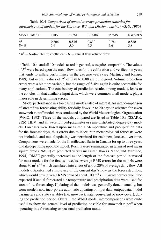
10.6 Snowmelt-runoff model performance and selection 299
Table 10.4 Comparison of annual average prediction statistics forsnowmelt-runoff models for the Durance, W3, and Dischma basins (WMO, 1986).
Model Criteriaa HBV SRM SSARR PRMS NWSRFS
R2 0.806 0.846 0.830 0.784 0.880Dv,% 5.6 5.0 6.3 7.6 5.8
a R2 = Nash–Sutcliffe coefficient, Dv = annual flow volume error
in Table 10.4, and all 10 models tested in general, was quite comparable. The values
of R2 were based upon the mean flow rates for the calibration and verification years
that tends to inflate performance in the extreme years (see Martinec and Rango,
1989), but overall values of R2 of 0.78 to 0.88 are quite good. Volume prediction
errors were a bit more variable, but the range of 5–8% again is quite acceptable for
many applications. The consistency of prediction results among models, leads to
the conclusion that available input data, which were common to all models, play a
major role in determining errors.
Model performance in a forecasting mode is also of interest. An inter comparison
of streamflow forecasting ability for daily flows up to 20 days in advance for seven
snowmelt-runoff models was conducted by the World Meteorological Organization
(WMO, 1992). Three of the models compared are listed in Table 10.3 (SSARR,
SRM, HBV) and all were lumped-parameter or semi-distributed, degree-day mod-
els. Forecasts were based upon measured air-temperature and precipitation data
for the forecast days, thus errors due to inaccurate meteorological forecasts were
not included, and model updating was permitted for each new forecast over time.
Comparisons were made for the Illecillewaet Basin in Canada for up to three years
of data depending upon the model. Results were summarized in terms of root mean
square error (RMSE) of predicted versus measured flows (Rango and Martinec,
1994). RMSE generally increased as the length of the forecast period increased
for most models for the first two weeks. Average RMS errors for the models were
about 30 m3 s−1 which translated into errors of about 20% of average daily flow. All
models outperformed simple use of the current day’s flow as the forecasted flow,
which would have given a RMS error of about 100 m3 s−1. Greater errors would be
expected if actual forecasted air-temperature and precipitation data were used for
streamflow forecasting. Updating of the models was generally done manually, but
some models now incorporate automatic updating of input data, output data, model
parameters and state variables (i.e. snowpack water equivalent or snow cover), dur-
ing the prediction period. Overall, the WMO model intercomparisons were quite
useful to show the general level of prediction possible for snowmelt runoff when
operating in a forecasting or seasonal prediction mode.

300 Modelling snowmelt runoff
Ensemble forecasting of streamflow from snowmelt has seen increasing attention
in order to provide daily forecasts for the entire snowmelt season (Day, 1985).
Ensemble forecasting makes use of models calibrated on specific watersheds to
predict future flows based upon a set or ensemble of historical meteorological
conditions measured in past years. For example, a model could be used to predict
daily flow rates beginning with the flow rate on April 1 in the current year up to
August 31 of the current year, using historical climatic data, such as air temperature
and precipitation, measured in each of the past years. Each set of climatic data for
a past year will produce a single forecast hydrograph of daily flows for April
1–August 31 and the ensemble of forecast hydrographs for all years on record can
be used to estimate the probability of exceedance of any individual hydrograph in
the ensemble.
10.7 Future work
Rapid advances in modelling snowmelt runoff are currently being made due
to interest in simulating global climate and subsequent changes in snowmelt
hydrology. A Snowmelt Modelers Internet Platform (www.geo.utexas.edu/climate/
Research/SNOWMIP/snowmip.htm) has been established to aid communications
among those developing, using, and testing models of snowpack processes through-
out the world. Bales et al. (2006) presented a detailed view of current research
questions facing modellers of mountain hydrology with specific applications to
snow. These questions generally fall into three topic categories: importance of and
processes controlling energy and water fluxes, interactions between hydrologic
fluxes and biogeochemical and ecological processes, and integrated measurement
and data/information systems. Specific research questions are given in each topic
category that can help guide future work.
10.8 References
Albert, M. and Krajeski, G. (1998). A fast, physically based point snowmelt model for usein distributed applications. Hydrol. Processes, 12, 1809–24.
American Society of Civil Engineers (1996). Hydrology Handbook, 2nd edn. Manuals andreports on engineering practice 28. New York: ASCE.
Anderson, E. A. (1973). National Weather Service River Forecast System-SnowAccumulation and Ablation Model, NOAA Tech. Memo, NWS-HYDRO-17. USDept. Commerce, NOAA, NWS.
Anderson, E. A. (1976). A Point Energy and Mass Balance Model of a Snow Cover,NOAA Tech. Rpt. NWS 19. US Dept. Commerce, NOAA, NWS.
Bales, R. C., Molotch, N. P., Painter, T. H., Dettinger, M. D., Rice, R., and Dozier, J.(2006). Mountain hydrology of the western United States. Water Resour. Res., 42,W08432.

10.8 References 301
Bathurst, J. C. and Cooley, K. R. (1996). Use of the SHE hydrological modelling systemto investigate basin response to snowmelt at Reynolds Creek, Idaho. J. Hydrol., 175,181–211.
Bathurst, J. C., Wicks, J. M., and O’Connell, P. E. (1995). Chapter 16: the SHE/SHESEDbasin scale water flow and sediment transport modelling system. In ComputerModels of Watershed Hydrology, ed V. P. Singh. Highlands Ranch, CO: WaterResources Publications, pp. 563–94.
Bell, V. A. and Moore, R. J. (1999). An elevation-dependent snowmelt model for uplandBritain. Hydrol. Processes, 13, 1887–903.
Bengtsson, L. (1976). Snowmelt estimated from energy budget studies. Nordic Hydrol., 7,3–18.
Bengtsson, L. and Singh, V. P. (2000). Model sophistication in relation to scales insnowmelt runoff modeling. Nordic Hydrol., 31(3/4), 267–86.
Bergstrom, S. (1976). Development and application of a conceptual runoff model forScandinavian catchments. In Swedish Meteorological and Hydrological InstituteReport RHO 7, Norrkoping, Sweden.
Bergstrom, S. (1995). Chapter 13: the HBV model. In Computer Models of WatershedHydrology, ed. V. P. Singh. Highlands Ranch, CO: Water Resources Publications,pp. 443–76.
Beven, K. J. (2000). Rainfall-Runoff Modelling. Chichester: John Wiley and Sons,Ltd.
Bloschl, G. and Kirnbauer, R. (1992). An analysis of snow cover patterns in a small alpinecatchment. Hydrol. Processes, 6, 99–109.
Bloschl, G., Gutknecht, D., and Kirnbauer, R. (1991a). Distributed snowmelt simulationsin an alpine catchment: 2. parameter study and model predictions. Water Resour.Res., 27(12), 3181–8.
Bloschl, G., Kirnbauer, R., and Gutnecht, D. (1991b). Distributed snowmelt simulationsin an alpine catchment: 1. Model evaluation on the basis of snow cover patterns.Water Resour. Res., 27(12), 3171–79.
Bloschl, G., Kirnbauer, R. and Gutknecht, D. (1991c). A spatially distributed snowmeltmodel for application in alpine terrain. In Snow, Hydrology and Forests in HighAlpine Areas, IAHS Publ. 205, ed. H. Bergman, Lang, H., Frey, W., Issler, D., andSalm, B., pp. 51–60.
Brandt, M. and Bergstrom, S. (1994). Integration of field data into operationalsnowmelt-runoff models. Nordic Hydrol., 25, 101–12.
Braun, L. N., Brun, E., Durand, Y., Martin, E., and Tourasse, P. (1994). Simulation ofdischarge using different methods of meteorological data distribution, basindiscretization and snow modelling. Nordic Hydrol., 25(1/2), 129–44.
Brubaker, K., Rango, A. and Kustas, W. (1996). Incorporating radiation inputs into thesnowmelt runoff model. Hydrol. Processes, 10, 1329–43.
Burnash, R. J. C. (1995). Chapter 10: the NWS river forecast system-catchment modeling.In Computer Models of Watershed Hydrology, ed. V. P. Singh. Highlands Ranch, CO:Water Resources Publications, pp. 311–66.
Cazorzi, F. and Fontana, G. D. (1996). Snowmelt modeling by combining air temperatureand a distributed radiation index. J. Hydrol., 181, 169–87.
Clark, M. P., Slater, A. G., Barrett, A. P., Hay, L. E., McCabe, G. J., Rajagopalan, B., andLeavesley, G. H. (2006). Assimilation of snow covered area information intohydrologic and land-surface models. Adv. Water Resour., 29, 1209–21.
Day, G. N. (1985). Extended streamflow forecasting using NWSRFS. J. Water Resour.Planning Manag., 111(2), 157–70.
302 Modelling snowmelt runoff
de Scally, F. A. (1992). Influence of avalanche snow transport on snowmelt runoff. J.Hydrol., 137, 73–97.
DeVries, J. J. and Hromadka, T. V. (1992). Chapter 21: Computer models for surfacewater. In Handbook of Hydrology, ed. D. R. Maidment. New York: McGraw-Hill Inc.
DeWalle, D. R., Eismeier, J. A., and Rango, A. (2003). Early forecasts of snowmelt runoffusing SNOTEL data in the Upper Rio Grande basin. In Proceedings of the 71stAnnual Meeting Western Snow Conference, Scottsdale, AZ April 22–25, 2003,pp. 17–22.
DeWalle, D. R., Henderson, Z., and Rango, A. (2002). Spatial and temporal variations insnowmelt degree-day factors computed from SNOTEL data in the Upper Rio GrandeBasin. In Proceedings of the 70th Annual Meeting of the Western Snow Conference,Granby, CO May 20–23, 2002, pp. 73–81.
Dressler, K. A., Leavesley, G. H., Bales, R. C., and Fassnacht, S. R. (2006). Evaluationof gridded snow water equivalent and satellite snow cover products for mountainbasins in a hydrologic model. Hydrol. Processes, 20, 673–88.
Fassnacht, S. R., Dressler, K. A., and Bales, R. C. (2003). Snow water equivalentinterpolation for the Colorado River Basin from snow telemetry (SNOTEL) data.Water Resour. Res., 39(8), 1208.
Federer, C. A. and Lash, D. (1983). Brook: A Hydrologic Simulation Model for EasternForests. Res. Rpt. 19. Water Resour. Res. Center, University of New Hampshire,Durham, NH.
Federer, C. A., Pierce, R. S., and Hornbeck, J. W. (1972). Snow management seemsunlikely in the Northeast. In Proceedings Symposium on Watersheds in Transition,American Water Resources Association, pp. 212–19.
Garstka, W. U., Love, L. D., Goodell, B. C., and Bertle, F. A. (1958). Factors AffectingSnowmelt and Streamflow. Washington, DC: United States Goverment PrintingOffice.
Gellens, D., Barbieux, K., Schadler, B., Roulin, E., Aschwanden, H., andGellens-Meulenberghs, F. (2000). Snow cover modelling as a tool for climate changeassessment in a Swiss alpine catchment. Nordic Hydrol., 31(2), 73–88.
Giesbrecht, M. A. and Woo, M. (2000). Simulation of snowmelt in a subarctic sprucewoodland: 2. open woodland model. Water Resour. Res., 36(8), 2287–95.
Hamlin, L., Pietroniro, A., Prowse, T., Soulis, R., and Kouwen, N. (1998). Application ofindexed snowmelt algorithms in a northern wetland regime. Hydrol. Processes, 12,1641–57.
Harrington, R. F., Elder, K., and Bales, R. C. (1995). Distributed snowmelt modeling usinga clustering algorithm. In Biogoechemistry of Seasonally Snow-Covered Catchments,IAHS, Publ. 228, ed. K. A. Tjonnessen, M. W. Williams and M. Tranter, pp. 167–74.
Hartman, M., J. S. Baron, R. B. Lammers, D. W. Cline, L. E. Band, G. E. Liston, and C.Tague. (1999). Simulations of snow distribution and hydrology in a mountain basin.Water Resour. Res., 35(5), 1587–603.
Hock, R. (1999). A distributed temperature-index ice- and snowmelt model includingpotential direct solar radiation. J. Glaciol., 45(149), 101–9.
Horne, F. and Kavvas, M. L. (1997). Physics of the spatially averaged snowmelt process.J. Hydrol., 191, 179–207.
Hottelet, Ch., Blazkova, S., and Bicik, M. (1994). Application of the ETH snow model tothree basins of different character in central Europe. Nordic Hydrol., 25, 113–28.
Ishikawa, N., Nakabayashi, H., Ishii, Y., and Kodama, Y. (1998). Contribution of snow tothe annual water balance in Moshiri Watershed, Northern Hokkaido, Japan. NordicHydrol., 29(4/5), 347–60.

10.8 References 303
Jordan, R. (1991). A one-dimensional temperature model for a snow cover, technicaldocumentation for SNTHERM.89. In Cold Regions Research and EngineeringLaboratory Special Report 91–16. Hanover, NH: US Army, Corps of Engineers.
Kane, D. L., Hinzman, L. D., Benson, C. S., and Liston, G. E. (1991). Snow hydrology ofa headwater Arctic basin: 1. Physical measurements and process studies. WaterResour. Res., 27(6), 1099–109.
Kirnbauer, R., Bloschl, G., and Gutknecht, D. (1994). Entering the era of distributed snowmodels. Nordic Hydrol., 25, 1–24.
Kuusisto, E. (1980). On the values and variability of degree-day melting factor in Finland.Nordic Hydrol., 11, 235–42.
Kuz′min, P. P. (1961). Protsess tayaniya shezhnogo pokrova (Melting of Snow Cover).Glavnoe Upravlenie Gidrometeorologischeskoi Sluzhby Pri Sovete Ministrov SSSRGosudarstvennyi Gidrologischeskii Institut. Main Admin. Hydrometeorol. Service,USSR Council Ministers, State Hydrol. Institute. Translated by Israel Program forScientific Translations. Avail from US Dept. Commerce, National Tech. Inform.Service, 1971, TT 71–50095.
Leaf, C. F. (1969). Aerial photographs for operational streamflow forecasting in theColorado Rockies. In Proceedings of the 37th Annual Western Snow Conference,April 1969, pp. 19–28.
Leaf, C. F. and Haeffner, A. D. (1971). A model for updating streamflow forecasts basedupon areal snow cover and a precipitation index. In Proceedings of the 39th AnnualWestern Snow Conference, April 1971, pp. 9–16.
Leavesley, G. H. and Stannard, L. G. (1995). Chapter 9: The precipitation-runoffmodeling system-PRMS. Computer Models of Watershed Hydrology, ed. V. P. Singh.Highlands Ranch, CO: Water Resources Publications, pp. 281–310.
Leavesley, G. H. and Striffler, W. E. (1978). A mountain watershed simulation model. InModeling of Snow Cover Runoff, Conf. Proc., ed. S. C. Colbeck and M. Ray.Hanover, NH: US Army Corps Engineers, pp. 379–86.
Leavesley, G. H., Markstrom, S. L., Restrepo, P. J., and Viger, R. J. (2001). A modularapproach to addressing model design, scale, and parameter estimation issues indistributed hydrological modeling. Hydrol. Processes, 16(2), 173–87.
Leavesley, G. H., Restrepo, P., Stannard, L. G., and Dixon, M. (1983).Precipitation-Runoff Modeling System: User’s Manual. Water Resour. Invest. Rpt.83–4238. US Dept. Interior, Geological Survey.
Liston, G. E. and Sturm, M. (1998). A snow-transport model for complex terrain. J.Glaciol., 44(148), 498–516.
Link, T. and Marks, D. (1999). Distributed simulation of snowcover mass- andenergy-balance in the boreal forest. Hydrol. Processes, 13, 2439–52.
Luce, C. H., Tarboton, D. G. and Cooley, K. R. (1999). Sub-grid parameterization of snowdistribution for an energy and mass balance snow cover model. Hydrol. Processes,13, 1921–33.
Maidment, D. R. (ed.) (1992). Handbook of Hydrology. New York: McGraw-Hill Inc.Marks, D., Domingo, J., Susong, S., Link, T., and Garen, D. (1999). A spatially distributed
energy balance snowmelt model for application in mountain basins. Hydrol.Processes, 13, 1935–59.
Marks, D., Dozier, J., and Davis, R. E. (1992). Climate and energy exchange at the snowsurface in the alpine region of the Sierra Nevada, 1. meteorological measurementsand monitoring. Water Resour. Res., 28(11), 3029–42.
Martinec, J. (1960). The degree-day factor for snowmelt-runoff forecasting. InProceedings General Assembly of Helsinki, Commission on Surface Waters, IASHPubl. 51, pp. 468–77.

304 Modelling snowmelt runoff
Martinec, J. (1976). Chapter 4: Snow and ice. In Facets of Hydrology, ed. J. C. Rodda.New York: John Wiley and Sons, pp. 85–118.
Martinec, J. and deQuervain, M. R. (1975). The effect of snow displacement byavalanches on snow melt and runoff. In Snow and Ice Symposium Proceedings,IAHS-AISH Publ. 104, August 1971 Moscow, Russia, pp. 364–77.
Martinec, J. and Rango, A. (1989). Merits of statistical criteria for the performance ofhydrological models. Water Resour. Bull., 25(2), 421–32.
Martinec, J. and Rango, A. (1991). Indirect evaluation of snow reserves in mountainbasins. In Snow, Hydrology and Forests in High Alpine Areas, IAHS Publ. 205, ed H.Bergman, H. Lang, W. Frey, D. Issler and B. Salm, pp. 111–19.
Martinec, J., Rango, A., and Roberts, R. (1998). Snowmelt Runoff Model (SRM) User’sManual. In Geographica Bernisia Series P, no. 35, ed. M. F. Baumgartner and G. M.Apfl, University of Berne.
Mashayekhi, T. and Mahjoub, M. (1991). Snowmelt runoff forecasting: case study ofKaradj reservoir, Iran. In Snow, Hydrology and Forests in High Alpine Areas, IAHS,Publ. No. 205, ed. H. Bergman, H. Lang, W. Frey, D. Issler and B. Salm, pp. 213–20.
Mcguire, M., Wood, A. W., Hamlett, A. F., and Lettenmaier, D. P. (2006). Use of satellitedata for streamflow and reservoir storage forecasts in the Snake River basin, ID. J.Water Resour. Planning Manag, 132, 97–110.
Metcalfe, R. A. and Buttle, J. M. (1998). A statistical model of spatially distributedsnowmelt rates in a boreal forest basin. Hydrol. Processes, 12, 1701–22.
Mitchell, K. M. and DeWalle, D. R. (1998). Application of the SRM using multipleparameter landscape zones on the Towanda Creek Basin, Pennsylvania. J. Amer.Water Resour. Assoc., 34(2), 335–46.
Molotch, N. P., Colee M. T., Bales, R. C., and Dozier, J. (2005). Estimating the spatialdistribution of snow water equivalent in an alpine basin using binary regression treemodels: the impact of digital elevation data and independent variable selection.Hydrol. Processes, 19, 1459–79.
Moore, R. D. (1993). Application of a conceptual streamflow model in a glacierizeddrainage basin. J. Hydrol., 150, 151–68.
Morris, E. M. (1982). Sensitivity of the European hydrological system snow models. InProceedings Symposium on Hydrological Aspects of Alpine and High-MountainAreas, IAHS Publ. 138, pp. 221–31.
Pomeroy, J. W., Gray, D. M., and Landine, P. G. (1993). The prairie blowing snow model:characteristics, validation and operation. J. Hydrol., 144, 165–92.
Rango, A. and Martinec, J. (1994). Model accuracy in snowmelt-runoff forecastsextending from 1–20 days. Water Resour. Bull., 30(3), 463–70.
Rango, A. (1996). Spaceborne remote sensing for snow hydrology applications. Hydrol.Sci. J., 41, 477–93.
Ranzi, R. and Rosso, R. (1991). A physically based approach to modelling distributedsnowmelt in a small alpine catchment. In Snow, Hydrology and Forests in HighAlpine Areas, IAHS, Publ. 205, ed. H. Bergman, H. Lang, W. Frey, D. Issler, and B.Salm, pp. 141–50.
Rao, S. V. N., Ramasastri, K. S., and Singh, R. N. P. (1996). A simple monthly runoffmodel for snow dominated catchments in the Western Himalayas. Nordic Hydrol.,27(4), 255–74.
Refsgaard, J. C. and Storm, B. (1995). Chapter 23-MIKE SHE. In Computer Models ofWatershed Hydrology, ed. V. P. Singh. Highlands Ranch, CO: Water ResourcesPublications, pp. 809–46.
Rodell, M. and Houser, P. R. (2004). Updating a land surface model with MODIS-derivedsnow cover. J. Hydrometeorol., 5, 1064–75.

10.8 References 305
Rohrer, M. B. and Braun, L. N. (1994). Long-term records of the snow cover waterequivalent in the Swiss Alps-2. Simulation. Nordic Hydrol., 25(1/2), 65–78.
Schaper, J., Martinec, J., and Seidel, K. (1999). Distributed mapping of snow and glaciersfor improved runoff modelling. Hydrol. Processes, 13, (12/13), 2023–32.
Singh, V. P. (1995). Computer Models of Watershed Hydrology. Highlands Ranch, CO:Water Resources Publications.
Singh, P. and Singh, V. P. (2001). Snow and Glacier Hydrology. Dordrecht: KluwerAcademic Publishers.
Speers, D. D. (1995). Chapter 11: SSARR model. In Computer Models of WatershedHydrology, ed. V. P. Singh. Highlands Ranch, CO: Water Resources Publications,pp. 367–94.
Thapa, K. B. (1993). Estimation of snowmelt runoff in Himalayan catchmentsincorporating remote sensing data. In Snow and Glacier Hydrology, IAHS Publ. 218,ed. G. J. Young, pp. 69–74.
Turpin, O., Ferguson, R., and Johansson, B. (1999). Use of remote sensing to test andupdate simulated snow cover in hydrologic models. Hydrol. Processes, 13, 2067–77.
Ujihashi, Y., Takase, N., Ishida, H., and Hibobe, E. (1994). Distributed snow cover modelfor a mountainous basin. In Snow and Ice Covers: Interactions with the Atmosphereand Ecosystems, IAHS Publ. 223, ed. H. G. Jones, T. D. Davies, A. Ohmura, andE. M. Morris, pp. 153–62.
United States Army Corp of Engineers (1956). Snow Hydrology, Summary Report of theSnow Investigations. Portland, OR: N. Pacific Div., COE.
Williams, K. S. and Tarboton, D. G. (1999). The ABC’s of snowmelt: a topographicallyfactorized energy component snowmelt model. Hydrol. Processes, 13, 1905–20.
Willen, D. W., Shumway, C. A., and Reid, J. E. (1971). Simulation of daily snow waterequivalent and melt. Proceedings Western Snow Conference, Billings, MT, Vol. 39,pp. 3–8.
Winstral, A., Elder, K., and Davis, R. E. (2002). Spatial snow modeling ofwind-redistributed snow using terrain-based parameters. J. Hydrometeorol., 3(5),524–38.
World Meteorological Organization (1986). Intercomparison of Models of SnowmeltRunoff, Operational Hydrol. Rpt. 23, No. 646, Geneva: WMO.
World Meteorological Organization (1992). Simulated Real-Time Intercomparison ofHydrological Models, Operational Hydrol. Rpt. 38, WMO-No. 779, Geneva: WMO.

11
Snowmelt-Runoff Model (SRM)
11.1 Introduction
The Snowmelt-Runoff Model (SRM) is designed to simulate and forecast daily
streamflow in mountain basins where snowmelt is a major runoff factor. Most
recently, it has also been applied to evaluate the effect of a changed climate on the
seasonal snow cover and runoff. SRM was developed by Martinec (1975) in small
European basins. Thanks to the progress of satellite remote sensing of snow cover,
SRM has been applied to larger and larger basins. The Ganges River Basin in the
Himalayas, the largest basin where SRM has been applied so far, is about 917 444
km2 (Seidel et al., 2000). Runoff computations by SRM appear to be relatively easily
understood. To date, the model has been applied by various agencies, institutes, and
universities in over 100 basins situated in 29 different countries as listed in Table
11.1. About 20% of these applications have been performed by the model developers
and 80% by independent users. Some of the localities are shown in Figure 11.1. SRM
also successfully underwent tests by the World Meteorological Organization with
regard to runoff simulations (WMO, 1986) and to partially simulated conditions of
real-time runoff forecasts (WMO, 1992).
Range of conditions for model applicationSRM can be applied in mountain basins of almost any size (so far from 0.76 to
917 444 km2) and any elevation range (for example 0–8848 m a.s.l.) (Table 11.1).
A model run starts with a known or estimated discharge value and can proceed
for an unlimited number of days, as long as the input variables – temperature,
precipitation, and snow-covered area – are provided. As a test, a ten-year period
was computed without reference to measured discharges (Martinec and Rango,
1986).
In addition to the input variables, the area–elevation curve of the basin is required.
If other basin characteristics are available (forested area, soil conditions, antecedent
306

Tab
le11.1
SRM
appl
icat
ions
and
resu
lts
#C
ou
ntr
yB
asin
Siz
e(k
m2)
Ele
vati
on
Ran
ge
(ma.
s.l.
)R
2D
v
(%)
Yea
rsS
easo
ns
Zo
nes
Yea
rsA
pp
lied
1U
SA
EG
L(R
ock
yM
ou
nta
ins)
0.2
93
30
0–
34
50
N/A
N/A
N/A
N/A
19
89
2U
SA
WG
L(R
ock
yM
ou
nta
ins)
0.6
33
00
–3
45
0N
/AN
/AN
/AN
/A1
98
93
Ger
man
yL
ang
eB
ram
ke
(Har
z)0
.76
54
0–
70
0N
/AN
/A1
11
98
14
Ger
man
yW
inte
rtal
(Har
z)0
.76
56
0–
75
4N
/AN
/A1
11
98
15
Cze
chR
.M
od
ryD
ul
(Krk
on
ose
)2
.65
10
00
–1
55
40
.96
1.7
21
19
62
,1
96
66
US
AG
LE
ES
(Ro
cky
M.)
2.8
73
30
0–
34
50
N/A
N/A
N/A
N/A
19
89
7E
cuad
or
An
tisa
na
(An
des
)3
.72
45
00
–5
76
0N
/AN
/A1
31
99
68
Arg
enti
na
Ech
aurr
en4
.53
00
0–
42
00
0.8
47
.51
11
98
59
Sp
ain
Lag
oM
ar(P
yre
nee
s)4
.52
23
4–
30
04
N/A
N/A
11
19
65
10
Sp
ain
Lla
use
td
am(P
yre
nee
s)7
.82
10
0–
30
00
0.6
95
.51
21
99
91
1U
SA
W-3
(Ap
pal
ach
ian
s)8
.42
34
6–
69
50
.81
8.8
10
11
96
9–
19
78
12
Ger
man
yL
ainbac
hta
l(A
llgau
erA
lps)
18.7
670–1800
N/A
N/A
51
1978,
1979
13
Sp
ain
Sal
enca
enB
aser
ca(P
yre
nee
s)2
2.2
14
60
–3
20
00
.72
4.3
33
19
99
14
Sp
ain
No
gu
era
Rib
ago
rzan
aen
Bas
erca
(Py
ren
ees)
36
.81
48
0–
30
00
0.7
13
.73
21
99
5
15
Sw
itze
rlan
dR
ho
ne-
Gle
tsch
(Alp
s)3
8.9
17
55
–3
63
0N
/AN
/A1
41
97
91
6S
wit
zerl
and
Dis
chm
a(A
lps)
43
.31
66
8–
31
46
0.8
62
.51
03
19
73
,1
97
0–
19
79
17
Jap
anS
ai(J
apan
Alp
s)5
73
00
–1
60
00
.86
N/A
33
19
79
–1
98
11
8S
pai
nT
or
enA
lin
s6
01
88
0–
30
40
0.7
17
.31
41
99
91
9S
pai
nF
lam
isel
len
Cap
del
la8
41
44
0–
29
40
0.6
88
.11
41
99
92
0S
pai
nV
ello
sen
An
iscl
o8
51
14
0–
33
60
0.8
31
.51
51
99
92
1A
ust
ria
Ro
fen
ach
e(A
lps)
98
18
90
–3
77
10
.88
2.4
18
19
92
–1
99
32
2U
nit
edK
ing
do
mF
esh
ie(C
airn
go
rms)
10
63
50
–1
26
50
.88
N/A
21
19
79
,1
98
02
3S
wit
zerl
and
Sed
run
(Alp
s)1
08
18
40
–3
21
00
.79
1.9
23
19
85
,1
99
32
4A
ust
ria
Tu
xb
ach
11
68
79
–3
06
20
.44
12
.73
71
99
6–
19
98
25
Au
stri
aS
chle
gei
s1
21
17
90
–3
51
00
.86
8.7
38
19
96
–1
99
8 (con
t.)
307

Tab
le11.1
(con
t.)
#C
ou
ntr
yB
asin
Siz
e(k
m2)
Ele
vati
on
Ran
ge
(ma.
s.l.
)R
2D
v
(%)
Yea
rsS
easo
ns
Zo
nes
Yea
rsA
pp
lied
26
Au
stra
lia
Gee
hi
Riv
er(S
now
yM
tns.
)1
25
10
32
–2
06
20
.76
.66
31
98
9–
19
94
27
US
AA
mer
ican
Fo
rk(U
tah
)1
30
18
20
–3
58
00
.90
1.7
14
19
83
28
Au
stri
aV
ente
rA
che
16
51
85
0–
37
71
0.8
25
.41
81
99
22
9S
wit
zerl
and
Lan
dw
asse
r–
Fra
uen
kir
ch(A
lps)
18
31
50
0–
31
46
N/A
N/A
13
19
79
30
Sw
itze
rlan
dM
assa
-Bla
tten
(Alp
s)c
19
61
44
7–
41
91
0.9
1−5
.31
61
98
53
1In
dia
Ku
lan
g(H
imal
ayas
)2
05
23
50
–5
00
0N
/AN
/AN
/AN
/A–
32
Sw
itze
rlan
dT
avan
asa
(Alp
s)2
15
12
77
–3
21
00
.82
3.1
24
19
85
,1
99
33
3U
SA
Din
wo
od
y(W
ind
Riv
er)
22
81
98
1–
42
02
0.8
52
.82
41
97
4,
19
76
34
Ital
yC
ord
evo
le(A
lps)
24
89
80
–3
25
00
.89
4.6
13
19
84
35
US
AS
alt
Cre
ek(U
tah
)2
48
15
64
–3
62
0N
/A2
.61
5–
36
Ind
iaB
eas-
Man
ali
(Him
alay
as)
34
51
90
0–
60
00
0.6
81
24
N/A
–3
7A
rgen
tin
aE
lY
eso
35
02
47
5–
65
50
0.9
12
.62
31
99
1,
19
93
38
No
rway
Lae
rdal
selv
en(L
oB
ru)
37
55
30
–1
72
00
.86
5.2
15
19
91
39
No
rway
Viv
eli
(Har
dan
ger
vid
da)
38
68
80
–1
61
30
.73
11
.32
11
99
14
0U
SA
Sco
fiel
dD
am,
Pri
esR
iver
(Uta
h)
40
12
32
3–
31
09
0.8
5.0
21
19
96
,1
99
84
1S
pai
nC
ard
os
enT
irv
ia4
17
17
20
–3
24
00
.82
.61
41
99
94
2Ja
pan
Ok
uta
dam
i(M
iku
ni)
42
27
82
–2
34
60
.83
5.4
33
19
84
43
US
AJo
esV
alle
yD
am,
Co
tto
nw
oo
dC
reek
(Uta
h)
43
52
13
1–
33
53
0.8
31
8.5
23
19
85
44
Sp
ain
Gar
on
aen
Bo
sso
st4
49
16
20
–3
08
00
.75
3.0
14
19
99
45
Sp
ain
No
gu
era
Pal
lare
saen
Esc
alo
45
01
86
0–
29
60
0.8
73
.31
31
99
94
6U
SA
Bu
llL
ake
Cre
ek(R
ock
yM
ts.)
48
41
79
0–
41
85
0.8
24
.81
41
97
64
7S
wit
zerl
and
Tie
fen
cast
el(A
lps)
52
98
37
–3
41
80
.55
11
.32
51
98
2,
19
85
48
Sp
ain
Val
ira
enS
eod
’Urg
el(P
yre
nee
s)5
45
17
40
–3
08
00
.92
0.9
14
19
99
49
US
AT
owan
da
Cre
ekb
55
02
40
–7
33
0.7
88
.33
61
99
0,
19
93
,1
99
45
0S
pai
nG
aro
na
enP
on
td
eR
ei5
58
14
20
–3
08
00
.72
2.7
15
19
99
51
US
AS
ou
thF
ork
(Co
lora
do
)5
59
25
06
–3
91
40
.89
1.8
73
19
73
–1
97
95
2S
pai
nN
og
uer
aR
ibag
orz
ana
enP
on
td
eS
uer
t5
73
92
0–
33
80
0.9
1−0
.61
61
99
9
308

53
Arg
enti
na
Las
Cu
evas
enL
os
Alm
end
ros
(An
des
)6
00
25
00
–7
00
0N
/AN
/AN
/AN
/A1
98
1
54
US
AIn
dep
end
ence
R.
(Ad
iro
nd
ack
s)6
18
26
1–
70
20
.81
5.0
11
19
87
55
Ch
ile
Map
och
o(A
nd
es)
63
01
02
4–
44
50
0.4
22
9.9
13
19
87
56
Po
lan
dD
un
ajec
(Hig
hT
atra
)7
00
57
7–
23
01
0.7
33
.81
31
97
55
7In
dia
Sai
ng
(Him
alay
as)
70
51
40
0–
55
00
N/A
N/A
N/A
N/A
–5
8U
SA
Co
nej
os
(Ro
cky
Mts
)7
30
25
21
–4
01
70
.87
1.1
73
19
73
–1
97
95
9S
wit
zerl
and
Ilan
z(A
lps)
77
66
93
–3
61
40
.53
8.6
25
19
82
,1
98
56
0S
pai
nC
inca
enL
asp
un
a7
98
11
20
–3
38
00
.78
5.6
15
19
99
61
Ch
ina
To
utu
nh
e8
40
14
30
–4
45
00
.81
2.0
36
19
84
–1
98
66
2A
ust
ria
Otz
tale
rA
che
(Alp
s)8
93
67
0–
37
74
0.8
49
.18
16
<1
99
86
3A
rgen
tin
aL
ago
Alu
min
(An
des
)9
11
11
45
–2
49
6N
/AN
/AN
/AN
/A1
98
56
4C
hin
aG
on
gn
isi
(Tie
nS
han
)9
39
17
76
–4
20
00
.80
.97
15
<1
99
96
5C
hin
aU
rum
qi
(Tie
nS
han
)9
50
18
80
–4
20
00
.62
2.7
81
6<
19
99
66
Uzb
ekis
tan
An
gre
n1
08
21
20
0–
38
00
0.6
32
.33
6–
67
Ind
iaP
arb
ati
(Him
alay
as)
11
54
15
00
–6
40
00
.73
7.5
15
19
86∼1
99
16
8C
anad
aIl
leci
llew
aet
(Ro
cky
Mts
)1
15
55
09
–3
15
00
.86
7.0
44
19
76
,1
98
1,
19
83
,1
98
46
9S
pai
nS
egre
enS
eod
’Urg
el(P
yre
nee
s)1
21
73
60
–2
90
0N
/AN
/AN
/A5
19
96
70
Ind
iaB
un
tar
(Him
alay
as)
13
70
12
00
–5
00
0N
/AN
/AN
/AN
/A1
98
5∼1
99
17
1C
hil
eT
ing
uir
iric
aB
ajo
Bri
on
es(A
nd
es)
14
60
52
0–
45
00
0.8
8−0
.31
31
98
7
72
New
Zea
lan
dH
awea
(S.
Alp
s)1
50
03
00
–2
50
0N
/AN
/AN
/AN
/A1
98
97
3S
wit
zerl
and
Tic
ino
-Bel
lin
zon
a(A
lps)
15
15
22
0–
34
02
0.8
6−0
.61
51
99
47
4U
SA
Sp
anis
hF
ork
(Uta
h)
16
65
14
84
–3
27
70
.85
1.0
14
19
83
75
Sw
itze
rlan
dIn
nat
Tar
asp
(Alp
s)1
70
01
23
5–
40
05
0.7
78
.0–
11
99
676
Arg
enti
na
Tupungat
o(A
ndes
)1800
2500–6000
0.6
36.4
18
1981
77
Sw
itze
rlan
dIn
n-M
arti
na
(Alp
s)1
94
31
03
0–
40
49
0.8
24
.31
21
99
07
8A
rgen
tin
aC
hic
o(T
ierr
ad
elF
ueg
o)
20
00
N/A
N/A
N/A
N/A
N/A
N/A
79
US
AB
ois
e(R
ock
yM
ts.)
21
50
98
3–
31
24
0.8
43
.33
31
97
6–
19
78
80
Fra
nce
Du
ran
ce(A
lps)
21
70
78
6–
41
05
0.8
52
.65
51
97
5–
19
79
(con
t.)
309

Tab
le11.1
(con
t.)
#C
ou
ntr
yB
asin
Siz
e(k
m2)
Ele
vati
on
Ran
ge
(ma.
s.l.
)R
2D
v
(%)
Yea
rsS
easo
ns
Zo
nes
Yea
rsA
pp
lied
81
US
AM
adis
on
(Mo
nta
na)
23
44
19
65
–3
23
40
.89
1.5
22
19
76
,1
97
88
2U
zbek
ista
nP
skem
24
48
10
00
–4
20
00
.97
−1.0
37
<2
00
28
3M
oro
cco
Til
lou
gu
it(A
tlas
)2
54
41
05
0–
34
11
0.8
40
.51
31
97
98
4A
ust
ria
Sal
zach
-St.
Joh
ann
(Alp
s)2
60
05
70
–3
66
6N
/AN
/AN
/AN
/A>
19
91
85
US
AH
enry
’sF
ork
(Id
aho
)2
69
41
55
3–
31
25
0.9
11
.52
31
97
6,
19
79
86
US
AC
ach
ela
Po
ud
re(C
olo
rad
o)
27
32
15
96
–4
13
3N
/AN
/A1
31
98
38
7C
hil
eA
con
cag
ua
enC
hab
abu
qu
ito
(An
des
)2
90
09
00
–6
10
00
.91
0.9
13
19
87
88
US
AS
evie
rR
iver
(Uta
h)
29
29
19
23
–3
26
00
.75
5.1
14
19
83
89
Sw
itze
rlan
dR
hin
e-F
elsb
erg
(Alp
s)a
32
49
56
2–
34
25
0.7
07
.27
51
98
2,
19
85
,1
98
8,
19
89
,1
99
2,
19
94
,1
99
6,
19
85
90
Sw
itze
rlan
dR
ho
ne-
Sio
n(A
lps)
b3
37
14
91
–4
63
40
.97
−2.1
17
91
US
AR
ioG
ran
de
(Co
lora
do
)a3
41
42
43
2–
42
15
0.8
43
.81
33
19
76
–1
97
7,1
97
99
2U
SA
Kin
gs
Riv
er(C
alif
orn
ia)a
40
00
17
1–
43
41
0.8
23
.25
71
97
3–
19
75
,1
98
2,
19
88
93
Ch
ile
Mai
po
enel
Man
zan
o(A
nd
es)
49
60
85
0–
56
00
0.7
70
.92
31
98
2,
19
88
94
Ind
iaB
eas-
Th
alo
t(H
imal
ayas
)5
14
41
10
0–
64
00
0.8
01
.52
61
98
6–
19
87
95
US
AU
pp
erY
akim
a(C
asca
des
)5
51
73
66
–2
12
10
.92
2.8
15
19
89
96
Uzb
ekis
tan
Ch
atk
al6
59
11
00
0–
40
00
0.8
11
.63
7–
97
Can
ada
Stu
rgeo
n(O
nta
rio
)7
00
0N
/AN
/AN
/AN
/AN
/A1
96
79
8A
rgen
tin
aG
ran
de
(Tie
rra
del
Fu
ego
)9
05
0N
/AN
/AN
/AN
/AN
/AN
/A9
9C
anad
aIs
ku
t(C
oas
t)9
35
02
00
–2
55
6N
/AN
/AN
/AN
/AN
/A1
00
Tu
rkey
Kar
asu
(Up
per
Eu
ph
rate
s)1
02
16
11
25
–3
48
70
.95
0.2
53
51
99
7–
19
99
10
1U
zbek
ista
n,
Ky
rgy
stan
Kar
adar
ya
12
05
61
10
0–
45
68
0.8
74
.04
81
99
6,
19
98
,1
99
9
10
2T
adji
kis
tan
Zer
afsh
an1
22
14
41
0–
55
00
N/A
N/A
18
–
310

10
3U
zbek
ista
n,
Kaz
akh
stan
Kafi
nir
gan
a1
23
69
50
5–
30
05
0.5
78
.63
61
98
8–
19
91
10
4U
SA
Sev
ier
Riv
er(U
tah
)1
33
80
15
06
–3
71
90
.93
4.0
14
19
83
10
5U
SA
Sn
ake
Riv
er(I
dah
o)
14
89
71
52
4–
41
96
0.9
00
.41
1N
/A1
97
2–
19
82
10
6T
adji
kis
tan
Vak
hsh
a3
77
59
17
91
–5
29
10
.63
2.8
38
19
88
–1
99
01
07
Ky
rgy
stan
Nar
yn
53
23
78
00
–5
00
00
.96
1.0
28
–1
08
Pak
ista
nK
abu
lR
iver
(Him
alay
as)
63
65
73
05
–7
69
00
.66
6.0
11
19
75
10
9T
adji
kis
tan
,A
fgh
anis
tan
Py
and
zh(P
amir
san
dH
ind
uK
ush
)1
20
53
42
14
1–
55
64
0.6
55
.63
81
98
8–
19
91
11
0C
hin
aY
ello
w(A
ny
emo
gen
Sh
an)
12
19
72
25
00
–5
22
4N
/AN
/AN
/A3
19
93
11
1In
dia
,B
ang
lad
esh
Bra
hm
apu
traa
54
73
46
0–
88
48
0.7
5−7
.51
71
99
5
11
2In
dia
,B
ang
lad
esh
Gan
ges
a9
17
44
40
–8
84
80
.94
8.3
17
19
95
acl
imat
ech
ang
eev
alu
ated
;b
lan
d-u
sezo
nes
;c
sep
arat
em
app
ing
of
snow
cover
and
gla
cier
s.If
mo
reth
ano
ne
yea
rw
asev
alu
ated
,av
erag
eso
fR
2an
dav
erag
eso
fD
V(s
ing
leva
lues
taken
inab
solu
tete
rms)
are
list
ed.
Th
eac
cura
cycr
iter
iaR
2an
dD
Vli
sted
inT
able
11
.1ar
ed
efin
edas
:
R2
=1
−
n ∑ i=1
(Qi−
Q′ i)
2
n ∑ i=1
(Qi−
Q)2
Dv=
VR
−V
′ R
VR
·10
0
wh
ere:
R2
=a
mea
sure
of
mo
del
effi
cien
cyQ
i=
mea
sure
dd
aily
dis
char
ge
Q′ i=
sim
ula
ted
dai
lyd
isch
arg
e
Q=
aver
age
dai
lyd
isch
arg
efo
rth
esi
mu
lati
on
yea
ro
rsi
mu
lati
on
seas
on
n=
nu
mb
ero
fd
aily
dis
char
ge
valu
esD
V=
per
cen
tag
ed
iffe
ren
ceb
etw
een
the
tota
lm
easu
red
and
sim
ula
ted
run
off
(%)
VR
=m
easu
red
run
off
volu
me
V′ R
=si
mu
late
dru
no
ffvo
lum
e
311

312 Snowmelt-Runoff Model (SRM)
Figure 11.1 Selected locations where SRM has been tested worldwide.
precipitation, and runoff data), they are of course useful for facilitating the deter-
mination of the model parameters.
SRM can be used for the following purposes:
(1) Simulation of daily flows in a snowmelt season, in a year, or in a sequence of years. The
results can be compared with the measured runoff in order to assess the performance of
the model and to verify the values of the model parameters. Simulations can also serve to
evaluate runoff patterns in ungauged basins using satellite monitoring of snow-covered
areas and extrapolation of temperatures and precipitation from nearby stations.
(2) Short-term and seasonal runoff forecasts. The microcomputer program (Micro-SRM)
includes a derivation of modified depletion curves which relate the snow-covered areas
to the cumulative snowmelt depths as computed by SRM. These curves enable the
snow coverage to be extrapolated manually by the user several days ahead employing
temperature forecasts so that this input variable is available for discharge forecasts.
The modified depletion curves can also be used to evaluate the snow reserves for
seasonal runoff forecasts. The model performance may deteriorate if the forecasted air
temperature and precipitation deviate from the observed values, but the inaccuracies
can be reduced by periodic updating.

11.2 Model structure 313
(3) In recent years, SRM was applied to the new task of evaluating the potential effect of
climate change on the seasonal snow cover and runoff. The microcomputer program
has been complemented accordingly.
11.2 Model structure
Each day, the water produced from snowmelt and from rainfall is computed, super-
imposed on the calculated recession flow, and transformed into daily discharge
from the basin according to Equation (11.1):
Qn + 1 = [cSn · an(Tn + �Tn)Sn + cRn Pn]A · 10 000
86 400(1 − kn+1) + Qnkn+1
(11.1)
where:
Q = average daily discharge (m3 s−1)
c = runoff coefficient expressing the losses as a ratio (runoff/precipitation), with
cS referring to snowmelt and cR to rain
a = degree-day factor (cm ◦C−1 d−1) indicating the snowmelt depth resulting from
1 degree-day, see DDF, Section 10.3.2
T = number of degree-days (◦C d)
�T = the adjustment by temperature lapse rate when extrapolating the temperature
from the station to the average hypsometric elevation of the basin or zone (◦C d)
S = ratio of the snow-covered area to the total area
P = precipitation contributing to runoff (cm)
A preselected threshold temperature, TCRIT, determines whether this contribution
is rainfall and immediate. If precipitation is determined by TCRIT to be new snow,
it is kept on storage over the hitherto snow-free area until melting conditions
occur.
A = area of the basin or zone (km2)
k = recession coefficient indicating the decline of discharge in a period without
snowmelt or rainfall:
k = k = Qm+1
Qm(m, m + 1 are the sequence of days during a true recession flow
period)
n = sequence of days during the discharge computation period. Equation (11.1)
is written for a time lag between the daily temperature cycle and the resulting
discharge cycle of 18 hours. In this case, the number of degree-days measured
on the nth day corresponds to the discharge on the n + 1 day. Various lag times
can be introduced by a subroutine.
10 000
86 400= conversion from cm km2 d−1 to m3 s−1

314 Snowmelt-Runoff Model (SRM)
T, S, and P are variables to be measured or determined each day. cR, cS, lapse rate to
determine �T, TCRIT, k and the lag time are parameters which are characteristic for
a given basin or, more generally, for a given climate. A guidance for determining
these parameters will be given in Section 11.3.3.
If the elevation range of the basin exceeds 500 m, it is recommended that the
basin be subdivided into elevation zones of about 500 m each. For an elevation range
of 1500 m and three elevation zones A, B, and C, the model equation becomes:
Qn+1 ={
[cSAn · aAn(Tn + �TAn)SAn + cRAn · PAn]AA · 10 000
86 400
+ [cSBn · aBn(Tn + �TBn)SBn + cRBn · PBn]AB · 10 000
86 400
+ [cSCn · aCn(Tn + �TCn)SCn + cRCn · PCn]AC · 10 000
86 400
}(1 − kn+1)
+ Qn · kn+1 (11.2)
The indices A, B, and C refer to the respective elevation zones and a time lag of
18 hours is assumed. Other time lags can be selected and automatically taken into
account as explained in Section 11.3.3.
In the simulation mode SRM can function without updating. The discharge data
serve only to evaluate the accuracy of simulation. In ungauged basins the simulation
is started with a discharge estimated by analogy to a nearby gauged basin. In the
forecasting mode the model provides an option for updating by the actual discharge
every one to nine days.
Equations (11.1) and (11.2) are written for the metric system but an option for
model operation in English units is also provided in the computer program.
11.3 Data necessary for running the model
11.3.1 Basin characteristics
Basin and zone areasThe basin boundary is defined by the location of the streamgauge (or some arbitrary
point on the streamcourse) and the watershed divide is identified on a topographic
map. The basin boundary can be drawn at a variety of map scales. For the larger
basins, a 1:250 000 scale map is adequate, whereas 1:24 000 scale maps are appro-
priate for small basins. All topographic maps (at 1:24 000 and 1:250 000 scales)
are available by state in the United States in digital form on sets of CD-ROMs;
this digital product can be used for basin and zone definition. After examining
the elevation range between the streamgauge and the highest point in the basin
(total basin relief), elevation zones can be delineated in intervals of about 500 m or

11.3 Data necessary for running the model 315
Figure 11.2 Elevation zones and areas of the South Fork of the Rio Grande Basin,Colorado, USA.
1500 ft. In addition to drawing the basin and zone boundaries, several intermediate
topographic contour lines should be highlighted for later use in constructing the
area–elevation curve. Once the boundaries and the contours have been determined,
the areas formed by these boundaries should be planimetered manually or auto-
matically using the digital data. Figure 11.2 shows the elevation zones and areas of
the South Fork of the Rio Grande basin in Colorado, USA. The elevation range of
1408 m dictated the division of the basin into three elevation zones. Once the zones
are defined, the various model variables and parameters are applied to each zone
for the calculation of snowmelt runoff. To facilitate this application, the mean hyp-
sometric elevation of the zone must be determined through use of an area–elevation
curve. Many of these steps can be expedited through the use of computer analysis
and a Digital Elevation Model (DEM).
Area–elevation curveBy using the zone boundaries plus other selected contour lines in the basin, the areas
enclosed by various elevation contours can be determined manually by planime-
tering or automatically. These data can be plotted (area vs. elevation) and an area–
elevation (hypsometric) curve derived as shown in Figure 11.3 for the South Fork
Basin. This area–elevation curve can also be derived automatically if the user
has access to digital elevation data and computer algorithms used in an image

316 Snowmelt-Runoff Model (SRM)
Figure 11.3 Determination of zonal mean hypsometric elevations (h) using anarea–elevation curve for the South Fork of the Rio Grande basin.
processing system. The zonal mean hypsometric elevation, h, can then be deter-
mined from this curve by balancing the areas above and below the mean elevation
as shown in Figure 11.3. The h value is used as the elevation to which base station
temperatures are extrapolated for the calculation of zonal degree-days in SRM.
11.3.2 Variables
Temperature and degree-days, TIn order to compute the daily snowmelt depths, the number of degree-days must be
determined from temperature measurements or, in a forecasting mode, from tem-
perature forecasts. The program accepts either the daily mean temperature (option
0) or two temperature values on each day: TMax, TMin (option 1). The temperatures
are extrapolated by the program from the base station elevation to the hypsometric
mean elevations of the respective elevation zones.
For option 1, the average temperature is computed in each zone as
T = TMax + TMin
2(11.3)

11.3 Data necessary for running the model 317
When using daily means (option 0) or when using TMax, TMin (option 1), it is
recommended that negative temperature values (when they occur) be used in the
calculation. In line with this recommendation, the original “effective minimum
temperature” alternative (automatic change of negative temperatures to 0 ◦C) was
removed from the computer program beginning with Version 3.0. If the user still
prefers this alternative, the occasional negative temperatures can be changed man-
ually to 0 ◦C when inputting the data to SRM.
Because the average temperatures refer to a 24-hour period starting always at
0600 hrs, they become degree-days T (◦C d). The altitude adjustment �T in Equa-
tion (11.1) is computed as follows:
�T = γ · (hst − h) · 1
100(11.4)
where:
γ = temperature lapse rate (◦C per 100 m)
hst = altitude of the temperature station (m)
h = hypsometric mean elevation of a zone (m)
Whenever the degree-day numbers (T +�T in Equation (11.1)) become negative,
they are automatically set to zero so that no negative snowmelt is computed. The
values of the temperature lapse rate are dealt with in Section 11.3.3.
The program accepts either temperature data from a single station (option 0,
basin wide) or from several stations (option 1, by zone). With option 0, the altitude
of the station is entered and temperature data are extrapolated to the hypsometric
mean elevations of all zones using the lapse rate. If more stations are available, the
user can prepare a single “synthetic station” and still use option 0 or, alternatively,
use option 1. With option 1, the user may use separate stations for each elevation
zone, however, the temperatures entered for each zone must have already been
lapsed to the mean hypsometric elevation of the zone. Although SRM will take
separate stations for each zone in this way, it is only optional. The measurement
of correct air temperatures is difficult, and therefore one good temperature station
(even if located outside the basin) may be preferable to several less reliable stations.
In the forecast mode of the model, it is necessary to obtain representative temper-
ature forecasts for the given region and altitude in order to extrapolate the expected
numbers of degree-days for each elevation zone.
Precipitation, PThe evaluation of representative areal precipitation is particularly difficult in moun-
tain basins. Also, quantitative precipitation forecasts are seldom available for
the forecast mode, although current efforts in this field are improving this situ-
ation. Fortunately, snowmelt generally prevails over the rainfall component in the
318 Snowmelt-Runoff Model (SRM)
mountain basins. However, sharp runoff peaks from occasional heavy rainfalls must
be given particular attention and the program includes a special treatment of such
events (see section 11.3.3).
The program accepts either a single, basin-wide precipitation input (from one
station or from a “synthetic station” combined from several stations) (option 0) or
different precipitation inputs zone by zone (option 1). If the program is switched
to option 1 and only one station happens to be available, for example in the zone
A, precipitation data entered for zone A must be copied to all other zones. Oth-
erwise no precipitation from these zones is taken into account by the program.
Further program options refer to the rainfall contributing area as explained in Sec-
tion 11.3.3. In basins with a great elevation range, the precipitation input may be
underestimated if only low-altitude precipitation stations are available. It is rec-
ommended to extrapolate precipitation data to the mean hypsometric altitudes of
the respective zones by an altitude gradient, for example 3% or 4% per 100 m.
If two stations at different altitudes are available, it is possible to assign the aver-
aged data to the average elevation of both stations and to extrapolate by an alti-
tude gradient from this reference level to the elevation zones. It should be noted
that the increase of precipitation amounts with altitude does not continue indef-
initely but stops at a certain altitude, especially in very high elevation mountain
ranges.
A critical temperature (see Section 11.3.3) is used to decide whether a precipita-
tion event will be treated as rain (T ≥ TCRIT) or as new snow (T < TCRIT). When the
precipitation event is determined to be snow, its delayed effect on runoff is treated
differently depending on whether it falls over the snow-covered or snow-free por-
tion of the basin. The new snow that falls over the previously snow-covered area
is assumed to become part of the seasonal snowpack and its effect is included in
the normal depletion curve of the snow coverage. The new snow falling over the
snow-free area is considered as precipitation to be added to snowmelt, with this
effect delayed until the next day warm enough to produce melting. This precipita-
tion is stored by SRM and then melted as soon as a sufficient number of degree-days
has occurred. The example in Table 11.2 illustrates a case where 2.20 cm water
equivalent of snow fell on day n and then was melted on the three successive days.
In this example, S is decreasing on consecutive days because it is interpolated
previously from the snow-cover depletion curve. In reality it should remain constant
as long as the seasonal snowpack is covered with new snow, however, the model
currently uses the incremental decrease of S shown in Table 11.2.
Sharp peaks of discharge are typical for rainfall runoff as opposed to the relatively
regular daily fluctuations of the snowmelt runoff. SRM has been adapted to better
simulate these rainfall peaks whenever the average daily rainfall calculated over
the whole basin equals or exceeds 6 cm. This threshold can be changed by the user

11.3 Data necessary for running the model 319
Table 11.2 Calculation of the melt of new snow deposited on a snow-freearea (Pn = 2.20 cm; TCRIT = +1.0 ◦C)
Daya
(cm ◦C–1 d−1)T
(◦C d) SP
(cm)
MeltedDepth
a·T (cm)P Stored
(cm)
PContributing
to Runoffa·T′(1 − S)
(cm)
n 0.45 0 0.72 2.20 0 2.20 0n + 1 0.45 0.11 0.70 0 0.05 2.15 0.02n + 2 0.45 2.70 0.68 0 1.22 0.93 0.39n + 3 0.45 3.70 0.66 0 0.93 0 0.32
according to the characteristics of the selected basin. The procedure is described
in Section 11.3.3 in connection with the recession coefficient. In spite of these
precautions, rainfall runoff peaks may cause problems because local rainstorms
may be missed if the network of precipitation stations is not dense enough. Also,
the timing of rainfalls within the 24-hour period is frequently unknown. Actually,
this period (for Pn) usually lasts from 0800 hrs on the day n to 0800 hrs on the day
n + 1 and is published as precipitation on the day n. In some cases, however, the
same precipitation amount is ascribed to the day n + 1 on which the measurement
period ended. In such case precipitation data must be shifted backwards by one day
before input to SRM.
Snow-covered area, SIt is a typical feature of mountain basins that the areal extent of the seasonal snow
cover gradually decreases during the snowmelt season. Depletion curves of the
snow coverage can be interpolated from periodical snow-cover mapping so that
the daily values can be read off as an important input variable to SRM. The snow
cover can be mapped by terrestrial observations (in very small basins), by aircraft
photography (especially in a flood emergency) and, most efficiently, by satellites.
The minimum area which can be mapped with an adequate accuracy depends on
the spatial resolution of the remote sensor. Examples are listed in Table 11.3.
Figure 11.4 shows the snow cover in the alpine basin Felsberg mapped from
Landsat 5-MSS data (Seidel and Martinec, 2004; Baumgartner, 1987). When the
time interval between the subsequent satellite images becomes too long, e.g. due to
visibility obscured by clouds, the depletion curves derived from the measured points
may be distorted by occasional summer snowfalls. To avoid such errors, satellite
images showing the short-lived snow cover from the summer snowfalls must be
disregarded when deriving the depletion curves. In order to identify the new snow

320 Snowmelt-Runoff Model (SRM)
Table 11.3 Some of the possibilities of remote sensing for snow-cover mapping.Estimated minimum area sizes are for binary snowmapping. Sub-pixel mapping
techniques reduce the areas considerably
Platform Sensor Spectral BandsSpatialResolution
MinimumArea Size Repeat Period
Aircraft Orthophoto Visible/NIR 2 m 1 km2 flexibleIRS
Pan Green to NIR 5.8 m 2 km2 24 daysLISS-II 1–3 Green to NIR 23 m 2.5–5 km2 24 daysWiFS 1 Red/2 NIR 188 m 10–20 km2 5 days
SPOTHRVIR 1–3 Green to NIR 2.5–20 m 1–3 km2 26 days
LandsatMSS 1–4 Green to NIR 80 m 10–20 km2 16–18 daysTM 1–4 Green to NIR 30 m 2.5–5 km2 16–18 daysETM-Pana Visible to NIR 15 m 2–3 km2 16–18 days
Terra/AquaASTER 1–3 Visible to NIR 15 m 2–3 km2 16 daysb
1 Red/2 NIR 250 m 20–50 km2 1 dayMODIS 3–8 Blue to MIR 500 m 50–100 km2 1 day
NOAAAVHRR 1 Red/2 NIR 1.1 km 10–500 km2 12 hr
MeteosatSEVIRI 1–3 Red to NIR 3 km 500–1000 km2 30 min
12 Visible 1 km 10–500 km2 30 min
Acronyms:ASTER = Advanced Spaceborne Thermal Emission and Reflection Radiometer;AVHRR = Advanced Very High Resolution Radiometer; HRVIR = High Resolution Visi-ble and Near Infrared; IRS = Indian Remote Sensing; LISS = Linear Imaging Self-scanningSensor; MIR = Middle Infrared; MODIS = Moderate Resolution Imaging Spectrora-diometer; MSS = Multi-Spectral Scanner; NIR = Near Infrared; Pan = Panchromatic;SEVIRI = Spinning Enhanced Visible and Infrared Imager; SPOT = SatellitePour l’Observation de La Terre; TM = Thematic Mapper; WiFS = Wide Field Sensor;ETM-Pan = Enhanced Thematic Mapper – Panchromatica Landsat 6 and 7 only; b Depends on availability
events, coincident precipitation and temperature data should be examined. The
transitory new snow is accounted for by the model as stored precipitation eventually
contributing to runoff as just explained in the section on precipitation.
Figure 11.5 shows depletion curves of the snow coverage derived for five ele-
vation zones of the alpine basin Felsberg from the Landsat imagery (Baumgartner,
1987; Seidel and Martinec, 2004; Baumgartner and Rango, 1995). Together with
temperature and precipitation data, such depletion curves enable SRM to simulate
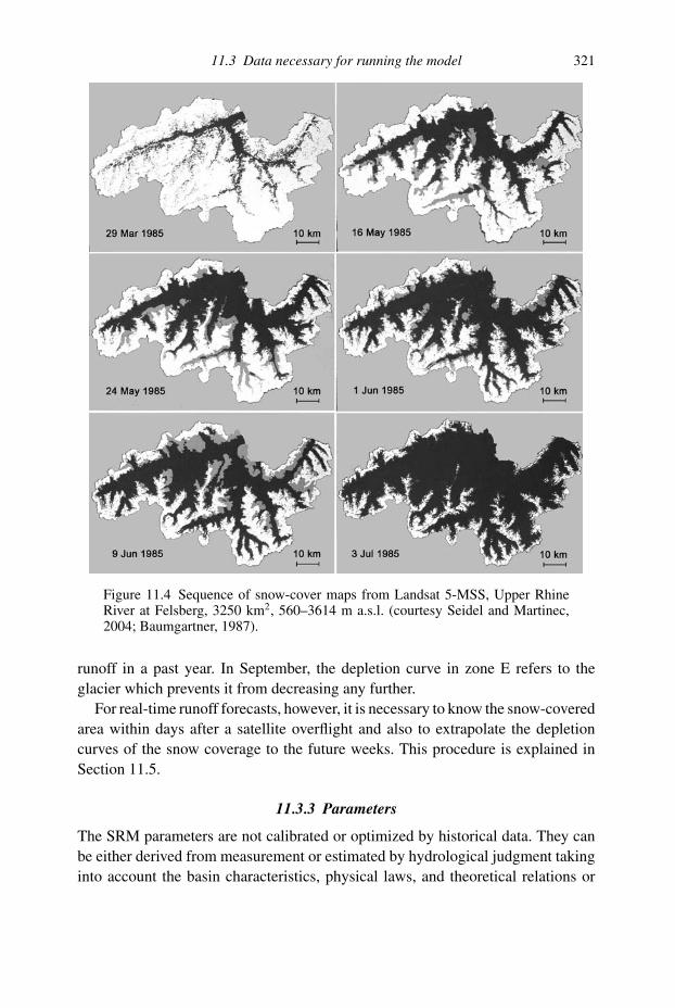
11.3 Data necessary for running the model 321
Figure 11.4 Sequence of snow-cover maps from Landsat 5-MSS, Upper RhineRiver at Felsberg, 3250 km2, 560–3614 m a.s.l. (courtesy Seidel and Martinec,2004; Baumgartner, 1987).
runoff in a past year. In September, the depletion curve in zone E refers to the
glacier which prevents it from decreasing any further.
For real-time runoff forecasts, however, it is necessary to know the snow-covered
area within days after a satellite overflight and also to extrapolate the depletion
curves of the snow coverage to the future weeks. This procedure is explained in
Section 11.5.
11.3.3 Parameters
The SRM parameters are not calibrated or optimized by historical data. They can
be either derived from measurement or estimated by hydrological judgment taking
into account the basin characteristics, physical laws, and theoretical relations or

322 Snowmelt-Runoff Model (SRM)
Figure 11.5 Depletion curves of the snow coverage for five elevation zones ofthe basin Felsberg, derived from the Landsat imagery shown in Figure 11.4. A:560–1100 m a.s.l., B: 1100–1600 m a.s.l., C: 1600–2100 m a.s.l., D: 2100–2600m a.s.l., E: 2600–3600 m a.s.l. (courtesy Seidel and Martinec, 2004; Baumgartner,1987).
empirical regression relations. Occasional subsequent adjustments should never
exceed the range of physically and hydrologically acceptable values.
Runoff coefficient, cThis coefficient takes care of the losses, that is to say of the difference between the
available water volume (snowmelt + rainfall) and the outflow from the basin. On
a long-term basis, it should correspond to the ratio of the measured precipitation
to the measured runoff. In fact, comparison of historical precipitation and runoff
ratios provide a starting point for the runoff coefficient values. However, these
ratios are not always easily obtained in view of the precipitation catch deficit which
particularly affects snowfall and of inadequate precipitation data from mountain
regions. At the start of the snowmelt season, losses are usually very small because
they are limited to evaporation from the snow surface, especially at high elevations.
In the next stage, when some soil becomes exposed and vegetation grows, more
losses must be expected due to evapotranspiration and interception. Towards the
end of the snowmelt season, direct channel flow from the remaining snowfields
and glaciers may prevail in some basins which leads to a decrease of losses and to
an increase of the runoff coefficient. In addition, c is usually different for snowmelt
and for rainfall. The computer program accepts separate values for snow, cS, and
rain, cR, and allows for half-monthly (and, if required, daily) changes of values in
each elevation zone. Examples of seasonal trends of runoff coefficients are given
in Figures 11.6 and 11.7, with the half-monthly values connected by straight lines.

11.3 Data necessary for running the model 323
Figure 11.6 Average runoff coefficient for snow (cS) for the alpine basins Dis-chma (43.3 km2, 1668–3146 m a.s.l.) and Durance (2170 km2, 786–4105 m a.s.l.)(Martinec and Rango, 1986).
Figure 11.7 Average runoff coefficient for rainfall (cR) for the basins Dischma andDurance (Martinec and Rango, 1986).
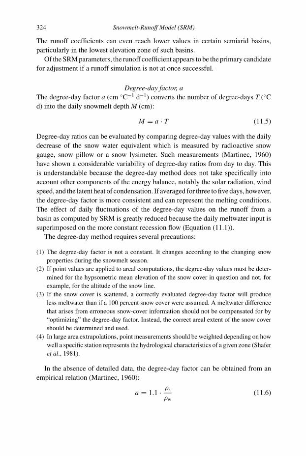
324 Snowmelt-Runoff Model (SRM)
The runoff coefficients can even reach lower values in certain semiarid basins,
particularly in the lowest elevation zone of such basins.
Of the SRM parameters, the runoff coefficient appears to be the primary candidate
for adjustment if a runoff simulation is not at once successful.
Degree-day factor, aThe degree-day factor a (cm ◦C−1 d−1) converts the number of degree-days T (◦C
d) into the daily snowmelt depth M (cm):
M = a · T (11.5)
Degree-day ratios can be evaluated by comparing degree-day values with the daily
decrease of the snow water equivalent which is measured by radioactive snow
gauge, snow pillow or a snow lysimeter. Such measurements (Martinec, 1960)
have shown a considerable variability of degree-day ratios from day to day. This
is understandable because the degree-day method does not take specifically into
account other components of the energy balance, notably the solar radiation, wind
speed, and the latent heat of condensation. If averaged for three to five days, however,
the degree-day factor is more consistent and can represent the melting conditions.
The effect of daily fluctuations of the degree-day values on the runoff from a
basin as computed by SRM is greatly reduced because the daily meltwater input is
superimposed on the more constant recession flow (Equation (11.1)).
The degree-day method requires several precautions:
(1) The degree-day factor is not a constant. It changes according to the changing snow
properties during the snowmelt season.
(2) If point values are applied to areal computations, the degree-day values must be deter-
mined for the hypsometric mean elevation of the snow cover in question and not, for
example, for the altitude of the snow line.
(3) If the snow cover is scattered, a correctly evaluated degree-day factor will produce
less meltwater than if a 100 percent snow cover were assumed. A meltwater difference
that arises from erroneous snow-cover information should not be compensated for by
“optimizing” the degree-day factor. Instead, the correct areal extent of the snow cover
should be determined and used.
(4) In large area extrapolations, point measurements should be weighted depending on how
well a specific station represents the hydrological characteristics of a given zone (Shafer
et al., 1981).
In the absence of detailed data, the degree-day factor can be obtained from an
empirical relation (Martinec, 1960):
a = 1.1 · ρs
ρw
(11.6)

11.3 Data necessary for running the model 325
Figure 11.8 Average degree-day ratio (a) used in runoff simulations by the SRMmodel in the basins Dischma (10 years), Durance (five years) and Dinwoody(228 km2; 1981–4202 m a.s.l., Wyoming, 2 years) (Martinec and Rango, 1986).
where:
a = the degree-day factor (cm ◦C−1d−1)
ρs = density of snow
ρw = density of water
When the snow density increases, the albedo decreases and the liquid water
content in snow increases. Thus the snow density is an index of the changing
properties which favor the snowmelt.
Figure 11.8 illustrates the seasonal trend of the degree-day factor in the Alps and
in the Rocky Mountains. Because the geographic latitude of a basin influences the
solar radiation, it may be advisable to adjust the degree-day factors accordingly. In
glacierized basins, the degree-day factor usually exceeds 0.6 cm ◦C−1 d−1 towards
the end of the summer when ice becomes exposed (Kotlyakov and Krenke, 1982).
The computer program accepts different degree-day factors for up to eight eleva-
tion zones which are usually changed twice a month (although daily changes are
possible).
Sometimes the occurrence of a large, late-season snowfall will produce depressed
a-values for several days due to the new low-density snow. The a-values in the model
can be manually modified and inserted to reflect these unusual snowmelt conditions.
326 Snowmelt-Runoff Model (SRM)
As is evident from Equation (11.1), the degree-day method could be readily
replaced by a more refined computation of snowmelt without changing the struc-
ture of SRM. Such refinement appeared to be imperative in a study of outflow from
a snow lysimeter (Martinec, 1989) but is not considered to be expedient for hydro-
logical basins until the necessary additional variables and their forecasts become
available. The degree-day method is explained in more detail in a separate publi-
cation (Rango and Martinec, 1995).
Temperature lapse rate, γ
If temperature stations at different altitudes are available, the lapse rate can be
predetermined from historical data. Otherwise it must be evaluated by analogy from
other basins or with regard to climatic conditions. In SRM simulations, a lapse rate
of 0.65 ◦C per 100 m was usually employed. Slightly higher, seasonally changing
values appeared to be a characteristic of tests in the Rocky Mountains. The computer
program accepts either a single or a basin-wide lapse rate (option 0) or different rates
for each zone (option 1). Seasonal variations can also be accommodated by inputting
predetermined lapse rates every 15 days, and the lapse rate can be changed manually
on selected days if a special meteorological situation (for example, a temperature
inversion) requires a different value.
If the temperature station is situated near the mean elevation of the basin, possible
errors in the lapse rate are to some extent canceled out because the extrapolation
of temperature takes place upwards as well as downwards. If, on the other hand,
the temperature station is at a low altitude, SRM becomes sensitive to the lapse
rate. For some basins in Wyoming, for example, the closest temperature station
was more than 100 km away and 2000 m lower than the highest snow-covered parts
of the basins. In such a case, an error in the lapse rate of only 0.05 ◦C per 100 m
causes a deviation of one degree-day from the correct degree-day value which
corresponds to an error of about 0.5 cm of the computed daily meltwater depth late
in the snowmelt season.
Such situations sometimes necessitate an adjustment of the originally selected
lapse rate taking into account the course of the depletion curves of snow coverage. If
high temperatures result from extrapolation by a certain lapse rate but no change in
the snow areal extent is observed, then probably no appreciable snowmelt is taking
place at this altitude. The high temperatures result from a false lapse rate which
must be increased or decreased, depending on whether the temperature station is
lower or higher than the mean zone elevation.
Critical temperature, TCRIT
The critical temperature determines whether the measured or forecasted precip-
itation is rain or snow. Models which simulate the build-up of the snow cover

11.3 Data necessary for running the model 327
first in order to simulate the runoff depend heavily on this parameter not only
in the ablation period but particularly in the accumulation period. SRM needs
the critical temperature only in order to decide whether precipitation immedi-
ately contributes to runoff (rain), or, if T < TCRIT, whether snowfall took place.
In this case, SRM automatically keeps the newly fallen snow in storage until
it is melted on subsequent warm days, as explained in Section 11.3.2 under
“Precipitation”.
When SRM was applied in the alpine basin Dischma, TCRIT started at +3 ◦C
in April at the beginning of snowmelt and diminished to +0.75 ◦C in July. This
seasonal trend with a narrower range appears to be applicable in other basins. At
certain times, SRM may not take notice of a sharp rainfall runoff peak because
the corresponding precipitation is determined to be snow, the extrapolated tem-
perature being just slightly below the critical temperature. In such cases the
assignment of critical-temperature and the temperature-lapse-rate values should
be reviewed and logical adjustments made in order to change snow to rain. It
is of course difficult to distinguish accurately between rain and snow because
the temperature used is the daily mean while precipitation may occur at any
time, day or night, i.e., in the warmer or colder portion of the daily temperature
cycle.
As a possible refinement, formulas have been proposed (Higuchi et al., 1982) to
determine the proportion of rain and snow in mixed precipitation conditions.
Rainfall contributing area, RCAWhen precipitation is determined to be rain, it can be treated in two ways. In the
initial situation (option 0), it is assumed that rain falling on the snowpack early
in the snowmelt season is retained by the snow which is usually dry and deep.
Rainfall runoff is added to snowmelt runoff only from the snow-free area, that is to
say the rainfall depth is reduced by the ratio snow-free area/zone area. At some later
stage, the snow cover becomes ripe (the user must decide on which date) and the
computer program should be switched to option 1. Now, if rain falls on this snow
cover, it is assumed that the same amount of water is released from the snowpack
so that rain from the entire zone area is added to snowmelt. The melting effect of
rain is neglected because the additional heat supplied by the liquid precipitation is
considered to be small (Wilson, 1941).
Recession coefficient, kAs is evident from Equation (11.1), the recession coefficient is an important feature
of SRM since (1 − k) is the proportion of the daily meltwater production which
immediately appears in the runoff. Analysis of historical discharge data is usually

328 Snowmelt-Runoff Model (SRM)
Figure 11.9 Recession flow plot Qn vs Qn+1 for the Dischma basin in Switzerland.Either the solid envelope line or the dashed medium line is used to determinek-values for computing the constants x and y in Equation (11.7) (Martinec andRango, 1986).
a good way to determine k. Figure 11.9 shows such an evaluation for the alpine
basin Dischma (43.3 km2, 1668–3146 m a.s.l.). Values of Qn and Qn+1 are plotted
against each other and the lower envelope line of all points is considered to indi-
cate the k-values. Based on the relation k = Qn+1/Qn, it can be derived that for
example k1 = 0.677 for Qn = 14 m3 s−1 and k2 = 0.85 for Qn = 1 m3 s−1. This
means that k is not constant, but increases with the decreasing Q according to the
equation:
kn+1 = x · Q−yn (11.7)
where the constants x and y must be determined for a given basin by solving the
equations:
k1 = x · Q−y1
k2 = x · Q−y2
log k1 = log x − y log Q1 (11.8)
log k2 = log x − y log Q2 (11.9)

11.3 Data necessary for running the model 329
In the given example,
log 0.677 = log x − y log 14
log 0.85 = log x − y log 1
x = 0.85
y = 0.086
As a formal change from the SRM User’s Manual of 1983 (Martinec et al., 1983),
a negative sign appears in the exponent of Equation (11.7) so that the numerical
values of x and y are positive.
The variability of k according to Equation (11.7) was also confirmed in other
basins. This means that the recession does not exactly follow the usual equation
Qn = Q0 · kn (11.10)
where:
Q0 = the initial discharge
Qn = the discharge after n days
but the following equation Jaccard (personal communication, 1982)
Qn = x1y
(Q0
x1y
)(1−y)n
(11.11)
where x and y are the constants of Equation (11.7).
The envelope line in Figure 11.9 and the resulting values of x and y must be
determined for each basin. For ungauged basins and when historical discharge data
are insufficient, x and y can be derived indirectly from the size of the basin as
follows:
kNn =[
xM
(QM
QN
· QNn − 1
)−yM] 4
√AM/AN
(11.12)
where: xM, yM are the known constants for the basin M; QM, QN are average
discharge values from the basin M and the new basin N; and AM, AN are the areas
of the respective basins.
Equation (11.12) indicates that recession coefficients are generally higher in large
basins than in small basins. If the increase in k with size appears to be too large, the
exponent may be replaced by 8√
AM/AN. Even if the envelope line in Figure 11.9
can be reliably derived in a basin, it is possible that the resulting k-values may be
too low to represent average conditions during the snowmelt season, especially in
large basins. In such cases the SRM model will react too quickly to any change of
the daily input. The simulated peaks would be too high and the simulated recession

330 Snowmelt-Runoff Model (SRM)
Figure 11.10 Range of recession coefficients, k, related to discharge Q resultingfrom various evaluations: In Dischma, the range results from using either theenvelope line or the medium line in Figure 11.9. In Modry Dul, the relation variesin different years. In Felsberg, the relations (1) and (2) are derived from the sizeof the basin by two alternative formulas (Martinec and Rango, 1986).
too fast. A quick improvement is possible by deriving a new x and y, not from the
envelope line, but from an intermediate or medium line between the envelope and
the 1:1 line. This modification may especially be needed if the runoff simulation
is extended to the whole year. Recession coefficients which may be right for the
snowmelt period are usually too low for the winter months so that the simulated
flows drop below the measured minimum values.
In very small basins, noticeable differences in the recession flow conditions and
the k-values may occur from year to year. Figure 11.10 illustrates the range of
k-values for varying basin size and for the mentioned alternatives of evaluation.
For a very small mountain basin, the range includes the variations of k in different
years (Martinec, 1970). For a larger alpine basin, the limits refer to the envelope
line and to the medium line in Figure 11.9. For the largest basin, the higher limit
(1) of the indicated range was derived by substituting the constants x = 0.085,
y = 0.086 derived for the Dischma basin into Equation (11.12). The lower limit (2)
was obtained by replacing 4√
AM/AN in Equation (11.12) with 8√
AM/AN.
Figure 11.10 shows that k can theoretically exceed 1 for very small discharges
in large basins. This does not really happen because such small discharges do not
occur there. Such a situation could be produced, however, by the user inadvertently

11.3 Data necessary for running the model 331
taking over the x and y values derived in a large basin and using them for a small
basin without modification. In this case, if the daily snowmelt input exceeds the
previous day’s runoff, SRM computes a runoff decrease instead of increase. In order
to avoid this error, the computer program prevents k from exceeding 0.99. However,
it is advisable to avoid approaching this limiting situation by checking the x and y
values with regard to the lowest flow to be expected. Recalling Equation (11.11),
it follows for n = ∞, because y > 0 and (1 − y) < 1:
Q∞ = x1y
(Q0
x1y
)(<1)∞
= x1y (11.13)
Therefore the values x and y should fulfill the condition:
QMin > x1y (11.14)
where QMin = the minimum discharge in the given basin.
Adjustment of the recession coefficient for heavy rainfalls The equation (11.7)
for computing the recession coefficient reflects the usual conditions characterizing
the snowmelt runoff in the given basin. When a heavy rainfall occurs, the input
is concentrated in a short time interval creating an abrupt rise and subsequent
decline of the hydrograph. In order to simulate such events, the computer program
automatically adjusts the recession coefficient whenever the daily rainfall averaged
over the whole basin equals or exceeds 6 cm:
If P (rain)n ≥ 6 cm −→ kn+1 = x(4 Qn)−y
kn+2 = x(4 Qn+1)−y
kn+3 = x(4 Qn+2)−y
kn+4 = x(4 Qn+3)−y
kn+5 = x(4 Qn+4)−y (11.15)
after which it returns to the normal equation (11.7). In this way, k gets lower so
that the basin response to input becomes faster. If the precipitation is recognized
by TCRIT as snow and not rain, the mechanism will not be activated.
The threshold value can be changed in order to activate the rainfall peak program
for smaller rainfall amounts or to delay activation until higher rainfall amounts are
reached.
Time lag, LThe characteristic daily fluctuations of snowmelt runoff enable the time lag to
be determined directly from the hydrographs of the past years. If, for example, the
discharge starts rising each day around noon, it lags behind the rise of temperature by
332 Snowmelt-Runoff Model (SRM)
Figure 11.11 Snowmelt hydrographs illustrating the conversion of computedrunoff amounts for 24-hour periods to calendar day periods. The various time lags(bold lines) are taken into account by proportions of the daily inputs, I (Martinecand Rango, 1986).
about six hours. Consequently, temperatures measured on the nth day correspond to
discharge between 1200 hrs on the nth day and 1200 hrs on the n + 1 day. Discharge
data, however, are normally published for midnight-to-midnight intervals and need
adjustments in order to be compared with the simulated values. Conversely, the
simulated values can be adjusted (Shafer et al., 1981) to refer to the midnight-to-
midnight periods. Figure 11.11 illustrates the procedure for different time lags. For
L = 6 hour, 50% of input computed for temperature and precipitation on the nth
day (In) plus 50% of In +1 results in the n + 1 day’s runoff after being processed by
the SRM computer program:
L = 6 h 0.5 · In + 0.5 · In+1 → Qn+1 (11.16)
Similarly:
L = 12 h 0.75 · In + 0.25 · In+1 → Qn+1 (11.17)
L = 18 h In → Qn+1 (11.18)
L = 24 h 0.25 · In + 0.75 · In+1 → Qn+2 (11.19)
This procedure is preferable, at least in mountain basins smaller than 5000 km2,
to evaluations of L by calculating the velocity of overland flow and channel flow. It
11.4 Assessment of the model accuracy 333
has been shown by environmental isotope tracer studies (Martinec, 1985) that over-
land flow is not a major part of the snowmelt runoff as previously believed. There
is increasing evidence that a major part of meltwater infiltrates and quickly stim-
ulates a corresponding outflow from the groundwater reservoir. With this runoff
concept in mind, the seemingly oversimplified treatment of the time lag in the
SRM model is better understood. If the hydrographs are not available or if their
shape is distorted by reservoir operations, the time lag can be estimated accord-
ing to the basin size and by analogy with other comparable basins. Generally,
the time lag in a basin increases as the snow line retreats. In the WMO inter-
comparison test (WMO, 1986), most models calibrated the time lag. However,
these results appear to be of little help to determine the proper values. Contra-
dictory time lags have been calibrated by different models. However, if the time
lags for all models participating in the WMO intercomparison test are averaged for
each basin, the resulting values support the expected relation between L and basin
size:
Basin W-3 (8.42 km2) : 3.0 h
Dischma (43.3 km2) : 7.2 h
Dunajec (680 km2) : 10.5 h
Durance (2170 km2) : 12.4 h
If there is some uncertainty, L (percentages in Equations (11.16)–(11.19)) can be
adjusted in order to improve the synchronization of the simulated and measured
peaks of average daily flows. It should be noted that a similar effect results from
an adjustment of the recession coefficient.
11.4 Assessment of the model accuracy
Accuracy criteriaThe SRM computer program includes a graphical display of the computed hydro-
graph and of the measured runoff. A visual inspection shows at the first glance
whether the simulation is successful or not. SRM additionally uses two well-
established accuracy criteria, namely, the coefficient of determination, R2, and the
volume difference, Dv.
The coefficient of determination is computed as follows:
R2 = 1 −
n∑i=1
(Qi − Q′i)
2
n∑i=1
(Qi − Q)2
(11.20)

334 Snowmelt-Runoff Model (SRM)
where:
Qi = the measured daily discharge
Q′i = the computed daily discharge
Q = the average measured discharge of the given year or snowmelt season
n = the number of daily discharge values
Equation (11.20) also corresponds to the Nash–Sutcliffe coefficient in which
case Q is a long-term average measured discharge applied to the respective years
or seasons.
The deviation of the runoff volumes, Dv, is computed as follows:
Dv[%] = VR − V ′R
VR
· 100 (11.21)
where:
VR is the measured yearly or seasonal runoff volume
V ′R is the computed yearly or seasonal runoff volume
Numerical accuracy criteria are never perfect, as illustrated by Figure 11.12.
From the visual judgment both simulations look good because the fundamental
Figure 11.12 Runoff simulations in the basin of the Rio Grande near Del Norte,Colorado (3419 km2, 2432–4215 m a.s.l.) (Martinec and Rango, 1989).

11.4 Assessment of the model accuracy 335
difference between two extreme years is well reproduced. However, R2 = 0.95 in
1979 while it amounts only to 0.48 in 1977. In spite of this unfavorable value, the
simulation (or forecast) in 1977 would certainly be useful for water management
because it correctly reveals an extremely low runoff.
With Q as a long-term average substituted into Equation (11.20) (Nash–Sutcliffe)
instead of the average for the specific year, a much more favorable but deceptive
value for R2 of 0.97 results for the year 1977. This value is high because the long-
term Q is much higher than any Q in 1977. Consequently, the daily deviations of
the simulated runoff become relatively insignificant although in absolute terms they
are not negligible. In addition to these criteria which are automatically computed
and displayed after each model run, the coefficient of gain from daily means, DG,
could be computed by the user as follows:
DG = 1 −
n∑i=1
(Qi − Q′i)
2
n∑i=1
(Qi − Qi)2
(11.22)
where:
Qi = the measured daily discharge
Q′i = the computed daily discharge
Qi = the average measured discharge from the past years for each day of the period
n = the number of days
Thus, R2 compares the performance of a model with “no model” (average dis-
charge) and DG with a “seasonal model” (long-term average runoff pattern). Neg-
ative values signal that the model performed worse than “no model” or worse than
the “seasonal model.”
Model accuracy outside the snowmelt seasonSRM has been designed to compute runoff during the snowmelt season, but it
can be run for the whole year if required. According to the mentioned WMO
intercomparison test (WMO, 1986), about the same accuracy as for the snowmelt
season can be achieved for the entire year in mountain basins with a low winter
runoff. An example in Figure 11.13 shows that SRM can even be run without
updating for ten years.
Elimination of possible errorsIt is not possible to give threshold values of accuracy criteria which would deter-
mine whether a model run is successful or whether something must be changed.
With good data, a value like R2 = 0.80 might still be improved. In unfavorable
conditions, with incomplete data, a user may be satisfied even with lower R2 values.

Fig
ure
11
.13
Ru
no
ffsi
mu
lati
on
sin
the
bas
inD
isch
ma
(43
.3k
m2,
16
68
–3
14
6m
a.s.
l.).
Co
mp
uta
tio
no
fd
aily
flow
sis
exte
nd
edto
10
yea
rsw
ith
ou
tu
pd
atin
g(M
arti
nec
and
Ran
go
,1
98
6).

11.5 Operation of the model for real-time forecasts 337
Sometimes, however, the graphical display as well as the numerical criteria indicate
that something went definitely wrong. Before adjusting one or the other parameter,
it is recommended to check several probable sources of error first. Examples in
Table 11.4 are based on the actual experience of various users.
11.5 Operation of the model for real-time forecasts
In order to be applied for real-time discharge forecasts, a model should be able to
simulate the runoff not only in selected test basins with good data or in specially
equipped experimental basins where a particular calibration model was developed,
but also in basins where such forecasts are required by the user. SRM has relatively
modest requirements for input variables (temperature, precipitation, and snow-
covered area) and therefore it was easily possible to shift the runoff simulations
to the basins delivering water for hydroelectric schemes, as required by an electric
company. An example of such simulations is shown in Figure 11.14.
As mentioned in Section 11.1, SRM can be used for short-term (for example
weekly) forecasts of daily flows as well as for longer time period forecasts such
as monthly runoff volumes or seasonal runoff volumes. For short-term forecasts,
temperature, precipitation, and snow-covered area must be forecasted or prede-
termined for the coming days and substituted into the model. Temperature and
even precipitation forecasts are becoming increasingly available from meteoro-
logical services, but the snow-covered areas must be extrapolated by the model
user.
Extrapolation of the snow coverageThe future course of the depletion curves of the snow coverage can be evalu-
ated from the so-called modified depletion curves (MDC). These curves are auto-
matically derived by SRM from the conventional curves (CDC) by replacing the
time scale with cumulative daily snowmelt depths as computed by the model.
Consequently, if SRM is run in a whole hydrological year, the derivation of
MDC from CDC starts with the summer half year and not earlier. The decline
of the modified depletion curves depends on the initial accumulation of snow
and not on the climatic conditions, as is the case with the conventional depletion
curve.
Procedure for weekly forecasts of daily flowsAssumption: A family of modified depletion curves has been derived from the past
snow-cover monitoring and temperature measurements in the given basin. Two of
these curves representing the initial water equivalents HW = 20 cm and HW =60 cm are plotted in Figure 11.15.

Tab
le11.4
Err
ors
expe
rien
ced
bySR
Mus
ers
and
thei
rco
rrec
tion
Err
or
Cau
se
1R
un
off
sim
ula
tio
nw
ent
too
hig
h(D
inw
oo
dy,
19
76
;D
isch
ma,
19
77
).S
now
-cover
dep
leti
on
curv
esd
isto
rted
by
sum
mer
snow
fall
:E
lim
inat
esa
tell
ite
ob
serv
atio
naf
ter
asn
owfa
llev
ent
and
red
raw
the
dep
leti
on
curv
es.
2R
un
off
sim
ula
tio
nsu
dd
enly
det
erio
rate
d(D
isch
ma)
.In
pu
to
fsn
ow-c
over
age
dat
aS
shif
ted
by
1m
on
th:
Co
rrec
tth
eS-
inp
ut.
3T
he
sim
ula
ted
run
off
hy
dro
gra
ph
dec
lin
edu
nco
ntr
oll
ably
inS
epte
mb
er(I
llec
ille
wae
tb
asin
).In
pu
to
fsn
ow-c
over
age
dat
ab
roken
off
by
the
end
of
Au
gu
st:
Co
mp
lete
the
S-in
pu
t.4
Ru
no
ffsi
mu
lati
on
far
bel
owth
em
easu
red
run
off
(Ill
ecil
lew
aet)
.D
ecim
alp
oin
tin
the
mea
sure
dp
reci
pit
atio
nan
dd
isch
arg
ed
ata
shif
ted
and
ther
eby
incr
easi
ng
the
mea
sure
dru
no
ff1
0×,
but
the
sim
ula
ted
run
off
on
lysl
igh
tly
:C
orr
ect
the
dec
imal
po
int.
5A
fter
the
star
to
fsn
owm
elt,
the
sim
ula
ted
run
off
kep
td
ecre
asin
gin
spit
eo
fsn
owm
elt
inp
ut
(sm
all
trib
uta
ryb
asin
so
fu
pp
erR
hin
e,1
98
5).
Val
ues
x,
yfo
rth
ere
cess
ion
coef
fici
ent
form
ula
(Eq
uat
ion
(11
.7))
wer
eta
ken
over
fro
ma
mu
chla
rger
bas
inso
that
kex
ceed
ed1
.0fo
rlo
wQ
:C
orr
ect
x,
yw
ith
regar
dto
the
bas
insi
ze.
Poss
ibil
ity
of
this
erro
rw
asel
imin
ated
inth
eco
mp
ute
rp
rog
ram
Ver
sio
n2
.01
and
late
rver
sio
ns
(3.0
,3
.1,
3.1
1,
and
4.0
).6
Fre
qu
ent
dev
iati
on
sfr
om
the
mea
sure
dru
no
ff,
per
iodic
allo
ws
of
the
hydro
gra
ph
not
sim
ula
ted
(Fel
sber
g,
19
82
).
SR
Msi
mu
late
sn
atu
ral
run
off
wh
ile
the
mea
sure
dru
no
ffw
asin
flu
ence
db
yst
ora
ge
(on
wee
ken
ds)
and
rele
ase
from
arti
fici
alre
serv
oir
sfo
rhydro
pow
er.
Th
ese
inte
rven
tio
ns
mu
stb
eco
rrec
ted
ino
rder
toco
mp
are
sim
ula
ted
and
mea
sure
dru
no
ff.
7R
ain
fall
pea
ks
inad
equ
atel
ysi
mu
late
d(I
llec
ille
wae
t).
Rai
nfa
llin
pu
tis
con
cen
trat
edto
sho
rter
per
iod
sth
ansn
owm
elt
inp
ut
wh
ich
acce
lera
tes
the
bas
inre
spo
nse
.P
rog
ram
Ver
sio
ns
2.0
1an
dla
ter
ver
sio
ns
take
this
feat
ure
auto
mat
ical
lyin
toac
cou
nt
wh
enev
erra
infa
llex
ceed
sa
pre
sele
cted
thre
sho
ld.
8R
ain
fall
pea
kin
adeq
uat
ely
sim
ula
ted
even
wit
hth
esp
ecia
lra
infa
llp
eak
pro
gra
m(s
mal
ltr
ibu
tary
bas
ins
of
up
per
Rh
ine
Au
gu
st2
5,
19
85
).
Tem
per
atu
reex
trap
ola
ted
fro
mst
atio
n8
00
ma.
s.l.
tozo
ne
D2
38
0m
a.s.
l.b
y0
.65
◦ C/1
00
m→
T=
+0
.43
◦ Cw
hil
eT
CR
ITis
+0
.75
◦ C.
By
dec
reas
ing
TC
RIT
,sn
owfa
llw
asco
nver
ted
tora
infa
llan
dth
eru
no
ffp
eak
was
bet
ter
sim
ula
ted
.

9R
ain
fall
pea
kin
adeq
uat
ely
sim
ula
ted
bec
ause
the
dai
lyam
ou
nt
was
bel
owth
esp
ecia
lp
rog
ram
auto
mat
icth
resh
old
.T
hre
sho
ldw
aslo
wer
edbu
tth
ep
eak
sim
ula
tio
nd
eter
iora
ted
furt
her
(sm
all
trib
uta
ryb
asin
so
fu
pp
erR
hin
e,1
98
5).
On
lyo
ne
pre
cip
itat
ion
stat
ion
was
avai
lab
lebu
tth
e“b
yzo
ne”
op
tio
nw
assw
itch
edo
n.
Co
nse
qu
entl
yp
reci
pit
atio
nin
pu
tto
ok
pla
ceo
nly
ino
ne
zon
e.W
ith
on
est
atio
n,
sele
cto
pti
on
“bas
inw
ide.
”
10
Ru
no
ffsi
mu
lati
on
wen
tver
yh
igh
ina
bas
inw
ith
ala
rge
elev
atio
nra
ng
eo
f7
40
0m
(Kab
ul
Riv
er,
19
76
).
Co
mp
act
snow
cover
was
assu
med
above
the
snow
lin
eso
that
the
snow
-cover
edar
eaw
asex
agg
erat
ed.T
emp
erat
ure
was
extr
apo
late
db
yto
olo
wa
lap
sera
te.S
now
mel
tw
asn
ot
com
pu
ted
sep
arat
ely
for
elev
atio
nzo
nes
but
for
the
enti
reb
asin
.T
his
usu
ally
lead
sto
over
esti
mat
ion
of
mel
twat
erin
pu
t.S
imu
lati
on
was
imp
roved
by
re-e
valu
atin
gth
esn
owco
ver
age
and
sele
ctin
ga
hig
her
tem
per
atu
rela
pse
rate
corr
esp
on
din
gto
the
clim
ate.
Wit
hre
gar
dto
the
larg
eel
evat
ion
range,
the
bas
insh
ould
hav
ebee
ndiv
ided
inse
ver
alel
evat
ion
zon
es.
11
Dis
tort
edru
no
ffsi
mu
lati
on
(ou
tflow
fro
ma
snow
lysi
met
er).
Val
ues
of
rece
ssio
nco
effi
cien
tfa
lse:
Neg
ativ
ey
valu
esuse
dw
ith
the
equ
atio
nk
=x
·Q−y
soth
atth
eex
po
nen
tb
ecam
ep
osi
tive.
Co
nse
qu
entl
y,k
incr
ease
dw
ith
the
incr
easi
ng
Qw
hil
eit
sho
uld
hav
ed
ecre
ased
.U
seeq
uat
ion
k=
x·Q
−yan
dp
osi
tive
valu
eso
fy,
soth
atth
eex
po
nen
tis
alw
ays
neg
ativ
e.1
2D
iffi
cult
ies
wit
hth
eti
min
go
fra
infa
ll-r
un
off
pea
ks
(WM
Ote
stfo
rsi
mu
late
do
per
atio
nal
fore
cast
s,Il
leci
llew
aet
bas
in).
Pre
cip
itat
ion
dat
afr
om
on
eo
fth
est
atio
ns
wer
eas
crib
edto
the
dat
eo
nw
hic
hit
was
mea
sure
dat
08
00
.D
ata
had
tob
esh
ifte
do
ne
day
bac
kw
ard
s.S
eeal
soS
ecti
on
5.2
.2.
13
Fore
cast
edru
noff
for
hydro
elec
tric
stat
ions
Sed
run
and
Tav
anas
ato
olo
win
Ap
ril–
Jun
e1
99
4.
Ino
ne
run
,sn
owco
ver
was
no
tco
mp
lete
lym
elte
db
yth
een
do
fS
epte
mb
er.
Sn
owm
elt
was
com
pu
ted
by
smo
oth
lon
g-t
erm
aver
age
tem
per
atu
reth
us
dec
reas
ing
the
nu
mb
ero
fd
egre
ed
ays.
Rei
ntr
od
uce
the
dai
lyfl
uct
uat
ion
so
fte
mp
erat
ure
s.
14
Dis
crep
anci
esin
run
off
sim
ula
tio
ns
for
Rio
Gra
nd
eat
Del
No
rte.
Err
atic
pre
cip
itat
ion
dat
a.A
uto
mat
icex
trap
ola
tio
nb
yal
titu
de
gra
die
nts
from
two
stat
ions
resu
lted
inneg
ativ
epre
cipit
atio
nam
ounts
inth
ehig
hes
tzo
ne
wh
eng
rad
ien
tw
asn
egat
ive.
Ex
trap
ola
teav
erag
edp
reci
pit
atio
nd
ata
by
au
nif
orm
gra
die
nt
asre
com
men
ded
inS
ecti
on
5.2
.A
lway
sv
isu
ally
insp
ect
inp
ut
pre
cip
itat
ion
dat
a.1
5D
iscr
epan
cies
inru
no
ffsi
mu
lati
on
sfo
rR
ioG
ran
de
atD
elN
ort
eO
ccas
ion
ally
mis
sin
gte
mp
erat
ure
dat
aw
ere
inte
rpre
ted
by
the
com
pu
ter
pro
gra
mas
0=
0◦ C
.In
spec
tte
mp
erat
ure
dat
aan
dco
mp
lete
mis
sin
gva
lues
by
inte
rpo
lati
on
.(c
ont.)

Tab
le11.4
(con
t.)
Err
or
Cau
se
16
Eff
ect
of
clim
ate
chan
ge
(see
Sec
tio
n8
.3):
Dec
reas
eo
fru
no
ffco
mp
ute
db
yan
incr
ease
dte
mp
erat
ure
(Rio
Gra
nd
eat
Del
No
rte)
Th
e“w
inte
rd
efici
t”w
asex
ceed
edo
na
war
md
ayw
ith
ah
igh
snow
mel
td
epth
,so
that
too
mu
chw
ascu
to
fffr
om
MD
CE
XC
L.
Co
nse
qu
entl
yC
DC
CL
IMw
assh
ifte
dto
om
uch
and
less
run
off
resu
lted
.C
ut
off
MD
CE
XC
L
by
the
valu
eo
fth
ep
rev
iou
sd
ay(“
nea
rly
equ
alle
d”)
.1
7O
ver
esti
mat
ion
of
run
off
inth
eR
hin
e-F
elsb
erg
bas
in1
–1
5M
ay1
99
3w
ith
usu
alte
mp
erat
ure
lap
sera
teo
f0
.65
◦ C/1
00
m.
Fre
qu
ent
foh
n-w
ind
inth
isp
erio
d,
tem
per
atu
red
iffe
ren
ces
bet
wee
nW
eiss
flu
hjo
ch(2
69
3m
a.s.
l.)
and
Dav
os
(15
60
ma.
s.l.
)co
rres
po
nd
toa
lap
sera
teas
hig
has
0.9
5◦ C
/10
0m
.T
he
valu
eo
f0
.8◦ C
/10
0m
was
use
d.
18
Eva
luat
ion
of
the
clim
ate
effe
ctin
the
Kin
gs
Riv
erb
asin
19
73
:F
or
ate
mp
erat
ure
incr
ease
+4◦ C
,sn
owco
ver
on
Ap
ril
1d
isap
pea
rsin
the
Czo
ne
(17
00
–2
30
0m
.a.s
.l.)
but
stil
lex
ists
inth
elo
wer
Bzo
ne
(11
00
–1
70
0m
a.s.
l.)
Th
ed
ecre
ase
of
the
snow
wat
ereq
uiv
alen
to
nA
pri
l1
du
eto
war
min
gis
eval
uat
edfr
om
un
ifo
rmam
ou
nts
of
pre
cip
itat
ion
and
snow
mel
td
epth
sin
win
ter
inea
chzo
ne
(Fig
ure
s1
1.2
0,
11
.21
).T
he
snow
inth
eB
zon
ew
asco
mp
lete
lym
elte
dfo
rT
◦ Co
nA
pri
l1
soth
atn
ow
inte
rd
efici
tre
sult
edfo
rT
+4
◦ .H
owev
er,
inre
alit
y,so
me
snow
surv
ived
for
T◦ C
du
eto
vari
able
snow
dep
ths
asse
enb
ysa
tell
ites
(S=
27
%o
nA
pri
l1
).W
ith
no
com
pu
ted
snow
for
T◦ C
asw
ell
asfo
rT
+4
◦ C,
no
win
ter
defi
cit
resu
lted
and
ther
efo
reth
eex
isti
ng
snow
cover
was
fals
ely
pre
serv
edfo
rT
+4
◦ C.
Am
anu
alco
rrec
tio
n(e
lim
inat
ion
of
CD
CC
LIM
)w
asn
eces
sary
.In
the
Czo
ne
ther
ew
asen
ou
gh
snow
toav
oid
the
erro
rfr
om
un
ifo
rm,
inst
ead
of
vari
able
,sn
owd
epth
sin
win
ter,
soth
atth
esn
owco
ver
du
lyd
isap
pea
red
asa
resu
lto
fth
eev
alu
ated
win
ter
defi
cit.
Th
iser
ror
can
occ
ur
on
lyw
ith
ver
yli
ttle
snow
ina
zon
eo
nA
pri
l1
and
can
be
read
ily
corr
ecte
d.
Wh
enev
ersa
tell
ites
see
som
esn
owo
nA
pri
l1
and
the
win
ter
accu
mu
lati
on
of
snow
fro
mp
reci
pit
atio
nan
dsn
owm
elt
isze
ro,
elim
inat
eC
DC
CL
IM.
19
Fai
lure
of
run
off
sim
ula
tio
ns
inth
eb
asin
Psk
em:
the
der
ived
con
stan
ty
inth
ere
cess
ion
form
ula
(Equat
ion
11.7
)is
neg
ativ
e,so
that
the
rece
ssio
nis
stee
per
for
low
flow
sth
anfo
rh
igh
flow
s.T
he
envel
op
eli
ne
inF
igu
re1
1.1
0w
asd
eriv
edta
kin
gin
toac
cou
nt
evid
entl
yfa
lse
po
ints
inth
elo
wra
ng
eo
ffl
ows.
Su
chp
oin
tsm
ayo
ccu
r,fo
rex
amp
le,
wh
enth
eri
ver
flow
isar
tifi
cial
lyst
op
ped
by
free
zin
g.
Th
ere
cess
ion
of
the
nat
ura
lru
no
ffsl
ows
dow
nw
ith
ad
ecre
asin
gd
isch
arg
e.T
oth
isef
fect
,y
mu
stb
e>
0.In
alo
g–
log
rep
rese
nta
tio
n(F
igu
re1
1.1
0),
the
po
ints
ou
tsid
eth
era
ng
eb
etw
een
the
1:1
lin
ean
da
par
alle
lli
ne
for
po
ints
inth
era
ng
eo
fh
igh
flow
s(b
elow
the
das
hed
lin
ein
Fig
ure
11
.10
)m
ust
be
dis
regar
ded
.W
ith
this
mea
sure
,th
epro
ble
mof
the
runoff
sim
ula
tion
was
elim
inat
ed.

11.5 Operation of the model for real-time forecasts 341
Figure 11.14 Runoff simulation in the catchment area of the hydroelectric sta-tion Tavanasa (Swiss Alps, 215 km2, 1277–3210 m a.s.l.) (Baumann et al., 1990,courtesy K. Seidel).
Figure 11.15 Extrapolation of snow-cover depletion curves in real-time from mod-ified depletion curves with the use of temperature forecasts. HW MAX is the waterequivalent of the snow cover at the beginning of the snowmelt season (courtesy D.Hall and J. Martinec).

342 Snowmelt-Runoff Model (SRM)
Example 1 – Snow accumulation in the basin unknown, snow coverage measured
by Landsat on May 15, S = 80%, cumulative snowmelt depth (from degree-days
and degree-day ratios) to date: 30 cm. Temperature forecast: 30 degree-days for
the next week, converted to meltwater depth M = 15 cm by a degree-day ratio
a = 0.5 cm ◦C−1d−1, S = 80% and �M = 30 cm indicate that the curve for
HW = 60 cm is applicable. The snow coverage will drop to 64% in seven days.
Extrapolated conventional depletion curve indicates values for day-to-day discharge
computations.
Example 2 – As above, but the cumulative snowmelt depth to date is only 10
cm. Consequently, the curve for HW = 20 cm is applicable and the snow coverage
will drop to 33% in seven days, which leads to a different extrapolation of the
conventional depletion curve and to a different weekly total of forecasted daily
runoff volumes. If the initial water equivalent is known, for example from SNOTEL
(a system of data transmission using meteor paths for reflecting the signals and
operated in the USA) or from manual snow surveys taken near the beginning of
the forecast period, the appropriate modified depletion curve can be selected at
the start of the snowmelt season. Otherwise, the average curve (dotted line in
Figure 11.15) is used until the correct curve can be identified by satellite data.
Figure 11.16 shows that it is possible to derive a nomograph of modified depletion
curves (Rango and van Katwijk, 1990) for a given basin from the past years. As
Figure 11.16 Nomograph of modified depletion curves for the elevation zone B(1284 km2, 2926–3353 m a.s.l.) of the Rio Grande basin. The curves are labelledwith the areal average water equivalent (April 1) of the snow cover which theyrepresent (Rango and van Katwijk, 1990).

11.5 Operation of the model for real-time forecasts 343
noticed in Figure 11.15, the area below a modified depletion curve indicates the
water volume stored in the snow cover if the y-axis scale is in km2. If the y-axis scale
is in percent snow coverage, it indicates the water equivalent of the snow cover as
an areal average. Therefore each curve in Figure 11.16 can be labelled by the water
equivalent which it indicates. The rectangular shaded area means 0.1 × 10 cm =1 cm. Because the area below the highest curve is 83 times larger, this curve indicates
that at the beginning of computations of the cumulative snowmelt depth (usually
on April 1), the snow accumulation corresponded to the water equivalent of 83 cm.
The values for each curve are automatically determined by the computer program.
The nomograph is used for real-time forecasts as follows: In a current year,
the snow-covered area is monitored from the start of the snowmelt season and
simultaneously the cumulative snowmelt depth is computed. The snow-covered
area must be evaluated as quickly as possible after each satellite overflight. The
degree-days necessary for melting the temporary snow cover from intermittent
snowfalls are disregarded. If, after some time, for example on May 15, the snow
coverage amounts to 80% and the cumulative snowmelt depth amounts to 15 cm,
the modified depletion curve labeled by 37 cm is identified to be valid for that year.
This curve can be used for extrapolating the snow-covered area. For example, if
another 15 cm will be melted in the next week according to temperature forecasts
(total 30 cm), the snow coverage will drop to 55%. The snow-covered areas thus
extrapolated are used for real-time forecasts of daily flows. The modified curve also
indicates the water equivalent of snow (37 cm) at the start of the snowmelt season
for seasonal runoff forecasts. If, in another future year, the cumulative computed
snowmelt depth coincides for example with the snow coverage of only 36%, the
curve labeled 13 cm is valid. The appropriate curve can thus be identified but
with a certain time delay. If the initial water equivalent of the snow cover can be
evaluated from point measurements, the proper curve can be selected at the start of
the snowmelt season with no time delay.
The computer program also provides an option for plotting a modified depletion
curve in which the totalized melt depth includes new snow that falls occasionally
during the snowmelt period. While the new snow-excluded MDC is used to evaluate
the water equivalent of the seasonal snow cover at the start of the snowmelt period,
the new snow-included MDC can be used to evaluate the shifting of the conventional
depletion curves by changed temperatures, as will be explained in Section 11.6. The
depletion curves of snow-covered areas are dealt with in more detail in an earlier
publication (Hall and Martinec, 1985).
Figure 11.17 shows a simulated runoff forecast for the Rio Grande basin in which
the forecasted temperatures were replaced by seasonal average temperatures, the
precipitation was 110% of the average precipitation randomly distributed over each
month, and the snow-covered area was forecasted by using temperatures and the
appropriate modified depletion curve. Evidently the seasonal average temperatures

344 Snowmelt-Runoff Model (SRM)
–D
Figure 11.17 Simulated real-time runoff forecast for the Rio Grande basin usinglong-term average temperature instead of actual temperatures for the year 1983(Rango and van Katwijk, 1990).
Figure 11.18 Real-time availability of temperature and precipitation data for short-term runoff forecasts in contrast to runoff simulation.
do not show the cold spell in the second half of May 1987 and therefore the runoff
decline is not simulated.
The difference between the runoff simulation and short-term forecast is illus-
trated by Figure 11.18. The temperature Tn, precipitation Pn, and snow-covered area
Sn are used to compute Qn+1 with L = 18 h. At the time of simulation, these values

11.5 Operation of the model for real-time forecasts 345
are known. When Qn+1 is forecasted in the morning of the day n, Tn and Pn are not
yet known and forecasted values must be used. In order to forecast further ahead
(Qn+2, Qn+3), the forecasted values Tn+1 and Pn+1, Tn+2 and Pn+2 are used. The
snow-covered areas Sn, Sn+1, Sn+2 are extrapolated by using temperature forecasts
and the modified depletion curve MDC.
For other lag times, SRM automatically combines Q in the appropriate propor-
tions of two subsequent inputs, as explained in Section 11.3.3. For example, if
L = 24 h, the input from Tn−1 and Pn−1 (which might be already known at the time
of the forecast) is represented by 25% and the input from Tn and Pn (forecasted
values) by 75%.
In the absence of temperature and precipitation forecasts, runoff forecasts can be
issued on condition, for example, that long-term average values or extreme values
(maxima, minima) will occur. It is also possible to use fictitious values as will be
shown in the section dealing with climate change.
The feasibility of real-time forecasts was demonstrated for two hydroelectric
stations in the Swiss Alps (Brusch, 1996). With the use of snow-cover monitor-
ing by Landsat as well as of temperature and precipitation forecasts from the
Swiss Meteorological Office, the daily runoff was forecasted always for four sub-
sequent days. The runoff volume from April through September was forecasted
and updated with the use of modified depletion curves (Martinec and Rango,
1995).
UpdatingThe model performance in the forecasting mode is naturally affected by the reduced
accuracy and reliability of temperature and precipitation forecasts. The propagation
of errors can be avoided by periodical updating. In earlier versions of the computer
program (starting with Versions 3.11 and 3.2 and continuing to the present), the
computed discharge can be replaced every one to nine days by the measured dis-
charge which becomes known for the corresponding day so that each subsequent
forecast period is computed by using a correct discharge value.
Even without this updating, SRM prevents persistent large errors by a built-in
self-adjusting feature which is efficient if Equation (11.7) is carefully assessed:
Figure 11.19(a) shows a model runoff simulation starting with computed discharge
of only one half of the correct value. Updating by actual discharge improves the
simulation as shown in Figure 11.19(b). Even without updating, however, the initial
discrepancy is soon eliminated automatically.
Further possibilities of updating will be made available to users when more
experience in real-time situations is accumulated. For example, it should be possible
to adjust some parameters (e.g., the runoff coefficient) in the progress of the forecast,
but only within hydrologically and physically acceptable limits. In any case, false

346 Snowmelt-Runoff Model (SRM)
Figure 11.19 Discharge simulation in the Dinwoody Creek basin (228 km2, 1981–4202 m a.s.l.) in Wyoming, (a) without updating, and (b) with updating by actualdischarge on August 1.
forecasts of temperature and precipitation should be updated whenever a correction
by new data is indicated.
What is generally called “updating” can be thus divided into three categories:
(1) Updating the computed discharge by the measured discharge when it becomes known,
i.e., checking with the measured discharge to avoid carry-over of errors when the next
forecast is issued.
(2) Adjustment of model parameters in the process of forecast.
(3) Correction of temperature, precipitation, and snow-cover forecasts according to actual
observations.
Short-term discharge forecasts can be updated as frequently as each day
(Baumann et al., 1990).
11.6 Year-round runoff simulation for a changed climate
SRM uses a real snow cover from satellite monitoring in the present climate in
order to produce a snow cover and runoff in a changed climate. This requires
a rather sophisticated procedure, but uncertainties arising from a fictitious snow
cover simulated from precipitation and arbitrary threshold temperatures are avoided.
In any event, the SRM program finishes this task, including printout of figures,
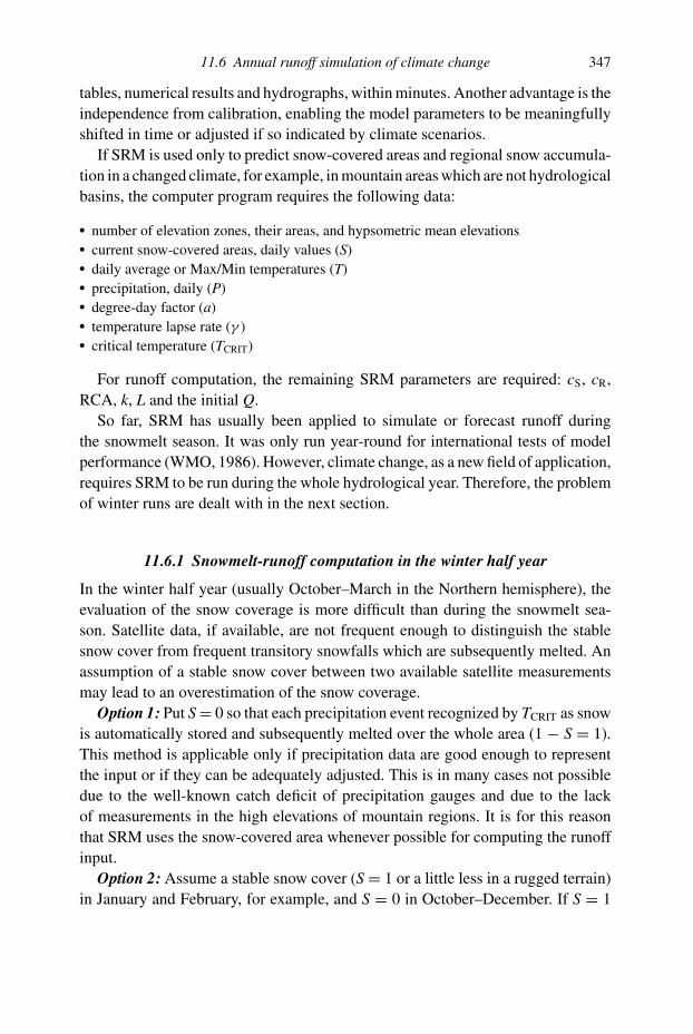
11.6 Annual runoff simulation of climate change 347
tables, numerical results and hydrographs, within minutes. Another advantage is the
independence from calibration, enabling the model parameters to be meaningfully
shifted in time or adjusted if so indicated by climate scenarios.
If SRM is used only to predict snow-covered areas and regional snow accumula-
tion in a changed climate, for example, in mountain areas which are not hydrological
basins, the computer program requires the following data:
� number of elevation zones, their areas, and hypsometric mean elevations� current snow-covered areas, daily values (S)� daily average or Max/Min temperatures (T)� precipitation, daily (P)� degree-day factor (a)� temperature lapse rate (γ )� critical temperature (TCRIT)
For runoff computation, the remaining SRM parameters are required: cS, cR,
RCA, k, L and the initial Q.
So far, SRM has usually been applied to simulate or forecast runoff during
the snowmelt season. It was only run year-round for international tests of model
performance (WMO, 1986). However, climate change, as a new field of application,
requires SRM to be run during the whole hydrological year. Therefore, the problem
of winter runs are dealt with in the next section.
11.6.1 Snowmelt-runoff computation in the winter half year
In the winter half year (usually October–March in the Northern hemisphere), the
evaluation of the snow coverage is more difficult than during the snowmelt sea-
son. Satellite data, if available, are not frequent enough to distinguish the stable
snow cover from frequent transitory snowfalls which are subsequently melted. An
assumption of a stable snow cover between two available satellite measurements
may lead to an overestimation of the snow coverage.
Option 1: Put S = 0 so that each precipitation event recognized by TCRIT as snow
is automatically stored and subsequently melted over the whole area (1 − S = 1).
This method is applicable only if precipitation data are good enough to represent
the input or if they can be adequately adjusted. This is in many cases not possible
due to the well-known catch deficit of precipitation gauges and due to the lack
of measurements in the high elevations of mountain regions. It is for this reason
that SRM uses the snow-covered area whenever possible for computing the runoff
input.
Option 2: Assume a stable snow cover (S = 1 or a little less in a rugged terrain)
in January and February, for example, and S = 0 in October–December. If S = 1

348 Snowmelt-Runoff Model (SRM)
on April 1 from satellite data, assume S = 1 in March as well. If it is less than 1 on
April 1, the snow coverage in March is put to 0 or, which may be more accurate,
it is interpolated from 1 on March 1 to the S-value on April 1. Naturally, S = 1
can be assumed for a longer part of the winter in higher elevation zones while
in the lowest zone option 1 may be preferable. The present program keeps the
snow coverage estimated for the present climate unchanged for climate runs. It is
therefore recommended to assume a complete snow coverage only in months in
which it is expected to last in a warmer climate as well.
Whenever S = 1 is introduced, the SRM program cancels any existing stor-
age of preceding temporary snowfalls because such snow becomes a part of the
seasonal snow cover. Snow storage is also automatically canceled on April 1
because all existing snow is then accounted for by the depletion curve of the
snow coverage. With the variables thus accounted for, SRM is run as usual.
Because the estimated snow coverage is less accurate than CDC in the sum-
mer, the water equivalent of new snow is reduced at once by the simultaneous
(1 − S) to prevent an inadequate S from influencing the computation on a later
melt day. This deviates from the summer procedure explained in Section 11.3.3,
Table 11.2.
The model parameters should be adapted to winter conditions. In particular,
the constants x, y for the recession formula (Equation (11.7)) derived usually for
summer conditions sometimes allow the discharge to decrease too low so that a
slower recession formula is indicated. By using the equation
QMin > x1y (11.14)
x, y can be adjusted in order to prevent the discharge from sinking below a selected
level after a long recession period.
In view of frequent snowfalls, values of the degree-day factor lower than those
used in the summer are recommended. Values of cS and cR higher than in summer
can be expected. The main purpose of the winter runoff simulation is the evaluation
of the runoff redistribution in the winter and summer half years. Consequently it is
more important to compute the winter runoff volume as accurately as possible than
to try to improve the daily accuracy (R2).
Change of snow accumulation in the new climateAs the first step, the effect of a climate change on snow-covered areas and runoff
was evaluated in the summer half year only, assuming an unchanged initial snow
cover on April 1 (Martinec et al., 1994; 1998). For a year-round temperature
increase, the seasonal snow cover on April 1 is deprived of a certain snow water
equivalent by additional snowmelt and by a conversion of some precipitation
events from snow to rain in October through March. This decrease of the snow

11.6 Annual runoff simulation of climate change 349
water equivalent is computed by rewriting the input part of the SRM formula as
follows:
�HW =182∑n=1
[an · Tn · Sn + an · Tn(1 − Sn) + PRn]
−182∑n=1
[an · T ′n · S′
n + an · T ′n(1 − S′
n) + P ′Rn] (11.23)
where:
� HW = difference between the present and future areal water equivalent of the
snow cover on April 1 (cm).
a = degree-day factor (cm ◦C−1 d−1)
T = temperature in the present climate at mean hypsometric elevation, as degree-
days (◦C d)
T ′ = temperature in a warmer climate as degree-days (◦C d)
S = ratio of snow-covered area to total area, present climate
S′ = ratio of snow-covered area to total area, warmer climate
PR = rain according to TCRIT, present climate
P′R = rain according to TCRIT, warmer climate
182 = number of days October through March
Equation (11.23) thus summarizes the SRM input to runoff which consists of
snowmelt from the stable snow cover (S), melting of snow which temporarily covers
the snow-free area (1 − S) and rain. The distinction between a stable and tempo-
rary snow cover during the snow accumulation in winter is rather arbitrary due to
insufficient satellite monitoring, but the total of both snowmelt inputs always equals
100% of the occurring snowmelt M:
M · S + M(1 − S) = M(S + 1 − S) = M (11.24)
In March, however, if S is put to 0 while there is a stable snow cover, and there
happens to be little snowfall, the snowmelt input may be underestimated.
Figure 11.20 illustrates the areal water equivalent of the snow cover on April 1 as a
difference between the winter precipitation and the winter input to runoff. This water
equivalent can be also computed by accumulating the daily zonal melt depths. In
this hypothetical example there is an agreement of the water equivalent determined
either way. In natural conditions, discrepancies are to be expected mainly due to
difficulties in evaluating the areal precipitation value for mountainous regions. In
such cases, it is recommended that the value from the accumulated zonal melt be
considered as more reliable. The accumulated zonal melt value might even be used
to correct the winter precipitation data and to estimate the altitude precipitation

350 Snowmelt-Runoff Model (SRM)
MS
Figure 11.20 Illustration of the snow accumulation in the winter and snowmelt inthe summer in the present climate (hypothetical example).
gradient. Another advantage of this method is that it takes into account a possible
redeposition of snow by wind during the accumulation season.
On the other hand, no losses are normally considered (losses indicated by the
runoff coefficient are assumed to take place after meltwater has left the snow cover).
This may lead to underestimation of the retrospectively computed water equivalents
if significant evaporation from the snow surface takes place. However, if degree-
day ratios are used which have been derived from lysimeter measurements under
similar evaporation conditions, this error is eliminated.
In a warmer climate, the winter input to runoff increases, as shown in
Figure 11.21, so that there is less snow on April 1 if winter precipitation remains
unchanged. A combined effect of a warmer climate and increased winter precipi-
tation can result in rare cases (low temperatures in high mountains with little or no
effect of the temperature increase) in an increased snow accumulation.
Runoff simulation for scenarios of the future climateIn order to evaluate the effect of a warmer climate on runoff in mountain basins,
the SRM program uses the real seasonal snow cover of the present as monitored by
satellites and models a climate-affected seasonal snow cover.
The future snow conditions in terms of snow-covered areas and areal water
equivalents in different elevation zones constitute useful information for planning
water management and winter tourism. Using snow-coverage data as model input,
the climate-affected runoff in the whole hydrological year is computed. It allows
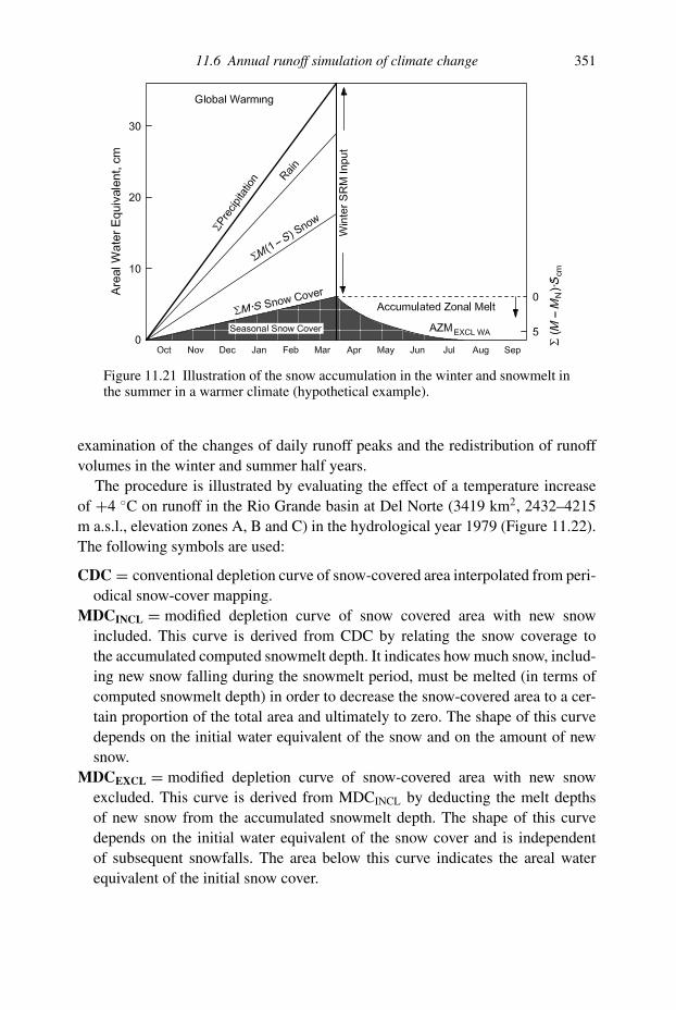
11.6 Annual runoff simulation of climate change 351
Figure 11.21 Illustration of the snow accumulation in the winter and snowmelt inthe summer in a warmer climate (hypothetical example).
examination of the changes of daily runoff peaks and the redistribution of runoff
volumes in the winter and summer half years.
The procedure is illustrated by evaluating the effect of a temperature increase
of +4 ◦C on runoff in the Rio Grande basin at Del Norte (3419 km2, 2432–4215
m a.s.l., elevation zones A, B and C) in the hydrological year 1979 (Figure 11.22).
The following symbols are used:
CDC = conventional depletion curve of snow-covered area interpolated from peri-
odical snow-cover mapping.
MDCINCL = modified depletion curve of snow covered area with new snow
included. This curve is derived from CDC by relating the snow coverage to
the accumulated computed snowmelt depth. It indicates how much snow, includ-
ing new snow falling during the snowmelt period, must be melted (in terms of
computed snowmelt depth) in order to decrease the snow-covered area to a cer-
tain proportion of the total area and ultimately to zero. The shape of this curve
depends on the initial water equivalent of the snow and on the amount of new
snow.
MDCEXCL = modified depletion curve of snow-covered area with new snow
excluded. This curve is derived from MDCINCL by deducting the melt depths
of new snow from the accumulated snowmelt depth. The shape of this curve
depends on the initial water equivalent of the snow cover and is independent
of subsequent snowfalls. The area below this curve indicates the areal water
equivalent of the initial snow cover.

352 Snowmelt-Runoff Model (SRM)
Figure 11.22 Measured and simulated runoff in the Rio Grande basin near DelNorte in the hydrological year 1979.
AZMINCL = accumulated zonal melt with new snow included. This curve accumu-
lates daily computed snowmelt depths multiplied by the respective snow coverage
(as decimal number) and shows the totals on a time scale.
AZMEXCL = accumulated zonal melt with new snow excluded. This curve is
derived from AZMINCL by deducting the zonal melt of new snow from the accu-
mulated zonal melt. Again it relates the successive totals to time. The final
total is the areal water equivalent of the initial snow cover (as also indicated by
MDCEXCL).
MDCCLIM = modified depletion curve of snow covered area for a changed climate.
This curve takes into account the amount of snowfalls changed by the new
climate. If there is no change, it is identical with MDCINCL.
CDCCLIM = conventional depletion curve of snow-covered area in a changed
climate.
CDCCLIM MA = conventional depletion curve of snow-covered area in a changed
climate (derived from MDCINCL) adjusted for the input to SRM runoff compu-
tation (model adjusted). It appears in publications disregarding the winter effect
of a changed climate.
MDCEXCL WA = winter adjusted curve. The effect of a warmer winter is taken
into account by decreasing the curve according to the “winter deficit.” With a
simultaneous increase of winter precipitation a positive balance of the winter

11.6 Annual runoff simulation of climate change 353
snow accumulation may result in which case the curve is increased. The area
below this curve indicates the areal water equivalent of the initial snow cover in
a changed climate.
AZMEXCL WA = winter adjusted curve. The effect of a warmer winter and, if nec-
essary, of a changed precipitation is taken into account. The final total is the
water equivalent of the initial snow cover in a changed climate.
MDCCLIM WA = winter adjusted curve. It is derived from MDCEXCL WA by taking
into account snowfalls “surviving” in the new climate.
CDCCLIM WA = conventional depletion curve of snow-covered area in a changed
climate. The curve is derived from MDCCLIM WA.
CDCCLIM WA, MA = curve adjusted for the model input (model adjusted). If the
derivation from MDCCLIM WA results in more than one S-value on a date, the
first (highest) value is used. If there is no new S-value on a date, the previous
day’s S-value is repeated until there is a new S-value. With this adjustment
CDCCLIM WA, MA can be used as input to SRM which requires one S-value on
each day, like provided by the original CDC. This curve is used to compute the
year-round climate-affected runoff.
Due to the time shift by the changed climate, the derivation of SCLIM WA values from
MDCCLIM WA may stop before the end of the computation period. If SCLIM WA < S,
the program decreases the depletion curve CDCCLIM WA, MA to the last S-value of
the original CDC, which is typically zero, and repeats it for the missing days. If an
elevation zone contains glaciers or permanent snow cover, CDCCLIM WA, MA drops
to the residual snow or ice coverage, again taken over from the original CDC. In less
frequent cases (no effect of a temperature increase in a high elevation zone, increased
precipitation), SCLIM WA > S. The program then determines �S = SCLIM WA
− S and extrapolates CDCCLIM WA as CDC + �S on the missing days.
In order to evaluate the effect of a temperature increase on the Rio Grande basin,
the following steps are to be taken:
(1) Runoff in the whole hydrological year is simulated (Figure 11.22) in order to verify
the preselected parameters and the estimated snow coverage in winter.
(2) Conventional depletion curves of the snow coverage (CDC) used as input variable in
the summer are plotted (Figure 11.23).
(3) Winter runoff is simulated separately for T and T + 4 ◦C in order to obtain the respective
runoff volumes (hydrographs are printed).
(4) The decrease of the snow water equivalent on April 1 due to the increased snowmelt
in winter (“winter deficit” or “negative winter adjustment”) is computed as explained
earlier in Section 11.6.1 under “change of snow accumulation in the new climate”.
(5) Summer runoff is simulated separately for T in order to obtain the runoff volume
(hydrographs are printed).

354 Snowmelt-Runoff Model (SRM)
Figure 11.23 Conventional depletion curves of the snow coverage from Landsatdata in the elevation zones A, B, and C of the Rio Grande basin near Del Norte in1979.
Figure 11.24 Modified depletion curves for zone A: MDCINCL derived fromCDC, therefore including new snow, MDCEXCL with new snowmelt excluded,MDCEXCL WA with “winter deficit” (shaded area) cut off.
At this point, the climate-affected conventional depletion curves, CDCCLIM, which
are needed as input variables for computing the summer part (since they do not exist
in the accumulation period in the winter) of the climate-affected runoff, are derived as
follows:
(6) The modified depletion curve MDCINCL is derived from the CDC. This curve relates the
snow coverage with cumulative snowmelt depths including new snow in the summer
(Figure 11.24).

11.6 Annual runoff simulation of climate change 355
(7) MDCEXCL is derived by eliminating melt depths referring to new snow from cumulative
snowmelt depth (Figure 11.24). The area below this curve indicates the initial areal
water equivalent of the snow cover, as shown in Section 11.5.
(8) The climate effect is taken into account by depriving MDCEXCL of the “winter deficit”
computed in step (4), and MDCEXCL WA (winter adjusted) is derived. The program
prints both MDCEXCL and MDCEXCL WA. In zone A, �HW =−36.94 cm was computed
so that MDCEXCL is cut off on the day when this value was equalled or exceeded. This
happened on April 27, when �M for MDCEXCL was 42.04 cm (not reduced by S,
therefore higher). MDCEXCL WA thus derived is shifted to start on April 1.
(9) The cumulative snowmelt is printed in relation to time as zonal snowmelt, that is
to say reduced each day by the respective percentage of the snow coverage. The
accumulated zonal melt curve AZMEXCL indicates graphically (Figure 11.25) that the
“winter deficit,” in this example �HW = −36.94 cm, was exceeded on April 27, when
the accumulated zonal melt amounted to 37.69 cm. The previous day’s total 35.9 cm
is also printed so that the user can cut off the MDCEXCL at the previous day’s value if
the next day’s value is much higher than the computed �HW.
(10) After melt depths of new snow of the present climate and the winter deficit had been
taken out of MDCINCL to derive MDCEXCL WA, melt depths of new snow “surviving”
in the warmer climate are put back to derive MDCCLIM WA as illustrated for zone A in
Figure 11.26.
(11) The climate-affected conventional depletion curves adjusted for the “winter deficit”,
CDCCLIM WA, are derived as follows: MDCCLIM WA indicates, for example, that
a snowmelt depth of 22 cm is needed to decrease the snow coverage to 50%
Figure 11.25 Accumulated zonal melt curves for zone A: AZMINCL: computeddaily melt depth multiplied by S from CDC (= zonal melt). AZMEXCL with newsnow zonal melt excluded and AZMEXCL WA derived from AZMEXCL by cutting itoff on April 27 and transferring it to April 1.

356 Snowmelt-Runoff Model (SRM)
Figure 11.26 Modified depletion curve, adjusted for the “winter deficit” and includ-ing new snow of the changed climate (MDCCLIM WA) derived from MDCEXCL WA
for zone A.
Figure 11.27 Effect of a changed climate (T + 4 ◦C) on snow-covered areas of1979 in elevation zones A, B, and C of the Rio Grande basin near Del Norte.CDCCLIM WA is shifted from the original CDC due to a reduced snow cover onApril 1 and due to increased temperatures in the snowmelt season.
(Figure 11.26). This occurs in the present climate, according to CDC in Figure 11.23
on May 5. In a warmer climate (T + 4 ◦C in this example) a cumulative snowmelt
depth of 22 cm and a corresponding decrease of the snow coverage to 50% are reached
already on April 9, so that the 50% point is shifted to that date (Figure 11.27). The
program takes the cumulative snowmelt depth computed by present temperatures on

11.6 Annual runoff simulation of climate change 357
each day and searches for the date on which this snowmelt depth was equalled or
exceeded when the higher temperatures are used for computation. If the new climate
implies changes of the degree-day factor (see discussion under “Model parameters
in a changed climate” later in this section), the cumulative snowmelt depth must be
computed not only by higher temperatures, but also by changed (usually higher) a-
values. The computer program takes care of this matter. Comparable snowmelt depths
are reached about one month earlier so that CDCCLIM WA is shifted in time against the
original CDC as illustrated in Figure 11.27 for all elevation zones. The method of CDC
shifting in the summer is also explained by a numerical example elsewhere (Rango
and Martinec, 1994). In view of the stepwise character of the cumulative snowmelt
depths, a slightly higher snow water equivalent than the “winter deficit” may be cut
off to derive MDCEXCL WA (see step (9) above) which would ultimately accelerate the
decline of CDCCLIM WA. On the other hand, searching for cumulative snowmelt depths
equalled or exceeded in deriving CDCCLIM WA may result in a very slight delay of the
decline.
(12) CDCCLIM WA is used to compute the climate-affected runoff in the summer half
year. It should be noted that in contrast to the model runs in the simulation mode,
R2 in the climate-change runs does not indicate the model accuracy, but results
from the difference between the hydrographs computed for the present and changed
climate.
Figure 11.28 shows the climate-affected runoff computed by original precipi-
tation, temperature T + 4 ◦C and snow-covered areas according to CDCCLIM WA
compared with the original runoff simulation in Figure 11.22. The run is started by
discharge computed on March 31 with T + 4 ◦C (see step (3)). The year-round
climate-affected hydrograph thus consists of a winter simulation with T + 4 ◦C and
Figure 11.28 Climate-affected runoff (T + 4 ◦C) in the Rio Grande basin near DelNorte, compared with the runoff simulated by data of 1979 (as shown in Figure11.22) for April–September.

358 Snowmelt-Runoff Model (SRM)
Figure 11.29 Simulated runoff in the Rio Grande basin near Del Norte in the hydro-logical year 1979 and climate-affected runoff computed by increased temperatures(T + 4 ◦C) and correspondingly changed snow conditions.
estimated S and of a summer computation by the climate program with T + 4 ◦C
and S from CDCCLIM WA.
Figure 11.29 shows year-round hydrographs computed with temperatures of
1979 and with temperatures increased by +4 ◦C. As listed in Table 11.5, the future
winter runoff would be increased at the expense of the summer runoff. The actual
effect is greater because the increased climate-affected runoff in late March is car-
ried over to April as recession flow as explained elsewhere (Rango and Martinec,
1997). Proportionally the redistribution of runoff is relatively small because the
cold winter of 1979 did not allow much snowmelt even with the increased tem-
peratures (see Section 11.6.1, Normalization of data to represent the present
climate).
In the given example, precipitation was not changed in the new climate but the
climate program can also handle the combined effect of changed temperatures and
changed precipitation. Usually the temperature effect prevails but, as mentioned
earlier in Section 11.6.1 under “change of snow accumulation in the new climate”,
increased precipitation and absence of melting conditions in high altitudes in winter
may convert the “winter deficit” to “winter gain” or “positive winter adjustment.”
In this case, the computer program derives MDCEXCL WA by stretching MDCEXCL
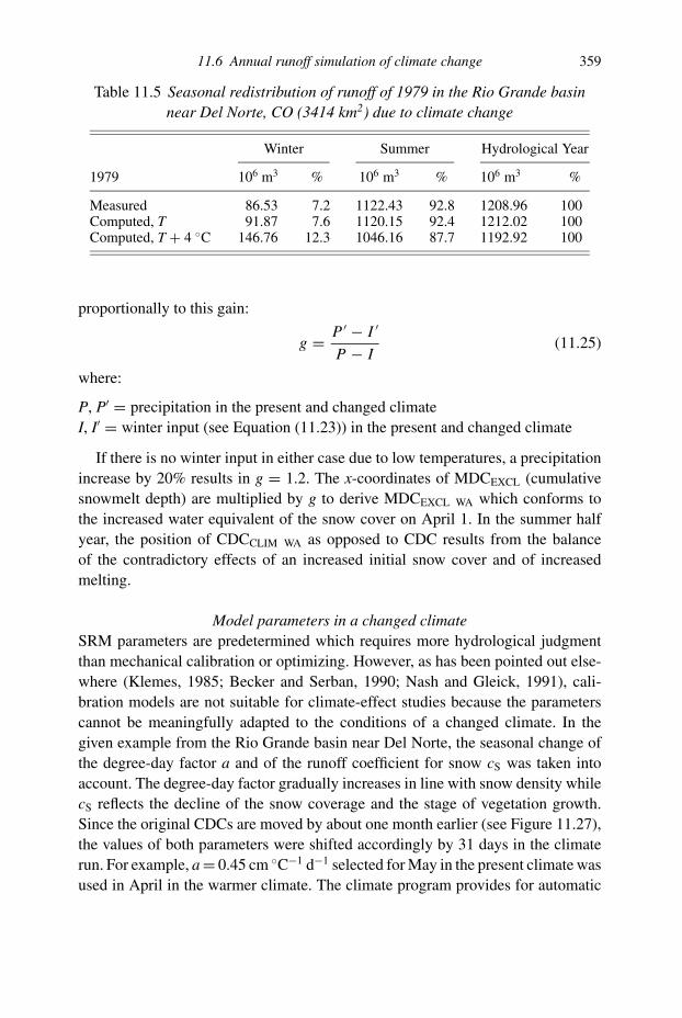
11.6 Annual runoff simulation of climate change 359
Table 11.5 Seasonal redistribution of runoff of 1979 in the Rio Grande basinnear Del Norte, CO (3414 km2) due to climate change
Winter Summer Hydrological Year
1979 106 m3 % 106 m3 % 106 m3 %
Measured 86.53 7.2 1122.43 92.8 1208.96 100Computed, T 91.87 7.6 1120.15 92.4 1212.02 100Computed, T + 4 ◦C 146.76 12.3 1046.16 87.7 1192.92 100
proportionally to this gain:
g = P ′ − I ′
P − I(11.25)
where:
P, P′ = precipitation in the present and changed climate
I, I′ = winter input (see Equation (11.23)) in the present and changed climate
If there is no winter input in either case due to low temperatures, a precipitation
increase by 20% results in g = 1.2. The x-coordinates of MDCEXCL (cumulative
snowmelt depth) are multiplied by g to derive MDCEXCL WA which conforms to
the increased water equivalent of the snow cover on April 1. In the summer half
year, the position of CDCCLIM WA as opposed to CDC results from the balance
of the contradictory effects of an increased initial snow cover and of increased
melting.
Model parameters in a changed climateSRM parameters are predetermined which requires more hydrological judgment
than mechanical calibration or optimizing. However, as has been pointed out else-
where (Klemes, 1985; Becker and Serban, 1990; Nash and Gleick, 1991), cali-
bration models are not suitable for climate-effect studies because the parameters
cannot be meaningfully adapted to the conditions of a changed climate. In the
given example from the Rio Grande basin near Del Norte, the seasonal change of
the degree-day factor a and of the runoff coefficient for snow cS was taken into
account. The degree-day factor gradually increases in line with snow density while
cS reflects the decline of the snow coverage and the stage of vegetation growth.
Since the original CDCs are moved by about one month earlier (see Figure 11.27),
the values of both parameters were shifted accordingly by 31 days in the climate
run. For example, a = 0.45 cm ◦C−1 d−1 selected for May in the present climate was
used in April in the warmer climate. The climate program provides for automatic

360 Snowmelt-Runoff Model (SRM)
shifting by any number of days. When September values are shifted to August, the
value of September 30 is repeated in September. The shifting is stopped in January
in order to prevent winter conditions being transferred to the autumn. There is no
consensus yet whether a warmer climate will increase losses in which case the
values of cS and cR would be generally decreased, because a decreased evapotran-
spiration due to the CO2 increase might offset the temperature effect (Carlson and
Bunce, 1991; Gifford, 1988).
Selected parameters can be shifted or changed in accordance with the expected
conditions of a future climate. Future versions will also enable the constants x, y
for the recession formula to be adjusted if, for example, a steeper recession would
be indicated by drier soil conditions.
Normalization of data to represent the present climateThe climate effect is evaluated by comparing present snow and runoff conditions
with conditions modelled for a climate scenario. The current climate can be rep-
resented by precipitation, temperatures, snow-covered areas, and simulated runoff
of a single year, especially if this year appears to be “normal”. Average data from
a number of years would seem to be more representative. However, the use of
long-term average daily temperatures, with day-to-day fluctuations smoothed out,
may considerably underestimate snowmelt depths and the runoff as mentioned in
Table 11.4.
A normalized data set can be prepared by adjusting daily temperatures of a
selected year by monthly deviations from long-term averages and by multiplying
daily precipitation amounts by ratios of long-term and actual monthly totals. The
normalized depletion curves of the snow coverage can be derived from the curves of
the selected year by considering the normalized temperatures and precipitation as
a “new climate” for that year and running the SRM climate program. The normal-
ized temperatures, precipitation, and snow-covered areas are then considered as a
standard year and the climate program is run again with specifications of a changed
climate. The present climate program Version 4.0, however, allows only uniform
changes of temperature and precipitation for the winter and summer half year. The
next version will be adjusted in order to carry out the outlined normalization of data
as well as to take into account more detailed climate scenarios.
OutlookThe SRM program Version 4.0 evaluates the snow coverage, the areal water equiv-
alent, and computes runoff for any increase of temperature and any change of
precipitation in the winter and summer half year. Options are open concerning
model parameters to be shifted in time or adjusted in magnitude in response to a
changed climate. Currently, data from actual years are used to represent today’s

11.7 Micro-SRM computer program 361
climate. The next program version will enable temperature and precipitation to be
changed monthly. With this refinement, it will be possible to derive daily temper-
atures, precipitation and snow-covered area for a “normalized” year which will
represent the current climate better than a selected actual year. A refined computa-
tion of snowmelt and glacier melt with a radiation component is under preparation
in order to take into account climate scenarios with changed cloud conditions and
to predict the behavior of glaciers in the next century.
Information about new developments will be available on the Internet and in
SRM-Workshops.
11.7 Micro-SRM computer program
BackgroundThe Martinec/Rango Snowmelt-Runoff Model (SRM) was originally a FORTRAN
model designed to operate on an IBM 370-series mainframe computer. The first
computerized version of the model was developed by Martinec et al. (1983). In
1986 the model’s FORTRAN code was downloaded to an IBM PC and modified to
operate in the PC environment. That same year a decision was made to develop a
unique PC-oriented version of the model, taking full advantage of the PC’s inherent
capabilities. The results of that decision was Micro-SRM, Version 1.0.
Additional refinements have been incorporated in several subsequent Micro-
SRM Versions up to and including 4.0. However, SRM itself remains unchanged
and relatively simple, so that the computations by Equation (11.1) can still be
performed by any pocket calculator which has a function xy . Of course the PC
program automatically handles the multiple input of temperature and precipitation
for up to eight elevations zones of a basin, any desired lag time, and complicated
snow/rain situations. A model run for up to 365 days is finished within several
seconds, the computed hydrograph is immediately displayed in comparison with
the measured discharge and, if desired, quickly printed. Also, the achieved accuracy
is automatically computed and displayed. A summary of parameter values can be
displayed after each run so that adjustments can be made and their effect assessed.
SRM does not require numerous runs because calibration is not necessary. The
ease with which the results are obtained should not lead to a replacement of the
deterministic approach of SRM by a “try and see” philosophy. SRM is designed
to operate with physically based estimates of parameters which should not require
much change after the initial selection. As mentioned earlier, seemingly unsatis-
factory results have been frequently improved not by adjusting the parameters but
by correcting errors in data sets and in the input of variables.
A prime consideration in the design of Micro-SRM was to develop a snowmelt
modelling “environment” such that the model user was provided not just model

362 Snowmelt-Runoff Model (SRM)
algorithms, but a complete set of tools for managing the associated model processes:
data entry, storage and retrieval, display of data, and results. Traditionally, the most
time-consuming and error-prone activity involved in using any physically based
model has been the accumulation of large amounts of input data in the form and
format needed to drive the simulation, with actual execution of the model a trivial
task by comparison. Recognizing this, the developers chose to pattern the design of
Micro-SRM after that originally developed during the automation of the Soil Con-
servation Service’s (SCS) Technical Release Number 55 (TR-55), Urban Hydrology
for Small Watersheds (Soil Conservation Service, 1986). This joint Agricultural
Research Service (ARS)/SCS effort provided valuable experience in developing
highly interactive “front-ends” for interfacing complex models with model users.
The approach used by the ARS/SCS programming team that automated TR-55
was to develop an efficient, easy-to-use, highly interactive data entry/manipulation
environment, and include model algorithms as just one of many functions that sup-
port and use that environment (Cronshey et al., 1985). Micro-SRM consists of an
integration of the mainframe SRM FORTRAN algorithms converted to Basic and a
variation of TR-55’s data entry/data management algorithms. The current version
of the model, Micro-SRM, Version 4.0, was developed using Microsoft QuickBA-
SIC 4.5 and contains several subroutines from QuickPak Professional, a BASIC
toolbox developed by Crescent Software, Inc.1
Micro-SRM and WinSRM availabilityThe Hydrology and Remote Sensing Laboratory supports and distributes the
Snowmelt-Runoff Model free of charge to any interested party. The program and
related files are available via the Internet by accessing the SRM home page at,
http://ars.usda.gov/services/docs.htm?docid=8872. This site also includes an elec-
tronic version of the SRM User’s Manual. A distribution diskette, available on either
5′′ or 31/2′′ media, containing the executable code, supporting files, and example
data files can be provided upon request. To obtain the latest version of Micro-SRM,
contact:
USDA-ARS, Hydrology and Remote Sensing Laboratory
Bldg. 007, Room 104, BARC-W
10300 Baltimore Avenue
Beltsville, MD 20705–2350 USA
(301) 504–7490
or via electronic mail to:
1 Trademarks used in this document (e.g., IBM PC, IBM CORP.; MS-DOS, QuickBASIC, Microsoft Corp.;QuickPak Professional, Crescent Software) are used solely for the purpose of providing specific information.

11.8 References 363
11.8 References
Baumann, R., Burkart, U. and Seidel, K. (1990). Runoff forecasts in an Alpine catchmentof satellite snow cover monitoring. In Proceedings International Symposium onRemote Sensing and Water Resources. Enschede, The Netherlands: InternationalAssociation of Hydrogeologists, pp. 181–90.
Baumgartner, M. F. (1987). Schneeschmelz-Abflusssimulationen basierend aufSchneeflachenbestimmungen mit digitalen Landsat-MSS and NOAA-AVHRRDaten. (Snowmelt runoff simulations based on snow cover mapping using digitalLandsat-MSS and NOAA-AVHRR data). In Remote Sensing Series 11, Germanversion, Tech. Report HL-16, Zurich, Switzerland: Department of Geography,University of Zurich. English summary: Beltsville, MD: USDA, AgriculturalResearch Service, Hydrology Laboratory.
Baumgartner, M. F. and Rango, A. (1995). A microcomputer-based alpine snow coveranalysis system. Photogramm. Eng., 61(12), 1475–86.
Becker, A. and Serban, P. (1990). Hydrological models for water resources system designand operation. Operational Hydrology Report 34. Geneva: WMO.
Brusch, W. (1996). Das Snowmelt Runoff Model ETH (SRM-ETH) als universellesSimulations- und Prognosesystem von Schneeschmelz-Abflussmengen. (TheSnowmelt Runoff Model ETH as a universal simulation and forecast system forsnowmelt runoff). In Remote Sensing Series 27, German version, Zurich: Universityof Zurich Remote Sensing Laboratories.
Carlson, T. N. and Bunce, J. A. (1991). The effect of atmospheric carbon dioxide doublingon transpiration. In Proceedings American Meteorological Society, Special Sessionon Hydrometeorology, Salt Lake City, Utah, pp. 196–9.
Cronshey, R. G., Roberts, R. T., and Miller, N. (1985). Urban Hydrology for SmallWatersheds (TR-55 Revised). In Proceedings ASCE Hydraulic Division SpecialtyConference, Orlando, Florida.
Gifford, R. M. (1988). Direct effects of CO2 concentrations on vegetation. In GreenhousePlanning for Climate Change, ed. G. L. Pearlman. Melbourne: CSIRO,pp. 506–19.
Hall, D. K. and Martinec, J. (1985). Remote Sensing of Ice and Snow. New York:Chapman and Hall Ltd.
Higuchi, K., Ageta, Y., Yasunari, T., and Inoue, J. (1982). Characteristics of precipitationduring the monsoon season in high-mountain areas of the Nepal Himalaya. InHydrological Aspects of Alpine and High Mountain Areas, Proc. Exeter Symposium,IAHS Publ. 138, pp. 21–30.
Klemes, V. (1985). Sensitivity of Water Resources Systems to Climate Variations, WCPReport 98. Geneva: WMO.
Kotlyakov, V. M. and Krenke, A. N. (1982). Investigations of the hydrological conditionsof alpine regions by glaciological methods. In Hydrological Aspects of Alpine andHigh-Mountain Areas, Proc. Exeter Symposium, IAHS Publ. 138, pp. 31–42.
Martinec, J. (1960). The degree-day factor for snowmelt runoff forecasting. In IUGGGeneral Assembly of Helsinki, IAHS Commission of Surface Waters, IAHS Publ. 51,pp. 468–77.
Martinec, J. (1970). Study of snowmelt runoff process in two representative watershedswith different elevation range. In IAHS-UNESCO Symposium, IAHS Publ. 96,Wellington, New Zealand, pp. 29–39.
Martinec, J. (1975). Snowmelt-Runoff Model for stream flow forecasts. Nordic Hydrol.6(3), 145–54.
Martinec, J. (1985). Time in hydrology. In Facets of Hydrology, vol. II, ed. J. C. Rodda.London: John Wiley and Sons, pp. 249–90.

364 Snowmelt-Runoff Model (SRM)
Martinec, J. (1989). Hour-to-hour snowmelt rates and lysimeter outflow during an entireablation period. In Snow Cover and Glacier Variations, Proc. Baltimore Symp. IAHSPubl. No. 183, pp. 19–28.
Martinec, J. and Rango, A. (1986). Parameter values for snowmelt runoff modelling. J.Hydrol. 84, 197–219.
Martinec, J. and Rango, A. (1989). Merits of statistical criteria for the performance ofhydrological models. Water Resour. Bull. 25(20), 421–32.
Martinec, J. and Rango, A. (1995). Seasonal runoff forecasts for hydropower based onremote sensing. In Proceedings of the 63rd Annual Western Snow Conference,Sparks, NV, pp. 10–20.
Martinec, J., Rango, A., and Major, E. (1983). The Snowmelt-Runoff Model (SRM) User’sManual, NASA Reference Publ. 1100. Washington, DC.
Martinec, J., Rango, A., and Roberts, R. (1994). Snowmelt Runoff Model (SRM) user’smanual. In Geographica Bernensia, ed. M. F. Baumgartner. Berne: Department ofGeography, University of Berne.
Martinec, J., Rango, A., and Roberts, R. (1998). Snowmelt Runoff Model (SRM) user’smanual. In Geographica Bernisia, ed. M. F. Baumgartner. Berne: Department ofGeography, University of Berne.
Nash, L. L and Gleick, J. A. (1991). Sensitivity of streamflow in the Colorado Basin toclimatic changes. J. Hydrol., 125, 221–41.
Rango, A. and Martinec, J. (1994). Areal extent of seasonal snow cover in a changedclimate. Nordic Hydrol., 25, 233–46.
Rango, A. and Martinec, J. (1995). Revisiting the degree-day method for snowmeltcomputation. Water Resour. Bull. 31(4), 657–69.
Rango, A. and Martinec, J. (1997). Water storage in mountain basins from satellite snowcover monitoring. In Remote Sensing and Geographic Information Systems forDesign and Operation of Water Resources Systems, Proc. 5th Scientific Assembly ofIAHS, Rabat, Morocco, IAHS Publication 242, ed. M. F. Baumgartner, G. A. Schultzand A. L. Johnson, pp. 83–91.
Rango, A. and van Katwijk, V. (1990). Development and testing of a snowmelt runoffforecasting technique. Water Resour. Bull., 26(1), 135–44.
Seidel, K. and Martinec, J. (2004). Remote Sensing on Snow Hydrology. New York:Springer-Verlag.
Seidel, K., Martinec, J. and Baumgartner, M. F. (2000). Modelling runoff and impact ofclimate change in large Himalayan basins. In Proceedings of the InternationalConference on Integrated Water Resources Management for SustainableDevelopment, New Dehli, India, pp. 1020–28.
Shafer, B. A., Jones, E. B., and Frick, D. M. (1981). Snowmelt Runoff Simulations Usingthe Martinec-Rango Model on the South Fork Rio Grande and Conejos River inColorado, AgRISTARS Report CP-G1–04072. Greenbelt, MD: Goddard SpaceFlight Center.
Soil Conservation Service. (1986). Urban Hydrology for Small Watersheds, Tech. Release55, 2nd edn, Washington, DC: Department of Agriculture.
Wilson, W. T. (1941). An outline of the thermodynamics of snow-melt. Trans. Am.Geophys. Union, 1, 182–95.
World Meteorological Organization (1986). Intercomparison of Models of SnowmeltRunoff. Operational Hydrol. Report 23, No. 646, Geneva: WMO.
World Meteorological Organization (1992). Simulated real-time intercomparison ofhydrological models. Operational Hydrol. Report 38, WMO – No. 779, Geneva,Switzerland: WMO.

12
Snowpack management and modifications
Snow in the global environment is altered by human activity in many ways, some
intentional and others inadvertent. Among the deliberate changes made to snow-
packs are blowing-snow management to benefit agriculture and transportation, for-
est management to protect and enhance water yields from snowpacks, urban snow
management to improve transportation and habitation in developed areas, albedo
modification to enhance snowmelt rates, and ski-area management for enhanced
and safe recreational opportunities. The major inadvertent change that may impact
snowpacks is the possibility of climate change that is being forecast for the twenty-
first century. This final chapter generally discusses these human–snow interactions
from the viewpoint of the snow hydrologist.
All management of snow should be based upon a thorough understanding of the
processes involved at a given site and how they may be varied to accomplish a given
goal. Furthermore, the management recommendations must consider acceptability,
cost, ease of use, risks, maintenance requirements, and long-term environmental
impacts. Many processes affecting snow that can be altered to meet management
goals have been described in earlier chapters.
12.1 Blowing-snow management
Blowing-snow management generally has the objective of creating snow drifts in
useful or non-problematic locations by using some type of barrier to the wind.
Barriers take the form of constructed snow fences, rows of living shrubs or trees,
and crop stubble. Farmers have realized for centuries that seeds and seedling plants
survive and grow faster when located in furrows that accumulated small drifts of
snow that supplemented soil moisture. More recently, agriculturalists have used
interplantings of tall and short crops (Bilbro and Fryrear, 1988; Scholten, 1988),
planted rows of trees or shrubs (Scholten, 1988; Shaw, 1988), or constructed snow
fences to accumulate and store more snow on the landscape. Constructed snow
365

366 Snowpack management and modifications
/
/
Figure 12.1 Stages of snow-drift growth upwind and downwind from a 50% poros-ity Wyoming snow fence. Drift depth and length are scaled to fence height (H).(Tabler, 2003, C© 2003 by Ronald D. Tabler, all rights reserved. Reprinted withpermission).
fencing has been used on rangeland to create drifts in natural drainages that supply
stock ponds with water and to reduce water losses from sublimation of blowing
snow (Sturges and Tabler, 1981). Finally, use of snow fences to improve visibility
and prevent drifting of blowing snow on roads or others areas with public access has
become standard practice in regions with blowing-snow problems. Factors control-
ling the transport of snow by the wind were described in Chapter 2, basic principles
governing functioning and use of constructed snow fences, living windbreaks, and
crop stubble to drift snow are reviewed below.
12.1.1 Growth of snow drifts
Impacts of snow fences or windbreaks on snow accumulation depends upon the
alteration of air flow through, around and over the barrier (Heisler and DeWalle,
1988). Tabler (1991, 1994) described stages of growth of snow drifts around a con-
structed snow fence (Figure 12.1) that can illustrate how drifts form in general. Stage
One represents initial growth of a drift due to slowing of the wind in the lee of the
snow fence which allows accumulation of creeping or saltating ice particles extend-
ing for distances up to 5H upwind and 15H downwind, where H is vertical fence

12.1 Blowing-snow management 367
height. After sufficient initial drift growth, Stage Two begins with the formation of
an eddy or recirculation zone downwind from the fence. Recirculating air creates a
steep, concave slip face on the downwind drift and causes further accumulation of
snow transported by turbulent transport that primarily deepens the downwind drift.
Stages Two to Three continue the accumulation until the downwind drift reaches a
maximum depth of about 1H or 1.2H depth for a 50% fence porosity. Stages Four to
Six are characterized by a gradual reduction in size of the recirculation zone as the
downwind drift lengthens to a position of 20H downwind. Once recirculating air is
eliminated due to growth of the drift, further drifting of snow marks the beginning of
Stage Seven that smoothes and elongates the downwind drift to lengths up to about
30H. During the entire process a smaller drift gradually forms upwind of the snow
fence that can reach a distance up of 10–15H upwind. Upwind drifts generally only
store about 15% of total drift water. The process is completed with the formation
of equilibrium snow drifts upwind and downwind of the fence, which represent the
maximum storage of snow for a specific type of fence and location. Formation of
equilibrium drifts is dependent upon having a sufficient supply of blowing snow.
12.1.2 Constructed snow fences
Several design features of constructed snow fences such as height, porosity, and
bottom gap are important to maximize snow storage and control drift dimensions.
Drift size generally increases with fence height (H) up to the maximum height
of blowing snow above the ground. Constructed fences up to about 4 m height
have been used. Snow fence porosity combined with height generally controls the
downwind extent of snow-drift formation. Solid barriers produce relatively short,
deep drifts that can bury the fence, while fences with around 40–50% porosity
produce drifts that extend to 30H and are considered to be most efficient. Bottom
gaps in the fence of about 0.1H are also considered necessary to allow wind to
sweep snow away from the base of the fence.
One design that has been extensively studied and used is the Wyoming snow
fence (Figure 12.2), which is constructed with horizontal wooden slats arranged
to give 40–50% porosity and 3.78 m vertical height (Tabler, 1980). The Wyoming
fence is inclined about 15◦ in the downwind direction and has a 0.1H bottom gap.
Total storage of snow water equivalent in drifts on level terrain around the Wyoming
fence can be computed as (Tabler et al., 1990):
Q = 8500 H2.2 (12.1)
where Q is the maximum volume of stored water in upwind and downwind drifts
at equilibrium, expressed as kg of water per m length of fence; and H is fence
height in m. These types of relationships in combination with estimates of the total

368 Snowpack management and modifications
Figure 12.2 Wyoming snow fence that has been extensively tested and used tocontrol blowing snow in Western United States (Tabler 2003, C© 2003 by RonaldD. Tabler, all rights reserved. Reprinted with permission).
amount of blowing snow at a site (see Chapter 2) are extremely useful in planning
installation of snow fences. Fence height needed to store water as well as volumes
of water stored for a fence of finite length can be computed.
Given a seasonal volume of blowing snow of 150 000 kg of water per meter
perpendicular to wind direction (see Equation (2.4) in Chapter 2), determine the
height of snow fence needed to store this snow. By setting Equation (12.1) equal to
the seasonal blowing-snow estimate, the height of the fence needed can be found
as:
Q = 8500 H2.2 = 150 000 kg m−1
H = 3.68 m
Thus, a single Wyoming snow fence of 3.68 m height, could conceivably store all
of the blowing snow during a winter season for this site. Total volumes of water
stored for a 100 m long fence segment would be:
(150 000 kg m−1)(100 m) = 1.5 × 10⁷ kg
Where calculated fence heights exceed the practical limits for construction, parallel
fences of lesser height could be used with suitable spacing of 20–30H to avoid
overlap of upwind and downwind drifts between fences. Within limits, a single
tall fence is often more cost effective and improves downwind visibility more than
several short fences.

12.1 Blowing-snow management 369
The fraction of water stored in drifts around snow fences that eventually becomes
streamflow or groundwater recharge depends upon sublimation and evaporation
losses during the melt season and watershed soils and geology. Sturges (1992)
showed that an 800 m long Wyoming snow fence deployed upwind and parallel
to a major channel on a 306 ha rangeland catchment increased streamflow from
snowmelt by 129%. Fence placement caused accumulation of snow directly into
the channel area and, combined with soil and geologic conditions that favored
shallow or surface flow of meltwater, total volumes of streamflow from melt and
the duration of melt runoff were significantly increased. Under conditions where
meltwater from drifts around snow fences becomes groundwater recharge, direct
streamflow increases from snow fencing may be much less. Regardless, snow fences
increase water from blowing snow that becomes groundwater or streamflow at some
point downstream.
Deployment of snow fences to prevent drifting and blowing snow on roadways,
around buildings or in other public access areas must be conducted with prevailing
wind directions in mind. Wind directions during blowing-snow events differ from
general wind directions during winter and observations of the orientation of natural
snow drifts in an area are needed prior to construction or planting of snow fences
and windbreaks. When prevailing winds during blowing snow are perpendicular to
the long axis of any area to be protected, fences can be simply placed parallel to
the long axis with suitable space for the downwind drift to form. When prevailing
winds during blowing snow are parallel to the long axis of the area or structure
to be protected, then multiple parallel fences located at about 45◦ to the long axis
are needed. Many more practical considerations for deployment of snow fences for
roads and buildings, beyond the scope of this text, are given in Tabler (1991, 1994,
2003), Verge and Williams (1981), and Tabler et al. (1990).
12.1.3 Living windbreaks
Living windbreaks are more difficult to manage to achieve design criteria, but
offer a natural and often lower-cost alternative for control of blowing snow. Living
windbreaks are used for two general purposes: (1) field windbreaks to spread snow
across downwind fields to augment soil moisture and (2) living snow fences to
accumulate snow in deep, dense drifts upwind from areas used for public access.
Effective field windbreaks to drift snow across downwind fields can be obtained
with one row of deciduous hardwood trees with a parallel row of low shrub planted
about 3 m upwind. The deciduous hardwood trees offer low wind resistance and
allow for long downwind drifts to form over the downwind field, while the upwind
row of shrubs is helpful in drifting snow as the trees grow tall and lose their lower
branches. For living snow fences a single dense row of conifer trees with persistent

370 Snowpack management and modifications
foliage is often sufficient. A living snow fence of trees or shrubs must of course be
planted a sufficient distance upwind so that large drifts do not form in the area to
be protected. Trees and shrubs selected for planting must be those adapted to the
region and local plant nurseries or government agencies can often give good advice
on species to plant for each type of windbreak. Deployment of these windbreaks
follows general criteria given earlier for constructed fences. Living snow-fence
programs have been established in several states in the western United States that
provide more specific advice, especially on plant species selections, planting and
maintenance.
12.1.4 Crop stubble as a windbreak
Crop stubble can also be an effective windbreak to accumulate snow on fields in
winter in dryland farming regions. Stubble height, just like snow fence height, is
an important determinant of the amount of snow accumulated. Grain stubble 20–
30 cm high can increase soil water content at spring planting time by 2–4 cm in
the Great Plains of North America which can significantly increase crop yields.
Alternating swaths of tall and short stubble oriented perpendicular to the wind is
even more effective in accumulating snow than uniform stubble height (Bilbro and
Fryrear,1988; Scholten, 1988). Stubble that protrudes through the drifted snow helps
to reduce melt rates and evaporation/sublimation losses from accumulated snow by
reducing wind speeds and shading the snow. Increased snow within stubble can
also insulate the soil and reduce frost heaving of root systems for crops like alfalfa.
12.2 Forest management
Forest management activities, chiefly related to timber cutting, can have profound
effects on the snow hydrology of small watersheds. Timber harvesting that reduces
or temporarily eliminates forest canopy cover can influence both snow interception
losses and melt rates of snowpacks. Changes in snow interception loss and melt
rates in turn will influence the timing and yield of water as streamflow. Early
studies clearly demonstrated the influence of forest management on streamflow
and principles derived therefrom have been codified into best management practices
for foresters to follow. Forest management in cold regions is generally conducted
using methods that seek to minimize impacts of cutting on peak flows and increase
water yields from snowpacks by altering the distribution and amount of snow that
accumulates. Concern with forest-cutting effects on snow hydrology is generally
confined to regions where snowfall represents over 20% of annual precipitation and
natural snowpacks accumulate in forests through much of the winter season.

12.2 Forest management 371
0
5
10
15
20
25
30
35
40
45
50
0 20 40 60 80 100
Forest basal area cut %
Sn
ow
pac
k w
ater
eq
uiv
alen
t in
crea
se %
Figure 12.3 Effects of conifer forest cutting on peak snow accumulation at FraserExperimental Forest, Colorado, USA (modified from Troendle, 1987 courtesyUSDA Forest Service).
12.2.1 Forest cutting and snow accumulation
Impacts of forestry on snow hydrology largely vary with the amount and pattern of
forest cutting. Individual tree removal for selective regeneration cutting, thinnings,
timber stand improvement and salvage cuttings, will create many small openings
that reduce the biomass available for snow interception and allow somewhat greater
transmission of solar radiation and increased melt and evaporation/sublimation.
Larger clear-cut openings within watersheds also reduce canopy interception losses,
but expose surface snowpacks to increased wind speeds which affects scouring by
the wind and evaporation/sublimation losses. Figure 12.3 summarizes results of
experiments at the Fraser Experimental Forest in Colorado, USA and shows effects
of a variety of partial forest cuttings on peak snowpack accumulation. A roughly
linear percentage increase in snowpack accumulation is indicated with increas-
ing percentage of basal area removal, although there is much scatter in the data.
Anderson et al. (1976) summarized data from the western USA that showed sim-
ilar results; heavy forest cutting created increases in maximum snowpack accu-
mulation of 22–45%, while light cutting increased snowpack accumulation by
10–17%.
Increased accumulations in partially cut forests should be viewed as the net effect
of gains from reduced canopy interception losses and losses due to increased
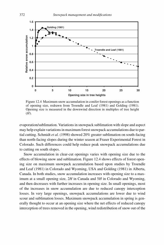
372 Snowpack management and modifications
0
0.2
0.4
0.6
0.8
1
1.2
1.4
1.6
0 5 10 15 20 25 30
Opening size in tree heights
Rel
ativ
e sn
ow
acc
um
ula
tio
n
Troendle and Leaf (1981)
Golding (1981)
Figure 12.4 Maximum snow accumulation in conifer forest openings as a functionof opening size, redrawn from Troendle and Leaf (1981) and Golding (1981).Opening size is measured in the downwind direction in multiples of tree height(H).
evaporation/sublimation. Variations in snowpack sublimation with slope and aspect
may help explain variations in maximum forest snowpack accumulations due to par-
tial cutting. Schmidt et al. (1998) showed 20% greater sublimation on south-facing
than north-facing slopes during the winter season at Fraser Experimental Forest in
Colorado. Such differences could help reduce peak snowpack accumulations due
to cutting on south slopes.
Snow accumulation in clear-cut openings varies with opening size due to the
effects of blowing snow and sublimation. Figure 12.4 shows effects of forest open-
ing size on maximum snowpack accumulation based upon studies by Troendle
and Leaf (1981) in Colorado and Wyoming, USA and Golding (1981) in Alberta,
Canada. In both studies, snow accumulation increases with opening size to a max-
imum at a small opening size, 2H in Canada and 5H in Colorado and Wyoming,
and then decreases with further increases in opening size. In small openings, most
of the increases in snow accumulation are due to reduced canopy interception
losses. In very large openings, snowpack accumulations are lower due to wind
scour and sublimation losses. Maximum snowpack accumulation in spring is gen-
erally thought to occur at an opening size where the net effects of reduced canopy
interception of trees removed in the opening, wind redistribution of snow out of the

12.2 Forest management 373
opening, increased sublimation from snow in the opening due to wind, and pos-
sibly wind transport into the opening from the upwind forest produce maximum
accumulation.
The contributions of wind transport into the opening from the upwind forest
remain unclear. Schmidt and Troendle (1989) showed, by measuring the flux of
blowing-snow particles, that a plume of blowing snow from the upwind forest
appeared to add to the accumulation of snow in a downwind clearing in Colorado
subalpine forest. Existence of blowing-snow conditions may add to variability of
snowpack accumulation experienced when openings are created, but other direct
evidence of wind transport of intercepted snow from the upwind forest into openings
is not available.
Some studies show patterns of reduced snowpack accumulations immediately
downwind from openings (Golding and Swanson, 1986; Gary, 1980; Gary and
Troendle, 1982; Golding, 1981). An example from Gary and Troendle (1982) in
Figure 12.5 based upon experiments in Wyoming shows gains in the opening that
were essentially completely offset by losses in the downwind forest. One interpreta-
tion of such patterns is that a clear-cut opening causes a back eddy that scours snow
from the forest snowpack immediately downwind from the cut and adds it to the
accumulation in the opening or transports snow farther downwind (Gary, 1980).
Another interpretation of reduced snow accumulation downwind from openings
is that snowpacks in the downwind forest are subjected to increased early-season
melting and evaporation/sublimation that reduces peak springtime accumulations
due to increased snowpack exposure to wind and radiation (Meiman, 1987; Golding
and Swanson, 1986).
Whether forest cutting in a patchwork of openings and uncut areas actually
increases snowpack available for streamflow across large watersheds has been
debated. Hoover and Leaf (1967) presented arguments for Fool Creek watershed
in Colorado that increased snow accumulations in openings were offset by reduced
accumulations in the downwind forest such that the net precipitation to the par-
tially cut watershed was unaffected. However, analysis of more data from the same
watershed by Troendle and King (1985) did show that maximum snow accumula-
tion across the Fool Creek watershed (cut and uncut areas) was increased 9% due
to cutting. Thus, it appears that increased snowpack accumulation does occur over
large partially cut watersheds, but relative roles of processes leading to increased
accumulations are difficult to sort out.
Overall, it is clear that either clear-cut openings or selective removal of individual
trees, can lead to increased snowpack accumulations. Increases in clear-cut open-
ings are best achieved with 2H to 5H opening sizes. See Chapter 2 for a discussion
of snow interception and blowing-snow processes.

374 Snowpack management and modifications
Figure 12.5 Patterns of snowpack increases within a 3H forest opening and snow-pack depletion in the downwind forest (Gary and Troendle, 1982, courtesy USDAForest Service).
12.2.2 Forest cutting and snowpack ablation
Ablation of snowpacks is the sum of losses due to melting and the net effect of vapor
exchange. Ablation rates are largely controlled by the energy budget at the snow-
pack surface in forest or in clear-cut openings. Basic principles controlling energy

12.2 Forest management 375
0
5
10
15
20
25
30
35
1/7/
1969
1/21
/196
9
2/4/
1969
2/18
/196
9
3/4/
1969
3/18
/196
9
4/1/
1969
4/15
/196
9
4/29
/196
9
5/13
/196
9
Sn
ow
pac
k w
ater
eq
uiv
alen
t, c
mShaded Border
Sunny Border
Interior Forest
Figure 12.6 Snow accumulation and ablation patterns in interior forest and alongthe shaded and sunny border of a 1H wide, E–W oriented clear-cut strip in Engle-mann spruce (Picea engelmanni Parry) forest in New Mexico (redrawn from Gary,1974 courtesy USDA Forest Service).
exchange were considered in Chapter 6 and forest effects on energy exchange were
covered in Chapter 7. Ablation rates are increased as the forest canopy is selectively
thinned due to increased solar radiation transmission and increased wind speeds.
Increased accumulations due to reduced interception are often offset by greater
rates of snowpack ablation in thinned stands, so that snow disappearance occurs at
approximately the same time in thinned and uncut stands. Effects of changing forest
density can be indexed by changes in leaf-area index (LAI), radiation extinction
coefficients or canopy density. Based upon periodic measurements of snowpack
water equivalent in eastern US forests, ablation rates in open/deciduous hardwood
forest/conifer forest cover types can be approximated using the ratios 3:2:1 (Federer
et al., 1972).
Shadow patterns cast by forest edges play a major role in controlling ablation
rates in clear-cut openings, even though some solar radiation is transmitted through
the forest. Snowpacks along forest edges that are shaded, melt and sublimate more
slowly. Those in more exposed locations ablate rapidly due to more frequent and
intense direct beam solar radiation received during mid-day (Figure 12.6).
Figure 12.6 shows typical variations in accumulation and ablation within a clear-
cut strip in conifer forest that was 1H wide and oriented E–W in New Mexico,

376 Snowpack management and modifications
Figure 12.7 Shadow length–solar geometry relationships along infinite forest edge.
USA. Accumulation totals, until major melting began in March, were lowest in the
interior forest, intermediate along the sunny border, and greatest along the shaded
border due to interception, evaporation/sublimation and blowing-snow effects. Gary
(1974) found that daily snowpack evaporation/sublimation rates were 87% higher
along the sunny than shaded border during a 12-week winter period in this opening.
After ablation began, the greatest ablation rates occurred along the sunny border,
intermediate rates occurred along the shaded border, and lowest rates were found in
the interior forest. Snow disappeared several weeks earlier along the sunny border
of the cut strip, but both interior forest and shaded border retained snow until
mid-May.
Widths of forest openings can be varied to control shadow length and average
melt rates across an opening. For level terrain, the shadow length cast by an infinite
forest edge at any time of day or year can be computed as (Figure 12.7):
S = H sin B cot A (12.2)
where:
S = shadow length measured perpendicular to the forest edge
H = tree height
A = solar altitude
B = acute angle between the solar beam direction and the forest edge direction
Equation (12.2) applies when a shadow is cast by the forest edge. Shadow lengths
change with solar altitude and solar azimuth during the day and during the winter
and spring melt seasons at a given latitude. Shadow lengths can be quite long at high
latitudes where solar altitudes are low during the accumulation and melt seasons.
If trees were 18 m tall along a forest edge oriented SW to NE (edge azimuth =45◦ east of north) where the Sun’s altitude above the horizon was 60◦ at an azimuth
of 180◦ (= solar noon, Sun from due south) on May 1, what length shadow would

12.2 Forest management 377
be cast by the edge? The acute angle between the solar beam and edge would be
45◦ and thus:
S = 18 sin 45◦ cot 60◦ = (18)(0.7071)(0.5774) = 7.35 m
Thus, at noon on this day only a relatively narrow band of snowpack surface, about
7.35/18 or 0.4H wide, would be shaded.
Orientation of long rectangular cut openings and tree height obviously are also
important controls on shadow lengths. Slope angle will also affect shadow length
but is not considered here.
12.2.3 Forest cutting and snowmelt runoff
Forest cutting can affect both the volume and timing of streamflow and ground-
water recharge from snowmelt. Changes in the natural timing of snowmelt runoff
due to cutting will depend upon the pattern of cutting and synchronization of melt
runoff from cut and uncut portions of a watershed. Volumes of snowmelt water
yielded as streamflow also can be increased due to reduced canopy interception
losses and wind redistribution of snow into openings in combination with reduc-
tions in growing-season evapotranspiration rates in the openings due to absence of
trees.
General recommendations for forest harvesting using clear-cut openings in sub-
alpine conifer forest are available. Opening size and orientation should vary some-
what with objectives of the harvesting: increasing the volume of streamflow or
preventing changes in flow regimen and peak flows. In all cases, intervening uncut
forest areas at least as wide as clear-cuts should be used to provide shade and a
source of blowing snow. When cutting to primarily enhance water yields, foresters
should use: wider openings about 5H wide (H = average tree height) to optimize
snow accumulation, forest edges oriented perpendicular to prevailing winds to take
advantage of blowing-snow effects, and relatively large portions of watershed area
cut to effect greater evapotranspiration losses, but never more than 50% area cut at
any time.
When cutting to primarily protect the natural flow regimen and minimize changes
in peak flows, foresters should use: smaller openings, about 2H, to keep average
melt rates in openings low and wherever possible use strip cuts orientated to provide
shade, e.g. E–W orientations. Smaller total fractions of watershed area cut (<1/4 to
1/3 of basin area in a cycle) should also be used. Successive cuttings generally are
made in the direction of the Sun to provide shade from original or regrowing forest
to produce what is known as a wall-and-step cutting pattern (Figure 12.8). To further
control peak flows, advantage can be taken of the natural melt desynchronization
by cutting wider strips at lower elevations and on south-facing slopes that naturally

378 Snowpack management and modifications
Figure 12.8 Wall-and-step cutting used to remove forest in three cutting cycleswhile providing shade to control melt rates and minimize impacts on peak flows.
melt earlier. Cutting narrower strips at high elevations and on north-facing slopes
that naturally melt later also can help to prevent changes to flow regimen.
Fool Creek watershed in the Rocky Mountains of Colorado, USA (Troendle
and King, 1985) is a classic paired-watershed experiment on impacts of forestry
practices on snow hydrology in subalpine conifer forest (Chapter 1; Figure 1.8).
The 289 ha basin had 50% of timbered area cut in forest strips ranging in width
from 1H to 6H. Over a 28-year period since cutting, annual water yields had been
increased an average of 8.2 cm per year or an increase in flow of about 36%.
Annual peak flows in spring on the basin were increased about 20% and advanced
7.5 days due to cutting. Flow increases were greater in years with greater winter
and spring precipitation and appear to be very long lasting. Estimates indicate that
nearly 70+ years will be required for flows to return to pre-cut levels due to slow
growth rates in the subalpine forest. Interestingly too, flow increases generally
occurred during the early spring melt season due to reduced evapotranspiration
during the previous growing season in cut areas. In the Colorado subalpine, summer
rainfalls are generally insufficient to recharge the soil and thus increases in soil water
content in cut areas due to reduced evapotranspiration have a delayed impact on
streamflow until melt begins and recharges soil the following spring. Troendle and
Kaufmann (1987) indicate that selective forest cutting, rather than using clear-cut
strips, can also increase annual flows by similar amounts in Colorado subalpine
forest.

12.3 Urban snow management 379
0
1
2
3
4
5
6
7
0 4 8 12 16 20 24
Time of day
Dis
char
ge,
mm
d
Pre-Cut
20% Cut
45% Cut
Figure 12.9 Impact of harvesting of deciduous forest in Pennsylvania on dailysnowmelt hydrographs (based upon data from DeWalle and Lynch, 1975).
In regions where peak runoff and total water yields are not greatly affected
by snowmelt, clear-cutting in large blocks can still produce significant changes
in streamflow for selected melt events. For example, DeWalle and Lynch (1975)
found for deciduous hardwood forest in Pennsylvania, that daily peak streamflows
for melt events during complete snow cover were increased by 18% and 29%
following successive large block clear-cuts covering 20% and 45% of basin area,
respectively (Figure 12.9). Snowpack melt rates and net allwave radiation were more
than doubled in the clear-cut area compared to adjacent uncut forest (DeWalle et al.,1977). Reductions in peak daily flows on watersheds with large block cuts would
be expected later in the spring season, due to desynchronization of melt runoff,
after snow was depleted in the openings (Hornbeck and Pierce, 1970).
Inadvertent forest disturbances such as mortality or defoliation due to fire, insects
and diseases, and windthrow can in some cases cause changes in snow hydrology
similar to that due to cutting. Loss of foliage obviously affects shading and the
snowpack energy balance. Mortality followed by windthrow reduces shading by
tree boles even further. Any aerodynamic changes to the forest canopy can affect
blowing-snow transport and have implications for snowmelt due to convection.
12.3 Urban snow management
The snow hydrology of urban and suburban areas is modified significantly from that
of undeveloped watersheds. Interconnected impervious areas in developed areas
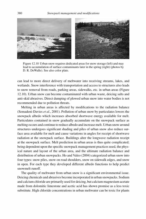
380 Snowpack management and modifications
Figure 12.10 Urban snow requires dedicated areas for snow storage (left) and maylead to accumulation of surface contaminants later in the spring (right) (photos byD. R. DeWalle). See also color plate.
can lead to more direct delivery of meltwater into receiving streams, lakes, and
wetlands. Snow interference with transportation and access to structures also leads
to snow removal from roads, parking areas, sidewalks, etc. in urban areas (Figure
12.10). Urban snow can become contaminated with urban waste, deicing salts and
anti-skid abrasives. Direct dumping of plowed urban snow into water bodies is not
recommended due to pollution threats.
Melting in urban areas is affected by modifications to the radiation balance
(Semadeni-Davies et al., 2001). Pollution of urban snow by particulates lowers the
snowpack albedo which increases absorbed shortwave energy available for melt.
Particulates contained in snow gradually accumulate on the snowpack surface as
melting occurs and continue to reduce albedo and increase melt. Urban snow around
structures undergoes significant shading and piles of urban snow also reduce sur-
face area available for melt and cause variations in angles for receipt of shortwave
radiation at the snowpack surface. Buildings alter the longwave radiation receipt
at the snowpack surface. Melt prediction in urban areas is thus quite complicated;
being dependent upon the specific snowpack management practices used, the phys-
ical nature and layout of the urban area, and the ultimate radiation balance and
distribution of urban snowpacks. Ho and Valeo (2004) categorized urban snow into
four types: snow piles, snow on road shoulders, snow on sidewalk edges, and snow
in open. For each type they developed different albedo functions to help predict
snowmelt runoff.
The quality of meltwater from urban snow is a significant environmental issue.
Deicing chemicals and abrasives become incorporated in urban snowpacks. Sodium
and calcium chloride are primarily used for deicing, but calcium magnesium acetate
made from dolomitic limestone and acetic acid has shown promise as a less toxic
substitute. High chloride concentrations in urban meltwater can be toxic for plants

12.4 Albedo modification 381
and aquatic organisms. Anti-caking compounds, such as cadmium, added to deicing
salts to aid in salt spreading can exacerbate pollution problems. In addition to
deicing chemicals, urban snow receives significant particulate inputs from human
activity and anti-skid sand or cinder applications, especially snow that accumulates
curbside. Dry deposition of trace metals from human activity in urban areas also
contributes to contamination. Presence of snow in winter reduces the opportunity
for street sweeping, which can increase the particulates, solid organic debris (leaves
and trash) and trace-metal pollutant load in urban snow. See guidelines established
by transportation departments in many regions, such as the Road Salt and Snowand Ice Control Primer among others published by the Transportation Association
of Canada.
As in natural snowpacks, the first flush of meltwater from urban snow will
generally yield much higher concentrations of dissolved solids than later melt (see
Chapter 8). Particulates, trash, and trace metals adsorbed on particulates often
remain on the soil at the snow disposal site. High chloride content of urban meltwater
can increase mobility of trace metals in melt water, which enhances the threat of
downstream contamination.
Snow removed from streets, roads, and parking areas in central business districts
where large snowfalls are commonly encountered, should be transported and dis-
posed of in dedicated storage areas. Large snow piles can result that often persist
late into the melt season. Since snow storage areas can be the depository for pol-
lutants in urban snow, it is recommended that a small retention basin be employed
downslope from snow piles to help retain meltwater pollutants (see Figure 12.10).
Snow storage sites should also be fenced and located to avoid wellhead protection
and playground areas.
12.4 Albedo modification
Albedo modification to influence shortwave radiation exchange at the snowpack sur-
face has been used for centuries to increase melt rates (Slaughter, 1969). Increases
in melt can augment soil water content for early-season crop production, clear side-
walks and streets to improve accessibility, reduce ice jams in rivers, and control
snowmelt runoff in streams. Air pollutants that settle onto the snowpack surface
can also contribute to acceleration of melt rates. Dusting of river ice and snow to
speed melt and prevent ice jams at critical locations in channels is still commonly
practiced.
Various types of blackening agents such as wood ash, cinders, fly ash, coal dust,
etc. applied to the snowpack surface can greatly reduce the surface albedo, thereby
increasing the amount of absorbed shortwave radiation and melt. Small reductions
in albedo can have a disproportionately large effect on absorbed shortwave radiation

382 Snowpack management and modifications
and melt. A 25% reduction in albedo, e.g. a decrease from 80% to 60% reflection,
would cause a 100% increase in absorbed shortwave from 20% to 40% absorption.
Since melt rates are generally closely linked to absorbed shortwave radiation, melt
rates generally also increase by large amounts. For example, Beyerl (1999) showed
that 0.03 kg m−2 surface application of wood ash reduced snowpack albedo by
35% and increased melt rates by 70%. Warren and Wiscombe (1981) found that
fine particulates such as soot and soil dust could reduce snow albedo by 5–15% in
the wavelength bands up to about 0.9 μm without affecting radiation exchange at
larger wavelengths where snow is a good absorber.
Practical application of albedo modification to enhance melt is not as straightfor-
ward as might be imagined (Slaughter, 1969). Properties of ideal surface additives
are: high shortwave absorptivity, high thermal conductivity, low solubility, low tox-
icity, and high particle density (nonfloatable). In addition, the material should be
low cost, readily available, easily applied, and otherwise environmentally benign.
Materials that meet all or most of these criteria are not easy to find. Timing of
surface applications also must be considered so that fresh snowfall does not cover
treated surfaces, although dark layers rapidly reappear unless the fresh snowfall is
deep. Finally, surface accumulations of debris can insulate the surface and decel-
erate melt, as evidenced by large piles of urban snow covered by thick layers of
leaves, landscape mulch, and other particulates that can endure into late spring
(Figure 12.10). Kongoli and Bland (2002) found that manure applications to snow
actually decreased melt rates compared to untreated snow. Prediction of the albedo
modification effects of various surface additives on melt rates is difficult, but the
method can be quite effective in altering melt rates.
12.5 Snow management in ski areas
Snow is modified or managed in many ways in ski-area developments to enhance
recreational opportunities and provide a safe environment for visitors. A major
activity at ski areas is snow-making to augment snow accumulation. In addition,
skiers in steep terrain with large natural snow accumulations also require protection
from avalanches which is achieved by managing snow in avalanche startup, track,
and runout zones.
Snow making is accomplished using specialized machines to spray a fine mist of
water droplets into cold air to create snowfall where desirable for skiing. Various
types of snow-making equipment are available, but two basic types are compressed-
air snow guns and fan-type sprayers (Figure 12.11). Snow making requires fairly
significant water supplies and energy for compressors, pumps, and fans. Generally
a wet-bulb temperature in the air of less than −2 ◦C is required for proper freez-
ing. Nucleating agents may be added to the sprayed water to enhance freezing of
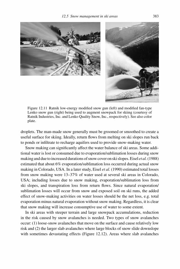
12.5 Snow management in ski areas 383
Figure 12.11 Ratnik low-energy modified snow gun (left) and modified fan-typeLenko snow gun (right) being used to augment snowpack for skiing (courtesy ofRatnik Industries, Inc. and Lenko Quality Snow, Inc., respectively). See also colorplate.
droplets. The man-made snow generally must be groomed or smoothed to create a
useful surface for skiing. Ideally, return flows from melting on ski slopes run back
to ponds or infiltrate to recharge aquifers used to provide snow-making water.
Snow making can significantly affect the water balance of ski areas. Some addi-
tional water is lost or consumed due to evaporation/sublimation losses during snow
making and due to increased durations of snow cover on ski slopes. Eisel et al. (1988)
estimated that about 6% evaporation/sublimation loss occurred during actual snow
making in Colorado, USA. In a later study, Eisel et al. (1990) estimated total losses
from snow making were 13–37% of water used at several ski areas in Colorado,
USA; including losses due to snow making, evaporation/sublimation loss from
ski slopes, and transpiration loss from return flows. Since natural evaporation/
sublimation losses will occur from snow and exposed soil on ski runs, the added
effect of snow-making activities on water losses should be the net loss, e.g. total
evaporation minus natural evaporation without snow making. Regardless, it is clear
that snow making will increase consumptive use of water to some extent.
In ski areas with steeper terrain and large snowpack accumulations, reduction
in the risk caused by snow avalanches is needed. Two types of snow avalanches
occur: (1) loose-snow avalanches that move on the surface and cause relatively low
risk and (2) the larger slab avalanches where large blocks of snow slide downslope
with sometimes devastating effects (Figure 12.12). Areas where slab avalanches

384 Snowpack management and modifications
Figure 12.12 Large slab avalanche in Colorado, USA that began in the alpinestartup zone (photo courtesy of Richard Armstrong, US National Snow and IceData Center, Boulder, CO). See also color plate.
typically occur are easily distinguished with well-defined startup zones at high
elevation (often above timber line), avalanche tracks that follow confined drainage-
ways or sometimes slide down broad slopes, and runout zones in valleys where the
avalanches generally come to rest. Avalanche tracks in subalpine regions are often
recognizable by the absence of older trees.
Snow management practices employed to reduce risk from avalanches in ski
areas or to protect structures and transportation corridors vary for the startup, track,
and runout zones (Table 12.1). Risk at ski areas can be reduced by simply closing
facilities when avalanche hazards are deemed highest; however, artificial triggering
of avalanches by using explosives and artillery under very carefully controlled

12.5 Snow management in ski areas 385
Table 12.1 Summary of snow management practices for reduction of avalanchehazards (Perla and Martinelli, 1978)
AVALANCHE ZONE OBJECTIVE PRACTICE
Startup Zone Prevent snow cornice formation Wind accelerators anddeflectors, explosives,upwind snow fences
Retard avalanche initiation Walls, fencing, netting,reforestation
Trigger avalanches at safe times Explosives, artilleryTrack Zone Prevent damage to new
structuresLand-use zoning by avalanche
hazard classesProtect roads and rail lines Tunnels, shed roofsPrevent damage to existing
structuresDeflecting walls and
foundations at base ofstructures
Runout Zone Stop snow movement Earthen mounds andconstructed walls
Protect new structures Land-use zoning by avalanchehazard classes
conditions can be quite effective. In addition, snow accumulations in high-elevation
avalanche startup zones can be stabilized by using snow fences, nets, and walls.
Formation of cornices of wind-blown snow and ice above avalanche startup zones,
that may collapse and trigger avalanches, can also be minimized using explosives
or wind deflectors that accelerate blowing snow past the cornice-formation regions.
Reforestation of startup zones to stabilize snowpacks can also be attempted, but
is extremely difficult given the typically severe growing conditions in subalpine
regions. Within avalanche track zones, various types of deflecting walls can be
used to divert avalanching snow away from the base or foundation of structures.
Avalanching snow in track zones can also be deflected over roads and rail lines by
using tunnels or shed roofs. Finally, within avalanche runout zones, deflecting walls
and sets of rounded earthen mounds can be used to slow and confine avalanches
to safe areas. The most effective method for protecting new human development
from snow avalanches is land-use zoning based upon avalanche hazard classes.
Readers are referred to the Avalanche Handbook (1978) by Perla and Martinelli
for more details related to snow-avalanche forecasting and protection practices.
Also see McClung and Schaerer (2006) for further details on mountain weather
and formation and occurrence of avalanches. Finally, a handbook by Weir (2002)
that deals with avalanche hazards and forest practices is another excellent source
of information.
386 Snowpack management and modifications
When large volumes of snow are displaced by inducement of snow avalanches,
the timing of snowmelt runoff may be altered (Martinec, 1989). Avalanched snow
deposited in flat, exposed runout zones at low elevations, generally is exposed
to earlier and higher surface melt rates, which could accelerate snowmelt runoff
in spring. However, avalanched snow that is concentrated in large deposits with
reduced surface area, especially if it accumulates in narrow, steep-sided shaded
runout zones, may extend the snowmelt-runoff season.
12.6 Climate change and snow hydrology
Climate change due to increases in atmospheric greenhouse gases could cause
increases in air temperatures and changes in precipitation regimes that would have
important impacts on snow hydrology. Increases in air temperatures can cause
greater occurrence of rainfall than snowfall events as well as increases in snow-
pack melt rates. Any accompanying alterations in precipitation regimes due to
climate change can also influence total snowfall and meltwater runoff amounts,
the seasonal timing of that runoff, and/or the occurrence of extreme melt and rain-
on-snow events. Loss of snow and ice cover over large land areas due to warming
and atmospheric pollution also can greatly reduce the global albedo and enhance
absorption of solar radiation at the Earth’s surface; thereby producing positive
feedback to the climate-change processes (see Figure 12.13). The likelihood of
occurrence of climate change is currently very uncertain and implications of climate
change for many aspects of present-day society are being actively researched (IPCC,
2001).
The impact of climate change on streamflow from mountainous areas and high
latitudes where snowfall is significant will depend upon the combination of air tem-
perature and precipitation changes that occur. Estimates of air-temperature changes
using various global climate models are reasonably consistent, at least in sign, but
precipitation change forecasts are highly variable. Increases in air temperature alone
would causes decreases in annual flows due to increases in evaporation. Changes
in mean air temperature of +2 to +4 ◦C, which are commonly predicted using
General Circulation Models for the year 2100 (Wigley, 1999), would result in
annual flow declines up to about 10%. However, such warming trends in com-
bination with annual precipitation changes ranging from –25% to +25%, could
cause annual streamflow changes to range from –51% to +67%, respectively,
for mountainous basins in western United States (Frederick and Gleick, 1999).
Increases in annual mean streamflows are more likely at higher latitudes because
warming is expected to be accompanied by increases in precipitation at these lat-
itudes. Seasonal estimates of climate change for specific regions across the world

12.6 Climate change and snow hydrology 387
66 68 70 72 74 76 78 80 82 84 86 88 90 92 94 96 98 00 02 04
Mill
ion
Squ
are
kmNorthern Hemisphere Snow Cover Anomalies
November 1966–May 20059
8
7
6
5
4
3
2
1
0
−1
−2
−3
−4
−5
−6
Figure 12.13 Variations in monthly snow cover over the Northern Hemisphereincluding Greenland for Nov 1966–May 2005 showing a decline in snow-coverpossibly due to global warming about a mean snow-covered area of 25.6 millionkm2 (courtesy of Dr. David A. Robinson, Rutgers University, Snow Lab.).
are needed in the future to improve estimates of climate-change effects on snow
hydrology.
The timing as well as volume of streamflow from snowmelt would be affected by
the climate-change scenario assumed. For example, Rango et al. (2003) estimated
the impacts of climate change on seasonal snowmelt runoff in the Rio Grande at
Del Norte, Colorado for 2050 and 2100 using the Snowmelt-Runoff Model (Figure
12.14). Based upon global climate model forecasts for the area, they assumed a
2 ◦C increase in air temperature and a 5% increase in precipitation by year 2050
and shifts of 4 ◦C and 10%, respectively, by year 2100. Increased air temperatures
caused earlier and more concentrated snowmelt runoff due to higher melt rates
and more rainfall events earlier in the winter. Increased peakflows also would be
expected by year 2100 for the assumed climate-change scenarios. More frequent
occurrence of large rain-on-snow events, often associated with serious flooding,
could be a further consequence, but the forecasting of large individual storm events
due to climate change is currently not possible.
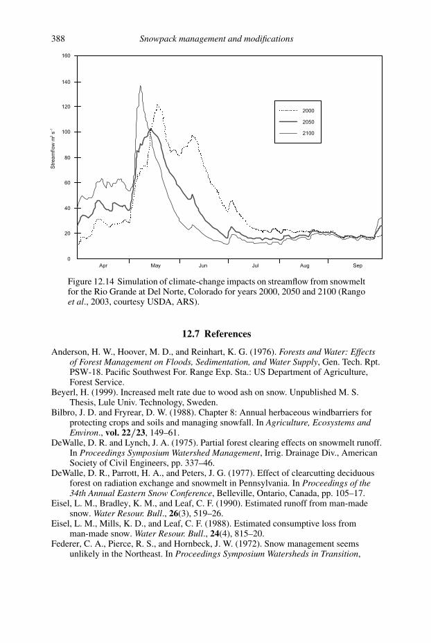
388 Snowpack management and modifications
Figure 12.14 Simulation of climate-change impacts on streamflow from snowmeltfor the Rio Grande at Del Norte, Colorado for years 2000, 2050 and 2100 (Rangoet al., 2003, courtesy USDA, ARS).
12.7 References
Anderson, H. W., Hoover, M. D., and Reinhart, K. G. (1976). Forests and Water: Effectsof Forest Management on Floods, Sedimentation, and Water Supply, Gen. Tech. Rpt.PSW-18. Pacific Southwest For. Range Exp. Sta.: US Department of Agriculture,Forest Service.
Beyerl, H. (1999). Increased melt rate due to wood ash on snow. Unpublished M. S.Thesis, Lule Univ. Technology, Sweden.
Bilbro, J. D. and Fryrear, D. W. (1988). Chapter 8: Annual herbaceous windbarriers forprotecting crops and soils and managing snowfall. In Agriculture, Ecosystems andEnviron., vol. 22/23, 149–61.
DeWalle, D. R. and Lynch, J. A. (1975). Partial forest clearing effects on snowmelt runoff.In Proceedings Symposium Watershed Management, Irrig. Drainage Div., AmericanSociety of Civil Engineers, pp. 337–46.
DeWalle, D. R., Parrott, H. A., and Peters, J. G. (1977). Effect of clearcutting deciduousforest on radiation exchange and snowmelt in Pennsylvania. In Proceedings of the34th Annual Eastern Snow Conference, Belleville, Ontario, Canada, pp. 105–17.
Eisel, L. M., Bradley, K. M., and Leaf, C. F. (1990). Estimated runoff from man-madesnow. Water Resour. Bull., 26(3), 519–26.
Eisel, L. M., Mills, K. D., and Leaf, C. F. (1988). Estimated consumptive loss fromman-made snow. Water Resour. Bull., 24(4), 815–20.
Federer, C. A., Pierce, R. S., and Hornbeck, J. W. (1972). Snow management seemsunlikely in the Northeast. In Proceedings Symposium Watersheds in Transition,
12.7 References 389
American Water Resources Association, Ft. Collins, CO June 19–22, 1972,pp. 212–19.
Frederick, K. D. and Gleick, P. H. (1999). Water and Global Climate Change: PotentialImpacts on U. S. Water Resources. Pew Center on Global Climate Change,www.pewclimate.org.
Gary, H. L. (1974). Snow Accumulation and Melt Along Borders of a Strip Cut in NewMexico, Res. Note RM-279. Rocky Mtn. For. Range Exp. Sta.: US Department ofAgriculture, Forest Service.
Gary, H. L. (1980). Patch clearcuts to manage snow in lodgepole pine. In Proceedings,Watershed Management Symposium, vol. I, Irrig. and Drainage Div., AmericanSociety of Civil Engineers, Boise, ID July 21–23, 1980, pp. 335–46.
Gary, H. L. and Troendle, C. A. (1982). Snow Accumulation and Melt Under VariousStand Densities in Lodgepole pine in Wyoming and Colorado, Res. Note RM-417.Rocky Mtn. For. Range Exp. Sta.: US Department of Agriculture, ForestService.
Golding, D. L. (1981). Hydrologic relationships in Interior West Watersheds., InProceedings, Symposium Interior West Watershed Management, Spokane, WA April8–10, 1980. Pullman, WA: Washington State University Cooperative Extension,pp. 107–16.
Golding, D. L. and Swanson, R. H. (1986). Snow distribution patterns in clearing andadjacent forest. Water Resour. Res., 22(13), 1931–40.
Heisler, G. M. and DeWalle, D. R. (1988). Chapter 2: Effects of windbreak structure onwind flow. In Agriculture, Ecosystems and Environ., vol. 22/23, 41–69.
Ho, C. L. I. and C. Valeo (2004). Observations of urban snow properties in Calgary,Canada. Hydrol. Processes, 19, 459–73.
Hoover, M. D. and Leaf, C. F. (1967). Processes and significance of interception inColorado subalpine forest. In Proceedings Seminar Forest Hydrology, ed. W. E.Sopper and H. W. Lull, Univ. Park, PA Aug. 29–Sept. 10, 1965. Oxford: PergamonPress, pp. 213–24.
Hornbeck, J. W. and Pierce, R. S. (1970). Changes in snowmelt runoff after forest clearingon a New England watershed. In Proceedings of the Eastern Snow Conference, 1969,pp. 104–12.
IPCC (2001). Chapter 2: Observed climate variability and change. In Climate Change2001: Working Group I: The Scientific Basis, Intergovernmental Panel on ClimateChange, www.grida.no/climate/ipcc tar/wg1/index.htm.
Kongoli, C. E. and W. L. Bland. (2002). Influence of manure application on surfaceenergy and snow cover. J. Environ. Qual., 31, 1166–1173.
Martinec, J. (1989). Hydrological consequences of snow avalanches. In WorldMeteorological Organization, Proc. Technical Conf., Geneva, Hydrology andDisasters, ed. O. Starosolszky. London: James and James, pp. 284–93.
McClung, D. and P. Schaerer. (2006). The Avalanche Handbook, 3rd Edition. Seattle, WA:The Mountaineers Books.
Meiman, J. R. (1987). Influence of forests on snowpack accumulation. In Management ofSubalpine Forests: Building Upon 50 Years of Research, Proc. Tech. Conf., Gen.Tech. Report RM-149. US Department of Agriculture, pp. 61–7.
Perla, R. I. and Martinelli, Jr, M. (1978). Avalanche Handbook. In Agric. Handbook 489.Washington, D.C.: US Printing Office.
Rango, A., Gomez-Landesa, E., Bleiweiss, M., Havstad, K., and Tanksley, K. (2003).Improved satellite snow mapping, snowmelt runoff forecasting, and climate changesimulations in the Upper Rio Grande Basin. World Resource Rev., 15(1), 25–41.

390 Snowpack management and modifications
Schmidt, R. A. and Troendle, C. A. (1989). Snowfall into a forest and clearing. J. Hydrol.,110, 335–48.
Schmidt, R. A., Troendle, C. A. and Meiman, J. R. (1998). Sublimation of snowpacks insubalpine conifer forests. Can. J. For. Res., 28, 501–13.
Scholten, H. (1988). Chapter 20: Snow distribution on crop fields. In Agriculture,Ecosystems and Environ., vol. 22/23, 363–80.
Semadeni-Davies, A., A. Lundberg, and L. Bengtsson. (2001). Radiation balance of urbansnow: a water management perspective. Cold Regions Sci. and Technol., 33,59–76.
Shaw, D. L. (1988). Chapter 19: The design and use of living snow fences in NorthAmerica. In Agriculture, Ecosystems and Environ., vol. 22/23, 351–62.
Slaughter, C. W. (1969). Snow Albedo Modification: a Review of Literature, TechnicalRep. 217. Hanover, NH: US Army Cold Regions Research and EngineeringLaboratory.
Sturges, D. L. (1992). Streamflow and sediment transport responses to snow fencing arangeland watershed. Water Resour. Res., 28(5), 1347–56.
Sturges, D. L. and Tabler, R. D. (1981). Management of blowing snow on sagebrushrangelands. J. Soil and Water Conserv., 36(5), 287–92.
Tabler, R. D. (1980). Geometry and density of drifts formed by snow fences. J. Glaciol.,26(94), 405–19.
Tabler, R. D. (1991). Snow Fence Guide. Strategic Highway Research Program,SHRP-W/FR-91–106, National Res. Council, Washington, DC: National Academyof Sciences.
Tabler, R. D. (1994). Design Guidelines for the Control of Blowing and Drifting Snow.Strategic Highway Research Program, SHRP-H-91–381, Washington, DC: NationalAcademy of Sciences.
Tabler, R. D. (2003). Controlling Blowing and Drifting Snow with Snow Fences and RoadDesign. Final Report, NCHRP Project 20–7(147).
Tabler, R. D., Pomeroy, J. W., and Santana, B. W. (1990). Drifting Snow. In Cold RegionsHydrology and Hydraulics, Tech. Council on Cold Regions Engin. Monograph, ed.W. L. Ryan and R. D. Crissman. New York: American Society of Civil Engineers,pp. 95–145.
Transportation Association of Canada (1999). Road Salt and Snow and Ice Control.(www.tac-atc.ca/)
Troendle, C. A. (1987). The Potential Effect of Partial Cutting and Thinning onStreamflow from the Subalpine Forest, Res. Paper RM-274. Rocky Mountain Forestand Range Exp. Sta.: US Department of Agriculture, Forest Service.
Troendle, C. A. and Kaufmann, M. R. (1987). Influence of forests on the hydrology of thesubalpine forest. In Management of Subalpine Forests: Building on 50 Years ofResearch, Proc., Tech. Conf., Gen. Tech. Rept., RM-149. Rocky Mtn. Forest andRange Exp. Sta.: US Department of Agriculture, Forest Service, pp. 68–78.
Troendle, C. A. and King, R. M. (1985). The effect of timber harvest on the Fool CreekWatershed, 30 years later. Water Resour. Res., 21(12), 1915–22.
Troendle, C. A. and Leaf, C. F. (1981). Effects of timber harvest in the snow zone onvolume and timing of water yield. In Proceedings, Symp. Interior West WatershedManagement, Spokane, WA April 8–10, 1980. Pullman, WA: Washington StateUniversity Cooperative Extension, pp. 231–44.
Verge, R. W. and Williams, G. P. (1981). Chapter 16: Drift control. In Handbook of Snow,Principles, Processes, Management and Use, ed. D. M. Gray and D. H. Male.Toronto: Pergamon Press, pp. 630–47.

12.7 References 391
Warren, S. G. and W. J. Wiscombe. (1981). A model for the spectral albedo of snow. II:Snow containing atmospheric aerosols. J. Atmos. Sci., 37, 2734–45.
Weir, P. (2002). Snow Avalanche Management in Forested Terrain. Land ManagementHandbook Series, 55, British Columbia, Canada, Ministry of Forests, Forest ScienceProgram.
Wigley, T. M. L. (1999). The Science of Climate Change: Global and US Perspectives.Pew Center on Global Climate Change, www.pewclimate.org.

Appendix A
Physical constants
Table A.1 Saturation vapor pressure variations with temperature (List, 1963)a
Temperature (◦C) Over liquid water (Pa)b Over ice (Pa)
−30 50.88 37.98−25 80.70 63.23−20 125.40 103.2−15 191.18 165.2−10 286.27 259.7−5 421.48 401.5
0 610.78 610.75 871.92
10 1227.215 1704.420 2337.325 3167.130 4243.0
a List, R. J. (1963). Smithsonian Meteorological Tables, Sixth Revised Edn. SmithsonianMisc. Collections, Vol. 114, Washington, DC.b1 mb = 100 Pascals (Pa)
392

Tab
leA
.2D
ensi
ty,s
peci
fiche
at,a
ndth
erm
alco
nduc
tivi
tyof
air,
ice
and
wat
er(L
ist,
1963
;M
onte
ith,
1973
;U
SN
avy,
2003
)a
AIR
Ice/
Wat
er
Tem
per
atu
re(◦ C
)d
ryd
ensi
tyb
(kg
m−3
)sa
tura
ted
den
sity
b
(kg
m−3
)sp
ecifi
ch
eatc
(Jk
g−1
K−1
)th
erm
alco
nd
uct
ivit
y(W
m−1
K−1
)d
ensi
ty(k
gm
−3)
spec
ific
hea
t(J
kg
−1K
−1)
ther
mal
con
du
ctiv
ity
(Wm
−1K
−1)
−40
1.5
11
.51
10
05
92
41
73
02
.65
−30
1.4
51
.45
10
05
0.0
23
92
31
82
52
.55
−20
1.3
91
.39
10
05
0.0
24
92
21
92
02
.44
−15
1.3
71
.37
10
05
0.0
24
92
11
97
02
.39
−10
1.3
41
.34
10
05
0.0
25
92
12
02
02
.33
−51
.32
1.3
11
00
50
.02
59
21
20
60
2.2
80
1.2
91
.29
10
05
0.0
25
92
0/1
00
02
11
0/4
22
02
.23
0/0
.56
75
1.2
71
.26
10
05
0.0
26
10
00
42
00
0.5
75
10
1.2
51
.24
10
05
0.0
26
10
00
41
90
0.5
82
15
1.2
21
.22
10
05
0.0
26
99
94
19
00
.59
02
01
.21
.19
10
05
0.0
27
99
94
18
00
.59
73
01
.16
1.1
51
00
60
.02
79
96
41
70
0.6
12
aL
ist
(19
63
)S
eeT
able
A.1
.M
on
teit
h,
J.L
.(1
97
3).
Pri
ncip
les
ofE
nvir
onm
enta
lPhy
sics
.N
ewY
ork
:A
mer
ican
Els
evie
rP
ub
lish
ing
Co
.,In
c.U
SN
avy,
Co
ast
Gu
ard
(19
99
).C
hem
ical
Haz
ard
sR
esp
on
seIn
form
atio
nS
yst
em,
Sel
ecte
dP
rop
erti
eso
fF
resh
Wat
er,
Sea
Wat
er,
Ice
and
Air
.(w
ww
.ch
rism
anu
al.c
om
/In
tro
/pro
p.h
tm)
bat
stan
dar
dp
ress
ure
cat
con
stan
tp
ress
ure

Appendix B
Potential solar irradiation theory
Potential solar irradiation theory considers physical factors affecting receipt of
shortwave radiation, but excludes effects of the atmosphere (see Lee, 1963; Frank
and Lee, 1966). This theory includes the effects of times of year and day, latitude,
slope inclination and aspect on incoming solar radiation. Once potential solar irra-
diation data are computed for a specific site and time, empirical adjustments can be
added to approximate the effects of the atmosphere and the distribution of incoming
solar radiation into diffuse and beam fractions as described in Chapters 6 and 7.
This appendix provides a brief discussion of the theory with example calculations
divided into two sections: one for horizontal surfaces and the second for sloping
surfaces.
B.1 Potential solar irradiation on horizontal surfaces
Potential solar irradiation on a horizontal surface for any instant in time (Is) can be
computed as:
Is = (I0/e2) cos Z (B.1)
where:
I0 = the solar constant
e = the radius vector
Z = zenith angle
The solar constant is the average flux density of radiation received outside the
Earth’s atmosphere perpendicular to the solar beam. The value of the solar constant
has been given as 1360 to 1400 W m−2 (1.94 or 2.00 cal cm−2 min−1) (Monteith,
1973) and 1360 W m−2 is used for calculations here. The radius vector adjusts
the solar constant for the slight effects (±3%) of variations in the Earth–Sun dis-
tance during the year. Radius vector values can be obtained from solar ephemeris
394

Appendix B 395
Table B.1 Solar declination and radius vector for days during year (after Frankand Lee, 1966).
Dates, approximateJulian Dates(Jan 1 = 1)
Solar Declinationδ, degrees
(Radius Vector)2
e2
6/22 summer solstice 173 +23.5 1.032976/1 and 7/12 152 and 193 +21.967 1.030905/18 and 7/27 138 and 208 +19.333 1.027285/3 and 8/10 123 and 222 +15.583 1.021904/19 and 8/25 109 and 237 +10.917 1.015284/4 and 9/9 94 and 252 +5.633 1.007393/21 and 9/23 equinoxes 80 and 266 0 0.999603/7 and 10/8 66 and 281 −5.633 0.991542/20 and 10/22 51 and 295 −10.917 0.984042/7 and 11/5 38 and 309 −15.583 0.977901/24 and 11/19 24 and 323 −19.333 0.972851/10 and 12/3 10 and 337 −21.967 0.9693812/22 winter solstice 356 −23.5 0.96759
tables for a given date (see Table B.1). Zenith angle is the angle between the solar
beam and a perpendicular to the horizontal surface, e.g. Z = 0 when the Sun is
directly overhead and 90◦ at sunrise and sunset. The cosine law of illumination,
represented in Equation (B.1), dictates that flux density of radiation received is
reduced according to the cosine of the zenith angle; maximum irradiation occurs at
normal incidence when cos Z = 1. The complement of the zenith angle is the solar
altitude or the elevation angle of the Sun above the horizon.
Zenith angle (Z) can be computed from three other angles: latitude, solar decli-
nation, and hour angle according to:
cos Z = (sin θ sin δ + cos θ cos δ cos ωt) (B.2)
where:
θ = latitude
δ = solar declination
ωt = hour angle
Latitude indexes the position of a site in degrees north (+) or south (−) of the
equator. Solar declination accounts for seasonal effects and ranges between +231/2◦
on the summer solstice and −231/2◦ on the winter solstice (see Table B.1). The hour

396 Appendix B
d
wt
wtdq
q
Figure B.1 Angles used to compute potential solar irradiation on horizontal sur-faces.
angle is the angle the Earth must rotate so that the Sun is directly above the meridian
of the designated site. The hour angle accounts for time of day and is the product of
the angular velocity of the Earth’s rotation (ω = 360◦/24 h = 15◦ h−1) and the true
solar time (t) in hours before (−) or after (+) solar noon. These angles are illustrated
in Figure B.1. True solar time can be computed from local standard time plus a
correction for the difference in longitude between the meridian for the surface
and the reference meridian for the appropriate standard time zone [(longitude of
RM◦ – longitude of surface◦)/15◦ h−1] and a small correction for the equation of
time (−0.24 to +0.27 h) that also varies with time of year (see ephemeris tables
such as List, 1968).To illustrate the use of Equations (B.1) and (B.2) combined, Is is computed for a
site on February 7 (δ = −15.583◦ and e2 = 0.9779 from Table B.1) at a time equalto two hours before solar noon [ωt = (−2 h) (15◦ h−1) = −30◦] and a latitude of55◦ north of the equator (θ = 55◦) as:
Is = (1360/0.9779)[(sin 55◦)(sin −15.583◦)+(cos 55◦)(cos −15.583◦)(cos −30◦)]
= (1390.74)[(0.8191)(−0.2686) + (0.5736)(0.9632)(0.8660)]
= (1390.74)(0.2584) = 359 W m−2
The flux density of incoming potential shortwave radiation is obviously reduced
well below the solar constant of 1360 W m−2. The zenith angle equivalent to this
time of day can also be found from the term in brackets as cos Z = 0.2584 and Z =arcos 0.2584 = 75.02◦. Solar altitude (90◦− Z) would thus be 14.98◦ for this time,
date, and location.
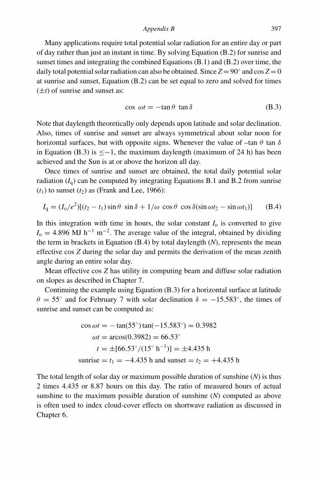
Appendix B 397
Many applications require total potential solar radiation for an entire day or part
of day rather than just an instant in time. By solving Equation (B.2) for sunrise and
sunset times and integrating the combined Equations (B.1) and (B.2) over time, the
daily total potential solar radiation can also be obtained. Since Z = 90◦ and cos Z = 0
at sunrise and sunset, Equation (B.2) can be set equal to zero and solved for times
(±t) of sunrise and sunset as:
cos ωt = −tan θ tan δ (B.3)
Note that daylength theoretically only depends upon latitude and solar declination.
Also, times of sunrise and sunset are always symmetrical about solar noon for
horizontal surfaces, but with opposite signs. Whenever the value of –tan θ tan δ
in Equation (B.3) is ≤−1, the maximum daylength (maximum of 24 h) has been
achieved and the Sun is at or above the horizon all day.
Once times of sunrise and sunset are obtained, the total daily potential solar
radiation (Iq) can be computed by integrating Equations B.1 and B.2 from sunrise
(t1) to sunset (t2) as (Frank and Lee, 1966):
Iq = (Io/e2)[(t2 − t1) sin θ sin δ + 1/ω cos θ cos δ(sin ωt2 − sin ωt1)] (B.4)
In this integration with time in hours, the solar constant Io is converted to give
Io = 4.896 MJ h−1 m−2. The average value of the integral, obtained by dividing
the term in brackets in Equation (B.4) by total daylength (N), represents the mean
effective cos Z during the solar day and permits the derivation of the mean zenith
angle during an entire solar day.
Mean effective cos Z has utility in computing beam and diffuse solar radiation
on slopes as described in Chapter 7.
Continuing the example using Equation (B.3) for a horizontal surface at latitude
θ = 55◦ and for February 7 with solar declination δ = −15.583◦, the times of
sunrise and sunset can be computed as:
cos ωt = − tan(55◦) tan(−15.583◦) = 0.3982
ωt = arcos(0.3982) = 66.53◦
t = ±[66.53◦/(15◦ h−1)] = ±4.435 h
sunrise = t1 = −4.435 h and sunset = t2 = +4.435 h
The total length of solar day or maximum possible duration of sunshine (N) is thus
2 times 4.435 or 8.87 hours on this day. The ratio of measured hours of actual
sunshine to the maximum possible duration of sunshine (N) computed as above
is often used to index cloud-cover effects on shortwave radiation as discussed in
Chapter 6.
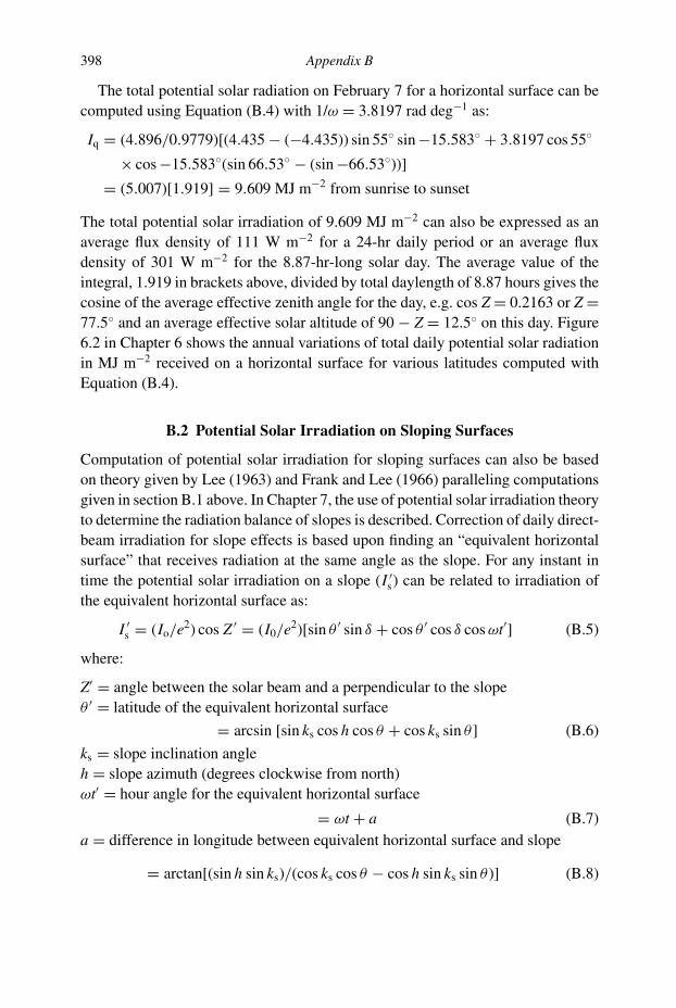
398 Appendix B
The total potential solar radiation on February 7 for a horizontal surface can be
computed using Equation (B.4) with 1/ω = 3.8197 rad deg−1 as:
Iq = (4.896/0.9779)[(4.435 − (−4.435)) sin 55◦ sin −15.583◦ + 3.8197 cos 55◦
× cos −15.583◦(sin 66.53◦ − (sin −66.53◦))]
= (5.007)[1.919] = 9.609 MJ m−2 from sunrise to sunset
The total potential solar irradiation of 9.609 MJ m−2 can also be expressed as an
average flux density of 111 W m−2 for a 24-hr daily period or an average flux
density of 301 W m−2 for the 8.87-hr-long solar day. The average value of the
integral, 1.919 in brackets above, divided by total daylength of 8.87 hours gives the
cosine of the average effective zenith angle for the day, e.g. cos Z = 0.2163 or Z =77.5◦ and an average effective solar altitude of 90 − Z = 12.5◦ on this day. Figure
6.2 in Chapter 6 shows the annual variations of total daily potential solar radiation
in MJ m−2 received on a horizontal surface for various latitudes computed with
Equation (B.4).
B.2 Potential Solar Irradiation on Sloping Surfaces
Computation of potential solar irradiation for sloping surfaces can also be based
on theory given by Lee (1963) and Frank and Lee (1966) paralleling computations
given in section B.1 above. In Chapter 7, the use of potential solar irradiation theory
to determine the radiation balance of slopes is described. Correction of daily direct-
beam irradiation for slope effects is based upon finding an “equivalent horizontal
surface” that receives radiation at the same angle as the slope. For any instant in
time the potential solar irradiation on a slope (I ′s) can be related to irradiation of
the equivalent horizontal surface as:
I ′s = (Io/e2) cos Z ′ = (I0/e2)[sin θ ′ sin δ + cos θ ′ cos δ cos ωt′] (B.5)
where:
Z′ = angle between the solar beam and a perpendicular to the slope
θ ′ = latitude of the equivalent horizontal surface
= arcsin [sin ks cos h cos θ + cos ks sin θ ] (B.6)
ks = slope inclination angle
h = slope azimuth (degrees clockwise from north)
ωt′ = hour angle for the equivalent horizontal surface
= ωt + a (B.7)
a = difference in longitude between equivalent horizontal surface and slope
= arctan[(sin h sin ks)/(cos ks cos θ − cos h sin ks sin θ )] (B.8)

Appendix B 399
In computations for a sloping surface the zenith angle is replaced by the angle of
incidence between the solar beam and a perpendicular to the slope (see Figure B.2).
Sunrise and sunset times for the equivalent horizontal surface are found in similar
manner as in our previous example for a horizontal surface, but with the latitude of
the equivalent horizontal surface rather the latitude of the slope as:
cos ωt′ = −tan θ ′ tan δ (B.10)
and with the further stipulation that sunrise and sunset times for the slope can
not occur before or after that, respectively, for a horizontal surface at the latitude
and longitude of the slope. Times between the slope and the equivalent horizontal
surface must be adjusted for the longitude shift.
Equation (B.5) must be integrated from sunrise to sunset times and angles for the
slope to find a daily potential slope irradiation sum. The equation can be integrated
from sunrise to sunset for the slope to obtain the total daily potential solar irradiation
on the slope (I ′q) as:
I ′q = (Io/e2)[(t2 − t1) sin θ ′ sin δ + 1/ω cos θ ′ cos δ(sin ωt′2 − sin ωt′1)] (B.11)
Again, the term in brackets on the right side of Equation (B.11) divided by the
length of the solar day (t2 – t1) gives an approximation of the mean cos Z′ for the
entire day for the slope. The equations appear daunting, but can be programmed
and easily solved on the computer. A step-by-step computation is given below to
illustrate the procedure.
B.2.1 Computing instantaneous potential irradiation on slope
The previous example in section B.1 above, where potential solar was computed
for a horizontal surface at latitude 55◦ on Feb 7 (δ = −15.583), will be continued. It
will be assumed that slope inclination angle ks = 30◦ and that the slope is oriented
to the southeast (SE aspect) equivalent to an azimuth angle (h) of 135◦ measured
clockwise from north.
First, the latitude of the equivalent horizontal surface must be determined as:
θ ′ = arcsin[sin 30 cos 135 cos 55 + cos 30 sin 55] = arcin[0.5065] = 30.43◦
which indicates that the latitude of the “equivalent horizontal surface” is south of
the latitude of the actual slope (actual θ = 55◦). A negative θ ′ can occur and would
indicate that the equivalent horizontal surface was in the southern hemisphere.
Next the longitude shift needed to find the “equivalent horizontal surface” must
be evaluated as:
a = arctan[(sin 135 sin 30)/(cos 30 cos 55 − cos 135 sin 30 sin 55)]
= arctan[0.4496] = 24.21◦

400 Appendix B
Since the slope faces to the east, the equivalent horizontal surface is 24.21◦ of
longitude to the east of the slope. For slopes facing toward the west, the longitude
shift to the equivalent horizontal surface is towards the west. Equivalent horizontal
surfaces for slopes facing due north or south have zero longitude shifts.
Given our earlier example, enough information is now available to compute the
instantaneous potential irradiation on a slope with Equation (B.5). Computations
assume an hour angle (ωt) equal to two hours before solar noon or (ωt = –30◦) on
the slope for a comparison with computations for a horizontal surface at that same
latitude and time. First the hour angle for the equivalent horizontal surface must be
adjusted for the longitude shift using Equation (B.7), which gives:
ωt′ = −30 + 24.21 = −5.79◦′
and
I ′s = (1360/0.9779)[sin 30.43◦ sin −15.583◦ + cos 30.43◦ cos −15.583◦ cos −5.79◦]
= (1390.74)[0.6902] = 960 W m−2
Z ′ = arcos[0.6902] = 46.35◦
The instantaneous flux density of potential solar irradiation for the slope of 960 W
m−2 is much greater than that for a horizontal surface for the same date and time of
359 W m−2 computed in section B.1. This difference in receipt of radiation occurs
because the angle of incidence Z′ for radiation on the slope (Z′ = 46.35◦) is less
than the zenith angle for the horizontal surface (Z = 75.02◦ from section B.1) for
the same time and date.
B.2.2 Computing daily potential irradiation on slope
Computation of the potential solar irradiation for an entire solar day begins with
finding the sunrise and sunset times for the “equivalent horizontal surface” using
Equations (B.7) and (B.10) as:
cos ωt′ = − tan 30.43◦ tan −15.583◦ = 0.1638
ωt ′ = ±80.57◦
sunrise t ′1 = −80.57◦/15◦ h−1 = −5.37 h
sunset t ′2 = +80.57◦/15◦ h−1 = +5.37 h
These times represent sunrise and sunset for the equivalent horizontal surface at a
different longitude. Again a correction is needed for the longitude shift to obtain
the times for the slope and to compare them with the limiting case of sunrise and
sunset times found previously for the horizontal surface at that same latitude and
longitude; ± 4.435 h. The shift in longitude is equivalent to a time difference

Appendix B 401
between the equivalent horizontal surface and the slope of a/ω = 24.21◦/15◦ h−1
= 1.61 h, thus:
t ′1 = t1 + a
−5.37 h = t1 + 1.61 h
t1 = −6.98 h
and
t ′2 = t2 + a
+5.37 h = t2 + 1.61 h
t2 = 3.76 h
The indicated sunrise time of – 6.98 hours before solar noon for the slope can not
actually occur because it can not occur before sunrise for a horizontal surface for
that latitude and day which is only – 4.435 h before solar noon. Thus, the sunrise
time for the horizontal surface (t1 = − 4.435 h) becomes the limiting condition and
its equivalent hour angle using Equation (B.7) [ωt′1 = (15◦ h−1)(− 4.435) + 24.21◦
= 42.32◦] must be substituted in Equation (B.11). The sunset time of +3.76 hours
for the slope occurs before the sunset time of +4.435 for a horizontal surface for
that day and no adjustment is needed; therefore for sunset t2 = +3.76 h and ωt′2 =+80.57◦ in Equation (B.11).
Total solar daylength for the slope from sunrise to sunset is 8.195 h (4.435 h +3.76 h), which is less than daylength for the horizontal surface of 8.87 h (2 × 4.435 h)
found previously. Note that the sunrise and sunset times for a similarly inclined slope
facing to the southwest would simply be the reverse of the southeast-facing slope
case.
Using Equation (B.11) and the appropriate sunrise and sunset times and hour
angles the potential solar irradiation on the slope for the day (Iq′) can be computed
as:
I ′q = (4.896/0.9779)[(3.76 − (−4.435))(sin 30.43◦)(sin −15.583◦)]
+ (3.8197)(cos 30.43◦)(cos −15.583◦)(sin 80.57◦ − sin(−42.32◦)) h]
= (5.007)[5.15353] = 25.8 MJ m−2
For comparison, the potential solar irradiation received on a horizontal surface for
the same day and latitude was only 9.609 MJ m−2 which illustrates the relatively
large effect that slope orientation can have on receipt of radiation. The average value
of the integral, 5.15353 in brackets above, divided by total daylength of 8.195 hours
gives an effective cos Z′ = 0.6289 or an average effective angle of incidence of
Z′ = 51◦ for the slope on this day. This angle of incidence becomes important to

402 Appendix B
scaling of the fractions of diffuse and beam solar irradiation for slopes as described
in Chapter 7.
B.3 References
Frank, E. C. and Lee, R. (1966). Potential Solar Beam Irradiation on Slopes: Tables for30◦ to 50◦ Latitude. Res. Paper RM-18. Rocky Mtn. For. Range Exp. Sta.: USDepartment of Agriculture, Forest Service.
Lee, R. (1963). Evaluation of Solar Beam Irradiation as a Climatic Parameter ofMountain Watersheds, Hydrol. Paper. No. 2, Ft. Collin, CO: Colorado StateUniversity.
List, R. J. (1968). Smithsonian Meteorological Tables, 6th edn., Smithsonian Misc.Collection, Smithsonian Publ. 4014, vol. 114. Washington, DC: SmithsonianInstitution Press.
Monteith, J. L. (1973). Principles of Environmental Physics. New York: AmericanElsevier Publishing Co., Inc.
Index
ablation of snowpacks 374acid neutralizing capacity (ANC) 225acidification of streams 222, 225, 226acoustic snowfall sensor 87acre–feet 269active layer, permafrost 248, 256active microwave radiometers 126active microwave remote sensing
radar applications outlook 137–8Adirondack snow tube 91advection 164–5aeolian dust 220aerial markers of snow depth 86–7aerosols 211albedo 139, 380albedo modification 381–2
surface additive characteristics 382albedo of snowpack 147, 183albedo, snow 153–6
factors affecting 154alcohol calorimetry 98Alter wind shield 80, 81aluminum toxicity 225Anaxagoras 7angular velocity of Earth’s rotation 396Atmospheric Integrated Monitoring Network
(AIRMoN) 217automatic weather stations 160avalanches 294
loose snow type 383slab type 383, 384
runout zones 384–5startup zones 384, 385tracks 384, 385
basin area–elevation curve 315, 316beam shortwave radiation
horizontal surface 148slopes 183
example calculations 185–6Bergeron process 21, 22black body radiator 157black snow 220
black snowfall 212blowing snow 29–35blowing-snow management 365–70
applications and importance 365–6constructed snow fences 367–9crop stubble windbreaks 370drift formation 366–7example calculations 34–5factors influencing 31–3living windbreaks 369–70modelling 33–5, 36modes of transport 30shear stress vs. strength 31–2sublimation losses 33topography 32–3vegetation 32
Bowen ratio 167–9brightness temperature 126bulk aerodynamic method 160bulk deposition 217–18bulk Richardson number 162–3bulk transfer coefficient
sensible heat 161–5vapor exchange 166
Canadian MSG snow sampler 91Canadian prairie snow water equivalent mapping
131–3canopy cover 41canopy interception loss 37Central Sierra Snow Laboratory, U.S. 8–10centrifugal method, liquid water in snow 98channel precipitation 244chemical flux density 213, 215, 221chemical storage load 220Clean Air Status and Trends Network (CASTNET)
217climate change 386–7climate change and snow
streamflow amounts 386–7streamflow timing 387, 388
coefficient of determination 333cold content 63–4, 238, 256, 281
403

404 Index
cold front 24cold-content degree–day factors 278conservative hydrologic tracer 226constructed windbreaks
deployment 369design features 367
bottom gapheight 367porosity 367tilt angle 367
cornice control 385cosine law of illumination 395cosmic radiation measurements of snowpack water
equivalent 94–5creep 30critical temperatures, rain vs. snow 272crop stubble windbreaks 370
Darcy’s Law 67–70daylength 397degree-day cold content computation 277–9degree-day factor (SRM) 324–6degree-day melt computation 274–7degree-day melt factors
base temperature 275daily vs. other time periods 275example computations 275forest cover effects 277hybrid models 277reference temperature 274–5seasonal variation 275–7summary of controlling factors 276
degree-days 250deicing chemicals 380densification, snowpack 55density
air 161dry air 393dry soil 252ice/water 170, 393saturated air 393
depth hoar 52desynchronization of melt runoff 379deuterium 228dielectric method, liquid water in snow 98diffuse shortwave radiation
horizontal surface 148slopes 183
example calculations 189sky view factor 188
dilution method, liquid water in snow 98dipolar molecule, water 14distributed-snowmelt models
elevation 289–91forest cover 291frozen ground 292glaciers 293–4slope and aspect 290–1snow avalanches 294snow-covered area 286–9
measured snow-cover data 288–9
snow-cover depletion curves 286–8topographic shading 294wind redistribution 292–3
double-fence wind shield 80dry deposition on snowpacks 215–18
atmospheric concentrations of pollutants 216data sources 217deposition velocity 215–16example calculations 216–17factors affecting 215
dual precipitation measurement intercomparisons81–5
Dubovskoye Hydrological Laboratory, Russia
eddy covariance methods 160effective saturation 69effective thermal conductivity 57–60El Nino 28electromagnetic spectrum 119, 120elevation zones 314, 315energy budget of snowpack 146–7
change in internal heat storage 146convective exchange of latent heat 146convective exchange of sensible heat 146examples 178ground heat conduction 146meltwater loss 146net longwave radiant energy exchange 146net shortwave radiant energy 146, 147–56open and deciduous forest sites 206open horizontal surfacerainfall latent and sensible heat 146reviews 147topographic influences 182–93topographic shading 186–7
ensemble forecasting 299–300equation of time 396equilibrium snow drift 367equinox 395equitemperature metamorphism 49, 50equivalent horizontal surface 398event water 225, 245extinction coefficient, shortwave radiation in snow
152
firn 54fish kills 222, 225flow fingers 73flux density 227Fool Creek forest management experiment, U.S. 11,
373, 378forest block clear cutting 379forest cutting and snow accumulation 371–3, 375
blowing snow near opening 373, 374causes of increased accumulation 371–2effect on basin-wide snowpacks 373effect of forest opening size 372–3
forest cutting and snowmelt runoff 377–9general management recommendations 377–8
forest cutting and snowpack ablationmelt and sublimation impacts 374–5

Index 405
shading by forest edges 375–7, 378example shadow length calculation 376–7
forest disturbances 379forest edge orientation 376forest influences 193–206
air temperature 204atmospheric stability 205humidity 204–5longwave radiation 199–202
canopy closure 195, 200canopy view factor 199importance of tree boles 200forest influences
net allwave radiation 200–2comparison of conifers and hardwoods 201
shortwave radiation 193–9Beer’s law 196–9comparison of conifers and hardwoods 201diffuse and direct beam transmission 198direct beam path length 198extinction coefficients 195–6, 197
snowpack energy budgets 205–6wind speed 202–4
forest management and snow hydrology 370–9forest selection cutting 378forest strip clear cutting 377forest wall-and-step cutting 378fractionation
isotopic 228–31melt 221–4
Fraser Experimental Forest, US 8, 11freezing calorimetry 98, 100–1
equipment and materials 101freezing-point depression method, liquid water in
snow 98friction velocity 31, 161frost-bulb depression 272frozen ground 246–56
frost formation processes 249–50infiltration rates 255–6
degree-day method 256prediction from soil properties 255–6
influence of snow cover on 248, 253–5influence on meltwater flow paths 247–8, 249predicting soil frost depth 249–55
modified Berggren method 250–3soil, climate and vegetation influences 248–9
gamma radiation aerial surveys 120–2, 139gamma radiation snowpack profiling gauges 95glaciers 293–4Global Meteoric Water Line (GMWL) 228global radiation 148graupel 21Great Lakes, US 1, 24, 28ground heat conduction 171–2
example computations 172soil temperature gradient 171soil thermal conductivity 171
ground-based radar snowfall measurement 88–9groundwater flows 245–6
heat capacity of soil 252heat conduction in snowpacks 57–61
convection by wind 60density effects, effective thermal conductivity 60prediction 60–1radiation transmission 60solid phase conduction 57vapor transport 57–60
hexagonal lattice structure 15historical development of snow hydrology 7–10hotplate snowfall gauge 87–8hour angle 395hydrogen bonds 15hydrograph separations 245–6hydrologic flushing 225hypsometric curve 315, 316hypsometric mean elevation 290
importance of snowremote sensing 118–20
incoming shortwave radiation 148–52diffuse fraction of global radiation 185empirical estimation 151–2
air temperature range method 151–2cloud cover method 151–2sunshine duration method 151–1
example empirical computations 152measurement 148–50potential solar radiation theory 150–1, 394–402transmission in snow 152–3
Beer’s Law 152–3extinction coefficient 152–3
interflowinternal snowpack energy storage 172–4
computations 173–4latent heat of fusion storage 173sensible heat 172–3
international classification system for seasonal snowcover 58–9
international symbols for snowpack properties 106internet snow information sources, U.S. 12–13intrinsic permeability 69irreducible water content 69
Kirchhoff’s Law 157
La Nina 28–9lag times, liquid water runoff 241lake-effect snowfall 1, 25–7land-use zoning 385lapse rates for temperature 192–3latent heat convection 165–9
Bowen ratio 167–9wet-bulb analogy 169example computations 166–7
latent heat of fusion 17, 170, 250latent heat of sublimation 17latent heat of vaporization 17latitude 395leaf-area index 39, 41light attenuation snowfall sensor 87
406 Index
limestone dust 220liquid water in snow 64–7, 74
capillary effects 67–8intrinsic permeability 69–70preferential flow paths 73–4
flow fingers 73thermal quality 65–7water movement theory 67–74gravity effects 68–74shock wave formation 71–3
living windbreaks 369–70local standard time 396logistic growth curve, interception 42–4longitude shift, slope radiation 398longwave radiation, defined 156longwave radiation exchange 156–9
incoming longwave radiation 158–9clear sky 158cloudy sky conditions 159
outgoing longwave radiation 157–8snow emissivity 157
longwave radiation on slopes 190–2atmospheric and terrain inputs 190comparison with horizontal surface 191example computations 190–1
macropore flow 246management of snowpacks
albedo modification 381–2blowing-snow management 365–70forest management and snow 370–9ski area snowpack management 382–6urban snow management 379–81
Marmot Creek Basin, Canada 9mean effective zenith angle 397measuring snow on the ground 89–105
liquid-water measurements 97–103other methods for snowpack water equivalentsnow course surveys 89–93snow pits 103–5snowpack telemetry system (SNOTEL) 93–4
melt energy 174–5example computation of melt rate 175
melt–freeze metamorphism 49, 53melting calorimetry method, liquid water in snow 98,
102melting degree-day factor 274meltwater chemistry 221–5
chemical flux density 221melt fractionation 221–4preferential elution 224–5stream acidification 221–2
meltwater flow paths 242, 243–6channel precipitation 244groundwater 245–6overland flow 244subsurface stormflow or interflow 244–5
meltwater lag timescold-content effects 238–9
nocturnal 239seasonal 238–9
lag and route method 241–2example computations 242–3
liquid water storage capacity effects 239–40total 241transmission of meltwater effects 240–3
metamorphism of snow 48–57microwave radiation surveys 139model forecasting updates 299, 345–6modelling snowmelt runoff
distributed-snowmelt models 284–94future directions 300model types 266–7point-snowmelt models 271–84snowmelt-runoff model performance and selection
298–300snowmelt-runoff models 294–8statistical methods 267–71
predicting spring runoff volumes 268–9using snow-covered area vs. runoff curves
270–1modifications of snowpacks
climate change and snow hydrology 386–7modified Berggren method 250–3
example calculations 253
Nash–Sutcliffe coefficient 334National Atmospheric Deposition Program (NADP)
213National Operational Hydrologic Remote Sensing
Centergamma radiation airborne surveys 131snow cover maps 130–1snow data assimilation systems (SNODAS) 131
net shortwave radiation exchange 156Nipher wind shield 80, 81Northeast Snowfall Impact Scale 5National Weather Service River Forecast System
(NWSRFS) model 296
operational snowmelt-runoff forecasts 133–6India runoff forecast 134Norway power applications 133–4Spain power applications 134United States applications 136
orographic lifting 22–4outgoing or reflected shortwave radiation 153–6overland flow 244, 249
passive and active microwave radiation 126–9passive microwave remote sensing 131
improving algorithms 136–7improving resolution 136
passive microwave satellite data 132permafrost 246phase changes of water 17physical properties of air, ice, water 393point snowmelt model algorithms 271–84
basic scenarios 279–81estimating form of precipitation 271–4example computations 281–3SNOTEL data simulation 283
Index 407
storage terms 281degree-day cold content computations
277–9degree-day melt computation 274–7temperature-index methods 274–9
potential solar irradiation theory 394–402horizontal surfaces 394–8
finite or daily time periods 396–8instantaneous 396
sloping surfaces 398–402finite or daily time periods 400–2instantaneous 399–400
Prairie Blowing Snow Model 35precipitation gauge intercomparisons 84Precipitation Runoff Modeling System (PRMS) 288,
297predicting spring runoff volumes 268–9pre-event water 225, 245preferential elution 224–5pressure metamorphism 49, 53pressure pillow 93pressure pumping 60properties of water 13–16pyranometer 149pyrgeometer 149, 158pyrheliometer 149
radius vector 394, 395rainfall contributing area (SRM) 327rainfall energy additions 169–71
example computations 170freezing rain effects 171humidity feedback 171rainfall intensity effects 170
rain-on-snow floods 261–2contributing factors 261–2role of forest harvesting 262
rainout 212, 213recession coefficient (SRM) 327–31reference meridian 396remote sensing of the snowpack
acronyms for satellites, instruments andprograms
advantages and disadvantages of methods 139current applications 130–6future directions 136–9gamma radiation surveys 120integration of data types 138–9National Operational Hydrologic Remote Sensing
Center 130–1passive and active microwave radiation surveys
126–9photo interpretationsnow maps, hand-drawn 129–30spaceborne imaging systems 125thermal infrared radiation surveys 125visible and near infrared radiation surveys
122–5Reynolds Creek, US 11, 12, 80riming 21, 212Rio Grande, US 1
ripe snow 62, 173Rocky Mountains, US 23roughness length 31roughness obstacles 162routing coefficient for liquid water 242runoff coefficient (SRM) 322–4
saltation 30saturated overland flow 245saturation vapor pressure
at snowpack surface 166variation with temperature 392
scanning electron microscopy 108, 111materials and methods 107–12
coating samples 111recording images 111–12sampling procedures 109–11secondary specimen holders 107shipping sampling plates 109
scavenging by snowflakes 212sensible heat convection 159–65
roughness length 161–2atmospheric stability 161, 162–4
neutral stability 162stable air 162unstable air 162
sensible heat exchangeexample computations
shear strength 31shear stress 31, 161shock wave 71shortwave radiation, defined 147shortwave radiation on slopes 183–90
comparison with horizontal surface 191diffuse shortwave radiation 187–90direct-beam shortwave radiation 183–7example computation 189net shortwave radiation 183
sintering 50ski-area snow management 382–6
avalanche risk reduction 383–5management practices 384–5
snow making 382–3Sleepers River Basin, US 11, 13slip face, snowdrift 367slope inclination angle 186, 188, 190, 398SNOTEL 93–4, 95, 268
data availability 94, 96snow boards 85snow course 268snow course surveys 89–93
data availability 93–4snow cover mapping data sources 320snow-covered area (SRM) 319–21, 341, 342snow crystal imaging 105–12
light microscopy 105scanning electron microscopy 105–12
snow crystal types 22, 23, 24snow damming 256snow drift, ultimate disposition 369snow drift formation 366–7
408 Index
snow fences 366snow guns 382, 383snow hydrology
importance of blowing snow andinterception 44
research basins 10–13textbooks 10
snow importance 1–7agriculture 1climate control 5–6ecological 6–7impact rating 5remote sensing 6transportation 1–5water supply 6
snow interception 36–44factors affecting 37–9
meteorological 39vegetative 37–9
modelling snow interception 39–44snow lysimeters 103snow-making machines
compressed-air type 382fan-type 382
snow pillow 97, 268snow pit 104snow stakes 85–6snow tube samplers 91, 92snow wind redistribution parameter 292snow-cover depletion curves 286–8, 322snowfall chemistry 211–15
differences between rain and snow 212interaction with vegetation 213regional differences 213, 214
snowfall formation 20–9altitude 20convergence 25frontal activity 24–5, 27lake-effect snowfall 25–7latitude 20orographic lifting 22–4, 25Southern Oscillation effects 28–9
snowfall measurement 76–89acoustic transducer 87automatic weather stations 87gauge placement 81ground-based radar 88–9hotplate snow gage 87–8Idaho case study 81–5light attenuation 87manual depth measurements 85–7measurement errors 78–81precipitation gauges 76–8
nonrecording gauges 76storage gauges 76–7
recording gauges 77–8tipping-bucket gauges 77–8weighing-type gauges 77
snowfall records 89vibrating wire-strain gauge 88wind correction factors 78–81
wind-shields 78snowmelt hydrographs 256–60
annual patterns 257–8effect of glaciers 258
daily variations 258basin runoff lag times 259
one day’s melt contribution 259–60streamflow data sources 260
Snowmelt-Runoff Model (SRM) 133, 135, 289climate change simulations 346–61
example for Rio Grande, CO 359future scenario simulations 350–9model parameters in changed climate 359–60normalization of data to present climate 360snow accumulation changes 348–50, 354, 357,
358winter half-year simulations 347–8
data needs 314–33basin characteristics 314–16model parameters 321–33variables 316–21
errors noted by users and corrections 338–40Micro-SRM computer program 361–2model accuracy assessment 333–7model structure 313–14real time forecasting 337–46
examples 317, 342, 344updating 345–6
simulation for Dischma basin 336simulation for Rio Grande basin 334simulation for Tavanasa station 341SRM applications and results 307–11, 312
snowmelt-runoff models performance and selection298–300
World Meteorological Organization (WMO)comparisons 298–9
snowmelt-runoff models 294–7, 298National Weather Service River Forecast System
(NWSRFS) 296Precipitation Runoff Modeling Systems (PRMS)
297Snowmelt-Runoff Model (SRM) 296–7, 306–62Streamflow Synthesis and Reservoir Regulation
Model (SSARR) 297Swedish Meteorological and Hydrological Institute
Model (HBV) 297Systeme Hydrologique Europeen model (SHE)
297–8snowpack chemistry 217–21
chemical load calculation 220factors affectingmeasurement problems 220–1regional variations 219–20
snowpack density 54–5snowpack liquid-water holding capacity 239snowpack liquid-water measurements
calorimetry 99–100centrifugal methods 97–8dielectric method 98, 99dilution method 98–9freezing calorimetry 100–1
Index 409
intercomparison of methods 103snow lysimeters 103
snowpack management and modifications365–87
snowpack metamorphism 48–57grain faceting 51–3grain rounding 48–50ice lens formation 54international classification system for seasonal
snow cover 57snowpack density 54–5, 56surface sublimation 54wet snow processes 53–4wind effects 54
snowpack water equivalent 17–18, 235snowpack
cold content 63–4control of soil nitrogen assimilation 227liquid water content 65–7temperatures 62–3
soil freezingfusion parameter 252thermal ratio 252
soil thermal conductivity 250solar altitude 148, 376solar constant 394solar declination 395solar ephemeris 394Southern Oscillation 28specific heat
air 161, 393ice/water 170, 393
stability corrections, atmospheric 163stable isotopes 246stable isotopes in snowpack 227–31
characterizing abundances 228fractionation 228–31melt fractionation 230–1phase differences 228–9seasonal variations in precipitation 229vapor migration 229, 230, 231
Stefan–Boltzmann constant 157Stefan–Boltzmann equation 157, 158stemflow 36–7storage-type snowfall gauges 76–7streamflow chemistry and melting 225–7
chemical mass flux 227hydrograph separations 226nitrogen assimilation and export 227
subsurface stormflow 244–5summer solstice 395sunrise time 397, 400sunset time 397, 400surface hoar 54surface roughness 31surface temperature degree-day factorSURFRAD network 149, 150Swedish Meterological and Hydrological Institute
model (HBV) 297synchronization of melt runoff 377synthetic aperture radar (SAR) 126
Systeme Hydrologique Europeen model (SHE)297–8
temperature lapse rate (SRM) 317, 326–7, 342temperature-gradient metamorphism 49thermal conductivity
air 393ice/water 393frozen soil 250
thermal infrared radiation surveys 125, 139thermal quality 65–7, 175threshold velocity 32throughfall 36throughfall chemistry 212, 213Tian Shan Glaciological Station, China 10time lag (SRM) 331–3tipping-bucket type snowfall gauges 77–8topographic influences
air temperature 192–3potential solar radiation on slopes 184topographic shading 187wind speed 193
translatory flow 245transmission of radiation in snow 152–3
example computations 153transmission rate, liquid water in snow 240Tretyakov shelded precipitation gauge 80, 81tritium 227true solar time 396
US Cooperative Snow Investigations, US Army Corpof Engineers 8–9
US Cooperative Snow Investigations, US ForestService 8
urban snow management 379–81meltwater quality 380snow storage areas 380, 381variations in melt rates 380
Valdai Hydrological Research Laboratory, Russia 9Vallisnieri 8vibrating wire snowfall gauge 88Vienna Standard Mean Ocean Water (VSMOW) 228visible and near infrared radiation surveys 122–5, 139visible and near infrared remote sensing
cloud cover effects 123frequency of observations 122–3snow cover depletion curves 123–4
von Karman’s constant 161, 164, 166
Wagon Wheel Gap experiment, U.S. 10warm front 24washout 212water balance of snowpacks 235–7
determination of melt rates 237water molecules 14–16
density 16dipolar molecule 14–15hexagonal ice lattice 15–16hydrogen bonds 15quasi-liquid layer 16

410 Index
watershed lid concept 191weighing-type snowfall gaugeswet deposition from atmosphere 213–15
data 213example calculations 214–15
wind slab 54winter solstice 395
Wyoming snow fence 367–8computation of optimum height 368maximum drift water storage
367–8Wyoming wind shield 80, 81
zenith angle 148, 394