1

ANSWERS TO PROBLEMS ON HYDROLOGY From the lecture notes Hydrology, LN0262/09/1

P.J.M. de Laat

1a Q = 0.5 m3/s = 0.5x86400x365/(800x10

6) = 0.0197 m/a = 19.7 mm/a

Water balance P – E – Q = ΔS/Δt

ΔS/Δt ≈ 0 because data refer to long-time averages, hence

E = P – Q = 200 – 19.7 = 180.3 mm/a

1b P – Erest – Eirr – Qnew = 0 (ΔS/Δt ≈ 0 because water balance components refer to long-time

averages)

Express all water balance components in volumes (m3/a):

0.2 x 800x106 - 790x10

6x0.1803 - Eirrx10x10

6 - 0.175x86400x365 = 0

Eirr = 1.2 m/a = 1200 mm/a

2a

Largest amount stored end of March

Smallest amount stored end of September

Difference = 220-(-225) = 445 mm = 0.445 m

Volume difference (given area = 120 km2): 0.445 x 120x10

6 = 53.4x10

6 m

3

2b Arid climate has P < 300 mm/a and humid tropical climate shows high evaporation in wet

period, hence this is a humid temperate climate (low evaporation is winter season).

3a Water balance root zone (see figure 1.2):

F + CR – ET –R ≈ 0, where infiltration F, capillary rise CR, evapotranspiration ET, recharge

groundwater system R

400 + CR – 340 -100 = 0, hence CR = 40 mm/a

3b Water balance groundwater system:

R – CR – Qb ≈ 0, where base flow is Qb

P E Q ΔS ΣΔS

Jan 250 5 150 95 95

Feb 205 25 110 70 165

Mar 165 30 80 55 220

Apr 50 50 5 -5 215

May 5 80 0 -75 140

Jun 0 100 0 -100 40

Jul 0 150 0 -150 -110

Aug 5 70 0 -65 -175

Sep 10 60 0 -50 -225

Oct 55 20 10 25 -200

Nov 65 10 15 40 -160

Dec 190 5 120 65 -95

2

100 – 40 - Qb = 0, hence Qb = 60 mm/a

3c Interception water balance:

P – Ei – Ps ≈ 0, where interception evaporation Ei and precipitation reaching surface Ps

Ps = F + Qs, where surface flow is Qs

Q = Qb + Qs = 1.1x86400x365/(100x106) = 0.347 m/a = 347 mm/a

Qs = 347 – 60 = 287 mm/a

Ps = 400 + 287 = 687 mm/a

Ei = 800 – 687 = 113 mm/a

Alternative solution:

P – Ei – ET – Q ≈ 0

800 – Ei – 340 – 347 = 0, hence Ei = 113 mm/a

3d E = ET + Ei = 340 + 113 = 453 mm/a

3e Water balance groundwater system:

R – CR – Qb – Qe ≈ 0, where the extracted groundwater is Qe

Qe = 0.16 m3/s = 0.16x86400x365/(100x10

6) = 0.05 m/a = 50 mm/a

100 – 0 – Qb -50 = 0, Qb = 50 mm/a

Total runoff Q = Qs + Qb = 287 + 50 = 337 mm/a, hence decreased by 10 mm/a

Water balance root zone:

F + CR – R – ET ≈ 0

400 + 0 – 100 – ET = 0, so ET = 300 mm/a, hence decreased by 40 mm/a

E = ET + Ei = 300 + 113 = 413 mm/a

As a result of groundwater extraction evaporation and runoff decreased!

4a Water balance polder (neglecting change in storage, because long-time average values):

P – Eo – Eg – Qout + Qin + S = 0, where open water evaporation Eo, evapotranspiration grass Eg,

water pumped out Qout, water let in Qin and seepage S

Total area A = Ao + Ag = 10x106 m

2, where open water area Ao = 2x10

6 m

2 and grass area Ag

= 8 x 106 m

2

Components of water balance are written in volumes:

0.8x10x106 - 0.6x2x10

6 - 0.75x0.6x8x10

6 - 5x10

6 + 0.7x10

6 + S = 0, hence

S = 1.1x106 m

3/a = 0.11 m/a = 110 mm/a

4b Inaccuracy in rainfall measurement at least a few percent (> 20 mm)

Error estimated evaporation possibly > 10% (> 60 mm)

So error seepage computed from these water balance components could be larger than 10 mm

4c Lower water level causes lower evapotranspiration of grass,

hence new Eg* = 0.9x0.75x600 = 405 mm/a

Lower water level causes the seepage to increase,

hence new S* = 1.1x110 =121 mm/a

Set up water balance in volumes:

0.8x10x106 – 0.6x2x10

6 – 0.405x8x10

6 – Qout* + 0.7x10

6 + 0.121x10x10

6 = 0

Qout* = 5.47x106 m

3/a = 547 mm/a

3

0

40

80

120

160

1 2 3 4 5

Pre

cip

itat

ion

(m

m/d

ay)

Days

Hyetograph

0

100

200

300

400

500

600

700

800

900

1000

0 200 400 600 800 1000 1200

A - B

B - C

A - C

Year A B C Sum A Sum B Sum C

0 0 0

1971 90 100 100 90 100 100

1972 60 100 80 150 200 180

1973 70 80 70 220 280 250

1974 80 120 100 300 400 350

1975 50 50 50 350 450 400

1976 50 50 50 400 500 450

1977 100 100 100 500 600 550

1978 50 100 80 550 700 630

1979 120 200 170 670 900 800

1980 60 100 100 730 1000 900

Weight (-) Rainfall (mm) weighted

rainfall (mm)

A 8x8/2/120 = 0.27 75 20

B (8x8/2+8x2)/120 = 0.4 40 16

C 4x10/120 = 0.33 30 10

Thiessen mean areal rainfall = 46

5

6

Station A is not reliable, because it does not give a linear relation with B, nor with C.

7 Total area: 10x12 = 120 units

8a There is no linear increase of the mass curve between

3 and 5 hours since the rainfall rate is not constant.

8b Lowering the raingauge results in a larger catch. The

mass curve will show higher values, e.g. an increase

of 10 %.

Day Rain (%) Rain (mm/d)

1 10 24

2 10 24

3 10 24

4 60 144

5 10 24

Total 100 240

4

Duration n (d) R depth (mm) Intensity (mm/d)

1 50 50

3 90 30

5 110 22

10 130 13

Year Rank Depth (mm) p=m/(N+1) T=1/p LogT

1986 1 110 0.09 11.0 1.041

1991 2 99 0.18 5.5 0.740

1992 3 93 0.27 3.7 0.564

1987 4 89 0.36 2.8 0.439

1990 5 86 0.45 2.2 0.342

1984 6 82 0.55 1.8 0.263

1989 7 80 0.64 1.6 0.196

1985 8 78 0.73 1.4 0.138

1993 9 76 0.82 1.2 0.087

1988 10 74 0.91 1.1 0.041

60

70

80

90

100

110

120

0.0 0.2 0.4 0.6 0.8 1.0 1.2 1.4

Dai

ly r

ain

fall

de

pth

(m

m)

Log return period

9a

9b

10

5

0

10

20

30

40

50

60

70

80

Jan Feb Mrt Apr Mei Jun Jul Aug Sep Okt Nov Dec

Precipitation Evaporation

LogT for T = 20 years equals 1.3. Interpolation in the above figure yields an extreme value for

the daily rainfall depth of about 119 mm/d.

11a For P(X < 100) = q = 0.90 It follows y = -ln(-ln q) = 2.25

For P(X < 130) = q = 0.98 It follows y = -ln(-ln q) = 3.90

Application of y = a(X-b) with the above data gives

a = 0.055 and b = 59.1,

hence the Gumbel equation reads: y = 0.055(X - 59.1)

For T = 100 years, p = 1/T = 0.01, hence q = 1-p = 0.99, which yields y = 4.6

4.6 = 0.055(X – 59.1) gives X (T = 100) = 142.7 mm

11b Gumbel distribution should be based on annual extremes

At least 20 years of data

Time series should be stationary

Data should be independent

Data are from the same population

12a

Only during April, May and June the rainfall is less than the potential evapotranspiration. This

is the “dry” period. Reduction occurs at the end of the dry period, hence in the month June.

12b Total potential evapotranspiration equals 630 mm, the actual evapotranspiration is given as 610,

hence there is a reduction of 20 mm, which occurs in June, so the actual evapotranspiration in

that month is 50 mm.

12c P – Q – E = ΔS/Δt = 0 or Q = P – E = 660 – 610 = 50 mm/a

13a Eo is generally (slightly) larger than Epot and Epot > Eact, moreover the actual evapotranspiration

Eact is in a natural catchment always less than the precipitation P, This results in the following

P = 100 mm/a

Eo = 3000 mm/a

Epot = 2500 mm/a

Eact = 40 mm/a

13b With an annual rainfall of less than 300 mm this is an arid climate.

6

14a Curve A is the deep lake, it heats up slowly in spring, the shallow lake (curve B) heats up faster

and reaches peak evaporation earlier in the year. Curve C is pan evaporation, which is generally

higher that the evaporation of a nearby lake (see lecture notes for arguments).

14b Pan coefficients : fdeep = 18.7/23.4 = 0.8 and fshallow = 19.3/23.4 = 0.825

15a Dividing radiation given in J/d/m2 by the latent heat (L = 2.45x10

6 J/kg) yields the radiation in

terms of evaporation (mm/d) as follows:

Rs (august 15) = 20482000/(2.45x106) = 8.36 mm/d

Rs (august 16) = 16758000/(2.45x106) = 6.84 mm/d

The extraterrestrial radiation RA is read from table 3.3 for latitude 15oN as (440+429)/2 = 434.5

W/m2 or expressed in terms of mm/d the value for RA = (434.5 x 86400)/(2.45x10

6) = 15.3

mm/d

The equation Rs = RA(a + b n/N) could be written for both dates as:

8.36 = 15.3 (a + b 6.3/12.6) = 15.3 (a + 0.5b)

6.84 = 15.3 (a + b 4.2/12.6) = 15.3 (a + b/3)

The coefficients from these equations can now be solved as follows: a = 0.25 and b = 0.60

15b

Sunshine duration n 10.4 hr

Air temperature T 31.0 oC

Relative Humidity RH 0.384

Wind speed U 2.0 m/s

Saturation vapour pressure es Eq. 3.11 0.6108*exp((17.27*T)/

(237.3+T)) 4.49 kPa

Slope curve s Eq. 3.12 4098*4.49/(237.3+31)2 0.256

Dew point vapour pressure ed Eq. 2.1 4.49*0.384 1.724

Extraterrestrial Radiation RA Table 3.3 (452+423)/2 437.5 W/m2

Day length N Table 3.4 13.0 hr

Short wave radiation Rs Table 3.5 (0.25+0.6*10.4/13)*437.5 319.4 W/m2

Net long wave radiation RnL Eq. 3.4

5.6745*10-8

*(273+31)4*

(0.34-0.139*SQRT(1.724))

*(0.1+0.9*10.4/13)

62.6 W/m2

Net radiation RN Eq. 3.5 (1 - 0.06)*319.4-62.6 237.6 W/m2

Aerodynamic resistance ra Eq. 3.13 245/(0.54*2+0.5) 155.1 s/m

Penman Eo Eq. 3.10

86400/(2.45*106)*

(0.256*237.6+1004.6*

1.2047*(4.49-1.724)/155.1)/

(0.256+0.067)

9.0 mm/d

Radiation method ETMakkink Eq. 3.18 86400*0.8*0.256*319.4/

(0.256+0.067)/(2.45*106)

7.14 mm/d

7

Time Time step Vol added Vol per dt fp fp

minutes hours cm3 cm3 cm3/hr cm/hr

0 0 0

1 0.017 60 60 3600 6.00

3 0.033 162 102 3060 5.10

5 0.033 252 90 2700 4.50

10 0.083 427 175 2100 3.50

20 0.167 657 230 1380 2.30

40 0.333 837 180 540 0.90

60 0.333 957 120 360 0.60

90 0.500 1122 165 330 0.55

120 0.500 1272 150 300 0.50

0.00

1.00

2.00

3.00

4.00

5.00

6.00

7.00

0 20 40 60 80 100 120 140

fp in

cm

/hr

time in minutes

12

13

14

15

16

17

18

19

0 2 4 6 8 10

fp in

cm

/hr

time in hours

Few hours later

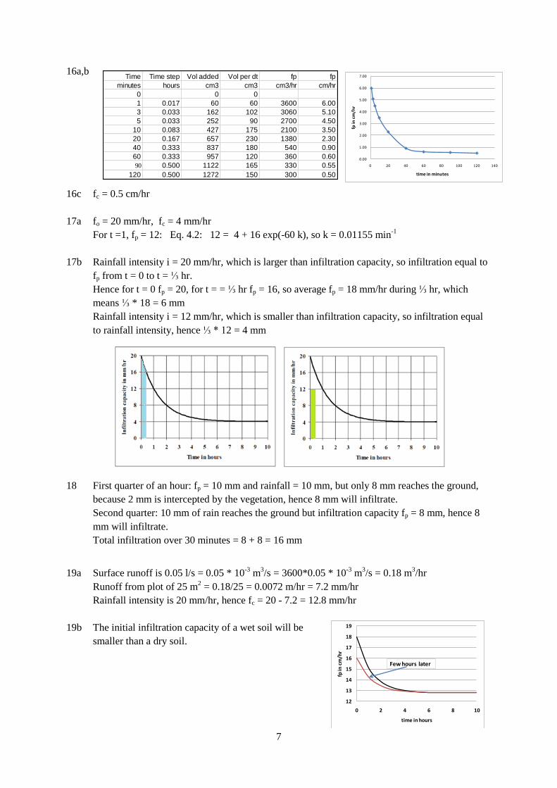
16a,b

16c fc = 0.5 cm/hr

17a fo = 20 mm/hr, fc = 4 mm/hr

For t =1, fp = 12: Eq. 4.2: 12 = 4 + 16 exp(-60 k), so k = 0.01155 min-1

17b Rainfall intensity i = 20 mm/hr, which is larger than infiltration capacity, so infiltration equal to

fp from t = 0 to t = ⅓ hr.

Hence for t = 0 fp = 20, for t = = ⅓ hr fp = 16, so average fp = 18 mm/hr during ⅓ hr, which

means ⅓ * 18 = 6 mm

Rainfall intensity i = 12 mm/hr, which is smaller than infiltration capacity, so infiltration equal

to rainfall intensity, hence ⅓ * 12 = 4 mm

18 First quarter of an hour: fp = 10 mm and rainfall = 10 mm, but only 8 mm reaches the ground,

because 2 mm is intercepted by the vegetation, hence 8 mm will infiltrate.

Second quarter: 10 mm of rain reaches the ground but infiltration capacity fp = 8 mm, hence 8

mm will infiltrate.

Total infiltration over 30 minutes = 8 + 8 = 16 mm

19a Surface runoff is 0.05 l/s = 0.05 * 10-3

m3/s = 3600*0.05 * 10

-3 m

3/s = 0.18 m

3/hr

Runoff from plot of 25 m2 = 0.18/25 = 0.0072 m/hr = 7.2 mm/hr

Rainfall intensity is 20 mm/hr, hence fc = 20 - 7.2 = 12.8 mm/hr

19b The initial infiltration capacity of a wet soil will be

smaller than a dry soil.

8

0

10

20

30

40

50

1 2 3

P (m

m/h

ou

r)

Hour

20a Available Moisture AM, Moisture Content Field Capacity MCFC and

Moisture Content Wilting point MCWP, Depth root zone Dr

Equation: AM = Dr (MCFC - MCWP)

MCFC MCWP AM (cm)

Sand 0.14 0.03 6.6

Loam 0.28 0.07 12.6

Clay 0.42 0.28 8.4

20b AM(Sand) = 66 mm, readily available 50% = 66/2 = 33 mm

Irrigation interval is 33/4 = 8 days.

Similar for loam: 63/4 = 15 days and Clay: 42/4 = 10 days

21 With infiltration F, percolation D and storage S, the water balance of the root zone reads:

F - D = ∆S = 500*(0.28 - 0.12) = 80 mm

D = F - ∆S = 110 - 80 = 30 mm

22a,b Apply Eq. 4.11: Q6 = Q0 exp(-6/K) = 1.8 = 10 exp(-6/K), hence K = 3.5 weeks. Use the equation

to compute Q at the end of each week (see table below).

Water released from the dam site Qout = 5 m3/s = 5*86400*7/20,000 = 151.2 mm/week

Water balance reservoir: Q + P - E - Qout = ∆S/∆t

Week Q Av Q Q P E Qout ∆S/∆t Level

0 10.0 m3/s mm/w mm/w mm/w mm/w mm/w 20.00

1 7.51 8.75 264.6 0 40 151.2 73.4 20.07

2 5.64 6.58 199.0 0 40 151.2 7.8 20.08

3 4.24 4.94 149.0 0 45 151.2 -42.2 20.04

4 3.18 3.71 112.2 0 45 151.2 -74.0 19.96

5 2.39 2.78 84.1 0 45 151.2 -112.1 19.84

6 1.80 2.10 63.5 23 45 151.2 -109.7 19.73

23a The total runoff from the catchment is the area under curve A: (15+60+65+30+12.5+2.5)*3600

= 666,000 m3 or 666000/33300000*1000 = 20 mm

Hence the runoff coefficient is 20/100 = 0.2 or 20%

23b Total losses are 100 - 20 = 80 mm. A first estimate of the loss

rate is 80/3 = 27 mm/hr.

This is more than the rainfall in the last hour (20 mm). The

losses in the first two hours are therefore 80 - 20 = 60 mm,

hence a constant loss rate of 60/2 = 30 mm/hr

9

Day Q (mm/d) Log Q

1 1.72 0.24

2 1.5 0.18

3 1.31 0.12

4 1.14 0.06

5 1 0.00

6 6 0.78

7 10 1.00

8 6 0.78

9 4 0.60

10 3 0.48

11 2.62 0.42

12 2.29 0.36

13 2 0.30

14 1.75 0.24

0.00

0.20

0.40

0.60

0.80

1.00

1.20

0 5 10 15Lo

g Q

Day

0

2

4

6

8

10

12

0 5 10 15

Q (m

m/d

)

Day

Direct Runoff

Base flow

Area Q (mm)

1 2.5

2 7

3 7

4 4

5 2.5

6 -5

Direct runoff (mm)= 18 0

2

4

6

8

10

12

0 5 10 15

Q (m

m/d

)

Day

Direct Runoff

Base flow

1

2 3

4

5

6

Area Q (mm)

1 2.5

2 7

3 7

4 4

5 2.5

6 -5

Direct runoff (mm)= 18

23c Volume of flood hydrograph in point B = (0+10+40+45+20+5)*3600 = 432000 m3.

Total infiltration between A and B = 666000-432000 = 234000 m3 over an area of 50*20000 =

1000000 m2, which means an average depth of 234 mm. It takes 5 to 6 hours for the flood wave

to pass, hence the average infiltration rate is 234/5.5 = 42.5 mm/hr

24a

From a plot of Log Q against

time it is shown that the depletion

curve starts on day number 10.

24b

24c Depletion curve is Eq. 4.11:

1.0 = 1.72 exp(4/K), hence K = 7.4 days

QB = 3.0 mm/d (given)

Eq. 4.11 : QA= 1.0 exp(-5/7.4) = 0.5 mm/d

10

Total runoff under depletion curve

0K

tt

0

t

kQt d e Q =CT0

0

Grey area is base flow produced by rainstorm

of 50 mm=

CT (B) – CT(A) + triangle under base flow

separation line = 7.4*3-7.4*0.5+5*(3-0.5) =

18.5 + 6.25 = 24.75 mm

25 From graph: Rainfall depth for tc = 3 hr equals 33 mm,

so intensity i = 11 mm/hr = 0.011/3600 m/s

Eq. 6.3: Qp = 0.4 * 0.011/3600 * 6 * 106 = 7.3 m

3/s