A Meshfree Method based on the Local Partition of Unity for Cohesive Cracks

Comput Mech (2006)DOI 10.1007/s00466-006-0067-4

ORIGINAL PAPER

Timon Rabczuk · Goangseup Zi

A meshfree method based on the local partition of unityfor cohesive cracks

Received: 8 November 2005 / Accepted: 23 February 2006© Springer-Verlag 2006

Abstract We will present a meshfree method based on thelocal partition of unity for cohesive cracks. The cracks aredescribed by a jump in the displacement field for particleswhose domain of influence is cut by the crack. Particles withpartially cut domain of influence are enriched with branchfunctions. Crack propagation is governed by the material sta-bility condition. Due to the smoothness and higher order con-tinuity, the method is very accurate which is demonstrated forseveral quasi static and dynamic crack propagation examples.

Keywords Extended element-gree Galerkin method(XEFG) · Cracks · Cohesive models · Dynamic fracture

1 Introduction

Different methods have been presented to model cracks infinite element and meshfree methods. Simple and robust meth-ods are interelement separation models in which cracks aremodelled along element interfaces in the mesh, see Xu andNeedleman [43], Camacho and Ortiz [17], Ortiz and Pandolfi[33], and Zhou and Molinari [44]. Another simple methodwas proposed by Remmers et al. [37] who introduced cracksegments in finite elements. Rabczuk and Belytschko [34]developed a ‘cracking particle’ model in meshfree methodswhere discontinuities are introduced at the particle positions.The major advantage of these methods are their robustnessand ease in implementation. However, for certain classes ofproblems, more accurate methods are needed.

The embedded discontinuity model [3, 7, 39] is anothermethod for crack problems. However, its effectiveness in

T. Rabczuk (B)Institute for Numerical Mechanics, Technical University of Munich,Boltzmannstr. 15, 85748 Garching b. Munich, GermanyE-mail: [email protected].: +49-89-289915304

G. ZiDepartment of Civil and Environmental Engineering, Korea University,5-1, Anam-dong, Sungbuk- Ku, Seoul 136-701, KoreaE-mail: [email protected]

crack dynamics has still not been assessed and these methodsrequire the crack to propagate one element at a time.

A very accurate method for crack problems is the ex-tended finite element method (XFEM) developed by the groupof Prof. Belytschko [5, 31]. This method is based on the ‘lo-cal’ partition of unity, in which the solution space is enrichedby a priori knowledge about the behaviour of the solution nearcracks. Because only the nodes belonging to the elements cutby cracks are enriched, the number of additional degrees offreedom for the local enrichment is minimized. The detaileddiscussion about the (local) partition of unity is found in theliterature, e.g. Melenk and Babuska [30]; Chessa et al. [18].This method has been successfully applied to static prob-lems in two and three dimensions, (see e.g. [22, 31, 32, 45,47]) and to dynamic problems ([6, 46]) in two dimensions.

Previous meshfree methods for cracking [9, 11, 14, 26,29] in two and three dimensions were treated by the so calledvisibility criterion or some modifications of it. Therefore, thesupport is truncated by the line of discontinuity. Other novelapproaches which were able to treat kinked and curve crackswere proposed by [41]. They also enriched the MLS basefunctions p around the crack tip and significantly improvedthe convergence behaviour. The major drawback is the needfor an explicit representation of the crack.

A meshfree concept of XFEM was proposed by Venturaet al. [41] for linear elastic fracture mechanics in statics. Wewill pursue this idea and extend it to dynamics and cohesivecracks. The advantage of this meshfree method over XFEMis the higher smoothness, non-local interpolation characterand higher order continuity which results in a better stressdistribution around the crack tip which is important for thepropagation of the crack.

In XFEM, mainly piecewise linear crack opening is as-sumed (due to the use of low order shape functions) but itis well known that in reality, the crack opening displace-ment is nonlinear, especially near the crack tip. Nonlinearcrack opening relations can be easily incorporated in mesh-free methods. In XFEM, Laborde et al. [27] have shown thata wider support for the crack tip enrichment improves theaccuracy and convergence; more nodes are enriched for the

T. Rabczuk, G. Zi

Fig. 1 Crack with partial cut and complete cut domain of influenceparticles

crack tip than in the classical XFEM. Meshfree methods natu-rally have a wider support due to their non-local interpolationcharacter than FEM. However, this results in difficulties inimposing the Dirichlet boundary conditions at the crack, i.e.the crack has to close at the crack tip. A possible solution isaddressed in the next section.

The paper is arranged as follows: in the next section, wewill describe the concept, i.e. the approximation of the jumpin the displacement. The meshfree method is briefly reviewedafterwards. In Sect. 4, we will give the governing equationsand derive the discrete equations in Sect. 5. We will verify ourmodel first for linear elastic fracture mechanics and compareresults to former meshfree methods. Finally, we will solveseveral quasi-static and dynamic crack propagation problemsand compare the results to experimental data or other data inthe literature.

2 Approximation of the test and trial functions

The main idea to capture the crack is to enrich the test andtrial functions with additional unknowns so that the approxi-mation is continuous in the whole domain but discontinuousalong the crack as done in many former methods such asXFEM [31]. Therefore, the test and trial functions are writ-ten in terms of a signed distance function f (see Fig. 1):

δu(X) =∑

I∈W(X)

�I (X) δuI

+∑

I∈Wb(X)

�I (X) H ( f I (X)) δaI

+∑

I∈Ws(X)

�I (X)∑

K

BK (X) δbK I (1)

u(X) =∑

I∈W(X)

�I (X) uI

+∑

I∈Wb(X)

�I (X) H ( f I (X)) aI

+∑

I∈Ws(X)

�I (X)∑

K

BK (X) bK I (2)

where W(X) is the entire domain, Wb(X) is the completelycut domain, Ws(X) is the partial cut domain, and H and Bare the enrichment functions explained later. The first termon the right hand side of Eq. (1) or (2), respectively, is theusual approximation where �I are the shape functions, anduI and δuI are the parameters. The second and third term isthe enrichment, in which the coefficient δa and δb or a andb, respectively, are additional unknowns introduced for thecrack in the variational formulation.

H( f (X)) depends on the signed distance function f I (X)and is defined as:

H ( f I (X)) = 1 if f I (X) > 0H ( f I (X)) = −1 if f I (X) < 0 (3)

with

f I (X)

={

sign[n · (XI − X)] min ‖XI − X‖, for XI ∈ Wbn · (Xtip − XI ), for XI ∈ Ws

(4)

where Xtip are the coordinates of the crack tip and n is thecrack normal. Only nodes which are located in the domainWb(X) are enriched with the additional unknowns δa and a.The second term of Eq. (1) or (2) is called the ‘step’ enrich-ment.

The third term of Eqs. (1) and (2) is applied around thecrack tip Ws(X). In linear elastic fracture mechanics, B ischosen to be continuous in the whole domain Ws(X), butdiscontinuous at the crack line:

B =(√

r sinθ

2,√

r cosθ

2,√

r sinθ

2sin θ,

√r cos

θ

2sin θ

)(5)

according to the analytical solution around the crack tip wherer is the distance of X to the crack tip and θ(X) = sin−1 ( f/r)is the angle between the tangent to the crack line and the seg-ment X−Xtip, see Fig. 1. It is called the ‘branch’ enrichment.

For cohesive cracks, there is no crack tip singularity andthe crack opening displacement, which the cohesive tractiondepends on, may be described by the additional unknowna only. In XFEM, this procedure is straightforward since itis easy to impose the appropriate boundary conditions, seeFig. 2a, i.e. the crack has to close at the end of the elementedge. This can be accomplished e.g. by not enriching thenodes at the element edge where the crack tip is located asshown in Fig. 2a. However, in meshfree methods, this tech-nique cannot be applied analogous to the way in XFEM, seeFig. 2b.

Therefore, we keep the branch enrichment for cohesivecracks, but without the crack tip singularity:

B =(

rm sinθ

2

)m = 1, 2, 3 (6)

A meshfree method based on the local partition of unity for cohesive cracks

(a) (b)

Fig. 2 Crack with enriched nodes in a XFEM and b meshfree methods

While lower order finite elements (that are usually applied)can capture only linear crack opening, meshfree methodshave the advantage to capture more realistic crack openings,as measured in experiments, due to their ease of increasingthe order of continuity. Another advantage is the non-localinterpolation character, i.e. many particles are enriched. Wehave tested the branch functions, Eq. (6), for cohesive cracks.

Furthermore, we shifted the function HI ( f (X)) and BK(X)by their values at the position of particle I , i.e. HI ( f (XI ))and BK (XI ), respectively:

HnI (X) = Hn (

f n(X)) − Hn (

f n(XI ))

(7)

BmK (X) = Bm

K (X) − BmK (XI ) (8)

which makes the enriched region narrower. To avoid havingheavy notations, we drop · in the following sections; unlessmentioned otherwise, H and B stand for H and B of Eqs. (7)and (8), respectively.

We would like to mention that for particles in the blend-ing region, i.e. the particles whose domain of influence is notcut but influenced by the ‘enriched’ particles, only the ‘usual’approximation [first term on the right hand side of Eqs. (1)and (2)] is considered in the approximation of the test andtrial functions.

2.1 Tracing the crack paths

The level set techniques is often used to trace the crack paths,Moes et al. [31]; Ventura et al. [41]; Belytschko et al. [12];Rabczuk and Belytschko [35]. We believe it is easier to tracethe crack paths by piecewise linear lines. However, in certaincases, e.g. for non-linear crack paths, the use of level sets canbe advantageous. The crack is defined by an implicit func-tion f which is zero along the crack path and has the value ofthe minimum distance to the crack with plus or minus sign.The choice of the sign is completely arbitrary as long as itis consistent throughout the entire calculation. We will notexplain the crack tracing procedure with level sets in moredetail and refer the interested reader to the literature, e.g.[12, 31, 41]. However, we briefly describe how to treat crackbranching and crack intersection which is different from theapproach in [19] and [12] in the sense that we do not useany special branch function in addition to the ‘usual’ enrich-ment. Consider cracks shown in Fig. 3. Let W1

b be the set of

II

f1 (x)=0 f1 (x)=0

f2 (x)=0 f2 (x)=0

a) b)

Fig. 3 Support of node I with a intersecting discontinuities and bbranching discontinuities

nodes whose domain of influence is completely cut by thediscontinuity f1(X) = 0 and W2

b the corresponding set forf2(X) = 0. W3

b = W1b

⋂ W2b . The same applies accordingly

for nodes whose domain of influence is cut by the crack tipenrichment. We will denote this set of nodes with W1

s andW2

s . Then the approximation of the displacement may begiven by [19]

u(X) =∑

I∈W(X)

�I (X) uI

+∑

I∈W1b (X)

�I (X) H ( f1(X)) a(1)I

+∑

I∈W2b (X)

�I (X) H ( f2(X)) a(2)I

+∑

I∈W3b (X)

�I (X) H ( f1(X)) H ( f2(X)) a(3)I

+∑

I∈W1s (X)

�I (X)∑

K

B(1)K (X) b(1)

K I

+∑

I∈W2s (X)

�I (X)∑

K

B(2)K (X) b(2)

K I (9)

Principally, more than two branches can be included at onetime and a branched crack can branch again. As can be easilyseen by Eq. (9), additional complexity is then introduced. Wewould like to mention, that Eq. (9) looks worse than it is sinceonly very few nodes are included in all sets W . However, acrack branching requires the introduction of another level setwhich makes the computation cumbersome for many cracks.

Zi et al. [47] proposed a computationally more efficientapproach than (9) by modifying the signed distance func-tions so that no cross terms are needed for junction or branchproblems.

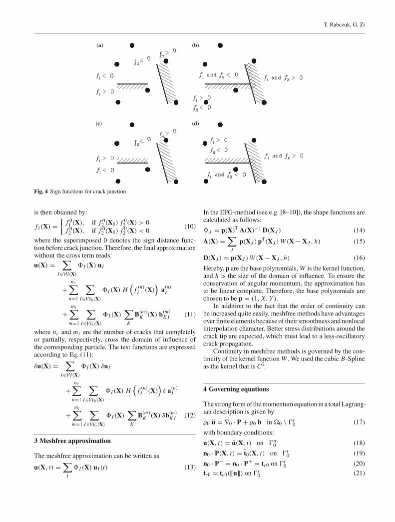
When two cracks are joining, the crack tip enrichment isremoved. By using the signed distance functions of the pre-existing and approaching crack, the signed distance functionof the approaching crack is modified. Consider Fig. 4. Threedifferent subdomains have to be considered: ( f1 < 0, f2 <0), ( f1 > 0, f2 > 0), ( f1 > 0, f2 < 0) as in Fig. 4b or( f1 > 0, f2 < 0), ( f1 > 0, f2 > 0), ( f1 < 0, f2 < 0) as inFig. 4d. The signed distance function of crack 1 of a point X

T. Rabczuk, G. Zi

(a) (b)

(d)(c)

Fig. 4 Sign functions for crack junction

is then obtained by:

f1(X) ={

f 01 (X), if f 0

2 (X1) f 02 (X) > 0

f 02 (X), if f 0

2 (X1) f 02 (X) < 0

(10)

where the superimposed 0 denotes the sign distance func-tion before crack junction. Therefore, the final approximationwithout the cross term reads:

u(X) =∑

I∈W(X)

�I (X) uI

+nc∑

n=1

∑

I∈Wb(X)

�I (X) H(

f (n)I (X)

)a(n)

I

+mt∑

m=1

∑

I∈Ws(X)

�I (X)∑

K

B(m)K (X) b(m)

K I (11)

where nc and mt are the number of cracks that completelyor partially, respectively, cross the domain of influence ofthe corresponding particle. The test functions are expressedaccording to Eq. (11):

δu(X) =∑

I∈W(X)

�I (X) δuI

+nc∑

n=1

∑

I∈Wb(X)

�I (X) H(

f (n)I (X)

)δ a(n)

I

+mt∑

m=1

∑

I∈Ws(X)

�I (X)∑

K

B(m)K (X) δb(m)

K I (12)

3 Meshfree approximation

The meshfree approximation can be written as

u(X, t) =∑

I

�I (X) uI (t) (13)

In the EFG-method (see e.g. [8–10]), the shape functions arecalculated as follows:

�J = p(X)T A(X)−1 D(XJ ) (14)

A(X) =∑

J

p(XJ ) pT(XJ ) W (X − XJ , h) (15)

D(XJ ) = p(XJ ) W (X − XJ , h) (16)

Hereby, p are the base polynomials, W is the kernel function,and h is the size of the domain of influence. To ensure theconservation of angular momentum, the approximation hasto be linear complete. Therefore, the base polynomials arechosen to be p = (1, X, Y ).

In addition to the fact that the order of continuity canbe increased quite easily, meshfree methods have advantagesover finite elements because of their smoothness and nonlocalinterpolation character. Better stress distributions around thecrack tip are expected, which must lead to a less-oscillatorycrack propagation.

Continuity in meshfree methods is governed by the con-tinuity of the kernel function W . We used the cubic B-Splineas the kernel that is C2.

4 Governing equations

The strong form of the momentum equation in a total Lagrang-ian description is given by

�0 u = ∇0 · P + �0 b in �0 \ �c0 (17)

with boundary conditions:

u(X, t) = u(X, t) on �u0 (18)

n0 · P(X, t) = t0(X, t) on �t0 (19)

n0 · P− = n0 · P+ = tc0 on �c0 (20)

tc0 = tc0([[u]]) on �c0 (21)


where �0 is the initial density, u is the acceleration, P denotesthe nominal stress tensor, b designates the body force, u andt0 are the prescribed displacement and traction, respectively,n0 is the outward normal to the domain and �u

0

⋃�t

0

⋃�c

0 =�0, (�u

0

⋂�t

0)⋃

(�t0

⋂�c

0)⋃

(�c0

⋂�u

0 ) = Ø. Moreover,we assume that the stresses P at the crack surface �c

0 arebounded. Since the stresses are not well defined in the crack,the crack surface �c

0 is excluded from the domain �0 whichis considered as an open set.

5 The discrete momentum equation

Starting point is the weak form of the momentum equationwhich is given byδW = δWint − δWext + δWkin = 0 (22)where

δWint =∫

�0\�c0

(∇ ⊗ δu)T : P d�0 (23)

δWext =∫

�0\�c0

�0 δu · b d�0 +∫

�t0

δu · t0 d�0

+∫

�c0

[[δu]] · tc0 d�0 (24)

δWkin =∫

�0\�c0

�0 δu · u d�0 (25)

Substituting the test and trial functions (Eqs. (11) and(12), respectively) into Eqs. (23) to (25), we obtain

Wkin =∫

�0\�c0

�0 (�I (X) δuI

+�I (X) H(

f (n)I (X)

)δa(n)

I

+�I (X) B(m)K δb(m)

K I

)

· (�J (X) uJ

+�J (X)H(

f (n)J (X)

)a(n)

J

+�J (X) B(m)K b(m)

K J

)d�0 (26)

Wint =∫

�0\�c0

δuI ∇0�I (X) · P d�0

+∫

�0\�c0

δa(n)I

[∇0�I (X) H

(f (n)I (X)

)

+ �I (X)∇0 H(

f (n)I (X)

)]· P d�0

+∫

�0\�c0

[(∇0�I (X) B(m)

K

+ �I (X) ∇0B(m)K

)δb(m)

K I

]· P d�0 (27)

∫

�0\�c0

�0 δu · b d�0 =∫

�0\�c0

�0 (�I (X) δuI

+�I (X) H(

f (n)I (X)

)δa(n)

I

+�I (X) B(m)K δb(m)

I

)· b d�0 (28)

∫

�t0

δu · t0 d�0 =∫

�t0

(�I (X)δuI +�I (X)H

(f (n)I (X)

)δa(n)

I

+ �I (X)B(m)K δb(m)

K I

)· t0 d�0 (29)

∫

�c0

[[δu]] · tc0 d�0 =∫

�c0

[[�I (X)δuI +�I (X)H

(f (n)I (X)

)δa(n)

I

+ �I (X) B(m)K δb(m)

K I

]]· tc0 d�0

=∫

�c0

[[�I (X) H

(f (n)I (X)

)δa(n)

I

+ �I (X) B(m)K δb(m)

K I

]]· tc0 d�0 (30)

where Eqs. (28) to (30) are for Wext. After some algebraicoperations the final form of the equation of motion is obtainedby

MI J · uI = FextI − Fint

I (31)

with

MI J =⎡

⎣muu

I J muaI J mub

I Jmau

I J maaI J mab

I Jmbu

I J mbaI J mbb

I J

⎤

⎦ (32)

uI =⎡

⎣uu

IaI

bI K

⎤

⎦ (33)

FextI =

⎡

⎣fu,ext

Ifa,ext

Ifb,ext

I K

⎤

⎦ (34)

FintI =

⎡

⎣fu,int

Ifa,int

Ifb,int

I K

⎤

⎦ (35)

with

muuI J =

∫

�0\�c0

�0 �I (X) �J (X) d�0

muaI J =

∫

�0\�c0

�0 �I (X) �J (X) H(

f (n)I (X)

)d�0 ,

muaI J = mau

I J

mubI J =

∫

�0\�c0

�0 �I (X) �J (X) B(m)K d�0 ,

mubI J = mbu

I J

T. Rabczuk, G. Zi

maaI J =

∫

�0\�c0

�0 �I (X) H(

f (n)I (X)

)

ϕJ (X) H(

f (n)I (X)

)d�0

mabI J =

∫

�0\�c0

�0 �I (X) H(

f (n)I (X)

)

ϕJ (X) B(m)K d�0 , mab

I J = mbaI J

mbbI J =

∫

�0\�c0

�0 �I (X) B(m)K �J (X) B(m)

K d�0 (36)

fu,extI =

∫

�0\�c0

�0 b �I (X) d�0

+∫

�t0

t0 �I (X) d�0 + fu,crI

fa,extI =

∫

�0\�c0

�0 b �I (X) H(

f (n)I (X)

)d�0

+∫

�t0

t0 �I (X) H(

f (n)I (X)

)d�0 + fa,cr

I

fb,extI =

∫

�0\�c0

�0 b �I (X) B(m)K d�0

+∫

�t0

t0 �I (X) B(m)K d�0 + fb,cr

I (37)

where

fa,crI =

∫

�c0

�I (X)[[

H(

f (n)I (X)

)]]tc0 d�0

fb,crI =

∫

�c0

�I (X)[[

B(m)K

]]tc0 d�0 (38)

fu,intI =

∫

�0\�c0

∇0�I (X) · P d�0

fa,intI =

∫

�0\�c0

((∇0�I (X) H

(f (n)I (X)

)

+ �I (X) ∇0 H(

f (n)I (X)

))· P

)d�0

fb,intI K =

∫

�0\�c0

((∇0�I (X) B(m)

K

+ �I (X) ∇0B(m)K

)· P

)d�0 (39)

Equation (36) is the consistent mass matrix. In Eq. (39),the spatial derivatives of H vanish since the domain is con-sidered as an open set. The cohesive forces are taken into

crack

background cell

1

23

4

56

7

8

9

1011

crack

5

9

6

7

8

1

2

3

4

background cellCrack path produced

by level set Crack path recognized by the code

Fig. 5 Sub-triangulation of background cells

account in the external forces, Eq. (37). Gauss quadrature isused to obtain the discrete equations. Generally, four nodesare arranged so that they form the quadrature cell. Integra-tion cells cut by a crack are sub-triangulated as in XFEM.Note, that the crack tip does not necessarily cross the entirebackground cell, see Fig. 5 for possible sub-triangulations.Quadrature points are added to the new sampling points. Theintegration may be erroneous if any sampling points for trian-gle 3 is positioned above of the actual crack path, see Fig. 5.To minimize such an error, a point in the middle of the crackpath in the cell is added as shown in the bottom Fig. 5. Addingone more point, the error is reduced second order small.

In LEFM, care should be taken at the crack tip since asingularity is present. Laborder et al. [27] found an elegantsolution by expressing the integral in polar coordinates thatgave excellent results even for very small number of inte-gration points. This may be implemented in the method pre-sented. Since we were mainly interested in nonlinear materi-als without the crack tip singularity, we did not do any specialarrangements near the crack tip.

An alternative of this approach that does not require tri-angulation of the background cell would be the appropriatemodification of the integration weights. For more details, seeAreias et al. [2].

The cohesive tractions across the crack are integrated bythe standard surface integration.

6 Constitutive model

6.1 Continuum model

We used Rankine type materials, the Lemaitre damage model[28] and the Johnson–Cook model [24]. For the Lemaitre


model, the stress–strain behaviour is given by

σ = (1 − D) C : ε (40)

where D is a scalar damage variable which ranges from 0to a maximum of 1 and C is the initial elasticity tensor. Thedamage evolution depends on the effective strain ε:

D(ε) = 1 − (1 − A) εD0 ε−1 − Ae−B(ε−εD0 ) (41)

with

ε =√√√√

3∑

i=1

ε2i H(εi ) (42)

where εi are the principal strains and with

H(x) = 1 if x > 0

H(x) = 0 if x < 0 (43)

A, B and εD0 are material parameters.The Johnson–Cook model [24] is based on J2 plasticity

but takes into account strain rate and temperature effects. Theeffective yield stress of the Johnson–Cook model is given by

σY = (A + Bγ n) (

1 + C ln ε∗) (1 − T ∗) (44)

where ε∗ = γ /γ0, γ is the effective plastic strain, γ0 is thereference strain rate taken to be 1.0/s and A, B, C are materialparameters, respectively. T ∗ is given by

T ∗ = T − Tr

Tm − Tr(45)

where Tr is the reference temperature and Tm is the meltingtemperature. We assume that the plastic deformation is com-pletely transformed into heat, so β = 1 for the temperatureupdate:

�T =γ∫

0

β

�cv

σYdγ (46)

where � is the mass density and cv is the specific heat perunit mass.

Gummalle [23] pointed out that the initial negative slopeof the effective plastic stress–effective plastic strain curvehighly determines the shear band initiation. He suggested thefollowing form of the effective yield stress that gave betterresults in his computations:

σY = max

[ (A + Bγ n) (

1 + C ln ε∗)

(1 − δ

(exp

(T − T0

κ0

)− 1

)), 0

](47)

6.2 Cohesive crack model

6.2.1 Cracking criteria

We employed the loss of hyperbolicity criterion for crackinitiation and propagation. Therefore, a crack is initiated or

propagated if the minimum eigenvalue of the acoustic tensorQ is smaller or equal to zero:min eig(Q) ≤ 0 with Q = n · A · n and A = Ct+σ ⊗ I

(48)where n = [cos(θ) sin(θ)] is the normal to the crack surfacedepending on the angle θ , Ct is the fourth order tangentialmodulus tensor and I is the second order identity tensor.

For a crack propagation, we checked the loss of hyperbo-licity condition in a half circle around the crack tip for everymaterial point. If the PDE looses hyperbolicity at one materialpoint, the crack is advanced from the crack tip. The directionof crack propagation is completely determined by n obtainedfrom the localization analysis. Crack branching occurs if thePDE looses hyperbolicity at two material points with differ-ent n. Now, it still remains the question of how to propagatethe crack.

There are numerous possibilities how to determine thecrack velocity. The easiest way is to control the crack length,[45]. However, we believe this approach is not accurate enoughand adopt an approximation suggested by Belytschko et al.[6]. Key assumption is that the hyperbolicity indicator e =h · Q · h must vanish at the crack tip:∂e

∂t+ vc · ∇e = 0 with vc = vc s (49)

where vc is the crack speed, s gives its direction which mustfulfill the condition n · s = 0 and h is assumed to be parallelto n (h is the eigenvector of Q obtained from the localizationanalysis). To obtain the crack length, the Eq. (49) has to besolved for vc. In [6], they used an incremental version of sthough the advantage is not clear to us. Hence, we used therate form of the hyperbolicity indicator.

6.2.2 Jump in the displacement

The jump in the displacement is governed only by the enrich-ment and is given by

[[u(X)]] =nc∑

n=1

∑

I∈Wb(X)

�I (X)[[H(X)]]qI

+mt∑

m=1

∑

I∈Ws (X)

�I (X)∑

K

[[BK (X)]] bK I

= 2nc∑

n=1

∑

I∈Wb(X)

�I (X) qI

+mt∑

m=1

∑

I∈Ws (X)

�I (X)∑

K

[[BK (X)]] bK I (50)

The normal part δn, i.e. the crack opening and the tangentialpart δt , the crack sliding is given byδn = [[u(X)]]n = n · [[u(X)]] (51)

δt = [[u(X)]]τ = ‖[[u(X)]] − (δnn)‖ (52)More details are given in Belytschko et al. [6]. If not men-tioned otherwise, we only consider normal forces and neglectmode II effects.

T. Rabczuk, G. Zi

trac

tion

Crack opening

trac

tion

Crack opening

trac

tion

Crack opening

a) b) c)

Fig. 6 Cohesive models: a linear models, b bilinear models, c exponential models

p

p

y

x

2a

b2b

Γ

p

p

y

x

a

a) b)

Fig. 7 a Mode I problem, b (mixed) mode I–II problem

6.2.3 Cohesive law

The cohesive laws that are most popularly used are shown inFig. 6. We used linear and exponentially decaying cohesivelaws among them because of their simplicity.

7 Verification using linear elastic fracture mechanics

7.1 Crack problem

Consider a mode I crack problem illustrated in Fig. 7a. Planestrain conditions and linear elastic material behaviour areassumed. For an infinite plate, Westergaard [42] provided asolution for this problem:

σxx = p

(r0√r1 r2

cos

(φ0 − φ1 + φ2

2

)

− a2 r0

(r1 r2)1.5sin φ0 sin [1.5 (φ1 + φ2)] − 1

)

(53)

σyy = p

(r0√r1 r2

cos

(φ0 − φ1 + φ2

2

)

+ a2 r0

(r1 r2)1.5sin φ0 sin [1.5 (φ1 + φ2)]

)(54)

τxy = pa2 r0

(r1 r2)1.5sin φ0 cos [1.5(φ1 + φ2)] (55)

aax

y

f2 f0 f1

r2r0

r1

Fig. 8 The Griffith problem

where the parameters r0, r1, r2, φ0, φ1 and φ2 are explainedin Fig. 8. The exact tractions may be calculated fromEqs. (53) to (55) and are applied to the boundary shown inFig. 7. The near tip stress field is given by

σxx (r, φ) = KI√2πr

cosφ

2

(1 − sin

φ

2sin

3φ

2

)(56)

σyy(r, φ) = K I√2πr

cosφ

2

(1 + sin

φ

2sin

3φ

2

)(57)

τxy(r, φ) = K I√2πr

sinφ

2cos

φ

2cos

3φ

2(58)

with polar coordinates r and φ. The stress intensity factorfor the Griffith problem is dependent on the boundary con-dition and the loading type, and for the quasi-static problemin Fig. 7, is given by KI = p

√πa where p is the external

traction. In numerical simulations, the relation between theJ -integral and KI is used to check the local convergence nearthe crack tip;

J = K 2I

1 − ν2

E(59)

The J -integral gives the change in strain energy with a unitchange in the crack length a and may be calculated by

J =∫

�

(w dy − t

∂u∂x

d�

)(60)


Fig. 9 a Error in the energy for the mode I problem; b normalized stress intensity factor versus h

where w = ∫ ε

0 σ : dε is the energy density, t the traction,u the displacements and � the path around the crack tip asillustrated in Fig. 7. The integration path � is chosen to com-pletely encompass the enriched region near the crack tip.

We will study the error in the energy given by

‖err‖energy = ‖uh − uanalytic‖energy

‖uanalytic‖energy(61)

with

‖u‖energy =⎛

⎜⎝∫

�0

ET(u) : C : E(u) d�0

⎞

⎟⎠

1/2

(62)

where E is the Green strain. Additionally, we will checkstress intensity factors KI to compare local convergence.Note the branch enrichment in Eq. (5) is used for the lin-ear elasticity problems.

The error in the energy norm is illustrated in Fig. 9afor the mode I problem. We have also included results ob-tained by EFG with visibility criterion. The local partitionof unity enrichment gives more accurate results and a bet-ter convergence rate than the crack approach with visibilitycriterion. This is expected due to the crack tip enrichmentwith the Westergaard solution. Also local convergence is ob-tained much faster by the local partition of unity enrichmentas shown in Fig. 9b.

7.2 The mode I–II problem

Let us consider a (mixed) mode I–II problem. We study againthe error in the energy norm. The analytical near-tip fieldsolution for this problem is given e.g. by Saehn [38]:

σr = 1

4√

2πr

[KI

(5 cos

θ

2− cos

3θ

2

)

+ KII

(−5 sin

θ

2+ 3 sin

3θ

2

)](63)

σθ = 1

4√

2πr

[KI

(3 cos

θ

2− cos

3θ

2

)

+ KII

(−5 sin

θ

2+ 3 sin

3θ

2

)](64)

τrθ = 1

4√

2πr

[KI

(sin

θ

2+ sin

3θ

2

)

+ KII

(cos

θ

2+ cos

3θ

2

)](65)

where r and θ are explained in Fig. 10 and with KI = σn√

π aand KII = τn

√π a, with the loading conditions σn and τn

from Fig. 10 and where

σny = σx + σy

2+ σx − σy

2cos 2α (66)

σnx = σx + σy

2− σx − σy

2cos 2 α (67)

τnxy = σx − σy

2sin 2α (68)

We study again the error in the energy norm and compareit to the error obtained by the visibility method. The sametendency as for the mode I crack is observed for the mixedmode problems (see Fig. 10). Again, the local partition ofunity enrichment gives more accurate results and a higherconvergence rate. However, the error is larger than the onein the previous example (Fig. 11).

8 Examples

In the following sections, we will present results for severalquasi-static and dynamic problems, in which the traction onthe crack surface is given by the cohesive crack model. There-fore, the branch enrichment in Eq. (6) is used. Prenotches areassumed to be traction-free. We show the results with m = 1in Eq. (6), since the enrichment with higher m gave very sim-ilar results. In all our examples, we used a structured uniformparticle arrangement if not stated otherwise. This appears at

T. Rabczuk, G. Zi

Fig. 10 Mixed mode crack problem

Fig. 11 a Error in the energy for the mode I problem; b normalized stress intensity factor versus h

first to be dissonant with the philosophy of meshfree meth-ods. However, a structured particle arrangement is advanta-geous when incorporating features such as adaptivity. It alsofacilitates pre- and postprocessing.

8.1 Quasi-static examples

8.1.1 Arrea–Ingraffea beam

The first example is the Arrea and Ingraffea [4] beam. Thebeam is loaded at two points as shown in Fig. 12. The initialelastic modulus is 28,000 MPa, tensile strength is 2.8 MPa,Poisson’s ratio ν = 0.18 and the fracture energy is Gf =100 N/m. The beam failed due to a mixed tensile/shear failure.

We have used the Lemaitre [28] model for the contin-uum in tension and the loss of hyperbolicity condition for thecrack initiation and growth. A linear decaying cohesive lawis used. The critical crack opening displacement δc beyondwhich the cohesive traction is reduced to zero is calculatedas δc = 2Gf/ ft in which ft is the traction at which the mate-rial at the crack tip loses its hyperbolicity. The concrete is

Fig. 12 The tensile/shear beam from Arrea–Ingraffea

assumed to be linear elastic in compression. The beam isdiscretized with approximately 2,000 and 7,800 particles.

The crack path for the fine particle distribution is shownin Fig. 13. The curvature of the crack is similar to the onein the experiment. The load-displacement curves (measuredat the right of the notch) are shown in Fig. 14 and lie in theexperimental scatter. We note that we need significantly lessparticles to obtain convergent results in the load–deflection


Fig. 13 Crack pattern of the Arrea–Ingraffea beam

Displacement right of the notch [m]

Rea

ctio

n F

orc

e [M

N]

0 0.05 0.1 0.150

0.05

0.1

0.15

7800 particles

Experiment2000 particles

Fig. 14 Load–deflection curve of the tensile/shear beam from Arrea–Ingraffea for different numbers of particles

curve than the ‘cracking particle’ method described in Rab-czuk and Belytschko [34], where approximately 13,000 par-ticles were necessary.

We tested also the influence of higher order branch func-tions. Though higher order branch functions provide a bet-ter stress distribution around the crack tip, the influence withregard to the overall crack pattern or the load–deflection curveis not very high.

8.1.2 Four-point-bending with two notches

Consider a four-point beam in bending with two notches asshown in Fig. 15. Experimental data were given by Boccaet al. [16]. The Lemaitre [28] material model and the loss ofhyperbolicity for the crack initiaion and growth, and a lineardecaying cohesive law are employed. The material parame-ters are: E = 27, 000 MPa, ν = 0.18, ft = 2.0 MPa, Gf =100 N/m where E is Young’s modulus, ν is Poisson ratio, ftthe tensile strength and Gf the fracture energy. Number ofparticles between 660 and 160,000 are studied.

The load–deflection curve is shown in Fig. 16 and agreesvery well with the experiment. At 2,550 particles, mesh depen-dence is completely removed. However, the load–deflectioncurve even with 660 particles was very close to the converged

Fig. 15 The four-point-bending beam with two notches from Boccaet al. [15]

Fig. 16 Load–deflection curve of the four-point-bending beam with twonotches from Bocca et al. [15]

one. The final crack patterns for computations with differentnumbers of particles are illustrated in Fig. 18. The crack pathis obtained by storing the coordinates of the crack tip.

The crack patterns agree very well with the experimentalcrack pattern. Again, we need only a few particles to obtaingood results. With the ‘cracking particle’ method in [34],4,000 particles did neither give an appropriate crack path nora reasonable load–deflection curve. At a number of 2,550particles, we get here mesh independent results in the load–deflection curve and the crack path.

In Fig. 17, the enriched particles are shown. The enrichednodes for the 660 particle discretization is shown in Fig. 17a.The enriched region of one crack is overlapped with that ofthe other. This results in a steeper crack path. This problemcan be overcome by decreasing the support size slightly, seeFig. 18a. Usually, the support size is chosen to be 3.5 timesthe particle separation. By decreasing this support size so that

T. Rabczuk, G. Zi

a)

c)

e)

g)

Fig. 17 Enriched nodes of the two notched beam

the cracked particles of one crack are not influenced by theother crack, improves the crack paths.

8.2 Dynamic examples

8.2.1 Kalthoff problem

Kalthoff and Winkler [25] performed a series of experimentsin which a steel plate was hit by a projectile with differentimpact velocities as shown in Fig. 19. They discovered differ-ent failure phenomena for different impact velocities. Up toa certain velocity of the projectile vc = 20 m/s, the steel platefails brittle and a crack develops in a 70◦ angle against theaxis parallel to the flight direction of the projectile. When thevelocity exceeds vc, they found a completely different failurepattern. A shear band develops from the onset of the notchin a much flatter angle of the opposite direction. We will firstfocus on the brittle failure pattern and an impact velocity of17 m/s.

We used 1,700, 6,500 and 26,000 particles in our simu-lations. We tested two material models, the Johnson–Cookmodel [24] and the Lemaitre [28] model. The latter modelwas applied in Belytschko et al. [6] for the Kalthoff problemand a brittle failure mechanism. For the Lemaitre model, the

a)

c)

e)

g)

Fig. 18 Crack paths of the two notched beam

100 mm

75 mm

75 mm

50 mm 200 mmnotch

75 mm

cylindrical impactordiameter =50 mm

thickness=6.35mm

u0

Fig. 19 The Kalthoff problem: test setup

material parameters are: Young’s modulus E = 190 GPa,Poisson ratio ν = 0.3, fracture energy Gf = 22, 170 J/m2,critical crack opening displacement δmax = 5.378×10−5 m,damage threshold εD0 = 3 × 10−3 and parameters A = 1.0


a) b)

d)c)

e) f)

Fig. 20 a, c, e Crack pattern for the 26,000 particle arrangement, b, d, f crack pattern for the 1,700 particle arrangement using the new approach

and B = 200. The material parameters of the Johnson–Cookmodel are: A = 2 GPa, B = 94.5 GPa, C = 0.0165, T0 =293 K, γ0 = 1.3×10−13 s−1 and κ0 = 500 K. An exponentialcohesive law is used.

We exploited the symmetry in our discretization. Thecrack paths for the Lemaitre model is shown in Fig. 20 for

two different numbers of particles. The experimental crackangle at the prenotch of 70◦ versus the crack orientation isreproduced well by our simulation. However, in the courseof the computation, the crack starts to curve and gets flatter.A similar crack pattern was obtained by Xu and Needleman[43]. The damage is plotted in Fig. 20. A higher damage at

T. Rabczuk, G. Zi

a) b)

d)c)

Fig. 21 Kalthoff problem with brittle failure for different particle refinements; a–c Enriched nodes (red colour); d crack pattern

the right lower corner occurs in Fig. 20b, d, f. However, nocrack initiates. The crack is shown as solid line at the endof the computation. We therefore conclude that the Lemaitremodel is not well suited to model crack propagation for theKalthoff problem.

The results of the different particle arrangement for theJohnson Cook model are shown in Fig. 21. As in Fig. 20,only the upper part of the specimen is illustrated. Particlesenriched are shown in red colour.

The crack is shown in Fig. 21d for the 26,000 particlediscretization and is almost identical with the crack patternof the coarser simulations. The experimental crack angle atthe prenotch of 70◦ versus the crack orientation is reproducedwell by our simulation. The crack path is very smooth.

Figure 22 shows the speed of the crack tip for the threedifferent refinements. The Rayleigh wave speed is never ex-ceeded and the course of the crack speed looks very similar.For the coarsest discretization with 1,700 particles, the crackstarts to propagate a little later. The course of the crack speedis similar to the one obtained in Belytschko et al. [6].

We increased the impact velocity to 30 m/s, at which aductile failure appeared in the experiments. The failure pat-tern of our simulation is shown in Fig. 23; enriched nodes areplotted in red colour. We were able to reproduce the failuremode of the experiment well. Only 1,700 particles are neededto resolve the shear band. The results do not show any mesh

Fig. 22 Crack speed time history of the Kalthoff problem with brittlefailure

dependence. Note, that for the shear band we allow only tan-gential jumps in the displacement field while normal jumpsare suppressed. For details of this concept, see Belytschkoet al. [13].

8.2.2 Crack branching

In the following, we examine the performance of the methodin a crack branching problem. Consider a rectangular


a) b)

Fig. 23 a, b Kalthoff problem with ductile failure for different particle refinements; enriched nodes are plotted in red colour

prenotched specimen as shown in Fig. 24. The length of therectangle is 0.1 m and width 0.04 m. Initially, a horizontalcrack is placed from the left edge to the center of the plate.Tensile tractions of 1 MPa are applied on the top and bottomedges.

We used the Lemaitre [28] damage law, loss of hyperbo-licity and we tested different cohesive laws. We will presentthe results for an exponential decaying law. The materialconstants are � = 2, 450 kg/m3, E = 32 MPa, ν = 0.2and A = 1.0, B = 7, 300 and εD0 = 8.5 × 10−5 for theLemaitre model. Computations of this problem have previ-ously been reported by Xu and Needleman [43], Falk et al.[20], Belytschko et al. [6] and Rabczuk and Belytschko [34].Experimental data is available, too; see Ravi-Chandar [36],[40] or [21], but for different dimensions.

We used discretizations with approximately 4,000–16,000particles. In contrast to Rabczuk and Belytschko [34], we ap-plied the load as ramp, meaning the maximum load of 1 MPais reached linearly within 0.001 ms. An abrupt loading ledto difficulties in tracing the crack paths. The crack patternis shown in Fig. 25 for different particle refinements anddoes not show mesh dependence. Note that we added forillustration purposes additional interpolation points for thecoarse discretization. The crack started to branch at approx-imately 0.03 ms. No more branching occurred in the courseof the simulation. Our crack pattern looks similar to the oneobtained in Belytschko et al. [6].

As in [6], we suffer some difficulties in advancing thecrack paths. One of the most difficult tasks is to decide if thecrack branches or not. This depends on the radius of the circlearound the crack tip where loss of hyperbolicity is checked.

As already noticed in Belytschko et al. [6], in dynamics,the cracktip direction and speed can become rather erratic.Therefore, they smoothed the direction by using an averageof the current and several preceding directions. We will useanother approach and smooth the stresses around the cracktip with a smooth meshfree shape function. One might ques-tion if this is necessary in meshfree methods but we found outthat the branching enrichment causes some numerical noise.We used dynamic damping, i.e. added a damping term α v in

0.05 m

0.1 m

0.04 m

σ

σ

Fig. 24 Plate with an edge crack

the equation of motion, where α is a damping parameter thatshould be chosen small since it may influence wave effectsand v is the particle velocity.

The time history of the crack speed is shown in Fig. 26.Both discretizations give a similar course of the crack speed.The crack starts to propagate at about 0.012 ms. As expected,the crack speed is the highest at the time of crack branching.At that point, the crack speed almost reaches the theoreticalRayleigh wave speed. Afterwards, the crack branches andthe crack speed decreases. The crack speed of only the upperbranch is shown in the figure. The crack speed of the lowerbranch is very similar as Fig. 25 might indicate.

We tested higher order branch functions. The results inthe crack pattern were marginal.

8.3 Multiple cracking with crack junctions

Our last example is multiple cracking with crack junctions.Therefore, consider a square cell with several precracks. Itis assumed that the precracks are traction-free. This problemwas studied by the cracking particle method to investigate mi-crocracking of a unit cell under uniaxial and biaxial tension.We will study two unit cells with five precracks of differentsizes as shown in Fig. 27a, b in this paper.

T. Rabczuk, G. Zi

a)

b)

c)

d)

e)

f)

Fig. 25 Crack pattern of the prenotched specimen at different t time steps for a–c 4,000 particles, d–f 16,000 particles; for a better illustration,additional interpolation points are added in the a–c

Fig. 26 Crack speed time history for the crack branching problem

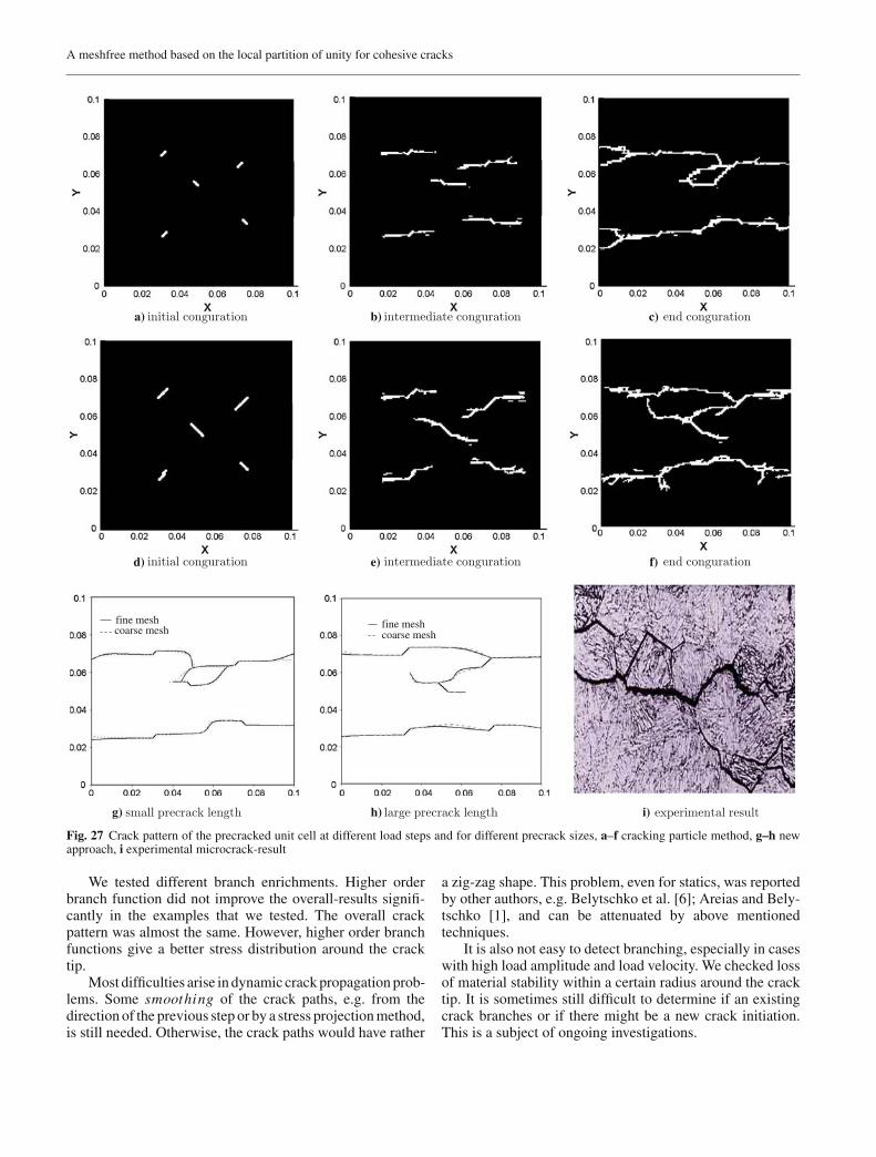
The unit cell is discretized with two different refinements,1,600 and 6,400 particles. The Lemaitre [28] damage modelis used in tension and linear elastic behaviour is assumed incompression. We will compare the results to those obtainedwith the cracking particle method in which approximately23,000 particles were used. The crack pattern at an interme-diate step and the final crack pattern for the cracking particlemethod is shown in Figs. 27a–f. In Figs. 27d–f we consideredlonger precracks. The final crack pattern of our new approachis shown in Figs. 27g,h. The results are mesh-independent andvery similar to the ones obtained with the cracking particlemethod. However, we need significantly less particles com-pared to the cracking particle method. An experimental resultis shown in Fig. 27i.

The crack patterns for different precrack sizes are differ-ent. For small precracks, cracks propagate from the onsetof the precrack perpendicular to the load direction. In thelower part of the unit cell where two preflaws are located, thecracks join in the middle of the specimen. The same tendencyis observed for longer precracks. However, in the upper partwhere three precracks are located, the cracks subdivide thespecimen into four parts when the precracks are sufficientlysmall while for larger precracks, three fragments occur. Thisis due to the fact that for the latter case, the two upper cracksjoin and hence unload the region below. The cracks in thelower region are arrested. If the cracks are small, the middleprecrack joins with the upper right precrack.

9 Conclusion

We have presented a meshfree method – extended elementfree Galerkin method (XEFG) – for crack propagation prob-lems. The method is based on the introduction of a discontinu-ity in the displacement field after the material looses stability.The crack tip enrichment with branch functions is employed.A cohesive model is used that solely depends on the discon-tinuous part of the displacement field.

The method is applied to several static and dynamic prob-lems where experimental or other numerical data is available.It is also applied to mode I and I-II crack problems of whichthe analytical solutions are available. The method is veryaccurate. It resolves the crack path with low particle resolu-tions. In two dimensions, more than 10 times less particleswere necessary than in the cracking particle method, [34].


fine meshcoarse mesh coarse mesh

fine mesh

a) b) c)

f)e)d)

g) h) i)

Fig. 27 Crack pattern of the precracked unit cell at different load steps and for different precrack sizes, a–f cracking particle method, g–h newapproach, i experimental microcrack-result

We tested different branch enrichments. Higher orderbranch function did not improve the overall-results signifi-cantly in the examples that we tested. The overall crackpattern was almost the same. However, higher order branchfunctions give a better stress distribution around the cracktip.

Most difficulties arise in dynamic crack propagation prob-lems. Some smoothing of the crack paths, e.g. from thedirection of the previous step or by a stress projection method,is still needed. Otherwise, the crack paths would have rather

a zig-zag shape. This problem, even for statics, was reportedby other authors, e.g. Belytschko et al. [6]; Areias and Bely-tschko [1], and can be attenuated by above mentionedtechniques.

It is also not easy to detect branching, especially in caseswith high load amplitude and load velocity. We checked lossof material stability within a certain radius around the cracktip. It is sometimes still difficult to determine if an existingcrack branches or if there might be a new crack initiation.This is a subject of ongoing investigations.

T. Rabczuk, G. Zi

Acknowledgements We would like to thank the support of Korea Insti-tute of Construction & Transportation Technology Evaluation and Plan-ning (KICTTEP) grant 05-CTRM-D04-03.

References

1. Areias PMA, Belytschko T (2005) Analysis of three-dimensionalcrack initiation and propagation using the extended finite elementmethod. Comput Mech

2. Areias PMA, Song JH, Belytschko T (2006) Analysis of fracturein thin shells by overlapping paired elements (in press)

3. Armero F, Garikipati K (1996) An analysis of strong discontinu-ities in multiplicative finite strain plasticity and their relation withthe numerical simulation of strain localization in solids. Int J SolidsStruct 33(20–22):2863–2885

4. Arrea M, Ingraffea AR (1982) Mixed-mode crack propagation inmortar and concrete. Technical Report 81-13, Department of Struc-tural Engineering, Cornell University Ithaka

5. Belytschko T, Black T (1999) Elastic crack growth in finiteelements with minimal remeshing. Int J Numer Methods Eng45(5):601–620

6. Belytschko T, Chen H, Xu J, Zi G (2003) Dynamic crack prop-agation based on loss of hyperbolicity and a new discontinuousenrichment. Int J Numer Methods Eng 58(12):1873–1905

7. Belytschko T, Fish J, Englemann B (1988) A finite element methodwith embedded localization zones. Comput Methods Appl MechEng 70:59–89

8. Belytschko T, Krongauz Y, Organ D, Fleming M, Krysl P (1996)Meshless methods: An overview and recent developments. ComputMethods Appl Mech Eng 139:3–47

9. Belytschko T, Lu YY (1995) Element-free galerkin methods forstatic and dynamic fracture. Int J Solids Struct 32:2547–2570

10. Belytschko T, Lu YY, Gu L (1994) Element-free galerkin methods.Int J Numer Methods Eng 37:229–256

11. Belytschko T, Lu YY, Gu L (1995) Crack propagation by element-free galerkin methods. Eng Fracture Mech 51(2):295–315

12. Belytschko T, Moes N, Usui S, Parimi C (2001) Arbitrarydiscontinuities in finite elements. Int J Numer Methods Eng50(4):993–1013

13. Belytschko T, Rabczuk T, Samaniego E, Areias PMA (2006) Two-and three dimensional modelling of shear bands using a meshfreemethod with cohesive surfaces. Int J Numer Methods Eng (in press)

14. Belytschko T, Tabbara M (1996) Dynamic fracture using element-free galerkin methods. Int J Numer Methods Eng 39(6):923–938

15. Bocca P, Carpinteri A, Valente S (1991) Mixed model fracture ofconcrete. Int J Solids Struct 33:2899–2938

16. Bocca P, Carpintieri A, Valente S (1990) Size effect in the mixedmode crack propagation: softening and snap-back analysis. EngFracture Mech 35:159–170

17. Camacho GT, Ortiz M (1996) Computational modeling of impactdamage in brittle materials. Int J Solids and Struct 33:2899–2938

18. Chessa J, Wang H, Belytschko T (2003) On the construction ofblending elements for local partition of unity enriched finite ele-ments. Int J Numer Methods Eng 57(7):1015–1038

19. Daux C, Moes N, Dolbow J, Sukumar N, Belytschko T (2000)Arbitrary branched and intersection cracks with the extended finiteelement method. Int J Numer Methods Eng 48:1731–1760

20. Falk ML, Needleman A, Rice JR (2001) A critical evalua-tion of cohesive zone models of dynamic fracture. J Phys IV11(PR5):43–50

21. Fineberg J, Sharon E, Cohen G (2003) Crack front waves in dy-namic fracture. Int J Fracture 121(1–2):55–69

22. Gravouil A, Moes N, Belytschko T (2002) Non-planar 3D crackgrowth by the extended finite element and level sets – part ii: Levelset update. Int J Numer Methods Eng 53:2569–2586

23. Gummalla RR (1999) Effect of material and geometric parameterson deformations of a dynamically loaded prenotched plate. Mas-ter’s Thesis, Virginia Polytechnical Institute and State University

24. Johnson GR, Cook WH (1983) A constitutive model and data formetals subjected to large strains, high strain rates, and high tem-peratures. In: Proceedings of the 7th international Symposium onBallistics

25. Kalthoff JF, Winkler S (1987) Failure mode transition at highrates of shear loading. Int Conf Impact Loading Dyn Behav Mater1:185–195

26. Krysl P, Belytschko T (1999) The element free galerkin method fordynamic propagation of arbitrary 3-D cracks. Int J Numer MethodsEng 44(6):767–800

27. Laborde P, Pommier J, Renard Y, Solau M (2005) Higher-orderextended finite element method for cracked domains. Int J NumerMethods Eng 64(3):354–381

28. Lemaitre J (1971) Evaluation of dissipation and damage in metalsubmitted to dynamic loading. Proceedings ICM 1

29. Lu YY, Belytschko T, Tabbara M (1995) Element-free galerkinmethod for wave-propagation and dynamic fracture. Comput Meth-ods Appl Mech Eng 126(1–2):131–153

30. Melenk JM, Babuska I (1996) The partition of unity finite ele-ment method: Basic theory and applications. Comput MethodsAppl Mech Eng 139:289–314

31. Moes N, Dolbow J, Belytschko T (1999) A finite element methodfor crack growth without remeshing. Int J Numer Methods Eng46(1):133–150

32. Moes N, Gravouil A, Belytschko T (2002) Non-planar 3-D crackgrowth by the extended finite element method and level sets, parti:mechanical model. Int J Numer Methods Eng 53(11):2549–2568

33. Ortiz M, Pandolfi A (1999) Finite-deformation irreversible cohe-sive elements for three-dimensional crack-propagation analysis. IntJ Numer Methods Eng 44:1267–1282

34. Rabczuk T, Belytschko T (2004) Cracking particles: a simplifiedmeshfree method for arbitrary evolving cracks. Int J Numer Meth-ods Eng 61(13):2316–2343

35. Rabczuk T, Belytschko T (2005) Adaptivity for structured mesh-free particle methods in 2D and 3D. Int J Numer Methods Eng63(11):1559–1582

36. Ravi-Chandar K (1998) Dynamic fracture of nominally brittlematerials. Int J Fracture 90(1–2):83–102

37. Remmers JJC, de Borst R, Needleman A (2003) A cohesive seg-ments method for the simulation of crack growth. Comput Mech31:69–77

38. Saehn S. Technische Bruchmechanik, Vorlesungsm-anuskript. Technische Universitaet Dresden, Institut fuerFestkoerpermechanik

39. Samaniego E, Oliver X, Huespe A (2003) Contributions to thecontinuum modelling of strong discontinuities in two-dimensionalsolids. PhD thesis, International Center for Numerical Methods inEngineering, Monograph CIMNE No. 72

40. Sharon E, Fineberg J (1996) Microbranching instability and the dy-namic fracture of brittle materials. Phys Rev B 54(10):7128–7139

41. Ventura G, Xu J, Belytschko (2002) A vector level set method andnew discontinuity approximations for crack growth by efg. Int JNumer Methods Eng 54(6):923–944

42. Westergaard HM (1939) Bearing pressures and cracks. J ApplMech 6:A49–A53

43. Xu X-P, Needleman A (1994) Numerical simulations of fast crackgrowth in brittle solids. J Mech Phys Solids 42:1397–1434

44. Zhou F, Molinari JF (2004) Dynamic crack propagation with cohe-sive elements: a methodolgy to address mesh dependence. Int JNumer Methods Eng 59(1):1–24

45. Zi G, Belytschko T (2003) New crack-tip elements for xfemand applications to cohesive cracks. Int J Numer Methods Eng57(15):2221–2240

46. Zi G, Chen H, Xu J, Belytschko T (2005) The extended finite ele-ment method for dynamic fractures. Shock Vib 12(1):9–23

47. Zi G, Song J-H, Budyn E, Lee S-H, Belytschko T (2004) A methodfor grawing multiple cracks without remeshing and its applica-tion to fatigue crack growth. Model Simul Materials Sci Eng12(1):901–915

A Meshfree Method based on the Local Partition of Unity for Cohesive Cracks

Documents

Transcript of A Meshfree Method based on the Local Partition of Unity for Cohesive Cracks