DISCLAIMER STATEMENT

This document is disseminated in the interest of information exchange. The contents of this report reflect the views of the authors who are responsible for the facts and accuracy of the data presented herein. The contents do not necessarily reflect the official views or policies of the State of California or the Federal Highway Administration. This publication does not constitute a standard, specification or regulation. This report does not constitute an endorsement by the Department of any product described herein.

For individuals with sensory disabilities, this document is available in alternate formats. For information, call (916) 654-8899, TTY 711, or write to California Department of Transportation, Division of Research, Innovation and System Information, MS-83, P.O. Box 942873, Sacramento, CA 94273-0001.

Department of Civil and Environmental Engineering University of California, Davis Davis, California 95616

Final Report No. CA17-2346

Controlling Temperature and Shrinkage Cracks in Bridge Decks and Slabs

John E. Bolander

August 2018

Final Report submitted to the California Department of Transportation (Caltrans) under Contract No. 65A0532

Contents

1 Introduction 5 1.1 Overview . . . . . . . . . . . . . . . . . . . . . . . . . . . . . . 5 1.2 Background . . . . . . . . . . . . . . . . . . . . . . . . . . . . 6 1.3 Hypothesis . . . . . . . . . . . . . . . . . . . . . . . . . . . . . 7 1.4 Project tasks and goals . . . . . . . . . . . . . . . . . . . . . . 9 1.5 Report contents . . . . . . . . . . . . . . . . . . . . . . . . . . 9

2 Early-age concrete behavior: Overview 10 2.1 Factors influencing early-age cracking . . . . . . . . . . . . . . 10

2.1.1 Mixture composition and proportioning . . . . . . . . . 11 2.1.2 Volume changes due to hygral effects . . . . . . . . . . 15 2.1.3 Volume changes due to thermal effects . . . . . . . . . 18 2.1.4 Tensile capacity . . . . . . . . . . . . . . . . . . . . . . 19 2.1.5 Structural configuration . . . . . . . . . . . . . . . . . 25

2.2 Strategies for reducing early-age cracking . . . . . . . . . . . . 26 2.2.1 Concrete mixture design . . . . . . . . . . . . . . . . . 26 2.2.2 Conventional and enhanced water curing . . . . . . . . 27 2.2.3 Control of thermal history . . . . . . . . . . . . . . . . 28 2.2.4 Control of concrete volumetric stability . . . . . . . . . 29 2.2.5 Fiber reinforcement and other reinforcement . . . . . . 29

2.3 Summary . . . . . . . . . . . . . . . . . . . . . . . . . . . . . 30

3 Modeling framework 31 3.1 Program structure . . . . . . . . . . . . . . . . . . . . . . . . 31 3.2 Cementitious materials hydration . . . . . . . . . . . . . . . . 33 3.3 Primary analysis modules . . . . . . . . . . . . . . . . . . . . 34

3.3.1 Thermal analysis . . . . . . . . . . . . . . . . . . . . . 34 3.3.2 Hygral analysis . . . . . . . . . . . . . . . . . . . . . . 34

2

3.3.3 Structural analysis . . . . . . . . . . . . . . . . . . . . 35

4 Early-age cracking potential of concrete bridge decks: 2D modeling 37 4.1 Model definition . . . . . . . . . . . . . . . . . . . . . . . . . . 39

4.1.1 Thermal analysis inputs . . . . . . . . . . . . . . . . . 41 4.1.2 Hygral analysis inputs . . . . . . . . . . . . . . . . . . 43 4.1.3 Mechanical analysis inputs . . . . . . . . . . . . . . . . 45

4.2 Simulation results . . . . . . . . . . . . . . . . . . . . . . . . . 46 4.2.1 Deck temperature simulations . . . . . . . . . . . . . . 46 4.2.2 Determination of degree of hydration at final set . . . . 50 4.2.3 Strength simulations . . . . . . . . . . . . . . . . . . . 50 4.2.4 Shrinkage simulations . . . . . . . . . . . . . . . . . . . 51

4.3 Parametric study . . . . . . . . . . . . . . . . . . . . . . . . . 54 4.3.1 Curing protocol . . . . . . . . . . . . . . . . . . . . . . 54 4.3.2 Structural configuration . . . . . . . . . . . . . . . . . 59 4.3.3 Concrete materials composition . . . . . . . . . . . . . 62 4.3.4 Discussion . . . . . . . . . . . . . . . . . . . . . . . . . 62

5 Cracking potential at early ages: 3D modeling 65 5.1 Model definition . . . . . . . . . . . . . . . . . . . . . . . . . . 65

5.1.1 Domain discretization . . . . . . . . . . . . . . . . . . 65 5.1.2 Model inputs and boundary conditions . . . . . . . . . 68

5.2 Comparisons with field measurements . . . . . . . . . . . . . . 71 5.2.1 Deck temperatures . . . . . . . . . . . . . . . . . . . . 71 5.2.2 Deck strains . . . . . . . . . . . . . . . . . . . . . . . . 72

5.3 Design examples . . . . . . . . . . . . . . . . . . . . . . . . . 74 5.3.1 Drying shrinkage . . . . . . . . . . . . . . . . . . . . . 75 5.3.2 Autogenous shrinkage . . . . . . . . . . . . . . . . . . 79 5.3.3 Coefficient of thermal expansion . . . . . . . . . . . . . 81 5.3.4 Cementitious materials usage . . . . . . . . . . . . . . 83 5.3.5 Bridge configuration: deck continuity . . . . . . . . . . 85 5.3.6 Effects of long-term exposure to the environment . . . 85

6 Project summary and recommendations 90 6.1 Modeling results and findings . . . . . . . . . . . . . . . . . . 91 6.2 Practical insights and recommendations . . . . . . . . . . . . . 94 6.3 Potential directions for investigation . . . . . . . . . . . . . . 98

3

A Modeling of cementitious materials hydration 99

B Model components 103 B.1 Temperature field modeling . . . . . . . . . . . . . . . . . . . 103 B.2 Moisture field modeling . . . . . . . . . . . . . . . . . . . . . . 106 B.3 Displacement field modeling . . . . . . . . . . . . . . . . . . . 109

B.3.1 Formulation of rigid-body-spring elements . . . . . . . 109 B.3.2 Stiffness and creep representation . . . . . . . . . . . . 113

C Validation exercises and needs 116 C.1 Stiffness and basic creep development . . . . . . . . . . . . . . 116 C.2 Strength development . . . . . . . . . . . . . . . . . . . . . . . 119 C.3 Autogenous and drying shrinkage . . . . . . . . . . . . . . . . 121 C.4 Simulation of restrained ring test . . . . . . . . . . . . . . . . 125 C.5 Structural displacements . . . . . . . . . . . . . . . . . . . . . 128

C.5.1 Half-span simulations . . . . . . . . . . . . . . . . . . . 128 C.6 Validation needs . . . . . . . . . . . . . . . . . . . . . . . . . . 131

D Plastic shrinkage cracking 135 D.1 Methods for reducing plastic shrinkage cracking . . . . . . . . 135 D.2 General use of short-fiber reinforcement . . . . . . . . . . . . . 136 D.3 Glass fiber reinforcement . . . . . . . . . . . . . . . . . . . . . 139 D.4 Laboratory testing: preliminary results . . . . . . . . . . . . . 146 D.5 Summary . . . . . . . . . . . . . . . . . . . . . . . . . . . . . 149

E Nomenclature 152

Bibliography 155

4

Chapter 1

Introduction

1.1 Overview Early-age cracking is a root cause of premature loss of serviceability of con-crete structures, including reinforced concrete bridge decks and slabs. Crack-ing may occur while concrete is still in a plastic state or after its hardening. Although the causes of such cracking have been studied extensively over the past several decades, and corrective actions have been proposed, widespread problems persist [39, 70, 103]. Cracking resistance can be improved through materials design optimization, but such efforts must extend beyond the realm of laboratory testing. The prevailing conditions during placement and hard-ening of the concrete bridge deck need to be considered. Model-based simula-tion enables parametric analyses within that comprehensive setting, in which concrete materials science interconnects with construction practice and struc-tural behavior. This project involves: 1) the development of a methodology for simu-

lating the early-age behavior of structural concrete; and 2) application of the methodology to assessing early-age cracking of concrete bridge decks and slabs. The methodology employs simple lattice models, which depend on a modeling of cementitious materials hydration. From this basis, realistic connections are made between the design parameters (including materials composition, construction practice, environmental conditions, and structural configuration) and properties that strongly affect susceptibility to cracking, such as volumetric stability, strength, stiffness, and creep potential. The approach developed herein is suitable for analyses of hardened concrete, yet

5

inferences can be made regarding cracking in the plastic state. Validation exercises are conducted using measurements taken from bridge

decks, including a bridge monitored through a Caltrans sponsored project, and small-scale laboratory tests. The validated model is used for parametric studies that cover variations in casting/curing protocols, cementitious mate-rials composition, structural configuration, and environmental conditions, as well as the usage of special admixtures (e.g., shrinkage reducing admixtures). The importances of thermal and hygral contributions to cracking potential are assessed. The simulation results show that thermal effects may signifi-cantly contribute to cracking and its severity, particularly in the presence of restraint against deck movement. Laboratory testing and observations of field performance cover a small set

of possible combinations of the design parameters related to early-age crack-ing of bridge decks. The methodology developed through this project enables examination of a much larger region of the design parameter space, which is necessary for establishing comprehensive design guidelines for controlling early-age cracking.

1.2 Background Early-age cracking of bridge decks may occur due to plastic shrinkage or set-tlement, prior to concrete setting, or as a consequence of volumetric changes associated with thermal, hygral, or chemical phenomena that occur after setting. Such cracking can be superficial or extend through the deck thick-ness. Previous studies have found that tensile stresses associated with such volumetric instabilities are larger than those due to traffic loading [70]. The duration of the early-age period depends on the properties of inter-

est, ranging from the first few hours after casting (e.g., when investigating plastic shrinkage cracking and settlement) to days after the completion of curing operations. Herein, the early-age period begins with concrete casting and extends through the time of curing, including initial exposure to the en-vironment after curing measures are completed. It is during this period that a variety of distress mechanisms are manifested and the efficacy of design decisions, with respect to crack prevention, can be studied. The factors that affect cracking potential can be categorized in different

ways, such as the grouping presented in Fig. 1.1. These factors can be viewed as design parameters, since they are considered prior to and during the time

6

of construction and curing. To simplify the categorization, the many environ-mental boundary conditions are represented in terms of heat and moisture exchange. Hygral shrinkage, due to autogenous mechanisms and external drying, is

a primary source of early-age cracking of concrete bridge decks. The lifetime shrinkage potential of ordinary concrete ranges from 400 to 1000 µm/m; up to half of this amount occurs within the first month after exposure to the environment and about 90% occurs within the first year [32]. Control of hy-gral shrinkage has been effective in avoiding significant cracking in structural concrete [81]. Nonetheless, the significance of additional factors, acting alone or in combination, needs to be assessed. Thermally induced cracking is a concern in mass concrete applications,

which are typically defined by a minimum dimension criterion [26]. For exam-ple, the Japan Concrete Institute classifies reinforced slabs with large surface area and thickness greater than 0.8 m as mass concrete [63]. According to the Concrete Technology Manual [32], a thermal control plan is typically needed when one dimension of a concrete placement exceeds 2.13 m (7 ft). An equiv-alent thickness has been defined to account for size and geometry of the structural element [43], providing a more consistent measure for identifying mass concrete applications. Clearly, concrete bridge decks of ordinary dimensions do not qualify as

mass concrete applications. Nonetheless, deck concretes typically contain a large amount of cementitious materials, which causes higher heats of hydra-tion. The large surface areas of decks and slabs also make them prone to solar heating and variations in the ambient temperature. The placement of decks over steel or mature concrete girders, which provide restraint and may also be thermally loaded, further heightens the potential of cracking. For these reasons, thermal contributions to cracking potential need to be assessed.

1.3 Hypothesis Early-age cracking behavior of reinforced concrete bridge decks depends on a variety of factors. Whereas hygral shrinkage effects are thought to be domi-nant, thermal effects can also have a primary influence on cracking potential. The occurrence and severity of early-age cracking can be controlled through the simultaneous consideration of hygral and thermal factors, along with their dependence on structural restraint conditions.

7

Figure 1.1: Design parameters affecting early-age cracking of bridge decks

8

1.4 Project tasks and goals The project tasks and goals pertain to: 1) development and validation of a methodology for simulating the early-age behavior of structural concrete; and 2) application of the methodology to assessing the susceptibility of concrete bridge decks to early-age cracking. Realistic connections are made between the design variables (including materials composition, construction practice, environmental conditions, and structural configuration) and properties that strongly affect susceptibility to cracking, such as concrete strength, stiffness, shrinkage, and creep capacity. Through quantitative accounting of these relationships, the methodology supports the formation of comprehensive de-sign guidelines for controlling early-age cracking in concrete bridge decks and slabs.

1.5 Report contents This report first provides background information regarding early-age crack-ing of structural concrete. Common strategies for reducing the likelihood of such cracking are reviewed. The report then summarizes the modeling framework and its capabilities, as demonstrated through validation exercises. Much of the background information on the model and most of the validation exercises are presented in appendices. The validated model is used for model-based parametric study of bridge deck cracking. Finally, the results of the parametric study, and surveys of existing literature, support the development of recommendations and guidelines for controlling such cracking.

9

Chapter 2

Early-age concrete behavior: Overview

This section reviews selections from the available literature with emphasis on the early-age cracking performance of concrete bridge decks. The review will include coverage of several state DOT sponsored projects related to early-age cracking of concrete. It will also cover the topic of modeling early-age concrete behavior and provide justifications for some of the modeling assumptions employed herein. Definition of the early-age period varies between studies, depending on

the properties or behavior of interest. Several studies have defined early-age concrete to be that within the first 24 h after mixing [60, 109]. Riding et al. [105] refer to an early-age period of 4 to 5 days after casting. Others include the period of curing and possibly beyond to cover the time when concrete remains susceptible to cracking caused by thermal-hygral phenom-ena. Initial deck cracking may occur up to several weeks after casting and early-age conditions likely play a significant role in such later cracking. Ex-amination of bridge decks has shown that cracking progresses over longer periods of time and that it takes several years for the extent of cracking to become evident (Fig. 2.1) [40].

2.1 Factors influencing early-age cracking A variety of factors influence early-age cracking [34]. Several of the prominent factors are briefly described in this section.

10

Figure 2.1: Development of crack density over time [40]

2.1.1 Mixture composition and proportioning

Cement composition and fineness

Cement composition has a major impact on the short- and long-term perfor-mance of structural concrete. Cement composition affects both the rate and products of hydration. It therefore governs rate of heat production and the development of relevant properties, such as strength and stiffness. For bridge deck concrete, Caltrans limits the choice of portland cement to ASTM types II and V, which effectively limits the C3S contents. Equivalent alkali content of the cement has an upper limit of 0.6% to reduce problems associated with alkali-silica reactivity, but also to reduce drying shrinkage and avoid strength loss [62]. The influences of cement composition on early-age cracking poten-tial, and on the durability-related properties of concrete in general, have been summarized by several technical documents and reports [32, 85]. Increasing cement fineness refines the initial pore-size distribution of the

cement paste, which typically increases autogenous shrinkage [25]. Upper limits on cement fineness (e.g., 320 m2/kg) have been recommended to reduce the potential for large autogenous shrinkage. Due to higher surface area, finer cements also increase the rate of cement hydration and thus the rate of heat production at early-ages. Although those tendencies can be reduced by coarsening the cement particle-size distribution, early-age strength may also be compromised.

11

Supplementary cementitious materials

A variety of supplementary cementitious materials (SCMs) are approved for use on Caltrans projects. Several SCM categories, usage rates, and relevant specifications are listed in Table 2.1. SCM type and usage rate influence: 1) particle size distribution and thus the initial packing of the particle structure; 2) particle morphology and its effects on water demand and workability; 3) reactivity; 4) specific surface area available for reaction; and 5) composition and microstructure of the reaction products. These influences lead to changes in fresh and hardened properties of concrete, as presented in Table 2.2. As SCMs are commonly industrial by-products, or produced from variable source materials, their composition and properties exhibit variation. More than one SCM may be blended with OPC. For example, ternary blends have been developed to enhance binder properties and address specific needs. Partial replacements of cement by inert filler materials (e.g., limestone powder) may accelerate early-age hydration and reduce, or maintain, setting times [23]. The particle size distributions can be controlled through grinding. Typi-

cally, more finely ground materials have higher specific surface area and there-fore are more reactive (mechanical activation). Fine particles may also serve as nucleation sites for portland cement hydration. The dense microstruc-tures that are produced by grading particle size reduce the permeability of the matrix. However, fine or finely ground materials refine the pore structure, which can increase autogenous shrinkage and lower bleeding rates, which is a contributor to plastic shrinkage cracking. When portland cement is partially replaced by a less reactive SCM (e.g.,

fly ash), there is a dilution effect causing delay in setting and lower early-age strengths. The cementing properties of several SCMs (e.g., fly ash) result from the pozzolanic reaction, which is a secondary reaction that relies on calcium hydroxide produced by cement hydration. Long term strength is recovered through the pozzolanic reaction, often surpassing the strength of OPC binders. A common goal in concrete mixture design is to reduce the environmen-

tal impact of components of the civil infrastructure. The partial replacement of OPC reduces cement use and thus the relatively large amounts of CO2 associated with cement production. For the common case where the SCM is an industrial by-product, the value added use of a waste material is an additional benefit. However, premature loss of serviceability of bridge decks has large negative economic and environmental consequences. It can be ar-

12

Table 2.1: Supplementary cementitious materials [32]

gued that durability should be the primary objective in designing concrete mixtures for bridge deck applications.

Water/air content

Increasing water content increases the amount of evaporable water and thus shrinkage potential. Increasing cement content also increases shrinkage po-tential, due to the larger amount of cement paste. For the water-to-cement ratios of ordinary concrete, reducing w/c reduces the drying shrinkage po-tential, as shown in Fig. 2.2. For water-to-cement ratios less than about 0.40, however, autogenous shrinkage due to self-desiccation becomes a concern. Increasing air content improves workability, which allows for reductions

in w/c and therefore reductions in shrinkage. The strength reductions asso-ciated with increased air content are thought increase creep under sustained load, which also reduces cracking potential [40]. The same study recommends air contents of 8 ±1.5% for durable concrete.

Aggregate type, amount, and gradation

Increasing the volume fraction of aggregate typically reduces the amount of drying shrinkage, as shown in Fig. 2.2. Studies of concrete beyond 24 h have shown that the type of aggregate can have significant influence on re-sistance to cracking. Whereas paste is volumetrically unstable under hygral variations, aggregates are more stable, providing restraint against shrinkage.

13

Table 2.2: Influence of supplementary cementitious materials on concrete properties [32]

Figure 2.2: Dependence of drying shrinkage on w/c and aggregate content (adapted from Neville [93])

14

Recent study by Roziere et al. [109] considered the influence of various ag-gregate types on cracking behavior within the first 24 h. They did not find a significant influence of aggregate type in that early stage. Increasing a/c has been found to be highly effective in reducing shrinkage cracking [12]. For the same amount of paste, the size distribution of aggregates does not affect the shrinkage of concrete. Aggregate type and amount have a strong influence on the coefficient of

thermal expansion (CTE) of the concrete (Table 2.3). The lower and upper values of the range of CTE values differ by a factor of about 2. The angularity of aggregates may affect cracking potential. In particular,

deck concretes produced with angular aggregates exhibited less cracking than those produced with river gravel with rounded features [70]. This implies that better bonding along the aggregate-paste interface improves the cracking resistance of early-age concrete. Aggregates with higher absorption capacities have the potential to draw

water from the pore structure and, in effect, act as drying agents. Aggregates with low absorption capacities, or those batched in saturated surface dry condition, are preferred. Stiffer aggregates reduce long-term shrinkage, but the effects on early-age behavior are less significant due to the large mismatch between the elastic moduli of the aggregate and paste phases.

Aggregate type concrete CTE (×10−6/◦C) limestone granite sandstone quartzite

6 9 10 12

Table 2.3: Effect of aggregate type on coefficient of thermal expansion (CTE) of hardened concrete [93].

2.1.2 Volume changes due to hygral effects Plastic shrinkage

For higher water-to-cement ratios (e.g., for w/c greater than about 0.4), the cement-based matrix is initially a suspension of cement grains and other solid particles within the mixture water. Due to the differences in specific gravity, the particles settle and there is a net flow (bleeding) of water upward [22].

15

At lower w/c, the grains are in partial or near-contact from the start, such that there is less settlement and bleeding. If the upper surface is exposed to a drying environment, and if the rate of drying is greater than the rate of bleeding, the near surface porosity is gradually emptied of water, beginning with coarser pores. Menisci formation within the emptying pores induces an underpressure in the capillary water, which causes contraction of the particle network near the drying surface. This contraction, and ultimately air entry into the particle network, is the source of plastic shrinkage cracking. Mixtures that provide sufficient bleeding rate are less susceptible to plastic

shrinkage cracking. Silica fume additions, and other additions that densify the packing structure, can be problematic in that they densify the parti-cle network and impede water transport. On the other hand, the addition of short synthetic fibers is thought to improve water transport toward the drying surface and reduce the tendency for plastic shrinkage cracking. The potential for plastic shrinkage cracking can also be reduced through con-trol of the evaporation rate, which depends on the concrete temperature, air temperature, ambient relative humidity and wind velocity. Interconnection of the cement particles, via the products of cement hy-

dration, leads to setting of the concrete and its ability to resist penetration or shear. Concretes with higher w/c typically take more time to set due to the larger initial spacing of the particles. The delay in setting can increase the probability of plastic shrinkage cracking. Further evolution of the percolated network leads to mechanical property development with respect to elastic modulus, strength, and creep. Leemann and Lura [75] describe the beneficial effects of selected admixtures on reducing plastic shrinkage cracking.

Autogenous shrinkage

Autogenous deformation is the macroscopic volume change when moisture exchange with the environment is prevented. Such deformation results from chemical shrinkage, which is an internal volume reduction [125]. The volume of the reaction products of cement hydration is less than that of the reactants. This chemical shrinkage is on the order of 6-7 ml/100 g of cement reacted for ordinary cement pastes [100] and can be higher for some blends containing supplementary cementitious materials (e.g., silica fume). Prior to setting, while the cement paste is in liquid state, chemical shrinkage is converted entirely to external volume change. With further hydration, the particle network becomes percolated (i.e., solid pathways have formed across the

16

material volume) and increasingly resistant to volume changes. This enables gas bubbles to nucleate within the larger porosity features. In turn, water-air menisci are produced along with an accompanying drop in RH, as described by Kelvin’s law [79]. The formation of menisci leads to underpressure in the capillary fluid. The autogenous shrinkage is much smaller (up to two orders of magni-

tude less) than that of the unrestrained chemical shrinkage [22]. Even so, since autogenous shrinkage develops early in the hydration history, when the skeleton of solid hydration products has low stiffness and is prone to creep deformation, the capillary underpressure can produce large deformation of the solid skeleton. This capillary tension explanation of autogenous shrinkage (and hygral

shrinkage, in general) is thought to be valid for the upper RH range, say above 45% [79]. Other mechanisms are present, including disjoining pressure between the solid particles resulting from van der Waals forces, double layer repulsion, and structural forces [53]. When RH decreases, the disjoining pressure lowers, which causes shrinkage. However, this shrinkage mechanism is thought to be dominant only in the lower RH range. It is therefore not a primary contributor to autogenous shrinkage, which occurs at RH above 75-80%. With respect to early-age cracking of structural concrete, several points

are relevant.

• Autogenous deformation of portland cement systems increases dramat-ically as the water-to-cement ratio is reduced below about 0.35. This is caused by the concomitant reduction in pore size and therefore capillary stresses.

• The reduction of internal RH due to autogenous effects depends on w/c, amongst other factors. The highest RH drops are seen for lower w/c values [36, 95, 98].

• Reduction of internal RH decreases hydration rates and therefore strength development [135]. However, this reduction is significantly less for higher w/c concrete due to their larger porosity.

• Finer cement leads to larger reduction in RH for a given degree of hydration. Autogenous shrinkage is greater for finer cement.

17

• Superplasticizers improve the dispersion of cement particles that, in turn, increases early-age autogenous shrinkage.

• Various strategies have been proposed to mitigate autogenous shrink-age effects [59, 120]. Drying shrinkage can be prevented by construction practice (e.g., wet curing and other means of reducing water loss to the environment.) Autogenous shrinkage is much less addressable through construction practice. Rather, it should be addressed through materi-als design: use of slower hardening cements that have lower chemical shrinkage. For example, cements with lower C3A and C3S contents should be used, since those compounds are the greatest contributors to chemical shrinkage. Furthermore, aggregate content should be maxi-mized and delay of setting avoided.

Drying shrinkage

The rate and amount of drying shrinkage is affected by internal and exter-nal factors. The internal factors include the type and amount of aggregate, water-to-cement ratio, water content, cement content, and the use of special admixtures. For concretes containing dimensionally stable aggregates, the primary factors are the proportion of aggregates, water-to-cementitious ma-terials ratio, and total amount of water. As fly ash allows for a reduction in water content, all else being equal, fly ash usage reduces drying shrinkage. The external factors include the methods of curing and the temperature, wind velocity, and RH of the environment. Drying shrinkage increases with increases in temperature or wind velocity, and reductions in RH.

2.1.3 Volume changes due to thermal effects Cement hydration is an exothermal process. The amount and rate of heat produced depends on the phase composition of the cementitious materials and additives, as described in Appendix A. For sufficiently high rates of hydration and boundary conditions that restrict heat loss, the concrete heats and expands. Cracking may occur if subsequent cooling is rapid, particularly if the thermal contractions are restrained [26]. The temperature changes of the concrete, and the consequent dimensional

instabilities, are governed by the thermophysical properties of concrete, in-cluding heat capacity, thermal conductivity, and coefficient of expansion.

18

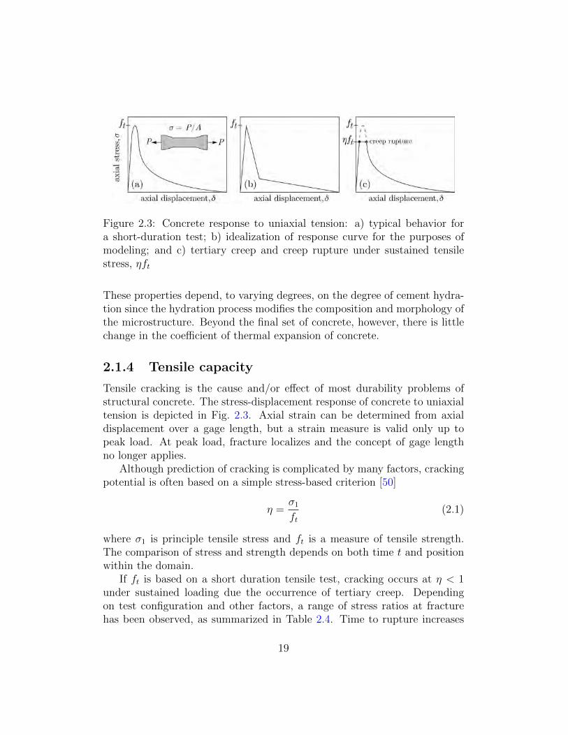
Figure 2.3: Concrete response to uniaxial tension: a) typical behavior for a short-duration test; b) idealization of response curve for the purposes of modeling; and c) tertiary creep and creep rupture under sustained tensile stress, ηft

These properties depend, to varying degrees, on the degree of cement hydra-tion since the hydration process modifies the composition and morphology of the microstructure. Beyond the final set of concrete, however, there is little change in the coefficient of thermal expansion of concrete.

2.1.4 Tensile capacity Tensile cracking is the cause and/or effect of most durability problems of structural concrete. The stress-displacement response of concrete to uniaxial tension is depicted in Fig. 2.3. Axial strain can be determined from axial displacement over a gage length, but a strain measure is valid only up to peak load. At peak load, fracture localizes and the concept of gage length no longer applies. Although prediction of cracking is complicated by many factors, cracking

potential is often based on a simple stress-based criterion [50]

σ1 η = (2.1)

ft

where σ1 is principle tensile stress and ft is a measure of tensile strength. The comparison of stress and strength depends on both time t and position within the domain. If ft is based on a short duration tensile test, cracking occurs at η < 1

under sustained loading due the occurrence of tertiary creep. Depending on test configuration and other factors, a range of stress ratios at fracture has been observed, as summarized in Table 2.4. Time to rupture increases

19

Figure 2.4: Probabilistic description of cracking potential (adapted from van Breugel and Lokhorst [126])

with lower stress-strength ratios. The descending branch of the static loading curve can serve as an envelope for creep rupture, as depicted in Fig. 2.3c [139].

Study ηc notes Altoubat and Lange [1] Altoubat and Lange [1] Domone [47] Emborg [50, 49] Riding et al. [105] van Breugel and Lokhorst [126] Wittmann et al. [131]

0.60-0.64 0.75-0.80 0.75 0.7 0.57 0.75 0.6-0.8

split cylinder tests uniaxial tension tests creep rupture under sustained load conditions typical of cooling of mass concrete split cylinder tests (50% probability of cracking) self-induced stress beam tests

Table 2.4: Stress-to-strength ratio at fracture, ηc

Considering the stochastic nature of the factors affecting both restraint stress and strength, however, cracking potential ought to be estimated in probabilistic terms. At any time t, there is a scatter in both strength and restraint stress produced within a set of nominally identical systems, dif-fering only by random variations of the parameters and processes defining the systems. If stress and strength are represented by probability distribu-tions about their mean values, the probability of cracking can be related to the overlap of the two distributions as suggested by Fig. 2.4. The estima-tion of cracking potential is also affected by spatial variation of these values within the structural domain. Considering these observations, and the afore-

20

Figure 2.5: Dependence of probability of cracking on stress-to-splitting strength ratio (from Riding et al. [105])

mentioned dependence of strength on load duration, it follows that η values much less than unity are reasonable as design limits [126]. Based on restrained shrinkage tests of several concrete mixtures, in con-

junction with strength tests of match-cured cylinders, Riding et al. [105] determined the stress-to-splitting strength ratio at cracking. Compressive strength was measured, from which splitting strength was calculated using one of several common relations. Lognormal fits of probability of cracking and stress-to-splitting strength ratio were made from restrained shrinkage testing of 64 specimens. The concrete mixtures varied with respect to water-to-cement ratio (0.32 to 0.53), total amount of cementitious materials (279 to 390 kg/m3), OPC type, and blend of OPC with fly ash, slag and/or silica fume. One such lognormal fit is presented in Fig. 2.5. Cracking potential can be categorized according to probability of occurrence, as indicated in Fig. 2.6. Another practical means for assessing the risk of cracking involves com-

parison of a cracking index

1 ft Icr = = (2.2)

η σt

with an empirically derived safety index γcr, which relates to probability of

21

Figure 2.6: Stress-based categories for probability of cracking. The bound-aries between categories are defined by 25, 50, and 75% probabilities of crack-ing (from Riding et al. [105])

cracking [65] " # � �−4.29 Icr

P (Icr) = 1 − exp − × 100 (2.3) 0.92

This relationship, which is plotted in Fig. 2.7, was determined by thermo-mechanical analyses of 65 mass concrete structures whose construction condi-tions, materials and mixture proportions, and cracking behavior were known [63]. With respect to thermal cracking, cracking risk can be categorized into one of several levels [65]:

≥ 1.75 : cracking prevented γcr ≥ 1.45 : number of cracks controlled (2.4)

≥ 1.00 : cracks allowed, but crack width controlled

Icr = 1.85 (or, equivalently, η = 0.54) corresponds to a 5% probability of cracking in mass concrete applications. With appropriate data and calibra-tion, this concept could be applied more generally to early-age cracking of structural concrete. The presence of reinforcing steel is not considered in the cracking risk

assessment. However, the amount of reinforcement does affect the openings of cracks. Crack opening can be related to γcr and reinforcement ratio [63], again for the case of thermal cracking of mass concrete.

22

Figure 2.7: Probability of thermal cracking (adapted from [65])

When evaluating the cracking potential of a concrete mixture, the infor-mation needed for this form of stress-strain comparison is often not available. The potential for cracking due to thermal effects has traditionally been as-sessed in terms of allowable temperature differentials. However, experience with this index has shown that it only offers a crude approximation of crack-ing potential [26]. For general applications, free shrinkage testing is arguably the simplest

indicator of cracking potential. A conservative estimate of cracking poten-tial can be based on net shrinkage strain �max, determined by differencing the peak expansion and contraction strains after concrete setting. This is illustrated in Fig. 2.8, which is based on experimental results of Cusson [38]. The actual strain producing tensile stress, �t, is unknown from this type of test. Finally, early-age cracking is influenced not only by concrete strength,

but also by its tensile strain capacity. Tensile strain capacity is initially larger, but reduces over the first 0.5 days after mixing to a minimum value (Fig. 2.9), and remains at about 100 microstrain thereafter. This critical stage with respect to plastic shrinkage cracking includes the setting time and early hardening. Minimum strain capacity, and the time at which it occurs (approximately 5 to 10 h after casting), is influenced by mixture design [109]. Thereafter, strain at peak stress increases for a short period of time. The re-ported values for strain capacity exhibit large variation and depend strongly on experimental factors (e.g., loading rate), such that stress criteria are thought to be a more reliable indicator of cracking potential [58, 109]. From 1 day onward, the strain capacity exhibits relatively less variation and is

23

Figure 2.8: Tensile strain and stress development in restrained concrete (adapted from Cusson [38])

Figure 2.9: Dependence of tensile strain capacity on time after mixing (adapted from Roziere et al. [109])

24

Figure 2.10: Plan view of deck cracking (adapted from Darwin et al. [39])

about 100µm/m.

2.1.5 Structural configuration Restraint conditions

With respect to bridge decks, crack patterns often vary with location along the span length(s). This suggests that restraint conditions influence deck cracking. Restraint is provided by the supporting girders, internal diaphragms, and possibly integration of the deck with abutments at the span ends. Local to such end restraints, finely spaced longitudinal cracking has been observed, whereas lateral cracking is predominant elsewhere particularly near the inter-mediate supports, which are negative moment regions [39]. Simply-supported spans have tended to exhibit lesser amounts of cracking, relative to spans that are continuous over supports. Cracking is often transverse to the longitudinal direction of the bridge

and spaced over portions of the deck [70]. Often, such transverse cracking is over, or runs parallel to, reinforcing bars in the top layer of reinforcement.

Reinforcing steel

Plastic settlement over reinforcing steel introduces tension in the fresh con-crete above the bar, which may cause cracking. This is an important concern in deep members, due to large plastic settlements, or when the concrete mix-ture itself is especially prone to settlement. The amount of drying shrinkage of reinforced concrete is about 200 to

300 µm/m, which is about one-third of that of a comparable mass of plain

25

concrete without reinforcement [32]. The thermal coefficient of reinforcing steel is 12×10−6/◦C, which is similar to that of ordinary concrete. Steel bars therefore do not promote or restrain concrete volume changes due to thermal effects, except possibly at very early ages when the thermal coefficient of concrete can be much larger. Reinforcing steel also serves to control the openings of cracks. However,

the control of crack opening is typically not as effective as that of short-fiber reinforcement distributed throughout the concrete volume [89].

2.2 Strategies for reducing early-age cracking A variety of strategies have proven to be effective in reducing early-age crack-ing, used individually or in combination. Several of these strategies are sum-marized.

2.2.1 Concrete mixture design Cracking potential can be reduced through concrete mixture design. De-sign recommendations and specific procedures have been published [34, 85]. Typical features of such recommendations and procedures include

• Limiting the cement content of the concrete. An upper limit of 320 kg/m3

has been recommended [40].

• Control of aggregate amount, size, and gradation. Increasing the ag-gregate to cementitious materials ratio decreases shrinkage. Increasing the maximum size of the coarse aggregates reduces shrinkage;

• Selection of aggregates with lower coefficient of thermal expansion;

• Controlling the amount, size, and gradation of the cementitious parti-cles. Higher cementitious materials contents lead to increased heat of hydration and increased shrinkage, since the amount of paste is greater.

• Controlling the water-to-cement ratio. Lowering w/c reduces drying shrinkage, although for w/c less than about 0.4 autogenous shrinkage becomes significant. Ratios of 0.42 to 0.45 have been preferred for bridge deck applications.

26

• Controlling air content. Occurrence of cracking is significantly reduced when air contents are 6.5% or more [40]. It is thought that air content improves workability without increasing shrinkage.

• Limiting concrete strength. Although strength is influenced by many factors, there is a correlation between strength (measured by labora-tory cured specimens) and deck cracking. Decks made with concrete of nominal strengths of 6500 psi exhibited about three times as much cracking as decks made with 4500 psi concrete [40].

• Limiting concrete slump. High slump promotes cracking due to set-tlement over reinforcing bars. Settlement cracking can be reduced by decreasing slump, increasing clearance above bars, and the use of polypropylene fibers.

2.2.2 Conventional and enhanced water curing Conventional curing typically involves the application of a curing compound to the finished concrete surface, preferably just before its moisture sheen disappears. Although there are many formulations of curing compound, they all provide a thin membrane that reduces moisture exchange between the concrete and the environment. Light colored compounds have the additional benefit of increasing the reflectivity of the cast surface and therefore reducing solar heating of the concrete. According to Caltrans specifications, highway bridge decks shall be cured

by application of curing compound and water curing for a period of at least 7 days [32, 33]. To facilitate water curing, the specifications allow for place-ment of a curing medium, consisting of white opaque polyethylene sheeting extruded onto burlap, over the deck. Since this sheeting does not completely prevent evaporation of water, the fabric should be periodically rewetted to maintain the water cure. Similar requirements are specified by other trans-portation agencies. As an alternative to the use of curing compound or sheeting, misting has

proven to be an effective means for preventing early-age cracking. Slowik et al. [121] identified the air entry value as being critical in the formation of plastic shrinkage cracking. Misting is applied when the vapor pressure, close to the concrete surface, approaches a critical value associated with air entry (i.e., the formation of a plastic shrinkage crack).

27

As a supplement to conventional water curing, internal curing via pre-soaked lightweight aggregate (LWA) has proven to be effective in reducing the autogenous shrinkage of concretes, especially those with high cement con-tents and low water-to-cementitious materials ratios [38]. The LWA is typi-cally introduced as partial replacement of regular fine aggregate. Internally cured concretes are less sensitive to variations in external curing practice or unfavorable environmental conditions. The degree of effectiveness depends on cementitious materials composition [38]. In some studies, the introduction of LWA did not reduce 28-day compressive strength, but rather increased it (e.g., by 20% [38]) by providing water to needy hydration sites.

2.2.3 Control of thermal history Thermal cracking is thought to depend on the temperature difference between the hydrating concrete and supporting elements (e.g., concrete girders). In particular, the maximum temperature difference in the first 10 h, or so, af-ter casting should be controlled. A maximum difference of 14◦C has been recommended [40]. Temperature differences can be controlled by reducing the temperature of the cast concrete, reducing cement content, accounting for anticipated heat input from solar radiation and ambient temperatures. Lower concrete temperatures also reduce the evaporation rate, which is the driver of plastic shrinkage. Neithalath et al. [2] have shown that micro-encapsulated phase change

materials (PCMs) can reduce concrete temperature rise due to heat of hydra-tion and also reduce the diurnal temperature variations of mature concrete. The PCMs have been added as a partial replacement of cement or fine ag-gregate, at replacement rates of 1.25% to 5% of the total volume of concrete. At such replacement rates, strength development was not compromised. The phase transition temperature can be tuned to climate of application. For example, based on simulated conditions, Neithalath et al. [2] found that phase transition temperatures of 24 and 35◦C were effective for year-round reduction in pavement temperature for Phoenix, AZ, whereas a 24◦C phase transition temperature is more suitable for the cooler, wetter climate of San Francisco, CA.

28

2.2.4 Control of concrete volumetric stability Shrinkage reducing admixtures

Shrinkage reducing admixture (SRA) reduces the surface tension of the pore fluid, which acts to reduce drying shrinkage of cement-based materials in the fresh or hardened state [22, 113]. SRA dosages of a few percent (by mass of cement) can reduce the surface tension of the pore solution by a factor of 2 [24]. SRA additions have been successful in controlling drying shrinkage and cracking in concrete bridge decks [81]. Studies have found that the drying front in SRA concrete is more pro-

nounced from the surface inward, rather than more uniformly with depth. This, in turn, reduced the evaporation rate. Moreover, SRA addition reduces settlement and capillary tension. All of these effects combine to lower the shrinkage cracking potential of the topmost layer of mortar studied [80]. SRA increases viscosity of the pore solution, which may affect mois-

ture transport. For ultra-high-performance fiber reinforced concrete, Yoo et al. [138] found that increased dosage of SRA reduced mass loss and the max-imum rate of evaporation, thus reducing the potential for plastic shrinkage cracking. Increasing cover and SRA dosage both decreased maximum crack width. Initial and final setting time were delayed with increasing dosage of SRA.

Expansive cement

Shrinkage compensating cements expand during the early stages of hydra-tion. If such expansion is restrained, compressive stresses develop, which serve to offset the effects of contractions due to drying shrinkage. The abil-ities of shrinkage compensating cements to reduce bridge deck cracking are unproven [32].

2.2.5 Fiber reinforcement and other reinforcement Fiber reinforcement acts to restrict shrinkage and swelling, but does not pre-vent such volume instabilities. Fiber additions are thought to enhance the transport of water while concrete is in the plastic state [133]. This helps maintain bleeding rate when plastic shrinkage cracking due to surface dry-ing is a concern. Polypropylene fibers have been found to reduce cracking

29

associated with plastic settlement over reinforcing bars [124]. Control of plas-tic shrinkage cracking through additions of polypropylene or glass fibers is discussed further in Appendix D.2.

2.3 Summary Knowledge of early-age cracking has been gained primarily through labora-tory testing, often using small-scale specimens, and through the monitoring of field performance. Laboratory testing allows for the examination of mul-tiple specimens under controlled conditions, but it only approximates the circumstances of concrete bridge decks. In particular, laboratory testing might not adequately account for the restraint mechanisms and volumetric instabilities associated with actual structural and environmental boundary conditions. On the other hand, data from the monitoring of field performance are scarce and typically provide an incomplete picture of the reasons for good or poor performance. Furthermore, the consequences of variations in mate-rial composition, construction processes, and environmental conditions are difficult to anticipate without appropriate models. It is imperative to assess the robustness of design procedures with respect to such uncertainties. The discussions in this section serve to illustrate the complexity of assess-

ing early-age cracking potential and the opportunities for learning through model-based simulation. The comparison of restraint stress and strength de-velopment relies on the robustness and accuracy of the computational model. The model should resolve the spatial distributions of temperature, relative humidity, and displacement within the aging concrete, as well as account for the development of material properties at early ages. The model developed in this project meets these criteria, as demonstrated by the validation exercises presented later in this report.

30

Chapter 3

Modeling framework

Simple lattice modes are used to represent concrete behavior at early ages; al-ternative approaches (e.g., those based on finite element technology [51, 46]) might serve the project needs equally well. As an essential feature, property development depends on a modeling of cementitious materials hydration. This section overviews program structure, the modeling of cementitious ma-terials hydration, and the modules for coupled thermal-hygral-mechanical analyses. Details regarding these program features are given in Appendices A and B.

3.1 Program structure The analysis of early-age behavior interrelates several complex processes and contributing factors. To handle such complexity, existing code was rewrit-ten using the module-based programming features of Fortran 95. Separate modules were developed to simulate (and couple) the temperature, relative humidity, and displacement fields, which are relevant to the early-age crack-ing assessment. These respective modules hold the thermal, hygral, and mechanical anal-

ysis routines that are called within a conventional time-stepping procedure, as indicated in Fig. 3.1. The outer DO loop sets the parameters (e.g., time step size dt) for each time sequence; the inner DO loop increments the time. A user-input array iatype defines the type of analysis:

• {1 0 0} : thermal analysis

• {0 1 0} : hygral analysis

• {0 0 1} : structural analysis

31

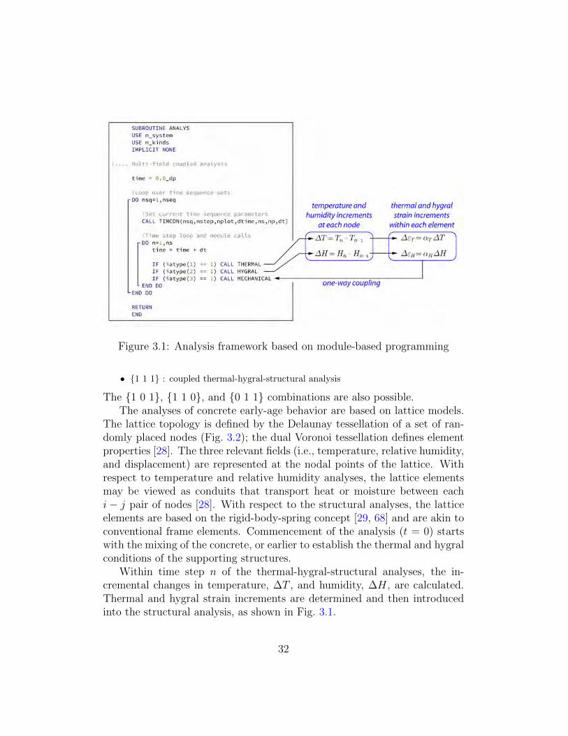
Figure 3.1: Analysis framework based on module-based programming

• {1 1 1} : coupled thermal-hygral-structural analysis

The {1 0 1}, {1 1 0}, and {0 1 1} combinations are also possible. The analyses of concrete early-age behavior are based on lattice models.

The lattice topology is defined by the Delaunay tessellation of a set of ran-domly placed nodes (Fig. 3.2); the dual Voronoi tessellation defines element properties [28]. The three relevant fields (i.e., temperature, relative humidity, and displacement) are represented at the nodal points of the lattice. With respect to temperature and relative humidity analyses, the lattice elements may be viewed as conduits that transport heat or moisture between each i − j pair of nodes [28]. With respect to the structural analyses, the lattice elements are based on the rigid-body-spring concept [29, 68] and are akin to conventional frame elements. Commencement of the analysis (t = 0) starts with the mixing of the concrete, or earlier to establish the thermal and hygral conditions of the supporting structures. Within time step n of the thermal-hygral-structural analyses, the in-

cremental changes in temperature, ΔT , and humidity, ΔH, are calculated. Thermal and hygral strain increments are determined and then introduced into the structural analysis, as shown in Fig. 3.1.

32

Figure 3.2: Lattice model: a) Delaunay/Voronoi dual tessellation of nodal point set; and b) lattice element ij

3.2 Cementitious materials hydration Herein, we use a versatile model of heat of hydration of cementitious ma-terials [104, 115], which is described in Appendix A. The hydration model accounts for the chemical composition and proportioning of the cementi-tious materials. The hydration of multi-species blends can be simulated, in contrast to the previous study that was limited to portland cement hydra-tion [132]. The heat of hydration is used to determine the degree of reaction, which is used to guide the development of properties relevant to early-age cracking, including stiffness, strength, and tendency for creep. As shown in Fig. 3.3, the lattice model simulations of an adiabatic calorime-

try test provide time versus temperature curves in agreement with expecta-tions. A dormant period follows the mixing of the cementitious materials, which can be shortened or lengthened by the addition of accelerating or re-tarding admixtures, respectively. Temperature within the domain increases uniformly (i.e., all nodal points have the same temperature value), asymp-totically approaching an ultimate value.

33

Figure 3.3: Heat of cementitious materials hydration: a) lattice model; and b) adiabatic temperature rise

3.3 Primary analysis modules

3.3.1 Thermal analysis The governing equation for thermal analysis and handling of the associated boundary conditions are described in Appendix B.1. The equation includes a source term, which accounts for the heat produced by cementitious materials hydration.

3.3.2 Hygral analysis The routines used for modeling moisture diffusion and drying from exposed surfaces [18, 28] are are analogous to those for thermal analysis. Rather than including a source term associated with heat of hydration, however, the equations for hygral analysis include a sink term to account for water consumption by the hydration process. The governing equation for hygral analysis and handling of the associated boundary conditions are described in Appendix B.2.

34

Figure 3.4: Elemental unit

3.3.3 Structural analysis A lattice element is defined by two neighboring nodes, i and j, and their common Voronoi facet (Fig. 3.4). The element stiffness relations are based on a zero-size spring set, located at the area centroid (point C) of the Voronoi facet, and connected to the element nodes via rigid-arm constraints. Details regarding the element formulation are given in Appendix B.3. In this project, the uniaxial springs of the rigid-body-spring network have

been replaced with the series construct shown in Fig. 3.5. In this way, the structural elements not only respond to instantaneous mechanical loading, but also to sustained loading. Furthermore, the series construct allows for representation of temperature and hygral effects on the mechanical response. Concrete structures are susceptible to additional deformation over time as

a result of sustained loads, or creep. However, due to the ongoing changes in the concrete micro-structure, creep is reduced for a given load duration when concrete is loaded at a later age. This phenomena, known as the aging affect, can be modeled using the solidification and microprestress theories [16, 46]. Implementation of these theories assumes that the total creep strain rate is the sum of the viscoelastic and viscous strain rates. Further details regarding the theory and formulation are given in Appendix B.3.2

35

Figure 3.5: Series construction of total strain components

36

Chapter 4

Early-age cracking potential of concrete bridge decks: 2D modeling

As part of a recent Caltrans sponsored project [132], the early-age behavior of concrete bridge decks was studied through their instrumentation and data acquisition for a period of time after concrete casting. These decks were integral components of post-tensioned, box girder structures. A typical cross-section of the Markham Ravine Bridge, which is simulated herein, is shown in Fig. 4.1. An aerial view of the Markham Ravine Bridge is given in Fig. 4.2. The bridge was instrumented at several locations, including two locations

within the deck: midspan between the girder lines and over one of the girder lines. Each instrument packet included three thermocouples, three strain gages and two relative humidity sensors (Table 4.1). Data provided by the instrument packets was recorded for 17 days from the time of casting. A weather station, set up on site, also recorded ambient temperature, relative humidity, and local wind speed. The deck of the Markham Ravine Bridge was cast on April 14, 2010 [132].

Water was applied to the formwork about 30 minutes prior to casting. Con-crete placement began at 7 am and advanced past the sensor locations at 10:30 am. Placement over the entire bridge length of two 36 m (120 ft) spans was completed by about 12 pm. Curing compound was applied to the fin-ished deck about 1 h after casting. A combination of burlap and plastic sheeting (Transgard 4000) was used to cover the bridge deck at about 6 h after concrete placement; the sheeting was removed after approximately 8

37

Figure 4.1: Cross-section view of Markham Ravine Bridge deck

Figure 4.2: Aerial view of Markham Ravine Bridge deck (image acquired from Google Maps)

38

sensor type midspan girder depth (mm)∗

thermocouple thermocouple thermocouple

TC1 TC2 TC3

TC4 TC5 TC6

25 101 177

strain gage strain gage strain gage

SG1 SG2 SG3

SG4 SG5 SG6

25 101 177

RH sensor RH sensor

RH1 RH2

RH3 RH4

25 177

∗depth measured from the upper surface of the deck.

Table 4.1: Designations and locations of deck-embedded sensors

days. Periodic inspections were made for deck cracking. Plastic shrinkage cracking was observed prior to placement of the curing sheets. The project included a materials testing component to determine the

strength and shrinkage properties of the deck concrete. Along with the recorded deck temperatures, the strength and shrinkage measurements are used to validate and calibrate the numerical model.

4.1 Model definition Discretization of the bridge deck/girder system is shown in Fig. 4.3. Nodes are placed at the thermocouple locations, as indicated in the figure, so that direct comparisons can be made between the simulated and measured tem-peratures. Concrete forming the soffit and girder stems is assumed to be mature. Simulation of cementitious materials hydration is limited to the freshly cast deck. Inputs to the hydration model, described in Appendix A, are indicated

in Fig. 4.4. Whereas the computational framework is three-dimensional, the simulations presented in this section are for planar characterizations of the structure. The restraint provided by reinforcing steel reduces the free shrink-age of concrete, but the modeling of this effect in a planar analysis framework is not straightforward. Reinforcing bars are not included in the 2D model; within planned future work, bars will be included in the 3D model presented in section 5. Model inputs and boundary conditions for the thermal, hygral, and mechanical analyses are described in the following subsections.

39

Figure 4.3: Lattice representation of symmetric portion of Markham Ravine Bridge deck. The locations of thermocouples TC1, TC2, TC3 (midspan) and TC4, TC5, TC6 (over girder stem) are indicated. Dimensions are in meters.

Figure 4.4: Input parameters for hydration model

40

Parameter Value Source ambient temperature, Ta

ambient relative humidity, ha wind speed, v

thermal conductivity, concrete thermal conductivity, plywood

solar radiation

variable variable variable

2.3 W/(m K) 0.12 W/(m K) variable

measured on-site measured on-site measured on-site

[45] [90] [92]

Table 4.2: Parameter values for thermal-hygral-mechanical analyses of the Markham Ravine Bridge

Figure 4.5: Solar radiation intensities for clear and overcast days

4.1.1 Thermal analysis inputs The initial temperature of the simulated cast concrete was set to its measured value at the time of casting (19.5◦C). The initial temperature of the simulated mature concrete was set to the value measured by thermocouple TC7, located within one of the girder stems, at the time of casting (14.9◦C). Figure 4.5 shows typical measured solar radiation intensities for clear and

overcast days for the geographic proximity and time of the year when casting occurred [92]. Along with an additional profile, representing broken cloud cover, these intensity plots are used as templates for the daily solar radiation input to the model over the 17-day measurement period.

41

The influence of the Transgard 4000 thermal/curing sheets, which were placed on the deck surface, is one point of interest. Placement of this curing medium modifies the various forms of thermal energy exchange with the environment. The modifications are represented by

0 qconv = η1 qconv 0 qsun = η2 qsun for 0.25 ≤ t ≤ 9 days (4.1) 0 qsky = η3 qsky

in which qconv, qsun, and qsky are the heat fluxes associated with convection, solar radiation, and grey body radiation, respectively, for the case when the sheeting is absent; η1, η2, and η3 are reduction factors corresponding to each respective form of energy exchange. The value for η1 is determined as follows. In an experimental study, Lee

et al. [74] found that blankets composed of fabric and plastic sheeting reduce the convective heat transfer coefficient by severalfold. The reduction in the coefficient depends on wind speed and age of the concrete. For the case of no wind velocity, as shown in Fig. 4.6, use of such curing media reduces the convective coefficient by a factor of about 5. Similar reductions were mea-sured for differing wind velocities. Based on these observations, η1 has been set to 0.2, which roughly represents the reduction in thermal convection for concretes beyond 1 day of age. The larger degrees of convective heat trans-fer at early ages are partly due to evaporation of water in the experiments, which was partially prevented by the application of curing compound on the bridge decks. The values of η2 and η3 are determined as follows. The product sheet

for Transgard 4000 indicates a light reflectivity of 0.85, which is equivalent to an absorptivity of 0.15. The reflectance values of ordinary portland ce-ment concrete range from about 0.34 to 0.48 [83], for which the mean value is equivalent to an absorptivity 0.59. A similar range of reflectivity values has been reported by another study, which also notes dependences of reflec-tivity on concrete composition, moisture content and age [77]. Comparing absorptivity values,

0.15 η2 = = 0.25 (4.2)

0.59 A slightly smaller value of η2 = 0.23 was used, since it provided better agree-ments with the measured temperature values. For lack of information on the insulating effects of the blanket with respect to grey body radiation, the same value was assumed for the other reduction coefficient (i.e., η3 = 0.23).

42

Figure 4.6: Influence of curing media on thermal convection coefficient of concrete (data values taken from Lee et al. [74] for v = 0 m/s).

Based on a series model [51], a modified value for ΛT was utilized to account for the presence of 1/200 (12.7 mm) plywood formwork along the lower face of the fresh concrete. The thermal conductivity of plywood was assumed to be 0.12 W/(m · K) [90]. A zero-flux condition was enforced across the plane of symmetry (z = 0). The coefficient of thermal expansion (CTE) of hardened samples, taken

from the deck concrete, was determined to be βT = 8.63×10−6 [132]. This value was used for the model calculations, except for the fresh concrete for which a higher CTE value used. In the fresh state and just beyond setting, the CTE value depends on degree of hydration as described in Section B.1.

4.1.2 Hygral analysis inputs The ultimate value of relative humidity, associated with self-desiccation, was assumed to be hsu = 0.9 with s = 3 governing the rate of self-desiccation according to Eq. B.10. The assumed value of hsu is relatively large, but not unreasonable for the w/b (= 0.42) of the deck concrete. The parameter

˜ values expressing hygral diffusivity, according to Eqs. B.11 and B.13, are: D0 = 0.017 mm2/h; D

1 = 9mm2/h, and n = 5.

43

Figure 4.7: Temperature variation within the Markham Ravine Bridge deck: a) mid-deck at location TC2; b) solar radiation profiles selected for each day; and above girder stem at location TC5.

44

The concrete surfaces bounded by plywood formwork are assumed to be sealed (i.e., no moisture exchange occurs between the concrete and plywood formwork.) This approximation follows from the wetting of the plywood surfaces prior to concrete casting. While the curing sheets are in place (0.25 d ≤ t ≤ 9 d), along with periodic wetting, no moisture is exchanged between the upper surface of the concrete deck and the environment. Otherwise, the exposed surface exchanges moisture with the environment according to Eq. B.14, using Λh = 0.25 mm/h. Soon after finishing of the cast concrete, a light-colored membrane curing compound was sprayed on the deck surface. Based on efficiency values of moisture retention measured elsewhere [52], this membrane is assumed to reduce convective transport across the surface by a factor of 2 (i.e., qh

0 = 0.5 qh). The hygral shrinkage coefficient βh = 0.0030 was calibrated with experimental measurements given in Section 4.2. A zero-flux condition was enforced across the plane of symmetry (z = 0).

4.1.3 Mechanical analysis inputs The parameters for the solidification and microprestress modeling of concrete behavior are presented in Table 4.3. The creep parameter values were set ac-cording to the B4 model [106], based on the actual mixture composition. We did not distinguish between tensile creep, of interest herein, and compressive creep (even though tensile creep may be much larger than compressive creep for the same levels of applied stress [54].)

Table 4.3: Parameter values associated with creep and stiffness development

Parameter value∗

q1 q2 q4 nα κ0 κ1

29.0×10−6/MPa 69.9×10−6/MPa 5.50×10−6/MPa

2.2 0.01/(MPa · d) 5 MPa/K

∗ q1, q2, and q4 values are based on the B4 model [106] for E28 = 24.1 GPa; w/c = 0.42; a/c = 6.13; and 25% replacement of normal cement with fly ash.

All stresses originate from thermal and hygral strains. Externally applied

45

loads (e.g. due to construction activities) were not considered at this stage of the analysis. A zero-displacement condition was enforced across the plane of symmetry (z = 0), along with a single support along that plane to prevent rigid-body motion in the vertical direction.

4.2 Simulation results The temperature history of the bridge deck was simulated, along with the strength and shrinkage of laboratory specimens cast on-site. These exercises, based mainly on quantities measured on-site or taken from the literature, help to validate the model prior to its use for parametric study in the next section.

4.2.1 Deck temperature simulations The simulated temperature histories are compared with the field measure-ments in Fig. 4.7, for the case of thermocouples TC2 and TC5 located within the mid-deck region and above the girder stem, respectively. The recorded ambient temperature history is also plotted in the figures. Comparisons with the entire set of deck thermocouple readings are presented in Fig. 4.8. Fig-ure 4.9 shows simulated temperatures for TC7, located in the girder stem, in comparison with the measured values. Several comments can be made.

• The influence of environmental factors is evident from the oscillatory behavior of the temperature history recorded by each thermocouple. After the first day, locations closer to the surface exhibit larger tem-perature swings, whereas deeper locations are less affected by environ-mental changes. This meets expectations.

• Peak temperatures occur at about 10 h after concrete casting. Fig-ure 4.10 shows the distribution of temperature at that time. The lower temperatures over the supporting girders are due to conduction of heat toward the cooler substrate concrete. Conversely, the insulative proper-ties of the plywood formwork give rise to higher temperatures between the supporting girders. These temperatures are significantly higher than the ambient temperature. With time, particularly over the first 3 days, the differences between the ambient and measured deck temper-atures diminish.

46

Figure 4.8: Measured and simulated temperatures at deck thermocouple lo-cations

47

Figure 4.9: Measured and simulated temperatures at TC7 thermocouple lo-cation

Figure 4.10: Simulated iso-contours of temperature (in ◦C) at t = 10 h

48

Figure 4.11: Influence of curing blanket placement on simulated deck tem-peratures.

• Diurnal variations in deck temperature increase upon removal of the curing blanket. This point is reinforced by comparing deck tempera-tures with and without the blanket in place, as shown in Fig. 4.11 for TC5. In particular, the influence of solar heating is accentuated after removal of the blanket. The effects at other thermocouple locations are similar. Furthermore, the temperature gradient through the deck thick-ness tends to increase upon removal of the curing blanket (Fig. 4.8). The implications of the larger thermal gradients are discussed later.

• Temperatures inside the box girder cells were not measured and there-fore had to be simulated to apply temperature boundary conditions along the cell walls. It was assumed that temperatures within each cell were a weighted combination of the cell wall temperatures. In that sense, the ambient (outside) conditions influence the cell temperature via heat conduction through the walls. The two simulation cases in Fig. 4.9 differ only in relative weighting of each wall temperature, with case 1 placing a larger weight on the upper cell wall. There are sev-eral possible reasons for not capturing the first temperature peak at t ≈ 10 h. For one, the start of the simulation (t = 0) should begin at a sufficiently long time before casting so that initial, nonuniform tem-perature conditions at the time of casting can be better represented.

49

4.2.2 Determination of degree of hydration at final set The degree of hydration at concrete setting, α0, is required for the strength development model expressed by Eq. B.22. Within the test program associ-ated with the Markham Ravine Bridge deck concrete, penetration resistance was measured according to ASTM C403 [10] to determine initial and final setting times, tis and tfs, respectively. As per standard, mortar was extracted from the deck concrete and subjected to penetration testing. The results are shown in Fig. 4.12, in which σp is the measured penetration resistance and σfs is the penetration resistance associated with final set. The prescribed resistance levels associated with initial and final set are 3.5 MPa (500 psi) and 27.6 MPa (4000 psi), respectively. The initial and final set times (tis = 4.9 h and tfs = 6.33 h) are determined by the intersections of these respective stress levels with the resistance curve. To determine the degrees of hydration at initial and final set, a volume of

mortar was simulated using the measured initial temperature of the mortar (18.89 ◦C) and ambient temperature (21.1 ◦C). For the thermal calculations, the coarse aggregates were removed within the hydration routine and in the calculation of specific heat capacity. The simulated degrees of hydration are plotted in Fig. 4.12. The degrees of hydration associated with tis and tfs are α0i = 0.085 and α0 = 0.13, respectively. Some studies suggest the development of the mechanical threshold of hardening concrete begins rather close to the time of initial setting [58]. Other sources use the point of final set to define the mechanical threshold [85, 109]. The α0 value is used for strength development in the bridge deck simulations that follow.

4.2.3 Strength simulations Concrete cylinder specimens were cast on site and kept local to the bridge deck for 7 days, prior to laboratory storage and measurement of splitting tensile strength. Strength development was simulated using Eq. B.22, with α0 = 0.13, and the same lattice model adopted for the creep test simulations (Fig. C.1). Ambient temperature for the modeling exercise was constant and set equal to the average recorded temperature over the curing period. Figure 4.13a compares simulated strength development with the measured values, where the 28-day splitting tensile strength is used as a normalizing factor.

50

Figure 4.12: Determination of degrees of hydration at initial and final sets using recorded penetration resistance data [132]

4.2.4 Shrinkage simulations For measuring the drying shrinkage properties of the concrete mixture, prisms were cast on-site and transferred to the laboratory within 24 h, after which they were kept in a moist condition until exposure to a drying environment at t = 7 days. Testing was done according to ASTM C157, except for the 7 days of moist pre-conditioning according to Caltrans recommendations. The measured and simulated shrinkage strains are compared in Fig. 4.13b. Initial swelling of the prisms was simulated by prescribing h = 0.97 as an initial condition prior to moist curing at 1 day. As seen in the examples of autogenous and drying shrinkage (Appendix C.3), the shape of the simulated shrinkage curve does not conform to that of the experimental curve: the simulated rate of shrinkage over the first several days is lower. This could be remedied by increasing hygral diffusivity and/or the shrinkage coefficient, but the ultimate shrinkage strain would then be overestimated. It appears that the effects of microcracking need to be incorporated into the analyses.

51

Figure 4.13: Property development in on-site cast and simulated specimens: a) splitting tensile strength; and b) shrinkage strain.

52

Figure 4.14: Simulated stresses at mid-deck location when the curing media is absent: a) thermal stress component; b) hygral stress component (*recorded daily rainfall, in mm, at the Carmichael 0.9 S meteorological station); and c) total stress.

53

4.3 Parametric study Through the preceding examples, basic workings of the thermal, hygral, and mechanical components of the model have been validated. The model is now used to assess the early-age cracking potential of the Markham Ravine Bridge. In particular, the relative importances of thermal and hygral contri-butions to cracking potential are evaluated for several design factors: 1) the use of curing media; 2) degree of restraint against deck movement; and 3) ce-mentitious materials composition. Cracking of the concrete is not simulated, except for the analysis results presented near the end of Section 4.3.2. The scope of this exercise is limited to planar analyses of the bridge deck using the lattice model shown in Fig. 4.3. The implications of this simplification of the bridge deck configuration and boundary conditions are discussed later. For all analyses in this section, t = 0 corresponds to the time of concrete casting at the sensor group locations (10:30 am on April 14, 2010.)

4.3.1 Curing protocol Curing media absent

As noted above, curing compound and polymer/fabric sheets were applied on the concrete deck as part of the curing protocol. Concrete stresses at the mid-deck location, normalized by the 28-day tensile strength, are plotted in Fig. 4.14 for the case when these curing media are absent. To compare the thermal and hygral stress contributions with their sum, the z-component (Fig. 4.3) of the stress tensor has been evaluated at the TC1 and TC3 thermo-couple locations. These σZ values are roughly equal to the principle tensile stress values at the same locations. The hygral and thermal contributions to total stress are isolated by setting βT = 0 and Λh = 0, respectively. For com-parison, the evolution of tensile strength at the TC1 location is also plotted in the figure. As expected, exposure to the drying environment produces tension near

the deck surface, due to the hygral gradient in the y-direction (Fig. 4.14a). Location TC3 is in compression, as is much of the depth of the deck, to equilibriate the surface tension. The oscillatory nature of these stress curves is due to diurnal variations in ambient relative humidity: relative humid-ity climbs at night due to decreasing temperature such that moisture intake and swelling occurs near the upper surface of the deck. The large drops in

54

stress magnitudes beginning at about t = 6 and 13 days are due to rain-fall events. The rainfall amounts indicated in the figure were recorded at the Carmichael 0.9 S meteorological station, located about 30 km south of the bridge construction site. Rainfall was not modeled directly, but rather captured through the recorded relative humidity boundary condition. Sus-tained, large relative humidity values were measured on-site during most of those rain dates. Based on simulated field testing of concrete, Asamoto et al. [5] have found that shrinkage of concrete is significantly reduced by rain-fall and that continuous rainy days have such influence even if the amount of precipitation is small. Fig. 4.14b plots the stresses associated with thermal effects. During day-

time heating, the upper surface of the deck expands relative to the lower surface, producing compression at the TC1 location and tension at the TC3 location. This tendency is reversed during nighttime cooling. For either case, the tensile stresses are significantly smaller than those produced by hygral loading. For both the hygral and thermal loading cases, stress variations over the girder stem (at TC4 and TC6) are qualitatively similar, but slightly smaller in magnitude. Tensile strength of the concrete at the TC1 location, as determined from

the degree of cementitious material reaction (Eq. B.22), is indicated in each plot within Fig. 4.14. The rate of early strength gain is high, relative to the curve used for calibration (Fig. 4.13), due to the higher deck temperatures associated with heat of hydration. The evolution of tensile strength, scaled by a reduction factor of 0.7 (as discussed in Section B.3.1), is also indicated in Fig. 4.14c. The tensile stresses in Days 2, 3, and 4 cross over this curve, which suggests the occurrence of cracking.

Curing media utilized

While in place during the 0.25 ≤ t ≤ 9 days interval, the curing sheets act to significantly reduce both the hygral and thermal stresses, as shown in Fig. 4.15. Upon removal of the blanket, however, sudden drying of the deck surface from the nearly saturated state causes high tensile stresses. For this case, as well, the tensile stress values cross over the scaled tensile strength curve indicating the likelihood of cracking. Knowing the stress state and tensile strength at each nodal location, we

can plot maps of cracking potential (i.e., σ1/f , where σ1 is principle tensile stress and f is the current tensile strength value at that location) over the

55

Figure 4.15: Simulated stresses at mid-deck location when the curing media is present during 0.25 ≤ t ≤ 9 days: a) thermal stress component; b) hygral stress component; and c) total stress

Figure 4.16: Spatial maps of cracking potential at t = 11.42 days (8 pm on day 11) for the case where the curing sheets were removed at t = 9 days: a) thermal stress component; b) total stress.

56

computational domain. Figure 4.16 provides such plots for the thermal stress contributor and total stress at t = 11.42 days (9 pm on April 14), which is near the time of maximum σ1/f for the TC1 location. To highlight thermal stresses, different scales are used for each plot. The highly stressed region extends about 40 mm (or 1/5 of the deck thickness) from the drying surface. Similarly steep stress gradients have been found near the surface of concrete pavements [56] and bridge decks [123]. Cracking would tend to relieve stress along the drying surface and, due to the sharp gradient in stress, it appears that cracks would not propagate through the deck thickness. This hypothesis is evaluated using concrete fracture mechanics, as presented in Section 4.3.2. The strong potential for cracking indicated by Figs. 4.14 through 4.16

is accentuated by at least three factors: 1) the high 28-day shrinkage mea-sured in the laboratory and used for the analyses (Fig. 4.13b); 2) the low tensile strength of the test prisms used for this comparison; and 3) lack of consideration of membrane-type curing compound applied on the Markham Ravine Bridge deck. These simulations have been rerun after: 1) scaling the drying shrinkage curve in Fig. 4.13 to meet the 28-day limit of 450 µm/m prescribed by several transportation agencies [55]; and 2) calculating the 28-day tensile strength according to ft = 0.3(fc)2/3 , where fc is the measured 28-day compressive strength [85]. Based on these assumptions, the likeli-hood for cracking is greatly reduced, as shown in Fig. 4.17a and b for each respective simulation case. The strength development curves in Fig. 4.17a as-sume cement hydration is not hindered by continuous exposure to the drying environment. Furthermore, if a curing compound has been applied, the cracking po-

tential is further reduced. For the simulation results presented in Fig. 4.17c, application of the curing compound is assumed to reduce the hygral con-vective coefficient by 50%, as described in Section 4.1.2. The analyses that follow are based on the parameter combination corresponding to Fig. 4.17b (in which the prism 28-day shrinkage strain is 450 µm/m and the tensile strength is based on the measured compressive strength). Creep serves to reduce the stress peaks due to both hygral and ther-

mal loading. If creep deformation is neglected, the stress peaks shown in Figs. 4.14c are larger by about 80%. As stresses rise above the linear range, microcracking also serves to reduce the stress magnitudes. The question of whether cracks occur, and their severity, ultimately needs to be addressed through the application of fracture mechanics to the concrete under sustained loading, as done in section 4.3.2.

57

Figure 4.17: Simulated stresses at mid-deck location based on 28-day strain limit of 450µm/m: a) the curing sheet is absent; b) curing sheet is present; and c) curing sheet and curing compound used

58

Figure 4.18: Discretization of box girder cross-section including cell volumes

4.3.2 Structural configuration The structural configuration used for the previous analyses is representative of in-plane conditions away from supports or diaphragms placed along the span length. As a rough approximation of the conditions local to such stiff-ening elements, the cell volumes have been filled with concrete (Fig. 4.18). The concrete within the cells is given the same properties as those of the soffit and girder stems. Otherwise, the following analyses retain the same set of parameter values used to produce the results in Fig. 4.17b.

Stress components

Stress values due to the thermal component are plotted in Fig. 4.19a. The amplitudes of the diurnal variations are larger than for the unrestrained cases presented in Figs. 4.14a and 4.15a. Furthermore, the entire deck cross-section experiences tension, in contrast to the previous results where temperature gradients through the thickness produced mainly tension-compression cou-ples. The increase in deck tension over the first several days corresponds to the overall cooling of the deck, as shown in Fig. 4.8. The deck stresses due to hygral effects are plotted in Figs. 4.19b and c.

The stresses due to autogenous shrinkage are significant, in contrast to the unrestrained cases where such stresses were negligible and therefore not plot-ted in the previous examples. In Fig. 4.17b, for example, there is no upward

59

drift into tension over the first 9 days when the curing sheets are in place. For the case of moisture loss to the environment (Fig. 4.19c), the stress am-plitudes are slightly higher than for the case without restraint. Otherwise, the results for the two cases are qualitatively similar. Total stresses at the mid-span location, which include the thermal, au-

togenous, and drying shrinkage components, are plotted in Fig. 4.19d. The total stresses are not a simple summation of the component values, since the autogenous and drying shrinkages are coupled through the dependence of hy-gral diffusivity on internal relative humidity (Eq. B.11). Comparing with the case where restraint is absent (for the case associated with Fig. 4.17c), the stress amplitudes plotted in Fig. 4.19d are greater and the entire cross-section experiences tension.

Fracture analyses

By allowing fracture to occur, according to the procedure outlined in Sec-tion B.3.1, consequences of the restraint conditions become evident (Fig. 4.20). When restraint is absent, the sharp humidity gradient (with secondary con-tributions from the thermal gradient) produces cracking near the drying sur-face. This has been observed in other studies, as well [41]. When the re-straint is present, both autogenous shrinkage and global temperature change of the deck introduce tension over the deck cross-section. Crack density is higher and some cracks propagate through the deck cross-section, as shown in Fig. 4.20b. Similar cracking behavior has been noted in field studies where concrete

abutments provided fixity to the deck ends [39, 123]. The crack map shown earlier in Fig. 2.10 exemplifies the differences in cracking behavior caused by restraint conditions. When the deck is lowly restrained (away from the abutments), there is practically no longitudinal cracking; when it is highly restrained, longitudinal cracking is densely distributed. Whereas the 2D sim-ulations only consider the possibility of longitudinal cracking, the simulation results exhibit well the tendency for longitudinal cracking when the deck is laterally restrained. The surface cracking due to hygral and thermal gradients is more ex-

tensive than shown in Fig. 4.20, which only depicts cracks larger than a prescribed threshold. Furthermore, the openings of such surface cracks are much smaller than those of the through cracks that form when restraint is present. This is seen in the histogram of cracked-element openings given in

60

Figure 4.19: Simulated stresses at mid-deck location in the presence of con-straint: a) thermal stress component; b) hygral stress component (due to self-desiccation); c) hygral stress component (due to external drying); d) total stress assuming hsu = 0.9

61

Fig. 4.20c. The large number of openings less than 0.1µm can be understood as diffuse microcracking, mostly invisible to the unaided eye. As the drying front progresses with time, many of the surface cracks have closed and are therefore not counted in the histogram. The time of day also influences the opening counts. For the 12:00 pm

counting shown in Fig. 4.20c, solar heating of the top surface has reduced or closed some of the surface cracks. The scatter in openings for the through cracks, about an average opening of about 0.7 mm, is mainly due to flexure of the deck under thermal/hygral loading. Crack opening is proportional to depth within the deck cross-section. Whereas these results indicate deck cracking would occur, the assumed

restraint condition associated with the internal diaphragm is an extreme case. Three-dimensional analysis of the deck is necessary to more accurately assess the effects of structural configuration on deck stresses. Furthermore, the effects of restraint and thermal straining in the longitudinal direction of the bridge are not captured by these planar analyses, even though such effects might contribute significantly to cracking potential. Finally, three-dimensional analysis more readily accommodates the modeling of reinforcing steel, which serves to reduce crack opening.

4.3.3 Concrete materials composition One of the benefits of using fly ash, as a partial replacement of portland cement, is reduced rate of heat production during cementitious materials hydration. By using portland cement as the sole binder, the temperature histories look qualitatively similar to those for the 0.75 : 0.25 blend (shown in Fig. 4.8), but the early-age peak temperatures increase by about 15%. Since temperature is just one of several contributors to stress, there is a corresponding increase in early-age tensile stress of about 5%, as shown in Fig. 4.21. Some of this increase would be offset by the higher tensile strength of the material, due to the higher concrete temperatures in the first few days.

4.3.4 Discussion Several observations can be made from the preceding 2D simulations of the Markham Ravine Bridge deck.

• Moisture gradient due to drying of exposed surfaces is a primary con-

62

Figure 4.20: Simulated deck cracking: a) without restraint; b) with restraint associated with an internal diaphragm; and c) crack opening histogram for the latter case

Figure 4.21: Effect of fly ash use on simulated stresses at the mid-deck loca-tion

63

tributor to cracking potential.

• Whereas the restraint condition considered (by the filling of the box girder cells with concrete) is extreme, it helps illustrate the relevance of restraint conditions toward cracking potential. The in-plane stiff-ness of the open-cell deck system is relatively small, such that stresses produced by thermal and autogenous shrinkage effects are secondary in magnitude to those produced by drying of the concrete surface. Re-straint increases all of the stress components, but it has the largest influence on the thermal and autogenous stress components. The mag-nitudes of tensile stress are not only higher for the thermal and auto-genous stress components, but also the whole deck section goes into tension.

• The examples presented in this section are severe in that large 28-day shrinkage values were assumed for the base cases. Furthermore, the effects of curing compounds (not applied to the shrinkage test prisms used for calibration) were not included. As seen in the figure, reduction of the hygral convective coefficient (e.g., through application of curing compound) reduces likelihood of cracking. Also, the hygral shock illus-trated in Fig. 4.15b is likely to be tempered by some degree of drying prior to blanket removal.

• Plastic shrinkage has not been covered by these analyses. Field obser-vations identified significant plastic shrinkage cracking in the Markham Ravine Bridge and other bridges within the project scope. Such early-age cracking, even if partially healed, would compromise strength, in-creasing the probability of drying induced cracking at later ages. In effect the strength curves in Fig. 4.19, for example, would be lowered.

• Tensile creep is larger than creep in compression [54]. The importance of distinguishing between tensile and compressive creep needs to be addressed through further study.

• In the example, temperature evolution in the concrete was significantly affected by the insulative properties of thermal/curing blankets placed on the deck surface. Such properties are typically poorly understood and quantified. It can be argued that such forms of uncertainty pervade these types of analysis.

64

Chapter 5

Cracking potential at early ages: 3D modeling

The two-dimensional analyses presented in section 4 were effective for study-ing features of the modeling approach with respect to early-age behavior of concrete bridge decks. The bridge deck section was assumed to be either: 1) sufficiently far from an abutment or diaphragm region, where the degree of restraint against in-plane movements is minor; or 2) highly restrained by mature concrete placed in the cells of the box girder. For the purposes of cracking assessment under general restraint conditions, however, three-dimensional models are necessary. In particular, three-dimensional models accommodate longitudinal straining/stressing of the deck, which enables sim-ulation of transverse cracking. Furthermore, the supporting girders influence deck behavior in a three-dimensional sense. Three-dimensional analyses of the Markham Ravine Bridge are presented

in this section. The modeling approach is conceptually the same as that of the planar deck models employed earlier in this report.

5.1 Model definition

5.1.1 Domain discretization Symmetry conditions are exploited to reduce the model size and thus the computational expense. The deck/girder cross-section is modeled as shown in Fig. 5.1. Domain discretization is automatic and based on the parameter

65

Figure 5.1: Parametric representation of deck/girder section (symmetric por-tion)

values indicated in the figure, along with the longitudinal dimension of the deck system and a spatial description of nodal point density. In accordance with symmetry conditions, roller supports are introduced along the x = 0 and x = bf /2 faces of the model. This corresponds to the case of full restraint in the lateral direction. To account for lateral flexibility of the deck/girder system, the stiffnesses of the zones adjacent to the x = bf /2 boundary can be adjusted. The cross-section representation of Fig. 5.1 is used to discretize the span

length, as shown in Fig. 5.2. The origin of the coordinate system is located where the longitudinal and transverse planes of symmetry meet (i.e., coordi-nates x and z are measured from the center of the pier). To reduce compu-tational expense, half of the span length has been coarsely discretized using block-like cells. Furthermore, a non-uniform distribution of nodal points is used for the remaining half-span length. Denser distributions of nodal points are used for discretizing: 1) the region adjacent to the center pier, where the frequency of deck cracking is typically higher; and 2) in the vicinity of the embedded sensor units. Figure 5.3 provides a longitudinal, perspective view of the span-length discretization from the pier location.

66

Figure 5.2: Discretization of full span length (left) and magnified view of end region (right)

Figure 5.3: Perspective view of discretized span length

67

5.1.2 Model inputs and boundary conditions Material description

The same materials properties used for the 2D model, summarized in Sec-tion 4.1, are assumed for the 3D model analyses.

Structural boundary conditions

As shown previously in Fig. 5.2, the half-span length adjacent to the pier is finely discretized, whereas the portion framing into the abutment is rep-resented by block-like elements. Deflections of the model due to self-weight of the concrete are compared with theoretical elastic curves for two sets of boundary conditions: 1) simply supported span; and 2) full rotational re-straint at the pier location with roller support at the abutment. The latter case approximates the field conditions and is used for the design examples presented in Section 5.3. For each case, the simulated deflections compare well with theory in Fig. 5.4. For the simply-supported case, the simulated displacements are practically symmetric about center span. This implies the coarse block-like discretization of half of the span length does not sig-nificantly degrade the accuracy of the displacement results. The displaced configurations of the model (for each respective set of boundary conditions) are shown in Fig. 5.5.

Strain gage simulation

The sensor clusters used in the field study of the Markham Ravine Bridge [132] included thermocouples, RH sensors, and strain gages. To enable compar-isons between simulated and measured strains, nodal pairs were inserted at the locations of the strain gages identified in Table 4.1. The nodal pairs possess identical x and y coordinates, but are spaced 20 mm apart in the z-direction (i.e., the gage length is 20 mm.) The theoretical strain in the longitudinal direction can be determined from

εz = −κy (5.1)

where κ is curvature due to bending and y is the distance from the neutral axis to the point of interest. Curvature can be determined from

M(z) κ = (5.2)

EI

68

Figure 5.4: Lateral deflections due to girder self-weight

69

Figure 5.5: Elastic deformations due to girder self-weight: a) simply sup-ported; and b) rotationally fixed at the pier location and roller supported at the abutment

70

According to these relations, and assuming E = 30 GPa, self-weight load-ing of the girder produces a strain at the location of gage SG2 of εz = 4.96×10−5 . This is simply a hypothetical case to validate the strain calcu-lations of the model. Comparing the theoretical and simulated values for longitudinal strain, the percentage difference is

εtheory − εsimulated z z 4.96 − 4.88

Δ = × 100% = × 100% = 1.57% (5.3) εtheory z 4.96

The simulated and theoretical strain values differ by only a small amount.

Environmental boundary conditions

The same on-site recordings of ambient temperature, wind speed, and rela-tively humidity (used for the 2D bridge analyses) serve to define the thermal and hygral convective boundary conditions for the 3D model. Likewise, the same solar radiation and cloud cover patterns are assumed for the 3D model. To obtain a more realistic temperature distribution in the substrate con-

crete, at the time of casting, the simulations begin at 24 h prior to the time of casting. As shown in Fig. 5.6, the April 2010 temperature record obtained from the Lincoln, CA, station agrees well with that recorded on the Markham Ravine Bridge site. In the absence of such pre-conditioning of the concrete girders, artificial straining occurs at the time of casting, since the assumed initial temperature distribution of the concrete girders is not in dynamic equilibrium with the environmental conditions.

5.2 Comparisons with field measurements

5.2.1 Deck temperatures The three-dimensional model of the Markham Ravine Bridge, shown in Fig. 5.2, should exhibit the same temperature results as the two-dimensional model considered in Section 4. Using the same thermal properties and input values as for the preceding analyses, Fig. 5.7 compared the simulation results and measured values. Apart from some differences in temperature over the first two days, the results of the 2D and 3D simulations are nearly indistinguish-able.

71

Figure 5.6: Supplemental temperature data used to pre-condition the con-crete girders 24 h prior to concrete casting (Lincoln Station data for April 2010)

5.2.2 Deck strains Each of the sensor clusters within the Markham Ravine Bridge deck included a set of strain gages. The gages were aligned with the longitudinal axis of the bridge and positioned at depths of 1, 4, and 700 from the deck surface. Simulated longitudinal strains are compared with the strain gage mea-

surements in Fig. 5.8 up to the time of deck prestressing. The zero-strain reading of field-measured values has been taken from WJE (2011) [132]. Also, those measured values have been shifted on the time axis, so that peak strains correspond to peaks of the diurnal temperature cycles. Considering the mul-titude of factors and uncertainties that influence the strain values, the two sets of data agree well over most of the time range. The simulated strains correspond to the temperature history more closely. For example, the cooling of the deck concrete between t = 5 and 9 days (as shown in Fig. 5.7) results in a decrease in simulated tensile strain, whereas the measured values do not show that tendency. Both sets of data indicate larger diurnal variations in strain after removal of the curing blankets at about t = 9 days. This first set of simulations has not considered the effect of shoring, which was in place over this time interval. The effects of shoring may account for some of the discrepancies between the measured and simulated behaviors.

72

Figure 5.7: Simulated and measured deck temperatures

73

Figure 5.8: Simulated and measured deck strains up to the time of prestress application.

5.3 Design examples The preceding examples have served to validate the 3D model for parametric analyses. In this section, the validated models are used to study the influence of design parameters on the newly cast concrete deck within the Markham Ravine Bridge. For the given bridge configuration and environmental con-ditions, materials design and placement operations are assessed to limit the probability of cracking to acceptable limits. The as-built Markham Ravine Bridge serves as the base case for the

design parameter evaluations. The main input parameters and their values are summarized in Table 5.1. The effects of design parameter changes on cracking potential are given in

probabilistic terms. For this purpose, the probability density of cracking as a function of stress ratio η is used, based on the experimental program of Riding et al. [105]. The experimental program considered bridge deck concretes and measured stress level at cracking relative to split-cylinder tensile strength. Figure 5.9a presents the experimental data. The discrete data values are fit with a lognormal probability density function, similar to that employed by Riding et al. [105]. The corresponding cumulative distribution function, from

74

Table 5.1: Parameter values for Markham Ravine Bridge analyses

Parameter symbol value source cementitious materials contenta fly ash content water-to-cementitious materials ratio

c FA w/c

400.6 kg/m3

0.25c 0.42

b b b

ambient temperature wind speed relative humidity

T v h

recorded recorded recorded

c c c

elastic modulus at 28 days compressive strength at 28 days coefficient of thermal expansion hygral shrinkage coefficient

E28 fc 28 βT βh

24.1 GPa 35.7 MPa

8.63×10−6/◦C 0.00198

d d d e

a chemical composition of the OPC and other input parameters are indicated in Table 4.4. b from plan quantities for the Markham Ravine Bridge. c from field measurements and station data local to the Markham Ravine Bridge [91, 132]. d from laboratory testing of the deck concrete of the Markham Ravine Bridge. e corresponds to a 28-day shrinkage of 450µ of the companion prism specimens.

which cracking probabilities can be estimated, is given in Fig. 5.9b. For this dataset, and fitting of the probability density function, the lognormal mean and standard deviation are µ = -0.53 and σ = 0.16, respectively. A stress-to-splitting tensile strength ratio of 0.6 corresponds to a 50% probability of cracking.

5.3.1 Drying shrinkage In lieu of representing the myriad individual contributions to drying shrink-age, the shrinkage capacity of a concrete can be represented by its hygral shrinkage coefficient βh, which forms an incremental relationship between rel-ative humidity and hygral straining (Eq. B.15). The βh value was chosen to provide a range of 28-day shrinkages of the prism specimens: the 630µm/m value measured in the laboratory component of the field study [132] , a 450µm/m limit, and a 320µm/m limit (which is the current Caltrans spec-ification). The influence of shrinkage capacity on longitudinal stress at the sensor locations is plotted in Fig. 5.10, along with tensile strength devel-

75

Figure 5.9: a) Probability density of crack occurrence as a function of stress-to-split cylinder strength ratio. The discrete data values are taken from Riding et al. [105]; and b) cumulative distribution of crack occurrence as a function of stress-to-split cylinder strength ratio.

76

Figure 5.10: Influence of 28-day shrinkage strain values on deck stresses.

77

Figure 5.11: Influence of 28-day shrinkage values on the probability of deck cracking.

opment over time. The longitudinal restraint provided by the soffit/girder system is sufficient to generate high tensile stress in the deck during its con-traction, even at mid-span between the girder lines. While the curing sheets are in place (0.25 d ≤ t ≤ 8 d) it is assumed

that no moisture exchange occurs between the upper surface of the deck and the environment. In addition, the humidity drop due to self-desiccation is assumed to be negligible in this example. During that interval, the βh value has practically no effect on the deck stress values. The stress values depend mainly on thermal influences. Upon removal of the curing media, however, the efficacy of the shrink-

age reduction measures becomes evident. Stress peaks develop during each episode of nighttime cooling. The tensile stress peaks increase in magni-tude for the first few days after exposure to the drying environment, but then flatten due to maturation of the hyrgral gradient and reduced ambi-ent temperatures. A longer-term estimation of deck stresses is presented in Section 5.3.6. The probabilities of cracking for each 28-day shrinkage value, estimated

using the cumulative distribution function presented in Fig. 5.9b, are pre-

78

sented in Fig. 5.11. Based on the simulated longitudinal stress values, results are given for locations: a) near the deck surface (SG1 location); and b) at mid-depth of the deck (SG2 location). The results for the mid-deck location pertain to the severity of cracking (i.e., whether cracking is superficial due to high stress gradient near the surface or through the deck thickness.) Reducing the allowable 28-day shrinkage from 450µm/m to 320µm/m

reduces the probability of cracking near the deck surface by 20 to 30%. The case of βh = 0 removes the hygral effects. It is seen that thermal stresses acting alone provide an insignificant probability of cracking. In this 3D configuration, the whole deck is put into tension. As seen in the fracture analyses presented in Section 4.3.2, this fosters cracking through the deck thickness.

5.3.2 Autogenous shrinkage Concretes with a water-to-cementitious materials ratio of about 0.40 or lower typically exhibit autogenous shrinkage. The relative humidity drop becomes more significant as the water-to-cementitious materials ratio is decreased. The governing equation for the humidity field (Eq. B.9) includes a sink

term associated with self-desiccation due to the hydration reactions. The parameter hsu, in Eq. B.10, controls the ultimate drop in relative humidity. Based on this modeling assumption, Fig. 5.12 presents the influence of au-togenous shrinkage on the deck stresses. Ultimate humidity drops of 0, 0.1, and 0.2 are considered, which span the common range of values. While the curing media is in place, autogenous shrinkage has a propor-

tional influence on the deck stresses, both near the surface and at mid-depth of the deck. Upon removal of the curing media, the effect diminishes over time as the deck is subject to external drying. The occurrence of autogenous shrinkage increases the probability of cracking during the simulation period, as shown in Fig. 5.13. The effect near the surface in minor, since the proba-bility of cracking in the base case (no autogenous shrinkage) is already high. At mid-depth of the deck, however, autogenous shrinkage effects are signifi-cant, greatly increasing the probability of cracking that extends through the depth of the deck.

79

Figure 5.12: Deck stresses for different degrees of autogenous shrinkage.

80

Figure 5.13: Influence of self-desiccation on the probability of deck cracking.

5.3.3 Coefficient of thermal expansion The common range of concrete CTE values (based on aggregate type, as presented in Table 2.3) is simulated. As observed in laboratory studies [66, 84, 117], the CTE values are magnified up to just beyond the time of final set, as described in Section B.1. The influences of CTE on the deck stresses, near the exposed surface

and at mid-depth of the deck, are presented in Fig. 5.14. Increasing CTE increases the amplitudes of the stress peaks, which are caused mainly by diurnal exchanges of heat and moisture with the environment. The greatest effect on stresses is near the deck surface, since that region experiences larger temperature variations. However, tensile stresses due to heat of hydration (i.e., the gradual cooling after peak temperature at about 10 h) are significant over the deck cross-section. Based on the information in Fig. 5.14, maximum stress-to-splitting tensile

strength ratios can be calculated, from which the probability of cracking can be estimated. From Fig. 5.15, it is understood that CTE of the concrete strongly affects cracking potential. The severity of cracking can be estimated from the cracking probability at mid-depth of the deck. The higher the probability of cracking at mid-depth, the more likely cracking will extend through the deck thickness. For βT = 6×10−6/◦C, η < 0.3 for the extent of

81

Figure 5.14: Influence of coefficient of thermal expansion (CTE) of concrete on deck stresses: a) at SG1 location; and b) at SG2 location.

82

Figure 5.15: Influence of coefficient of thermal expansion (CTE) of concrete on cracking probability.

the simulation, which suggests a low possibility of cracking through the deck thickness.

5.3.4 Cementitious materials usage Heat of hydration of the deck concrete can be reduced by decreasing the amount of portland cement in the mixture. This can be done through the partial replacement of portland cement with a less reactive supplementary cementitious material (e.g., fly ash) or by decreasing the overall cementitious materials content. Figure 5.16 compares longitudinal stress at the SG2 loca-tion for ratios of portland cement to fly ash of 75:25 (which is the base case) and 100:0. As expected, the 75:25 blend ratio produces less heat and there-fore the tensile stress due to initial cooling is lower. Also, tensile strength develops more slowly. These results are qualitatively similar to those pro-duced with the 2D model (Fig. 4.21). Differences in the stress values between the two cases are evident up

until the time of removing the curing sheets and exposing the deck to the environment. Thereafter, little difference is seen between the stress values for the two cases. In general, the influences of heat of hydration are less than

83

Figure 5.16: Influence of partial replacement of portland cement with fly ash on deck stresses (at SG2 location): a) 0 ≤ t ≤ 16 d; and b) 0 ≤ t ≤ 2 d.

84

those of typical mass concrete applications. This is due, in part, to the large surface to volume ratio of the deck. Looking at the stress development over the first 48 h from the time of

casting, both cases initially exhibit compression due to temperature increases caused by heat of hydration (Fig. 5.16). Peak temperature is achieved at about 10 h, after which gradual cooling introduces tensile stress.

5.3.5 Bridge configuration: deck continuity The box-girder of the Markham Ravine Bridge is continuous over the central pier. Such full continuity is assumed for the base case, with simple sup-port conditions at the abutment(s). The analyses assume the supporting girder/soffit system carries its self-weight plus the weight of the freshly cast deck. In the absence of shoring, effects of prestressing, or construction load-ing, the bridge deflections (after casting of the deck concrete) are due solely to thermal and hygral effects. These deflections are shown in Fig. 5.17 for t = 14.7 and 15.2 d, which correspond to peak tensile stress in the deck and the ensuing local minimum stress, respectively. At t = 14.7 d, peak tensile stress varies linearly over the span length, such that longitudinal stress local to the pier support is about 20% larger than that at the sensor location. All else being equal, tensile stresses generated by thermal and hygral

effects are smaller for the case of a simply supported span (Fig. 5.17b). In contrast to the two-span continuous system, peak tensile stress is nearly uniform over much of the simply supported span length. These results are supported by field observations of increased frequency of cracking local to supports with rotational restraint.

5.3.6 Effects of long-term exposure to the environment Shrinkage cracking is known to also occur at later ages, beyond the 17-day measurement period covered in preceding simulations. To simulate the longer-term performance of the Markham Ravine Bridge deck, the on-site measured environmental conditions are supplemented with temperature, wind speed, and relative humidity data recorded at the Lincoln Regional Karl Harder Field (KLHM) station [91]. As shown in Fig. 5.18, the data runs for 78 days (from casting of the bridge deck on April 14 through June 30.) As done for the preceding calculations, representative solar radiation profiles for

85

Figure 5.17: Effect of support conditions on deck behavior: a) longitudinal stress; and b) vertical deflections over the girder length at different times (left: continuous girder over pier support; right: simply supported girder)

Figure 5.18: Extension of the analyses (April 14 through June 30): a) am-bient temperatures recorded on-site and at the Lincoln CA station; and b) selected daily solar radiation profiles

86

Figure 5.19: Longitudinal stresses for 68 d after casting: a) at location SG1; and b) at location SG3

87

Figure 5.20: Relationship between deck stress and the amount of nighttime cooling. Each data point corresponds to a daily peak in tensile stress at the SG1 location. Results for the last 38 d of the simulation (i.e., for t ≥ 30 d) are plotted.

clear, broken cloud, and overcast days were obtained from the National So-lar Radiation database [92] and set according to the appearance of the daily temperatures. For example, lower peak temperatures within a cluster of days were assumed to be due to overcast conditions. This is reasonable for the April through June timeframe for the analyses. Figure 5.19 presents longitudinal stress variation for this extended time

period. Whereas the stress peaks continue to be affected by diurnal variations in heating/cooling, magnitudes of the stress peaks near the deck surface diminish due to the disappearance of the strong gradient in relative humidity within the deck and the effects of concrete creep. At later times, higher stress peaks appear to result from larger amounts of nighttime cooling, as shown in Fig. 5.20. The degree of correlation is affected by additional factors, including rate of cooling, relative humidity, and cloud cover. In all simulations, the influence of prestressing and shoring removal at about 17 d after casting has not been considered. For 24 ≤ t ≤ 68 d, a significant fraction of the stress peaks are above

0.6f28, which corresponds to a 50% probability of cracking. Furthermore, stress variations near the lower face of the deck are significant and mainly in

88

the tensile regime. If the patterns of stress variation seen in Fig. 5.19 were to continue indefinitely, fatigue resistance of the deck concrete could be an issue. Studies have found deck cracking continues to develop for about two years after casting [40]. Strategies to reduce tensile stress amplitudes would likely improve long term performance.

89

Chapter 6

Project summary and recommendations

This project has produced a means for modeling the early-age behavior of concrete materials with realistic structural and environmental boundary con-ditions. The relevant field quantities (temperature, relative humidity, and displacement) and their couplings are represented within the structural do-main. The model-based simulations begin at the time of mixing of the concrete materials, or earlier to allow for temperature conditioning of the supporting structure. Starting with a multi-species modeling of cementitious materials hydration, the simulations provide a spatial description of property (e.g., stiffness, strength) and stress development, from which the potential for early-age cracking can be assessed. The contributions of the thermal and hygral fields to cracking potential are largely separable, such that their relative importances can be evaluated. As part of a previous Caltrans funded project, two bridge decks were in-

strumented to obtain data relevant to their early-age behavior. In particular, temperature, RH, and strains were recorded within the freshly cast bridge decks with interests in understanding early-age cracking phenomena. One of these cases, the Markham Ravine Bridge deck, serves as a basis for vali-dating and interpreting the modeling results presented in this report. Model calibration was supported by laboratory tests of the strength and shrink-age properties of the deck concrete. Other model parameters were either measured at nearby weather stations or acquired from the related literature. Hereafter, summary statements are given on modeling aspects of the

project. Based on the modeling results, and surveys of existing literature,

90

practical findings and recommendations are then provided.

6.1 Modeling results and findings Simulations with the calibrated/validated 2D and 3D models led to the fol-lowing results:

• There is good agreement between the simulated temperatures and those measured within the Markham Ravine Bridge deck over the 17-day recording period. The 2D and 3D models provided temperatures that are indistinguishable, except for minor differences in the first 24 h. The influences of relevant factors are clearly evident in the temperature histories.

– The effects of heat of hydration on the recorded temperatures are pronounced over the first few days after casting. Thereafter, the temperature history of the deck concrete corresponds more closely to environmental influences (i.e., to diurnal variations in ambient temperature and solar energy intensity.) Peak temperatures occur at about 10h after concrete casting and are significantly higher than the ambient temperature.

– The slightly lower deck temperatures over the supporting girders are due to conduction of heat toward the cooler substrate concrete. Conversely, the insulative properties of the plywood formwork give rise to higher temperatures between the supporting girders.

– The model captures the expected variations in temperature through the deck thickness: at thermocouple locations closer to the deck surface, the temperatures are largely affected by environmental variations. The amplitudes of temperature variations lessen with distance from the deck surface.

– The placement of insulative curing media (burlap/plastic sheet-ing) at about 6 h after casting has a profound effect on the tem-perature history of the deck concrete. As expected, the curing me-dia reduces solar heating and nighttime cooling, such that diurnal variations in deck temperature are reduced. Temperature varia-tions of the deck concrete increase dramatically upon removal of the curing media.

91

• Thermal gradients are produced from cycles of solar heating and night-time cooling. Such thermal gradients cause compressive stress (for heating) or tensile stress (for cooling) near the exposed concrete sur-faces.

• Moisture gradients, due to drying from the exposed concrete surface, produce high tensile stresses near the drying surface. As expected, the uses of low shrinkage concrete and/or curing compounds significantly reduce the magnitude of such tensile stresses.

• Restraint conditions strongly affect the magnitudes of thermal and hy-gral stresses and the distribution of such stresses over the deck cross-section. This was observed through both 2D and 3D analyses.

– Restraint against lateral movement of the deck, due to an inter-nal diaphragm or integration of the box-girder with an abutment, promotes longitudinal cracking local to that restraint.

– The supporting girders restrain the deck longitudinally, which pro-motes lateral cracking.

– Rotational restraint, due to deck/girder continuity over a support or integration of the girders with an abutment, further promotes lateral cracking over much of the girder length. The effects are greatest local to the restraint.

• Tensile stresses arise from both gradient and volumetric effects within the deck concrete.

– Gradient effects (due to thermal and/or hygral actions) can pro-duce high tension near the deck surface. Depending on restraint conditions, however, the lower part of the deck cross-section might be in compression or lowly stressed in tension. Furthermore, mi-crocracking near the concrete surface relaxes the tension field. Un-der such scenarios, crack propagation may be arrested. Arrested, near-surface microcracks are typically diffuse and have small open-ings.

– Volumetric effects occur due to relatively uniform changes in tem-perature and/or internal relative humidity within the deck con-crete, as would be produced by heat of hydration and autogenous

92

drying, respectively. In the presence of restraint, such volumetric effects tend to uniformly stress the deck cross-section.

Even mild to moderate tensile stresses caused by volumetric effects can provide the conditions for severe cracking, through the deck thickness, initiated by gradient effects near the exposed surface.

• In light of the previous item, stress-to-strength ratio is lacking as an indicator of the potential for cracking and its severity. Knowledge of the stress distribution through the cross-section depth is necessary to assess whether cracks are arrested (as fine microcracks) or propagate through the depth of the deck. Preferably, fracture mechanics-based analysis should be used to assess the potential for cracking and its severity. The fracture mechanics sim-ulations presented herein indicated through-the-deck cracking, caused by the combination of hygral/thermal stresses and restraint. The large cracks in each span are due, in part, to the lack of reinforcing steel in the model. Through-cracking may still occur in the presence of reinforcing steel, but crack openings would be significantly smaller.

• The strength-based criteria for crack initiation must account for load duration effects, materials variability, and other factors that influence cracking potential. Herein, this has been done by either: 1) reducing (e.g., by a factor of 0.7) the tensile strength value measured by stan-dardized short-duration tests; or 2) using a probabilistic description of crack occurrence as a function of stress-to-strength ratio. The latter approach is advantageous, since it provides estimates of the probability of cracking.

• The phenomenological approach used herein to model strength gain is not suitable for high-fidelity simulations of strength development over the first 24h, when the concrete passes the mechanical threshold and gains strength rapidly. Nonetheless, for the low levels of autogenous shrinkage and moderate temperature differentials considered herein, significant cracking does not appear to be likely on Day 1. The basic simulations do show, however, that early cracking could arise from high amounts of autogenous shrinkage or from high cooling rates.

93

6.2 Practical insights and recommendations The project results support the hypothesis that early-age cracking of bridge decks and slabs can be controlled through the simultaneous consideration of thermal and hygral factors, and their dependence on restraint conditions. The modeling exercises have led to practical findings and recommendations for reducing the occurrence and severity of early-age cracking. These findings are based on results obtained from both planar and 3D models of concrete decks within box-girder systems.

• Sheet materials [9] placed over the deck concrete play an important role in controlling temperature and moisture exchange with the envi-ronment.

– In the absence of large autogenous shrinkage, the probability of cracking is insignificant while the curing sheets are in place and accompanied by wetting.

– Upon removal of the curing sheets, the thermal and hygral contri-butions to cracking potential (near the deck surface) grow rapidly. This trend extends for several days, such that cracking becomes likely near the deck surface.

– The times of placement and removal of the sheets can be optimized to reduce cracking potential. Such optimization should consider relevant material, structural, and environmental factors. In par-ticular, sudden exposure to severe drying environments and large overnight temperature drops should be avoided. The practice of placement and removal at prescribed times does not account for such factors.

– The application of membrane-forming curing compounds at the time of sheet removal is beneficial in reducing cracking potential.

• When estimating the probability of cracking and its severity, knowledge of the stress conditions over the deck cross-section is important. For the design parameter combinations considered herein, two types of cracking scenario emerged:

– High probability of cracking local to the upper surface; low probabil-ity of cracking at mid-depth of the deck. This situation is produced

94

by sharp strain gradients near the surface due to heat and/or mois-ture exchange between the concrete and environment. If cracking occurs, it is likely in the form of diffuse, shallow microcracking that is invisible to the naked eye.

– High probability of cracking local to the upper surface; moderate to high probability of cracking at mid-depth of the deck. This sit-uation is produced by thermal and hygral gradients local to the deck surface in combination with volumetric effects acting over the deck cross-section. Such volumetric effects result from auto-genous shrinkage, if present, and heating/cooling associated with cementitious materials hydration. These stress conditions imply larger crack openings, possibly through the depth of the deck.

Ultimately, the extent of cracking depends on the fracture mechan-ics of concrete, which involves additional considerations such as the amount/configuration of the reinforcing steel and fracture energy of the concrete. Reinforcing steel serves to reduce tensile stress at mid-depth of the deck and thus the potential for cracking through the depth of the deck.

• The high stresses after removal of the curing media are due to a gra-dient effect. The transition from a fully saturated state to the drying environment sets up a steep hygral gradient near the deck surface. Sim-ulations show that allowing for controlled partial drying, or avoiding drying shock upon removal, reduces the probability of cracking.

• Reducing drying shrinkage of the concrete (e.g., through addition of shrinkage reducing admixtures) has a large, positive effect on reducing cracking potential. For the design example considered, reducing the 28-day limits from 450µm/m to 320µm/m yielded 20 to 30% smaller probabilities of cracking at the deck surface.

• Reducing the coefficient of thermal expansion (CTE) of the concrete has a large, positive effect on reducing cracking potential. For the design examples considered, deck concrete with a CTE value of 12×10−6/◦C has a high probability of cracking through the depth of the deck. For a CTE value of 6×10−6/◦C, there is a moderate probability of cracking near the upper surface and essentially zero probability of cracking near

95

the lower surface. For those conditions, damage would likely be limited to fine, diffuse microcracking over the deck surface.

• Large autogenous shrinkage of deck concrete is typically avoided by lim-iting the minimum water-to-cementitious materials ratio. For w/c = 0.42 specified for the Markham Ravine Bridge deck, autogenous shrink-age was assumed to be negligible. For w/c less than about 0.40, how-ever, autogenous shrinkage can greatly contribute to cracking poten-tial. In particular, autogenous shrinkage induces tension over the deck cross-section, which increases the likelihood of cracking through the deck thickness.

• The inclusion of reinforcing steel in the deck significantly reduces hygral shrinkage of the composite system [32]. Including reinforcing steel in the model would reduce the estimated cracking probabilities for the deck interior. However, cracking potential near the deck surface might increase due to the restraining effects of reinforcing steel and problems associated with plastic settlement.

• Control of early-age temperatures is thought to be an effective means for reducing deck cracking and its severity. Such temperature controls may involve modification of the mixture design, restricting the temper-ature of the placed concrete, scheduling of placement to account for special ambient conditions, use of thermally insulating sheets over the deck concrete, etc. The conventional goal is to limit the maximum tem-perature difference, ΔT , between the deck concrete and the supporting concrete girders. According to the design examples, however, smaller ΔT values yield only moderate decreases in cracking potential because

– the surface area-to-volume ratio of the deck is large, such that the maximum temperature difference occurs relatively soon after casting (at about 10 h for the design examples considered herein.) Furthermore, the cooling period is relatively brief.

– From the time of peak temperature difference, and the brief cool-ing period that follows, the concrete has relatively low stiffness and high creep potential. This is in contrast to mass concrete applications in which high temperatures persist for several weeks and the concrete has matured prior to cooling.

96

In summary, control of temperatures associated with concrete place-ment and the heat of hydration can be beneficial for ordinary bridge deck applications. However, such measures do not have the same pri-mary effect on cracking potential as for mass concrete applications.

• The tensile stresses due to thermal and hygral actions are not in-phase. Mid-day heating of the deck surface introduces a compressive stress due to thermal expansion of the concrete. Whereas nighttime cool-ing of the deck surface introduces tensile stress due to contraction of the concrete, the increase in relative humidity with falling temperature causes a slowing or reversal of the drying action. The critical time for gradient-induced cracking was several hours after the initiation of am-bient cooling for the 2D simulations and several hours prior to ambient heating (at about 4 am) for the 3D simulations.

• Extending the analysis beyond the 17-day measurement period, it is seen that

– the duration of highest cracking potential near the deck surface extends to about 24 d after casting. Gradual drying of the deck section eventually reduces the sharpness of the moisture gradient near the exposed surface, such that the probability of cracking is reduced at later ages. This internal drying, however, increases the net tension acting on the deck section.

– a significant fraction of the longer-term stress values exceeded 0.6f28, which corresponds to a 50% probability of cracking. As-suming the diurnal patterns of stress variation continue indefi-nitely, fatigue cracking may become an issue. Phase change mate-rials [2] can potentially be used to reduce the diurnal temperature variations of mature concrete and thus the associated stress am-plitudes.

– at later ages, stress amplitudes near the deck surface correlate to the amounts of nighttime cooling. Larger overnight temperature drops tend to yield larger tensile stresses in the deck concrete.

• The provision of deck continuity over the center pier support magnifies the potential for cracking due to thermal and hygral effects. This is a superimposed effect that acts regardless of whether external loading or

97

prestressing is active. The amount of magnification is largest near the support, but the effects act over the span length. The various benefits of continuity at the pier should be weighed against such increases in cracking potential.

These findings are in general agreement with conventional knowledge of the factors affecting cracking potential of deck concrete. The present work is valuable in its use of physical bases to attain these findings and abilities to quantify the contributions to cracking potential. These capabilities are es-sential for establishing comprehensive guidelines for controlling temperature and shrinkage cracks in bridge decks and slabs.

6.3 Potential directions for investigation The insights and recommendations reported herein stem from analyses of a two-span concrete box-girder bridge. Now that the modeling approach has been developed and validated, the design examples can be extended to cover variations in:

• concrete materials design;

• creep properties of the concrete;

• structural configuration, including the depth, spacing, and end fixity of the girders;

• thermal and mechanical properties of the concrete forming the sof-fit/girder system;

• curing media, including media type, time of placement, and duration of use; and

• environmental conditions at the time of casting, during curing, and over significantly longer time periods.

98

Appendix A

Modeling of cementitious materials hydration

Model development and calibration, done by Riding et al. [104], was based on a data set of 204 concrete mixtures, which were tested using semi-adiabatic calorimetry. The cementitious materials considered by the model include portland cement, slag, fly ash and/or silica fume. The model has been vali-dated through comparisons with a separate set of 57 semi-adiabatic calorime-try tests. It is a generalization of an earlier model [115] to account for a wider variety of concretes and usage of common admixtures. The modeling of heat of hydration is now summarized. The influence of temperature on the rate of hydration is represented by

a maturity relation � � Xt Ea 1 1 te(Tr) = exp − ( − ) Δt (A.1)

R Tc Tr 0

in which te (h) is the equivalent age for a material hydrating at reference temperature Tr (K); R is the universal gas constant (8.314 J/mol/K); Tc is the temperature of the concrete (K); and Ea is the apparent activation energy (J/mol), which depends on composition and proportioning of the cementitious materials [99]. The degree of cementitious materials reaction can be expressed by the

amount of chemically combined water or, equivalently, by

H(t) α(t) = (A.2)

Hu

99

�

where H(t) is the cumulative amount of heat produced by the hydration reaction (J/g); and Hu is total heat available from reaction (J/g). The degree of reaction governs property development, such as strength gain, as shown schematically in Fig. A.1. The total available heat depends on the composition and proportioning of the cementitious materials:

Hu = Hcem pcem + 461 pslag + 1800 pFA−CaO pFA + 330 pSF (A.3)

in which each term represents the heat of hydration of component i multiplied by its weight fraction, pi. Symbols appearing in these relations are defined in Table E.1 of Appendix E. The heat of hydration of the cement (J/g) is

Hcem = 500 pC3S + 260 pC2S + 866 pC3A + 420 pC4AF + (A.4)

624 pSO3 + 1186 pfree Ca + 850 pMgO

The relationship between degree of hydration and equivalent age is ! � �β τ

α(te) = αu exp − (A.5) te

The rate of heat release with respect to time is calculated by combining the information presented in Eqs. A.1, A.2, and A.5. ! � �β � � � �β � � ��

τ β τ Ea 1 1 Qh(t) = Huc αu exp − exp + (A.6)

te te te R Tr Tc

where c is the cementitious materials content (g/m3). Dependence on tem-perature in the last term accounts for the fact that hydration is not only exothermic, but it is also a thermo-activated process. The rate of heat re-lease depends on the three hydration parameters, αu, τ , and β that, in turn, depend on cementitious materials composition and proportioning. The fol-lowing dependencies were established through multi-variate regression anal-yses based on 204 concrete mixtures with a wide range of compositions. The cement phases were established by either Rietveld analysis or Bogue calcu-lations [104]. For the case of Bogue calculations:

1.031w/cm αu = +

0.194 + w/cm (A.7)

exp −0.0885 − 13.7pC4AF pcem − 283pNa2O+0.658K2O pcem� − 9.90pFA pFA−CaO − 339WRRET − 95.4PCHRWR

100

Figure A.1: Relationships between concrete hydration and strength develop-ment at early ages [114]

101

� �

τ = exp 2.92 − 0.757pC3S pcem + 98.8pNa2O pcem + 1.44pslag � (A.8) + 4.12 pFA pFA−CaO − 11.4ACCL + 98.1WRRET

β = exp −0.464 + 3.41pC3A pcem − 0.846pslag + 107WRRET � (A.9) + 33.8LRWR + 15.7MRWR + 38.3PCHRWR + 8.97NHRWR

102

Appendix B

Model components

B.1 Temperature field modeling The governing differential equation for heat conduction is

Q ∂T r · (λrT ) + ρcp = ρcp (B.1) cp ∂t

in which T is temperature (K), Q is the rate of heat production (J/(kg · s)), λ is thermal conductivity (W/(m · K)), ρ is mass density (kg/m3), and cp is specific heat capacity (J/(kg · K)). The boundary conditions for Eq. B.1 involve either prescribed tempera-

tures or heat flux across the boundary. For bridge deck systems, heat ex-change with the environment is of primary importance. Herein, the following types of heat exchange are modeled:

• Convection - Convective heat exchange across exposed surfaces depends on the difference between the solid surface temperature Ts and that of the surrounding ambient medium Ta

qconv = ΛT (Ts − Ta) (B.2)

where ΛT is the coefficient of convective heat transfer, which depends on wind speed [20] and other conditions [74].

• Solar radiation - The amount of solar radiation reaching the concrete surface depends on several factors including the structure’s location,

103

surface orientation, altitude, atmospheric conditions, time of day, and day of the year. Incoming heat due to solar radiation is

qsun = γabsqinc (B.3)

in which γabs is the solar absorptivity of the concrete and qinc is the in-cident solar radiation acting on a horizontal surface (W/m2). Solar ab-sorptivity is influenced by the concrete composition, moisture content, and age, as well as the color and texture of the concrete surface [77]. Values for incident solar radiation can be obtained from analysis of solar energy processes [48] or from recorded weather data for the time period and region of interest. Figure 4.5 shows typical measured solar radiation intensities for both clear and overcast days.

• Thermal radiation - Heat loss to the surroundings due to grey-body radiation is calculated using

= σ�(T 4 − T 4 (B.4) qsky sK sky)

where σ is the Stefan-Boltzmann constant (5.669 × 10−2 W/(m2 · K4)), � is the emissivity of the concrete (= 0.9, in this study), and TsK is the temperature of the concrete surface (K). Tsky is the sky temperature, which depends on the sky emissivity, the dew point temperature, and the cloud conditions [20]. If not available, dew point temperatures can be calculated from the recorded temperature and relative humidity data [73].

Heat exchange also occurs due to evaporation and condensation, but those mechanisms are considered to be of secondary importance for ordinary con-crete structures. Some other relevant aspects of the thermal analyses are:

• The heat capacity of the cement paste is estimated using an approach given by Bentz [21], in which heat capacity is a function of degree of reaction of the cement. The heat capacity of the concrete is then de-termined from the heat capacities of the cement paste and aggregates, according to the mass fractions of each using an ordinary rule of mix-tures.

• Thermal conductivity of the concrete is estimated by taking the average of the Hashin-Shtrikman bounds for a two-phase composite formed of paste and aggregates [21].

104

Figure B.1: Lattice model for thermal and hygral field analyses

For the lattice modeling of heat conduction, the material continuum is represented by a collection of 1D elements connected on a semi-random col-lection of nodal points (Fig. B.1). The topology of the lattice is defined by the Delaunay tessellation of the nodal points. Each edge of the Delaunay tes-sellation, connecting natural neighbor nodes i and j, acts as a lineal conduit element. A semi-discrete form of Eq. B.1 serves as the basis for this lattice modeling of heat conduction.

MH + KH = f (B.5)

where the capacity M and conductivity K matrices are assembled from their respective elemental contributions: � �

hij Aij Me =

6d 2 1 1 2 , (B.6)

� � Aij

Ke = D hij

1 −1

−1 1 (B.7)

in which Aij is the area of the Voronoi facet associated with nodes i and j, hij is the distance between the nodes, and D is thermal diffusivity (= λ/ρcp). In the element capacity matrix, d = 1, 2, and 3 for 1D, 2D, and 3D networks, respectively. For each time step, Eq. B.5 is solved using the Crank-Nicholson method [78] in conjunction with a fixed-point algorithm

105

to achieve convergence. That is, Eq. B.5 is solved and corrected (for the dependencies of Q on T and c on α) until the L2 norm of the difference of nodal temperature values between iterations is satisfactorily small. Thermal strains in the elastic material arise from changes in temperature

at the lattice nodes: ΔεT = βT ΔT (B.8)

where βT is the coefficient of thermal expansion (CTE) and ΔT is the differ-ence in nodal temperature over the time step. Equation B.8 uses the average of ΔT calculated at the nodes of a given element; ΔεT is then introduced in the axial direction of the corresponding element. The value of βT depends on several factors, including moisture content

and the type of aggregate. The dependence on moisture content is partic-ularly strong, such that βT is significantly larger during the setting process and for several hours thereafter [66, 84, 117]. To account for this behavior, the coefficient of thermal expansion is modeled as indicated in Table B.1, in which αTh is the CTE of hardened concrete and χ represents the magnifi-cation of CTE prior to final setting. The relationship between βT , degree of reaction α, and the setting parameters (α0i, α0, and ϕ, as described by Krauß and Rostasy [71]) is shown in Fig. B.2.

αT /αT h hydration degree interval χ

χ − (χ − 1)(α/α0 − 1)/(γ − 1) 1

α ≤ α0 α0 < α < γα0

α ≥ γα0

Table B.1: Modeling of coefficient of thermal expansion

Based on measurements of Kada et al. [66] for various high-performance concrete mixtures, χ = 3.5 has been assumed herein. Similar large variations were observed for cement pastes and mortars in other studies [134].

B.2 Moisture field modeling The moisture field within the concrete varies with time due to both au-togenous and drying effects. Using relative humidity h as the field vari-able [18, 64], the governing differential equation can be expressed as

∂h ∂hs = div(Dh(h)gradh) + (B.9)

∂t ∂t

106

Figure B.2: Assumed relationship between coefficient of thermal expansion and degree of cementitious materials reaction

where Dh is hygral diffusivity and hs is the relative humidity associated with self-desiccation. Herein, hs is assumed to be a function of degree of hydration [95] � �

α s

hs = (hsu − 1) + 1 (B.10) αu

where hsu is the asymptotic value of relative humidity as α/αu approaches unity under sealed conditions. Parameter s controls the rate of humidity drop and is thought to depend on w/c [95]. Various expressions have been used to represent the dependence of hygral

diffusivity on moisture content of the material. Herein, the expression of di Luzio and Cusatis is employed [45]. � � � �−1

D1 Dh(h, T ) = ψ(T )D1 1 + − 1 (1 − h)n (B.11)

D0

where � � �� Ea 1 1

ψ(T ) = exp − , (B.12) R T0 T

which represents the influence of temperature on diffusivity. D1 (m2/h) is

the diffusivity in the saturated state (h = 1), D0 (m2/h) is the diffusivity of

the fully dried material (h = 0), and T0 is the reference temperature (K). Parameter n controls the position of the diffusivity drop as the concrete

107

Figure B.3: Modeling the dependence of hygral diffusivity on relative humid-ity according to Eq. B.11

dries from a saturated state (Fig. B.3). The temperature dependence of Dh is deemed to be important, since concrete bridge decks may experience significant solar heating during the day and cooling at night. For a portland cement concrete, the dependence of diffusivity on water-to-cement ratio, w/c, can be represented by [45] � �3 w ˜D0 = D0 and

� �2.5 w ˜D1 = D1 (B.13) c c

where D 0 (m

2/h) and D 1 (m

2/h) are material parameters. Convective transport of moisture across exposed surfaces is governed by

qh = Λh(h − ha) (B.14)

in which Λh is the hygral convection coefficient and ha is the ambient relative humidity. The lattice representation of the hygral field, and its solution procedure,

are analogous to that of the thermal field (i.e., the lattice elements can be viewed as conduits that transfer moisture between nodes of differing relative humidity). This approach was developed by Sadouki and van Mier [111] and later adapted to this form of random lattice [28, 127]. At this stage of model development, it is assumed that the diffusion pro-

cess is uncoupled from the mechanical behavior of the material and any dam-age incurred during mechanical or hygral loading. Shrinkage strains in the elastic material arise from changes in relative humidity at the lattice nodes.

108

A constant hygral shrinkage coefficient βh is used in this one-way coupling of the hygral and mechanical analyses

Δεh = βhΔh (B.15)

where Δh is the difference in nodal relative humidity over the time step. Equation B.15 uses the average of Δh calculated at the nodes of a given element and Δεh is then introduced in the axial direction of the corresponding element.

B.3 Displacement field modeling

B.3.1 Formulation of rigid-body-spring elements A structural element is defined by two neighboring nodes, i and j, and their common Voronoi facet (Fig. 3.2). The element stiffness relations are based on a zero-size spring set, located at the area centroid (point C) of the Voronoi facet, and connected to the element nodes via rigid-arm constraints. The spring set consists of three axial springs, oriented normal and tangential to the facet, and three rotational springs about the same local (n-s-t) axes. The stiffness coefficients of the axial springs are:

Aij kn = ξks = ξkt = E , (B.16)

hij

where Aij is the Voronoi facet area; hij is the distance between nodes i and j; factor ξ relates the normal and shear spring stiffnesses, which can be adjusted to simulate macroscopic Poisson ratio of the material. For ξ = 1, which is used herein, the lattice is elastically homogeneous under uniform modes of straining [27], although Poisson ratio ν = 0. Correct representation of the Poisson effect, both macroscopically and in an element-local sense, has recently been accomplished using an iterative procedure [3]. The stiffness coefficients of the rotational springs are:

Jp I11 I22 kφn = E , kφs = E , kφt = E , (B.17)

hij hij hij

where Jp is the polar second moment of the facet area, and I11 and I22 are the two principal second moments of the facet area. Directions s and t are

109

aligned with the facet principal axes. The spring constants appear on the diagonal of the material matrix, D, given by h i

D = (1 − ω) diag kn, ks, kt, kφn, kφs, kφt , (B.18)

where ω is a scalar damage parameter used to model material fracture. Prior to fracture initiation, ω = 0. The element stiffness matrix (with respect to element local coordinates) is

Ke = BT DB. (B.19)

in which B relates the generalized spring displacements and nodal displace-ments [27]. After transforming Ke to global coordinates, the direct stiffness approach is used to assemble element stiffness matrices and internal force contributions into the structural equation set

KΔu = (R + F) (B.20)

in which Δu is the increment in generalized nodal displacements; K is the system stiffness matrix assembled from the elemental components; R and F are the external and internal nodal force vectors, respectively. After each equilibrium iteration within a load increment, the spring set

forces of each element ij are updated based on Δu and the spring stiffnesses (Eqs. B.16 and B.17), which are related through the rigid-body constraints. The tensile stress resultant acting in a given element is p

F 2 2 2 + F + F t n s σR (B.21) = AP

ij

where Fn, Fs, and Ft are the forces in the normal and two tangential springs, respectively; and AP

ij is the projection of the Voronoi facet area of element ij on a plane perpendicular to the force resultant. A planar representation of this concept is shown in Fig. B.4a, where θR indicates the inclination of the force resultant relative to the element axis; and sij is the length of the Voronoi segment common to nodes i and j, such that AP

ij = bsij cos θR where b is the element thickness. The dimension of hij cos θR represents the crack band width [19]. Tensile fracture is simulated using an event-by-event approach [107, 116],

in which the element with the largest stress ratio κ = max [σR/f(α, w)] ≥ 1

110

Figure B.4: a) Determination of tensile stress for planar analyses; and b) tension softening relation. Parameters ϑ1 and ϑ2 define the break point of the softening diagram in terms of tensile strength f(αu) and traction-free crack opening wc, respectively.

undergoes fracture. At degree of hydration α, residual tensile strength f(α, w) is defined by a softening relation in terms of crack opening w (Fig. B.4b). This approach provides energy conserving, grid-insensitive simulations of tensile fracture, as confirmed by previous studies [27, 30]. The spring set properties evolve with degree of cementitious materials

hydration. Creep and stiffness development are based on solidification and microprestress theory, as described in the next section. The development of tensile strength is represented by � �ζ

α − α0 f(α) = f(αu) for α ≥ α0 (B.22)

αu − α0

where f(αu) is the tensile strength at the ultimate degree of hydration; α0 is the degree of hydration associated with setting; and coefficient ζ =1 when tensile strength is being modeled [42, 71]. The softening relation evolves as a function of degree of hydration, as shown in Fig. B.4b where r is the fraction of ultimate tensile strength acting at hydration degree, α. By holding wc constant, fracture energy (i.e., the area under the softening curve) grows with degree of hydration, whereas the characteristic length decreases [49, 96, 44]. Kinetics of the reaction are also influential and can be modeled [35, 46], but are neglected herein for the sake of simplicity and in light of the

111

Figure B.5: Series construction of total strain components

uncertainties in the model inputs. In Eq. B.22, strength development depends phenomenologically on the degree of hydration. If f is based on a short duration tensile test, cracking occurs at σR/f < 1

under sustained loading due the occurrence of tertiary creep. From uniaxial tension tests, Domone [47] found that creep rupture occurs when the sus-tained stress exceeds 0.75 f . Altoubat and Lange [1] measured the fraction of tensile strength acting at the time of cracking to be about 0.60 to 0.64 for split cylinder tests, and 0.75 to 0.80 for uniaxial tension tests. van Breugel found that, under longer duration loading caused by self-induced stress, early-age cracking occurs at about 0.75 f [126]. From beam tests, Wittmann et al. [53] determined the stress at failure to be less than the tensile strength (measured by a short duration test) by a factor of 0.6 to 0.8. Emborg [50, 49] reports that for low loading rates, such as those associated with the cooling of mass concrete, the reduction factor applied to tensile strength is about 0.7. A reduction factor of 0.7 is assumed for the parametric analyses presented in Section 4.3.

112

B.3.2 Stiffness and creep representation The stiffness and creep of concrete are modeled using solidification and mi-croprestress theory [17, 16, 46]. In effect, the axial (n-component) springs of the rigid-body-spring network have been replaced with the series construct shown in Fig. B.5. The construct consists of: 1) a spring representing in-stantaneous elastic deformation, εi; 2) a chain of m solidifying Kelvin units representing viscoelastic creep, εv; 3) an aging dashpot with viscosity that is dependent on microprestress, representing viscous creep, εf ; and 4) a unit representing the combination of thermal strain, εT , and hygral strain, εh . The shear (s- and t-component) springs of the rigid-body-spring network are replaced by the same construct, but without the thermal and hygral unit. Superposition of the individual strain units, and differentiating their values with respect to time, produces the total strain rate:

ε = εi + εv + εf + εh + εT (B.23)

The relationship between instantaneous strain rate and uniaxial stress rate, σ , can be expressed by

εi = q1σ (B.24)

where q1 (MPa−1) is an age independent parameter.

According to solidification theory, viscoelastic strains arise from creep of the solidified hydration products (which are mainly calcium-silicate-hydrate gels) whose properties do not change with age. Viscoelastic microstrain has the following formulation: Z t

γ = Φ(tr(t) − tr σdτ (τ)) ˙ (B.25) 0

in which tr(t) is a reduced time function that accounts for the effects of temperature and humidity on fine-scale creep processes; Φ(t − t0) represents the non-aging micro-compliance function of cement gel, which can be defined as � �

Φ (t − t0) = q2 ln [1+( t − t0 0.1 (B.26)

where t − t0 is the load duration, and q2 (MPa−1) is an adjustable model

parameter [17]. Aging of the cement paste matrix is attributed to accumulation of the

solidified hydration products. The viscoelastic micro- and macro-strain rates

113

����������

are related as follows: 1

�v(t) = γ (B.27) v(α)

where v(α) is an aging function, representing the volume fraction of solidified material at degree of hydration, α. Following di Luzio and Cusatis [46], the aging function is expressed as: � �nα α

v(α) = (B.28) αu

where nα is an adjustable model parameter. This relation provides a consis-tent basis for the simulation of aging, particularly when considering cemen-titious material blends that involve multiple chemical reactions. The determination of viscoelastic microstrains, γ, using the history inte-

gral formulation of Eq. B.25 is computationally expensive, even for modest numbers of degrees of freedom. The problem is therefore recast as a rate for-mulation based on a Dirichlet series expansion of Φ(t − t0). Details regarding this approximation, the determination of viscoelastic compliance, and other aspects of the numerical implementation of the viscoelastic creep model are given elsewhere [17, 46]. According to the microprestress theory [17], hindered adsorbed water

produces a disjoining pressure within the micropores, which induces a micro-prestress in the solidified material. For modeling purposes, microprestress S is defined as the average stress acting on bonds that bridge the micropores. Viscous creep results from shear slip caused by the breakage of overstressed bonds. Under varying temperature and humidity conditions, the viscous creep flow is

σ(t) εf (t) = ψ(t) (B.29)

η (S) where the viscosity η is a decreasing function of the microprestress, which is given by

1 = q4κ0S (B.30)

η (S) where q4 (MPa

−1) and κ0 are adjustable parameters [46]. The evolution of microprestress is governed by

˙ S + ψS κ0S

2 = κ1 T ln (h) + Th

(B.31) h

114

where κ1 is a model parameter. In the above formulation, ψ and ψS are reduced time coefficients representing the effects of temperature and relative humidity on the creep processes and microprestress evolution, respectively. The coefficient applied to the creep processes is � � ��

Ev 1 1 ψ = (0.1 + 0.9h2) exp − (B.32)

R T0 T (t)

where Ev is the activation energy (Ev/R ≈ 5000 K). The coefficient applied to microprestress evolution, ψS, takes the same form except that activation energy ES replaces Ev (ES /R ≈ 3000 K). Microprestress can be determined from a central difference approximation of Eq. B.31. Details of this de-termination, and other aspects of the viscous creep modeling, are provided elsewhere [17, 46].

115

Appendix C

Validation exercises and needs

Past work has validated several capabilities of this form of lattice model. In particular, the lattice model:

• is elastically homogeneous under uniform modes of straining (i.e., the collection of 1D elements behaves as a continuum) [29, 30]. Likewise, simulations of steady-state potential fields are not biased by the use of 1D elements [4],

• provides results for transient analyses of potential fields (e.g., tem-perature) that agree precisely with theory for simple cases and FEM benchmarks for more complicated cases [28], and

• provides energy conserving, grid insensitive representations of tensile fracture [27, 30]. The simple, accurate means by which this is done can be viewed as an advantage over finite element methods.

Examples provided in the following subsections validate several additional capabilities, which have been newly introduced as parts of this project.

C.1 Stiffness and basic creep development Solidification and microprestress theory [16, 46] is used to simulate property development and creep processes. The implementation of the theory is val-idated for the case of basic creep. Although numerous creep test data are available for comparison, cases of early age loading are of primary interest.

116

Figure C.1: Discretization for creep test simulations: a) lattice representa-tion; and b) volume rendering of cylindrical specimens

The results of Laplante [72] have been commonly used as a benchmark for creep behavior beginning with loading at 24 h [35, 46]. Cylindrical specimens were loaded at 1, 3, 7, and 28 days after cast-

ing [72]. The specimens were sealed to prevent moisture exchange between the concrete and environment. The specimens were loaded at 30% of the concrete strength at each respective age. For the creep simulations, the cylindrical specimens are discretized as

shown in Fig. C.1. The cylinder dimensions of 100 mm by 200 mm differ from those of the experiment [72], but that is irrelevant for the simulation of basic creep of a material with uniform properties. A compressive load is applied uniformly over the top and bottom faces of the cylinder without lateral restraint. Each element of the lattice is a spring-dashpot construct that also accounts for hygral and thermal effects, as shown in Fig. 3.5. At t = 0, the freshly cast concrete is assumed to be saturated (h =

1). The radial surface of the concrete exchanges heat with the environment (at T = 21◦C, as recorded in the experiment) via a convective boundary condition. The cement composition is required as model input, as indicated

117

Figure C.2: Basic creep curves for loading at different ages

in Appendix A. For this simulation, a typical ASTM Type I cement was assumed [87]: C3S = 55%; C2S = 22%; C3A = 10%; C4AF = 8%; and Blaine fineness = 365 m2/kg. Regarding the creep model parameters, the following single set of values has been used for the series of simulations: q1 = 11.5×10−6/MPa; q2 = 28×10−6/MPa; q4 = 0.18×10−6/MPa; and nα = 1.6 . These values agree well with those adopted by di Luzio and Cusatis [46] for the same series of specimens. Comparisons of the model and experimental results are presented in

Fig. C.2. The simulation results are reasonably accurate except for the case of 3-day loading, for which the experimentally measured creep values are sig-nificantly underestimated. Creep associated with microprestress is activated by changes in temperature and internal humidity of the concrete [46]. Al-though moisture exchange with the environment is prevented by sealing, free water is consumed by the hydration process and such drying activates creep due to microprestress (i.e., the model simulates the effects of self-desiccation on creep). Due to the lack of friction on the planes of load application, all mate-

rial points are in a state of uniaxial compression. Neglecting the effects of

118

Figure C.3: Basic creep curves produced from a single element and from a fully discretized cylindrical specimen

non-uniform temperature within the specimen, due to heat exchange with the environment, the cylinder model of Fig. C.1 should provide precisely the same results as a single element aligned with the loading direction. Such a comparison in given in Fig. C.3. The small difference between the 1-day loading curves is attributable to the accounting of heat of hydration in the cylinder model, whereas the single element was held at the ambient tempera-ture of 21◦C. The differences in loading curves are shown in Fig. C.4. Heat of hydration increases the degree of reaction, albeit only slightly for the case of a small cylindrical test specimen. At later ages of loading, the differences in degree of hydration are insignificant, such that the creep deformation curves are indistinguishable.

C.2 Strength development Strength development is assumed to be a function of the degree of cemen-titious materials reaction, as described in Appendix B.3. For compressive

119

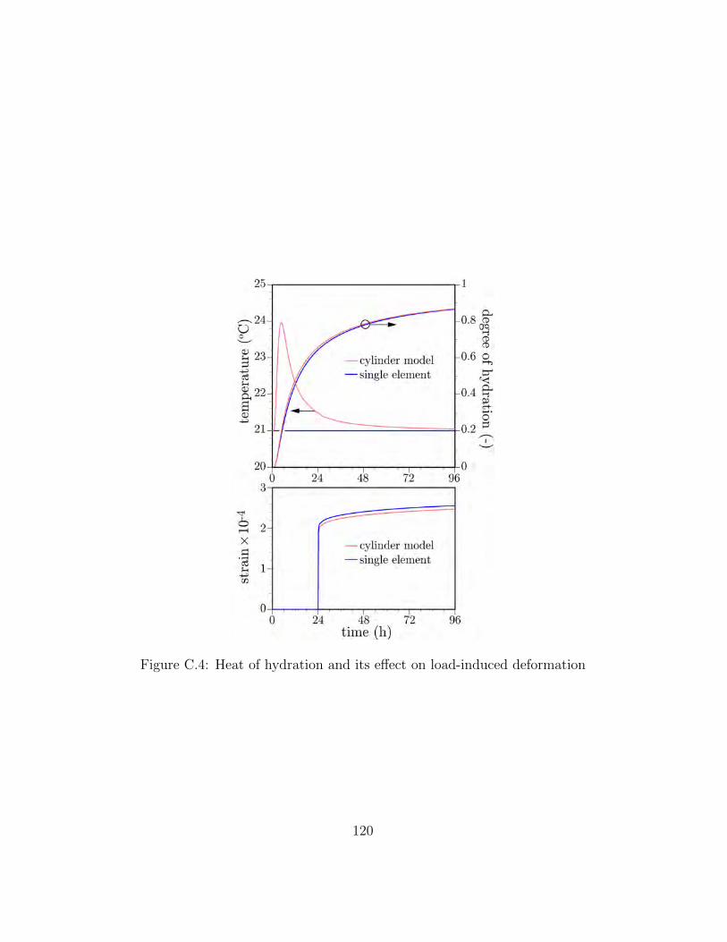
Figure C.4: Heat of hydration and its effect on load-induced deformation

120

Figure C.5: Strength development as a function of degree of hydration: de-pendence on setting parameter, α0

strength development, Eq. B.22 becomes � �ζ α − α0

fc(α) = fc(αu) for α ≥ α0 (C.1) αu − α0

where fc(αu) is the asymptotic limit of compressive strength with time and α0 is the degree of reaction associated with concrete setting. Herein, exponent ζ is assigned the typical value of 1.5 [71]. Figure C.5 compares estimated strength values with those of the Laplante study, which was considered in the previous section. Strengthening commences for α ≥ α0. Strength simulations based on the chosen range of α0 (from 0.10 to 0.25) bracket the early-age test results and provide reasonably good estimates of strength development at later times.

C.3 Autogenous and drying shrinkage The series of tests of Yang et al. [136] is simulated. The test program involved the autogenous and drying shrinkage testing of blended cement concrete at three water-to-binder ratios: 0.25, 0.35, and 0.45. The binder consisted of ordinary portland cement and ground blast furnace slag at a 50:50 propor-tion. The blast furnace slag was finely ground, having a Blaine fineness

121

of 600m2/g, which likely accentuated autogenous shrinkage. For each w/b value, both autogenous shrinkage and drying shrinkage tests were conducted using 100×100×400 mm3 prisms. When considered, drying was initiated at 1, 3, or 7 days. The 3-day and 7-day tests are simulated hereafter. Results from the 1-day drying experiments exhibit a qualitatively different trend that could not be captured using the same set of model parameters. For the lattice modeling of the tests, symmetry conditions are exploited

such that 1/8 of the prism volume is discretized (Fig. C.6). Heat and moisture exchange occur across the exterior surfaces. To enforce symmetry boundary conditions, heat and moisture exchange are prevented across the planes of symmetry. In addition, nodes along the planes of symmetry do not move normal to those planes of symmetry. Nodes were placed at the ends of the prism, along the longitudinal axis, to serve as gage points for calculating longitudinal strain. Nodal density has been reduced within the core of the specimen where temperature and hygral gradients are relatively small. The concrete mixture parameters, used as input to the hydration rou-

tines, are: cement content c = 170 kg/m3; and slag content s = 170 kg/m3 . Chemical composition of the portland cement fraction was not reported, so that values typical for Type I OPC have been used for the hydration model calculations. Humidity change due to self-desiccation and concrete diffusivity are represented by Eqs. B.10 through B.13 with the parameter values given in Table C.1. The large hsu values are due, in part, to the high volumes of finely ground slag in the concrete mixtures.

Table C.1: Parameter settings for simulations of autogenous and drying shrinkage

Parameter w/c = 0.25 w/c = 0.45 D0

D1 n hsu s Λh βh

0.017 mm2/h 9 mm2/h

6 0.76 1.4

0.25 mm/h 0.0025

0.017 mm2/h 9 mm2/h

5 0.88 3.0

0.25 mm/h 0.0021

122

Figure C.6: Discretization for shrinkage test simulations: a) dimensions (in mm); b) lattice representation; and c) volume rendering of prism specimens

123

Figure C.7: Autogenous and drying shrinkage simulations

124

The simulated shrinkage strains are compared with the experimental val-ues in Fig. C.7. The overall trends are captured well particularly for the autogenous shrinkage strain curves, which are relatively easy to fit. The appearance of the curves matches those reported by Kim et al. [69]. For the cases of drying, however, the experimental results exhibit sustained high rates of shrinkage in the first few days. That behavior can be simulated more precisely by increasing the diffusivity and/or hygral coefficient of the concrete, but then the ultimate shrinkage values are too large. The model is limited to the service range of loading (i.e., linear behavior, including creep) and does not account for the nonlinear effects of microcracking and creep damage under sustained high loading. Ultimately, those effects need to be incorporated into the analyses.

C.4 Simulation of restrained ring test The restrained ring test is a means for assessing the early-age cracking po-tential of a concrete mixture. Due to its simple experimental setup and operation, and the fact that measurements can be made from the time of casting onward, it is also an effective means for model validation. Restrained ring tests were conducted as a means for validating the lattice

model. The mixture parameters were chosen to promote early-age shrink-age and are summarized in Table C.2. The ring setup, shown in Fig. C.8, and testing procedure were according to ASTM C1581 specifications [8]. For each specimen, two strain gages were attached to opposing sides of the inner radius of the steel ring. Gage readings were recorded using an automated data acquisition system based on NI LabVIEW R . After casting, the speci-mens where covered with a vapor barrier until the time of form removal and exposure to the environment at 2 days. The upper surfaces of the concrete rings were sealed with aluminum tape so that drying occurred from the outer circumferential face of the concrete ring. Both the concrete matrix and the steel ring are represented by a lattice

model (Fig. C.9). A two-dimensional simulation is conducted, which is rea-sonable considering the axisymmetric nature of moisture consumption and movement. Moisture transport does not occur in the vertical (z) direction due to sealing of the top and bottom surfaces in the experiment. The top and bottom surfaces are also assumed to be thermally insulated, which is an approximation.

125

Figure C.8: Restrained ring test setup prior to concrete casting

Figure C.9: Lattice model representation of restrained ring test

126

Figure C.10: Strain development due to heat of hydration, autogenous shrinkage, and drying shrinkage.

127

Constituents Mixture 1 Mixture 2 cement 526 526

fine aggregate 1590 1590 water 263 263

steel fibers - 74.8

Table C.2: Concrete mixture proportions (kg/m3)

Strains develop in the steel ring due to thermal and hygral effects (Fig. C.10). Soon after mixing of the concrete, heat of hydration of the cement causes ther-mal expansion of the steel ring. This is seen in both the experimental and simulation results. After about 8 to 12 h, cooling and autogenous shrinkage of the concrete cause contraction of the steel ring. Due to autogenous shrink-age, the steel ring exhibits compressive strain before the concrete is exposed to the drying environment. Drying commences with form removal 2 days after casting, initiating rapid shrinkage of the outer portions of the concrete ring. This shrinkage, along with concrete creep, produces the upward non-linear trend in steel strain seen in Fig. C.10. The good agreement between experimentally and numerically simulated strains in Fig. C.10 validates basic capabilities of the model. The simulation model does not yet account for creep damage, which is

thought to be significant as the tensile stresses in the concrete approach the tensile strength. For this reason the simulation was not continued be-yond about 4 days. In a separate study, using simplified models for property evolution and cracking, the beneficial effects of the fiber additions are demon-strated [67].

C.5 Structural displacements

C.5.1 Half-span simulations Validation exercises are conducted to support the 3D simulations of the Markham Ravine Bridge deck. For the half-span discretization shown in Fig. C.11, simulated displacements of the deck/girder system due to self-weight are compared with theory in Fig. C.12. Two cases have been con-sidered, in which the model represents: 1) a cantilevered beam; and 2) the symmetric portion of a span where both ends are fixed (Fig. C.13). The

128

Figure C.11: Discretization of symmetric (half-span) portion of Markham Ravine Bridge deck

elastic curves are based on beam theory, supplemented to account for shear deformations. According to Euler-Bernoulli beam theory

d2v −M(z) = (C.2)

dz2 EI where flexural rigidity EI is based on uniform properties over the cross sec-tion. Integrating twice and applying the appropriate boundary conditions, the flexural components of the elastic curve for cases 1 and 2 are � �

4 L2 2 w z Lz3 z v(z) = − − + (C.3)

2EI 12 3 2

and w

v(z) = − (z 4 − 2Lz3 + L2 z 2) (C.4) 24EI

respectively, where w is self-weight per unit length of the girder. With respect to shear deformation

dv V (z) = − (C.5)

dz kAG in which A is the total section area; G is the shear modulus; and the shape factor is approximated as k = Aw/A, where Aw is the area of the web. Integrating once and applying the boundary conditions yields the component of the elastic curve associated with shear deformation.

w vs(z) = − (Lz − z 2/2) (C.6)

kAG As seen in Fig. C.12, the simulated elastics curves for each case agree well with theory.

129

Figure C.12: Elastic curves due to girder self-weight. The theoretical curves account for both flexural and shear deformation.

Figure C.13: Deformation pattern for the symmetric portion of a span where both ends are fixed

130

Figure C.14: Bending stress in deck under gravity loading

As an additional check on the accuracy of the mechanical model, bending stress is calculated according to

M(z)y σzz = (C.7)

I

where y is the height of the measurement point relative to the section cen-troid. Figure C.14 compares model results for bending stress along the length of the beam with values obtained from Eq. C.7. The point of interest is mid-depth of the deck. The stress values obtained from the model and theory are in good agreement.

C.6 Validation needs The practical value of computational models depends on their validity with respect to accurately simulating real-world behavior within the application area. In other words, the model must accurately represent the real-world behavior for a sufficiently large region within the design parameter space. Verification and validation of computational models is a mature subject

in some fields, such as computational fluid dynamics [108]. Figure C.15

131

Figure C.15: Framework for Verification and Validation of computational models (ASME, 2012)

132

Figure C.16: Use of laboratory data to validate model simulations of field performance (*Caltrans Photography Catalog Set #7861)

presents a framework for verification and validation [6]. As implied by the figure, validations are made through comparisons with physical models of the end-applications. This follows from the ability to generate sufficient data from physical (i.e. laboratory) models. Due to the scarcity of field data, it is atypical to validate computational models via comparisons with the end-applications. As an example, early-age cracking performance can be studied using the

restrained ring test [8, 61]. In this sense, the restrained ring test becomes a physical model of concrete within the freshly cast bridge deck. Some of the restraint mechanisms are represented, but a full accounting of design parameters and their ranges is lacking. A full factorial examination of the discretized parameter space involves

N test cases N = n1n2n3 · · · nk (C.8)

in which k is the number of parameters and ni represents the number of different values assignable to parameter i. This large number of test cases presents several problems.

• Laboratory data serve to validate models (Fig. C.16), but cover only a small portion of the parameter space associated with the application domain. This is schematically illustrated in Fig. C.17 for the hypothet-ical case of two design parameters, χ1 and χ2.

• There are uncertainties with respect to both model accuracy and the

133

Figure C.17: Schematic representation of validation and application domains within a two-dimensional design parameter space

assignable values to each design parameter.

• The production of practical, validated models will involve compromises between model simplicity and the accuracy with which physical pro-cesses (and their mutual couplings) are represented.

In lieu of having a complete data set for validation, model credibility is improved by increased physical bases. Free parameters, specified through calibration processes, are often invalid for cases outside of the data set used for calibration. Existing designs can be used as bases from which to conduct sensitivity analyses, although such explorations might be confined to the neighborhoods of local optima.

134

Appendix D

Plastic shrinkage cracking

D.1 Methods for reducing plastic shrinkage cracking

Plastic shrinkage cracking (PSC) occurs within fresh concrete, before its final setting. It is due to drying and consequent contraction of the exposed con-crete surface prior to sufficient strength development [76, 121, 130]. Plastic shrinkage cracks typically appear 30 min to 6 h after casting. The occurrence and severity of plastic shrinkage cracking can be reduced by:

• Lowering the evaporation rate;

• Wetting of the concrete surface (e.g., via controlled fogging);

• Increasing the volume of bleed water reaching the surface;

• Use of short-fiber reinforcement;

• Reducing plastic settlement; and

• Effective design of the concrete materials.

A variety of test methods have been developed to assess the PSC potential of concrete materials [7, 8]. A key feature of most methods is the provision of restraint against plastic shrinkage. Some methods also introduce stress risers and details to activate the effects of plastic settlement. Ideally, evaporation rate is regulated through tight controls of temperature, relative humidity, and air speed across the concrete surface.

135

As indicated above, it is commonly accepted that small additions of fiber reinforcement reduce the occurrence and severity of plastic shrinkage cracking of concrete. Fiber type influences the cracking behavior and other factors, such as workability of the concrete mixture. The literature indicates that glass fibers are effective in reducing plastic shrinkage cracking, comparing well with the most commonly used polyolefin fibers. The following sections review the abilities of fibers to reduce plastic shrinkage cracking, along with other consequences of their use.

D.2 General use of short-fiber reinforcement This section briefly reviews the use of short-fiber reinforcement to reduce PSC. The effectiveness of glass fiber reinforcement, in particular, is discussed in Section D.3. Short-fiber reinforcement improves the cracking performance of concrete,

both at early ages and in the longer term. Steel fibers can be used to control plastic shrinkage cracking, but non-metallic fibers provide similar perfor-mance at much lower volume fractions. For example, crack width reductions of approximately 80% were obtained using steel fibers at a dosage of 0.5 vol%, yet similar reductions in crack width were obtained using only 0.1 vol% of non-metallic fibers [112]. This tendency is due, at least in part, to the higher surface area of non-metallic microfibers relative to that of ordinary metal fibers on a per volume basis. With respect to plastic shrinkage cracking, polypropylene (PP) fibers have been the most widely studied and used in commercial applications [122, 128, 137].

Fiber amount kg/m3 (vol%)

Water permeability coefficient (×10−12m/s)

Gas permeability coefficient (×10−10m2)

0 (0%) 4.65 (0.20%) 5.80 (0.25%) 7.00 (0.30%)

5.94 14.89 24.19 30.65

47.92 49.30 76.71 181.03

Table D.1: Permeability characteristics of polypropylene fiber reinforced con-cretes [110].

The presence of fibers may affect the transport properties of the cement-based composite. As indicated by Table D.1, by increasing the amounts of polypropylene fibers both the water and gas permeabilities increase relative

136

Figure D.1: Influences of shrinkage reducing admixture and PVA fibers on cracking widths during the exposure time (from Passuello et al. [97]). F200 indicates a mixture with PVA microfibers; F45 indicates a mixture with PVA macrofibers

to the control case without fibers [110]. This study involved monofilament PP fibers that were 6±1 mm in length and 20±5 µm in diameter. Banthia and Gupta [11] found that small amounts of PP fibers, within

the range of 0.1 to 0.3% by volume, are effective in reducing total crack area, maximum crack width, and the number of cracks. Increasing the fiber amount improves performance, yet workability may degrade at higher volume fractions. Longer fibers and low denier fibers were more effective in reducing crack areas and crack widths. Fibrillated fibers were found to be more effec-tive in controlling shrinkage cracking than their monofilament counterparts. These findings suggest that the total surface area of fibers is an important parameter: higher surface area leads to reductions in PSC. Sadiqul Islam and Gupta [110] examined concretes containing 0.1 to 0.3%

PP fibers and found that increasing fiber content effectively reduced both crack area and crack width relative to the control case without fibers. Passuello et al. [97] studied the influences of shrinkage reducing admix-

tures (SRA), in combination with PVA fibers, on plastic shrinkage cracking. They found that SRA greatly reduced crack widths relative to the control case of plain concrete without SRA (Fig. D.1). In addition, the use of SRA delayed

137

Figure D.2: Role of fibers in reducing plastic settlement (from Qi et al. [101]).

the time of crack appearance. Whereas the use of PVA fibers alone (at 0.5% by volume) did not delay the time of crack appearance, crack widths were greatly reduced. The microfibers (F200), likely due to their larger bonded surface area, performed better than the macrofibers (F45). The use of both SRA and fibers (at 0.25% by volume) provided both a delay in cracking and reduced crack widths. Plastic shrinkage cracking may be fostered by plastic settlement. Qi et

al. [101] investigated the influence of PP fiber additions (at volume fractions ranging from 0 to 0.7%) on plastic shrinkage cracking. Both fine fibrillated and coarse monofilament fibers were considered. They found that fiber usage dramatically reduced plastic settlement (Fig. D.2). The finer fibrillated fibers were more effective in reducing settlement, possibly due to their larger surface area. However, monofilament fibers were effective at higher dosages with less negative impact on workability. Qi et al. [101] also observed that the fiber concretes had higher evapo-

ration rates (Fig. D.3). It appears that PP fibers facilitate the transport of bleed water to the exposed surface. This has also been observed else-where [31]. However, other studies suggest the wetting properties of the fibers influence bleeding rate. In particular, fibers made of hydrophobic ma-terials (e.g., PP) appear to cause higher bleeding rates than fibers made of hydrophilic materials [37].

138

Figure D.3: Effect of fiber reinforcement on evaporation (from Qi et al. [101]).

D.3 Glass fiber reinforcement There have been relatively fewer studies on the effectiveness of glass fibers in reducing PSC. Modern-day use of glass fibers is restricted to materials that are resistant to the alkaline environment of concrete. However, fiber degradation is not an issue while the concrete is in a plastic state.

Fiber type Relative density

Elastic modulus (GPa)

Tensile strength (MPa)

Strain at failure (%)

Source

PP PP PP PP

0.91 0.91 0.9 0.91

8.48 -5 4–5

480 300–400 450

620–758

--18 8–10

[15] [102] [119] [129]

Glass Glass Glass Glass Glass

2.58 2.7 2.74 2.72 2.68

70 77 -80 72

-2000 2450 2280 1700

---3.6 4.5

[14] [94] [102] [119] [129]

Table D.2: Comparison of PP and glass fiber properties.

Some of the relevant properties of glass and polypropylene fibers are com-pared in Table D.2. The properties vary between the different studies, but the general trends are clear. The PP fibers have a significantly lower unit weight, which might affect their dispersion within concrete mixtures; the unit weight of glass fibers is closer to those of cement and aggregate, such that

139

Figure D.4: Comparison of tensile stress at 2 mm crack opening and crack area due to plastic shrinkage (from Gupta and Banthia [57])

segregation due to buoyancy effects is not an issue. Glass fibers are much stiffer than PP fibers. Some studies attribute higher stiffness to improved control of plastic shrinkage. In addition, higher stiffness typically improves dispersion of the fibers within the concrete. Gupta and Banthia examined mortar mixtures containing 0.1% of either

glass, cellulose, or one of three synthetic fibers [57]. They found that total crack area is inversely proportional to post-cracking residual strength at early age (Fig. D.4). According to fiber pullout tests conducted at early ages, glass fibers exhibited exceptionally good post-peak load carrying capacity, as shown in Fig. D.5. The other fiber types, including PP, provided little resistance to pullout following peak load. For this reason, glass fibers were the most effective in controlling crack propagation and crack area. Barluenga and Hernandez Olivares [14] investigated the use of two differ-

ent types of AR-glass fibers, at several volumetric fractions, in both ordinary and self-compacting concrete compositions. Both fiber types were composed of monofilament fibers with a length of 12 mm and a diameter of 14 µm. The fiber dosages were 0.6, 0.9, and 1.0 kg/m3 . For these dosages, there was no influence of the fibers on the fresh state consistency of the concrete. For both concrete types, addition of glass fibers reduced total cracked area and maximum length of the cracks. Fibers were introduced as part of the dry mixture and, in a separate test, after the addition of water. Both means for

140

Figure D.5: Load versus deflection curves for: a) PP fibers; and b) glass fibers (from Gupta and Banthia [57])

introducing the fibers led to similar results with respect to PSC. Independent of the type or amount of the glass fibers, all fiber reinforced mixtures led to a reduction of crack length of about 90% relative to that of the control case without fibers. The 0.6 kg/m3 dosage provided the largest reduction in crack area relative to the control case. Senthilkumar and Natesan [118] investigated the performance of three

fibers types (glass, PP, and polyester) at different volume fractions within three concrete mixtures. Glass fibers were found to be the most effective with respect to reducing PSC. It was also found that, for the same volume fraction of fibers, smaller fiber diameters improved cracking resistance. A similar finding was made in other studies [13, 88]. Messan et al. [86] investigated the plastic shrinkage cracking of mixtures

containing cellulose ether and either EVA (ethylene-vinyl acetate) or glass fibers. For the case of glass fibers, they were added to the mortar in the proportion of 0.035% by volume (1 kg/m3) of mortar. Figure D.6 shows the reduction in shrinkage strain at the drying surface, which was measured optically using digital image correlation. The glass fibers are highly effective in reducing the free shrinkage and local strain variations at the drying surface of the mortar. Both these results explain the observed effectiveness of glass fibers in reducing PSC. Malathy et al. [82] found that glass fibers were highly effective in reducing

plastic shrinkage cracks. In particular, their tests showed that 0.3% volume fraction of glass fibers prevented PSC in concrete containing 10% silica fume by weight of cement, as shown by the crack width measurements in Fig. D.7.

141

Figure D.6: Influence of EVA and glass fibers on free shrinkage of the drying surface (from Messan et al. [86]). Legend values are in terms of weight percent. For example, the glass fibers were dosed at 0.06% as a weight fraction, which is 0.035% as a volume fraction.

Figure D.7: Reduction of crack width for normal concrete and concrete con-taining 10% silica fume by weight of cement (from Malathy et al. [82]). The legend indicates drying: a) at 45◦C; and b) at 52◦C

142

Table D.3: Fiber dimensions and properties (from Rahmani et al. [102]).

Similar favorable trends were observed between glass fiber content and crack area. Boghossian and Wegner [129] investigated the use of flax fibers to reduce

PSC and produced results for PP and glass fibers for comparison. Different fiber lengths were also evaluated. Some of the main results of that study are presented in Fig. D.8. For each parameter combination, the coefficient of variation of the results is large, even though a minimum of four and a max-imum of six replicate specimens were tested. Results for the most effective fiber lengths are plotted in Fig. D.9. It is clear that glass fibers performed well. PSC was practically eliminated for dosages of 0.1 vol% and above. Rahmani et al. [102] evaluated the performance of steel, glass, and PP

fibers with respect to reducing PSC. They used the ASTM C1579 test con-figuration (which involves a restrained slab with a stress riser). The fiber dimensions and properties are summarized in Table D.3. All fiber types were dosed at 0.1% by volume. The test results are summarized in Table D.4. Two replicate specimens were tested for each type of fiber mixture. This is an unusual case where hooked steel fibers, though having less specific surface area, performed best with respect to reducing crack widths. With respect to reducing both crack width and crack area, the glass fibers performed better than the PP fibers. As for many of the experimental studies cited herein, however, variations of the crack width and area measurements were not re-ported. Therefore, one cannot make statistically significant conclusions on the relative effectiveness of the fiber types. Sivakumar and Santhanam [119] investigated combinations of steel and

other fiber types to reduce PSC. Hooked steel fibers were combined with ei-ther PP, glass, or polyester fibers. All hybrid combinations were more effec-tive in improving cracking behavior, relative to the use of a single fiber type. Steel-polypropylene combinations offered the best results. Whereas steel-glass combinations were the least effective, the glass fibers were shorter than

143

Figure D.8: Total crack area relative to plain control specimens and maxi-mum crack widths (from Boghossian and Wegner [129]). Coefficient of Vari-ation (CoV) is shown by the bar indicators.

144

Figure D.9: Comparisons of total crack areas and maximum crack widths based on most effective fiber lengths (from Boghossian and Wegner [129]).

Table D.4: Plastic shrinkage test results (from Rahmani et al. [102]).

145

Figure D.10: Influence of dosage of non-metallic fibers on total crack area. All hybrid fiber combinations had an overall volume fraction of 0.5% (from Sivakumar and Santhanam [119]).

the other non-metallic fibers (i.e., 6, 20, and 12 mm for the glass, polypropy-lene, and polyester fibers, respectively). When using a single fiber type, volume fractions above 0.25% severely reduced workability for polypropylene and polyester fibers; in contrast, the glass fibers suffered less workability loss up to dosages of 0.38% by volume.

D.4 Laboratory testing: preliminary results An apparatus has been constructed for assessing plastic shrinkage cracking of concrete mixtures. Such evaluations complement the computational mod-eling done in this project. Although the computational modeling begins with the mixing of the concrete constituents, it does not represent the processes associated with plastic shrinkage cracking prior to setting of the concrete. The formwork and stress-risers for the apparatus, shown in Fig. D.11,

are in accordance with ASTM specifications [7]. As per specification, the evaporation rate is increased by forcing air across the exposed surface using a fan. A LabVIEW R Virtual Instrument (VI) has been developed to acquire

relative humidity and temperature readings of ambient conditions and at the concrete surface. Honeywell (model HIH-4000 series) analogue sensors are used for this purpose. The front panel and wiring diagram for the VI are

146

Figure D.11: Formwork for plastic shrinkage test

displayed in Figs. D.12 and D.13, respectively. The VI records and displays the sensor readings, along with an estimation of evaporation rate based on the readings. In addition, the VI captures images of the concrete surface (via a digital camera) and determines crack opening and crack area using a series of image analysis routines. The image acquisition rate is adjustable. Tests of plastic shrinkage cracking demonstrated the efficacy of short-fiber

reinforcement in delaying cracking and restricting crack growth. Figure D.14 compares crack opening measurements for two mortar mixtures, with and without short-fiber reinforcement. The addition of 0.2%vol polypropylene fibers (Fibermesh 150) delays the appearance of cracking and then reduces crack opening. The differences in crack opening are clearly evident in Fig. D.15. The crack opening values given in Fig. D.14 were obtained using a hand-

held gage. The use of automated image analysis to measure crack opening provided qualitatively similar results, but with greater variation about the mean values due to low resolution of the camera. We anticipate obtaining a better camera/lens setup for accurate, full-field measurements of crack opening. Additional plastic shrinkage tests have been conducted. The results sug-

gest the tests are not easily reproducible. Apparently, the tendency for plastic shrinkage cracking is sensitive to variations in mixture composition, produc-

147

Figure D.12: Virtual instrument front panel

Figure D.13: Virtual instrument wiring diagram

148

Figure D.14: Measured average crack widths. Ranges of measured values are also indicated.

tion methods, or environmental conditions. Additional formwork has recently been constructed, such that dual testing can be conducted (i.e., a control case and one with parametric variations can be tested side-by-side.) In this way, unintended differences in composition, production methods, or environmen-tal conditions can be reduced or eliminated.

D.5 Summary Synthetic fibers (e.g., polyolefin fibers) are commonly used to control plastic shrinkage cracking (PSC). Their use is supported by careful examination within the literature. The number of studies on glass fibers is relatively fewer. Nonetheless, there is sufficient data to conclude that glass fibers provide at least the same degree of protection against PSC. Based on the survey of the literature, several observations can be made.

1. Short fibers affect PSC through two mechanisms. The fibers:

• are dimensionally stable and stiffer than the cement-based matri-ces at early ages. These stiff fibers restrict plastic shrinkage and crack development; and

149

Figure D.15: Typical observed cracking patterns (left: without PP fiber re-inforcement; right: with PP fiber reinforcement)

• promote (or hinder) the transfer of bleed water to the exposed surface, thus delaying (or hastening) the onset of drying. The tendency to either promote or hinder bleeding appears to depend on the wetting properties of the fibers. Fibers made of hydropho-bic material (e.g., PP) tend to promote bleeding, whereas fibers made of hydrophilic material may have the opposite tendency.

2. Relative to the commonly used polyolefin fibers, glass fibers have a significantly larger elastic modulus. For example, glass fibers are stiffer than polypropylene fibers by a factor of about 10. This higher stiffness lessens PSC, all other factors being equal. The higher stiffness of the glass fibers also facilitates their dispersion within the concrete mixture.

3. The unit weight of glass fibers is similar to those of the aggregates and cementitious ingredients within the concrete mixture. This facilitates fiber dispersion during mixing. In contrast, commonly used polyolefin fibers have a much lower unit weight, which can cause them to segregate during mixing and placement.

4. The contact area between the fibers and matrix appears to be a key factor in controlling PSC. Fibers of smaller diameter, and thus larger surface area per unit volume, are more effective in reducing PSC.

5. Substantial reductions of PSC are obtained even for small (e.g., 0.05 vol%) additions of glass micro-fibers. Increasing the fiber dosage improves re-sistance to PSC. According to the different studies cited herein, dosages in the range of 0.1 to 0.3 vol% provide the desirable performance.

150

6. Comparisons between different fiber material types (e.g., glass versus PP) are complicated by differences in the fiber dimensions. Length and/or diameter of the compared fibers were often different, both within and between the studies. Furthermore, few of the studies cited herein reported variations between the replicate specimens with respect to crack area and crack width. Such information is needed to make sta-tistically significant conclusions on the relative performances of the different fiber types.

151

Appendix E

Nomenclature

Table E.1: Cementitious materials parameters - Nomenclature

Symbol Constituent FA SF LRWR MRWR NHRWR PCHRWR WRRET ACCL

fly ash silica fume ASTM C494 Type A low-range water reducing admixture ASTM C494 Types A and F medium-range water reducing admixture ASTM C494 Type F napthalene sulfonate high-range water reducing admixture ASTM C494 Type F polycarboxylate high-range water reducing admixture retarding agent accelerating agent

Table E.2: List of symbols

Symbol Definition

hij Euclidean distance between nodes i and j [m] t time [s, h, d] Aij area of Voronoi facet common to nodes i and j [m2]

Thermal analysis a/c aggregate to cementitious materials ratio [kg/kg] c cementitious materials content [kg/m3] cp specific heat capacity [J/(kg · K)]

0 qconv, q heat flux due to convection and its modified value [W/m2] conv 0 heat flux due to solar radiation and its modified value [W/m2] qsun, qsun

152

0 qsky, qsky te w/c D Ea H Hcem Hu Q R T Ta, Tc, Tr, Ts Tsky α, αu β, τ βT , βTh γabs � η1, η2, η3 λ ρ σ χ ΛT Me, M Ke , K

Hygral analysis h ha hs, hsu n

0 qh, qh s

˜ D0, D0 ˜ D1, D1

Dh βh Λh

heat flux due to radiation and its modified value [W/m2] concrete equivalent age [h] water-to-cementitious materials ratio [kg/kg] thermal diffusivity [m2/s] apparent activation energy [J/mol] cumulative amount of heat produced by hydration [J/kg] heat of hydration of cement [J/kg] total heat available for reaction [J/kg] rate of heat production by cementitious materials hydration [J/(kg · s)] universal gas constant [J/(mol · K)] temperature [◦C] ambient, concrete, reference, and surface temperatures [◦C] sky temperature [◦C] degree of cementitious materials hydration and its ultimate value hydration model parameters coefficient of thermal expansion and its long-term value [1/◦C] solar absorptivity of concrete emissivity of concrete heat flux reduction factors thermal conductivity [W/(m · K)] mass density of concrete [kg/m3] Stefan-Boltzmann constant [W/(m2 · K4)] magnifying factor for coefficient of thermal expansion at early-ages coefficient of convective heat transfer [W/(m2 · K)] elemental and system capacity matrices elemental and system conductivity matrices

relative humidity [-] ambient relative humidity [-] relative humidity associated with self-desiccation and its ultimate value [-] parameter relating hygral diffusivity and relative humidity moisture flux due to convection and its modified value [m/s] parameter relating humidity decrease and self-desiccation diffusivity values associated with fully dried material [m2/s] diffusivity values associated with saturated material [m2/s] hygral diffusivity [m2/s] hygral shrinkage coefficient hygral convection coefficient [m/s]

153

Mechanical analysis b fc, fcu f kn, ks, kt kφx, kφy, kφz nα q1, q2, q4 t0

te tr tis, tfs w wc AP

ij E Ev, ES Fn, Fs, Ft I11, I22, Jp D Ke, K α0i , α0 ϕ γ �h , �T

�i , �v , �f

ζ η κ κ0 κ1 ν θR ϑ1, ϑ2 σ σR σp, σfs ψ, ψS ξ ω

element thickness [m] compressive strength and its asymptotic limit [MPa] tensile strength [MPa] stiffness coefficients of the uniaxial springs [N/m] stiffness coefficients of the rotational springs [N · m] parameter relating rate of solidification to degree of hydration instantaneous elastic, viscoelastic, and viscous strain parameters [1/MPa] age of loading [h] equivalent age [h] reduced time representing the thermal-hygral effects on creep [h] times of initial and final concrete setting [h] crack opening [m] traction-free crack opening [m] projected area of element facet [m2] elastic modulus of concrete [MPa] activation energies for creep and microprestress processes [J/mol] spring-set forces in the normal and two tangential directions [N] principal planar and polar second moments of facet area [m4] material constitutive matrix elemental and global stiffness matrices degrees of hydration at initial and final setting coefficient governing concrete setting behavior viscoelastic microstrain hygral and thermal strains instantaneous elastic, viscoelastic, and viscous flow strains coefficient governing material property development effective microscopic viscosity [MPa/s] stress-to-strength ratio microprestress model parameter [1/(MPa · d)] microprestress model parameter [MPa/K] Poisson’s ratio inclination of tensile force resultant relative to the element axis parameters defining the break-point in the tension softening relation axial stress [MPa] stress resultant [MPa] penetration resistance and its value at final setting [MPa] reduced time coefficients for creep and microprestress processes factor relating normal and shear spring stiffnesses degree of damage

154

Φ non-aging micro-compliance function [1/MPa]

155

Bibliography

[1] Altoubat SA, Lange DA (2001) Creep, shrinkage, and cracking of re-strained concrete at early age. ACI Materials Journal 98(4): 323–331.

[2] Arora A, Sant G, Neithalath N (2017) Numerical simulations to quan-tify the influence of phase change materials (PCMs) on the early- and later-age thermal response of concrete pavements. Cement and Con-crete Composites 81: 11–24.

[3] Asahina D, Aoyagi K, Kim K, Birkholzer J, Bolander JE (2017) Elastically-homogeneous lattice models of damage in geomaterials. Computers and Geotechnics 81: 195–206.

[4] Asahina D, Kim KH, Li Z, Bolander JE (2014) Flow field calculations within discrete models of multiphase materials. Composites B 58: 293– 302.

[5] Asamoto S, Ohtsuka A, Kuwahara Y, Miura C (2011) Study on effects of solar radiation and rain on shrinkage, shrinkage cracking and creep of concrete. Cement and Concrete Research 41: 590–601.

[6] ASME (2012) An illustration of the concepts of verification and val-idation in computational solid mechanics, V&V 10.1-2012. Technical report, American Society of Mechanical Engineers.

[7] ASTM C1579-13 (2013) Evaluating plastic shrinkage cracking of re-strained fiber reinforced concrete. Technical report, ASTM Interna-tional, West Conshohocken, PA.

[8] ASTM C1581-09 (2009) Determining age at cracking and induced tensile stress characteristics of mortar and concrete under restrained

156

shrinkage. Technical report, ASTM International, West Conshohocken, PA.

[9] ASTM C171-16 (2016) Standard specification for sheet materials for curing concrete. Technical report, ASTM International, West Con-shohocken, PA.

[10] ASTM C403-08 (2008) Standard test method for time of setting of concrete mixtures by penetration resistance. Technical report, ASTM International, West Conshohocken, PA.

[11] Banthia N, Gupta R (2006) Influence of polypropylene fiber geome-try on plastic shrinkage cracking of concrete. Cement and Concrete Research 36: 1263–1267.

[12] Banthia N, Gupta R (2009) Plastic shrinkage cracking in cementitious repairs and overlays. Materials and Structures 42: 567–579.

[13] Banthia N, Yan C (2000) Shrinkage cracking in polyolefin fiber rein-forced concrete. ACI Materials Journal 97(4): 432–437.

[14] Barluenga G, Hernandez-Olivares F (2007) Cracking control of con-cretes modified with short AR-glass fibers at early age. Experimental results on standard concrete and SCC. Cement and Concrete Research 37: 1624–1638.

[15] BASF (2017). Technical Data Sheet for MasterFiber M 100, BASF.

[16] Bazant Z, Prasannan S (1989) Solidification theory for concrete creep. I: Formulation. Journal of Engineering Mechanics, ASCE 115(8): 1691– 1703.

[17] Bazant ZP, Cusatis G, Cedolin L (2004) Temperature effect on con-crete creep modeled by microprestress-solidification theory. Journal of Engineering Mechanics, ASCE 130(6): 691–699.

[18] Bazant ZP, Najjar LJ (1971) Drying of concrete as a non-linear diffusion problem. Cement Concrete Research 1(5): 461–473.

[19] Bazant ZP, Oh BH (1983) Crack band theory for fracture of concrete. Materials and Structures 16: 155–177.

157

[20] Bentz DP (2000) A computer model to predict the surface temperature and time of wetness of concrete pavements and bridge decks. Technical Report NISTIR 6551, National Institute of Standards and Technology.

[21] Bentz DP (2007) Transient plane source measurements of the thermal properties of hydrating cement pastes. Materials and Structures 40: 1073–1080.

[22] Bentz DP (2008) A review of early-age properties of cement-based ma-terials. Cement and Concrete Research 38: 196–204.

[23] Bentz DP, Ferraris C, Jones SZ, Lootens D, Zunino F (2017) Limestone and silica powder replacements for cement: early-age performance. Ce-ment and Concrete Composites 78: 43–56.

[24] Bentz DP, Geiker MR, Hansen KK (2001) Shrinkage-reducing admix-tures and early age desiccation in cement pastes and mortars. Cement and Concrete Research 31(7): 1075–1085.

[25] Bentz DP, Jensen OM, Hansen KK, Olesen JF, Stang H, Haecker CJ (2001) Influence of cement particle-size distribution on early age auto-genous strains and stresses in cement-based materials. Journal of the American Ceramic Society 84(1): 129–135.

[26] Bernander S (1998) Practical measures to avoiding early age thermal cracking in concrete structures. In R Springenschmid, ed., Prevention of Thermal Cracking in Concrete at Early Ages, RILEM Report 15, pages 255–314. RILEM, E & FN Spon.

[27] Berton S, Bolander JE (2006) Crack band model for fracture in irregu-lar lattices. Computer Methods in Applied Mechanics and Engineering 195: 7172–7181.

[28] Bolander JE, Berton S (2004) Simulation of shrinkage induced cracking in cement composite overlays. Cement and Concrete Composites 26: 861–871.

[29] Bolander JE, Saito S (1998) Fracture analyses using spring networks with random geometry. Engineering Fracture Mechanics 61: 569–591.

158

[30] Bolander JE, Sukumar N (2005) Irregular lattice models for quasistatic crack propagation. Physical Review B 71: 094106–1.

[31] Boshoff WP, Combrinck R (2013) Modelling the severity of plastic shrinkage cracking in concrete. Cement and Concrete Research 48: 34–39.

[32] Caltrans (2013) Concrete Technology Manual. California Department of Transportation, Division of Engineering Services, Structure Con-struction.

[33] Caltrans (2015) Bridge Deck Construction Manual - Revision No. 1. State of California, Department of Transporation, Division of Engi-neering Services, Structure Construction.

[34] CEB (1992) Durable concrete structures - Design guide. Comite Euro-International du Beton (CEB), Thomas Telford Ltd., London.

[35] Cervera M, Oliver J, Prato T (1999) Thermo-chemo-mechanical model for concrete. II: damage and creep. Journal of Engineering Mechanics, ASCE 125(9): 1028–1039.

[36] Chen H, Wyrzykowski M, Scrivener K, Lura P (2013) Prediction of self-desiccation in low water-to-cement ratio pastes based on pore structure evolution. Cement and Concrete Research 49: 38–47.

[37] Combrinck R (2011) Plastic shrinkage cracking in conventional and low volume fibre reinforced concrete. Master’s thesis, Department of Civil Engineering, University of Stellenbosch.

[38] Cusson D (2009) Effect of blended cements on effectiveness of internal curing in HPC. In BJ Mohr, DP Bentz, eds., SP-256, Internal Curing of High-Performance Concrete: Lab and Field Experiences, 9, pages 1–16. American Concrete Institute.

[39] Darwin D, Browning J, Lindquist W (2004) Control of cracking in bridge decks: observations from the field. Cement, Concrete, and Ag-gregates 26(2): CCA12320.

[40] Darwin D, Browning J, Lindquist W, McLeod HAK, Yuan J, Toledo M, Reynolds D (2010) Low-cracking, high-performance concrete bridge

159

decks: Case studies over first 6 years. Transportation Research Record (2202): 61–69.

[41] de Sa C, Benboudjema F, Thiery M, Sicard J (2008) Analysis of micro-cracking induced by differential drying shrinkage. Cement and Concrete Composites 30(10): 947–956.

[42] de Schutter G, Taerwe L (1996) Degree of hydration-based description of mechanical properties of early age concrete. Materials and Structures 29: 335–344.

[43] de Schutter G, Taerwe L (1996) Estimation of early-age thermal crack-ing tendency of massive concrete elements by means of equivalent thick-ness. ACI Materials Journal 93: 403–408.

[44] de Schutter G, Taerwe L (1997) Fracture energy of concrete at early ages. Materials and Structures 30: 67–71.

[45] di Luzio G, Cusatis G (2009) Hygro-thermo-chemical modeling of high performance concrete, I: theory. Cement and Concrete Composites 31: 301–308.

[46] di Luzio G, Cusatis G (2013) Solidification-microprestress-microplane (SMM) theory for concrete at early age: Theory, validation and appli-cation. International Journal of Solids and Structures 50(6): 957–975.

[47] Domone PL (1974) Uniaxial tensile creep and failure of concrete. Mag-azine of Concrete Research 26(88): 144–152.

[48] Duffie JA, Beckman WA (2006) Solar Engineering of Thermal Pro-cesses. John Wiley & Sons, Inc., Hoboken, New Jersey, 3rd edition.

[49] Emborg M (1998) Development of mechanical behaviour at early ages. In R Springenschmid, ed., Prevention of Thermal Cracking in Concrete at Early Ages, RILEM Report 15, pages 76–148. RILEM, E & FN Spon.

[50] Emborg M, Bernander S (1994) Assessment of risk of thermal crack-ing in hardening concrete. Journal of Structural Engineering, ASCE 120(10): 2893–2912.

160

[51] Faria R, Anzenha M, Figueiras JA (2006) Modeling of concrete at early ages: application to an externally restrained slab. Cement and Concrete Composites 28: 572–585.

[52] Fattuhi NI (1986) Curing compounds for fresh or hardened concrete. Building and Environment 21(2): 119–125.

[53] Ferraris C, Wittmann FH (1987) Shrinkage mechanisms of hardened cement paste. Cement and Concrete Research 17: 453–464.

[54] Forth JP (2015) Predicting the tensile creep of concrete. Cement and Concrete Composites 55: 70–80.

[55] Fu T, Deboodt T, Ideker JH (2016) Development of shrinkage limit specification for high performance concrete used in bridge decks. Ce-ment and Concrete Composites 72: 17–26.

[56] Grasley ZC, Lange DA, D’Ambrosia MD (2006) Internal relative hu-midity and drying stress gradients in concrete. Materials and Structures 39: 901–909.

[57] Gupta R, Banthia N (2016) Correlating plastic shrinkage cracking po-tential of fiber reinforced cement composites with its early-age consti-tutive response in tension. Materials and Structures 49: 1499–1509.

[58] Hammer TA, Fossa KT, Bjøntegaard Ø (2007) Cracking tendency of HSC: Tensile strength and self generated stress in the period of setting and early hardening. Materials and Structures 40: 319–324.

[59] Holt E, Leivo M (2004) Cracking risks associated with early age shrink-age. Cement and Concrete Research 26(5): 521–530.

[60] Holt EE (2001) Early age autogenous shrinkage of concrete. Techni-cal Report 446, Technical Research Centre of Finland - VTT, Espoo, Finland.

[61] Hossain AB, Weiss J (2004) Assessing residual stress development and stress relaxation in restrained concrete ring specimens. Cement and Concrete Composites 26(5): 531–540.

161

[62] Jawed I, Skalny J (1978) Alkalis in cement: a review: II. effects of alkalis on hydration and performance of portland cement. Cement and Concrete Research 8: 37–52.

[63] JCI (2008) JCI Guidelines for Control of Cracking of Mass Concrete. Japan Concrete Institute.

[64] Jonasson JE (1985) Moisture fixation and moisture transfer in concrete. In Concrete Structures, SMiRT 8 - Brussels, Belgium, pages 235–242. IASMiRT.

[65] JSCE (2010) Standard specifications for concrete structures-2007 (En-glish Version). Technical report, Japan Society of Civil Engineers.

[66] Kada H, Lachemi M, Petrov N, Bonneau O, Aıtcin P (2002) Deter-mination of the coefficient of thermal expansion of high performance concrete from initial setting. Materials and Structures 35: 35–41.

[67] Kang J, Bolander JE (2016) Lattice modeling of early-age cracking in restrained ring specimens. ACI Special Publication SP-311: 1–10.

[68] Kawai T (1978) New discrete models and their application to seismic response analysis of structures. Nuclear Engineering and Design 48: 207–229.

[69] Kim JK, Lee CS (1999) Moisture diffusion of concrete considering self-desiccation at early ages. Cement and Concrete Research 29: 1921– 1927.

[70] Kraus PD, Rogalla EA (1996) Transverse cracking in newly constructed bridge decks. Technical Report NCHRP Report 380, Transportation Research Board, National Academy Press.

[71] Krauß M, Rostasy FS (2002) Determination of initial degree of hydration by means of ultrasonic measurements. In H Mihashi, FH Wittmann, eds., Control of Cracking in Early Age Concrete, Pro-ceedings of the International Workshop on Control of Cracking in Early Age Concrete, pages 19–28. AA Balkema.

[72] Laplante P (1993) Mechanical properties of hardening concrete: a com-parative analysis of classical and high strength concretes. Ph.D. thesis, Ecole Nationale des Ponts et Chaussees, Paris (in French).

162

[73] Lawrence MG (2005) The relationship between relative humidity and the dewpoint temperature in moist air. Bulletin of the American Me-terological Society (BAMS) pages 225–233.

[74] Lee Y, Choi M, Yi ST, Kim JK (2009) Experimental study on the convective heat transfer coefficient of early-age concrete. Cement and Concrete Composites 31: 60–71.

[75] Leemann A, Lura P (2014) Impact of admixtures on the plastic shrink-age cracking of self-compacting concrete. Cement and Concrete Com-posites 46: 1–7.

[76] Leemann A, Nygaard P, Lura P (2014) Impact of admixtures on the plastic shrinkage cracking of self-compacting concrete. Cement and Concrete Composites 46: 1–7.

[77] Levinson R, Akbari H (2002) Effects of composition and exposure on the solar reflectance of portland cement concrete. Cement and Concrete Research 32: 1679–1698.

[78] Lewis RW, Morgan K, Thomas HR, Seetharamu KN (1996) The Finite Element Method in Heat Transfer Analysis. John Wiley & Sons, Inc.

[79] Lura P, Jensen OM, van Breugel K (2003) Autogenous shrinkage in high-performance cement paste: An evaluation of basic mechanisms. Cement and Concrete Research 33: 223–232.

[80] Lura P, Pease B, Mazzotta G, Rajabipour F, Weiss J (2007) Influence of shrinkage-reducing admixtures on the development of plastic shrinkage cracks. ACI Materials Journal 104(2): 187–194.

[81] Maggenti R, Knapp C, Fereira S (2013) Controlling shrinkage cracking. Concrete International 35(7): 36–41.

[82] Malathy R, Subramanian K, Rameshkumar M (2007) Effect of glass fibers on restrained plastic shrinkage cracking of HPC with silica fume. Journal of Scientific & Industrial Research 66: 748–751.

[83] Marceau ML, VanGeem MG (2008) Solar reflectance values for con-crete. Concrete International 30(8): 52–58.

163

[84] Maruyama I, Teramoto A, Igarashi G (2014) Strain and thermal ex-pansion coefficients of various cement pastes during hydration at early ages. Materials and Structures 47: 27–37.

[85] Mehta PK, Monteiro PJM (2014) Concrete - Microstructure, Proper-ties, and Materials. McGraw-Hill, 4th edition.

[86] Messan A, Ienny P, Nectoux D (2011) Free and restrained early-age shrinkage of mortar: Influence of glass fiber, cellulose ether and EVA (ethylene-vinyl acetate). Cement and Concrete Composites 33: 402– 410.

[87] Mindess S, Young JF, Darwin D (2003) Concrete. Prentice Hall, 2nd edition.

[88] Naaman A, Wongtanakitcharoen T, Hauser G (2005) Influence of dif-ferent fibers on plastic shrinkage cracking of concrete. ACI Materials Journal 102: 49–58.

[89] Naaman AE, Reinhardt HW, eds. (1996) High Performance Fiber Re-inforced Cement Composites 2 (HPFRCC2). RILEM Proceedings 31, E & FN Spon.

[90] National Center for Forensic Science (2009) Burning item database. Technical report, Department of Fire Protection Engineering, Univer-sity of Maryland.

[91] National Oceanic and Atmospheric Administration. Na-tional Climatic Data Center, NNDC Climate Data Online, https://www7.ncdc.noaa.gov/CDO/cdo.

[92] National Renewable Energy Laboratory. National So-lar Radiation Database, U.S. Department of Energy, http://rredc.nrel.gov/solar/old data/nsrdb/.

[93] Neville AM (1995) Properties of Concrete. John Wiley & Sons, Inc.

[94] NYCON (2017). Technical Data Sheet for NYCON-AR-DM (Fiber-glass), Nycon Corp.

164

[95] Oh BH, Cha SW (2003) Nonlinear analysis of temperature and mois-ture distributions in early-age concrete structures based on degree of hydration. ACI Materials Journal 100(5): 361–370.

[96] Østergaard L, Lange D, Stang H (2004) Early-age stress-crack open-ing relationships for high performance concrete. Cement and Concrete Composites 26: 563–572.

[97] Passuello A, Moriconi G, Shah SP (2009) Cracking behavior of con-crete with shrinkage reducing admixtures and pva fibers. Cement and Concrete Composites 31: 699–704.

[98] Persson B (1997) Self-desiccation and its importance in concrete tech-nology. Materials and Structures 30: 293–305.

[99] Poole JL (2007) Modeling temperature sensitivity and heat evolution of concrete. Ph.D. thesis, University of Texas at Austin.

[100] Powers TC, Brownyard TL (1948) Studies of the physical properties of hardened portland cement paste. Technical report, Bulletin 22, Re-search Laboratories of the Portland Cement Association, Chicago.

[101] Qi C, Weiss J, Olek J (2003) Characterization of plastic shrinkage cracking in fiber reinforced concrete using image analysis and a modi-fied Weibull function. Materials and Structures 36: 386–393.

[102] Rahmani T, Kiani B, Bakhshi M, Shekarchizadeh M (2012) Application of different fibers to reduce plastic shrinkage cracking of concrete. In 7th RILEM International Conference on Cracking in Pavements, pages 635–642. RILEM.

[103] Rettner DL (2014) A review of mechanisms, analysis of MnDOT bridge construction data, and recommendation for treatment and prevention bridge construction data, and recommendation for treatment and pre-vention. Technical report, Minnesota Department of Transportation.

[104] Riding KA, Folliard KJ, Juenger MCG, Schindler AK (2012) Modeling hydration of cementitious systems. ACI Materials Journal 109(2): 225–234.

165

[105] Riding KA, Poole JL, Schindler AK, Juenger MCG, Folliard KJ (2014) Statistical determination of cracking probability for mass concrete. Journal of Materials in Civil Engineering 26: 4014058.

[106] RILEM TC-242 (2015) Rilem draft recommendation: TC-242-MDC multi-decade creep and shrinkage of concrete: material model and structural analysis. Materials and Structures 48(4): 753–770.

[107] Rots J, Bellitti B, Invernizzi S (2008) Robust modeling of RC structures with an event-by-event strategy. Engineering Fracture Mechanics 3-4: 590–614.

[108] Roy CJ, Oberkampf WL (2011) A comprehensive framework for verifi-cation, validation, and uncertainty quantification in scientific comput-ing. Computer Methods in Applied Mechanics and Engineering 200: 2131–2144.

[109] Roziere E, Cortas R, Loukili A (2015) Tensile behaviour of early age concrete: New methods of investigation. Cement and Concrete Com-posites 55: 153–161.

[110] Sadiqul Islam GM, Gupta SD (2016) Evaluating plastic shrinkage and permeability of polypropylene fiber reinforced concrete. International Journal of Sustainable Built Environment 5(2): 345–354.

[111] Sadouki H, van Mier JGM (1997) Simulation of hygral crack growth in concrete repair system. Materials and Structures 203: 518–526.

[112] Sandbakk S (2007) Influence of fibers on cracking due to plastic and drying shrinkage: state of the art. Technical report, SINTEF Building and Infrastructure, Trondheim, Norway.

[113] Sato T, Goto T, Sakai K (1983) Mechanism for reducing drying shrink-age of hardened cement by organic additives. CAJ Rev pages 52–54.

[114] Schindler AK (2002) Concrete hydration, temperature development, and setting at early ages. Ph.D. thesis, University of Texas at Austin.

[115] Schindler AK, Folliard KJ (2005) Heat of hydration models for cemen-titious materials. ACI Materials Journal 102(1): 24–33.

166

[116] Schlangen E, van Mier JGM (1992) Experimental and numerical anal-yses of micromechanisms of fracture of cement-based composites. Ce-ment and Concrete Composites 14((2)): 105–118.

[117] Sellevold EJ, Bjøntegaard Ø (2006) Coefficient of thermal expansion of cement paste and concrete: Mechanisms of moisture interaction. Materials and Structures 39: 809–815.

[118] Senthilkumar SRR, Natesan SC (2004) Prediction and prevention of plastic shrinkage cracking in cementitious composites. In 29th Con-ference on Our World in Concrete & Structures, pages 475–484. CI-Premier PTE LTD.

[119] Sivakumar A, Santhanam M (2007) A quantitative study on the plastic shrinkage cracking in high strength hybrid fibre reinforced concrete. Cement and Concrete Composites 29: 575–581.

[120] Slatnick S, Riding KA, Folliard KJ, Juenger MCG, Schindler AK (2011) Evaluation of autogenous deformation of concrete at early ages. ACI Materials Journal 108(1): 21–28.

[121] Slowik V, Schmidt M, Fritzch R (2008) Capillary pressure in fresh cement-based materials and identification of the air entry value. Ce-ment and Concrete Composites 30: 557–565.

[122] Soroushian P, Mirza F, Alhozaimy A (1995) Plastic shrinkage crack-ing of polypropylene fiber reinforced concrete. ACI Materials Journal 92(5): 553–560.

[123] Subramaniam K (2016) Identification of early-age cracking in concrete bridge decks. Journal of Performance of Constructed Facilities 30(6): DOI:10.1061/(ASCE)CF.1943–5509.0000915.

[124] Suprenaut BA, Malisch WR (1999) The fiber factor. Concrete Con-struction October: 43–46.

[125] Tazawa E, Miyazawa S (1995) Influence of cement and admixture on autogenous shrinkage of cement paste. Cement and Concrete Research 25(2): 281–287.

167

[126] van Breugel K, Lokhorst SJ (2003) Stress-based crack criterion as a basis for the prevention of through cracks in concrete structures at early-ages. In K Kovler, A Bentur, eds., International RILEM Confer-ence on Early Age Cracking in Cementitious Systems, pages 229–236.

[127] Savija B, Pacheco J, Schlangen E (2013) Lattice modeling of chloride diffusion in sound and cracked concrete. Cement and Concrete Com-posites 42: 30–40.

[128] Wang K, Shah SP, Phuaksuk P (2001) Plastic shrinkage cracking in concrete materials - Influence of fly ash and fibers. ACI Materials Journal 98(6): 458–464.

[129] Wegner LD, Boghossian E (2008) Use of flax fibres to reduce plastic shrinkage cracking in concrete. Cement and Concrete Composites 30: 929–937.

[130] Wittmann FH (1976) On the action of capillary pressure in fresh con-crete. Cement and Concrete Research 6(1): 49–56.

[131] Wittmann FH, Roelfstra PE, Mihashi H, Huang YJ, Zhang XH, No-mura N (1987) Influence of age at loading, water-cement ratio and rate of loading on fracture energy of concrete. Materials and Structures 20(116): 103–110.

[132] WJE (2011) On-call structural concrete bridge deck cracking investi-gation services. Technical Report WJE No. 2009.2643, Prepared for Caltrans by Wiss, Janney, Elstner Associates, Inc.

[133] Wongtanakitcharoen T, Naaman AE (2007) Unrestrained early-age shrinkage of concrete with polypropylene, PVA, and carbon fibers. Ma-terials and Structures 40(3): 289–300.

[134] Wyrzykowski M, Lura P (2013) Moisture dependence of thermal ex-pansion in cement-based materials at early ages. Cement and Concrete Research 53: 25–35.

[135] Wyrzykowski M, Lura P (2016) Effect of relative humidity decrease due to self-desiccation on the hydration kinetics of cement. Cement and Concrete Research 85: 75–81.

168

[136] Yang Y, Sato R, Kawai K (2001) Evaluation of autogenous shrinkage and drying shrinkage based on bound water content of cementitious materials. Proceedings of JSCE (English translation) 53(690): 193– 207.

[137] Yin S, Tuladhar R, Shi F, Combe M, Collister T, Sivakugan N (2015) Use of macro plastic fibres in concete: A review. Construction and Building Materials 93: 180–188.

[138] Yoo DY, Banthia N, Yoon YS (2016) Mitigating early-age cracking in thin UHPFRC precast concrete products using shrinkage-reducing admixtures. PCI Journal 61(1): 39–50.

[139] Zhou FP (1992) Time-dependent crack growth and fracture in concrete. Ph.D. thesis, Division of Building Materials, LTH, Lund University.

169